Asset tangibility and capital structure

Asset Tangibility and Capital Structure

Murillo Campello Erasmo Giambona

University of Illinois & NBER University of Amsterdam

[email protected] [email protected]

This Draft: February 28, 2010

Abstract

We study the effect of asset tangibility on capital structure by exploiting variation in the salability ofcorporate assets. We do so using an instrumental variables approach that incorporates measures ofsupply and demand for different types of tangible assets (e.g., machines, land and buildings). Theorysuggests that tangibility matters because it allows creditors to more easily repossess a bankrupt firm’sassets. However, tangible assets are often illiquid and hard to redeploy. Our study shows new evidencethat the redeployability of tangible assets is a key determinant of firm capital structure (beyond stan-dard measures of tangibility). Consistent with a credit supply-side view of capital structure, we findthat asset redeployability is a particularly important driver of leverage for firms that are more likelyto face credit frictions (small, unrated, and low payout firms). Additional tests show that asset rede-ployability facilitates borrowing the most during periods of tight credit in the economy. Our findingsare consistent with capital structure models of contract incompleteness and limited enforceability.

Key words: Asset tangibility, capital structure, credit frictions, instrumental variables, asset demand.

JEL classification: G32.

1 Introduction

Theory suggests that contract incompleteness and limited enforceability reduce a firm’s ac-

cess to external finance (Hart and Moore (1994) and Holmstrom and Tirole (1997)). In the

presence of contracting frictions, assets that are tangible are more desirable from the point of

view of creditors because they are easier to repossess in bankruptcy states. Tangible assets,

however, often lose value when they are later reallocated (see evidence in Berger et al. (1996),

Pulvino (1998), Maksimovic and Phillips (1998), and Acharya et al. (2007)). Such losses imply

that only those tangible assets that can be easily redeployed should sustain high debt capacity

(Shleifer and Vishny (1992)). Differently put, tangible assets should facilitate firm borrowing

only to the extent that they are salable.

This paper gauges the impact of asset tangibility on capital structure by exploiting variation

in the supply and demand for different types of corporate assets. Assets that are less firm-

specific should allow for higher debt capacity because they are easier to resell (e.g., to other

firms in the industry). In addition, assets that respond to supply and demand forces in their

secondary markets are likely to be more redeployable. Using these insights, we partition the

measure of asset tangibility commonly used in capital structure studies (“plant, property and

equipment”) into its main components. We then assess variation in salability across those differ-

ent components by way of an instrumental variables approach that utilizes proxies for redeploy-

ability in the secondary markets. Our study reports novel findings on the relation between asset

tangibility and firm capital structure, identifying when and how tangibility affects leverage.

Our analysis proceeds as follows. We first study the economic relevance of asset tangibility

relative to traditional demand-side determinants of leverage; motivated, for example, by the

pecking order, trade-off, and market timing arguments. Based on standard empirical tests, we

find a strong positive relation between the usual proxy for asset tangibility (the ratio of fixed

assets-to-total assets) and firm leverage. Comparing variables on the basis of reduced-form

estimates of economic impact, we find that tangibility is one of the single most important

drivers of leverage. We then examine the relative importance of the various components of

tangibility. This examination entails breaking down corporate fixed assets into its identifiable

parts, which include land and buildings, machines and equipment, and other miscellaneous

tangible assets. Notably, we look for variation coming from the redeployability of those differ-

ent components of tangible assets using an instrumental variables approach that is helpful in

dealing with potential endogeneity between tangibility and leverage.1

1While one may argue that the optimal combination of tangible and non-tangible assets in a firm’s

production process is a function of factors determined outside of the firm (e.g., the state of technology and

1

We use three different sets of instruments. The first set includes industry proxies capturing

information on firms’ use of land and buildings, machinery, and other tangible assets. This set

is motivated by the product-market literature, which predicts a technology-driven level and mix

of fixed assets usage that varies across industries (see, e.g., Maksimovic and Zechner (1991) and

Williams (1995)). Our second set of instruments speaks to the salability of land and buildings.

The instruments in this set capture drivers of supply and demand conditions of the real estate

markets where the firm operates, including proxies for the number of real estate operators in

the firm’s headquarter state, the local disposal of real estate by the Government, as well as the

pricing and volatility of rental rates (see Sinai and Souleles (2005) and Ortalo-Magne and Rady

(2002)). The third set of instruments relates to the liquidity of the market for machinery and

equipment and includes proxies for the volume of transactions of second-hand machinery and

equipment in the industry where the firm operates. It also includes information on firm work-

force, which affects capital/labor ratios (see MacKay and Phillips (2005), Campello (2006), and

Garmaise (2008)). Sources of data for these instruments range from standard COMPUSTAT, to

the SNL Datasource, to authors’ request of information under the Freedom of Information Act.

Our estimations imply that tangible assets drive observed capital structure to the extent

that they are redeployable: it is the salable component of tangibility that explains firm leverage.

In addition, across the various categories of tangible assets, we find that land and buildings –

presumably, the least firm-specific assets – have the most explanatory power over leverage.2

The results we report are consistent with the idea that financing frictions such as contract in-

completeness and limited enforceability are key determinants of capital structure. While prior

literature has considered the notion that these financing imperfections are potentially relevant,

we show that they have first-order effects on leverage.

To further characterize those leverage effects, we compare firms that are more likely to

face financing frictions (small, unrated, and low dividend payout firms) – for which collat-

eral recourse is particularly important in the borrowing process – and firms that are less

likely to face those frictions (large, rated, and high dividend payout firms). We find that our

redeployability—leverage results are pronounced across the first set of firms. For example, our

estimates imply that a one-interquartile range change in redeployability is associated with a

41% increase in market leverage for small firms. This is equivalent to a sharp shift in market

leverage from its mean of about 22% to 31%. In contrast, for unconstrained firms, redeploya-

bility is an irrelevant driver of observed leverage. These cross-sectional contrasts are consistent

consumer preferences), the observed ratio of fixed-to-total assets is ultimately a choice variable for the firm.2Other tangible asset categories, such as machines and equipment, have insignificant explanatory power

over leverage.

2

with the financing friction argument: variation in asset redeployability only affects the credit

access of those firms that are credit-constrained.

Prior literature shows that the extent to which credit frictions bind and influence firm be-

havior is a function of the state of the economy (see, among others, Gertler and Gilchrist (1994)

and Bernanke and Gertler (1995)). This observation points to time-series variation that can

be explored to further study our redeployability—leverage story. In an additional set of tests,

we find that the role for redeployability in alleviating financing frictions is heightened during

episodes of credit tightening. In particular, our estimations suggest that a one-percentage point

increase in the fed funds rate (our proxy for credit tightening) leads to a 40% increase in the

sensitivity of leverage to asset redeployability. Consistent with a supply-side view of capital

structure, these results imply that asset tangibility increases debt capacity by ameliorating

credit frictions in the market for corporate borrowing.3

Our evidence points to asset tangibility as a key driver of leverage. In particular, we identify

an explicit channel (asset redeployability) through which this relation operates. It is important

that we put our findings in context with recent literature that relates closely to our analysis.

Faulkender and Petersen (2006) find that firms with credit ratings (a proxy for access to the

public debt markets) have higher leverage. The authors interpret their result as evidence of a

supply-side view of capital structure. Other studies imply, nonetheless, that there is a demand-

side dimension to debt issuance decisions that is associated with ratings. Graham and Harvey

(2001), for example, report evidence suggesting that 6 out of 10 CFOs take credit ratings as

a crucial factor in their decision of how much debt to issue. Relatedly, Kisgen (2006) finds

that firms close to a credit rate change choose to issue less debt. Empirically, Faulkender and

Petersen find that the economic effect of debt ratings on leverage is sizable. As we show below,

when we compare our asset redeployability-based proxy with Faulkender and Petersen’s rat-

ings dummy, we find that the economic effect of redeployability on leverage is much stronger

(twice as large). The more substantive contribution of our findings relative to theirs is that,

rather than using a broadly-defined measure of access to credit (one that confounds various

elements of demand and supply of capital, as well as different features of financial contracting),

we identify a specific channel through which creditworthiness affects capital structure.

We also experiment with Lemmon et al.’s (2008) leverage model to check whether our con-

clusions about asset tangibility passes those authors’ “fixed-effects stress tests.” Lemmon et al.

show that traditional determinants of leverage become largely irrelevant once the econometri-

3Korajczyk and Levy (2003) report that the leverage ratios of financially constrained firms are more

sensitive to aggregate shocks. The authors, however, do not establish a link between this empirical regularity

and any particular feature of financial contracting.

3

cian accounts for time-invariant firm effects. Like those authors, we find a pattern of decline in

the size of the regression coefficients of traditional determinants of leverage after we account

for firm effects. The coefficients associated with our tangibility proxies are notable exceptions,

nonetheless. In fact, the effect of land and buildings on leverage increases by a factor of almost

3 in the firm-fixed effects instrumental variables specification relative to the simple OLS. These

experiments highlight the robustness of the redeployability—leverage channel we propose.

Our paper adds to the research on capital structure by considering credit supply-side fric-

tions as determinants of observed variation in leverage. A few recent papers have explored

similar ideas. Benmelech (2009) uses variation in the width of the track gauges from the 19th

century railroad industry in the U.S. to measure asset salability. Empirically, he finds that

firms using track gauges that are easier to sell (to other railroad companies) use more long-term

debt. Benmelech, however, does not find systematic evidence on the impact of asset salability

on leverage. Looking at data from the U.S. airline industry, Benmelech and Bergman (2009)

find that debt tranches secured by more liquid collateral pay lower interest rates and sustain

higher loan-to-value ratios.4 Using the emergence of certificates of deposits in the 1960s, Leary

(2009) shows that shocks to the supply of bank lending affect firm leverage. Finally, Lemmon

and Roberts (2009) use a natural experiment (the 1989 collapse of the junk bond market) to

study the effect of a supply-side credit shock on the investment and leverage of junk bond

issuers. The authors do not find an effect of credit supply on firm leverage. Our paper con-

tributes to this literature by providing systematic evidence (across firms, time, and industries)

of first-order effects of supply-side factors on capital structure. In addition, our paper uniquely

pins down a well-defined channel – the redeployability of tangible assets – in identifying one

way in which financing frictions affect leverage ratios.5

The reminder of this paper is organized as follows. The next section describes the data

and compares our sample to those of standard capital structure studies. Section 3 presents our

central results on the effect asset tangibility (and its various components) on leverage. Section

4 presents results for partitions of firms facing financing frictions, and during periods of credit

tightening in the economy. Section 5 relates the effect of tangibility to determinants of leverage

identified in other recent papers. Section 6 concludes the paper.

4Relatedly, Benmelech et al. (2005) find a positive relation between the liquidation value of commercial

real estate and mortgage contracts.5In contemporary work, Sibilkov (2009) estimates OLS regressions of leverage on an industry-level index of

firm liquidity. The approach is different from ours in that we consider the liquidity of tangible, collateralizable

assets, while his evidence concerns all assets of a firm (including intangible, unpledgeable ones). Rampini and

Viswanathan (2010) find evidence of correlation between fixed assets (PP&E) and leverage, but similar to

early papers, they do not look at the salability of those assets, do not differentiate between different types of

tangible assets, nor account for the endogeneity of tangibility.

4

2 Base Analysis

2.1 Sampling and Variable Construction

Our sample consists of active and inactive firms from COMPUSTAT with main operations in

the U.S. for the years between 1984 and 1996. We focus on that time window because one of our

goals is to gauge the relative importance of the different components of firms’ property, plant

and equipment, and COMPUSTAT does not report that decomposition in other years. The

raw sample includes all firms except, financial, lease, REIT and real estate-related, non-profit,

and governmental firms. We exclude firm-years for which the value of total assets or net sales

is less than $1 million. We drop observations if total tangible assets or any of its partitions are

larger than 100% of total assets. We further exclude firm-years observing an increase in size

or sales of more than 100% or for which market-to-books ratio are greater than 10. Similarly,

we exclude firms involved in major restructuring, bankruptcy or merger activities.

We combine the COMPUSTAT data with several data sources. We do this in order to

implement an instrumental variable approach that deals with the endogeneity of tangibility.

We model the endogeneity of asset tangibility as a function of industry characteristics, real

estate market conditions, and the structure and liquidity of the secondary market for machin-

ery and equipment. To streamline the discussion, we dedicate the remainder of this section to

describing sample statistics, variable construction, and regression models that are commonly

found in the existing literature. We describe our instruments in the following section.

The basic left-hand side regressor of the empirical models in this study is market leverage.

Following the literature, MarketLeverage is the ratio of total debt (COMPUSTAT’s items dltt

+ dlc) to market value of total assets, or (at — ceq + (prcc_f×cshpri)). In every estimation per-formed, we also look at book values of debt, where we compute BookLeverage as the ratio of to-

tal debt to book value of total assets (at). The drivers of leverage that we examine are also stan-

dard, coming from an intersection of papers written on the topic in the last two decades.6 Size is

the natural logarithm of the market value of total assets (measured in millions of 1996 dollars).

Profitability is the ratio of income before interest, taxes, depreciation and amortization (oibdp)

to book value of total assets. Q is the ratio of market value of total assets to book value of total

assets. EarningsVolatility is the ratio of the standard deviation of income before interest, taxes,

depreciation and amortization to book assets, computed from four-year windows of consecutive

firm observations. MarginalTaxRate is Graham’s (2000) marginal tax rate, available from John

6The list of papers used in our variable selection process includes Barclay and Smith (1995), Rajan and Zin-

gales (1995), Graham (2000), Baker and Wurgler (2002), Frank and Goyal (2003), Korajczyk and Levy (2003),

Campello (2006), Faulkender and Petersen (2006), Flannery and Rangan (2006), and Lemmon et al. (2008).

5

Graham’s website. RatingDummy is a dummy variable that takes a value of 1 if the firm has

either a bond rating (splticrm) or a commercial paper rating (spsticrm), and zero otherwise.

Our focus is on asset tangibility and its components. We denote the usual measure of asset

tangibility by OverallTangibility, which is defined as the ratio of total tangible assets (ppent ;

“PP&E”) to book value of total assets. Land&Building is the ratio of net book value of land

and building (ppenli + ppenb) to the book value of total assets. Machinery&Equipment is the

ratio of net book value of machinery and equipment (ppenme) to book value of total assets.

OtherTangibles is the ratio of plant and equipment in progress and miscellaneous tangible

assets (ppenc + ppeno) to book value of total assets.

2.2 Descriptive Statistics

Table 1 presents the descriptive statistics of our sample. Our sampling methods and variable

construction approach are similar to those used in existing capital structure studies and, not

surprisingly, the associated descriptive statistics mimic those of existing papers. Faulkender

and Petersen (2006), for example, report average market and book leverage of, respectively,

19.9% and 26.1%. This is very similar to the corresponding averages of 20.2% and 25.7% that

we find for our sample. Similarly, the average OverallTangibility of 35.6% that we report is

comparable to the average of 34% reported in the Lemmon et al. (2008) and Frank and Goyal

(2003) studies; or the 33.1% reported by Faulkender and Petersen.

A novel feature of our study is the decomposition of asset tangibility. Table 1 shows that

Land&Building and Machinery&Equipment are both key components of OverallTangibility.

These items are also quite relevant in terms of the total asset base of the firms in COMPUS-

TAT. The mean (median) ratio of Land&Building to total assets is equal to 11.8% (10.2%). For

Machinery&Equipment the mean (median) ratio is 18.9% (16.1%). In contrast, OtherTangibles

accounts for only 1.5% of total assets.

Table 1 About Here

2.3 Standard Leverage Regressions

We verify that our sample is representative of previous capital structure studies by running

“standard leverage regressions” for both the 1984—1996 window (the one we use due to data

availability) and a larger 1971—2006 window. Similar to previous studies, we estimate a bench-

mark regression model for Leverage (either market or book values) of the following form:

= + + βX +X

+X

+ (1)

6

where the index denotes a firm, the denotes a year, c is a constant, and X is a matrix

containing the common control variables just described (Size, Q, Profitability, etc.). Firm and

Year absorb firm- and time-specific effects, respectively. Our focus is on the importance and

robustness of the coefficients returned for OverallTangibility. We will use these estimates as a

benchmark case in the tests conducted subsequently in the paper.7 All of our regressions are

estimated with heteroskedasticity-consistent errors clustered by firm (Rogers (1993)).

The results are reported in Table 2. The standard leverage regression (Eq. (1)) is estimated

four times, considering different combinations for the definition of leverage (MarketLeverage

vs. BookLeverage) and the sample period used (1984—1996 vs. 1971—2006). For our purposes, a

key result from Table 2 is that the coefficient returned for OverallTangibility is of similar mag-

nitude across the 1984—1996 and 1971—2006 windows. For the MarketLeverage model, we find

that the coefficient on OverallTangibility is 0.210 in the 1984—1996 baseline sample, compared

to 0.220 in the 1971—2006 extended sample. These estimates are economically and statistically

indistinguishable from each other. Inferences are similar for BookLeverage. The magnitudes of

the coefficients associated with the other regressors are also generally similar across samples.

To avoid repetition, we discuss the coefficients of the other regressors in further detail in the

tests performed in the next section.

Table 2 About Here

3 Main Results

3.1 The Components of Asset Tangibility

We investigate whether redeployability of a firm’s assets is a first-order determinant of observed

dispersion in capital structure. We first focus on the commonplace measure of asset tangibil-

ity (OverallTangibility). We then partition this measure into its identifiable components from

COMPUSTAT (Land&Building,Machinery&Equipment, and OtherTangibles) under an instru-

mental variables approach that considers the redeployability of each of these components. Our

strategy is motivated by prior theoretical literature suggesting that the differential degree of

redeployability of tangible assets affects a firm’s ability to raise credit (see, e.g., Shleifer and

Vishny (1992) and Hart and Moore (1994)). In the next section, we discuss univariate evi-

dence on the relation between asset tangibility, including its different components, and leverage.

Multivariate evidence is discussed subsequently.

7Our inferences are the same whether or not we lag the right-hand side variables of Eq. (1).

7

3.1.1 Leverage and Asset Tangibility: Univariate Analysis

We start out by presenting univariate evidence on how leverage varies with overall asset tan-

gibility, and across the different components of tangibility. Table 3 presents mean comparison

tests of leverage for subsamples of firms in the bottom and top quartiles of the distribution

of OverallTangibility (alternatively, Land&Building, Machinery&Equipment, and OtherTangi-

bles). We note that this detailed analysis has not been presented in the literature.8

The evidence in Table 3 suggests that asset tangibility and leverage are related, and this

relation varies across the different components of tangible assets. The first row of Panel A

shows that going from the bottom to the top quartile of the distribution of OverallTangibility

is associated with an increase in market leverage of 50% (from 16 to 24%). For book lever-

age (Panel B), the increase associated with an equivalent change in OverallTangibility is 43%

(from 21 to 30%). Similarly, going from the bottom to the top quartile of the distribution for

Land&Building implies an increase in market leverage of 33%. The increase in leverage asso-

ciated with a bottom-to-top quartile change in Machinery&Equipment is considerably lower,

only 20%. The patterns of changes on Land&Building and Machinery&Equipment are similar

when we look at to book leverage. These cross-sectional differences are all highly statistically

significant. The evidence is less clear-cut for OtherTangibles. In fact, firms in the bottom

quartile of the distribution for OtherTangibles tend to have higher leverage.

Table 3 About Here

In sum, univariate evidence suggests that asset tangibility and leverage are correlated, and

that this correlation might be stronger for certain types of tangible assets, such as land and

buildings. Naturally, the univariate analysis does not allow us to see whether this relation is

confounded with other sources of firm heterogeneity. Moreover, it does not allow us to assess

the economic importance of asset tangibility relative to other determinants of leverage. The

next section deals with these issues.

3.1.2 Leverage Regression: Unrestricted Model

The estimation of Eq. (1) restricts the coefficient on the different components of asset tangi-

bility to a single estimate. We refer to that equation as “restricted model.” In this section, we

re-estimate Eq. (1) under different approaches, but alternatively also allow the different com-

ponents of asset tangibility to attract individual coefficients. We call this alternative model the

8Rampini and Viswanathan (2010) report a positive relation between fixed assets (PP&E) and leverage,

but the authors do not look at different components of tangibility.

8

“unrestricted model.” Our unrestricted tangibility model of leverage can be written as follows:

= +1& +2& +3

+βX +X

+X

+ (2)

where Leverage, c, and X are defined similarly to Eq. (1), with Firm and Year absorbing firm-

and time-specific effects, respectively.

The standard approach to the estimation of Eq. (2) is the OLS model, but one should be

concerned with the potential for endogenous biases in this estimation. While the tangibility

of a firm’s assets – the type and mix of assets it uses – might be determined by the lines

of business it operates, one can argue that the firm makes marginal decisions regarding the

proportion of inputs it employs in its production process (e.g., different combinations of land,

machinery, labor, and intangibles), making observed asset tangibility an endogenous variable.

Unfortunately, the existing literature does not explicitly deal with this concern. In turn, we

look for variation coming from the redeployability of different components of tangible assets

using an instrumental variables approach that is helpful in dealing with potential endogeneity

between tangibility and leverage.

3.2 An Instrumental Variables Approach

The remainder of our analysis will focus on inferences based on instrumental variables (IV)

approaches to modeling the relation between a firm’s capital structure and the various com-

ponents of its tangible assets. The issue of endogeneity of tangibility has not been previously

addressed in the empirical capital structure literature. This task is challenging due to the

heterogeneity engendered in the traditional measure of tangibility, which includes assets as

diverse as machines and land. Econometrically, this implies finding valid instruments for each

of the identifiable types of tangible assets. We experiment with multiple sets of instruments,

which we describe in turn.

3.2.1 Instrumental Sets

Our first set of instruments includes 4-digit SIC industry-year averages for Land&Building,

Machinery&Equipment, and OtherTangibles. Our motivation for choosing these instruments is

that industry characteristics are thought to play a central role in determining the level and mix

of tangible assets used by the firm. Theoretically, the argument that a firm’s financial and real

decisions are linked to the industry where the firm operates is grounded on the product-market

9

literature (see, e.g., Maksimovic and Zechner (1991), Williams (1995), and Fries et al. (1997)).

Evidence of these links is presented in MacKay and Phillips (2005) and Campello (2006).

Our second set of instruments capture drivers of demand/supply conditions in the real

estate markets where our sample firms’ headquarters are located. The rationale for these in-

struments is that firms operating in real estate markets where office buildings and production

facilities are readily available will need to keep less of these facilities in their balance sheets,

leasing or renting them instead (see Sinai and Souleles (2005) and Ortalo-Magne and Rady

(2002) for evidence in the real estate literature). We use leasing expenses (COMPUSTAT’s

xrent/sale) as a proxy for the firm’s leasing decision of real estate facilities. Additionally, we

proxy for the supply of real estate facilities using the natural logarithm of the number of Real

Estate Investment Trusts (REITs) and other real estate firms operating in the firm’s head-

quarter state as reported in the SNL Datasource database. We also include the state-level

Herfindahl Index for commercial bank concentration since bank concentration is known to af-

fect the availability of real state loans. Finally, we include in the instrument set the average

rental volatility of commercial real estate lessors operating in the firm’s state (measured over a

4-year period). Sinai and Souleles (2005) show that real estate ownership increases with rental

volatility because ownership provides an insurance against fluctuations in rental rates.

Our third set of instruments looks at the market for machinery and equipment. Prior

literature argues that manufacture structure (machinery and equipment) and labor configu-

ration are related decisions (see MacKay and Phillips (2005) and Garmaise (2008) for recent

evidence). Following Garmaise, we use the ratio of number of employees to costs of good sold

(COMPUSTAT’s emp/cogs) as an instrument for asset tangibility. While firms may choose dif-

ferently between capital and labor, depending on considerations such as financing constraints,

we expect these two quantities to be moving in the same direction along the firm’s investment

expansion path (MacKay and Phillips). Our second instrument in this set considers the liquid-

ity of machinery and equipment within the industry where the firm operates. Firms operating

in industries with an active secondary market for their machinery and equipment will be more

likely to carry those assets at a lower cost in their balance sheets (see Almeida and Campello

(2007)). In particular, since those assets can be easily found in the secondary market, they need

not be built (custom made) for the firm. Instead can be bought as used goods and integrated in

the firm’s production process at a lower user cost. Following Schlingemann et al. (2002), we use

the 4-digit SIC industry-year ratios of sales of property, plant and equipment to the sum of sales

of property, plant and equipment and capital expenditures (i.e., COMPUSTAT’s sppe/(sppe +

capx)) as a proxy for the liquidity of machinery and equipment in the industry a firm operates.

10

3.2.2 First-Stage Results and Instrument Assessment

It is important that we verify the validity and relevance of our proposed instruments. Test

statistics that speak to these properties are reported in Table 4. The table displays the slope

coefficients returned from four different first-stage regressions that feature, alternatively, Over-

allTangibility, Land&Building, Machinery&Equipment, and OtherTangibles as the dependent

(endogenous) variable. The instruments we consider deliver results that agree with our priors.

For example, proxies for leasing expenses and the supply of rentable real estate in a firm’s

headquarter location load negatively on the firm’s propensity to acquire land and buildings.

Likewise, liquidity in the market for machinery and equipment leads firms to carry less of those

assets in their balance sheets, while the ratio of employees to cost of goods sold is positively

associated with the demand for capital. At the same time, some of the instruments we include

based on our priors prove to have somewhat lower (individual) explanatory power ex-post. It

is therefore important that we examine the relevance of our instrumental set.

The first statistic we consider in this examination is Shea’s Partial R2 (Shea (1997)). Shea’s

R2 measures the overall relevance of the instruments for the case of multiple endogenous vari-

ables after accounting for their correlation. Table 4 shows that the Shea’s R2’s associated with

our instruments are relatively large for panel studies of the type we conduct, in the range of

5.6% to 7.9%.9 We also conduct first-stage exclusion F -tests for our set of instruments and

the associated p-values for those tests are all lower than 1% (confirming the explanatory power

of our instruments). One potential concern with the first-stage F -test in the case of multiple

endogenous regressors is that it might have associated low p-values for all first-stage regres-

sions even if only one valid instrument is available (see Stock and Yogo (2005)). To address

this issue, we conduct the Kleibergen-Paap test for weak identification (Kleibergen and Paap

(2006)). In the case of multiple endogenous variables, this is a test of the maximal IV bias

that is possibly caused by weak instruments. For the unrestricted model, the Kleibergen-Paap

F -test statistic is 10.9. Since the corresponding Stock and Yogo critical value for a maximal

IV bias of 10% is 9.4, the maximal bias of our IV estimations will be below 10%.10 In all, these

various checks imply that our results seem robust to concerns about weak instruments.

We have also explored the relevance of several other instruments. For example, we checked

9Notably, the simple Partial 2’s are, respectively, 6.7% for the Land&Building model and 8.3% for

Machinery&Equipment. Baum et al. (2003) recommend as a rule of thumb that if the Shea’s Partial 2 and

the simple Partial 2 are of similar magnitude, then one can infer that instruments used in the identification

have adequate explanatory power. Our instruments perform well under that metric.10Following Stock and Yogo, for further robustness, we re-estimate our models using the Limited Information

Maximum Likelihood (LIML) estimator and the Fuller’s modified LIML estimator, which are both robust to

weak instruments. Our results are not affected when we use these maximum likelihood estimators.

11

whether a proxy for sale activities of real estate assets by the Federal Government (the largest

real estate “investor” in the U.S.) should enter our first stage regressions. Our prior was that

firms operating in those states with significant disposition activities would hold less land and

buildings in their balance sheets. We needed to file a request under the Freedom of Information

Act to obtain data on Government dealings with real estate assets. The variable turned out

to have little statistical power ex-post. Similarly, proxies for real estate performance and the

volume of commercial mortgage-backed securities linked to real estate assets located in the

sample firms’ states did not prove to have explanatory power. Econometric theory suggests

that many (weak) instruments will bias the IV estimator. In particular, the inclusion of many

weak instruments exacerbates this bias and produces misleadingly small standard errors.11

Accordingly, we have used parsimony in the selection of the final instrumental set.

Finally, we also examine the validity of the exclusion restrictions associated with our set of

instruments. We do this using Hansen’s (1982) J -test statistic for overidentifying restrictions.12

The p-values associated with Hansen’s test statistic are reported in the last row of Table 4. The

high p-values reported in the table imply the acceptance of the null hypothesis that the identi-

fication restrictions that justify the instruments chosen are met in the data. Specifically, these

reported statistics suggest that we do not reject the joint null hypotheses that our instruments

are uncorrelated with the error term in the leverage regression and the model is well-specified.

Table 4 About Here

3.2.3 Second-Stage Results

Restricted Model Second-stage coefficient estimates for the restricted model (which in-

cludes only OverallTangibility) are presented in Table 5. We first discuss the statistical prop-

erties of these estimates (economic magnitudes are discussed shortly). We start by noting that

OverallTangibility enters the MarketLeverage and BookLeverage regressions with a positive,

statistically significant sign. Turning to the control variables, they enter the regressions with

the expected signs. Size enters the leverage regressions with the expected positive sign, al-

though statistically insignificant. Profitability has a negative effect on leverage, a result that

is commonly associated with Myers’s (1984) pecking order story. The coefficient on Q obtains

the expected negative sign, a finding often seen as consistent with the predictions in Myers

(1977) and Hart (1993) that firms with significant growth opportunities use less debt to avoid

11See Wooldridge (2002), Arellano (2003), Hayashi (2000), and Ruud (2000).12In practice, the Hansen’s J -test statistic is a test of whether the residuals from the leverage regression are

uncorrelated with the instruments (cf. Wooldridge (2002)). Accordingly, we have only one Hansen’s J -test

statistic even in the case of multiple endogenous variables in our “unrestricted model.”

12

underinvestment. Cash flow volatility may increase the costs of financial distress. Accordingly,

EarningsVolatility enters the leverage regressions with the expected negative sign, though sta-

tistically insignificant. Firms with a high marginal tax rate should increase leverage to shield

their tax burden. Contrary to this prediction, theMarginalTaxRate variable enters the leverage

regressions with a negative coefficient, a finding that is similarly reported by Faulkender and

Petersen (2006). Consistent with Faulkender and Petersen’s argument that firms with access

to the public debt market are less opaque and can borrow more, we find that our bond market

access indicator (RatingDummy) enters all regressions with a positively significant coefficient.

Table 5 About Here

The economic effects of OverallTangibility and the other standard regressors on leverage are

reported in square brackets in Table 5. These effects are displayed in terms of percentage change

in leverage relative to its sample mean as each continuous regressor increases from the 25th to

the 75th percentile (one interquartile range (IQR) change), while all other variables are kept at

their sample mean. One may find it surprising that the extant literature has paid little attention

to the relative economic importance of the various forces driving observed firm capital structure.

This makes our exercise particularly worthwhile. At the same time, we are cautious about the

interpretation of these results since estimates are derived from reduced-form-type equations.

Taken at face value, the results in Table 5 imply that OverallTangibility is the single most

important economic determinant of MarketLeverage. For example, a one-IQR change in Over-

allTangibility induces MarketLeverage to increase by 0.051, which is a 25.3% increase relative

to the sample mean leverage of 0.202. In this regression, the coefficient for Q implies a sizeable

effect, but this is about only two-thirds of the economic impact of tangibility on leverage under

the experimental design we consider.13 Other important variables such as Size and Profitability

are shown to have very limited economic impact on MarketLeverage. For the BookLeverage

regressions, OverallTangibility is the most important driver of leverage, but its economic sig-

nificance is comparable to that of Size, which, in contrast, is not statistically significant.

UnrestrictedModel Our empirical analysis allows for the fact that corporate assets differ in

their degree of redeployability. Assets such as land and buildings are generally more easily rede-

ployable than machinery and equipment because they have a lower level of firm specificity. Ac-

13We also considered experiments where we perturb the variable of interest with shifts measured in terms of

standard deviations. Because some variables are highly skewed (such as Q), this purely parametric approach

could lead us to conclude that those variables have disproportionately larger economic effects. As it turns out,

our conclusions hold even when we consider standard deviation shifts in our experimental design for economic

impact measurement.

13

cordingly, we expect that among those assets that might be seen as tangible, land and buildings

should be particularly helpful in easing contracting frictions between lenders and borrowers rel-

ative to other types of tangible assets. This dimension has not been previously examined in the

empirical literature. We are able to do so by decomposing the standard measure of asset tan-

gibility (OverallTangibility) into various components: Land&Building, Machinery&Equipment,

and OtherTangibles. With this decomposition, we can re-estimate the models of Table 5, then

assess the economic significance of individual components of a firm’s tangible assets.

The results from our asset decomposition analysis are reported in Table 6. To highlight the

role played by redeployability, we present estimates of Eq. (2) that are obtained from standard

OLS, OLS with fixed effects (FE), and instrumental variables with fixed effects (IV). Focus-

ing on the IV specification, Land&Building stands out as the single most important economic

determinant of leverage (either book- or market-based leverage measures). In theMarketLever-

age model, a one-IQR change in Land&Building is associated with an increase of 30.3% in the

firm’s leverage. This is almost twice as high as the economic effect of Q (which is 17.0%)

and multiple times larger than any other traditional determinant of leverage. These contrasts

are even sharper in the BookLeverage IV specification. In that model, a one-IQR change in

Land&Building causes leverage to increase by 20.1%. This is about six-fold the economic effect

of traditional drivers of capital structure, such as Profitability and Q. The only regressor in the

BookLeverage model that has appreciable economic meaning is Size, which is not statistically

significant.

Table 6 About Here

In sum, for either definition of leverage (market or book leverage) and under alternative

estimation approaches (OLS, FE, or IV), we find evidence pointing to land and buildings –

presumably, the least firm-specific, most redeployable assets – as a first-order driver of lever-

age. Estimates for the other components of tangibility imply smaller economic effects and

are statistically unreliable. Importantly, as highlighted in the comparisons between the IV

model and the other least square-based approaches, it is the component of land and buildings

that responds to redeployability in secondary markets that explains the observed dispersion in

corporate leverage.

4 Credit Frictions and Macroeconomic Movements

The evidence thus far supports the argument that asset tangibility enables firms to sustain

higher debt ratios, but only to the extent that tangible assets are redeployable. Taking this

argument to its next logical steps, in this section we first contrast firms that are more likely to

14

face financing frictions – for which asset collateral should be particularly important in raising

debt finance – with firms that are less likely to face those problems. In a second set of ex-

periments, we examine whether assets such as land and buildings become particularly stronger

drivers of leverage during those times when contracting frictions are likely to be heightened,

such as periods of aggregate credit contraction. These tests are described in turn.

4.1 Cross-Sectional Variation in Credit Constraints and Leverage

We investigate whether asset tangibility is a particularly important driver of leverage for those

firms that are more likely to face financial constraints. The first step in this examination is to

sort firms into “financially constrained” and “financially unconstrained” categories. The litera-

ture offers a number of plausible approaches to this sorting. Since we do not have strong priors

about which approach is best, we use a variety of alternative schemes to partition our sample:

• Scheme #1: We rank firms based on their asset size over the 1984 to 1996 period, andassign to the financially constrained (unconstrained) group those firms in the bottom

(top) three deciles of the size distribution. The rankings are performed on an annual

basis. This approach resembles that of Gilchrist and Himmelberg (1995), who also dis-

tinguish between groups of financially constrained and unconstrained firms on the basis

of size. Fama and French (2002) and Frank and Goyal (2003) also associate firm size with

the degree of external financing frictions. The argument for size as a good observable

measure of financial constraints is that small firms are typically young, less well known,

and thus more vulnerable to credit imperfections.

• Scheme #2: We retrieve data on firms’ bond ratings and classify those firms without arating for their public debt as financially constrained. Given that unconstrained firms

may choose not to use debt financing and hence not obtain a debt rating, we only assign

to the constrained subsample those firm-years that both lack a rating and report positive

long-term debt (see Faulkender and Petersen (2006)).14 Financially unconstrained firms

are those whose bonds have been rated. Related approaches for characterizing financial

constraints are used by Gilchrist and Himmelberg (1995) and Lemmon and Zender (2004).

• Scheme #3: In every year over the 1984 to 1996 period, we rank firms based on theirpayout ratio and assign to the financially constrained (unconstrained) group those firms

14Firms with no bond rating and no debt are excluded, but our results are not affected if we treat these firms

as either constrained or unconstrained. In robustness checks, we restrict the sample to the period where firms’

bond ratings are observed every year (from 1984 to 1996), allowing firms to migrate across constraint categories.

15

in the bottom (top) three deciles of the annual payout distribution. We compute the

payout ratio as the ratio of total distributions (dividends and repurchases) to operating

income. The intuition that financially constrained firms have significantly lower payout

ratios follows from Fazzari et al. (1988), among others, in the financial constraints liter-

ature. In the capital structure literature, Fama and French (2002) use payout ratios as

a measure of difficulties firms may face in assessing the financial markets.

Table 7 reports second-stage IV estimation results for our three financing friction partition

schemes. For the three subsamples of constrained firms (small, unrated, and low dividend pay-

out firms), Land&Building appears as the main first-order driver of capital structure. Panel

A, for example, shows that a one-IQR change in Land&Building is associated with a 41.2%

increase in MarketLeverage for the small firm partition. This is equivalent to a shift in market

leverage from its mean of about 22% to virtually 31%. In contrast, other categories of tan-

gible assets (Machinery&Equipment and OtherTangibles) allow for less debt financing. Their

economic effect is smaller and statistically insignificant. Similarly, other determinants of lever-

age have small economic effects compared to Land&Building. For example, within the same

small firm partition, a one-IQR change in Q is associated with a negative 12.9% change in

MarketLeverage. This is less than one-third of the effect of Land&Building. Most of the other

factors have negligible economic importance and sometimes attract the “wrong” sign in ex-

plaining capital structure variation for small firms. We reach very similar conclusions for the

other financially constrained firm partitions (unrated and low dividend payout firms).

In contrast to the above results, asset tangibility does not seem to affect debt contract-

ing across unconstrained firms (large, rated, and high payout firms). The tangibility proxies

enter the market leverage regressions with generally negative, statistically insignificant coeffi-

cients. These contrasting results imply that only constrained firms have their observed capital

structure dispersion explained by credit supply-side considerations (creditworthiness based on

redeployable collateral).

Panel B reports regressions featuring BookLeverage as the dependent variable. In these re-

gressions, Land&Building more sharply dominates other traditional determinants of leverage.

For instance, for the small firm partition, a one-IQR change in Land&Building leads Book-

Leverage to increase by about 29% from its mean. By contrast, the economic effects of Size,

Profitability, and Q are negligible. One reaches similar conclusions examining the unrated and

low payout firm partitions.

Table 7 About Here

16

It is worthwhile summarizing the results of Table 7. The estimates in the table imply that

Land&Building is the most important economic determinant of leverage, with its effect con-

centrated among firms that face higher financing frictions (firms that are small, unrated, and

pay low dividends). Those estimates also imply that the types of tangible assets that are less

suitable to resolve financing frictions (e.g., machinery and equipment) are also economically

and statistically less relevant in explaining leverage. The results in Table 7 are consistent with

the notion that the effect of asset tangibility on capital structure operates through its ability

to ameliorate financing frictions between lenders and borrowers: tangible assets allow for more

credit conditional on their redeployability.

4.2 Macroeconomic Shocks and Leverage

We now focus on the role of asset tangibility in explaining capital structure when credit frictions

shift exogenously as a result of macroeconomic shocks. According to Bernanke and Gertler

(1995), examining firm financing patterns over the business cycle is important because during

those times credit frictions become more acute (e.g., agency problems are heightened). During

contractions, tangibility may more significantly affect the availability of external finance for

firms that are most affected by credit constraints. To isolate the friction-mitigating effect of

tangibility during a contraction, one needs to control for a possible shift in the demand for credit

(firms demand less credit when business fundamentals are weak). If, as we have argued, tan-

gible assets are first-order drivers of leverage because they ease borrowing through a collateral

channel, then the redeployability—leverage relation should strengthen during aggregate credit

contractions, after controlling for real activity. We implement a test of this type in this section.

A number of empirical studies have used economy-wide shocks to study firms’ leverage

decisions (e.g., Korajczyk and Levy (2003)), liquidity management (Almeida et al. (2004)),

and inventory behavior (Carpenter et al. (1994)). While these papers have not examined the

role of tangible assets in driving capital structure over the business cycle, we build on their

approach to examine that association. Here, we follow the two-step procedure used by Almeida

et al., which borrow this testing strategy from Kashyap and Stein (2000).

The first step of the procedure consists of estimating the baseline regression model (Eq. (2))

every year for our sample period. From each sequence of cross-sectional regressions, we collect

the coefficients returned for Land&Building (i.e., 1) and ‘stack’ them into the vector Ψ, which

is then used as the dependent variable in the following (second stage) time-series regression:

Ψ = +

3X=1

∆− + + (3)

17

where the term ∆ represents innovations to credit supply. We proxy for ∆ using

changes in the Fed Funds Rate. The impact of shocks to credit supply on the sensitivity of

MarketLeverage to Land&Building is gauged from the sum of the coefficients 0s on the three

lags of the Fed Funds Rate.15 A time trend () is included to capture secular changes in

capital structure. To control for innovations in the demand for credit, in multivariate versions

of Eq. (3), we include respectively the natural log of GDP and both the natural log of GDP

and consumer expenditures.16 All of our regressions are estimated with Newey-West consistent

standard errors, which are robust to heteroskedasticity (Newey and West (1987)).

The results from the second step estimation are reported in Table 8. The evidence in

the table suggests that the role of land and buildings as a first-order determinant of leverage

becomes noticeably more important during credit contractions. Using the univariate model

from the full sample as an example (Panel A), the positive estimate for the Fed Funds Rate

variable (i.e., the sum of the coefficients for the three lags of the Fed Funds Rate) implies that

the coefficient on Land&Building increases by 0.191 when the Fed Funds Rate increases by 1

percentage point. This is a significant shift given that the Land&Building coefficient equals

0.486 in the first-stage IV.

The evidence in Panel B and C shows that our conclusions holds after we control for shifts

in the demand for credit using GDP (Panel B) and both GDP and consumer expenditures

(Panel C). The results in Table 8 also show that the increased sensitivity of MarketLeverage to

Land&Building is especially strong for firms in the high financing friction partitions. In partic-

ular, the coefficient on the Fed Funds Rate is positive and highly statistically significant for the

small, unrated, and low payout firms. In contrast, the same macro variable attracts coefficients

that are very small in magnitude and statistically insignificant for large and unrated firms. High

payout firms constitute an exception – at least partially – in that the coefficient on the Fed

Funds Rate variable is positively significant in this case, but its magnitude is small and its

effect disappears after controlling for innovations in the demand for credit (Panels B and C).

Table 8 About Here

To summarize, the estimates in Table 8 add to prior evidence in the paper pointing to

the redeployability of tangible assets as a feature that facilitates borrowing by firms that are

likely to be credit constrained (small, unrated, and low payout firms) during times when credit

constraints bind the most (aggregate credit contractions).

15Although Ψ is a generated regressand, coefficient estimates for Eq. (3) are consistent (cf. Pagan (1984)).16These series are obtained from the Bureau of Labor Statistics.

18

5 Comparisons with Recent Studies

The analysis thus far uses standard leverage models so as to ease comparisons with the broader

capital structure literature. However, our priors on the relation between tangibility and lever-

age are not model-specific. They should appear in empirical specifications used in papers that

are more closely related to ours. We experiment with this idea in this section. First, we repli-

cate Faulkender and Petersen’s (2006) study, introducing our asset tangibility decomposition

in their model. Within those authors’ test setting, we assess the economic effect of asset tan-

gibility and compare it with their proposed credit ratings proxy. We then consider Lemmon

et al.’s (2008) leverage regression analysis. Lemmon et al. find that the economic importance

of traditional drivers of leverage nearly disappear when one accounts for firm-specific, time-

invariant effects. Accordingly, we subject our tangibility proxies to a similar experiment, using

those authors’ model.

5.1 Asset Tangibility and Access to the Public Debt Market

Faulkender and Petersen (2006) argue that access to the public debt market mitigates credit

rationing, allowing firms to increase their leverage. The authors’ inferences are based on the

use of credit ratings as a proxy for access to debt markets. Other studies suggest, however,

that there is a demand-side dimension to leverage decisions that is associated with credit rat-

ings. Survey evidence in Graham and Harvey (2001) suggest that about 57% of CFOs consider

credit ratings an important factor in the decision of how much debt to issue. A more system-

atic analysis by Kisgen (2006) shows that firms that are close to a credit rate change issue less

debt. Arguably, unrated firms might opt for a lower leverage ratio (relative to rated firms) to

increase their chance of being granted access to the public debt market.

Empirically, Faulkender and Petersen find that a firm’s access to the public debt market

has a substantial effect on its leverage ratio. In particular, evidence in Table 5 of their paper

shows that a ratings dummy increases the market leverage ratio by 0.051 (see column 3). Rel-

ative to the average market leverage ratio of 0.222 that these authors report in their Table 1,

this corresponds to an increase in leverage of 22.9% relative to the sample mean. The authors

report that leverage increases range from 0.057 to 0.063 in instrumental variable models that

tackle the endogeneity of ratings (see their Table 8). These numbers correspond to an increase

in leverage in the order of 25.7% to 28.4% relative to the sample average leverage.

We use our sample to replicate the test in Table 4 of Faulkender and Petersen (2006). In

columns 1 and 2 of Table 9 below, we report OLS and IV results for our restricted model. In

column 3, we report IV results for the unrestricted model. Notably, the evidence reported in

19

Table 9 is very consistent with the results reported by Faulkender and Petersen. Focusing on

the rating dummy (their key variable), column 3 shows that access to the public debt market

increases leverage by 0.045. Relative to the average market leverage of 0.202, this corresponds

to an increase in leverage in percentage terms relative to the sample mean of 22.1%, which is

very similar to the 22.9% found by Faulkender and Petersen.

Table 9 About Here

Noting that we are able to replicate their findings, our main task is to gauge the rela-

tive economic importance of our measures of tangibility and Faulkender and Petersen’s rating

dummy. Table 9 reports, in square brackets, the percentage change in leverage relative to its

sample mean as each variable increase from the 10th to the 90th percentile while all the other

variables are kept at their mean.17 The only exception is the rating dummy, which should be

interpreted as the percentage change in leverage relative to its sample mean for firms with a

rating relative to those without one.

The estimates of Table 9 imply that asset tangibility is the main driver of leverage in

Faulkender and Petersen’s regression model. One finds, for example, that as Land&Building

increases from the 10th to the 90th percentile, leverage increases by 0.098. Relative to the

sample mean leverage of 0.202, this corresponds to an increase of 48.5%. This is about twice

as large as the increase in leverage that is associated with the rating dummy (i.e., 22.1%), or

what the authors find for their best performing IV regression (28.4%). Similar economic mag-

nitudes are associated with the more standard measure of asset tangibility, OverallTangibility

(see column 2). This is an interesting finding since both our main arguments and Faulkender

and Petersen’s central story revolve around supply-side determinants of capital structure. The

more substantive contribution of our findings relative to theirs is that, rather than using

a broadly-defined measure of access to credit, we identify a specific channel through which

creditworthiness affects capital structure. Overall, our results add to those of Faulkender and

Petersen in understanding of supply-side determinants of observed capital structure dispersion.

5.2 Asset Tangibility and Firm Effects in Leverage Regressions

Lemmon et al. (2008) show that most of the empirical variation in leverage can be explained by

unobserved, time-invariant firm effects. On this basis, the authors claim that capital structure

models estimated via OLS might overestimate the marginal effects of the traditional deter-

minants of leverage. Consistently, they report that coefficient estimates for the traditional

17We use the 10th−90th percentile change for our continuous variables in this case to resemble the impactof a dummy variable (i.e., debt rating dummy).

20

determinants of market leverage drop on average by about 60% after accounting for the time-

invariant component of leverage via firm-fixed effects. Their paper gives a “dim picture” (p.

1605) of existing models’ ability to explain capital structure.

We replicate the results reported in Table V of Lemmon et al. for our sample. The results

are reported in Table 10. Comparing OLS estimates in column 1 and 3 with those of the

firm-fixed effects IV specifications in columns 2 and 4 we find a clear pattern of decline in the

size of the coefficients attracted by traditional determinants of leverage, similar to the pattern

reported by Lemmon et al.18 The coefficients associated with our main tangibility proxies are

noticeable exceptions, however. For OverallTangibility, a comparison of results across columns

1 and 2 shows an increase in the magnitude of the coefficient from 0.157 to 0.295. In economic

terms, this implies that a one-standard deviation increase in OverallTangibility makes leverage

increase by 24.0% from its mean, compared to 12.8% in the OLS specification. Notably, we

find a much sharper increase if we compare the coefficient estimates for Land&Building across

columns 3 and 4 (unrestricted model). In this case, the tangibility coefficient increases by a

factor of almost 3 (from 0.163 in the OLS to 0.439 in the IV specification).

Table 10 About Here

We also compare the economic effects of Land&Building and initial leverage (a firm’s lever-

age at the time it first appears in COMPUSTAT). This is an interesting comparison in that

Lemmon et al. find that initial leverage is one of the main predictors of capital structure.

We start by replicating Table II (full model) of Lemmon et al. In unreported regressions, we

find that a one-standard deviation increase in initial leverage causes leverage to increase by

0.06. Relative to our sample mean for leverage, this change corresponds to an increase of 27%.

This result is consistent with the evidence in Lemmon et al., who report in Table II (column

6) of their paper that a one-standard deviation increase in initial leverage causes leverage to

increase by 0.07. Relative to their sample mean for leverage (see Table I of their paper), this

figure implies a percentage increase in market leverage of 25%. As it turns out, we obtain

a similar estimate for the economic impact of Land&Building. In particular, we find that a

one-standard deviation increase in Land&Building causes leverage to increase by 0.05. Relative

to the sample mean, this figure implies a percentage increase in leverage of 24%.

To sum up, our tests show that, unlike traditional determinants of leverage, our measures

of asset tangibility strengthen after controlling for firm-fixed effects. Differently put, they pass

the “fixed effects stress test” proposed by Lemmon et al. (2008). These results highlight the

importance and robustness of the redeployability—leverage channel we propose.

18As in Lemon et al., one exception to this empirical pattern is the estimate associated with Log(Sales).

21

6 Conclusions

Understanding the role of collateral in lending is important because of its implications for

corporate financing. In the presence of contracting frictions, assets that are tangible are more

desirable from the point of view of creditors because they are easier to repossess in bankruptcy

states. Tangible assets, however, often lose value in liquidation states. It is thus unclear

whether and how they affect a firm’s debt capacity.

The results of this paper suggest that the redeployable component of tangible assets drives

observable capital structure. Furthermore, across the various categories of tangible assets, it is

land and buildings – presumably, the least firm-specific assets – that have the most explana-

tory power over leverage. The evidence we present implies that financing frictions are key deter-

minants of capital structure. While prior literature has considered the notion that these financ-

ing imperfections are potentially relevant, we show that they have first-order effects on leverage.

Our analysis sheds additional light on the effect of credit market imperfections on leverage

by comparing firms that are more likely to face financing frictions (small, unrated, and low

dividend payout firms) and firms that are less likely to face those frictions (large, rated, and

high dividend payout firms). We find that our redeployability—leverage results are pronounced

across the first set of firms. In contrast, for unconstrained firms, redeployability is not relevant

to explain observed leverage. These cross-sectional contrasts are consistent with the financ-

ing friction argument: variation in asset redeployability only affects the credit access of those

firms that are credit-constrained. Additional tests show that asset redeployability facilitates

borrowing the most when credit availability is scarce.

Our paper uniquely identifies a well-defined channel – the redeployability of tangible as-

sets – to characterize the impact of financing frictions on leverage. We believe future research

should more carefully consider trade-offs between credit constraints, credit supply, and firms’

demand for debt. It should do so emphasizing concrete aspects (and frictions) of real-world

financial contracts. More generally, this strategy can also be useful for research focusing on

the interplay between access to collateral, corporate financing, and investment. For example,

our redeployability-based measure is general enough – relative to other measures proposed in

the literature – to help understand how contracting frictions might hinder the borrowing and

investment processes of small businesses, private firms, and start-ups.

22

References

Acharya, V., S. Bharath, and A. Srinivasan, 2007, “Does Industry-wide Distress Affect De-faulted Firms? Evidence from Creditor Recoveries,” Journal of Financial Economics 85,787-821.

Almeida, H., and M. Campello, 2007, “Financial Constraints, Asset Tangibility, and Corpo-rate Investment,” Review of Financial Studies 20, 1429-1460.

Almeida, H., M. Campello, and M. Weisbach, 2004, “The Cash Flow Sensitivity of Cash,”Journal of Finance 59, 1777-1804.

Arellano, M., 2003, Panel Data Econometrics, Oxford: Oxford University Press.

Baker, M., and J. Wurgler, 2002, “Market Timing and Capital Structure,” Journal of Finance57, 1—32.

Barclay, M., and C. Smith, 1995, “The Maturity Structure of Corporate Debt,” Journal ofFinance 50, 609-631.

Baum, C., M. Schaffer, and S. Stillman, 2003, “Instrumental variables and GMM: Estimationand Testing,” Stata Journal 3, 1-31.

Benmelech, E., 2009, “Asset Salability and Debt Maturity: Evidence from 19th CenturyAmerican Railroads,” Review of Financial Studies 22, 1545-1583.

Benmelech, E., and N. Bergman, 2009, “Collateral Pricing,” Journal of Financial Economics91, 339-360.

Benmelech, E., M. Garmaise, and T. Moskowitz, 2005, “Do Liquidation Values Affect Fi-nancial Contracts? Evidence from Commercial Loan Contracts and Zoning Regulation,”Quarterly Journal of Economics 120, 1121—1154.

Berger, P., E. Ofek, and I. Swary, 1996, “Investor Valuation and Abandonment Option,”Journal of Financial Economics 42, 257—87.

Bernanke, B., and M. Gertler, 1995, “Inside the Black Box: The Credit Channel of MonetaryPolicy Transmission,” Journal of Economic Perspectives 9, 27-48.

Campello, A., 2006, “Debt Financing: Does it Boost or Hurt Firm Performance in ProductMarkets?” Journal of Financial Economics 82, 135-172.

Carpenter R., Fazzari S., and R. Hubbard, 1994, “Inventory Investment, Internal-FinanceFluctuations, and the Business Cycle,” Brooking Papers on Economic Activity 2, 75-138.

Fama, E., and K. French, 2002, “Testing Trade-Off and Pecking Order Predictions aboutDividends and Debt,” Review of Financial Studies 15, 1-33.

Faulkender, M., and M. Petersen, 2006, “Does the Source of Capital Affect Capital Struc-ture?” Review of Financial Studies 19, 45-79.

Fazzari S., R. Hubbard, and B. Petersen, 1988, “Financing Constraints and Corporate In-vestment,” Brooking Papers on Economic Activity 1, 141-195.

Flannery, M., and K. Rangan, 2006, “Partial Adjustment Toward Target Capital Structure,”Journal of Financial Economics 79, 469—506.

23

Frank, M., and V. Goyal, 2003, “Testing the Pecking Order Theory of Capital Structure,”Journal of Financial Economics 67, 217-248.

Fries, S., M. Miller, and W. Perraudin, 1997, “Debt in Industry Equilibrium,” Review ofFinancial Studies 10, 39-67.

Garmaise, M., 2008, “Production in Entrepreneurial Firms: The Effects of Financial Con-straints on Labor and Capital,” Review of Financial Studies 21, 543-577.

Gertler, M., and S. Gilchrist, 1994, “Monetary Policy, Business Cycles, and The Behavior ofSmall Manufacturing Firms,” Quarterly Journal of Economics 109, 309-340.

Gilchrist, S., and C. Himmelberg, 1995, “Evidence on the Role of Cash Flow for Investment,”Journal of Monetary Economics 36, 541-572.

Graham, J., 2000, “How Big are the Tax Benefits of Debt?” Journal of Finance 55, 1901-1941.

Graham, J., and C. Harvey, 2001, “The Theory and Practice of Corporate Finance: Evidencefrom the Field,” Journal of Financial Economics 60, 187-243.

Hansen, L., 1982, “Large Sample Properties of Generalized Methods of Moments Estimators,”Econometrica 34, 646-660.

Hart, O., 1993, “Theories of Optimal Capital Structure: A Managerial Discretion Perspec-tive”, M. Blair, editor: The Deal Decade. Washington, D.C.: The Brookings Institution.

Hart, O., and J. Moore, 1994, “A theory of Debt Based on the Inalienability of HumanCapital,” Quarterly Journal of Economics 109, 841-879.

Hayashi, F., 2000, Econometrics, Princeton, NJ: Princeton University Press.

Holmstrom, B., and J. Tirole, 1997, “Financial Intermediation, Loanable Funds, and the RealSector,” Quarterly Journal of Economics 3, 663-691.

Kashyap, A., and J. Stein, 2000, “What Do a Million Observations on Banks Say about theTransmission of Monetary Policy?” American Economic Review 90, 407-428.

Kisgen, D., 2006, “Credit Ratings and Capital Structure,” Journal of Finance 61, 1035-1072.

Kleibergen, F., and R. Paap, 2006, “Generalized Reduced Rank Tests Using the SingularValue Decomposition,” Journal of Econometrics 127, 97-126.

Korajczyk, R., and A. Levy, 2003, “Capital Structure Choice: Macroeconomic Conditionsand Financial Constraints,” Journal of Financial Economics 68, 75-109.

Leary, M., 2009, “Bank Loan Supply, Lender Choice, and Corporate Capital Structure,”Journal of Finance 64, 1143-1185.

Lemmon, M., and M. Roberts, 2009, “The Response of Corporate Financing and Investmentto Changes in the Supply of Credit,” Journal of Financial and Quantitative Analysis,forthcoming.

Lemmon, M., M. Roberts, and J. Zender, 2008, “Back to the Beginning: Persistence and theCross-Section of Corporate Capital Structure,” Journal of Finance 63, 1575-1608.

Lemmon, M., and J. Zender, 2004, “Debt Capacity and Tests of Capital Structure Theories,”Working paper.

24

MacKay, P., and G. Phillips, 2005, “How Does Industry Affect Firm Financial Structure?”Review of Financial Studies 18, 1433-1466.

Maksimovic, V., and G. Phillips, 1998, “Asset Efficiency and Reallocation Decisions of Bank-rupt Firms,” Journal of Finance 53, 1495-1532.

Maksimovic, V., and J. Zechner, 1991, “Debt, Agency Costs and Industry Equilibrium,”Journal of Finance 46, 1619-1643.

Myers, S., 1977, “Determinants of Corporate Borrowing,” Journal of financial Economics 5,147-175.

Myers, S., 1984, “The Capital Structure Puzzle,” Journal of Finance 39, 575-592.

Newey, W., and K. West, 1987, “A Simple Positive Semi-definite, Heteroskedasticity andAutocorrelation Consistent Covariance Matrix,” Econometrica 55, 703-708.

Ortalo-Magne, F., and S. Rady, 2002, “Tenure Choice and the Riskiness of Non-housingConsumption,” Journal of Housing Economics 11, 266-279.

Ortiz-Molina, H., and G. Phillips, 2099, “Asset Liquidity and the Cost of Capital,” Workingpaper.

Pagan, A., 1984, “Econometric Issues in the Analysis of Regressions with Generated Regres-sors,” International Economic Review 25, 221-247.

Pulvino, T., 1998, “Do Asset Fire-Sales Exist?: An Empirical Investigation of CommercialAircraft Transactions,” Journal of Finance 53, 939-978.

Rajan, R., and L. Zingales, 1995, “What Do We Know about Capital Structure? Some Evi-dence from International Data,” Journal of Finance 50, 1421-1460.

Rampini, A., and S. Viswanathan, 2010, “Collateral and Capital Structure,” Working paper.

Rogers, W., 1993, “Regression Standard Errors in Clustered Samples,” Stata Technical Bul-letin 13, 19-23.

Ruud, P., 2000, Classical Econometrics, New York, NY: Oxford University Press.

Schlingemann, F., R. Stulz, and R. Walkling, 2002, “Divestitures and the Liquidity of theMarket for Corporate Assets,” Journal of Financial Economics 64, 117-144.

Shea, J., 1997, “Instruments Relevance in Multivariate Linear Models: A Simple Measure,”Review of Economics and Statistics 79, 348-352.

Shleifer, A., and R. Vishny, 1992, “Liquidation Values and Debt Capacity: A Market Equi-librium Approach,” Journal of Finance 47, 1343-1366.

Sibilkov, V., 2009, “Asset Liquidity and Capital Structure”, Journal of Financial and Quan-titative Analysis 44, 1173—1196.

Sinai, T., and N. Souleles, 2005, “Owner-Occupied Housing as a Hedge Against Rent Risk,”Quarterly Journal of Economics 120, 763-789.

Stock, J., and M. Yogo, 2005, “Testing for Weak Instruments in Linear IV Regression,” In D.Andrews and J. Stock, eds., Identification and Inference for Econometric Models: Essaysin Honor of Thomas Rothenberg, Cambridge: Cambridge U. Press.

25

Williams, J., 1995, “Financial and Industrial Structure with Agency,” Review of FinancialStudies 8, 431-474.

Wooldridge, J., 2002, Econometric Analysis of Cross Section and Panel Data, Cambridge,MA: MIT Press.

26

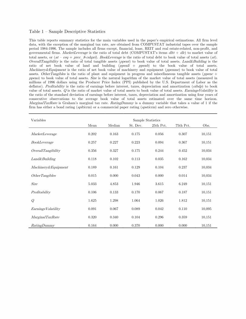
Table 1 — Sample Descriptive Statistics

This table reports summary statistics for the main variables used in the paper’s empirical estimations. All firm level data, with the exception of the marginal tax rate, are obtained from COMPUSTAT industrial tapes over the sample period 1984-1996. The sample includes all firms except, financial, lease, REIT and real estate-related, non-profit, and governmental firms. MarketLeverage is the ratio of total debt (COMPUSTAT’s items dltt + dlc) to market value of

total assets, or (at — ceq + prcc_fcshpri). BookLeverage is the ratio of total debt to book value of total assets (at). OverallTangibility is the ratio of total tangible assets (ppent) to book value of total assets. Land&Building is the ratio of net book value of land and building (ppenli + ppenb) to the book value of total assets. Machinery&Equipment is the ratio of net book value of machinery and equipment (ppenme) to book value of total assets. OtherTangibles is the ratio of plant and equipment in progress and miscellaneous tangible assets (ppenc + ppeno) to book value of total assets. Size is the natural logarithm of the market value of total assets (measured in millions of 1996 dollars using the Producer Price Index (PPI) published by the U.S. Department of Labor as the deflator). Profitability is the ratio of earnings before interest, taxes, depreciation and amortization (oibdp) to book value of total assets. Q is the ratio of market value of total assets to book value of total assets. EarningsVolatility is the ratio of the standard deviation of earnings before interest, taxes, depreciation and amortization using four years of consecutive observations to the average book value of total assets estimated over the same time horizon. MarginalTaxRate is Graham’s marginal tax rate. RatingDummy is a dummy variable that takes a value of 1 if the firm has either a bond rating (splticrm) or a commercial paper rating (spsticrm) and zero otherwise.

Variables Sample Statistics

Mean Median St. Dev. 25th Pct. 75th Pct. Obs.

MarketLeverage 0.202 0.163 0.175 0.056 0.307 10,151 BookLeverage 0.257 0.227 0.223 0.094 0.367 10,151 OverallTangibility 0.356 0.327 0.175 0.244 0.452 10,034 Land&Building 0.118 0.102 0.113 0.035 0.162 10,034 Machinery&Equipment 0.189 0.161 0.129 0.104 0.237 10,034 OtherTangibles 0.015 0.000 0.043 0.000 0.014 10,034 Size 5.033 4.853 1.946 3.615 6.249 10,151 Profitability 0.106 0.133 0.170 0.067 0.187 10,151 Q 1.625 1.298 1.064 1.026 1.812 10,151 EarningsVolatility 0.091 0.067 0.089 0.042 0.110 10,095 MarginalTaxRate 0.320 0.340 0.104 0.296 0.359 10,151 RatingDummy 0.164 0.000 0.370 0.000 0.000 10,151

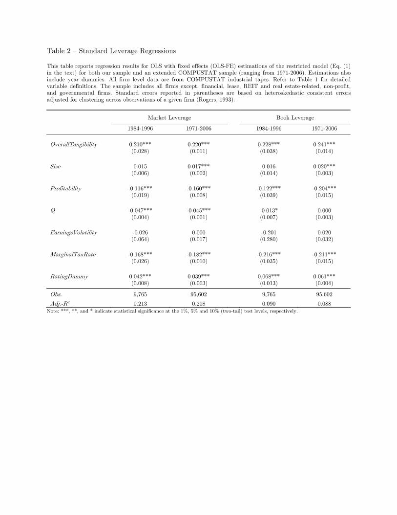
Table 2 — Standard Leverage Regressions This table reports regression results for OLS with fixed effects (OLS-FE) estimations of the restricted model (Eq. (1) in the text) for both our sample and an extended COMPUSTAT sample (ranging from 1971-2006). Estimations also include year dummies. All firm level data are from COMPUSTAT industrial tapes. Refer to Table 1 for detailed variable definitions. The sample includes all firms except, financial, lease, REIT and real estate-related, non-profit, and governmental firms. Standard errors reported in parentheses are based on heteroskedastic consistent errors adjusted for clustering across observations of a given firm (Rogers, 1993).

Market Leverage

Book Leverage

1984-1996 1971-2006 1984-1996 1971-2006

OverallTangibility 0.210*** 0.220***

0.228*** 0.241***

(0.028) (0.011) (0.038) (0.014)

Size 0.015 0.017***

0.016 0.020***

(0.006) (0.002) (0.014) (0.003)

Profitability -0.116*** -0.160***

-0.122*** -0.204***

(0.019) (0.008) (0.039) (0.015)

Q -0.047*** -0.045***

-0.013* 0.000

(0.004) (0.001) (0.007) (0.003)

EarningsVolatility -0.026 0.000

-0.201 0.020

(0.064) (0.017) (0.280) (0.032)

MarginalTaxRate -0.168*** -0.182***

-0.216*** -0.211***

(0.026) (0.010) (0.035) (0.015)

RatingDummy 0.042*** 0.039***

0.068*** 0.061***

(0.008) (0.003) (0.013) (0.004)

Obs. 9,765 95,602 9,765 95,602

Adj.-R2 0.213 0.208 0.090 0.088

Note: ***, **, and * indicate statistical significance at the 1%, 5% and 10% (two-tail) test levels, respectively.

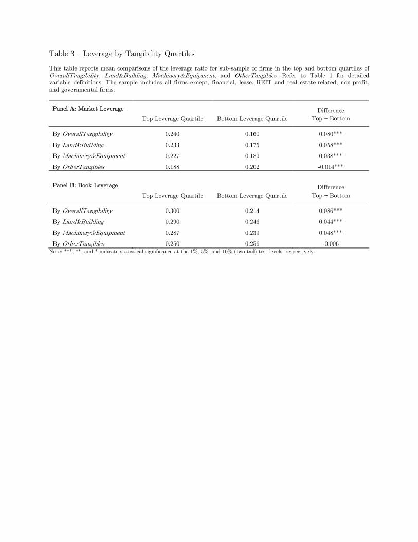
Table 3 — Leverage by Tangibility Quartiles This table reports mean comparisons of the leverage ratio for sub-sample of firms in the top and bottom quartiles of OverallTangibility, Land&Building, Machinery&Equipment, and OtherTangibles. Refer to Table 1 for detailed variable definitions. The sample includes all firms except, financial, lease, REIT and real estate-related, non-profit, and governmental firms.

Panel A: Market Leverage

Top Leverage Quartile

Bottom Leverage Quartile

Difference

Top − Bottom

By OverallTangibility 0.240 0.160 0.080***

By Land&Building 0.233 0.175 0.058***

By Machinery&Equipment 0.227 0.189 0.038***

By OtherTangibles 0.188 0.202 -0.014***

Panel B: Book Leverage

Top Leverage Quartile

Bottom Leverage Quartile

Difference

Top − Bottom

By OverallTangibility 0.300 0.214 0.086***

By Land&Building 0.290 0.246 0.044***

By Machinery&Equipment 0.287 0.239 0.048***

By OtherTangibles 0.250 0.256 -0.006

Note: ***, **, and * indicate statistical significance at the 1%, 5%, and 10% (two-tail) test levels, respectively.

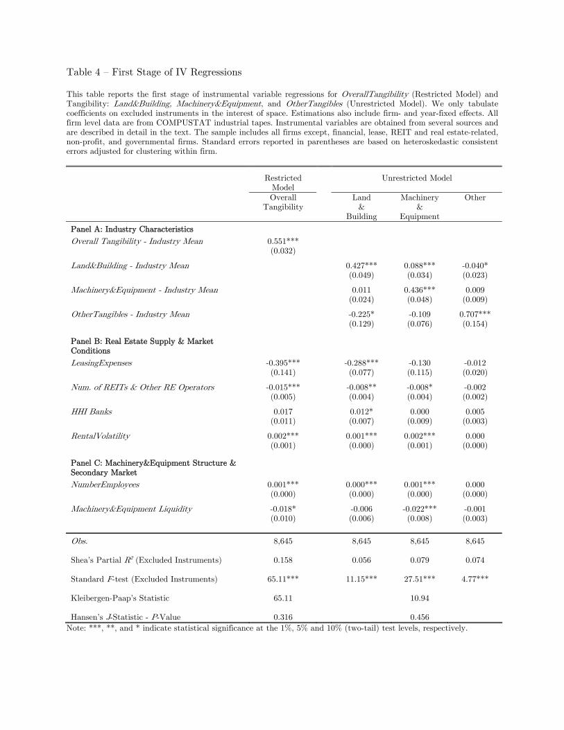
Table 4 — First Stage of IV Regressions

This table reports the first stage of instrumental variable regressions for OverallTangibility (Restricted Model) and Tangibility: Land&Building, Machinery&Equipment, and OtherTangibles (Unrestricted Model). We only tabulate coefficients on excluded instruments in the interest of space. Estimations also include firm- and year-fixed effects. All firm level data are from COMPUSTAT industrial tapes. Instrumental variables are obtained from several sources and are described in detail in the text. The sample includes all firms except, financial, lease, REIT and real estate-related, non-profit, and governmental firms. Standard errors reported in parentheses are based on heteroskedastic consistent errors adjusted for clustering within firm.

Restricted Model

Unrestricted Model

Overall Tangibility

Land &

Building

Machinery &

Equipment

Other

Panel A: Industry Characteristics

Overall Tangibility - Industry Mean 0.551*** (0.032)

Land&Building - Industry Mean 0.427*** 0.088*** -0.040* (0.049) (0.034) (0.023)

Machinery&Equipment - Industry Mean 0.011 0.436*** 0.009 (0.024) (0.048) (0.009)

OtherTangibles - Industry Mean -0.225* -0.109 0.707*** (0.129) (0.076) (0.154)

Panel B: Real Estate Supply & Market Conditions

LeasingExpenses -0.395*** -0.288*** -0.130 -0.012 (0.141) (0.077) (0.115) (0.020)

Num. of REITs & Other RE Operators -0.015*** -0.008** -0.008* -0.002 (0.005) (0.004) (0.004) (0.002)

HHI Banks 0.017 0.012* 0.000 0.005 (0.011) (0.007) (0.009) (0.003)

RentalVolatility 0.002*** 0.001*** 0.002*** 0.000 (0.001) (0.000) (0.001) (0.000)

Panel C: Machinery&Equipment Structure & Secondary Market

NumberEmployees 0.001*** 0.000*** 0.001*** 0.000 (0.000) (0.000) (0.000) (0.000)

Machinery&Equipment Liquidity -0.018* -0.006 -0.022*** -0.001 (0.010) (0.006) (0.008) (0.003)

Obs. 8,645 8,645 8,645 8,645 Shea’s Partial R2 (Excluded Instruments) 0.158 0.056 0.079 0.074 Standard F-test (Excluded Instruments) 65.11*** 11.15*** 27.51*** 4.77*** Kleibergen-Paap’s Statistic 65.11

10.94

Hansen’s J-Statistic - P-Value 0.316 0.456

Note: ***, **, and * indicate statistical significance at the 1%, 5% and 10% (two-tail) test levels, respectively.

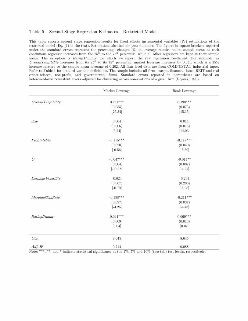
Table 5 — Second Stage Regression Estimates — Restricted Model

This table reports second stage regression results for fixed effects instrumental variables (IV) estimations of the restricted model (Eq. (1) in the text). Estimations also include year dummies. The figures in square brackets reported under the standard errors represent the percentage changes [%] in leverage relative to its sample mean as each continuous regressor increases from the 25th to the 75th percentile, while all other regressors are kept at their sample mean. The exception is RatingDummy, for which we report the raw regression coefficient. For example, as OverallTangibility increases from its 25th to its 75th percentile, market leverage increases by 0.051, which is a 25% increase relative to the sample mean leverage of 0.202. All firm level data are from COMPUSTAT industrial tapes. Refer to Table 1 for detailed variable definitions. The sample includes all firms except, financial, lease, REIT and real estate-related, non-profit, and governmental firms. Standard errors reported in parentheses are based on heteroskedastic consistent errors adjusted for clustering across observations of a given firm (Rogers, 1993).

Market Leverage

Book Leverage

OverallTangibility 0.251*** 0.190***

(0.055) (0.073)

[25.34] [15.15]

Size 0.004 0.014

(0.006) (0.015)

[5.24] [14.03]

Profitability -0.115*** -0.118***

(0.020) (0.040)

[-6.56] [-5.30]

Q -0.047*** -0.014**

(0.004) (0.007)

[-17.78] [-4.27]

EarningsVolatility -0.024 -0.231

(0.067) (0.296)

[-0.79] [-5.98]

MarginalTaxRate -0.158*** -0.211***

(0.027) (0.037)

[-4.26] [-4.46]

RatingDummy 0.044*** 0.069***

(0.009) (0.013)

[0.04] [0.07]

Obs. 8,645 8,645 Adj.-R2 0.214 0.088

Note: ***, **, and * indicate statistical significance at the 1%, 5% and 10% (two-tail) test levels, respectively.

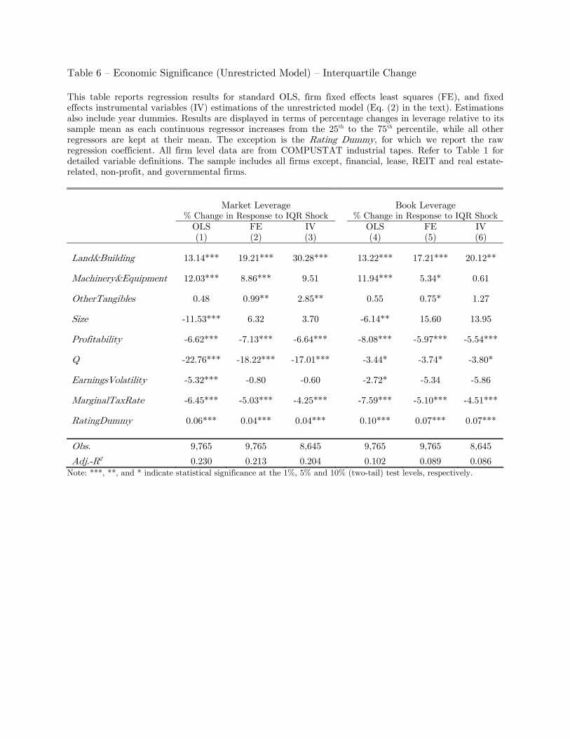
Table 6 — Economic Significance (Unrestricted Model) — Interquartile Change

This table reports regression results for standard OLS, firm fixed effects least squares (FE), and fixed effects instrumental variables (IV) estimations of the unrestricted model (Eq. (2) in the text). Estimations also include year dummies. Results are displayed in terms of percentage changes in leverage relative to its sample mean as each continuous regressor increases from the 25th to the 75th percentile, while all other regressors are kept at their mean. The exception is the Rating Dummy, for which we report the raw regression coefficient. All firm level data are from COMPUSTAT industrial tapes. Refer to Table 1 for detailed variable definitions. The sample includes all firms except, financial, lease, REIT and real estate-related, non-profit, and governmental firms.

Market Leverage

% Change in Response to IQR Shock

Book Leverage

% Change in Response to IQR Shock

OLS (1)

FE (2)

IV (3)

OLS (4)

FE (5)

IV (6)

Land&Building 13.14*** 19.21*** 30.28***

13.22*** 17.21*** 20.12**

Machinery&Equipment 12.03*** 8.86*** 9.51

11.94*** 5.34* 0.61

OtherTangibles 0.48 0.99** 2.85**

0.55 0.75* 1.27

Size -11.53*** 6.32 3.70

-6.14** 15.60 13.95

Profitability -6.62*** -7.13*** -6.64***

-8.08*** -5.97*** -5.54***

Q -22.76*** -18.22*** -17.01***

-3.44* -3.74* -3.80*

EarningsVolatility -5.32*** -0.80 -0.60

-2.72* -5.34 -5.86

MarginalTaxRate -6.45*** -5.03*** -4.25***

-7.59*** -5.10*** -4.51***

RatingDummy 0.06*** 0.04*** 0.04***

0.10*** 0.07*** 0.07***

Obs. 9,765 9,765 8,645 9,765 9,765 8,645

Adj.-R2 0.230 0.213 0.204 0.102 0.089 0.086

Note: ***, **, and * indicate statistical significance at the 1%, 5% and 10% (two-tail) test levels, respectively.

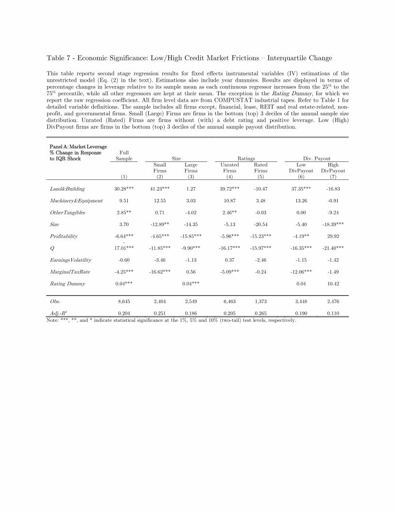
Table 7 - Economic Significance: Low/High Credit Market Frictions — Interquartile Change This table reports second stage regression results for fixed effects instrumental variables (IV) estimations of the unrestricted model (Eq. (2) in the text). Estimations also include year dummies. Results are displayed in terms of percentage changes in leverage relative to its sample mean as each continuous regressor increases from the 25th to the 75th percentile, while all other regressors are kept at their mean. The exception is the Rating Dummy, for which we report the raw regression coefficient. All firm level data are from COMPUSTAT industrial tapes. Refer to Table 1 for detailed variable definitions. The sample includes all firms except, financial, lease, REIT and real estate-related, non-profit, and governmental firms. Small (Large) Firms are firms in the bottom (top) 3 deciles of the annual sample size distribution. Unrated (Rated) Firms are firms without (with) a debt rating and positive leverage. Low (High) DivPayout firms are firms in the bottom (top) 3 deciles of the annual sample payout distribution.

Panel A: Market Leverage % Change in Response to IQR Shock

Full Sample

Size

Ratings

Div. Payout

(1)

Small Firms (2)

Large Firms (3)

Unrated Firms (4)

Rated Firms (5)

Low DivPayout

(6)

High DivPayout

(7)

Land&Building 30.28***

41.23*** 1.27

39.72*** -10.47

37.35*** -16.83

Machinery&Equipment 9.51

12.55 3.03

10.87 3.48

13.26 -0.91

OtherTangibles 2.85**

0.71 -4.02

2.46** -0.03

0.00 -9.24

Size 3.70

-12.89** -14.35

-5.13 -20.54

-5.40 -18.39***

Profitability -6.64***

-4.65*** -15.85***

-5.96*** -15.23***

-4.19** 29.92

Q

-17.01***

-11.85*** -9.90***

-16.17*** -15.97***

-16.35*** -21.40***

EarningsVolatility -0.60

-3.46 -1.13

0.37 -2.46

-1.15 -1.42

MarginalTaxRate -4.25***

-16.62*** 0.56

-5.09*** -0.24

-12.06*** -1.49

Rating Dummy 0.04***

0.04***

0.04 10.42

Obs. 8,645

2,404 2,549

6,463 1,373

3,448 2,476 Adj.-R2 0.204

0.251 0.186

0.205 0.265

0.190 0.110

Note: ***, **, and * indicate statistical significance at the 1%, 5% and 10% (two-tail) test levels, respectively.

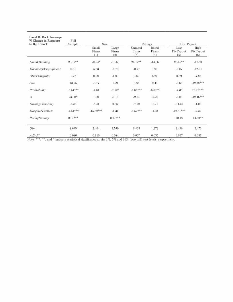
Panel B: Book Leverage % Change in Response to IQR Shock

Full Sample

Size

Ratings

Div. Payout

Small Firms (1)

Large Firms (2)

Unrated Firms (3)

Rated Firms (4)

Low DivPayout

(5)

High DivPayout

(6)

Land&Building 20.12**

28.94* -18.66

26.12** -14.66

28.56** -17.80

Machinery&Equipment 0.61

5.83 -5.73

-0.77 1.94

-0.87 -12.01

OtherTangibles 1.27

0.98 -1.89

0.69 6.22

0.89 -7.85

Size 13.95

-6.77 1.29

5.83 2.44

-3.65 -12.38***

Profitability -5.54***

-4.81 -7.62*

-5.65*** -6.89**

-4.38 76.76***

Q -3.80*

1.98 -3.16

-2.04 -2.70

-0.85 -12.46***

EarningsVolatility -5.86

-8.41 0.36

-7.99 -2.71

-11.39 -1.02

MarginalTaxRate -4.51***

-15.82*** -1.31

-5.52*** -1.03

-12.81*** -2.32

RatingDummy 0.07***

0.07***

20.18 14.50**

Obs. 8,645

2,404 2,549

6,463 1,373

3,448 2,476 Adj.-R2 0.086

0.110 0.084

0.067 0.035

0.057 0.037

Note: ***, **, and * indicate statistical significance at the 1%, 5% and 10% (two-tail) test levels, respectively.

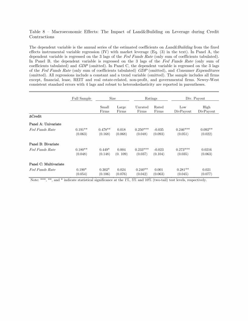
Table 8 — Macroeconomic Effects: The Impact of Land&Building on Leverage during Credit Contractions

The dependent variable is the annual series of the estimated coefficients on Land&Building from the fixed effects instrumental variable regression (IV) with market leverage (Eq. (3) in the text). In Panel A, the dependent variable is regressed on the 3 lags of the Fed Funds Rate (only sum of coefficients tabulated). In Panel B, the dependent variable is regressed on the 3 lags of the Fed Funds Rate (only sum of coefficients tabulated) and GDP (omitted). In Panel C, the dependent variable is regressed on the 3 lags of the Fed Funds Rate (only sum of coefficients tabulated) GDP (omitted), and Consumer Expenditures (omitted). All regressions include a constant and a trend variable (omitted). The sample includes all firms except, financial, lease, REIT and real estate-related, non-profit, and governmental firms. Newey-West consistent standard errors with 4 lags and robust to heteroskedasticity are reported in parentheses.

Full Sample

Size

Ratings

Div. Payout

Small Firms

Large Firms

Unrated Firms

Rated Firms

Low

DivPayout

High

DivPayout

Credit

Panel A: Univariate

Fed Funds Rate 0.191** 0.478** 0.018 0.250*** -0.035 0.246*** 0.092**

(0.063) (0.168) (0.068) (0.048) (0.093) (0.051) (0.022)

Panel B: Bivariate

Fed Funds Rate 0.180** 0.449* 0.004 0.233*** -0.023 0.273*** 0.0216

(0.048) (0.148) (0. 109) (0.037) (0.104) (0.035) (0.063)

Panel C: Multivariate

Fed Funds Rate 0.190* 0.302* 0.024 0.240** 0.001 0.281** 0.021

(0.054) (0.106) (0.076) (0.042) (0.063) (0.045) (0.077)

Note: ***, **, and * indicate statistical significance at the 1%, 5% and 10% (two-tail) test levels, respectively.

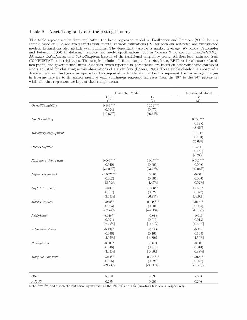
Table 9 — Asset Tangibility and the Rating Dummy

This table reports results from replicating the basic regression model in Faulkender and Petersen (2006) for our sample based on OLS and fixed effects instrumental variable estimations (IV) for both our restricted and unrestricted models. Estimations also include year dummies. The dependent variable is market leverage. We follow Faulkender and Petersen (2006) in defining variables and model specifications but in Column 3 we use our Land&Building, Machinery&Equipment and OtherTangibles instead of the traditional tangibility proxy. All firm level data are from COMPUSTAT industrial tapes. The sample includes all firms except, financial, lease, REIT and real estate-related, non-profit, and governmental firms. Standard errors reported in parentheses are based on heteroskedastic consistent errors adjusted for clustering across observations of a given firm (Rogers, 1993). To resemble closely the impact of a dummy variable, the figures in square brackets reported under the standard errors represent the percentage changes in leverage relative to its sample mean as each continuous regressor increases from the 10th to the 90th percentile, while all other regressors are kept at their sample mean.

Restricted Model Unrestricted Model

OLS (1)

IV (2)

IV (3)

OverallTangibility 0.189*** 0.262***

(0.024) (0.070)

[40.67%] [56.52%]

Land&Building 0.393***

(0.125)

[48.46%]

Machinery&Equipment 0.191*

(0.100)

[25.68%]

OtherTangibles 0.357*

(0.187)

[7.28%]

Firm has a debt rating 0.069*** 0.047*** 0.045***

(0.010) (0.009) (0.009)

[34.00%] [23.07%] [22.06%]

Ln(market assets) -0.007*** 0.001 -0.000

(0.002) (0.006) (0.006)

[-18.53%] [2.45%] [-0.02%]

Ln(1 + firm age) -0.006 0.066** 0.059**

(0.007) (0.027) (0.027)

[-2.64%] [26.89%] [23.9%]

Market-to-book -0.065*** -0.048*** -0.047***

(0.003) (0.004) (0.004)

[-57.74%] [-42.93%] [-41.87%]

R&D/sales -0.049** -0.013 -0.013

(0.021) (0.013) (0.013)

[-2.27%] [-0.61%] [-0.60%]

Advertising/sales -0.139* -0.225 -0.214

(0.076) (0.161) (0.163)

[-2.97%] [-4.80%] [-4.56%]

Profits/sales -0.030* -0.009 -0.008

(0.016) (0.010) (0.010)

[-3.44%] [-0.96%] [-0.88%]

Marginal Tax Rate -0.274*** -0.216*** -0.218***

(0.036) (0.026) (0.027)

[-39.28%] [-30.97%] [-31.23%]

Obs. 8,638 8,638 8,638

Adj.-R2 0.235 0.206 0.200

Note: ***, **, and * indicate statistical significance at the 1%, 5% and 10% (two-tail) test levels, respectively.

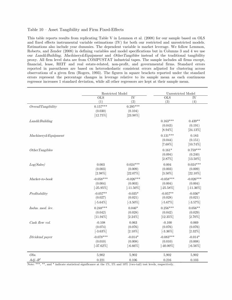
Table 10 — Asset Tangibility and Firm Fixed-Effects

This table reports results from replicating Table V in Lemmon et al. (2008) for our sample based on OLS and fixed effects instrumental variable estimations (IV) for both our restricted and unrestricted models. Estimations also include year dummies. The dependent variable is market leverage. We follow Lemmon, Roberts, and Zender (2008) in defining variables and model specifications but in Columns 3 and 4 we use our Land&Building, Machinery&Equipment and OtherTangibles instead of the traditional tangibility proxy. All firm level data are from COMPUSTAT industrial tapes. The sample includes all firms except, financial, lease, REIT and real estate-related, non-profit, and governmental firms. Standard errors reported in parentheses are based on heteroskedastic consistent errors adjusted for clustering across observations of a given firm (Rogers, 1993). The figures in square brackets reported under the standard errors represent the percentage changes in leverage relative to its sample mean as each continuous regressor increases 1 standard deviation, while all other regressors are kept at their sample mean.

Restricted Model Unrestricted Model

OLS (1)

IV (2)

OLS (3)

IV (4)

OverallTangibility 0.157*** 0.295***

(0.030) (0.104)

[12.75%] [23.98%]

Land&Building 0.163*** 0.439**

(0.043) (0.191)

[8.94%] [24.13%]

Machinery&Equipment 0.131*** 0.183

(0.044) (0.151)

[7.68%] [10.74%]

OtherTangibles 0.161* 0.759***

(0.094) (0.240)

[2.87%] [13.50%]

Log(Sales) 0.003 0.024*** 0.004 0.024***

(0.003) (0.009) (0.003) (0.009)

[2.98%] [22.07%] [3.50%] [22.10%]

Market-to-book -0.058*** -0.026*** -0.058*** -0.026***

(0.004) (0.003) (0.004) (0.004)

[-25.95%] [-11.50%] [-25.58%] [-11.36%]

Profitability -0.057** -0.035* -0.057** -0.036* (0.027) (0.021) (0.028) (0.021)

[-5.64%] [-3.50%] [-5.67%] [-3.57%]

Indus. med. lev. 0.248*** 0.046* 0.256*** 0.056**

(0.042) (0.028) (0.042) (0.029)

[11.94%] [2.24%] [12.35%] [2.70%]

Cash flow vol. -0.108 0.063 -0.100 0.069

(0.074) (0.076) (0.076) (0.076)

[-3.63%] [2.10%] [-3.36%] [2.32%]

Dividend payer -0.078*** -0.014* -0.083*** -0.014*

(0.010) (0.008) (0.010) (0.008)

[-37.62%] [-6.66%] [-40.00%] [-6.56%]

Obs. 5,902 5,902 5,902 5,902

Adj.-R2 0.221 0.106 0.216 0.103

Note: ***, **, and * indicate statistical significance at the 1%, 5% and 10% (two-tail) test levels, respectively.