Asset returns, news topics, and media effects - Norges Bank

Asset returns, news topics, and media effects

NORGES BANKRESEARCH

17 | 2017

VEGARD H. LARSENANDLEIF ANDERS THORSRUD

WORKING PAPER

NORGES BANK

WORKING PAPERXX | 2014

RAPPORTNAVN

2

Working papers fra Norges Bank, fra 1992/1 til 2009/2 kan bestilles over e-post: [email protected]

Fra 1999 og senere er publikasjonene tilgjengelige på www.norges-bank.no Working papers inneholder forskningsarbeider og utredninger som vanligvis ikke har fått sin endelige form. Hensikten er blant annet at forfatteren kan motta kommentarer fra kolleger og andre interesserte. Synspunkter og konklusjoner i arbeidene står for forfatternes regning.

Working papers from Norges Bank, from 1992/1 to 2009/2 can be ordered by e-mail:[email protected]

Working papers from 1999 onwards are available on www.norges-bank.no

Norges Bank’s working papers present research projects and reports (not usually in their final form) and are intended inter alia to enable the author to benefit from the comments of colleagues and other interested parties. Views and conclusions expressed in working papers are the responsibility of the authors alone.

ISSN 1502-819-0 (online) ISBN 978-82-7553-999-9 (online)

Asset returns, news topics, and media effects∗

Vegard H. Larsen† Leif Anders Thorsrud‡

September 19, 2017

Abstract

We decompose the textual data in a daily Norwegian business newspaper into

news topics and investigate their predictive and causal role for asset prices. Our

three main findings are: (1) a one unit innovation in the news topics predict roughly

a 1 percentage point increase in close-to-open returns and significant continuation

patterns peaking at 4 percentage points after 15 business days, with little sign of

reversal; (2) simple zero-cost news-based investment strategies yield significant an-

nualized risk-adjusted returns of up to 20 percent; and (3) during a media shortage,

due to an exogenous strike, returns for firms particularly exposed to our news mea-

sure experience a substantial fall. Our estimates suggest that between 20 to 40

percent of the news topics’ predictive power is due to the causal media effect. To-

gether these findings lend strong support for a rational attention view where the

media alleviate information frictions and disseminate fundamental information to a

large population of investors.

JEL-codes: C5, C8, G4, G12

Keywords: Stock returns, News, Machine learning, Latent Dirichlet Allocation (LDA)

∗This Working Paper should not be reported as representing the views of Norges Bank. The views

expressed are those of the authors and do not necessarily reflect those of Norges Bank. We thank Farooq

Akram, Andre K. Anundsen, Drago Bergholt, Hilde C. Bjørnland, Jon Fiva, Hashem Pesaran, Johannes

Skjeltorp, Rune Sorensen, Mike West, and colleagues at BI and Norges Bank for valuable comments.

This work is part of the research activities at the Centre for Applied Macro and Petroleum Economics

(CAMP) at the BI Norwegian Business School.†Centre for Applied Macro and Petroleum Economics, BI Norwegian Business School, and Norges

Bank. Email: [email protected]‡Centre for Applied Macro and Petroleum Economics, BI Norwegian Business School, and Norges

Bank. Email: [email protected]

1

1 Introduction

Can news in a business newspaper explain daily returns, and what is the effect of the media

itself? To the extent that new information is broadcasted through the media, and inter-

preted through the lens of classical economic theory, the answer to the first question should

be an unambiguously yes. Asset prices should respond to new information. However, as

exemplified by Roll (1988), the economic literature has had a hard time finding a robust

relationship between stock prices and news. This has led to alternative explanations,

like irrational noise trading and the revelation of private information through trading,

for understanding stock price movements (see, e.g., Shiller (1981), Campbell (1991), and

Tetlock (2007)). Below we suggest an alternative explanation, echoing the one given in

Boudoukh et al. (2013), namely that the finance literature simply has been doing a poor

job of identifying relevant news. On the other hand, in a world where arbitrage forces

were unlimited one could argue that new information should be incorporated into prices

as soon as it is made public and before the (mass) media have time to report it. Ac-

cording to this view, evidence of non-predictability is as expected. Still, even though the

news reported might not be genuine new information in itself, news broadcasted through

the media might matter because it can reach a broad population of investors, alleviate

informational frictions, and contribute to gradual diffusion of information (Peress (2014)).

However, establishing causal link from the media to financial markets is difficult, because

one has to separate the new information component from the effect of the ether.

In this paper we offer new insights regarding the relationship between news, returns,

and the media. We informally assume a rational attention view where investors faced with

information processing costs, or limited cognitive ability, potentially learn about economic

developments important for multiple stocks through the media (Peng and Xiong (2006),

Kacperczyk et al. (2009), and Schmidt (2013)). We operationalize this view by decom-

posing the textual information in a business newspaper into different types of news about

economic developments, and analyze market responses to these news items. In particu-

lar, we use a Latent Dirichlet Allocation model (Blei et al. (2003)), proven to summarize

textual data in much the same manner as humans would do (Chang et al. (2009)), to

decompose the textual information in the major business newspaper in Norway into news

topics. We then construct series representing how much, and in which tone, each topic

is written about in the newspaper across time, where news topics are tone adjusted, i.e.,

classified as either positive or negative news, using a dictionary-based approach commonly

applied in the literature (see, e.g., Tetlock (2007), Loughran and Mcdonald (2011)). Fi-

nally, the resulting news topic time series are linked to a large cross section of companies

listed on the Oslo Stock Exchange between 1996-2014.

Our hypothesis is simple: To the extent that the newspaper provides a relevant de-

2

scription of the economy, the more intensive a given topic is represented in the newspaper

at a given point in time, the more likely it is that this topic represents something of impor-

tance for the economy’s current and future needs and developments. As such, it should

also move stock prices. For example, we hypothesize that when the newspaper writes

extensively about developments in, e.g., the oil sector, and the tone is positive, it reflects

that something is happening in this sector that potentially has positive economy-wide

effects, and especially for firms related to the oil sector.

The newspaper content is available in the morning, at least two hours prior to the

when the market opens. Controlling for lagged returns, time- and firm-fixed effects, and

other well known predictors, numerous regressions show that a one unit positive innova-

tion in the news predicts roughly a 1 percentage point increase in close-to-open returns,

and 1.5 percentage points increase in close-to-close returns. In the days following the

initial news release, the effect accumulates further, suggesting a significant continuation

pattern peaking at 4 percentage points after 15 business days, with little sign of reversal.

To gauge the robustness and economic significance of these pooled time series regres-

sions we implement simple zero-cost news-based investment strategies yielding significant

annualized risk-adjusted returns (Alpha) of up to 20 percent.

By exploiting an exogenous strike in the Norwegian newspaper market in 2002 we

are, under the assumption that new information is released also during the strike period

(although not through the mass media), able to isolate the media component of the news

signal from the new information component. Unconditionally, the cross sectional average

return falls by roughly 60 basis points during the strike period relative to the periods

before and after the strike. Conditioning on how exposed the various firms are to our

news measure during the year prior to the strike, we find significant differences in mean

returns of the same magnitude: Returns for individual firms with a significant exposure to

our news measures fall by 57 basis points during the strike period relative to firms with an

insignificant news topic exposure. Thus, the DN news topics seem to be representative for

the total causal media effect. Since the average firm in the sample has a positive exposure

to news, our results imply that the media component of the news signal accounts for

between 20 to 40 percent of the documented overall predictive effect of news topics.

Compared with existing studies in the financial literature using textual data to un-

derstand asset prices, the novelty of our approach relates to the usage of news topics and

how we relate them to firms. Each topic is a distribution of words, and together the

topics summarizes the words and articles in the business newspaper into interpretable

factors that we use to capture the continuously evolving narrative about economic con-

ditions. Individual news topics are subsequently linked to companies using their textual

description provided by Reuters. For example, a news topic that contains words mostly

3

associated with the oil market will be linked to an oil company if the textual description

of this company contains many of the same words. In contrast, typical textual approaches

applied in the asset pricing literature link companies to items in the news using explicit

mentioning of their names, abbreviations, or other firm specific characteristics, and con-

duct event studies to uncover how stock prices respond to news. To us, this seems like an

overly restrictive approach inasmuch many news items might be relevant for stock prices

without explicitly mentioning, e.g, company names. Consequently, in our setup, all days

are news days, but to varying degree, and we avoid “dredging for anomalies”, which is

Fama’s phrase for conducting event studies of different event types until one finds an

apparent market inefficiency (Fama (1998, p. 287)).

The validity of our approach for linking news to firms is tested when we randomly

assign news topics to firms, and find that no significant predictive power between news

and returns can be established in this case. We also show that our results are not driven

by well known industry or day-of-the-week effects, and that they are not associated with

firm characteristics like book-to-market value, size, or liquidity. When analyzing the

news-return relationship across three different sub-samples, we do, however, find that the

relationship becomes largely insignificant for the latter part of the sample (2008-2014).

Interestingly, this loss of significance is alleviated when we expand the breadth of news

sources utilized, suggesting that a broad-based news corpus needs to be applied to capture

informative news signals in today’s markets.

In sum, our results lend significant support towards classical efficient market based

theories where new information should predict subsequent returns. Our results also speak

to the growing literature documenting behavioral biases or rational attention, where in-

vestors only partially adjust to real information. The fact that we find significant con-

tinuation patterns following news innovations, as opposed to reversal, suggests that our

methodology correctly parses out fundamental information, and that the media is an

important channel for such information diffusion.

Our study contributes to two different strands of the financial literature. First, we

relate to a large number of studies using textual information to explain and predict

stock price movements. Prominent examples include Antweiler and Frank (2004), Tetlock

(2007), and Garcia (2013), while Tetlock (2014), Kearney and Liu (2014), and Loughran

and Mcdonald (2016) provide recent literature overviews. While a large share of these

studies use textually derived sentiment indicators, finding weak evidence of predictability,

evidence saying that only negative news matters, and reversal patterns following news

releases, we find relatively strong evidence towards predictability and clear continuation

patterns when focusing on news topics. Interestingly, Boudoukh et al. (2013) also find

that once news is identified by its type (topic), there is a considerably stronger rela-

4

tionship between news and returns than what is commonly found. However, while the

approach taken in Boudoukh et al. (2013) relies on a substantial number of hard coded

rules for classifying the news, our approach utilizes a fully automated machine learning

algorithm. As such, our methodology is closer to those implemented in Antweiler and

Frank (2006) and Calomiris and Mamaysky (2017), who use a Naıve Bayes classifier and

the Louvain method to derive news topics, respectively. We differ in that we do not limit

ourself to an event study approach, and by considering individual company returns on a

daily frequency.1

Second, our study belongs to a smaller group of studies establishing the causal role of

the media in financial markets (see, in particular, Engelberg and Parsons (2011), Dougal

et al. (2012), and Peress (2014)). In fact, we use the same exogenous strike as identified in

Peress (2014) (for the Norwegian market) to disentangle the new information and media

effect of the news signal. Novel to our study is that we are able to provide an estimate of

the relative importance of the media effect in a given predictive relationship. In terms of

interpreting the results and the underlying mechanisms through which the media might be

important, Dougal et al. (2012) appeal to a sentiment story, while Peress (2014) provide

an information dissemination explanation. The latter is also what we document. However,

Peress (2014) argues that the strike likely increased the cost of accessing information and

led individual stocks to move more in synch, while our findings suggest that investors also

looked for other opportunities when a primary media channel fell out, thus taking aboard

the cost of seeking additional and new information. There are clear patterns in the data,

although not statistically strong, suggesting that such strike-induced behavior result in

more noise trading.

More generally, this study relates to a growing literature in economics where textual,

or non-quantitative, information is used to explain economic fluctuations. It is especially

noteworthy that when we use the same news topics as here, we find that news predicts

quarterly productivity, consumption, and aggregate stock market developments (Larsen

and Thorsrud (2015)). Thus, expectations about future cash flows are likely impounded

in the news topic signal (Fama (1990)).

The rest of this paper is organized as follows. Section 2 describes the data, the topic

model, and how we link news to firms. Section 3 establishes that news topics explain

returns, while Section 4 investigates the causal impact of the media. Section 5 concludes.

1Calomiris and Mamaysky (2017) use various decompositions of news articles to predict monthly and

yearly risk and return developments in 51 aggregate stock markets. Antweiler and Frank (2006) run an

event study covering U.S. stocks and Wall Street Journal corporate news stories.

5

2 Data

Our raw data consist of a long sample of the entire newspaper corpus for a daily business

newspaper in Norway, and a large panel of daily information for firms listed on the Oslo

Stock Exchange. Although the Norwegian stock market is relatively small compared

to international markets,2 we focus on the case of Norway because it allows us to use

a long history of the entire publications from the country’s most important business

newspaper, and we can utilize a well defined exogenous strike in the newspaper market

(in 2002) to investigate the causal link from the media to financial markets. Moreover,

small economies, like Norway, typically have only one or two business newspapers, making

the corpus from one newspaper more representative for the mass media as a whole than

in countries where the media landscape is much more diverse. Here, we simply choose the

corpus associated with the largest and most read business newspaper, Dagens Næringsliv

(DN), noting that DN is also the fourth largest newspaper in Norway irrespective of

subject matter.

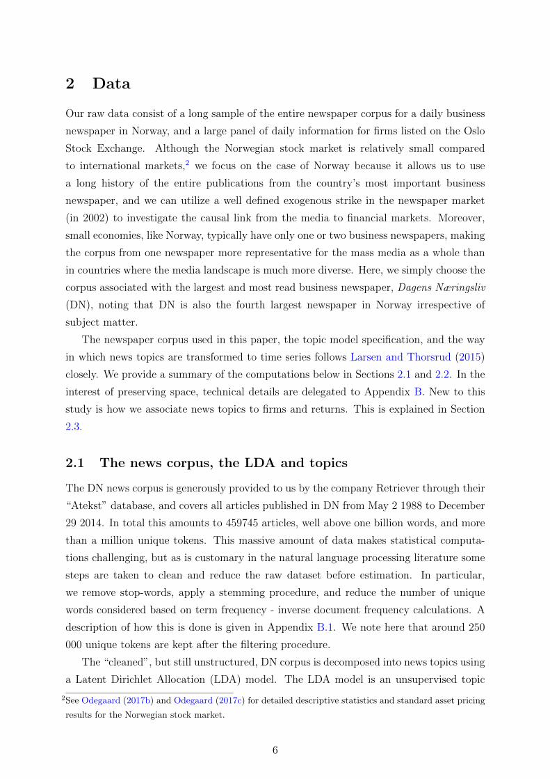
The newspaper corpus used in this paper, the topic model specification, and the way

in which news topics are transformed to time series follows Larsen and Thorsrud (2015)

closely. We provide a summary of the computations below in Sections 2.1 and 2.2. In the

interest of preserving space, technical details are delegated to Appendix B. New to this

study is how we associate news topics to firms and returns. This is explained in Section

2.3.

2.1 The news corpus, the LDA and topics

The DN news corpus is generously provided to us by the company Retriever through their

“Atekst” database, and covers all articles published in DN from May 2 1988 to December

29 2014. In total this amounts to 459745 articles, well above one billion words, and more

than a million unique tokens. This massive amount of data makes statistical computa-

tions challenging, but as is customary in the natural language processing literature some

steps are taken to clean and reduce the raw dataset before estimation. In particular,

we remove stop-words, apply a stemming procedure, and reduce the number of unique

words considered based on term frequency - inverse document frequency calculations. A

description of how this is done is given in Appendix B.1. We note here that around 250

000 unique tokens are kept after the filtering procedure.

The “cleaned”, but still unstructured, DN corpus is decomposed into news topics using

a Latent Dirichlet Allocation (LDA) model. The LDA model is an unsupervised topic

2See Odegaard (2017b) and Odegaard (2017c) for detailed descriptive statistics and standard asset pricing

results for the Norwegian stock market.

6

model that clusters words into topics, which are distributions over words, while at the

same time classifying articles as mixtures of topics. By unsupervised learning algorithm

we mean an algorithm that can learn/discover an underlying structure in the data without

the algorithm being given any labeled samples to learn from. The term “latent” is used

because the words, which are the observed data, are intended to communicate a latent

structure, namely the meaning of the article. The term “Dirichlet” is used because the

topic mixture is drawn from a conjugate Dirichlet prior. As such, the LDA shares many

features with latent (Gaussian) factor models used in conventional econometrics, but

with factors (representing topics) constrained to live in the simplex and fed through

a multinomial likelihood at the observation equation. A richer description and more

technical details of the LDA is provided in Appendix B.2. Here we note that we classify

the DN corpus intoK = 80 different topics using a Gibbs sampling algorithm. AlthoughK

might seem somewhat arbitrary chosen, statistical tests conducted in Larsen and Thorsrud

(2015) confirm that 80 topics give a good description of the corpus.

The LDA estimation procedure does not give the topics any name or label. To do

so, labels are subjectively given to each topic based on the most important words associ-

ated with each topic. As shown in Table 7, in Appendix A, which lists all the estimated

topics together with the most important words associated with each topic, it is, in most

cases, conceptually simple to classify them. The labeling plays no material role in the

experiment, it just serves as a convenient way of referring to the different topics instead

of using, e.g., topic numbers or long lists of words. What is more interesting, however, is

whether the LDA decomposition gives a meaningful and easily interpretable topic classi-

fication of the DN newspaper. As illustrated in Figure 4, in Appendix A, it does: The

topic decomposition reflects how DN structures its content, with distinct sections for par-

ticular themes, and that DN is a Norwegian newspaper writing about news of particular

relevance for Norway. We observe, for example, separate topics for Norway’s immedi-

ate Nordic neighbors (Nordic countries); largest trading partners (EU and Europe); and

biggest and second biggest exports (Oil production and Fishing). A richer discussion

about this decomposition is provided in Larsen and Thorsrud (2015).

2.2 News topics as time series

Given knowledge of the topics (and their word distributions), the topic decompositions are

translated into time series. This is done in two steps, which are described in greater detail

in Appendix B.3 and B.4. In short, we first collapse all the articles in the newspaper for

a particular day into one document, and compute, using the estimated word distribution

for each topic, the topic frequencies for this newly formed document. This yields a set of

K daily time series, where each represent how much (in percent) a given topic is written

7

about for a given day. Then, for each observation in these time series we identify their

sign, i.e., whether or not the news is positive or negative. For each topic, this is done at

the article level: For every daily observation, we find the article in the newspaper that

is best explained by the topic. The tone of this article is identified using an external

word list and simple word counts. The word list used here takes as a starting point

the classification of positive/negative words defined by the Harvard IV-4 Psychological

Dictionary, and then translates the words to Norwegian. The count procedure delivers

two statistics, containing the number of positive and negative words. These statistics are

then normalized such that each observation reflects the fraction of positive and negative

words and subtracted from each other. If the difference is negative (positive), we set the

sign equal to -1 (1), and adjust the topic frequencies accordingly.

We note that this procedure explicitly uses the output from the topic model also when

defining the sign of the news, and that different topics might get their sign defined from

the same article. We have experimented with other ways of identifying the sign of the topic

frequencies, finding that the method outlined above seems to work the best in a number

of different applications (Thorsrud (2016a), Thorsrud (2016b), and Larsen (2017)).3

2.3 Financial data and linking news to firms

We obtain daily data for all firms listed on the Oslo Stock Exchange from Reuters Datas-

tream. For each firm, we collect both open and close prices, and compute (log) close-to-

open (c2o), open-to-close (o2c), and close-to-close (c2c) daily returns. We also collect the

commonly used predictors (log) book-to-market (B/M), (log) market value (MV ), and

turnover (Turn), where the latter is computed by dividing the total number of shares

traded by the number of shares outstanding. In addition we use three measures of ob-

served common time-fixed effects, namely (log) close-to-close returns on the Oslo Stock

Exchange Benchmark index (Rmh), the close-to-close return on the S&P500 (Rmi), and

the daily (log) change in the price of oil (Roil).4 Stocks listed for less than half a year

are removed from the sample. To avoid including extreme price observations associated

with listing and de-listing of firms, we exclude the first and last week of each firm’s return

observations. In total we are left with 233 individual firms. The full sample stretches

3We have also used the word list suggested by Loughran and Mcdonald (2011) as a starting point for

classifying positive/negative words, finding that this does not alter the end result by much. Still, there

are undoubtedly more sophisticated methods that can be applied to identify the tone of the news (see,

e.g., Pang et al. (2002)).4As roughly 50 percent of Norway’s exports are linked to petroleum products and a large share of the

companies traded on the Oslo Stock Exchange are directly exposed to the oil sector, controlling for the

price of oil in asset pricing equations is often done when working with Norwegian data (see, e.g., Næs

et al. (2009)).

8

from 1996 to 2014, but only a few stocks are traded throughout the whole sample period.

To link companies to news, we use the word distributions estimated from the news

corpus and each firm’s textual description provided by Reuters. On average, across firms,

the textual description is roughly a half-page description of what each company’s primary

business is. The firms textual description are then classified using a procedure for querying

documents outside the set on which the LDA is estimated (Heinrich (2009) and Hansen

et al. (2014)). This corresponds to using the LDA model on the firm descriptions, but

with the difference that the sampler is run with the estimated word distributions from the

newspaper corpus held constant (see Appendix B.3). The end product of this procedure

are vectors with topic probabilities for each firm description. From these vectors we map

firms with topics using the topic with the highest weight (probability) in describing the

firm’s core business.

An example helps illustrating our procedure. The first three, out of 10, sentences

describing the firm Frontline reads:

Frontline Ltd. is a shipping company. The Company is engaged in the own-

ership and operation of oil tankers. The Company operates oil tankers of

two sizes: very large crude carriers (VLCCs), which are between 200,000 and

320,000 deadweight tons, and Suezmax tankers, which are vessels between

120,000 and 170,000 deadweight tons...

Following the steps described above, the elements with highest value in the vector with

topic probabilities for this firm description are Shipping, Airline industry, and Foreign,

with weights 0.31, 0.06, and 0.02, respectively. Thus, we associate Frontline with the

Shipping topic. As seen from the word cloud for this topic, Figure 1, the sentences and

the word distribution for the topic share many important words. In our setting, the better

the mapping is between the word distribution for a given topic and the words used in the

description of the firm, the more likely it is that we match this particular firm with this

topic.

Summary statistics for our firm and topic mapping are provided in Table 8 and Figure

5 in Appendix A. We highlight four overall impressions. First, of the 80 individual news

topics, 33 are successfully mapped to one or more firms. We have informally looked at

all estimated firm and topic mappings. It is our impression that the procedure produces

intuitive mappings in well over 70 percent of the cases. However, for some firms the

topic mapping seems weird. While we could have excluded companies from the sample

in such cases, or manually changed the mapping, we have refrained from doing so to

keep the analysis as transparent as possible. Second, a large share of topics are mapped

to relatively few companies. On the other hand, a large share of the firms are linked

to the topics Oil service, Shipping, and IT systems, in particular. Third, there are large

9

Figure 1. The Shipping topic represented as a word cloud. The size of a word reflects the probability

of this word occurring in the topic. The word cloud is created based on the 40 most important words in

the topic.

variations in average returns, standard deviations, average size and book-to-market values

across firms with different topic mappings, but no clear patterns indicating a systematic

relationship. Finally, we see from Figure 5 that the number of firms included in the panel

data set, and which topic assignments that dominate, changes considerably across time.

For example, during the 1990s the breadth of the market was much thiner than during

the 2000s, and topics associated with oil, health, and fishery have become more important

over the years.

3 News and returns

Let yi,t denote the return series for company i at time t, where we consider both the (log)

change in the price from market closing on day t−1 to either the opening (c2o) or closing

price (c2c) on day t as return measures. Then, our main statistical tool for analyzing

whether or not news explains returns is a general panel data regression of the form:

yi,t = γTk,t + z′i,tδ + αi + δt + ui,t (1)

where Tk,t is the news topic, associated with topic k, and γ the parameter of interest.

The newspaper, and thus Tk,t, becomes available after the market closes on day t − 1,

and usually in the morning on day t, at least 2 hours prior to when the market opens.

Accordingly, the timing used in (1) ensures that we do not use news that was generated

by market movements on day t itself. Additional commonly used predictors are included

in the vector zi,t, and αi and δt are firm- and time-fixed effects, respectively.

Table 1 highlights our first main result. Regressing c2o returns on the news measure

produces positive and highly significant news coefficients. Controlling only for lagged

returns (c2c) and firm- and time-fixed effects, we see from column I that a one unit

10

Table 1. Firm specific news topics and day t close-to-open (c2o) and close-to-close returns (c2c). In each

regression the key independent variable is Topict. All regressions control for the firm’s lagged close-to-

close return (Rt−p), for p = 1, . . . , 14. Control variables listed in the table include: close-to-close return on

the S&P500 (Rmit−1), close-to-close returns on the OSEBX (Rmh

t−1), the daily change in the oil price (Roilt−1),

the book-to-market value (B/Mt−1) the market value (MVt−1), and finally the turnover (Turnt−1). All

regressions are estimated by OLS. Fixed effects are included as specified in the table. Following Tetlock

et al. (2008), we compute clustered standard errors by trading day. Robust t-statistics are in parentheses.

The last column reports the unconditional standard deviation of the individual predictors.

c2o c2c

I II III I II III Std(X)

Topict 0.0107*** 0.0135*** 0.0090** 0.0153*** 0.0272*** 0.0208*** 0.017(0.0022) (0.0031) (0.0037) (0.0031) (0.0051) (0.0062)

Rmit−1 0.3453*** 0.3410*** 0.2816*** 0.2774*** 0.013

(0.0177) (0.0217) (0.0285) (0.0371)

Rmht−1 -0.0120 -0.0180 -0.0012 -0.0023 0.016

(0.0133) (0.0158) (0.0222) (0.0275)

Roilt−1 0.0139** 0.0067 0.0231* 0.0132 0.020

(0.0067) (0.0091) (0.0120) (0.0169)

B/Mt−1 -0.0007*** -0.0007*** -0.0008*** -0.0007*** 0.889(0.0001) (0.0001) (0.0002) (0.0002)

MVt−1 0.0002* 0.0002* -0.0003* -0.0003* 1.802(0.0001) (0.0001) (0.0001) (0.0002)

Turnt−1 0.0115*** 0.0076*** 0.047(0.0021) (0.0022)

R2 0.0088 0.0298 0.0301 0.0054 0.0128 0.0128

Obs. 540708 540708 391533 540708 540708 391533

αi yes yes yes yes yes yes

δt yes no no yes no no

(standard deviation) innovation in the news correspond to roughly a 1 (0.02) percent

increase in returns. Augmenting the regressions with various other control variables does

not alter this finding by much. At most, we obtain an effect size of 1.35 percent, and, when

controlling for turnover, in column III of the table, the effect size is 0.9 percent. Note

here, however, that the number of observations is somewhat reduced as not all firms have

recorded turnover for the whole sample period. As is common in this type of regressions,

the R2 is low, indicating that most of the day-to-day variation in individual firm valuations

is idiosyncratic. We observe from column II and III, however, that the returns on the

previous day’s S&P500 (Rmit−1) has a particularly positive and strong predictive power

for the subsequent returns. In unreported results we also confirm that it is this variable

that attributes the most to the increase in R2 across columns I and II. The U.S. market

closes over 6 hours after the Norwegian market, so the Rmit−1 variable also contains more

timely information than any of the other variables used in the regressions. Still, including

11

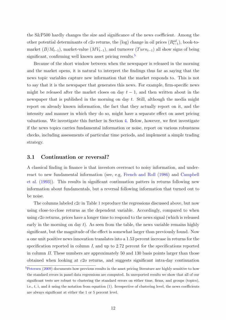
the S&P500 hardly changes the size and significance of the news coefficient. Among the

other potential determinants of c2o returns, the (log) change in oil prices (Roilt−1), book-to-

market (B/Mt−1), market-value (MVt−1), and turnover (Turnt−1) all show signs of being

significant, confirming well known asset pricing results.5

Because of the short window between when the newspaper is released in the morning

and the market opens, it is natural to interpret the findings thus far as saying that the

news topic variables capture new information that the market responds to. This is not

to say that it is the newspaper that generates this news. For example, firm-specific news

might be released after the market closes on day t − 1, and then written about in the

newspaper that is published in the morning on day t. Still, although the media might

report on already known information, the fact that they actually report on it, and the

intensity and manner in which they do so, might have a separate effect on asset pricing

valuations. We investigate this further in Section 4. Below, however, we first investigate

if the news topics carries fundamental information or noise, report on various robustness

checks, including assessments of particular time periods, and implement a simple trading

strategy.

3.1 Continuation or reversal?

A classical finding in finance is that investors overreact to noisy information, and under-

react to new fundamental information (see, e.g, French and Roll (1986) and Campbell

et al. (1993)). This results in significant continuation patters in returns following new

information about fundamentals, but a reversal following information that turned out to

be noise.

The columns labeled c2c in Table 1 reproduce the regressions discussed above, but now

using close-to-close returns as the dependent variable. Accordingly, compared to when

using c2o returns, prices have a longer time to respond to the news signal (which is released

early in the morning on day t). As seen from the table, the news variable remains highly

significant, but the magnitude of the effect is somewhat larger than previously found. Now

a one unit positive news innovation translates into a 1.53 percent increase in returns for the

specification reported in column I, and up to 2.72 percent for the specifications reported

in column II. These numbers are approximately 50 and 130 basis points larger than those

obtained when looking at c2o returns, and suggests significant intra-day continuation

5Petersen (2009) documents how previous results in the asset pricing literature are highly sensitive to how

the standard errors in panel data regressions are computed. In unreported results we show that all of our

significant tests are robust to clustering the standard errors on either time, firms, and groups (topics),

i.e., t, i, and k using the notation from equation (1). Irrespective of clustering level, the news coefficients

are always significant at either the 1 or 5 percent level.

12

Figure 2. Predicted cumulative close-to-close returns. The solid line is the mean response to a one unit

news innovation, and the broken lines represent the 99%, 95%, and 90% confidence intervals, respectively.

Standard errors are computed by clustering on trading day.

patterns.6

To investigate the degree to which our suggested news measure predicts asset prices

beyond the day in which the news is published, we look at how news predicts cumulative

close-to-close returns. In particular, let yi,t:t+h denote the cumulative close-to-close return

for firm i across horizons t to t+ h. Then, regression specification I from Table 1, which

yielded the smallest short-term effect size, is estimated for each h = 1, . . . , 20, using yi,t:t+h

as the dependent variable. Figure 2 reports the mean predictions together with 99%, 95%,

and 90% confidence intervals from this experiment. By construction, the impact effect

is as reported in Table 1, but the effect of a one unit news innovation also accumulates

substantially over time. A maximum effect of roughly 4 percent is obtained after 15

business days, before it levels off. Converting this number into the effect following a one

standard deviation news innovation gives an increase in returns of roughly 7 basis points.

Without exception, the response path is significant at the 1 percent level.7

Many textual studies in finance have given the news-return relationship a behavioral

interpretation and documented significant overreaction patterns (Tetlock (2014)). In our

results, confer Figure 2, we see little sign of reversal, suggesting that the news topics carries

new fundamental information (as opposed to noise). One plausible interpretation of the

observed continuation pattern is given by theories of rational attention where information

6In Table 11, in Appendix A, we run similar regressions for open-to-close returns (o2c), confirming that

the intra-day effect of the news is roughly, depending on the exact model specification, between 50 and

130 basis points.7We have also done these experiments by first cleansing the news topic variables for potential autocorre-

lation and common time fixed effects, giving the regressions an impulse response interpretation as in the

local linear projection framework (Oscar Jorda (2005)). Doing so we observe that the impact effect is of

the same magnitude as already documented in Table 1, suggesting that the news topic variables are fairly

exogenous to past developments in the market and not very persistent. Moreover, in the days following

the initial news shock, the effect on returns accumulates as above, with little sign of reversal.

13

gathering is costly and/or the investors are cognitively constrained. In such a setting,

the media matters because it can reach a broad population of investors and potentially

alleviate informational frictions by contributing to information diffusion (Peress (2014)).

Such an interpretation is also consistent with findings reported in Larsen and Thorsrud

(2015). They use the same news data as here, but construct a quarterly news index and

show that unexpected innovations to this index are followed by a permanent increase in

productivity and consumption. Thus, the news signal apparently generates co-movement

between productivity and asset prices, indicating that expectations about future cash

flows are impounded in the signal (Fama (1990)).

3.2 Randomization, additional fixed effects and interaction terms

A novelty of our analysis is that we treat every day as a news day by linking news topics

to returns using word distributions derived from the business newspaper and the firm’s

textual descriptions (confer Section 2.3). Panel A of Table 9, in Appendix A, shows

that the way we link companies to news is crucial for obtaining significant results. In

particular, when we randomly assign news topics to firms, and run exactly the same

regressions as described for Table 1, we find that almost no significant predictive power

can be established.8

One could suspect, however, that the way in which we link firms to news resembles

some type of industry classification, and that the results presented thus far capture indus-

try effects (see, e.g., Hou and Robinson (2006)), or that the news topic variables proxy

well known weekday effects (see, e.g., Doyle and Chen (2009)). In Panel B, in Table 9, we

redo the regressions from Table 1, but now include industry specific dummies and control

for the day of the week. As seen from the results, irrespective of which control variables

we include, the news topic coefficients are almost identical to those found earlier.

Another concern could be that the news topic variables are associated with particular

firm characteristics such as book-to-market value, size, or liquidity, i.e., well known pricing

factors (Fama and French (1993), Carhart (1997), and Pastor and Stambaugh (2003)).

In Table 10, in Appendix A, we interact the news variable with book-to-market values

(B/Mt−1 : Topict), market values (MVt−1 : Topict), and turnover (Turnt−1 : Topict), and

include these as additional control variables in the panel regressions. As seen from the

results, non of the interaction terms are significant, and, the coefficients associated with

the news topic variable remains significant at the 1 or 5 percent level with roughly the

same effect size as already presented. Thus, there are no significant patterns indicating

that our main results are driven by value, size, or liquidity characteristics.

8For close-to-close returns and the regression specification in column III of Table 9, the TopicRt variable

is barely significant at the 10 percent level.

14

We have also tried sorting firms into quantiles based on their average book-to-market

value, size, and turnover, and then, for each quantile and firm characteristic, estimated

the effect of news. The findings resemble those described above, namely that for most

quantiles and characteristics the news coefficient is positive, significant, and show no

pattern of being associated with specific firm characteristics.

In sum, we find that our results are robust to falsification tests (randomizing topic

assignments), various additional fixed effects (industry and weekday effects), and is not

driven by well known firm characteristics.

3.3 Changing market and media trends

During the last two decades both the media and stock market have undergone substantial

changes. First, as noted in Section 2.3, the breadth of the Norwegian stock market has

become much bigger over the years, potentially suggesting that also a broader set of media

is required to adequately cover it. For example, during the first years of our sample less

than 60 firms were listed on the Oslo Stock Exchange. In contrast, in 2014 over 120

companies were listed and included in our data set. Second, while printed news was a

primary media channel a decade ago, internet usage and online consumption of newspaper

content dominates today (SSB (2017)). In terms of the number of readers of printed news,

our primary source DN has been ranked as the fourth largest in Norway, irrespective of

subject matter, throughout the whole sample. In terms of online readers, however, DN has

faced substantially tougher competition. For example, DN’s share of the total number of

online readers declined by 25 percent around 2008 due to the establishment of competing

news media (Medianorway (2017)). Together these trends suggest that DN’s role as an

information diffusion channel might be weakened across time, and that the relationship

between the (DN) news topics and returns accordingly.

The results reported in Table 2 addresses this issue. Here we have divided the sample

(1996 - 2014) into three equally sized sub-samples, and redone the estimation from the

columns labeled I in Table 1. As seen from the table, the predictive effects are positive

and significant for all sub-samples and for both close-to-open and close-to-close returns,

but the strength of the effect tend to diminish over time. The graph to the left in Figure

3 shows that this general pattern carries through also for longer term predictions. During

the period 1996-2002 we find a positive, highly persistent, and significant predictive rela-

tionship between news and returns. For the period 2002-2008, this relationship weakens

somewhat, but remains significant. The really dramatic change is for the last sub-sample,

2008-2014, where the predictive relationship between news topics and returns becomes

insignificant after only one day.

In line with the discussion above, one interpretation of these findings is that DN,

15

Table 2. Firm specific news topics and day t close-to-open (c2o) and close-to-close returns (c2c) across

sub-samples. For each return variable, regression specification I from Table 1 is used. All regressions are

estimated by OLS. Fixed effects are included as specified in the table. Following Tetlock et al. (2008),

we compute clustered standard errors by trading day. Robust t-statistics are in parentheses.

c2o c2c

1996-2002 2002-2008 2008-2014 1996-2002 2002-2008 2008-2014

Topict 0.0169*** 0.0084*** 0.0086** 0.0267*** 0.0135*** 0.0099*(0.0047) (0.0031) (0.0039) (0.0065) (0.0042) (0.0055)

R2 0.0056 0.0100 0.0107 0.0045 0.0069 0.0062

Obs. 130332 197231 213412 130332 197231 213412

αi yes yes yes yes yes yes

δt yes yes yes yes yes yes

from which we derive our news signal, has become less important for understanding the

news-return relationship. On the other hand, the results might also indicate that financial

markets have become more efficient over time, and that information frictions that were

present during the 1990s and early 2000s are no longer binding.

To cast further light on these two competing explanations, our textual data provider

Retriever has provided us with a broad-based sample of news articles from the biggest

players in the Norwegian (business) newspaper market. This extra set of data covers

the period 2008-2014, and includes news from four additional sources.9 We utilize this

extra data in four steps. First, we clean the textual data, as described in Section 2.1.

Then, in a second step, we apply a procedure for querying documents outside the set

on which the LDA is estimated, as described in Section 2.3. That is, we keep the topic

definitions estimated from the DN corpus, and classify the augmented corpus based on

these existing word distributions. The advantage with this approach is that we ensure

that the topics, in terms of word distributions, stay the same across the extended data

set (multiple sources) and the original one (DN only).10 Third, we compute new topic

time series, for the period 2008-2014, based on the tone and frequency associated with

each topic from the aggregated corpus (DN and additional sources), as in Section 2.2. As

such, the extra data allows us to capture a much broader news base than when using DN

9The sources are Aftenposten, Finansavisen, Bergens Tidende, and E24. The latter media is an online

media channel only. To avoid using news content that are generated as a response to market movements

on day t, we define the online news corpus for a given day t as containing news articles from eight in the

morning on day t− 1 to eight in the morning on day t, i.e., before the market opens on day t.10Because of lack of identifiability in the LDA, the estimates of the topic and word distributions can not be

combined across samples for an analysis that relies on the content of specific topics. A disadvantage of

this approach is that by definition it does not take into account the possibility that the additional news

sources write about other news topics than those defined by DN.

16

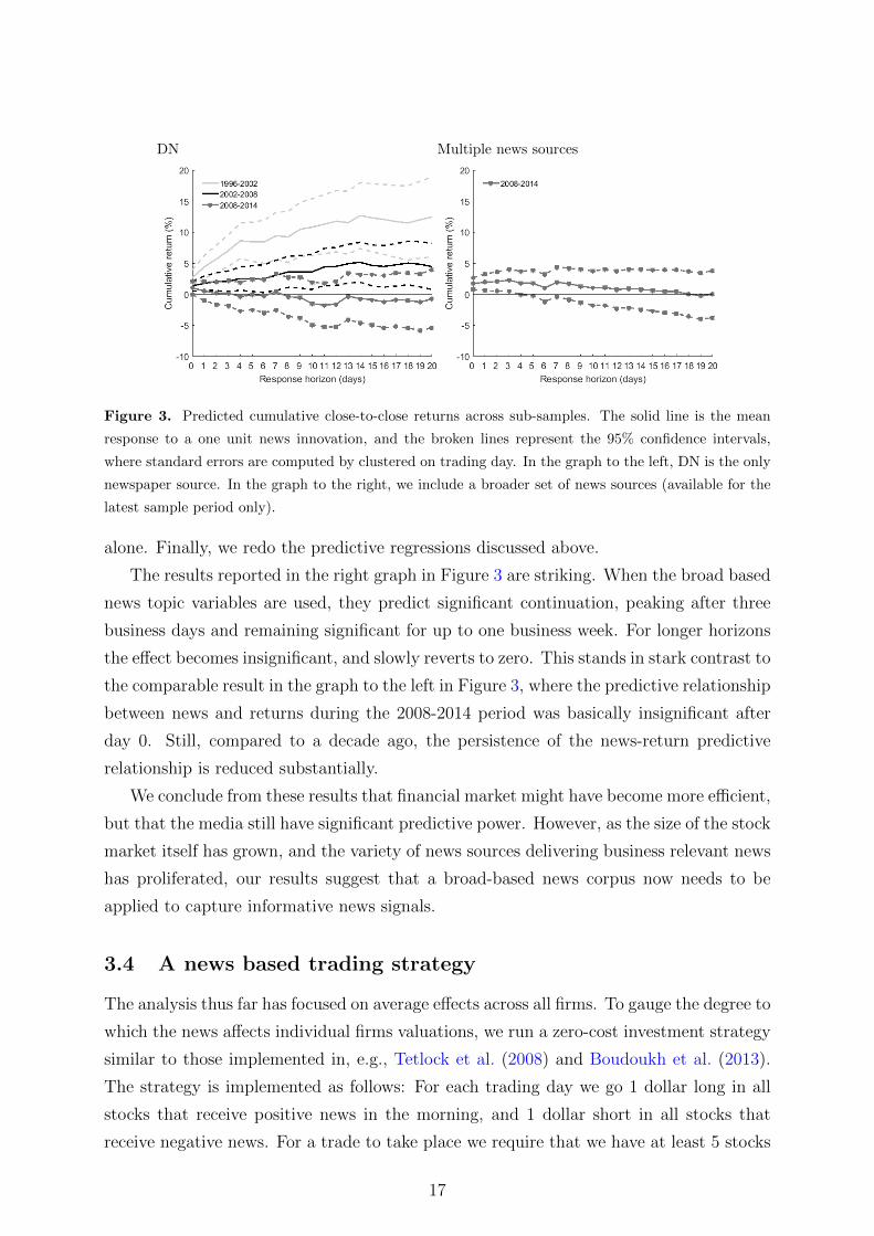
DN Multiple news sources

Figure 3. Predicted cumulative close-to-close returns across sub-samples. The solid line is the mean

response to a one unit news innovation, and the broken lines represent the 95% confidence intervals,

where standard errors are computed by clustered on trading day. In the graph to the left, DN is the only

newspaper source. In the graph to the right, we include a broader set of news sources (available for the

latest sample period only).

alone. Finally, we redo the predictive regressions discussed above.

The results reported in the right graph in Figure 3 are striking. When the broad based

news topic variables are used, they predict significant continuation, peaking after three

business days and remaining significant for up to one business week. For longer horizons

the effect becomes insignificant, and slowly reverts to zero. This stands in stark contrast to

the comparable result in the graph to the left in Figure 3, where the predictive relationship

between news and returns during the 2008-2014 period was basically insignificant after

day 0. Still, compared to a decade ago, the persistence of the news-return predictive

relationship is reduced substantially.

We conclude from these results that financial market might have become more efficient,

but that the media still have significant predictive power. However, as the size of the stock

market itself has grown, and the variety of news sources delivering business relevant news

has proliferated, our results suggest that a broad-based news corpus now needs to be

applied to capture informative news signals.

3.4 A news based trading strategy

The analysis thus far has focused on average effects across all firms. To gauge the degree to

which the news affects individual firms valuations, we run a zero-cost investment strategy

similar to those implemented in, e.g., Tetlock et al. (2008) and Boudoukh et al. (2013).

The strategy is implemented as follows: For each trading day we go 1 dollar long in all

stocks that receive positive news in the morning, and 1 dollar short in all stocks that

receive negative news. For a trade to take place we require that we have at least 5 stocks

17

on each side. Based on the continuation patterns shown in Figure 3, the stocks are held

for up to 5 trading days. At the end of each day we compute the total daily (close-to-close)

return from both the long and short portfolios we have at that point in time, controlling

for the fact that stocks are bought on opening prices and sold on close prices. The total

daily return from the strategy is the difference between the daily return from the long

and short portfolios.

Columns labeled I in Table 12, in Appendix A, summarize the yearly returns and

Sharp Ratios generated by the benchmark zero-cost portfolio using DN and multiple

media as news sources (from 2008), respectively. For the strategy utilizing only DN as a

news source, negative returns are observed for 5 our of 18 years; 1997, 2006, 2007, 2009,

and 2011. On average, across all the years, the annualized daily return is 16.8 percent,

with a Sharp Ratio of about 0.89. For comparison, this return is almost four times that

of the market as a whole, see Figure 6 in Appendix A, which has a Sharp Ratio of 0.33.

Although good, these numbers improve substantially when the news signal traded upon

utilizes multiple sources. It that case, negative portfolio returns are only observed in three

out of 18 years, and the annualized average return is 29.1 percent with a Sharp Ratio of

1.56. However, as also seen from the table, the average numbers of daily trades conducted

to form the long and short portfolios are substantial. In a real world setting, this would

have implied substantial trading costs which would likely have subtracted away a large

part of the aggregate returns.

To reduce the number of trades conducted, we also run an alternative trading strategy.

This strategy is similar to that above, but with the difference that news is only traded

upon if the news signal is over or below one standard deviation of the respective news

topic time series. Here, the computations of the standard deviations are recursively

updated throughout the trading experiment, using the past 252 observations to calculate

the standard deviations. As seen from the columns labeled II in Table 12, this more

restrictive trading strategy reduces the average returns on the portfolios somewhat. Still,

the annualized average daily returns are 11.7 and 21.3 percent, with Sharp Ratios of 0.60

and 1.1, for the DN only and multiple sources strategies, respectively. More importantly,

however, the alternative strategies generates these return by far fewer trades than above.

Do the two zero-cost investment strategies generate risk-adjusted returns as well? In

Table 3 we use the daily return series generated by the two strategies, subtract the risk-free

rate, and run regressions controlling for the standard risk factors (Fama and French (1993),

Jegadeesh and Titman (1993), Carhart (1997), and Pastor and Stambaugh (2003)): the

market (MR) size (SMB), book-to-market (HML), momentum (UMD), and liquidity

(LIQ).11 Only for the alternative trading strategy, and when using DN as the only news

11Professor Bernt Arne Ødegaard, at the University in Stavanger, constructs these risk factors for the

18

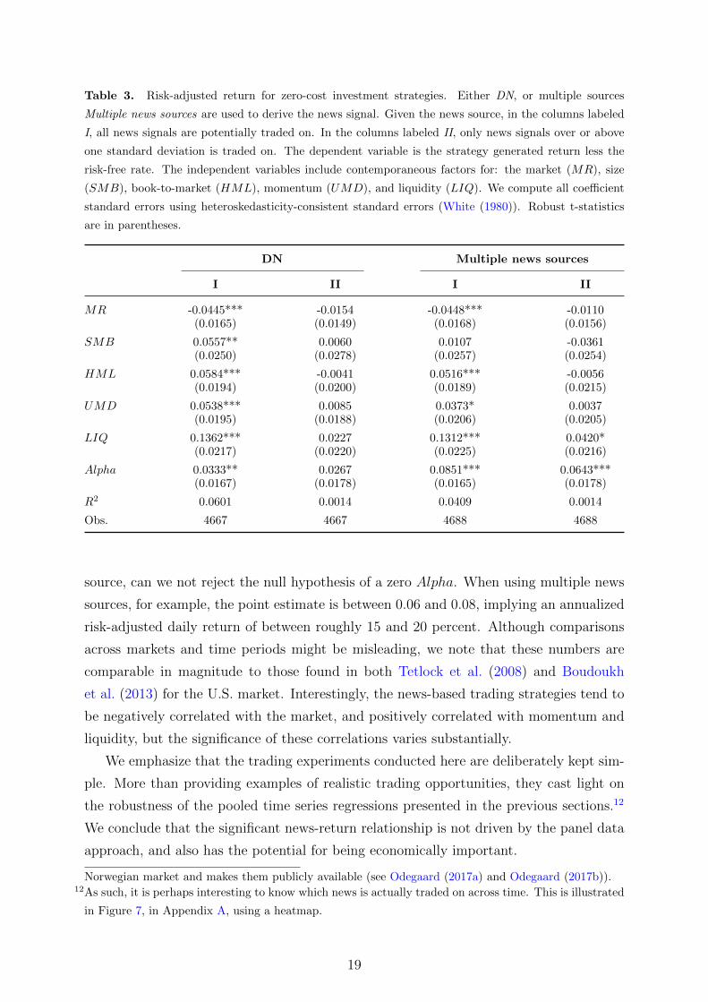
Table 3. Risk-adjusted return for zero-cost investment strategies. Either DN, or multiple sources

Multiple news sources are used to derive the news signal. Given the news source, in the columns labeled

I, all news signals are potentially traded on. In the columns labeled II, only news signals over or above

one standard deviation is traded on. The dependent variable is the strategy generated return less the

risk-free rate. The independent variables include contemporaneous factors for: the market (MR), size

(SMB), book-to-market (HML), momentum (UMD), and liquidity (LIQ). We compute all coefficient

standard errors using heteroskedasticity-consistent standard errors (White (1980)). Robust t-statistics

are in parentheses.

DN Multiple news sources

I II I II

MR -0.0445*** -0.0154 -0.0448*** -0.0110(0.0165) (0.0149) (0.0168) (0.0156)

SMB 0.0557** 0.0060 0.0107 -0.0361(0.0250) (0.0278) (0.0257) (0.0254)

HML 0.0584*** -0.0041 0.0516*** -0.0056(0.0194) (0.0200) (0.0189) (0.0215)

UMD 0.0538*** 0.0085 0.0373* 0.0037(0.0195) (0.0188) (0.0206) (0.0205)

LIQ 0.1362*** 0.0227 0.1312*** 0.0420*(0.0217) (0.0220) (0.0225) (0.0216)

Alpha 0.0333** 0.0267 0.0851*** 0.0643***(0.0167) (0.0178) (0.0165) (0.0178)

R2 0.0601 0.0014 0.0409 0.0014

Obs. 4667 4667 4688 4688

source, can we not reject the null hypothesis of a zero Alpha. When using multiple news

sources, for example, the point estimate is between 0.06 and 0.08, implying an annualized

risk-adjusted daily return of between roughly 15 and 20 percent. Although comparisons

across markets and time periods might be misleading, we note that these numbers are

comparable in magnitude to those found in both Tetlock et al. (2008) and Boudoukh

et al. (2013) for the U.S. market. Interestingly, the news-based trading strategies tend to

be negatively correlated with the market, and positively correlated with momentum and

liquidity, but the significance of these correlations varies substantially.

We emphasize that the trading experiments conducted here are deliberately kept sim-

ple. More than providing examples of realistic trading opportunities, they cast light on

the robustness of the pooled time series regressions presented in the previous sections.12

We conclude that the significant news-return relationship is not driven by the panel data

approach, and also has the potential for being economically important.

Norwegian market and makes them publicly available (see Odegaard (2017a) and Odegaard (2017b)).12As such, it is perhaps interesting to know which news is actually traded on across time. This is illustrated

in Figure 7, in Appendix A, using a heatmap.

19

4 The causal media effect

The news signal potentially contains (at least) two different components. First, news in

the business newspaper can be genuine new information. Second, the media might itself

affect markets by how they report news stories and by disseminating information to a

broad population of investors. As genuine new information is more likely to be generated

exogenous to the media (and reported in the media with a time lag), it is the second

component that reflects media’s potential causal role in predicting returns. To separate

between these two components, however, is difficult, because we only observe the signal,

and not its two underlying components.

To address this issue we exploit a strike in the Norwegian newspaper market in 2002,

which started on May 30 and ended on June 7, i.e., lasting for seven business days.

The same event was used in Peress (2014) to investigate the causal effect media has on

trading and price formation. But, in contrast to his cross-country event study, we focus

on the case of Norway, changes in returns, and condition our analysis on the news topic

variables. Although this might seem like a more narrow analysis, it allows us to obtain

a novel estimate of the media effect in a given predictive relationship. Simply put, we

ask how much of the increases in returns documented in the preceding sections can be

attributed to the causal (DN) news topics media effect.

According to Peress (2014), the newspaper strike affected the press on a national

scale, involved the media sector only, and occurred on days on which the stock market

was open. Moreover, the strike was called by the media profession itself due to their

working conditions, and it was not driven by stock market movements on the day of the

strike or the preceding days. Thus, we can safely assume that it was truly exogenous to

market developments.13

Conditional on the strike being truly exogenous, the central premise for being able to

quantify the media effect of news is that news in terms of new information was released

also during the strike period, although not through the mass media. As such, we follow

an event study approach where in total 103 stocks enter our sample in the year(s) prior

to, during and after the strike. We focus on both their close-to-open and close-to-close

returns, and use N days prior to and N days after the strike to compute the non-strike

affected returns. In the following, we denote the change in returns ∆ri,d−ba = ri,d − ri,ba,where r is the average return for company i, during the strike period (ri,d) and before

and after (ri,ba), respectively. By adjusting N , we can down-weight observations right

13See Peress (2014) for a richer discussion about these issues. It should be noted, however, that he also

includes a Norwegian newspaper strike in 2004. During this journalist strike the DN newspaper was in

fact published, and the event can not be used here. We further note that, given the timing of the strike

event in 2002, the explosion of digital media seen the last decade had hardly begun.

20

Table 4. Summary statistics of news and returns, before and during and after the strike. In the rows

labeled ∆rd−ba, each table entry is a function of ∆ri,d−ba = ri,d − ri,ba, where r is the average return

for company i, during the strike period (ri,d) and before and after (ri,ba), respectively. The length of

the strike period (ri,d) is constant and equal to seven business days. The total length of the window

used during and before and after the strike equals 51 days. In the interest of readability, the numbers

reported in the columns E(X), V AR(X), min(X), and max(X) are scaled by 100. The table row

labeled t(β) provides summary statistics for ti(β), a standardized firm specific news loading, estimated

on a classification sample prior to the strike period.

E(X) VAR(X) Skew(X) Kurtosis(X) min(X) max(X) N

∆rc2od−ba -0.3918 1.1684 0.0028 4.6416 -3.8829 3.0488 103

∆rc2cd−ba -0.6171 1.5688 -0.2377 4.6911 -4.5117 3.9407 103

t(β) 2.3016 3.9414 0.6000 3.3606 -1.3632 8.8093 103

before and right after the strike, as these might be driven by anticipation effects (about

the forthcoming strike) and adjustments following the end of the strike period. We denote

the total length of the before, during, and after strike sample by W . In the main results

presented below W = 51, but we show that our results are robust to both shorter and

longer windows.

4.1 Unconditional and conditional effects

The first row in Table 4 documents that, on average across firms, the average returns

during the strike period fell by between 40 to 60 basis points relative to the average returns

prior to and after the strike. The dispersion across firms is however large, with minimum

and maximum values reaching -3.88 and 3.04 percent, and -4.51 and 3.94 percent, for

c2o and c2c returns, respectively. Still, the skewness and kurtosis statistics suggest that

the distribution is not far from normal, albeit with some outliers. For both types of

returns, the mean effects are significantly different from zero on the 1 percent significance

level, suggesting that the media has a positive causal role in explaining short-term return

patterns.14

A valid objection to the simple calculations done above is that they do not necessarily

tell us something about how the media shortage affected returns. The fall might simply

be due to the effect the strike itself, or other not controlled for common events, had on

markets. Accordingly, we would ideally need two different groups of firms and returns.

One where the media shortage should matter, and one where it should not. Unfortunately,

such classifications are not observed. Moreover, although the numbers might reflect the

14A direct comparison of our results to those in Peress (2014) would have been interesting, but not feasible.

He focuses on pooled cross-country averages, trading volume, and volatility, and does not report raw

return statistics for the Norwegian newspaper strike in 2002.

21

causal media effect, they do not necessarily relate to the news topic variables used in this

study, i.e., those obtained from the DN newspaper.

To accommodate the concern, and to relate the media shortage to the DN news topic

variables, we run a difference-in-difference type of experiment, with some modifications.

As above, we first compute the difference between returns during the strike and those

before and after the strike. Then, conditioning on how sensitive the respective stocks

were to the news topic variables in the year prior to the strike, we construct a treatment

and control group, and run simple regressions to quantify the media effect due to the

shortfall of the DN news topics. Intuitively, all stocks might be affected by the strike,

but those firms that had a particularly high sensitivity to news topics prior to the strike

should also respond stronger to their shortfall during the strike.15

More formally, we consider the model:

ri,e = αi + δDe + τwi,e + ui,e (2)

where the event indicator e = {ba, d} indicates the periods before and after (ba) and

during (d) the strike, αi is a firm-fixed effect constant across e, De = 1 if e = d and zero

otherwise, and ui,e are idiosyncratic errors. The parameter of interest is τ , measuring the

effect of wi,e, a binary indicator of the treatment. Before and after the strike wi,ba = 0

for all i. During the strike, however, wi,d = 1 if firm i is in the treatment group, i.e.,

particularly sensitive to the DN news topics, and zero otherwise. A simple estimation

procedure of the two-period model in (2) is to first difference to remove αi:

∆ri,d−ba = ri,d − ri,ba = δ + τ∆wi + ∆ui (3)

with ∆wi = wi,d (since wi,ba = 0 for all firms i in period e = ba).

While (3) is a standard difference-in-difference model (Meyer (1995) and Angrist and

Krueger (1999)), the crux here is to construct wi,d, which depends on the firm’s news

topic sensitivity. We construct wi,d in two steps. First, we estimate news topic sensitivity,

denoted by ti(β), from time series regressions of each individuals firm’s close-to-open

return (yi,t) on news topics (Tk,t) during the year preceding the strike:

yi,t = βiTk,t + z′i,tδ + ui,t (4)

where ti(β) is the t-statistic associated with βi.16 The third row of Table 4 reports how

15Estimating the average media shortage effect only for returns in the treatment group would not permit us

to exclude the general effect the strike itself might have on returns. Of course, if the general strike effect

affects firms in the two groups differently, our experiment design will not be able to efficiently isolate the

strike effect from the (DN) media shortage effect.16We focus on t(β), rather than β, to control for differences in precision due to differences in residual

variance. To reduce potential biases in the regressions, we also include additional controls, zi,t, including

Rmit−1, B/Mi,t−1, MVi,t−1, and lagged close-to-close returns for stock i, i.e., the significant regressors in

the panel regressions run in Section 3.

22

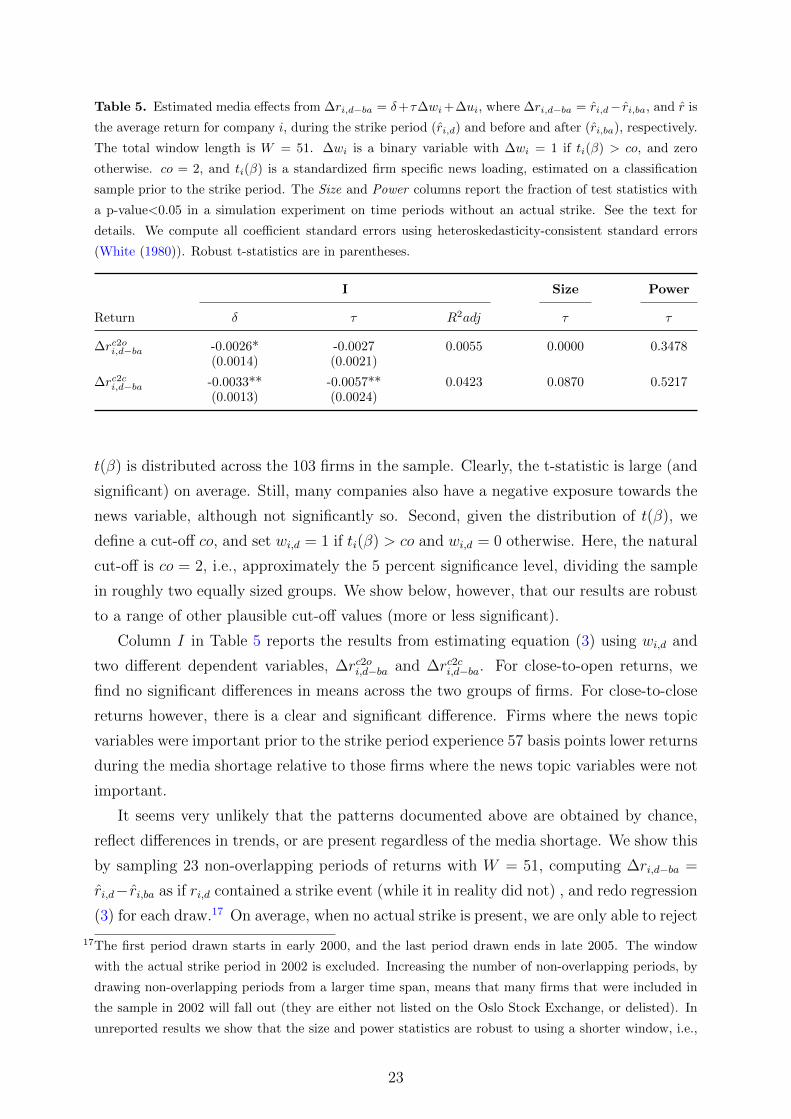
Table 5. Estimated media effects from ∆ri,d−ba = δ+τ∆wi+∆ui, where ∆ri,d−ba = ri,d− ri,ba, and r is

the average return for company i, during the strike period (ri,d) and before and after (ri,ba), respectively.

The total window length is W = 51. ∆wi is a binary variable with ∆wi = 1 if ti(β) > co, and zero

otherwise. co = 2, and ti(β) is a standardized firm specific news loading, estimated on a classification

sample prior to the strike period. The Size and Power columns report the fraction of test statistics with

a p-value<0.05 in a simulation experiment on time periods without an actual strike. See the text for

details. We compute all coefficient standard errors using heteroskedasticity-consistent standard errors

(White (1980)). Robust t-statistics are in parentheses.

I Size Power

Return δ τ R2adj τ τ

∆rc2oi,d−ba -0.0026* -0.0027 0.0055 0.0000 0.3478(0.0014) (0.0021)

∆rc2ci,d−ba -0.0033** -0.0057** 0.0423 0.0870 0.5217(0.0013) (0.0024)

t(β) is distributed across the 103 firms in the sample. Clearly, the t-statistic is large (and

significant) on average. Still, many companies also have a negative exposure towards the

news variable, although not significantly so. Second, given the distribution of t(β), we

define a cut-off co, and set wi,d = 1 if ti(β) > co and wi,d = 0 otherwise. Here, the natural

cut-off is co = 2, i.e., approximately the 5 percent significance level, dividing the sample

in roughly two equally sized groups. We show below, however, that our results are robust

to a range of other plausible cut-off values (more or less significant).

Column I in Table 5 reports the results from estimating equation (3) using wi,d and

two different dependent variables, ∆rc2oi,d−ba and ∆rc2ci,d−ba. For close-to-open returns, we

find no significant differences in means across the two groups of firms. For close-to-close

returns however, there is a clear and significant difference. Firms where the news topic

variables were important prior to the strike period experience 57 basis points lower returns

during the media shortage relative to those firms where the news topic variables were not

important.

It seems very unlikely that the patterns documented above are obtained by chance,

reflect differences in trends, or are present regardless of the media shortage. We show this

by sampling 23 non-overlapping periods of returns with W = 51, computing ∆ri,d−ba =

ri,d− ri,ba as if ri,d contained a strike event (while it in reality did not) , and redo regression

(3) for each draw.17 On average, when no actual strike is present, we are only able to reject

17The first period drawn starts in early 2000, and the last period drawn ends in late 2005. The window

with the actual strike period in 2002 is excluded. Increasing the number of non-overlapping periods, by

drawing non-overlapping periods from a larger time span, means that many firms that were included in

the sample in 2002 will fall out (they are either not listed on the Oslo Stock Exchange, or delisted). In

unreported results we show that the size and power statistics are robust to using a shorter window, i.e.,

23

the null-hypothesis of no significant effects at the 5 percent level in at most 8.7 percent of

the cases (see column Size of Table 5). Conversely, if we impose the media effect estimated

above on each of the ri,d periods sampled, we see from the column labeled Power that we

obtain a significant relationship in 52 percent of the cases (c2c), and a substantially lower

number for the effect that was not significant in the first place (c2o). Naturally, if we

increase the effect size imposed on the non-overlapping periods, the power increases, and

vice versa (not shown). Moreover, qualitatively, non of the results reported in column I

in Table 5 are affected by varying the cut-off value (co) between 1.6 to 3 (from weakly

significant to highly significant) when constructing wi,d, or by using a different window

length to construct ri,ba (see Tables 13 and 14, in Appendix A).

Together, these results provide strong evidence towards a causal (DN specific) news

topic media effect. For close-to-close returns, the difference in mean between the syn-

thetic control and treatment groups is even of the same magnitude as the total strike

effect documented in Table 4, i.e., 60 basis points. To put these numbers into context,

a conservative estimate implies that roughly 20 percent of the close-to-close returns pre-

dicted by news topics are due to the media effect alone, while a more positive estimate

suggests as much as 37 percent.18 Thus, seen through the lens of rational attention the-

ories where investors face information processing costs, or have limited cognitive ability

(Peng and Xiong (2006), Kacperczyk et al. (2009), and Schmidt (2013)), the media serves

an important independent role in alleviating informational frictions.

4.2 Accounting for treatment intensity and asymmetries

A weakness with the approach just taken is that it does not account for the basic intuition

that, all else equal, firms’ news topic sensitivity might affect the intensity at which the

media shortage affects returns. For example, firms with a particularly high (low) and

(in)significant sensitivity to news prior to the strike period might also be more negatively

(positively) affected than the other firms during the media shortage.

To investigate this hypothesis we extend the regression model in (2) by taking into

account potential differences in how the media shortage affects returns within and between

the treatment and control group. In particular, we consider the model:

ri,e = αi + δDe + τ twi,eti(β)t + τ cwi,eti(β)c + τwi,e + b2ti(β)t + b3ti(β)c + ui,e (5)

where αi, δDe, and ui,e have the same interpretations as before. Now, however, wi,e is a

binary strike indicator, where wi,e = 1 if e = d and zero otherwise for all firms i. This

with W = 31 and a larger number of non-overlapping periods.18According to the estimates in Table 5, the DN news topic effect is 57 basis point, while the maximum

(minimum) predictive effect from the pooled time series regression reported earlier in Table 1 is 272 (153)

basis points i.e., 57/272 = 0.21 (57/153 = 0.37).

24

strike event indicator is then interacted with the terms ti(β)t and ti(β)c. ti(β)t = ti(β) if

ti(β) > co and 0 otherwise, and ti(β)c = ti(β) if ti(β) <= co and 0 otherwise. As such,

in response to the media shortage, τ t and τ c capture the potential asymmetries between

firms with a significant and non-significant sensitivity to the news topics. For estimation,

we first difference (5), yielding the following model:

∆ri,d−ba = δ + τ tti(β)t + τ cti(β)c + ∆ui (6)

where δ = δ + τ , and apply ordinary least squares.

Column I of Table 6 reports the regression output. Starting with the results in the c2c

row, we see that the ti(β)t term is highly significant, and, based on the argument above,

have the correct negative sign. On the other hand, close-to-close returns for firms in the

control group are unaffected by the media shortage. As such, these results are consistent

with the results presented in the previous section. Moreover, as the average t-statistic in

Table 4 is well above 2, the effect of the media shortage, in percent of the total predictive

effect, is in the same ballpark as previously reported, i.e., 20-40 percent. Interestingly,

this pattern is reversed when we look at close-to-open returns, where only the ti(β)c term

is significant and positive. Thus, following the media shortage, firms in the treatment

group experience an extra underreaction, while the firms in the control group experience

an initial overreaction and subsequent intra-day reversal.

Size tests, conducted as described in the previous section, but now applied to the

model in 6, show that these results are highly unlikely to occur in time periods without

a strike, see the column labeled Size in Table 6. Therefore, and perhaps somewhat

surprising, because intra-day reversal is not something we easily observe for firms in the

control group in periods without a media shortage, the asymmetries documented in Table

6 suggest that the media shortage led to more noise trading. Or, in other words, that

the media actually reduces noise (trading). However, as seen from Tables 13 and 14, in

Appendix A, the significant overreaction obtained for the control group during the strike

is fairly robust to the window size (W ) used, but not robust to other cut-off values than 2.

That is, for all cut-off values considered, the sign of the ti(β)c coefficient is estimated to be

positive, but only for co = 2 do we obtain a significant ti(β)c coefficient for close-to-open

returns.

In sum, the results presented here and in Section 4.1 give media an important causal

role for understanding asset price fluctuations. Positive evidence of media’s causal role

in financial markets has also been documented in Engelberg and Parsons (2011), Dougal

et al. (2012) and (not surprisingly) Peress (2014). Of the three, however, only the two

latter analyses returns.19 Still, our interpretation of the media effect differs somewhat

19Engelberg and Parsons (2011) analyses trading volumes, and show that trades by individual investors

located in different locations respond to local newspaper coverage.

25

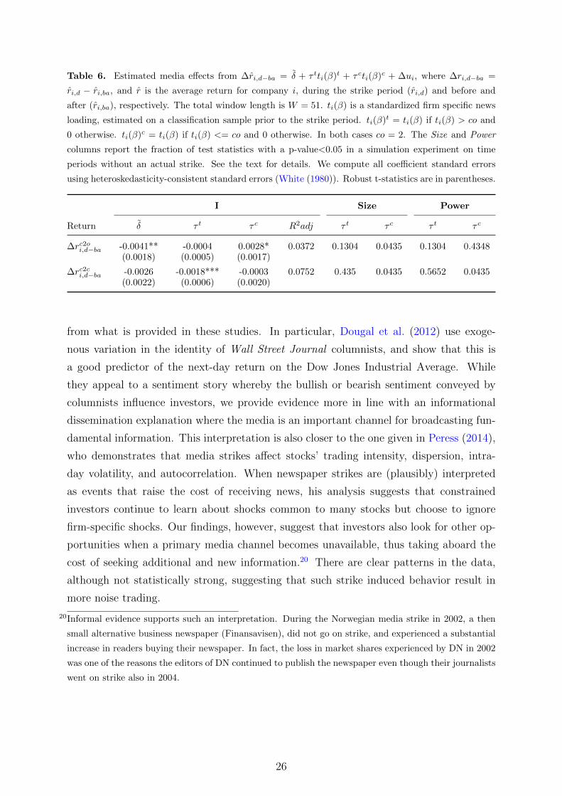
Table 6. Estimated media effects from ∆ri,d−ba = δ + τ tti(β)t + τ cti(β)c + ∆ui, where ∆ri,d−ba =

ri,d − ri,ba, and r is the average return for company i, during the strike period (ri,d) and before and

after (ri,ba), respectively. The total window length is W = 51. ti(β) is a standardized firm specific news

loading, estimated on a classification sample prior to the strike period. ti(β)t = ti(β) if ti(β) > co and

0 otherwise. ti(β)c = ti(β) if ti(β) <= co and 0 otherwise. In both cases co = 2. The Size and Power

columns report the fraction of test statistics with a p-value<0.05 in a simulation experiment on time

periods without an actual strike. See the text for details. We compute all coefficient standard errors

using heteroskedasticity-consistent standard errors (White (1980)). Robust t-statistics are in parentheses.

I Size Power

Return δ τ t τ c R2adj τ t τ c τ t τ c

∆rc2oi,d−ba -0.0041** -0.0004 0.0028* 0.0372 0.1304 0.0435 0.1304 0.4348(0.0018) (0.0005) (0.0017)

∆rc2ci,d−ba -0.0026 -0.0018*** -0.0003 0.0752 0.435 0.0435 0.5652 0.0435(0.0022) (0.0006) (0.0020)

from what is provided in these studies. In particular, Dougal et al. (2012) use exoge-

nous variation in the identity of Wall Street Journal columnists, and show that this is

a good predictor of the next-day return on the Dow Jones Industrial Average. While

they appeal to a sentiment story whereby the bullish or bearish sentiment conveyed by

columnists influence investors, we provide evidence more in line with an informational

dissemination explanation where the media is an important channel for broadcasting fun-

damental information. This interpretation is also closer to the one given in Peress (2014),

who demonstrates that media strikes affect stocks’ trading intensity, dispersion, intra-

day volatility, and autocorrelation. When newspaper strikes are (plausibly) interpreted

as events that raise the cost of receiving news, his analysis suggests that constrained

investors continue to learn about shocks common to many stocks but choose to ignore

firm-specific shocks. Our findings, however, suggest that investors also look for other op-

portunities when a primary media channel becomes unavailable, thus taking aboard the

cost of seeking additional and new information.20 There are clear patterns in the data,

although not statistically strong, suggesting that such strike induced behavior result in

more noise trading.

20Informal evidence supports such an interpretation. During the Norwegian media strike in 2002, a then

small alternative business newspaper (Finansavisen), did not go on strike, and experienced a substantial

increase in readers buying their newspaper. In fact, the loss in market shares experienced by DN in 2002

was one of the reasons the editors of DN continued to publish the newspaper even though their journalists

went on strike also in 2004.

26

5 Conclusion

News in the business newspaper predicts daily returns, and the media has an important

causal role in this predictive relationship. We reach these conclusions after decomposing

the corpus in the main Norwegian business newspaper into daily news topics and linking

them to firms and returns.

Although the news topics are available in the morning, well before the market opens,

we document significant underreaction in market prices to news and clear patterns of

continuation in the days following the initial news release. These results hold both in

pooled time series regression, simple zero-cost news-based trading strategies, and are

robust when controlling for numerous commonly used predictors. Interestingly, however,

the degree of predictability and persistence weakens over time, and towards the latter

parts of the sample a broader news corpus, including online media, is needed to achieve

significant continuation patterns.

Further, by exploiting an exogenous strike in the Norwegian newspaper market, in

2002, we are able to isolate the media component of the news signal from the new infor-

mation component. Returns for individual firms with a significant exposure to our news

measures fall by 57 basis points during the strike period relative to firms with an insignifi-

cant news topic exposure. Since the average firm in the sample has a positive exposure to

news, our results imply that the media component of the news signal accounts for between

20 to 40 percent of the documented overall predictive effect of news topics.

In sum, our analysis support a rational attention view where the media alleviate

information frictions and disseminate information to a large population of investors. In

that respect it is interesting to note that when using the same news topics as here, we find

that news topics also predicts quarterly productivity, consumption, and aggregate stock

market developments (Larsen and Thorsrud (2015)). Thus, decomposing news published

through a business newspaper into news topics puts unstructured textual data into a

format that seems fundamental for both macroeconomic developments and asset prices.

Although the methodology used to reach these conclusions is general, the empirical

findings are restricted to the Norwegian market. Exciting avenues for future research

includes expanding the scope of the analysis to more countries and larger markets, and

to investigate in greater detail how market responses to online versus printed news might

differ.

27

References

Angrist, J. D. and A. B. Krueger (1999). Empirical strategies in labor economics. In

O. Ashenfelter and D. Card (Eds.), Handbook of Labor Economics, Volume 3 of Hand-

book of Labor Economics, Chapter 23, pp. 1277–1366. Elsevier.

Antweiler, W. and M. Z. Frank (2004). Is all that talk just noise? the information content

of internet stock message boards. The Journal of Finance 59 (3), pp. 1259–1294.

Antweiler, W. and M. Z. Frank (2006). Do us stock markets typically overreact to corpo-

rate news stories? Available at SSRN 878091 .

Blei, D. M., A. Y. Ng, and M. I. Jordan (2003). Latent Dirichlet Allocation. J. Mach.

Learn. Res. 3, 993–1022.

Boudoukh, J., R. Feldman, S. Kogan, and M. Richardson (2013). Which News Moves

Stock Prices? A Textual Analysis. NBER Working Papers 18725, National Bureau of

Economic Research, Inc.

Calomiris, C. W. and H. Mamaysky (2017). How news and its context drive risk and

returns around the world. Research Paper 17-40, Columbia Business School.

Campbell, J. Y. (1991). A variance decomposition for stock returns. The Economic

Journal 101 (405), 157–179.

Campbell, J. Y., S. J. Grossman, and J. Wang (1993). Trading volume and serial corre-

lation in stock returns. The Quarterly Journal of Economics 108 (4), 905.

Carhart, M. M. (1997). On Persistence in Mutual Fund Performance. Journal of Fi-

nance 52 (1), 57–82.

Chang, J., S. Gerrish, C. Wang, J. L. Boyd-graber, and D. M. Blei (2009). Reading tea

leaves: How humans interpret topic models. In Y. Bengio, D. Schuurmans, J. Lafferty,

C. Williams, and A. Culotta (Eds.), Advances in Neural Information Processing Systems

22, pp. 288–296. Curran Associates, Inc.

Dougal, C., J. Engelberg, D. Garcia, and C. A. Parsons (2012). Journalists and the stock

market. Review of Financial Studies 25 (3), 639–679.

Doyle, J. R. and C. H. Chen (2009). The wandering weekday effect in major stock markets.

Journal of Banking & Finance 33 (8), 1388 – 1399.

Engelberg, J. E. and C. A. Parsons (2011). The causal impact of media in financial

markets. The Journal of Finance 66 (1), 67–97.

28

Fama, E. F. (1990). Stock returns, expected returns, and real activity. The Journal of

Finance 45 (4), 1089–1108.

Fama, E. F. (1998). Market efficiency, long-term returns, and behavioral finance. Journal

of Financial Economics 49 (3), 283 – 306.

Fama, E. F. and K. R. French (1993). Common risk factors in the returns on stocks and

bonds. Journal of Financial Economics 33 (1), 3–56.

French, K. R. and R. Roll (1986). Stock return variances. Journal of Financial Eco-

nomics 17 (1), 5 – 26.

Garcia, D. (2013). Sentiment during recessions. The Journal of Finance 68 (3), 1267–1300.

Griffiths, T. L. and M. Steyvers (2004). Finding scientific topics. Proceedings of the

National academy of Sciences of the United States of America 101 (Suppl 1), 5228–

5235.

Hansen, S., M. McMahon, and A. Prat (2014). Transparency and Deliberation within the

FOMC: A Computational Linguistics Approach. CEP Discussion Papers 1276, Centre

for Economic Performance, LSE.

Heinrich, G. (2009). Parameter estimation for text analysis. Technical report, Fraunhofer

IGD.

Hou, K. and D. T. Robinson (2006). Industry concentration and average stock returns.

The Journal of Finance 61 (4), 1927–1956.

Jegadeesh, N. and S. Titman (1993). Returns to buying winners and selling losers: Im-

plications for stock market efficiency. The Journal of Finance 48 (1), 65–91.

Kacperczyk, M., S. V. Nieuwerburgh, and L. Veldkamp (2009). Rational attention allo-

cation over the business cycle. Working Paper 15450, National Bureau of Economic

Research.

Kearney, C. and S. Liu (2014). Textual sentiment in finance: A survey of methods and

models. International Review of Financial Analysis 33, 171 – 185.

Larsen, V. H. (2017). Components of uncertainty. Working Paper 2017/5, Norges Bank.

Larsen, V. H. and L. A. Thorsrud (2015). The Value of News. Working Papers 34, Centre

for Applied Macro- and Petroleum economics (CAMP), BI Norwegian Business School.

29

Loughran, T. and B. Mcdonald (2011). When Is a Liability Not a Liability? Textual

Analysis, Dictionaries, and 10-Ks. The Journal of Finance 66 (1), 35–65.

Loughran, T. and B. Mcdonald (2016). Textual analysis in accounting and finance: A

survey. Journal of Accounting Research 54 (4), 1187–1230.

Medianorway (2017). Facts and Figures on Norwegian Media. http://http://www.

medienorge.uib.no/english/. Accessed: 25.06.2017.

Meyer, B. D. (1995). Natural and quasi-experiments in economics. Journal of Business

& Economic Statistics 13 (2), 151–161.

Næs, R., J. A. Skjeltorp, and B. A. Ødegaard (2009). What factors affect the Oslo Stock

Exchange? Working Paper 2009/24, Norges Bank.

Odegaard, B. A. (2017a). Asset pricing data at OSE. http://finance.bi.no/~bernt/

financial_data/ose_asset_pricing_data/index.html. Accessed: 15.01.2015.

Odegaard, B. A. (2017b). Empirics of the Oslo Stock Exchange. Asset Pricing results 1980-

2016. UiS Working Papers in Economics and Finance 2017/2, University of Stavanger.

Odegaard, B. A. (2017c). Empirics of the Oslo Stock Exchange. Basic, descriptive, re-

sults 1980-2016. UiS Working Papers in Economics and Finance 2017/3, University of

Stavanger.

Pang, B., L. Lee, and S. Vaithyanathan (2002). Thumbs up?: Sentiment classification

using machine learning techniques. In Proceedings of the ACL-02 Conference on Empir-

ical Methods in Natural Language Processing - Volume 10, EMNLP ’02, Stroudsburg,

PA, USA, pp. 79–86. Association for Computational Linguistics.

Pastor, L. and R. F. Stambaugh (2003). Liquidity Risk and Expected Stock Returns.

Journal of Political Economy 111 (3), 642–685.

Peng, L. and W. Xiong (2006). Investor attention, overconfidence and category learning.

Journal of Financial Economics 80 (3), 563 – 602.

Peress, J. (2014). The media and the diffusion of information in financial markets: Evi-

dence from newspaper strikes. The Journal of Finance 69 (5), 2007–2043.

Petersen, M. A. (2009). Estimating standard errors in finance panel data sets: Comparing

approaches. Review of Financial Studies 22 (1), 435–480.

Roll, R. (1988). R2. The Journal of Finance 43 (3), 541–566.

30

Oscar Jorda (2005). Estimation and Inference of Impulse Responses by Local Projections.

American Economic Review 95 (1), 161–182.

Schmidt, D. (2013). Investors’ attention and stock covariation. Working paper, HEC

Paris.

Shiller, R. (1981). Do stock prices move too much to be justified by subsequent changes

in dividends? American Economic Review 71 (3), 421–36.

SSB, S. N. (2017). Norwegian media barometer, 2015. http://www.ssb.no/

en/kultur-og-fritid/statistikker/medie/aar/2016-04-14#content. Accessed:

25.06.2017.

Tetlock, P. C. (2007). Giving content to investor sentiment: The role of media in the

stock market. The Journal of Finance 62 (3), 1139–1168.

Tetlock, P. C. (2014). Information Transmission in Finance. Annual Review of Financial

Economics 6 (1), 365–384.

Tetlock, P. C., M. Saar-Tsechansky, and S. Macskassy (2008). More Than Words: Quanti-

fying Language to Measure Firms’ Fundamentals. Journal of Finance 63 (3), 1437–1467.

Thorsrud, L. A. (2016a). Nowcasting using news topics. Big Data versus big bank. Work-

ing Papers 46, Centre for Applied Macro- and Petroleum economics (CAMP), BI Nor-

wegian Business School.

Thorsrud, L. A. (2016b). Words are the new numbers: A newsy coincident index of busi-

ness cycles. Working Papers 44, Centre for Applied Macro- and Petroleum economics

(CAMP), BI Norwegian Business School.

White, H. (1980). A Heteroskedasticity-Consistent Covariance Matrix Estimator and a

Direct Test for Heteroskedasticity. Econometrica 48 (4), 817–838.

31

Appendices

Appendix A Additional results

Table 7. Estimated topics and labeling. The topics are labeled based on the meaning of the most

important words, while the words are translated from Norwegian to English using Google Translate. See

the text for details.

Topic Label First words

Topic 0 Calendar january, march, october, september, november, february

Topic 1 Family business family, foundation, name, dad, son, fortune, brothers

Topic 2 Institutional investing fund, investments, investor, return, risk, capital

Topic 3 Justice lawyer, judge, appeal, damages, claim, supreme court

Topic 4 Surroundings city, water, meter, man, mountain, old, outside, nature

Topic 5 Housing housing, property, properties, apartment, square meter

Topic 6 Movies/Theater movie, cinema, series, game, producer, prize, audience

Topic 7 Argumentation word, besides, interesting, i.e., in fact, sure, otherwise

Topic 8 Unknown road, top, easy, hard, lift, faith, outside, struggle,fast

Topic 9 Agriculture industry, support, farmers, export, production, agriculture

Topic 10 Automobiles car, model, engine, drive, volvo, ford, møller, toyota

Topic 11 USA new york, dollar, wall street, president, usa, obama, bush

Topic 12 Banking dnb nor, savings bank, loss, brokerage firm, kreditkassen

Topic 13 Leadership position, chairman, ceo, president, elected, board member

Topic 14 Negotiation solution, negotiation, agreement, alternative, part, process

Topic 15 Newspapers newspaper, media, schibsted, dagbladet, journalist, vg

Topic 16 Health care hospital, doctor, health, patient, treatment, medication

Topic 17 IT systems it, system, data, defense, siem, contract, tandberg, deliver

Topic 18 Stock market stock exchange, fell, increased, quote, stock market

Topic 19 Macroeconomics economy, budget, low, unemployment, high, increase

Topic 20 Oil production statoil, oil, field, gas, oil company, hydro, shelf, stavanger

Topic 21 Wage payments income, circa, cost, earn, yearly, cover, paid, salary

Topic 22 Regions trondheim, llc, north, stavanger, tromsø, local, municipality

Topic 23 Family woman, child, people, young, man, parents, home, family

Topic 24 Taxation tax, charge, revenue, proposal, remove, wealth tax, scheme

Topic 25 EU eu, eea, commission, european, brussel, membership, no

Topic 26 Industry hydro, forest, factory, production, elkem, industry, produce

Topic 27 Unknown man, he, friend, smile, clock, evening, head, never, office

Topic 28 Mergers and acquisitions orkla, storebrand, merger, bid, shareholder, acquisitions

Topic 29 UK british, london, great britain, the, of, pound, england

Topic 30 Narrative took, did, later, never, gave, stand, happened, him, began

Continued on next page

32

Table 7 – continued from previous page

Topic Label First words

Topic 31 Shipping ship, shipping, dollar, shipowner, wilhelmsen, fleet, proud

Topic 32 Projects project, nsb, development, fornebu, entrepreneurship

Topic 33 Oil price dollar, oil price, barrel, oil, demand, level, opec, high

Topic 34 Sports olympics, club, football, match, play, lillehammer, sponsor

Topic 35 Organizations leader, create, organization, challenge, contribute, expertise

Topic 36 Drinks wine, italy, taste, drinks, italian, fresh, fruit, beer, bottle

Topic 37 Nordic countries swedish, sweden, danish, denmark, nordic, stockholm

Topic 38 Airline industry sas, fly, airline, norwegian, braathens, airport, travel

Topic 39 Entitlements municipality, public, private, sector, pension, scheme

Topic 40 Employment cut, workplace, measures, salary, labor, working, employ

Topic 41 Politics conservatives, party, ap, labor party, stoltenberg, frp

Topic 42 Funding loan, competition, creditor, loss, bankruptcy, leverage

Topic 43 Literature book, books, read, publisher, read, author, novel, wrote

Topic 44 Statistics count, increase, investigate, share, average, decrease

Topic 45 Watercraft ship, boat, harbor, strait, shipowner, on board, color

Topic 46 Results quarter, surplus, deficit, tax, group, operating profit, third

Topic 47 TV tv, nrk, channel, radio, digital, program, media

Topic 48 International conflicts war, africa, irak, south, un, army, conflict, troops, attack

Topic 49 Elections election, party, power, politics, vote, politician, support

Topic 50 Music the, music, record, of, in, artist, and, play, cd, band, song

Topic 51 Oil service rig, dollar, contract, option, offshore, drilling, seadrill

Topic 52 Tourism hotel, room, travel, visit, stordalen, tourist, guest A

Topic 53 Unknown no, thing, think, good, always, pretty, actually, never

Topic 54 Engineering aker, kværner, røkke, contract, shipyard, maritime

Topic 55 Fishery fish, salmon, seafood, norway, tons, nourishment, marine

Topic 56 Europe german, russia, germany, russian, west, east, french, france

Topic 57 Law and order police, finance guards, aiming, illegal, investigation

Topic 58 Weekdays week, financial, previous, friday, wednesday, tdn, monday

Topic 59 Supervision report, information, financial supervision, enlightenment

Topic 60 Retail shop, brand, steen, rema, reitan, as, group, ica, coop

Topic 61 Startups bet, cooperation, establish, product, party, group

Topic 62 Food food, restaurant, salt, nok, pepper, eat, table, waiter

Topic 63 Stock listings shareholder, issue, investor, holding, stock exchange listing

Topic 64 Asia china, asia, chinese, india, hong kong, south, authorities

Topic 65 Art picture, art, exhibition, gallery, artist, museum, munch

Topic 66 Disagreement criticism, express, asserting, fault, react, should, alleging

Topic 67 Debate degree, debate, context, unequal, actually, analysis

Topic 68 Life man, history, dead, him, one, live, church, words, strokes

Topic 69 Goods and services customer, post, product, offers, service, industry, firm

Topic 70 Telecommunication telenor, mobile, netcom, hermansen, telia, nokia, ericsson

Continued on next page

33

Table 7 – continued from previous page

Topic Label First words

Topic 71 IT technology internet, net, pc, microsoft, technology, services, apple

Topic 72 Monetary policy interest rate, central bank, euro, german, inflation, point

Topic 73 Education school, university, student, research, professor, education

Topic 74 Regulations rules, authorities, competition, regulations, bans

Topic 75 Trade organizations lo, nho, members, forbund, strike, organization, payroll

Topic 76 Fear fear, emergency, hit, severe, financial crisis, scared

Topic 77 Fiscal policy suggestions, parliamentary, ministry, selection, minister

Topic 78 Energy energy, emissions, statkraft, industry, environment

Topic 79 Foreign foreign, abroad, japan, japanese, immigration, games

Figure 4. A Network representation of the estimated news topics. The nodes in the graph represent

the identified topics. All the edges represent words that are common to the topics they connect. The

thickness of the edges represents the importance of the word that connect the topics, calculated as edge

weight = 1/ (ranking of word in second topic + ranking of word in first topic). The topics with the same

color are clustered together using a community detection algorithm called Louvain modularity. Topics for

which labeling is Unknown, confer Table 7, are removed from the graph in the interest of visual clarity.

34

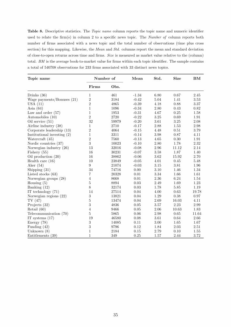
Table 8. Descriptive statistics. The Topic name column reports the topic name and numeric identifier

used to relate the firm(s) in column 2 to a specific news topic. The Number of column reports both

number of firms associated with a news topic and the total number of observations (time plus cross

section) for this mapping. Likewise, the Mean and Std. columns report the mean and standard deviation

of close-to-open returns across time and firms. Size is measured as market value relative to the (column)

total. BM is the average book-to-market value for firms within each topic identifier. The sample contains

a total of 540708 observations for 233 firms associated with 33 distinct news topics.

Topic name Number of Mean Std. Size BM

Firms Obs.

Drinks (36) 1 461 -1.34 6.80 0.67 2.45Wage payments/Bonuses (21) 2 3184 -0.42 5.04 1.41 3.53USA (11) 2 4865 -0.39 4.18 0.88 3.37Asia (64) 1 1096 -0.34 2.80 0.43 0.82Law and order (57) 1 1953 -0.31 4.67 0.25 1.58Automobiles (10) 2 2720 -0.22 3.25 0.69 1.91Oil service (51) 32 59979 -0.20 3.61 3.25 2.08Airline industry (38) 1 2710 -0.17 2.88 1.53 2.98Corporate leadership (13) 2 4064 -0.15 4.48 0.51 3.79Institutional investing (2) 1 3311 -0.14 3.98 0.87 4.11Watercraft (45) 2 7560 -0.13 4.65 0.30 1.91Nordic countries (37) 3 10023 -0.10 2.80 1.78 2.32Norwegian industry (26) 13 32016 -0.08 2.96 11.12 2.14Fishery (55) 16 30231 -0.07 3.58 1.87 1.40Oil production (20) 16 38862 -0.06 3.62 15.92 2.70Health care (16) 10 23849 -0.05 4.01 0.45 5.48Aker (54) 9 21074 -0.03 3.15 3.81 1.96Shipping (31) 34 74716 0.00 3.10 1.46 1.34Listed stocks (63) 7 20328 0.01 3.34 1.66 1.61Norwegian groups (28) 4 8668 0.01 2.36 6.24 1.54Housing (5) 5 8894 0.03 2.49 1.69 1.23Banking (12) 8 32174 0.03 1.78 5.85 1.19IT technology (71) 14 27514 0.04 4.00 0.63 19.78Norwegian regions (22) 3 13821 0.04 1.29 0.38 0.97TV (47) 5 13474 0.04 2.69 16.03 4.11Projects (32) 3 4836 0.05 3.57 2.23 2.99Retail (60) 4 9466 0.05 2.06 10.63 1.83Telecommunication (70) 5 5865 0.06 2.98 0.65 11.64IT systems (17) 19 46580 0.08 3.61 0.64 2.66Energy (78) 3 14085 0.11 3.00 1.65 1.67Funding (42) 3 9796 0.12 1.84 2.03 2.51Unknown (8) 1 2184 0.15 2.79 0.10 1.55Entitlements (39) 1 349 0.25 1.57 2.44 3.72

35

Firm counts

Firm and topic mappings

Figure 5. The upper graph reports the number of unique firms in the dataset at each point in time.

The line in the lower graph reports how many firms (in percent) each topic is associated with on average

across time. The bars report the change (in percentage point) in how many firms each topic is associated

with when splitting the sample into two equally sized parts and computing the difference (second sample

- first sample).

36

Table 9. News topics and day t close-to-open (c2o) and close-to-close returns (c2c) with random topic

assignments (Panel A) and day and industry effects (Panel B). The second row refers to the model

specification, i.e., which control variables that are included in the regressions apart from the variables

listed, confer the descriptions and headers used in Table 1. Fixed effects are included as specified in the

table. Following Tetlock et al. (2008), we compute clustered standard errors by trading day. Robust

t-statistics are in parentheses.

c2o c2c

I II III I II III

Panel A

TopicRt 0.0008 0.0018 0.0000 0.0000 0.0060 0.0101*(0.0021) (0.0029) (0.0033) (0.0029) (0.0047) (0.0056)

R2 0.0087 0.0297 0.0301 0.0054 0.0126 0.0127

Obs. 540708 540708 391533 540708 540708 391533

αi yes yes yes yes yes yes

δt yes no no yes no no

Panel B

Topict 0.0153*** 0.0134*** 0.0090** 0.0285*** 0.0267*** 0.0205***(0.0036) (0.0031) (0.0037) (0.0053) (0.0051) (0.0062)

R2 0.0063 0.0304 0.0310 0.0037 0.0130 0.0129

Obs. 540708 540708 391533 540708 540708 391533

αi yes yes yes yes yes yes

δt no no no no no no

Weekdayt yes yes yes yes yes yes

Industryg yes yes yes yes yes yes

37

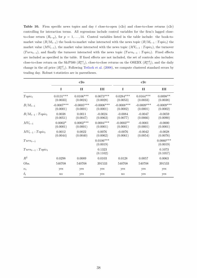
Table 10. Firm specific news topics and day t close-to-open (c2o) and close-to-close returns (c2c)

controlling for interaction terms. All regressions include control variables for the firm’s lagged close-

to-close return (Rt−p), for p = 1, . . . , 14. Control variables listed in the table include: the book-to-

market value (B/Mt−1) the book-to-market value interacted with the news topic (B/Mt−1 : Topict) the

market value (MVt−1), the market value interacted with the news topic (MVt−1 : Topict), the turnover

(Turnt−1), and finally the turnover interacted with the news topic (Turnt−1 : Topict). Fixed effects

are included as specified in the table. If fixed effects are not included, the set of controls also includes:

close-to-close return on the S&P500 (Rmit−1), close-to-close returns on the OSEBX (Rmh

t−1), and the daily

change in the oil price (Roilt−1). Following Tetlock et al. (2008), we compute clustered standard errors by

trading day. Robust t-statistics are in parentheses.

c2o c2c

I II III I II III

Topict 0.0131*** 0.0106*** 0.0073*** 0.0284*** 0.0164*** 0.0098**(0.0033) (0.0024) (0.0028) (0.0053) (0.0033) (0.0038)

B/Mt−1 -0.0007*** -0.0005*** -0.0006*** -0.0008*** -0.0009*** -0.0009***(0.0001) (0.0001) (0.0001) (0.0002) (0.0001) (0.0002)

B/Mt−1 : Topict 0.0038 0.0011 -0.0024 -0.0084 -0.0047 -0.0059(0.0051) (0.0047) (0.0063) (0.0077) (0.0066) (0.0090)

MVt−1 0.0002* 0.0002*** 0.0004*** -0.0003** -0.0001 -0.0000(0.0001) (0.0001) (0.0001) (0.0001) (0.0001) (0.0001)

MVt−1 : Topict 0.0012 0.0022 0.0076 -0.0076 -0.0042 -0.0028(0.0044) (0.0040) (0.0062) (0.0061) (0.0054) (0.0076)

Turnt−1 0.0106*** 0.0060***(0.0019) (0.0019)

Turnt−1 : Topict 0.1323 0.1073(0.1102) (0.1057)

R2 0.0298 0.0089 0.0103 0.0128 0.0057 0.0063

Obs. 540708 540708 391533 540708 540708 391533

αi yes yes yes yes yes yes

δt no yes yes no yes yes

38

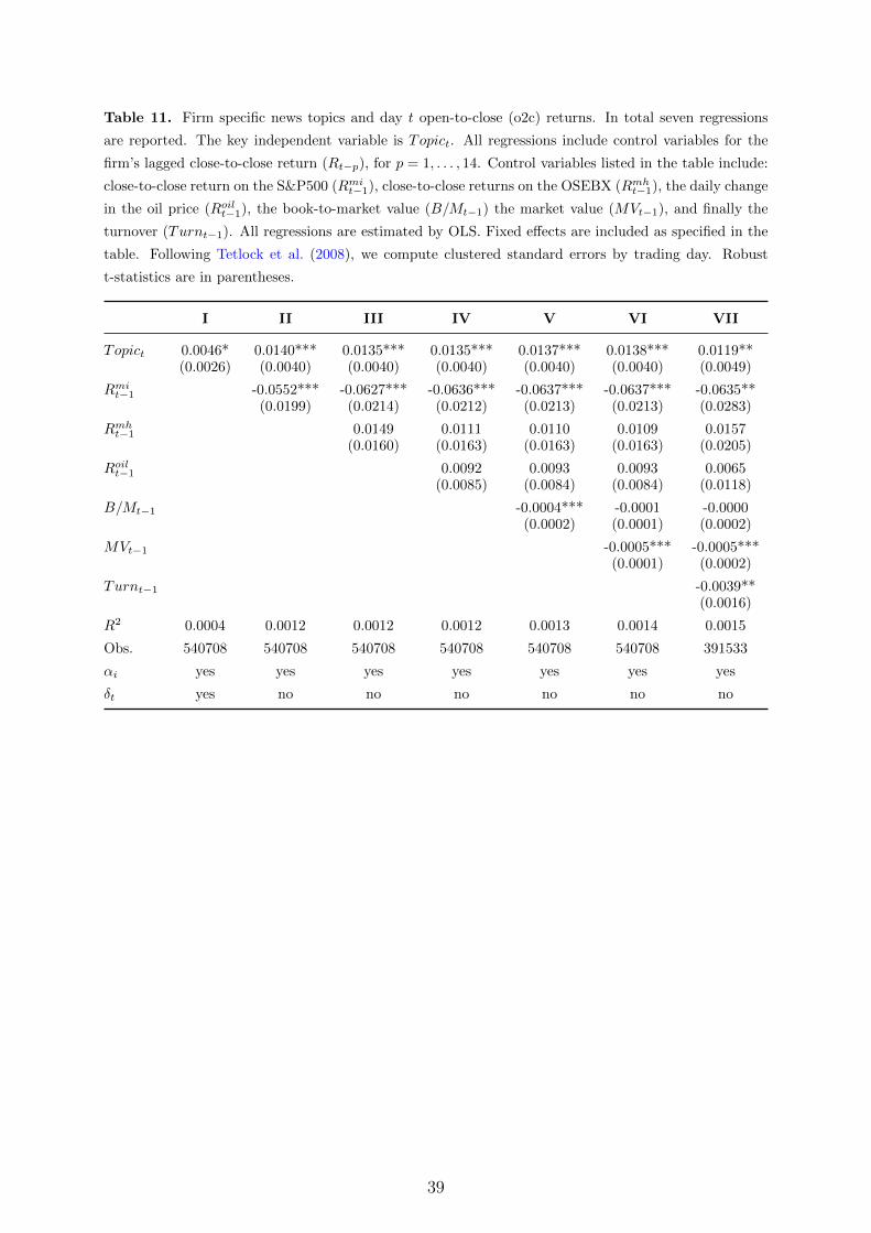
Table 11. Firm specific news topics and day t open-to-close (o2c) returns. In total seven regressions

are reported. The key independent variable is Topict. All regressions include control variables for the

firm’s lagged close-to-close return (Rt−p), for p = 1, . . . , 14. Control variables listed in the table include:

close-to-close return on the S&P500 (Rmit−1), close-to-close returns on the OSEBX (Rmh

t−1), the daily change

in the oil price (Roilt−1), the book-to-market value (B/Mt−1) the market value (MVt−1), and finally the

turnover (Turnt−1). All regressions are estimated by OLS. Fixed effects are included as specified in the

table. Following Tetlock et al. (2008), we compute clustered standard errors by trading day. Robust

t-statistics are in parentheses.

I II III IV V VI VII

Topict 0.0046* 0.0140*** 0.0135*** 0.0135*** 0.0137*** 0.0138*** 0.0119**(0.0026) (0.0040) (0.0040) (0.0040) (0.0040) (0.0040) (0.0049)

Rmit−1 -0.0552*** -0.0627*** -0.0636*** -0.0637*** -0.0637*** -0.0635**

(0.0199) (0.0214) (0.0212) (0.0213) (0.0213) (0.0283)

Rmht−1 0.0149 0.0111 0.0110 0.0109 0.0157

(0.0160) (0.0163) (0.0163) (0.0163) (0.0205)

Roilt−1 0.0092 0.0093 0.0093 0.0065

(0.0085) (0.0084) (0.0084) (0.0118)

B/Mt−1 -0.0004*** -0.0001 -0.0000(0.0002) (0.0001) (0.0002)

MVt−1 -0.0005*** -0.0005***(0.0001) (0.0002)

Turnt−1 -0.0039**(0.0016)

R2 0.0004 0.0012 0.0012 0.0012 0.0013 0.0014 0.0015

Obs. 540708 540708 540708 540708 540708 540708 391533

αi yes yes yes yes yes yes yes

δt yes no no no no no no

39

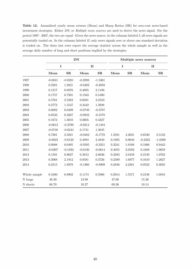
Table 12. Annualized yearly mean returns (Mean) and Sharp Ratios (SR) for zero-cost news-based

investment strategies. Either DN, or Multiple news sources are used to derive the news signal. For the

period 1997 - 2007, the two are equal. Given the news source, in the columns labeled I, all news signals are

potentially traded on. In the columns labeled II, only news signals over or above one standard deviation

is traded on. The three last rows report the average statistic across the whole sample as well as the

average daily number of long and short positions implied by the strategies.

DN Multiple news sources

I II I II

Mean SR Mean SR Mean SR Mean SR

1997 -0.0041 -0.0281 -0.2093 -1.5361

1998 0.2201 1.2821 -0.0402 -0.2058

1999 0.1217 0.6976 0.4085 2.1186

2000 0.1757 0.7391 0.1563 0.5490

2001 0.5761 2.5282 0.6931 3.2523

2002 0.3772 1.5547 0.3442 1.3928

2003 0.0082 0.0409 -0.0740 -0.3787

2004 0.0533 0.3267 -0.0942 -0.5578

2005 0.1674 1.3010 0.0605 0.4327

2006 -0.0612 -0.3790 -0.0214 -0.1484

2007 -0.0748 -0.6244 0.1741 1.3045

2008 0.7301 2.5021 -0.0483 -0.1770 1.2581 4.2631 0.6530 2.5132

2009 -0.0023 -0.0120 0.4894 2.4840 0.1985 0.9640 -0.2322 -1.0380

2010 0.0088 0.0495 -0.0585 -0.3351 0.3241 1.8168 0.1866 0.9442

2011 -0.0397 -0.1933 -0.0130 -0.0614 0.4055 2.0592 0.4488 1.9659

2012 0.1501 0.9627 0.3812 2.0636 0.3283 2.0459 0.2130 1.0762

2013 0.3068 2.1912 0.0581 0.3726 0.2389 1.6977 0.1610 1.2627

2014 0.2515 1.8978 -0.1360 -0.8909 0.2846 2.2381 0.0523 0.3035

Whole sample 0.1680 0.8902 0.1174 0.5986 0.2914 1.5571 0.2138 1.0816

N longs 46.30 13.98 47.00 15.26

N shorts 68.70 10.27 69.36 10.14

40

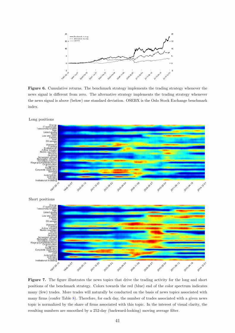
Figure 6. Cumulative returns. The benchmark strategy implements the trading strategy whenever the

news signal is different from zero. The alternative strategy implements the trading strategy whenever

the news signal is above (below) one standard deviation. OSEBX is the Oslo Stock Exchange benchmark

index.

Long positions

Short positions

Figure 7. The figure illustrates the news topics that drive the trading activity for the long and short

positions of the benchmark strategy. Colors towards the red (blue) end of the color spectrum indicates

many (few) trades. More trades will naturally be conducted on the basis of news topics associated with

many firms (confer Table 8). Therefore, for each day, the number of trades associated with a given news

topic is normalized by the share of firms associated with this topic. In the interest of visual clarity, the

resulting numbers are smoothed by a 252-day (backward-looking) moving average filter.

41

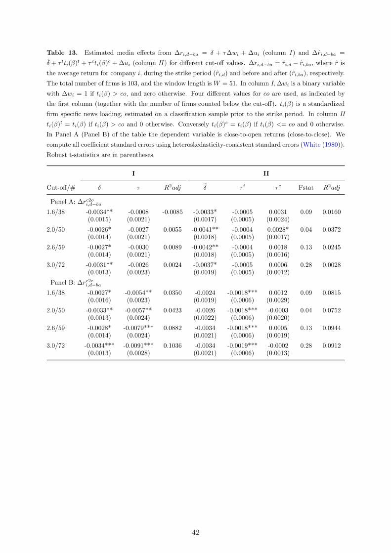
Table 13. Estimated media effects from ∆ri,d−ba = δ + τ∆wi + ∆ui (column I ) and ∆ri,d−ba =

δ + τ tti(β)t + τ cti(β)c + ∆ui (column II ) for different cut-off values. ∆ri,d−ba = ri,d − ri,ba, where r is

the average return for company i, during the strike period (ri,d) and before and after (ri,ba), respectively.

The total number of firms is 103, and the window length is W = 51. In column I, ∆wi is a binary variable

with ∆wi = 1 if ti(β) > co, and zero otherwise. Four different values for co are used, as indicated by

the first column (together with the number of firms counted below the cut-off). ti(β) is a standardized

firm specific news loading, estimated on a classification sample prior to the strike period. In column II

ti(β)t = ti(β) if ti(β) > co and 0 otherwise. Conversely ti(β)c = ti(β) if ti(β) <= co and 0 otherwise.

In Panel A (Panel B) of the table the dependent variable is close-to-open returns (close-to-close). We

compute all coefficient standard errors using heteroskedasticity-consistent standard errors (White (1980)).

Robust t-statistics are in parentheses.

I II

Cut-off/# δ τ R2adj δ τ t τ c Fstat R2adj

Panel A: ∆rc2oi,d−ba

1.6/38 -0.0034** -0.0008 -0.0085 -0.0033* -0.0005 0.0031 0.09 0.0160(0.0015) (0.0021) (0.0017) (0.0005) (0.0024)

2.0/50 -0.0026* -0.0027 0.0055 -0.0041** -0.0004 0.0028* 0.04 0.0372(0.0014) (0.0021) (0.0018) (0.0005) (0.0017)

2.6/59 -0.0027* -0.0030 0.0089 -0.0042** -0.0004 0.0018 0.13 0.0245(0.0014) (0.0021) (0.0018) (0.0005) (0.0016)

3.0/72 -0.0031** -0.0026 0.0024 -0.0037* -0.0005 0.0006 0.28 0.0028(0.0013) (0.0023) (0.0019) (0.0005) (0.0012)

Panel B: ∆rc2ci,d−ba

1.6/38 -0.0027* -0.0054** 0.0350 -0.0024 -0.0018*** 0.0012 0.09 0.0815(0.0016) (0.0023) (0.0019) (0.0006) (0.0029)

2.0/50 -0.0033** -0.0057** 0.0423 -0.0026 -0.0018*** -0.0003 0.04 0.0752(0.0013) (0.0024) (0.0022) (0.0006) (0.0020)

2.6/59 -0.0028* -0.0079*** 0.0882 -0.0034 -0.0018*** 0.0005 0.13 0.0944(0.0014) (0.0024) (0.0021) (0.0006) (0.0019)

3.0/72 -0.0034*** -0.0091*** 0.1036 -0.0034 -0.0019*** -0.0002 0.28 0.0912(0.0013) (0.0028) (0.0021) (0.0006) (0.0013)

42

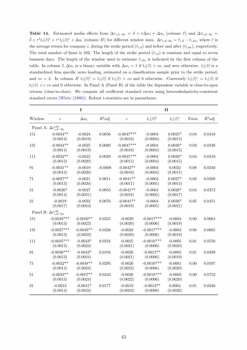
Table 14. Estimated media effects from ∆ri,d−ba = δ + τ∆wi + ∆ui (column I ) and ∆ri,d−ba =

δ + τ tti(β)t + τ cti(β)c + ∆ui (column II ) for different window sizes. ∆ri,d−ba = ri,d − ri,ba, where r is

the average return for company i, during the strike period (ri,d) and before and after (ri,ba), respectively.

The total number of firms is 103. The length of the strike period (ri,d) is constant and equal to seven

business days. The length of the window used to estimate ri,ba is indicated by the first column of the

table. In column I, ∆wi is a binary variable with ∆wi = 1 if ti(β) > co, and zero otherwise. ti(β) is a

standardized firm specific news loading, estimated on a classification sample prior to the strike period,

and co = 2. In column II ti(β)t = ti(β) if ti(β) > co and 0 otherwise. Conversely ti(β)c = ti(β) if

ti(β) <= co and 0 otherwise. In Panel A (Panel B) of the table the dependent variable is close-to-open

returns (close-to-close). We compute all coefficient standard errors using heteroskedasticity-consistent

standard errors (White (1980)). Robust t-statistics are in parentheses.

I II

Window c ∆wi R2adj c ti(β)t ti(β)c Fstat R2adj

Panel A: ∆rc2oi,d−ba

151 -0.0034** -0.0024 0.0056 -0.0047*** -0.0004 0.0025* 0.04 0.0416(0.0014) (0.0019) (0.0016) (0.0004) (0.0015)

131 -0.0034** -0.0025 0.0060 -0.0047*** -0.0004 0.0026* 0.03 0.0426(0.0014) (0.0019) (0.0016) (0.0004) (0.0015)

111 -0.0032** -0.0022 0.0029 -0.0045*** -0.0004 0.0026* 0.04 0.0410(0.0013) (0.0020) (0.0015) (0.0004) (0.0015)

91 -0.0031** -0.0019 -0.0008 -0.0042** -0.0004 0.0022 0.08 0.0240(0.0013) (0.0020) (0.0016) (0.0004) (0.0015)

71 -0.0027** -0.0021 0.0011 -0.0041** -0.0003 0.0027* 0.03 0.0388(0.0013) (0.0020) (0.0017) (0.0005) (0.0015)

51 -0.0026* -0.0027 0.0055 -0.0041** -0.0004 0.0028* 0.04 0.0372(0.0014) (0.0021) (0.0018) (0.0005) (0.0017)

31 -0.0019 -0.0032 0.0076 -0.0041** -0.0004 0.0036* 0.05 0.0451(0.0017) (0.0024) (0.0019) (0.0005) (0.0021)

Panel B: ∆rc2ci,d−ba

151 -0.0038*** -0.0050** 0.0325 -0.0029 -0.0017*** -0.0004 0.00 0.0664(0.0013) (0.0023) (0.0020) (0.0006) (0.0019)

131 -0.0037*** -0.0049** 0.0326 -0.0028 -0.0017*** -0.0004 0.00 0.0665(0.0013) (0.0023) (0.0020) (0.0006) (0.0019)

111 -0.0035*** -0.0043* 0.0216 -0.0025 -0.0016*** -0.0005 0.01 0.0550(0.0013) (0.0023) (0.0021) (0.0006) (0.0020)

91 -0.0036*** -0.0042* 0.0194 -0.0026 -0.0015** -0.0005 0.01 0.0499(0.0013) (0.0024) (0.0021) (0.0006) (0.0019)

71 -0.0032** -0.0048** 0.0295 -0.0026 -0.0016*** -0.0001 0.00 0.0597(0.0013) (0.0024) (0.0022) (0.0006) (0.0020)

51 -0.0033** -0.0057** 0.0423 -0.0026 -0.0018*** -0.0003 0.00 0.0752(0.0013) (0.0024) (0.0022) (0.0006) (0.0020)

31 -0.0013 -0.0041* 0.0177 -0.0010 -0.0013** 0.0004 0.01 0.0346(0.0014) (0.0024) (0.0023) (0.0006) (0.0020)

43

Appendix B The textual data and the LDA

B.1 Filtering the news corpus

To clean the raw textual dataset a stop-word list is first employed. This is a list of common

words not expected to have any information relating to the subject of an article. Examples

of such words are the, is, are, and this. The most common Norwegian surnames and given

names are also removed. In total the stop-word list together with the list of common

surnames and given names removed roughly 1800 unique tokens from the corpus. Next,

an algorithm known as stemming is run. The objective of this algorithm is to reduce all

words to their respective word stems. A word stem is the part of a word that is common

to all of its inflections. An example is the word effective whose stem is effect. Finally,

a measure called tf-idf, which stands for term frequency - inverse document frequency,

is calculated. This measures how important all the words in the complete corpus are in

explaining single articles. The more often a word occurs in an article, the higher the tf-idf

score of that word. On the other hand, if the word is common to all articles, meaning the

word has a high frequency in the whole corpus, the lower that word’s tf-idf score will be.

Around 250 000 of the stems with the highest tf-idf score are kept, and used as the final

corpus.

B.2 LDA intuition, estimation and specification

The LDA model was developed in Blei et al. (2003). Here the estimation algorithm

described in Griffiths and Steyvers (2004) is implemented.

Figure 8 illustrates the LDA model graphically. The outer box, or plate, represent

the whole corpus as M distinct documents (articles). N =∑M

m=1Nm is the total number

of words in all documents, and K is the total number of latent topics. Letting bold-

font variables denote the vector version of the variables, the distribution of topics for a

document is given by θm, while the distribution of words for each topic is determined by

ϕk. Both θm and ϕk are assumed to have conjugate Dirichlet distributions with (hyper)

parameter (vectors) α and β, respectively. Each document consists of a repeated choice

of topics Zm,n and words Wm,n, drawn from the Multinomial distribution using θm and

ϕk. The circle associated with Wm,n is gray colored, indicating that these are the only

observable variables in the model.

At an intuitive level, the best way to understand the LDA model is likely to make a

thought experiment of how the articles in the newspaper (the corpus) were generated.

1. Pick the overall theme of articles by randomly giving them a distribution over topics,

i.e.: Choose θm ∼ Dir(α), where m ∈ {1, . . . ,M}.

44

, ,

∈ [1, ]

∈ [1, ]

∈ [1, ]

Figure 8. The LDA model visualized using plate notation.

2. Pick the word distribution for each topic by giving them a distribution over words,

i.e.: Choose ϕk ∼ Dir(β) , where k ∈ {1, . . . , K}.3. For each of the word positions m, n, where n ∈ {1, . . . , Nm}, and m ∈ {1, . . . ,M}

3.1. From the topic distribution chosen in 1., randomly pick one topic, i.e.: Choose

a topic Zm,n ∼ Multinomial(θm).

3.2. Given that topic, randomly choose a word from this topic, i.e.: Choose a word

Wm,n ∼ Multinomial(ϕzm,n).

More formally, the goal of the LDA estimation algorithm is to approximate the distri-

bution:

P (Z|W ;α, β) =P (W ,Z;α, β)

P (W ;α, β)(7)

using Gibbs simulations, where α and β are the (hyper) parameters controlling the prior

conjugate Dirichlet distributions for θm and ϕk, respectively. A very good explanation

for how this method works is found in Heinrich (2009). The description below provides a

brief summary only.

First, let V denote the size of the vocabulary, and t a term in V . Then, denote

P (t|z = k) as the mixture component, one for each topic, by Φ = {ϕk}Kk=1, and let

P (z|d = m) define the topic mixture proportion for document m, with one proportion for

each document Θ = {θm}Mm=1. The total probability of the model can then be written as:

P (W ,Z,Θ,Φ;α, β) =K∏k=1

P (ϕi; β)M∏

m=1

P (θm;α)N∏t=1

P (zm,t|θm)P (wm,t|ϕzm,t) (8)

Integrating out the parameters ϕ and θ:

P (Z,W ;α, β) =

∫Θ

∫Φ

P (W ,Z,Θ,Φ;α, β) dΦ dΘ

=

∫Φ

K∏k=1

P (ϕk; β)M∏

m=1

N∏t=1

P (wm,t|ϕzm,t) dΦ

∫Θ

M∏m=1

P (θm;α)N∏t=1

P (zm,t|θm) dΘ

(9)

45

In (9), the terms inside the first integral do not include a θ term, and the terms inside

the second integral do not include a ϕ term. Accordingly, the two terms can be solved

separately. Exploiting the properties of the conjugate Dirichlet distribution it can be

shown that:∫Θ

M∏m=1

P (θm;α)N∏t=1

P (zm,t|θm) dΘ =Γ(∑K

k=1 αk

)∏Kk=1 Γ(αk)

∏Kk=1 Γ(n

(k)m + αk)

Γ(∑K

k=1 n(k)m + αk

) (10)

and ∫Φ

K∏k=1

P (ϕk; β)M∏

m=1

N∏t=1

P (wm,t|ϕzm,t) dΦ =K∏k=1

Γ(∑V

t=1 βt)∏V

t=1 Γ(βt)

∏Vt=1 Γ(n

(t)k + βt)

Γ(∑V

t=1 n(t)k + βt

) (11)

where n(k)m denotes the number of word tokens in the mth document assigned to the kth

topic, and n(t)k is the number of times the tth term in the vocabulary has been assigned to

the kth topic.

Since P (W ;α, β), in (7), is invariable for any of Z, the conditional distribution

P (Z|W ;α, β) can be derived from P (W ,Z;α, β) directly using Gibbs simulation and

the conditional probability:

P (Z(m,n) | Z−(m,n),W ;α, β) =P (Z(m,n),Z−(m,n),W ;α, β)

P (Z−(m,n),W ;α, β)(12)

where Z(m,n) denotes the hidden variable of the nth word token in the mth document,

and Z−(m,n) denotes all Zs but Z(m,n). Denoting the index of a word token by i =

(m,n), and using the expressions in (10) and (11), cancellation of terms (and some extra

manipulations exploiting the properties of the gamma function) yields:

P (Zi = k | Z−(i),W ;α, β) ∝ (n(k)m,−i + αk)

n(t)k,−i + βt∑V

t=1 n(t)k,−i + βt

(13)

where the counts n(·)·,−i indicate that token i is excluded from the corresponding document

or topic. Thus, sampling topic indexes using equation (13) for each word in a document

and across documents until convergence allows us to approximate the posterior distribu-

tion given by (7). As noted in Heinrich (2009), the procedure itself uses only five larger

data structures; the count variables n(k)m and n

(t)k , which have dimension M×K and K×V ,

respectively, their row sums nm and nk, as well as the state variable zm,n with dimension

W .

With one simulated sample of the posterior distribution for P (Z|W ;α, β), ϕ and θ

can be estimated from:

ϕk,t =n(t)k + βt∑V

t=1 n(t)k + βr

(14)

46

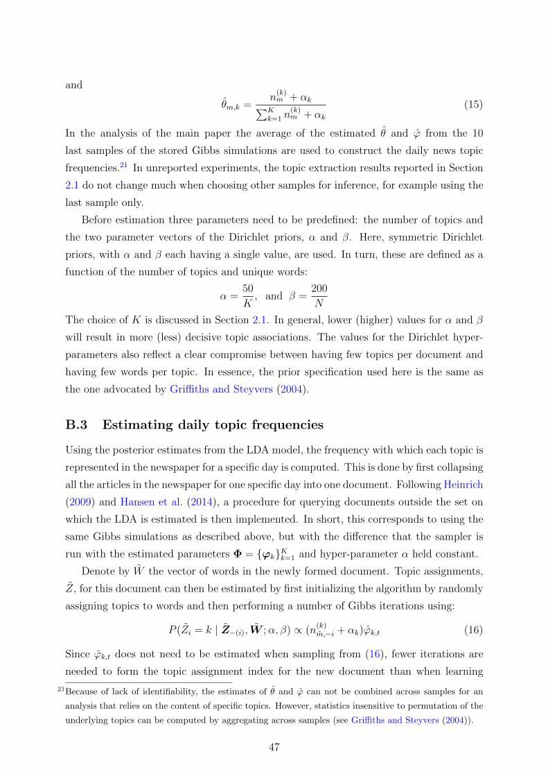
and

θm,k =n(k)m + αk∑K

k=1 n(k)m + αk

(15)

In the analysis of the main paper the average of the estimated θ and ϕ from the 10

last samples of the stored Gibbs simulations are used to construct the daily news topic

frequencies.21 In unreported experiments, the topic extraction results reported in Section

2.1 do not change much when choosing other samples for inference, for example using the

last sample only.

Before estimation three parameters need to be predefined: the number of topics and

the two parameter vectors of the Dirichlet priors, α and β. Here, symmetric Dirichlet

priors, with α and β each having a single value, are used. In turn, these are defined as a

function of the number of topics and unique words:

α =50

K, and β =

200

N

The choice of K is discussed in Section 2.1. In general, lower (higher) values for α and β

will result in more (less) decisive topic associations. The values for the Dirichlet hyper-

parameters also reflect a clear compromise between having few topics per document and

having few words per topic. In essence, the prior specification used here is the same as

the one advocated by Griffiths and Steyvers (2004).

B.3 Estimating daily topic frequencies

Using the posterior estimates from the LDA model, the frequency with which each topic is

represented in the newspaper for a specific day is computed. This is done by first collapsing

all the articles in the newspaper for one specific day into one document. Following Heinrich

(2009) and Hansen et al. (2014), a procedure for querying documents outside the set on

which the LDA is estimated is then implemented. In short, this corresponds to using the

same Gibbs simulations as described above, but with the difference that the sampler is

run with the estimated parameters Φ = {ϕk}Kk=1 and hyper-parameter α held constant.

Denote by W the vector of words in the newly formed document. Topic assignments,

Z, for this document can then be estimated by first initializing the algorithm by randomly

assigning topics to words and then performing a number of Gibbs iterations using:

P (Zi = k | Z−(i), W ;α, β) ∝ (n(k)m,−i + αk)ϕk,t (16)

Since ϕk,t does not need to be estimated when sampling from (16), fewer iterations are

needed to form the topic assignment index for the new document than when learning

21Because of lack of identifiability, the estimates of θ and ϕ can not be combined across samples for an

analysis that relies on the content of specific topics. However, statistics insensitive to permutation of the

underlying topics can be computed by aggregating across samples (see Griffiths and Steyvers (2004)).

47

both the topic and word distributions. Here 2000 iterations are performed, and only

the average of every 10th draw is used for the final inference. After sampling, the topic

distribution can be estimated as before:

˜θm,k =

n(k)m + αk∑K

k=1 n(k)m + αk

(17)

We note that the same procedure for querying documents outside the set on which the

LDA is estimated is implemented when we classify the firms’ textual description, confer

Section 2.3.

B.4 Sign adjustment

Given knowledge of the topics and the daily topic frequencies, we identify their sign using

a dictionary based approach. In particular, for each day, all newspaper articles that day,

and each of the K news topics, the article that news topic k describes the best is found.

Given knowledge of this topic article mapping, positive/negative words in the articles

are identified using an external word list and simple word counts. The word list used

here takes as a starting point the classification of positive/negative words defined by the

Harvard IV-4 Psychological Dictionary. As this dictionary contains English words only,

the set of words must be translated into Norwegian. The translated set of words consists

of 40 positive and 39 negative Norwegian words, which is somewhat different from the

Harvard IV-4 Psychological Dictionary both in terms of numbers and exact meaning. The

translated word list may be obtained upon request.

The count procedure delivers two statistics for each article, containing the number of

positive and negative words. These statistics are then normalized such that each article

observation reflects the fraction of positive and negative words, i.e.:

Post,na =#positivewords

#totalwordsNegt,na =

#negativewords

#totalwords(18)

The overall tone of article na, for na = 1, . . . , Nat at day t, is defined as:

St,na = Post,na −Negt,na (19)

Letting St,na,k denote the sign statistic associated with topic k and T opict,k the daily topic

frequency, the sign of topic k is adjusted simply as:

Topick,t = T opick,t if St,na,k >= 0 and Topick,t = −T opick,t if St,na,k < 0

48