Asset Liability Management for Pension Funds A Multistage Chance Constrained Programming Approach (Asset Liability Management voor Pensioenfondsen Een meer-perioden optimalisatiemodel met kansrestricties) Proefschrift ter verkrijging van de graad van doctor aan de Erasmus Universiteit Rotterdam, op gezag van de Rector Magnificus Prof.dr. P.W.C. Akkermans M.A. En volgens besluit van het College voor Promoties. De openbare verdediging zal plaatsvinden op donderdag 30 november 1995 om 16.00 uur door Cornelis Ludovicus bert geboren te Vlissingen

Welcome message from author
This document is posted to help you gain knowledge. Please leave a comment to let me know what you think about it! Share it to your friends and learn new things together.
Transcript
Asset Liability Management for Pension Funds
A Multistage Chance Constrained Programming Approach
(Asset Liability Management voor Pensioenfondsen
Een meer-perioden optimalisatiemodel met kansrestricties)
Proefschrift
ter verkrijging van de graad van doctor
aan de Erasmus Universiteit Rotterdam,
op gezag van de Rector Magnificus
Prof.dr. P.W.C. Akkermans M.A.
En volgens besluit van het College voor Promoties.
De openbare verdediging zal plaatsvinden op
donderdag 30 november 1995 om 16.00 uur
door
Cornelis Ludovicus bert
geboren te Vlissingen

Promotiecommissie
Promotores:
Overige leden:
UNIVERSITEITS3iBUOTHEEK Erasmus Un!versiteit Burgemeas~a Gudlaan 50
prof.dr. A.H.G. Rinnooy Kan 3062 PA ROTTERDAM . prof.dr. C.G.E. Boender
prof.dr. J.M.G. Frijns
prof.dr. R.A.H. van der Meer
prof.dr. A.C.F. Vorst
55

To my parents


Preface
It has been nine years since I accepted Alexander Rinnooy Kan's proposal to set out on a Ph.D. study on a part time basis. Would I do it again? I think I would: business people are not that dull and academics are not so unworldly after all. Moreover, salary at the university is not that bad and neither is the commercial time pressure in industry.
I am greatly indebted to my supervisors, Alexander Rinnooy Kan and Guus Boender. Both of them have rather substantial obligations, other than advising on Ph.D. research. Nevertheless, they were always available to discuss ideas, read preliminary drafts of this thesis and to make formal arrangements with the Operations Research Department when necessary. Even though there have been extended periods of time during which I did not pay sufficient attention to my research, Alexander never seized the opportunity to quit. On the contrary, any reading material delivered by 2.00 am on Saturday would be
commented and discussed by Monday at 10.00 am.
It would not have been possible to complete this thesis without the support of former
employers and colleagues. At AKB, as well as at Pacific Investments, I was allowed to
spend substantial time on research that was of no direct importance to them, even in times when business was difficult. In this respect I am especially grateful to Bob Out who granted me a sabbatical leave from Pacific Investments.
It has not been easy to initiate joint research on a subject that was not in the focus of interest of any department at the Erasmus University. This made the cooperation with Sjoerd Mosterd, Dennis Barns and Karin Aarssen all the more fruitful and enjoyable.
The computational results in this thesis would have been difficult to obtain without the support of Ortec Consultants, in particular from Fred Heemskerk and Jan van Mierlo, Jan Bisschop from Paragon Decision Technology, who provided me with a copy of the excellent AIMMS Modeling System, and Mn Services, the service organisation of the Pension Fund for the Metalworking, Pipe, Mechanical and Automotive Trades.
The importance of the indirect contributions of colleagues at the Operations Research
Department, family and friends can hardly be overstated. Without them, there would be no point in the predominantly solitary task of preparing a dissertation.
Karin did not only contribute in an excellent way to the research on asset liability management: after she finished her studies, she abandoned the field of ALM, only to return as a new, overwhelming dimension to my life, which enriches it in every respect.

Contents
Notation ................................................ vi
Chapter 1 Introduction and Summary . . . . . . . . . . . . . . . . . . . . . . . . . . . . . . . . . . . . 1
1.1 Problem Description . . . . . . . . . . . . . . . . . . . . . . . . . . . . . . . . . 1
1.2 Modelling an Uncertain Future by Scenarios . . . . . . . . . . . . . . . . . . . 5
1.3 The Position of our ALM Approach in the Literature . . . . . . . . . . . . . 7
1.4 A Scenario Generator for Asset Liability Management . . . . . . . . . . . . . 9
1. 5 A Dynamic Optimisation Model for Asset Liability Management . . . . . . 11
1. 6 Computational Complexity . . . . . . . . . . . . . . . . . . . . . . . . . . . . . . 13
1. 7 Computational Experiments . . . . . . . . . . . . . . . . . . . . . . . . . . . . . 14
Chapter 2
Asset Liability Management for Pension Funds, A Survey . . . . . . . . . . . . . . . . . 17
2.1 Introduction ....................................... 17
2.2 Model Classification ................................. 17
2.3 Anticipative Models for ALM ............................ 19
2.3.1 Mean-Variance Models .......................... 19
2.3.2 Chance Constrained Models ....................... 21
2.3.3 Chance Constrained Programming, Normally Distributed
Returns and Mean-Variance Optimisation . . . . . . . . . . . . . . 22
2.4 Recourse Models for ALM . . . . . . . . . . . . . . . . . . . . . . . . . . . . . 26
2.5 Summary ........................................ 28
Chapter 3
Modelling Asset Liability Management . . . . . . . . . . . . . . . . . . . . . . . . . . . . . 31
3 .1 The Essential Elements of an Optimisation Model for Asset Liability
Management . . . . . . . . . . . . . . . . . . . . . . . . . . . . . . . . . . . . 31
3 .1.1 Elements Constituting a Dynamic Asset Liability Management
Policy .................................... 32
3.1.2 Risk and Reward .............................. 33
3.1.3 Consequences for Modelling Asset Liability Management ..... 35 3.2 A Conceptual Asset Liability Management Model ................ 36
3.3 Formulating a Dynamic Chance Constrained Program for ALM ....... 41
3. 3 .1 A Scenario Structure to Reflect an Uncertain Future . . . . . . . . 41
3.3.2 A Multistage Chance Constrained ALM Model ........... 42
iii
Asset Liability Management for Pension Funds
Chapter 4
Scenario Generation for Asset Liability Management . . . . . . . . . . . . . . . . . . . . 4 7
4.1 Introduction ....................................... 47
4.2 Requirements on Scenario Generation ....................... 48
4.3 A Scenario Generation Model for Asset Liability Management . . . . . . 51
4.3.1 A Vector Autoregressive Model to Generate Scenarios of
Economic Variables ........................... 51
4.3.2 Arbitrage Free Scenarios . . . . . . . . . . . . . . . . . . . . . 58
4.3.3 Generating Future Time Series of Liabilities and Cost of Salaries . . . . . . . . . . . . . . . . . . . . . . . . . . . . . . . . . . . 66
4.3.4 Generating Future Time Series of Economic and Actuarial
Variables .................................. 67
Chapter 5 Model Tractability, from Multistage to Two Stage . . . . . . . . . . . . . . . . . . . . . . 69
5 .1 Introduction . . . . . . . . . . . . . . . . . . . . . . . . . . . . . . . . . . . . . . . 69
5.2 Reducing the Number of States of the World .................. 73
5.3 A Sequence of Two Stage Problems to Solve t4e ALM Model ........ 74 5.3.1 A Feasible Solution to the ALM Model ................ 78
5.4 A Metamodel to Estimate Optimal Decisions ................... 81
5 .4 .1 Introduction . . . . . . . . . . . . . . . . . . . . . . . . . . . . . . . . . 81
5.4.2 Requirements on the Metamodel ...... . . . . . . . . . . . . . . 81
5.4.3 Mechanisms that Drive the ALM Model .. . 82 5.4.4 A Metamodel to Derive Horizon Constraints ............. 82
5.4.5 Selecting an Objective Function for .................. 88
5. 5 A Forward Procedure . . . . . . . . . . . . . . . . . . . . . . . . . . . . . . . . . 89 5. 6 Summary . . . . . . . . . . . . . . . . . . . . . . . . . . . . . . . . . . . . . . . . 92
Chapter 6 Model Tractability, Variance Reduction . . . . . . . . . . . . . . . . . . . . . . . . . . . . 95
6 .1 Introduction . . . . . . . . . . . . . . . . . . . . . . . . . . . . . . . . . . . . . . . 95
6. 2 Importance Sampling . . . . . . . . . . . . . . . . . . . . . . . . . . . . . . . . . 96
6.2.1 The Potential Merits of Importance Sampling . . . . . . . . . . . . . 96 6.2.2 Importance Sampling in Stochastic Linear Programming ...... 98
6.3 Importance Sampling in ALM . . . . . . . . . . . . . . . . . . . . . . . . . . . 101
6.4 Computational Results .................. , . . . . . . . . . . . . 105
iv
Contents
Chapter 7
Computational Results 109 7.1 Introduction . . . . . . . . . . . . . . . . . . . . . . . . . . . . . . . . . . . . . . 109 7.2 The Exogenous Environment ........................... 110
7.2.1 The Scenario Generator ......................... 110
7.2.2 Requirements on the ALM Policy ................... 116
7.2.3 Comparison of the ALM Model to Other Approaches . . . . . . 118
7.3 Numerical Results . . . . . . . . . . . . . . . . . . . . . . . . . . . . . . . . . . 120
7.3 .1 The Behaviour of the ALM Model . . . . . . . . . . . . . . . . . . 120
7.3.2 Results From the Forward-only Procedure . . . . . . . . . . . . . 121 7.3.3 Results From Optimal Static Decisions . . . . . . . . . . . . . . . . 122
7.3.4 Results from the ALM Model ..................... 123
7.4 Summary ....................................... 131
Appendix A. Chance Constrained Programmi~g, Normally Distributed Returns and
Mean-Variance Optimisation . . . . . . . . . . . . . . . . . . . . . . . . . . . . . . 133
Appendix B. The ALM Model With Transaction Costs 134
Appendix C. Illustrations of Importance Sampling 135
References ............................................. 138
Samenvatting (Summary in Dutch) ............................... 145
v

Notation
General
The notion of time will be reflected by points in time t, t = O, ... ,T. Period t, t = 1, ... ,T
refers to the span of time from t-1 to t . A scenario or a path through time will be
defined as a consecutive sequence of states of the world. Each state has exactly one
predecessor and may have rpany successors. The predecessor of t,s will be indexed by
t-1 ,s. The set I1
denotes all the information that is available at point in time t .
[ .. ] Closed interval
( .. ) Open interval
a1.[.] Linear function that aggregates a sequence of cashflows to a lumpsum
payment at point in time t in state s .
c(.)
exp(.)
0(.)
Pr[.]
Pr[.l.]
<p (.)
a[.,.]
In(.)
N(~,:E)
I
Linear or piecewise linear cost function
e(.)
Landau's 0 symbol
Probability operator
Conditional probability operator
Cumulative density function of the standard normal distribution.
Covariance operator
Natural logarithm
Gaussian distribution with mean-vector ~ and covariance matrix :E .
Identity matrix
E [.] Mathematical expectation operator
Nodes(t) Set of nodes that were included in model Twostage(t)
Intertemp( t) Set of nodes ( 7, s), 1 :::;; 7 :::;; t- 2 for which solvency requirements are
enforced.
Superscripts
a optimal solution to Adjust
f short notation for a value which is an upper bound of a decision variable as
well as a lower bound (i.e. xf =a ** x" =x 1 =a)
lower bound on decision variables
vi

Notation
m
u
T
Parameters
r(A),s
r(L),s
R.s
optimal solution to MinAssets
upper bound on decision variables
transpose of a matrix
Demanded funding level
Maximal raise in contribution per period as a fraction of the cost of
wages at point in time t
Realisation from random sampling
Discount factor for a cash flow at point in time t in state s
Benefit payments and costs to the fund at point in time t in state s
Continuous price inflation over period t in state s
Short notation for exp(r;r,)
Actuarial reserve at point in time t in state s
Penalty parameter to penalise remedial contributions
Weighing coefficients
Large constant at point in time t in state s
Weighting to determine importance sampling probability of state s
Number of states that succeed state (t ,s) with positive probability
Probability of state s at point in time t
Importance sampling probability of state s at point in time t
Continuous return on investment i over period t in state s
Continuous return on investment portfolio A over period t in state s
Continuous growth of liabilities over period t in state s
Vector of continuous returns on asset classes, price inflation, wage inflation
and increase in gross national product over period t in state s
Number of states of the world at point in time t
First order autocorrelation matrix
Continuous wage inflation over period t in state s
Cost of wages over period t in state s
vii
I

Asset Liability Management for Pension Funds
~ Random variable
Z Probability space
Decision variables
A1; Value of assets to invest at point in time t in state s in excess of the
minimum required amount
Ats Total asset value before receiving regular contributions and making benefit
payments at point in time t in state s
Bts Surplus at point in time t in state s
Cits Amount of asset class i to sell at point in time t in state s
Dits Amount of asset class i to buy at point in time t in state s
Lly Annual raise in contribution as of time 0 as a fraction of the costs of wages
fes Binary variable to register remedial contributions at point in time t in state s
1jr ts Probability of underfunding at point in time t + 1 , given state of the
world s at point in time t
V Objective function value
X;rs Amount of money invested in asset class i at point in time t in state
s
X;~ Amount of money invested in asset class i at point in time t in state
s in excess of the minimally required amount.
xits Fraction of asset value invested in asset class i at point in time t in state s
Yrs Regular contribution over period t in state s
Yrs Regular contribution as a fraction of the cost of wages over period t in state
s Zts Remedial contribution at point in time t in state s
viii
Chapter 1 Introduction and Summary
This thesis presents a scenario based optimisation model to analyze the investment policy and funding policy for pension funds, taking into account the development of the liabilities in conjunction with the economic environment. Such a policy will be referred to as an asset liability management (ALM) policy.
The model has been developed to compute dynamic ALM policies that:
- guarantee an acceptably small probability of underfunding, - guarantee sufficiently stable future contributions,
-minimise the present value of expected future contributions by the plan sponsors.
1.1 Problem Description
Pension Funds
A pension fund will be considered to be an institute that has been set the task to make benefit payments to people that have ended their active career. The payments to be made
to the retirees must be in accordance with the benefit formulae that prescribe the flow of
payments to which each participant in the fund is entitled. The word participant will be used to refer to all members of the pension fund: active members as well as inactive members.
In general, the pension fund has two sources to fund its liabilities: revenues from its asset portfolio (investment income and appreciation of the value of the portfolio) and contributions to the fund. Contributions are, by definition, made by the sponsor of the fund. The sponsor can be the employer, the active participants, or a combination thereof. Thus, at
given points in time, the value of the assets of the fund is increased by receiving contributions and by appreciation of the value of invested assets and it is decreased by making benefit payments. It is the responsibility of the pension fund to balance this process in such a way that the fund meets the solvency standards in force, and that all benefit payments, now and in the future, can be made timely.
Important decisions that determine whether or not the pension fund will manage to fulfil
its tasks are the level of contributions and the allocation of assets over asset classes in
which the fund is willing to invest. This allocation is referred to as the asset mix.
1

2 Asset Liability Management for Pension Funds
These decisions cannot be made freely. The level of contributions has to be set in such a
way that the sponsor of the fund is able and willing to pay them. This constraint is often reflected by a maximum level of contributions as a percentage of the costs of wages. Moreover, it is customary that annual hikes in contribution, again, as a percentage of the costs of wages, may not exceed a given level.
In principle, the fund is not restricted in its choice of asset mix. However, there are widely accepted perceptions of acceptable asset mixes which, in practice, result in upper and lower bounds on the percentage of assets to be invested in each asset category.
Moreover, one has to heed constraints that are implied by the size and liquidity of the capital markets of interest, relative to the value of the securities that one would want to trade in a given period of time.
It depends on the ratio of income from contributions and revenues from the investment portfolio which decision, contribution level or assetallocation, is the more important one. In general, the higher the degree to which the pension fund has matured, i.e., the large~ the percentage of participants who have ended their active career, the greater the relative impact of the investment decisions.
Although the way in which the level of future benefit payments will be deteriJ1ined is _given by the benefit formulae, the actual level is uncertain: Ii: is subject to the development of the characteristics of the participants which are determined by future career paths, life and death etc. 'The major source of uncertainty that affects the level of future benefit payments to be made by many Dutch pension funds, is the future development of price inflation and wage inflation: _at retirement, the level of old age-pensionjs_usually_ 70% of the final salary. This pension includes a state pension to a fixed amount. It
follows that pension rights of active participants that have been earned over past years of service will be increased by wage inflation. The benefits of inactive participants are often indexed with price inflation.
Once the value of assets proves to be insufficient to make benefits payments that are due, it is in general too late to take any measures to strengthen the financial position of the fund. To avoid this potential problem, the regulating authorities, in The Netherlands the
'"" . t{ Insurance Chamber have formulated solvency requirements for pension funds. They see ';)hxLas; il- to it that, at the end of each year, the pension fund has accumulated a level of assets that
(OVI~· ..W. 'it, is sufficient to fund its Iiabilitie~.
~'-' .. ~t3----£> . It seems only natural to require the present value of assets to be at least as high as the present value of liabilities. However, the investment returns as well as the level of future
Introduction and Summary 3
benefit payments are uncertain. As a consequence, it is unclear what the minimal present value of assets is that is sufficient to fund future benefit payments. Neither the present value of assets nor the present value of liabilities can be determined by a universally accepted method. In this monograph, the assets will be valued against their market prices. The valuation of liabilities is the domain of the actuary. Our ALM approach can be used in conjunction with any actuarial method of valuing liabilities. Nevertheless, to appreciate the problem of ALM, it is useful to have some background in actuarial principles. The present value of liabilities is usually determined by computing the present value of the expected future benefit payments. Given the characteristics of the current participants in the fund, the expected development of the characteristics (based on mortality tables, invalidity chances etc.) is computed. In conjunction with the benefit formulae, this development serves to compute the expected annual benefit payments for the planning
period. Then, the present value of the liabilities can be obtained by discounting this flow of expected benefits. The discount rate that is used to compute the present value of the liabilities is often referred to as the actuarial rate. In The Netherlands, the annual
actuarial rate that is commonly used to discount liabilities is 4%.
It is tempting to take a clear stand in the ongoing debate on the appropriate level of the actuarial rate. This discussion is frequently blurred by the fact that a substantial portion of the liabilities of Dutch pension funds stems from indexation of future benefits with
price inflation and/or wage inflation. However, the indexation is usually conditional on the financial position of the pension fund. An actuarial rate equal to 4% can be considered high if it is used to discount indexed liabilities: one would have to realise an investment return equal to 4% + inflation, which would exceed an average of 8% annually over the past 50 years. On the other hand, if the benefit formulae do not contain
. any indexation promises, then a 4% discount rate seems to be rather low: over the past 50 years, an investor could easily have secured an average return on investments of 6%, without superb investment timing and without having to accept significant price risk or
credit risk.
In the sequel, we shall not distinguish between conditional and unconditional liabilities. Liabilities will refer to the sum of conditional and unconditional liabilities. Thus, if the benefit formulae contain conditional indexation promises, our ALM approach will aim for a policy that enables one to make indexed benefit payments. As a consequence, one would expect that the minimum funding levels that follow from solutions to our ALM approach will generally exceed the minimum levels that are implied by solvency requirements which have been formulated solely on the basis of unconditional promises.

4 Asset Liability Management for Pension Funds
ALM Policy
A starting point for the analysis is the present state of a pension fund, defined by its actuarial and financial situation (asset value, premium reserve, level of benefit payments etc.), the benefit formulae and/or contribution formulae and the characteristics of the participants.
A good ALM strategy consists of investment decisions and decisions on the level of
contributions that result in a desirable risk/reward structure with respect to the financial development of a pension plan. It minimises the cost of funding while safeguarding the
pension fund's ability to meet its liabilities. The fund should be able to make all benefit payments timely, without becoming underfunded. Given these requirements, the present value of contributions to the fund should be minimised and contributions may be raised only modestly from one year to the next. Unfortunately, even an impeccable implementation of an excellent ALM policy cannot guarantee that all liabilities can be met under all circumstances. For example, when liabilities are indexed with inflation, exceptional
situations may occur, in which inflation rates become so high that it is impossible to meet all liabilities, other than by raising contributions to a fantastic level. Since inflation rates can become very high over extended periods of time, one has to accept that there is a
probability that the pension fund cannot meet its funding requirements. This probability is referred to as the probability of underfunding. To account for the fact that one cannot expect a pension fund to meet solvency standards under all circumstances, the solvency requirement has to be posed as a chance constraint. I.e., the ALM policy should ensure that the probability of becoming underfunded does not exceed a given level.
Neither asset mixes nor levels of contribution will be fixed for the entire planning period. Instead, decisions will be revisited when warranted by newly emerged circumstances, such as a changes in the funding level and altered perceptions of the future development of the world. However, stability requirements on the ALM policy may imply that one can only· deviate so far from decisions that have been made in the past. These observations
show that current decisions and future decisions cannot be made independently. Therefore, an ALM policy should consist of decisions to be made now and sequences of decisions to be made in the future. Future decisions should be conditional on the situation that has emerged at the time of decision making. Current decisions should anticipate on the ability to adjust decisions later on. Furthermore, to the extent to which they restrict choices in the future, they should reflect a correct trade-off of shorter term effects and
longer term effects. Such a policy is referred to as a dynamic policy.

Introduction and Sununary
Defined Benefit Plans and Defined Contribution Plans
In the above description of the ALM problem, is has been assumed that the benefit formulae are given, whereas the contributions to the fund are to be determined. This is the case with benefit defined pension plans. In contrast with this type of pension plan, a contribution defmed plan is characterised by fixed contribution formulae and uncertain benefit payments. Although the models and illustrations in this thesis assume a defmed benefit pension plan, the approach that we present is also suited to determine investment policies for defined contribution plans.
1.2 Modelling an Uncertain Future by Scenarios
5
,- One of the central issues in ALM modelling, is the way in which uncertainty is. modelled.
Here, uncertainty will be modelled by a large number of scenarios, each of which reflects
a plausible development of the environment within which ALM decisions have to be ~ More specifically, future environments will be reflected by states of the world, which are defined by the level of actuarial reserve, the level of benefit payments, the
level of costs of wages and the return on each of the asset classes over the previous period. These states of the world are independent of the decisions to be made with respect to asset mix and contribution policy. They are defined completely by factors that are
exogenous to the decision model. A path through consecutive states of the world will be referred to as a scenario.
After generating a large set of scenarios, it is assumed that this set is a reasonable
representation of the uncertain future: the model assumption is made that one of these paths will materialize. The uncertainty is still preserved in that the decision maker does
not know yet which scenario describes the true future states of the worlq.
Scenario Structure
In order to model a multistage decision process with recourse, the states must be structured so that they can reflect the notion of time and the princtple of information being revealed as time goes by. The desired information structure and the notion of time are ensured by imposing the tree shape scenario structure as depicted in Figure 1.
At point in time 0, there is only one state of the world: the state that can currently be observed. Given this state of the world there are many states of the world which could
emerge by the end of period 1 . Which one of them actually materializes will be known

6
only at time 1. In general, given state of
the world s at time t , there are many
states at time t + 1 which succeed (t, s)
with positive probability. This reflects the uncertainty regarding the future environment. At any point in time, the history by which the prevailing state of the world was reached is known: the scenarios are structured so that each node has a unique
predecessor.
Asset Liability Management for Pension Funds
y ~:~.=~· ... .......... ···1::
..:
<. ___ :~~6 0
Figure 1 A Scenario Structure for ALM
Statistics of endogenous and exogenous state variables, such as the probability of underfunding and the expected surplus, play an important role in the ALM model. In order to compute these statistics, the scenarios have to be equipped with a probability
structure on which the statistics can be de_tined. This structure should specify the probability of each state of the world to occur; unconditional, as well a_s conditional on the state of the world that has prevailed at the preceding point in time.
Consistency and Variety
The scenarios should be generated in such a way that future states of the world are
consistent, i.e., stochastic and deterministic relationships between state variables at each
point in time should be reflected correctly, subsequent states of the world should reflect the intertemporal relationships between state variables, and the variety of the states of
the world should suffice to capture all future circumstances that one would want to reckon with. The scenario- generator that is presented in chapter 4 satisfies these requirements. The ALM model that we propose, however, can be used in conjunction with any scenario generator that meets the requirements that have been specified above. For example, one could choose to employ a model that is based on economic theory, instead of the time series model that has been included in our scenario generator.
A noteworthy special case of reflecting sufficient uncertainty is the requirement that the scenarios may not allow for arbitrage opportunities. I.e., they may not include any states of the world in which it is possible to compose investment portfolios at price zero which have positive probability of a positive pay out, and which never have a negative pay out. In reality these opportunities will not occur to an extent that it is possible to exploit them systematically in an ALM policy. Therefore a realistic ·model should not

Introduction and Summary 7
allow for arbitrage. Section 4.3.2 has been devoted to this subject. There, it is proven
that the continuous probability distribution of states of the world that underlies our scenario generator does not allow for arbitrage opportunities. Moreover, for flnite sample sizes, an algorithm is given that eliminates all arbitrage opportunities, if any, by extending a sample of given size by one well chosen state of the world.
1.3 The Position of our ALM Approach in the Literature
Chapter 2 contains an extensive discussion of publications on ALM for pension funds. Here, we shall restrict ourselves to a short characterisation of the main types of models, after which we shall position our approach relative to the existing methods.
One of the criteria that will be used to classify ALM approaches is whether or not the approacti"Is dynamic. Dynamic models can be employed to compute policies that consist of actions to be taken now, and sequences of reactions to future developments. In contrast with dynamic models, static models do not make optimal use of the opportunity to react to future circumstances. Static decisions do not anticipate on the ability of making recourse decisions. As a consequence, the employment of static models may lead to:
- current decisions that do not reflect a correct trade-off between short term effects and longer term effects,
- current decisions that are extremely conservative because the ability to reduce risks in
the future, when necessary, is neglected. This will cause the costs of funding to tum out unnecessarily high.
Still, most of the models that are currently being used for ALM decision support are static. This is probably caused by the fact that the computational effort to formulate and solve dynamic models for realistic problem sizes is large in comparison with static models. If computationally feasible, however, one should prefer a dynamic model.
Many ALM publications are based on mean-variance analyses of the surplus of a pension fund at a given horizon, taking into account stochastic liabilities. The trade-off ·· between risk and reward, in this approach, is usually quantified as the trade-off between the expected level of the surplus at a given horizon ~~ the standard deviation thereof.
One of the main drawbacks of standard deviation as a measure of risk is that it does not
distinguish between returns higher than expected and returns lower than expected. Chance constrained programming offers an alternate to quantifying risk by standard deviation
which does not suffer from this shortcoming. One defines the probability that a certain
8 Asset Liability Management for Pension Funds
event will happen as a function of the model's decision variables. The probability of
undesirable situations to occur can then be bounded by including constraints on the value of the associated statistics. To facilitate tractability, chance constrained models are usually presented in combination with the assumption that exogenous stochastic parameters, e.g., the growth of liabilities and investment returns, follow a probability distribution that is convenient from a computational point of view.
More recently published models on ALM are stochastic programming models. These models can be used to compute dynamic ALM strategies that are based on a set of scenarios which reflect the future circumstances that one wants to take into account. In principle, these scenarios can be based on any stochastic process that is considered to be appropriate to describe the environment for ALM decisions.
We propose a mixed integer stochastic programming model. It has the desirable properties of the aforementioned stochastic programming models in the sense that it can
be employed to determine dynamic ALM policies that are based on scenarios, which can reflect any set of assumptions that one c~ooses to make on future circumstances. In contrast with the stochastic programming models that were mentioned earlier, our ALM model includes binary variables that enables one to count the number of times that a certain event happens. This possibility has been used to formulate chance constraints that are based on the probability distribution of states of the world that follows from the scenarios. In the case of ALM, this property is used to model and to restrict the probability of underfunding: at the planning horizon, as well as at intertemporary points in time.
The choice has been made to sacrifice the ability to compute optimal solutions to problems of small sizes. Instead, we have opted for developing a heuristic by which good
solutions can be computed to problems, the size of which suffices to model realistic problems. The main characteristics of the models that have been discussed in this section are presented in Table 1.
To conclude, let us summarize the properties which an ALM model should satisfy: The model should be suitable to determine a dynamic ALM strategy, consisting of an investment strategy and a contribution policy, which account for the development of liabilities. Decisions to be made now should anticipate on the ability to make state dependent decisions in the future. They should be the result of a trade-off between short term effects and long term effects. Risk must be reflected by the probability of underfunding and the magnitude of-deficits when they occur. The model should
accommodate the employment of realistic probability distributions of exogenous random variables, and, finally, the model should be feasible from a computational point of view.
Introduction and Summary
.apprqach
.·•··
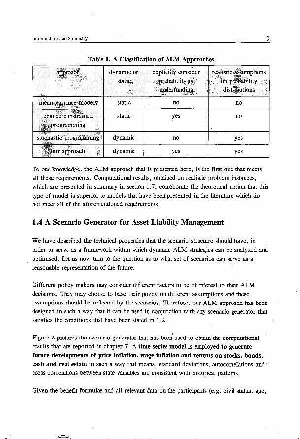
Table 1. A Classification of ALM Approaches
d .. ·.··
ynanuc or . static ·
··•• · realistic aSSllJl'lptl,t)j:iS on probability ·
9
explicitlY consider probability of underfunding distribution$ . / ....
niean"Yaiia:rJ.cemo~e}s·
.· chance constrained .
•······. ··•·•·••••••· J>rog;~~g · ..• · .. · . . :· ·:·> .. . . • .•.• . ·: .. sto¢hastic prog;ramm~g;·.·
static
static
dynamic
dynamic
no no
yes no
no yes
yes yes
To our knowledge, the ALM approach that is presented here, is the first one that meets all these requirements. Computational results, obtained on realistic problem instances, which are presented in summary in section 1. 7, corroborate the theoretical notion that this type of model is superior to models that have been presented in the literature which do not meet all of the aforementioned requirements.
1.4 A Scenario Generator for Asset Liability Management
We have described the technical properties that the scenario structure should have, in order to serve as a framework within which dynamic ALM strategies can be analyzed and optimised. Let us now tum to the question as to what set of scenarios can serve as a reasonable representation of the future.
Different policy makers may consider different factors to be of interest to their ALM decisions. They may choose to base their policy on different assumptions and these assumptions should be reflected by the scenarios. Therefore, our ALM approach has been designed in such a way that it can be used in conjunction with any scenario generator that satisfies the conditions that have been stated in 1.2.
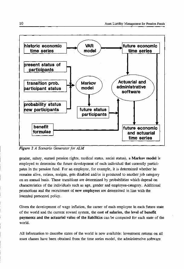
Figure 2 pictures the scenario generator that has been. used to obtain the computational
results that are reported in chapter 7. A time series model is employed to generate future developments of price inflation, wage inflation and returns on stocks, bonds, cash and real estate in such a way that means, standard deviations, autocorrelations and
cross correlations between state variables are consistent with historical patterns.
Given the benefit formulae and all relevant data on the participants (e.g. civil status, age,
--------~----, __________ _
10
historic economic time series
resent status of participants
transition prob. articipant status
robability status new participants
benefit formulae
Asset Liability Management for Pension Funds
future status participants
Actuarial and administrative
software
future economic and actuarial time series
Figure 2 A Scenario Generator for ALM
gender, salary, earned pension rights, medical status, social status), a Markov model is employed to determine the future development of each individual that currently partici
pates in the pension fund. For an employee, for example, it is determined whether he remains alive, retires, resigns, gets disabled and/or is promoted to another job category on an annual basis. These transitions are determined by probabilities which depend on characteristics of the individuals such as age, gender and employee-category. Additional promotions and the recruitment of new employees are determined in line with the intended personnel policy.
Given the development of wage inflation, the career of each employee in each future state of the world and the current reward system, the cost of salaries, the level of benefit payments and the actuarial value of the liabilities can be computed for each state of the world.
All information to describe states of the world is now available: investment returns on all asset classes have been obtained from the time series model, the administrative software

Introduction and Summary 11
has generated the corresponding cost of wages and, to conclude, the actuarial software has provided the corresponding levels of benefit payments and actuarial reserves. Notice, that the scenario generator has been structured in such a way, that consistency between state variables within a state, as well as consistency between states of the world is
preserved.
Once the scenarios have been generated, the following information is available for each
state of the world:
- the level of benefit payments, - the level of the actuarial reserve,
- the level of the costs of wages, -the return on each of the asset classes over the preceding period of time.
Furthermore, the scenario structure implies that it is also known for each state
- what the preceding state of the world has been, - which states of the world are possible successors, and what the probability is that they will emerge, given the current state.
All information that is contained in the scenarios is independent of ALM decisions. They are the subject of the next section.
1.5 A Dynamic Optimisation Model for Asset Liability Management
Chapter 3 presents an optimisation model that determines an ALM policy that consists of an asset mix and a contribution level for each state of the world. These decisions also determine the level of asset value and, in combination with the exogenously given level of liabilities, the funding level in each state of the world. The decisions in all states of the world are made simultaneously. This allows for a trade-off between longer term effects and shorter term effects, as well as for a trade-off between the outcome of decisions in
different future states of the world.
The model has been developed to compute dynamic ALM policies that:
- guarantee an acceptably small probability of underfunding, - guarantee sufficiently stable future contributions,
-minimise the present value of expected future contributions oy the plan sponsors.

12 Asset Liability Management for Pension Funds
Because the probability of underfunding is an important concept in ALM and because it
can be modelled in many ways which have substantial implications for its interpretation,
we shall discuss it at more length in the following paragraph.
The Probability of Underfunding
The probability of underfunding has been defined on the set of scenarios. For example,
suppose that there are 100 states of the world, each of which succeeds a given state of the
world with probability 1/100, then the probability of underfunding, when starting from
the given state of the world is equal to 1/100 times the number of succeeding states in
which underfunding occurs. In general, if a maximum probability of underfunding equal
to 1/;" is considered to be acceptable, then this is reflected by constraints which ensure
that for each state of the world, the probability of being succeeded by a state in which
underfunding occurs, is less than or equal to 1/;". The probability of underfunding has
been modelled in such a way that:
1. The model can account for any probability distribution that can be reflected by the
scenarios. That includes distributions that are specified implicitly, such as the distribution
of liabilities which may be given by benefit formulae in the form of computer
programmes.
2. Probabilities of underfunding are endogenous to the model.
3. Probabilities of underfunding are taken into account explicitly, at intertemporal points
in time, as well as at the planning horizon.
Underfunding
What would happen when a situation of underfunding occurs ? It is not clear what would
happen in practice. In our model, however, it will be assumed that a remedial payment is
made which is precisely sufficient to restore the required funding level. The remedial
contributions are included in the costs of funding. Thus, the probability of underfunding,
as well as the magnitude of deficits when they occur are taken into account. The structure
of the model can accommodate other assumptions with respect to measures to be taken in
situations of underfunding as well. Alternative reactions that can be accommodated
include remedial contributions to be made during a prespecified number of years until the
desired funding level has been restored and, entirely or partially, failing to meet
conditional indexation promises.
Introduction and Summary 13
In summary, the ALM model that will be presented in chapter 3 can be used to compute ALM strategies which specify investment decisions and contribution levels to be set under a wide range of future circumstances. The decisions are made in such a way that the present value of expected contributions to the fund is minimal, subject to raising sufficiently stable annual contributions and the probability of underfunding at the end of each year being acceptably small when starting from the current situation, as well as from all future states of the world that the policy makers of the pension fund choose to take
into account.
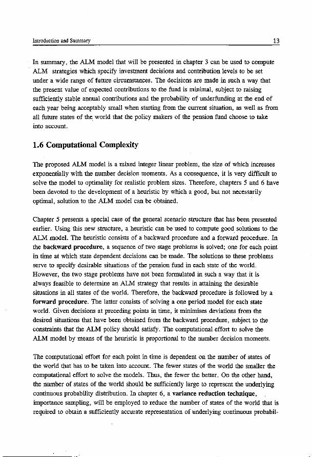
1.6 Computational Complexity
The proposed ALM model is a mixed integer linear problem, the size of which increases
exponentially with the number decision moments. As a consequence, it is very difficult to solve the model to optimality for realistic problem sizes. Therefore, chapters 5 and 6 have been devoted to the development of a heuristic by which a good, but not necessarily
optimal, solution to the ALM model can be obtained.
Chapter 5 presents a special case of the general scenario structure that has been presented earlier. Using this new structure, a heuristic can be used to compute good solutions to the ALM model. The heuristic consists of a backward procedure and a forward procedure. In the backward procedure, a sequence of two stage problems is solved; one for each point in time at which state dependent decisions can be made. The solutions to these problems serve to specify desirable situations of the pension fund in each state of the world. However, the two stage problems have not been formulated in such a way that it is always feasible to determine an ALM strategy that results in attaining the desirable
situations in all states of the world. Therefore, the backward procedure is followed by a forward procedure. The latter consists of solving a one period model for each state world. Gl.ven decisions at preceding points in time, it minimises deviations from the desired situations that have been obtained from the backward procedure, subject to the constraints that the ALM policy should satisfy. The computational effort to solve the
ALM model by means of the heuristic is proportional to the number decision moments.
The computational effort for each point in time is dependent on the number of states of the world that has to be taken into account. The fewer states of the world the smaller the computational effort to solve the models. Thus, the fewer the better. On the other hand, the number of states of the world should be sufficiently large to represent the underlying
continuous probability distribution. In chapter 6, a variance reduction technique, importance sampling, will be employed to reduce the number of states of the world that is required to obtain a sufficiently accurate representation of underlying continuous probabil-
14 Asset Liability Management for Pension Funds
ity distribution of states of the world.
1. 7 Computational Experiments
Chapter 7 presents results of computational experiments with the ALM model. In order to
obtain insight in the behaviour of the model on realistic problem instances, it has been
applied to the data of a Dutch pension fund with an actuarial reserve in excess of 16
billion Dfl. and approximately 1,020,000 participants of which 240,000 are still in their
active career.
One would expect ALM decisions for a wealthy pension fund to be different from those
for a thinly funded pension fund. Therefore, three settings have been selected, which
differ in the initial funding level and in the amount by which annual contributions may be
raised from one year to the next:
Setting 1: a low initial funding level and a low maximum increase of contributions,
Setting 2: a high initial funding level and a high maximum increase of contributions,
Setting 3: the initial funding level to be determined by the ALM model in such a way
that costs of funding are minimised subject to satisfying the solvency con
straints with moderate maximum increases of contribution.
In all settings, the probability of underfunding was allowed to be at most 5% in each
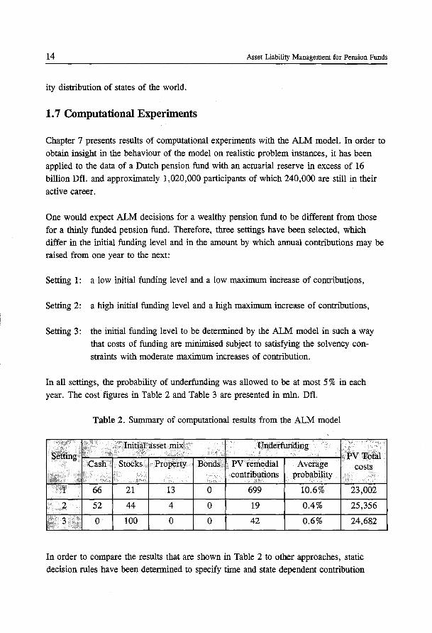
year. The costfigures in Table 2 and Table 3 are presented in mln. Dfl.
Table 2. Summary of computational results from the ALM model
Initial asset mix Underfunding >,':\ettip.g . .. PVTotal •..
'.·Cash ·'·'.•Stocks I'' .... Property Bonds· PV remedial Average costs
I ... contributions probability
I .1. 66 21 13 0 699 10.6% 23,002
1> ... , •••.•. ~.' 52 44 4 0 19 0.4% 25,356 · .. $., ·'
0 100 0 0 42 0.6% 24,682
In order to compare the results that are shown in Table 2 to other approaches, static
decision rules have been determined to specify time and state dependent contribution
•••
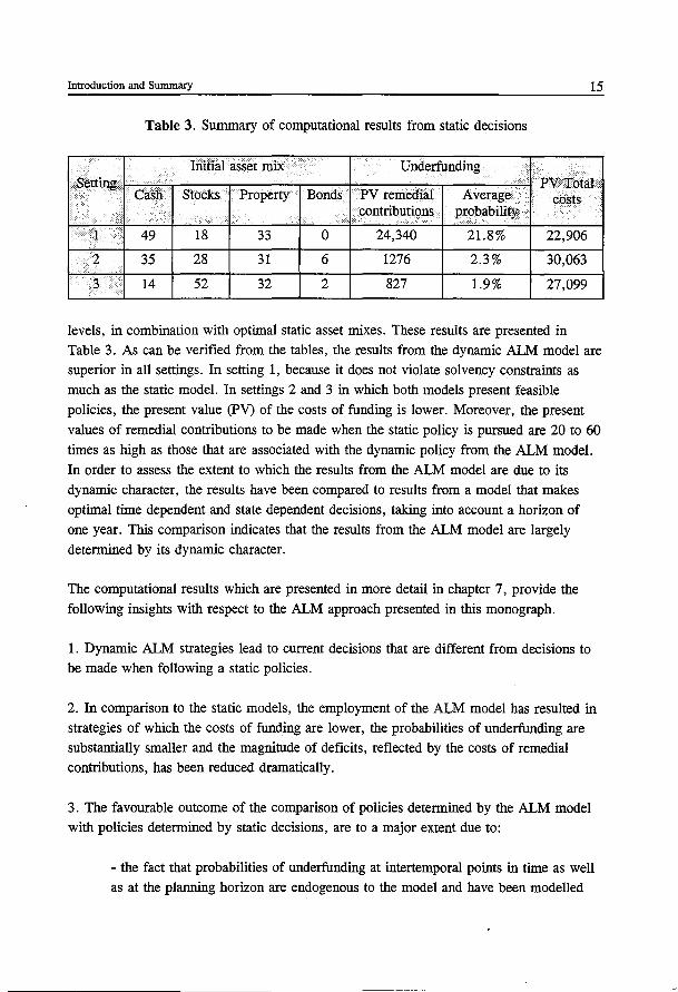
Introduction and Summary 15
Table 3. Summary of computational results from static decisions
Initial asset mix Underfunding Setting . PV Total
I ·.····•· Cash Stocks Property Bonds PVremedial Average costs contnlmtions probability
l 49 18 33 0 24,340 21.8% 22,906
2 35 28 31 6 1276 2.3% 30,063
3 14 52 32 2 827 1.9% 27,099 .
levels, in combination with optimal static asset mixes. These results are presented in Table 3. As can be verified from the tables, the results from the dynamic ALM model are superior in all settings. In setting 1, because it does not violate solvency constraints as much as the static model. In settings 2 and 3 in which both models present feasible policies, the present value (PV) of the costs of funding is lower. Moreover, the present
values of remedial contributions to be made when the static policy is pursued are 20 to 60 times as high as those that are associated with the dynamic policy from the ALM model.
In order to assess the extent to which the results from the ALM model are due to its dynamic character, the results have been compared to results from a model that makes optimal time dependent and state dependent decisions, taking into account a horizon of
one year. This comparison indicates that the results from the ALM model are largely determined by its dynamic character.
The computational results which are presented in more detail in chapter 7, provide the
following insights with respect to the ALM approach presented in this monograph.
1. Dynamic ALM strategies lead to current decisions that are different from decisions to be made when following a static policies.
2. In comparison to the static models, the employment of the ALM model has resulted in strategies of which the costs of funding are lower, the probabilities of underfunding are substantially smaller and the magnitude of deficits, reflected by the costs of remedial contributions, has been reduced dramatically.
3. The favourable outcome of the comparison of policies determined by the ALM model with policies determined by static decisions, are to a major extent due to:
- the fact that probabilities of underfunding at intertemporal points in time as well as at the planning horizon are endogenous to the model and have been modelled

16 Asset Liability Management for Pension Funds
explicitly, and
- the dynamic character of the ALM model which enables the policies to react to situations that have emerged at the time of decision making and to reflect a correct
trade-off between their longer term effects and their short term effects.
Chapter 2 Asset Liability Management for Pension Funds, A
Survey
2.1 Introduction
Asset liability management has drawn attention from academics and practitioners for Se>.<efli-1-(;~aal~ Most of the literature focuses on techniques aimed at managing a portfolio of fixed income securities in such a way that the cash flow received from holding the portfolio in some sense matches the (projected) cash out flow of a stream of
liabilities. Closely related is the extensive research published on asset liability management for banks, mainly concentrating on financial risks incurred from changes in interest rates. Recently published surveys on this field of interest can be found in Smink
(1994) and Klaassen (1994).
In comparison, the literature on ALM for pension funds is rather modest although the
recent flow of publications in this domain seems to indicate a growing interest from people with different backgrounds. Both actuarial and financial journals publish research on asset liability management for pension funds. Judging from the references, it seems that authors from one discipline are not always aware of the ALM literature published in
journals from the other discipline. Non-members of the actuarial community can be referred to the debate among actuaries on the proposition that "This house believes that
the contribution of actuaries to investment could be enhanced by the work of financial economists", Wilkie et al. (1993), for an enlightening exposition of the actuarial view on the merits and shortcomings of financial theory.
2.2 Model Classification
In chapter 3, it is shown that one of the key issues in modelling ALM concerns the way
in which information is resolved. The available information at the moment of decision making can consist of data that are known with certainty, e.g. the premium reserve that
an actuary would consider sufficient to cover all liabilities, and information of a stochastic nature, e.g. the perceived probability distribution of the return on stocks in the next
decade.
The field of stochastic programming has developed techniques to model and solve problems in which information with a stochastic nature plays a dominant role. Since this is the case in the domain of ALM, we shall classify ALM models by means of a
17

18 Asset Liability Management for Pension Funds
classification from the stochastic programming literature, taken from Wets (1989a). The
classification distinguishes between anticipative models and recourse models.
Anticipative Models
Those are models for which the decision does not depend in any way on future observations of the environment. These models are also referred to as static models. The present decision has to take into account all possible future environments since there is no opportunity to adapt decisions later on.
For example, imagine a wealthy pension fund which can afford to reduce contributions from 15% of the wages now to 2% of the wages next year, without serious risk of insolvency in the short term. Should it do so ?
Using an anticipative model, the answer would probably be negative: the model assumes that there will be no opportunity to increase contributions again if the tide turns. As a consequence, it would be too risky to lower contributions now.
If it is possible, contrary to the model assumptions, to react to future circumstances, then the use of an anticipative model may lead to overly conservative decisions.
Recourse Models
The recourse model allows for different decisions at different points in time which may
be contingent on the state of the world at the time of decision making. The anticipative
model is a special case of a recourse model. Decisions made in state
( t, s) , t = 1 , ... , T- 1 , s = 1 , ... , St are adaptive as well as anticipative. They are adaptive
with respect to period t since they depend on information that has been revealed during
this period. With respect to period t + 1, however, the decisions are anticipative: they do
not depend on observations at time t + 1 . A solution to a recourse model thus consists of a
decision to be made now, and a sequence of decisions which is contingent on the prevailing states of the world. Such a solution will be referred to as a dynamic policy or strategy. Deciding simultaneously on present actions and future recourse actions allows for a trade-off between longer term effects and short term effects.
The knowledge that there will be recourse decisions in the future affects present decision making in several ways. In comparison with the anticipative model, one has greater freedom to pursue short term benefits because the decision to be taken now is not a once
A Survey 19
and for all decision. The present decision does not only maximise short term benefits. It also reckons with the impact on the ability to respond to different circumstances in the future. Especially when it is conceivable that the environment alters rapidly in comparison with one's speed of response, it may be optimal to pay a price now for flexibility in the
future.
Let us return to the example of the wealthy pension fund. Using a recourse model one would probably decide to lower contributions. The contributions would be reduced by as much as possible, subject to the existence of a feasible contribution policy in the future which ensures solvency of the fund, in the short term as well as in the longer term.
Iri general, a recourse model distinguishes between points in time and states of the world at which decisions can be made. Each decision utilizes all the information that is available at the moment of decision making. Anticipating on future decisions and recognizing the impact of present decisions on future decisions allow for an optimal trade-off between
short term effects and long term effects of present decisions.
2.3 Anticipative Models for ALM
2.3.1 Mean-Variance Models
A considerable portion of the ALM publications is based on mean-variance analysis. This approach on which extensive literature can be found in financial text books (e.g. Haugen (1993), Elton & Gruber (1989) and journals, has been introduced by Markowitz. He considered the problem of composing a portfolio of securities such that the expected return on the portfolio would be maximal, given the level of risk that one is willing to accept. Risk, in this approach, is defined as the variance of the return about the mean. It is common practice to report the standard deviation instead of the variance because standard deviation can be expressed in the same units as expected return, which makes it an easier measure to interpret in a risk-return trade-off.
Most of the publications on ALM focus on determining an asset mix that goes well with a given set of liabilities. This problem definition reduces the ALM problem to making the right investment decision. It is only natural then to pose the ALM problem as a variant of the mean-variance investment problem. There appears to be a straight forward analogy. Where traditional portfolio theory concentrates on selecting a portfolio of marketable
assets, ALM considers a portfolio which consists of two components: a portfolio of marketable assets and a given portfolio of liabilities. The choice of the asset portfolio
determines the expected return on investments and the standard deviation thereof. The
20 Asset Liability Management for Pension Funds
expected return of the entire portfolio equals the expected return on investments less the
expected growth of the liability portfolio. The important difference between an ordinary
investment decision and an investment decision in an ALM context lies in the fact that the ~--~~------~~~--~~~~~---variance of the return on the whole portfolio is partly detennined by the covariance
between the return on the asset portfolio and the growth of the liability portfolio.
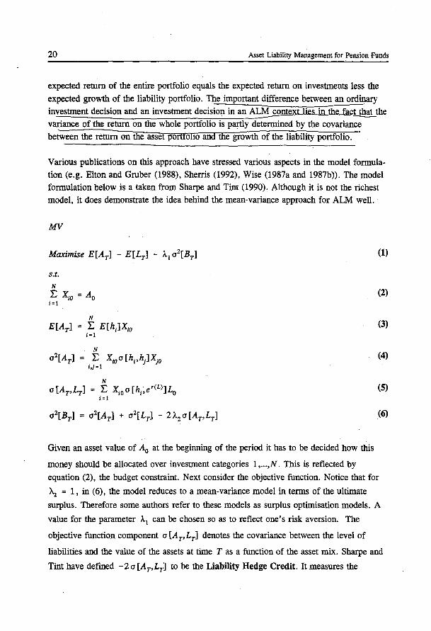
Various publications on this approach have stressed various aspects in the model fonnula
tion (e.g. Elton and Gruber (1988), Sherris (1992), Wise (1987a and 1987b)). The model
fonnulation below is a taken from Sharpe and Tint (1990). Although it is not the richest
model, it does demonstrate the idea behind the mean-variance approach for ALM well.
MV
s.t. N
:E X;o = Ao i=l
N
E[Arl L E[h;JXw i~t
N
a[AT'LT] = L Xwa[hi'er(L)]L0 i=l
(1)
(2)
(3)
(4)
(5)
(6)
Given an asset value of A0 at the beginning of the period it has to be decided how this
money should be allocated over investment categories 1 , ... ,N. This is reflected by
equation (2), the budget constraint. Next consider the objective function. Notice that for
~ = 1, in (6), the model reduces to a mean-variance model in tenns of the ultimate
surplus. Therefore some authors refer to these models as surplus optimisation models. A
value for the parameter /..1 can be chosen so as to reflect one's risk aversion. The
objective function component a [AT'LT] denotes the covariance between the level of
liabilities and the value of the assets at time T as a function of the asset mix. Sharpe and
Tint have defmed -2 a [Ar,Lrl to be the Liability Hedge Credit. It measures the
A Survey 21
contribution to the variance of the surplus due to the correlation between the return on the
asset portfolio and the growth of the liabilities. In absence of liabilities (LT = 0) or if the
growth of liabilities is uncorrelated with each of the asset categories
(a [hi'erCLl] =0, i = 1, ... ,N), the Liability Hedge Credit is equal to zero. The parameter
A.2 has been introduced to enable the user of the model to indicate the importance of
volatility of the asset value risk in relation to the Liability Hedge Credit.
Does standard deviation of the surplus reflect the investor's risk perception well ?
Although standard deviation is a widely used risk measure, there have been many
publications which point out the limitations of standard deviation as a risk measure, among them Markowitz (1959), Hagigi and Kluger (1987) and Amott and Bernstein
(1988). More recently, Sortino and VanderMeer (1991) have shown lucidly why
standard deviation is an inappropriate risk measure for many investment situations. Their
exposition seems to be particularly relevant for ALM strategies. One of the main
drawbacks of the standard deviation as a measure of risk is that it does not distinguish
between returns higher than expected and returns lower than expected. To the investor
this difference is rather important.
2.3.2 Chance Constrained Models
Chance constrained programming offers an alternate to quantifying risk by standard
deviation which does not suffer from this shortcoming. One defines the probability of a certain event to happen as a function of the model's decision variables. Then, the
probability of undesirable situations to occur can be bounded by inclui:ling constraints on
the value of the associated statistics.
If one assumes that the returns on all asset categories and on the portfolio of liabilities are
normally distributed1 with a known vector of means and a known covariance matrix, then
it is well known that the level of surplus at the end of the planning horizon is also
normally distributed (see e.g. Kall (1976)). Several authors, among which Wilkie (1985), and Brocket, Charnes and Li Sun (1993), have used this property to formulate a chance constraint on insolvency:
1 Notice that the normality assumption does not apply to the continuous returns. It applies to
(h; - 1), i = 1, ... ,N and to (er(L) - 1).
22 Asset Liability Management for Pension Funds
Pr[AT~ LT] ~ 'itu =
E[AT]- E[LT] ~ q> -1( 'itu) a [BT] (7)
For lltu E (0, 1/2) this constraint is equivalent to the following combination of a convex
quadratic constraint and a linear constraint:
E[AT] ~ E[LT] (8)
(E[AT]- E[LT])z ~ (q> -1( 'itu))2 az[BT] (9)
This type of chance constrained program was first suggested by Charnes and Cooper
(1959). A chance constrained programming model for ALM can be obtained by combining equations (2), ... ,(6), (8) and (9). In the remainder of this chapter we shall refer to
this model as CC. In the financial literature, investment models which employ chance
constraints can be found under several key words among which downside risk (Harlow (1991)), shortfall constraints (Leibowitz and Henrikkson (1989), Leibowitz and Kogelman (1991), Leibowitz and Langetieg '(1990)) and shortfall returns (Albrecht (1993,1994)).
2.3.3 Chance Constrained Programming, Normally Distributed Returns and Mean
Variance Optimisation
Although the philosophy behind the mean-variance approach may be quite different from the idea underlying chance constrained programming, one could wonder to what extent
their solutions would differ if all returns are assumed to be distributed normally. Let us
compare solutions to MV with solutions to CC. Any optimal solution to MV has the
property that a higher expected surplus is not attainable without accepting a higher
variance of the surplus. This follows directly from the objective function. Instead of
indicating one's risk aversion by specifying a value for A. 1 one could specify an upper
bound on a2[BT] and maximize the expected surplus. An alternative formulation of MV
could thus be obtained by replacing the objective by maximise E[AT-LT] and imposing
an upper bound on the variance of the ultimate surplus: cr 2[Brl ~ a2 [Brlu; The differ
ence between CC and MV is now confined_to the way in which risk is modelled. MV
bounds the variance of the surplus whereas CC bounds the probability of insolvency.
However, under the assumption of normally distributed returns, any relevant optimal.
solution to MV can be obtained as an optimal solution to CC and vice versa.
A Survey
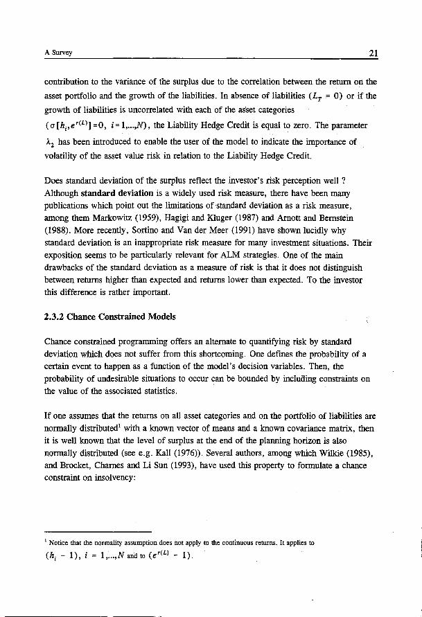
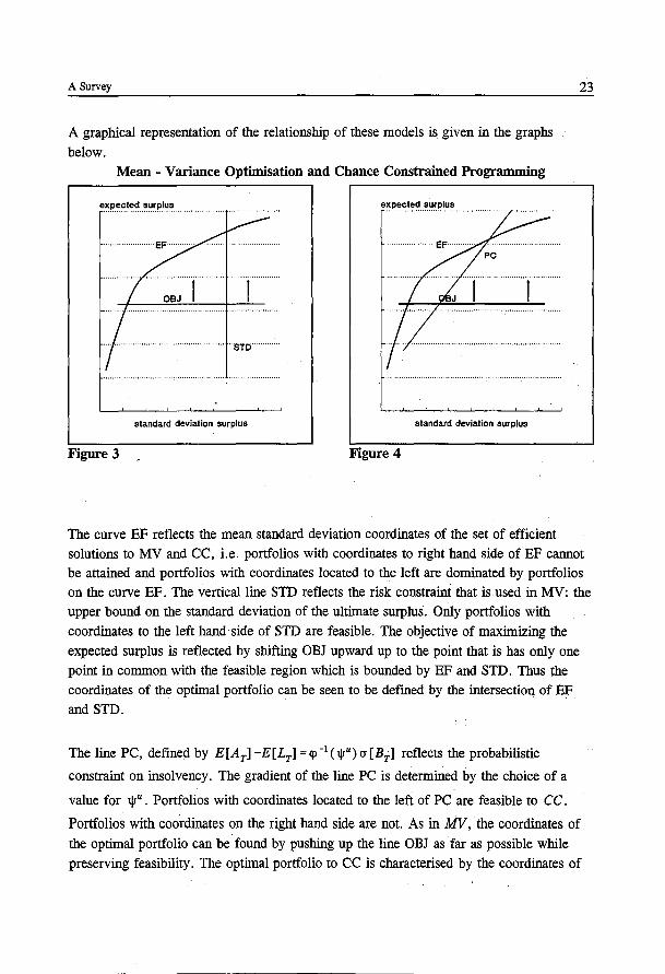
A graphical representation of the relationship of these models is given in the graphs
below. Mean - Variance Optimisation and Chance Constrained Programming
·-~~~ r ······ · ·· · · r · .. ·-· ......... "STO'"".
standard deviation surplus standard deviation surplus
Figure 3 Figure 4
23
The curve EF reflects the mean standard deviation coordinates of the set of efficient
solutions to MV and CC, i.e. portfolios with coordinates to right hand side of EF cannot be attained and portfolios with coordinates located to the left are dominated by portfolios on the curve EF. The vertical line STD reflects the riskconstraint that is used in MV: the
upper bound on the standard deviation of the ultimate surplus. Only portfolios with
coordinates to the left hand side of STD are feasible. The objective of maximizing the
expected surplus is reflected by shifting OBJ upward up to the point that is has only one
point in common with the feasible region which is bounded by EF and STD. Thus the coordinates of the optimal portfolio can be seen to be defmed by the intersection of EF
and STD.
The line PC, defined by E[Ar1 -E[Lr1 =<p-I ( 1Jr") a [Br1 reflects the probabilistic
constraint on insolvency. The gradient of the line PC is determined by the choice of a
value for 1Jr" . Portfolios with coordinates located to the left of PC are feasible to CC.
Portfolios with coordinates on the right hand side are not. As in MV, the coordinates of
the optimal portfolio can be found by pushing up the line OBJ as- far as possible while
preserving feasibility. The optimal portfolio to CC is characterised by the coordinates of
24 Asset Liability Management for Pension Funds
the intersection of EF and PC.
Now consider a choice for the value of lJr" so that the line PC goes through the intersec
tion of EF and STD. Then the optimal solution to MV is also optimal to CC. Likewise,
for any choice of lJr" , the upperbound on the standard deviation can be specified so that
the coordinates of the optimal solutions to the two models coincide. Thus, any optimal
solution to one model can also be obtained as an optimal solution to the other model2 •
To summarize, in general probabilistic constraints on insolvency reflect the risk of the
funding level dropping below a minimally required level. Since the standard deviation of
the surplus does not distinguish between upside potential and downside risk, the probabili
ty of insolvency appears to be the better measure of risk. However, most publications on
ALM models which utilize the probability of insolvency as a risk measure do so under the
assumption of normally distributed returns. Due to the symmetry about the mean of the normal probability density function, the probability of a lower than expected return is
always equal to the probability of a higher than expected return. As a consequence chance
constrained programmes under the assumption of normally distributed returns distinguish
between downside risk and upward potential no more than mean-variance models do.
Multiperiod Models
MV as well as CC takes asingle period into account: from t=O until t=T. It is not clear
what value would be an appropriate choice for T. Pension funds typically have a long
horizon, say 30 years. This would call for choosing T equal to 30 years. However, since
the models discussed up to now do not include any requirements for t, 0 < t < T, it may
well be that the optimal solution to MV with T = 30 implies an unacceptably high risk of
insolvency at one or more points in time t, t E [ 1 , ... , T -1]. To illustrate this point,
consider an asset mix such that the expected surplus at the horizon equals E[BT] with a
standard deviation equal to o [Brl. If chance constraint (7) is binding, then it is likely
that the probability of insolvency at time t, t E [ 1 , ... , T- 1] is greater than 1Jr". To see
why this is the case, ass~e that the annual returns on the surplus are distributed independently and identically. Then, the cumulative expected return decreases
proportionally ~ith t whereas the standard deviation decreases proportionally with {t . A
more specific example would be the selection of an asset mix which largely consists of
2 A formal exposition of the relationship between these models can be found in appendix A.
A Survey 25
stocks. Assuming independently distributed annual returns in conjunction with a high
expected return, such an asset mix may well seem to be attractive when judged by its
long term perspectives. Nevertheless, it would not be recommendable to select such an
asset mix, unless one can afford to sustain considerable losses in the shorter term.
In general, as is also argued in Elton and Gruber (1988), one should not only worry about
the situation of the fund at the end of the period. Assuming that one has to satisfy a
solvency requirement that is checked with a certain frequency, the model should only
allow for solutions that would meet intertemporal requirements as well as end of period
requirements. This calls for a multiperiod model.
\c.l.I-Multiperiod models have been {ro~d by several authors. Most publications which
present multistage models employ some form of simulation to arrive at a solution of the
model. Wilkie (1986a,b) simulates the behaviour of inflation and returns on various asset
classes by means of a stochastic model which generates paths through time. These paths
consist of consecutive states of the world defined by realisations from the stochastic
process. Wilkie (1995) contains an extension of Wilkie (1986). It presents stochastic
models to reflect returns on asset classes, using more advanced time series analyses.
Hardy (1993) employs a stochastic simulation method, based on Wilkie (1986) to analyze
a number of investment strategies for life offices. These strategies consist of simple
decision rules which are applied at the end of each year for a period of 20 years. Hardy
concludes that the stochastic simulation method provides the user with insights that could
not be obtained from earlier studies in which these strategies were evaluated on a
deterministic set of (worst case) scenarios. Moreover, the stochastic simulation led to the
assessment that some of the strategies were unacceptably risky, whereas earlier studies
indicated that all of the strategies were virtually riskfree.
Several authors use a single period mean-variance model in combination with a multiperi
od simulation. It enables them to judge investment decisions obtained from a static single
period model on its characteristics at the horizon T as well as at intertemporal p~ints in
time. Examples of this approach can be found in Booth and Ong (1994), inspired by the·
work of Sherris (1992), and Boender (1994). Unlike most ALM models, the one proposed
in Boender (1994) does not aim for optimal mean-variance characteristics of the ultimate
surplus. Assuming clean funding3, it determines an asset mix which minimises the
volatility of contributions to the fund, subject to an upper bound on the average level of
contributions. This variant of mean-variance optimisation is particularly relevant to policy
3 Under this policy ultimo period contributions are defined to be equal to the amount necessary to maintain the
required funding level, ~ 7' aL1 -At"
26 Asset Liability Management for Pension Funds
makers who are predominantly interested in striving for a stable development of contribu
tions.
2.4 Recourse Models for ALM
So far only static models have been considered. When using these models in practice, one
would generally use them repetitively. After making decisions at time t , one updates the
model with the latest observations at time t + 1 and determines the contribution level and
an asset mix at that time. This approach would be as good as a recourse model if
decisions made at different points in time can be made independently of each other.
However, this is usually not the case in ALM applications. In many cases there will be a
constraint on the annual amount of buying and selling of securities. If this. is not an issue of interest in itself, then it may play a role indirectly in the form of transaction costs.
More important is the requirement of a stable development of annual contributions. This is one of the issues at the heart of a realistic ALM policy. Neither of these topics can be
handled properly by employing a static model in a repetitive fashion.
Ziemba and Vickson (1975) already present dynamic models with financial applications.
The need for dynamic models for ALM has been recognised by several authors in the
field (see e.g. Booth and Ong (1994), Ludvik (1994), Sherris (1993), Janssen and Manca
(1994)). Notwithstanding the notion that much is to be gained by employing recourse
models to determine dynamic ALM strategies, only few models have been published
which deal with this subject. Many of the proposed recourse models for investment decisions concentrate on portfolio optimisation without taking into account stochastic
liabilities and funding decisions. These models are usually formulated as stochastic linear
programmes. Kusy and Ziemba (1986) contains an application to ALM for banks. Golub
et al (1993) and Holmer et al (1993) present stochastic programming models for fixed
income investments. The latter contains computational results which corroborate the
superiority of multistage models over single period models. Mulvey and Vladimirou (1988,1991) and Lustig, Mulvey and Carpenter (1990) report on quadratic multistage
models for financial planning. Thibse publications present computational results obtained
from applying interior point methods and the progressive hedging algorithm which was proposed in Rockafellar and Wets (1991) and in Wets (1989b).
A two stage mean-variance model for ALM has been formulated in Mulvey (1994). It is
not clear how the allocation of assets depends on the liabilities. This element of the
system has not been published because of proprietary reasons. Carifi.o et al (1994) report on the development of the Russell Yasuda Kasai (RYK) model, an ALM model for a
A Survey 27
Japanese insurance company. We shall discuss this model at more length since it can
serve well to convey the basic idea of using stochastic linear programming for ALM to
take stochastic liabilities into account. Consider the following model which is based on
Carino et al (1994)4•
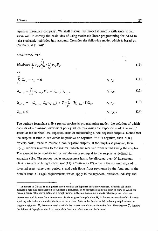
MODIFIED RYK.
Maximise E Pr,sf~s- E Pt,sBts s \./ s,t
s.t. N
E Xits - Ats = 0 i=I
(10)
V t,s (11)
V t,s (12)
V t,s (13)
V i,t,s (14)
The authors formulate a five period stochastic programming model, the solution of which
consists of a dynamic investment policy which maximises the expected market value of assets at the horizon less expected costs of maintaining a non negative surplus. Notice that
the surplus at time t can either be positive or negative. If it is negative, then c(B,)
reflects costs, made to restore a non negative surplus. If the surplus is positive, then
c(B) reflects revenues to the insurer, which are received from withdrawing the surplus.
The amount to be contributed or withdrawn. is set equal to the surplus as defmed in
equation (13). The money under management has to be allocated over N investment
classes subject to budget constraint (11). Constraint (12) reflects the accumulation of
invested asset value over period t and cash flows from payments· by the fund and to the
fund at time t. Legal requirements which apply to the Japanese insurance industry and
4 The model in Cariiio et a! is geared more towards the Japanese Insurance business, whereas the model discussed here has been adapted to facilitate a discussion of its properties from the point of view of ALM for pension funds. The above model is a simplification in that no distinction is made between price return on
investments and income from investments. In the original interpretation B, is the net income shortfall. Loosely
speaking this is the amount that the insurer has to contribute to the fund to satisfy solvency requirements. A
negative value for B1
denotes a surplus which the insurer can withdraw from the fund. Furthermore Yr denotes
the inflow of deposits to the fund. As such it does not reflect costs to the insurer.
28 Asset Liability Management for Pension Funds
the role that the model was intended to play apparently called for a rather detailed
description of cash flows. Modelling the flow of funds in such detail requires many
decision variables at each time and state. In order to keep the size of the model down to
tractable proportions, the number of scenarios has been kept small: to describe all
relevant states of the world (in terms of the development of liabilities, interest rates for
various types of fixed income investments and returns on several classes of equity
investments) over 5 periods, adding up to a span of time of five years, the RYK model
uses only 256 scenarios. The scenarios are generated by a Monte Carlo procedure under
the assumption that the random variables are not autocorrelated. Next, the sample is
corrected in such a way that all realisations satisfy prespecified upper and lower bounds
and the sample variance of each of the random variables is equal to a desired variance which was determined on forehand. It is interesting to see that the model concentrates on
the reward component: it maximises the expected growth of net assets. The risk
component is not explicitly included in the model. Neither the magnitude of payments to restore the required funding level at given times, nor the volatility of these payments or
the probability of large deficits is constrained directly. Risk is accounted for by the
variety of future environments over which the expectation in the objective function is
computed. These future states of the world are largely determined by subjective
assessments of appropriate bounds on the state variables. For a detailed description of the
RYK model, as well as for an interesting comparison of computational results of different
stochastic programming algorithms and commercial optimisation software, the reader can
be referred to Cariiio et al (1993).
2.5 Summary
In the preceding paragraphs the literature on ALM for pension funds has been discussed. A distinction has been made between anticipative models and recourse models, the latter
being the more suitable type of model for ALM since this class of models allows for a more realistic reflection of the true decision making process.
Somehow or other each of the ALM models facilitates a risk-reward trade-off. The
reward is usually linked to the magnitude of the expected surplus of the pension fund. A
few models do include the funding policy as an endogenous variable. In these models the reward is usually linked to the cost of funding, the expected annual contributions or the volatility thereof. Most models include a notion of risk quantified by the standard
deviation of the surplus, either directly or via a chance constraint on insolvency, coupled to the assumption of normally distributed returns.
The reflection of risk is one of the major issues in modelling ALM. Sortino and Vander
A Survey 29
Meer (1991) have argued that appropriate risk measures for investment strategies should:
- explicitly consider the investor's goals, - distinguish between true risk (uncertainty associated with undesirable events) and
uncertainty (which can also be associated with outcomes that are better than expected), -consider both the chance and the magnitude of adverse outcomes,
- be intuitively appealing.
It may not always be clear whether the latter requirement has been met. However, one
would want an ALM model to reflect the notion of risk in accordance with the former
three requirements.
One of the elements which plays a role in the above criteria is the probability of adverse
outcomes. This assumes that it is possible to give an acceptably accurate assessment of this probability in the first place. Thus, the reflection of risk is not only determined by
the variables and statistics by which an ALM strategy is analyzed. The assumptions with
respect to the underlying stochastic process and the way in which this process is incorpo
rated in the ALM decision model can also have a major impact on the outcome of the
model. This issue will be treated more extensively in chapter 4 where the stochastic
structure of our ALM model is discussed.
To conclude, let us summarize the properties which an ALM model should satisfy:
1. The model should be suitable to determine a dynamic ALM strategy, consisting of an investment strategy and a contribution policy, which account for the development of
liabilities. Decisions to be made now should anticipate on the ability to make state
dependent decisions in the future. They should be the result of a trade-off between short
term effects and long term effects.
2. Risk must be modelled in accordance with the first three criteria as specified by
Sortino and Van der Meer. This implies that the stochastic nature of the model should
allow for computing the risk measures that they suggest.
3. It should be feasible from a computational point of view.
None of the models that has been discussed in this chapter satisfies all of these require
ments.

Chapter 3 Modelling Asset Liability Management
This chapter presents a new optimisation model for ALM. The purpose of the model is to
come up with an ALM policy, consisting of an investment policy and a funding policy for benefit defined pension plans5
• Since the expense and benefit payments to be made are
already defined (although the exact amounts to be paid are not known yet), the question becomes against what costs the plan 'can be funded. Of course, the lower the better; and
therefore the reward component in our model is the present value of contributions to the
fund. Risk in the context of ALM has to do with the possibility of failure to pay benefits
and expenses whilst maintaining solvency. If the benefit formulae contain indexation promises, then they will be reflected by the level of benefit payments and the level of the
actuarial reserves; not only when these promises are unconditional, but also when they
are conditional. The model takes the probability of underfunding into account, as well as
the cost of remedial contributions required to restore the desired funding level.
Section 3.2 develops a model formulation which aims at describing the ALM problem in
mathematical terms without heeding the tractability requirement. This results in an infinite
dimensional multistage stochastic optimisation problem for which no effective solution
method exists. In section 3.3 the infinite dimensional optimisation problem will be
reduced to a finite dimensional multistage stochastic programming problem through the use of a scenario representation of the uncertain future which should be taken into
account. Although finite dimensional, the size of this model grows exponentionally with the number of decision points. Consequently it is still too big to solve directly. Chapter 5 discusses the way in which this problem is handled. Before turning to the development of
the model formulations, the next section discusses conditions which an ALM model
should satisfy.
3.1 The Essential Elements of an Optimisation Model for .Asset Liability Management
The concluding paragraph of chapter 2 lists the requirements which an ALM model
should satisfy. This section goes into more detail regarding these requirements and their
5 The approach which we !'resent is equally well suited to aid decision making for contribution defined plans. In case of a contribution defined one maximises future benefit payments given the contributions to the fund. In case of defined benefit plan one minimises the contributions given the defined benefit payments to be made. From a modelling point of viev.r the difference is not an essential one. The reader can be referred to Ludvik (1994) for an interesting exposition of the similarity of the requirements to ALM policies for defined benefit plans and contribution defmed plans.
31
32 Asset Liability Management for Pension Funds
consequences from a modelling point of view.
3.1.1 Elements Constituting a Dynamic Asset Liability Management Policy
The goal is to come up with a policy which minimizes the cost of funding while safeguar
ding the pension funds's ability to meet its liabilities. The fund should be able to make all
benefit payments timely, without becoming underfunded. After all payments have been
made, the value of the remaining assets should at least be equal to the minimum level
which is required to fund future benefit payments according to the actuarial standards in
force. The policy should consist of actions to be taken now, and sequences of reactions to
future developments. Clearly none of the decisions may use information which is not
available at the time of decision making. To make optimal use of the opportunity to react
to future circumstances, decisions should anticipate on the ability of making recourse
decisions.
Contribution Policy
One of the important instruments by which the pension fund can pursue its goals is the contribution policy. However, when setting contribution levels the fund will have to take
into account the sponsor's ability and willingness to pay these contributions. It is
questionable whether contributions can always be collected if they show unexpectedly
steep annual increases. In order to accommodate the sponsor in making a multi-annual
budget plan which includes realistic (upper bounds on) contributions to the pension fund,
the funding policy should guarantee sufficiently stable annual contributions. More
specifically we shall require the raise in annual contributions as a percentage of the costs
of wages not to exceed a prespecified level.
Investment Policy
The second important instrument at the disposal of the pension fund is its investment policy. In this study we shall concentrate on strategic decisions of the investment strategy. More precisely, we consider the sequence of decisions regarding the allocation of assets
over a limited number of asset classes. Such an allocation of assets will be referred to as
an asset mix. Chapter 7 presents computational results based on a classification of investment £lasses which distinguishes between four investment categories: stocks, bonds, property and cash. The model should allow for more refined classifications as well. For
example, it should be possible to make a further distinction by differentiating witli respect
to the maturity of security markets or geographical regions within the four classes which
are mentioned above. On the other hand, the model need not be suitable to support
Modelling Asset Liability Management 33
answering questions like 'Should I prefer Royal Dutch, or would 1 rather buy Exxon?'
The asset mix policy should be feasible to implement. This requires that proposed changes do not entail trading volumes which cannot be absorbed by the market without substantial impact on market prices. Furthermore there may be considerations exogenous to the model reflected by upper and lower bounds on proportions invested in one or more
of the asset categories6•
Asset Liability Management Policy
A good investment policy and a sound contribution policy do not necessarily constitute an acceptable ALM policy. A good ALM strategy results in a desirable risk/reward structure
with respect to the financial development of the pension plan. Such a policy comprises an
investment policy and a contribution policy which take into account the development of the liabilities of the plan. In conjunction they should secure the desired risk/reward
structure. In this monograph reward is quantified as cost of funding: the lower the better1·8• Risk will be modelled in relation to the failure of the fund to meet solvency standards while making timely benefit payments. The next paragraph contains a more elaborate exposition of the requirements with respect to modelling risk and reward.
3.1.2 Risk and Reward
In the case of ALM risk and reward are two sides of the same coin. Therefore we shall discuss both risk and reward in this paragraph. The discussion is structured along the list
of requirements on risk modelling which was given in paragraph 2.5.
Goals for Asset Liability Management
Pension funds adopt their right of existence from managing money that should serve to provide people with a pension after they retire. They are expected to be able to provide retirees with benefit payments. At this point, two types of pension plans have to be
6 Notice that constraints on trading volume in combination with constraints on asset proportions can quickly reduce a policy's feasible region. Especially when there are large differences between returns on different asset classes.
7 This interpretation of reward is formulated from the plan sponsor's point of view. In The Netherlands, pension plans are usually sponsored by employers or jointly by employees and employers.
8 Recall that we assume that the pension plan under consideration is benefit defined, thus there is no point in maximising benefit payments.

34 Asset Liability Management for Pension Funds
distinguished: benefit defined plans and contribution defined plans. The latter type of
plan levies contributions, the level of which is determined by fixed contribution formulae. These formulae are typically exogenous to the pension fund's decision making. Given these contributions the pension fund should pursue an ALM policy aimed at maximising
utility of present and future pensioners, defmed as a function of benefits which they receive. This thesis focuses, however, predominantly on defmed benefit plans. These are characterised by fixed formulae which specify the level of present and future benefit payments to be made. The benefits are typically defined as a function of one's salaries during active service. Usually the benefits are indexed with a combination of wage inflation and price inflation. Given the benefit formulae, the challenge becomes to devise an ALM strategy for providing the associated pension payments against minimal costs of
funding. Pension funds typically accept the obligation to make indexed benefit payments for many years to come. Horizons longer than 30 years are commonplace. How should
one value such a stream of future benefit payments ? Posing this question lures one into the domain of the actuary. Using actuarial methods of computation and actuarial judgement, one (i.e., an actuary) can determine the value of current assets which is minimally
required to fund future benefits. In the sequel we shall refer to this value as the actuarial reserve or the value of the remaining liabilities. Actuarial practice may not always be transparent to laymen. Nevertheless the actuarial reserve is a rather important figure: solvency requirements imposed by the regulating authorities demand pension funds to maintain a non-negative surplus, defined as the present value of assets less the actuarial reserve9
•
In summary, an ALM policy should aim for a contribution policy and investment policy
which enable the fund to make benefit payments in accordance with the benefit formulae, while maintaining the solvency of the pension fund. Given these requirements, the present value of contributions to the fund should be minimised and contributions may only be raised modestly from one year to the next.
The Distinction between Risk and Uncertainty
Uncertainty becomes manifest in investment returns, growth of liabilities and the development of the composition of participants to the fund. Realisations of these random variables are all reflected in the development of the surplus of the pension fund. Hence, uncertainty applies predominantly to the development of the fund's surplus.
9 Actually, there is no unique and widely accepted method to value current assets. We shall assume assets to be valued at their market price.
Modelling Asset Liability Management 35
Risk is associated with adverse development of the surplus, i.e. with situations in which
the surplus decreases to such a level that the desired level of funding cannot be sustained
any more, or worse, that the ability of the fund to meet its liabilities comes at issue. This
could happen in case of a rapid growth of liabilities in comparison with the growth of
asset value.
Magnitude and Chance of Adverse Outcomes
As explained earlier, a negative surplus would be considered an adverse outcome. Thus
an ALM model should take into account the probability of insolvency, as well as the
magnitude of the deficit when it occurs.
3.1.3 Consequences for Modelling Asset Liability Management
The foregoing illustrates that the development of the level of asset values, the develop
ment of the minimally required actuarial reserve, th~velopment of the annual cash _____,____ inflows and cash outflows all play an important role in determining an ALM strategy~
None of these quantities is known with certain~ture asset values depend on uncertain
investment returns, future liabilities depend on ~in future participant compositions
and may also depend on the uncertain development of Tila~ro~QJ:!2!!liC variables like
price inflation and wage inflation. Many pension plans aim to provide indexed retirement
payments. Under these circumstances, the development of the value of liabilities depends
to a substantial extent on future price inflation and wage inflation10• The dominant
question in ALM now becomes how to cope with the uncertainty regarding the values of
these exogenous key variabl:?deally one would want to take all possible future states of
the world (in terms of liabilities, cash flows and investment returns) into account, together
with their probability of occurrence and derive an optimal decision for each possible state
of the world. This is clearly not feasible. It is possible, however, to state some of the
properties which the stochastic structure of the model should exhibit:
- Future states of the world that are taken into account should be consistent. I.e. ,
stochastic and deterministic relationships between state variables at each point in time
10 Dutch pension funds usually do not guarantee to make indexed benefit payments. Instead, they often express their firm intention to do so, conditional on the financial position of the fund. In this thesis, no distinction is made between conditional and unconditional liabilities.
36 Asset Liability Management for Pension Funds
should be reflected correctly11•
- Subsequent states of the world should reflect the intertemporal relationships between state variables.
- The variety of the states of the world should be sufficient to capture, implicitly or explicitly, all future circumstances that one would want to reckon with.
To the extent that relationships between state variables cannot be identified, it is important that the uncertainty with respect to their future values is sufficiently reflected by the variation in states of the world.
·3.2 A Conceptual Asset Liability Management Model
Consider the following setting. A pension fund wants to determine an ALM policy for a
span of time of T periods. Presently, at time 0, a contribution level for the first period
and an asset mix at time 0 have to be decided on. At time t, t = 1 , .. , T- 1 , corrective
actions may be taken. These decisions will be made, given all the available information at that point in time. This includes the financial state of the pension fund and the perception of the future development of the random state variables. To indicate the state dependency
of decision variables at a given time they are denoted as functions of 11
•
A Mathematical Description of the ALM Process
Now let us develop a conceptual ALM model by following the chain of events that constitutes the ALM process.
At time 0 the contribution level for period 1 should be set. It should be between given minimum and maximum levels in dollar terms as well as relative to the costs of wages:
11 In many cases the exact relationship between state variables may not be known. In these cases the future states of the world should be in accordance with the assumptions on which the decision makers want to base their policy. These assumptions can be drawn from different sources, e.g. from a panel of wise men, from statistical analysis of historic data etc.

Modelling Asset Liability Management
Benefit payments for period 1 should be made and the remaining wealth should be
allocated over the asset classes, taking into account upper and lower bounds on the
proportion to be invested in each class:
N
Ao + Yo - lo = E xiO i = I
At time t, t = 1 , ... , T the asset value has been increased by the return on investments.
The asset value ultimo period t is defined as:
N
At<Jr) E hirxi,r-1 Ur-I) i = 1
The solvency requirement dictates that this asset level should at least be equal to the required funding level times the value of the remaining liabilities:
37
(15)
(16)
(17)
(18)
(19)
(20)
Including this constraint may be too restrictive: worst case realisations of Lt can be
arbitrarily large, requiring arbitrarily large asset values, which in turn -call for infinitely high investment returns or infinitely high contributions. It is the stochastic nature of the
model that makes constraint (20) unrealistic. The solvency requirement can be included in
a natural and consistent way by formulating it as a chance constraint:
(21)
Constraint (21) requires the probability of becoming underfunded at time t , given the
situation at time t- 1 , to be less than or equal to ljr~ _1 . It is not clear what would happen
38 Asset Liability Management for Pension Funds
in practice when a situation of underfunding occurs. The benefit formulae usually contain
small print which enables the pension fund to reduce the liabilities by adjusting the benefit formulae. The fund could also call on the sponsor to make an remedial contribution to the fund. Yet another way to cope with the problem would be to accept the lower funding level for the time being and to initiate an ALM policy which is geared toward restoring
the desired funding level at some point in the future. Of course, the latter solution would
be possible only if there is no liquidity problem and if this is acceptable to the regulating authorities. In any case, it may be expected that measures will be taken to safeguard the
existence of the pens~on fund. We shall assume that in case of underfunding a remedial payment is made which is precisely sufficient to restore the required funding level. To reflect this assumption constraint (19) should be replaced by:
N
At(It) = Z/lt) + E hitXi,t-1 (/r-1) i = 1
(22)
And chance constraint (21) on the asset value dropping below the required level can now
be replaced by a probabilistic constraint on Z/11
) taking on a positive value:
(23)
Now, still at time t , it should be decided to what percentage of the costs of wages the
contribution for period t should be set, observing that it may not be raised by more than
100 ~~% percent points of the costs of wages:
(24)
After receiving the regular contributions and making benefit payments for period t + 1 it
has to be decided how to reallocate the assets,
N
At(It) + Yt(lt) - lt = E Xit(lt) i = 1
(25)
Modelling Asset Liability Management 39
subject to upper bounds on trading volumes
(26)
and subject to upper -and lower bounds on the asset mix:
(27)
The equations describing the ALM process have now been specified. When transaction costs are considered to be of importance, then the model can easily be extended to account for proportional transaction costs. Appendix B contains a model formulation which takes transaction costs into account explicitly.
Selecting an Objective Function for ALM
To reflect the goal of minimising the costs of providing the pension insurance the following objective is added to the model:
T-1 T Minimise V = A0 + Y0 + E E[y
1Y
1] + A E E[y
1Z
1]
t = 1 t = 1
(28)
The objective as specified above is to minimise the expected costs of funding. These costs consist of the current value of the assets, the expected present value of regular contributions to the fund and the expected present value of remedial contributions. In many cases
current assets will be given. A0 would then be a constant instead of a decision variable.
A is a penalty parameter which reflects the preference of asking regular contributions
over remedial contributions. Its value should be chosen so that an optimal solution will not allow for remedial contributions in excess of the minimal amount required to restore
solvency. Such a value can be obtained as a function of y and r. The discount factors y
serve to compute the present value of future cash flows. They reflect preferences with respect to the timing of contribution payments12
.
The choice of values for y can have a major impact on solutions to the model. To
12 Notice tbat tbe outcome of tbis trade-off also determines tbe extent to which tbe funding policy requires
solidarity over time. If contributions are largely paid by tbe participants, tben tbe choice fory implies to which extent older participants are expected to pay for younger ones and vice versa.
40 Asset Liability Management for Pension Funds
illustrate this point, consider the following example.
Suppose that a fund has no obligations except for one benefit payment to the amount of 1
dollar, due after 1 year. Suppose that the return on investments equals 100r%. Minimi
sing the cost of funding, subject to meeting the liability then corresponds
Minimise y0 + y 1y1 s.t. ( 1 + r)y0 +y1 = 1. After eliminating y0 the problem reduces to
minimise - 1- + ( y 1 - -1-) y 1. If y 1 - -
1- * 0 the problem is unbounded. The use of
1+r 1+r 1+r
different discount functions for the liability ( 1/ ( 1 + r)) and the contributions ( y 1) creates
an arbitrage opportunity.
The example presents a deterministic environment in which there are no constraints which limit exploiting the arbitrage oppC)rtunity. The ALM model contains uncertainty with respect to the investment returns and the level of liabilities and sets of additional constraints which may prevent the problem from becoming unbounded. However, the ALM model incorporates this mechanism as well: discount factors higher than the return on investments will result in postponing contributions as much as possible, whereas discount factors lower than the return on the investments will lead to a solution where present contributions are maximised in order to make restitutions later on. This property reflects the choice between making financial investments (in excess of the minimally
required amount) via the pensionfund and reserving the money to invest in business projects. Although this trade-off is perfectly valid, one should be aware of it and specify
to what extent this arbitrage may be carried out. A natural upper bound on contributions to the fund follows from the maximum amount of money that is available with the sponsor to invest in the pension fund. This can be reflected in the model by specifying
appropriate values for Y u and y u •
Several ways of determining y are defensible. If y r is chosen so as to reflect the yield on
a t- period zero coupon bond, then v can be interpreted as the amount of cash that
would be needed now to fund all expected future contributions to the pension fund. One could also choose to set the value of the discount factors so that they reflect the cost of capital or the internal rate of return of the sponsor. This would be appropriate from a corporate ftnance point of view. The discount factors would then be consistent with the opportunity costs of capital which the sponsor invests in the pension fund instead of business projects. The above choices have in common that the future cash flows are treated as random variables whereas the discount factors are assumed to be known with certainty. One might argue that discount factors to be applied in the future are random
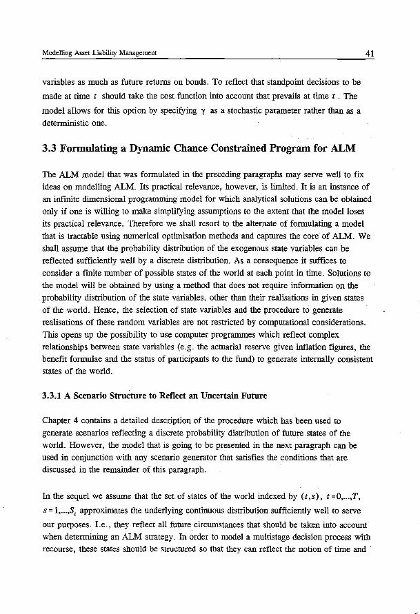
Modelling Asset Liability Management
variables as much as future returns on bonds. To reflect that standpoint decisions to be
made at time t should take the cost function into account that prevails at time t . The
model allows for this option by specifying y as a stochastic parameter rather than as a
deterministic one.
3.3 Formulating a Dynamic Chance Constrained Program for ALM
41
The ALM model that was formulated in the preceding paragraphs may serve well to fix ideas on modelling ALM. Its practical relevance, however, is limited. It is an instance of an infinite dimensional programming model for which analytical solutions can be obtained only if one is willing to make simplifying assumptions to the extent that the model loses its practical relevance. Therefore we shall resort to the alternate of formulating a model
that is tractable using numerical optimisation methods and captures the core of ALM. We shall assume that the probability distribution of the exogenous state variables can be reflected sufficiently well by a discrete distribution. As a consequence it suffices to consider a finite number of possible states of the world at each point in time. Solutions to the model will be obtained by using a method that does not require information on the probability distribution of the state variables, other than their realisations in given states of the world. Hence, the selection of state variables and the procedure to generate realisations of these random variables are not restricted by computatiomil considerations. This opens up the possibility to use computer programmes whichreflect complex relationships between state variables (e.g. the actuarial reserve given inflation figures, the benefit formulae and the status of participants to the fund) to generate internally consistent states of the world.
3.3.1 A Scenario Structure to Reflect an Uncertain Future
Chapter 4 contains a detailed description of the procedure which has been used to generate scenarios reflecting a discrete probability distribution of future .states of the world. However, the model that is going to be presented in the next paragraph can be used in conjunction with any scenario generator that satisfies the conditions that are discussed in the remainder of this paragraph.
In the sequel we assume that the set of states of the world indexed by (t,s), t=O, ... ,T,
s = l, ... ,S1
approximates the underlying continuous distribution sufficiently well to serve
our purposes. I.e., they reflect all future circumstances that should be taken into account when determining an ALM strategy. In order to model a multistage decision process with recourse, these states should be structured so that they can reflect the notion of time and
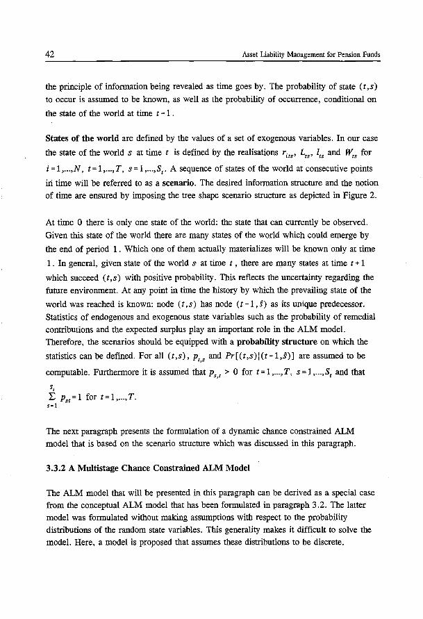
42 Asset Liability Management for Pension Funds
the principle of information being revealed as time goes by. The probability of state (t,s)
to occur is assumed to be known, as well as the probability of occurrence, conditional on
the state of the world at time t - 1 .
States of the world are defined by the values of a set of exogenous variables. In our case
the state of the world s at time t is defined by the realisations rits' Lts' Its and ~s for
i = 1 , ... ,N, t = 1 , ... , T, s = 1 , ... ,St. A sequence of states of the world at consecutive points
iri time will be referred to as a scenario. The desired information structure and the notion of time are ensured by imposing the tree shape scenario structure as depicted in Figure 2.
At time 0 there is only one state of the world: the state that can currently be observed.
Given this state of the world there are many states of the world which could emerge by
the end of period 1 . Which one of them actually materializes will be known only at time
1 . In general, given state of the world s at time t , there are many states at time t + 1
which succeed (t, s) with positive probability. This reflects the uncertainty regarding the
future environment. At any point in time the history by which the prevailing state of the
world was reached is known: node (t, s) has node (t -1 , s) as its unique predecessor.
Statistics of endogenous and exogenous state variables such as the probability of remedial contributions and the expected surplus play an important role in the ALM model. Therefore, the scenarios should be equipped with a probability structure on which the
statistics can be defined. For all (t,s), Pt,s and Pr[(t,s)l(t-1,§)] are assumed to be
computable. Furthermore it is assumed that Ps,t > 0 for t = 1 , ... , T, s = 1 , ... ,St and that
s, :E Pst=1 for t=1, ... ,T. s=l
The next paragraph presents the formulation of a dynamic chance constrained ALM model that is based on the scenario structure which was discussed in this paragraph.
3.3.2 A Multistage Chance Constrained ALM Model
The ALM model that will be presented in this paragraph can be derived as a special case from the conceptual ALM model that has been formulated in paragraph 3.2. The latter model was formulated without making assumptions with respect to the probability distributions of the random state variables. This generality makes it difficult to solve the model. Here, a model is proposed that assumes these distributions to be discrete.
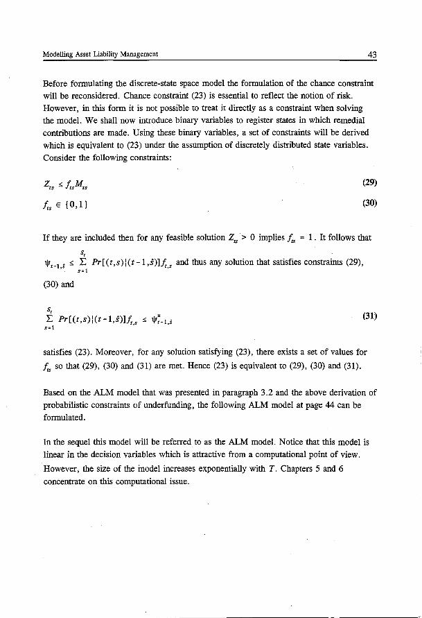
Modelling Asset Liability Management 43
Before formulating the discrete-state space model the formulation of the chance constraint will be reconsidered. Chance constraint (23) is essential to reflect the notion of risk. However, in this form it is not possible to treat it directly as a constraint when solving the model. We shall now introduce binary variables to register states in which remedial contributions are made. Using these binary variables, a set of constraints will be derived which is equivalent to (23) under the assumption of discretely distributed state variables.
Consider the following constraints:
frs E { 0, 1}
(29)
(30)
If they are included then for any feasible solution z,. > 0 implies /,. = 1 . It follows that
s, 'l!rt-l,s ~ :E Pr[ (t,s) I (t -1 ,s)]/r,s and thus any solution that satisfies constraints (29),
s=l
(30) and
s, :E Pr[(t,s)l(t-1,s)]fr s ~ llr~-1.;
s= 1 '
(31)
satisfies (23). Moreover, for any solution satisfying (23), there exists a set of values for
f,. so that (29), (30) and (31) are met. Hence (23) is equivalent to (29), (30) and (31).
Based on the ALM model that was presented in paragraph 3.2 and the above derivation of probabilistic constraints of underfunding, the following ALM model at page 44 can be
formulated.
In the sequel this model will be referred to as the ALM model. Notice that this model is
linear in the decision variables which is attractive from a computational point of view.
However, the size of the inodel increases exponentially with T. Chapters 5 and 6
concentrate on this computational issue.
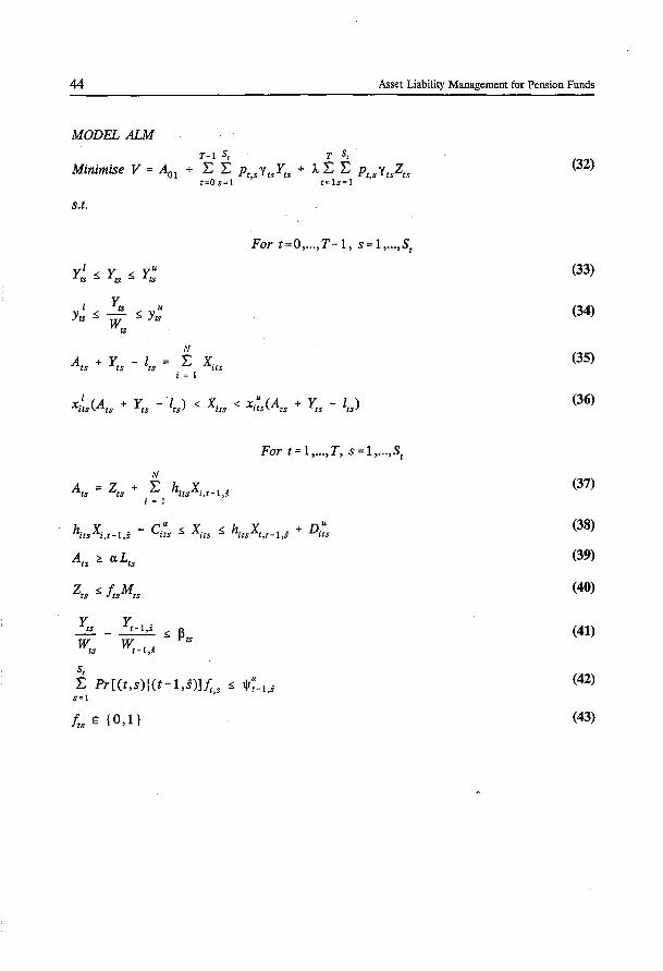
44 Asset Liability Management for Pension Funds
MODEL ALM T-1 S, T S,
Minimise V = A01 + :E L P,sYtsyts +ALL P,,sYcszts t=Os=l ' r•ls=l
s.t.
For t=O, ... ,T-1, s=l, ... ,s,
l yts u Yrs ::;
wts ::; Yrs
N
A,s + Yts - z,s = :E xits i = 1
For t=l, ... ,T, s=l, ... ,s,
s, :E Pr[(t,s)l(t-l,s)l.t;,s::; W~-1,s s=l
J;sE{O,l}
(32)
(33)
(34)
(35)
(36)
(37)
(38)
(39)
(40)
(41)
(42)
(43)
Modelling Asset Liability Management
Before turning to the subject of scenario generation we shall list the input which is
required to fonnulate the ALM model. Three groups of exogenous parameters can be
distinguished:
-the exogenous state variables l, L, r and W,
-parameters to reflect the user's objective and requirements on the ALM policy,
XI, xU, y, yl, yu, yl, yu, cu, Du, ljru, a; and p,
- parameters for which the values are detennined on computational grounds, M and A. .
These follow from the values of the previously mentioned input as will be explained in
chapter 7.
The next chapter treats the subject of scenario generation for ALM. It describes the
scenario generator that has been used to provide for the input to the ALM model.
45

Chapter 4 Scenario Generation for Asset Liability Management
4.1 Introduction
The bulk of input required by the ALM model consists of scenarios which reflect the discrete probability distribution that has been selected to describe future states of the world. These scenarios form the basis for the ALM model.
Before turning to the discussion of the scenario generator, recall the following definitions
which were given in paragraph 3. 3.1: A state of the world, indexed by ( t, s), is defined
by realisations rus, L,s, l,s and w;s. A path of consecutive states of the world is referred
to as a scenario.
The scenarios provide the framework within which the ALM policy is analyzed. Clearly
one would want this framework to be a realistic and relevant one. However, different policy makers may consider different factors to be of interest to their ALM decisions.
They may choose to base their policy on different assumptions and these assumptions should be reflected by the scenarios. Therefore, a set of scenarios which is well suited to serve as a basis for ALM decision making for one policy maker may be a rather poor setting for another decision maker. Hence, it is of importance to pay sufficient attention to the selection of a scenario generator when using these models in practice.
The selection of an appropriate scenario generator is subjective, but only to some extent.
Paragraph 3. 3. 1 already listed the conditions and assumptions with regard to' the scenario structure which follow from its role in our ALM approach:
- each state of the world has many possible successors and precisely one predecessor, s,
- Pr,s and Pr[(t,s)l(t-1,.§)] are computable, Pr,s > 0 and L Pr,s = 1. s~l
Such a structure is reflected by the tree shaped scenario structure, which is pictured in Figure 1 at page 5, and serves as input to the ALM model. The remainder of this chapter
is devoted to the procedure that has been used to obtain values for L, l, r and W in this
scenario structure. Figure 2 pictures the scenario generator that was used to obtain the
computational results in chapter 7. A time series model, more specifically a vector
autoregressive model, is employed ~laustble futUre oeyelo.pments_of.pr~-
47
48 Asset Liability Management for Pension Funds
inflation, wage inflation and returns on stocks, 'bonds, cash and real e~tate:_._'I'riese time
~eries are generated in SUCh a way that means, standard deviations, autocorrelatiOn§ and cross correlations between state variables are consistent with historical patterns ..
To compute the corresponding values for the actuarial reserves, the level of benefit payments and the cost of salaries, the status of all ~articipants in the fund and the benefit formulae are required. The development of the status of current and future participants is modelled by means of a Markov model which generates the future status of .each participant to the fund, based on transition probabilities from one status to another. Next, these data serve as input to actuarial and administrative software which compute the associated levels of benefit payments, actuarial reserves and costs of salaries.
All information to describe states of the world is now available: investment returns on all asset classes have been obtained from time series model, the administrative software has generated the corresponding cost of wages and, to conclude, the actuarial software has provided for corresponding levels of benefit payments and actuarial reserves. As will be
explained in paragraph 4.3.1 the probability of state (t,s) to emerge follows directly
from the way in which the future economic times series are generated.
4.2 Requirements on Scenario Generation
Some of the requirements follow from the purpose that the scenarios serve in the ALM model. These concern the structure of the scenarios and the associated probability
structure. These issues have been discussed in paragraph 3.3.1 and reviewed in the previous paragraph. This paragraph discusses additional conditions which the set of scenarios should s;~.tisfy. For an interesting survey regarding the merits and potential pitfalls of the use of scenarios to model an uncertain future environment, the reader can be referred to Bunn and Salo (1993).
Regardless of the decision procedure to be used, the scenarios should be internally consistent and they should be generated in accordance with the assumptions on which the
decision makers wish to base their policy. The set of scenarios should reflect expected developments of the environment· as well as the uncertainty with respect to the future environment. Notice that policies based on scenarios which do not reflect sufficient uncertainty may appear less risky than they actually are.
Policy assumptions to be made can be drawn from sources which are far apart from a methodological point of view. One could for instance rely upon a panel of experts, but
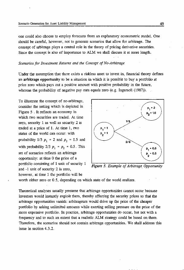
Scenario Generation for Asset Liability Management
one could also choose to employ forecasts from an explanatory econometric model. One should be careful, however, not to generate scenarios that allow for arbitrage. The concept of arbitrage plays a central role in the theory of pricing derivative securities. Since the concept is also of importance to ALM we shall discuss it at more length.
Scenarios for Investment Returns and the Concept of No-Arbitrage
49
Under the assumption that there exists a riskless asset to invest in, fmancial theory defines an arbitrage opportunity to be a situation in which it is possible to buy a portfolio at price zero which pays out a positive amount with positive probability in the future, whereas the probability of negative pay outs equals zero (e.g. Ingersoll (1987)).
To illustrate the concept of no-arbitrage, consider the setting which is depicted in Figure 5 . It reflects an economy in which two securities are traded. At time ze(o, security 1 as well as security 2 is traded at a price of 1. At time 1, two states of the world can occur: with
probability 1/3 p 1 = 2 and p 2 = 1.5 and
with probability 2/3 p 1 = p2 = 0.5. This
set of scenarios reflects an arbitrage opportunity: at time 0 the price of a portfolio consisting of 1 unit of security 1 and -1 unit of security 2 is zero,
however, at time 1 the portfolio will be
113
2/3
Figure 5. Example of Arbitrage_ Opportunity
worth either zero or 0.5, depending on which state of the world realizes.
Theoretical analyses usually presume that arbitrage opportunities cannot occur because investors would instantly exploit them, thereby affecting the security prices so that the arbitrage opportunities vanish: arbitrageurs would drive up the price of the cheaper portfolio by asking unlimited amounts while exerting selling pressure on the price of the more expensive portfolio. In practice, arbitrage opportunities do occur, but not with a frequency and to such an extent that a realistic ALM strategy could be based on them. Therefore, the scenarios should not contain arbitrage opportunities. We shall address this
issue in section 4.3.2.
50 Asset Liability Management for Pension Funds
Pricing Derivative Securities and ALM
The concept of no-arbitrage is frequently used in financial literature to derive equilibrium
prices for derivative securities. The assumption underlying this approach is that two
investment strategies that generate identical future pay outs should have the same present
value. Thus, to compute the price of a derivative security, i.e. a security of which the
price is a function of one or more underlying values, such as an interest rate or a stock
price, one designs a portfolio strategy which only trades in securities of which prices are
known and which generates a pay out pattern that is identical to the pay out pattern of the
derivative security that has to be priced. If such a strategy has been found, then, in an
equilibrium situation, the price of the derivative should be equal to the price at which the
portfolio strategy can be purchased.
Applying this line of reasoning to ALM, one could argue that the objective function value of an optimal solution to the ALM model is the present value of a portfolio strategy that
generates a pay out pattern identical to the pattern of benefit payments. Thus, ALM could
be viewed as a pricing problem of a complex derivative security: the level of benefit
payments depends on underlying values such as the rate_ofinfl~. the status of
participants etc. Financial markets are incomplete in the sense that there is no
(combination of) fmancial instruments by which the pay out pattern, as defined by the
liability process can be replicated exactly. Moreover, given the present state of the art of
financial theory, the process that determines the actual levels of future benefit payments
and actuarial reserves is too complex to be described sufficiently accurate by a stochastic
process that can serve to derive realistic dynamic ALM strategies analytically. In this
thesis we shall not pursue the development of ALM from this viewpoint. Instead, we aim
for a model that can be solved numerically to obtain useful ALM strategies. From the
standpoint of option pricing, one might consider our ALM approach as a simulation based
procedure to determine the price of a very complex derivative security.
For more extensive discussions of the concept of no-arbitrage and its role in financial
theory the reader can be referred to textbooks on finance such as Duffie (1988) and
Ingersoll (1987).
The following section presents a scenario generator for ALM which is based on the assumption that economic state variables can be described by a vector autoregressive
process.
Scenario Generation for Asset Liability Management
4.3 A Scenario Generation Model for Asset Liability Management
This section contains a detailed description of the scenario generator that was used to obtain the results in chapter 7. We shall subsequently discuss the components of the generator a~depicted in Figure 2. The first part to be discussed is the model that generates investment returns and inflation rates, a vector autoregressive time series
51
model. The second part concerns a Markov model, employed to describe the development of participants in the fund, which has been developed by Boender (1994). The remaining components of the scenario generator, administrative software to compute costs of salaries
and actuarial software to calculate actuarial reserves and benefit payments, will not be discussed in this thesis. A discussion of actuarial principles which apply in The Netherlands can be found in Petersen (1992). Notice, however, that the scenario generator can be equipped with any module that provides for actuarial figures, given the economic state of the world and the status of the participants in the fund. More precisely, such a module
should generate values for L,, and l,, that are consistent with realisations of the associated
economic state variables R,s.
4.3.1 A Vector Autoregressive Model to Generate Scenarios of Economic Variables
The first topic that will be discussed is the generation of plausible future time series of annual price inflation, wage inflation and total returns on the asset categories. Time series of economic states of the world will be generated in such a way that correlations, autocorrelations, variances and expectations of the elements that defme the states of world converge to the corresponding statistics of observations that were made in the past. To accomplish this, a time series model is employed. ~
Time series models relate the value of variables at given points in time to values that these variables took on at preceding points in time. The difference between time series models and econometric models lies in the fact the latter type of models is usually based on economic theory whereas the former is not. Time series models are treated in many econometric textQooks (e.g. Judge et al (1985,1988)) and numerous publications. It is beyond the scope of this thesis to discuss the questions arising in model selection, estimation and testing in depth. This paragraph presents the main ideas underlying vector autoregressive models and briefly reviews methods to estimate their parameter values. It concludes with a stepwise description of the procedure by which future time series of
economic variables are generated. For an extensive exposition of empirical vector autore
gressive modelling the reader can be referred to Ooms (1993).
52 Asset Liability Management for Pension Funds
Vector Autoregressive (VAR) Models
Following the strong arguments of Sims (1980), we model the economic time series by means of a V AR model. Sims discusses the pros and cons of V AR models with respect to econometric models to support macroeconomic policy making. On methodological
grounds as well as on technical grounds he argues that V AR models are more suitable to this end than econometric models. In addition to the theoretical arguments of Sims, when practising our ALM approach, the simple structure of a V AR model of order 1 allows for
a straight forward interpretation of the model parameters. This provides for the opportunity to discuss results with policy makers who did not receive a quantitatively oriented education. When called for, coefficients of the V AR model can be adjusted in order to reflect subjective beliefs regarding future economic developments.
It is not uncommon in the financial theory to assume that asset prices follow a lognormal distribution13
• In conformity with this assumption, we shall assume that the disturbances of the V AR model are distributed normally.
Autoregressive models can be used to describe linear relationships between the value of a variable at given times and the lagged values of this variable. Suppose, for instance, that annual rates of return on deposits tend to be high if they were high last year and that they tend to be low if they were low last year. More generally, suppose that the rate of return at given times can be explained partially by past rates of return. Such a relationship can
be described by the following autoregressive model, allowing for autocorrelations up to
the order K:
K
gt = Po + :E pkgt-k + ut k=l
(44)
To gain more insight in this model, consider the case that K = 1: g1
= Po + p1g1 _ 1 + U1
•
For lp 11> 1 g1
does not converge when t-oo. For IP 11< 1 a mean reversion model·
remains14 with a long term mean equal to p0/(l-p 1). Mean reversion models are
characterised by the property that the values of the explained variable show a tendency towards their long term average. The more a realisation deviates from the long term
13 Even though empirical evidence to the contrary has been reported (see e.g. Guimaraes, Kingsman and Taylor (1989) and Dert (1989)).
14 This type of model has been discussed extensively in the econometric literature (see e.g. Ooms (1993). and Rudebusch (1989)).
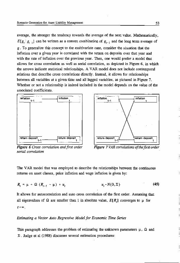
Scenario Generation for Asset Liability Management 53
average, the stronger the tendency towards the average of the next value. Mathematically,
E[g1 I g
1_ 1] can be written as a convex combination of g
1_ 1 and the long term average of
g. To generalize this concept to the multivariate case, consider the situation that the inflation over a given year is correlated with the return on deposits over that year and with the rate of inflation over the previous year. Then, one would prefer a model that allows for cross correlation as well as serial correlation, as depicted in Figure 6, in which the arrows indicate statistical relationships. A V AR model does not include contemporal relations that describe cross correlations directly. Instead, it allows for relationships
between all variables at a given time and all lagged variables, as pictured in Figure 7.
Whether or not a relationship is indeed included in the model depends on the value of the associated coefficients.
linflation inflation I t-1 J t
I return deposit I t-1
1 return deposit t I
Figure 6 Cross correlatwn and first order serial correlation
inflation t-1
Figure 7VAR correlations ofthefirstorder
The V AR model that was employed to describe the relationships between the continuous returns on asset classes, price inflation and wage inflation is given by:
Rt = IJ. + Q (Rt-I - IJ.) + ut u1-N(O,I:) (45)
It allows for autocorrelation and auto cross correlation of the ftrst order. Assuming that
all eigenvalues of Q are smaller than 1 in absolute value, E[R1] converges to IJ. for
t-oo.
Estimating a Vector Auto Regressive Model for Economic Time Series
This paragraph addresses the problem of estimating the unknown parameters 1J., Q and
:E. Judge et al (1988) discusses several estimation procedures:
54 Asset Liability Management for Pension Funds
1. Ordinary Least Squares (OLS)
2. Seemingly Unrelated Regression (SUR) as introduced by Zellner (1962) 3. Maximum Likelihood (ML) by repeated SUR estimation
As is well known, the OLS estimator is the best linear unbiased estimator under the assumption that disturbances from different equations are uncorrelated and that disturbances are independently and identically distributed over time. OLS estimates of the coefficients of one equation are obtained by minimising the sum over time of the squared
residuals. In case of a V AR model, values for all coefficients of the system of equations can be estimated by computing row wise OLS estimates, i.e. by performing OLS on each of the equations separately. This is equivalent to computing OLS estimators for the entire system simultaneously because, within the framework of OLS, covariances between disturbances from different equations are not taken into account; it is assumed that they are zero.
In the presence of correlation between disturbances from different equations at a given
time, known as contemporaneous correlation, covariances between disturbances from different equations should be taken into account when estimating parameter values. In this case better estimates can be obtained through the use of SUR methods15
• Zellner's SUR estimator is obtained by applying OLS, followed by a Generalised Least Squares (GLS)
estimation. GLS estimates are obtained by minimising a quadratic function of the residuals from all equations simultaneou~ly. The quadratic function, which is based on the covariance matrix of the disturbances, is chosen so that the variance of GLS estimates of the parameter values is minimal, given the covariance matrix of disturbances. In general
this covariance matrix is not known and one uses an estimate thereof. Zellner uses a covariance matrix which is estimated from the OLS residuals.
After performing an OLS procedure, one can apply GLS in an iterative fashion: in each
iteration, E is estimated from the residuals of the previous iteration. The newly estimated
covariance matrix, in turn, is used to compute a new GLS estimate of p. and 0 . The
estimates obtained from this iterative procedure converge to Maximum Likelihood estimates.
Although the asymptotic properties of the SUR estimators are superior to those of OLS estimators, it is not guaranteed that applying SUR methods on small samples will indeed produce better estimates than OLS. This is due to the fact that it is in general not possible
15 This is not the case if all of the equations have the same explanatory variables, then it can be shown that OLS estimates and SUR estimates are identical.
Scenario Generation for Asset Liability Management 55
to obtain an unbiased estimate of the covariance matrix of the distUrbances for finite numbers of observations16
• There is no ready made recipe to decide which estimation
method to choose. The smaller the sample size and the greater the difference between the number of explanatory variables, the better OLS. The greater the presence of contemporaneous correlation, the better SUR.
We have chosen to apply a stepwise ML method. Starting with an umestricted ML estimation, an iterative procedure is ~arried out in which one non-significant parameter per iteration is removed from the model and new ML estimates are computed for the remaining coefficients until all insignificant coefficients have been removed. In case of more than one statistically insignificant parameter, the one to be fixed at zero is selected on statistical and economic grounds. The procedure is as follows:
Step 1. Specify for each of the coefficients whether its value, based on economic theory, is expected to be negative, zero or positive.
Step 2. Compute Maximum Likelihood estimates by applying GLS iteratively.
Step 3. If all coefficients are statistically significant at the 1% level, STOP.
Otherwise, select one of the non-significant coefficients to be fixed at zero, applying the following pick order:
1. The least significant coefficient which was expected to be zero. 2. The least significant coefficient which has a sign opposite to the expected
sign. 3. The least significant coefficient with a sign equal to its expected sign.
Go to Step 2.
A Vector Auto Regressive Model to Generate Economic Time Series
Given the estimated ·values of the parameters 1.1., Q and :E, (45) is applied iteratively to
generate many scenarios of future time-series, structured as illustrated in Figure 1: At
time 0 there is only one economic state of the world, defmed by Ro1 , the current values
16 This problem only arises when the number of explanatory variables per equation varies. Otherwise T
( 1/ (T- k)) I; u,u: in which k denotes the number of explanatory variables in each equation is an s,t=l
unbiased estimator of I: , given a set of T observations.
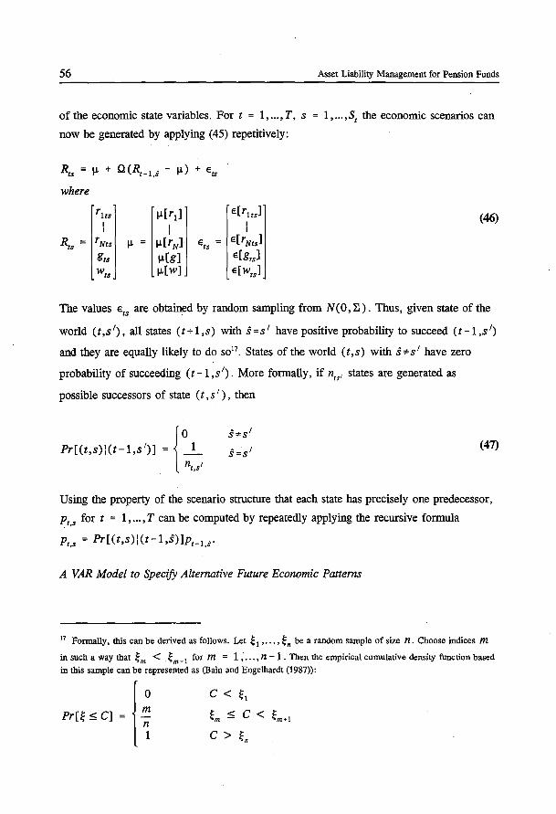
56 Asset Liability Management for Pension Funds
of the economic state variables. For t = 1, ... , T, s 1 , ... , St the economic scenarios can
now be generated by applying (45) repetitively:
~s = j.L + Q(Rt-l,s- IJ.) + Ets
where
rlts IJ.[rl] e[rlrsl (46) I I I I
~s rNts j.L !J.[rN] Ets = e[r Nts]
gts j.L[g] e[gts]
wts !J.[W) e[wrsl
The values ers are obtained by random sampling from N ( 0, :E) . Thus, given state of the
world (t,s 1), all states (t+1,s) with s=s 1 have positive probability to succeed (t-1,s 1
)
and they are equally likely to do so17• States of the world (t,s) with S*s' have zero
probability of succeeding ( t -1, s 1) • More formally, if nrs' states are generated as
possible successors of state (t, s 1 ) , then
Pr[(t,s)l(t-1,s 1)] = {~
nt,s 1
S*S'
s=s' (47)
Using the property of the scenario structure that each state has precisely one predecessor,
Pr,s for t = 1, ... , T can be computed by repeatedly applying the recursive formula
Pr,s = Pr[(t,s)l(t-1,s)]pt-l,s"
A VAR Model to Specify Alternative Future Economic Patterns
17 Formally, this can be derived as follows. Let ~ 1 , .•. , ~n be a random sample of size n. Choose indices m
in such a way that ~ m < ~ m + 1 for m = 1 ; ... , n - 1 . Then the empirical cumulative density function based in this sample can be represented as (Bain and Engelhardt (1987)):
c < ~1
~m ::;; C < ~m+l
C > ~n
Scenario Generation for Asset Liability Management 57
Notice that ( 46) can also be used to generate scenarios that are based on parameter values
other than those obtained from following the estimation method that we described in the
previous paragraphs. This flexibility is of importance when one chooses to base an ALM policy on economic patterns which do not resemble historic patterns. When doing so, one
could begin by specifying why future economic patterns are expected to be different from
the ones that have been observed in the past. Given these motives, elements of f.', 0 and
E 18 can be adjusted accordingly. Employing ( 46) then serves to structure the formulation
of assumptions and to generate scenarios that are consistent with these assumptions.
Moreover, the estimated values of f.' , 0 and E can serve as a starting point to specify
parameter values that correspond to policy assumptions; it is an arduous task to specify parameter values without the frame of reference provided by estimates that are based on
historic observations. A discussion on the asymptotic properties of the distribution of R
when using different parameter values can be found in Boender and Romeijn (1991).
Extending the Scenario Generator to Account for Multiple Economic Regimes
Suppose that the historical time series cover periods of time with several economic
regimes, then one could prefer to estimate one V AR model for each economic regime and
to accommodate changes of regime in the scenario generator. That raises the question,
however, how transition probabilities from one regime to another should be specified.
Historical time series typically do not contain sufficient information to estimate them: either the number of transitions is too small, or the time series goes back so far that one should question its relevance for the specification of the future. One way out of this
dilemma is to proceed as follows:
Given a small number of V AR models and the corresponding likelihood functions of
states of the world (one model and one likelihood function for each economic regime) and
the current state of the world:
step 1: compute the value of each of the likelihood functions,
step 2: specify a probability distribution of the current economic regime, based on the relative values of their likelihood function values,
18 If the perceived changes in the economic structure give rise to adjustments of elements of ~ , then it is
recommendable to present ~ in a product form of standard deviations of disturbances per equation and correlations between these disturbances. It is easier to assess how these can be adjusted to be in accordance with policy assumptions than to adjust variances and covariances directly. Moreover, this approach enables one to
preserve consistency between the elements of ~ so that it can still be interpreted as a covariance matrix.
58 Asset Liability Management for Pension Funds
step 3: for each possible state of the world that succeeds the current one:
- sample a current economic regime,
- generate the succeeding state by means of the corresponding V AR model, as has been described above.
Of course, as with the parameters of the V AR model, one can also choose to specify
transition probabilities that are based on sources other than historic data and assumptions
that come with the V AR model.
4.3.2 Arbitrage Free Scenarios
Does the scenario generator preclude arbitrage opportunities ? In this section it will be
shown that the scenario generator does not systematically generate arbitrage opportunities.
Nothwithstanding this desirable property it is conceivable that a finite sample of scenarios
does allow for arbitrage. Therefore, this section also presents an algorithm to identify and
eliminate arbitrage opportunities if there are any.
The Underlying Continuous Probability Distribution and Arbitrage
Given ( 46), the return on each of the asset classes is a lognormally distributed random
variable. Thus, the return on each of the asset classes can take on any value greater than
-100%. If we assume that all random variables are distributed independently, i.e.
i ¢ j "'* u [ i ,j] = 0 , then, the return on any investment portfolio equals a linear
combination of independently lognormally distributed random variables. Hence, the
portfolio has a positive probability of a negative return, as well as a positive probability
of a positive return. As a consequence, no pair of portfolios exists, such that one portfolio
outperforms the other portfolio with probability 1. It follows that there are no arbitrage
opportunities if the state variables are an exact representation of the underlying continuous
probability distribution. Fortunately, the assumption of independence is stronger than necessary. It suffices to preclude pathetic cases of correlation. More formally:
The continuous probability distribution which underlies the scenario generator precludes
arbitrage if the conditional variance of the return on risky asset class j , given the returns
on asset classes i, i = 1 , ... , N, i ¢ j, is positive for all risky assets j .
Proof: Let X denote an arbitrage portfolio, i.e.
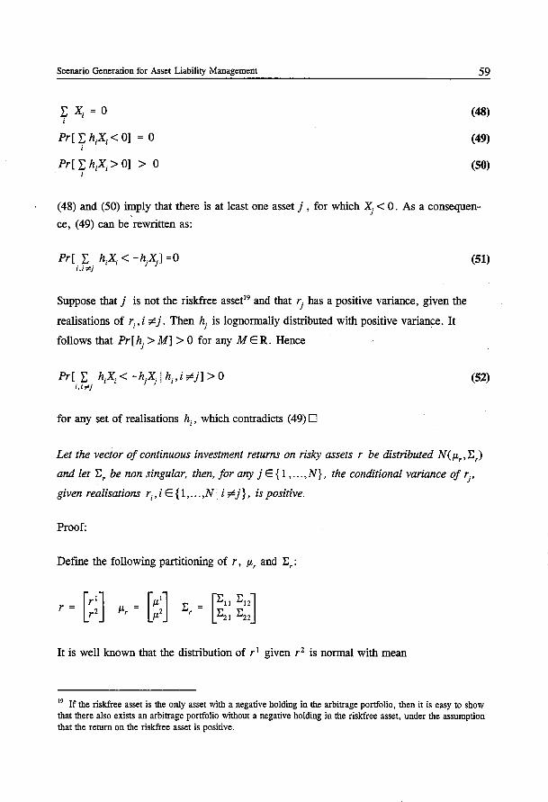
Scenario Generation for Asset Liability Management
Pr[ L h;X; < 0] = 0 i
Pr[ L h;X; > 0] > 0 i
59
(48)
(49)
(50)
(48) and (50) ~ply that there is at least one asset j, for which~< 0. As a consequen
ce, (49) can be rewritten as:
Pr[ L h.X. < -h.X.] =0 i,i ¢j l l J J
Suppose that j is not the riskfree asset19 and that rj has a positive variance, given the
realisations of r;, i ¢ j. Then hj is lognormally distributed with positive variance. It
follows that Pr [ hj > M] > 0 for any MER. Hence
Pr[ L. h;X; < -hj~ I h;,i ¢j] > 0 l,l '¢}
for any set of realisations h;, which contradicts ( 49) D
(51)
(52)
Let the vector of continuous investment returns on risky assets r be distributed N(p,,,E,)
and let E, be non singular, then, for any j E { 1 , ... ,N}, the conditional variance of rj'
given realisations r;, i E { 1, ... ,N I i ¢ j}, is positive.
Proof:
Defme the following partitioning of r, P-, and E,:
It is well known that the distribution of r 1 given r 2 is normal with mean
19 If the riskfree asset is the only asset with a negative holding in the arbitrage portfolio, then it is easy to show that there also exists an arbitrage portfolio without a negative holding in the riskfree asset, under the assumption that the return on the riskfree asset is positive.
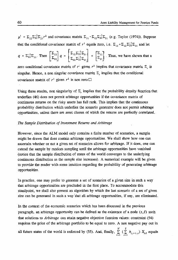
60 Asset Liability Management for Pension Funds
p.1 + 1;12
I;;il;21
r 2 and covariance matrix 1; 11 -1; 12 1;2il;21 (e.g. Taylor (1974)). Suppose
that the conditional covariance matrix of r 1 equals zero, i.e. 1; 11 =1; 12 I;;il;21 and let
zero conditional covariance matrix of r 1 given r 2 implies that covariance matrix I;, is
singular. Hence, a non singular covariance matrix I;, implies that the conditional
covariance matrix of r 1 given r 2 is non zero 0
Using these results, non singularity of I;, implies that the probability density function that
underlies ( 46) does not permit arbitrage opportunities if the covariance matrix of continuous returns on the risky assets has full rank. This implies that the continuous probability distribution which underlies the scenario generator does not permit arbitrage opportunities, unless there are asset classes of which the returns are perfectly correlated.
The Sample Distribution of Investment Returns and Arbitrage
However, since the ALM model only contains a finite number of scenarios, a sample might be drawn that does contain arbitrage opportunities. We shall show how one can ascertain whether or not a given set of scenarios allows for arbitrage. If it does, one can extend the sample by random sampling until the arbitrage opportunities have vanished (notice that the sample distribution of states of the world converges to the underlying continuous distribution as the sample size increases). A numerical example will be given to provide the reader with some intuition regarding the probability of generating arbitrage
opportunities.
In practice, one may prefer to generate a set of scenarios of a given size in such a way that arbitrage opportunities are precluded in the first place. To accommodate this standpoint, we shall also present an algorithm by which the last scenario of a set of given size can be generated in such a way ·that all arbitrage opportunities, if any, are eliminated.
In the context of the economic scenarios which has been discussed in the previous
paragraph, an arbitrage oppmtunity can be defined as the existence of a node (t,s) such
that solutions to Arbitrage can attain negative objective function values: constraint (54)
requires the price of the arbitrage portfolio to be equal to zero. A non negative pay out in N S
all future states of the world is enforced by (55). And, fmally, ~ ( ~ hi,r+1,s) xir§ equals i=l S"=l
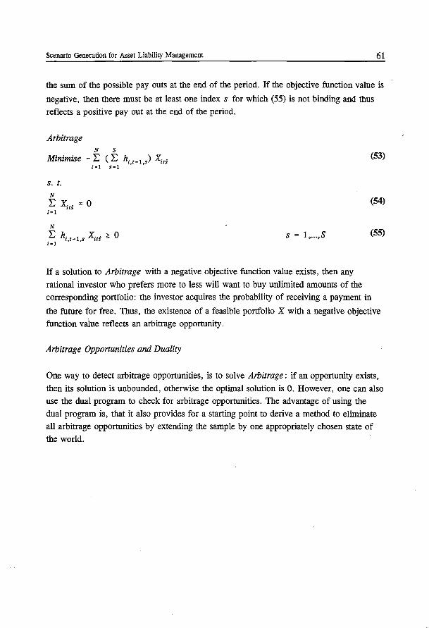
Scenario Generation for Asset Liability Management 61
the sum of the possible pay outs at the end of the period. If the objective function value is
negative, then there must be at least one index s for which (55) is not binding and thus
reflects a positive pay out at the end of the period.
Arbitrage N S
Minimise - E ( E h; t+t s) X;,8 i =1 s= 1 ' ,
s. t. N
E X;,,. = o i=l
N
E hi,t+t,s Xits ~ o i=l
(53)
(54)
s = I, ... ,s (55)
If a solution to Arbitrage with a negative objective function value exists, then any
rational investor who prefers more to less will want to buy unlimited amounts of the corresponding portfolio: the investor acquires the probability of receiving a payment in
the future for free. Thus, the existence of a feasible portfolio X with a negative objective function value reflects an arbitrage opportunity.
Arbitrage Opportunities and Duality
One way to detect arbitrage opportunities, is to solve Arbitrage: if an opportunity exists,
then its solution is unbounded, otherwise the optimal solution is 0. However, one can also use the dual program to check for arbitrage opportunities. The advantage of using the dual program is, that it also provides for a starting point to derive a method to eliminate
all arbitrage opportunities by extending the sample by one appropriately chosen state of the world.
62 Asset Liability Management for Pension Funds
The dual program of Arbitrage reads:
Dual Arbitrage s
Maximise 0TC 0 + :E 0TC5
s=1
s. t. s s 'ItO + :E hi t+1 s1Cs= - :E hi,t+1,s
s= 1 ' ' s=1 i = l, ... ,N
s = l, ... ,s
Applying the duality theorem of linear programming to Arbitrage and its dual gives:
If X is a feasible solution to Arbitrage and 1r is a feasible solution to Dual Arbitrage
N S S
then - :E ( :E h.t 1 ) x.t. ~ OTCo + :E OTCS = 0. l, + ,s l s
i=1 s=1 s=1
(56)
(57)
(58)
Hence, if there is a feasible solution to Dual Arbitrage, then there is no feasible solution
to Arbitrage with a negative objective function value. It follows that any set of the states
of the world which allows for a feasible solution 1r to Dual Arbitrage precludes arbitrage opportunities. The above argument is a generalisation of a similar argument for a special class of arbitrage opportunities which has been given in Ingersoll (1987).
Eliminating Arbitrage Opportunities
Consider Dual Arbitrage and suppose that there is no feasible solution 1r. Then, there
may be arbitrage opportunities. To eliminate them, it would suffice to extend the set of possible future states of the world in such a way that the corresponding dual problem has
feasible solutions. We shall show how to eliminate arbitrage opportunities by a well chosen extension of the sample of states of the world.
Intuitively speaking, arbitrage opportunities occur if it is possible to construct two portfolios of which one provides for higher returns than the other under all future circumstances. Such a situation can be eliminated by adding a state of the world in which the reversed situation occurs. Given a set of states of the world, arbitrage opportunities can be eliminated by extending this set with states in which portfolios that appeared to be
superior, perform poorly and vice versa. As will be shown now, it takes only one additional state of the world to accomplish this.
Scenario Generation for Asset Liability Management 63
More formally, given a set of S states of the world at time t + 1 , the question is how an
additional state of the world ( t + 1 , S + 1 ) can be specified which ensures the existence of
a feasible solution to the dual program that is associated with states of the world
(t + 1, 1), ... , (t + 1, S + 1). In other words, how to determine hi,t+I,S+l > 0 such that there
S+! S+!
existvaluesfor 1r, 7rs;:::Ofors=1, ... ,S+l thatsatisfy 1r0 + L hi,t+l,s7rs= -L hi,t+l,s s•l s=l
Vi.
Thus, values hi,t+I,S+I have to be chosen so that there are values for 1r that satisfy the
following system of equations:
S+l
1to + E (1 +1ts)hi t+l s = O s•l ' '
1, ... ,N
i = 1, ... ,N
s = 1 , ... ,S + 1
Rearranging (59) gives:
s -1to - E (1 +1ts)hi,t+l,s
s=l
(59)
(60)
(61)
(62)
Substituting 1rri = -1r0 /(1 +7r5 • 1) and 1r: = (1 +7rs)/(1 +7r5 • 1) for s=1,._..,S in (61) and
(62) leads to the following set of equations, which is equivalent to (59), ... ,(61):
I s
1tl h. hi,t+I,S+l E 1, ... ,N (63) = 1to - s r,t+l,s
s=l
hi,t+I,S+I > 0 = 1, ... ,N (64)
I 1ts > 0 s = 1, ... ,s (65)
As can be verified from (63), ... ,(65), there are many values for hi,t+I,S•t and 1r which
can serve to eliminate arbitrage opportunities. How could one select the best set of values
for hi,t•I,S+I that precludes arbitrage ? One may want to select values for hi,r+I,S+t in
64 Asset Liability Management for Pension Funds
such a way that they are in line with the underlying probability distribution. For instance,
one could choose R,+l.S+ 1 so as to maximise the likelihood function that follows from
(46), subject to precluding arbitrage opportunities. This corresponds to the following
problem in which aii denotes the element at row i , column j of the covariance matrix
E:
Max Likelihood
Minimise
e,R,+t S+I • 1t1
s.t.
N+2
:E i,j=l
N+2
R;,t+!,S+l IJ.;+ L W;/R;,r,s+t-1-L)+E; j=l
s ln[Ri,r+l,S+l] = 1t~ - :E 1t~ln[R;,t+t)
s=l
Ri,t+l,S+l > 1
(66)
1, ... ,N (67)
1, ... ,N (68)
= 1, ... ,N (69)
1, ... ,N, s = 1, ... ,S (70)
Notwithstanding its intuitive appeal, Max Likelihood may prove difficult to solve, due to
the nonlinear functions that appear in the constraints. Therefore, one may prefer to
specify a model that requires less computational effort to solve and results in a reasonable
additional state of the world that precludes arbitrage. For instance, one could avoid
unnecessarily extreme values for hi,r+ 1,s+t by solving Max Deviation, which minimises
the largest absolute deviation of h;,l+ 1,s+ 1 from its expected value. Recall that
E [ h; ,t + 1 ,s + 1] denotes the mathematical expectation of returns over period t + 1 that
follows from (46), it is independent of the decision variables hi,t+ 1,s+ 1 •
These results can be used to generate an arbitrage free set of economic scenarios.
One should be aware, however, the distribution of any scenario that has specifically been constructed so as to eliminate arbitrage opportunities, is different from, and possibly
dependent on, the other scenarios. This may_ complicate statistical inference in a later stadium. For practical purposes, one may choose to neglect this. From a theoretical point
of view one might prefer to generate the entire set of states of the world by random
Scenario Generation for Asset Liability Management
sampling, checking for arbitrage opportunities, and extending the sample by random
sampling until there are no arbitrage opportunities left.
Max Deviation
Minimise
hi r+t S+l'A,n'
hi,t+l,S+l > 0
11"~ > 0 1, ... ,N
l, ... ,N
l, ... ,N
l, ... ,N
l, ... ,N
= l, ... ,N
s = 1, ... ,s
65
(71)
(72)
(73)
(74)
(75)
(76)
(77)
For sufficiently large sample sizes and realistic coefficients of the V AR model, it is
unlikely that it is necessary to extend the sample substantially in order to eliminate
arbitrage opportunities. To illustrate this point, consider the setting that there are only two
assets to invest in. Suppose that their returns follow a bivariate normal distribution with
mean f.' and covariance matrix 1: 20• Then, the difference of the returns is normally
distributed with mean 1-'t- 1-'z and variance c?[ 1] -2u[ 1, 2] + c?-[2]. Hence, the probabil
ity that the return on one asset exceeds the other can be obtained from the table of the
standard normal distribution, after transforming the normal distribution of the difference of the two returns to the standard normal distribution. Let the return on the first asset
exceed that of the second asset with probability p . Then, the probability that asset 1
outperforms asset 2 in all cases equals p s. Likewise, the probability that asset 2
outperforms asset 1 under all circumstances is given by ( 1 - p )s. The probability of an
arbitrage opportunity, given a random sample of size S, equals the probability that the
first asset is superior plus the probability that the second asset is superior, i.e.
p s + ( 1 - p )s . Table 4 above presents a numerical example of the probability of creating
arbitrage opportunities by random sampling as a function of the sample size. Of course,
20 The following analysis also holds if the continuous returns are assumed to be distributed normally.
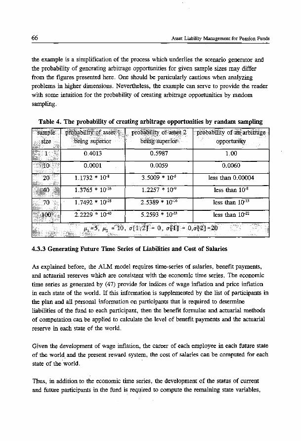
66 Asset Liability Management for Pension Funds
the example is a simplification of the process which underlies the scenario generator and
the probability of generating arbitrage opportunities for given sample sizes may differ
from the figures presented here. One should be particularly cautious when analyzing
problems in higher dimensions. Nevertheless, the example can serve to provide the reader
with some intuition for the probability of creating arbitrage opportunities by random
sampling.
Table 4. The probability of creating arbitrage opportunities by randam sampling
1 /.:·. . ' ...
· ........ <lQ.····.········· ·:···········:itt··········· I > .· ... < ..•.
70
probability of asset 2 probability of an arbitrage
· peingsuperior being superior opportullity .·.·
0.4013 0.5987 1.00
0.0001 0.0059 0.0060
1.1732 * 10"8 3.5009 * 10·5 less than 0.00004
1.3765 * 10"16 1.2257 * 10"9 less than 10"8
1. 7492 * 10"28 2.5389 * w-16 less than 10"15
2.2229 * lQ-40 5.2593 * 10"23 less than 10·22
. P,.1 =5, 1-S = 10, a[1,2l = 0, a[l] = .O,a[2]=2Q
. . .. . .. ·. · .. ·· . .
4.3.3 Generating Future Time Series of Liabilities and Cost of Salaries
.
As explained before, the ALM model requires time-series of salaries, benefit payments,
and actuarial reserves which are consistent with the economic time series. The economic
time series as generated by (47) provide for indices of wage inflation and price inflation
in each state of the world. If this information is supplemented by the list of participants in
the plan and all personal information on participants that is required to determine
liabilities of the fund to each participant, then the benefit formulae and actuarial methods
of computation can be applied to calculate the level of benefit payments and the actuarial
reserve in each state of the world.
Given the development of wage inflation, the career of each employee in each future state
of the world and the present reward system, the cost of salaries can be computed for each
state of the world.
Thus, in addition to the economic time series, the development of the status of current
and future participants in the fund is required to compute the remaining state variables,

Scenario Generation for Asset Liability Management 67
i.e. the actuarial reserve, the level of benefit payments and the costs of salaries.
As with the method of generating economic scenarios, our ALM approach is independent of the way in which the development of participants is obtained. Below we briefly discuss a Markov model that has been used in studies for Dutch pension funds as well as for the case study in this monograph. For a more elaborate exposition of this model the reader
can be referred to Boender (1994). Markov models in the context of ALM are also presented in Janssen and Mancca (1994).
Modelling the Development of Participants in the Fund
The purpose of modelling the development of participants in the fund is to provide for all relevant personal information on participants that is required to compute liabilities of the fund, and costs of salaries to the company in each future state of the world.
Given the pension-rules and all relevant data on the participants (e.g. civil status, age, gender, salary, earned pension rights, medical status, social status), a Markov model is used to determine the future development of each individual that currently participates in the pension fund. For an employee this implies that each year it is determined whether he remains alive, retires, resigns, gets disabled and/or is promoted to another job category.
These transitions are determined by probabilities which depend on characteristics of the individuals such as age, gender and employee-category21
• Disabled, resigned and retired people in the file are modelled analogously.
Given the situation of each current employee in each future year, the m<;>del determines additional promotions and the recruitment of new employees, such that the number of employees in each job category in each future year is in line with prespecified values. The age and gender of new employees are random variables which depend on the categories to which they are assigned.
4.3.4 Generating Future Time Series of Economic and Actuarial Variables
The economic state variables and the corresponding status of the participants in the fund constitute the base information by which the states of the world are described. To construct consistent descriptions of states of the world which include figures that derive from the data that is now available, administrative and actuarial software is used to
21 Most of the transition probabilities also depend on the company by which participants are employed and the
type of work that they do. This should be taken into account when specifying them.

68 Asset Liability Management for Pension Funds
compute the corresponding actuarial reserve, benefit payments and the cost of salaries for
each state of the world. Thus, consistent future time series of states of the world are
obtained.
Consistency
To conclude this chapter let us briefly review the concept of consistency of scenarios. The
scenario generator that has been described above ensures consistency on various levels.
The V AR model ensures consistency over time as well as at points in time between
economic state variables.
It is unlikely that arbitrage opportunities will be introduced. It is possible to prevent them
from being generated all together by appropriately choosing the last scenario that is generated. One can also check first whether a given set of scenarios incorporates arbitrage
opportunities. If it does, then the set of scenarios can be extended by continued random sampling until there are no arbitrage opportunities left. One can also choose to add one
well chosen scenario to eliminate all arbitrage opportunities. By applying the scenario
generator in combination with one of these procedures, the scenarios are consistent with
the widely accepted non arbitrage hypothesis.
The Markov model safeguards consistency of scenarios in terms of the development of
participants. Next, the economic data and the data on participants serve as input to
actuarial software by means of which the corresponding actuarial data (actuarial reserves
and benefit payments) are calculated22•
22 The extent to which it is desirable and feasible to pursue consistency of scenario data in practice may vary. The specification of transition probabilities, for instance, is highly dependent on the pension fund under consideration. In some cases it may very difficult to formulate a longer term personnel policy, let alone transition probabilities from one status to another of future participants to the fund. On the other hand, there may be cases where it is possible to indicate a relationship between the economic environment as reflected by the economic time series and transition probabilities.
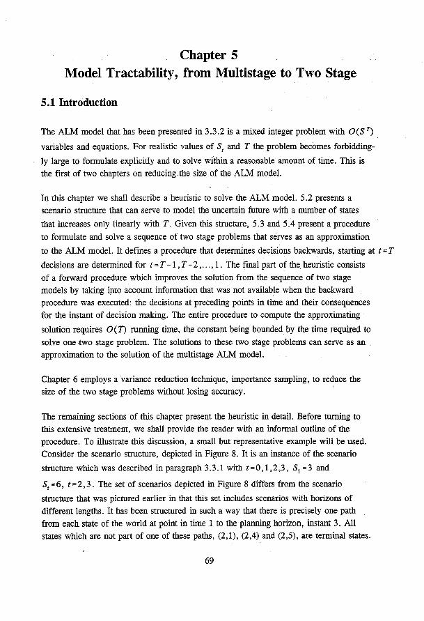
Chapter 5 Model Tractability, from Multistage to Two Stage
5.1 Introduction
The ALM model that has been presented in 3.3.2 is a mixed integer problem with O(S T)
variables and equations. For realistic values of S1
and T the problem becomes forbidding
ly large to formulate explicitly and to solve within a reasonable amount of time. This is the first of two chapters on reducing the size of the ALM model.
In this chapter we shall describe a heuristic to solve the ALM model. 5.2 presents a scenario structure that can serve to model the uncertain future with a number of states
that increases only linearly with T. Given this structure, 5.3 and 5.4 present a procedure
to formulate and solve a sequence of two stage problems that serves as an approximation
to the ALM model. It defines a procedure that determines decisions backwards, starting at t = T
decisions are determined for t = T- 1 , T- 2 , ... , 1 . The final part of the heuristic consists
of a forward procedure which improves the solution from the sequence of two stage models by taking into account information that was not available when the backward procedure was executed: the decisions at preceding points in time and their consequences for the instant of decision making. The entire procedure to compute the approximating
solution requires O(T) running time, the constant being bounded by the time required to
solve one two stage problem. The solutions to these two stage problems can serve as an approximation to the solution of the multistage ALM model.
Chapter 6 employs a variance reduction technique, importance sampling, to reduce the size of the two stage problems without losing accuracy.
The remaining sections of this chapter present the heuristic in detail. Before turning to
this extensive treatment, we shall provide the reader with an informal outline of the procedure. To illustrate this discussion, a small but representative example will be used. Consider the scenario structure, depicted in Figure 8. It is an instance of the scenario
structure which was described in paragraph 3.3.1 with t=0,1,2,3, S1 =3 and
S1 = 6, t = 2, 3. The set of scenarios depicted in Figure 8 differs from the scenario
structure that was pictured earlier in that this set includes scenarios with horizons of different lengths. It has been structured in such a way that there is precisely one path
from each state of the world at point in time 1 to the planning horizon, instant 3. All states which are not part of one of these paths, (2,1), (2,4) and (2,5), are terminal states.
69
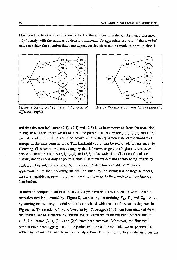
70 Asset Liability Management for Pension Funds
This structure has the attractive property that the number of states of the world increases only linearly with the number of decision moments. To appreciate the role of the terminal states consider the situation that state dependent decisions can be made at point in time 1
2,6~
2,5 "8 ~~~.4 ~~ 2,3 3,3
Figure 8 Scenario structure with horizons of different lenghts
Figure 9 Scenario structure for Twostage2(2)
and that the terminal states (2, 1), (2,4) and (2,5) have been removed from the scenarios in Figure 8. Then, there would only be one possible successor for (1,1), (1,2) and (1,3).
I.e., at point in time 1, it would be known with certainty which state of the world will
emerge at the next point in time. This hindsight could then be exploited, for instance, by allocating all assets to the asset category that is known to give the highest return over period 2. Including states (2,1), (2,4) and (2,5) safeguards the reflection of decision
making under uncertainty at point in time 1, it prevents decisions from being driven by
hindsight. For sufficiently large 81
, this scenario structure can still serve as an
approximation to the underlying distribution since, by the strong law of large numbers, the state variables at given points in time still converge to their underlying continuous
distribution.
In order to compute a solution to the ALM problem which is associated with the set of
scenarios that is illustrated by Figure 8, we start by determining Z3s, Y2s and X;zs v i, s
by solving the two stage model which is associated with the set of scenarios depicted in
Figure 10. This model will be referred to by Twostagel (3). It has been obtained from
the original set of scenarios by eliminating all states which do not have descendants at
t=3, i.e., states (2,1), (2,4) and (2,5) have been removed. Moreover, the first two
periods have been aggregated to one period from t = 0 to t = 2 This two stage model is
solved by means of a branch and bound algorithm. The solution to this model includes the
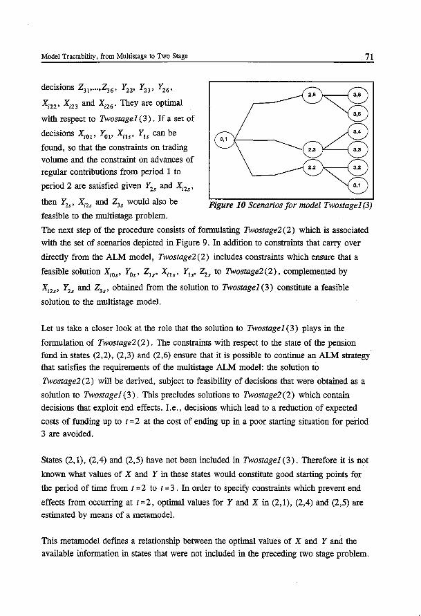
Model Tractability, from Multistage to Two Stage
decisions z31'"""'z36• y22' y23' y26•
X;22 , Xm and X;26 . They are optimal
with respect to Twostagel ( 3) . If a set of
decisions xiOl' Yol' xi!s' y!s can be
found, so that the constraints on trading
volume and the constraint on advances of regular contributions from period 1 to
period 2 are satisfied given y2s and xi2s,
then y2s ' xi2s and z3s would also be
feasible to the multistage problem.
71
2,6~
~
~ Figure 10 Scenarios for model Twostagel (3)
The next step of the procedure consists of formulating Twostage2(2) which is associated
with the set of scenarios depicted in Figure 9. In addition to constraints that carry over
directly from the ALM model, Twostage2(2) includes constraints which ensure that a
feasible solution Xios• Y0s, Z1s, Xits' Y 1s, Z2s to Twostage2(2), complemented by
Xi 2s, Y2s and Z3s, obtained from the solution to Twostagel (3) constitute a feasible
solution to the multistage model.
Let us take a closer look at the role that the solution to Twostagel (3) plays in the
formulation of Twostage2 ( 2) . The constraints with respect to the state of the pension
fund in states (2,2), (2,3) and (2,6) ensure that it is possible to continue an ALM strategy
that satisfies the requirements of the multistage ALM model: the solution to
Twostage2 (2) will be derived, subject to feasibility of decisions that were obtained as a
solution to Twostagel (3). This precludes solutions to Twostage2(2) which contain
decisions that exploit end effects. I.e., decisions which lead to a reduction of expected
costs of funding up to t = 2 at the cost of ending up in a poor starting situation for pel:iod
3 are avoided.
States (2,1), (2,4) and (2,5) have not been included in Twostagel (3). Therefore it is not
known what values of X and Y in these states would constitute good starting points for
the period of time from t = 2 to t = 3 . In order to specify constraints which prevent end
effects from occurring at t=2, optimal values for Y and X in (2,1), (2,4) and (2,5) are
estimated by means of a metamodel.
This metamodel defines a relationship between tl1e optimal values of X and Y and the
available information in states that were not included in the preceding two stage problem.
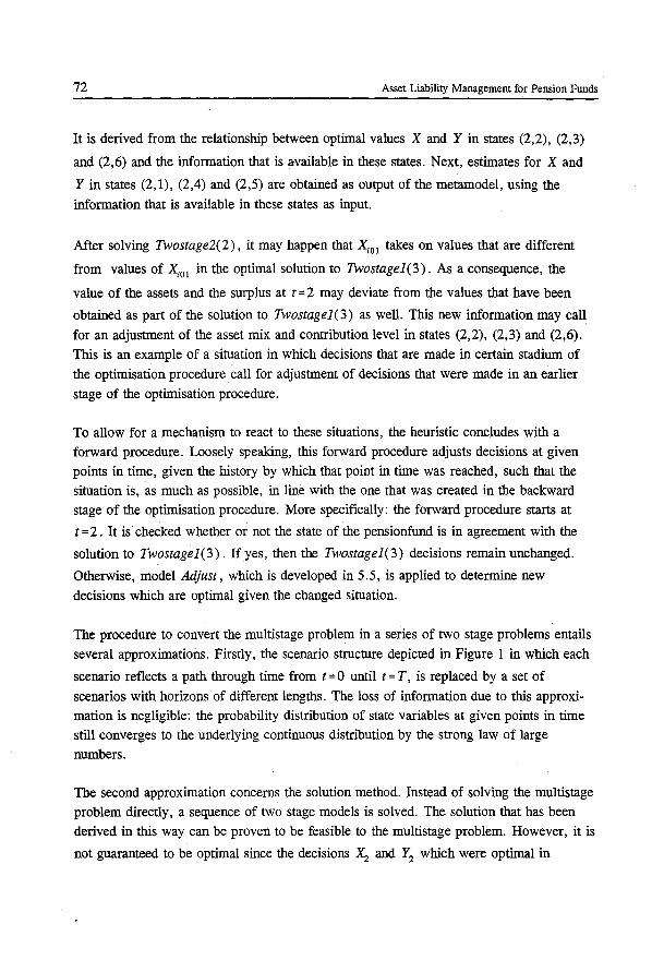
72 Asset Liability Management for Pension Funds
It is derived from the relationship between optimal values X and Y in states (2,2), (2,3)
and (2,6) and the information that is available in these states. Next, estimates for X and
Y in states (2, 1), (2,4) and (2,5) are obtained as output of the metamodel, using the
information that is available in these states as input.
After solving Twostage2( 2) , it may happen that Xw 1 takes on values that are different
from values of X;01 in the optimal solution to Twostage1(3). As a consequence, the
value of the assets and the surplus at t=2 may deviate from the values that have been
obtained as part of the solution to Twostage1(3) as well. This new information may call
for an adjustment of the asset mix and contribution level in states (2,2), (2,3) and (2,6). This is an example of a situation in which decisions that are made in certain stadium of
the optimisation procedure call for adjustment of decisions that were made in an earlier stage of the optimisation procedure.
To allow for a mechanism to react to these situations, the heuristic concludes with a forward procedure. Loosely speaking, this forward procedure adjusts decisions at given points in time, given the history by which that point in time was reached, such that the situation is, as much as possible, in line with the one that was created in the backward stage of the optimisation procedure. More specifically: the forward procedure starts at
t = 2. It is· checked whether or not the state of the pensionfund is in agreement with the
solution to Twostagel ( 3). If yes, then the Twostagel ( 3) decisions remain unchanged.
Otherwise, model Adjust, which is developed in 5.5, is applied to determine new
decisions which are optimal given the changed situation.
The procedure to convert the multistage problem in a series of two stage problems entails
several approximations. Firstly, the scenario structure depicted in Figure 1 in which each
scenario reflects a path through time from t = 0 until t = T, is replaced by a set of
scenarios with horizons of different lengths. The loss of information due to this approximation is negligible: the probability distribution of state variables at given points in time still converges to the underlying continuous distribution by the strong law of large
numbers.
The second approximation concerns the solution method. Instead of solving the multistage problem directly, a sequence of two stage models is solved. The solution that has been derived in this way can be proven to be feasible to the multistage problem. However, it is
not guaranteed to be optimal since the decisions X2 and Y2 which were optimal in

Model Tractability, from Multistage to Two Stage 73
combination with the optimal X0 ,Xl' Y0 and Y1 to Twostagel (3), are not necessarily
optimal in combination with the ultimate choice of X0 ,X1, Y0· and Y1 • The trade-off
between costs which are incurred by decisions at t = 2 and costs which result from
decisions at points in time 0 and 1, does not have to be optimal, because these decisions
were not made simultaneously. The decisions at points in time 0 and 1 are optimal, given
the decisions that were made earlier at point in time 2. It is nottrivial to indicate whether this approximation leads to a systematic bias in the outcomes because the two stage
problems are neither relaxations nor special cases of the multistage problem: at intertemp
oral points in time no recourse decisions can be made, but neither is the policy required to meet actuarial solvency requirements at these points.
The third approximation is due to the metamodel. In states (2, 1), (2,4) and (2,5), the
constraints that account for end effects are based on estimates of the optimal horizon
situations instead of the truly optimal situation as obtained from a preceding two stage
solution. In case of inaccurate estimates, these constraints may either be too conservative,
which leads to excessively comfortable financial situations of the pension fund at the cost
of unnecessarily high contributions in earlier periods, or, if the constraints are not strict
enough, the policy determined from the period up to instant t may lead to undesirable
starting points for the period from t to T. Notice that the latter type of error can only
occur to the extent that the funding level that is required to meet actuarial solvency
constraints is less than the optimal funding level.
5.2 Reducing the Number of States of the World
Consider the scenario structure that has been discussed in 3. 3 .1 and let S1 = S2 ,
t = 2 , ... , T. This choice of parameter values of the number of nodes in the set of scenarios
equals 1 + S1 + ( T -1) S2 . As can be verified from the ALM model, the number of
variables per node is bounded by 3 + 3 N and the number of equations per node never
exceeds 8 +4N. Given this set of scenarios, the size of the model is O(NS2T), it is
bounded by a linear function of the number of decision moments, which implies a drastic
reduction of the computational complexity of solving the model.
Given the values of S1
, the number of possible states of the world at each point in time
has been fixed. Let us now examine the relationship between consecutive states of the world and the probability with which one state succeeds another. Figure 8 depicts an
example of the structure that will be used. In general, the structure is defined as follows:·
at time 0, there is op.Iy one state of the world, the one that can be observed, state (0,1).

74 Asset Liability Management for Pension Funds
At the end of the first period, there are S1 states of the world, which succeed (0,1) with
probability p 1s. State of the world ( 1, s), for s = 1, ... , Sl' has n1s possible successors,
where n1s has been chosen in such a way that the underlying conditional probability
distribution of state ( t + 1 , s 1 ) given ( t, s) is represented sufficiently well, and
s\ I; n
1s = S2 • So far, the scenario structure is identical to the one that has been presented
s=l
in 3.3.1. For t > 2, however, the structure is different. Instead of generating n,s possible
successors of (t, 1), (t, 2), ... , (t, S), succeeding states are generated for a subset of these
states only. The selection of this subset is done in such a way that the history of each
state of the world is unique, and that each state of the world at t = 1 has precisely one
descendant at time T. As a consequence, the number of states of the world does not
increase exponentially with T any more. Now, it increases linearly with T. Notice that
each state in which an ALM decisions can be made has many possible successors. This
prevents decisions to be made with hindsight.
It is easy to verify that this structure preserves the requirements on the scenario structure that have been derived in 3.3.1.
The question is now, whether this set of scenarios suffices to approximate the underlying continuous probability distribution of the state variables. Using the strong law of large
numbers, it can easily be verified that it does if S1 and S2 are chosen sufficiently large.
For S1
and S2
..... oo , the sample distribution of the state variables at time t converges
stochastically to the underlying distribution, if the mean and variance of this distribution exist (see e.g. Hogg and Craig (1978)). Hence, this scenario structure can serve to
describe the uncertain future, provided that sl and s2 are chosen sufficiently large.
5.3 A Sequence of Two Stage Problems to Solve the ALM Model
This paragraph proposes a heuristic to obtain a solution to the ALM model which requires
a running time that is bounded by a linear function of T. The solution will be obtained by solving a sequence of two stage problems. Firstly, decisions are obtained for points in
time T and T -1 . Then, working backward, two stage problems are formulated and
solved in such a way that their solutions constitute a feasible solution to the ALM model.
Decisions at given points in time affect states of the world at later times. However, the backward procedure does not allow to alter decisions at these times, given decisions at
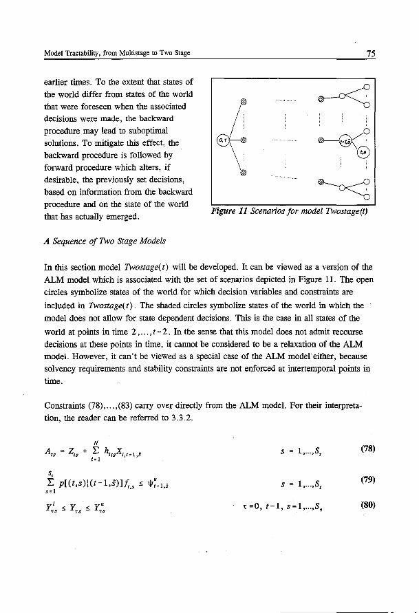
Model Tractability, from Multistage to Two Stage
earlier times. To the extent that states of
the world differ from states of the world
that were foreseen when the associated
decisions were made, the backward
procedure may lead to suboptimal
solutions. To mitigate this effect, the
backward procedure is followed by
forward procedure which alters, if
desirable, the previously set decisions,
based on information from the backward
procedure and on the state of the world
that has actually emerged.
A Sequence of Two Stage Models
75
0
~· . ' C0
Figure 11 Scenarios for model Twostage(t)
In this section model Twostage(t) will be developed. It can be viewed as a version of the
ALM model which is associated with the set of scenarios depicted in Figure 11. The open
circles symbolize states of the world for which decision variables and constraints are
included in Twostage(t) . The shaded circles symbolize states of the world in which the
model does not allow for state dependent decisions. This is the case in all states of the
world at points in time 2 , ... , t - 2 . In the sense that this model does not admit recourse
decisions at these points in time, it cannot be considered to be a relaxation of the ALM
model. However, it can't be viewed as a special case of the ALM model either, because
solvency requirements and stability constraints are not enforced at intertemporal points in
time.
Constraints (78), ... ,(83) carry over directly from the ALM model. For their interpreta~
tion, the reader can be referred to 3.3.2.
s = I, ... ,st (78)
s, L p[(t,s)l(t-1,s)lt;.::: W~-1,s
s=! • s = 1, ... ,st (79)
,;=0, t-1, s=l, ... ,s, (80)
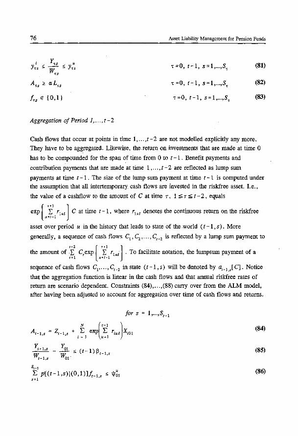
76 Asset Liability Management for Pension Funds
t =0, t-1, s=1, ... ,s,
t=O, t-1, s=1, ... ,S,
f .. E {0,1} t =0, t-1, s=1, ... ,s,
Aggregation of Period 1, ... , t- 2
(81)
(82)
(83)
Cash flows that occur at points in time 1, ... ,t-2 are not modelled explicitly any more.
They have to be aggregated. Likewise, the return on investments that are made at time 0
has to be compounded for the span of time from 0 to t -1 . Benefit payments and
contribution payments that are made at time 1 , ... , t - 2 are reflected as lump sum
payments at time t - 1 . The size of the lump sum payment at time t - 1 is computed under
the assumption that all intertemporary cash flows are invested in the riskfree asset. I.e.,
the value of a cashflow to the amount of C at time 7 , 1 ~ 7 ~ t - 2 , equals
exp ( u ~~~ / 1 us ) C at time t- 1 , where r1 us denotes the continuous return on the riskfree
asset over period u in the history that leads to state of the world ( t - 1 , s) . More
generally' a sequence of cash flows cl ' c2 ' ... ' c, -2 is reflected by a lump sum payment to
the amount of X:: Crexp (,E~/Ius) . To facilitate notation, the lumpsum payment of a
sequence of cash flows Cl' ... , C, _2 in state (t -1 , s) will be denoted by at-!) C) . Notice
that the aggregation function is linear in the cash flows and that annual riskfree rates of
return are scenario dependent. Constraints (84), ... ,(88) carry over from the ALM model,
after having been adjusted to account for aggregation over time of cash flows and returns.
for s = 1, ... ,S,_ 1
At-1,s = zt-1,s + f exp('i! rius)xi01 i = 1 u=1
s,_, E p[(t-1,s)l(0,1)]J;.1,s s; W~1
s= 1
(84)
(85)
(86)
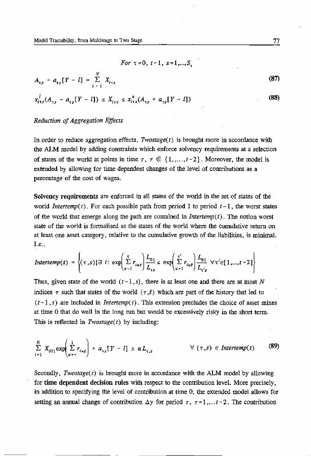
Model Tractability, from Multistage to Two Stage
N
A,s + au[Y - l] = :E X;,s i = 1
For 't=O, t-1, s=1, ... ,S,
Reduction of Aggregation Effects
77
(87)
(88)
In order to reduce aggregation effects, Twostage(t) is brought more in accordance with
the ALM model by adding constraints which enforce solvency requirements at a selection
of states of the world at points in time 7, 7 E { 1, ... , t- 2} . Moreover, the model is
extended by allowing for time dependent changes of the level of contributions as a
percentage of the cost of wages.
Solvency requirements are enforced in all states of the world in the set of states of the
world Intertemp(t). For each possible path from period 1 to period t -1, the worst states·
of the world that emerge along the path are contained in Intertemp(t). The notion worst
state of the world is formalised as the states of the world where the cumulative return on at least one asset category, relative to the cumulative growth of the liabilities, is minimal. I.e.,
lntertemp(t) = J(,,s)l3 i: exp(~rius)L01 ,; exp(~rius)L01 'i7''t 1E[1, ... ,t-2]} 1 u-1 Lts u-1 L,'s
Thus, given state of the world ( t- 1 , s), there is at least one and there are at most N
indices 7 such that states of the world ( 7 ,.S) which are part of the history that led to
(t -1, s) are included in lntertemp(t). This extension precludes the choice of asset mixes
at time 0 that do well in the long run but would be excessively risky in the short term.
This is reflected in Twostage(t) by including:
'i7' ( 't ,s) E Intertemp(t) (89)
Secondly, Twostage(t) is brought more in accordance with the ALM model by allowing
for time dependent decision rules with respect to the contribution level. More precisely, in addition to specifying the level of contribution at time 0, the extended model allows for
setting an annual change of contribution .6. y for period 7, 7 = 1 , ... t - 2 . The contribution
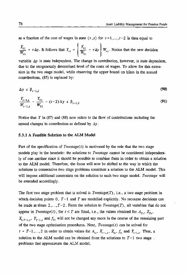
78 Asset Liability Management for Pension Funds
as a fraction of the cost of wages in state ( 7 , s) for 7 = 1 , ... , t - 2 is then equal to
Yo! + 7!l.y. It follows that YTS = [YO! + 7!l.yl wrs· Noticethatthenewdecision WOI WOI
variable !iy is state independent. The change in contribution, however, is state dependent,
due to the exogenously determined level of the costs of wages. To allow for this extension in the two stage model, while observing the upper bound on hikes in the annual contributions, (85) is replaced by:
~-l,s
w;-l,s
Notice that Yin (87) and (88) now refers to the flow of contributions including the
annual changes in contribution as defined by !iy .
5.3.1 A Feasible Solution to the ALM Model
Part of the specification of Twostage(t) is motivated by the role that the two stage
(90)
(91)
models play in the heuristic: the solutions to Twostage cannot be considered independent
ly of one another since it should be possible to combine them in order to obtain a solution to the ALM model. Therefore, the focus will now be shifted to the way in which the solutions to consecutive two stage problems constitute a solution to the ALM model. This
will impose additional constraints on the solution to each two stage model. Twostage will
be extended accordingly.
The first two stage problem that is solved is Twostage( T), i.e., a two stage problem in
which decision points 0 , T- 1 and T are modelled explicitly. No recourse decisions can
be made at times 2, ... , T- 2 . From the solution to Twostage( T), all variables that do not
appear in Twostage(t), for t < T are fixed, i.e., the values obtained for Ars, Z75 ,
Xi.T-t.s' Y7 _1,s and frs will not be changed any more in the course of the remaining part
of the two stage optimisation procedures. Next, Twostage(t) can be solved for
t = T-1, ... , 2 in order to obtain values for A,s, X,_ 1 ,s, Z,s, frs and ~-t,s. Thus, a
solution to the ALM model can be obtained from the solutions to T -1 two stage problems that approximate the ALM model.
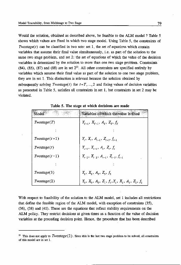
Model Tractability, from Multistage to Two Stage 79
Would the solution, obtained as described above, be feasible to the ALM model? Table 5
shows which values are fixed in which two stage model. Using Table 5, the constraints of
Twostage(t) can be classified in two sets: set 1, the set of equations which contain variables that assume their final value simultaneously, i.e. as part of the solution to the same two stage problem, and set 2: the set of equations of which the value of the decision variables is determined by the solution to more than one two stage problem. Constraints (84), (85), (87) and (88) are in set 223. All other constraints are specified entirely by variables which assume their final value as part of the solution to one two stage problem, they are in set 1. This distinction is relevant because the solution obtained by
subsequently solving Twostage(t) for t=T, ... ,2 and fixing values of decision variables
as presented in Table 5, satisfies all constraints in set 1, but constraints in set 2 may be violated.
Table 5. The stage at which decisions are made
. Mddel . · .
· Variables ofwhiCbthe.value is flied· .. .. . . . ..
Twostage(T) YT-1' XT-1' AT, Zro fr
Twostage(t + 1) ~. ~. At•l • zt•l' Ir.1
Twostage(t) ~-1' ~-!• At, Zt, fr
Twostage ( t -1) ~-2' xl-2' At-1' zt-1' fr-1
Twostage( 3) Y2, Xz, A3, z3.A
Twostage(2) Yo, Xo, Ao, zl·h·Y,· XI' AI' z2• fz
With respect to feasibility of the solution to the ALM model, set 1 includes all restrictions that define the feasible region of the ALM model, with exception of constraints (35), (36), (38) and (41). These are the equations that reflect stability requirements on the ALM policy. They restrict decisions at given times as a function of the value of decision variables at the preceding decision point. Hence, the procedure that has been described
23 This does not apply to Twostage (2). Since this is the last two stage problem to be solved, all constraints of this model are in set 1.
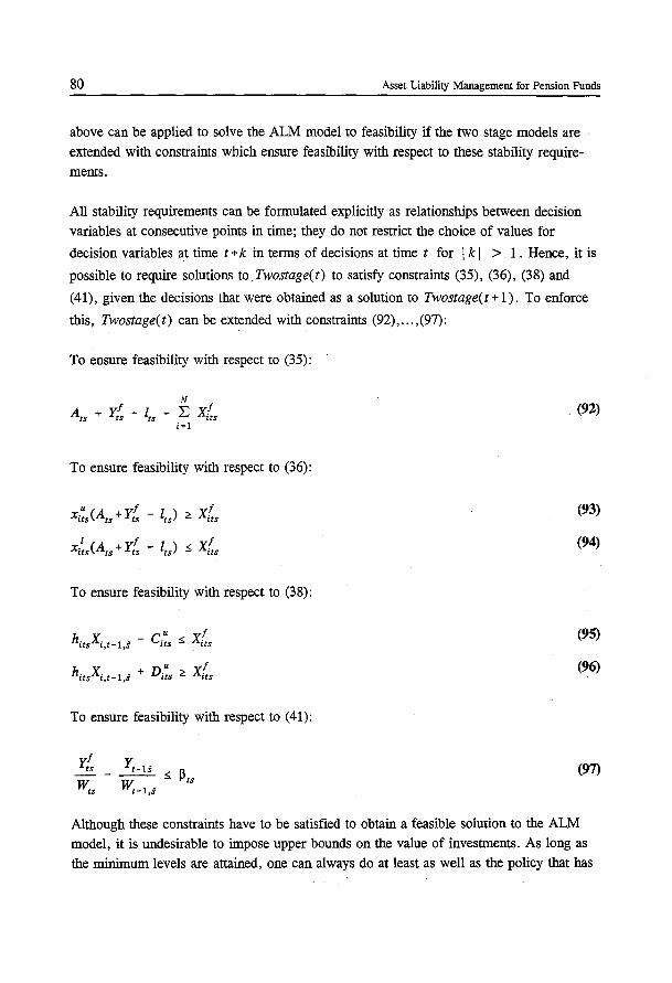
80 Asset Liability Management for Pension Funds
above can be applied to solve the ALM model to feasibility if the two stage models are extended with constraints which ensure feasibility with respect to these stability require
ments.
All stability requirements can be formulated explicitly as relationships between decision variables at consecutive points in time; they do not restrict the choice of values for
decision variables at time t + k in terms of decisions at time t for I k I > 1 . Hence, it is
possible to require solutions to Twostage(t) to satisfy constraints (35), (36), (38) and
(41), given the decisions that were obtained as a solution to Twostage(t + 1). To enforce
this, Twostage(t) can be extended with constraints (92), ... , (97):
To ensure feasibility with respect to (35):
N I :E xits i= I
To ensure feasibility with respect to (36):
x;~.<A,. + yfs - z,.) 2:: xft.
x;~.(A,. + Yis - z,.) !> xfr.
To ensure feasibility with respect to (38):
hitsxi,t-l,s - ci~s !> xfr.
h;,sXi,t-l,s + D;~s <:: xfrs
To ensure feasibility with respect to (41):
(92)
(93)
(94)
(95)
(96)
(97)
Although these constraints have to be satisfied to obtain a feasible solution to the ALM model, it is undesirable to impose upper bounds on the value of investments. As long as the minimum levels are attained, one can always do at least as well as the policy that bas
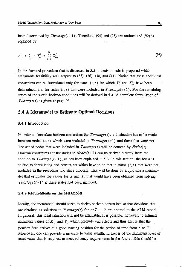
Model Tractability, from Multistage to Two Stage
been determined by Twostage( t + 1) . Therefore, (94) and (95) are omitted and (92) is
replaced by:
81
(98)
In the forward procedure that is discussed in 5.5, a decision rule is proposed which safeguards feasibility with respect to (35), (36), (38) and (41). Notice that these additional
constraints can be formulated only for states (t, s) for which Yfs and X/r, have been
determined, i.e. for states (t, s) that were included in Twostage(t + 1). For the remaining states of the world horizon conditions will be derived in 5.4. A complete formulation of
Twostage(t) is given at page 93.
5.4 A Metamodel to Estimate Optimal Decisions
5.4.1 Introduction
In order to formulate horizon constraints for Twostage(t), a distinction has to be made
between nodes ( t, s) which were included in Two stage (t + 1) and those that were not.
The set of nodes that were included in Twostage(t) will be denoted by Nodes(t).
Horizon constraints for the nodes in Nodes( t + 1) can be derived directly from the
solution to Twostage ( t + 1 ) , as has been explained in 5. 3. In this section, the focus is
shifted to formulating end constraints which have to be met in states (t, s) that were not
included in the preceding two stage problem. This will be done by employing a metamo
del that estimates the values for X and Y, that would have been obtained from solving
Twostage ( t + 1 ) if these states had been included.
5.4.2 Requirements on the Metamodel
Ideally, the metamodel should serve to derive horizon constraints so that decisions that
are obtained as solutions to Twostage(t) for t=T, ... ,2 are optimal to the ALM model.
In general, this ideal situation will not be attainable. It is possible, however, to estimate
minimum values of X;1, and r;, which preclude end effects and thus ensure that the
pension fund arrives at a good starting position for the period of time from t to T.
Moreover, one can provide a measure to value wealth, in excess of the minimum level of asset value that is required to meet solvency requirements in the future. This should be
82 Asset Liability Management for Pension Funds
accomplished without excessive computational effort. After solving Twostage(t + 1) , the
following information is available to serve as input to the metamodel:
- The states of the world at ( r , s) for r = 0 , t - 1 , t , s = 1 , ... , S,
- Solutions to Twostage (t + 1) for states (t, s) E Nodes(t + 1)
- The probability distribution of R1 + 1., given R1 .s for s = 1 , ... , S1•
Notice that the problem to be solved by the metamodel is different from the single period ALM problems that have been discussed in chapter 2. Firstly, here, it is not the intention
to arrive at a decision that is optimal with respect to the single period that starts at the moment of decision making. The intention is to estimate decisions that are optimal in the
sequence of decisions that are made for t = 0, ... , T. Secondly, there is additional
information available: the optimal decisions in states of the world in Nodes(t + 1).
5.4.3 Mechanisms that Drive the ALM Model
Model ALM is rather complicated to solve. Nevertheless, the forces that drive it are few and they are easy to understand: to minimise expected costs of funding, investment decisions should be made in such a way that the expected return on investments is maximal. However, this goal can be pursued only to the extent that it does not lead to unacceptable risks of underfunding. The risk of underfunding is linked to the probability that the growth of liabilities exceeds the appreciation of the investment portfolio to the extent that a substantial erosion of the surplus occurs.
Given the proportional allocation of assets over the investment classes, the risk of underfunding becomes smaller in accordance with the degree to which the surplus to start with is greater. With difficult times ahead, the multistage character of the ALM model tends to yield solutions which allow for building up a surplus in earlier times that can serve as a buffer under more difficult circumstances. Likewise, rosy perspectives will generally lead to modest surpluses since the costs of maintaining a larger surplus would outweigh the reduction of risk that could be brought about.
The challenge is to formulate a metamodel that reflects these properties while there is no
explicit information available on states of the world that succeed (t, s) f1. Nodes(t + 1) .
5.4.4 A Metamodel to Derive Horizon Constraints
Before turning to the metamodel, let us analyze how the surplus at time t + 1 depends on
Model Tractability, from Multistage to Two Stage
the asset value and asset allocation at time t . The conceptual ALM model that has been
developed in 3.2 will serve as a starting point, together with the scenario generator that has been specified by ( 46).
(19) and (46) imply that the value of the asset portfolio at time t + 1 is given by
N
83
I: xitexp[ri t+l] (99)
i = 1 '
Using a first order Taylor approximation (e.g. Almering et. all (1988)), (99) cari be
formulated as:
In the sequel of this section the asset value at time t + 1 will be modelled as:
N
A,+I I: (1 +ri,r+r)Xit i=l
(100)
(101)
This introduces an approximation error of the order of magnitude of I: X;,O(r;~ 1 + 1). It i
follows that the expected approximation error is bounded by a weighted sum of the
variance of r about 0. ri.t+l will typically take on values in the order of magnitude of
0.08. This implies a relative estimation error of the asset value at time t + 1 of the order
of magnitude of 0.6%24•
The distribution of liabilities at time t + 1 is more difficult to specify. It is a function of
price inflation, wage inflation and the development of the characteristics of the partici-
24 Actually, one can obtain better Taylor approximations by approximating the exponential powers about their expected value. The remaning analyses remain unchanged when this is done.
84 Asset Liability. Management for Pension Funds
pants. This function is defmed by the benefit formulae and the actuarial standards. Given
a specific pension plan, the specification can be extracted from the benefit formulae.
Here, it will be assumed that liabilities can be divided in four components: a constant, a
component that is indexed with price inflation, a component that is indexed with wage
inflation and, finally, a component that depends on a number of unspecified factors,
which are assumed not to be state dependent. These assumptions are reflected by (102):
(102)
As with the asset value, the value of liabilities at time t + 1 will be approximated by using
a ftrst order Taylor approximation of exp[g,. 1] and exp[w,. 1 ]:
(103)
The coefficients 1J specify the relative sizes of the components which constitute the
liabilities at time t . They can be estimated from observations in pairs of states (t, s) ,
(t + 1 , s) in Nodes(t + 1) . Estimating them can thus be done by solving for 1J in
regression model (104). Notice that one may expect to obtain a very good fit because
(104) virtually reflects the administrative definition equation that is implicitly given by the
actuarial rules that are applied to determine the level of liabilities.
(104)
Given the distribution of the asset value and the liabilities, the surplus at time t + 1 can be
approximated by:
N
Bt•l L (l+ri,t•l)X;, - 'llot - C111t(l +g,.l) + 'll2t(l +wt•l) + '113t)Lt i=l
(105)
Since r, g and w are normally distributed, the level of the surplus at time t + 1 is a
linear combination of normally distributed random variables. This implies that B,. 1 is
Model Tractability, from Multistage to Two Stage 85
distributed normally and that the mean and variance of this distribution are determined by
the choice of X,. This brings us back in the domain of mean variance type ALM models.
The Minimally Required Level of Asset Value
First, let us determine the minimum level of the value of assets that is required at the
beginning of period t to meet solvency c.onstraints at time t + 1 with probability ,_g. This
is done by utilizing a variant of the chance constrained programming model that has been
discussed in chapter 2:
Min Assets(t,s)
N
Min E X;,.s i= 1
s.t. N
E X;,.s ~ ct L,.s i=l
N
E (1 +E[r;i(t,s)])Xits - 11 0 , -i=l
N
a2[At+l,s] = . ~ X;,,. a [r;,r)Xjts ,,J=l
N
a [At+l,s'Lt+J .l = L xitsa [r;,r(L, .. ),.]L,,. ' i=l
(106)
(107)
(108)
(109)
(110)
(111)
(112)
(113)
(114)
MinAssets(t,s) computes the minimal asset value that is required in state (t,s), in order
to satisfy the probabilistic solvency constraint on a minimum surplus at the end of period
t. (107) ensures that the funding requirement at the beginning of period t is met as well.
86 Asset Liability Management for Pension Funds
After solving MinAssets(t ,s) for s = 1 , ... , S,, a mean variance efficient estimate of the
minimally required asset level and the associated asset mix have been obtained for all
terminal states of Twostage( t) . By using X;~, the solution to MinAssets( t, s) , as a lower
bound on X;,, in Twostage(t), any feasible solution to Twostage(t) constitutes a feasible
starting point for period t . Therefore, the following constraints are included for
(t,s) ~Nodes (t+1):
(115)
1, ... ,N (116)
1, ... ,N (117)
Clearly, these constraints are not overly restrictive. It is conceivable, however, that an
optimal multistage solution would call for asset levels in excess of X;~ . The next section
proposes a method to determine whether, and if so, by how much asset levels should
exceed X;~. The method is based upon mean variance theory and exploits the information
that is available from the solution to Twostage(t + 1) .
The Optimal Asset Level and Asset mix
For states (t, s) E Nodes(t + 1), X/,, is available, as well as X1~. Let X1;., = X/,, - X1~ N
and A,; = I; X;;,. Then; A,; can be interpreted as the amount that, under the optimal i=I
policy, should be invested in excess of the minimally required amount. Given the
probability distribution of the investment returns in state (t, s), the standard deviation of
the return on the additional investments over period t in state ( t + 1 , s) equals:
(118)
Model Tractability, from Multistage to Two Stage
Assuming that the optimal standard deviation depends linearly25 on the additional level
of assets, the following regression model can be specified:
87
(119)
(119) is the estimated relationship between the optimal standard deviation of the return on the asset value in addition to the minimally required level and the level of additional
assets.
For nodes ( t, s) ft. Nodes( t + 1), the capital market line, as is well known from mean
variance investment theory, defines a linear relationship between standard deviation and
expected return of mean variance efficient portfolios:
which implies:
E[r(At~)ts] - ko
k,
Substituting (119) in (121) gives
(120)
(121)
(122)
which relates the expected return under the optimal asset allocation of an additional unit
of wealth to the level of additional wealth. For instance, let the additional wealth be equal
to At;. Then, the expected additional revenues from the asset portfolio over period t are
equal to (k0 + k1(60 + 61A,;))A,;. Taking the first derivative to A,; it can be shown that
one unit of additional wealth in state (t, s) is equivalent to k0 + k1 60 + 2k1 61 A1; units of
additional expected wealth in ( t + 1 , s) . Notice that one unit of additional investments at
time t can lead to a more than proportional increase in the expected level of assets at
25 In order to obtain a more accurate reflection of the relationship between expected return and excess investments, a piecewise linear relation can be estimated in an analogous way. This does not affect the remaining analyses in a substantial way.
88 Asset Liability Management for Pension Funds
time t + 1 . This is caused by the fact that a higher surplus allows for a riskier asset mix which comes with a higher expected return for the entire asset portfolio.
Now the value of an additional unit to invest in state (t, s) has been established, it is
possible to incorporate the trade-off between costs to generate the additional unit to invest and the benefits from the additional wealth. Using the discount factors from the objective function of the ALM model, the present value of one unit of additional wealth in state
{t+1,s) equals -y1• 1./k0 + k100 + 2k101A1;).
These results will be used to quantify the trade-off between additional costs of funding
and the benefits from a higher surplus at the outset of period t in states of the world
(t, s) €/:. Nodes(t + 1 ) . This will be discussed in 5 .4. 5.
5.4.5 Selecting an Objective Function for Twostage(t)
A natural way to choose an objective function for Twostage(t) would be to take the
objective function of the ALM model and adjust it for the aggregation over the period
from decision point 1 to decision point t-1. However, in that case the objective function
would only reflect the cost of funding of up to time t . Given the analysis above, the
objective function can be extended by a component that reflects the value of finishing at
time t in a position that is better than the minimally required position.
In order to incorporate the trade-off in Twostage(t), credit should be given for a larger
than necessary asset value. This has been done by specifying the following objective for
Twostage(t):
Minimise V = A01 + Y01 +
S, N
E Prs Yrs< -2{<181 E (Xits - xi;:) + J..Zts) s=l i=l
The other side of the coin, the costs, were already included since the objective is to minimise expected costs of funding.
(123)
Model Tractability, from Multistage to Two Stage
5.5 A Forward Procedure
The forward procedure that is described here serves two purposes:
- adjusting the solutions to Twostage( T), . .-., Twostage( 3) in such a way that they
constitute a feasible solution to the ALM model,
89
- improving the solutions by altering the decisions made in state (t, s) in such a way that
decisions at earlier times and their consequences are taken into account. Notice that this
information was not available when the associated two stage models were solved.
The idea behind the forward procedure is, that given state of the world (t, s), the
decisions xfts, Y(. are part of a good solution to the ALM model in view of the span of
time from t to T. However, when the values of Xfts and Y(. were fixed,. the decisions at
preceding points in time were not yet known. Given this new information it may be
possible to do better than just choosing Xfts and Y(.. For instance, if the surplus in state
(t, s) turns out to be substantially lower than expected, then it may be optimal to choose
a less risky asset mix. Vice versa, if the surplus is unexpectedly high, it may be optimal
to cut contributions or to select a riskier asset mix. It may also happen that Xfts and Y(.
are infeasible to the ALM model, given the new information. Model Adjust(t, s)
minimises deviations from the ALM policy that has been specified by Xfts, Yfts, A(. and
z(., subject to being feasible to the ALM model.
Givenstate (t,s) E Nodes(t+1), 2~t~T-1, (37)and(39)imply N
Z,s = max(O,aL,s - E husXi,r-l,s), which, in conjunction with (37) fixes A,s: i= 1
N
A,s = Z,s + E husXi , _1 s. In order to satisfy the constraints of the ALM model with i=1 ' •
respect to decisions to be made in state (t,s), constraints (33), ... ,(36), (38) and (41)
have to be met. Moreover, in order to be able to pursue the ALM policy in succeeding
states at instant t + 1, (37), ... ,(43) should be satisfied. This leads to model Adjust at page
90.
If there is no solution to Adjust(t,s) which satisfies (136), ... ,(139), then it cannot be
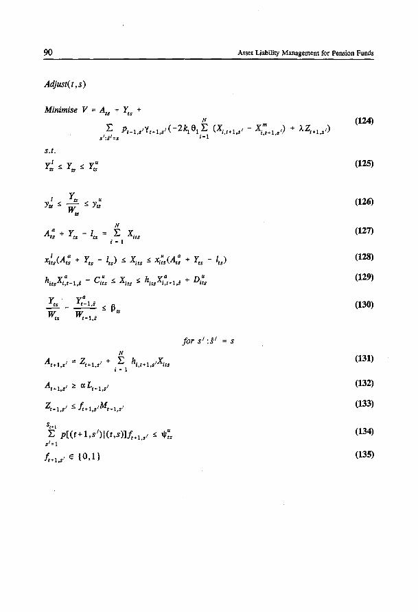
90
Adjust(t, s)
Minimise V = A1s + r;s +
st+l
N
:E xits i = I
:E p[(t+l,s1)1(t,s)]J;. 1,s' ~ lJr~s s1 =I
J;+l,s' E { 0,1}
Asset Liability Management for Pension Funds
(124)
(125)
(126)
(127)
(128)
(129)
(130)
for s' :s 1 = s
(131)
(132)
(133)
(134)
(135)
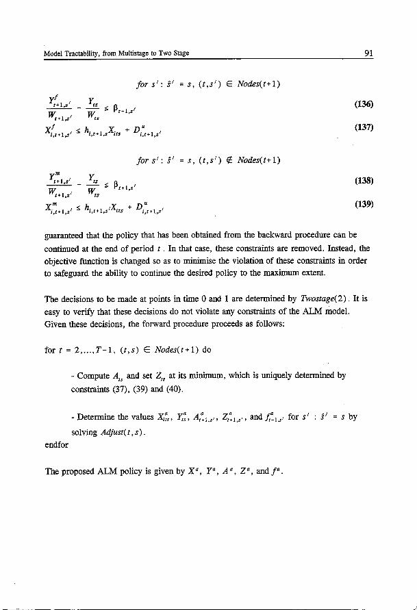
Model Tractability, from Multistage to Two Stage
Yts
W ::; J3t+l,s 1
ts
for s 1 : s' = S, (t,s') E Nodes(t+1)
for s': s' = s, (t,s') 9!: Nodes(t+1)
x.m I I ::; hi t+l s1xits + D.u I I l,t+ ,s ' ' l,t+ ,s
91
(136)
(137)
(138)
(139)
guaranteed that the policy that has been obtained from the backward procedure can be
continued at the end of period t . In that case, these constraints are removed. Instead, the
objective function is changed so as to minimise the violation of these constraints in order to safeguard the ability to continue the desired policy to the maximum extent.
The decisions to be made at points in time 0 and 1 are determined by Twostage( 2) . It is
easy to verify that these decisions do not violate any constraints of the ALM model.
Given these decisions, the forward procedure proceeds as follows:
for t = 2, ... , T -1, (t, s) E Nodes(t + 1) do
endfor
- Compute A1s and set z,s at its minimum, which is uniquely determined by
constraints (37), (39) and (40).
- Determine the values X;~., Y,~, A,~I.s', Zt~I.s', and fr~v for s' s' = s by
solving Adjust(t, s) .
The proposed ALM policy is given by x•, ya, A •, za, and jD.
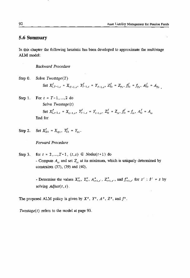
92 Asset Liability Management for Pension Funds
5.6 Summary
In this chapter the following heuristic has been developed to approximate the multistage
ALM model:
Bacbvard Procedure
Step 0. Solve Twostage(T)
Set X{r-l,s = xiT-l.s' yf-l.s YT-I.s' z?. = ZTs' !/. = Irs• A/. = ATs
Step 1. For t = T- 1 , ... , 2 do
Solve Twostage(t)
Set X{t-t,s = Xir-t,s• yf-t.s = Y,_t,s• zfs = z, •• Jfs = hs• A(. =A,.
End for
Forward Procedure
Step 3. for t = 2 , ... , T- 1 , (t, s) E Nodes(t + 1) do
- Compute A,. and set z,. at its minimum, which is uniquely determined by
constraints (37), (39) and (40).
-Determine the values X;~., Y;~. A,:v. z,:t.s'• andfr:t,s' for s1 : §' = s by
solving Adjust(t , s) .
The proposed ALM policy is given by xa, ya, A a, za, and j".
Twostage(t) refers to the model at page 93.
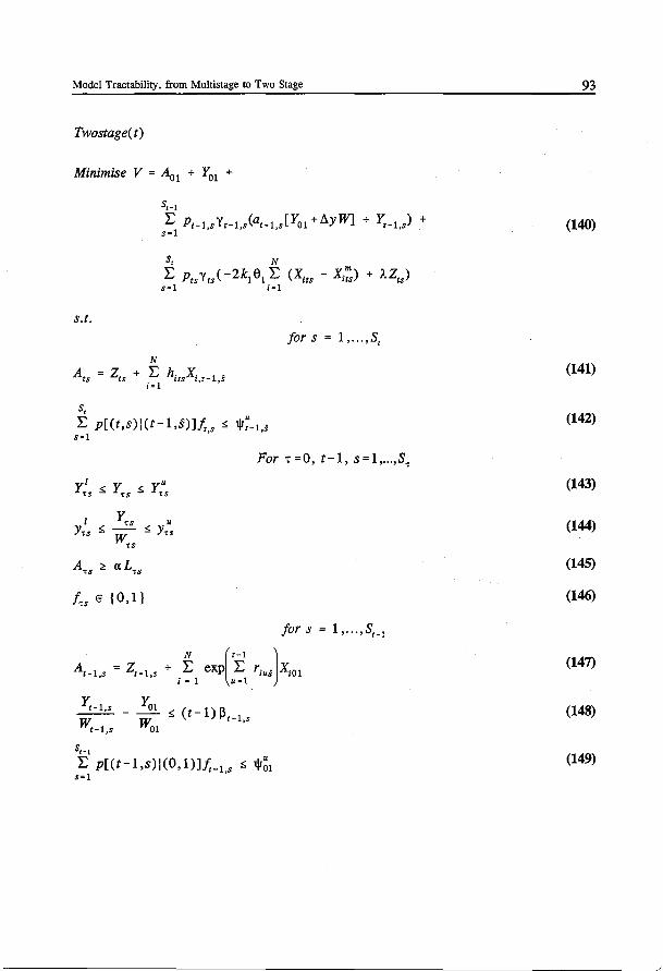
Model Tractability, from Multistage to Two Stage 93
Twostage(t)
Minimise V = A01 + Y01 +
(140)
S, N
E Prs Yr/ -2kl elL (Xits - X;~) + A.Zts) s=1 i=l
s.t. for s 1 , ... ,S1
N A = Z + E h. X.
1 • (141) ts ts rts r,t- ,s
i=l
s, E p[(t,s)l(t-1,s)]frs ~ W~- 1 •5 (142)
s= 1 '
For 1:=0, t-1, s=l, ... ,s,
fu E {0,1}
for s
At-i,s = zt-1,s + E exp(ti! rius)xw1 i = 1 u=l
Yt-1,s
~-!,s s,_. L p[(t-1,s)l(0,1)].t;_ 1,s ~ W~1
s=1
1 , ... ,St-1
(143)
(144)
(145)
(146)
(147)
(148)
(149)
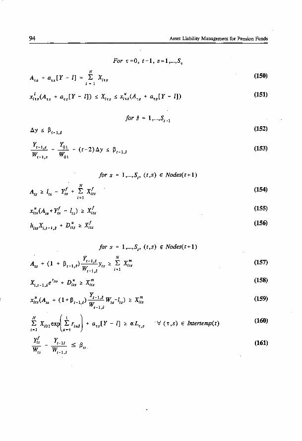
94 Asset Liability Management for Pension Funds
N
A,s + a,s[Y - l] = E Xiu i = I
For ,;=0, t-1, s=1, ... ,s,
(150)
(151)
for s 1 , ... ,SH
f1y ~ Pt-l,s (152)
Yt-l,s
~-l,s
for s 1, ... ,St, (t,s) E Nodes(t+1)
(153)
Xi~s(A18 + yfs - l,s) ::<: X(,s (155)
for s = 1, ... ,St, (t,s) $ Nodes(t+1)
X r,,. D" Xm i,t-l,.fe + its ~ its
u f I. X (A + ( 1 +A .) ~ W -1 ) X m
its ts 1-'t-l,s W ts ts :<: its t-t,s
r;_l! -- ::::; f3rs w;_l J
V (,; ,s) E Intertemp(t)
(157)
(158)
(159)
(160)
(161)
Chapter 6 Model Tractability, Variance Reduction
6.1 Introduction
The approach to the ALM problem that is proposed in this monograph can be characterised as a hybrid simulation and optimisation procedure: first, the development of the environment is being simulated, then, an optimisation procedure is employed in order to determine optimal decisions. The exogenous environment, the contingent decisions to be made and the dynamics by which the value of assets and liabilities carries over from one point in time to the next constitute a system that simulates the development of the pension fund under a variety of future circumstances, assuming that the optimal policy will be implemented.
The fundamental role of the concept of simulation in our approach is evident. There
seems to be no consensus in the literature on a unique and useful definition of simulation. In this thesis we shall use one of definitions given in Kleijnen (1971). He defmes simulation as "experimenting with an (abstract) model over time, this experimenting involving the sampling of values of stochastic variables from their distribution. Because
random numbers are used, this type of simulation is sometimes denoted as Monte Carlo simulation". The experiments are usually aimed at determining the value of one or more unknown variables. These variables are referred to as the response variables of the simulation system. Due to the stochasticity in the simulation process, the value of the
response variables is dependent on the sample of values of the stochastic variables that are involved. Thus, different samples may lead to different values of the response variables. As a conse.quence of the use of random sampling, the outcome of the simulation is random itself.
Let us assume that the simulation system has been designed in such a way that the values of response variables yield unbiased estimates of the true values, i.e., when the sample size goes to infinity, the estimated values of the response variables converge to the true
values of the response variables. The inaccuracy of the estimates can then be quantified by the variance of the estimator. One would thus be interested in unbiased estimates
with a minimal variance. The variance can be reduced by increasing the sample size, at the cost of the corresponding computational effort. One can also obtain more reliable estimates without increasing the sample size by the employment of variance reduction techniques. For an extensive treatment of the theory of simulation, the reader can be
referred to Naylor et al (1967), Kleijnen (1974,1975) and Bratley, Fox and Schrage (1987).
95
96 Asset Liability Management for Pension Funds
In the case of the ALM model, the size of the two stage models is determined by the
number of states of the world that is included. The fewer ~t~Jes of the world the smaller the computational effort to solve the models. Thus, the fewer the better. On the other hand, the number of states of the world should be sufficiently large to represent the underlying continuous probability distribution. In this chapter, a variance reduction technique, importance sampling, will be employed to reduce the number of states of the
world that is required to obtain a sufficiently accurate estimate of the optimal objective function value.
The next section presents a general exposition of the main idea behind importance sampling, the way in which it can be applied-to reduce the size of stochastic linear programmes and a characterisation of optimal importance sampling distributions.
6.2 Importance Sampling .•. !
6.2.1 The Potential Merits of Importance Sampling
The basic idea of importance sampling is to replace the original sampling process by another one. This distortion is corrected by weighing the observations from the new sampling process, so that the average of the weighted observations is an unbiased
estimator of the mean of the original process. When the new sampling process is designed well, a substantial reduction of the variance of the estimator can be achieved.
Let ~ be a discrete random variable with probability space Z = U 1 , ~2 , ••• , ~5,} and
density functionp(n, p(~8 ) = Ps for s = l, ... ,SP, p(~) = 0 elsewhere. Suppose that
one would like to estimate the mean of the random variable c( ~):
(162)
To obtain an estimate of EP [ c( ~)] , one can generate a random sample of size S from p
and calculate the sample mean of the observations:
(163)
l •. \
' :' ',l~··· ~ ,l_t_
Model Tractability, Variance Reduction
It is well known that cf is an unbiased estimator of EP[c(O], given a sample
~~· ~z····· ~s fromp.
97
Let q( 0 be a density function with q( 0 > 0 <=> p( 0 > 0 . Then, q( ~ ) can be written
as q(~.) = qs for s = 1, ... , SP, q(O = 0 elsewhere. We shall refer to q as an
importance sampling distribution. Given p and q,
L qs s s SP (p c( ~ ) )
s=! qs (164)
s It follows that liSE c(~s)p.fqs, themeanofsample c(~ 1)p1 /q1 , ••• ,c(~s)Psfqs from
s=l
probability density function q, is also an unbiased estimate of EP [ c( ~)] ..
To demonstrate the advantage of importance sampling, suppose that qs is chosen as
follows:
(165)
Let Csq denote the average of a sample of size S from density q. Then, the variance of
ci is given by (166).
I.e., even with a sample size of 1, the variance of the estimator has been reduced to zero.
Of course, if one is able to choose qs as specified in (165), the value of EP[c(O] would
already be known and one would not have to estimate it any more. Nevertheless, this
analysis provides insight in the potential merits of employing importance sampling. Notice
that the reduction of variance is independent of the sample size. Moreover, it is useful as
a characterisation of the optimal importance sampling distributions: the maximal variance
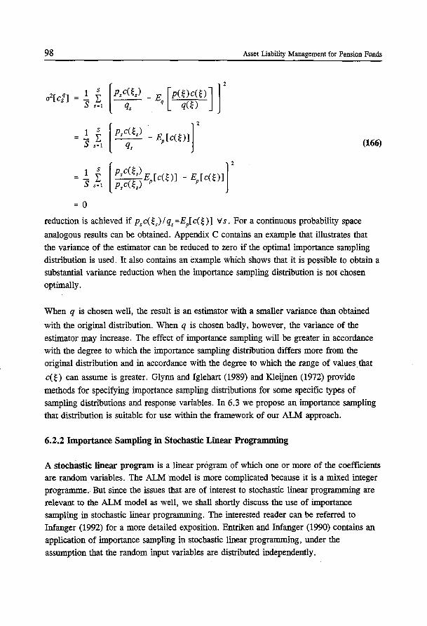
98
1 s a2[ci] = - ~
S s=l [ p.c(~,) _ E [p(nc(~) J ]2
q, q q(O
= }_ f [p,cq(,~,)- EP[c(~)]]2
S s=l
1 s =- ~
S s=l
= 0
Asset Liability Management for Pension Funds
(166)
reduction is achieved if p,c(~.) I q, =EP[c(~)] v s. For a continuous probability space
analogous results can be obtained. Appendix C contains an example that illustrates that the variance of the estimator can be reduced to zero if the optimal importance sampling distribution is used. It also contains an example which shows that it is possible to obtain a substantial variance reduction when the importance sampling distribution is not chosen optimally.
When q is chosen well, the result is an estimator with a smaller variance than obtained
with the original distribution. When q is chosen badly, however, the variance of the
estimator may increase. The effect of importance sampling will be greater in accordance with the degree to which the importance sampling distribution differs more from the original distribution and in accordance with the degree to which the range of values that
c(~) can assume is greater. Glynn and Iglehart (1989) and Kleijnen (1972) provide
methods for specifying importance sampling distributions for some specific types of sampling distributions and response variables. In 6.3 we propose an importance sampling that distribution is suitable for use within the framework of our ALM approach.
6.2.2 Importance Sampling in Stochastic Linear Programming
A stochastic linear program is a linear program of which one or more of the coefficients are random variables. The ALM model is more complicated because it is a mixed integer programme .. But since the issues that are of interest to stochastic linear programming are relevant to the ALM model as well, we shall shortly discuss the use of importance sampling in stochastic linear programming. The interested reader can be referred to Infanger (1992) for a more detailed exposition. Entriken and Infanger (1990) contains an application of importance sampling in stochastic linear programming, under the
assumption that the random input variables are distributed independently.
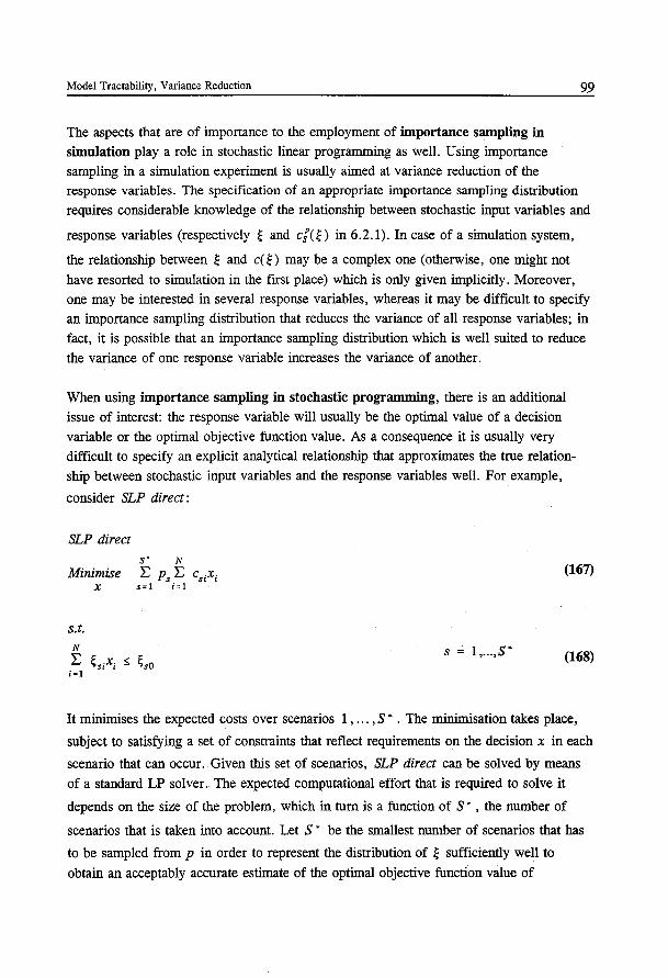
Model Tractability, Variance Reduction 99
The aspects that are of importance to the employment of importance sampling in
simulation play a role in stochastic linear programming as well. Using importance
sampling in a simulation experiment is usually aimed at variance reduction of the
response variables. The specification of an appropriate importance sampling distribution
requires considerable knowledge of the relationship between stochastic input variables and
response variables (respectively ~ and cf(~) in 6.2.1). In case of a simulation system,
the relationship between ~ and c(O may be a complex one (otherwise, one might not
have resorted to simulation in the first place) which is only given implicitly. Moreover,
one may be interested in several response variables, whereas it may be difficult to specify
an importance sampling distribution that reduces the variance of all response variables; in
fact, it is possible that an importance sampling distribution which is well suited to reduce
the variance of one response variable increases the variance of another.
When using importance sampling in stochastic programming, there is an additional
issue of interest: the response variable will usually be the optimal value of a decision
variable or the optimal objective function value. As a consequence it is usually very
difficult to specify an explicit analytical relationship that approximates the true relation
ship between stochastic input variables and the response variables well. For example,
consider SLP direct :
SLP direct
s· N
Minimise E Ps E csixi X s=l i=l
s.t. N
E ~sixi => ~.o i=l
(167)
s = 1 , ... ,s• (168)
It minimises the expected costs over scenarios 1 , ... , S • . The minimisation takes place,
subject to satisfying a set of constraints that reflect requirements on the decision x in each
scenario that can occur. Given this set of scenarios, SLP direct can be solved by means
of a standard LP solver. The expected computational effort that is required to solve it
depends on the size of the problem, which in tum is a function of S • , the number of
scenarios that is taken into account. Let S • be the smallest number of scenarios that has
to be sampled from p in order to represent the distribution of ~ sufficiently well to
obtain an acceptably accurate estimate of the optimal objective function value of
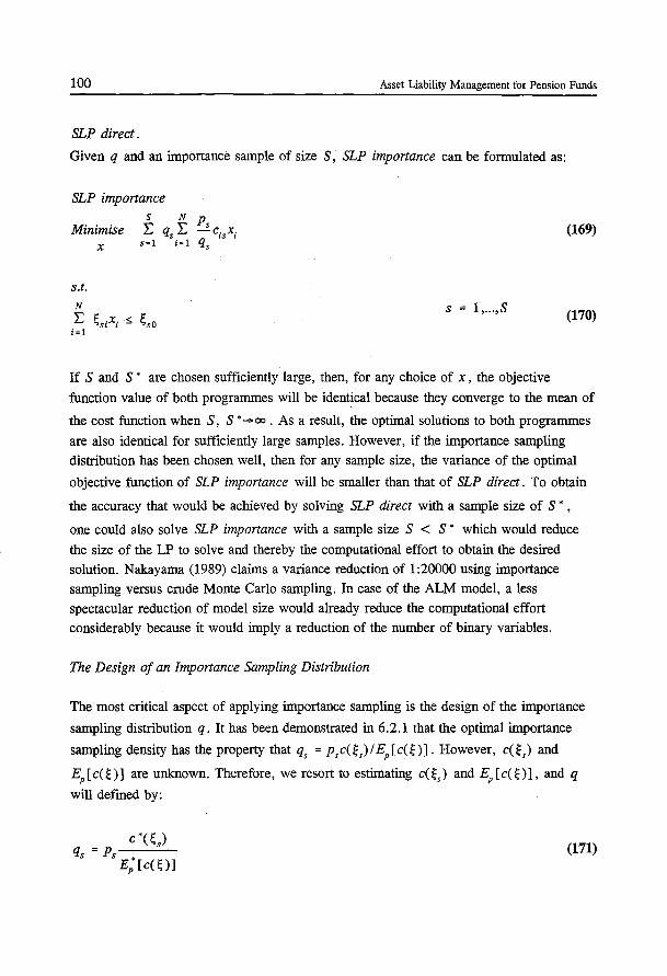
100 Asset Liability Management for Pension Funds
SLP direct.
Given q and an importance sample of size S, SLP importance can be formulated as:
SLP importance s N Ps
Minimise E qs L -c. x. X s=l i = 1 qS IS I
(169)
s.t. N
E ~.ixi ~ ~.a s = 1, ... ,s (170)
i=l
If S and S • are chosen sufficiently large, then, for any choice of x , the objective
function value of both programmes will be ident~cal because they converge to the mean of
the cost function when S, S • ..... oo . As a result, the optimal solutions to both programmes
are also identical for sufficiently large samples. However, if the importance sampling distribution has been chosen well, then for any sample size, the variance of the optimal
objective function of SLP importance will be smaller than that of SLP direct. To obtain
the accuracy that would be achieved by solving SLP direct with a sample size of S • ,
one could also solve SLP importance with a sample size S < S • which would reduce
the size of the LP to solve and thereby the computational effort to obtain the desired solution. Nakayama (1989) claims a variance reduction of 1:20000 using importance sampling versus crude Monte Carlo sampling. In case of the ALM model, a less
spectacular reduction of model size would already reduce the computational effort considerably because it would imply a reduction of the number of binary variables.
The Design of an Importance Sampling Distribution
The most critical aspect of applying importance sampling is the design of the importance
sampling distribution q. It has been demonstrated in 6.2.1 that the optimal importance
sampling density has the property that q s = p s c( O I EP [ c( 0] . However, c( ~ s) and
EP[c(~)] are unknown. Therefore, we resort to estimating c(~.) and EP[c(O], and q
will defmed by:
(171)
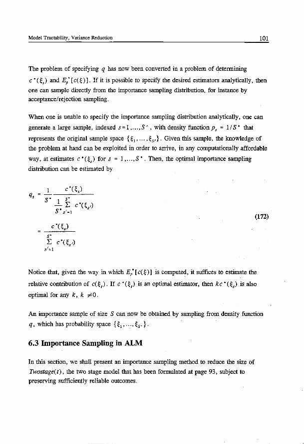
Model Tractability, Variance Reduction 101
The problem of specifying q has now been converted in a problem of determining
c • ( U and EP* [ c( n]. If it is possible to specify the desired estimators analytically, then
one can sample directly from the importance sampling distribution, for instance by acceptance/rejection sampling.
When one is unable to specify the importance sampling distribution analytically, one can
generate a large sample, indexed s = 1 , ... , S • , with density function p. = 1 IS • that
represents the original sample space { ~1' ... , ~s,}. Given this sample, the knowledge of
the problem at hand can be exploited in order to arrive, in any computationally affordable
way, at estimates c • ( ~.) for s = 1 , ... , S • . Then, the optimal importance sampling
distribution can be estimated by
1 c *( ~.) q, = -s-· --s-· __:::....__., _
_!_ E c •( ~.,) S • s 1=!
(172)
Notice that, given the way in which EP*[c(~)] is computed, it suffices to estiinate the
relative contribution of c( ~.) . If c • ( ~.) is an optimal estimator, then k c • ( t) is also
optimal for any k, k ¢ 0 .
An importance sample of size S can now be obtained by sampling from density function
q, which has probability space { ~1' ... , ~s·}.
6.3 Importance Sampling in ALM
In this section, we shall present an importance sampling method to reduce the size of
Twostage(t), the two stage model that has been formulated at page 93, subject to
preserving sufficiently reliable outcomes.
102 Asset Liability Management for Pension Funds
Response Variables and Stochastic Input in Twostage(t)
In 6. 2.1, ~ denoted the stochastic input variables and c( 0 denoted the derivative random
variable of which the mean was to be estimated. In relation to Twostage(t), ~ is
associated with the randomly sampled states of the world (recall that they are exogenous
to the model) at time t . More precisely, t contains the realisations rus, Lrs and l1s.
Suppose that a sufficiently large sample of states of the world, sampled from (46), is
given. Let this sample contain S • states of the world at time t . Given the sampling
procedure, the probability of state (t ,s) to occur is 1/ S •. Here, it is the intention to
design conditional importance sampling distributions q[ (t, s) l (t -1, s)] which specify the
importance sampling probability of (t, s) being the state that succeeds (t -1, s).
Fonnulating Twostage(t) when Applying Importance Sampling
The states of the world at time t will be sampled from an importance sampling distribu
tion q[ (t, s) I (t -1, s)]. The design of q[ (t, s) I (t -1, s)] is the subject of the next
paragraph. First, let us examine the procedure to formulate Twostage(t), including a
provision to apply importance sampling. The way in which an appropriate importance sampling distribution can be obtained will be discusses later. A stepwise description is given at page 103.
Model Tractability, Variance Reduction 103
Formulating Twostage(t) when Applying Importance Sampling, a Stepwise Description
Given states of the world (0, 1) and (t -1, s) for s = 1 , ... , St-1:
For s=1, ... ,SI-1 do
- Sample n1 \.~ states of the world, indexed ( t, 1), ... , (t, n1 \ 8), from ( 46), each
of which succeeds (t -1, s) with probability 11 n1:u.
- For s = 1 , ... , n1: u estimate ms, the relative contribution of state ( t, s) to the
optimal objective function. The way in which these estimates can be obtained will
be discussed of 104.
n,: .. ~ -For s=1, ... ,n1:u define q[(t,s) I (t-1,s)] = m.f L ms,.
s' =1
- Sample n1_1.s states of the world from the conditional importance sampling
den~ity q[ (t, s) I (t -1, s)]. The unconditional importance sampling probability of
(t, s) to occur equals q1s = p1_ 1•8q[(t, s) I (t -1, s)]
Formulate and solve the importance sampling variant on Twostage(t) that is presented
below.
Adjusting the Formulation of Twostage(t) to Accommodate Importance Sampling
In order to obtain unbiased results with respect to the probability distribution of states of the world that has been defined by (46), the computation of probabilities and expectations
in Twostage(t) has to be adjusted: they should be equipped with correction factors pts/ q1s
to account for the fact the sample of states of the world at time t has been drawn from
the importance sampling distribution instead of from the distribution that is defmed by
(46). It follows that the objective function should be changed into (173) and (142) has to
be replaced by (174).
104 Asset Liability Management for Pension Funds
Minimise V = A0 + Y01 +
s,_l
L Pt-l,s Y t-1,/at-l,s[Yol + ily W] + Yt-I) + s=l
s, E p[(t,s)l(t-1,s)] /, ~ *~-l,s
s=l q[(t,s)l(t-1,.§)] t,s
The Specification of an Importance Sampling Distribution
(173)
(174)
Given a set of states of the world (t, 1 ) , ... , (t, nt: 1.s) that succeed state (t - 1 , s) with
probability p,, the aim is now to define a probability density function q on the probabil
ity space that consists of the aforementioned states of the world. More precisely, a
Twostage(t)-specific version of (172) has to be specified.
In line with the argument the that led to (172), the importance sampling probability of
(t, s) will be based on an estimate of its contribution to the optimal objective function
value of the ALM model, relative to the contribution of other states that succeed
(t-1,&):
q[(t,s) 1 (t-1,&)] (175)
where m, equals the estimated relative contribution to the objective function.
To assess the contribution of state (t, s) to the expected costs of period t , relative to the
contribution of other states at the world that succeed (t -1, s), a mean variance efficient
estimate of the optimal asset mix in (t -1, s) is obtained from MinAssets(t -1, s)
(specified at page 85). Given X;~-I.I, the value of the investments at the beginning of
N
period t will be increased by a factor exp[r(At-1 Jrs] = ~ hit,x;~-I.s at the end of • i=l
period t , if state of the world (t , s) occurs. In order to arrive at (t , s) with an asset
portfolio of which the value is equal to the value of the remaining liabilities, the value at
Model Tractability, Variance Reduction 105
the beginning of period t should be equal to exp[ -r(At-!)18
] 01.L18
• Thus, it determines
the minimum asset level to start with in order to meet the funding requirement at ( t, s) .
Based on this choice of asset mix, the weighting factor to specify the importance sampling
probability of state (t , s) is computed by:
(176)
I.e., m, is the minimal asset value that is required to be invested in (t -1 , s) in order to
satisfy the solvency requirement in (t, s) given that the assets have been invested in the
mean variance optimal portfolio according to MinAssets( t -1 , s) . It is conceivable,
however, that the optimal policy requires funding levels that exceed 01.L18
• As long as
these funding levels can be attained by increasing the initial asset level and maintaining
the asset mix that has been selected by MinAssets( t - 1 , s) , q [ (t, s) i (t - 1 , s)] remains a
good importance sampling density, because it is only affected by changes in the relative
contributions to the costs, not by changes of the level of expected costs.
Given m, , q[(t, s) i (t - 1 , s)] is computed by normalizing q[(t, s) i (t - 1 , s)] so that the
summation of q[ ( t, s) i (t- 1 , s)] over all possible states of the world adds up to 1.
Notice that ms has been constructed so that, given positive liabilities, ms > 0 v s which
implies that qs, as specified above, is indeed a density function.
The computational results in 6.4 provide insight in the relationship between variance of
the response variables, the sample size when sampled from the original distribution and the sample size when using importance sampling with the choice of importance sampling
distribution that has been described above.
6.4 Computational Results
In order to obtain insight in the practical use of importance sampling, TEST _IS, a one
period chance constrained programming model, has been solved by three methods:
-by quadratic programming, - by scenario optimisation, based on scenarios that have been obtained from random
sampling from the underlying distribution,
- by scenario optimisation, based on scenarios that have been obtained from importance
sampling, using the importance sampling distribution that has been described earlier.
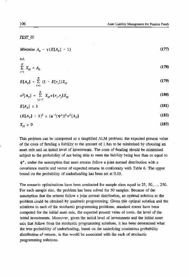
106
TEST IS
Minimise A0 - y (E[AT] - 1)
s.t. N
EX;0 =A0 i=l
N
:E (1 + E[r;DXw i•l
N
o2[Arl = :E X;0 o [ri'rj]Xjo i,j=l
E[AT] ~ 1
(E[AT] - 1)2 ~ (q>-l(ljr")?o2[AT]
Asset Liability Management for Pension Funds
(177)
(178)
(179)
(180)
(181)
(182)
(183)
This problem can be interpreted as a simplified ALM problem: the expected present value
of the costs of funding a liability to the amount of 1 has to be minimised by choosing an
asset mix and an initial level of investments. The costs of funding should be minimised
subject to the probability of not being able to meet the liability being less than or equal to
ljr", under the assumption that asset returns follow a joint normal distribution with a
covariance matrix and vector of expected returns in conformity with Table 6. The upper
bound on the probability of underfunding has been set at 0.05.
The scenario optimisations have been conducted for sample sizes equal to 25, 50, ... , 250.
For each sample size, the problem has been solved for 50 samples. Because of the assumption that the returns follow a joint normal distribution, an optimal solution to the
problem could be obtained by quadratic programming. Given this optimal solution and the
solutions to each of the stochastic programming problems, standard errors have been computed for the initial asset mix, the expected present value of costs, the level of the
initial investments. Moreover, given the initial level of investments and the initial asset mix that follow from the stochastic programming solutions, it has been determined what
the true probability of underfunding, based on the underlying continuous probability
distribution of returns, is that would be associated with the each of stochastic
programming solutions.
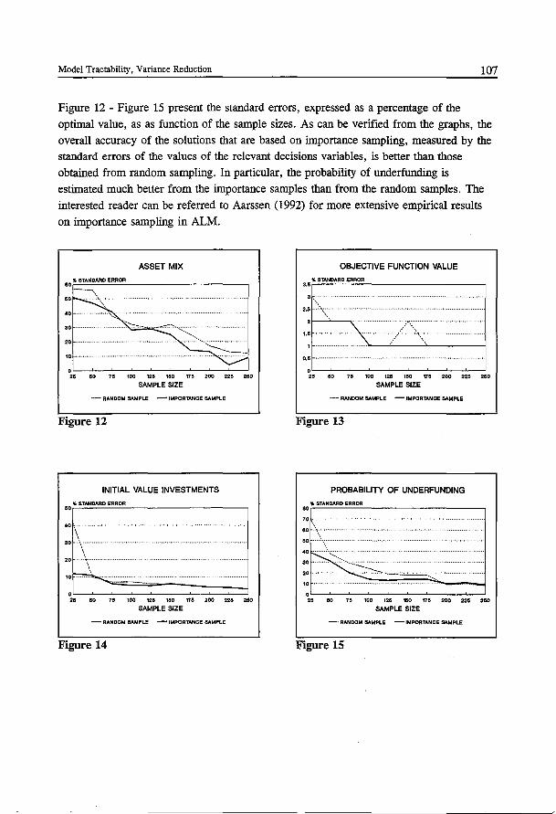
Model Tractability, Variance Reduction 107
Figure 12 - Figure 15 present the standard errors, expressed as a percentage of the
optimal value, as as function of the sample sizes. As can be verified from the graphs, the
overall accuracy of the solutions that are based on importance sampling, measured by the
standard errors of the values of the relevant decisions variables, is better than those
obtained from random sampling. In particular, the probability of underfunding is
estimated much better from the importance samples than from the random samples. The
interested reader can be referred to Aarssen (1992) for more extensive empirical results
on importance sampling in ALM.
ASSET MIX
~ n m m ~ m - = = SAMPLE SIZE
- RANDOM SAMPLE - IMPORTANCE SAMPLE
Figure 12
INITIAL VALUE INVESTMENTS
•or~~~~·N~D~AR=D~E~RR=O~R---------------------,
0~~--~--~--~~--~--~--~~ u ~ n m m ~ m - = ~
SAMPLE SIZE
~~- RANDOM SAMPLE - IMPORTANCE SAMPLE
Figure 14
OBJECTIVE FUNCTION VALUE
0.5
0~~--~--~--~~--~--~~~~
u ~ n m m ~ m - = = SAMPLE SIZE
-RANDOM SAMPLE -IMPORTANCE SAMPLE
Figure 13
PROBABILITY OF UNDERFUNDING
20
10
0~~--~--~--~~--~--~--~~
u ~ n m m ~ m - = = SAMPLE SIZE
-· RANDOM SAMPLE - IMPORTANCE SAMPLE
Figure 15

7.1 Introduction
Chapter 7 Computational Results
This chapter presents results of computational experiments with the ALM model. In order to obtain insight in the behaviour of the model on realistic problem instances, it has been applied to the data of a Dutch pension fund with an actuarial reserve in excess of 16
billion Dfl. and approximately 1,020,000 participants of which 240,000 premium payers.
Computational results on a matter as complex as dynamic ALM may give rise to many questions from different viewpoints. In particular, it offers a host of possibilities for sensitivity analyses: with respect to decision parameters, with respect to economic scenarios, with respect to the historical period and with respect to the estimation technique that has been used to obtain coefficients for the scenario generator, with respect to the characteristics of the participants of the pension fund, with respect to the financial
starting position of the pension fund, with respect to the asset categories that have been selected to invest in, with respect to the optimisation parameters, with respect to the horizon, with respect to further future lagging of the state pensions, with respect to the employment of derivatives etc. It is beyond the scope of this monograph to pay attention to all the questions that could be raised from the above viewpoints, however interesting many of them may be. At this stage, the focus will be on experiments that give insight in the behaviour of the ALM model, in comparison to some of the leading models that are currently being used. Moreover, results will be presented to show to what extent solutions are sensitive to small changes in the most relevant exogenous parameter values.
The selection of computational experiments has been made in such a way that the results provide insight in the following questions:
1. How do the results of our ALM approach compare to the results that follow from
making optimal static decisions ?
2. To what extent are the solutions to the ALM model driven by its multistage character?
In other words, how does the backward procedure affect the outcomes?
3. How sensitive is the solution to small changes in the most relevant exogenous parameter values ?
The next section discusses the environment within which ALM policies will be determi-
109
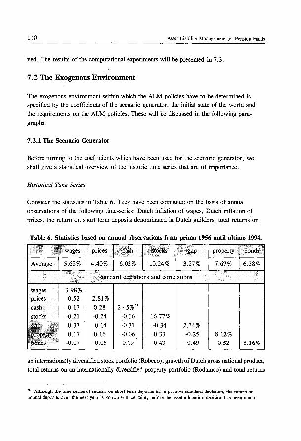
110 Asset Liability Management for Pension Funds
ned. The results of the computational experiments will be presented in 7.3.
7.2 The Exogenous Environment
The exogenous environment within which the ALM policies have to be determined is
specified by the coefficients of the scenario generator, the initial state of the world and
the requirements on the ALM policies. These will be discussed in the following para
graphs.
7.2.1 The Scenario Generator
Before turning to the coefficients which have been used for the scenario generator, we
shall give a statistical overview of the historic time series that are of importance.
Historical Time Series
Consider the statistics in Table 6. They have been computed on the basis of annual
observations of the following time-series: Dutch inflation of wages, Dutch inflation of
prices, the return on short term deposits denominated in Dutch guilders, total returns on
Table 6. Statistics based on annual observations from primo 1956 until ultimo 1994 . ..
. ···••· . wages •... prices .· cash .. . stocks gnp
· Av¢rage 5.68% . ·.··.·
wages
p~j¢~S >cash · i
s~otks· · .. •····
·····~················.·.•• pr()p~rty ·· ..
Borids .. ···•·•
3.98%
0.52
-0.17
-0.21
0.33
0.17
-0.07
4.40% 6.02% 10.24% 3.27%
standard·. deviations an:d correlations
2.81%
0.28 2.45%26
-0.24 -0.16 16.77%
0.14 -0.31 -0.34 2.34%
0.16 -0.06 0.33 -0.25
-0.05 0.19 0.43 -0.49
property .. · bonds
7.67% 6.38%
•· ..
8.12%
0.52 8.16%
an internationally diversified stock portfolio (Robeco), growth of Dutch gross national product,
total returns on an internationally diversified property portfolio (Rodamco) and total returns
26 Although the time series of returns on short term deposits has a positive standard deviation, the return on armual deposits over the next year is known with certainty ,before the asset allocation decision has been made.
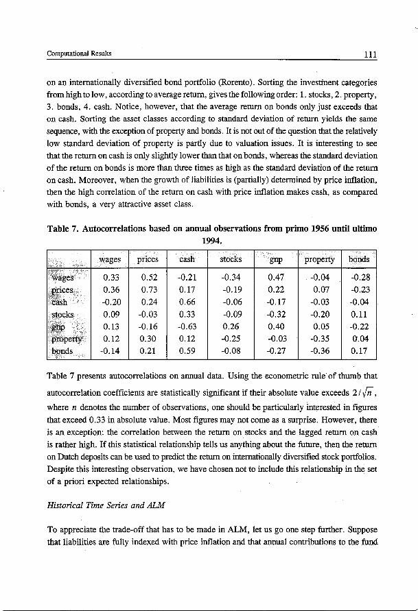
Computational Results 111
on an internationally diversified bond portfolio (Rorento). Sorting the investinent categories
from high to low, according to average return, gives the following order: 1. stocks, 2. property, 3. bonds, 4. cash. Notice, however, that the average return on bonds only just exceeds that on cash. Sorting the asset classes according to standard deviation of return yields the same
sequence, with the exception of property and bonds. It is not out of the question that the relatively
low standard deviation of property is partly due to valuation issues. It is interesting to see
that the return on cash is only slightly lower than that on bonds, whereas the standard deviation
of the return on bonds is more than three times as high as the standard deviation of the return on cash. Moreover, when the growth of liabilities is (partially) determined by price inflation, then the high correlation of the return on cash with price inflation makes cash, as compared
with bonds, a very attractive asset class.
Table 7. Autocorrelations based on annual observations from primo 1956 until ultimo 1994.
.. .wages prices cash stocks gnp property bonds
wages 0.33 0.52 -0.21 -0.34 0.47 -0.04 -0.28
prices 0.36 0.73 0.17 -0.19 0.22 0.07 -0.23. ··cash -0.20 0.24 0.66 -0.06 -0.17 -0.03 -0.04
stocks 0.09 -0.03 0.33 -0.09 -0.32 -0.20 0.11
gnp 0.13 -0.16 -0.63 0.26 0.40 0.05 -0.22
· p:r:operty 0.12 0.30 0.12 -0.25 -0.03 -0.35 0.04
bonds -0.14 0.21 0.59 -0.08 -0.27 -0.36 0.17
Table 7 presents autocorrelations on annual data. Using the econometric ruleofthumb that
autocorrelation coefficients are statistically significant if their absolute value exceeds 2 I [n, where n denotes the number of observations, one should be particularly interested in figures
that exceed 0.33 in absolute value. Most figures may not come as a su:r:prise. However, there
is an exception: the correlation between the return on stocks and the lagged return on cash
is rather high. If this statistical relationship tells us anything about the future, then the return
on Dutch deposits can be used to predict the return on internationally diversified stock portfolios.
Despite this interesting observation, we have chosen not to include this relationship in the set
of a priori expected relationships.
Historical Time Series and ALM
To appreciate the trade-off that has to be made in ALM, let us go one step further. Suppose
that liabilities are fully indexed with price inflation and that annual contributions to the fund
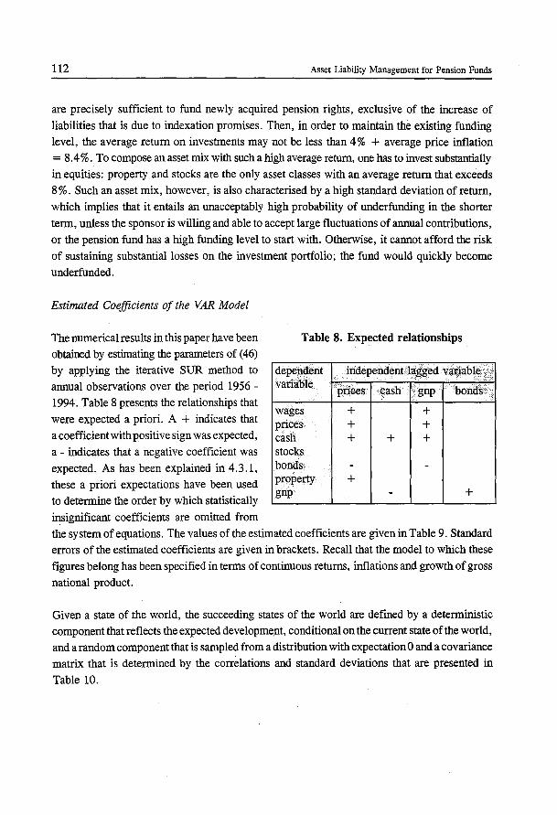
112 Asset Liability Management for Pension Funds
are precisely sufficient to fund newly acquired pension rights, exclusive of the increase of
liabilities that is due to indexation promises. Then, in order to maintain the existing funding
level, the average return on investments may not be less than 4% + average price inflation
= 8.4%. To compose an asset mix with such a high average return, one has to invest substantially
in equities: property and stocks are the only asset classes with an average return that exceeds
8%. Such an asset mix, however, is also characterised by a high standard deviation of return,
which implies that it entails an unacceptably high probability of underfunding in the shorter
term, unless the sponsor is willing and able to accept large fluctuations of annual contributions,
or the pension fund has a high funding level to start with. Otherwise, it cannot afford the risk
of sustaining substantial losses on the investment portfolio; the fund would quickly become
underfunded.
Estimated Coefficients of the VAR Model
The numerical results in this paper have been
obtained by estimating the parameters of ( 46)
by applying the iterative SUR method to
annual observations over the period 1956-
1994. Table 8 presents the relationships that
were expected a priori. A + indicates that
a coefficient with positive sign was expected,
a - indicates that a negative coefficient was
expected. As has been explained in 4.3.1,
these a priori expectations have been used
to determine the order by which statistically
insignificant coefficients are omitted from
Table 8. Expected relationships
dependent independentlagged variable variable
prices cash boilds gnp
wages + + prices + + cash + + + stocks bonds - -property + gnp - +
the system of equations. The values of the estimated coefficients are given in Table 9. Standard
errors of the estimated coefficients are given in brackets. Recall that the model to which these
figures belong has been specified in terms of continuous returns, inflations and growth of gross
national product.
Given a state of the world, the succeeding states of the world are defmed by a deterministic
component that reflects the expected developme_nt, conditional on the current state of the world,
and a random component that is sampled from a distribution with expectation 0 and a covariance
matrix that is determined by the correlations and standard deviations that are presented in
Table 10.
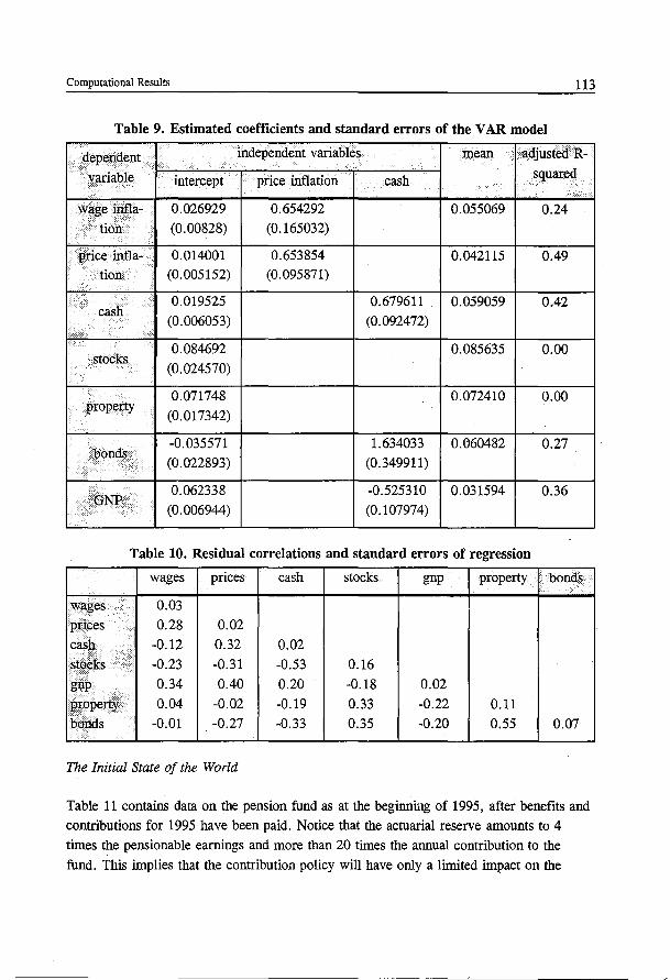
Computational Results 113
Table 9. Estimated coefficients and standard errors of the V AR model .··
dependent independent variables ····mean adjustedR-
variable intercept price inflation cash squared ..
. wage irifla~ 0.026929 0.654292 0.055069 0.24 tion (0.00828) (0.165032)
price infla- 0.014001 0.653854 0.042115 0.49 tion (0.005152) (0.095871)
cash· 0.019525 0.679611 0.059059 0.42
(0.006053) (0.092472)
··. 0.084692 0.085635 0.00 ··stocks
(0.024570)
0.071748 0.072410 0.00 property
(0.017342)
bonds -0.035571 1.634033 0.060482 0.27 (0.022893) (0.349911)
..•
0.062338 -0.525310 0.031594 0.36 ··GNP
(0.006944) (0.107974)
Table 10. Residual correlations and standard errors of regression
wages prices cash stocks gnp property bonds
wages 0.03 prices
.·.····
0.28 0.02 cash. -0.12 0.32 0.02 stocks
.•• -0.23 -0.31 -0.53 0.16 .· ..
gt;lp 0.34 0.40 0.20 -0.18 0.02
property 0.04 -0.02 -0.19 0.33 -0.22 0.11 bonds -0.01 -0.27 -0.33 0.35 -0.20 0.55 0.07
The Initial State of the World
Table 11 contains data on the pension fund as at the beginning of 1995, after benefits and contributions for 1995 have been paid. Notice that the actuarial reserve amounts to 4 times the pensionable earnings and more than 20 times the annual contribution to the
' '
fund. This implies that the contribution policy will have only a limited impact on the
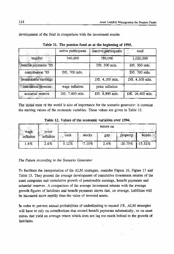
114 Asset Liability Management for Pension Funds
development of the fund in comparison with the investment results.
Table 11. The pension fund as at the beginning of 1995.
active participants inactive participants total
number 240,000 780,000 1,020,000
benefit payments '9.S Dfl. 300 mln. Dfl. 300 mln.
contribution '95 Dfl. 700 mln. Dfl. 700 mln.
pepsionable earriings Dfl. 4,100 mln . Dfl. 4,100 mln. ....
indexation promise . .... . ... · .... ·· wage inflation price inflation
I actuatilll tese!Ve Dfl. 7,600 mln. Dfl. 8,800 mln. Dfl. 16,400 mln.
The initial state of the world is also of importance for the scenario generator: it contains the starting values of the economic variables. These values are given in Table 12.
Table 12. Values of the economic variables over 1994.
return on
wage price
inflation inflation cash stocks gnp property bonds I
1.6% 2.6% 5.12% -7.10% 2.4% -20.75% -15.52%
The Future According to the Scenario Generator
To facilitate the interpretation of the ALM strategies, consider Figure 16, Figure 17 and
Table 13. They present the average development of cumulative investment returns of the
asset categories and cumulative growth of pensionable earnings, benefit payments and
actuarial reserves. A comparison of the average investment returns with the average
growth figures of liabilities and benefit payments shows that, on average, liabilities will
be increased more rapidly than the value of invested assets.
In order to prevent annual probabilities of underfunding to exceed 5%, ALM strategies
will have to rely on contributions that exceed benefit payments substantially, or on asset
mixes that yield an average return which does not lag too much behind to the growth of
liabilities.
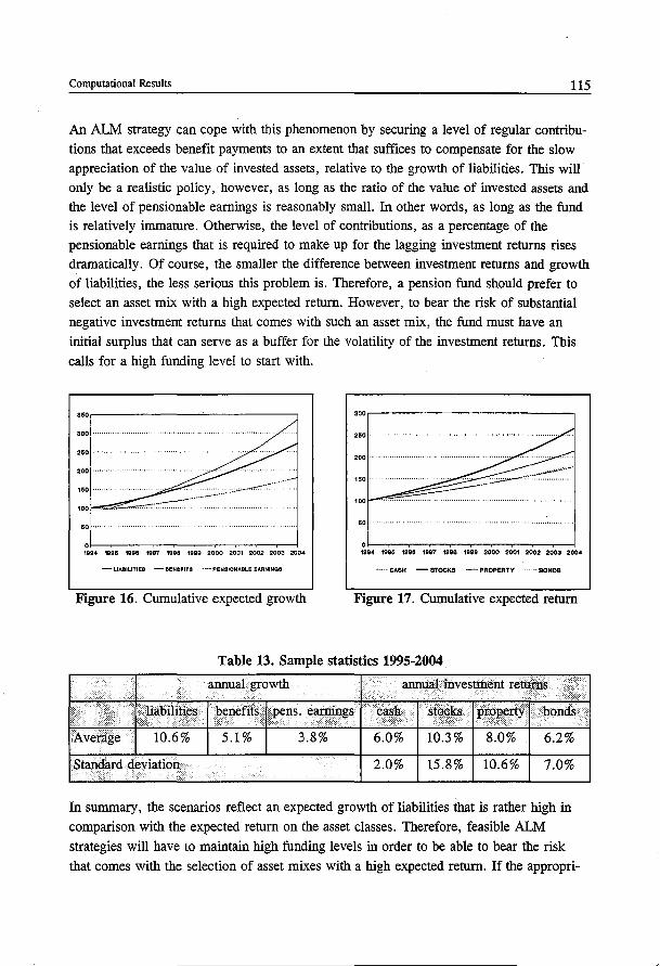
Computational Results 115
An ALM strategy can cope with this phenomenon by securing a level of regular contribu
tions that exceeds benefit payments to an extent that suffices to compensate for the slow
appreciation of the value of invested assets, relative to the growth of liabilities. This will only be a realistic policy, however, as long as the ratio of the value of invested assets and the level of pensionable earnings is reasonably small. In other words, as long as the fund is relatively immature. Otherwise, the level of contributions, as a percentage of the pensionable earnings that is required to make up for the lagging investment returns rises
dramatically. Of course, the smaller the difference between investment returns and growth
of liabilities, the less serious this problem is. Therefore, a pension fund should prefer to
select an asset mix with a high expected return. However, to bear the risk of substantial negative investment returns that comes with such an asset mix, the fund must have an
initial surplus that can serve as a buffer for the volatility of the investment returns. This
calls for a high funding level to start with.
60 ....... .
·~~-T--~~~--~~~--~~ 1884 18915 1&01S 1997 1998 UIQQ 2000 2001 2002 2003 2004
-LIABILITIES - BI!N!"T!I ····-PENSIONABLE EAANING8
soor------------------------,
250 ........................................................ .
200 ....
60 .....
·~~-T--~~~--~~~--~~ 10Q4 18SI6 1Q!iiiS 1087 1CIQB 1098 2000 2001 2002 2003 2004
----- CASH - STOCKS - PROPERTY · · · · ·· BONDS
Figure 16. Cumulative expected growth Figure 17. Cumulative expected return
Table 13. Sample statistics 1995-2004
an.Ilual.growth ~~.~ ~ ...
'i •... · ... ·. ··.• Ual).Hities benefits .. pens. earnings
1\cyb~a.ge. . 10.6% 5.1% 3.8%
st~iid.atd c1evhition. . . ...... · .... . ...•..
...
.. · ...
annual iilvestment :returns
cash
6.0%
2.0%
stocks
······ 10.3%
. . . )
prope,qy •· bonds ...• 8.0% 6.2%
15.8% 10.6% 7.0%
In summary, the scenarios reflect an expected growth of liabilities that is rather high in
comparison with the expected return on the asset classes. Therefore, feasible ALM
strategies will have to maintain high funding levels in order to be able to bear the risk
that comes with the selection of asset mixes with a high expected return. If the appropri-
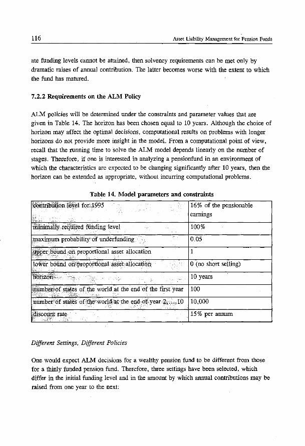
116 Asset Liability Management for Pension Funds
ate funding levels cannot be attained, then solvency requirements can be met only by
dramatic raises of annual contribution. The latter becomes worse with the extent to which the fund has matured.
7.2.2 Requirements on the ALM Policy
ALM policies will be determined under the constraints and parameter values that are given in Table 14. The horizon has been chosen equal to 10 years. Although the choice of
horizon may affect the optimal decisions, computational results on problems with longer
horizons do not provide more insight in the model. From a computational point of view,
recall that the running time to solve the ALM model depends linearly on the number of
stages. Therefore, if one is interested in analyzing a pensionfund in an environment of
which the characteristics are expected to be changing significantly after 10 years, then the
horizon can be extended as appropriate, without incurring computational problems.
Table 14. Model parameters and constraints
contribution level for 1995 16% of the pensionable
earnings
milriinally required. funding level 100%
maximum probability of underfunding 0.05
upper bound on proportional asset allocation 1 ···.
lower bound on proportional asset· allocation 0 (no short selling)
horizon 10 years .· number of states of the world at the end of the . first year 100
nur;riber ofstates ofthe world at the end of year 2, ... ,1 0 10,000
discciurit rate .. · 15% per annum
Different Settings, Different Policies
One would expect ALM decisions for a wealthy pension fund to be different from. those for a thinly funded pension fund. Therefore, three settings have been selected, which
differ in the initial funding level and in the amount by which annual contributions may be
raised from one year to the next:
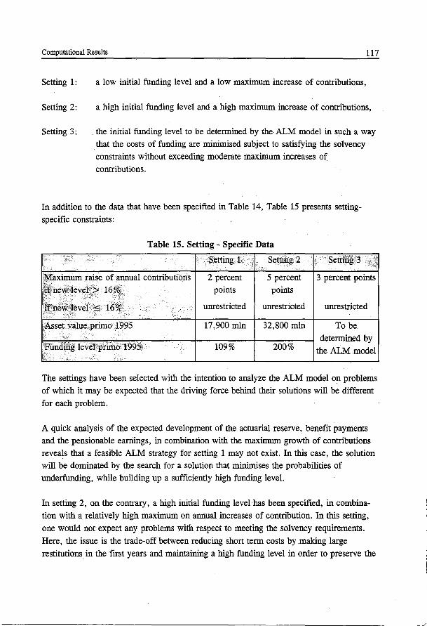
Computational Results 117
Setting 1: a low initial funding level and a low maximum increase of contributions,
Setting 2: a high initial funding level and a high maximum increase of contributions,
Setting 3: the initial funding level to be determined by the ALM model in such a way
that the costs of funding are minimised subject to satisfying the solvency
constraints without exceeding moderate maximum increases of
contributions.
In addition to the data that have been specified in Table 14, Table 15 presents setting
specific constraints:
Table 15. Setting - Specific Data
:M'aX.imulll.raise ofannual contributions ifnewlevei··> 16%
ifnew level ::;:: .. 16% . ···.• .. :
Asset value primo 1995
Fun~~I1g tevetpriino 1995 . :: ··,
1 Setting!
2 percent points
unrestricted
17,900 mln
109%
Setting·2
5 percent points
unrestricted
32,800 min
200%
Setting . 3 ··••···. >.··•·
3 percent points
unrestricted
To be.
determined by
the ALM model
The settings have been selected with the intention to analyze the ALM model on problems
of which it may be expected that the driving force behind their solutions will be different
for each problem.
A quick analysis of the expected development of the actuarial reserve, benefit payments
and the pensionable earnings, in combination with the maximum growth of contributions reveals that a feasible ALM strategy for setting 1 may not exist. In this case, the solution will be dominated by the search for a solution that minimises the probabilities of
underfunding, while building up a sufficiently high funding level.
In setting 2, on the contrary, a high initial funding level has been specified, in combina
tion with a relatively high maximum on annual increases of contribution. In this setting,
one would not expect any problems with respect to meeting the solvency requirements.
Here, the issue is the trade-off between reducing short term costs by making large
restitutions in the first years and maintaining a high funding level in order to preserve the

118 Asset Liability Management for Pension Funds
ability to meet solvency constraints, and to reduce longer term costs.
If the fund has insufficient financial elbow room in setting 1, and excessive wealth in setting 2, then the question arises what the optimal initial funding level and the corresponding ALM strategy should be. In other words, how much should be contributed to the
fund, or may be withdrawn from the fund, such that it can meet the solvency requirements with moderate hikes of contribution only, at minimal expected costs of funding. That problem is reflected by setting 3.
In practice, one may want to impose other constraints, such as upper and lower bounds on the proportional allocation of assets, as well. Although the ALM model has been developed to accommodate other constraints as well, we have chosen to present computational results which are driven by policy constraints as little as possible in order not to veil the main forces that drive the ALM model.
7.2.3 Comparison of the ALM Model to Other Approaches
One of the most interesting questions that remains is the extent to which our ALM approach yields decisions that differ from other ·types of models and how the results
compare.
Dynamic Stochastic Programming Approaches
It is difficult to compare our results to other scenario approaches: to our knowledge there have been no publications of computational results on a widely accepted set of test problems. Carifio et al (1993,1994) report on computational results of a 5 stage stochastic programming model that uses a small number of states of the world to describe the development of an environment that contains more than 5 stochastic state variables. This has been discussed in chapter 2. Dempster and Corvera Poirt~ (1995) have developed a stochastic programming technique on which they have presented computational results on 10 stage problems with up to 2000 states of the worlds. In this chapter, we present results on 10 stage problems, taking into account more than 100,000 states of the world. One should be cautious, however, notto attach too much value to the number of states of the world that is taken into account: the employment of different variance reduction techniques may imply that one approach needs a greater number of states of the world than other approaches, in order to obtain a similar representation of the uncertain development of the exogenous environment. As a consequence, it is difficult to assess how well the stochastic environment is modelled when only the number of states of the world is given.

Computational Results 119
A more fundamental difference between the aforementioned models and our model, is the
fact that we employ endogenous binary variables to register in which states of the world underfunding occurs. This enables us, in contrast with the other approaches, to include probabilities of underfunding in each state explicitly. Moreover, the fact that these
probabilities have been defined as a function of events that happen in the scenarios, implies that it is not necessary to specify the probability distribution of the states of the
world at various times explicitly. The optimisation model accommodates any probability
distribution that can be reflected by the set of states of the world.
Static Approaches
To compare our results to the results from static models, a static asset mix has been
determined, in combination with a maximum funding level and a minimally desired funding level. These funding levels serve to determine state dependent contribution levels
by the decision rules that are specified in Table 16.
Table 16. Static Contribution Policy
•· actUal funding level contribution level •·· .·• .... · .. , ...
L > maxiinl.lrn funding level restitution such that the maximum funding level I remains I
··•· 2. > nl.ininium funding level and 16% of the pensionable earnings
I :< maximum fundirig level
I ~-· . .
minimum of the contribution level that is required .. ·.··~ JOO% and<< minimum
funding level to restore the minimum funding level and the
maximum contribution that follows from the
I constraint on annual rises of contribution
.··.· .. I 4~ <100% remedial contribution to restore 100% funding
I ..... ·•
level and regular contribution as in 3 .
The optimal asset mix and the optimal values of the funding levels below which regular
contributions are increased and above which restitutions are made, have been determined
by a brute force random search method. To our knowledge, the static models in the
literature, this includes mean variance approaches, do not allow for more flexible decision rules than the ones that have been used here. Therefore, the solutions that have been
obtained from this static approach, will be at least as good as solutions that can be
obtained from static models from the literature.
120 Asset Liability Management for Pension Funds
The Contribution of Dynamic_ Decisions to the Results from the ALM Model
It has not been possible to prove the effectiveness of the backward procedure analyti
cally. Recall that it serves to collect and transfer information on years to come in order to guide decision making at earlier instants. To obtain insight in the effect that the backward
procedure has on the solutions to the ALM model, the heuristic by which we solve the
ALM model has also been run without the backward procedure. In that case, the forward
procedure remains. This method will be referred to as forward-only. Without the input from the backward procedure, the forward procedure minimises expected costs of funding
in each state of the world, subject to satisfying solvency constraints that follow directly from the level of actuarial reserves at the succeeding states of the world. This method
simulates a policy where optimal time and state dependent decisions are made, taking into account a one year horizon only. The differences between the results from the forward
only procedure and the proposed ALM approach can be attributed to the backward
procedure.
7.3 Numerical Results
7.3.1 The Behaviour of the ALM Model
Which Policy is the Better One ?
The ALM policies will be judged on three criteria: stability of regular contributions, the
. extent to which solvency requirements are met and the present value of the costs of
funding.
The stability requirements with respect to regular contributions are always met, by each
policy, in each setting: the level of regular contributions is set at the beginning of each
year, such that it satisfies the upper bound that follows from the maximum raises of
contribution and the regular contribution level that has been set in the preceding year. If it
turns out, by the end of the year, that previous decisions have led to a situation of underfunding, then a remedial payment is made to restore the minimally required funding
level.
The solvency requirements are reflected by upper bounds on the annual probability that
underfunding occurs. In each scenario, at the end of each year the funding level is computed, before remedial contributions are made. If it is less than 100%, it counts as a situation of underfunding. A policy is feasible if the solvency requirements are met. In
other words, it is feasible if the probability of underfunding is less than or equal to 5% in

Computational Results 121
each year. The extent to which this requirement is met is reflected by the average excess probability of underfunding. Feasible policies have an average excess probability of underfunding that is equal to 0. The extent to which a policy leads to situations of underfunding can also be measured by the magnitude of deficits when they occur. This is
reflected by the present value of expected remedial payments.
The requirements on the ALM policies and the objective to minimise the present value of expected costs of funding imply that, given two sets of results, the following stepwise
analysis should be used to determine which of the associated policies is the better one:
Step 1. Feasibility - If both policies are feasible go to Step 2. - If both policies are infeasible, then the one with the lower average excess probability of underfunding is the better policy. - If one of the policies is feasible and the other is not, then the feasible policy is the better one.
Step 2. Costs of funding - The policy with the lower present value of total costs is the better one.
7 .3.2 Results From the Forward-only Procedure
The main results from the forward-only procedure are presented at page 126. In setting 1, the low initial funding level leads to the selection of an asset mix with a low volatility of investment returns. Riskier asset mixes cannot be chosen because it would imply too high a probability of underfunding by the end of 1995. The latter argument holds for years to come as well: regular annual contributions may be raised by only 2 percent points of the pensionable earnings which is insufficient to increase the funding level substantially. The average return on the 'safe' asset mixes, however, is lower than the growth of liabilities. These effects result in unacceptably high probabilities of underfunding.
The initial asset mixes in settings 2 and 3, 100% stocks, reflect the attractiveness of a high expected investment return, combined with a surplus that is sufficiently high to bear the risk of unfavourable investment returns. More interesting, however, is the greedy character of the forward-only procedure that becomes manifest in the results in Settings 2 and 3. Instead of making decisions that preserve the high initial funding levels to ensure
solvency in the longer term, large restitutions are made during the first years of the planning period. As a consequence, it takes only a few years, after which the fund arrives in a situation that is comparable to the starting situation in setting 1 : a low funding level

122 Asset Liability Management for Pension Funds
from which it is difficult to recover.
The results of the forward procedure are a clear illustration of the risk of following a policy that is driven by short term results only: the price for short term reductions of the costs of funding is paid by arriving in an arduous situation from which it is difficult to recover.
In summary, due to the fact that decisions are made on a short term basis only, the
forward procedure leads to infeasible policies, independent of the starting situation.
7.3.3.Results From Optimal Static Decisions
Page 127 displays the main results from the static model. The static model differs from the forward-only procedure in two important respects. The forward-only procedure determines state dependent and time decisions whereas the static model makes all decisions at the beginning of the planning period, independently of the scenario that will materialize. Thus, in case of the static model, the initial asset mix is the asset mix that
will be held in all future states of the world, irrespective of the prevailing funding level. The other main difference is the fact that the static decisions do take into account the
entire planning period, whereas the results of the forward-only model were substantially affected by the fact that it only reckons with a horizon of one year.
As one would expect, the results of the static model are to a large extent determined by the inability to make state dependent decisions. This is reflected by the choice of asset mixes, as well as by the development of the probability of underfunding. This effect is illustrated particularly well by the results in setting 1. The optimal asset mix is too risky to meet short term solvency requirements: ultimo 1995, the probability of underfunding equals 15% and it rises to a dramatic 28% in 1999. Thereafter, it stays high but it starts to decline. This due to the fact that, by then, the increased level of contributions in combination with the fact that the asset mix which does provide an investment return that, in combination with the increased contribution level, suffices to ensure a gradual rise of
the average funding level. The high probabilities of underfunding that occur despite the fact that the average funding level exceeds 120% towards the end of the planning period, reflect the limitations of the static model: the asset mix is too risky in states of the world with a low funding level and too conservative in states of the world with high funding levels. The forward-only model performed much better in this setting.
In settings 2 and 3, the optimal asset mixes are on the conservative side given the high funding levels during the first years. At the end of the planning period; however, the

Computational Results 123
probabilities of underfunding rise steadily which result in slight violations of the solvency constraint for 2003 and 2004 in setting 2; the asset mix which may have been too conservative in earlier years, proves to be too risky to be selected in all states of the world towards the end of the planning period.
The static policies remind one of a man who stands in the blazing sun in ice cold water up to his hips: the average temperature is fme, but the situation is far from ideal.
In summary, the inability to react to situations that have emerged at the time of decision making, which is inherent to static models, leads to poor solutions. The optimal static
decisions result in dramatically high probabilities of underfunding in setting 1. In setting 2 and setting 3, this shortcoming is demonstrated as clearly as in setting 1: the high initial funding levels and the fact that the static decisions do take the entire planning period into
account, result in an almost feasible strategy for setting 2 and a feasible strategy for
setting 3.
7 .3.4 Results from the ALM Model
In relation to the forward-only model and the static model, the ALM model should offer best of worlds: decisions make use of the situation that has emerged at the time of· decision making and the entire planning period is taken into account. The numerical
results are presented at page 128.
First, let us discuss the choice of initial asset mixes. The choice for setting 1 has been driven by the solvency requirement at the end of the first year: given the low initial funding level, the asset mixes with higher expected returns are too risky. Particularly
interesting is the choice of asset mix for setting 2. One would expect an initial funding
level of 200% to be sufficiently high to bear the risk of the asset mix with the highest expected return, 100% stocks. And in fact, this observation is correct. However, this decision is not so much driven by the short term probability of underfunding. Instead, it
is driven by the target of maintaining a funding level that, according to the backward procedure, is optimal in view of the objective of minimising the present value of expected
costs of funding. This also explains why the initial funding level that has been selected in setting 3 amounts to a figure a high as 251 % : it is the minimum funding level for which all assets can be invested in stocks while satisfying chance constraints on arriving at optimal funding levels at the end of 1995.
At first sight, it may seem strange that it is optimal to maintain an unnecessarily high funding level when the expected return on investments is at most 10.3% whereas the
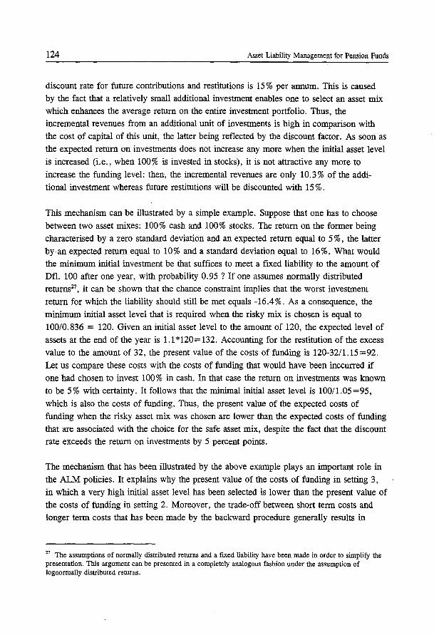
124 Asset Liability Management for Pension Funds
discount rate for future contributions and restitutions is 15% per annum. This is caused
by the fact that a relatively small additional investment enables one to select an asset mix
which enhances the average return on the entire investment portfolio. Thus, the
incremental revenues from an additional unit of investments is high in comparison with
the cost of capital of this unit, the latter being reflected by the discount factor. As soon as
the expected return on investments does not increase any more when the initial asset level
is increased (i.e., when 100% is invested in stocks), it is not attractive any more to
increase the funding level: then, the incremental revenues are only 10.3% of the addi
tional investment whereas future restitutions will be discounted with 15%.
This mechanism can be illustrated by a simple example. Suppose that one has to choose
between two asset mixes: 100% cash and 100% stocks. The return on the former being
characterised by a zero standard deviation and an expected return equal to 5 % , the latter
by· an expected return equal to 1 0% and a standard deviation equal to 16%. What would
the minimum initial investment be that suffices to meet a fixed liability to the amount of
Dfl. 100 after one year, with probability 0.95 ? If one assumes normally distributed
returns27, it can be shown that the chance constraint implies that the worst investment
return for which the liability should still be met equals -16.4%. As a consequence, the
minimum initial asset level that is required when the risky mix is chosen is equal to
100/0.836 = 120. Given an initial asset level to the amount of 120, the expected level of
assets at the end of the year is 1.1 *120= 132. Accounting for the restitution of the excess
value to the amount of 32, the present value of the costs of funding is 120-32/1.15 =92.
Let us compare these costs with the costs of funding that would have been inccurred if
one had chosen to invest 100% in cash. In that case the return on investments was known
to be 5% with certainty. It follows that the minimal initial asset level is 100/1.05=95,
which is also the costs of funding. Thus, the present value of the expected costs of
funding when the risky asset mix was chosen are lower than the expected costs of funding
that are associated with the choice for the safe asset mix, despite the fact that the discount
rate exceeds the return on investments by 5 percent points.
The mechanism that has been illustrated by the above example plays an important role in
the ALM policies. It explains why the present value of the costs of funding in setting 3,
in which a very high initial asset level has been selected is lower than the present value of
the costs of funding in setting 2. Moreover, the trade-off between short term costs and
longer term costs that has been made by the backward procedure generally results in
27 The assumptions of normally distributed returns and a fixed liability have been made in order to simplify the presentation. This argument can be presented in a completely analogous fashion under the assumption of lognormally distributed returns.

Computational Results 125
desired funding levels that exceed the ones that are minimally required in order to satisfy solvency constraints. This can lead to optimal funding levels that increase with the length of the planning horizon.
In this respect, it is interesting to compare the development of the average funding level
in setting 3 with that in setting 2. The higher initial funding level in setting 3 has been reduced rapidly by making large restitutions from 1996 until 2001. During the first years of the planning period, the ALM policy in setting 2 is geared more towards maintaining the given funding level, which results in substantially higher contributions until 1998. As of 1998, the average funding levels, as well as average contributions and probabilities of underfunding in setting 2 closely follow the development of the corresponding statistics of setting 3. The slightly lower average funding level that is maintained in setting 2, may reflect the greater flexibility in setting 2 with respect to raises in regular contributions (5 percent of the pensionable earnings in setting 2, as compared to 3 percent in setting 3).
In summary, the results from the ALM model do indeed reflect a trade-off between long
term effects and short term effects.
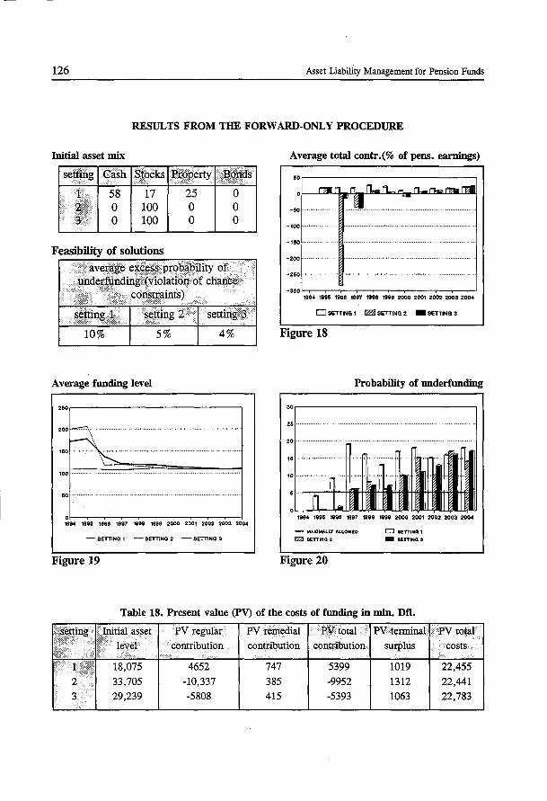
126 Asset Liability Management for Pension Funds
RESULTS FROM THE FORWARD-ONLY PROCEDURE
Initial asset mix
··.~~~·. C::lish ~tocks :Bropert,y · Bonds 58 17 25 0 0 100 0 0 0 100 0 0
Feasibility of solutions
x.· .. ··•·•···.· i ~vet~~ exc~sw~r()bability.of · .. ·. H9:d.¢~n,c1ll).g (yio~atioJ;l of chance · .. · · .· · constraints) ·· ... ··•·· •· •.. ··.i . . . .• .· ./ ..
~~!PM A··· ···•····· ~~WP:? 2 •.. · .. ·•••• s~tJ:iilg :?··· ·. 10% 5% 4%
Average funding level
••or-----------------,
HiD·· \
\ '--
100 ............. ·········· ..
60
0~-r-,----r-r--r-r--r-r--r~ 199-4 1905 1885 1987 1998 1999 2000 2001 2002 2003 2004
- SETTING 1 --- SETTING 2 - SETTING 3
Figure 19
Average total contr.(% of pens. earnings)
-100
-160 •···
-200 .
-250 .
-300 '--r--,----,---,--,--r----,--r----,--,----,--J 199-4 18915 1988 1997 1998 1999 2000 2001 2002 2003 2004
0 SETTING 1 IZi2J SETTING 2 - SETTING 3
Figure 18
Probability of underfunding
30,----------------.
25 •·· .
20 ......
15 ....
1994 1995 1998 1997 1998 1999 2000 2001 2002 2003 2004
- MAXIMALLY ALLOWED
P'2.ZI BETTING 2
Figure 20
CJ SETTING 1
- IIETTING3
PV reiTlediaf PVto~ai contribution contribution contribution surplus
4652 747 5399 1019 22,455
33,705 -10,337 385 -9952 1312 22,441 29,239 -5808 415 -5393 1063 22,783
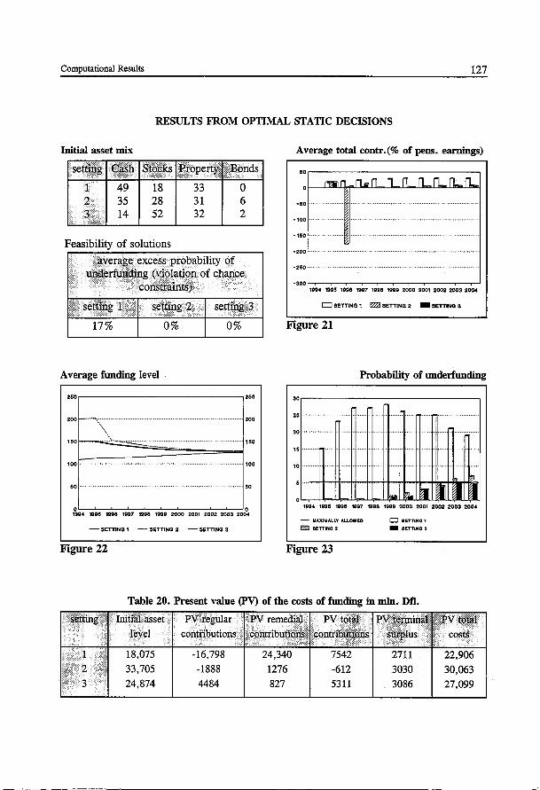
Computational Results 127
RESULTS FROM OPTIMAL STATIC DECISIONS
Initial asset mix
~§#til '<2~$h Stocks 49 18 35 28 14 52
Feasibility of solutions
Pro percy
33 31 32
.Bonds 0 6 2
··•···.········ ii:Yt:t~~~ ~x¢es~ ~r()bability ·of .·. ~1lct¢ft[rindipg(violation of chance.
1 · COJ:IStraints) . . _ ..
setting 3
17% 0% 0%
Average funding level
260r----------------,260
200~--, ............ ····•·•········ 200
\,\,
1 tiD 1--- · · .\··--·~~.:.:.:.:.~:.:.::::_~:.:.:_ ___________ _ 160
100 ...... 100
150 ········· ............. . 60
0 0 1994 19915 19915 1997 1998 1999 2000 2001 2002 2003 2004
- SETTINO 1 -·- SETTINC3 2 - SETTINO 3
Figure 22
Average total contr.(% of pens. earnings)
60.-----------------~
r. r . ~ ll ll _r11. _ n. .I"LJL ll... -60 .
-100 .
-150 .
-200 ................................................ .
-250 . '
1994 19915 1998 1997 1988 1999 2000 2001 2002 2003 2004
0 SETTING 1 e:zl SETTING 2 - SETTING 3
Figure 21
Probability of underfunding
30.------------------~
215 ...
20 ..
115 .... ---------_::.:::::··r··
10 , ..
15····
~~~--t 1994 19915 1988 1997 1998 1999 2000 2001 2002 2003 2004
- MAXIMALLY AJ..LOWED
f22J 8ETTINB 2
Figure 23
D 8ETTINQ1
-BETTING 3
Table 20. Present value (PV) of the costs of funding in min. Dfl.
:r¥ :t6~Iar } :PY remediiOi / J>V totki •
24,874 4484 827 5311 3086
··-.·.•.·.-·.· ¢Rst~
22,906
30,063 27,099
128 Asset Liability Management for Pension Funds
RESULTS FROM THE ALM MODEL
Initial asset mix
1. 66 21 13 2 52 44 4 j 0 100 0
.. '.,.
Feasibility of solutions
Bonds
0 0 0
<• ~v~~~~e ~¥c~s~ P~?bability of '···. uri.derfrindillg (yiolation of chance
cqnstraints)
Average fundiJig level
300,------,...-------------,
100 .
50 .. "
o~~-.-~-.-~-.-~-.-~~ 1894 1085 1908 1997 1998 1999 2000 2001 2002 2003 200-4
- SETTING 1 --· SETTINQ 2 - SETTING 3
Figure 25
-100 . •···
-160 ......
-200 . .. ········ ....... .
-250 ...
1994 1995 1998 1997 1998 1999 2000 2001 2002 2003 2004
c:J SETTING 1 ~SETTING 2 -SETTING 3
Figure 24
Probability of underfunding
30,----------------.
25 ........ .
20 ..
16 ..
10·-· ......... n···-
• n Ill n ~IL
1994 1995 1998 1997 1998 1999 2000 2001 2002 2003 2004
- MAXIMALLY ALLOWED
IZZJ SETTING 2
Figure 26
D 8ETTING1
- 8ETTINQ3
Table 22. Pre5ent value (PV) of the costs of funding in min. Dfl.
·····~IE ...• ~ .. ·l·:ielll .••• ,v: •..•.•• ·.·.·,e •. a .•• ls·· .. •,.,·,s .. • •.••. •.e,'.T ~¥ f~gutar; ···'·.·' E'Yi teirie~~~ •''······ py t?tal . . ·'· ,. 2bJihibhticiD.S < .d8.i:itriB\iti<>mi • <::dtiid6uf~~ns< \ 18,075 33,705 42,083
6494 -1580
-10,069
699 19 42
7194 -1561
-10,027
2266 6788 7374
23,003 25,356 24,682
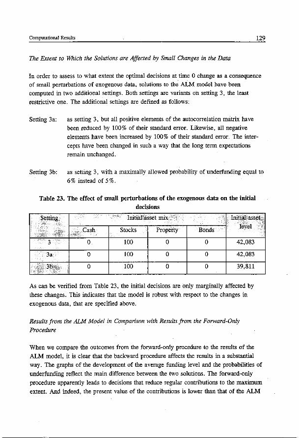
Computational Results 129
The Extent to Which the Solutions are Affected by Small Changes in the Data
In order to assess to what extent the optimal decisions at time 0 change as a consequence of small perturbations of exogenous data, solutions to the ALM model have been computed in two additional settings. Both settings are variants on setting 3, the least restrictive one. The additional settings are defined as follows:
Setting 3a: as setting 3, but all positive elements of the autocorrelation matrix have been reduced by 100% of their standard error. Likewise, all negative elements have been increased by 100% of their standard error. The intercepts have been changed in such a way that the long term expectations remain unchanged.
Setting 3b: as setting 3, with a maximally allowed probability of underfunding equal to 6% instead of 5%.
Table 23. The effect of small perturbations of the exogenous data on the initial decisions
......... S6ttjhg Initial asset mix Initial ass6f ( level i Cash Stocks Property Bonds 1···> .• ..
3 . 0 100 0 0 42,083
.... · 3a 0 100 0 0 42,083
.3b ••
0 100 0 0 39,811
As can be verified from Table 23, the initial decisions are only marginally affected by
these changes. This indicates that the model is robust with respect to the changes in exogenous data, that are specified above.
Results from the ALM Model in Comparison with Results from the Forward-Only
Procedure
..... •
When we compare the outcomes from the forward-only procedure to the results of the ALM model, it is clear that the backward procedure affects the results in a substantial way. The graphs of the development of the average funding level and the probabilities of
underfunding reflect the main difference between the two solutions. The forward-only procedure apparently leads to decisions that reduce regular contributions to the maximum extent. And indeed, the present value of the contributions is lower than that of the ALM
130 Asset Liability Management for Pension Funds
model. However, this is achieved at cost of rendering infeasible strategies in all settings:
the probabilities of underfunding are much higher than the maximum of 5% per annum. The ALM model does much better: for setting 2 and for setting 3, feasible solutions have been presented. Because no feasible solution could be found for setting 1, the objective has been changed into minimising violations of the solvency constraints. The policy that has been determined by the ALM model resulted in an average probability of underfunding equal to 11 % whereas the average probability of underfunding under the forward-only policy amounted to 15%. Given these observations, it can be stated that the results of the policy from the ALM model are superior to those that have been obtained from the forward-only model. This is due to the employment of the backward procedure in conjunction with the forward procedure.
Results from The ALM Model in Comparison with Results from Optimal Static Decisions
Neither the ALM model nor the static model has resulted in a feasible policy for setting 1. The extent to which solvency constraints are violated, however, differs greatly. Whereas the policy from the ALM model results in an average probability of underfund
ing of 11%, that of the static policy amounts to 22%. Even more dramatic is the difference between present values of the expected costs of remedial contributions: 24,340 mln Dfl. for the static model, compared to 699 min Dfl. for the ALM model. Notice that the difference between the present values of the expected total costs is only marginal. Again, the results from the static model suffer from the fact that the static decisions reflect a trade-off of their consequences in all states of the world.
The ALM model has determined a feasible policy for setting 2 as well as for setting 3.
Let us ignore the small infeasibilities of the static policy in setting 2. Instead, compare the present values of the expected costs of funding of the two policies in settings 2 and 3. In both settings, the present value of the expected costs of funding, associated with the policy from the ALM model is the smaller one, which shows the superiority of the ALM
model over the static model.
However, there is another noteworthy observation to be made. Consider the composition of the costs of total contributions. In all settings, the remedial contributions of the static model are a multiple order of magnitude higher than those of the ALM model: they are respectively 30 times, 20 times and 60 times as high in setting 1, 2 and 3. As a consequence, the level of total contributions to the fund that follows from the static model will vary enormously from one year to the next.
Finally, notice that the initial asset mixes and, in setting 3, the initial asset level from the
Computational Results 131
ALM model are rather different from those of the static model. Thus, one cannot expect to achieve results that are comparable to those from the ALM model by following a static policy and making recourse decisions when times goes by.
7.4Summary
In this chapter, computational results have been presented that provide the following insights with respect to the ALM approach that has been proposed in this monograph:
1. Dynamic ALM strategies lead to current decisions that are different from static policies. This applies to state dependent as well as to time dependent static policies.
2. In comparison to the static models, the employment of the ALM model has resulted in strategies of which the costs of funding are lower, the probabilities of underfunding are
substantially smaller and the magnitude of deficits, reflected by the costs of remedial contributions, has been reduced dramatically.
3. The favourable outcome of the comparison of policies determined by the ALM model with policies determined by optimal static decisions, are to a major extent due to:
- the fact that probabilities of underfunding at intertemporal points in time as well as at the planning horizon are endogenous to the model and have been modelled explicitly, and
- the dynan1ic character of the ALM model which enables the policies to react to situations that have emerged at the time of decision making and to reflect a correct trade-off between their longer term consequences and their short term effects.
Limited though this computational experience might be, it does tend to validate our approach towards asset liability management in a satisfactory manner.

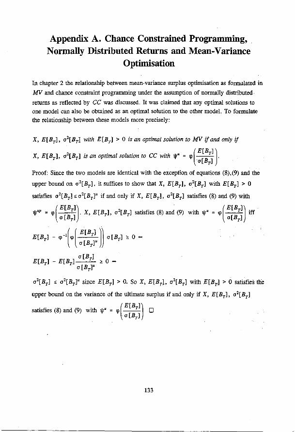
Appendix A. Chance Constrained Programming, Normally Distributed Returns and Mean-Variance
Optimisation
In chapter 2 the relationship between mean-variance surplus optimisation as formulated in
MV and chance constraint programming under the assumption of normally distributed
returns as reflected by CC was discussed. It was claimed that any optimal solutions to
one model can also be obtained as an optimal solution to the other model. To formulate the relationship between these models more precisely:
X, E[BT], o2[Brl with E[BT] > 0 is an optimal solution to MV if and only if
X, E[BT], o2[Br] is an optimal solution to CC with lj!u = <p( E[BT] )· ·o[BT]
Proof: Since the two models are identical with the exception of equations (8),(9) and the
upper bound on o2[Br], it suffices to show that X, E[BT], o2[Brl with E[Br] > 0
satisfies o2[Brl :5: o2 [BT]u if and only if X, E[BT], o2[Brl satisfies (8) and (9) with
lj!up = <p(E[BT])· X, E[BT], o2[BT] satisfies (8) and (9) with lj!u = <p(E[BT]) iff o [BT] o[BT]
E[BT] - <p -l(<p ( E[BT] ll o [BT] ;,;: 0 .,. o [BT]u
E[BT] - E[B] o[BT] ;,;: 0.,. T 0 [BT]u
o2[Brl :5: o2[Brlu since E[BT] > 0. So X, E[BT], o2[Br1 with E[Brl > 0 satisfies the
upper bound on the variance of the ultimate surplus if and only if X, E[Brl, o2[Brl
satisfies (8) and (9) with lj!u = <p( E[Brl) 0 o [BT]
133
Appendix B. The ALM Model With Transaction Costs
In order to extend the ALM model with transaction costs, these costs have to be
accounted for in two respects: it has to be registered how much costs are incurred from
trading and this has to be reflected in the constraint that reflects the asset level at the
beginning of the year.
In this appendix the following additional notation will be used:
c; costs of buying asset class i , as a fraction of the amount to be bought,
d; costs of selling asset class i , as a fraction of the amount to be sold,
To register the amounts that are bought and sold as of t = 1 , it suffices to include the
following equation in the ALM model:
For t=1, ... ,T-1, s=l, ... ,ST-1' i=l, ... ,N
(184)
To reflect the effect of transaction costs on the asset level at the beginning of each year,
(35) has to replaced by:
For t = 1, ... , T-1, s = l, ... ,Sr_ 1
N N
Ats + Yrs - Its - L (d;Dits + ciCits)= :E Xits (185) i=1 i = 1
If one chooses to account for transaction costs at time 0 as well, then, analogous
equations have to be included, given the asset mix at time 0, before the first allocation
decision has been made.
134
Appendix C. Illustrations of Importance Sampling
Given a bowl with 5 balls, each of which carries a number, one is allowed to draw 3
times with replacement. Then one is asked to estimate the mean of the numbers that are printed on the balls in the bowl. Suppose that, after drawing 3 times, the numbers 1, 2
and 15 have been observed. The classical unbiased estimate of the mean of the 5 numbers
in the bowl would be the sample mean: 113(1 +2+ 15) = 6.
Now, let us assume that there is additional information: there are two balls with a number
smaller than 4 and 3 balls which carry numbers that exceed 12. One would hope to
sample balls that carry the larger numbers: they contribute most to the mean that has to
be estimated, so once they are observed, the remaining uncertainty is relatively small.
Each of the larger numbers is greater than 4 times any of the smaller numbers. There
fore, a new distribution, which will be referred to as the importance sampling distribu
tion, can be specified of which it may be expected that the probability of drawing a
number is proportional to its relative contribution to the mean of the population, or at
least, the importance sampling distribution will come closer to this property than the
original distribution in which all numbers are equally likely to be drawn.
Suppose that the sampling process has been manipulated in such a way that the probability
of drawing· any of the smaller numbers equals 1114 and the probability of drawing any of
the larger numbers is 4/14, and let the numbers 2, 16 and 20 be drawn. How should the
mean of the population be estimated, given these observations, the original probability
distribution and the importance sampling distribution ? Since the sample has been
manipulated, it would be incorrect to estimate the mean of the population by the sample
average. Instead, one should construct a correction factor for each of the observations, so
that they contribute to the extent that is in agreement with the original probability
distribution. Because the sample has been drawn from the importance sampling distribu-
tion, the correction factor of the balls with the larger numbers should be 115 = 0.7 and 4/14
the correction factor for the balls which carry the smaller numbers should be
~ = 2.8. It follows that the mean should now be estimated as 113(2.8 * 2 + 0.7 * 16 1114
+ 0.7 * 20) = 10.27. It will be shown in? that both estimates of the mean are unbiased.
Nevertheless, the difference is more than 70% of the smaller estimate.
In order to analyze the variance of each estimator, suppose that the bowl contained balls
135
136 Asset Liability Management for Pension Funds
that are numbered 1, 2, 15, 16 and 20. Then, under the original probability distribution,
the mean. and variance of the population are 10.8 and 60.56 respectively. It follows that
the variance of the first estimator equals 119(60.56 + 60.56 + 60.56) = 20.19.
To analyze the variance of the importance sampling estimator, notice that drawing numbers and then multiplying them by a correction factor is equivalent to multiplying the
numbers first and sampling from the population 2.8 * 1, 2.8 * 2, 0.7 * 15, 0.7 * 16, 0.7
* 20, where each of the first two elements has probability 1114 to be sampled and each of
the other elements is drawn with probability 4/14. The mean of the importance sampling
distribution is equal to 1114(2.8 + 5.6) + 4/14(10.5 + 11.2 + 14) = 10.8. Apparently, the correction factors have indeed been chosen in such a way that the mean of importance
sampling distribution is equal to the mean of the original population. The variance of the
importance sampling distribution is equal to 1114((2.8 - 10.8)2 + (5.6 - 10.8)2) + 4/14((10.5 - 10.8)2 + (11.2 - 10.8? + (14 - 10.8)2) = 9.5. As a consequence, the
variance of the importance sampling estimator of the mean of the original distribution
equals 119(9. 5 + 9. 5 + 9. 5) = 3 .17. I.e. , the variance of the estimator of the mean has
been reduced by more than 80%.
This example shows that additional information on the distribution of a random variable
can be exploited to specify an importance sampling distribution which in tum enables one
to obtain an estimate of the mean of the unknown population that is superior to the average of a sample from the original distribution.
As has been shown in (166), the optimal choice of the importance sampling distribution
reduces the variance of the estimate to zero. To illustrate that case as well, consider
Table 24. The second and third column present the importance sampling probability and the associated correction factor. As in the previous example, drawing from the importance
sampling distribution and multiplying the observations by the correction factor is equivalent to multiplying all elements of the original population by the associated
correction factor and sampling from the original density.
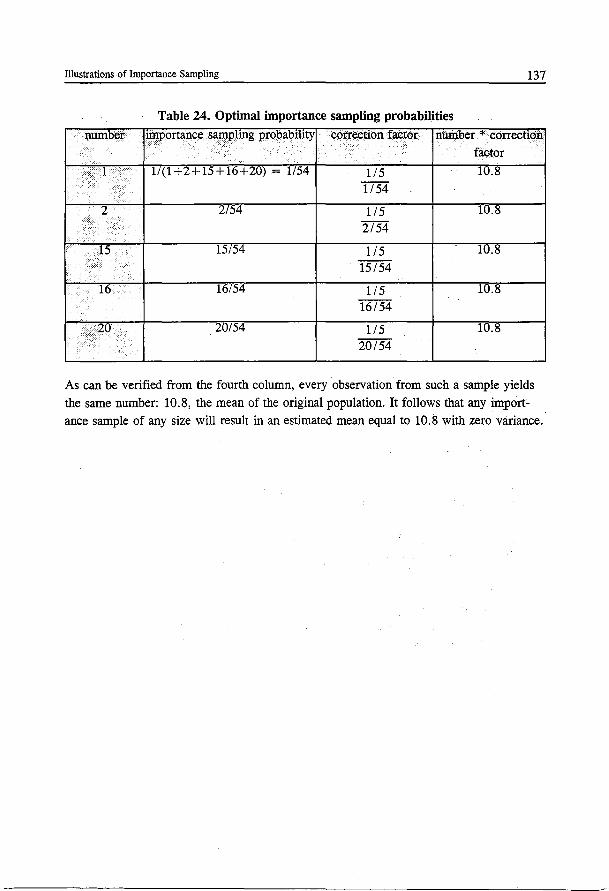
Illustrations of Importance Sampling 137
Table 24. Optimal importance sampling probabilities
l'luinber lD1POrtance. sampling probability · correction factor nuiD.ber. * · cottection 1.' .,·, factor
:·.L. 11(1+2+15+16+20)- 1154 115 10.8 :
1154 ~
2 2/54 115 10.~
2/54
15 15/54 1/5 lU.~
15/54
16 16/54 115 10.8 i: 16/54
·. zq ·.·.·.· 20/54 1/5 10.8 20/54
As can be verified from the fourth column, every observation from such a sample yields the same number: 10.8, the mean of the original population. It follows that any import~ ance sample of any size will result in an estimated mean equal to 10.8 with zero variance.
References
Aarssen, K. (1992), A Stochastic Programming Approach to Asset Liability Management,
Masters Thesis, Erasmus University Rotterdam, The Netherlands.
Albrecht, P. (1993), Normal and Lognormal Shortfall-Risk, Transactions of the 3rd
International AFIR Colloquium, pp. 417-430.
Albrecht, P. (1994), Shortfall Returns and Shortfall Risk, Transactions of the 4th
international AFIR Colloquium, pp. 87-110.
Almering, J.H.J., H. Bavinck and R.W. Goldbach (1988), Analyse, Delftse Uitgeversma
atschappij b.v., The Netherlands.
Arnott, R.D. (1988) and P.L. Bernstein, The Right Way to Manage Your Pension Fund,
Harvard Business Review, January, p.98.
Bain, L.J. and M. Engelhardt (1987), Introduction to Probability and Mathematical
Statistics, PWS Publishers (Boston).
Boender, C.G.E. (1994), Mean Variance Models for Asset Liability Management,
submitted.
Boender, C.G.E. (1995), A Hybrid Simulation/Optimization Scenario Model for
Asst/Liability Management, submitted.
Boender, C.G.E. and H.E. Romeijn (1991), The multidimensional Markov chain with
specified asymptotic means and (auto-) covariances., Communications in Statistics -Theory
meth., 20(1), pp.345-359.
Booth, P. and A. Ong (1994), A Simulation Based Approach to Asset Allocation Deci
sions, Transactions of the 4rd international AFIR Colloquium, pp. 217-239.
Bratley, L.P., B.L. Fox and L.E. Schrage (1987), A Guide To Simulation, second
edition, Springer Verlag New York Inc.
Brocket, P.L. , A. Charnes and Li Sun (1993), A chance constrained programming
approach to pension plan management, Contents of Actuarial Research Clearing House,
vol.3 pp.324-357.
138
References
Bunn, D.W. and A.A. Salo (1993), Forecasting with scenarios, European Journal of Operational Research, pp. 291-303.
139
Carino, D.R., T. Kent, D.H. Myers, C. Stacy, M. Sylvanus, A.C. Turner, K. Watanabe
and W.T. Ziemba (1993), The Russel-Yasuda Kasai Model: An Asset/Liability Model for
a Japanese Insurance Company Using Multistage Stochastic Programming, Frank Russel
Research Report.
Carillo, D.R., T. Kent, D.H. Myers, C. Stacy, M. Sylvanus, A.C. Turner, K. Watanabe and W.T. Ziemba (1994), The Russel-Yasuda Kasai Model: An Asset/Liability Model for
a Japanese Insurance Company Using M!Atistage Stochastic Programming, Interfaces 24:January-February pp. 29-49.
Chvatal, V. (1983), Linear Programming, Freeman and Company, New York.
Charnes, A. and W.W. Cooper (1959), Chance-constrained programming, Management Science, vol. 6 pp. 73-80.
Dempster, M.A.H. and X. Cervera Poin! (1995), Stochastic Programming: A New
Approach to Asset/Liability Management, Summerschool Institute of Actuaries
Dert, C.L. (1989), Irrationeel Beleggersgedrag en Outpeiformance Strategieen, in Portefeuille-Strategisch beleggen in het Verre Oosten, Pacific Investments Research Institute, Amsterdam, The Netherlands.
Dert, C.L and A.H. Rinnooy Kan, Fixed income asset liability management, Transactions of the 2nd international AFIR Colloquium, vol. 3, 17-20 April1991, pp.285-300
Diebold, F.X. and G. Rudebusch (1989), Long Memory and Persistence in Aggregate
Output, Journal of Monetary Economics, 24, pp. 189-209.
Dothan, M. V. (1990), Prices in Financial Markets, Oxford University Press, New York.
Duffie, D. (1988), Security Markets: Stochastic Models, Academic Press, Boston.
Entriken, R. and G. Infanger (1990), Decomposition and Importance Sampling For
Stochastic Linear Models, IBM Research Report RC 15545.
Ford P. (1991), Cashflow matching using modified linear programming, Transactions of
140 Asset Liability Management for Pension Funds
the 2nd international AFIR Colloquium, vol. 3, pp.301-322.
Frijns, J.M.G. en J.H.W. Goslings (1989), Matching voor het pensioenbedrijf,
Economische statistische berichten, september, pp. 868-871.
Guimaraes, R.M.C., B. G. Kingsman and S.J. Taylor (1989), A Reappraisal of the
Efficiency of Financial Markets, Springer Verlag.
Glynn, P.W. and D.L. Iglehart (1989), Importance sampling for stochastic simulations,
Management Science, Vol35, No 11, november, pp.1367-1391.
Golub, B., M. Holmer, R. McKendall, L. Pohlman and S.A. Zenios (1993), A Stochastic
Programming Model for Money Management, to appear in European Journal of Operati
ons Research.
Griffm, M. (1993), A New Rationale for the Different Asset Allocation of Dutch and UK
Pension Funds, Transactions of the 3rd International AFIR Colloquium, pp. 575-588.
Haigigi, M. and B. Kluger (1987), Safety First: An Alternative Performance Measure,
Journal of Portfolio Management summer.
Holmer, M.R., R. McKendall, C. Vassiadou-Zeniou and S.A. Zenios (1993), Dynamic
Models for Fixed-Income Portfolio Management Under Uncertainty, Report 93-03,
University of Cyprus.
Hardy, M.R. (1993), Stochastic simulation in Life Office Solvency Assessment, Journal of
the Institute of Actuaries 120, vol. 1, pp. 131-152.
Harlow, W.V. (1991), Asset Allocation in a Downside-Risk Framework, Financial Analyst
Journal, september-october, pp. 28-40.
Hogg, R.V. and A.T. Craig (1978), Introduction to mathematical statistics, fourth
edition, Macmillan Publishing Co., Inc. New York.
Infanger, G. (1992), Monte Carlo Importance Sampling within a Benders Decomposition
Algorithm for Stochastic Linear Programs, Annals of Operations Research vol. 39, pp.
69-95.
Ingersoll, J.E. Jr. (1987), Theory of Financial Decision Making, Studies in Financial
References 141
Economics, Rowan & Littlefield, Totowa, New Jersey.
Janssen and Manca (1994), Semi-Markov Modelization for the Financial Managment of
Pension Funds, Transactions of the 4th international AFIR Colloquium, pp. 1369 - 1387.
Judge, G.G., R.C. Hill, W.E. Griffiths, H. Liitkepohl and T.C. Lee (1985), Introduction
to the Theory and Practice of Econometrics, John Wiley and Sons.
Judge, G.G., R.C. Hill, W.E. Griffiths, H. Liitkepohl and T.C. Lee (1988), The Theory
and Practice of Econometrics, John Wiley and Sons.
Kall, P. (1976), Stochastic Linear Programming, Econometrics and Operations Research, vol. XXI (Springer Verlag, Berlin).
Klaassen, P. (1994), Stochastic Programming Models for Interest-RAte Risk Management,
Ph.d. thesis, M.I.T., Sloan School of Management.
Kleijnen, J.P.C. (1971), Variance Reduction Techniques in Simulation, Ph.d. thesis,
Katholieke Hogeschool Tilburg, Tilburg, The Netherlands.
Kleijnen, J.P.C. (1974), Statistical techniques in simulation, part 1, Marcel Dekker, Inc., New York.
Kleijnen, J.P.C. (1975), Statistical techniques in simulatiqn, part 2, Marcel Dekker, Inc., New York.
Kusy, M.l. and W.T. Ziemba (1986), A bank asset and liability model, Operations Research, vol. 34, no. 3, pp. 356-376.
Leibowitz, M.L. (1986), Total Portfolio Duration: A new Perspective on Asset Allocation,
Salomon Brothers, Inc february.
Leibowitz, M.L. and R.D. Hemiksson (1987), Portfolio optimization within a surplus
framework, a new perspective on asset allocation, Salomon Brothers, Inc, april.
Ludvik, P. (1994), Investment Strategy for Defined Constribution Plans, Transactions of the 4th international AFIR Colloquium, pp. 1389- 1400.
Lustig, I.J., J.M. Mulvey and T.J. Carpenter (1990), Operations Research, vol. 39, no.
142 Asset Liability Management for Pension Funds
5, pp. 757-772.
Markowitz H.M. (1952), Portfolio Selection, The Journal of Finance, vol. VII, no.1, pp. 77-91.
Markowitz, H.M. (1959), Portfolio Selection: Efficient Diversification of Investments,
Cowles Foundation for Research in Economics at Yale University, Monograph 16, Yale University Press, New Haven.
Minoux, M. (1986), Mathematical Programming, Theory and Algorithms, John Wiley and Sons (New York).
Mulvey, J.M. and H. Vladimirou (1988), Solving Multistage Stochastic Networks: An
Application of Scenario Aggregation, Report SOR-88-1, Dept. of Civil Engineering and Operations Research, School of Engineering and Applied Science, Princeton University.
Mulvey, J.M. and H. Vladimirou (1991), Applying the progressive hedging algorithm to
stochastic generalized networks, Annals of Operations Research, vol. 31, pp. 399-424.
Mulvey, J.M. (1994), An Asset liability Investment System, Interfaces 24:may-june, pp.
22-33.
Munnik, J.F.J. de (1992), The Valuation of Interest Rate Derivative Securities, Ph.D. thesis Erasmus University Rotterdam.
Naylor, T.H., J.L. Balintfy, D.S. Burdick and K. Chu (1967), Computer Simulation
Techniques, John Wiley & Sons, Inc., New York.
Ooms, M. (1993), Empirical Vector Autoregressive Modeling, Ph.d. thesis, Erasmus University Rotterdam.
Petersen, C. Pensioenen in West-Europa, Economische Statistische Berichten, 3 januari
1990, pp.10-13.
Petersen, C., Pensioenen: uitkeringen, financiering en beleggingen, Stenfert Kroese,
Leiden-Antwerpen 1990.
Rockafellar, R.T. and R.J.-B. Wets (1991), Scenario's and policy aggregation in
optimization under uncertainty, Mathematics of Operations Research, february, vol. 16
References
no. 1, pp. 119-147.
Sharpe, W.F. and L.G. Tint (1990), Liabilities- A new approach, Journal of Portfolio Management, winter, pp. 5-10.
143
Sherris, M. (1992), Ponfolio Selection and Matching: a synthesis, Journal of the Institute of Actuaries, vol. 119, part I, pp. 87-105.
Sherris, M. (1993), 221 Portfolio Selection models for Life Insurance and Pension
fundors, in Proceedings of the 3rd AFIR International Colloquium, pp. 915-930.
Sims, C.A. (1980), Macroeconomics and Reality, Econometrica vol. 48, nr. 1, pp. 1-48.
Smink, A Numerical Examination of Asset liability Management Strategies, Transactions of the 4th international AFIR:Colloquium, pp. 969-997.
Sortino, F.A. and R. van der Meer (1991), Downside Risk, Journal Portfolio Management, summer, pp. 27-31.
Ross, S.M. (1985), Introduction to Probability Models, Academic Press Inc.
Taylor, L.D. (1974), Probability and Mathematical Statistics Statistics, Harper & Row, Publishers (New York).
Wets, R.I.-B. (1987), Large-scale lineair programming techniques in stochastic
programming, in: Y. Ermoliev and R. Wets, Numerical methods for stochastic
optimization, Springer Verlag, Berlin.
Wets, R.I.-B. (1989a), StochasticProgramming, ch. 8 in: G.L. Nemhauser, A.H.G. Rinnooy Kan and M.J. Todd (1989), Handbooks in operations research and management
science, vol1: optimization, Elsevier Science Publishers B.V. (North-Holland).
Wets, R.I.-B. (1989b), The Aggregation Principle in Scenario Analysis and Stochastic
Optimization, in: S.W. Wallace, Algorithms and Model Formulations in Mathematical
Programming, Springer Verlag, Berlin, pp. 91-113.
Wilkie, A.D. (1985), Portfolio seclection in the presence of fixed liabilities: a comment
on the matching of assets to liabilities, Journal of the Institute of Actuaries, vol. 112, pp. 229-277.
144 Asset Liability Management for Pension Funds
Wilkie, A.D. (1986a), A Stochastic Investment Model for Actuarial Use, Transactions of
the Faculty of Actuaries 39, pp. 341 - 403.
Wilkie, A.D. (1986b), Some Applications of Stochastic Investment Models, J.I.A.S.S. 29, pp. 25- 51.
Wilkie, A.D. (1995), More on a Stochastic Asset Model for Actuarial Use, presented to
the Institute of Actuaries 24 april.
Wilkie, A.D., J.A. Tilley, T.G. Arthur and R.S. Clarkson (1993), This house believes
that the contribution of actuaries to investment could be enhanced by the work of financial
economists, Journal of the Institute of Actuaries 120, part III, pp. 393-414.
Wilkie, A.D. (1995), More on a stochastic asset model for actuarial use, Presented to the Institute of Actuaries, 24 April 1995.
Wise, A.J. (1984a), A theoretical analysis of the matching of assets to liabilities, Journal of the Institute of Actuaries, vol. 111, pp. 375-402.
Wise, A.J. (1984b), The matching of assets to liabilities, Journal of the Institute of Actuaries; vol. 111, pp. 445-501.
Wise, A.J. (1987a), Matching and Portfolio Selection: Part 1, Journal of the Institute of
Actuaries, vol. 114, pp. 113-133.
Wise, A.J. (1987b), Matching and Portfolio Selection: Part 2, Journal of the Institute of Actuaries, vol. 114, pp. 551-568.
Zellner, A. (1962), An Efficient Method of Estimating Seemingly Unrelated Regressions
and Tests of Aggregation Bias, Journal of the American Statistical Association, vol. 57, pp. 348-368.
Ziemba, W.T., and R.G. Vickson (1975) Stochastic Optimization Models in Finance,
· Academic Press, New York.

Samenvatting (Summary in Dutch)
In dit proefschrift wordt een optimalisatiemodel gepresenteerd voor het analyseren van
beleggingsbeleid en premiebeleid van pensioenfondsen, rekening houdend met de
ontwikkeling van verplichtingen in samenhang met economische omstandigheden. Een dergelijk beleid beet asset liability management (ALM). De aanpak die bier wordt
voorgesteld is gebaseerd op scenario analyse.
Met deze aanpak kan een dynamisch ALM beleid bepaald worden, zodanig dat de kosten
om een gegeven pensioenreglement te financieren geminimaliseerd worden onder de
voorwaarden dat de kans op onderdekking acceptabel klein is en de pensioenpremies van
jaar op jaar voldoende stabiel zijn.
Probleembeschrijving
Pensioenfondsen hebben de taak om pensioenen uit te betalen aan deelnemers aan het
pensioenfonds die hun actieve carriere hebben beeindigd en aan nabestaanden daarvan.
Deze uitkeringen dienen in overeenstemming te zijn met bet pensioenreglement waarin is
vastgelegd op welke wijze de hoogte van de uitkering berekend wordt, waneer deze ingaat
en wanneer deze beeindigd wordt.
Gedurende de tijd neemt bet vermogen van bet pensioenfonds, de waarde van beleggings
portefeuille, toe met beleggingsopbrengsten en premieontvangsten. Het neemt af door het
uitbetalen van pensioenen. Het is de taak van bet pensioenfonds om deze inkomende en
uitgaande geldstromen in evenwicht te houden zodat het fonds aan de geldende
solvabiliteitseisen voldoet en dat aile uitkeringen, nu en in de toekomst, tijdig gedaan
kunnen worden.
Beslissingen die in belangrijke mate bepalen of bet pensioenfonds erin slaagt haar taak uit
te voeren zijn de hoogte van de pensioenpremies en de verdeling van te beleggen gelden
over de beleggingscategorieen waarin bet pensioenfonds wil beleggen. Deze verdeling
wordt de beleggingsmix genoemd.
De hoogte van de pensioenpremie dient zodanig vastgesteld te worden dat de sponsor in
staat en bereid is de premies te betalen. Deze beperking komt vaak tot uiting in een bovengrens op de pensioenpremie en op eventuele premieverhogingen, beide als percentage van de loonkosten.
In principe is bet pensioenfonds vrij in haar keuze van een beleggingsmix.. De facto leiden
145

146 Asset Liability Management for Pension Funds
algemeen geaccepteerde noties van acceptabele en onacceptabele beleggingsmixen echter
al snel tot minima en maxima op het aandeel van verschillende beleggingscategorieen in
de beleggingsmix. Bij het effectueren van veranderingen in de beleggingsmix dient
bovendien rekening gehouden te worden met de liquiditeit van de effectenmarkten waarin
men actief is.
Onzekerheden, waardering van vetplichtingen en beleggingen
In het pensioemeglement is vastgelegd op welke wijze de hoogte van toekomstige
uitkeringen berekend dient te worden. De hoogte van de toekomstige uitkeringen is echter onzeker. Deze is onder meer afhankelijk van toekomstige ontwikkelingen in het
deelnemersbestand, zoals sterfte, invaliditeit, loopbaanontwikkeling en burgerlijke staat.
Voor veel Nederlandse pensioenfondsen is de belangrijkste bran van onzekerheid de
toekomstige ontwikkeling van prijsinflatie en toekomstige loomonden: de hoogte van
oudedagspensioenen bedraagt veelal zeventig procent van het laatst verdiende loon28•
Gevolg hiervan is dat pensioemechten van actieve deelnemers die zijn opgebouwd tijdens
eerdere dienstjaren toenemen met looninflatie. Pensioemechten van slapers en ingegane
pensioenen zijn vaak gei:ndexeerd met prijsinflatie.
In de regel doen pensioenfondsen slechts conditionele indexatietoezeggingen, dat wil
zeggen dat indexatie slechts plaatsvindt voor zover de financiele situatie van het
pensioenfonds dat toelaat. In het vervolg zullen we echter geen onderscheid maken naar
conditionele en onconditionele verplichtingen. Als een reglement conditionele
indexatietoezeggingen bevat, dan is onze ALM aanpak erop gericht gei:ndexeerde
pensioenen uit te keren.
AIM beleid
Goed ALM beleid bestaat uit beleggingsbeslissingen en premiebeleid die resulteren in een
gewenste risico-rendement structuur in termen van de ontwikkeling van de financiele staat
van het pensioenfonds. Daarbij worden de pensioenkosten geminimaliseerd terwijl
gezorgd wordt dat het fonds aan haar verplichtingen kan voldoen. Helaas kan zelfs bij een
perfecte uitvoering van een uitmuntende ALM strategie niet gegarandeerd worden dat alle
toezeggingen onder alle omstandigheden kunnen worden nagekomen.
28 Inclusief een staatspensioen op basis van de Algemene Ouderdorils Wet (AOW). Het AOW bestanddeel is wei gelndexeerd, maar onafhankelijk van de salarisontwikkeling. Nu de hoogte van de AOW uitkering onderwerp van politieke discussie is geworden, !open pensioenfondsen het risico dat zij hogere uitkeringen zullen moeten doen ter compensatie van eventuele lagere AOW uitkeringen.

Samenvatting (Summary in Dutch) 147
Indien de verplicbtingen geindexeerd zijn met inflatie, bij voorbeeld,. kan bet in tijden van
uitzonderlijk boge inflatie voorkomen dat bet fonds niet aan alle verplicbtingen kan
voldoen zonder extreem boge premies te beffen. De kans bestaat dat pensioenfondsen in een situatie verzeild i:aken waarin de waarde van de beleggingen kleiner is dan die van de
verplicbtingen. Deze kans noemen we de kans op onderdekking. Het ALM beleid moet
er dan ook op gericbt zijn de kans op onderdekking acceptabel klein te bouden.
N ocb beleggingsmixen, nocb premieboogtes worden vastgesteld voor de gebele plannings
periode. Beslissingen worden bijgesteld als veranderende omstandigbeden, zoals een
gewijzigde dekkingsgraad en een gewijzigde kijk op de toekomstige ontwikkeling van de
economiscbe omstandigbeden, daartoe nopen. Stabiliteitseisen aan bet ALM beleid, zoals
een maximum op premieverbogingen, kunnen ecbter impliceren dat corrigerende
beslissingen slecbts in beperkte mate genomen kunnen worden. Hieruit volgt dat huidige
beslissingen en toekomstige beslissingen niet onatbankelijk van elkaar genomen kunnen
worden. Daarom dient een ALM beleid te bestaan uit beslissingen die nu. genomen
worden en uit reeksen van beslissingen die in de toekomst genomen worden. Toekomstige
beslissingen dienen afhankelijk te zijn van situatie die ontstaan is op bet moment dat de
beslissing genomen wordt. Huidige beslissingen dienen te anticiperen op de mogelijkheid
om beslissingen later bij te sturen. V oor zover zij de toekomstige beslissingsvrijbeid
beperken dienen zij bovendien bet resultaat te zijn van een correcte afweging van korte
termijn effecten en langere termijn effecten. Zo'n beleid wordt een dynamiscbe politiek
genoemd.
Scenario's om een onzekere toekomst te modelleren
Een van de cruciale aspecten van een ALM model is de wijze waarop onzekerbeid
gemodelleerd wordt. Wij modelleren onzekerbeid met bebulp van een groot aantal
scenario's. Elk van deze scenario's bestaat uit een reeks van opeenvolgende toestanden en
geeft een mogelijk verloop weer van de omgeving waarin ALM beslissingen genomen
dienen te worden. Toekomstige omstandigbeden worden gedefinieerd door de boogte
van de loonsom, de boogte van de verplicbtingen, de boogte van de uitkeringen en bet
totale rendement op elk van de beleggingscategorieen over de voorafgaande periode. Deze
mogelijke toestanden zijn onafhankelijk van de te nemen beslissingen met betrekking tot
de beleggingsmix en bet premiebeleid. Ze worden volledig gedefinieerd door factoren die
exogeen zijn aan bet beslissingsmodel.
De scenario's worden zo gegenereer<i dat toekomstige toestanden van de wereld consistent
zijn, dat wil zeggen dat deterministiscbe en stocbastiscbe relaties tussen
toestandsvariabelen erin tot uitdrukking komen. Dat geldt zowel voor relaties tussen

148 Asset Liability Management for Pension Funds
toestandsvariabelen die tezamen een toestand defmieren als voor relaties tussen
toestandsvariabelen van opeenvolgende toestanden. Beleidsmakers kunnen zelf aangeven welke mogelijke toekomstige ontwikkelingen zij bij het bepalen van hun ALM
beleid relevant achten. De scenenariogenerator kan dan gebruikt worden om alle toekomstige omstandigheden te weerspiegelen waarvan de beslisser vindt dat er bij de
besluitvorming rekening mee gehouden moet worden.
In dit proefschrift zijn de scenario's gebaseerd op een tijdreeksmodel. De ALM methode
die hier wordt voorgesteld kan echter ook gebruikt worden in combinatie met scenario's
die op een andere manier gegenereerd zijn. Zo kan men er bij voorbeeld voor kiezen om bij de scenariogeneratie een model te gebruiken dat gebaseerd is op economische theorie.
Een dynamisch optimalisatiemodel voor asset liability management
In hoofdstuk 3 wordt een optimalisatiemodel gepresenteerd waarmee een ALM beleid
bepaald kan worden dat voor elke toestand de premiehoogte en de beleggingsmix
specificeert. Deze beslissingen bepalen eveneens voor elke toestand de waarde van de
beleggingsportefeuille en, in combinatie met de exogeen bepaalde waarden van de
verplichtingen, de dekkingsgraad. De beslissingen in alle toestanden worden simultaan
bepaald. Dit maakt bet mogelijk om zowel afwegingen te maken tussen korte termijn
effecten en langere termijn effecten als afwegingen tussen de consequenties van
beslissingen in verschillende mogelijke toekomstige toestanden. Het model is ontwikkeld
ter ondersteuning van het formuleren van ALM beleid dat:
- een acceptabel kleine kans op onderdekking waarborgt,
- voldoende stabiele premies als percentage van de loonsom garandeert,
- de pensioenkosten, gekwantificeerd als de contante waarde van de verwachte
pensioenpremies, minimaliseert.
De kans op onderdekking is zodanig ge~odelleerd dat:
1. het model gebruikt kan worden met elke kansverdeling die door scenario's kan worden weergegeven. Dus ook met kansverdelingen die impliciet gespecificeerd zijn. Ben voorbeeld hiervan is de kansverdeling van de ontwikkeling van verplichtingen. Deze is vaak impliciet gegeven door het computerprogrammatuur waarmee de uit te keren
I
bedragen op basis van het pensioenreglement, loonronden en prijsinflatie berekend worden,,
2. vanuit elke toestand de kans dat een jaar later een situatie van onderdekking optreedt,

Samenvatting (Summary in Dutch)
acceptabel klein is,
3. bij de optimalisatie expliciet rekening wordt gehouden met kansen op onderdekking. Zowel op het eind van de planningsperiode als tussentijdstippen.
149
Samenvattend, in deze dissertatie wordt een gemengd geheeltallig stochastisch
programmerings model voorgesteld. Het kan gebruikt kan worden om dynamische
ALM strategieen te bepalen die gebaseerd zijn op scenario's die elke set van
vooronderstellingen kunnen weerspiegelen waarop men het ALM beleid wenst te baseren. Kansen op onderdekking worden daarbij expliciet gemodelleerd op basis van
realistische vooronderstellingen ten aanzien van de kansverdelingen van exogene
kansvariabelen.
V oor zover ons bekend is dit model het eerste waarmee een dynamisch beleid bepaald kan
worden dat gebaseerd wordt op realistische vooronderstellingen.
Rekenkundige experimenten
Teneinde inzicht te krijgen in het gedrag van het model bij toepassing op realistische
problemen, zijn er ALM politieken berekend op basis van de data van een Nederlands
pensioenfonds met een actuariele reserve van ruim 16 miljard gulden en ongeveer 1
miljoen participanten, waarvan ca. 240.000 actieven.
De rekemesultaten zijn verkregen door de heuristiek toe te passen die wordt
gepresenteerd in hoofdstuk 5. Het meer-perioden beslissingsprobleem wordt daarbij
benaderd door een reeks van twee-perioden problemen. De benodigde rekentijd om met
deze heuristiek een dynamisch ALM beleid te bepalen is proportioneel met het aantal perioden dat in beschouwing wordt genomen. De resultaten geven de volgende indicaties met betrekking tot de ALM methode die in dit proefschrift is gepresenteerd:
1. Dynamische ALM strategieen leiden tot huidige beslissingen die afwijken van beslissin
gen die genomen worden binnen een statische politiek.
2. In vergelijking met statische modellen resulteert het gebruik van dynamische modellen
in lagere pensioenkosten, kleinere kansen op onderdekking en, in geval van onderdekking, een enorme reductie van de mate van onderdekking,
3. De bevredigende uitkomst van de vergelijking van ALM beleid, bepaald door het
voorgestelde dynamische model, en beleid, bepaald door statische modellen, zijn voor het

150 Asset Liability Management for Pension Funds
grootste deel toe te schrijven aan:
- het feit dat kansen op onderdekking op zowel op tussentijdstippen als op de
planningshorizon expliciet zijn gemodelleerd en endogeen zijn aan het beslissingsmodel en
- het dynamische karakter van het ALM model dat de mogelijkheid biedt om te reageren
op gewijzigde omstandigheden en om een correcte afweging te maken tussen kortere
termijn en langere termijn effecten.


I I

Related Documents