Przegląd Statystyczny. Statistical Review, 2020, vol. 67, 2, 114–151 DOI: 10.5604/01.3001.0014.5726 Assessment of the size of VaR backtests for small samples Daniel Kaszyński, a Bogumił Kamiński, b Bartosz Pankratz c Abstract. The market risk management process includes the quantification of the risk connect- ed with defined portfolios of assets and the diagnostics of the risk model. Value at Risk (VaR) is one of the most common market risk measures. Since the distributions of the daily P&L of financial instruments are unobservable, literature presents a broad range of backtests for VaR diagnostics. In this paper, we propose a new methodological approach to the assessment of the size of VaR backtests, and use it to evaluate the size of the most distinctive and popular backtests. The focus of the paper is directed towards the evaluation of the size of the backtests for small-sample cases – a typical situation faced during VaR backtesting in banking practice. The results indicate significant differences between tests in terms of the p-value distribution. In particular, frequency-based tests exhibit significantly greater discretisation effects than duration-based tests. This difference is especially apparent in the case of small samples. Our findings prove that from among the considered tests, the Kupiec TUFF and the Haas Discrete Weibull have the best properties. On the other hand, backtests which are very popular in bank- ing practice, that is the Kupiec POF and Christoffersen’s Conditional Coverage, show significant discretisation, hence deviations from the theoretical size. Keywords: Value at Risk, market risk management, backtesting, empirical size assessment. JEL: C00, C12, C15, D81, G32 1. Introduction In 2009, the Basel Committee on Banking Supervision has introduced the Basel II Accord, which includes recommendations for banks as well as for regulators operat- ing in the EU (Basle Committee on Banking Supervision [BCBS], 2009). Within the Basel II framework, financial institutions, in particular, are recommended to ensure capital buffers against market risks – this recommendation is also sustained in Basel III, which will be implemented (and come into force) in January 2022. The market risk management process carried out by financial institutions includes the quantifi- cation of the risk connected with defined portfolios of assets. One of the most com- monly used risk measures that has gained significant attention is Value at Risk (VaR). Among the consequences of implementing the Basel Accord is that banks are required to perform proper diagnostics, i.e. backtests of their VaR models. a SGH Warsaw School of Economics, Institute of Econometrics, Decision Analysis and Support Unit, e-mail: [email protected] (corresponding author), ORCID: https://orcid.org/0000-0002-0865-0732. b SGH Warsaw School of Economics, Institute of Econometrics, Decision Analysis and Support Unit, e-mail: [email protected], ORCID: https://orcid.org/0000-0002-0678-282X. c SGH Warsaw School of Economics, Institute of Econometrics, Decision Analysis and Support Unit, e-mail: [email protected], ORCID: https://orcid.org/0000-0001-7618-9119.

Welcome message from author
This document is posted to help you gain knowledge. Please leave a comment to let me know what you think about it! Share it to your friends and learn new things together.
Transcript

Przegląd Statystyczny. Statistical Review, 2020, vol. 67, 2, 114–151 DOI: 10.5604/01.3001.0014.5726
Assessment of the size of VaR backtests for small samples
Daniel Kaszyński,a Bogumił Kamiński,b Bartosz Pankratzc Abstract. The market risk management process includes the quantification of the risk connect-ed with defined portfolios of assets and the diagnostics of the risk model. Value at Risk (VaR) is one of the most common market risk measures. Since the distributions of the daily P&L of financial instruments are unobservable, literature presents a broad range of backtests for VaR diagnostics. In this paper, we propose a new methodological approach to the assessment of the size of VaR backtests, and use it to evaluate the size of the most distinctive and popular backtests. The focus of the paper is directed towards the evaluation of the size of the backtests for small-sample cases – a typical situation faced during VaR backtesting in banking practice. The results indicate significant differences between tests in terms of the p-value distribution. In particular, frequency-based tests exhibit significantly greater discretisation effects than duration-based tests. This difference is especially apparent in the case of small samples. Our findings prove that from among the considered tests, the Kupiec TUFF and the Haas Discrete Weibull have the best properties. On the other hand, backtests which are very popular in bank-ing practice, that is the Kupiec POF and Christoffersen’s Conditional Coverage, show significant discretisation, hence deviations from the theoretical size. Keywords: Value at Risk, market risk management, backtesting, empirical size assessment. JEL: C00, C12, C15, D81, G32
1. Introduction
In 2009, the Basel Committee on Banking Supervision has introduced the Basel II Accord, which includes recommendations for banks as well as for regulators operat-ing in the EU (Basle Committee on Banking Supervision [BCBS], 2009). Within the Basel II framework, financial institutions, in particular, are recommended to ensure capital buffers against market risks – this recommendation is also sustained in Basel III, which will be implemented (and come into force) in January 2022. The market risk management process carried out by financial institutions includes the quantifi-cation of the risk connected with defined portfolios of assets. One of the most com-monly used risk measures that has gained significant attention is Value at Risk (VaR). Among the consequences of implementing the Basel Accord is that banks are required to perform proper diagnostics, i.e. backtests of their VaR models.
a SGH Warsaw School of Economics, Institute of Econometrics, Decision Analysis and Support Unit, e-mail:
[email protected] (corresponding author), ORCID: https://orcid.org/0000-0002-0865-0732. b SGH Warsaw School of Economics, Institute of Econometrics, Decision Analysis and Support Unit, e-mail:
[email protected], ORCID: https://orcid.org/0000-0002-0678-282X. c SGH Warsaw School of Economics, Institute of Econometrics, Decision Analysis and Support Unit, e-mail:
[email protected], ORCID: https://orcid.org/0000-0001-7618-9119.

D. KASZYŃSKI, B. KAMIŃSKI, B. PANKRATZ Assessment of the size of VaR backtests for small samples 115
A standard approach to backtesting a predictive model involves the comparison of ex-post realisations with the ex-ante forecasts of interest values (Hurlin & Tokpavi, 2006). This process is straightforward if the ex-post realisations (observations) of the forecasted values are measurable (i.e. observable). In the case of VaR backtesting, this approach is not applicable since the VaR is a quantile of the distribution of a random variable. It means that one can only observe the realisation of this random variable (Jorion, 2010), and not its distribution. Therefore, VaR backtesting is a non-trivial task, and significant research has been devoted to the development of appro-priate test procedures, c.f. Berkowitz et al. (2011), Hurlin (2013) or Nieto and Ruiz (2016). A natural approach to the assessment of ex-ante VaR forecast is to base it on ex- post observed series of times when the VaR is violated. Such a series should possess two essential properties (Hurlin & Tokpavi, 2006): • unconditional coverage, i.e. the probability of a violation in a given period should
be equal to the VaR level; • independence of violations, i.e. the probability of violation in a given period should
not depend on the occurrence of violations in the past. Based on these two properties, a broad range of statistical tests for the VaR model evaluation have been proposed in literature. Hurlin (2013) classifies the VaR back- tests into one of the following types: • Frequency-based tests, which are based on the number of observed VaR violations,
i.e. observations for which the daily P&L is below the calculated VaR, and the ex-pected number of violations.
• Independence-based tests, which measure the dependency of VaR violations be-tween consecutive days; these tests validate whether the probability of VaR viola-tions depends on the occurrence of previous VaR violations.
• Duration-based tests that use the fact that, assuming the correctness of the VaR model, the periods between consecutive violations should follow the geometric distribution. Duration-based tests validate the latter.
• Magnitude-based tests, which are based not only on the number of VaR viola-tions, but also on the severity of the violation: the bigger the difference between the P&L and the corresponding forecasted VaR during the occurrence of a viola-tion, the more severe the violation.
• Multivariate-based tests, which evaluate the risk model based on more than one level of the VaR; these tests measure the correctness of VaR predictions based on joint tests for multiple VaR levels, e.g. 1% and 5% jointly.

116 Przegląd Statystyczny. Statistical Review 2020 | 2
In this paper, we argue that during the application of VaR backtesting procedures in practice, the samples of ex-post data are small (i.e. involve short time series) rela-tive to the VaR level, i.e. the number of observations of VaR violations is scarce. Within this perspective, we review the current approaches to VaR backtesting. Due to a large body of literature on this subject, we focus on backtests which consid-er series of violations for a fixed VaR level, further denoted by 𝛼𝛼. Technically, this class of tests is designed to check if a sequence of 0 and 1 values (non-violation and violation observations, respectively) is generated as IID Bernoulli variables with the probability of success equal to 𝛼𝛼. We have presented VaR backtesting results based on an independently developed library containing a set of the most popular back- tests, allowing an efficient, intuitive simulation and straightness to benchmark. Given the typology of VaR backtests mentioned earlier, we focus on frequency-based, independence-based and duration-based tests. Several reviews of backtesting procedures have been recently presented in literature. One of the first texts that compare different VaR backtesting procedures is Campbell (2006). This article describes the Kupiec (1995) proportion of failures test, the Christoffersen (1998) independence and joint tests, tests based on multi-level VaR, the Lopez (1998) loss function-based test and the Pearson Q test for goodness of fit. Nieto and Ruiz (2016) provide a recent review of methodological and empirical achievements in VaR estimation and backtesting. In terms of VaR backtests, this 2016 study describes the most popular tests which are based on the binary hit variable for single and multiple α levels. The authors also present an approach based on the loss function proposed by Lopez (1998). Zhang and Nadarajah’s (2017) paper focuses solely on VaR backtesting. The authors provide descriptions of different procedures, referring to source papers for further details on power and size evaluations. The research presents the most popular backtest approaches and 28 different tests. The above-mentioned studies provide mainly qualitative descriptions of back- testing procedures and refer readers to source articles for an evaluation of their statis- tical properties. Evers and Rohde’s (2014) article additionally presents the results of a quantitative size evaluation of selected backtesting procedures. The scope of the analysed tests covers the Kupiec (1995) proportion of failures test, the Christoffersen (1998) conditional coverage (with a division into independence and joint tests), the Escanciano and Olmo (2011) test, the Christoffersen and Pelletier (2004) duration test, and Candelon et al. (2011). As pointed out by the authors, most of the evaluated tests present problems relating to heavy-size distortions for small samples. This finding is consistent with conclusions presented in some other research papers (e.g. Escanciano and Olmo (2011), and indicates that the proposed univariate

D. KASZYŃSKI, B. KAMIŃSKI, B. PANKRATZ Assessment of the size of VaR backtests for small samples 117
backtests display size-related issues in small samples. It needs to be pointed out that some research (Małecka, 2014) shows that the empirical size for large samples is greater than for small samples (which is also presented in our research – see Fig. 7). Nevertheless, the current studies on the subject do not present a coherent approach comparing different VaR backtests – moreover, the cited papers consider only the most popular backtests. Therefore, in our opinion, there is a need for the unification of the backtests’ size evaluation methodology. There are two criteria that can be used to assess a backtest procedure (and, in fact, any statistical test), namely size and power of the test (Everitt, 2006). The size of the test is defined as the probability of rejecting the 𝐻𝐻0 when it is met. The size of the test is also called Type I error. The power of the test is defined as the probability of rejecting the null hypothesis 𝐻𝐻0 when the alternative 𝐻𝐻1 is true. The power of the test strictly corresponds to Type II error (i.e. not rejecting the null hypothesis when it is false). The power of the test is one minus the probability of Type II error (Altman, 1991). In this text, we propose a new methodology for the assessment of the test size in the case of small ex-post sample size and apply it to the VaR backtesting procedures proposed in literature. The motivation for this work is threefold. Firstly, the VaR backtesting literature mostly refers the readers to source papers (i.e. papers introducing particular backtests) when discussing test sizes. In the study presented in this paper, we develop a unified framework consistently applied to all considered tests, which enabled us to obtain results of test size analysis which are directly comparable. Secondly, when the ex-post sample size is small, many VaR tests exhibit high discretisation of test statistics (i.e. they take only a small number of possible values with significant probabilities). This means that the evaluation of the size of a given test for a fixed 𝑝𝑝-value can be misleading, as one cannot easily assess if the distribu-tion of the test statistics has a large jump near the 𝑝𝑝-value threshold or not. There-fore we adopted a test-size visualisation and assessment procedure that enables us to check by how much the distribution of 𝑝𝑝-values of the test diverges from the uni-form distribution over a [0,1] interval (a 𝑝𝑝-value of an ideal test should have such a distribution), after Murdoch et al. (2008). Thirdly, the recent literature regarding backtesting has expanded, but our study focuses on tests whose size has not been analysed in earlier publications. An addition- al benefit of this unified approach is that for the purpose of the analyses presented in the article, we have implemented backtesting procedures reviewed within one software package. The library is available free of charge to everyone at https://github.com/dkaszynski/VVaR. One particular feature of the implemented

118 Przegląd Statystyczny. Statistical Review 2020 | 2
procedures is that corner cases of all the considered statistical tests are carefully managed, which is often not the case, even in source papers introducing them. For instance, in relation to small samples and low values of 𝛼𝛼, an important issue to be appropriately dealt with is the case of no violations of VaR in an ex-post data set. To sum up, the study presented in this paper contributes to VaR backtesting re-search in the following ways: 1) it provides a systematic evaluation and comparison of a wide range of VaR backtest procedures, including the ones most recently pro-posed in literature, that has been carried out for the first time; 2) it proposes a new method of analysing the size of VaR backtests evaluated on small samples; 3) it carefully reviews the specifications of all the analysed tests in order to properly manage corner cases, and offers a software package implementing them. The paper has the following structure: Section 2 provides a formal definition of VaR and the proposed methodology for the procedure of verifying the VaR backtest sizes. Section 3 presents a comprehensive review of VaR backtesting pro- cedures. In Section 4 the results of numerical simulations of the considered back- testing procedures are discussed. The fifth section consists of conclusions and re-marks for future studies.
2. Methodology
In this section, formal definitions of Value at Risk (VaR) and the backtesting pro- cedure (also referred to as backtest) are provided.
2.1. Value at risk notation
Let 𝑉𝑉𝑉𝑉𝑅𝑅𝛼𝛼(𝑋𝑋) be a VaR of a random variable 𝑋𝑋 with a tolerance level of 𝛼𝛼. The formal notation is as follows:
𝑉𝑉𝑉𝑉𝑅𝑅𝛼𝛼(𝑋𝑋) = −𝑖𝑖𝑖𝑖𝑖𝑖{𝑥𝑥 ∈ 𝑹𝑹: 𝑃𝑃𝑃𝑃(𝑋𝑋 ≤ 𝑥𝑥) > 𝛼𝛼}. (1) Therefore, if 𝑋𝑋 is a continuous random variable, we receive the following:
𝑃𝑃𝑃𝑃(𝑋𝑋 ≤ − 𝑉𝑉𝑉𝑉𝑅𝑅𝛼𝛼(𝑋𝑋)) = 𝛼𝛼. (2) If X is not assumed to be continuous, we have in general:
𝑃𝑃𝑃𝑃(𝑋𝑋 ≤ − 𝑉𝑉𝑉𝑉𝑅𝑅𝛼𝛼(𝑋𝑋)) ≥ 𝛼𝛼 (3) and lim
𝑥𝑥→𝑉𝑉𝑉𝑉𝑅𝑅α(𝑋𝑋)+𝑃𝑃𝑃𝑃(𝑋𝑋 ≤ −𝑥𝑥 ) ≤ 𝛼𝛼. In the further parts of this paper we assume
that 𝑋𝑋 is continuous, unless explicitly stated otherwise.
D. KASZYŃSKI, B. KAMIŃSKI, B. PANKRATZ Assessment of the size of VaR backtests for small samples 119
Given those definitions, we will consider VaR forecasts in discrete time 𝑡𝑡 ∈ 𝑵𝑵. In this article, time units are assumed to be days. Let us consider an asset whose daily returns are denoted as 𝑃𝑃𝑡𝑡. By 𝑅𝑅𝑡𝑡|𝑡𝑡′, we denote a random variable describing the rt distribution, which takes into account all the information available at time 𝑡𝑡′. Clearly when 𝑡𝑡′ ≥ 𝑡𝑡, then 𝑅𝑅𝑡𝑡|𝑡𝑡′ is constant with Pr (𝑅𝑅𝑡𝑡|𝑡𝑡′ = 𝑃𝑃𝑡𝑡) = 1. Most of the time we will assume that 𝑡𝑡′ = 𝑡𝑡 − 1 and, therefore, we will use the notation 𝑅𝑅𝑡𝑡 ≔ 𝑅𝑅𝑡𝑡|𝑡𝑡−1. Having assumed the above, we receive a formally defined value 𝑉𝑉𝑉𝑉𝑅𝑅𝛼𝛼(𝑅𝑅𝑡𝑡|𝑡𝑡′), where 𝑡𝑡′ < 𝑡𝑡, which is a true and unknown value of Value at Risk at time 𝑡𝑡 assessed at time 𝑡𝑡′ with an 𝛼𝛼 tolerance level.
2.2. Backtesting – definition
Now consider that we are given a forecast for 𝑉𝑉𝑉𝑉𝑅𝑅𝛼𝛼(𝑅𝑅𝑡𝑡|𝑡𝑡′) in time 𝑡𝑡′, which we will
denote as 𝑉𝑉𝑉𝑉𝑅𝑅𝛼𝛼𝑡𝑡|𝑡𝑡′. As in the case of the definition of 𝑅𝑅𝑡𝑡, we write 𝑉𝑉𝑉𝑉𝑅𝑅𝛼𝛼𝑡𝑡 when
𝑡𝑡0 = 𝑡𝑡 − 1. Since 𝑉𝑉𝑉𝑉𝑅𝑅𝛼𝛼(𝑅𝑅𝑡𝑡) is not observable if we want to assess the quality of 𝑉𝑉𝑉𝑉𝑅𝑅𝛼𝛼𝑡𝑡 , we can only test it against the observed values of 𝑃𝑃𝑡𝑡. Let us denote a random function, which indicates if value 𝑥𝑥 was less than or equal to 𝑣𝑣, by 𝑆𝑆(𝑣𝑣, 𝑥𝑥) = 1[−𝑖𝑖𝑖𝑖𝑓𝑓,𝑣𝑣](𝑥𝑥). Using this notation, 𝑆𝑆(𝑉𝑉𝑉𝑉𝑅𝑅𝛼𝛼𝑡𝑡 , 𝑃𝑃𝑡𝑡) takes the value of 1 if the observed 𝑃𝑃𝑡𝑡 was less than or equal to the value of the prediction of a VaR, or otherwise 0. Additionally, 𝑆𝑆𝛼𝛼𝑡𝑡 = 𝑆𝑆(𝑉𝑉𝑉𝑉𝑅𝑅𝛼𝛼𝑡𝑡 ,𝑅𝑅𝑡𝑡) is a sequence of random variables and 𝑠𝑠𝛼𝛼𝑡𝑡 = 𝑆𝑆(𝑉𝑉𝑉𝑉𝑅𝑅𝛼𝛼𝑡𝑡 , 𝑃𝑃𝑡𝑡) is a sequence of their real-isations. We will call the sequence of forecasts 𝑉𝑉𝑉𝑉𝑅𝑅α𝑡𝑡 unbiased if 𝑉𝑉𝑉𝑉𝑅𝑅α𝑡𝑡 = 𝑉𝑉𝑉𝑉𝑅𝑅α(𝑅𝑅𝑡𝑡). Since it is not possible to directly verify this condition, we will check the implied properties of 𝑆𝑆𝛼𝛼𝑡𝑡 . Formally, if a sequence of forecasts is unbiased, then we have 𝑃𝑃𝑟𝑟(𝑆𝑆𝛼𝛼𝑡𝑡 = 1) = 𝐸𝐸(𝑆𝑆𝛼𝛼𝑡𝑡) = 𝛼𝛼. This is a condition that can be verified. Observe that 𝑆𝑆𝛼𝛼𝑡𝑡 is defined as subject to information available until time 𝑡𝑡 − 1. In particular, this means that 𝑆𝑆𝛼𝛼𝑡𝑡 is a sequence of independent Bernoulli random variables with an 𝛼𝛼 probability of success. On the other hand, if 𝑉𝑉𝑉𝑉𝑅𝑅𝛼𝛼𝑡𝑡 ≠ 𝑉𝑉𝑉𝑉𝑅𝑅𝛼𝛼(𝑅𝑅𝑡𝑡) for at least time moment 𝑡𝑡, then the sequence 𝑆𝑆𝛼𝛼𝑡𝑡 does not display this property. In order to validate the assumption that VaR forecasts are unbiased at tolerance level 𝛼𝛼, we can use tests which check if the sequence 𝑠𝑠𝛼𝛼𝑡𝑡 was sampled from a process generating independent Bernoulli random values with an 𝛼𝛼 probability of success. Less formally, backtesting, also referred to as reality check (Jorion, 2007), is a statis-tical framework of techniques for verifying the accuracy of risk models (including VaR models) and a part of a broader model validation process (Jorion, 2007). In es-sence, VaR backtesting refers to the comparison of P&L results with risk measures generated by the Value at Risk model. As stated by BCBS (1996), a backtest

120 Przegląd Statystyczny. Statistical Review 2020 | 2
consists of a periodic comparison of daily Value at Risk measures to the subsequent daily P&L. The Value at Risk measures are intended to be under 1− 𝛼𝛼% trading outcomes.
2.3. Notation
Now let us assume that we have a sequence 𝑠𝑠𝛼𝛼𝑡𝑡 sampled for time points from 1 to 𝑖𝑖. In order to simplify the notation, we add two virtual values 𝑠𝑠𝛼𝛼0 and 𝑠𝑠𝛼𝛼𝑖𝑖+1, both equal to 1. We denote an increasing sequence of time points for which 𝑠𝑠𝛼𝛼
𝑣𝑣𝑖𝑖 equals 1 by 𝑣𝑣𝑖𝑖. Note that the length l of this sequence is at least two and at most 𝑖𝑖 + 2 elements. Based on this sequence, we can define inter-event times 𝑑𝑑𝑖𝑖 = 𝑣𝑣𝑖𝑖+1 − 𝑣𝑣𝑖𝑖 − 1 for 𝑖𝑖 ∈ {1, … , 𝑙𝑙 − 1}. Now observe that if we sample the sequence 𝑠𝑠𝛼𝛼𝑡𝑡 as independent Bernoulli random values with a probability of success 𝛼𝛼, then the random variable 𝐷𝐷 representing the value of 𝑑𝑑𝑖𝑖 uniformly selected from the set {𝑑𝑑1, … ,𝑑𝑑𝑙𝑙−1} has censor- ed the geometric distribution (let us stress here that we consider the distribution of 𝐷𝐷 before sampling 𝑠𝑠𝛼𝛼𝑡𝑡 ). Formally, the notation is as follows:
𝑃𝑃𝑃𝑃(𝐷𝐷 = 𝑖𝑖) = �𝛼𝛼(1− 𝛼𝛼)𝑖𝑖,(1− 𝛼𝛼)𝑖𝑖,
0, 𝑖𝑖𝑖𝑖 0 ≤ 𝑖𝑖 ≤ 𝑖𝑖 − 1𝑖𝑖𝑖𝑖 𝑖𝑖 = 𝑖𝑖 𝑜𝑜𝑡𝑡ℎ𝑒𝑒𝑃𝑃𝑒𝑒𝑖𝑖𝑠𝑠𝑒𝑒
. (4)
Observe that if 𝑇𝑇 is a random variable with geometric distribution with success probability 𝛼𝛼 that is independent from the random variable 𝐷𝐷, then the variable 𝐷𝐷� is defined as
𝐷𝐷� = � 𝐷𝐷,𝐷𝐷 + 𝑇𝑇,
𝑖𝑖𝑖𝑖 𝐷𝐷 < 𝑖𝑖𝑖𝑖𝑖𝑖 𝐷𝐷 = 𝑖𝑖 (5)
and displays a geometric distribution with success probability 𝛼𝛼. This fact is utilised in duration-based tests, i.e. tests evaluating whether the duration between VaR violations are drawn from a geometric distribution.
2.4. Size evaluation methodology
Consider a statistical test with significance level 𝑝𝑝. By 𝑞𝑞 we will denote the size of this test, i.e. the probability of the rejection of 𝐻𝐻0 under 𝐻𝐻0. We say that the test has a proper size at the significance level 𝑝𝑝 if 𝑝𝑝 = 𝑞𝑞. Additionally, we will say that it has a strictly proper size if it has a proper size for all 𝑝𝑝 ∈ [0,1]. We can state that the test is oversized (rejects 𝐻𝐻0 too often) at the significance level 𝑝𝑝 if 𝑞𝑞 > 𝑝𝑝, and undersized (rejects 𝐻𝐻0 too rarely) if 𝑞𝑞 < 𝑝𝑝.

D. KASZYŃSKI, B. KAMIŃSKI, B. PANKRATZ Assessment of the size of VaR backtests for small samples 121
We define oversize frequency as a measure of the set 𝑇𝑇𝑂𝑂 = {𝑝𝑝 ∈ [0,1]:𝑞𝑞 > 𝑝𝑝} and the average oversize as 𝐴𝐴𝑂𝑂 = ∫ (𝑞𝑞 − 𝑝𝑝)𝑑𝑑𝑝𝑝/∫ 𝑑𝑑𝑝𝑝
𝑇𝑇𝑂𝑂 𝑇𝑇𝑂𝑂
. By the same token, we define the undersize frequency as a measure of the set 𝑇𝑇𝑈𝑈 = {𝑝𝑝 ∈ [0,1] ∶ 𝑞𝑞 < 𝑝𝑝} and the average undersize as 𝐴𝐴𝑈𝑈 = ∫ (𝑝𝑝 − 𝑞𝑞)𝑑𝑑𝑝𝑝/∫ 𝑑𝑑𝑝𝑝
𝑇𝑇𝑈𝑈 𝑇𝑇𝑈𝑈
. Observe that in finite samples it is impossible for a test to have a uniformly proper size, because typically the set of possible values of 𝑞𝑞 over all values of 𝑝𝑝 ∈ [0,1] is finite. We will denote this set by 𝑄𝑄. Therefore, we will say that the test has a weakly proper size if it has a proper size for all 𝑝𝑝 that belong to set 𝑄𝑄. In practice, this prop-erty is realised when a function 𝑞𝑞(𝑝𝑝) has a property 𝑞𝑞(𝑝𝑝−) < 𝑝𝑝 ≤ 𝑞𝑞(𝑝𝑝) for all 𝑝𝑝 ∈ 𝑄𝑄, or, equivalently, a function 𝑝𝑝(𝑞𝑞) has a property 𝑝𝑝 ∈ 𝑝𝑝({𝑞𝑞}). For each analysed test, we will discuss the given VaR level α and sample size 𝑖𝑖 if it has a weakly proper size, and report: • 𝑇𝑇𝑂𝑂, i.e. oversize frequency (if for all 𝑝𝑝 ∈ [0,1] the test does not exhibit a proper
size, then 𝑇𝑇𝑂𝑂 + 𝑇𝑇𝑈𝑈 = 1); • 𝑇𝑇𝑈𝑈, i.e. undersize frequency; • 𝐴𝐴𝑂𝑂, i.e. average oversize value; • 𝐴𝐴𝑈𝑈, i.e. average undersize value; • 𝐴𝐴, i.e. average deviation from the correct size.
3. Evaluated backtests
This section provides a detailed description of the tests that have been assessed in terms of size. For convenience, we define ℎ𝑖𝑖 = 𝑣𝑣𝑖𝑖 − 𝑣𝑣𝑖𝑖 − 1 = 𝑑𝑑𝑖𝑖 + 1, where 𝑖𝑖 ∈ 1, … , 𝑙𝑙 − 1, which may be interpreted, c.f. Małecka (2014), as the period of time between two consecutive VaR violations; in this manner, we denote the time until the first VaR violation by ℎ1, and the number of days after the last 1 in the hit se-quence by ℎ𝑙𝑙−1.
3.1. Kupiec 1995 – Proportion of failures
The proportion of failures – POF, also referred to as the Unconditional coverage test, examines how many times a VaR is violated over a given time span (Kupiec, 1995). The null hypothesis assumes that the observed violation rate equals the expected number of VaR violations. This test belongs to the category of the frequency-based ones, as presented in Section 1. The statistic of the test takes the following form:
𝐿𝐿𝑅𝑅𝑃𝑃𝑂𝑂𝑃𝑃(𝛼𝛼,𝑖𝑖, 𝑠𝑠) = −2 𝑙𝑙𝑜𝑜𝑙𝑙 �(1− 𝛼𝛼)𝑖𝑖−𝑠𝑠𝛼𝛼𝑠𝑠
(1− 𝛼𝛼�)𝑖𝑖−𝑠𝑠 𝛼𝛼�𝑠𝑠 �
𝑉𝑉𝑠𝑠𝑎𝑎 𝜒𝜒
2 (1), (6)
where 𝑠𝑠 = ∑ 𝑠𝑠𝑡𝑡α𝑖𝑖
𝑡𝑡=1 , and 𝛼𝛼� = 𝑠𝑠𝑖𝑖
.

122 Przegląd Statystyczny. Statistical Review 2020 | 2
Observe that when 𝑠𝑠 = 0 and 𝑠𝑠 = 𝑖𝑖, this formula is undefined. In those cases, the limit of the 𝐿𝐿𝑅𝑅𝑃𝑃𝑂𝑂𝑃𝑃 expression in 0+ and 𝑖𝑖−, respectively, can be used, because they exist and are finite, namely 𝐿𝐿𝑅𝑅𝑃𝑃𝑂𝑂𝑃𝑃(𝛼𝛼,𝑖𝑖, 0) = −2𝑖𝑖 log(1 –𝛼𝛼) and 𝐿𝐿𝑅𝑅𝑃𝑃𝑂𝑂𝑃𝑃(𝛼𝛼,𝑖𝑖,𝑖𝑖) = = −2𝑖𝑖𝑙𝑙𝑜𝑜𝑙𝑙(𝛼𝛼).
3.2. Binomial test
An alternative approach to Kupiec’s POF test is the one presented by Jorion (2007). Under the null hypothesis, the number of VaR violations follows the Bernoulli distri-bution, and by assuming that 𝑖𝑖 is large, one can use the central limit theorem and approximate the binomial distribution with a normal distribution, i.e. Wald’s statistics:
𝑖𝑖(𝛼𝛼,𝑖𝑖, 𝑠𝑠) =𝑠𝑠 − 𝛼𝛼𝑖𝑖
�𝛼𝛼(1− 𝛼𝛼)𝑖𝑖
𝑉𝑉𝑠𝑠𝑎𝑎 𝑁𝑁(0,1). (7)
In contrast to Kupiec’s POF test, the 𝑖𝑖(𝛼𝛼,𝑖𝑖, 𝑠𝑠) statistic is well-defined also when no violation is observed. The possibility that there was no violation of VaR in the case of small-sample time series (i.e. financial backtesting), especially for a small 𝛼𝛼, is not trivial (Campbell, 2006). The Binomial test is also a frequency-based test.
3.3. Christoffersen 1998 tests
The previously-mentioned unconditional coverage tests are based solely on the pro-portion of VaR violations. Alternatively, Christoffersen (1998) proposed a very in-fluential and popular conditional coverage test, where the null hypothesis assumes that 𝐸𝐸[𝑠𝑠𝑡𝑡𝛼𝛼|𝑠𝑠𝑡𝑡−1𝛼𝛼 ] = 𝛼𝛼. This test verifies the frequency of the VaR violation occurrence as well as its independence. In terms of the independence property, it is evaluated using the following:
𝐿𝐿𝑅𝑅𝐼𝐼𝐼𝐼𝐼𝐼(𝑠𝑠) = −2 𝑙𝑙𝑜𝑜𝑙𝑙�𝜋𝜋∙0𝑖𝑖00+𝑖𝑖10𝜋𝜋∙1
𝑖𝑖01+𝑖𝑖11
𝜋𝜋00𝑖𝑖00𝜋𝜋01
𝑖𝑖01𝜋𝜋10𝑖𝑖10𝜋𝜋11
𝑖𝑖11� 𝑉𝑉𝑠𝑠𝑎𝑎
𝜒𝜒2(1), (8)
where 𝑖𝑖𝑖𝑖𝑖𝑖 is the number of observations, 𝑠𝑠𝑡𝑡𝛼𝛼 stands for 𝑖𝑖 and 𝑠𝑠𝑡𝑡+1𝛼𝛼 for 𝑗𝑗, 𝜋𝜋𝑖𝑖𝑖𝑖 = = 𝑖𝑖𝑖𝑖𝑖𝑖𝑖𝑖𝑖𝑖𝑖𝑖/∑ 𝑖𝑖𝑖𝑖𝑖𝑖𝑖𝑖 , and 𝜋𝜋·𝑖𝑖 = ∑ 𝑖𝑖𝑖𝑖𝑖𝑖/∑ 𝑖𝑖𝑖𝑖𝑖𝑖𝑖𝑖,𝑖𝑖𝑖𝑖 . The likelihood ratio of conditional coverage test which takes into account Kupiec’s unconditional test likelihood and independence likelihood results is as follows:
𝐿𝐿𝑅𝑅𝐶𝐶𝐶𝐶(𝛼𝛼,𝑖𝑖, 𝑠𝑠) + 𝐿𝐿𝑅𝑅𝐼𝐼𝐼𝐼𝐼𝐼(𝑠𝑠) + 𝐿𝐿𝑅𝑅𝑃𝑃𝑂𝑂𝑃𝑃(𝛼𝛼,𝑖𝑖, 𝑠𝑠) 𝑉𝑉𝑠𝑠𝑎𝑎
𝜒𝜒2(2). (9)

D. KASZYŃSKI, B. KAMIŃSKI, B. PANKRATZ Assessment of the size of VaR backtests for small samples 123
Note that the 𝐿𝐿𝑅𝑅𝐶𝐶𝐶𝐶 tests only the first order autocorrelation of the VaR violations – the process generating VaR violations in 𝐻𝐻0 of the independence test is assumed to be a first-order Markov chain with independence of violation / non-violation state transitions.
3.4. Kupiec 1995 – Time until first failure
Kupiec (1995) also presents an alternative approach to examining the proportion of VaR violations – the time until the first failure (TUFF) test. The null hypothesis assumes that the random variable denoting the number of days until the first VaR violation is geometrically distributed – note that the definition of geometric distribu-tion may include two distinct cases: the series 1, 2, … and the series 0, 1, …; in the case of Kupiec’s TUFF test, we refer to the former.
𝐿𝐿𝑅𝑅𝑇𝑇𝑈𝑈𝑃𝑃𝑃𝑃(𝛼𝛼,𝑑𝑑1) = −2 𝑙𝑙𝑜𝑜𝑙𝑙
⎝
⎛ 𝛼𝛼(1 − 𝛼𝛼)ℎ1−1
1ℎ1�1 − 1
ℎ1�ℎ1−1
⎠
⎞ 𝑉𝑉𝑠𝑠𝑎𝑎
𝜒𝜒2 (1), (10)
where ℎ1 denotes the time until the first failure occurs, as defined earlier. As indicated by Dowd (1998), Evers and Rohde (2014) or Haas (2001), the TUFF test has a low power to discriminate among alternative hypotheses and, therefore, it may be difficult to observe whether the VaR model is biased or not. The TUFF test is best applied as a preliminary procedure for the frequency of excessive losses tests and may be utilised whenever the VaR violation is observed (Dowd, 1998), or there is not enough data available to perform more sophisticated tests.
3.5. Haas 2001 – Time Between Failures
Based on the intuition of the TUFF and independence tests, Haas (2001) extended the TUFF approach by including not only the time until the first failure but also an entire distribution of a time interval between VaR violations. Modelling the inde-pendence of VaR violations in the framework of the time between failures (TBF) test has the following likelihood ratio:
𝐿𝐿𝑅𝑅𝐼𝐼𝐼𝐼𝐼𝐼𝑇𝑇𝑇𝑇𝑃𝑃(𝛼𝛼, 𝑠𝑠) = �
⎝
⎛−2 𝑙𝑙𝑜𝑜𝑙𝑙
⎝
⎛ 𝛼𝛼(1− 𝛼𝛼)ℎ1−1
1ℎ1�1 − 1
ℎ1�ℎ1−1
⎠
⎞
⎠
⎞ 𝑉𝑉𝑠𝑠𝑎𝑎
𝜒𝜒2 (𝑙𝑙 − 1),
𝑙𝑙−1
𝑖𝑖=1
(11)

124 Przegląd Statystyczny. Statistical Review 2020 | 2
where ℎ𝑖𝑖 is defined as above. Note that the last duration time is being neglected, i.e. the TBF test does not take into account the time span after the last VaR violation. When combining the likelihood ratio of Kupiec’s POF test with the likelihood ratio of the TBF test, we obtain the ‘Mixed Kupiec’s test’ with the following likeli-hood ratio:
𝐿𝐿𝑅𝑅𝑀𝑀𝐼𝐼𝑋𝑋(𝛼𝛼,𝑖𝑖, 𝑠𝑠) + 𝐿𝐿𝑅𝑅𝐼𝐼𝐼𝐼𝐼𝐼𝑇𝑇𝑇𝑇𝑃𝑃(𝛼𝛼, 𝑠𝑠) + 𝐿𝐿𝑅𝑅𝑃𝑃𝑂𝑂𝑃𝑃(𝛼𝛼,𝑖𝑖, 𝑠𝑠) 𝑉𝑉𝑠𝑠𝑎𝑎
𝜒𝜒2(𝑙𝑙). (12)
The TUFF and TBF tests are both duration-based tests, as the time interval between failures, i.e. the duration, is utilised.
3.6. Christoffersen and Pelletier 2004 – Continuous Weibull
Christoffersen and Pelletier (2004) present an alternative approach to the backtest VaR which is based on the analysis of the time between consecutive VaR violations. As defined earlier, let ℎ𝑖𝑖, 𝑖𝑖 = 1, … , 𝑙𝑙 represent time spans between all observable VaR violations which should be IID, because VaR violations should be independent from each other. Under the null hypothesis of the test, the VaR violation sequence process has no memory property and, thus, the no-hit distribution follows the formula:
𝑖𝑖𝐸𝐸𝑋𝑋𝑃𝑃(ℎ𝑖𝑖;𝜆𝜆) = 𝜆𝜆 𝑒𝑒𝑥𝑥𝑝𝑝(−𝜆𝜆ℎ𝑖𝑖). (13)
Alternatively, if the process contains the property of memory, the distribution of no-hit durations may follow the Continuous Weibull distribution:
𝑖𝑖𝐶𝐶𝐶𝐶(ℎ𝑖𝑖 ,𝑉𝑉, 𝑏𝑏) = 𝑉𝑉𝑏𝑏𝑏𝑏ℎ𝑖𝑖𝑏𝑏−1𝑒𝑒𝑥𝑥𝑝𝑝 (−(𝑉𝑉ℎ𝑖𝑖)𝑏𝑏. (14)
Note that 𝑖𝑖𝐶𝐶𝐶𝐶(ℎ𝑖𝑖,𝑉𝑉,𝑏𝑏)|𝑏𝑏=1,𝑉𝑉=𝑝𝑝 = 𝑖𝑖𝐺𝐺𝐺𝐺𝑀𝑀𝑀𝑀𝐺𝐺(ℎ𝑖𝑖,𝑉𝑉,𝑏𝑏) = 𝑖𝑖𝐸𝐸𝑋𝑋𝑃𝑃(ℎ𝑖𝑖,𝑝𝑝). The duration between VaR violations should be IID. The test is based on the fit-ting of the continuous Weibull distribution (alternatively the Gamma distribution) to empirical data of durations between VaR violations. The null hypothesis of the test is 𝐻𝐻0:𝑏𝑏 = 1. Because the {ℎ𝑖𝑖}𝑖𝑖=1𝑙𝑙 may be censored (𝑠𝑠1𝛼𝛼 ≠ 1 𝑜𝑜𝑃𝑃 𝑠𝑠𝑖𝑖𝛼𝛼 ≠ 1), along with creating a duration sequence ℎ𝑖𝑖, 𝑖𝑖 = 1, … , 𝑙𝑙, one has to also create a flag variable denoted as 𝑐𝑐𝑖𝑖, 𝑖𝑖 = 1, … , 𝑙𝑙, which indicates whether ℎ𝑖𝑖 is censored. Except the first and the last duration (ℎ1and ℎ𝑙𝑙), all durations ℎ𝑖𝑖 are uncensored (𝑐𝑐𝑖𝑖 = 0, 𝑖𝑖 = 2, … , 𝑙𝑙 − 1). When 𝑠𝑠1𝛼𝛼 = 0 (𝑠𝑠𝑖𝑖𝛼𝛼 = 0), then 𝑐𝑐0 = 1 (𝑐𝑐𝑙𝑙 = 1).

D. KASZYŃSKI, B. KAMIŃSKI, B. PANKRATZ Assessment of the size of VaR backtests for small samples 125
The log-likelihood is as follows:
𝐿𝐿𝑅𝑅𝐶𝐶𝐶𝐶(𝛼𝛼, 𝑙𝑙, {ℎ𝑖𝑖}𝑖𝑖=1𝑙𝑙 , {𝑐𝑐𝑖𝑖}𝑖𝑖=1𝑙𝑙 𝑐𝑐1 log�1− 𝐹𝐹𝐶𝐶𝐶𝐶(ℎ1)�+ (1− 𝑐𝑐1) log�𝑖𝑖𝐶𝐶𝐶𝐶(ℎ1)�+
+𝑐𝑐𝑙𝑙 log�1− 𝐹𝐹𝐶𝐶𝐶𝐶(ℎ𝑙𝑙)�+ (1− 𝑐𝑐1) log�𝑖𝑖𝐶𝐶𝐶𝐶(ℎ𝑙𝑙)�+ � log�𝑖𝑖𝐶𝐶𝐶𝐶(ℎ𝑖𝑖)�,𝑙𝑙−1
𝑖𝑖=2
(15)
where 𝐹𝐹𝐶𝐶𝐶𝐶(∙) takes on the continuous Weibull cumulative distribution function.
3.7. Haas 2005 – Discrete Weibull
On the basis of the previous duration-based test, Haas (2005) suggests using the discrete Weibull distribution to backtest 𝑑𝑑𝑖𝑖, 𝑖𝑖 = 1, … , 𝑙𝑙 − 1 instead of applying the continuous one by Christoffersen and Pelletier (2004). Since the support of time between VaR violations are natural numbers, Haas (2005) argued that the duration between violations follows the discrete Weibull distribution
𝑖𝑖𝐼𝐼𝐶𝐶(𝑑𝑑𝑖𝑖 ,𝑉𝑉, 𝑏𝑏) = 𝑒𝑒𝑥𝑥𝑝𝑝[−𝑉𝑉𝑏𝑏 (𝑑𝑑𝑖𝑖 − 1)𝑏𝑏] − 𝑒𝑒𝑥𝑥 𝑝𝑝�−𝑉𝑉𝑏𝑏𝑑𝑑𝑖𝑖𝑏𝑏�, (16) where 𝑑𝑑𝑖𝑖 = 1 is the time between 𝑖𝑖 and 𝑖𝑖 + 1 VaR violation and 𝑏𝑏 > 0. The null hypothesis of the correct conditional probability α corresponds to 𝑏𝑏 = 1 and 𝑉𝑉 = −𝑙𝑙𝑜𝑜𝑙𝑙(1− 𝛼𝛼). The null hypotheses of independence corresponds to 𝑏𝑏 = 1. These hypotheses can be tested by means of the likelihood ratio test. As shown by Candelon et al. (2011), the discrete distribution test exhibits higher power than its continuous competitor test. Moreover, the discrete distribution has a more intuitive interpretation in the context of modelling integer time durations.
3.8. Krämer and Wied 2015 – the Gini coefficient
Another duration-type approach to the backtesting of Value at Risk, proposed by Krämer and Wied (2015), is based on the inequality measure of di (Gini-coefficient):
𝑙𝑙(𝑑𝑑1, … ,𝑑𝑑𝑙𝑙) = 𝑙𝑙−2∑ (𝑑𝑑𝑖𝑖 − 𝑑𝑑𝑖𝑖)𝑙𝑙𝑖𝑖,𝑖𝑖=1
2��𝑑, (17)
where: ��𝑑 is the arithmetic average of {𝑑𝑑𝑖𝑖}𝑖𝑖=1𝑙𝑙 . For the geometrically distributed di, the Gini coefficient is 𝑙𝑙(𝑑𝑑) = 1−𝛼𝛼
2−𝛼𝛼 ,where 0 ≤ 𝑙𝑙(𝑑𝑑) ≤ 1
2. This test rejects the independ-
ence assumption, when 𝑙𝑙(𝑑𝑑1, … ,𝑑𝑑𝑙𝑙) becomes too large. The test statistic is as fol-lows:

126 Przegląd Statystyczny. Statistical Review 2020 | 2
𝑇𝑇 = √𝑖𝑖�𝑙𝑙−2∑ �𝑑𝑑𝑖𝑖 − 𝑑𝑑𝑖𝑖�𝑙𝑙𝑖𝑖,𝑖𝑖=1
2��𝑑−
1 − 1𝑖𝑖
2 − 𝑙𝑙𝑖𝑖�. (18)
Critical values of the statistics can be obtained by a simulation, which is an ap-proach preferred by the authors. This observation is also confirmed by our study.
3.9. Engle and Manganelli 2004 – DQ
Engle and Manganelli (2004) introduced a test that utilises the linear regression model and links the violation in t to all past violations. This test falls into the catego-ry of independence-based tests. For the purpose of the test, the following term is constructed:
𝐻𝐻𝐻𝐻𝑡𝑡𝑡𝑡�(𝛼𝛼) = �1 − 𝛼𝛼,−𝛼𝛼,
𝑖𝑖𝑖𝑖 𝑃𝑃𝑡𝑡 < 𝑉𝑉𝑉𝑉𝑅𝑅𝑡𝑡|𝑡𝑡−1(𝛼𝛼) 𝑖𝑖𝑖𝑖 𝑃𝑃𝑡𝑡 ≥ 𝑉𝑉𝑉𝑉𝑅𝑅𝑡𝑡|𝑡𝑡−1(𝛼𝛼) �1 − 𝛼𝛼,
−𝛼𝛼, 𝑖𝑖𝑖𝑖 𝑃𝑃𝑡𝑡 < 𝑉𝑉𝑉𝑉𝑅𝑅𝑡𝑡|𝑡𝑡−1(𝛼𝛼) 𝑖𝑖𝑖𝑖 𝑃𝑃𝑡𝑡 ≥ 𝑉𝑉𝑉𝑉𝑅𝑅𝑡𝑡|𝑡𝑡−1(𝛼𝛼). (19)
Based on the above-defined 𝐻𝐻𝑖𝑖𝑡𝑡𝑡𝑡(𝛼𝛼), Engle and Manganelli (2004) proposed the following linear regression model:
𝐻𝐻𝑖𝑖𝑡𝑡𝑡𝑡(𝛼𝛼) = 𝜎𝜎 + �𝛽𝛽𝑘𝑘𝐻𝐻𝑖𝑖𝑡𝑡𝑡𝑡−𝑘𝑘(𝛼𝛼) + 𝜖𝜖𝑡𝑡 .𝐾𝐾
𝑘𝑘=1
(20)
The test specification usually includes also other variables from the available in-formation set (e.g. past returns, square of past returns, the values of VaR forecasts). Whatever the chosen specification, the null hypothesis test of conditional efficiency corresponds to testing joint nullity of coefficients 𝛽𝛽𝑘𝑘 and 𝜎𝜎:
𝐻𝐻0 ∶ 𝜎𝜎 = 𝛽𝛽𝑘𝑘 = 0, ∀𝑘𝑘 = 1, … ,𝐾𝐾. (21) The Wald statistic is used to test the nullity of these coefficients simultaneously. We denote the vector of the 𝐾𝐾 + 1 parameters in the model by 𝛹𝛹 = [𝜎𝜎,𝛽𝛽1, … ,𝛽𝛽𝐾𝐾]′. Let 𝑍𝑍 be a matrix of the explanatory variables of the model. The Wald statistic (noted as 𝐷𝐷𝑄𝑄𝐶𝐶𝐶𝐶) is as follows:
𝐷𝐷𝑄𝑄𝐶𝐶𝐶𝐶 =𝛹𝛹�′𝑍𝑍′𝑍𝑍𝛹𝛹�𝛼𝛼(1− 𝛼𝛼)
𝑉𝑉𝑠𝑠𝑎𝑎
𝜒𝜒2(𝐾𝐾 + 1). (22)

D. KASZYŃSKI, B. KAMIŃSKI, B. PANKRATZ Assessment of the size of VaR backtests for small samples 127
3.10. Berkowitz 2005 – Ljung-Box
The author of another approach points out that for a practical financial setup, i.e. short time series and low percentile (e.g. within one year of observations and 𝛼𝛼 = 0.01), the duration test can be computed only in 6 out of 10 cases. Berkowitz et al. (2011) proposed a test of spectral density of the 𝐻𝐻𝑖𝑖𝑡𝑡(𝛼𝛼) process and also on the univariate Ljung-Box test, which makes it possible to test the absence of autocorrelation in the 𝐻𝐻𝑖𝑖𝑡𝑡(𝛼𝛼) sequence:
𝐿𝐿𝐿𝐿(𝐾𝐾) = 𝑇𝑇(𝑇𝑇 + 2)�𝜌𝜌�𝑘𝑘2
𝑇𝑇 − 𝑘𝑘 𝑉𝑉𝑠𝑠𝑎𝑎
𝜒𝜒2(𝐾𝐾),
𝐾𝐾
𝑘𝑘=1
(23)
where 𝜌𝜌�𝑘𝑘2 is the empirical autocorrelation coefficient of order 𝑘𝑘 of the 𝐻𝐻𝑖𝑖𝑡𝑡(𝛼𝛼) pro-cess. It should be recalled here, as the authors emphasise, that a test has good prop- erties when 𝐾𝐾 > 1; in their Monte Carlo simulations 𝐾𝐾 ∈ {1,5}.
3.11. Candelon 2011 – GMM test
The test introduced by Candelon et al. (Candelon et al., 2011) is the last one to be discussed in this study. The authors use the GMM test framework proposed by Bontemps (2008) to evaluate the assumptions of the geometric distributional in the case of the VaR forecasts backtesting. The method is based on the J-statistic utilising the moments defined by the orthonormal polynomials connected with the geometric distribution. From the practical point of view, this test is simple to implement, as it consists of a simple GMM moment condition test. The orthonormal polynomials of the geometric distribution are defined as follows:
𝑀𝑀𝑖𝑖+1(ℎ,𝛽𝛽) =(1− 𝛽𝛽)(2𝑗𝑗 + 1) + 𝛽𝛽(𝑗𝑗 − ℎ + 1)
(𝑗𝑗 + 1)�1− 𝛽𝛽𝑀𝑀𝑖𝑖(ℎ,𝛽𝛽)−
𝑗𝑗𝑗𝑗 + 1
𝑀𝑀𝑖𝑖−1(ℎ,𝛽𝛽), (24)
where 𝑀𝑀−1(ℎ,𝛽𝛽) = 0 and 𝑀𝑀0(ℎ,𝛽𝛽) = 1, and h is the vector representing times between consecutive VaR violations (i.e., ℎ𝑖𝑖 = 𝑣𝑣𝑖𝑖 − 𝑣𝑣𝑖𝑖 − 1 defined as before). The 𝑝𝑝 is the hyperparameter of this test and refers to the number of orthogonal conditions (i.e. 𝑀𝑀(ℎ𝑖𝑖 ,𝛽𝛽) is the (𝑝𝑝, 1) vector representing all of the 𝑀𝑀𝑖𝑖(ℎ𝑖𝑖 ,𝛽𝛽) orthogonal condi-tions).
128 Przegląd Statystyczny. Statistical Review 2020 | 2
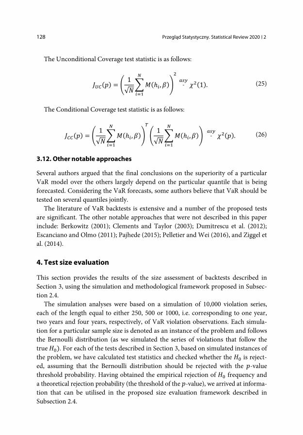
The Unconditional Coverage test statistic is as follows:
𝐽𝐽𝑈𝑈𝐶𝐶(𝑝𝑝) = �1√𝑁𝑁
�𝑀𝑀(ℎ𝑖𝑖 ,𝛽𝛽)𝐼𝐼
𝑖𝑖=1
�
2 𝑉𝑉𝑠𝑠𝑎𝑎
𝜒𝜒2(1). (25)
The Conditional Coverage test statistic is as follows:
𝐽𝐽𝐶𝐶𝐶𝐶(𝑝𝑝) = �1√𝑁𝑁
�𝑀𝑀(ℎ𝑖𝑖 ,𝛽𝛽)𝐼𝐼
𝑖𝑖=1
�
𝑇𝑇
�1√𝑁𝑁
�𝑀𝑀(ℎ𝑖𝑖 ,𝛽𝛽)𝐼𝐼
𝑖𝑖=1
�
𝑉𝑉𝑠𝑠𝑎𝑎
𝜒𝜒2(𝑝𝑝). (26)
3.12. Other notable approaches
Several authors argued that the final conclusions on the superiority of a particular VaR model over the others largely depend on the particular quantile that is being forecasted. Considering the VaR forecasts, some authors believe that VaR should be tested on several quantiles jointly. The literature of VaR backtests is extensive and a number of the proposed tests are significant. The other notable approaches that were not described in this paper include: Berkowitz (2001); Clements and Taylor (2003); Dumitrescu et al. (2012); Escanciano and Olmo (2011); Pajhede (2015); Pelletier and Wei (2016), and Ziggel et al. (2014).
4. Test size evaluation
This section provides the results of the size assessment of backtests described in Section 3, using the simulation and methodological framework proposed in Subsec-tion 2.4. The simulation analyses were based on a simulation of 10,000 violation series, each of the length equal to either 250, 500 or 1000, i.e. corresponding to one year, two years and four years, respectively, of VaR violation observations. Each simula-tion for a particular sample size is denoted as an instance of the problem and follows the Bernoulli distribution (as we simulated the series of violations that follow the true 𝐻𝐻0). For each of the tests described in Section 3, based on simulated instances of the problem, we have calculated test statistics and checked whether the 𝐻𝐻0 is reject-ed, assuming that the Bernoulli distribution should be rejected with the 𝑝𝑝-value threshold probability. Having obtained the empirical rejection of 𝐻𝐻0 frequency and a theoretical rejection probability (the threshold of the 𝑝𝑝-value), we arrived at informa- tion that can be utilised in the proposed size evaluation framework described in Subsection 2.4.
D. KASZYŃSKI, B. KAMIŃSKI, B. PANKRATZ Assessment of the size of VaR backtests for small samples 129
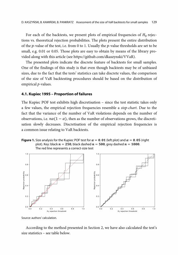
For each of the backtests, we present plots of empirical frequencies of 𝐻𝐻0 rejec-tions vs. theoretical rejection probabilities. The plots present the entire distribution of the 𝑝𝑝-value of the test, i.e. from 0 to 1. Usually the 𝑝𝑝-value thresholds are set to be small, e.g. 0.01 or 0.05. Those plots are easy to obtain by means of the library pro- vided along with this article (see https://github.com/dkaszynski/VVaR). The presented plots indicate the discrete feature of backtests for small samples. One of the findings of this study is that even though backtests may be of unbiased sizes, due to the fact that the tests’ statistics can take discrete values, the comparison of the size of VaR backtesting procedures should be based on the distribution of empirical p-values.
4.1. Kupiec 1995 – Proportion of failures
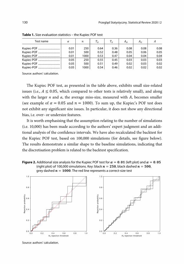
The Kupiec POF test exhibits high discretisation – since the test statistic takes only a few values, the empirical rejection frequencies resemble a step-chart. Due to the fact that the variance of the number of VaR violations depends on the number of observations, i.e. 𝑖𝑖𝛼𝛼(1− 𝛼𝛼), then as the number of observations grows, the discreti-sation slowly decreases. Discretisation of the empirical rejection frequencies is a common issue relating to VaR backtests. Figure 1. Size analysis for the Kupiec POF test for 𝜶𝜶 = 𝟎𝟎.𝟎𝟎𝟎𝟎 (left plot) and 𝜶𝜶 = 𝟎𝟎.𝟎𝟎𝟎𝟎 (right
plot). Key: black 𝒏𝒏 = 𝟐𝟐𝟎𝟎𝟎𝟎, black dashed 𝒏𝒏 = 𝟎𝟎𝟎𝟎𝟎𝟎, grey dashed 𝒏𝒏 = 𝟎𝟎𝟎𝟎𝟎𝟎𝟎𝟎. The red line represents a correct-size test
Source: authors’ calculation.
According to the method presented in Section 2, we have also calculated the test’s size statistics – see table below.
0.0 0.2 0.4 0.6 0.8 1.0H0 reject ion threshold
0.0
0.2
0.4
0.6
0.8
1.0
Rej
ectio
n pr
obab
ility
0.0 0.2 0.4 0.6 0.8 1.0H0 reject ion threshold
0.0
0.2
0.4
0.6
0.8
1.0
Rej
ectio
n pr
obab
ilit y
130 Przegląd Statystyczny. Statistical Review 2020 | 2
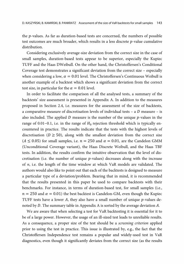
Table 1. Size evaluation statistics – the Kupiec POF test
Test name 𝛼𝛼 𝑖𝑖 𝑇𝑇𝑂𝑂 𝑇𝑇𝑈𝑈 𝐴𝐴𝑂𝑂 𝐴𝐴𝑈𝑈 𝐴𝐴
Kupiec-POF ................................. 0.01 250 0.64 0.36 0.08 0.08 0.08 Kupiec-POF ................................. 0.01 500 0.52 0.48 0.05 0.06 0.05 Kupiec-POF ................................. 0.01 1000 0.53 0.47 0.04 0.04 0.04 Kupiec-POF ................................. 0.05 250 0.55 0.45 0.03 0.03 0.03 Kupiec-POF ................................. 0.05 500 0.51 0.49 0.02 0.03 0.02 Kupiec-POF ................................. 0.05 1000 0.54 0.46 0.02 0.02 0.02
Source: authors’ calculation.
The Kupiec POF test, as presented in the table above, exhibits small size-related issues (i.e., 𝐴𝐴 ≤ 0.05, which compared to other tests is relatively small), and along with the larger n and α, the average miss-size, measured with 𝐴𝐴, becomes smaller (see example of 𝛼𝛼 = 0.05 and 𝑖𝑖 = 1000). To sum up, the Kupiec’s POF test does not exhibit any significant size issues. In particular, it does not show any directional bias, i.e. over- or undersize features. It is worth emphasising that the assumption relating to the number of simulations (i.e. 10,000) has been made according to the authors’ expert judgment and an addi-tional analysis of the confidence intervals. We have also recalculated the backtest for the Kupiec POF test, based on 100,000 simulations (for details, see figure below). The results demonstrate a similar shape to the baseline simulations, indicating that the discretisation problem is related to the backtest specification.
Figure 2. Additional size analysis for the Kupiec POF test for 𝜶𝜶 = 𝟎𝟎.𝟎𝟎𝟎𝟎 (left plot) and 𝜶𝜶 = 𝟎𝟎.𝟎𝟎𝟎𝟎
(right plot) of 100,000 simulations. Key: black 𝒏𝒏 = 𝟐𝟐𝟎𝟎𝟎𝟎, black dashed 𝒏𝒏 = 𝟎𝟎𝟎𝟎𝟎𝟎, grey dashed 𝒏𝒏 = 𝟎𝟎𝟎𝟎𝟎𝟎𝟎𝟎. The red line represents a correct-size test
Source: authors’ calculation.
0.0 0.2 0.4 0.6 0.8 1.0H0 reject ion threshold
0.0
0.2
0.4
0.6
0.8
1.0
Rej
ectio
n pr
obab
ility
0.0 0.2 0.4 0.6 0.8 1.0H0 reject ion threshold
0.0
0.2
0.4
0.6
0.8
1.0
Rej
ectio
n pr
obab
ility

D. KASZYŃSKI, B. KAMIŃSKI, B. PANKRATZ Assessment of the size of VaR backtests for small samples 131
4.2. Binomial test
The Binomial test, as presented in the figure below, exhibits similar or even higher discretisation issues, especially for small α and n, than the Kupiec POF test. As in the case of the test statistic taking only a few values, the empirical rejection frequencies resemble a step-chart. Also, due to the variance of the number of VaR, violation de-pends on the number of observations – as the number of observations and 𝛼𝛼 grow, the discretisation gradually decreases. Figure 3. Size analysis for the Binomial POF test for 𝜶𝜶 = 𝟎𝟎.𝟎𝟎𝟎𝟎 (left plot) and 𝜶𝜶 = 𝟎𝟎.𝟎𝟎𝟎𝟎
(right plot). Key: black 𝒏𝒏 = 𝟐𝟐𝟎𝟎𝟎𝟎, black dashed 𝒏𝒏 = 𝟎𝟎𝟎𝟎𝟎𝟎, grey dashed 𝒏𝒏 = 𝟎𝟎𝟎𝟎𝟎𝟎𝟎𝟎. The red line represents a correct-size test
Source: authors’ calculation. Table 2. Size evaluation statistics – the Binomial POF test
Test name 𝛼𝛼 𝑖𝑖 𝑇𝑇𝑂𝑂 𝑇𝑇𝑈𝑈 𝐴𝐴𝑂𝑂 𝐴𝐴𝑈𝑈 𝐴𝐴
Binomial-POF ............................. 0.01 250 0.55 0.45 0.09 0.08 0.09 Binomial-POF ............................. 0.01 500 0.45 0.55 0.06 0.06 0.06 Binomial-POF ............................. 0.01 1000 0.46 0.54 0.05 0.04 0.04 Binomial-POF ............................. 0.05 250 0.51 0.49 0.04 0.04 0.04 Binomial-POF ............................. 0.05 500 0.47 0.53 0.03 0.03 0.03 Binomial-POF ............................. 0.05 1000 0.50 0.50 0.02 0.02 0.02
Source: authors’ calculation. The Binomial POF test, as presented in the table above, demonstrates small size-related issues (but still bigger than the Kupiec POF test), and along with the growth of 𝑖𝑖 and 𝛼𝛼, the average miss-size, measured with A, becomes smaller (see example of 𝛼𝛼 = 0.05 and 𝑖𝑖 = 1000). The above indicates that the Binomial POF test does not exhibit any significant size issues. More specifically, there is no trace of a significant directional bias, i.e. over- or undersize features.
0.0 0.2 0.4 0.6 0.8 1.0H0 reject ion threshold
0.0
0.2
0.4
0.6
0.8
1.0
Rej
ectio
n pr
obab
ility
0.0 0.2 0.4 0.6 0.8 1.0H0 reject ion threshold
0.0
0.2
0.4
0.6
0.8
1.0R
ejec
tion
prob
abili
ty

132 Przegląd Statystyczny. Statistical Review 2020 | 2
4.3. Christoffersen 1998 tests
The Christoffersen Independence test – one of the most popular of all the backtests presented in this study – verifies whether the VaR violations tend to cluster. The 𝑝𝑝-value of the test is highly discrete, as the number of possible outcomes is finite and small. In fact, this test measures the number of cases where one VaR violation is strictly followed by another violation, which is a very rare situation in the case of small samples.
Figure 4. Size analysis for the Christoffersen Independence Coverage test for 𝜶𝜶 = 𝟎𝟎.𝟎𝟎𝟎𝟎
(left plot) and 𝜶𝜶 = 𝟎𝟎.𝟎𝟎𝟎𝟎 (right plot). Key: black 𝒏𝒏 = 𝟐𝟐𝟎𝟎𝟎𝟎, black dashed 𝒏𝒏 = 𝟎𝟎𝟎𝟎𝟎𝟎, grey dashed 𝒏𝒏 = 𝟎𝟎𝟎𝟎𝟎𝟎𝟎𝟎. The red line represents a correct-size test
Source: authors’ calculation.
Table 3. Size evaluation statistics – Christoffersen Independence Coverage test
Test name 𝛼𝛼 𝑖𝑖 𝑇𝑇𝑂𝑂 𝑇𝑇𝑈𝑈 𝐴𝐴𝑂𝑂 𝐴𝐴𝑈𝑈 𝐴𝐴
Christoffersen-Ind. ................... 0.01 250 0.07 0.93 0.04 0.31 0.29 Christoffersen-Ind. ................... 0.01 500 0.14 0.86 0.03 0.26 0.23 Christoffersen-Ind. ................... 0.01 1000 0.28 0.72 0.09 0.19 0.16 Christoffersen-Ind. ................... 0.05 250 0.77 0.23 0.12 0.03 0.10 Christoffersen-Ind. ................... 0.05 500 0.81 0.19 0.06 0.01 0.05 Christoffersen-Ind. ................... 0.05 1000 0.91 0.09 0.02 0.01 0.02
Source: authors’ calculation.
The size of the test improves significantly with the increase of 𝛼𝛼. In this case, the backtest demonstrates a significantly improved distribution of the 𝑝𝑝-value.
0.0 0.2 0.4 0.6 0.8 1.0H0 reject ion threshold
0.0
0.2
0.4
0.6
0.8
1.0
Rej
ectio
n pr
obab
ility
0.0 0.2 0.4 0.6 0.8 1.0H0 reject ion threshold
0.0
0.2
0.4
0.6
0.8
1.0
Rej
ectio
n pr
obab
ility

D. KASZYŃSKI, B. KAMIŃSKI, B. PANKRATZ Assessment of the size of VaR backtests for small samples 133
As regards the combined test, i.e. the conditional coverage, devised by Christoffersen (1998), the results are presented below.
Figure 5. Size analysis for the Christoffersen Conditional Coverage test for 𝜶𝜶 = 𝟎𝟎.𝟎𝟎𝟎𝟎 (left plot)
and 𝜶𝜶 = 𝟎𝟎.𝟎𝟎𝟎𝟎 (right plot). Key: black 𝒏𝒏 = 𝟐𝟐𝟎𝟎𝟎𝟎, black dashed 𝒏𝒏 = 𝟎𝟎𝟎𝟎𝟎𝟎, grey dashed 𝒏𝒏 = 𝟎𝟎𝟎𝟎𝟎𝟎𝟎𝟎. The red line represents a correct-size test
Source: authors’ calculation.
Table 4. Size evaluation statistics – the Christoffersen Conditional Coverage test
Test name 𝛼𝛼 𝑖𝑖 𝑇𝑇𝑂𝑂 𝑇𝑇𝑈𝑈 𝐴𝐴𝑂𝑂 𝐴𝐴𝑈𝑈 𝐴𝐴
Christoffersen-CCoverage ..... 0.01 250 0.29 0.71 0.04 0.13 0.10 Christoffersen-CCoverage ..... 0.01 500 0.50 0.50 0.04 0.09 0.07 Christoffersen-CCoverage ..... 0.01 1000 0.67 0.33 0.05 0.05 0.05 Christoffersen-CCoverage ..... 0.05 250 1.00 0.00 0.14 0.00 0.14 Christoffersen-CCoverage ..... 0.05 500 0.99 0.01 0.12 0.00 0.12 Christoffersen-CCoverage ..... 0.05 1000 1.00 0.00 0.11 0.00 0.11
Source: authors’ calculation.
4.4. Kupiec 1995 – Time until first failure
The Kupiec TUFF test, which, due to a significantly higher number of possible out-comes (i.e. the distribution of the possible outcome is much wider than in the POF test), exhibits less severe discretisation issues than the Kupiec POF test. Moreover, this test does not show any significant deviation, e.g. in terms of the maximal measure, from the uniform distribution, i.e. the black/grey lines lie close to the red line. This finding – a better size of the duration test – will be further discussed along with other examples of VaR backtests of this kind.
0.0 0.2 0.4 0.6 0.8 1.0H0 reject ion threshold
0.0
0.2
0.4
0.6
0.8
1.0
Rej
ectio
n pr
obab
ility
0.0 0.2 0.4 0.6 0.8 1.0H0 reject ion threshold
0.0
0.2
0.4
0.6
0.8
1.0
Rej
ectio
n pr
obab
ility

134 Przegląd Statystyczny. Statistical Review 2020 | 2
Figure 6. Size analysis for the Kupiec TUFF test for 𝜶𝜶 = 𝟎𝟎.𝟎𝟎𝟎𝟎 (left plot) and 𝜶𝜶 = 𝟎𝟎.𝟎𝟎𝟎𝟎 (right plot). Key: black 𝒏𝒏 = 𝟐𝟐𝟎𝟎𝟎𝟎, black dashed 𝒏𝒏 = 𝟎𝟎𝟎𝟎𝟎𝟎, grey dashed 𝒏𝒏 = 𝟎𝟎𝟎𝟎𝟎𝟎𝟎𝟎. The red line represents a correct-size test
Source: authors’ calculation.
According to the method presented in Section 2, the test’s size statistics have also been calculated (for details see the table below). Table 5. Size evaluation statistics – the Kupiec TUFF test
Test name 𝛼𝛼 𝑖𝑖 𝑇𝑇𝑂𝑂 𝑇𝑇𝑈𝑈 𝐴𝐴𝑂𝑂 𝐴𝐴𝑈𝑈 𝐴𝐴
Kupiec-TUFF ............................... 0.01 250 0.78 0.22 0.02 0.02 0.02 Kupiec-TUFF ............................... 0.01 500 0.98 0.02 0.02 0.00 0.02 Kupiec-TUFF ............................... 0.01 1000 0.99 0.01 0.02 0.00 0.02 Kupiec-TUFF ............................... 0.05 250 0.92 0.08 0.02 0.01 0.02 Kupiec-TUFF ............................... 0.05 500 0.93 0.07 0.03 0.01 0.03 Kupiec-TUFF ............................... 0.05 1000 0.94 0.06 0.03 0.01 0.03
Source: authors’ calculation.
The Kupiec TUFF test (which is an example of a duration test), as presented in the table above, demonstrates small size-related issues. The size of the test shows small improvement along with the increase in 𝛼𝛼 and 𝑖𝑖.
4.5. Haas 2001 – Time Between Failures
The Haas’s TBF test is another example of a duration approach towards VaR evalu- ation. As in the Kupiec TUFF, the distribution of the 𝑝𝑝-value is less discrete than it was in the case of the POF tests. Although, intuitively, the observation of more VaR violations should improve the test specification, the results suggest oversize-related issues. This is not surprising, though, as the test statistic assumes the independence
0.0 0.2 0.4 0.6 0.8 1.0H0 reject ion threshold
0.0
0.2
0.4
0.6
0.8
1.0
Rej
ectio
n pr
obab
ility
0.0 0.2 0.4 0.6 0.8 1.0H0 reject ion threshold
0.0
0.2
0.4
0.6
0.8
1.0
Rej
ectio
n pr
obab
ility

D. KASZYŃSKI, B. KAMIŃSKI, B. PANKRATZ Assessment of the size of VaR backtests for small samples 135
of aggregated random variables, while – especially for small samples (as in our tests) – they are in fact dependent; e.g. if we observe that first-time failure is very extensive, then clearly in the subsequent instances it must be small, as we have a short test horizon. Figure 7. Size analysis for Haas’s TBF test for 𝜶𝜶 = 𝟎𝟎.𝟎𝟎𝟎𝟎 (left plot) and 𝜶𝜶 = 𝟎𝟎.𝟎𝟎𝟎𝟎 (right plot).
Key: black 𝒏𝒏 = 𝟐𝟐𝟎𝟎𝟎𝟎, black dashed 𝒏𝒏 = 𝟎𝟎𝟎𝟎𝟎𝟎, grey dashed 𝒏𝒏 = 𝟎𝟎𝟎𝟎𝟎𝟎𝟎𝟎. The red line represents a correct-size test
Source: authors’ calculation. Table 6. Size evaluation statistics – Haas’s TBF test
Test name 𝛼𝛼 𝑖𝑖 𝑇𝑇𝑂𝑂 𝑇𝑇𝑈𝑈 𝐴𝐴𝑂𝑂 𝐴𝐴𝑈𝑈 𝐴𝐴
Haas-TBF ...................................... 0.01 250 0.86 0.14 0.05 0.01 0.05 Haas-TBF ...................................... 0.01 500 1.00 0.00 0.05 0.00 0.05 Haas-TBF ...................................... 0.01 1000 1.00 0.00 0.08 0.00 0.08 Haas-TBF ...................................... 0.05 250 1.00 0.00 0.09 0.00 0.09 Haas-TBF ...................................... 0.05 500 1.00 0.00 0.14 0.00 0.14 Haas-TBF ...................................... 0.05 1000 1.00 0.00 0.20 0.00 0.20
Source: authors’ calculation.
As presented in the table above, the Haas TBF test exhibits relatively small size-related issues. However, with the larger 𝛼𝛼 and 𝑖𝑖 the test exhibits significant oversize issues.
4.6. Christoffersen and Pelletier 2004 – Continuous Weibull
The Christoffersen Continuous Weibull test is yet another instance of a duration approach. Unlike the previous examples, however, this test assumes the distribution of a duration between VaR violations, thus it falls within the category of analytical-based approaches. In terms of small VaR violation cases (e.g. 𝛼𝛼 = 0.01), the 𝑝𝑝-value
0.0 0.2 0.4 0.6 0.8 1.0H0 reject ion threshold
0.0
0.2
0.4
0.6
0.8
1.0
Rej
ectio
n pr
obab
ility
0.0 0.2 0.4 0.6 0.8 1.0H0 reject ion threshold
0.0
0.2
0.4
0.6
0.8
1.0
Rej
ectio
n pr
obab
ility

136 Przegląd Statystyczny. Statistical Review 2020 | 2
distribution of the tests indicated significant deviations from the uniform distribu-tion. The distinctive jump on the right-hand side of the plots (in both 𝛼𝛼 = 0.01 and 𝛼𝛼 = 0.05) is caused by problems with convergence of numerical optimisation methods – in this example, the Weibull distribution parameters were calibrated using only a few examples. Figure 8. Size analysis for the Christoffersen Continuous Weibull test for 𝜶𝜶 = 𝟎𝟎.𝟎𝟎𝟎𝟎 (left plot)
and 𝜶𝜶 = 𝟎𝟎.𝟎𝟎𝟎𝟎 (right plot). Key: black 𝒏𝒏 = 𝟐𝟐𝟎𝟎𝟎𝟎, black dashed 𝒏𝒏 = 𝟎𝟎𝟎𝟎𝟎𝟎, grey dashed 𝒏𝒏 = 𝟎𝟎𝟎𝟎𝟎𝟎𝟎𝟎. The red line represents a correct size-test
Source: authors’ calculation. Table 7. Size evaluation statistics – the Christoffersen Continuous Weibull test
Test name 𝛼𝛼 𝑖𝑖 𝑇𝑇𝑂𝑂 𝑇𝑇𝑈𝑈 𝐴𝐴𝑂𝑂 𝐴𝐴𝑈𝑈 𝐴𝐴
Christoffersen-CWeibull ......... 0.01 250 0.00 1.00 0.00 0.28 0.28 Christoffersen-CWeibull ......... 0.01 500 0.00 1.00 0.00 0.18 0.18 Christoffersen-CWeibull ......... 0.01 1000 0.00 1.00 0.00 0.11 0.11 Christoffersen-CWeibull ......... 0.05 250 0.26 0.74 0.00 0.09 0.07 Christoffersen-CWeibull ......... 0.05 500 0.60 0.40 0.03 0.06 0.04 Christoffersen-CWeibull ......... 0.05 1000 0.78 0.22 0.06 0.04 0.05
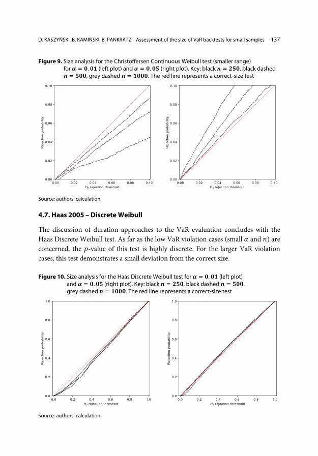
Source: authors’ calculation. The Christoffersen Continuous Weibull test, as duration tests in general, size of the test improves as the number of VaR violations increases. Even though the tests appear to depart from the perfect size (i.e. red line on the plot) throughout the entire range of rejection thresholds, as mentioned earlier, the thresholds of statistical tests are usually small. In the case of the Christoffersen Continuous Weibull, the figure on the smaller range, i.e. 0 − 0.1, is presented below. As regards the figure, the test on the threshold usually applied (for the 𝛼𝛼 = 0.05), appears to be more adequate.
0.0 0.2 0.4 0.6 0.8 1.0H0 reject ion threshold
0.0
0.2
0.4
0.6
0.8
1.0
Rej
ectio
n pr
obab
ility
0.0 0.2 0.4 0.6 0.8 1.0H0 reject ion threshold
0.0
0.2
0.4
0.6
0.8
1.0
Rej
ectio
n pr
obab
ility
D. KASZYŃSKI, B. KAMIŃSKI, B. PANKRATZ Assessment of the size of VaR backtests for small samples 137
Figure 9. Size analysis for the Christoffersen Continuous Weibull test (smaller range) for 𝜶𝜶 = 𝟎𝟎.𝟎𝟎𝟎𝟎 (left plot) and 𝜶𝜶 = 𝟎𝟎.𝟎𝟎𝟎𝟎 (right plot). Key: black 𝒏𝒏 = 𝟐𝟐𝟎𝟎𝟎𝟎, black dashed 𝒏𝒏 = 𝟎𝟎𝟎𝟎𝟎𝟎, grey dashed 𝒏𝒏 = 𝟎𝟎𝟎𝟎𝟎𝟎𝟎𝟎. The red line represents a correct-size test
Source: authors’ calculation.
4.7. Haas 2005 – Discrete Weibull
The discussion of duration approaches to the VaR evaluation concludes with the Haas Discrete Weibull test. As far as the low VaR violation cases (small 𝛼𝛼 and 𝑖𝑖) are concerned, the 𝑝𝑝-value of this test is highly discrete. For the larger VaR violation cases, this test demonstrates a small deviation from the correct size. Figure 10. Size analysis for the Haas Discrete Weibull test for 𝜶𝜶 = 𝟎𝟎.𝟎𝟎𝟎𝟎 (left plot)
and 𝜶𝜶 = 𝟎𝟎.𝟎𝟎𝟎𝟎 (right plot). Key: black 𝒏𝒏 = 𝟐𝟐𝟎𝟎𝟎𝟎, black dashed 𝒏𝒏 = 𝟎𝟎𝟎𝟎𝟎𝟎, grey dashed 𝒏𝒏 = 𝟎𝟎𝟎𝟎𝟎𝟎𝟎𝟎. The red line represents a correct-size test
Source: authors’ calculation.
0.00 0.02 0.04 0.06 0.08 0.10H0 reject ion threshold
0.00
0.02
0.04
0.06
0.08
0.10
Rej
ectio
n pr
obab
ility
0.00 0.02 0.04 0.06 0.08 0.10H0 reject ion threshold
0.00
0.02
0.04
0.06
0.08
0.10
Rej
ectio
n pr
obab
ility
0.0 0.2 0.4 0.6 0.8 1.0H0 reject ion threshold
0.0
0.2
0.4
0.6
0.8
1.0
Rej
ectio
n pr
obab
ility
0.0 0.2 0.4 0.6 0.8 1.0H0 reject ion threshold
0.0
0.2
0.4
0.6
0.8
1.0
Rej
ectio
n pr
obab
ility

138 Przegląd Statystyczny. Statistical Review 2020 | 2
Table 8. Size evaluation statistics – the Haas Discrete Weibull test
Test name 𝛼𝛼 𝑖𝑖 𝑇𝑇𝑂𝑂 𝑇𝑇𝑈𝑈 𝐴𝐴𝑂𝑂 𝐴𝐴𝑈𝑈 𝐴𝐴
Haas-DWeibull .......................... 0.01 250 0.17 0.83 0.00 0.04 0.03 Haas-DWeibull .......................... 0.01 500 0.02 0.98 0.00 0.04 0.04 Haas-DWeibull .......................... 0.01 1000 0.04 0.96 0.00 0.03 0.02 Haas-DWeibull .......................... 0.05 250 0.70 0.30 0.02 0.02 0.02 Haas-DWeibull .......................... 0.05 500 0.84 0.16 0.01 0.01 0.01 Haas-DWeibull .......................... 0.05 1000 0.92 0.08 0.01 0.00 0.01
Source: authors’ calculation.
Due to the approach applied in the test, it is usually compared with its continuous version, i.e. the Christoffersen Continuous Weibull. Regarding those two specifica-tions, the discrete version preserves better size properties taking into account the size evaluation statistics.
4.8. Engle and Manganelli 2004 – DQ
The Engle and Manganelli backtest verifies whether VaR violations can be explained by a linear regression of previous violations (in fact, this test can also take into ac-count other exogenous variables). Figure 11. Size analysis for the Engle DQ test for 𝜶𝜶 = 𝟎𝟎.𝟎𝟎𝟎𝟎 (left plot) and 𝜶𝜶 = 𝟎𝟎.𝟎𝟎𝟎𝟎 (right plot).
Key: black 𝒏𝒏 = 𝟐𝟐𝟎𝟎𝟎𝟎, black dashed 𝒏𝒏 = 𝟎𝟎𝟎𝟎𝟎𝟎, grey dashed 𝒏𝒏 = 𝟎𝟎𝟎𝟎𝟎𝟎𝟎𝟎. The red line represents a correct-size test
Source: authors’ calculation.
0.0 0.2 0.4 0.6 0.8 1.0H0 reject ion threshold
0.0
0.2
0.4
0.6
0.8
1.0
Rej
ectio
n pr
obab
ility
0.0 0.2 0.4 0.6 0.8 1.0H0 reject ion threshold
0.0
0.2
0.4
0.6
0.8
1.0
Rej
ectio
n pr
obab
ility

D. KASZYŃSKI, B. KAMIŃSKI, B. PANKRATZ Assessment of the size of VaR backtests for small samples 139
Table 9. Size evaluation statistics – the Engle DQ test
Test name 𝛼𝛼 𝑖𝑖 𝑇𝑇𝑂𝑂 𝑇𝑇𝑈𝑈 𝐴𝐴𝑂𝑂 𝐴𝐴𝑈𝑈 𝐴𝐴
Engle-DQ ..................................... 0.01 250 0.12 0.88 0.06 0.40 0.36 Engle-DQ ..................................... 0.01 500 0.21 0.79 0.08 0.35 0.29 Engle-DQ ..................................... 0.01 1000 0.38 0.62 0.04 0.25 0.17 Engle-DQ ..................................... 0.05 250 0.26 0.74 0.03 0.09 0.08 Engle-DQ ..................................... 0.05 500 0.25 0.75 0.01 0.05 0.04 Engle-DQ ..................................... 0.05 1000 0.27 0.73 0.00 0.02 0.02
Source: authors’ calculation.
The 𝑝𝑝-value of the test relating to low VaR violation cases is highly deviated from the uniform distribution. As far as the high VaR violation cases are concerned, the size of the tests significantly improves.
4.9. Berkowitz 2005 – Ljung-Box
Berkowitz’s Ljung-Box backtest verifies whether VaR violations are autocorrelated with the degree of 𝑘𝑘 (in this experiment, a 𝑘𝑘 = 5 set is implemented). Figure 12. Size analysis for Berkowitz’s Ljung-Box test for 𝜶𝜶 = 𝟎𝟎.𝟎𝟎𝟎𝟎 (left plot) and 𝜶𝜶 = 𝟎𝟎.𝟎𝟎𝟎𝟎
(right plot). Key: black 𝒏𝒏 = 𝟐𝟐𝟎𝟎𝟎𝟎, black dashed 𝒏𝒏 = 𝟎𝟎𝟎𝟎𝟎𝟎, grey dashed 𝒏𝒏 = 𝟎𝟎𝟎𝟎𝟎𝟎𝟎𝟎. The red line represents a correct-size test
Source: authors’ calculation.
Table 10. Size evaluation statistics – Berkowitz’s Ljung-Box test
Test name 𝛼𝛼 𝑖𝑖 𝑇𝑇𝑂𝑂 𝑇𝑇𝑈𝑈 𝐴𝐴𝑂𝑂 𝐴𝐴𝑈𝑈 𝐴𝐴
Berkowitz-BoxLjung ................ 0.01 250 0.06 0.94 0.02 0.44 0.42 Berkowitz-BoxLjung ................ 0.01 500 0.11 0.89 0.03 0.39 0.36 Berkowitz-BoxLjung ................ 0.01 1000 0.14 0.86 0.03 0.31 0.27
0.0 0.2 0.4 0.6 0.8 1.0H0 reject ion threshold
0.0
0.2
0.4
0.6
0.8
1.0
Rej
ectio
n pr
obab
ility
0.0 0.2 0.4 0.6 0.8 1.0H0 reject ion threshold
0.0
0.2
0.4
0.6
0.8
1.0
Rej
ectio
n pr
obab
ility

140 Przegląd Statystyczny. Statistical Review 2020 | 2
Table 11. Size evaluation statistics – Berkowitz’s Ljung-Box test (cont.)
Test name 𝛼𝛼 𝑖𝑖 𝑇𝑇𝑂𝑂 𝑇𝑇𝑈𝑈 𝐴𝐴𝑂𝑂 𝐴𝐴𝑈𝑈 𝐴𝐴
Berkowitz-BoxLjung ................ 0.05 250 0.03 0.97 0.01 0.16 0.15 Berkowitz-BoxLjung ................ 0.05 500 0.02 0.98 0.00 0.13 0.13 Berkowitz-BoxLjung ................ 0.05 1000 0.01 0.99 0.00 0.11 0.11
Source: authors’ calculation.
The 𝑝𝑝-value of the test for the low VaR violation cases is highly deviated from the uniform distribution. Concerning the high VaR violation cases, the size of the tests improves, but, nevertheless, remains below the correct value.
4.10. Krämer and Wied 2015 – Gini coefficient
The Krämer and Wied backtest is a duration-type test, but contrary to the previous ones, it is based on the Gini coefficient. Figure 13. Size analysis of Krämer’s Gini coefficient test for 𝜶𝜶 = 𝟎𝟎.𝟎𝟎𝟎𝟎 (left plot)
and 𝜶𝜶 = 𝟎𝟎.𝟎𝟎𝟎𝟎 (right plot). Key: black 𝒏𝒏 = 𝟐𝟐𝟎𝟎𝟎𝟎, black dashed 𝒏𝒏 = 𝟎𝟎𝟎𝟎𝟎𝟎, grey dashed 𝒏𝒏 = 𝟎𝟎𝟎𝟎𝟎𝟎𝟎𝟎. The red line represents a correct-size test
Source: authors’ calculation.
Table 12. Size evaluation statistics – Krämer’s Gini coefficient test
Test name 𝛼𝛼 𝑖𝑖 𝑇𝑇𝑂𝑂 𝑇𝑇𝑈𝑈 𝐴𝐴𝑂𝑂 𝐴𝐴𝑈𝑈 𝐴𝐴
Kramer-GINI ................................ 0.01 250 1.00 0.00 0.29 0.00 0.29 Kramer-GINI ................................ 0.01 500 1.00 0.00 0.30 0.00 0.30 Kramer-GINI ................................ 0.01 1000 1.00 0.00 0.30 0.00 0.30 Kramer-GINI ................................ 0.05 250 1.00 0.00 0.09 0.00 0.09 Kramer-GINI ................................ 0.05 500 1.00 0.00 0.09 0.00 0.09 Kramer-GINI ................................ 0.05 1000 1.00 0.00 0.07 0.00 0.07
Source: authors’ calculation.
0.0 0.2 0.4 0.6 0.8 1.0H0 reject ion threshold
0.0
0.2
0.4
0.6
0.8
1.0
Rej
ectio
n pr
obab
ility
0.0 0.2 0.4 0.6 0.8 1.0H0 reject ion threshold
0.0
0.2
0.4
0.6
0.8
1.0
Rej
ectio
n pr
obab
ility
D. KASZYŃSKI, B. KAMIŃSKI, B. PANKRATZ Assessment of the size of VaR backtests for small samples 141
As the authors emphasise in the article (Krämer and Wied 2015), simulation is the preferable approach to size evaluation. Based on our calculation (assuming asymp-totic distribution of a test’s statistics), the test for low VaR violation instances proves strongly oversized. This problem is much smaller in the case of the high-volume VaR violations scenarios.
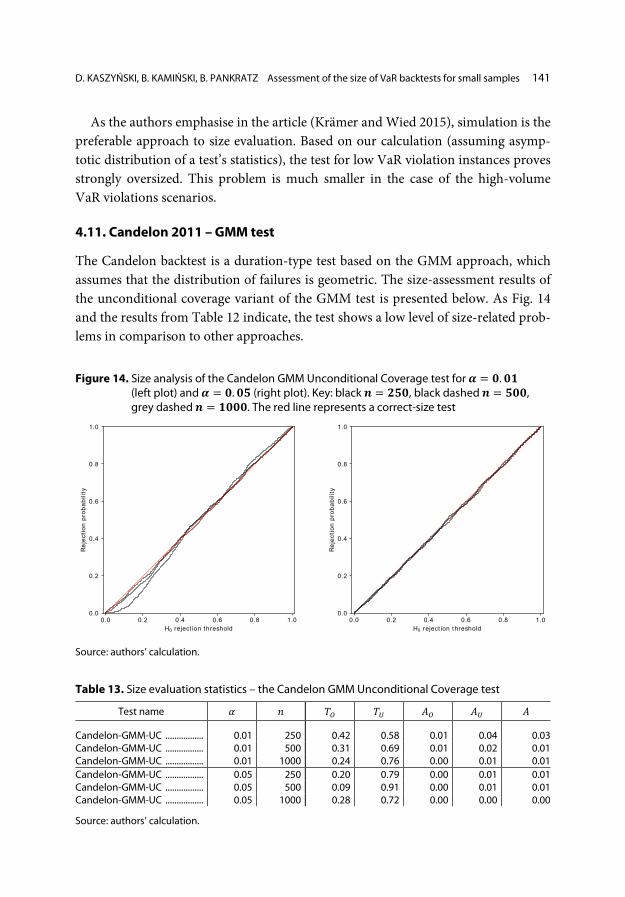
4.11. Candelon 2011 – GMM test
The Candelon backtest is a duration-type test based on the GMM approach, which assumes that the distribution of failures is geometric. The size-assessment results of the unconditional coverage variant of the GMM test is presented below. As Fig. 14 and the results from Table 12 indicate, the test shows a low level of size-related prob-lems in comparison to other approaches.
Figure 14. Size analysis of the Candelon GMM Unconditional Coverage test for 𝜶𝜶 = 𝟎𝟎.𝟎𝟎𝟎𝟎
(left plot) and 𝜶𝜶 = 𝟎𝟎.𝟎𝟎𝟎𝟎 (right plot). Key: black 𝒏𝒏 = 𝟐𝟐𝟎𝟎𝟎𝟎, black dashed 𝒏𝒏 = 𝟎𝟎𝟎𝟎𝟎𝟎, grey dashed 𝒏𝒏 = 𝟎𝟎𝟎𝟎𝟎𝟎𝟎𝟎. The red line represents a correct-size test
Source: authors’ calculation.
Table 13. Size evaluation statistics – the Candelon GMM Unconditional Coverage test
Test name 𝛼𝛼 𝑖𝑖 𝑇𝑇𝑂𝑂 𝑇𝑇𝑈𝑈 𝐴𝐴𝑂𝑂 𝐴𝐴𝑈𝑈 𝐴𝐴
Candelon-GMM-UC ................. 0.01 250 0.42 0.58 0.01 0.04 0.03 Candelon-GMM-UC ................. 0.01 500 0.31 0.69 0.01 0.02 0.01 Candelon-GMM-UC ................. 0.01 1000 0.24 0.76 0.00 0.01 0.01 Candelon-GMM-UC ................. 0.05 250 0.20 0.79 0.00 0.01 0.01 Candelon-GMM-UC ................. 0.05 500 0.09 0.91 0.00 0.01 0.01 Candelon-GMM-UC ................. 0.05 1000 0.28 0.72 0.00 0.00 0.00
Source: authors’ calculation.
0.0 0.2 0.4 0.6 0.8 1.0H0 reject ion threshold
0.0
0.2
0.4
0.6
0.8
1.0
Rej
ectio
n pr
obab
ility
0.0 0.2 0.4 0.6 0.8 1.0H0 reject ion threshold
0.0
0.2
0.4
0.6
0.8
1.0
Rej
ectio
n pr
obab
ility

142 Przegląd Statystyczny. Statistical Review 2020 | 2
In terms of the Conditional Coverage variant of that test, the simulation results are shown in the figure / table below. Figure 15. Size analysis of the Candelon GMM Conditional Coverage test for 𝜶𝜶 = 𝟎𝟎.𝟎𝟎𝟎𝟎 (left
plot) and 𝜶𝜶 = 𝟎𝟎.𝟎𝟎𝟎𝟎 (right plot). Key: black 𝒏𝒏 = 𝟐𝟐𝟎𝟎𝟎𝟎, black dashed 𝒏𝒏 = 𝟎𝟎𝟎𝟎𝟎𝟎, grey dashed 𝒏𝒏 = 𝟎𝟎𝟎𝟎𝟎𝟎𝟎𝟎. The red line represents a correct-size test
Source: authors’ calculation. Table 14. Size evaluation statistics – the Candelon GMM Conditional Coverage test
Test name 𝛼𝛼 𝑖𝑖 𝑇𝑇𝑂𝑂 𝑇𝑇𝑈𝑈 𝐴𝐴𝑂𝑂 𝐴𝐴𝑈𝑈 𝐴𝐴
Candelon-GMM-CC ................. 0.01 250 0.06 0.94 0.01 0.16 0.16 Candelon-GMM-CC ................. 0.01 500 0.02 0.98 0.00 0.13 0.12 Candelon-GMM-CC ................. 0.01 1000 0.05 0.95 0.00 0.09 0.09 Candelon-GMM-CC ................. 0.05 250 0.04 0.96 0.01 0.08 0.08 Candelon-GMM-CC ................. 0.05 500 0.05 0.95 0.01 0.05 0.05 Candelon-GMM-CC ................. 0.05 1000 0.08 0.92 0.00 0.04 0.04
Source: authors’ calculation.
5. Conclusions
The presented methodology and size plots indicate the discrete nature of backtests for small samples. One of the findings demonstrates that even though backtests may have unbiased sizes, the comparison of the size of VaR backtesting procedures should be based on the distribution of empirical 𝑝𝑝-values due to the fact that tests’ statistics can take discrete values. The authors’ intention was to strongly emphasise the relatively significant discretisation of POF tests, which is less severe in the case of duration-based tests. This effect results from the number of possible (and probable) values of the tests’ inputs. As regards frequency-based tests, for small samples the test statistic is usually limited to only a few values, and in effect a few test outcomes –
0.0 0.2 0.4 0.6 0.8 1.0H0 reject ion threshold
0.0
0.2
0.4
0.6
0.8
1.0
Rej
ectio
n pr
obab
ility
0.0 0.2 0.4 0.6 0.8 1.0H0 reject ion threshold
0.0
0.2
0.4
0.6
0.8
1.0
Rej
ectio
n pr
obab
ility
D. KASZYŃSKI, B. KAMIŃSKI, B. PANKRATZ Assessment of the size of VaR backtests for small samples 143
the 𝑝𝑝-values. As far as duration-based tests are concerned, the numbers of possible test outcomes are much broader, which results in a less discrete 𝑝𝑝-value cumulative distribution. Considering exclusively average-size deviation from the correct size in the case of small samples, duration-based tests appear to be superior, especially the Kupiec TUFF and the Haas DWeibull. On the other hand, the Christoffersen’s Conditional Coverage test demonstrates a significant deviation from the correct size – especially when considering a low, 𝛼𝛼 = 0.01 level. The Christoffersen’s Continuous Weibull is another example of a backtest which shows a significant deviation from the correct test size, in particular for the 𝛼𝛼 = 0.01 level. In order to facilitate the comparison of all the analysed tests, a summary of the backtests’ size assessment is presented in Appendix A. In addition to the measures proposed in Section 2.4, i.e. measures for the assessment of the size of backtests, a comparative measure of discretisation levels of individual tests – a 𝐷𝐷 measure – is also included. The applied 𝐷𝐷 measure is the number of the unique 𝑝𝑝-values in the range of 0.01−0.1, i.e. in the range of 𝐻𝐻0 rejection threshold which is typically en-countered in practice. The results indicate that the tests with the highest levels of discretisation (𝐷𝐷 ≥ 50), along with the smallest deviation from the correct size (𝐴𝐴 ≤ 0.05) for small samples, i.e. 𝑖𝑖 = 250 and 𝛼𝛼 = 0.01, are the Candelon GMM (Unconditional Coverage variant), the Haas Discrete Weibull, and the Haas TBF tests. In addition, the results confirm the intuitive observation that the level of dis-cretisation (i.e. the number of unique 𝑝𝑝-values) decreases along with the increase of n, i.e. the length of the time window at which VaR models are validated. The authors would also like to point out that each of the backtests is designed to measure a particular type of a deviation/problem. Bearing that in mind, it is recommended that the results presented in this paper be used to compare backtests with their benchmarks. For instance, in terms of duration-based test, for small samples (i.e., 𝑖𝑖 = 250 and 𝛼𝛼 = 0.01) the best backtest is Candelon-GM, even though the Kupiec TUFF tests have a lower 𝐴𝐴, they also have a small number of unique 𝑝𝑝-values de- noted by 𝐷𝐷. The summary table in Appendix A is sorted by the average deviation 𝐴𝐴. We are aware that when selecting a test for VaR backtesting it is essential for it to be of a large power. However, the usage of an ill-sized test leads to unreliable results. As a consequence, a proper size of the test should be a screening criterion applied prior to using the test in practice. This issue is illustrated by, e.g., the fact that the Christoffersen Independence test remains a popular and widely-used test in VaR diagnostics, even though it significantly deviates from the correct size (as the results

144 Przegląd Statystyczny. Statistical Review 2020 | 2
of our analysis show). In practice, the analysis of the power of the considered tests should be performed along with the consideration of the proper size of the test. However, regarding VaR backtesting, it is challenging to provide a similar analysis to the one we presented for test sizes, as there are no equally-powerful VaR backtests (different tests are sensitive to different violations of the assumptions). Therefore, the choice of an appropriate backtest should depend on the kind of deviation the analyst strives most to detect (alternatively, using several tests in combination may be consid-ered, provided that all of them are of an acceptable quality in terms of their size). The practical suggestion resulting from this study is that instead of using theoretic- al formulas for 𝑝𝑝-values of the discussed tests (that are only asymptotic), which is common practice, it is advisable to produce a simulated distribution of the statistics for a given test (knowing 𝛼𝛼 and 𝑖𝑖), and compute the 𝑝𝑝-values against such a distri-bution. This procedure makes it possible, at least to some extent, to mitigate the risk of applying over- or undersized tests in the case of the limited sample size 𝑖𝑖 and small 𝛼𝛼 level. Unfortunately, such a simulation does not remove the discretisation effect in tests which display such features.
References
Altman, D. G. (1991). Practical Statistics for Medical Research. London: Chapman & Hall/CRC. https://www.scribd.com/doc/273959883/Douglas-G-Altman-Practical-Statistics-for-Medical -Research-Chapman-Hall-CRC-1991
BCBS. (1996). Supervisory framework for the use of “backtesting” in conjunction with the internal models approach to market risk capital requirements. Basel: Basle Committee on Banking Super-vision. https://www.bis.org/publ/bcbs22.pdf
BCBS. (2009). Revisions to the Basel II market risk framework. Basel: Bank for International Settle-ments. https://www.bis.org/publ/bcbs158.pdf
Berkowitz, J. (2001). Testing Density Forecasts, with Applications to Risk Management. Journal of Business & Economic Statistics, 19(4), 465–474. https://doi.org/10.1198/07350010152596718
Berkowitz, J., Christoffersen, P., Pelletier, D. (2011). Evaluating Value-at-Risk Models with Desk- -Level Data. Management Science, 57(12), 2213–2227. https://doi.org/10.1287/mnsc.1080.0964
Bontemps, C. (2014). Moment-based tests for discrete distributions. (IDEI Working Paper, n. 772). http://idei.fr/sites/default/files/medias/doc/by/bontemps/discrete-15oct2014.pdf
Campbell, S. D. (2006). A review of backtesting and backtesting procedures. Journal of Risk, 9(2), 1–17. http://dx.doi.org/10.21314/JOR.2007.146
Candelon, B., Colletaz, G., Hurlin, C., Tokpavi, S. (2011). Backtesting Value-at-Risk: a GMM Duration-Based Test. Journal of Financial Econometrics, 9(2), 314–343. https://doi.org/10.1093 /jjfinec/nbq025
Christoffersen, P. F. (1998). Evaluating Interval Forecasts. International economic review, 39(4), 841–862. https://doi.org/10.2307/2527341
D. KASZYŃSKI, B. KAMIŃSKI, B. PANKRATZ Assessment of the size of VaR backtests for small samples 145
Christoffersen, P., Pelletier, D. (2004). Backtesting Value-at-Risk: A Duration-Based Approach. Journal of Financial Econometrics, 2(1), 84–108. https://doi.org/10.1093/jjfinec/nbh004
Clements, M. P., Taylor, N. (2003). Evaluating interval forecasts of high-frequency financial data. Journal of Applied Econometrics, 18(4), 445–456. https://doi.org/10.1002/jae.703
Dowd, K. (1998). Beyond Value at Risk: The New Science of Risk Management. Chichester: John Wiley & Sons.
Dumitrescu, E. I., Hurlin, C., Pham, V. (2012). Backtesting Value-at-Risk: From Dynamic Quantile to Dynamic Binary Tests. Finance, 33(1), 79–112. https://www.cairn-int.info/journal-finance -2012-1-page-79.htm?WT.tsrc=cairnPdf#
Engle, R. F., Manganelli, S. (2004). CAViaR: Conditional Autoregressive Value at Risk by Regres-sion Quantiles. Journal of Business & Economic Statistics, 22(4), 367–381. https://doi.org /10.1198/073500104000000370
Escanciano, J. C., Olmo, J. (2011). Robust Backtesting Tests for Value-at-risk Models. Journal of Financial Econometrics, 9(1), 132–161. https://doi.org/10.1093/jjfinec/nbq021
Everitt, B. S. (Ed.). (2006). The Cambridge Dictionary of Statistics (3rd edition). Cambridge: Cam-bridge University Press.
Evers, C., Rohde, J. (2014). Model Risk in Backtesting Risk Measures (HEP Discussion Paper No. 529). http://diskussionspapiere.wiwi.uni-hannover.de/pdf_bib/dp-529.pdf
Haas, M. (2001). New Methods in Backtesting. https://www.ime.usp.br/~rvicente/risco/haas.pdf Haas, M. (2005). Improved duration-based backtesting of value-at-risk. Journal of Risk, 8(2),
17–38. http://dx.doi.org/10.21314/JOR.2006.128 Hurlin, C. (29.04.2013). Backtesting Value-at-Risk Models. Séminaire Validation des Modèles
Financiers, University of Orléans. https://www.univ-orleans.fr/deg/masters/ESA/CH/Slides _Seminaire_ Validation.pdf
Hurlin, C., Tokpavi, S. (2006). Backtesting Value-at-Risk Accuracy: A Simple New Test. Journal of Risk, 9(2), 19–37. http://dx.doi.org/10.21314/JOR.2007.148
Jorion, P. (2007). Value at Risk: The New Benchmark for Managing Financial Risk (3rd edition). New York: The McGraw-Hill Companies. https://www.academia.edu/8519246/Philippe_Jorion _Value_at_Risk_The_New_Benchmark_for_Managing_Financial_Risk_3rd_Ed_2007
Jorion, P. (2010). Financial Risk Manager Handbook: FRM Part I/Part II. Hoboken: John Wiley & Sons.
Krämer, W., Wied, D. (2015). A simple and focused backtest of value at risk. Economics Letters, 137, 29–31. https://doi.org/10.1016/j.econlet.2015.10.028
Kupiec, P. H. (1995). Techniques For Verifying the Accuracy of Risk Measurement Models. The Journal of Derivatives, 3(2), 73–84. https://doi.org/10.3905/jod.1995.407942
Lopez, J. A. (1998). Methods for Evaluating Value-at-Risk Estimates. Economic Policy Review, 4(3), 119–124. https://www.newyorkfed.org/medialibrary/media/research/epr/1998/EPRvol4no3.pdf
Małecka, M. (2014). Duration-Based Approach to VaR Independence Backtesting. Statistics in Transition new series, 15(4), 627–636. http://yadda.icm.edu.pl/yadda/element/bwmeta1.element .ekon-element-000171338797
Murdoch, D. J., Tsai, Y. L., Adcock, J. (2008). P-Values are Random Variables. The American Statistician, 62(3), 242–245. https://doi.org/10.1198/000313008X332421
146 Przegląd Statystyczny. Statistical Review 2020 | 2
Nieto, M. R., Ruiz, E. (2016). Frontiers in VaR forecasting and backtesting. International Journal of Forecasting, 32(2), 475–501. https://doi.org/10.1016/j.ijforecast.2015.08.003
Pajhede, T. (2015). Backtesting Value-at-Risk: A Generalized Markov Framework (Univ. of Co- penhagen Dept. of Economics Discussion Paper No. 15–18). http://dx.doi.org/10.2139/ssrn .2693504
Pelletier, D., Wei, W. (2016). The Geometric-VaR Backtesting Method. Journal of financial economet-rics, 14(4), 725–745. https://pdfs.semanticscholar.org/644b/ced159cafb17e48a24ffa36bbaf2ac776f18 .pdf?_ga=2.260873924.817706028.1606139341-1947910505.1605732686
Zhang, Y., Nadarajah, S. (2017). A review of backtesting for value at risk. Communications in Statistics – Theory and Methods, 47(15), 3616–3639. https://doi.org/10.1080/03610926.2017 .1361984
Ziggel, D., Berens, T., Weiß, G. N. F., Wied, D. (2014). A new set of improved Value-at-Risk backtests. Journal of Banking & Finance, 48, 29–41. https://doi.org/10.1016/j.jbankfin.2014 .07.005
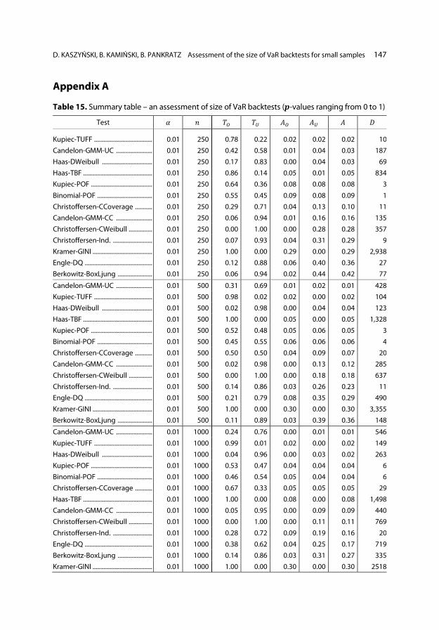
D. KASZYŃSKI, B. KAMIŃSKI, B. PANKRATZ Assessment of the size of VaR backtests for small samples 147
Appendix A
Table 15. Summary table – an assessment of size of VaR backtests (𝒑𝒑-values ranging from 0 to 1)
Test 𝛼𝛼 𝑖𝑖 𝑇𝑇𝑂𝑂 𝑇𝑇𝑈𝑈 𝐴𝐴𝑂𝑂 𝐴𝐴𝑈𝑈 𝐴𝐴 𝐷𝐷
Kupiec-TUFF ..................................... 0.01 250 0.78 0.22 0.02 0.02 0.02 10 Candelon-GMM-UC ....................... 0.01 250 0.42 0.58 0.01 0.04 0.03 187 Haas-DWeibull ................................ 0.01 250 0.17 0.83 0.00 0.04 0.03 69 Haas-TBF ............................................ 0.01 250 0.86 0.14 0.05 0.01 0.05 834 Kupiec-POF ....................................... 0.01 250 0.64 0.36 0.08 0.08 0.08 3
Binomial-POF ................................... 0.01 250 0.55 0.45 0.09 0.08 0.09 1 Christoffersen-CCoverage ........... 0.01 250 0.29 0.71 0.04 0.13 0.10 11 Candelon-GMM-CC ....................... 0.01 250 0.06 0.94 0.01 0.16 0.16 135 Christoffersen-CWeibull ............... 0.01 250 0.00 1.00 0.00 0.28 0.28 357 Christoffersen-Ind. ......................... 0.01 250 0.07 0.93 0.04 0.31 0.29 9 Kramer-GINI ...................................... 0.01 250 1.00 0.00 0.29 0.00 0.29 2,938 Engle-DQ ........................................... 0.01 250 0.12 0.88 0.06 0.40 0.36 27 Berkowitz-BoxLjung ...................... 0.01 250 0.06 0.94 0.02 0.44 0.42 77
Candelon-GMM-UC ....................... 0.01 500 0.31 0.69 0.01 0.02 0.01 428 Kupiec-TUFF ..................................... 0.01 500 0.98 0.02 0.02 0.00 0.02 104 Haas-DWeibull ................................ 0.01 500 0.02 0.98 0.00 0.04 0.04 123 Haas-TBF ............................................ 0.01 500 1.00 0.00 0.05 0.00 0.05 1,328 Kupiec-POF ....................................... 0.01 500 0.52 0.48 0.05 0.06 0.05 3 Binomial-POF ................................... 0.01 500 0.45 0.55 0.06 0.06 0.06 4 Christoffersen-CCoverage ........... 0.01 500 0.50 0.50 0.04 0.09 0.07 20 Candelon-GMM-CC ....................... 0.01 500 0.02 0.98 0.00 0.13 0.12 285
Christoffersen-CWeibull ............... 0.01 500 0.00 1.00 0.00 0.18 0.18 637 Christoffersen-Ind. ......................... 0.01 500 0.14 0.86 0.03 0.26 0.23 11 Engle-DQ ........................................... 0.01 500 0.21 0.79 0.08 0.35 0.29 490 Kramer-GINI ...................................... 0.01 500 1.00 0.00 0.30 0.00 0.30 3,355 Berkowitz-BoxLjung ...................... 0.01 500 0.11 0.89 0.03 0.39 0.36 148
Candelon-GMM-UC ....................... 0.01 1000 0.24 0.76 0.00 0.01 0.01 546
Kupiec-TUFF ..................................... 0.01 1000 0.99 0.01 0.02 0.00 0.02 149 Haas-DWeibull ................................ 0.01 1000 0.04 0.96 0.00 0.03 0.02 263 Kupiec-POF ....................................... 0.01 1000 0.53 0.47 0.04 0.04 0.04 6 Binomial-POF ................................... 0.01 1000 0.46 0.54 0.05 0.04 0.04 6 Christoffersen-CCoverage ........... 0.01 1000 0.67 0.33 0.05 0.05 0.05 29 Haas-TBF ............................................ 0.01 1000 1.00 0.00 0.08 0.00 0.08 1,498 Candelon-GMM-CC ....................... 0.01 1000 0.05 0.95 0.00 0.09 0.09 440 Christoffersen-CWeibull ............... 0.01 1000 0.00 1.00 0.00 0.11 0.11 769
Christoffersen-Ind. ......................... 0.01 1000 0.28 0.72 0.09 0.19 0.16 20 Engle-DQ ........................................... 0.01 1000 0.38 0.62 0.04 0.25 0.17 719 Berkowitz-BoxLjung ...................... 0.01 1000 0.14 0.86 0.03 0.31 0.27 335 Kramer-GINI ...................................... 0.01 1000 1.00 0.00 0.30 0.00 0.30 2518

148 Przegląd Statystyczny. Statistical Review 2020 | 2
Table 16. Summary table – an assessment of size of VaR backtests (𝒑𝒑-values ranging from 0 to 1) (cont.)
Test 𝛼𝛼 𝑖𝑖 𝑇𝑇𝑂𝑂 𝑇𝑇𝑈𝑈 𝐴𝐴𝑂𝑂 𝐴𝐴𝑈𝑈 𝐴𝐴 𝐷𝐷
Candelon-GMM-UC ....................... 0.05 250 0.20 0.79 0.00 0.01 0.01 362 Haas-DWeibull ................................ 0.05 250 0.70 0.30 0.02 0.02 0.02 638 Kupiec-TUFF ..................................... 0.05 250 0.92 0.08 0.02 0.01 0.02 49 Kupiec-POF ....................................... 0.05 250 0.55 0.45 0.03 0.03 0.03 7 Binomial-POF ................................... 0.05 250 0.51 0.49 0.04 0.04 0.04 6
Candelon-GMM-CC ....................... 0.05 250 0.04 0.96 0.01 0.08 0.08 474 Christoffersen-CWeibull ............... 0.05 250 0.26 0.74 0.00 0.09 0.07 932 Engle-DQ ........................................... 0.05 250 0.26 0.74 0.03 0.09 0.08 752 Haas-TBF ............................................ 0.05 250 1.00 0.00 0.09 0.00 0.09 1,643 Kramer-GINI ...................................... 0.05 250 1.00 0.00 0.09 0.00 0.09 1,828 Christoffersen-Ind. ......................... 0.05 250 0.77 0.23 0.12 0.03 0.10 49 Christoffersen-CCoverage ........... 0.05 250 1.00 0.00 0.14 0.00 0.14 69
Berkowitz-BoxLjung ...................... 0.05 250 0.03 0.97 0.01 0.16 0.15 397
Candelon-GMM-UC ....................... 0.05 500 0.09 0.91 0.00 0.01 0.01 502 Haas-DWeibull ................................ 0.05 500 0.84 0.16 0.01 0.01 0.01 913 Kupiec-POF ....................................... 0.05 500 0.51 0.49 0.02 0.03 0.02 9 Kupiec-TUFF ..................................... 0.05 500 0.93 0.07 0.03 0.01 0.03 46 Binomial-POF ................................... 0.05 500 0.47 0.53 0.03 0.03 0.03 8
Engle-DQ ........................................... 0.05 500 0.25 0.75 0.01 0.05 0.04 745 Christoffersen-CWeibull ............... 0.05 500 0.60 0.40 0.03 0.06 0.04 1,161 Christoffersen-Ind. ......................... 0.05 500 0.81 0.19 0.06 0.01 0.05 89 Candelon-GMM-CC ....................... 0.05 500 0.05 0.95 0.01 0.05 0.05 600 Kramer-GINI ...................................... 0.05 500 1.00 0.00 0.09 0.00 0.09 1,702 Christoffersen-CCoverage ........... 0.05 500 0.99 0.01 0.12 0.00 0.12 110 Berkowitz-BoxLjung ...................... 0.05 500 0.02 0.98 0.00 0.13 0.13 456 Haas-TBF ............................................ 0.05 500 1.00 0.00 0.14 0.00 0.14 1,869
Candelon-GMM-UC ....................... 0.05 1000 0.28 0.72 0.00 0.00 0.00 588 Haas-DWeibull ................................ 0.05 1000 0.92 0.08 0.01 0.00 0.01 955 Engle-DQ ........................................... 0.05 1000 0.27 0.73 0.00 0.02 0.02 788 Kupiec-POF ....................................... 0.05 1000 0.54 0.46 0.02 0.02 0.02 13 Binomial-POF ................................... 0.05 1000 0.50 0.50 0.02 0.02 0.02 12 Christoffersen-Ind. ......................... 0.05 1000 0.91 0.09 0.02 0.01 0.02 162
Kupiec-TUFF ..................................... 0.05 1000 0.94 0.06 0.03 0.01 0.03 44 Christoffersen-CWeibull ............... 0.05 1000 0.78 0.22 0.06 0.04 0.05 1,375 Candelon-GMM-CC ....................... 0.05 1000 0.08 0.92 0.00 0.04 0.04 669 Kramer-GINI ...................................... 0.05 1000 1.00 0.00 0.07 0.00 0.07 1,564 Christoffersen-CCoverage ........... 0.05 1000 1.00 0.00 0.11 0.00 0.11 208 Berkowitz-BoxLjung ...................... 0.05 1000 0.01 0.99 0.00 0.11 0.11 478 Haas-TBF ............................................ 0.05 1000 1.00 0.00 0.20 0.00 0.20 2,389
Source: authors’ calculation.

D. KASZYŃSKI, B. KAMIŃSKI, B. PANKRATZ Assessment of the size of VaR backtests for small samples 149
Appendix B
Table 17. Summary table – an assessment of size of VaR backtests (𝒑𝒑-values ranging from 0 to 0.1)
Test 𝛼𝛼 𝑖𝑖 𝑇𝑇𝑂𝑂 𝑇𝑇𝑈𝑈 𝐴𝐴𝑂𝑂 𝐴𝐴𝑈𝑈 𝐴𝐴 𝐷𝐷
Kupiec-TUFF ..................................... 0.01 250 0.95 0.05 0.01 0.00 0.01 10 Christoffersen-CCoverage ........... 0.01 250 0.46 0.54 0.01 0.01 0.01 11 Haas-DWeibull ................................ 0.01 250 0.00 1.00 0.00 0.01 0.01 82 Binomial-POF ................................... 0.01 250 0.27 0.73 0.01 0.03 0.02 1 Berkowitz-BoxLjung ...................... 0.01 250 0.62 0.38 0.02 0.02 0.02 90 Christoffersen-CWeibull ............... 0.01 250 0.00 1.00 0.00 0.02 0.02 412
Candelon-GMM-UC ....................... 0.01 250 0.00 1.00 0.00 0.04 0.04 169 Kupiec-POF ....................................... 0.01 250 0.75 0.25 0.05 0.01 0.04 3 Christoffersen-ICoverage ............ 0.01 250 0.00 1.00 0.00 0.04 0.04 8 Candelon-GMM-CC ....................... 0.01 250 0.00 1.00 0.00 0.04 0.04 137 Haas-TBF ............................................ 0.01 250 1.00 0.00 0.05 0.00 0.05 791 Engle-DQ ........................................... 0.01 250 1.00 0.00 0.06 0.00 0.06 20 Kramer-GINI ...................................... 0.01 250 0.97 0.03 0.30 0.00 0.29 3,059
Kupiec-POF ....................................... 0.01 500 0.52 0.48 0.01 0.01 0.01 3
Binomial-POF ................................... 0.01 500 0.56 0.44 0.01 0.01 0.01 4 Christoffersen-CWeibull ............... 0.01 500 0.00 1.00 0.00 0.01 0.01 624 Kupiec-TUFF ..................................... 0.01 500 0.96 0.04 0.02 0.00 0.02 108 Haas-DWeibull ................................ 0.01 500 0.00 1.00 0.00 0.02 0.02 151 Candelon-GMM-UC ....................... 0.01 500 0.12 0.88 0.00 0.02 0.02 394 Candelon-GMM-CC ....................... 0.01 500 0.07 0.93 0.00 0.03 0.03 321 Christoffersen-ICoverage ............ 0.01 500 0.00 1.00 0.00 0.03 0.03 13 Berkowitz-BoxLjung ...................... 0.01 500 0.96 0.04 0.04 0.00 0.03 160
Christoffersen-CCoverage ........... 0.01 500 1.00 0.00 0.04 0.00 0.04 21 Haas-TBF ............................................ 0.01 500 1.00 0.00 0.04 0.00 0.04 1,253 Engle-DQ ........................................... 0.01 500 1.00 0.00 0.11 0.00 0.11 485 Kramer-GINI ...................................... 0.01 500 1.00 0.00 0.38 0.00 0.38 3,394
Binomial-POF ................................... 0.01 1000 0.47 0.53 0.01 0.01 0.01 6 Christoffersen-CWeibull ............... 0.01 1000 0.00 1.00 0.00 0.01 0.01 736
Candelon-GMM-UC ....................... 0.01 1000 0.17 0.83 0.00 0.01 0.01 532 Kupiec-POF ....................................... 0.01 1000 0.64 0.36 0.01 0.01 0.01 6 Kupiec-TUFF ..................................... 0.01 1000 0.98 0.02 0.02 0.00 0.01 146 Candelon-GMM-CC ....................... 0.01 1000 0.31 0.69 0.01 0.02 0.01 447 Haas-DWeibull ................................ 0.01 1000 0.00 1.00 0.00 0.03 0.03 253 Christoffersen-ICoverage ............ 0.01 1000 0.00 1.00 0.00 0.03 0.03 17 Berkowitz-BoxLjung ...................... 0.01 1000 1.00 0.00 0.04 0.00 0.04 337 Christoffersen-CCoverage ........... 0.01 1000 1.00 0.00 0.05 0.00 0.05 24
Haas-TBF ............................................ 0.01 1000 1.00 0.00 0.06 0.00 0.06 1,503 Engle-DQ ........................................... 0.01 1000 1.00 0.00 0.06 0.00 0.06 710 Kramer-GINI ...................................... 0.01 1000 1.00 0.00 0.41 0.00 0.41 2,576

150 Przegląd Statystyczny. Statistical Review 2020 | 2
Table 18. Summary table – an assessment of size of VaR backtests (𝒑𝒑-values ranging from 0 to 0.1) (cont.)
Test 𝛼𝛼 𝑖𝑖 𝑇𝑇𝑂𝑂 𝑇𝑇𝑈𝑈 𝐴𝐴𝑂𝑂 𝐴𝐴𝑈𝑈 𝐴𝐴 𝐷𝐷
Candelon-GMM-UC ....................... 0.05 250 0.36 0.64 0.00 0.00 0.00 365 Christoffersen-CWeibull ............... 0.05 250 0.99 0.01 0.00 0.00 0.00 920 Binomial-POF ................................... 0.05 250 0.45 0.55 0.01 0.01 0.01 6 Kupiec-POF ....................................... 0.05 250 0.60 0.40 0.01 0.01 0.01 7 Engle-DQ ........................................... 0.05 250 1.00 0.00 0.01 0.00 0.01 768
Candelon-GMM-CC ....................... 0.05 250 0.34 0.66 0.01 0.02 0.01 469 Berkowitz-BoxLjung ...................... 0.05 250 0.32 0.68 0.01 0.02 0.01 399 Kupiec-TUFF ..................................... 0.05 250 0.80 0.20 0.02 0.00 0.02 46 Haas-DWeibull ................................ 0.05 250 0.00 1.00 0.00 0.03 0.03 685 Christoffersen-ICoverage ............ 0.05 250 0.00 1.00 0.00 0.03 0.03 50 Haas-TBF ............................................ 0.05 250 1.00 0.00 0.05 0.00 0.05 1,636 Kramer-GINI ...................................... 0.05 250 0.99 0.01 0.07 0.00 0.06 1,744
Christoffersen-CCoverage ........... 0.05 250 1.00 0.00 0.07 0.00 0.07 69
Candelon-GMM-UC ....................... 0.05 500 0.20 0.80 0.00 0.00 0.00 478 Binomial-POF ................................... 0.05 500 0.56 0.44 0.01 0.01 0.01 8 Engle-DQ ........................................... 0.05 500 0.88 0.12 0.01 0.00 0.01 799 Kupiec-POF ....................................... 0.05 500 0.76 0.24 0.01 0.00 0.01 9 Candelon-GMM-CC ....................... 0.05 500 0.50 0.50 0.01 0.01 0.01 554
Haas-DWeibull ................................ 0.05 500 0.00 1.00 0.00 0.01 0.01 889 Christoffersen-ICoverage ............ 0.05 500 0.21 0.79 0.01 0.01 0.01 86 Berkowitz-BoxLjung ...................... 0.05 500 0.14 0.86 0.00 0.02 0.02 444 Kupiec-TUFF ..................................... 0.05 500 0.78 0.22 0.02 0.00 0.02 43 Christoffersen-CWeibull ............... 0.05 500 1.00 0.00 0.02 0.00 0.02 1,179 Kramer-GINI ...................................... 0.05 500 1.00 0.00 0.07 0.00 0.07 1,603 Haas-TBF ............................................ 0.05 500 1.00 0.00 0.08 0.00 0.08 1,881 Christoffersen-CCoverage ........... 0.05 500 1.00 0.00 0.08 0.00 0.08 106
Haas-DWeibull ................................ 0.05 1000 0.56 0.44 0.00 0.00 0.00 948 Engle-DQ ........................................... 0.05 1000 0.83 0.17 0.00 0.00 0.00 806 Candelon-GMM-UC ....................... 0.05 1000 0.23 0.77 0.00 0.00 0.00 590 Kupiec-POF ....................................... 0.05 1000 0.73 0.27 0.00 0.00 0.00 13 Binomial-POF ................................... 0.05 1000 0.65 0.35 0.00 0.00 0.00 12 Candelon-GMM-CC ....................... 0.05 1000 0.58 0.42 0.01 0.01 0.01 641
Berkowitz-BoxLjung ...................... 0.05 1000 0.06 0.94 0.00 0.02 0.02 452 Kupiec-TUFF ..................................... 0.05 1000 0.82 0.18 0.02 0.00 0.02 48 Christoffersen-ICoverage ............ 0.05 1000 0.86 0.14 0.03 0.00 0.03 145 Christoffersen-CWeibull ............... 0.05 1000 1.00 0.00 0.04 0.00 0.04 1,370 Kramer-GINI ...................................... 0.05 1000 1.00 0.00 0.06 0.00 0.06 1,490 Christoffersen-CCoverage ........... 0.05 1000 1.00 0.00 0.10 0.00 0.10 186 Haas-TBF ............................................ 0.05 1000 1.00 0.00 0.12 0.00 0.12 2,404
Source: authors’ calculation.
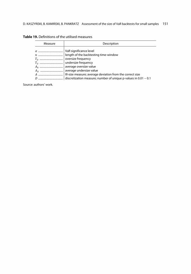
D. KASZYŃSKI, B. KAMIŃSKI, B. PANKRATZ Assessment of the size of VaR backtests for small samples 151
Table 19. Definitions of the utilised measures
Measure Description
𝛼𝛼 .................................... VaR significance level 𝑖𝑖 .................................... length of the backtesting time-window 𝑇𝑇𝑂𝑂 .................................. oversize frequency 𝑇𝑇𝑈𝑈 .................................. undersize frequency 𝐴𝐴0 .................................. average oversize value 𝐴𝐴𝑈𝑈 ................................. average undersize value 𝐴𝐴 .................................... Ill-size measure; average deviation from the correct size 𝐷𝐷 .................................... discretization measure; number of unique p-values in 0.01 − 0.1
Source: authors’ work.
Related Documents