Assessment of Predictive Fire Algorithms and Models

Examination of Fire DynamicsAnalysis Techniques:Assessment of Predictive FireAlgorithms and Models

Mark McKinnonJoseph WilliDaniel Madrzykowski

UL Firefighter Safety Research InstituteColumbia, MD 20145

TM

UNDERWRITERS

LABORATORIES

©Underwriters Laboratories Inc. All rights reserved. UL and the UL logo are trademarks of UL LLC

Examination of Fire DynamicsAnalysis Techniques:Assessment of Predictive FireAlgorithms and Models

Mark McKinnonJoseph WilliDaniel Madrzykowski

UL Firefighter Safety Research InstituteColumbia, MD 21045

March 31, 2021

TM

UNDERWRITERS

LABORATORIES

Underwriters Laboratories Inc.Terrence Brady, President

UL Firefighter Safety Research InstituteStephen Kerber, Director

©Underwriters Laboratories Inc. All rights reserved. UL and the UL logo are trademarks of UL LLC

In no event shall UL be responsible to anyone for whatever use or non-use is made of theinformation contained in this Report and in no event shall UL, its employees, or its agentsincur any obligation or liability for damages including, but not limited to, consequentialdamage arising out of or in connection with the use or inability to use the informationcontained in this Report. Information conveyed by this Report applies only to the specimensactually involved in these tests. UL has not established a factory Follow-Up Service Programto determine the conformance of subsequently produced material, nor has any provision beenmade to apply any registered mark of UL to such material. The issuance of this Report in noway implies Listing, Classification or Recognition by UL and does not authorize the use ofUL Listing, Classification or Recognition Marks or other reference to UL on or in connectionwith the product or system.

Contents

List of Figures iii

List of Tables iv

List of Abbreviations v

1 Introduction 11.1 Motivation . . . . . . . . . . . . . . . . . . . . . . . . . . . . . . . . . . . . . . 1

2 Literature Review 3

3 Description of Experiments 53.1 Fuel Loads . . . . . . . . . . . . . . . . . . . . . . . . . . . . . . . . . . . . . . 53.2 Instrumentation . . . . . . . . . . . . . . . . . . . . . . . . . . . . . . . . . . . 73.3 Compartment Experiments . . . . . . . . . . . . . . . . . . . . . . . . . . . . . . 8

3.3.1 Structure . . . . . . . . . . . . . . . . . . . . . . . . . . . . . . . . . . . . 93.3.2 Instrumentation . . . . . . . . . . . . . . . . . . . . . . . . . . . . . . . . 11

4 Predictive Fire Algorithms & Models 154.1 Model Background . . . . . . . . . . . . . . . . . . . . . . . . . . . . . . . . . . 15

4.1.1 NRC Fire Dynamics Tools . . . . . . . . . . . . . . . . . . . . . . . . . . 154.1.2 Zone Models . . . . . . . . . . . . . . . . . . . . . . . . . . . . . . . . . 204.1.3 Field Models . . . . . . . . . . . . . . . . . . . . . . . . . . . . . . . . . 21

4.2 Model Construction for Compartment Experiments . . . . . . . . . . . . . . . . . 224.2.1 FDTs . . . . . . . . . . . . . . . . . . . . . . . . . . . . . . . . . . . . . 234.2.2 CFAST . . . . . . . . . . . . . . . . . . . . . . . . . . . . . . . . . . . . 244.2.3 FDS . . . . . . . . . . . . . . . . . . . . . . . . . . . . . . . . . . . . . . 24

4.3 Model Sensitivity . . . . . . . . . . . . . . . . . . . . . . . . . . . . . . . . . . 26

5 Model Assessment 275.1 Temperatures . . . . . . . . . . . . . . . . . . . . . . . . . . . . . . . . . . . . . 28

5.1.1 Layer Temperatures . . . . . . . . . . . . . . . . . . . . . . . . . . . . . . 335.1.2 Layer Heights . . . . . . . . . . . . . . . . . . . . . . . . . . . . . . . . . 36

5.2 Flame Heights . . . . . . . . . . . . . . . . . . . . . . . . . . . . . . . . . . . . 415.3 Heat Flux . . . . . . . . . . . . . . . . . . . . . . . . . . . . . . . . . . . . . . . 445.4 Velocity . . . . . . . . . . . . . . . . . . . . . . . . . . . . . . . . . . . . . . . 495.5 Oxygen Concentration . . . . . . . . . . . . . . . . . . . . . . . . . . . . . . . . 51

i

6 Discussion 56

7 Recommendations 58

8 Research Needs 59

9 Summary 60

References 61

A Detailed Results 66A.1 Compartment Experiments . . . . . . . . . . . . . . . . . . . . . . . . . . . . . . 66

A.1.1 Gas Temperature . . . . . . . . . . . . . . . . . . . . . . . . . . . . . . . 66A.1.2 Plume Temperature and Velocity . . . . . . . . . . . . . . . . . . . . . . . 87A.1.3 Flame Height . . . . . . . . . . . . . . . . . . . . . . . . . . . . . . . . . 107A.1.4 Heat Flux . . . . . . . . . . . . . . . . . . . . . . . . . . . . . . . . . . . 115

ii

List of Figures

3.1 Natural Gas Burners Used in Experiments . . . . . . . . . . . . . . . . . . . . . 63.2 Sofa Designs Used as Experimental Fuel Loads . . . . . . . . . . . . . . . . . . . 73.3 Fuel Load Positions . . . . . . . . . . . . . . . . . . . . . . . . . . . . . . . . . 93.4 Dimensioned Floor Plan & Image of the Compartment . . . . . . . . . . . . . . . 103.5 Fixed Instrumentation Layout for the Compartment Experiments . . . . . . . . . 113.6 Locations of Ceiling Jet BDPs . . . . . . . . . . . . . . . . . . . . . . . . . . . . 12

4.1 Furniture Designs Used as Experimental Fuel Loads . . . . . . . . . . . . . . . . 25

5.1 Comparison of Temperature Predictions to Experimental Data Collected in Com-partment Experiments with Burners . . . . . . . . . . . . . . . . . . . . . . . . . 29

5.2 Comparison of Temperature Predictions to Experimental Data Collected in Com-partment Experiments with Furniture . . . . . . . . . . . . . . . . . . . . . . . . 31

5.3 Comparison of Layer Temperature Predictions to Experimental Data Collected inCompartment Experiments with Burners . . . . . . . . . . . . . . . . . . . . . . 33

5.4 Comparison of Layer Temperature Predictions to Experimental Data Collected inCompartment Experiments with Furniture . . . . . . . . . . . . . . . . . . . . . . 35

5.5 Comparison of Layer Interface Elevation Predictions to Experimental Data Col-lected in Compartment Experiments with Burners . . . . . . . . . . . . . . . . . 37

5.6 Comparison of Layer Interface Elevation Predictions to Experimental Data Col-lected in Compartment Experiments with Furniture . . . . . . . . . . . . . . . . . 39

5.7 Comparison of Flame Height Predictions to Experimental Data Collected in Com-partment Experiments with Burners . . . . . . . . . . . . . . . . . . . . . . . . . 41

5.8 Comparison of Flame Height Predictions to Experimental Data Collected in Com-partment Experiments with Furniture . . . . . . . . . . . . . . . . . . . . . . . . 43

5.9 Comparison of Heat Flux Predictions to Experimental Data Collected in Com-partment Experiments with Burners . . . . . . . . . . . . . . . . . . . . . . . . . 45

5.10 Comparison of Heat Flux Predictions to Experimental Data Collected in Com-partment Experiments with Furniture . . . . . . . . . . . . . . . . . . . . . . . . 46

5.11 Comparison of Velocity Predictions to Experimental Data Collected in Compart-ment Experiments with Burners . . . . . . . . . . . . . . . . . . . . . . . . . . . 49

5.12 Comparison of Velocity Predictions to Experimental Data Collected in Compart-ment Experiments with Furniture . . . . . . . . . . . . . . . . . . . . . . . . . . 51

5.13 Comparison of Oxygen Concentration Predictions to Experimental Data Collectedin Compartment Experiments with Burners . . . . . . . . . . . . . . . . . . . . . 52

5.14 Comparison of Oxygen Concentration Predictions to Experimental Data Collectedin Compartment Experiments with Furniture . . . . . . . . . . . . . . . . . . . . 54

iii

List of Tables

3.1 Summary of Compartment Experiments . . . . . . . . . . . . . . . . . . . . . . . 9

4.1 Material Properties Used in Models . . . . . . . . . . . . . . . . . . . . . . . . . 224.2 Radiative Fraction Calculated for Each Fuel Package . . . . . . . . . . . . . . . . 234.3 Grid Resolution Metrics . . . . . . . . . . . . . . . . . . . . . . . . . . . . . . . 26

5.1 Color Code for Bias and Uncertainty Tables . . . . . . . . . . . . . . . . . . . . 285.2 Model Fitness Metrics for Temperature in Compartment Burner Experiments . . . 305.3 Model Fitness Metrics for Temperature in Compartment Furniture Experiments . . 325.4 Model Fitness Metrics for Layer Temperature in Compartment Burner Experiments 345.5 Model Fitness Metrics for Layer Temperature in Compartment Furniture Experi-

ments . . . . . . . . . . . . . . . . . . . . . . . . . . . . . . . . . . . . . . . . . 365.6 Model Fitness Metrics for Layer Interface Elevation in Compartment Burner Ex-

periments . . . . . . . . . . . . . . . . . . . . . . . . . . . . . . . . . . . . . . . 385.7 Model Fitness Metrics for Layer Interface Elevation in Compartment Furniture

Experiments . . . . . . . . . . . . . . . . . . . . . . . . . . . . . . . . . . . . . 405.8 Model Fitness Metrics for Flame Height in Compartment Burner Experiments . . 425.9 Model Fitness Metrics for Flame Height in Compartment Furniture Experiments . 445.10 Model Fitness Metrics for Heat Flux in Compartment Burner Experiments . . . . 475.11 Model Fitness Metrics for Heat Flux in Compartment Furniture Experiments . . . 485.12 Model Fitness Metrics for Velocity in Compartment Burner Experiments . . . . . 505.13 Model Fitness Metrics for Velocity in Compartment Furniture Experiments . . . . 505.14 Model Fitness Metrics for Oxygen Concentration in Compartment Burner Exper-

iments . . . . . . . . . . . . . . . . . . . . . . . . . . . . . . . . . . . . . . . . 535.15 Model Fitness Metrics for Oxygen Concentration in Compartment Furniture Ex-

periments . . . . . . . . . . . . . . . . . . . . . . . . . . . . . . . . . . . . . . . 55

iv

List of Abbreviations

AF Above floorATF Bureau of Alcohol, Tobacco and FirearmsBC Below ceilingBDP Bi-directional probeCFAST Consolidated Model of Fire and Smoke TransportCFD Computational Fluid DynamicsEPRI Electric Power Research InstituteFIVE Fire Induced Vulnerability EvaluationFDS Fire Dynamics SimulatorFDTs Fire Dynamics ToolsHGL Hot Gas LayerHRR Heat Release RateHRRPUA Heat Release Rate per Unit AreaHRRPUL Heat Release Rate per Unit LengthNBS National Bureau of StandardsNFPA National Fire Protection AssociationNIJ National Institute of JusticeNIST National Institute of Standards and TechnologyNRC Nuclear Regulatory CommissionPUF Polyurethane FoamRI Resolution IndexSI International System of UnitsTC ThermocoupleUL Underwriters LaboratoriesUL FSRI UL Firefighter Safety Research InstituteV&V Verification and ValidationVTT Technical Research Centre of Finland

v

Acknowledgments

This project was supported by Award No. 2017-DN-BX-O163, provided by the National Instituteof Justice, Office of Justice Programs, U.S. Department of Justice. The opinions, findings, andconclusions or recommendations expressed in this publication are those of the author(s) and do notnecessarily reflect those of the Department of Justice.

The authors would also like to acknowledge Kelly Opert and the technical staff of the UL LargeFire Lab for their assistance in preparing and conducting the full-scale experiments. Staff thatprovided particularly valuable assistance include Andres Sarmineto, Jeff Mlyniec, Eric Anderson,and Derek Dziekonski. These experiments would not have been possible without the supportof the UL FSRI team. The UL FSRI team instrumented, conducted, and collected data fromthese experiments. Special thanks go to Craig Weinschenk and Jack Regan of UL FSRI, and RoyMcLane of Thermal Fabrications.

Abstract

Fire investigations are an integral piece of a holistic fire protection strategy that has been developedto improve the safety of the built environment for occupants. The use of fire dynamics analysesthat utilize specialized fire dynamics routines, zone fire models, and field fire models is encouragedin the course of an investigation. In these analyses, there is a need to understand the accuracy ofthe models, the inherent uncertainties in each model, and the limitations of application of the firemodels to ensure a given model is appropriate and physical phenomena are accurately represented.This work is focused on conducting an engineering assessment of three types of models that arecommonly used in fire investigations on the ability of each to predict characteristics of the fireenvironment generated from gas burners and modern upholstered furniture composed of syntheticmaterials in a compartment with a single entrance. A quantitative analysis of the accuracy ofpredicting plume and compartment temperatures, flow velocities, flame heights, heat fluxes, theelevation of the interface between the upper and lower layers in the compartment, and oxygenconcentrations is provided for each model.

The specialized fire dynamics routines were capable of accurately characterizing the flame height,but did not accurately predict the other quantities for the furniture-fueled fire experiments con-ducted in the compartment. The zone fire model accurately predicted the layer interface heights,layer temperatures, flame heights, and oxygen concentrations in the compartment fire scenar-ios. The field model predicted accurate temperatures throughout the compartment, layer interfaceheights, velocities through the open door of the compartment, flame heights, and oxygen concen-trations. In general, the predictive ability of all the models was better in the gas burner experimentsthan in the furniture experiments. More research is needed to develop recommendations on geom-etry and burning definitions for upholstered furniture in field models as well as improved methodsfor model practitioners to predict heat flux.

1 Introduction

Fire investigations are an integral piece of a holistic fire protection strategy that has been developedto improve the safety of the built environment for occupants. Investigations provide a means toidentify the cause of a fire as well as collect data that may provide insight about the developmentand spread of the fire. By determining the cause of a fire and identifying products and phenomenathat contributed to fire spread, investigators may be able to prove guilt or innocence in criminalproceedings, assign blame in civil proceedings, or contribute to the knowledge base that mayinform the fire protection and safety community in future designs, effectively reducing the lossesfrom fires. Data such as the area of fire origin, the time until target materials or products ignite, thetime to flashover of a compartment, the influence of ventilation on the dynamics of the developingfire, and the ultimate cause of the fire are critical to understanding and reducing the number andseverity of fires.

Fire models are increasingly relied upon in fire investigations, the design process, and scientificstudies to test hypotheses and improve the understanding of fire dynamics and fire-induced fluidflows. Models that are currently available range in complexity from simple algebraic heuristics thatare derived from fundamental physical concepts and empirical data to generalized, physics-basedcomputational fluid dynamics (CFD) codes that require a wide range of property values as inputsand may require significant computational resources. Due to the complexity of fire phenomena,empirical correlations are often adopted in various sub-models within CFD codes to reduce thecomputational expense of fire dynamics analyses.

NFPA 921 Guide for Fire and Explosion Investigations encourages the use of fire dynamics anal-yses that utilize specialized fire dynamics routines (simple heuristics), zone fire models, and CFD(field) fire models to answer specific questions that arise in the course of an investigation. NFPA 921emphasizes the need to understand the uncertainties inherent in each potential model as well as thelimitations of fire models to ensure a given model is appropriate and physical phenomena are accu-rately represented [1]. This work is focused on evaluating three types of models that are commonlyused in fire investigations on the ability of each to predict characteristics of the fire environmentgenerated from gas burners as well as burning modern upholstered furniture composed of syntheticmaterials.

1.1 Motivation

Many of the heuristics and correlations that are used in fire dynamics analyses rely on experimentaldata collected in tests conducted with a gas burner or a liquid pool fire source and have had mini-mal, if any, validation against data collected in experiments with solid fuel packages. Additionally,studies conducted to validate field models and zone models generally use laboratory fuels as firesources to minimize the contribution of uncertainty in the heat release rate, combustion by-product

1

yields, and fuel configuration effects to the total uncertainty of all measurands over the courseof the experiments. Because of the relative lack of data collected in experiments conducted withupholstered furniture fuel packages, the efficacy of these models to describe the fire environmentgenerated by furniture-fueled fires is uncertain.

The materials used in the manufacturing of typical upholstered furniture have changed over thepast few decades as synthetic polymers have proliferated all industries due to the low cost ofthese materials relative to the natural materials used in legacy designs. This change has largely re-sulted in petroleum-based materials with relatively high heating values displacing natural materialsthroughout the built environment. This shift in the upholstered furniture industry has contributedto a phenomenon in which modern residential occupancies facilitate more rapid fire growth thanresidential occupancies did in the mid-to-late 1900s [2].

Every household in the U.S. contains an average of approximately four pieces of upholstered fur-niture [3, 4]. The ubiquity of upholstered furniture throughout the built environment makes it aprimary fuel source in residential fires. From 2010 to 2014, there was an average of 5,360 struc-ture fires per year in the U.S. in which upholstered furniture was the first item ignited. These firesaccounted for an average of 440 civilian deaths, 700 civilian injuries, and an estimated $269 mil-lion in direct damage annually [5]. It was also estimated that between 2006 and 2010, residentialfires in the U.S. in which an item of upholstered furniture was not the first item ignited, but was theprimary fuel source accounted for an additional 2,200 residential fires and 130 civilian deaths an-nually [6]. Similar trends are evident in Europe, where furniture fires account for an estimated 6%of all residential fires and 15% of fatalities from fires [7]. Particularly important to the fire inves-tigation community were the approximately 890 residential fires that originated from intentionallyignited furniture in the U.S. annually from 2010 to 2014 [8].

An objective assessment of the ability of the analytical and computational tools to perform firedynamics analyses is required to develop an understanding of the uncertainties and limitationsassociated with the tools. This exercise also helps to evaluate the level of confidence in applyingthe tools in situations that may be outside of the conditions at which the tools were developed andhave been validated. The assessment of these tools and development of recommendations for fireinvestigators to use in analyses involving residential structure fires will support the appropriate useof mathematical models in fire investigations. In this work, experiments compartment fires fueledby natural gas burners and upholstered furnishings were conducted to assess the accuracy of arange of predictive fire algorithms and models.

2

2 Literature Review

Several research efforts have been undertaken to evaluate the predictive capabilities of the mod-els available for characterizing the dynamics of fire scenarios. In 2002, Floyd conducted a studyin which hand calculations and computational zone and field models were validated against datacollected in propane burner and oil pool fire experiments conducted in compartments within adecommissioned nuclear reactor building [9]. It was concluded that hand calculations yieldedrelatively imprecise, yet useful information when they were applied within the limits of their un-derlying assumptions. The zone model generally predicted near-field phenomena more accuratelythan far-field phenomena, but also yielded some problematic predictions in the near-field as well.The field model showed promise for predicting detailed information that zone models and handcalculations were and still are incapable of predicting.

In 2006, Rein et al. conducted a study in which real fire scenarios were modeled using a simplifiedanalytical model, a zone model, and a field model [10]. Each model was parameterized with datacollected during a forensic investigation of each scenario, and it was noted that the input parameterswere independent of each other, in part to show the sensitivity of the model predictions to variationin inputs. It was concluded that each model was capable of accurately predicting simple aspects ofthe fires in the early stages of fire growth, but the models diverged at later stages of the fire. Theanalytical model provided reasonable results, but it was noted that only the field model had thecapability of representing flame spread.

The U.S. Nuclear Regulatory Commission (NRC) funded model validation research conducted bythe NRC, National Institute of Standards and Technology (NIST), and the Electric Power ResearchInstitute (EPRI) that culminated in 2007. The aim of the research was to validate the predictivecapabilities of field, zone, and simple fire dynamics analysis models that are all currently used innuclear power plants [11]. Empirical correlations in the form of closed-form algebraic expressionscollected in a group called the Fire Dynamics Tools (FDTs) [12] as well as a collection of algebraicengineering calculations referred to as Fire Induced Vulnerability Evaluation (FIVE) [13] werevalidated against experimental data. Additionally, the zone fire models Consolidated Model of FireGrowth and Smoke Transport (CFAST) developed by NIST and MAGIC developed by Electricitede France, and the field model Fire Dynamics Simulator (FDS) developed by NIST were validatedagainst the same corpus of data. The validation data were collected from several experimentalseries in which almost all used liquid or gaseous fuel as the fire source. A single experimentalseries used mattresses and chairs, but the maximum heat release rate (HRR) in these experimentswas approximately 350 kW.

It was concluded that measured room pressures, oxygen concentrations, flame heights, plume tem-peratures, ceiling jet temperatures, hot gas layer heights, and hot gas layer temperatures were pre-dicted approximately within experimental uncertainty by the zone and field models. Flame heightwas also accurately predicted by the empirical correlations investigated in the study. Smoke con-centrations, target temperatures, radiant heat fluxes, total heat fluxes, and wall temperatures werephysically represented by the zone and field models, but the error in the predictions was outside

3

the experimental uncertainty.

Overholt conducted a study in 2014 that involved validation of the set of empirical correlations col-lected in the FDTs [14]. The data used in the validations were collected in experiments conductedin compartments that had been compiled for validation of FDS. The fuels for the fires in the exper-iments were primarily hydrocarbon, with few experiments collected in experiments that involvedupholstered furniture. The results of the study indicated generally good agreement between thecorrelation predictions and the peaks of the experimental data, although many of the comparisonsof the quantities exhibited significant scatter.

A supplement to the NRC study was published in 2016 that expanded the scope of the verificationand validation (V&V) and utilized more developed versions of the computational models [15]. Itwas cautioned in the conclusions of the supplemental study that empirical correlations should onlybe used within their stated limitations and range of applicability. It was also concluded that thenewer versions of the zone and field models and the validation data added to the corpus in theinterim increased the range of applicability for both types of models.

Janssens et al. conducted a study in 2012 aimed at evaluating and reducing uncertainty in char-acterizing upholstered furniture fires [16]. The authors conducted experiments on chair and chairmock-ups constructed of permutations of two fabrics and six padding materials. Bench-scale ex-periments were also conducted on the component materials. The data collected in full-scale fur-niture mock-up experiments and bench-scale tests were used to assess the predictive capability ofseveral empirical upholstered furniture burning rate models and to make modifications as neces-sary. The authors also used FDS and CFAST to determine modifications required for the empiricalmodels to describe the HRR of the furniture to yield the most accurate results. Additional experi-ments were conducted on used upholstered furniture to validate the produced models. The authorsconcluded with recommendations of methods for fire investigators to predict upholstered furnitureHRRs. It was determined that ignition source and ignition location have a significant effect on theburning rate and HRR histories and that FDS and CFAST accurately predict the hot upper gas layertemperature when the HRR of the furniture item is accurately represented.

4

3 Description of Experiments

A series of experiments were conducted with gas burners and upholstered furniture inside a com-partment. Temperatures and velocities of the ceiling jet, plume, and the flow through the dooropening, and oxygen concentrations in the compartment experiments were also collected. Experi-ments were conducted at the UL Large Fire Lab in Northbrook, IL. The experiments and fuel loadsare described in more detail in the following sections.

3.1 Fuel Loads

Experiments were performed with two sizes of gas burners, one upholstered chair design, and oneupholstered sofa design. Figure 3.1 displays photographs of the gas burners that were used in thegas burner experiments. Both gas burners had a square cross-section with the surface of the largeburner elevated 0.5 m above the floor and the surface of the small burner elevated 0.65 m abovethe floor. The cross-section side length of the smaller burner was 0.3 m and the cross-section sidelength of the larger burner was 0.6 m. The burners were fueled by natural gas supplied to thelaboratory from the local gas utility company. For experiments conducted at the NIST facility, thechemical composition of the gas was provided as 95% methane, 3.4% ethane, 0.3% propene, withthe balance trace gases and no nitrogen or carbon dioxide. The heat of combustion of the naturalgas supplied to the NIST experimental facility was approximately 46,900 kJ/kg. The compositionat the UL facility was approximately 92.2% methane, 5.8% ethane, 1.3% nitrogen, and 0.7% car-bon dioxide with a heat of combustion of approximately 53,100 kJ/kg. The composition of thenatural gas supplied to the ATF facility was unknown, but the heat of combustion was measuredas approximately 53,400 kJ/kg. For experiments in which a gas burner was used, ignition wasachieved via a pilot light and the opening of a valve to allow natural gas to flow to the burner. Inthe experiments with furniture, ignition of the furniture item was performed via an electric match.

5

(a) 0.3 m Natural Gas Burner (b) 0.6 m Natural Gas Burner

Figure 3.1: Image of the natural gas burners used during experiments.

Figure 3.2 displays the chair designs that served as the fuel sources for the compartment experi-ments. The “Red Accent Chair” was approximately 0.71 m wide, 0.76 m deep, and approximately0.88 m high with a seat height of 0.45 m. The outer covering of the Red Accent Chair was polyester,and the frame of the chair was constructed from wood. The cushions of the chair were comprisedof polyurethane foam covered by polyester batting on its top and bottom. The mean mass of theRed Accent Chair was 20.4 kg ± 0.3 kg. The Red Accent Chair was also a fuel source in thecompartment experiments.

The “Overstuffed Sofa” was approximately 2.26 m wide, 0.97 m deep, and approximately 0.96 mhigh with a seat height of 0.55 m. The construction of the Overstuffed Sofa was identical to theOverstuffed Chair in that the outer covering was polyester, the frame was oriented strand board,and the cushions consisted of polyurethane foam covered by polyester batting on both sides. Theaverage mass of the sofa across experiments was 49.1 kg ± 0.8 kg. The Overstuffed Sofa was alsoa fuel source in the compartment experiments.

6

(a) Red Accent Chair (b) Overstuffed Sofa

Figure 3.2: Images of the upholstered sofas utilized during experiments.

3.2 Instrumentation

HRR data were measured during all experiments conducted with the compartment door open. TheUL oxygen consumption calorimetry hood had a diameter of 7.6 m and was positioned approx-imately 7.6 m above the floor. In a previous study, Bryant and Mullholland estimated the totalexpanded uncertainty of oxygen consumption calorimeters during full-scale fire experiments to be± 11% [17]. The authors identified several sources of error within the calorimeter, with one of theprimary sources being the uncertainty of the gas concentration measurements.

Nominal 25 mm diameter, water-cooled Schmidt-Boelter gauges were utilized to measure the totalheat flux at several locations in the experiments. Zirconium plates were installed over the facesof select gauges to prevent heat flux contributions from convection to exclusively measure radiantheat flux incident to the gauge. These gauges are referred to as radiometers throughout the re-mainder of this report. Results from an international study on total heat flux gauge calibration andresponse demonstrated that the total expanded uncertainty of a Schmidt-Boelter gauge is typically± 8% [18].

Bi-directional probes (BDPs) paired with type K, inconel-sheathed thermocouples with nominaldiameters of 1.6 mm were utilized to measure gas flow velocity. The stainless steel probes wereconnected to Setra Model 264 differential pressure transducers (± 125 Pa measurement range). Aprevious gas velocity measurement study focused on flow through doorways during pre-flashovercompartment fires yielded total expanded uncertainties ranging from± 14% to± 22% for measure-ments from BDPs similar to those described here [19]. Therefore, the total expanded uncertaintyfor gas velocity measured during these experiments is estimated to be ± 18%.

Arrays of bare-bead thermocouples were positioned throughout the compartment. Thermocouplemeasurements may be affected by imperfect weldments between the dissimilar metals, radiative

7

heat transfer from the fire source or the hot gas layer, and small variations in orientation alongthe thermocouple array. Theoretical error as high as approximately 11% (measured in Celsius)for upper layer temperatures and significantly higher for lower layer temperatures measured usingbare-bead type-K thermocouples with bead diameters ranging from 1 mm to 1.5 mm have beenreported by researchers at NIST [20, 21]. The total expanded relative uncertainty associated withthe temperature measurements from these experiments is estimated to be ± 15%.

Gas samples were collected through stainless steel tubes to measure oxygen (O2) concentration.After they were collected from the interior of the compartment, the gas samples were drawnthrough a coarse, 2 micron paper filter followed by a condensing trap to remove moisture. Then,they passed through a high-efficiency particulate air filter before oxygen concentrations of the sam-ples were measured by Servomex O2 Analyzers. Based on a study by Lock et al. [22], the estimatedtotal expanded uncertainty of the O2 concentration data is considered to be ± 12%.

In addition to the instrumentation discussed in this section, videos of the experiments were recordedand a machine learning algorithm was deployed to determine the mean flame heights (50% visualintermittency). Additional information about the algorithm and flame height determination is avail-able in a related report [23]. The machine learning algorithm employed an object detection modelthat returned the known heights of a calibration standard within ± 0.08 m. Due to the accuracy ofthis model, the total expanded uncertainty of the flame heights presented in this work is estimatedto be ± 6%.

3.3 Compartment Experiments

A total of 117 experiments were conducted with gas burners and furniture items inside a sim-ple compartment constructed under a large hood equipped with oxygen consumption calorimetry.The compartment was instrumented throughout to characterize the fire environment during the ex-periments. The effect of the location of the fuel package on the fire environment as well as theventilation conditions were investigated in this set of experiments. The door to the compartmentwas either open or closed through the entirety of each experiment.

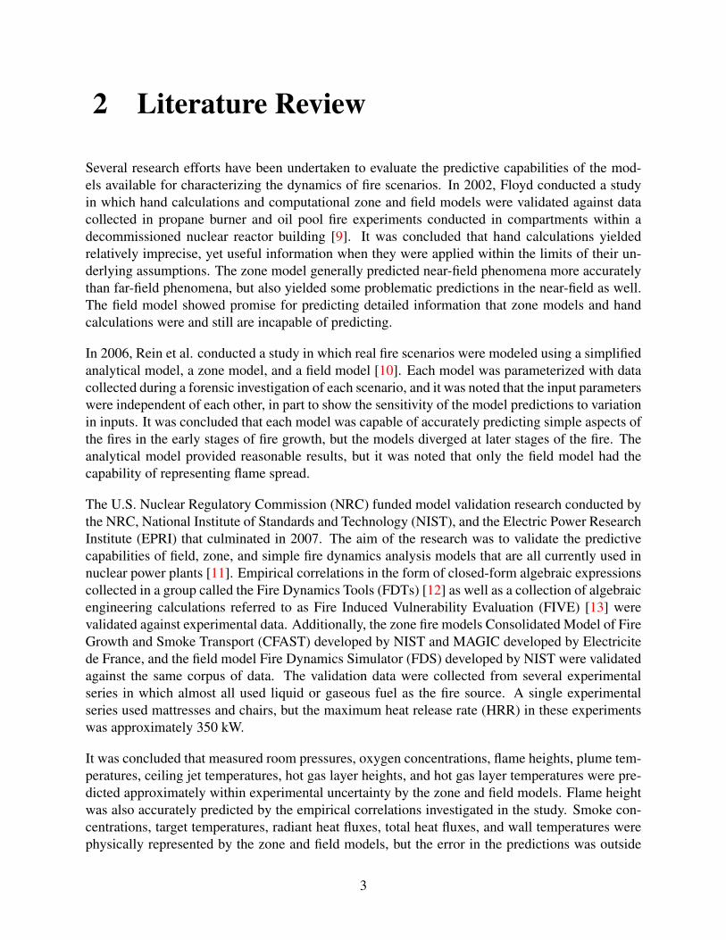
Experiments were conducted with the fuel item in four distinct locations within the compartment.The locations are referenced as the center, side, corner, and back of the compartment and arepresented in Figure 3.3. A summary of the set of configurations for the compartment experimentsare organized by fuel type in Table 3.1. Almost every combination of fuel, location, and state ofthe door was tested in triplicate. Additional information about the experiments and the results arepresented in a related report [23].

8

(a) Corner Position (b) Back Position (c) Side Position (d) Center Position

Figure 3.3: Schematics showing the four positions of the fuel (represented by the gray square).

Table 3.1: Summary of Compartment Experiments

Fuel Door Status Fuel Position(s)Experiments per

Configuration0.3 m Burner at 100 kW Open, Closed Corner, Back, Side, Center 30.6 m Burner at 100 kW Open, Closed Corner, Back, Side, Center 30.6 m Burner at 250 kW Open, Closed Corner, Back, Side, Center 30.6 m Burner at 500 kW Open, Closed Back, Side, Center 30.6 m Burner at 500 kW Open, Closed Corner 1Red Accent Chair Open, Closed Corner, Center 3Red Accent Chair Open, Closed Back 1Overstuffed Sofa Open, Closed Corner 3Overstuffed Sofa Open Back 3Overstuffed Sofa Closed Back 1

3.3.1 Structure

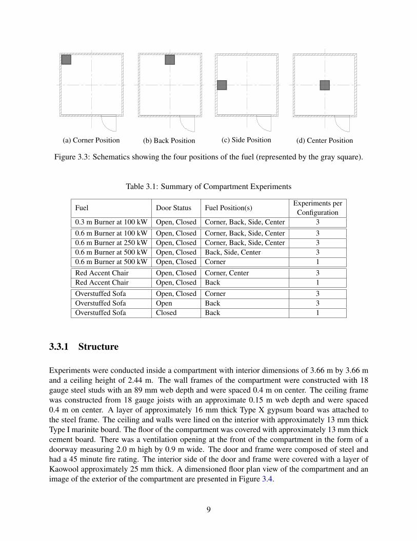
Experiments were conducted inside a compartment with interior dimensions of 3.66 m by 3.66 mand a ceiling height of 2.44 m. The wall frames of the compartment were constructed with 18gauge steel studs with an 89 mm web depth and were spaced 0.4 m on center. The ceiling framewas constructed from 18 gauge joists with an approximate 0.15 m web depth and were spaced0.4 m on center. A layer of approximately 16 mm thick Type X gypsum board was attached tothe steel frame. The ceiling and walls were lined on the interior with approximately 13 mm thickType I marinite board. The floor of the compartment was covered with approximately 13 mm thickcement board. There was a ventilation opening at the front of the compartment in the form of adoorway measuring 2.0 m high by 0.9 m wide. The door and frame were composed of steel andhad a 45 minute fire rating. The interior side of the door and frame were covered with a layer ofKaowool approximately 25 mm thick. A dimensioned floor plan view of the compartment and animage of the exterior of the compartment are presented in Figure 3.4.

9

3.66m

2.44m

3.34m3.66m

Ceiling Height: 2.44 m

Front

Back

Left Right

Figure 3.4: Dimensioned floor plan and image of the compartment utilized during the experiments.The image is a view of the front left corner from the compartment exterior.

Leakage

To characterize ventilation within the experimental compartment, a leakage test was conductedwith all exterior vents closed. The standard test method described in ASTM E 779 Standard TestMethod for Determining Air Leakage Rate by Fan Pressurization was followed to determine theair changes per hour and the equivalent leakage area [24]. The leakage from the compartmentwas 2.75 air changes per hour (ACPH) at 50 Pa with an effective leakage area of approximately0.0019 m2 at 4 Pa. This effective leakage area was calculated with Equation 3.1 and Equation 3.2,assuming a pressure exponent, n, of 0.65, which is the approximate mean pressure exponent forsingle-family homes in the United States [25].

AL = VL

√ρ

2 |ptest |(3.1)

AL,e f f = AL

(pre f

ptest

)n−0.5

(3.2)

Appendix A of NFPA 92 Standard for Smoke Control Systems provides a table of typical leakageratios collected from experimental research conducted on commercial and multi-family structures.According to NFPA 92, the effective leakage area for the compartment used in these experimentswould be 0.0016 m2 for tight construction, 0.0056 m2 for average construction, 0.012 m2 forloose construction, and 0.041 m2 for very loose construction. The leakage rate calculated for the

10

compartment in these experiments is between tight and average construction.

3.3.2 Instrumentation

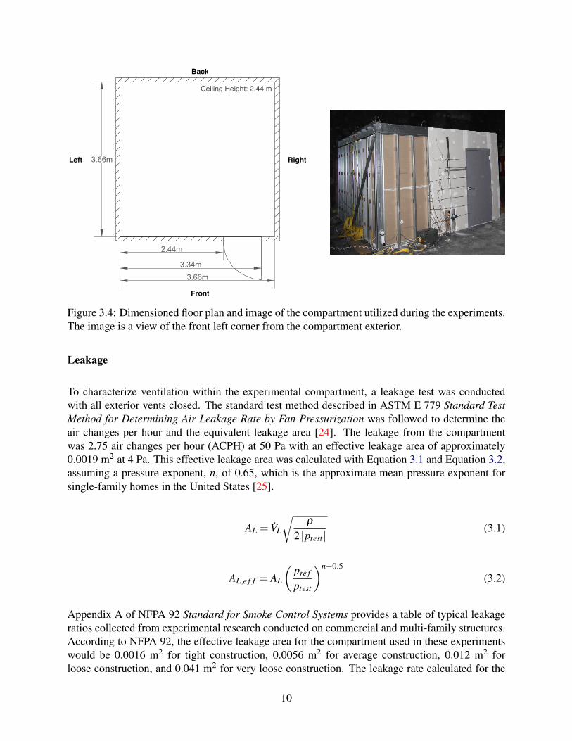
Figure 3.5 displays a dimensioned plan view of the experimental compartment with the locationsof the fixed instrumentation denoted by symbols. Total and radiative heat flux to the right sidewall were measured by gauges centered along the wall and positioned 0.65 m and 1.3 m belowthe ceiling. These total heat flux gauges and radiometers, represented by the blue diamond andred pentagon in Figure 3.5, were installed such that their faces were flush with the interior sideof the wall. Additionally, a pair of gauges at identical heights were used to measure the totalheat flux from the fire plume to the nearest wall during experiments in which the fuel load wasagainst a wall (i.e., at the corner, back, or side location). These two gauges were also flush withthe interior surface of the wall and were aligned with the center of the fuel load. These gauges arenot displayed in the figure because their locations moved when the fuel location changed.

EQ EQ

0.30 m

0.15 m

1.83 m

0.92 m

0.92 m

0.92 m

0.92 m

Icon Instrumentation

Thermocouple Array & O2 Probes

Pressure Tap

Radiometer

Heat Flux Gauge

Bi-Directional Probe∗

∗Arrow indicates positive flow direction

Figure 3.5: Floor plan showing location of fixed instrumentation for the compartment experiments.

BDPs paired with thermocouples were installed at the door opening to measure the flow velocitythrough the compartment doorway during open door experiments. These BDPs, represented bythe orange square in Figure 3.5, were installed along the exterior side of the compartment andpositioned so that they were horizontally-centered in the doorway. The seven BDPs were spaced0.25 m apart between the top of the doorway and the floor. Additionally, during experiments in

11

which the fuel load was against a wall (i.e., at the corner, back, or side location), two BDPs pairedwith thermocouples located 0.65 m and 1.3 m below the ceiling were positioned over each fuelload to measure the gas velocity and temperature within the fire plume.

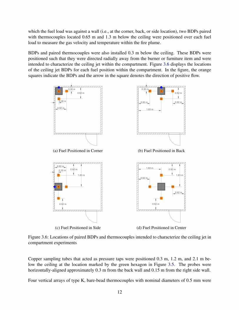
BDPs and paired thermocouples were also installed 0.3 m below the ceiling. These BDPs werepositioned such that they were directed radially away from the burner or furniture item and wereintended to characterize the ceiling jet within the compartment. Figure 3.6 displays the locationsof the ceiling jet BDPs for each fuel position within the compartment. In the figure, the orangesquares indicate the BDPs and the arrow in the square denotes the direction of positive flow.

0.92 m

0.92 m

0.30 m

0.30 m

(a) Fuel Positioned in Corner

0.92 m

1.83 m

0.92 m

0.30 m

0.92 m

(b) Fuel Positioned in Back

0.92 m

0.92 m0.92 m

1.83 m

0.30 m

(c) Fuel Positioned in Side

1.83 m 0.92 m

0.92 m

0.92 m

0.92 m1.83 m

(d) Fuel Positioned in Center

Figure 3.6: Locations of paired BDPs and thermocouples intended to characterize the ceiling jet incompartment experiments

Copper sampling tubes that acted as pressure taps were positioned 0.3 m, 1.2 m, and 2.1 m be-low the ceiling at the location marked by the green hexagon in Figure 3.5. The probes werehorizontally-aligned approximately 0.3 m from the back wall and 0.15 m from the right side wall.

Four vertical arrays of type K, bare-bead thermocouples with nominal diameters of 0.5 mm were

12

installed in the compartment. Each array contained eight thermocouples positioned at 25 mm,0.3 m, 0.6 m, 0.9 m, 1.2 m, 1.5 m, 1.8 m, and 2.1 m below the compartment ceiling. These arrayswere centered in each quadrant of the compartment, as shown in Figure 3.5. Gas samples werecollected through stainless steel tubes located 0.6 m and 1.8 m below the ceiling at the center ofeach quadrant as shown in Figure 3.5.

HRR and flow velocities through the door opening were not measured for experiments conductedwith the door to the compartment closed. Video analysis of the flame height was not possible whenthe fuel was positioned in the center location because the field of the video frame was limited atthe available distance and there was no reference against which flame heights could be compared,so mean flame height data was unavailable for these experiments. The smoke layer developmentin the closed door experiments obstructed the view of the fire plume, which limited the amount oftime for which flame height data could be collected.

Determination of Layer Temperatures and Interface Elevation

A method developed by Janssens and Tran [26] to estimate the upper gas layer and lower gas layertemperatures as well as the elevation of the interface between the two layers from a continuous,vertical profile of temperature was used to estimate these quantities from data collected in experi-ments conducted in the compartment described in this report. This method has also been adoptedby the developers of FDS for fire model validation.

Data from the quadrant thermocouple arrays were used to define T (z), a continuous function thatdesignates temperature (T ) as a function of height above the compartment floor (z) where z = 0at the floor and z = H at the ceiling. Then, the upper layer temperature (Tu), the lower layertemperature (Tl), and the height of the interface between the two layers (zint) were estimated ateach time step by computing I1 and I2 as in Equation 3.3 and Equation 3.4.

I1 =∫ H

0T (z)dz = (H− zint)Tu + zintTl (3.3)

I2 =∫ H

0

1T (z)

dz = (H− zint)1Tu

+ zint1Tl

(3.4)

The definitions of I1 and I2 were combined into the form of Equation 3.5, which was solved todetermine the interface elevation (zint). In these equations, Tl is the temperature measured by thethermocouple nearest to the floor and Tu is defined according to Equation 3.6. The total expandeduncertainty of the layer interface height was estimated as ± 14% [27].

zint =Tl(I1I2−H2)

I1 + I2T 2l −2TlH

(3.5)

13

(H− zint)Tu =∫ H

zint

T (z)dz (3.6)

14

4 Predictive Fire Algorithms & Models

When choosing a model, it is useful to understand the input data needed for the model and thesensitivity of the model to uncertainties in the input parameters. In this section, model inputs arediscussed and the results of sensitivity analyses for the models are reviewed.

Three types of models were used in this study to predict the fire environment generated by theexperiments described in Section 3. These models included simple fire dynamics analyses in theform of algebraic expressions coded into spreadsheets, a zone fire model, and a field fire model.Data collected at steady state for each set point HRR were compared across each modeling methodfor the gas burner experiments. Because most of the algebraic expressions provided a single pre-dicted value based on a single HRR, it was necessary for the experiments conducted with furniturethat a representative HRR be defined. In these cases, the maximum HRR, the mean HRR, and thesteady HRR in the decay phase were used to predict the desired measurands, which were com-pared to corresponding maximum, mean, and steady values of the measured quantities as well asthe quantities predicted by the field and zone models.

4.1 Model Background

The models used in this study represent the three categories of models identified in NFPA 921.These models can be used to conduct fire dynamic analyses to test hypotheses regarding fire originand development. The three categories of models are: specialized fire dynamics routines, zonemodels, and field, or CFD, models [1]. Further, each of the models chosen for this assessment arecurrently maintained and undergo verification and validation checks as part of the NRC and NISTprogram.

4.1.1 NRC Fire Dynamics Tools

The Fire Dynamics Tools (FDTs) is a set of quantitative methods that were originally compiled bythe NRC to allow fire protection inspectors to quickly and easily conduct fire hazard analyses [12].A collection of spreadsheets were developed to facilitate fire dynamics analyses using the FDTs.The convenience of these spreadsheets has led to adoption of the FDTs as a tool that is commonlyused by investigators conducting fire dynamics analyses. The equations presented in this sectionrequire standard units as defined by the International System of Units (SI).

15

Hot Gas Layer Temperature & Height

The collection of FDTs includes correlations for hot gas layer temperatures and interface height.A method for predicting hot gas layer temperature in a compartment with a single vertical wallopening with natural ventilation known as the Method of McCaffrey, Quintiere, and Harkleroad(MQH) is included in the collection of FDTs. The MQH method was derived based on an energybalance for a simplistic compartment fire scenario. Empirical constants in the functional form ofthe MQH correlation were determined based on analysis of 112 experiments with cellulosic andsynthetic polymer sheets and cribs as well as gaseous hydrocarbon fuels in compartments withheights that ranged from 0.3 m to 2.7 m. The authors of the study indicated that the plume theorycorrelation used to derive the temperature rise correlation does not hold in scenarios in which thetemperature rise in the upper gas layer exceeds 600◦C [28]. In deriving the correlation for upperlayer temperature, the study authors did not consider fire locations that deviated significantly fromthe center of the compartment, which introduces uncertainty about the ability of the correlation,as published in the FDTs, to predict the hot gas layer temperature when the fire source is locatedagainst a wall or in a corner.

The MQH correlation as it appears in the FDTs is displayed as Equation 4.1. In the equation, ∆Tgis the temperature rise in the upper gas layer, Q is the HRR, Av is the total ventilation area, hv is theheight of the ventilation opening, AT is the total surface area of the interior of the compartment lessthe ventilation area, and hk is the total heat transfer coefficient. The quantity Av

√hv is sometimes

referred to as the ventilation factor, which will be adopted for the remainder of this report.

∆Tg = 6.85[

Q2

(Av√

hv)(AT hk)

] 13

(4.1)

For long periods of time in which conditions within the compartment achieve steady state, hk is aconstant defined as hk =

kδ

, where k denotes the thermal conductivity of the wall lining materialand δ denotes the thickness of the wall. For times in which heat does not completely penetrate the

material lining the compartment, the heat transfer coefficient may be defined as hk =√

kρct , where

k, ρ , and c are the thermal conductivity, density, and specific heat capacity of the wall lining, andt is the time after ignition.

The correlation for the hot gas layer temperature in a closed compartment was presented by Beylerin 1991 [29]. The experiments Beyler analyzed to develop the correlation were conducted in atest compartment with a 4 m x 6 m footprint and a ceiling height of 4.5 m. The fire source was amethane gas burner in the center of the room with a height ranging from 0.23 m to 2.06 m above theground which supplied constant heat release rates (HRRs) in the range of 50 kW to 400 kW. Thecorrelation was derived by solving a non-steady energy balance for the closed compartment thataccounted for heat loss through the wall material assuming a constant HRR and ignoring energylost through leakage. This correlation is presented as Equation 4.2. In the correlation, K1 is aconstant described by Equation 4.3 where k, ρ , and c are the thermal conductivity, density, andspecific heat capacity of the wall lining material, m is the mass of gas in the compartment, cp is the

16

specific heat capacity of the gas in the compartment. K2 is a constant described by Equation 4.4,where Q is the HRR. The symbol t in Equation 4.2 is the time after ignition.

∆Tg =2K2

K21(K1√

t−1+ e−k√

t) (4.2)

K1 =0.8√

kρcmcp

(4.3)

K2 =Q

mcp(4.4)

The Method of Yamana and Tanaka is a non-steady method to predict the height of the interface be-tween the smoke layer and smoke-free air in a compartment with no smoke venting. The equationfor the smoke layer interface was derived using a plume flow correlation and assuming the smokelayer density is constant [30]. The form of the correlation adopted for the FDTs was also derivedunder the assumption of a constant HRR. The correlation was validated against experiments con-ducted in an experimental facility with a footprint of 24 m x 30 m and a ceiling height of 26.3 m.The fire source for the experiments was an approximately 1.8 m x 1.8 m square methanol pool firesource located in the center of the facility on the floor [31]. The smoke layer height correlation ispresented as Equation 4.5. In the correlation, k is a constant described by Equation 4.6 in which ρgis the hot gas density, ρa is the ambient density, g is the gravitational constant, cp is the spsecificheat capacity of the air, and Ta is the ambient temperature. In Equation 4.5, Q denotes the HRR, tis the time after ignition, Ac is the compartment floor area, and hc is the compartment height.

z =

(2kQ

13 t

3Ac+

1

h23c

)− 32

(4.5)

k =0.21ρg

(ρ2

a gcpTa

) 13

(4.6)

Flame Height

The FDTs include two correlations for flame height developed by Heskestad and Thomas that rep-resent fire plumes that are not influenced by walls, ceilings, other obstructions. The FDTs alsoinclude two correlations for fire plumes located adjacent to a wall, or in a corner of a compartment.Thomas derived the expression for flame height through a dimensional analysis accounting fortemperatures and velocities in the plume as well as the entrainment rate of air into the plume. Em-pirical coefficients in the Thomas correlation were determined through analysis of photographic

17

evidence of flame heights from wood crib fire experiments conducted in an open laboratory envi-ronment [32]. The correlation derived by Thomas is displayed as Equation 4.7, where m′′ is theburning rate of the fuel per unit area, ρa is the ambient density, g is the gravitational constant, andD is the equivalent diameter of the fire.

H f = 42D(

m′′

ρa√

gD

)0.61

(4.7)

Heskestad derived a functional relationship between the flame height of a circular turbulent diffu-sion flame and several parameters associated with the geometry and chemistry of the fire source,primarily the HRR and fire source diameter. Correlation constants were determined through re-gression analysis of experimental data, which were mostly comprised of liquid and gaseous fuelsburning in open laboratory conditions [33]. The correlation was later applied to palletized rackstorage using an effective fire area and was found to reasonably represent flame heights measuredfrom the base of the storage [34]. The correlation derived by Heskestad is displayed as Equa-tion 4.8, where Q is the HRR and D is the equivalent diameter of the fire.

H f = 0.235Q25 −1.02D (4.8)

Delichatsios developed the functional form of a correlation to describe the flame height from aline fire source and a two-dimensional fire source against a wall [35]. The proposed correlationwas dependent primarily on the heat release rate, radiative fraction, combustion efficiency, andthermal properties of air. The correlation was simplified to the form published in the FDTs byfitting experimental data on small scale alcohol-fueled fires [36]. That form of the correlation isdisplayed here as Equation 4.9, where Q′ is the HRR per unit length along the wall.

H f = 0.034Q′23 (4.9)

Hasemi and Tokunaga developed a correlation for the flame height in a corner using a non-dimensional HRR parameter known as the Froude number under the assumption that air may onlybe entrained from one side of the fire source [37]. The coefficient for the correlation developedby the study authors was determined by fitting data collected on buoyant plumes in an unconfinedlaboratory setting. Experiments involved square gas burners with side lengths ranging from 0.2 mto 0.5 m in a non-combustible corner. The correlation developed by Hasemi and Tokunaga isdisplayed here as Equation 4.10, where Q is the HRR.

H f = 0.075Q35 (4.10)

18

Radiant Heat Flux to a Target

Three correlations are provided in the FDTs to determine the radiant heat flux from the fire tosurrounding targets. These methods include:

1. point source fuel to target at ground level

2. solid flame radiation model to target at ground level

3. solid flame radiation model to target above ground level

The method for calculating the radiant heat flux to a target from a point source provided in theFDTs was derived as a straightforward, simplistic radiation heat transfer equation. The pointsource model is generally applicable for fire sources that are circular or that have a low aspectratio radiating to far-field targets. The equation to describe the radiative heat flux from a pointsource is displayed here as Equation 4.11, where χr is the radiative fraction, Q is the HRR, and Ris the radial distance from the center of the flame to the edge of the target. It has been suggestedthat the upper limit for heat fluxes that may be accurately described by the point source model is 5kW/m2 [38].

q′′ =χrQ

4πR2 (4.11)

The solid flame method to calculate radiant heat flux at targets was presented by Shokri and Beylerand relies on configuration factors between the flame plume, which is assumed to be cylindrical,and the target [39]. The correlation for the solid flame model is presented as Equation 4.12, whereF1→2 is the total configuration factor. The flame height used to compute the total configurationfactor is described by the Heskestad correlation, and the emissive power of the flame is estimatedusing a correlation derived from experimentally measured heat fluxes from liquid pool fires toexternal targets, presented here as Equation 4.13, where D is the effective diameter of the pool fire.A different set of configuration factors is utilized when the target is at ground level compared withan elevated target. Details of the configuration factors may be found in the original presentation ofthe correlation [39] or in standard references [12, 38].

q′′ = EF1→2 (4.12)

E = 58(10−0.00823D) (4.13)

19

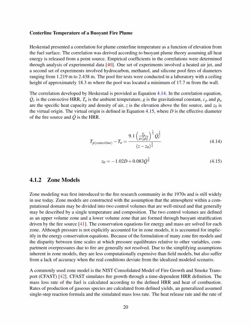
Centerline Temperature of a Buoyant Fire Plume

Heskestad presented a correlation for plume centerline temperature as a function of elevation fromthe fuel surface. The correlation was derived according to buoyant plume theory assuming all heatenergy is released from a point source. Empirical coefficients in the correlations were determinedthrough analysis of experimental data [40]. One set of experiments involved a heated air jet, anda second set of experiments involved hydrocarbon, methanol, and silicone pool fires of diametersranging from 1.219 m to 2.438 m. The pool fire tests were conducted in a laboratory with a ceilingheight of approximately 18.3 m where the pool was located a minimum of 17.7 m from the wall.

The correlation developed by Heskestad is provided as Equation 4.14. In the correlation equation,Qc is the convective HRR, Ta is the ambient temperature, g is the gravitational constant, cp and ρaare the specific heat capacity and density of air, z is the elevation above the fire source, and z0 isthe virtual origin. The virtual origin is defined in Equation 4.15, where D is the effective diameterof the fire source and Q is the HRR.

Tp(centerline)−Ta =9.1(

Tagc2

pρ2a

) 13

Q23c

(z− z0)53

(4.14)

z0 =−1.02D+0.083Q25 (4.15)

4.1.2 Zone Models

Zone modeling was first introduced to the fire research community in the 1970s and is still widelyin use today. Zone models are constructed with the assumption that the atmosphere within a com-putational domain may be divided into two control volumes that are well-mixed and that generallymay be described by a single temperature and composition. The two control volumes are definedas an upper volume zone and a lower volume zone that are formed through buoyant stratificationdriven by the fire source [41]. The conservation equations for energy and mass are solved for eachzone. Although pressure is not explicitly accounted for in zone models, it is accounted for implic-itly in the energy conservation equations. Because of the formulation of many zone fire models andthe disparity between time scales at which pressure equilibrates relative to other variables, com-partment overpressures due to fire are generally not resolved. Due to the simplifying assumptionsinherent in zone models, they are less computationally expensive than field models, but also sufferfrom a lack of accuracy when the real conditions deviate from the idealized modeled scenario.

A commonly used zone model is the NIST Consolidated Model of Fire Growth and Smoke Trans-port (CFAST) [42]. CFAST simulates fire growth through a time-dependent HRR definition. Themass loss rate of the fuel is calculated according to the defined HRR and heat of combustion.Rates of production of gaseous species are calculated from defined yields, an generalized assumedsingle-step reaction formula and the simulated mass loss rate. The heat release rate and the rate of

20

production of gaseous products decreases to zero when the oxygen concentration decreases belowthe lower oxygen limit. CFAST has the ability to model leakage to or from compartments to thesurrounding atmosphere based on the pressure differential across the compartment wall. Leakagefor a compartment is defined with a leakage ratio that relates the total area of leaks through thewalls of a compartment to the total surface area of the walls and ceiling of the compartment.

Flame height, centerline temperature, and mass entrainment of the fire plume in CFAST are rep-resented by the correlations developed by Heskestad [42]. Wall and corner plumes in CFAST arecalculated using modified versions of the Heskestad correlations that utilize the virtual heat sourceconcept in which the fire source is mirrored across the boundary to calculate a new virtual ori-gin and augmented plume entrainment rate. Radiant heat transfer to defined targets is calculatedthrough a heat transfer analysis and energy balance between the target, the six bounding surfacesin the compartment, the upper gas layer, and the lower gas layer. A companion program, Smoke-view [43], is used for visualizing the results of the FDS computations

4.1.3 Field Models

Field models divide the computational domain into finite volumes with the assumption that the tem-perature, pressure, and mass fractions are uniform in each volume and that the velocity and fluxesare uniform over each surface of the volumes. Field models are capable of resolving more physicalphenomena than zone models as well as transient effects in the development of fire-induced flow,but do so at a significantly higher computational cost than zone models.

The NIST Fire Dynamics Simulator (FDS) is the most commonly used field fire model in fireinvestigations and research. FDS is a CFD model used to simulate fire-driven fluid flow thathas been developed by a multi-national team led by NIST and the Technical Research Centre ofFinland (VTT) [44, 45]. FDS Version 1 was released in 2000 and has constantly been undergoingdevelopment, improvements, and validation since. FDS has undergone extensive and ongoingV&V [11,27,46]. The model numerically solves a form of the Navier-Stokes equations appropriatefor low-speed, thermally-driven flow. The partial derivatives of the conservation equations of mass,momentum, and energy are approximated as finite differences, and the solution is updated in timeon a three-dimensional, rectilinear grid. The model is open source and generalized for the widestpossible set of applications. To make FDS as generalized as possible, it includes an array ofsubmodels that represent phenomena characterized by length scales that are typically smaller ormuch larger than the computational grid or that cannot be explicitly described by the governingequations [44]. FDS typically uses the Large Eddy Simulation (LES) approach, which presumesthat the grid resolution is sufficient to resolve the dominant eddy structures and the Deardorffsubmodel is used for unresolved turbulence.

FDS applies a lumped species approach to model combustion where three lumped species whichrepresent fuel, air, and combustion products are tracked. Reaction rates are mixing-controlled [47]with a simple extinction model based on a critical flame temperature [48] by default. Thermal radi-ation is computed through solution of the radiation transport equation for a gray gas using the FiniteVolume Method on the same grid as the flow solver. A companion program, Smokeview [43], is

21

used for visualizing the results of the FDS computations.

The resolution index (RI), which is the ratio of the characteristic fire diameter (D∗) to the gridresolution (dx), provides a metric by which model practitioners may evaluate the relative resolutionof a model. The characteristic fire diameter is defined in Equation 4.16, where Q is the HRR,ρ∞ is the ambient air density, cp is the specific heat capacity of air, and T∞ is the ambient airtemperature, and g is the gravitational constant. An RI between 4 and 10 is generally consideredcoarse resolution, 10 to 16 is considered moderate resolution, and above 16 is considered fineresolution.

The developers of FDS conducted a study to determine the optimal method to characterize themean flame height in FDS simulations [27]. The authors developed a method whereby the HRRper unit length of elevation in the computational domain were integrated along the elevation abovethe fire source. The authors concluded that all available empirical flame height correlations arebounded by the elevations at which between 95% and 99% of the total HRR was realized. Thismethod of defining the mean flame height has been adopted in this work.

D∗ =(

Qρ∞cpT∞

√g

) 25

(4.16)

4.2 Model Construction for Compartment Experiments

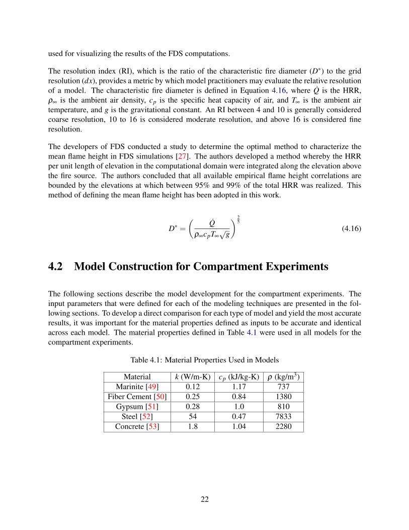
The following sections describe the model development for the compartment experiments. Theinput parameters that were defined for each of the modeling techniques are presented in the fol-lowing sections. To develop a direct comparison for each type of model and yield the most accurateresults, it was important for the material properties defined as inputs to be accurate and identicalacross each model. The material properties defined in Table 4.1 were used in all models for thecompartment experiments.

Table 4.1: Material Properties Used in Models

Material k (W/m-K) cp (kJ/kg-K) ρ (kg/m3)Marinite [49] 0.12 1.17 737

Fiber Cement [50] 0.25 0.84 1380Gypsum [51] 0.28 1.0 810

Steel [52] 54 0.47 7833Concrete [53] 1.8 1.04 2280

22

Radiative Fraction

The UL testing facility where the experiments were conducted is equipped to conduct calorimetryusing the oxygen-depletion method (ASTM E2067) as well as the thermopile method (ASTM E906).These methods provide the chemical and convective HRR, respectively. With both of these quan-tities measured, the radiative fraction, χr, of the fire that results from burning each fuel was deter-mined. The χr values presented in the following tables were determined through direct measure-ment of the HRR components.

Table 4.2 displays the radiative fraction that was directly determined for each fuel in preliminaryexperiments conducted outside the compartment. The uncertainty in the radiative fraction, σχr , isexpressed as plus or minus two standard deviations of the radiative fraction for each fuel. Therewere typically three replicates of each experiment conducted at the UL laboratory. The smallsample size resulted in large standard deviations relative to the mean values.

Table 4.2: Radiative Fraction Calculated for Each Fuel Package

Fuel Package χr σχr

Red Accent Chair 0.35 ±0.11Overstuffed Sofa 0.32 ±0.10

4.2.1 FDTs

The FDT methods typically required a single representative value for the HRR of the fire. Becausethe HRR of the furniture items evolved over a significant range over the course of the experi-ments, three representative values of the HRR were used in FDT predictions for the furnitureexperiments. The maximum, mean, and steady HRRs were calculated from the mean data of allreplicates conducted over the three experimental facilities. The mean HRR was calculated overthe entire duration of the mean experimental data. The steady HRR was also a mean of the datawith the lower limit of the time range over which the mean was calculated defined as the time atwhich the mean burning rate decreased to below 36.8% (1/e) of the peak HRR value and the rateof change of the burning rate was below 3% of the maximum rate of change of the burning ratefor 30 s continuously. These criteria accounted for noise and other spurious data in the mean data.The steady HRR was always taken during the portion of the experiments in which the HRR was indecay.

The inputs required for the methods to predict heat flux, plume temperature, and flame heightthat are collected in the FDTs require knowledge of the geometry of the experimental setup andthe HRR of the fire. The gas burners had a square cross-section, so an effective diameter wascalculated that was defined as the diameter of a circular cross-section burner with an equivalentsurface area. The radiative fraction of the gas burner flame was determined to be 0.23 throughdirect measurement.

The MQH correlation for the hot gas layer temperature requires the total surface area of the interior

23

of the compartment, the area and height of the doorway, and the total heat transfer coefficient. Thetotal surface area of the compartment was 60.7 m2 and the doorway had an area of 1.8 m2 and aheight of 2.0 m. The walls and ceiling of the compartment were lined with a 16 mm thick layer ofgypsum wallboard on top of a 13 mm thick layer of marinite. The effective kρc for the wall liningmaterials was approximately 0.145 (kW/m2K)2s.

4.2.2 CFAST

CFAST (Version 7.5.0) was used to construct models to simulate the gas burner and furnitureexperiments conducted in the compartment. The duration of the simulations was defined as 600 sand data were output at 15 s intervals. The initial and ambient temperature was defined as 15◦C andthe lower oxygen index was defined as 0.15. The thermal properties of marinite were defined andassigned to the walls and ceiling of the compartment. The thermal properties of the fiber cementboard were assigned to the floor of the compartment. The emissivity of the marinite board and thefiber cement board was assumed to be 0.95 and defined as such.

A single vent in the front of the compartment was defined with the dimensions of the door openingfor the simulations of open door experiments. A leakage ratio of 0.526 cm2/m2 was defined overthe walls of the compartment to simulate leakage in the closed door experiments. Targets weredefined at the locations of the heat flux gauges and radiometers in the compartment experiments.

The fire source was located consistent with the experiment to be simulated at an elevation of 0.5 m.The area of the fire source was defined as 0.09 m2 for the 0.3 m burner and 0.36 m2 for the 0.6 mburner. The fuel chemistry was defined as methane (CH4) with a heat of combustion of 53100 kJ/kgfor the simulations of the gas burner experiments. The radiative fraction for the fire was defined as0.23. The HRR for the fire source was defined to achieve the set point HRR in 10 s and no decayperiod was included at the end of the simulation.

The fire sources for the furniture experiments were defined with areas that approximated the pro-jection of the specific furniture item to the floor (i.e., 0.54 m2 for the Red Accent Chair and 2.18 m2

for the Overstuffed Sofa) and the elevation of the fire source was defined as the seat height. The fuelchemistry was defined with a chemical formula that approximated polyurethane (C6.3H7.1O2.1N).The heat of combustion was defined as the mean measured heat of combustion from the exper-iments and the soot yield was defined as 0.18. The HRR defined for each CFAST simulationmimicked the mean measured HRR for each furniture item with a resolution of 15 s.

4.2.3 FDS

FDS (Version 6.7.5) was used to simulate the experiments in which the burners and furniture itemswere ignited in the compartment to match conditions in the laboratory as closely as possible. Thefuel sources and instrumentation were positioned as geometrically similar to the experiments aspossible. The ambient temperature was assumed to be 15◦C in all simulations.

24

The gas burner was represented in each model as a supply vent attached to a solid obstructionwith a predefined total mass flux that yielded the set point HRR from the experiments. The fuelfor the gas burners was defined according to the chemical composition provided by the gas utilitycompany for the experiments conducted at the UL facility (92.2% methane, 5.8% ethane, 1.3%nitrogen, and 0.7% carbon dioxide) with a heat of combustion of 53,100 kJ/kg. The sides of theburner were assigned the thermal properties of steel (see Table 4.1) with a thickness of 0.003 m.

The furniture items were represented as closely as possible to their physical dimensions whileadhering to the underlying rectilinear grid. This allowed conclusions to be drawn about the impor-tance of representing an approximation of the actual geometry for accurately predicting quantitiesincluding heat fluxes and flame height. Images of the geometric representations of the furnitureitems are displayed in Figure 4.1. These may be directly compared to the images presented inFigure 3.2. A single simple reaction was defined to describe combustion of the pyrolyzate releasedfrom the condensed phase sofa materials during burning. The only pyrolyzate species released wasdefined as polyurethane with a heat of combustion defined as approximately 16,180 kJ/kg and asoot yield of 0.18, which was the approximate mean of values that have been reported for flexiblepolyurethane foams [54]. For each furniture item, the heat release rate per unit area (HRRPUA)for all surfaces was defined such that the total HRR matched the mean time-dependent HRR mea-sured in the experiments. By doing so, the model did not accurately represent the real spatial flamespread or the material burn away process, however the overall energetics of the burning processwere represented.

(a) FDS Representation of the Red Accent Chair

(b) FDS Representation of the Overstuffed Sofa

Figure 4.1: Renderings of the upholstered chair and sofa geometries utilized in FDS simulations.

The computational domain was defined with dimensions of 3.9 m by 5.4 m by 4.8 m. This allowedthe computational domain to coincide with the boundaries of the compartment and extend 1.6 mfrom the front of the compartment to resolve flow through the door and 2.4 m above the compart-ment to resolve the thermal plume that flowed out the door. All boundaries, with the exception ofthe ground were defined with the ‘OPEN’ surface definition. The fire source was defined consis-tent with the location of the fire source in the experiment to be simulated with the surface of theburner elevated either 0.5 m above the floor of the compartment (0.3 m burner) or 0.65 m above

25

the floor of the compartment (0.6 m burner) and the furniture items represented with geometry assimilar to the actual geometries as possible. The time-dependent HRR of the furniture items forthe simulations of the experiments conducted with the door open and closed was defined to followthe instantaneous mean of the measured HRR across all replicate experiments with the door openfor the furniture item in the location to be simulated.

The compartment was defined as a pressure zone for the simulations of the experiments conductedwith the door closed. The pressure zone leakage method was applied to assign a leakage areaof 0.0019 m2 to the closed door of the compartment. Two levels of resolution were investigated.Two levels of resolution were investigated. The grid was defined to be uniform throughout thecomputational domain with all cubic elements and cell sizes of 0.1 m and 0.05 m. These resolutionscorresponded to the characteristic fire diameters and RIs provided in Table 4.3. The table indicatesthat simulations with a grid size of 0.1 m had coarse resolution for the burner experiments andranged from coarse to moderate for the furniture items. The simulations with a grid size of 0.05 mranged from coarse to fine resolution with greater HRR yielding better resolution. The grid wasdefined to be uniform throughout the computational domain with all cubic elements and cell sizesof 0.1 m and 0.05 m.

Table 4.3: Characteristic fire diameter and resolution index for compartment experiment simula-tions

Fire Size D∗ D∗/0.1 D∗/0.0550 kW 0.29 2.9 5.8

100 kW 0.38 3.8 7.7500 kW 0.73 7.3 14.7

Red Accent Chair (mean) 0.53 5.3 10.6Overstuffed Sofa (mean) 0.76 7.6 15.2

4.3 Model Sensitivity

The proper use of predictive fire models requires a complete understanding of the sensitivity of themodel results to the input parameters. By understanding the sensitivity of the model to the inputsto the model, uncertainty in the inputs may be propagated through to the final results to assign alevel of confidence to the conclusions drawn from the use of the model. Determining the sensitivityof the model to specific model inputs is straightforward for the algebraic models collected as theFDTs, but it is more difficult for the computational models utilized in this work. Several researchershave conducted sensitivity analyses on these computational models and detailed descriptions ofthe findings of these sensitivity analyses are left to the original authors [55–58]. It is essential thatmodel practitioners have a comprehensive and complete understanding of the affect of changes ineach parameter on the results of the model.

26

5 Model Assessment

The following sections present a quantitative assessment of the ability of the models to predicteach measurand. All comparisons of FDS predictions that are presented in this section used theresults from the higher resolution (cell size of 0.05 m) simulations. Also presented are metricscalculated to describe the ability of each model to predict the fire environment. In the followingfigures, the solid black line that runs from the bottom left to the upper right corner of the plotindicates the expected perfect agreement between the experimentally measured data and the modelprediction. The dashed black lines offset from the solid black line represent the total estimatedexpanded experimental uncertainty for each measurement as presented in Section 3.2.

It is assumed that deviations from perfect agreement between the predictions and the experimentaldata are the result of simplifying assumptions, model implementation, and uncertainty in definedparameters which manifests as a systematic bias in the predictions. In the analysis presented in thissection, the bias is assumed to scale the expectation line by a bias factor. The biased expectationline runs through the center of the distribution of points which indicate the comparison for theindicated collection of data with the specific model. The bias-adjusted model uncertainty presentedin the tables in this section represents the scatter in the distribution of points which representthe agreement between the model predictions and the corresponding experimental data about thebiased expectation line.

The bias factors presented in the following tables can be considered a measure of the typical ac-curacy of the model for the collection of data points considered, where a bias factor of 1 indicatesperfect agreement and larger deviations above and below 1 indicate less accurate predictions. Theuncertainty presented in the following tables is the observed total expanded uncertainty of thebias factor, which is analogous to the dashed lines presented in the figures. This can be taken asa measure of how closely grouped the points are which represent the comparison of measured topredicted quantities. Bias factors and uncertainty in the bias factors have been calculated accordingto the equations described in the FDS Validation Guide [27].

Model developers strive for predictions to be consistently within the experimental uncertainty ofmeasured quantities. Deviation of the bias factor beyond the total expanded uncertainty of a mea-sured quantity indicates the model does not accurately represent the physics of the scenario, withlarger deviations from perfect agreement indicating less accuracy in the predictive capabilities ofthe model. For example, if the bias factor for a collection of predictions of a particular measure-ment is 1.1, the model overpredicts the measurement by 10% on average, and if the bias factor fora set of measurement-prediction pairs is 0.91 (1/1.1), the model underpredicts the measurement by10% on average.

Large uncertainty in the bias factor indicates significant scatter in the agreement between the mea-surements and the predictions. This uncertainty represents the level of confidence a practitionermay have in the bias factor, with low uncertainty correlated to more confident determinations of thebias factor for a given scenario. As an example, the bias factor may be 1 but the uncertainty may

27

be ±50%, which indicates that 95% of the measurement-prediction pairs lies in the range of biasfactors from 0.667 (1/1.5) to 1.5. Although the average bias factor indicates perfect agreement,the uncertainty indicates that the model does not consistently yield perfect agreement. For thepurposes of this work, uncertainty of the bias factor that is within the total expanded experimentaluncertainty of the measurement indicates the predictions are consistent and evokes the highest con-fidence in the bias factor. Deviations of the uncertainty in the bias factor above the total expandedexperimental uncertainty indicate decreased confidence in the presented bias factor.

The values in the tables have been shaded to simplify the visual representation of the predictiveassessment for each dataset. Table 5.1 provides a definition for each color presented in the tablesin this section. The symbol σ in the table corresponds to the total expanded uncertainty of themeasurand. As an example, a green shaded cell in the ‘Bias’ column indicates that, on average,the quantity was predicted to within the total expanded uncertainty. A green shaded cell in the‘Uncertainty’ column indicates that the scatter in the agreement between the prediction and themeasured quantity, as quantified by the standard deviation of the bias, exceeds the total expandeduncertainty of the measured quantity.

Table 5.1: Color Code for Bias and Uncertainty Tables

Shading Range≤ ± σ

± σ to ± 2σ

± 2σ to ± 3σ

> ± 3σ

Because the furniture experiments involved a growth phase and a long duration decay phase, threemetrics were used to provide a comprehensive assessment of the agreement between the modelpredictions and the experimental data. The method used to determine the mean and steady HRRused in FDT calculations was described in Section 4.2. The same method was adopted to de-termine the mean and steady values for each measurand from the experimental data, the CFASTpredictions, and the FDS predictions. An inner shading color of black inside the symbols in allfigures that display the agreement between model predictions and experimental data for furnitureitems denotes the maximum value, an inner shading of silver denotes the mean value, and an innershading of white denotes the steady value attained in the decay phase of the experiment.

Individual comparisons for each experiment with commentary on the agreement between eachmodel and the experimental data are provided in Appendix A.

5.1 Temperatures

The agreement between the steady temperatures and the model predictions for the compartmentexperiments with the gas burners is presented in Figure 5.1. The figure includes data from thermo-couples located to measure the fire plume, the ceiling jet, and the flow through the door. An FDT

28

method was only available for the plume temperatures.

0 200 400 600 800 1000 1200Measured Temperature Rise ( C)

0

200

400

600

800

1000

1200

Pred

icted

Tem

pera

ture

Rise

(C)

PlumeCeiling JetDoor

FDSFDT

Figure 5.1: Comparison of Steady Temperature Predictions to Experimental Data Collected inCompartment Experiments with Burners

Prediction biases and uncertainties calculated for the gas burner compartment experiments are pre-sented in Table 5.2 in which the 0.3 m burner experiments are denoted with labels that include‘SB’ and 0.6 m burner experiments are denoted with the set point HRR.. The FDT method over-predicted the plume temperatures. The magnitude of overprediction increased with increasingHRR, was higher when the door was closed than when it was open, and was not dependent on thelocation of the burner in the compartment. The majority of the steady temperatures predicted byFDS were less than 200◦C and many of these predictions were within the experimental uncertaintyof the measurement. Overall, FDS provided reasonable agreement with the temperature measuredin the compartment gas burner experiments, with a slight underprediction of the temperatures andhigh scatter in the agreement. The accuracy of the FDS predictions was highest for the 100 kWexperiments with the 0.3 m burner, in the experiments with the open door, and the experimentswith the burner in the back position.

29

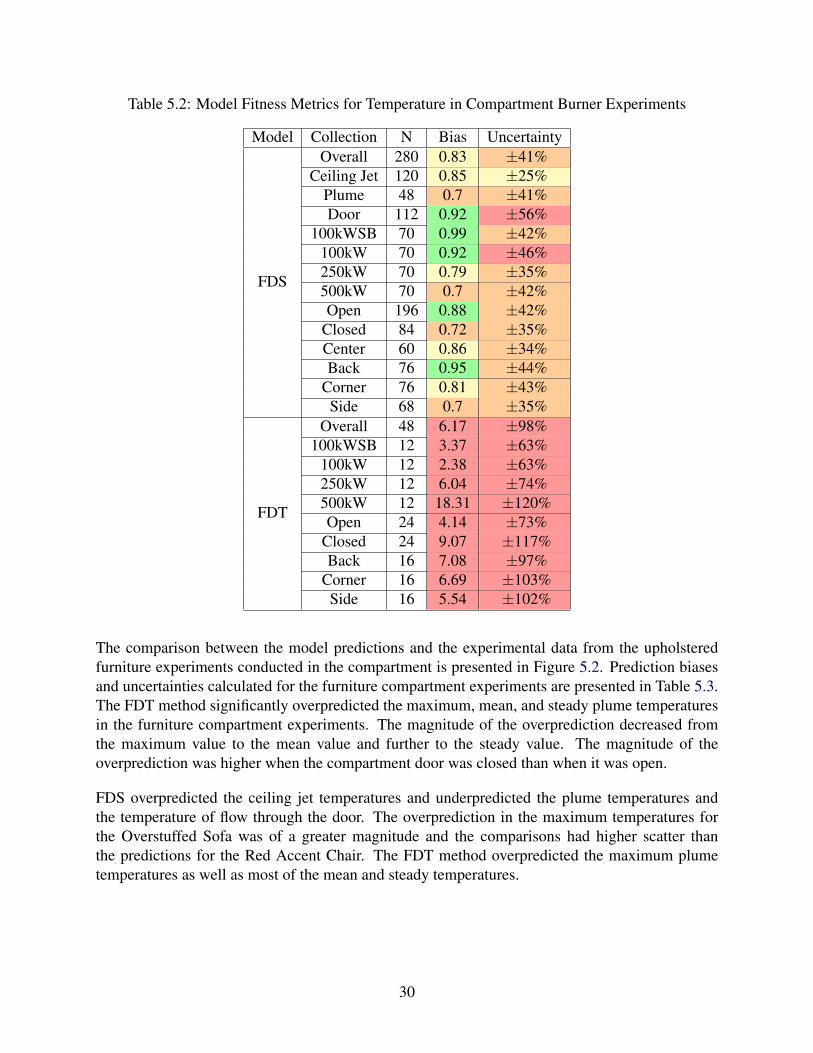
Table 5.2: Model Fitness Metrics for Temperature in Compartment Burner Experiments

Model Collection N Bias Uncertainty

FDS

Overall 280 0.83 ±41%Ceiling Jet 120 0.85 ±25%

Plume 48 0.7 ±41%Door 112 0.92 ±56%

100kWSB 70 0.99 ±42%100kW 70 0.92 ±46%250kW 70 0.79 ±35%500kW 70 0.7 ±42%Open 196 0.88 ±42%

Closed 84 0.72 ±35%Center 60 0.86 ±34%Back 76 0.95 ±44%

Corner 76 0.81 ±43%Side 68 0.7 ±35%

FDT

Overall 48 6.17 ±98%100kWSB 12 3.37 ±63%

100kW 12 2.38 ±63%250kW 12 6.04 ±74%500kW 12 18.31 ±120%Open 24 4.14 ±73%

Closed 24 9.07 ±117%Back 16 7.08 ±97%

Corner 16 6.69 ±103%Side 16 5.54 ±102%

The comparison between the model predictions and the experimental data from the upholsteredfurniture experiments conducted in the compartment is presented in Figure 5.2. Prediction biasesand uncertainties calculated for the furniture compartment experiments are presented in Table 5.3.The FDT method significantly overpredicted the maximum, mean, and steady plume temperaturesin the furniture compartment experiments. The magnitude of the overprediction decreased fromthe maximum value to the mean value and further to the steady value. The magnitude of theoverprediction was higher when the compartment door was closed than when it was open.

FDS overpredicted the ceiling jet temperatures and underpredicted the plume temperatures andthe temperature of flow through the door. The overprediction in the maximum temperatures forthe Overstuffed Sofa was of a greater magnitude and the comparisons had higher scatter thanthe predictions for the Red Accent Chair. The FDT method overpredicted the maximum plumetemperatures as well as most of the mean and steady temperatures.

30

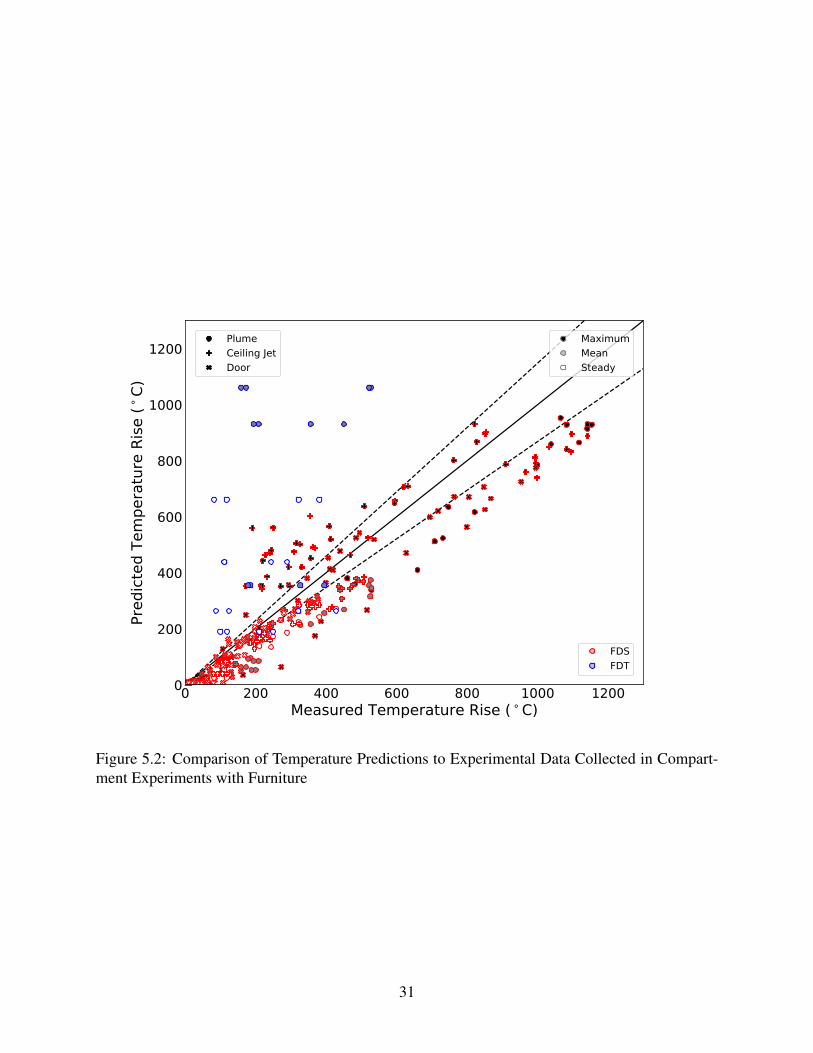
0 200 400 600 800 1000 1200Measured Temperature Rise ( C)

0

200

400

600

800

1000

1200

Pred

icted

Tem

pera

ture

Rise

(C)

PlumeCeiling JetDoor

MaximumMeanSteady

FDSFDT

Figure 5.2: Comparison of Temperature Predictions to Experimental Data Collected in Compart-ment Experiments with Furniture

31

Table 5.3: Model Fitness Metrics for Temperature in Compartment Furniture Experiments

Metric Maximum Mean SteadyModel Collection N Bias Uncertainty N Bias Uncertainty N Bias Uncertainty

FDS

Overall 104 1.01 ±42% 104 0.69 ±35% 104 0.68 ±58%Ceiling Jet 48 2.41 ±97% 48 1.56 ±102% 48 1.15 ±88%

Plume 16 0.78 ±10% 16 0.53 ±31% 16 0.57 ±38%Door 42 0.81 ±44% 42 0.72 ±51% 42 0.75 ±86%

Overstuffed Sofa 51 0.93 ±48% 51 0.62 ±38% 51 0.59 ±63%Red Accent Chair 53 1.09 ±31% 53 0.76 ±29% 53 0.75 ±49%

Open 74 1.33 ±87% 74 1.18 ±91% 74 1.04 ±95%Closed 32 1.4 ±38% 32 0.62 ±27% 32 0.56 ±36%Center 30 3.21 ±130% 30 2.41 ±135% 30 1.7 ±128%Back 38 0.97 ±34% 38 0.69 ±35% 38 0.67 ±52%

Corner 38 0.96 ±39% 38 0.69 ±42% 38 0.7 ±61%

FDT

Overall 12 50.22 ±140% 16 6.14 ±96% 16 2.51 ±71%Overstuffed Sofa 4 70.67 ±47% 8 10.71 ±92% 8 3.14 ±86%Red Accent Chair 8 24.45 ±131% 8 2.49 ±57% 8 2.06 ±58%

Open 6 36.5 ±136% 8 3.48 ±82% 8 1.27 ±44%Closed 6 77.15 ±151% 8 9.3 ±94% 8 3.77 ±53%Back 6 56.16 ±147% 8 6.49 ±98% 8 2.82 ±82%

Corner 6 57.24 ±148% 8 6.49 ±104% 8 2.43 ±69%

32

5.1.1 Layer Temperatures

The agreement between the steady layer temperatures and the model predictions for the compart-ment experiments with the gas burners is presented in Figure 5.3. Table 5.4 displays the calculatedbias and uncertainty in agreement between the models and the experimental data. FDS providedthe most accurate predictions of the gas layer temperatures, although the agreement exhibited highscatter about the bias value. with moderate scatter. CFAST yielded reasonable predictions of thegas layer temperatures Gas layer temperatures were generally overpredicted with the FDT method,although the estimates for the upper gas layer temperature with the door open were remarkablyaccurate and were closely clustered together. The most significant variable for the magnitude anddirection of the bias for FDS was the state of the door, with FDS underpredicting the layer tem-peratures when the door was open and accurately predicting the temperatures when the door wasclosed.

0 200 400 600 800 1000 1200Measured Temperature ( C)

0

200

400

600

800

1000

1200

Pred

icted

Tem

pera

ture

(C)

Upper LayerLower Layer

CFASTFDSFDT

Figure 5.3: Comparison of Steady Layer Temperature Predictions to Experimental Data Collectedin Compartment Experiments with Burners

33

Table 5.4: Model Fitness Metrics for Layer Temperature in Compartment Burner Experiments

Model Collection N Bias Uncertainty

FDS

Overall 64 0.86 ±56%100kWSB 16 0.86 ±49%

100kW 16 0.9 ±53%250kW 16 0.93 ±66%500kW 16 0.84 ±65%Open 32 0.62 ±60%

Closed 32 1.05 ±16%Center 16 0.9 ±58%Back 16 0.99 ±62%

Corner 16 0.86 ±59%Side 16 0.79 ±55%

FDT

Overall 32 3.55 ±92%100kWSB 8 1.67 ±31%

100kW 8 1.76 ±36%250kW 8 4.82 ±99%500kW 8 10.41 ±139%Open 16 1.17 ±4%

Closed 16 6.86 ±86%Center 8 3.91 ±98%Back 8 4.18 ±99%

Corner 8 3.9 ±103%Side 8 3.24 ±89%

CFAST

Overall 64 0.82 ±35%100kWSB 16 0.78 ±40%

100kW 16 0.82 ±34%250kW 16 0.91 ±40%500kW 16 0.86 ±40%Open 32 0.81 ±44%

Closed 32 0.83 ±23%Center 16 0.84 ±39%Back 16 0.92 ±39%

Corner 16 0.83 ±38%Side 16 0.78 ±38%

The comparison between the model predictions and the experimental data from the upholsteredfurniture experiments in the compartment is presented in Figure 5.4. Table 5.5 displays the cal-culated bias and uncertainty in agreement between the models and the experimental data from thecompartment furniture experiments. FDS and CFAST generally provided more accurate predic-tions than the FDT methods. The maximum layer temperatures were accurately represented byFDS, although the scatter in the agreement was large. The mean and steady temperatures wereless accurately predicted by FDS, although the scatter in the agreement was lower than for the

34

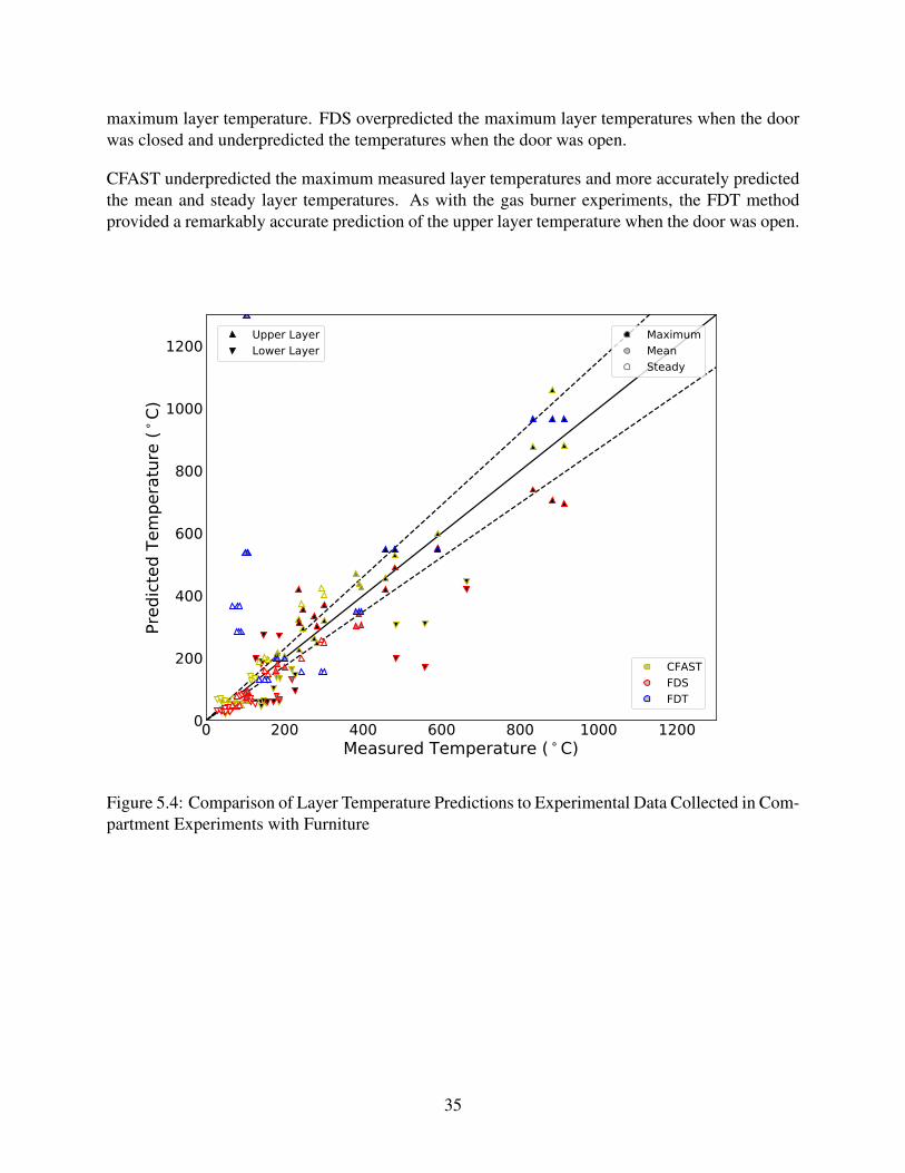
maximum layer temperature. FDS overpredicted the maximum layer temperatures when the doorwas closed and underpredicted the temperatures when the door was open.

CFAST underpredicted the maximum measured layer temperatures and more accurately predictedthe mean and steady layer temperatures. As with the gas burner experiments, the FDT methodprovided a remarkably accurate prediction of the upper layer temperature when the door was open.

0 200 400 600 800 1000 1200Measured Temperature ( C)

0

200

400

600

800

1000

1200

Pred

icted

Tem

pera

ture

(C)

Upper LayerLower Layer

MaximumMeanSteady

CFASTFDSFDT

Figure 5.4: Comparison of Layer Temperature Predictions to Experimental Data Collected in Com-partment Experiments with Furniture

35

Table 5.5: Model Fitness Metrics for Layer Temperature in Compartment Furniture Experiments

Metric Maximum Mean SteadyModel Collection N Bias Uncertainty N Bias Uncertainty N Bias Uncertainty

FDS

Overall 24 1.03 ±52% 24 0.72 ±19% 24 0.75 ±23%Overstuffed Sofa 12 1.11 ±56% 12 0.65 ±22% 12 0.63 ±20%Red Accent Chair 12 0.97 ±49% 12 0.8 ±12% 12 0.89 ±13%

Open 12 0.65 ±43% 12 0.72 ±31% 12 0.81 ±28%Closed 12 1.39 ±11% 12 0.75 ±13% 12 0.73 ±25%Center 8 1.17 ±56% 8 0.71 ±19% 8 0.72 ±25%Back 8 1.0 ±49% 8 0.75 ±23% 8 0.82 ±24%

Corner 8 1.03 ±60% 8 0.74 ±30% 8 0.77 ±32%

FDT

Overall 12 11.04 ±141% 12 5.34 ±114% 12 2.56 ±92%Overstuffed Sofa 6 20.87 ±168% 6 9.39 ±144% 6 3.22 ±117%Red Accent Chair 6 6.74 ±121% 6 3.39 ±86% 6 2.26 ±72%

Open 6 1.09 ±6% 6 0.98 ±8% 6 0.73 ±27%Closed 6 17.33 ±49% 6 9.04 ±48% 6 4.1 ±19%Center 4 15.87 ±160% 4 6.35 ±129% 4 2.76 ±98%Back 4 12.41 ±154% 4 6.17 ±126% 4 3.06 ±107%

Corner 4 14.09 ±157% 4 6.39 ±128% 4 2.82 ±104%

CFAST

Overall 24 0.78 ±42% 24 0.86 ±27% 22 1.14 ±32%Overstuffed Sofa 12 0.82 ±45% 12 0.84 ±14% 12 1.1 ±18%Red Accent Chair 12 0.75 ±40% 12 0.88 ±37% 10 1.21 ±47%

Open 12 0.84 ±24% 12 1.07 ±23% 12 1.43 ±20%Closed 12 0.73 ±54% 12 0.68 ±18% 10 0.82 ±21%Center 8 0.84 ±45% 8 0.84 ±25% 8 1.03 ±32%Back 8 0.77 ±48% 8 0.91 ±33% 8 1.24 ±43%

Corner 8 0.8 ±45% 8 0.88 ±37% 6 1.24 ±28%

5.1.2 Layer Heights

The agreement between the steady depth of descent of the layer interface and the model predictionsfor the compartment experiments with the gas burners is presented in Figure 5.5. Table 5.6 displaysthe calculated bias and uncertainty in agreement between the models and the experimental datafrom the compartment burner experiments. The FDT method consistently overpredicted the depthof descent of the layer interface when the door was closed and underpredicted the depth of descentwhen the door was open. When the door was closed, the model predicted that the layer descendedto the floor, and when the door was opened, the method was limited by the height of the door,which was 2 m.

Because the calculation of bias and uncertainty involves logarithms, and all of the FDT closeddoor predictions reached approximately 0, the closed door predictions were excluded from thetable. Model practitioners should understand that the FDT method provides a prediction of thelayer interface height that is not necessarily accurate and is directly correlated with the status ofthe door for a fire in the size of compartment that was investigated in this work.

FDS provided a reasonable prediction of the layer interface when the door was open but overpre-

36

dicted its depth of descent in all the other situations. CFAST provided accurate overall predictionsbut underpredicted the descent when the door was open and overpredicted its descent when thedoor was closed.

0.0 0.5 1.0 1.5 2.0 2.5Measured Depth (m)

0.0

0.5

1.0

1.5

2.0

2.5

Pred

icted

Dep

th (m

)

Height

CFASTFDSFDT

Figure 5.5: Comparison of Steady Layer Interface Elevation Predictions to Experimental DataCollected in Compartment Experiments with Burners

The comparison between the model predictions and the experimental data from the upholsteredfurniture is presented in Figure 5.6. Table 5.7 displays the calculated bias and uncertainty in agree-ment between the models and the experimental data from the compartment furniture experiments.The same trend for the FDT method that was observed in the gas burner experiments was also ob-served in the furniture experiments. FDS provided an accurate prediction of the mean and steadylayer interface elevation for all experiments but overpredicted the maximum depth of descent of thelayer in all cases. CFAST provided reasonable overall predictions, but generally underpredictedthe layer descent when the door was open and overpredicted its descent when the door was closed.

37

Table 5.6: Model Fitness Metrics for Layer Interface Elevation in Compartment Burner Experi-ments

Model Collection N Bias Uncertainty

FDS

Overall 32 0.64 ±43%100kWSB 8 0.68 ±28%

100kW 8 0.66 ±39%250kW 8 0.64 ±56%500kW 8 0.67 ±58%Open 16 0.9 ±10%

Closed 16 0.4 ±23%Center 8 0.61 ±42%Back 8 0.65 ±51%

Corner 8 0.72 ±52%Side 8 0.68 ±44%

FDT

Overall 16 1.76 ±6%100kWSB 4 1.61 ±4%

100kW 4 1.68 ±4%250kW 4 1.79 ±5%500kW 4 1.99 ±3%Open 16 1.76 ±8%Center 4 1.73 ±9%Back 4 1.83 ±7%

Corner 4 1.72 ±12%Side 4 1.8 ±10%

CFAST

Overall 32 0.92 ±37%100kWSB 8 0.99 ±24%

100kW 8 0.94 ±32%250kW 8 0.89 ±48%500kW 8 0.93 ±51%Open 16 1.23 ±4%

Closed 16 0.62 ±22%Center 8 0.92 ±40%Back 8 0.93 ±47%

Corner 8 0.93 ±40%Side 8 0.99 ±35%

38

0.0 0.5 1.0 1.5 2.0 2.5Measured Depth (m)

0.0

0.5

1.0

1.5

2.0

2.5

Pred

icted

Dep

th (m

)

Height MaximumMeanSteady

CFASTFDSFDT

Figure 5.6: Comparison of Layer Interface Elevation Predictions to Experimental Data Collectedin Compartment Experiments with Furniture

39

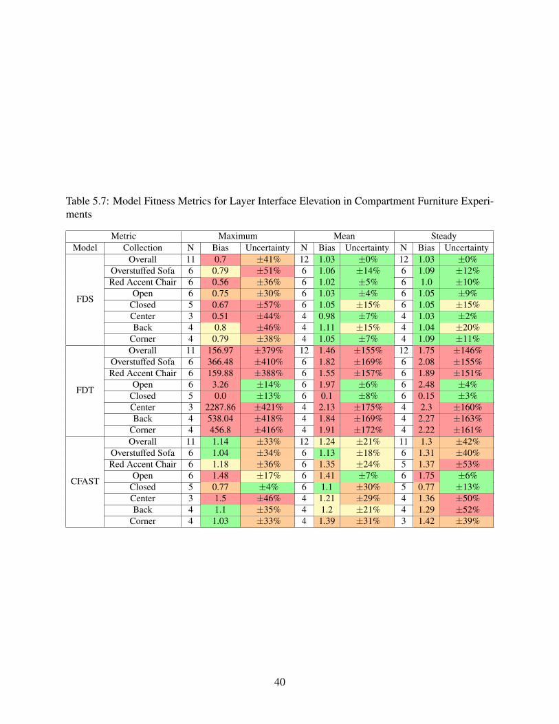
Table 5.7: Model Fitness Metrics for Layer Interface Elevation in Compartment Furniture Experi-ments

Metric Maximum Mean SteadyModel Collection N Bias Uncertainty N Bias Uncertainty N Bias Uncertainty

FDS

Overall 11 0.7 ±41% 12 1.03 ±0% 12 1.03 ±0%Overstuffed Sofa 6 0.79 ±51% 6 1.06 ±14% 6 1.09 ±12%Red Accent Chair 6 0.56 ±36% 6 1.02 ±5% 6 1.0 ±10%

Open 6 0.75 ±30% 6 1.03 ±4% 6 1.05 ±9%Closed 5 0.67 ±57% 6 1.05 ±15% 6 1.05 ±15%Center 3 0.51 ±44% 4 0.98 ±7% 4 1.03 ±2%Back 4 0.8 ±46% 4 1.11 ±15% 4 1.04 ±20%

Corner 4 0.79 ±38% 4 1.05 ±7% 4 1.09 ±11%

FDT

Overall 11 156.97 ±379% 12 1.46 ±155% 12 1.75 ±146%Overstuffed Sofa 6 366.48 ±410% 6 1.82 ±169% 6 2.08 ±155%Red Accent Chair 6 159.88 ±388% 6 1.55 ±157% 6 1.89 ±151%

Open 6 3.26 ±14% 6 1.97 ±6% 6 2.48 ±4%Closed 5 0.0 ±13% 6 0.1 ±8% 6 0.15 ±3%Center 3 2287.86 ±421% 4 2.13 ±175% 4 2.3 ±160%Back 4 538.04 ±418% 4 1.84 ±169% 4 2.27 ±163%

Corner 4 456.8 ±416% 4 1.91 ±172% 4 2.22 ±161%

CFAST

Overall 11 1.14 ±33% 12 1.24 ±21% 11 1.3 ±42%Overstuffed Sofa 6 1.04 ±34% 6 1.13 ±18% 6 1.31 ±40%Red Accent Chair 6 1.18 ±36% 6 1.35 ±24% 5 1.37 ±53%

Open 6 1.48 ±17% 6 1.41 ±7% 6 1.75 ±6%Closed 5 0.77 ±4% 6 1.1 ±30% 5 0.77 ±13%Center 3 1.5 ±46% 4 1.21 ±29% 4 1.36 ±50%Back 4 1.1 ±35% 4 1.2 ±21% 4 1.29 ±52%

Corner 4 1.03 ±33% 4 1.39 ±31% 3 1.42 ±39%

40

5.2 Flame Heights

The agreement between the observed steady flame heights and the model predictions for the com-partment experiments with the gas burners is presented in Figure 5.7. Table 5.8 displays the biasand uncertainty in the agreement between the model predictions and the experimental flame heightsfrom the burner experiments conducted in the compartment. FDS typically overpredicted the flameheights, which were limited by the ceiling height in the compartment. The FDT method for theflame height when the fuel source was adjacent to a wall or corner tended to overpredict the mea-sured flame height. CFAST slightly overpredicted the flame height on average, but provided themost accurate representation of the flame height for the burner experiments conducted in the com-partment.

0.0 0.5 1.0 1.5 2.0 2.5 3.0 3.5 4.0Measured Flame Height (m)

0.0

0.5

1.0

1.5

2.0

2.5

3.0

3.5

4.0

Pred

icted

Fla

me

Heig

ht (m

)

Flame Height

CFASTFDTFDS

Figure 5.7: Comparison of Steady Mean Flame Height Predictions to Experimental Data Collectedin Compartment Experiments with Burners

41

Table 5.8: Model Fitness Metrics for Flame Height in Compartment Burner Experiments

Model Collection N Bias Uncertainty

FDS (Upper Limit)

Overall 26 1.93 ±54%100kWSB 8 2.75 ±80%

100kW 7 2.25 ±51%250kW 6 1.43 ±20%500kW 5 1.23 ±2%Open 13 1.26 ±14%

Closed 13 2.73 ±63%Center 3 7.61 ±125%Back 7 1.83 ±37%

Corner 8 1.46 ±29%Side 8 1.56 ±32%

FDS (Lower Limit)

Overall 26 1.55 ±63%100kWSB 8 2.23 ±92%

100kW 7 1.8 ±72%250kW 6 1.11 ±26%500kW 5 1.14 ±10%Open 13 0.93 ±29%

Closed 13 2.29 ±67%Center 3 7.31 ±142%Back 7 1.47 ±49%

Corner 8 1.17 ±39%Side 8 1.22 ±43%

FDT

Overall 26 1.82 ±32%100kWSB 8 2.11 ±56%

100kW 7 1.5 ±11%250kW 6 1.75 ±10%500kW 5 2.0 ±7%Open 13 1.61 ±25%

Closed 13 2.04 ±35%Center 3 2.77 ±95%Back 7 1.85 ±12%

Corner 8 1.61 ±20%Side 8 1.82 ±19%

CFAST

Overall 19 1.16 ±67%100kWSB 8 1.11 ±45%

100kW 5 0.98 ±107%250kW 3 1.24 ±13%500kW 3 1.34 ±2%Open 13 1.19 ±11%

Closed 6 0.93 ±104%Center 3 1.75 ±117%Back 5 1.16 ±30%

Corner 5 1.02 ±26%Side 6 1.19 ±93%

42

The comparison between the model predictions and the experimental data from the upholsteredfurniture is presented in Figure 5.8. Table 5.9 displays the bias and uncertainty in the agree-ment between the model predictions and the experimental flame heights from the compartmentfurniture experiments. FDS overpredicted the the maximum flame height and underpredicted themean and steady flame heights. The FDT methods overpredicted the maximum, mean, and steadyflame heights. CFAST overpredicted the maximum and mean flame heights and underpredictedthe steady flame heights.

0.0 0.5 1.0 1.5 2.0 2.5 3.0 3.5 4.0Measured Flame Height (m)

0.0

0.5

1.0

1.5

2.0

2.5

3.0

3.5

4.0

Pred

icted

Fla

me

Heig

ht (m

)

Flame Height MaximumMeanSteady

CFASTFDTFDS

Figure 5.8: Comparison of Flame Height Predictions to Experimental Data Collected in Compart-ment Experiments with Furniture

For the burner experiments, the base of the flame was easily determined, but in the furniture ex-periments, the elevation of the base of the flame changed as the chair or sofa material burnedaway. This contributed to uncertainty in the comparisons because the model did not represent thedecreasing elevation of the base of the flame. Given that the compartment ceiling was 2.44 mabove the floor, predicted maximum vertical flame heights above 2.44 m are not physically possi-ble. However, flames in excess of the wall height would continue to spread across the ceiling. TheFDT methods and CFAST predicted flame heights above 2.4 m in some compartment experiments.These predictions of the flame height may have affected prediction of other quantities includingthe upper layer temperature and the heat fluxes.

43

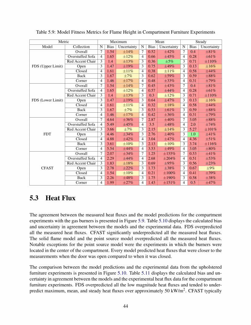
Table 5.9: Model Fitness Metrics for Flame Height in Compartment Furniture Experiments

Metric Maximum Mean SteadyModel Collection N Bias Uncertainty N Bias Uncertainty N Bias Uncertainty

FDS (Upper Limit)

Overall 7 1.54 ±14% 7 0.52 ±42% 7 0.4 ±81%Overstuffed Sofa 4 1.65 ±12% 4 0.66 ±45% 4 0.28 ±61%Red Accent Chair 3 1.4 ±13% 3 0.36 ±5% 3 0.71 ±110%

Open 3 1.47 ±19% 3 0.75 ±49% 3 0.13 ±16%Closed 4 1.61 ±11% 4 0.38 ±11% 4 0.58 ±44%Back 3 1.67 ±7% 3 0.62 ±59% 3 0.59 ±88%

Corner 4 1.46 ±17% 4 0.48 ±33% 4 0.31 ±79%

FDS (Lower Limit)

Overall 7 1.54 ±14% 7 0.45 ±43% 7 0.4 ±81%Overstuffed Sofa 4 1.65 ±12% 4 0.57 ±44% 4 0.28 ±61%Red Accent Chair 3 1.4 ±13% 3 0.3 ±12% 3 0.71 ±110%

Open 3 1.47 ±19% 3 0.64 ±47% 3 0.13 ±16%Closed 4 1.61 ±11% 4 0.32 ±18% 4 0.58 ±44%Back 3 1.67 ±7% 3 0.53 ±61% 3 0.59 ±88%

Corner 4 1.46 ±17% 4 0.42 ±36% 4 0.31 ±79%

FDT

Overall 7 4.64 ±36% 7 2.87 ±40% 7 3.05 ±88%Overstuffed Sofa 4 5.49 ±45% 4 3.5 ±48% 4 2.0 ±74%Red Accent Chair 3 3.66 ±7% 3 2.15 ±14% 3 5.27 ±101%

Open 3 4.46 ±34% 3 2.76 ±40% 3 1.0 ±41%Closed 4 4.88 ±42% 4 3.04 ±47% 4 4.36 ±51%Back 3 3.61 ±10% 3 2.13 ±10% 3 3.74 ±116%

Corner 4 5.54 ±44% 4 3.53 ±49% 4 3.05 ±80%

CFAST

Overall 7 2.07 ±34% 7 1.25 ±155% 7 0.53 ±41%Overstuffed Sofa 4 2.29 ±44% 4 2.68 ±204% 4 0.51 ±53%Red Accent Chair 3 1.83 ±18% 3 0.69 ±95% 3 0.56 ±23%

Open 3 2.78 ±22% 3 1.73 ±38% 3 0.67 ±9%Closed 4 1.54 ±10% 4 0.21 ±100% 4 0.41 ±39%Back 3 2.26 ±48% 3 1.75 ±190% 3 0.58 ±38%

Corner 4 1.99 ±27% 4 1.43 ±151% 4 0.5 ±47%

5.3 Heat Flux

The agreement between the measured heat fluxes and the model predictions for the compartmentexperiments with the gas burners is presented in Figure 5.9. Table 5.10 displays the calculated biasand uncertainty in agreement between the models and the experimental data. FDS overpredictedall the measured heat fluxes. CFAST significantly underpredicted all the measured heat fluxes.The solid flame model and the point source model overpredicted all the measured heat fluxes.Notable exceptions for the point source model were the experiments in which the burners werelocated in the center of the compartment. Every model predicted heat fluxes that were closer to themeasurements when the door was open compared to when it was closed.

The comparison between the model predictions and the experimental data from the upholsteredfurniture experiments is presented in Figure 5.10. Table 5.11 displays the calculated bias and un-certainty in agreement between the models and the experimental heat flux data for the compartmentfurniture experiments. FDS overpredicted all the low magnitude heat fluxes and tended to under-predict maximum, mean, and steady heat fluxes over approximately 50 kW/m2. CFAST typically

44

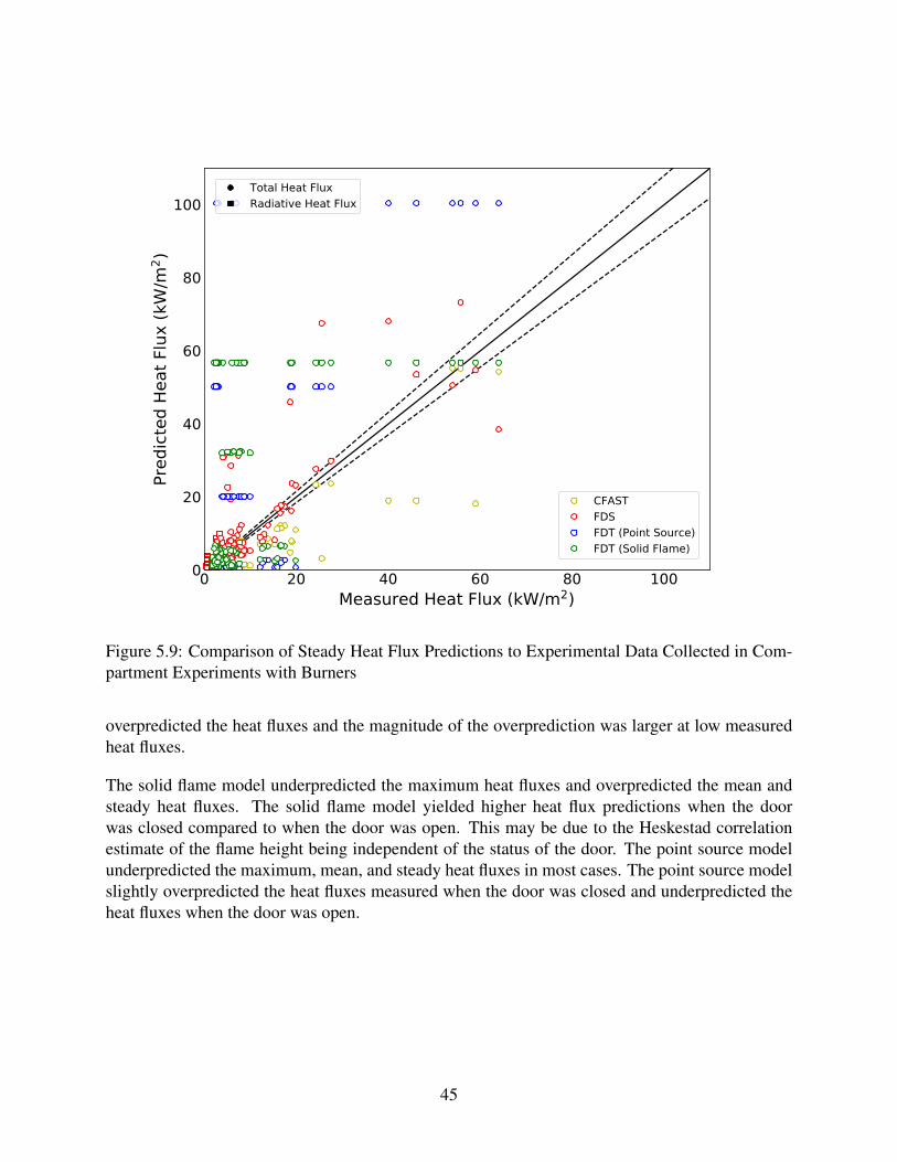
0 20 40 60 80 100Measured Heat Flux (kW/m2)

0

20

40

60

80

100

Pred

icted

Hea

t Flu

x (k

W/m

2 )Total Heat FluxRadiative Heat Flux

CFASTFDSFDT (Point Source)FDT (Solid Flame)

Figure 5.9: Comparison of Steady Heat Flux Predictions to Experimental Data Collected in Com-partment Experiments with Burners

overpredicted the heat fluxes and the magnitude of the overprediction was larger at low measuredheat fluxes.

The solid flame model underpredicted the maximum heat fluxes and overpredicted the mean andsteady heat fluxes. The solid flame model yielded higher heat flux predictions when the doorwas closed compared to when the door was open. This may be due to the Heskestad correlationestimate of the flame height being independent of the status of the door. The point source modelunderpredicted the maximum, mean, and steady heat fluxes in most cases. The point source modelslightly overpredicted the heat fluxes measured when the door was closed and underpredicted theheat fluxes when the door was open.

45

0 50 100 150 200 250Measured Heat Flux (kW/m2)

0

50

100

150

200

250

Pred

icted

Hea

t Flu

x (k

W/m

2 )

Total Heat FluxRadiative Heat Flux

MaximumMeanSteady

CFASTFDSFDT (Point Source)FDT (Solid Flame)

Figure 5.10: Comparison of Heat Flux Predictions to Experimental Data Collected in CompartmentExperiments with Furniture

46

Table 5.10: Model Fitness Metrics for Heat Flux in Compartment Burner Experiments

Model Collection N Bias Uncertainty

FDS

Overall 187 1.75 ±90%100kWSB 48 1.99 ±82%

100kW 47 2.44 ±94%250kW 46 1.43 ±73%500kW 46 1.17 ±94%Open 96 1.4 ±53%

Closed 91 2.23 ±117%Center 48 1.9 ±92%Back 47 2.17 ±81%

Corner 44 1.49 ±88%Side 48 1.45 ±92%

FDT (Solid Flame)

Overall 122 3.22 ±138%100kWSB 32 2.07 ±133%

100kW 26 2.49 ±131%250kW 32 4.76 ±136%500kW 32 3.82 ±145%Open 61 1.55 ±103%

Closed 61 6.19 ±162%Center 32 1.01 ±64%Back 30 4.64 ±129%

Corner 30 5.29 ±174%Side 30 4.15 ±155%

FDT (Point Source)

Overall 128 3.53 ±197%100kWSB 32 2.01 ±191%

100kW 32 1.86 ±183%250kW 32 4.85 ±197%500kW 32 7.29 ±209%Open 64 1.36 ±160%

Closed 64 8.74 ±227%Center 32 0.3 ±67%Back 32 5.93 ±188%

Corner 32 9.31 ±242%Side 32 6.64 ±224%

CFAST

Overall 128 0.44 ±50%100kWSB 32 0.44 ±62%

100kW 32 0.37 ±43%250kW 32 0.48 ±39%500kW 32 0.47 ±52%Open 64 0.59 ±39%

Closed 64 0.29 ±33%Center 32 0.46 ±40%Back 32 0.46 ±48%

Corner 32 0.41 ±51%Side 32 0.43 ±61%

47

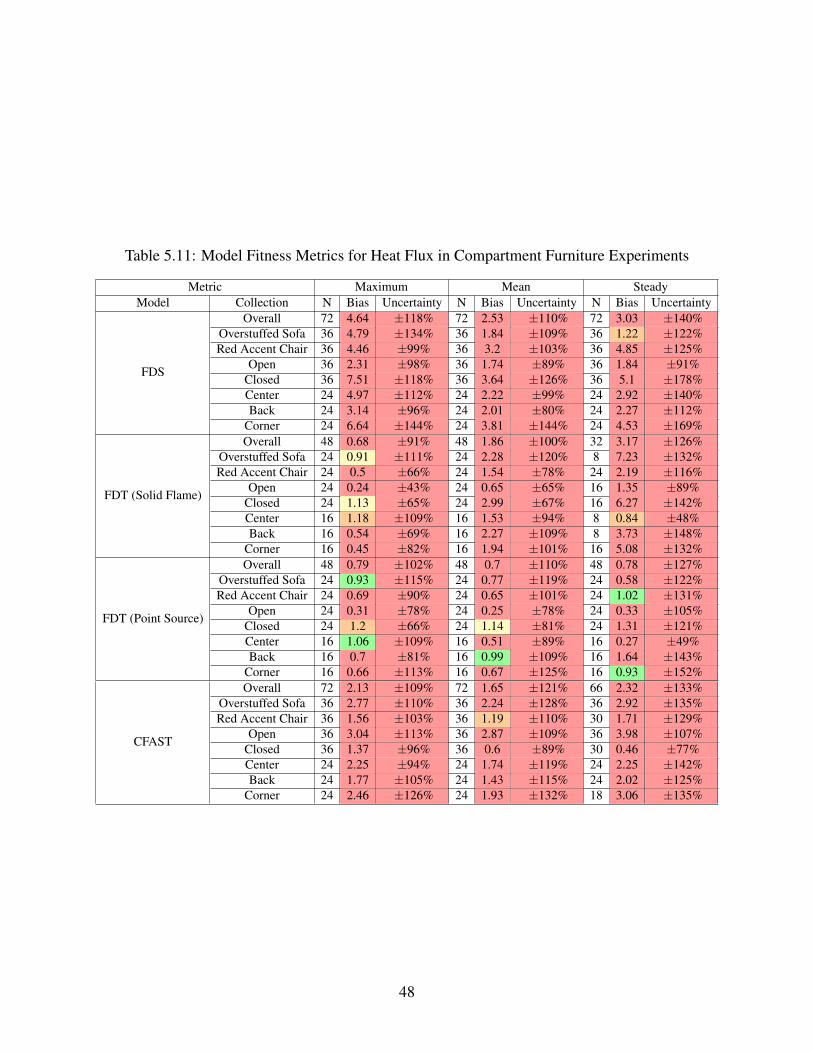
Table 5.11: Model Fitness Metrics for Heat Flux in Compartment Furniture Experiments

Metric Maximum Mean SteadyModel Collection N Bias Uncertainty N Bias Uncertainty N Bias Uncertainty

FDS

Overall 72 4.64 ±118% 72 2.53 ±110% 72 3.03 ±140%Overstuffed Sofa 36 4.79 ±134% 36 1.84 ±109% 36 1.22 ±122%Red Accent Chair 36 4.46 ±99% 36 3.2 ±103% 36 4.85 ±125%

Open 36 2.31 ±98% 36 1.74 ±89% 36 1.84 ±91%Closed 36 7.51 ±118% 36 3.64 ±126% 36 5.1 ±178%Center 24 4.97 ±112% 24 2.22 ±99% 24 2.92 ±140%Back 24 3.14 ±96% 24 2.01 ±80% 24 2.27 ±112%

Corner 24 6.64 ±144% 24 3.81 ±144% 24 4.53 ±169%

FDT (Solid Flame)

Overall 48 0.68 ±91% 48 1.86 ±100% 32 3.17 ±126%Overstuffed Sofa 24 0.91 ±111% 24 2.28 ±120% 8 7.23 ±132%Red Accent Chair 24 0.5 ±66% 24 1.54 ±78% 24 2.19 ±116%

Open 24 0.24 ±43% 24 0.65 ±65% 16 1.35 ±89%Closed 24 1.13 ±65% 24 2.99 ±67% 16 6.27 ±142%Center 16 1.18 ±109% 16 1.53 ±94% 8 0.84 ±48%Back 16 0.54 ±69% 16 2.27 ±109% 8 3.73 ±148%

Corner 16 0.45 ±82% 16 1.94 ±101% 16 5.08 ±132%

FDT (Point Source)

Overall 48 0.79 ±102% 48 0.7 ±110% 48 0.78 ±127%Overstuffed Sofa 24 0.93 ±115% 24 0.77 ±119% 24 0.58 ±122%Red Accent Chair 24 0.69 ±90% 24 0.65 ±101% 24 1.02 ±131%

Open 24 0.31 ±78% 24 0.25 ±78% 24 0.33 ±105%Closed 24 1.2 ±66% 24 1.14 ±81% 24 1.31 ±121%Center 16 1.06 ±109% 16 0.51 ±89% 16 0.27 ±49%Back 16 0.7 ±81% 16 0.99 ±109% 16 1.64 ±143%

Corner 16 0.66 ±113% 16 0.67 ±125% 16 0.93 ±152%

CFAST

Overall 72 2.13 ±109% 72 1.65 ±121% 66 2.32 ±133%Overstuffed Sofa 36 2.77 ±110% 36 2.24 ±128% 36 2.92 ±135%Red Accent Chair 36 1.56 ±103% 36 1.19 ±110% 30 1.71 ±129%

Open 36 3.04 ±113% 36 2.87 ±109% 36 3.98 ±107%Closed 36 1.37 ±96% 36 0.6 ±89% 30 0.46 ±77%Center 24 2.25 ±94% 24 1.74 ±119% 24 2.25 ±142%Back 24 1.77 ±105% 24 1.43 ±115% 24 2.02 ±125%

Corner 24 2.46 ±126% 24 1.93 ±132% 18 3.06 ±135%

48

5.4 Velocity

The agreement between the measured plume, ceiling jet, and door velocities and the model predic-tions for the compartment experiments with the gas burners is presented in Figure 5.11. Table 5.12presents the calculated bias and uncertainty for the FDS predictions of the velocities measured inthe burner experiments. The velocities below approximately 0.5 m/s were overpredicted and theplume velocities above 0.5 m/s were underpredicted. FDS predicted higher velocities at the dooropening more accurately.

0 1 2 3 4 5 6 7Measured Velocity (m/s)

0

1

2

3

4

5

6

7

Pred

icted

Vel

ocity

(m/s

)

Ceiling JetPlumeDoor

FDS

Figure 5.11: Comparison of Steady Velocity Predictions to Experimental Data Collected in Com-partment Experiments with Burners

49

Table 5.12: Model Fitness Metrics for Velocity in Compartment Burner Experiments

Model Collection N Bias Uncertainty

FDS

Overall 177 1.83 ±88%Ceiling Jet 52 2.36 ±54%

Plume 33 0.7 ±90%Door 92 1.76 ±75%

100kWSB 42 1.83 ±117%100kW 50 1.78 ±66%250kW 45 1.76 ±75%500kW 40 1.91 ±86%Open 162 1.88 ±85%

Closed 15 1.19 ±103%Center 36 1.61 ±59%Back 52 1.83 ±84%

Corner 42 2.35 ±124%Side 47 1.63 ±73%

The comparison between the model predictions and the experimental data from the upholsteredfurniture experiments is presented in Figure 5.12. Table 5.12 presents the calculated bias anduncertainty for the FDS predictions of the measured velocities in the furniture experiments. FDSgenerally overpredicted the maximum velocities while overpredicting the mean velocities by asmaller margin.

Table 5.13: Model Fitness Metrics for Velocity in Compartment Furniture Experiments

Metric Maximum Mean SteadyModel Collection N Bias Uncertainty N Bias Uncertainty N Bias Uncertainty

FDS

Overall 106 1.8 ±55% 106 1.14 ±62% 106 1.27 ±86%Ceiling Jet 48 2.68 ±45% 48 1.22 ±57% 48 1.25 ±100%

Plume 16 0.88 ±42% 16 0.73 ±96% 16 1.09 ±114%Door 42 1.2 ±14% 42 1.17 ±23% 42 1.29 ±30%

Overstuffed Sofa 53 1.86 ±61% 53 1.18 ±62% 53 1.32 ±97%Red Accent Chair 53 1.74 ±49% 53 1.1 ±62% 53 1.22 ±73%

Open 74 1.48 ±37% 74 1.3 ±38% 74 1.53 ±55%Closed 32 2.71 ±78% 32 0.68 ±69% 32 0.44 ±70%Center 30 2.21 ±59% 30 1.22 ±44% 30 1.28 ±73%Back 38 1.58 ±47% 38 1.07 ±71% 38 1.23 ±91%

Corner 38 1.71 ±57% 38 1.14 ±63% 38 1.31 ±91%

50

0 1 2 3 4 5 6 7Measured Velocity (m/s)

0

1

2

3

4

5

6

7Pr

edict

ed V

eloc

ity (m

/s)

Ceiling JetPlumeDoor

MaximumMeanSteady

FDS

Figure 5.12: Comparison of Velocity Predictions to Experimental Data Collected in CompartmentExperiments with Furniture

5.5 Oxygen Concentration

The agreement between the measured oxygen concentrations and the model predictions for thecompartment experiments with the gas burners is presented in Figure 5.13. Table 5.14 presents thecalculated bias and uncertainty for the FDS predictions of the minimum oxygen concentrations inthe burner experiments. The CFAST and FDS predictions for the steady oxygen concentration inthe compartment burner experiments were generally accurate, although FDS showed more con-sistently accurate predictions. The CFAST predictions were distributed according to the elevationof the measurement, with the higher elevation prediction of approximately 10% O2 and the lowerelevation minimum prediction of approximately 20% O2. The comparisons between the predic-tions and measurements for both models was more repeatable when the door was open comparedto when the door was closed.

51

0.0 2.5 5.0 7.5 10.0 12.5 15.0 17.5 20.0Measured Oxygen Concentration (vol.%)

0.0

2.5

5.0

7.5

10.0

12.5

15.0

17.5

20.0

Pred

icted

Oxy

gen

Conc

entra

tion

(vol

.%)

Upper LayerLower Layer

CFASTFDS

Figure 5.13: Comparison of Oxygen Concentration Predictions to Experimental Data Collected inCompartment Experiments with Burners

52

Table 5.14: Model Fitness Metrics for Oxygen Concentration in Compartment Burner Experiments

Model Collection N Bias Uncertainty

FDS

Overall 248 1.0 ±10%100kWSB 64 1.09 ±8%

100kW 59 1.0 ±6%250kW 61 0.98 ±14%500kW 64 0.97 ±20%Open 125 1.06 ±3%

Closed 123 0.96 ±18%Center 61 1.02 ±18%Back 64 0.98 ±12%

Corner 61 1.03 ±15%Side 62 1.02 ±11%

CFAST

Overall 248 1.17 ±20%100kWSB 64 1.22 ±26%

100kW 59 1.12 ±23%250kW 61 1.17 ±22%500kW 64 1.24 ±19%Open 125 1.06 ±6%

Closed 123 1.32 ±29%Center 61 1.2 ±24%Back 64 1.13 ±22%

Corner 61 1.21 ±23%Side 62 1.21 ±23%

53

The comparison between the model predictions and the experimental data from the upholsteredfurniture experiments is presented in Figure 5.14. Table 5.15 presents the calculated bias anduncertainty for the FDS predictions of the minimum oxygen concentrations in the compartmentexperiments. CFAST and FDS generally accurately predicted the mean and steady oxygen con-centrations and overpredicted the minimum oxygen concentration.

0.0 2.5 5.0 7.5 10.0 12.5 15.0 17.5 20.0Measured Oxygen Concentration (vol.%)

0.0

2.5

5.0

7.5

10.0

12.5

15.0

17.5

20.0

Pred

icted

Oxy

gen

Conc

entra

tion

(vol

.%)

Upper LayerLower Layer

MaximumMeanSteady

CFASTFDS

Figure 5.14: Comparison of Oxygen Concentration Predictions to Experimental Data Collected inCompartment Experiments with Furniture

54

Table 5.15: Model Fitness Metrics for Oxygen Concentration in Compartment Furniture Experi-ments

Metric Minimum Mean SteadyModel Collection N Bias Uncertainty N Bias Uncertainty N Bias Uncertainty

FDS

Overall 96 1.69 ±99% 96 0.93 ±13% 96 0.87 ±30%Overstuffed Sofa 48 3.12 ±138% 48 0.92 ±20% 48 0.84 ±41%Red Accent Chair 48 0.9 ±18% 48 0.96 ±8% 48 0.91 ±16%

Open 48 2.97 ±130% 48 0.99 ±10% 48 0.99 ±4%Closed 48 0.94 ±46% 48 0.9 ±21% 48 0.77 ±40%Center 32 2.99 ±132% 32 0.94 ±19% 32 0.9 ±36%Back 32 1.03 ±64% 32 0.93 ±16% 32 0.87 ±31%

Corner 32 1.61 ±90% 32 0.96 ±18% 32 0.89 ±31%

CFAST

Overall 92 1.49 ±63% 96 1.11 ±12% 88 1.11 ±13%Overstuffed Sofa 44 1.98 ±81% 48 1.14 ±16% 48 1.14 ±17%Red Accent Chair 48 1.14 ±35% 48 1.09 ±10% 40 1.08 ±13%

Open 44 1.37 ±83% 48 0.97 ±5% 48 0.96 ±3%Closed 48 1.57 ±24% 48 1.28 ±10% 40 1.31 ±11%Center 28 1.71 ±67% 32 1.11 ±14% 32 1.14 ±18%Back 32 1.23 ±55% 32 1.11 ±15% 32 1.11 ±15%

Corner 32 1.67 ±68% 32 1.16 ±19% 24 1.11 ±19%

55

6 Discussion

Each of the modeling methods has advantages and disadvantages relative to the other methods.The FDT methods are simplistic and have been compiled into convenient and freely availablespreadsheets. These spreadsheets make interpretation of data and assessment of the sensitivity ofinput parameters straightforward and may help investigators attain a better understanding of the firedynamics of given fire scenarios. CFAST is open source and provides more functionality than theFDT spreadsheets while also requiring relatively little computational expense. CFAST is limitedto compartment scenarios and the assumptions that govern the two-zone model limit the breadthof quantities that may be predicted. FDS is open source and provides the most functionality andpredicted quantities of the three modeling methods that have been investigated. Because of itscomplexity relative to the other methods, FDS simulations are the most computationally expensiveand generally require more inputs to be defined. The larger set of required inputs for FDS alsoincreases the degrees of freedom and the likelihood that the results will be overly sensitive touncertainty in a specific input parameter.

The FDT correlation for plume temperatures yielded predictions that were significantly higher thanthe maximum plume temperatures for the furniture experiments. FDS overpredicted the maximumplume temperatures for the burner experiments. The plume temperatures in the compartment ex-periments were underpredicted, which indicates the influence of compartment effects which werenot adequately represented with the physics invoked in the FDS models presented here. FDS pro-vided reasonable predictions of the ceiling jet temperatures and temperatures of gas flow throughthe door for the compartment experiments.

The FDT method to predict the temperature of the upper layer yielded accurate predictions forthe open door compartment experiments, but it significantly overpredicted the upper layer tem-perature when the door was closed. FDS and CFAST accurately predicted the upper and lowerlayer temperatures for the compartment experiments with the gas burners but predicted the gaslayer temperatures less accurately for the furniture experiments. CFAST predicted the maximumand mean depth of descent of the layer interface while FDS accurately predicted the mean depthof descent of the gas layer and overpredicted the maximum depth of descent. The FDT methodyielded a binary result with the layer interface located either at the floor of the compartment or atthe top of the door, which corresponded to underpredictions with the compartment door open andoverpredictions with the compartment door closed.

The Heskestad and Thomas flame height correlations generally overpredicted the flame height inthe compartment experiments with the fuel source located at a wall or in a corner. The rangeof flame heights predicted by FDS encompassed the observed flame height for the compartmentburner experiments conducted with the door open. The observed flame height for the compartmentburner experiments when the door was closed and for the furniture experiments in the compartmentwere generally overpredicted. CFAST overpredicted most of the measured flame heights in thecompartment experiments.

56

The point source heat flux model overpredicted the measured fluxes in the compartment experi-ments. The solid flame model overpredicted heat fluxes in all experiments. FDS tended to predictmaximum and mean heat fluxes with large scatter in agreement for the compartment experiments.CFAST underpredicted the heat fluxes in the compartment experiments with the burners and gen-erally overpredicted the heat fluxes in the experiments with the furniture items.

Plume velocities were reasonably predicted in the compartment experiments with furniture, butwere underpredicted in the compartment burner experiments. Mean and steady ceiling jet velocitieswere accurately predicted but maximum ceiling jet velocities were overpredicted and velocities offlow through the open compartment door were typically accurately predicted by FDS.

CFAST and FDS both provided reasonable estimates for the minimum oxygen concentration,although both models appeared to have difficulty representing ventilation-limited conditions inwhich the oxygen concentration was measured as approximately 0%. The mean and steady oxy-gen concentrations were typically accurately predicted by both models. In general, CFAST tendedto overpredict oxygen concentrations and FDS tended to underpredict oxygen concentrations.

57

7 Recommendations

Because fire investigators are expected to almost exclusively encounter compartment fires fueledby materials and products that are common to residential and commercial occupancies, the recom-mendations presented in this work focus on the furniture experiments conducted in the compart-ment. The FDT methods for predicting flame height are the only FDT methods investigated in thiswork that yielded accurate predictions. The FDT methods for flame height were generally accu-rate when the observed flame heights were below the ceiling height and also correctly indicatedwhen the flame impinged on the ceiling. The FDT predictions of plume temperature and layertemperature were overly conservative and cannot be recommended to investigators.

CFAST is recommended for predicting the layer interface height with the understanding that themaximum depth of descent was typically underpredicted when the door was open and overpre-dicted when the door was closed. If CFAST is used for layer temperature prediction, practitionersshould understand that all predicted temperatures were typically lower than the measurements.CFAST was able to accurately predict that flames impinged on the ceiling in the furniture com-partment experiments and is expected to slightly overestimate flame heights below the ceiling whenthe door to the compartment is open. Temperature and flame height predictions in CFAST are mostsensitive to the uncertainty in the HRR, so it is recommended that uncertainty in the defined HRRbe reduced and that a sensitivity analysis be conducted to define the uncertainty in the predictionsand declare a level of confidence for the conclusions drawn from the analysis.

FDS is capable of predicting realistic temperatures throughout the computational domain. It isthe recommended method for predicting layer temperatures because it generally yielded accuratepredictions for the maximum layer temperatures. If FDS is used to predict the depth of descent ofthe layer interface, the mean and steady layer interface heights are more reliable than the predictedmaximum depth of descent of the interface. FDS is capable of conservative plume velocity andceiling jet velocity predictions as well as accurate prediction of the flow velocity through the opencompartment door. Model practitioners should understand the relatively high uncertainty whenusing FDS for velocity predictions. FDS was capable of predicting flame impingement on theceiling for the furniture-fueled fires and is a recommended method to predict flame heights whenthe compartment door is open and flames are not expected to impinge on the ceiling.

Both FDS and CFAST are recommended for oxygen concentration predictions. In general, CFASTand FDS are capable of accurate predictions of the mean oxygen concentration but model practi-tioners should be cognizant of the uncertainties when using either model to predict the minimumoxygen concentration in a compartment. Both models have shown issues simulating underventi-lated fires and those concerns have been confirmed in this work.

The scatter exhibited in all the modeling methods for heat flux predictions make recommendationof a method for predicting heat flux from a furniture-fueled fire in a compartment impossible. Be-cause of the uncertainty in the results in each case, none of the methods can reliably be consideredto provide a conservative estimate. This is an area that requires further research and development.

58

8 Research Needs

Additional research is necessary to determine a heat flux correlation or modeling method that ismore consistently accurate and representative of the dynamics of furniture-fueled enclosure fires.Because the flame, fire plume, hot gas layer, and walls participate in radiative heat flux incident toa target in a compartment, it is not surprising that the simplistic FDT methods did not accuratelyrepresent the experimental heat fluxes. The zone modeling approach improves on the simplis-tic algebraic equations for heat flux from the fire by including other participating surfaces, butthe calculation is too heavily reliant on empirical correlations to represent the heat flux from acomplex-shaped burning furniture item. FDS further improves on the representation of heat flux inCFAST by allowing geometric shapes to be represented in the model, but this work has shown thatthe representations of the furniture in the FDS models did not ultimately result in accurate heat fluxpredictions. Research on the effect of burning definitions, defined geometry, spatial resolution, andmodel-specific input parameters on the heat flux as well as all the predicted quantities will providerecommendations for fire investigators on the use of FDS.

The idealistic use of a computational fire model for fire scene reconstruction involves defining allthe required material properties for component materials and the geometry of the scene and allow-ing for complete prediction of flame spread over furniture items and throughout the compartmentto test hypotheses. This type of model is theoretically possible with the current version of FDSbut the implementation of such a complicated representation of burning has yet to be standardizedand validated. Additional research to understand the best methods to implement such a modelfor burning items will improve the state of fire modeling and the conclusions that may be drawnfrom models like FDS and CFAST. Additionally, the wide breadth of material properties and in-put parameters required for such an implementation are generally not available or, when they areavailable, are incomplete or do not represent the exact component materials in the fire scenario.The development of a comprehensive fire material properties database will expand the possibilitiesfor fire investigators that use FDS and similar models and help to realize the full potential andpredictive capabilities of field fire models.

59

9 Summary

UL Firefighter Safety Research Institute conducted a study to evaluate the ability of commonly-used fire dynamics analyses to predict the fire environment generated from gas burners and modernupholstered furniture in a simple compartment. Two sizes of burners were used in experiments withheat release rates ranging from 50 kW to 500 kW. Two furniture items including one upholsteredchair and one upholstered sofas were tested. Variables investigated in the compartment experi-ments included location of the burner or fuel package and the status of the door.

Specialized fire dynamics routines, a zone fire model, and a field fire model were used to predictvarious quantities measured in the compartment experiments. The accuracy of each model wascalculated based on a comparison of the maximum observed and predicted quantities in the burnerexperiments and the maximum, mean, and steady values in the decay period for the compartmentexperiments. The accuracy of each model was evaluated for collections of experimental parameters(fuel package, location of the fuel package, status of the door, etc.) to define the limitations of eachmodel.

The specialized fire dynamics routines were capable of accurately characterizing the flame height,but did not accurately predict the other quantities for the furniture-fueled fire experiments con-ducted in the compartment. The zone fire model accurately predicted the layer interface heights,layer temperatures, flame heights, and oxygen concentrations in the compartment fire scenar-ios. The field model predicted accurate temperatures throughout the compartment, layer interfaceheights, velocities through the open door of the compartment, flame heights, and oxygen concen-trations. In general, the predictive ability of all the models was better in the gas burner experimentsthan in the furniture experiments. More research is needed to develop recommendations on geom-etry and burning definitions for upholstered furniture in field models as well as improved methodsfor model practitioners to predict heat flux.

60

References

[1] National Fire Protection Association. NFPA 921, Guide for Fire and Explosion Investiga-tions, 2021.

[2] S. Kerber. Analysis of Changing Residential Fire Dynamics and Its Implications on Fire-fighter Operational Timeframes. Technical report, Underwriters Laboratories, Northbrook,Illinois, 2012.

[3] C.L. Smith. Preliminary Regulatory Analysis of a Draft Proposed Rule to Address Cigaretteand Small Open Flame Ignitions of Upholstered Furniture. Directorate for Economic Analy-sis, U.S. Consumer Product Safety Commission, Washington, D.C., November 2005.

[4] U.S. Census Bureau. Quickfacts. https://www.census.gov/quickfacts/fact/table/US/HSD410218,2020.

[5] M. Ahrens. Home Fires That Began with Upholstered Furniture. Report, National FireProtection Agency (NFPA), February 2017.

[6] National Fire Protection Agency (NFPA). White Paper on Upholstered Furniture Flammabil-ity. Report, September 2013.

[7] Eric Guillaume, Rene de Feijter, and Laurens van Gelderen. An overview and experimentalanalysis of furniture fire safety regulations in Europe. Fire and Materials, 44(5), 2020.

[8] R. Campbell. Intentional Fires. Report, National Fire Protection Association, July 2017.

[9] J. Floyd. Comparison of CFAST and FDS for Fire Simulation with the HDR T51 and T52Tests. NISTIR 6866, National Institute of Standards and Technology, Gaithersburg, Mary-land, March 2002.

[10] G. Rein, A. Bar-Ilan, A.C. Fernandez-Pello, and N. Alvarez. A Comparison of Three Modelsin the Simulations of Accidental Fires. Journal of Fire Protection Engineering, 2005.

[11] K. Hill, J. Dreisbach, F. Joglar, B. Najafi, K. McGrattan, R. Peacock, and A. Hamins. Verifica-tion and Validation of Selected Fire Models for Nuclear Power Plant Applications. NUREG-1824, United States Nuclear Regulatory Commission, Washington, DC, 2007.

[12] N. Iqbal and M. Salley. Fire Dynamics Tools (FDTs): Quantitative Fire Hazard AnalysisMethods for the U.S. Nuclear Regulatory Commission Fire Protection Inspection Program.NUREG-1805, United States Nuclear Regulatory Commission, Washington, DC, 2004.

[13] F. Joglar. Verification and Validation of Selected Fire Models for Nuclear Power Plant Ap-plications Volume 4: Fire-Induced Vulnerability Evaluation (FIVE-Rev1). NUREG-1824,United States Nuclear Regulatory Commission, Washington, DC, 2007.

61

[14] K.J. Overholt. Verification and Validation of Commonly Used Empirical Correlations for FireScenarios. NIST Special Publication 1169, National Institute of Standards and Technology,Gaithersburg, Maryland, 2014.

[15] M.H. Salley and A. Lindeman. Verification and Validation of Selected Fire Models for Nu-clear Power Plant Applications. NUREG-1824, Supplement 1, United States Nuclear Regu-latory Commission, Washington, DC, 2016.

[16] M.L. Janssens, D.M. Ewan, C. Gomez, M.M. Hirschler, J.P. Huczek, R.L. Mason, K.J. Over-holt, and J.M. Sharp. Reducing Uncertainty of Quantifying the Burning Rate of UpholsteredFurniture. Technical report, SwRI Project No. 0.1.15998, Award No. 2010-DN-BX-K221,for National Institute of Justice, 2012.

[17] R.A. Bryant and G. Mullholland. A guide to characterizing heat release rate measurementuncertainty for full-scale fire tests. Fire and Materials, 32:121–139, 2008.

[18] W.M. Pitts, A.V. Murthy, J.L. de Ris, J. Filtz, K. Nygård, D. Smith, and I. Wetterlund. Roundrobin study of total heat flux gauge calibration at fire laboratories. Fire Safety Journal,41(6):459–475, 2006.

[19] R.A. Bryant. A comparison of gas velocity measurements in a full-scale enclosure fire. FireSafety Journal, 44:793–800, 2009.

[20] L.G. Blevins. Behavior of bare and aspirated thermocouples in compartment fires. In NationalHeat Transfer Conference, 33rd Proceedings, pages 15–17, 1999.

[21] W.M. Pitts, E. Braun, R. Peacock, H. Mitler, E. Johnson, P. Reneke, and L.G. Blevins. Tem-perature uncertainties for bare-bead and aspirated thermocouple measurements in fire envi-ronments. ASTM Special Technical Publication, 1427:3–15, 2003.

[22] A. Lock, M. Bundy, E.L. Johnsson, A. Hamins, G.H. Ko, C. Hwang, P. Fuss, and R. Harris.Experimental study of the effects of fuel type, fuel distribution, and vent size on full-scaleunderventilated compartment fires in an ISO 9705 room. NIST Technical Note 1603, NationalInstitute of Standards and Technology, Gaithersburg, MD, 2008.

[23] J. Willi and D. Madrzykowski. Examination of Fire Dynamics Analysis Techniques: Com-partment Fire Experiments. Technical report, UL Firefighter Safety Research Institute,Columbia, Maryland, April 2021.

[24] ASTM International. Standard E 779: Standard Test Method for Determining Air LeakageRate by Fan Pressurization, 2010.

[25] Wanyu R. Chan, Jeffrey Joh, and Max H. Sherman. Analysis of air leakage measurements ofus houses. Energy and Buildings, 66:616 – 625, 2013.

[26] M.L. Janssens and H.C. Tran. Data Reduction of Room Tests for Zone Model Validation.Journal of Fire Science, 10:528–555, 1992.

62

[27] K. McGrattan, S. Hostikka, J. Floyd, R. McDermott, and M. Vanella. Fire Dynamics Simu-lator, Technical Reference Guide Volume 3: Validation. National Institute of Standards andTechnology, Gaithersburg, Maryland, USA, and VTT Technical Research Centre of Finland,Espoo, Finland, sixth edition, September 2019.

[28] B.J. McCaffrey, J.G. Quintierea, and M.F. Harkelroad. Estimating Room Temperatures andthe Likelihood of Flashover Using Fire Test Data Correlations. Fire Technology, 17(2):98–119, 1981.

[29] C. Beyler. Analysis of Compartment Fires with Overhead Forced Ventilation. In Fire SafetyScience – Proceedings of the Third International Symposium, pages 291–300. InternationalAssociation for Fire Safety Science, 1991.

[30] Takeyoshi Tanaka and Toshio Yamana. Smoke Control in Large Scale Spaces (Part 1: Ana-lytic Theories For Simple Smoke Control Problems). Fire Science and Technology, 5(1):31–40, 1985.

[31] Toshio Yamana and Takeyoshi Tanaka. Smoke Control in Large Scale Spaces (Part 2: SmokeControl Experiments In A Large Storage Space). Fire Science and Technology, 5(1):41–54,1985.

[32] P.H. Thomas. The size of flames from natural fires. Symposium (International) on Combus-tion, 9(1):844 – 859, 1963.

[33] G. Heskestad. Luminous Heights of Turbulent Diffusion Flames. Fire Safety Journal, 5:103–108, 1983.

[34] G. Heskestad. Flame Heights of Fuel Arrays with Combustion in Depth. In Fire SafetyScience – Proceedings of the Fifth International Symposium, pages 427–438. InternationalAssociation for Fire Safety Science, 1997.

[35] M.A. Delichatsios. Flame heights in turbulent wall fires with significant flame radiation.Combustion Science and Technology, 39:195–214, 1984.

[36] T. Ahmad and G.M. Faeth. Turbulent wall fires. Symposium (International) on Combustion,17(1):1149 – 1160, 1979. Seventeenth Symposium (International) on Combustion.

[37] Y. Hasemi and T. Tokunaga. Some Experimental Aspects of Turbulent Diffusion Flames andBuoyant Plumes from Fire Sources Against a Wall and in a Corner of Walls. CombustionScience and Technology, 40(1-4):1–17, 1984.

[38] C. Beyler. SFPE Handbook of Fire Protection Engineering, chapter Chapter 66 - Fire HazardCalculations for Large, Open Hydrocarbon Fires. Springer, Bethesda, MD, 2016.

[39] M. Shokri and C.L. Beyler. Radiation from large pool fires. Journal of Fire ProtectionEngineering, 1(4):141–149, 1989.

[40] Gunnar Heskestad. Engineering relations for fire plumes. Fire Safety Journal, 7(1):25 – 32,1984.

63

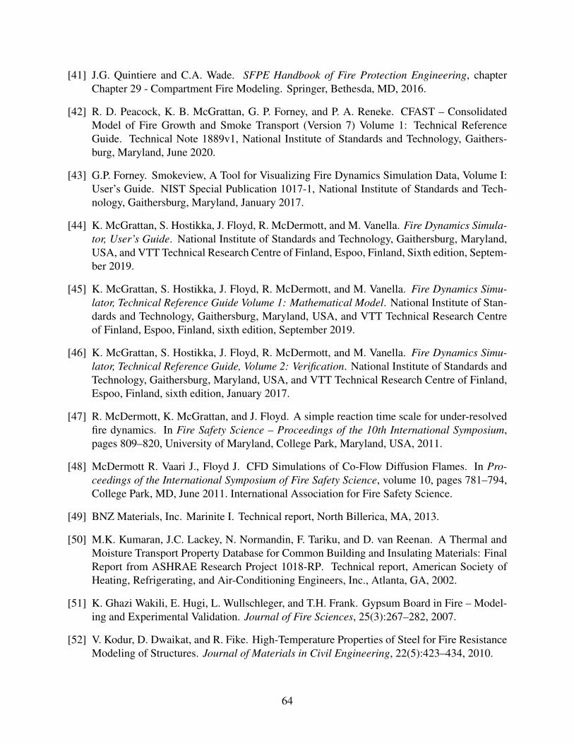
[41] J.G. Quintiere and C.A. Wade. SFPE Handbook of Fire Protection Engineering, chapterChapter 29 - Compartment Fire Modeling. Springer, Bethesda, MD, 2016.

[42] R. D. Peacock, K. B. McGrattan, G. P. Forney, and P. A. Reneke. CFAST – ConsolidatedModel of Fire Growth and Smoke Transport (Version 7) Volume 1: Technical ReferenceGuide. Technical Note 1889v1, National Institute of Standards and Technology, Gaithers-burg, Maryland, June 2020.

[43] G.P. Forney. Smokeview, A Tool for Visualizing Fire Dynamics Simulation Data, Volume I:User’s Guide. NIST Special Publication 1017-1, National Institute of Standards and Tech-nology, Gaithersburg, Maryland, January 2017.

[44] K. McGrattan, S. Hostikka, J. Floyd, R. McDermott, and M. Vanella. Fire Dynamics Simula-tor, User’s Guide. National Institute of Standards and Technology, Gaithersburg, Maryland,USA, and VTT Technical Research Centre of Finland, Espoo, Finland, Sixth edition, Septem-ber 2019.

[45] K. McGrattan, S. Hostikka, J. Floyd, R. McDermott, and M. Vanella. Fire Dynamics Simu-lator, Technical Reference Guide Volume 1: Mathematical Model. National Institute of Stan-dards and Technology, Gaithersburg, Maryland, USA, and VTT Technical Research Centreof Finland, Espoo, Finland, sixth edition, September 2019.

[46] K. McGrattan, S. Hostikka, J. Floyd, R. McDermott, and M. Vanella. Fire Dynamics Simu-lator, Technical Reference Guide, Volume 2: Verification. National Institute of Standards andTechnology, Gaithersburg, Maryland, USA, and VTT Technical Research Centre of Finland,Espoo, Finland, sixth edition, January 2017.

[47] R. McDermott, K. McGrattan, and J. Floyd. A simple reaction time scale for under-resolvedfire dynamics. In Fire Safety Science – Proceedings of the 10th International Symposium,pages 809–820, University of Maryland, College Park, Maryland, USA, 2011.

[48] McDermott R. Vaari J., Floyd J. CFD Simulations of Co-Flow Diffusion Flames. In Pro-ceedings of the International Symposium of Fire Safety Science, volume 10, pages 781–794,College Park, MD, June 2011. International Association for Fire Safety Science.

[49] BNZ Materials, Inc. Marinite I. Technical report, North Billerica, MA, 2013.

[50] M.K. Kumaran, J.C. Lackey, N. Normandin, F. Tariku, and D. van Reenan. A Thermal andMoisture Transport Property Database for Common Building and Insulating Materials: FinalReport from ASHRAE Research Project 1018-RP. Technical report, American Society ofHeating, Refrigerating, and Air-Conditioning Engineers, Inc., Atlanta, GA, 2002.

[51] K. Ghazi Wakili, E. Hugi, L. Wullschleger, and T.H. Frank. Gypsum Board in Fire – Model-ing and Experimental Validation. Journal of Fire Sciences, 25(3):267–282, 2007.

[52] V. Kodur, D. Dwaikat, and R. Fike. High-Temperature Properties of Steel for Fire ResistanceModeling of Structures. Journal of Materials in Civil Engineering, 22(5):423–434, 2010.

64

[53] V.K.R. Kodur and M.A. Sultan. Effect of Temperature on Thermal Properties of High-Strength Concrete. Journal of Materials in Civil Engineering, 15(2):101–107, March/April2003.

[54] M. Hurley, editor. SFPE Handbook of Fire Protection Engineering. Springer, New York, 5thedition, 2016.

[55] H. Brohus, P.V. Nielsen, A.J. Petersen, and K. Sommerlund-Larsen. Sensitivity Analysisof Fire Dynamics Simulation. In Proceedings of Roomvent, pages 1341–1352, June 2007.Helsinki.

[56] R. Upadhyay and O. Ezekoye. Treatment of design fire uncertainty using Quadrature Methodof Moments. Fire Science Journal, 43:127–139, 2008.

[57] W. Jahn, G. Rein, and J. Torrero. The Effect of Model Parameters on the Simulation of FireDynamics. In Fire Safety Science – Proceedings of the Ninth International Symposium, pages1341–1352, September 2008. Karlsruhe, Germany.

[58] R. D. Peacock, G. P. Forney, and P. A. Reneke. CFAST – Consolidated Model of Fire Growthand Smoke Transport (Version 7) Volume 3: Verification and Validation Guide. Techni-cal Note 1889v3, National Institute of Standards and Technology, Gaithersburg, Maryland,February 2021.

65

Appendix A Detailed Results

A.1 Compartment Experiments

This section presents comparisons of the experimental data and model predictions for the compart-ment experiments. In each figure, data that was measured with the fuel package in each locationare presented along with the corresponding model predictions using the FDT methods, CFAST,and FDS. The data collected with the door open and closed are presented separately in each of thefollowing sections.

A.1.1 Gas Temperature

Open Door

A comparison of the layer temperature data collected in the experiments with the 0.3 m Burnerand a HRR of 100 kW is presented in Figure A.1. The FDT method tended to underpredict theupper layer temperature, but gradually increased as the measured temperature reached a steadystate, effectively decreasing the error over time. FDS tended to underpredict the steady upper layertemperature, but accurately predicted the lower layer temperature. CFAST predicted the upperlayer temperature remarkably well, but tended to slightly overpredict the lower layer temperature.There was no significant difference based on the location of the burner in each experiment.

A comparison of the layer interface elevation collected in the experiments with the 0.3 m Burnerand a HRR of 100 kW is presented in Figure A.2. The FDT method predicted a rapid descent ofthe layer interface, but was limited by the door height, so a true comparison is unavailable. FDStended to overpredict the descent of the upper layer and CFAST tended to underpredict the descentof the upper layer. There was no significant difference in the data or predictions based on thelocation of the burner in each experiment.

A comparison of the layer temperature data collected in the experiments with the 0.6 m Burnerand a HRR of 100 kW is presented in Figure A.3. The FDT method tended to underpredict theupper layer temperature, but gradually increased as the measured temperature reached a steadystate, effectively decreasing the error over time. FDS tended to underpredict the steady upper layertemperature, but accurately predicted the lower layer temperature. CFAST slightly underpredictedthe upper layer temperature and tended to overpredict the lower layer temperature. There was nosignificant difference based on the location of the burner in each experiment.

A comparison of the layer interface elevation collected in the experiments with the 0.6 m Burnerand a HRR of 100 kW is presented in Figure A.4. The FDT method predicted a rapid descent ofthe layer interface, but was limited by the door height, so a true comparison is unavailable. FDS

66

0 100 200 300 400 500 600Time (s)

0

20

40

60

80

100

120

140Te

mpe

ratu

re (

C)

Upper Layer -- MeanLower Layer -- Mean

FDS -- Upper LayerFDS -- Lower Layer

CFAST -- T_upperCFAST -- T_lower

FDT -- 100kWSB_T

(a) Center Position

0 100 200 300 400 500 600Time (s)

0

20

40

60

80

100

120

140

Tem

pera

ture

(C

)

Upper Layer -- MeanLower Layer -- Mean

FDS -- Upper LayerFDS -- Lower Layer

CFAST -- T_upperCFAST -- T_lower

FDT -- 100kWSB_T

(b) Back Position

0 100 200 300 400 500 600Time (s)

0

20

40

60

80

100

120

140

Tem

pera

ture

(C

)

Upper Layer -- MeanLower Layer -- Mean

FDS -- Upper LayerFDS -- Lower Layer

CFAST -- T_upperCFAST -- T_lower

FDT -- 100kWSB_T

(c) Corner Position

0 100 200 300 400 500 600Time (s)

0

20

40

60

80

100

120

140

160

Tem

pera

ture

(C

)

Upper Layer -- MeanLower Layer -- Mean

FDS -- Upper LayerFDS -- Lower Layer

CFAST -- T_upperCFAST -- T_lower

FDT -- 100kWSB_T

(d) Side Position

Figure A.1: Comparison of the Layer Temperatures in 0.3 m Burner, 100 kW Experiments withDoor Open

tended to slightly overpredict the descent of the upper layer and CFAST tended to underpredict thedescent of the upper layer. There was no significant difference in the data or predictions based onthe location of the burner in each experiment.

A comparison of the layer temperature data collected in the experiments with the 0.6 m Burnerand a HRR of 500 kW is presented in Figure A.5. The FDT method tended to underpredict theupper layer temperature, but gradually increased as the measured temperature reached a steadystate, effectively decreasing the error over time. FDS tended to underpredict the steady upper layertemperature, and slightly underpredicted the lower layer temperature. CFAST accurately predictedthe upper layer temperature, but continued increasing at as the experimental data reached a steadystate, effectively increasing the error between the two. CFAST tended to overpredict the lowerlayer temperature. There was no significant difference based on the location of the burner in eachexperiment.

67

0 100 200 300 400 500 600Time (s)

0.0

0.5

1.0

1.5

2.0

2.5H

eigh

t (m

)

Layer Interface -- Mean FDS -- Layer Interface CFAST -- Height FDT -- 100kWSB_z

(a) Center Position

0 100 200 300 400 500 600Time (s)

0.0

0.5

1.0

1.5

2.0

2.5

Hei

ght (

m)

Layer Interface -- Mean FDS -- Layer Interface CFAST -- Height FDT -- 100kWSB_z

(b) Back Position

0 100 200 300 400 500 600Time (s)

0.0

0.5

1.0

1.5

2.0

2.5

Hei

ght (

m)

Layer Interface -- Mean FDS -- Layer Interface CFAST -- Height FDT -- 100kWSB_z

(c) Corner Position

0 100 200 300 400 500 600Time (s)

0.0

0.5

1.0

1.5

2.0

2.5

Hei

ght (

m)

Layer Interface -- Mean FDS -- Layer Interface CFAST -- Height FDT -- 100kWSB_z

(d) Side Position

Figure A.2: Comparison of the Layer Interface Elevation in 0.3 m Burner, 100 kW Experimentswith Door Open

A comparison of the layer interface elevation collected in the experiments with the 0.6 m Burnerand a HRR of 500 kW is presented in Figure A.6. The FDT method predicted a rapid descent ofthe layer interface, but was limited by the door height, so a true comparison is unavailable. FDSaccurately predicted the elevation of the upper layer interface and CFAST accurately predicted thedescent of the upper layer until approximately 150 s, at which point CFAST predicted a rise inthe interface that was not observed. There was no significant difference in the data or predictionsbased on the location of the burner in each experiment.

A comparison of the layer temperature data collected in the experiments with the Red Accent Chairis presented in Figure A.7. The FDT method was developed for a constant HRR fire source awayfrom the walls of the compartment and does not account for a growth period or decay period. Themaximum upper and low layer temperature was highest when the chair was in the back position.In this case, the upper layer temperature predicted with the FDT method using the maximum HRRwas comparable to the measured maximum in the range of 400 s to 800 s, but the same prediction

68

0 100 200 300 400 500 600Time (s)

0

20

40

60

80

100

120

140

Tem

pera

ture

(C

)

Upper Layer -- MeanLower Layer -- Mean

FDS -- Upper LayerFDS -- Lower Layer

CFAST -- T_upperCFAST -- T_lower

FDT -- 100kW_T

(a) Center Position

0 100 200 300 400 500 600Time (s)

0

20

40

60

80

100

120

Tem

pera

ture

(C

)

Upper Layer -- MeanLower Layer -- Mean

FDS -- Upper LayerFDS -- Lower Layer

CFAST -- T_upperCFAST -- T_lower

FDT -- 100kW_T

(b) Back Position

0 100 200 300 400 500 600Time (s)

0

20

40

60

80

100

120

140

Tem

pera

ture

(C

)

Upper Layer -- MeanLower Layer -- Mean

FDS -- Upper LayerFDS -- Lower Layer

CFAST -- T_upperCFAST -- T_lower

FDT -- 100kW_T

(c) Corner Position

0 100 200 300 400 500 600Time (s)

0

20

40

60

80

100

120

140

Tem

pera

ture

(C

)

Upper Layer -- MeanLower Layer -- Mean

FDS -- Upper LayerFDS -- Lower Layer

CFAST -- T_upperCFAST -- T_lower

FDT -- 100kW_T

(d) Side Position

Figure A.3: Comparison of the Layer Temperatures in 0.6 m Burner, 100 kW Experiments withDoor Open

was high for the corner and center positions. The FDT predictions made using the mean and steadyHRRs accurately described the approximate mean and steady upper layer temperatures. The upperand lower gas layer temperatures predicted with FDS and CFAST generally agreed with eachother. FDS and CFAST accurately represented the upper layer temperature, but neither capturedthe maximum temperature in the lower layer.

A comparison of the layer interface elevation collected in the experiments with the Red AccentChair is presented in Figure A.6. The FDT method predicted a rapid descent of the layer inter-face, but was limited by the door height, so a true comparison is unavailable. FDS accuratelypredicted the elevation of the upper layer interface from approximately 200 s to the end of theexperiment and the CFAST predictions tracked with the FDS prediction until approximately 200 s,after which CFAST predicted the interface height was at a higher elevation than measured. Therewas no significant difference in the data or predictions based on the location of the burner in eachexperiment.

69

0 100 200 300 400 500 600Time (s)

0.0

0.5

1.0

1.5

2.0

2.5H

eigh

t (m

)

Layer Interface -- Mean FDS -- Layer Interface CFAST -- Height FDT -- 100kW_z

(a) Center Position

0 100 200 300 400 500 600Time (s)

0.0

0.5

1.0

1.5

2.0

2.5

Hei

ght (

m)

Layer Interface -- Mean FDS -- Layer Interface CFAST -- Height FDT -- 100kW_z

(b) Back Position

0 100 200 300 400 500 600Time (s)

0.0

0.5

1.0

1.5

2.0

2.5

Hei

ght (

m)

Layer Interface -- Mean FDS -- Layer Interface CFAST -- Height FDT -- 100kW_z

(c) Corner Position

0 100 200 300 400 500 600Time (s)

0.0

0.5

1.0

1.5

2.0

2.5

Hei

ght (

m)

Layer Interface -- Mean FDS -- Layer Interface CFAST -- Height FDT -- 100kW_z

(d) Side Position

Figure A.4: Comparison of the Layer Interface Elevation in 0.6 m Burner, 100 kW Experimentswith Door Open

A comparison of the layer temperature data collected in the experiments with the OverstuffedSofa is presented in Figure ??. The maximum upper layer temperature over the 200 s to 400 srange was accurately predicted by the FDT method using the maximum HRR. The FDT predictioncalculated with the mean HRR accurately represented the approximate mean temperature for theupper gas layer. The FDS and CFAST predictions of the upper and lower layer temperatureswere qualitatively similar to the measured upper and lower layer temperature profiles, but CFASTgenerally accurately represented the maximum upper layer temperature and FDS underpredictedthe maximum upper layer temperature. CFAST and FDS both underpredicted the maximum lowerlayer temperature.

A comparison of the layer interface elevation collected in the experiments with the OverstuffedSofa is presented in Figure A.10. The FDT method predicted a rapid descent of the layer interface,but was limited by the door height, so a true comparison is unavailable. FDS accurately predictedthe elevation of the layer interface from approximately 200 s to the end of the experiment in the

70

0 100 200 300 400 500 600Time (s)

0

50

100

150

200

250

300

350Te

mpe

ratu

re (

C)

Upper Layer -- MeanLower Layer -- Mean

FDS -- Upper LayerFDS -- Lower Layer

CFAST -- T_upperCFAST -- T_lower

FDT -- 500kW_T

(a) Center Position

0 100 200 300 400 500 600Time (s)

0

50

100

150

200

250

300

350

400

Tem

pera

ture

(C

)

Upper Layer -- MeanLower Layer -- Mean

FDS -- Upper LayerFDS -- Lower Layer

CFAST -- T_upperCFAST -- T_lower

FDT -- 500kW_T

(b) Back Position

0 100 200 300 400 500 600Time (s)

0

50

100

150

200

250

300

350

Tem

pera

ture

(C

)

Upper Layer -- MeanLower Layer -- Mean

FDS -- Upper LayerFDS -- Lower Layer

CFAST -- T_upperCFAST -- T_lower

FDT -- 500kW_T

(c) Corner Position

0 100 200 300 400 500 600Time (s)

0

50

100

150

200

250

300

350Te

mpe

ratu

re (

C)

Upper Layer -- MeanLower Layer -- Mean

FDS -- Upper LayerFDS -- Lower Layer

CFAST -- T_upperCFAST -- T_lower

FDT -- 500kW_T

(d) Side Position

Figure A.5: Comparison of the Layer Temperatures in 0.6 m Burner, 500 kW Experiments withDoor Open

Corner and Back positions, but underpredicted the descent of the layer in the center position.CFAST underpredicted the descent of the layer interface in all positions.

Although the MQH correlation, presented as the FDT method for the open door experiment com-parisons, was only formulated to predict temperatures up to 600◦C with fuel sources away fromthe walls and corners of the compartment, the predictions made using the maximum HRR yieldedconservative results for the maximum upper layer temperature and those calculated with the meanHRR yielded a reasonable estimate for the mean upper layer temperature over the duration of theexperiment. The location of the fuel package did not significantly affect the accuracy of thesepredictions.

71

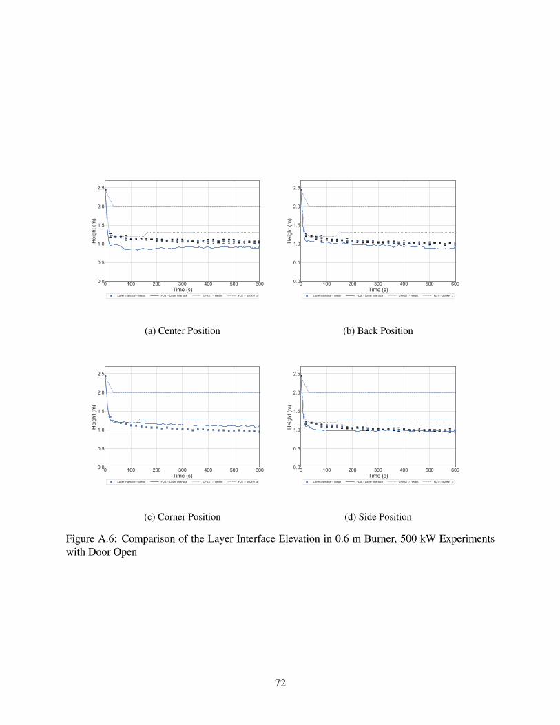
0 100 200 300 400 500 600Time (s)

0.0

0.5

1.0

1.5

2.0

2.5

Hei

ght (

m)

Layer Interface -- Mean FDS -- Layer Interface CFAST -- Height FDT -- 500kW_z

(a) Center Position

0 100 200 300 400 500 600Time (s)

0.0

0.5

1.0

1.5

2.0

2.5

Hei

ght (

m)

Layer Interface -- Mean FDS -- Layer Interface CFAST -- Height FDT -- 500kW_z

(b) Back Position

0 100 200 300 400 500 600Time (s)

0.0

0.5

1.0

1.5

2.0

2.5

Hei

ght (

m)

Layer Interface -- Mean FDS -- Layer Interface CFAST -- Height FDT -- 500kW_z

(c) Corner Position

0 100 200 300 400 500 600Time (s)

0.0

0.5

1.0

1.5

2.0

2.5

Hei

ght (

m)

Layer Interface -- Mean FDS -- Layer Interface CFAST -- Height FDT -- 500kW_z

(d) Side Position

Figure A.6: Comparison of the Layer Interface Elevation in 0.6 m Burner, 500 kW Experimentswith Door Open

72

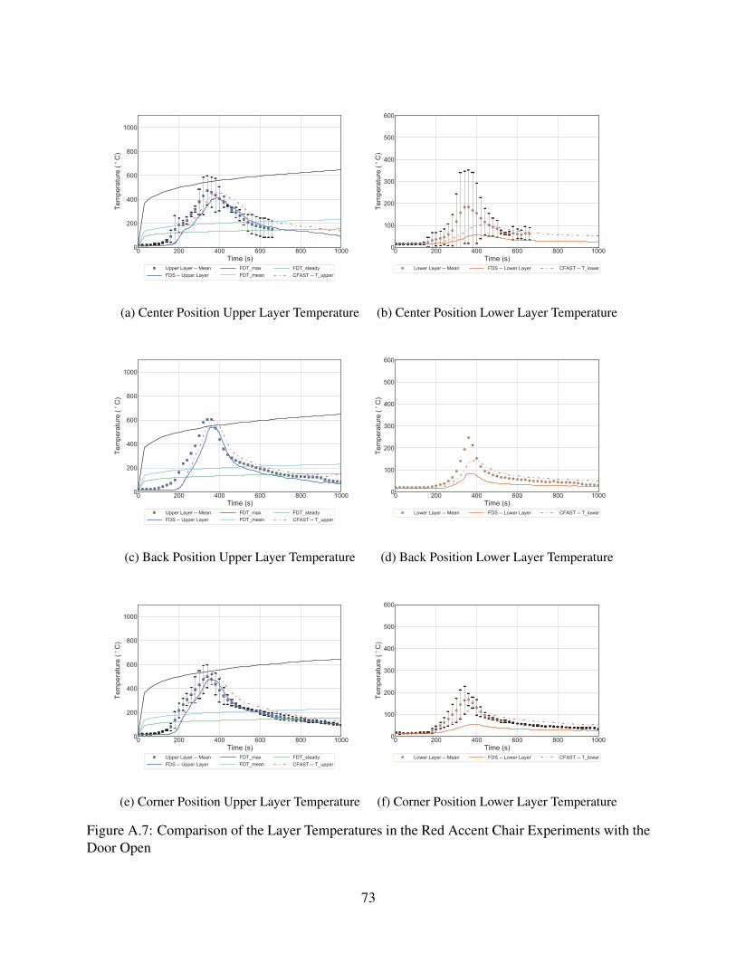
0 200 400 600 800 1000Time (s)

0

200

400

600

800

1000Te

mpe

ratu

re (

C)

Upper Layer -- MeanFDS -- Upper Layer

FDT_maxFDT_mean

FDT_steadyCFAST -- T_upper

(a) Center Position Upper Layer Temperature

0 200 400 600 800 1000Time (s)

0

100

200

300

400

500

600

Tem

pera

ture

(C

)

Lower Layer -- Mean FDS -- Lower Layer CFAST -- T_lower

(b) Center Position Lower Layer Temperature

0 200 400 600 800 1000Time (s)

0

200

400

600

800

1000

Tem

pera

ture

(C

)

Upper Layer -- MeanFDS -- Upper Layer

FDT_maxFDT_mean

FDT_steadyCFAST -- T_upper

(c) Back Position Upper Layer Temperature

0 200 400 600 800 1000Time (s)

0

100

200

300

400

500

600

Tem

pera

ture

(C

)

Lower Layer -- Mean FDS -- Lower Layer CFAST -- T_lower

(d) Back Position Lower Layer Temperature

0 200 400 600 800 1000Time (s)

0

200

400

600

800

1000

Tem

pera

ture

(C

)

Upper Layer -- MeanFDS -- Upper Layer

FDT_maxFDT_mean

FDT_steadyCFAST -- T_upper

(e) Corner Position Upper Layer Temperature

0 200 400 600 800 1000Time (s)

0

100

200

300

400

500

600

Tem

pera

ture

(C

)

Lower Layer -- Mean FDS -- Lower Layer CFAST -- T_lower

(f) Corner Position Lower Layer Temperature

Figure A.7: Comparison of the Layer Temperatures in the Red Accent Chair Experiments with theDoor Open

73

0 200 400 600 800 1000Time (s)

0.0

0.5

1.0

1.5

2.0

Hei

ght (

m)

Layer Interface -- MeanFDS -- Layer Interface

FDT_maxFDT_mean

FDT_steadyCFAST -- Height

(a) Center Position

0 200 400 600 800 1000Time (s)

0.0

0.5

1.0

1.5

2.0

Hei

ght (

m)

Layer Interface -- MeanFDS -- Layer Interface

FDT_maxFDT_mean

FDT_steadyCFAST -- Height

(b) Back Position

0 200 400 600 800 1000Time (s)

0.0

0.5

1.0

1.5

2.0

Hei

ght (

m)

Layer Interface -- MeanFDS -- Layer Interface

FDT_maxFDT_mean

FDT_steadyCFAST -- Height

(c) Corner Position

Figure A.8: Comparison of the Layer Interface Elevation in Red Accent Chair with the Door Open

74

0 200 400 600 800 1000Time (s)

0

200

400

600

800

1000Te

mpe

ratu

re (

C)

Upper Layer -- MeanFDS -- Upper Layer

FDT_maxFDT_mean

FDT_steadyCFAST -- T_upper

(a) Center Position Upper Layer Temperature

0 200 400 600 800 1000Time (s)

0

100

200

300

400

500

600

Tem

pera

ture

(C

)

Lower Layer -- Mean FDS -- Lower Layer CFAST -- T_lower

(b) Center Position Lower Layer Temperature

0 200 400 600 800 1000Time (s)

0

200

400

600

800

1000

Tem

pera

ture

(C

)

Upper Layer -- MeanFDS -- Upper Layer

FDT_maxFDT_mean

FDT_steadyCFAST -- T_upper

(c) Back Position Upper Layer Temperature

0 200 400 600 800 1000Time (s)

0

100

200

300

400

500

600

Tem

pera

ture

(C

)

Lower Layer -- Mean FDS -- Lower Layer CFAST -- T_lower

(d) Back Position Lower Layer Temperature

0 200 400 600 800 1000Time (s)

0

200

400

600

800

1000

Tem

pera

ture

(C

)

Upper Layer -- MeanFDS -- Upper Layer

FDT_maxFDT_mean

FDT_steadyCFAST -- T_upper

(e) Corner Position Upper Layer Temperature

0 200 400 600 800 1000Time (s)

0

100

200

300

400

500

600

Tem

pera

ture

(C

)

Lower Layer -- Mean FDS -- Lower Layer CFAST -- T_lower

(f) Corner Position Lower Layer Temperature

Figure A.9: Comparison of the Layer Temperatures in the Overstuffed Sofa Experiments with theDoor Open

75

0 200 400 600 800 1000Time (s)

0.0

0.5

1.0

1.5

2.0

Hei

ght (

m)

Layer Interface -- MeanFDS -- Layer Interface

FDT_maxFDT_mean

FDT_steadyCFAST -- Height

(a) Center Position

0 200 400 600 800 1000Time (s)

0.0

0.5

1.0

1.5

2.0

Hei

ght (

m)

Layer Interface -- MeanFDS -- Layer Interface

FDT_maxFDT_mean

FDT_steadyCFAST -- Height

(b) Back Position

0 200 400 600 800 1000Time (s)

0.0

0.5

1.0

1.5

2.0

Hei

ght (

m)

Layer Interface -- MeanFDS -- Layer Interface

FDT_maxFDT_mean

FDT_steadyCFAST -- Height

(c) Corner Position

Figure A.10: Comparison of the Layer Interface Elevation in Overstuffed Sofa with the Door Open

76

Closed Door

A comparison of the layer temperature data collected in the experiments with the 0.3 m Burnerand a HRR of 100 kW is presented in Figure A.11. The FDT method tended to underpredictthe upper layer temperature until approximately 300 s, at which point the HRR and temperaturesmeasured with the burner in all locations presumably decreased due to a lack of ventilation. TheCFAST predictions for upper and lower gas layer temperatures followed the same qualitative trendas the experimental data, but underpredicted the temperatures throughout the experiment. FDSgenerally predicted the qualitative shape of the temperature curves, but underpredicted the upperlayer temperature and overpredicted the lower layer temperature.

0 100 200 300 400 500 600Time (s)

0

50

100

150

200

Tem

pera

ture

(C

)

Upper Layer -- MeanLower Layer -- Mean

FDS -- Upper LayerFDS -- Lower Layer

CFAST -- T_upperCFAST -- T_lower

FDT -- 100kWSB_T

(a) Center Position

0 100 200 300 400 500 600Time (s)

0

50

100

150

200

Tem

pera

ture

(C

)

Upper Layer -- MeanLower Layer -- Mean

FDS -- Upper LayerFDS -- Lower Layer

CFAST -- T_upperCFAST -- T_lower

FDT -- 100kWSB_T

(b) Back Position

0 100 200 300 400 500 600Time (s)

0

50

100

150

200

Tem

pera

ture

(C

)

Upper Layer -- MeanLower Layer -- Mean

FDS -- Upper LayerFDS -- Lower Layer

CFAST -- T_upperCFAST -- T_lower

FDT -- 100kWSB_T

(c) Corner Position

0 100 200 300 400 500 600Time (s)

0

50

100

150

200

Tem

pera

ture

(C

)

Upper Layer -- MeanLower Layer -- Mean

FDS -- Upper LayerFDS -- Lower Layer

CFAST -- T_upperCFAST -- T_lower

FDT -- 100kWSB_T

(d) Side Position

Figure A.11: Comparison of the Layer Temperatures in 0.3 m Burner, 100 kW Experiments withDoor Closed

A comparison of the layer interface elevation collected in the experiments with the 0.3 m Burnerand a HRR of 100 kW is presented in Figure A.12. The FDT method predicted the hot gas layerwould descend to the floor of the compartment by approximately 300 s, which was a conservative

77

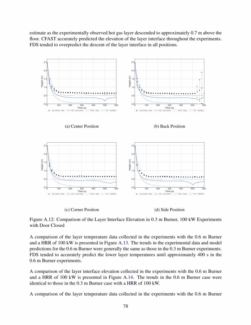
estimate as the experimentally observed hot gas layer descended to approximately 0.7 m above thefloor. CFAST accurately predicted the elevation of the layer interface throughout the experiments.FDS tended to overpredict the descent of the layer interface in all positions.

0 100 200 300 400 500 600Time (s)

0.0

0.5

1.0

1.5

2.0

2.5

Hei

ght (

m)

Layer Interface -- Mean FDS -- Layer Interface CFAST -- Height FDT -- 100kWSB_z

(a) Center Position

0 100 200 300 400 500 600Time (s)

0.0

0.5

1.0

1.5

2.0

2.5

Hei

ght (

m)

Layer Interface -- Mean FDS -- Layer Interface CFAST -- Height FDT -- 100kWSB_z

(b) Back Position

0 100 200 300 400 500 600Time (s)

0.0

0.5

1.0

1.5

2.0

2.5

Hei

ght (

m)

Layer Interface -- Mean FDS -- Layer Interface CFAST -- Height FDT -- 100kWSB_z

(c) Corner Position

0 100 200 300 400 500 600Time (s)

0.0

0.5

1.0

1.5

2.0

2.5

Hei

ght (

m)

Layer Interface -- Mean FDS -- Layer Interface CFAST -- Height FDT -- 100kWSB_z

(d) Side Position

Figure A.12: Comparison of the Layer Interface Elevation in 0.3 m Burner, 100 kW Experimentswith Door Closed

A comparison of the layer temperature data collected in the experiments with the 0.6 m Burnerand a HRR of 100 kW is presented in Figure A.13. The trends in the experimental data and modelpredictions for the 0.6 m Burner were generally the same as those in the 0.3 m Burner experiments.FDS tended to accurately predict the lower layer temperatures until approximately 400 s in the0.6 m Burner experiments.

A comparison of the layer interface elevation collected in the experiments with the 0.6 m Burnerand a HRR of 100 kW is presented in Figure A.14. The trends in the 0.6 m Burner case wereidentical to those in the 0.3 m Burner case with a HRR of 100 kW.

A comparison of the layer temperature data collected in the experiments with the 0.6 m Burner

78

0 100 200 300 400 500 600Time (s)

0

50

100

150

200

250

Tem

pera

ture

(C

)

Upper Layer -- MeanLower Layer -- Mean

FDS -- Upper LayerFDS -- Lower Layer

CFAST -- T_upperCFAST -- T_lower

FDT -- 100kW_T

(a) Center Position

0 100 200 300 400 500 600Time (s)

0

50

100

150

200

250

Tem

pera

ture

(C

)

Upper Layer -- MeanLower Layer -- Mean

FDS -- Upper LayerFDS -- Lower Layer

CFAST -- T_upperCFAST -- T_lower

FDT -- 100kW_T

(b) Back Position

0 100 200 300 400 500 600Time (s)

0

50

100

150

200

Tem

pera

ture

(C

)

Upper Layer -- MeanLower Layer -- Mean

FDS -- Upper LayerFDS -- Lower Layer

CFAST -- T_upperCFAST -- T_lower

FDT -- 100kW_T

(c) Corner Position

0 100 200 300 400 500 600Time (s)

0

50

100

150

200

250

Tem

pera

ture

(C

)

Upper Layer -- MeanLower Layer -- Mean

FDS -- Upper LayerFDS -- Lower Layer

CFAST -- T_upperCFAST -- T_lower

FDT -- 100kW_T

(d) Side Position

Figure A.13: Comparison of the Layer Temperatures in 0.6 m Burner, 100 kW Experiments withDoor Closed

and a HRR of 500 kW is presented in Figure A.15. The FDT method predicted the rise in upperlayer temperature to its peak at approximately 50 s. CFAST accurately predicted the upper layertemperature, but underpredicted the lower layer temperature throughout the experiment. FDS gen-erally predicted the qualitative shape of the temperature curves, but erroneously predicted a localmaximum in the upper and lower layer temperatures.

A comparison of the layer interface elevation collected in the experiments with the 0.3 m Burnerand a HRR of 100 kW is presented in Figure A.14. The FDT method predicted the hot gas layerwould descend to the floor of the compartment by approximately 300 s, which was a conservativeestimate as the experimentally observed hot gas layer descended to approximately 0.6 m above thefloor. CFAST accurately predicted the elevation of the layer interface throughout the experiments.FDS tended to overpredict the descent of the layer interface in all positions. The layer interfaceelevation increased after approximately 300 s and none of the models predicted the increase.

79

0 100 200 300 400 500 600Time (s)

0.0

0.5

1.0

1.5

2.0

2.5H

eigh

t (m

)

Layer Interface -- Mean FDS -- Layer Interface CFAST -- Height FDT -- 100kW_z

(a) Center Position

0 100 200 300 400 500 600Time (s)

0.0

0.5

1.0

1.5

2.0

2.5

Hei

ght (

m)

Layer Interface -- Mean FDS -- Layer Interface CFAST -- Height FDT -- 100kW_z

(b) Back Position

0 100 200 300 400 500 600Time (s)

0.0

0.5

1.0

1.5

2.0

2.5

Hei

ght (

m)

Layer Interface -- Mean FDS -- Layer Interface CFAST -- Height FDT -- 100kW_z

(c) Corner Position

0 100 200 300 400 500 600Time (s)

0.0

0.5

1.0

1.5

2.0

2.5

Hei

ght (

m)

Layer Interface -- Mean FDS -- Layer Interface CFAST -- Height FDT -- 100kW_z

(d) Side Position

Figure A.14: Comparison of the Layer Interface Elevation in 0.6 m Burner, 100 kW Experimentswith Door Closed

A comparison of the layer temperature data collected in the experiments with the Red Accent Chairis presented in Figure A.17. The FDT method calculated with the maximum, mean, and steadyHRR from the experiments significantly overpredicted the hot gas layer temperatures. The CFASTprediction for upper layer temperature qualitatively matched the experimental data, although theupper and lower layer temperatures were underpredicted. FDS slightly overpredicted the maximumupper and lower layer temperatures and accurately predicted the temperatures in the growth anddecay phases. The location of the fuel package did not significantly affect the experimental data orpredictions.

A comparison of the layer interface elevation measured in the experiments with the Red AccentChair is presented in Figure A.18. The FDT method predicted the hot gas layer would rapidlydescend to the floor of the compartment within 100 s, which was a conservative estimate as theexperimentally observed hot gas layer descended to approximately 0.6 m above the floor by ap-proximately 200 s. CFAST and FDS qualitatively predicted the rate of descent of the layer interface

80

0 100 200 300 400 500 600Time (s)

0

50

100

150

200

250

300

350

400Te

mpe

ratu

re (

C)

Upper Layer -- MeanLower Layer -- Mean

FDS -- Upper LayerFDS -- Lower Layer

CFAST -- T_upperCFAST -- T_lower

FDT -- 500kW_T

(a) Center Position

0 100 200 300 400 500 600Time (s)

0

50

100

150

200

250

300

350

400

Tem

pera

ture

(C

)

Upper Layer -- MeanLower Layer -- Mean

FDS -- Upper LayerFDS -- Lower Layer

CFAST -- T_upperCFAST -- T_lower

FDT -- 500kW_T

(b) Back Position

0 100 200 300 400 500 600Time (s)

0

50

100

150

200

250

300

350

400

Tem

pera

ture

(C

)

Upper Layer -- MeanLower Layer -- Mean

FDS -- Upper LayerFDS -- Lower Layer

CFAST -- T_upperCFAST -- T_lower

FDT -- 500kW_T

(c) Corner Position

0 100 200 300 400 500 600Time (s)

0

50

100

150

200

250

300

350

400

Tem

pera

ture

(C

)

Upper Layer -- MeanLower Layer -- Mean

FDS -- Upper LayerFDS -- Lower Layer

CFAST -- T_upperCFAST -- T_lower

FDT -- 500kW_T

(d) Side Position

Figure A.15: Comparison of the Layer Temperatures in 0.6 m Burner, 500 kW Experiments withDoor Closed

and slightly overpredicted the descent of the layer at steady state.

A comparison of the layer temperature data collected in the experiments with the OverstuffedSofa is presented in Figure A.19. The FDT method calculated with the maximum, mean, andsteady HRR from the experiments significantly overpredicted the hot gas layer temperatures. TheCFAST prediction for upper layer temperature qualitatively matched the experimental data andgenerally predicted the maximum upper layer temperature, although the lower layer temperatureswere underpredicted. FDS accurately predicted the temperatures in growth period, overpredictedthe maximum upper and lower layer temperatures, and underpredicted the temperatures in thedecay phases. The location of the fuel package did not significantly affect the experimental data orpredictions.

A comparison of the layer interface elevation measured in the experiments with the OverstuffedSofa is presented in Figure A.20. The FDT method predicted the hot gas layer would rapidly

81

0 100 200 300 400 500 600Time (s)

0.0

0.5

1.0

1.5

2.0

2.5H

eigh

t (m

)

Layer Interface -- Mean FDS -- Layer Interface CFAST -- Height FDT -- 500kW_z

(a) Center Position

0 100 200 300 400 500 600Time (s)

0.0

0.5

1.0

1.5

2.0

2.5

Hei

ght (

m)

Layer Interface -- Mean FDS -- Layer Interface CFAST -- Height FDT -- 500kW_z

(b) Back Position

0 100 200 300 400 500 600Time (s)

0.0

0.5

1.0

1.5

2.0

2.5

Hei

ght (

m)

Layer Interface -- Mean FDS -- Layer Interface CFAST -- Height FDT -- 500kW_z

(c) Corner Position

0 100 200 300 400 500 600Time (s)

0.0

0.5

1.0

1.5

2.0

2.5

Hei

ght (

m)

Layer Interface -- Mean FDS -- Layer Interface CFAST -- Height FDT -- 500kW_z

(d) Side Position

Figure A.16: Comparison of the Layer Interface Elevation in 0.6 m Burner, 500 kW Experimentswith Door Closed

descend to the floor of the compartment within 100 s, which was a conservative estimate as theexperimentally observed hot gas layer interface descended to a steady state of approximately 0.6 mabove the floor in the range of 200 s to 400 s. CFAST and FDS qualitatively predicted the rate ofdescent of the layer interface. CFAST accurately predicted the steady interface elevation and FDStended to predict a higher elevation for the steady interface height.

82

0 200 400 600 800 1000Time (s)

0

200

400

600

800

1000Te

mpe

ratu

re (

C)

Upper Layer -- MeanFDS -- Upper Layer

FDT_maxFDT_mean

FDT_steadyCFAST -- T_upper

(a) Center Position Upper Layer Temperature

0 200 400 600 800 1000Time (s)

0

100

200

300

400

500

600

Tem

pera

ture

(C

)

Lower Layer -- Mean FDS -- Lower Layer CFAST -- T_lower

(b) Center Position Lower Layer Temperature

0 200 400 600 800 1000Time (s)

0

200

400

600

800

1000

Tem

pera

ture

(C

)

Upper Layer -- MeanFDS -- Upper Layer

FDT_maxFDT_mean

FDT_steadyCFAST -- T_upper

(c) Back Position Upper Layer Temperature

0 200 400 600 800 1000Time (s)

0

100

200

300

400

500

600

Tem

pera

ture

(C

)

Lower Layer -- Mean FDS -- Lower Layer CFAST -- T_lower

(d) Back Position Lower Layer Temperature

0 200 400 600 800 1000Time (s)

0

200

400

600

800

1000

Tem

pera

ture

(C

)

Upper Layer -- MeanFDS -- Upper Layer

FDT_maxFDT_mean

FDT_steadyCFAST -- T_upper

(e) Corner Position Upper Layer Temperature

0 200 400 600 800 1000Time (s)

0

100

200

300

400

500

600

Tem

pera

ture

(C

)

Lower Layer -- Mean FDS -- Lower Layer CFAST -- T_lower

(f) Corner Position Lower Layer Temperature

Figure A.17: Comparison of the Layer Temperatures in the Red Accent Chair Experiments withthe Door Closed

83

0 200 400 600 800 1000Time (s)

0.0

0.5

1.0

1.5

2.0

Hei

ght (

m)

Layer Interface -- MeanFDS -- Layer Interface

FDT_maxFDT_mean

FDT_steadyCFAST -- Height

(a) Center Position

0 200 400 600 800 1000Time (s)

0.0

0.5

1.0

1.5

2.0

Hei

ght (

m)

Layer Interface -- MeanFDS -- Layer Interface

FDT_maxFDT_mean

FDT_steadyCFAST -- Height

(b) Back Position

0 200 400 600 800 1000Time (s)

0.0

0.5

1.0

1.5

2.0

Hei

ght (

m)

Layer Interface -- MeanFDS -- Layer Interface

FDT_maxFDT_mean

FDT_steadyCFAST -- Height

(c) Corner Position

Figure A.18: Comparison of the Layer Interface Elevation in Red Accent Chair with the DoorClosed

84

0 200 400 600 800 1000Time (s)

0

200

400

600

800

1000Te

mpe

ratu

re (

C)

Upper Layer -- MeanFDS -- Upper Layer

FDT_maxFDT_mean

FDT_steadyCFAST -- T_upper

(a) Center Position Upper Layer Temperature

0 200 400 600 800 1000Time (s)

0

100

200

300

400

500

600

Tem

pera

ture

(C

)

Lower Layer -- Mean FDS -- Lower Layer CFAST -- T_lower

(b) Center Position Lower Layer Temperature

0 200 400 600 800 1000Time (s)

0

200

400

600

800

1000

Tem

pera

ture

(C

)

Upper Layer -- MeanFDS -- Upper Layer

FDT_maxFDT_mean

FDT_steadyCFAST -- T_upper

(c) Back Position Upper Layer Temperature

0 200 400 600 800 1000Time (s)

0

100

200

300

400

500

600

Tem

pera

ture

(C

)

Lower Layer -- Mean FDS -- Lower Layer CFAST -- T_lower

(d) Back Position Lower Layer Temperature

0 200 400 600 800 1000Time (s)

0

200

400

600

800

1000

Tem

pera

ture

(C

)

Upper Layer -- MeanFDS -- Upper Layer

FDT_maxFDT_mean

FDT_steadyCFAST -- T_upper

(e) Corner Position Upper Layer Temperature

0 200 400 600 800 1000Time (s)

0

100

200

300

400

500

600

Tem

pera

ture

(C

)

Lower Layer -- Mean FDS -- Lower Layer CFAST -- T_lower

(f) Corner Position Lower Layer Temperature

Figure A.19: Comparison of the Layer Temperatures in the Overstuffed Sofa Experiments with theDoor Closed

85

0 200 400 600 800 1000Time (s)

0.0

0.5

1.0

1.5

2.0

Hei

ght (

m)

Layer Interface -- MeanFDS -- Layer Interface

FDT_maxFDT_mean

FDT_steadyCFAST -- Height

(a) Center Position

0 200 400 600 800 1000Time (s)

0.0

0.5

1.0

1.5

2.0

Hei

ght (

m)

Layer Interface -- MeanFDS -- Layer Interface

FDT_maxFDT_mean

FDT_steadyCFAST -- Height

(b) Back Position

0 200 400 600 800 1000Time (s)

0.0

0.5

1.0

1.5

2.0

Hei

ght (

m)

Layer Interface -- MeanFDS -- Layer Interface

FDT_maxFDT_mean

FDT_steadyCFAST -- Height

(c) Corner Position

Figure A.20: Comparison of the Layer Interface Elevation in Overstuffed Sofa with the DoorClosed

86

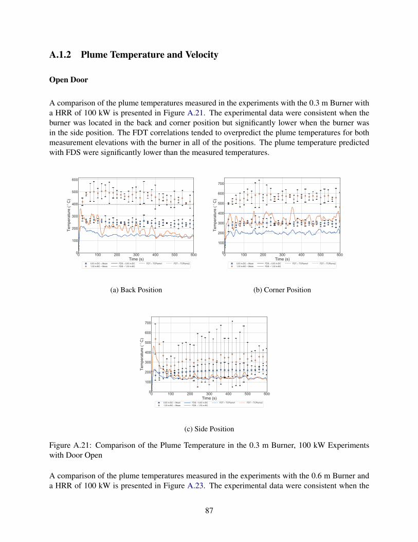
A.1.2 Plume Temperature and Velocity

Open Door

A comparison of the plume temperatures measured in the experiments with the 0.3 m Burner witha HRR of 100 kW is presented in Figure A.21. The experimental data were consistent when theburner was located in the back and corner position but significantly lower when the burner wasin the side position. The FDT correlations tended to overpredict the plume temperatures for bothmeasurement elevations with the burner in all of the positions. The plume temperature predictedwith FDS were significantly lower than the measured temperatures.

0 100 200 300 400 500 600Time (s)

0

100

200

300

400

500

600

Tem

pera

ture

(C

)

0.65 m BC -- Mean1.30 m BC -- Mean

FDS -- 0.65 m BCFDS -- 1.30 m BC

FDT -- TCPlume1 FDT -- TCPlume2

(a) Back Position

0 100 200 300 400 500 600Time (s)

0

100

200

300

400

500

600

700

Tem

pera

ture

(C

)

0.65 m BC -- Mean1.30 m BC -- Mean

FDS -- 0.65 m BCFDS -- 1.30 m BC

FDT -- TCPlume1 FDT -- TCPlume2

(b) Corner Position

0 100 200 300 400 500 600Time (s)

0

100

200

300

400

500

600

700

Tem

pera

ture

(C

)

0.65 m BC -- Mean1.30 m BC -- Mean

FDS -- 0.65 m BCFDS -- 1.30 m BC

FDT -- TCPlume1 FDT -- TCPlume2

(c) Side Position

Figure A.21: Comparison of the Plume Temperature in the 0.3 m Burner, 100 kW Experimentswith Door Open

A comparison of the plume temperatures measured in the experiments with the 0.6 m Burner anda HRR of 100 kW is presented in Figure A.23. The experimental data were consistent when the

87

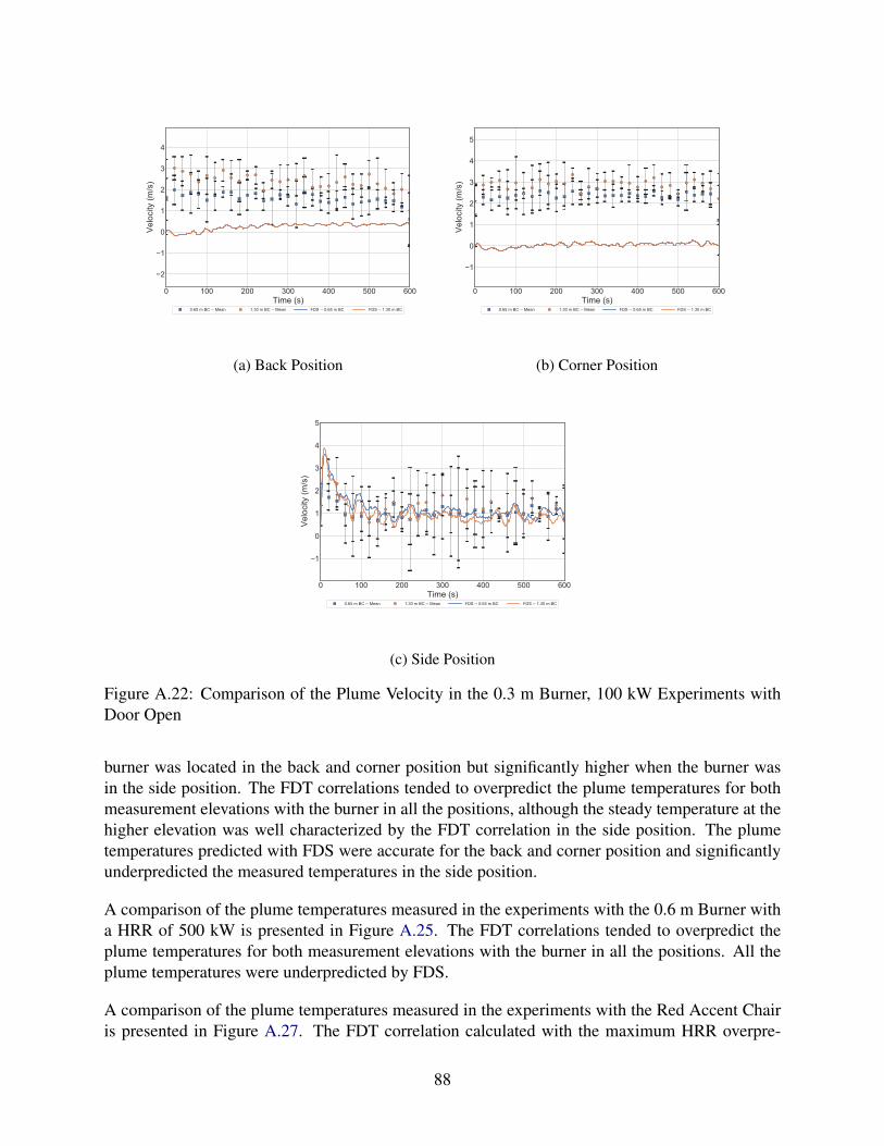
0 100 200 300 400 500 600Time (s)

2

1

0

1

2

3

4Ve

loci

ty (m

/s)

0.65 m BC -- Mean 1.30 m BC -- Mean FDS -- 0.65 m BC FDS -- 1.30 m BC

(a) Back Position

0 100 200 300 400 500 600Time (s)

1

0

1

2

3

4

5

Velo

city

(m/s

)

0.65 m BC -- Mean 1.30 m BC -- Mean FDS -- 0.65 m BC FDS -- 1.30 m BC

(b) Corner Position

0 100 200 300 400 500 600Time (s)

1

0

1

2

3

4

5

Velo

city

(m/s

)

0.65 m BC -- Mean 1.30 m BC -- Mean FDS -- 0.65 m BC FDS -- 1.30 m BC

(c) Side Position

Figure A.22: Comparison of the Plume Velocity in the 0.3 m Burner, 100 kW Experiments withDoor Open

burner was located in the back and corner position but significantly higher when the burner wasin the side position. The FDT correlations tended to overpredict the plume temperatures for bothmeasurement elevations with the burner in all the positions, although the steady temperature at thehigher elevation was well characterized by the FDT correlation in the side position. The plumetemperatures predicted with FDS were accurate for the back and corner position and significantlyunderpredicted the measured temperatures in the side position.

A comparison of the plume temperatures measured in the experiments with the 0.6 m Burner witha HRR of 500 kW is presented in Figure A.25. The FDT correlations tended to overpredict theplume temperatures for both measurement elevations with the burner in all the positions. All theplume temperatures were underpredicted by FDS.

A comparison of the plume temperatures measured in the experiments with the Red Accent Chairis presented in Figure A.27. The FDT correlation calculated with the maximum HRR overpre-

88

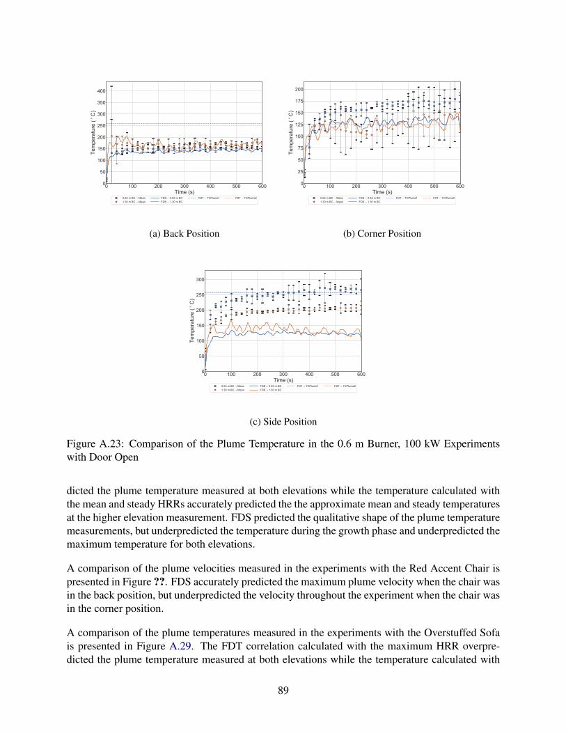
0 100 200 300 400 500 600Time (s)

0

50

100

150

200

250

300

350

400Te

mpe

ratu

re (

C)

0.65 m BC -- Mean1.30 m BC -- Mean

FDS -- 0.65 m BCFDS -- 1.30 m BC

FDT -- TCPlume1 FDT -- TCPlume2

(a) Back Position

0 100 200 300 400 500 600Time (s)

0

25

50

75

100

125

150

175

200

Tem

pera

ture

(C

)

0.65 m BC -- Mean1.30 m BC -- Mean

FDS -- 0.65 m BCFDS -- 1.30 m BC

FDT -- TCPlume1 FDT -- TCPlume2

(b) Corner Position

0 100 200 300 400 500 600Time (s)

0

50

100

150

200

250

300

Tem

pera

ture

(C

)

0.65 m BC -- Mean1.30 m BC -- Mean

FDS -- 0.65 m BCFDS -- 1.30 m BC

FDT -- TCPlume1 FDT -- TCPlume2

(c) Side Position

Figure A.23: Comparison of the Plume Temperature in the 0.6 m Burner, 100 kW Experimentswith Door Open

dicted the plume temperature measured at both elevations while the temperature calculated withthe mean and steady HRRs accurately predicted the the approximate mean and steady temperaturesat the higher elevation measurement. FDS predicted the qualitative shape of the plume temperaturemeasurements, but underpredicted the temperature during the growth phase and underpredicted themaximum temperature for both elevations.

A comparison of the plume velocities measured in the experiments with the Red Accent Chair ispresented in Figure ??. FDS accurately predicted the maximum plume velocity when the chair wasin the back position, but underpredicted the velocity throughout the experiment when the chair wasin the corner position.

A comparison of the plume temperatures measured in the experiments with the Overstuffed Sofais presented in Figure A.29. The FDT correlation calculated with the maximum HRR overpre-dicted the plume temperature measured at both elevations while the temperature calculated with

89

0 100 200 300 400 500 600Time (s)

1

0

1

2

3Ve

loci

ty (m

/s)

0.65 m BC -- Mean 1.30 m BC -- Mean FDS -- 0.65 m BC FDS -- 1.30 m BC

(a) Back Position

0 100 200 300 400 500 600Time (s)

1

0

1

2

3

Velo

city

(m/s

)

0.65 m BC -- Mean 1.30 m BC -- Mean FDS -- 0.65 m BC FDS -- 1.30 m BC

(b) Corner Position

0 100 200 300 400 500 600Time (s)

1

0

1

2

3

4

Velo

city

(m/s

)

0.65 m BC -- Mean 1.30 m BC -- Mean FDS -- 0.65 m BC FDS -- 1.30 m BC

(c) Side Position

Figure A.24: Comparison of the Plume Velocity in the 0.6 m Burner, 100 kW Experiments withDoor Open

the steady HRR accurately predicted the approximate steady temperature at the higher elevationmeasurement. FDS predicted the qualitative shape of the plume temperature measurements, butunderpredicted the temperature during the growth phase and underpredicted the maximum temper-ature for both elevations.

A comparison of the plume velocities measured in the experiments with the Overstuffed Sofa ispresented in Figure A.30. FDS accurately predicted the maximum plume velocity when the sofawas in both positions, but did not capture the qualitative shape of either velocity curve.

90

0 100 200 300 400 500 600Time (s)

0

200

400

600

800

Tem

pera

ture

(C

)

0.65 m BC -- Mean1.30 m BC -- Mean

FDS -- 0.65 m BCFDS -- 1.30 m BC

FDT -- TCPlume1 FDT -- TCPlume2

(a) Back Position

0 100 200 300 400 500 600Time (s)

0

200

400

600

800

Tem

pera

ture

(C

)0.65 m BC -- Mean1.30 m BC -- Mean

FDS -- 0.65 m BCFDS -- 1.30 m BC

FDT -- TCPlume1 FDT -- TCPlume2

(b) Corner Position

0 100 200 300 400 500 600Time (s)

0

200

400

600

800

Tem

pera

ture

(C

)

0.65 m BC -- Mean1.30 m BC -- Mean

FDS -- 0.65 m BCFDS -- 1.30 m BC

FDT -- TCPlume1 FDT -- TCPlume2

(c) Side Position

Figure A.25: Comparison of the Plume Temperature in the 0.6 m Burner, 500 kW Experimentswith Door Open

91

0 100 200 300 400 500 600Time (s)

1

0

1

2

3

4

5

6

Velo

city

(m/s

)

0.65 m BC -- Mean 1.30 m BC -- Mean FDS -- 0.65 m BC FDS -- 1.30 m BC

(a) Back Position

0 100 200 300 400 500 600Time (s)

1

0

1

2

3

4

5

Velo

city

(m/s

)0.65 m BC -- Mean 1.30 m BC -- Mean FDS -- 0.65 m BC FDS -- 1.30 m BC

(b) Corner Position

0 100 200 300 400 500 600Time (s)

1

0

1

2

3

4

5

6

Velo

city

(m/s

)

0.65 m BC -- Mean 1.30 m BC -- Mean FDS -- 0.65 m BC FDS -- 1.30 m BC

(c) Side Position

Figure A.26: Comparison of the Plume Velocity in the 0.6 m Burner, 500 kW Experiments withDoor Open

92

0 200 400 600 800 1000Time (s)

0

200

400

600

800

1000

1200

Tem

pera

ture

(C

)

0.65 m BC -- MeanFDS -- 0.65 m BC

FDT_maxFDT_mean

FDT_steady

(a) Back Position Plume TC1

0 200 400 600 800 1000Time (s)

0

200

400

600

800

1000

1200

Tem

pera

ture

(C

)

1.30 m BC -- MeanFDS -- 1.30 m BC

FDT_maxFDT_mean

FDT_steady

(b) Corner Position Plume TC2

0 200 400 600 800 1000Time (s)

0

200

400

600

800

1000

1200

Tem

pera

ture

(C

)

0.65 m BC -- MeanFDS -- 0.65 m BC

FDT_maxFDT_mean

FDT_steady

(c) Corner Position Plume TC1

0 200 400 600 800 1000Time (s)

0

200

400

600

800

1000

1200

Tem

pera

ture

(C

)

1.30 m BC -- MeanFDS -- 1.30 m BC

FDT_maxFDT_mean

FDT_steady

(d) Corner Position Plume TC2

Figure A.27: Comparison of the Plume Temperature in the Red Accent Chair Experiments withthe Door Open

93

0 200 400 600 800 1000Time (s)

1

0

1

2

3

4

5

Velo

city

(m/s

)

0.65 m BC -- Mean FDS -- 0.65 m BC

(a) Back Position Plume BDP1

0 200 400 600 800 1000Time (s)

1

0

1

2

3

4

5

Velo

city

(m/s

)1.30 m BC -- Mean FDS -- 1.30 m BC

(b) Back Position Plume BDP2

0 200 400 600 800 1000Time (s)

1

0

1

2

3

4

5

Velo

city

(m/s

)

0.65 m BC -- Mean FDS -- 0.65 m BC

(c) Corner Position Plume BDP1

0 200 400 600 800 1000Time (s)

1

0

1

2

3

4

5

Velo

city

(m/s

)

1.30 m BC -- Mean FDS -- 1.30 m BC

(d) Corner Position Plume BDP2

Figure A.28: Comparison of the Plume Velocity in the Red Accent Chair Experiments with theDoor Open

94

0 200 400 600 800 1000Time (s)

0

200

400

600

800

1000

Tem

pera

ture

(C

)

0.65 m BC -- MeanFDS -- 0.65 m BC

FDT_maxFDT_mean

FDT_steady

(a) Back Position Plume TC1

0 200 400 600 800 1000Time (s)

0

200

400

600

800

1000

Tem

pera

ture

(C

)

1.30 m BC -- MeanFDS -- 1.30 m BC

FDT_maxFDT_mean

FDT_steady

(b) Corner Position Plume TC2

0 200 400 600 800 1000Time (s)

0

200

400

600

800

1000

1200

Tem

pera

ture

(C

)

0.65 m BC -- MeanFDS -- 0.65 m BC

FDT_maxFDT_mean

FDT_steady

(c) Corner Position Plume TC1

0 200 400 600 800 1000Time (s)

0

200

400

600

800

1000

1200

Tem

pera

ture

(C

)

1.30 m BC -- MeanFDS -- 1.30 m BC

FDT_maxFDT_mean

FDT_steady

(d) Corner Position Plume TC2

Figure A.29: Comparison of the Plume Temperature in the Overstuffed Sofa Experiments with theDoor Open

95

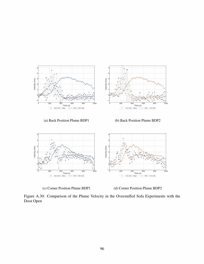
0 200 400 600 800 1000Time (s)

1

0

1

2

3

4

5

Velo

city

(m/s

)

0.65 m BC -- Mean FDS -- 0.65 m BC

(a) Back Position Plume BDP1

0 200 400 600 800 1000Time (s)

1

0

1

2

3

4

5

Velo

city

(m/s

)1.30 m BC -- Mean FDS -- 1.30 m BC

(b) Back Position Plume BDP2

0 200 400 600 800 1000Time (s)

1

0

1

2

3

4

5

Velo

city

(m/s

)

0.65 m BC -- Mean FDS -- 0.65 m BC

(c) Corner Position Plume BDP1

0 200 400 600 800 1000Time (s)

1

0

1

2

3

4

5

Velo

city

(m/s

)

1.30 m BC -- Mean FDS -- 1.30 m BC

(d) Corner Position Plume BDP2

Figure A.30: Comparison of the Plume Velocity in the Overstuffed Sofa Experiments with theDoor Open

96

Closed Door

A comparison of the plume temperatures measured in the experiments with the 0.3 m Burner witha HRR of 100 kW is presented in Figure A.21. The FDT correlation overpredicted the lowerelevation plume temperature measurement and accurately represented the approximate mean tem-perature measured at the higher elevation location. The plume temperature predicted with FDSwere generally lower than the measured temperatures and FDS did not qualitatively capture theshape of the curves.

0 100 200 300 400 500 600Time (s)

0

100

200

300

400

500

600

700

800

Tem

pera

ture

(C

)

0.65 m BC -- Mean1.30 m BC -- Mean

FDS -- 0.65 m BCFDS -- 1.30 m BC

FDT -- TCPlume1 FDT -- TCPlume2

(a) Back Position

0 100 200 300 400 500 600Time (s)

0

100

200

300

400

500

600

700

800

Tem

pera

ture

(C

)

0.65 m BC -- Mean1.30 m BC -- Mean

FDS -- 0.65 m BCFDS -- 1.30 m BC

FDT -- TCPlume1 FDT -- TCPlume2

(b) Corner Position

0 100 200 300 400 500 600Time (s)

0

200

400

600

800

Tem

pera

ture

(C

)

0.65 m BC -- Mean1.30 m BC -- Mean

FDS -- 0.65 m BCFDS -- 1.30 m BC

FDT -- TCPlume1 FDT -- TCPlume2

(c) Side Position

Figure A.31: Comparison of the Plume Temperature in the 0.3 m Burner, 100 kW Experimentswith Door Closed

A comparison of the plume temperatures measured in the experiments with the 0.6 m Burner witha HRR of 100 kW is presented in Figure A.23. The FDT correlation overpredicted the lowerelevation plume temperature measurement and accurately represented the approximate mean tem-perature measured at the higher elevation location when the burner was in the back and cornerpositions. The plume temperature predicted with FDS were generally lower than the measured

97

0 100 200 300 400 500 600Time (s)

1

0

1

2

3

4

5

Velo

city

(m/s

)

0.65 m BC -- Mean 1.30 m BC -- Mean FDS -- 0.65 m BC FDS -- 1.30 m BC

(a) Back Position

0 100 200 300 400 500 600Time (s)

1

0

1

2

3

4

5

Velo

city

(m/s

)

0.65 m BC -- Mean 1.30 m BC -- Mean FDS -- 0.65 m BC FDS -- 1.30 m BC

(b) Corner Position

0 100 200 300 400 500 600Time (s)

1

0

1

2

3

4

5

Velo

city

(m/s

)

0.65 m BC -- Mean 1.30 m BC -- Mean FDS -- 0.65 m BC FDS -- 1.30 m BC

(c) Side Position

Figure A.32: Comparison of the Plume Velocity in the 0.3 m Burner, 100 kW Experiments withDoor Closed

temperatures and FDS did not qualitatively capture the shape of the curves.

A comparison of the plume temperatures measured in the experiments with the 0.6 m Burner witha HRR of 500 kW is presented in Figure A.25. The FDT correlation overpredicted the plumetemperatures. FDS was generally able to predict the qualitative shape of the plume temperaturedata although the magnitudes were underpredicted throughout the experiments.

A comparison of the plume temperatures measured in the experiments with the Red Accent Chairis presented in Figure A.37. The FDT correlation calculated with the maximum HRR overpre-dicted the plume temperature measured at both elevations while the temperature calculated with thesteady HRR approximated the mean temperature measured at the higher elevation. FDS predictedthe qualitative shape of the plume temperature measurements, but underpredicted the temperatureduring the growth phase and underpredicted the maximum temperature for both elevations.

98

0 100 200 300 400 500 600Time (s)

0

100

200

300

400

500Te

mpe

ratu

re (

C)

0.65 m BC -- Mean1.30 m BC -- Mean

FDS -- 0.65 m BCFDS -- 1.30 m BC

FDT -- TCPlume1 FDT -- TCPlume2

(a) Back Position

0 100 200 300 400 500 600Time (s)

0

100

200

300

400

Tem

pera

ture

(C

)

0.65 m BC -- Mean1.30 m BC -- Mean

FDS -- 0.65 m BCFDS -- 1.30 m BC

FDT -- TCPlume1 FDT -- TCPlume2

(b) Corner Position

0 100 200 300 400 500 600Time (s)

0

100

200

300

400

500

Tem

pera

ture

(C

)

0.65 m BC -- Mean1.30 m BC -- Mean

FDS -- 0.65 m BCFDS -- 1.30 m BC

FDT -- TCPlume1 FDT -- TCPlume2

(c) Side Position

Figure A.33: Comparison of the Plume Temperature in the 0.6 m Burner, 100 kW Experimentswith Door Closed

A comparison of the plume velocities measured in the experiments with the Red Accent Chairis presented in Figure A.38. FDS generally underpredicted the plume velocity at both elevationsthroughout the experiment.

A comparison of the plume temperatures measured in the experiments with the Overstuffed Sofais presented in Figure A.39. The FDT correlation overpredicted all the temperatures. FDS pre-dicted the qualitative shape of the plume temperature measurements, and accurately predicted themaximum temperature in the higher elevation measurement position, but underpredicted the tem-peratures during the growth and decay phases.

A comparison of the plume velocities measured in the experiments with the overstuffed Sofa ispresented in Figure A.38. FDS generally underpredicted the plume velocity at both elevationswhen the sofa was in the back position and accurately predicted the maximum velocity measuredwhen the sofa was in the corner position.

99

0 100 200 300 400 500 600Time (s)

1

0

1

2

3

Velo

city

(m/s

)

0.65 m BC -- Mean 1.30 m BC -- Mean FDS -- 0.65 m BC FDS -- 1.30 m BC

(a) Back Position

0 100 200 300 400 500 600Time (s)

1.0

0.5

0.0

0.5

1.0

1.5

2.0

2.5

3.0

Velo

city

(m/s

)0.65 m BC -- Mean 1.30 m BC -- Mean FDS -- 0.65 m BC FDS -- 1.30 m BC

(b) Corner Position

0 100 200 300 400 500 600Time (s)

1

0

1

2

3

Velo

city

(m/s

)

0.65 m BC -- Mean 1.30 m BC -- Mean FDS -- 0.65 m BC FDS -- 1.30 m BC

(c) Side Position

Figure A.34: Comparison of the Plume Velocity in the 0.6 m Burner, 100 kW Experiments withDoor Closed

100

0 100 200 300 400 500 600Time (s)

0

200

400

600

800

1000

Tem

pera

ture

(C

)

0.65 m BC -- Mean1.30 m BC -- Mean

FDS -- 0.65 m BCFDS -- 1.30 m BC

FDT -- TCPlume1 FDT -- TCPlume2

(a) Back Position

0 100 200 300 400 500 600Time (s)

0

200

400

600

800

Tem

pera

ture

(C

)0.65 m BC -- Mean1.30 m BC -- Mean

FDS -- 0.65 m BCFDS -- 1.30 m BC

FDT -- TCPlume1 FDT -- TCPlume2

(b) Corner Position

0 100 200 300 400 500 600Time (s)

0

200

400

600

800

Tem

pera

ture

(C

)

0.65 m BC -- Mean1.30 m BC -- Mean

FDS -- 0.65 m BCFDS -- 1.30 m BC

FDT -- TCPlume1 FDT -- TCPlume2

(c) Side Position

Figure A.35: Comparison of the Plume Temperature in the 0.6 m Burner, 500 kW Experimentswith Door Closed

101

0 100 200 300 400 500 600Time (s)

1

0

1

2

3

4

5

Velo

city

(m/s

)

0.65 m BC -- Mean 1.30 m BC -- Mean FDS -- 0.65 m BC FDS -- 1.30 m BC

(a) Back Position

0 100 200 300 400 500 600Time (s)

1

0

1

2

3

4

5

Velo

city

(m/s

)0.65 m BC -- Mean 1.30 m BC -- Mean FDS -- 0.65 m BC FDS -- 1.30 m BC

(b) Corner Position

0 100 200 300 400 500 600Time (s)

1

0

1

2

3

4

Velo

city

(m/s

)

0.65 m BC -- Mean 1.30 m BC -- Mean FDS -- 0.65 m BC FDS -- 1.30 m BC

(c) Side Position

Figure A.36: Comparison of the Plume Velocity in the 0.6 m Burner, 500 kW Experiments withDoor Closed

102

0 200 400 600 800 1000Time (s)

0

200

400

600

800

Tem

pera

ture

(C

)

0.65 m BC -- MeanFDS -- 0.65 m BC

FDT_maxFDT_mean

FDT_steady

(a) Back Position Plume TC1

0 200 400 600 800 1000Time (s)

0

200

400

600

800

Tem

pera

ture

(C

)

1.30 m BC -- MeanFDS -- 1.30 m BC

FDT_maxFDT_mean

FDT_steady

(b) Corner Position Plume TC2

0 200 400 600 800 1000Time (s)

0

200

400

600

800

1000

Tem

pera

ture

(C

)

0.65 m BC -- MeanFDS -- 0.65 m BC

FDT_maxFDT_mean

FDT_steady

(c) Corner Position Plume TC1

0 200 400 600 800 1000Time (s)

0

200

400

600

800

1000

Tem

pera

ture

(C

)

1.30 m BC -- MeanFDS -- 1.30 m BC

FDT_maxFDT_mean

FDT_steady

(d) Corner Position Plume TC2

Figure A.37: Comparison of the Plume Temperature in the Red Accent Chair Experiments withthe Door Closed

103

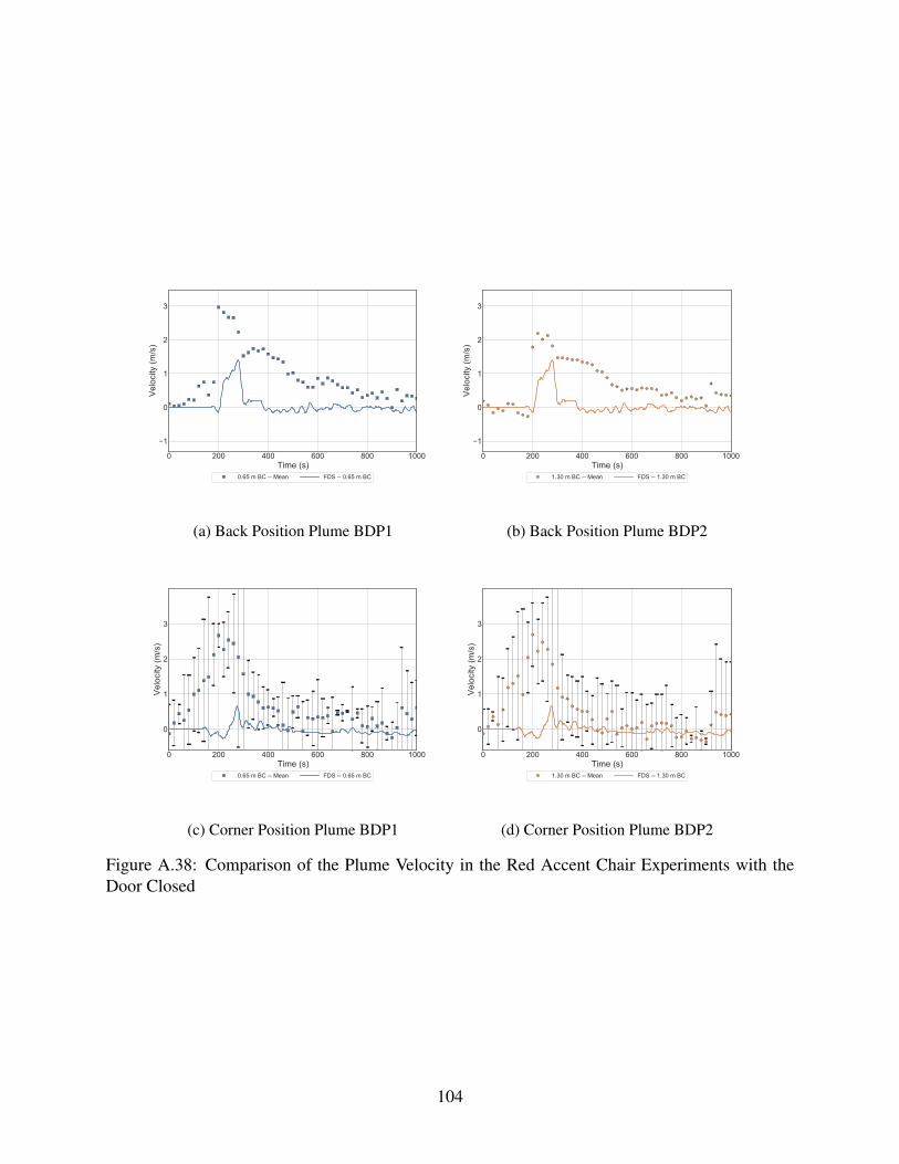
0 200 400 600 800 1000Time (s)

1

0

1

2

3

Velo

city

(m/s

)

0.65 m BC -- Mean FDS -- 0.65 m BC

(a) Back Position Plume BDP1

0 200 400 600 800 1000Time (s)

1

0

1

2

3

Velo

city

(m/s

)1.30 m BC -- Mean FDS -- 1.30 m BC

(b) Back Position Plume BDP2

0 200 400 600 800 1000Time (s)

0

1

2

3

Velo

city

(m/s

)

0.65 m BC -- Mean FDS -- 0.65 m BC

(c) Corner Position Plume BDP1

0 200 400 600 800 1000Time (s)

0

1

2

3

Velo

city

(m/s

)

1.30 m BC -- Mean FDS -- 1.30 m BC

(d) Corner Position Plume BDP2

Figure A.38: Comparison of the Plume Velocity in the Red Accent Chair Experiments with theDoor Closed

104

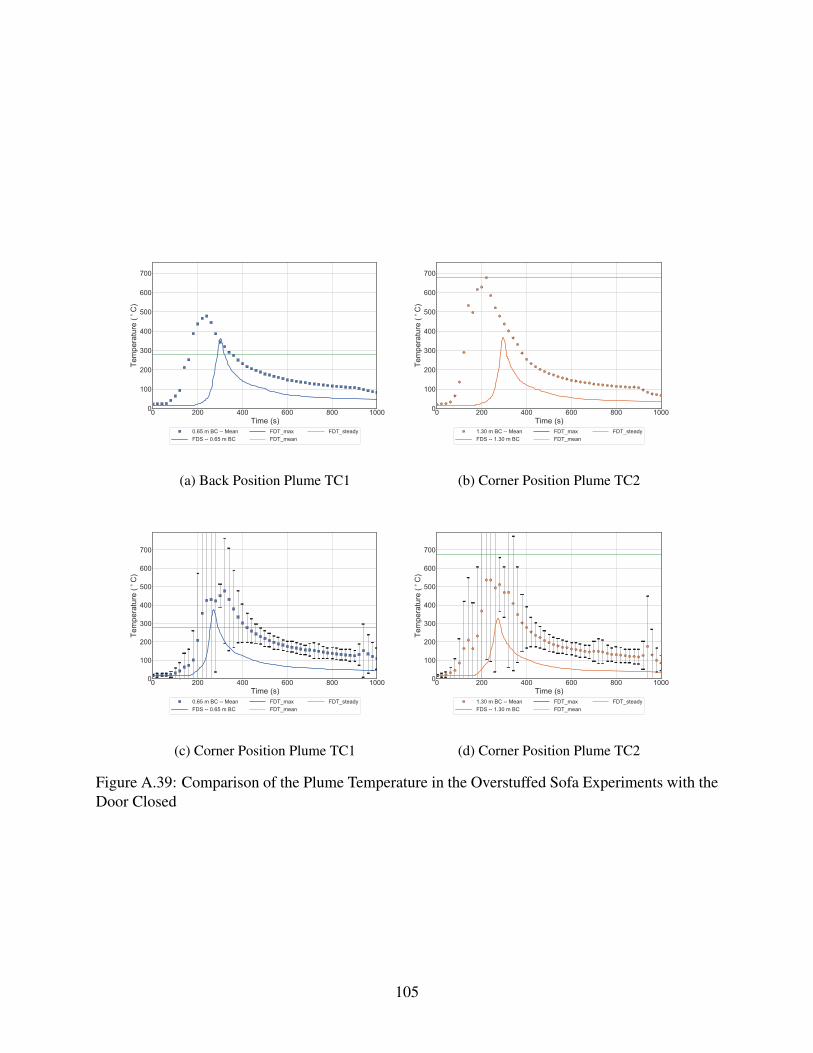
0 200 400 600 800 1000Time (s)

0

100

200

300

400

500

600

700

Tem

pera

ture

(C

)

0.65 m BC -- MeanFDS -- 0.65 m BC

FDT_maxFDT_mean

FDT_steady

(a) Back Position Plume TC1

0 200 400 600 800 1000Time (s)

0

100

200

300

400

500

600

700

Tem

pera

ture

(C

)

1.30 m BC -- MeanFDS -- 1.30 m BC

FDT_maxFDT_mean

FDT_steady

(b) Corner Position Plume TC2

0 200 400 600 800 1000Time (s)

0

100

200

300

400

500

600

700

Tem

pera

ture

(C

)

0.65 m BC -- MeanFDS -- 0.65 m BC

FDT_maxFDT_mean

FDT_steady

(c) Corner Position Plume TC1

0 200 400 600 800 1000Time (s)

0

100

200

300

400

500

600

700

Tem

pera

ture

(C

)

1.30 m BC -- MeanFDS -- 1.30 m BC

FDT_maxFDT_mean

FDT_steady

(d) Corner Position Plume TC2

Figure A.39: Comparison of the Plume Temperature in the Overstuffed Sofa Experiments with theDoor Closed

105

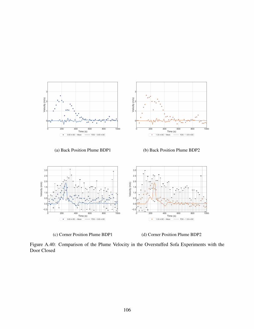
0 200 400 600 800 1000Time (s)

0

1

2

3

Velo

city

(m/s

)

0.65 m BC -- Mean FDS -- 0.65 m BC

(a) Back Position Plume BDP1

0 200 400 600 800 1000Time (s)

0

1

2

3

Velo

city

(m/s

)1.30 m BC -- Mean FDS -- 1.30 m BC

(b) Back Position Plume BDP2

0 200 400 600 800 1000Time (s)

0.5

0.0

0.5

1.0

1.5

2.0

2.5

3.0

Velo

city

(m/s

)

0.65 m BC -- Mean FDS -- 0.65 m BC

(c) Corner Position Plume BDP1

0 200 400 600 800 1000Time (s)

0.5

0.0

0.5

1.0

1.5

2.0

2.5

3.0

Velo

city

(m/s

)

1.30 m BC -- Mean FDS -- 1.30 m BC

(d) Corner Position Plume BDP2

Figure A.40: Comparison of the Plume Velocity in the Overstuffed Sofa Experiments with theDoor Closed

106

A.1.3 Flame Height

Open Door

Figure A.41 displays the measured and predicted mean flame heights for the 0.3 m Burner experi-ments with the 100 kW HRR. The experimental flame height does not appear to be influenced bythe location of the burner for this HRR or burner size. FDS and CFAST accurately predicted theflame height when the burner was in all positions. In the center position, the Heskestad correlationprovided a better prediction than the Thomas correlation. The FDT correlation for the flame heightin the back and side positions overpredicted the measured flame heights, although the correlationfor the corner provided a good prediction of the measured flame height.

0 100 200 300 400 500 600Time (s)

0.0

0.5

1.0

1.5

2.0

Flam

e H

eigh

t (m

)

Flame Height -- MeanFDS Prediction

CFAST -- Flame_Height FDT -- Flame_Height Heskestad FDT -- Flame_Height Thomas

(a) Center Position

0 100 200 300 400 500 600Time (s)

0.0

0.5

1.0

1.5

2.0

2.5

Flam

e H

eigh

t (m

)

Flame Height -- Mean FDS Prediction CFAST -- Flame_Height FDT -- Flame_Height

(b) Back Position

0 100 200 300 400 500 600Time (s)

0.0

0.5

1.0

1.5

2.0

Flam

e H

eigh

t (m

)

Flame Height -- Mean FDS Prediction CFAST -- Flame_Height FDT -- Flame_Height

(c) Corner Position

0 100 200 300 400 500 600Time (s)

0.0

0.5

1.0

1.5

2.0

Flam

e H

eigh

t (m

)

Flame Height -- Mean FDS Prediction CFAST -- Flame_Height FDT -- Flame_Height

(d) Side Position

Figure A.41: Comparison of the Mean Flame Height in the 0.3 m Burner, 100 kW Experimentswith Door Open

Figure A.42 displays the measured and predicted mean flame heights for the 0.6 m Burner exper-iments with the 100 kW HRR. The experimental flame height was slightly larger when the burner

107

was in the corner position relative to when the burner was in the back and side positions. FDSaccurately predicted the flame height when the burner was in all positions. CFAST accurately pre-dicted the flame height in the corner, but overpredicted the flame height at the side and back. TheFDT correlations for the flame height in each position overpredicted the measurement.

0 100 200 300 400 500 600Time (s)

0.0

0.5

1.0

1.5

2.0

Flame Height -- MeanFDS Prediction

CFAST -- Flame_Height FDT -- Flame_Height Heskestad FDT -- Flame_Height Thomas

(a) Center Position

0 100 200 300 400 500 600Time (s)

0.0

0.5

1.0

1.5

2.0

Flam

e H

eigh

t (m

)

Flame Height -- Mean FDS Prediction CFAST -- Flame_Height FDT -- Flame_Height

(b) Back Position

0 100 200 300 400 500 600Time (s)

0.0

0.5

1.0

1.5

2.0

Flam

e H

eigh

t (m

)

Flame Height -- Mean FDS Prediction CFAST -- Flame_Height FDT -- Flame_Height

(c) Corner Position

0 100 200 300 400 500 600Time (s)

0.0

0.5

1.0

1.5

2.0

Flam

e H

eigh

t (m

)

Flame Height -- Mean FDS Prediction CFAST -- Flame_Height FDT -- Flame_Height

(d) Side Position

Figure A.42: Comparison of the Mean Flame Height in the 0.6 m Burner, 100 kW Experimentswith Door Open

Figure A.43 displays the measured and predicted mean flame heights for the 0.6 m Experimentswith the 500 kW HRR. CFAST and FDS predicted that the mean flame height was consistent withthe ceiling height when the burner was in all the positions. The FDT correlations were not limitedby the flame height and predicted that the flame height was larger than the ceiling height, so theydo not appear in the plots. The experimental data reached a maximum at approximately 1.6 m.

Figure A.44 displays the measured and predicted mean flame heights for the Red Accent Chair.CFAST and FDS predicted that the mean flame height was consistent with the ceiling height whenthe burner was in all the positions. The FDT correlations were not limited by the flame heightand predicted that the flame height calculated with the maximum HRR was larger than the ceiling

108

0 100 200 300 400 500 600Time (s)

0.0

0.5

1.0

1.5

2.0

Flame Height -- MeanFDS Prediction

CFAST -- Flame_Height FDT -- Flame_Height Heskestad FDT -- Flame_Height Thomas

(a) Center Position

0 100 200 300 400 500 600Time (s)

0.0

0.5

1.0

1.5

2.0

Flam

e H

eigh

t (m

)

Flame Height -- Mean FDS Prediction CFAST -- Flame_Height FDT -- Flame_Height

(b) Back Position

0 100 200 300 400 500 600Time (s)

0.0

0.5

1.0

1.5

2.0

Flam

e H

eigh

t (m

)

Flame Height -- Mean FDS Prediction CFAST -- Flame_Height FDT -- Flame_Height

(c) Corner Position

0 100 200 300 400 500 600Time (s)

0.0

0.5

1.0

1.5

2.0Fl

ame

Hei

ght (

m)

Flame Height -- Mean FDS Prediction CFAST -- Flame_Height FDT -- Flame_Height

(d) Side Position

Figure A.43: Comparison of the Mean Flame Height in the 0.6 m Burner, 500 kW Experimentswith Door Open

height, so they do not appear in the plots. The flame FDT correlations calculated with the meanand steady HRRs also overpredicted the respective flame heights. The experimental data reacheda maximum at approximately 1.5 m before data collection stopped.

Figure A.45 displays the measured and predicted mean flame heights for the Overstuffed Sofa.CFAST and FDS predicted that the mean flame height was consistent with the ceiling height whenthe burner was in all the positions. The FDT correlations were not limited by the flame heightand predicted that the flame height calculated with the maximum HRR was larger than the ceilingheight, so they do not appear in the plots. The flame FDT correlations calculated with the meanand steady HRRs also overpredicted the respective flame heights. The experimental data reacheda maximum at approximately 1.4 m before data collection stopped.

109

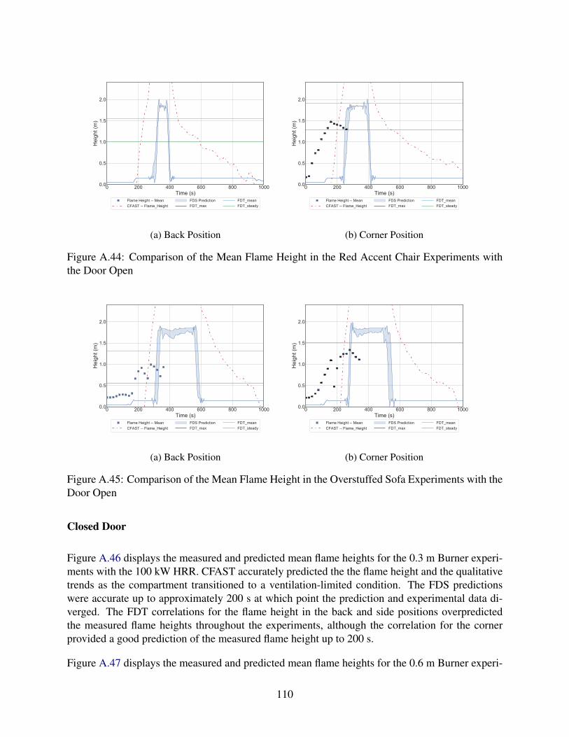
0 200 400 600 800 1000Time (s)

0.0

0.5

1.0

1.5

2.0H

eigh

t (m

)

Flame Height -- MeanCFAST -- Flame_Height

FDS PredictionFDT_max

FDT_meanFDT_steady

(a) Back Position

0 200 400 600 800 1000Time (s)

0.0

0.5

1.0

1.5

2.0

Hei

ght (

m)

Flame Height -- MeanCFAST -- Flame_Height

FDS PredictionFDT_max

FDT_meanFDT_steady

(b) Corner Position

Figure A.44: Comparison of the Mean Flame Height in the Red Accent Chair Experiments withthe Door Open

0 200 400 600 800 1000Time (s)

0.0

0.5

1.0

1.5

2.0

Hei

ght (

m)

Flame Height -- MeanCFAST -- Flame_Height

FDS PredictionFDT_max

FDT_meanFDT_steady

(a) Back Position

0 200 400 600 800 1000Time (s)

0.0

0.5

1.0

1.5

2.0

Hei

ght (

m)

Flame Height -- MeanCFAST -- Flame_Height

FDS PredictionFDT_max

FDT_meanFDT_steady

(b) Corner Position

Figure A.45: Comparison of the Mean Flame Height in the Overstuffed Sofa Experiments with theDoor Open

Closed Door

Figure A.46 displays the measured and predicted mean flame heights for the 0.3 m Burner experi-ments with the 100 kW HRR. CFAST accurately predicted the the flame height and the qualitativetrends as the compartment transitioned to a ventilation-limited condition. The FDS predictionswere accurate up to approximately 200 s at which point the prediction and experimental data di-verged. The FDT correlations for the flame height in the back and side positions overpredictedthe measured flame heights throughout the experiments, although the correlation for the cornerprovided a good prediction of the measured flame height up to 200 s.

Figure A.47 displays the measured and predicted mean flame heights for the 0.6 m Burner experi-

110

0 100 200 300 400 500 600Time (s)

0.0

0.5

1.0

1.5

2.0Fl

ame

Hei

ght (

m)

Flame Height -- MeanFDS Prediction

CFAST -- Flame_Height FDT -- Flame_Height Heskestad FDT -- Flame_Height Thomas

(a) Center Position

0 100 200 300 400 500 600Time (s)

0.0

0.5

1.0

1.5

2.0

Flam

e H

eigh

t (m

)

Flame Height -- Mean FDS Prediction CFAST -- Flame_Height FDT -- Flame_Height

(b) Back Position

0 100 200 300 400 500 600Time (s)

0.0

0.5

1.0

1.5

2.0

Flam

e H

eigh

t (m

)

Flame Height -- Mean FDS Prediction CFAST -- Flame_Height FDT -- Flame_Height

(c) Corner Position

0 100 200 300 400 500 600Time (s)

0.0

0.5

1.0

1.5

2.0

2.5

Flam

e H

eigh

t (m

)

Flame Height -- Mean FDS Prediction CFAST -- Flame_Height FDT -- Flame_Height

(d) Side Position

Figure A.46: Comparison of the Mean Flame Height in the 0.3 m Burner, 100 kW Experimentswith Door Closed

ments with a HRR of 100 kW. CFAST accurately predicted the the flame height and the qualitativetrends as the compartment transitioned to a ventilation-limited condition. The FDS predictionswere accurate up to approximately 200 s, at which point the prediction and experimental datadiverged. The FDT correlations for the flame height in the back, corner, and side positions over-predicted the measured flame heights throughout the experiments, although the Thomas correlationfor the center provided a good prediction of the measured flame height up to 200 s.

Figure A.49 displays the measured and predicted mean flame heights for the Red Accent Chairexperiments. The FDS and CFAST predictions agreed well with each other and qualitatively withthe experimental data, but overpredicted the peak mean flame height magnitude and timing.

Figure A.50 displays the measured and predicted mean flame heights for the Overstuffed Sofaexperiments. The FDS and CFAST predictions agreed with each other and qualitatively with theexperimental data, but overpredicted the peak mean flame height magnitude and timing.

111

0 100 200 300 400 500 600Time (s)

0.0

0.5

1.0

1.5

2.0

Flam

e H

eigh

t (m

)

Flame Height -- MeanFDS Prediction

CFAST -- Flame_Height FDT -- Flame_Height Heskestad FDT -- Flame_Height Thomas

(a) Center Position

0 100 200 300 400 500 600Time (s)

0.0

0.5

1.0

1.5

2.0

Flam

e H

eigh

t (m

)Flame Height -- Mean FDS Prediction CFAST -- Flame_Height FDT -- Flame_Height

(b) Back Position

0 100 200 300 400 500 600Time (s)

0.0

0.5

1.0

1.5

2.0

Flam

e H

eigh

t (m

)

Flame Height -- Mean FDS Prediction CFAST -- Flame_Height FDT -- Flame_Height

(c) Corner Position

0 100 200 300 400 500 600Time (s)

0.0

0.5

1.0

1.5

2.0

Flam

e H

eigh

t (m

)

Flame Height -- Mean FDS Prediction CFAST -- Flame_Height FDT -- Flame_Height

(d) Side Position

Figure A.47: Comparison of the Mean Flame Height in the 0.6 m Burner, 100 kW Experimentswith Door Closed

112

0 100 200 300 400 500 600Time (s)

0.0

0.5

1.0

1.5

2.0

Flame Height -- MeanFDS Prediction

CFAST -- Flame_Height FDT -- Flame_Height Heskestad FDT -- Flame_Height Thomas

(a) Center Position

0 100 200 300 400 500 600Time (s)

0.0

0.5

1.0

1.5

2.0

Flame Height -- Mean FDS Prediction CFAST -- Flame_Height FDT -- Flame_Height

(b) Back Position

0 100 200 300 400 500 600Time (s)

0.0

0.5

1.0

1.5

2.0

Flam

e H

eigh

t (m

)

Flame Height -- Mean FDS Prediction CFAST -- Flame_Height FDT -- Flame_Height

(c) Corner Position

0 100 200 300 400 500 600Time (s)

0.0

0.5

1.0

1.5

2.0

2.5

Flam

e H

eigh

t (m

)

Flame Height -- Mean FDS Prediction CFAST -- Flame_Height FDT -- Flame_Height

(d) Side Position

Figure A.48: Comparison of the Mean Flame Height in the 0.6 m Burner, 500 kW Experimentswith Door Closed

113

0 200 400 600 800 1000Time (s)

0.0

0.5

1.0

1.5

2.0

Hei

ght (

m)

Flame Height -- MeanCFAST -- Flame_Height

FDS PredictionFDT_max

FDT_meanFDT_steady

(a) Back Position

0 200 400 600 800 1000Time (s)

0.0

0.5

1.0

1.5

2.0

Hei

ght (

m)

Flame Height -- MeanCFAST -- Flame_Height

FDS PredictionFDT_max

FDT_meanFDT_steady

(b) Corner Position

Figure A.49: Comparison of the Mean Flame Height in the Red Accent Chair Experiments withthe Door Closed

0 200 400 600 800 1000Time (s)

0.0

0.5

1.0

1.5

2.0

Hei

ght (

m)

Flame Height -- MeanCFAST -- Flame_Height

FDS PredictionFDT_max

FDT_meanFDT_steady

(a) Back Position

0 200 400 600 800 1000Time (s)

0.0

0.5

1.0

1.5

2.0

Hei

ght (

m)

Flame Height -- MeanCFAST -- Flame_Height

FDS PredictionFDT_max

FDT_meanFDT_steady

(b) Corner Position

Figure A.50: Comparison of the Mean Flame Height in the Overstuffed Sofa Experiments with theDoor Closed

114

A.1.4 Heat Flux

The following sections display the experimental total and radiative heat flux measurements fromthe experiments conducted in the compartment as well as the model predictions.

Open Door

A comparison of the measured and predicted heat fluxes to the right wall of the compartment forthe 0.3 m Burner with a HRR of 100 kW is provided in Figure A.51. FDS and CFAST accuratelypredicted the heat flux to the lower elevation gauge while the point source method underpredictedand the solid flame correlation overpredicted the heat flux to the lower elevation gauge when theburner was in the center position. FDS accurately predicted the heat flux to the upper elevationgauge and the point source method, the solid flame method, and CFAST underpredicted the heatflux to the higher elevation gauge when the burner was in the center position. The same trendswere evident when the burner was in the other positions except that all of the models, with theexception of the point source model yielded good predictions of the data measured at the lowerelevation gauge.

A comparison of the measured and predicted heat fluxes to the back wall of the compartment for the0.3 m Burner with a HRR of 100 kW is provided in Figure A.52. Although the heat flux betweenthe right wall and the back wall from the burner placed in the center of the compartment should beidentical in quiescent conditions, that is not evident in the figure. None of the models accuratelypredicted the heat fluxes to the back wall when the burner was in the center of the compartment.CFAST and FDS predicted the heat flux to the lower elevation gauge on the back wall when theburner was in the back position. FDS accurately predicted the heat fluxes when the burner was inthe corner position and side position, and CFAST predicted the heat flux top the lower elevationgauge with the burner in the side position.

A comparison of the measured and predicted heat fluxes to the right wall of the compartment forthe 0.6 m Burner with a HRR of 100 kW is provided in Figure A.53. FDS, CFAST, and the pointsource method accurately predicted the heat flux to the lower elevation gauge while the solid flamecorrelation overpredicted the heat flux to the lower elevation gauge when the burner was in thecenter position. FDS and the solid flame method accurately predicted the heat flux to the upperelevation gauge and the point source method and CFAST underpredicted the heat flux to the higherelevation gauge when the burner was in the center position. The same trends were evident whenthe burner was in the other positions except that all the models, with the exception of the pointsource model yielded good predictions of the data measured at the lower elevation gauge and onlyFDs predicted the heat flux to the higher elevation gauge.

A comparison of the measured and predicted heat fluxes to the right wall of the compartmentfor the 0.6 m Burner with a HRR of 100 kW is provided in Figure A.54. CFAST and the pointsource method accurately predicted the heat flux to the lower elevation gauge while the solid flamecorrelation and FDS overpredicted the heat flux to the lower elevation gauge when the burner was

115

0 100 200 300 400 500 600Time (s)

4

2

0

2

4

6

8

10

Hea

t Flu

x (k

W/m

2 )

0.65 m BC; HF -- Mean1.30 m BC; HF -- Mean

FDS -- 0.65 m BC; HFFDS -- 1.30 m BC; HF

CFAST -- HF1CFAST -- HF2

FDT -- HF1 (PS)FDT -- HF1 (SF)

FDT -- HF2 (PS)FDT -- HF2 (SF)

(a) Center Position

0 100 200 300 400 500 600Time (s)

4

2

0

2

4

6

Hea

t Flu

x (k

W/m

2 )

0.65 m BC; HF -- Mean1.30 m BC; HF -- Mean

FDS -- 0.65 m BC; HFFDS -- 1.30 m BC; HF

CFAST -- HF1CFAST -- HF2

FDT -- HF1 (PS)FDT -- HF1 (SF)

FDT -- HF2 (PS)FDT -- HF2 (SF)

(b) Back Position

0 100 200 300 400 500 600Time (s)

4

2

0

2

4

6

8

Hea

t Flu

x (k

W/m

2 )

0.65 m BC; HF -- Mean1.30 m BC; HF -- Mean

FDS -- 0.65 m BC; HFFDS -- 1.30 m BC; HF

CFAST -- HF1CFAST -- HF2

FDT -- HF1 (PS)FDT -- HF1 (SF)

FDT -- HF2 (PS)FDT -- HF2 (SF)

(c) Corner Position

0 100 200 300 400 500 600Time (s)

4

2

0

2

4

6

8

Hea

t Flu

x (k

W/m

2 )

0.65 m BC; HF -- Mean1.30 m BC; HF -- Mean

FDS -- 0.65 m BC; HFFDS -- 1.30 m BC; HF

CFAST -- HF1CFAST -- HF2

FDT -- HF1 (PS)FDT -- HF1 (SF)

FDT -- HF2 (PS)FDT -- HF2 (SF)

(d) Side Position

Figure A.51: Comparison of the Heat Flux to the Right Side Wall in the 0.3 m Burner, 100 kWExperiments with Door Open

in the center position. The solid flame method accurately predicted, FDS overpredicted, and thepoint source method and CFAST underpredicted the heat flux to the higher elevation gauge whenthe burner was in the center position. None of the models accurately predicted the heat flux to theback wall when the burner was in the back, corner, and side positions.

A comparison of the measured and predicted heat fluxes to the right wall of the compartment forthe 0.6 m Burner with a HRR of 500 kW is provided in Figure A.55. The measured data does notappear to reach steady state in the 600 s displayed in the figure. The CFAST and FDS predictionqualitatively capture the continually increasing heat fluxes that were measured and FDS generallyaccurately predicted the heat flux at both elevations. CFAST predicted the lower elevation heatflux and underpredicted the higher elevation heat flux when the burner was in each position. Thesolid flame method predicted the approximate mean heat flux at the lower elevation gauge whenthe burner was in the center and the back positions, and the point source method underpredictedall heat fluxes.

116

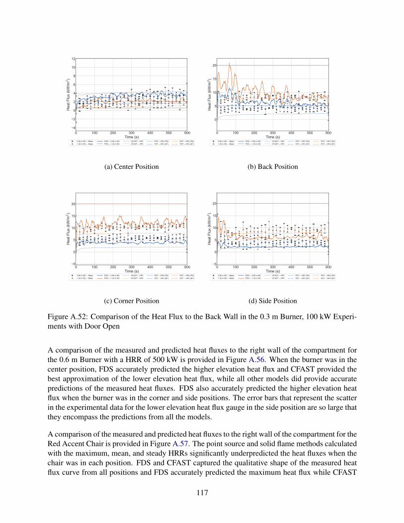
0 100 200 300 400 500 600Time (s)

4

2

0

2

4

6

8

10

12

Hea

t Flu

x (k

W/m

2 )

0.65 m BC -- Mean1.30 m BC -- Mean

FDS -- 0.65 m BCFDS -- 1.30 m BC

CFAST -- HF3CFAST -- HF4

FDT -- HF3 (PS)FDT -- HF3 (SF)

FDT -- HF4 (PS)FDT -- HF4 (SF)

(a) Center Position

0 100 200 300 400 500 600Time (s)

0

5

10

15

20

Hea

t Flu

x (k

W/m

2 )

0.65 m BC -- Mean1.30 m BC -- Mean

FDS -- 0.65 m BCFDS -- 1.30 m BC

CFAST -- HF3CFAST -- HF4

FDT -- HF3 (PS)FDT -- HF3 (SF)

FDT -- HF4 (PS)FDT -- HF4 (SF)

(b) Back Position

0 100 200 300 400 500 600Time (s)

5

0

5

10

15

20

Hea

t Flu

x (k

W/m

2 )

0.65 m BC -- Mean1.30 m BC -- Mean

FDS -- 0.65 m BCFDS -- 1.30 m BC

CFAST -- HF3CFAST -- HF4

FDT -- HF3 (PS)FDT -- HF3 (SF)

FDT -- HF4 (PS)FDT -- HF4 (SF)

(c) Corner Position

0 100 200 300 400 500 600Time (s)

5

0

5

10

15

20H

eat F

lux

(kW

/m2 )

0.65 m BC -- Mean1.30 m BC -- Mean

FDS -- 0.65 m BCFDS -- 1.30 m BC

CFAST -- HF3CFAST -- HF4

FDT -- HF3 (PS)FDT -- HF3 (SF)

FDT -- HF4 (PS)FDT -- HF4 (SF)

(d) Side Position

Figure A.52: Comparison of the Heat Flux to the Back Wall in the 0.3 m Burner, 100 kW Experi-ments with Door Open

A comparison of the measured and predicted heat fluxes to the right wall of the compartment forthe 0.6 m Burner with a HRR of 500 kW is provided in Figure A.56. When the burner was in thecenter position, FDS accurately predicted the higher elevation heat flux and CFAST provided thebest approximation of the lower elevation heat flux, while all other models did provide accuratepredictions of the measured heat fluxes. FDS also accurately predicted the higher elevation heatflux when the burner was in the corner and side positions. The error bars that represent the scatterin the experimental data for the lower elevation heat flux gauge in the side position are so large thatthey encompass the predictions from all the models.

A comparison of the measured and predicted heat fluxes to the right wall of the compartment for theRed Accent Chair is provided in Figure A.57. The point source and solid flame methods calculatedwith the maximum, mean, and steady HRRs significantly underpredicted the heat fluxes when thechair was in each position. FDS and CFAST captured the qualitative shape of the measured heatflux curve from all positions and FDS accurately predicted the maximum heat flux while CFAST

117

0 100 200 300 400 500 600Time (s)

2

0

2

4

6H

eat F

lux

(kW

/m2 )

0.65 m BC; HF -- Mean1.30 m BC; HF -- Mean

FDS -- 0.65 m BC; HFFDS -- 1.30 m BC; HF

CFAST -- HF1CFAST -- HF2

FDT -- HF1 (PS)FDT -- HF1 (SF)

FDT -- HF2 (PS)FDT -- HF2 (SF)

(a) Center Position

0 100 200 300 400 500 600Time (s)

4

2

0

2

4

6

8

Hea

t Flu

x (k

W/m

2 )

0.65 m BC; HF -- Mean1.30 m BC; HF -- Mean

FDS -- 0.65 m BC; HFFDS -- 1.30 m BC; HF

CFAST -- HF1CFAST -- HF2

FDT -- HF1 (PS)FDT -- HF1 (SF)

FDT -- HF2 (PS)FDT -- HF2 (SF)

(b) Back Position

0 100 200 300 400 500 600Time (s)

4

2

0

2

4

6

8

Hea

t Flu

x (k

W/m

2 )

0.65 m BC; HF -- Mean1.30 m BC; HF -- Mean

FDS -- 0.65 m BC; HFFDS -- 1.30 m BC; HF

CFAST -- HF1CFAST -- HF2

FDT -- HF1 (PS)FDT -- HF1 (SF)

FDT -- HF2 (PS)FDT -- HF2 (SF)

(c) Corner Position

0 100 200 300 400 500 600Time (s)

4

2

0

2

4

6

Hea

t Flu

x (k

W/m

2 )

0.65 m BC; HF -- Mean1.30 m BC; HF -- Mean

FDS -- 0.65 m BC; HFFDS -- 1.30 m BC; HF

CFAST -- HF1CFAST -- HF2

FDT -- HF1 (PS)FDT -- HF1 (SF)

FDT -- HF2 (PS)FDT -- HF2 (SF)

(d) Side Position

Figure A.53: Comparison of the Heat Flux to the Right Side Wall in the 0.6 m Burner, 100 kWExperiments with Door Open

slightly underpredicted the maximum heat flux.

A comparison of the measured and predicted heat fluxes to the back wall of the compartment for theRed Accent Chair is provided in Figure A.58. The point source and solid flame methods calculatedwith the maximum, mean, and steady HRRs significantly underpredicted the heat fluxes when thechair was in each position. FDS and CFAST captured the qualitative shape of the measured heatflux curve from all positions and FDS slightly underpredicted the maximum heat flux while CFASTsignificantly underpredicted the maximum heat flux.

A comparison of the measured and predicted heat fluxes to the right wall of the compartment for theOverstuffed Sofa is provided in Figure A.59. The point source and solid flame methods calculatedwith the maximum, mean, and steady HRRs significantly underpredicted the heat fluxes when thesofa was in each position. FDS and CFAST captured the qualitative shape of the measured heatflux curve from all positions. FDS underpredicted the maximum heat flux measured with the sofa

118

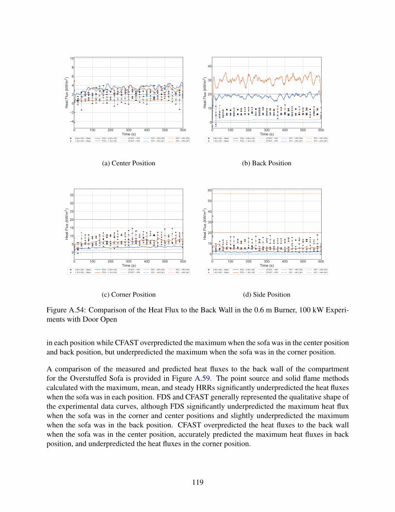
0 100 200 300 400 500 600Time (s)

4

2

0

2

4

6

8

10

Hea

t Flu

x (k

W/m

2 )

0.65 m BC -- Mean1.30 m BC -- Mean

FDS -- 0.65 m BCFDS -- 1.30 m BC

CFAST -- HF3CFAST -- HF4

FDT -- HF3 (PS)FDT -- HF3 (SF)

FDT -- HF4 (PS)FDT -- HF4 (SF)

(a) Center Position

0 100 200 300 400 500 600Time (s)

0

10

20

30

40

Hea

t Flu

x (k

W/m

2 )

0.65 m BC -- Mean1.30 m BC -- Mean

FDS -- 0.65 m BCFDS -- 1.30 m BC

CFAST -- HF3CFAST -- HF4

FDT -- HF3 (PS)FDT -- HF3 (SF)

FDT -- HF4 (PS)FDT -- HF4 (SF)

(b) Back Position

0 100 200 300 400 500 600Time (s)

0

5

10

15

20

25

30

35

Hea

t Flu

x (k

W/m

2 )

0.65 m BC -- Mean1.30 m BC -- Mean

FDS -- 0.65 m BCFDS -- 1.30 m BC

CFAST -- HF3CFAST -- HF4

FDT -- HF3 (PS)FDT -- HF3 (SF)

FDT -- HF4 (PS)FDT -- HF4 (SF)

(c) Corner Position

0 100 200 300 400 500 600Time (s)

0

10

20

30

40

50

60

Hea

t Flu

x (k

W/m

2 )

0.65 m BC -- Mean1.30 m BC -- Mean

FDS -- 0.65 m BCFDS -- 1.30 m BC

CFAST -- HF3CFAST -- HF4

FDT -- HF3 (PS)FDT -- HF3 (SF)

FDT -- HF4 (PS)FDT -- HF4 (SF)

(d) Side Position

Figure A.54: Comparison of the Heat Flux to the Back Wall in the 0.6 m Burner, 100 kW Experi-ments with Door Open

in each position while CFAST overpredicted the maximum when the sofa was in the center positionand back position, but underpredicted the maximum when the sofa was in the corner position.

A comparison of the measured and predicted heat fluxes to the back wall of the compartmentfor the Overstuffed Sofa is provided in Figure A.59. The point source and solid flame methodscalculated with the maximum, mean, and steady HRRs significantly underpredicted the heat fluxeswhen the sofa was in each position. FDS and CFAST generally represented the qualitative shape ofthe experimental data curves, although FDS significantly underpredicted the maximum heat fluxwhen the sofa was in the corner and center positions and slightly underpredicted the maximumwhen the sofa was in the back position. CFAST overpredicted the heat fluxes to the back wallwhen the sofa was in the center position, accurately predicted the maximum heat fluxes in backposition, and underpredicted the heat fluxes in the corner position.

119

0 100 200 300 400 500 600Time (s)

0

5

10

15

20

25

Hea

t Flu

x (k

W/m

2 )

0.65 m BC; HF -- Mean1.30 m BC; HF -- Mean

FDS -- 0.65 m BC; HFFDS -- 1.30 m BC; HF

CFAST -- HF1CFAST -- HF2

FDT -- HF1 (PS)FDT -- HF1 (SF)

FDT -- HF2 (PS)FDT -- HF2 (SF)

(a) Center Position

0 100 200 300 400 500 600Time (s)

0

5

10

15

20

25

Hea

t Flu

x (k

W/m

2 )0.65 m BC; HF -- Mean1.30 m BC; HF -- Mean

FDS -- 0.65 m BC; HFFDS -- 1.30 m BC; HF

CFAST -- HF1CFAST -- HF2

FDT -- HF1 (PS)FDT -- HF1 (SF)

FDT -- HF2 (PS)FDT -- HF2 (SF)

(b) Back Position

0 100 200 300 400 500 600Time (s)

0

5

10

15

20

25

Hea

t Flu

x (k

W/m

2 )

0.65 m BC; HF -- Mean1.30 m BC; HF -- Mean

FDS -- 0.65 m BC; HFFDS -- 1.30 m BC; HF

CFAST -- HF1CFAST -- HF2

FDT -- HF1 (PS)FDT -- HF1 (SF)

FDT -- HF2 (PS)FDT -- HF2 (SF)

(c) Corner Position

0 100 200 300 400 500 600Time (s)

0

5

10

15

20

25

Hea

t Flu

x (k

W/m

2 )

0.65 m BC; HF -- Mean1.30 m BC; HF -- Mean

FDS -- 0.65 m BC; HFFDS -- 1.30 m BC; HF

CFAST -- HF1CFAST -- HF2

FDT -- HF1 (PS)FDT -- HF1 (SF)

FDT -- HF2 (PS)FDT -- HF2 (SF)

(d) Side Position

Figure A.55: Comparison of the Heat Flux to the Right Side Wall in the 0.6 m Burner, 500 kWExperiments with Door Open

120

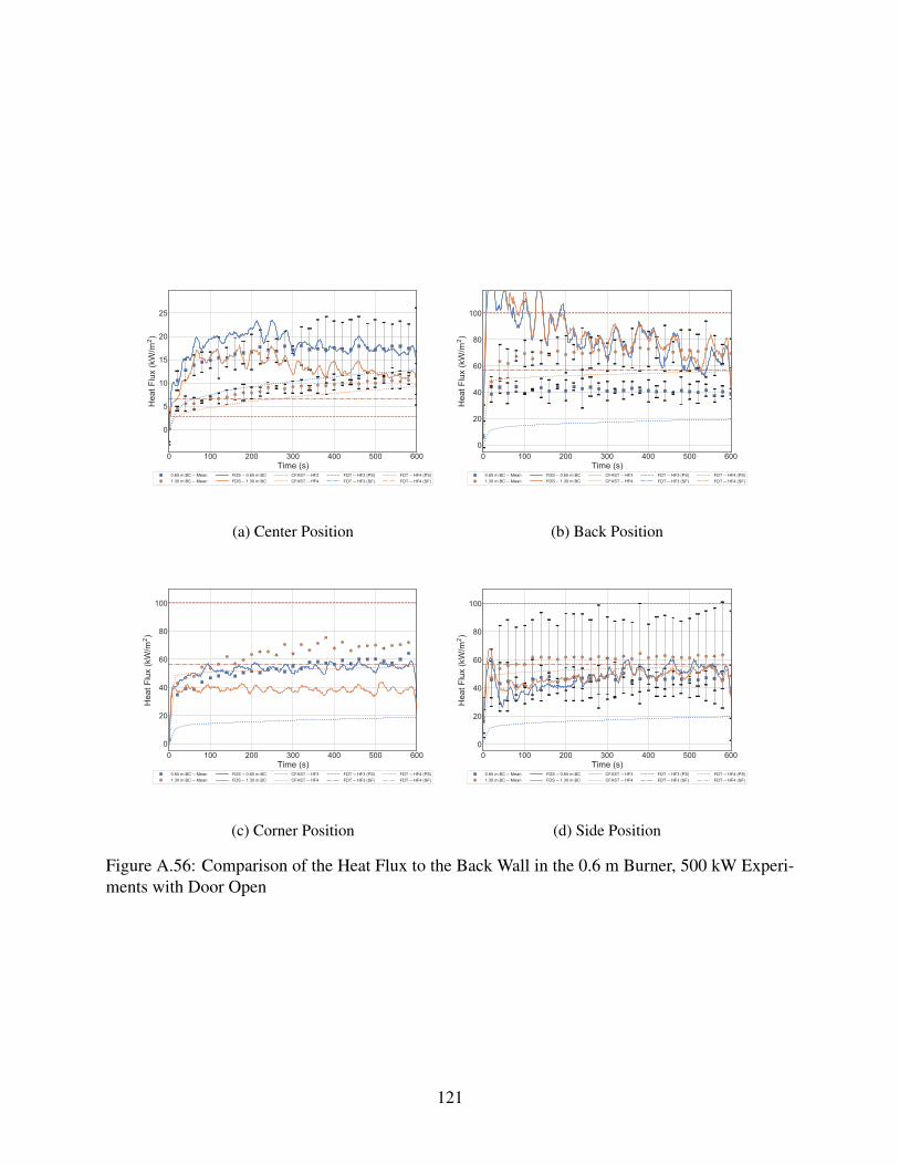
0 100 200 300 400 500 600Time (s)

0

5

10

15

20

25

Hea

t Flu

x (k

W/m

2 )

0.65 m BC -- Mean1.30 m BC -- Mean

FDS -- 0.65 m BCFDS -- 1.30 m BC

CFAST -- HF3CFAST -- HF4

FDT -- HF3 (PS)FDT -- HF3 (SF)

FDT -- HF4 (PS)FDT -- HF4 (SF)

(a) Center Position

0 100 200 300 400 500 600Time (s)

0

20

40

60

80

100

Hea

t Flu

x (k

W/m

2 )0.65 m BC -- Mean1.30 m BC -- Mean

FDS -- 0.65 m BCFDS -- 1.30 m BC

CFAST -- HF3CFAST -- HF4

FDT -- HF3 (PS)FDT -- HF3 (SF)

FDT -- HF4 (PS)FDT -- HF4 (SF)

(b) Back Position

0 100 200 300 400 500 600Time (s)

0

20

40

60

80

100

Hea

t Flu

x (k

W/m

2 )

0.65 m BC -- Mean1.30 m BC -- Mean

FDS -- 0.65 m BCFDS -- 1.30 m BC

CFAST -- HF3CFAST -- HF4

FDT -- HF3 (PS)FDT -- HF3 (SF)

FDT -- HF4 (PS)FDT -- HF4 (SF)

(c) Corner Position

0 100 200 300 400 500 600Time (s)

0

20

40

60

80

100

Hea

t Flu

x (k

W/m

2 )

0.65 m BC -- Mean1.30 m BC -- Mean

FDS -- 0.65 m BCFDS -- 1.30 m BC

CFAST -- HF3CFAST -- HF4

FDT -- HF3 (PS)FDT -- HF3 (SF)

FDT -- HF4 (PS)FDT -- HF4 (SF)

(d) Side Position

Figure A.56: Comparison of the Heat Flux to the Back Wall in the 0.6 m Burner, 500 kW Experi-ments with Door Open

121

0 200 400 600 800 1000Time (s)

0

5

10

15

20

25

Hea

t Flu

x (k

W/m

2 )

0.65 m BC; HF -- MeanFDS -- 0.65 m BC; HFCFAST -- HF1

FDT_HF1 (PS)_maxFDT_HF1 (SF)_maxFDT_HF1 (PS)_mean

FDT_HF1 (SF)_meanFDT_HF1 (PS)_steadyFDT_HF1 (SF)_steady

(a) Center Position, Heat Flux Gauge 1

0 200 400 600 800 1000Time (s)

0

5

10

15

20

Hea

t Flu

x (k

W/m

2 )

1.30 m BC; HF -- MeanFDS -- 1.30 m BC; HFCFAST -- HF2

FDT_HF2 (PS)_maxFDT_HF2 (SF)_maxFDT_HF2 (PS)_mean

FDT_HF2 (SF)_meanFDT_HF2 (PS)_steadyFDT_HF2 (SF)_steady

(b) Center Position, Heat Flux Gauge 2

0 200 400 600 800 1000Time (s)

0

10

20

30

40

50

Hea

t Flu

x (k

W/m

2 )

0.65 m BC; HF -- MeanFDS -- 0.65 m BC; HFCFAST -- HF1

FDT_HF1 (PS)_maxFDT_HF1 (SF)_maxFDT_HF1 (PS)_mean

FDT_HF1 (SF)_meanFDT_HF1 (PS)_steadyFDT_HF1 (SF)_steady

(c) Back Position, Heat Flux Gauge 1

0 200 400 600 800 1000Time (s)

0

5

10

15

20

25

30H

eat F

lux

(kW

/m2 )

1.30 m BC; HF -- MeanFDS -- 1.30 m BC; HFCFAST -- HF2

FDT_HF2 (PS)_maxFDT_HF2 (SF)_maxFDT_HF2 (PS)_mean

FDT_HF2 (SF)_meanFDT_HF2 (PS)_steadyFDT_HF2 (SF)_steady

(d) Back Position, Heat Flux Gauge 2

0 200 400 600 800 1000Time (s)

0

5

10

15

20

25

30

35

40

Hea

t Flu

x (k

W/m

2 )

0.65 m BC; HF -- MeanFDS -- 0.65 m BC; HFCFAST -- HF1

FDT_HF1 (PS)_maxFDT_HF1 (SF)_maxFDT_HF1 (PS)_mean

FDT_HF1 (SF)_meanFDT_HF1 (PS)_steadyFDT_HF1 (SF)_steady

(e) Corner Position, Heat Flux Gauge 1

0 200 400 600 800 1000Time (s)

0

5

10

15

20

25

Hea

t Flu

x (k

W/m

2 )

1.30 m BC; HF -- MeanFDS -- 1.30 m BC; HFCFAST -- HF2

FDT_HF2 (PS)_maxFDT_HF2 (SF)_maxFDT_HF2 (PS)_mean

FDT_HF2 (SF)_meanFDT_HF2 (PS)_steadyFDT_HF2 (SF)_steady

(f) Corner Position, Heat Flux Gauge 2

Figure A.57: Comparison of the Heat Flux to the Right Side Wall in the Red Accent Chair Exper-iments with the Door Open

122

0 200 400 600 800 1000Time (s)

0

5

10

15

20

25

30

35H

eat F

lux

(kW

/m2 )

0.65 m BC -- MeanFDS -- 0.65 m BCCFAST -- HF3

FDT_HF3 (PS)_maxFDT_HF3 (SF)_maxFDT_HF3 (PS)_mean

FDT_HF3 (SF)_meanFDT_HF3 (PS)_steadyFDT_HF3 (SF)_steady

(a) Center Position, Heat Flux Gauge 3

0 200 400 600 800 1000Time (s)

0

5

10

15

20

25

Hea

t Flu

x (k

W/m

2 )

1.30 m BC -- MeanFDS -- 1.30 m BCCFAST -- HF4

FDT_HF4 (PS)_maxFDT_HF4 (SF)_maxFDT_HF4 (PS)_mean

FDT_HF4 (SF)_meanFDT_HF4 (PS)_steadyFDT_HF4 (SF)_steady

(b) Center Position, Heat Flux Gauge 4

0 200 400 600 800 1000Time (s)

0

25

50

75

100

125

150

175

Hea

t Flu

x (k

W/m

2 )

0.65 m BC -- MeanFDS -- 0.65 m BCCFAST -- HF3

FDT_HF3 (PS)_maxFDT_HF3 (SF)_maxFDT_HF3 (PS)_mean

FDT_HF3 (SF)_meanFDT_HF3 (PS)_steadyFDT_HF3 (SF)_steady

(c) Back Position, Heat Flux Gauge 3

0 200 400 600 800 1000Time (s)

0

25

50

75

100

125

150

175

200

Hea

t Flu

x (k

W/m

2 )

1.30 m BC -- MeanFDS -- 1.30 m BCCFAST -- HF4

FDT_HF4 (PS)_maxFDT_HF4 (SF)_maxFDT_HF4 (PS)_mean

FDT_HF4 (SF)_meanFDT_HF4 (PS)_steadyFDT_HF4 (SF)_steady

(d) Back Position, Heat Flux Gauge 4

0 200 400 600 800 1000Time (s)

0

25

50

75

100

125

150

175

Hea

t Flu

x (k

W/m

2 )

0.65 m BC -- MeanFDS -- 0.65 m BCCFAST -- HF3

FDT_HF3 (PS)_maxFDT_HF3 (SF)_maxFDT_HF3 (PS)_mean

FDT_HF3 (SF)_meanFDT_HF3 (PS)_steadyFDT_HF3 (SF)_steady

(e) Corner Position, Heat Flux Gauge 3

0 200 400 600 800 1000Time (s)

0

25

50

75

100

125

150

175

Hea

t Flu

x (k

W/m

2 )

1.30 m BC -- MeanFDS -- 1.30 m BCCFAST -- HF4

FDT_HF4 (PS)_maxFDT_HF4 (SF)_maxFDT_HF4 (PS)_mean

FDT_HF4 (SF)_meanFDT_HF4 (PS)_steadyFDT_HF4 (SF)_steady

(f) Corner Position, Heat Flux Gauge 4

Figure A.58: Comparison of the Heat Flux to the Back Wall in the Red Accent Chair Experimentswith the Door Open

123

0 200 400 600 800 1000Time (s)

0

20

40

60

80

100

120

140

160H

eat F

lux

(kW

/m2 )

0.65 m BC; HF -- MeanFDS -- 0.65 m BC; HFCFAST -- HF1

FDT_HF1 (PS)_maxFDT_HF1 (SF)_maxFDT_HF1 (PS)_mean

FDT_HF1 (SF)_meanFDT_HF1 (PS)_steadyFDT_HF1 (SF)_steady

(a) Center Position, Heat Flux Gauge 1

0 200 400 600 800 1000Time (s)

0

20

40

60

80

100

120

Hea

t Flu

x (k

W/m

2 )

1.30 m BC; HF -- MeanFDS -- 1.30 m BC; HFCFAST -- HF2

FDT_HF2 (PS)_maxFDT_HF2 (SF)_maxFDT_HF2 (PS)_mean

FDT_HF2 (SF)_meanFDT_HF2 (PS)_steadyFDT_HF2 (SF)_steady

(b) Center Position, Heat Flux Gauge 2

0 200 400 600 800 1000Time (s)

0

20

40

60

80

Hea

t Flu

x (k

W/m

2 )

0.65 m BC; HF -- MeanFDS -- 0.65 m BC; HFCFAST -- HF1

FDT_HF1 (PS)_maxFDT_HF1 (SF)_maxFDT_HF1 (PS)_mean

FDT_HF1 (SF)_meanFDT_HF1 (PS)_steadyFDT_HF1 (SF)_steady

(c) Back Position, Heat Flux Gauge 1

0 200 400 600 800 1000Time (s)

0

20

40

60

80H

eat F

lux

(kW

/m2 )

1.30 m BC; HF -- MeanFDS -- 1.30 m BC; HFCFAST -- HF2

FDT_HF2 (PS)_maxFDT_HF2 (SF)_maxFDT_HF2 (PS)_mean

FDT_HF2 (SF)_meanFDT_HF2 (PS)_steadyFDT_HF2 (SF)_steady

(d) Back Position, Heat Flux Gauge 2

0 200 400 600 800 1000Time (s)

0

20

40

60

80

100

120

140

Hea

t Flu

x (k

W/m

2 )

0.65 m BC; HF -- MeanFDS -- 0.65 m BC; HFCFAST -- HF1

FDT_HF1 (PS)_maxFDT_HF1 (SF)_maxFDT_HF1 (PS)_mean

FDT_HF1 (SF)_meanFDT_HF1 (PS)_steadyFDT_HF1 (SF)_steady

(e) Corner Position, Heat Flux Gauge 1

0 200 400 600 800 1000Time (s)

0

20

40

60

80

100

120

Hea

t Flu

x (k

W/m

2 )

1.30 m BC; HF -- MeanFDS -- 1.30 m BC; HFCFAST -- HF2

FDT_HF2 (PS)_maxFDT_HF2 (SF)_maxFDT_HF2 (PS)_mean

FDT_HF2 (SF)_meanFDT_HF2 (PS)_steadyFDT_HF2 (SF)_steady

(f) Corner Position, Heat Flux Gauge 2

Figure A.59: Comparison of the Heat Flux to the Right Side Wall in the Overstuffed Sofa Experi-ments with the Door Open

124

0 200 400 600 800 1000Time (s)

0

20

40

60

80

100

120

140H

eat F

lux

(kW

/m2 )

0.65 m BC -- MeanFDS -- 0.65 m BCCFAST -- HF3

FDT_HF3 (PS)_maxFDT_HF3 (SF)_maxFDT_HF3 (PS)_mean

FDT_HF3 (SF)_meanFDT_HF3 (PS)_steadyFDT_HF3 (SF)_steady

(a) Center Position, Heat Flux Gauge 3

0 200 400 600 800 1000Time (s)

0

20

40

60

80

100

120

Hea

t Flu

x (k

W/m

2 )

1.30 m BC -- MeanFDS -- 1.30 m BCCFAST -- HF4

FDT_HF4 (PS)_maxFDT_HF4 (SF)_maxFDT_HF4 (PS)_mean

FDT_HF4 (SF)_meanFDT_HF4 (PS)_steadyFDT_HF4 (SF)_steady

(b) Center Position, Heat Flux Gauge 4

0 200 400 600 800 1000Time (s)

0

20

40

60

80

100

120

Hea

t Flu

x (k

W/m

2 )

0.65 m BC -- MeanFDS -- 0.65 m BCCFAST -- HF3

FDT_HF3 (PS)_maxFDT_HF3 (SF)_maxFDT_HF3 (PS)_mean

FDT_HF3 (SF)_meanFDT_HF3 (PS)_steadyFDT_HF3 (SF)_steady

(c) Back Position, Heat Flux Gauge 3

0 200 400 600 800 1000Time (s)

0

20

40

60

80

100

120

140H

eat F

lux

(kW

/m2 )

1.30 m BC -- MeanFDS -- 1.30 m BCCFAST -- HF4

FDT_HF4 (PS)_maxFDT_HF4 (SF)_maxFDT_HF4 (PS)_mean

FDT_HF4 (SF)_meanFDT_HF4 (PS)_steadyFDT_HF4 (SF)_steady

(d) Back Position, Heat Flux Gauge 4

0 200 400 600 800 1000Time (s)

0

50

100

150

200

Hea

t Flu

x (k

W/m

2 )

0.65 m BC -- MeanFDS -- 0.65 m BCCFAST -- HF3

FDT_HF3 (PS)_maxFDT_HF3 (SF)_maxFDT_HF3 (PS)_mean

FDT_HF3 (SF)_meanFDT_HF3 (PS)_steadyFDT_HF3 (SF)_steady

(e) Corner Position, Heat Flux Gauge 3

0 200 400 600 800 1000Time (s)

0

50

100

150

200

Hea

t Flu

x (k

W/m

2 )

1.30 m BC -- MeanFDS -- 1.30 m BCCFAST -- HF4

FDT_HF4 (PS)_maxFDT_HF4 (SF)_maxFDT_HF4 (PS)_mean

FDT_HF4 (SF)_meanFDT_HF4 (PS)_steadyFDT_HF4 (SF)_steady

(f) Corner Position, Heat Flux Gauge 4

Figure A.60: Comparison of the Heat Flux to the Back Wall in the Overstuffed Sofa Experimentswith the Door Open

125

Closed Door

A comparison of the measured and predicted heat fluxes to the right wall of the compartment forthe 0.3 m Burner with a HRR of 100 kW is provided in Figure A.61. FDS accurately predictedthe heat fluxes when the burner was in the back, corner, and side positions. All other modelsunderpredicted the heat flux to the right side wall for the experiments.

0 100 200 300 400 500 600Time (s)

2.5

0.0

2.5

5.0

7.5

10.0

12.5

Hea

t Flu

x (k

W/m

2 )

0.65 m BC; HF -- Mean1.30 m BC; HF -- Mean

FDS -- 0.65 m BC; HFFDS -- 1.30 m BC; HF

CFAST -- HF1CFAST -- HF2

FDT -- HF1 (PS)FDT -- HF1 (SF)

FDT -- HF2 (PS)FDT -- HF2 (SF)

(a) Center Position

0 100 200 300 400 500 600Time (s)

2.5

0.0

2.5

5.0

7.5

10.0

12.5

15.0

Hea

t Flu

x (k

W/m

2 )0.65 m BC; HF -- Mean1.30 m BC; HF -- Mean

FDS -- 0.65 m BC; HFFDS -- 1.30 m BC; HF

CFAST -- HF1CFAST -- HF2

FDT -- HF1 (PS)FDT -- HF1 (SF)

FDT -- HF2 (PS)FDT -- HF2 (SF)

(b) Back Position

0 100 200 300 400 500 600Time (s)

5.0

2.5

0.0

2.5

5.0

7.5

10.0

12.5

Hea

t Flu

x (k

W/m

2 )

0.65 m BC; HF -- Mean1.30 m BC; HF -- Mean

FDS -- 0.65 m BC; HFFDS -- 1.30 m BC; HF

CFAST -- HF1CFAST -- HF2

FDT -- HF1 (PS)FDT -- HF1 (SF)

FDT -- HF2 (PS)FDT -- HF2 (SF)

(c) Corner Position

0 100 200 300 400 500 600Time (s)

4

2

0

2

4

6

8

10

12

Hea

t Flu

x (k

W/m

2 )

0.65 m BC; HF -- Mean1.30 m BC; HF -- Mean

FDS -- 0.65 m BC; HFFDS -- 1.30 m BC; HF

CFAST -- HF1CFAST -- HF2

FDT -- HF1 (PS)FDT -- HF1 (SF)

FDT -- HF2 (PS)FDT -- HF2 (SF)

(d) Side Position

Figure A.61: Comparison of the Heat Flux to the Right Side Wall in the 0.3 m Burner, 100 kWExperiments with Door Closed

A comparison of the measured and predicted heat fluxes to the back wall of the compartment forthe 0.3 m Burner with a HRR of 100 kW is provided in Figure A.62. CFAST accurately predictedthe heat flux to the lower elevation gauge with the burner in the back, corner, and side positionsand to the higher elevation gauge with the burner in the center position up to approximately 200 s,at which point the heat flux precipitously dropped due to the ventilation limitation, which was notaccurately predicted.

126

0 100 200 300 400 500 600Time (s)

2.5

0.0

2.5

5.0

7.5

10.0

12.5H

eat F

lux

(kW

/m2 )

0.65 m BC -- Mean1.30 m BC -- Mean

FDS -- 0.65 m BCFDS -- 1.30 m BC

CFAST -- HF3CFAST -- HF4

FDT -- HF3 (PS)FDT -- HF3 (SF)

FDT -- HF4 (PS)FDT -- HF4 (SF)

(a) Center Position

0 100 200 300 400 500 600Time (s)

5

0

5

10

15

20

25

30

35

Hea

t Flu

x (k

W/m

2 )

0.65 m BC -- Mean1.30 m BC -- Mean

FDS -- 0.65 m BCFDS -- 1.30 m BC

CFAST -- HF3CFAST -- HF4

FDT -- HF3 (PS)FDT -- HF3 (SF)

FDT -- HF4 (PS)FDT -- HF4 (SF)

(b) Back Position

0 100 200 300 400 500 600Time (s)

0

5

10

15

20

25

30

Hea

t Flu

x (k

W/m

2 )

0.65 m BC -- Mean1.30 m BC -- Mean

FDS -- 0.65 m BCFDS -- 1.30 m BC

CFAST -- HF3CFAST -- HF4

FDT -- HF3 (PS)FDT -- HF3 (SF)

FDT -- HF4 (PS)FDT -- HF4 (SF)

(c) Corner Position

0 100 200 300 400 500 600Time (s)

0

10

20

30

40

Hea

t Flu

x (k

W/m

2 )

0.65 m BC -- Mean1.30 m BC -- Mean

FDS -- 0.65 m BCFDS -- 1.30 m BC

CFAST -- HF3CFAST -- HF4

FDT -- HF3 (PS)FDT -- HF3 (SF)

FDT -- HF4 (PS)FDT -- HF4 (SF)

(d) Side Position

Figure A.62: Comparison of the Heat Flux to the Back Wall in the 0.3 m Burner, 100 kW Experi-ments with Door Closed

A comparison of the measured and predicted heat fluxes to the right wall of the compartment forthe 0.6 m Burner with a HRR of 100 kW is provided in Figure A.63. FDS accurately predictedthe heat fluxes when the burner was in the back, corner, and side positions. All other modelsunderpredicted the heat flux to the right side wall for the experiments.

A comparison of the measured and predicted heat fluxes to the back wall of the compartmentfor the 0.3 m Burner with a HRR of 100 kW is provided in Figure A.64. None of the modelssystematically accurately predicted the magnitude of the heat fluxes to the back walls with theburner in any of the positions.

A comparison of the measured and predicted heat fluxes to the right wall of the compartment forthe 0.6 m Burner with a HRR of 500 kW is provided in Figure A.65. FDS accurately predictedthe heat fluxes when the burner was in all the positions. The solid flame model typically predictedthe approximate mean heat flux when the burner was in the back and center positions. CFAST

127

0 100 200 300 400 500 600Time (s)

2

0

2

4

6

8

10

12

Hea

t Flu

x (k

W/m

2 )

0.65 m BC; HF -- Mean1.30 m BC; HF -- Mean

FDS -- 0.65 m BC; HFFDS -- 1.30 m BC; HF

CFAST -- HF1CFAST -- HF2

FDT -- HF1 (PS)FDT -- HF1 (SF)

FDT -- HF2 (PS)FDT -- HF2 (SF)

(a) Center Position

0 100 200 300 400 500 600Time (s)

2.5

0.0

2.5

5.0

7.5

10.0

12.5

Hea

t Flu

x (k

W/m

2 )

0.65 m BC; HF -- Mean1.30 m BC; HF -- Mean

FDS -- 0.65 m BC; HFFDS -- 1.30 m BC; HF

CFAST -- HF1CFAST -- HF2

FDT -- HF1 (PS)FDT -- HF1 (SF)

FDT -- HF2 (PS)FDT -- HF2 (SF)

(b) Back Position

0 100 200 300 400 500 600Time (s)

5.0

2.5

0.0

2.5

5.0

7.5

10.0

12.5

Hea

t Flu

x (k

W/m

2 )

0.65 m BC; HF -- Mean1.30 m BC; HF -- Mean

FDS -- 0.65 m BC; HFFDS -- 1.30 m BC; HF

CFAST -- HF1CFAST -- HF2

FDT -- HF1 (PS)FDT -- HF1 (SF)

FDT -- HF2 (PS)FDT -- HF2 (SF)

(c) Corner Position

0 100 200 300 400 500 600Time (s)

2

0

2

4

6

8

10

12

Hea

t Flu

x (k

W/m

2 )

0.65 m BC; HF -- Mean1.30 m BC; HF -- Mean

FDS -- 0.65 m BC; HFFDS -- 1.30 m BC; HF

CFAST -- HF1CFAST -- HF2

FDT -- HF1 (PS)FDT -- HF1 (SF)

FDT -- HF2 (PS)FDT -- HF2 (SF)

(d) Side Position

Figure A.63: Comparison of the Heat Flux to the Right Side Wall in the 0.6 m Burner, 100 kWExperiments with Door Closed

predicted the qualitative shape of the experimental heat flux curve, but significantly underpredictedthe maximum measured heat fluxes.

A comparison of the measured and predicted heat fluxes to the back wall of the compartment forthe 0.6 m Burner with a HRR of 500 kW is provided in Figure A.66. FDS accurately predictedthe heat fluxes when the burner was in the center, corner, and side positions, but overpredicted theheat flux when the burner was in the back position. The solid flame method provided an accuraterepresentation of the approximately steady heat flux after the growth phase.

A comparison of the measured and predicted heat fluxes to the right wall of the compartment forthe Red Accent Chair is provided in Figure A.67. The point source method provided a reasonableprediction of the maximum heat flux when the chair was in the center position. FDS overpredictedthe maximum heat flux and underpredicted the heat flux in the decay phase when the chair was inall the positions and CFAST underpredicted the heat flux when the chair was in all the positions.

128

0 100 200 300 400 500 600Time (s)

5.0

2.5

0.0

2.5

5.0

7.5

10.0

12.5H

eat F

lux

(kW

/m2 )

0.65 m BC -- Mean1.30 m BC -- Mean

FDS -- 0.65 m BCFDS -- 1.30 m BC

CFAST -- HF3CFAST -- HF4

FDT -- HF3 (PS)FDT -- HF3 (SF)

FDT -- HF4 (PS)FDT -- HF4 (SF)

(a) Center Position

0 100 200 300 400 500 600Time (s)

0

10

20

30

40

Hea

t Flu

x (k

W/m

2 )

0.65 m BC -- Mean1.30 m BC -- Mean

FDS -- 0.65 m BCFDS -- 1.30 m BC

CFAST -- HF3CFAST -- HF4

FDT -- HF3 (PS)FDT -- HF3 (SF)

FDT -- HF4 (PS)FDT -- HF4 (SF)

(b) Back Position

0 100 200 300 400 500 600Time (s)

5

0

5

10

15

20

25

30

Hea

t Flu

x (k

W/m

2 )

0.65 m BC -- Mean1.30 m BC -- Mean

FDS -- 0.65 m BCFDS -- 1.30 m BC

CFAST -- HF3CFAST -- HF4

FDT -- HF3 (PS)FDT -- HF3 (SF)

FDT -- HF4 (PS)FDT -- HF4 (SF)

(c) Corner Position

0 100 200 300 400 500 600Time (s)

0

10

20

30

40

50

Hea

t Flu

x (k

W/m

2 )

0.65 m BC -- Mean1.30 m BC -- Mean

FDS -- 0.65 m BCFDS -- 1.30 m BC

CFAST -- HF3CFAST -- HF4

FDT -- HF3 (PS)FDT -- HF3 (SF)

FDT -- HF4 (PS)FDT -- HF4 (SF)

(d) Side Position

Figure A.64: Comparison of the Heat Flux to the Back Wall in the 0.6 m Burner, 100 kW Experi-ments with Door Closed

A comparison of the measured and predicted heat fluxes to the back wall of the compartment forthe Red Accent Chair is provided in Figure A.68. The point source method accurately predictedthe maximum heat flux to the lower elevation heat flux gauge when the chair was in all the po-sitions. FDS overpredicted the maximum heat flux when the chair was in all the positions andunderpredicted the heat flux in the decay phase when the chair was in the center position. CFASTunderpredicted the heat flux when the chair was in all the positions.

A comparison of the measured and predicted heat fluxes to the right wall of the compartment forthe Overstuffed Sofa is provided in Figure A.69. The point source method calculated with the meanHRR provided a reasonable prediction of the mean heat flux when the sofa was in the center andback positions. FDS overpredicted the maximum heat flux and underpredicted the heat flux in thedecay phase when the sofa was in all the positions and CFAST accurately predicted the maximumheat flux when the sofa was in the center and corner positions, and underpredicted the heat fluxwhen the chair was in the back position. Although CFAST accurately predicted the maximum heat

129

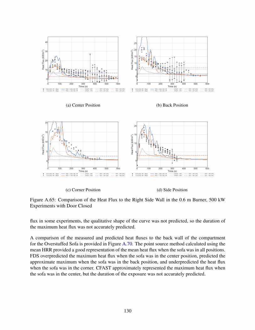
0 100 200 300 400 500 600Time (s)

0

10

20

30

40H

eat F

lux

(kW

/m2 )

0.65 m BC; HF -- Mean1.30 m BC; HF -- Mean

FDS -- 0.65 m BC; HFFDS -- 1.30 m BC; HF

CFAST -- HF1CFAST -- HF2

FDT -- HF1 (PS)FDT -- HF1 (SF)

FDT -- HF2 (PS)FDT -- HF2 (SF)

(a) Center Position

0 100 200 300 400 500 600Time (s)

0

5

10

15

20

25

Hea

t Flu

x (k

W/m

2 )

0.65 m BC; HF -- Mean1.30 m BC; HF -- Mean

FDS -- 0.65 m BC; HFFDS -- 1.30 m BC; HF

CFAST -- HF1CFAST -- HF2

FDT -- HF1 (PS)FDT -- HF1 (SF)

FDT -- HF2 (PS)FDT -- HF2 (SF)

(b) Back Position

0 100 200 300 400 500 600Time (s)

0

5

10

15

20

Hea

t Flu

x (k

W/m

2 )

0.65 m BC; HF -- Mean1.30 m BC; HF -- Mean

FDS -- 0.65 m BC; HFFDS -- 1.30 m BC; HF

CFAST -- HF1CFAST -- HF2

FDT -- HF1 (PS)FDT -- HF1 (SF)

FDT -- HF2 (PS)FDT -- HF2 (SF)

(c) Corner Position

0 100 200 300 400 500 600Time (s)

0

5

10

15

20

Hea

t Flu

x (k

W/m

2 )

0.65 m BC; HF -- Mean1.30 m BC; HF -- Mean

FDS -- 0.65 m BC; HFFDS -- 1.30 m BC; HF

CFAST -- HF1CFAST -- HF2

FDT -- HF1 (PS)FDT -- HF1 (SF)

FDT -- HF2 (PS)FDT -- HF2 (SF)

(d) Side Position

Figure A.65: Comparison of the Heat Flux to the Right Side Wall in the 0.6 m Burner, 500 kWExperiments with Door Closed

flux in some experiments, the qualitative shape of the curve was not predicted, so the duration ofthe maximum heat flux was not accurately predicted.

A comparison of the measured and predicted heat fluxes to the back wall of the compartmentfor the Overstuffed Sofa is provided in Figure A.70. The point source method calculated using themean HRR provided a good representation of the mean heat flux when the sofa was in all positions.FDS overpredicted the maximum heat flux when the sofa was in the center position, predicted theapproximate maximum when the sofa was in the back position, and underpredicted the heat fluxwhen the sofa was in the corner. CFAST approximately represented the maximum heat flux whenthe sofa was in the center, but the duration of the exposure was not accurately predicted.

130

0 100 200 300 400 500 600Time (s)

0

5

10

15

20

25

Hea

t Flu

x (k

W/m

2 )

0.65 m BC -- Mean1.30 m BC -- Mean

FDS -- 0.65 m BCFDS -- 1.30 m BC

CFAST -- HF3CFAST -- HF4

FDT -- HF3 (PS)FDT -- HF3 (SF)

FDT -- HF4 (PS)FDT -- HF4 (SF)

(a) Center Position

0 100 200 300 400 500 600Time (s)

0

20

40

60

80

Hea

t Flu

x (k

W/m

2 )0.65 m BC -- Mean1.30 m BC -- Mean

FDS -- 0.65 m BCFDS -- 1.30 m BC

CFAST -- HF3CFAST -- HF4

FDT -- HF3 (PS)FDT -- HF3 (SF)

FDT -- HF4 (PS)FDT -- HF4 (SF)

(b) Back Position

0 100 200 300 400 500 600Time (s)

0

20

40

60

80

Hea

t Flu

x (k

W/m

2 )

0.65 m BC -- Mean1.30 m BC -- Mean

FDS -- 0.65 m BCFDS -- 1.30 m BC

CFAST -- HF3CFAST -- HF4

FDT -- HF3 (PS)FDT -- HF3 (SF)

FDT -- HF4 (PS)FDT -- HF4 (SF)

(c) Corner Position

0 100 200 300 400 500 600Time (s)

0

20

40

60

80

100

Hea

t Flu

x (k

W/m

2 )

0.65 m BC -- Mean1.30 m BC -- Mean

FDS -- 0.65 m BCFDS -- 1.30 m BC

CFAST -- HF3CFAST -- HF4

FDT -- HF3 (PS)FDT -- HF3 (SF)

FDT -- HF4 (PS)FDT -- HF4 (SF)

(d) Side Position

Figure A.66: Comparison of the Heat Flux to the Back Wall in the 0.6 m Burner, 500 kW Experi-ments with Door Closed

131

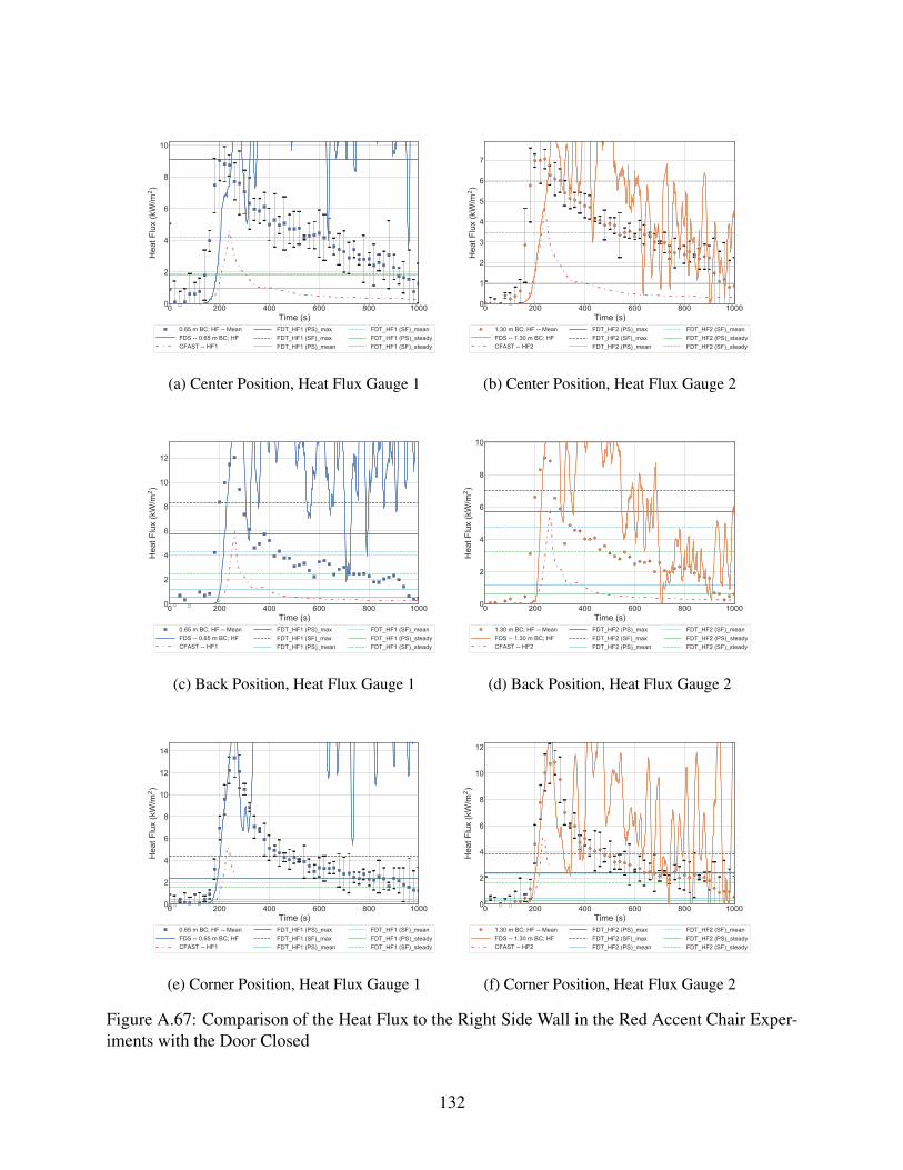
0 200 400 600 800 1000Time (s)

0

2

4

6

8

10H

eat F

lux

(kW

/m2 )

0.65 m BC; HF -- MeanFDS -- 0.65 m BC; HFCFAST -- HF1

FDT_HF1 (PS)_maxFDT_HF1 (SF)_maxFDT_HF1 (PS)_mean

FDT_HF1 (SF)_meanFDT_HF1 (PS)_steadyFDT_HF1 (SF)_steady

(a) Center Position, Heat Flux Gauge 1

0 200 400 600 800 1000Time (s)

0

1

2

3

4

5

6

7

Hea

t Flu

x (k

W/m

2 )

1.30 m BC; HF -- MeanFDS -- 1.30 m BC; HFCFAST -- HF2

FDT_HF2 (PS)_maxFDT_HF2 (SF)_maxFDT_HF2 (PS)_mean

FDT_HF2 (SF)_meanFDT_HF2 (PS)_steadyFDT_HF2 (SF)_steady

(b) Center Position, Heat Flux Gauge 2

0 200 400 600 800 1000Time (s)

0

2

4

6

8

10

12

Hea

t Flu

x (k

W/m

2 )

0.65 m BC; HF -- MeanFDS -- 0.65 m BC; HFCFAST -- HF1

FDT_HF1 (PS)_maxFDT_HF1 (SF)_maxFDT_HF1 (PS)_mean

FDT_HF1 (SF)_meanFDT_HF1 (PS)_steadyFDT_HF1 (SF)_steady

(c) Back Position, Heat Flux Gauge 1

0 200 400 600 800 1000Time (s)

0

2

4

6

8

10

Hea

t Flu

x (k

W/m

2 )

1.30 m BC; HF -- MeanFDS -- 1.30 m BC; HFCFAST -- HF2

FDT_HF2 (PS)_maxFDT_HF2 (SF)_maxFDT_HF2 (PS)_mean

FDT_HF2 (SF)_meanFDT_HF2 (PS)_steadyFDT_HF2 (SF)_steady

(d) Back Position, Heat Flux Gauge 2

0 200 400 600 800 1000Time (s)

0

2

4

6

8

10

12

14

Hea

t Flu

x (k

W/m

2 )

0.65 m BC; HF -- MeanFDS -- 0.65 m BC; HFCFAST -- HF1

FDT_HF1 (PS)_maxFDT_HF1 (SF)_maxFDT_HF1 (PS)_mean

FDT_HF1 (SF)_meanFDT_HF1 (PS)_steadyFDT_HF1 (SF)_steady

(e) Corner Position, Heat Flux Gauge 1

0 200 400 600 800 1000Time (s)

0

2

4

6

8

10

12

Hea

t Flu

x (k

W/m

2 )

1.30 m BC; HF -- MeanFDS -- 1.30 m BC; HFCFAST -- HF2

FDT_HF2 (PS)_maxFDT_HF2 (SF)_maxFDT_HF2 (PS)_mean

FDT_HF2 (SF)_meanFDT_HF2 (PS)_steadyFDT_HF2 (SF)_steady

(f) Corner Position, Heat Flux Gauge 2

Figure A.67: Comparison of the Heat Flux to the Right Side Wall in the Red Accent Chair Exper-iments with the Door Closed

132

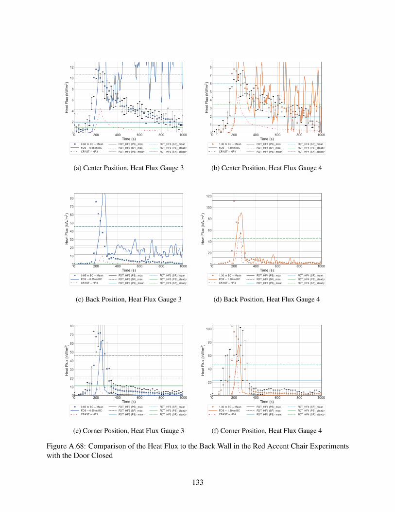
0 200 400 600 800 1000Time (s)

0

2

4

6

8

10

12H

eat F

lux

(kW

/m2 )

0.65 m BC -- MeanFDS -- 0.65 m BCCFAST -- HF3

FDT_HF3 (PS)_maxFDT_HF3 (SF)_maxFDT_HF3 (PS)_mean

FDT_HF3 (SF)_meanFDT_HF3 (PS)_steadyFDT_HF3 (SF)_steady

(a) Center Position, Heat Flux Gauge 3

0 200 400 600 800 1000Time (s)

0

1

2

3

4

5

6

7

8

Hea

t Flu

x (k

W/m

2 )

1.30 m BC -- MeanFDS -- 1.30 m BCCFAST -- HF4

FDT_HF4 (PS)_maxFDT_HF4 (SF)_maxFDT_HF4 (PS)_mean

FDT_HF4 (SF)_meanFDT_HF4 (PS)_steadyFDT_HF4 (SF)_steady

(b) Center Position, Heat Flux Gauge 4

0 200 400 600 800 1000Time (s)

0

10

20

30

40

50

60

70

80

Hea

t Flu

x (k

W/m

2 )

0.65 m BC -- MeanFDS -- 0.65 m BCCFAST -- HF3

FDT_HF3 (PS)_maxFDT_HF3 (SF)_maxFDT_HF3 (PS)_mean

FDT_HF3 (SF)_meanFDT_HF3 (PS)_steadyFDT_HF3 (SF)_steady

(c) Back Position, Heat Flux Gauge 3

0 200 400 600 800 1000Time (s)

0

20

40

60

80

100

120

Hea

t Flu

x (k

W/m

2 )

1.30 m BC -- MeanFDS -- 1.30 m BCCFAST -- HF4

FDT_HF4 (PS)_maxFDT_HF4 (SF)_maxFDT_HF4 (PS)_mean

FDT_HF4 (SF)_meanFDT_HF4 (PS)_steadyFDT_HF4 (SF)_steady

(d) Back Position, Heat Flux Gauge 4

0 200 400 600 800 1000Time (s)

0

10

20

30

40

50

60

70

80

Hea

t Flu

x (k

W/m

2 )

0.65 m BC -- MeanFDS -- 0.65 m BCCFAST -- HF3

FDT_HF3 (PS)_maxFDT_HF3 (SF)_maxFDT_HF3 (PS)_mean

FDT_HF3 (SF)_meanFDT_HF3 (PS)_steadyFDT_HF3 (SF)_steady

(e) Corner Position, Heat Flux Gauge 3

0 200 400 600 800 1000Time (s)

0

20

40

60

80

100

Hea

t Flu

x (k

W/m

2 )

1.30 m BC -- MeanFDS -- 1.30 m BCCFAST -- HF4

FDT_HF4 (PS)_maxFDT_HF4 (SF)_maxFDT_HF4 (PS)_mean

FDT_HF4 (SF)_meanFDT_HF4 (PS)_steadyFDT_HF4 (SF)_steady

(f) Corner Position, Heat Flux Gauge 4

Figure A.68: Comparison of the Heat Flux to the Back Wall in the Red Accent Chair Experimentswith the Door Closed

133

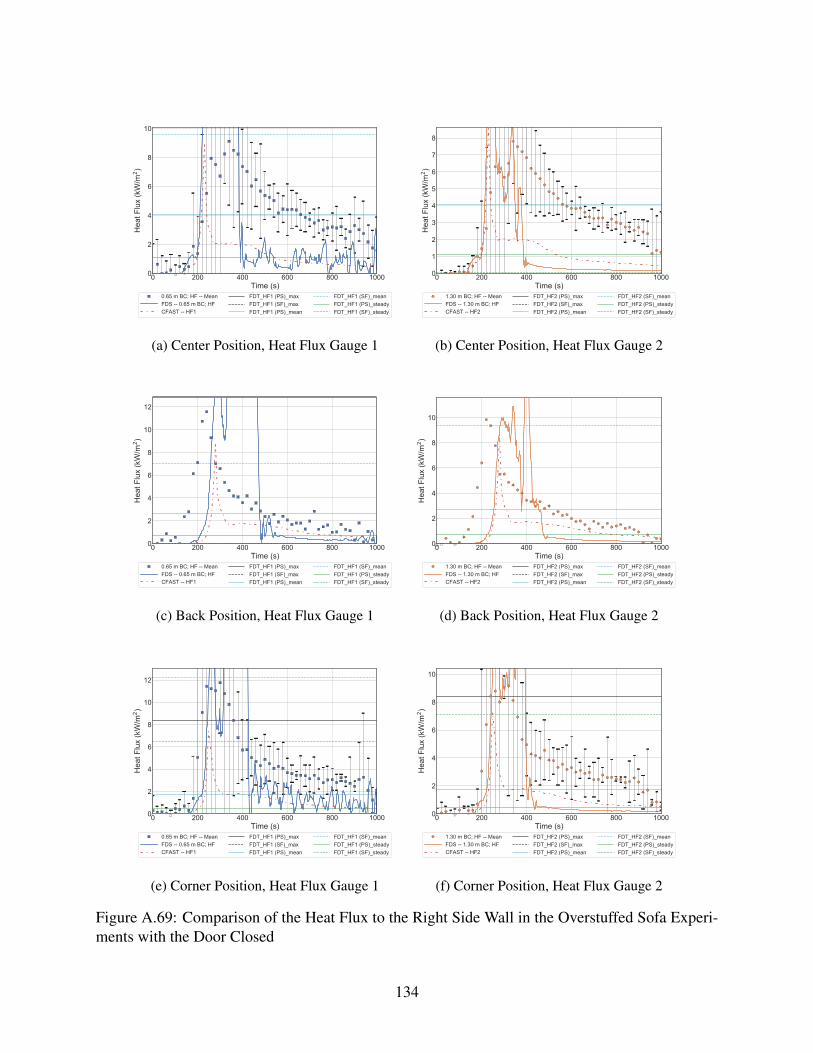
0 200 400 600 800 1000Time (s)

0

2

4

6

8

10H

eat F

lux

(kW

/m2 )

0.65 m BC; HF -- MeanFDS -- 0.65 m BC; HFCFAST -- HF1

FDT_HF1 (PS)_maxFDT_HF1 (SF)_maxFDT_HF1 (PS)_mean

FDT_HF1 (SF)_meanFDT_HF1 (PS)_steadyFDT_HF1 (SF)_steady

(a) Center Position, Heat Flux Gauge 1

0 200 400 600 800 1000Time (s)

0

1

2

3

4

5

6

7

8

Hea

t Flu

x (k

W/m

2 )

1.30 m BC; HF -- MeanFDS -- 1.30 m BC; HFCFAST -- HF2

FDT_HF2 (PS)_maxFDT_HF2 (SF)_maxFDT_HF2 (PS)_mean

FDT_HF2 (SF)_meanFDT_HF2 (PS)_steadyFDT_HF2 (SF)_steady

(b) Center Position, Heat Flux Gauge 2

0 200 400 600 800 1000Time (s)

0

2

4

6

8

10

12

Hea

t Flu

x (k

W/m

2 )

0.65 m BC; HF -- MeanFDS -- 0.65 m BC; HFCFAST -- HF1

FDT_HF1 (PS)_maxFDT_HF1 (SF)_maxFDT_HF1 (PS)_mean

FDT_HF1 (SF)_meanFDT_HF1 (PS)_steadyFDT_HF1 (SF)_steady

(c) Back Position, Heat Flux Gauge 1

0 200 400 600 800 1000Time (s)

0

2

4

6

8

10H

eat F

lux

(kW

/m2 )

1.30 m BC; HF -- MeanFDS -- 1.30 m BC; HFCFAST -- HF2

FDT_HF2 (PS)_maxFDT_HF2 (SF)_maxFDT_HF2 (PS)_mean

FDT_HF2 (SF)_meanFDT_HF2 (PS)_steadyFDT_HF2 (SF)_steady

(d) Back Position, Heat Flux Gauge 2

0 200 400 600 800 1000Time (s)

0

2

4

6

8

10

12

Hea

t Flu

x (k

W/m

2 )

0.65 m BC; HF -- MeanFDS -- 0.65 m BC; HFCFAST -- HF1

FDT_HF1 (PS)_maxFDT_HF1 (SF)_maxFDT_HF1 (PS)_mean

FDT_HF1 (SF)_meanFDT_HF1 (PS)_steadyFDT_HF1 (SF)_steady

(e) Corner Position, Heat Flux Gauge 1

0 200 400 600 800 1000Time (s)

0

2

4

6

8

10

Hea

t Flu

x (k

W/m

2 )

1.30 m BC; HF -- MeanFDS -- 1.30 m BC; HFCFAST -- HF2

FDT_HF2 (PS)_maxFDT_HF2 (SF)_maxFDT_HF2 (PS)_mean

FDT_HF2 (SF)_meanFDT_HF2 (PS)_steadyFDT_HF2 (SF)_steady

(f) Corner Position, Heat Flux Gauge 2

Figure A.69: Comparison of the Heat Flux to the Right Side Wall in the Overstuffed Sofa Experi-ments with the Door Closed

134

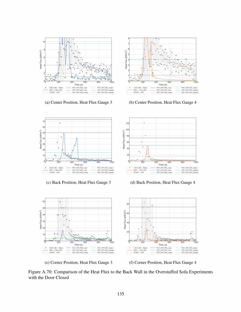
0 200 400 600 800 1000Time (s)

0

2

4

6

8

10H

eat F

lux

(kW

/m2 )

0.65 m BC -- MeanFDS -- 0.65 m BCCFAST -- HF3

FDT_HF3 (PS)_maxFDT_HF3 (SF)_maxFDT_HF3 (PS)_mean

FDT_HF3 (SF)_meanFDT_HF3 (PS)_steadyFDT_HF3 (SF)_steady

(a) Center Position, Heat Flux Gauge 3

0 200 400 600 800 1000Time (s)

0

1

2

3

4

5

6

7

8

Hea

t Flu

x (k

W/m

2 )

1.30 m BC -- MeanFDS -- 1.30 m BCCFAST -- HF4

FDT_HF4 (PS)_maxFDT_HF4 (SF)_maxFDT_HF4 (PS)_mean

FDT_HF4 (SF)_meanFDT_HF4 (PS)_steadyFDT_HF4 (SF)_steady

(b) Center Position, Heat Flux Gauge 4

0 200 400 600 800 1000Time (s)

0

10

20

30

40

50

60

70

Hea

t Flu

x (k

W/m

2 )

0.65 m BC -- MeanFDS -- 0.65 m BCCFAST -- HF3

FDT_HF3 (PS)_maxFDT_HF3 (SF)_maxFDT_HF3 (PS)_mean

FDT_HF3 (SF)_meanFDT_HF3 (PS)_steadyFDT_HF3 (SF)_steady

(c) Back Position, Heat Flux Gauge 3

0 200 400 600 800 1000Time (s)

0

20

40

60

80

100

120H

eat F

lux

(kW

/m2 )

1.30 m BC -- MeanFDS -- 1.30 m BCCFAST -- HF4

FDT_HF4 (PS)_maxFDT_HF4 (SF)_maxFDT_HF4 (PS)_mean

FDT_HF4 (SF)_meanFDT_HF4 (PS)_steadyFDT_HF4 (SF)_steady

(d) Back Position, Heat Flux Gauge 4

0 200 400 600 800 1000Time (s)

0

10

20

30

40

50

60

Hea

t Flu

x (k

W/m

2 )

0.65 m BC -- MeanFDS -- 0.65 m BCCFAST -- HF3

FDT_HF3 (PS)_maxFDT_HF3 (SF)_maxFDT_HF3 (PS)_mean

FDT_HF3 (SF)_meanFDT_HF3 (PS)_steadyFDT_HF3 (SF)_steady

(e) Corner Position, Heat Flux Gauge 3

0 200 400 600 800 1000Time (s)

0

20

40

60

80

Hea

t Flu

x (k

W/m

2 )

1.30 m BC -- MeanFDS -- 1.30 m BCCFAST -- HF4

FDT_HF4 (PS)_maxFDT_HF4 (SF)_maxFDT_HF4 (PS)_mean

FDT_HF4 (SF)_meanFDT_HF4 (PS)_steadyFDT_HF4 (SF)_steady

(f) Corner Position, Heat Flux Gauge 4

Figure A.70: Comparison of the Heat Flux to the Back Wall in the Overstuffed Sofa Experimentswith the Door Closed

135