March 19, 2021 Bank of Japan Assessment for Further Effective and Sustainable Monetary Easing The Background [Note] (English translation prepared by the Bank's staff based on the Japanese original) [Note] "The Background" provides explanations of "The Bank's View," which was decided by the Policy Board of the Bank of Japan at the Monetary Policy Meeting held on March 18 and 19, 2021, and released as Attachment 1 to the statement on monetary policy.

Welcome message from author
This document is posted to help you gain knowledge. Please leave a comment to let me know what you think about it! Share it to your friends and learn new things together.
Transcript

March 19, 2021
Bank of Japan
Assessment for Further Effective
and Sustainable Monetary Easing
The Background[Note]
(English translation prepared by the Bank's staff based on the Japanese original)
[Note] "The Background" provides explanations of "The Bank's View," which was decided by the
Policy Board of the Bank of Japan at the Monetary Policy Meeting held on March 18 and 19,
2021, and released as Attachment 1 to the statement on monetary policy.
1
I. Motivation behind the Assessment
The Bank has been pursuing powerful monetary easing since the introduction of
quantitative and qualitative monetary easing (QQE) in April 2013, with a view to achieving
the price stability target of 2 percent. Setting the price stability target at 2 percent is
appropriate when considering the characteristics of price statistics and in terms of securing
room for future policy responses, and is a global standard. The Bank introduced the price
stability target of 2 percent in January 2013.1 It also clearly stated this target in the joint
statement released together with the government.2
In September 2016, the Bank conducted the Comprehensive Assessment of developments in
economic activity and prices since the introduction of QQE as well as its policy effects.3
Based on the findings, a new policy framework, QQE with Yield Curve Control, was
introduced. This framework has been working well, including in response to the impact of
the novel coronavirus (COVID-19). However, due to that impact, economic activity and
prices are projected to remain under downward pressure for a prolonged period, and it is
expected to take time until the price stability target of 2 percent is achieved. Under these
circumstances, the Bank decided to conduct an assessment for further effective and
sustainable monetary easing, with a view to achieving the 2 percent target.
1 Bank of Japan, "The 'Price Stability Target' under the Framework for the Conduct of Monetary
Policy," January 2013, https://www.boj.or.jp/en/announcements/release_2013/k130122b.pdf. 2 Cabinet Office, Ministry of Finance, and Bank of Japan, "Joint Statement of the Government and
the Bank of Japan on Overcoming Deflation and Achieving Sustainable Economic Growth," January
2013, https://www.boj.or.jp/en/announcements/release_2013/k130122c.pdf. 3 Bank of Japan, Comprehensive Assessment: Developments in Economic Activity and Prices as well
as Policy Effects since the Introduction of Quantitative and Qualitative Monetary Easing (QQE),
September 2016, https://www.boj.or.jp/en/announcements/release_2016/rel160930d.pdf.

2
II. Developments in Economic Activity and Prices under QQE with Yield Curve
Control
A. The Comprehensive Assessment and Policy Responses Based on the Findings
In September 2016, the Bank conducted the Comprehensive Assessment of developments in
economic activity and prices since the introduction of QQE as well as its policy effects. The
findings of the assessment showed the following. First, reflecting the introduction of QQE
in April 2013, financial conditions improved significantly, thereby boosting economic
activity and corporate profits. Second, under such economic conditions, the economy no
longer was in deflation in the sense of a sustained decline in prices. Third, however, the
price stability target of 2 percent had not been achieved. In this context, the mechanism
through which inflation expectations are formed played an important role. The formation of
inflation expectations in Japan is largely adaptive, and raising them in the presence of
adaptive expectations formation is associated with uncertainties and likely to take time.
Fourth, monetary easing affects the functioning of the Japanese government bond (JGB)
market and may have a negative impact on the functioning of financial intermediation
through the cumulative impact mainly on financial institutions' profits and the investment
environment for insurance and pension products.
Based on these findings, the Bank introduced QQE with Yield Curve Control in September
2016 (Chart 1). This framework consists of two major components. The first is yield curve
control, in which the Bank controls short- and long-term interest rates. In order to achieve
the price stability target of 2 percent, the Bank encourages the formation of the most
appropriate shape of the yield curve while taking into account developments in economic
activity and prices as well as financial conditions. Under the guideline for market operations,
in which the short-term policy interest rate is set at minus 0.1 percent and the target level of
10-year JGB yields is around zero percent, the Bank has thus far managed to encourage the
formation of an appropriate shape of the yield curve. The second component is an
inflation-overshooting commitment, in which the Bank commits to continuing to "expand
the monetary base until the year-on-year rate of increase in the observed consumer price
index (CPI) exceeds 2 percent and stays above the target in a stable manner."

3
The introduction of this framework has three aims. The first, in order to achieve the price
stability target of 2 percent, is to maintain the output gap in positive territory for as long as
possible, given that the formation of inflation expectations in Japan is largely adaptive. The
second is to introduce a framework in which the Bank controls interest rates to appropriate
levels while taking into consideration both the positive and side effects of monetary easing,
with the expectation that monetary easing will be prolonged. The third is to strengthen the
forward-looking element of inflation expectations formation with the inflation-overshooting
commitment.
B. Developments in Economic Activity and Prices since the Comprehensive Assessment
The situation where inflation rates do not rise easily continued even after the conduct of the
Comprehensive Assessment. Given this, a further assessment of the mechanism behind
inflation developments shows the following (Appendix 1). The mechanism of adaptive
inflation expectations formation reflects not only the observed inflation rate at the time but
also people's past experiences, and therefore it is relatively complex and sticky. In other
words, changing people's mindset and behavior based on the assumption that prices will not
increase easily, which have become deeply entrenched because of the experience of
prolonged deflation, will take time. In addition, elastic labor supply, mainly of women and
seniors, and a rise in firms' labor productivity have consequently constrained inflation.
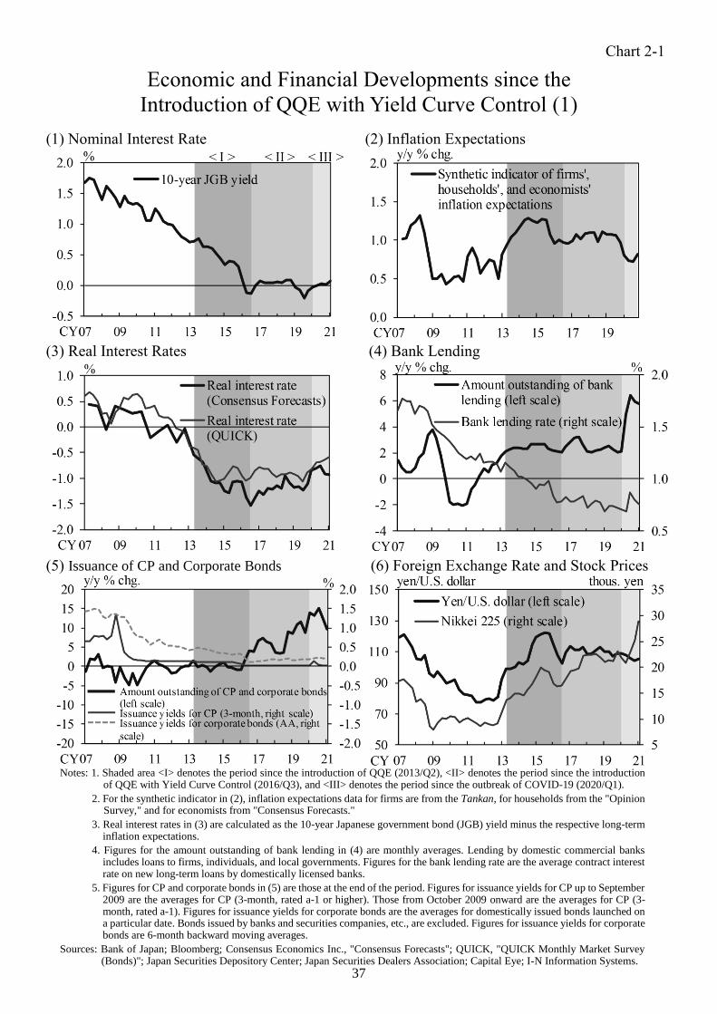
Under these circumstances, QQE with Yield Curve Control has had positive effects in line
with the intended mechanism (Chart 2). First, with nominal interest rates being kept at
extremely low levels through yield curve control and inflation expectations that are higher
than those prior to the introduction of QQE, real interest rates (calculated by subtracting
inflation expectations from nominal interest rates) have been clearly negative. Second, the
low real interest rates have improved financial conditions, mainly through low funding costs
as well as favorable conditions in financial and capital markets. The year-on-year rate of
change in the amount outstanding of bank lending has continued to be at around 2 percent,
and that in the aggregate amount outstanding of CP and corporate bonds has increased, with
its pace of acceleration also increasing since 2016. In financial and capital markets, foreign
exchange rates have been stable on the whole and stock prices have been on an uptrend.
Third, as a result, these developments have pushed up economic activity, and corporate

4
profits and the employment situation have improved. The output gap turned clearly positive
(representing excess demand) in 2017 and expanded within positive territory. Fourth, with
these favorable economic conditions, wages have increased moderately, as seen in the fact
that base pay -- which did not rise during the period of deflation -- has increased for seven
consecutive years, and underlying inflation has taken hold in positive territory.
Under QQE with Yield Curve Control, the output gap has improved and labor market
conditions have tightened. Under these circumstances, as mentioned earlier, labor force
participation of women and seniors has increased and firms have improved their labor
productivity. With economic developments continuing to be favorable, positive moves
toward addressing the medium- to long-term challenges facing Japan's economy have been
observed.
III. Policy Effects of QQE with Yield Curve Control
A. Effects of QQE with Yield Curve Control on Nominal Interest Rates
Looking at developments in JGB yields under yield curve control, long-term interest rates
(10-year JGB yields) have been at around 0 percent and yields on JGBs with other
maturities also have been stable at low levels (Chart 3). After the outbreak of COVID-19,
liquidity in the JGB market declined temporarily and a subsequent increase in issuance of
JGBs intensified upward pressure on yields. Even in this situation, the yield curve has been
stable at a low level on the whole.
Long-term interest rates reflect factors such as the outlook for economic activity and prices
as well as long-term interest rates abroad. Controlling for these factors, quantitative analysis
of the effects of the Bank's JGB purchases shows that its purchases have statistically
significant effects on long-term interest rates in terms of lowering them by around 1
percentage point on average (Chart 4).
B. Effects of Accommodative Financial Conditions on Economic Activity and Prices
The main transmission mechanism of QQE with Yield Curve Control is to achieve
accommodative financial conditions, mainly brought about by low real interest rates, and

5
thereby exert positive effects on economic activity and prices. Actual developments in
economic activity and prices as described earlier have been in line with this mechanism.
Using its large-scale macroeconomic model -- the Quarterly Japanese Economic Model
(Q-JEM) -- the Bank examined the effects of monetary easing under QQE with Yield Curve
Control on economic activity and prices (Appendix 2). Specifically, it carried out
counterfactual simulations to compare actual developments in economic activity and prices
with simulated developments obtained assuming QQE had not been introduced. The
simulation results show that actual figures are higher than the counterfactual estimates for
the period through the July-September quarter of 2020; on average, the level of real GDP is
between around 0.9 and 1.3 percent higher, the output gap is between around 0.9 and 1.3
percentage points higher, and the year-on-year rate of change in the CPI (all items less fresh
food and energy) is between around 0.6 and 0.7 percentage points higher. This suggests that
QQE (and QQE with Yield Curve Control) has had positive effects to those extents on
economic activity and prices.
Since 2020, reflecting the decline in demand stemming from the large shock due to the
COVID-19 pandemic, the output gap has deteriorated significantly, inflation has been
restrained, and inflation expectations have weakened somewhat (Chart 2). However, the
simulation results indicate that monetary easing under QQE with Yield Curve Control has
been effective in supporting economic activity and prices even amid the COVID-19 shock.
C. Transmission Channels through Which a Decline in Interest Rates Affects
Economic Activity and Prices
There are two transmission channels through which a decline in interest rates affects
economic activity and prices. The first is via funding costs. In fact, under QQE with Yield
Curve Control, lending rates have declined clearly and interest rates on CP and corporate
bonds have been at extremely low levels (Chart 5). The second channel is via financial and
capital markets. That is, a decline in interest rates also affects economic activity and prices
through favorable conditions in financial and capital markets. Although financial
transactions such as lending are not usually conducted at negative interest rates, transactions
in financial and capital markets more commonly take place even at such rates. Thus, it has
6
been pointed out that the transmission channel via financial and capital markets is less
susceptible to the effective lower bound on nominal interest rates (Chart 3[1]).
To examine these points, the Bank used a vector-autoregressive (VAR) model to analyze
the transmission channels through which a decline in interest rates improves the output gap
(Chart 6). The analysis shows that the transmission channel via funding costs accounts for
more than 30 percent of the effects on the output gap, while that via financial and capital
markets accounts for more than 50 percent. Although the results should be interpreted with
some latitude, they indicate that the decline in interest rates has been exerting positive
effects on economic activity and prices through both funding costs and financial and capital
markets.
D. Effects of a Decline in Interest Rates with Different Maturities on Economic
Activity and Prices
The degree to which a decline in real interest rates affects economic activity and prices
depends on the maturity of those interest rates. In the Comprehensive Assessment
conducted in 2016, the Bank examined the effects of a given decline in real interest rates on
the output gap, employing the concept of the "natural yield curve."4 The results indicated
that the effects were relatively large for short- and medium-term interest rates and became
smaller the longer the maturity. While taking changes in economic and financial
developments to date into account, the Bank examined the effects in this assessment, using
the same approach. The results indicate that this pattern is unchanged (Chart 7[1]).
In addition, in the 2016 Comprehensive Assessment, the results pointed to the possibility
that an excessive decline in super-long-term interest rates will lead to anxiety about the
future sustainability of the functioning of financial activities in a broader sense and have a
negative impact on economic activity by, for example, undermining people's sentiment. In
4 The "natural yield curve" applies the concept of the natural rate of interest not to the interest rate at
a certain maturity but across the entire yield curve. For details on the analysis, see Appendix 8 in the
Comprehensive Assessment: Developments in Economic Activity and Prices as well as Policy Effects
since the Introduction of Quantitative and Qualitative Monetary Easing (QQE) released in
September 2016 (https://www.boj.or.jp/en/announcements/release_2016/rel160930d.pdf).
7
the current assessment, the effects of a decline in super-long-term interest rates on the
consumer confidence index were examined, using the VAR model. The results indicate that
a decline in super-long-term interest rates does have a negative impact on consumer
sentiment (Chart 7[2]).
E. Market Participants' Expectations with Regard to Short-Term Interest Rate Cuts
The results of a survey of market participants show that fewer of them expect short-term
interest rate cuts to be an option for additional easing compared with the time immediately
after the introduction of the negative interest rate policy (Chart 8). While market
participants' expectations with regard to short-term interest rate cuts could change in
response to economic and price developments at any given time, anecdotal information
suggests that an increasing number of those who are not expecting interest rate cuts tend to
point to the impact on the functioning of financial intermediation.
F. Effects of Policy Responses to the Impact of COVID-19
Since March 2020, in response to the impact of COVID-19, the Bank has conducted
powerful monetary easing under QQE with Yield Curve Control. The aim is to provide
support for financing, mainly of firms, so that they can sustain their businesses, and to
maintain stability in financial and capital markets in order to prevent a vicious cycle
between turmoil in the markets and deterioration in the real economy.
The Bank's responses to the impact of COVID-19 have been effective (Chart 9). Through
the Special Program to Support Financing in Response to the Novel Coronavirus
(COVID-19), coupled with the government's measures to support financing and active
efforts made by financial institutions, the environment for external funding has remained
accommodative. Through the Special Funds-Supplying Operations to Facilitate Financing
in Response to the Novel Coronavirus (COVID-19), the Bank has been encouraging
financial institutions' efforts, in that it provides funds on favorable terms for their
COVID-19 support lending by applying interest rates as an incentive to their current
account balances that correspond to the amounts outstanding of loans provided through this
operation. The increase in purchases of CP and corporate bonds by the Bank has prevented

8
a rise in spreads, thereby helping to maintain a favorable environment for firms to obtain
funding through the issuance of CP and corporate bonds.
Looking at financial and capital markets, JGB yields have been stable at low levels under
yield curve control even after the outbreak of COVID-19, when liquidity in the JGB market
declined temporarily and a subsequent increase in issuance of JGBs intensified upward
pressure on yields. Although U.S. dollar funding costs rose significantly in response to the
surge in demand for dollar funding due to the COVID-19 shock, the impact was only
temporary due to the provision of U.S. dollar liquidity through the cooperation of six central
banks, including the Federal Reserve and the Bank of Japan. In addition, flexible purchases
of exchange-traded funds (ETFs) and Japan real estate investment trusts (J-REITs) have
contained instability in financial and capital markets (see Section V for more details).
IV. Effects on the Functioning of the JGB Market and Financial Intermediation
A. Effects on the Functioning of the JGB Market
Yield curve control has affected the functioning of the JGB market. With the range of
fluctuations in interest rates having narrowed, many indicators suggest that the functioning
of the JGB market has decreased since the introduction of yield curve control (Chart 10).
The effects of yield curve control on the functioning of the JGB market are, in a sense, an
inevitable consequence of maintaining interest rates stably at extremely low levels. In terms
of the sustainable conduct of yield curve control, it is important to strike an appropriate
balance between maintaining market functioning and controlling interest rates. On this point,
although significant fluctuations in interest rates could lead to adverse effects on
developments in economic activity and prices, fluctuations within a certain range could
have positive effects on the functioning of the JGB market without impairing the effects of
monetary easing. Examination on the effects of interest rate fluctuations on business fixed
investment indicates that the degree to which monetary easing affects business fixed
investment is more or less unchanged, except when the range of fluctuations in 10-year JGB
yields over the preceding six months exceeds 50 basis points (Appendix 3).

9
In July 2018, in order to enhance the sustainability of QQE with Yield Curve Control, the
Bank made the conduct of JGB purchases more flexible, making clear that 10-year JGB
yields might move upward and downward to some extent, mainly depending on
developments in economic activity and prices. Specifically, regarding the range of
fluctuations in 10-year JGB yields, it announced that those yields might move upward and
downward in about double the range, which was previously between around plus and minus
0.1 percent from the target level. In fact, from July 2018 through 2019, the range widened to
between plus 0.16 and minus 0.29, and many indicators suggested that the functioning of
the JGB market had improved.
Looking at developments since the spread of COVID-19 in 2020, 10-year JGB yields
temporarily fluctuated to a considerable degree with financial and capital markets becoming
volatile, but thereafter remained within a narrow range through the beginning of this year.
Meanwhile, even though the functioning of the JGB market has recovered from the
significant deterioration, it has not yet returned to the level prior to the pandemic.
B. Effects on the Functioning of Financial Intermediation
Downward pressure on financial institutions' profits stemming from low interest rates could
have a negative impact on the functioning of financial intermediation by, for example,
making financial institutions more reluctant to lend.
Financial institutions' core profitability has continued to decline as a trend, mainly due to a
shrinking of the margin between domestic deposit and lending rates (Chart 11). The
shrinking of net interest margins is caused by the prolonged low interest rate environment
and structural factors such as the downtrend in loan demand due to, for example, the
declining population and the resultant severe competition among financial institutions.
Meanwhile, financial institutions have continued to make efforts to enhance their
profitability, mainly through risk taking in lending and securities investment as well as
through cost cutting and saving. Owing to QQE with Yield Curve Control, economic
activity has been boosted and corporate profits have improved, which in turn likely had
positive effects on financial institutions' profits, mainly through increased loans and
contained credit costs.
10
That said, profits of financial institutions, regional ones in particular, are expected to remain
under downward pressure, continuing to be affected by the low interest rate environment
and structural factors. Since the effects of financial institutions' profits on their financial
soundness is cumulative, attention needs to be paid to the risk that prolonged downward
pressure on profits may lead to a gradual pullback in financial intermediation. On the other
hand, while financial institutions are expected to continue making various efforts to enhance
their profitability, the vulnerability of the financial system could increase in the process,
mainly as a result of financial institutions' search for yield behavior. As for these
overheating and pullback risks, in the Outlook for Economic Activity and Prices, the Bank,
based on the Financial System Report, has been examining financial imbalances from a
longer-term perspective.
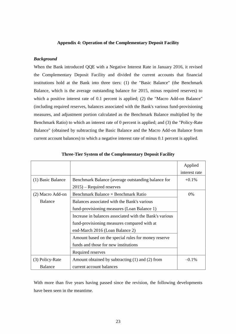
C. Operation of the Complementary Deposit Facility
In January 2016, the Bank introduced QQE with a Negative Interest Rate. This aims to
lower the short end of the yield curve by slashing the deposit rate on current account
balances into negative territory and to exert further downward pressure on interest rates
across the entire yield curve, in combination with large-scale purchases of JGBs. In keeping
short-term interest rates in negative territory, the Bank decided to apply a negative interest
rate only to the marginal increase in current account balances so that the direct burden on
financial institutions' profits is eased. Specifically, the Bank revised the Complementary
Deposit Facility. It divided the current account balance into three tiers: the Basic Balance,
the Macro Add-on Balance, and the Policy-Rate Balance. To the Basic Balance and the
Macro Add-on Balance, which make up most of the current account balance, a positive
interest rate of 0.1 percent and a zero interest rate are applied respectively, and a negative
interest rate of minus 0.1 percent is applied only to the Policy-Rate Balance. Under this
three-tier system, short-term interest rates have been stable in negative territory to date.
That said, with more than five years having passed since the revision of the Complementary
Deposit Facility, there is a gap between the actual Policy-Rate Balances and the
"hypothetical" Policy-Rate Balances, which are calculated based on the assumption that
arbitrage transactions fully take place, and the gap has been widening recently (Appendix 4).
In order to address this situation, the Bank can make technical adjustments to compress the

11
unused amounts of Macro Add-on Balances and a portion of the Policy-Rate Balances by
reviewing some parts of the method to calculate the limit of the Macro Add-on Balances.
V. Effects of ETF and J-REIT Purchases and Points to Note
A. Effects of ETF and J-REIT Purchases
The Bank has been purchasing ETFs and J-REITs to lower risk premia in the stock and
J-REIT markets in order to exert positive effects on economic activity and prices.
The Bank estimated the effects of ETF purchases, using two of the indicators of risk premia
-- equity risk premium implied by option prices and yield spreads (Chart 12 and Appendix
5).5 The results show that ETF purchases have the effect of lowering risk premia. Further,
the Bank estimated how effects differ depending on market conditions and the size of ETF
purchases. The estimation results suggest that the effects of ETF purchases per single
amount are larger (1) the lower the level of stock prices relative to their trend at the time of
purchases, (2) the higher the volatility in the stock market when stock prices are below their
trend, (3) the larger the rate of decline in stock prices immediately before the conduct of
purchases, and (4) the larger the size of purchases.
These results are consistent with the view of market participants (Chart 13). Namely, survey
results of market participants indicate that, during periods of market instability such as
when stock prices decline or volatility heightens, ETF purchases by the Bank draw the
market's attention and are seen as a positive factor for the stock market. On the other hand,
when the market is stable, they lose its attention and fewer market participants see such
purchases as positive.
5 Since there is no single indicator that captures developments in risk premia, the Bank incorporates
various pieces of data and indicators to judge them from a comprehensive perspective -- such as
developments in corporate profits, dividends, and stock prices, as well as the level of interest rates --
and also anecdotal information from market participants. The analysis in this assessment uses two of
these indicators to estimate the effects of ETF purchases.

12
B. Points to Note with Regard to ETF and J-REIT Purchases
While the results show that purchases of ETFs and J-REITs are effective, some points to
note have been raised.
One example is the effects that the Bank's holding of ETFs may have on corporate
governance. Specifically, it has been argued that, when the Bank holds ETFs, this will
weaken business discipline in the management of individual firms. However, voting rights
in ETF component firms are to be exercised appropriately by asset management companies
that have accepted the Stewardship Code. With this, management discipline is being exerted.
That said, it is possible that such concern could grow as the Bank further increases its ETF
holdings (Chart 14). Another point is that the Bank's indirect shareholding ratio in some
ETF component firms tends to increase much more rapidly through such purchases in the
case of ETFs tracking the Nikkei 225 Stock Average or the JPX-Nikkei Index 400
(JPX-Nikkei 400) than ETFs tracking the Tokyo Stock Price Index (TOPIX). The Bank has
been addressing this issue by increasing the share of purchases of ETFs tracking the TOPIX.
With regard to J-REIT purchases, while the Principal Terms and Conditions stipulate that
the maximum amount of each J-REIT to be purchased shall not exceed 10 percent of the
total amount of that J-REIT issued, there are some J-REITs for which the percentage of the
Bank's holdings has been rising toward this threshold. Besides these points, some have
pointed to the potential impact of ETF and J-REIT purchases on the Bank's balance sheet.
In this context, the Principal Terms and Conditions stipulate that in case the total market
value of ETFs or J-REITs purchased by the Bank falls below their total book value, the
Bank shall record provisions for possible losses. This has ensured its financial soundness.
However, as the Bank's ETF holdings increase further, the impact on the Bank's balance
sheet would become large.
VI. Examination on the Effectiveness of the Inflation-Overshooting Commitment
Given that it may take time to raise inflation expectations, of which the formation in Japan
is largely adaptive, the Bank decided in September 2016 to adopt a new policy framework,
with yield curve control at its core. Under this framework, it aims to enhance the
sustainability of monetary easing while striking a balance between the positive and side
effects of monetary easing.

13
Together with yield curve control, the Bank introduced an inflation-overshooting
commitment so as to strengthen the forward-looking element of inflation expectations
formation. Through this commitment, the Bank commits to expanding the monetary base
until the year-on-year rate of increase in the observed CPI exceeds the price stability target
of 2 percent and stays above the target in a stable manner. Generally, it is considered
desirable for central banks to conduct monetary policy based on the outlook for economic
activity and prices, since it takes a certain amount of time for monetary policy to affect
economic activity and prices. From this perspective, the inflation-overshooting commitment
is an extremely strong commitment, in that the Bank promises to continue with monetary
easing based on observed CPI inflation rather than the outlook for CPI inflation.
Through an inflation-overshooting commitment, the Bank is implementing the so-called
makeup strategy, in which monetary easing is conducted taking into account instances when
the observed inflation rate continued to stay below the target. The idea underlying this
strategy is that a central bank would aim to attain a situation where the inflation rate is 2
percent on average over the business cycle. The Bank has clearly stated its stance of
adopting this idea.6
The results of simulations using a simple macroeconomic model show that, when the
observed inflation rate in Japan is below the inflation target, monetary policy should be
conducted by also referring to the past inflation rate for some period of time (Appendix 6).
In addition, the results indicate that the lower the natural rate of interest, the longer the past
inflation rate should be used for reference.
6 In the Bank's policy statement, it is described that "[a]chieving the price stability target means
attaining a situation where the inflation rate is 2 percent on average over the business cycle." For
details, see "New Framework for Strengthening Monetary Easing: 'Quantitative and Qualitative
Monetary Easing with Yield Curve Control'," January 2016,
https://www.boj.or.jp/en/announcements/release_2016/k160921a.pdf.

14
Appendix 1: Mechanism behind Inflation Developments in Japan
Based on the situation since the Comprehensive Assessment, the Bank conducted a further
assessment of the mechanism behind inflation developments in Japan.
Complex and Sticky Mechanism of Adaptive Inflation Expectations Formation
As pointed out in the Comprehensive Assessment, the adaptive element plays a strong role
in the mechanism of inflation expectations formation in Japan. Using data up until recently,
the Bank examined this mechanism and found that the adaptive element still plays a much
larger role in the mechanism in Japan than in the United States and other countries
(Appendix Chart 1-1).
The adaptive formation of inflation expectations has the characteristic that it reflects not
only the observed inflation rate at the time but also people's past experiences.7 With regard
to households' perception of inflation in Japan, microdata from the Opinion Survey on the
General Public's Views and Behavior show that the younger the age groups, which have not
experienced inflation, (1) the lower inflation expectations and (2) the less sensitive their
inflation expectations to actual fluctuations in prices. The results suggest that past
experiences and the norms developed in the process have deeply affected the formation of
inflation expectations (Appendix Chart 1-2).
In theoretical frameworks, the formation of inflation expectations has been assumed
traditionally to follow "full-information rational expectations," where economic entities use
all available information to form their expectations.8 However, in recent years it has been
pointed out that, considering the stickiness and complexity of the formation process, other
7 For studies analyzing the effects of past experiences on inflation expectations, see the following
papers: Malmendier, U. and Nagel, S., "Learning from Inflation Experiences," The Quarterly
Journal of Economics, vol. 131, issue 1 (2016): 53-87; Diamond, J., Watanabe, K., and Watanabe, T.,
"The Formation of Consumer Inflation Expectations: New Evidence from Japan's Deflation
Experience," International Economic Review, vol. 61, issue 1 (2020): 241-281. 8 For "full-information rational expectations," see, for example, Sargent, T. J. and Wallace, N.,
"'Rational' Expectations, the Optimal Monetary Instrument, and the Optimal Money Supply Rule,"
Journal of Political Economy, vol. 83, no. 2 (1975): 241-254.

15
hypotheses such as the "sticky information hypothesis" (a hypothesis that it takes time for
information to be incorporated into expectations given that acquiring information involves
costs) and the "rational inattention hypothesis" (a hypothesis that information judged to be
of little importance will not be incorporated into expectations when information processing
capacity is limited) may be empirically valid.9,10 In this context, a recent analysis examines
the empirical validity of "full-information rational expectations," the "sticky information
hypothesis," and the "rational inattention hypothesis" in the inflation expectations formation
process of Japanese firms. The results show that about 60 percent of the firms are subject to
sticky information constraints, whereas about 40 percent frequently acquire information and
update their expectations.11 Of the roughly 40 percent of the firms that are not subject to
sticky information constraints, half are "rationally inattentive," in that they form inflation
expectations without using information to which they attach little importance, and the other
half, which accounts for about 20 percent of the total, follows "full-information rational
expectations" and thereby form inflation expectations by using all available information at
the time (Appendix Chart 1-3).
These findings suggest that the mechanism of adaptive inflation expectations formation in
Japan is relatively complex and sticky. This means that, with regard to people's mindset and
behavior based on the assumption that prices will not increase easily having become deeply
entrenched because of the experience of prolonged deflation, it will take time for these to
change.
Elastic Labor Supply and Enhancement of Firms' Labor Productivity
In addition, price developments since the Comprehensive Assessment have been affected by
the fact that elastic labor supply has absorbed upward pressure on wages and that
9 For the "sticky information hypothesis," see, for example, Mankiw, N. G. and Reis, R., "Sticky
Information versus Sticky Prices: A Proposal to Replace the New Keynesian Phillips Curve," The
Quarterly Journal of Economics, vol. 117, no. 4 (2002): 1295-1328. 10 For the "rational inattention hypothesis," see, for example, Sims, C. A., "Implications of Rational
Inattention," Journal of Monetary Economics, vol. 50, no. 3 (2003): 665-690. 11 Kitamura, T. and Tanaka, M., "Firms' Inflation Expectations under Rational Inattention and Sticky
Information: An Analysis with a Small-Scale Macroeconomic Model," Bank of Japan Working
Paper Series, no. 19-E-16, November 2019.
16
enhancement of firms' labor productivity has absorbed upward pressure on costs.
Since the mid-2010s, with the output gap improving and labor shortage intensifying, labor
participation by women and seniors has accelerated, mainly against the background of the
government's initiatives to improve their working environment and of the increase in the
elderly population. In Japan, wage elasticity, which is the rate of increase in labor supply in
response to a given increase in wages, tends to be higher for women and seniors than for
working-age men. Thus, although an acceleration in labor participation by women and
seniors has been favorable for Japan's economy, it has constrained a rise in wages in the
short run (for details, see Box 1 in the July 2018 Outlook for Economic Activity and Prices).
Meanwhile, in order to address labor shortage, firms have absorbed upward pressure on
costs by enhancing labor productivity. Labor-saving and efficiency-improving investments
through the use of IT have become more active, mainly in labor-intensive industries
including retail, accommodations, eating and drinking, and construction. In addition, firms
have been streamlining their business processes, such as reconsidering existing services
they provide. In the long run, these efforts are likely to improve firms' productivity, raise
Japan's economic growth potential, and thereby intensify upward pressure on prices.
However, they have constrained inflation in the short run (for details, see Box 3 in the July
2017 Outlook for Economic Activity and Prices and Box 4 in the July 2018 Outlook for
Economic Activity and Prices).

17
Appendix 2: Examination on Policy Effects
Using the Bank's Macroeconomic Model (Q-JEM)
The Bank's large-scale macroeconomic model, Q-JEM, was used to examine the policy
effects since the introduction of QQE. 12 In its examination, the Bank estimated the
counterfactual path that major financial variables would have followed if QQE had not been
introduced. Assuming that they followed each of their own counterfactual paths, it
conducted a counterfactual simulation of developments in real GDP, the output gap, and the
CPI. The difference between actual values and simulation results is regarded as the policy
effects.
Outline of the Simulation
The simulation assumes that the Bank's policy measures will affect economic activity and
prices through channels of four financial variables: (1) a decline in real interest rates, (2)
improvement in loan availability in lending markets, (3) a depreciation of the yen, and (4)
an increase in stock prices.
The Bank estimated as follows the counterfactual paths of these four financial variables in
the case that QQE had not been introduced.
(1) Real interest rates
The counterfactual path of nominal long-term interest rates was assumed by using two
estimation approaches. Approach (a) is based on variables such as the active job
openings-to-applicants ratio. Specifically, by employing the method shown in Chart 4-1, the
Bank used developments before the introduction of QQE in nominal long-term interest rates
12 Q-JEM is a large-scale macroeconomic model with more than 200 variables that are important for
analyzing Japan's economy, including real variables, financial variables, and expectations variables.
Each equation is estimated using historical data for Japan. For details, see Hirakata, N. et al., "The
Quarterly Japanese Economic Model (Q-JEM): 2019 Version," Bank of Japan Working Paper Series,
no. 19-E-7, 2019; Kan, K., Kishaba, Y., and Tsuruga, T., "Policy Effects since the Introduction of
Quantitative and Qualitative Monetary Easing (QQE): Assessment Based on the Bank of Japan's
Large-scale Macroeconomic Model (Q-JEM)," Bank of Japan Working Paper Series, no. 16-E-15,
2016.

18
as a dependent variable and those in the active job openings-to-applicants ratio, the CPI,
and U.S. Treasury bond yields as independent variables, and estimated the counterfactual
path of subsequent developments in nominal long-term interest rates. Estimation approach
(b) is based on the share of the Bank's JGB holdings. The Bank estimated how much the
Bank's JGB purchases have lowered nominal long-term interest rates by using the method
shown in Chart 4-2, and the counterfactual path was assumed by subtracting their effects.
As for the counterfactual path of medium- to long-term inflation expectations, it was
assumed that they were unchanged since the October-December quarter of 2012. On this
basis, two counterfactual paths of real interest rates were assumed, calculated by subtracting
the path of inflation expectations from that of nominal long-term interest rates.
(2) Loan availability in lending markets
The loan availability in lending markets can be indicated by the lending attitude DI. The
estimation approach for the loan availability is based on the correlation between
developments in the business conditions DI and the lending attitude DI before the
introduction of QQE. The level of the lending attitude DI as suggested by subsequent
developments in the business conditions DI was considered as the counterfactual path of the
loan availability in lending markets.
(3) Foreign exchange rates
Two approaches were taken to estimate the counterfactual path of foreign exchange rates.
One is (a) the estimation approach, in which the levels of foreign exchange rates were
estimated under the counterfactual path of real interest rates (as shown by the
aforementioned approach (1)(a)). The other is (b), the event study approach, in which the
counterfactual path was estimated assuming that various changes to policy measures had
not been made and the levels of foreign exchange rates prior to the announcement on policy
changes have continued through the following quarter.
(4) Stock prices
As for stock prices, the Bank also took two approaches to estimate the counterfactual path.
One is (a) the estimation approach, in which the levels were estimated under the
counterfactual paths of real interest rates and foreign exchange rates (as shown by the

19
aforementioned approaches (1)(a) and (3)(a)). The other is (b), the event study approach, in
which the counterfactual path was estimated assuming that various changes to policy
measures had not been made and the levels of stock prices prior to the announcement on
policy changes have continued through the following quarter.
The Bank conducted four counterfactual simulations -- namely, Simulations A, B, C, and D
-- with different combinations of the counterfactual paths of the four financial variables as
described below.
Methodology for Estimating Policy Effects in Each Simulation:
Counterfactual path of each financial variable without the conduct of QQE
Counterfactual path used in each simulation
A B C D
(1) Real
interest rates
(a) Estimation approach
(based on variables such as the active
job openings-to-applicants ratio)
(b) Estimation approach
(based on the share of the Bank's
JGB holdings)
(2) Loan
availability
in lending
markets
Estimation approach
(3) Foreign
exchange
rates (a) Estimation
approach
(b) Event study
approach
(a) Estimation
approach
(b) Event study
approach
(4) Stock prices
In addition to the above four simulations, the Bank, as with the simulation carried out in the
Comprehensive Assessment, conducted a counterfactual simulation -- namely, Simulation E.
In this simulation, it was assumed as counterfactual paths that real interest rates were
unchanged since before the conduct of QQE and that the other three financial variables --
loan availability in lending markets, foreign exchange rates, and stock prices -- were
obtained endogenously from the counterfactual path of real interest rates using Q-JEM.

20
Simulation Results
The results indicate that, in all cases, real GDP, the output gap, and the year-on-year rate of
change in the CPI (excluding fresh food and energy) in the counterfactual scenario
assuming no policy effects are below the actual values (Appendix Charts 2[1][2][3]). In
other words, the results suggest that the policy effects since the introduction of QQE via
lower real interest rates, favorable conditions in financial and capital markets, and
accommodative lending attitudes have pushed up the output gap and prices.
In terms of the size of the policy effects, the results suggest that, during the period from the
introduction of QQE through the July-September quarter of 2020, QQE, on average, pushed
up the level of real GDP by between around 0.9 and 1.3 percent, the level of the output gap
by between around 0.9 and 1.3 percentage points, and the year-on-year rate of change in the
CPI (excluding fresh food and energy) by between around 0.6 and 0.7 percentage points
(Appendix Chart 2[4]).
Although the results differ depending on how the counterfactual paths of financial variables
with no policy effects are captured, it is clear that QQE (and QQE with Yield Curve
Control) has had positive effects on Japan's economic activity and prices. Moreover, the
simulation results also show that monetary easing has been effective in supporting
economic activity and prices even since 2020, when the economy faced a major negative
shock due to COVID-19.

21
Appendix 3: Estimation of the Impact of Interest Rate Fluctuations
on the Real Economy
Interest rate fluctuations, if significant, can have a negative impact on economic activity and
prices through an increase in uncertainties, which can impair the effects of monetary easing.
In order to examine how significant fluctuations would have to be to create a negative
impact, this appendix focuses on business fixed investment, which is relatively sensitive to
interest rates.
Outline of the Estimation
The effects of monetary easing on business fixed investment were estimated by regressing
business fixed investment (investment-capital stock ratio) on the real interest rate gap,
which represents the degree of monetary easing, while controlling for economic variables
and economic uncertainty. To capture the impact of interest rate fluctuations on the easing
effects, two different coefficients were set for the real interest rate gap: coefficient β1, which
can be captured regardless of the range of fluctuations in long-term interest rates; and
coefficient β2, which can be captured for each range of fluctuations in long-term interest
rates (Appendix Chart 3[1]).
Investment-capital stock ratio (%)
= α1 × Lagged dependent variable (1 quarter) + α2 × Real GDP growth forecast (%)
+ α3 × Economic uncertainty index (level)
+ β1 × Real interest rate gap (%)
+ β2 × Real interest rate gap (%) × Dummy for interest rate fluctuationsi
+ Constant
Estimation period: 1995/Q1 to 2020/Q3.
Dummy for interest rate fluctuationsi takes a value of 1 when the range of fluctuations in
long-term interest rates (10-year JGB yields) over the preceding six months falls into the
ith quartile. The real GDP growth forecast is the forecast for the next 6-10 years. The
economic uncertainty index is an index calculated by counting the number of newspaper
articles that simultaneously contain words related to the economy and policy as well as
words related to uncertainty.

22
Estimation Results
The estimation results show that the coefficient of the real interest rate gap (β1 + β2) is close
to zero for the fourth quartile (fluctuations of more than 0.51 percentage points in the
long-term interest rate level), where the range of interest rate fluctuations is largest. This
indicates that, even when the real interest rate gap is accommodative, business fixed
investment is not pushed up (Appendix Chart 3[2]). On the other hand, for the first to third
quartiles of the range of interest rate fluctuations (fluctuations of 0.51 percentage points or
less in the long-term interest rate level), the coefficients (β1 + β2) show more or less the
same negative figures, indicating that an accommodative (negative) real interest rate gap
pushes up business fixed investment to about the same extent for all three quartiles. Thus,
the results show that the degree to which monetary easing affects business fixed investment
is more or less unchanged, except when the range of fluctuations in long-term interest rates
over the preceding six months exceeds 50 basis points.
23
Appendix 4: Operation of the Complementary Deposit Facility
Background
When the Bank introduced QQE with a Negative Interest Rate in January 2016, it revised
the Complementary Deposit Facility and divided the current accounts that financial
institutions hold at the Bank into three tiers: (1) the "Basic Balance" (the Benchmark
Balance, which is the average outstanding balance for 2015, minus required reserves) to
which a positive interest rate of 0.1 percent is applied; (2) the "Macro Add-on Balance"
(including required reserves, balances associated with the Bank's various fund-provisioning
measures, and adjustment portion calculated as the Benchmark Balance multiplied by the
Benchmark Ratio) to which an interest rate of 0 percent is applied; and (3) the "Policy-Rate
Balance" (obtained by subtracting the Basic Balance and the Macro Add-on Balance from
current account balances) to which a negative interest rate of minus 0.1 percent is applied.
Three-Tier System of the Complementary Deposit Facility
Applied
interest rate
(1) Basic Balance Benchmark Balance (average outstanding balance for
2015) – Required reserves
+0.1%
(2) Macro Add-on
Balance
Benchmark Balance × Benchmark Ratio 0%
Balances associated with the Bank's various
fund-provisioning measures (Loan Balance 1)
Increase in balances associated with the Bank's various
fund-provisioning measures compared with at
end-March 2016 (Loan Balance 2)
Amount based on the special rules for money reserve
funds and those for new institutions
Required reserves
(3) Policy-Rate
Balance
Amount obtained by subtracting (1) and (2) from
current account balances
–0.1%
With more than five years having passed since the revision, the following developments
have been seen in the meantime.

24
1. The calculation for determining the limits of the Basic Balance and the Macro Add-on
Balance for each eligible counterparty is based on the Benchmark Balance with the
benchmark period of 2015, which is before the introduction of QQE with a Negative
Interest Rate. In this regard, since the introduction, current account balances for some
counterparties have increased substantially, due mainly to inflows of funds, and net
interest payments to the Bank have become a normal situation.
2. It is assumed that the Policy-Rate Balances encourage arbitrage transactions between
counterparties holding Policy-Rate Balances and those holding unused amounts of Macro
Add-on Balances, and thus are compressed to a minimum amount of outstanding
balances that is necessary for transactions at negative interest rates to take place in money
markets (these outstanding balances are referred to hereinafter as Hypothetical
Policy-Rate Balances, which are calculated based on the assumption that arbitrage
transactions fully take place). However, in practice, due to transaction costs and other
factors, arbitrage transactions have not fully occurred. As a result, it has always been the
case that actual Policy-Rate Balances have been higher than the Hypothetical Policy-Rate
Balances, while there remain unused amounts of Macro Add-on Balances (Appendix
Chart 4[1]).
Moreover, with a view to providing incentives to use various fund-provisioning measures,
balances of those measures (Loan Balances 1) as well as the increase in balances
compared with at the end of March 2016 (Loan Balances 2) are included in the
calculation of the Macro Add-on Balance limit. In this regard, with the share of
loan-related balances in the limit of the Macro Add-on Balances growing as a result of
the use of measures such as the Special Funds-Supplying Operations to Facilitate
Financing in Response to the Novel Coronavirus (COVID-19), current account balances
have not risen to the same extent as the loan-related balances and thus the unused
amounts of Macro Add-on Balances have been on an increasing trend recently (Appendix
Chart 4[2]).

25
3. Due to the rise in the share of loan-related balances in the limit of the Macro Add-on
Balances reflecting the increased use of various fund-provisioning measures, as described
in 2., the adjustment portion based on the Benchmark Ratio has been shrinking. As a
result, the Benchmark Ratio has fallen to around 10-15 percent (Appendix Chart 4[3]).
Revisions
In light of the aforementioned developments in current account balances, and from the
perspective of contributing to the smoother operation of the Complementary Deposit
Facility, the Bank considers it appropriate to implement the following revisions.
Revision regarding 1.
For counterparties whose current account balances have increased substantially since the
introduction of QQE with a Negative Interest Rate and for which net interest payments to
the Bank have become a normal situation, a certain amount will be added in the calculation
of the limit of the Macro Add-on Balance in accordance with the degree of increase in
current account balances through 2019.
Revision regarding 2.
The limit of the Macro Add-on Balances of counterparties who regularly have large unused
amounts will be reduced to a certain degree and then the reduced amount will be reallocated
across all counterparties. Specifically, a counterparty who has used less than a certain
Illustration
Benchmark Balance (average
outstanding balance for 2015)
Average current account balances for reserve maintenance periods between
February 2016 and December 2019 (excluding the increase in loan-related balances)
Of the average current account
balance that exceeds the Benchmark
Balance by three times, a third will
be added to the limit of the Macro
Add-on Balance.

26
degree (e.g., 50 percent)1 of the limit of its Macro Add-on Balance excluding required
reserves for a certain period of time (e.g., three consecutive reserve maintenance periods)
will have the limit reduced by a fraction (e.g., 25 percent) in the second reserve
maintenance period after said certain period of time. This will create an environment where
arbitrage transactions can proceed more smoothly.
1 To determine whether the usage against the limit of the Macro Add-on Balance has been less than a
certain degree, its limit before a reduction takes place -- which is the sum of Loan Balance 1, Loan
Balance 2, and the adjustment portion based on the Benchmark Ratio -- is used as a basis.
2 Excluding required reserves.
Revision regarding 3.
The Bank will make clear the treatment of cases where the Benchmark Ratio declines
further. Specifically, it will set the lower limit of the Benchmark Ratio at zero. On this basis,
in the case that the Macro Add-on Balance limit cannot be adjusted even when the
Benchmark Ratio is reduced to zero, Loan Balance 2 will be multiplied by a ratio between 0
and 1 (this newly introduced ratio will be called the "Add-on Ratio").
T-4 Reserve maintenance
period T
Less than 50% usage1 against the limit of the
Macro Add-on Balance2 for 3 consecutive
reserve maintenance periods
The limit of the Macro Add-on
Balance1 for reserve maintenance
period T will be reduced by 25%,
and the reduced amount will be
reallocated across all
counterparties by taking this
amount into account when
calculating the Benchmark Ratio.
"3 consecutive reserve maintenance
periods," "less than 50% usage,"
and "25% reduction" are for
illustration only
T-3 T-2
Illustration

27
Illustration
Required reserves, etc.
Loan Balance 1
Loan Balance 2
Adjustment portion
(Benchmark Balance ×
Benchmark Ratio)
Required reserves, etc.
Loan Balance 1
Loan Balance 2 × Add-on
Ratio (between 0 and 1)
Current adjustment method When the Benchmark Ratio is zero

28
Appendix 5: Estimation of the Effects of ETF Purchases
The Bank examined whether its ETF purchases have had an impact on risk premia in the
stock market and how the effects differ depending on market conditions and the details of
purchases, such as their size.
Outline of the Estimation
The effects of ETF purchases were estimated by regressing indicators related to risk premia
in the stock market on the indicators representing the volume of the Bank's ETF purchases
(purchase volume indicators). Two estimations were conducted. Estimation I examined
whether the purchase volume indicators have a statistically significant effect on risk premia.
Estimation II examined whether the effects of ETF purchases per single amount differ
depending on market conditions and the purchase details. Specifically, in Estimation II, the
coefficient of the purchase volume indicators (θ in Estimation I), which indicates the effects
of purchases, is formulated so that it changes depending on state variables, such as stock
prices at the time of purchase, the volatility, and the size of purchases (purchase effect
function). The estimation period starts from December 2010, when the Bank began
purchasing ETFs.
Estimation I:
Dependent variable (risk premium indicator)
= β × Control variables + θ × Purchase volume indicator
Estimation II:
Dependent variable (risk premium indicator)
= β × Control variables
+ Purchase effect function × Purchase volume indicator,
where Purchase effect function = F (state variable)
Estimation period: December 2010 to December 2020
Variables Used in the Estimation
Two different dependent variables were used as a risk premium indicator: (1) the change in
the equity risk premium (ERP) implied by option prices and (2) changes in the yield spreads

29
of individual stocks.13 The change in the ERP is a single time series of daily frequency,
whereas changes in the yield spreads constitute a panel data set of weekly frequency. As a
purchase volume indicator, the amount of ETF purchases relative to the TOPIX market
capitalization was used for dependent variable (1), and the amount of individual stocks
purchased indirectly through ETF purchases relative to the market capitalization of the
corresponding stocks was used for dependent variable (2).14
Dependent variable Definition Control variable
(1) Change in ERP
implied by option
prices
Change in the ERP
estimate from the close of
the morning session to the
close of the day15
・Dollar/yen exchange rate at close
of morning session of the stock
market (compared with previous
day's close)
・TOPIX at close of morning
session (compared with previous
day's close)
・Variables used in the definition of
the state variables
13 The ERP is the excess return required by investors for taking on the risk of stock price volatility.
It is defined as the expected return on stocks minus the risk-free interest rate. The estimation in this
appendix uses the estimates (annualized estimates of the expected return over the next 30 days minus
the risk-free rate) of the ERP obtained using Nikkei 225 options price data and employing the
approach in the following study: Martin, I., "What is the Expected Return on the Market?" The
Quarterly Journal of Economics, vol. 132, issue 1, (2017): 367-433. 14 Following the existing studies (e.g., Charoenwong, B., Morck, R., and Wiwattanakantang, Y.,
"Bank of Japan Equity Purchases: The (Non-)Effects of Extreme Quantitative Easing," NBER
Working Paper, no. 25525, 2020, forthcoming in Review of Finance), the amount of indirect
purchases of the corresponding stocks was estimated by using the weights of ETFs tracking the
TOPIX, the Nikkei 225, and the JPX-Nikkei 400 in the Bank's purchases, as well as the weights of
individual stocks in the basket of stocks of these indices. 15 The use of the change from the closing price in the morning session to the closing price of the day
follows the existing studies on the effect of ETF purchases (e.g., Shirota, T., "Evaluating the
Unconventional Monetary Policy in Stock Markets: A Semi-parametric Approach," Hokkaido
University Discussion Paper Series A, no. 2018-322, 2018; Harada, K. and Okimoto, T., "The BOJ's
ETF Purchases and Its Effects on Nikkei 225 Stocks," RIETI Discussion Paper Series, no. 19-E-014,
2019).
30
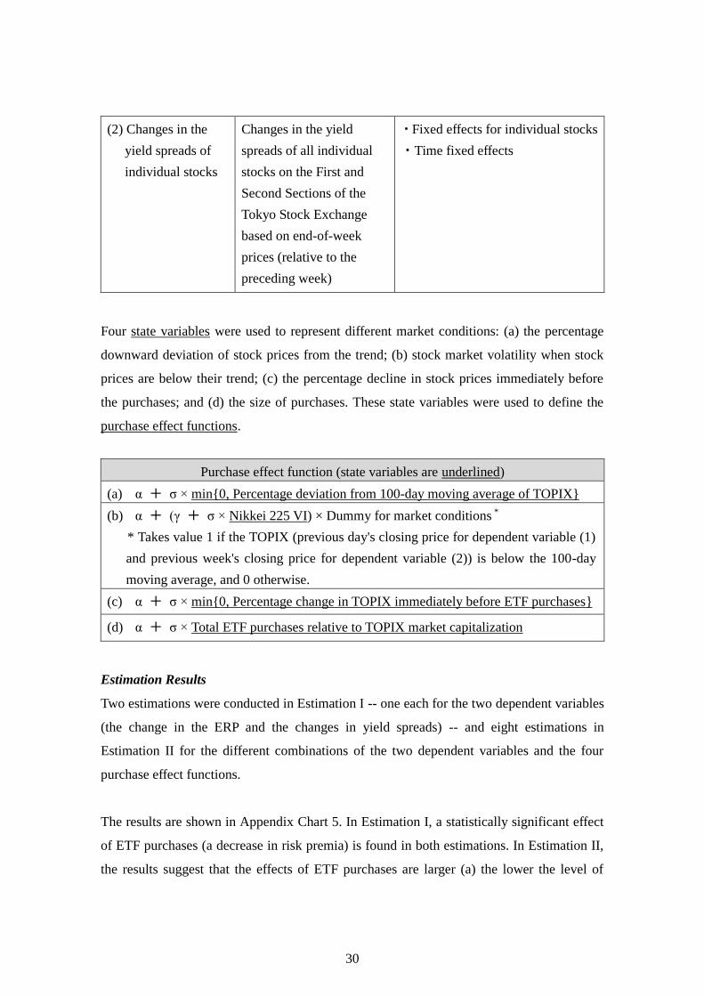
(2) Changes in the
yield spreads of
individual stocks
Changes in the yield
spreads of all individual
stocks on the First and
Second Sections of the
Tokyo Stock Exchange
based on end-of-week
prices (relative to the
preceding week)
・Fixed effects for individual stocks
・Time fixed effects
Four state variables were used to represent different market conditions: (a) the percentage
downward deviation of stock prices from the trend; (b) stock market volatility when stock
prices are below their trend; (c) the percentage decline in stock prices immediately before
the purchases; and (d) the size of purchases. These state variables were used to define the
purchase effect functions.
Purchase effect function (state variables are underlined)
(a) α + σ × min{0, Percentage deviation from 100-day moving average of TOPIX}
(b) α + (γ + σ × Nikkei 225 VI) × Dummy for market conditions *
* Takes value 1 if the TOPIX (previous day's closing price for dependent variable (1)
and previous week's closing price for dependent variable (2)) is below the 100-day
moving average, and 0 otherwise.
(c) α + σ × min{0, Percentage change in TOPIX immediately before ETF purchases}
(d) α + σ × Total ETF purchases relative to TOPIX market capitalization
Estimation Results
Two estimations were conducted in Estimation I -- one each for the two dependent variables
(the change in the ERP and the changes in yield spreads) -- and eight estimations in
Estimation II for the different combinations of the two dependent variables and the four
purchase effect functions.
The results are shown in Appendix Chart 5. In Estimation I, a statistically significant effect
of ETF purchases (a decrease in risk premia) is found in both estimations. In Estimation II,
the results suggest that the effects of ETF purchases are larger (a) the lower the level of

31
stock prices relative to their trend at the time of purchases, (b) the higher the volatility in the
stock market when stock prices are below their trend, (c) the larger the percentage decline in
stock prices immediately before the purchases, and (d) the larger the size of purchases.
32
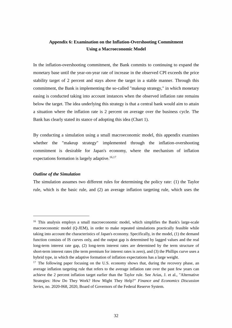
Appendix 6: Examination on the Inflation-Overshooting Commitment
Using a Macroeconomic Model
In the inflation-overshooting commitment, the Bank commits to continuing to expand the
monetary base until the year-on-year rate of increase in the observed CPI exceeds the price
stability target of 2 percent and stays above the target in a stable manner. Through this
commitment, the Bank is implementing the so-called "makeup strategy," in which monetary
easing is conducted taking into account instances when the observed inflation rate remains
below the target. The idea underlying this strategy is that a central bank would aim to attain
a situation where the inflation rate is 2 percent on average over the business cycle. The
Bank has clearly stated its stance of adopting this idea (Chart 1).
By conducting a simulation using a small macroeconomic model, this appendix examines
whether the "makeup strategy" implemented through the inflation-overshooting
commitment is desirable for Japan's economy, where the mechanism of inflation
expectations formation is largely adaptive.16,17
Outline of the Simulation
The simulation assumes two different rules for determining the policy rate: (1) the Taylor
rule, which is the basic rule, and (2) an average inflation targeting rule, which uses the
16 This analysis employs a small macroeconomic model, which simplifies the Bank's large-scale
macroeconomic model (Q-JEM), in order to make repeated simulations practically feasible while
taking into account the characteristics of Japan's economy. Specifically, in the model, (1) the demand
function consists of IS curves only, and the output gap is determined by lagged values and the real
long-term interest rate gap, (2) long-term interest rates are determined by the term structure of
short-term interest rates (the term premium for interest rates is zero), and (3) the Phillips curve uses a
hybrid type, in which the adaptive formation of inflation expectations has a large weight. 17 The following paper focusing on the U.S. economy shows that, during the recovery phase, an
average inflation targeting rule that refers to the average inflation rate over the past few years can
achieve the 2 percent inflation target earlier than the Taylor rule. See Arias, J. et al., "Alternative
Strategies: How Do They Work? How Might They Help?" Finance and Economics Discussion
Series, no. 2020-068, 2020, Board of Governors of the Federal Reserve System.
33
inflation rates over the past few years for reference.18 The second rule is asymmetric, in
that average inflation targeting is followed only when the average inflation rate used for
reference is below 2 percent (see the table below). Moreover, two cases are set for the
natural rate of interest: (a) 0.5 percent, which is close to the average since 2000, and (b) a
lower rate of minus 0.1 percent. The average developments in economic activity and prices
in Japan were gauged by repeating 10 years of simulations for 1,000 times in which the
economic model was subjected to random shocks using the distributions of demand and
price shocks estimated from actual data for Japan's economy.19 Then, the average social
welfare loss function was calculated under each rule.20
Policy Rules Assumed in the Simulation
(1) Taylor rule The policy rate is determined by the difference between the inflation
rate and the inflation target
(Policy rule interest rate)t = (Equilibrium interest rate)t + 1.0 ×
{(Inflation rate)t – Inflation target} + 0.5 × (Output gap)t
(2) Average
inflation
targeting rule
(i) Average inflation rate over N years ≤ Inflation target
The policy rate is determined by the difference between the average
inflation rate over N years and the inflation target
(Policy rule interest rate)t = (Equilibrium interest rate)t + 1.0 × N
× {(Average inflation rate over N years)t – Inflation target} + 0.5
× (Output gap)t
(ii) Average inflation rate over N years > Inflation target
The policy rate is determined by the Taylor rule
18 In the simulation, the policy rule is formulated with lagged values. Specifically, it is specified as
follows: Policy interest ratet = q × Policy interest ratet-1 + (1 – q) × Policy rule interest ratet, q = 0.9.
In addition, the lower bound for interest rates is set to minus 0.1 percent. That is, even if the policy
rate implied by the policy rule falls below minus 0.1 percent, interest rates do not fall below minus
0.1 percent. 19 The initial values for the simulation are set as follows: short-term interest rate = –0.1 percent,
inflation rate = 0.7 percent, output gap = 0.3 percent. The value for the inflation rate is the median of
Policy Board members' forecast for CPI inflation for fiscal 2022 in the January 2021 Outlook for
Economic Activity and Prices, while the output gap is estimated from the long-term relationship
between the output gap and the inflation rate (i.e., the Phillips curve).
20 The loss function is defined in terms of the fluctuations in the output gap and the deviation of the
inflation rate from the inflation target. Specifically, Loss function = Output gap2 + (Inflation rate –
Inflation target of 2 percent)2.
34
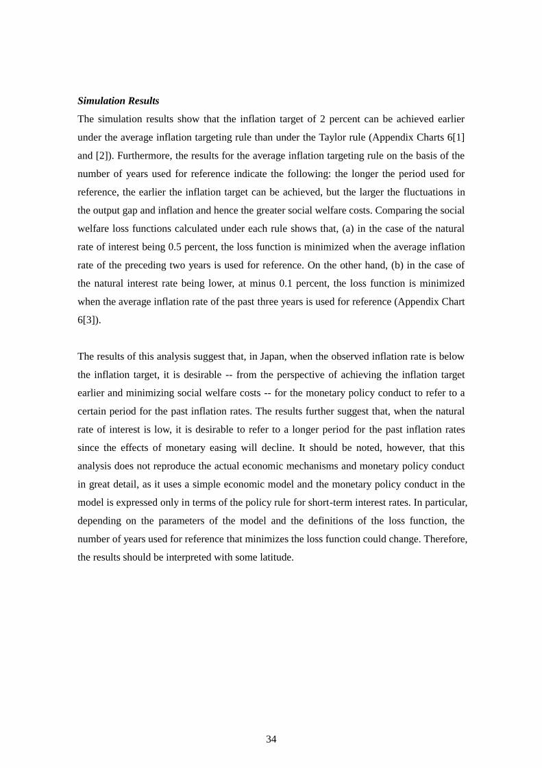
Simulation Results
The simulation results show that the inflation target of 2 percent can be achieved earlier
under the average inflation targeting rule than under the Taylor rule (Appendix Charts 6[1]
and [2]). Furthermore, the results for the average inflation targeting rule on the basis of the
number of years used for reference indicate the following: the longer the period used for
reference, the earlier the inflation target can be achieved, but the larger the fluctuations in
the output gap and inflation and hence the greater social welfare costs. Comparing the social
welfare loss functions calculated under each rule shows that, (a) in the case of the natural
rate of interest being 0.5 percent, the loss function is minimized when the average inflation
rate of the preceding two years is used for reference. On the other hand, (b) in the case of
the natural interest rate being lower, at minus 0.1 percent, the loss function is minimized
when the average inflation rate of the past three years is used for reference (Appendix Chart
6[3]).
The results of this analysis suggest that, in Japan, when the observed inflation rate is below
the inflation target, it is desirable -- from the perspective of achieving the inflation target
earlier and minimizing social welfare costs -- for the monetary policy conduct to refer to a
certain period for the past inflation rates. The results further suggest that, when the natural
rate of interest is low, it is desirable to refer to a longer period for the past inflation rates
since the effects of monetary easing will decline. It should be noted, however, that this
analysis does not reproduce the actual economic mechanisms and monetary policy conduct
in great detail, as it uses a simple economic model and the monetary policy conduct in the
model is expressed only in terms of the policy rule for short-term interest rates. In particular,
depending on the parameters of the model and the definitions of the loss function, the
number of years used for reference that minimizes the loss function could change. Therefore,
the results should be interpreted with some latitude.

35
Charts
1. Charts for Main Text
Chart 1 Quantitative and Qualitative Monetary Easing (QQE) with Yield Curve Control
Chart 2-1 Economic and Financial Developments since the Introduction of QQE with Yield Curve
Control (1)
Chart 2-2 Economic and Financial Developments since the Introduction of QQE with Yield Curve
Control (2)
Chart 3 JGB Yields under Yield Curve Control
Chart 4-1 Effects of JGB Purchases on Nominal Long-Term Interest Rates (1)
Chart 4-2 Effects of JGB Purchases on Nominal Long-Term Interest Rates (2)
Chart 5 Lending, CP and Corporate Bond Rates
Chart 6 Transmission Channel of the Decline in Interest Rates
Chart 7 Effects of Decline in Interest Rates on Economic Activity and Prices
Chart 8 Market Participants' Expectations with Regard to Short-Term Interest Rate Cuts
Chart 9 Financial Conditions under COVID-19 Response Measures
Chart 10 Functioning of the JGB Market
Chart 11 Functioning of Financial Intermediation
Chart 12 Estimation of the Effects of ETF Purchases
Chart 13 Market Participants' Views on ETF Purchases
Chart 14 Amounts of ETFs and J-REITs Held by the Bank
2. Charts for Appendixes
Appendix Chart 1-1 Mechanism behind Inflation Developments in Japan:
International Comparison of Adaptive Expectations Formation
Appendix Chart 1-2 Mechanism behind Inflation Developments in Japan:
Inflation Expectations by Cohort
Appendix Chart 1-3 Mechanism behind Inflation Developments in Japan:
Firms' Inflation Expectations Formation
Appendix Chart 2 Examination on Policy Effects Using the Bank's Macroeconomic Model
(Q-JEM): Counterfactual Simulation
Appendix Chart 3 Impact of Interest Rate Fluctuations on the Real Economy
Appendix Chart 4 Operation of the Complementary Deposit Facility
Appendix Chart 5 Estimation of the Effects of ETF Purchases
Appendix Chart 6 Examination on the Inflation-Overshooting Commitment Using a
Macroeconomic Model

36
Quantitative and Qualitative Monetary Easing (QQE)
with Yield Curve Control
(1) Yield Curve Control (2) Inflation-Overshooting Commitment
(3) Transmission Mechanism of QQE with Yield Curve Control
Chart 1
Sources: Bank of Japan; Bloomberg.
The Bank will continue expanding the
monetary base until the year-on-year rate
of increase in the observed CPI (all items
less fresh food) exceeds the price stability
target of 2 percent and stays above the
target in a stable manner.
Achieving the price stability target means
attaining a situation where the inflation rate
is 2 percent on average over the business
cycle.
(Statement released after the MPM in Sept. 2016)
37
Economic and Financial Developments since the
Introduction of QQE with Yield Curve Control (1)
(1) Nominal Interest Rate (2) Inflation Expectations
(3) Real Interest Rates (4) Bank Lending
(5) Issuance of CP and Corporate Bonds (6) Foreign Exchange Rate and Stock Prices
Notes: 1. Shaded area <I> denotes the period since the introduction of QQE (2013/Q2), <II> denotes the period since the introduction of QQE with Yield Curve Control (2016/Q3), and <III> denotes the period since the outbreak of COVID-19 (2020/Q1).
2. For the synthetic indicator in (2), inflation expectations data for firms are from the Tankan, for households from the "Opinion Survey," and for economists from "Consensus Forecasts."
3. Real interest rates in (3) are calculated as the 10-year Japanese government bond (JGB) yield minus the respective long-term inflation expectations.
4. Figures for the amount outstanding of bank lending in (4) are monthly averages. Lending by domestic commercial banks includes loans to firms, individuals, and local governments. Figures for the bank lending rate are the average contract interest rate on new long-term loans by domestically licensed banks.
5. Figures for CP and corporate bonds in (5) are those at the end of the period. Figures for issuance yields for CP up to September 2009 are the averages for CP (3-month, rated a-1 or higher). Those from October 2009 onward are the averages for CP (3-month, rated a-1). Figures for issuance yields for corporate bonds are the averages for domestically issued bonds launched on a particular date. Bonds issued by banks and securities companies, etc., are excluded. Figures for issuance yields for corporate bonds are 6-month backward moving averages.
Sources: Bank of Japan; Bloomberg; Consensus Economics Inc., "Consensus Forecasts"; QUICK, "QUICK Monthly Market Survey (Bonds)"; Japan Securities Depository Center; Japan Securities Dealers Association; Capital Eye; I-N Information Systems.
Chart 2-1

38
Economic and Financial Developments since the
Introduction of QQE with Yield Curve Control (2)
(7) Corporate Profits (8) Unemployment Rate
(9) Output Gap (10) Wages
(11) Consumer Price Index (CPI)
-1
0
1
2
3
4
5
07 09 11 13 15 17 19
Base pay increase
Scheduled cash earnings
(full-time employees)
Hourly scheduled cash earnings
(part-time employees)
y/y % chg.
FY
Notes: 1. Figures for current profits in (7) are based on the "Financial Statements Statistics of Corporations by Industry, Quarterly," excluding "finance and insurance." Figures from 2009/Q2 onward exclude "pure holding companies."
2. Figures for scheduled cash earnings in (10) from 2016/Q1 onward are based on continuing observations following sample revisions.
3. Figures for the CPI (less fresh food and energy) in (11) exclude the effects of the consumption tax hikes, policies concerning the provision of free education, and the "Go To Travel" campaign, which covers a portion of domestic travel expenses. The figures from April 2020 onward are based on staff estimations and exclude the effects of measures such as free higher education introduced in April 2020. Figures for the CPI (less fresh food) exclude the effects of the consumption tax hikes in April 1989, April 1997, and April 2014.
Sources: Ministry of Finance; Ministry of Internal Affairs and Communications; Bank of Japan; Ministry of Health, Labour and Welfare; Japanese Trade Union Confederation (Rengo).
Chart 2-2

39
JGB Yields under Yield Curve Control
(1) JGB Yields
(2) The Bank's JGB Holdings by Residual Maturity (Amount Outstanding)
Notes: 1. I: Introduction of QQE (Apr. 2013), II: Expansion of QQE (Oct. 2014), III: Introduction of QQE with a Negative Interest Rate (Jan. 2016), IV: Introduction of QQE with Yield Curve Control (Sept. 2016), V: Strengthening the Framework for Continuous Powerful Monetary Easing (July 2018), VI: Enhancement of Monetary Easing in Light of the Impact of the Outbreak of the Novel Coronavirus (Mar. 2020).
2. Figures for overnight yields in (1) are the uncollateralized overnight call rate.
3. Figures in (2) exclude T-Bills, floating-rate JGBs, and inflation-indexed JGBs.
Sources: Bloomberg; Bank of Japan.
Chart 3

40
Effects of JGB Purchases
on Nominal Long-Term Interest Rates (1)
(1) Estimation Using Difference between Counterfactual and Actual Paths of 10-Year JGB Yields
(a) Estimation Result
(b) Estimated and Actual 10-year JGB Yields
Notes: 1. ** and * denote statistical significance at the 1 percent and 5 percent levels, respectively.
2. The CPI figures used in the estimations exclude the effects of the consumption tax hikes, policies concerning the provision of free education, and the "Go To Travel" campaign, which covers a portion of domestic travel expenses. The figures from April 2020 onward are based on staff estimations and exclude the effects of measures such as free higher education introduced in April 2020.
Sources: Ministry of Health, Labour and Welfare; Ministry of Internal Affairs and Communications; Bloomberg.
JGB yields (10-year, %)
= 0.22 *
+ 0.26 **
× Active job openings-to-applicants ratio
+ 0.10 **
× CPI (all items less fresh food, y/y change, %)
+ 0.25 **
× U.S. Treasury bond yields (10-year, %)
Estimation period: Jan. 1997 to Mar. 2013. Adjusted R-squared: 0.71.
Lagged values (lag order: 1) are used for the active job openings-to-applicants ratio and the CPI.
Chart 4-1
Using data before the introduction of QQE, the Bank conducted linear regression analysis
employing 10-year JGB yields as an independent variable and the following three variables as
dependent variables: the active job openings-to-applicants ratio, the CPI, and U.S. Treasury bond
yields (10-year). Using the estimation results, the Bank estimated the counterfactual path that 10-
year JGB yields would have followed if QQE had not been introduced. The difference between the
counterfactual and actual paths of 10-year JGB yields is regarded as the effects of the Bank's JGB
purchases on 10-year yields since the introduction of QQE.
As shown in (b) below, the counterfactual estimates of 10-year JGB yields have been at around 1
percent on average. Actual figures for 10-year JGB yields under yield curve control have been
stable at around 0 percent. The policy effects as implied in the difference between the counterfactual
estimates and the actual figures are estimated to be around minus 1 percentage point.

41
Effects of JGB Purchases
on Nominal Long-Term Interest Rates (2)
(2) Estimation Using the Bank's Share of JGB Holdings
(a) Estimation Result
(b) Decomposition of 10-year JGB Yields
-1.5
-1.0
-0.5
0.0
0.5
1.0
1.5
12 13 14 15 16 17 18 19 20 21
%
CY
JGB yields
Constant
U.S. Treasury bond yieldsResidual
Expected real GDP growth rateThe Bank's share of JGB holdings
JGB yields (10-year, %)
= 0.25 *
+ 0.16 * × U.S. Treasury bond yields (10-year, %)
+ 0.45 * × Expected real GDP growth rate (%)
- 0.02 **
× The Bank's share of JGB holdings (%)
Estimation period: Jan. 2005 to Feb. 2021. Adjusted R-squared: 0.95.
Newey-West standard errors are used.
Chart 4-2
The Bank conducted linear regression analysis employing 10-year JGB yields as an independent
variable and the following three variables as dependent variables: the Bank's share of JGB holdings,
U.S. Treasury bond yields (10-year), and the expected real GDP growth rate. The changes in 10-
year JGB yields that are attributable to the Bank's share of JGB holdings are regarded as the effects
of the Bank's JGB purchases on 10-year yields.
Looking at developments in 10-year JGB yields shown in (b) below, the contribution of the
Bank's share of JGB holdings to 10-year JGB yields expanded, pushing down the yields by about
1 percentage point as the Bank's share increased. The contribution has generally remained the
same thereafter.
Notes 1. ** and * denote statistical significance at the 1 percent and 5 percent levels, respectively.
2. The Bank's share of JGB holdings is calculated taking into account changes in the average residual maturity. The expected real GDP growth rate and the Bank's share of JGB holdings are converted to monthly data mainly using quarterly data. The expected real GDP growth rate is the forecast for the next 6-10 years.
Sources: Bloomberg; Consensus Economics Inc., "Consensus Forecasts"; Bank of Japan; Ministry of Finance.

42
Lending, CP and Corporate Bond Rates
(1) Average Contract Interest Rates on New Loans and Discounts
(2) Issuance Yields for CP
(3) Issuance Yields for Corporate Bonds
Notes: 1. The vertical lines denote the introduction of QQE (Apr. 2013) and the introduction of QQE with Yield Curve Control (Sept. 2016).
2. Figures for issuance yields for corporate bonds in (3) are obtained by adding yields on 5-year JGBs to the average issuance spreads for domestically issued bonds launched on a particular date. Bonds issued by banks and securities companies, etc., are excluded. Bonds are classified based on the highest rating among the ratings from Moody's, S&P, R&I, and JCR.
Sources: Bank of Japan; Japan Securities Depository Center; Capital Eye; I-N Information Systems; Bloomberg.
Chart 5

43
Transmission Channel of the Decline in Interest Rates
(1) Model
(2) Overview of Transmission Channel of a Decline in Interest Rates
(3) Improvement in the Output Gap through the Decline in Interest Rates by Channel
A VAR model with coefficient restrictions using the following eight variables is estimated.
1. Output gap, 2. Interest rates (3-month),
3. Interest rate spread (2-year minus 3-month),
4. Interest rate spread (5-year minus 2-year),
5. Interest rate spread (10-year minus 5-year), 6. Aggregate funding costs,
7. Nominal effective exchange rate of the yen, 8. Stock prices
Estimation period: 1998/Q1-2019/Q4. Lag order: 1.
Calculated as the 5-year cumulative impact on the output gap.
Chart 6
The Bank used a vector-autoregressive (VAR) model with coefficient restrictions to estimate through
which transmission channels a decline in interest rates improves the output gap. Specifically, the
effects of each transmission channel (shaded area in (2) and the variables numbered 6 to 8) are
calculated by imposing the restriction that the coefficients of other transmission channels are zero.
The transmission channel through which a decline in interest rates improves the output gap via
funding costs accounts for more than 30 percent of the effects on the output gap, while that via
financial and capital markets (foreign exchange rate and stock prices) accounts for more than 50
percent.
Channel via financial
and capital markets
Notes: 1. Aggregate funding costs are the weighted average of bank lending rates and issuance yields for CP and corporate bonds.
2. Figures in (3) show the 5-year cumulative effects.
Sources: Bank of Japan; Bloomberg, etc.
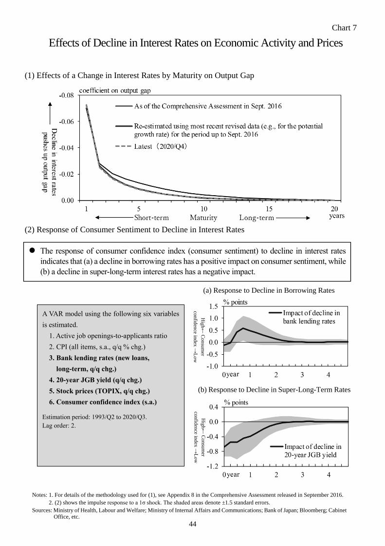
44
Effects of Decline in Interest Rates on Economic Activity and Prices
(1) Effects of a Change in Interest Rates by Maturity on Output Gap
(2) Response of Consumer Sentiment to Decline in Interest Rates
(a) Response to Decline in Borrowing Rates
(b) Response to Decline in Super-Long-Term Rates
A VAR model using the following six variables
is estimated.
1. Active job openings-to-applicants ratio
2. CPI (all items, s.a., q/q % chg.)
3. Bank lending rates (new loans,
long-term, q/q chg.)
4. 20-year JGB yield (q/q chg.)
5. Stock prices (TOPIX, q/q chg.)
6. Consumer confidence index (s.a.)
Estimation period: 1993/Q2 to 2020/Q3.
Lag order: 2.
Chart 7
The response of consumer confidence index (consumer sentiment) to decline in interest rates
indicates that (a) a decline in borrowing rates has a positive impact on consumer sentiment, while
(b) a decline in super-long-term interest rates has a negative impact.
Notes: 1. For details of the methodology used for (1), see Appendix 8 in the Comprehensive Assessment released in September 2016.
2. (2) shows the impulse response to a 1σ shock. The shaded areas denote ±1.5 standard errors.
Sources: Ministry of Health, Labour and Welfare; Ministry of Internal Affairs and Communications; Bank of Japan; Bloomberg; Cabinet Office, etc.
Hig
h←
Co
nsu
mer
con
fiden
ce ind
ex →
Lo
w
Hig
h←
Co
nsu
mer
con
fiden
ce ind
ex →
Lo
w

45
Market Participants' Expectations with Regard to
Short-Term Interest Rate Cuts
(1) Share of Respondents Expecting Additional Easing and Short-Term Interest Rate Cut in a
Survey of Economists
(2) Share of Respondents Expecting Short-Term Interest Rate Cut among Those Expecting
Additional Easing (B/A)
Chart 8
Notes: 1. Based on a survey conducted by Bloomberg before each Monetary Policy Meeting. "Expect additional easing" in (1) is the sum of all respondents expecting the next policy change of the Bank to be additional easing, regardless of when they expect it to be implemented. "Expect short-term interest rate cut" is the sum of all respondents expecting the Bank to cut the short-term policy interest rate in the future.
2. (2) shows the share of respondents expecting the Bank to cut short-term interest rates in the future (B) among those expecting additional easing as the Bank's next policy change (A). Although not all those who responded with (B) also responded with (A), the calculation here assumes that they did. For 2016, results from the January survey before the introduction of the negative interest rate policy are excluded.
Source: Bloomberg.
The share of respondents in a survey of market participants expecting short-term interest rate cuts
to be an option for additional easing (B in chart (1)) among those expecting additional easing (A in
chart (1)) shows that, as indicated in (2), the share has decreased recently to about 20 percent from
about 70 percent, which was the share immediately after the introduction of the negative interest
rate policy.
Anecdotal information suggests that an increasing number of those who are not expecting interest
rate cuts tend to point to the impact on the functioning of financial intermediation.
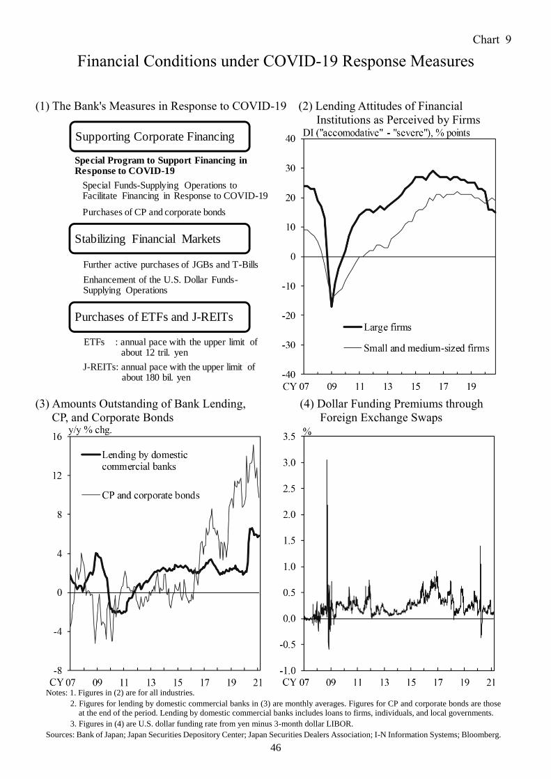
46
Financial Conditions under COVID-19 Response Measures
(1) The Bank's Measures in Response to COVID-19 (2) Lending Attitudes of Financial
Institutions as Perceived by Firms
(3) Amounts Outstanding of Bank Lending, (4) Dollar Funding Premiums through
CP, and Corporate Bonds Foreign Exchange Swaps
ETFs : annual pace with the upper limit of about 12 tril. yen
Special Program to Support Financing inResponse to COVID-19
Special Funds-Supplying Operations toFacilitate Financing in Response to COVID-19
Purchases of CP and corporate bonds
Further active purchases of JGBs and T-Bills
Enhancement of the U.S. Dollar Funds-Supplying Operations
Supporting Corporate Financing
Stabilizing Financial Markets
Purchases of ETFs and J-REITs
J-REITs: annual pace with the upper limit of about 180 bil. yen
Notes: 1. Figures in (2) are for all industries.
2. Figures for lending by domestic commercial banks in (3) are monthly averages. Figures for CP and corporate bonds are those at the end of the period. Lending by domestic commercial banks includes loans to firms, individuals, and local governments.
3. Figures in (4) are U.S. dollar funding rate from yen minus 3-month dollar LIBOR.
Sources: Bank of Japan; Japan Securities Depository Center; Japan Securities Dealers Association; I-N Information Systems; Bloomberg.
Chart 9

47
Functioning of the JGB Market
(1) 10-Year JGB Yields (2) Range of Fluctuations in JGB Yields
(3) Transaction Volume in the JGB Market (4) Bond Market Survey (Market Functioning)
(5) Sensitivity of JGB Yields (to U.S., 10Y) (6) Sensitivity of JGB Yields (to Germany, 10Y)
Notes: 1. I: Introduction of QQE with Yield Curve Control (Sept. 2016), II: Strengthening the Framework for Continuous Powerful Monetary Easing (July 2018), III: Enhancement of Monetary Easing in Light of the Impact of the Outbreak of the Novel Coronavirus (COVID-19) (Mar. 2020).
2. (2) shows the difference between the maximum and minimum values in JGB yields in the preceding 6-months.
3. (3) shows the gross amount of outright purchases by banks, investors, and bond dealers.
4. (5) and (6) show rolling regression estimates for 90-day windows. The shaded areas represent ±1 standard errors.
Sources: Bloomberg; Japan Securities Dealers Association; Bank of Japan.
Chart 10

48
Functioning of Financial Intermediation
(1) Domestic Deposit-Lending Margins (2) Balance Sheet of Domestic Banks
(3) Net Income of Banks
(a) Major Financial Groups (b) Regional Banks
-3
-2
-1
0
1
2
3
06 08 10 12 14 16 18Others Tax-related expensesRealized gains/losses on stockholdings Realized gains/losses on bondholdingsCredit costs Pre-provision net revenue (excluding trading income)Net income
tril. yen
FY
-6
-4
-2
0
2
4
6
06 08 10 12 14 16 18FY
tril. yen
0
200
400
600
800
1,000
1,200
1,400
1,600
Stockholders' equityOther liabilitiesDepositsOther assetsInvestment securities other than central government securitiesCentral government securitiesLoans and bills discounted
tril. yen
2012 20202015year-end
Chart 11
Notes: 1. The vertical lines in (1) indicate the introduction of QQE (Apr. 2013), the introduction of QQE with a Negative Interest Rate (Jan. 2016), and the introduction of QQE with Yield Curve Control (Sept. 2016), respectively.
2. Figures for (2) are based on accounts held in Japan.
3. Figures for major financial groups in (3) are on a consolidated basis. From fiscal 2012, profits from investment trusts due to cancellations are excluded from "pre-provision net revenue (excluding trading income)."
Sources: Bloomberg; published accounts of each bank; Bank of Japan.

49
Estimation of the Effects of ETF Purchases
Chart 12
Estimation I:
Test whether ETF purchases have a significant effect on risk premia in the stock market.
Statistically significant effect found.
Estimation II:
Test whether the effects of ETF purchases on risk premia in the stock market differ
depending on market conditions at the time of purchases and on the size of purchases (four
cases).
The results indicate that the more volatile the market and the larger the size of
purchases, the larger the effects of ETF purchases per single amount.
Note: See Appendix 5 for details.
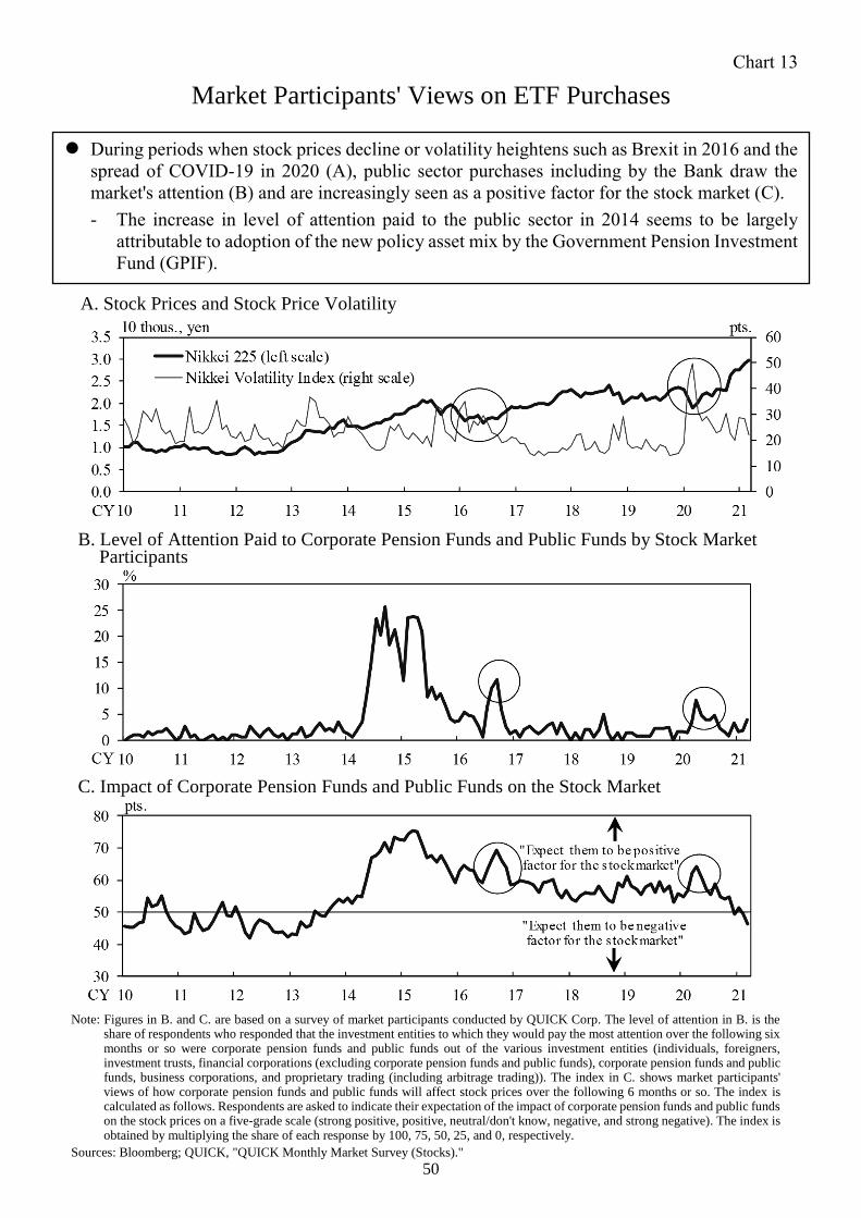
50
Market Participants' Views on ETF Purchases
A. Stock Prices and Stock Price Volatility
B. Level of Attention Paid to Corporate Pension Funds and Public Funds by Stock Market Participants
C. Impact of Corporate Pension Funds and Public Funds on the Stock Market
Chart 13
During periods when stock prices decline or volatility heightens such as Brexit in 2016 and the
spread of COVID-19 in 2020 (A), public sector purchases including by the Bank draw the
market's attention (B) and are increasingly seen as a positive factor for the stock market (C).
- The increase in level of attention paid to the public sector in 2014 seems to be largely
attributable to adoption of the new policy asset mix by the Government Pension Investment
Fund (GPIF).
Note: Figures in B. and C. are based on a survey of market participants conducted by QUICK Corp. The level of attention in B. is the share of respondents who responded that the investment entities to which they would pay the most attention over the following six months or so were corporate pension funds and public funds out of the various investment entities (individuals, foreigners, investment trusts, financial corporations (excluding corporate pension funds and public funds), corporate pension funds and public funds, business corporations, and proprietary trading (including arbitrage trading)). The index in C. shows market participants' views of how corporate pension funds and public funds will affect stock prices over the following 6 months or so. The index is calculated as follows. Respondents are asked to indicate their expectation of the impact of corporate pension funds and public funds on the stock prices on a five-grade scale (strong positive, positive, neutral/don't know, negative, and strong negative). The index is obtained by multiplying the share of each response by 100, 75, 50, 25, and 0, respectively.
Sources: Bloomberg; QUICK, "QUICK Monthly Market Survey (Stocks)."

51
Amounts of ETFs and J-REITs Held by the Bank
(1) ETFs
(2) J-REITs
Chart 14
Sources: JPX; The Association for Real Estate Securitization; Bank of Japan.
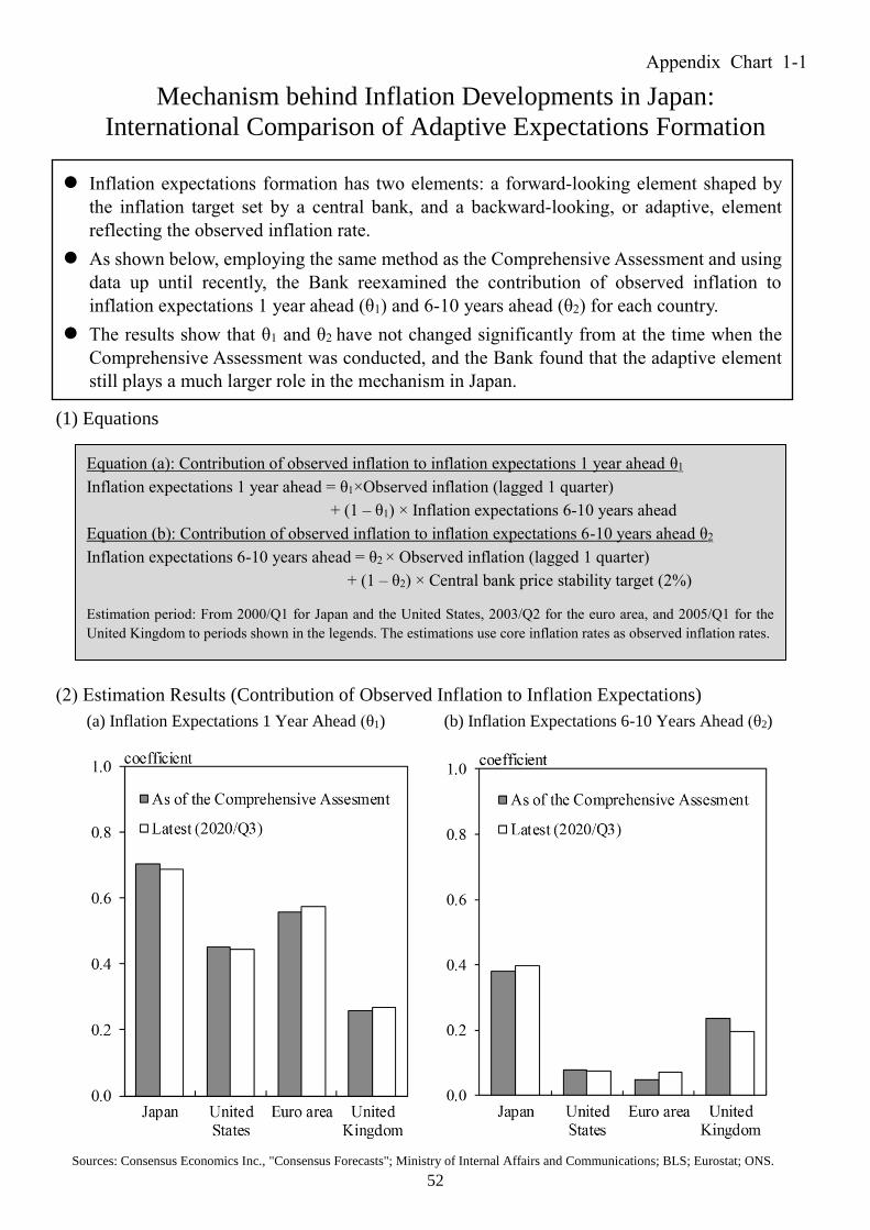
52
Mechanism behind Inflation Developments in Japan:
International Comparison of Adaptive Expectations Formation
(1) Equations
(2) Estimation Results (Contribution of Observed Inflation to Inflation Expectations)
(a) Inflation Expectations 1 Year Ahead (θ1) (b) Inflation Expectations 6-10 Years Ahead (θ2)
Equation (a): Contribution of observed inflation to inflation expectations 1 year ahead θ1
Inflation expectations 1 year ahead = θ1×Observed inflation (lagged 1 quarter)
+ (1 – θ1) × Inflation expectations 6-10 years ahead
Equation (b): Contribution of observed inflation to inflation expectations 6-10 years ahead θ2
Inflation expectations 6-10 years ahead = θ2 × Observed inflation (lagged 1 quarter)
+ (1 – θ2) × Central bank price stability target (2%)
Estimation period: From 2000/Q1 for Japan and the United States, 2003/Q2 for the euro area, and 2005/Q1 for the
United Kingdom to periods shown in the legends. The estimations use core inflation rates as observed inflation rates.
Appendix Chart 1-1
Inflation expectations formation has two elements: a forward-looking element shaped by
the inflation target set by a central bank, and a backward-looking, or adaptive, element
reflecting the observed inflation rate.
As shown below, employing the same method as the Comprehensive Assessment and using
data up until recently, the Bank reexamined the contribution of observed inflation to
inflation expectations 1 year ahead (θ1) and 6-10 years ahead (θ2) for each country.
The results show that θ1 and θ2 have not changed significantly from at the time when the
Comprehensive Assessment was conducted, and the Bank found that the adaptive element
still plays a much larger role in the mechanism in Japan.
Sources: Consensus Economics Inc., "Consensus Forecasts"; Ministry of Internal Affairs and Communications; BLS; Eurostat; ONS.
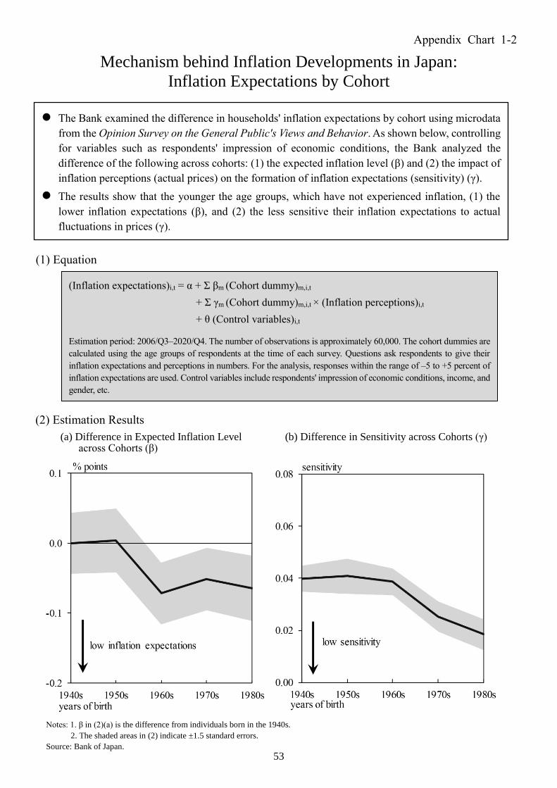
53
Mechanism behind Inflation Developments in Japan:
Inflation Expectations by Cohort
(1) Equation
(2) Estimation Results
(a) Difference in Expected Inflation Level (b) Difference in Sensitivity across Cohorts (γ) across Cohorts (β)
(Inflation expectations)i,t = α + Σ βm (Cohort dummy)m,i,t
+ Σ γm (Cohort dummy)m,i,t × (Inflation perceptions)i,t
+ θ (Control variables)i,t
Estimation period: 2006/Q3–2020/Q4. The number of observations is approximately 60,000. The cohort dummies are
calculated using the age groups of respondents at the time of each survey. Questions ask respondents to give their
inflation expectations and perceptions in numbers. For the analysis, responses within the range of –5 to +5 percent of
inflation expectations are used. Control variables include respondents' impression of economic conditions, income, and
gender, etc.
Appendix Chart 1-2
The Bank examined the difference in households' inflation expectations by cohort using microdata
from the Opinion Survey on the General Public's Views and Behavior. As shown below, controlling
for variables such as respondents' impression of economic conditions, the Bank analyzed the
difference of the following across cohorts: (1) the expected inflation level (β) and (2) the impact of
inflation perceptions (actual prices) on the formation of inflation expectations (sensitivity) (γ).
The results show that the younger the age groups, which have not experienced inflation, (1) the
lower inflation expectations (β), and (2) the less sensitive their inflation expectations to actual
fluctuations in prices (γ).
Notes: 1. β in (2)(a) is the difference from individuals born in the 1940s.
2. The shaded areas in (2) indicate ±1.5 standard errors.
Source: Bank of Japan.
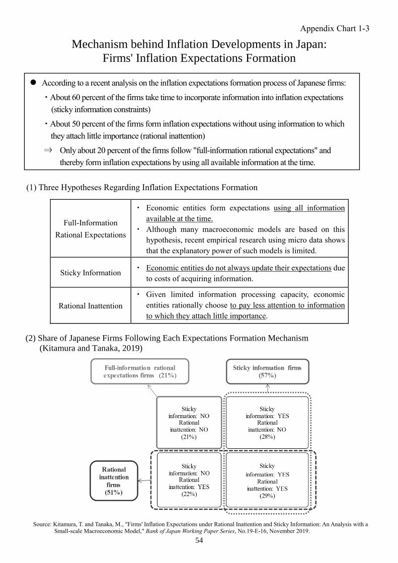
54
Mechanism behind Inflation Developments in Japan:
Firms' Inflation Expectations Formation
(1) Three Hypotheses Regarding Inflation Expectations Formation
Full-Information
Rational Expectations
・ Economic entities form expectations using all information
available at the time.
・ Although many macroeconomic models are based on this
hypothesis, recent empirical research using micro data shows
that the explanatory power of such models is limited.
Sticky Information ・ Economic entities do not always update their expectations due
to costs of acquiring information.
Rational Inattention
・ Given limited information processing capacity, economic
entities rationally choose to pay less attention to information
to which they attach little importance.
(2) Share of Japanese Firms Following Each Expectations Formation Mechanism
(Kitamura and Tanaka, 2019)
Appendix Chart 1-3
According to a recent analysis on the inflation expectations formation process of Japanese firms:
・About 60 percent of the firms take time to incorporate information into inflation expectations
(sticky information constraints)
・About 50 percent of the firms form inflation expectations without using information to which
they attach little importance (rational inattention)
⇒ Only about 20 percent of the firms follow "full-information rational expectations" and
thereby form inflation expectations by using all available information at the time.
Source: Kitamura, T. and Tanaka, M., "Firms' Inflation Expectations under Rational Inattention and Sticky Information: An Analysis with a Small-scale Macroeconomic Model," Bank of Japan Working Paper Series, No.19-E-16, November 2019.

55
Examination on Policy Effects Using the Bank's
Macroeconomic Model (Q-JEM): Counterfactual Simulation
(1) Real GDP (2) Output Gap
(3) CPI (less fresh food and energy) (4) Policy Effects
(average since the introduction of QQE)
Note: For details of simulations A to E, see the main text of Appendix 2.
Sources: Cabinet Office; Bank of Japan; Ministry of Internal Affairs and Communications, etc.
Appendix Chart 2

56
Impact of Interest Rate Fluctuations on the Real Economy
(1) Range of Fluctuations in JGB Yields (max. – min. within past 6-months)
(2) Impact of Interest Rate Fluctuations on Business Fixed Investment
(Sensitivity to Real Interest Rate Gap <β1+β2>)
Appendix Chart 3
Note: Figures for the real interest rate gap in (2) are calculated using the natural yield curve model (10-year).
The vertical bands indicate ±1.5 standard errors.
Sources: Bloomberg; Consensus Economics Inc., "Consensus Forecasts"; Economic Policy Uncertainty; Cabinet Office.
← Small Range of fluctuations in interest rates Large →
0.25%points 0.25 0.36 more than
or less to 0.36%points to 0.51%points 0.51%points
Range of
fluctuations in
interest rates

57
Operation of the Complementary Deposit Facility
(1) Unused Amounts of Macro Add-on Balances, etc. and the Policy-Rate Balances
(2) Amounts of Macro Add-on Balances and their Breakdown
(3) Benchmark Ratio
Appendix Chart 4
Note: Figures for unused amounts in (1) include unused amounts of Basic Balances.
Source: Bank of Japan.

58
Estimation of the Effects of ETF Purchases
Dependent variable (risk premia in the stock market)
(a) Change in the equity risk premia
implied by option prices
(b) Changes in the yield spreads of
individual stocks
Estimation I Coefficient of the purchase volume indicator
θ: -5.06*
Coefficient of the purchase volume indicator
θ: -0.85*
Estim
ation II: P
urch
ases effect functio
n (state v
ariable)
(a) % d
ow
nw
ard d
eviatio
n o
f
stock
prices fro
m th
e trend
Coefficient of state variable σ: 0.69* Coefficient of state variable σ: 0.18*
(b) S
tock
mark
et volatility
Coefficient of state variable × dummy for market
condition σ: -0.49*
Coefficient of state variable × dummy for market
condition σ: -0.07*
(c) % d
ecline in
stock
price
s
imm
ediately
befo
re the p
urch
ases Coefficient of state variable σ: -1.51
Coefficient of state variable σ: 0.22*
(d) S
ize of p
urch
ases
Coefficient of state variable σ: -137.71
Coefficient of state variable σ: -16.66*
Note: * indicates that the variable is statistically significant at the 5 percent level.
Sources: Bloomberg; QUICK; JPX.
Appendix Chart 5

59
Examination on the Inflation-Overshooting Commitment Using a Macroeconomic Model
(1) Natural Rate of Interest: +0.5%
(a) Output Gap (b) Inflation Rate
(2) Natural Rate of Interest: -0.1%
(a) Output Gap (b) Inflation Rate
(3) Average Losses Calculated in Simulations under Each Rule
Loss function
(a) Natural rate of interest:
+0.5%
(b) Natural rate of interest:
-0.1%
(a) Taylor rule 5.40 7.21
(b) Average
inflation
targeting rule
1 year average 5.31 7.02
2 year average 4.84 6.01
3 year average 5.01 5.83
4 year average 5.34 5.86
Sources: Bank of Japan; Ministry of Internal Affairs and Communications, etc.
Appendix Chart 6
Related Documents


