i Assessment and Modeling of Surface Water Quality Dynamics in Awash River basin, Ethiopia A Dissertation by AMARE SHIBERU KERAGA Submitted to the School of Chemical and Bio-Engineering in Partial Fulfillment of the Requirements for the Degree of DOCTOR OF PHILOSOPHY (ENVIRONMENTAL ENGINEERING) Advisors: Dr. Ing. Zebene Kiflie (Main supervisor) Dr. Agizew Nigussie Addis Ababa Institute of Technology, Addis Ababa University Addis Ababa, Ethiopia 2019

Welcome message from author
This document is posted to help you gain knowledge. Please leave a comment to let me know what you think about it! Share it to your friends and learn new things together.
Transcript

i
Assessment and Modeling of Surface Water Quality Dynamics in
Awash River basin, Ethiopia
A Dissertation
by
AMARE SHIBERU KERAGA
Submitted to the School of Chemical and Bio-Engineering
in Partial Fulfillment of the Requirements for the Degree of
DOCTOR OF PHILOSOPHY (ENVIRONMENTAL ENGINEERING)
Advisors: Dr. Ing. Zebene Kiflie (Main supervisor)
Dr. Agizew Nigussie
Addis Ababa Institute of Technology, Addis Ababa University
Addis Ababa, Ethiopia
2019

i
Addis Ababa University
School of Graduate Studies
School of Chemical and Bio Engineering
Environmental Engineering Post Graduate Program
As members of Examining Board of the final PhD Dissertation public defense, we certify that
we have read and evaluated the dissertation prepared by Amare Shiberu, titled “Assessment
and Modeling of Surface Water Quality Dynamics in Awash River basin, Ethiopia” and
recommended that it can be accepted as fulfilling the dissertation requirements for the Doctor
of Philosophy in Chemical Engineering (Environmental Engineering Stream).
By: AMARE SHIBERU KERAGA
Approved by the Examining Board: Signature Date
Dr. Ing. Zebene Kiflie __________________ ________________
Main Advisor
Dr. Agizew Nigussie _ __________________ ________________
Co-Advisor
Prof. Assefa M. Melesse __________________ ________________
External Examiner
Dr. Nigus Gabbiye_Habtu __________________ ________________
Internal Examiner
__________________________________ __________________ ________________
School Dean
ii
Abstract
Awash River has the most important economic values in Ethiopia. However, it has been
recognized as being impaired by high amount of various pollutants owing to waste released
from different socio-economic activities in its basin since the basin encompasses the main
urban, industrial and agricultural centers of the nation. However, investigation of pollution
level of the basin is necessary for decision makers to safeguard Awash River and its end users,
which has not been addressed yet. This research was therefore aimed at evaluating the status,
assessing the spatial-temporal dynamics and modeling surface water quality dynamics in
relation to different land use scenarios in Awash River basin.
Status of water quality of Awash River was evaluated with respect to drinking and irrigation
water uses by choosing 17 sample sites along the River based on accessibility and land use
severity and sampling was done twice in each of the dry and wet seasons. Then both onsite and
offsite water quality analyses were undertaken following standard procedures. After
comparing different water quality indices in use todate, Canadian council of ministers of
environment water quality index was applied to compute the water quality indices. The
drinking and irrigation water quality indices of the upper basin were 34.79 and 46.39
respectively, which were in the poor and marginal categories of the Canadian water quality
ranking. Similarly, the respective indices for the middle/lower basin, which were 32.25 and
62.78, lie in the same ranges of the ranking. Although the difference in the used dataset of the
two cases and natural purification in the course of the River might contribute to the difference
in WQI, it is generally conceivable that the water quality of the River is below the fair rank.
To assess the spatial and temporal variation of water quality in the basin, means of the 9 years’
(2005-2013) water quality dataset of 19 parameters from 10 stations in the basin were used.
After validating, normalizing and checking the sampling adequacy and internal consistency of
the data, principal component analysis was computed and four principal components were
generated. Factor loadings, correlations between variables and the principal factors as well
as between sites and the principal factors were tabulated. Agglomerative hierarchical
clustering done on the dataset resulted in four clusters based on similarity of water quality
characteristics. The Mann-Kendall’s two tailed trend test detected temporal trends for total
hardness in February over all sites and for most parameters in the basin in the 9 years period.
Spatial analysis of the 14 sampling sites of the basin showed that as one moves from upper to
lower parts of the basin, electrical conductivity, total hardness and chloride levels decrease in

iii
the dry season. However, total hardness slightly increases and total dissolved solids, chloride,
and sulfate content decrease in the rainy season. Cl- and EC/TDS/SO4- are maximized
respectively at before Beseka and Beseka in both seasons and Beseka, before Beseka and
Sodere spring are found to be important sites responsible for the spatial variation.
To see the relation between land use/land cover (LULC) and water quality in the basin, LULC
dynamics was assessed by using cloud-free LS 5 and 7 TM imageries of 1994, 2000 and 2014.
The images were captured from EROS center of USGS GloVis viewer and classified by
supervised classification coupled with maximum likelihood algorithm in ERDAS Imagine. The
dominant LULC of the eight identified land use types were agriculture, barren land, and shrub-
land in the 3 years’ period. Built-up and water bodies were found to have increased and
decreased respectively by about 147% and 63% as one goes from 1994 to 2014.
Moreover, in line with the changes in land use specifically of urbanization and agricultural
intensification from 2000 to 2014, around which water quality have been analyzed, the
parameters EC, TDS, Alkalinity, TH, SO42-, Na+, Cl-, K+, and NH3 were found to increase
monotonically. Mean values of water quality indicators such as EC, nitrate, and some anions
have been compared in the agriculture-dominated, industry-dominated and urban-dominated
land uses. As a result, EC within the urban and industrial land uses was found to be maximized.
Nitrate, on the contrary, is observed to be higher in agriculture-dominated land uses and
higher concentration of anions (bicarbonates and chlorides) and hardness have been
generated from urbanized areas.
This study also evaluated performance of the Soil and Water Assessment Tool (SWAT) by
modeling nitrate and phosphate at the basin scale. First, the model was set up using digital
elevation model (DEM), climate, soil, and land use data. Thereafter, overall performance of
the model was assessed by linking its outputs to the Sequential Uncertainty FItting Version 2
(SUFI2) procedure of the SWAT Calibration and Uncertainty Program (SWAT-CUP). The
most sensitive parameters for the flow and nutrients were identified using t-stat and p-values
from global sensitivity analysis of the SWAT-CUP. The goodness-of-fit of the monthly
calibration measured by coefficient of determination (R2), Nash-Sutcliffe Efficiency (NSE), and
root mean square error-observations standard deviation ratio (RSR) were respectively 0.79,
0.64 and 0.60 for flow; 0.73, 0.71 and 0.54 for nitrate and 0.77, 0.76 and 0.49 for phosphate.
During validation, R2, NSE and RSR were respectively 0.81, 0.52 and 0.70 for flow; 0.68, 0.63

iv
and 0.61 for nitrate and 0.82, 0.81 and 0.44 for phosphate. The results suggested that the model
is promising to predict nutrients in the basin.
From the modeling, concentrations of nutrients were found to be both seasonally and spatially
variable. Sub-basins 4, 8, 13, 21 and 39 were hotspots both in 1994 and 2014 with respect to
exporting higher amounts TN and TP. From the temporal investigation of nutrients’ monthly
averages in the period from 1997 to 2014 of sub-basin 3, the rainy months (March, July and
August) export higher amounts. Basin-wide comparison of the monthly averages of nitrate,
phosphate, TN and TP losses from the model simulations with the 2000 and 2014 LU’s indicate
that the respective values were generally greater in 2014 than in 2000. From the trends of TN
and TP for each of the 53 sub-basins in 1994, 2000 and 2014, slight reduction was observed
for the year 2000 as compared to that in 1994. However, since the increment from 2000 to
2014 was significant, the overall trend from 1994 to 2014 was found to be positive (increasing).
Results of the study have applications of filling the existing knowledge gap, facilitating
informed decision making, using as a customizable framework for similar studies in other river
basins of the nation.
Keywords: Agglomerative hierarchical clustering, Awash River basin, CCME WQI, Drinking,
Ethiopia, Irrigation, Land use/Land cover, Mann-Kendall’s trend, model, nutrients, principal
component analysis, spatial and temporal, SUFI2 algorithm, SWAT-CUP, Water quality.

v
Acknowledgements
Above all, Great Thanks be to the Almighty God for all His blessings! This dissertation would
not have been produced without the support of different individuals and organizations.
First and foremost, I am very much grateful to my supervisors Dr. Ing. Zebene Kiflie and Dr.
Agizew Nigussie. They have devoted to advise me and accomplish the PhD study. I would then
like to acknowledge school of Chemical and Bio-Engineering and all its staffs, as well as school
of Civil and Environmental Engineering of the Technology institute of Addis Ababa University
for providing the necessary technical and financial support for conducting the research.
I would also like to express my utmost gratitude to the school of Civil Engineering, Technology
institute of Hawassa University that offered me the PhD study leave. Here in the school, all
staffs particularly Mihretu Gebrie, Desta Basore, Aklilu G/Giorgis and others are highly
acknowledged for cooperating me one way or another to finish this work.
Next, the general manager of Awash Basin Authority, Mr Getachew Gizaw, for mobilizing
other staffs to cooperate and facilitate the necessary logistics is highly appreciated. There in
the authority, special thanks go to Miss Konjit Mersha, Mr Husien Hassen, Mr Yoseph Abebe,
Mr Dawit Assefa and Mr Abel for their cooperation in the overall field work, and provision of
the required documents. My special appreciation and thanks go to staffs in the laboratory of
the Water Works Design and Supervision Enterprise (WWDSE), particularly Mr. Fekadu, for
conducting the water quality analyses. Similarly, Addis Ababa Environmental Protection
Authority (AAEPA) laboratory staffs (especially Birikti) for enabling me conduct/have the
water quality analyses.
I would like to express my sincere gratitude to staffs in different departments of Ministry of
Water, Irrigation and Energy. These are: Mrs. Semunesh Golla, Mr. Dawit Tefera, Mr. Eyob
Abebe, Mr. Surafel Mamo, Mr. Mihreteab G/Tsadik, and Mrs Genet Geleta of the hydrology
and water quality department for providing the available water quality and flow data; Tsegaye
Debebe and Tiruwork Tadege of the GIS lab staffs and Wubeshet Demeke (the director of Geo-
information and information technology directorate) for their provision of the available geo-
information data. There in the ministry, Yohannes Zerihun (ecohydrology project coordinator),
Mr. Teffera Arega as well as Asmamaw Kume (director of the basin administration directorate)
have contributed a lot in directing me get information and hence I’d like to thank them very
much.

vi
My gratitude extends to staffs in the National Meteorology Service Agency (especially Mr.
Zerihun) for providing all the climate data of the study area. I would also be indebted to staffs
in the central water office of Oromia region, especially Mr Kassahun, for providing me the
available water quality data. Center for Environmental Science of AAU is also highly
appreciated for enabling me attend required courses together with the center’s PhD students.
In the center, I am thankeful to Mr. Temesgen for providing me HANNA multi-parameter
water quality testing instrument and icebox for field work. In the institute of Biotechnology of
AAU, Dr. Addis and Ms Hana are also duly acknowledged for their provision of filamentous
icebox for field work.
Furthermore, I sincerely admire all my family members, especially my senior brothers Mr.
Murezha, Dr. Admasu, Ms. Yeshi and Engineer Aberra for initiating, at the very beginning,
directing, helping one way or another, and continuously encouraging me in order that I could
have this study realized. My genuine thanks go to my dearest mother, Wembechi, for her
incomplete love and for all her miseries in trying to provide the best of everything for her
children. My thanks also go to my wife Tizita and my children for their patience.
I would like to extend my appreciation to my friends: Yishak Worku, Mulugeta Yilma,
Mulugeta Teamir, and others here in the institute and Dr. Gashaw Mulu in the University of
Gondar for their support and encouragement to make this happen.
Publications
a. Keraga, A. S., Kiflie, Z., & Engida, A. N. (2017). Evaluating water quality of Awash River
using water quality index. International Journal of Water Resources and Environmental
Engineering, 9(11), 243-253.
b. Keraga, A. S., Kiflie, Z., & Engida, A. N. (2017). Spatial and temporal water quality
dynamics of Awash River using multivariate statistical techniques. African Journal of
Environmental Science and Technology, 11(11), 565-577.
c. Keraga, A. S., Kiflie, Z., & Engida, A. N. (2019). Evaluation of SWAT performance in
modeling nutrients of Awash River basin, Ethiopia. Modeling Earth Systems and
Environment, 5(1), 275- 289.

vii
Table of Contents
ABSTRACT .............................................................................................................................. II
ACKNOWLEDGEMENTS ...................................................................................................... V
PUBLICATIONS ..................................................................................................................... VI
TABLE OF CONTENTS ....................................................................................................... VII
LIST OF FIGURES ............................................................................................................... XII
LIST OF TABLES ................................................................................................................ XVI
PREFACE .......................................................................................................................... XVIII
CHAPTER 1 INTRODUCTION ............................................................................................... 1
1.1 BACKGROUND .............................................................................................................. 1
1.2 STATEMENT AND JUSTIFICATION OF THE PROBLEM....................................................... 5
1.3 RESEARCH QUESTIONS ................................................................................................. 9
1.4 OBJECTIVES ................................................................................................................ 10
1.4.1 Main objective ....................................................................................................... 10
1.4.2 Specific objectives .................................................................................................. 10
1.5 SIGNIFICANCE OF THE STUDY ..................................................................................... 10
1.6 STRUCTURE OF THE THESIS ......................................................................................... 11
CHAPTER 2 LITERATURE REVIEW .................................................................................. 12
2.1 GLOBAL SURFACE WATER POLLUTION ........................................................................ 12
2.2 FACTORS AFFECTING WATER QUALITY AND ITS VARIATION IN RIVER BASINS ............. 13
2.2.1 Natural water quality determinants ....................................................................... 14
2.2.2 Anthropogenic water quality determinants ........................................................... 14
2.2.2.1 Impacts of land use on water quality .............................................................. 16
2.2.2.2 Discharge and water quality ........................................................................... 17
2.2.2.3 Effect of topography on water quality............................................................ 17
2.3 WATER QUALITY MANAGEMENT AS A TOOL FOR INTEGRATED WATER RESOURCES
MANAGEMENT (WQM-IWRM NEXUS) ................................................................................. 18
2.4 WATER QUALITY DYNAMICS ...................................................................................... 19
2.4.1 Water quality dynamics in Ethiopia ...................................................................... 19
2.4.2 Water quality in Awash River basin ...................................................................... 22

viii
2.5 ASSESSMENT OF IRRIGATION AND DRINKING WATER QUALITY PARAMETERS ............. 25
2.6 WATERSHED HYDROLOGY AND SIGNIFICANCE OF MODELING ..................................... 27
2.7 HYDROLOGICAL (WATER QUALITY) MODELING AND CLASSIFICATION OF MODELS ..... 28
2.8 OVERVIEW OF AVAILABLE WATERSHED AND WATER QUALITY MODELS ..................... 30
2.9 WATER QUALITY MODEL SELECTION .......................................................................... 39
2.10 THE SOIL AND WATER ASSESSMENT TOOL (SWAT) MODEL ..................................... 41
2.10.1 Development of SWAT model ................................................................................ 41
2.10.2 Theoretical concepts and general aspects of the SWAT model ............................. 42
2.10.3 Surface runoff and infiltration ............................................................................... 44
2.10.4 Evapo-transpiration............................................................................................... 46
2.10.4.1 Potential evapo-transpiration (PET) ............................................................... 47
2.10.4.2 Actual Evapo-transpiration (AET) ................................................................. 47
2.10.5 Pollutant transport and nutrient dynamics in SWAT ............................................ 48
2.10.5.1 Pollutant transport and fate ............................................................................ 48
2.10.5.2 Nitrogen and phosphorus dynamics and their simulation in SWAT .............. 49
CHAPTER 3 MATERIALS AND METHODS ...................................................................... 51
3.1 DESCRIPTION OF THE STUDY AREA ............................................................................. 51
3.1.1 Location ................................................................................................................. 51
3.1.2 Basin physiography ............................................................................................... 52
3.1.2.1 Physical characteristics .................................................................................. 52
3.1.2.2 Land use/land cover ....................................................................................... 53
3.1.2.3 Topography .................................................................................................... 54
3.1.3 Hydrology, climate and agro-ecological conditions ............................................. 55
3.1.3.1 Hydrology and climate of the Awash River basin ......................................... 55
3.1.3.2 Agro-ecology .................................................................................................. 59
3.1.4 Water resources (lakes and tributary rivers) in Awash River basin ..................... 59
3.1.5 Soil and geology .................................................................................................... 60
3.1.6 Population, settlement and socio-economy ........................................................... 61
3.1.7 Water supply and sanitation .................................................................................. 62
3.1.8 Industrial and irrigation development ................................................................... 63
3.2 GENERAL FRAME WORK OF THE STUDY ...................................................................... 63
3.3 RECONNAISSANCE SURVEY, DATA COLLECTION AND ANALYTICAL METHODS ............ 64
3.3.1 Site selection .......................................................................................................... 64

ix
3.3.2 Equipment used, sampling and analyses ............................................................... 65
3.3.2.1 Equipments used ............................................................................................ 65
3.3.2.2 Sampling......................................................................................................... 65
3.3.2.3 Analyses ......................................................................................................... 66
3.3.2.4 Assessment and validation of data errors and anomalies of middle and lower
basin…… ...................................................................................................................... 67
3.3.2.5 Validation of data anomalies of the upper basin ............................................ 72
3.4 ASSESSMENT OF TOOLS FOR EVALUATION AND MULTIVARIATE ANALYSIS OF WATER
QUALITY ................................................................................................................................ 74
3.4.1 Evaluation of water quality by WQI ...................................................................... 75
3.4.1.1 Water Quality Indices..................................................................................... 75
3.4.1.2 Comparison of the water quality indices ........................................................ 77
3.4.1.3 Conceptual Framework of CCME WQI......................................................... 78
3.4.2 Analysis of water quality by multivariate statistical techniques ........................... 79
3.4.2.1 Principal component analysis ......................................................................... 79
3.4.2.2 Cluster analysis .............................................................................................. 81
3.4.2.3 Mann-Kendall trend test ................................................................................. 82
3.5 LAND USE/LAND COVER AND CHANGE DETECTION ..................................................... 83
3.5.1 Causes of land use/land cover change and image capturing ................................ 83
3.5.2 Land use/land cover classification ........................................................................ 84
3.6 SWAT MODEL ........................................................................................................... 85
3.6.1 Input data acquisition and preparation ................................................................. 85
3.6.1.1 Hydro-meteorological Data ............................................................................ 86
3.6.1.2 Topography .................................................................................................... 87
3.6.1.3 Soil Data ......................................................................................................... 88
3.6.1.4 Land use/land cover ....................................................................................... 93
3.6.2 The SWAT project .................................................................................................. 94
3.6.2.1 SWAT project setup, watershed delineation and HRU analysis .................... 94
3.6.2.2 Writing input tables, editing SWAT inputs, and SWAT simulation .............. 95
3.7 SWAT MODEL PERFORMANCE EVALUATION ............................................................ 100
3.7.1 Sensitivity analysis ............................................................................................... 101
3.7.2 Calibration and validation .................................................................................. 103
3.7.3 Uncertainty analysis ............................................................................................ 106

x
CHAPTER 4 RESULTS AND DISCUSSION ...................................................................... 108
4.1 EVALUATION OF WATER QUALITY IN AWASH RIVER BASIN ...................................... 108
4.1.1 Comparison of upper basin water quality parameters with drinking and irrigation
water quality standards .................................................................................................. 108
4.1.2 Determination of WQI and status of Awash River in the upper basin ................ 108
4.1.3 WQI and status of Awash River in the middle and lower basins ......................... 109
4.2 INVESTIGATION OF THE SPATIAL AND TEMPORAL SURFACE WATER QUALITY DYNAMICS
IN AWASH RIVER BASIN ...................................................................................................... 115
4.2.1 Principal Component Analysis (PCA) ................................................................. 116
4.2.2 Cluster Analysis (CA) .......................................................................................... 121
4.2.3 Temporal trend analysis ...................................................................................... 123
4.2.4 Spatial trend analysis .......................................................................................... 130
4.3 LAND USE/LAND COVER AND WATER QUALITY ......................................................... 132
4.3.1 Land use/land cover dynamics ............................................................................ 132
4.3.2 Land use-water quality relationship in Awash River basin ................................. 138
4.4 WATER QUALITY MODELING .................................................................................... 143
4.4.1 Watershed delineation and characterization ....................................................... 143
4.4.2 The SWAT model simulation................................................................................ 144
4.4.3 Quantification of the SWAT model performance ................................................. 148
4.4.3.1 Monthly calibration and validation of the river flow ................................... 149
4.4.3.2 Sensitivity analysis, calibration and validation of the monthly nitrate ........ 155
4.4.3.3 Sensitivity analysis, calibration and validation of the monthly phosphate .. 162
4.4.4 Distribution of nutrients temporally and spatially .............................................. 170
4.4.4.1 Subbasin-based (spatial) distribution and comparative analysis of nutrients
and hotspot areas of pollution ..................................................................................... 170
4.4.4.2 Temporal variation of nutrients as LU changes from 1994 to 2014 ............ 173
CHAPTER 5 CONCLUSION, IMPLICATIONS AND RECOMMENDATIONS .............. 179
5.1 CONCLUSION ............................................................................................................ 179
5.2 IMPLICATIONS OF THE STUDY AND CONTRIBUTION TO KNOWLEDGE ......................... 181
5.3 RECOMMENDATIONS ................................................................................................ 182
BIBLIOGRAPHY .................................................................................................................. 183
APPENDIX 1: LONG TERM (9 YEARS’) WATER QUALITY DATA (AWBA) ............ 202

xi
APPENDIX 2: TWO YEARS’ WATER QUALITY DATA (OROMIA WATER OFFICE)
................................................................................................................................................ 207
APPENDIX 3: SUMMARY OF THE WEATHER DATA USED AS USERWGN IN
SETTING UP THE MODEL ................................................................................................. 209
APPENDIX 4: OBSERVED AVERAGE MONTHLY FLOW DATA USED FOR
CALIBRATION AND VALIDATION OF SWAT MODEL SIMULATION AT DUBTI .. 210
APPENDIX 5: TEMPORAL VARIATION OF TN IN EACH SUBBASIN........................ 210
APPENDIX 6: TEMPORAL VARIATION OF TP IN EACH SUBBASIN ........................ 211
APPENDIX 7: WATER QUALITY SAMPLING AND ONSITE ANALYSES OF SOME
SITES ..................................................................................................................................... 212
APPENDIX 8: ACRONYMS ................................................................................................ 213
xii
List of Figures
FIGURE 2-1 CLASSIFICATION OF FACTORS AFFECTING WATER QUALITY ................................... 15
FIGURE 2-2 CLASSIFICATION OF MATHEMATICAL MODELS (SOURCE: ARAL, 2010) .................. 30
FIGURE 2-3: SCHEMATIC DIAGRAM OF SWAT DEVELOPMENTAL HISTORY, INCLUDING
SELECTED SWAT ADAPTATIONS. ...................................................................................... 41
FIGURE 2-4: SCHEMATIC REPRESENTATION OF THE HYDROLOGIC CYCLE (NEITSCH ET AL., 2009)
.......................................................................................................................................... 44
FIGURE 2-5 SWAT SOIL NITROGEN POOLS AND PROCESSES THAT MOVE NITROGEN IN AND OUT
OF POOLS (NEITSCH ET AL. 2011) ...................................................................................... 50
FIGURE 2-6 SWAT SOIL PHOSPHORUS POOLS AND PROCESSES THAT MOVE PHOSPHORUS IN AND
OUT OF POOLS (NEITSCH ET AL. 2011) ............................................................................... 50
FIGURE 3-1. LOCATION MAP OF AWASH RIVER BASIN WITH THE SAMPLING SITES .................. 52
FIGURE 3-2 LAND USE/LAND COVER MAP OF AWASH BASIN .................................................. 54
FIGURE 3-3 DEM OF AWASH RIVER BASIN ............................................................................... 55
FIGURE 3-4 AVERAGE (1994-2014) MONTHLY RAINFALL OF SOME STATIONS IN THE BASIN
(SOURCE: OWN) ................................................................................................................. 57
FIGURE 3-5 AVERAGE (1990-2010) MONTHLY HYDROGRAPH (FLOW) OF SOME STATIONS IN THE
BASIN ................................................................................................................................. 58
FIGURE 3-6 GRAPHICAL PRESENTATION OF MONTHLY AVERAGE TEMPERATURE (0C) TREND OF
DUBTI STATION ON THE BASIS OF MEAN OF THE 21 YEARS (1994-2014) ............................ 58
FIGURE 3-7 SOIL MAP OF THE STUDY AREA BY TEXTURE ........................................................ 61
FIGURE 3-8 GENERAL WORK FLOW OF THE STUDY .................................................................... 63
FIGURE 3-9 DETECTION OF OUTLIERS BY DIXON TEST FROM THE MEAN OF THE 9-YEAR ANNUAL
AVERAGE WATER QUALITY DATASET OF THE 8 MONITORING SITES OF AWASH RIVER WITH
STANDARD SCORE (Z-SCORE) VALUES OF TDS (A) ALKALINITY (B) HCO3- (C) AND SO4
-
(D). .................................................................................................................................... 69
FIGURE 3-10 Z-SCORE OF CONCENTRATIONS OF SO4- OF THE 9 MONTHS OF 2012 AT METEKA (A)
AND TDS OF THE 10 MONTHS OF 2012 AT OFFICE AREA (B) .............................................. 70
FIGURE 3-11 DEMONSTRATION OF STANDARD SCORE OF OUTLYING SITES FOR TURBIDITY (A),
CHROMIUM (B) AND CHLORINE (C) .................................................................................... 73
FIGURE 3-12 SOIL MAP OF THE STUDY AREA BY SOIL TYPE .................................................... 90
FIGURE 3-13 SOIL MAP OF ARB BY TEXTURE .......................................................................... 92
FIGURE 3-14 PRINT SCREEN OF THE SPAW HYDROLOGY MODEL .............................................. 93

xiii
FIGURE 3-15 WEATHER STATIONS CONSIDERED IN SIMULATING THE MODEL (SOURCE: OWN) .. 99
FIGURE 4-1 PARAMETERS IN THE FOUR SITES OF THE UB EXCEEDING THE DWQG (S) ........... 109
FIGURE 4-2 SPATIAL VARIATION OF SOME PARAMETERS IN THE BASIN ................................... 113
FIGURE 4-3 SPATIAL VARIATION OF WATER QUALITY VARIABLES (BOTH A & B) IN THE MLB 114
FIGURE 4-4 BIPLOT OF SAMPLE SITES AND WATER QUALITY VARIABLES (AXES F1 AND F2: 72.71
%) OBTAINED FROM PRINCIPAL COMPONENT ANALYSIS ................................................... 120
FIGURE 4-5 DENDROGRAM SHOWING CLUSTERING OF SAMPLING SITES BASED ON THE WATER
QUALITY CHARACTERISTICS OF AWASH RIVER. ............................................................... 122
FIGURE 4-6 TEMPORAL VARIATION OF TH AND F- AT DUBTI (A); EC, TDS, NH3, NA, K, AND
CL AT THE OFFICE AREA (B); TH AT WONJI (D) IN THE DRY SEASONS AND THAT OF TH AT
DUBTI AND K AT WONJI IN THE WET SEASONS (C). ......................................................... 125
FIGURE 4-7 TREND ANALYSIS OF THE WATER QUALITY DATA IN THE NINE YEARS’ PERIOD AT
DUBTI, OFFICE AREA, AFTER BESEKA, BESEKA AND WONJI ........................................... 128
FIGURE 4-8 SEASONAL VARIATION OF EC AND TH IN THE THREE MAIN SEASONS OF THE YEAR
(A) AND OF AVERAGE [TH] OF ALL SITES IN FEBRUARY OVER THE YEARS 2005-2013 (B) 129
FIGURE 4-9 SEASONAL TREND ANALYSIS OF THE WATER QUALITY PARAMETERS IN THE DRY AND
WET SEASONS .................................................................................................................. 130
FIGURE 4-10 SPATIAL VARIATION OF EC, TH, AND CL IN THE DRY (A) AND TH, CL, SO42-
AND
TDS IN THE WET (B) SEASONS OF ARB. ......................................................................... 131
FIGURE 4-11 LU/LC MAPS OF THE STUDY AREA IN 1994 (A), 2000 (B), AND 2014 (C) ............ 136
FIGURE 4-12 TRENDS OF EC, TOTAL HARDNESS, ALKALINITY, SO4, AND TDS IN 2000’S AND
2010’S ............................................................................................................................. 139
FIGURE 4-13 VARIATION OF NITRATE AND ELECTRICAL CONDUCTIVITY WITH LANDUSES ..... 141
FIGURE 4-14 VARIATION OF ALKALINITY, BICARBONATE, TOTAL HARDNESS AND CHLORIDE
WITH LANDUSES ............................................................................................................... 142
FIGURE 4-15 ARB SWAT CONFIGURATION WITH THE SUB-BASINS AND WEATHER STATIONS
........................................................................................................................................ 145
FIGURE 4-16 PLOT OF GLOBAL SENSITIVITY ANALYSIS OF PARAMETERS OF STREAM FLOW
SORTED BY T-STAT .......................................................................................................... 147
FIGURE 4-17 GLOBAL SENSITIVITY ANALYSIS SETTING OF THE 19 PARAMETERS .................. 148
FIGURE 4-18 THE 95PPU PLOT OF UNCERTAINTY ANALYSIS FOR THE MONTHLY CALIBRATION OF
THE FLOW AT THE BASIN OUTLET ..................................................................................... 149
FIGURE 4-19. OBSERVED AND PREDICTED HYDROGRAPH AFTER MONTHLY CALIBRATION OF THE
MODEL SIMULATION BY THE 2000 LU/LC ....................................................................... 151

xiv
FIGURE 4-20. OBSERVED AND PREDICTED HYDROGRAPH AFTER MONTHLY VALIDATION OF THE
MODEL SIMULATION BY THE 2000 LU/LC ....................................................................... 152
FIGURE 4-21 ILLUSTRATION OF THE 95PPU PLOT OF UNCERTAINTY ANALYSIS FOR THE MONTHLY
VALIDATION OF THE FLOW AT THE BASIN OUTLET ............................................................ 153
FIGURE 4-22 PLOT OF GLOBAL SENSITIVITY ANALYSIS OF PARAMETERS OF NITRATE SORTED BY
P-VALUES ........................................................................................................................ 157
FIGURE 4-23 GLOBAL SENSITIVITY ANALYSIS OF PARAMETERS DETERMINING NO3-............... 158
FIGURE 4-24 ILLUSTRATION OF THE 95PPU OF THE SIMULATED AND OBSERVED MONTHLY
NITRATE LOAD CARRIED AT THE BASIN OUTLET ............................................................... 159
FIGURE 4-25 OBSERVED AND PREDICTED NITRATE AFTER MONTHLY CALIBRATION BY THE 2000
LU ................................................................................................................................... 160
FIGURE 4-26 DOTTY PLOTS ILLUSTRATING PERFORMANCE MEASURED BY NSE (VERTICAL-Y)
VERSUS VALUES OF THE PARAMETERS (HORIZONTAL-X) FOR LESS SENSITIVE (CDN) AND
THE MOST SENSITIVE (NPERCO) PARAMETERS WHILE CALIBRATING NO3- ..................... 160
FIGURE 4-27 OBSERVED AND PREDICTED NITRATE AFTER MONTHLY VALIDATION OF THE
MODEL SIMULATION FOR THE 2000 LU/LC SCENARIO ..................................................... 161
FIGURE 4-28 PLOT OF GLOBAL SENSITIVITY ANALYSIS OF PARAMETERS OF PHOSPHATE SORTED
BY P-VALUES ................................................................................................................... 165
FIGURE 4-29 GLOBAL SENSITIVITY ANALYSIS OF PARAMETERS DETERMINING PO42- .............. 166
FIGURE 4-30 ILLUSTRATION OF THE SIMULATED AND OBSERVED MONTHLY MINERAL
PHOSPHORUS LOADS AT THE BASIN OUTLET ..................................................................... 167
FIGURE 4-31 OBSERVED AND PREDICTED PHOSPHATE AFTER MONTHLY CALIBRATION OF THE
MODEL SIMULATION BY THE 2000 LU ............................................................................. 167
FIGURE 4-32 DOTTY PLOTS ILLUSTRATING PERFORMANCE MEASURED BY NSE (VERTICAL-Y)
VERSUS VALUES OF THE PARAMETERS (HORIZONTAL-X) FOR LESS SENSITIVE (SOL_CON)
AND THE MOST SENSITIVE (ERORGP) PARAMETERS WHILE CALIBRATING PO42- ............ 168
FIGURE 4-33 OBSERVED AND PREDICTED PHOSPHATE AFTER MONTHLY VALIDATION OF THE
MODEL SIMULATION BY THE 2000 LU/LC SCENARIO....................................................... 169
FIGURE 4-34 SPATIAL DISTRIBUTION OF TOTAL NITROGEN IN KG PER SUB-BASIN SIMULATED
FROM THE 1994 (A), 2000 (B) AND 2014 (C) LU’S ........................................................... 172
FIGURE 4-35 SPATIAL DISTRIBUTION OF TOTAL PHOSPHORUS IN KG PER SUB-BASIN SIMULATED
FROM THE 1994 (A), AND 2014 (B) LUS ........................................................................... 173
FIGURE 4-36 AVERAGE MONTHLY DISTRIBUTION OF NITROGEN LOSS BY 2014 LU (A) AND
PHOSPHORUS LOSS BY 2000 LU (B) IN THE ARB (1997-2014) ........................................ 174

xv
FIGURE 4-37 MONTHLY AVERAGE NO3- (A) AND PO4
2- (B) LOADS IN THE BASIN BASED ON 2000
AND 2014 LULC DATA .................................................................................................... 174
FIGURE 4-38 MONTHLY AVERAGE TOTAL N (A) AND TOTAL P (B) LOADS IN THE BASIN BASED
ON THE 2000 AND 2014 LULC DATA ............................................................................... 175
FIGURE 4-39 TOTAL NITROGEN IN ARB IN THE THREE YEARS: 1994, 2000 AND 2014 ............ 176
FIGURE 4-40 TEMPORAL VARIATION OF SUBBASIN AVERAGES OF TOTAL N AND TOTAL P LOADS
IN THE BASIN BASED ON 1994 LULC DATA ..................................................................... 177
FIGURE 4-41 TOTAL PHOSPHORUS IN ARB IN THE THREE YEARS: 1994, 2000 AND 2014 ........ 177

xvi
List of Tables
TABLE 2-1. SUMMARY OF MODELS WITH THEIR SIMULATION CAPABILITIES AND APPLICATION
CONSIDERATIONS ............................................................................................................... 37
TABLE 2-2. WATER QUALITY MODELS EVALUATED BY THEIR DIFFERENT ASPECTS OF
SIMULATION ...................................................................................................................... 37
TABLE 2-3. SUMMARY OF WATERSHED MODELS WITH THEIR SIMULATION CAPABILITIES ......... 38
TABLE 2-4. TMDL END POINT SUPPORTED ............................................................................... 38
TABLE 3-1 IMPORTANT FEATURES OF THE MAIN DRAINAGE BASINS OF ETHIOPIA ..................... 56
TABLE 3-2 WATER QUALITY PARAMETERS, THEIR UNITS AND METHODS OF ANALYSIS (SOURCE:
APHA) .............................................................................................................................. 81
TABLE 3-3 FOUR STATIONS AND THEIR CALCULATED WEIGHTING FACTORS BY IDW FROM THE
NEIGHBORING STATIONS .................................................................................................... 98
TABLE 3-4 GENERAL PERFORMANCE RATINGS FOR THE RECOMMENDED STATISTICS FOR A
MONTHLY TIME STEP ........................................................................................................ 105
TABLE 4-1 MEAN VALUES OF WATER QUALITY PARAMETERS IN THE SIX SITES OF UB ............ 110
TABLE 4-2 MEAN VALUES OF WATER QUALITY PARAMETERS IN THE TWO DRY AND TWO WET
MONTHS OF THE MIDDLE AND LOWER BASINS (MLB) OF THE AWASH RIVER .................. 112
TABLE 4-3 WQIS FOR DOMESTIC AND IRRIGATION WATER USES AND STATUS OF AWASH RIVER
........................................................................................................................................ 113
TABLE 4-4 MEAN VALUES OF WATER QUALITY PARAMETERS FOR THE TEN SAMPLING SITES OF
ARB DURING 2005-2013. (SOURCE: AWBA) .................................................................. 117
TABLE 4-5 CORRELATION MATRIX (SPEARMAN) ..................................................................... 118
TABLE 4-6 EIGENVALUES ....................................................................................................... 119
TABLE 4-7 FACTOR LOADINGS AND CORRELATIONS BETWEEN VARIABLES AND THE PRINCIPAL
FACTORS .......................................................................................................................... 119
TABLE 4-8 % CONTRIBUTION OF THE VARIABLES TO THE PCS (A) AND % CONTRIBUTION OF
OBSERVATIONS TO THE PCS (B) ....................................................................................... 121
TABLE 4-9 PROXIMITY MATRIX (EUCLIDEAN DISTANCE) ........................................................ 122
TABLE 4-10 RESULTS BY CLASS .............................................................................................. 123
TABLE 4-11 AREA CONTRIBUTION OF THE LAND USE CLASSES IN HECTARE AND PERCENTAGE134
TABLE 4-12 TRANSITION PROBABILITY TABLE (CONFUSION MATRIX) SHOWING
TRANSFORMATION OF ONE LAND USE TYPE TO ANOTHER FROM 1994 TO 2014 ................ 138
TABLE 4-13 PERCENTAGES OF LAND USES OF THE BASIN IN 2000 AND 2014 ........................... 140

xvii
TABLE 4-14 SELECTED INPUT PARAMETERS TO SWAT-CUP IN THE SENSITIVITY ANALYSIS TO
STREAM FLOW .................................................................................................................. 146
TABLE 4-15 BEST PARAMETERS GOT WHILE CALIBRATION OF STREAMFLOW ......................... 150
TABLE 4-16 VALUES OF OBJECTIVE FUNCTIONS WHILE CALIBRATING THE STREAMFLOW AT THE
DUBTI STATION (OUTLET POINT) ..................................................................................... 150
TABLE 4-17 VALUES OF OBJECTIVE FUNCTION FOR VALIDATING THE STREAMFLOW AT THE
DUBTI STATION ................................................................................................................ 151
TABLE 4-18 SELECTED INPUT PARAMETERS TO SWAT-CUP IN THE SENSITIVITY ANALYSIS OF
NO3 ................................................................................................................................. 156
TABLE 4-19 BEST PARAMETERS GOT WHILE CALIBRATION OF NITRATE .................................. 159
TABLE 4-20 VALUES OF OBJECTIVE FUNCTIONS WHILE CALIBRATING NITRATE AT THE DUBTI
STATION ........................................................................................................................... 159
TABLE 4-21 VALUES OF OBJECTIVE FUNCTIONS WHILE VALIDATING THE NITRATE AT THE DUBTI
STATION (OUTLET POINT) ................................................................................................ 161
TABLE 4-22 SELECTED INPUT PARAMETERS TO SWAT-CUP IN THE SENSITIVITY ANALYSIS OF
PO42-................................................................................................................................ 163
TABLE 4-23 BEST PARAMETERS GOT WHILE CALIBRATION OF PHOSPHATE ............................. 166
TABLE 4-24 VALUES OF OBJECTIVE FUNCTIONS WHILE CALIBRATING PHOSPHATE AT THE DUBTI
STATION ........................................................................................................................... 166
TABLE 4-25 VALUES OF OBJECTIVE FUNCTIONS WHILE VALIDATING THE PHOSPHATE AT THE
DUBTI STATION ................................................................................................................ 168
TABLE 4-26 PERCENTAGE CHANGE OF TN DUE TO LU CHANGES BETWEEN THE THREE YEARS
........................................................................................................................................ 176
TABLE 4-27 PERCENTAGE CHANGE OF TP DUE TO LU CHANGES BETWEEN THE THREE YEARS 178

xviii
Preface
This study was part of the AAU Thematic Research titled “Development of Dynamic and
Integrated Water Resources Management System for River Basins of Ethiopia”. The project
hosted various MSc and other components. The overall project goal was to integrate water
quality, hydrology, demand, supply and the general governance to highlight the
interdependencies between policies, activities and aspirations in order to identify constraints
and explore mutually acceptable alternatives. The water quality part, carried out by the PhD
candidate in this document, is owned by the school of Civil and Environmental Engineering
and school of Chemical and Bio-Engineering, AAIT of AAU bound by a Memorandum of
Understanding (MoU). The information provided in this study, shared by the two parties, could
aid in customizing governance of Ethiopian river basins in general and Awash River Basin in
particular: a critical but severely threatened part of all the national river basins.

1
Chapter 1 Introduction
1.1 Background
Water is a factor within the economic, social and environmental pillars of sustainable
development (Marseille, 2012). “Water is an essential element of life, and a satisfactory
(adequate, safe and accessible) supply must be available to all since diseases related to
contamination of drinking-water impose a major burden on human health” and it is impossible
for a single life to exist without it (WHO, 2008; Degefu et al., 2013 & WHO, 2006). However,
shortage of water and sanitation persist in every corner of the globe and tackling such water
challenges have become a global topic for the 21st century (WWC and WWFS, 2005) and
therefore watershed and wellhead protection regulations should be a primary consideration
(Nemerow et al., 2009).
The ecological and human crises resulting from inadequate access to, and the inappropriate
management of, freshwater resources are numerous. These include destruction of aquatic
ecosystems and extinction of species, millions of deaths from water-related illnesses, and a
growing risk of regional and international conflicts over water supplies. Hence, a sustainable,
which is a long-term water planning and management are required by national and international
water experts and organizations (Gleick, 1998).
Recently water demand has increased in response to the increase in the global population,
industrialization, urbanization, and development which led to a more utilization of water
(Aweng-Eh, 2010). This has resulted in the generation and discharge of high amount of
wastewater either treated, partially treated, or untreated into the water bodies. Consequently,
water resources have been deteriorated, and water has become a more vulnerable natural
resource in both quality and quantity. A unified and holistic approach is therefore required for
the sustainable management of these vulnerable resources (Ekdal et al., 2011).
Like that of ensuring supply of sufficient quantity of water to society, water quality is equally
imperative to be addressed for an integrated management of water resources, which in turn will

2
enhance an effective social, economic and ecological development thereby promoting
sustainable development (Worako, 2015). Although the term ‘water quality’, whether related
to surface or groundwater, is extremely broad, it is effectively the sum of different physical,
chemical and biological properties. These properties of concern in a given water often vary
depending on the purpose for which the water is used (Haygarth and Jarvis, 2002; Chin, 2013;
Wang, 2001). It is also a measure of the condition of water relative to its impact on one or more
of the intended uses (Rock and Rivera, 2014). Moreover, the presence, diversity, abundance
and distribution of aquatic species in surface waters are dependent upon a myriad of physico-
chemical factors, such as temperature, suspended solids, pH, nutrients, chemicals, and in-
stream and riparian habitats (Wang, 2001).
The problems are visualized by the annual death of over three million people, mostly children,
from water-related diseases in addition to subtle or indirect adverse health effects such as
weakened and physically stunted children by frequent diarrhea episodes, permanent cognitive
damage, and the immune-compromised people imposing significant social and economic
burdens. This has implications of difficulty to achieve poverty alleviation and the other
millennium development goals without improvements in water quality (UNICEF, 2008;
Tebbutt, 1998).
Water quality problems are caused by various factors, which can broadly be divided into natural
and anthropogenic (UNEP and WHO, 1996; Harrison, 2001). The most important of the natural
influences are geological, hydrological and climatic, since these affect both the quantity and
the quality of water available. Their influence is magnified especially when the available water
quantity is low and maximum use is expected to be made of the limited resource. This is
exemplified by the frequent high salinity problem in arid and coastal areas where water scarcity
is observed like that of Awash River basin. Additionally, even if water may be available in
adequate quantities, its unsuitable quality limits the uses that can be made of it. Even though
the natural ecosystem is in harmony with natural water quality, any significant changes to water
quality will usually be disruptive to the ecosystem and vice versa (UNEP and WHO, 1996).

3
The impact of human activities on water quality is versatile in the degree to which it disrupts
the ecosystem and restricts its use. One way through which human activities can usually affect
quality of a water body in a watershed is by point sources (discrete, localized, and often readily
measurable discharges of chemicals) such as runoff and leachate from waste disposal sites;
runoff and infiltration from animal feedlots; runoff from mines, oil fields, un-sewered industrial
sites; storm sewer outfalls from cities; overflows of combined storm and sanitary sewers; runoff
from construction sites.
The other way is through non-point sources (diffuse, and typically distributed over large areas)
such as agriculture runoff and irrigation return flow; runoff from pasture and range; urban
runoff; septic tank leachate and runoff from failed septic systems; runoff from construction
sites; runoff from abandoned mines; atmospheric deposition over a water surface; activities on
land that generate contaminants (Carpenter et al., 1998; Hemond & Fechner, 2015). One of
such effects comes from human feces. Fecal pollution may occur because there are no
community facilities for waste disposal, collection and treatment facilities are inadequate or
improperly operated, or on-site sanitation facilities drain directly into water bodies.
Eutrophication, for instance, results not only from point sources, such as wastewater discharges
with high nutrient loads, but also from diffuse sources such as run-off from livestock feedlots
or agricultural land fertilized with organic and inorganic fertilizers (Wang, 2001; UNEP and
WHO, 1996).
The problem of water quality degradation and its spatial and temporal variability in developing
countries like Ethiopia is becoming a threat to human, animals and the natural water resources.
This is because of the rapid increase in population, climate change, industrialization, and the
associated land use dynamics in the countries (Kithiia, 2012; Abbaspour, 2011; Davies and
Simonovic, 2011). Surface water quality and its spatial variation is governed by both natural
processes and anthropogenic activities such as climatic variables, types of soils and soil
erosion, rocks, hydrology and surfaces through which it moves, agricultural land use, and
sewage discharge (Bu et al., 2010; Pejman et al., 2009).

4
Though there is no detailed study of water quality done at the basin level, a number of
researches have been conducted on water quality at the sub-basin levels of Awash River Basin
(ARB) especially where some sorts of developments are undertaken. Salinity, which is
expressed by EC and sodium hazard (SAR) is found to be the main determinant for water to be
used for irrigation. Basin wise, salinity of water has been increasing progressively from the
upper basin where it is low to the middle where it is moderate and then to the lower basin at
which it is highest (Taddese et al., 2003; Halcrow, 1989). On the other hand, sodium hazard is
found to be low in the upper and middle basins and become moderate in the lower basin. The
possible causes for this increase in salinity were suggested to be irrigation return flows and hot
springs. Temporally, there were indications of water quality being generally deteriorating in
the low flow season certainly because of the decrease in dilution as abstractions for irrigation
increase and low rainfall (Halcrow, 1989). The study by Halcrow (1989), also evidently
showed that the pollution level in the upper part of the basin was worse owing to the Little and
Great Akaki tributaries, which satisfy neither the physico-chemical nor the bacteriological
requirements for water supply and contact even. In the meantime, these streams have been used
for livestock watering, domestic, irrigation and washing.
According to Taddese et al. (2003), nitrate, mean concentration of heavy metals including
manganese, chromium, nickel, lead, arsenic (As) and zinc (Zn) are reported to be higher in
soils irrigated by the Akaki River. The authors found out that salinity problems are recognized
throughout the Lower Awash Valley. Another common problem in drained marshes and
swamps is that soils become infertile and acidic. They added that there is a development of
persistent shallow saline groundwater due to large scale irrigation projects without functional
drainage system and appropriate water management practices in the middle awash region,
capillary rise. There is also a reduction of NO3, Fe, Zn and Cu. Discharge to the groundwater
by surplus irrigation water has caused a rise in the water table in middle awash irrigated field
and problems with secondary salinity in surface and sub - surface soil horizons (Taddese et al.,
2003).

5
1.2 Statement and justification of the problem
Ethiopia is endowed with a number of large rivers and lakes which have a potential of providing
immense values to the overall socio-economic development. In fact, the nation has 12 main
rivers in the 12 basins, 11 fresh water lakes, 9 saline lakes, 4 creator lakes and more than 12
major swamps and wetlands (Worako, 2015). From these resources, the country produces about
124.4 billion cubic meter (BCM) of river water, 70 BCM lake water (totally 194.4 BCM surface
water potential), and 30 BCM of groundwater resources. It has a potential of developing 3.8
million ha of irrigation and 45,000 MW hydropower production (Melesse et al., 2014).
However, despite these potential, adequacy and quality of water reaching to the society is being
threatened (Worako, 2015).
Lakes and rivers in the Ethiopian rift, which pass through valleys of the study area, are means
for mechanized irrigation, soda abstraction, commercial fishery, recreation and support a wide
variety of endemic birds and wild animals. Such an intensive utilization of water resources is
found to endanger the resource nowadays (Ayenew, 2007). Improper management of water
resources in the region is seen by the shrinkage of lake Abjiata due to excessive abstraction of
water and expansion of Lake Beseka due to increased surface runoff and groundwater flux from
percolated over-irrigated fields and active tectonism. Apart from these quantitative challenges,
the water bodies are also facing water quality problems as a result of these and the natural
factors as climate and geology (Ayenew, 2007).
River water pollution in developing countries, including Ethiopia, is a growing challenge and
needs urgent action to implement inter-sectoral collaboration for water resource management
that will ultimately lead to integrated watershed management (Awoke et al., 2016). There is a
downside of the water sector with regard to water quality monitoring and surveillance in
Ethiopia. The root cause for this is the less focus given to water quality monitoring compared
to provision of access and coverage. Absence of organized and well equipped central water
quality monitoring laboratory, lack of sufficient capacity to monitor water quality, weak
community-based awareness raising activities in the area of drinking water quality and absence

6
of fully functional data management system are other factors inhibiting water quality nationally
(MoH, 2011).
Despite the fact that the water quality variation is assessed at the global scale, the type and
magnitude of quality degradation and impacts of the determining factors for the dynamics at a
river basin scale is not investigated in most part of Ethiopia. Furthermore, implementation gap
of water quality management being observed in Ethiopia at a basin scale is witnessing not to
see the required quality level for intended water uses (Romilly and Gebremichael, 2011). The
water quality of most rift valley lakes is also very poor in most water quality parameters
especially in salinity and alkalinity and hence not suitable for irrigation, domestic or industrial
purposes. There is also a spatial difference in water quality between the lakes (Tiruneh, 2005;
HGL and GIRDC, 2009).
Among the major Ethiopian rivers, Awash has the most important economic value to the nation.
However, it has special water quality problems to which attention needs to be paid. Since much
of the wastewater (domestic, agricultural and industrial) produced in the basin reaches the
Awash River untreated, the River is prone to various types of serious pollution. The exposure
is due to the fact that the river serves as a major water supply source for domestic and large to
small-scale irrigation schemes and as a sink for the basin-wide urban, industrial and rural
wastes. On the other hand, there are no significant treatment systems corresponding to the
wastewater generated in response to the water use. Though the then water of the Awash River
was reported to be quite suitable for irrigation, water from the saline springs and wells or from
lakes fed by saline springs of the basin was recommended not to be used (UNFAO, 1965) but
the situation even of the river is changing currently.
Extensive and diverse socio-economic activities such as urbanization, agricultural activities,
industrialization, and deforestation are being expanded at an alarming rate recently in the ARB.
Particularly, the upper part of the basin is relatively more mountainous, populated and humid
than the lower part. As a result, the nature and concentration of the pollutants entering into the
river from tributaries originating from the two parts were observably quite different. These

7
differences in sub-basin characteristics such as topography, population density and regional
climate may account for the high indices of flow variability. This would contribute to the
seasonal variability of inflow in these regions, which may in turn magnify the loading
differences of nutrients.
Nowadays, like that of other basins in the nation where agricultural-led industrialization is
being implemented, there are a number of small, medium and large scale industries booming
in the basin. Most of Ethiopian chemical, printing, metal machinery, and equipment
manufaturing industries in addition to the leather, food, cotton, non-metallic mineral and textile
industries are concentrated along the tributaries mainly in Addis Ababa, Alem Gena, Dukem,
Bishoftu, Mojo and Adama. The practice of these industrial, urban and comercial centers to
discharge their liquid waste into open areas, the river stream, or its tributaries has caused the
basin’s water resources to become highly polluted (Kloos & Legesse, 2010).
Moreover, the contaminated surface and ground water around Addis Ababa metropolitan area
is used widely for domestic, hyegiene, medicinal purposes (holy springs) and for production of
vegetables by irrigation. This is because most industrial firms and urban centers within the
basin do not have the required treatment mechanism for their waste. These industries if
continued at present trend, one way or another, will have potentially adverse impacts on the
quality of Awash River. Irrigation schemes of different scales (sugarcane plantations) as Wonji,
Wonji-showa and Metahara sugar estate and subsistence farms also contribute to the water
pollution in Awash valley. One example of which is application of agro-chemicals such as
fertilizers and pesticides (insecticides, herbicides, fungicides and rodenticides) (Kloos &
Legesse, 2010).
It has also been reported by Akele (2011) that there is an inadequate participation of
stakeholders in the management and usage of water parallel to the various development
activities that have been intensively carried out in the basin. Subsequently, the river receives
back the untreated domestic and agricultural wastewater from the catchment area and effluents
from industries directly during its course. The polluted river from the uncontrolled waste serves

8
again in the downstream as water supply source of domestic, hydropower, industrial, irrigation,
and disposal of wastewater (Belay, 2009; Alemayehu, 2001; AwBA, 2014).
On the other hand, developing water quality criteria, guidelines and standards for all intended
water uses as well as formulating receiving water quality standards and legal limits for
pollutants for the control and protection of indiscriminate discharges of effluents into natural
water courses are crucial for the end users. But these are specific cases of the general national
policy of ensuring water resources management, development and utilization is compatible and
integrated with overall socio-economic development framework and other natural resources as
well as river basin development plans. Since the Ethiopian water sector policy focuses mainly
on river basins as fundamental planning unit and water resources management domain, the
research is believed to contribute to the realization of these issues. The research also addresses
the specific water quality management included in the national policy of developing
appropriate water pollution prevention and control strategies in the Ethiopian context. That is
related to one of the national general water resource policy of recognizing that water supply
and sanitation, watershed management, water resources development, protection, conservation
and related activities need integration and addressing in unison (MoWIE, 1999).
The majority of people living in the rural parts of Ethiopia rely on water from unprotected
sources such as rivers, lakes and springs which are unsafe to drink, and Awash River basin
(ARB) is no exception. As a result, nationally more than half a million people die every year
of water borne and water related diseases, mostly infants and children below 5 years of age
though different ministries and regional authorities concerned with water quality have been
involved in water quality monitoring to safeguard the quality of drinking water (HGL and
GIRD, 2008) and hence water related diseases are the major causes of morbidity and mortality
in rural areas of Ethiopia. Natural water constituents such as fluorides and inputs of socio-
economic activities such as pesticides, herbicides and heavy metals and pollution from
industrial effluents, domestic wastes are also threats to the water resources nationally (HGL
and GIRD, 2009). To that end, assessment of spatio-temporal variability of water quality

9
parameters due to land use variation is of great importance in the conservation of water with
respect to quality basin wide (Li et al., 2008).
Communication of the status of quality of a water body between water quality professionals,
general public and the policy makers is needed to curb the quality problem thereby to safeguard
the public health and the environment in general. One of the strategies by which this can be
realized is by having an evaluation result of the water quality variables. Such an evaluation is
effected by developing some water quality indices, which provide a broad overview of
environmental performance rather than detailed information. These indices provide water
resource experts the ability to represent measurements of different variables in a single number,
the ability to combine various measurements in a variety of different measurement units in a
single metric, and the facilitation of communication of the results (Hambright et al., 2000;
Cude, 2001).
1.3 Research questions
What is the status of water quality of Awash River (in ARB)?
How is water quality of Awash River vary spatially and temporally?
What is the effect of changes in land use/land cover on water quality of ARB?
Which methods are suitable to look at the spatial and temporal dynamics of water quality
in ARB?
Which multivariate statistical tools can show the dynamics?
How can hydrologic/water quality models be prioritized to model nutrients?
How strong is the SWAT model in simulating nutrients in the basin?

10
1.4 Objectives
1.4.1 Main objective
The general objective of the study was to undertake the analysis and modeling of water quality
dynamics in Awash River Basin (ARB) and look for its nexus with land use/land cover.
1.4.2 Specific objectives
The specific objectives were to:
a. Evaluate water quality of Awash River using water quality index,
b. Investigate the spatial and temporal water quality variation (and trends) of Awash River,
c. Assess the land use/land cover (LU/LC) dynamics of the basin and assess the effect of
change in the LU/LC on water quality,
d. Model nutrients of ARB and identify hotspots of the basin w.r.t nutrient loss.
1.5 Significance of the Study
Basin-wide dealing with water quality status of Awash River parallel to its exhaustive usage
for different activities, its spatial and temporal dynamics, and relationship of the quality with
land use in the basin is non-existent to the best of our knowledge. But such a study has a
scientific and practical significance in that it fills the existing knowledge gap and establishes a
water quality database. This insight, which provided on the spatio-temporal water quality
dynamics, facilitates informed decision making and implementation of sound management
options. It is also used for fair water allocation by figuring out the exact amount of usable water
to be supplied to consumers. It contributes towards quantification and understanding (the status
of the river’s water by figuring out exactly which of the parameters and sites are showing
deviations from standards) of the status of the river basin’s water quality at different locations
in terms of relevant water quality parameters. Ultimately, it enables decision makers to have
ample information on the status so as to suggest if the water is suitable for intended use in the
downstream. Establishment of water conservation strategies robust enough to accommodate
the quality changes which could possibly occur due to anthropogenic changes can also be
realized only if the status of the basin water is assessed well.
11
1.6 Structure of the thesis
The chapters in the manuscript are outlined in such a way that the idea is well built. The first
chapter introduces the general background, rationalizes the problems and states the main and
specific objectives of the research. The second chapter reviews literatures related to water
quality. Current status of water pollution (quality) is reviewed from the global, regional, and
national perspectives together with previous water quality studies in the ARB. Water quality
management as a tool for integrated water resources management, spatio-temporal water
quality dynamics in river basins, causes and observable effects of water quality degradation in
ARB, characterization and assessment of water quality, factors affecting water quality and its
variation in river basins are some of the issues addressed here. Next, the general materials and
methods are briefly described in the third chapter. Here location, topography, climate (rainfall,
temperature of the basin), hydrology, and basin ecosystem structure of the study area are
described. The main methodologies used to meet the objectives are sequentially stated in this
chapter. Chapter 4 explains the main findings of the study by starting with evaluation of water
quality in the basin. Then, spatial and temporal variations of water quality of the river are
assessed using long-term water quality data. Modeling results relating land use and water
quality in ARB are also highlighted here. It also discusses the results with respect to literatures
already reviewed on the study area. Finally, chapter 5 closes up the whole chapters by
concluding and recommending all the necessary and possible solutions for the betterment of
the basin water quality.

12
Chapter 2 Literature Review
2.1 Global surface water pollution
As a result of fast population growth, increasing resources’ utilization and industrial
development, water is becoming a very scarce and valuable resource. Due to the scarcity of
water and its quality related problems, the ability of developing countries specially to supply
their population with water and to satisfy their future water demand for the economic and
environmental needs have already been affected. In a country sustainable development is
possible only if water resources of the country are managed and utilized properly. Proper
utilization of water resources requires knowledge, basic understanding of the hydrologic
system and the processes influencing them both spatially and temporally (Chekol et al., 2007).
Therefore, literatures conducted on the global, regional and local status of water pollution, its
determinants (causes) and effects, the nexus that quality has with management, the modeling
philosophy and studies in line with the study objective done in different spatial and temporal
extents were reviewed according to Randolph, (2009).
The main environmental and public health dimensions of the global freshwater quality problem
are: five million people die annually from water-borne diseases; ecosystem dysfunction and
loss of biodiversity; contamination of marine ecosystems from land-based activities;
contamination of groundwater resources and global contamination by persistent organic
pollutants (Ongley, 1996). Furthermore, Ongley (1996) added that freshwater quality would
become the principal limitation for sustainable development in many countries early in this
century since pollution can no longer be remedied by dilution and this has global implications
as: declining in sustainable food resources due to pollution, cumulative effect of poor water
resource management decisions because of inadequate water quality data in many countries,
many countries can no longer manage pollution by dilution leading to higher levels of aquatic
pollution and escalating cost of remediation and potential loss of creditworthiness.
A variety of land uses resulting from different human activities such as agriculture, urban and
industrial development, mining and recreation potentially and significantly alter the water

13
quality differently (Li et al., 2008; Tong and Chen, 2002; Abbaspour et al., 2007). This is
because of the fact that these various land use types produce runoff enriched with different
kinds of contaminants or that they can modify the land surface characteristics, water balance,
hydrologic cycle, and the surface water temperature. For example, while runoff from
agricultural lands may be enriched with nutrients, sediments and pesticides; runoff from highly
developed urban areas may be enriched with rubber fragments, heavy metals, hydrocarbons,
chlorides as well as sodium and sulfate from road deicers (Tong and Chen, 2002; Abbaspour
et. al., 2007). As a result, the physico-chemical and biological processes in the receiving water
bodies are being affected in recent years and the cause for the declining availability of usable
freshwater is such an unsustainable land use practices (Tong and Chen, 2002). Major water
quality issues in rivers include changes in physical characteristics (such as temperature,
turbidity and TSS), fecal contamination, organic matter, river eutrophication, salinization,
acidification, trace elements, nitrate pollution in rivers, and organic micro-pollutants (Chapman
& WHO, 1996).
2.2 Factors affecting water quality and its variation in river basins
There are various factors that have either direct or indirect impacts on water quality. Such
factors as demography, economy, policy changes, current spatial pattern of houses and land
use are generalized as of either natural or anthropogenic causes (Figure 2-1) (Bartram &
Ballance, 1996; Khatri & Tyagi, 2015; Harrison, 2001). The specific factors governing water
quality at a given river station include: a) the proportion of surface run-off and groundwater,
b) reactions within the river system governed by internal processes, c) the mixing of water from
tributaries of different quality, and d) inputs of pollutants. The chemical weathering of surficial
rocks; volcanic fallout; recycled oceanic aerosols; continental Aeolian erosion; decay of
vegetation; leaching of organic soils; atmospheric inputs are the particular processes adding
elements to a river water (Lintern et al., 2018; Chapman & WHO, 1996).
Chaudhry and Malik (2017) suggested that precipitation, climate, soil type, vegetation,
geology, flow conditions, ground water and human activities such as industries, mining, urban

14
development and agriculture, generate non-point sources of pollution (including nutrients,
sediments and toxic contaminants), but the biggest cause of all are industrialization and
increase in population (Chaudhry and Malik, 2017). In the assessment of effects of land use,
topography and socio-economic factors on river water quality of agricultural watershed; TN,
pH and temperature were found to generally be higher in the rainy season, whereas BOD5, DO
and turbidity were higher in the dry season. Spatial variations were found to be related to
numerous anthropogenic and natural factors (Chen & Lu, 2014).
2.2.1 Natural water quality determinants
Naturally, water quality varies due to catchment characteristics such as the type of bedrock
(geological), soil, meteorological (climate change), topographical, hydrological, biological and
population growth (driving increased social and economic development, globalization, and
urbanization), rainfall, and vegetation (Cosgrove & Loucks, 2015; Zimmerman et al., 2008;
Bartram & Ballance, 1996). It is also affected by biochemical processes such as denitrification
in aquatic and terrestrial ecosystems through the amount of nitrogen in water. On top of that,
surface water-groundwater interaction (ground-water discharge) also determines the quality in
either of them (Gedion, 2009; Varanka, 2016). Torrential rainfall and hurricanes as natural
factors may also lead to excessive erosion and landslides (Bartram & Ballance, 1996). The
occurrence of highly soluble or easily weathered minerals of which the order of weathering is
halite > gypsum > calcite > dolomite > pyrite > olivine; the distance to the coastline; the
precipitation/river run-off ratio; the occurrence of peat bogs, wetlands and marshes which
release large quantities of dissolved organic matter; ambient temperature; thickness of
weathered rocks; and organic soil cover are other factors (Chapman & WHO, 1996).
2.2.2 Anthropogenic water quality determinants
Human activities have changed the nature of most rivers in the world by controlling their
floods, constructing large impoundments, overexploiting their living and non-living resources
and by using rivers for disposal of wastes. Threatening rivers and riverine resources these ways
have often led to serious decline in river water quality, which in turn led to impairing their use

15
for agricultural, drinking, recreational and other purposes and causing serious implications on
human health and the environment (Carpenter et al., 1998). Anthropogenic activities are found
to be more detrimental than the natural ones in affecting water quality (Khatri & Tyagi, 2015;
Bartram & Ballance, 1996). For instance, effects of anthropogenic activities on water quality
of rivers was identified in Taihu watershed of china and they are found to have had significant
effects on quality of the rivers. The rivers strongly influenced by household wastewater
presented the highest concentrations of nutrients (TN and TP), while agriculture was proved to
put less pressure on the case in the rivers. Rivers in the vicinity of cities presented serious
negative feedback of water pollution due to their low DO level, while those flowing through
the countryside, especially through hilly areas, were found to have high DO content (Wang et.
al., 2007). The main factor in the tropical countries like Ethiopia is found to be a combination
of human, geology, warm climate, and physiographic factors such as rugged terrain. These
impair water bodies qualitatively through increasing the rate of mineralization, soil erosion and
transport of particulates and solutes (Zinabu et al., 2002; Khatri & Tyagi, 2015).
Figure 2-1 Classification of factors affecting water quality
Sources of Water Pollution
Agricultural activities
Run-off from croplands
Barnyards & feedlots
Wasteland application & storage
facilities
Construction sites
Mining operations
Sewage discharge
Washing clothes, vehicles,
bathing of animals in water body
Timber harvesting
Pasture land (poultry farms)
Urban Rural
Geology of rocks
Climate change
Natural disasters
(floods, droughts,
earthquakes etc.)
Atmospheric
deposition
Weathering of rocks
Natural
Same in Rural and Urban
areas
Anthropogenic
Industrial discharge
• Channelization
• Municipal discharges
• Land fill sites
• Domestic effluent
• Septic system & livestock
waste in residential areas
• Land use/land cover
change

16
Some of the socio-economic factors include: economic factors (industrialization, agricultural
intensification), climate change, urbanization (demographic-population growth), technology
(exemplified as commercial farming and dam construction relocate communities against their
will and induce land degradation), level of affluence, political structures, attitudes and values
(Briassoulis, 2009)- all causing change in land use and land cover. But discharge/flow is
another cause resulting from land use change. Other factors having no cause-effect relationship
with land uses include, but not limited to, soil, geology, topography and other natural ones. The
formation, chemistry, morphology, and type of soil contribute to a greater extent to the quality
of surface water. Water quality changes are seen by fluctuation and/or change in the
amount/type of waste resulting from change (s) in these factors.
2.2.2.1 Impacts of land use on water quality
Specially in recent years, there is a rapid declining availability of usable freshwater in terms of
water quality due to unsustainable land use practices since quality components such as
sediments and nutrients are highly linked to land use and land cover in a catchment (Li et al.,
2008; Maidment, 1993). The impact of land use on water quality, which should be assessed as
part of water resource management, should take into consideration: land cover modification;
extraction activities; construction/modification of waterways; application of fertilizers,
herbicides, pesticides and other chemicals; livestock density and application of manure; road
construction, maintenance and use; various forms of recreation; urban or rural residential
development, with particular attention to excreta disposal, sanitation, landfill and waste
disposal; and other potentially polluting human activities, such as industry, military sites, etc
(WHO, 2006). The change in water quality could generally be elaborated in terms of
manifestations of land use change in the form of urbanization (Kasarda & Crenshaw, 1991;
Pugh, 1995; Teng, et al., 2011; Giri & Singh, 2013; Tegenu, 2010; Adeba et al., 2015; CIA,
2008), agriculture (Ongley, 1996), and industrialization (Ademe and Alemayehu, 2014; Kloos
& Legesse, 2010).

17
2.2.2.2 Discharge and water quality
Understanding discharge of a river is very important to the interpretation of water quality
measurements (e.g suspended sediment) as water quality is highly dependent on river flow
conditions. Discharge of a river is a function of the catchment characteristics such as climate,
meteorology, topography, hydrology, vegetation, geology, and geography. The discharge
regime of, specifically, a tropical river is largely determined by the annual cycle of wet and dry
seasons. Erosion, which is a cause for sediment (a carrier of water quality determinants) is a
function of the amount and pattern of rainfall and resultant river regime, slope of the land,
extent of destruction and regeneration of vegetation, soil type and resistance to the effects of
temperature changes (Bartram & Ballance, 1996). River flow affects its water quality by
altering dilution, residence time, mixing, and erosion (Ji, 2008).
There are also a number of other studies relating river discharge (which is largely determined
by climate) and water quality. Aweng-Eh (2010), for instance, found out that there is a negative
relationship between values of water quality variables (pH, DO, EC and temperature) and
discharge. Variability in water quality is also found, by Chapman & WHO (1996), to depend
on the hydrological regime of the river (water discharge variability), the number of floods per
year and their importance. Different origins of the water: surface and sub-surface run-off, and
groundwater discharge during flood periods show significant variations of water quality.
Surface run-off is usually highly turbid and carries large amounts of total suspended solids
(including particulate organic carbon (POC)). Sub-surface run-off, on the other hand, leaches
dissolved organic carbon and nutrients (N and P) from soils, whereas groundwater provide
most of the elements resulting from rock weathering (SiO2, Ca2+, Mg2+, Na+, K+) (Chapman &
WHO, 1996).
2.2.2.3 Effect of topography on water quality
Topographical factors played important roles in explaining spatial variations in river water
quality in a river basin. Most studies are said to have shown that higher catchment slope or
elevation lead to higher erosion rates, which subsequently increase the rate at which particulate

18
matter enters a water body and hence the pollution loads on surface water bodies is greater
there due to higher discharge though inverse relation may be seen when sloppy areas are
occupied by forests and flatty ones are used for crop production (Chen & Lu, 2014). Water
quality in rivers is also reported to be strongly related to land use and topography (Ye et al.,
2009).
2.3 Water quality management as a tool for integrated water resources
management (WQM-IWRM Nexus)
Recent socio-economic development and climate change demand multi-viewpoint and/or
multi-criteria on river basin for a sustainable resource utilization in it. This needs incorporation
and optimization of all components one way or another affecting water quantity, quality, and
the ecosystem (Kojiri, 2008). Integrated Water Resources Management (IWRM) is a process
of promoting the coordinated development and management of water, land and related
resources, to maximize the resultant economic and social welfare in an equitable manner
without compromising the sustainability of vital ecosystems (Tessema, 2011). IWRM is an
important issue nowadays since the global environment is being threatened by factors such as
climate change, regional development and population growth (Kojiri, 2008). IWRM needs
communicative participation among multi-stakeholders, political commitment from the
government side, capacity building, awareness raising and experience sharing among the
participants, which can step-by-step be effective in Ethiopia (Jembere, 2009).
According to the Global Water Partnership (2000) guiding principles, successful
implementation of IWRM relies on: an enabling legislative and policy environment; an
appropriate institutional framework composed of a mixture of central, local, river basin specific
and public/private organizations, which provides the governance arrangements for
administration; and a set of management instruments for gathering data and information,
assessing resource availability and needs, and allocating resources (enabling environment,
institutional roles and management instruments) (GWP, 2000).

19
Water quality management is a discipline that integrates the technical and management
activities as well as decision needed for effective maintenance of a guaranteed supply of water
of suitable quality for the intended uses. A fundamental principle on dynamic water quality
management for sustainable development embraces the inseparable concepts of increasing
productivity in all its forms while concurrently protecting and conserving water quality and
quantity as well as the environment in general (MoWIE, 2010). The best approach to manage
water resources therefore links the environmental aspects of water quality directly to social and
economic factors (Palmer et al., 2004).
Integrated River Basin Management (IRBM), which embraces IWRM, involves all
management issues related to the supply, use, pollution, protection and rehabilitation in a river
basin. Integrated implies that relations between the abiotic and the biotic part of the various
water systems, between the ecological and economic factors and between the various
stakeholder interests are taken into consideration in decision process (Matthies et al., 2003).
Therefore, water quality management is a major instrument and critical component for
integrated water resources management (Loucks and Beek, 2005). Specifically, maintenance
of the quality and quantity of freshwater has a long-term ecological, health, and economic
implications as it is an essential and integral parts of the natural resource (Ferrier et al., 2001)
2.4 Water quality dynamics
Variation in water quality can be dealt in terms of dfferent spatial and temporal scales. This is
because of the fact that every unique point of catchment areas is exposed to and endowed with
physiography and natural and anthropogenic attributes differently. Even a single point of a
place may attain different climatic and physiographic features, which directy or indirectly, are
determining causes for water quality dynamics.
2.4.1 Water quality dynamics in Ethiopia
Ethiopia parallel to its economic development, is showing an increasing rate of release of
pollutants into water bodies. In recent years, increasing amounts of sewage originating from
domestic and industrial sources in Ethiopia are being discharged to rivers and agricultural lands
20
with only low-level or even no treatment. Additionally, other factors such as climate change,
soil type and topography are found to be causes for Ethiopian water quality deterioration.
Nationally, a number of scholars have conducted studies on assessment of water quality at
different spatial and temporal scales. For instance, water resources and specifically the rift-
valley lakes in Ethiopia are in the vicinity of fast growing cities and agricultural lands. As a
result, they are usually exposed to water quality changes due to land use modification,
irrigation, waste disposal, and other practices associated with population and socio-economic
growth (Zinabu et al., 2002).
Infact, sources of specifically organic water pollution have been identified using
autoregressive, dynamic and distributed lag model for time series data taking into account
exogenous variables (previous year water pollution, gross capital formation, industrial growth,
agricultural value added), inflation, Foreign Direct Investment (FDI), and dependent
population number. Among the exogenous variables it is only the industrial growth that has a
direct relation with water pollution while the rest all (previous year water pollution, gross
capital formation, and agricultural value added) have an inverse relation. Others which directly
affect water pollution are found to be inflation and dependent population number but FDI has
an inverse impact (Ademe and Alemayehu, 2014).
Moreover, many rivers in Ethiopia showed water quality deterioration as well as showing
variation of this problem spatially and temporally (Degefu et al., 2013; HGL and GIRDC,
2009). The Ethiopian river basins show large variations in their seasonal rainfall patterns and
total rainfall amounts (Romilly and Gebremichael, 2011), which is an indication of the spatial
variation of water quality. An overall long-term change in some water quality parameters of
most Ethiopian rift-valley lakes has been identified despite differences in the analytical
methods and ways of handling samples. Since 1960s, for instance salinity of the lakes increased
in lakes Abijata and Chamo, decreased in Awassa and Langano, and was maintained as it is in
lakes Abaya, Shalla and Ziway (Zinabu et al., 2002).
21
In the characterization of the spatial and temporal variability of water quality parameters and
sediment distribution in Lake Abaya, Gebremariam (2007) came up with a result that water
temperature, pH, conductivity, dissolved oxygen (DO), total suspended solids (TSS), and total
dissolved solids (TDS) at fixed stations in the lake varied respectively from 21.9 to 30°C; 8.8
to 9.3, 861 to 1162 μScm-1, 5.4 to 7.9 mg. L-1, 4 to 404 mg. L-1, and 618 to 1206 mg. L-1.
Fitsum Merid (2005) has forwarded a baseline report assessing the dataset of three Ethiopian
river basins [Blue Nile (Abay), Baro-Akobo (Sobat) and Tekeze (Atbara)], which are sub-
basins of the Nile basin. In his report, values for Abay basin of pH (10.9%), EC (19%), TDS
(0.7%), Nitrate (2.4%), fluoride (1.6%), sulfate (0%) and iron (25.3%) were found not to
comply with the Ethiopian guideline values for drinking water quality. The high nitrate
concentration (up to 145 mg/l) could be ascribed to the poor solid and liquid waste management
practices around towns and the water quality problems with regard to pH, TDS, fluoride, sulfate
and iron could possibly be associated with the natural geological formation of the Basin.
Though the proportion of surface water samples from the collected and analyzed ones of
Tekeze basin is not representative, exceptionally high EC values were recorded in the rivers
located in Tigray Region. These unusual values could be attributed either to pollution of
domestic waste around towns or to sample taking during low flow conditions. On the other
hand, for Baro-Akobo (Sobat) River basin, Turbidity (65 FTU), Color (342 TCU), Iron
(1.05mg/l) and Manganese (0.5mg/l) were found to exceed the standards while pH, SAR, TDS,
EC, Nitrate and Nitrite were found to be within the acceptable range (Fitsum Merid, 2005).
In addition to urban and industrial wastes, agricultural activities such as those associated with
processing of agricultural products in Ethiopia such as coffee and food processing discharge
usually to water courses directly (Kloos & Legesse, 2010). On the other hand, except in lakes
Abaya and Hawassa, chlorophyll a concentrations showed an overall increase in all the lakes
when concentrations measured during 1990 - 2000 are compared to values recorded during the
1960s and 1980s (Zinabu et al., 2002).

22
2.4.2 Water quality in Awash River basin
Nowadays, improper utilization of water resources especially in the Main Ethiopian Rift
(MER) lakes and feeder rivers by, for instance, direct water abstraction for irrigation, soda ash
abstraction, commercial fish farming, recreation, domestic and industrial purposes is being
observed. This resulted in lake level decreasing change for almost all lakes including lake
Abiyata (except lake Beseka), increase in the supply of nutrients to the water bodies, the change
in the chemistry of the water resource, disappearance of aquatic flora and fauna, water supply
scarcity for the population at large (Ayenew, 2007). Lake Beseka, on the contrary, is drastically
expanding due to the enhanced groundwater recharge caused by very high infiltration from
nearby over-irrigated fields. This results in threatening the passage from the central part of the
country to the east and the harbor. On top of that, mixing of the lake with Awash River affects
hydrochemistry of the river thereby the aquatic ecosystem downstream is affected. The highly
saline nature of the lake water is challenging to the irrigation schemes and water users
downstream (Alemayehu et al., 2006; Ayenew, 2006).
Recently, Dinka (2017) analyzed the temporal water quality dynamics of Lake Baseka of the
basin. This study showed that lake Beseka was so saline (EC ~ 6.3 dS/m), alkaline (Residual
Sodium Carbonate (RSC)) ~ 80, pH ~ 9.5) and sodic (SAR ~ 300) that it was hardly usable for
irrigation and drinking purposes. It also indicated that Na, K, Cl, and HCO3 contents were
dominant and the recent trend of Na, Mg, Ca, Cl, and SO4 were increasing and the causes were
attributed to be natural (weathering of rocks, soil erosion, sediment loading, deposition of
animal and plant debris, and solution of minerals in the basin) and anthropogenic (discharges
from factory, domestic sewage, and farming activities which introduce ions and metals from
agro-chemicals (fertilizers, herbicides, fungicides, etc)) factors. However, ionic concentration
was found to be decreasing as expected since the volume of the lake was increasing (Dinka et
al., 2015; Dinka, 2017).
The presence of high concentration of natural inorganic constituents as F, Li, Sr, Cu, Pb, and
Hg is found to result from the volcanic and tectonic activities in the basin as they can’t increase
23
in the surface water by runoff. This is because of the fact that these activities, with the help of
high temperature of the area, favor removal of toxic contaminants from volcanic rocks and
make ground water to be full of the chemicals, which in turn are imparted to surface water that
consequently is deteriorated by these constituents (Alemayehu, 2000). Particularly, F in the
MER could possibly originate from chemical weathering, magmatic emissions, atmospheric
dust from continental sources and industrial pollution. The main reason for the bicarbonate in
the area is reported to be the high rate of carbon dioxide outgassing. This, combined with acid
volcanics, geothermal heating, high subsurface CO2 pressure, low Ca and low salinity, is also
one of the causes of high fluoride in the active volcanic zone of the East African Rift (Gizaw,
1996).
Expansion of new industries and disposal of industrial and domestic wastes to the Awash River
with high nitrate and phosphate contents enrich the biological growth and degrade the quality
of fresh water. This leads to raising suspended solids, nitrates, chlorides, eutrophication, BOD
and coliforms (when the flow rate of these streams is very low) and this is reported to be of
great concern to the nation (Taddese, 2001).
The main sources of pollution that enters surface water bodies are untreated effluent and
wastewater from industries, households and institutions, municipal solid waste and oily wastes
from garages and fuel stations. Most of the registered industries (over 2,000) in Addis Ababa
are located along the river banks. According to Gebre & Van Rooijen, (2009), 90% of all these
industries lack facilities for onsite treatment, and subsequently discharge any effluents into
adjacent streams. More than 25% of the uncollected, un-composted and un-recycled solid waste
is being dumped into open spaces, ditches and water bodies. In addition to solid waste,
domestic wastewater is a major contributor to water pollution in the basin. Due to lack of any
form of sanitation facility dwellers use open spaces and river banks to relieve themselves
(Gebre & Van Rooijen, 2009).
Since Awash River is being used by Jile, Kereyu, Arsi Oromo, the most Afar pastoralists and
subsistent farmers for all domestic (bathing, washing clothes, watering livestock, cooking, and

24
drinking), and irrigation purposes, acute illnesses and occasional deaths associated with
pesticide poisoning were reported (Kloos & Legesse, 2010). Surface water - groundwater
interactions can be one cause for water quality change. The effect of this can be observed by
quality change of the mixing of Beseka lake with Awash River. Agro-chemicals and wastes
from large and small scale irrigation activities and industries such as leather and food
processing industries in the basin are some of the causes (Gedion 2009; Belay, 2009).
Additionally, population growth and the associated land use dynamics, climate change, soil
type and topography are unforgettable causes for WQD which needs a further study of
identification and prioritization among the factors.
The river water in most part of the basin is being used for drinking (both for human and
animals), domestic consumption and industrial purpose. The observable resulting effects are
direct water borne diseases to animals and human being, indirect concentration of heavy metals
on plant and vegetables and coliforms. Water pollution is also likely to have contributed to the
disappearance of aquatic species (Gebre & Van Rooijen, 2009).
In addition to direct water-borne diseases to animals and human beings, indirect concentration
of heavy metals on vegetables grown by irrigating the river and coliforms in the river are
observed. Heavy bacteriological and helminths pollution load, as well as toxicity level and the
slight to moderate salinity effects of the irrigation waters made the little Akaki River, which is
a tributary of Awash River, unfit for any intended use. Though high fluoride concentration is
especially apparent in the Rift Valley Lakes basin, the problem is also observed to have a
negative impact on public health in the Awash Basin too. This is proved by the well
documented fact that there were incidences of dental and skeletal fluorosis from huge
concentration of fluoride in its valleys (Reimann et al., 2003). Few investigations conducted in
the basin showed that nitrate levels are above 10 mg/l in the surface water, and according to
Taddese et al. (2003), mean concentration of heavy metals including manganese, chromium,
nickel, lead, arsenic and zinc in Addis Ababa catchments are higher in the soils irrigated by
Akaki River. The irrigation water’s heavy metal content is shown to exceed the irrigation water
quality standard (Mekonnen, 2007).

25
In assessing the pollution level of Awash River, Benti et al., (2014) came up to the conclusion
that attention need to be paid in using the river for fear of public health effects. This was
confirmed by examining the bacteriological contaminant level of leafy vegetables in Melka
Hida and Wonji Gefersa farms around Adama town that is grown with Awash River and finding
heavy pollution loads on the vegetables (Benti et al., 2014).
2.5 Assessment of irrigation and drinking water quality parameters
Selection of variables in a water quality assessment must be related to the objectives of the
program (Chapman & WHO, 1996). There are basically two forms of assessments in a
catchment: use-oriented and impact-oriented. While the use-oriented one tests whether water
quality is satisfactory for specific purposes (for drinking, industries or irrigation), impact-
oriented one is governed by knowledge of the pollution sources and the expected impacts on
the receiving water body (Chapman & WHO, 1996).
Chemical water quality for irrigation in the study area is of particular importance since lots of
irrigation schemes are found in the area. Irrigaton water quality depends on a number of factors
as: soil type, crop growth, climatic conditions, irrigation methods used, drainage condition of
the area, type and amount of fertilizer used, and farm management practices. However, the
main determinants are permeability, salinity and toxicity (Hussain et al., 2010; Bauder et al.,
2011). Permeability affects infiltration rate of water into the soil and is determined by the
relative concentrations of EC and sodicity. Sodicity is a measure of the relative amount of
sodium to calcium and magnesium and gives an indication of the level at which the
exchangeable sodium percentage of the soil will stabilize after prolonged irrigation (Holmes,
1996). Soil sodicity, which is expressed by a ratio called Sodium Adsorption Ratio (SAR), can
be calculated from the major cations and anions studied for the criteria of irrigation water
quality and suitability for irrigation.
Salinity, expressed by EC and TDS, affects crop water availability. Usually it is severely
restricted for irrigation use if their concentration exceeds 3dS/m and 2000mg/l respectively.
Even so; pH, alkalinity and some other specific ions such as chloride, sulfate, boron, nitrate

26
and bicarbonate, the toxicity of which severely affects sensitive crops if their concentration is
above the tolerable limit, are also issues of considaration to some extent.
The (drinking) water quality determinants (parameters) are broadly classified as of physical,
microbiological and chemical properties. The physical water quality parameters are taste, odor,
color, turbidity, temperature, flow, bed substrate, instream and riparian habitat, specific weight,
viscosity, surface tension, enthalpy and others (Chin, 2013; Maidment, 1993). The microbial
factors include waterborne microorganisms such as bacteria, viruses, protozoa, helminths,
schistosoma, helicobacter pylori, tsukamurella, iso-spora belli and cryptosporidium parvum
and microsporidia, hazardous cyanobacteria (algae) and indicator organisms listed as total
coliform bacteria, Escherichia coli, thermos-tolerant coliform bacteria, heterotrophic plate
counts, intestinal enterococci, clostridium perfringens, coliphages, bacteroides fragilis phages,
and enteric viruses.
The chemical factors that are of health concern include: BOD, COD, DO, SS, fluoride (which
causes mottling of teeth and in severe cases results in crippling skeleton). Presence of arsenic
implicates the risk of cancer and skin lesions. Nitrate and nitrite cause methaemoglobinaemia.
Lead can have adverse neurological effects, mainly in areas with acidic waters and where it is
used for pipes, fittings and solder. Its accumulation in the bloodstream has effects including
anemia, kidney damage, elevated blood pressure, and central nervous system effects, such as
mental retardation. pH can control the solubility and reaction rates of most metal species. Iron,
lead, copper, calcium (in the form of silicates, aluminates and lime), magnesium, brass and
nickel added into water sources have aesthetically unpleasant properties. High-calcium water
suppresses parathyroid hormone both acutely and chronically relative to low-calcium water
(WHO, 2009). Manganese can cause an undesirable taste as well as staining laundry when it
exceeds 0.1 mg/L. Total dissolved solids, EC, and low pH levels can enhance corrosive
characteristics (WHO, 2011; Amenu, 2014).
Phosphate, zinc, chloride, sulphate, cadmium, chromium, Mercury and Synthetic organic
chemicals are some others determining potable water quality (Chin, 2013; Sorlini et al., 2013).

27
Cadmium causes high blood pressure and kidney damage and is a probable human carcinogen.
Though Chromium in Cr+3 oxidation state is an essential trace element in human diets, Cr+4
causes a variety of adverse health effects, including liver and kidney damage, internal
hemorrhage, respiratory disorders, and cancer. Mercury is a metal of particular concern in
surface waters, where the biological magnification of mercury in freshwater food fish is a
significant hazard to human health. Synthetic organic chemicals, including pesticides, PCBs,
industrial solvents, petroleum hydrocarbons, surfactants, organometallic compounds, and
phenols are hazardous to human in relatively small concentrations (Chin, 2013).
These chemical ones are categorized either as inorganic or organic contaminants. While the
inorganic contaminants include: lead, nitrate, aluminum, fluoride, arsenic, water hardness, and
other contaminants, the organic ones are listed as: disinfection by-products, pesticides,
endocrine disrupters, Polycyclic Aromatic Hydrocarbons (PAH), tri- and tetra-chloroethene
(Harrison, 2001).
2.6 Watershed hydrology and significance of modeling
Watershed hydrology deals with interaction of water with the bio-physical environment,
transport of sediment and pollutant constituents as well as various phases in the hydrologic
cycle (Edwards et al., 2015; Han, 2010; Raghunath, 2006). Watershed hydrology is determined
by watershed characteristics including: landscape topographic and geomorphological factors
(such as area, length, slope, shape, topographic contours, aspect, streamlines, land use and soil
characteristics, vegetation, channel geomorphology and its spatial variation, drainage density,
climate characteristics and its spatial variation, population and its distribution); subsurface
characteristics; aquatic features including rivers and streams, lakes and inland seas, oceans,
seas, and estuaries and wetlands; as well as sources of streamflow such as precipitation,
interflow and base flow of the watershed (Wainwright and Mulligan, 2004). Alteration of one
or more of the catchment characteristics result in a change in the catchment hydrology and in
turn in the pollution loads from the catchments since the main media for pollutant transport
from a point to another is water.

28
Overland hydrologic processes (runoff, infiltration, and evapo-transpiration), soil erosion, and
nutrient/pesticide wash-off and leaching processes are represented in sufficient detail in
watershed models (Narasimhan et al., 2010). Simulation models of watershed hydrology and
accompanying pollutants are extensively used for water resources planning and management
(Leon and George, 2011; Loucks and Beek, 2005). Understanding the hydrology of a watershed
and modeling different hydrological processes within a watershed is very important for
assessing the environmental and economic well-being of the watershed. This can be visualized
by understanding the basic mathematical equations governing surface runoff, overland flow,
ground water discharge, and infiltration capacity. In other words, the complex relationships
between waste loads from different sources and the resulting water qualities of the receiving
waters are best described with mathematical models (Kannel et al., 2007). Additionally, the
types of land uses, soil texture, intensity and frequency of rainfall help to estimate the upcoming
point and non-point sources (Leon and George, 2011). Hence hydrological modeling is crucial
to examine the pollution dynamics in a catchment.
2.7 Hydrological (water quality) modeling and classification of models
Water quality is defined by physical, biological and chemical parameters and its deterioration
is controlled mainly by the geological structure and lithology of watersheds/aquifers, the
chemical reactions as well as the type of land uses and anthropogenic activities taking place in
these watersheds/aquifers (Tsakiris & Alexakis, 2012). The complex relationships between
waste loads from different sources and the resulting water quality of receiving water bodies are
best described with mathematical models (Gao & Li, 2014). Measured data alone are usually
insufficient to make informed decisions on water quality, especially when it comes to large and
complex waterbodies. This is because data errors can result in ambiguous interpretation and
misunderstanding of the real physico-chemical and biological processes. Hence, modeling is
crucial as it develops tools capable of realistically representing surface waters, which enable
better understand the physical, chemical, and biological processes involved; and as it plays a
critical role in advancing the state - of - the - art of hydrodynamics, sediment transport, water
quality, and of water resources management (Ji, 2008).

29
Surface water quality models have become important tools to identify water pollution, to
simulate and predict the fate and behaviors of pollutants in the water environment (Wang et
al., 2013). Watershed hydrologic models are basic to water resources management,
development, assessment and planning by analyzing, for instance, the quality of streams since
monitoring of water quality continuously is expensive and impractical in mixed land uses. This
can subsequently control pollution by developing TMDL through simulating loads/waste to
receiving water bodies under various BMPs (Santhi et al., 2001; Gao & Li, 2014; Chu et al.,
2004). They are used to understand the natural processes, as well as to find solutions for
problems, while assessing the environmental conditions on a watershed scale (Qi et al., 2017).
Watershed models are usually used to estimate the long–term effects of individual management
practices and can account for long-term weather, soil, land use/cover and topography
variability (Santhi et al., 2001).
Models can be classified according to the: type of approach (physically based, conceptual,
empirical); pollution item (nutrient, sediment, salt, etc); area of application (catchment, ground-
water, river system, coastal water, integrated); nature (Deterministic, stochastic); state analyzed
(Steady state or dynamic simulation); spatial analysis (lumped, distributed); dimension (1-d, 2-
d or 3-d); and data requirement (extensive database, minimum requirement) (Khandan, 2002;
Tsakiris & Alexakis, 2012; Aral, 2010) and are briefly given by Figure 2-2.
Models containing elements of randomness, to account for uncertainty associated with the
model input variables and parameter values and model structure, are called stochastic. Thus,
stochastic models generate a range of values (rather than a single one) as model output. If the
model contains no elements of randomness, or does not comprise uncertainty, or its output is a
single value, then it is a deterministic one. A deterministic model can further be divided into
white-box (mechanistic), grey-box and black-box models. White-box (mechanistic) models are
based on physical, chemical and biological principles, whereas the black-box ones are those
models that are not based on any physico-chemical or biological laws; rather they are based on
a data driven transfer function. If a model contains elements of both the white-box and the
black-box model, the model is called grey-box (Deksissa, 2004). On the basis of the level of

30
representation, the mechanistic models are divided into very simple (lumped models) and
relatively complex (distributed models). In the lumped models, several processes may be
combined and expressed as one, whereas in the distributed model, the model attempts to
represent every significant process (Deksissa, 2004).
Figure 2-2 Classification of mathematical models (Source: Aral, 2010)
2.8 Overview of available watershed and water quality models
A number of watershed and water quality models have been developed and used by different
scholars since 1925 when Streeter and Phelps built the first water quality model to control river
pollution (Wang et al., 2013; Ekdal et al., 2011). Water quality models for catchments are
becoming more and more complex because of landscape and riverine processes as well as
transport and transformartion processes for reactive substances. There are a number of water
quality models of different complexity in use to date. To mention some: AGNPS/AnnAGNPS,
ANSWERS, AQUATOX, EFDC, GLEAMS/CREAMS, QUALs (e.g. QUAL2K), HSPF,
SWAT, GWLF, WASP, AquaChem, BASINS, AGWA, TMDL Toolbox, and others. However,
scholars have reported that an increase in model complexity doesn’t increase model
performance for a number of investigated cases (Qi et al., 2017). Evaluation of some watershed
and receiving water quality models based on their features, level of experience required, time
Mathematical Models
Deterministic Models
Continuous Models
Static Models
Linear Models
Stochastic Models
Discrete Models
Dynamic Models
Non-linear Models
Analytical Numerical

31
needed for application, data needed, support availability, software tools affecting their
application as well as their simulation capabilities of quality parameters is described below and
shown in Table 2-1, Table 2-2, Table 2-3, and Table 2-4 which enable one decide which
model to choose.
AGricultural Non-Point Source (AGNPS) pollution model is an event-based model that
simulates runoff, sediment, and nutrient transport from agricultural watersheds. It is a tool used
for evaluating the effect of management practices on water, sediment and chemical loadings
within a watershed system. The nutrients considered include nitrogen and phosphorus, both
essential plant nutrients and major contributors to surface water pollution. Basic model
components include hydrology, erosion, and sediment and chemical transport. In addition, the
model considers point sources of sediment from gullies and inputs of water, sediment,
nutrients, and chemical oxygen demand from animal feedlots, springs, and other point sources
(Young et al., 1989). Outputs related to soluble & attached nutrients (nitrogen, phosphorus, &
organic carbon) and any number of pesticides is provided. Water and sediment yield by particle
size class and source are calculated. Nutrient concentrations from feedlots and other point
sources are modelled as well (Young et al., 1995).
Aerial Nonpoint-Source Watershed Environmental Response Simulation (ANSWERS) is used
to simulate the effects that various combinations of land uses, management schemes, and
conservation practices could have on the hydrologic and erosion responses of a watershed.
ANSWERS is a public domain, GIS-based, distributed parameter, physically-based,
continuous simulation, farm or watershed scale, upland planning model developed for
evaluating the effectiveness of agricultural and urban BMPs in reducing sediment and nutrient
delivery to streams in surface runoff and leaching of nitrogen through the root zone. The model
is intended for use by planners on ungagged watersheds where data for model calibration is not
available. The model simulates interception; surface retention/detention; infiltration;
percolation; sediment detachment and transport of mixed particle size classes; crop growth;
plant uptake of nutrients; N and P dynamics in the soil; nitrate leaching; and losses of nitrate,

32
ammonium, total nitrogen, and P in surface runoff as affected by soil, nutrient, cover and
hydrologic conditions (Beasley et al., 1980).
Aquatic ecosystems simulation model (AQUATOX) is a one-dimensional and ecosystem
model that predicts the fate of nutrients and organic chemicals in water bodies by simulating
multiple environmental stressors as well as their direct and indirect effects on the resident
organisms in the ecology unlike many other models (Shoemaker et al., 2005). AQUATOX
simulates the transfer of biomass and chemicals from one compartment of the ecosystem to
another by simultaneously computing important chemical and biological processes over time.
It simulates multiple environmental stressors (including nutrients, organic loadings, sediments,
toxic chemicals, and temperature) and their effects on the algal, macrophyte, invertebrate, and
fish communities. It can represent a variety of aquatic ecosystems, including vertically
stratified lakes, reservoirs and ponds, rivers and streams, and estuaries (Shoemaker et al.,
2005).
Environmental Fluid Dynamic Code (EFDC) is single-source-code 3-D modeling system
having hydrodynamic, water quality-eutrophication, sediment transport, and toxic contaminant
transport components transparently linked together (Shoemaker et al., 2005). EFDC can
simulate water and water quality constituent transport in geometrically and dynamically
complex water bodies, such as rivers, stratified estuaries, lakes, and coastal seas. The code
solves the three-dimensional primitive variable vertically hydrostatic equations of motion for
turbulent flow in a coordinate system which is curvilinear and orthogonal in the horizontal
plane and stretched to follow bottom topography and free surface displacement in the vertical
direction that is aligned with the gravitational vector. A second moment turbulence closure
scheme relates turbulent viscosity and diffusivity to the turbulence intensity and a turbulence
length scale. Transport equations for the turbulence intensity and length scale as well as
transport equations for salinity, temperature, suspended cohesive and non-cohesive sediment,
dissolved and adsorbed contaminants, and a dye tracer are also solved. An equation of state
relates density to pressure, salinity, temperature and suspended sediment concentration
(Shoemaker et al., 2005).

33
Hydrological Simulation Program - FORTRAN (HSPF) is a comprehensive package for
simulation of watershed hydrology and water quality for both conventional and toxic organic
pollutants. HSPF incorporates watershed-scale ARM and NPS models into a basin-scale
analysis framework that includes fate and transport in one dimensional stream channels. It is
the only comprehensive model of watershed hydrology and water quality that allows the
integrated simulation of land and soil contaminant runoff processes with in-stream hydraulic
and sediment-chemical interactions. The result of this simulation is a time history of the runoff
flow rate, sediment load, and nutrient and pesticide concentrations, along with a time history
of water quantity and quality at any point in a watershed. HSPF simulates three sediment types
(sand, silt, and clay) in addition to a single organic chemical and transformation product of that
chemical. Although HSPF simulates water quality and hydrology components with a slightly
better accuracy, HSPF is less user-friendly than SWAT with relatively high data need due to
numerous parameters to control and represent hydrologic cycle, sediment and nutrients
transport (Mostaghimi, 2003, July; Im et al., 2007).
River and stream water quality model (QUAL2’s) is a widely used mathematical model for
conventional pollutant impact evaluation though it has inadequacies of providing information
for conversion of algal death to carbonaceous biochemical oxygen demand. Then it is modified
and developed into QUAL2K, which included the addition of new water quality interactions,
such as conversion of algal death to BOD, denitrification, and DO change caused by fixed
plants. Currently, this is also further developed into QUAL2Kw. QUAL2Kw is a one-
dimensional, steady flow stream water quality model and thus its application is limited to steady
state flow condition. It includes DO interaction with fixed plants, conversion of algal death to
CBOD, reduction of amount of CBOD due to denitrification, and auto-calibration system. It
can simulate a number of constituents such as temperature, pH, carbonaceous biochemical
demand, sediment oxygen demand, dissolved oxygen, organic nitrogen, ammonia nitrogen,
nitrite and nitrate nitrogen, organic phosphorus, inorganic phosphorus, total nitrogen, total
phosphorus, phytoplankton and bottom algae along a river and its tributaries and is useful in

34
data limited conditions and is freely available (Kannel et al., 2007; Park & Lee, 2002). It
doesn’t offer a room to link water quality with land use as it is a receiving water quality model.
Generalized Watershed Loading Function (GWLF) is a mid-range watershed loading model
developed to simulate nonpoint sources of mixed land use watersheds to evaluate the effect of
different land use practices on flow (runoff) and downstream loads of sediment and nutrients.
It is typically used to evaluate long-term loadings from urban and rural watersheds. As a
loading function model, it simulates runoff and sediment delivery using the Curve Number
(CN) and Universal Soil Loss Equation (USLE), combined with average nutrient
concentration, based on land use. It has also algorithms for calculating septic system loads, and
allows for the inclusion of point source discharge data. GWLF is considered to be a combined
distributed/lumped parameter watershed model, which is based on a combination of simple
runoff, sediment, and groundwater relationships and empirical chemical parameters
(Shoemaker et al., 2005). GWLF is similar with SWAT model in that both are continuous,
pollutant-loading models that operate with a daily time step (though the outputs are only given
monthly because of lack of detail in predictions and stream routing) (Qi et al., 2017). It differs
from SWAT in that it requires fewer data to set up, less time to run, and is easier to be used
than SWAT. However, it is not suitable for application in large catchments and cannot reflect
spatial variations. SWAT simulates with higher accuracy and offers advantage than GWLF
when measured data are scarce. Additionally, SWAT performed more dependably and robust
in sediment and total nitrogen (Qi et al., 2017).
Water Quality Analysis Simulation Program (WASP5,6,7) is a dynamic and general-purpose
compartment-modelling program to simulate the fate and transport of conventional and toxic
contaminants in surface water bodies. It interprets, analyzes and predicts water quality
responses to natural phenomena and man-made pollution in such diverse water bodies as ponds,
streams, lakes, reservoirs, rivers, estuaries, and coastal waters for various pollution
management decisions. WASP can also be linked with hydrodynamic and sediment transport
models that can provide flows, depths velocities, temperature, salinity and sediment fluxes
(Paul et al., 2010). Hence, it is one of the most widely used water quality models throughout

35
the world in the development of Total Maximum Daily Loads (TMDL). The model is based on
the concept of flexible compartmentalization and simulates conservation of mass both spatially
and temporally which is accounted using fluid dynamics equation for each segment. The basic
program includes time-varying processes of transport, loading, and transformation are
simulated using advection, dispersion, kinetic transformation, point and diffuse mass loading
and boundary exchange. It can be applied in 1D, 2D and 3D on a water body and according to
Sharma & Kansal, (2013). WASP7, unlike the previous versions, included additional sub-
models like advanced EUTRO simulating benthic algae and multiple phytoplankton classes
(named periphyton), mercury and heat. The model has a user-friendly windows-based interface
with a pre-processor; sub-model processors and a graphical post-processor though it is not a
watershed model to associate land use with water quality.
AquaChem is a software package which features a fully customizable database of physical and
chemical parameters and a comprehensive selection of analysis, calculation, modeling and
graphing tools for water quality data (Lukas and Waterloo, 2017). AquaChem's data analysis
capabilities cover a wide range of functionalities and calculations including, statistical
summaries, trend analysis, unit conversions, charge balances, sample comparison and mixing.
AquaChem also has a customizable database of water quality standards with up to three
different action levels for each parameter. Any samples exceeding the selected standard are
automatically highlighted with the appropriate action level color for easily identifying and
qualifying potential problems. Additionally, AquaChem features a built-in link to the popular
geochemical modeling program PHREEQC for calculating equilibrium concentrations (or
activities) of chemical species in solution and saturation indices of solid phases in equilibrium
with a solution. It is ideally suited for ground water quality analysis, not capable showing the
effect of land use change on water quality and is licensed (Lukas and Waterloo, 2017).
The Automated Geospatial Watershed Assessment (AGWA) tool is a continuous-simulation
model for use in large watersheds (basin scale). AGWA tool integrates the Soil and Water
Assessment Tool and the Kinematic Erosion and Runoff (KINEROS2) hydrologic models,
which operate at different temporal and spatial scales to evaluate the impacts of land use and

36
land-cover changes on hydrologic and erosion response. It is a GIS-based hydrologic modeling
tool that uses commonly available GIS data layers to fully parameterize, execute, and spatially
visualize results for the KINEROS2 and SWAT. The AGWA tool combines these models in
an intuitive interface for performing multi-scale change assessment, and provides the user with
consistent, reproducible results. Data requirements include elevation, land-cover, soils, and
precipitation data. Model input parameters are derived directly from these data using optimized
look-up tables that are provided with the tool (Miller et al., 2007).
Better Assessment Science Integrating point and Nonpoint Sources (BASINS) is one of the
integrated modeling systems, originally released to link models like HSPF and PLOAD, which
allow the user to simulate the loading of pollutants and nutrients from the land surface, and
AQUATOX that is used to simulate aquatic ecosystems (Shoemaker et al., 2005). Since this
initial release of BASINS, several additional models have been incorporated through a plug-in
to BASINS, including SWAT, KINEROS, and WASP. The plug-in for each model uses the
BASINS GIS and meteorological data to assemble the required model input (Shoemaker et al.,
2005). It is a multi-purpose environmental analysis system, which integrates a geographical
information system (GIS), national watershed data, and state-of-the-art environmental assessment and
modeling tools into one convenient package designed to help regional, state, and local agencies to
perform watershed- and water quality-based studies. It was developed by the U.S.
Environmental Protection Agency to assist in watershed management and TMDL development
by integrating environmental data, analysis tools, and watershed and water quality models
(Mahdi, 2012).

37
Table 2-1. Summary of models with their simulation capabilities and application
considerations
Model
Water Quality Application Considerations
Sed
imen
t
Nu
trie
nt
Tox
ics
Met
als
BO
D
DO
Bac
teri
a
Experience
Required
Time
Needed
Data
Needs
Support
Availability
Software
Tools
Su
bst
anti
al
Mod
erat
e
Lim
ited
tra
inin
g
Lit
tle
or
no
< 1
mo
nth
> 1
mo
nth
> 3
mo
nth
s
> 6
mo
nth
s
Lo
w
Med
ium
Hig
h
Lo
w
Med
ium
Hig
h
Lo
w
Med
ium
Hig
h
QUAL2K X X X X X X X X X AQUATOX
X X X X X X X X X X
CE-
QUAL-W2
X X X X X X X X X
WASP X X X X X X X X X X X
EFDC X X X X X X X X X X X X
HSPF X X X X X X X X X X X X
SWAT X X X X X X X X X X X
The watershed and receiving water quality models are also characterized in Table 2-2 based
on their modelling environment, availability, spatial and temporal resolution, nature of the
processes and data involved. Other commonly used watershed/water quality models are also
characterized based on their type, level of complexity, time step, hydrology and simulation
capabilities of quality parameters as shown in Table 2-3 (Shoemaker et al., 2005).
Table 2-2. Water quality models evaluated by their different aspects of simulation
Applicability considers the defining characteristics of project applications including pollutants,
land and water characteristics, management alternatives, data, and user interfaces. The basic
Mo
del
Model
Environment
Degree of
Analysis
Availabilit
y/Cost
Temporal
Variabilit
y
Spatial
Resolution Process
Supp
ort
Proces
s
descrip
tion
Natur
e of
data
Hy
dro
dyn
amic
Riv
er W
Q
Lak
e W
Q
Est
uar
y W
Q
Wat
ersh
ed W
Q
Scr
een
ing
Inte
rmed
iate
Ad
van
ced
Pu
bli
c D
om
ain
Pro
pri
etar
y
Ste
ady
Sta
te
Qu
asi
dyn
amic
Dy
nam
ic
1-D
2-D
3-D
Flo
w M
odel
Tra
nsp
ort
Mo
del
Both
Use
r S
up
po
rt
Av
aila
bil
ity
Use
r M
anu
al
Av
aila
bil
ity
Em
pir
ical
Mec
han
isti
c
Det
erm
inis
tic
Sto
chas
tic
AQU
ATOX
𝝬 𝝬 𝝬 𝝬 𝝬 𝝬 𝝬 𝝬 𝝬 𝝬 𝝬 𝝬 𝝬
QUA
L2K 𝝬
𝝬 𝝬 𝝬 𝝬 𝝬 𝝬 𝝬 𝝬 𝝬 𝝬
CE-
QUAL-W2
𝝬 𝝬 𝝬 𝝬 𝝬 𝝬 𝝬 𝝬 𝝬 𝝬 𝝬 𝝬 𝝬 𝝬
WAS
P 𝝬 𝝬 𝝬 𝝬 𝝬 𝝬 𝝬 𝝬 𝝬 𝝬 𝝬 𝝬 𝝬 𝝬 𝝬
EFDC 𝝬 𝝬 𝝬 𝝬 𝝬 𝝬 𝝬 𝝬 𝝬 𝝬 𝝬 𝝬
𝝬
HSPF 𝝬 𝝬 𝝬 𝝬 𝝬 𝝬 𝝬 𝝬 𝝬 𝝬
SWA
T 𝝬 𝝬 𝝬 𝝬 𝝬 𝝬 𝝬 𝝬 𝝬 𝝬

38
capabilities in watershed, receiving water, BMP simulation and some application criteria were
used to evaluate the applicability of models to perform TMDL analyses, including training,
level of effort, and user interface capabilities.
Model’s ability to simulate typical TMDL target pollutants and expressions (e.g., load vs.
concentration) and characterizing the models depending on the time-step of the simulation for
the target - steady state, storm event, annual, daily or hourly is evaluated by and presented in
table 5 (Shoemaker et al., 2005).
Table 2-3. Summary of watershed models with their simulation capabilities
Model
Type Level of
Complexity Time-step
Hydrolog
y Water Quality
Gri
d-b
ased
Str
eam
ro
uti
ng
incl
ud
ed
Ex
po
rt c
oef
fici
ents
Lo
adin
g f
un
ctio
ns
Ph
ysi
call
y b
ased
Su
b-d
aily
Dai
ly
Mo
nth
ly
An
nu
al
Su
rfac
e
Su
rfac
e an
d
gro
un
dw
ater
Use
r-d
efin
ed
Sed
imen
t
Nu
trie
nts
To
xic
s/p
esti
cid
es
Met
als
BO
D
Bac
teri
a
AnnAGN
PS ― 𝝬 ― ― 𝝬 ― 𝝬 ― ― 𝝬 ― ― 𝝬 𝝬 𝝬 ― ― ―
BASINS ― 𝝬 𝝬 𝝬 𝝬 𝝬 𝝬 ― ― 𝝬 𝝬 𝝬 𝝬 𝝬 𝝬 𝝬 𝝬 𝝬 HSPF ― 𝝬 ― ― 𝝬 𝝬 ― ― ― ― 𝝬 𝝬 𝝬 𝝬 𝝬 𝝬 𝝬 𝝬 SWAT ― 𝝬 ― ― 𝝬 ― 𝝬 ― ― ― 𝝬 ― 𝝬 𝝬 𝝬 𝝬 ― ―
Toolbox ― 𝝬 ― ― 𝝬 𝝬 ― ― ― ― 𝝬 𝝬 𝝬 𝝬 𝝬 𝝬 𝝬 𝝬
Table 2-4. TMDL end point supported
Model TP load [TP] TN load [TN] [NO3] [NH3] TN:TP ratio Pathogen count Temp.
AnnAGNPS ⊕ ⊕ ⊕ ⊕ — — — — —
AQUATOX — — — — ⊕ ⊕ — — —
BASINS ● ● ● ● ● ● ● ● ●
HSPF ● ● ● ● ● ● ● ● ●
QUAL2K + + + + + + + + +
SWAT ⊕ ⊕ ⊕ ⊕ ⊕ ⊕ ⊕ ⊕ ⊕
Toolbox ● ● ● ● ● ● ● ● ●
WASP ● ● ● ● ● ● ● — —
Key: — Not supported, + Steady state, ⊕ Daily, ● Hourly (or less)

39
2.9 Water quality model selection
Appropriate model selection for water quality simulation, which meets minimum but
acceptable evaluation criteria, depends on the types of water quality problems, potential
sources and timing of their occurrence, desired spatial and temporal scales of model results,
data availability (sources), accessibility and format, model complexity, uncertainty, and
available resources. Models are evaluated mainly on the basis of: application, technicality,
operation, data requirements and technical expertise (Rakesh et al., 2013; Sharma & Kansal,
2013; Shoemaker et al., 2005).
Evaluation with respect to application, as can be seen from Table 2-1 upto Table 2-4, is
checking availability of model at reasonable cost; computer hardware limitations; modeling
methods for the major process flows, chemical fate and transport processes; type of outputs,
output options and level of outputs; and user interface-input helpers, windows based or raw
edits of input files, GIS interface for data. Technical evaluation considers modeling
environment (such as river, lake, estuary, ocean, watershed); degree of analysis (screening,
intermediate, advanced); availability (public, proprietary); type (Steady state, dynamic); level
of complexity (1-D, 2-D, 3-D); processes (flow, transport, both); water quality (chemical,
biological, radiological, sediment); scale (spatial, temporal) and input data required for model
simulation, calibration and validation (Rakesh et al., 2013).
Operational evaluation of models takes into account the supporting materials-example input
and output data sets, identification of sensitive input parameters, calibration procedures for
field measurements, continuing education and training; availability and user friendliness of the
interface for ease of input preparation; GIS linkage-for large modeled areas; model availability-
model contacts, documentation, source availability, version tracking (Sharma & Kansal, 2013).
Collection and preparation of data even for a simple model requires time and may not even be
freely available. On the other hand, since the modeler is the human interface in the whole
modeling exercise, he/she not only collects and prepares the data and runs the model but also
calibrates the model, validates the results, and interprets the output. Hence, effective modeling

40
is dependent on: level of technical expertise needed and manpower required, training
requirements and IT support for the model (Shoemaker et al., 2005). Additionally, a critical
requirement of several government agencies is to acquire the capability to model “unusual
events” in the aquatic environment. These “unusual events” have certain modeling and data
unknowns as illustrated below. These unknowns that are the limiting factors for model
selection are site characteristics; sources of contamination (point, polygon, instantaneous,
continuous); release rate of contaminants and deposition rate of contaminants (Rakesh et al.,
2013).
Based on the evaluation criteria assessed so far, SWAT is recommended to be applied in this
study though it has some limitations as: its difficulty to manage and modify when there are
hundreds of input files because the watershed is so large and divided into hundreds of
hydrologic response units; inability of simulating sub-daily events such as a single storm event
and diurnal changes of DO in a water body; its inability to simulate detailed events based flood
and sediment routing; and during the spring and winter months, its difficulties in modeling
floodplain erosion and snowmelt erosion (Gao & Li, 2014).
Its preference is because of the fact that SWAT model has the ability to predict changes in
nutrient loadings from different management conditions (point and nonpoint sources) and is
freely available for public use. The fact that SWAT model is readily applicable through the
development of Geographic Information System (GIS) based interfaces and its easy linkage to
sensitivity, calibration and uncertainty analysis tools made it popular. The online and free
availability of basic GIS data that are required for SWAT made its applicability more
straightforward even in data-scarce areas (Griensven et al., 2012). The SWAT model is proven
to be an effective tool for assessing water resource and nonpoint‐source pollution problems for
a wide range of scales and environmental conditions globally and it is concluded that it is a
very flexible and robust tool that can be used to simulate a variety of watershed problem
(Gassman et al. 2007). The study area is large and agricultural dominated and hence according
to Shukla (2011) and Borah & Bera, (2004), for such a basin of large spatial extent SWAT is
recommended (Arnold et al. 1998).

41
2.10 The Soil and Water Assessment Tool (SWAT) model
2.10.1 Development of SWAT model
Development of the SWAT model could be traced to the previously developed U.S.
Department of Agriculture’s Agricultural Research Service (USDA-ARS) models including
the Chemicals, Runoff, and Erosion from Agricultural Management Systems (CREAMS)
model, the Groundwater Loading Effects on Agricultural Management Systems (GLEAMS)
model, and the Environmental Impact Policy Climate (EPIC) model, which was originally
called the Erosion Productivity Impact Calculator (Gassman et al. 2007). The current SWAT
model is a direct outgrowth of the Simulator for Water Resources in Rural Basins (SWRRB)
model, which was designed to simulate management impacts on water and sediment movement
for ungauged rural basins (Neitsch, Arnold, Kiniry, & Williams, 2011).
Figure 2-3: Schematic diagram of SWAT developmental history, including selected SWAT
adaptations.
Incorporating ground water, reservoir storage, weather, peak runoff predicting method, flood
routing, sediment transport, EPIC and other components, the daily rainfall hydrology model,
CREAMS, was modified to result in SWRRB. In the late 1980’s provision of emphasis to water
quality issues led SWRRB to incorporate the pesticide fate and transport component called
GLEAMS, the optional Soil Conservation Service (SCS) technology for peak runoff

42
estimation, and sediment yield equation (Neitsch et al. 2011). However, SWRRB model was
limited to simulating only a few hundred square kilometer of area by dividing into sub-basins
and the materials transported out of the sub-basins are routed directly to the watershed outlet.
This drawback led to the development of a model called Routing Outputs To Outlet (ROTO),
which overcame the SWRRB limitation by linking multiple SWRRB runs together (Neitsch et
al. 2002). But since the input and output of multiple SWRRB files is cumbersome and since all
SWRRB runs had to be made independently input to ROTO, which is awkward, ROTO and
SWRRB were merged into a single model called SWAT (Neitsch et al. 2011). Since its creation
in the early 1990s, SWAT has undergone continued review with key enhancements for
previous versions of the model (SWAT94.2, 96.2, 98.1, 99.2, and 2000) (Gassman et al. 2007)
(Figure 2-3). Detailed theoretical documentation and a user's manual for the latest version of
the model (SWAT2009) are given by Neitsch et al. (2011).
2.10.2 Theoretical concepts and general aspects of the SWAT model
SWAT is a long-term, continuous, basin-scale and conceptual hydrologic and water quality
simulation model that operates on a daily time step interfaced with GIS. It is designed to predict
the impact of land management practices on water, sediment, and agricultural chemical yields
with varying soils, land use, and management conditions over long periods of time (Neitsch et
al. 2011). The model is a quasi-physically based, computationally efficient, and capable of
simulating a high level of spatial detail (Gassman et al. 2007). SWAT is a very flexible,
powerful, robust and strong tool that can be used to simulate a variety of land management and
conservation problems in different catchments with various climatic and land cover conditions
(Kiros et al., 2015).
In SWAT, a watershed is divided into multiple sub-watersheds, which are further subdivided
into unique soil, land use and slope characteristics called Hydrologic Response Units (HRUs)
(Gassman et al. 2007). The HRUs are used to describe the spatial heterogeneity in terms of
land cover, soil type and slope class within a watershed. The water balance of each HRU is
represented by four storage volumes: snow, soil profile, shallow aquifer, and deep aquifer.
Flow generation, sediment yield and pollutant loadings are added across all HRUs in a sub-

43
watershed, and the resulting flow and loads are then routed through channels, ponds, and/or
reservoirs to the watershed outlet (Jha et al., 2007).
It simulates eight major components: hydrology (evapo-transpiration, surface runoff,
infiltration, percolation, shallow and deep aquifer flow, and channel routing), weather, erosion
and sediment transport, soil temperature, crop growth, nutrients, pesticides, and agricultural
(land) management for each HRUs (Neitsch et al., 2002; Arnold et al., 1998; Jha et al., 2007).
The hydrological components in the SWAT model are simulated in the order of precipitation
interception, surface runoff and infiltration, lateral flow and percolation, evaporation and
transpiration, groundwater recharge and groundwater flow based on the water balance equation
(2-1) (Neitsch et al. 2002):
𝑺𝑾𝒕 = 𝑺𝑾𝟎 + ∑ (𝑹𝒅𝒂𝒚 − 𝑸𝒔𝒖𝒓𝒇 −𝑬𝒂 − 𝒘𝒔𝒆𝒆𝒑 − 𝑸𝒒𝒘)𝒊
𝒕
𝒊=𝟏 …….. (2-1)
where, SWt is the final soil water content (mm water), SWo is the initial soil water content in
day i (mm water), t is the time (days), Rday is the amount of precipitation in day i (mm water),
Qsurf is the amount of surface runoff in day i (mm water), Ea is the amount of evapo-
transpiration in day i (mm water), Wseep is the amount of water entering the vadose zone from
the soil profile in day i (mm water), and Qgw is the amount of return flow in day i (mm water)
(Setegn et al., 2010; Kim et al., 2010) taking into account all the processes involved in the
hydrologic cycle in Figure 2-4.

44
Figure 2-4: Schematic representation of the hydrologic cycle (Neitsch et al., 2009)
The water balance equation (2-1) is the driving force behind everything that happens in a
watershed no matter what type of problem is simulated with SWAT. To accurately predict the
movement of pesticides, sediment, or nutrients the hydrologic cycle, as simulated by the model,
must conform to what is happening in the watershed. Simulation of the hydrology of a
watershed can be separated into two main divisions: the land phase and the routing phases of
the hydrologic cycles. While the first controls the amount of water, sediment, nutrient and
pesticide loadings to the main channel in each sub-basin, the second controls the movement of
water, sediments, etc. through the channel network of the watershed to the outlet (Neitsch et
al., 2011). The hydrological components simulated in the land phase of the hydrological cycle
include canopy storage, infiltration, redistribution, evapo-transpiration, lateral subsurface flow,
surface runoff, ponds, tributary channels and return flow (Kiros et al., 2015).
2.10.3 Surface runoff and infiltration
Since runoff is the main driving force for pollutant transport, quantifying and characterizing
the amount of runoff from catchments based on rainfall pattern is an important issue. Though
different modelers have tried to simulate runoff from catchments differently, there are two
schools of thoughts for runoff generation: saturation-excess and infiltration-excess.

45
The infiltration excess mechanism, originally proposed by Horton, (1933) usually occurs in
arid and semi-arid regions owing to high rainfall intensities on soils with low infiltration rates.
Infiltration-excess overland flow (also known as ‘Hortonian overland flow’) occurs when the
rate at which rain arrives exceeds the rate at which water can infiltrate the soil, assuming that
any depression storage has already been filled. This type of runoff is most common in summer
in temperate regions, when rainfall intensities are high and the soil infiltration capacity has
been reduced because of compaction processes, surface sealing or crusting especially where
there is too little vegetation to protect the soil surface from raindrop impact (Bosch and Hewlett,
1982).
Saturation excess overland flow, constituting the main mechanism of runoff generation in
humid regions, is generated when the soil is saturated with water and depression storage is
filled if rainfall continues. The spatial pattern of saturated areas, including wetlands and lakes,
is a key characteristic of boreal landscapes and a factor controlling variables such as stream
water quality (Davie, 2008). If a watershed is dominantly producing its runoff through
saturation excess overland flow, the proportion of the watershed which produces runoff can be
estimated from the ratio of the change of runoff to the corresponding change in precipitation
depth (Steenhuis et al., 2009).
Generally, the dominant features used to determine the runoff includes topography (digital
elevation model) and soil characteristics (depth and hydraulic conductivity of the soil) to
distribute and locate saturated areas in the landscape with the soil topographic index (Walter et
al., 2005; Easton et al., 2008). Based on the watershed physical characteristics and the overall
goal of the watershed modeling, either SCS CN procedure or Green and Ampt infiltration
methods are chosen for SWAT to generate run-off (Zhang & Ficklin, 2013; Kiros et al., 2015).
Green & Ampt infiltration method
It requires sub-daily precipitation data and calculates infiltration as a function of the wetting
front matric potential and effective hydraulic conductivity. Water that does not infiltrate
becomes surface runoff. SWAT includes a provision for estimating runoff from frozen soil

46
where a soil is defined as frozen if the temperature in the first soil layer is less than 0°C. The
model increases runoff for frozen soils but still allows significant infiltration when the frozen
soils are dry (Neitsch et al., 2002).
The SCS-CN Method
Though both methods are suggested for SWAT, the SCS curve number method has usually
been used to estimate surface runoff because of the unavailability of sub-daily weather data for
Green & Ampt method (Kiros et al., 2015). In saturated excess overland flow, the SCS curve
number equation is often used to predict storm runoff from a watershed. Indeed, the SCS CN
method is estimating the amount of runoff based on local land use, soil type, and antecedent
moisture condition (USDA-SCS, 1986; Jha et al., 2007) and is depicted by equation (2-3).
𝑄 =(𝑃−𝐼𝑎)2
(𝑃−𝐼𝑎)+𝑆=
𝑃𝑒2
𝑃𝑒+𝑆=
(𝑃−0.2𝑆)2
(𝑃+0.8𝑆), 𝑖𝑓 𝑃 > 0.2𝑆; 𝑄 = 0 𝑜𝑡ℎ𝑒𝑟𝑤𝑖𝑠𝑒… (2-2)
Where Q is the accumulated runoff volume or rainfall excess (mm), P is the depth of total
precipitation (and snowmelt) for the day (mm); Pe (mm) is the depth of effective precipitation
after runoff begins (P – Ia), I (mm) is the initial abstraction, S is the retention parameter (mm)
(depth of the watershed-wide storage of water in the soil profile) and equals 5Ia. The retention
parameter is defined by equation (2-4).
𝑺 = 𝟐𝟓𝟒 (𝟏𝟎𝟎
𝑪𝑵− 𝟏) … … … … … .. (2-3)
where; CN is the curve number for the day (Chow et al., 1988) which depends on land use, soil
type and hydrologic soil condition (Young et al., 1989).
Readers can refer for important concepts such as peak runoff rate, transmission losses, channel
routing and others that do have significant impacts on hydrological and nutrient balances to
Lane, 1983; Lange, 2005; Thornes, 2009; Jha et al., 2007 and from the SWAT user’s manual,
Neitsch et al., 2002.
2.10.4 Evapo-transpiration
Evapo-transpiration (consumptive use), which is an essential part of the hydrologic cycle, is a
collective term for all processes by which water in the liquid or solid phase at or near the earth's

47
surface becomes atmospheric water vapor. It includes evaporation from rivers and lakes, bare
soil, and vegetative surfaces; evaporation from within the leaves of plants (transpiration); and
sublimation from ice and snow surfaces (Neitsch et al., 2002; Raghunath, 2006; Chow et al.,
1988). The two main factors influencing evaporation from an open water surface are the supply
of energy to provide the latent heat of vaporization and the ability to transport the vapor away
from the evaporative surface (Han, 2010; Chow et al., 1988). ET is divided into potential and
actual.
2.10.4.1 Potential evapo-transpiration (PET)
Potential evapo-transpiration (ET) is the measure of the ability of the atmosphere to remove
water from the earth’s surface through processes of evaporation and transpiration. It is usually
expressed as a depth (cm, mm) over the area (Chow et al., 1988). SWAT, being a semi-
distributed and physically based model, uses the integrated converting methods, which first
estimates potential evapo-transpiration (PET) and then converts it into actual evapo-
transpiration (AET) applying the Soil Moisture Extraction Function (Zhao et al., 2013). There
are three ways of estimating PET in SWAT: Penman-Monteith, Priestley-Taylor, and
Hargreaves’ (Neitsch et al., 2002; Jha et al., 2007; Zhao et al., 2013). Hargreaves method is an
energy-based method of estimating potential evapo-transpiration selectively in arid and semi-
arid as well as for grasslands. It was used during edition of the PET parameter in this study due
to its requirement only of temperature as input (Neitsch et al., 2002; Zhao et al., 2013; Wang
et al., 2006). The governing equations of all the three are found in Neitsch et al., (2002).
2.10.4.2 Actual Evapo-transpiration (AET)
AET (mm/month) is a measure of the amount of water that is actually removed from earth’s
surface due to processes of evaporation and transpiration. It is limited to the availability of
water by precipitation and soil moisture stored; AET ≤ PET, and is dependent on vegetation
type and availability of soil water content. Other concepts, such as lateral flow; percolation;
groundwater flow; and base-flow, which have either positive or negative contributions to the
water balance and to the nutrient may be referred from the SWAT theoretical documentation
(Neitsch et al., 2011) and user’s manual (Neitsch et al., 2002).

48
2.10.5 Pollutant transport and nutrient dynamics in SWAT
2.10.5.1 Pollutant transport and fate
The fate and transport of pollutants in general and nutrients in particular in a watershed depend
on the transformation the compounds undergo in and on the soil. The fate (eventual disposition)
of pollutants in water depend on both transport through the water and on sources, sinks,
reactions and decay mechanisms. Therefore, the generalized contaminant transport and fate
models usually couple source mechanisms with transport, transformation, and removal
processes in order to predict the spatial and temporal distribution of pollutants. Their transport
is actually governed mainly by processes as advection, dispersion, and diffusion. Advection is
the transport of contaminants along with the mean or bulk flow of fluid, diffusion is the mixing
of contaminants driven by concentration gradients (molecular diffusion and turbulent
diffusion), and dispersion is defined as mixing due to velocity gradients in the fluid (Logan,
1999; Maidment, 1993; Ramaswami et al., 2005; Hemond & Fechner, 2015).
Governing Advection-Diffusion Equation
The governing conservation of mass equation for a constituent can be derived, according to
Maidment (1993), by equating the change of mass in a control volume to the sum of the net
(advective plus diffusive) flux through the control volume plus sources and sinks. The general
three-dimensional form in Cartesian coordinates is given by equation (2-5).
𝜕𝐶
𝜕𝑡+ 𝑢
𝜕𝐶
𝜕𝑥+ 𝑣
𝜕𝐶
𝜕𝑦+ 𝑤
𝜕𝐶
𝜕𝑧=
𝜕
𝜕𝑥(𝐸𝑥
𝜕𝐶
𝜕𝑥) +
𝜕
𝜕𝑦(𝐸𝑦
𝜕𝐶
𝜕𝑦) +
𝜕
𝜕𝑧(𝐸𝑧
𝜕𝐶
𝜕𝑧) − 𝐾𝐶……..(2-4),
in which u, v, and w = velocity components in the three coordinate directions, x, y, z; C =
concentration in the turbulent flow; 𝐸𝑥, 𝐸𝑦, 𝐸𝑧 = nonisotropic (a function of direction),
nonhomogeneous (a function of location) turbulent diffusivities in the x, y, z directions; and
first-order decay (with coefficient K) is assumed.
For two dimension, the continuity equation becomes equation (2-6);
𝜕(ℎ𝐶)
𝜕𝑡+
𝜕(𝑢ℎ𝐶)
𝜕𝑥+
𝜕(𝑣ℎ𝐶)
𝜕𝑦=
𝜕
𝜕𝑥(ℎ𝐸𝑥
′ 𝜕𝐶
𝜕𝑥) +
𝜕
𝜕𝑦(ℎ𝐸𝑦
′ 𝜕𝐶
𝜕𝑦) − ℎ𝐾𝐶………………(2-5),
Here the concentration, u and v (velocities in the x and y directions) are vertically averaged
over the variable depth h (x, y). Thus, 𝐸𝑥′ and 𝐸𝑦
′ include a diffusive mixing component due to
sheer–flow dispersion.

49
2.10.5.2 Nitrogen and phosphorus dynamics and their simulation in SWAT
Out of the five major life-forming elements: nitrogen (N), carbon (C), phosphorus (P), oxygen
(O), and sulfur (S), N has the greatest total abundance (more than the mass of all four of these
other elements combined) in Earth’s atmosphere, hydrosphere, and biosphere though it is the
element least readily available to sustain life. However, more than 99% of this N is not available
to more than 99% of living organisms because most of it exists in the form of a non-reactive,
molecular nitrogen (N2) (Galloway et al., 2003). Totally five different pools of N (two pools
are inorganic forms of N (ammonium [NH4+] and nitrate [NO3]) while the other three are
organic forms) and six different pools of P in the soil are monitored by the SWAT model.
However, only one of the reactive nitrogen and phosphorus forms (NO3-, PO4
2-) were modelled
by SWAT completely for the basin, which may be transported with percolation, lateral flow,
or surface runoff (Jiang et al., 2014).
Transport and cycling of nutrients from land areas to streams (and water bodies) and
atmosphere and vice versa is a result of soil weathering and erosion processes. In the soil,
transformations of nitrogen and phosphorus from one form to another are governed by the
nitrogen and phosphorus cycles respectively as depicted in and (Neitsch et al., 2001). They
may be added to the soil by fertilizer, manure, bacterial fixation, and rain and can also be
removed from the soil by plant uptake, leaching, volatilization, denitrification and erosion as
can be seen in Figure 2-5 and Figure 2-6.

50
Figure 2-5 SWAT soil nitrogen pools and processes that move nitrogen in and out of pools
(Neitsch et al. 2011)
Figure 2-6 SWAT soil phosphorus pools and processes that move phosphorus in and out of
pools (Neitsch et al. 2011)
Algorithms governing the movement (with surface runoff, lateral flow or percolation) of
mineral forms of nitrogen and phosphorus from land areas to the stream network are found in
Neitsch et al., (2001). In SWAT, nutrient routing, transformations and kinetics in streams are
controlled by the in-stream water quality component of the model, QUAL2E. The QUAL2E
model, operated in a quasi-dynamic mode, simulates temporal variations in water quality
conditions under steady flow conditions, and discharges and withdrawals are constant for a
given simulation (Neitsch et al., 2001). A detailed theoretical explanation of SWAT and its
other major components can be found in Neitsch et al. (2002).

51
Chapter 3 Materials and Methods
3.1 Description of the study area
3.1.1 Location
The Basin is located between latitudes 7°53′N - 12°0°N and longitudes of 37°57′E - 43°25′E
in Ethiopia (Figure 3-1). It covers a total land area of about 114,000 km2 of which 66,000 km2
is in the western section of the basin. This section of the basin drains to the Awash River or its
tributaries. The remaining 48,000 km2, most of which comprises of the so-called Eastern
Catchment and drains into a desert area and does not contribute to the Awash River course.
The Awash River has a total length and an annual flow respectively of 1250 km and 4.6 billion
m3 and originates at an elevation of about 3000 m in the central Ethiopian highlands near Ginchi
town about 80 km west of Addis Ababa. It flows in north-easterly direction along the Rift
Valley through Amhara, Addis Ababa, Oromia (passing through Koka Reservoir), Afar, Dire
Dawa, Somali territory and eventually discharging into the low land salty Lake Abbe at the
border of Ethiopia and Djibouti, which has an altitude of about 250 m.a.s.l (Getahun & Gebre,
2015; Tessema, 2011; Berhe et al., 2013; Degefu et al., 2013).
Unlike most of the 12 main rivers in the 12 river basins of Ethiopia, Awash River is
characterized by its closed system (no outlet or not trans-boundary) (Fekadu Moreda, 1999)
and surrounded by six main national river basins namely: Danakil to the north, Abay (Blue
Nile) on its western side, Omo-Gibe and Rift valley lakes to the south west, Wabi shebele and
Ogaden river basins to the south east and to the east by the Djibouti territory. Its catchment
includes parts of 5 regional states (Oromiya, Afar, Amhara, Somali, and SNNP) and 2
administrative councils (Dire Dawa and Addis Ababa).

52
Figure 3-1. Location Map of Awash River basin with the Sampling Sites
3.1.2 Basin physiography
3.1.2.1 Physical characteristics
The physiography of Ethiopia in general and Awash basin in particular is an expression of the
underlying geology (Halcrow, 1989). The two main physiographic units of ARB are highlands
(Ethiopian plateaus) and the MER widening to the north of Afar triangular depression, in which
grassland, shrub-land, woodland and forests are the main units. The basin is endowed with
several wetlands of various types as well as artificial and natural lakes (Gedion, 2009; Halcrow,
1989).
Awash upstream of Koka: comprises of the headwaters of Awash River (west of Addis Ababa)
down to Koka reservoir/dam. Important rivers like Awash Kunture, Mojo, Little and Great
Akaki rivers are found in this sub basin. Awash Awash: includes part of the valley between
Koka dam and Metahara. Keleta-Werenso Rivers and Awash Arba 1 and 2 Rivers are located
in this sub basin. Awash Halidebi: covers part of the valley between Metahara area (Awash

53
Falls) and Adaitu. This sub-basin contains Kesem-Kebena Rivers, Ankober River, Negeso-
Gera River, Awadi River and Gedebasa Swamp. Awash Adaitu is part of the valley between
Adaitu and Tendaho. Awash Adaitu sub-basin includes Ataye River, Borkena River, Cheleka
Gewis River and Adaitu River. Awash Terminal: area downstream of Tendaho up to the
farthest lake called Abe. In this sub basin Mile River and Logia River are located and drained
into the main Awash River. Eastern Catchment: extends from the eastern highlands of
Hararghe, stepping down through a series of piedmonts to a vast plain. The surface runoffs
(Mulu, Doba, Adu, Harewa, Erer streams) generated in this catchment does not have direct
surface access to the mainstream Awash, forming effectively a closed sub-basin.
3.1.2.2 Land use/land cover
As the basin includes the two extreme climatic zones, variety of land uses are observed
including agricultural, forest, water bodies, grass, shrub, urban, bare lands, sands, and exposed
rocks. There are also a number of natural and artificial lakes in the basin. According to Figure
3-2 the land use/land cover map of ARB is dominated by bare lands, followed by agricultural
lands. Grass, forest, shrub, sandy/exposed rocks, built-up areas and water bodies, in the same
order of level of dominance, are other land cover types in the basin on the basis of the 2000
LU/LC data. The current proportion of land use also comprises of cultivation, urbanization and
deforestation/land degradation as well as on-going catchment treatment activities.
The main percentage of the shrubs in the middle and lower parts of the basin is taken by the
invasive plant species, Prosopis juliflora (also locally called ‘Dergihara’). However, this
species has a number of socio-economic and ecological impacts. The impacts include: that on
food security and livelihoods in the basin as it invades about 15% of the region’s productive
(cultivable and grazing) land (Admasu, 2008; Mehari, 2015).
The land management is an important factor partly affecting runoff generation in a catchment.
The land management system of the highlands, arid and semi-arid agro-ecosystem of Ethiopia
is characterized by combination of intensive agriculture (rain-fed and irrigation), pastoralists,
and fallow desert areas. Cultivation might reach to valley slopes of 50% gradient or above that

54
exacerbates erosion despite an extension advice to cultivate only lands with slopes below 35%.
As land holding of farmers is far less per individual household, the same land is cultivated
annually without rest and this aggravated chemical soil degradation. The dominant form of
cropped land is occupied by a cereal which is about 90%. Hence, the topsoil is exposed to
severe erosion and become of poor soil fertility.
Figure 3-2 Land Use/Land Cover Map of Awash Basin
3.1.2.3 Topography
It consists of various topographical features (flat to mountainous) with elevation ranging from
210 to 4195 meter above sea level (m.a.s.l). The topographical landscape of the basin comprises
of highlands, escarpments and rift. Its safe topography and ease of access have made the basin
to host the most intensive irrigation developments at substantial scales of all Ethiopian river
basins. It is divided generally into sections including upland (above 1500m), middle (1000 –
1500m), lower valley (500–1000m) though the basin’s DEM in Figure 3-3.Error! Reference
source not found. is categorized into 5 topographic classes.

55
Figure 3-3 DEM of Awash River basin
3.1.3 Hydrology, climate and agro-ecological conditions
3.1.3.1 Hydrology and climate of the Awash River basin
Rainfall of Awash River basin
The seasonal distribution and pattern of rainfall that vary spatially in the Awash Basin is
determined by the annual migration of Inter-Tropical Convergence Zone (ITCZ). In March the
ITCZ advances across the Basin from the south, bringing the small or spring rains. In June and
July, the rainfall reaches its most northerly location beyond the basin which then experiences
the heavy summer rains. It then returns southwards during August to October, restoring the
drier easterly airstreams which prevails until the cycle repeats itself in March (Halcrow, 1989).
The annual rainfall distribution resulting from this cycle is shown most clearly in the two
distinct rainy periods which are characteristic of the northern plains of the basin (Belete &
Semu, 2013; Gedion, 2009).

56
Table 3-1 Important features of the main drainage basins of Ethiopia
Basin Name
Temp (oc)
Catch.
Area, %
Annual
Discharge,
km3
Mean
Rf
(mm)
Mean
Evaporation
(mm)
Surface
Water
resource
potential
(Bm3)
Min. Max.
Abbay 11 25.5 17.56 54.4 1420 1300 54.4
Awash and Ayisha 17 34.5 10.09 4.9 557 1800 4.9
Baro-Akobo <17 >28 6.51 23.2 1419 1800 23.23
Genale Dawa <15 >25 15.03 6.1 528 1450 6
Tekeze <10 >22 7.9 8.2 1300 1400 8.2
Wabishebelle 6 27 17.59 3.16 425 1500 3.4
Omo-Ghibe 17 29 6.87 16.6 1140 1600 16.6
Mereb 18 27 0.52 0.72 na 1500 0.72
Rift Valley Lakes <10 >27 4.63 5.64 na 1607 5.64
Denakil 5.7 57.3 6.5 0.86 na na 0.86
Ogaden 25 39 6.77 0 400 na 0
The major source of recharge for the vast surface and groundwater system is the rainfall on the
highlands during the rainy season. The main recharge comes from the north-western, south-
eastern highlands and upper basin, where annual rainfall is high. Seasonal floods occur in
summer and the highland’s fractured volcanic cover is favorable for groundwater recharge
(Getahun & Gebre, 2015).
Rainfall and evapo-transpiration (especially in the highlands) are also shown to vary linearly
with altitude strongly according to Belete & Semu, (2013). The basin mainly experiences two
rainy seasons during the periods of spring (February-May) and summer (June to September)
depending on the position of the zone (Berhe et al., 2013; Gedion, 2009). The Mean annual
rainfall varies spatially across the catchment between 160 mm at Asayita and 1978 mm at
Ankober per annum according to Berhe et al. (2013) and Halcrow, (1989) (Figure 3-4).

57
Figure 3-4 Average (1994-2014) monthly rainfall of some stations in the basin (Source: own)
The mean annual rainfall, according to Berhe et al. (2013), over the entire western catchment
is 850 mm. The total annual water resources of the basin amount to about 4527 MCM (Berhe
et al., 2013). The area is dominated by a bimodal rainfall pattern. According to the National
Meteorological Services Agency, the study area is characterized by a quasi-double maxima
rainfall pattern with a small peak in April and maximum peak in August, the intensive rainfall
occuings between June and September (Ndomba and Griensven, 2011).
Flow of Awash River
The seasonal flow distributions for few selected stations located in different physiographic
units of the basin are portrayed in Figure 3-5.
0
30
60
90
120
150
180
210
240
270
300P
CP
(m
m)
Month
Dubti Ayisha
Asaita Metahara
Nazaret Shewarobit
Sholagebeya Addis
Gewane Dire
Majete Mile
D/Zeit Hombole

58
Figure 3-5 Average (1990-2010) Monthly hydrograph (flow) of some stations in the basin
Temperature of Awash Riber basin
There is a considerable variation of mean annual temperature spatially across the basin and
ranges from 16.7°C at Addis Ababa to about 34.5°C at Lake Abe area. The mean monthly
temperatures, which is highly correlated with altitude, ranges from 9.6°C in the capital Addis
to 34 °C around Lake Abe area (Figure 3-6). Mean annual relative humidity in the basin varies
from 60.2% to 49.7%. The mean annual wind speed is 1.85 m/s. Wind flow patterns are
influenced by the seasonal variation of ITCZ. Patterns are bimodal in the Upper Basin Region,
with peaks in March and September, and minimum speeds in July and August (Ndomba and
Griensven, 2011; Halcrow, 1989; Berhe et al., 2013; Gedion, 2009).
Figure 3-6 Graphical presentation of monthly average temperature (0C) trend of Dubti station
on the basis of mean of the 21 years (1994-2014)
0
50
100
150
200
250
300
Jan Feb Mar Apr May Jun Jul Aug Sep Oct Nov Dec
Flo
w (
cum
ecs)
Month
M/Sedi M/Werer
Adaitu Mile
Dubti
25
27
29
31
33
35
Jan Feb Mar Apr May Jun Jul Aug Sep Oct Nov Dec
T (
0C
)
Month
Tmp_Av

59
3.1.3.2 Agro-ecology
ARB is characterized by wide-ranging agro-climatic zones with various ecological conditions.
With extreme ranges of topography, vegetation, rainfall, temperature and soils, the basin
extends from both semi-desert (arid) lowlands to cold high mountain (humid subtropical) zones
(Gedion, 2009). The upper parts of the basin are characterized by Woina-Dega and partly Dega
climatic condition. In this part of the basin rain-fed agriculture is adapted because this area
receives a considerable amount of rainfall during belg time (March to April) and the long rainy
season Kiremt (June to August). Conversely, the middle and lower parts of the basin is
dominantly semi-arid or Lower Kolla to Bereha. These zones are characterized by irrigation
practices because the amount of rainfall is minimal to meet the crop water requirement. These
parts of the Basin are also the most developed part by irrigation as favorable topography and
accessibility of the Awash River water has encouraged irrigation development (ASTU, 2016).
Although altitude has been the major determinant for this agro-climatic classification of
regions, it can be refined more with temperature and rainfall (Hailemariam, 1999; Gedion,
2009).
3.1.4 Water resources (lakes and tributary rivers) in Awash River basin
Although the basin stands 4th in the catchment area coverage and 7th in the surface water
resource potential, annual discharge and total annual runoff (generating about 4.9 BCM) Table
3-1, which is smaller as compared to most of the other basins in Ethiopia, Awash is the most
utilized and developed basin since 77.4% of the irrigable land in the basin has been cultivated
(Adeba et al., 2015; Berhe et al., 2013; AwBA, 2014). An estimated 1.05 BCM or 21% of the
water resources of the basin are lost by evaporation and seepage due, most likely, to a
substantial decrease in annual runoff, which in turn reduce the volume of water bodies over the
ARB resulting from the generally warming climate (Hailemariam, 1999). Average specific
yield and per-capita availability of surface water are estimated to be 1.4 l/s/km2 or 44.5
mm/year and 445 m3/person, respectively (http://www.mowie.gov.et/).
Most of the water resources of the basin exist in or drain from the western plain of the valley.
Although the eastern plains account for some 40% of the area of the basin, its drainage channel

60
terminates before reaching Awash River and also receives low rainfall (less than 600 mm per
year) (Fekadu, 2006). There are many natural and artificial lakes in the basin. Some of the
artificial reservoirs include Tendaho (on almost the terminal of Awash basin in the lower tip),
Kesem (the tributary of Awash River and found in Awash Halidebi at the middle basin), Koka,
Abasamuel, Legedadi, Dire and Gefersa (found in the upper basin). While Tendaho and Kesem
are built for sugarcane production, Koka and Abasamuel were built for hydropower generation
though Koka dam is being highly affected by siltation. Legedadi, Dire and Gefersa were
constructed purposely for Addis Ababa city water supply. The natural ones are Lake Bishoftu,
Lake Kuriftu, Lake Hora, Hora kalu, Lake Babo Gaya, Lake Wedecha, Lake Belbela (which
are situated in and around Bishoftu) (located in the upper part), Lake Beseka (found in the
middle), Lake Yardi (near Gewane situated in the lower basin), Lake Gamari (just next to
Afambo town in the lower basin), lake Afambo, and lake Abe (located at the north-east edge
of the basin and terminal point of the Awash River). Tributaries to Awash River include:
Abasamuel (joining the river in the upper basin), Keleta, Wererso and Arba (Dengego)
(between Koka and Awash station), Kesem and Kebena (between the Awash Station and
Gedebessa swamp (Hartale station) and they originate from western highlands), Mile, Borkena,
Ataye and Cheleta (joining the river between Hertale station and the Tendaho Station
originating from Wollo mountains) and many more ephemeral ones (Fekadu, 2006) all being
collected from streams. Additionally, there are a number of hot springs too in the basin namely:
Sodere and Addis Ababa springs.
3.1.5 Soil and geology
Two major relief features found in the Awash Basin include: the highlands of the Ethiopian
Plateau and the lowlands of the Rift Valley. The bedrock and soil in the area determine the
amount and composition of transported sediments in the river. The geology of the basin is
dominated by sedimentary rocks such as limestone and sandstone. Through time the river
deeply incised and the volcanic masses in the plateau area rose to over 3,000 m. Fault scarps
and the effects of Pleistocene and Holocene volcanic activity frequently break the flat floor of
the Rift Valley. The alluvium deposits consist of clay, sand, tuff, ignimbrites, and rhyolites.

61
Texturally, the soil types in the basin are around nine including water: clay, clay loam, loam,
sand, sandy clay, sandy clay loam, sandy loam, silty loam, and water (Figure 3-7). The basin
is comprised of different soil types dominated by Vertisols, Cambisols, Nitosol, and Leptosol.
The clay mineral expands when there is a wet condition and shrinks when there is a dry
condition, causing cracks at the surface in the dry season (Moreda, 1999; Getahun & Gebre,
2015).
Figure 3-7 Soil Map of the Study Area by Texture
3.1.6 Population, settlement and socio-economy
The ARB, containing main population centers of the country such as Addis Ababa, Dire Dawa,
Adama and Bishoftu, has about 14.8 million human populations. These inhabitants are

62
distributed accordingly into Addis Ababa (22.73%), Amhara (18.74%), Afar (9.85%), Dire
Dawa (2.71%), Oromia (37.5%), SNNPR (0.9%) and Somali (7.55%) (FAO and MoWIE,
2013). The main population centers lie in the upper part of the basin mainly above an elevation
of 1,500m because of its strategy for life supporting (Fufa, 2016). Majority of this population
is engaged in agriculture and animal husbandry. From 48 to 70% of the existing large-scale
irrigated agriculture (such as Wonji-Shoa, Metehara, Upper Awash Agro-industry, Amibara
and Gewane) and more than 65% of the national industries are located in the basin (Tessema,
2011; AwBA, 2014). Wide varieties of crops, ranging from cereals, vegetables, flowers, cotton
to perennial fruit orchards and sugarcane, are cultivated in the basin. As there is currently a
shift in crop preference following the government’s interest, the dominantly cotton cultivating
middle and lower valleys have now been transformed to sugarcane production (AwBA, 2014).
Settled rain-fed agriculture is practiced with possible double cropping in areas receiving
considerable spring rainfall (January-May) in addition to the main summer rainfall. Cultivated
lands are mainly croplands under rain-fed or irrigation. Most of the upper basin, north-western
and south-eastern highlands including some parts of the upper valley are intensively cultivated.
The main crops grown under rain-fed agriculture include ‘teff”, barely, wheat, beans, maize,
lentils, etc.
3.1.7 Water supply and sanitation
Water supply in the rural areas of the basin was inadequate as only about 15% of beneficiaries
could get 20 liters of water per day per capita. Moreover, most of the water sources were
exposed to waste emanating from human, wild life, livestock and uncontrolled flooding. In
other words, sanitary practices in rural areas around Adama town were poor as only about 3.4%
had ventilated and improved pit latrine and open pit and/or open field defecation were widely
practiced (Tadesse et al., 2013).
Microbiological contamination to the surface and groundwater and pollution by heavy metals
concentration of Akai River are indications of absence of adequate sanitation facility in the
upper basin. Additionally, in the middle and lower Awash Valley increasing prevalence and
severity of water-related diseases such as malaria, schistosomiasis and diarrhoea have been

63
associated with improperly developed irrigated agriculture (Taddese et al., 2003). The higher
nitrate and chromium level in the surface and springs of the basin is attributed to the improper
waste disposal practice (Alemayehu, 2001).
3.1.8 Industrial and irrigation development
In the ARB, in addition to other socio-economic activities, the main industrial sectors and
intensive irrigation agriculture are practiced especially in its upper and middle basins. Though
Awulachew et al (2008) has reported that irrigation water used in Wonji/Shoa sugar plantation
is of good quality, SAR/adjRNa to EC ratio is shown to indicate that a slight to moderate
reduction in the infiltration rate might occur. The observed destruction of the natural structure
of the soil in some places of the plantation could possibly be attributed to unfavorable SAR
values and SAR/adjRNa to EC ratio in the irrigation water of some of the water samples. The
measured pH values of both irrigation water and Factory used water samples varied from 7.4
to 8.1 (Awulachew et al., 2008).
3.2 General frame work of the study
Figure 3-8 General work flow of the study

64
3.3 Reconnaissance survey, data collection and analytical methods
It is only after certain observations were made that theoretical analysis and modeling can help
understand either the hydrodynamics or the water quality processes and produce reliable results
for supporting decision-making (Ji, 2008). Hence, preliminary assessment of the study area and
gathering information about geography, population, hydrology, socio-economic and
demographic data of the catchment area was done using interviews and through observations.
To have an overall picture for characterizing, evaluating, spatio-temporal assessment and
modeling the water quality of the basin, collection and analysis of both 1o and 2o data were
undertaken. The secondary data that have been gathered from different organizations include:
long term (11 years’) water quality data from the Awash basin authority to see the spatial and
temporal trend. Dataset of water quality of different sites in the basin (on the river, tributaries
and lakes) has also been collected from MoWIE. A two years’ water quality dataset of the
upper basin analyzed and compiled in collaboration with Vitens Evides international granting
organization of Netherlands and Oromia regional water office was collected from Oromia
regional water office. As 1o sources for attaining the objectives, collection of water samples
from Awash River and its tributaries in the entire basin was undertaken to analyze the physical
and chemical parameters.
3.3.1 Site selection
Sampling points were chosen based on the objectives of looking for spatial and seasonal
changes of the parameters. Most of these were judged to be the sites where AwBA has been
taking samples for long and additional sites were also selected as of critical importance with
respect to sources of pollution. These additional ones were along the river, joining points of
the river and tributaries, and tributaries coming from cities and industries just before their mix
and just after mixing such as Aba-Samuel tributary. They all took accessibility and inputs of
different socio-economic activities into account.

65
3.3.2 Equipment used, sampling and analyses
3.3.2.1 Equipments used
Since rational sampling and analytical strategy should incorporate carefully selected parameter
tests using simple methods and portable water-testing equipments, all the available materials
were used to make the collection and analyses of samples as effective as possible. Multi-
parameter (HANNA HI 991300) onsite water quality testing meter (used to test pH, EC, TDS
and To), Global Positioning System (GPS), digital camera, turbidity (NTU) meter, plastic
sample containers, plaster, long rope, sample taking vessel, ice box, mobile phone were some
of the field materials taken to the field with the researcher. Latitude and longitude of the
sampling sites were measured using a hand-held GPS (Garmin).
3.3.2.2 Sampling
To assess the status, spatial and temporal variability of quality of the river water, grab samples
were taken continuously at each of the sub-catchments under low flow and high flow
conditions. The sampling process has been designed in such a way as to decide the exact
number, sites and time the samples were taken. This is done in order that representativeness of
the samples is attained. Sampling was done in four phases throughout the study period, twice
in each of the dry (February 2016 and January of 2017) and wet seasons (May of 2015 and
June 2016). So, in all the phases, grab samples of water have been collected from 17 sites: three
of them in the lower, ten in the middle, and four in the upper basins. These were chosen based
on accessibility and types of land use (agricultural, urban and industrial) found in the
catchment. Since extensive irrigation agriculture and urbanization effects are observable in the
upper and middle sub-basins, a lot of sample sites were considered in these sub-basins. From
the upper basin it is done from the joining points of the industrial, urban and agricultural sewage
with the river. Sampling has begun from the authority branch office in the lower basin, Dubti.
It was done in triplicate using the plastic vessel tied with the long rope to bring from
representative [midpoint (vertically and laterally)] points of the river as can be seen in
Appendix 7. The water samples were collected in polyethylene plastic bottles rinsed 3 times
with distilled water both for onsite testing and laboratory analysis. All samples for offsite
66
analysis were kept in a refrigerator at 4oC in dark place until further use immediately after each
day they were collected.
Quality control procedures while sampling from field
When samples were collected, transported, and preserved from the field, quality control (QC)
procedures were followed to produce quality data with respect to precision and accuracy.
Therefore, field QC samples such as equipment blank and trip blanks were collected to test the
presence or absence of errors occurring in the field according to Zhang, (2007) procedures. The
QC samples (totally around 10% of the samples taken for laboratory analysis) that were used
for assuring quality during laboratory analysis were duplicates (to know the analytical
precision) and blanks (to identify any potential contamination).
3.3.2.3 Analyses
The samples collected in the first and second phases, which were prepared for offsite analyses,
were analyzed in WWDSE laboratory using standard methods for examination of water and
wastewater (APHA, 1998). AAEPA was also used to test the water quality samples collected
from the entire river of the basin in the third and fourth phases by using similar procedures.
However, the field analyses for EC, T, pH, and TDS were carried out by the investigator onsite
using the HANNA meter (Appendix 7) since they would otherwise have changed during
storage and transport.
The river water is being consumed mainly for irrigation and domestic uses in the basin. Hence,
eco-hydrological parameters affecting these uses such as pH, Turbidity (Turb.), Temperature
(Temp.), TDS, Total Solids (TS), Total Hardness (TH), Total Nitrogen (TN), ECo, TC,
Alkalinity (Alk.), NH3, EC, DO, BOD, COD, Na, Ca, Mg, F-, Cl-, NO2-, NO3
-, CO32-, HCO3
-,
and PO42-, SAR, pathogens, nitrogen species and other concentrations with a synoptic sampling
scheme were considered for analysis. The parameters analyzed and methods used for their
analyses in this study were illustrated in Table 3-2.
Quality control procedures while preparing and analysing the samples

67
The significant errors that can occur during sample preparation are due to cross-contamination
from glassware or from chemicals used, contaminant loss owing to sorption or volatilization,
matrix effects or interference, and incomplete digestion or extraction of the analyte as a result
of an improper procedure. Matrix and surrogate types of spiking QC samples were used for the
purpose of QA/QC to assess sample preparation procedures. The three types of QC samples
that are used for the QA/QC purpose during laboratory analysis are blanks - used to assess any
potential contamination, spikes - used to obtain the percentage recovery and therefore the
accuracy, and replicates (duplicates) - used to determine the analytical precision. For each batch
(at least one per twenty samples) there were a QC sample including blanks, spikes, and
duplicates of various types. Adding all these QC samples together, the total number of required
QC samples was around 25% of the samples to be sent out for laboratory analyses.
3.3.2.4 Assessment and validation of data errors and anomalies of middle and lower
basin
Assessment of integrity and validity of a given data-set based on knowledge, experience and
intuition is an important and initial step of any water quality data analysis to draw meaningful
conclusions from a study (Rangeti et. al., 2015). It could be realized that the water quality
dataset of ARB had lots of errors and anomalies that need to be validated. Data validation is a
rigorous process of reviewing the quality of data, which is crucial especially when a secondary
data is used for a study. The anomalies observed in the water quality dataset are outliers,
missing values and censored data. Errors like pH values of greater than 14 at Adaitu, Meteka
and Weir site in 2008, 2009 and 2012, respectively and TDS value of greater than EC at office
area in the year 2012 were observed from the visual scan. Some of the errors may be
transcription errors like an incorrect positioning of a decimal point at the data entry phase or
when converting data from one format to another.
Among the observational (box-plots, time series, histogram, ranked data plots and normal
probability plots) and statistical (Grubbs, Dixons, Cochran’s C test and Mendel’s h and k
statistics) techniques available to test outliers, Dixon test is preferred since the number of
values to be tested are greater than 6 and less than 25, the test is intended to be undertaken on

68
non-normal raw data (Rangeti et. al., 2015). It is based on the ratio of the distance between the
potential outlier value to its nearest value (Qgap) to the range of the whole data set (Qrange) as
shown by equation (3-1).
Q𝑒𝑥𝑝 =Q𝑔𝑎𝑝
Q𝑟𝑎𝑛𝑔𝑒 …………………..…….(3-1)
If Qgap is large enough as compared to Qrange, then the value is considered as an outlier.
Performing Dixon test on the mean of the 9-years annual average of the non-normalized water
quality data set excluding only Beseka shows that most of the parameters such as F-, Cl-, Na+
and alkalinity are outliers at after Beseka. TS, SO4- and PO4
- are outliers respectively at Wonji,
Meteka and Awash water supply. The reason of excluding lake Beseka is that it had maximum
values of these and other parameters due to property of the lake water (Wubet, 2007; Gedion,
2009; Song et al., 2016).
-1.5
-1
-0.5
0
0.5
1
1.5
2
2.5
1 2 3 4 5 6 7 8
Z-sc
ore
Observationsa)-1.5
-1
-0.5
0
0.5
1
1.5
2
2.5
1 2 3 4 5 6 7 8
Z-sc
ore
Observationsb)

69
Figure 3-9 Detection of outliers by Dixon test from the mean of the 9-year annual average
water quality dataset of the 8 monitoring sites of Awash River with standard score (z-score)
values of TDS (a) Alkalinity (b) HCO3- (c) and SO4
- (d).
But since outlying of the mentioned parameters at after Beseka may be the influence of lake
beseka, Dixon test is also run excluding both lake beseka and after beseka sites on the same
dataset. This resulted in outlying of alkalinity, HCO3-, and SO4
- at Meteka; TDS at office area
and PO4- at awash water supply as plotted by Figure 3-9. Tracing back to the source data,
identification of which specific year and month have a significant contribution on the outlier
was required. However, running the test for alkalinity, HCO4- and SO4
- of the 9 years’ annual
average at Meteka show alkalinity and HCO4- to have no outlier but SO4- to have an outlier of
1029 in the year 2012 from all years’ values of less than 100. Going again back to the
contributing months to this annual mean, the specific month having a significant effect on this
outlier is identified. Accordingly for the site (Meteka), SO4- is found to have an outlier value
of 8617 at November since the two-tailed p-value (< 0.0001), computed using 106 Monte Carlo
simulations, is less than α=0.05 while other months’ values being in the range from 38.5 to
108.5. This is informed by the lab technicians of the authority to be an error of misplacing the
decimal point which had to be 86.17.
Similarly, running the test on the 9 years’ concentrations of TDS for the office area, an outlier
of 5144.4 in the year 2012 is observed as compared to all years’ values of 299.7-592.3. Re-
running the test to identify which specific month is the effect resulting from, presence of an
-1.5
-1
-0.5
0
0.5
1
1.5
2
2.5
1 2 3 4 5 6 7 8
Z-sc
ore
Observationsc)-1.5
-1
-0.5
0
0.5
1
1.5
2
2.5
1 2 3 4 5 6 7 8
Z-sc
ore
Observationsd)
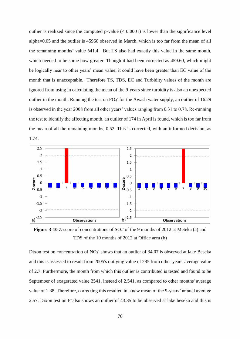
70
outlier is realized since the computed p-value (< 0.0001) is lower than the significance level
alpha=0.05 and the outlier is 45960 observed in March, which is too far from the mean of all
the remaining months’ value 641.4. But TS also had exactly this value in the same month,
which needed to be some how greater. Though it had been corrected as 459.60, which might
be logically near to other years’ mean value, it could have been greater than EC value of the
month that is unacceptable. Therefore TS, TDS, EC and Turbidity values of the month are
ignored from using in calculating the mean of the 9-years since turbidity is also an unexpected
outlier in the month. Running the test on PO4- for the Awash water supply, an outlier of 16.29
is observed in the year 2008 from all other years’ values ranging from 0.31 to 0.78. Re-running
the test to identify the affecting month, an outlier of 174 in April is found, which is too far from
the mean of all the remaining months, 0.52. This is corrected, with an informed decision, as
1.74.
Figure 3-10 Z-score of concentrations of SO4- of the 9 months of 2012 at Meteka (a) and
TDS of the 10 months of 2012 at Office area (b)
Dixon test on concentration of NO3- shows that an outlier of 34.07 is observed at lake Beseka
and this is assessed to result from 2005's outlying value of 285 from other years' average value
of 2.7. Furthermore, the month from which this outlier is contributed is tested and found to be
September of exagerated value 2541, instead of 2.541, as compared to other months' average
value of 1.38. Therefore, correcting this resulted in a new mean of the 9-years’ annual average
2.57. Dixon test on F- also shows an outlier of 43.35 to be observed at lake beseka and this is
-2.5
-2
-1.5
-1
-0.5
0
0.5
1
1.5
2
2.5
1 2 3 4 5 6 7 8 9Z-sc
ore
Observationsa)-2.5
-2
-1.5
-1
-0.5
0
0.5
1
1.5
2
2.5
1 2 3 4 5 6 7 8 9 10Z-sc
ore
Observationsb)

71
investigated to result from 2013's outlying value of 179.1 from other years' average value of
26.4. Additinally, the month from which this outlier is obtained is tested and found to be
December of exagerated value 1954 as compared to other months' average value of 17.74.
Communicating the staffs of the authority, together with personal judjement, it is found the
value to be 19.54.
In 2010, EC at Adaitu has been wrongly registered as 4045 being the correct mean value of all
months’ for the year 404.5. Hence correcting this, the mean became 656.16. The outlying year
of TS from the 9-year mean value, 490.02, of Wonji is assessed. However, there is no any
significant outlying year’s value from the contributing ones. The year 2005, recognized by the
test here, doesn’t mean the real contributing one because all years of value ranging from 334
to 774 are observed to be small as compared to other sites’ mean values ranging from 1914.78
to 3613.78. Therefore, the outlying value, 490.02, of TS at Wonji is left as it is as all the years
are found to contribute equally to minimize the 9-year mean value. At lake Beseka, SO4- was
also showing an oulier that came from the 2006 value of 5104. This has come from the wrong
placing of average of the months’ values of the year, which was 510.14, rather than showing
outlier in a month’s value. Correcting this resulted in the 9-year SO4- mean of 497.84. Mg of
value 612 in place of 6.12 and F- of value 27.8 instead of 2.78 at Dubti respectively in August
and October of 2008 seem to be outliers, while Mg of value 672 instead of being 6.72 at Adaitu
in June of 2011 also seem to be outlier. But they are not the real outliers rather they are born
from personal errors.
The statistical test results could also be supported by observing the dataset at some sites. At
Adaitu, for instance, exaggerated increments of EC in 2010 and Mg in 2011 is seen while at
Weir site a similar increase of TDS (which is unexpectedly greater than its conductivity value)
in 2009 and potassium in 2010 are observed. Abnormal exceedences at Dubti of NO3-, F- and
Mg in 2008 and TFe in 2007 are also observed. At Beseka, increment of SO4- to 5104 in 2006
from the common 300's and 400's in all the eight years and increment of F- abruptly to 179.1
in 2013 from an average value of 26.4 for all the remaining eight years are also unexpected.

72
At office area, a sudden increase of TDS and PO4- were observed in 2012. This may probably
be an error of placing the decimal point (being 514.44 rather than 5144.4) since it contradicts
to the fact that TDS needs to be less than EC as in eqn. (3-2) while recording, transferring data
or else. At before Beseka, a similar growth of alkalinity, SO4-, HCO3
- and Na in 2012 is seen.
EC = ke*TDS………………..(3-2)
where TDS is expressed in mg/l and EC is in μs/cm, the factor ke Є (1.2, 1.8) (Rangeti et. al.,
2015).
A rough observation of plots of the after Beseka dataset shows also that except pH, Mg, NO3-,
TDS, Ca, TH and turbidity, almost all the 13 parameters got larger values in 2009 and 2010
than in other years. These may all be due either to technical, personal, or instrumental errors.
3.3.2.5 Validation of data anomalies of the upper basin
Water quality analysis for the upper basin (UB) has been prepared and compiled by Vitens
Evides international granting organization of Netherlands together with Oromia regional water
office of Ethiopia in seven rounds at about 2.5 months’ interval from 26/06/2014 - 30/11/2015.
They considered ten sample sites of which only four sites were of interest and only those
parameters having full data in all the sites were selected for the current study. Since a lot of
samples were taken from each site, a number of parameters were considered and choice of
sampling sites was strategic enough, this dataset was preferred to be used for computation of
Water Quality Index (WQI) in the sub-basin.
Validity of the water quality dataset of the upper basin was checked. There were missing and
censored values in the dataset marked as x, ?, empty, nil, <R and TNTC and they were refined
by ignoring from calculation of the mean (some of them) and appropriate substitution (others).
The other anomalies observed in the dataset were outliers. Dixon test (given by eqn. 3-1) was
used again to detect the outliers and is shown by Figure 3-11.
Accordingly, out of the selected 28 variables, only 3 of them showed outliers. These are
turbidity at the 6th (19th) site, chromium at the 4th (17th) site and chlorine at the 5th (18th) site,

73
sites being numbered from the lower tip of the upper (entire basin). But the 19th, 17th, and 18th
sites are respectively Awash River at Awash Melka kuntire, Mojo River before Lake Koka,
and Akaki River after Lake Aba Samuel, which are respectively exposed usually to high
disturbance, tannery effluent and urban sewage effluent. Therefore, high amount of turbidity,
chromium and chlorine are expected and hence they are the real and expected outliers and
therefore they need no correction.
Figure 3-11 Demonstration of standard score of outlying sites for Turbidity (a), Chromium
(b) and Chlorine (c)
Since only concentrations of Ca2+ and Mg2+ ions were given for the upper basin, total hardness
(TH) is computed as the concentration of calcium and magnesium ions expressed as equivalent
of calcium carbonate (CaCO3) by equation (3-3)1 (Lenntech, 2014) .
1 http://www.lenntech.com/ro/water-hardness.htm
-1.5
-1
-0.5
0
0.5
1
1.5
2
2.5
1 2 3 4 5 6
Z-s
core
Observationsa) Turbidity
-1.5
-1
-0.5
0
0.5
1
1.5
2
2.5
1 2 3 4 5 6
Z-s
core
Observationsb) Cr
-1.5
-0.5
0.5
1.5
2.5
1 2 3 4 5 6
Z-s
core
Observations c) Cl2

74
[𝐶𝑎𝐶𝑂3] = 2.5 ∗ [𝐶𝑎2+] + 4.1 ∗ [𝑀𝑔2+]…………..(3-3)
The cations used in the calculation of SAR, which were expressed in mg/L, were all changed
into milli-equivalents per liter (meq/L) and the SAR, depicted in Table 4-2, is calculated by
equation (3-4) (Lesch and Suarez, 2009; Seid and Genanew, 2013; Hussain et al., 2010):
𝑆𝐴𝑅 (𝑚𝑒𝑞 L⁄ ) =[Na+]
√[𝐶𝑎2+]+[Mg2+]
2
…………..(3-4)
The other chemical index of irrigation water quality importance such as RSC was also
calculated from the measured water quality parameters by using equation (3-5) (Dinka, 2016).
The cations and anions, which were expressed in mg/L, were all changed into mili-equivalents
per liter (meq/L).
𝑅𝑆𝐶 = (𝐶𝑂32− + 𝐻𝐶𝑂3
−) − (𝐶𝑎2+ + 𝑀𝑔2+)……(3-5)
3.4 Assessment of tools for evaluation and multivariate analysis of water
quality
Water quality requirements, expressed as water quality criteria and objectives, are use-specific
or are targeted to the protection of the most sensitive water use among a number of existing or
planned uses within a catchment. Evaluation of whether a given water body is satisfactorily
meeting the criteria for an intended use or not is therefore essential. On the other hand, water
quality of water bodies at different localities in a basin may show difference at a time or a given
water body may show variation of quality in different time scales. However, determination of
the extent and way of these spatial and/or temporal variations is of important concern to decide
either for the resource utilization or mitigation of pollution problems. Evaluation of the status
of water bodies could be facilitated by WQI by considering selected stations and parameters
along Awash River, discussing ranks of indices of sub-basins, determining the water quality
status in the basin and assessing extent of suitability for irrigation and drinking purposes.
Spatial and temporal variation of the water quality is managed using multivariate statistical
analysis as usual.

75
3.4.1 Evaluation of water quality by WQI
3.4.1.1 Water Quality Indices
Environmental indices provide a broad overview of environmental performance rather than
detailed information. WQIs, in particular, are practical methods of describing the problem of
pollution in a water body by combining various measurements of different units in a single
metric, summarizing bulk of water quality data in a single number that can logically be used
for expression, comparison and determination of trends over time. They are, therefore, useful
for communication of the results, modification of policies thereby developing a decision
making tool as it allows to evaluate the state of a water body easily and make suggestions for
a more efficient water resources and river basin management by formulating pollution control
strategies (CCME, 2001b; Tyagi et al., 2013; Barceló-Quintal et al., 2013; Sargaonkar &
Deshpande, 2003).
Determination of WQI is a very reliable, useful and efficient way for assessing and
communicating the information on the overall quality of water (Gibrilla et al., 2011; Barceló-
Quintal et al., 2013). WQI estimation helps in deciding the suitability of surface water sources
for their intended use by humans, aquatic and wildlife (CCME, 2001a). WQI can also be used
to assess water quality relative to its desirable state defined by water quality objectives and to
provide insight into the degree to which water quality is affected by human activity. Though
most indices measure the same attributes of deviation from objectives, there are various ways
of determining WQI for evaluating water bodies intended for different uses (Wills & Irvine,
1996). Some of them being used worldwide are: Canadian Council of Ministers of the
Environment (CCME) WQI, Weighted Arithmetic WQI (CCME, 2001b), National Sanitation
Foundation (NSF) WQI (Kaurish & Youno, 2007), Overall Water Quality Index (OWQI),
Oregon WQI and others (Tyagi et al., 2013; CCME, 2001b; Poonam et al., 2015).
Weighted arithmetic WQI method, which classifies the water quality according to the degree
of purity by using the most commonly measured water quality variables, according to Tyagi et
al., (2013), makes use of equation (3-5).

76
𝑊𝑄𝐼 = ∑ 𝑄𝑖𝑊𝑖 ∑ 𝑊𝑖⁄ ………………………..………(3-5)
The unit weight (Wi) for each water quality parameter is calculated by using equation (3-6).
𝑊𝑖 = 𝐾 𝑆𝑖⁄ …………………………………………(3-6)
Where,
K=proportionality constant and can be calculated using the equation (3-7).
𝐾 =1
∑(1 𝑆𝑖)⁄…………………………………………(3-7)
The quality rating scale (Qi) for each parameter is calculated by using the expression (3-8).
𝑄𝑖 = 100[(𝑉𝑖 − 𝑉𝑜 𝑆𝑖 − 𝑉𝑜)]⁄ ………………………(3-8)
Where,
Vi is estimated concentration of ith parameter in the analyzed water
Vo (ideal value of this parameter in pure water) = 0 (except pH =7.0 and DO = 14.6 mg/l)
Si is the recommended standard value of ith parameter.
NSF WQI has been developed by selecting parameters, developing a common scale and
assigning weights and was based upon nine water quality parameters namely: Dissolved
Oxygen (DO), BOD, fecal Coliforms, pH, temperature change, total phosphates, nitrates,
turbidity and total dissolved solids (Tyagi et al., 2013; Wills & Irvine, 1996; Poonam et al.,
2015) and is given by equation (3-9).
𝑊𝑄𝐼 = ∑ 𝑄𝑖𝑊𝑖𝑛𝑖=1 ……………………………..…(3-9)
Where,
Qi = sub-index for ith water quality parameter;
Wi = weight associated with ith water quality parameter;
n = number of water quality parameters.
For this NSFWQI method, the ratings of water quality have been defined as excellent (91-100),
good (71-90), medium (51-70), bad (26-50), very bad (0-25)
Overall Water Quality Index (OWQI), on the other hand, was developed following the four
steps: parameter selection, development of sub-indices function, assignment of weights and
aggregation of sub-indices to construct an overall index (Singh et al., 2015) and is given by
equation (3-10).
𝑂𝑊𝑄𝐼 = ∑ 𝑊𝑖. 𝑌𝑖𝑛𝑖=1 ………………………(3-10)

77
Where,
Wi=weight of the ith water quality parameter
Yi=sub-index value of the ith parameter
In this index, the quality of a water body is classified into five categories: heavily polluted (0-
24), poor (25-49), fair (50-74), good (75-94) and excellent (95-100).
The Oregon WQI, according to Cude (2001), has been developed to provide a simple and
concise method of expressing and reporting water quality status and trends of WQ dataset so
as to enable decision making. The index has taken into account the parameters: Dissolved
oxygen, BOD, pH, total solids, ammonia, nitrate, and fecal coliform and were classified
according to impairment category: oxygen depletion, eutrophication or the potential for excess
biological growth, physical characteristics, dissolved substances, and health hazards (Cude,
2001). The unweighted harmonic square mean formula, as a method of aggregating sub-index
results of OWQI, is given by equation (3-11).
𝑊𝑄𝐼 = √𝑛
∑ (1 𝑆𝐼𝑖2)⁄𝑛
𝑖=1
………………………(3-11)
where WQI is water quality index result, n is the number of sub-indices, and SIi is Sub-index i
(Cude, 2001; Tyagi et al., 2013).
3.4.1.2 Comparison of the water quality indices
Though NSF, CCME and OWQI are water quality indices which are frequently used for water
quality assessment, CCME is the most efficient for low parameter values. General or Overall
WQI (OWQI) is an efficient one but parameters here should be carefully selected depending
on the source and time. The main drawback of NSF WQI is the eclipsing effect. Due to this
effect one or more parameters which have values above permissible limit are masked if the rest
of the parameters are within the limits (Poonam et al., 2015). Oregon WQI aids in the
assessment only of water quality for general recreational uses (i.e., fishing and swimming).
Additionally, it is designed only for Oregon's streams and its application to other regions or
waterbody types need a caution (Cude, 2001). Therefore, it is not recruited to evaluate water

78
quality of the study area as the intention was mainly for the betterment of irrigation and
drinking water rather than for recreation.
CCME WQI, on the other hand, is flexible with respect to the type and number of water quality
variables to be tested, the period of application, and the type of water body (stream, river reach,
lake, etc.) tested. The Council’s WQI determining formula is used to simplify complex water
quality data from streams, rivers and lakes and communicate the results even to a non-technical
audience. The index produces a ranking (good, fair, poor, etc.) based on exceedances of
objectives for key water quality variables in the watershed (Andrea et al., 2005). Comparison
of different WQI methods, Awash River water quality status is found to be better evaluated
using the WQI method proposed by CCME due to its easy computation, accessibility and
flexibility.
3.4.1.3 Conceptual Framework of CCME WQI
CCME developed a WQI determining formula to simplify complex water quality data from
streams, rivers and lakes and communicate the results to both technical and non-technical
audience. The index is based on a combination of three factors: scope (number of variables
whose objectives are not met), frequency (frequency with which the objectives aren’t met) and
amplitude (amount by which the objectives are not met) (Tyagi et al., 2013; CCME, 2001a;
CCME, 2001b). CCME WQI is given by eqn. (3-12):
CCME WQI = 100 −√𝐹1
2+𝐹22+𝐹3
2
1.732……….(3-12)
Where,
F1 (Scope) = Number of variables whose objectives are not met.
F1= [No. of failed variables/Total no. of variables] *100
F2 (Frequency) = Number of times by which the objectives are not met.
F2= [No. of failed tests/Total no of tests] *100
F3 (Amplitude) = Amount by which the objectives are not met. This can be determined by
three steps as follows:
a) excursion= [Failed test value i /Objective]-1
79
b) normalized sum of excursions (nse):
(𝑛𝑠𝑒) = ∑excursions𝑖
𝑁𝑜 𝑜𝑓 𝑡𝑒𝑠𝑡𝑠
𝑛
𝑖=1
c) F3 = nse/(0.01*nse+0.01) is an asymptotic function that scales the normalized sum of
excursions from objectives (nse) to yield a range between 0 and 100.
Based on results of this index calculation, which is based on exceedances of objectives for
water quality variables, water quality of a water body is ranked into five classes: excellent (95-
100), good (80-94), fair (65-79), marginal (45-64), and poor (0-44) (Tyagi et al., 2013; CCME,
2001a; Andrea et al., 2005; CCME, 2001b). Rules that should be taken into consideration while
applying the index, according to CCME (2001b), are: index comparisons should only be made
when the same sets of objectives and parameters are being used, care should be taken with
older data, the index should be run on parameter sets relevant to the water body being tested,
and minimal data sets should not be used (CCME, 2001b).
3.4.2 Analysis of water quality by multivariate statistical techniques
Multivariate statistical analysis approaches have, for long, b e e n used to analyze and
characterize water quality data. Such approaches have been useful to deal with complex
environmental dataset exposed to varying natural and anthropogenic factors and solve the
associated problems without misinterpretation. They provide a means of handling large dataset
with large number of variables by summarizing the redundancy, as well as reflecting, detecting
and quantifying the multivariate nature of ecological data accurately (Hulya and Hayal, 2008;
Wang et al., 2007). Principal Component Analysis (PCA) and Cluster Analysis (CA) are
specifically useful for considering several related random environmental variables
simultaneously, and thus for identifying a new, small set of uncorrelated variables that
accounted for a large proportion of the total variance in the original variables (Wang et al.
2007).
3.4.2.1 Principal component analysis
Principal Component Analysis (PCA) was applied to sort the variables of water quality
indicators, reducing into smaller but key principal (independent) factors or classify the
80
variations of the water quality indicators. PCA is a very effective tool used to reduce the
dimension of a data set consisting of a large number of inter-related variables by reducing the
contribution of variables with minor significance, while retaining as much variability of the
data set as possible and interprets the total variability of the dataset. This is accomplished by
transforming the data set into a small number of new set of variables called Principal
Components (PCs). The PCs are orthogonal (non-correlated), linear combinations of the
originally observed water quality data and are arranged in decreasing order of importance
(Shrestha and Kazama, 2007; Singh et al., 2004). The PCs can be expressed by equation (3-
13).
𝑍𝑖𝑗 = 𝑎𝑖1𝑥1𝑗 + 𝑎𝑖2𝑥2𝑗 + 𝑎𝑖3𝑥3𝑗 + ⋯ + 𝑎𝑖𝑚𝑥𝑚𝑗…………………(3-13)
where Z is the component score, a is the component loading, x is the measured value of variable,
i is the component number, j is the sample number and m is the total number of variables
(Muangthong, 2015; Shrestha and Kazama, 2007).
Dataset of 16 water quality monitoring stations, containing 22 parameters monitored monthly
over 11 years (2005-2015) were collected from AwBA for the study. Among the 16 stations
and the 11 years’ data, only 10 stations and 9 years were selected respectively ignoring others
due to incompleteness of data. Taking domestic and irrigation water uses into account, which
are dominant in the basin, 19 of the 22 parameters were considered. The water quality
parameters considered in this analysis, their abbreviations, their units and methods of analysis
(following standard methods for the examination of water and wastewater (APHA, 1998)) are
summarized in Table 3-2. The means of the monthly measured 9-year data-set on the river
water quality are summarized in Table 4-4.

81
Table 3-2 Water quality parameters, their units and methods of analysis (Source: APHA)
Parameters Abbreviation Units Methods
Turbidity Turb NTU Turbid metric method
Total solids 105OC TS mg/l Gravimetric method
Total dissolved Solid TDS mg/l Gravimetric method
Electrical Conductivity EC µs/cm Calorimetric method
pH pH - Calorimetric method
Ammonia NH3 mg/l NH3 Aluminon method
Sodium Na mg/l Na+ Flame photometer
Potassium K mg/l K+ Flame photometer
Total Hardness TH mg/l CaCO3 Titrimetric method
Calcium Ca mg/l Ca+2 Titrimetric method
Magnesium Mg mg/l Mg+2 Periodate oxidation method
Total Iron TFe mg/l Fe+3 Phenanthroline Method
Fluoride F- mg/l F- SPADNS Method
Chloride Cl- mg/l Cl- Argentometric Method
Nitrate NO3- mg/l NO3
-2 Cadmium reduction method
Alkalinity Alkal mg/l CaCO3 Titrimetric method
Bicarbonate HCO3- mg/l HCO3
- Titrimetric method
Sulphate SO4- mg/l SO4
-2 Turbid metric method
Phosphate PO4- mg/l PO4
-3 Ascorbic acid, Molybdate blue method
3.4.2.2 Cluster analysis
Cluster analysis (CA) is a multivariate procedure which classifies data based on placing of
objects into more or less homogeneous groups, in a manner such that the relationship between
groups is revealed. The main idea behind clustering is to combine identical sites as one cluster
and group, two clusters of highest similarity as a new cluster, which in turn is combined with
another most similar cluster as another new cluster and so on until all clusters become one
cluster (Xu et al., 2012). Agglomerative Hierarchical Clustering (AHC) is the most common
and iterative classification method in which clusters are formed sequentially by starting with
the most similar pair of objects and forming higher clusters step by step (Singh et al., 2004).
The Euclidean distance, which is used to quantify the similarities or differences between the
two sites (sampling locations) i and j, was calculated by formula (3-14).
……………………………………………..(3-14)
where dij is the Euclidean distance, Zi,k and Zj,k - variable k for objects i and j respectively, and
m is the number of variables (Gibrilla et al., 2011; Singh et al., 2004). The Euclidean distance,
according to Singh et. al., 2004, gives the similarity between two samples and a ‘distance’ can
be represented by the ‘difference’ between analytical values from both samples.

82
3.4.2.3 Mann-Kendall trend test
Mann-Kendall trend test is a rank-based and non-parametric statistical test to detect trends and
assess the significance of trends in hydro-meteorological time series data such as water quality,
streamflow, temperature, and precipitation. This non-parametric test is also documented to be
more suitable and powerful for detecting trends of non-normally distributed and censored data
(Yue et. al., 2002; H.S. Xu et. al, 2012) such as that of ARB. To avoid the influence of
streamflow on water quality, only quality data of the same season should be analyzed over
some time period. In this regard, seasonal Mann-Kendall trend test has been useful for non-
parametric trend analysis of water quality over time. It can be used in place of the parametric
linear regression analysis, which requires that the residuals from the fitted regression line be
normally distributed. Basically, it separately calculates the test statistics and variance of water
quality data in each season and then overall statistics is calculated (H.S. Xu et. al, 2012).
Letting x1, x2, . . . , xn, to be a sequence of measurements over time, it is proposed to test the
null hypothesis, Ho, that the data come from a population where the random variables are
independent and identically distributed (Hipel, and McLEOD, 1994). The alternative
hypothesis, H1, is that the data follow a monotonic trend over time. Under Ho, the Mann-
Kendall test statistic is given by equation (3-15).
𝑆 = ∑ ∑ 𝑠𝑔𝑛(𝑥𝑗 − 𝑥𝑘)𝑛𝑗=𝑘+1
𝑛−1𝑘=1 …………………………….(3-15)
where, sgn(x) = {+1, 𝑥 > 0
0, 𝑥 = 0
−1, 𝑥 < 0
and S is asymptotically normally distributed and gave the mean and variance of S, for the
situation where there may be ties in the x values, by equation (3-16).
E[S]=0
Var[S]= {𝑛(𝑛 − 1)(2𝑛 + 5) − ∑ 𝑡𝑗(𝑡𝑗 − 1)(2𝑡𝑗 + 5)𝑝𝑗=1 }/18… (3-16)
where p is the number of tied groups in the data set and tj is the number of data points in the jth
tied group.
When using eqn. 3-15, a positive value of S indicates that there is an upward trend in which
the observations increase with time. On the other hand, a negative value of S means that there

83
is a downward trend. Because it is known that S is asymptotically normally distributed and has
a mean of zero and variance given by eqn. 3-16, one can check whether or not an upward or
downward and is significantly different from zero. If the S is significantly different from zero,
based upon the available information Ho can be rejected at a chosen significance level and the
presence of a monotonic trend, H1, can be accepted (Hipel, and McLEOD, 1994). The
multivariate statistical techniques were employed here to sort out the variables of water quality
parameters and sampling stations.
3.5 Land use/land cover and change detection
3.5.1 Causes of land use/land cover change and image capturing
Land-use/land-cover: Land-cover is the observed biophysical cover of the earth’s land surface
and is composed of patterns that occur due to a variety of natural and anthropogenic processes.
Land-use, on the other hand, is human utilization of the land, influenced by socio-economic,
cultural, political, historical, and land-tenure factors (Rozenstein & Karnieli, 2011).
Causes for land use/land cover change: Land-use and land-cover change means a change in
the biophysical cover of the earth’s land surface and are influenced by a variety of biophysical
and societal factors operating on several spatial and temporal levels. Biophysical influences
include: climate, landform, geology, soils, hydrology, vegetation, and fauna while societal
factors are those relating to population structure and dynamics, income and affluence,
technology, socio-economic organization, culture, institutions, and political systems, demand
for land, land-use patterns and their change (Briassoulis, 2009). Land-cover characterization
and definition of land-use through observations of the land-cover is often made possible by
remotely-sensed data (aerial imagery or earth observing satellites using their sensors’ capturing
information remotely) (Rozenstein & Karnieli, 2011).
Image capturing techniques and sensors: Land Use and Land Cover data of different spatial
(5, 15, 30, 90, …, meter), spectral (500-12500 nm), radiometric and temporal resolution needed
for change detection and other analyses are captured from sensors remotely. Remote sensing
is the science (and to some extent, art) of acquiring information about the earth's surface
without actually being in contact with it. Nowadays, Landsat data are widely applied for land-

84
use classification on a regional scale owing to their relatively lower cost, longer history, and
higher frequency of archives in comparison to other remote-sensing data sources as MODIS
200m, Quick bird 0.5m, Aster 15m, Spot 5m, and others (Rozenstein & Karnieli, 2011).
Landsat types and characteristics: Landsat (LS) satellites have continuously acquired space-
based images of the Earth’s land surface since 1972 when Thematic Mapper (TM) on board
Landsat-1 was launched but terminated its operations on January 6, 1978. The launches of
Landsat 2, Landsat 3, and Landsat 4 followed in 1975, 1978, and 1982, respectively and their
respective dates of functional termination were on January 22, 1981, March 31, 1983 and 1993.
While Landsat-5 has been launched in 1984, Landsat-7 has been launched in 1999 but Landsat
6 failed to achieve orbit in 1993. Recently in 2013, Landsat 8, has been launched and continued
the mission. Landsat 9, is expected to be launched in 2020. They have been providing data that
serve as valuable resources for land use/land cover change researches. The data gathered by
these satellites are useful to a number of applications including forestry, agriculture, hydrology,
geology, regional planning, and education.
Currently, two of the Landsat sensors in orbit are operational: TM on board Landsat-5 and
Enhanced Thematic Mapper Plus (ETM+) on board Landsat-7. Both of the sensors acquire
measurements in all major portions of the solar electromagnetic spectrum (visible, near-
infrared, and shortwave-infrared).
3.5.2 Land use/land cover classification
Automatic classification of remote sensing images is more suitable for mapping land-use in a
large area than manual digitization of land-use patches as it is extremely tedious and subjective.
However, when automatically classifying a complex landscape from remote-sensing imagery,
it is challenging to achieve an accurate classification. This is because automated classification
techniques do not possess the superior pattern recognition capabilities of the human brain
though land-use and land-cover patterns may be obvious to an image interpreter (Rozenstein
& Karnieli, 2011). There are two types of classification: supervised and unsupervised ones, the
efficiency of which is dependent on accuracy assessment. There are two types of map accuracy

85
assessment: positional and thematic. Positional accuracy deals with the accuracy of the location
of map features, and measures how a spatial feature on a map is far from its true or reference
location on the ground. Thematic accuracy deals with the labels or attributes of the features of
a map, and measures whether the mapped feature labels are different from the true feature label
(Jensen & Lulla, 1987).
3.6 SWAT model
Application of SWAT to assess the impact of land use on water resources in the horn of Africa,
in which the study area is located, is well documented by Baker & Miller (2013). Their
assessment showed that changes in land use have resulted in an increase in surface runoff,
decrease in groundwater recharge and correspondingly hydrologic changes were highly
variable both spatially and temporally (Baker & Miller, 2013). Additionally, SWAT is found
to be a promising model for continuous and long-term simulations of all major components
(hydrology, sediment, and chemical) in predominantly agricultural watersheds (Borah & Bera
2003). The model is applicable to semi-arid and similar environments where there is limited
number of gauge stations (Kiros et al., 2015) like that of ARB.
The SWAT model used here is of a release version 2012 and a version number identifying the
executable file rev. 632 released on 09 September 2015. The four basic inputs for the model
were prepared as follows.
3.6.1 Input data acquisition and preparation
The basic data sets required to simulate the SWAT model as prerequisites included:
meteorological data; topography (DEM); soil properties; and vegetation or land use and land
cover data. Others usually considered as inputs are hydrological and hydraulic data (including
river discharge gage data and water quality data) as well as land management practices
undertaken in a basin (Neitsch et al. 2011). The SWAT model has limitations of not explicitly
allowing for inclusion of spatial data as model inputs. Dataset need to be processed into a form
that the model can use. Processing these data, even with the help of GIS, is tedious and time

86
consuming due to the large number of model parameters required to run the model. The spatial
variation of the outputs of the model was visualized making use of SWAT output viewer
software of version 0.1.
3.6.1.1 Hydro-meteorological Data
Climate in a basin gives the moisture and energy that controls the water balance and determines
the relative importance of different components in the hydrologic cycle (Neitsch et al., 2002).
The climate data needed by the model include daily values of: precipitation, maximum and
minimum temperature, relative humidity (required only if either Penman-Monteith or
Priestley-Taylor methods are used to calculate evapo-transpiration (Gassman et al., 2007)), sun
shine hour (solar radiation) and wind speed (only necessary if the Penman‐Monteith method is
used for ET determination) of the 20 stations (Neitsch et al., 2011).
These daily meteorological datasets for the required weather stations (for 1/1/1994-
12/31/2014) in the study area were gathered from the National Meteorological Service Agency
(NMSA). Some data were also captured from the global weather database
(http://globalweather.tamu.edu/) of Texas A&M University Climate Forecast System
Reanalysis (CFSR) to fill the missing parts as recommended by Dile & Srinivasan, (2014) and
Fuka et al., (2013). Then the data is formatted in such a way that it can be fed to the SWAT
model.
The observed data (though not complete) on flow for the period 1972 – 2009 (though the time
period for all the gaging stations were not uniform) were collected from the hydrology and
water quality department of Federal Ministry of Water, Irrigation and Energy (MoWIE) of
Ethiopia. Shape files and all the GIS data were gathered from the GIS department of the
MoWIE.
For all the 20 stations Figure 3-15, a summary of the monthly average values of all the 14
parameters [TMPMX (average maximum air temperature for month (°C)), TMPMN (average
minimum air temperature for month (°C)), TMPSTDMX (standard deviation for maximum air

87
temperature in month (°C)), TMPSTDMN (standard deviation for minimum air temperature in
month (°C)), PCPMM (average amount of precipitation falling in month (mm H2O)), PCPSTD
(standard deviation for daily precipitation in month (mm H2O), PCPSKW (skew coefficient for
daily precipitation in month (mm H2O)), PR_W1 (probability of a wet day following a dry day
in month), PR_W2 (probability of a wet day following a wet day in month), PCPD (average
number of days of precipitation in month), RAINHHMX (extreme half-hour rainfall for month
(mm H2O)), SOLARAV (average daily solar radiation for month (MJ/m2/day)), DEWPT
(average daily dew point temperature in month (ºC)), and WNDAV (average daily wind speed
in month (m/s))] over the 21 years together with their TITLE (the first line of the .wgn file of
80 spaces reserved for user comments), locations [WLATITUDE (latitude of weather station)
& WLONGITUDE (longitude of weather station)], WELEV (elevation of weather station (m)),
RAIN_YRS (the number of years of maximum monthly 0.5 h rainfall data) were prepared
supported by pcpstat program, filled into the weather generator input file (.WGN) and
formatted for input to SWAT. Totally, (14*12+4) *20=3440 entries of an excel sheet have been
filled and imported into the database. Likewise, daily dataset of precipitation, maximum and
minimum temperature, sun shine hour (solar radiation), relative humidity, and wind speed are
prepared according to the format recommended by Neitsch et al., (2002) and Arnold et al.,
(2012).
3.6.1.2 Topography
Along with soil, meteorology, and land use/land cover data, topography data is one of the main
inputs for SWAT. It is used to delineate the watershed and to further divide the watershed into
multiple sub-basins and Hydrologic Response Units (HRUs). It calculates the basin’s and sub-
basins’ parameters such as slope and slope length. Resolution of the DEM is too critical to
affect the watershed delineation, stream network, and sub-basin classification in the model. It
affects the number of sub-basins and HRUs, which in turn affects the predicted sediment yield
for a watershed (Gassman et al., 2007; Bingner et al., 1997). A decrease in DEM resolution
leads to a decrease in stream flow and watershed area. Since the runoff volume and total
sediment load depends on the watershed area, the decrease in the DEM resolution resulted in

88
large error in the predicted output. Input DEM data resolution affected SWAT model
predictions by affecting total area of the delineated watershed, predicted stream network and
sub basin classification (Chaubey et al., 2005).
Topography data was made available from the Global Land Cover Facility (GLCF) website to
prepare Digital Elevation Model (DEM) of the basin. It was of 90-m spatial resolution (because
of the vast spatial extent of the study area) and obtained from the Shuttle Radar Topography
Mission (SRTM) of paths 44 and 45 and rows 10 and 11 (http://www.landcover.org/data/srtm/).
This DEM was used as input for the model from which the flow direction, flow accumulation,
stream length, outlet selection, watershed discretization and delineation were determined.
3.6.1.3 Soil Data
Two files, the soil input file (.sol) (the required physical properties) and the soil chemical input
file (.chm) (information on the optional chemical properties) contain the soil properties used
by SWAT. The soil input file, defining the physical properties and initializing chemical
quantities for all layers in the soil, governs the movement of water and air through the profile
and have a major impact on the cycling of water within the HRUs. The soil chemical input file,
initializing additional chemical quantities for the first soil layer, sets initial levels of the
different chemicals in the soil (Neitsch et al., 2002).
Variables in the soil input file of the model include: soil name (SNAM), soil hydrologic group
(A, B, C, or D) (HYDGRP), maximum rooting depth of soil profile (mm) (SOL_ZMX),
fraction of porosity (void space) from which anions are excluded (ANION_EXCL), crack
volume potential of soil (SOL_CRK), texture of soil layer (TEXTURE), depth from soil surface
to bottom of layer (mm) (SOL_Z), moist bulk density (Mg/m3 or g/cm3) (SOL_BD), available
water capacity of the soil layer (mm H2O/mm soil) (SOL_AWC), saturated hydraulic
conductivity (mm/hr) (SOL_K), % organic carbon content (SOL_CBN), % clay content
(CLAY), % silt content (SILT), % sand content (SAND), % rock fragment content (ROCK),
moist soil albedo (SOL_ALB), USLE equation soil erodibility (K) factor (units: 0.013 (metric

89
ton m2 hr)/(m3-metric ton cm)) (USLE_K), and electrical conductivity (dS/m) (SOL_EC)
(Neitsch et al., 2002).
ARB is covered by fourteen (as shown by Figure 3-12) of the 28 major soil groups in the
legend of soil map of the world (FAO/UNESCO): Luvisols, Leptosols, Vertisols, Fluvisols,
Nitosols, Regosols, Cambisols, Acrisols, Andosols, Arenosols, Gleysols, Phaeozems,
Solonchaks, and Gypsisols (Xerosols and Yermosols). The general characteristics of only
major soil groups in the basin is presented briefly as follows (Driessen et al., 2001; FAO et al.,
2012; Engida, 2010).
Leptosols: Very shallow soils over hard rock or in unconsolidated very gravelly material mostly
located at medium-high altitude and strongly dissected topography. They are found in all
climatic zones, in particular in strongly eroding areas. By and large, they are free draining and
have low water holding capacity.
Vertisols: are dark-coloured cracking and swelling deep clay soils that expand upon wetting
and shrink upon drying. They are found in level to undulating terrain with distinct wet and dry
periods. They are poorly drained and largely have good water holding capacity.
Fluvisols: These are young soils developed in fluvial, alluvial, lacustrine or marine deposits
and are common along rivers and lakes, in floodplains and deltaic areas. Fluvisols in upstream
parts of river systems are normally confined to narrow strips of land adjacent to the actual
riverbed. In the middle and lower stretches, the flood plain is wider and has the classical
arrangement of levees and basins, with coarsely textured fluvisols on the levees and more finely
textured soils in basin areas further away from the river. Fluvisols on river levees are porous
and better drained than those in low landscape positions.
Regosols: are soils in unconsolidated material without significant evidence of soil formation.
They are particularly common in mountainous regions associated with Leptosols. They are
well-drained and medium-textured soils with lower water holding capacity.
Cambisols: are soils at an early stage of soil formation. They exhibit different characteristics
depending on the environmental setting in which they are developed. However, most cambisols

90
are medium-textured soils with high porosity, good water holding capacity and internal
drainage.
Figure 3-12 Soil Map of the Study Area by Soil Type
Arenosols: consists of sandy soils developed either in residual sands or in recently deposited
sands as occur in deserts and beach lands. They exist in all climatic regions extending from
extremely cold to extremely hot. Arenosols are permeable to water and depending on the grain
size distribution and organic matter content, the Available Water Storage Capacity (AWC) may
be as low as 3 to 4 percent or as high as 15 to 17 percent. They have relatively high bulk density
and their saturated hydraulic conductivity and infiltration vary. Arenosols in humid temperate
or tropical regions are deeply leached and contain little or poorly decomposed organic matter.
Solonchaks: includes soils that have a high concentration soluble salts. are largely confined to
the arid and semiarid climatic zones and to coastal regions in all climates notably in seasonally
or permanently waterlogged areas with grasses and/or halophytic herbs, and in poorly managed
irrigation areas where evapo-transpiration is considerably greater than precipitation.
Solonchaks with extreme salinity and thick surface crusts occur in depressions that collect

91
water from surrounding (higher) land in the winter but dry out in the warm season. The salic
soil horizon of solonchaks has an electrical conductivity value in excess of 15 dS/m at 25oC at
some time of the year.
Xerosols and Yermosols (are merged as Gypsisols in the revised legend of soil map of the
world): are mostly of unconsolidated alluvial, colluvial or aeolian deposits of base-rich
weathering parent materials. They are soils with substantial secondary accumulation of gypsum
(CaSO4.2H2O). They are found in the driest parts of the arid climate zone where the natural
vegetation is sparse and dominated by xerophytic shrubs and trees and/or ephemeral grasses
like that of the study area. The typical Gypsisol has 20 to 40 cm of yellowish brown, loamy or
clayey surface soil over a pale brown subsurface soil with distinct white gypsum pockets and/or
pseudo-mycelium. Saturated hydraulic conductivity values vary from 5 to >500 cm/d.
Infiltration of surface water is almost zero in severely encrusted soils. Higher gypsum contents
(>25 %) upset the nutrient balance and lower the availability of essential plant nutrients, which
in turn harm plants.
Therefore, the soil data requirement for the SWAT model was prepared from the
FAO/UNESCO Digital Soil Map of the World, which is too large in resolution to fetch the
detail information regarding soil of the study area and is given by Figure 3-13. It was first cut
by the study area’s shape file and conversion of vector into raster and vise-versa is undertaken.
It is of 1:5,000,000 scale FAO/UNESCO digital soil map of the world.

92
Figure 3-13 Soil Map of ARB by Texture
In addition to soils’ properties fetched from FAO soil, additional characteristics of soil required
to set up the SWAT model such as soil saturated hydraulic conductivity, bulk density, soil
available water content and texture class of each soil type class at different soil depths were
determined using the Soil Plant Air Water (SPAW) Hydrology model as depicted in Figure
3-14. SPAW hydrology is a daily hydrologic budget model for agricultural fields and ponds
(wetlands, lagoons, ponds and reservoirs). It also Includes irrigation scheduling and soil
nitrogen while its data input and results are graphical screens. This SPAW hydrology program
characterizes the soil and water in the terrain. Soil water characteristics, soil texture
(percentages of clay and sand) and percentage of organic carbon content were fed as an inputs
by the SPAW model and the soil characteristics such as texture class, wilting point, field
capacity and saturation in percent by volume, available soil water, saturated hydraulic
conductivity and bulk density were computed.

93
Figure 3-14 Print screen of the SPAW hydrology model
3.6.1.4 Land use/land cover
The source for LULC data was Earth Resources Observation and Science (EROS) Center of
U.S. Geological Survey (USGS) Global Visualization (GloVis) Viewer
(http://glovis.usgs.gov/). From the site, three years’ (1994, 2000 and 2014) Landsat Thematic
Mapper cloud-free Imagery of eight scenes to cover the study area were downloaded. The
scenes were of respective paths and rows: 166-53, 167-52, 167-53, 167-54, 168-52, 168-53,
168-54, and 169-54. After layer stacking these images, mosaicking and cutting by the study
area shape file, they were made ready for classification.
The 1994 and 2000 images were Landsat 5 but the 2014 images were Landsat 7. The reason
why the 1994 images were chosen is to represent the 1990’s LU/LC when the governmental
transition was observed in the nation (1991), which was associated with a change in economic
policy. Likewise, the 2000 images were taken to get the 2000’s representation (draught, flood)
and the 2014 images were taken to get the recent overview of the basin’s LU (2010’s). These
images were then layer stacked, mosaicked and cut by the study area shape file. Next, their

94
preliminary classifications were performed by supervised classification technique coupled with
maximum likelihood classification algorithm.
Verification of the land use
GPS readings of sub-classes of each land use class were collected from different locations of
the catchment to be used as training sites for the classification. That is, four different
coordinates for five of the land use classes, and five coordinates for the remaining three land
use classes were collected to verify the land uses. It is verified using these ground truth data of
land use and land cover and being supported by Google Earth. The three years’ land use images
were then finally classified using maximum likelihood of supervised image classification
technique. Lookup table (containing two columns for SWAT_CODE and LANDUSE_ID) for
land use of the study area has been prepared and loaded to the SWAT database.
3.6.2 The SWAT project
The fundamental processes embraced in the modeling are: SWAT project setup, watershed
delineation, HRU analysis, writing input tables, editing SWAT inputs, and SWAT simulation.
3.6.2.1 SWAT project setup, watershed delineation and HRU analysis
In setting up the SWAT model, pre-processing tasks, such as making map units similar, were
carried out before applying the maps in the model. These helped to facilitate overlaying of
DEM, Land use, soil and slope maps. Then lookup tables (table for soil containing two columns
of SNAM and SOIL_ID and that for land use containing two columns of land use ID and
SWATCODE) of the study area have been prepared. Furthermore, soil and land use maps along
with their respective prepared look up tables were loaded to the the SWAT database for
reclassification according to SWAT coding convention.
The model configuration divided the basin into a number of sub-basin spatial units (about 53).
The sub-basin delineation of the study area was made based on the 90m Χ 90m resolution DEM
at a scale of 1:50,000 and matches the available flow and water quality monitoring stations.
The DEM was used to determine the slope and flow direction, which is used to determine sub-
basin outlets and areas contributing discharge to the outlets.

95
The sub-basins were further discretized using areas with the same land use, soil types and slope
to create the SWAT model computational units that are assumed to be homogeneous in
hydrologic response, also called Hydrologic Response Units (HRUs). Each HRU has its own
unique parameters that are utilized in the simulation process. The rest necessary spatial datasets
and database input files for the ARB SWAT model were all prepared and organized following
the guidelines of Neitsch et al. (2001) and Arnold et al., (2012).
3.6.2.2 Writing input tables, editing SWAT inputs, and SWAT simulation
All stations’ daily max temp, min temp, precipitation, relative humidity, wind and solar
radiation data for all the 21 years are arranged vertically in MS excel containing two columns
of date and respective weather data. The userwgn database file is prepared by using the
WGNMaker4.xlsm excel macro. This is designed to create user’s weather station files, which
are used by SWAT’s weather generator to fill in the missing information and/or simulate
weather data.
Temperature and relative humidity
Then to prepare the SWAT database, the input file storing the maximum and minimum daily
temperature [oC] and the average daily humidity [%] data are made ASCII text files with three
columns. The first column stores the maximum temperature data, the second column the
minimum temperature data and the third column the average daily humidity data. Since the
period of temperature and humidity measurement must start on January 1st and end on
December 31st, they are made so. Finally, putting both the text file and the dew02.exe software
in a folder, the software is run being fed the file name of the text file as an input (Liersch,
2003a). The program calculates the dew-point temperature of each day by first deriving the
saturation vapor pressure from the daily minimum and maximum temperature data.
Precipitation (PCP)
The input file storing the daily precipitation [mm] data is made ASCII text files with a column
of rainfall. Since the period of rainfall measurement must start on January 1st and end on
December 31st, they are made so. Finally, putting both the text file and the pcpstat.exe software
in a folder, the software is run being fed the file name of the text file as an input (Liersch,

96
2003b). The program generates the pcp.out (which gave PCP_MM, PCPSTD, PCPSKW,
PR_W1, PR_W2, and PCPD needed by the SWAT database), totalpcp.sta and mean_pcp.sta
files from the daily rainfall data.
Solar Radiation
Since the sunshine hour collected from the meteorological agency is not ready-made for the
solar radiation consumption for the model’s database, Hargreaves calculation sheet was used
to determine solar radiation of each station (Hanief & Laursen, 2017). This program uses
elevation, latitude, longitude, minimum and maximum temperatures of the station as inputs
corresponding to the respective dates.
Maximum Half Hour Rainfall (RAINHHMX)
The maximum half hour rainfall in the database is calculated following the method described
by Arnold and Williams (1989) and stated by equation (3-17). This method uses the assumption
that precipitation amounts are exponentially distributed. Either historically recorded daily
measured amounts or that estimated by weather generators such as WGEN are input to the
model (Arnold and Williams 1989).
𝑅0.5𝑝 = 𝛼0.5𝑅….(3-17)
Where, 𝑅0.5𝑝 is maximum 0.5 h rainfall amount in mm, 𝛼0.5 is the parameter that expresses the
maximum portion of total rainfall occurring during 0.5 h (dimensionless), and R is total daily
rainfall in mm (Arnold and Williams 1989). Supplying 1/3 to the value of 𝛼0.5, maximum half-
hour rainfall (RAINHHMX) of the day could be estimated and RAINHHMX in the entire
period of record for the months is taken as being the average of the daily RAINHHMX
estimated (Neitsch et al., 2011; Essenfelder, 2016).
Filling the missing data
i. Inverse Distance Weighting (IDW)
One of the main challenges faced in modeling most hydrological processes has been the limited
availability of hydro-meteorological data (Dile & Srinivasan, 2014) and ARBa is no exception
since the weather data gathered from the national meteorological agency is full of gaps
(missing). However, this need to be filled for the model to simulate, for instance in this case,
the water quality with the required reliability. To fill missed data of the stations, interpolation

97
technique is used. Spatial interpolation methods offer tools to fulfil the values of an
environmental variable at unmeasured sites using data from point observations within the same
region (Li and Heap, 2008). Different interpolation methods such as Deterministic methods
(Nearest Neighborhood (NN) and triangulation, Inverse Distance Weighting (IDW),
Polynomial functions (splines), Linear regression, Artificial Neural Networks (ANN)) and
probabilistic methods (Optimum interpolation, and different Kriging types) were reviewed
(Sluiter, 2009) to determine the missing relative humidity, solar radiation and wind data of
stations such as Hombole, Awash Sheleko, and Cheffa, which were neither principal nor
synoptic meteorological stations.
IDW interpolation was used to fill the data gap of the stations since it is found to be fast, easy
to implement and easily “tailored” for specific needs and widely used in meteorology (Li and
Heap, 2008; Sluiter, 2009). This method explicitly makes the assumption that things that are
close to one another are more alike than those that are farther apart. To predict a value for any
unmeasured location, IDW uses the measured values surrounding the prediction location. The
measured values closest to the prediction location have more influence on the predicted value
than those farther away. IDW assumes that each measured point has a local influence that
diminishes with distance. That is, it gives greater weights to points closest to the prediction
location, and the weights diminish as distance increases hence the name inverse distance
weighted. The principle of IDW methods is to assign more weight to nearby points than to
distant points (Deraman et al., 2014; Ly et al., 2013). The expression for IDW is:
𝑍(𝑠0) = ∑ λ𝑘𝑍(𝑠𝑘)𝑛
𝑘=1……….(3-18),
where, 𝑍(𝑠0) = the value to be predicted for location 𝑠0, n = the number of measured sample
points surrounding the prediction location that will be used in the prediction, λ𝑘 = the weight
assigned to each measured point to be used, 𝑍(𝑠𝑘) = the observed value at location 𝑠𝑘.
The classical form of the weight function, λ𝑘 , is:

98
𝜆𝑘 =ℎ𝑖
−𝑝
∑ ℎ𝑗−𝑝𝑛
𝑗=1
………..(3-19),
where p is an arbitrary positive real number called the power parameter (typically, p=2) and
hi=the distance between the station for which data is calculated and the scatter station from
which data is used to calculate the unknown, which is determined from the measure toolbar of
ArcGIS using the distance formula given by equation (3-20):
ℎ𝑖 = √(𝑥 − 𝑥𝑖)2 + (𝑦 − 𝑦𝑖)2...........(3-20),
where (x, y) are the coordinates of the interpolation point and (xi,yi) are the coordinates of each
scatter point. The weight function varies from a value of unity at the scatter point to a value
approaching zero as the distance from the scatter point increases. The weight functions are
normalized so that the weights’ sum is unity (1). Accordingly, interpolation is done taking into
account combination of highland and lowland stations relative to the station of interest and the
weighting factor, wi, is determined as depicted by Table 3-3.
Table 3-3 Four stations and their calculated weighting factors by IDW from the neighboring
stations
Inter. Stn. Hombole Awash Sheleko
Sca. Stn Melkasa Nazareth D/Zeit Gewane Metahara Sholla
Gebeya
hi (m) 92744 78485 38632 153194 251996 210503
wi 0.12 0.17 0.71 0.2 0.48 0.32
Inter. Stn. Teji Cheffa
Sca. Stn Hombole Addis D/Zeit Majete Gewane
hi (m) 68280 46625 65101 38282 118173
wi 0.24 0.51 0.26 0.91 0.09
ii. Global weather database (TAMU) Climate Forecast System Reanalysis (CFSR)
Though different studies have used satellite and different statistical methods to improve the
quality of conventional meteorological data, the global weather data generator called Climate
Forecast System Reanalysis (CFSR) of the National Centers for Environmental Prediction
(NCEP) of TAMU is found to handle such an incomplete data soundly. It can reliably be used
as inputs in place of the traditional land-based weather station data (Fuka et al., 2013; Dile &
Srinivasan, 2014; Tolera et al., 2018). They concluded that CFSR-derived data could well
predict stream flow and other hydrological processes deficient with data because of the fact
that these data are averaged over areas comparable to watershed areas they tested. Though

99
CFSR data solely is proved not to be recommendable especially for small watersheds, it is
advantageous for comprehensive watersheds and for filling longer gaps in conventionally
recorded weather data (Roth and Lemann, 2016).
After capturing the weather data from global weather database site, it is corrected using the
fixweather application. This program is used to look for weatherdata-*.csv files in the folder
in which it is run and within each of these files it searches for missing dates and then assigns
records of -99’s for these missing days. Then the usual interpolation technique using the IDW
method is applied to estimate the data gaps of some stations. Weather data of global stations
from both uplands and lowlands (in the vicinity) of the stations of interest (Erer, Ayisha, Asaita,
Mile, Shewarobit, and Sholagebeya) were used to calculate the missing data. Only these out of
the 20 stations are chosen as their data gaps (missing) were more than 25% of the total. Since
one grid of latitude 10.150 and longitude 40.630 lies exactly on Gewane, some of its weather
values were used to fill the missing parameters of the station at Gewane.
Figure 3-15 Weather stations considered in simulating the model (Source: own)
100
3.7 SWAT model performance evaluation
Performance of hydrological models need to be evaluated: a) to examine improvements to the
modeling approach through adjustment of model parameter values, model structural
modifications, the inclusion of additional observational information, and representation of
important spatial and temporal characteristics of the watershed; b) to get a quantitative estimate
of the model’s ability to reproduce historic and future watershed behavior; and c) to compare
current modeling efforts with previous study results (Krause et al., 2005).
The software that was used for evaluating performance of the SWAT model was a
public domain computer program called SWAT Calibration and Uncertainty Programs
(SWAT-CUP), version 5.1.6. It has been developed in the Swiss Federal Institute of Aquatic
Science and Technology (Eawag) (Abbaspour, 2009). The program is capable of linking each
of the Sequential Uncertainty FItting Version 2 (SUFI2), Particle Swarm Optimization
(PSO), Generalized Likelihood Uncertainty Estimation (GLUE), Parameter Solution
(ParaSol), and Markov Chain Monte Carlo (MCMC) procedures (algorithms) to SWAT
outputs. They enable sensitivity analysis, calibration, validation, and uncertainty analysis of
SWAT model results (Abbaspour, 2015). Here in SWAT-CUP, users can manually adjust
parameters and ranges iteratively between auto-calibration runs (Arnold et al., 2012).
The logical procedure suggested by literature is followed for calibrating SWAT outputs. Hence
first and foremost hydrology is calibrated then water quality parameters. In this study, it is to
the SUFI2 procedures of SWAT-CUP program that SWAT 2012 outputs were linked for
calibration to see the overall performance in the program. This is because SUFI2 procedures
enable sensitivity analysis, calibration, validation, and uncertainty analysis of the SWAT
model results. It is practically impossible to include all pollutant sources as it is difficult to
represent all components of the system in the modeling effort (Engel et al., 2007). Therefore,
only nitrate and phosphate were considered here as pollutants of interest because they are
causes for freshwater eutrophication which in turn have effects of increased growth of algae

101
and aquatic weeds that interfere with the use of water for fisheries, recreation, industry,
agriculture, and drinking and consequently loss of aquatic bio-diversity (Carpenter et al., 1998).
Pruning (validation) of flow data
Mostly, performance evaluation of watershed modeling projects involves comparison of model
output to the corresponding measured data with the assumption that all errors are contained
within the predicted values and that observed values are error free. However, measured data
are practically not error free (Moriasi et al., 2007). Therefore, before calibrating the simulated
result, value of the Relative Error (RE) was calculated to see the extent to which the observed
data is close to the seasonal expectations and simulated one. The RE, which is used to check
the monthly observed data, is given by equation (3-21).
𝑅𝐸 =𝑂𝑖−𝑃
𝑂𝑖∗ 100 …(3-21)
The calculation has shown the error for some of the months to be above tolerable limit, i.e.,
greater than 20%. This was indicating the fact that the simulated one were somehow far from
the observed ones for the respective months. Hence, before the observed data is used for
calibration, it is prunned with repect to the rainfall data.
3.7.1 Sensitivity analysis
Hydrologic and water quality models usually involve a large number of adjustable parameters
the impact of which on selected model outputs is thus investigated with the help of Sensitivity
Analysis (SA) so as to measure the performance. SA is used mainly to quantify the strength of
the relationships between model inputs and outputs or it determines the extent to which model
outputs are changed with respect to changes in model inputs (parameters) and decreases the
number of parameters for the calibration procedure by eliminating the parameters identified as
not sensitive (Arnold et al., 2012; Yuan et al., 2015; Abbaspour et al., 2017). The sensitivity of
various outputs of the SWAT model are determined specifically by different specialized
parameters. For instance, important parameters for surface runoff are curve number (CN2),
available water capacity of the soil layer (AWC), soil evaporation compensation factor
(ESCO), plant uptake compensation factor (EPCO).
102
On top of that, while the organic P settling rate in the reach at 20°C, rate constant for
mineralization of P to dissolved P, fraction of algal biomass that is phosphorus, phosphorus
percolation coefficient, and phosphorus soil partitioning coefficient are influential for
phosphorus loss, the rate constant for hydrolysis of organic N to NH4+ in the reach at 20°C,
nitrate percolation coefficient, and denitrification threshold water content are influential
parameters for nitrogen loss (Yuan et al., 2015).
SA, in general, is the process of determining the rate of change in model output with respect to
changes in model inputs (parameters). There are two types of sensitivity analyses. These are
global and local sensitivity analyses.
a) Global sensitivity analysis: In global or all-at-a-time (AAT) sensitivity analysis,
sensitivities of parameters are determined by calculating the multiple regression system, which
regresses the Latin hypercube generated parameters against the objective function values in the
file goal.txt as:
𝑔 = 𝛼 + ∑ 𝑖𝑏𝑖 … … … . (𝑚
𝑖=1 3‐22)
A t-test is used to identify the relative significance of each parameter, bi. The sensitivities given
above are estimates of the average changes in the objective function resulting from changes in
each parameter, while all other parameters are changing. Here, the larger, in absolute value, the
value of t-stat, and the smaller the p-value, the more sensitive the parameter. This global
sensitivity analysis has a limitation that it needs a large (500–1000 or more, depending on the
number of parameters and procedure) number of simulations to see the impact of each
parameter on the objective function (Abbaspour, 2007; Abbaspour et al., 2017; Arnold et al.,
2012).
b) Local sensitivity analysis: Local or one-at-a-time (OAT) sensitivity analysis shows
the sensitivity of a variable to changes in a parameter if all other parameters are kept constant.
The drawback of this approach is that it is not capable of showing what the value of those other
constant parameters should be, which need to be considered as sensitivity of one parameter is
dependent on the value of the other (Abbaspour et al., 2017). On the other hand, OAT design
is an example of an integration of a local to a global sensitivity method. It is a technique that

103
falls under the category of screening methods. In the OAT sensitivity analysis, each model run
involves perturbation of only one parameter in turn. This way, the variation of model output
can be unambiguously attributed to the perturbation of the corresponding factor. The output
analysis is based on the study of the random sample of observed elementary effects, which are
generated from each considered input (Mengistu, 2009).
3.7.2 Calibration and validation
Calibration and validation are basic processes used to show that hydrologic and water quality
models can produce suitable results in a particular application and need to be undertaken before
using the result in research and real-world applications (Guzman et al., 2015; Moriasi et al.,
2012). SWAT, being semi-physically based model, need calibration and validation tools for its
outputs (Arnold et al., 2012). In hydrologic and water quality models like SWAT, calibration
(parameter optimization) is a process in which the model is adjusted so that the model
predictions better represent site-specific processes and conditions or it refers to a procedure
where the difference between model simulation and observation are minimized (Abbaspour et
al., 2017). It is done by selecting model parameter values carefully, adjusting them within their
recommended ranges, and comparing predicted output variables with observed data for a given
set of conditions (Daggupati et al., 2015). In calibration, model parameters are optimized to
increase accuracy or reduce model prediction uncertainty (Arnold et al., 2012).
On the other hand, validation (V) is the process of demonstrating that a given site-specific
model is capable of making sufficiently accurate simulations, though this sufficient accuracy
may vary based on project goals (Moriasi et al., 2007). It is used to build confidence in the
calibrated parameters. Hence, the calibrated parameter ranges are applied to an independent
measured dataset of different time period, without changing the parameter values. Doing one
iteration with the same number of simulations as in the last calibration iteration is required to
see applicability of the model (Abbaspour et al., 2017).

104
These model calibration and validation are measured by p-factor, r-factor and objective
functions such as: Coefficient of determination (R2), Nash-Sutcliffe Efficiency (NSE), and
RMSE-observations standard deviation ratio (RSR), which are described as follows.
Coefficient of determination (R2): indicates the strength of the relationship between observed
and simulated values as in eqn. (3-23). It describes the proportion of the variance in measured
data explained by the model. R2 ranges from 0 to 1, with higher values indicating less error
variance, and typically values greater than 0.5 are considered acceptable (Moriasi et al., 2007).
R2 =[∑ (Oi− )n
i=1 (Pi− )]2
∑ (Oi− )2
ni=1 ∑ (Pi− )
2ni=1
… … … … … … … (3-23)
where, Oi, , Pi and are respectively the ith observation, the mean of observed data, the ith
simulated (predicted) value, and the mean of predicted data for the constituent being evaluated.
Nash-Sutcliffe Efficiency (NSE): The Nash-Sutcliffe efficiency (NSE) is a normalized
statistic that determines the relative magnitude of the residual variance (“noise”) compared to
the measured data variance (“information”). NSE indicates how well the plot of observed
versus simulated data fits the 1:1 line (Moriasi et al., 2007). NSE is computed by equation (3-
24).
𝑁𝑆𝐸 = 1 −∑ (𝑂𝑖−𝑃𝑖)2𝑛
𝑖=1
∑ (𝑂𝑖− )2
𝑛𝑖−1
… … … … … … …(3-24)
Where, Oi is the ith observation for the constituent being evaluated, Pi is the ith simulated
(predicted) value for the constituent being evaluated, is the mean of observed data for the
constituent being evaluated, and n is the total number of observations.
RMSE-observations standard deviation ratio (RSR): To explicitly qualify the low value of
RMSE recommended by Singh et al. (2004) for good model performance, Moriasi et al. (2007)
developed RSR that standardizes RMSE using the observations standard deviation, and it
combines both an error index and additional information as scaling/normalization factor for the
resulting statistic and reported values can apply to various constituents. RSR varies from the
optimal value of 0 to a large positive value. The lower RSR, the lower the RMSE, and the better

105
will be the model simulation performance. RSR is calculated as the ratio of the RMSE and
standard deviation of observed data, as shown by equation (3-25) (Moriasi et al., 2007).
𝐑𝐒𝐑 =𝐑𝐌𝐒𝐄
𝐒𝐓𝐃𝐄𝐕𝐨𝐛𝐬=
√∑ (𝑶𝒊−𝑷𝒊)𝟐𝒏𝒊=𝟏
√∑ (𝑶𝒊− )𝟐
𝒏𝒊=𝟏
………...(3-25)
Where, Where, Oi is the ith observation for the constituent being evaluated, Pi is the ith simulated
(predicted) value for the constituent being evaluated, is the mean of predicted data for the
constituent being evaluated, and n is the total number of observations.
Performance evaluation criteria for the recommended statistical performance measures for
watershed-scale models as formulated by Moriasi et al., 2007 and Moriasi et al., 2015 were
indicated by Table 3-4.
Table 3-4 General performance ratings for the recommended statistics for a monthly time step
Objective
function
Output
Response
Performance Ratings
Very good Good Satisfactory Unsatisfactory
R2 Streamflow 0.85 < R2 ≤ 1.0 0.75 < R2 ≤ 0.85 0.60 < R2 ≤ 0.75 R2 ≤ 0.60
N, P R2 > 0.70 0.60 < R2 ≤0.70 0.30 < R2 ≤ 0.60 R2 ≤ 0.30
RSR Streamflow
0 ≤ RSR ≤0.50 0.50 < RSR ≤ 0.60 0.60 < RSR ≤ 0.70 RSR > 0.70 N, P
NSE Streamflow 0.80 < NSE ≤ 1.0 0.70 < NSE ≤ 0.80 0.50 < NSE ≤ 0.70 NSE ≤ 0.50
N, P NSE > 0.65 0.50 < NSE ≤ 0.65 0.35< NSE ≤ 0.50 NSE ≤ 0.35
adopted from both Moriasi et al., (2015) & Moriasi et al., (2007)
Calibration and validation of flow and water quality are typically performed with data collected
at the assumed outlet of the basin. The basin outlet for this study is assumed to be a sampling
site located at Dubti to which approximately about 80% of the entire basin drains (Figure
4-15).
The dataset used as observed for calibration and validation of the simulated nutrients is
generated from the monthly analyzed water quality result of eight years (2006-2013). The first
5 years’ data was utilized for calibration while that of the remaining 3 years’ was set for
validation. The concentrations of NO3- and PO4
2- in mg/l were converted into mg/m3; the flow
in m3/s is changed into m3/month; and then the mass (mg/m3) is multiplied with the flow

106
(m3/month) and finally the resulting mass (in mg/month) is converted into kg/month since it
was the monthly run model (of loads in kg) which was required to be calibrated. The snapshot
below illustrates print screen of the sample of the excel calculation of mineral phosphorus mass
for month 1, 2006 and the mass of nitrate was similarly computed.
Alternatively, the dataset for calibration and validation of the two nutrient loads could
identically be generated, according to Smarzyńska & Miatkowski (2016), from the monthly
discharge and water quality data related by equation (3-26).
𝑳 = ∑ (𝟖𝟔. 𝟒𝑸𝒕𝑪𝒕𝑰)
𝒕=𝑻
𝒕=𝟏 …………………………….(3-26)
where: L = NO3- and PO4
2- loads, kg; 𝐶𝑡𝐼= mean monthly NO3
-/ PO42- concentrations, mg/l; 𝑄𝑡
= mean monthly discharge, m3/s; t = time, months.
3.7.3 Uncertainty analysis
Uncertainty originates from the fact that almost all measurements are subject to some error,
models are simplifications of reality, and the inferences are usually statistical (Abbaspour et
al., 2017). The conceptual model uncertainty (structural uncertainty) could be due to: a)
simplifications in the conceptual model, b) processes occurring in the watershed but not
included in the model, c) processes that are included in the model, but their occurrences in the
model are unknown to the modeler, and d) processes unknown to the modeler and not included
in the model either. Specifically, in SUFI-2, parameter uncertainty accounts for all sources of
uncertainties such as uncertainty in driving (input) variables, conceptual model, parameters,
and measured data. Input uncertainty is due to errors in input data such as rainfall, and more
importantly, extension of point data to large areas in distributed models like SWAT
(Abbaspour, 2015). Parameter uncertainty is usually caused as a result of inherent non-
uniqueness of parameters in inverse modelling. Parameters represent processes. The fact that
processes can compensate for each other gives rise to many sets of parameters that produce the
same output signal (Abbaspour, 2015).

107
The degree to which all uncertainties are accounted for (model output uncertainty) is quantified
by a measure referred to as the P-factor, which is the percentage of measured data bracketed
by the 95% prediction uncertainty (95PPU) band. The percentage of data captured (bracketed)
by the prediction uncertainty is a good measure to assess the strength of our uncertainty analysis
(Abbaspour et al., 2007). The other measure quantifying the strength of a
calibration/uncertainty analysis is the R-factor, which is the average thickness of the 95PPU
band divided by the standard deviation of the corresponding measured data (Abbaspour, 2009).
The goodness of fit and the degree to which the calibrated model accounts for the uncertainties
are assessed by the above two measures. Theoretically, the value for P-factor ranges between
0 and 100%, while that of R-factor ranges between 0 and infinity. A P-factor of 1 and R-factor
of zero is an ideal simulation that exactly corresponds to measured data, which can be attained
with no uncertainty at all but in practice lots of uncertainties are faced in modeling. The degree
to which we are away from these numbers can be used to judge the strength of our calibration.
A larger P-factor can be achieved at the expense of a larger R-factor. Hence, often a balance
must be reached between the two. In the final iteration, when acceptable values of R-factor and
P-factor are reached, then the parameter uncertainties are taken as the desired (calibrated)
parameter ranges (Abbaspour, 2013).

108
Chapter 4 Results and Discussion
4.1 Evaluation of water quality in Awash River basin
4.1.1 Comparison of upper basin water quality parameters with drinking and
irrigation water quality standards
Before the index was calculated the water body, variables, and appropriate objectives have
been defined. Though the time period chosen depends on the amount of data available, here
dataset of two years has been used since data from different years can be combined when
monitoring in certain years is incomplete (CCME, 2001a; CCME, 2001b). Looking at the
averages (Av) overall sites of each parameter, those which failed to meet the WHO DWQG
(S), according to WHO (2011, 2017), were turbidity, DO, BOD, COD, Pb, Fe, Mn, NH3, Cu,
TH, ECo and TC in the UB as depicted by Figure 4-1 (a) and (b). Those that are not in
harmony with the FAO irrigation water quality guideline, according to Ayers & Westcot
(1985), were TN, K+, SO4, Mn, NH3, Cu, Mg, TH, ECo and TC in the UB.
4.1.2 Determination of WQI and status of Awash River in the upper basin
Temperature, DO, NO2- and TH were excluded while calculating WQI and evaluating the status
for irrigation as their guideline values were not available. The calculation of WQI in the UB
was done assuming values of TNTC of fecal and total coliforms to be 270 each while nil in the
MLB was assumed to be zero. In the calculation of amplitude (F3), the objectives of ECo and
TC were assumed to be 1 to prevent an infinity excursion though the actual standard was 0.
The only parameters in Table 4-1 considered in the index calculation were those for which the
WHO, FAO or US EPA guidelines were specified. The three factors F1, F2, and F3 determining
the CCME WQI and the resulting indices were computed for drinking and agricultural uses.
The factors in this sub-basin got the respective values of 39.29, 42.31 and 97.08 for drinking
and 36, 27.72 and 80.97 for irrigation uses. The drinking and irrigation WQIs for the basin,
which were computed using equation (3-12), were found respectively to be 34.79 and 46.39
(Table 4-3).

109
Figure 4-1 Parameters in the four sites of the UB exceeding the DWQG (S)
4.1.3 WQI and status of Awash River in the middle and lower basins
Since guideline values for TS and SAR were not available, these parameters were excluded
from the calculation of drinking WQI. For the same reason, TS, TH and NO2- were ignored in
the calculation of irrigation WQI (Table 4-2). The total number of tests was reduced by two as
there were two no data values of CO32-
for the tenth and eleventh sites. Taking average values
of water quality parameters for the two seasons (dry and wet) in the sub-basins, the three factors

110
Table 4-1 Mean values of water quality parameters in the six sites of UB2
Par. S14 S15 S16 S17 G1 G2 Par. S14 S15 S16 S17 G1 G2
Turb. 149 185 556 2675 4 2 SO42- 25.1 23.7 24.86 21.3 250 20
pH 7.25 7.46 7.12 7.41 6.5-8.5 8.5 Fe 1.25 1.15 2.55 2.37 0.3 5
Temp. 22.8 23.3 22.9 20.4 15-30 NS Mn 0.41 0.75 0.24 0.17 0.1 0.2
TDS 169 163 219 167.9 1000 2000 F- 0.71 0.8 0.59 0.41 1.5 1
EC 338 323 437 335.6 1500 3000 NH3 1.8 1.56 2.26 4.62 1.5 5
DO 4.21 4.92 3.13 3.67 >5 NS Cu 7.2 8.8 15.2 6 1 0.2
BOD 8.23 7.59 14.7 14.98 <5 <10 Cl2 0.11 0.1 0.12 0.5 5 10
COD 36.4 54.8 112 35.2 <30 <60 Cl- 20.3 18.6 14.3 25 250 355
Pb 3.5 1.25 4 3.33 0.01 5 Ca 98.9 104 163 153 200 400
Zn 0.05 0.05 0.03 0.07 4 2 Mg 78.6 59.1 69.4 50.9 150 61
Cr 0.02 0.02 0.03 0.03 0.05 0.1 TH 569 502 691.8 590 500 NS
TN 2.36 3.44 11.64 6.2 55 5 Alk. 143 138 180 184 400 750
K+ 6.68 5.57 8.17 4.02 20 2 ECo 61.6 86.6 TNTC 180 0 <10
NO3- 11.5 7.5 19.48 3.39 50 30
TC 102 96 TNTC TNTC 0 <50 NO2
- 0.07 0.04 1.07 0.06 3 NS
The sites: S14= Awash River after Lake Koka, S15= Awash River at Koka Dam, S16= Awash
River before Lake Koka, S17= Awash River at Awash Melka Kuntire, G1= WHO & US EPA
Drinking Water Quality Guidelines (DWQG), G2= FAO Irrigation Water Quality Guidelines
(IWQG), TNTC= Too Numerous To Count, and NS= No Standard, Bold numbers=parameters
violating DWQG, and Red numbers=those parameters violating the IWQG
F1, F2, and F3 determining the CCME WQI were computed for the respective water uses,
drinking and irrigation. Accordingly, their respective values were found to be 60, 33.16 and
95.25 for drinking and 57.14, 24.44 and 17.14 for irrigation uses. As a result, the drinking and
irrigation WQIs for the basin were computed using equation (3-12) and were found respectively
to be 32.25 and 62.78 (Table 4-3).
Looking at the averages (Av) overall sites of each parameter, those which failed to meet the
WHO DWQG (S), according to WHO (2011, 2017), were TH, Na, F-, alkalinity, and PO4- in
the MLB as depicted by Figure 4-1 (a) and (b). Those that are not in harmony with the FAO
irrigation water quality guideline, according to Ayers & Westcot (1985), were Na, F-,
2All parameters, except Turbidity, EC, Temperature, pH, ECo and TC, were expressed in mg/L.
Turbidity, EC and Temperature were measured respectively by NTU, μS/cm, and oC; ECo and TC both
in counts/100ml; while pH is unit less

111
alkalinity, HCO3-, PO4
-, and SAR in the MLB. The drinking and irrigation WQIs in both UB
and MLB were respectively in the poor and marginal categories of the Canadian water quality
classification except that in the MLB the irrigation quality index (62.78) approaches to fair as
compared to the UB.
Comparison among sites within the UB showed that S16 (Awash River just before Koka dam)
had higher values of almost all parameters than S17 (Melka kuntire) (Figure 4-1, Figure 4-2
and (Table 4-1), i.e, as one goes from uplands to downstream, except turbidity, BOD, TC and
NH3, all have shown increasing trends. This may be attributed to effluents discharged from
tanneries, oil mill factories, slaughterhouses and poultry farms around Mojo town (discharging
their raw effluent directly into the Mojo river-a tributary of Awash), similar wastes of Addis
Ababa city (through Great and Little Akaki Rivers, which in turn converge to Abasamuel-
another tributary of Awash) and that of the nearby rural areas concentrated by floriculture and
other industrial establishments (Degefu et al., 2013).
However, some others such as COD, Fe, ECo, and TC were observed to decrease in the way
from the 16th to the 14th site. Comparison among sites within the MLB also indicates some
variation with exceptional peaks especially of EC, TDS, and alkalinity at S9 and S12 (Lake
Beseka and Sodere hot spring respectively) (Figure 4-2 & Figure 4-3 (a)).
The graphical representations of the spatial variation of the determining parameters indicate
clearly why domestic water quality decreases as one goes from upper to downstream sub-basins
and why the opposite is true for irrigation water quality.
Abundance of nutrients in the UB is expected from the ground truth that agricultural activities
using intensive nutrients are pronounced more in the UB than that in the downstream basins.
Hardness, as expected, is higher in the UB since ground water is being utilized and released
into the River and the discharge of greywater, full of Ca and Mg, from urban centers can
potentially raise hardness.

112
Table 4-2 Mean values of water quality parameters in the two dry and two wet months of the middle and lower basins (MLB) of the Awash River
Par S1 S2 S3 S4 S5 S6 S7 S8 S9 S10 S11 S12 S13 G1 G2
TDS 327.7 505.4 569.4 580.7 559.2 610.6 804.7 933.9 2275 240.7 520.0 1445 229.0 1000 2000
TS 722.9 1855 1793 2577 6233 1689 859.8 1457 3621 812.4 704.0 1514 456.0 NS NS
NH3 0.9 1.7 1.4 1.3 2.5 1.7 3.7 1.4 1.3 1.0 0.9 0.7 1.0 1.5 5.0
TH 663.0 959.0 737.0 713.0 610.5 435.0 100.0 520.5 437.0 1071 664.0 635.0 686.5 500.0 NS
Na 104.4 153.9 210.6 182.3 180.4 251.2 290.3 423.2 1279 55.6 188.0 557.5 44.6 200.0 220.8
Ca 31.6 32.3 31.4 29.4 27.6 28.0 27.1 27.2 8.6 34.1 30.4 20.7 30.5 200.0 400.0
Mg 7.3 9.3 10.5 8.6 7.3 6.3 6.8 8.7 3.2 6.7 3.4 9.2 7.0 150.0 61.0
F- 0.7 1.3 2.2 2.3 2.7 2.3 2.7 2.6 2.2 1.3 2.4 5.3 1.6 1.5 1.0
Cl- 57.9 107.8 92.4 102.8 108.1 153.6 211.1 171.3 211.0 55.0 80.3 181.1 47.3 250.0 355.0
NO2- 0.0 0.0 0.1 0.1 0.1 0.2 0.1 0.1 0.1 0.1 0.1 0.0 0.1 3.0 NS
NO3- 0.2 0.8 0.7 1.0 1.1 2.0 3.2 1.3 2.8 0.5 2.9 1.3 4.3 50.0 30.0
Alk. 655.0 692.5 916.5 903.0 1217 827.0 506.0 827.5 1292 647.0 805.0 1188 572.0 500.0 750
EC 593.7 944.4 1040 1097 980.8 1115 1370 1437 3823 435.8 915.0 2201 405.5 1500 3000
CO32- 10.6 10.0 30.9 37.0 102.7 106.3 101.9 85.9 493.0 ND ND 288.0 6.8 250.0 180
HCO3- 252.2 370.1 434.6 401.2 375.4 457.5 436.8 470.3 982.0 310.2 896.7 1111 334.6 580.0 518.5
PO42- 2.3 22.5 9.7 8.3 0.8 4.5 0.4 6.7 3.4 7.6 4.5 0.8 5.6 0.0 2.0
SAR 4.4 6.3 8.3 7.5 7.9 11.7 12.9 17.6 98.3 2.3 8.6 25.7 1.9 NS 15.0
RSC 2.3 4.02 5.73 5.64 7.6 9.12 8.65 8.5 31.8 ND ND 26 3.6 NS 7.5
Where the sites, S1= Dubti, S2= Adaitu, S3= Meteka, S4= Office area, S5= Weir site, S6= Awash water supply, S7= Awash fall, S8= After Beseka, S9= Lake
Beseka intake, S10= Before Beseka, S11= Mix of Sodere & Awash, S12= Sodere spring, and S13= Wonji, G1= WHO & US EPA DWQG, G2= FAO IWQG,
ND= No Data, NS= No Standard, Bold numbers=those violating DWQG, and Red numbers=those parameters violating the IWQG.

113
Table 4-3 WQIs for domestic and irrigation water uses and status of Awash River
Water Use Zone Calculated WQI Status
(With Reference to CCME WQI)
Domestic Water Use
UB 34.79 Poor
MLB 32.25 Poor
Irrigation Water Use
UB 46.39 Marginal
MLB 62.78 Marginal
Figure 4-2 Spatial variation of some parameters in the basin
0
2
4
6
8
10
12
14
16
18
20
0
500
1000
1500
2000
2500
3000
3500
4000
S1 S2 S3 S4 S5 S6 S7 S8 S9 S10 S11 S12 S13 S14 S15 S16 S17
NO
3-,
F-
(mg
/L
TDS,
TH
, T.A
lk (
mg
/L)
EC (
S/cm
)
Sample Sites
TDS TH T.Alk.
EC F- NO3-
0
500
1000
1500
2000
2500
3000
3500
4000
4500
0
50
100
150
200
250
S1 S2 S3 S4 S5 S6 S7 S8 S9 S10 S11 S12 S13
TDS,
TH
, Alk
, EC
Ca,
Cl-
Sitesa)
Ca Cl- TDS
TH Alk. EC

114
Figure 4-3 Spatial variation of water quality variables (both a & b) in the MLB
The water quality status for irrigation use in the MLB seems to have significantly been
improved from that of the post-Addis UB. This might be attributed to the natural purification
process in the course of the River and the release of relatively smaller amount and less polluted
effluent in the MLB. Though it may be difficult to compare due to the fact, for instance, that
the bacteriological parameters like ECo and TC having significant impact weren’t considered
in the MLB, it can clearly be seen from Figure 4-2 that the upper basin’s waste is being
stabilized at Lake Koka (S15) after attaining peak values at the 16th site (just before Lake
Koka). Alemayehu et al., (2006) also found out that the domestic water quality status seems to
have been deteriorated more in the MLB than that in the UB. This might be the impact of the
hydro-geochemical nature of the downstream sub-basin, which includes part of the Ethiopian
rift valley (Dinka, 2017).
On the other hand, the value of SAR for sites S8, S9 and S12, which were respectively After
Beseka, Lake Beseka and Sodere spring, exceeded the FAO guideline and hence these water
bodies were found not to fit for irrigation unless some intervention is exercised at these
hotspots. Similarly, RSC for sites S5, S6, S7, S8, S9, and S12 was greater than 7.5 and hence
these sites were found to be unfit for irrigation while only S1 and S2 were shown to lie
respectively in the fit and marginal ranges (Table 4-2). This finding is supported by the
conclusions of Dinka, (2017) and Alemayehu et al., (2006), who reported that Lake Beseka’s
and other rift valley lakes’ salinity, sodicity and alkalinity were too high to affect the River.
0
2
4
6
8
10
12
0
0.05
0.1
0.15
0.2
S1 S2 S3 S4 S5 S6 S7 S8 S9 S10 S11 S12 S13
NH
3, F
- , M
g, N
O3
(mg
/l)
NO
2-(m
g/l
)
Sitesb)
NO2 NH3 Mg F- NO3

115
Means of the commonly analyzed 11 variables (TDS, EC, NO3-, NO2
-, NH3, F-, Cl-, Ca, Mg,
TH and alkalinity) were compared between the UB and MLB and between sites in each sub-
basin as shown by Figure 4-2 and Figure 4-3 (a) & (b). The comparison showed that TDS,
EC, F-, Cl-, and alkalinity were greater in the MLB than that in the UB. However; NO3-, NO2
-,
NH3, Ca, Mg, and TH showed higher values in the UB than that in the downstream. This is in
agreement with that studied by Dinka et al., (2015), which may be due to the fact that the upper
basin is relatively more dominated by agro-chemicals and hardness. The former is consistent
with the fact that the water from Sodere hot spring and Lake Beseka is of exceptionally high
TDS and EC values and to previous studies such as that conducted by Reimann et al., (2003)
and Halcrow (1989) indicating high fluoride concentration in Awash valley.
4.2 Investigation of the spatial and temporal surface water quality dynamics
in Awash River basin
Testing normality of the data using MS XLSTAT and SPSS, except turbidity, TS, NH3, TFe,
pH and Mg, all the parameters were not normally distributed. This is justified by the significant
values of both Kolmogorov- Smirnov and Shapiro-Wilk tests which are relatively large (> 0.05)
for the normal ones but close to zero for the rest. However, transformation into normality,
according to Singh et. al., 2004, increases the influence of variables whose variance is small,
reduces the influence of those whose variance is large and also eliminates the influence of
different units of measurement thereby making the data dimensionless. Therefore, eight of
these non-normal ones; EC, Na, K, F–, Cl–, NO3–, SO4
–, and PO4– are transformed to normal by
Box-cox (Osborne, 2010) variable transformation of the software (XLSTAT). While TDS is
standardized using a combination of logarithmic and inverse transformation, Ca and TH are
transformed respectively by cubing (x3) and squaring (x2) their values (Cook & Wheater, 2005)
using IBM SPSS Statistics 20. Alkalinity is transformed by Rv.T functions and special
variables under random numbers function group of SPSS but HCO3- is normalized by inverse
transformation. After transforming, their normality is checked by XLSTAT and all are then
found to conform to normality.
116
In the raw water quality dataset, there were a number of variables containing missing values,
which may either be due to imperfect data entry, equipment error, loss of sample before
analysis or incorrect measurements. But they are ignored while calculating the mean. Some
censored data such as ‘nil’ and ‘trace’ were also identified in the dataset, which are also treated
as non-contributing for the mean and then the desired multivariate statistical analyses are done
on all the remaining dataset.
The original whole dataset is computed by spearman rank-order correlation to study the
correlation structure between variables to account for non-normal distribution of water quality
parameters (Shrestha and Kazama, 2007). From the resulting correlation matrix of Table 4-5;
TS, TDS and EC are highly correlated with each other while Ca, Mg and TH are observed to
show a similar correlation to each other as expected. The table also clearly shows that Na, Cl,
Alkal and PO42- are strongly correlated with K, TS, TDS and EC. On the other hand, variables
which highly correlate to HCO3- like TDS, EC, Na, Cl, and alkalinity do also the same to SO4
-
while HCO3- and alkalinity are similarly correlated to TDS, EC, Na, K, F and Cl. Additionally,
alkalinity, HCO3-, SO4
2-, and PO42- are highly correlated to each other and to TDS, EC, Na, and
Cl, while turbidity is correlated only to NH3. These correlations are attributed to their chemical
nature and activity in the water media. However, pH, TFe, and NO3- are observed not to be
positively correlated with the rest of the variables significantly.
4.2.1 Principal Component Analysis (PCA)
Before undertaking the analysis, suitability of the data for PCA was checked in terms of
sampling adequacy and internal consistency of the data using Kaiser–Meyer-Olkin (KMO) and
Cronbach’s alpha respectively. They are measures of testing consistency of variable values by
offering information on whether or not data can be modelled with PCA. If the KMO value is
greater than 0.50, it can be said that a data set can be factorized (Sen, et. al., 2016; Ghosh and
Jintanapakanont, 2004). Accordingly, for this study KMO is found to be 0.563 (>0.5).
Additionally, it resulted in an overall Cronbach’s alpha test score of 0.78 verifying internal
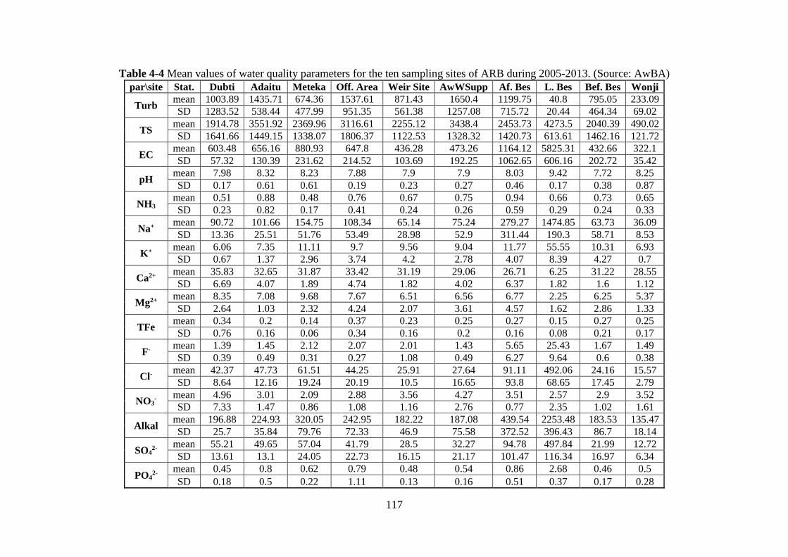
117
Table 4-4 Mean values of water quality parameters for the ten sampling sites of ARB during 2005-2013. (Source: AwBA)
par\site Stat. Dubti Adaitu Meteka Off. Area Weir Site AwWSupp Af. Bes L. Bes Bef. Bes Wonji
Turb mean 1003.89 1435.71 674.36 1537.61 871.43 1650.4 1199.75 40.8 795.05 233.09
SD 1283.52 538.44 477.99 951.35 561.38 1257.08 715.72 20.44 464.34 69.02
TS mean 1914.78 3551.92 2369.96 3116.61 2255.12 3438.4 2453.73 4273.5 2040.39 490.02
SD 1641.66 1449.15 1338.07 1806.37 1122.53 1328.32 1420.73 613.61 1462.16 121.72
EC mean 603.48 656.16 880.93 647.8 436.28 473.26 1164.12 5825.31 432.66 322.1
SD 57.32 130.39 231.62 214.52 103.69 192.25 1062.65 606.16 202.72 35.42
pH mean 7.98 8.32 8.23 7.88 7.9 7.9 8.03 9.42 7.72 8.25
SD 0.17 0.61 0.61 0.19 0.23 0.27 0.46 0.17 0.38 0.87
NH3 mean 0.51 0.88 0.48 0.76 0.67 0.75 0.94 0.66 0.73 0.65
SD 0.23 0.82 0.17 0.41 0.24 0.26 0.59 0.29 0.24 0.33
Na+ mean 90.72 101.66 154.75 108.34 65.14 75.24 279.27 1474.85 63.73 36.09
SD 13.36 25.51 51.76 53.49 28.98 52.9 311.44 190.3 58.71 8.53
K+ mean 6.06 7.35 11.11 9.7 9.56 9.04 11.77 55.55 10.31 6.93
SD 0.67 1.37 2.96 3.74 4.2 2.78 4.07 8.39 4.27 0.7
Ca2+ mean 35.83 32.65 31.87 33.42 31.19 29.06 26.71 6.25 31.22 28.55
SD 6.69 4.07 1.89 4.74 1.82 4.02 6.37 1.82 1.6 1.12
Mg2+ mean 8.35 7.08 9.68 7.67 6.51 6.56 6.77 2.25 6.25 5.37
SD 2.64 1.03 2.32 4.24 2.07 3.61 4.57 1.62 2.86 1.33
TFe mean 0.34 0.2 0.14 0.37 0.23 0.25 0.27 0.15 0.27 0.25
SD 0.76 0.16 0.06 0.34 0.16 0.2 0.16 0.08 0.21 0.17
F- mean 1.39 1.45 2.12 2.07 2.01 1.43 5.65 25.43 1.67 1.49
SD 0.39 0.49 0.31 0.27 1.08 0.49 6.27 9.64 0.6 0.38
Cl- mean 42.37 47.73 61.51 44.25 25.91 27.64 91.11 492.06 24.16 15.57
SD 8.64 12.16 19.24 20.19 10.5 16.65 93.8 68.65 17.45 2.79
NO3-
mean 4.96 3.01 2.09 2.88 3.56 4.27 3.51 2.57 2.9 3.52
SD 7.33 1.47 0.86 1.08 1.16 2.76 0.77 2.35 1.02 1.61
Alkal mean 196.88 224.93 320.05 242.95 182.22 187.08 439.54 2253.48 183.53 135.47
SD 25.7 35.84 79.76 72.33 46.9 75.58 372.52 396.43 86.7 18.14
SO42-
mean 55.21 49.65 57.04 41.79 28.5 32.27 94.78 497.84 21.99 12.72
SD 13.61 13.1 24.05 22.73 16.15 21.17 101.47 116.34 16.97 6.34
PO42-
mean 0.45 0.8 0.62 0.79 0.48 0.54 0.86 2.68 0.46 0.5
SD 0.18 0.5 0.22 1.11 0.13 0.16 0.51 0.37 0.17 0.28

118
Table 4-5 Correlation matrix (Spearman)
Var. Turb TS TDS EC PH NH3 Na+ K+ TH Ca2+ Mg2+ TFe F- Cl- NO3- Alkal HCO3
- SO42- PO4
2-
Turb 1
TS 0.31 1
TDS -0.07 0.65 1
EC -0.01 0.70 0.99 1
PH -0.42 0.35 0.50 0.52 1
NH3 0.67 0.49 0.15 0.18 -0.19 1
Na+ 0.01 0.67 0.98 0.99 0.43 0.16 1
K+ -0.30 0.45 0.64 0.62 0.07 0.16 0.66 1
TH 0.33 -0.24 -0.08 -0.09 -0.19 -0.33 -0.08 -0.54 1
Ca2+ 0.41 -0.21 -0.14 -0.15 -0.37 -0.12 -0.14 -0.50 0.89 1
Mg2+ 0.47 -0.03 0.27 0.28 -0.14 -0.05 0.30 -0.19 0.84 0.76 1
TFe 0.44 -0.38 -0.31 -0.30 -0.59 0.32 -0.21 -0.28 0.12 0.32 0.16 1
F- -0.42 0.35 0.66 0.61 0.20 0.08 0.66 0.92 -0.47 -0.50 -0.19 -0.26 1
Cl- -0.01 0.70 0.99 1.00 0.52 0.18 0.99 0.62 -0.09 -0.15 0.28 -0.30 0.61 1
NO3- 0.38 -0.39 -0.53 -0.52 -0.22 0.04 -0.54 -0.72 0.15 0.08 -0.03 0.39 -0.73 -0.52 1
Alkal -0.01 0.66 0.95 0.98 0.41 0.18 0.99 0.68 -0.12 -0.13 0.28 -0.18 0.65 0.98 -0.59 1
HCO3- -0.08 0.60 0.94 0.95 0.37 0.16 0.96 0.72 -0.14 -0.10 0.26 -0.15 0.68 0.95 -0.65 0.99 1
SO42- -0.07 0.55 0.95 0.96 0.50 0.02 0.95 0.54 -0.03 -0.12 0.32 -0.24 0.52 0.96 -0.37 0.94 0.92 1
PO42- 0.03 0.81 0.78 0.81 0.58 0.45 0.79 0.61 -0.41 -0.44 -0.08 -0.32 0.66 0.81 -0.56 0.78 0.75 0.65 1

119
consistency of the data. Both values imply that the sample is adequate and PCA can suitably
be applied on the dataset. Removing the three redundant variables TDS, TH and HCO3– from
the list of 19 parameters that are highly correlated to others, PCA on the normalized 16
variables was then computed to produce significant PCs and to further reduce the contribution
of variables with minor significance. It is done using Pearson type of correlation automatically
without fixing the number of components/factors to be generated because of the width of the
study area.
Table 4-6 Eigenvalues
F1 F2 F3 F4 F5 F6 F7 F8 F9
Eigenvalue 9.02 2.61 1.62 1.05 0.78 0.42 0.34 0.12 0.04
Variability(%) 56.39 16.32 10.1 6.57 4.87 2.62 2.13 0.75 0.26
Cumulative(%) 56.39 72.71 82.81 89.38 94.24 96.86 98.99 99.74 100
The 16 variables were reduced by PCA to 9 factors. PCA based on the water quality dataset
indicated that 4 factors were significant (i.e., PCs with an eigenvalue >1). These were retained
as the principal (significant) components because they could explain about 89.38% of the total
variation as shown by Table 4-6. This table shows the sorted Eigen values (variances of the
PCs) from large to small and percentage of variability versus principal components.
Table 4-7 Factor loadings and correlations between variables and the principal factors
Turb TS EC PH NH3 Na+ K+ Ca2+ Mg2+ TFe F- Cl- NO3- Alkal SO4
2- PO42-
F1 -0.29 0.73 0.92 0.79 0.15 0.93 0.84 -0.72 -0.48 -0.52 0.85 0.91 -0.54 0.97 0.89 0.88
F2 0.88 0.41 0.29 -0.42 0.40 0.31 -0.18 0.50 0.54 0.48 -0.09 0.32 0.25 0.19 0.34 0.16
F3 0.21 0.15 -0.19 -0.01 0.79 -0.14 0.11 -0.42 -0.61 0.25 0.08 -0.19 0.36 -0.12 -0.16 0.19
F4 -0.21 -0.05 0.13 0.26 -0.31 0.11 -0.29 -0.01 -0.25 0.34 -0.06 0.16 0.66 0.05 0.26 -0.14
As can be seen in the factor loadings and correlations between variables and factors of Table
4-7 and Table 4-8, the analysis also revealed that the first component, explaining about 56.39%
of the total variance, was highly and positively correlated with TS, EC, pH, Na, K, F–, Cl–,
Alkal, SO4– and PO4
– and negatively to Ca and TFe. The second component, of 16.32%
variability explanatory, was relatively more correlated with turbidity, Ca and magnesium. The
third and the fourth ones were related respectively to NH3 and NO3-.

120
Figure 4-4 Biplot of sample sites and water quality variables (axes F1 and F2: 72.71 %)
obtained from principal component analysis
A biplot of the variables and the sampling sites is shown by factors F1 against F2 in Figure
4-4. Both the plot and Table 4-8 indicate that F1 had a high and positive loading in TS, EC,
pH, Na, K, F–, Cl–, Alkalinity, SO4– and PO4
– which were 0.73, 0.92, 0.79, 0.93, 0.84, 0.85,
0.91, 0.97, 0.89 and 0.88 respectively. These large and positive loadings show strong linear
correlation between the factor and parameters. From the table of correlation (percentage
contributions) of variables to the four principal components, it can also be observed that F1 is
affected most by TS, EC, pH, Na, K, F-, Cl-, alkalinity, SO42- and PO4
3-; F2 by turbidity, Ca
and Mg; F3 by NH3 and F4 by NO3-.
When contribution of each of the sites to the factors is examined with reference to Table 4-8,
the largest percentage of about 59.5 for F1 is taken by lake Beseka. This is consistent with the
respective factor loading values (0.73, 0.92, 0.79, 0.93, 0.84, 0.85, 0.91, 0.97, 0.89 and 0.88)
of TS, EC, pH, Na, K, F–, Cl–, Alkalinity, SO4– and PO4
– of the water being taken from the
sites. Similarly, it can also be seen from the table that among the remaining sampling sites F2
was affected most by Wonji, F3 by Meteka, and F4 by Dubti and hence these sites are
Dubti Adaitu
Meteka
Off. Area
W. Site
Aw.W. Supp
Af. Bes
L. Bes
Bef. Bes
Wonji
Turb
TS EC
PH
NH3 Na
K
CaMg TFe
F
ClNO3- AlkalSO4-PO4-
-2.5
-2
-1.5
-1
-0.5
0
0.5
1
1.5
-1.5 -1 -0.5 0 0.5 1 1.5 2 2.5
F2 (
16
.32
%)
F1 (56.39 %)

121
considered as the most important pollution generating ones. However, the pH values of the 10
stations in Table 4-4 showed generally less variation as it ranges only from 7.72 to 9.42 though
it deviates a bit from the common pH range of surface water system, which is 6.5-8.5.
Table 4-8 % contribution of the variables to the PCs (a) and % contribution of observations to
the PCs (b)
a) % Contribution of the Variables to
PCs
b) % Contribution of the Observations to
PCs
Variables
% C
on
trib
uti
on
of
vari
ab
les
F1 F2 F3 F4 Sites F1 F2 F3 F4
Turbidity 0.92 29.7 2.69 4.16 Dupti
% C
on
trib
uti
on
of
Ob
serv
ati
on
s
7.73 6.31 13.7 59.2
TS 5.84 6.33 1.35 0.2 Adaitu 0.05 6.91 1.12 5.24
EC 9.45 3.21 2.32 1.63 Meteka 1.95 0.81 62.2 15.6
pH 6.85 6.83 0 6.3 Off.Area 0.02 16.2 0.48 2.68
NH3 0.24 6.2 38.2 9.41 W.Site 2.5 2.03 0.15 0.37
Na+ 9.53 3.7 1.27 1.08 Aw.W.Supp. 2.08 3.01 8.7 0.01
K+ 7.78 1.28 0.76 7.95 Af.Bes. 6.51 8.88 8.61 0.12
Ca2+ 5.69 9.67 10.9 0.01 L.Bes. 59.5 12.8 0.83 9.78
Mg2+ 2.52 11.1 22.9 6.14 Bef.Bes. 3.93 2.61 0.54 6.72
TFe 3.03 8.86 3.98 11 Wonji 15.7 40.5 3.68 0.27
F- 8.08 0.29 0.41 0.35
Cl- 9.21 3.84 2.24 2.36
NO3- 3.25 2.37 8.07 41
Alkalinity 10.3 1.33 0.95 0.22
SO42- 8.69 4.32 1.66 6.4
PO43- 8.61 0.95 2.25 1.83
4.2.2 Cluster Analysis (CA)
Agglomerative hierarchical clustering (AHC) using Euclidean distance with Ward’s method
was applied on the original dataset to assess the similarity among sampling sites. All the 10
sites of the basin are grouped into four statistically significant clusters at (Dlink/Dmax)*100<20.
Results of application of the cluster analysis are best visualized by a dendrogram or binary tree
given by Figure 4-5. The clustering has also offered the proximity matrix shown by Table 4-9.

122
Table 4-9 Proximity matrix (Euclidean distance)
Sites
Dub
ti
Adait
u
Mete
ka
Off.
Area
W.
Site
Aw.W.
Sup
Af.
Bes
L.
Bes
Bef.
Bes
Won
ji
Dubti 0
Adaitu 4.53 0
Meteka 4.67 3.90 0
Off.Area 3.52 2.71 4.44 0
W.Site 2.90 2.56 3.26 2.77 0
Aw.W.Sup 3.30 2.30 4.61 2.57 2.14 0
Af.Bes 4.28 2.35 4.69 2.71 2.61 2.54 0
L.Bes 13.04 11.75 11.74 12.33 11.98 12.15 10.85 0
Bef.Bes 3.56 2.84 3.58 2.55 1.20 2.71 2.53 12.02 0
Wonji 3.75 4.33 4.18 4.37 2.36 4.13 3.80 12.09 2.40 0
This table shows Euclidean distance between paired samples. The smaller the number of point
of intersection of two sites is, the more similar the sites are. e.g. before Beseka is more similar
to Weir site (1.20) than to L.Bes (12.02).
(Dlink/Dmax)*100
Figure 4-5 Dendrogram showing clustering of sampling sites based on the water quality
characteristics of Awash River.
The dendrogram in Figure 4-5 clearly depicts grouping of the sites based on similarity of water
quality characteristics. Accordingly, it classified before Beseka, Weir site, Wonji and Dubti as
L. Bes
Off. Area
Af. Bes
Adaitu
Aw.W. Supp
Meteka
Dubti
Wonji
W. Site
Bef. Bes
0 20 40 60 80 100 120 140
Cluster 2
Cluster 3
Cluster 4
Cluster 1

123
cluster 1. This grouping seems to be reasonable as these sites resemble in that they all are in
the vicinity of specialized sugarcane state farms. Adaitu, Office area, Awash water supply and
after Beseka are grouped as cluster 2. This is also consistent to the ground truth that the sites
receive waste contributing to turbidity, TS and NH3 from dominantly urban and bare-lands.
However, Meteka and Lake Beseka are categorized respectively as clusters 3 and 4. Meteka
seems to be unique in that it receives waste from small subsistence-oriented and diversified
agricultural and rural areas. Similarly, Lake Beseka is unique in that the lake water quality is
by far different from others as it shows the highest values of almost all parameters except for
turbidity, TH, Ca, Mg, TFe and NO3-. This is confirmed by the study of Dinka (2016) who has
urged in his conclusion to avoid even the contact of Lake Basaka water to crops and productive
soil in the region because of its pollution. The observations in the second cluster of brown
color are relatively more homogeneous than cluster 1 as they are more flat by the truncation.
This is confirmed by the within class variance shown by Table 4-10, where its value is less
than that of cluster 1.
Table 4-10 Results by class
Class 1 2 3 4
Objects 4 4 1 1
Within-class variance 780685.8 442212.0 0 0
Average distance to centroid 669.3 502.3 0 0
4.2.3 Temporal trend analysis
Trend analysis of TDS, EC, pH, NH3, Na, K, TH, F, Cl, and NO3 is performed in the 9 years’
period (2005 – 2013) by Mann-Kendall's (MK) two tailed trend test for the 4 sites in the basin
including Dubti, office area, after Beseka and Wonji. The analysis at 5% significant level in
the dry season (Dec-Feb) of Dubti showed that except TH and F none of the parameters are
found to show any trend since their p values computed by exact method are greater than the
significance level α=0.05. The test done for Dubti revealed that TH had a significant increasing
and F- a decreasing trend since their respective computed p-values 0.011 and 0.03 are less than
the significance level α=0.05 as can be explained by Figure 4-6 (a). Similarly, the analysis for
the office area indicated that only TDS has shown a trend, which is monotonic upward

124
throughout the years of consideration, and EC, NH3, Cl, Na and K also show increasing trends
only after 2009 (Figure 4-6 (b)) but the rest are all found to show no trend at all. At Wonji in
the dry season, except TH none of the parameters indicated a trend in the years from 2006 –
2013; TH has shown a significant increasing trend in the period as can be seen by Figure 4-6
(d). The test is undertaken in the wet season (June-August) of the parameters and most of them
are found to show no trend. However, TH and K respectively at Dubti and Wonji showed a
significant decreasing and increasing trends as depicted in Figure 4-6 (c).
y = -0.2294x + 462.49
y = 3.6779x - 7275.7
90
95
100
105
110
115
120
125
130
0.5
1.0
1.5
2.0
2.5
2006 2008 2010 2012
[TH
] (m
g/l
)
[F-]
(m
g/l
)
Year(a)
F TH
-4
1
6
11
16
0
150
300
450
600
750
900
1050
1200
1350
1500
2009 2010 2011 2012 2013
[NH
3],
[K
] (m
g/l
)
[EC
], [
TDS]
, [N
a], [
Cl]
(m
g/l
)
Year(b)
EC Na Cl
TDS NH3 K

125
Figure 4-6 Temporal Variation of TH and F- at Dubti (a); EC, TDS, NH3, Na, K, and Cl at the
Office area (b); TH at Wonji (d) in the Dry Seasons and that of TH at Dubti and K at Wonji in
the Wet Seasons (c).
Temporal trend analysis of the annual average values of turbidity, TS, TDS, EC, pH, NH3, Na,
K, TH, Ca, Mg, TFe, F, Cl, NO3-, alkalinity, HCO3
-, SO4- and PO4
- is undertaken throughout
the nine years’ period by MK two tailed trend test for Dubti, Adaitu, office area, Weir site,
after Beseka, Beseka, Before Beseka, and Wonji. The analysis at 5% significant level for Dubti
tell us that only SO4- and F- show a trend while others all don’t as their p-value, computed by
the exact and approximation methods, is greater than the significance level alpha=0.05. While
the former showed an increasing trend, the later a decreasing one (Figure 4-7a). A similar
analysis at office area indicates that TDS, EC, Na, K, Mg, TFe, alkalinity and SO4- show an
y = -2.8641x + 5858.5
y = 0.4356x - 867.29
6
7
8
9
10
11
12
85
90
95
100
105
110
115
120
2005 2007 2009 2011 2013
[K]
(mg
/l)
at W
on
ji
[TH
] (m
g/l
) at
Du
bti
Year(c)
TH K
y = 0.1878x - 376.72
0
0.5
1
1.5
2
2.5
2006 2007 2008 2009 2010 2011 2012 2013
[TH
] (m
g/l
)
Year(d)
TH

126
increasing trend since their computed p-value is lower than the significance level alpha=0.05.
The test at Beseka resulted in the fact that TS, TDS, EC, NH3, Na, K, F, Cl, NO3-, alkalinity,
HCO3- and PO4
- to have shown trends since their p-values is smaller than alpha=0.05. Among
these, except NH3, all of them are decreasing. While both turbidity and TS show a decreasing
trend at after Beseka, the rest all are found to show no trend at all.
On the other hand, performing MK test on NH3, K, Mg, TH and SO4- show increasing while
F- a decreasing trend at Wonji as show by Figure 4-7 (e) as their p-values computed by exact
method is lower than the significance level alpha=0.05 while others all don’t. At before Beseka
TDS, EC, NH3, Na, K, TH, TFe, Cl-, alkalinity, and HCO3- show a trend in the years 2005-
2013 while at Weir site TDS, EC, NH3, Na, K, Mg, TFe, Cl-, alkalinity, HCO3-, SO4
-, and PO4-
show a trend. With a similar argument MK test indicated at Adaitu that only EC, NH3, HCO3-
, and SO4- have shown trends.
y = 4.6768x - 9340.6R² = 0.7872
y = -0.1082x + 218.82R² = 0.5117
0.7
0.9
1.1
1.3
1.5
1.7
1.9
2.1
2.3
30
40
50
60
70
F-
SO4
-
Yeara) Dubti
SO4 F

127
-10
10
30
50
70
350
2350
4350
6350
NH
3,N
O3
, P
O4, K
, F
-
TS
, T
DS
, E
C,
Na,
Cl,
Alk
al,
HC
O3
-
Yeard) Beseka
TS TDS EC NaCl Alkal HCO3- NH3

128
Figure 4-7 Trend analysis of the water Quality data in the nine years’ period at Dubti, Office
area, After Beseka, Beseka and Wonji
5
15
25
35
45
55
65
75
85
95
0
1
2
3
4
5
6
7
8
9
2005 2006 2007 2008 2009 2010 2011 2012 2013
TH, S
O4
-
NH
3, K
, Mg,
F-
Yeare) Wonji
NH3 K Mg F TH SO4-
0.0
200.0
400.0
600.0
800.0
1000.0
1200.0
EC TH EC TH EC TH EC TH
AfBes Off. Area Dubti Wonji
EC (
S/cm
) &
TH
(m
g/l
)
a) Seasonal trend
Bega Belg Kiremt

129
Figure 4-8 Seasonal Variation of EC and TH in the three main seasons of the year (a) and of
average [TH] of all sites in february over the years 2005-2013 (b)
Investigation of water quality parameters such as EC and TH is undertaken to see the temporal
trends along Ethiopian seasons of Bega (October-January), Belg (February-May) and Kiremt
(June-September) at the four sites namely Dubti, Office area, after Beseka and Wonji. MK
trend test for an average over all sites of [TH] in a month of February on the eight years (2005-
2013) is also examined. The graphs in Figure 4-8 (a) exhibit that both variables get absolute
maximum values in the Belg season at all sites except that TH got largest value in Kiremt at
the Office area. In the MK trend test for [TH], the null hypothesis declaring absence of a trend
in the series of [TH] along the years is rejected and the alternative hypothesis saying that there
is a trend in the series is accepted since the computed p-value = 0.001, is lower than the
significance level α=0.05. The type of trend is positive though not monotonic as can be seen
by Figure 4-8 (b).
Analysis of EC, pH, NH3, TH, TDS and alkalinity is done to see their general change in the
dry (October-January) and wet (June-September) seasons of the 14 monitoring sites namely:
Dubti, Adaitu, Meteka, Office area, Weir site, Awash W. Supp, Awash fall, Af. Bes., Beseka,
Bef. Beseka, Sodere, Wonji, Koka dam and Mojo. The general truth, as can be seen in Figure
4-9, is that average values of all of them is higher in the dry than in the wet season.
y = 2.5597x - 5048.5
80
85
90
95
100
105
110
[TH
]
Yearb)
[TH]

130
Figure 4-9 Seasonal trend analysis of the water quality parameters in the dry and wet seasons
4.2.4 Spatial trend analysis
Spatial analysis of water quality parameters was assessed at the 14 sampling sites of ARB.
From slopes of trendlines of graphs of the water quality indicators, it can be seen generally that
as one moves from upper to lower parts of basin in the dry season (October-January), EC, TH
and Cl were observed to be decreasing (Figure 4-10). From the trendlines of the graphs, one
can also observe that the parameters change abruptly and significantly in and around the hot
springs and lake Beseka.
TH was slightly increasing while TDS, Cl, and SO42- were decreasing in the same direction in
the rainy season (June-September). It can also be seen from the graph that among the sites in
both the dry and wet seasons, Cl and EC/TDS/SO42- were maximized respectively at bef Beseka
and Beseka. At Beseka in both seasons, TH showed a trend opposite to that of EC/TDS/ SO42-
, i.e it revealed an absolute minimum. The most important sites responsible for the spatial
variation were Beseka, before Beseka and Sodere spring as they are where, for instace, EC,
TDS, TH, Cl, and SO42- showed significant variation. The reason of decreasing concentraion
of most pollutants (immersed into the river mostly from the upper basin) might be the natural
purification process taking place in the course of the river.
200
1000
1800
2600
3400
4200
5000
5800EC
(m
g/l)
Dry Season Wet Season
Mean
Outliers(2)
Minimum/Maximum
7
7.5
8
8.5
9
9.5
pH
Val
ues
Dry Season Wet Season 0.25
0.75
1.25
1.75
2.25
NH
3
Dry Season Wet Season
30
50
70
90
110
130
150
170
190
TH
Dry Season Wet Season
100
600
1100
1600
2100
2600
3100
3600
[TD
S] (
mg/
l)
Dry Season Wet Season0
500
1000
1500
2000
2500
ALk
alin
ity
(mg/
l)
Dry Season Wet Season

131
Figure 4-10 Spatial Variation of EC, TH, and Cl in the Dry (a) and TH, Cl, SO42- and TDS in
the Wet (b) Seasons of ARB.
The MK test at Beseka resulted in the fact that TS, TDS, EC, Na, K, F-, Cl-, NO3- TDS,
EC, Na, K, F-, Cl-, NO3-, showed decreasing trends. This finding is in agreement with that
of Dinka (2017) who found that in the previous two decades (1960-1980) water quality
parameters especially ionic concentrations had shown decreasing trends in response to the fast
increasing volume of the lake, which has a dilution effect although his finding has unexpectedly
shown stability of most and even increasing trend of other parameters post 2000. Throughout
0
50
100
150
200
250
300
350
400
450
0
1000
2000
3000
4000
5000
6000
TH a
nd
Cl-
EC
Sampling Sites in the Basina)
EC Cl TH
0
500
1000
1500
2000
2500
3000
3500
4000
0
100
200
300
400
500
600
TDS
TH, C
l-, S
O4
-2
Sitesb)
Cl- TH
SO4- TDS

132
the years from 2005 to 2013, almost all parameters except NH3 in Figure 4-7 ( d ) were
showing a temporal decreasing trend. This is suggested to be due to ever increasing
volume of the lake from time to time which could dilute the water more (Alemayehu et al.,
2006; Dinka, 2017).
On the other hand, EC (salinity-determinant) has shown a spatially increasing trend from
upper to middle and then decreasing afterwards (Figure 4-10), though it was concluded by
Taddese et al. (2003) that salinity is generally increasing from the upper to lower basin. The
state of EC being maximum in t h e middle seems, however, to be reasonable since there are
Lake Beseka and Sodere spring here having high EC values. Cl has also shown a similar trend
as EC throughout the basin while TH showed decreasing trend in the upper and increasing
trend in the middle and lower sub-basins. Most other pollutants (discharged into the River from
the upper basin) are also seen to decrease their concentration in the downstream (except for
EC, TDS, SO4-, and Cl- at lake Beseka and Sodere hot spring). This might be due to the
natural purification process taking place in the course of the river and the lesser amount of
waste discharged into the river in the middle and lower basins though the climate is worsening
in the downstream tending to concentrate the pollutants while concurrently diminishing the
volume of the river due to diversion for different purposes in the lower part.
4.3 Land use/land cover and water quality
Since rivers are vulnerable to land use changes, understanding the relationship between water
quality and land use is useful for identifying primary threats to water quality. These
understandings are meaningful for effective water quality management because they can be
used to target critical land use areas and to institute relevant measures to minimize pollutant
loadings (Ding et al., 2015).
4.3.1 Land use/land cover dynamics
The changes in land use and land cover in the three years considered were attributed to factors
such as draught year, transition of government, economic and land use policy change observed
in the nation at large and in the basin in particular.
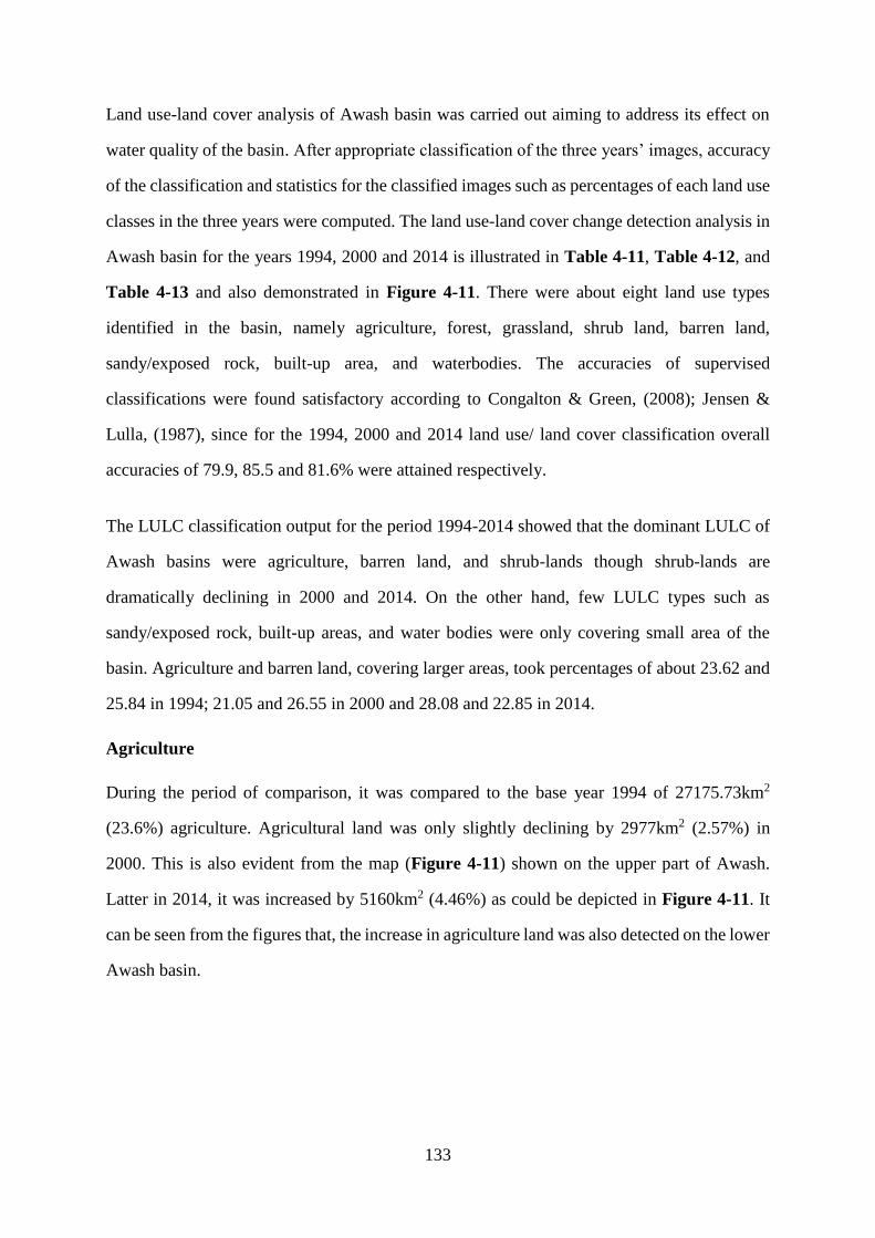
133
Land use-land cover analysis of Awash basin was carried out aiming to address its effect on
water quality of the basin. After appropriate classification of the three years’ images, accuracy
of the classification and statistics for the classified images such as percentages of each land use
classes in the three years were computed. The land use-land cover change detection analysis in
Awash basin for the years 1994, 2000 and 2014 is illustrated in Table 4-11, Table 4-12, and
Table 4-13 and also demonstrated in Figure 4-11. There were about eight land use types
identified in the basin, namely agriculture, forest, grassland, shrub land, barren land,
sandy/exposed rock, built-up area, and waterbodies. The accuracies of supervised
classifications were found satisfactory according to Congalton & Green, (2008); Jensen &
Lulla, (1987), since for the 1994, 2000 and 2014 land use/ land cover classification overall
accuracies of 79.9, 85.5 and 81.6% were attained respectively.
The LULC classification output for the period 1994-2014 showed that the dominant LULC of
Awash basins were agriculture, barren land, and shrub-lands though shrub-lands are
dramatically declining in 2000 and 2014. On the other hand, few LULC types such as
sandy/exposed rock, built-up areas, and water bodies were only covering small area of the
basin. Agriculture and barren land, covering larger areas, took percentages of about 23.62 and
25.84 in 1994; 21.05 and 26.55 in 2000 and 28.08 and 22.85 in 2014.
Agriculture
During the period of comparison, it was compared to the base year 1994 of 27175.73km2
(23.6%) agriculture. Agricultural land was only slightly declining by 2977km2 (2.57%) in
2000. This is also evident from the map (Figure 4-11) shown on the upper part of Awash.
Latter in 2014, it was increased by 5160km2 (4.46%) as could be depicted in Figure 4-11. It
can be seen from the figures that, the increase in agriculture land was also detected on the lower
Awash basin.

134
Table 4-11 Area contribution of the land use classes in hectare and percentage
LU classses 1994 2000 2000-
1994
2014 2014-
1994 Area_km2 % Area_km2 % Area_km2 %
Agriculture 27175.73 23.62 24198.74 21.05 -2.57 32335.80 28.08 4.46
Forest 9466.82 8.23 15671.71 13.63 5.41 12905.76 11.21 2.98
Grassland 12087.29 10.51 15990.50 13.91 3.41 13900.25 12.07 1.56
Shrubland 27109.39 23.56 15464.67 13.45 -10.11 15904.15 13.81 -9.75
Barrenland 29730.16 25.84 30521.42 26.55 0.71 26315.10 22.85 -2.99
Sandy/Exposed rock 5223.07 4.54 9449.03 8.22 3.68 7543.49 6.55 2.01
Builtup area 2134.59 1.86 2614.78 2.27 0.42 5416.63 4.70 2.85
Waterbodies 2128.53 1.85 1027.24 0.89 -0.96 851.90 0.74 -1.11
Nowadays, improper management of wastes from urban and rural areas such as that of farm
residues, fertilizer and agro-chemical, as in the case of catchments in many developing nations,
the burden on the quality of water increases.
Built up areas
The built up areas include both urban and rural areas builtups. This was only covering
2134.59km2 (1.9%) in 1994. The built-up area cover was consistently increasing to 2.3% and
4.7% of the basin in 2000 and 2014 respectively. Compared to its base year 1994, the cover of
built-up areas was increased by 2.9% in 2014. Built-up areas were the major source of non-
point sources of pollution. There are several towns and cities found in ARB, which have
continuously increased their cover since 1994. The growth in number and size of these towns
and cities were accompanied by industries, large service providing centers, manufacturers,
which are inevitably release their effluent to the nearby surface water. Built-ups, including
impervious areas such as roads and rooftops, accelerate movement of wastes with storm water
that ultimately release directly into running water especially during rainy seasons.
Sandy /Exposed rock
Sandy and exposed rocks are often found in the lower parts of south-eastern Awash basin. This
is an area inhibiting vegetation growth. Sand and exposed rock was only covering 5223.07km2
(4.5%) in 1994, this was remarkably increased by 3.7% and 2% in 2000 and 2014 respectively.

135
This is susceptible to erosion especially during erratic rainfall conditions, which releases waste
into the river to affect quality of water.
Shrub-land
The lower region of Awash basin is a low-lying semi-arid area dominated by shrub-lands
covering large area in 1994 (about 27109.39km2 or 23.6%). This was depleted in 2000 and
2014. Shrub-land is one of the three dominant land covers with agriculture and barren-land by
1994 in Awash basin. This has dramatically fallen to 15464.67km2 (13.5%) and 15904.15km2
(13.8%) in 2000 and 2014 respectively.
Barren land
Barren lands show slight change in the period, 1994-2014. From the three years, the largest
coverage was detected in 2000 for an estimated cover of 30521.42km2 (26.5%). It was latter
declined by 390188ha (3%) in 2014 from the base year. All forms of land use land cover change
affects water quality of the basin, however agriculture and barren lands were important in the
basin due to their large and persistent coverage. Both land uses assume exceptionally major
source of accelerated soil erosion due to its loosen soil particles and agrochemicals added on
the farmlands. These and others forms of residues consequently enter into the river and affect
water quality.
Grass lands
Grassland was another LULC noticed in the basin. According to Figure 4-11, it is largely found
between the buffer of forest areas and shrub-land. It was also significantly found on the gorges
of Awash basin (Figure 4-11). About 12087.29 km2 (10.5%) was covered by grass lands in
1994, and this was increased by 3.4% and 1.6% in 2000 and 2014 respectively.

136
Figure 4-11 LU/LC maps of the study area in 1994 (a), 2000 (b), and 2014 (c)
(a) (b)

137
Forest
Relative to the large area coverage of Awash basin, it was only a small portion that is covered
by forest. Most of the forest cover was located on the upper region of Awash basin (Figure
4-11). The forest cover was estimated to be 9466.82 km2 (8.2%) in 1994, while this was
increased by 5.4% and 3% in 2000 and 2014 respectively. In other words, forest cover of 2014
reduced by 2.4% from 2000. According to Figure 4-11, the upper escarpment of Awash basin
was persistently covered with forest for the period 1994-2014.
Water bodies
Water bodies were other important land cover types identified in Awash basin. The change in
area coverage of water appeared to reduce by 0.96% in 2000 relative to the base year 1994,
which was 2128.53km2 (1.8%). This was only slightly reduced by 1.1% in 2014.
Transition matrices
A matrix is produced by multiplying columns in the transition probability matrix by the number
of cells of corresponding land uses in the later image. The transition matrix produced for land
use maps of years 1994 and 2014 is shown by Table 4-12. The transition matrices between
1994 and 2014 indicated that about 18.3% of agriculture is converted to built-up area from
1994 to 2014 largest proportion of 43.8% of forest was cleared for cultivation (farm land).
Significant proportion of grass land was converted to agriculture (29.5%), to barren land (30%)
and built-up area (25.5%). Similarly, shrub land was largely converted to agriculture (35.7%).
There was about 38.8% water bodies shrunk due to cultivation. Similarly, large proportion of
built up areas (37.7%) and (27.6%) were also converted to barren-land and agriculture
respectively.

138
Table 4-12 Transition probability table (Confusion matrix) showing transformation of one
land use type to another from 1994 to 2014
2014
LULC Agriculture Forest Grass Shrub Barren Sand Built-up Water
Agriculture 27.1% 15.1% 12.6% 3.3% 17.9% 5.0% 18.3% 0.8%
Forest 43.8% 32.5% 8.0% 1.2% 6.2% 1.5% 5.9% 1.0%
1994 Grass 29.5% 1.6% 6.3% 2.6% 33.0% 1.2% 25.5% 0.2%
Shrub 35.7% 11.7% 16.7% 5.7% 19.9% 1.3% 8.7% 0.2%
Barren 19.3% 5.7% 13.4% 4.7% 31.6% 10.3% 14.8% 0.1%
Sand 8.3% 3.8% 2.2% 1.8% 18.6% 46.5% 18.6% 0.2%
Builtup 27.6% 4.2% 9.9% 1.6% 37.7% 0.0% 18.7% 0.2%
Water 38.8% 20.1% 2.9% 0.6% 5.9% 0.0% 6.6% 25.2%
Unit of area of change is in percent (%).
Such LU/LC changes are not healthy either from environmental or socio-economic points of
view and therefore, are matters of concern. The land cover dominance in the basin has shifted
from bare lands (in 1994) to agricultural (in 2014). This result is in line with the suggestion of
ASTU (2016) that in middle Awash shrub and pasture lands were cleared for irrigation recently
and hence increase in percentage of the agricultural land. The LULC changes and associated
human activities have deteriorated the water quality in the study areas as evident from low DO,
higher electrical conductivity, total hardness, total dissolved solids, turbidity, nitrate, chloride,
sulphate, BOD and total coliform, presence of pollution tolerant macro-invertebrates etc.
4.3.2 Land use-water quality relationship in Awash River basin
The land use land cover change in the basin was compared to values of some water quality
parameters for the period 2000-2014 (Figure 4-12).

139
Figure 4-12 Trends of EC, Total hardness, Alkalinity, SO4, and TDS in 2000’s and 2010’s
Most water quality parameters did not show a trend for the period 2000-2014, while few of
which including EC, TDS, Alkal, TotHard and SO4 were significantly showing trends. There
was an increase in agriculture and built-up areas by 6.8% and 2.5% respectively from 2000 to
2014; on the other hand, there was a decrease in forest and grassland by 2.4 and 1.8%
respectively in the period. In association with these land use changes, the water quality
parameters EC, TDS, Alkal, TotHard and SO42- were rising 64.92, 36.2, 48.89, 17.24 and 5.61
times a year for the period 2005-2014. Exceptionally, barren land was reduced by 3.4% which
was expected to affect the water quality positively. This might be attributed to the location of
the change in barren land, which was eastern region of Awash basin.
After classification of images of 2000 and 2014, the area in hectare (ha) and percentage
statistics for the classified images of each land use class in the two years, around which the
water quality data were collected, have been computed. Table 4-13 clearly shows why some
parameters like SO42-
, TH, EC, Na+, Cl-, K+, and NH3 increase monotonically at some sites
and why the rest vary in the other sites of the basin temporally, which is corresponding to the
land use changes in the respective sites. For instance, agriculture and built-up areas have
significantly increased in the basin from 2000 to 2014. The associated pollution by agro-
chemicals, nutrients, and hardness resulting from urbanization and agricultural intensification
y = 64.919x + 546.38R² = 0.658
y = 17.244x + 50.105R² = 0.3037
y = 48.894x + 110.78R² = 0.5225
y = 5.6089x + 25.99R² = 0.4981
y = 36.199x + 373R² = 0.5251
0
200
400
600
800
1000
1200
2005 2006 2007 2008 2009 2010 2011 2012 2013 2015/16
EC
(m
S/c
m),
TotH
ard, A
lkal
, S
O4
-,
TD
S (
mg/L
)
YearEC TotHard Alkal SO4- TDS

140
was observed. From the 2014 land use map, the land is more degradable as one moves from
upper to lower basin.
Table 4-13 Percentages of land uses of the basin in 2000 and 2014
LU classses 2000 2014
Area_km2 % Area_km2 %
Agriculture 24198.74 21.05 32335.80 28.08
Forest 15671.71 13.63 12905.76 11.21
Grassland 15990.50 13.91 13900.25 12.07
Shrubland 15464.67 13.45 15904.15 13.81
Barrenland 30521.42 26.55 26315.10 22.85
Sandy/Exposed rock 9449.03 8.22 7543.49 6.55
Builtup area 2614.78 2.27 5416.63 4.70
Waterbodies 1027.24 0.89 851.90 0.74
The land in the lower part of the basin is mostly bare, sandy, rocky and the rest is covered by
shrubs, which is an indication of an arid zone. In the middle part of the basin, there are Lake
Beseka and Sodere hot spring, both of which are located in a tectonically active Main Ethiopian
Rift region and discharge to Awash River. Lake Beseka is not only the fastest growing unlike
other lakes in the region but also unique in its water quality characteristics (Dinka, 2017;
Alemayehu et al., 2006). The exceptional pollution of this lake and at the site just before it,
found in this study by parameters as EC, TDS, SO4- and Cl-, is in line with these findings.
This is found to be due to the underlying anthropogenic (increased discharge of the hot springs
and discharge of huge amount of irrigation wastewater upstream of the lake, discharges
from factory and domestic sewage), natural (weathering of rocks, soil erosion, sediment
loading, deposition of animal and plant debris, and solution of minerals in the basin), climatic
and geologic factors (Goerner et al., 2009; Dinka, 2017).
The relationship between important land use types with respect to pollution and mean values
of water quality in wet season is also visualized by Figure 4-13 and Figure 4-14. Two of the
land use types are tributaries to the river and one of them is the river itself, which are
differentiated as Agriculture-dominated (AD), Industry-Dominated (ID) and Urban-dominated
(UD). AD land use (Wonji) is the one that is a mixture of rural housing and dominantly
agricultural areas. Agricultural activities typically cover the cultivation of vegetables and
arable crops for subsistence consumption and large-scale irrigation schemes of sugarcane. UD
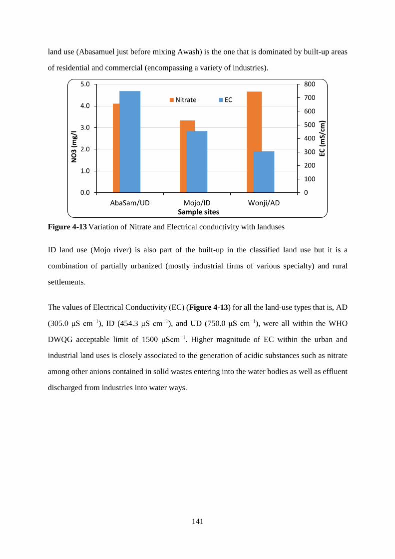
141
land use (Abasamuel just before mixing Awash) is the one that is dominated by built-up areas
of residential and commercial (encompassing a variety of industries).
Figure 4-13 Variation of Nitrate and Electrical conductivity with landuses
ID land use (Mojo river) is also part of the built-up in the classified land use but it is a
combination of partially urbanized (mostly industrial firms of various specialty) and rural
settlements.
The values of Electrical Conductivity (EC) (Figure 4-13) for all the land-use types that is, AD
(305.0 μS cm−1), ID (454.3 μS cm−1), and UD (750.0 μS cm−1), were all within the WHO
DWQG acceptable limit of 1500 μScm−1. Higher magnitude of EC within the urban and
industrial land uses is closely associated to the generation of acidic substances such as nitrate
among other anions contained in solid wastes entering into the water bodies as well as effluent
discharged from industries into water ways.
0
100
200
300
400
500
600
700
800
0.0
1.0
2.0
3.0
4.0
5.0
AbaSam/UD Mojo/ID Wonji/AD
EC (
mS/
cm)
NO
3 (
mg/
l
Sample sites
Nitrate EC

142
Figure 4-14 Variation of Alkalinity, Bicarbonate, Total hardness and Chloride with landuses
Increasing levels of conductivity may also be due to the existence of inorganic suspended solids
in runoff as well as the presence of chloride and nitrate from sewage systems as well as the
product of decomposition and mineralization of organic materials (Alemayehu, 2006, 2001,
2000). On the other hand, nitrate is observed to be higher in agriculture-dominated areas of
Wonji than that in the urbanized and industrial areas although each of these generate to some
extent. Figure 4-14 generally depicts higher concentration of anions (bicarbonates and
chlorides) and hardness to have been generated from urbanized areas than that from the
agricultural areas. For instance, the mean chloride concentration of 75.54 mg/l was the highest
in the UD land use. This could be as a result of wastewater from industries such as that of metal
(Paul, 2000).
0
10
20
30
40
50
60
70
80
0
50
100
150
200
250
300
350
AbaSam/UD Wonji/AD Mojo/ID
Cl-
(mg/
l)
Alk
. & B
icar
b. (
mg/
l
Sample sites
Alkalinity Total Hardness
Bicarbonate Chloride
143
4.4 Water quality modeling
In addition to simulating flow, sediments, nutrients and other water quality determinants, the
GIS-interfaced SWAT model here is also found to be a good tool to visualize the temporal and
spatial changes of water quality parameters due to change in land uses. This is assisted by the
model keeping all other input parameters of the model fixed since performance of the SWAT
model is found to be satisfactory to very good in analyzing land use land cover changes in
semi-arid environment (Kiros et al., 2015) like the study area. So, considering the three years’
(1994, 2000, and 2014) land uses of the basin, the change in the water quality is examined
resulting from changes in LU/LC from 1994 to 2000, from 2000 to 2014 and from 1994 to
2014.
4.4.1 Watershed delineation and characterization
ARB covers an area of about 115,055.58km2 (11,505,558ha). Various GIS data preprocessing
tasks were done beforehand. Generally, the watershed delineation task was accomplished by
overlaying the Digital Elevation Model (DEM), soil, stream network, slope and land use and
land cover maps. Awash basin consisted of 8 land uses, 8 soil texture classes and 5 major slope
classes. There were also 20 metrological stations considered in the basin.
The DEM was used to delineate the topography, characterize the watershed and determine the
hydrological parameters of the watershed such as slope, flow accumulation and direction, and
stream network. The watershed delineation step discretizes the watershed in to 53 sub-basins.
The sub-basins were overlaid with land uses and soil data to produce 561, 665 and 507 HRUs
in running the model with the 1994, 2000 and 2014 land uses respectively but the basin having
in each case constantly 53 sub-basins (Figure 4-15). The reason why the number of HRUs vary
is that there is a slight difference in the total area of the catchment that may be obtained by
buffering the watershed by different distances in the three cases (as the DEM was required to
be a bit greater than the basin). The HRUs were determined by unique intersections
(overlaying) of the land use and land cover, slope and soils within the watershed. This process
allows capturing the heterogeneity of the physical properties. The HRUs are the spatial level

144
at which the model computes the effect of management practices on water quality. In each sub-
basin, each land use representing over 10% of the sub basin area was included in the model;
also included were each soil representing 2% or more of that land use area and each land slope
representing 5% or more of that land use area.
Finally, the 20 weather stations were submitted and all the necessary data were fitted to run
SWAT model successfully. The model was then setup and run for the three land use land cover
years 1994, 2000 and 2014.
4.4.2 The SWAT model simulation
The preliminary model was set up using drainage areas of 115055.582, 114938.084, and
115173.08km2 respectively in the 1994 (base year), 2000 and 2014 lad uses as the threshold
for delineation of the watershed. This resulted in 53 sub-basins in all cases which were
characterized by dominant soil, land use, and slope (Figure 4-15). The initial simulation period
was 1997–2014, considering the first 3 years’ time (1994-1996) as a setup (warm-up) period.
Modeling of nutrients (nitrogen and phosphorus) was made after calibration and validation of
SWAT’s hydrology component.
4.4.2.1 Sensitivity Analysis of Flow
The first step in the process of calibration and validation of simulation results of the SWAT
model is determination of the most sensitive parameters for a given basin (Arnold et al., 2012).
The parameter sensitivity analysis was conducted using the global sensitivity analyses that is
integrated to SWAT2012.

145
Figure 4-15 ARB SWAT Configuration with the Sub-basins and Weather Stations

146
Table 4-14 Selected input parameters to SWAT-CUP in the sensitivity analysis to stream flow
No. Input Parameter Name Description of Parameter Min Max t-Stat P-Value Rank
1 17:V_CH_K2.rte Effective hydraulic conductivity of channel (mm/hr) 0 0.3 -0.151 0.880 19
2 2:R_OV_N.hru Manning's "n" value for overland flow -0.1 1 0.213 0.831 18
3 10:V_GW_REVAP.gw Groundwater "revap" coefficient 0.02 0.2 -0.286 0.775 17
4 18:V_ALPHA_BF.gw Base flow alpha factor (days) 0 1 0.581 0.561 16
5 14:V_ALPHA_BNK.rte Base flow alpha factor for bank storage (days) 0 1 0.621 0.535 15
6 6:V_SURLAG.bsn Saturated hydraulic conductivity (mm/hr) -10 24 0.708 0.479 14
7 9:V_REVAPMN.gw Threshold water level in shallow aquifer for revap or percolation
to deep aquifer (mm H2O) 0 500 0.990 0.323 13
8 16:V_CH_N2.rte Manning's "n" value for the main channel 0 15 -1.103 0.270 12
9 12:R_SOL_AWC(..).sol Available water capacity of the soil layer (mm H2O/mm soil) -0.2 0.4 1.917 0.056 11
10 3:V_GW_DELAY.gw Groundwater delay (days) 0 500 2.017 0.044 10
11 8:V_EPCO.bsn Plant water uptake compensation factor 0.01 1 -2.091 0.037 9
12 15:V_RCHRG_DP.gw Aquifer percolation coefficient 0 1 -2.362 0.019 8
13 13:V_ESCO.hru Soil evaporation compensation factor 0.01 1 -2.953 0.003 7
14 19:V_GWQMN.gw Threshold water level in shallow aquifer for base flow (mm H2O) 0 5000 -3.122 0.002 6
15 5:R_SOL_K(..).sol Saturated hydraulic conductivity (mm/hr) 0 2 -3.184 0.002 5
16 11:R_SOL_BD(..).sol Bulk density of soil's first layer (Mg m-3) -0.5 0.6 -5.276 0.000 4
17 4:V_SLSUBBSN.hru Average slope length (m) 10 150 5.436 0.000 3
18 7:V_HRU_SLP.hru Average slope steepness (fraction) -0.5 1 -7.341 0.000 2
19 1:R_CN2.mgt SCS runoff curve number -15 15 -33.018 0.000 1
Explanations: V— existing parameter value is to be replaced by given value or absolute change; R— existing parameter value is multiplied by (1
+ a given value) or relative change (Abbaspour, 2009). (..) first layer of soil profile.

147
Figure 4-16 Plot of Global Sensitivity Analysis of parameters of stream flow sorted by t-Stat
Accordingly, nineteen hydrologic parameters that may have an influence on streamflow of
Awash River were used in the sensitivity analysis. Table 4-14 shows the model parameters and
the sensitivity analysis result, ranked with most sensitive parameter in its last row. The
parameters used were: REVAPMN.gw, SOL_AWC(..).sol, RCHRG_DP.gw, GWQMN.gw,
ALPHA_BF.gw, EPCO.bsn, OV_N.hru, ALPHA_BNK.rte, SOL_K(..).sol, CH_N2.rte,
GW_DELAY.gw, SURLAG.bsn, GW_REVAP.gw, CH_K2.rte, HRU_SLP.hru, CN2.mgt,
SLSUBBSN.hru, ESCO.hru, and SOL_BD(..).sol,

148
Figure 4-17 Global Sensitivity Analysis Setting of the 19 Parameters
With respect to absolute values of t-Stat values in the grid from the global SA, plotted in Figure
4-17, sensitivities of the parameter were ranked and put in Table 4-14 according to (Khalid et
al., 2016). Parameters of larger t-Stat in absolute values or those of p-values less than or equal
to 0.05 have been taken as those to which the streamflow was most sensitive. On the basis of
the p-values, ten parameters were therefore pointed out to be more sensitive, namely (in the
increasing order of sensitivity); V_GW_DELAY.gw, V_EPCO.bsn, V_RCHRG_DP.gw,
V_ESCO.hru, V_GWQMN.gw, R_SOL_K(..).sol, R_SOL_BD(..).sol, V_SLSUBBSN.hru,
V_HRU_SLP.hru, and R_CN2.mgt. Hence, these parameters were found to be the most crucial
parameters for the studied basin as they generally govern the surface hydrological processes
and stream routing. The hydrology is observed to be exceptionally sensitive to curve number
(CN2).
4.4.3 Quantification of the SWAT model performance
Calibration of such a large-scale model was not straight forward. Important issues to address
were how to deal with the availabile input data, watershed parameterization, and uncertainties
associated with input data accuracy and scarcity (flow, rainfall), model uncertainty and
parameter non-uniqueness.
-35.00
-30.00
-25.00
-20.00
-15.00
-10.00
-5.00
0.00
5.00
10.00
17:V
__C
H_K
2.r
te
2:R
__O
V_N
.hru
10:V
__G
W_R
EV
A…
18:V
__A
LP
HA
_B
…
14:V
__A
LP
HA
_B
…
6:V
__S
UR
LA
G.b
sn
9:V
__R
EV
AP
MN
.gw
16:V
__C
H_N
2.r
te
12:R
__S
OL
_A
WC
…
3:V
__
GW
_D
EL
A…
8:V
__E
PC
O.b
sn
15:V
__R
CH
RG
_D
…
13:V
__E
SC
O.h
ru
19:V
__G
WQ
MN
.gw
5:R
__S
OL
_K
(..)
.sol
11:R
__S
OL
_B
D(.
.)…
4:V
__S
LS
UB
BS
N.…
7:V
__H
RU
_S
LP
.hru
1:R
__C
N2.m
gt
t-S
tat
val
ues
Parameters used in the sensitivity analysis of flow
t-Stat

149
4.4.3.1 Monthly calibration and validation of the river flow
a) Calibration and uncertainty analysis
Three groundwater parameters (GW_REVAP.gw, RCHRG_DP.gw, GWQMN.gw), two soil
parameters, (SOL_BD(..).sol and SOL_K(..).sol), one evaporation parameter (ESCO.hru), one
plant water uptake parameter (EPCO.hru), one runoff parameter (CN2.mgt), and two HRU
general input files (HRU_SLP.hru and SLSUBBSN.hru) were considered in the model
calibration (Table 4-15) of the flow. Simulated monthly streamflow versus the observed
streamflow is also plotted in Figure 4-19.
Automatic calibration of the model is handled making use of the long term monthly flow data
on these ten flow determining parameters. Dataset of 1997-2005 with a 3 escape years (1994-
1996) were used for calibration of the streamflow at Dubti. The resulting calibration at Dubti
gaging station depicted that the 95PPU were satisfactory for monthly time series simulations
of discharge (Figure 4-18). This is because of the fact that out of the Dubti station data, about
46% of observed stream flow is bracketed by the 95PPU band and thickness of the 95ppu
measured by r-factor was found to be 0.52 a bit close to zero.
Figure 4-18 The 95ppu plot of uncertainty analysis for the monthly calibration of the flow at
the basin outlet
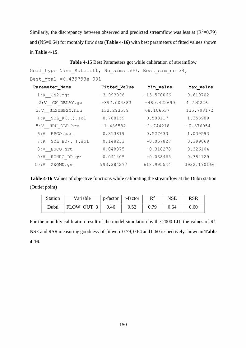
150
Similarly, the discrepancy between observed and predicted streamflow was less at (R2=0.79)
and (NS=0.64) for monthly flow data (Table 4-16) with best parameters of fitted values shown
in Table 4-15.
Table 4-15 Best Parameters got while calibration of streamflow
Goal_type=Nash_Sutcliff, No_sims=500, Best_sim_no=34,
Best_goal =6.439793e-001
Parameter_Name Fitted_Value Min_value Max_value
1:R__CN2.mgt -3.993096 -13.570066 -0.610702
2:V__GW_DELAY.gw -397.004883 -489.422699 4.790226
3:V__SLSUBBSN.hru 133.293579 68.106537 135.798172
4:R__SOL_K(..).sol 0.788159 0.503117 1.353989
5:V__HRU_SLP.hru -1.436584 -1.744218 -0.376954
6:V__EPCO.bsn 0.813819 0.527633 1.039593
7:R__SOL_BD(..).sol 0.148233 -0.057827 0.399069
8:V__ESCO.hru 0.048375 -0.318278 0.326104
9:V__RCHRG_DP.gw 0.041405 -0.038465 0.384129
10:V__GWQMN.gw 993.384277 618.995544 3932.170166
Table 4-16 Values of objective functions while calibrating the streamflow at the Dubti station
(Outlet point)
Station Variable p-factor r-factor R2 NSE RSR
Dubti FLOW_OUT_3 0.46 0.52 0.79 0.64 0.60
For the monthly calibration result of the model simulation by the 2000 LU, the values of R2,
NSE and RSR measuring goodness-of-fit were 0.79, 0.64 and 0.60 respectively shown in Table
4-16.

151
Figure 4-19. Observed and predicted hydrograph after monthly calibration of the model
simulation by the 2000 LU/LC
The same model parameters of Awash basin that were used for calibrating the model run by
the 2000 land use (Table 4-14) were also used for calibrations of the model outputs of 1994
and 2014 land uses. In order to distinguish the resulting difference in water quality from
different land use/land covers, the same meteorological data from same stations was given to
the SWAT model and run.
b) Validation of Flow
The validation process was performed by running the model for time periods different from
that of calibration, (dataset of 2006-2014), using the previously calibrated input parameters.
Figure 4-20 show the monthly graphical performance evaluation of SWAT model during
validation period. The monthly graph implied that the model simulation is best fitted with the
observed flow measurement. The three goodness-of-fit measures were also calculated for the
validation period.
Table 4-17 Values of objective function for validating the streamflow at the Dubti station
Station Variable p-factor r-factor R2 NSE RSR
Dubti FLOW_OUT_3 0.59 0.82 0.81 0.52 0.70
0
50
100
150
200
250
300
350
400
450
500
550
Jan-9
7
Jun-9
7
Nov-9
7
Ap
r-9
8
Sep
-98
Feb
-99
Jul-
99
Dec
-99
May
-00
Oct
-00
Mar
-01
Aug-0
1
Jan-0
2
Jun-0
2
No
v-0
2
Apr-
03
Sep
-03
Feb
-04
Jul-
04
Dec
-04
May
-05
Oct
-05
Str
eam
flo
w (
cm3
/s)
Months
Observed Simulated

152
For the monthly validation result of the model simulation by the 2000 LU, shown in Table
4-17, the values of the objective functions measuring goodness-of-fit such as R2 and NSE
were 0.81 and 0.52 respectively. Moriasi et al., (2015) in their performance evaluation criteria
for recommended statistical performance measures for watershed-scale models, suggested
that NSE in the range of (0.5, 0.7] to be satisfactory and R2 in the range of (0.75, 0.85] to be
good. According to these arguments, the values indicated that the model performance was
good and is in the acceptable limit. Then the model is re-run with these calibrated parameters
taken into account.
Figure 4-20. Observed and predicted hydrograph after monthly validation of the model
simulation by the 2000 LU/LC
Uncertainty analysis
Different studies carried out previously to test the applicability of the SWAT model in tropical
regions reported reasonable accuracy. For instance, in the Anjeni watershed of northwestern
Ethiopia, Setegn et al. (2010) assessed soil loss rate using ArcSWAT model and an R2 value
of 0·9 and NSE value of 0·9 were provided as model performances for monthly time step
sediment simulation. On the other hand, an NSE of 0·7 and R2 values of 0·7 for monthly time
steps, were achieved when simulating sediment yield for the Hombole watershed in central
0
100
200
300
400
500
600
Jan
-06
May
-06
Sep
-06
Jan
-07
May
-07
Sep
-07
Jan
-08
May
-08
Sep
-08
Jan
-09
May
-09
Sep
-09
Jan
-10
May
-10
Sep
-10
Jan
-11
May
-11
Sep
-11
Jan
-12
May
-12
Sep
-12
Jan
-13
May
-13
Sep
-13
Jan
-14
May
-14
Sep
-14
Flo
w (
cum
ecs)
Months
Observed Simulated

153
Ethiopia (Alamirew, 2006). Results of this study also revealed that ArcSWAT model is capable
of simulating various hydrological and water quality components.
Figure 4-21 Illustration of the 95ppu plot of uncertainty analysis for the monthly validation of
the flow at the basin outlet
Model efficiency during monthly calibration of the model flow simulation by the 2000 LU
evaluated by R2, NSE and RSR measuring goodness-of-fit of stream flow were respectively
0.79, 0.64 and 0.60 as shown in Table 4-16. Likewise, during validation 0.81, 0.52, and 0.70
were obtained as their respective values (Table 4-17). For monthly and watershed-scale
hydrological models, Moriasi et al., (2015) and Moriasi et al., 2007 in their evaluation criteria
for recommended statistical performance measures put in Table 3-4 suggested both for
calibration and validation that NSE in the range of (0.5, 0.7], in which flow NSE of the study
lie, is satisfactory. Their suggestion of R2 in the range (0.75, 0.85], where value of this study
lie, indicate that the model performance is good. Similarly, RSR values of 0.60 and 0.70
generated by the SWAT-CUP program respectively during calibration and validation of flow
were also in permissible ranges as its ratings as recommended by Moriasi et al., 2007 are good
and satisfactory. According to the arguments by Moriasi et al., 2007 and 2015, the values of
the objective functions of this study both in the calibration and validation periods indicated that
154
the model’s overall performance for flow was good and is in the acceptable limit since they
conform to the standard.
There were deviations and abnormal patterns of the observed data from the corresponding
months’ simulated ones as could be exemplified by the 16th, 24-29th, 85th, 87th, 88th, 100th and
101st months. This may actually be due to inaccuracies in the rainfall data used in running the
model. It can also probably be due to inaccurate measurement of discharge at the gaging station
instead of the input rainfall data of the model. The reason why the unexpected mismatch
between the observed and simulated values, which were seen especially in some months may
also be due to Tendaho reservoir just upstream of the station. This stores water during the rainy
season and releases afterwards (as required for development). There were some values of flow
encountered both in the observed and simulated results like in Jan 2000, Aug 2000, Aug 2001,
Aug 2002, Sep 2003, Apr 2004, Aug 2004, and Aug 2005 that were too far from expectations
in the respective seasons. Some values of flow, e.g., increasing in Nov 1997, Sept 1999, Jan
2000, April 2004, being dry seasons and decreasing in all years of June being wet seasons. The
reason for such a result in the observed flow may be due to the sudden releasing of the dam’s
discharge while in cause for the predicted case may be attributed to inaccuracies in the inputs
to the model. Generally, the model simulation is realized to give higher values of flow than
the observed ones.
Gessesse et al. (2015) had assessed the response of stream flow to changes in land use/land
cover from 1973 to 2007 for the mojo watershed of the upper basin by using the same model.
The flow modeling seemed to have shown better performance than that of this study as the
NSE values in monthly calibration of both 1973 and 2007 LUs was 0.9 and validation of both
years was 0.8 while those of this study were 0.64 and 0.52. The reason of deviating efficiency
of this study from the sub-basin’s counterparts may be large size of the study area, difference
of the parameters tuned in the process of calibration, estimation of the flow data used for
calibration. Anyway, the set standard statistical value for the model by Moriasi et al. (2007)
states that the monthly time step calibration and validation for flow of NSE > 0·5 can be

155
accepted as ‘satisfactory’. According to the standard, this study’s performance is also
satisfactory and hence was proved to be acceptable.
Though bracketing of the observed data by the 95ppu (46%) seems to be somehow far from
the ideal expectation of unity, thickness of the band confirmed by the r-factor value of 0.52
(close to 0) is relatively good. This implies that the model is within the acceptable range of
uncertainty since it is compromised by good NSE and R2 values. P-factor could be made as
close to 1 as possible at the expense of r-factor by repeating the iteration but such actions have
risks of reducing values of R2 and NSE sometimes.
4.4.3.2 Sensitivity analysis, calibration and validation of the monthly nitrate
a. Sensitivity analysis of parameters determining NO3–
Out of the five major life-forming elements: nitrogen (N), carbon (C), phosphorus (P), oxygen
(O), and sulfur (S), N has the greatest total abundance (more than the mass of all four of these
other elements combined) in the Earth’s atmosphere, hydrosphere, and biosphere though it is
the element least readily available to sustain life. However, more than 99% of this N is not
available to more than 99% of living organisms because most of it exists in the form of a non-
reactive, molecular nitrogen (N2) (Galloway et al., 2003). Here one of the reactive nitrogen
forms, NO3- is modelled by SWAT for the basin.
The relative sensitivity of different parameters to nitrate-nitrogen was analyzed. For this
analysis, eighteen water quality parameters, ANION_EXCL.sol, BC1_BSN.bsn,
BC2_BSN.bsn, BC3_BSN.bsn, CDN.bsn, CH_ONCO.rte, CMN.bsn, ERORGN.hru,
FIXCO.bsn, N_UPDIS.bsn, NFIXMX.bsn, NPERCO.bsn, RCN.bsn, RSDCO.bsn,
SDNCO.bsn, SHALLST_N.gw, SOL_NO3().bsn, SOL_ORGN().bsn (Table 4-18) that might
have a potential influence on mineral nitrogen load of Awash River, were used in the sensitivity
analysis. Setting the number of simulations to be 600, SWAT-CUP was run with these
parameters.

156
Table 4-18 Selected input parameters to SWAT-CUP in the sensitivity analysis of NO3
No. Input Parameter Description of Parameter Min and
Max Range t-Stat P-Value Rank
1 V_BC1_BSN.bsn Rate constant for biological oxidation of
NH3 0.1 - 1 -0.73 0.46 13
2 V_BC2_BSN.bsn Rate constant for biological oxidation NO2
to NO3 0.2 - 2 -1.04 0.30 8
3 V_BC3_BSN.bsn Rate constant for hydrolysis of organic
nitrogen to ammonia 0.02 - 0.4 0.60 0.55 15
4 V_NFIXMX.bsn Maximum daily-n fixation 1 - 20 -0.31 0.76 17
5 V_CMN.bsn Rate factor for humus mineralization of
active organic nitrogen 0 - 0.7 -0.47 0.64 16
6 V_NPERCO.bsn Nitrogen percolation coefficient 0 - 1.0 -22.40 0.00 1
7 V_N_UPDIS.bsn Nitrogen uptake distribution parameter 10 - 60.0 1.26 0.21 6
8 V_SOL_NO3.bsn Initial NO3 concentration in the soil layer 0 - 100 0.91 0.36 9
9 V_SOL_ORGN.bsn Initial organic N concentration in the soil
layer 0 - 100 0.74 0.46 12
10 V_RSDCO.bsn Residue decomposition coefficient 0 - 0.5 -0.90 0.37 10
11 V_SDNCO.bsn Denitrification threshold water content 0 - 1.0 -11.37 0.00 3
12 R_ANION_EXCL.sol Fraction of porosity from which anions are
excluded 0 - 1.0 1.31 0.19 5
13 V_CDN.bsn Denitrification exponential rate coefficient 0 - 3 13.41 0.00 2
14 V_CH_ONCO.rte Channel organic nitrogen concentration in
basin 0 - 100 0.86 0.39 11
15 V_ERORGN.hru Organic N enrichment ratio 0 - 1 1.15 0.25 7
16 V_FIXCO.bsn Nitrogen fixation coefficient 0 - 1 0.70 0.48 14
17 V_SHALLST_N.gw Concentration of nitrate in groundwater
Contribution to streamflow from sub-basin 0 - 0.05 1.91 0.06 4
18 R_RCN.bsn Concentration of nitrogen in rainfall 0 - 15 0.00 1.00 18
V-parameter value is replaced by given value or absolute change; R-parameter value is
multiplied by (1 + a given value) or relative change.
Sensitivities of the parameter are ranked and put in Table 4-18 according to Khalid et al.,
(2016). The table shows the model parameters, minimum values, maximum values, t-Stat, p-
value and their sensitivities (ranked in its last row) with respect to absolute values of t-Stat
values in the grid from the global SA plotted in Figure 4-22. Therefore, out of the eighteen,
eight parameters are pointed out to be more sensitive to NO3, namely (in the increasing order

157
of sensitivity); BC2_BSN.bsn, ERORGN.hru, UPDIS.bsn, ANION_EXCL.sol,
SHALLST_N.gw, SDNCO.bsn, CDN.bsn and NPERCO.bsn, as their p-values are less than or
equal to 0.05 and those of little bit greater than 0.05 (t-stat value in absolute value greater than
1.0). Hence, these parameters were found to be the most crucial parameters for the studied
basin as they generally govern the surface nitrate loading.
Figure 4-22 Plot of Global Sensitivity Analysis of parameters of nitrate sorted by P-values
Among the eight sensitive parameters filtered above, sensitivity analysis is again done and
ranked as depicted in Figure 4-23. The figure shows that NO3 was most sensitive to NPERCO
followed by CDN, and then by SDNCO.

158
Figure 4-23 Global sensitivity analysis of parameters determining NO3-
b. Monthly calibration and uncertainty analysis of nitrate (NO3-)
After calibration and assessment of hydrologic simulations, NO3-N-related variables reported
in Table 4-18 were adjusted during calibration to observed monthly NO3-N concentrations.
Calibration and validation of the SWAT model for NO3-N are very important since the nitrogen
components in the model are very complex and its input data requirements are intensive.
Observed long-term dataset of 2006-2010 were used for calibration. The ARB SWAT model
calibration and validation was made on a monthly basis using r-factor, p-factor, coefficient of
determination (R2), Nash–Sutcliffe simulation efficiency (NSE) and RSR values as measuring
objective functions. With the identified sensitive parameters of minimum and maximum ranges
remaining as that of the sensitivity analysis, SWAT-CUP was run for 500 simulations first.
Then re-running the program now and then replacing the parameters of initial min and max
ranges by the new pars generated in the previous iteration, optimum values of objective
functions were obtained in the summary stat of the last iteration of the SUFI-2 algorithm.
As a first output of calibration of this iteration, the 95 percent prediction uncertainty plot is
produced and is presented in Figure 4-24.
-25.00
-20.00
-15.00
-10.00
-5.00
0.00
5.00
10.00
15.00
13:R
__R
CN
.bsn
11:V
__N
FIX
MX
.bsn
7:V
__C
MN
.bsn
4:V
__B
C3_B
SN
.bsn
9:V
__
FIX
CO
.bsn
2:V
__B
C1_B
SN
.bsn
18:V
__S
OL
_O
RG
N(…
6:V
__C
H_O
NC
O.r
te
14:V
__R
SD
CO
.bsn
17:V
__S
OL
_N
O3(.
.)…
3:V
__B
C2_B
SN
.bsn
8:V
__E
RO
RG
N.h
ru
10:V
__N
_U
PD
IS.b
sn
1:R
__A
NIO
N_E
XC
…
16:V
__S
HA
LL
ST
_N
…
15:V
__S
DN
CO
.bsn
5:V
__C
DN
.bsn
12:V
__N
PE
RC
O.b
sn
t-S
tat
Val
ues
Parameters used in the global sensitivity analysis of NO3-
t-Stat

159
Figure 4-24 Illustration of the 95ppu of the simulated and observed monthly nitrate load
carried at the basin outlet
The best parameters that produced the optimum objective functional values, their minimum
and maximum values and the fitted values are put in Table 4-19. The model is exceptionally
sensitive to nitrogen percolation coefficient (NPERCO) as can be seen by Figure 4-23. It is
secondly most sensitive to CDN.bsn, followed by SDNCO.bsn and so on.
Table 4-19 Best parameters got while calibration of nitrate
Goal_type= Nash_Sutcliff; No_sims= 500; Best_sim_no= 298; Best_goal
= 7.120754e-001
Parameter_Name Fitted_Value Min_value Max_value
1:R__ANION_EXCL.sol -0.219045 -0.226832 0.481048
2:V__BC2_BSN.bsn 1.749598 1.334103 2.110730
3:V__CDN.bsn -0.771819 -1.233156 0.023892
4:V__ERORGN.hru 1.290814 0.811160 1.298118
5:V__N_UPDIS.bsn 82.777107 58.501129 85.148743
6:V__NPERCO.bsn 0.062949 -0.065246 0.200168
7:V__SDNCO.bsn 1.198989 1.080159 1.677293
8:V__SHALLST_N.gw -0.001281 -0.014063 0.003471
Table 4-20 Values of objective functions while calibrating Nitrate at the Dubti station
Station Variable p-factor r-factor R2 NSE RSR
Dubti NO3_OUT_3 0.64 1.24 0.73 0.71 0.54

160
Figure 4-25 Observed and predicted Nitrate after monthly calibration by the 2000 LU
After performing 500 simulations for calibration and uncertainty analysis in the iteration that
gave good measure, dotty plots were produced as an output. These plots show the distribution
of the number of simulations in parameter sensitivity analysis after comparing the parameter
values with the objective function (NSE) for the monthly calibrations via SUFI-2. The vertical
numbered axes in the left show performance measured by NSE and the horizontal ones in each
of the plots give values of the parameters Figure 4-26.
Figure 4-26 Dotty plots illustrating performance measured by NSE (vertical-y) versus values
of the parameters (horizontal-x) for less sensitive (CDN) and the most sensitive (NPERCO)
parameters while calibrating NO3-
0
200000
400000
600000
800000
1000000
1200000
1400000
1600000
1800000
2000000
Jan-0
6
Apr-
06
Jul-
06
Oct
-06
Jan-0
7
Apr-
07
Jul-
07
Oct
-07
Jan-0
8
Apr-
08
Jul-
08
Oct
-08
Jan-0
9
Apr-
09
Jul-
09
Oct
-09
Jan-1
0
Apr-
10
Jul-
10
Oct
-10
[NO
3]
(kg)
Months
Observed Simulated

161
c. Monthly Validation of Nitrate (NO3-)
The validation process was performed by running the model for time periods 2011 – 2013 using
the previously calibrated input parameters. Figure 4-27 show the monthly graphical
performance evaluation of SWAT model in validating NO3. The monthly graph implied that
the model simulation is best fitted with the observed flow measurement. The three goodness-
of-fit measures were also calculated for the validation period.
Figure 4-27 Observed and predicted Nitrate after monthly validation of the model simulation
for the 2000 LU/LC scenario
Assessment of performance of the calibration process of nitrate at the presumed outlet station
was undertaken in a monthly basis to see goodness-of-fit of the simulated dataset with the
observed one. This monthly calibration result of the model simulation by the 2000 LU,
Table 4-21 Values of objective functions while validating the Nitrate at the Dubti station
(Outlet point)
Station Variable p-factor r-factor R2 NSE RSR
Dubti NO3_OUT_3 0.53 0.72 0.68 0.63 0.61
shown in Table 4-20, produced R2, NSE and RSR values of 0.73, 0.71 and 0.54 respectively.
While the first two measuring functions, R2 and NSE, lie in their respective ‘very good’ rating
ranges recommended for nutrients, the last one, RSR lies in the ‘good’ range of Moriasi et al.,
(2015) and Moriasi et al., (2007). The functional values of R2, NSE and RSR obtained during
0
500000
1000000
1500000
2000000
2500000
Jan-1
1
Mar
-11
May
-11
Jul-
11
Sep
-11
Nov-1
1
Jan-1
2
Mar
-12
May
-12
Jul-
12
Sep
-12
Nov-1
2
Jan-1
3
Mar
-13
May
-13
Jul-
13
Sep
-13
Nov-1
3
[NO
3]
(kg)
Date
Observed
Simulated

162
monthly validation of NO3, shown in Table 4-21, were respectively 0.68, 0.63 and 0.61. The
first two numbers, however, lie in the good rating range while the third one, value of RSR, lies
in the satisfactory range of Table 3-4. Generally speaking, all the values were found to be in
an acceptable limit, indicating that the observed data fits well with the predicted ones.
There were under prediction of NO3 in months, for instance, of August 2006, July 2007, August
2008, August 2009, and August 2010, which may be associated to the lower values of weather
data (fed to the model) at the station surrounding Dubti while the actually observed one is from
the water collected from sub basins upstream of the station. However, this is consistent with
the under prediction of the flow by the model as could be seen in Figure 4-20. The p-factor in
the case of nitrate has grown to 64% as opposed to that of flow at the expense of going further
away of r-factor (value 1.24) from zero. Similar to the case of flow, because efficiencies,
measured by NSE and R2, of calibration of nitrate were in the acceptable ranges and the p-
factor is good enough to approach to 1, the uncertainty can also be taken as in the tolerable
limit.
4.4.3.3 Sensitivity analysis, calibration and validation of the monthly phosphate
a. Sensitivity analysis of parameters determining mineral phosphorus (PO42-- P)
The relative sensitivity of different parameters to phosphate was analyzed. For this analysis
also, seventeen phosphorus-related parameters listed in the second column of Table 4-22 that
might have a potential influence on phosphate load of Awash River were used in the sensitivity
analysis.
After running 500 simulations, level of sensitivity of phosphate to the parameters was identified
and the global SA for phosphate was plotted in Figure 4-29. With respect to absolute values
of t-Stat in the grid from the global SA, sensitivities of the parameter are ranked and put in
Table 4-22 according to Khalid et al., (2016).
The table shows the model parameters and the sensitivity analysis result, with level of
sensitivities ranked in its last row. Therefore, nine parameters are identified to be more

163
sensitive, namely (in the increasing order of sensitivity (t-Stat value)); V__SOLP_CON.hru,
V__PSETLP1.pnd, V__ORGP_CON.hru, R__SOL_LABP(..).chm, V__PHOSKD.bsn,
V__P_UPDIS.bsn, V__SOL_ORGP(..).chm, V__BC4.swq, and V__ERORGP.hru, as their t-
stat value in absolute value is greater than 1.0. Hence, these parameters were found to be the
most crucial parameters for PO42- of the studied basin as they generally govern the surface
phosphate loading.
a. Monthly Calibration and uncertainty analysis of Mineral Phosphorus
Calibration and validation of the SWAT model for PO4-P are equally important as that of nitrate
since the phosphorus components in the model are also very complex and its input data
requirements are also intensive. After calibration and assessment of the hydrology, PO4-related
variables reported in Table 4-22 were optimized during calibration. Observed long-term
dataset of 2006-2010 were used for calibration.
The ARB SWAT model calibration and validation was made on a monthly basis using r-factor,
p-factor, coefficient of determination (R2), and Nash–Sutcliffe simulation efficiency (NSE)
values as measuring objective functions. With the identified sensitive parameters of minimum
and maximum ranges remaining as that of the sensitivity analysis, SWAT-CUP was run for
500 simulations first.
Table 4-22 Selected input parameters to SWAT-CUP in the sensitivity analysis of PO42-
Input Parameter Description of Parameter Min and
Max Range
t-
Stat
P-
Value Rank
PSP.bsn Phosphorus sorption coefficient 0.01 - 0.7 -0.66 0.51 13
PHOSKD.bsn Phosphorus soil partitioning
coefficient 100 - 200 3.06 0 5

164
P_UPDIS.bsn Phosphorus uptake distribution
parameter 0 - 100 6.8 0 4
SOL_ORGP(..).chm Initial organic P concentration in
surface soil layer 0 - 100 -12.9 0 3
BC4.swq Rate constant for decay of organic
phosphorus to dissolved phosphorus 0.01 - 0.7 -17.7 0 2
ERORGP.hru Organic P enrichment ratio 0 - 5 -21.4 0 1
CH_OPCO.rte Channel organic phosphorus
concentration in basin 0 - 100 -0.5 0.62 15
RSDCO.bsn Residue decomposition coefficient 0.02 - 0.1 -0.88 0.38 10
PSETLP1.pnd Phosphorus settling rate in pond for
months IPND1 through IPND2 0 - 20 -1.15 0.25 8
PSETLW2.pnd Phosphorus settling rate in wetlands
for months other than IPND1-IPND2 0 - 20 -0.01 0.99 17
PSETLP2.pnd Phosphorus settling rate in pond for
months other than IPND1-IPND2 0 - 20 -0.62 0.54 14
PSETLW1.pnd Phosphorus settling rate in wetland
for months IPND1 through IPND2 0 - 20 0.67 0.5 12
SOL_LABP(..).chm Initial labile (soluble) P concentration
in surface soil layer 0 - 100 -1.84 0.07 6
SOLP_CON.hru Soluble phosphorus concentration in
runoff, after urban BMP is applied 0 - 3 1.14 0.26 9
GWSOLP.gw
Concentration of soluble phosphorus
in groundwater contribution to
streamflow from sub-basin
0 - 0.5 0.22 0.83 16
ORGP_CON.hru Organic phosphorus concentration in
runoff, after urban BMP is applied 0 - 50 1.69 0.09 7
PPERCO.bsn Phosphorus percolation coefficient 9.04 - 16.45 0.72 0.47 11

165
Figure 4-28 Plot of Global Sensitivity Analysis of parameters of phosphate sorted by P-values
Then re-running the program now and then replacing the parameters of initial min and max
ranges by the new pars generated in the preceding iteration, optimum values of objective
functions were obtained in the summary stat of the last iteration of the SUFI-2 algorithm.
Accordingly, the resulting best parameters offering the required objective functional values
together with their respective fitted values, and min and max values of the parameters are given
in Table 4-23.

166
Figure 4-29 Global sensitivity analysis of parameters determining PO42-
Table 4-23 Best parameters got while calibration of phosphate
Goal_type= Nash_Sutcliff, No_sims= 500, Best_sim_no= 9, Best_goal = 7.612467e-001
Parameter_Name Fitted_Value Min_value Max_value
1:V__PHOSKD.bsn 168.441025 117.639984 172.560028
2:V__P_UPDIS.bsn 42.802216 25.139648 75.460350
3:V__BC4.swq 0.594467 0.309038 0.907422
4:V__ERORGP.hru 0.150025 -2.043099 2.653099
5:V__ORGP_CON.hru 43.735344 24.320002 72.980003
6:V__PSETLP1.pnd 5.808162 2.928020 14.311979
7:R__SOL_LABP(..).chm 50.610909 -7.859918 64.059921
8:V__SOL_ORGP(..).chm -20.041847 -37.560593 54.160591
9:V__SOLP_CON.hru 1.933549 1.180195 3.541805
The resulting performance of the model after calibrating gives respective values of the
objective functions given in Table 4-24.
Table 4-24 Values of objective functions while calibrating phosphate at the Dubti station
Station Variable p-factor r-factor R2 NSE RSR
Dubti PO4_OUT_3 0.32 1.34 0.77 0.76 0.49
-25.00
-20.00
-15.00
-10.00
-5.00
0.00
5.00
10.00
14
:V_
_P
SE
TL
W2
.pn
d
9:V
__G
WS
OL
P.g
w
7:V
__C
H_O
PC
O.r
te
12:V
__P
SE
TL
P2.p
nd
4:V
__P
SP
.bsn
13:V
__P
SE
TL
W1.p
nd
1:V
__P
PE
RC
O.b
sn
2:V
__R
SD
CO
.bsn
17:V
__S
OL
P_C
ON
.hru
11:V
__P
SE
TL
P1.p
nd
10:V
__O
RG
P_C
ON
.hru
15:R
__S
OL
_L
AB
P(.
.).c
hm
3:V
__P
HO
SK
D.b
sn
5:V
__
P_
UP
DIS
.bsn
16:V
__S
OL
_O
RG
P(.
.).c
hm
6:V
__B
C4.s
wq
8:V
__E
RO
RG
P.h
ru
t-S
tat
val
ues
Parameters used in the sensitivity analysis of PO42-
t-Stat

167
Figure 4-30 Illustration of the simulated and observed monthly mineral phosphorus loads at
the basin outlet
Figure 4-31 Observed and predicted phosphate after monthly calibration of the model
simulation by the 2000 LU
The table tells us that the functions measure the model to perform very good since the Nash
Sutcliffe Efficiency and R2 values respectively of 0.76 and 0.77 are above 0.65 and 0.70. These
0
500000
1000000
1500000
2000000
2500000
Jan-0
6
Apr-
06
Jul-
06
Oct
-06
Jan-0
7
Apr-
07
Jul-
07
Oct
-07
Jan-0
8
Apr-
08
Jul-
08
Oct
-08
Jan-0
9
Apr-
09
Jul-
09
Oct
-09
Jan-1
0
Apr-
10
Jul-
10
Oct
-10
[PO
4]
(kg
)
Months
Observed
Simulated

168
results show the fact that there is a very good fit between the simulated and the observed
concentrations as the calibration output is depicted by Figure 4-31.
After performing 500 simulations in the iteration that gave good performance, dotty plots were
produced as an output. These plots show the distribution of the number of simulations in
parameter sensitivity analysis after comparing the parameter values with the objective function
(NSE) for the monthly calibrations via SUFI-2. The vertical axes show performance (measured
by NSE) and the horizontal line gives values of the parameters as can be seen in Figure 4-32.
Figure 4-32 Dotty plots illustrating performance measured by NSE (vertical-y) versus values
of the parameters (horizontal-x) for less sensitive (SOL_CON) and the most sensitive
(ERORGP) parameters while calibrating PO42-
b. Monthly Validation of Mineral Phosphorus (PO4-2)
The validation process was performed by running the SWAT-CUP for time periods 2011 –
2013 using the previously calibrated input parameters. Figure 4-33 show the monthly graphical
performance evaluation of SWAT model in validating PO42-. The monthly graph implied that
the model simulation is best fitted with the observed phosphate measurement. The three
goodness-of-fit measures were also calculated for the validation period.
Table 4-25 Values of objective functions while validating the phosphate at the Dubti station
Station Variable p-factor r-factor R2 NSE RSR
Dubti PO4_OUT_3 0.33 1.09 0.82 0.81 0.44

169
Figure 4-33 Observed and predicted phosphate after monthly validation of the model
simulation by the 2000 LU/LC scenario
Monthly calibration of the model simulation of phosphate by the 2000 LU was also evaluated
for goodness-of-fit and shown in Table 4-24. Values of the performance measuring statistics:
R2, NSE and RSR were 0.77, 0.76 and 0.49 respectively. According to Table 3-4, their
performance ratings were all ‘very good’. On the other hand, the values for the respective
objective functions during validation, shown in Table 4-25, were 0.82, 0.81 and 0.44, which
all are also in the ‘very good’ rating ranges for nutrients. This implies that the predicted mineral
phosphorus agrees nicely to the observed one. Similarly, phosphate prediction is also seen to
be less than the observed ones in wet seasons as in the case of August 2008 and August 2010
during calibration and as in July 2012 and August 2011 during validation. The under-prediction
of phosphorus loading could be due to the fact that P from atmospheric deposition and stream
banks were not taken into consideration in the SWAT model.
Here in the validation the evaluating statistics of the model, R2 and NSE, were slightly better
than those got in the calibration. This shows that the model has an ability to mimic discharge
and phosphate load in a wide range of hydrologic conditions.
0
250000
500000
750000
1000000
1250000
1500000
1750000
2000000
2250000
2500000
Jan-1
1
Mar
-11
May
-11
Jul-
11
Sep
-11
Nov-1
1
Jan-1
2
Mar
-12
May
-12
Jul-
12
Sep
-12
Nov-1
2
Jan-1
3
Mar
-13
May
-13
Jul-
13
Sep
-13
Nov-1
3
[PO
4]
(kg
)
Months
Observed
Simulated
170
4.4.4 Distribution of nutrients temporally and spatially
After setting up and running SWAT model, the most sensitive parameters were identified, and
then calibration and validation were performed. Modeling the water quality (nutrients) of
Awash River was carried out following calibration of stream flow of the basin. Following the
calibration and validation of the model simulations (including those resulted from 1994 and
2014 land uses), re-running of the model for all the three scenarios is undertaken. Pivot table
of the MS excel has made the huge output of the model too summarized and manageable. The
‘rch’ file of the database that resulted from re-running the model after calibration offered
information enabling us to judge if there were either increasing or decreasing changes of
nutrients with time and space.
4.4.4.1 Subbasin-based (spatial) distribution and comparative analysis of nutrients
and hotspot areas of pollution
With the help of SWAT output viewer, the spatial variations of nutrients produced by all the
three years’ land uses have been investigated.
The 53 subbasins have been scrutinized for their exportation of nutrient loads. Comparison of
the nutrient loadings among the sub-basins suggest generally that the western highlands take
the major share of export (Figure 4-34 and Figure 4-35). About 5.92 kg/ha of NO3, 5.89 kg/ha
of PO42-, 39.16 kg/ha of TN and 12.5 kg/ha of TP are found to be exported annually from the
basin as computed by the 2000 LU. Subbasins in the western side adjacent to the river in the
middle and lower subbasins are shown to produce largest TN and TP in kg per subbasin.
Specifically, subbasins 4, 8, 13, 21 and 39 are hotspots both in 1994 and 2014 with respect to
TN and TP.
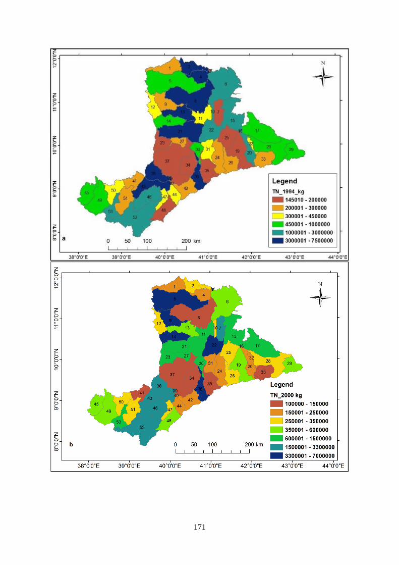
171
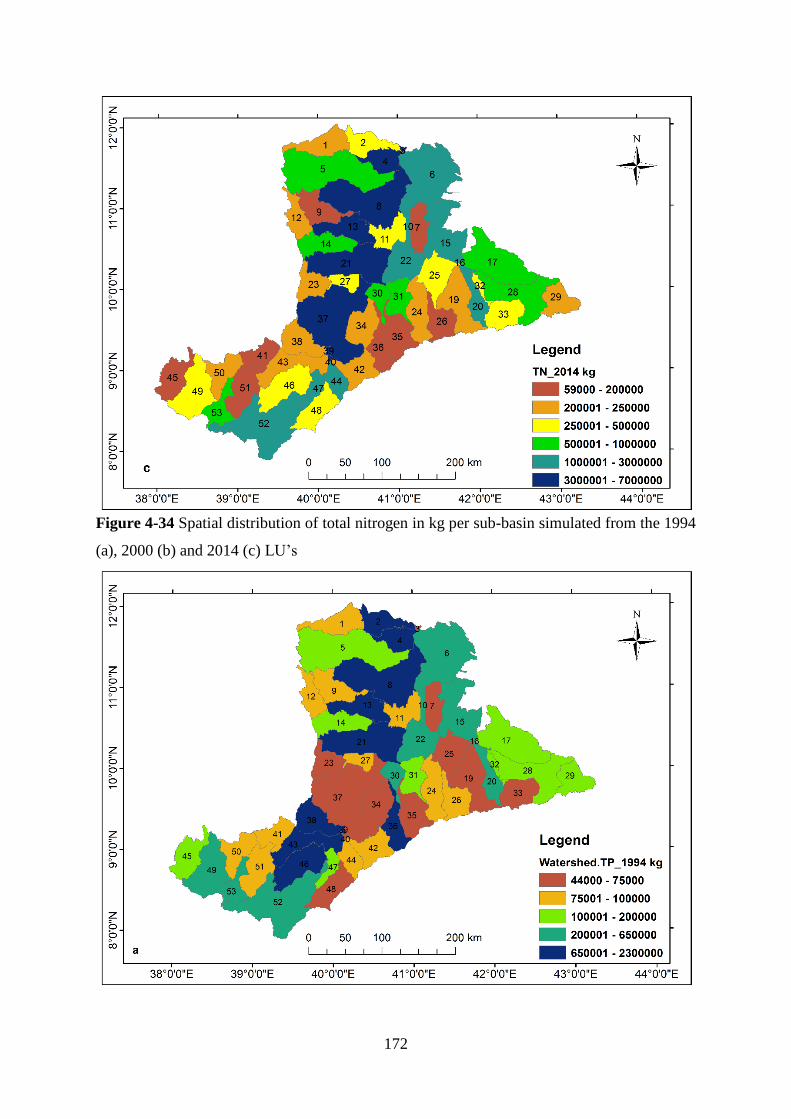
172
Figure 4-34 Spatial distribution of total nitrogen in kg per sub-basin simulated from the 1994
(a), 2000 (b) and 2014 (c) LU’s

173
Figure 4-35 Spatial distribution of total phosphorus in kg per sub-basin simulated from the
1994 (a), and 2014 (b) LUs
4.4.4.2 Temporal variation of nutrients as LU changes from 1994 to 2014
Dynamics of nutrients was explored by considering the monthly averages overall the years
from 1997 to 2014 of sub-basin 3. From this examination, it is found that the rainy months are
exporting higher amounts of nutrients. One can observe from Figure 4-36 that the three
months, March, July and August, account for about 58% and 54% of TN and NO3- respectively
from the total annual while only the two, July and August, account for about 45% and 41% of
the respective parameters. On the other hand, only these two months account for 47% and
47.8% of the TP and PO42- losses respectively while the three, including March, account both
for 60% of the TP and PO42-.

174
Figure 4-36 Average monthly distribution of nitrogen loss by 2014 LU (a) and phosphorus
loss by 2000 LU (b) in the ARB (1997-2014)
Nutrients have also been compared for the two years’ simulation (2000 and 2014) (Figure
4-37). Here the 18 years’ monthly averages of the two LU simulations were computed and
compared.
Figure 4-37 Monthly average NO3- (a) and PO4
2- (b) loads in the basin based on 2000 and 2014
LULC data
0
5
10
15
Jan
Feb
Mar
Ap
r
May Jun
Jul
Au
g
Sep
Oct
No
v
Dec
Av T
N &
NO
3 (
kg)
Mil
lio
ns
Montha)
AvTN (kg)
AvNO3 (kg)
0
1
2
3
4
5
Jan
Feb
Mar
Ap
r
May Jun
Jul
Au
g
Sep
Oct
No
v
Dec
Av T
P &
PO
4 (
kg)
Mil
lio
ns
Monthb)
AvTP (kg)
AvMINP (kg)
600000
1100000
1600000
2100000
1997
1998
1999
2000
2001
2002
2003
2004
2005
2006
2007
2008
2009
2010
2011
2012
2013
2014
2000 &
2014 [
NO
3]
(kg/m
onth
)
Yeara)
NO3_00 NO3_14
400000
600000
800000
1000000
1200000
1400000
1997
1998
1999
2000
2001
2002
2003
2004
2005
2006
2007
2008
2009
2010
2011
2012
2013
2014
20
00
& 2
01
4 [
PO
4]
(kg/m
on
th)
Yearb)
MINP_00kg MINP_14kg

175
From Figure 4-37, one can see that the nitrate (a) and phosphate (b) losses from the basin are
generally greater in the 2014 than that in the 2000 LU-based simulation. To see the effects of
land use change on the TN and TP, the two years’ simulation results (that of 2000 and 2014)
were also considered. Similarly, net increments of TN and TP are observed generally as one
goes from 2000 to 2014 as can be evident from Figure 4-38 (a and b).
Even though there is a general increase in nutrients due to the landuse change from 2000 to
2014, the trend lines of each of the graphs in Figure 4-37 and Figure 4-38 show decreasing
temporally though it is increasing after 1999. The decrease may be attributed to other factors
than land use/cover such as climate.
Figure 4-38 Monthly average total N (a) and total P (b) loads in the basin based on the 2000
and 2014 LULC data
1500000
2500000
3500000
4500000
5500000
6500000
1997
1998
1999
2000
2001
2002
2003
2004
2005
2006
2007
2008
2009
2010
2011
2012
2013
20142
000 &
2014 T
N (
kg/m
on
th)
Yeara)
TN_00kg TN_14kg
500000
1000000
1500000
2000000
2500000
1997
1998
1999
2000
2001
2002
2003
2004
2005
2006
2007
2008
2009
2010
2011
2012
2013
20142
00
0 &
20
14
TP
(kg
/mo
nth
)
Yearb)
TP_00kg TP_14kg

176
Spatial and Temporal variation of nutrients as LU changes from 1994 to 2014
a. Total Nitrogen (TN)
Figure 4-39 Total nitrogen in ARB in the three years: 1994, 2000 and 2014
To investigate the changes in TN as LU changes from one year to the other, subtraction of total
nitrogen of 1994 from that of 2000, total nitrogen of 2000 from that of 2014 and finally that of
1994 from that of 2014 for each of the 53 sub-basins is undertaken. Therefore, details of the
calculations being given in Appendix 5, the indicative result so generated is given by Table
4-26, which can show clearly whether there is a positive or a negative change in the nutrients
of 2014 from the base year’s (1994) counterparts.
Table 4-26 Percentage change of TN due to LU changes between the three years
2000-1994 2014-2000 2014-1994
Sum of all -ve differences -34926776 -16581759 -4456252
Sum of all +ve differences 25697819.9 36589361 15234899
Net -9228956.5 20007603 10778646
TN from Table 4-26 and graph of Figure 4-39 is shown to be decreasing as one goes from
1994 to 2000 but increasing afterwards. However, the net (cumulative) of both 2014-2000 and
2000-1994 differences (i.e 2014-1994) is positive. That is, as one goes from 1994 to 2014, it
can be generalized that TN is showing an increasing trend.
0500000
10000001500000200000025000003000000350000040000004500000500000055000006000000650000070000007500000
1 3 5 7 9
11
13
15
17
19
21
23
25
27
29
31
33
35
37
39
41
43
45
47
49
51
53
Tota
l N
itro
gen
(kg)
Sub-basins
TN_1994 (kg)
TN_2000 (kg)
TN_2014 (kg)

177
Figure 4-40 Temporal variation of subbasin averages of total N and total P loads in the basin
based on 1994 LULC data
b. Total Phosphorus (TP)
Similarly, to assess the changes in TP as LU changes from one year to the other, subtraction of
total phosphorus of 1994 from that of 2000, total phosphorus of 2000 from that of 2014 and
finally TP of 1994 from that of 2014 for each of the 53 sub-basins is undertaken. Therefore,
the details of the calculations being given in Appendix 6, the summarized and indicative result
so generated is given by Table 4-27, which can show clearly whether there is a positive or a
negative change.
Figure 4-41 Total phosphorus in ARB in the three years: 1994, 2000 and 2014
0
200000
400000
600000
800000
1000000
1200000S
bn A
v o
f T
N &
TP
(kg)
Year
Sbn Av of TN (kg)
Sbn Av of TP (kg)
0
250000
500000
750000
1000000
1250000
1500000
1750000
2000000
2250000
2500000
1 4 7
10
13
16
19
22
25
28
31
34
37
40
43
46
49
52
To
tal
ph
osp
ho
rus
(kg
)
Subbasins
TP_1994 TP_2000 TP_2014
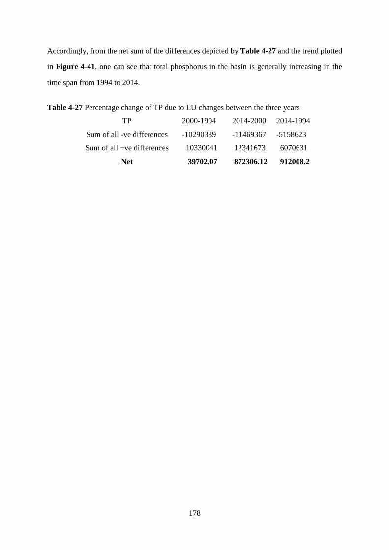
178
Accordingly, from the net sum of the differences depicted by Table 4-27 and the trend plotted
in Figure 4-41, one can see that total phosphorus in the basin is generally increasing in the
time span from 1994 to 2014.
Table 4-27 Percentage change of TP due to LU changes between the three years
TP 2000-1994 2014-2000 2014-1994
Sum of all -ve differences -10290339 -11469367 -5158623
Sum of all +ve differences 10330041 12341673 6070631
Net 39702.07 872306.12 912008.2

179
Chapter 5 Conclusion, implications and recommendations
5.1 Conclusion
The study evaluated the physico-chemical (throughout the Awash River) and bacteriological
(only in its UB) water quality for drinking and irrigation water uses. The water quality analysis
results examined from different sites of the River showed that most of the parameters of
concern do not comply with the drinking water quality guidelines and hence unsuitable for
drinking. It also showed that most parameters need great care to be used even for irrigation.
Domestic WQIs of both UB and MLB lie in the poor while the irrigation WQI throughout the
basin is in the marginal range of the CCME ranking. Although the difference in the used water
quality dataset of the two cases might contribute for the difference in the indices to some extent,
it was generally conceivable that the water quality of the River was below even the fair rank of
the council.
Spatial-temporal water quality analyses usually involve huge multi-dimensional data that need
multivariate statistical methods. Since the dataset used for multivariate analysis is secondary,
it was validated for errors and anomalies and normalized before applying the multivariate
statistical methods. The PCA resulted in four principal components representing the whole
dataset and most parameters are shown by the analysis to vary spatially. It could also identify
the most contributing sites and parameters for the principal components. The most sensitive
site for the variation is found to be Lake Beseka for which appropriate management need to be
sought. Here, agglomerative hierarchical cluster analysis is used to group the ten sampling sites
into four clusters pertaining to water quality characteristics. The seasonal Mann-Kendall trend
test detected that most of the parameters show temporal as well as spatial trends. If special
attention is not payed to the water quality parameters that show a monotonic increasing trends
such as EC, TDS, Na, alkalinity, SO42-, NH3, K, and Cl at the Office area; K, Mg, SO4
2- at
Wonji; and TH in all the sites, the water quality of the river and the basin in general will be
deteriorated to the extent that it will not be fit for the intended uses. Thus, the multivariate
statistical techniques were proved to be excellent exploratory tools in the analysis and

180
interpretation of the complex dataset on water quality and in understanding their temporal and
spatial variations.
In the present study, the ArcSWAT hydrological model was used to see how the changes in
LU/LC results in nutrient dynamics in the ARB. Performance of SWAT was evaluated in this
study when simulating flow and nutrients in the basin although it has not yet been applied to
model these variables in the entire basin. Setting up and running the model with the 1994, 2000
and 2014 land uses, respectively 561, 665 and 507 number of HRUs were produced and the
basin is commonly divided into 53 sub-basins in each case. Then the simulated flow was
calibrated and validated using the long-term record of observed data on a monthly basis and
the performances measured by R2, NSE and RSR were found to be good. Next, the simulated
nitrate and phosphate were also calibrated and validated with their historical records of
observed data. The objective functional values during calibration and validation of the nutrients
were found to be within the acceptable ranges of the standards put in literature. Though nutrient
transport in (and/or export to) a running water is conditional on landscape features like
hydrology, climate, topography and soil types, the impact of land use on nutrient dynamics is
seen here by comparing the simulation results of the model (in which climate, topography and
soil types have been considered) corresponding to the three years’ land uses. Based on the
result obtained from the modeling and its performance, the hydrological and water quality
model, SWAT, was proved to be a promising model to predict flow and nutrients in the basin
successfully since its performance evaluated by the functions was good.
From results of the modeling, it can be concluded that concentration of nutrients is both season
and place dependent. Spatially, the sub basins identified as exporting higher amounts are those
that are intensively cultivated and residential areas. Temporally, nutrient export is observed to
be higher in rainy than in the dry seasons. Likewise, nutrient load is also seen to be land cover
dependent. This is because the load from the 1994 LU has evidently been greater than that of
2000 while the overall load resulting from 2014 LU is greater than that from both 1994 and
2000.

181
5.2 Implications of the study and contribution to knowledge
Previous literature results, though did not address detail spatial and temporal dynamics in
relation specifically to land use, reported only water quality characterization of some parts of
Awash basin. The outcomes of this research in one of the most polluted basins of the nation,
Awash river basin, improve our understanding of the water quality status and quality dynamics
resulting mostly from various anthropogenic activities in the basin. Results of the status, spatial
and temporal dynamics, and relationship of the quality with land use of Awash River basin
have a number of applications. To mention some:
1. It has a scientific and practical significance in that it fills the existing knowledge gap and
establishes a water quality database.
2. It facilitates informed decision making and implementation of sound management options
since it provides ample information on the status so as to suggest if the water is suitable for
intended use.
3. It can be customized as a framework (roadmap) for studies dealing with similar issues in
other river basins of the nation.

182
5.3 Recommendations
One ultimate goal of water resources management in a basin is to implement programs that
conserve water quality. Therefore, from the study conducted, the following recommendations
are forwarded.
The higher concentrations of nitrogen and phosphorus suggest that nutrient abatement from
domestic wastewater are strongly needed to recover the water quality of this river. Therefore,
wastewater infrastructure should be constructed and revitalized regularly in line with the fast
industrialization and urbanization in the basin and wastewater treatment facilities should be
upgraded to improve their nitrogen and phosphorus removal efficiencies. Inter-sectoral
consultation and adaptation of integrated planning approach for the wastewater
infrastructure’s effectiveness need to be developed.
It would be imperative to have a continuous and long-term monitoring program at selected
sites. This program, together with establishment of municipal wastewater and storm-water
treatment plants for identified dischargers (for point sources) (at hotspot areas, for instance,
effluent from Mojo town and Addis Ababa city) in the basin, would be among the potential
solution to increase the indices, which show improvement of the River water quality.
Identifying all pollutant sources exhaustively in the basin and allocating loads for the non-
point sources and waste loads for each of the point sources discharging to the river or its
tributaries is essential. This can be realized by developing waste load allocation models for
TMDL assignment (facilitated by applying BMP’s at the hotspot sub-basins of the basin) that
helps as a roadmap to meet standards. Results of the present study are therefore expected to
be used as tools in this regard.
Application of distributed hydrological models and forecasting necessitate availability of
long period of quality data. The application of SWAT model was very challenging and a lack
of appropriate data was one of the biggest concern throughout the modeling activities.
Without proper data, modeling is very difficult if not impossible. The use of new data
gathering techniques should be envisaged for the basin especially.

183
Bibliography
Abbaspour, K. C. (2009). SWAT-CUP2 SWAT Calibration and Uncertainty Programs.
Version2.
Abbaspour, K. C. (2013). SWAT-CUP 2012. SWAT Calibration and Uncertainty Program—
A User Manual.
Abbaspour, K. C. (2015). SWAT-CUP4: SWAT calibration and uncertainty programs–a user
manual. Swiss Federal Institute of Aquatic Science and Technology, Eawag.
Abbaspour, K. C., Rouholahnejad, E., Vaghefi, S., Srinivasan, R., Yang, H., & Kløve, B.
(2015). A continental-scale hydrology and water quality model for Europe: Calibration
and uncertainty of a high-resolution large-scale SWAT model. Journal of Hydrology, 524,
733-752.
Abbaspour, K. C., Vaghefi, S. A., & Srinivasan, R. (2017). A Guideline for Successful
Calibration and Uncertainty Analysis for Soil and Water Assessment: A Review of Papers
from the 2016 International SWAT Conference.
Abbaspour, K., Yang J., Maximov I., Siber R., Bogner K., Mieleitner J., Zobrist J., Srinivasan
R. (2007). Modelling hydrology and water quality in the pre-alpine/alpine Thur watershed
using SWAT, Journal of Hydrology 333, 413– 430, Switzerland.
Abbaspour, S. (2011). Water Quality in Developing Countries, South Asia, South Africa,
Water Quality Management and Activities that Cause Water Pollution. International
Conference on Environmental and Agriculture Engineering, IPCBEE vol.15. IACSIT
Press, Singapore
Adeba, D., Kansal, M. L., & Sen, S. (2015). Assessment of water scarcity and its impacts on
sustainable development in Awash basin, Ethiopia. Sustainable Water Resources
Management, 1(1), 71-87.
Ademe, A. S., & Alemayehu, M. (2014). Source and determinants of water pollution in
Ethiopia: Distributed lag modeling approach. Intellectual Property Rights: 2: 110.
doi:10.4172/2375-4516.1000110, Open Access.
Admasu, D. (2008). Invasive plants and food security: the case of Prosopis juliflora in the Afar
region of Ethiopia. FARM-Africa, IUCN, 1-13.
AECOM. (2009). Watershed and Lake Modelling for a TMDL Evaluation of Barr Lake and
Milton Reservoir, Second Revision – Final.
Akele, T. (2011). The practice and challenges of lake management in Ethiopia-the case of lake
Koka, An Independent Masters Thesis Presented to the Department of Urban and Rural

184
Development, Unit of Environmental Communication at Swedish University of
Agricultural Sciences, Uppsala, Sweden.
Alemayehu, T. (2000). Water pollution by natural inorganic chemicals in the central part of the
Main Ethiopian Rift. SINET: Ethiopian Journal of Science, 23(2), 197-214.
Alemayehu, T. (2001). The impact of uncontrolled waste disposal on surface water quality in
Addis Ababa, Ethiopia. SINET: Ethiop. j. Sci., 24(1): 93-104.
Alemayehu, T.; Ayenew, T. Kebede, S. (2006). Hydrogeochemical and lake level changes in
the Ethiopian Rift, Journal of Hydrology 316 290–300.
Andrea, R.; Beverly, M.; and Stephanie, S. (2005). Calculation of the CCME Water Quality
Index for Selected Rivers in the Georgia Basin, Proceedings of the Puget Sound Georgia
Basin Research Conference.
APHA (American Public Health Association) (1998). Standard methods for the examination
of water and wastewater, 20th Edition, Washington DC.
Aral, M. A. (2010). Environmental modeling and health risk analysis (ACTS/RISK). Springer
Science & Business Media.
Arnold, J. G., & Williams, J. R. (1989). Stochastic generation of internal storm structure at a
point. Transactions of the ASAE, 32(1), 161-0167.
Arnold, J. G., Kiniry, J. R., Srinivasan, R., Williams, J. R., Haney, S. L., & Neitsch, S. L.
(2012). Soil and Water Assessment Tool Input/Output Documentation, Version 2012,
Texas Water Resources Institute, Temple, TX, USA. TR-439.
Arnold, J. G., Moriasi, D. N., Gassman, P. W., Abbaspour, K. C., White, M. J., Srinivasan, R.,
... & Kannan, N. (2012). SWAT: Model use, calibration, and validation. Transactions of
the ASABE, 55(4), 1491-1508.
Arnold, J. G., Srinivasan, R., Muttiah, R. S., & Williams, J. R. (1998). Large area hydrologic
modeling and assessment part I: model development 1. JAWRA Journal of the American
Water Resources Association, 34(1), 73-89.
ASTU (Adama Science and Technology University), (2016). Water Quality Modeling of
Awash River Basin (Final Report), Adama, Ethiopia.
AwBA (Awash Basin Authority), (2014). Strategic River Basin Plan for Awash Basin, Werer,
Ethiopia.
Aweng-Eh, R. (2010). Effect of river discharge fluctuation on water quality at three rivers in
Endau catchment area, Kluang, Johor. Australian Journal of Basic and Applied Sciences,
4(9), 4240-4249.

185
Awoke, A., Beyene, A., Kloos, H., Goethals, P. L., & Triest, L. (2016). River Water Pollution
Status and Water Policy Scenario in Ethiopia: Raising Awareness for Better
Implementation in Developing Countries. Environmental management, 58(4), 694-706.
Awulachew, S. B., Loulseged, M., & Yilma, A. D. (2008). Impact of irrigation on poverty and
environment in Ethiopia: draft proceedings of the symposium and exhibition, Addis
Ababa, Ethiopia, 27-29 November 2007. In Conference Proceedings (No. h044062).
International Water Management Institute.
Ayenew, T. (2006). Some improper water resources utilization practices and Environmental
problems in the Ethiopian rift. African Water Journal, 1(1), 80-105.
Ayenew, T. (2007). Water management problems in the Ethiopian rift: Challenges for
development. Journal of African Earth Sciences, 48(2), 222-236.
Baker, T. J., & Miller, S. N. (2013). Using the Soil and Water Assessment Tool (SWAT) to
assess land use impact on water resources in an East African watershed. Journal of
Hydrology, 486, 100-111.
Bartram, J., & Ballance, R. (Eds.). (1996). Water quality monitoring: a practical guide to the
design and implementation of freshwater quality studies and monitoring programmes.
CRC Press.
Beasley, D. B., Huggins, L. F., & Monke, A. (1980). ANSWERS: A model for watershed
planning. Transactions of the ASAE, 23(4), 938-0944.
Belay, E. A. (2009). Growing lake with growing problems: integrated hydrogeological
investigation on Lake Beseka, Ethiopia. ZEF. Germany.
Belete, B. and Semu, A. (2013). Background Report: Hydro-Meteorological Trends. Awash
River Basin Water Audit (ARBWA) Project, Addis Ababa, Ethiopia.
Berhe, F. T., Melesse, A. M., Hailu, D., & Sileshi, Y. (2013). MODSIM-based water allocation
modeling of Awash River Basin, Ethiopia. Catena, 109, 118-128.
Bicknell, B. R., Imhoff, J. C., Kittle Jr, J. L., Donigian Jr, A. S., & Johanson, R. C. (1996).
Hydrological simulation program-FORTRAN. user's manual for release 11. US EPA.
Bingner, R. L., Garbrecht, J., Arnold, J. G., & Srinivasan, R. (1997). Effect of watershed
subdivision on simulation runoff and fine sediment yield. Transactions of the ASAE, 40(5),
1329-1335.
Boardman, J., & Favis-Mortlock, D. (1998). Modelling soil erosion by water. In Modelling Soil
Erosion by Water (pp. 513). Springer, Berlin, Heidelberg.
Borah, D. K., & Bera, M. (2003). Watershed-scale hydrologic and nonpoint-source pollution
models: Review of mathematical bases. Transactions of the ASAE, 46(6), 1553.

186
Borah, D. K., & Bera, M. (2004). Watershed-scale hydrologic and nonpoint-source pollution
models: Review of applications. Transactions of the ASAE, 47(3), 789.
Bosch, J.M., Hewlett, J.D. (1982). A review of catchment experiments to determine the effect
of vegetation changes on water yield and evapotranspiration. J. Hydrol. 55, 3–23.
Briassoulis, H. (2009). Factors influencing land-use and land-cover change. Land cover, land
use and the global change, encyclopedia of life support systems (EOLSS), 1, 126-146.
Brown, L. C., & Barnwell, T. O. (1987). The enhanced stream water quality models QUAL2E
and QUAL2E-UNCAS: documentation and user manual. Athens, Georgia: US
Environmental Protection Agency. Office of Research and Development. Environmental
Research Laboratory.
Bu, H., Tan, X., Li, S., & Zhang, Q. (2010). Temporal and spatial variations of water quality
in the Jinshui River of the South Qinling Mts., China. Ecotoxicology and Environmental
Safety, 73(5), 907-913.
Carpenter, S. R., Caraco, N. F., Correll, D. L., Howarth, R. W., Sharpley, A. N., & Smith, V.
H. (1998). Nonpoint pollution of surface waters with phosphorus and nitrogen. Ecological
applications, 8(3), 559-568.
CCME (Canadian Council of Ministers of the Environment). (2001a). Canadian water quality
guidelines for the protection of aquatic life: CCME Water Quality Index 1.0, User’s
Manual. In: Canadian environmental quality guidelines, 1999, Canadian Council of
Ministers of the Environment, Winnipeg.
CCME (Canadian Council of Ministers of the Environment). (2001b). Canadian water quality
guidelines for the protection of aquatic life: CCME Water Quality Index 1.0, Technical
Report. In: Canadian environmental quality guidelines, 1999, Canadian Council of
Ministers of the Environment, Winnipeg.
Chapman, D. V., & WHO. (1996). Water quality assessments: a guide to the use of biota,
sediments and water in environmental monitoring, published by E&FN Spon, an imprint
of Chapman & Hall on behalf of UNESCO, WHO and UNEP, 2nd edition, Cambridge,
Great Britain
Chaubey, I., Cotter, A. S., Costello, T. A., & Soerens, T. S. (2005). Effect of DEM data
resolution on SWAT output uncertainty. Hydrological Processes, 19(3), 621-628.
Chaudhry, F.N. and Malik, M.F. (2017). Factors Affecting Water Pollution: A Review, Journal
of Ecosystem & Ecography, 7: 225. doi:10.4172/2157-7625.1000225
187
Chekol, D. A., Bernhard Tischbein, Helmut Eggers and Paul Vlek, (2007). Application of
SWAT for assessment of spatial distribution of water resources and analyzing impact of
different land management practices on soil erosion in Upper ARB watershed
Chen, J., & Lu, J. (2014). Effects of land use, topography and socio-economic factors on river
water quality in a mountainous watershed with intensive agricultural production in East
China. PloS one, 9(8), e102714.
Chin, D. A. (2013). Water-quality engineering in natural systems: fate and transport processes
in the water environment. John Wiley & Sons.
Chow, V. T., Maidment, D. R., & Mays, L. W. (1988). Applied hydrology, 572 pp. Editions
McGraw-Hill, New York.
Chu, T. W., Shirmohammadi, A., Montas, H., & Sadeghi, A. (2004). Evaluation of the SWAT
model’s sediment and nutrient components in the Piedmont physiographic region of
Maryland. Transactions of the ASAE, 47(5), 1523.
Congalton, R. G., & Green, K. (2008). Assessing the accuracy of remotely sensed data:
principles and practices. CRC press.
Cook, P. A., & Wheater, P. (2005). Using statistics to understand the environment. Routledge.
Cosgrove, W. J., & Loucks, D. P. (2015). Water management: Current and future challenges
and research directions. Water Resources Research, 51(6), 4823-4839.
Daggupati, P., Pai, N., Ale, S., Douglas-Mankin, K. R., Zeckoski, R. W., Jeong, J., ... &
Youssef, M. A. (2015). A recommended calibration and validation strategy for hydrologic
and water quality models. Transactions of the ASABE, 58(6), 1705-1719.
Davie, T. (2008). Fundamentals of hydrology, 2. ed., fundamentals of physical geography
series. Routledge, London.
Davies, E. G., & Simonovic, S. P. (2011). Global water resources modeling with an integrated
model of the social–economic–environmental system. Advances in water resources, 34(6),
684-700.
Degefu, F., Lakew, A., Tigabu, Y., & Teshome, K. (2013). The Water Quality Degradation of
Upper Awash River, Ethiopia. Ethiopian Journal of Environmental Studies and
Management, 6(1). doi: 10.4314/ejesm.v6i1.7
Deksissa, T. (2004). Dynamic integrated modelling of basic water quality and fate and effect
of organic contaminants in rivers. PhDThesis, Ghent University, Belgium.
Deraman, S. N. C., FA, W. C., Muhammad, M. K. A., Ramli, N. I., Majid, T. A., & Ahamad,
M. S. S. (2014). Case Study: Wind Speed Estimation of High-Rise Building Using Surface
Interpolation Methods. Journal of Civil Engineering Research, 4(3A), 145-148.
188
Dile, Y. T., & Srinivasan, R. (2014). Evaluation of CFSR climate data for hydrologic prediction
in data‐scarce watersheds: an application in the Blue Nile River Basin. JAWRA Journal of
the American Water Resources Association, 50(5), 1226-1241.
Ding, J., Jiang, Y., Fu, L., Liu, Q., Peng, Q. and Kang, M., (2015). Impacts of Land Use on
Surface Water Quality in a Subtropical River Basin: A Case Study of the Dongjiang River
Basin, Southeastern China, Water, 7, 4427-4445; doi:10.3390/w7084427
Dinka, M. O. (2016). Quality Composition and Irrigation Suitability of Various Surface Water
and Groundwater Sources at Matahara Plain. Water Resour. 43(4):677-689. ISSN
0097_8078.
Dinka, M. O. (2017). Analyzing the temporal water quality dynamics of Lake Basaka, Central
Rift Valley of Ethiopia, International Conference on Energy Engineering and
Environmental Protection (EEEP2016) IOP Conf. Series: Earth and Environmental
Science 52 012057, doi:10.1088/1755-1315/52/1/012057, South Africa.
Dinka, M. O., Loiskandl, W. & Ndambuki, J. M. (2015). Hydrochemical characterization of
various surface water and groundwater resources Available in Matahara areas, Fantalle
Woreda of Oromiya region, South Africa, Journal of Hydrology: Regional Studies 3, 444–
456
Driessen, P., Deckers, J., Spaargaren, O., & Nachtergaele, F. (2000). Lecture notes on the major
soils of the world (No. 94). Food and Agriculture Organization (FAO) of the United
Nations, 307 pp, Rome.
Easton, Z.M.; Fuka, D.R.; Walter, M.T.; Cowan, D.M.; Schneiderman, E.M.; Steenhuis, T.S.
(2008). Re-conceptualizing the Soil and Water Assessment Tool (SWAT) model to predict
runoff from variable source areas. J. Hydrol., 348, 279–291.
Edwards, P. J.; Williard, K. W.J. & Schoonover, J. E. (2015). Fundamentals of Watershed
Hydrology, issue 154, pp 3-20, Journal of Contemporary Water research & education.
USDA Forest Service, Northern Research Station, Parsons, WV, USA.
EEPA & UNIDO (Ethiopian Environmental Protection Authority and United Nations
Industrial Development Organization), (2003). Guideline Ambient Environment
Standards for Ethiopia, Addis Ababa.
Ekdal, A., Gürel, M., Guzel, C., Erturk, A., Tanik, A. and Gonenc, I. E., (2011). Application
of WASP and SWAT models for a Mediterranean Coastal Lagoon with limited seawater
exchange. Journal of Coastal Research, SI 64 (Proceedings of the 11th International
Coastal Symposium), 1023 – 1027. Szczecin, Poland, ISSN 0749-0208

189
Engel, B., Storm, D., White, M., Arnold, J., & Arabi, M. (2007). A Hydrologic/Water Quality
Model Application Protocol. JAWRA Journal of the American Water Resources
Association, 43(5), 1223-1236.
Engida, A. N. (2010). Hydrological and suspended sediment modeling in the Lake Tana Basin,
Ethiopia (Doctoral dissertation, Université Joseph-Fourier-Grenoble I), France.
Essenfelder, A. H., (2016). SWAT Weather Database: A Quick Guide
FAO; IIASA; ISRIC; ISSCAS; & JRC, (2012). Harmonized World Soil Database (version 1.2).
FAO, Rome, Italy and IIASA, Laxenburg, Austria.
Fekadu, N. (2006). Engineering geological studies for suitability of construction material and
foundation condition evaluation – with special emphasis on seepage studies, Tendaho dam
Afar region, Ethiopia, AAU Dissertation, http://hdl.handle.net/123456789/14487
Ferrier, R. C.; Littlewood, I. G.; Edwards, A. C.; Watts, C. D.; Hirst, D. & Morris, R. (2001).
Water quality of Scottish rivers: spatial and temporal Trends, The Science of the Total
Environment 265 327-342
Fitsum, M. (2005). National Water Quality Monitoring Baseline Report in the Nile River Basin,
Nile Basin Initiative, Transboundary Environmental Action Project, Ethiopia.
Fufa, T. (2016). Development of Water Allocation and Utilization System for Koka Reservoir
under Climate Change and Irrigation Development Scenarios (Case Study Downstream of
Koka Dam to Metahara) (A Masters thesis, Addis Ababa University).
Fuka, D. R., Walter, M. T., MacAlister, C., Degaetano, A. T., Steenhuis, T. S., & Easton, Z.
M. (2013). Using the Climate Forecast System Reanalysis as weather input data for
watershed models. Hydrological Processes, 28(22), 5613-5623, DOI: 10.1002/hyp.10073.
Galloway, J. N., Aber, J. D., Erisman, J. W., Seitzinger, S. P., Howarth, R. W., Cowling, E. B.,
& Cosby, B. J. (2003). The nitrogen cascade. AIBS Bulletin, 53(4), 341-356.
Gao, L., & Li, D. (2014). A review of hydrological/water-quality models. Frontiers of
Agricultural Science and Engineering, 1(4), 267-276.
Gassman, P. W., Reyes, M. R., Green, C. H., & Arnold, J. G. (2007). The soil and water
assessment tool: historical development, applications, and future research directions.
Transactions of the ASABE, 50(4), 1211-1250.
Gebre, G., & Van Rooijen, D. (2009, May). Urban water pollution and irrigated vegetable
farming in Addis Ababa. In Water, sanitation and hygiene: sustainable development and
multisectoral approaches. Proceedings of the 34th WEDC international Conference,
United Nations Conference Centre, Addis Ababa, Ethiopia (pp. 18-22).
190
Gebremariam, B. (2007). Basin scale sedimentary and water quality responses to external
forcing in Lake Abaya, southern Ethiopian Rift Valley (Doctoral dissertation, Freie
Universität Berlin).
Gessesse, B., Bewket, W., & Bräuning, A. (2015). Model‐based characterization and
monitoring of runoff and soil erosion in response to land use/land cover changes in the
Modjo watershed, Ethiopia. Land degradation & development, 26(7), 711-724.
Getahun, Y. S., & Gebre, S. L. (2015). Flood hazard assessment and mapping of flood
inundation area of the Awash River Basin in Ethiopia using GIS and HEC-GeoRAS/HEC-
RAS model. Journal of Civil & Environmental Engineering, 5(4), 1.
Ghosh, S., & Jintanapakanont, J. (2004). Identifying and assessing the critical risk factors in
an underground rail project in Thailand: a factor analysis approach. International Journal
of Project Management, 22(8), 633-643.
Giri, N., & Singh, O. P. (2013). Urban growth and water quality in Thimphu, Bhutan. Journal
of Urban and Environmental Engineering, 7(1): 82-95.
Gizaw, B. (1996). The origin of high bicarbonate and fluoride concentrations in waters of the
Main Ethiopian Rift Valley, East African Rift system. Journal of African Earth Sciences,
22(4), 391-402.
Gleick, P. H. (1998). Water in crisis: paths to sustainable water use. Ecological applications,
8(3), 571-579.
Goerner, A., Jolie, E., & Gloaguen, R. (2009). Non-climatic growth of the saline Lake Beseka,
Main Ethiopian Rift. Journal of arid Environments, 73(3), 287-295.
Griensven, A. V., Ndomba, P., Yalew, S., & Kilonzo, F. (2012). Critical review of SWAT
applications in the upper Nile basin countries. Hydrology and Earth System Sciences,
16(9), 3371-3381.
Guzman, J. A., Shirmohammadi, A., Sadeghi, A. M., Wang, X., Chu, M. L., Jha, M. K., ... &
Hernandez, J. E. (2015). Uncertainty considerations in calibration and validation of
hydrologic and water quality models. Transactions of the ASABE, 58(6), 1745-1762.
Hailemariam, K. (1999). Impact of climate change on the water resources of Awash River
Basin, Ethiopia. Climate Research, 12(2/3), 91-96.
Halcrow, (1989). Masterplan for the development of surface water resources in the Awash
basin, Final Report-vol.6, Ministry of Water Resources, Addis Ababa, Ethiopia.
Halcrow, Sir William, et al (1989). Master plan for the development of surface water resources
in the Awash Basin, Final Report-Vol. 2, Annex J: Irrigation and Drainage. Ministry of
Water Resources, Addis Ababa, Ethiopia.

191
Hambright, K. D., Parparov, A., & Berman, T. (2000). Indices of water quality for sustainable
management and conservation of an arid region lake, Lake Kinneret (Sea of Galilee),
Israel. Aquatic Conservation Marine and Freshwater Ecosystems, 10(6), 393-406.
Han, D. (2010). Concise Hydrology, Dawei Han & Ventus Publishing, Bookboon, ApS ISBN
978-87-7681-536-3, www.bookboon.com
Hanief, A., & Laursen, A. E. (2017). SWAT modeling of hydrology, sediment and nutrients
from the Grand River, Ontario. Water Quality Research Journal, 52(4), 243-257.
Harrison, R. M. (Ed.). (2001). Pollution: causes, effects and control. Royal Society of
Chemistry. The University of Birmingham, UK
Haygarth, P.M. and Jarvis, S.C. (2002). Agriculture, Hydrology and Water Quality, ISBN 0
85199 545 4, CAB International, Institute of Grassland and Environmental Research,
North Wyke Research Station, Devon, UK.
Hemond, H. F., & Fechner, E. J. (2015). Chemical fate and transport in the environment. Third
edition, Elsevier, San Diego, USA.
HGL and GIRD (Halcrow Group Limited and Generation Integrated Rural Development
Consultants), (2008). Rift Valley Lakes Basin Integrated Resources Development Master
Plan Study Project, Phase 1-Report, Part II-Sector Assessments, Volume 7 – Environment,
Annex D: Water Quality, Ministry of Water, Irrigation and Energy, Addis Ababa Ethiopia.
HGL and GIRDC-Halcrow Group Limited and Generation Integrated Rural Development
Consultants, (2009). The Federal Democratic Republic of Ethiopia, Rift Valley Lakes
Basin Integrated Resources Development Master Plan Study Project, Phase 2 Final Report,
Part I Master Plan, Volume 1: Master Plan and Stakeholder Consultation, Ministry of
Water, Irrigation and Energy.
Hipel, K. W., & McLeod, A. I. (1994). Time series modelling of water resources and
environmental systems (Vol. 45). Elsevier, Developments in Water Sciences, University
of Waterloo, Canada.
Horton, R.E. (1933). The role of infiltration in the hydrological cycle. Trans. Am. Geophys.
Union 14.
Hussain G, Alquwaizany A, Al-Zarah A (2010). Guidelines for irrigation water quality and
water management in the Kingdom of Saudi Arabia: An overview. J. Appl. Sci. 10(2):79-
96.
Icela, D. B.; Mónica, L. S.; Julisa, G.; Eloisa, D.; Ulrico, J. L.; Sergio, G. (2013). Evaluation
of Water Quality Index in Lerma River Upper Basin, Journal of Environmental Protection,
4, 98-103, http://dx.doi.org/10.4236/jep.2013.47A012
192
Jembere, K. (2009). Participatory integrated water resources management (IWRM) Planning:
Lessons from Berki Catchments; Water Sanitation and Hygiene: Sustainable development
and multi-sectoral approaches, 34th WEDC International conference, Addis Ababa,
Ethiopia.
Jensen, J. R., & Lulla, K. (1987). Introductory digital image processing: a remote sensing
perspective, 3rd Edn., Prentice Hall, Upper Saddle River, NY.
Jha, M. K., Gassman, P. W., & Arnold, J. G. (2007). Water quality modeling for the Raccoon
River watershed using SWAT. Transactions of the ASABE, 50(2), 479-493.
Ji, Z. G. (2008). Waterbody Hydrodynamic and Water Quality Modeling. John Wiley & Sons,
Inc., Hoboken, New Jersey
Jiang, R., Wang, C. Y., Hatano, R., Hayakawa, A., Woli, K. P., & Kuramochi, K. (2014).
Simulation of stream nitrate-nitrogen export using the Soil and Water Assessment Tool
model in a dairy farming watershed with an external water source. Journal of Soil and
Water Conservation, 69(1), 75-85.
Johanson, R. C., & Davis, H. H. (1980). User’s manual for hydrological simulation program-
FORTRAN (HSPF) (Vol. 80, No. 15). Environmental Research Laboratory, Office of
Research and Development, US Environmental Protection Agency.
Kannel, P. R., Lee, S., Lee, Y. S., Kanel, S. R., & Pelletier, G. J. (2007). Application of
automated QUAL2Kw for water quality modeling and management in the Bagmati River,
Nepal. ecological modelling, 202(3), 503-517.
Kasarda, J. D., & Crenshaw, E. M. (1991). Third world urbanization: Dimensions, theories,
and determinants. Annual Review of Sociology, 17(1), 467-501.
Khalid, K., Ali, M. F., Rahman, N. F. A., Mispan, M. R., Haron, S. H., Othman, Z., & Bachok,
M. F. (2016). Sensitivity analysis in watershed model using SUFI-2 algorithm. Procedia
engineering, 162, 441-447.
Khandan, N. (2002). Modeling Tools for Environmental Engineers and Scientists, CRC Press
LLC, USA
Khatri, N., & Tyagi, S. (2015). Influences of natural and anthropogenic factors on surface and
groundwater quality in rural and urban areas. Frontiers in Life Science, 8(1), 23-39.
Kim, N. W.; Lee, J. W.; Lee, J. & Lee, J. E. (2010). SWAT Application to Estimate Design
Runoff Curve Number for South Korean Conditions, Hydrol. Process. 24, 2156–2170,
Doi: 10.1002/Hyp.7638, www.Interscience.wiley.com, Republic of Korea

193
Kiros, G., Shetty, A., & Nandagiri, L. (2015). Performance evaluation of SWAT model for
land use and land cover changes in semi-arid climatic conditions: a review. Hydrology:
Current Research., 6(3), http://dx.doi.org/10.4172/2157-7587.1000216.
Kithiia, S. M. (2012). Water quality degradation trends in Kenya over the last decade, In Water
Quality Monitoring and Assessment. InTech ISBN: 978-953-51-0486-5, Postgraduate
Programme in Hydrology, Department of Geography and Environmental Studies,
University of Nairobi, Kenya.
Kloos, H., & Legesse, W. (Eds.). (2010). Water resources management in Ethiopia:
implications for the Nile basin. Cambria Press, Amherst, Newyork.
Kojiri, T. (2008). Importance and necessity of integrated river basin management, Water
Resources Research Center, Physics and Chemistry of the Earth, Parts A/B/C, 33(5), 278-
283, Disaster Prevention Research Institute, Kyoto University, Gokasho, Uji, Kyoto 611-
0011, Japan.
Krause, P., Boyle, D. P., & Bäse, F. (2005). Comparison of different efficiency criteria for
hydrological model assessment. Advances in geosciences, 5, 89-97.
Lane, L. J. (1983). Chapter 19: Transmission Losses, SCS–National Engineering Handbook,
Section 4, Hydrology. United States Department of Agriculture, US Government Printing
Office, Washington, DC, 19.
Lange, J. (2005). Dynamics of transmission losses in a large arid stream channel. Journal of
Hydrology, 306(1), 112-126.
Lauren, G. and Venkatesh, M. (). Creating SWAT Soil Database using FAO Soil and Terrain
Database of East Africa (SOTER) Data
Leon, L. F. and C. George. (2011). MapWindow Interface for AGNPS (MWAGNPS), from
http://www.mapwindow.com.
Lesch SM, Suarez DL (2009). Technical note: a short note on calculating the adjusted SAR
index. Trans. ASABE 52(2):493-496.
Li, J. and Heap, A.D., (2008). A Review of Spatial Interpolation Methods for Environmental
Scientists. Geoscience Australia, Record 2008/23, 137 pp.
Li, S., Gu, S., Liu, W., Han, H., & Zhang, Q. (2008). Water quality in relation to land use and
land cover in the upper Han River Basin, China. Catena, 75(2), 216-222.
Lick, W. (2008). Sediment and contaminant transport in surface waters. CRC press. (not cited)
Liersch, S., (2003a). The Programs dew.exe and dew02.exe User’s Manual, Berlin.
Liersch, S., (2003b). The Program pcpSTAT User’s Manual, Berlin.

194
Lintern, A., Webb, J. A., Ryu, D., Liu, S., Bende‐Michl, U., Waters, D., ... & Western, A. W.
(2018). Key factors influencing differences in stream water quality across space. Wiley
Interdisciplinary Reviews: Water, 5(1), e1260.
Logan, B. E. (1999). Environmental transport processes. John Wiley & Sons. The
Pennsylvania State University, University Park, PA.
Loucks, D. P. and Beek, E. V. (2005). Water Resources Systems Planning and Management:
An Introduction to Methods, Models and Applications, UNESCO Publishing, The
Netherlands.
Ly, S., C. Charles, A. Degré, 2013. Different methods for spatial interpolation of rainfall data
for operational hydrology and hydrological modeling at watershed scale. A review.
Biotechnol. Agron. Soc. Environ. 17(2), 392-406.
Mahdi, N. G. I. (2012). Land use effects on water quality: Building a framework for Chicago
River watershed. Illinois Institute of Technology.
Maidment, D. R. (1993). Handbook of hydrology (Vol. 1). New York: McGraw-Hill.
Mann, H. B. (1945). Nonparametric tests against trend. Econometrica, 13: 245-259
Marseille, (2012). Water, an Essential Element for Life, Designing Sustainable Solutions: A
Contribution of the Holy See to the Sixth World Water Forum, Vatican City.
Matthies, M., Berlekamp, J., Lautenbach, S., Graf, N., & Reimer, S. (2003). Decision support
system for the Elbe river water quality management. In Proceedings of the International
Congress on Modelling and Simulation (MODSIM 2003), Townsville, Australia.
Mehari, Z. H. (2015). The invasion of Prosopis juliflora and Afar pastoral livelihoods in the
Middle Awash area of Ethiopia. Ecological Processes, 4(1), 13.
Mekonen, A. (2007). Suitability assessment of Little Akaki River for irrigation. unpublished
M. Sc. thesis, Department of Chemical Engineering, Addis Ababa University, Ethiopia.
Melesse, A. M., Abtew, W., & Setegn, S. G. (Eds.). (2014). Nile River basin: Ecohydrological
challenges, climate change and hydropolitics. Springer Science & Business Media,
Switzerland.
Mengistu, K. T. (2009). Watershed hydrological responses to changes in land use and land
cover, and management practices at Hare Watershed, Ethiopia.
Miller, S. N., Semmens, D. J., Goodrich, D. C., Hernandez, M., Miller, R. C., Kepner, W. G.,
& Guertin, D. P. (2007). The automated geospatial watershed assessment tool.
Environmental Modelling & Software, 22(3), 365-377.
MoH (FDRE Ministry of Health). (2011). National Drinking Water Quality Monitoring and
Surveillance Strategy, Addis Ababa.

195
Moreda, F. (1999). Conceptual rainfall-runoff models for different time steps with special
consideration for semi-arid and arid catchments. Laboratory of Hydrology Faculty of
Applied Sciences, VUB Pleinlaan, 2, 1050. PhD thesis, Brussels, Belgium.
Moriasi, D. N., Arnold, J. G., Van Liew, M. W., Bingner, R. L., Harmel, R. D., & Veith, T. L.
(2007). Model evaluation guidelines for systematic quantification of accuracy in
watershed simulations. Transactions of the ASABE, 50(3), 885-900.
Moriasi, D. N., Gitau, M. W., Pai, N., & Daggupati, P. (2015). Hydrologic and water quality
models: Performance measures and evaluation criteria. Transactions of the ASABE, 58(6),
1763-1785.
Moriasi, D. N., Wilson, B. N., Douglas-Mankin, K. R., Arnold, J. G., & Gowda, P. H. (2012).
Hydrologic and water quality models: Use, calibration, and validation. Transactions of the
ASABE, 55(4), 1241-1247.
MoWIE (Federal Democratic Republic of Ethiopia Ministry of Water, Irrigation and
Electricity), (2002). Ethiopian Guidelines Specification for Drinking Water Quality, Addis
Ababa.
MoWIE (Ministry of Water, Irrigation and Electricity), 1999. Ethiopian Water Resources
Management Policy.
MoWIE-Ministry of Water, Irrigation and Energy, (2010). Existing Water Quality Situation in
Ethiopia, http://www.mowr.gov.et/index.php?pagenum=2.3
Muangthong, S. (2015). Assessment of surface water quality using multivariate statistical
techniques: A case study of the Nampong River Basin, Thailand. The Journal of Industrial
Technology, 11(1), 25-37.
Mostaghimi, S. (2003, July). A comparison of SWAT and HSPF models for simulating
hydrologic and water quality responses from an urbanizing watershed. In ASAE Annual
Int. Meeting.
Narasimhan, B., Srinivasan, R., Bednarz, S. T., Ernst, M. R., & Allen, P. M. (2010). A
comprehensive modeling approach for reservoir water quality assessment and
management due to point and nonpoint source pollution. Transactions of the ASABE,
53(5), 1605-1617.
Ndomba, P. M. and Griensven A., (2011). Suitability of SWAT Model for Sediment Yields
Modelling in the Eastern Africa, Advances in Data, Methods, Models and Their
Applications in Geoscience, Dr. DongMei Chen (Ed.), ISBN: 978-953-307-737-6, InTech,
Available from: http://www.intechopen.com/books/advances-in-data-methods-models-
196
and-their-applications-ingeoscience/suitability-of-swat-model-for-sediment-yields-
modelling-in-the-eastern-africa
Neitsch, S. L., Arnold, J. G., Kiniry, J. E. A., Srinivasan, R., & Williams, J. R. (2002). Soil and
water assessment tool user’s manual version 2000. GSWRL report, 202(02-06), Texas
Water Resources Institute. TR-192, College Station, Texas.
Neitsch, S. L., Arnold, J. G., Kiniry, J. R., & Williams, J. R. (2011). Soil and water assessment
tool theoretical documentation version 2009. Texas Water Resources Institute, Texas.
Nemerow, N. L., Agardy, F. J., Sullivan, P. and Salvato, J. A. (2009). Environmental
Engineering: Water, Wastewater, Soil and Groundwater Treatment and Remediation, 6th
edition, John Wiley & Sons, Inc. ISBN: 978-0-470-08303-1, USA.
Ongley, E. D. (1996). Control of water pollution from agriculture - FAO irrigation and drainage
paper 55, GEMS/Water Collaborating Centre, Canada Centre for Inland Waters,
Burlington, Canada, Food and Agriculture Organization of the United Nations
Osborne, J. W. (2010). Improving your data transformations: Applying the Box-Cox
transformation. Practical Assessment, Research & Evaluation, 15(12), 2.
Palmer, C. G., Berold, R., & Muller, W. J. (2004). Environmental water quality in water
resources management. Water Research Commission. WRC Report No TT 217/04,
Pretoria, South Africa.
Paul, B., Duda, Daniel P. Ames, and James N. Carleton, (2010). BASINS 4.0: Overview and
Recent Developments, Spring Specialty Conference.
Paul, F. H. (2000). Sulphate and chloride concentration in Texas aquifer. Environmental
international. Pergamon Publishing, USA.
Pejman, A. H., Bidhendi, G. N., Karbassi, A. R., Mehrdadi, N., & Bidhendi, M. E. (2009).
Evaluation of spatial and seasonal variations in surface water quality using multivariate
statistical techniques. International Journal of Environmental Science & Technology, 6(3),
467-476.
Pugh, C. (1995). Urbanization in developing countries: an overview of the economic and policy
issues in the 1990s. Cities, 12(6), 381-398.
Qi, Z., Kang, G., Chu, C., Qiu, Y., Xu, Z., & Wang, Y. (2017). Comparison of SWAT and
GWLF Model Simulation Performance in Humid South and Semi-Arid North of China.
Water, 9(8), 567.
Raghunath, H.M. (2006). Hydrology: Principles, Analysis and Design, Revised 2nd Ed. New
Age International (P) Ltd., Publishers, ISBN (13): 978-81-224-2332-7, New Delhi

197
Rakesh B., David E. Amstutz, William B. Samuels., (2013). Water Contamination Modeling-
A Review of the State of the Science, Center for Water Science and Engineering, Science
Applications International Corporation, Journal of Water Resource and Protection, 2013,
5, 142-155 McLean, USA
Ramaswami, A., Milford, J. B., & Small, M. J. (2005). Integrated environmental modeling:
pollutant transport, fate, and risk in the environment. John Wiley & Sons.
Randolph, J. J. (2009). A guide to writing the dissertation literature review. Practical
Assessment, Research & Evaluation, 14(13), 1-13.
Rangeti, I., Dzwairo, B., Barratt, G. J., & Otieno, F. A. (2015). Validity and Errors in Water
Quality Data—A Review. In Research and Practices in Water Quality. InTech.
http://dx.doi.org/10.5772/59059
Romilly T. G., and Gebremichael M., (2011). Evaluation of satellite rainfall estimates over
Ethiopian river basins, Civil & Environmental Engineering, University of Connecticut,
CT, USA.
Roth, V., & Lemann, T. (2016). Comparing CFSR and conventional weather data for discharge
and soil loss modelling with SWAT in small catchments in the Ethiopian Highlands.
Hydrology and earth system sciences, 20(2), 921-934.
Rozenstein, O., & Karnieli, A. (2011). Comparison of methods for land-use classification
incorporating remote sensing and GIS inputs. Applied Geography, 31(2), 533-544.
Sander, G. C., Rose, C. W., Hogarth, W. L., Parlange, J. Y., & Lisle, I. G. (2009). Mathematical
soil erosion modeling. Water Interactions with Energy, Environment, Food and
Agriculture-Volume II, 318.
Santhi, C., Arnold, J. G., Williams, J. R., Dugas, W. A., Srinivasan, R., & Hauck, L. M. (2001).
Validation of the SWAT model on a large river basin with point and nonpoint sources.
JAWRA Journal of the American Water Resources Association, 37(5), 1169-1188.
Seid, M., & Genanew, T. (2013). Evaluation of soil and water salinity for irrigation in North-
eastern Ethiopia: Case study of Fursa small scale irrigation system in Awash River Basin.
African Journal of Environmental Science and Technology, 7(5), 167-174.
Sen, S., Yilmaz, A., & Temel, S. (2016). Adaptation of the Attitude toward the Subject of
Chemistry Inventory (ASCI) into Turkish. Journal of Education and Training Studies,
4(8), 27-33.
Setegn, S. G., Srinivasan, R., & Dargahi, B. (2008). Hydrological modelling in the Lake Tana
Basin, Ethiopia using SWAT model. The Open Hydrology Journal, 2(1).

198
Sharma, D., & Kansal, A. (2013). Assessment of river quality models: a review. Reviews in
Environmental Science and Biotechnology, 12(3), 285-311.
Shoemaker, L., Dai, T., Koenig, J., & Hantush, M. (2005). TMDL model evaluation and
research needs. National Risk Management Research Laboratory, US Environmental
Protection Agency. Tetra Tech, Inc
Shrestha, S., & Kazama, F. (2007). Assessment of surface water quality using multivariate
statistical techniques: A case study of the Fuji river basin, Japan. Environmental Modelling
& Software, 22(4), 464-475.
Shukla, M. K. (2011). Soil Hydrology, Land Use and Agriculture: Measurement and
Modelling, New Mexico State University, ISBN-13: 978 1 84593 797 3, CAB
International, www.cabi.org, USA
Singh, K. P., Malik, A., Mohan, D., & Sinha, S. (2004). Multivariate statistical techniques for
the evaluation of spatial and temporal variations in water quality of Gomti River (India)—
a case study. Water research, 38(18), 3980-3992.
Sluiter, R., 2009. Interpolation methods for climate data - literature review, De Bilt, The
Netherlands.
Smarzyńska, K., & Miatkowski, Z. (2016). Calibration and validation of SWAT model for
estimating water balance and nitrogen losses in a small agricultural watershed in central
Poland. Journal of Water and Land Development, 29(1), 31-47.
Song, X.; Zhang, B.; Zhang, Y.; Tang, Ch.; Yang, L.; Ma, Y. ; & Wang, Z. (2016). The
interaction between surface water and groundwater and its effect on water quality in the
Second Songhua River basin, northeast China, J. Earth Syst. Sci., DOI 10.1007/s12040-
016-0742-6, 125, No. 7, pp. 1495–1507, Indian Academy of Sciences.
Steenhuis, T.S., Taylor, J., Easton, Z., Collick, A., van de Giesen, N., Liebe, J., Ahmed, A.A.,
Andreini, M. (2009). Rainfall-discharge relationships for monsoonal climates 141.
Taddese, G. (2001). Land degradation: a challenge to Ethiopia. Environmental management,
27(6), 815-824.
Taddese, G., Sonder, K., & Peden, D. (2003). The water of the Awash River basin a future
challenge to Ethiopia. International Livestock Research Institute, Addis Ababa.
Tadesse, A., Bosona, T., & Gebresenbet, G. (2013). Rural water supply management and
sustainability: The case of Adama Area, Ethiopia. Journal of Water Resource and
Protection, 5(02), 208.
Tebbutt, T. H. Y. (1998). Principles of Water Quality Control, Fifth edition, School of
Construction, Sheffield Hallam University, UK.

199
Tegenu, T. (2010). Urbanization in Ethiopia: Study on Growth, Patterns, Functions and
Alternative Policy Strategy.
Teng, Y., Yang, J., Zuo, R., & Wang, J. (2011). Impact of urbanization and industrialization
upon surface water quality: A pilot study of Panzhihua mining town. Journal of earth
science, 22(5), 658-668.
Tessema, S. M. (2011). Hydrological modeling as a tool for sustainable water resources
management: a case study of the Awash River Basin, Licentiate Thesis in Royal Institute
of Technology (KTH), Stockholm, Sweden.
Thornes, J. B. (2009). Catchment and channel hydrology. In Geomorphology of desert
environments (pp. 303-332). Springer Netherlands.
Tiruneh, A.T. (2005). Water Quality Monitoring in Lake Abaya and Lake Chamo Region. PhD
Thesis, University of Siegen, Germany.
Tolera, M., Chung, I. M., & Chang, S. (2018). Evaluation of the Climate Forecast System
Reanalysis Weather Data for Watershed Modeling in Upper Awash Basin, Ethiopia.
Water, 10(6), 725.
Tong, S. T., & Chen, W. (2002). Modeling the relationship between land use and surface water
quality. Journal of environmental management, 66(4), 377-393.
Tsakiris, G., & Alexakis, D. (2012). Water quality models: an overview. European Water, 37,
33-46.
Tsegaye, G. (2009). Surface Water-Groundwater Interactions and Effects of Irrigation on
Water and Soil Resources in the Awash Valley (MSc Thesis, Addis Ababa University.
Addis Ababa, Ethiopia).
Tyagi, S., Sharma, B., Singh, P., & Dobhal, R. (2013). Water quality assessment in terms of
water quality index. American Journal of Water Resources, 1(3), 34-38.
UNEP (United Nations Environment Programme) and WHO (World Health Organization).
(1996). Water Quality Monitoring - A Practical Guide to the Design and Implementation
of Freshwater Quality Studies and Monitoring Programmes.
UNEP/WHO_United Nations Environment Program and the World Health Organization.
(1996), Water Quality Monitoring - A Practical Guide to the Design and Implementation
of Freshwater Quality Studies and Monitoring Programs.
UNFAO (Food and Agriculture Organization of the United Nations), (1965). Report on Survey
of the Awash River Basin, General Report, Volume I, Rome.
United Nations Children’s Fund (UNICEF). (2008). UNICEF Handbook on Water Quality,
New York, NY 10017, USA.

200
Central Intelligence Agency of US (CIA), (2008). CIA The World Fact Book.
USDA-SCS, (1986). Urban hydrology for small watersheds. Tech. Release 55 Wash. 267.
Varanka, S. (2016). Multiscale Influence of Environmental Factors on Water Quality in Boreal
Rivers: Application of Spatial-Based Statistical Modelling, University of Oulu, Finland.
Wainwright, J. & Mulligan. M. (2004). Environmental Modelling: Finding Simplicity in
Complexity, John Wiley & Sons Ltd, ISBN 0-471-49617-0, England.
Walter, M.T.; Shaw, S.B. (2005). Discussion of curve number hydrology in water quality
modeling: Uses, abuses, and future directions by Garen and Moore. J. Am. Water Resour.
Assoc., 41, 1491–1492.
Wang, Q., Li S., Jia P., Qi C., and Ding, F. (2013). A Review of Surface Water Quality Models,
Appraisal Center for Environment and Engineering, Ministry of Environmental Protection,
Hindawi Publishing Corporation, The Scientific World Journal, China.
http://dx.doi.org/10.1155/2013/231768
Wang, X. (2001). Integrating water-quality management and land-use planning in a watershed
context, Journal of Environmental Management 61, 25±36 doi:10.1006/jema.2000.0395
Wang, X. L., Lu, Y. L., Han, J. Y., He, G. Z., & Wang, T. Y. (2007). Identification of
anthropogenic influences on water quality of rivers in Taihu watershed. Journal of
Environmental Sciences, 19(4), 475-481.
Wang, X., A. Melesse and W. Yang. (2006). Influences of potential evapotranspiration
estimation methods on SWAT's hydrologic simulation in a northwestern Minnesota
watershed. Transactions of the ASAE. 49(6): 1755-1771.
Lukas, C., and Waterloo, H., Inc. (2017). User’s Manual-AquaChem 2014.2 Water Quality
Analysis & Geochemical Modeling, Ontario, Canada.
WHO (World Health Organization), (2008). Guidelines for Drinking-Water Quality
Incorporating 1st and 2nd addenda, Vol.1, Recommendations. – 3rd ed, ISBN 978 92 4
154761 1, Geneva.
WHO (World Health Organization). (2006). Guidelines for drinking-water quality:
incorporating first addendum. Vol. 1, Recommendations. 3 ed. ISBN 92 4 154696 4,
Geneva, Switzerland.
Worako, A. W. (2015). Evaluation of the Water Quality Status of Lake Hawassa by Using
Water Quality Index, Vol. 7(4), pp. 58-65, DOI: 10.5897/IJWREE2014, 0528 ISSN2141-
6613, Southern Ethiopia.

201
Wubet, A., (2007). Hydrogeochemical Investigation of Lake Beseka with Some Selected
Parameters. Dissertation, School of Graduate Studies, Environmental Science Program,
AAU, Ethiopia.
WWC (World Water Council) and (WWFS) 7th World Water Forum Secretariat, (2005). 7th
World Water Forum, Daegu Gyeongbuk, Republic of Korea.
Xu, H. S., Xu, Z. X., Wu, W., & Tang, F. F. (2012). Assessment and spatiotemporal variation
analysis of water quality in the Zhangweinan River Basin, China. Procedia Environmental
Sciences, 13, 1641-1652.
Ye, L., Cai, Q. H., Liu, R. Q., & Cao, M. (2009). The influence of topography and land use on
water quality of Xiangxi River in Three Gorges Reservoir region. Environmental Geology,
58(5), 937-942.
Young, R. A., Onstad, C. A., Bosch, D. D., & Anderson, W. P. (1989). AGNPS: A nonpoint-
source pollution model for evaluating agricultural watersheds. Journal of soil and water
conservation, 44(2), 168-173.
Young, R. A., Onstad, C. A., Bosch, D. D., & Singh, V. P. (1995, May). AGNPS: An
agricultural nonpoint source model. In WORKSHOP ON COMPUTER APPLICATIONS
IN WATER MANAGEMENT (p. 33).
Yuan, Y., Khare, Y., Wang, X., Parajuli, P. B., Kisekka, I., & Finsterle, S. (2015). Hydrologic
and water quality models: Sensitivity. Transactions of the ASABE, 58(6), 1721-1744.
Yue, S., Pilon, P., & Cavadias, G. (2002). Power of the Mann–Kendall and Spearman's rho
tests for detecting monotonic trends in hydrological series. Journal of hydrology, 259(1-
4), 254-271.
Zhang, M. & Ficklin, D. L. (2013). A Comparison of the Curve Number and Green-Ampt
Models in an Agricultural Watershed Vol. 56(1): 61-69, American Society of Agricultural
and Biological Engineers (ASABE), ISSN 2151-0032, California, USA.
Zhao, L., Xia, J., Xu, C. Y., Wang, Z., Sobkowiak, L., & Long, C. (2013). Evapotranspiration
estimation methods in hydrological models. J. Geogr. Sci, 23(2), 359-369.
Zimmerman, J. B., Mihelcic, J. R., & Smith, A. J. (2008). Global stressors on water quality and
quantity.
Zinabu, G. M., Kebede-Westhead, E., & Desta, Z. (2002). Long-term changes in chemical
features of waters of seven Ethiopian rift-valley lakes. Hydrobiologia, 477(1), 81-91.
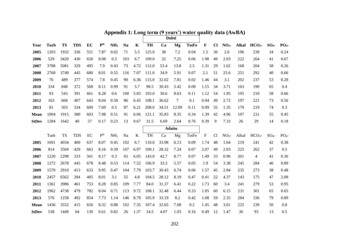
202
Appendix 1: Long term (9 years’) water quality data (AwBA) Dubti
Year Turb TS TDS EC PH NH3 Na K TH Ca Mg TotFe F Cl NO3- Alkal HCO3- SO4- PO4-
2005 1203 1932 336 551 7.87 0.02 71 5.5 125.0 38 7.2 0.04 1.5 36 2.6 196 239 34 0.24
2006 529 3420 430 650 8.08 0.5 103 6.7 109.0 32 7.25 0.06 1.98 49 2.03 222 264 41 0.67
2007 3788 5081 329 495 7.9 0.43 73 4.72 112.0 53.4 13.8 2.5 1.31 29 1.62 168 204 58 0.26
2008 2768 3749 445 680 8.01 0.55 116 7.07 111.0 34.9 5.91 0.07 2.1 51 25.6 251 292 40 0.66
2009 76 489 377 574 7.8 0.45 90 6.36 115.0 32.02 7.81 0.02 1.46 44 3.1 202 237 53 0.28
2010 334 848 372 568 8.11 0.99 91 5.7 98.5 30.43 5.42 0.08 1.15 34 3.71 163 190 65 0.4
2011 93 543 391 661 8.28 0.6 100 5.83 103.0 30.6 8.63 0.11 1.12 54 1.95 195 218 58 0.66
2012 163 668 407 643 8.04 0.58 86 6.45 108.1 36.62 7 0.1 0.94 49 2.72 197 221 73 0.56
2013 81 503 334 609 7.69 0.5 87 6.21 208.0 34.51 12.09 0.11 0.99 35 1.35 179 219 74 0.3
Mean 1004 1915 380 603 7.98 0.51 91 6.06 121.1 35.83 8.35 0.34 1.39 42 4.96 197 231 55 0.45
StDev 1284 1642 40 57 0.17 0.23 13 0.67 31.5 6.69 2.64 0.76 0.39 9 7.33 26 29 14 0.18
Adaitu
Turb TS TDS EC PH NH3 Na K TH Ca Mg TotFe F Cl NO3- Alkal HCO3- SO4- PO4-
2005 1691 4034 400 637 8.07 0.45 102 6.7 110.0 33.98 6.13 0.09 1.74 48 1.64 219 241 42 0.38
2006 814 3504 429 663 8.16 0.39 107 6.97 100.1 28.32 7.24 0.07 2.07 49 2.03 225 262 37 0.5
2007 1220 2298 333 501 8.17 0.3 65 6.05 143.0 42.7 8.77 0.07 1.49 33 0.96 201 4 41 0.36
2008 1272 2678 445 678 8.48 0.53 114 7.52 106.9 33.3 5.57 0.05 1.9 54 3.38 245 284 46 0.89
2009 1570 2910 413 633 9.95 0.47 104 7.79 103.7 30.43 6.74 0.06 1.57 45 2.84 235 273 38 0.48
2010 2457 6562 284 405 8.01 3.1 55 4.8 104.5 28.12 8.19 0.47 0.41 22 4.37 143 175 47 2.09
2011 1361 3986 461 753 8.28 0.85 109 7.77 84.0 31.37 6.41 0.22 1.73 60 3.4 241 279 53 0.95
2012 1962 4738 479 782 8.04 0.71 113 9.72 108.1 32.48 6.44 0.33 1.05 60 6.15 231 301 65 0.65
2013 576 1258 492 854 7.73 1.14 146 8.79 105.9 33.19 8.2 0.42 1.08 59 2.35 284 336 79 0.89
Mean 1436 3552 415 656 8.32 0.88 102 7.35 107.4 32.65 7.08 0.2 1.45 48 3.01 225 239 50 0.8
StDev 538 1449 64 130 0.61 0.82 26 1.37 14.5 4.07 1.03 0.16 0.49 12 1.47 36 93 13 0.5

203
Meteka
Turb TS TDS EC PH NH3 Na K TH Ca Mg TotFe F Cl NO3- Alkal HCO3- SO4- PO4-
2005 1182 3578 326 519 7.86 0.32 73 7.08 101.1 31.44 5.6 0.07 1.95 30 2.61 192 232 21 0.23
2006 1453 3882 358 567 8.04 0.38 84 8.27 105.4 32.2 6.21 0.06 2.08 37 1.82 206 248 29 0.39
2007 684 1252 406 608 8.17 0.35 99 8.6 118.3 32.44 9.03 0.13 1.61 40 0.97 240 288 40 0.9
2008 155 900 714 1090 8.08 0.39 201 12.4 126.6 30.64 11.83 0.17 2.62 79 2.77 410 491 65 0.78
2009 577 4706 627 960 7.88 0.32 182 10.7 118.2 28.41 11.48 0.04 2.33 65 1.8 358 435 72 0.41
2010 291 1228 708 1072 8.19 0.44 208 12 120.8 31.45 10.23 0.2 2.42 72 3.85 405 471 63 0.55
2011 302 2557 596 977 8.35 0.58 154 11 115.0 36.11 9.38 0.21 2.33 70 1.6 338 391 43 0.64
2012 1272 2327 710 1147 9.84 0.65 199 17.8 109.5 31.96 10.4 0.14 1.81 88 2.32 375 438 81 0.79
2013 154 899 669 989 7.63 0.85 195 12.2 120.8 32.14 12.95 0.2 1.89 73 1.06 355 390 99 0.88
Mean 674 2370 568 881 8.23 0.48 155 11.1 115.1 31.87 9.68 0.14 2.12 62 2.09 320 376 57 0.62
StDev 478 1338 151 232 0.61 0.17 52 2.96 7.7 1.89 2.32 0.06 0.31 19 0.86 80 91 24 0.22
Office area
Turb TS TDS EC PH NH3 Na K TH Ca Mg TotFe F Cl NO3- Alkal HCO3- SO4- PO4-
2005 576 1229 330 533 7.86 0.46 78 7.35 99.4 31.78 4.87 0.07 2.34 33 2.55 207 252 26 0.26
2006 1670 6612 342 551 7.83 0.55 83 8.42 101.6 32.22 5.28 0.05 2.33 35 1.54 202 246 19 0.27
2007 3570 5597 300 450 8.07 0.35 64 6.7 105.0 35.57 3.92 0.32 1.6 29 1.1 187 224 24 0.45
2008 1912 3158 328 563 8 0.44 96 7.84 92.4 29.9 4.39 0.1 2.02 40 4.09 213 269 27 0.67
2009 2493 3139 360 542 7.74 0.38 86 7.59 111.2 35.69 5.4 0.58 2.08 31 3.99 219 267 44 0.34
2010 1327 3360 337 463 7.91 1.31 64 7.95 122.8 30.7 10.57 0.23 2.15 28 4.16 178 153 36 0.7
2011 922 2418 410 658 8.14 0.7 106 8.9 100.4 29.79 6.22 0.33 1.84 46 3.46 245 287 36 0.53
2012 950 1415 641 1021 7.9 1.29 159 18.7 94.7 45.34 10.76 1.19 1.79 64 3.05 327 424 79 3.86
2013 419 1121 592 1049 7.46 1.4 239 13.9 164.7 29.78 17.6 0.46 2.49 93 1.98 411 478 85 0
Mean 1538 3117 405 648 7.88 0.76 108 9.7 110.2 33.42 7.67 0.37 2.07 44 2.88 243 289 42 0.79
StDev 951 1806 117 215 0.19 0.41 53 3.74 21.1 4.74 4.24 0.34 0.27 20 1.08 72 95 23 1.11

204
Weir site
Turb TS TDS EC PH NH3 Na K TH Ca Mg TotFe F Cl NO3- Alkal HCO3- SO4- PO4-
2005 1874 4377 249 384 7.88 0.5 50 7 100.0 30.7 5.4 0.09 1.95 19 3.66 153 182 19 0.36
2006 647 1469 146 346 7.82 0.44 50 7.71 98.0 31 5 0.11 2.19 19 2 156 190 17 0.32
2007 1731 2155 194 288 8.22 0.55 32 5.3 98.0 27.5 7.1 0.09 1.08 14 2.3 124 146 20 0.35
2008 944 1680 249 378 7.98 0.57 50 6.72 93.4 29.4 4.85 0.1 1.3 22 3.69 158 190 13 0.5
2009 288 1542 554 414 7.62 0.51 53 7.4 106.8 33.9 5.3 0.12 2.14 23 4.21 169 206 26 0.38
2010 389 3344 259 392 7.97 0.78 51 20.1 96.2 33.17 5.41 0.42 1.47 20 5.74 159 188 24 0.51
2011 423 3506 349 562 8.23 0.7 84 8.91 104.9 31.83 6.07 0.34 1.77 35 3.45 213 246 31 0.6
2012 425 1164 356 571 7.88 0.76 82 11.4 109.0 31 7.75 0.26 1.3 31 4.72 218 248 37 0.66
2013 1122 1059 461 592 7.48 1.26 134 11.6 108.8 32.17 11.75 0.54 4.88 50 2.31 289 347 70 0.66
Mean 871 2255 313 436 7.9 0.67 65 9.56 101.7 31.19 6.51 0.23 2.01 26 3.56 182 216 29 0.48
StDev 561 1123 123 104 0.23 0.24 29 4.2 5.5 1.82 2.07 0.16 1.08 11 1.16 47 55 16 0.13
Awash W. Supply
Turb TS TDS EC PH NH3 Na K TH Ca Mg TotFe F Cl NO3- Alkal HCO3- SO4- PO4-
2005 1435 3873 235 372 8.02 0.45 46 6.94 93.1 30.91 3.87 0.08 1.83 18 2.21 151 172 17 0.31
2006 ND ND ND ND ND ND ND ND ND ND ND ND ND ND ND ND ND ND ND
2007 ND ND ND ND ND ND ND ND ND ND ND ND ND ND ND ND ND ND ND
2008 1968 2692 250 380 8.13 0.53 52 6.91 92.6 30.1 4.22 0.07 1.5 21 2.66 159 187 15 0.63
2009 4538 4987 204 315 7.83 0.55 37 6.1 83.0 25.62 4.59 0.03 1.23 14 10.7 125 152 20 0.37
2010 1125 2931 193 276 7.8 1.12 33 8.25 75.1 20.88 5.49 0.63 0.49 15 4.57 110 134 20 0.78
2011 749 5225 316 504 8.3 0.88 73 8.54 100.7 31.21 5.44 0.38 1.27 28 4.27 192 211 27 0.53
2012 1234 3318 382 593 7.82 0.59 88 13.5 114.0 33.66 7.26 0.26 1.57 32 3.12 223 266 52 0.46
2013 504 1042 531 874 7.39 1.11 197 13 104.4 31.04 15.03 0.31 2.15 65 2.36 351 434 76 0.73
Mean 1650 3438 302 473 7.9 0.75 75 9.04 94.7 29.06 6.56 0.25 1.43 28 4.27 187 222 32 0.54
StDev 1257 1328 112 192 0.27 0.26 53 2.78 12.1 4.02 3.61 0.2 0.49 17 2.76 76 95 21 0.16

205
After Beseka
Turb TS TDS EC PH NH3 Na K TH Ca Mg TotFe F Cl NO3- Alkal HCO3- SO4- PO4-
2005 508 1175 236 373 8.16 0.41 48 7.41 89.1 28.87 4.16 0.12 2.23 19 2.54 149 170 16 0.27
2006 ND ND ND ND ND ND ND ND ND ND ND ND ND ND ND ND ND ND ND
2007 ND ND ND ND ND ND ND ND ND ND ND ND ND ND ND ND ND ND ND
2008 2331 4544 260 395 8.17 0.56 55 12.4 89.5 26.8 5.4 0.13 1.9 23 4.5 163 181 18 0.48
2009 1702 4099 1838 2692 8.28 0.39 709 18.9 63.4 19.5 3.6 0.04 14.4 224 3.7 1028 756 222 1.41
2010 1670 3422 2062 2969 8.74 2.22 820 7.65 54.3 15.2 3.87 0.43 16.6 251 3.43 1015 799 281 1.84
2011 449 1256 337 544 8.1 0.9 79 9.7 99.5 30.6 5.5 0.45 1.54 38 3.31 202 230 31 0.69
2012 1404 1873 285 437 7.44 0.93 56 9.98 114.1 33.59 7.24 0.27 1.14 22 4.6 181 218 31 0.69
2013 334 807 446 738 7.29 1.2 189 16.4 105.0 32.44 17.61 0.46 1.74 61 2.52 338 408 64 0.66
Mean 1200 2454 781 1164 8.03 0.94 279 11.8 87.8 26.71 6.77 0.27 5.65 91 3.51 440 395 95 0.86
StDev 716 1421 745 1063 0.46 0.59 311 4.07 20.2 6.37 4.57 0.16 6.27 94 0.77 373 253 101 0.51
Lake Beseka
Turb TS TDS EC PH NH3 Na K TH Ca Mg TotFe F Cl NO3- Alkal HCO3- SO4- PO4-
2005 8 4621 4529 6745 9.12 0.12 1758 60.1 15.5 4.5 1.1 0.03 34.3 585 1.5 2418 1426 480 3.23
2006 6 4420 4403 6678 9.52 0.42 1645 68 19.8 6.21 1.09 0.12 35.9 592 6.15 2469 1604 510 3.27
2007 57 4325 4233 6288 9.63 0.76 1525 65.1 46.3 8.85 5.9 0.22 32.8 531 2.1 2568 1533 397 2.69
2008 39 5617 3829 5531 9.62 0.61 1437 61 33.0 9.77 2.08 0.12 30.6 458 7.61 2292 1360 475 2.44
2009 44 4308 4226 6068 9.39 0.49 1595 59 15.2 4.48 1.33 0.06 33.6 554 1.29 2205 1595 554 2.84
2010 49 4404 4075 5510 9.47 0.67 1613 48.8 17.7 5.6 0.9 0.3 6.9 422 1.3 2100 1557 792 2.73
2011 42 3645 3513 5382 9.51 0.77 1218 46.8 18.0 4.55 1.56 0.23 20 438 1.08 2932 1306 427 2.33
2012 74 3624 3383 5292 9.32 0.85 1286 46.9 21.7 5.34 1.99 0.15 17 437 1.04 1754 1028 374 2.48
2013 47 3498 3017 4934 9.21 1.22 1196 44.3 21.6 6.92 4.31 0.15 17.9 412 1.03 1543 892 473 2.08
Mean 41 4274 3912 5825 9.42 0.66 1475 55.6 23.2 6.25 2.25 0.15 25.4 492 2.57 2253 1367 498 2.68
StDev 20 614 483 606 0.17 0.29 190 8.39 9.6 1.82 1.62 0.08 9.64 69 2.35 396 240 116 0.37

206
Before Beseka
Turb TS TDS EC PH NH3 Na K TH Ca Mg TotFe F Cl NO3- Alkal HCO3- SO4- PO4-
2005 1698 5255 207 315 7.77 0.55 36 6.86 9.8 30.12 3.88 0.08 1.78 14 2.1 132 154 17 0.35
2006 357 1007 207 323 7.79 0.53 33 7.9 100.9 31.62 5.41 0.12 1.86 16 1.71 138 169 10 0.25
2007 1102 605 230 345 8.29 0.67 44 8.05 88.5 28.12 4.33 0.19 1.55 18 3.74 154 170 19 0.49
2008 1202 2183 218 331 7.92 0.6 38 7.05 91.3 34.4 3.85 0.2 1.45 17 5 140 170 8 0.41
2009 384 2159 249 381 7.65 0.41 49 7.84 101.3 31.54 ND 0.09 1.47 20 3.59 167 204 16 0.33
2010 658 3188 275 419 7.65 0.81 53 10.4 114.0 30.67 9.03 0.28 1.46 22 1.82 179 218 21 0.39
2011 278 755 239 380 7.89 0.86 44 8.66 102.0 32.12 5.12 0.51 3.21 20 2.91 150 253 15 0.76
2012 1063 2700 645 998 7.77 0.84 229 16.7 100.5 30.6 5.81 0.18 1.23 73 3 425 512 68 0.73
2013 413 511 232 401 6.79 1.28 48 19.3 102.8 31.8 12.6 0.76 0.99 19 2.2 167 201 25 0.41
Mean 795 2040 278 433 7.72 0.73 64 10.3 90.1 31.22 6.25 0.27 1.67 24 2.9 184 228 22 0.46
StDev 464 1462 131 203 0.38 0.24 59 4.27 29.2 1.6 2.86 0.21 0.6 17 1.02 87 105 17 0.17
Wonji
Turb TS TDS EC PH NH3 Na K TH Ca Mg TotFe F Cl NO3- Alkal HCO3- SO4- PO4-
2005 400 774 193 296 8.09 0.24 32 6.3 87.3 28.3 4.04 0.07 1.98 13 2.76 123 141 9 0.2
2006 151 410 189 312 8.25 0.43 33 6.29 80.5 28.81 3.94 0.12 1.89 14 1.72 126 144 7 0.28
2007 257 539 180 267 8.47 0.74 26 6.43 91.2 29.92 4 0.3 1.4 12 0.91 116 129 8 0.2
2008 249 503 219 330 10.6 0.54 41 6.49 92.2 29.7 4.64 0.25 1.9 17 2.8 148 174 6 0.52
2009 257 537 225 342 7.71 0.42 38 7.16 88.8 28.2 6.12 0.09 1.42 17 5.1 152 175 13 0.36
2010 179 381 260 403 7.88 0.43 57 8.45 88.9 27.04 5.13 0.11 1.74 22 2.7 175 213 10 1.14
2011 224 512 211 323 8.19 0.83 34 6.95 96.8 29.3 5.54 0.59 1.02 16 5.51 132 155 23 0.73
2012 182 420 205 324 7.76 0.79 32 7.75 98.8 26.43 7.86 0.26 1.01 16 5.26 131 254 19 0.48
2013 198 334 178 302 7.37 1.42 32 6.56 93.6 29.26 7.09 0.49 1.03 13 4.96 118 138 22 0.56
Mean 233 490 207 322 8.25 0.65 36 6.93 90.9 28.55 5.37 0.25 1.49 16 3.52 135 169 13 0.5
StDev 69 122 24 35 0.87 0.33 9 0.7 5.1 1.12 1.33 0.17 0.38 3 1.61 18 39 6 0.28

207
Appendix 2: Two years’ water quality data (Oromia water office)
Rds Par
Stn Turb pH Temp TDS EC DO BOD COD Pb Zn Cr TN K+ NO3 NO2 SO4 Fe Mn F- NH3 Cu Cl2 Cl- Ca Mg TAlk ECo TCo
1st
S14 310 7.7 21.6 262 525 3.6 26.1 87 6 0.12 0.01 4.6 12.7 7.04 0.102 23 2.95 0.17 1.56 3.01 2 0.4 10 122 78 170 28 TNTC
S15 500 8.2 23.3 237 475 5.5 16.6 111 3 0.13 0.01 3.7 9.02 10.1 0.003 25 2.69 0.01 1.65 2.23 2 0.38 24 110 70 123 37 TNTC
S16 430 7.8 21.4 181 355 2.2 19.4 346 8 0.02 0.05 26.4 8.5 52.8 2.5 23 3.5 0.05 0.98 2.44 15 Nil 24 108 66 110 TNTC TNTC
S17 120 8 21.5 300 601 5.8 7.94 71 15 0.02 0.17 6.7 11 7.04 1.16 35 1.56 4.6 1.07 6.75 10 0.33 24 134 38 208 TNTC TNTC
S18 176 8.2 23.6 289 577 4.2 6.6 31 1 0.01 0.02 10.7 17.1 0.44 1.39 47 0.22 0.01 0.57 10.6 9 0.13 42 132 26 172 TNTC TNTC
S19 1,337 7.8 18.8 81 162 2.4 13 17 5 0.03 0.03 27 0.1 13.6 0.05 10 2.27 0.01 0.4 16.2 6 Nil 38 84 22 130 TNTC TNTC
2nd
S14 116 6.7 23.7 116 232 4.7 6.15 16 1 0.03 <R 2.7 4.3 47.3 0.08 30 1.89 1.19 0.54 1.34 13 0.05 60 50 166 88 40 TNTC
S15 116 6.9 23.4 113 227 5.5 4 18 0 0.05 <R 8.3 4.1 12.3 0.09 28 1.12 4.2 0.46 1.14 5 0.02 40 60 100 110 32 TNTC
S16 725 6.7 21.7 132 264 4.5 9.3 89 3 0.06 <R 5.7 3.2 14.5 0.44 2 4.5 <0.2 <0.02 3.64 25 0.08 5 82 42 156 TNTC TNTC
S17 470 7 21.7 316 632 3.7 10.2 117 5 0.01 0.13 11.5 5.6 30.8 0.36 30 2.94 0.3 <0.02 3.7 100 0.76 57 126 26 130 TNTC TNTC
S18 52 6.8 20.8 184 369 2.4 K 9 2 0.03 0.01 1.7 6.9 7.04 0.752 24 0.38 0.4 0.22 5.14 2 0.12 54 108 132 136 TNTC TNTC
S19 1380 6.9 20.1 79 158 4.6 8.12 60 3 0.2 <R 2.7 0.5 0.44 0.033 2 1.57 0.2 0.05 3.32 2 1.89 28 128 46 120 TNTC TNTC
3rd
S14 73 7.8 22.7 124 248 4.3 2.85 10 <R 0.1 <R 3.2 5.75 12.2 0.004 58 0.13 1 0.66 1.08 8 0.06 4 58 78 86 37 TNTC
S15 77 8 23.5 121 242 4.6 2.85 9 <R 0.01 <R 4.1 5.25 15.8 <R 56 0.74 0.2 0.79 0.95 15 0.04 18 92 56 88 49.5 TNTC
S16 50 7.2 22.2 319 639 3.9 4.74 19 1 <R <R 6.1 9.8 16.7 1.42 52 0.38 0.8 0.56 0.77 1 0.23 24 250 130 194 TNTC TNTC
S17 70 7.1 20.4 597 1196 1.7 6.3 57 0 <R 0.05 13.8 15.4 10.6 0.95 64 0.16 0.6 1.16 14.9 1 0.13 16 278 78 360 TNTC TNTC
S18 203 7.2 21.4 470 939 0.3 14.4 688 <R 0.01 <R 15.6 15.5 21.1 0.004 62 4.56 3.4 0.51 24.8 1 0.4 4 112 58 166 TNTC TNTC
S19 20 7.6 20.1 217 434 4.3 2.55 12 2 0.01 0.01 1.3 4.2 2.64 0.016 50 0.2 0.4 0.33 0.4 <R 0.05 2 196 32 134 TNTC TNTC
4th
S14 90 7.6 22.5 156 311 ND 4.8 40 ND 0.02 0.02 1.3 4.6 0 0.033 14 0.57 0.1 0.84 1.14 10 0.07 18 142 46 138 11 51
S15 178 7.7 22.4 156 312 ND 10 111 ND 0.04 0.02 1.1 4.5 0 0.01 14 0.46 0.1 0.86 1.04 7 0.03 18 158 26 136 8 43
S16 100 7.4 24.4 344 688 ND 5.3 59 ND 0 0 20 13.5 15.4 0.64 51 0.82 0.2 0.7 1.39 23 0.21 8 240 44 240 TNTC TNTC
S17 240 7.7 22 745 1491 ND 32 208 ND 0 0.02 27.4 13 43.1 0.231 36 1.18 0.5 1.34 32.1 41 0.41 18 330 22 518 TNTC TNTC
S18 285 7.4 20.6 493 984 ND 25.9 150 ND 0 0 2.3 16.5 16.3 0.158 30 2.2 0.7 ND 51.5x 18 0.45 24 280 80 420 TNTC TNTC
S19 35 7.3 20.6 273 546 ND 2 6 ND 0 0.01 0 8.82 0 0.043 12 0.14 0.3 ND 0.49 2 0.21 70 210 70 300 180 TNTC

208
5th
S14 230 7.2 23.5 244 488 4 2.1 29 ND 0.01 <R ND 6.2 6.6 0.01 20 1.44 <R 0.7 2.89 <R 0.04 32 99 75 184 ND 51
S15 220 7.5 25.6 219 436 5.4 1.6 25 ND 0.03 <R ND 5.9 5.28 0.036 16 1.45 <R 0.96 2.78 <R 0.01 10 110 64 186 ND 43
S16 350 7.3 25.1 234 469 2.9 6.4 49 ND 0.04 <R ND 7 18.5 0.867 16 1.55 0.1 0.34 4.9 <R 0.03 22 118 67 146 TNTC TNTC
S17 600 8.1 25.9 748 1495 0 45.6 914 ND <R 0.15 ND 8.75 7.38 0.42 124 1.37 1.1 0.49 2.3 4 0.15 40 174 98 214 TNTC TNTC
S18 172 7.4 25 591 1180 5.4 26.1 406 ND <R 0.01 ND 8.75 13.7 0.148 59 1.56 1.7 0.62 22.3 18 0.22 <R 380 94 408 TNTC TNTC
S19 560 7.3 21.9 157 314 1.3 7 81 ND <R <R ND 4.8 4.78 0.145 <R 6.49 <R <R 7.54 <R 0.06 <R 122 68 168 180 TNTC
6th
S14 136 7 26.3 122 243 4.4 7.4 ND ND 0.01 0.03 ND 5 1.84 0.198 13 1.13 0 0.21 1.68 <R 0.12 14 99 75 184 192 TNTC
S15 124 7 25.2 135 252 3.6 10.5 ND ND 0.01 0.02 ND 5.1 2.33 0.013 12 1 0 0.27 1.54 <R 0.14 16 110 64 186 223 147
S16 2050 6.5 22.4 121 243 2.1 42.8 ND ND 0.01 <R ND 3.7 1.3 0.83 10 5.63 0 0.37 1.17 <R 0.04 11 118 67 146 TNTC TNTC
S17 1350 7.2 25.4 240 479 3.7 25.5 ND ND 0.04 0.02 ND 5.1 1.08 0.78 23 1.57 0 1.07 2.69 <R 0.06 14 118 54 214 TNTC TNTC
S18 44 6.4 24.7 176 353 4.5 5.09 ND ND 0.2 0.05 ND 7 8.36 2.97 23 0.53 0.01 <R 5.69 0.4 11 10 286 54 266 260 TNTC
S19 3200 8 22.1 54 109 5.7 57.2 ND ND <R <R ND 2 1.19 0.099 30 5.8 0 <R 4.11 <R 0.07 10 122 68 168 TNTC TNTC
7th
S14 87.4 6.8 19.6 160 321 ND Nil Nil ND 0.04 0.02 1.12K 8.2 5.28 0.053 18 0.65 0 0.48 1.43 3 0.06 4 122 32 154 TNTC 203
S15 81.2 6.9 20 159 318 ND Nil Nil ND 0.07 0.02 1.96K 5.1 6.6 0.083 15 0.62 0 0.58 1.23 15 0.09 4 86 34 134 170 151
S16 190 6.9 22.9 200 400 ND Nil Nil ND 0.02 Nil 0.84K 11.5 17.2 0.792 20 1.46 0.3 <R 1.5 12 0.14 6 224 70 268 TNTC TNTC
S17 34.5 7.6 21.5 832 1673 ND Nil 40 ND 0.02 0.02 1.96K 16.5 5.72 0.109 59 0.35 0.4 1.09 27.4 1 0.18 10 271 65 528 TNTC TNTC
S18 819 7.2 20.1 776 960 ND 120 200 ND <R 0.1 2.52K 25.5 0.14 0.33 90 2.84 3.2 Nil 39.6 <R 0.25 4 290 50 408 TNTC TNTC
S19 165 7.1 19.2 314 626 ND Nil Nil ND 0.13 0.06 1.12K 7.75 1.06 0.017 24 0.15 0.08 0.85 0.3 14 0.74 2 206 50 270 TNTC TNTC
Rds: rounds, S14: Awash River after Lake Koka, S15: Lake Koka at Koka Dam, S16: Awash River before Lake Koka, S17: Mojo River before
Lake Koka, S18: Akaki River after Lake Aba Samuel, S19: Awash River at Awash MelkaKuntire, Stn: station, Par: parameter, ECo: E. coli,
TCo: Total coliform, R=0.01, K=10^-3

209
Appendix 3: Summary of the weather data used as userwgn in setting up the model
3 The suffix Av in column headings from TMXAv to WNDAv refers to their respective 12 months’ average value.
STN WLAT WLON
G
WELE
V
RAIN
_YRS TMXAv
TMN
Av
TSDMX
Av
TSDMN
Av
PCPMM
Av
PCPSD
Av
PCPSKW
Av
PR_W1_
Av
PR_W2_
Av
PCPD
Av
RAINHHM
XAv
SOLAR
Av
DEWPT
Av
WND
Av
Ayisha 10.76 42.58 721 21 33.7 21 1.18 1.03 17.76 2.32 9.41 0.12 0.66 8.57 5.92 22.46 16.59 3.35
Asaita 11.53 41.53 430 21 37.16 23.61 1.49 1.95 14.37 2.5 12.04 0.08 0.51 4.64 4.79 22.13 18.72 2.2
Dubti 11.72 41.01 376 21 37.71 22.83 1.23 1.41 16.98 2.76 11.8 0.06 0.72 5.12 5.67 22.47 20.79 1.55
Melkasa 8.4 39.32 1540 21 28.91 13.56 0.94 1.97 72.62 6.07 5.79 0.2 0.61 8.91 24.21 22.17 15.42 4.88
Metahara 8.86 39.92 944 21 33.88 17.95 0.96 1.27 41.43 4.17 7.16 0.17 0.43 6.6 13.81 23.27 17.63 1.63
Nazaret 8.55 39.28 1622 21 27.95 15.06 0.95 1.01 75.18 6.17 6.58 0.21 0.51 8.34 25.06 21.08 13.85 2.6
Shewaro 10.01 39.89 1277 21 27.26 12.07 2.51 1.9 57.25 4.58 7.47 0.21 0.73 13.25 19.09 25.5 9.91 2.32
Sholageb 9.22 39.55 2500 21 23.01 9.67 2.9 1.38 48.47 3.32 5.87 0.2 0.68 11.3 16.16 22.73 8.15 2.2
Addis 9.02 38.75 2386 21 22.27 10.25 0.73 0.8 101.75 6.01 5.46 0.29 0.71 12.99 33.91 20.48 9.53 0.55
Gewane 10.15 40.63 568 21 37.38 22.04 2.03 1.47 40.15 4.69 7.97 0.14 0.55 6.44 13.38 22.45 13.29 2.16
Abomsa 8.47 39.82 1630 21 28.06 15.49 0.97 0.63 75.11 6.12 5.7 0.24 0.6 10.52 25.03 20.15 13.9 1.54
Dire 9.97 42.53 1180 21 32.59 18.96 0.96 0.87 55.48 5.6 7.85 0.18 0.58 8.39 18.5 20.9 15.86 1.72
Majete 10.5 39.85 2000 21 28.66 14.67 0.92 0.94 99.77 6.95 5.35 0.23 0.68 11.5 33.24 21.11 14.71 1.09
Mile 11.43 40.77 487 21 36.11 22.1 1.31 1.77 35.22 3.52 8.63 0.17 0.72 12.08 11.74 23.01 13.85 0.29
D/Zeit 8.73 38.95 1900 21 26.59 7.98 0.71 0.91 73.11 5.08 6.28 0.22 0.75 11.93 24.37 24.68 10.8 2.2
Hombol 8.37 38.77 1743 21 27.11 9.88 1.58 1.7 67.15 4.22 5.53 0.16 0.85 15.85 22.43 23.76 11.89 3.52
AwShel 9.33 40.25 737 21 36.38 18.51 2.13 3.24 39.01 3.61 8.95 0.09 0.88 14.56 13.05 21.74 15.63 1.86
Teji 8.83 38.37 2091 21 24.53 9.58 2.89 2.14 78.01 4.81 5.48 0.26 0.69 12.41 25.99 22.34 10.42 1.68
Cheffa 10.84 39.81 1466 21 30.08 13.34 1.99 2.84 78.18 4.17 6.94 0.17 0.9 19.88 26.12 22.14 19.73 1.99
Erer 9.58 41.36 1065.3 21 30.61 15.71 2.14 2.01 17.06 2.47 9.68 0.16 0.64 9.22 5.69 24.03 11.87 2.83

210
Appendix 4: Observed average monthly flow data used for calibration and
validation of SWAT model simulation at Dubti Flow (m3/s)
Month\Yr 1997 1999 2001 2003 2005 2007 2009 2011 2013
Jan. 20.7 25.43 27.82 24.89 14.89 19.63 19.86 25.11 55.2
Feb. 10.39 25.19 8.67 21.31 14.27 16.87 17.52 14.66 50.91
Mar. 45.69 35.08 39.91 37.89 20.89 20.47 27.16 47.61 97
Apr. 93.13 29.65 23.84 100 75.07 18.27 33.67 82.46 45.49
May 43.12 20.1 14.49 13.92 14.09 18.75 13.32 66.16 57.67
Jun. 32.41 5.57 57.58 4.45 6.52 5.38 4.19 42.68 36.83
Jul. 67.53 91.13 223.9 12.95 26.76 66.74 61.52 58.04 100.5
Aug. 131.3 250.6 195.3 314.3 166.2 273.7 189 179.7 284
Sep. 87.37 312.5 130.2 133.9 82.16 244.5 186.5 184.7 333.5
Oct. 125.6 199.5 62.27 104.8 48.97 141.8 117.9 153.1 246.6
Nov. 116.8 84.32 39.32 44.86 25.86 79.56 48.4 90.5 72.31
Dec. 118.7 38.32 40.12 48.17 22.07 42.09 33.54 76.74 30.83
Month\Yr 1998 2000 2002 2004 2006 2008 2010 2012 2014
Jan. 75.96 13.83 14.29 15.48 14.65 48.33 24.36 45.72 31.97
Feb. 74.35 8.56 9.86 18.68 13.62 42.37 18.67 46.51 23.21
Mar. 125.7 5.86 19.25 22.54 14.2 85.71 43.76 74.14 58.9
Apr. 69.69 6.89 37.68 112.5 59.67 81.41 29.49 91.08 46.54
May 47.81 17.41 6.55 21.63 19.52 45.46 37.04 34.72 78.37
Jun. 28.76 5.19 2.81 10.22 7.71 30.58 23.86 19.49 48.93
Jul. 129.5 42.35 31.91 21.62 31.98 98.49 51.68 75.53 59.99
Aug. 370.6 296.9 127.3 205 250.9 250.9 162.4 287.8 212.8
Sep. 412.7 176.5 60.49 103.8 140.1 250 157.5 258.2 268.2
Oct. 314.3 84.16 36.25 61.68 72.92 219.9 107.5 188 179.7
Nov. 81.31 74.79 12.49 39.24 57.02 99.06 37.9 60.27 63.75
Dec. 33.79 45.87 28.76 15.39 30.63 76.23 28.32 24.59 31.35
Appendix 5: Temporal variation of TN in each subbasin
Sbn TN_1994 (kg) TN_2000 (kg) TN_2014 (kg) 2000-1994 2014-2000 2014-1994
1 223593.75 212722.41 244692.25 -10871.35 31969.84 21098.49
2 7031731.18 260212.13 275814.22 -6771519.05 15602.09 -6755916.96
3 145009.90 6519350.52 6693364.61 6374340.62 174014.09 6548354.71
4 6686051.60 205298.15 7438611.89 -6480753.46 7233313.75 752560.29
5 509468.66 6278804.40 590575.66 5769335.75 -5688228.74 81107.01
6 1984924.13 499042.84 2256096.89 -1485881.29 1757054.04 271172.75
7 154184.90 1762654.82 167347.50 1608469.92 -1595307.32 13162.60
8 6016901.54 123331.28 6710848.15 -5893570.26 6587516.87 693946.61
9 235050.53 672556.19 698081.83 437505.66 25525.64 463031.30
10 1667778.55 266932.76 1851994.89 -1400845.78 1585062.12 184216.34
11 335790.26 1487319.36 340515.48 1151529.10 -1146803.87 4725.22
12 305299.81 311960.01 535240.87 6660.20 223280.86 229941.06
13 5198780.90 440893.20 5977086.69 -4757887.70 5536193.49 778305.79
14 633526.51 4909417.81 747117.22 4275891.31 -4162300.59 113590.71
15 2037424.02 807916.47 2073835.12 -1229507.55 1265918.65 36411.10
16 1607489.19 1976668.07 1634745.68 369178.88 -341922.38 27256.49
17 620594.66 1466614.28 565903.13 846019.61 -900711.15 -54691.54
18 438310.11 550892.83 492855.03 112582.72 -58037.80 54544.92
19 176559.17 449902.19 203838.38 273343.02 -246063.81 27279.21
20 1187876.75 175697.23 1191871.92 -1012179.53 1016174.70 3995.17
21 4072153.95 1026001.71 4094786.19 -3046152.23 3068784.47 22632.24
22 1294037.81 4007448.79 1470620.64 2713410.98 -2536828.15 176582.83
23 183716.61 1146318.01 236427.34 962601.40 -909890.67 52710.73
24 262083.02 177267.53 270954.97 -84815.49 93687.44 8871.95
25 153741.48 274292.59 289325.92 120551.11 15033.33 135584.44
26 281912.52 342762.52 268017.03 60850.00 -74745.49 -13895.49
27 277981.02 643808.98 330893.10 365827.96 -312915.88 52912.08
28 643115.58 275125.58 675466.43 -367990.00 400340.86 32350.86

211
29 484770.57 408378.07 519785.08 -76392.50 111407.01 35014.51
30 808303.69 713298.23 527315.33 -95005.46 -185982.91 -280988.37
31 354199.90 238191.20 638149.73 -116008.70 399958.53 283949.83
32 354569.01 268326.78 325332.44 -86242.23 57005.66 -29236.57
33 215585.98 143176.19 430863.57 -72409.79 287687.38 215277.59
34 154730.33 179571.52 330722.91 24841.18 151151.39 175992.58
35 148121.28 139810.85 188123.50 -8310.43 48312.65 40002.22
36 3099352.85 3467182.35 3728947.56 367829.50 261765.21 629594.71
37 184088.21 240369.42 720498.92 56281.20 480129.51 536410.71
38 3606930.02 3245527.79 3913646.35 -361402.23 668118.57 306716.34
39 3261052.92 3093015.18 3318197.61 -168037.74 225182.43 57144.69
40 155630.21 104015.08 3131292.35 -51615.13 3027277.27 2975662.14
41 208360.16 143252.94 58515.75 -65107.21 -84737.20 -149844.41
42 290702.86 192744.23 226553.16 -97958.63 33808.93 -64149.70
43 3483299.41 2978551.97 2219148.04 -504747.44 -759403.92 -1264151.37
44 308651.01 191999.65 2927831.34 -116651.36 2735831.69 2619180.33
45 478950.10 398445.18 168604.36 -80504.93 -229840.81 -310345.74
46 2537958.63 2481148.41 2494201.70 -56810.22 13053.29 -43756.93
47 348200.02 293362.93 655713.20 -54837.09 362350.27 307513.18
48 191746.06 441467.78 439595.60 249721.71 -1872.18 247849.54
49 850650.84 675779.72 998802.95 -174871.12 323023.23 148152.11
50 333871.56 317186.49 432234.30 -16685.07 115047.81 98362.73
51 266027.87 261893.44 389739.06 -4134.43 127845.62 123711.19
52 2374103.77 2011123.14 2474271.29 -362980.63 463148.15 100167.52
53 1231258.11 968215.82 1289834.71 -263042.29 321618.88 58576.60
Appendix 6: Temporal variation of TP in each subbasin
Sbn TP_1994(kg) TP_2000(kg) TP_2014(kg) 2000-1994 2014-2000 2014-1994
1 79485.552 76636.301 83292.813 -2849.25 6656.511 3807.261
2 2295568.9 74563.167 76716.633 -2221006 2153.466 -2218852
3 54588.305 2218719.7 2233618 2164131 14898.35 2179030
4 2156187.6 74532.457 2161853.3 -2081655 2087321 5665.694
5 156005.41 2149101.4 171129.21 1993096 -1977972 15123.8
6 526826.71 154697.38 601671.98 -372129 446974.6 74845.27
7 55162.594 495662.14 60004.711 440499.5 -435657 4842.117
8 1975017.7 44409.764 1983079.6 -1930608 1938670 8061.897
9 83209.883 1954176.6 67210.754 1870967 -1886966 -15999.1
10 429663.37 91936.538 478751.7 -337727 386815.2 49088.33
11 80211.215 406896.35 82632.958 326685.1 -324263 2421.743
12 77890.343 74575.44 54787.853 -3314.9 -19787.6 -23102.5
13 1696993.8 106214.43 1684081 -1590779 1577867 -12912.7
14 156951.22 1686140.9 166525.58 1529190 -1519615 9574.366
15 620595.34 194348.17 620464.29 -426247 426116.1 -131.046
16 513729.38 574823.64 522352.52 61094.25 -52471.1 8623.133
17 159396 468629.77 136849.67 309233.8 -331780 -22546.3
18 136234.51 137639.36 154407.78 1404.853 16768.42 18173.27
19 60585.902 138707.33 71431.182 78121.43 -67276.1 10845.28
20 379435.74 65659.881 369988.98 -313776 304329.1 -9446.75
21 1481256.2 331749.43 1447334.5 -1149507 1115585 -33921.6
22 338658.06 1432575 384531.54 1093917 -1048043 45873.49
23 59774.903 323512.44 69767.192 263737.5 -253745 9992.289
24 75733.741 56832.122 75382.661 -18901.6 18550.54 -351.08
25 51276.086 73053.668 83041.096 21777.58 9987.428 31765.01
26 82504.973 100125.59 54096.999 17620.62 -46028.6 -28408
27 95826.451 202211.5 87085.438 106385.1 -115126 -8741.01
28 199514.67 91336.642 202411.76 -108178 111075.1 2897.084
29 140748.4 123478.74 83621.452 -17269.7 -39857.3 -57126.9

212
30 218515.09 206118.05 155032.86 -12397 -51085.2 -63482.2
31 111581.63 76184.026 257435.47 -35397.6 181251.4 145853.8
32 119637.32 55628.597 105969.18 -64008.7 50340.58 -13668.1
33 69309.576 42945.837 115763.38 -26363.7 72817.54 46453.8
34 43766.143 40893.716 75253.975 -2872.43 34360.26 31487.83
35 49575.828 40474.622 53137.699 -9101.21 12663.08 3561.871
36 275285.98 1188624.5 118017.39 913338.5 -1070607 -157269
37 61667.181 46155.714 1222586.2 -15511.5 1176430 1160919
38 1077826.8 990918.31 103229.26 -86908.5 -887689 -974598
39 988320.79 928647.29 985345.31 -59673.5 56698.03 -2975.48
40 58246.188 41074.661 922039.18 -17171.5 880964.5 863793
41 80021.07 55562.672 23381.121 -24458.4 -32181.6 -56639.9
42 95091.258 67551.095 104008.9 -27540.2 36457.81 8917.646
43 912913.78 877704.07 67235.21 -35209.7 -810469 -845679
44 92034.838 60260.724 841649.01 -31774.1 781388.3 749614.2
45 113153.03 98297.429 40258.13 -14855.6 -58039.3 -72894.9
46 748651.46 729355.39 118180.54 -19296.1 -611175 -630471
47 117660.61 80574.751 675108.85 -37085.9 594534.1 557448.2
48 66300.82 118481.67 110898.42 52180.85 -7583.26 44597.6
49 228736.56 165427.53 307864.31 -63309 142436.8 79127.76
50 92780.668 88366.025 67283.381 -4414.64 -21082.6 -25497.3
51 87068.998 82301.472 95146.414 -4767.53 12844.94 8077.416
52 605902.8 604887.78 526334.49 -1015.02 -78553.3 -79568.3
53 323441.7 286843.33 409249.3 -36598.4 122406 85807.6
Appendix 7: Water quality sampling and onsite analyses of some sites
Dubti Adaitu

213
Awash fall Beseka
Ziway road Mojo
Samples in the laboratory
Appendix 8: Acronyms
AAEPA -Addis Ababa Environmental Protection Authority
AET -Actual Evapotranspiration
AGNPS -AGricultural NonPoint Source
AGWA -Automated Geospatial Watershed Assessment Tool
AHC -Agglomerative Hierarchical Clustering
Alk. -Alkalinity
ANN -Artificial Neural Networks
AnnAGNPS -Annualized AGricultural Non-Point Source
ANSWERS -Aerial Nonpoint-Source Watershed Environmental Response Simulation
APHA -American Public Health Association
AQUATOX -Simulation Model for Aquatic Systems
ARB -Awash River Basin
AwBA -Awash Basin Authority
BASINS -Better Assessment Science Integrating point and Nonpoint Sources
BCM -Billion Cubic Meter
BMP’s - Best Management Practices

214
BOD -Biochemical Oxygen Demand
CA -Cluster analysis
CCME -Canadian Council of Ministers of the Environment
CFSR -Climate Forecast System Reanalysis
CIA -Central Intelligence Agency
COD -Chemical Oxygen Demand
CREAMS -Chemicals, Runoff, and Erosion from Agricultural Management Systems
DDT -DichloroDiphenylTrichloroethane
DEM -Digital Elevation Model
DN -Digital Number
DO -Dissolved Oxygen
EC -Electrical Conductivity
ECo -Escherichia Coli
EFDC -Environmental Fluid Dynamic Code
EPIC -Environmental Impact Policy Climate
EROS -Earth Resources Observation and Science
ET -Evapo-Transpiration
ETM+ -Enhanced Thematic Mapper Plus
FDI -Foreign Direct Investment
FTU -formazine turbidity unit
GIS -Geographic Information System
GLCF -Global Land Cover Facility
GLEAMS -Groundwater Loading Effects of Agricultural Management Systems
GloVis -Global Visualization Viewer
GloVis -Global Visualization Viewer
GPS -Global Positioning System
GWLF -Generalized Watershed Loading Function
GWP -Global Water Partnership
HRU -Hydrologic Response Unit
HSPF -Hydrological Simulation Program – FORTRAN
IDW -Inverse Distance Weighting
IRBM -Integrated River Basin Management
IT -Information Technology
ITCZ -Inter-Tropical Convergence Zone
IWRM -Integrated Water Resources Management
KINEROS2 -Kinematic Erosion and Runoff
LS -LandSat
LS TM -Landsat Thematic Mapper
LU/LC -Land Use/Land Cover
MCM -Million Cubic Meter

215
MER -Main Ethiopian Rift
MoH -Ministry of Health
MoWIE -Ministry of Water, Irrigation and Energy
MUSLE -Modified Universal Soil Loss Equation
MW -Megawatt
NCEP -National Centers for Environmental Prediction
NMSA -National Meteorological Service Agency
NSF -National Sanitation Foundation
NTU -Nephelometric Turbidity Unit
OWQI -Overall Water Quality Index
PAH -Polycyclic Aromatic Hydrocarbons
PCA -Principal Component Analysis
PCBs -Poly Chlorinated Biphenyl
PCP -Precipitation
PCs -Principal Components
PET -Potential Evapo-transpiration
POC -Particulate Organic Carbon
QA/QC -Quality Assurance/Quality Control
QUAL2E -Enhanced Stream Water Quality Model
RE -Relative Error
ROTO -Routing Outputs To Outlet
RSC -Residual Sodium Carbonate
SA -Sensitivity Analysis
SAR -Sodium Adsorption Ratio
SCS CN -Soil Conservation Service curve number
SNNP -Southern Nations Nationalities and Peoples
SPAW -Soil Plant Air Water hydrology
SRTM -Shuttle Radar Topography Mission
SUFI2 -Sequential Uncertainty FItting Version 2
SWAT -Soil and Water Assessment Tool
SWAT-CUP -SWAT Calibration and Uncertainty Programs
SWRRB -Simulator for Water Resources in Rural Basins
TC -Total Coliform
TCU -True Color Unit
TDS -Total Dissolved Solids
TH -Total Hardness
TM -Thematic Mapper
TMDL -Total Maximum Daily Load
TN -Total Nitrogen
TP -Total Phosphorus

216
TS -Total Solids
TSS -Total Suspended Solids
UNEP -United Nations Environment Program
UNESCO - United Nations Educational, Scientific and Cultural Organization
UNFAO -United Nations Food and Agricultural Organization
UNICEF -United Nations Children’s Fund
USDA SCS -United States Department of Agriculture Soil Conservation Service
USDA-ARS- United States Department of Agriculture’s Agricultural Research Service
USGS -United States Geological Survey
USLE -Universal Soil Loss Equation
WASP -Water Quality Analysis Simulation Program
WHO -World Health Organization
WQD -Water Quality Dynamics
WQI -Water Quality Index
WQMS -Water Quality Monitoring and Surveillance
WWC -World Water Council
WWDSE -Water Works Design and Supervision Enterprise
WWFS -World Water Forum Secretariat
Personal and Ethical statements
No specific permits were required for the described field studies. This is because the sampling,
onsite analysis, travelling in the study area and other activities conducted during the field trip
did not cause any disturbances to the environment or to the protected species.
Declaration
I, Amare Shiberu Keraga, declare that this thesis is my original work and has not been presented
for a degree in any other university, and that all sources of material used for the thesis have
been duly acknowledged.
Submitted by: Amare Shiberu Keraga ________________________________________
Related Documents


