Assessing when a sample is mostly normal

Assessing when a sample is mostly normal

Pedro C. Alvarez-Esteban a,∗ Eustasio del Barrio a

Juan A. Cuesta-Albertos b Carlos Matran a

aDept. de Estadıstica e Investigacion Operativa, Universidad de Valladolid. Pradode la Magdalena s.n., 47005 Valladolid. Spain.

bDept. Matematicas, Estadıstica y Computacion, Universidad de Cantabria. Avda.los Castros s.n. 39005 Santander, Spain.

Abstract

The use of trimming procedures constitutes a natural approach to robustifying sta-tistical methods. This is the case of goodness-of-fit tests based on a distance, whichcan be modified by choosing trimmed versions of the distributions minimizing thatdistance. In this paper we consider the L2-Wasserstein distance and introduce thetrimming methodology for assessing when a data sample can be considered mostlynormal. The method can be extended to other location and scale models, intro-ducing a robust approach to model validation, and allows an additional descriptiveanalysis by determining the subset of the data with the best improved fit to themodel. This is a consequence of our use of data-driven trimming methods insteadof more classical symmetric trimming procedures.

Key words: Model Assessment, Asymptotics, Impartial Trimming, Wassersteindistance, Similarity.

1 Introduction.

Trimming methods are a main tool in the design of robust statistical proce-dures. For univariate data a classical way of trimming is based on deleting thesame proportion of observations in each tail of the distribution. This approach

∗Email address: [email protected] (Pedro C. Alvarez-Esteban).

1 Research partially supported by the Spanish Ministerio de Educacion y Cien-cia, grant MTM2008-06067-C02-01, and 02 and by the Consejerıa de Educacion yCultura de la Junta de Castilla y Leon, GR150.

Preprint submitted to Elsevier 29 January 2009

has some drawbacks. First, the implicit assumption that the possible contam-ination is only due to outliers. Second, the lack of “a priori” directions to trimin the multivariate setting. Several alternatives to the symmetric trimminghave been proposed in the statistical literature. Among the proposed alter-natives to overcome these difficulties we focus on those minimizing some dis-tance criterium, leading to the “impartial” trimming introduced by Rousseeuw(1985) and in greater generality in Gordaliza (1991). This impartial trimmingmethodology is based on the idea that the trimming zone should be determinedby the data themselves and has been successfully applied to different statisticalproblems including location estimation, (Rousseeuw, 1985; Gordaliza, 1991),regression problems (Rousseeuw, 1985), cluster analysis (Cuesta-Albertos etal., 1997; Garcıa-Escudero et al., 2003, 2008), and principal component anal-ysis (Maronna, 2005).

This approach looks very appropriate for the goodness-of-fit framework, wherethe procedures are often based on minimizing distances. However, only sometimid attempts have been reported in this sense so far. In fact, to our bestknowledge, the only related approach is that of Munk and Czado (1998), wherea symmetric trimming is introduced to robustify an analysis of similarity basedon the Wasserstein distance. In our setting, the questionable fact about thisapproach, would be why should two distributions largely different at their tailsbe considered similar but they should be considered as non-similar if they areslightly different in their central parts?

This observation led to a new proposal in Alvarez-Esteban et al. (2008a),where similarity of distributions is assessed on the basis of the comparison oftheir trimmed versions. The approach was based on considering that two dis-tributions are similar at level α whenever suitable chosen α-trimmed versionsof such distributions coincide. This key idea is naturally related to Robust-ness, and can be combined with the use of a distance between probabilitiesto measure their degree of dissimilarity. The L2-Wasserstein distance was thechoice in Alvarez-Esteban et al. (2008a) to introduce a nonparametric test ofsimilarity that can be considered as a robust version of a goodness-of-fit testto a completely specified distribution or, rather, a way to assess whether thecore of the distribution underlying the data fits a fixed distribution.

In this work we show how these ideas can be used to assess whether thecore of the distribution underlying the data can be assumed to follow a givenlocation-scale model. For the sake of simplicity and its relevance, we considerthe normal model, but it will become apparent that the methodology can beextended to cover other patterns. More precisely, we measure the minimaldistance between trimmed versions of the empirical distribution and trimmednormal distributions and provide the necessary distributional theory to make itusable for inferences about its population counterpart. Our procedure involvesthe computation of a best trimming and it can be considered not only as a

2

way to robustify a statistical procedure but also as a method to discard a partof the data to achieve the best possible fit to normality of the remaining data.Thus, this kind of robustification provides an added value as a descriptive toolfor the analysis of the data.

On the real line, the L2-Wasserstein distance between two probability measurescan be obtained as the L2 distance between their quantile functions, so it hasan easy interpretation in terms of probability plots. In the particular case oftesting for normality its use leads to a version of the omnibus Shapiro-Wilkstest (see e.g. del Barrio et al., 1999, 2000, 2005). The L2-Wasserstein distanceis also well behaved with respect to trimmings (see Alvarez-Esteban et al.(2008a)) and will also be our choice here to introduce a robust approach tomodel validation.

This paper is organized as follows. In Section 2 we give the necessary back-ground on trimmed distributions and Wasserstein distance and use it to intro-duce an estimator for the trimmed distance to normality. We show how to useit to assess whether a sufficiently large fraction of the distribution underlyingthe data can be assumed to be normal. We include in this section some asymp-totic results that justify our approach. We describe the algorithm involved inthe computation of our estimators and discuss further implementation details.In Section 3 we provide empirical evidence of the performance of our proposal.This will be made through real and simulated examples giving support to theprocedure. Finally, an Appendix is devoted to the proof of the results.

2 Trimmed distributions in testing for normality.

2.1 Trimmed distance to normality.

Trimmed probabilities can be defined in general spaces, but for the applicationpresented in this paper we will restrict to the real line. Let P be a probabilityon R and 0 ≤ α < 1, we say that a probability P ∗ is an α-trimming of P ifP ∗ is absolutely continuous with respect to P and dP ∗

dP≤ 1

1−α. We will denote

by Tα(P ) the set of α-trimmings of P ,

Tα(P ) ={P ∗ ∈ P : P ∗ ¿ P, dP ∗

dP≤ 1

1−αP -a.s.

}.

An equivalent characterization, useful to gain some insight about the meaningof an α-trimming is that P ∗ ∈ Tα(P ) if P ∗ ¿ P and there exists a function fsuch that dP ∗

dP= 1

1−αf where 0 ≤ f ≤ 1 P -a.s. Here, f(x) gives the fraction of

density not trimmed at a point x in the support of P . If f(x) = 0, the point xis completely removed, while if f(x) = 1 there is no trimming at x. For those

3

points in the support of P where 0 < f < 1 their weight after trimming isdecreased. Note that this is a natural generalization of the common practice oftrimming observations, which amounts to replacing the empirical distributionby a new version with new weights on the data: 0 for the points removedand 1/(n(1 − α)) for the points kept in the sample (if we remove k = nαobservations).

Interesting properties of α-trimmings can be found in Alvarez-Esteban et al.(2008a,b). We mention here one which is essential for the proposal in thispaper. General α-trimmings can be parametrized in terms of the α-trimmingsof the uniform distribution on (0, 1). More precisely, if Cα is the class of ab-solutely continuous functions h : [0, 1] → [0, 1] such that, h(0) = 0, h(1) = 1,with derivative h′ such that 0 ≤ h′ ≤ 1

1−αand we write Ph for the proba-

bility with distribution function h(P (−∞, t]), then, for any real probabilitymeasure, P , we have,

Tα(P ) = {Ph : h ∈ Cα} .

We note that Cα is the set of distribution functions of α-trimmings of theuniform distributions on (0, 1). As a consequence, if P has distribution functionF and quantile function F−1, the set of α-trimmings of P equals the set ofprobability measures with quantile functions of type F−1(h−1(t)), t ∈ (0, 1)with h ∈ Cα.

Let F2 be the set of univariate distributions with finite second moments. TakeP , Q ∈ F2 with quantile functions F−1, G−1, respectively. The L2-Wassersteindistance between these two distributions is defined as

W2(P,Q) := inf{(

E(X − Y )2)1/2

: L(X) = P, L(Y ) = Q}

,

where X and Y are random variables defined on some arbitrary probabilityspace. The fact that W2 metrizes weak convergence of probability measuresplus convergence of moments of order two (see Bickel and Freedman (1981)),makes this distance specially convenient for statistical purposes. Moreover, onthe real line, it equals the L2-distance between the quantile functions, namely,

W2(P,Q) =[∫ 1

0

(F−1(t)−G−1(t)

)2dt

]1/2

.

It could be the case, when trying to assess normality of a data sample,X1, . . . , Xn, that some significant deviation is found but, in fact, this devi-ation is caused only by some small fraction of the data. It seems natural toremove or downplay the importance of the disturbing range of observationsand measure the distance between the trimmed versions of the empirical mea-sure and the normal distributions, with a trimming pattern chosen in order to

4

optimize fit. If we measure distance by W2 this amounts to considering

Tn,α := infh∈Cα, Q∈N

W22 ((Pn)h, Qh), (1)

where Pn denotes the empirical distribution and N stands for the family ofnormal distributions on the line. We assume that X1, . . . , Xn are i.i.d. obser-vations with common distribution P . The population version of (1),

τα(P,N ) := infh∈Cα, Q∈N

W22 (Ph, Qh), (2)

measures how far from normality is the core of the underlying distributionP . We refer to τα(P,N ) as the (squared) trimmed distance to normality. Ifτα(P,N ) = 0 then there is some normal distribution Q which is equal to Pafter removing a fraction of mass, of size at most α, on P and Q. A smallvalue of τα(P,N ) indicates that most of the distribution underlying the datais not far from normality, which might be enough for the validity of someinferences. Assessment of this small deviation from normality means, in moreformal terms, fixing a threshold ∆2

0 and testing

H0 : τα(P,N ) ≥ ∆20 vs. τα(P,N ) < ∆2

0. (3)

Given the sample X1, . . . , Xn we compute Tn,α, defined in (1), and reject H0

for small values of it.

Note that the choice of the null and the alternative hypotheses is in agreementto the fact that, as in other goodness-of-fit problems, the consequences ofassuming (approximate) normality when it is not true are worse than those ofthe other possible error. Thus, rejecting H0 can be done at a controlled errorrate. We refer to Munk and Czado (1998) for further discussion on this issue.The difficulty posed by the arbitrary choice of the threshold ∆2

0 can be dealtwith by the consideration of the p-value curve, as in Munk and Czado (1998)or Alvarez-Esteban et al. (2008a). We turn to this point in Subsection 2.3.

It can be easily checked that τα(P,N ) is location invariant, but not scaleinvariant. In order to avoid this dependence on scale, and as usual in assessingfit to location-scale models (see, e.g., del Barrio et al. (1999)), we consider alocation and scale invariant modification of τα(P,N ). It is convenient to thinkof F−1(h−1(y)) =: (F−1 ◦ h−1)(y) as a random variable defined on (0, 1) andsimilarly for other expressions of this type. We note then that if Q = N(µ, σ2),Φ denotes the standard normal distribution function and h ∈ Cα, we haveW2

2 (Ph, Qh) = E(F−1 ◦ h−1 − µ− σΦ−1 ◦ h−1)2. Thus, for a fixed h,

v(h) := minQ∈N

W22 (Ph, Qh) = Var(F−1◦h−1)−Cov2(F−1 ◦ h−1, Φ−1 ◦ h−1)

Var(Φ−1 ◦ h−1), (4)

5

the min being attained at Q = N(µ(h), σ2(h)), where

σ(h) =Cov(F−1 ◦ h−1, Φ−1 ◦ h−1)

Var(Φ−1 ◦ h−1), µ(h) = E(F−1◦h−1−σ(h)Φ−1◦h−1). (5)

With this notation we have τα(P,N ) = infh∈Cα v(h). It can be shown that thisinf is attained (see Lemma A.1 in the Appendix). To simplify our expositionwe make the following technical assumption:

v(h) admits a unique minimizer, h0. (6)

Now, under (6), we define

τα(P,N ) :=τα(P,N )

rα(P ),

with rα(P ) = Var(F−1◦h−10 ). Note that τα(P,N ) = 1−Corr2(F−1◦h−1

0 , Φ−1◦h−1

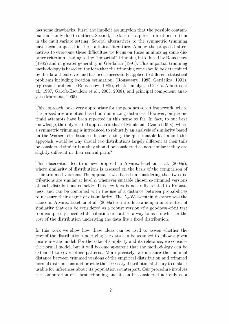
0 ). Hence, τα(P,N ) is location scale invariant and satisfies 0 ≤ τα(P,N ) ≤1. We refer to it as the standardized trimmed distance to normality. We cansee in Figure 1 how τα(P,N ) and τα(P,N ) change with α for two choices ofP : the mixture 0.9N(0, 1)+0.1∗N(4, 1/4) (left) and the mixture 0.5N(0, 1)+0.5 ∗ N(3, 1/4). We can appreciate how after trimming a bit more than thelevel of ‘contamination’ we achieve almost perfect fit to normality.

0.0 0.2 0.4 0.6 0.8 1.0

0.00

0.05

0.10

0.15

τα(P, N)

α

Standardized distanceTrimmed distance

0.0 0.2 0.4 0.6 0.8 1.0

0.0

0.1

0.2

0.3

0.4

τα(P, N)

α

Standardized distanceTrimmed distance

Figure 1: Trimmed distance to normality.

If we admit that our assessment about the normality of the core of the dis-tribution should not depend on the scale of measurement of the data then weshould replace the testing problem (3) by

H0 : τα(P,N ) ≥ ∆20 vs. τα(P,N ) < ∆2

0. (7)

6

The threshold is now to be chosen in (0, 1) but, again, this arbitrary choicecan be avoided with the use of the p-value curve.

2.2 Asymptotic theory.

In order to make Tn,α usable in pratice for testing (3) (or (7)) we include thisSubsection with a result giving its asymptotic normality as well as providinga consistent estimator of the corresponding asymptotic variance. The com-putations involve the use of empirical versions of µ(h), σ(h), defined in (5),evaluated at a empirical version of h0. To be precise we define

vn(h) := minQ∈N

W22 ((Pn)h, Qh), h ∈ Cα. (8)

Now, Tn,α = infh∈Cα vn(h) and, as for v(h), we have that the inf is attained(Lemma A.1). We denote hn := argminh∈Cα

vn(h) and

σn =

∫ 10 F−1

n Φ−1h′n −∫ 10 F−1

n h′n∫ 10 Φ−1h′n∫ 1

0 (Φ−1)2h′n − (∫ 10 Φ−1)h′n)2

, µn =∫ 1

0(F−1

n − σnΦ−1)h′n. (9)

We refer to Subsection 2.3 below for details on the practical computation ofTn,α, hn and related estimators. Now we can state the main result in thisSection.

Theorem 2.1 If P satisfies (6), has absolute moments of order 4 + δ, forsome δ > 0, and a distribution function F with continuously differentiabledensity F ′ = f such that

supx∈R

∣∣∣∣∣F (x)(1− F (x))f ′(x)

f 2(x)

∣∣∣∣∣ < ∞, (10)

then √n(Tn,α − τα(P,N )) →

wN(0, σ2

α(P,N ))

where

σ2α(P,N ) = 4

(∫ 1

0l2(t)dt−

(∫ 1

0l(t)dt

)2)

,

l(t) =∫ F−1(t)

F−1(1/2)(x− µ(h0)− σ(h0)Φ

−1(F (x)))h′0(F (x))dx,

µ(h0), σ(h0) are as in (5) and h0 is the minimizer defined in (6).

If S2n,α := 4

(∫ 10 l2n(t)dt−

(∫ 10 ln(t)dt

)2)

, where

ln(t) =∫ F−1

n (t)

F−1n (1/2)

(x− µn − σnΦ−1(Fn(x)))h′n(Fn(x))dx

7

and µn, σn are given in (9), then S2n,α → σ2

α(P,N ) in probability.

The proof of Theorem 2.1 can be found in the Appendix.

2.3 Practical issues, p-value curves, algorithms.

As we noted before, the testing problem (3) involves the choice of a threshold,∆2

0. Rather than choosing it in an arbitrary way we consider, as in Munk andCzado (1998) or Alvarez-Esteban et al. (2008a), the p-value curves. Thesecurves are built using the asymptotic p-value computed from the test statisticZn,α := (Tn,α−∆2

0)/Sn,α. Note that from Theorem 2.1 we have Zn,α → N(0, 1)in distribution if ∆2

0 = τα(P,N ) (hence, Zn,α → +∞ for ∆ < τα(P,N ) andZn,α → −∞ for ∆ > τα(P,N )).

For each threshold value ∆0 we compute

p(∆0) := supF∈H0

limn→∞PF (Zn,α ≤ z0) = Φ

(√n

tn,α−∆20

sn,α

),

where z0 =√

ntn,α−∆2

0

sn,αis the observed value of Zn,α. Then, we plot p(∆0) versus

∆0. These p-value curves can be used in two ways. On one hand, fixing ∆0,which controls the degree of dissimilarity, we can find the level of significanceat which F cannot be considered essentially normal (at trimming level α). Onthe other hand, for a fixed test level (p-value), we can find the value of ∆0 suchthat for every ∆ ≥ ∆0 we should reject the hypothesis H0 : τα(P,N ) ≥ ∆2.

In practice we will be interested in testing (7) rather than (3). We can rewrite(7) as

H0 : τα(P,N ) ≥ ∆20rα(P ) vs. τα(P,N ) < ∆2

0rα(P ),

a family of testing problems that could be analysed using the p-value curvep(∆0r

1/2α (P )). Since rα(P ) is unknown we replace it by the consistent estimator

Rn,α =∫ 10 (F−1

n )2h′n −(∫ 1

0 F−1n h′n

)2and obtain the estimated p-value curve for

(7):p(∆0) := p(∆0R

1/2n,α), 0 < ∆0 < 1.

The values of ∆0 should be interpreted taking into account that τα(P,N ) takesvalues in [0, 1]. τα(P,N ) = 0 means perfect fit to normality after trimming,while large values of τα(P,N ) (close to 1) mean severe nonnormality even aftertrimming.

We turn now to computational details. First, to compute the value of Tn,α weobserve that

Tn,α = minh∈Cα,µ∈R,σ≥0

∫ 1

0(F−1

n − µ− σΦ−1)2h′ = minµ∈R,σ≥0

Vn(µ, σ),

8

where

Vn(µ, σ) = minh∈Cα

∫ 1

0(F−1

n − µ− σΦ−1)2h′.

If σ > 0 then Vn(µ, σ) =∫ 10 (F−1

n − µ− σΦ−1)2h′n,µ,σ, where

h′n,µ,σ =1

1− αI|F−1

n −µ−σΦ−1|≤kn,µ,σ

and kn,µ,σ is the (unique) k such that the set {t ∈ (0, 1) : |F−1n (t) − µ −

σΦ−1(t)| ≤ k} has Lebesgue measure 1−α. We use this to compute numericallyVn(µ, σ) as follows

(1) Compute the values of |F−1n (t)− µ− σΦ−1(t)| in a (fine) grid of [0, 1].

(2) Approximate kn,µ,σ as the (1− α)-quantile of these values.(3) Approximate Vn(µ, σ) as the average of (F−1

n (t)− µ− σΦ−1(t))2h′n,µ,σ(t)over the grid.

Now, minimization of Vn(µ, σ) yields Tn,α. We carry out this step through asimple search-in-a-grid of (µ, σ), although this could be replaced by an opti-mization procedure based in gradient methods avalaible in R (see e.g. nlm,optim), using the sample values as initial values.

If µn and σn are the minimizers of Vn(µ, σ) obtained with the above algorithm,then take

hn = hn,µn,σn .

Finally, aproximate

S2n,α = 4

[∫ 1

0ln(t)2dt−

(∫ 1

0ln(t)dt

)2]

computing numerically the integrals, where

ln(t) :=∫ F−1

n (t)

F−1n (1/n)

(x− µn − σnΦ−1(Fn(x))

)h′n(Fn(x))dx

is evaluated numerically by averaging in the grid in (0, 1) as above. Similarlywe compute Rn,α.

All these procedures have been implemented in an R program avalaible athttp:// www.eio.uva.es/ ∼pedroc/R. These computations have been codedin a vectorized way and the result is that for moderate sizes of n (100-500)the time required in a PC is just a few seconds, while for big sizes (5000) is acouple of minutes, depending on the grid for (µ, σ). The grid in [0, 1] for thecomputation of Vn(µ, σ) was obtained splitting [0, 1] into 105 intervals of equallength.

We end this Section with a remark on the computational convenience of thenormalization chosen here for the standardized trimmed distance to normality,

9

τα(P,N ). Other alternatives could be chosen, the most natural being perhapsτ ∗α(P,N ) = minh∈Cα w(h) with

w(h) =v(h)

Var(F−1 ◦ h−1)= 1− Cov2(F−1 ◦ h−1, Φ−1 ◦ h−1)

Var(F−1 ◦ h−1)Var(Φ−1 ◦ h−1),

(recall the notation in (4)). Now w(h) is location-scale free for every h ∈ Cα andso is τ ∗α(P,N ). Using the method of proof of Theorem 2.1 we could prove alsoasymptotic normality of an empirical version of τ ∗α(P,N ). Its use in practice,however, is rather troublesome. If we try to mimick the algorithm that weused to evaluate Tn,α we should be able to compute

Wn(µ, σ) = minh∈Cα

W22 ((Pn)h, N(µ, σ2)h)

Var(Ph)

for fixed µ and σ. Unfortunalety there is no easy expression for the optimalh in this minimisation problem. We could rewrite it as an optimal controlproblem and use appropriate numerical methods but, yet, the computationalburden required for a single evaluation of Wn(µ, σ) discourages its use.

3 Examples and Simulations

3.1 Example 1, real data.

Cholesterol

mg/dl

Fre

quen

cy

0 100 200 300 400 500

020

4060

80

Triglycerides

mg/dl

Fre

quen

cy

0 200 400 600 800 1000

020

4060

8010

012

0

Figure 2: Histogram for variables Cholesterol and Triglycerides.

We use the variables concentration of plasma cholesterol and plasma triglyc-erides (mg/dl) collected from n = 371 patients (see Hand et al., 1994) toillustrate the application of our procedure to investigate whether these sam-

10

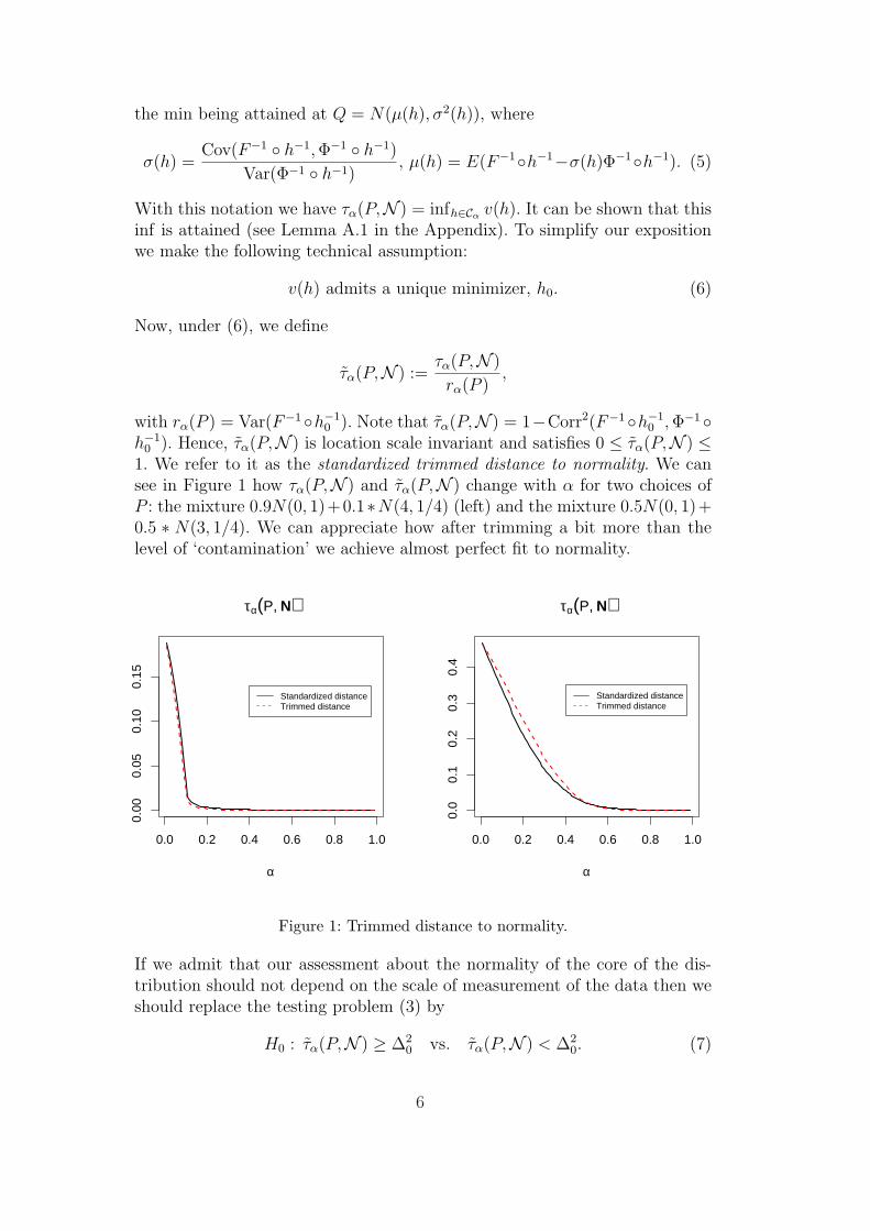
ples can be considered normal at some reasonable trimming level. Figure 2shows the histograms for both samples. The cholesterol sample shows a slightpositive skewness with two possible outliers. The triglycerides sample exhibitsa clear positive skewness and a clear outlier at the right tail. Using classicalprocedures such as the Shapiro-Wilks test would reject the hypothesis of nor-mality, even if we remove the mentioned outliers (p = .0306 and p < .0000,respectively).

Cholesterol Triglycerides

α µn σn τα(Pn,N ) µn σn τα(Pn,N )

0 213.31 42.07 0.026 173.94 88.90 0.193

0.05 212.08 39.64 0.005 165.92 71.27 0.112

0.10 211.75 39.88 0.004 161.16 63.87 0.089

0.20 211.02 41.68 0.002 153.15 53.04 0.048

Table 1: Distances, means and standard deviations of the best α-trimmed normaldistribution.

We use instead our data-driven trimming method to obtain the best α-trimmedGaussian approximation to each sample. Table 1 shows the means and stan-dard deviations of the best normal approximation as well as the standardizedtrimmed distances to normality, τα(Pn,N ), for both samples and differenttrimming sizes.

0.0 0.2 0.4 0.6 0.8 1.0

010

2030

4050

6070

Cholesterol (α = 0.05)

t

Fn−1

(t)−

µ n−

σ nΦ

−1(t)

0.0 0.2 0.4 0.6 0.8 1.0

010

2030

4050

6070

Cholesterol (α = 0.1)

t

Fn−1

(t)−

µ n−

σ nΦ

−1(t)

0.0 0.2 0.4 0.6 0.8 1.0

010

2030

4050

6070

Cholesterol (α = 0.2)

t

Fn−1

(t)−

µ n−

σ nΦ

−1(t)

0.0 0.2 0.4 0.6 0.8 1.0

020

0040

0060

0080

00

Triglycerides (α = 0.05)

t

Fn−1

(t)−

µ n−

σ nΦ

−1(t)

0.0 0.2 0.4 0.6 0.8 1.0

020

0040

0060

0080

00

Triglycerides (α = 0.1)

t

Fn−1

(t)−

µ n−

σ nΦ

−1(t)

0.0 0.2 0.4 0.6 0.8 1.0

020

0040

0060

0080

00

Triglycerides (α = 0.2)

t

Fn−1

(t)−

µ n−

σ nΦ

−1(t)

Figure 3: Optimal trimming functions for both Cholesterol and Triglycerides

11

samples, for different trimming sizes (α = 0.05, 0.1 and 0.2).

Figure 3 shows the optimal trimming functions for Cholesterol and Triglyc-erides samples for different values of α (0.05, 0.1 and 0.2). In each graph weplot the value of Jn(t) := |F−1

n (t) − µn − σnΦ−1(t)| and the cutting valueskn,µn,σn , where µn and σn are the mean and the standard deviation of theclosest normal distribution (see Table 1) estimated using the algorithm de-scribed in Subsection 2.3. These plots show that trimming should be mademostly at the tails of the distributions to make them as normal as possible.This optimal trimming, though, is not symmetric, and not always removingall the observations at the tails. The plot corresponding to the Cholesterolsample and α = 0.2 suggests that if we increase the trimming size then someobservations in the center of the distribution would be trimmed.

0.0 0.2 0.4 0.6 0.8

0.0

0.2

0.4

0.6

0.8

1.0

Cholesterol

∆0

p−va

lue

α = 0α = 0.05α = 0.1α = 0.2

0.0 0.2 0.4 0.6 0.8

0.0

0.2

0.4

0.6

0.8

1.0

Triglycerides

∆0

p−va

lue

α = 0α = 0.05α = 0.1α = 0.2

0.0 0.2 0.4 0.6 0.8

0.0

0.2

0.4

0.6

0.8

1.0

N(0,1)

∆0

p−va

lue

α = 0α = 0.05α = 0.1α = 0.2

Figure 4: P-value curves for Cholesterol, Tryglicerides and the reference case. Thedotted line is a reference line (p = 0.05).

In order to assess the degree of normality of the samples we use the p-valuecurves, p(∆), introduced in Subsection 2.3. Figure 4 shows these curves for

12

Cholesterol and Triglycerides samples for different trimming sizes and the “Notrimming” case. Note that although the asymptotic distribution has not beenexplicitly given for this case in this paper, it can be easily derived following thesame arguments as for Theorem 2.1 and coincides with the limit case α = 0in this theorem. The third graph corresponds to a random sample of the samesize (n = 371) drawn from the standard normal distribution. This graph hasbeen included as a reference to simplify the assessment of the normality of theprevious samples.

Although in both cases there is a significant improvement after trimming theinitial 5% (fixing p = 0.05, from ∆0 = 0.24 when α = 0 to ∆0 = 0.11 whenα = 0.05 for Cholesterol sample; and from ∆0 = 0.57 to ∆0 = 0.41 forTriglycerides sample), both samples exhibit a different behaviour. While inthe first sample the trimmed distance to normality reaches similar values tothose of a normal distribution (see the third graph), it does not in the secondsample. In this last sample the trimmed distance to normality does not reachthe same levels even if the trimming size is α = 0.2 or α = 0.3 (not shown inFigure 4). Thus, the Cholesterol sample can be considered normal after littletrimming (α = 0.05, then, mostly normal), however, the Triglycerides samplecan not be considered normal at reasonable levels of trimming.

3.2 Example 2, simulated data

To better illustrate the use of the p-value curves to assess essential normalitywe have generated 100 random observations from six different models (twodifferent normal models, two normal models with a small contamination thatafter trimming, are very close to the normality, a chi-square model and anexponential model). Figure 5 shows the associated p-value curves. Graph (a)corresponds to the N(0,1) model. The behaviour is clear, the standardizeddistance before trimming is very close to 0, and there is a small decrease afterthe initial 5% of trimming -probably due to some smoothing effect in therandomness-. Finally, a stabilization of the standardized trimmed distance isobserved when α is increased. In other words, there is no improvement inthe degree of normality increasing the size of trimming. Graph (b) shows thep-value curves for the N(10,4) model, quite similar to those of the previousmodel, illustrating that the standardization introduced in (2) performs asexpected. Otherwise we would have noticed a scale effect that would affectthe scale in the horizontal axis.

13

0.0 0.2 0.4 0.6 0.8 1.0

0.0

0.2

0.4

0.6

0.8

1.0

(a)

∆0

p−va

lue

α = 0α = 0.05α = 0.1α = 0.2

0.0 0.2 0.4 0.6 0.8 1.0

0.0

0.2

0.4

0.6

0.8

1.0

(b)

∆0

p−va

lue

α = 0α = 0.05α = 0.1α = 0.2

0.0 0.2 0.4 0.6 0.8 1.0

0.0

0.2

0.4

0.6

0.8

1.0

(c)

∆0

p−va

lue

α = 0α = 0.05α = 0.1α = 0.2

0.0 0.2 0.4 0.6 0.8 1.0

0.0

0.2

0.4

0.6

0.8

1.0

(d)

∆0

p−va

lue

α = 0α = 0.05α = 0.1α = 0.2

0.0 0.2 0.4 0.6 0.8 1.0

0.0

0.2

0.4

0.6

0.8

1.0

(e)

∆0

p−va

lue

α = 0α = 0.05α = 0.1α = 0.2

0.0 0.2 0.4 0.6 0.8 1.0

0.0

0.2

0.4

0.6

0.8

1.0

(f)

∆0

p−va

lue

α = 0α = 0.05α = 0.1α = 0.2

Figure 5: p−value curves for simulated data: (a) N(0,1); (b) N(10,4); (c) 0.9*N(0,1)+ 0.1*N(-5,1); (d) 0.9*N(0,1) + 0.1*N(-3,1); (e) χ2

4; and (f) exp(1). Thedotted line is a reference line (p = 0.05).

14

Graphs (c) and (d) correspond to the mixtures 0.9 ∗N(0, 1) + 0.1 ∗N(−5, 1)and 0.9 ∗ N(0, 1) + 0.1 ∗ N(−3, 1), respectively. The behaviour is different.In the first case the contamination is clearly detected, fixing p = 0.05 thesignificant standardized distance is approximately ∆0 = 0.5 before trimming,and this value decreases to ∆0 = 0.07 when α = 0.2, similar to the valuesobserved in the normal models. Then, this sample can be considered normalat level α = 0.2. The crossings observed in the p-value curves when α = 0.05 or0.1 are related to the variability in the estimation of the asymptotic varianceσ2(P,N ). In the second case, graph (d), the contamination is timidly detectedas the significant standardized distance when p = 0.05 is slightly greater thanthose in the normal models (∆0 = 0.24 in (d), whereas ∆0 = 0.17 in (a) or∆0 = 0.14 in (b) ). This distance decreases to values similar to those of thenormal models when α = 0.05 or 0.1.

The remaining graphs in Figure 5, (e) and (f), correspond to cases wherenormality is not reached at reasonable levels of trimming, a χ2

4 model andan exponential model, respectively. In both cases the significant standardizeddistance after trimming is clearly far from that of the normal model (∆0 = 0.34and ∆0 = 0.64 vs ∆0 = 0.17 in (a)). There is also a clear improvement in thisdistance when the trimming size increases. However, in both cases this distancedoes not reach similar values to those of the normal model, even if α = 0.2. Inthe chi-square case the difference with respect to the normal model is lowerthan in the exponential case where this standardized distance is quite far fromthat of the normal model (∆0 = 0.41 in (f) vs ∆0 = 0.09 in (a)). Thus, thesesamples can not be considered normal at any reasonable level of trimming.

3.3 Simulation study

We finish this section with a short simulation study of the power of the pro-posed test to assess mostly normality for finite samples. We consider twodifferent population models: P1 = 0.9 ∗N(0, 1) + 0.1 ∗N(−3, 1) and P2 = χ2

2,the first one mostly normal and the second one farther away from normality.

We want to test the null hypothesis H i0 : τα(Pi,N ) ≥ ∆2

0 vs H ia : τα(Pi,N ) <

∆20 for different values of ∆0 and two trimming sizes (α = 0.05 and α = 0.1).

To do that, for each situation we obtain 10000 replicas of the statistic p(∆0)for several values of n, rejecting H0 when p(∆0) < 0.05. Tables 2 and 3 containthe observed rejection frequencies for P1 and P2 respectively. τα represents thetheoretical standardized trimmed distance and has been estimated in all casesfrom ten samples of 100000 observations. In both cases the simulation studyshows that even for moderate sample sizes the performance of the test is quitegood. We observe that the rejection frequency is low when the threshold valueis smaller than the true distance and high otherwise. When the threshold

15

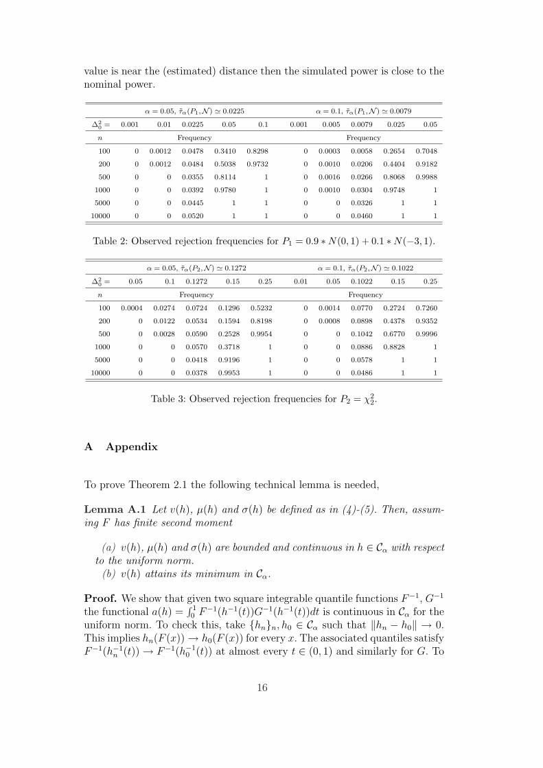
value is near the (estimated) distance then the simulated power is close to thenominal power.

α = 0.05, τα(P1,N ) ' 0.0225 α = 0.1, τα(P1,N ) ' 0.0079

∆20 = 0.001 0.01 0.0225 0.05 0.1 0.001 0.005 0.0079 0.025 0.05

n Frequency Frequency

100 0 0.0012 0.0478 0.3410 0.8298 0 0.0003 0.0058 0.2654 0.7048

200 0 0.0012 0.0484 0.5038 0.9732 0 0.0010 0.0206 0.4404 0.9182

500 0 0 0.0355 0.8114 1 0 0.0016 0.0266 0.8068 0.9988

1000 0 0 0.0392 0.9780 1 0 0.0010 0.0304 0.9748 1

5000 0 0 0.0445 1 1 0 0 0.0326 1 1

10000 0 0 0.0520 1 1 0 0 0.0460 1 1

Table 2: Observed rejection frequencies for P1 = 0.9 ∗N(0, 1) + 0.1 ∗N(−3, 1).

α = 0.05, τα(P2,N ) ' 0.1272 α = 0.1, τα(P2,N ) ' 0.1022

∆20 = 0.05 0.1 0.1272 0.15 0.25 0.01 0.05 0.1022 0.15 0.25

n Frequency Frequency

100 0.0004 0.0274 0.0724 0.1296 0.5232 0 0.0014 0.0770 0.2724 0.7260

200 0 0.0122 0.0534 0.1594 0.8198 0 0.0008 0.0898 0.4378 0.9352

500 0 0.0028 0.0590 0.2528 0.9954 0 0 0.1042 0.6770 0.9996

1000 0 0 0.0570 0.3718 1 0 0 0.0886 0.8828 1

5000 0 0 0.0418 0.9196 1 0 0 0.0578 1 1

10000 0 0 0.0378 0.9953 1 0 0 0.0486 1 1

Table 3: Observed rejection frequencies for P2 = χ22.

A Appendix

To prove Theorem 2.1 the following technical lemma is needed,

Lemma A.1 Let v(h), µ(h) and σ(h) be defined as in (4)-(5). Then, assum-ing F has finite second moment

(a) v(h), µ(h) and σ(h) are bounded and continuous in h ∈ Cα with respectto the uniform norm.(b) v(h) attains its minimum in Cα.

Proof. We show that given two square integrable quantile functions F−1, G−1

the functional a(h) =∫ 10 F−1(h−1(t))G−1(h−1(t))dt is continuous in Cα for the

uniform norm. To check this, take {hn}n, h0 ∈ Cα such that ‖hn − h0‖ → 0.This implies hn(F (x)) → h0(F (x)) for every x. The associated quantiles satisfyF−1(h−1

n (t)) → F−1(h−10 (t)) at almost every t ∈ (0, 1) and similarly for G. To

16

conclude that a(hn) → a(h0) it suffices to show that F−1 ◦ h−1G−1 ◦ h−1 isuniformly integrable. But this follows from the fact that

suph∈Cα

∫ 1

0|F−1(h−1(t))G−1(h−1(t))|I(|F−1(h−1(t))G−1(h−1(t))| > K)dt

= suph∈Cα

∫ 1

0|F−1(y)G−1(y)|I(|F−1(y)G−1(y)| > K)h′(y)dy

≤ 1

1− α

∫ 1

0|F−1(y)G−1(y)|I(|F−1(y)G−1(y)| > K)dy → 0

as K → ∞. This proves continuity of Var(F−1 ◦ h−1), Var(Φ−1 ◦ h−1) andCov(F−1 ◦ h−1, Φ−1 ◦ h−1). Since Cα is compact for the uniform topology (seeAlvarez-Esteban et al. (2008a)) we have that Var(Φ−1 ◦ h−1) attains its min-imum value: minh∈Cα Var(Φ−1 ◦ h−1) = Var(Φ−1 ◦ h−1

opt). But this shows thatVar(Φ−1◦h−1) is bounded away from 0 in Cα (a distribution with a density can-not have zero variance). This implies that v(h), µ(h) and σ(h) are continuous.All the remaining claims follow from compactness of Cα.

To complete the proof of Theorem 2.1 we note that, similarly as in (4), wecan define

vn(h) := minQ∈N

W22 ((Pn)h, Qh) = Var(F−1

n ◦ h−1)− Cov2(F−1n ◦ h−1, Φ−1 ◦ h−1)

Var(Φ−1 ◦ h−1)

and then we have

√n(Tn,α − τα(P,N )) =

√n

(minh∈Cα

vn(h)− minh∈Cα

v(h))

. (A.1)

We will obtain the conclusion in Theorem 2.1 from the study of the pro-cess Mn(h) =

√n(vn(h) − v(h)), h ∈ Cα. We note that, writing ρn(t) =√

n(F−1n (t) − F−1(t))f(F−1(t)) (the quantile process) we can see after some

routine computations that

Mn(h) = 2∫ 1

0

ρn(t)

f(F−1(t))(F−1(t)− µ(h)− σ(h)Φ−1(t))h′(t)dt (A.2)

+1√n

∫ 1

0

ρ2n(t)

f 2(F−1(t))h′(t)dt−

(∫ 1

0

ρn(t)

f(F−1(t))h′(t)dt

)2

+1

σ2Φ(h)

(∫ 1

0

ρn(t)

f(F−1(t))Φ−1(t)h′(t)dt−

(∫ 1

0

ρn(t)

f(F−1(t))h′(t)dt

)µΦ(h)

)2 ,

17

where µΦ(h) =∫ 10 Φ−1 ◦h−1 and σ2

Φ(h) =∫ 10 (Φ−1 ◦h−1)2−µ2

Φ(h). We considera Brownian bridge, {B(t)}t∈(0,1), and define

M(h) := 2∫ 1

0

B(t)

f(F−1(t))(F−1(t)− µ(h)− σ(h)Φ−1(t))h′(t)dt.

Observe that {M(h)}h∈Cα is a centered Gaussian process with covariance func-tion

K(h1, h2) = 4∫ 1

0l1(t)l2(t)dt− 4

∫ 1

0l1(t)dt

∫ 1

0l2(t)dt,

where

li(t) =∫ F−1(t)

F−1(1/2)(x− µ(hi)− σ(hi)Φ

−1(F (x)))h′i(F (x))dx, i = 1, 2.

This follows from noting that, integrating by parts, M(hi) = −2∫ 10 li(t)dB(t).

The key result in this Appendix is the following.

Proposition A.2 Under the assumptions of Theorem 2.1 M is a tight Borelmeasurable map and Mn converges weakly to M in `∞(Cα).

Proof. We assume w.l.o.g. that there exist Brownian bridges Bn satisfying

n1/2−ν sup1n≤t≤1− 1

n

|ρn(t)−Bn(t)|(t(1− t))ν

=

OP (log n), if ν = 0

OP (1), if 0 < ν ≤ 1/2(A.3)

(this is guaranteed by (10), see Theorem 6.2.1 in Csorgo and Horvath (1993)).Now we define.

Nn(h) := 2∫ 1

0

Bn(t)

f(F−1(t))(F−1(t)− µ(h)− σ(h)Φ−1(t))h′(t)dt

We claim that ‖Mn − Nn‖Cα := suph∈Cα|Mn(h) − Nn(h)| → 0 in probability.

To check this we write

suph∈Cα

1√n

∫ 1

0

ρ2n(t)

f 2(F−1(t))h′(t)dt ≤ 1

1− α

1√n

∫ 1

0

ρ2n(t)

f 2(F−1(t))dt →Pr. 0, (A.4)

where the last convergence follows from the moment assumption on F (seeLemma A.1 and the proof of Theorem 2 in Alvarez-Esteban et al. (2008a)).Thus we can (uniformly) neglect the second term in expression (A.2) for Mn.A similar bound and the fact that minh∈Cα σ2

Φ(h) > 0 is enough to control thethird term. Hence, it suffices to show that

suph∈Cα

∫ 1

0

|ρn(t)−Bn(t)|f(F−1(t))

|F−1(t)− µ(h)− σ(h)Φ−1(t))|dt →Pr. 0.

18

This can be done using boundedness of µ(h), σ(h) and arguing as in the proofof Theorem 2 in Alvarez-Esteban et al. (2008a).

Since Nn and M are equally distributed, to complete the proof we have toshow that M is tight or, equivalently, that it is uniformly equicontinuous inprobability for some metric d for which Cα is totally bounded (see Theorems1.5.7 and 1.10.2 in van der Vaart and Wellner (1996)). We take d to be theuniform norm in Cα (then Cα is compact) and note that we have to prove thatfor any given ε, η > 0 there exists δ > 0 such that

P

(sup

‖h1−h2‖∞<δ|M(h1)−M(h2)| > ε

)< η.

From Markov’s inequality and compactness we see that it is enough to showthat the map h 7→ E|M(h)| is ‖ · ‖∞-continuous and this can done arguing asin the proof of Lemma A.1

Proposition A.2 has the following simple, but important consequences

Corollary A.3 Under the assumptions of Theorem 2.1

suph∈Cα

|vn(h)− v(h)| →Pr. 0.

As a consequence ‖hn − h0‖ →Pr. 0.

Proof. Proposition A.2 implies that√

n suph |vn(h) − v(h)| = suph |Mn(h)|converges weakly to suph∈Cα

|M(h)|. This proves the first claim. To completethe proof, observe that compactness allows to extract convergent subsequencesfrom hn: hn′ → ha and also to ensure that vn′(h) → v(h) uniformly. Sincevn′(hn′) ≤ v′n(h) we see, taking limits, that ha must be a minimizer of v.Hence, by the uniqueness asumption (6) we have ha = h0. This completes theproof.

Proof of Theorem 2.1. From (A.1) we see that√

n(Tn,α − τα(P,N )) =√n(vn(hn) − v(h0)) = Mn(h0) −

√n(vn(h0) − vn(hn)). Optimality implies

v(hn)− v(h0) ≥ 0 and vn(h0)− vn(hn) ≥ 0. On the other hand

√n(v(hn)− v(h0)) +

√n(vn(h0)− vn(hn)) = Mn(h0)−Mn(hn) →Pr. 0,

the last convergence implied by Proposition A.2, Corollary A.3 and equicon-tinuity. From this we get

√n(vn(h0) − vn(hn)) →Pr. 0, hence

√n(Tn,α −

τα(P,N )) converges in distribution to M(h0), proving the first part of Theo-rem 2.1. The second claim can be proved with the aid of Corollary A.3 andcontinuity arguments as in Lemma A.1. We skip details.

19

References

Alvarez-Esteban, P.C.; del Barrio, E.; Cuesta-Albertos, J.A. andMatran, C. (2008a). Trimmed comparison of distributions. J. Amer.Statist. Assoc., 103, 697-704.

Alvarez-Esteban, P.C.; del Barrio, E.; Cuesta-Albertos, J.A. andMatran, C. (2008b). Similarity of probability measures through trimming.Submitted.

del Barrio, E.; Cuesta-Albertos, J.A.; Matran, C. and RodrıguezRodrıguez, J. (1999). Tests of goodness of fit based on the L2-Wassersteindistance. Ann. Statist. 27: 1230-1239.

del Barrio, E.; Cuesta-Albertos, J.A. and Matran, C. (2000).Contributions of empirical and quantile processes to the asymptotic theoryof goodness-of-fit tests. Test, 9: 1-96.

del Barrio, E.; Gine, E. and Utzet, F. (2005). Asymptotics for L2 func-tionals of the empirical quantile process, with applications to tests of fitbased on weighted Wasserstein distances. Bernoulli 11, 131–189.

Bickel, P. J., and Freedman, D. A. (1981). Some Asymptotic Theory forthe Bootstrap, Ann. Statist., 9, 1196–1217.

Csorgo, M. and L. Horvath (1993). Weighted Approximations in Prob-ability and Statistics. Wiley. New York.

Cuesta Albertos, J.A.; Gordaliza, A. and Matran, C. (1997).Trimmed k-means: An attempt to robustify quantizers. Ann. Statist., 25,553–576.

Garcıa Escudero, L.A.; Gordaliza, A. and Matran, C. (2003). Trim-ming tools in exploratory data analysis. J. Comput. and Graph. Stat. 12,434–449.

Garcıa Escudero, L.A.; Gordaliza, A.; Matran, C. and Mayo-Iscar, A. (2008). A general trimming approach to robust cluster analysis.Ann. Statist. 36, 1324–1345.

Gordaliza, A. (1991). Best approximations to random variables based ontrimming procedures. J. Approx. Theory, 64, 162–180.

Hand, D.J.; Daly, F.; Lunn, A.D.; McConway. K.J. and Ostrowski,E. A Handbook of Small Data Sets. Chapman & Hall. London.

Maronna, R. (2005). Principal components and orthogonal regression basedon robust scales. Technometrics , 47, 264–273.

Munk, A. and C. Czado (1998). Nonparametric validation of similardistributions and assessment of goodness of fit. J. Roy. Statist. Soc. Ser.B 60, 223–241.

R Development Core Team (2008). R: A Language and Environ-ment for Statistical Computing. R Foundation for Statistical Computing.http://www.R-project.org. Viena, Austria.

Rousseeuw, P. (1985). Multivariate estimation with high breakdown point.In W. Grossmann, G. Pflug, I. Vincze, y W. Werz (Eds.), in MathematicalStatistics and Applications, Volume B. Reidel, Dordrecht.

van der Vaart, A.W. and Wellner, J.A. (1996). Weak Convergenceand Empirical Processes. Springer. New York.

20