Wind Energ. Sci., 3, 845–868, 2018 https://doi.org/10.5194/wes-3-845-2018 © Author(s) 2018. This work is distributed under the Creative Commons Attribution 4.0 License. Assessing variability of wind speed: comparison and validation of 27 methodologies Joseph C. Y. Lee 1,2 , M. Jason Fields 1 , and Julie K. Lundquist 1,2 1 National Renewable Energy Laboratory, Golden, CO 80401, USA 2 Department of Atmospheric and Oceanic Sciences, University of Colorado Boulder, Boulder, CO 80309, USA Correspondence: Joseph C. Y. Lee ([email protected]) Received: 12 June 2018 – Discussion started: 30 July 2018 Revised: 4 October 2018 – Accepted: 16 October 2018 – Published: 5 November 2018 Abstract. Because wind resources vary from year to year, the intermonthly and interannual variability (IAV) of wind speed is a key component of the overall uncertainty in the wind resource assessment process, thereby creating challenges for wind farm operators and owners. We present a critical assessment of several common ap- proaches for calculating variability by applying each of the methods to the same 37-year monthly wind-speed and energy-production time series to highlight the differences between these methods. We then assess the accuracy of the variability calculations by correlating the wind-speed variability estimates to the variabilities of actual wind farm energy production. We recommend the robust coefficient of variation (RCoV) for systematically estimating variability, and we underscore its advantages as well as the importance of using a statistically robust and resistant method. Using normalized spread metrics, including RCoV, high variability of monthly mean wind speeds at a location effectively denotes strong fluctuations of monthly total energy generation, and vice versa. Meanwhile, the wind-speed IAVs computed with annual-mean data fail to adequately represent energy-production IAVs of wind farms. Finally, we find that estimates of energy-generation variability require 10 ± 3 years of monthly mean wind-speed records to achieve a 90 % statistical confidence. This paper also provides guidance on the spatial distribution of wind-speed RCoV. 1 Introduction The P50, a widely used parameter in the wind-energy indus- try, is an estimate of the threshold of annual energy produc- tion of a wind farm that the facility is expected to exceed 50 % of the time (Clifton et al., 2016). The P50 is usually estimated to apply over the lifetime of a wind farm, typi- cally 20 years. To estimate P50 in the wind resource assess- ment process, a single percentage value is usually assigned to represent the uncertainty for the desired time period at a wind site (Brower, 2012). The interannual variability (IAV) of wind resources, along with site measurements and wind- power-plant performance, is an important component of the overall uncertainty in power production (Clifton et al., 2016; Klink, 2002; Lackner et al., 2008; Pryor et al., 2006). The IAV is also incorporated in the measure–correlate–predict process (Lackner et al., 2008), which usually considers wind measurements spanning less than 2 years. Analysts and researchers use numerous metrics to quantify wind-speed variability, and the most common method is stan- dard deviation (σ ). For instance, the variability in historical or future wind resources is often represented as the σ from the annual-mean wind speed of a certain location (Brower, 2012). As wind turbine power generation is a function of wind speed, the variability of wind resources has important implications for the resultant long-term energy production. Financially, when the wind resource is projected to fluctuate more from year to year (Hdidouan and Staffell, 2017), the levelized cost of wind energy increases as well. Because the profitability of wind farms depends on wind variability, past research has explored the implications of in- terannual and long-term variability in wind energy. Pryor et al. (2009) analyze trends of annual wind speed and IAV, without explicitly quantifying IAV values. Archer and Jacob- son (2013) evaluate the seasonal variability of wind-energy Published by Copernicus Publications on behalf of the European Academy of Wind Energy e.V.

Welcome message from author
This document is posted to help you gain knowledge. Please leave a comment to let me know what you think about it! Share it to your friends and learn new things together.
Transcript

Wind Energ. Sci., 3, 845–868, 2018https://doi.org/10.5194/wes-3-845-2018© Author(s) 2018. This work is distributed underthe Creative Commons Attribution 4.0 License.
Assessing variability of wind speed: comparison andvalidation of 27 methodologies
Joseph C. Y. Lee1,2, M. Jason Fields1, and Julie K. Lundquist1,2
1National Renewable Energy Laboratory, Golden, CO 80401, USA2Department of Atmospheric and Oceanic Sciences, University of Colorado Boulder, Boulder, CO 80309, USA
Correspondence: Joseph C. Y. Lee ([email protected])
Received: 12 June 2018 – Discussion started: 30 July 2018Revised: 4 October 2018 – Accepted: 16 October 2018 – Published: 5 November 2018
Abstract. Because wind resources vary from year to year, the intermonthly and interannual variability (IAV)of wind speed is a key component of the overall uncertainty in the wind resource assessment process, therebycreating challenges for wind farm operators and owners. We present a critical assessment of several common ap-proaches for calculating variability by applying each of the methods to the same 37-year monthly wind-speed andenergy-production time series to highlight the differences between these methods. We then assess the accuracy ofthe variability calculations by correlating the wind-speed variability estimates to the variabilities of actual windfarm energy production. We recommend the robust coefficient of variation (RCoV) for systematically estimatingvariability, and we underscore its advantages as well as the importance of using a statistically robust and resistantmethod. Using normalized spread metrics, including RCoV, high variability of monthly mean wind speeds at alocation effectively denotes strong fluctuations of monthly total energy generation, and vice versa. Meanwhile,the wind-speed IAVs computed with annual-mean data fail to adequately represent energy-production IAVs ofwind farms. Finally, we find that estimates of energy-generation variability require 10± 3 years of monthlymean wind-speed records to achieve a 90 % statistical confidence. This paper also provides guidance on thespatial distribution of wind-speed RCoV.
1 Introduction
The P50, a widely used parameter in the wind-energy indus-try, is an estimate of the threshold of annual energy produc-tion of a wind farm that the facility is expected to exceed50 % of the time (Clifton et al., 2016). The P50 is usuallyestimated to apply over the lifetime of a wind farm, typi-cally 20 years. To estimate P50 in the wind resource assess-ment process, a single percentage value is usually assignedto represent the uncertainty for the desired time period at awind site (Brower, 2012). The interannual variability (IAV)of wind resources, along with site measurements and wind-power-plant performance, is an important component of theoverall uncertainty in power production (Clifton et al., 2016;Klink, 2002; Lackner et al., 2008; Pryor et al., 2006). TheIAV is also incorporated in the measure–correlate–predictprocess (Lackner et al., 2008), which usually considers windmeasurements spanning less than 2 years.
Analysts and researchers use numerous metrics to quantifywind-speed variability, and the most common method is stan-dard deviation (σ ). For instance, the variability in historicalor future wind resources is often represented as the σ fromthe annual-mean wind speed of a certain location (Brower,2012). As wind turbine power generation is a function ofwind speed, the variability of wind resources has importantimplications for the resultant long-term energy production.Financially, when the wind resource is projected to fluctuatemore from year to year (Hdidouan and Staffell, 2017), thelevelized cost of wind energy increases as well.
Because the profitability of wind farms depends on windvariability, past research has explored the implications of in-terannual and long-term variability in wind energy. Pryoret al. (2009) analyze trends of annual wind speed and IAV,without explicitly quantifying IAV values. Archer and Jacob-son (2013) evaluate the seasonal variability of wind-energy
Published by Copernicus Publications on behalf of the European Academy of Wind Energy e.V.

846 J. C. Y. Lee et al.: Assessing variability of wind speed
capacity factor. Lee et al. (2018) assess the spatial discrep-ancies between wind-speed variabilities of different tempo-ral scales, from hourly mean to annual-mean data. Bett etal. (2013) use σ and Weibull parameters to assess the windvariability in Europe. Extreme event analysis also offers an-other perspective to assess variability. For example, Cannonet al. (2015) examine extreme wind-energy generation eventsvia reanalysis data and discuss the associated seasonal andIAV qualitatively. Leahy and McKeogh (2013) also quantifythe return periods of multiweek wind droughts.
To quantify variability, the normalized σ or the coefficientof variation (CoV), the σ divided by the mean of a timeseries, is a commonly used tool. Justus et al. (1979) cal-culate and compare the CoVs of monthly and annual windspeeds at different sites across the United States. Baker etal. (1990) quantify interannual and interseasonal variationsof both wind speed and energy production at three loca-tions in the Pacific Northwest. They find the annual CoVsranged from 4 % to 10 %, matching the conclusions fromJustus et al. (1979). Recently, Li et al. (2010) calculate hub-height wind-speed variance and σ over 30 years to spatiallyevaluate seasonal and IAV in the Great Lakes region. Bo-dini et al. (2016) estimate the IAV of wind resources witha modified version of CoV, using observed meteorologicaldata in Canada. As the sample period increases, the IAVs ofmost sites gradually increase, averaging 5 % to 6 % amongthe chosen sites (Bodini et al., 2016). Krakauer and Co-han (2017) correlate the CoVs of monthly mean wind speedswith different climate oscillation indices and find the globalmean CoV at 8 %. In addition to characterizing wind speed,the metric is also used to evaluate the benefits of grid inte-gration. For example, Rose and Apt (2015) conclude that theinterannual CoV of aggregate wind-energy generation in thecentral United States is 3± 0.1 %, much smaller than thatof individual wind plants, which varies between 5.4 % and12 %, ±4.2 %.
Aside from CoV, other metrics representing the spreadof data have also been chosen to estimate variability in theliterature. For example, the robust coefficient of variation(RCoV) normalizes the median absolute deviation (MAD)with the median. Gunturu and Schlosser (2012) quantify thespatial RCoV of wind-power density in the United Statesand demonstrate that the regions east of the Rockies, es-pecially the Plains, generally have weaker variability andhigher availability of wind resources. The seasonality index,originally used in Walsh and Lawler (1981) for precipitationpurposes, is another measure to express variability. The sea-sonality index is defined as the sum of the absolute deviationsof monthly averages from the annual mean, normalized withthe annual mean. Chen et al. (2013) use the seasonality in-dex to assess the interannual trend and the variability of windspeed in China, and they relate wind-speed IAVs to climateoscillations.
Alternative variability metrics emphasize the long-termtrends via contrasting wind speeds of different periods. The
“wind index”, used in Pryor et al. (2006) and Pryor andBarthelmie (2010), is a ratio of wind speeds of a referenceperiod and an analysis period. An entirely different wind in-dex evaluated in Watson et al. (2015) is a ratio of spatiallyaveraged wind speeds during two different periods.
Despite the importance of long-term variability, the wind-energy industry lacks a systematic method to quantify thisuncertainty. As various metrics to assess variability exist, acomprehensive comparison of measures is necessary. There-fore, the goal of this study is to evaluate various methodsof estimating intermonthly and IAV in a reliable way us-ing a long-term, consistent database. Specifically, our objec-tive is to determine an optimal metric or metrics for relat-ing wind-speed variability to energy-production variability.We describe the wind-speed and energy-generation data, themethodology, and the chosen variability metrics in Sect. 2.We evaluate different variability measures via two case stud-ies in Sect. 3. We also contrast the results computed frommonthly mean and annual-mean data, and we illustrate thespatial distribution of wind-speed variability in Sect. 3. Wethen recommend the best practice in using the ideal methodin Sect. 4. We focus on the applicability of imposing suchmetrics to quantify the variabilities of wind speeds and wind-energy production.
2 Data and methodology
2.1 Wind and energy data
In this study, we use a 37-year time series of monthly meanwind speed and monthly total wind-energy production inthe contiguous United States (CONUS). For wind speed, weuse hourly horizontal wind components in the National At-mospheric and Space Administration’s Modern-Era Retro-spective Analysis for Research and Applications, Version 2(MERRA-2), reanalysis data set (Gelaro et al., 2017; GMAO,2015) from 1980 to 2016. We use these components to de-rive the monthly mean wind speed at 80 m above the surface,which represents hub height in this study, via the power law(Eq. 1) and the hypsometric equation (Eq. 2):
u (z2)u (z1)
=
(z2
z1
)α, (1)
z2− z1 = RdT ln(p2
p1
). (2)
In Eq. (1), u (z1) and u (z2) are the horizontal wind speeds, atheights z1 and z2, in which wind speeds are the square rootof the sum of squared horizontal wind components, and α isthe shear exponent. In Eq. (2), Rd is the dry air gas constant,T is the average temperature between levels z1 and z2, andp1 and p2 are the atmospheric pressures at z1 and z2. In mostgrid cells, we use the MERRA-2 meteorological output at 10and 50 m above the surface to calculate α, so as to extrapolatethe wind speed at 80 m. In mountainous regions, the heights
Wind Energ. Sci., 3, 845–868, 2018 www.wind-energ-sci.net/3/845/2018/
J. C. Y. Lee et al.: Assessing variability of wind speed 847
at 850 or 500 hPa may be closer to 80 than 10 m above thesurface; in that case, we use data at the next available levelof 850 or 500 hPa to derive the heights of that level and thusto extrapolate the wind speed at 80 m.
The horizontal resolution of the MERRA-2 is 0.5◦ in lat-itude (about 56 km) and 0.625◦ in longitude (about 53 km).The MERRA-2 reanalysis interpolates the data and the meta-data at the exact output latitude and longitude; hence thewind speed, air density, and elevation refer to the grid pointswith the particular sets of latitude and longitude (Bosilovichet al., 2016). Thus, the longest distance between a wind farmand the closest MERRA-2 grid-cell center is about 39 km.
For energy-production data, we use the net monthly energyproduction of wind farms in megawatt hours (MWh) from theUS Energy Information Administration (EIA) between 2003and 2016. Each of the wind farms has a unique EIA identifi-cation number. After we leave out about 300 wind sites withincomplete or substantially zero production data, a total of607 wind farms in the CONUS are selected for this analy-sis. For simplicity, the CONUS in this analysis is defined asthe area bounded by 127◦W, 65◦W, 24◦ N, and 50◦ N, andgeographically includes the 48 states in CONUS and Wash-ington, D.C. (Fig. 1).
2.2 Methodology
2.2.1 Linear regression and data post-processing
We focus on the direct relationship between wind speed andenergy production to investigate approaches for calculatinglong-term variability. Therefore, we must minimize the in-fluence from other determinants of energy production, suchas curtailment and maintenance. First, we eliminate data withzero values for monthly energy production, which is typicalin the first months of a new wind farm. Next, we linearlyregress the monthly total energy production on the monthlymean MERRA-2 80 m wind speed at the closest grid pointto each wind farm from 2003 to 2016. In other words, eachwind site is assigned its own regression equation. We then re-move any production data below the 90 % prediction intervalto exclude underproduction for reasons other than low windspeeds, and omit the data above the 99 % prediction interval,or potentially erroneous overproduction. Prediction intervalsare calculated via the t values and the standard error of pre-diction (Montgomery and Runger, 2014). In other words, wedefine the outliers of energy production using the thresholdof 1.64 times below the standard error and 2.58 times abovethe standard error of the site-specific regression. We also ap-ply a third-order polynomial fit (Archer and Jacobson, 2013),and it leads to very similar results to the linear model. Hence,we focus on presenting the results from the linear fit in thisstudy.
After regressing the outlier-free energy data on windspeed, we then filter the wind farms based on the coefficientof determination (R2), which indicates the confidence of the
Figure 1. Wind farm locations in the CONUS: nonfiltered 607 sitesin dark red, R2-filtered 349 sites in orange, and r-filtered 195 sitesin yellow. The yellow square represents the Oregon site and the yel-low star indicates the Texas site (Table 2). The grey box illustratesthe boundary of the CONUS used in this study.
linear regression. We select the R2 threshold of 0.75: 349 ofthe original 607 wind farms pass this filter. Through this fil-ter, we ensure that wind speed is the primary driver of energyproduction in the wind farms with high R2 values. Lunaceket al. (2018) also use a similar R2-filtering method with athreshold of 0.7. Considering some farms lack years of com-plete generation data, we extend the monthly energy produc-tion to 37 years using the same site-specific linear modelswith the monthly MERRA-2 wind speed. In other words, wecompute any missing energy-production data from 1980 to2016 based on the linear fit from the years that do exist in thedata set. Herein, we refer to this long-term extension of dataas the predicted energy production. Of the 349 wind farms,7.5 years is the median of the energy data that are derived viathe linear fit, given the available EIA records between 2003and 2016.
We then further apply a second filter using the Pearson’scorrelation coefficient (r) between the predicted and actualmonthly energy production, and we only choose the 195wind farms with r larger than 0.8. As a result, of the r-filteredwind sites, we ensure wind speed is the primary driver ofwind-power production, and we confirm the energy predic-tions match well with those observed.
The nonfiltered, R2-filtered, and r-filtered wind farms car-pet most of the popular wind farm regions across the CONUS(Fig. 1), even with the high r threshold of 0.8. Thus, ther-filtered samples provide a sufficient representation of thewind farms across the United States. To illustrate our anal-ysis with examples, we select one site in Oregon (OR) andanother site in Texas (TX) that demonstrate distinct wind-speed distributions. We choose the two sites to contrast theresults of different variability metrics throughout the paper;both sites pass the r filter (Fig. 1).
Recognizing that the horizontal resolution of the MERRA-2 data could be perceived as undermining the linear regres-sions, we explore any possible role of the distance between
www.wind-energ-sci.net/3/845/2018/ Wind Energ. Sci., 3, 845–868, 2018
848 J. C. Y. Lee et al.: Assessing variability of wind speed
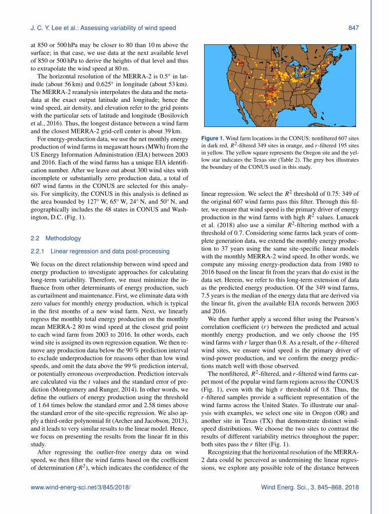
the closest MERRA-2 grid point and the actual wind farm,but we find no statistical relationship. In particular, horizon-tal and vertical discrepancies between the model and the ob-servations do not affect the resultant R2 in the linear regres-sions. More than half of the 607 wind farms pass the R2 fil-ter, and more than half of those pass the r filter (Fig. 2a).Additionally, the correlation between R2 and the horizontaldistance between the closest MERRA-2 grid point and theactual wind farm is close to zero (Fig. 2b); the correlationbetween R2 and the vertical difference between the modeledgrid point and the actual wind site is also weak (Fig. 2c).In other words, the horizontal and vertical distances betweenthe MERRA-2 grid points and the wind farms have no appar-ent impact on the representativeness of the wind farms in thelinear regression.
Additionally, we analyze the uncertainty of the linear-regression method. We first test the influence of the errorterm in the regression, to account for the uncertainty asso-ciated with the input data. After a wind farm passes the R2
threshold of 0.75, we add a random value within 1 standarderror to the predicted energy production of each month. Thisrandom error term introduces uncertainty to the regressionprocess but does not affect the R2 of the site-specific regres-sion. Furthermore, we also test the sensitivity of the R2 andr thresholds by analyzing the results after modifying thoselimits. Specifically, we loosen the R2 and r thresholds to 0.6and 0.7, and we tighten the R2 and r thresholds to 0.85 and0.9. Loosening these thresholds increases the sample sizes ofthe wind farms that pass the filters and tightening the thresh-olds results in the opposite.
We test other factors that could undermine these regres-sions. We considered the hub-height air density extrapolatedfrom MERRA-2 as another regressor in the regressions, butair density is a statistically insignificant predictor and thus isnot discussed in the rest of this study. When we replace theprediction interval with the confidence interval, the samplesizes increase from 349 and 195 sites to 555 and 209 windfarms. However, at least 7 years of energy data are derivedfrom the regression for 99 % of the samples, because confi-dence intervals are smaller than prediction intervals by def-inition. We also considered removing the long-term meansand the impacts of annual cycles, yet the sample sizes de-crease to 121 and 69 locations, and the regression fills atleast some of the energy data for more than 99 % of thesites. Finally, to ensure these results were not specific to theMERRA-2 data set, we perform the same analysis on theERA-Interim reanalysis data set (Dee et al., 2011). The re-sults of the key variability parameters such as σ , CoV, andRCoV resemble the findings using MERRA-2; hence we fo-cus on the MERRA-2 findings in this study.
Our analysis, although comprehensive, is constrained bythe quality of our data. On the one hand, reanalysis datasets have errors and biases in wind-speed predictions fromcomplexities in elevation and surface roughness (Rose andApt, 2016). Reanalysis data sets also demonstrate long-term
trends of surface wind speeds (Torralba et al., 2017). TheMERRA-2 data set can also depict different meteorologi-cal environments than those at the wind farm locations, es-pecially in complex terrain. The MERRA-2 data of coarsetemporal and spatial resolutions may also represent a lowerintermonthly or IAV than the wind sites actually experi-ence. Thus, regressing actual energy production on reanaly-sis wind speed adds uncertainty to our analysis. On the otherhand, constrained by the monthly total energy-productiondata from the EIA, our analysis ignores the signals finer thanmonthly cycles. The quality of the EIA data also varies acrosswind sites; therefore the filtering process via linear regressionis necessary.
2.2.2 Variability metrics relating wind speeds andenergy production
To evaluate the variabilities of both the wind speeds and thepredicted energy generation from the filtered wind farms, weinvestigate a total of 27 combinations and variations of ex-isting methods describing the spread of data. We categorizedifferent variability metrics according to statistical robust-ness (insensitivity to assumptions about the data; for exam-ple, Gaussian distribution) and statistical resistance (insensi-tivity to outliers) (Wilks, 2011). Of the 27 variability meth-ods tested, we select four representative measures to performa comparison and discuss in detail, according to their robust-ness, resistance, and the nature of normalization by an aver-age metric:
1. RCoV, defined as the MAD divided by the median(Gunturu and Schlosser, 2012; Watson, 2014), is aspread metric divided by an average metric and is bothstatistically robust and resistant.
2. Range (maximum minus minimum) divided by trimean(weighted average among quartiles) is a spread metricnormalized by an average metric, and the numerator isnot resistant.
3. CoV (Baker et al., 1990; Bodini et al., 2016; Hdidouanand Staffell, 2017; Krakauer and Cohan, 2017; Rose andApt, 2015; Wan, 2004), defined as the σ divided by themean, is a spread metric normalized by an average met-ric, and neither the denominator nor the numerator arerobust or resistant.
4. σ is simply a spread metric that is not robust or resistant.
Among the four measures, only RCoV is completely statis-tically robust and resistant, and the first three methods areall normalized spread metrics. We further describe all thetested variability methods comprehensively in Table B1 inAppendix B. Each of these metrics is easy to implement viabasic Python packages such as NumPy and SciPy with nomore than a few lines of code. In addition, based on the ex-ponential scaling relationship between power and wind speed
Wind Energ. Sci., 3, 845–868, 2018 www.wind-energ-sci.net/3/845/2018/
J. C. Y. Lee et al.: Assessing variability of wind speed 849
0.0 0.2 0.4 0.6 0.8 1.0R2
0
10
20
30
40
50
Cou
nt
(a)607 sites349 sites: R2 threshold = 0.75195 sites: r threshold = 0.8
0 10 20 30 40Horizontal distance (km)
0.0
0.2
0.4
0.6
0.8
1.0
R2
r = -0.001
(b)
1000 0 1000Elevation difference (m)
0.0
0.2
0.4
0.6
0.8
1.0
R2
r = -0.197
(c)
Figure 2. (a) Histogram of R2 of all nonfiltered sites (dark red), R2-filtered sites (orange), and r-filtered sites (yellow); (b) scatterplot ofthe R2 and the horizontal distance between the closest MERRA-2 grid cell and the actual locations of the sites using the same color schemein (a); (c) scatterplot of the R2 and the elevation difference between the closest MERRA-2 grid cell and the actual locations of the wind sitesusing the same color scheme in (a). The r in (b) and (c) represents the Pearson’s r using all nonfiltered sites.
developed by Bandi and Apt (2016), we also analyze the re-sults from the exponential CoV and the exponential RCoV inthis paper (Table B1).
In addition to calculating variabilities with the spread mea-sures, we evaluate other diagnostics that describe distributioncharacteristics. These diagnostics include averaging metrics,such as the arithmetic mean (not resistant) and median (the50th percentile, which is resistant); symmetry metrics, suchas skewness (involving the third moment, not robust or resis-tant) and the Yule–Kendall Index (YKI, robust and resistant);a tailedness metric, namely kurtosis (involving the fourthmoment, not robust or resistant); the Weibull scale and shapeparameters (not robust); and the autocorrelation with a 1-yearlag to dissect the interannual cycles. We summarize the diag-nostics evaluated in this analysis in Table B2. Along with theregression results, results from the four representative vari-ability metrics and other distribution diagnostics demonstratedifferences between the two selected sites (Table 2).
Herein, we quantify the variabilities of the 37-year ex-tended time series of wind speed and energy production viadifferent methods, using a range of time frames: 1 year,2 years, and up to 37 years for each wind farm. A metricis considered useful when the resultant wind-speed variabil-ity correlates well with the resultant energy-production vari-ability across wind farms, even when random errors are im-
plemented and the thresholds R2 and r are changed. In thisanalysis, we compare results with three correlation metrics:Pearson’s r , Spearman’s rank correlation coefficient (rs), andKendall’s rank correlation coefficient (τ ) (Table 1).
To assess the applicable time frames of various variabilitymetrics, we evaluate the asymptote period of correlations foreach method. In most cases, the correlation coefficients ap-proach the 37-year value after a certain analysis time frame.Using RCoV as an example, the Pearson’s r’s of shorter anal-ysis periods (1-year, 2-year, etc.) gradually converge to the37-year value at 0.856 as the RCoV-calculation time frameexpands (Fig. 5a). Hence, for each metric, assuming the 37-year correlation coefficient represents the long-term corre-lation, we calculate the normalized differences between thecorrelation coefficients and the 37-year value in each timeframe, starting from 1 year. When the absolute mean of thenormalized differences drops below 0.05 in a particular year,we determine that year as the length of data required for re-liable results via that variability method. In other words, theasymptote year of a certain metric illustrates that the errorof the resultant correlation between wind-speed and energy-production variability via that data length is less than 5 %from the long-term value. For example, the asymptote periodof RCoV correlations is 3 years according to Pearson’s r (Ta-ble 3).
www.wind-energ-sci.net/3/845/2018/ Wind Energ. Sci., 3, 845–868, 2018
850 J. C. Y. Lee et al.: Assessing variability of wind speed
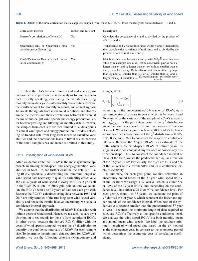
Table 1. Details of the three correlation metrics applied, adapted from Wilks (2011). All three metrics yield values between −1 and 1.
Correlation metrics Robust and resistant Description
Pearson’s correlation coefficient (r) No Calculate the covariance of x and y, divided by the product ofσ ’s of x and y.
Spearman’s rho, or Spearman’s rankcorrelation coefficient (rs)
Yes Transform x and y values into ranks within x and y themselves,then calculate the covariance of ranks in x and y, divided by theproduct of σ ’s of ranks in x and y.
Kendall’s tau, or Kendall’s rank corre-lation coefficient (τ )
Yes Match all data pairs between x and y, with n(n−1)2 matches pos-
sible with a sample size of n. Define concordant pair as both x1larger than x2 and y1 larger than y2, or both x1 smaller than x2and y1 smaller than y2. Define discordant pair as either x1 largerthan x2 and y1 smaller than y2, or x1 smaller than x2 and y1larger than y2. Calculate τ = 2(Concordant pairs−Discordant pairs)
n(n−1) .
To relate the IAVs between wind speed and energy pro-duction, we also perform the same analysis for annual-meandata. Strictly speaking, calculating the variabilities usingmonthly mean data yields intermonthly variabilities, becausethe results account for monthly, seasonal, and annual signals.To isolate the signals from interannual variations, we also ex-amine the metrics and their correlations between the annualmeans of hub-height wind speeds and energy production, af-ter linear regressing and filtering via monthly data. However,the samples from each site are then limited to 37 data pointsof annual wind speed and energy production. Besides, select-ing de-trended data from long-term means to calculate vari-abilities and their correlations leads to trivial results becauseof the small sample sizes and hence is omitted in this study.
2.2.3 Investigation of wind-speed RCoV
After we demonstrate that RCoV is the most systematic ap-proach in linking wind-speed and energy-generation vari-abilities in Sect. 3.2, we further examine the details of us-ing RCoV, specifically determining the minimum length ofwind-speed data necessary to quantify variability effectively.We use 37 years of wind speed in every MERRA-2 grid cellin the CONUS (a total of 5049 grid points), and we calcu-late the RCoVs with 1 to 37 years of data for each grid cell.Because the RCoVs calculated using data between 1980 and2016 are only samples of the true long-term wind-speed vari-ability and hence the results involve uncertainty, we select aconfidence interval approach.
We assume that the distribution of RCoV is Gaussian withinfinite years of wind speed. Hence, we use a chi-square (χ2)distribution to set bounds for the σ ’s from samples of RCoV.In other words, because the derived RCoVs differ with theyears of wind speeds sampled, we use the χ2 distribution toquantify the confidence intervals of RCoV for each samplesize. To determine the minimum data required for RCoV cal-culation, we use the following criterion (Montgomery and
Runger, 2014):
σ37 ≥
∣∣∣∣∣∣√√√√ (ni − 1)σ 2
i
χ2α/2,ni−1
∣∣∣∣∣∣ , (3)
where σ37 is the predetermined 37-year σ of RCoV; ni isthe sample size of n years in year i, which is between 1 and36 years; σ 2
i is the variance of the sample of RCoVs in year i;and χ2
α/2,ni−1 is the percentage point of the χ2 distributiongiven the confidence level of α and the degrees of freedomof ni − 1. We select a pair of α levels, 90 % and 95 %; hencewe use four percentage points of the χ2 distribution at 0.025,0.05, 0.95, and 0.975 to construct the respective confidenceintervals. Because the 37-year RCoV is an estimate of thetruth, which is the wind-speed RCoV of infinite years, itssingular value does not yield any variance or possess any dis-tribution shape. Thus, to construct the confidence interval ofthe σ of the truth, we set the predetermined σ37 as a fractionof the 37-year RCoV. Particularly, the σ37’s are 10 % and 5 %of the 37-year RCoV for the 90 % and 95 % confidence lev-els, respectively.
In summary, for each grid point, we first determine anuncertainty bound based on the 37-year wind-speed RCoVof the location: we assign a 37-year σ , which is either 5 %or 10 % of the 37-year RCoV and, depending on the confi-dence level, has either a 95 % or 90 % confidence level. Foreach year i, from 1 to 37 years, we calculate the pairs ofχ2-derived σ ’s of year i, which represent the lower and up-per bounds of the confidence interval. When both of the χ2-derived σ ’s become smaller than the predetermined 37-yearσ , year i becomes the minimum length of data required tocalculate RCoV effectively at the specific confidence level.We analyze the wind-speed RCoV via both monthly meanand annual-mean wind speeds. We label the resultant min-imum length of wind-speed data based on the χ2 methodas the convergence year, in contrast to the asymptote periodwhich determines the asymptote year of correlation coeffi-cients.
Wind Energ. Sci., 3, 845–868, 2018 www.wind-energ-sci.net/3/845/2018/
J. C. Y. Lee et al.: Assessing variability of wind speed 851
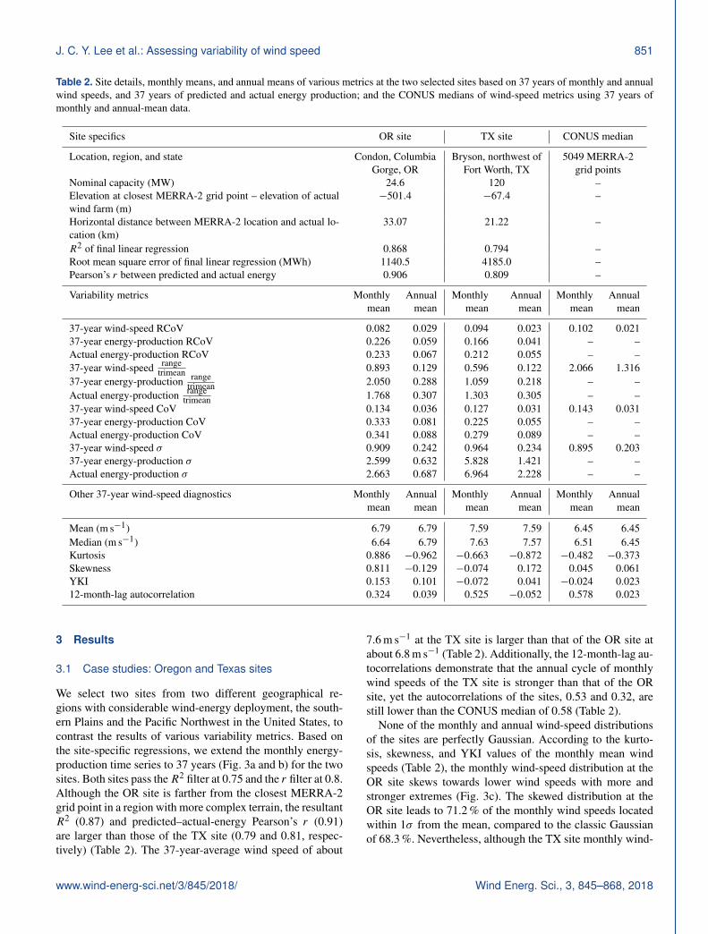
Table 2. Site details, monthly means, and annual means of various metrics at the two selected sites based on 37 years of monthly and annualwind speeds, and 37 years of predicted and actual energy production; and the CONUS medians of wind-speed metrics using 37 years ofmonthly and annual-mean data.
Site specifics OR site TX site CONUS median
Location, region, and state Condon, Columbia Bryson, northwest of 5049 MERRA-2Gorge, OR Fort Worth, TX grid points
Nominal capacity (MW) 24.6 120 –Elevation at closest MERRA-2 grid point – elevation of actualwind farm (m)
−501.4 −67.4 –
Horizontal distance between MERRA-2 location and actual lo-cation (km)
33.07 21.22 –
R2 of final linear regression 0.868 0.794 –Root mean square error of final linear regression (MWh) 1140.5 4185.0 –Pearson’s r between predicted and actual energy 0.906 0.809 –
Variability metrics Monthly Annual Monthly Annual Monthly Annualmean mean mean mean mean mean
37-year wind-speed RCoV 0.082 0.029 0.094 0.023 0.102 0.02137-year energy-production RCoV 0.226 0.059 0.166 0.041 – –Actual energy-production RCoV 0.233 0.067 0.212 0.055 – –37-year wind-speed range
trimean 0.893 0.129 0.596 0.122 2.066 1.31637-year energy-production range
trimean 2.050 0.288 1.059 0.218 – –Actual energy-production range
trimean 1.768 0.307 1.303 0.305 – –37-year wind-speed CoV 0.134 0.036 0.127 0.031 0.143 0.03137-year energy-production CoV 0.333 0.081 0.225 0.055 – –Actual energy-production CoV 0.341 0.088 0.279 0.089 – –37-year wind-speed σ 0.909 0.242 0.964 0.234 0.895 0.20337-year energy-production σ 2.599 0.632 5.828 1.421 – –Actual energy-production σ 2.663 0.687 6.964 2.228 – –
Other 37-year wind-speed diagnostics Monthly Annual Monthly Annual Monthly Annualmean mean mean mean mean mean
Mean (m s−1) 6.79 6.79 7.59 7.59 6.45 6.45Median (m s−1) 6.64 6.79 7.63 7.57 6.51 6.45Kurtosis 0.886 −0.962 −0.663 −0.872 −0.482 −0.373Skewness 0.811 −0.129 −0.074 0.172 0.045 0.061YKI 0.153 0.101 −0.072 0.041 −0.024 0.02312-month-lag autocorrelation 0.324 0.039 0.525 −0.052 0.578 0.023
3 Results
3.1 Case studies: Oregon and Texas sites
We select two sites from two different geographical re-gions with considerable wind-energy deployment, the south-ern Plains and the Pacific Northwest in the United States, tocontrast the results of various variability metrics. Based onthe site-specific regressions, we extend the monthly energy-production time series to 37 years (Fig. 3a and b) for the twosites. Both sites pass theR2 filter at 0.75 and the r filter at 0.8.Although the OR site is farther from the closest MERRA-2grid point in a region with more complex terrain, the resultantR2 (0.87) and predicted–actual-energy Pearson’s r (0.91)are larger than those of the TX site (0.79 and 0.81, respec-tively) (Table 2). The 37-year-average wind speed of about
7.6 m s−1 at the TX site is larger than that of the OR site atabout 6.8 m s−1 (Table 2). Additionally, the 12-month-lag au-tocorrelations demonstrate that the annual cycle of monthlywind speeds of the TX site is stronger than that of the ORsite, yet the autocorrelations of the sites, 0.53 and 0.32, arestill lower than the CONUS median of 0.58 (Table 2).
None of the monthly and annual wind-speed distributionsof the sites are perfectly Gaussian. According to the kurto-sis, skewness, and YKI values of the monthly mean windspeeds (Table 2), the monthly wind-speed distribution at theOR site skews towards lower wind speeds with more andstronger extremes (Fig. 3c). The skewed distribution at theOR site leads to 71.2 % of the monthly wind speeds locatedwithin 1σ from the mean, compared to the classic Gaussianof 68.3 %. Nevertheless, although the TX site monthly wind-
www.wind-energ-sci.net/3/845/2018/ Wind Energ. Sci., 3, 845–868, 2018
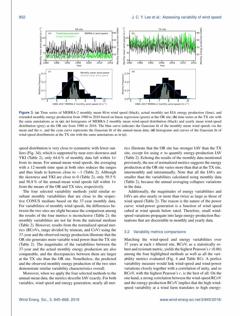
852 J. C. Y. Lee et al.: Assessing variability of wind speed
Figure 3. (a) Time series of MERRA-2 monthly mean 80 m wind speed (black), actual monthly net EIA energy production (lime), andextended monthly energy production from 1980 to 2016 based on linear regression (green) at the OR site; (b) time series at the TX site withthe same annotations as in (a); (c) histograms of MERRA-2 monthly mean wind-speed distribution (black) and yearly mean wind-speeddistribution (grey) at the OR site from 1980 to 2016. The blue curve indicates the Gaussian fit of the monthly mean wind speeds via themean and the σ , and the cyan curve represents the Gaussian fit of the annual-mean data; (d) histograms and curves of the Gaussian fit ofwind-speed distributions at the TX site with the same annotations as in (c).
speed distribution is very close to symmetric with fewer out-liers (Fig. 3d), which is supported by near-zero skewness andYKI (Table 2), only 64.6 % of monthly data fall within 1σfrom its mean. For annual-mean wind speeds, the averagingwith a 12-month time span at both sites reduces the rangesand thus leads to kurtosis close to −1 (Table 2). Althoughthe skewness and YKI are close to 0 (Table 2), only 59.5 %and 56.8 % of the annual-mean wind speeds fall within 1σfrom the means of the OR and TX sites, respectively.
The four selected variability methods yield similar re-sultant monthly variabilities that are close to the respec-tive CONUS medians based on the 37-year monthly data.For variabilities of monthly wind speeds, the differences be-tween the two sites are slight because the comparison amongthe results of the four metrics is inconclusive (Table 2): themonthly variabilities are not far from the national medians(Table 2). However, results from the normalized spread met-rics (RCoVs, range divided by trimean, and CoV) using the37-year and the observed energy production illustrate that theOR site generates more variable wind power than the TX site(Table 2). The magnitudes of the variabilities between the37-year and the actual monthly energy production are alsocomparable, and the discrepancies between them are largerat the TX site than the OR site. Nonetheless, the predictedand the observed monthly energy production of the two sitesdemonstrate similar variability characteristics overall.
Moreover, when we apply the four selected methods to theannual-mean data, the metrics describe IAV exactly. For bothvariables, wind speed and energy generation, nearly all met-
rics illustrate that the OR site has stronger IAV than the TXsite, except for using σ to quantify energy-production IAV(Table 2). Echoing the results of the monthly data mentionedpreviously, the use of normalized metrics suggests the energyproduction at the OR site varies more than that at the TX site,intermonthly and interannually. Note that all the IAVs aresmaller than the variabilities calculated using monthly data(Table 2), because the annual averaging collapses variationsin the data.
Additionally, the magnitudes of energy variabilities andIAVs are also nearly or more than twice as large as those ofwind speed (Table 2). The reason is the nature of the powercurve: wind-power generation is a function of wind speedcubed at wind speeds below rated. Therefore, small wind-speed variations propagate into large energy-production fluc-tuations that are discernible in monthly and yearly data.
3.2 Variability metrics comparisons
Matching the wind-speed and energy variabilities over37 years at each r-filtered site, RCoV, as a statistically ro-bust and resistant metric, yields the highest Pearson’s r (0.86)among the four highlighted methods as well as all the vari-ability metrics evaluated (Fig. 4 and Table B1). A perfectvariability measure would link wind-speed and wind-powervariations closely together with a correlation of unity, and soRCoV, with the highest Pearson’s r , is the best of all. On theone hand, a strong correlation between the wind-speed RCoVand the energy-production RCoV implies that the high wind-speed variability at a wind farm translates to high energy-
Wind Energ. Sci., 3, 845–868, 2018 www.wind-energ-sci.net/3/845/2018/

J. C. Y. Lee et al.: Assessing variability of wind speed 853
0.050 0.075 0.100 0.125 0.150 0.175Wind-speed RCoV
0.10
0.15
0.20
0.25
0.30
0.35
0.40
Ener
gy-p
rodu
ctio
n R
CoV
(a)
r = 0.856
0.5 0.6 0.7 0.8 0.9Wind-speed range
t rim ean
1.0
1.5
2.0
2.5
Ener
gy-p
rodu
ctio
n ra
nge
trim
ean
(b)
r = 0.635
0.100 0.125 0.150 0.175 0.200 0.225Wind-speed CoV
0.15
0.20
0.25
0.30
0.35
0.40
0.45
0.50
Ener
gy-p
rodu
ctio
n C
oV
(c)
r = 0.704
0.6 0.8 1.0 1.2 1.4 1.6Wind-speed
0
5
10
15
20
25
30
Ener
gy-p
rodu
ctio
n
(d)
r = 0.184
Figure 4. Scatterplots of 37-year wind-speed variability and energy variability via four metrics: (a) RCoV, (b) rangetrimean , (c) CoV, and (d) σ ,
based on monthly data from the 195 r-filtered wind sites. Each black dot represents each filtered site, and the r value at the corner of eachpanel indicates the Pearson’s r between each pair of wind-speed and energy-production spread metrics. The yellow square and the yellowstar denote the OR and the TX sites, respectively.
generation variability, and vice versa (Fig. 4a). For instance,the moderate 37-year wind-speed RCoVs of the OR and TXsites indicate modest fluctuations in energy production be-tween months (Fig. 4a). On the other hand, a nonresistantmethod, range divided by trimean, leads to a lower r (0.64)and suggests the OR site has variable wind speed and energyproduction (Fig. 4b). For the other two nonrobust and non-resistant methods, the CoV results in a modest r (0.70) witha similar scatter as the RCoV (Fig. 4c); the σ , not normal-ized by an average metric, does not relate wind-speed andenergy variabilities effectively (Fig. 4d). The positions of thetwo wind farms relative to the rest of the sites in Fig. 4 il-lustrate that the TX site experiences average variabilities inwind resource and energy production, whereas the OR sitehas above-average energy-generation variability. Overall, thefour methods lead to different representations of energy vari-ability at the OR site.
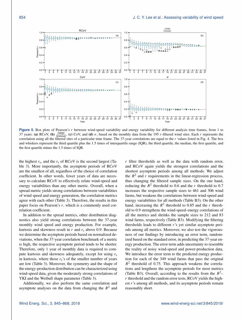
By increasing the years included in the variability cal-culations using monthly data, the resultant correlations ofmost metrics vary less, the correlations gradually convergeto their 37-year values, and their asymptote periods vary.The 37-year Pearson’s r values from the four selected met-rics between wind-speed and energy-production variabilitiesin Fig. 4 transform into the 37-year marks in Fig. 5, and weuse a 5 % threshold of normalized deviation to determine theasymptote periods. Particularly, the r’s from RCoV and CoV
(Fig. 5a and c) reach their respective asymptotes steadilywith longer length of data, whereas the r’s from range di-vided by trimean do not (Fig. 5b). The 37-year correlationusing σ is weak and thus the method is not actually useful:while the r’s approach the 37-year benchmark (Fig. 5d), thiscorrelation value is so low (0.2) as to be ineffective. Pairedwith a high long-term r , the asymptote period of a metricindicates the appropriate time span of wind-speed data re-quired to represent the variability of wind-energy production.For example, the resultant r’s using RCoV approach a highvalue after just 3 years, meaning one needs 3 years of wind-speed data to estimate the wind-speed variability so as to ad-equately infer the energy-production variability of a certainor potential wind farm via RCoV.
The three correlation coefficients (Pearson’s r , Spearman’srs, and Kendall’s τ ) yield consistent results among all vari-ability metrics tested; hence we primarily present the resultsusing Pearson’s r here. Table 3 summarizes the 37-year cor-relations (r , rs, and τ ), between the wind-speed variabilitiesand the energy-production variabilities using the r-filtereddata, and the respective asymptote periods of the methods.The r and τ of RCoV are the largest (0.86 and 0.67, re-spectively) among all variability metrics, and the associateasymptote periods are also relatively short (2 to 3 years) (Ta-ble 3). Another normalized, robust, and resistant spread met-ric, interquartile range (IQR) divided by median, results in
www.wind-energ-sci.net/3/845/2018/ Wind Energ. Sci., 3, 845–868, 2018
854 J. C. Y. Lee et al.: Assessing variability of wind speed
1 3 5 7 9 11 13 15 17 19 21 23 25 27 29 31 33 35 370.0
0.2
0.4
0.6
0.8
1.0
Pear
son'
s r
(a)
RCoV
1 3 5 7 9 11 13 15 17 19 21 23 25 27 29 31 33 35 370.0
0.2
0.4
0.6
0.8
1.0(b)
ranget rim ean
1 3 5 7 9 11 13 15 17 19 21 23 25 27 29 31 33 35 37Year
0.0
0.2
0.4
0.6
0.8
1.0
Pear
son'
s r
(c)
CoV
1 3 5 7 9 11 13 15 17 19 21 23 25 27 29 31 33 35 37Year
0.0
0.2
0.4
0.6
0.8
1.0(d)
Figure 5. Box plots of Pearson’s r between wind-speed variability and energy variability for different analysis time frames, from 1 to37 years: (a) RCoV, (b) range
trimean , (c) CoV, and (d) σ , based on the monthly data from the 195 r-filtered wind sites. Each r represents thecorrelation using all the filtered sites of a particular time frame. The 37-year correlations are equal to the r values listed in Fig. 4. The boxand whiskers represent the third quartile plus the 1.5 times of interquartile range (IQR), the third quartile, the median, the first quartile, andthe first quartile minus the 1.5 times of IQR.
the highest rs, and the rs of RCoV is the second largest (Ta-ble 3). More importantly, the asymptote periods of RCoVare the smallest of all, regardless of the choice of correlationcoefficient. In other words, fewer years of data are neces-sary to calculate RCoV to effectively relate wind-speed andenergy variabilities than any other metric. Overall, when aspread metric yields strong correlations between variabilitiesof wind speed and energy generation, the correlation metricsagree with each other (Table 3). Therefore, the results in thispaper focus on Pearson’s r , which is a commonly used cor-relation coefficient.
In addition to the spread metrics, other distribution diag-nostics also yield strong correlations between the 37-yearmonthly wind speed and energy production. For example,kurtosis and skewness result in r and rs above 0.9. Becausewe determine the asymptote periods based on normalized de-viations, when the 37-year correlation benchmark of a metricis high, the respective asymptote period tends to be shorter.Therefore, only 1 year of monthly data is required to com-pute kurtosis and skewness adequately, except for using rsin kurtosis, where those rs’s of the smaller number of yearsare low (Table 3). Moreover, the symmetry and the shape ofthe energy-production distribution can be characterized usingwind-speed data, given the moderately strong correlations ofYKI and the Weibull shape parameter (Table 3).
Additionally, we also perform the same correlation andasymptote analyses on the data from changing the R2 and
r filter thresholds as well as the data with random error,and RCoV again yields the strongest correlations and theshortest asymptote periods among all methods. We adjustthe R2 and r requirements in the linear-regression process,thus changing the filtered sample sizes. On the one hand,reducing the R2 threshold to 0.6 and the r threshold to 0.7increases the respective sample sizes to 461 and 306 windfarms, but weakens the correlations between wind-speed andenergy variabilities for all methods (Table B3). On the otherhand, increasing the R2 threshold to 0.85 and the r thresh-old to 0.9 strengthens the wind-speed–energy correlations ofall the metrics and shrinks the sample sizes to 212 and 83wind farms, respectively (Table B3). Modifying the filteringthresholds leads to different r’s yet similar asymptote peri-ods among all metrics. Moreover, we also test the vigorous-ness of our findings by introducing an error term, random-ized based on the standard error, in predicting the 37-year en-ergy production. The error term adds uncertainty to resemblethe reality of noisy wind-speed and power-production data.We introduce the error term to the predicted energy produc-tion for each of the 349 wind farms that pass the originalR2 threshold of 0.75. This approach weakens the correla-tions and lengthens the asymptote periods for most metrics(Table B3). Overall, according to the results from the R2–r threshold and the random error tests, RCoV yields the high-est r’s among all methods, and its asymptote periods remainreasonably short.
Wind Energ. Sci., 3, 845–868, 2018 www.wind-energ-sci.net/3/845/2018/
J. C. Y. Lee et al.: Assessing variability of wind speed 855
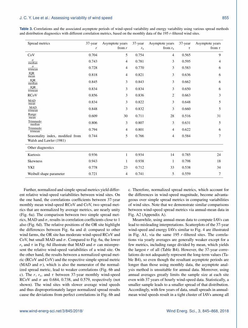
Table 3. Correlations and the associated asymptote periods of wind-speed variability and energy variability using various spread methodsand distribution diagnostics with different correlation metrics, based on the monthly data of the 195 r-filtered wind sites.
Spread metrics 37-year Asymptote years 37-year Asymptote years 37-year Asymptote yearsr from r rs from rs τ from τ
CoV 0.704 5 0.754 4 0.565 9σ
median 0.743 4 0.781 3 0.595 4σ
trimean 0.728 4 0.770 3 0.583 6IQRmean 0.818 4 0.821 3 0.636 6
IQRmedian 0.845 3 0.843 3 0.662 6
IQRtrimean 0.834 3 0.834 3 0.650 6
RCoV 0.856 3 0.836 2 0.663 3MADmean 0.834 3 0.822 3 0.648 5MAD
trimean 0.848 3 0.832 3 0.660 5Rangemean 0.609 30 0.711 28 0.516 31Trimmedσ
median 0.806 3 0.807 3 0.631 5Trimmedσ
trimean 0.794 4 0.801 4 0.622 6
Seasonality index, modified fromWalsh and Lawler (1981)
0.744 5 0.766 4 0.584 7
Other diagnostics
Kurtosis 0.936 1 0.934 14 0.785 24
Skewness 0.943 1 0.938 1 0.798 18
YKI 0.778 23 0.712 33 0.538 34
Weibull shape parameter 0.721 4 0.741 5 0.559 7
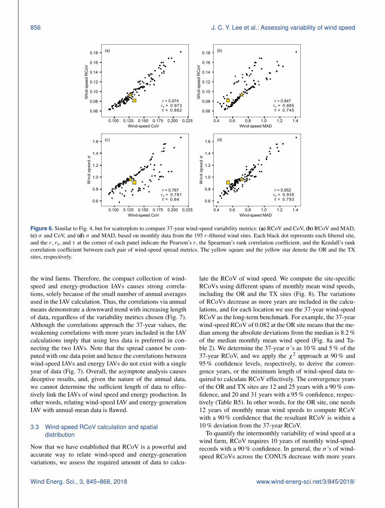
Further, normalized and simple spread metrics yield differ-ent relative wind-speed variabilities between wind sites. Onthe one hand, the correlations coefficients between 37-yearmonthly mean wind-speed RCoV and CoV, two spread met-rics that are normalized by average metrics, are nearly unity(Fig. 6a). The comparison between two simple spread met-rics, MAD and σ , results in correlation coefficients close to 1also (Fig. 6d). The relative positions of the OR site highlightthe differences between Fig. 6a and d: compared to otherwind farms, the OR site has moderate wind-speed RCoV andCoV, but small MAD and σ . Compared to Fig. 6a, the lowerrs and τ in Fig. 6d illustrate that MAD and σ can misrepre-sent the relative wind-speed variabilities of a wind site. Onthe other hand, the results between a normalized spread met-ric (RCoV and CoV) and the respective simple spread metric(MAD and σ ), which is also the numerator of the normal-ized spread metric, lead to weaker correlations (Fig. 6b andc). The r , rs, and τ between 37-year monthly wind-speedRCoV and σ are 0.684, 0.738, and 0.579, respectively (notshown). The wind sites with slower average wind speedsand thus disproportionately larger normalized spread resultscause the deviations from perfect correlations in Fig. 6b and
c. Therefore, normalized spread metrics, which account forthe differences in wind-speed magnitude, become advanta-geous over simple spread metrics in comparing variabilitiesof wind sites. Note that we demonstrate similar comparisonsbetween wind-speed spread metrics via annual-mean data inFig. A2 (Appendix A).
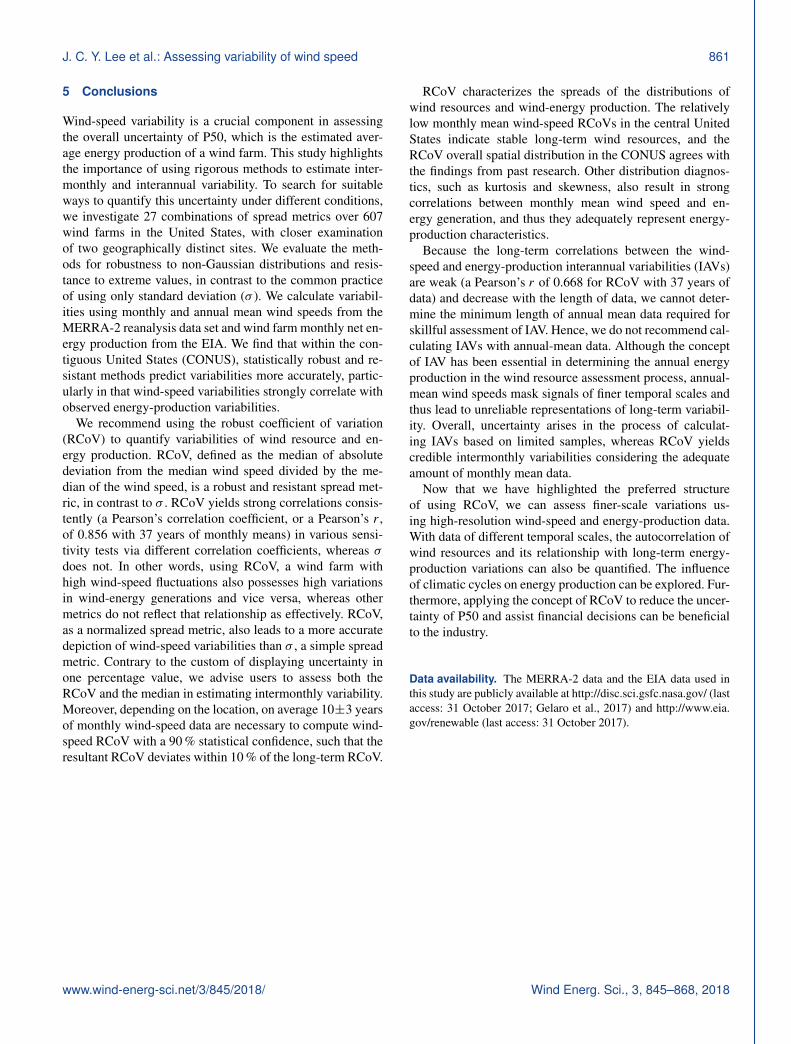
Meanwhile, using annual-mean data to compute IAVs canlead to misleading interpretations. Scatterplots of the 37-yearwind-speed and energy IAVs similar to Fig. 4 are illustratedin Fig. A1, via the same 195 r-filtered sites. The correla-tions via yearly averages are generally weaker except for afew metrics, including range divided by mean, which yieldsthe largest r of all (Table B4). However, the 37-year corre-lations do not adequately represent the long-term values (Ta-ble B4), so even though the resultant asymptote periods arelonger than those using monthly data, the asymptote anal-ysis method is unsuitable for annual data. Moreover, usingannual averages greatly limits the sample size at each siteeven with 37 years of hourly wind-speed data. Statistically, asmaller sample leads to a smaller spread of that distribution.Accordingly, with few years of data, small spreads in annual-mean wind speeds result in a tight cluster of IAVs among all
www.wind-energ-sci.net/3/845/2018/ Wind Energ. Sci., 3, 845–868, 2018
856 J. C. Y. Lee et al.: Assessing variability of wind speed
0.100 0.125 0.150 0.175 0.200 0.225Wind-speed CoV
0.06
0.08
0.10
0.12
0.14
0.16
0.18
Win
d-sp
eed
RC
oV
(a)
r = 0.974rs = 0.973
= 0.862
0.4 0.6 0.8 1.0 1.2 1.4Wind-speed MAD
0.06
0.08
0.10
0.12
0.14
0.16
0.18
Win
d-sp
eed
RC
oV
(b)
r = 0.847rs = 0.885
= 0.745
0.100 0.125 0.150 0.175 0.200 0.225Wind-speed CoV
0.6
0.8
1.0
1.2
1.4
1.6
Win
d-sp
eed
(c)
r = 0.767rs = 0.781
= 0.64
0.4 0.6 0.8 1.0 1.2 1.4Wind-speed MAD
0.6
0.8
1.0
1.2
1.4
1.6
Win
d-sp
eed
(d)
r = 0.952rs = 0.935
= 0.793
Figure 6. Similar to Fig. 4, but for scatterplots to compare 37-year wind-speed variability metrics: (a) RCoV and CoV, (b) RCoV and MAD,(c) σ and CoV, and (d) σ and MAD, based on monthly data from the 195 r-filtered wind sites. Each black dot represents each filtered site,and the r , rs, and τ at the corner of each panel indicate the Pearson’s r , the Spearman’s rank correlation coefficient, and the Kendall’s rankcorrelation coefficient between each pair of wind-speed spread metrics. The yellow square and the yellow star denote the OR and the TXsites, respectively.
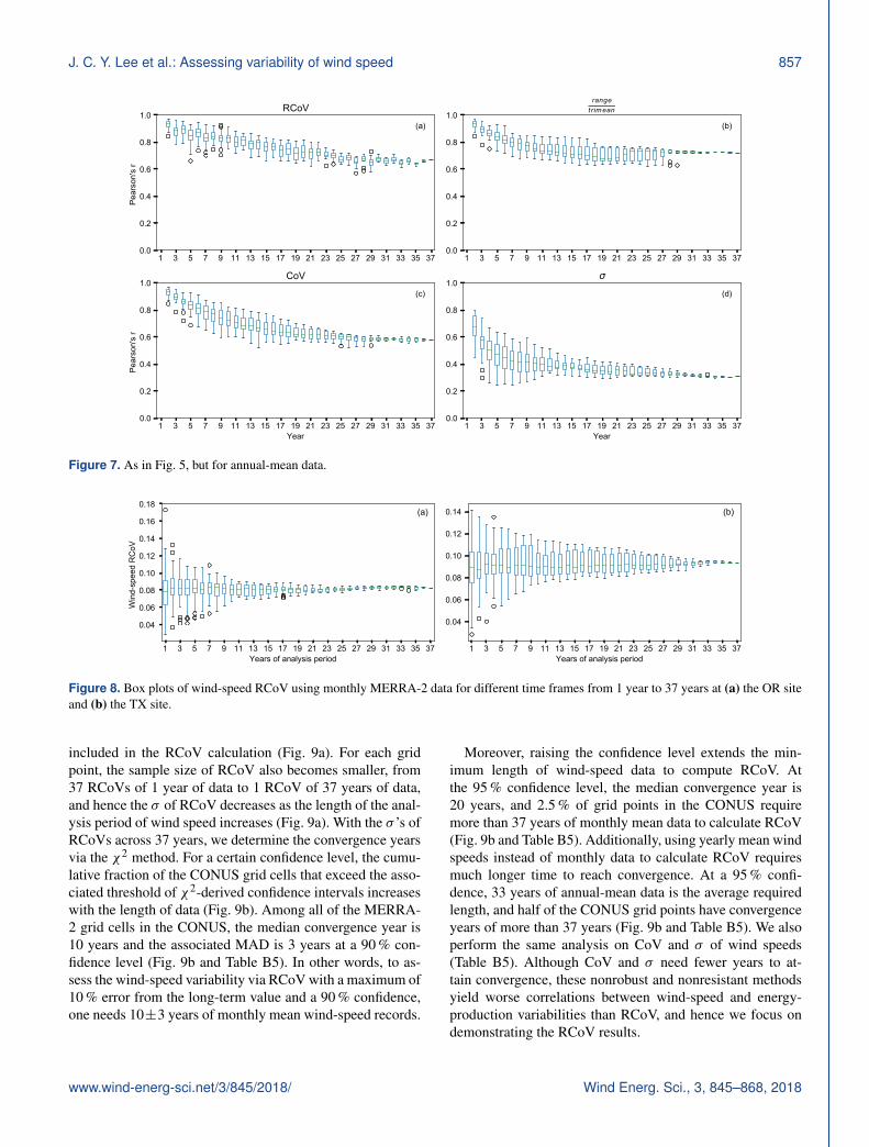
the wind farms. Therefore, the compact collection of wind-speed and energy-production IAVs causes strong correla-tions, solely because of the small number of annual averagesused in the IAV calculation. Thus, the correlations via annualmeans demonstrate a downward trend with increasing lengthof data, regardless of the variability metrics chosen (Fig. 7).Although the correlations approach the 37-year values, theweakening correlations with more years included in the IAVcalculations imply that using less data is preferred in con-necting the two IAVs. Note that the spread cannot be com-puted with one data point and hence the correlations betweenwind-speed IAVs and energy IAVs do not exist with a singleyear of data (Fig. 7). Overall, the asymptote analysis causesdeceptive results, and, given the nature of the annual data,we cannot determine the sufficient length of data to effec-tively link the IAVs of wind speed and energy production. Inother words, relating wind-speed IAV and energy-generationIAV with annual-mean data is flawed.
3.3 Wind-speed RCoV calculation and spatialdistribution
Now that we have established that RCoV is a powerful andaccurate way to relate wind-speed and energy-generationvariations, we assess the required amount of data to calcu-
late the RCoV of wind speed. We compute the site-specificRCoVs using different spans of monthly mean wind speeds,including the OR and the TX sites (Fig. 8). The variationsof RCoVs decrease as more years are included in the calcu-lations, and for each location we use the 37-year wind-speedRCoV as the long-term benchmark. For example, the 37-yearwind-speed RCoV of 0.082 at the OR site means that the me-dian among the absolute deviations from the median is 8.2 %of the median monthly mean wind speed (Fig. 8a and Ta-ble 2). We determine the 37-year σ ’s as 10 % and 5 % of the37-year RCoV, and we apply the χ2 approach at 90 % and95 % confidence levels, respectively, to derive the conver-gence years, or the minimum length of wind-speed data re-quired to calculate RCoV effectively. The convergence yearsof the OR and TX sites are 12 and 25 years with a 90 % con-fidence, and 20 and 31 years with a 95 % confidence, respec-tively (Table B5). In other words, for the OR site, one needs12 years of monthly mean wind speeds to compute RCoVwith a 90 % confidence that the resultant RCoV is within a10 % deviation from the 37-year RCoV.
To quantify the intermonthly variability of wind speed at awind farm, RCoV requires 10 years of monthly wind-speedrecords with a 90 % confidence. In general, the σ ’s of wind-speed RCoVs across the CONUS decrease with more years
Wind Energ. Sci., 3, 845–868, 2018 www.wind-energ-sci.net/3/845/2018/
J. C. Y. Lee et al.: Assessing variability of wind speed 857
1 3 5 7 9 11 13 15 17 19 21 23 25 27 29 31 33 35 370.0
0.2
0.4
0.6
0.8
1.0
Pear
son'
s r
(a)
RCoV
1 3 5 7 9 11 13 15 17 19 21 23 25 27 29 31 33 35 370.0
0.2
0.4
0.6
0.8
1.0(b)
ranget rim ean
1 3 5 7 9 11 13 15 17 19 21 23 25 27 29 31 33 35 37Year
0.0
0.2
0.4
0.6
0.8
1.0
Pear
son'
s r
(c)
CoV
1 3 5 7 9 11 13 15 17 19 21 23 25 27 29 31 33 35 37Year
0.0
0.2
0.4
0.6
0.8
1.0(d)
Figure 7. As in Fig. 5, but for annual-mean data.
1 3 5 7 9 11 13 15 17 19 21 23 25 27 29 31 33 35 37Years of analysis period
0.04
0.06
0.08
0.10
0.12
0.14
0.16
0.18
Win
d-sp
eed
RC
oV
1 3 5 7 9 11 13 15 17 19 21 23 25 27 29 31 33 35 37Years of analysis period
0.04
0.06
0.08
0.10
0.12
0.14(a) (b)
Figure 8. Box plots of wind-speed RCoV using monthly MERRA-2 data for different time frames from 1 year to 37 years at (a) the OR siteand (b) the TX site.
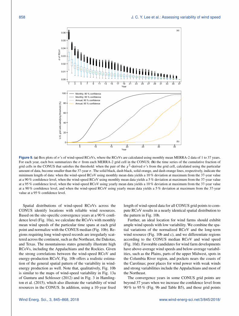
included in the RCoV calculation (Fig. 9a). For each gridpoint, the sample size of RCoV also becomes smaller, from37 RCoVs of 1 year of data to 1 RCoV of 37 years of data,and hence the σ of RCoV decreases as the length of the anal-ysis period of wind speed increases (Fig. 9a). With the σ ’s ofRCoVs across 37 years, we determine the convergence yearsvia the χ2 method. For a certain confidence level, the cumu-lative fraction of the CONUS grid cells that exceed the asso-ciated threshold of χ2-derived confidence intervals increaseswith the length of data (Fig. 9b). Among all of the MERRA-2 grid cells in the CONUS, the median convergence year is10 years and the associated MAD is 3 years at a 90 % con-fidence level (Fig. 9b and Table B5). In other words, to as-sess the wind-speed variability via RCoV with a maximum of10 % error from the long-term value and a 90 % confidence,one needs 10±3 years of monthly mean wind-speed records.
Moreover, raising the confidence level extends the min-imum length of wind-speed data to compute RCoV. Atthe 95 % confidence level, the median convergence year is20 years, and 2.5 % of grid points in the CONUS requiremore than 37 years of monthly mean data to calculate RCoV(Fig. 9b and Table B5). Additionally, using yearly mean windspeeds instead of monthly data to calculate RCoV requiresmuch longer time to reach convergence. At a 95 % confi-dence, 33 years of annual-mean data is the average requiredlength, and half of the CONUS grid points have convergenceyears of more than 37 years (Fig. 9b and Table B5). We alsoperform the same analysis on CoV and σ of wind speeds(Table B5). Although CoV and σ need fewer years to at-tain convergence, these nonrobust and nonresistant methodsyield worse correlations between wind-speed and energy-production variabilities than RCoV, and hence we focus ondemonstrating the RCoV results.
www.wind-energ-sci.net/3/845/2018/ Wind Energ. Sci., 3, 845–868, 2018
858 J. C. Y. Lee et al.: Assessing variability of wind speed
1 3 5 7 9 11 13 15 17 19 21 23 25 27 29 31 33 35 37Year
0.00
0.01
0.02
0.03
0.04
0.05
0.06
of R
CoV
(a)
5 10 15 20 25 30 35Year
0
20
40
60
80
100
U.S
. grid
cel
ls s
atis
fyin
g th
resh
old
(%)
(b)
Monthly; 90 % confidenceMonthly; 95 % confidenceAnnual; 90 % confidenceAnnual; 95 % confidence
Figure 9. (a) Box plots of σ ’s of wind-speed RCoVs, where the RCoVs are calculated using monthly mean MERRA-2 data of 1 to 37 years.For each year, each box summarizes the σ from each MERRA-2 grid cell in the CONUS; (b) the time series of the cumulative fraction ofgrid cells in the CONUS that satisfies the threshold: when the pair of the χ2-derived σ ’s from the grid cell, calculated using the particularamount of data, become smaller than the 37-year σ . The solid black, dash black, solid orange, and dash orange lines, respectively, indicate theminimum length of data: when the wind-speed RCoV using monthly mean data yields a 10 % deviation at maximum from the 37-year valueat a 90 % confidence level, when the wind-speed RCoV using monthly mean data yields a 5 % deviation at maximum from the 37-year valueat a 95 % confidence level, when the wind-speed RCoV using yearly mean data yields a 10 % deviation at maximum from the 37-year valueat a 90 % confidence level, and when the wind-speed RCoV using yearly mean data yields a 5 % deviation at maximum from the 37-yearvalue at a 95 % confidence level.
Spatial distributions of wind-speed RCoVs across theCONUS identify locations with reliable wind resources.Based on the site-specific convergence years at a 90 % confi-dence level (Fig. 10a), we calculate the RCoVs with monthlymean wind speeds of the particular time spans at each gridpoint and normalize with the CONUS median (Fig. 10b). Re-gions requiring long wind-speed records are irregularly scat-tered across the continent, such as the Northeast, the Dakotas,and Texas. The mountainous states generally illustrate highRCoVs, including the Appalachians and the Rockies. Giventhe strong correlations between the wind-speed RCoV andenergy-production RCoV, Fig. 10b offers a realistic estima-tion of the general spatial pattern of the variability in wind-energy production as well. Note that, qualitatively, Fig. 10bis similar to the maps of wind-speed variability in Fig. 13aof Gunturu and Schlosser (2012) and in Fig. 3 in Hamling-ton et al. (2015), which also illustrate the variability of windresources in the CONUS. In addition, using a 10-year fixed
length of wind-speed data for all CONUS grid points to com-pute RCoV results in a nearly identical spatial distribution tothe pattern in Fig. 10b.
Further, an ideal location for wind farms should exhibitample wind speeds with low variability. We combine the spa-tial variations of the normalized RCoV and the long-termwind resource (Fig. 10b and c), and we differentiate regionsaccording to the CONUS median RCoV and wind speed(Fig. 10d). Favorable candidates for wind farm developmentshave above-average wind speeds and below-average variabil-ities, such as the Plains, parts of the upper Midwest, spots inthe Columbia River region, and pockets nears the coasts ofthe Carolinas; poor places for wind power with weak windsand strong variabilities include the Appalachians and most ofthe Northeast.
The convergence years in some CONUS grid points arebeyond 37 years when we increase the confidence level from90 % to 95 % (Fig. 9b and Table B5), and those grid points
Wind Energ. Sci., 3, 845–868, 2018 www.wind-energ-sci.net/3/845/2018/
J. C. Y. Lee et al.: Assessing variability of wind speed 859
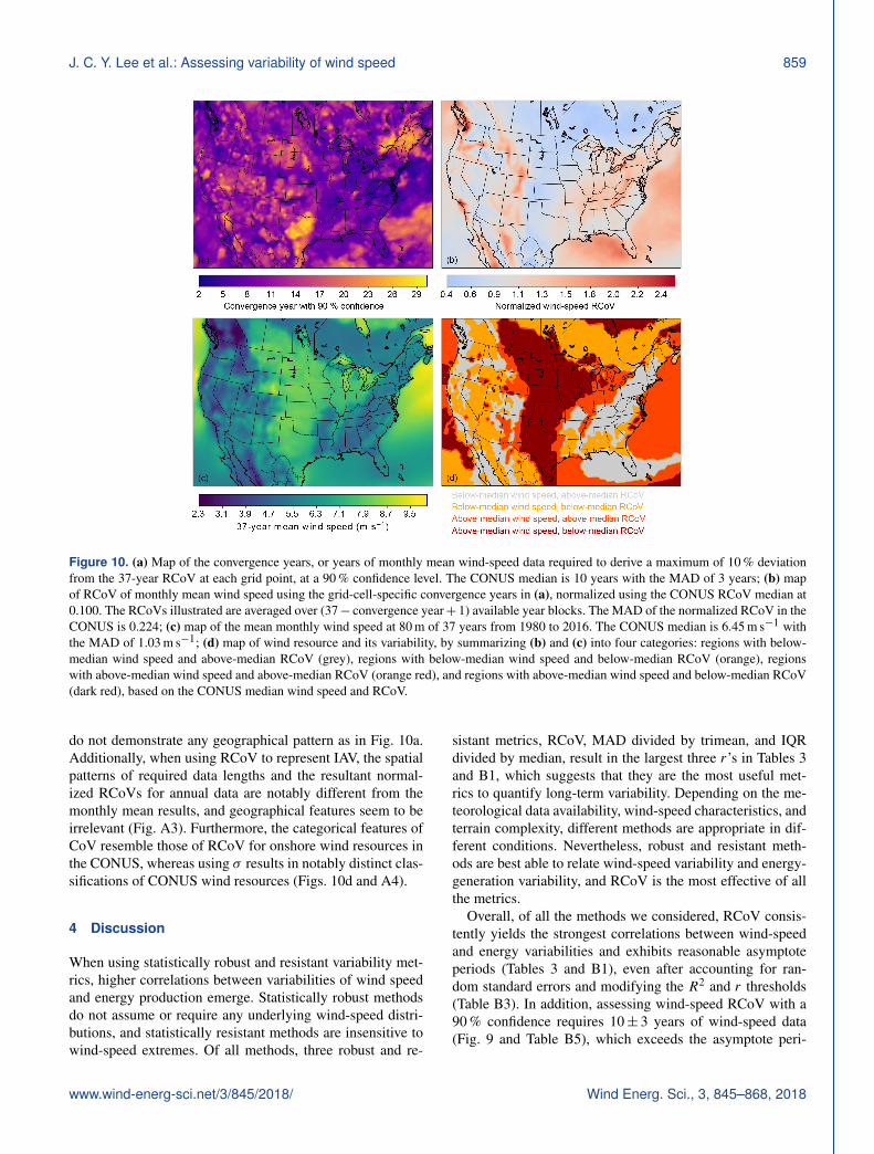
Figure 10. (a) Map of the convergence years, or years of monthly mean wind-speed data required to derive a maximum of 10 % deviationfrom the 37-year RCoV at each grid point, at a 90 % confidence level. The CONUS median is 10 years with the MAD of 3 years; (b) mapof RCoV of monthly mean wind speed using the grid-cell-specific convergence years in (a), normalized using the CONUS RCoV median at0.100. The RCoVs illustrated are averaged over (37− convergence year+ 1) available year blocks. The MAD of the normalized RCoV in theCONUS is 0.224; (c) map of the mean monthly wind speed at 80 m of 37 years from 1980 to 2016. The CONUS median is 6.45 m s−1 withthe MAD of 1.03 m s−1; (d) map of wind resource and its variability, by summarizing (b) and (c) into four categories: regions with below-median wind speed and above-median RCoV (grey), regions with below-median wind speed and below-median RCoV (orange), regionswith above-median wind speed and above-median RCoV (orange red), and regions with above-median wind speed and below-median RCoV(dark red), based on the CONUS median wind speed and RCoV.
do not demonstrate any geographical pattern as in Fig. 10a.Additionally, when using RCoV to represent IAV, the spatialpatterns of required data lengths and the resultant normal-ized RCoVs for annual data are notably different from themonthly mean results, and geographical features seem to beirrelevant (Fig. A3). Furthermore, the categorical features ofCoV resemble those of RCoV for onshore wind resources inthe CONUS, whereas using σ results in notably distinct clas-sifications of CONUS wind resources (Figs. 10d and A4).
4 Discussion
When using statistically robust and resistant variability met-rics, higher correlations between variabilities of wind speedand energy production emerge. Statistically robust methodsdo not assume or require any underlying wind-speed distri-butions, and statistically resistant methods are insensitive towind-speed extremes. Of all methods, three robust and re-
sistant metrics, RCoV, MAD divided by trimean, and IQRdivided by median, result in the largest three r’s in Tables 3and B1, which suggests that they are the most useful met-rics to quantify long-term variability. Depending on the me-teorological data availability, wind-speed characteristics, andterrain complexity, different methods are appropriate in dif-ferent conditions. Nevertheless, robust and resistant meth-ods are best able to relate wind-speed variability and energy-generation variability, and RCoV is the most effective of allthe metrics.
Overall, of all the methods we considered, RCoV consis-tently yields the strongest correlations between wind-speedand energy variabilities and exhibits reasonable asymptoteperiods (Tables 3 and B1), even after accounting for ran-dom standard errors and modifying the R2 and r thresholds(Table B3). In addition, assessing wind-speed RCoV with a90 % confidence requires 10± 3 years of wind-speed data(Fig. 9 and Table B5), which exceeds the asymptote peri-
www.wind-energ-sci.net/3/845/2018/ Wind Energ. Sci., 3, 845–868, 2018

860 J. C. Y. Lee et al.: Assessing variability of wind speed
ods of 2 to 6 years to yield strong wind-speed and energy-production correlations (Table 3). Even though different lo-cations require various spans of data (Fig. 10a), the averageof the resultant RCoVs using 10 years of wind speeds leadsto nearly identical spatial distributions (Fig. 10b). Therefore,to effectively quantify wind-speed variability and thus ade-quately derive energy-generation variability, we recommendusing the RCoV with 10 years of monthly mean wind-speeddata.
Annual-mean data are inadequate to relate wind-speed andenergy-production IAVs or to represent wind-speed IAVs.We cannot determine the minimum years of data to relate an-nual wind-speed and energy IAVs because their correlationsdecline with the length of data (Fig. 7). Moreover, the coarsetime resolution of annual averages smooths out the fluctua-tions of smaller timescales. Yearly mean wind speeds alsopossess different distribution characteristics, such as skew-ness and kurtosis, compared to those of finer temporal res-olutions (Lee et al., 2018). The nonzero kurtosis and skew-ness in Table 2 and in Lee et al. (2018) illustrate that most ofthe distributions of annual-mean wind speeds in the CONUSare non-Gaussian. Hence, using nonrobust metrics, such asσ , to evaluate IAV with samples of annual means from non-Gaussian distributions can lead to incorrect representationsof variability.
Additionally, extended years of wind-speed data are alsonecessary to compute RCoV and represent IAV (Fig. A3a),and the resultant IAVs (Fig. A3b) differ from the variabili-ties calculated via monthly wind speeds (Fig. 10b). For in-stance, the low IAVs in the Appalachians (Fig. A3b) calcu-lated with yearly mean wind speeds contradict the patternof high monthly mean wind-speed RCoVs in mountainousareas (Fig. 10b) as well as the findings in past research (Gun-turu and Schlosser, 2012; Hamlington et al., 2015). Further-more, some of the grid points require more than 37 years ofyearly mean data to calculate wind-speed RCoV with statis-tical confidence (Fig. 9 and Table B5). Although RCoV doesnot yield the strongest 37-year r in relating wind-speed andenergy IAVs, readers should be cautious when using a lim-ited number of annual-mean data to derive IAVs. In short, toeffectively assess the long-term variability of wind farm pro-ductivity, one should use wind speeds finer than yearly meandata.
Regions with ample wind resources and low variabilityfavor wind-energy developments, coinciding with the loca-tions of many existing wind farms in the CONUS (Fig. 10d).Wind farms in the Plains and parts of the upper Midwestbenefit from the above-average wind speeds and the below-average wind-speed RCoVs. Other regions, such as parts ofthe Columbia River region and the Carolinas, also experiencestrong, consistent winds. The Northeast and the Appalachi-ans are relatively unfavorable for producing a stable, onshorewind-energy supply, whereas the area east of Cape Cod inMassachusetts and the sections along the West Coast exhibita promising offshore wind resource. Wind farm developers
should account for wind resource as well as its long-termvariability in repowering existing turbines and building newwind farms.
Furthermore, mathematically, a normalized spread metric,namely a spread statistic divided by an average metric, ismore useful than solely a spread metric in assessing variabil-ity, and a normalized spread metric should always be pre-sented with the corresponding averaging metric. For exam-ple, RCoV and CoV between wind speed and energy yieldlarger r’s than MAD and σ (Table 3 and Fig. A1), and ther’s between wind-speed RCoV and CoV are also higher thanthose comparisons involving MAD and σ (Fig. 6). For σ , theroot mean square of the deviation from the mean is not sta-tistically robust or resistant, and 1σ means the uncertainty is18.3 % from the mean. Hence, CoV, or the σ divided by themean, is the respective normalized uncertainty metric to σ .For instance, the wind-speed CoVs of both the OR and TXsites are about 0.13 (Table 2), implying the σ is 13 % fromthe mean. In contrast, using RCoV, or the MAD divided bythe median, is a robust and outlier-resistant metric of normal-ized uncertainty. For example, the wind-speed RCoVs of theOR and TX sites are 0.08 and 0.09, respectively (Table 2), in-dicating the MADs are 8 % and 9 % from their median windspeeds. Even though RCoV is not as commonly used and notas intuitive as σ or CoV, RCoV is unrestricted by any un-derlying distribution assumptions. Overall, to correctly andeffectively use the normalized spread metrics, both the nor-malized spread metric and the average value need to be statedclearly in pairs. In other words, the interpretation of “thevariability is 2 %” oversimplifies the statistics of uncertaintyquantification. Therefore, we recommend presenting both theRCoV and the median of a time series together in estimatingvariability.
Distribution diagnostics, other than the variability metrics,are also effective in identifying the characteristics of wind-energy production. We examine distribution parameters re-sulting in strong wind-speed–energy correlations, includingkurtosis and YKI (Tables 3 and B2), which assess the de-gree of deviations from a Gaussian distribution. For example,we confirm that the monthly and annual wind-speed distri-butions for our case studies in OR and TX are not perfectlyGaussian because of their nonzero kurtosis and skewness val-ues (Table 2), as well as their portions of data within 1σ .Moreover, a multimodal or an asymmetric wind-speed distri-bution (Fig. 3c and d) also implies a non-Gaussian energy-production distribution. Gaussian distribution is invalid forwind speeds across averaging timescales in general (Lee etal., 2018). Hence, understanding the underlying distributionof wind resources can validate the applications and the le-gitimacy of Gaussian statistics, especially in quantifying P50and the associated losses and uncertainties.
Wind Energ. Sci., 3, 845–868, 2018 www.wind-energ-sci.net/3/845/2018/
J. C. Y. Lee et al.: Assessing variability of wind speed 861
5 Conclusions
Wind-speed variability is a crucial component in assessingthe overall uncertainty of P50, which is the estimated aver-age energy production of a wind farm. This study highlightsthe importance of using rigorous methods to estimate inter-monthly and interannual variability. To search for suitableways to quantify this uncertainty under different conditions,we investigate 27 combinations of spread metrics over 607wind farms in the United States, with closer examinationof two geographically distinct sites. We evaluate the meth-ods for robustness to non-Gaussian distributions and resis-tance to extreme values, in contrast to the common practiceof using only standard deviation (σ ). We calculate variabil-ities using monthly and annual mean wind speeds from theMERRA-2 reanalysis data set and wind farm monthly net en-ergy production from the EIA. We find that within the con-tiguous United States (CONUS), statistically robust and re-sistant methods predict variabilities more accurately, partic-ularly in that wind-speed variabilities strongly correlate withobserved energy-production variabilities.
We recommend using the robust coefficient of variation(RCoV) to quantify variabilities of wind resource and en-ergy production. RCoV, defined as the median of absolutedeviation from the median wind speed divided by the me-dian of the wind speed, is a robust and resistant spread met-ric, in contrast to σ . RCoV yields strong correlations consis-tently (a Pearson’s correlation coefficient, or a Pearson’s r ,of 0.856 with 37 years of monthly means) in various sensi-tivity tests via different correlation coefficients, whereas σdoes not. In other words, using RCoV, a wind farm withhigh wind-speed fluctuations also possesses high variationsin wind-energy generations and vice versa, whereas othermetrics do not reflect that relationship as effectively. RCoV,as a normalized spread metric, also leads to a more accuratedepiction of wind-speed variabilities than σ , a simple spreadmetric. Contrary to the custom of displaying uncertainty inone percentage value, we advise users to assess both theRCoV and the median in estimating intermonthly variability.Moreover, depending on the location, on average 10±3 yearsof monthly wind-speed data are necessary to compute wind-speed RCoV with a 90 % statistical confidence, such that theresultant RCoV deviates within 10 % of the long-term RCoV.
RCoV characterizes the spreads of the distributions ofwind resources and wind-energy production. The relativelylow monthly mean wind-speed RCoVs in the central UnitedStates indicate stable long-term wind resources, and theRCoV overall spatial distribution in the CONUS agrees withthe findings from past research. Other distribution diagnos-tics, such as kurtosis and skewness, also result in strongcorrelations between monthly mean wind speed and en-ergy generation, and thus they adequately represent energy-production characteristics.
Because the long-term correlations between the wind-speed and energy-production interannual variabilities (IAVs)are weak (a Pearson’s r of 0.668 for RCoV with 37 years ofdata) and decrease with the length of data, we cannot deter-mine the minimum length of annual mean data required forskillful assessment of IAV. Hence, we do not recommend cal-culating IAVs with annual-mean data. Although the conceptof IAV has been essential in determining the annual energyproduction in the wind resource assessment process, annual-mean wind speeds mask signals of finer temporal scales andthus lead to unreliable representations of long-term variabil-ity. Overall, uncertainty arises in the process of calculat-ing IAVs based on limited samples, whereas RCoV yieldscredible intermonthly variabilities considering the adequateamount of monthly mean data.
Now that we have highlighted the preferred structureof using RCoV, we can assess finer-scale variations us-ing high-resolution wind-speed and energy-production data.With data of different temporal scales, the autocorrelation ofwind resources and its relationship with long-term energy-production variations can also be quantified. The influenceof climatic cycles on energy production can be explored. Fur-thermore, applying the concept of RCoV to reduce the uncer-tainty of P50 and assist financial decisions can be beneficialto the industry.
Data availability. The MERRA-2 data and the EIA data used inthis study are publicly available at http://disc.sci.gsfc.nasa.gov/ (lastaccess: 31 October 2017; Gelaro et al., 2017) and http://www.eia.gov/renewable (last access: 31 October 2017).
www.wind-energ-sci.net/3/845/2018/ Wind Energ. Sci., 3, 845–868, 2018
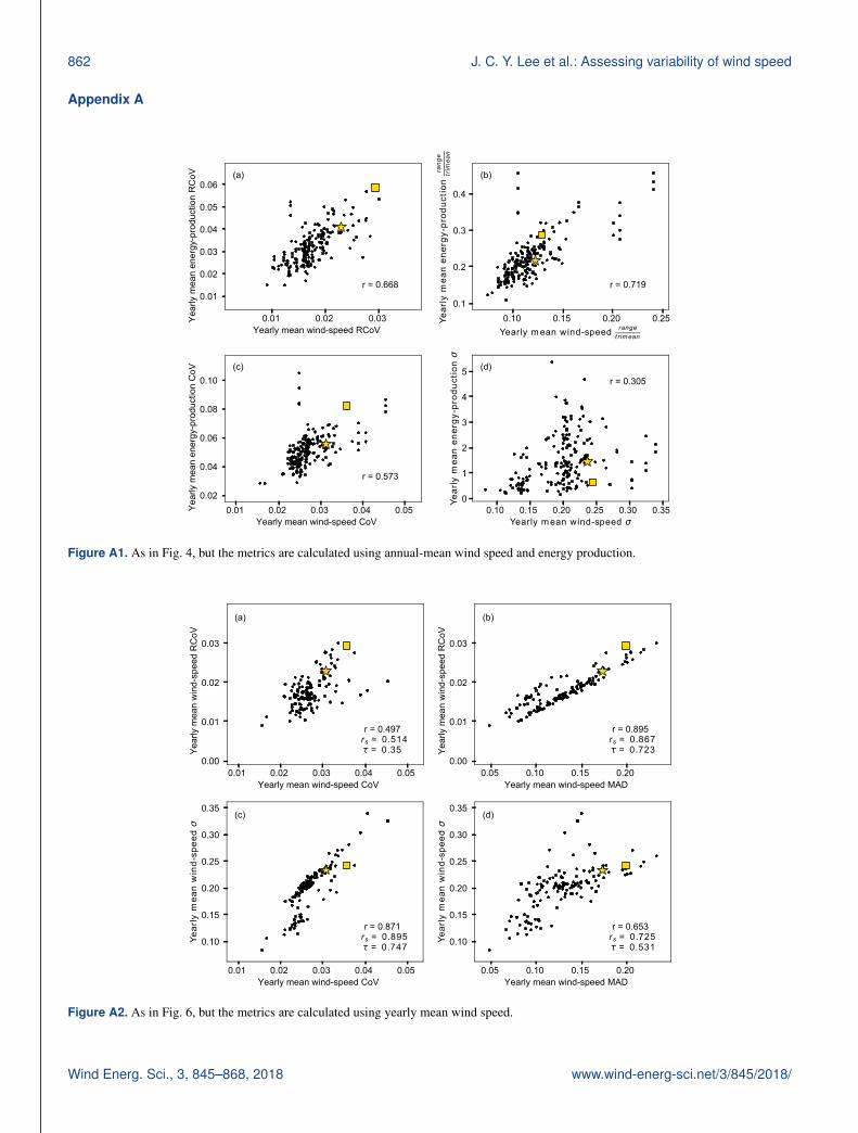
862 J. C. Y. Lee et al.: Assessing variability of wind speed
Appendix A
0.01 0.02 0.03Yearly mean wind-speed RCoV
0.01
0.02
0.03
0.04
0.05
0.06Ye
arly
mea
n en
ergy
-pro
duct
ion
RC
oV (a)
r = 0.668
0.10 0.15 0.20 0.25Yearly m ean wind-speed range
t rim ean
0.1
0.2
0.3
0.4
Year
ly m
ean
ener
gy-p
rodu
ctio
n ra
nge
trim
ean
(b)
r = 0.719
0.01 0.02 0.03 0.04 0.05Yearly mean wind-speed CoV
0.02
0.04
0.06
0.08
0.10
Year
ly m
ean
ener
gy-p
rodu
ctio
n C
oV (c)
r = 0.573
0.10 0.15 0.20 0.25 0.30 0.35Yearly m ean wind-speed
0
1
2
3
4
5
Year
ly m
ean
ener
gy-p
rodu
ctio
n (d)r = 0.305
Figure A1. As in Fig. 4, but the metrics are calculated using annual-mean wind speed and energy production.
0.01 0.02 0.03 0.04 0.05Yearly mean wind-speed CoV
0.00
0.01
0.02
0.03
Year
ly m
ean
win
d-sp
eed
RC
oV
(a)
r = 0.497rs = 0.514
= 0.35
0.05 0.10 0.15 0.20Yearly mean wind-speed MAD
0.00
0.01
0.02
0.03
Year
ly m
ean
win
d-sp
eed
RC
oV
(b)
r = 0.895rs = 0.867
= 0.723
0.01 0.02 0.03 0.04 0.05Yearly mean wind-speed CoV
0.10
0.15
0.20
0.25
0.30
0.35
Year
ly m
ean
win
d-sp
eed
(c)
r = 0.871rs = 0.895
= 0.747
0.05 0.10 0.15 0.20Yearly mean wind-speed MAD
0.10
0.15
0.20
0.25
0.30
0.35
Year
ly m
ean
win
d-sp
eed
(d)
r = 0.653rs = 0.725
= 0.531
Figure A2. As in Fig. 6, but the metrics are calculated using yearly mean wind speed.
Wind Energ. Sci., 3, 845–868, 2018 www.wind-energ-sci.net/3/845/2018/
J. C. Y. Lee et al.: Assessing variability of wind speed 863
Figure A3. As in Fig. 10a and b, but the data plotted are annual-mean wind speeds: (a) map of the convergence years, or years of wind-speeddata required to derive a maximum of 10 % deviation from the 37-year RCoV at each grid point at a 90 % confidence level. Because 12.6 % ofthe CONUS grid points yield convergence years beyond 37 years using annual data (solid orange line in Fig. 9 and first column in Table B5),we assign 37 years as the convergence years for those grid points. After excluding the non-numeric values, the CONUS median is 27 yearsand the MAD is 4 years; (b) map of RCoV of annual-mean wind speed using the grid-cell-specific convergence years in (a), normalizedusing the CONUS RCoV median at 0.020. The RCoVs illustrated are averaged over (37− convergence year+ 1) available year blocks. TheMAD of the normalized RCoV in the CONUS is 0.205.
(a)Below-median wind speed, above-median variabilityBelow-median wind speed, below-median variabilityAbove-median wind speed, above-median variabilityAbove-median wind speed, below-median variability
(b)
CoV
Figure A4. As in Fig. 10d, but the spread metrics are (a) σ and (b) CoV, calculated using monthly mean wind speeds of 37 years.
www.wind-energ-sci.net/3/845/2018/ Wind Energ. Sci., 3, 845–868, 2018
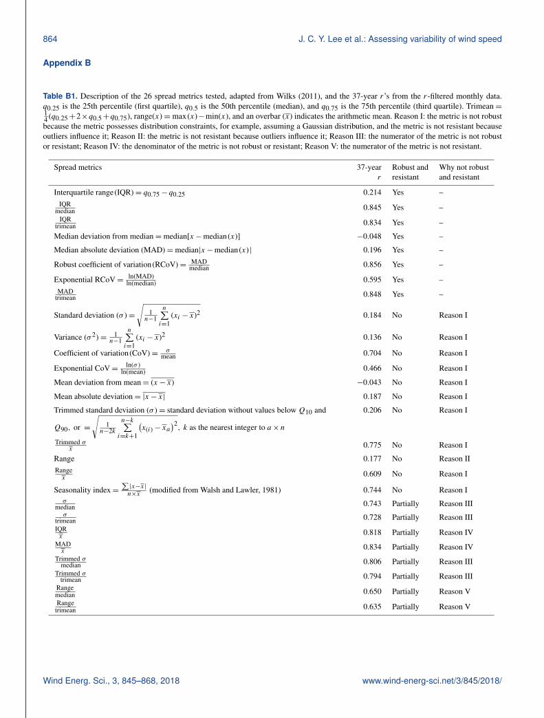
864 J. C. Y. Lee et al.: Assessing variability of wind speed
Appendix B
Table B1. Description of the 26 spread metrics tested, adapted from Wilks (2011), and the 37-year r’s from the r-filtered monthly data.q0.25 is the 25th percentile (first quartile), q0.5 is the 50th percentile (median), and q0.75 is the 75th percentile (third quartile). Trimean=14 (q0.25+2×q0.5+q0.75), range(x)=max(x)−min(x), and an overbar (x) indicates the arithmetic mean. Reason I: the metric is not robustbecause the metric possesses distribution constraints, for example, assuming a Gaussian distribution, and the metric is not resistant becauseoutliers influence it; Reason II: the metric is not resistant because outliers influence it; Reason III: the numerator of the metric is not robustor resistant; Reason IV: the denominator of the metric is not robust or resistant; Reason V: the numerator of the metric is not resistant.
Spread metrics 37-year Robust and Why not robustr resistant and resistant
Interquartile range(IQR)= q0.75− q0.25 0.214 Yes –IQR
median 0.845 Yes –IQR
trimean 0.834 Yes –
Median deviation from median=median[x−median(x)] −0.048 Yes –
Median absolute deviation (MAD)=median|x−median(x) | 0.196 Yes –
Robust coefficient of variation(RCoV)= MADmedian 0.856 Yes –
Exponential RCoV= ln(MAD)ln(median) 0.595 Yes –
MADtrimean 0.848 Yes –
Standard deviation (σ )=
√1n−1
n∑i=1
(xi − x)2 0.184 No Reason I
Variance (σ 2)= 1n−1
n∑i=1
(xi − x)2 0.136 No Reason I
Coefficient of variation(CoV)= σmean 0.704 No Reason I
Exponential CoV= ln(σ )ln(mean) 0.466 No Reason I
Mean deviation from mean= (x− x) −0.043 No Reason I
Mean absolute deviation= |x− x| 0.187 No Reason I
Trimmed standard deviation (σ )= standard deviation without values below Q10 and
Q90, or =
√1
n−2k
n−k∑i=k+1
(x(i)− xa
)2, k as the nearest integer to a× n
0.206 No Reason I
Trimmed σx
0.775 No Reason I
Range 0.177 No Reason IIRangex
0.609 No Reason I
Seasonality index=∑|x−x|n×x
(modified from Walsh and Lawler, 1981) 0.744 No Reason Iσ
median 0.743 Partially Reason IIIσ
trimean 0.728 Partially Reason IIIIQRx
0.818 Partially Reason IVMADx
0.834 Partially Reason IVTrimmed σ
median 0.806 Partially Reason IIITrimmed σ
trimean 0.794 Partially Reason IIIRangemedian 0.650 Partially Reason VRange
trimean 0.635 Partially Reason V
Wind Energ. Sci., 3, 845–868, 2018 www.wind-energ-sci.net/3/845/2018/
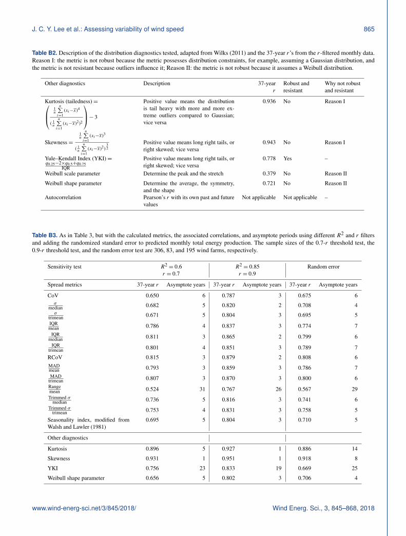
J. C. Y. Lee et al.: Assessing variability of wind speed 865
Table B2. Description of the distribution diagnostics tested, adapted from Wilks (2011) and the 37-year r’s from the r-filtered monthly data.Reason I: the metric is not robust because the metric possesses distribution constraints, for example, assuming a Gaussian distribution, andthe metric is not resistant because outliers influence it; Reason II: the metric is not robust because it assumes a Weibull distribution.
Other diagnostics Description 37-year Robust and Why not robustr resistant and resistant
Kurtosis (tailedness)= 1n
n∑i=1
(xi−x)4
( 1n
n∑i=1
(xi−x)2)2
− 3
Positive value means the distributionis tail heavy with more and more ex-treme outliers compared to Gaussian;vice versa
0.936 No Reason I
Skewness=
1n
n∑i=1
(xi−x)3
( 1n
n∑i=1
(xi−x)2)32
Positive value means long right tails, orright skewed; vice versa
0.943 No Reason I
Yule–Kendall Index (YKI)=q0.25−2×q0.5+q0.75
IQR
Positive value means long right tails, orright skewed; vice versa
0.778 Yes –
Weibull scale parameter Determine the peak and the stretch 0.379 No Reason II
Weibull shape parameter Determine the average, the symmetry,and the shape
0.721 No Reason II
Autocorrelation Pearson’s r with its own past and futurevalues
Not applicable Not applicable –
Table B3. As in Table 3, but with the calculated metrics, the associated correlations, and asymptote periods using different R2 and r filtersand adding the randomized standard error to predicted monthly total energy production. The sample sizes of the 0.7-r threshold test, the0.9-r threshold test, and the random error test are 306, 83, and 195 wind farms, respectively.
Sensitivity test R2= 0.6 R2
= 0.85 Random errorr = 0.7 r = 0.9
Spread metrics 37-year r Asymptote years 37-year r Asymptote years 37-year r Asymptote years
CoV 0.650 6 0.787 3 0.675 6σ
median 0.682 5 0.820 2 0.708 4σ
trimean 0.671 5 0.804 3 0.695 5IQRmean 0.786 4 0.837 3 0.774 7
IQRmedian 0.811 3 0.865 2 0.799 6
IQRtrimean 0.801 4 0.851 3 0.789 7
RCoV 0.815 3 0.879 2 0.808 6MADmean 0.793 3 0.859 3 0.786 7MAD
trimean 0.807 3 0.870 3 0.800 6Rangemean 0.524 31 0.767 26 0.567 29Trimmed σ
median 0.736 5 0.816 3 0.741 6Trimmed σ
trimean 0.753 4 0.831 3 0.758 5
Seasonality index, modified fromWalsh and Lawler (1981)
0.695 5 0.804 3 0.710 5
Other diagnostics
Kurtosis 0.896 5 0.927 1 0.886 14
Skewness 0.931 1 0.951 1 0.918 8
YKI 0.756 23 0.833 19 0.669 25
Weibull shape parameter 0.656 5 0.802 3 0.706 4
www.wind-energ-sci.net/3/845/2018/ Wind Energ. Sci., 3, 845–868, 2018
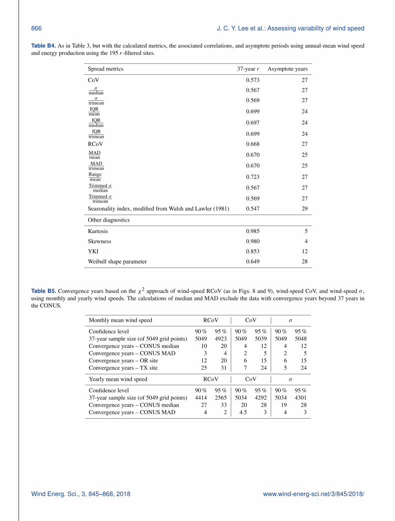
866 J. C. Y. Lee et al.: Assessing variability of wind speed
Table B4. As in Table 3, but with the calculated metrics, the associated correlations, and asymptote periods using annual-mean wind speedand energy production using the 195 r-filtered sites.
Spread metrics 37-year r Asymptote years
CoV 0.573 27σ
median 0.567 27σ
trimean 0.569 27IQRmean 0.699 24
IQRmedian 0.697 24
IQRtrimean 0.699 24
RCoV 0.668 27MADmean 0.670 25MAD
trimean 0.670 25Rangemean 0.723 27Trimmed σ
median 0.567 27Trimmed σ
trimean 0.569 27
Seasonality index, modified from Walsh and Lawler (1981) 0.547 29
Other diagnostics
Kurtosis 0.985 5
Skewness 0.980 4
YKI 0.853 12
Weibull shape parameter 0.649 28
Table B5. Convergence years based on the χ2 approach of wind-speed RCoV (as in Figs. 8 and 9), wind-speed CoV, and wind-speed σ ,using monthly and yearly wind speeds. The calculations of median and MAD exclude the data with convergence years beyond 37 years inthe CONUS.
Monthly mean wind speed RCoV CoV σ
Confidence level 90 % 95 % 90 % 95 % 90 % 95 %37-year sample size (of 5049 grid points) 5049 4923 5049 5039 5049 5048Convergence years – CONUS median 10 20 4 12 4 12Convergence years – CONUS MAD 3 4 2 5 2 5Convergence years – OR site 12 20 6 15 6 15Convergence years – TX site 25 31 7 24 5 24
Yearly mean wind speed RCoV CoV σ
Confidence level 90 % 95 % 90 % 95 % 90 % 95 %37-year sample size (of 5049 grid points) 4414 2565 5034 4292 5034 4301Convergence years – CONUS median 27 33 20 28 19 28Convergence years – CONUS MAD 4 2 4.5 3 4 3
Wind Energ. Sci., 3, 845–868, 2018 www.wind-energ-sci.net/3/845/2018/
J. C. Y. Lee et al.: Assessing variability of wind speed 867
Author contributions. All authors formulated the research ideaand designed the methodology together. JCYL performed the anal-ysis; MJF and JKL provided critical feedback. JCYL prepared themanuscript with contributions from the two co-authors.
Competing interests. Julie K. Lundquist is an Associate Editorof Wind Energy Science. Joseph C. Y. Lee and M. Jason Fields haveno conflict of interest.
Acknowledgements. This work was authored by the NationalRenewable Energy Laboratory, operated by the Alliance for Sus-tainable Energy, LLC, for the U.S. Department of Energy (DOE),under contract no. DE-AC36-08GO28308. Funding was providedby the U.S. Department of Energy Office of Energy Efficiency andRenewable Energy’s Wind Energy Technologies Office. The viewsexpressed in the article do not necessarily represent the views ofthe DOE or U.S. Government. The U.S. Government retains andthe publisher, by accepting the article for publication, acknowledgesthat the U.S. Government retains a nonexclusive, paid up, irrevoca-ble, worldwide license to publish or reproduce the published form ofthis work, or allow others to do so, for U.S. Government purposes.
The authors would like to thank our collaborators, Vineel Yet-tella and Mark Handschy of the Cooperative Institute for Researchin Environmental Sciences (CIRES) at the University of ColoradoBoulder; our colleagues at NREL, especially Paul Veers; andCory Jog at EDF Renewable Energy.
Edited by: Christian MassonReviewed by: two anonymous referees
References
Archer, C. L. and Jacobson, M. Z.: Geographical and seasonal vari-ability of the global “practical” wind resources, Appl. Geogr., 45,119–130, https://doi.org/10.1016/j.apgeog.2013.07.006, 2013.
Baker, R. W., Walker, S. N., and Wade, J. E.: Annual and seasonalvariations in mean wind speed and wind turbine energy pro-duction, Sol. Energy, 45, 285–289, https://doi.org/10.1016/0038-092X(90)90013-3, 1990.
Bandi, M. M. and Apt, J.: Variability of the Wind Turbine PowerCurve, Appl. Sci., 6, 262, https://doi.org/10.3390/app6090262,2016.
Bett, P. E., Thornton, H. E., and Clark, R. T.: Europeanwind variability over 140 yr, Adv. Sci. Res., 10, 51–58,https://doi.org/10.5194/asr-10-51-2013, 2013.
Bodini, N., Lundquist, J. K., Zardi, D., and Handschy, M.:Year-to-year correlation, record length, and overconfidence inwind resource assessment, Wind Energ. Sci., 1, 115–128,https://doi.org/10.5194/wes-1-115-2016, 2016.
Bosilovich, M. G., Lucchesi, R., and Suarez, M.: MERRA-2: FileSpecification, GMAO Office Note No. 9 (Version 1.1), availableat: https://gmao.gsfc.nasa.gov/pubs/docs/Bosilovich785.pdf (lastaccess: 1 August 2017), 2016.
Brower, M. C.: Wind resource assessment: a practical guide to de-veloping a wind project, Wiley, Hoboken, New Jersey, USA,2012.
Cannon, D. J., Brayshaw, D. J., Methven, J., Coker, P.J., and Lenaghan, D.: Using reanalysis data to quan-tify extreme wind power generation statistics: A 33 yearcase study in Great Britain, Renew. Energy, 75, 767–778,https://doi.org/10.1016/j.renene.2014.10.024, 2015.
Chen, L., Li, D., and Pryor, S. C.: Wind speed trends over China:quantifying the magnitude and assessing causality, Int. J. Clima-tol., 33, 2579–2590, https://doi.org/10.1002/joc.3613, 2013.
Clifton, A., Smith, A., and Fields, M.: Wind Plant Preconstruc-tion Energy Estimates: Current Practice and Opportunities,NREL/TP-5000-64735, National Renewable Energy Laboratory,Golden, Colorado, USA, available at: http://www.nrel.gov/docs/fy16osti/64735.pdf (last access: 19 July 2017), 2016.
Dee, D. P., Uppala, S. M., Simmons, A. J., Berrisford, P., Poli,P., Kobayashi, S., Andrae, U., Balmaseda, M. A., Balsamo, G.,Bauer, P., Bechtold, P., Beljaars, A. C. M., van de Berg, L., Bid-lot, J., Bormann, N., Delsol, C., Dragani, R., Fuentes, M., Geer,A. J., Haimberger, L., Healy, S. B., Hersbach, H., Hólm, E. V,Isaksen, L., Kållberg, P., Köhler, M., Matricardi, M., McNally,A. P., Monge-Sanz, B. M., Morcrette, J.-J., Park, B.-K., Peubey,C., de Rosnay, P., Tavolato, C., Thépaut, J.-N., and Vitart, F.: TheERA-Interim reanalysis: configuration and performance of thedata assimilation system, Q. J. Roy. Meteor. Soc., 137, 553–597,https://doi.org/10.1002/qj.828, 2011.
Gelaro, R., McCarty, W., Suárez, M. J., Todling, R., Molod, A.,Takacs, L., Randles, C. A., Darmenov, A., Bosilovich, M. G., Re-ichle, R., Wargan, K., Coy, L., Cullather, R., Draper, C., Akella,S., Buchard, V., Conaty, A., da Silva, A. M., Gu, W., Kim, G.-K., Koster, R., Lucchesi, R., Merkova, D., Nielsen, J. E., Par-tyka, G., Pawson, S., Putman, W., Rienecker, M., Schubert, S. D.,Sienkiewicz, M., and Zhao, B.: The Modern-Era RetrospectiveAnalysis for Research and Applications, Version 2 (MERRA-2),J. Climate, 30, 5419–5454, https://doi.org/10.1175/JCLI-D-16-0758.1, 2017.
GMAO (Global Modeling and Assimilation Office): MERRA2tavg1_2d_slv_Nx: 2d, 1-Hourly, Time-Averaged, Single-Level,Assimilation, Single-Level Diagnostics V5.12.4, Greenbelt, MD,USA, 2015.
Gunturu, U. B. and Schlosser, C. A.: Characterization of windpower resource in the United States, Atmos. Chem. Phys., 12,9687–9702, https://doi.org/10.5194/acp-12-9687-2012, 2012.
Hamlington, B. D., Hamlington, P. E., Collins, S. G., Alexander,S. R., and Kim, K.-Y.: Effects of climate oscillations on windresource variability in the United States, Geophys. Res. Lett., 42,145–152, https://doi.org/10.1002/2014GL062370, 2015.
Hdidouan, D. and Staffell, I.: The impact of climate change onthe levelised cost of wind energy, Renew. Energ., 101, 575–592,https://doi.org/10.1016/j.renene.2016.09.003, 2017.
Justus, C. G., Mani, K., and Mikhail, A. S.: Interannualand Month-to-Month Variations of Wind Speed, J. Appl.Meteorol., 18, 913–920, https://doi.org/10.1175/1520-0450(1979)018<0913:IAMTMV>2.0.CO;2, 1979.
Klink, K.: Trends and Interannual Variability ofWind Speed Distributions in Minnesota, J. Cli-mate, 15, 3311–3317, https://doi.org/10.1175/1520-0442(2002)015<3311:TAIVOW>2.0.CO;2, 2002.
Krakauer, N. and Cohan, D.: Interannual Variability and SeasonalPredictability of Wind and Solar Resources, Resources, 6, 29,https://doi.org/10.3390/resources6030029, 2017.
www.wind-energ-sci.net/3/845/2018/ Wind Energ. Sci., 3, 845–868, 2018
868 J. C. Y. Lee et al.: Assessing variability of wind speed
Lackner, M. A., Rogers, A. L., and Manwell, J. F.: UncertaintyAnalysis in MCP-Based Wind Resource Assessment and EnergyProduction Estimation, J. Sol. Energy Eng., 130, 31006–31010,https://doi.org/10.1115/1.2931499, 2008.
Leahy, P. G. and McKeogh, E. J.: Persistence of low wind speedconditions and implications for wind power variability, Wind En-ergy, 16, 575–586, https://doi.org/10.1002/we.1509, 2013.
Lee, J. C.-Y., Fields, M. J., Lundquist, J. K., and Lu-nacek, M.: Determining variabilities of non-Gaussian wind-speed distributions using different metrics and timescales, J.Phys. Conf. Ser., 1037, 072038, https://doi.org/10.1088/1742-6596/1037/7/072038, 2018.
Li, X., Zhong, S., Bian, X., and Heilman, W. E.: Climate and cli-mate variability of the wind power resources in the Great Lakesregion of the United States, J. Geophys. Res., 115, D18107,https://doi.org/10.1029/2009JD013415, 2010.
Lunacek, M., Jason Fields, M., Craig, A., Lee, J. C. Y., Meissner,J., Philips, C., Sheng, S., and King, R.: Understanding Biases inPre-Construction Estimates, J. Phys. Conf. Ser., 1037, 062009,https://doi.org/10.1088/1742-6596/1037/6/062009, 2018.
Montgomery, D. C. and Runger, G. C.: Applied statistics and proba-bility for engineers, 6th Edn., Wiley, Hoboken, New Jersey, USA,2014.
Pryor, S. C. and Barthelmie, R. J.: Climate change impacts onwind energy: A review, Renew. Sust. Energ. Rev., 14, 430–437,https://doi.org/10.1016/j.rser.2009.07.028, 2010.
Pryor, S. C., Barthelmie, R. J., and Schoof, J. T.: Inter-annual vari-ability of wind indices across Europe, Wind Energy, 9, 27–38,https://doi.org/10.1002/we.178, 2006.
Pryor, S. C., Barthelmie, R. J., Young, D. T., Takle, E. S., Arritt, R.W., Flory, D., Gutowski, W. J., Nunes, A., and Roads, J.: Windspeed trends over the contiguous United States, J. Geophys. Res.,114, D14105, https://doi.org/10.1029/2008JD011416, 2009.
Rose, S. and Apt, J.: What can reanalysis data tell usabout wind power?, Renew. Energ., 83, 963–969,https://doi.org/10.1016/j.renene.2015.05.027, 2015.
Rose, S. and Apt, J.: Quantifying sources of uncertainty in re-analysis derived wind speed, Renew. Energ., 94, 157–165,https://doi.org/10.1016/j.renene.2016.03.028, 2016.
Torralba, V., Doblas-Reyes, F. J., and Gonzalez-Reviriego, N.: Un-certainty in recent near-surface wind speed trends: a globalreanalysis intercomparison, Environ. Res. Lett., 12, 114019,https://doi.org/10.1088/1748-9326/aa8a58, 2017.
Walsh, R. P. D. and Lawler, D. M.: Rainfall seasonality: description,spatial patterns and change through time, Weather, 36, 201–208,https://doi.org/10.1002/j.1477-8696.1981.tb05400.x, 1981.
Wan, Y.-H.: Wind Power Plant Behaviors: Analyses of Long-Term Wind Power Data, NREL/TP-500-36551, National Re-newable Energy Laboratory, Golden, Colorado, USA, avail-able at: https://www.nrel.gov/docs/fy04osti/36551.pdf (last ac-cess: 19 July 2017), 2004.
Watson, S.: Quantifying the variability of wind energy, WIREsEnergy Environ., 3, 330–342, https://doi.org/10.1002/wene.95,2014.
Watson, S. J., Kritharas, P., and Hodgson, G. J.: Wind speed vari-ability across the UK between 1957 and 2011, Wind Energy, 18,21–42, 2015.
Wilks, D. S.: Statistical methods in the atmospheric sciences, Aca-demic Press, Amsterdam, the Netherlands, 2011.
Wind Energ. Sci., 3, 845–868, 2018 www.wind-energ-sci.net/3/845/2018/
Related Documents