Assessing time scales of atmospheric turbulence at - HAL - OBSPM

HAL Id: tel-00171277https://tel.archives-ouvertes.fr/tel-00171277

Submitted on 12 Sep 2007

HAL is a multi-disciplinary open accessarchive for the deposit and dissemination of sci-entific research documents, whether they are pub-lished or not. The documents may come fromteaching and research institutions in France orabroad, or from public or private research centers.

L’archive ouverte pluridisciplinaire HAL, estdestinée au dépôt et à la diffusion de documentsscientifiques de niveau recherche, publiés ou non,émanant des établissements d’enseignement et derecherche français ou étrangers, des laboratoirespublics ou privés.

Assessing time scales of atmospheric turbulence atobservatory sites

Aglae Kellerer

To cite this version:Aglae Kellerer. Assessing time scales of atmospheric turbulence at observatory sites. Astrophysics[astro-ph]. Université Paris-Diderot - Paris VII, 2007. English. <tel-00171277>

U D DP 7

presentee

pour obtenir le grade de

Docteur de l’Universite Paris VII

Specialite: Astrophysique et Instrumentations Associees

A K

Assessing time scales of atmospheric

turbulence at observatory sites

Soutenue le 7 Septembre 2007 devant la Commission d’examen :

President : Pr. Gerard RoussetDirecteurs de these : Dr. Vincent Coude du Foresto

Dr. Monika Petr-GotzensRapporteurs : Dr. Tony Travouillon

Dr. Jean VerninExaminateurs : Dr. Thierry Fusco

Dr. Marc Sarazin

2

The worst moment for the atheist

is when he is really thankful

and has nobody to thank.

Dante Gabriel Rossetti (1828-1882)

For me – as a really thankful atheist – it is a pleasure to have many peopleto thank, and first of all, my family.

I am grateful to my thesis supervisors Monika Petr-Gotzens and VincentCoude du Foresto and I am indebted to Marc Sarazin for very useful discussionsand constant help. Thanks to Rodolphe Krawczyk who has followed my workwith his natural enthusiasm, and to Tony Travouillon and Jean Vernin whohave kindly accepted to referee this dissertation.

It was a pleasure and privilege to work with many other colleagues: KarimAgabi, Nancy Ageorges, Eric Aristidi, Gerardo Avila, Timothy Butterley, JohnDavis, Rosanna Faraggiana, Thierry Fusco, Michele Gerbaldi, Christian Hum-mel, Pierre Kervella, Victor Kornilov, Stefan Kraus, Isabelle Mocoeur, GerardRousset, Tatyana Sadibekova, Klara Shabun, Bruno Valat, Martin Vannier,Richard Wilson, Markus Wittkowski.

Endless thanks go to Andrei Tokovinin. He patiently read through manydrafts of my work. Deficiencies that remain, do so despite his best endeavors.

4

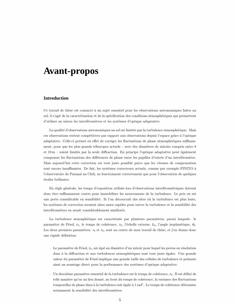
Avant-propos

Introduction

Ce travail de these est consacre a un sujet essentiel pour les observations astronomiques faites au

sol; il s’agit de la caracterisation et de la specification des conditions atmospheriques qui permettent

d’utiliser au mieux les interferometres et les systemes d’optique adaptative.

La qualite d’observations astronomiques au sol est limitee par la turbulence atmospherique. Mais

ces observations restent competitives par rapport aux observations depuis l’espace grace a l’optique

adaptative. Celle-ci permet en effet de corriger les fluctuations de phase atmospheriques suffisam-

ment, pour que les plus grands telescopes actuels – avec des diametres de miroirs compris entre 8

et 10m – soient limites par la seule diffraction. En principe l’optique adaptative peut egalement

compenser les fluctuations des differences de phase entre les pupilles d’entree d’un interferometre.

Mais aujourd’hui cette correction est tout juste possible parce que les vitesses de compensation

sont encore insuffisantes. De fait, les systemes correcteurs actuels, comme par exemple FINITO a

l’observatoire de Paranal au Chili, ne fonctionnent correctement que pour l’observation de quelques

etoiles brillantes.

En regle generale, les temps d’exposition utilises lors d’observations interferometriques doivent

donc etre suffisamment courts pour immobiliser les mouvements de la turbulence. Le prix en est

une perte considerable en sensibilite. Si l’on decouvrait des sites ou la turbulence est plus lente,

les systemes de correction seraient alors assez rapides pour suivre la turbulence et la sensibilite des

interferometres en serait considerablement amelioree.

La turbulence atmospherique est caracterisee par plusieurs parametres, parmi lesquels: le

parametre de Fried, r0, le temps de coherence, τ0, l’echelle externe, L0, l’angle isoplanetique, θ0.

Les deux premiers parametres: r0 et τ0, sont au centre de mon travail de these, et j’en donne donc

une rapide definition:

– Le parametre de Fried, r0, est egal au diametre d’un miroir pour lequel les pertes en resolution

dues a la diffraction et aux turbulences atmospheriques sont tout juste egales. Une grande

valeur du parametre de Fried implique une grande taille des cellules de turbulence et presente

ainsi un avantage direct pour la performance des systemes d’optique adaptative.

– Un deuxieme parametre essentiel de la turbulence est le temps de coherence, τ0. Il est defini de

telle maniere qu’en un lieu donne, au bout du temps de coherence, la variance des fluctuations

temporelles de phase dues a la turbulence soit egale a 1 rad2. Le temps de coherence determine

notamment la sensibilite des interferometres.

5

6

Ces deux parametres varient d’un site a l’autre, mais a la difference de r0, le temps de coherence

depend egalement de la vitesse de la turbulence. Et comme il n’existe actuellement aucune methode

adaptee pour mesurer le temps de coherence avec un petit telescope, les campagnes de selection

et de monitoring s’appuient principalement sur la mesure du parametre de Fried. En pratique,

on se refere plutot au seeing, ε0, qu’au parametre de Fried, mais ces deux quantites sont en fait

equivalentes: le seeing est egal a la resolution angulaire d’un telescope avec un miroir de diametre

r0.

Un nouvel instrument FADE

Au cours de mon travail de these, nous avons propose une methode pour mesurer le temps de

coherence. Elle consiste a defocaliser l’image d’une etoile et a en faire – grace a une obstruction

centrale sur le miroir primaire – un anneau diffus. Une lentille avec une aberration spherique est

alors placee sur le trajet du faisceau, la combinaison d’une defocalisation et de l’aberration spherique

etant choisie de facon a s’apparenter au mieux a une aberration conique: l’anneau diffus est ainsi

focalise sur un anneau fin. De fait, notre methode est la fille isotrope du Differential Image Motion

Monitor, DIMM, l’instrument de reference pour la mesure du seeing.

La turbulence atmospherique deforme l’image; ces deformations peuvent etre convenablement

mesurees parce qu’au premier ordre elles se traduisent par des changements de rayons de l’anneau.

L’avantage de cette methode est notamment son insensibilite aux aberrations de tip et tilt qui sont

causees en partie par la turbulence mais aussi par les vibrations de telescope, et qui n’interessent

donc pas la turbulence seule. Au lieu du tip et tilt , nous mesurons le coefficient de defocalisation

qui est a l’origine des variations du rayon. Une relation entre les fluctuations temporelles du rayon

et le temps de coherence a ete etabli dans le cadre du modele de Kolmogorov de la turbulence

atmospherique.1

Des premieres mesures avec ce Fast Defocus Monitor, FADE, ont ete obtenues a l’observatoire de

Cerro Tololo au Chili, du 29 Octobre au 2 Novembre 2006. L’instrument comportait un telescope

de 0.35 m de diametre et une camera a lecture rapide; nous avons enregistre des images d’anneaux

pendant cinq nuits en faisant varier les parametres instrumentaux. L’analyse de ces mesures et de

leurs incertitudes est presentee dans le manuscrit. Il nous a fallu faire particulierement attention

aux aberrations optiques du telescope et aux taches de scintillation causees par la turbulence dans

la haute atmosphere. Ces deux effets pouvant modifier le rayon de l’anneau, nous avons etablis des

criteres de rejet des images trop deformees.

Le seeing et le temps de coherence estimes avec FADE ont ete compares aux resultats obtenus

par les instruments de reference que sont DIMM et le Multi Aperture Scintillation Sensor, MASS. A

Cerro Tololo, MASS et DIMM sont installes derriere un meme telescope, sur une tour de 6 m a 10 m

du dome dans lequel se trouvait FADE. Les resultats ne sont pas identiques parce que MASS et

DIMM observaient des etoiles moins brillantes que FADE, et sondaient donc une partie differente

de l’atmosphere. Statistiquement, sur l’ensemble des 5 nuits, FADE a tendance a sous-estimer le

seeing. Nous avons pu reproduire cet effet avec des simulations d’anneaux diffus. Et nous pensons

donc que cette sous-estimation est due – sur cet instrument prototype – a ce que la combinaison de

1On prefere souvent caracteriser la turbulence en utilisant le modele de Van Karman, qui est essentiellement equivalent aumodele de Kolmogorov a ceci pres qu’il prend en compte l’effet de l’echelle externe. Or l’echelle externe n’a pas d’effet surles fluctuations rapides qui determinent le temps de coherence, et nous nous sommes donc places dans le cadre plus simpledu modele de Kolmogorov.

7

defocalisation et d’aberrations spherique n’etait pas optimisee et ne s’apparentait pas bien a une

aberration conique.

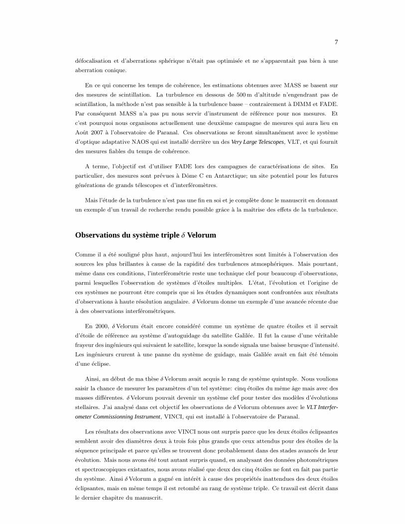
En ce qui concerne les temps de coherence, les estimations obtenues avec MASS se basent sur

des mesures de scintillation. La turbulence en dessous de 500 m d’altitude n’engendrant pas de

scintillation, la methode n’est pas sensible a la turbulence basse – contrairement a DIMM et FADE.

Par consequent MASS n’a pas pu nous servir d’instrument de reference pour nos mesures. Et

c’est pourquoi nous organisons actuellement une deuxieme campagne de mesures qui aura lieu en

Aout 2007 a l’observatoire de Paranal. Ces observations se feront simultanement avec le systeme

d’optique adaptative NAOS qui est installe derriere un des Very Large Telescopes, VLT, et qui fournit

des mesures fiables du temps de coherence.

A terme, l’objectif est d’utiliser FADE lors des campagnes de caracterisations de sites. En

particulier, des mesures sont prevues a Dome C en Antarctique; un site potentiel pour les futures

generations de grands telescopes et d’interferometres.

Mais l’etude de la turbulence n’est pas une fin en soi et je complete donc le manuscrit en donnant

un exemple d’un travail de recherche rendu possible grace a la maıtrise des effets de la turbulence.

Observations du systeme triple δ Velorum

Comme il a ete souligne plus haut, aujourd’hui les interferometres sont limites a l’observation des

sources les plus brillantes a cause de la rapidite des turbulences atmospheriques. Mais pourtant,

meme dans ces conditions, l’interferometrie reste une technique clef pour beaucoup d’observations,

parmi lesquelles l’observation de systemes d’etoiles multiples. L’etat, l’evolution et l’origine de

ces systemes ne pourront etre compris que si les etudes dynamiques sont confrontees aux resultats

d’observations a haute resolution angulaire. δVelorum donne un exemple d’une avancee recente due

a des observations interferometriques.

En 2000, δVelorum etait encore considere comme un systeme de quatre etoiles et il servait

d’etoile de reference au systeme d’autoguidage du satellite Galilee. Il fut la cause d’une veritable

frayeur des ingenieurs qui suivaient le satellite, lorsque la sonde signala une baisse brusque d’intensite.

Les ingenieurs crurent a une panne du systeme de guidage, mais Galilee avait en fait ete temoin

d’une eclipse.

Ainsi, au debut de ma these δVelorum avait acquis le rang de systeme quintuple. Nous voulions

saisir la chance de mesurer les parametres d’un tel systeme: cinq etoiles du meme age mais avec des

masses differentes. δVelorum pouvait devenir un systeme clef pour tester des modeles d’evolutions

stellaires. J’ai analyse dans cet objectif les observations de δVelorum obtenues avec le VLT Interfer-

ometer Commissionning Instrument, VINCI, qui est installe a l’observatoire de Paranal.

Les resultats des observations avec VINCI nous ont surpris parce que les deux etoiles eclipsantes

semblent avoir des diametres deux a trois fois plus grands que ceux attendus pour des etoiles de la

sequence principale et parce qu’elles se trouvent donc probablement dans des stades avances de leur

evolution. Mais nous avons ete tout autant surpris quand, en analysant des donnees photometriques

et spectroscopiques existantes, nous avons realise que deux des cinq etoiles ne font en fait pas partie

du systeme. Ainsi δVelorum a gagne en interet a cause des proprietes inattendues des deux etoiles

eclipsantes, mais en meme temps il est retombe au rang de systeme triple. Ce travail est decrit dans

le dernier chapitre du manuscrit.

8

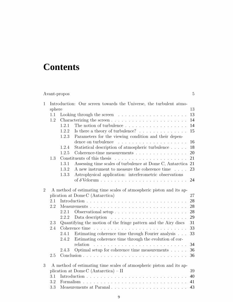
Contents

Avant-propos 5

1 Introduction: Our screen towards the Universe, the turbulent atmo-sphere 131.1 Looking through the screen . . . . . . . . . . . . . . . . . . . . 131.2 Characterizing the screen . . . . . . . . . . . . . . . . . . . . . . 14

1.2.1 The notion of turbulence . . . . . . . . . . . . . . . . . . 141.2.2 Is there a theory of turbulence? . . . . . . . . . . . . . . 151.2.3 Parameters for the viewing condition and their depen-

dence on turbulence . . . . . . . . . . . . . . . . . . . . 161.2.4 Statistical description of atmospheric turbulence . . . . . 181.2.5 Coherence-time measurements . . . . . . . . . . . . . . . 20

1.3 Constituents of this thesis . . . . . . . . . . . . . . . . . . . . . 211.3.1 Assessing time scales of turbulence at Dome C, Antarctica 211.3.2 A new instrument to measure the coherence time . . . . 231.3.3 Astrophysical application: interferometric observations

of δVelorum . . . . . . . . . . . . . . . . . . . . . . . . . 24

2 A method of estimating time scales of atmospheric piston and its ap-plication at DomeC (Antarctica) 272.1 Introduction . . . . . . . . . . . . . . . . . . . . . . . . . . . . . 282.2 Measurements . . . . . . . . . . . . . . . . . . . . . . . . . . . . 28

2.2.1 Observational setup . . . . . . . . . . . . . . . . . . . . . 282.2.2 Data description . . . . . . . . . . . . . . . . . . . . . . 29

2.3 Quantifying the motion of the fringe pattern and the Airy discs 312.4 Coherence time . . . . . . . . . . . . . . . . . . . . . . . . . . . 33

2.4.1 Estimating coherence time through Fourier analysis . . . 332.4.2 Estimating coherence time through the evolution of cor-

relation . . . . . . . . . . . . . . . . . . . . . . . . . . . 342.4.3 Optimal setup for coherence time measurements . . . . . 36

2.5 Conclusion . . . . . . . . . . . . . . . . . . . . . . . . . . . . . . 36

3 A method of estimating time scales of atmospheric piston and its ap-plication at DomeC (Antarctica) – II 393.1 Introduction . . . . . . . . . . . . . . . . . . . . . . . . . . . . . 403.2 Formalism . . . . . . . . . . . . . . . . . . . . . . . . . . . . . . 413.3 Measurements at Paranal . . . . . . . . . . . . . . . . . . . . . . 43

9

10

3.3.1 Observational set-up . . . . . . . . . . . . . . . . . . . . 433.3.2 Derivation of atmospheric parameters . . . . . . . . . . . 443.3.3 Performance of the piston scope . . . . . . . . . . . . . . 45

3.4 Measurements at DomeC . . . . . . . . . . . . . . . . . . . . . 483.5 Conclusions . . . . . . . . . . . . . . . . . . . . . . . . . . . . . 51

4 Atmospheric coherence times in interferometry: definition and mea-surement 534.1 Introduction . . . . . . . . . . . . . . . . . . . . . . . . . . . . . 544.2 Atmospheric coherence time in interferometry . . . . . . . . . . 54

4.2.1 Atmospheric coherence time τ0 . . . . . . . . . . . . . . 544.2.2 Piston time constant . . . . . . . . . . . . . . . . . . . . 564.2.3 Piston power spectrum and structure function . . . . . . 574.2.4 Error of a fringe tracking servo . . . . . . . . . . . . . . 584.2.5 Summary of definitions and discussion . . . . . . . . . . 59

4.3 Measuring the atmospheric time constant . . . . . . . . . . . . . 604.3.1 Existing methods of τ0 measurement . . . . . . . . . . . 604.3.2 The new method: FADE . . . . . . . . . . . . . . . . . . 61

4.4 Conclusions . . . . . . . . . . . . . . . . . . . . . . . . . . . . . 644.5 Appendix A - Derivation of the piston structure function . . . . 654.6 Appendix B - Fast focus variation . . . . . . . . . . . . . . . . . 67

5 FADE, an instrument to measure the atmospheric coherence time 695.1 Introduction . . . . . . . . . . . . . . . . . . . . . . . . . . . . . 705.2 The instrument . . . . . . . . . . . . . . . . . . . . . . . . . . . 71

5.2.1 Operational principle . . . . . . . . . . . . . . . . . . . . 715.2.2 Hardware . . . . . . . . . . . . . . . . . . . . . . . . . . 725.2.3 Optics . . . . . . . . . . . . . . . . . . . . . . . . . . . . 725.2.4 Acquisition software . . . . . . . . . . . . . . . . . . . . 735.2.5 Observations . . . . . . . . . . . . . . . . . . . . . . . . 74

5.3 Data analysis . . . . . . . . . . . . . . . . . . . . . . . . . . . . 745.3.1 Estimating the ring radius . . . . . . . . . . . . . . . . . 745.3.2 Noise and limiting stellar magnitude . . . . . . . . . . . 765.3.3 The response coefficient of FADE . . . . . . . . . . . . . 775.3.4 Derivation of the seeing and coherence time . . . . . . . 78

5.4 Analysis of observations . . . . . . . . . . . . . . . . . . . . . . 805.4.1 Influence of instrumental parameters . . . . . . . . . . . 805.4.2 Comparison with MASS and DIMM . . . . . . . . . . . . 82

5.5 Conclusions and perspectives . . . . . . . . . . . . . . . . . . . . 835.6 Appendix A – Estimator of the ring radius and center . . . . . . 845.7 Appendix B – Structure function of atmospheric defocus . . . . 855.8 Appendix C – Simulations . . . . . . . . . . . . . . . . . . . . . 86

5.8.1 Simulation tool . . . . . . . . . . . . . . . . . . . . . . . 86

6 Interferometric observations of the multiple stellar system δVelorum 936.1 Introductory remarks to the article . . . . . . . . . . . . . . . . 936.2 Introduction . . . . . . . . . . . . . . . . . . . . . . . . . . . . . 97

11

6.3 Characteristics of δ Vel A derived from previous measurements . 986.3.1 Orbit orientation and eccentricity . . . . . . . . . . . . . 986.3.2 Semi-major axis and stellar parameters . . . . . . . . . . 100

6.4 VLT Interferometer/VINCI observations . . . . . . . . . . . . . 1016.4.1 Data description . . . . . . . . . . . . . . . . . . . . . . 1016.4.2 Comparison to a model . . . . . . . . . . . . . . . . . . . 102

6.5 Results and discussion . . . . . . . . . . . . . . . . . . . . . . . 1046.5.1 The close eclipsing binary δVel (Aa-Ab) . . . . . . . . . 1046.5.2 The physical association of δVel C and D . . . . . . . . . 105

6.6 Summary . . . . . . . . . . . . . . . . . . . . . . . . . . . . . . 105

7 Conclusion 107

Bibliography 111

Summary 115

12 Contents

Chapter 1

Introduction: Our screen towards the

Universe, the turbulent atmosphere

Life on earth and its evolution have become possible because of the radiationshield, i.e. the atmosphere layer with a mass equivalent to about 10m of water.While it is a precondition for existence, it complicates life for the astronomerand astrophysicist, who desires an unfiltered view of the universe. Lookingthrough the screen in order to find those locations on the planet where theview is least obstructed is, thus, an important task. It is also the major issueof the research outlined in this thesis.

1.1 Looking through the screen

It is doubtlessly a tribute to the astronomers and engineers that they havedeveloped instruments precise enough to detect earth-like planets several lightyears removed. An example of current interest are the lately discovered com-panions of the 20 light-years distant Gliese 581[9]. Their detection was, ofcourse, indirect: temporal line-shifts on the spectrum of the star, correspond-ing to velocity variations of only 2 to 3 meters per second, were used to inferthe presence of a planet about 5 times the mass of Earth. To resolve the planetagainst its central star, i.e. to obtain a separate point image (1 pixel) at opticalwavelengths, a telescope with mirror diameter of at least 15m would be re-quired. To obtain more than a point image a truly gigantic mirror, far beyondtechnical feasibility would be required. While a point image will probably beachieved with the next generation of large telescopes, the system could alreadybe resolved by combining the light collected by several telescopes, that is byinterferometry – provided the distortion by atmospheric fluctuations could beovercome. At present the angular resolution and contrast of single-dish tele-scopes, as well as the sensitivity of interferometers, are limited by atmosphericturbulence and the planets of Gliese 581can, therefore, not yet be resolved.

13

14 Chapter 1

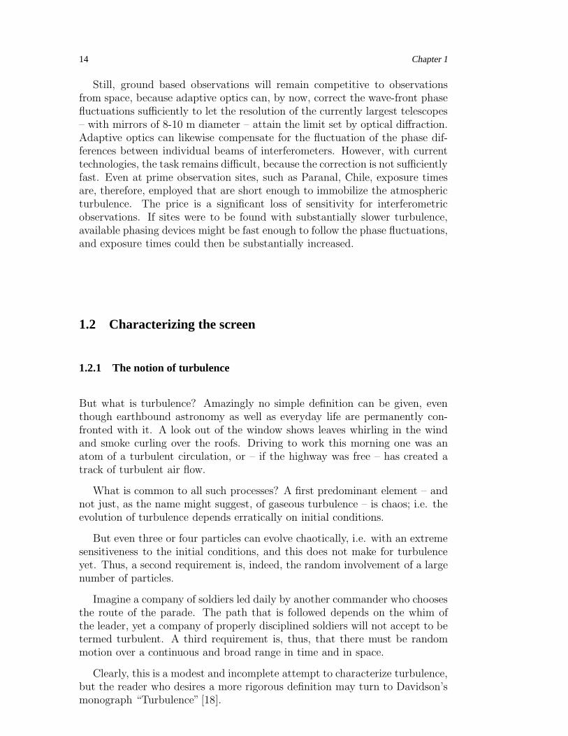
Still, ground based observations will remain competitive to observationsfrom space, because adaptive optics can, by now, correct the wave-front phasefluctuations sufficiently to let the resolution of the currently largest telescopes– with mirrors of 8-10 m diameter – attain the limit set by optical diffraction.Adaptive optics can likewise compensate for the fluctuation of the phase dif-ferences between individual beams of interferometers. However, with currenttechnologies, the task remains difficult, because the correction is not sufficientlyfast. Even at prime observation sites, such as Paranal, Chile, exposure timesare, therefore, employed that are short enough to immobilize the atmosphericturbulence. The price is a significant loss of sensitivity for interferometricobservations. If sites were to be found with substantially slower turbulence,available phasing devices might be fast enough to follow the phase fluctuations,and exposure times could then be substantially increased.

1.2 Characterizing the screen

1.2.1 The notion of turbulence

But what is turbulence? Amazingly no simple definition can be given, eventhough earthbound astronomy as well as everyday life are permanently con-fronted with it. A look out of the window shows leaves whirling in the windand smoke curling over the roofs. Driving to work this morning one was anatom of a turbulent circulation, or – if the highway was free – has created atrack of turbulent air flow.

What is common to all such processes? A first predominant element – andnot just, as the name might suggest, of gaseous turbulence – is chaos; i.e. theevolution of turbulence depends erratically on initial conditions.

But even three or four particles can evolve chaotically, i.e. with an extremesensitiveness to the initial conditions, and this does not make for turbulenceyet. Thus, a second requirement is, indeed, the random involvement of a largenumber of particles.

Imagine a company of soldiers led daily by another commander who choosesthe route of the parade. The path that is followed depends on the whim ofthe leader, yet a company of properly disciplined soldiers will not accept to betermed turbulent. A third requirement is, thus, that there must be randommotion over a continuous and broad range in time and in space.

Clearly, this is a modest and incomplete attempt to characterize turbulence,but the reader who desires a more rigorous definition may turn to Davidson’smonograph “Turbulence” [18].

Chapter 1 15

1.2.2 Is there a theory of turbulence?

Turbulence is in general merely a nuisance phenomenon. Where it becomescritical, however, for example in aerodynamics, thermodynamics or meteorol-ogy it needs to be studied and it is found to be complex and quite diverse. Apilot may be well informed about turbulence in aerodynamics, yet he wouldbe confused, when the meteorologist were to add to the weather forecast hisanalysis of atmospheric turbulence. Likewise an astrophysicist might approachhis colleague from the thermodynamics department and give him mass, tem-perature and size of a star of particular interest whose spectral image he wouldlike to understand. He, too, might be confounded by a host of information inthe answer, that is difficult to relate to his problem and by the great numberof associated caveats.

To simplify matters, one would wish to have a theory that predicts large-scale movements in turbulent flows, and that indicates the energy distributionover different spatial scales. Ideally, it should be applicable to a broad range ofphenomena, from gas flows in galaxies to currents in the oceans. But presentlythere are as many theories as there are problems.

Yet astronomers are fortunate: where they wish to characterize atmosphericturbulence, they profit from one of the exceptional success stories in turbulencephysics. It is due to the Russian mathematician Andrei N. Kolmogorov whostudied turbulent flows from air jets and published his results in 1931 [43]. Ashis point of departure, Kolmogorov used Richardson’s assumption that – ina turbulent medium – the energy is continually transferred from large-scaleto small-scale structures, where it is eventually dissipated by viscosity [56]; hethen assumed an isotropic medium in equilibrium and deduced the law:

E( f , ǫ) = α ǫ2/3 f −5/3 (1.1)

where f is the norm of the three-dimensional spatial-frequency vector f ,and E( f , ǫ) d f equals the energy contained in vortices with spatial frequenciesbetween f and f + d f , in a fluid characterized by its rate, ǫ, of viscous dissi-pation. The Kolmogorov constant, α, is a function of the Reynolds number,R= LV/ν, where L and V are the characteristic size and speed of the turbulentflow, while ν is the viscosity of the fluid. The viscosity of air is 15· 10−6m2 s−1;taking L = 15m/s and V = 1m/s leads to R = 106 which corresponds to fullydeveloped turbulence. Landau and Lifshitz [45] have shown that α ∼ 1.52, atsuch high Reynolds numbers.

This law, which predicts the energy distribution over spatial scales, restsentirely on the hypothesis of a continuous dissipation of kinetic energy fromlarge to small scales. Even though it is heuristic and not strictly proven,the law is in excellent agreement with observations, within the inertial range1/L0 ≪ f ≪ 1/l0. Here L0 denotes the size of the largest vortices, which – for

16 Chapter 1

our atmosphere – may vary between roughly 10m and 100m. While l0 – thescale, below which the energy is predominantly dissipated by viscous friction– ranges from a few millimeters to about 1 cm.

Figure 1.1: A turbulent cascade as seen by Leonardo da Vinci.Reproduced from [19].

1.2.3 Parameters for the viewing condition and their dependence on turbu-

lence

The viewing conditions at an observatory site relate to two major aspects. Thefirst aspect is the resolution attainable with long exposures and a telescope ofgiven mirror diameter, D. For small telescopes the angular resolution is entirelylimited by diffraction:

ε = 0.976λ/D (1.2)

For a 0.1m-telescope, the angular resolution at wavelength λ = 0.5µmequals 4.9 · 10−6 rad, i.e. 1”.

With increasing mirror sizes the resolution tends to be increasingly affectedby the wavefront distortions due to atmospheric turbulence. To characterizethe magnitude of this influence, it is convenient to refer to the mirror diam-eter where the effect of diffraction becomes just equal to the degradation ofresolution due to the atmosphere. This diameter is termed Fried parameter,r0, where the somewhat uncommon use of the letter r for a diameter needsto be noted. Under poor conditions – for example even during clear nights atsea level – the Fried parameter may rarely be better than about 1 cm. Underoptimum conditions, such as on clear nights at Paranal, Chile, the value maygo up to 1m for wavelengths between 0.5 to 1µm. Large telescope mirrorscan then profitably be used, and they will attain excellent resolution, whenadaptive optics are being used that correct for phase differences by acting onindividual mirror segments.

Chapter 1 17

In practice one tends to refer to the seeing, ε0, rather than the Fried pa-rameter, r0, but the two quantities are essentially equivalent, the seeing beingthe angular resolution of a telescope with mirror diameter r0:

ε0 = 0.976λ/r0 (1.3)

Thus, the Fried parameters 1 cm and 1m correspond, at the wavelength0.5 µm, to seeing values of 10” and 0.1”.

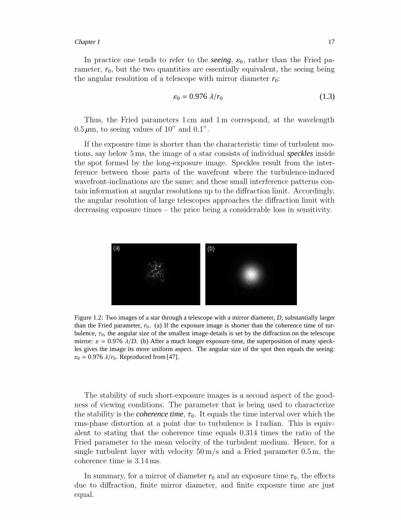
If the exposure time is shorter than the characteristic time of turbulent mo-tions, say below 5ms, the image of a star consists of individual specklesinsidethe spot formed by the long-exposure image. Speckles result from the inter-ference between those parts of the wavefront where the turbulence-inducedwavefront-inclinations are the same; and these small interference patterns con-tain information at angular resolutions up to the diffraction limit. Accordingly,the angular resolution of large telescopes approaches the diffraction limit withdecreasing exposure times – the price being a considerable loss in sensitivity.

Figure 1.2: Two images of a star through a telescope with a mirror diameter,D, substantially largerthan the Fried parameter,r0. (a) If the exposure image is shorter than the coherence timeof tur-bulence,τ0, the angular size of the smallest image-details is set by thediffraction on the telescopemirror: ε = 0.976 λ/D. (b) After a much longer exposure time, the superposition ofmany speck-les gives the image its more uniform aspect. The angular sizeof the spot then equals the seeing:ε0 = 0.976λ/r0. Reproduced from [47].

The stability of such short-exposure images is a second aspect of the good-ness of viewing conditions. The parameter that is being used to characterizethe stability is the coherence time, τ0. It equals the time interval over which therms-phase distortion at a point due to turbulence is 1 radian. This is equiv-alent to stating that the coherence time equals 0.314 times the ratio of theFried parameter to the mean velocity of the turbulent medium. Hence, for asingle turbulent layer with velocity 50m/s and a Fried parameter 0.5m, thecoherence time is 3.14ms.

In summary, for a mirror of diameter r0 and an exposure time τ0, the effectsdue to diffraction, finite mirror diameter, and finite exposure time are justequal.

18 Chapter 1

1.2.4 Statistical description of atmospheric turbulence

In his extensive analysis of the statistical properties of atmospheric turbulence,Roddier [58] examined the implications of Kolmogorov’s law for the propaga-tion of optical wavefronts. Some of the results that are used in the subsequentchapters can be summarized as follows.

The turbulent mixing of the air creates inhomogeneities of temperature, T,which likewise follow Kolmogorov’s law:

WT( f ) ∝ f −5/3 (1.4)

WT( f ) = |T( f )2| is the power spectrum of temperature fluctuations, wherethe symbol: · denotes the Fourier transform. In an isotropic medium, thethree-dimensional power spectrum WT(f ) = WT( fx, fy, fz) is related to the one-dimensional power spectrum through an integration over two directions:

WT( f ) = 4π f 2 WT(f ) (1.5)

Thus,

WT(f ) ∝ f −11/3 (1.6)

The refractive index of air, n, is a function not only of the temperaturebut also of the humidity. However at visible and near infrared wavelengths, nproves to be largely insensitive to water vapor concentration; its fluctuationsfollow therefore the same law as the temperature fluctuations:

Wn(f ) = 3.9 · 10−5 C2n f −11/3 (1.7)

The index structure constant, C2n, is related to the local gradient of the optical

index. It determines the contribution of the turbulence in the specified airlayer to optical propagation and typically it varies between 10−15m−2/3 and10−13m−2/3.

Fluctuations of the wavefront phase, ϕ, are due to the fluctuations of theoptical index. In the case of many thin turbulent layers – contributing eachonly a small phase change: dϕ ≪ 1rad – the spectrum of phase fluctuationsis, accordingly:

Wϕ(f ) = 9.7 · 10−3 k2 f −11/3

∫ hmax

0Cn(h)2 dh (1.8)

k = 2π/λ is the spectral wave number, and h denotes the altitude of aturbulent layer with thickness dh. This spectrum applies within the inertialrange 1/L0 ≪ f ≪ 1/l0.

Chapter 1 19

So much for the results of Roddier’s analysis. We conclude that, with regardto the propagation of visible light through the atmosphere, three essentialparameters are: C2

n, l0 and L0. A fourth parameter is the mean velocity,V, of the turbulent medium. Together these parameters determine the Friedparameter (or the seeing) and the coherence time:

– The Fried parameter, r0, is an integral over the structure index constant,C2

n:

r0 = [ 0.423k2 cos(γ)−1

∫ hmax

0Cn(h)2 dh ]−3/5 (1.9)

where γ is the zenith-angle. The viewing conditions are optimized, whenobservations are directed at the zenith; for lower angles the Fried param-eter decreases.

– The coherence time is a combination of the Fried parameter and of anaveraged wind speed, V5/3 (see Chapter 4):

τ0 = 0.314 r0/V5/3 (1.10)

Vp =

∫ hmax

0V(h)p Cn(h)2 dh

∫ hmax

0Cn(h)2 dh

1/p

(1.11)

This definition is based on the assumption that independent layers atdifferent heights, h, contribute to the turbulence, and that – in each layer– the turbulence as a whole is being displaced horizontally with velocityV(h).1

Both parameters, the seeing, ε0, and the coherence time, τ0, are site depen-dent. But there is a difference: the coherence time depends also on wind speed,and there is currently no adequate technique to measure the coherence time.For this reason, site testing and monitoring campaigns are currently restrictedto the assessment of the seeing.

1Turbulence arises predominantly at the interface of cold and warm layers that move in different directions. The resultingshear layer is displaced along the layers’ interface in goodagreement with Taylor’s hypothesis which assumesfrozen flows:“If the velocity of the air stream which carries the eddies isvery much greater than the turbulent velocity, one may assumethat the sequence of changes at a fixed point are simply due to the passage of an unchanging pattern of turbulent motion overthat point” [66]. But is this hypothesis adequate in spite of the fact that there are – relative to the overall motion of the layer –motions of the vortices and eddies? Most astronomers are familiar with the aspect of turbulent patterns that are formed overa telescope-mirror, because these patterns are readily observed on defocused stellar images: Generally, the pattern translates,indeed, with a common global motion, yet each individual, turbulent cell evolves and moves during the time it crosses thetelescope aperture. This suggests that the turbulent motion is a combination of a frozen-flow and a dispersive motion andTaylor’s hypothesis is, accordingly, an approximation. Infact, it has been shown that hisfrozen-flow hypothesisdescribes theturbulent motions up to time intervals 20 to 30 milliseconds, i.e. typically a few coherence-times (Gendron & Lena [24]andSchoeck & Spillar [62]).

20 Chapter 1

1.2.5 Coherence-time measurements

Because it determines the sensitivity of interferometers and the performance ofadaptive optic systems, the atmospheric coherence time, τ0, is a parameter ofmajor importance. Several instruments measure τ0 or related parameters, butall current methods have limitations: either the instrument is not well suitedfor site monitoring, or the method is burdened by intrinsic uncertainties andbiases.

– SCIDAR (Scintillation Detection And Ranging) has provided good resultson τ0, but it requires large telescopes and is not suitable for monitoring,since it necessitates manual data processing (Fuchs et al. [22]).

– Balloons provide only single-shot profiles of low statistical significance(Azouit & Vernin [8]).

– Adaptive-optic systems and interferometers give good results, but aresuitable neither for testing projected sites nor for long-term monitoring(Fusco et al. [23]).

The four subsequent methods all use small telescopes and can, thus, be usedfor site-testing. They all have their special attractions. However, with regardto the coherence time each has intrinsic problems:

– SSS (Single Star SCIDAR) in essence extends the SCIDAR technique tosmall telescopes: profiles of Cn(h)2 and V(h) are obtained with less altituderesolution than with SCIDAR, and are then used to derive the coherencetime (Habib et al. [29]).

– The GSM (Generalized Seeing Monitor) measures velocities of prominentatmospheric layers. By refined data processing, a coherence time, τAA –but one with a different dependence on the turbulence profile than τ0 –is deduced from the angle-of-arrival fluctuations (Ziad et al [73]).

– MASS (Multi-Aperture Scintillation Sensor) is a recent, but already wellproven, turbulence monitor. One of the measured quantities, related toscintillation in a 2 cm-aperture, approximates the coherence time, but thisaveraging does not include low-altitude layers and thus gives a biasedestimate of τ0 (Kornilov et al. [44]).

– DIMM (Differential Image Motion Monitor) is not actually meant to de-termine τ0, but an estimation of the coherence time can nevertheless beobtained by combining the measured r0 with meteorological wind-speeddata (Sarazin & Tokovinin [59]).

We conclude from this brief survey, that there is, at this point, no sufficientlysimple technique to measure τ0 with a small telescope.

Chapter 1 21

1.3 Constituents of this thesis

1.3.1 Assessing time scales of turbulence at Dome C, Antarctica

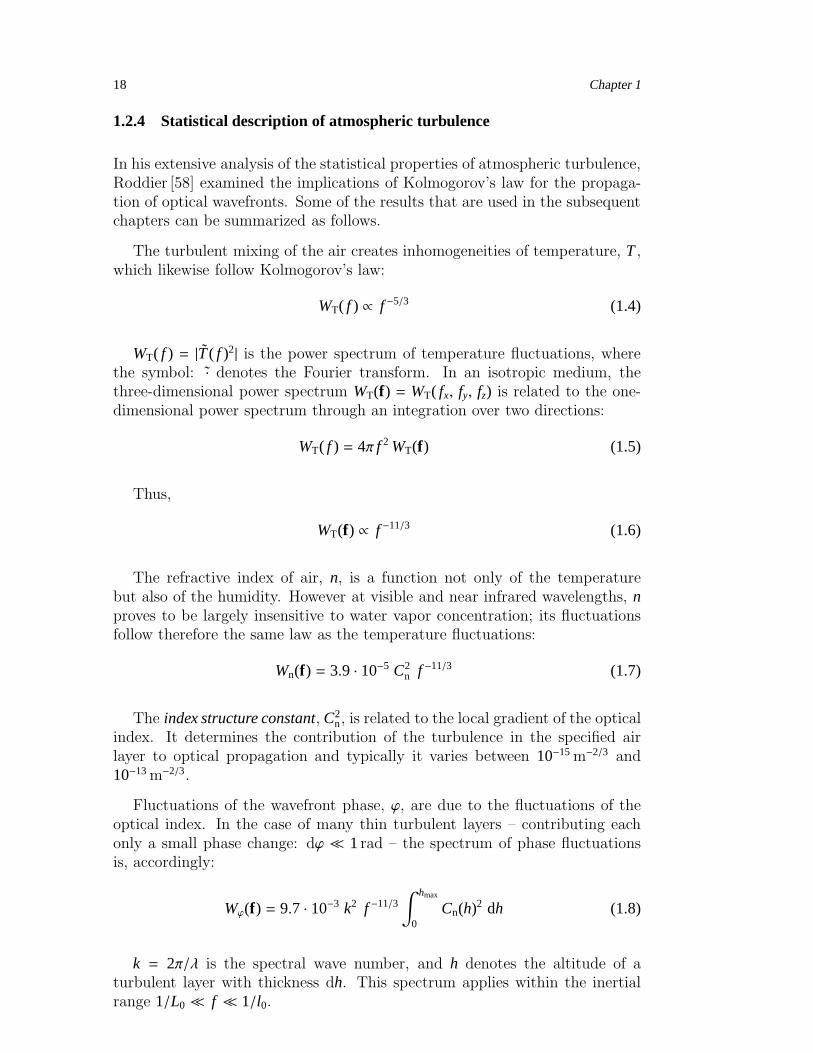
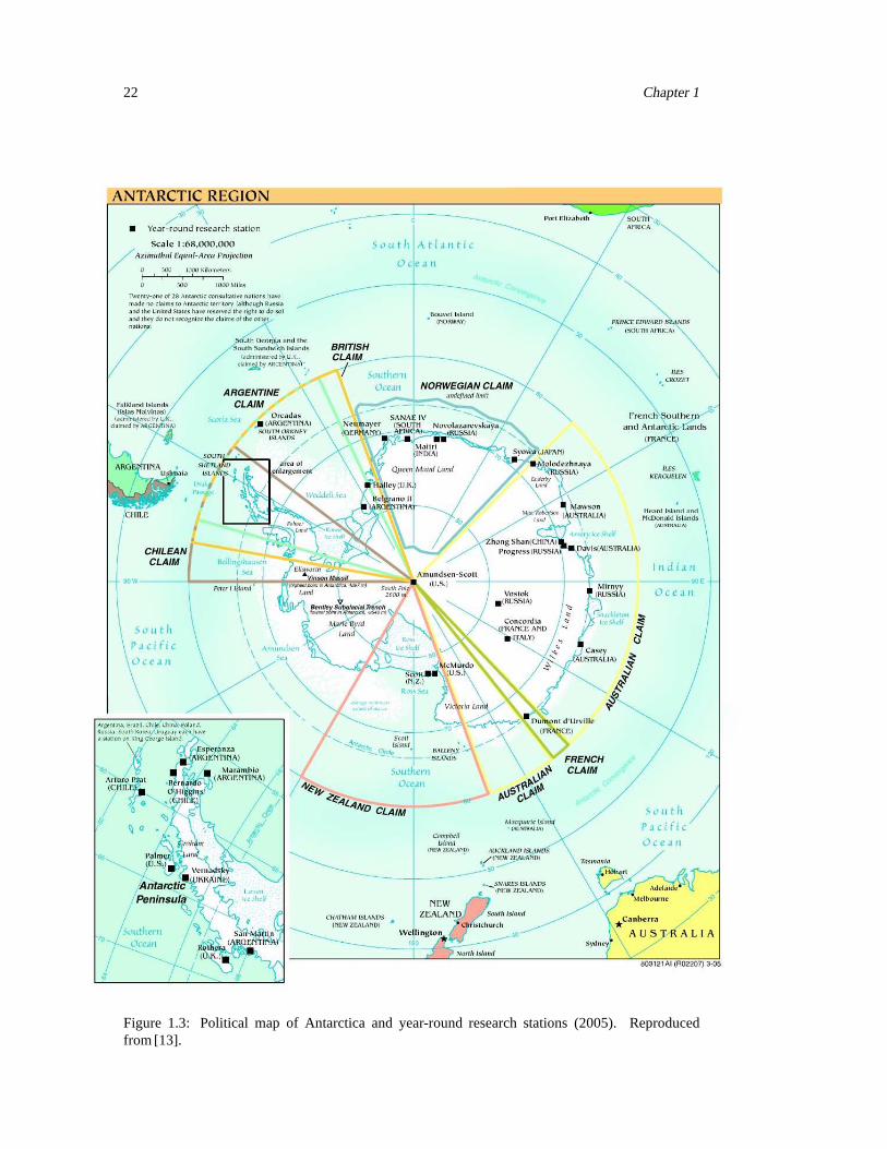
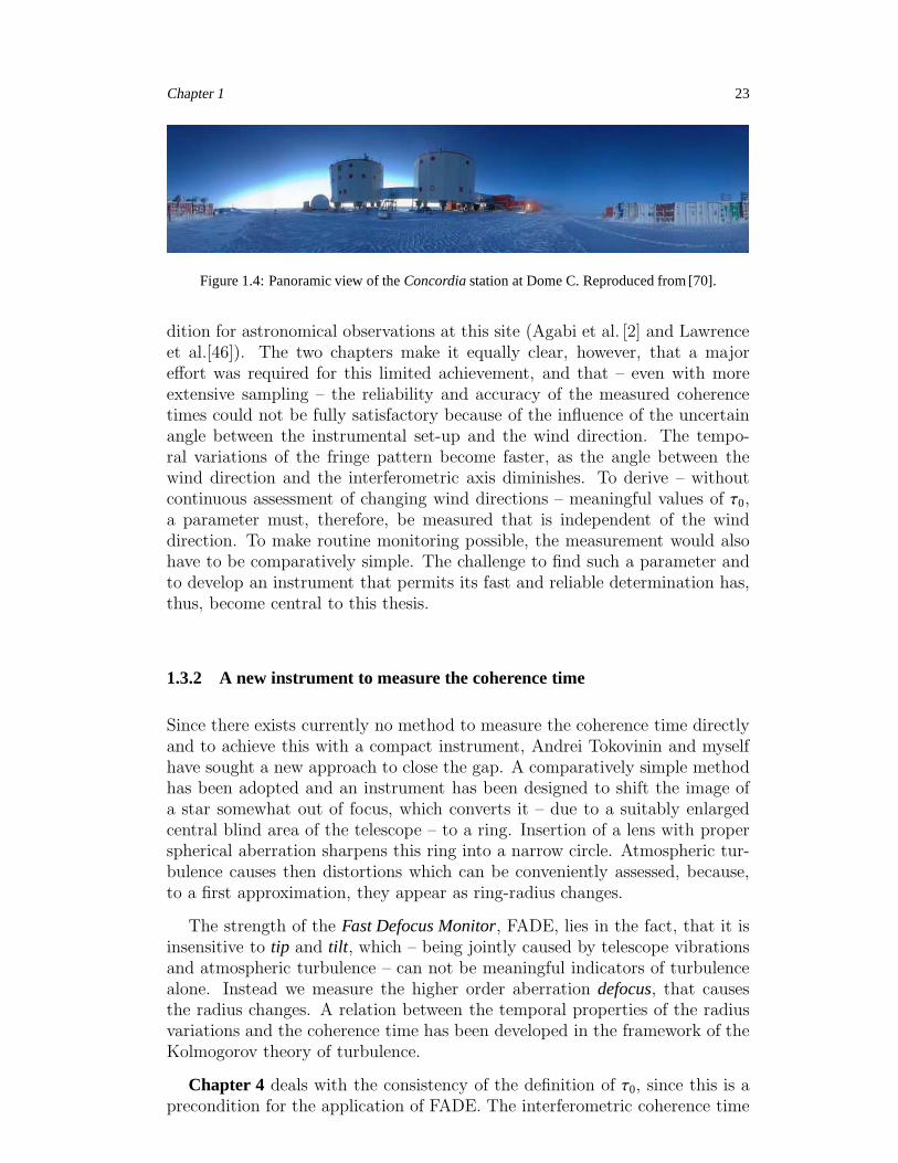
Dome C is a 3235m high summit (7506′ S, 12323′ E) on the Antarctic plateau.Because of its elevation, the location does not experience the winds that aretypical for the coastal regions of Antarctica. This has led to the assumption,that the atmospheric conditions might be particularly advantageous. In 2005,Concordia, a French-Italian station opened on Dome C, for research in astron-omy, glaciology, earth-science, etc. Aristidi et al. [5] and Lawrence et al. [46]determined the size of the turbulent cells, as measured 30m above ground,to be 2 to 3 times larger than at the best mid-latitude sites. The latter au-thors concluded, that an interferometer built on Dome C could potentiallywork on projects that would otherwise require a space mission. This is a clearpossibility, but it needs to be confirmed by measurements of the coherencetime.

Chapter 2 presents an analysis of the first interferometric fringes recordedat Dome C, Antarctica. Measurements were taken between January 31st andFebruary 2nd 2005 at daytime. The instrumental set-up, termed Pistonscope,aims at measuring temporal fluctuations of the atmospheric piston, which arecritical for interferometers and determine their sensitivity. The characteristictime scales are derived through the motion of the image that is formed in thefocal plane of a Fizeau interferometer. Although the coherence time of pistoncould not be determined directly – due to insufficient temporal and spatialsampling – a lower limit was, nevertheless, determined by studying the decayrate of correlation between successive fringes. Coherence times in excess of10ms were determined in the analysis, i.e. at least three times higher than themedian coherence time measured at the site of Paranal (3.3ms).

To test the validity of the results derived in terms of the pistonscope, mea-surements with this instrument have subsequently been obtained at the ob-servatory of Paranal, Chile, in April 2006 with high temporal and spatialresolution. In Chapter 3 the observations are analyzed, and it is found thatthe resulting atmospheric parameters are consistent with the data from theastronomical site monitor, if the Taylor hypothesis of “frozen flow” is invokedwith a single turbulent layer, i.e. if the atmospheric turbulence is taken to bedisplaced along a single direction. This has permitted a reassessment of ourpreliminary measurements – recorded with lower temporal and spatial resolu-tion – at the Antarctic site of Dome C, and it was seen that the calibrationin terms of the new data sharpened the conclusions of the first qualitativeexamination in Chapter 2.

As seen in Chapters 2 and 3, we have, in spite of the current limitations inmethodology and instrumentation, been able to infer considerably increasedcoherence times at Dome C, Antarctica, which is consistent with the earlier ex-tensive determinations of other parameters that demonstrate the superior con-

22 Chapter 1

Figure 1.3: Political map of Antarctica and year-round research stations (2005). Reproducedfrom [13].

Chapter 1 23

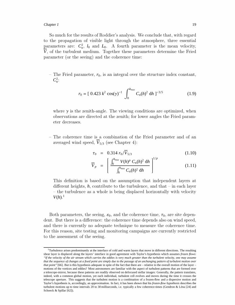
Figure 1.4: Panoramic view of theConcordiastation at Dome C. Reproduced from [70].

dition for astronomical observations at this site (Agabi et al. [2] and Lawrenceet al.[46]). The two chapters make it equally clear, however, that a majoreffort was required for this limited achievement, and that – even with moreextensive sampling – the reliability and accuracy of the measured coherencetimes could not be fully satisfactory because of the influence of the uncertainangle between the instrumental set-up and the wind direction. The tempo-ral variations of the fringe pattern become faster, as the angle between thewind direction and the interferometric axis diminishes. To derive – withoutcontinuous assessment of changing wind directions – meaningful values of τ0,a parameter must, therefore, be measured that is independent of the winddirection. To make routine monitoring possible, the measurement would alsohave to be comparatively simple. The challenge to find such a parameter andto develop an instrument that permits its fast and reliable determination has,thus, become central to this thesis.

1.3.2 A new instrument to measure the coherence time

Since there exists currently no method to measure the coherence time directlyand to achieve this with a compact instrument, Andrei Tokovinin and myselfhave sought a new approach to close the gap. A comparatively simple methodhas been adopted and an instrument has been designed to shift the image ofa star somewhat out of focus, which converts it – due to a suitably enlargedcentral blind area of the telescope – to a ring. Insertion of a lens with properspherical aberration sharpens this ring into a narrow circle. Atmospheric tur-bulence causes then distortions which can be conveniently assessed, because,to a first approximation, they appear as ring-radius changes.

The strength of the Fast Defocus Monitor, FADE, lies in the fact, that it isinsensitive to tip and tilt , which – being jointly caused by telescope vibrationsand atmospheric turbulence – can not be meaningful indicators of turbulencealone. Instead we measure the higher order aberration defocus, that causesthe radius changes. A relation between the temporal properties of the radiusvariations and the coherence time has been developed in the framework of theKolmogorov theory of turbulence.

Chapter 4 deals with the consistency of the definition of τ0, since this is aprecondition for the application of FADE. The interferometric coherence time

24 Chapter 1

– that characterizes the time scale of the fringe motion in an interferometer – isanalyzed and is found to have the same dependence on atmospheric parametersas the coherence time which is used in adaptive optics.

First measurements with FADE were obtained at Cerro Tololo, Chile, fromOctober 29th to November 2nd 2006. The instrumental set-up is based on atelescope with mirror diameter 0.35m and a fast CCD detector. Ring imageswere recorded during five nights with a broad range of instrument settings.The measurements and their uncertainties are analyzed in Chapter 5, andthe seeing and coherence-time values obtained in terms of our instrument arecompared with simultaneous measurements from the MASS and DIMM site-monitoring instruments.

1.3.3 Astrophysical application: interferometric observations ofδVelorum

Chapter 6 presents an example of how research is facilitated, when the influ-ence of the atmospheric fluctuations can be partly overcome. Interferometershave been introduced in astronomy to gain spatial resolution without the needto build extremely large telescopes. To resolve δVelorum in the infrared wouldrequire a telescope of about 100m mirror diameter. In contrast, the VLT In-terferometer Commissionning Instrument, VINCI, installed on Paranal in Chile,allows to resolve the bright, eclipsing binary Aa-Ab in δVelorum with twosmall 0.4m siderostats 100m apart.

Today, interferometric observations are limited to the brightest sources be-cause of turbulence-related rapid motions of the image. In spite of this currentlimitation, interferometry proves to be a key technique in many astrophysicaldomains. The study of multiple star systems is an example: to understand thestate, evolution and origin of such systems, the results of dynamical studiesneed to be compared to observations with high angular resolutions.

In 2000, δVelorum had become infamously famous among the engineers ofthe Galileo spacecraft; δVelorum was used as reference star for the guidancesystem, but at some point the system failed. While an instrumental defect wasassumed at first, it turned out subsequently that the star, not the space probe,was at fault. Galileo had in fact witnessed an eclipse. Since then δVelorumhad been classified as a quintuple stellar system and it promised to become akey system for testing stellar evolutionary models: five stars of same age andwith different masses.

Three years ago, I began analyzing observations that had been obtainedwith the VINCI recombination instrument. The results were startling, be-cause the diameters of the two eclipsing stars appear to be 2 to 3 times largerthan expected for main sequence stars: the two stars are thus probably in amore advanced evolutionary state. In the continued analysis of existing pho-tometric and spectroscopic data we found, that two of the five stars are, infact, not part of the system. Thus, δVelorum has become more attractive due

Chapter 1 25

to the unexpected properties of the eclipsing binary, while, at the same time,it relapsed to the status of a triple stellar system. This work is detailed inChapter 6.

26 Chapter 1

Chapter 2

A method of estimating time scales of

atmospheric piston and its

application at Dome C (Antarctica)

A. Kellerer, M. Sarazin, V. Coude du Foresto, K. Agabi, E. Aristidi, T.Sadibekova, 2006, Applied Optics, 45, 5709-5715

Abstract

This article presents the analysis of the first interferometric fringes recordedat DomeC, Antarctica. Measurements were done on January 31st and Febru-ary 1st 2005 at daytime.

The aim of the analysis is to measure temporal fluctuations of the atmo-spheric piston, which are critical for interferometers and determine their sensi-tivity. These scales are derived through the motion of the image that is formedin the focal plane of a Fizeau interferometer.

We could establish a lower limit to the coherence time by studying the decayrate of correlation between successive fringes. Coherence times are measured tobe larger than 10ms, i.e. at least three times higher than the median coherencetime measured at the site of Paranal (3.3ms).

27

28 Chapter 2

2.1 Introduction

While astronomical sites are usually selected mostly for the mild intensityof the atmospheric turbulence (large values of the Fried parameter r0), anequally important performance driver for ground based stellar interferometersis its temporal behavior. In passive arrays, a fast turbulence requires shorterexposure times to be frozen, thus reducing the sensitivity. In new generationactive arrays (which include phase control through adaptive optics and fringetracking), the optimum loop rate (for a given detection noise) is determinedmostly by the coherence time t0 of the atmospheric phase fluctuations, or ina more complete way by their temporal spectral power density. In a low fluxregime, a slower turbulence enables a lock of active systems on fainter sources,and therefore a higher sensitivity. For bright sources, a slower optimum looprate results in lower phase residuals, which are critical in high dynamic rangeapplications such as coronography or interferometric nulling [1]. Even in asingle-mode interferometer, where residual phase fluctuations accross a singlesub-pupil can be removed by proper spatial filtering (at the expense of a lossof photons), turbulence power remains in the form of the piston mode betweentwo separate sub-pupils, which causes fringe jitter and can be reduced only byactive fringe tracking.

Much interest has recently arisen in the potential of the high Antarcticplateau for astronomical observations. At DomeC (7506′ S, 12323′ E, 3235maltitude), Agabi et al. [2] and Lawrence et al. [46] have – during the antarticnight and for a telescope positioned 30m above the ground – determined aFried parameter roughly equal to 37 cm, which is 2 to 3 times larger than atthe best mid-latitude sites. However, direct measurements of the fluctuationtimes have yet to be performed.

In this paper we exploit the first stellar fringes recorded at DomeC (ob-tained with a Fizeau interferometer on a 20 cm baseline) and investigate how,despite their incomplete spatial and temporal sampling, they can be used toderive information on the coherence time of the piston.

2.2 Measurements

2.2.1 Observational setup

Several observations of Canopuswere made at DomeC on January 31st andFebruary 1st 2005, i.e. during the antarctic day. To track the fluctuations of theatmospheric piston, a modified Differential Image Motion Monitor (DIMM) [60]was placed 3.50m above the ground. The DIMM is a telescope with a focallength of 2.80m and 0.28m diameter primary mirror, whose entrance pupil iscovered by a mask with two 0.06m diameter circular openings, with centers0.20m apart.

Chapter 2 29

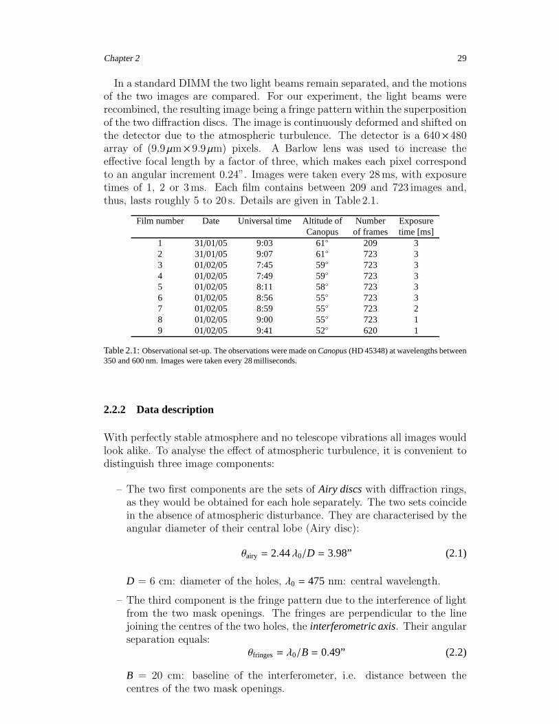
In a standard DIMM the two light beams remain separated, and the motionsof the two images are compared. For our experiment, the light beams wererecombined, the resulting image being a fringe pattern within the superpositionof the two diffraction discs. The image is continuously deformed and shifted onthe detector due to the atmospheric turbulence. The detector is a 640× 480array of (9.9µm× 9.9 µm) pixels. A Barlow lens was used to increase theeffective focal length by a factor of three, which makes each pixel correspondto an angular increment 0.24”. Images were taken every 28ms, with exposuretimes of 1, 2 or 3ms. Each film contains between 209 and 723 images and,thus, lasts roughly 5 to 20 s. Details are given in Table 2.1.

Film number Date Universal time Altitude of Number ExposureCanopus of frames time [ms]

1 31/01/05 9:03 61 209 32 31/01/05 9:07 61 723 33 01/02/05 7:45 59 723 34 01/02/05 7:49 59 723 35 01/02/05 8:11 58 723 36 01/02/05 8:56 55 723 37 01/02/05 8:59 55 723 28 01/02/05 9:00 55 723 19 01/02/05 9:41 52 620 1

Table 2.1:Observational set-up. The observations were made onCanopus(HD 45348) at wavelengths between350 and 600 nm. Images were taken every 28 milliseconds.

2.2.2 Data description

With perfectly stable atmosphere and no telescope vibrations all images wouldlook alike. To analyse the effect of atmospheric turbulence, it is convenient todistinguish three image components:

– The two first components are the sets of Airy discswith diffraction rings,as they would be obtained for each hole separately. The two sets coincidein the absence of atmospheric disturbance. They are characterised by theangular diameter of their central lobe (Airy disc):

θairy = 2.44λ0/D = 3.98” (2.1)

D = 6 cm: diameter of the holes, λ0 = 475 nm: central wavelength.

– The third component is the fringe pattern due to the interference of lightfrom the two mask openings. The fringes are perpendicular to the linejoining the centres of the two holes, the interferometric axis. Their angularseparation equals:

θfringes= λ0/B = 0.49” (2.2)

B = 20 cm: baseline of the interferometer, i.e. distance between thecentres of the two mask openings.

30 Chapter 2

The interference pattern is finite, because the observations are made on abroad spectral band from 350 nm to 600 nm. The characteristic angularwidth where fringes appear is:

θcoh = 2λ20/(B∆λ) = 1.86” (2.3)

∆λ = 250 nm: width of the wavelength interval.

The intensity profiles along the interferometric axis, is:

I (θ) = 2 I (0)

[

J1

(

2.44πθθairy

)

/

(

2.44πθθairy

)]2 [

1+ sinc

(

2πθθcoh

)

cos

(

2πθθfringes

)]

(2.4)

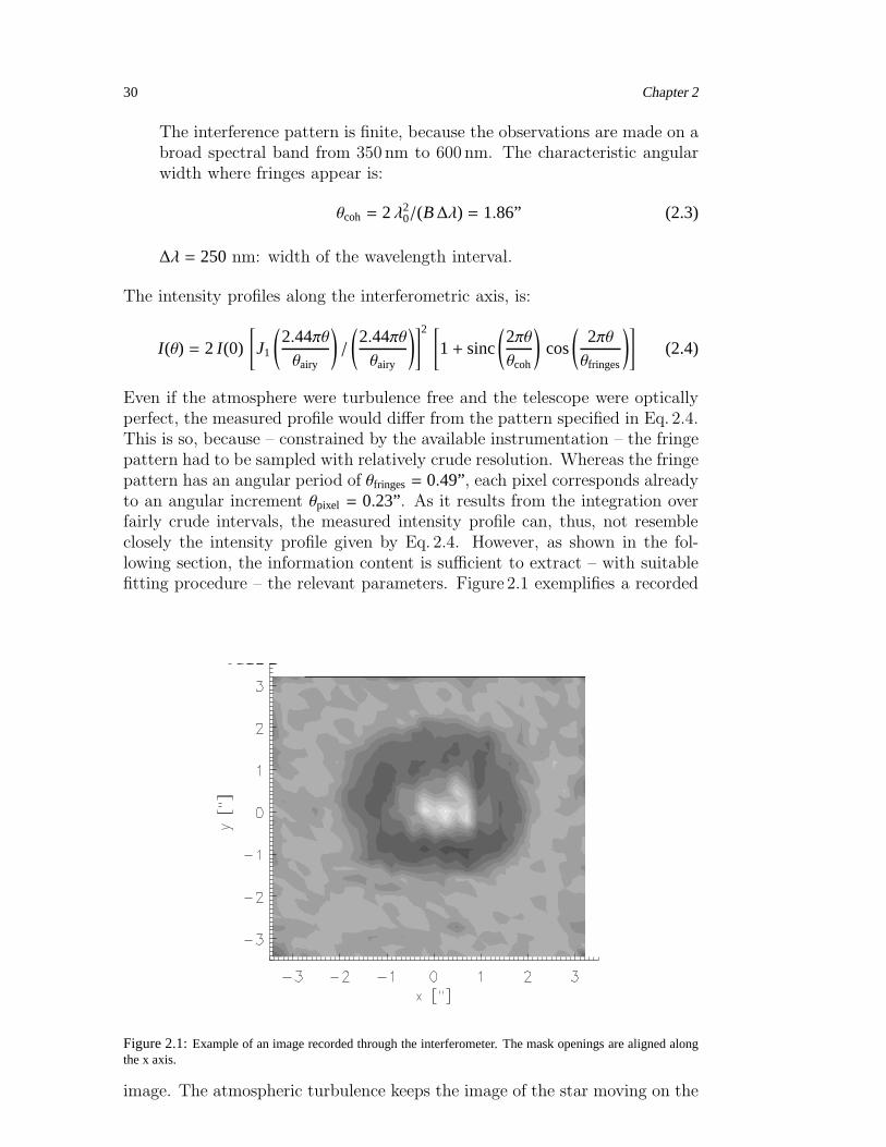
Even if the atmosphere were turbulence free and the telescope were opticallyperfect, the measured profile would differ from the pattern specified in Eq. 2.4.This is so, because – constrained by the available instrumentation – the fringepattern had to be sampled with relatively crude resolution. Whereas the fringepattern has an angular period of θfringes= 0.49”, each pixel corresponds alreadyto an angular increment θpixel = 0.23”. As it results from the integration overfairly crude intervals, the measured intensity profile can, thus, not resembleclosely the intensity profile given by Eq. 2.4. However, as shown in the fol-lowing section, the information content is sufficient to extract – with suitablefitting procedure – the relevant parameters. Figure 2.1 exemplifies a recorded

Figure 2.1:Example of an image recorded through the interferometer. The mask openings are aligned alongthe x axis.

image. The atmospheric turbulence keeps the image of the star moving on the

Chapter 2 31

detector. The local inclination of the wave front over each of the holes causesthe movements of the Airy discs, whereas difference in the optical path for thetwo holes, i.e. the piston, shifts the fringe pattern relative to the centre of theAiry discs. Telescope vibrations, on the other hand, cause merely a commonmovement of Airy discs and fringes. The relative movements between airydiscs and fringes are, therefore, solely due to the atmospheric turbulence. Thesubsequent analysis deals with their temporal patterns.

Piston changes shift the fringe pattern relative to the Airy discs along theinterferometric axis. Accordingly, in order to assess the temporal fluctuationsof the piston it is sufficient to consider the shift along the axis.

2.3 Quantifying the motion of the fringe pattern and the Airy

discs

Observations with a DIMM are commonly aimed at measuring the seeing pa-rameter by observing the relative motions of the Airy discs. In the presentmeasurements the two beams have been combined in order to analyze thepiston in terms of the motion of the fringe packet relative to the combinedAiry discs. The quantification of the axial motion requires the extraction of 4parameters from the observed images:

– position of the central fringe θf and contrast of the fringe pattern k,

– position, along the interferometric axis, of the center of the combined Airydiscs: θ0,

– intensity at the center of the combined Airy discs: I0.

No attempt was made to separate the two airy discs, since this would havemeant fitting six parameters on intensity profiles specified in terms of only 8(∼ θcoh/θpixel) data points.

The intensity profile is made up of three components with different spatialperiods (cf. Eq. 2.4): θairy/1.22, θcoh and θfringes. In line with relations discussedin the previous section, all three periods are superior to twice the pixel sizeθpixel. Hence, in spite of the fairly crude detector resolution the intensity profileis adequately sampled to extract unambiguously the central position of the twoAiry discs and the fringe pattern. To do so, the following profile was fittedonto the recorded intensity profiles:

I (θ) =∫ θ+θpixel/2

θ−θpixel/22I0

[

J1

(

2.44π(θ′ − θ0)θairy

)

/

(

2.44π(θ′ − θ0)θairy

)]2

[

1+ ksinc

(

2π(θ′ − θf )θcoh

)

cos

(

2π(θ′ − θf )θfringes

)]

dθ′ (2.5)

32 Chapter 2

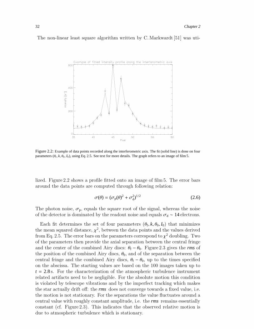
The non-linear least square algorithm written by C.Markwardt [51] was uti-

Figure 2.2:Example of data points recorded along the interferometric axis. The fit (solid line) is done on fourparameters (θf , k, θ0, I0), using Eq. 2.5. See text for more details. The graph refers to an image of film 5.

lized. Figure 2.2 shows a profile fitted onto an image of film5. The error barsaround the data points are computed through following relation:

σ(θ) = (σp(θ)2 + σ2

d)1/2 (2.6)

The photon noise, σp, equals the square root of the signal, whereas the noiseof the detector is dominated by the readout noise and equals σd ∼ 14electrons.

Each fit determines the set of four parameters (θf , k, θ0, I0) that minimizesthe mean squared distance, χ2, between the data points and the values derivedfrom Eq. 2.5. The error bars on the parameters correspond to χ2 doubling. Twoof the parameters then provide the axial separation between the central fringeand the center of the combined Airy discs: θf − θ0. Figure 2.3 gives the rms ofthe position of the combined Airy discs, θ0, and of the separation between thecentral fringe and the combined Airy discs, θf − θ0, up to the times specifiedon the abscissa. The starting values are based on the 100 images taken up tot = 2.8s. For the characterization of the atmospheric turbulence instrumentrelated artifacts need to be negligible. For the absolute motion this conditionis violated by telescope vibrations and by the imperfect tracking which makesthe star actually drift off: the rms does not converge towards a fixed value, i.e.the motion is not stationary. For the separations the value fluctuates around acentral value with roughly constant amplitude, i.e. the rms remains essentiallyconstant (cf. Figure 2.3). This indicates that the observed relative motion isdue to atmospheric turbulence which is stationary.

Chapter 2 33

Figure 2.3:Solid line: rms deviations of the axial image motion, measured over subsetsof increasing sizebetween 100 and 723 images. Dashed line:rms deviations of the axial separation between the central fringeand the combined Airy discs. The graph refers to the data set of film 5.

2.4 Coherence time

2.4.1 Estimating coherence time through Fourier analysis

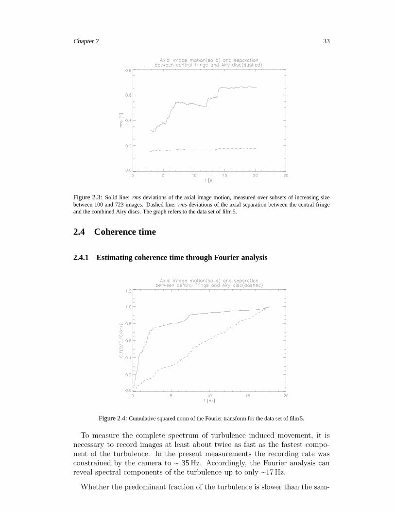
Figure 2.4:Cumulative squared norm of the Fourier transform for the data set of film 5.

To measure the complete spectrum of turbulence induced movement, it isnecessary to record images at least about twice as fast as the fastest compo-nent of the turbulence. In the present measurements the recording rate wasconstrained by the camera to ∼ 35Hz. Accordingly, the Fourier analysis canreveal spectral components of the turbulence up to only ∼17Hz.

Whether the predominant fraction of the turbulence is slower than the sam-

34 Chapter 2

pling rate is judged by taking the Fourier transform of the image motions andplotting the cumulated squared norm versus the frequency (cf. Figure 2.4).According to the Kolmogorov theory of turbulence the cumulative squarednorm, CF(f), becomes constant after the highest frequencies of atmosphericturbulence.

– For the absolute motions the nearly horizontal slope at 17Hz impliesthat the main part of the telescope vibrations is associated with lowerfrequencies.

– For the relative motions the dependence CF(f) still has positive slope atf = 17Hz, which suggests that the fastest components of the turbulenceexceed the recording rate. Thus, the characteristic time scales of atmo-spheric turbulence are inferior to ∼ 60ms, which is a very loose constraint,given typical atmospheric time scales. [46] It is of interest, whether theconclusions can be sharpened in terms of other considerations.

2.4.2 Estimating coherence time through the evolution of correlation

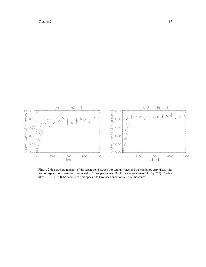
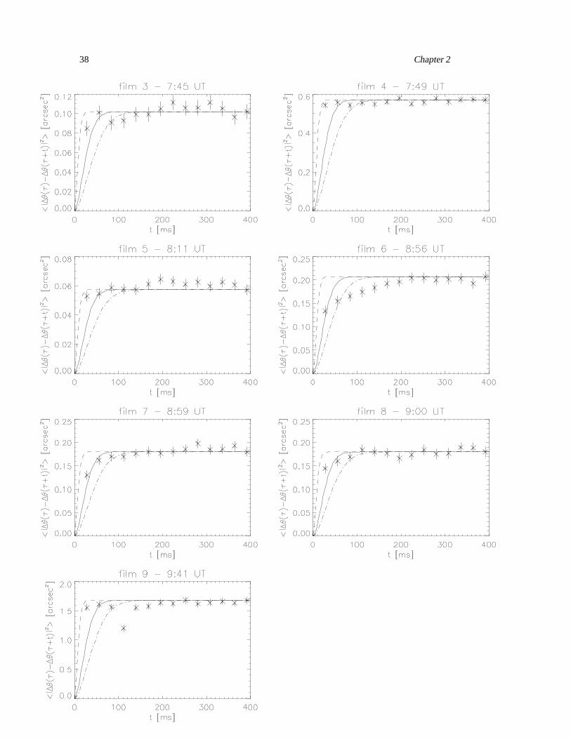
Although the sampling rates were too low in the present measurements toassess the fastest atmospheric turbulence through Fourier analysis, some in-formative inferences are still possible, because relevant information can beobtained by tracing the decay time of correlation between successive fringepositions. Figure 2.6 represents the following structure function as a functionof temporal separation:

D∆θ(t) = < |∆θ(τ + t) − ∆θ(τ)|2 > (2.7)

∆θ = θf − θ0: separation between the central fringe and the combined Airydiscs.

Figure 2.6 suggests that during films 1, 3, 5, 6, 7, 8 the cells of the turbulentatmosphere were correlated up to a hundred milliseconds, which is a verypromising result.

The coherence time of piston is estimated by comparing the structure func-tion predicted by the Kolmogorov spectrum of fluctuations [58] with the ob-served data:

D(t) = D(t ≫ t0) × (1− exp(−(t/t0)−5/3)) (2.8)

t0: coherence time.

Theoretical calculations have shown temporal power spectra of fringe mo-tion to have a shape that is unaffected by wind direction and baseline orien-tation. [17] In the case of differential image motion, only the low frequencydomain is dependent of wind direction. Evolution times of the separation

Chapter 2 35

between the central fringe and the combined Airy discs should, thus, be un-sensitive to wind direction and baseline orientation on times scales of severalcoherence times. We therefore take Eq. 2.8 as a valid approximation indepen-dently of wind direction and baseline orientation.

In Figure 2.6 the measured correlation curve is compared to theoreticalcurves obtained for the coherence times: 10, 30 and 50milliseconds. At mostfive data points lie inside the domain where the structure function has notreached its asymptotic value. Still, Figure 2.6 appears to suggest that duringfilms 1, 3, 5, 6, 7, 8, the coherence time of piston was superior to ten mil-liseconds. The coherence time was highest during films 6, 7, 8, i.e. around9:00 UT on February 1st. This is consistent with measurements of the seeing

Figure 2.5:Seeing angles measured by two DIMM instruments located 3.5 mand 8.5 m above the ground, onJanuary 31st and February 1st 2005.

angle at the same epoch: Figure 2.5 gives the seeing angles measured by twoDIMM instruments located 3.5m and 8.5m above the ground, on January 31st

and February 1st. The upper data series were acquired by the same telescopewhich was used for recording the fringes here analyzed. This explains the in-terruptions of the upper data series around 9:00UT the first day and startingfrom 7:45UT the second day. As can be seen from the data recorded with the

36 Chapter 2

instrument located at 8.5m, the seeing angle reached a local minimum around9:00UT on February 1st.

2.4.3 Optimal setup for coherence time measurements

The observations reported here were made with the equipment available on thesite and are subject to the following limitations, which will need to be liftedin future observations:

– The recording speed of the camera was not fully sufficient for sampling ofatmospheric turbulence. Increased recording rate will permit the precisedetermination of the actual coherence time. The highest frequencies of thepiston should – in line with the earlier (Agabi et al. [2] and Lawrence etal. [46]) and the present measurements – be less than 500Hz. Accordinglya recording rate of 1000Hz should ensure adequate temporal sampling.

– Caution is required, when the turbulent cells are larger than the distancebetween the two mask openings (20 cm). In these cases the differencebetween piston and tilt becomes too small to infer coherence times withsufficient precision. At the time of observations, the seeing varied between0.5” and 1.0” (cf. Figure 2.5). Thus, at 500 nm wavelength, the turbulentcells had a characteristic size (Fried parameter) between 10 cm and 20 cm,i.e. only just smaller than the baseline. For future measurements, weconsider the use of larger baselines up to 2m.

2.5 Conclusion

Stellar fringes were recorded at the Antarctic site of DomeC during day time,using a Fizeau configuration on a modified DIMM telescope. Despite the par-tial temporal and spatial sampling limitations imposed by the locally availableequipment, it was possible to determine a promising lower limit (around 10ms)to the coherence time of piston and to validate our experimental procedure.We are now considering regular observations using a dedicated setup – withlarger baselines and higher recording rates – to characterize the time scales ofatmospheric piston at DomeC, both during day and night time.

Chapter 2 37

Figure 2.6:Structure function of the separation between the central fringe and the combined Airy discs. Thefits correspond to coherence times equal to 10 (upper curve),30, 50 ms (lower curve) (cf. Eq. 2.8). Duringfilms 1, 3, 5, 6, 7, 8 the coherence time appears to have been superior to ten milliseconds.

38 Chapter 2

Chapter 3

A method of estimating time scales of

atmospheric piston and its

application at Dome C (Antarctica) –

II

A. Kellerer, M. Sarazin, T. Butterley, R. Wilson, 2007, Applies Optics, inpress

Abstract

Temporal fluctuations of the atmospheric piston are critical for interferom-eters as they determine their sensitivity. We characterize an instrumentalset-up, termed the piston scope, that aims at measuring the atmospheric timeconstant, τ0, through the image motion in the focal plane of a Fizeau interfer-ometer.

High-resolution piston scope measurements have been obtained at the obser-vatory of Paranal, Chile, in April 2006. The derived atmospheric parametersare shown to be consistent with data from the astronomical site monitor, pro-vided that the atmospheric turbulence is displaced along a single direction.Piston scope measurements, of lower temporal and spatial resolution, were forthe first time recorded in February 2005 at the Antarctic site of DomeC. Theirre-analysis in terms of the new data calibration sharpens the conclusions of afirst qualitative examination [41].

39

40 Chapter 3

3.1 Introduction

Interferometers have been introduced in astronomy to gain in spatial resolu-tion without the need to build extremely large telescopes. To resolve Sirius,observations in the infrared domain (∼ 2µm) would require a telescope ofabout 170m mirror diameter. Fortunately, Sirius can also be resolved by twotelescopes of more modest size, separated by 170m and operated as an inter-ferometer. Yet, despite this considerable gain in resolution, interferometers arenot the prime tool of today’s astronomers. This is largely due to their limitedsensitivity: atmospheric turbulence makes the interferometric fringe patternmove in the detector plane. Accordingly, one tends to use exposure times thatare short enough to “freeze” the turbulence, i.e. typically several milliseconds.To increase the sensitivity, phasing devices are being designed that measurethe position of the fringe pattern due to a reference star, and correct contin-uously for the fringe motion of the target object. For such devices to work, asufficient number of photons need to be collected on the reference star duringthe time when the atmosphere is frozen, i.e. during the atmospheric coherencetime τ0 = 0.314 r0/V5/3, where r0 is the Fried parameterand V5/3 is a weightedaverage of the turbulent layers’ velocities. Clearly, the coherence time is theparameter that determines the performance of today’s interferometers. Dif-ferent definitions of the atmospheric coherence time have been introduced inrelation to various observational techniques: single telescopes with or withoutadaptive-optics, interferometers with or without fringe trackers etc. Howeverthe standard adaptive-optics coherence time τ0 has been shown to quantify theperformance of all these techniques [42].

In a previous article [41], we characterized the temporal evolution of fringemotion at DomeC, a summit on the antarctic continent, and a potential sitefor a future interferometer, using the motion of the fringe pattern formed inthe focal plane of a Fizeau interferometer. The temporal and spatial samplingof the measurements were low due to the available equipment and, insteadof determining coherence-time values, the mean duration of correlation wasassessed by fitting the fringe correlation-function onto an exponential curve(cf. Section 3.4). Such measurements have now been repeated at the site ofParanal, Chile, with sufficient spatial and temporal sampling, to allow thedetermination of the coherence time. Further, all relevant atmospheric param-eters are constantly monitored at Paranal by a meteorological station, hencethe parameter values derived through our set-up (termed piston scope) can bechecked against reference values.

In the first Section, the quantities measured with the piston scope are relatedto the following atmospheric parameters: the Fried parameter, the turbulentlayers velocities and the coherence time – using the Kolmogorov theory ofatmospheric turbulence. The relations are then tested on the observationsperformed at Paranal. It is shown that when the sampling is sufficient, theprecision on the coherence time is limited by the piston scope’s sensitivity towind direction. Given these results, the third Section presents a new analysis

Chapter 3 41

of the measurements obtained at DomeC [41]. The lower limits to the coher-ence time, derived through our first qualitative analysis, are confirmed andadditional results on the Fried parameter and wavefront speed are given.

3.2 Formalism

The purpose of the piston scope experiment is to track the rapid fluctuationsof the atmospheric piston. To this effect, the entrance pupil of a telescopeis covered by a mask with two circular openings. The resulting image is afringe pattern within the superposition of the two diffraction discs. Atmo-spheric turbulence keeps the image of the star moving on the detector. Thelocal inclination of the wave front over each of the holes causes the movementof the Airy discs, whereas difference in the optical path for the two holes, i.e.the piston, shifts the fringe pattern relative to the center of the Airy discs.Telescope vibrations, on the other hand, cause merely a common movement ofAiry discs and fringes. The relative movements between Airy discs and fringesare, therefore, solely due to the atmospheric turbulence. The subsequent anal-ysis deals with their temporal patterns. Piston changes shift the fringe patternrelative to the Airy discs along the interferometric axis. Accordingly, in orderto assess the temporal fluctuations of the piston it is sufficient to consider theshift along the axis.

As suggested by Conan et al. [17], the spatial power spectrum Wφ of therelative movements between Airy discs and fringes is derived from the phasespectrum Wϕ, assuming a Kolmogorov model of turbulence with an infiniteouter scale. In the following we use the notations of Conan et al. [17].

Wϕ(f ) = 0.00969k2

∫ +∞

0f −11/3 C2

n dh, (3.1)

where f is the spatial frequency and k = 2π/λ the wavenumber. The turbulenceintensity of a layer i of thickness dh at altitude h is specified in terms of C2

n dh.The explicit dependence of C2

n and all following parameters on h is dropped toease the reading of the formulae. The measured quantity is the separation –along the interferometric axis, x – between the central fringe and the center ofthe combined Airy discs. The spatial filter M that converts Wϕ into the powerspectrum Wφ equals:

M(f ) = λ/(2π) A(f ) FT[(δB − δ0)/B− (δB + δ0)/2 ∗ d /dx](f ), (3.2)

for a baseline vector B and the aperture filter function A(f ). For a circularaperture of diameter D, A(f ) = 2J1(π f D)/(π f D) and f = |f |. Jn stands for theBessel function of order n. FT represents the Fourier transform, δL is the deltafunction centered on L and ∗ denotes convolution. Hence,

M(f ) = λ/(2π) A(f ) [2 sin(πfB) − 2πfB cos(πfB)] / B (3.3)

42 Chapter 3

Wφ(f ) = M2(f ) Wϕ(f ). (3.4)

In the single layer approximation, we assume the turbulent layer to be trans-ported with a velocity V directed at an angle α with respect to the baseline.The temporal power spectrum of the measured quantity is obtained by in-tegrating in the frequency plane over a line displaced by fx = ν/V from thecoordinate origin and inclined at angle α. Let fy be the integration variablealong this line and f 2 = f 2

x + f 2y . The temporal power spectrum equals:

wφ(ν) =1V

∫ +∞

−∞Wφ

(

fx cosα + fy sinα, fy cosα − fx sinα)

d fy (3.5)

We then derive the expression of the structure function:

Dφ(t) = 2∫ +∞

−∞(1− cos(2πνt))wφ(ν)dν (3.6)

= 2× 0.00969C2n dh / B2

∫ +∞

0f −8/3(2J1(π f d)/(π f d))2d f

∫ 2π

0(1− cos(2π f cos(θ + α)Vt))

[2 sin(πB f cosθ) − 2π f Bcosθ cos(π f Bcosθ)]2dθ (3.7)

The best estimate of the parameters is obtained by fitting the measured points

Figure 3.1: Structure functions of the fringe position relative to the combined Airy discs, for aninterferometer with mirror diametersD and baseline lengthB. The atmosphere is assumed to consistof a single layer displaced with wind speedV at an angleα from the baseline. The values ofα areindicated in the bottom right box.

to: Dφ(t) + K, where K is a constant that allows for white measurement noise.As seen from Eq. 3.7, the structure function depends on the wind orientation αbecause the mask of the piston scope is not rotationally symmetric. Temporalevolutions of the structure functions, for different values of α, are representedon Figure 3.1. The asymptotic value of the structure function at large time

Chapter 3 43

increments is determined by the Fried parameter r0, whereas the time neededto reach the asymptotic value is a function of the velocity V.

3.3 Measurements at Paranal

3.3.1 Observational set-up

Several observations of Spicawere obtained at Paranal on the nights from 22-23 and 23-24 April 2006, using a modified SLODAR [12] (Slope detection andranging). This SLODAR is designed to measure profiles of the atmosphericturbulence with a telescope that has a 0.4m diameter primary mirror, and afocal length of 4.064m. The detector is a 128× 128 array of (24× 24)µm2

pixels with a peak quantum efficiency of 92% at λ0 = 550nm and next tozero read-out noise. For our experiment the entrance pupil of SLODAR wascovered by a mask with two circular openings of diameter D = 0.115m andcenters B = 0.260m apart. The resulting image is a fringe pattern of angularperiod λ0/B = 0.44” within the superposition of two Airy discs of diameter2.44λ0/D = 2.41”. Two lenses were used to increase the focal length by a factor16.67, this makes each pixel correspond to an angular increment of 0.073”.During the first night, a sequence of 1000 images was recorded at 240Hz withan exposure time equal to 2ms. On the following night, six sequences of 1000images were recorded at 300Hz with 1ms exposure time.

The piston is quantified in terms of the motion of the fringe packet relativeto the combined Airy discs. The quantification of the axial motion requires theextraction of the following parameters from the observed images: the positionof the central fringe and the position – along the interferometric axis – of thecenter of the combined Airy discs. This extraction has been described in detailin a previous article [41]. An example of a raw image is shown on Figure 3.2with the corresponding, fitted intensity profile.

Figure 3.2: Example of an image recorded with 1 ms exposure time at Paranal on the night of 23-24April at 02:03:55 UT and fitted intensity profile along the axial direction.

44 Chapter 3

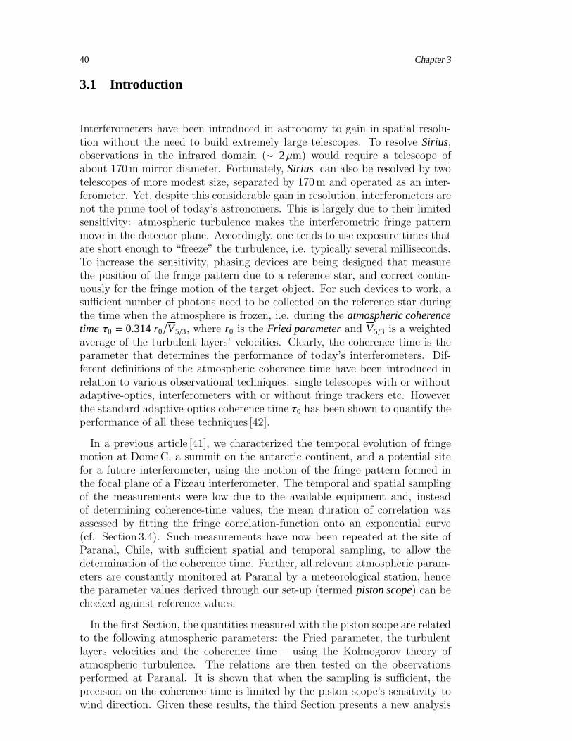
3.3.2 Derivation of atmospheric parameters

The Fried parameter r0, the wavefront velocity V and orientation α arederived by fitting Dφ(t) + K onto the data points, as described in Section 3.2.Dφ(t) corresponds to an atmospheric model where the turbulence is containedin a single layer, that is displaced as a whole with the velocity V under anangle α.

The resulting parameter values and uncertainties are indicated on Figure 3.3.The latter correspond to a doubling of the squared deviation of the data pointsto the theoretic structure function. The Fried parameter is determined by theasymptotic value of the structure function at large time increments. To ease

Chapter 3 45

Figure 3.3: Theoretical structure functions (dashed lines) fitted onto data obtained at Paranal, theresulting seeingǫ0, velocityV, wind orientationα and coherence timeτ0 are indicated.

the comparison with the meteorological station of Paranal, we indicate theseeing angleǫ0 rather than the Fried parameter r0, these two parameters areessentially equivalent: ǫ0 = 0.976λ/r0 [rad]. V and α are derived from the firstfew measurement points and the coherence time, τ0, is then obtained throughthe classic relation: τ0 = 0.314 r0/V.

3.3.3 Performance of the piston scope

Figure 3.4: Seeing values measured at Paranal with the DIMM and the piston scope. The uncertain-ties of the piston scope values correspond to a twofold increase in the quality of the data adjustment.

On Figures 3.4-3.6, the values of ǫ0,Vps and τ0 obtained with the pistonscope are compared to measurements in terms of the Paranal monitoring-instruments. We do not compare the wind orientations, because the value ofα that is obtained with the piston scope depends on the position of the mask,hence on the pointing of the telescope, and it is difficult to relate it to theangle measured by the meteorological station.

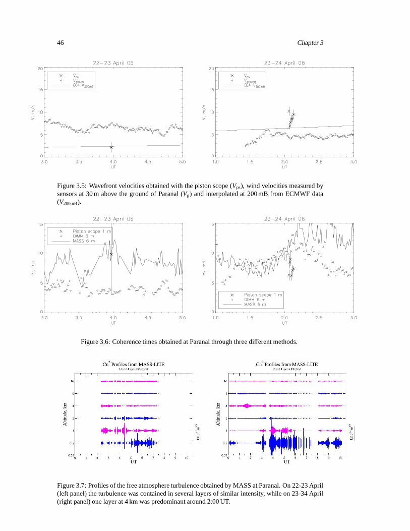
46 Chapter 3

Figure 3.5: Wavefront velocities obtained with the piston scope (Vps), wind velocities measured bysensors at 30 m above the ground of Paranal (Vg) and interpolated at 200 mB from ECMWF data(V200mB).

Figure 3.6: Coherence times obtained at Paranal through three different methods.

Figure 3.7: Profiles of the free atmosphere turbulence obtained by MASS at Paranal. On 22-23 April(left panel) the turbulence was contained in several layersof similar intensity, while on 23-34 April(right panel) one layer at 4 km was predominant around 2:00 UT.

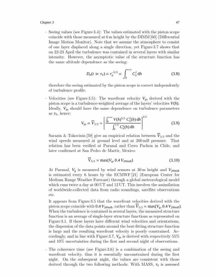
Chapter 3 47

– Seeing values (see Figure 3.4): The values estimated with the piston scopecoincide with those measured at 6m height by the DIMM[60] (DifferentialImage Motion Monitor). Note that we assume the atmosphere to consistof one layer displaced along a single direction, yet Figure 3.7 shows thaton 22-23 April the turbulence was contained in several layers with similarintensity. However, the asymptotic value of the structure function hasthe same altitude dependence as the seeing:

Dφ(t ≫ τ0) ∝ r−5/30 ∝

∫ +∞

0C2

n dh (3.8)

therefore the seeing estimated by the piston scope is correct independentlyof turbulence profile.

– Velocities (see Figure 3.5): The wavefront velocity Vps derived with thepiston scope is a turbulence-weighted average of the layers’ velocities V(h).Ideally, Vps should have the same dependence on turbulence parametersas τ0, hence:

Vps ∝ V5/3 =

∫ +∞0

V(h)5/3 C2n(h) dh

∫ +∞0

C2n(h) dh

3/5

(3.9)

Sarazin & Tokovinin [59] give an empirical relation between V5/3 and thewind speeds measured at ground level and at 200mB pressure. Thatrelation has been verified at Paranal and Cerro Pachon in Chile, andlater confirmed at San Pedro de Martir, Mexico:

V5/3 ≈ max(Vg, 0.4V200mB) (3.10)

At Paranal, Vg is measured by wind sensors at 30m height and V200mB

is estimated every 6 hours by the ECMWF [21] (European Center forMedium Range Weather Forecast) through a global meteorological modelwhich runs twice a day at 00UT and 12UT. This involves the assimilationof worldwide-collected data from radio soundings, satellite observationsetc.

It appears from Figure 3.5 that the wavefront velocities derived with thepiston scope coincide with 0.4V200mB, rather than V5/3 ≈ max(Vg, 0.4V200mB).When the turbulence is contained in several layers, the measured structurefunction is an average of single-layer structure functions as represented onFigure 3.1. If these layers have different wind velocities and orientations,the dispersion of the data points around the best-fitting structure functionis large and the resulting wavefront velocity is poorly constrained. Ac-cordingly, and in line with Figure 3.7, Vps is derived with respectively 55%and 10% uncertainties during the first and second night of observations.

– The coherence time (see Figure 3.6) is a combination of the seeing andwavefront velocity, thus it is essentially unconstrained during the firstnight. On the subsequent night, the values are consistent with thosederived through the two following methods: With MASS, τ0 is assessed

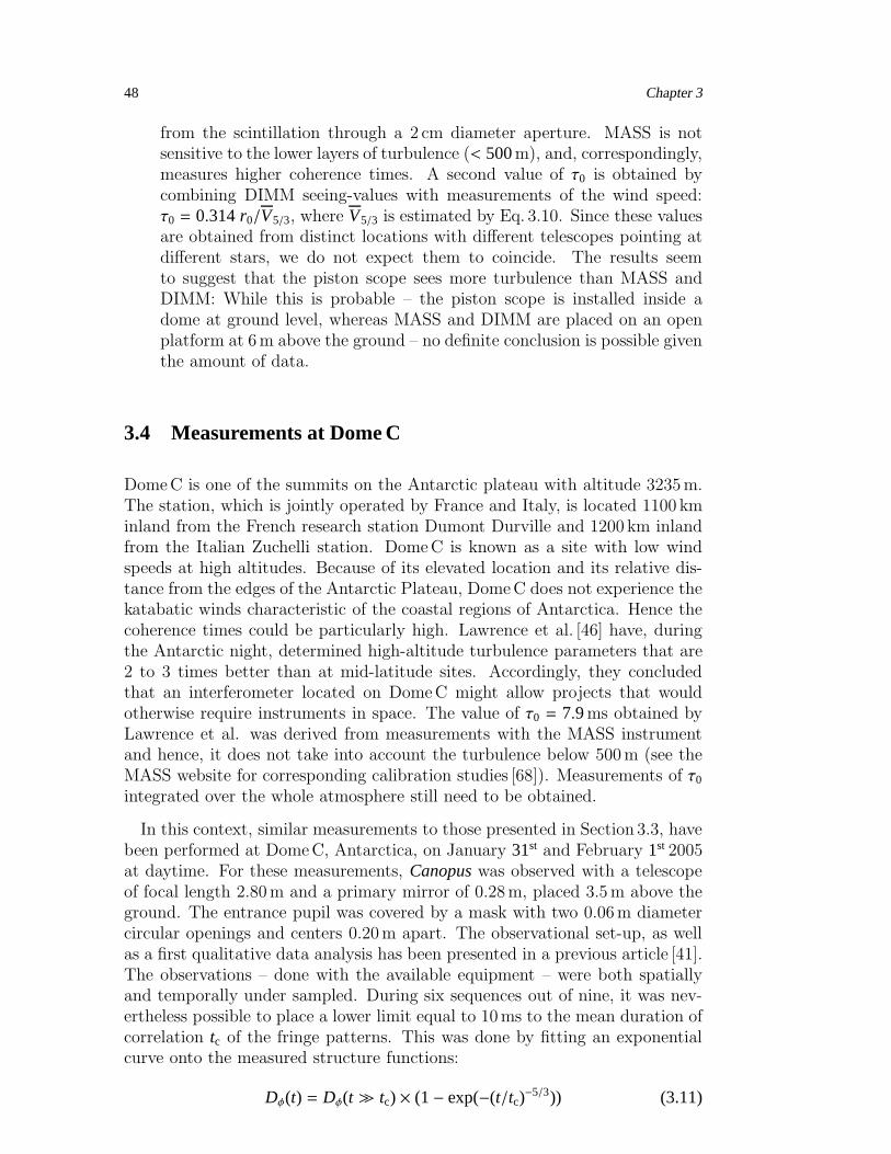
48 Chapter 3

from the scintillation through a 2 cm diameter aperture. MASS is notsensitive to the lower layers of turbulence (< 500m), and, correspondingly,measures higher coherence times. A second value of τ0 is obtained bycombining DIMM seeing-values with measurements of the wind speed:τ0 = 0.314r0/V5/3, where V5/3 is estimated by Eq. 3.10. Since these valuesare obtained from distinct locations with different telescopes pointing atdifferent stars, we do not expect them to coincide. The results seemto suggest that the piston scope sees more turbulence than MASS andDIMM: While this is probable – the piston scope is installed inside adome at ground level, whereas MASS and DIMM are placed on an openplatform at 6m above the ground – no definite conclusion is possible giventhe amount of data.

3.4 Measurements at Dome C

DomeC is one of the summits on the Antarctic plateau with altitude 3235m.The station, which is jointly operated by France and Italy, is located 1100 kminland from the French research station Dumont Durville and 1200 km inlandfrom the Italian Zuchelli station. DomeC is known as a site with low windspeeds at high altitudes. Because of its elevated location and its relative dis-tance from the edges of the Antarctic Plateau, DomeC does not experience thekatabatic winds characteristic of the coastal regions of Antarctica. Hence thecoherence times could be particularly high. Lawrence et al. [46] have, duringthe Antarctic night, determined high-altitude turbulence parameters that are2 to 3 times better than at mid-latitude sites. Accordingly, they concludedthat an interferometer located on DomeC might allow projects that wouldotherwise require instruments in space. The value of τ0 = 7.9ms obtained byLawrence et al. was derived from measurements with the MASS instrumentand hence, it does not take into account the turbulence below 500m (see theMASS website for corresponding calibration studies [68]). Measurements of τ0integrated over the whole atmosphere still need to be obtained.

In this context, similar measurements to those presented in Section 3.3, havebeen performed at DomeC, Antarctica, on January 31st and February 1st 2005at daytime. For these measurements, Canopuswas observed with a telescopeof focal length 2.80m and a primary mirror of 0.28m, placed 3.5m above theground. The entrance pupil was covered by a mask with two 0.06m diametercircular openings and centers 0.20m apart. The observational set-up, as wellas a first qualitative data analysis has been presented in a previous article [41].The observations – done with the available equipment – were both spatiallyand temporally under sampled. During six sequences out of nine, it was nev-ertheless possible to place a lower limit equal to 10ms to the mean duration ofcorrelation tc of the fringe patterns. This was done by fitting an exponentialcurve onto the measured structure functions:

Dφ(t) = Dφ(t ≫ tc) × (1− exp(−(t/tc)−5/3)) (3.11)

Chapter 3 49

Figure 3.8: Atmospheric parameter values derived from measurements at Dome C.

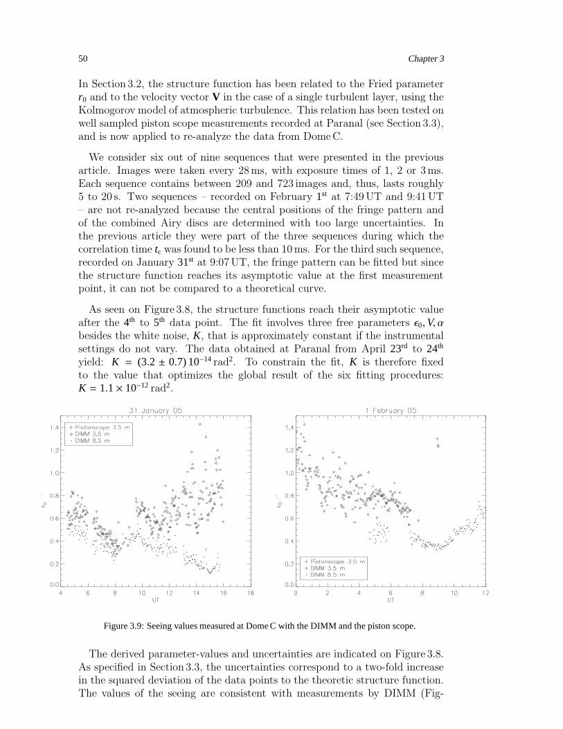
50 Chapter 3

In Section 3.2, the structure function has been related to the Fried parameterr0 and to the velocity vector V in the case of a single turbulent layer, using theKolmogorov model of atmospheric turbulence. This relation has been tested onwell sampled piston scope measurements recorded at Paranal (see Section 3.3),and is now applied to re-analyze the data from DomeC.

We consider six out of nine sequences that were presented in the previousarticle. Images were taken every 28ms, with exposure times of 1, 2 or 3ms.Each sequence contains between 209 and 723 images and, thus, lasts roughly5 to 20 s. Two sequences – recorded on February 1st at 7:49UT and 9:41UT– are not re-analyzed because the central positions of the fringe pattern andof the combined Airy discs are determined with too large uncertainties. Inthe previous article they were part of the three sequences during which thecorrelation time tc was found to be less than 10ms. For the third such sequence,recorded on January 31st at 9:07UT, the fringe pattern can be fitted but sincethe structure function reaches its asymptotic value at the first measurementpoint, it can not be compared to a theoretical curve.

As seen on Figure 3.8, the structure functions reach their asymptotic valueafter the 4th to 5th data point. The fit involves three free parameters ǫ0,V, αbesides the white noise, K, that is approximately constant if the instrumentalsettings do not vary. The data obtained at Paranal from April 23rd to 24th

yield: K = (3.2 ± 0.7) 10−14 rad2. To constrain the fit, K is therefore fixedto the value that optimizes the global result of the six fitting procedures:K = 1.1× 10−12 rad2.

Figure 3.9: Seeing values measured at Dome C with the DIMM andthe piston scope.

The derived parameter-values and uncertainties are indicated on Figure 3.8.As specified in Section 3.3, the uncertainties correspond to a two-fold increasein the squared deviation of the data points to the theoretic structure function.The values of the seeing are consistent with measurements by DIMM (Fig-

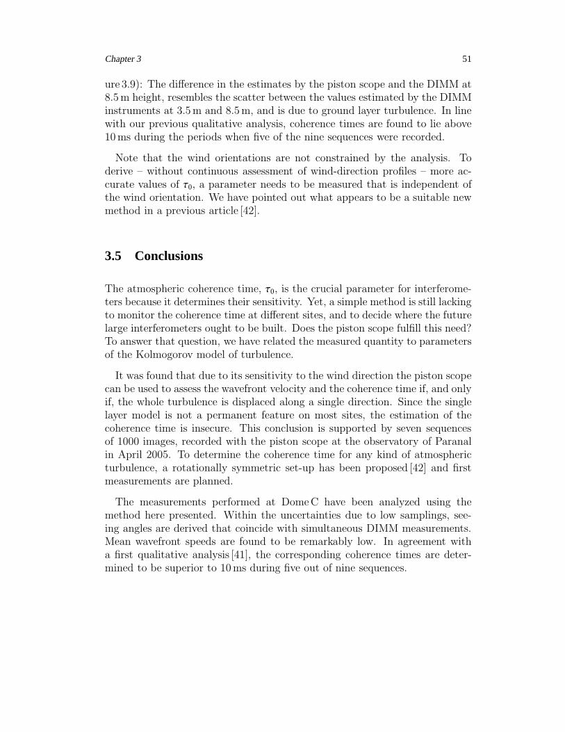
Chapter 3 51

ure 3.9): The difference in the estimates by the piston scope and the DIMM at8.5m height, resembles the scatter between the values estimated by the DIMMinstruments at 3.5m and 8.5m, and is due to ground layer turbulence. In linewith our previous qualitative analysis, coherence times are found to lie above10ms during the periods when five of the nine sequences were recorded.

Note that the wind orientations are not constrained by the analysis. Toderive – without continuous assessment of wind-direction profiles – more ac-curate values of τ0, a parameter needs to be measured that is independent ofthe wind orientation. We have pointed out what appears to be a suitable newmethod in a previous article [42].

3.5 Conclusions

The atmospheric coherence time, τ0, is the crucial parameter for interferome-ters because it determines their sensitivity. Yet, a simple method is still lackingto monitor the coherence time at different sites, and to decide where the futurelarge interferometers ought to be built. Does the piston scope fulfill this need?To answer that question, we have related the measured quantity to parametersof the Kolmogorov model of turbulence.

It was found that due to its sensitivity to the wind direction the piston scopecan be used to assess the wavefront velocity and the coherence time if, and onlyif, the whole turbulence is displaced along a single direction. Since the singlelayer model is not a permanent feature on most sites, the estimation of thecoherence time is insecure. This conclusion is supported by seven sequencesof 1000 images, recorded with the piston scope at the observatory of Paranalin April 2005. To determine the coherence time for any kind of atmosphericturbulence, a rotationally symmetric set-up has been proposed [42] and firstmeasurements are planned.

The measurements performed at DomeC have been analyzed using themethod here presented. Within the uncertainties due to low samplings, see-ing angles are derived that coincide with simultaneous DIMM measurements.Mean wavefront speeds are found to be remarkably low. In agreement witha first qualitative analysis [41], the corresponding coherence times are deter-mined to be superior to 10ms during five out of nine sequences.

52 Chapter 3

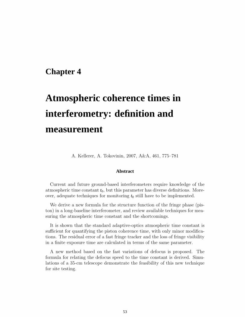
Chapter 4

Atmospheric coherence times in

interferometry: definition and

measurement

A. Kellerer, A. Tokovinin, 2007, A&A, 461, 775–781

Abstract

Current and future ground-based interferometers require knowledge of theatmospheric time constant t0, but this parameter has diverse definitions. More-over, adequate techniques for monitoring t0 still have to be implemented.

We derive a new formula for the structure function of the fringe phase (pis-ton) in a long-baseline interferometer, and review available techniques for mea-suring the atmospheric time constant and the shortcomings.

It is shown that the standard adaptive-optics atmospheric time constant issufficient for quantifying the piston coherence time, with only minor modifica-tions. The residual error of a fast fringe tracker and the loss of fringe visibilityin a finite exposure time are calculated in terms of the same parameter.

A new method based on the fast variations of defocus is proposed. Theformula for relating the defocus speed to the time constant is derived. Simu-lations of a 35-cm telescope demonstrate the feasibility of this new techniquefor site testing.

53

54 Chapter 4

4.1 Introduction

Astronomical sites for classical observations are characterized in terms of at-mospheric image quality (seeing). For high-angular resolution techniques suchas adaptive optics (AO) and interferometry, we need to know additional pa-rameters. The atmospheric coherence time is one of these. Here we refine thedefinition of the interferometric coherence time, review available techniques,and propose a new method for its measurements.

The AO time constant,τ0, is a well-defined parameter related to the verticaldistribution of turbulence and wind speed (Roddier [58]). To correct wavefronts in real time, a sufficient number of photons from the guide star is neededwithin each coherence area during time τ0. This severely restricts the choiceof natural guide stars and tends to impose the complex use of laser guide stars(Hardy [30]). It is shown below that new, simple methods of τ0 monitoring arestill needed.

Modern ground-based stellar interferometers attain extreme resolution, buttheir sensitivity is limited by the atmosphere. Even at the best observing sites,such as Paranal in Chile, fast fringe tracking is not fully operative yet, and onetherefore tends to employ exposure times that are short enough to “freeze” theatmospheric turbulence. The price is a substantial loss in limiting magnitude.It is hence important to measure the time constant, t0, of the piston – i. e. themean phase over the telescope aperture – at existing and future sites. However,the exact definition of t0 is not clear, any more than are methods to measureit. Do we need an interferometer to evaluate t0? Is t0 different from τ0? Doesit depend on the aperture size and baseline? We review various definitions ofthe interferometric time constant based on the piston structure function(SF),on the error of a fringe tracker, and on the loss of fringe contrast during afinite exposure time. It is shown that the piston time constant is proportionalto the AO coherence time τ0, both depending on the same combination ofatmospheric parameters.

During site exploration campaigns, one would like to predict the performanceof large base-line interferometers, and it is desirable to do this with single-dishand, preferably, small telescopes. The existing techniques for τ0 measurementare listed and a new method for site testing proposed.

4.2 Atmospheric coherence time in interferometry

4.2.1 Atmospheric coherence timeτ0

First, we introduce the relevant atmospheric parameters and the AO timeconstant τ0. For convenience, we outline the essential formulae, but for thegeneral background, we refer the reader to Roddier [58].

Chapter 4 55

The spatial and temporal fluctuations of atmospheric phase distortion ϕ areusually described by the SF

Dϕ(r , t) = 〈[

ϕ(r ′, t′) − ϕ(r + r ′, t + t′)]2〉, (4.1)

which depends on the transverse spatial coordinate r and time interval t. Theangular brackets indicate statistical average.

The atmosphere consists of many layers. The contribution of a layer i ofthickness dh at altitude h to the turbulence intensity is specified in terms ofC2

n(h)dh, equivalently expressed through the Fried parameter:

r−5/30,i = 0.423k2C2

n(h)dh, (4.2)

k = 2π/λ being the wavenumber. The spatial SF in the inertial range(betweeninner and outer scales) is

Dϕ(r , 0) = 6.883 (|r |/r0)5/3. (4.3)

It is assumed that each layer moves as a whole with the velocity vector V(h)(Taylor hypothesis). The temporal SF of the piston fluctuations Dϕ,i(0, t) inone small aperture due to a single layer is then equal to, the spatial SF at shiftVt,

Dϕ,i(0, t) = 6.883 [V(h)t/r0,i]5/3. (4.4)

Summing the contributions of all layers, we obtain

Dϕ(0, t) = 2.910 t5/3 k2

∫ +∞

0V5/3(h)C2

n(h)dh

= 6.883 (tV5/3/r0)5/3 = (t/τ0)

5/3, (4.5)

where τ0 = 0.314 (r0/V5/3) is the AO time constant (Roddier 1981) and theaverage wind speed Vp is computed as

Vp =

∫ +∞0

Vp(h)C2n(h)dh

∫ +∞0

C2n(h)dh

1/p

. (4.6)

The formulae are valid for observations at zenith. At angle γ from the zenith,the optical path is increased in proportion to the air mass, secγ, and theSF increases by the same factor. Further, the transverse component of thewind velocity changes. In the following, we neglect these complications andconsider only observations at zenith, but the analysis of real data must accountfor γ , 0.

56 Chapter 4

4.2.2 Piston time constant

In an interferometer with a large baseline (B ≫ L0, where L0: turbulenceouter scale) the phase patterns over the apertures are uncorrelated on shorttime scales. Thus, for a small time interval (t < B/V), the SF of the phasedifference φ (do not confuse with the phase ϕ) in an interferometer with twosmall apertures will simply be two times larger, Dφ(t) = 2Dϕ(0, t) (Conan et al.[17]). As a result the differential piston variance reaches 1 rad2 for a time delayt0 = 2−3/5 τ0 = 0.66 τ0. Note that, in the case of smaller baselines and largeouter scales – when the assumption B≫ L0 becomes invalid – Dφ(t) < 2Dϕ(0, t)and the resulting coherence time, accordingly, lies between 0.66 τ0 and τ0.Yet, B≫ L0 applies to the characterization of large baseline interferometers atlow-turbulence sites.

When an interferometer with larger circular apertures of diameter d is con-sidered, phase fluctuations are averaged inside each aperture. As shown later,for time increments smaller than d/V, the piston structure function is quadraticin t and is essentially determined by the average wave-front tilt over the aper-ture. The variance of the gradient tilt α (in radians) in one direction is (Roddier[58], Conan et al. [17], Sasiela [61])

σ2α = 0.170λ2r−5/3

0 d−1/3. (4.7)

We write the piston SF in this regime as Dφ(t) ≈ 2 (kσαVt)2, sum the contri-butions of all layers, and obtain the expression

Dφ(t) ≈ 13.42 (V2t/r0)2(r0/d)1/3 = (t/t1)

2, (4.8)

where the modified time constant t1 = 0.273 (r0/V2) (d/r0)1/6. The analysis ofthe tilt variance with finite outer scale by Conan et al. [15] is applicable here.The finite outer scale reduces the amplitude of the tilt and hence increases thepiston time constant, but this effect depends on the aperture size and is notvery strong for d < 1m.

Note that for small time intervals there is a weak dependence of the SF onthe aperture diameter. Also, the wind velocity averaging is slightly modified.However, the expressions for t1 and t0 produce similar numerical results as longas d/r0 is not too large. Thus, the system-independent definition of the AOtime constant (4.5) also gives a good description of the temporal variations ofthe piston.

For time delays of approximately B/V and larger, the pistons on two aper-tures are no longer independent. However, estimates of the time interval overwhich the Taylor hypothesis is valid range from ∼ 40ms (Schoeck & Spillar[63]) to several seconds (Colavita et al. [14]). Hence, at time intervals of 1 sor more, the Taylor hypothesis is insecure. Moreover, the finite turbulenceouter scale reduces the amplitude of slow piston variations substantially. Herewe concentrate only on rapid piston variations where our approximations are

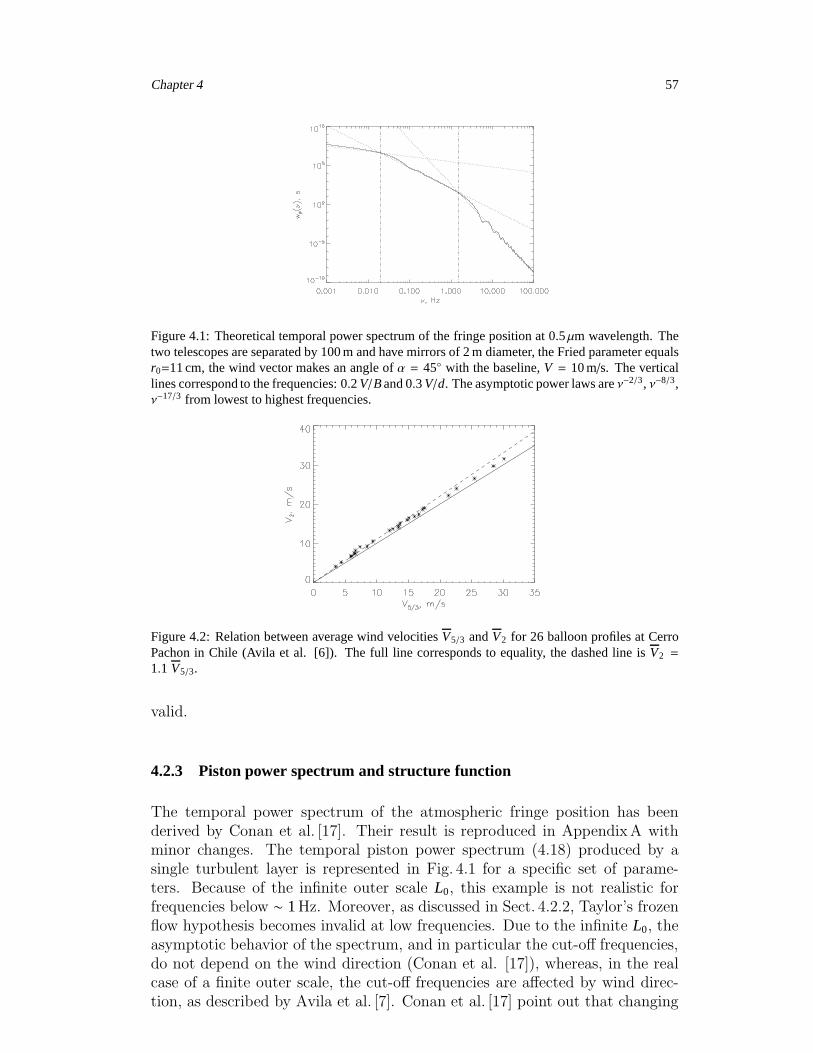
Chapter 4 57

Figure 4.1: Theoretical temporal power spectrum of the fringe position at 0.5µm wavelength. Thetwo telescopes are separated by 100 m and have mirrors of 2 m diameter, the Fried parameter equalsr0=11 cm, the wind vector makes an angle ofα = 45 with the baseline,V = 10 m/s. The verticallines correspond to the frequencies: 0.2V/Band 0.3V/d. The asymptotic power laws areν−2/3, ν−8/3,ν−17/3 from lowest to highest frequencies.

Figure 4.2: Relation between average wind velocitiesV5/3 andV2 for 26 balloon profiles at CerroPachon in Chile (Avila et al. [6]). The full line correspondsto equality, the dashed line isV2 =

1.1 V5/3.

valid.

4.2.3 Piston power spectrum and structure function

The temporal power spectrum of the atmospheric fringe position has beenderived by Conan et al. [17]. Their result is reproduced in AppendixA withminor changes. The temporal piston power spectrum (4.18) produced by asingle turbulent layer is represented in Fig. 4.1 for a specific set of parame-ters. Because of the infinite outer scale L0, this example is not realistic forfrequencies below ∼ 1Hz. Moreover, as discussed in Sect. 4.2.2, Taylor’s frozenflow hypothesis becomes invalid at low frequencies. Due to the infinite L0, theasymptotic behavior of the spectrum, and in particular the cut-off frequencies,do not depend on the wind direction (Conan et al. [17]), whereas, in the realcase of a finite outer scale, the cut-off frequencies are affected by wind direc-tion, as described by Avila et al. [7]. Conan et al. [17] point out that changing

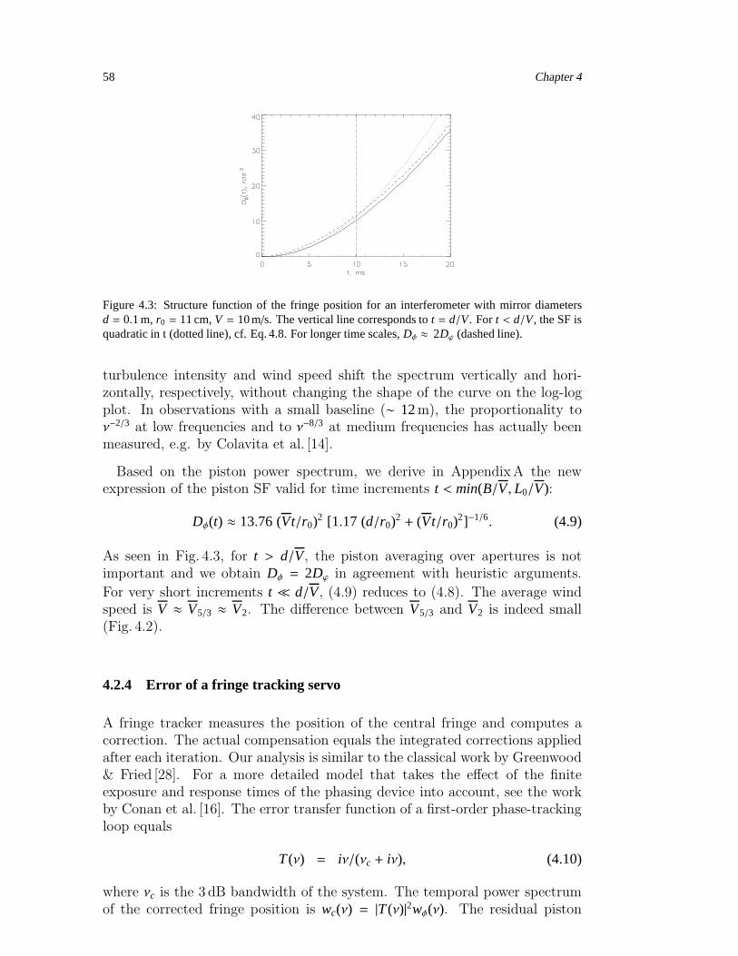
58 Chapter 4

Figure 4.3: Structure function of the fringe position for aninterferometer with mirror diametersd = 0.1 m, r0 = 11 cm,V = 10 m/s. The vertical line corresponds tot = d/V. For t < d/V, the SF isquadratic in t (dotted line), cf. Eq. 4.8. For longer time scales,Dφ ≈ 2Dϕ (dashed line).

turbulence intensity and wind speed shift the spectrum vertically and hori-zontally, respectively, without changing the shape of the curve on the log-logplot. In observations with a small baseline (∼ 12m), the proportionality toν−2/3 at low frequencies and to ν−8/3 at medium frequencies has actually beenmeasured, e.g. by Colavita et al. [14].

Based on the piston power spectrum, we derive in AppendixA the newexpression of the piston SF valid for time increments t < min(B/V, L0/V):

Dφ(t) ≈ 13.76 (Vt/r0)2 [1.17 (d/r0)

2 + (Vt/r0)2]−1/6. (4.9)

As seen in Fig. 4.3, for t > d/V, the piston averaging over apertures is notimportant and we obtain Dφ = 2Dϕ in agreement with heuristic arguments.

For very short increments t ≪ d/V, (4.9) reduces to (4.8). The average windspeed is V ≈ V5/3 ≈ V2. The difference between V5/3 and V2 is indeed small(Fig. 4.2).

4.2.4 Error of a fringe tracking servo

A fringe tracker measures the position of the central fringe and computes acorrection. The actual compensation equals the integrated corrections appliedafter each iteration. Our analysis is similar to the classical work by Greenwood& Fried [28]. For a more detailed model that takes the effect of the finiteexposure and response times of the phasing device into account, see the workby Conan et al. [16]. The error transfer function of a first-order phase-trackingloop equals

T(ν) = iν/(νc + iν), (4.10)

where νc is the 3 dB bandwidth of the system. The temporal power spectrumof the corrected fringe position is wc(ν) = |T(ν)|2wφ(ν). The residual piston

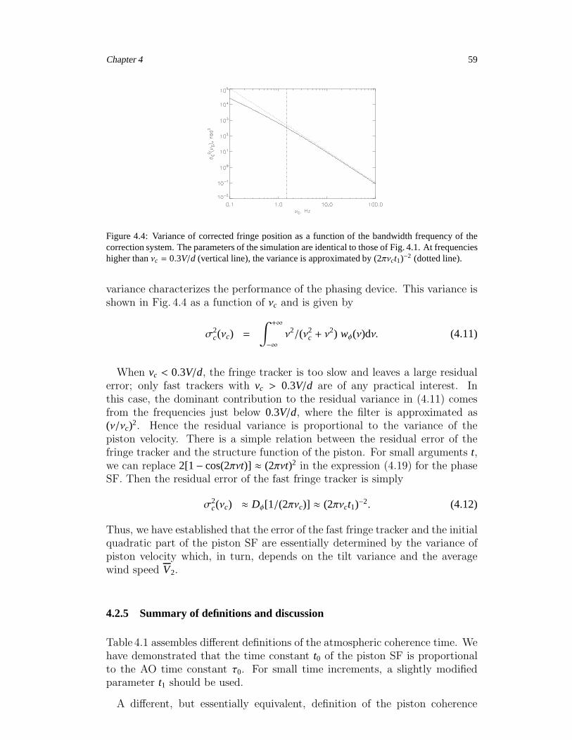
Chapter 4 59

Figure 4.4: Variance of corrected fringe position as a function of the bandwidth frequency of thecorrection system. The parameters of the simulation are identical to those of Fig. 4.1. At frequencieshigher thanνc = 0.3V/d (vertical line), the variance is approximated by (2πνct1)−2 (dotted line).

variance characterizes the performance of the phasing device. This variance isshown in Fig. 4.4 as a function of νc and is given by

σ2c(νc) =

∫ +∞

−∞ν2/(ν2c + ν

2) wφ(ν)dν. (4.11)

When vc < 0.3V/d, the fringe tracker is too slow and leaves a large residualerror; only fast trackers with vc > 0.3V/d are of any practical interest. Inthis case, the dominant contribution to the residual variance in (4.11) comesfrom the frequencies just below 0.3V/d, where the filter is approximated as(ν/νc)2. Hence the residual variance is proportional to the variance of thepiston velocity. There is a simple relation between the residual error of thefringe tracker and the structure function of the piston. For small arguments t,we can replace 2[1− cos(2πνt)] ≈ (2πνt)2 in the expression (4.19) for the phaseSF. Then the residual error of the fast fringe tracker is simply

σ2c(νc) ≈ Dφ[1/(2πνc)] ≈ (2πνct1)−2. (4.12)

Thus, we have established that the error of the fast fringe tracker and the initialquadratic part of the piston SF are essentially determined by the variance ofpiston velocity which, in turn, depends on the tilt variance and the averagewind speed V2.

4.2.5 Summary of definitions and discussion

Table 4.1 assembles different definitions of the atmospheric coherence time. Wehave demonstrated that the time constant t0 of the piston SF is proportionalto the AO time constant τ0. For small time increments, a slightly modifiedparameter t1 should be used.

A different, but essentially equivalent, definition of the piston coherence

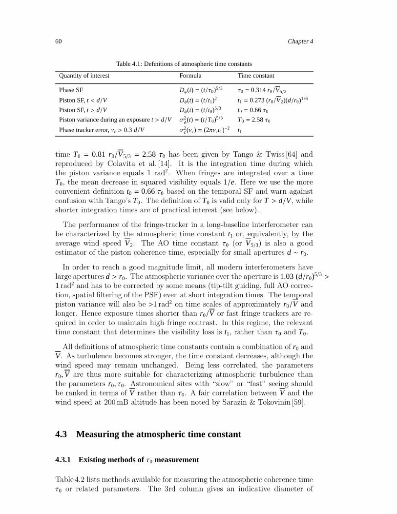
60 Chapter 4

Table 4.1: Definitions of atmospheric time constants

Quantity of interest Formula Time constant

Phase SF Dϕ(t) = (t/τ0)5/3 τ0 = 0.314r0/V5/3

Piston SF,t < d/V Dφ(t) = (t/t1)2 t1 = 0.273 (r0/V2)(d/r0)1/6

Piston SF,t > d/V Dφ(t) = (t/t0)5/3 t0 = 0.66 τ0Piston variance during an exposuret > d/V σ2

φ(t) = (t/T0)5/3 T0 = 2.58 τ0

Phase tracker error,νc > 0.3 d/V σ2c(νc) = (2πνct1)−2 t1

time T0 = 0.81 r0/V5/3 = 2.58 τ0 has been given by Tango & Twiss [64] andreproduced by Colavita et al. [14]. It is the integration time during whichthe piston variance equals 1 rad2. When fringes are integrated over a timeT0, the mean decrease in squared visibility equals 1/e. Here we use the moreconvenient definition t0 = 0.66 τ0 based on the temporal SF and warn againstconfusion with Tango’s T0. The definition of T0 is valid only for T > d/V, whileshorter integration times are of practical interest (see below).

The performance of the fringe-tracker in a long-baseline interferometer canbe characterized by the atmospheric time constant t1 or, equivalently, by theaverage wind speed V2. The AO time constant τ0 (or V5/3) is also a goodestimator of the piston coherence time, especially for small apertures d ∼ r0.

In order to reach a good magnitude limit, all modern interferometers havelarge apertures d > r0. The atmospheric variance over the aperture is 1.03 (d/r0)5/3 >

1rad2 and has to be corrected by some means (tip-tilt guiding, full AO correc-tion, spatial filtering of the PSF) even at short integration times. The temporalpiston variance will also be >1 rad2 on time scales of approximately r0/V andlonger. Hence exposure times shorter than r0/V or fast fringe trackers are re-quired in order to maintain high fringe contrast. In this regime, the relevanttime constant that determines the visibility loss is t1, rather than τ0 and T0.

All definitions of atmospheric time constants contain a combination of r0 andV. As turbulence becomes stronger, the time constant decreases, although thewind speed may remain unchanged. Being less correlated, the parametersr0,V are thus more suitable for characterizing atmospheric turbulence thanthe parameters r0, τ0. Astronomical sites with “slow” or “fast” seeing shouldbe ranked in terms of V rather than τ0. A fair correlation between V and thewind speed at 200mB altitude has been noted by Sarazin & Tokovinin [59].

4.3 Measuring the atmospheric time constant

4.3.1 Existing methods ofτ0 measurement

Table 4.2 lists methods available for measuring the atmospheric coherence timeτ0 or related parameters. The 3rd column gives an indicative diameter of

Chapter 4 61

Table 4.2: Methods ofτ0 measurement

Method Measurables d, m Problems Reference

SCIDAR C2n(h), V(h) >1 Needs large telescope Fuchs et al. [22]

Balloons C2n(h), V(h) none Expensive, no monitoring Azouit & Vernin [8]

AO system r0, τ0 >1 Needs working AO Fusco et al. [23]SSS C2

n(h), V(h) >0.4 Low height resolution Habib et al. [29]GSM r0, V, τAA 4x0.1 No obvious relation toτ0 andt1 Ziad et al [73]MASS τ∗0 0.02 Biased (low layers ignored) Kornilov et al. [44]DIMM r0 0.25 Indirectτ0 estimate Sarazin & Tokovinin [59]FADE r0, t1 0.35 New method This work

the telescope aperture required for each method. Short comments on eachtechnique are given below.

SCIDAR (SCIntillation Detection And Ranging) has provided good resultson τ0. It is not suitable for monitoring because manual data processing isstill needed to extract V(h), despite efforts to automate the process. Balloonsprovide only single-shot profiles of low individual statistical significance. TheAO systems and interferometers give reliable results, but are not suitable fortesting new sites or for long-term monitoring.

The methods listed in the next four rows of Table 4.2 all require small tele-scopes and can thus be used for site-testing. However, all these techniqueshave some intrinsic problems. SSS (Single Star SCIDAR) essentially extendsthe SCIDAR technique to small telescopes: profiles of C2

n(h) and V(h) are ob-tained with lower height resolution than with the SCIDAR, and are then usedto derive the coherence time. The GSM (Generalized Seeing Monitor) canonly measure velocities of prominent layers after careful data processing. Acoherence time, τAA – which, however, does not have a similar dependence onthe turbulence profile than τ0 and t1 – is deduced from the angle of arrival fluc-tuations. MASS (Multi-Aperture Scintillation Sensor) is a recent, but alreadywell-proven, turbulence monitor. One of its observables related to scintillationin a 2 cm aperture approximates V5/3 (Tokovinin [68]), but this averaging doesnot include low layers and thus gives a biased estimate of τ0. An even less se-cure evaluation of τ0 can be obtained from DIMM (Differential Image MotionMonitor) by combining the measured r0 with meteorological data on the windspeed (Sarazin & Tokovinin [59]).

We conclude from this brief survey that a correct yet simple technique formeasuring τ0 with a small-aperture telescope is still lacking. Such a methodis proposed in the next section.

4.3.2 The new method: FADE

To measure the interferometric or AO time constant, we need an observablerelated to V2 or V5/3. The atmosphere consists of many layers with differentwind speeds and directions, so a true C2

n-weighted estimator (4.6) is required.

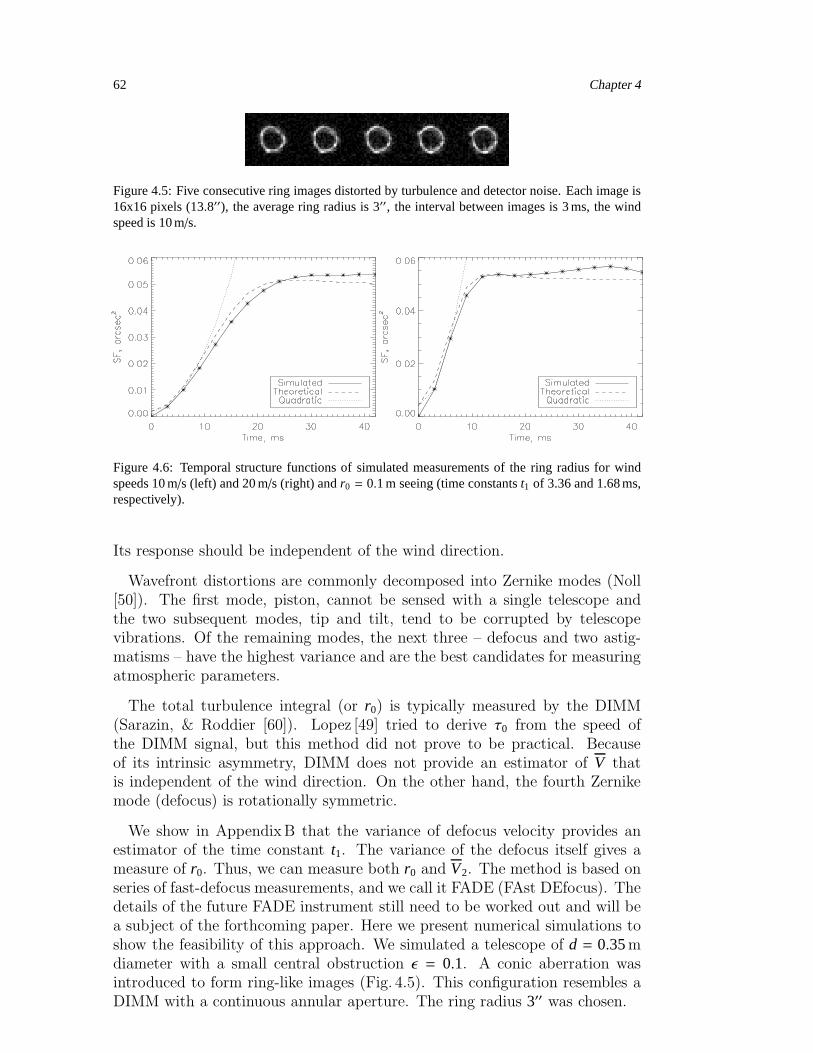
62 Chapter 4

Figure 4.5: Five consecutive ring images distorted by turbulence and detector noise. Each image is16x16 pixels (13.8′′), the average ring radius is 3′′, the interval between images is 3 ms, the windspeed is 10 m/s.

Figure 4.6: Temporal structure functions of simulated measurements of the ring radius for windspeeds 10 m/s (left) and 20 m/s (right) andr0 = 0.1 m seeing (time constantst1 of 3.36 and 1.68 ms,respectively).

Its response should be independent of the wind direction.

Wavefront distortions are commonly decomposed into Zernike modes (Noll[50]). The first mode, piston, cannot be sensed with a single telescope andthe two subsequent modes, tip and tilt, tend to be corrupted by telescopevibrations. Of the remaining modes, the next three – defocus and two astig-matisms – have the highest variance and are the best candidates for measuringatmospheric parameters.

The total turbulence integral (or r0) is typically measured by the DIMM(Sarazin, & Roddier [60]). Lopez [49] tried to derive τ0 from the speed ofthe DIMM signal, but this method did not prove to be practical. Becauseof its intrinsic asymmetry, DIMM does not provide an estimator of V thatis independent of the wind direction. On the other hand, the fourth Zernikemode (defocus) is rotationally symmetric.

We show in AppendixB that the variance of defocus velocity provides anestimator of the time constant t1. The variance of the defocus itself gives ameasure of r0. Thus, we can measure both r0 and V2. The method is based onseries of fast-defocus measurements, and we call it FADE (FAst DEfocus). Thedetails of the future FADE instrument still need to be worked out and will bea subject of the forthcoming paper. Here we present numerical simulations toshow the feasibility of this approach. We simulated a telescope of d = 0.35mdiameter with a small central obstruction ǫ = 0.1. A conic aberration wasintroduced to form ring-like images (Fig. 4.5). This configuration resembles aDIMM with a continuous annular aperture. The ring radius 3′′ was chosen.

Chapter 4 63

Monochromatic (λ = 500nm) images were computed on a 642 pixel gridfrom the interpolated distortions and binned into CCD pixels of 0.86′′ size.We simulated photon noise corresponding to a star of R = 2 magnitude and3ms exposure time (20 000 photons per frame) and added a readout noise of15 electrons rms in each pixel.

The radius ρ of the ring image is calculated in the same way as standardcentroids, by simply replacing coordinate with radius. The radius fluctuations∆ρ serve as an estimator for the defocus coefficient a4. The radius change isapproximated by the average slope of the Zernike defocus between inner andouter borders of the aperture:

∆ρ = Cρ a4 ≈ [2√

3(1+ ǫ)/π (λ/d)] a4. (4.13)

The complex amplitude of the light distorted by two phase screens at 0and 10 km altitude with combined r0 = 0.1m was pre-calculated on a largesquare grid (15m size, 0.015m pixels). This distribution is periodic in bothcoordinates, and it was “moved” in front of the aperture in a helical patternwith the wind speed V to simulate the temporal evolution of the wave-front.The exposure time ∆t = 3ms corresponds to a wave-front shift V∆t = 0.06mfor V = 20m/s, such that the initial quadratic part of the defocus SF (β =2Vt/d < 1) extends only to ∼ 3∆t.

Figure 4.6 shows the structure function, Dρ, of the ring-image radius cal-culated from several seconds of simulated data. It contains a small additivecomponent due to the measurement noise (in this case 0.05′′ rms), which wasdetermined from the data itself by a quadratic fit to the 2nd and 3rd pointsand its extrapolation to zero. The dashed lines are the theoretical SFs of de-focus computed by (4.32) and converted into radius with the coefficient Cρ(4.13). The slope between the second and third points of the simulated SFclosely matches the analytical formula.

To measure the speed of defocus variations, it is sufficient to fit a quadraticapproximation to the initial part of the measured SF, Dρ(t) ≈ at2. Consideringthe noise, the best estimate of the coefficient a is obtained from the secondand third points, a = [Dρ(2∆t) − Dρ(∆t)]/(3∆t2). This estimator is not biasedby white measurement noise. Equating the quadratic fit to the theoreticalexpression Dρ(t) = 0.0269 (Cρ t/t1)2, we get a recipe for calculating the timeconstant from the experimental data,

t1 ≈ 0.284Cρ∆t [Dρ(2∆t) − Dρ(∆t)]−1/2. (4.14)

Application of this formula to the simulated data gives t1 values of 3.88 and2.20ms for wind speeds 10 and 20m/s, while the input values are 3.36 and1.68ms. Our simulated instrument slightly over-estimates t1 because the cho-sen exposure time of 3ms is too long. Indeed, the error gets worse for a higherwind speed and disappears for V = 5m/s (true and measured t1 are 6.73 and6.62ms) or for a shorter exposure time. In the real situation of a multi-layer

64 Chapter 4

atmosphere, the experimental SF will be the sum of the SFs produced by dif-ferent layers. The contribution to the “jump” of the SF Dρ(2∆t)−Dρ(∆t) fromfast layers will be reduced (in comparison with the quadratic formula) and willcause a bias in the measured t1, increasing its value.

The crudeness of our simulations (discrete shifts of the phase screen, ap-proximate Cρ, etc.) also contributes to the mismatch. Averaging of the imageduring finite exposure time has not been simulated yet. The response and biasof a real instrument will be studied thoroughly by a more detailed simulation.However, the feasibility of the proposed technique for measuring t1 is alreadyclear.

The next two Zernike modes number 5 and 6 (astigmatism) are not rota-tionally symmetric. However, the sum of the variances of the velocities of twoastigmatism coefficients is again symmetric. In fact, it has the same spatialand temporal spectra as defocus, with a twice larger variance. Therefore, si-multaneous measurement of the two astigmatism coefficients can be used toestimate the atmospheric time constant in the same way as defocus. Othermeasurables that are symmetric and have a cutoff at high frequencies can beused as well. However, defocus and astigmatism have the largest and slow-est atmospheric variances making it easier to measure than other higher-ordermodes.

The FADE technique can be applied in a straightforward way to the analysisof the AO loop data, as a simple alternative to the more complicated methoddeveloped by Fusco et al. [23].

4.4 Conclusions

We reviewed the theory of fast temporal variations in the phase differencein a large-baseline interferometer. For a practically interesting case of largeapertures d > r0, the piston SF usually exceeds 1 rad2 at the aperture crossingtime t = d/V. Hence, shorter times are of interest where the piston SF isquadratic (rather than ∝ t5/3). The relevant atmospheric time constant is t1.However, the standard AO time constant τ0 also provides a good estimationof the piston coherence time. Both these parameters essentially depend on theturbulence-weighted average wind speed V.

A brief review of available methods for measuring τ0 shows the need fora simple technique suitable for site testing or monitoring, i.e. working on asmall-aperture telescope. The FAst DEfocus (FADE) method proposed herefulfills this need. We argue that, for a given aperture size, this is the best wayof extracting the information on τ0. The feasibility of the method is provenby simulation, which opens a way to the development of a real instrument.An instrument concept using a small telescope, some simple optics, and a fastcamera will be described in a subsequent article.

Chapter 4 65

4.5 Appendix A - Derivation of the piston structure function

The spatial power spectrum of the piston is derived from the spatial atmo-spheric phase spectrum (Roddier [58])

Wϕ(f ) = 0.00969k2

∫ +∞

0( f 2 + L−2

0 )−11/6 C2n dh, (4.15)

where f is the spatial frequency, L0 the turbulence outer scale at height h,and the other notations were introduced in Sect. 4.2.1. We drop the explicitdependence of Cn, L0, and all following altitude dependent-parameters on h,to ease the reading of the formulae. The spatial filter that converts Wϕ(f ) intothe piston power spectrum Wφ(f ) is

M2(f ) = [2 sin(πfB) A(f )]2 (4.16)

Wφ(f ) = M2(f ) Wϕ(f ), (4.17)

for a baseline vector B and the aperture filter function A(f ). For a circularaperture of diameter d, A(f ) = 2J1(π f d)/(π f d) and f = |f |. There Jn stands forthe Bessel function of order n.

As usual, we assume that turbulent layers are transported with wind speedV directed at an angle α with respect to the baseline. The temporal powerspectrum of the piston is then obtained by integrating in the frequency planeover a line displaced by fx = ν/V from the coordinate origin and inclined atangle α. Let fy be the integration variable along this line and f 2 = f 2

x + f 2y .

The temporal spectrum equals

wφ(ν) =1V

∫ +∞

−∞Wφ

(

fx cosα + fy sinα, fy cosα − fx sinα)

d fy

= 0.0388k2

∫ +∞

0V−1C2

n dh∫ +∞

−∞( f 2 + L−2

0 )−11/6

×[

sin(

πB fx cosα + πB fy sinα)

A( f )]2

d fy. (4.18)

We use the rotational symmetry of the aperture filter. This formula can befound in Conan et al. [17] in a slightly different form. The temporal powerspectrum is defined here on ν = (−∞,+∞) to keep the analogy with spatialpower spectra.

The temporal structure function of the piston is

Dφ(t) =∫ +∞

−∞2[1− cos(2πtν)] wφ(ν) dν. (4.19)

66 Chapter 4

For an interferometer with a large baseline B≫ d, the width of the aperturefilter is much larger than the period of the sin2 factor in (4.18). We can thenreplace the sin2 with its average value 0.5. Assuming also that L0 ≫ d, weobtain an approximation for the piston power spectrum

wφ(ν) ≈ 0.0194k2

∫ +∞

0V−1 C2

n dh∫ +∞

−∞A2( f ) f −11/3 d fy. (4.20)

With this approximation,

Dφ(t) = 0.0388k2

∫ +∞

0C2

n dh∫ ∫ +∞

−∞[1 − cos(2πt fxV)] A2( f ) f −11/3 d fxd fy

= 0.244k2

∫ +∞

0C2

n dh∫ +∞

0[1 − J0(2πtV f)] A2( f ) f −8/3 d f . (4.21)

We used the relation (Gradshteyn & Ryzhik [26]):∫ 2π

0cos(2πzcosθ)dθ = 2π J0(2πz).

For a circular aperture of diameter d,

Dφ(t) = 1.641k2d5/3

∫ +∞

0C2

n dh K1(2tV/d), (4.22)

where the new dimensionless variables are β = 2tV/d and x = π f d and thefunction K1(β)

K1(β) =∫ +∞

0[2J1(x)/x]2x−8/3 [1 − J0(βx)] dx

≈ 1.1183β2

(4.7+ β2)1/6. (4.23)

The approximation of K1(β) is accurate to 1% for all values of the argumentand reproduces the analytic solutions of the integral for very large and verysmall β. For example, for large β the aperture filter tends to one; hence

K1(β) ≈∫ ∞

0x−8/3 [1 − J0(βx)] dx

= π/[28/3 Γ2(11/6) sin(5π/6)] β5/3 = 1.1183β5/3 (4.24)

(cf. Eq. 20 in Noll [50]). It follows that for t > d/V

Dφ(t) ≈ 13.77 (V5/3 t/r0)5/3 = (t/t0)

5/3. (4.25)

For t < d/V, K1(β) ≈ 0.864β2 and

Dφ(t) ≈ 13.41 (V2 t/r0)2 (r0/d)1/3 = (t/t1)

2. (4.26)

We recover (4.8). This proves that the initial part of the piston SF is indeed

Chapter 4 67

defined by the overall wavefront tilts.

For a single turbulent layer, the piston SF is directly proportional to K1(β).Considering the small difference between two alternative definitions of theaverage wind speed, V5/3 ≈ V2 ≈ V, a good approximation for the SF at alltime increments will be

Dφ(t) ≈ 3.88 (d/r0)5/3 K1(2tV/d). (4.27)

With the approximation (4.23), we finally obtain (4.9).

4.6 Appendix B - Fast focus variation

The temporal power spectrum of the Zernike defocus coefficient a4 is given inConan et al. [17] as

w4(ν) = 0.00969k2

∫ +∞

−∞V−1C2

n dh∫ +∞

−∞A2

4( f ) f −11/3d fy, (4.28)

where A4( f ) = 2√

3J3(π f d)/(π f d) is the spatial filter corresponding to thedefocus on a clear aperture of diameter d (Noll [50]), fx = ν/V, f 2 = f 2

x + f 2y ,

and we assume L0 ≫ d. This expression is similar to (4.20) but has a two timessmaller coefficient and a different aperture filter. The variance of defocus is afunction of the Fried parameter:

σ24 =

∫ +∞

−∞w4(ν)dν

= 0.00969k2

∫ +∞

0C2

ndh∫ ∫ +∞

−∞A2

4( f ) f −11/3d fx d fy

= 0.0232 (d/r0)5/3. (4.29)

The variance of the defocus velocity has the following dependence on atmo-spheric parameters:

S24 =

∫ +∞

−∞(2πν)2w4(ν)dν

= 0.383k2

∫ +∞

0V2C2

ndh∫ ∫ +∞

−∞f 2x A2

4( f ) f −11/3d fx d fy. (4.30)

We set x = π f d and find:

S24 ≈ 9.858k2 d−1/3

∫ +∞

0V2C2

ndh∫ +∞

0J2

3(x)x−8/3dx

= 0.360 (V2/r0)2 (r0/d)1/3 = 0.0269t−2

1 . (4.31)

68 Chapter 4

The transformation from (4.30) to (4.31) involves a coefficient increase by12π2/3, while the definite integral is equal to Γ(8/3)Γ(13/6)/[28/3Γ2(11/6)Γ(29/6)] =0.01547.

The SF of defocus D4(t) is derived in analogy with the piston SF, replacingthe response A1( f ) for piston with A4( f ) for defocus. The coefficient is 2 timessmaller because only one aperture is considered. In analogy with (4.22),

D4(t) = 0.821k2d5/3

∫ +∞

0C2

n dh K4(2tV/d), (4.32)

K4(β) = 12∫ +∞

0[J3(x)/x]2x−8/3 [1 − J0(βx)] dx

≈ 0.0464β2 + 0.024β6

1+ 1.2β2 + β6. (4.33)

The approximation has a relative error less than 2% and correct asymptotes.Unlike K1, the K4 function saturates for large arguments. Considering only theinitial quadratic part of K4 at β ≪ 1, we write for small time intervals

D4(t) ≈ 0.360 (tV2/r0)2 (r0/d)1/3 = 0.0269 (t/t1)

2. (4.34)

Chapter 5

FADE, an instrument to measure the

atmospheric coherence time

A. Tokovinin, A. Kellerer, V. Coude du Foresto, 2007, submitted to A&A

Abstract

A new method to derive the atmospheric time constant from the speed ofthe focus variations has been proposed by Kellerer & Tokovinin (2007). Theinstrument FADE implements this idea.

FADE uses a 36-cm Celestron telescope that is modified to transform stellarpoint images into a ring by increasing the central obstruction and combiningdefocus with spherical aberration. Sequences of such images are recorded witha fast CCD detector and are processed to determine the defocus and its vari-ations in time, from the ring radii. The temporal structure function of thedefocus is fitted with a model to derive the atmospheric seeing and time con-stant. The data reduction algorithm and instrumental biases are investigatedby numerical simulation.

Bias caused by instrumental effects such as optical aberrations, detectornoise, acquisition frequency etc. is quantified. The ring image must be wellfocused, i.e. must have a sufficiently sharp radial profile, otherwise scintilla-tion seriously affects the results. An acquisition frequency of 700 Hz appearsadequate. FADE was operated for 5 nights at the Cerro Tololo observatory inparallel to the regular site monitor. Reasonable agreement between the resultsfrom the two instruments has been obtained.

69

70 Chapter 5

5.1 Introduction

The site- and time-dependent performance of telescopes, and especially of in-terferometers, can be characterized by the parameters seeing, ε0 (or, equiv-alently, the Fried parameter r0 = 0.98λ/ε0), and the coherence time, τ0, thatdetermines the required reaction speed of adaptive-optics (Roddier [58]). Thevariability of these parameters makes monitoring instruments essential. See-ing is usually measured with the Differential Image Motion Monitor, DIMM(Sarazin & Roddier [60]). However, a correct and simple technique to measureτ0 is still lacking. At present this parameter is, therefore, variously inferredfrom the vertical profiles of wind speed and turbulence, from the temporalanalysis of image motion, from scintillation, etc. (cf. the review in Kellerer &Tokovinin [42], hereafter KT07). In particular, a Multi-Aperture ScintillationSensor, MASS (Kornilov et al. [44]) deduces the coherence time, τ0, from scin-tillation, but this method (Tokovinin [68]) is only approximate and has not,as yet, been verified by comparison with other techniques.

All current techniques having intrinsic limitations and shortcomings, a newmethod to measure the coherence time with a small telescope has recentlybeen proposed in KT07. This method, termed FADE (FAst DEfocus), is basedon recording and processing focus fluctuations produced by the atmosphericturbulence in a small telescope. The amplitude of defocus variation givesa measure of the seeing, ε0, while the speed of the defocus change gives ameasure of the time constant, τ0 (cf. Section 5.3.4 for more details). FADEcan be useful for site testing and monitoring, but its reliability has so far beendemonstrated only by numerical simulation. Here we present an instrumentimplementing the new method.

The need for the new instrument is apparent from an overview of alterna-tive ways to measure τ0. In principle, this quantity can be obtained from thetemporal analysis of almost any quantity affected by turbulence, but all cur-rent approaches have weaknesses. Tilts, the easiest to measure, are typicallycorrupted by telescope shake and guiding errors, hence they are not suitable.The DIMM instrument is immune to the wind shake, but it is intrinsicallyasymmetric. An early attempt to extract τ0 from the DIMM signal by Lopez[49] revealed the complexity of this approach and did not result in a practicalinstrument. If we discard tilts, the next second largest and slowest atmosphericterms are defocus and astigmatism. Defocus has angular symmetry and therate of its variation is closely related to τ0 (KT07). Thus, FADE, an instru-ment based on defocus analysis, is nearly optimal for τ0 measurements. It isa full-aperture, i.e. symmetric, equivalent of DIMM and has some advantageover the latter even for classical seeing measurements.

The instrumental set-up is described in Section 5.2. Section 5.3 outlines thedata analysis algorithm. In Section 5.4 the seeing and coherence time measuredwith FADE are checked for consistency and are compared to simultaneous datafrom the DIMM and MASS instruments. Section 5.5 contains conclusions andan outline of further work. Mathematical derivations and a detailed analysis

Chapter 5 71

of instrumental biases by means of numerical simulation are given in Appen-dices 5.6–5.8.

5.2 The instrument

5.2.1 Operational principle

Figure 5.1: Overview of the FADE instrument and data analysis.

Defocusaberration can be measured with a wave-front sensor of any typeor can be simply inferred from the size of a slightly defocused long-exposurestellar image (Tokovinin & Heathcote [67]). For FADE, a simple, fast, andaccurate method is required. We chose to introduce a conic aberration intothe beam in order to form a ring-like image. A small defocus slightly changesthe radius of the ring. Ring-like images, “donuts”, are obtained by defocusinga telescope that has a central obstruction. However, unlike a donut, the ring isfairly sharp in the radial direction, which means that the determination of thering radius is largely insensitive to intensity fluctuations (scintillation) at thetelescope pupil. There is an inherent similarity between FADE and DIMM.In a DIMM, two peripheral beams are selected and are deviated by prisms toform an image of two spots. In FADE, the prisms are replaced by a cone andthe whole annular aperture is used to form a ring-like image.

The ring images are recorded by a fast CCD detector and stored on a com-puter disk (Fig. 5.1). They are processed off-line to determine a temporalsequence of ring radii, ρ(t). In order to estimate the atmospheric parametersε0 and τ0, the temporal structure function of the radius variations is then fittedto a model.

72 Chapter 5

Atmospheric defocus fluctuations are fast: their temporal correlations de-crease with a half-width 0.3 times the aperture crossing time tcross= D/V, i.e.with 2.2ms for a telescope diameter D = 0.36m and wind speed V = 50m/s(cf. Appendix B). To capture the focus variations of interest, an acquisitionfrequency ν ≥ 500Hz is required, which is attainable with today’s fast CCDdetectors.

5.2.2 Hardware

Table 5.1: Components of the FADE instrument

Component DescriptionTelescope CelestronC14,D = 0.356 m,F = 3.910mCentral obstruction Circular mask of 150 mm diameterAberrator PCX lenses (Linos312321 & 314321),

dL = 25 mm, fL = ±50 mmDetector ProsilicaGE 680, 640× 480,

pixel 7.4µm (0.39′′)Interface Gigabit Ethernet IEEE 802.3 1000baseTComputer & OS Dell D410,WindowsXP

We assembled the FADE prototype from readily available commercial com-ponents (Table5.1). A 36-cm telescope was selected because the focus vari-ations are too weak and too fast in a smaller telescope to be convenientlymeasured. Use of a fast CCD – GE680 from Prosilica – is critical for the in-strument, because it permits continuous acquisition with an image frequency740 Hz when a 100x100 region-of-interest (ROI) is used. The signal is digitizedin 12 bits. With the lowest internal gain setting, 0 dB, the conversion factor2.86ADU per electron, and the readout noise 38ADU, i.e. 13.4 e, were mea-sured. According to the specifications, the maximum quantum efficiency (QE)is 0.5 electrons per photon at wavelength λ = 0.50 µm with a full-width half-maximum response of roughly ∆λ = 0.25 µm. Indeed, the measured fluxes fromstars correspond to the overall system QE of 0.35–0.40 electrons per photon,atmospheric and optical losses are included.

5.2.3 Optics

To create annular images, a conic aberration must be introduced into thebeam. Conic lenses, axicons, have wide technical and research applicationsand are commercially available. For FADE the required conic aberration isso small that instead of an axicon a pair of conventional lenses can be used.The difference between quadratic (defocus) and conic aberrations on annularapertures with a large relative central obstruction ǫ is already small. It can bereduced even further, if the next term, spherical aberration, is added in a suit-able proportion. For a relative central obstruction ǫ = 0.42, the mean squareddeviation from a conic surface is minimized when a11 = −0.1 a4 (throughout

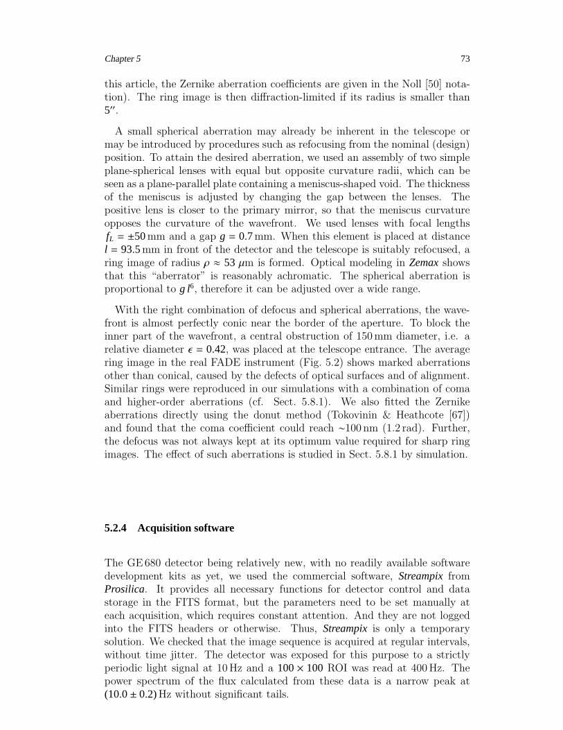
Chapter 5 73

this article, the Zernike aberration coefficients are given in the Noll [50] nota-tion). The ring image is then diffraction-limited if its radius is smaller than5′′.

A small spherical aberration may already be inherent in the telescope ormay be introduced by procedures such as refocusing from the nominal (design)position. To attain the desired aberration, we used an assembly of two simpleplane-spherical lenses with equal but opposite curvature radii, which can beseen as a plane-parallel plate containing a meniscus-shaped void. The thicknessof the meniscus is adjusted by changing the gap between the lenses. Thepositive lens is closer to the primary mirror, so that the meniscus curvatureopposes the curvature of the wavefront. We used lenses with focal lengthsfL = ±50mm and a gap g = 0.7mm. When this element is placed at distancel = 93.5mm in front of the detector and the telescope is suitably refocused, aring image of radius ρ ≈ 53 µm is formed. Optical modeling in Zemaxshowsthat this “aberrator” is reasonably achromatic. The spherical aberration isproportional to g l6, therefore it can be adjusted over a wide range.

With the right combination of defocus and spherical aberrations, the wave-front is almost perfectly conic near the border of the aperture. To block theinner part of the wavefront, a central obstruction of 150mm diameter, i.e. arelative diameter ǫ = 0.42, was placed at the telescope entrance. The averagering image in the real FADE instrument (Fig. 5.2) shows marked aberrationsother than conical, caused by the defects of optical surfaces and of alignment.Similar rings were reproduced in our simulations with a combination of comaand higher-order aberrations (cf. Sect. 5.8.1). We also fitted the Zernikeaberrations directly using the donut method (Tokovinin & Heathcote [67])and found that the coma coefficient could reach ∼100 nm (1.2 rad). Further,the defocus was not always kept at its optimum value required for sharp ringimages. The effect of such aberrations is studied in Sect. 5.8.1 by simulation.

5.2.4 Acquisition software

The GE680 detector being relatively new, with no readily available softwaredevelopment kits as yet, we used the commercial software, StreampixfromProsilica. It provides all necessary functions for detector control and datastorage in the FITS format, but the parameters need to be set manually ateach acquisition, which requires constant attention. And they are not loggedinto the FITS headers or otherwise. Thus, Streampixis only a temporarysolution. We checked that the image sequence is acquired at regular intervals,without time jitter. The detector was exposed for this purpose to a strictlyperiodic light signal at 10Hz and a 100× 100 ROI was read at 400Hz. Thepower spectrum of the flux calculated from these data is a narrow peak at(10.0± 0.2)Hz without significant tails.

74 Chapter 5

5.2.5 Observations

Figure 5.2: From left to right: Simulated ring image – Image of Sirius – Average of 1024 simulatedimages – Average of 1024 Sirius images. The sequence of Sirius images was recorded on Nov 2nd at6:46 UT. The parameters for the data and simulations are given in Sec. 5.8.1.

The FADE instrument has been installed in the USNO dome of the CerroTololo Inter-American Observatory (CTIO) in Chile for the period October 27to November 3, 2006. We pointed FADE at bright stars, Fomalhaut(α PsA,A3V, mV = 1.16) in the evening, then Sirius (α CMa, A1V, mV = −1.47).Figure 5.2 shows typical instantaneous and average images of Sirius, as well assimulated images. During our test run, the seeing was not very good, beingroughly 1′′, and the turbulence in the high atmosphere was strong and fast, asevidenced by the MASS data.

5.3 Data analysis

A correct algorithm of data processing and interpretation is critical to derivethe atmospheric parameters ε0 and τ0. We selected carefully the most robustmethod of calculating atmospheric defocus from the ring-like images and stud-ied by numerical simulation the influence of various instrumental effects andof optical propagation on the results (Appendix 5.8).

5.3.1 Estimating the ring radius

The center of gravity of the image (xc, yc) is calculated by the usual formula

xc =∑

l,k

xl,k I l,k/∑

l,k

I l,k and yc =∑

l,k

yl,k I l,k/∑

l,k

I l,k. (5.1)

The ring radius ρ can then be estimated in a similar way, as the intensity-averaged distance from this center:

ρ =∑

l,k

r l,k I l,k/∑

l,k

I l,k. (5.2)

Chapter 5 75

Here I l,k is the light intensity at pixel (l, k), and r l,k is the distance of this pixelfrom the center. There are various caveats below the apparent simplicity ofthis procedure.

There is no unambiguous way to assign a center to a real, distorted and noisyring image. A simple center-of-gravity is a very rough estimate of (xc, yc),in particular it is affected by the intensity fluctuations in the ring due toscintillation. It is better to compute (xc, yc) with clipped intensities: 0 below athreshold and 1 above, the threshold being set safely above the background andits fluctuations. This initial estimate can be further improved by minimizingthe intensity-weighted mean distance of the pixels from the ring, as describedin Appendix A. However, small inaccuracies in the center determination do notaffect the resulting radius critically and, in fact, we found the initial estimateto be adequate.

A second caveat concerns the choice of the pixels used for the radius estimate.A considerable fraction of pixels lie outside the ring in an empty area thatcontributes only noise. To reduce the noise with a minimal loss of information,we have restricted the pixels used in (5.2) to a mask of inner radius ρ−∆ρ andouter radius ρ + ∆ρ, where ρ is the average ring radius. We express the maskhalf-width ∆ρ as a fraction δ of the diffraction half-width of the ring,

∆ρ = δ λ/[0.5 D (1− ǫ)]. (5.3)

Figure 5.3 shows that a mask with δ = 2 would be good for an ideal,diffraction-limited ring. For a typical image sequence, however, the ring iswidened by telescope aberrations and atmospheric distortions. So we set δ = 4which covers the actual ring image with a sufficiently conservative, but stillreasonable margin.

The simulations show that scintillation and aberrations add to the fluctua-tions of the estimated radii and thus bias the results of FADE. To reduce thiseffect, we sub-divide the ring into eight 45 sectors and – utilizing the samecenter estimate (xc, yc) – apply Eq. 5.2 to each sector separately, and then av-erage the result. This reduces the effect of azimuthal intensity variations. Anadded advantage of the procedure is that the relative variance s of the totalintensities in the sectors Ik with respect to their average I k serves as a measureof the scintillation, hence of the turbulence height,

s =18

8∑

k=1

(Ik − I k)2 / I k

2. (5.4)

The method of calculating the ring parameters (xc, yc, ρ) is less rigorous thanfitting a wave-front model directly to the image. The great advantage of theestimator (5.2), however, is its simplicity.

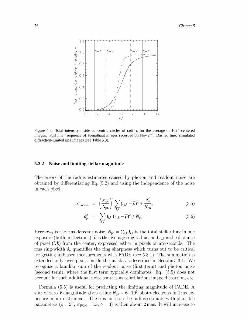
76 Chapter 5

Figure 5.3: Total intensity inside concentric circles of radii ρ for the average of 1024 centeredimages. Full line: sequence of Fomalhaut images recorded onNov 2nd. Dashed line: simulateddiffraction-limited ring images (see Table 5.3).

5.3.2 Noise and limiting stellar magnitude

The errors of the radius estimates caused by photon and readout noise areobtained by differentiating Eq. (5.2) and using the independence of the noisein each pixel:

σ2ρ,noise =

(

σron

Nph

)2∑

l,k

(r l,k − ρ)2 +δ2ρ

Nph, (5.5)

δ2ρ =∑

l,k

I l,k (r l,k − ρ)2 / Nph. (5.6)

Here σron is the rms detector noise, Nph =∑

l,k I l,k is the total stellar flux in oneexposure (both in electrons), ρ is the average ring radius, and r l,k is the distanceof pixel (l, k) from the center, expressed either in pixels or arc-seconds. Therms ring-width δρ quantifies the ring sharpness which turns out to be criticalfor getting unbiased measurements with FADE (see 5.8.1). The summation isextended only over pixels inside the mask, as described in Section 5.3.1. Werecognize a familiar sum of the readout noise (first term) and photon noise(second term), where the first term typically dominates. Eq. (5.5) does notaccount for such additional noise sources as scintillation, image distortion, etc.

Formula (5.5) is useful for predicting the limiting magnitude of FADE. Astar of zero V-magnitude gives a flux Nph ∼ 6 · 105 photo-electrons in 1ms ex-posure in our instrument. The rms noise on the radius estimate with plausibleparameters (ρ = 5′′, σRON = 13, δ = 4) is then about 2mas. It will increase to

Chapter 5 77

20mas for a star with mV = 2.5m – still much less than the atmospheric signal.Hence, despite very short exposures, FADE is not photon-starved.

5.3.3 The response coefficient of FADE

The relation between the ring radius fluctuations ∆ρ and the atmospheric defo-cus (Zernike coefficient a4) is intuitively clear. But what is the exactcoefficientA in the formula ∆ρ = Aa4? Recall that the atmsopheric defocus a4 is relatedto the phase distortion ϕ(r) as

a4 =

∫

z4(r) ϕ(r) d2r , (5.7)

where r is the normalized coordinate vector on the pupil and z4(r) is the orto-normal Zernike defocus given by Noll [50] for the circular aperture and inFig. 5.4 for the annular aperture.

1

z z z

1ee

1e

Defocus Cone Gradient

rr

r

Defocus z(r) =√

12(

r2 − 1+ǫ2

2

)

/(1− ǫ2)

Cone z(r) =[

r − 2(1−ǫ3)3(1−ǫ2)

] [

1+ǫ2

2 −4(1−ǫ3)2

9(1−ǫ2)2

]−1/2

Gradient z(r) =[

δ(r−1)2πr −

δ(r−ǫ)2πǫr

]

Figure 5.4: Response functionsz(r) on annular aperture for Zernike defocus, conic aberration, andaverage radial gradient. The first two functions are normalized in the Noll [50] sense. The coeffi-cientsa4, ac andag are calculated as integrals (5.7). Hereδ is the Dirac’s delta-function.

A reaction of our simple radius estimator (5.2) to a small perturbation ofphase and amplitude at the telescope pupil can be determined analytically (cf.Perrin et al. [54] for an example of similar analytics). It turns out that theresponse to a phase perturbation in the pupil plane is not exactly proportionalto the Zernike defocus. Moreover, it depends on the adopted mask half-width δ.For δ ∼ 1, the response resembles a cone, therefore FADE measures somethingsimilar to a conic aberration. On the other hand, for δ ≥ 2 the computedring radius is related to the average radial gradient of the wave-front, andtherefore FADE measures the difference ag between the phase averaged on theouter and inner edges of its annular aperture. Its response is further modifiedwhen the ring is distorted by aberrations. In this case, the radius estimate issensitive to both amplitude and phase fluctuations. Although we developeda full analytical treatment of this problem, it is omitted here for the sake ofsimplicity.

The three quantities – Zernike defocus a4, conic aberration ac, and averagephase gradient ag – are similar, especially on the annular aperture (Fig. 5.4).

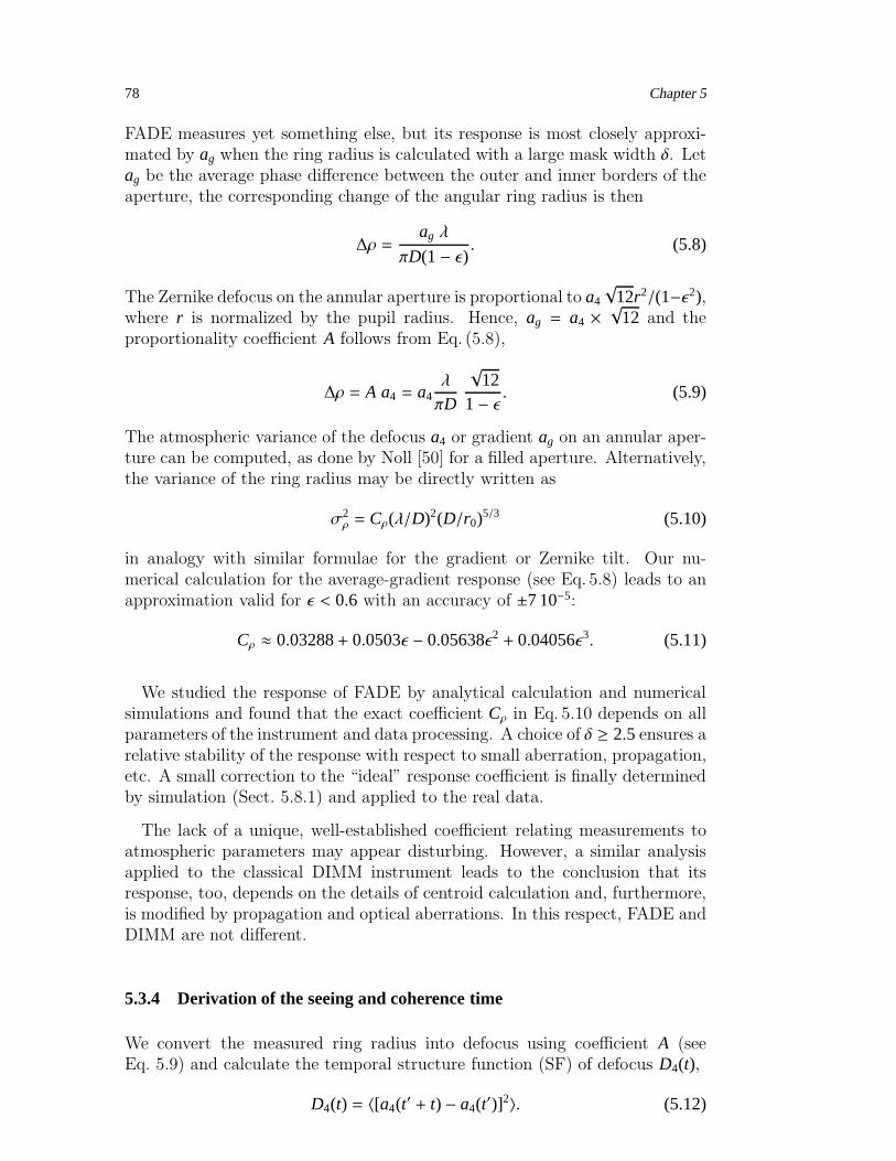
78 Chapter 5

FADE measures yet something else, but its response is most closely approxi-mated by ag when the ring radius is calculated with a large mask width δ. Letag be the average phase difference between the outer and inner borders of theaperture, the corresponding change of the angular ring radius is then

∆ρ =ag λ

πD(1− ǫ). (5.8)

The Zernike defocus on the annular aperture is proportional to a4

√12r2/(1−ǫ2),

where r is normalized by the pupil radius. Hence, ag = a4 ×√

12 and theproportionality coefficient A follows from Eq. (5.8),

∆ρ = A a4 = a4λ

πD

√12

1− ǫ. (5.9)

The atmospheric variance of the defocus a4 or gradient ag on an annular aper-ture can be computed, as done by Noll [50] for a filled aperture. Alternatively,the variance of the ring radius may be directly written as

σ2ρ = Cρ(λ/D)2(D/r0)

5/3 (5.10)

in analogy with similar formulae for the gradient or Zernike tilt. Our nu-merical calculation for the average-gradient response (see Eq. 5.8) leads to anapproximation valid for ǫ < 0.6 with an accuracy of ±7 10−5:

Cρ ≈ 0.03288+ 0.0503ǫ − 0.05638ǫ2 + 0.04056ǫ3. (5.11)

We studied the response of FADE by analytical calculation and numericalsimulations and found that the exact coefficient Cρ in Eq. 5.10 depends on allparameters of the instrument and data processing. A choice of δ ≥ 2.5 ensures arelative stability of the response with respect to small aberration, propagation,etc. A small correction to the “ideal” response coefficient is finally determinedby simulation (Sect. 5.8.1) and applied to the real data.

The lack of a unique, well-established coefficient relating measurements toatmospheric parameters may appear disturbing. However, a similar analysisapplied to the classical DIMM instrument leads to the conclusion that itsresponse, too, depends on the details of centroid calculation and, furthermore,is modified by propagation and optical aberrations. In this respect, FADE andDIMM are not different.

5.3.4 Derivation of the seeing and coherence time

We convert the measured ring radius into defocus using coefficient A (seeEq. 5.9) and calculate the temporal structure function (SF) of defocus D4(t),

D4(t) = 〈[a4(t′ + t) − a4(t

′)]2〉. (5.12)

Chapter 5 79

Figure 5.5: Structure function of focus variations measured at 700 Hz (crosses) fitted with a modelof three turbulent layers (line).

A typical SF is plotted in Fig. 5.5.

A theoretical expression for the defocus SF has been derived in KT07. Wegeneralize it to annular apertures in Appendix B. The initial, quadratic partof the SF is directly related to the combined time constant τ0 of all turbulentlayers. However, the acquisition frequency is not fast enough to capture theinitial quadratic part of the SF extending only to time lags of < 0.1tcross. Inorder to get two points on this part for a layer moving with V = 50m/s, aframe rate of ∼ 3kHz would be required.

To overcome the sampling problem, we fit the initial part of the SF to a modelof N turbulent layers with Fried parameters r0,i and velocities Vi, 1 ≤ i ≤ N:

D4(t > 0) = 1.94D5/3N

∑

i=1

r−5/30,i K4(2tVi/D, ǫ) +

2σ2ρ,noise

A2, (5.13)

where the function K4(β, ǫ) is defined in Appendix B and σ2ρ,noise is the noise

of the radius estimate determined by Eq. 5.5. The adjusted parameters are r0,i

and Vi . As will be seen in Section 5.4.1, the estimate of τ0 is independent ofN if N ≥ 3. Accordingly, a three-layer model is chosen for the data analysis(Fig. 5.5). We fit only the initial part of the SF, up to the time increment ∆t.Its exact value is not critical, as long as it is large enough for unambiguousfitting of the parameters, ∆t ν > 2N + 1. For further data analysis, we set∆t = 40ms.

80 Chapter 5

The atmospheric parameters (r0,V, τ0) are calculated as

r−5/30 =

N∑

i=1

r−5/30,i , (5.14)

(V/r0)5/3 =

N∑

i=1

(Vi/r0,i)5/3, (5.15)

τ0 = 0.314 r0/V. (5.16)

The estimate of r0 is also obtained directly from the ring-radius variance σ2ρ

by subtracting the noise,

σ2ρ − σ2

ρ,noise= Cρ(λ/D)2(D/r0)5/3. (5.17)

When the SF reaches its asymptotic value on time increments smaller than40ms, the same value of r0 is derived from the ring-radius variance (Eq. 5.17)and from the model (Eq. 5.14). The robustness of parameter estimates derivedby model fitting has been confirmed by numerical simulation and by fittingalternative models to real data (Section 5.4.1).

5.4 Analysis of observations

Seeing and coherence time were estimated from all sequences of 4000 imagesrecorded with FADE at Cerro Tololo between October 29th and November 2nd,2006. In this Section, we check the FADE results for consistency and comparethem with the MASS-DIMM.

5.4.1 Influence of instrumental parameters

During data acquisition, instrumental parameters were varied over a broadrange to evaluate their effect on the results. Even though the non-stationarityof the atmosphere precludes direct comparisons, some conclusions can never-theless be drawn.

The ring sharpness, δρ, has been identified as a major source of instrumentalbias in FADE when significant high-altitude turbulence is present. In ourdata, most images have 1′′ < δρ < 1.5′′, whereas a perfect diffraction-limitedring has δρ = 0.9′′. Analysis of the average ring-images confirms that theoptimum combination of defocus and spherical aberrations was not reached,a4 and a11 often being of the same sign rather than of opposite signs. Forour data, the dispersion and mean of τ0 increase when δ > 1.25′′, accordinglysequences with δρ > 1.25′′ are disregarded. Still, some bias caused by radiallydefocused images remains.

Chapter 5 81

Figure 5.6: Coherence time derived from the recorded data byfitting a model withN = 3 layers(x-axis) is compared to the coherence time derived withN = 2 (dotted line) andN = 4 (solid line)models.

As described in Sect. 5.3.4, the data are fitted to a model with a discretenumber of turbulent layers, N. Which is the minimum value of N that permitsa correct derivation of τ0? Figure 5.6 shows that the τ0 values obtained with3 and 2 (resp. 4) layers differ on average by 7% (resp. 2%). An averagedifference of 2% is likewise obtained when comparing the estimates with of 3and 5 layers. A 3-layer model is thus a good compromise enabling to fit thedata with only six parameters.

The influence of the acquisition frequencyon the measured coherence time isexamined in Fig. 5.7. The data sequences recorded at frequencies ν ≥ 700Hzwere re-analyzed considering every other image. The coherence time obtainedwith a slower ν/2 sampling is on the average 9% longer than with the fastsampling. This difference is reproduced by simulations if the turbulence isplaced at 5 km altitude and if the ring-images are slightly defocused in theradial direction (a11/a4 ≈ −0.07 or −0.14 instead of a11/a4 = −0.11 correspond-ing to a sharp ring). The effect of temporal under-sampling is perceptible ifthe same comparison is repeated with sequences recorded at frequencies below700Hz: the number of points on the initial, increasing part of the SF is thennot always sufficient to extract unambiguously the six fitted parameters andthe coherence time is hence poorly constrained. To ensure a correct temporalsampling under fast turbulence, we disregard the sequences with ν < 500Hz.

In line with the simulations, the coherence time estimates do not depend onthe average ring image radius. Similarly, the parameter statistics seems unbi-ased by the stellar fluxand by the exposure time. While the sequences of Sirius(mV = −1.5) and Fomalhaut (mV = 1.2) images were recorded with exposuretimes of dt < 0.5ms and 1.0 < dt < 1.9ms respectively, no obvious difference

82 Chapter 5

Figure 5.7: Coherence time derived from all sequences recorded withν ≥ 700 Hz when every image(x axis) and every other image (y axis) is considered.

exists between the mean and rms of the atmospheric parameters measured interms of these two stars,ǫS0 : (0.9± 0.2)′′ ǫF0 : (0.8± 0.1)′′

τS0 : (1.4± 0.5)ms τF0 : (1.3± 0.5)ms.

5.4.2 Comparison with MASS and DIMM

In this section, the seeing and coherence time obtained with FADE are com-pared to simultaneous measurements by the CTIO site monitor located at 10mdistance from FADE on a 6m high tower. The monitor consists of a combinedMASS-DIMM instrument fed by the 25-cm Meade telescope and looking atbright (V = 2m...3m) stars near zenith. Of particular interest here is the timeconstant τ0 estimated by MASS from the temporal characteristics of scintil-lation by the method of Tokovinin [68]. This method is intrinsically biasedbecause it does not account for the turbulence below ∼ 500m. Moreover, ithas been recently established by simulations that the coefficient used to cal-culate τ0 in the MASS software must be increased by 1.27.1 In the following,we correct τ0 by applying this coefficient and including the contribution of theground layer:

τ−5/30 = (1.27 τMASS)−5/3 + 118λ−2 V5/3

GL (C2n dh)GL. (5.18)

The turbulence integral in the ground layer, (C2n dh)GL, is computed from the

difference between the turbulence integrals measured by DIMM (whole atmo-

1See the unpublished report by Tokovinin (2006) at http://www.ctio.noao.edu/˜atokovin/profiler/timeconst.pdf

Chapter 5 83

sphere) and MASS (above 500m), while the ground layer wind speed, VGL,is known from the local meteorological station. Even after correction byEq. (5.18), the coherence time measured by MASS-DIMM should be takenwith some reservation because it has never been checked against independentinstruments and some bias is possible.

Figure 5.8 compares the estimates of ε0 and τ0 obtained with FADE fromOctober 29th to November 2nd, to the results of MASS-DIMM. We do notexpect detailed correlation because the instruments were sampling differentatmospheric volumes. As seen on Fig. 5.8, the seeing measurements are bettercorrelated than the coherence times.

Statistically, it appears that FADE slightly under-estimates the seeing. Thiseffect is reproduced with simulations of high-altitude turbulence if the ratio ofspherical aberration to defocus a11/a4 is set larger than its optimum value −0.1corresponding to sharp ring images. In this case, FADE also under-estimatesthe coherence time. The bias on τ0 can however not be ascertained by Fig. 5.8because the τ0 estimates by MASS might likewise be biased.

5.5 Conclusions and perspectives

We have built a first prototype of the site-testing monitor, FADE, suitablefor routine measurements of the atmospheric coherence time, τ0, as well asthe seeing, ε0. The instrument has been tested on the sky. Extensive sim-ulations substantiate the validity of the FADE results and indicate potentialinstrumental biases. Our main conclusions are as follows:

– The sampling time of the image sequence must be a small fraction of theaperture crossing time tcross = D/V (∼10 ms for D = 0.36m and windspeed V = 36m/s). Sampling at ν ≥ 500Hz appears adequate under mostconditions.

– The sharpness of the ring image in the radial direction does not bias theresults when the turbulence is located near the ground. But it can biasboth τ0 and ε0 estimates when high layers dominate, and strict control ofthe telescope aberrations is thus required.The aberrations (hence the datavalidity) can be evaluated a posteriorifrom the average ring image. Real-time estimates of the ring radius ρ and width δρ are necessary to ensuregood optical adjustment of the instrument.

– The FADE monitor with 36-cm telescope can work on stars as faint asmV = 3m.

– A simple estimator of the ring radius (Eq. 5.2) is adequate and robust,provided a wide enough mask around the ring (δ ∼ 4) is used in thecalculation.

84 Chapter 5

– Moderate telescope aberrations such as coma are acceptable. The resultsare not critically influenced by small telescope focus errors.

The current FADE prototype stores all image sequences, leading to a largedata volume; the data are processed off-line. While this procedure was nec-essary for the first experiments, on-line processing will be implemented in adefinitive instrument. We have formulated and tested the data processingalgorithm and can now develop adequate real-time software.

We plan to develop an improved version of FADE with real-time data analy-sis. It will be compared to simultaneous estimates of the atmospheric time con-stant from currently working adaptive-optics systems (Fusco et al. [23]) and/orlong-baseline interferometers such as VLTI. Characterization of Antarctic sitesfor future interferometers is an obvious application for FADE.

Acknowledgements: This work was stimulated by discussionswith Marc Sarazinand other colleagues involved in site characterization. Weacknowledge financialand logistic help from ESO in building and testing the first FADE prototype. Wethank Cerro Tololo Inter-American Observatory for its hospitality and support ofthe first FADE mission.

5.6 Appendix A – Estimator of the ring radius and center

The parameters of the ring-like image – its center (xc, yc) and radius ρ – canbe derived by minimizing the intensity-weighted mean squared distance of thepixels from the circle, δ2ρ:

δ2ρ =∑

l,k

I l,k (r l,k − ρ)2 /∑

l,k

I l,k, (5.19)

where r l,k = [(l − xc)2 + (k − yc)2]0.5 is the distance of pixel (l, k) from the ring-center, (xc, yc). Setting the partial derivative of δ2ρ over ρ to zero, we obtainthe radius estimator of Eq. 5.2. However, it still depends on the unknownparameters (xc, yc). By use of Eq. 5.2, Eq. 5.19 is simplified to:

δ2ρ =

∑

l,k I l,kr2l,k

∑

l,k I l,k−

[∑

l,k I l,k r l,k∑

l,k I l,k

]2

. (5.20)

This formula does not contain ρ. The center coordinates (xc, yc) can be derivedby setting the partial derivatives of δ2ρ over parameters to zero and solving theequations. We determine the center numerically by minimizing Eq. 5.20 andusing the center-of-gravity coordinates as a starting point.

Chapter 5 85

5.7 Appendix B – Structure function of atmospheric defocus

The temporal structure function of atmospherically-induced defocus variations– Zernike coefficient a4 in Noll’s [50] notation – has been derived in KT07 for afilled circular aperture. Here we generalize it to an annular aperture. Withoutrepeating the whole derivation, we refer the reader to KT07 and modify onlythe spatial spectrum of the Zernike defocus, taking into account the centralobstruction ratio ǫ. The resulting expression is

D4(t) = 0.821k2D5/3

∫ +∞

0dh Cn(h)2 K4

(

2tV(h)D, ǫ

)

, (5.21)

K4(β, ǫ) =12

(1− ǫ2)4

∫ +∞

0dx x−8/3 [1 − J0(βx)]

×[

J3(x)x− ǫ4 J3(ǫx)

ǫx+ ǫ2

J1(x)x− ǫ2 J1(ǫx)

ǫx

]2

, (5.22)

where k = 2π/λ, Jn is the Bessel function of order n, Cn(h)2 and V(h) arethe altitude profiles of the refractive-index structure constant and wind speed,respectively. Considering the known relation between the turbulence integraland the Fried parameter, r−5/3

0 = 0.423k2 C2ndh, we can also write the defocus

SF produced by a single layer as

D4(t) = 1.94 (D/r0)5/3K4(2tV/D, ǫ). (5.23)

For calculating the function K4, it is convenient to approximate the integral(5.22) by an analytical formula, as in KT07. We suggest the approximation

K4(β, ǫ) ≈C1 β

2 +C2 β6

1+C3 βα + β6, (5.24)

where the coefficients are cubic polynomials of ǫ:

Ci = Ci,0

3∑

k=0

ci,k ǫk, (5.25)

cf. Table 5.2. This approximation is valid for ǫ < 0.6 with a maximum relativeerror of less than 5% (3% for ǫ = 0.42) and correct asymptotes. The asymptoticvalue K4(∞, ǫ) = C2 gives the focus variance on annular aperture, analogousto the Noll’s coefficient. For ǫ = 0, we get C2 = 0.024 and the focus variancecoefficient of 1.94× 0.024/2 = 0.0233, in agreement with the Noll’s result.

The function K4(β, ǫ) reaches half its saturation value at β = 0.63, hence theatmospheric defocus correlation time is ∼ 0.3D/V, as is well known in adaptiveoptics.

The above analysis is valid for instantaneous measurements, while in fact thedefocus is averaged over the exposure time. This effect is usually important for

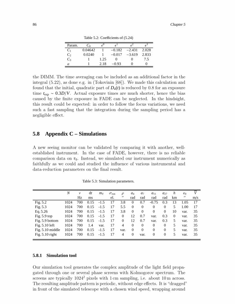
86 Chapter 5

Table 5.2: Coefficients of (5.24)

Param. C0 ǫ0 ǫ1 ǫ2 ǫ3

C1 0.04642 1 −0.182 −2.431 2.028C2 0.0240 1 −0.017 −3.619 2.833C3 1 1.25 0 0 7.5α 1 2.18 −0.93 0 0

the DIMM. The time averaging can be included as an additional factor in theintegral (5.22), as done e.g. in (Tokovinin [68]). We made this calculation andfound that the initial, quadratic part of D4(t) is reduced by 0.8 for an exposuretime texp ∼ 0.3D/V. Actual exposure times are much shorter, hence the biascaused by the finite exposure in FADE can be neglected. In the hindsight,this result could be expected: in order to follow the focus variations, we needsuch a fast sampling that the integration during the sampling period has anegligible effect.

5.8 Appendix C – Simulations

A new seeing monitor can be validated by comparing it with another, well-established instrument. In the case of FADE, however, there is no reliablecomparison data on τ0. Instead, we simulated our instrument numerically asfaithfully as we could and studied the influence of various instrumental anddata-reduction parameters on the final result.

Table 5.3: Simulation parameters.

N ν dt mV σron ρ a4 a7 a11 a27 h ε0 VHz ms el. ′′ rad rad rad rad km ′′ m/s

Fig. 5.2 1024 700 0.15 -1.5 17 3.8 0 0.7 -0.75 0.3 13 1.05 17Fig. 5.3 1024 700 0.15 -1.5 17 5.5 0 0 0 0 5 1.00 17Eq. 5.26 1024 700 0.15 -1.5 17 3.8 0 0 0 0 10 var. 35Fig. 5.9 top 1024 700 0.15 -1.5 17 0 12 0.7 var. 0.3 0 var. 35Fig. 5.9 bottom 1024 700 0.15 -1.5 17 0 12 0.7 var. 0.3 5 var. 35Fig. 5.10 left 1024 700 1.4 var. 17 4 0 0 0 0 5 var. 35Fig. 5.10 middle 1024 700 0.15 -1.5 17 var. 0 0 0 0 5 var. 35Fig. 5.10 right 1024 700 0.15 -1.5 17 4 0 var. 0 0 5 var. 35

5.8.1 Simulation tool

Our simulation tool generates the complex amplitude of the light field propa-gated through one or several phase screens with Kolmogorov spectrum. Thescreens are typically 10242 pixels with 1 cm sampling, i.e. about 10m across.The resulting amplitude pattern is periodic, without edge effects. It is “dragged”in front of the simulated telescope with a chosen wind speed, wrapping around

Chapter 5 87

edges in both coordinates and eventually covering the whole area. The monochro-matic images created by a telescope with a perfect conic aberration of specifiedamplitude and, possibly, some additional intrinsic aberrations are re-binnedinto the detector pixels, distorted by readout and photon noise and fed to thedata-analysis routine instead of the real data. Our tool has been verified bycomparing with analytical results for weak perturbations and has been used forsimulating other instruments such as DIMM and MASS. The limitations of thistool are: monochromatic light, single wind velocity for all layers, instantaneousexposure time.

We used two alternative, nearly equivalent ways of producing ring images.In the first method, a perfect conic wavefront was generated, and its amplitudewas expressed as a ring radius ρ. In the second method, we do not apply conicaberration (ρ = 0), but, instead, select a combination of defocus and sphericalaberrations to mimic a real telescope. The sense of the Zernike coefficients a4

and a11 in both cases is distinct.

Parameters of the simulations

For convenience, the simulation parameters are gathered in Table 5.3. Theseparameters are:

– number of images in the sequence N,

– acquisition frequency ν,

– exposure time dt,

– visual stellar magnitude m,

– readout noise σron,

– conic aberration quantified by the average ring radius ρ,

– amplitudes of the Zernike aberrations a4 (defocus), a7 (coma), a11 (spher-ical), and a27,

– altitude of the single turbulent layer h,

– seeing ε0,

– wind speed V.

Simulated ring images are compared in Fig. 5.2 to the images of Siriusrecorded on Nov. 2nd. The combination of exposure time and magnitude resultsin the detected flux of 3·105 electrons per simulated image, as in the actual im-ages of Sirius. For this sequence, the estimated turbulence parameters equal:ε0 = 1.05”, V = 17m/s, τ0 = 1.86ms (Fig. 5.5). The same parameters arechosen for the simulated images. For best resemblance between simulated andreal images, telescope aberrations are set to a7 = 0.7rad, a11 = −0.75rad,

88 Chapter 5

a27 = 0.3rad. The turbulence is placed at 13 km altitude to reproduce theactual level of scintillation, evaluated from the intensity variance between ringsectors s= 0.011 (cf. Eq. 5.4).

Refining the response coefficient

The coefficient A relating radius variation to defocus is given by Eq. 5.9. Itsactual numerical value, however, depends on the method of radius estimation,and in particular on the choice of the mask width δ. For δ = 4, we determined itto equal 1.077 by comparing τ0 estimates from sequences of simulated images,to the nominal input value of τ0 when Eq. 5.9 is used to relate the radius to de-focus. The corresponding simulation parameters are summarized in Table 5.3.Thus,

∆ρ/a4 = 1.077λ

πD

√12

1− ǫ. (5.26)

Instrumental biases

The data analysis relies on radius estimates that can be altered by telescopeaberrations, scintillation, detector and photon noise, etc. Here we evaluatethe instrumental bias by changing some parameters, while other parametersare fixed. In each case, a sequence of 1024 simulated images is generated withparameter values listed in Table 5.3. The wind speed is set to 35m/s and thecoherence time is then changed by modifying the seeing.

Ring sharpness. The ring is sharp in the radial direction when the wavefrontis exactly conic. A good approximation of the conic wavefront is achieved bythe optimum combination of defocus and spherical aberrations, a11 = −0.1a4.Here we explore the effect of unsharp ring images by setting a4 = 12rad andvarying a11 about its optimum value a11 = −1.2rad. Unlike the rest of thesimulations, we do not apply conic aberration and set ρ = 0. Wrong values ofa11 make the ring wider, as evidenced by its rms width, δρ (Eq. 5.6).

As seen in Fig. 5.9, the seeing and coherence-time estimates are biased in caseof blurred rings and high-altitude turbulence. The sign of the bias depends onthe sign of the deviation from the optimum a11. When the turbulent layers arelow, the scintillation is weak and the parameters are correctly derived even ifthe ring images are blurred.

To ensure a correct derivation under any atmospheric conditions, the ringwidth should be close to its diffraction-limited value δρ,0:

δρ < 1.2δρ,0 ; δρ,0 = 1.7λ/[D (1− ǫ)], (5.27)

where the coefficient 1.7 is determined from the width, δρ = 0.87′′, of diffraction-

Chapter 5 89

limited rings. Given the instrumental set-up, images should be rejected ifδρ < 1′′. However, all images recorded with the FADE prototype have δρ > 1′′.Hence we apply a softer data-selection criterion: δρ < 1.25′′, and note that theresulting estimates might still be biased if the turbulence was high.

Stellar magnitude, ring radius and coma. Figure 5.10 examines the stability of theseeing and coherence time estimates with respect to the stellar magnitudemV, ring image radius ρ, and coma aberration a7. In agreement with Eq. 5.5,estimates are correct up to stellar magnitudes 2–3. Spatial sampling and comaaberration do not affect the estimates if ρ ≥ 2′′ (i.e. 5 pixels) and a7 ≤ 2rad.

90 Chapter 5

Figure 5.8: Seeing and coherence time measured with FADE between October 29th and Novem-ber 2nd, compared to simultaneous measurements by the MASS-DIMM. The average values andstandard deviations of parameters and the correlation coefficients are indicated.

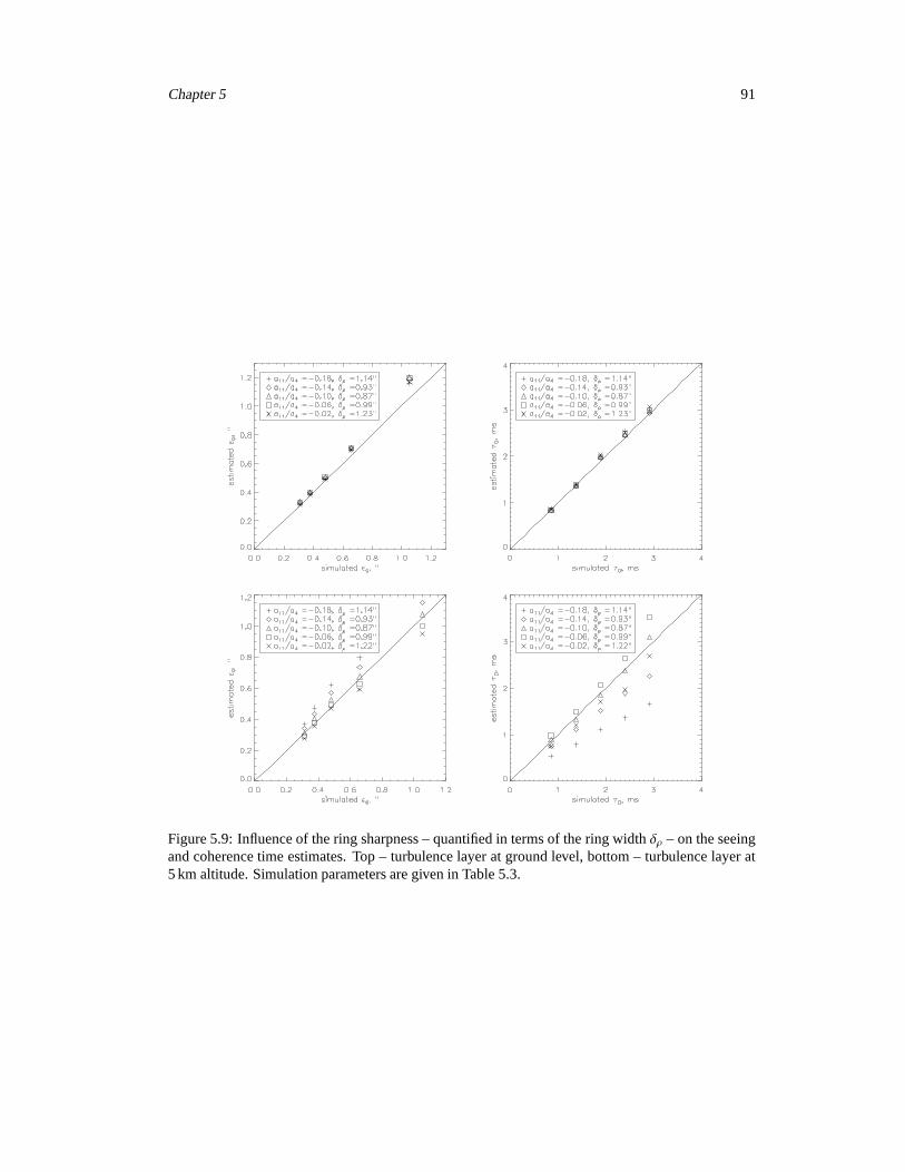
Chapter 5 91

Figure 5.9: Influence of the ring sharpness – quantified in terms of the ring widthδρ – on the seeingand coherence time estimates. Top – turbulence layer at ground level, bottom – turbulence layer at5 km altitude. Simulation parameters are given in Table 5.3.

92 Chapter 5

Figure 5.10: Dependence of the seeing and coherence time estimates on stellar magnitudemV, meanring radiusρ and coma aberrationa7. Simulation parameters are given in Table 5.3.

Chapter 6

Interferometric observations of the

multiple stellar systemδVelorum

6.1 Introductory remarks to the article

New techniques for characterizing atmospheric turbulence and an improvementof the underlying theory are not an end in itself; for the astronomers they are ofconsequence where they facilitate and advance observational techniques. Thischapter is meant to exemplify one area where interferometry is of particularimportance.

A central issue in astrophysics, the theory of stellar evolution, has madeconsiderable progress during the last century, but it is still incomplete and inmany major aspects tentative. In the range of intermediate stellar masses,luminosities and ages, the theory is essentially consistent. But where the earlyand the final phases of stellar evolution are concerned, and also the extremelymassive and the very low-mass stars, it tends to fail. Essential mechanismsremain largely unresolved. The energy transport out of the stellar centers,i.e. the efficiency and relative contribution of the two major mechanisms,conduction and convection, is reasonably known for a star of lower mass, suchas our sun, but outside the normal range no reliable answers can currently begiven.

The underlying problem is the impossibility to determine, with conventionaltechniques, the relevant parameters of a star. The mass, the chemical com-position and the age of a star are the essential characteristics that determineits luminosity, size, heavy-element generation, and ultimately its fate. How-ever, the stellar age can never be determined directly and the mass only underspecial conditions. These two parameters must, therefore, be derived from theluminosity, color or effective temperature by the use of relations obtained viaevolutionary models.

93

94 Chapter 6

To calibrate these relations, observations are required that are not possiblewith single stars, but can be made on physical binary and multiple-star sys-tems, i.e., on star systems that are not associated by chance alignment, butare coupled by their gravitational forces. Such systems offer the possibility todetermine directly the masses of stars that have been formed from the samepre-stellar cloud and are, thus, of same age. For a binary system the massesare inferred from Kepler’s laws of motion, provided a number of parameters areobtained: the period, the semi-major axis and the eccentricity of the binary’sorbit, and the ratio of the two stars’ distances to their center of mass. Theseparameters are inferred from the stellar radial velocities via the Doppler shiftsof spectral lines, and from the stars’ positions via astrometric measurements.

Astrometry requires the stars to be sufficiently separated to be resolvedas separate objects, i.e. the stars in binaries or multiple systems need tobe reasonably widely separated. This, however, implies long orbital cyclesand, accordingly, it obviates the quick acquisition of the relevant data. It is,thus, more desirable to work on close binaries or on the closely associatedcomponents in multiple stars, which usually are hierarchical, i.e. contain closebinaries. But in all these cases, where small distances are involved, positionsand separations need to be obtained through interferometric measurements.While – as documented in the most up-to-date 1999 revision of Tokovinin’scatalogue [69] – speckle interferometry has been successful in past observations,long-baseline interferometry is required to deal with the close distances thatare currently of much interest.

It must be noted that the true three-dimensional orbit can be reconstructedonly if the interferometric measurements of the positions and the Doppler-measurements of the radial-velocity are combined. This is so, because theactual measured quantities are, first, the two-dimensional projections of thepositions onto the celestial sphere and, second, the one-dimensional projectionof the velocities along the line of sight. In practice, the measurements areoften not yet sufficient to derive the two stellar masses without additionalassumptions, such as for example the mass of the primary, which might beestimated indirectly from the luminosity or spectral type.

In an eclipsing binary, the orbit is oriented so that one star passes in frontof the other as we observe the system. This not only reduces the problem totwo dimensions, but also permits to readily derive several parameters from thetemporal variations of the stellar flux: Twice during an orbital period the fluxdrops as one star eclipses the other. The relative durations of these eclipses andthe relative durations between the eclipses are related to the eccentricity andthe orientation of the orbit. Further, the ratio of the stellar surface brightnessesis obtained from the intensity ratio of the two eclipses. The orbital and physicalproperties of two eclipsing stars can therefore be determined far more preciselythan with conventional binary systems.

The subsequent article exemplifies the use of interferometry in its applicationto δ Velorum, which is prominent in the center of the Southern hemisphere,where it is going to be the polar star in the year 9000. While δVelorum contains

Chapter 6 95

an eclipsing close binary, (Aa,Ab), which causes two substantial brightnessreductions during the 45-days orbital period, it has, amazingly, been taken fora single star until recently. Only after δ VelorumA was chosen as reference forthe space probe Galileo, and after it failed as such, it was recognized to be abinary system. The subsequent article outlines the study that has come, bythe use of interferometry, to some unexpected conclusions on the multiple-starsystem δ Velorum.

96 Chapter 6

Interferometric observations of the multiplestellar systemδVelorum

A. Kellerer, M.G.Petr-Gotzens, P. Kervella, V. Coude du Foresto, 2007,A&A, 469, 633-637

Abstract

The nearby (∼24 pc) triple stellar system δVelorum contains a close, eclips-ing binary (Aa, Ab) discovered in 2000. Multiple systems provide an opportu-nity to determine the set of fundamental parameters (mass, luminosity, size,chemical composition) of coeval stars.

These parameters can be obtained with particular precision in the case ofeclipsing binaries; so we exploited this potential for δVelorum’s components(Aa, Ab).

We have analysed interferometric observations of the close binary (Aa, Ab),obtained with the VINCI instrument and two VLTI siderostats. The measure-ments, which resolve the two components for the first time, are fitted onto thesimple model of two uniformly bright, spherical stars.

The observations suggest that Aa and Ab have larger diameters than ex-pected for stars on the main sequence, hence they must be in a later evolu-tionary state.

Chapter 6 97

6.2 Introduction

One of the fifty brightest stars on the sky, with a visual magnitude of mV = 1.96mag (Johnson et al. [39]), δVelorum (HD 74956), is a multiple stellar system(e.g.Worley & Douglass [71]). But in spite of its brightness and proximity,π = (40.90± 0.38)mas (Perryman et al. [55]), the issue of its composition re-mains unresolved. As early as 1847, Herschel published his detection of twofaint visual companions, δ Vel C and D, at a distance of 69′′ from δ Vel A.Another companion – δ Vel B at the time separated by ∼ 3′′ from δ Vel A– was later discovered by Innes [37]. The separation 0.′′736± 0.′′014 betweencomponents A and B appeared surprising when measured by Hipparcos, butit was explained later in terms of the orbit computation of Argyle et al. [4],which showed a highly elliptical orbit of component B with period P = 142yr.In 1979, preliminary results from speckle interferometry suggested yet anothercomponent of the system (Tango et al. [65]). This apparent companion wasfound at a separation of ∼ 0.′′6 and was taken to be a further component,because the separation for star B at the time was believed to be ∼ 3′′.

By now, however, it seems very likely that the speckle observations resolvedδ Vel B; while there is still an unexplained disagreement for the position angle,the measured small separation does fit well with the orbital solution found byArgyle et al. [4]. As noted in earlier publications (Hoffleit et al. [35], Otero atal. [52]), the two stars that are currently termed δ Vel C and D were taken tobe associated with the pair AB because of seemingly similar proper motion.However, we have not found the source of the proper motion measurement ofC and D. Finally, the most luminous component, A, was recently recognizedto be a close eclipsing binary with a period T = 45.15days (Otero et al. [52]).Since then, δVel has been classified as a quintuple stellar system.

This investigation is focussed on the bright eclipsing binary, δVelA, butwe also argue that δVelC and D are not physically associated with δVelA,B.While this makes δVel a triple system, it takes little away from its challengingpotential for obtaining important information on stellar evolution. As theinclination, i, of its orbital plane is constrained to be close to 90, an eclipsingbinary system provides one of the best means to obtain, in terms of the Keplerlaws of motion, fundamental stellar parameters.

In this research note, we present the first interferometric observations of theeclipsing binary δVelA, obtained with ESO’s Very Large Telescope Interferom-eter (VLTI) and its “commissioning instrument” VINCI. The measurementsresolve this binary system for the first time. They are analysed here with non-linear least-square fitting methods. We combine our interferometric resultswith existing photometric and spectroscopic observations, estimate some or-bital parameters of the δVelA binary system, and discuss the stellar propertiesof the individual components based on the results.

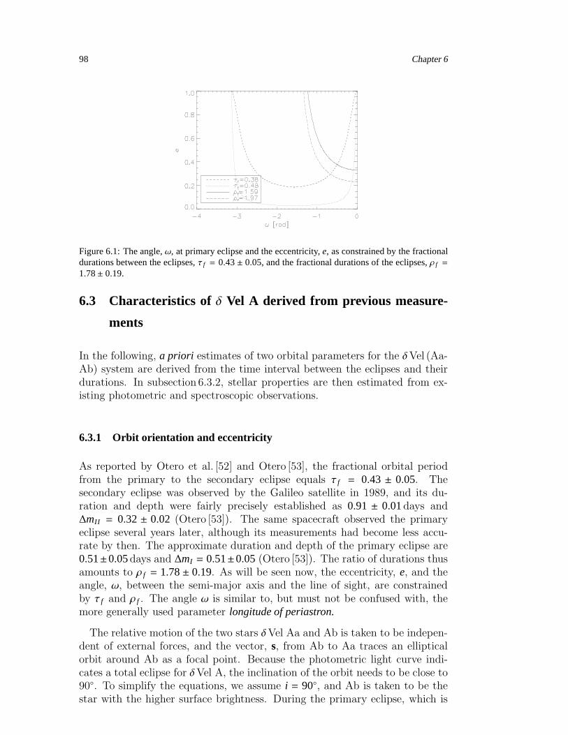
98 Chapter 6

Figure 6.1: The angle,ω, at primary eclipse and the eccentricity,e, as constrained by the fractionaldurations between the eclipses,τ f = 0.43± 0.05, and the fractional durations of the eclipses,ρ f =

1.78± 0.19.

6.3 Characteristics ofδ Vel A derived from previous measure-

ments

In the following, a priori estimates of two orbital parameters for the δVel (Aa-Ab) system are derived from the time interval between the eclipses and theirdurations. In subsection 6.3.2, stellar properties are then estimated from ex-isting photometric and spectroscopic observations.

6.3.1 Orbit orientation and eccentricity

As reported by Otero et al. [52] and Otero [53], the fractional orbital periodfrom the primary to the secondary eclipse equals τ f = 0.43 ± 0.05. Thesecondary eclipse was observed by the Galileo satellite in 1989, and its du-ration and depth were fairly precisely established as 0.91 ± 0.01days and∆mII = 0.32± 0.02 (Otero [53]). The same spacecraft observed the primaryeclipse several years later, although its measurements had become less accu-rate by then. The approximate duration and depth of the primary eclipse are0.51±0.05days and ∆mI = 0.51±0.05 (Otero [53]). The ratio of durations thusamounts to ρ f = 1.78± 0.19. As will be seen now, the eccentricity, e, and theangle, ω, between the semi-major axis and the line of sight, are constrainedby τ f and ρ f . The angle ω is similar to, but must not be confused with, themore generally used parameter longitude of periastron.

The relative motion of the two stars δVel Aa and Ab is taken to be indepen-dent of external forces, and the vector, s, from Ab to Aa traces an ellipticalorbit around Ab as a focal point. Because the photometric light curve indi-cates a total eclipse for δVel A, the inclination of the orbit needs to be close to90. To simplify the equations, we assume i = 90, and Ab is taken to be thestar with the higher surface brightness. During the primary eclipse, which is

Chapter 6 99

deeper, Ab is thus eclipsed by Aa. The angle θ of s, also called the true anomaly,is zero at periastron and increases to π as the star moves towards apastron.The distance between the stars depends on θ according to the relation:

s(θ) = a(1− e2)/(1+ ecos(θ)), (6.1)

where a denotes the semi-major axis. In line with Kepler’s second law, thevector s covers equal areas per unit time. The fractional orbital period toreach angle θ is, accordingly:

τ(θ) =2A

∫ θ

0s2(θ′)dθ′ (6.2)

= [2arctan(f1 tan(θ/2)− f2 sin(θ)/(1+ ecos(θ))]/2π, (6.3)

where A = πa2√

(1− e2) equals the area of the ellipse, and f1 =√

((1− e)/(1+ e))and f2 = e

√

(1− e2).

During the primary eclipse, when the star with the lower surface brightness,Aa, covers Ab, the vector s is directed towards Earth, and θ equals ω. Duringthe secondary eclipse θ equals ω + π. Thus:

τ f = 0.43± 0.05 (6.4)

=

∫ ω+π

ω

dθ/(1+ ecos(θ))2 (6.5)

= [arctan(f1 tan((ω + π)/2))− arctan(f1 tan(ω/2))

+ f2 sin(ω)/(1− e2 cos(ω)2)]/π, (6.6)

which determines ω for any given eccentricity, e (Fig. 6.1). The orbital velocitydecreases as θ goes from zero to π, i.e. from the periastron to the apastron. Inthe subsequent interval, π to 2π (or -π to 0), it increases again. If the line ofsight contained the orbital major axis, i.e. ω = 0 or π, the fractional durationbetween eclipses τ would equal 0.5. Note that for such values of ω, Eq. 6.6 isnot defined, yet τ tends towards 0.5 when ω approaches 0, or π. If the lineof sight contained the orbital minor axis, i.e. ω = π/2 or -π/2, the maximumand minimum values of τ would be reached. Values of τ less than 0.5 are thusassociated with negative ω values. Since the fractional orbital period from theprimary to the secondary eclipse is 0.43, the angle ω must lie between -π and0. As Fig. 6.1 shows, the eccentricity needs to be larger than ≈ 0.03.

On the other hand, ω can be further constrained through the ratio of theeclipse durations as follows. The eclipse durations are inversely proportional tothe product r dθ/dt of radius and angular velocities during the eclipses. Theyare thus proportional to s(θ), and their ratio is:

ρ(ω) = (1− ecos(ω))/(1+ ecos(ω)). (6.7)

Given ρ f = 1.78± 0.19, this leads to a second relation between e and ω. Asillustrated by Fig. 6.1, simultaneous agreement with both observed values τ f

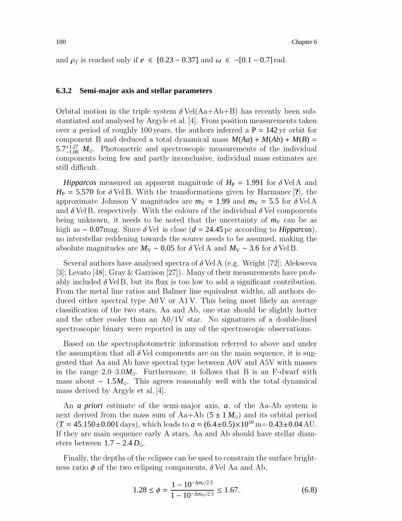
100 Chapter 6

and ρ f is reached only if e ∈ [0.23− 0.37] and ω ∈ −[0.1− 0.7] rad.

6.3.2 Semi-major axis and stellar parameters

Orbital motion in the triple system δVel(Aa+Ab+B) has recently been sub-stantiated and analysed by Argyle et al. [4]. From position measurements takenover a period of roughly 100 years, the authors inferred a P = 142yr orbit forcomponent B and deduced a total dynamical mass M(Aa) + M(Ab) + M(B) =5.7+1.27−1.08 M⊙. Photometric and spectroscopic measurements of the individual

components being few and partly inconclusive, individual mass estimates arestill difficult.

Hipparcosmeasured an apparent magnitude of HP = 1.991 for δVelA andHP = 5.570 for δVelB. With the transformations given by Harmanec [?], theapproximate Johnson V magnitudes are mV = 1.99 and mV = 5.5 for δVelAand δVelB, respectively. With the colours of the individual δVel componentsbeing unknown, it needs to be noted that the uncertainty of mV can be ashigh as ∼ 0.07mag. Since δVel is close (d = 24.45pc according to Hipparcos),no interstellar reddening towards the source needs to be assumed, making theabsolute magnitudes are MV ∼ 0.05 for δVelA and MV ∼ 3.6 for δVelB.

Several authors have analysed spectra of δVelA (e.g. Wright [72]; Alekseeva[3]; Levato [48]; Gray & Garrison [27]). Many of their measurements have prob-ably included δVelB, but its flux is too low to add a significant contribution.From the metal line ratios and Balmer line equivalent widths, all authors de-duced either spectral type A0V or A1V. This being most likely an averageclassification of the two stars, Aa and Ab, one star should be slightly hotterand the other cooler than an A0/1V star. No signatures of a double-linedspectroscopic binary were reported in any of the spectroscopic observations.

Based on the spectrophotometric information referred to above and underthe assumption that all δVel components are on the main sequence, it is sug-gested that Aa and Ab have spectral type between A0V and A5V with massesin the range 2.0–3.0M⊙. Furthermore, it follows that B is an F-dwarf withmass about ∼ 1.5M⊙. This agrees reasonably well with the total dynamicalmass derived by Argyle et al. [4].

An a priori estimate of the semi-major axis, a, of the Aa-Ab system isnext derived from the mass sum of Aa+Ab (5 ± 1 M⊙) and its orbital period(T = 45.150±0.001days), which leads to a = (6.4±0.5)×1010m= 0.43±0.04AU.If they are main sequence early A stars, Aa and Ab should have stellar diam-eters between 1.7− 2.4D⊙.

Finally, the depths of the eclipses can be used to constrain the surface bright-ness ratio φ of the two eclipsing components, δVel Aa and Ab,

1.28≤ φ = 1− 10−∆mI /2.5

1− 10−∆mI I /2.5≤ 1.67. (6.8)

Chapter 6 101

Table 6.1: Details of the VINCI measurements. The uncertainty on the phase determination equals±0.002.

Date Julian Date Phase V2 σV2 Ns

- 2452700 % %21 Apr 03 50.628 0.937 57.40 3.60 383

50.633 0.937 54.20 3.60 29850.639 0.937 54.00 3.50 311

03 May 03 62.498 0.200 27.54 0.66 9662.502 0.200 34.03 0.70 39362.507 0.201 43.40 2.20 26062.512 0.201 42.20 5.07 6862.542 0.201 13.37 0.45 8062.545 0.201 8.47 0.58 12262.554 0.202 5.06 0.17 35662.562 0.202 15.32 0.33 416

10 May 03 69.551 0.357 44.30 1.80 43569.556 0.357 52.20 2.00 44669.561 0.357 56.40 2.10 455

11 May 03 70.492 0.377 8.30 0.45 25870.506 0.378 2.92 0.40 11670.519 0.378 1.30 1.40 45

6.4 VLT Interferometer /VINCI observations

6.4.1 Data description

During April-May 2003, the ESO Very Large Telescope Interferometer (VLTI)was used to observe the eclipsing binary δVel(Aa+Ab) in the K-band at fourorbital phases with the single-mode fiber-based instrument VINCI (Glinde-mann [25]; Kervella et al. [40]). The observations were performed with twosiderostats, placed at stations B3 and M0, separated by 155.368 m. Table 6.1lists the observing dates, the orbital phases of δVel (Aa+Ab), the calibratedsquared visibilities V2 and their standard deviations σV2, and the number ofaccepted scans NS (out of 500).

Every interferometric observation yields a fringe contrast or squared visi-bility, V2, whose variations are due not only to interferometric modulation,but also to atmospheric and instrumental fluctuations. Accordingly the rawsquared visibilities need to be calibrated by a reference star. To this purposethe observations of δVel were combined with observations of HD 63744, a starof spectral type K0III, with an estimated diameter of 1.63± 0.03mas (Bordeet al. [10]). The interferometric measurements were then analysed by use ofthe VINCI data reduction pipeline, described in detail in Kervella et al. [40].

Additionally, the calibrated V2 values need to be corrected for the influenceof the nearby component δVelB. The diffraction on the sky (through an in-dividual VLTI 0.4m siderostat) of the fundamental fiber mode, which definesthe interferometric field of view, is equivalent to an Airy disk with a 1.′′38 di-ameter. At the time of the observations, Aa+Ab and B were separated by

102 Chapter 6

Figure 6.2: Corrected visibility values and standard deviation, compared to a model of two uniformlyluminous, spherical stars. The parameter values of the bestfit (solid line) are indicated in the upperleft corner.

∼ (1.0± 0.3)′′. Depending on atmospheric conditions, the interferograms are,therefore, contaminated by a random and time-varying fraction of light, i.e. anincoherent signal, from star B. The visibilities must, accordingly, be multipliedby a factor:

Vc = V × (1+ IB/IAa+Ab) = (1.05± 0.05)× V, (6.9)

where IB and IAa+Ab are the intensities collected by the interferometer fromδVelB and δVel (Aa+Ab). The value of IB/IAa+Ab lies between 0 (no light fromB) and 10−∆m/2.5 = 0.09 (star B is completely in the field of view), where∆m∼ 2.6 equals the K-band magnitude difference between B and Aa+Ab.

6.4.2 Comparison to a model

The 17 visibility measurements, Vc2, were fitted to a model of a binary system

of two uniformly bright spherical stellar discs, observed at K-band with a filterof finite bandwith. Five parameters of the binary model (stellar diametersDa,Db, position angle of the ascending node Ω, semi-major axis a, eccentricitye) were adjusted for optimum fit to the observations. The fitting procedureutilises a non-linear least-square algorithm (Markwardt [51]) that follows thedirection of steepest descent of χ2 in the parameter space, χ2 being the reducedsum of squared deviations, i.e. the sum divided by the 13 degrees of freedom.To distinguish between local and absolute minima, the initial parameters werevaried over the broad ranges of their potential values: The semi major axis,a, was considered between 5.4 1010m and 8.0 1010m, which corresponds to atotal mass of Aa and Ab in the range 3 − 10M⊙. As specified in Sect. 6.3,e ∈ [0.23, 0.37]. The stellar diameters were examined between 0.4 and 12.4mas.

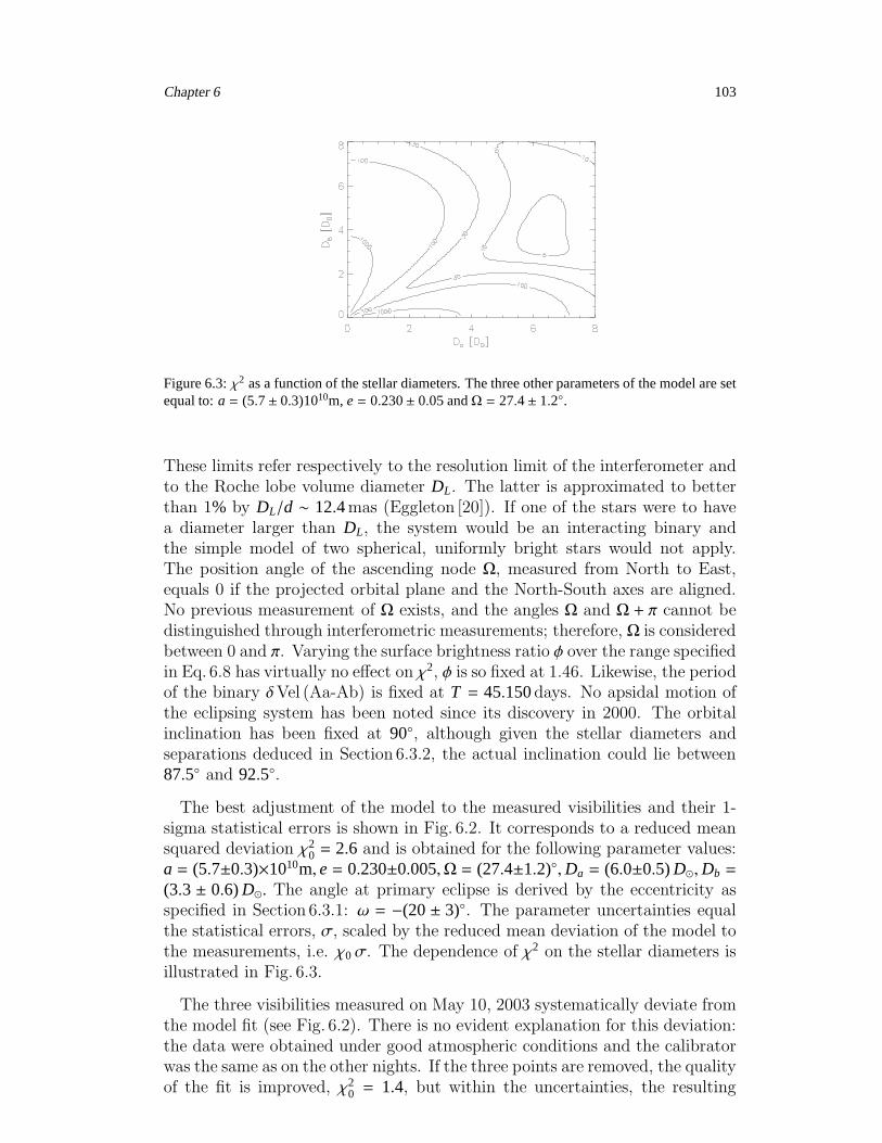
Chapter 6 103

Figure 6.3:χ2 as a function of the stellar diameters. The three other parameters of the model are setequal to:a = (5.7± 0.3)1010m, e= 0.230± 0.05 andΩ = 27.4± 1.2.

These limits refer respectively to the resolution limit of the interferometer andto the Roche lobe volume diameter DL. The latter is approximated to betterthan 1% by DL/d ∼ 12.4mas (Eggleton [20]). If one of the stars were to havea diameter larger than DL, the system would be an interacting binary andthe simple model of two spherical, uniformly bright stars would not apply.The position angle of the ascending node Ω, measured from North to East,equals 0 if the projected orbital plane and the North-South axes are aligned.No previous measurement of Ω exists, and the angles Ω and Ω + π cannot bedistinguished through interferometric measurements; therefore, Ω is consideredbetween 0 and π. Varying the surface brightness ratio φ over the range specifiedin Eq. 6.8 has virtually no effect on χ2, φ is so fixed at 1.46. Likewise, the periodof the binary δVel (Aa-Ab) is fixed at T = 45.150days. No apsidal motion ofthe eclipsing system has been noted since its discovery in 2000. The orbitalinclination has been fixed at 90, although given the stellar diameters andseparations deduced in Section 6.3.2, the actual inclination could lie between87.5 and 92.5.

The best adjustment of the model to the measured visibilities and their 1-sigma statistical errors is shown in Fig. 6.2. It corresponds to a reduced meansquared deviation χ2

0 = 2.6 and is obtained for the following parameter values:a = (5.7±0.3)×1010m, e= 0.230±0.005,Ω = (27.4±1.2),Da = (6.0±0.5)D⊙,Db =

(3.3 ± 0.6)D⊙. The angle at primary eclipse is derived by the eccentricity asspecified in Section 6.3.1: ω = −(20± 3). The parameter uncertainties equalthe statistical errors, σ, scaled by the reduced mean deviation of the model tothe measurements, i.e. χ0σ. The dependence of χ2 on the stellar diameters isillustrated in Fig. 6.3.

The three visibilities measured on May 10, 2003 systematically deviate fromthe model fit (see Fig. 6.2). There is no evident explanation for this deviation:the data were obtained under good atmospheric conditions and the calibratorwas the same as on the other nights. If the three points are removed, the qualityof the fit is improved, χ2

0 = 1.4, but within the uncertainties, the resulting

104 Chapter 6

parameter values are unchanged: a = (5.4±0.5)×1010m, e= 0.230±0.005,Ω =(29.2± 2.4),Da = (6.6± 0.5)D⊙,Db = (3.2± 0.5)D⊙.

It is apparent from the relatively high χ20 that there are deviations in addition

to the purely statistical errors. They might be due to an underestimation ofthe calibrator’s size or might reflect some inaccuracies in the model for twouniformly bright, spherical stars. This is discussed in the subsequent section.

6.5 Results and discussion

6.5.1 The close eclipsing binaryδVel (Aa-Ab)

The computations could be slightly biased if the diameter of the calibrator starwere substantially misestimated or if HD 63744 were a – still undiscovered –binary system. On the other hand, HD 63744 is part of the catalog of interfer-ometric calibrator stars by Borde et al. [10], with its diameter (1.63±0.03)masspecified to a precision of 1.8%. Furthermore, it has been studied simultane-ously with other calibrator stars in VINCI observations by one of the authors(P. Kervella). In these investigations the visibilities of HD 63744 equal thoseexpected for a single star of 1.63±0.03mas diameter. Thus, HD 63744 appearsto be a reliable calibrator.

Perhaps more relevant are the possible astrophysical complexities of δVel (Aa+Ab)that are disregarded in the model of two uniformly bright, spherical stars. Inparticular, the rotational velocities of Aa and/or Ab are found to be high,with values of ∼150 - 180 km/s (Royer et al. [57]; Hempel et al. [33]; Holwegeret al. [36]), which indicates that the two stars need not be uniformly luminousor circular.

Another possible over-simplification of our binary model is the constraint onthe orbital inclination, i, being fixed at 90. Given the fitted semi-major axisand stellar diameters, we note that the eclipse durations (0.51± 0.05days and0.91± 0.01days) are shorter than they should be in the case of i = 90, wherethe duration of the longer eclipse would have to exceed Da T/(2π a) = 1.06days.We conclude that i is ∼ 88 or ∼ 92, rather than 90. All observations wereperformed out of eclipse and, therefore, the visibility values are nearly un-affected by such a small variation in i. With substantially more visibilitymeasurements and an increased number of fitted parameters, the issue on theprecise orbital inclination might be addressed in more detail.

The most important and remarkable result of our analysis is that the stellardiameters of Aa and Ab are found to equal 6.0 ± 0.5D⊙ and 3.3 ± 0.6D⊙,respectively. This exceeds significantly, by factors ∼ 1.4 - 3, the values expectedif Aa and Ab are main sequence stars. If both diameters are constrained tolie below 2.5D⊙, the best fit corresponds to χ2 = 16.7, which is far beyond thepresent result and confirms that large diameters are required to account for

Chapter 6 105

the measured visibilities.

6.5.2 The physical association ofδVel C and D

Ever since the observations of Herschel [34], δVel has been taken to be a visualmultiple star, with δVel C and D the outer components of the system. WithmV of 11.0 mag and 13.5 mag (Jeffers et al. [38]), C and D would need to beof late spectral type, certainly no earlier than M, if they were as distant asδVel (Aa+Ab+B). To our knowledge, the only existing spectra of C and D wererecorded during a survey of nearby M dwarfs (Hawley et al. [32]). While thelimited range and resolution of the spectra precluded ready determination ofthe spectral types of C and D, they were nevertheless estimated as ∼G8V and∼K0V. Therefore, given their apparent magnitudes, C and D must be muchfarther away than δVel (Aa+Ab+B). We conclude that δVel C and D are notphysically associated. Hence, δVel ought to be only classified as a triple stellarsystem.

6.6 Summary

Seventeen VINCI visibility measurements of δVel (Aa+Ab) were fitted ontothe model of two uniformly bright, spherical stars. The adjustment to themeasurements does not provide individual diameters compatible with A-typemain sequence stars. The two stars thus appear to be in a more advancedevolutionary stage. More data are needed however to confirm this result. Asthe stellar evolution is fast during this period, more detailed knowledge ofthe system might also constrain the models more tightly. Precise photometricand spectroscopic observations of the eclipses should provide the separate in-tensities and chemical compositions of Aa and Ab and, hence, permit furtherinferences on the age and evolutionary state of δVel.

Acknowledgements: We thank Rosanna Faraggiana for her extensive help, Sebas-tian Otero for providing the light curvesδVel Aa, Ab, and Neil Reid for making thespectra ofδVel C, D available. The manuscript was improved by helpful commentsfrom the referee.

106 Chapter 6

Chapter 7

Conclusion

The various subjects in this thesis have as a common denominator the effectsof atmospheric turbulence on high-resolution astronomical observations. Inconclusion the main results are summarized and some perspectives are given.

Summary

Interferometric observations of δVelorum

The study of the close, double-star system in δVelorum exemplifies the po-tential of interferometric observations: With a single telescope a mirror of100-meter diameter would be required to resolve δVelorum Aa and Ab, butthis resolution has here been achieved with two small 0.4m telescopes placed100m apart.

The analysis of the observations suggests that the stellar diameters are con-siderably larger – by factors two to three – than indicated by their luminosityand the combined spectrum of δVelorum (Aa+Ab). Possibly the stars areolder than previously assumed, and have reached the stage where the hydro-gen in their cores has largely been converted into helium. They should thenbe expanding by now, while helium and heavier elements are being fused.

Interferometry falls short of providing images of a stellar system, it merelyyields parameter values for an assumed model. In our case it excludes the pos-sibility that δVelorum (Aa+Ab) is a system of two uniformly bright, sphericalstars that are located on the main-sequence. Given the small amount of avail-able data, the observations permit no more than this conclusion. In particular,it is not possible, at this point, to exclude a perhaps more realistic model thatmight include two circumstellar discs.

Further observations have recently been obtained with the new Astronomical

107

108 Chapter 7

Multiple Beam Recombiner, AMBER, that is installed behind the Very LargeTelescope Interferometer, VLTI, since 2001. The δVelorum binary (Aa+Ab)was observed with three 8m-telescopes during three nights, i.e. at three differ-ent configurations of the double-star system. The analysis of the raw AMBERdata is complex and has been carefully performed by Stefan Kraus from theMax-Planck Institut fur Radioastronomie, Bonn. The results should permitan assessment of various double-star models, and given the present conclusion,these models should include alternatives, such as circumstellar discs.

It must be emphasized, that δVelorum can be observed interferometrically,because it is a particularly bright star. In fact, interferometry is, at present,essentially limited by its poor sensitivity. This limitation is due to the detri-mental effects of turbulence and can only be overcome by phasing-devices whenthe turbulence is sufficiently slow. To make the best use of interferometers –and adaptive-optics as well – it is therefore essential to assess and specify thetime-scales of atmospheric turbulence. The focus of this work has, accordingly,been on improved methods to measure these time scales at existing observa-tories and at potential observatory sites.

The coherence time of atmospheric turbulence

Current corrections with adaptive-optics can react with sufficient amplitudeto compensate for the atmosphere-induced phase distortions, but they fail toattain the high speeds that are required. While the necessary amplitude isdetermined by the turbulent intensity, the speed requirements reflect the timescales of turbulence. Accordingly, the site selection for the coming genera-tions of single-dish telescopes and interferometers, should largely rely on thespecification of the turbulence-time scales. But which quantity – or, possibly,which quantities – must be measured? Does the same parameter determinethe operating performance of single dish-telescopes and of interferometers? Orare certain observational techniques more affected by high-altitude turbulentlayers, while others are particularly sensitive to low-altitude turbulence?

To answer these questions, several quantities were examined, that are jointlytermed “coherence time” while they are actually defined in relation to specificobservational techniques with single-dish telescopes or with interferometers,with or without adaptive-optic systems. These various coherence-times arefound to have almost the same dependance on the altitude profiles of tur-bulence and to be thus essentially equivalent. Accordingly, the sensitivity ofinterferometers and the performance of phasing devices and of adaptive-opticsystems can be predicted by measuring one and the same quantity: the coher-ence time, τ0.

Chapter 7 109

How is the coherence time to be measured?

Pistonscope A first attempt was made to measure the coherence time with thePistonscope, which is in essence a Differential Image Motion Monitor, DIMM,without prism. This endeavour turned out to be a very partial success forreasons inherent to the instrument. The pistonscope images a star throughtwo small, circular openings, the resulting image being a fringe pattern withintwo, superimposed diffraction discs. The difference between the turbulence-induced motion of the interference pattern and that of the two diffractiondiscs is then used to assess the coherence time. The principal limitation of thismethod is that it involves the measurement of a small, differential movementthat depends on the altitude-profile of the wind direction.

The pistonscope has been set up at Dome C, during daytime in Febru-ary 2005. The measurements have provided promising lower limits for thecoherence-times, but exact values could not be obtained, because the measure-ments are dependent on the unknown profiles of wind directions. The workhas, thus, affirmed the need for an approach that allows regular monitoring ofthe coherence-time with an appropriate instrument.

FADE To measure the coherence time without continuous assessment of thewind directions, an instrument has been conceived that can be seen as anisotropic analogue to DIMM. The image of a star is shifted somewhat out offocus, which converts it – due to a central obstruction on the primary mirror –into a blurred ring. The image is then sharpened into a narrow ring by insertionof a lens with proper spherical aberration. Turbulence-induced variations ofthe defocus aberration cause, then, fast changes of the ring radius, and thecoherence time and seeing are deduced from the amplitude and the velocity ofthese changes. The instrument is accordingly termed the Fast Defocus Monitor,FADE.

First observations with a prototype of the FADE monitor have been obtainedat the Cerro Tololo observatory in October 2006. The resulting seeing valuesand coherence-times agree with simultaneous estimates in terms of the MultiAperture Scintillation Sensor, MASS, and DIMM instruments.

FADE slightly underestimes the seeing; this bias is reproduced by simula-tions of somewhat blurred ring images, in the presence of optical aberrationsor scintillation spots. We conclude that, to minimize the effects of scintillationand telescope aberrations on the FADE monitor, relatively sharp ring imagesare needed, close to the diffraction limit.

110 Chapter 7

Further work required

Bringing the coherence-time monitor into practical use

Further tests The initial coherence-time estimates were obtained with the pro-totype of FADE and have been compared to results from the MASS monitor.MASS is based on scintillation measurements and is, therefore, insensitive tothe low turbulent layers roughly below 500m altitude. The actual coherencetimes are, accordingly, obtained from combined observations with MASS andDIMM. This estimation is indirect and can not be used to test the validity ofthe coherence times derived in terms of FADE.

To check the validity of the FADE estimates, observations must be obtainedin parallel to measurements by an adaptive optics system or by an interferom-eter. Simultaneous measurements with FADE and with NAOS, the adaptive-optic system installed behind one of the VLT telescopes, are, therefore, plannedfor August 2007 at the observatory of Paranal.

Making FADE user friendly Two major requirements must be met to establishFADE as a regular monitoring instrument. First, an automatic procedureneeds to be incorporated for bringing the ring-image close to its diffraction-limit and then measuring its width. Secondly there needs to be a standarddata-acquisition chain.

These conditions can not be attained with the current, commercial camera-software, and a suitable software is, therefore, now being developed at theobservatoire de Meudon; it should be available for the forth-coming observa-tions, in August 2007.

Application at Dome C, Antarctica

The measurements with the MASS monitor at the Concordiastation on DomeC, suggest that the coherence time of the high-altitude turbulence is at thislocation considerably longer than at mid-latitude sites [46]. On the other hand,estimates of seeing by the DIMM have shown that the low-layer turbulencemight be particularly strong at Dome C [2]. This raises a decisive question.Should coming generations of large telescopes and interferometers be installedat Concordia? Should they then be placed twenty or forty meters above theground?

This being an important issue, direct measurements of the coherence timeneed to be performed. FADE may be ideally suited for such measurements,provided the experimental setup can resist antarctic temperatures. FADE’ssurvival-ability under antarctic conditions is, therefore currently examined.

Bibliography

[1] Absil, O., den Hartog, R.H., Gondoin, P.A., et al., A&A, 448, 787 (2006)

[2] Agabi, A., Aristidi, E., Azouit, M., et al., PASP, 118, 344 (2006)

[3] Alekseeva, G.A., Arkharov, A. A., Galkin V. D. et al., Pulkovo Spec-trophotometric Catalog (1997)

[4] Argyle, R. W., Alzner, A. , & Horch, E. P., A&A, 384, 171 (2002)

[5] Aristidi, E., Agabi, K., Fossat, E., et al., A&A, 444, 651 (2005)

[6] Avila, R., Vernin, J., Chun M.R., et al., Proc. SPIE, 4007, 721 (2000)

[7] Avila, R., Ziad, A., Borgnino, J., et al., J. Opt. Soc. Am. A., 14, 3070(1997)

[8] Azouit, M., & Vernin, J., PASP, 117, 536 (2005)

[9] Bonfils, X., Forveille, T., Delfosse, X., et al., A&A, 443, L15 (2005)

[10] Borde, P., Coude du Foresto, V., Chagnon, G. & Perrin, G.,A&A,393,183B (2002)

[11] Butterley, T., Wilson, R., & Sarazin, M., MNRAS, 369, 835 (2006)

[12] Central Intelligence Agency, Reference maps,https://www.cia.gov/library/publications/the-world-factbook/docs/refmaps.html

[13] Colavita, M.M., Shao, M., & Staelin, D.H., Appl. Opt., 26, 4106 (1987)

[14] Conan, R., Borgnino, J., Ziad, A., et al., J. Opt. Soc. Am. A, 17, 1807(2000)

[15] Conan, R., Ziad, A., Borgnino, J. et al., proc. SPIE, 4006, 963 (2000)

[16] Conan, J.-M., Rousset, G., & Madec, P.Y., J. Opt. Soc. AM. A, 12, 1559(1995)

[17] Davidson, P.A., Turbulence – An Introduction for Scientists and Engi-neers. Oxford University Press, 1st ed. (2004)

[18] The drawings of Leonardo da Vinci, http://www.drawingsofleonardo.org/

[19] Eggleton, P. P., ApJ, 268, 368E (1983)

111

112 BIBLIOGRAPHY

[20] European Centre for Medium-Range Weather Forecasts,http://www.ecmwf.int/ (2007)

[21] Fuchs, A., Tallon, M., & Vernin, J., PASP, 110, 86 (1998)

[22] Fusco, T., Ageorges, N., Rousset, G., et al., proc. SPIE, 5490, 118 (2004)

[23] Gendron, E., Lena, P., Ap&AS, 239, 221 (1996)

[24] Glindemann, A., Bauvir, B., van Boeckel, R., et al., LIACo, 36, 27 (2001)

[25] Gradshteyn, I.S., & Ryzhik, I.M., Table of integrals, series, and products.New York: Academic Press, 5th ed. (1965)

[26] Gray, R. O., & Garrison, R. F., ApJS, 65, 581 (1987)

[27] Greenwood, D.P., & Fried, D.L., J. Opt. Soc. Am., 66, 193 (1976)

[28] Habib, A., Vernin, J., Benkhaldoun, Z., & Lanteri, H., MNRAS, 368, 1456(2006)

[29] Hardy, J.W., Adaptive Optics for Astronomical Telescopes. Oxford: Ox-ford Univ. Press (1998)

[30] Harmanec, P., A&A, 335, 173 (1998)

[31] Hawley, S., Gizis, J. E., & Reid, I, N., AJ, 112(6), 2799 (1996)

[32] Hempel, M., Holweger, H., & Kamp, I., CoSka, 27, 246 (1998)

[33] Herschel, J. F. W., London, Smith, Elder and co. (1847)

[34] Hoffleit, D., Warren, W. H., The Bright Star Catalogue, 5th Revised Ed.(Preliminary Version) (1991)

[35] Holweger, H., Hempel, M., & Kamp, I., A&A, 350, 603 (1999)

[36] Innes, R.T.A., MNRAS, 55, 312 (1895)

[37] Jeffers, H. M., van den Bos, W. H., & Greeby, F. M., Publications of theLick Observatory (1963)

[38] Johnson, H. L., Iriarte B., Mitchell R. I., & Wisniewski W. Z., CoLPL, 4,99 (1966)

[39] Kervella, P., Thevenin, F., Segransan, D., et al., A&A, 404, 1087 (2003)

[40] Kellerer, A., Sarazin, M., Coude Du Foresto, et al., Applied Optics, 45,5709 (2006)

[41] Kellerer, A., & Tokovinin, A., A&A, 461, 775 (2007)

[42] Kolmogorov, A.N., “About the Analytical Methods of Probability The-ory” in: Selected works of A.N. Kolmogorov, vol. 1, ed. Tikhomirov, V.M.. Springer-Verlag (2001)

[43] Kornilov, V.,Tokovinin, A., Vozyakova, O., et al., Proc. SPIE, 4839, 837(2003)

BIBLIOGRAPHY 113

[44] Landau, L.D., Lifshitz, E.M., Fluid Mechanics. Pergamon Press, 1st edi-tion (1959)

[45] Lawrence, J.S. , Ashley, M.C.B., Tokovinin, A., & Travouillon, T., Nature,431, 278 (2004)

[46] Lawrence Livermore National Laboratory, University of California,http://www.llnl.gov/str/June05/Carrano.html

[47] Levato, O. H., PASP, 82, 584 (1972)

[48] Lopez, B., A& A, 253, 635 (1992)

[49] Markwardt, C., Mpfit version 1.38, http://cow.physics.wisc.edu/∼craigm/idl/fitting.html (2005)

[50] Noll, R., J. Opt. Soc. Am., 66, 207 (1976)

[51] Otero, S. A., Fieseler, P. D., & Lloyd, C., IBVS, 4999 (2000)

[52] Otero, S.A., http://ar.geocities.com/varsao/delta Velorum.htm (2006)

[53] Perrin, M.D., Sivaramakrishnan, A., Makidon, R.B. et al., ApJ, 596, 702(2003)

[54] Perryman, M.A.C., Lindegren, L., Kovalevsky, J. et al., A&A, 323, L49(1997)

[55] Richardson, L.F., Proc. Roy. Soc. London A, 110, 709 (1926)

[56] Royer, F., Gerbaldi, M., Faraggiana, R., & Gomez, A.E., A&A, 381, 105(2002)

[57] F. Roddier, Prog. Optics, 19, 281 (1981)

[58] Sarazin, M., & Tokovinin, A., in: Beyond conventional adaptive optics,eds. E. Vernet, R. Ragazzoni, S. Esposito, N. Hubin, ESO Conf. WorkshopProc. No. 58, Garching: ESO (2002)

[59] Sarazin, M., & Roddier, F., A&A, 227, 294 (1990)

[60] Sasiela, R.J., Electromagnetic Wave Propagation in Turbulence. Berlin:Springer-Verlag (1994)

[61] Schoeck, M., Spillar, E.J., J. Opt. Soc. Am. A, 17, 1650 (2000)

[62] Schoeck, M., & Spillar, E.J., SPIE, 3353, 1092 (1998)

[63] Tango, W.J., & Twiss, R.Q., Progress in Optics, XVII, 239 (1980)

[64] Tango, W.J., Davis, J., Thompson, R.J., & Hanbury, R., PASAu, 3, 323(1979)

[65] Taylor, G.I., Proc. R. Soc. Lond. A, 164, 476 (1938)

[66] Tokovinin, A. & Heathcote, S. PASP,118, 1165 (2006)

[67] Tokovinin, A., Appl. Opt., 41, 957 (2002)

114 BIBLIOGRAPHY

[68] Tokovinin, A., A&A Suppl. Ser., 124, 75 (1997)

[69] Wikipedia, Concordia Station, http://en.wikipedia.org/wiki/Concordia Station

[70] Worley, C.E., & Douglass, G.G., A&A Suppl., 125, 523 (1997)

[71] Wright, C.O., Egan, M.P., Kraemer, K.E., & Price, S.D., The Tycho-2Spectral Type Catalog (2003)

[72] Ziad, A., Conan, R., & Tokovinin, A., et al., Appl. Opt., 39, 5415 (2000)

Summary The research brought together in this thesis is concerned with the distortion of astro-

nomical observations due to atmospheric fluctuations. These fluctuations are especially critical for

the technique of interferometry whose potential is here exemplified by the study of δVelorum. The

focus of the research is, accordingly, on improved methods to assess the changing viewing conditions

at existing observatories, as well as to determine the suitability of potential observatory sites.

Site-testing and site-monitoring missions are usually directed at the assessment of the Fried

parameter with instruments such as the Differential Image Motion Monitor, DIMM. An estimation of

the coherence time requires then, in addition, wind-speed measurements by weather stations. A

more refined evaluation is obtained with instruments such as the Multi Aperture Scintillation Sensor,

MASS, that measure the altitude profiles of the index structure constant, C2n, and the wind speed

with a resolution of about 500 m, and infer the coherence time from the integrated turbulence

profiles. The main error in the estimated coherence time results from the turbulence below 500 m

altitude not being accounted for.

To avoid these complexities, we suggest the direct measurement of a quantity proportional to

the coherence time. The variance of the defocus velocity is a suitable option, because it can be

evaluated through fast and continuous sampling of the atmospheric defocus coefficient. The concept

of a Fast Defocus Monitor, FADE, an instrument using a small telescope, some simple optics and a

fast camera is described, and first measurements are presented.

The final aim is to use FADE for site monitoring and site testing campaigns. A particularly

challenging and interesting project will be to monitor the coherence time at Dome C.

Resume La vie sur Terre est rendue possible grace au rideau protecteur que constitue l’atmosphere.

Avec sa masse equivalente a dix metres d’eau, l’atmosphere est une condition prealable a l’apparition

de la vie. Mais ce rideau rend la vie difficile aux astronomes qui prefereraient avoir une vue directe

sur l’Univers. Il est donc indispensable de caracteriser et de specifier les conditions atmospheriques

qui permettent la meilleure utilisation des systemes d’optiques adaptatives et des interferometres –

les interferometres, dont le potentiel est ici illustre a travers les observations d’un systeme de trois

etoiles, δVelorum.

Le temps de coherence de la turbulence est un parametre essentiel qui determine la sensibilite

des interferometres et la performance des systemes d’optiques adaptatives. Il existe plusieurs in-

struments qui mesurent le temps de coherence ou des parametres relies, mais tous ces instruments

ont des limitations intrinseques: ou bien ils necessitent de grands telescopes, ou bien l’analyse des

donnees est complexe, ou encore la methode n’est sensible qu’a une partie de la turbulence. C’est

pourquoi les campagnes de tests de sites et de monitoring reposent principalement sur la mesure

du seeing, avec des instruments comme le Differential Image Motion Monitor, DIMM.

Pour palier a ce manque, nous avons propose un instrument pour mesurer le temps de coherence:

le Fast Defocus Monitor, FADE. La methode consiste a transformer l’image d’une etoile, a travers un

petit telescope de 0.35 m de diametre, en un anneau fin. La turbulence cause alors des variations

temporelles du rayon de l’anneau, dont la vitesse et l’amplitude sont reliees au temps de coherence

et au seeing. Cette methode est presentee ici avec les resultats de premieres observations.