Assessing the value of travel time reductions in (sub)urban ...

Assessing the value of travel time reductions in (sub)urban freight transportation Master’s Thesis in the Master’s Programme Industrial Engineering and Management

NURIA CONESA GAGO JORDI JUANMARTI ARIMANY

Department of Technology Management and Economics Division of Service Management and Logistics CHALMERS UNIVERSITY OF TECHNOLOGY Gothenburg, Sweden 2018 Report No. E 2017:125

MASTER’S THESIS E 2017:125

Assessing the value of travel time reductions in (sub)urban freight

transportation

NURIA CONESA GAGO

JORDI JUANMARTI ARIMANY

Tutor, Chalmers: Iván Sánchez-Díaz

Department of Technology Management and Economics

Division of Service Management and Logistics

CHALMERS UNIVERSITY OF TECHNOLOGY

Gothenburg, Sweden 2018

Assessing the value of travel time reductions in (sub)urban freight transportation

© NURIA CONESA GAGO and JORDI JUANMARTI ARIMANY, 2018.

Master’s Thesis E 2017:125

Department of Technology Management and Economics Division of Service Management and Logistics

Chalmers University of Technology

SE-412 96 Gothenburg, Sweden Telephone: + 46 (0)31-772 1000

Chalmers Reproservice

Gothenburg, Sweden 2018

INDEX

ABSTRACT .................................................................................................................. 1

ACKNOWLEDGEMENT ............................................................................................... 2

1. INTRODUCTION AND BACKGROUND................................................................. 3

1.1 Aim ................................................................................................................. 6

1.2 Limitations ...................................................................................................... 7

2. THEORETICAL FRAMEWORK ............................................................................. 8

2.1 Reliability in supply chain ................................................................................ 8

2.2 Value of travel time ....................................................................................... 11

2.2.1 Freight value of time (VOT) definition .................................................... 11

2.2.2 Freight value of travel time saving (VTTS) definition .............................. 12

2.3 Definition of travel time reliability ................................................................... 13

2.4 Advantages of increasing reliability ............................................................... 14

2.5 Factors of reliability ....................................................................................... 15

2.6 Assessing reliability ...................................................................................... 17

2.6.1 Value of travel time reliability ................................................................. 17

2.6.2 Methods to assess reliability .................................................................. 18

3. METHOD ............................................................................................................. 22

3.1 Stated Preference Survey ............................................................................. 23

3.1.1. Survey design ........................................................................................ 23

3.1.2. Discrete choice modelling ...................................................................... 25

3.1.3. Survey data analysis .............................................................................. 26

3.2 Interviews ..................................................................................................... 27

3.2.1 Interviews design ................................................................................... 27

3.2.2 Interview data analysis .......................................................................... 29

3.3 Validity and transferability ............................................................................. 29

4. RESULTS AND ANALYSIS ................................................................................. 31

4.1 Data description ............................................................................................ 31

4.2 Discrete choice modelling results .................................................................. 35

4.3 Interview results ............................................................................................ 37

5. DISCUSSION AND PRACTICAL IMPLICATIONS ............................................... 39

6. CONCLUSIONS .................................................................................................. 42

REFERENCES ........................................................................................................... 43

APPENDIX ................................................................................................................. 47

LIST OF FIGURES

Figure 1 - Evolution of the e-commerce sales in Sweden .............................................. 3

Figure 2 - Parts of the supply chain ............................................................................. 10

Figure 3 - Units of analysis value of time ..................................................................... 12

Figure 4 - Advantages of having a higher reliability ..................................................... 15

Figure 5 - The four types of disturbances .................................................................... 16

Figure 6 - Normal distribution depending on standard deviation .................................. 19

Figure 7 - Frequency of answers of the experts about the most suitable definition of

reliability...................................................................................................................... 20

Figure 8 - Example of a choice set .............................................................................. 23

Figure 9 - Weight assigned to each attribute by respondents ...................................... 32

Figure 10 - Weight assigned to each attribute by carriers and shippers ...................... 32

Figure 11 - Number of respondents answering each possible definition of travel time

reliability...................................................................................................................... 33

Figure 12 - Results of shippers and carriers when defining travel time reliability ......... 33

Figure 13 - Classification of respondents depending on the type of products that

respondents work with ................................................................................................ 33

Figure 14 - Classification of respondents depending on type of vehicles of the company

................................................................................................................................... 34

Figure 15 - Classification of respondents depending on carrier/shipper, number of

employees and area of distribution ............................................................................. 34

Figure 16 - Classification of respondents depending on sector of the company .......... 34

Figure 17 - Factors that affect travel time variability .................................................... 38

LIST OF TABLES

Table 1 - VOT definitions ............................................................................................ 11

Table 2 - VTTS definitions .......................................................................................... 13

Table 3 - Freight Values of reliability studies ............................................................... 18

Table 4 - Advantages and disadvantages of using standard deviation for measure

reliability...................................................................................................................... 20

Table 5 - Valuation of traffic circumstances at places of principal roads ...................... 21

Table 6 - Classification of the respondents ................................................................. 24

Table 7 - Classification of the answers obtained in the survey .................................... 31

Table 8 - Attribute which respondents assigned the highest weight ............................ 32

Table 9 - Initial model .................................................................................................. 35

Table 10 - Final model ................................................................................................ 36

Table 11 - Willingness to pay per hour of reduced travel time (SEK), by sectors and

vehicle capacity .......................................................................................................... 36

Table 12 - Willingness to pay per hour of variability reduction (SEK), by sectors and

vehicle capacity .......................................................................................................... 37

Table 13 - Values of reliability for 21 tons ................................................................... 40

1

ABSTRACT

Growing urbanization in the last years have caused concentration of people and

economical activities in urban areas all around developed countries, causing high

levels of traffic congestion in roads. Freight transportation is one of the most affected

sectors by the congestion, as it generates uncertainty in time travels. However, a high

percentage of on time deliveries is crucial for companies to have an efficient and

optimized supply chain. High cost is associated with unreliable time deliveries, but the

value of this cost, the value of reliability, has never been calculated before in Sweden.

Considering this value in the Cost Benefit Analysis (CBA) of transportation and

infrastructure projects will lead to have more accurate information about the economic

impact, thus achieving better decision making. Through the theoretical study of the

concept of reliability, its causes and its consequences, and through surveying and

interviewing freight transportation and logistics companies, it has been found out how

much the companies are willing to pay to get more reliability, and also for less travel

time, in their transport journeys. These new empirical values of travel time and

reliability have been obtained using random utility maximization approach with discrete

choice modelling, defined by the analysis of the preferences of carriers and suppliers

through a stated preference survey. These preferences have been analysed according

to many variables, of which the sector of the company and the capacity of vehicles

have proved to be significant. The ÅSEK report, which is a summary of CBA principles

and values to be used in Swedish transport sector, recommends to use the value of

reliability as twice the value of travel time savings, but the output of this thesis revealed

that the value of reliability is 3,23 times higher than the value of travel time savings.

This thesis is part of the global project called "Ringroad logistics - efficient use of

infrastructure” which seek to dynamically prioritize socially valuable freight and

increase the capacity of existing infrastructure by streamlining transport in roads in

urban areas.

2

ACKNOWLEDGEMENT

First, we would like to thank our master thesis supervisor Iván Sánchez-Díaz for the

follow-up he has done of the project and the help offered at any stage of it. He has

guided us when we had to face new parts of the project, he has offered us help in the

resolution of problems that were arising, and he has always been available to help and

solve any doubt related to the project.

It should also be taken into consideration that this thesis would not have been possible

without the support of all the organizations that are part of the "Ringroad logistics -

efficient use of infrastructure" project that is being carried out: DB Schenker, CLOSER,

Chalmers, KTH, Trafikverket, Västra Götaland and Mind Connect. In particular, we

would like to thank Emelie Klasson from DB Schenker, for giving us the contact of the

companies that were interviewed.

Finally, we would also like to thank our families for the trust and support received from

them during the completion of our studies, and for having supported us whenever we

have needed it.

3

1. INTRODUCTION AND BACKGROUND

In the last decades, the world population has undergone a change of tendency in the

economic field and in the demographic scope (Thaller, Niemann et al., 2017). About

demographic change, there has been a phenomenon of increasing urbanization in

developed countries, which consists in the gradual concentration of economic activities,

causing the displacement of the population from rural areas to cities. In 1951, 79% of

the population lived in rural settlements (Bloom & Khanna, 2007). By 1967, half of the

population was already living in urban areas, and nowadays more than 54% is living in

urban territories. It is estimated that by 2050 more than 70% of the world population will

live in cities, continuing the trend followed for some decades (Thaller, Niemann et al.,

2017). In Sweden, this is not an exception, it is a more significant case, as in 2015

85,8% of the population was already living in urban areas, with an average increasing

rate of 0,83% per year in the last five-year period (United Nations, Department of

Economic and Social Affairs et al., 2014). It is expected that by 2050 the percentage of

urbanization will increase to 90%. The fact that so many people are living in

concentrated areas generates a freight attraction to the cities to satisfy the needs of

their population, in terms of food and consumer products (Thaller, Niemann et al.,

2017). This attraction causes a traffic congestion not only in commercial areas as some

years ago, but nowadays in living areas too.

About the economic field, there has been a very important boom in e-commerce both at

a global and national level, generating an increase in the number of vehicles in urban

freight transport, caused by several factors (Bakos, 2001). The first factor is the

increment in sales volume (Thaller, Niemann et al., 2017). E-commerce was worth 75,7

billion kronor in 2013 in Sweden (E-commerce news, 2017). Five years later, there has

been an annual average growth of 9,2%, reaching 109,5 billion kronor. Figure 1 shows

the evolution of e-commerce sales in Sweden in the last five years. The second factor

is the reduced delivery period since customers want the products purchased to be

delivered as soon as possible, raising the frequency of travels (Thaller, Niemann et al.,

2017). In addition, it is necessary a higher reliability in e-commerce to avoid failed

deliveries that would cause higher costs as customers are requiring reduced time

window deliveries. Moreover, it is important to consider the rise in storage costs, as

urban soil is now more expensive because of increasing urbanization and it makes

companies to have smaller storehouses.

Figure 1 - Evolution of the e-commerce sales in Sweden

Source: E-commerce news, 2017

4

Both factors, demographic and economic, have risen the number of freight travels and

the concentration of these in urban centres, causing growing traffic congestion (Trafik

Analys, 2017). In fact, Stockholm and Gothenburg (the two largest cities in Sweden)

are among the 50 European cities with the highest level of congestion, being

respectively 12th and 43rd position of the ranking (TomTom International, 2015).

Congestion entails multiple challenges, especially for freight transportation operators,

as it forces them to reduce the speed of transport, having higher an uncertainty travel

times, and consequently, recurrent delays. One potential solution to avoid congestion

in freight transportation could be off-hours deliveries, as this significantly increases

reliability (Holguín-Veras, Sánchez-Díaz et al., 2016). However, in supply chain and

logistic terms, shippers make agreements with the customers to deliver the shipment

within the agreed timeframe, and unfortunately most markets receivers have more

market power than carriers and suppliers, then the delivery ends up being scheduled at

the receivers will, which is often during business hours and highly congested hours (Jin

& Shams, 2016).

In this context the project entitled "Ringroad logistics - efficient use of infrastructure"

was proposed. It started after a feasibility study that revealed potential benefits, in

terms of both capacity and technology, to dynamically prioritize socially valuable freight

and increase the capacity of existing infrastructure by streamlining transport in roads in

urban areas. Therefore, the objective is to investigate the socio-economic potential

benefits and costs of a streamline in ring roads freight transportation, through dynamic

priority. This means giving access to the priority lane to some types of freight vehicles.

It is expected to result in a proposal for a full-scale demonstration, based on a study of

the feasibility and business benefits via cost-benefit analysis (CBA). The main applicant

of the project is Closer at Lindholmen Science Park, and collaborative partners are DB

Schenker, the Transport Administration, Västra Götaland, Chalmers, the Royal Institute

of Technology, Gothenburg city, City of Stockholm and Midconnect, which collaborate

in the 7 working packages of the project.

As a partner of the project, the research team at the division of Service Management

and Logistics of Chalmers is in charge of the Working package 3, which studies

valuation of time savings and delivery precision haulage, including definition of socially

useful goods transport. Time savings and delivery precision are directly related to travel

time. As congestion directly affects the travel time, and transportation has a major

impact (indirect) in several stages of the supply chain, the effect caused by congestion

must be minimized in order to achieve a supply chain as efficient as possible.

This thesis focuses on researching the concept of value of reliability. Reliability is a

complex concept, related to the uncertainty of unknowing the travel time of a freight

transport with precision. The complexity lies in the number of agents (stakeholders)

involved (Sánchez-Díaz & Palacios-Argüello, 2017):

1. Shippers that manufacture a commodity and sell it to get a profit.

2. Receivers that buy shippers' products and use them in other activities.

3. Carriers that are in charge of the transport of the product and can be carried out

by the shipper or by a third party.

4. Urban dwellers that are who benefit from having access to all types of goods to

fulfil their needs.

5

In addition, there are other relevant variables that can vary widely, such as modes of

transport (road, train, ship or plane), types of goods and its singularities (perishability,

value, etc.), the weight and the size, the distance of the transport, and units and

methods to quantify the reliability and to value it. All these variables make reliability a

complex concept as many unpredictable factors can modify it. For this reason,

companies want to minimise uncertainty and have high levels of reliability in freight

transport. In this thesis it will be studied the amount of money (willingness to pay) that

companies would be willing to pay to have more reliability in their travel times.

There are different factors that have motivated to carry out this thesis. First, it is the

increasing importance of the travel time reliability for the companies. Every company

looks to reach the best possible level of service at the lowest price, but as the traffic

congestion in urban areas is becoming higher, travel time variability and uncertainty are

raising (Trafik Analys, 2017), thus the cost associated is increasing too. For this

reason, some solutions are being studied (e.g. Ringroad logistics project). However,

before deciding which solutions have to be applied, real economic effect needs to be

calculated. There is any transport that is not economically affected by reliability, but are

the ones involving urban and suburban areas, that they are much more affected (Ando

& Taniguchi, 2006). Also from the social point of view, not only the companies can get

benefits of increasing reliability. Society seen as consumer would be benefited as

companies could offer more reliable deliveries, with reduced time window. This can be

specially applied to those socially useful goods, important for society, such as medical

supplies. In addition, freight transportation shares the roads with passengers’

transportation, therefore, the most efficient are the journeys of companies, everyone

would be more benefited in terms of fewer cars on the road and with less maintenance

and pollution (Eliasson, Hultkrantz et al., 2009).

Public sector is another stakeholder involved in the topic, as it is noteworthy that

building and management of roads are done by the public companies (e.g.

Trafikverket). Then it is necessary the interaction between the public and the private

sector to optimize the flow of vehicles in the roads. Because the public sector has to

ensure the common good, and not the individual profit, the impact of all decisions must

be taken into account. In this case, the methodology to analyse the impact is through

the Cost Benefit Analysis (CBA), with which it is possible to know the economic impact

of a project, allowing predicting the profitability and whether it is worthwhile to carry out

the project (Florio & Vignetti, 2003).

To consider reliability cost in the CBA it is necessary to know the values of reliability

(De Jong, Kouwenhoven et al., 2009), that is, the cost generated by the uncertainty of

not knowing exactly the travel time of certain journey. The aim of this thesis is to

calculate these values to be able to use them the in the CBA. Currently, for Sweden,

the values used are the ones recommended by the Swedish Transport Administration

(Trafikverket) in its ÅSEK manual (Bångman, 2016). This manual “is a summary of the

recommended CBA principles, costs, prices and shadow-prices presented in chapter 5-

15 of the ASEK report. The principles and values are recommended to be used in

social cost-benefit analyses (CBA) in the Swedish transport sector. The

recommendations are mainly applied in CBA of publicly provided infrastructure

investments”. The values recommended for evaluating the reliability are

6

approximations, as they are not based on empirical studies, thus with this study new

values empirically calculated will be obtained.

Although reliability is the main objective of this project, results regarding value of travel

time will also be obtained in the same study to assess the value of reliability. It is

noteworthy that travel time, together with reliability are the two key factors that

generate cost in the transport of goods. The quantification of value of travel time will

also be used in cost-benefit analysis to take decisions that can maximize the benefit of

the company.

1.1 Aim

The objective of this master thesis is to understand the concept of reliability, related to

travel time precision, and how can it add value to the companies. For this, the thesis

will evaluate the impact of traffic congestion, in ring roads for shippers and carriers,

separated according to the type of goods. More specifically, it will study the relevance,

in terms of costs, of uncertainty in delivery accuracy, i.e., reliability in the transport of

goods.

In the development of this master thesis, an exhaustive study will be carried out in

order to answer the following questions:

1. What is the meaning of reliability of freight transport? How can it be measured?

It is not possible to know the exact travel time of a transport involved in the

supply chain due to unpredictable factors (e.g. congestion) causing high

variance in journeys duration. For this reason, it would be useful to know deeply

the concept of reliability in freight transport and determine the best way to

calculate or measure it to deal with it and improve the efficiency of transport of

goods.

2. What factors affect the value of reliability?

As companies want higher reliability in their travel times, it is important to know

what factors affect the value of reliability. It will not be the same value for every

company and every journey, so the variables on which the reliability value

depends will be studied.

3. What is the value of reliability?

Knowing the value of reliability will make possible to calculate economic cost of

travel time variability in freight transport. It will be useful for decision making

about transport logistics projects, as the real economic impact will be known in

advance.

4. What is the value of time?

Along with reliability, knowing these two parameters, will allow to know in detail

the impact generated by a transport of goods, through the cost-benefit analysis.

Thus, it is a matter of studying in depth the concept of reliability, knowing the impact it

has on companies and determining its importance in the transport of goods and all the

steps of the supply chain.

7

1.2 Limitations

The possibilities for this study are widespread, so they must be limited to carry out the

work successfully. Due to the time restriction of the thesis, the project will focus on the

geographic area of the city of Gothenburg and its ring road, not the freeways, nor the

city centre. However, the results should be generalized once the project has been

finished.

Moreover, passenger transport and freight transport by boat, by train or by plane will

not be taken into account, as the solution proposed by the overall project is to give

priority to the bus lane to some type of goods. Therefore, this study is limited to freight

road transport.

This thesis will be carried out mainly in a quantitative level as there will be an analysis

to quantify the value of reliability. However, this study will be complemented with a

qualitative part by a previous literature review and later interviewing to some

companies to validate the results obtained with the quantitative part of the project.

In the quantitative part, values of reliability for Sweden will be calculated, defined for

certain types of goods in road transport in the ring road of the city of Gothenburg. The

interviews will be restricted due to the difficult get contact with big companies, so they

will be focused in a particular type of companies, the most representative ones in

Gothenburg area, which have a greater socially useful goods transport.

Within the impact of the reliability or value of reliability, only trucks operational costs

and product value depreciation, associated with transportation for such uncertainty will

be analysed. As only shippers and carriers companies will be interviewed and

surveyed, placing and order and inventory costs will not be taking into account in this

thesis.

8

2. THEORETICAL FRAMEWORK

Literature about time travel reliability in freight transport has been written since 1981,

but the complexity of the concept makes difficult to extrapolate results obtained before

in to Suburban Logistics project. Different countries than Sweden and other transport

modes (train and boat) have been used in other studies, but not values of reliability for

road transport in Sweden. For this reason, a deep review of the existing theoretical

framework has been carried out first, in order to obtain all the necessary knowledge to

carry on our own reliability study based on capturing the preferences of shippers and

carriers, focused in the suburban area of Gothenburg city.

In this section, it has been looked into the definitions of travel time reliability, value of

time, the advantages that they entail and the factors that they are caused by.

Moreover, methods to assess reliability have been also investigated and consequently,

the value of reliability and the models used so far to determine it.

2.1 Reliability in supply chain

The supply chain comprises the business processes, people, organization, technology

and infrastructure that allow the transformation of raw materials into intermediate and

final products and services that are offered and distributed to consumers to satisfy their

demand. The dynamism of the chain entails a constant flow of information and

products between the companies involved in each stage. There are many agents that

take part in the supply chain, including all stakeholders involved in the production,

distribution, handling, storage and commercialization of a product and its components.

These agents are shippers, manufacturers, distributors, carriers and retailers.

Therefore, the chain links many companies, from suppliers of raw materials until the

final consumers (Ellram & Cooper, 1990). It is highly difficult to get a proper functioning

of the whole supply chain, as any disruption in the system can appear for multiple

reasons such as labour actions or weather events (Snyder, 2003), or parameter

estimations can be inaccurate because of measurement errors, bad forecasts or other

factors (X. Miao, Xi et al., 2009). However, it is essential that all parts of the chain have

a good relationship and collaborate to achieve good management of the supply chain,

since the common goal is to meet the needs of the client in the most efficient way

(Vilana, 2011). For this reason, all the organizations that take part of a supply chain

need to work together, constructively and cohesively towards a big objective (Awasthi

& Grzybowska, 2014).

According to the Council of Supply Chain Management Professionals (CSCMP),

Supply Chain Management (SCM) “encompasses the planning and management of all

activities involved in the supply, acquisition, transformation and all logistic activities. It

is important to note that it is also including collaboration and coordination with channel

partners, which can be suppliers, intermediaries, third-party service providers and

customers. In essence, the supply chain management integrates supply and demand

management within and across companies” (Vitasek, 2006).

It is necessary an efficient SCM to establish continuous communication between the

companies involved in it. If it is achieved, problems that arise can be solved easily and

9

proactively (Golinska, 2014). Increasingly, an efficient SCM is necessary as there are

competitive pressures to reduce costs, improve quality of the process and increase

productivity of the organizations. For this reason, it is important to implement effective

SCM techniques arising in last years that make it easier for companies involved in a

chain to work together. SCM tries to form alliances and stable relationships among all

the members in order they have access to all the data that can allow them to take

better decisions and increase level of service of the company (Vilana, 2011).

The advantages that can be obtained by companies through integrated SCM are really

important, such as increase revenue, reduce inventory or improve productivity of staff

(Catalunya Innovació, 2012). It seems logical to assume that many companies will be

part of integrated supply chain to be able to benefit from all the improvements

mentioned above. However, SCM projects are complex and not always produce the

expected results due to it requires high levels of trust and collaboration between the

members (Vilana, 2011).

The SCM is a key element for the competitiveness of companies because of the

importance of business results through profit margin, delivery terms, product/service

quality and the customer satisfaction (Golinska, 2014). With the emergence of new

technologies, SCM has seen an important opportunity to improve due to the decrease

in costs of interaction with suppliers.

In order to achieve a synchronized supply chain, it is not enough to carry out isolated

actions. It is also necessary to develop a joint strategy that provides advantages to all

members and envisages a fast and reliable exchange of information, a coordinated

workflow and indicators that allow controlling the management of the chain.

It is also necessary a good management of the flow of materials to get the supply chain

working fluently and achieving the objective of satisfying the customer’s needs in the

most efficient way. The flow of materials is the one that goes from the raw material

supplier to the final customer and it is which has to send the physical product to the

customer (Vilana, 2011). It is noteworthy that urban freight reliability is very important

for an optimal SCM since it has a significant impact on the execution time of the logistic

process, on the supply chain’s logistic costs and on the quality and integrity of

delivered parties (Lukinskiy, Churilov et al., 2014). Marlin Thomas was the first who

defined the concept of Supply Chain Reliability (SCR). He said that it was “the

probability of the chain meeting mission requirements to provide the required supplies

to the critical transfer points within the system” (Thomas, 2002). Nevertheless, after he

showed this concept, some other authors have studied SCR, but from other

perspectives such as potential failure (Quigley & Walls, 2007) and arrival time (Van

Nieuwenhuyse & Vandaele, 2006).

In general, a supply chain is reliable in case it performs well when the parts of the chain

fail (X. Miao, Xi et al., 2009). The critical thing is to get that the goods arrive to delivery

places at the desired time. To get it, it has to be taken into account the complexity of all

the previous supply chain processes and the continuous flow of information between

companies that is necessary continuously (Lukinskiy, Churilov et al., 2014). For this

reason, some way to solve these difficulties has to be found out in order to improve

reliability and also the methods used to assess reliability in supply chain. Thus, it would

10

be possible to optimise and insure the efficiency and effectiveness of the processes

involved in the supply chain (Burkovskis, 2008). A high level of reliability with the

minimum travel time is essential because it will allow companies to have a higher level

of service and minimize their costs such as the one produced by uncertainty in travel

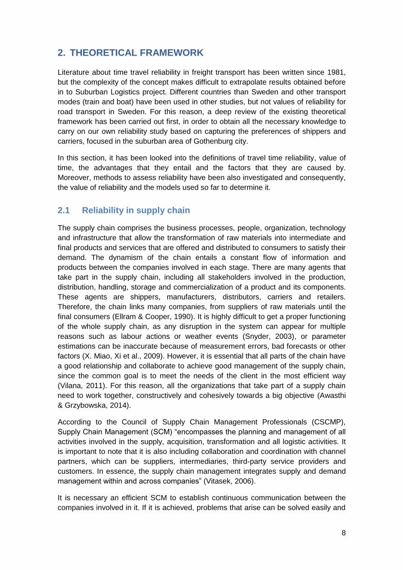
times. Figure 2 (Turmero, 2007) shows all the parts of the supply chain. Between each

one there is a flow of material, with its travel time, and here is where a fast and precise

transport is important.

Figure 2 - Parts of the supply chain

Source: Turmero, 2007

This thesis will focus the research of value of reliability in transport. It will only be

studied one of the last parts of the supply chain, which comprises the transport

between the distribution centres and retailers. This fact is due to the majority of

transport comprised between storage and manufacturing, or between manufacturing

and distribution centres are not located in urban area. So, as this thesis is located in

Gothenburg surroundings, it will only be taken into account transport at the end of

supply chain.

It is essential to know as quickly as possible the needs of the client so that the

deadlines are short. The information is the basis of a better management in the supply

chain, and for this reason, it is necessary to know when the needs of the market are

faster (Tseng, Yue et al., 2005). Otherwise, if the information passed slower and there

were delays and errors in product deliveries to customers, the inventories would

increase and the service would get worse, causing a decrease in the reaction capacity.

Transport is the part of the supply chain which is the principal linker between producers

and retailers. It is in charge of sending goods to the right place and at the correct time

in order to satisfy consumers’ preferences (Golinska, 2014). That is why the part of the

transport within the supply chain is very important, since if it does not work correctly

and deliver orders with delays, there may be a repercussion of very high costs for the

company. In this way, companies have to try to optimize the routes to achieve logistics

efficiency.

11

2.2 Value of travel time

2.2.1 Freight value of time (VOT) definition

The value of time is one of the most crucial factors for transport planners, modellers

and policy makers (Abrantes & Wardman, 2009). A lot of studies have been carried out

in order to estimate this “parameter” in different situations depending on the type of

vehicle, user and circumstances. It is expressed in monetary values (Abrantes &

Wardman, 2009) and it is used in the cost-benefit analysis (CBA) to examine the

feasibility of projects related to infrastructure and traffic (Sánchez-Díaz & Palacios-

Argüello, 2017).

The first who introduced the concept of value of time was Gary Becker. He considered

that the combination of two different factors defined the real value of any good (Becker,

1965). These two factors were the time that was necessary to have a good prepared to

be consumed, and the market cost of this good (Zamparini & Reggiani, 2007). A single

time unit represented the value that was defined by Becker. It was also estimated

considering a single person hourly salary. Later, M. Bruce Johnson introduced work

time (Johnson, 1966) and Jan Oort travel time in the utility function (Oort, 1969).

Up to now, there are a lot of authors who have been studying the value of travel time

and have defined it in different ways. Next, there is a table with some of these

definitions.

Definition Authors and Year

“VOT is the rate of substitution between travel cost and time”. (Feo-Valero, García-

Menéndez et al., 2011)

“VOT is the opportunity cost of travel time”. (Q. Miao, Wang et al., 2014)

“VOT is the ratio of the time coefficient to the cost coefficient”. (De Jong, 2007)

“VOT is the time-marginal transport cost”, which is the one that changes in consequence of variations in transport time.

(De Jong, Kouwenhoven et al., 2014)

“VOT is the ratio of the marginal utilities of time and money”. (Wardman, 2004)

Table 1 - VOT definitions

Source: author’s interpretation of Sánchez-Díaz & Palacios-Argüello,2017

To measure value of time, it is necessary to identify the main aspects that it is affected

by, as the transportation time is not the only one (Sánchez-Díaz & Palacios-Argüello,

2017). The factors distinguished are different depending on the authors.

Pekin, Macharis et al., (2013) consider that the different aspects that influence values

of time are transport time, order time, timing, punctuality and frequency.

- Transport time: time that takes a trip considering the duration of transport

(proportional to distance), the traffic time, and the road constraints.

- Order time: necessary time to get ready the ordered good before the departure.

- Timing: planned time of departure and arrival for the ordered good.

- Punctuality: quality of arriving at the scheduled time.

- Frequency: rate of departures within a given period.

12

However, there are some authors who consider other factors to determine the value of

time. Wigan, Rockliffe et al., (2000), Zamparini and Reggiani (2007), and Massiani

(2014) identify that the activities for the VOT unit of analysis are delivery time,

transportation time, and travel time.

- Transportation time: time that comprises all the process from the shipment’

departure in origin until the arrival to its destination. It also considers all logistics

operations involved such as the loading time, unloading, warehousing and

stocking among others.

- Travel time: duration comprised between the departure times from the origin

until the arrivals to its destination without taking into account logistics operations

that are involved in the travel.

- Delivery time: time comprised from the moment the shipper orders until the

good is delivered to its destination.

Figure 3 shows a diagram explaining the different approaches for the VOT unit of

analysis.

(Pekin, Macharis et al., 2013)

(Wigan, Rockliffe et al., 2000), (Zamparini & Reggiani, 2007) and (Massiani, 2014)

Figure 3 - Units of analysis value of time

Source: own elaboration

2.2.2 Freight value of travel time saving (VTTS) definition

Value of travel time saving (VTTS) is a concept also used in cost-benefit analysis of

network projects. It is commonly the largest benefit of a transport project (De Jong,

Tseng et al., 2007). Many authors have been studying this concept and have defined it

differently from others. Table 2 shows some definitions of value of travel time saving:

Definition Authors

“VTTS is the opposite of time losses” (expressed in terms of money units per hour).

(De Jong, 2007)

VTTS is the profit derived from reducing a unit on the time comprised between the origin and the destination when shipping a good.

(Zamparini & Reggiani, 2007)

13

“VTTS is a ratio between marginal utilities of time and money. It depends on budget and time constraints. VTTS is related to the value of the activity taking place”.

(Gwilliam, 1997)

“VTTS is the marginal rate of substitution between transport time and transport cost”.

(Bergkvist, 2001)

“VTTS is the sum of the value of getting the goods to the destination more quickly (VJT), savings in drivers’ wages (DWS), reductions in vehicle costs (VCS), and reduced disutility from being able to make a later start or earlier arrival (VAE, VAL). The VOT could vary according to the freight movement organisation”.

(T. Fowkes, 2007)

Table 2 - VTTS definitions

Source: author’s interpretation of Sánchez-Díaz & Palacios-Argüello,2017

2.3 Definition of travel time reliability

Usually, people measure how long it takes to drive from one point to another to choose

the route that is shorter in order to arrive earlier at the final destination. For this reason,

travel time is an efficient factor for measuring transport network performance and

shows the effectiveness of the road network (Tavassoli Hojati, Ferreira et al., 2016).

However, it is not the only factor to take into account.

Frequently, when travel time for a specific route is longer than expected, it is due to

demand exceeding road capacity causing congestion because of an increase in the

number of vehicles at a peak period time (predictable peak period traffic). If congestion

is repeated regularly (recurrent congestions), a user of this route may predict it and

choose an alternative route to ensure that he will not arrive late at the desired

destination (Tavassoli Hojati, Ferreira et al., 2016). This is the Wardrop’s first principle,

the “user equilibrium”, which says the entire demand for vehicles in paths with the

same origin and the same destination, knowing predictable congestions, end up being

distributed on all roads so that it takes the same time to make the journey for each one

of them (Wardrop, 1952). However, congestions are not always recurring because they

can be unpredictable (Tavassoli Hojati, Ferreira et al., 2016). This kind of congestions

are called non-recurring congestions and are caused by unexpected accidents, work

zones and adverse weather, among others.

Travellers who seek to avoid late arrivals allocate additional time or adjust the

departure time because the unexpected deviation from the estimated duration of travel

can make the journey longer than predicted (Jin & Shams, 2016). To know the

additional time needed, it is necessary to know the travel time reliability that defines the

range of time it can take the trip (without considering catastrophic events). It should be

noted that a higher reliability would be reached by a lower variability, since these two

concepts are opposite. However, a doubling of the variance does not necessarily mean

a halving of the reliability (Nicholson, 2003). Consequently, travel time reliability is a

measure of lack of travel time variability.

It can be differentiated two points of view about the travel time reliability: the first one

based on the variation in travel time, and the second one related to the possibility of

success or failure against a pre-fixed threshold travel time (Jin & Shams, 2016). Over

14

the years, a lot of definitions of travel time reliability have been made. Here are

presented the most relevant ones ordered chronologically:

- “Variability that can be measured using the standard deviation of transport time.

Transport models are needed to supply quantity changes in reliability and

standard deviation is relatively easy to integrate in models” (Krüger, Vierth et

al., 2013).

- The range between, e.g., the 0,5 and the 0,9 quantiles of the distribution of

durations (Brownstone & Small, 2005).

- “Percentage of travel that can be successfully finished within a specified time

interval” (Nicholson, 2003).

- “The range between the earliest possible arrival time and the 98th percentile of

arrival times” (A. Fowkes & Whiteing, 2006).

- “The degree to which randomness in journey time is realized. Although this

randomness is hard to measure, travel time reliability can be quantified

statistically based on the variance of travel times” (Jin & Shams, 2016).

- Uncertainty associated with travel time because the exact result of a known

experiment in successive attempts it is not fully predictable, so it is uncertain.

“Consistency or dependability in travel times, as measured from day-to-day

and/or across different times of the day” (Rakha, El-Shawarby et al., 2010).

As it can be observed, the reliability is not a closed concept, but different interpretations

are given according to each author. Over the years, the concept has evolved

increasingly towards something more tangible and quantifiable, thus being more useful

for companies to be aware of it, to measure it, and to be able to manage it to be more

efficient.

2.4 Advantages of increasing reliability

The fact of having higher travel time reliability in a route and therefore, less variability in

it, provides many benefits to the supply chain and to the companies involved in it that

are explained next (A. Fowkes & Whiteing, 2006).

For example, companies transporting products that lose value over time quickly (e.g.

perishable food) are conditioned by the duration of travel. Defining the maximum time

the product can be in transit before it has lost too much value, if the variability of the

route is lower, the maximum travel time of the route is reduced. Therefore, it is possible

to plan the departure of the route in a wider (and later) time range than in the case with

higher variability, ensuring the same quality of the product (Arvis, Marteau et al., 2010).

In road transport, this advantage may mean that tolled routes or performing 'double

shift' movements (when two drivers are needed to avoid having to stop the truck during

mandatory breaks) can be avoided with the consequent savings for the company (A.

Fowkes & Whiteing, 2006).

It is also possible to reduce the safety margin that companies use when scheduling

freight transport to be sure to arrive on time, by reducing the variability of the travel

time. Therefore, turn round times estimated may be more tight and reliable, leading to

better planning of routes (Halse & Ramjerdi, 2011). This could reduce the number of

trucks and drivers necessaries, ensuring the same level of service provided so far,

meaning having the same probability of arriving on time or the same risk of being late.

15

Otherwise, if the number of drivers and trucks used is maintained, as well as the same

schedule planned, there will not be any savings in direct transportation costs, but the

quality of service will be increased, gaining benefits of having goods at the destination

earlier, if there is any profit.

Therefore, if there is an increase in travel time reliability, the global benefits of the

company will be increased, either to arrive before, to be able to make departures later,

to reschedule routes saving resources (lorries and drivers) or avoiding tolled routes. In

this way, the carriers will have greater reliability in the travel time, the operational costs

will be reduced and deliveries will be consolidated or even plan for two-way operations.

It is considered that, in terms of generalised travel costs, including time, distance,

vehicle operating costs and public transport fares, travel time uncertainty represents an

important cost due to the fact that is about 15% of time costs on a usual urban path

(Fosgerau & Karlström, 2010).

In addition, the receivers will also get benefit from the availability of reliable

transportation networks, as they will reduce the amount of delays in deliveries, and

consequently, the losses caused either by lack of stock, the need for extra stock or

need for extra personnel in the company. In recent years, many companies of

manufacturing firms have implemented cost effective strategies such as just-in-time

(JIT) which is an inventory strategy to increase efficiency and decrease waste (Shams,

Asgari et al., 2017). In this type of strategy, company relies on its supply chain’s

reliability and operates with very low inventory levels. Therefore, in this type of

strategies the reliability is even more important.

Below, Figure 4 exposes a summary diagram which specifies the advantages of having

a higher reliability.

Figure 4 - Advantages of having a higher reliability

Source: own elaboration

2.5 Factors of reliability

Travel times that vehicles experience can be affected by many factors (Zheng, Liu et

al., 2017). These factors are variables that cause uncertainty and everyone is under

their effect. Fluctuations in traffic demand and supply, signal control at intersections,

turning vehicles from cross streets, bus manoeuvres at bus stops, parking vehicles

16

along the roadside or crossing pedestrians and cyclists are some examples that

nobody can avoid. It is necessary to know these variables that cause uncertainty to

take into consideration when planning journeys to avoid or minimize their effect. Only in

this way, the companies will be able to reach optimum reliability services and avoid the

disturbances causing recurrent delays (Shams, Asgari et al., 2017).

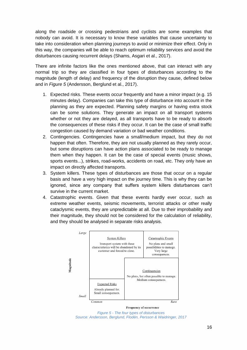
There are infinite factors like the ones mentioned above, that can interact with any

normal trip so they are classified in four types of disturbances according to the

magnitude (length of delay) and frequency of the disruption they cause, defined below

and in Figure 5 (Andersson, Berglund et al., 2017).

1. Expected risks. These events occur frequently and have a minor impact (e.g. 15

minutes delay). Companies can take this type of disturbance into account in the

planning as they are expected. Planning safety margins or having extra stock

can be some solutions. They generate an impact on all transport systems

whether or not they are delayed, as all transports have to be ready to absorb

the consequences of these risks if they occur. It can be the case of small traffic

congestion caused by demand variation or bad weather conditions.

2. Contingencies. Contingencies have a small/medium impact, but they do not

happen that often. Therefore, they are not usually planned as they rarely occur,

but some disruptions can have action plans associated to be ready to manage

them when they happen. It can be the case of special events (music shows,

sports events...), strikes, road-works, accidents on road, etc. They only have an

impact on directly affected transports.

3. System killers. These types of disturbances are those that occur on a regular

basis and have a very high impact on the journey time. This is why they can be

ignored, since any company that suffers system killers disturbances can’t

survive in the current market.

4. Catastrophic events. Given that these events hardly ever occur, such as

extreme weather events, seismic movements, terrorist attacks or other really

cataclysmic events, they are unpredictable at all. Due to their improbability and

their magnitude, they should not be considered for the calculation of reliability,

and they should be analysed in separate risks analysis.

Figure 5 - The four types of disturbances

Source: Andersson, Berglund, Flodén, Persson & Waidringer, 2017

17

All these disturbances cause variability in travel time duration, but they affect in

different frequency and periods of the day, month or year, so depending on its nature,

reliability caused by them can be classified into three different categories (Bates, Dix et

al., 1987) (Noland & Polak, 2002).

1. Variability in day-to-day travel times. It might be caused by demand fluctuations,

accidents, road-works and weather conditions. After taking into consideration

the day of the week, holidays and seasonal effects, it is considered that day-to-

day variability is purely random. Inter-day reliability.

2. Variability over the course of the day. Traffic congestion will vary during all the

day, so travel time will differ highly when departing during rush hours and when

departing during off-hour time. Inter-period reliability.

3. Variability from vehicle to vehicle. Mainly due to individual behaviour while

driving (speed, parking, traffic signals). Depending on drivers in road habits,

vehicle flow might be fluent or congested. Inter-vehicle reliability.

Historically, inter-period and inter-vehicle reliability have had little interest for being

studied (Zheng, Liu et al., 2017). Inter-period variability is rarely useful for carriers

because, as it has been mentioned before, market receivers are usually who fix the

arrival time for their commodities. Besides, there are clearly known differences

between rush hours and off-hour periods, but there are no great differences between

hours in each period. In reference to inter-vehicle variability, it makes low impact on

traffic congestion and its study would not contribute to a better scheduling or increase

reliability. That is why the majority of studies have focused on inter-day variability and

why most of them define reliability as a random variation in travel time (Bates, Polak et

al., 2001; Hollander, 2006; Hollander & Gleave, 2009).

2.6 Assessing reliability

2.6.1 Value of travel time reliability

As it has been seen above, reliability is a key concept that crucially affects the transport

of goods. Advantages caused by improving reliability have been mentioned but the real

economic effect can only be valuated with the value of reliability (VOR) (Jin & Shams,

2016). The value of reliability is created at the time that due to uncertainty in time

deliveries is necessary to have overstocks, use additional vehicles or drivers, extra

personnel in the warehouses or advance scheduled departure times (Landergren,

Berglund et al., 2015). Then, it refers to the monetary value that users are willing to pay

to reduce travel time variability when carrying commodities from the origin to the

destination to avoid this additional measures (De Jong, Kouwenhoven et al., 2009).

More specifically, there are three elements needed for including travel time reliability in

CBA (cost-benefit analysis) (De Jong & Bliemer, 2015):

1. Deriving a monetary value of reliability, the Value of Travel Time Reliability

(VTTR) or Variability (VTTV).

2. Taking into account the reaction of users to travel time variability in transport

forecasting models.

3. Forecasting the influence of infrastructure projects on reliability.

18

The second element (2) is necessary because the value of travel time reliability only

reflects preferences at an individual level, and it is not considering the global react of

users to a change in travel time variability (De Jong & Bliemer, 2015). De Jong and

Bliemer propose two ways for the valuation of travel time reliability. First option is to

carry it out completely in an extra post-process step, which is the simplest, but then

there is no feedback into the transport model. Second option entails to continue first

option by including travel time reliability in the cost of travel in the medium run.

Thereby, there is feedback into the transport model, although it is limited to mode and

route selection. Neither option affects to departure time scheduling.

The next table shows some valuations for truck freight travel time reliability in Europe

and Australia, that correspond to studies made until now.

Study Region

Data Collection Method

Evaluation Method

Definition Valuation Units USD Year Mode

Norway SP CE

Standard Deviation

27 NOK/STD

2010 Truck < 3,5 t

Norway SP CE

Standard Deviation

131 NOK/STD

2010 Truck > 3,5 t

Netherlands SP Regression Standard Deviation

14 €/hour 18,85 2010 Truck

Netherlands SP CE N/A Standard Deviation

0,8 VOR/VOT N/A Truck

Australia SP Regression Expected

Delay 1,93 avg.

AUS per 1

reduction 1,82 1998 Truck

Table 3 - Freight Values of reliability studies Source: Hirschman, Da Silva, Bryan, Strauss-Wieder & Tompkins, 2016.

2.6.2 Methods to assess reliability

To get the value of time travel reliability it is necessary to know how to measure or

quantify reliability first. In this way, the experiments are each of the travels made, and

the result obtained is the real time travel it takes (Rakha, El-Shawarby et al., 2010).

Each travel time trip may differ more or less, depending on all the circumstances

related to the route taken (distance, type of vehicle, state of the road, congestion, etc.).

The degree of reliability of the path will be defined by this variation of real travel times

(Andersson, Berglund et al., 2017).

In order to measure the reliability there are different possible definitions or criteria to

use. One of the most widespread approaches to assess reliability is determining the

transport system behaviour when there is congestion in the road (Sharov & Mikhailov,

2017). Congestion is interpreted as a state at which transport demand begins to

exceed transport supply capacity (Sharov & Mikhailov, 2017). Historically, the following

quantitative criteria have been used in studies carried out to date:

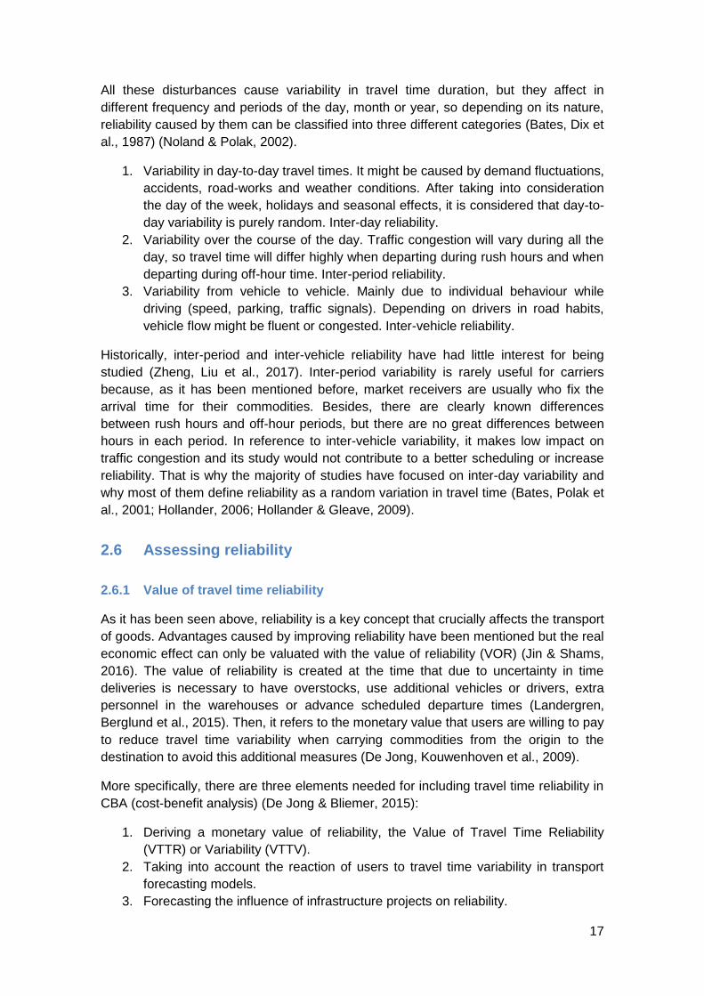
1. Standard deviation (Black, Hashimzade et al., 2017): mathematically, it is the

average of the squared differences from the mean and it is represented by σ. It

is commonly used to measure the dispersion of a set of observations of time

19

travels. A low standard deviation means that the travel time observations are

closely around the mean while a high standard deviation shows that the data

can be over a widely spread of time. Standard deviation is useful to standardize

a way to know what can be considered normal, and what can be considered

extra early or extra late. It is the only one criteria mentioned that allows knowing

the probability to get at destination at any possible time. Figure 6 (McNeese,

2009) shows an example of how standard deviation changes the normal

distribution. The three distributions have an average of 100, but different

standard deviation: 5 (blue curve), 10 (purple curve) and 20 (red curve).

Distribution with standard deviation of 20 (the largest one) corresponds to the

wider normal distribution.

Figure 6 - Normal distribution depending on standard deviation

Source: McNeese, 2009

2. Variance (Black, Hashimzade et al., 2017): it is the result of the

squared standard deviation of the travel time from its average value and it is

represented by σ2. It measures how far a set of random samples are spread out

from their mean time. Unlike standard deviation, it is not represented with the

identical units than the case study data. It is expressed with the square of the

units of the variable itself.

3. Buffer time (Sharov & Mikhailov, 2017): it can be applied to calculate economic

costs, incurred by the user in the way of scheduling extra time for departures

because of the uncertainty of the transport system.

𝑇𝑏 = 𝑇90% (95%) − �̅� (1)

With Tb being buffer time, T90% (95%) is 90% or 95% percentile of trip duration,

and �̅� is the average trip duration. Additionally, the buffer index can be

determined following the next expression:

𝐼𝑏 =𝑇𝑏

�̅�100% (2)

Both factors, Tb and Ib, define the reliability or uncertainty of the transport

systems studied. The extra time used because of the uncertainty, defined by

the buffer index allows estimating the costs incurred due to earlier departures to

assure being in time at destination.

4. Percentage of shipments that are delayed (Andersson, Berglund et al., 2017): it

is valuable (but incomplete) to know the ratio of shipments delayed. It is easy to

get, but it is not giving any information on the magnitude of the delay.

20

5. Schedule delay (Andersson, Berglund et al., 2017): it is the difference between

the expected arrival time and the real arrival time. It is differentiated between

Schedule Delays Early (SDE) and Schedule Delays Late (SDL), as the

coefficients associated with these variables are different in the models.

The coefficient of variation of arrival times (standard deviation divided by the mean) is

also a useful parameter, which is derived from standard deviation. It allows comparing

variabilities of journeys with different travel time mean. When referencing to travel

times calculation, this ratio is also called “Reliability Ratio” (Andersson, Berglund et al.,

2017). The following graphic (De Jong & Bliemer, 2015) shows that the standard

deviation its derivations are the most widely applied measure of time travel reliability,

being the most appropriate for use in CBA.

Figure 7 - Frequency of answers of the experts about the most suitable definition of reliability

Source: De Jong & Bliemer, 2015

As the most used one, these are the advantages (+) and disadvantages (-) of choosing

standard deviation to measure reliability (De Jong & Bliemer, 2015):

Advantages Disadvantages

It can be empirically calculated. It is rather sensitive to outliers.

Along with the mean, any distribution is well summarized.

Without knowing travel time distribution shape it is not possible to fully describe the transport model.

It is not difficult to use it in standard transport models, as it is only needed to add an extra term to consider reliability. It is not required to use a scheduling model in the global transport model.

Two standard deviations from different but consecutive paths cannot be added to calculate global standard deviation. Then, there is no additive property.

It fits very well with stated preference (SP) surveys, as the alternatives for every question differing in standard deviation values are well described by most of standard deviation models.

Table 4 - Advantages and disadvantages of using standard deviation for measure reliability Source: De Jong & Bliemer, 2015

With this approach, the value of reliability can be assumed as the value generated by a

change of the standard deviation of trip duration. Moreover, the approaches to

reliability evaluation are much more various and other measures have been used

21

occasionally by some authors for road networks. Below, the most relevant criteria are

explained.

- Average delay (Andersson, Berglund et al., 2017): it is useful to be aware of

how long is the common delay. However, no information about repeatability or

precision is obtained. One delay of 1 hour is not the same as twenty delays of 3

minutes, obtaining in both the same value of average delay.

- Spread (A. Fowkes & Whiteing, 2006): it is usually defined as the difference

between percentiles. It is useful to know the range to which most of the trips are

arriving, but within that range, no more information is known such as

repeatability or precision.

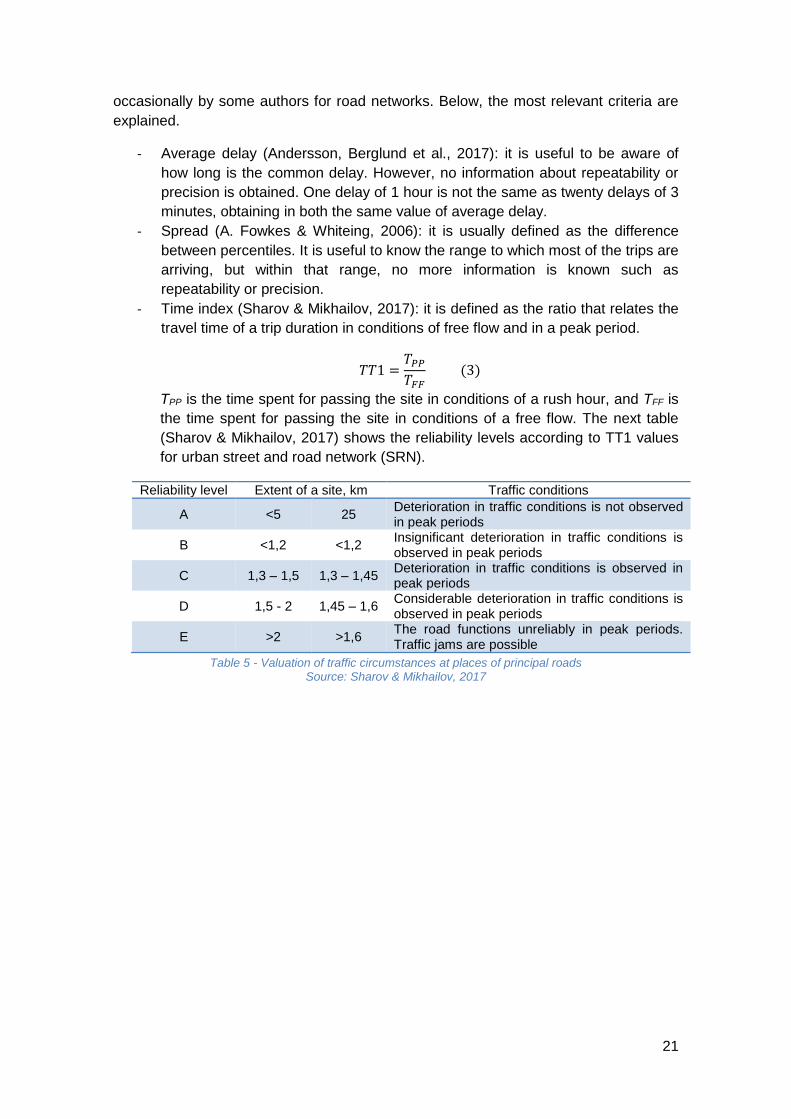
- Time index (Sharov & Mikhailov, 2017): it is defined as the ratio that relates the

travel time of a trip duration in conditions of free flow and in a peak period.

𝑇𝑇1 =𝑇𝑃𝑃

𝑇𝐹𝐹 (3)

TPP is the time spent for passing the site in conditions of a rush hour, and TFF is

the time spent for passing the site in conditions of a free flow. The next table

(Sharov & Mikhailov, 2017) shows the reliability levels according to TT1 values

for urban street and road network (SRN).

Reliability level Extent of a site, km Traffic conditions

A <5 25 Deterioration in traffic conditions is not observed in peak periods

B <1,2 <1,2 Insignificant deterioration in traffic conditions is observed in peak periods

C 1,3 – 1,5 1,3 – 1,45 Deterioration in traffic conditions is observed in peak periods

D 1,5 - 2 1,45 – 1,6 Considerable deterioration in traffic conditions is observed in peak periods

E >2 >1,6 The road functions unreliably in peak periods. Traffic jams are possible

Table 5 - Valuation of traffic circumstances at places of principal roads Source: Sharov & Mikhailov, 2017

22

3. METHOD

Main part of the thesis is based on theoretical concepts, so the first and foremost step

of the project is a literature review aimed having comprehensive synthesis of existing

studies related to the topic of the thesis. All scientific information related to the concept

of reliability, whether books, reports, research papers, etc. has been analysed. It has

been studied all the existing background in the framework of reliability, mainly related

to freight transportation. The studies carried out to date that have tried to quantify the

value of reliability, regardless of context (other countries, for passengers or different

transport modes), also have been a great source of valuable information. “Travel time”,

“Reliability”, “Variability”, “Freight”, “Transport” and “Value of time” have been the

keywords selected in order to find the information required, using Boolean operators

such as AND, OR, AND NOT in the search. The databases consulted are Scopus,

Science Direct, Taylor & Francis, Elsevier and Google Scholar, aided by Chalmers

Library database to have free access to all the information.

Next step of the thesis is the research design. A cross-sectional study has been

designed in order to collect data from agents involved in freight transportation. When

choosing the sample, different factors were considered. Several number of companies

had to participate in the study to obtain significant results and those companies should

represent a high variety of the market sectors. Taking into account these factors and

the difficulty to get in contact with them and time restriction, it was decided to take

advantage of Logistik & Transport fair held in the Swedish Exhibition and Congress

Centre in Gothenburg during 7th and 8th November 2017. This was a great opportunity

to collect a huge amount of valuable data, as some of the most important national and

international companies strongly related to transportation and logistics management

were meeting at the same place at the same time. Besides, DB Schenker was another

reliable source to get valuable information, as it was one of the companies taking part

of the project, and they could facilitate the contact with other companies that they work

with.

With these two possible sources of collecting data from companies, it was decided to

divide the study in two branches. The Logistik & Transport fair would be used to carry

out a Stated Preferences experiment in order to capture shippers and carriers

preferences. The profile of people attending the fair was mainly middle logistics

management employees. On the other hand, contacts through DB Schenker would be

used to arrange interviews with logistical and supply chains managers of some of the

most relevant companies in Gothenburg. The aim of the interviews was to get rather

qualitative information compared to quantitative in the survey.

At first, it was planned to do the interviews before the creation of the surveys to

establish a first contact with the companies, know their priorities and get more

information to design the survey. However, this was not possible due to the lack of

availability of companies interviewed. For this reason, the survey was first designed

and answers were obtained, and afterwards interviews were made with the companies,

which were useful to corroborate the hypotheses previously developed in the survey.

23

3.1 Stated Preference Survey

3.1.1. Survey design

The purpose of surveying was to know how companies prioritize reliability compared to

other attributes such as travel time and cost, and in consequence, to know how much,

companies would be willing to pay for higher values of reliability. With this information,

it has been possible to quantify the value of reliability and value of time for freight road

transportation in Sweden.

The aim of the surveys was to know the preferences of the companies by introducing

hypothetical transport offers and not by getting current information on the movements

of companies, travel times, trucks, etc. This process is called stated preference (SP)

survey in which respondents have to choose depending on the attributes values

assigned to each alternative. This method, together with discrete-choice modelling

technique, has the objective of knowing the contribution of each attribute to the utility

function. In this way, it is possible to establish the value of each attribute.

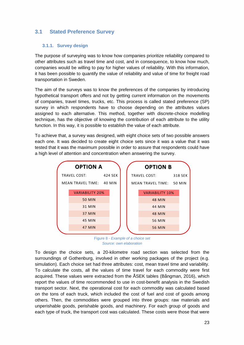
To achieve that, a survey was designed, with eight choice sets of two possible answers

each one. It was decided to create eight choice sets since it was a value that it was

tested that it was the maximum possible in order to assure that respondents could have

a high level of attention and concentration when answering the survey.

Figure 8 - Example of a choice set

Source: own elaboration

To design the choice sets, a 20-kilometre road section was selected from the

surroundings of Gothenburg, involved in other working packages of the project (e.g.

simulation). Each choice set had three attributes: cost, mean travel time and variability.

To calculate the costs, all the values of time travel for each commodity were first

acquired. These values were extracted from the ÅSEK tables (Bångman, 2016), which

report the values of time recommended to use in cost-benefit analysis in the Swedish

transport sector. Next, the operational cost for each commodity was calculated based

on the tons of each truck, which included the cost of fuel and cost of goods among

others. Then, the commodities were grouped into three groups: raw materials and

unperishable goods, perishable goods, and machinery. For each group of goods and

each type of truck, the transport cost was calculated. These costs were those that were

24

used for the creation of the choice sets. In reference to travel time, four possible times

were established for the 20 km route, according to the car’s speed that varies

depending on different level of traffic congestion. Finally, the variability was presented

in terms of percentage referring to mean travel time. Random values for travel time

were generated, according to the given mean travel time and variability, to facilitate the

understanding of the concept of variability by the respondents. The two options of each

choice set were assigned with the statistical software in order to assure that the

combination of the three attributes did not create any dominating option.

Previously to present the choice sets, each respondent had to answer what type of

truck was the most frequent in the company, as well as the type of good shipped, so

the values of the choice sets were adapted. Next, taking advantage of the moments of

maximum concentration, respondents were asked to answer the choice sets and then

the weight they had assigned to each attribute when answering the choice sets. Finally,

when their attention was decreasing they were asked for their point of view of the

concept of reliability, the role of the company within the supply chain (shipper or carrier)

and the sector of the company for which they worked. With all this information, apart

from establishing a value of reliability, it was also possible to classify each of the

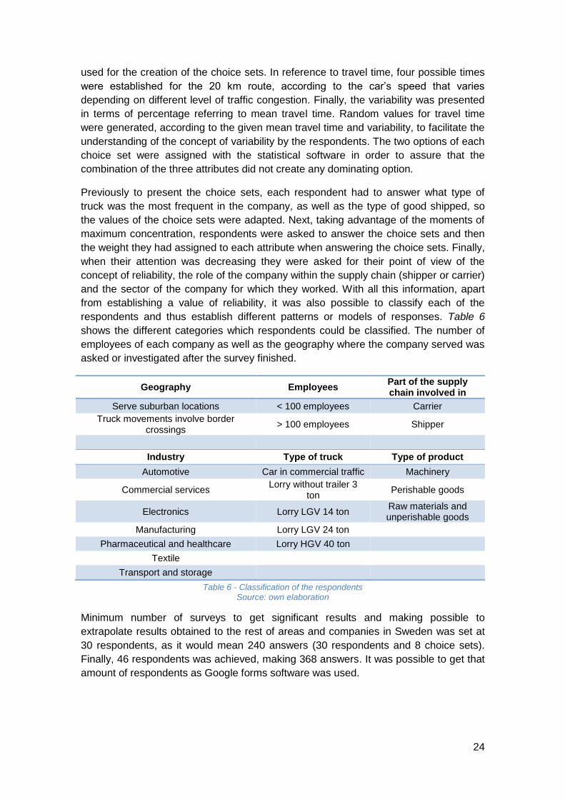
respondents and thus establish different patterns or models of responses. Table 6

shows the different categories which respondents could be classified. The number of

employees of each company as well as the geography where the company served was

asked or investigated after the survey finished.

Geography Employees Part of the supply chain involved in

Serve suburban locations < 100 employees Carrier

Truck movements involve border crossings

> 100 employees Shipper

Industry Type of truck Type of product

Automotive Car in commercial traffic Machinery

Commercial services Lorry without trailer 3

ton Perishable goods

Electronics Lorry LGV 14 ton Raw materials and unperishable goods

Manufacturing Lorry LGV 24 ton

Pharmaceutical and healthcare Lorry HGV 40 ton

Textile

Transport and storage

Table 6 - Classification of the respondents Source: own elaboration

Minimum number of surveys to get significant results and making possible to

extrapolate results obtained to the rest of areas and companies in Sweden was set at

30 respondents, as it would mean 240 answers (30 respondents and 8 choice sets).

Finally, 46 respondents was achieved, making 368 answers. It was possible to get that

amount of respondents as Google forms software was used.

25

3.1.2. Discrete choice modelling

To analyse the answers was decided to use discrete choice modelling. The utility of

discrete choice models is that they allow the modelling of qualitative variables, using

techniques of discrete variables (Medina, 2005). A variable is discrete when it is formed

by a finite number of alternatives that measure qualities (De Dios Ortuzar & Willumsen,

1994). This feature requires coding as a step prior to modelling. The modelling of this

type of variables is known as discrete choice models, within which there is a wide

typology of models. According to the function used for the estimation of the probability

there is the truncated linear probability model, the Logit model and the Probit model

(Medina, 2005).

In the literature, there are two approaches to the structural interpretation of discrete

choice models (Jin & Shams, 2016). The first one refers to the modelling of a latent

variable through an index function, which tries to model an unobservable or latent

variable. The second of the approaches allows interpreting discrete choice models

under the theory of random utility, so that the alternative selected in each case will be

one that maximizes the expected utility (Jin & Shams, 2016).

Under random utility maximization approach, an individual must adopt a decision that

allows him to choose between two or more exclusive alternatives, choosing the one

which will maximize the expected utility provided by each of the possible alternatives

(Shams, Asgari et al., 2017). Therefore, the individual will choose one of the

alternatives depending on whether the utility provided by chosen decision is superior to

the one provided by the other options. This utility can vary depending on some

characteristics and the value of different factors of the product or service. In this study,

utility is assigned by the companies depending on the value of the cost, the mean

travel time and the variability of each transport option, and the utility could be related to

economic profit obtained (De Los Santos, 2016). Depending on how utility varies,

according to a change in a variable, the importance of each element can be assessed.

In addition, each individual (or companies, sectors, etc.) can use different criteria for

each element to influence in the utility, so it depends on each subject.

The Random Utility Maximization model that has been used is the conditional logit

model (CLOGIT) (McFadden, 1973) or logistic regression model. Considering an r

consumer, and j alternatives in a set of J alternatives, the utility is set as Urj and it is

defined by:

𝑈𝑟𝑗 = 𝑉𝑟𝑗 + 𝜀𝑟𝑗 (4)

Where Vrj is defined as the observable term and it is called the Systematic Utility, and

εrj is the unobservable term, associated to an unknown heterogeneity factor associated

to the consumer r and product j. Some of these factors could be gender, educational or

generational influences that cannot be taken into account (Paczkowski, 2016).

Systematic utility is defined by:

𝑉𝑟𝑗 = 𝛽1 ∗ 𝑋𝑟𝑗 (5)

Being Xrj the value of the attribute X for product j seen by consumer r (e.g. the price of

a car). β1 is a part-worthy utility and must be estimated from data.

26

Assuming a probability distribution for εrj, the probabilities for consumer r choosing

product j from among J products is known as the acceptance rate or take rate and it

can be calculated with (De Los Santos, 2016):

𝑃𝑟𝑟𝑗 = 𝑒𝑉𝑟𝑗

∑ 𝑒𝑉𝑟𝑘𝐽𝑘=1

(6)

The probability for r consumer and j product is not conditioned by its total utility, but by

the relative utility with respect to the other products. Thus, it depends on the possible

choices available and the person making the choice. This discrete choice model has

two interesting properties (Paczkowski, 2016). Equivalent Differences Property (EDP)

says that an element or a variable that is constant for all J choice alternatives has no

effect on the choice probability, as it would be cancelled between the numerator and

denominator, so they do not need to be studied. Second property is Independence of

Irrelevant Alternatives Property (IIA) that says that the ratio of choosing probabilities of

two different alternatives only depends on these two alternatives and does not depend

on the presence or the absence of any other alternatives.

3.1.3. Survey data analysis

To start analysing the respondents’ answers, first, it was carried out a post-process to

be able to work with the results obtained. First, a preliminary analysis was done in

which it was found that all the answers obtained were correct. This step was completed

by verifying that all the choice sets had a variety of the answers (<90%) and therefore

there had not been any predominant attribute. In addition, the sample of the profiles of

respondents was analysed, according to sectors, type of material, carrier/shipper, and

type of truck. As commented before, it was also investigated the number of employees

of each company that had answered the survey in order to analyse whether size was a

factor that influenced the answers obtained.

When it was found that there were no anomalies (incoherent responses), the obtained

answers were analysed. Data obtained from surveys has been statistically analysed

with JMP. With this statistical software the objective was to find the concrete model that

best defined the priorities of the different types of companies among the different

attributes proposed. The first model simulated was only including the attributes of each

option, cost, mean travel time and variability, without taking into account the

characteristics of the respondent. With this model, it was intended, in a global way, to

see which attributes were significant when choosing the transport option and between

the three attributes, which was the most important. Later, a large number of models

were run in search of the best model, looking for the significant variables besides the

three attributes. It was checked the significance of each variable and the interaction

between them. To know whether a variable was significant, the p-value and logWorth

parameters were checked. The p-value indicates the probability that, when the null

hypothesis is true, the statistical summary would be the same as or of greater

magnitude than the actual observed results. Standard significance p-value is set at

0,05, thus any variable with p-value lower than 0,05 will be considered as significant.

The logWorth it is showing the same information but transforming the p-value with the

next equation (7):

27

𝑙𝑜𝑔𝑊𝑜𝑟𝑡ℎ = − log(𝑝_𝑣𝑎𝑙𝑢𝑒) (7)

In addition, in the Parameter Estimation section, it was checked the contribution of

each variable in to the utility function, and therefore β values of the Systematic utility.

This information allows knowing if the contribution of a variable adds or subtracts value

in the utility function, so it is useful to see the coherence of the obtained model.

Another factor that indicates the quality of the model is the AICc parameter (Akaike

Information Criterion). It allows comparing between two different models, being more

trustable the one with the lowest AICc value. Finally, the Willingness to Pay was

calculated, which allows knowing, according to the answers obtained in the survey and

by a concrete respondent profile, the amount that each profile of respondent would be

willing to pay for better specific values of variability and travel time. Considering these

parameters, multiple models were analysed in search of the best one, the one having a

better trade-off between a low AICc value, conceptual validity and significant coherent

factors.

In addition, a classification of similar response patterns by profiles, also known as

clusters, was also carried out. With the cluster analysis, it is intended to find a set of

groups to which the different individuals will be assigned by some criterion of

homogeneity. Referring to the survey, the individuals are the respondents and the

criterion of homogeneity are the answers to the choice sets. Unfortunately, cluster

analysis done did not show any significant result as the groups were set at three, but

there was no homogeneity in respondent’s profiles of each group.

3.2 Interviews

3.2.1 Interviews design

It was decided to interview some of the most important companies in Sweden of

different sectors that could be benefited with the project. In this way, it would be

possible to understand better their process and supply chain of the entities, and it

would be recollected qualitative and quantitative information about the companies’

approach of time travel reliability. Moreover, it was also wanted to know the opinion

and evaluation of the companies about the project that it is being carried out.

The companies that it was decided to interview were five important entities of different

sectors such as transport and storage, pharmaceutical and healthcare or food and

beverage. It was started contact with Volvo, the largest company in Sweden (Business

Insider Nordic, 2016) and a multinational manufacturing company, and DB Schenker, a

leader in logistic solutions and supply chain management. Moreover, it was contacted

with Coop, a hypermarket company which has the 21,5% grocery retail market in

Sweden (Coop Sverige, 2017), Mat, an online grocery store in Sweden which is

becoming very important in the last years, and Oriola, a company with a lot of

experience in pharmaceutical wholesale markets (100 years approximately) (Oriola,

2017).

As the aim of the interviews was to know better the point of view and the process of the

companies, it was wanted to contact with the high logistics employees of the

companies, such as the transport manager or the supply chain developer. As it was

28

difficult to have access to this group of people and stablish a meeting with them, DB

Schenker, a company involved in the global project, facilitated the contacts of the

companies chosen to interview.

The process followed to arrange a meeting with them was the recommended by Healey

and Rawlinson (1993). First, the interviewers did a telephone call to stablish a first

contact with the person and explain a little bit the project that is being carried out. Then,

an introductory mail was written to enclose a short outline of the objectives of the

project and it was also sent the interview guide so the interviewee could be better

prepared.

After a first contact with the companies, it was not possible to stablish an interview with

all of them because they were not available in short term to meet for an interview.

Thus, three interviews were carried out. The companies interviewed were Oriola, Coop

and DB Schenker and the media of communication was by phone calls. In this way, it

could not be identified non-verbal clues as facial expression, although the interviewers

could realise that sometimes the respondent changed the tone of voice.

The interview created was semi-structured to get more flexibility depending on the

direction that took the interview. In this way, the interviewer could change the

predetermined order of the questions or also add new questions to know more about

the respondent argument or to follow up interviewee’s replies. Generally, qualitative

interviews are used to comprehend the interviewee’s point of view by having detailed

answers, so the approach is less structured than a quantitative interview.

In order to achieve a useful interview, it was necessary to think about what it was

needed to know to answer the research questions. Thus, the interview questions had to

comprise all the areas of the research questions, but in a respondent’s point of view.

Some studies, for example Hirschman, Da Silva et al. (2016), were very useful to

design the interview guides as the type of interviews done were very similar to the one

that it was wanted to create.

Three different interviews guides were designed depending on the role of the company

in the supply chain that was interviewed (shipper, carrier or receiver). Each guide is

divided in three sections. Introduction is focused on information related to market

sector, types and number of deliveries associated to the company. The second section

is Deliveries information, where questions performed are related to time delivery

requirements, delays and solutions to time travel variability. In the last section, Project

evaluation, the companies are asked to evaluate the proposal of allowing certain types

of trucks to circulate along the bus lane in the ring roads (Bryman & Bell, 2015).

Interview guides can be found in Appendix II.

It is important to mention that the answers of some questions of the guide were coded

in order to facilitate the subsequent analysis. This would clarify the understanding of

the data collected and would also help with the theoretical sampling (Bryman & Bell,

2015).

During the interview, it was very important to be attentive to what the interviewee was

explaining the whole time, and also be flexible in the asking of questions. The

interviews were audio-recorded to make things easier and also due to the fact that in a

29

qualitative interview not only is important what respondents say but also the way they

explain it.

3.2.2 Interview data analysis

Once it was recollected all the data of the interviews, the next step was to analyse the

results obtained. The method followed to analyse them was based on the grounded

theory principles. Grounded theory was defined by Strauss and Corbin in 1998 as

“theory that was derived from data, systematically gathered and analysed through the

research process. In this method, data collection, analysis and eventual theory stand in

close relationship to one another” (Bryman & Bell, 2015).

To analyse results, it was carried out a constant comparison between answers

obtained in the different interviews. In this way, it was kept a close connection between

conceptualization and data collected, and the relation between categories with their

indicators, and concepts are maintained. Thanks to this method of constant

comparison, the researcher can continuously compare the data coded under a

category in order to find some theory that can be further developed.

On the other hand, as interviews were audio-recorded, they were listened by second

time in order to find out some word or important sentence that the respondent had

commented and it had not been reflected in the answers written in the guide.

3.3 Validity and transferability

A great emphasis has been placed on the design of both the interviews and the survey,

in order to obtain the desired information to answer the research questions of the

thesis. The trustworthiness of the results and conclusions obtained has to be evaluated

by looking at the robustness and external validity (Easterby-Smith, Thorpe et al., 2015).

The final model used to describe the respondents answers and the willingness to pay

associated can be considered robust as the statistical parameters such as the p-value

associated to each variable was significantly lower than 0,05 and the AICc indicator

was one the lowest in all the models run. At the same time conceptual validity and

significant coherent factors were matching in the same model. Very few alteration on

the values obtained would be by changes to a single data point or to data transcription

errors due to high number of answers obtained, 368. Moreover, in order to ensure that

there were no transcription errors, Google Forms was used and automatic data

transcription into Excel was done.

External validity is an indication of how much the conclusions can be generalized

outside the study (Easterby-Smith, Thorpe et al., 2015). The findings in this study,

related to values of reliability and values of travel time, can be generalizable to the

extent to Sweden market. Furthermore, the survey sample comprised of 46 companies

not only located in Gothenburg as companies working all around Sweden came to the

fair, which further strengthens the generalizability. However, since all the respondents

were Swedish, it is not possible to generalize the results obtained outside the Swedish

scene. It shall further be noted that the study needs to be extended with retailer’s point

of view to have a complete successful performance.

30

According to Easterby-Smith et al. (2015) one of the major concerns regarding survey

designs is whether the instruments are both stable and accurate. Google Forms can be

considered accurate and stable enough as the risk of choosing the wrong alternative

was very low as each alternative had a big picture associated. The software did not

accept sending in unanswered questions, turning the risk of a respondent forgetting to

respond to a question to zero since this was not possible. Moreover, it shall be noted

that the authors were present when the surveys were being carried out hence they

could assure the interviewee understood each question properly.

Moreover, all the data from the interviews has been treated with confidentiality to

guarantee the ethics of the thesis.

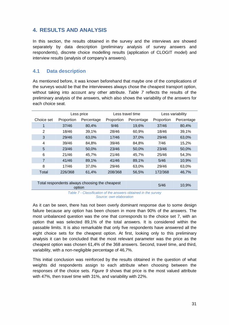
31

4. RESULTS AND ANALYSIS

In this section, the results obtained in the survey and the interviews are showed

separately by data description (preliminary analysis of survey answers and

respondents), discrete choice modelling results (application of CLOGIT model) and

interview results (analysis of company’s answers).

4.1 Data description

As mentioned before, it was known beforehand that maybe one of the complications of

the surveys would be that the interviewees always chose the cheapest transport option,

without taking into account any other attribute. Table 7 reflects the results of the

preliminary analysis of the answers, which also shows the variability of the answers for

each choice seat.

Less price Less travel time Less variability

Choice set Proportion Percentage Proportion Percentage Proportion Percentage

1 37/46 80,4% 9/46 19,6% 37/46 80,4%

2 18/46 39,1% 28/46 60,9% 18/46 39,1%

3 29/46 63,0% 17/46 37,0% 29/46 63,0%

4 39/46 84,8% 39/46 84,8% 7/46 15,2%

5 23/46 50,0% 23/46 50,0% 23/46 50,0%

6 21/46 45,7% 21/46 45,7% 25/46 54,3%

7 41/46 89,1% 41/46 89,1% 5/46 10,9%

8 17/46 37,0% 29/46 63,0% 29/46 63,0%

Total 226/368 61,4% 208/368 56,5% 172/368 46,7%

Total respondents always choosing the cheapest option

5/46 10,9%

Table 7 - Classification of the answers obtained in the survey Source: own elaboration

As it can be seen, there has not been overly dominant response due to some design

failure because any option has been chosen in more than 90% of the answers. The

most unbalanced question was the one that corresponds to the choice set 7, with an

option that was selected 89,1% of the total answers. It is considered within the

passable limits. It is also remarkable that only five respondents have answered all the

eight choice sets for the cheapest option. At first, looking only to this preliminary

analysis it can be concluded that the most relevant parameter was the price as the

cheapest option was chosen 61,4% of the 368 answers. Second, travel time, and third,

variability, with a non-negligible percentage of 46,7%.

This initial conclusion was reinforced by the results obtained in the question of what

weights did respondents assign to each attribute when choosing between the

responses of the choice sets. Figure 9 shows that price is the most valued attribute

with 47%, then travel time with 31%, and variability with 22%.

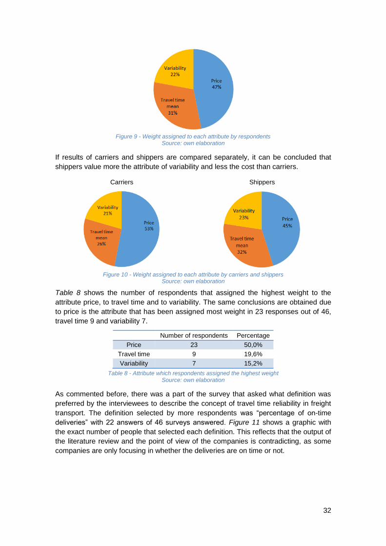
32

Figure 9 - Weight assigned to each attribute by respondents

Source: own elaboration

If results of carriers and shippers are compared separately, it can be concluded that

shippers value more the attribute of variability and less the cost than carriers.

Carriers Shippers

Figure 10 - Weight assigned to each attribute by carriers and shippers Source: own elaboration

Table 8 shows the number of respondents that assigned the highest weight to the

attribute price, to travel time and to variability. The same conclusions are obtained due

to price is the attribute that has been assigned most weight in 23 responses out of 46,

travel time 9 and variability 7.

Number of respondents Percentage

Price 23 50,0%

Travel time 9 19,6%

Variability 7 15,2%

Table 8 - Attribute which respondents assigned the highest weight Source: own elaboration

As commented before, there was a part of the survey that asked what definition was

preferred by the interviewees to describe the concept of travel time reliability in freight

transport. The definition selected by more respondents was “percentage of on-time

deliveries” with 22 answers of 46 surveys answered. Figure 11 shows a graphic with

the exact number of people that selected each definition. This reflects that the output of

the literature review and the point of view of the companies is contradicting, as some

companies are only focusing in whether the deliveries are on time or not.

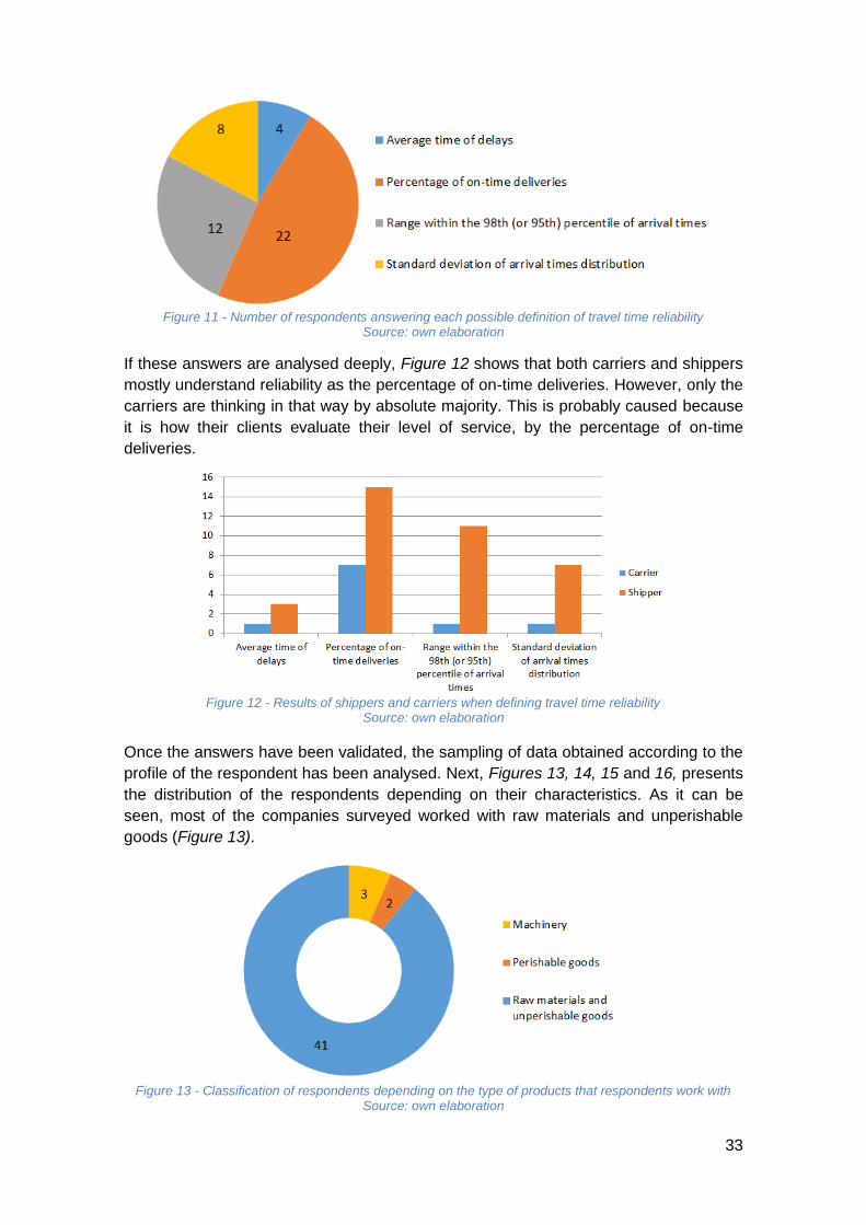
33

Figure 11 - Number of respondents answering each possible definition of travel time reliability

Source: own elaboration

If these answers are analysed deeply, Figure 12 shows that both carriers and shippers

mostly understand reliability as the percentage of on-time deliveries. However, only the

carriers are thinking in that way by absolute majority. This is probably caused because

it is how their clients evaluate their level of service, by the percentage of on-time

deliveries.

Figure 12 - Results of shippers and carriers when defining travel time reliability

Source: own elaboration

Once the answers have been validated, the sampling of data obtained according to the

profile of the respondent has been analysed. Next, Figures 13, 14, 15 and 16, presents

the distribution of the respondents depending on their characteristics. As it can be

seen, most of the companies surveyed worked with raw materials and unperishable

goods (Figure 13).

Figure 13 - Classification of respondents depending on the type of products that respondents work with

Source: own elaboration

34

Figure 14 - Classification of respondents depending on type of vehicles of the company

Source: own elaboration

Carrier / Shipper Number of employees Area of distribution

Figure 15 - Classification of respondents depending on carrier/shipper, number of employees and area of distribution

Source: own elaboration

Figure 16 - Classification of respondents depending on sector of the company

Source: own elaboration

As it can be observed, there is a deficit in people surveyed in the commercial,

pharmaceutical and textile sectors. This fact will make the conclusions that can be

obtained from these sectors less relevant. In addition, there are few answers for the

truck of 40 tons, although this is less relevant due to the fact that capacity is studied as

a continuous variable, and all the answers with all vehicle capacities will define the

tendency in the behaviour of this factor.

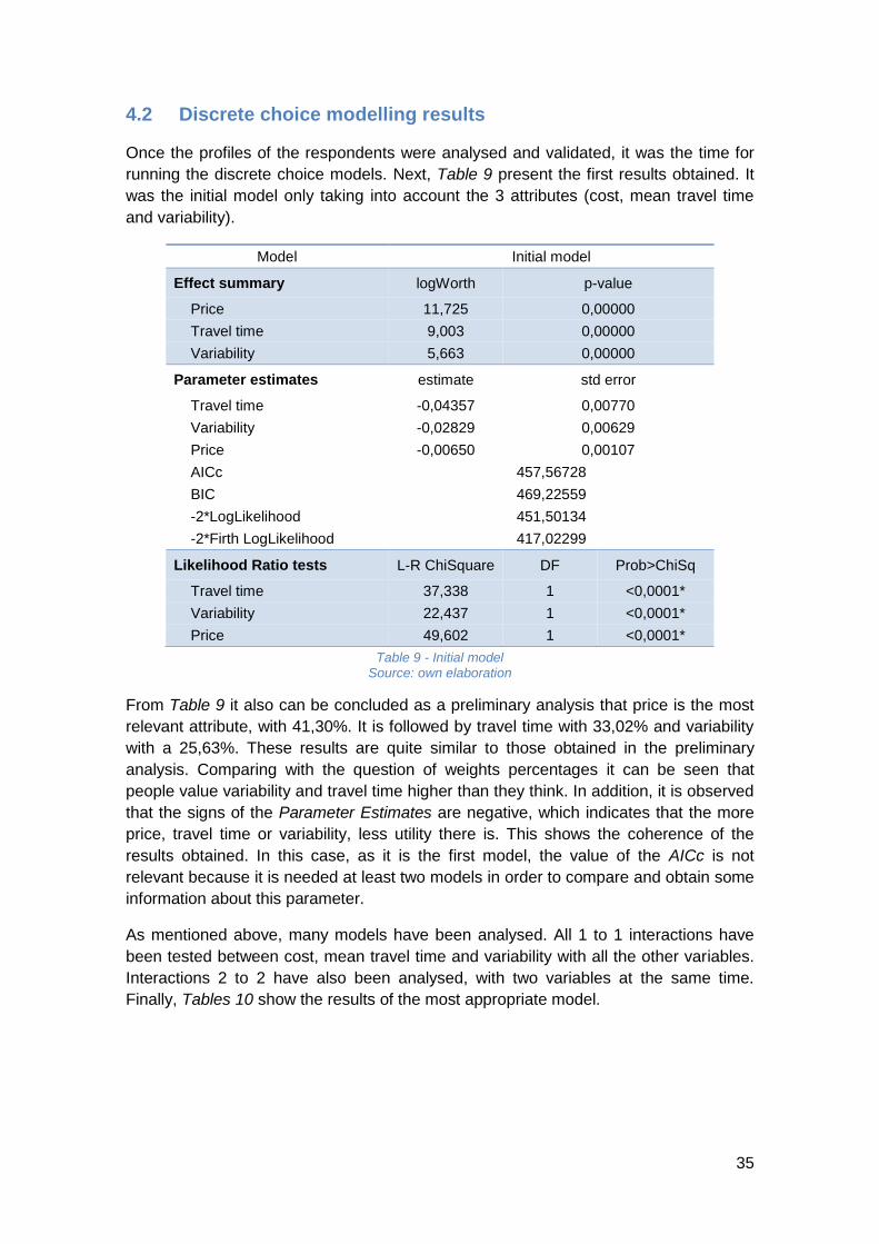
35

4.2 Discrete choice modelling results

Once the profiles of the respondents were analysed and validated, it was the time for

running the discrete choice models. Next, Table 9 present the first results obtained. It

was the initial model only taking into account the 3 attributes (cost, mean travel time

and variability).

Model Initial model

Effect summary logWorth p-value

Price 11,725 0,00000

Travel time 9,003 0,00000

Variability 5,663 0,00000

Parameter estimates estimate std error

Travel time -0,04357 0,00770

Variability -0,02829 0,00629

Price -0,00650 0,00107

AICc 457,56728

BIC 469,22559

-2*LogLikelihood 451,50134

-2*Firth LogLikelihood 417,02299

Likelihood Ratio tests L-R ChiSquare DF Prob>ChiSq

Travel time 37,338 1 <0,0001*

Variability 22,437 1 <0,0001*

Price 49,602 1 <0,0001*

Table 9 - Initial model Source: own elaboration

From Table 9 it also can be concluded as a preliminary analysis that price is the most

relevant attribute, with 41,30%. It is followed by travel time with 33,02% and variability

with a 25,63%. These results are quite similar to those obtained in the preliminary

analysis. Comparing with the question of weights percentages it can be seen that

people value variability and travel time higher than they think. In addition, it is observed

that the signs of the Parameter Estimates are negative, which indicates that the more

price, travel time or variability, less utility there is. This shows the coherence of the

results obtained. In this case, as it is the first model, the value of the AICc is not

relevant because it is needed at least two models in order to compare and obtain some

information about this parameter.

As mentioned above, many models have been analysed. All 1 to 1 interactions have

been tested between cost, mean travel time and variability with all the other variables.

Interactions 2 to 2 have also been analysed, with two variables at the same time.

Finally, Tables 10 show the results of the most appropriate model.

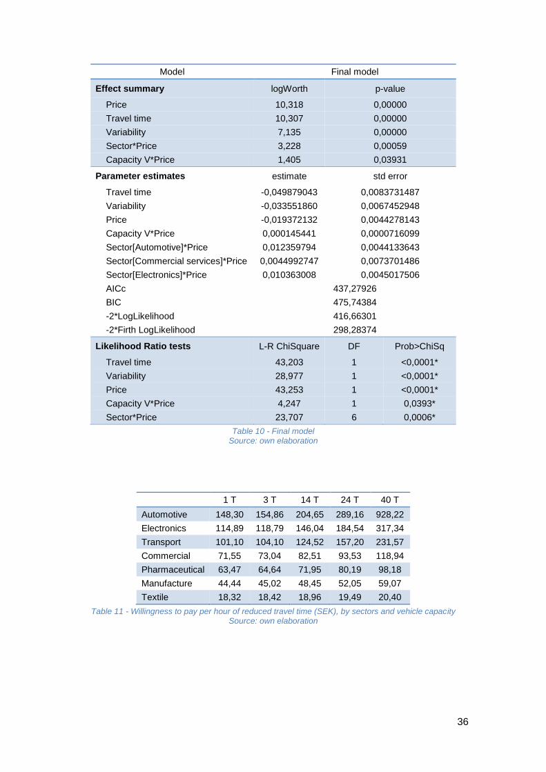
36

Model Final model

Effect summary logWorth p-value

Price 10,318 0,00000

Travel time 10,307 0,00000

Variability 7,135 0,00000

Sector*Price 3,228 0,00059

Capacity V*Price 1,405 0,03931

Parameter estimates estimate std error

Travel time -0,049879043 0,0083731487

Variability -0,033551860 0,0067452948

Price -0,019372132 0,0044278143

Capacity V*Price 0,000145441 0,0000716099

Sector[Automotive]*Price 0,012359794 0,0044133643

Sector[Commercial services]*Price 0,0044992747 0,0073701486

Sector[Electronics]*Price 0,010363008 0,0045017506

AICc 437,27926

BIC 475,74384

-2*LogLikelihood 416,66301

-2*Firth LogLikelihood 298,28374

Likelihood Ratio tests L-R ChiSquare DF Prob>ChiSq

Travel time 43,203 1 <0,0001*

Variability 28,977 1 <0,0001*

Price 43,253 1 <0,0001*

Capacity V*Price 4,247 1 0,0393*

Sector*Price 23,707 6 0,0006*

Table 10 - Final model Source: own elaboration

1 T 3 T 14 T 24 T 40 T

Automotive 148,30 154,86 204,65 289,16 928,22

Electronics 114,89 118,79 146,04 184,54 317,34

Transport 101,10 104,10 124,52 157,20 231,57

Commercial 71,55 73,04 82,51 93,53 118,94

Pharmaceutical 63,47 64,64 71,95 80,19 98,18

Manufacture 44,44 45,02 48,45 52,05 59,07

Textile 18,32 18,42 18,96 19,49 20,40

Table 11 - Willingness to pay per hour of reduced travel time (SEK), by sectors and vehicle capacity Source: own elaboration

37

1 T 3 T 14 T 24 T 40 T

Automotive 488,60 510,23 674,25 952,70 2808,35

Electronics 378,53 391,38 481,18 607,98 1051,30

Transport 333,08 343,00 410,05 498,70 762,38

Commercial 235,73 240,63 271,83 308,13 391,88

Pharmaceutical 209,10 212,98 237,05 264,20 323,48

Manufacture 146,43 148,33 159,60 171,48 194,63

Textile 60,35 60,68 62,48 64,23 67,20

Table 12 - Willingness to pay per hour of variability reduction (SEK), by sectors and vehicle capacity Source: own elaboration

As it will be commented in section 5. Discussion and practical implication, this is a

logical and consistent result, because as the vehicle is bigger, the load it carries is

more valuable and therefore, the company is less sensitive to price. For this reason,

they are willing to pay more money to improve in aspects such as travel time or

variability. The same happens with the sector due to the fact that those who work with

more expensive products such as machinery or electronics, are also less sensitive to

the price and are willing to pay more money. Consequently, it can be concluded that

the significant variables are those that influence the total value of the goods to be

transported. However, the type of good, the size of the company and the area in which

the goods are distributed, have not been significant.

4.3 Interview results

Three important companies from different sectors such as pharmaceutical and

healthcare, food and beverages, and transport and storage were interviewed. The

interviewees were workers with more than ten years of experience in their companies

and all of them were transport managers, operation managers or supply chain

developers.

First of all, they were asked some questions related to the company such as how it

operates. Most of the interviewers indicated that the size of shipment they had was

lower than three tons, and they sent more than 100 shipments per day. With this data it

can be seen that the companies interviewed are important firms in the sector and also

in the country. In addition, it should be noted that their percentage of shipments

delayed is lower than 5%. It is also necessary to comment that all interviewees decided

that the concept that fitted better with their idea of travel time reliability in freight

transport was "percentage of on-time deliveries".

Next, interviewees were asked to rate some variables as a source of travel time

variability, and they considered that accidents was the factor that most affected

variability, and the least one was paperwork and language barriers at receiving

facilities. Figure 17 shows the most and least relevant factors. It is noteworthy that

some company considered the factor “drivers unable to find locations” as one of the

least important because it did not affect to travel time variability. This is because these

companies teach their drivers in order they have a good knowledge of the route they

are going to drive. Others considered that “consistent travel times for road freight

moves” was not a very important factor because they only drove short distances in the

38

surroundings of Gothenburg. However, the majority of companies had the same

opinion about the most and least important factors that affected travel time reliability.

Accidents Delays at loading / outbound facility Availability of real-time traffic information Weather Consistent travel times for road freight moves Drivers unable to find locations Road works Vehicle breakdowns Paperwork and language barriers at receiving

facilities

Figure 17 - Factors that affect travel time variability Source: own elaboration

Companies plan the journey’s departure depending on the fixed delivery time, and they

organise the trips with the carrier although other firms establish the routes depending

on the truck’s space. Besides, interviewees answered that delivery requirements are

mostly defined by consistent delivery within a multi-day delivery window, and if some

shipment is delayed the carrier is more responsible than the shipper. If it happens,

companies stipulate penalties for missing the specified delivery requirements to their

transport company, and the customer also stipulate penalties to them. In addition, they

were asked for the measure that they take to assure deliveries arrive on time, and they

answered that they follow up every month all the shipments, and carriers use a type of

scanner or app to report delivery times.

Finally, it is noteworthy that interviewees considered that the project being carried out

is very interesting and they would be willing to pay in order to have more reliability in

their mean travel time and also less traffic queues.

+ A

ffe

cts

-

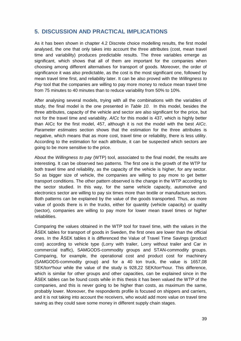
39

5. DISCUSSION AND PRACTICAL IMPLICATIONS

As it has been shown in chapter 4.2 Discrete choice modelling results, the first model

analysed, the one that only takes into account the three attributes (cost, mean travel

time and variability) produces predictable results. The three variables emerge as

significant, which shows that all of them are important for the companies when

choosing among different alternatives for transport of goods. Moreover, the order of

significance it was also predictable, as the cost is the most significant one, followed by

mean travel time first, and reliability later. It can be also proved with the Willingness to

Pay tool that the companies are willing to pay more money to reduce mean travel time

from 75 minutes to 40 minutes than to reduce variability from 50% to 10%.

After analysing several models, trying with all the combinations with the variables of

study, the final model is the one presented in Table 10. In this model, besides the

three attributes, capacity of the vehicle and sector are also significant for the price, but

not for the travel time and variability. AICc for this model is 437, which is highly better

than AICc for the first model, 457, although it is not the model with the best AICc.

Parameter estimates section shows that the estimation for the three attributes is

negative, which means that as more cost, travel time or reliability, there is less utility.

According to the estimation for each attribute, it can be suspected which sectors are

going to be more sensitive to the price.

About the Willingness to pay (WTP) tool, associated to the final model, the results are

interesting. It can be observed two patterns. The first one is the growth of the WTP for

both travel time and reliability, as the capacity of the vehicle is higher, for any sector.

So as bigger size of vehicle, the companies are willing to pay more to get better

transport conditions. The other pattern observed is the change in the WTP according to

the sector studied. In this way, for the same vehicle capacity, automotive and

electronics sector are willing to pay six times more than textile or manufacture sectors.

Both patterns can be explained by the value of the goods transported. Thus, as more

value of goods there is in the trucks, either for quantity (vehicle capacity) or quality

(sector), companies are willing to pay more for lower mean travel times or higher

reliabilities.

Comparing the values obtained in the WTP tool for travel time, with the values in the

ÅSEK tables for transport of goods in Sweden, the first ones are lower than the official

ones. In the ÅSEK tables it is differenced the Value of Travel Time Savings (product

cost) according to vehicle type (Lorry with trailer, Lorry without trailer and Car in

commercial traffic), SAMGODS-commodity groups and STAN-commodity groups.

Comparing, for example, the operational cost and product cost for machinery

(SAMGODS-commodity group) and for a 40 ton truck, the value is 1657,08

SEK/ton*hour while the value of the study is 928,22 SEK/ton*hour. This difference,

which is similar for other groups and other capacities, can be explained since in the

ÅSEK tables can be found costs while in this thesis it has been valued the WTP of the

companies, and this is never going to be higher than costs, as maximum the same,

probably lower. Moreover, the respondents profile is focused on shippers and carriers,

and it is not taking into account the receivers, who would add more value on travel time

saving as they could save some money in different supply chain stages.

40

Regarding to variability values, they are regularly considered in the ÅSEK tables as

twice the value of travel time savings. In the same example mentioned for value of time

travel savings, the relation is 3,02. In this study, global comparison between values of

travel time savings and values of reliability with all the sectors and capacities raise a

mean relation of 3,29. Then, these values are different from the ÅSEK tables ones and

they should be updated.

With the new and different values of reliability, it can be concluded that it was

necessary to carry out this study in order to use more accurate values when making

cost-benefit analysis. These values will help companies and governments to have more

precise data and economic impact valuations when making decisions related to

transport and infrastructure projects. Related to Suburban Logistics project, as this

thesis is just one of the seven working packages, it cannot be determined the final type

of vehicles that should be allowed to circulate along the bus lane as other factors than

the economical are also important (e.g. social value). Anyway, looking exclusively for

economic savings criteria it can be determined that automotive, electronics and

transport trucks are the ones who should be allowed first (depending on number of

trucks for each sector and road capacity).

Table 3 - Freight Values of reliability studies, shows values of reliability of previous

studies. As these studies have been carried out in different countries or with different

methods, they can differ, but comparison can be interesting to see the differences. In

the Netherlands one, all transport modes and both passenger and freight transports

were analysed. They obtained a value of reliability for road freight transport and 2-40

tons trucks of 38€/hour using standard deviation method. This value was calculated

with price level of 2010 and it is not including VAT. The next table shows the values of

reliability obtained in this thesis for 21 tons trucks.

21 tons

Automotive 674,25

Electronics 481,18

Transport 410,05

Commercial 271,83

Pharmaceutical 237,05

Manufacture 159,60

Textile 62,48

Table 13 - Values of reliability for 21 tons Source: own elaboration

As the values depend on the sector analysed, it cannot be directly compared, but the

Netherlands value of reliability is comprised between the lowest and the highest values

of this study. As the values of Table 13 are including VAT, it should be considered

lower values to compare both studies.

Referring to the Norwegian study carried out in 2010, it was studied with the same

method the value of reliability per vehicle for road transport, based on results from

shippers with hired transport. However, as the results are shown in NOK per hour

standard deviation, it cannot be compared with the values obtained in this thesis.

41

The interviews carried out were useful to corroborate the outcome obtained with the

analysis of the survey responses. Companies have proved that variability is a relevant

concept for their shipments, which they try to minimize in order to be as efficient as

possible. Related to that, it has been revealed some of the measures they take to avoid

time travel uncertainty. However, as it has been seen in the surveys, the cost is the

most relevant concept as the companies, when talking about reliability, their first priority

is to get the delivery on time, and not to get the maximum precision.

In addition, interviewees have explained the causes of variability in time travel

journeys, and that they are responsibility of both the carrier and the shipper, so all the

stakeholders have to be involved in order to avoid delays and get an efficient supply

chain.

To achieve that, companies think that the idea of allowing some trucks to circulate

along the bus lane could be interesting for them, and they would really be willing to pay

for that, even they have not quantified how much.

42

6. CONCLUSIONS

First of all and the most important conclusion of this thesis is that after this study there

are already values of reliability for freight road transportation in Sweden, based on

theoretical foundation. This is a powerful tool for the correct management decision-

making, which allows quantifying economically the impact of uncertainty in travel time.

The cost repercussion of reliability will be available to be considered in the cost-benefit

analysis, as it was expected when research question 3 arose.

The first example to this utility will be in the Ringroad logistics project, where the data

collected will allow transforming the reliability gain into economic profit, in order to

consider this positive impact to decide the feasibility of the project, among other

considerations. Due to the classification of values of reliability per sector and vehicle

capacity, it will not only help to decide about the feasibility, but also about which

companies and trucks should be allowed to circulate along the bus lane. In addition,

companies interviewed and surveyed have shown strong interest in the project as they

consider it would be useful for them to have access to the bus lane.

Throughout the course of the thesis, with the theoretical framework research questions

1 and 2 have been answered, proving that travel time reliability for freight transportation

is a key concept, which is growing, as many studies are coming out in the last few

years. Although there are many companies who are not still considering it, everyone

involved in the supply chain is affected by the variability in deliveries. For this reason, it

will gain more relevance and the companies will start looking for innovative solutions to

increase reliability, to improve their efficiency, increasing the level of service and

reducing operative costs.

Values of reliability have been obtained as it could have been expected. It was obvious

that companies would be willing to pay for less travel time and less variability. It was

also predictable that the willingness to pay patterns were behaving in function of value

of goods transported, expressed in terms of vehicle capacity and sector. Moreover, the

obtained values are close to others calculated in previous studies carried out with

similar methodology in other countries. Besides, interviews with most relevant

companies in Sweden from different sectors have also ratified the values.

Consequently, the validity of the results is more consistent.

For further research, it should be considered to carry out a study, which considers the

point of view of receivers, as in this thesis it has not been possible to contact some

receiver’s companies in Sweden. Retailers would also get potential benefits of higher

reliabilities as they could also get strong efficiency improvements in several stages of

supply chain and these benefits could increase the values of reliability obtained. In

addition, more companies from some sectors could be surveyed to get more significant

results, and also it could be used a more powerful statistical software to make a deeper

analysis of the information extracted from the surveys.

Individually, this project has allowed us to go in depth in a very important subject of

goods transportation and logistics, as it is the travel time and travel time reliability. A

strong knowledge has been acquired throughout the course of the thesis, which will be

useful for future experiences.

43

REFERENCES

Abrantes, P., & Wardman, M. (2009). Meta-analysis of uk values of time. Institute of Transport Studies, University of Leeds.

Andersson, M., Berglund, M., Flodén, J., Persson, C., & Waidringer, J. (2017). A method for measuring and valuing transport time variability in logistics and cost benefit analysis. Research in Transportation Economics, 1-11.

Ando, N., & Taniguchi, E. (2006). Travel time reliability in vehicle routing and scheduling with time windows. Networks and Spatial Economics, 6(3-4), 293-311. doi:10.1007/s11067-006-9285-8

Arvis, J.-F., Marteau, J.-F., & Raballand, G. (2010). The cost of being landlocked: World Bank. Awasthi, A., & Grzybowska, K. (2014). Barriers of the supply chain integration process Logistics

operations, supply chain management and sustainability (pp. 15-30): Springer. Bakos, Y. (2001). The emerging landscape for retail e-commerce. The Journal of Economic

Perspectives, 15(1), 69-80. Bångman, G. (2016). Kapitel 20 english summary of asek guidelines. Bates, J., Dix, M., & May, T. (1987). Travel time variability and its effect on time of day choice

for the journey to work. Transportation Planning Methods, 290, 293-311. Bates, J., Polak, J., Jones, P., & Cook, A. (2001). The valuation of reliability for personal travel.

Transportation Research Part E: Logistics and Transportation Review, 37, 191-229. Becker, G. S. (1965). A theory of the allocation time. The Economic Journal, 75. Bergkvist, E. (2001). Estimating value of time and forecasting transport choice in road freight

with a nonlinear profit specification. Black, J., Hashimzade, N., & Myles, G. (2017). A dictionary of economics. Oxford University

Press. Bloom, D. E., & Khanna, T. (2007). The urban revolution. Finance & Development. Brownstone, D., & Small, K. A. (2005). Valuing time and reliability: Assessing the evidence from

road pricing demonstrations. Transportation Research Part A: Policy and Practice, 39(4), 279-293.

Bryman, A., & Bell, E. (2015). Business research methods: Oxford University Press, USA. Burkovskis, R. (2008). Efficiency of freight forwarder's participation in the process of

transportation. Transport, 23(3), 208-213. Business Insider Nordic. (2016). These are the 10 biggest companies in sweden. Retrieved

from http://nordic.businessinsider.com/these-are-the-10-biggest-companies-in-sweden-2016-11

Catalunya Innovació. (2012). Sistemes de gestió de la cadena de subministrament. Coop Sverige. (2017). About coop. Retrieved from https://www.coop.se/Globala-sidor/In-

english/About-Coop/ De Dios Ortuzar, J., & Willumsen, L. G. (1994). Modelling transport: Wiley New Jersey. De Jong, G. C. (2007). Value of freight travel-time savings. RAND Europe and Institute for

Transport Studies, University of Leeds. De Jong, G. C., & Bliemer, M. C. J. (2015). On including travel time reliability of road traffic in

appraisal. Transportation Research Part A: Policy and Practice, 73, 80-95. De Jong, G. C., Kouwenhoven, M., Bates, J., Koster, P., Verhoef, E., Tavasszy, L., & Warffemius,

P. M. J. (2014). Values of time and reliability for freight transport in the netherlands. Logistics and Transportation Review, 64, 71-87.

De Jong, G. C., Kouwenhoven, M., Kroes, E., Rietveld, P., & Warffemius, P. M. J. (2009). Preliminary monetary values for the reliability of travel times in freight transport. European Journal of Transport and Infrastructure Research, 9, 83-99.

De Jong, G. C., Tseng, Y., Kouwenhoven, M., Verhoef, E., & Bates, J. (2007). The value of travel time and travel time reliability The Netherlands Ministry of Transport.

44

De Los Santos, M. A. (2016). Transport de passatgers. Departament d'Enginyeria Mecànica, Universitat Politècnica de Catalunya.

E-commerce news. (2017). E-commerce in sweden. Retrieved from https://ecommercenews.eu/ecommerce-per-country/ecommerce-sweden/

Easterby-Smith, M., Thorpe, R., & Jackson, P. R. (2015). Management and business research: Sage.

Eliasson, J., Hultkrantz, L., Nerhagen, L., & Rosqvist, L. S. (2009). The stockholm congestion–charging trial 2006: Overview of effects. Transportation Research Part A: Policy and Practice, 43(3), 240-250.

Ellram, L. M., & Cooper, M. C. (1990). Supply chain management, partnership, and the shipper ‐ third party relationship. The International Journal of Logistics Management, 1(2), 1-10.

Feo-Valero, M., García-Menéndez, L., & Garrido-Hidalgo, R. (2011). Valuing freight transport time using transport demand modelling: A bibliographical review. Transport Reviews, 31(5), 625-651.

Florio, M., & Vignetti, S. (2003). Cost-benefit analysis of infrastructure projects in an enlarged european union: An incentive-oriented approach.

Fosgerau, M., & Karlström, A. (2010). The value of reliability. Transportation Research Part B: Methodological, 44(1), 38-49.

Fowkes, A., & Whiteing, A. E. (2006). The value of freight travel time savings and reliability improvements - recent evidence from great britain. Proceedings of the European Transport Conference.

Fowkes, T. (2007). The design and interpretation of freight stated preference experiments seeking to elicit behavioural valuations of journey attributes. Transportation Research Part B: Methodological, 41(9), 966-980.

Golinska, P. (2014). Logistics operations, supply chain management and sustainability: Springer.

Gwilliam, K. (1997). The value of time in economic evaluation of transport project. Halse, A., & Ramjerdi, F. (2011). Value of reduced transport time variability in freight transport.

Institute of Transport Economics, Oslo. Holguín-Veras, J., Sánchez-Díaz, I., & Browne, M. (2016). Sustainable urban freight systems and

freight demand management. Transportation Research Procedia, 12, 40-52. Hollander, Y. (2006). Direct versus indirect models for the effects of unreliability. Transport

Research Part A, 40(9), 699-711. Hollander, Y., & Gleave, S. D. (2009). What do we really know about travellers' response to

unreliability? . International Choice Modelling Conference, Yorkshire, UK. Jin, X., & Shams, K. (2016). Examining the value of travel time reliability for freight

transportation to support freight planning and decision-making. Transportation Statistics Office.

Johnson, M. B. (1966). Travel time and the price of leisure Economic Inquiry, 4(2), 135-145. Krüger, N., Vierth, I., De Jong, G. C., Halse, A., & Killi, M. (2013). Value of freight time variability

reductions. The Swedish National Road and Transport Research Institute. Landergren, M., Berglund, M., Vierth, I., Persson, C., Waidringer, J., Andersson, M., & Flodén, J.

(2015). Value of transport time variability. Lukinskiy, V., Churilov, R., & Lukinskiy, V. (2014). Problems of the supply chain reliability

evaluation. Transport and Telecommunication Journal, 15(2), 120-129. Massiani, J. (2014). A micro founded approach to the valuation of benefits of freight travel

time savings. Research in Transportation Economics, 47(C), 61-69. McFadden, D. (1973). Conditional logit analysis of qualitative choice behavior. McNeese, B. (2009). Normal distribution. Retrieved from

https://www.spcforexcel.com/knowledge/basic-statistics/normal-distribution

45

Medina, E. (2005). Modelos de elección discreta. Publicaciones económicas de la universidad autónoma de madrid. España. 26. Pp. Diciembre 2003.

Miao, Q., Wang, X. B., & Adams, T. M. (2014). Assessing the value of delay to short-haul carriers. Journal of applied research and technology, 12, 642-653.

Miao, X., Xi, B., & Yu, B. (2009). The uncertainty evaluation method of supply chain reliability. Transport, 24(4), 296-300.

Nicholson, A. (2003). Transport network reliability measurement and analysis. Revista Transportes, 11, 49-62.

Noland, R. B., & Polak, J. W. (2002). Travel time variability: A review of theoretical and empirical issues. Transport Reviews, 22(1), 39-54.

Oort, C. J. (1969). The evaluation of travelling time. Journal of Transport Economics and Policy. Oriola. (2017). Oriola's history. Retrieved from http://www.oriola.lt/en/Company/History Paczkowski, W. R. (2016). Market data analysis using jmp: SAS Institute. Pekin, E., Macharis, C., Meers, D., & Rietveld, P. (2013). Location analysis model for belgian

intermodal terminals: Importance of the value of time in the intermodal transport chain. Computers in Industry, 64(2), 113-120.

Quigley, J., & Walls, L. (2007). Trading reliability targets within a supply chain using shapley's value. Reliability Engineering & System safety, 92(10), 1448-1457.

Rakha, H., El-Shawarby, I., & Arafeh, M. (2010). Trip travel-time reliability: Issues and proposed solutions. Journal of Intelligent Transportation Systems, 14(4), 232-250.

Sánchez-Díaz, I., & Palacios-Argüello, L. (2017). Suburban logistics. Wp 3a: Value of time. Division of Logistics and Transportation. Chalmers University of Technology.

Shams, K., Asgari, H., & Jin, X. (2017). Valuation of travel time reliability in freight transportation: A review and meta-analysis of stated preference studies. Transportation Research Part A: Policy and Practice, 102, 228-243.

Sharov, M., & Mikhailov, A. (2017). Urban transport system reliability indicators. Transportation Research Procedia, 20, 591-595.

Snyder, L. V. (2003). Supply chain robustness and reliability: Models and algorithms. Northwestern University Evanston, IL.

Tavassoli Hojati, A., Ferreira, L., Washington, S., Charles, P., & Shobeirinejad, A. (2016). Modelling the impact of traffic incidents on travel time reliability. Transportation Research Part C: Emerging Technologies, 65, 49-60.

Thaller, C., Niemann, F., Dahmen, B., Clausen, U., & Leerkamp, B. (2017). Describing and explaining urban freight transport by system dynamics. Transportation Research Part A: Policy and Practice, 25, 1075-1094.

Thomas, M. U. (2002). Supply chain reliability for contingency operations. Paper presented at the Reliability and Maintainability Symposium, 2002. Proceedings. Annual.

TomTom International. (2015). Tomtom traffic index. Retrieved from https://www.tomtom.com/en_gb/trafficindex/list?citySize=ALL&continent=EU&country=ALL

Trafik Analys. (2017). Sveriges officiella statistik: Fordon 2016. Tseng, Y.-y., Yue, W. L., & Taylor, M. A. P. (2005). The role of transportation in logistics chain.

Paper presented at the Eastern Asia Society for Transportation Studies. Turmero, I. (2007). Estrategias de cadena de suministro. Retrieved from

http://www.monografias.com/trabajos89/estrategias-cadena-suministro/estrategias-cadena-suministro.shtml

United Nations, Department of Economic and Social Affairs, & Population Division. (2014). World urbanization prospects: The 2014 revision, highlights.

Van Nieuwenhuyse, I., & Vandaele, N. (2006). The impact of delivery lot splitting on delivery reliability in a two-stage supply chain. International Journal of Production Economics, 104(2), 694-708.

46

Vilana, J. (2011). La gestión de la cadena de suministro. Dirección de operaciones. Executive MBA.

Vitasek, V. (2006). Terms and glossary. Supply Chain Visions. Wardman, M. (2004). Public transport values of time. Transport Policy. Wardrop, J. G. (1952). Road paper. Some theoretical aspects of road traffic research.

Proceedings of the Institution of Civil Engineers, 1(3), 325-362. Wigan, M., Rockliffe, N., Thoresen, T., & Tsolakis, D. (2000). Valuing long-haul and

metropolitan freight travel time and reliability. Journal of Transportation and Statistics, 3.

Zamparini, L., & Reggiani, A. (2007). Meta-analysis and the value of travel time savings: A transatlantic perspective in passenger transport. Networks and Spatial Economics, 7(4), 377-396.

Zheng, F., Liu, X., Zuylen, H. v., Li, J., & Lu, C. (2017). Travel time reliability for urban networks: Modelling and empirics. Journal of Advanced Transportation, 2017, 1-13.

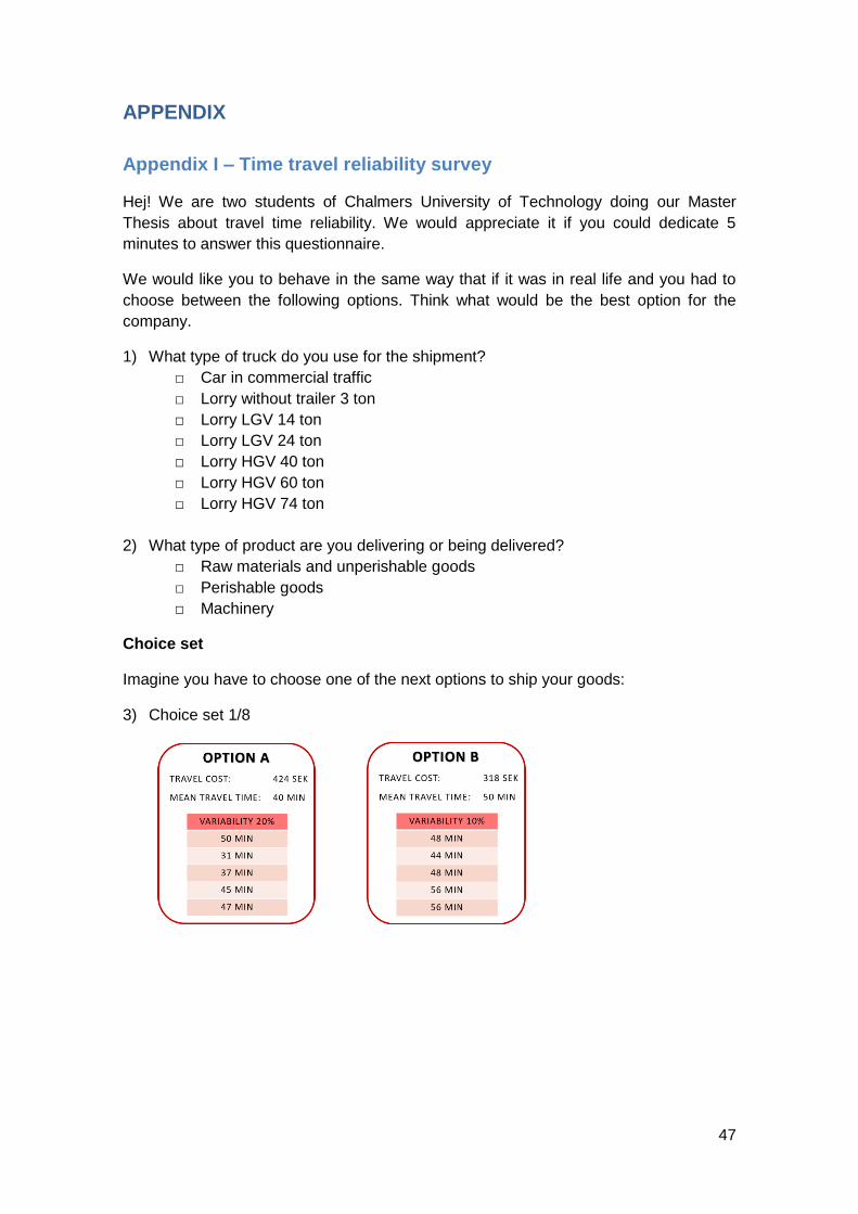
47

APPENDIX

Appendix I – Time travel reliability survey

Hej! We are two students of Chalmers University of Technology doing our Master

Thesis about travel time reliability. We would appreciate it if you could dedicate 5

minutes to answer this questionnaire.

We would like you to behave in the same way that if it was in real life and you had to

choose between the following options. Think what would be the best option for the

company.

1) What type of truck do you use for the shipment?

□ Car in commercial traffic

□ Lorry without trailer 3 ton

□ Lorry LGV 14 ton

□ Lorry LGV 24 ton

□ Lorry HGV 40 ton

□ Lorry HGV 60 ton

□ Lorry HGV 74 ton

2) What type of product are you delivering or being delivered?

□ Raw materials and unperishable goods

□ Perishable goods

□ Machinery

Choice set

Imagine you have to choose one of the next options to ship your goods:

3) Choice set 1/8

48

4) Choice set 2/8

5) Choice set 3/8

6) Choice set 4/8

7) Choice set 5/8

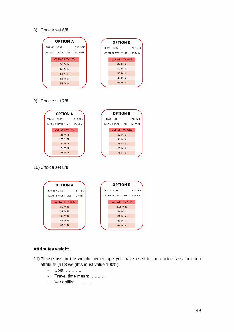
49

8) Choice set 6/8

9) Choice set 7/8

10) Choice set 8/8

Attributes weight

11) Please assign the weight percentage you have used in the choice sets for each

attribute (all 3 weights must value 100%).

- Cost: ………..

- Travel time mean: ………..

- Variability: ………..

50

Background

12) Which of the following concepts fits better with your idea of travel time reliability in

freight transport?

□ Percentage of on-time deliveries

□ Average time of delays

□ Range within the 98th (or 95th) percentile of arrival times

□ Standard deviation of arrival times distribution

13) What part of the supply chain are you involved in?

□ Shipper □ Carrier

□ Retailer □ Other: …….

14) What industry your business is in?

□ Automotive □ Commercial services

□ Food and beverages □ Textile

□ Building and construction □ Electronics

51

□ Manufacturing □ Pharmaceutical and healthcare

□ Transport and storage □ Other: …….

Thank you for your time!

52

Appendix II – Interview

Interview shipper

Travel time variability cause uncertainty in companies involved in the supply chain, generating

extra costs. Our thesis focus on understanding the concept of reliability and getting the value

of reliability for road freight transport. We need your help answering the following questions

to get the approach of the companies:

Introduction

1) Name: ……………………………………………………………………………………………………………………………….

Position in the company: …………………………………………………………………………………………………..

Years working for the company: ………………………………………………………………………………………..

2) Please tell us what industry your business is in by checking one box:

□ Automotive □ Building and construction

□ Commercial services □ Electronics

□ Food and beverage □ Manufacturing

□ Pharmaceutical and healthcare □ Textile

□ Transport and storage

□ Other. Please specify: …………………………….

3) Please list 3 top commodities that you typically ship with truck movements involved:

Commodity 1: ………………………………………………………………………………………………………………..

Commodity 2: ………………………………………………………………………………………………………………..

Commodity 3: ………………………………………………………………………………………………………………..

4) What is approximately the size of the shipments per customer?

□ 0 - 3 tons □ 3 - 14 tons □ 14 - 24 tons □ 24 - 40 tons □ +40 tons

5) Please indicate the geographies that you serve by checking the applicable boxes:

□ Serve urban locations □ Serve suburban locations

□ Truck movements involve border crossings □ Serve rural locations

6) Please indicate who is in charge of the transport:

□ Own transport fleet

□ Third party logistics

□ Postnord

□ Schenker

53

□ DHL

□ Other. Please specify: ………………………

7) How many shipments are leaving your distribution centre every day?

□ 1 - 5 □ 6 - 20 □ 21 - 50 □ + 50

8) Which of the following concepts fits better with your idea of travel time reliability in

freight transport? Please choose one option.

□ Percentage of on-time deliveries

□ Average time of delays

□ Range within the 98th (or 95th) percentile of arrival times

□ Travel time distribution and standard deviation

□ Other. Please specify: ……………

Deliveries information

1) Who is fixing time delivery requirements?

□ You as a shipper

□ Carrier

□ Receiver

1.1. How do you plan a journey’s departure time? 1.2. Is it part of the contract agreement with logistics services provider or is it an

informal agreement?

□ Yes □ No

2) How are time delivery requirements defined?

□ Consistent delivery between certain hours on a given day (e.g., 2-4 pm daily)

□ Consistent delivery within a stipulated delivery appointment

□ Consistent delivery on a specified day

□ Consistent delivery within a multi-day delivery window

□ Delivery requirements not specified

□ Other. Please specify ………………………

3) What percentage of delays does the company have?

□ 0 - 5% □ 6 - 10% □ 11 - 20% □ + 20%

54

4) Who is responsible for delays?

Carrier: %

Shipper: %

5) Do you stipulate penalties for missing the specified delivery requirements to your

transport company?

□ Yes □ No

6) Do your customers stipulate penalties for missing the specified delivery requirements?

□ Yes □ No

7) What measures does the company take to assure that deliveries arrive on time?

Project evaluation

1) Do you think it would be useful to get access to the bus lane in ring roads? What would be

the benefit?

2) How much would you be willing to pay for getting access to the bus lane in ring roads?

3) Do you see any inconveniences or do you propose any improvement?

Additional questions if shipper has own transport fleet

1) Considering that a journey is the route comprised since the truck leaves the distribution

centre until it arrives here again, what is the average travel distance of journeys?

□ 0 - 30 km □ 30 - 100 km □ 101 - 300 km □ + 300 km

2) Describe your company’s transport fleet:

2.1 Property:

□ Own □ Leased

2.2 Type of vehicles:

□ Light trucks □ Medium trucks □ Heavy trucks

3) How do you plan how long the journey will last?

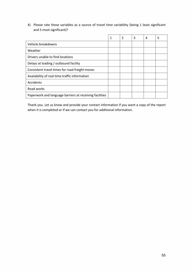
55

4) Please rate these variables as a source of travel time variability (being 1 least significant

and 5 most significant)?

1 2 3 4 5

Vehicle breakdowns

Weather

Drivers unable to find locations

Delays at loading / outbound facility

Consistent travel times for road freight moves

Availability of real-time traffic information

Accidents

Road works

Paperwork and language barriers at receiving facilities

Thank you. Let us know and provide your contact information if you want a copy of the report

when it is completed or if we can contact you for additional information.

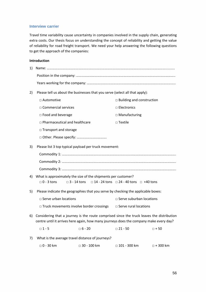
56

Interview carrier

Travel time variability cause uncertainty in companies involved in the supply chain, generating

extra costs. Our thesis focus on understanding the concept of reliability and getting the value

of reliability for road freight transport. We need your help answering the following questions

to get the approach of the companies:

Introduction

1) Name: ………………………………………………………………………………………………………………………..........

Position in the company: …………………………………………………………………………………………………..

Years working for the company: ………………………………………………………………………………………..

2) Please tell us about the businesses that you serve (select all that apply):

□ Automotive □ Building and construction

□ Commercial services □ Electronics

□ Food and beverage □ Manufacturing

□ Pharmaceutical and healthcare □ Textile

□ Transport and storage

□ Other. Please specify: …………………………….

3) Please list 3 top typical payload per truck movement:

Commodity 1: ………………………………………………………………………………………………………………….

Commodity 2: ………………………………………………………………………………………………………………….

Commodity 3: ………………………………………………………………………………………………………………….

4) What is approximately the size of the shipments per customer?

□ 0 - 3 tons □ 3 - 14 tons □ 14 - 24 tons □ 24 - 40 tons □ +40 tons

5) Please indicate the geographies that you serve by checking the applicable boxes:

□ Serve urban locations □ Serve suburban locations

□ Truck movements involve border crossings □ Serve rural locations

6) Considering that a journey is the route comprised since the truck leaves the distribution

centre until it arrives here again, how many journeys does the company make every day?

□ 1 - 5 □ 6 - 20 □ 21 - 50 □ + 50

7) What is the average travel distance of journeys?

□ 0 - 30 km □ 30 - 100 km □ 101 - 300 km □ + 300 km

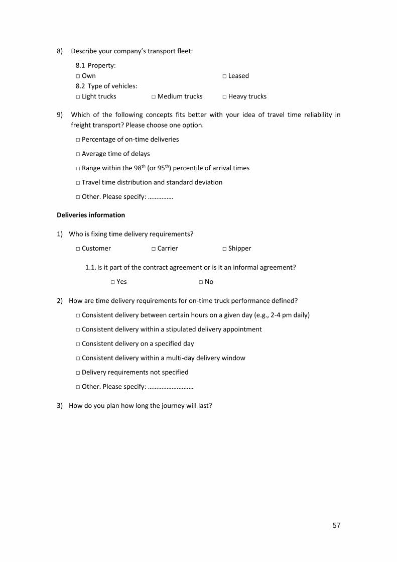
57

8) Describe your company’s transport fleet:

8.1 Property:

□ Own □ Leased

8.2 Type of vehicles:

□ Light trucks □ Medium trucks □ Heavy trucks

9) Which of the following concepts fits better with your idea of travel time reliability in

freight transport? Please choose one option.

□ Percentage of on-time deliveries

□ Average time of delays

□ Range within the 98th (or 95th) percentile of arrival times

□ Travel time distribution and standard deviation

□ Other. Please specify: ……………

Deliveries information

1) Who is fixing time delivery requirements?

□ Customer □ Carrier □ Shipper

1.1. Is it part of the contract agreement or is it an informal agreement?

□ Yes □ No

2) How are time delivery requirements for on-time truck performance defined?

□ Consistent delivery between certain hours on a given day (e.g., 2-4 pm daily)

□ Consistent delivery within a stipulated delivery appointment

□ Consistent delivery on a specified day

□ Consistent delivery within a multi-day delivery window

□ Delivery requirements not specified

□ Other. Please specify: ………………………

3) How do you plan how long the journey will last?

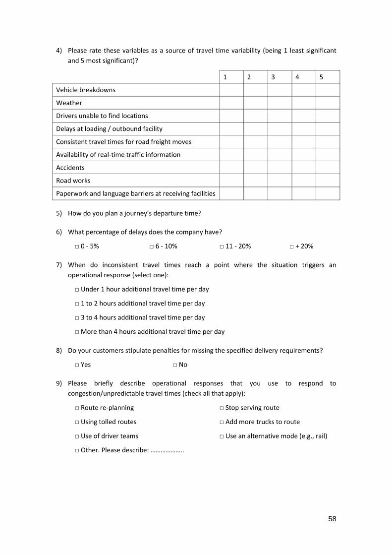
58

4) Please rate these variables as a source of travel time variability (being 1 least significant

and 5 most significant)?

1 2 3 4 5

Vehicle breakdowns

Weather

Drivers unable to find locations

Delays at loading / outbound facility

Consistent travel times for road freight moves

Availability of real-time traffic information

Accidents

Road works

Paperwork and language barriers at receiving facilities

5) How do you plan a journey’s departure time?

6) What percentage of delays does the company have?

□ 0 - 5% □ 6 - 10% □ 11 - 20% □ + 20%

7) When do inconsistent travel times reach a point where the situation triggers an

operational response (select one):

□ Under 1 hour additional travel time per day

□ 1 to 2 hours additional travel time per day

□ 3 to 4 hours additional travel time per day

□ More than 4 hours additional travel time per day

8) Do your customers stipulate penalties for missing the specified delivery requirements?

□ Yes □ No

9) Please briefly describe operational responses that you use to respond to

congestion/unpredictable travel times (check all that apply):

□ Route re-planning □ Stop serving route

□ Using tolled routes □ Add more trucks to route

□ Use of driver teams □ Use an alternative mode (e.g., rail)

□ Other. Please describe: ………………..

59

Project evaluation

1) Do you think it would be useful to get access to the bus lane in ring roads? What would be

the benefit?

2) How much would you be willing to pay for getting access to the bus lane in ring roads?

3) Do you see any inconveniences or do you propose any improvement?

Thank you. Let us know and provide your contact information if you want a copy of the report

when it is completed or if we can contact you for additional information.

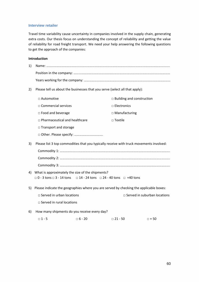
60

Interview retailer

Travel time variability cause uncertainty in companies involved in the supply chain, generating

extra costs. Our thesis focus on understanding the concept of reliability and getting the value

of reliability for road freight transport. We need your help answering the following questions

to get the approach of the companies:

Introduction

1) Name: ………………………………………………………………………………………………………………………..........

Position in the company: ……………………………………………………………………………………………………

Years working for the company: …………………………………………………………………………………………

2) Please tell us about the businesses that you serve (select all that apply):

□ Automotive □ Building and construction

□ Commercial services □ Electronics

□ Food and beverage □ Manufacturing

□ Pharmaceutical and healthcare □ Textile

□ Transport and storage

□ Other. Please specify: …………………………….

3) Please list 3 top commodities that you typically receive with truck movements involved:

Commodity 1: ………………………………………………………………………………………………………………….

Commodity 2: ………………………………………………………………………………………………………………….

Commodity 3: ………………………………………………………………………………………………………………….

4) What is approximately the size of the shipments?

□ 0 - 3 tons □ 3 - 14 tons □ 14 - 24 tons □ 24 - 40 tons □ +40 tons

5) Please indicate the geographies where you are served by checking the applicable boxes:

□ Served in urban locations □ Served in suburban locations

□ Served in rural locations

6) How many shipments do you receive every day?

□ 1 - 5 □ 6 - 20 □ 21 - 50 □ + 50

61

7) Which of the following concepts is it more important for you to consider a shipper/carrier

reliable?

□ Percentage of on-time deliveries

□ Average time of delays

□ Accurate tracking

□ Other. Please specify: ……………

Deliveries information

1) Who is fixing time delivery requirements?

□ You as a receiver □ Carrier □ Shipper

1.1. Is it part of the contract agreement with logistics services provider or is it an

informal agreement?

□ Yes □ No

2) How are time delivery requirements for on-time truck performance defined?

□ Consistent delivery between certain hours on a given day (e.g., 2-4 pm daily)

□ Consistent delivery within a stipulated delivery appointment

□ Consistent delivery on a specified day

□ Consistent delivery within a multi-day delivery window

□ Delivery requirements not specified

□ Other. Please specify: ………………………

3) What percentage of deliveries that you receive are delayed?

□ 0 - 5% □ 6 - 10% □ 11 - 20% □ + 20%

4) How a delay affects the company’s supply chain in short term?

5) How a delay affects the company’s supply chain in medium/long term?

□ Hire more workers

□ Decrease in level service

□ Difficulties to control inventory level

□ Others. Please specify: ……………

6) What short-term measures do you apply just in case there is a delayed delivery?

□ Safety stock

□ Safety margin in arrival times

□ Stipulate penalties to the carrier or shipper

□ Others. Please specify: ……………

62

7) What permanent measures do you apply just in case there are recurrent delayed

deliveries?

□ Stipulate higher penalties to the carrier or shipper

□ Ordering the goods earlier

□ Forecast the arrivals with a pattern

□ Safety stock planning

□ Safety margin in arrival times

□ Stop working with the shipper and find another one better

□ Stop working with the carrier and find another one better

□ Others. Please specify:…………………….

8) Do you stipulate penalties for missing the specified time delivery requirements?

□ Yes □ No

Project evaluation

1) Do you think it would be useful to get access to the bus lane in ring roads (for carriers)?

2) Would you be willing to pay for getting more reliability?

3) Do you see any inconveniences or do you propose any improvement?

Thank you. Let us know and provide your contact information if you want a copy of the report

when it is completed or if we can contact you for additional information.