Assessing the influence of prey-predator ratio, prey age structure and packs size on wolf kill rates

1

Assessing the influence of prey–predator ratio, prey age structure and packs size on wolf kill rates

Håkan Sand, John A. Vucetich, Barbara Zimmermann, Petter Wabakken, Camilla Wikenros, Hans C. Pedersen, Rolf O. Peterson and Olof Liberg

H. Sand ([email protected]), C. Wikenros and O. Liberg, Grimsö Wildlife Research Station, Dept of Ecology, Swedish Univ. of Agricultural Sciences, SE-73091 Riddarhyttan, Sweden. – J. A. Vucetich and R. O. Peterson, School of Forest Resources and Environmental Science, Michigan Technological Univ., Houghton, MI 49931, USA. – B. Zimmermann and P. Wabakken, Hedmark Univ. College, Faculty Applied Ecology and Agricultural Sciences, Evenstad, NO-2480 Koppang, Norway. – H. C. Pedersen, Norwegian Inst. for Nature Research, Tungasletta 2, NO-7485 Trondheim, Norway.

Traditional predation theory assumes that prey density is the primary determinant of kill rate. More recently, the ratio of prey-to-predator has been shown to be a better predictor of kill rate. However, the selective behavior of many predators also suggests that age structure of the prey population should be an important predictor of kill rate. We compared wolf– moose predation dynamics in two sites, south-central Scandinavia (SCA) and Isle Royale, Lake Superior, North America (IR), where prey density was similar, but where prey age structure and prey-to-predator ratio differed. Per capita kill rates of wolves preying on moose in SCA are three times greater than on IR. Because SCA and IR have similar prey densities differences in kill rate cannot be explained by prey density. Instead, differences in kill rate are explained by dif-ferences in the ratio of prey-to-predator, pack size and age structure of the prey populations. Although ratio-dependent functional responses was an important variable for explaining differences in kill rates between SCA and IR, kill rates tended to be higher when calves comprised a greater portion of wolves’ diet (p 0.05). Our study is the first to suggest how age structure of the prey population can affect kill rate for a mammalian predator. Differences in age structure of the SCA and IR prey populations are, in large part, the result of moose and forests being exploited in SCA, but not in IR. While predator conservation is largely motivated by restoring trophic cascades and other top–down influences, our results show how human enterprises can also alter predation through bottom–up processes.

Understanding predator–prey dynamics requires knowing what factors influence the per capita kill rate, often measured as kills/predator/unit time. The influence of prey density on kill rate has a long history of theoretical and empirical support (Holling 1966, Messier 1994). More recently, the ratio of prey-to-predator has been shown to be a better predictor of kill rate (Vucetich et al. 2002, Schenk et al. 2005). Nevertheless, there are still concerns, rooted in pre-dation theory, about using ratio as the primary predictor of kill rate (Abrams and Ginzburg 2000).

Other factors are also known to influence kill rate, such as predator group size (Creel 1997, Schmidt and Mech 1997, Vucetich et al. 2004) and winter severity (Post et al. 1999, Jedrzejewski et al. 2002). The predatory behavior of wolves Canis lupus also suggests that age structure of the prey population should be an important predictor of kill rate. Wolves are long known to be selective predators, preferring to kill calves over prime-aged ungulates (Peterson 1977, Smith et al. 2004, Wright et al. 2006). This preda-tory preference represents a strong a priori reason for think-ing that kill rates should be higher when calves are more

prevalent in a prey population. This preference likely indi-cates that calves are easier to kill than adults. A second, but related reason to expect kill rates to increase with the frequency of calves is that calves are smaller than adults, and wolves feeding primarily on calves may need more prey individuals to meet their energetic needs (Sand et al. 2008).

Another reason to understand whether prey age structure affects kill rate is that human enterprises, such as ungulate harvesting and forest management, can have an important impact on the age structure of ungulates on which wolves prey (Ginsberg and Milner-Guland 1994, Sæther et al. 2001, Milner et al. 2007). Despite the potentially important influence of age structure on predation dynamics, its effect has not to our knowledge ever been tested for a mammalian predator.

We compared wolf–moose (Alces alces) predation dynamics in two sites, south-central Scandinavia (SCA) and Isle Royale, Lake Superior, North America (IR), where prey density was similar, but where prey age structure and prey-to-predator ratio differed. Calves were much more prevalent in SCA as a result of intense harvest of moose

Oikos 000: 001–010, 2012doi: 10.1111/j.1600-0706.2012.20082.x

© 2012 The Authors. Oikos © 2012 Nordic Society Oikos Subject Editor: Stan Boutin. Accepted 24 January 2012

2

and forest management (Edenius et al. 2002, Lavsund et al. 2003). On IR, neither the moose nor the forest was exploited (Peterson 1977). Relatively recent re-colonization in SCA (Wabakken et al. 2001) also resulted in low popula-tion density of wolves and a much higher prey-to-predator ratio than the IR population.

Material and methods

Study sites

IR (48°00′N, 89°00′W) is an island (544 km2) in North America’s Lake Superior, covered by transition boreal forest (Abies balsamea, Picea glauca, Betula spp.). IR moose have never been harvested and its forests have not been logged since the early 20th century (Peterson 1977), although a severe forest fire burned approximately one third of IR in 1936, which today is very poor moose habitat (old spruce and birch forest). In recent decades, its forests have not produced abundant high quality forage (Krefting 1974). Since about 1950 the wolves and moose of IR have interacted essentially as an isolated single predator– prey system (Peterson et al. 1998). Wolves are moose’s only predator, moose comprise 90% of the biomass in wolf diet (Peterson et al. 1998), and the remainder is comprised of beaver Castor canadensis. These populations typically comprise 18–27 wolves (32–51/1000 km2) and 700–1100 moose (1.4–2.4 km22) (ranges are interquartile ranges, IQR) (Vucetich et al. 2002).

The SCA site (60°N, 12°E) is dominated by forests with mature stands dominated by Picea abies, Pinus silvestris, B. pubescens and B. pendula. Forest management is inten-sive with clear-cutting and old forest replaced by planting (Lavsund 1987) which increases the biomass of moose forage (Edenius et al. 2002, Lavsund 1987) and calf production (Cederlund and Markgren 1989). Early succes-sion after logging consists of preferred moose browsing spe-cies such as B. pendula, Sorbus aucuparia, Populus tremula and Salix spp. Annual moose harvest rates in SCA typically range between 25–30% of the pre-harvest population and comprise approximately equal portions of calves and adults (Lavsund et al. 2003).

Wolves began re-colonising SCA in the late 1970s (Wabakken et al. 2001). By 2010, this wolf population occupied ∼100 000 km2 and consisted of 250–290 indivi-duals distributed on 52 packs (Wabakken et al. 2010). Wolf territories in SCA are on average 1000 km2 (this study) and size of packs is on average 4–5 (including packs 2 wolves (Wabakken et al. 2010). This population’s winter diet in terms of biomass is 95% moose (Sand et al. 2005). The remaining diet is comprised of various smaller ungulates and other vertebrates, including roe deer Capreolus capreolus, wild reindeer Rangifer tarandus, beaver Castor fiber, badger Meles meles, capercaillie Tetrao urogallus, black grouse Tetrao tetrix and hares Lepus timidus, L. europaeus. Moose are not exposed to any other predators during the winter. Although SCA wolves have been legally protected, they have experienced high rates of human-caused mor-tality, mainly poaching and traffic-collisions (Liberg et al. 2011). Moose density during winter ranged between 0.8

and 3.4 moose km22 (median 1.35, IQR 0.97–1.48) among studied wolf territories which is typical of most moose populations found in south-central SCA (Lavsund et al. 2003). Moose from SCA and IR have similar body size, whereas SCA wolves are about 20% larger than IR wolves (Sand et al. 2006a).

Both IR and SCA are characterized by continental cli-mate, i.e. cold, snowy winters and warm summers. Inter-annual climatic variation has an important influence on the wolf–prey dynamics on IR (Vucetich and Peterson 2004) and likely an important influence in SCA (Wikenros et al. 2009).

Field methods

The data from IR span 40-years (1971–2010) and from SCA the data span 8-years (2001–2008) and include estimates of per capita kill rate during winter (i.e. kills per wolf per unit time and kg edible biomass available per wolf per day), wolf abundance, pack size, and density and age structure of the moose population. We also estimated the approximate size of winter territories from 100% minimum convex polygons. In SCA, the MCP:s were based on daily GPS-positions. On, IR the MCP:s were based daily observations of tracks in the snow during each winter field season, which was conducted each year from mid-January to early March. While this is a simple method of assessing territory size with important limitations, it is adequate for supporting the inferences that we make with these data (see also Shivik and Gese 2000). Although the methods associated with these data are described elsewhere (IR: Vucetich et al. 2002, SCA: Sand et al. 2005, Sand et al. 2006a, Wabakken et al. 2010), we briefly review these methods below.

Isle RoyaleWolf population size and pack sizes were counted annu-ally from a fixed-wing aircraft each January and February (Peterson et al. 1998). Confidence in the accuracy of these values was provided by the frequent visibility of entire wolf packs at a single location and time, and by making several complete counts during each winter survey. Moose abun-dance was estimated annually from 1997 to 2007 by aerial survey and a stratified design that involves counting moose on 91, 1-km2 plots from fixed-wing aircraft. From 1971 to 1996 moose abundance was estimated by a method of cohort analysis that is similar to that described by Solberg et al. (1999). Cohort analysis offers the opportunity to estimate the age structure of the population, in particular the proportion of the population that is calves each year.

Each January and February between 1971 and 2008, we observed the number of moose killed by wolves during a period of ∼44 days (median 44 d, IQR [38, 47 d]). Sites where moose had been killed were detected from fixed-wing aircraft by direct observation and by following pack tracks left in the snow (Peterson 1977). After wolves had finished feeding and left the site, we performed necropsies to determine the sex and age class (calf or adult) of each wolf-killed moose.

Several conditions reduce the risk of failing to detect a kill site. First, we searched for carcasses along the entire path of tracks that wolf packs leave in the snow. Consequently,

3

we are able to detect carcasses even if wolves kill a moose and abandon the site quickly. Second, packs typically spent 3–4 days consuming carcasses, giving us several opportuni-ties to detect it. Third, even after abandoning a site, packs typically return to that site later in the winter season, giving us an additional opportunity to detect it. Fourth, we regularly search areas that packs had visited several weeks previously. This allows us to detect carcasses from scaven-gers (lone wolves, foxes Vulpes vulpes, and eagles Haliaeetus leucocephalus) that often feed on carcasses for more than a week after a wolf pack has left.

ScandinaviaWolves were immobilized according to procedures pre-sented in Sand et al. (2006b). Wolves were equipped with GPS collars. During 2001–2008 we observed kill rates each winter (6 November to 24 April). From these obser-vations, we obtained 14 estimates of kill rate from ten different packs (we observed one pack for three win-ters and 2 packs for two winters). Study periods ranged from 33 to 132 days (median: 58 d, IQR [51, 63 d]) totaling 874 days. The use of GPS data and applications with GIS for searching, finding, and classifying killed prey followed methods described in Sand et al. (2005). Pack size was estimated from intensive monitoring of GPS- collared wolves on snow throughout the winter. Ten of the 14 estimates of kill rate were based on packs where both breeding adults were GPS collared, and the other four estimates involved packs with one of the breeding adults being GPS collared.

Estimating winter density of moose within all wolf territories studied was based on counts of new pellet groups (produced since leaf fall previous autumn) during spring (between snow melt and the onset of vegetation) (Neff 1968). Actual moose density for all territories was calculated from these pellet counts using daily defecation rate per moose as received from one study area (Grimsö) where population size from both aerial counts and the number of pellet groups were received for two separate years (14.4 (SE 0.71) in 2002 and 13.4 (SE 0.83) in 2006, Rönnegård et al. 2008). The number of moose (Nm) within wolf territories were estimated using the formula Nm p/d Nd where p was equal to the total num-ber of new pellet groups found, d was daily defecation rate, and Nd was the number of days during winter for which new pellet groups could be accumulated.

For 6 of our 14 estimates of kill rate, we also estimated the proportion of juveniles in the winter moose population by helicopter surveys, and for another five of the 14 cases, we relied on systematic observations made by hunters during the first seven days of the regular hunting season (Ericsson and Wallin 1999). Estimates of the proportion of juveniles were unavailable for 3 of the 14 cases.

Analytical methods

We first characterized differences between IR and SCA with respect to proportion of the population that are calves and social structure of the predator population (pack size). Specifically, we used t-tests to compare proportions of calf abundance and log-transformed pack sizes and territory sizes.

Kill rates were analyzed both in terms of kills/wolf/day and as kg consumable biomass/wolf/day. There are strong a priori reasons to think that kill rate is affected by moose density (Messier 1994, Hayes and Harestad 2000), moose- to-wolf ratio (Vucetich et al. 2002, Jost et al. 2005), pack size (Schmidt and Mech 1997, Thurber and Peterson 1993), and age structure of the prey population (Peterson et al. 1998). There is also a strong a priori expectation that kill rate is also influenced by a site effect. That is, kill rates in SCA may differ from IR for reason not explained by differences in moose density (ms), ratio of moose-to-wolves (ratio), pack size (pksz), or age structure, where age struc-ture was quantified as either the proportion of wolf diet comprised of calves (cfdiet), or proportion of prey popula-tion comprised of calves (cfpop). The next step of our analysis was intended only to provide a preliminary sense for whether the available data supported these a priori expec-tations, and whether or how the influence of each factor may differ between sites. To do this we, we constructed a several sets of models, where each set of models focused on only a single ecological factor (i.e. ms, ratio, pksz, cfdiet, cfpop). We also used the backward elimination procedure (with p 0.05 as a threshold) to build and compare sets of general linear mixed models (GLMM). Each set of models began with a full model comprised of one of these ecological factors, the site effect (IR or SCA, which we treated as a random effect), and an interaction term between the main effect and site effect (treated as a fixed effect). Random effects are often modeled to account for sources of variation that are not of ecological interest, but need to be taken into account due to study design. Alternatively, a random effect may, in some cases, be of ecological inter-est; and the goal of model selection can be evaluation of whether the random effect is important enough to include in a model. Here, the site effect (IR or SCA) is reasonably interpreted as random effect insomuch as these two sites are only two sites ‘randomly’ selected from many sites where wolves and moose interact. Moreover, site effect is a variable of great ecological interest. One aim of our analy-sis is to assess whether measured differences between study site (i.e. ms, ratio, pksz, cfdiet, cfpop) provide the best explana-tion of variation in kill rate, or whether IR and SCA differ in some unmeasured manner that can be accounted for, at least statistically, by including a term for site effect.

We used traditional measures of model performance (p-values, R2, and AIC) to assess whether the best- performing models did or did not include a term for a site effect. In particular, a statistically significant site effect would suggest that the intercept of the main predictor differed between the two sites, and a statistically sig-nificant interaction term would indicate that the slopes of the main predictor differed between the two sites. Because models based on kills/wolf/day and kg/wolf/day suffered from non-normal residuals, we assessed models based on log-transformed kill rate. The residuals of these mod-els had p-values 0.20 for Kolmogorov–Smirnov tests of normality.

Kill rate is expected to increase asymptotically with increasing moose density and ratio of moose-to-wolves (Vucetich et al. 2002). We log-transformed moose density and ratio of moose-to-wolves for models that focused on

4

differences between sites (i.e. a site effect). To perform this analysis, we built and compared two models that resulted from these two procedures: 1) a stepwise regression proce-dure where every main effect was included as a candidate variable, and 2) a stepwise procedure, where every main effect was included as a predictor, except site. These step-wise procedures used p 0.10 as the criterion for entry and p 0.11 for removal. While ratio and ms are expected (a priori) to have an asymptotic relationship with kill rate when ratio or ms is the only predictor of kill rate (Vucetich et al. 2002), this a priori expectation does not necessarily hold when ratio or ms is one of many predictors of kill rate. For this reason, we did not log-transform ratio or ms for this multivariate analysis. We also constructed several models that considered the influence of interactions among ecological variables included in the multivariate models (results not shown). None of those interaction terms

assessing those main effects because it is a parsimonious way to approximate an asymptotic relationship, given that we had log-transformed kill rates. If we had modeled the asymptotic relationship with a more traditional non-linear equation (e.g. kill rate ax/(b x), where x is the predic-tor and a and b are coefficients), then we would have been unable to compare these models to the others, because an AIC framework does not permit comparisons between models where only some of the response variables are log-transformed.

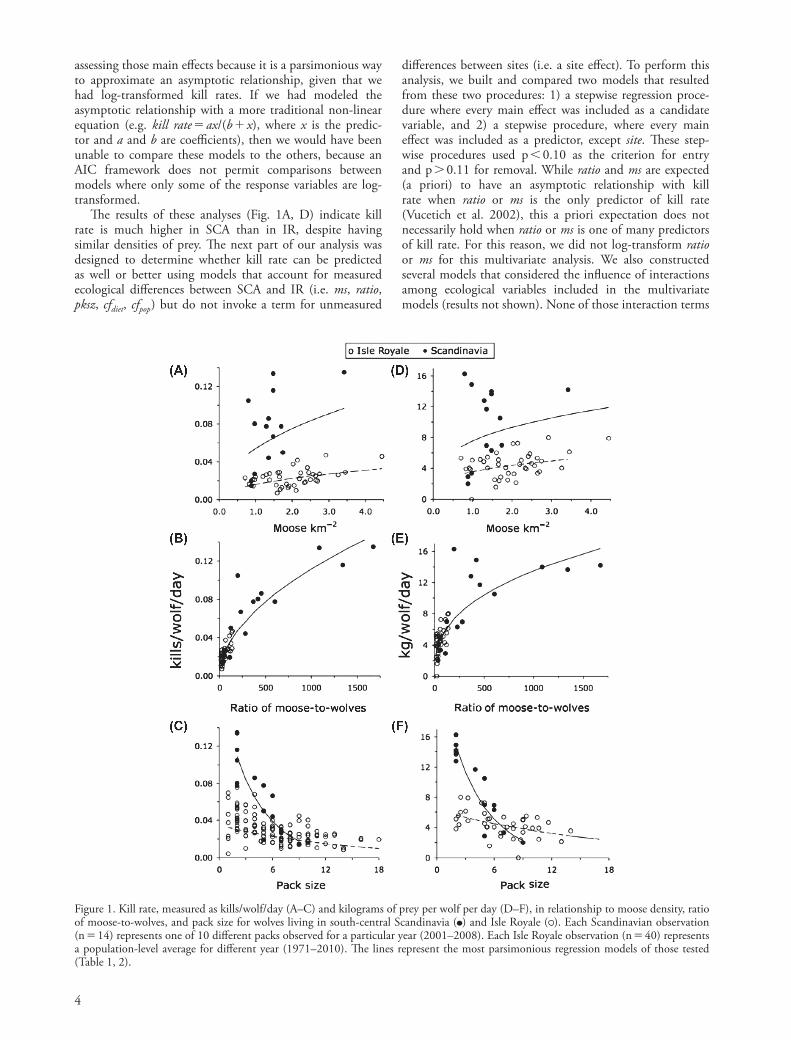
The results of these analyses (Fig. 1A, D) indicate kill rate is much higher in SCA than in IR, despite having similar densities of prey. The next part of our analysis was designed to determine whether kill rate can be predicted as well or better using models that account for measured ecological differences between SCA and IR (i.e. ms, ratio, pksz, cfdiet, cfpop) but do not invoke a term for unmeasured

Figure 1. Kill rate, measured as kills/wolf/day (A–C) and kilograms of prey per wolf per day (D–F), in relationship to moose density, ratio of moose-to-wolves, and pack size for wolves living in south-central Scandinavia ( ) and Isle Royale ( ). Each Scandinavian observation (n 14) represents one of 10 different packs observed for a particular year (2001–2008). Each Isle Royale observation (n 40) represents a population-level average for different year (1971–2010). The lines represent the most parsimonious regression models of those tested (Table 1, 2).

5

Kill rates: kills/wolf/day

Each ecological variable we assessed was a statistically significant predictor of kills/wolf/day (Fig. 1, 2, Table 1). Kills/wolf/day tended to increase with increasing moose density at both sites (p 1024, Fig. 1A). Moreover, the tendency for kills/wolf/day to be greater in SCA at similar moose densities was associated with SCA having a steeper slope (when presented on an untransformed scale, Fig. 1A) than IR (p 1024). Kills/wolf/day also tended to increase with increasing ratio of moose-to-wolves at both sites (p 1024, Fig. 1B). This relationship did not differ between sites, and it represented the most parsimonious of all the models that we constructed (dAICc 0, R2 0.80, Table 1).

Kills/wolf/day tended to decline with increasing pack size at both sites (p 1024, Fig. 1C). However, each site was characterized by its own intercept (p 1024) and slope (p 1024). Although kill rates are similar in SCA and IR for packs comprised of 5 to 9 wolves, the kill rates of small (2–4 wolves) packs in SCA are much greater than those observed from small packs in IR (Fig. 1C).

Kills/wolf/day had a slight tendency to increase with cfpop at each site (p 0.15) with each site characterized by its own intercept (p 0.01, Fig. 2A). The relationship between kills/wolf/day and cfdiet was similar to cfpop although statistically significant (p 0.01, Table 1, Fig. 2B).

The multivariate model that included each ecological factor plus the site effect as candidate predictor variable

were significant. Finally, none of the multivariate models suffered from high levels of multicollinearity (i.e. variance inflation factors were all 7 [Kutner et al. 2004]). All analyses were conducted in SPSS, ver. 11.

Results

Predator social structure

Mean pack sizes in SCA were 35% smaller than in IR (p 0.04, see x-axis of Fig. 1C). Specifically, the mean pack size was 4.1 (SE 0.61) for SCA and 6.3 for IR (SE 0.34). Mean territory sizes were also much larger for SCA than for IR (SCAave 960 km2 [SE 136]; IRave 306 km2

[SE 17], p 1024). An important consequence of differences in pack and territory size is that SCA tended to have a much higher ratio of moose-to-wolves (see x-axis in Fig. 1B; SCAave 499 [SE 136]; IRave 55 [SE 5.9], p 1024).

Age structure of prey population

The mean frequency of moose calves in the population (cfpop) was greater at SCA than IR (p 0.001, see x-axis of Fig. 2) and cfpop was unrelated to moose density at both sites (p 0.49). Specifically, the mean cfpop was 0.13 (SE 2.5 1022) for IR and 0.28 (SE 5.8 1023) for SCA.

Figure 2. Kill rate, measured as kills/wolf/day (A, B) and kilograms of prey/wolf/day (C, D), in relationship to the proportion of the moose population, and the proportion of wolves’ diet that are calves. Other details are as in the legend of Fig. 1.

6

to predicting ln(kills/wolf/day) as accurately and precisely as possible from the fewest number of predictor variables. Nevertheless, this model is ecologically unrealistic because there are such strong reasons to believe that kill rate is affected by many ecological processes.

Finally, there is occasion to explain why the model with only ratio had a slightly higher R2 (0.80) than the multivariate model that include ratio plus other variables (R2 0.75; Table 1). This small difference is due to having used ln(ratio) in one model, but ratio in the other model. However, the correlation between ratio and the residuals of the model based on ratio are not significant (p 1.0) and do not suggest the need to account for any non-linearity that might be accommodated by log-transformation.

Kill rates: kg/wolf/day

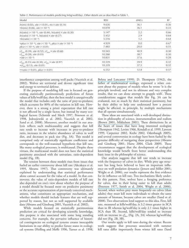
Results were similar for models where ln[kg/wolf/day] was the response variable (Table 2, Fig. 1D–F, 2C–D, 3B). However, the multivariate model that considered ecologi-cal factors and site effect as candidate variables suggests that only ratio and pksz explained significant portions of variation in ln[kg/wolf/day] (Fig. 3B).

Discussion

Traditional predation theory assumes that prey density is the primary determinant of kill rate (Holling 1966). Nevertheless, kill rates in Scandinavia (SCA) are 3.2 times greater, on average, than in Isle Royale (IR), despite both sites having similar prey densities (Fig. 1A, D). However, differences in the ratio of prey-to-predator between the sites can account for most of the differences in kill rate (Fig. 1B, E). Moreover, the model predicting kill rate from the ratio of prey-to-predator alone had the lowest AIC score of all the models we constructed. The behavioral mech-anism underlying this pattern is likely density-dependent

suggests that ratio (p 0.01), pksz (p 0.01), cfdiet (p 0.05), and site (p 0.02) were all important predic-tors of kill rate (R2 0.75; Fig. 3A). Moreover, the model resulting from a stepwise procedure that did not consider the site effect perform less well, with an R2 of 0.72 and an AICc score 3.5 points greater than the AICc score of the model that included site effect (see last two rows of Table 1).

Having considered these multivariate models, there is value in reconsidering the model that included only ln[ratio]. This model explained a similar amount of varia-tion in kill rate as the other two models we considered (i.e. R2 0.80, Table 1) and was, from a statistical perspec-tive, the most parsimonious (i.e. dAICc 0). This model is important to the extent that one’s concern is limited

Table 1. Performance of models predicting ln(kills/wolf/day). Models are based on data displayed in Fig. 1 anxd 2. The main effects are moose density (ms), ratio of moose to wolves (ratio), proportion of prey population comprised of calves (cfpop), proportion of diet comprised of calves (cfdiet), pack size (pksz), and site (Isle Royale or Scandinavia). Parenthetic values are p-values. RSS is the residual sum of squares, dAICc is the delta Aikiake’s information criterion, corrected for sample size, and R2 is the proportion of variation explained by the model. Dashed lines group models based on the same main effect, except for the set of models below the last dashed line. The rationale for examin-ing this last set of models is given in the ‘Analytical methods’. Models with an “*” are depicted in Fig. 1 and 2, those with a “**” in Fig. 3.

Model RSS dAICc R2

ln[ms] ( 0.01), site ( 1024), ms site (0.08) 10.197 45.0 0.57*ln[ms] ( 0.01), site ( 1024) 10.852 44.8 0.55

ln[ratio] ( 1024), site (0.44), ln[ratio] site (0.30) 4.651 2.8 0.81ln[ratio] ( 1024), ln[ratio] site (0.27) 4.708 1.0 0.80*ln[ratio] ( 1024) 4.827 0.0 0.80

pksz ( 1024), site ( 0.01), pksz site ( 0.01) 6.386 54.7 0.73*pksz ( 0.01), site ( 0.01) 8.419 52.3 0.65

cfpop (0.16), site (0.08), cfpop site (0.85) 12.164 52.2 0.49*cfpop (0.15), site ( 0.01) 12.173 19.9 0.49site ( 1024) 12.691 32.4 0.47

cfdiet ( 0.01) site (0.10), cfdiet site (0.74) 9.974 44.0 0.58*cfdiet ( 0.01), site ( 0.01) 9.996 41.6 0.58

ratio ( 1024), pksz ( 0.01), cfdiet ( 0.01) 6.634 21.9 0.72**ratio ( 0.01), pksz ( 0.01), cfdiet (0.05), site (0.02) 5.927 18.4 0.75

kills/wolf/day

0.24Ratio

0.20Pack size

0.14Calvesin diet

Site0.16

0.25Unexplained

0.30Ratio

0.27Pack size

0.43Unexplained

kg/wolf/day(A) (B)

Figure 3. Proportion of total variance in (A) kills/wolf/day and (B) kg/wolf/day observed in the Scandinavian and in the Isle Royale populations that is explained by the most parsimonious model that included multiple main effects, but no interaction terms (see Analytical Methods for rationale, Table 1, 2). Each proportion is the standardized partial regression coefficient for that predictor multiplied by the correlation coefficient between that predictor and the response variable, kills/wolf/day (Schumacker and Lomax 1996). The sum of the proportions associated with each factor is the total proportion of variance explained.

7

Belyea and Lancaster 1999). D. Thompson (1942), the father of mathematical ecology, expressed a relate con-cern about the purpose of models when he wrote ‘it is the principle involved, and not its ultimate and very complex results, that we can alone attempt to grapple with’. These considerations suggest that models like Fig. 3A can be evaluated, not so much by their statistical parsimony, but by their ability to help one understand how a process might be affected, in principle, by multiple mechanisms that all operate simultaneously.

These ideas are associated with a well-developed distinc-tion in philosophy of science, instrumentalism and realism (Brown 2001, Mikkelson 2001). These distinctions lie at the heart of issues that have long interested ecologists (Thompson 1942, Levins 1966, Kendall et al. 1999, Lawton 1999, Carpenter 2002, Krebs 2002, Odenbaugh 2005), and several controversies in ecology have been fueled by the genuine difficulty of navigating these perspectives (Abrams and Ginzburg 2001, Harte 2004, Clark 2009). These circumstances suggest that the development of ecological knowledge would benefit from better understanding this basic issue in the philosophy of science.

Our analysis suggests that kill rate tends to increase with the frequency of calves in diet. While prey age struc-ture has long been believed to have an important influ-ence on wolf predation dynamics (Jensen and Miller 2001, Wright et al. 2006), our results represent the first evidence for its influence on kill rate. Two mechanisms likely under-lie this pattern. First, wolves have a foraging preference for calves, due to their being easier to kill than adults (Peterson 1977, Smith et al. 2004, Wright et al. 2006). Second, when wolves prey more frequently on calves (than adults) they must kill more individuals to obtain the same amount of biomass, because calves are smaller (Sand et al. 2008). Two observations lend support to this idea. First, kill rate, measured as kills/wolf/day, is 3.2 times greater in SCA than in IR whereas kg/wolf/day is only 2.1 times higher in SCA than IR. Second, kills/wolf/day tended to increase with an increase in cfdiet (Fig. 2A, 3A) whereas kg/wolf/day did not (Fig. 2B, 3B).

Our results apply to kill rates during the winter. Recent work suggests that processes associated with summer kill rates differ importantly from winter kill rates (Sand

interference competition among wolf packs (Vucetich et al. 2002). Wolves are territorial and devote significant time and energy to territorial defense.

If the purpose of modeling kill rate is focused on gen-erating statistically parsimoniously predictions of future values of kills/wolf/day, then the best model is unequivocally the model that includes only the ratio of prey-to-predator, which accounts for 80% of the variation in kill rate. How-ever, there is a strong a priori expectation that kill rate is not affected by a single factor, but instead by many eco-logical factors (Schmidt and Mech 1997, Peterson et al. 1998, Jedrzejewski et al. 2002, Vucetich et al. 2002, Sand et al. 2008). Moreover, another model in our ana-lysis reflects such multicausality and suggests that kill rate tends to increase with increases in prey-to-predator ratio, increases in the relative abundance of calves in wolf diet, and decreases in pack size (Fig. 3A). This model is comprised only of statistically significant coefficients and corresponds to the well-reasoned hypothesis that kill rate, like many ecological processes, is multicausal. Despite these virtues, the multicausal model does not have the statistical parsimony associated with the univariate, ratio-dependent model (Fig. 1B).

The tension between these models rises from issues that fueled an earlier controversy about kill rate (Akcakaya et al. 1995, Abrams 1997). That controversy was ultimately explained by understanding that statistical performance alone cannot account for the value of a model. In that con-troversy, the value of ratio-dependent models of kill rate also depended on one’s view about whether the purpose of a model should be focused more on predictive parsimony or the accurate representation of previously conceived mech-anisms, what constitutes an appropriate mechanism, and whether models should include features that are well sup-ported by reason, but not so well supported by available data (Abrams and Ginzburg 2001, Vucetich et al. 2002).

While models focused on statistically parsimonious prediction are critical for developing scientific knowledge, this purpose is also associated with some long standing concerns. For example, the pervasive influence of histori-cal contingencies on ecological systems creates inescapable limitations in our ability to predict future states in ecologi-cal systems (Holling and Meffe 1996, Turner et al. 1998,

Table 2. Performance of models predicting ln(kg/wolf/day). Other details are as described in Table 1.

Model RSS dAICc R2

ln[ms] (0.02), site ( 0.01), ms site (0.14) 9.636 36.1 0.36*ln[ms] (0.06), site ( 1024) 10.078 36.1 0.33

ln[ratio] ( 1024), site (0.44), ln[ratio] site (0.30) 5.147 2.2 0.66ln[ratio] ( 1024), ln[ratio] site (0.27) 5.452 2.9 0.64*ln[ratio] ( 1024) 5.516 1.2 0.64

*pksz ( 1024), site ( 1024), pksz site ( 1024) 4.939 0.0 0.67pksz ( 1024), site ( 0.01) 7.483 20.0 0.51

cfpop (0.39), site (0.52), cfpop site (0.68) 10.543 40.9 0.30cfpop (0.28), site (0.03) 10.580 38.7 0.30*site ( 1024) 10.831 37.6 0.28

cfdiet (0.15) site (0.30), cfdiet site (0.97) 10.339 39.9 0.32*cfdiet (0.13), site (0.01) 10.339 37.5 0.32

**ratio ( 0.01), pksz ( 0.01) 6.552 12.8 0.57

8

1989). These human enterprises both ultimately affect age structure of the moose population including a higher fre-quency of calves in SCA, relative to IR.

Compared to many wolf–prey systems, IR and SCA likely represent opposite extremes with respect to the intensity of human exploitation. In most wolf–moose systems, the moose and forests are exploited more inten-sively than on IR and less intensively than in SCA. Consequently, there is reason to think that many wolf– prey systems are likely intermediate between IR and SCA with respect to prey age structure and kill rates. Because both forest management and human harvest of ungulates may affect the abundance and age structure of ungulate pop-ulations, this type of anthropogenic exploitation may also indirectly affect the rate at which predators kill individual prey and thus the dynamics of predator–prey populations. If kill rate is an important object of conservation concern, then our results indicate the importance of understanding how anthropogenic exploitation affects not only prey den-sity, but also the density and social structure of predator populations. Further, intense anthropogenic exploitation on all three trophic levels, as is the case in SCA, will likely also reduce the potential for predator-induced trophic cas-cades from occurring in such systems.

The motivation to restore and conserve wolves (and other large carnivores) is largely focused on valuing the ecological influence of predator–prey interaction, that are more-or-less naturally regulated (Sergio et al. 2008, Licht et al. 2010, Estes et al. 2011). If naturally-regulated predation is the object of conservation value, then bottom–up influences on predation, like those observed here, would also be of important to restore and conserve. If the motivation to conserve these aspects of predation seems tenuous, then there may be a need to justify more precisely the fundamental purpose and motivation of carnivore conservation. This would not be the first time that there is occasion to better understand more precisely what is object of conservation (Noss 1996, Leonard and Wayne 2008).

Acknowledgements – The two senior authors contributed equally to this paper. This work was supported in part by the US National Science Foundation (DEB-0918247), Isle Royale National Park, the Swedish Environmental Protection Agency, the Swedish Association for Hunting and Wildlife Management, World Wildlife Fund for Nature (Sweden), Swedish Univ. of Agricultural Sciences, the Directorate for Nature Management (Norway), Norwegian Research Council, Norwegian Inst. for Nature Research, Hedmark Univ. College, County Governors of Hedmark and Värmland, Borregaard Skoger, Glommen Skogeierforening, Norwegian Forestry Association, Norwegian Forest Owners Association, Olle and Signhild Engkvists Stiftelser, Carl Tryggers Stiftelse, Swedish Carnivore Association, and Stor-Elvdal, Åmot, Åsnes and Trysil municipalities. The views expressed here do not necessarily reflect those acknowledged here.

References

Abrams, P. 1997. Anomalous predictions of ratio-dependent models of predation. – Oikos 80: 163–171.

et al. 2008, Metz et al. 2011). Knowing which of these relationships apply to summer kill rates remains unknown.

Comparing data between studies collected with differ-ent methods may sometimes pose a risk that results may be biased due to the type of method used. It is possible that our results are spurious accident rising from the differ-ent methods used to estimate kill rate, wolf density, moose density, and prey age structure at the two sites being com-pared. However, we know of no specific reason to think that any of the methods used in this comparison differ in their tendency to over or under estimate. Moreover, the con-clusions presented here seem more a parsimonious than it would be to conclude that the results were merely a spurious accident.

Much of the difference in kill rate between IR and SCA seems to be explained by differences between these sites in frequency of calves in the diet, pack size, and prey-to-predator ratio. The greater prey-to-predator ratio in SCA is due to both smaller pack size and larger territory size. These patterns may be explained, in part, by SCA being a recently established and expanding population (Wabakken et al. 2001, 2010).

After accounting for these differences, kill rate is still greater in SCA than IR when kill rate measured as kills/wolf/day, but not as kg/wolf/day (Fig. 3). These differences may be attributable to factors affecting carcass utilization. SCA wolves may utilize calf carcasses less thoroughly than IR wolves (Sand et al. 2005, Vucetich et al. unpubl.). This difference may be attributable to SCA wolves’ reluctance to stay with their carcasses for long periods of time, due to the risk of being disturbed or poached. In addition, whereas Isle Royale moose are approximately equal in size to SCA moose, wolves are some 20% larger in SCA and are there-fore likely to require more kg biomass per day. Differences in carcass utilization, and in body size of wolves, may at least partly explain differences in kill rate between Isle Royale and Scandinavia and difference between kill rate models expressed in terms of kill/wolf/day and kg of prey/wolf/day (Fig. 3). Other differences between SCA and IR may also be important, but we are unaware of what they may be.

Kill rate was clearly associated with cfdiet (p 0.01), but only marginally associated with cfpop (p 0.15; Table 1). Lack of significance with cfpop may represent a type II sta-tistical error. Moreover, because cfdiet and cfpop are also highly correlated (p 1025), it is not surprising that only one of the two predictors appeared in the multivariate model (Fig. 3). Although the details cannot be resolved with the available data, it is difficult to imagine that kill rate would be associated with cfdiet without kill rate being in some way affected by the age structure of the prey population.

Intensive and selective human harvest of moose in SCA contributes to high rates of reproduction via structuring the population towards a high proportion of productive females (Sæther et al. 2001, Solberg et al. 2000, Nilsen and Solberg 2006) and restricts opportunities for density-dependent food limitation (Lavsund et al. 2003). Intensive forest management in SCA results in an increased produc-tion of moose forage (Edenius et al. 2002) which in turn increases rates of calf production (Cederlund and Markgren

9

Levins, R. 1966. The strategy of model building in population biology. – Am. Sci. 54: 421–431.

Liberg, O. et al. 2011. Shoot, shovel and shut up: cryptic poaching slows restoration of a large carnivore in Europe. – Proc. R. Soc. B doi: 10.1098/rspb.2011.1275.

Licht, D. S. et al. 2010. Using small populations of wolves for eco-system restoration and stewardship. – Bioscience 60: 147–153.

Messier, F. 1994. Ungulate population models with predation: a case study with the North American moose. – Ecology 75: 478–488.

Metz, M. C. et al. 2011. Effect of sociality and season on gray wolf (Canis lupus) foraging behavior: implications for esti-mating summer kill rate. – PLoS One 6(3): e17332.

Mikkelson, G. M. 2001. Complexity and verisimilitude: realism for ecology. – Biol. Philos. 16: 533–546.

Milner, J. M. et al. 2007. Demographic side effects of selective hunting in ungulates and carnivores. – Conserv. Biol. 21: 36–47.

Neff, D. J. 1968. The pellet-group count technique for big game trend, census, and distribution: a review. – J. Wildlife Manage. 32: 597–614.

Nilsen, E. B. and Solberg, E. J. 2006. Patterns of hunting mortal-ity in Norwegian moose (Alces alces) populations. – Eur. J. Wildlife Res. 52: 153–163.

Noss, R. F. 1996. Ecosystems as conservation targets. – Trends Ecol. Evol. 11: 351.

Odenbaugh, J. 2005. The structure of population ecology: philo-sophical reflections on unstructured and structured models. – In: Cuddington, K. and Beisner, B. (eds), Ecological para-digms lost: routes to theory change. Academic Press, pp. 63–77.

Peterson, R. O. 1977. Wolf ecology and prey relationships on Isle Royale. – US Natl Park Serv. Sci. Monogr. Ser. 11: 1–210.

Peterson, R. O. et al. 1998. Population limitation and the wolves of Isle Royale. – J. Mammal. 79: 487–841.

Post, E. et al. 1999. Ecosystem consequences of wolf behavioural response to climate. – Nature 401: 905–907.

Rönnegård, L. et al. 2008. Evaluation of four methods used to estimate population density of moose (Alces alces). – Wildlife Biol. 14: 358–371.

Sæther, B.-E. et al. 2001. Optimal harvest of age–structured populations of moose Alces alces in a fluctuating environment. – Wildlife Biol. 7: 171–179.

Sand, H. et al. 2005. Using GPS technology and GIS-cluster analyses to estimate kill rates in wolf–ungulate ecosystems. – Wildlife Soc. Bull. 33: 914–925.

Sand, H. et al. 2006a. Cross–continental differences in patterns of predation: will naive moose in Scandinavian ever learn? – Proc. R. Soc. B 273: 1–7.

Sand, H. et al. 2006b. Effects of hunting group size, snow depth and age on the success of wolves hunting moose. – Anim. Behav. 72: 781–789.

Sand, H. et al. 2008. Summer kill rates and predation pattern in a wolf–moose system: can we rely on winter estimates? – Oecologia 156: 53–64.

Schenk, D. et al. 2005. An experimental test of the nature of predation: neither prey- nor ratio-dependent. – J. Anim. Ecol. 74: 86–91.

Schmidt, P. A. and Mech, L. D. 1997. Wolf pack size and food acquisition. – Am. Nat. 150: 513–517.

Schumacker, R. E. and Lomax, R. G. 1996. A beginner’s guide to structural equation modeling. – Lawrence Erlbaum Associates, Mahwah, New Jersey, USA.

Sergio, F. et al. 2008. Top predators as conservation tools: ecological rationale, assumptions and efficacy. – Annu. Rev. Ecol. Evol. Syst. 39: 1–19.

Shivik, J. A. and Gese, E. M. 2000. Territorial significance of home range estimators for coyotes. – Wildlife Soc. Bull. 28: 940–946.

Abrams, P. A. and Ginzburg, L. R. 2000. The nature of predation: prey dependent, ratio dependent or neither? – Trends Ecol. Evol. 15: 337–341.

Akcakaya, H. R. et al. 1995. Ratio-dependent predation – an abstraction that works. – Ecology 76: 995–1004.

Belyea, L. R. and Lancaster, J. 1999. Assembly rules within a contingent ecology. – Oikos 86: 402–416.

Brown, J. R. 2001. Who rules in science. – Harvard Univ. Press.Carpenter, S. R. 2002. Ecological futures:building an ecology of

the long now. – Ecology 83: 2069–2083.Cederlund, G. and Markgren, G. 1989. The development of the

Swedish moose population 1970–1983. – Swe. Wildlife Res. Suppl. 1: 55–62.

Clark, J. S. 2009. Beyond neutral science. – Trends Ecol. Evol. 24: 8–15.

Creel, S. 1997. Cooperative hunting and group size: assumptions and currencies. – Anim. Behav. 54: 1319–1324.

Edenius, L. et al. 2002. The role of moose as a disturbance factor in managed boreal forests. – Silva Fenn. 36: 57–67.

Ericsson, G. and Wallin, K. 1999. Hunter observations as an index of moose Alces alces population parameters. – Wildlife Biol. 5: 177–185.

Estes, J. A. et al. 2011. Trophic downgrading of Planet Earth. – Science 333: 301–306.

Ginsberg, J. R. and Milner-Guland, E. J. 1994. Sex-biased harvesting and population dynamics in ungulates – implica-tions for conservation and sustainable use. – Conserv. Biol. 8: 157–166.

Harte, J. 2004. The value of null theories in ecology. – Ecology 85: 1792–1794.

Hayes, R. D. and Harestad, A. S. 2000. Wolf functional response and regulation of moose in the Yukon. – Can. J. Zool. 78: 60–66.

Holling, C. S. 1966. The functional response of invertebrate predators to prey density. Memo. – Entomol. Soc. Can. 48: 1–60.

Holling, C. S. and Meffe, G. K. 1996. Command and control and the pathology of natural resource management. – Conserv. Biol. 10: 328–337.

Jedrzejewski, W. et al. 2002. Kill rates and predation by wolves on ungulate populations in Bialowieza primeval forest (Poland). – Ecology 83: 1341–1356.

Jensen, A. L. and Miller, D. H. 2001. Age structured matrix predation model for the dynamics of wolf and deer popula-tions. – Ecol. Modell. 141: 299–305.

Jost, C. et al. 2005. The wolves of Isle Royale display scale- invariant satiation and ratio-dependent predation on moose. – J. Anim. Ecol. 74: 809–816.

Kendall, B. E. et al. 1999. Why do populations cycle? A synthesis of statistical and mechanistic modeling approahces. – Ecology 80: 1789–1805.

Krebs, C. J. 2002. Two complementary paradigms for analyzing population dynamics. – Phil. Trans. R. Soc. Lond. 357: 1211–1219.

Krefting, L. W. 1974. The ecology of Isle Royale moose with special reference to the habitat. – Agric. Exp. Stn, Tech. Bull. 297, Univ. of Minnesota Press.

Kutner, M. H. et al. 2004. Applied linear regression models, 4th ed. – McGraw-Hill.

Lavsund, S. 1987. Moose relationships to forestry in Finland, Norway and Sweden. – Swe. Wildlife Res. Suppl. 1: 229–246.

Lavsund, S. et al. 2003. Status of moose populations and chal-lenges to moose management in Fennoscandia. – Alces 39: 109–130.

Lawton, J. H. 1999. Are there general laws in ecology? – Oikos 84: 177–192.

Leonard, J. A. and Wayne, R. K. 2008. Native Great Lakes wolves were not restored. – Biol. Lett. 4: 95–98.

10

(Alces alces) population of Isle Royale. – Proc. R. Soc. B 271: 183–189.

Vucetich, J. A. et al. 2002. The effect of prey and predator densities on wolf predation. – Ecology 83: 3003–3013.

Vucetich, J. A. et al. 2004. Raven scavenging favors group foraging in wolves. – Anim. Behav. 67: 1117–1126.

Wabakken, P. et al. 2001. The recovery, distribution, and popula-tion dynamics of wolves on the Scandinavian peninsula, 1978–1998. – Can. J. Zool. 79: 710–725.

Wabakken, P. et al. 2010. The wolf in Scandinavia: status report of the 2009–2010 winter (in Norwegian with English summary). Rep. no. 4 – 2010, Høgskolen i Hedmark, Norway.

Wikenros, C. et al. 2009. Wolf predation on moose and roe deer: chase distances and outcome of encounters. – Acta Theriol. 54: 207–218.

Wright, G. J. et al. 2006. Selection of northern Yellowstone elk by gray wolves and hunters. – J. Wildlife Manage. 70: 1070–1078.

Smith, D. W. et al. 2004. Winter prey selection and estimation of wolf kill rates in Yellowstone National Park, 1995–2000. – J. Wildlife Manage. 68: 153–166.

Solberg, E. J. et al. 1999. Dynamics of a harvested moose popula-tion in a variable environment. – J. Anim. Ecol. 68: 186–204.

Solberg, E. J. et al. 2000. Age-specific harvest mortality in a Norwegian moose Alces alces population. – Wildlife Biol. 6: 41–52.

Thompson, D. W. 1942. On growth and form. Reprinted in 1992 by Dover.

Thurber, J. M. and Peterson, R. O. 1993. Effects of population density and pack size on the foraging ecology of gray wolves. – J. Mammal. 74: 879–889.

Turner, M. G. et al. 1998. Factors influencing succession: lessons from large, infrequent natural disturbances. – Ecosystems 1: 511.

Vucetich, J. A. and Peterson, R. O. 2004. The influence of top–down, bottom–up and abiotic factors on the moose