Assessing the Impact of Potential New Carbon Regulations in the United States Institute for 21st Century Energy • U.S. Chamber of Commerce www.energyxxi.org

Assessing the Impact of Potential New Carbon Regulations in the United States
Dec 12, 2015
Assessing the Impact of
Potential New Carbon
Regulations in the United States
Institute for 21st Century Energy • U.S. Chamber of Commerce
The analysis in this report is based on a detailed
existing power plant regulatory proposal by the
Natural Resources Defense Council (NRDC), and the
Obama Administration’s announced greenhouse gas
reduction goals. The NRDC proposal was utilized
for this effort due to the widespread view that it
incorporates many of the features that are likely to be
adopted by the EPA in its regulatory regime applicable
to existing power plants. While the analysis found
that NRDC’s proposed structure could not actually
achieve the Administration’s carbon reduction goal,
it nevertheless reflects a framework for achieving
greenhouse gas reductions that would be necessary
if the Administration intends to pursue its stated
emissions goal.
www.energyxxi.org
Welcome message from author
This document is posted to help you gain knowledge. Please leave a comment to let me know what you think about it! Share it to your friends and learn new things together.
Transcript

Assessing the Impact of Potential New Carbon
Regulations in the United States
Institute for 21st Century Energy • U.S. Chamber of Commerce
www.energyxxi.org

OUR MISSIONThe mission of the U.S. Chamber of Commerce’s Institute for 21st Century Energy is to unify policymakers, regulators,
business leaders, and the American public behind a common sense energy strategy to help keep America secure,
prosperous, and clean. Through policy development, education, and advocacy, the Institute is building support for
meaningful action at the local, state, national, and international levels.
The U.S. Chamber of Commerce is the world’s largest business federation representing the interests of more than
3 million businesses of all sizes, sectors, and regions, as well as state and local chambers and industry associations.
At the request of the Institute for 21st Century Energy, IHS conducted modeling and analysis of the impact of
power-sector carbon regulations on the power industry and the U.S. economy. The Institute for 21st Century Energy
provided assumptions about carbon regulations and policies. IHS experts analyzed the impact of carbon regulations
and policies using IHS proprietary models of the power system and the macro economy. The conclusions in this
report are those of the Institute for 21st Century Energy.
Copyright © 2014 by the United States Chamber of Commerce. All rights reserved. No part of this publication may be reproduced or transmitted
in any form—print, electronic, or otherwise—without the express written permission of the publisher.

Assessing the Impact of Potential New Carbon
Regulations in the United States

22
Assessing the Impact of Potential New Carbon Dioxide Regulations in the United States
Executive Summary
The U.S. power sector is undergoing a period of tremendous uncertainty, driven in large part by an unprecedented avalanche of new and anticipated regulations coming from the Environmental Protection Agency (EPA) covering everything from traditional air pollutants to carbon dioxide (CO2). This report focuses on the economic impacts of just one aspect of the EPA’s regulatory juggernaut: forthcoming EPA rules covering CO2 emissions from fossil fuel-fired electricity generating plants under the Clean Air Act (CAA). These rules threaten to suppress average annual U.S. Gross Domestic Product (GDP) by $51 billion and lead to an average of 224,000 fewer U.S. jobs every year through 2030, relative to baseline economic forecasts.
These new rules are a central part of President Obama’s June 2013 Climate Action Plan, a major initiative to cut U.S. greenhouse gas (GHG) emissions and “lead international efforts to address global climate change.” In compliance with this plan, the EPA announced in September 2013 its New Source Performance Standard (NSPS) rule applicable to the construction of new fossil-fueled power plants. The President also instructed the EPA to ready proposed rules for existing power plants by June 2014 and finalize them within a year. While the exact form the existing plant rule might take has been subject to a great deal of speculation, it is generally expected that it will be of unprecedented magnitude, reach, and complexity.
Fossil fuel-fired power stations comprise almost 75% of the generating capacity and nearly 66% of the electricity generated in the United States. Accordingly, it is critical that the regulatory decision-making process be informed by realistic and robust analysis of the costs, benefits, and practical implications of any proposed actions on such a critical segment of the economy.
The U.S. Chamber of Commerce’s Institute for 21st Century Energy (the “Energy Institute”) represents the businesses and consumers that could be impacted by new EPA rules. Our perspective is unique, because our membership spans the entire spectrum of the U.S. economy. As such, we set out to develop a robust and comprehensive analysis of the potential economic impacts of the Administration’s efforts. We undertook this effort in order to develop a better understanding of the true impacts of EPA’s forthcoming proposal so that we can have a national debate based on facts and analysis, rather than emotion and conjecture.
The Energy Institute commissioned IHS Energy and IHS Economics (collectively, “IHS”), to examine and quantify the expected impacts of forthcoming power plant rules on the electricity sector and the economy as a whole, based on policy scenarios provided by the Energy Institute which are explained in detail herein. The conclusions drawn from this analysis are those of the Energy Institute.
The analysis in this report is based on a detailed existing power plant regulatory proposal by the Natural Resources Defense Council (NRDC), and the Obama Administration’s announced greenhouse gas reduction goals. The NRDC proposal was utilized for this effort due to the widespread view that it incorporates many of the features that are likely to be adopted by the EPA in its regulatory regime applicable to existing power plants. While the analysis found that NRDC’s proposed structure could not actually achieve the Administration’s carbon reduction goal, it nevertheless reflects a framework for achieving greenhouse gas reductions that would be necessary if the Administration intends to pursue its stated emissions goal.

Assessing the Impact of Potential New Carbon Regulations in the United States
3
This analysis uses two power sector simulation cases: (1) a Reference Case with no additional federal regulations targeting U.S. power plant CO2 emissions; and (2) a Policy Case with federal standards covering both new and existing fossil fuel-fired power plants. The results of these simulations were analyzed to assess their impacts on key U.S. and regional macroeconomic indicators. The Policy Case developed by the Energy Institute marries the NRDC’s framework with the Obama Administration’s stated goals of an economy-wide reduction in gross U.S. GHG emissions of 42% below the 2005 level by 2030 (as stated in the Administration’s 2010 submission to the UN Framework Convention on Climate Change associating the U.S. with the Copenhagen Accord).
The Policy Case developed by the Energy Institute marries the NRDC’s framework with the Obama Administration’s stated goals of an economy-wide reduction in gross U.S. GHG emissions of 42% below the 2005 level by 2030.
In order to approach achievement of the Administration’s aggressive goal, it was necessary to assume that carbon capture and sequestration (CCS) for new natural gas plants will be required beginning in 2022. IHS notes that adding CCS to natural gas-fired power plants can more than double their construction costs and increases their total production cost by about 60%. IHS also emphasizes that the prospects for the technological and financial viability of CCS remain highly uncertain. The Obama Administration reached a similar conclusion in its recently released National Climate Assessment, noting that CCS is “still in early phases of development.”1
1 http://nca2014.globalchange.gov/
Power sector changes and costs of compliance
EPA regulation of CO2 from existing power plants would result in extensive and very rapid changes in the structure of the power sector. Energy efficiency mandates and incentives in the Policy Case would be expected to lower U.S. power demand growth from 2013 through 2030 to 1.2% per year, or about 0.2% lower compared with the Reference Case.
Not unexpectedly, baseload coal plant retirements would jump sharply in the Policy Case, with an additional 114 gigawatts—about 40% of existing capacity—being shut down by 2030 compared with the Reference Case. The new capacity built to replace retiring coal and to meet remaining power demand growth is dominated by natural gas and renewables. However, with the implementation of tighter NSPS standards beginning in 2022 – which becomes necessary to approach the Administration’s 2030 climate objectives – the new build mix shifts to a blend of combined cycle gas turbines (CCGT) with CCS, renewables, and a modest amount of nuclear capacity later in the analysis period. These changes mean coal’s share of total electricity generation decreases from 40% in 2013 to 14% in 2030, while natural gas’s share increases from 27% to 46%.
EPA regulation of CO2 from existing power plants would result in extensive and very rapid changes in the structure of the power sector.
As a result, annual power sector CO2 emissions decline to about 1,434 million metric tons CO2, resulting in an emissions reduction of about 970 million metric tons, or about 40% below the 2005 level by 2030. Even these dramatic changes fall short of the 42% emissions reduction goal in the Policy Case. To put this in perspective, the International Energy Agency estimates
4
that over the 2011-30 forecast period, the rest of the world will increase its power sector CO2 emissions by nearly 4,700 million metric tons (MMT), or 44%. Those non-U.S. global emissions increases are more than six times larger than the U.S. reductions achieved in the Policy Case from 2014-30.2 Considered in light of the challenges and costs associated with approaching 42% power sector CO2 reductions, this international context should be instructive as the U.S. seeks to negotiate a post-2020 emissions reduction agreement.
By accelerating the premature retirement of coal plants, the CO2 regulations included in the Policy Case force a significant increase in the unproductive deployment of capital by driving the noneconomic retirement of coal-fired generation facilities. Costs also are increased by a need to deploy nearly carbon-free new generation beginning in 2022—CCGT with CCS and nuclear—to approach a 42% emissions reduction goal in the power sector. When the costs for new incremental generating capacity, necessary infrastructure (transmission lines and natural gas and CO2 pipelines), decommissioning, stranded asset costs, and offsetting savings from lower fuel use and
2 International Energy Agency data from 2013 World Energy Outlook; 2014-2030 Policy Case emissions reductions versus the Reference Case equal to 750 million metric tons CO
2.
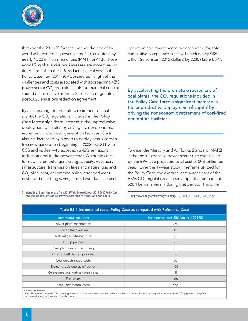
operation and maintenance are accounted for, total cumulative compliance costs will reach nearly $480 billion (in constant 2012 dollars) by 2030 (Table ES-1).
By accelerating the premature retirement of coal plants, the CO2 regulations included in the Policy Case force a significant increase in the unproductive deployment of capital by driving the noneconomic retirement of coal-fired generation facilities.
To date, the Mercury and Air Toxics Standard (MATS) is the most expensive power sector rule ever issued by the EPA, at a projected total cost of $9.6 billion per year.3 Over the 17-year study timeframe utilized for the Policy Case, the average compliance cost of the EPA’s CO2 regulations is nearly triple that amount, at $28.1 billion annually during that period. Thus, the
3 http://www.epa.gov/ocir/hearings/testimony/112_2011_2012/2012_0208_rm.pdf
Table ES-1 Incremental costs: Policy Case as compared with Reference Case
Incremental cost item Incremental cost ($billion, real 2012$)
Power plant construction 339
Electric transmission 16
Natural gas infrastructure 23
CCS pipelines 25
Coal plant decommissioning 8
Coal unit efficiency upgrades 3
Coal unit stranded costs 30
Demand-side energy efficiency 106
Operations and maintenance costs -5
Fuel costs -66
Total incremental costs 478
Source: IHS EnergyNote: Please see Appendix C for power generation addition unit costs and more detail on the calculation of natural gas pipelines, transmission, CCS pipelines, coal plant decommissioning, and coal unit stranded assets.

Assessing the Impact of Potential New Carbon Regulations in the United States
5
GHG regulations analyzed in the Policy Case would dwarf the most expensive EPA power sector regulation on the books.
The impacts will be felt differently in different regions of the country. In order to comply with the Policy Case, the analysis finds that the South and the Midcontinent Independent System Operator (MISO) power regions, on average, will incur over half the U.S. total costs during the 2014-30 timeframe. The regional economic impact analysis confirms that the U.S. Census Divisions that depend on the South and MISO power regions (South Atlantic, East North Central, East South Central, West North Central, West South Central) will shoulder more of the economic consequences of compliance. However, it must be noted that the West (Non-California) power region will need to spend almost as much as MISO to achieve compliance. Within the Pacific Census Region, the blending of cost impacts from West (Non-California) and California (which requires lower additional compliance costs) results in overall lower numbers in the Policy Case.
Electricity expenditures
Consumers can be expected to pay much more for electricity during the 2014-2030 Policy Case analysis period. EPA CO2 regulations will accelerate the already swift retirement of coal plants, currently underway
because of the EPA’s MATS rule and other regulations, combined with competition from natural gas. A visible byproduct of this shift will be higher electricity prices, as costs for compliance and system reconfiguration are passed through to consumers. Higher electricity prices ripple through the economy and reduce discretionary income, which affects consumer behavior, forcing them to delay or forego some purchases or lower their household savings rates.
Overall, the Policy Case will cause U.S. consumers to pay nearly $290 billion more for electricity between 2014 and 2030.
Table ES-2 shows the expected cumulative increases in retail electricity expenditures over three time periods and average annual increases in expenditures for different regions of the country. Overall, the Policy Case will cause U.S. consumers to pay nearly $290 billion more for electricity between 2014 and 2030, or an average of $17 billion more per year.
Table ES-2: Cumulative Changes in Electricity Expenditures, 2014-30 (Billions of Real 2012 Dollars)
Region 2014-2020 2014-2025 2014-2030 2014-2030 Annual Average Increase
West 4.9 17.5 46.9 2.8
California 0.6 1.3 2.2 0.1
RGGI 2.8 6.3 10.1 0.6
ERCOT 1.7 8.3 23.6 1.4
MISO 11.8 30.8 56.8 3.3
PJM 0.9 1.1 10.2 0.6
South 5.3 36.9 111.4 6.6
SPP 4.8 14.7 27.9 1.6
US 32.8 117.0 289.1 17.0
6
While consumers in all regions of the country will be paying more under the Policy Case, some areas will see larger increases than others, ranging anywhere from $2 billion to over $111 billion. Those regions that incur higher compliance costs will tend to see greater electricity expenditure increases and experience greater declines in real disposable income per household. Consumers in the South will pay much more on average annually ($6.6 billion) and in total ($111 billion) than any other area of the country. MISO ($57 billion) and the West ($47 billion) also show very large increases. Together, these three areas account for three-quarters of the U.S. total.
While the Policy Case has a very small impact in California, whose existing cap-and-trade program is included in the Reference Case, it and the Northeast are expected to continue to have the highest electricity prices in the continental U.S.
U.S. economy results and implications
The overarching objective of the economic impact analysis conducted for this study was to quantify the impacts, both on U.S. national and regional economies, of aiming for the Policy Case’s reduction in power sector CO2 emissions by 2030. These higher electricity prices will absorb more of the disposable income that households draw from to pay essential
expenses such as mortgages, food and utilities. In turn, this will lead to moderately less discretionary spending and lower consumer savings rates.
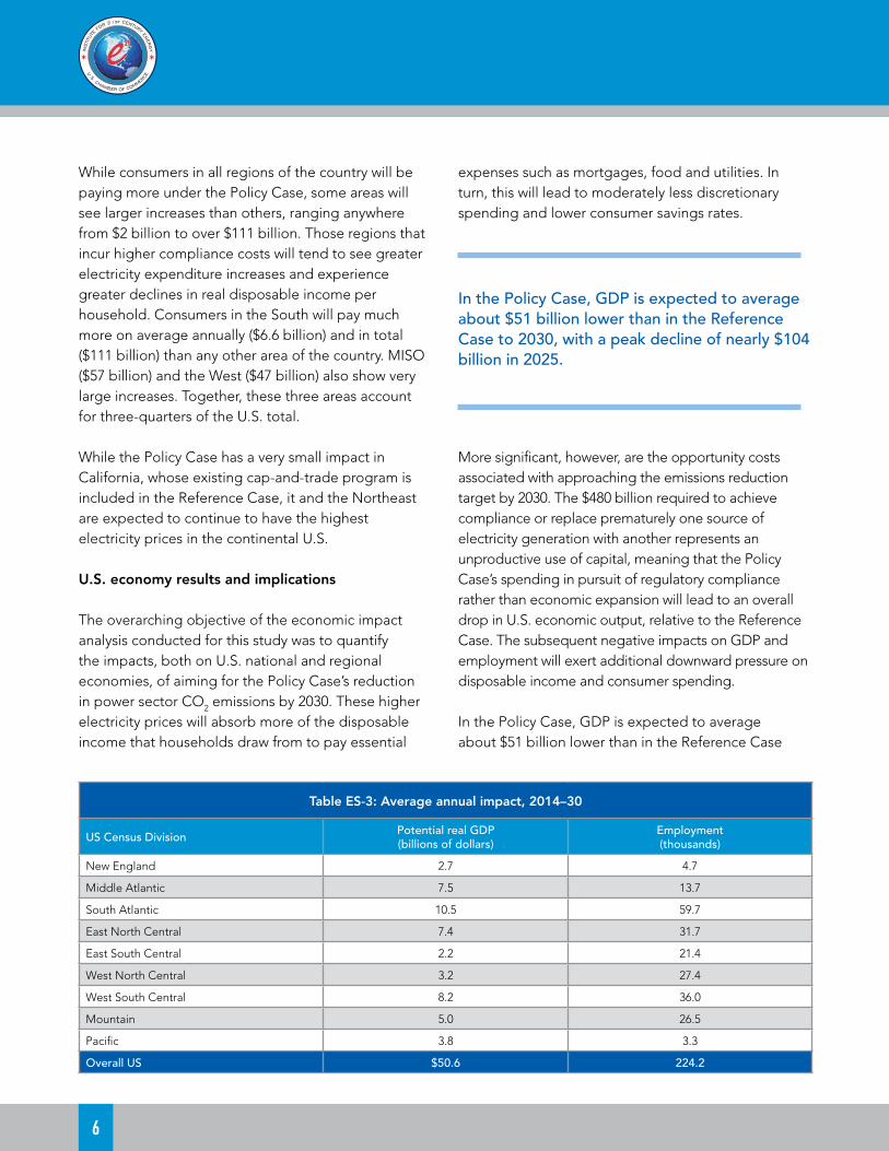
In the Policy Case, GDP is expected to average about $51 billion lower than in the Reference Case to 2030, with a peak decline of nearly $104 billion in 2025.
More significant, however, are the opportunity costs associated with approaching the emissions reduction target by 2030. The $480 billion required to achieve compliance or replace prematurely one source of electricity generation with another represents an unproductive use of capital, meaning that the Policy Case’s spending in pursuit of regulatory compliance rather than economic expansion will lead to an overall drop in U.S. economic output, relative to the Reference Case. The subsequent negative impacts on GDP and employment will exert additional downward pressure on disposable income and consumer spending.
In the Policy Case, GDP is expected to average about $51 billion lower than in the Reference Case
Table ES-3: Average annual impact, 2014–30
US Census Division Potential real GDP (billions of dollars)
Employment(thousands)
New England 2.7 4.7
Middle Atlantic 7.5 13.7
South Atlantic 10.5 59.7
East North Central 7.4 31.7
East South Central 2.2 21.4
West North Central 3.2 27.4
West South Central 8.2 36.0
Mountain 5.0 26.5
Pacific 3.8 3.3
Overall US $50.6 224.2

Assessing the Impact of Potential New Carbon Regulations in the United States
7
to 2030 (Table ES-3), with a peak decline of nearly $104 billion in 2025. These substantial GDP losses will be accompanied by losses in employment. On average, from 2014 to 2030, the U.S. economy will have 224,000 fewer jobs (Table ES-3), with a peak decline in employment of 442,000 jobs in 2022 (Figure ES-1). These job losses represent lost opportunities and income for hundreds of thousands of people that can never be recovered. Slower economic growth, job losses, and higher energy costs mean that annual real disposable household income will decline on an average of more than $200, with a peak loss of $367 in 2025. In fact, the typical household could lose a total of $3,400 in real disposable income during the modeled 2014-30 timeframe.
-500,000
-450,000
-400,000
-350,000
-300,000
-250,000
-200,000
-150,000
-100,000
-50,000
0
2014 2020 2025 2030
Figure ES-1: Employment Impact Policy Case deviation from the baseline
Source: IHS Economics
The economic impact will vary significantly across the nine U.S. Census Divisions examined. Because California’s cap and trade program and the Regional Greenhouse Gas Initiative (RGGI) that includes nine Northeastern States are included in the Reference Case, these regions are not significantly affected by federal CO2 regulations. The cost of compliance for state-based regimes in these regions will already result in significant economic impacts, including high electricity prices, making the discussion about federal regulations less relevant. Despite California’s lead in compliance, however, the remaining states will drag the Pacific region down moderately in the early years. The Northeast, on the other hand, will see little additional
impact on its already high and increasing electricity rates from the imposition of a federal CO2 regime.
The need to replace large portions of the coal generation fleet in the midcontinent Census Divisions (East North Central, East South Central, West North Central, and West South Central), however, means that these regions will experience the bulk of the economic distress in the early years, followed by the South Atlantic4 in the latter years.
Overall, the South Atlantic will be hit the hardest in terms of GDP and employment declines. Its GDP losses make up about one-fifth of total U.S. GDP losses, with an average annual loss of $10.5 billion and a peak loss of nearly $22 billion in 2025. This region also will have an average of 60,000 fewer jobs over the 2014-30 forecast period, hitting a 171,000 job loss trough in 2022.
Overall, the South Atlantic will be hit the hardest in terms of GDP and employment declines. Its GDP losses make up about one-fifth of total U.S. GDP losses.
The West South Central5 region also takes a big hit, losing on average $8.2 billion dollars in economic output each year and 36,000 jobs.
Cost per ton of reduced carbon
The economic cost to achieve each ton of emissions reduction also is extraordinarily high. This analysis indicates that the additional cuts in CO2 emissions in the Policy Case come with an average price tag of $51 billion per year in lost GDP over the forecast
4 Includes Delaware, District of Columbia, Florida, Georgia, Maryland, North Carolina, South Carolina, Virginia, and West Virginia.
5 Includes Arkansas, Louisiana, Oklahoma, and Texas.
8
period, which translates into an average undiscounted economic cost of $143 per ton of CO2 reduced. When EIA modeled the Waxman-Markey cap-and-trade bill, the economic cost per ton of CO2 in its “Basic” scenario averaged an undiscounted $82 over the same period, still quite high but considerably less than the $143 figure arrived at under the Policy Case.
The economic cost for each ton of reduced CO2 in the Policy Case also exceeds the upwardly revised social cost of carbon (SCC) estimates developed by the Administration’s Interagency Working Group on Social Cost of Carbon in 2013. Based on the average SCC from three integrated assessment models at discount rates of 2.5%, 3%, and 5%, the Working Group estimated that by 2030, the SCC will have risen to between $17 and $82 per ton (in 2012 dollars). Applying the same range of discount rates, the average cost in the Policy Case ranges from $153 to $163 per ton over the analysis period, much higher than even the Working Group’s 2030 figure.
Real disposable income per household
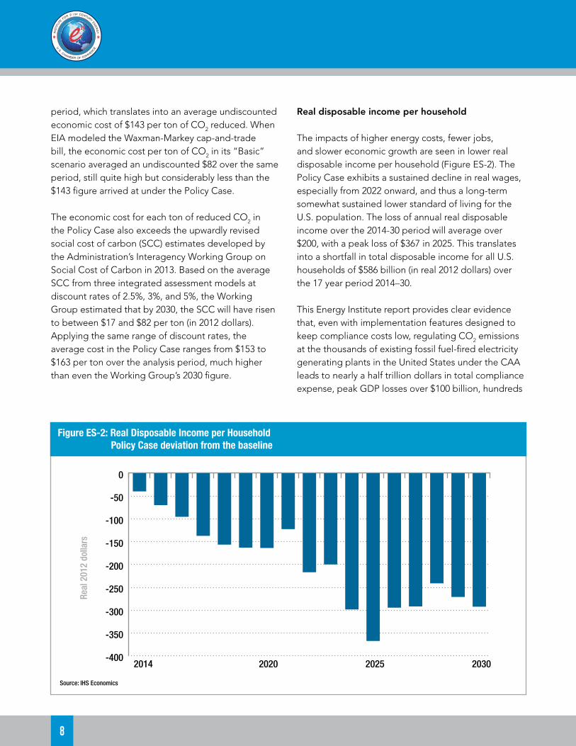
The impacts of higher energy costs, fewer jobs, and slower economic growth are seen in lower real disposable income per household (Figure ES-2). The Policy Case exhibits a sustained decline in real wages, especially from 2022 onward, and thus a long-term somewhat sustained lower standard of living for the U.S. population. The loss of annual real disposable income over the 2014-30 period will average over $200, with a peak loss of $367 in 2025. This translates into a shortfall in total disposable income for all U.S. households of $586 billion (in real 2012 dollars) over the 17 year period 2014–30.
This Energy Institute report provides clear evidence that, even with implementation features designed to keep compliance costs low, regulating CO2 emissions at the thousands of existing fossil fuel-fired electricity generating plants in the United States under the CAA leads to nearly a half trillion dollars in total compliance expense, peak GDP losses over $100 billion, hundreds
-400
-350
-300
-250
-200
-150
-100
-50
0
2014 2020 2025 2030
Real
201
2 do
llars
Figure ES-2: Real Disposable Income per Household Policy Case deviation from the baseline
Source: IHS Economics

Assessing the Impact of Potential New Carbon Regulations in the United States
9
of thousands of lost jobs, higher electricity costs for consumers and businesses, and more than $200 on average every year in lower disposable income for families already struggling with a weak economy.
Given the significant and sustained harm to the U.S economy coupled with the limited overall impact on worldwide greenhouse gas emissions that would result from implementing these regulations, serious questions must be raised and answered about the timing and scope of what EPA is pursuing.

10
Introduction
The electric power generating sector of the U.S. economy is facing a tremendous amount of change. The traditional vertically-integrated utility is facing competitive pressures from new and emerging generation resources. Net metering policies are driving the installation of distributed generation technologies. Intermittent renewable megawatts (MW) and “negawatts” associated with demand-side management programs are being integrated on a large scale. Electric automobiles are joining the country’s auto fleet along with the need for enhanced infrastructure to support their operation, and energy efficiency mandates are limiting demand growth, though not always in an economically efficient manner.
The evolution of the way that electrons are generated, transmitted, and distributed to customers, and in turn how customers utilize the services of electric utilities and cooperatives, will continue to change, and this transition remains manageable and incremental in nature. The electric utility industry is coming of age, and it is certainly up to the challenges it faces as the electric grid enters the digital generation.
However, an avalanche of new rules coming out of the EPA have the potential to turn this incremental transition of electricity infrastructure into an unmanageable upheaval that could lead to higher costs, less diversity, and less reliability. This matters because electricity is not just a job driver and immeasurable supporter of economic sustainability and growth, but also a vital public safety and health resource for our nation. This is why the International Energy Agency (IEA) views the availability of reliable and affordable electricity as crucial to human well-being and to a country’s economic development. Reliable electricity access is instrumental in providing clean water, sanitation, and healthcare, and for the provision of reliable and efficient lighting, heating, cooking, mechanical power, transportation and telecommunications services.6
6 IEA – World Energy Outlook http://www.worldenergyoutlook.org/resources/energydevelopment/#d.en.8630
A partial list of EPA power sector rules includes the agency’s MATS Rule, its Cross-State Air Pollution Rule, and those applicable to electric generation cooling techniques. In addition, in September 2013, the EPA released a proposed NSPS rule applicable to the construction of new fossil fuel power plants. This new rule would require coal-fired power plants to employ CCS technology, which is not commercially available and is not likely to be for some time, consistent with the conclusions stated within the Obama Administration’s National Climate Assessment released in May 2014. This NSPS rule is featured as part of President Obama’s Climate Action Plan, which was announced in June 2013 and includes major initiatives to cut U.S. GHG emissions and “lead international efforts to address global climate change.” The centerpiece of the President’s plan directs the EPA to complete new regulations under the CAA limiting CO2 emissions from new power plants that use fossil fuel, and to propose and finalize regulations applicable to CO2 emissions from existing power plants. The currently-proposed NSPS standards for plants fired with natural gas could be met easily with existing technology.
For existing plants, the EPA is expected to propose new rules in June 2014 and complete them within one year. The EPA has committed to follow these power sector rules with similar CO2 regulations applicable to other industrial sectors.
Regulating CO2 emissions from existing power plants is no small undertaking. In 2013, there were more than 5,000 coal- and natural gas-fired generating units in operation in the United States. These units comprised almost three-quarters of the country’s generating capacity and produced two-thirds of the electricity generated.
Clearly, the potential economic impacts of the EPA’s new rules could be quite large. The United States enjoys some of the lowest electricity rates among Organization for Economic Co-operation and Development countries,

Assessing the Impact of Potential New Carbon Regulations in the United States
11
which provide a tremendous competitive advantage, especially in energy-intensive sectors. Sweeping and aggressive changes to the way electricity is produced has the potential to threaten not only the affordability of our electricity supply, but also the diversity and reliability of that supply, all of which could damage our economy, reduce employment and income, and steer investment away from more productive purposes.
For these reasons, the EPA’s rules on existing power plants are expected to be of potentially unprecedented magnitude, reach, and complexity.
Moreover, it is anticipated that the EPA will mandate a level of CO2 emissions reductions that is unachievable at affected power plants, effectively forcing states to pursue “outside-the-fence” reductions as the only remaining compliance options.
For these reasons, the EPA’s rules on existing power plants are expected to be of potentially unprecedented magnitude, reach, and complexity. Accordingly, it is critical that the regulatory decision-making process be informed by realistic and robust analysis of the costs, benefits, and practical implications of any proposed actions.
Therefore, the Energy Institute commissioned IHS to apply its modeling capabilities to the EPA’s forthcoming CO2 emissions rules for power plants. The Energy Institute provided assumptions and policy premises for the modeling. These assumptions and policy premises that provided the starting point include the NRDC’s proposed performance standards for existing sources (the “NRDC Proposal”) in combination with the announced greenhouse gas reduction goals of the Obama Administration, which establish reduction targets of 17%, 42%, and 83% – below the 2005 CO2 emissions levels – by 2020, 2030, and
2050, respectively.7 The Energy Institute identified the conclusions to be drawn from the economic modeling.
Furthermore, to enhance the transparency and conservative nature of this analysis, the Energy Institute assigned a proportional share of these administration goals to the power sector, instead of the likely super-proportional share that would inevitably be necessary to meet the stated economy-wide goals. Limiting the Policy Case’s assumptions to the NRDC Proposal, as further informed by the Obama Administration’s stated emissions goals, the Energy Institute sought to provide a highly-credible and unbiased assessment and quantification of the impact that pending and future CO2 emissions regulations could have on GDP, employment, investment, productivity, household income, and electricity prices, both in the broader economy and at the regional level. The NRDC Proposal incorporates many of the kinds of features – including state-specific standards set by the EPA and broad flexibility to meet these standards “in the most cost-effective way, through a range of technologies and measures” – designed to keep costs low. However, the results of this report demonstrate that deep emissions reductions in the power sector will actually come at a very high economic cost.
The Background section provides an overview of the timeline for the EPA regulations of CO2 from power plants, describes the NRDC Proposal and its compliance measures, and discusses the basis for extending the analysis to 2030. The Analytical Approach section describes the modeling effort and lays out the parameters of the Reference Case and the Policy Case used in the analysis. The Reference and Policy Cases are discussed in greater detail in sections devoted to each of them. The Results section summarizes the outcomes of the analysis, including the costs of emission reductions and the impact on the U.S. economy, including individualized regional impacts. The policy implications of these results are
7 The White House, Office of Press Secretary, “President to Attend Copenhagen Climate Talks: Administration Announces U.S. Emission Target for Copenhagen,” November 25, 2009. Available at: http://www.whitehouse.gov/the-press-office/president-attend-copenhagen-climate-talks.

12
presented in the Conclusion section. In addition, three appendices are provided that include technical details about the models being used (Appendix A), the methodology for assessing impacts (Appendix B), and the specific costs utilized to complete the power sector modeling of impacts (Appendix C).
Background: Upcoming U.S. power sector CO2 regulations
The EPA is in the process of developing CO2 regulations for the U.S. power sector following the 2007 Supreme Court ruling that GHG emissions meet the definition of “pollutant” under the CAA. The agency is developing separate rules to limit CO2 emissions from new and existing power plants, according to a timeline prescribed by President Obama’s June 2013 Climate Action Plan and accompanying Presidential Memorandum.8 The EPA was instructed to issue final rules and begin implementation before the end of the president’s second term in 2016 (Figure 1).
8 Presidential Memorandum available at: http://www.whitehouse.gov/the-press-office/2013/06/25/presidential-memorandum-power-sector-carbon-pollution-standards. NOTE: Consistent with this memorandum, the EPA is also developing rules for “modified” power plants that undergo significant construction.
Although not yet final, the standards that the EPA will impose on new fossil fuel–fired power plants are reasonably clear. The agency’s September 2013 revised draft NSPS proposal would require new coal- and natural gas–fired power plants to achieve separate but similar unit-level CO2 emission rate thresholds. New coal plants would be required to install and operate CCS technology while new natural gas plants would be able, at least initially, to operate without CCS.
The exact form and stringency of the EPA’s upcoming proposal (anticipated June 2, 2014) to regulate existing power plants is unknown. Section 111(d) of the CAA governs existing sources and prescribes a joint federal-state process for establishing and implementing existing source performance standards (ESPS) for emissions. Specifically, the statute authorizes the EPA to establish a procedure under which states establish emissions reduction standards for existing sources such as power plants. In the past, the EPA has used Section 111(d) primarily to establish plant-level emissions performance standards.
However, in regulating CO2 emissions, it appears that the EPA will attempt to mandate a level of CO2 emissions reductions that is unachievable at the source (power plants), effectively forcing states to pursue “outside-the-fence” emissions reductions measures, such as renewable
Figure 1: Timeline for EPA power sector carbon dioxide regulations
*EPA is directed to �nalize the new rule as “expeditiously” as possible.Source: IHS Energy
Final rule Draft rule
2013 2014 2016 2017 2015
20 Sept. 2013
1 June 2014
1 June 2015
30 June 2016
State implementation plans
New president Election year
CO2 NSPS—New Source Performance Standards*
CO2 ESPS—Existing Source Performance Standards
2014–15
… 2022
First lookback
period

Assessing the Impact of Potential New Carbon Regulations in the United States
13
energy and demand-side energy efficiency mandates, as the key compliance options. The ESPS may also include the use of market-based trading programs.
Although the EPA has been instructed to draft, finalize, and begin implementing an existing source rule by the end of 2016, given the lead time needed for developing state implementation plans, this timeline appears aggressive and highly susceptible to slippage. Aside from the possible exception of California and the states in RGGI, which will likely rely on existing programs to demonstrate equivalence with whatever requirement the EPA ultimately pursues, generator compliance in most states is unlikely until 2018 at the earliest.
Future natural gas–fired power plants may require CCS
The EPA’s September 2013 draft CO2 NSPS proposes separate but similar unit-level emissions thresholds for new coal- and natural gas–fired power plants. The limits apply to units in the continental United States that are roughly 25 megawatts (MW) or greater and that supply the majority of their potential electric output to the grid. The standard targets primarily coal-fired steam boilers, including supercritical pulverized coal and coal-fired integrated gasification combined-cycle units, and natural gas–fired combined-cycle gas turbines (CCGT). Although combustion turbines are technically covered, in reality the majority would be exempted by the rule’s 33% capacity factor threshold.
The proposed standard for new coal-fired units is based on the EPA estimated emissions rate that can be achieved by a plant operating partial CCS. “Partial CCS” is defined as a CO2 capture rate below 90%, the threshold for full CCS. The emissions standard would prohibit new coal-fired units from emitting above 1,100 pounds (lb) per megawatt-hour (MWh) of gross electric output (i.e., excluding parasitic losses) on a 12-month rolling average basis, including start-up and shutdown periods. The emissions rate threshold would require new coal-fired units to capture and store between about 25% and 40% of their emissions, depending on their particular technology configuration. The
standards for natural gas-fired units are based on the CO2 emissions rate range of new CCGTs. The proposal establishes a 12-month rolling average 1,000 lb per MWh emissions rate for so-called large units and a 1,100 lb per MWh threshold for small units. Large units are distinguished from smaller, less efficient units by a roughly 100 MW capacity threshold.
Given the CAA’s requirement that the EPA review and consider revising its NSPS rules at least every eight years, there is the potential that new natural gas–fired power plants could one day also be required to implement CCS. In fact, the EPA’s revised draft proposal has opened the door to this possibility by choosing to go with separate standards for coal- and natural gas–fired units rather than a single standard–based approach.
The NRDC proposal for regulating existing power plants
In December 2012, the NRDC released a report entitled Closing the Power Plant Carbon Pollution Loophole. The report contains its recommendation to the EPA on how to regulate CO2 emissions from existing power plants. NRDC proposed that the EPA establish fossil-fleet average emission rate targets at the state level based on the following criteria:
• A series of national average emission rate benchmarks for existing coal- and natural gas/oil-fired power plants that become more stringent over time (Table 1); and
• The proportion of coal- and natural gas/oil-fired generation in a 2008–10 baseline period.
For example, Pennsylvania’s emission rate target during 2015–19 would be roughly 1,660 lb per MWh, based on the fact that 80% of the state’s fossil fuel–fired generation during 2008–10 was supplied by coal-fired generation, with the remaining 20% supplied by natural gas/oil-fired generation
(i.e., = 1,800lb/MWh x 80%coal + 1,035lb/MWh x 20%natural gas/oil).
14
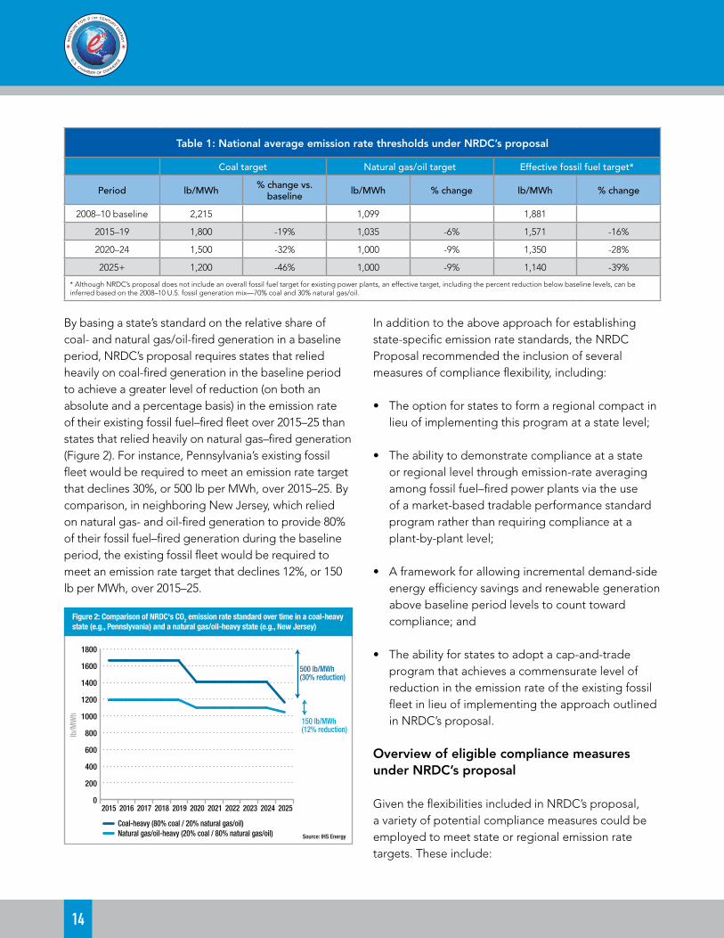
By basing a state’s standard on the relative share of coal- and natural gas/oil-fired generation in a baseline period, NRDC’s proposal requires states that relied heavily on coal-fired generation in the baseline period to achieve a greater level of reduction (on both an absolute and a percentage basis) in the emission rate of their existing fossil fuel–fired fleet over 2015–25 than states that relied heavily on natural gas–fired generation (Figure 2). For instance, Pennsylvania’s existing fossil fleet would be required to meet an emission rate target that declines 30%, or 500 lb per MWh, over 2015–25. By comparison, in neighboring New Jersey, which relied on natural gas- and oil-fired generation to provide 80% of their fossil fuel–fired generation during the baseline period, the existing fossil fleet would be required to meet an emission rate target that declines 12%, or 150 lb per MWh, over 2015–25.
2015 2016 2017 2018 2019 2020 2021 2022 2023 2024 2025
lb/M
Wh
0
200
400
600
800
1000
1200
1400
1600
1800
500 lb/MWh(30% reduction)
150 lb/MWh(12% reduction)
Coal-heavy (80% coal / 20% natural gas/oil) Natural gas/oil-heavy (20% coal / 80% natural gas/oil)
Figure 2: Comparison of NRDC's CO2 emission rate standard over time in a coal-heavy state (e.g., Pennslyvania) and a natural gas/oil-heavy state (e.g., New Jersey)
Source: IHS Energy
In addition to the above approach for establishing state-specific emission rate standards, the NRDC Proposal recommended the inclusion of several measures of compliance flexibility, including:
• The option for states to form a regional compact in lieu of implementing this program at a state level;
• The ability to demonstrate compliance at a state or regional level through emission-rate averaging among fossil fuel–fired power plants via the use of a market-based tradable performance standard program rather than requiring compliance at a plant-by-plant level;
• A framework for allowing incremental demand-side energy efficiency savings and renewable generation above baseline period levels to count toward compliance; and
• The ability for states to adopt a cap-and-trade program that achieves a commensurate level of reduction in the emission rate of the existing fossil fleet in lieu of implementing the approach outlined in NRDC’s proposal.
Overview of eligible compliance measures under NRDC’s proposal
Given the flexibilities included in NRDC’s proposal, a variety of potential compliance measures could be employed to meet state or regional emission rate targets. These include:
Table 1: National average emission rate thresholds under NRDC’s proposal
Coal target Natural gas/oil target Effective fossil fuel target*
Period lb/MWh % change vs. baseline lb/MWh % change lb/MWh % change
2008–10 baseline 2,215 1,099 1,881
2015–19 1,800 -19% 1,035 -6% 1,571 -16%
2020–24 1,500 -32% 1,000 -9% 1,350 -28%
2025+ 1,200 -46% 1,000 -9% 1,140 -39%
* Although NRDC’s proposal does not include an overall fossil fuel target for existing power plants, an effective target, including the percent reduction below baseline levels, can be inferred based on the 2008–10 U.S. fossil generation mix—70% coal and 30% natural gas/oil.

Assessing the Impact of Potential New Carbon Regulations in the United States
15
• Plant efficiency improvements. Supply-side investments to improve the energy efficiency of a power plant and thus reduce its average emission rate.
• Environmental dispatch. Shifting the share of generation at the portfolio level in an existing fossil fuel–fired portfolio from more carbon intensive to less carbon intensive power plants, including within fuels (i.e., from a higher emitting to a lower emitting coal plant) and across fuels (i.e., shifting from coal and toward natural gas–fired generation, and/or retiring coal-fired generators).
• Trading of emission allowances. Intrastate trading of emission allowances (denominated in tons of CO2) among fossil fuel–fired generators, renewable energy generators, and via a state/region-specific process for allocating allowances associated with incremental energy efficiency savings from ratepayer-funded programs, for carbon emissions generated within a given state.
Compliance under the NRDC proposal’s tradable performance standard
A market-based tradable performance standard serves as the mechanism under which compliance is achieved within the NRDC CO2 ESPS structure. A tradable performance standard is similar to a cap-and-trade program in that it uses a CO2 allowance price to drive a change in the merit order of dispatch in favor of less carbon intensive resources. The impact on dispatch under a tradable performance standard is equal to the price of one allowance multiplied by the difference between the emission rate of a fossil fuel–fired power plant and that plant’s state/regional emission rate target. Thus, dispatch costs increase for generators whose emission rate is above the performance standard rate (e.g., coal-fired power plants) and decrease for generators whose emission rate is below the target (e.g., natural gas–fired CCGTs).
The NRDC Proposal’s tradable performance standard also includes an additional feature in that it allows savings from demand-side energy efficiency measures
and renewable generation in excess of levels achieved during 2008–10 to qualify toward compliance. Under the proposal, incremental energy savings and renewable energy (in MWh) are converted to emission credits (in tons) by multiplying by a state/region’s emission rate target. This implies that compliance occurs when the “compliance emission rate” established for a state/region is less than or equal to the emission rate target in that state/region. The compliance emission rate is defined as follows:
Compliance emission rate CO2 emissions from existing fossil gen. (lb)
existing fossil gen. + incremental renewables gen. + incremental efficiency savings (MWh)
This definition gives generators and states/regions flexibility to achieve compliance partially by lowering the emission rate of their existing fossil fuel–fired portfolio and partially by increasing their reliance on renewable generation and savings from energy efficiency.
Laying the groundwork for cutting power sector emissions by 42% from 2005 levels by 2030
The policy case presented within marries the NRDC report’s framework with the Obama Administration’s stated goals of an economy-wide reduction in gross U.S. greenhouse gas (GHG) emissions of 17% below the 2005 level by 2020 and 42% below the 2005 level by 2030 (leading eventually to a national GHG emissions goal equal to 83% below the 2005 level by 2050). A GHG emissions trajectory of this magnitude is consistent with the Administration’s 2010 submission to the UN Framework Convention on Climate Change (UNFCCC) associating the United States with the Copenhagen Accord.
The international context is important because the Administration has made domestic regulation a key aspect of its approach to the ongoing international climate change talks. The 42% emissions reduction figure was chosen because, to date, it remains the only publicly announced Administration GHG reduction goal for 2030. The Administration has not said whether

16
or how this goal might be modified to form the basis of the GHG commitment the Administration will put forward as part of the negotiating sessions leading to a new post-2020 UNFCCC agreement. These talks are scheduled to conclude in Paris in late 2015. With no insight into the Administration’s thinking about a post-2020 UNFCCC goal, this report’s adoption of the 42% reduction figures for 2030—a goal the NRDC and the Obama Administration have endorsed—is justified.
As a practical matter, however, it is clear that the power sector would have to be responsible for much deeper cuts than those modeled here to achieve such aggressive economy-wide reductions by 2030.
The question then becomes how to apportion this economy-wide commitment to the electricity generation sector. Again, with no additional details available from the Obama Administration, it was assumed for the purposes of this analysis that the power sector would be responsible for a proportional share of the economy-wide reductions; that is, the power sector would have to reduce its CO2 emissions by about 17% by 2020 and 42% by 2030. As a practical matter, however, it is clear that the power sector would have to be responsible for much deeper cuts than those modeled here to achieve such aggressive economy-wide reductions by 2030. The
practical need for the electric utility sector to bear more than its proportional share of reductions, especially in 2030, is evident because anticipated reductions in other large-emitting sectors of the economy (for example, the transportation sector) do not approach these values. Therefore, the approach used in this analysis should be viewed as very conservative.
Analytical approach
The Energy Institute commissioned IHS to provide power sector simulations and U.S. and regional level macroeconomic simulations depicting the potential impact of adopting CO2 emissions regulations targeting U.S. power generators through 2030. In conducting its analysis and basing it on the assumptions and policy premises provided by the Energy Institute, IHS constructed two power sector simulation cases: (1) a Reference Case with no additional federal regulations targeting U.S. power plant CO2 emissions and (2) a Policy Case with federal standards covering both new and existing fossil fuel–fired power plants, based on policy assumptions specified by the Energy Institute and described in more detail below.9
9 The Reference Case for the analysis is based on the IHS North American Gas and Power Scenarios Advisory Service Planning Scenario. The Reference Case makes one key modification to the underlying IHS Planning Scenario in that no federal program targeting power sector CO
2 emissions emerges. The IHS North American Gas and Power Scenarios
Advisory Service, established in 1996, benefits from having a diverse client membership, including oil and gas exploration and production companies, electric and gas utilities, independent power producers, coal companies, original equipment manufacturers, engineering and construction companies, pipeline companies, energy marketers, and financial institutions. The IHS scenarios are openly shared with industry experts for scrutiny and vetting through delivery of written materials and biannual workshops, as well as through individual consulting engagements with clients.
Table 2: Key policy assumptions in the Reference Case and Policy Case
Reference Case Policy Case
MATS effective April 2015 MATS effective April 2015
California and RGGI carbon programs continue through 2030 CO2 ESPS effective 2018 (using structure proposed by NRDC
through 2025) with an extension and tightened standards in 2030 to meet Administration’s stated climate goals
No federal-level carbon program Tightening of CO2 NSPS effective 2022 requiring CCS for both coal
and gas plants
Current state EE programs Current state EE programs
Current state RPSs Current state RPSs
Source: IHS EnergyNote: MATS = Mercury and Air Toxics Standard, EE = energy efficiency, RPS = renewable portfolio standard

Assessing the Impact of Potential New Carbon Regulations in the United States
17
The Policy Case includes changes to the power sector as compared to the Reference Case—mainly incremental coal-fired generator retirements, energy efficiency investments, and construction of renewable power generation and other low CO2 emission technologies. The results of the power sector simulations—changes in power sector capital expense, fuel expense, and operations and maintenance expenses—were also analyzed to assess their impacts on key U.S. and regional macroeconomic indicators.
The background and structure underpinning the Reference Case and Policy Case are described below. The underlying models used to conduct the power sector and U.S. macroeconomic simulations are described in Appendices A and B, respectively.
Reference Case
The Reference Case, used as a point of comparison in examining the impact of carbon policy on the U.S. power sector, extrapolates today’s North American natural gas and power business conditions and extends them into the future. Because energy and economic policies evolve over time, this is not a “business-as-usual” scenario. Rather, rules and regulations are developed with some delay and in a more measured and flexible way than initially conceived, driven largely by concerns surrounding costs and system reliability. Key features of the Reference Case include the following:
• U.S. power demand grows, but at a slower pace than historically, averaging 1.4% per year compounded annually between 2013 and 2030.
• The U.S. natural gas outlook reflects a resource base adequate to support anticipated growth in both domestic and export demand at a price proximate to $4.00 per million British thermal units (MMBtu) at Henry Hub in real terms.
• Generator retirements from 2011 through 2030 total 154 gigawatts (GW), with 85 GW of coal-fired power plants retiring in this time frame.
• Natural gas–fired and renewable power generators, primarily wind and solar, dominate new generating capacity additions, accounting for about 90% of additions through 2030.
• Coal-fired generation declines from 40% in 2013 to 29% in 2030, while natural gas–fired generation increases from 27% to 38% over the same period. Fossil generation in the Reference Case—coal, natural gas, and oil—account for two-thirds of power generation in 2030.
• Power sector CO2 emissions fall 9% below 2005 levels by 2030.
Environmental policiesNon-carbon environmental regulations
The EPA is pressing forward with a long list of non-carbon environmental regulations that impact the power sector. Figure 3 shows the timeline for implementation of non-carbon environmental regulations.
The EPA’s MATS rule, which limits mercury, acid gases and particulate matter emissions, will be implemented as per the final rule in 2015, states approve several fourth-year compliance extensions requests, and the EPA makes use of risk management procedures to grant additional time.
The Clean Air Interstate Rule (CAIR) remains in effect until 2018, after which the EPA replaces it with a new rule for regulating power plant emissions of sulfur dioxide (SO2) and nitrogen oxides (NOX) that drift from one state to another. The replacement rule is based on a cap-and-trade model and allows for unlimited intrastate trading but limits the degree of interstate

18
trading of emission allowances.10
Other major non-carbon EPA rules will move forward with some delay in the Reference Case. The Cooling Water Intake Structures Rule becomes final in 2014 and gives states both flexibility and authority in determining compliance requirements, including the most contentious and costly decisions–converting once-though cooling systems to closed-loop systems. Finally, the EPA regulates coal ash as nonhazardous waste.
10 On April 29, 2014 the U.S. Supreme Court ruled to reinstate the EPA’s Cross-State Air Pollution Rule (CSAPR), reversing a federal appellate court’s decision in August, 2012 invalidating the rule. Originally slated to take effect on January 1, 2012, CSAPR was designed to replace CAIR, which itself had previously been struck down by the same appellate court but then subsequently allowed to remain in effect on a provisional basis until the EPA implemented a replacement rule. Having been conducted prior to the Supreme Court’s decision, the analysis in this report of both the Reference Case and Policy Case was based on the assumption that the EPA would ultimately be required to develop a new rule to replace CAIR. The replacement rule that was modeled, however, employed the same limited trading approach and similar regional emission budgets as CSAPR. Thus, although CSAPR may be implemented prior to 2018, the replacement rule modeled in this analysis provides a reasonable approximation of CSAPR’s impact on the U.S. power system thereafter.
Carbon programs
There is no federal program targeting power sector CO2 emissions in the Reference Case. However, California’s GHG cap-and-trade program (covering multiple sectors of the economy) and RGGI, a nine-state power-sector-only cap-and-trade program, are both operational. While the caps are not yet a major constraint on regional emissions and carbon allowance prices are therefore still relatively low, the balance between emission allowance supply and demand tightens over the course of the current decade and drives up allowance prices. Both the California program and RGGI are extended beyond 2020. Allowance prices for both programs remain, on average, close to the price ceilings established at the time of their inception. Figure 4 depicts the CO2 allowance price outlooks modeled for RGGI and California.
OUTLOOK
NAAQS ozone 2014
Draft Final Compliance
MATS(Hg, etc.)
Apr 2015 2012 2013 2014 2016 20172015
NAAQS PM2.5 Dec 2012
Dec 2011
CAIR replacement (SO2 and NOX)
Aug 2012 Struck down
Regional Haze (PM, NOx, SO2)
2018
2014 2015 2018
2020
2022+
Cooling Water Intake Structures
Coal Combustion Residuals
2014–28 2014
2014 2015
Figure 3: US EPA regulatory timeline for non-carbon environmental regulations
Source: IHS Energy. 30105-2Note: NAAQS = National Ambient Air Quality Standards; PM = particulate matter
2015+

Assessing the Impact of Potential New Carbon Regulations in the United States
19
0
10
20
30
40
50
60
2014 2015 2016 2017 2018 2019 2020 2021 2022 2023 2024 2025 2026 2027 2028 2029 2030
Real
201
2 US
dol
lars
per
met
ric to
n
CaliforniaRGGI
Figure 4: US regional CO2 allowance price outlooks in the Reference Case
Source: IHS Energy
Power demand
In the Reference Case, electricity demand is projected to grow 1.4% per year on average over 2013–30, driven by economic growth, changes in the price of electricity, and the evolution of public policies targeting investment in energy efficiency (Figure 5).
U.S. GDP is projected to grow roughly 2.5% per year over 2013–30. Historically, growth in electricity demand has been highly correlated with growth in GDP (Figure 6). Prior to the mid-1980s, electricity demand grew more quickly than GDP; during the 1960s, electric demand grew twice as fast as GDP. Since 1980, electricity demand has grown more slowly than GDP. During the previous decade, for every 1% increase in GDP, electricity demand grew roughly 0.6%. A similar relationship is expected to hold through the remainder of this decade but then become progressively weaker over time owing in large part to the countervailing effect of rising retail electricity prices and a continued strong emphasis on energy efficiency policies at both the U.S. federal and state levels.
0
1,000
2,000
3,000
4,000
5,000
1960 1965 1970 1975 1980 1985 1990 1995 2000 2005 2010 2015 2020 2025 2030
Terr
awat
t-ho
urs
Figure 5: US electricity sales, 1960-2030
Source: IHS Energy
OUTLOOK
-2
0
2
4
6
8
10
1960 1970 1980 1990 2000 2010 2020 2030
Perc
ent g
row
th (t
hree
-yea
r CAG
R)Figure 6: US electricity sales and GDP growth, 1960-2030
Note: CAGR = compound annual growth rate Source: IHS Energy, IHS Economics, and US EIA
2013-30CAGR2.5%
1.4%
ElectricitySales
GDP
2.0 1.37 0.79 0.66 0.59 0.58 0.38
Decadalelasticity
(% changeelectricity sales/% change GDP)
The Reference Case includes an increase in national average retail electric rates of 0.8% per year (in real dollars) over 2013–30 as a result of capital investments and expenses in the U.S. power sector. These include traditional investments in generation, transmission, and distribution, as well as environmentally-related policy costs, including RPS, pollution control laws, and energy efficiency and demand response programs, among other costs. In general, a 1% increase in real price leads to a roughly 0.7% decline in electricity demand over the long term.
In addition to rising retail electricity prices, energy efficiency policies are expected to continue to exert a

20
4 4
?
Figure 7: US states with energy ef�ciency resources standards
Source: IHS Energy, American Council for an Energy-Ef�cient Economy (ACEEE), US EPA and state regulatory commissions. Notes: In addition to having an EERS policy, Hawaii and Pennsylvania also allow energy ef�ciency to qualify for their RPS. Energy ef�ciency quali�es for Oklahoma, South Dakota, and Utah’s pending/voluntary RPS, the latter of which also has a pending EERS. 20805-23
POLICY TYPE
Pending and voluntary policies
Ef�ciency eligible under RPS
Binding Energy Ef�ciency Resource Standard (EERS)
No EERS
downward pull on electricity demand. At a federal level, IHS expects that the U.S. Department of Energy will continue to roll out new and revised appliance standards, albeit on a delayed basis when compared to its statutory schedule. At the state level, IHS projects that spending on ratepayer-funded energy efficiency programs will be driven by state energy efficiency resource standards (EERS), which are binding in 26 states and cover almost 65% of total U.S. electricity sales (Figure 7). It is estimated that roughly only 50% of aggregate state EERS targets are likely to be met, owing both to their stringency relative to current annual savings levels and to a lack of supporting policies, such as lost revenue recovery mechanisms, shareholder incentives, and/or penalty provisions to drive utilities to achieve their targets.11
11 Supporting policies are designed to counteract a utility’s inherent incentive to increase the sale of its product, electricity, and the fact that energy efficiency programs are generally expensed and thus do not earn a rate of return, similar to an investment in new power supply infrastructure. Of the 23 states where utilities are responsible for achieving a binding target (i.e., excluding Maine, Oregon, and Vermont, where programs are implemented solely by third parties), 10 states have implemented a revenue recovery mechanism or revenue decoupling and some form of shareholder incentive program, including 4 that also impose penalties for noncompliance. That leaves 13 states, which collectively account for about 50% of cumulative savings target in 2020, without a sufficient complement of utility incentives and penalties.
Fuel markets
Natural gas
The natural gas market environment is underpinned by technological advancements in drilling techniques, a resulting reduction in unit production costs, and an expanded domestic resource base estimated at 3,400 trillion cubic feet (Tcf)—enough to supply demand at current levels for more than 100 years, and 900 Tcf of which can be produced at $4 per MMBtu or less in real terms. U.S. natural gas supplies are competitive in the global marketplace, and U.S. liquefied natural gas (LNG) exports reach slightly more than 5.5 billion cubic feet per day (Bcf/day) by 2020 and roughly 6 Bcf/day by 2030. The resource base is adequate to support anticipated growth in both domestic and export demand at $4.00 per MMBtu in real terms (Figure 8). Environmental costs owing to factors such as water treatment do not materially affect shale gas development in the Reference Case. Natural

Assessing the Impact of Potential New Carbon Regulations in the United States
21
0
2
4
6
8
10
12
14
16
18
20
Figure 8: Break-even Henry Hub price for natural gas resources in 17 analyzed unconventional plays
Note: Proved, possible, and potential resources.Mcf = thousand cubic feet.Source: IHS Energy
Dolla
rs p
er M
cf
Tcf
IHS Energyestimates total
resources atgreater than
3,000 Tcf
10 yearsconsumption
(242 Tcf)
25 yearsconsumption
(606 Tcf)
50 yearsconsumption(1,211 Tcf)
0 200 400 600 800 1,000 1,200 1,400 1,600 1,800
gas production and market prices remain prone to multiyear cycles and volatility.
Coal
Eastern coal production declines in the Reference Case as a result of retiring coal generators, discussed in more detail below. Lost coal demand from retired coal-fired generators is initially offset by increased capacity factors of remaining coal plants. Export growth also helps sustain some thermal coal production. As the coal-fired generation fleet ages, additional retirements occur throughout the 2020s. Steady retirements cause a steady decline in coal-fired generation, with ripple effects on domestic coal production. Prices remain at or near the marginal production cost and trend up in the later years as costs increase. Figure 9 shows spot natural gas prices at Henry Hub and thermal coal prices for three major basins in the Reference Case.
0
2
4
6
8
10
12
2005 2007 2009 2011 2013 2015 2017 2019 2021 2023 2025 2027 2029
Real
201
2 US
dol
lars
per
MM
Btu
Figure 9: Reference Case natural gas and coal fuel price outlook, 2005-30
Source: IHS Energy
OUTLOOK
Central Appalachian coal Powder River Basin coal
Illinois Basin coal Henry Hub natural gas
22
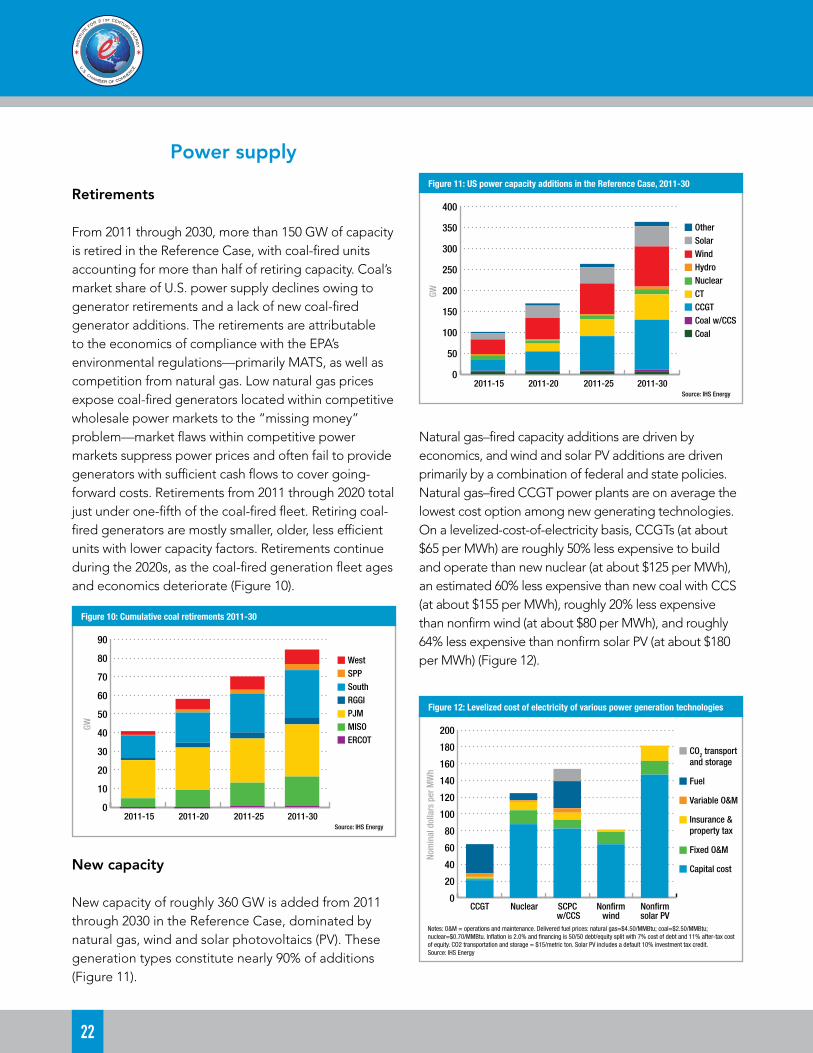
Power supply
Retirements
From 2011 through 2030, more than 150 GW of capacity is retired in the Reference Case, with coal-fired units accounting for more than half of retiring capacity. Coal’s market share of U.S. power supply declines owing to generator retirements and a lack of new coal-fired generator additions. The retirements are attributable to the economics of compliance with the EPA’s environmental regulations—primarily MATS, as well as competition from natural gas. Low natural gas prices expose coal-fired generators located within competitive wholesale power markets to the “missing money” problem—market flaws within competitive power markets suppress power prices and often fail to provide generators with sufficient cash flows to cover going-forward costs. Retirements from 2011 through 2020 total just under one-fifth of the coal-fired fleet. Retiring coal-fired generators are mostly smaller, older, less efficient units with lower capacity factors. Retirements continue during the 2020s, as the coal-fired generation fleet ages and economics deteriorate (Figure 10).
2011-15 2011-20 2011-25 2011-30
GW
Figure 10: Cumulative coal retirements 2011-30
Source: IHS Energy
0
10
20
30
40
50
60
70
80
90
West SPP South RGGI PJM MISO ERCOT
New capacity
New capacity of roughly 360 GW is added from 2011 through 2030 in the Reference Case, dominated by natural gas, wind and solar photovoltaics (PV). These generation types constitute nearly 90% of additions (Figure 11).
2011-15 2011-20 2011-25 2011-30
GW
Figure 11: US power capacity additions in the Reference Case, 2011-30
Source: IHS Energy
0
50
100
150
200
250
300
350
400
Other Solar Wind Hydro Nuclear CT CCGT Coal w/CCS Coal
Natural gas–fired capacity additions are driven by economics, and wind and solar PV additions are driven primarily by a combination of federal and state policies. Natural gas–fired CCGT power plants are on average the lowest cost option among new generating technologies. On a levelized-cost-of-electricity basis, CCGTs (at about $65 per MWh) are roughly 50% less expensive to build and operate than new nuclear (at about $125 per MWh), an estimated 60% less expensive than new coal with CCS (at about $155 per MWh), roughly 20% less expensive than nonfirm wind (at about $80 per MWh), and roughly 64% less expensive than nonfirm solar PV (at about $180 per MWh) (Figure 12).
Nom
inal
dol
lars
per
MW
h
Figure 12: Levelized cost of electricity of various power generation technologies
0
20
40
60
80
100
120
140
160
180
200
CO2 transportand storage Fuel Variable O&M Insurance & property tax Fixed O&M Capital cost
CCGT Nuclear SCPC Non�rm Non�rm w/CCS wind solar PV
Notes: O&M = operations and maintenance. Delivered fuel prices: natural gas=$4.50/MMBtu; coal=$2.50/MMBtu; nuclear=$0.70/MMBtu. In�ation is 2.0% and nancing is 50/50 debt/equity split with 7% cost of debt and 11% after-tax cost of equity. CO2 transportation and storage = $15/metric ton. Solar PV includes a default 10% investment tax credit.Source: IHS Energy

Assessing the Impact of Potential New Carbon Regulations in the United States
23
Although the costs of wind and solar generation have declined significantly in recent years, both continue to require policy support in the form of targets and incentives, particularly in the face of low natural gas prices. State RPSs remain the primary driver of U.S. renewables additions through 2025 (Figure 13). RPS policies are expected to remain stable, with renewables accounting for half or more of gross capacity additions through 2020. Over time, U.S. state RPSs are largely enforced and fulfilled, with target growth in some states counterbalanced by reductions in others (target reductions are the result of cost concerns and transmission limitations).
New wind turbine technology improves average capacity factors, which drives down unit production costs. Solar PV costs also decline an additional 30–35% through 2020, with slower annual reductions in the years that follow. No further federal policy for clean or renewable energy materializes in the
Reference Case. Recent Internal Revenue Service changes to the U.S. production tax credit for wind and other renewables, which expired at the end of 2013, allows projects coming online by the end of 2015 to capture the incentive. The 30% investment tax credit for commercial installations remains in effect through 2016, after which it reverts to a default 10% level. Demand for renewables in the later years of the Reference Case is driven by the increasing grid-competitiveness of wind and solar in regions with good to excellent resources.
Nuclear power continues to struggle within certain competitive market structures and in a lower natural gas price environment, though retirements remain modest. All existing nuclear units applying for a 20-year extension—beyond their current 40-year operating licenses—are successful. However, there are no new nuclear builds beyond the five units already under construction. With limited new builds and modest
Figure 13: US states with renewable portfolio standards
Source: IHS
Non-binding RPS
POLICY TYPE
Binding capacity target
Binding generation target
No RPS
Incentive-based, non-binding target
4 4
?

24
uprating of the existing fleet, nuclear’s capacity share declines from 10% in 2013 to about 9% in 2030. Consequently, nuclear’s generation share declines from about 20% in 2013 to roughly 17% in 2030.
Coal’s generation share declines from about 40% in 2013 to about 29% by 2030 in the Reference Case. Natural gas, wind, and solar pick up coal’s lost generation and capture the bulk of new power demand as well. In 2030, fossil fuels still account for about two-thirds of generation in the Reference Case and renewables gain a mainstream foothold of about 10% of generation (Figure 14). Despite the growing role for renewables, meaningful carbon emission reductions do not occur; in 2030 power sector CO2 emissions fall about 9% below 2005 levels (Figure 15).
TWh
Figure 14: US power sector electric generation mix in the Reference Case, 1980-2030
0
1000
2000
3000
4000
5000
6000
Other Solar Wind Hydro Nuclear Natural gas Coal
1980 1985 1990 1995 2000 2005 2010 2015 2020 2025 2030
Source: IHS Energy and US EIA
OUTLOOK
Mill
ion
met
ric to
ns
Figure 15: US power sector CO2 emissions in the Reference Case, 1980-2030
0
500
1000
1500
2000
2500
3000
Oil Natural gas Coal
Change from2005 levels:
2030-9%
1980 1985 1990 1995 2000 2005 2010 2015 2020 2025 2030
Source: IHS Energy and US EIA
OUTLOOK
Policy Case
As noted above, the Policy Case begins with the Reference Case and modifies it to include policies targeting CO2 emissions from existing generators and a tightening of the current EPA CO2 NSPS proposal in 2022 targeting new generators (Table 3), consistent with the NRDC Proposal structure carried out on a path intended to meet the Obama Administration’s international CO2 reduction goals.
These policies result in the changes summarized below (Tables 4 and 5). Detailed descriptions of the policy and resulting power sector changes are included in the sections that follow.
• Energy efficiency mandates and incentives lower U.S. power demand growth to a 1.2% per year compound annual growth rate (CAGR) in the Policy Case from 2013 to 2030—about 0.2% lower growth than in the Reference Case.
• Coal retirements from 2011 through 2030 total 199 GW in the Policy Case, an increase of roughly 114 GW compared with the Reference Case.
• New capacity built to replace retiring coal and to meet power demand growth is dominated by natural gas and renewables in the Policy Case, as in the Reference Case. However, with the implementation of tighter NSPS standards beginning in 2022, the new build mix shifts to a blend of CCGT with CCS, renewables, and a modest amount of nuclear capacity later in the analysis period (Table 5).
• The share of coal-fired generation declines from 40% in 2013 to 14% in 2030, while that of natural gas–fired generation increases from 27% to 46%.
• Power sector CO2 emissions decline roughly 40% below 2005 levels by 2030 in the Policy Case.

Assessing the Impact of Potential New Carbon Regulations in the United States
25
Table 3: CO2 policies modeled in the Policy Case
Policy Description
CO2 ESPS 2018-25 CO2 ESPS effective 2018 using structure proposed by NRDC
CO2 ESPS 2030+
Tightening CO2 emission standard in 2030, as an extension of the NRDC proposal (a tighter emission standard in 2030 was not
included in the NRDC proposal)ESPS effective 2018 (using structure proposed by NRDC through 2025) with an extension and tightened
standards in 2030 to meet Administration’s stated climate goals
California and RGGICA and RGGI programs continue through 2030 as compliance with
CO2 ESPS (same as Reference Case)
CO2 NSPS 2022+Tightening of CO2 NSPS effective 2022 requiring CCS for new coal-
fired and gas-fired generators
Table 4: Key power sector changes
US power demand growth CAGR 2014–30
Coal retirements 2011–30 (GW)
Power sector CO2 reduction 2030 over 2005
Average gas prices (real 2012$)
Reference Case 1.4% 85 9% 4.04
Policy Case 1.2% 199 40% 4.18
Table 5: Installed capacity and generation market share changes
Coal Gas Wind Solar Nuclear Hydro Other
Capacity additions2014-30 Reference Case (GW)
3 153 74 42 9 1 8
Capacity additions2014-30 Policy Case (GW)
3 216* 98 54 22 1 8
Fuel mix 2013 (%) 40% 27% 4% 0% 20% 7% 1%
Reference Case generation by fuel 2030 29% 38% 8% 2% 17% 5% 1%
Policy Case generation by fuel 2030 14% 46% 10% 3% 21% 6% 1%
*Includes 74 GW of CCGT with CCSNote: Totals may not equal 100% due to rounding
CO2 policies targeting existing generators
The Policy Case includes a CO2 ESPS policy targeting existing fossil fuel–fired generators. The CO2 ESPS is modeled after NRDC’s December 2012 proposal through 2025. Thus a blend of coal-fired generator retirements and incremental investments in demand-side energy efficiency measures and renewable generation contribute to compliance with the emission rate targets listed in Table 7. Power demand continues to grow at a lower rate in the Policy Case than in the Reference Case, as described below. New natural gas–fired generators replace retired coal generators as well as meet power
demand growth. As a result, the CO2 ESPS, as outlined in the NRDC Proposal, does not achieve the power sector’s 42% share CO2 emission reduction goal.
In light of the emissions reduction shortfall, the Policy Case also includes an extension of the CO2 ESPS with a further tightening of existing generator emissions targets in 2030. More specifically, NRDC’s 2025 national average emission rate benchmarks for coal-fired and natural gas/oil-fired power plants are held constant through 2029, with a further lowering in 2030 of the coal benchmark from 1,200 lb per MWh to 1,000 lb per MWh. The natural gas/oil benchmark was held

26
constant at 1,000 lb per MWh, effectively creating a uniform national fossil fuel emission rate target.
Consistent with NRDC’s own analysis, with the exception of California and the RGGI states, the
remaining states form tradable performance standard programs at a regional level based on the geographic footprint of existing U.S. power market independent system operator (ISO) and regional transmission organization boundaries (Figure 16 and Table 6).
Table 6: Policy Case CO2 ESPS trading regions
Trading region Definition Compliance mechanism
California State of CaliforniaEvolution of existing state policies
RGGI RGGI states
ERCOT ERCOT ISO
Tradable performance standard
MISOMidcontinent ISO
(including all of Delta NERC subregion )
PJMPJM ISO
(excluding DE and MD)
SouthUS South not covered by an ISO
(including SE, VACAR, FRCC, and Central)
SPPSPP ISO
(including portions of MRO not assigned to an ISO)
WestUS West not covered by an ISO
(including Desert SW, RMPA, NWPP, and Basin)
Figure 16: Policy Case CO2 ESPS trading regions
Source: IHS Energy
Mid-Continent
ERCOT
SPP
West
PJM
MISO
RGGI
South
California
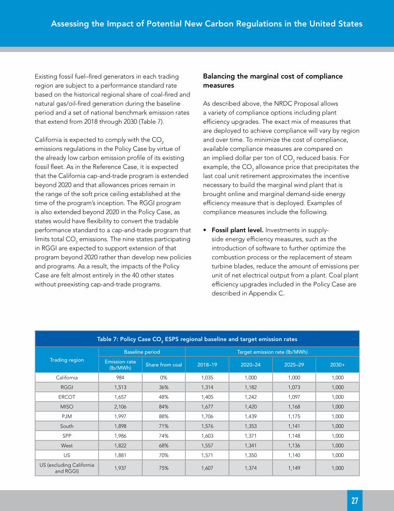
Assessing the Impact of Potential New Carbon Regulations in the United States
27
Existing fossil fuel–fired generators in each trading region are subject to a performance standard rate based on the historical regional share of coal-fired and natural gas/oil-fired generation during the baseline period and a set of national benchmark emission rates that extend from 2018 through 2030 (Table 7).
California is expected to comply with the CO2 emissions regulations in the Policy Case by virtue of the already low carbon emission profile of its existing fossil fleet. As in the Reference Case, it is expected that the California cap-and-trade program is extended beyond 2020 and that allowances prices remain in the range of the soft price ceiling established at the time of the program’s inception. The RGGI program is also extended beyond 2020 in the Policy Case, as states would have flexibility to convert the tradable performance standard to a cap-and-trade program that limits total CO2 emissions. The nine states participating in RGGI are expected to support extension of that program beyond 2020 rather than develop new policies and programs. As a result, the impacts of the Policy Case are felt almost entirely in the 40 other states without preexisting cap-and-trade programs.
Balancing the marginal cost of compliance measures
As described above, the NRDC Proposal allows a variety of compliance options including plant efficiency upgrades. The exact mix of measures that are deployed to achieve compliance will vary by region and over time. To minimize the cost of compliance, available compliance measures are compared on an implied dollar per ton of CO2 reduced basis. For example, the CO2 allowance price that precipitates the last coal unit retirement approximates the incentive necessary to build the marginal wind plant that is brought online and marginal demand-side energy efficiency measure that is deployed. Examples of compliance measures include the following.
• Fossil plant level. Investments in supply-side energy efficiency measures, such as the introduction of software to further optimize the combustion process or the replacement of steam turbine blades, reduce the amount of emissions per unit of net electrical output from a plant. Coal plant efficiency upgrades included in the Policy Case are described in Appendix C.
Table 7: Policy Case CO2 ESPS regional baseline and target emission rates
Trading region
Baseline period Target emission rate (lb/MWh)
Emission rate (lb/MWh) Share from coal 2018–19 2020–24 2025–29 2030+
California 984 0% 1,035 1,000 1,000 1,000
RGGI 1,513 36% 1,314 1,182 1,073 1,000
ERCOT 1,657 48% 1,405 1,242 1,097 1,000
MISO 2,106 84% 1,677 1,420 1,168 1,000
PJM 1,997 88% 1,706 1,439 1,175 1,000
South 1,898 71% 1,576 1,353 1,141 1,000
SPP 1,986 74% 1,603 1,371 1,148 1,000
West 1,822 68% 1,557 1,341 1,136 1,000
US 1,881 70% 1,571 1,350 1,140 1,000
US (excluding California and RGGI)
1,937 75% 1,607 1,374 1,149 1,000

28
• Fossil portfolio level. Shifting the share of generation from more carbon intensive (e.g., coal-fired) to less carbon intensive (e.g., natural gas–fired) power plants, including retiring the most carbon intensive plants, lowers the emission rate from the existing fossil fleet as a whole. In practice, a tradable performance standard would accomplish this “shift” by imposing an additional variable cost on generating units whose emission rate was above the applicable emission rate target in that region and by providing a credit to generating units whose emission rate was below the emission rate target, thereby altering the merit order in favor of dispatching less carbon intensive fossil units ahead of more carbon intensive units.
• Power sector level. Giving credit for incremental renewable generation and energy efficiency savings allows generators to get part way to their target by reducing their fossil emission rate and then bridge the rest of the gap with credits from incremental energy efficiency and renewables. Fossil plant owners also have the ability to purchase excess allowances from generators that are long on allowances and/or bank excess allowances (generated by their own portfolio or someone else’s) for use in future years.
The compliance flexibility described above translates into a larger role for energy efficiency and renewable power in the Policy Case as compared to the Reference Case. However, despite the flexibility included in the NRDC Proposal, meeting increasingly stringent fossil emission rate targets ultimately requires the retirement of a large portion of existing U.S. coal-fired power plants.
CO2 policies targeting new generators
Because regulation of existing power plants alone will not achieve the Obama Administration’s target for CO2 emission reductions, under the Policy Case the EPA is forced to revise its CO2 NSPS to require new natural gas–fired power plants to implement CCS beginning in 2022. This changes the relative competitiveness of
alternative generating technologies, resulting in a more diverse mix of new capacity additions than under the Reference Case, thereby threatening natural gas–fired generation’s dominance in the power sector. Specifically, adding CCS to natural gas–fired CCGT plants can more than double their construction cost, and increases their total production costs by about 60%.12
Because regulation of existing power plants alone will not achieve the Obama Administration’s target for CO2 emission reductions, under the Policy Case the EPA is forced to revise its CO2 NSPS to require new natural gas–fired power plants to implement CCS beginning in 2022.
Even with aggressive implementation of these costly compliance measures, reducing U.S. power sector CO2 emissions to 42% below 2005 levels by 2030 would be a tall order. The NRDC report implies that such a target could be achieved almost exclusively by regulating the CO2 emission rate of existing fossil fuel–fired power plants and by creating an incentive for incremental renewables and energy efficiency. However, a more realistic outlook on the potential impact of energy efficiency (i.e., one that does not lead to negative load growth at the U.S. aggregate level) suggests that a large amount of new generating capacity, made up significantly of natural gas–fired power plants, will be required both to fill in for retiring coal plants and to meet incremental load growth. It is on this basis that the Policy Case includes the additional assumption that EPA will inevitably limit CO2 emissions from all new fossil fuel–fired power plants. Specifically, EPA revisits its existing CO2 NSPS rule, consistent with the CAA’s mandatory look-back provision, and chooses to revise the CO2 emission rate targets for both new coal- and natural gas–fired power plants. The rates EPA establishes require all new fossil
12 Due to the fact that electric power sector CCS is not yet commercially proven for either coal- or natural gas-fired generation types, there is enhanced high-side cost risk associated with these technologies.

Assessing the Impact of Potential New Carbon Regulations in the United States
29
fuel–fired power plants that operate above a 33% capacity factor to capture and store roughly 90% of their CO2 emissions beginning in 2022.
Electricity demand and energy efficiency
Investments in energy efficiency are increased in the Policy Case. Electricity demand grows more slowly nationally and in most regions under the Policy Case as compared to the Reference Case (Figure 17). Nationally, increased investment in demand-side energy efficiency measures slows the growth rate of electricity demand by 0.2% per year over 2013–30, reducing it from 1.4% per year in the Reference Case to 1.2% per year in the Policy Case.
It is not feasible to assume, as NRDC did, that all states are able to scale to achieve best-in-class 2.0% per year savings levels on an ongoing basis.
This outlook for incremental energy efficiency investment is significantly lower than what NRDC assumed in its analysis. Based on an assessment of the cost of energy efficiency measures, which is described below, and an analysis of the current lack of complementary policies, it is not feasible to assume, as NRDC did, that all states are able to scale to achieve best-in-class 2.0% per year savings levels on an ongoing basis. In fact, to date Vermont is the only state that has achieved 2.0% per year savings, and replicating this performance is unlikely in all other places.
This analysis estimates that the levelized cost of demand-side energy efficiency to a utility is currently about $50 per MWh and escalates to $60–65 per MWh by 2030 in the Policy Case. This estimate was developed based on a cross-sectional regression analysis of 2012 U.S. state-level electricity demand. It
is consistent with the range cited in recent literature.13 Utility costs account for roughly 55% of the total cost, yielding a total levelized cost of demand-side energy efficiency of $90 per MWh today, escalating to $110–120 per MWh in 2030.
Com
poun
d an
nual
gro
wth
rate
Figure 17: Growth rate of electricity sales in the Reference Case and Policy Case, 2013-30
CA ERCOT MISO PJM RGGI South SPP West US
Source: IHS Energy
0.0%
0.2%
0.4%
0.6%
0.8%
1.0%
1.2%
1.4%
1.6%
1.8%
2.0%
Reference Case Policy Case
In practice, other factors are likely to come into play that influence the mix of resources. The amount of incremental wind or solar that gets deployed in competitive power markets, for instance, will depend on the ability of developers to enter into long-term contracts to sell the electricity from their projects. Likewise, the amount of incremental efficiency that gets deployed will depend on whether policies already exist at the state level, such as energy efficiency resource standards and/or decoupling, to encourage utilities to invest in demand-side energy efficiency or at least make them indifferent between investing in efficiency and building new supply.
Fuel markets
In the Policy Case, natural gas demand from the electric power sector grows from roughly 27 Bcf per day in 2018 to about 48 Bcf per day in 2030 in the U.S. Lower 48 at a CAGR of 4.5%. This represents a substantial acceleration of growth in power sector
13 Arimuri et al. 2011. Cost-Effectiveness of Electricity Energy Efficiency Programs. Resources for the Future Discussion Paper.

30
natural gas demand; demand from power generation grew at a CAGR of 3.4% from 2010 to 2013.
Gas demand from the electric sector increases at the fastest rate between 2017 and 2022 in the Policy Case, with year-over-year absolute growth of more than 3 Bcf per day from 2018 to 2021, the result of the substantial coal retirements discussed above. This pace of demand growth outstrips market expectations, challenging the upstream sector and boosting natural gas prices to levels that incentivize additional drilling. After 2021, when demand growth returns to more manageable levels, natural gas prices return closer to the long-term production cost. Figure 18 shows annual average natural gas prices for the Policy Case and the Reference Case.
Real
201
2 US
dol
lars
per
MM
Btu
Figure 18: Henry Hub natural gas prices in the Reference Case and Policy Case, 2014-30
2014 2015 2016 2017 2018 2019 2020 2021 2022 2023 2024 2025 2026 2027 2028 2029 2030
Source: IHS Energy
2
3
4
5
6
Policy Case Reference Case
Power supply
Coal unit retirements
As in the Reference Case, in the Policy Case retirements in the coal fleet increase and coal’s share of U.S. generation through the middle part of the current decade declines as a result of the economics of compliance with EPA’s environmental regulations—primarily MATS—and the missing money problem in competitive power markets.
Implementation of the CO2 ESPS regulation in 2018 results in substantial immediate coal generator retirements in coal-heavy regions, including MISO and the South. By 2025, all regions must retire coal generators to comply with the emission standard. Incremental coal retirements at the national level total 114 GW by 2030 in the Policy Case, as compared with the Reference Case (Figures 19 and 20). Over the course of two decades, from 2011 through 2030, a total of about 199 GW, or roughly 60% of the coal fleet, is retired in the Policy Case owing to the combination of non-carbon EPA regulations and the CO2 regulations. This compares with about 85 GW of retirements during the same period in the Reference Case. By 2030 about 126 GW of coal remains operational in the Policy Case.
Over the course of two decades, from 2011 through 2030, a total of about 199 GW, or roughly 60% of the coal fleet, is retired in the Policy Case owing to the combination of non-carbon EPA regulations and the CO2 regulations.
With the implementation of the existing generator standard in the Policy Case, some coal-fired generators will choose efficiency upgrade projects as a means of compliance in the early years of the policy, provided the projects have a reasonably short payback period.14
14 See Appendix C for a discussion of potential investments in coal unit efficiency upgrades.

Assessing the Impact of Potential New Carbon Regulations in the United States
31
2011-15 2011-20 2011-25 2011-30
GW
Figure 19: Cumulative coal retirements, 2011-30
Source: IHS Energy
0
20
40
60
80
100
120
140
160
180
200
West SPP South RGGI PJM MISO ERCOT
ReferencePolicy
GW
Figure 20: Installed coal-�red generating capacity in the Reference Case and Policy Case, 2010-30
2010 2015 2020 2025 2030
Source: IHS Energy
0
50
100
150
200
250
300
350
Reference Case Policy Case
OUTLOOK
Capacity additions
A total of approximately 475 GW of new capacity is added in the Policy Case from 2011 through 2030, a roughly 100 GW increase compared to the Reference Case. As in the Reference Case, natural gas, wind, and solar account for roughly 90% of the capacity additions.
The Policy Case requirement that new CCGTs implement CCS, however, significantly alters the competitive landscape beginning in 2022, lowering the economic bar for alternative forms of dispatchable and nondispatchable generating technologies (Figure 21). New CCGTs with CCS are assumed to cost roughly $100 per MWh, roughly 60% more than CCGTs without CCS. It is important to note that CCS is a frontier technology and that the cost and performance of CCS is highly uncertain; the risk for
costs higher than assumed in the Policy Case and for performance problems is substantial. Considering the significant technology risks, investments in alternatives to CCGT with CCS, including nuclear, become highly likely, particularly in the later years of the analysis period.
Nom
inal
dol
lars
per
MW
h
Figure 21: Levelized cost of electricity of various power generation technologies
0
20
40
60
80
100
120
140
160
180
200
CO2 transportand storage Fuel Variable O&M Insurance & property tax Fixed O&M Capital cost
CCGT CCGT Nuclear SCPC Non�rm Non�rm w/CCS w/CCS wind solar PV
Notes: Delivered fuel prices: natural gas=$4.50/MMBtu; coal=$2.50/MMBtu; nuclear=$0.70/MMBtu. In�ation is 2.0% and �nancing is 50/50 debt/equity split with 7% cost of debt and 11% after-tax cost of equity. CO2 transportation and storage = $15/metric ton. Solar PV includes a default 10% investment tax credit.Source: IHS Energy
The change in the relative competitiveness of alternative generating technologies, along with the difficulty of building and operating power plants with CCS in certain regions of the country (i.e., the Northeast and Southeast, among other regions remote from suitable geologic storage sites), results in a different mix of new capacity additions than in the Reference Case over 2022–30. During this period, an additional 33 GW of renewable capacity and 13 GW of new nuclear capacity are installed over that in the Reference Case (Figures 22 and 23). Additional renewable capacity additions are driven by a combination of the change in the relative cost of CCGT-based generation and by the value of the CO2 credits that incremental renewables are eligible to receive under EPA’s tradable performance standard program for existing sources. It is important to note that the addition of typically intermittent renewable resources does not provide many of the beneficial reliability attributes that are offered by fossil- and nuclear-fueled dispatchable generation capacity. Additional nuclear capacity is composed primarily of uprates at existing facilities and several projects currently pursuing a combined construction

32
and operating license from the U.S. Nuclear Regulatory Commission that are located in regulated states. Owing to nuclear’s long construction cycle, the majority of new additions do not come online until late in the 2020s.
2011-15 2011-20 2011-25 2011-30
GW
Figure 22: US power capacity additions in the Reference Case and Policy Case, 2011-30
Source: IHS Energy
0
50
100
150
200
250
300
350
400
450
500
ReferencePolicy
Other Solar Wind Hydro Nuclear CT CCGT w/CCS CCGT Coal w/CCS Coal
As described above, the U.S. power sector retires a large proportion of its base-load coal-fired generation fleet, invests in renewable power and demand-side energy efficiency, and adopts expensive and risky low-carbon generation technology in the Policy Case to comply with CO2 regulations. These actions result in a 40% reduction in power sector CO2 emissions from
2005 levels in 2030 (Figure 24).
Compliance under the tighter NSPS is straightforward in the Policy Case, as fossil fuel–fired additions, with a capacity factor exceeding about 33%, built as of 2022 include CCS. Compliance with CO2 ESPS regulations requires more analysis and description.
Under the Policy case, the U.S. (excluding California and the RGGI states) fossil fuel emission rate and the compliance emission rate decline significantly over time (Figure 25). The fossil fuel emission rate declines 18% in the Policy Case versus 4% in the Reference Case over 2018–30. The compliance emission rate, as calculated in the formula discussed above and repeated for convenience below, declines 38% over the same period, reaching 1,000 lb per MWh by 2030. The greater degree of decline in the compliance emission rate versus the fossil emission rate is a result of the additional credit from incremental renewable generation, and, to a lesser extent, energy efficiency savings.
Compliance emission rate CO2 emissions from existing fossil gen. (lb)
existing fossil gen. + incremental renewables gen. + incremental efficiency savings (MWh)
TWh
Figure 23: US power sector electric generation mix in the Policy Case, 1980-2030
Other
Solar
Wind
Hydro
Nuclear
Natural gas
Coal
10%6%
21%
46%
14%
8%5%
17%
38%
29%
1980 1985 1990 1995 2000 2005 2010 2015 2020 2025 2030
Source: IHS Energy and US EIA
0
1000
2000
3000
4000
5000
6000
OUTLOOK
2030Reference Case

Assessing the Impact of Potential New Carbon Regulations in the United States
33
mill
ion
met
ric to
ns
Figure 24: US power sector CO2 emissions in the Policy Case, 1980-30
Oil
Natural gas
Coal
1980 1985 1990 1995 2000 2005 2010 2015 2020 2025 2030
Source: IHS Energy and US EIA
0
500
1000
1500
2000
2500
3000
2030Reference Case
2030-9%
2030-40%
Change from 2005 levels:OUTLOOK
In total, the U.S. compliance emission rate declines about 940 lb per MWh below baseline period emission levels by 2030 under the Policy Case. Roughly 16% of the reduction is attributable to the decline in the fossil emission rate that would have occurred in the Reference Case, absent a federal carbon policy (Figure 26). This reduction is due primarily to retirements that have already occurred or are likely to occur in response to EPA’s MATS rule and competition from natural gas. A further 35% of the reduction is from a decline in the fossil emission rate due to coal plant retirements and coal-to-natural gas redispatch. Another 35% is due to incremental renewable generation above baseline period levels. And finally, the remaining 14% of the reduction is due to incremental savings from demand-side energy efficiency.
The relative contribution of each source of reduction in the compliance emission rate varies considerably from region to region. At one extreme, in South, about 30% of the reduction is due to a decline in the fossil emission rate that would have occurred anyway in the Reference Case. However, owing to that region’s relatively poor endowment of wind resources and its current lack of state-level energy efficiency policies, South is required to meet 46% of its total reduction
in compliance emission rate through coal plant retirements and coal-to-natural gas redispatch.
800
1000
1200
1400
1600
1800
2000
2200
2008 2010 2012 2014 2016 2018 2020 2022 2024 2026 2028 2030
lb/M
Wh
Figure 25: US* fossil and compliance CO2 emission rates, 2008-30
OUTLOOK
Baseline period emission rate Policy Case fossil emission rate
Reference Case fossil emission rate Policy Case compliance emission rate
* The US CO2 emission rates exclude California and RGGI since they are assumed to rely on existing programs in lieu of a federal model rule.Source: IHS Energy
At the other extreme is the neighboring Southwest Power Pool (SPP) which, like South, relied on coal-fired generation for a little over 70% of fossil fuel–fired generation in the baseline period and thus is required to achieve a similar level of emission rate reduction. Unlike in South, absent a federal carbon policy the

34
fossil emission rate in SPP declines by only 2% below baseline period levels by 2030. However, owing to the availability of strong wind resources in SPP, incremental renewables account for 61% of the total reduction in compliance emission rate. As a result, coal retirements and coal-to-natural gas redispatch contribute only 27% of the reduction in compliance emission rate, proportionally less than in South.
ERCOT MISO PJM South SPP West US*
Figure 26: Elements of compliance in the Policy Case, 2030
0%
10%
20%
30%
40%
50%
60%
70%
80%
90%
100%
Energy ef�ciency Renewables
Coal retirements and coal-to-gas redispatch
Reductions in Reference case
* The US CO2 emission rates exclude California and RGGI since they are assumed to rely on existing programs in lieu of a federal model rule.Source: IHS Energy
9% 11% 23% 17% 10% 10% 14%
44% 44% 30%
7%
61% 52%
35%
43%
34% 26%
46%
27%
28%
35%
4% 11% 21%
30%
2% 10% 16%
Cost of compliance for the U.S. power sector
Achieving compliance with the CO2 regulations included in the Policy Case will have cost implications for the power sector and impacts on the overall U.S. economy. In particular, the Policy Case CO2 ESPS precipitates significant unproductive deployment of capital by causing the noneconomic retirement of coal-fired power generators. An economically efficient coal unit retirement occurs when the going-forward costs of the plant exceed the expected revenue. In the Policy Case, the U.S. power sector prematurely retires 114 GW of coal capacity, or nearly 40% of the coal capacity operational in 2013, and replaces it with new generating resources, primarily a blend of CCGT and renewables. When added to the coal retirements resulting from competition from natural gas and the MATS rule this decade, roughly 60% of the U.S. coal fleet, some 199 GW, will retire by 2030 in the Policy Case.
Replacing retiring coal generators comes at a cost. Further, replacing retiring coal and meeting incremental power demand growth with CCGT capacity through 2030 is incompatible with a goal of reducing power sector emissions by 42% from 2005 levels. Thus the total bill for the power sector is increased by a need to deploy nearly carbon-free
Table 8: Incremental costs: Policy Case as compared with Reference Case
Incremental cost item Total incremental cost 2014-30 ($billion, real 2012$)
Power plant construction 339
Electric transmission 16
Natural gas infrastructure 23
CCS pipelines 25
Coal plant decommissioning 8
Coal unit efficiency upgrades 3
Coal unit stranded costs 30
Demand-side energy efficiency 106
Operations and maintenance costs -5
Fuel costs -66
Total incremental costs 478
Source: IHS EnergyNote: Please see Appendix C for power generation addition unit costs and more detail on the calculation of natural gas pipelines, transmission, CCS pipelines, coal plant decommissioning, and coal unit stranded assets.
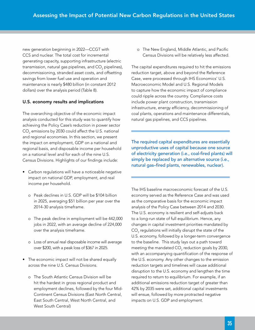
Assessing the Impact of Potential New Carbon Regulations in the United States
35
new generation beginning in 2022—CCGT with CCS and nuclear. The total cost for incremental generating capacity, supporting infrastructure (electric transmission, natural gas pipelines, and CO2 pipelines), decommissioning, stranded asset costs, and offsetting savings from lower fuel use and operation and maintenance is nearly $480 billion (in constant 2012 dollars) over the analysis period (Table 8).
U.S. economy results and implications
The overarching objective of the economic impact analysis conducted for this study was to quantify how achieving the Policy Case’s reduction in power sector CO2 emissions by 2030 could affect the U.S. national and regional economies. In this section, we present the impact on employment, GDP on a national and regional basis, and disposable income per household on a national level and for each of the nine U.S. Census Divisions. Highlights of our findings include:
• Carbon regulations will have a noticeable negative impact on national GDP, employment, and real income per household.
o Peak declines in U.S. GDP will be $104 billion in 2025, averaging $51 billion per year over the 2014-30 analysis timeframe.
o The peak decline in employment will be 442,000 jobs in 2022, with an average decline of 224,000 over the analysis timeframe.
o Loss of annual real disposable income will average over $200, with a peak loss of $367 in 2025.
• The economic impact will not be shared equally across the nine U.S. Census Divisions.
o The South Atlantic Census Division will be hit the hardest in gross regional product and employment declines, followed by the four Mid-Continent Census Divisions (East North Central, East South Central, West North Central, and West South Central)
o The New England, Middle Atlantic, and Pacific Census Divisions will be relatively less affected.
The capital expenditures required to hit the emissions reduction target, above and beyond the Reference Case, were processed through IHS Economics’ U.S. Macroeconomic Model and U.S. Regional Models to capture how the economic impact of compliance could ripple across the country. Compliance costs include power plant construction, transmission infrastructure, energy efficiency, decommissioning of coal plants, operations and maintenance differentials, natural gas pipelines, and CCS pipelines.
The required capital expenditures are essentially unproductive uses of capital because one source of electricity generation (i.e., coal-fired plants) will simply be replaced by an alternative source (i.e., natural gas–fired plants, renewables, nuclear).
The IHS baseline macroeconomic forecast of the U.S. economy served as the Reference Case and was used as the comparative basis for the economic impact analysis of the Policy Case between 2014 and 2030. The U.S. economy is resilient and self-adjusts back to a long-run state of full equilibrium. Hence, any changes in capital investment priorities mandated by CO2 regulations will initially disrupt the state of the U.S. economy, followed by a longer-term convergence to the baseline. This study lays out a path toward meeting the mandated CO2 reduction goals by 2030, with an accompanying quantification of the response of the U.S. economy. Any other changes to the emission reduction targets and timelines will cause additional disruption to the U.S. economy and lengthen the time required to return to equilibrium. For example, if an additional emissions reduction target of greater than 42% by 2035 were set, additional capital investments will ensue, followed by more protracted negative impacts on U.S. GDP and employment.

36
On a regional level, each U.S. Census Division will follow a different path to equilibrium dictated by the transformation required to bring regional generation fleets into compliance. Those areas forced to absorb the costs of retiring and replacing many coal-fired plants, such as the South Atlantic Census Division, will experience the deepest economic impact. In contrast, the New England Census Division will need substantially less compliance-mandated investment and will emerge relatively unscathed; not because RGGI is cost free, but rather because the burdens of RGGI already are accounted for within the Reference Case.
As discussed earlier in this report, the proposed CO2 regulations will accelerate the shift from coal to other fuel sources, primarily natural gas, but also renewables and nuclear power. Perhaps the most readily apparent by-product of the shift away from coal-fired generation is that much of the compliance costs will be passed on to consumers via higher electricity prices. Higher electricity prices take money out of consumers’ wallets, absorbing a larger portion of the disposable income (income after taxes) they draw from to pay for essential
expenses such as mortgages, food and utilities. This, in turn, affects consumer behavior, forcing reductions in discretionary spending as consumers forgo some purchases and/or lower their household savings rates. The rising costs of electricity also will be felt most acutely by those in lower income brackets.
In addition to absorbing modestly higher electricity prices into its cost structures, industrial sector production in the United States will decline under the Policy Case.
More significant, however, are the opportunity costs associated with reaching the emissions reduction target by 2030. The required capital expenditures are essentially unproductive uses of capital because one source of electricity generation (i.e., coal-fired plants) will simply be replaced by an alternative source
2014-20 2014-25 2014-30
Billi
ons
of R
eal 2
012
Dolla
rs
Source: IHS Energy
0
50
100
150
200
250
300
350
California
West
SPP
South
RGGI
PJM
MISO
ERCOT
Figure 27: Cumulative change in electric bills (real 2012$)
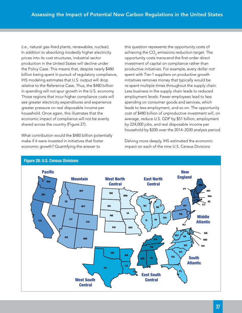
Assessing the Impact of Potential New Carbon Regulations in the United States
37
(i.e., natural gas–fired plants, renewables, nuclear). In addition to absorbing modestly higher electricity prices into its cost structures, industrial sector production in the United States will decline under the Policy Case. This means that, despite nearly $480 billion being spent in pursuit of regulatory compliance, IHS modeling estimates that U.S. output will drop relative to the Reference Case. Thus, the $480 billion in spending will not spur growth in the U.S. economy. Those regions that incur higher compliance costs will see greater electricity expenditures and experience greater pressure on real disposable income per household. Once again, this illustrates that the economic impact of compliance will not be evenly shared across the country (Figure 27).
What contribution would the $480 billion potentially make if it were invested in initiatives that foster economic growth? Quantifying the answer to
this question represents the opportunity costs of achieving the CO2 emissions reduction target. The opportunity costs transcend the first-order direct investment of capital on compliance rather than productive initiatives. For example, every dollar not spent with Tier-1 suppliers on productive growth initiatives removes money that typically would be re-spent multiple times throughout the supply chain. Less business in the supply chain leads to reduced employment levels. Fewer employees lead to less spending on consumer goods and services, which leads to less employment, and so on. The opportunity cost of $480 billion of unproductive investment will, on average, reduce U.S. GDP by $51 billion, employment by 224,000 jobs, and real disposable income per household by $200 over the 2014–2030 analysis period.
Delving more deeply, IHS estimated the economic impact on each of the nine U.S. Census Divisions
Figure 28: U.S. Census Divisions
ND
SD
NE
KS
MN
IA
WI MI
IL OH
IN
NV
ID
MT
WY
CO UT
AZ NM
OR
WA
CA
VT
ME
NH
MA
RI CT NY
NJ
PA
MO
TX
AR
LA
OK
VA
GA
FL
WV DE
MD
DC
SC
NC
AL
TN
MS
KY
Paci�c
Mountain West North Central
East North Central
West South Central
East South Central
South Atlantic
Middle Atlantic
New England
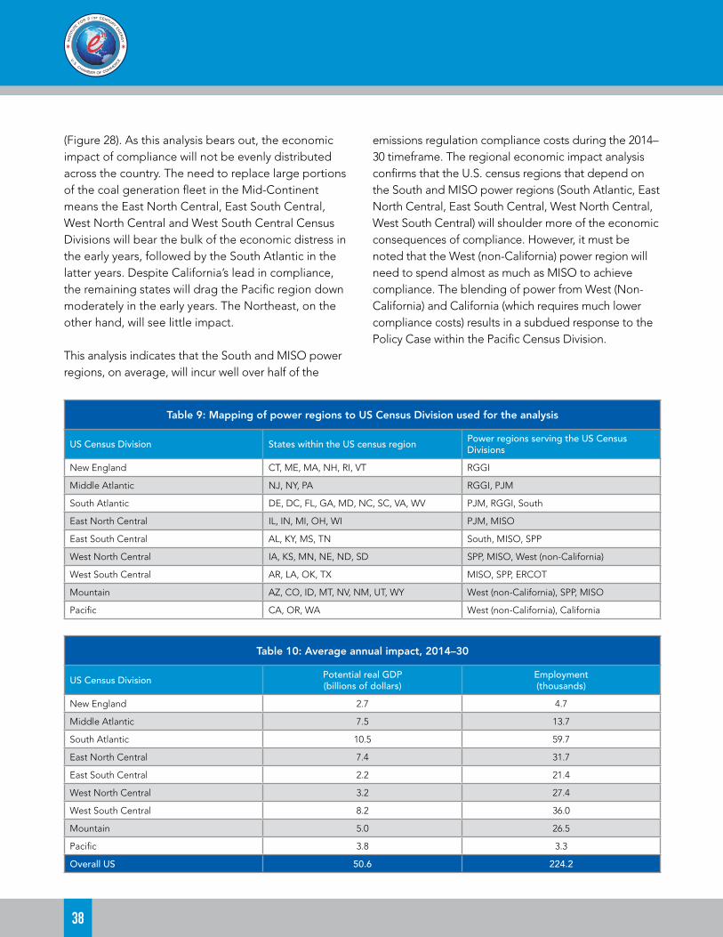
38
(Figure 28). As this analysis bears out, the economic impact of compliance will not be evenly distributed across the country. The need to replace large portions of the coal generation fleet in the Mid-Continent means the East North Central, East South Central, West North Central and West South Central Census Divisions will bear the bulk of the economic distress in the early years, followed by the South Atlantic in the latter years. Despite California’s lead in compliance, the remaining states will drag the Pacific region down moderately in the early years. The Northeast, on the other hand, will see little impact.
This analysis indicates that the South and MISO power regions, on average, will incur well over half of the
emissions regulation compliance costs during the 2014–30 timeframe. The regional economic impact analysis confirms that the U.S. census regions that depend on the South and MISO power regions (South Atlantic, East North Central, East South Central, West North Central, West South Central) will shoulder more of the economic consequences of compliance. However, it must be noted that the West (non-California) power region will need to spend almost as much as MISO to achieve compliance. The blending of power from West (Non-California) and California (which requires much lower compliance costs) results in a subdued response to the Policy Case within the Pacific Census Division.
Table 9: Mapping of power regions to US Census Division used for the analysis
US Census Division States within the US census region Power regions serving the US Census Divisions
New England CT, ME, MA, NH, RI, VT RGGI
Middle Atlantic NJ, NY, PA RGGI, PJM
South Atlantic DE, DC, FL, GA, MD, NC, SC, VA, WV PJM, RGGI, South
East North Central IL, IN, MI, OH, WI PJM, MISO
East South Central AL, KY, MS, TN South, MISO, SPP
West North Central IA, KS, MN, NE, ND, SD SPP, MISO, West (non-California)
West South Central AR, LA, OK, TX MISO, SPP, ERCOT
Mountain AZ, CO, ID, MT, NV, NM, UT, WY West (non-California), SPP, MISO
Pacific CA, OR, WA West (non-California), California
Table 10: Average annual impact, 2014–30
US Census Division Potential real GDP (billions of dollars)
Employment(thousands)
New England 2.7 4.7
Middle Atlantic 7.5 13.7
South Atlantic 10.5 59.7
East North Central 7.4 31.7
East South Central 2.2 21.4
West North Central 3.2 27.4
West South Central 8.2 36.0
Mountain 5.0 26.5
Pacific 3.8 3.3
Overall US 50.6 224.2
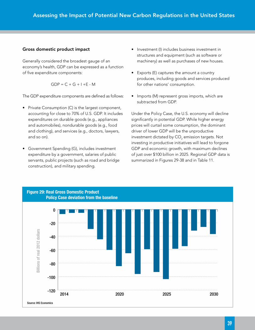
Assessing the Impact of Potential New Carbon Regulations in the United States
39
-120
-100
-80
-60
-40
-20
0
Billi
ons
of re
al 2
012
dolla
rs
Figure 29: Real Gross Domestic Product Policy Case deviation from the baseline
Source: IHS Economics
2014 2020 2025 2030
Gross domestic product impact
Generally considered the broadest gauge of an economy’s health, GDP can be expressed as a function of five expenditure components:
GDP = C + G + I +E - M
The GDP expenditure components are defined as follows:
• Private Consumption (C) is the largest component, accounting for close to 70% of U.S. GDP. It includes expenditures on durable goods (e.g., appliances and automobiles), nondurable goods (e.g., food and clothing), and services (e.g., doctors, lawyers, and so on).
• Government Spending (G), includes investment expenditure by a government, salaries of public servants, public projects (such as road and bridge construction), and military spending.
• Investment (I) includes business investment in structures and equipment (such as software or machinery) as well as purchases of new houses.
• Exports (E) captures the amount a country produces, including goods and services produced for other nations’ consumption.
• Imports (M) represent gross imports, which are subtracted from GDP.
Under the Policy Case, the U.S. economy will decline significantly in potential GDP. While higher energy prices will curtail some consumption, the dominant driver of lower GDP will be the unproductive investment dictated by CO2 emission targets. Not investing in productive initiatives will lead to forgone GDP and economic growth, with maximum declines of just over $100 billion in 2025. Regional GDP data is summarized in Figures 29-38 and in Table 11.
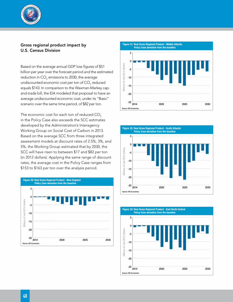
40
-25
-20
-15
-10
-5
0
5
2014 2020 2025 2030
Figure 32: Real Gross Regional Product - South Atlantic Policy Case deviation from the baseline
Source: IHS Economics
Billi
ons
of re
al 2
012
dolla
rs
-25
-20
-15
-10
-5
0
5
2014 2020 2025 2030
Figure 33: Real Gross Regional Product - East North Central Policy Case deviation from the baseline
Source: IHS Economics
Billi
ons
of re
al 2
012
dolla
rs
-25
-20
-15
-10
-5
0
5
2014 2020 2025 2030
Billi
ons
of re
al 2
012
dolla
rs
Figure 31: Real Gross Regional Product - Middle Atlantic Policy Case deviation from the baseline
Source: IHS Economics
Gross regional product impact by U.S. Census Division
Based on the average annual GDP loss figures of $51 billion per year over the forecast period and the estimated reduction in CO2 emissions to 2030, the average undiscounted economic cost per ton of CO2 reduced equals $143. In comparison to the Waxman-Markey cap-and-trade bill, the EIA modeled that proposal to have an average undiscounted economic cost, under its “Basic” scenario over the same time period, of $82 per ton.
The economic cost for each ton of reduced CO2 in the Policy Case also exceeds the SCC estimates developed by the Administration’s Interagency Working Group on Social Cost of Carbon in 2013. Based on the average SCC from three integrated assessment models at discount rates of 2.5%, 3%, and 5%, the Working Group estimated that by 2030, the SCC will have risen to between $17 and $82 per ton (in 2012 dollars). Applying the same range of discount rates, the average cost in the Policy Case ranges from $153 to $163 per ton over the analysis period.
-25
-20
-15
-10
-5
0
5
2014 2020 2025 2030
Figure 30: Real Gross Regional Product - New England Policy Case deviation from the baseline
Source: IHS Economics
Billi
ons
of re
al 2
012
dolla
rs
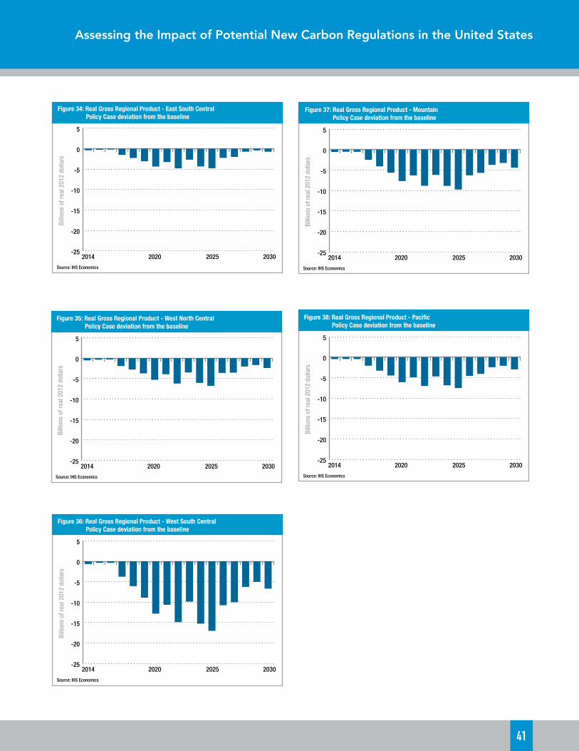
Assessing the Impact of Potential New Carbon Regulations in the United States
41
-25
-20
-15
-10
-5
0
5
2014 2020 2025 2030
Figure 34: Real Gross Regional Product - East South Central Policy Case deviation from the baseline
Source: IHS Economics
Billi
ons
of re
al 2
012
dolla
rs
-25
-20
-15
-10
-5
0
5
2014 2020 2025 2030
Figure 35: Real Gross Regional Product - West North Central Policy Case deviation from the baseline
Source: IHS Economics
Billi
ons
of re
al 2
012
dolla
rs
-25
-20
-15
-10
-5
0
5
2014 2020 2025 2030
Figure 36: Real Gross Regional Product - West South Central Policy Case deviation from the baseline
Source: IHS Economics
Billi
ons
of re
al 2
012
dolla
rs
-25
-20
-15
-10
-5
0
5
2014 2020 2025 2030
Figure 38: Real Gross Regional Product - Pacic Policy Case deviation from the baseline
Source: IHS Economics
Billi
ons
of re
al 2
012
dolla
rs
-25
-20
-15
-10
-5
0
5
2014 2020 2025 2030
Figure 37: Real Gross Regional Product - Mountain Policy Case deviation from the baseline
Source: IHS Economics
Billi
ons
of re
al 2
012
dolla
rs

42
Table 11: Annual GDP impact by US Census Region Policy Case deviation from the baseline (billions of unrealized real 2012 dollars)
Year US New England
Middle Atlantic
South Atlantic
East North
Central
East South
Central
West North
Central
West South
CentralMountain Pacific
2014 6.9 0.4 1.2 1.6 1.1 0.4 0.5 0.7 0.6 0.5
2015 5.3 0.4 0.9 1.4 0.7 0.3 0.4 0.4 0.5 0.5
2016 5.1 0.3 0.9 1.4 0.5 0.2 0.3 0.4 0.5 0.5
2017 29.1 1.7 4.4 6.8 4.4 1.5 1.9 3.8 2.5 2.1
2018 44.4 2.5 6.3 10.3 6.8 2.3 2.8 6.1 4.1 3.3
2019 60.2 3.3 8.4 13.5 9.2 3.1 3.7 8.9 5.6 4.5
2020 84.2 4.5 11.7 18.6 13.2 4.4 5.3 12.8 7.7 6.1
2021 65.1 3.4 8.7 13.9 10.1 3.3 3.9 10.6 6.3 4.9
2022 96.0 5.2 13.8 20.8 14.5 4.8 6.2 14.9 8.9 7.0
2023 59.1 3.0 7.9 12.6 8.7 2.7 3.5 9.9 6.2 4.7
2024 93.0 5.0 13.7 19.5 13.4 4.3 6.0 15.2 8.9 6.9
2025 103.5 5.5 15.2 21.7 15.1 4.8 6.8 17.0 9.8 7.6
2026 58.5 3.0 8.7 11.2 8.2 2.3 3.6 10.7 6.3 4.6
2027 54.6 2.8 8.7 10.2 7.6 2.0 3.5 10.0 5.7 4.1
2028 31.6 1.5 5.5 5.0 4.3 0.7 2.0 6.3 3.7 2.5
2029 26.1 1.2 4.7 4.1 3.6 0.4 1.7 5.0 3.3 2.1
2030 36.6 1.8 6.5 6.1 5.0 0.7 2.4 6.7 4.4 3.0
Average 50.6 2.7 7.5 10.5 7.4 2.2 3.2 8.2 5.0 3.8
Employment impact
Economic growth (e.g., expanding GDP) begets demand for and the sustainability of jobs. Consistent with the forgone GDP under the Policy Case, the U.S. economy will have a lower capacity to support jobs. Thus, employment levels will be lower under the Policy Case. The peak decline will exceed 440,000 jobs in 2022. The employment data is summarized nationally and by region in Figures 39-48, and in Table 12.
-500,000
-450,000
-400,000
-350,000
-300,000
-250,000
-200,000
-150,000
-100,000
-50,000
0
2014 2020 2025 2030
Source: IHS Economics
Employment Impact Average
Figure 39: Employment impact Policy Case deviation from the baseline
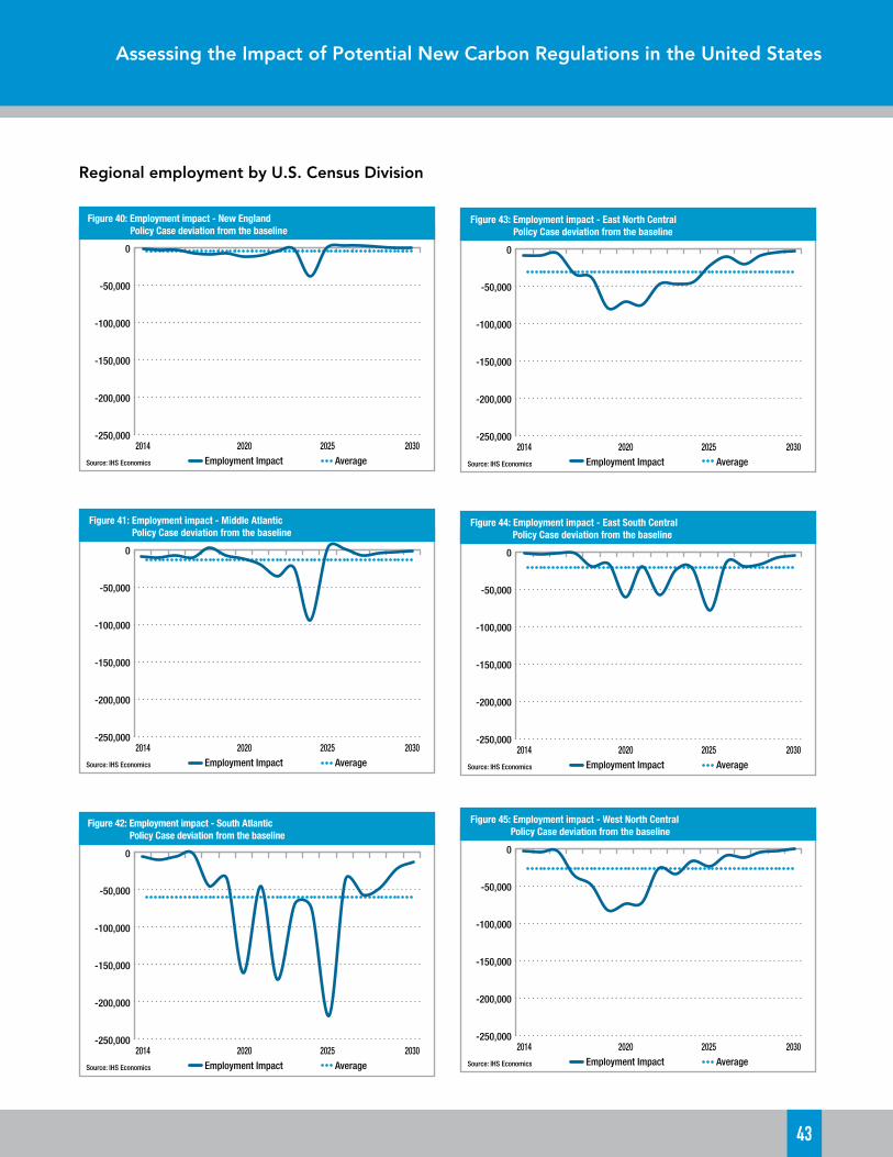
Assessing the Impact of Potential New Carbon Regulations in the United States
43
Regional employment by U.S. Census Division
-250,000
-200,000
-150,000
-100,000
-50,000
0
2014 2020 2025 2030
Figure 40: Employment impact - New England Policy Case deviation from the baseline
Source: IHS Economics Employment Impact Average
-250,000
-200,000
-150,000
-100,000
-50,000
0
2014 2020 2025 2030
Figure 41: Employment impact - Middle Atlantic Policy Case deviation from the baseline
Source: IHS Economics Employment Impact Average
-250,000
-200,000
-150,000
-100,000
-50,000
0
2014 2020 2025 2030
Figure 42: Employment impact - South Atlantic Policy Case deviation from the baseline
Source: IHS Economics Employment Impact Average
-250,000
-200,000
-150,000
-100,000
-50,000
0
2014 2020 2025 2030
Figure 43: Employment impact - East North Central Policy Case deviation from the baseline
Source: IHS Economics Employment Impact Average
-250,000
-200,000
-150,000
-100,000
-50,000
0
2014 2020 2025 2030
Figure 44: Employment impact - East South Central Policy Case deviation from the baseline
Source: IHS Economics Employment Impact Average
-250,000
-200,000
-150,000
-100,000
-50,000
0
2014 2020 2025 2030
Figure 45: Employment impact - West North Central Policy Case deviation from the baseline
Source: IHS Economics Employment Impact Average

44
-250,000
-200,000
-150,000
-100,000
-50,000
0
2014 2020 2025 2030
Figure 46: Employment impact - West South Central Policy Case deviation from the baseline
Source: IHS Economics Employment Impact Average
-250,000
-200,000
-150,000
-100,000
-50,000
0
2014 2020 2025 2030
Figure 47: Employment impact - Mountain Policy Case deviation from the baseline
Source: IHS Economics Employment Impact Average
-250,000
-200,000
-150,000
-100,000
-50,000
0
2014 2020 2025 2030
Figure 48: Employment impact - Pacic Policy Case deviation from the baseline
Source: IHS Economics Employment Impact Average
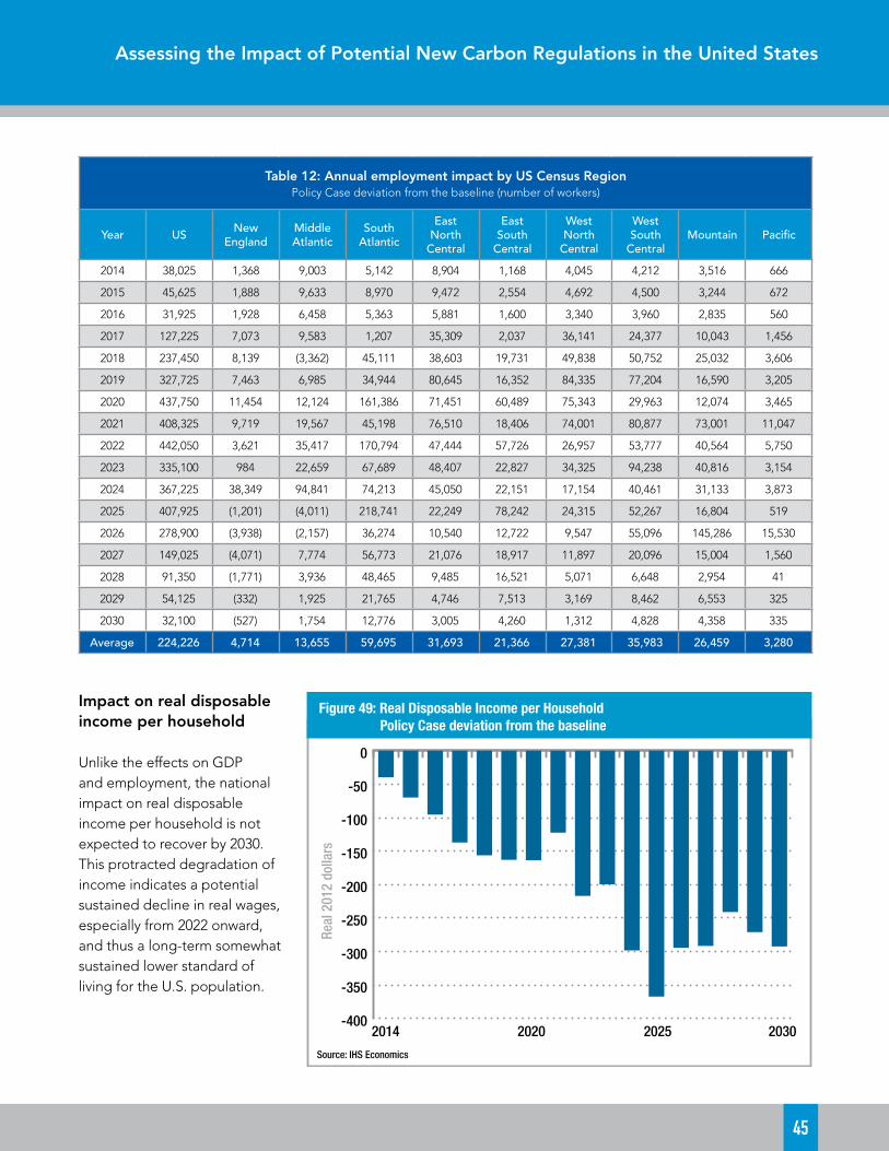
Assessing the Impact of Potential New Carbon Regulations in the United States
45
Table 12: Annual employment impact by US Census Region Policy Case deviation from the baseline (number of workers)
Year US New England
Middle Atlantic
South Atlantic
East North
Central
East South
Central
West North
Central
West South
CentralMountain Pacific
2014 38,025 1,368 9,003 5,142 8,904 1,168 4,045 4,212 3,516 666
2015 45,625 1,888 9,633 8,970 9,472 2,554 4,692 4,500 3,244 672
2016 31,925 1,928 6,458 5,363 5,881 1,600 3,340 3,960 2,835 560
2017 127,225 7,073 9,583 1,207 35,309 2,037 36,141 24,377 10,043 1,456
2018 237,450 8,139 (3,362) 45,111 38,603 19,731 49,838 50,752 25,032 3,606
2019 327,725 7,463 6,985 34,944 80,645 16,352 84,335 77,204 16,590 3,205
2020 437,750 11,454 12,124 161,386 71,451 60,489 75,343 29,963 12,074 3,465
2021 408,325 9,719 19,567 45,198 76,510 18,406 74,001 80,877 73,001 11,047
2022 442,050 3,621 35,417 170,794 47,444 57,726 26,957 53,777 40,564 5,750
2023 335,100 984 22,659 67,689 48,407 22,827 34,325 94,238 40,816 3,154
2024 367,225 38,349 94,841 74,213 45,050 22,151 17,154 40,461 31,133 3,873
2025 407,925 (1,201) (4,011) 218,741 22,249 78,242 24,315 52,267 16,804 519
2026 278,900 (3,938) (2,157) 36,274 10,540 12,722 9,547 55,096 145,286 15,530
2027 149,025 (4,071) 7,774 56,773 21,076 18,917 11,897 20,096 15,004 1,560
2028 91,350 (1,771) 3,936 48,465 9,485 16,521 5,071 6,648 2,954 41
2029 54,125 (332) 1,925 21,765 4,746 7,513 3,169 8,462 6,553 325
2030 32,100 (527) 1,754 12,776 3,005 4,260 1,312 4,828 4,358 335
Average 224,226 4,714 13,655 59,695 31,693 21,366 27,381 35,983 26,459 3,280
-400
-350
-300
-250
-200
-150
-100
-50
0
2014 2020 2025 2030
Real
201
2 do
llars
Figure 49: Real Disposable Income per Household Policy Case deviation from the baseline
Source: IHS Economics
Impact on real disposable income per household
Unlike the effects on GDP and employment, the national impact on real disposable income per household is not expected to recover by 2030. This protracted degradation of income indicates a potential sustained decline in real wages, especially from 2022 onward, and thus a long-term somewhat sustained lower standard of living for the U.S. population.

46
Conclusion
This study provides clear evidence that, even with implementation features designed to keep compliance costs low, regulating CO2 emissions at the thousands of existing fossil fuel-fired electricity generating plants in the United States under the CAA leads to nearly a half trillion dollars in total compliance expense, hundreds of thousands of lost jobs, higher electricity costs for consumers and businesses, and more than $200 on average, on an annual basis, in lower disposable income for families already struggling with a weak economy.
Specifically, this analysis finds that:
• The power industry will be forced to shut down an additional 40% of its coal fleet as a result of EPA carbon regulations assumed in the Policy Case. With carbon regulations, the coal fleet decreases in size by roughly two thirds between 2013 and 2030. Coal’s share of power generation declines from 40% in 2013 to 14% in 2030.
• The compliance cost of carbon regulations is estimated to be $480 billion (constant 2012 dollars, 2014–30), including construction costs of new power plants to replace retired coal plants, energy efficiency investments to curb demand growth, and natural gas and CCS pipeline construction; offset by fuel and O&M cost savings. Given that this expense averages to approximately $28 billion per year, the implementation costs of these regulations would be nearly three times as expensive as the total costs associated with EPA’s MATS rule, which is the most expensive EPA power sector regulation to date.
• The economic cost for each ton of reduced CO2 in the Policy Case in 2030 would be $143 per ton (undiscounted) which far exceeds the upwardly revised SCC estimates developed by the Administration’s 2013 Interagency Working Group on Social Cost of Carbon, which predicts the 2030 SCC to have risen to between $17 and $82 per ton
(in 2012 dollars, with discount rates of 2.5%, 3%, and 5%). Applying the same range of discount rates, the average cost in the Policy Case ranges from $153 to $163 per ton over the analysis period, much higher than even the Working Group’s 2030 figures.
• The carbon regulations will have a substantial impact on national and regional electricity expenditures.
o The United States will incur approximately $17 billion in additional expenses on electricity, on average, from 2014-30; with such amounts totaling nearly $290 billion in the aggregate.
o The studied regions will incur anywhere from over $2 billion to more than $111 billion in additional charges for electricity over the study period, with consumers in the South, MISO, and West regions being hit the hardest.
• The carbon regulations will have a noticeable negative impact on national GDP, employment, and real income per household.
o The peak decline in U.S. GDP will be nearly $104 billion, occurring in 2025.
o The peak decline in employment will be 442,000 jobs, occurring in 2022.
o Loss of annual real disposable income will average over $200, with a peak loss of $367 occurring in 2025; the typical household could lose a total of approximately $3,400 in real disposable income during the study period, which equates with a total disposable income loss for all U.S. households of $586 billion from 2014–30.
• The economic impact varies significantly across the nine U.S. Census Divisions.
Assessing the Impact of Potential New Carbon Regulations in the United States
47
o The South Atlantic Region will be hit the hardest in terms of gross regional product and employment declines, followed by the four Mid-Continent Census Divisions (ENC, ESC, WNC, WSC).
o New England, Mid-Atlantic, and Pacific Census Divisions will be relatively less affected.
An important aspect of this study is that it measures just the impacts of CO2 regulation on existing power plants and a necessary and complementary tightening of NSPS requirements for new natural gas plants beginning in 2022. Other recent power sector regulations and state-level mandates (such as renewable portfolio standards and energy efficiency goals) were incorporated into the Reference Case. If these other rules were included only in the Policy Case, rather than within the Reference Case, the projected economic impacts would be considerably higher.
Lower-cost natural gas certainly has created challenges for power generators using coal, but the biggest commercial threat has come from Washington. The potential EPA rules analyzed here will follow a large number of already announced new EPA regulations and will be the most costly rules to date , the combination of which can create an unmanageable upheaval in the power sector affecting the affordability, reliability, and diversity of the electricity supply that powers our economy.
For example, the EPA’s MATS Rule could ultimately be responsible for the vast majority of approximately 60 MW of electric generation capacity planned for shutdown by 2020, with many of these retirements coming within the next two years, when the new rule kicks in. EPA’s current NSPS rule effectively bans the construction of new coal-fired electric generation plants in America. Other pending and anticipated rules, including those applicable to electric generation cooling techniques, pose an additional threat to the continued provision of reliable and affordable electricity from coal, natural-gas, and even nuclear electricity generation resources—the unequivocal three-pronged backbone of our nation’s electric
generation portfolio. These three sources together have ensured and maintained the U.S. power grid’s world-class level of reliability.
Other recent power sector regulations and state-level mandates (such as renewable portfolio standards and energy efficiency goals) were incorporated into the Reference Case. If these other rules were included only in the Policy Case, rather than within the Reference Case, the projected economic impacts would be considerably higher.
While the focus of this report has been on the reduction of carbon emissions within the United States, the Energy Institute observes that EPA is proceeding down this path without heeding the lessons learned elsewhere. For example, in Europe—where electricity rates for residential and industrial users are two to three times higher than in the United States—carbon reduction policies are falling out of favor in large part because of how they are compromising economic competitiveness. Comparatively higher natural gas prices have caused many power producers in Europe to rediscover the benefits of affordable electricity produced from coal, resulting in the rapid development of new coal-fired units. Maintaining the competitive economic edge affordable energy gives the United States should be a priority in both domestic and international policymaking.
Moreover, it is important to recognize that the CO2 reductions in the Policy Case will have a very small impact on global CO2 emissions, which are set to rise rapidly. If the reductions outlined in the Policy Case were achieved, U.S. power sector emissions of CO2 would fall by 750 million metric tons (MMT) below the Reference Case from 2014-30. Meanwhile, the growth in global, non-U.S. CO2 power sector emissions, based

48
on IEA’s 2013 World Energy Outlook looking at roughly the same time period, would climb more than six-times the size of the reductions generated by the Policy Case, rising from 10,765 MMT in 2011 to 15,457 MMT in 2030. With respect to overall global CO2 emissions, the 750 MMT reduction achieved in the Policy Case represents a mere 1.8% of global CO2 emissions, which IEA predicts to otherwise grow by 31%, to 40,825 MMT, by 2030. Regardless of the national emissions reduction policies modeled in the Policy Case, and the adverse economic impacts resulting therefrom, global CO2 emissions – both in the power sector and overall – will continue to grow rapidly. Thus, this comprehensive analysis affirms that regulating CO2 emissions from U.S. power plants under the CAA will generate substantial adverse economic impacts in the United States in exchange for reductions significantly overshadowed by rapidly rising emissions elsewhere.

Assessing the Impact of Potential New Carbon Regulations in the United States
49
Appendix A: U.S. power and natural gas modeling
Figure A1 Schematic of the IHS North American Energy Market Modeling Methodology
Power MarketModule
Natural Gas Market Module
Electric sectorcoal dedmand
forecastEmissions permit price forecast,coal price forecast
Regional
economicgrowth
Coal MarketAnalysis
CapacityExpansion Model
AURORATM
GPCMTM Gas Marketdatabase
CapacityPrice Model
Scenariosdatabase
PowerDemand Model
Macro-economicOutlook
GasDemand Model
ProductiveCapacity Model
GlobalOil Outlook
GlobalLNG Outlook
Emissions MarketAnalysis
Natural gasprice forest
Oilpriceforecast
Oil price forecast
LNG price forecast
Regionaleconomicgrowth
Electric sectornatural gas
dedmand forecast
IHS Energy employs the AURORA™ power market simulation model and the Gas Pipeline Competition Model (GPCM™) for power and natural gas market fundamentals assessments—both using proprietary IHS Energy inputs. Underpinning our AURORA and GPCM analyses are specialized expert models and analytical frameworks focused on numerous topics, including energy and environmental policies, commodity markets, power capacity markets, and upstream and downstream oil. These models are regularly maintained by our team of energy market experts.
In addition to capturing the insights developed through our energy-specific models, macroeconomic analyses from IHS Economics—the widely respected macroeconomic forecasting service—underpin the
analytics and provide context for our energy demand forecasting.
At the center of the IHS Energy North American Power Market analysis is AURORA—a detailed power market simulation model that solves for zonal wholesale prices on an hourly basis. This fundamentals-based module employs a multi-area, transmission-constrained dispatch logic to simulate real market conditions and capture the dynamics and economics of electricity markets, both short term (hourly, daily, monthly) and long term (annual). The geographic coverage extends to all interconnected electric demand in Canada and the U.S. Lower 48, plus the small amount of interconnected resources in northern Baja California, Mexico. Feeding into the Aurora model are several proprietary models

50
and custom analytical processes developed by IHS Energy, as depicted in Figure A1 above.
The IHS Energy North American Natural Gas Market Module features RBAC’s Gas Pipeline Competition Model (GPCM)—a highly detailed natural gas transportation model—and simulates flows of natural gas on pipelines after taking into account the location and supply curve of each supply region, the demand curves for each demand region, a detailed grid model of the entire North American pipeline network, and the availability of underground natural gas storage. GPCM solves the entire North American natural gas market on an integrated basis, providing an outlook for flows and natural gas prices across the continent on a monthly basis. IHS Energy uses a customized version of GPCM that integrates with AURORA. This GPCM system develops an equilibrium set of spot prices, basis, and detailed gas flows throughout the entire pipeline grid as outputs based on the specified demand and supply inputs as well as markets for transportation and storage.
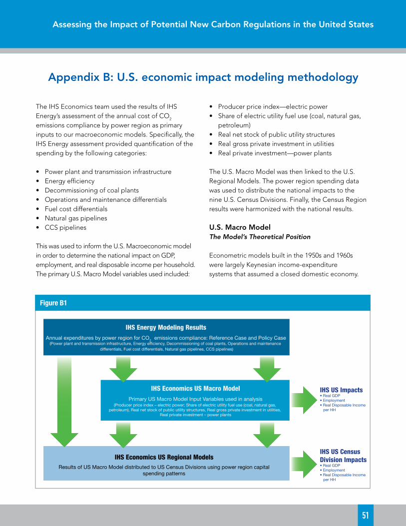
Assessing the Impact of Potential New Carbon Regulations in the United States
51
Appendix B: U.S. economic impact modeling methodology
Figure B1
IHS Energy Modeling Results Annual expenditures by power region for CO2 emissions compliance: Reference Case and Policy Case
(Power plant and transmission infrastructure, Energy ef�ciency, Decommissioning of coal plants, Operations and maintenance differentials, Fuel cost differentials, Natural gas pipelines, CCS pipelines)
IHS Economics US Macro Model
Primary US Macro Model Input Variables used in analysis (Producer price index – electric power; Share of electric utility fuel use (coal, natural gas,
petroleum), Real net stock of public utility structures, Real gross private investment in utilities, Real private investment – power plants
IHS Economics US Regional Models Results of US Macro Model distributed to US Census Divisions using power region capital
spending patterns
IHS US Impacts • Real GDP • Employment • Real Disposable Income per HH
IHS US Census Division Impacts • Real GDP • Employment • Real Disposable Income per HH
The IHS Economics team used the results of IHS Energy’s assessment of the annual cost of CO2 emissions compliance by power region as primary inputs to our macroeconomic models. Specifically, the IHS Energy assessment provided quantification of the spending by the following categories:
• Power plant and transmission infrastructure• Energy efficiency• Decommissioning of coal plants • Operations and maintenance differentials • Fuel cost differentials • Natural gas pipelines • CCS pipelines
This was used to inform the U.S. Macroeconomic model in order to determine the national impact on GDP, employment, and real disposable income per household. The primary U.S. Macro Model variables used included:
• Producer price index—electric power • Share of electric utility fuel use (coal, natural gas,
petroleum)• Real net stock of public utility structures• Real gross private investment in utilities• Real private investment—power plants
The U.S. Macro Model was then linked to the U.S. Regional Models. The power region spending data was used to distribute the national impacts to the nine U.S. Census Divisions. Finally, the Census Region results were harmonized with the national results.
U.S. Macro ModelThe Model’s Theoretical Position
Econometric models built in the 1950s and 1960s were largely Keynesian income-expenditure systems that assumed a closed domestic economy.

52
High computation costs during estimation and manipulation, along with the underdeveloped state of macroeconomic theory, limited the size of the models and the richness of the linkages of spending to financial conditions, inflation, and international developments. Since that time, however, computer costs have fallen spectacularly; theory has also benefited from four decades of postwar data observation and from the intellectual attention of many eminent economists.
The IHS Model is an econometric dynamic equilibrium growth model. It strives to incorporate the best insights of many theoretical approaches to the business cycle: Keynesian, neoclassical, monetarist, supply-side, and rational expectations. In addition, the IHS Model embodies the major properties of the long-term growth models presented by James Tobin, Robert Solow, Edmund Phelps, and others. This structure guarantees that short-run cyclical developments will converge to robust long-run equilibria.
In growth models, the expansion rate of technical progress, the labor force, and the capital stock determine the productive potential of an economy. Both technical progress and the capital stock are governed by investment, which in turn must be in balance with post-tax capital costs, available savings, and the capacity requirements of current spending. As a result, monetary and fiscal policies will influence both the short- and the long-term characteristics of such an economy through their impacts on national saving and investment.
A modern model of output, prices, and financial conditions is melded with the growth model to present the detailed, short-run dynamics of the economy. In specific goods markets, the interactions of a set of supply and demand relations jointly determine spending, production, and price levels. Typically, the level of inflation-adjusted demand is driven by prices, income, wealth, expectations, and financial conditions. The capacity to supply goods and services is keyed to a production function combining the basic inputs of labor hours, energy usage, and the capital stocks of business equipment and structures, and government
infrastructure. The “total factor productivity” of this composite of tangible inputs is driven by expenditures on research and development that produce technological progress.
Prices adjust in response to gaps between current production and supply potential and to changes in the cost of inputs. Wages adjust to labor supply-demand gaps (indicated by a demographically-adjusted unemployment rate), current and expected inflation (with a unit long-run elasticity), productivity, tax rates, and minimum wage legislation. The supply of labor positively responds to the perceived availability of jobs, to the after-tax wage level, and to the growth and age-sex mix of the population. Demand for labor is keyed to the level of output in the economy and the productivity of labor, capital, and energy. Because the capital stock is largely fixed in the short run, a higher level of output requires more employment and energy inputs. Such increases are not necessarily equal to the percentage increase in output because of the improved efficiencies typically achieved during an upturn. Tempering the whole process of wage and price determination is the exchange rate; a rise signals prospective losses of jobs and markets unless costs and prices are reduced.
For financial markets, the model predicts exchange rates, interest rates, stock prices, loans, and investments interactively with the preceding GDP and inflation variables. The Federal Reserve sets the supply of reserves in the banking system and the fractional reserve requirements for deposits. Private sector demands to hold deposits are driven by national income, expected inflation, and by the deposit interest yield relative to the yields offered on alternative investments. Banks and other thrift institutions, in turn, set deposit yields based on the market yields of their investment opportunities with comparable maturities and on the intensity of their need to expand reserves to meet legal requirements. In other words, the contrast between the supply and demand for reserves sets the critical short-term interest rate for interbank transactions, the federal funds rate. Other interest rates are keyed to this rate, plus expected inflation,

Assessing the Impact of Potential New Carbon Regulations in the United States
53
Treasury borrowing requirements, and sectoral credit demand intensities.
The old tradition in macroeconomic model simulations of exogenous fiscal or environmental policy changes was to hold the Federal Reserve’s supply of reserves constant at baseline levels. While this approach makes static analysis easier in the classroom, it sometimes creates unrealistic policy analyses when a dynamic model is appropriate. In the IHS Model, “monetary policy” is defined by a set of targets, instruments, and regular behavioral linkages between targets and instruments. The model user can choose to define unchanged monetary policy as unchanged reserves, or as an unchanged reaction function in which interest rates or reserves are changed in response to changes in such policy concerns as the price level and the unemployment rate.
The model pays due attention to valid lessons of monetarism by carefully representing the diverse portfolio aspects of money demand and by capturing the central bank’s role in long-term inflation phenomena.
The private sector may demand money balances as one portfolio choice among transactions media (currency, checkable deposits), investment media (bonds, stocks, short-term securities), and durable assets (homes, cars, equipment, structures). Given this range of choice, each medium’s implicit and explicit yield must therefore match expected inflation, offset perceived risk, and respond to the scarcity of real savings. Money balances provide benefits by facilitating spending transactions and can be expected to rise nearly proportionately with transactions requirements unless the yield of an alternative asset changes.
Now that even demand deposit yields can float to a limited extent in response to changes in Treasury bill rates, money demand no longer shifts quite as sharply when market rates change. Nevertheless, the velocity of circulation (the ratio of nominal spending to money demand) is still far from stable during a cycle of monetary expansion or contraction. Thus the simple monetarist link from money growth to price inflation or
nominal spending is therefore considered invalid as a rigid short-run proposition.
Equally important, as long run growth models demonstrate, induced changes in capital formation can also invalidate a naive long-run identity between monetary growth and price increases. Greater demand for physical capital investment can enhance the economy’s supply potential in the event of more rapid money creation or new fiscal policies. If simultaneous, countervailing influences deny an expansion of the economy’s real potential, the model will translate all money growth into a proportionate increase in prices rather than in physical output.
Since 1980, “supply-side” political economists have pointed out that the economy’s growth potential is sensitive to the policy environment. They focused on potential labor supply, capital spending, and savings impacts of tax rate changes. The IHS Model embodies supply-side hypotheses to the extent supportable by available data, and this is considerable in the many areas that supply-side hypotheses share with long-run growth models. These features, however, have been fundamental ingredients of our model since 1976.
As the rational expectations school has pointed out, much of economic decision-making is forward looking. For example, the decision to buy a car or a home is not only a question of current affordability but also one of timing. The delay of a purchase until interest rates or prices decline has become particularly common since the mid-1970s when both inflation and interest rates were very high and volatile. Consumer sentiment surveys, such as those conducted by the University of Michigan Survey Research Center, clearly confirm this speculative element in spending behavior.
However, households can be shown to base their expectations, to a large extent, on their past experiences: they believe that the best guide to the future is an extrapolation of recent economic conditions and the changes in those conditions. Consumer sentiment about whether this is a “good time to buy” can therefore be successfully modeled

54
as a function of recent levels and changes in employment, interest rates, inflation, and inflation expectations. Similarly, inflation expectations (influencing financial conditions) and market strength expectations (influencing inventory and capital spending decisions) can be modeled as functions of recent rates of increase in prices and spending.
This largely retrospective approach is not, of course, wholly satisfactory to pure adherents to the rational expectations doctrine. In particular, this group argues that the announcement of macroeconomic policy changes would significantly influence expectations of inflation or growth prior to any realized change in prices or spending. If an increase in government expenditures is announced, the argument goes, expectations of higher taxes to finance the spending might lead to lower consumer or business spending in spite of temporarily higher incomes from the initial government spending stimulus. A rational expectations theorist would thus argue that multiplier effects will tend to be smaller and more short-lived than a mainstream economist would expect.
These propositions are subject to empirical evaluation. Our conclusions are that expectations do play a significant role in private sector spending and investment decisions; but, until change has occurred in the economy, there is very little room for significant changes in expectations in advance of an actual change in the variable about which the expectation is formed. The rational expectations school thus correctly emphasizes a previously understated element of decision-making, but exaggerates its significance for economic policy-making and model building.
The IHS Model allows a choice in this matter. On the one hand, the user can simply accept IHS Global Inc.’s judgments and let the model translate policy initiatives into initial changes in the economy, simultaneous or delayed changes in expectations, and subsequent changes in the economy. On the other hand, the user can manipulate the clearly identified expectations variables in the model, i.e., consumer sentiment, and inflation expectations. For
example, if the user believes that fear of higher taxes would subdue spending, the user could reduce the consumer sentiment index. Such experiments can be made “rational” through model iterations that bring the current change in expectations in line with future endogenous changes in employment, prices, or financial conditions.
The conceptual basis of each equation in the IHS Model was thoroughly worked out before the regression analysis was initiated. The list of explanatory variables includes a carefully selected set of demographic and financial inputs. Each estimated coefficient was then thoroughly tested to be certain that it meets the tests of modern theory and business practice. This attention to equation specification and coefficient results has eliminated the “short circuits” that can occur in evaluating a derivative risk or an alternative policy scenario. Because each equation will stand up to a thorough inspection, the IHS Model is a reliable analytical tool and can be used without excessive iterations. The model is not a black box: it functions like a personal computer spreadsheet in which each interactive cell has a carefully computed, theoretically consistent entry and thus performs logical computations simultaneously.
Major Sectors
The IHS Model captures the full simultaneity of the U.S. economy, forecasting over 1200 concepts spanning final demands, aggregate supply, prices, incomes, international trade, industrial detail, interest rates, and financial flows. Figure B2 summarizes the structure of the eight interactive sectors (noted in Roman numerals). The following discussion presents the logic of each sector and the significant interactions with other sectors.
The domestic spending (I), income (II), and tax policy (III) sectors model the central circular flow of behavior as measured by the national income and product accounts. If the rest of the model were “frozen,” these blocks would produce a Keynesian system similar to the models pioneered by Tinbergen and Klein, except
Assessing the Impact of Potential New Carbon Regulations in the United States
55
that neoclassical price factors have been imbedded in the investment and other primary demand equations.
Consumer spending on durable goods is divided into eleven categories: two light vehicles categories; net purchases of used cars, motor-vehicle parts; recreational vehicles; computers; software; other household equipment and furnishings; ophthalmic and orthopedic products, and “other.” Spending on nondurable goods is divided into nine categories: three food categories; clothing and shoes; gasoline and oil; fuel oil and coal; tobacco; drugs; and “other.” Spending on services is divided into seventeen categories: housing; transportation; six household operation subcategories; five transportation categories; medical; recreation; two personal business service categories; and “other.” In nearly all cases, real consumption expenditures are motivated by real income and the user price of a particular category relative to the prices of other consumer goods. Durable and semidurable goods are also especially sensitive to current financing costs, and consumer speculation on whether it is a “good time to buy.” The University of Michigan Survey of Consumer Sentiment monitors this last influence, with the index itself modeled as a function of current and lagged values of inflation, unemployment, and the prime rate.
Business spending includes six fixed investment categories; four information processing equipment categories; industrial equipment; two transportation equipment categories; other producers’ durable equipment; four building categories; mining and petroleum structures; public utility structures; and miscellaneous. Equipment and (non-utility, non-mining) structures spending components are determined by their specific effective post-tax capital costs, capacity utilization, and replacement needs. The cost terms are sophisticated blends of post-tax debt and equity financing costs (offset by expected capital gains) and the purchase price of the investment good (offset by possible tax credits and depreciation-related tax benefits). This updates the well-known work of Dale Jorgenson, Robert Hall, and Charles Bischoff.
Given any cost/financing environment, the need to expand capacity is monitored by recent growth in national goods output weighted by the capital intensity of such production. Public utility structure expenditures are motivated by similar concepts except that the output terms are restricted to utility output rather than total national goods output. Net investment in mining and petroleum structures responds to movements in real domestic oil prices and to oil and natural gas production.
Inventory demand is the most erratic component of GDP, reflecting the pro-cyclical, speculative nature of private sector accumulation during booms and decumulation during downturns. The forces that drive the five nonfarm inventory categories are changes in spending, short-term interest rates and expected inflation, surges in imports, and changes in capacity utilization or the speed of vendor deliveries. Surprise increases in demand lead to an immediate drawdown of stocks and then a rebuilding process over the next year; the reverse naturally holds for sudden reductions in final demand. Inventory demands are sensitive to the cost of holding the stock, measured by such terms as interest costs adjusted for expected price increases and by variables monitoring the presence of bottlenecks. The cost of a bottleneck that slows delivery times is lost sales: an inventory spiral can therefore be set in motion when all firms accelerate their accumulation during a period of strong growth but then try to deplete excessive inventories when the peak is past.
The residential investment sector of the model includes two housing starts (single and multi-family starts) and three housing sales categories (new and existing single family sales, and new single family units for sale). Housing starts and sales, in turn, drive investment demand in five GDP account categories: single family housing; multi-family housing; improvements; miscellaneous; and residential equipment.
Residential construction is typically the first sector to turn down in a recession and the first to rebound in a recovery. Moreover, the magnitude of the building
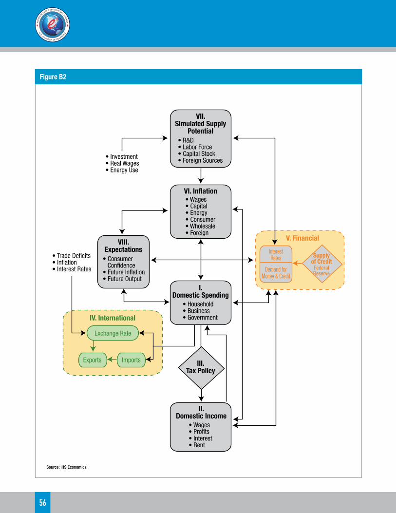
56
Figure B2
• Investment• Real Wages• Energy Use
• Trade Decits• In�ation• Interest Rates
• Consumer Condence• Future In�ation• Future Output
VIII.Expectations
Exchange Rate
Exports Imports
IV. International
• R&D• Labor Force• Capital Stock• Foreign Sources
VII.Simulated Supply
Potential
• Wages• Capital• Energy• Consumer• Wholesale• Foreign
VI. In�ation
InterestRates
Demand forMoney & Credit
V. Financial
• Household• Business• Government
I.Domestic Spending
FederalReserve
Supplyof Credit
• Wages• Prots• Interest• Rent
II.Domestic Income
III.Tax Policy
Source: IHS Economics

Assessing the Impact of Potential New Carbon Regulations in the United States
57
cycle is often the key to that of the subsequent macroeconomic cycle. The housing sector of the IHS Model explains new construction as a decision primarily based on the after-tax cost of home ownership relative to disposable income. This cost is estimated as the product of the average new home price adjusted for changes in quality, and the mortgage rate, plus operating costs, property taxes, and an amortized down payment. “Lever variables” allow the model user to specify the extent to which mortgage interest payments, property taxes, and depreciation allowances (for rental properties) produce tax deductions that reduce the effective cost.
The equations also include a careful specification of demographic forces. After estimating the changes in the propensity for specific age-sex groups to form independent households, the resulting “headship rates” were multiplied by corresponding population statistics to estimate the trend expansion of single- and multi-family households. The housing equations were then specified to explain current starts relative to the increase in trend households over the past year, plus pent-up demand and replacement needs. The basic phenomenon being scrutinized is therefore the proportion of the trend expansion in households whose housing needs are met by current construction. The primary determinants of this proportion are housing affordability, consumer confidence, and the weather. Actual construction spending in the GDP accounts is the value of construction “put-in-place” in each period after the start of construction (with a lag of up to six quarters in the case of multi-family units), plus residential improvements, and brokerage fees.
The last sector of domestic demand for goods and services, that of the government, is largely exogenous (user-determined) at the federal level and endogenous (equation-determined) at the state and local level. The user sets the real level of federal nondefense and defense purchases (for compensation, consumption of fixed capital, other consumption, and gross investment), medical and non-medical transfer payments, and medical and non-medical grants to state and local governments. The model calculates
the nominal values through multiplication by the relevant estimated prices. Transfers to foreigners, wage accruals, and subsidies (agricultural, housing, and other) are also specified by the user, but in nominal dollars. One category of federal government spending –net interest payments -- is determined within the model because of its dependence on the model’s financial and tax sectors. Net federal interest payments are determined by the level of privately-held federal debt, short and long-term interest rates, and the maturity of the debt.
The presence of a large and growing deficit imposes no constraint on federal spending. This contrasts sharply with the state and local sector where legal requirements for balanced budgets mean that declining surpluses or emerging deficits produce both tax increases and reductions in spending growth. State and local purchases (for compensation, consumption of fixed capital, other consumption, and construction) are also driven by the level of federal grants (due to the matching requirements of many programs), population growth, and trend increases in personal income.
Domestic spending, adjusted for trade flows, defines the economy’s value-added or gross national product (GNP) and gross domestic product (GDP). Because all value-added must accrue to some sector of the economy, the expenditure measure of GNP also determines the nation’s gross income. The distribution of income among households, business, and government is determined in sectors II and III of the model.
Pre-tax income categories include private and government wages, corporate profits, interest, rent, and entrepreneurial returns. Each pre-tax income category except corporate profits is determined by some combination of wages, prices, interest rates, debt levels, and capacity utilization or unemployment rates. In some cases such as wage income, these are identities based on previously calculated wage rates, employment, and hours per week.
Profits are logically the most volatile component of GNP on the income side. When national spending

58
changes rapidly, the contractual arrangements for labor, borrowed funds, and energy imply that the return to equity holders is a residual that will soar in a boom and collapse in a recession. The model reflects this by calculating wage, interest and rental income as thoroughly reliable near-identities (e.g., wages equal average earnings multiplied by hours worked) and then subtracting each non-profit item from national income to solve for profits.
Since post-tax rather than pre-tax incomes drive expenditures, each income category must be taxed at an appropriate rate; the model therefore tracks personal, corporate, payroll, and excise taxes separately. Users may set federal tax rates; tax revenues are then simultaneously forecast as the product of the rate and the associated pre-tax income components. However, the model automatically adjusts the effective average personal tax rate for variations in inflation and income per household, and the effective average corporate rate for credits earned on equipment, utility structures, and R&D. Substitutions or additions of “flat” taxes and value-added taxes for existing taxes are accomplished with specific tax rates and new definitions of tax bases. As appropriate, these are aggregated into personal, corporate or excise tax totals.
State and local corporate profits and social insurance (payroll) tax rates are exogenous in the model, while personal income and excise taxes are fully endogenous: the Model makes reasonable adjustments automatically to press the sector toward the legally-required approximate budget balance. The average personal tax rate rises with income and falls with the government operating surplus. Property and sales taxes provide the bulk of state excise revenue and reflect changes in oil and natural gas production, gasoline purchases, and retail sales, as well as revenue requirements. The feedback from expenditures to taxes and taxes to expenditures works quite well in reproducing both the secular growth of the state and local sector and its cyclical volatility.
The international sector (IV) is a critical, fully simultaneous block that can either add or divert
strength from the central circular flow of domestic income and spending. Depending on the prices of foreign output, the U.S. exchange rate, and competing domestic prices, imports capture varying shares of domestic demand.
Depending on similar variables and the level of world gross domestic product, exports can add to domestic spending on U.S. production. The exchange rate itself responds to international differences in inflation, interest rates, trade deficits, and capital flows between the U.S. and its competitors. In preparing forecasts, IHS U.S. Economic Service and the World Service collaborate in determining internally consistent trade prices and volumes, interest rates, and financial flows.
Eight categories of goods and one services category are separately modeled for both imports and exports, with one additional goods category for oil imports. For example, export and import detail for business machines is included as a natural counterpart to the inclusion of the office equipment component of producers’ durable equipment spending. The business machines detail allows more accurate analysis because computers are rapidly declining in effective quality-adjusted prices relative to all other goods, and because such equipment is rising so rapidly in prominence as businesses push ahead with new production and information processing technologies.
Investment income flows are also explicitly modeled. The stream of huge current account deficits incurred by the U.S. has important implications for the U.S. investment income balance. As current account deficits accumulate, the U.S. net international investment position and the U.S. investment income balance deteriorate. U.S. foreign assets and liabilities are therefore included in the model, with the current account deficit determining the path of the net investment position.
The reactions of overseas prices, interest rates and GDP to U.S. development are robust and automatic. In the case of dollar depreciation, for example, U.S. activity may expand at the expense of foreign activity

Assessing the Impact of Potential New Carbon Regulations in the United States
59
and U.S. inflation may rise while the rate in other countries slows.
The use of a detailed financial sector (V) and of interest rate and wealth effects in the spending equations recognizes the importance of credit conditions on the business cycle and on the long-run growth prospects for the economy.
Interest rates, the key output of this sector, are modeled as a term structure, pivoting off the federal funds rate. As noted earlier, the model gives the user the flexibility of using the supply of reserves as the key monetary policy instrument, reflecting the Federal Reserve’s open market purchases or sales of Treasury securities, or using a reaction function as the policy instruction. If the supply of reserves is chosen as the policy instrument, the federal funds rate depends upon the balance between the demand and supply of reserves to the banking system. Banks and other thrift institutions demand reserves to meet the reserve requirements on their deposits and the associated (exogenous) fractional reserve requirements. The private sector in turn demands deposits of various types, depending on current yields, income, and expected inflation.
If the reaction function is chosen as the monetary policy instrument, the federal funds rate is determined in response to changes in such policy concerns as inflation and unemployment. The reaction function recognizes that monetary policy seeks to stabilize prices (or to sustain a low inflation rate) and to keep the unemployment rate as close to the natural rate as is consistent with the price objective. A scenario designed to display the impact of a fiscal or environmental policy change in the context of “unchanged” monetary policy is arguably more realistic when “unchanged” or traditional reactions to economic cycles are recognized, than when the supply of reserves is left unchanged.
Longer-term interest rates are driven by shorter-term rates as well as factors affecting the slope of the yield curve. In the IHS Model, such factors include inflation
expectations, government borrowing requirements, and corporate financing needs. The expected real rate of return varies over time and across the spectrum of maturities. An important goal of the financial sector is to capture both the persistent elements of the term structure and to interpret changes in this structure. Twenty-eight interest rates are covered in order to meet client needs regarding investment and financial allocation strategies.
Inflation (VI) is modeled as a carefully controlled, interactive process involving wages, prices, and market conditions. Equations embodying a near accelerationist point of view produce substantial secondary inflation effects from any initial impetus such as a change in wage demands or a rise in foreign oil prices. Unless the Federal Reserve expands the supply of credit, real liquidity is reduced by any such shock; given the real-financial interactions described above, this can significantly reduce growth. The process also works in reverse: a spending shock can significantly change wage-price prospects and then have important secondary impacts on financial conditions. Inspection of the simulation properties of the IHS Model, including full interaction among real demands, inflation and financial conditions, confirms that the model has moved toward central positions in the controversy between fiscalists and monetarists, and in the debates among neoclassicists, institutionalists, and “rational expectationists.”
The principal domestic cost influences are labor compensation, nonfarm productivity (output per hour), and foreign input costs; the latter are driven by the exchange rate, the price of oil, and foreign wholesale price inflation. Excise taxes paid by the producer are an additional cost fully fed into the pricing decision. This set of cost influences drives each of the nineteen industry-specific producer price indexes, in combination with a demand pressure indicator and appropriately weighted composites of the other eighteen producer price indexes. In other words, the inflation rate of each industry price index is the reliably weighted sum of the inflation rates of labor, energy, imported goods, and domestic intermediate

60
goods, plus a variable markup reflecting the intensity of capacity utilization or the presence of bottlenecks. If the economy is in balance--with an unemployment rate near 5%, manufacturing capacity utilization steady near 80-85%, and foreign influences neutral--then prices will rise in line with costs and neither will show signs of acceleration or deceleration.
The first principle of the market economy is that prices and output are determined simultaneously by the factors underlying both demand and supply. As noted above, the “supply-siders” have not been neglected in the IHS Model; indeed, substantial emphasis on this side of the economy (VII) was incorporated as early as 1976. In the IHS Model, aggregate supply (or potential GDP excluding the energy sector) is estimated by a Cobb-Douglas production function that combines factor input growth and improvements in total factor productivity. Factor input equals a weighted average of labor, business fixed capital, public infrastructure, and energy provided by the energy sector. Based upon each factor’s historical share of total input costs, the elasticity of potential output with respect to labor is 0.64 (i.e., a 1% increase in the labor supply increases potential GDP 0.64%); the business capital elasticity is 0.26; the infrastructure elasticity is 0.02; and the energy elasticity is 0.07. Factor supplies are defined by estimates of the full employment labor force, the full employment capital stock, end-use energy demand, and the stock of infrastructure. Total factor productivity depends upon the stock of research and development capital and trend technological change. The energy sector employs its own capital and labor. Potential GDP is the sum of the energy and non-energy sector outputs less energy imports.
Taxation and other government policies influence labor supply and all investment decisions, thereby linking tax changes to changes in potential GDP. An expansion of potential GDP first reduces prices and then credit costs, and thus spurs demand. Demand rises until it equilibrates with the potential output. Thus, the growth of aggregate supply is the fundamental constraint on the long-term growth of demand.
Inflation, created by demand that exceeds potential GDP or by a supply-side shock or excise tax increase, raises credit costs and weakens consumer sentiment, thus putting the brakes on aggregate demand.
The contributions to the Model and its simulation properties of the rational expectations school are as rich as the data will support. Expectations (Sector VIII) impact several expenditure categories in the IHS Model, but the principal nuance relates to the entire spectrum of interest rates. Shifts in price expectations or the expected capital needs of the government are captured through price expectations and budget deficit terms, with the former impacting the level of rates throughout the maturity spectrum, and the latter impacting intermediate and long-term rates, and hence affecting the shape of the yield curve. On the expenditure side, inflationary expectations impact consumption via consumer sentiment, while growth expectations affect business investment.
An important goal of the IHS Model of the U.S. Economy is the provision of policy insights and guidance. Restrictive monetary policy is clearly the strategy of last resort for slowing the economy, even if inflation is the highest priority problem. The long-term consequences of restricted credit growth are clearly adverse: business investment and housing are significantly weaker, entailing a permanent reduction in the nation’s capital stock and labor productivity. Also important is the real appreciation of the dollar, leading to expanded imports and lost exports. The best cure for inflation is a carefully targeted reduction in federal spending.

Assessing the Impact of Potential New Carbon Regulations in the United States
61
IHS Economics - U.S. Regional Models
A. Overview of Modeling Approach
The IHS Economics approach to state, metropolitan area, census division and census region models represents a significant departure from most previous multiregional modeling and forecasting efforts. Most other regional models are constructed as proportions of the United States. In the IHS Economics system, however, each area is modeled individually and then linked into a national system. Thus, our models do not forecast regional growth as simple proportions of U.S. totals, but focus on internal growth dynamics and differential business cycle response. This approach is referred to as “top-down bottom-up.” It contrasts sharply with pure share (top-down) models, and models which are not linked to a national macroeconomic model (bottom-up), and contains the best of both approaches.
Our basic objective is to project how regional activity varies, given an economic environment as laid out by IHS Economics’ Macroeconomic and Industry forecasts. In order to do this; we must be able to explain the two key phenomena:
• Why states react differently from one another over the business cycle
• Why states grow or decline relative to each other over the longer run
These issues are addressed using information about detailed industrial mix, interindustry and interregional relationships, productivity and relative costs, and migration trends.
B. Core Economic Forecasting Module
The IHS Regional models are econometric and have a quarterly periodicity. Consequently, each model is able to capture the full business cycle behavior of the economy, including the timing and amplitude of the turning points.
Another general characteristic of the models is that they are policy sensitive — they respond to changes in tax rates, military spending, utility costs, etc. There are a number of reasons for this sensitivity, and these will be highlighted in the description below. A few of these reasons are the following:
• Each state is modeled individually, with different model structures specified according to the characteristics of the state
• National policy is explicitly captured,
• The comparative advantage of one state over another is explicitly modeled using relative cost variables.
The three major components of the IHS Economics approach are summarized below:
• The major linkages among the models occur in the economic base or export sectors. These we identify as primarily agriculture, mining, the federal government, and most manufacturing industries. In a few states, banking, insurance, or services (hotels) sectors also can be classified as export sectors. For the most part, these industries serve national rather than local markets or are not dependent upon the local market. On the other hand, the income generated from these sectors provides one of the major stimuli to the local economy. The local growth and decline of these sectors has a lot to do with the economic health of the region.
• The local economy is composed of construction, transportation, utilities and communications, finance, insurance, and real estate, wholesale and retail trade, services, and state and local government. The major driving forces in this part of the economy are local in nature. The income generated by the export sectors circulates and multiplies through the local economy and generates the greater part of regional employment. These

62
interactions and simultaneities can only be captured in an independent model.
• In our demographic sector, net migration is driven by economic conditions. The principal assumption here is that people follow jobs and higher incomes rather than vice-versa. This does not mean that nonpecuniary determinants of migration do not exist. However, these are either fixed (climate and landscape) or vary only slowly (urbanization) or are special in nature (the ability to sell homes and retire to Sunbelt areas). The important thing is to provide the correct direction of causality. Demographic factors are most important on the consumption side of the regional economy. They are a significant factor in housing, retail sales, autos, etc., and the relationships are captured in the models. Population is also an important longterm determinant of the size of such sectors as state and local government.
Manufacturing, for example, is a prime determinant of utilities and transportation employment. In highly industrialized states, it has an effect on almost every nonmanufacturing support sector. In certain western states; on the other hand, it is agriculture or mining, which are important export sectors. The appropriate export sector is explicitly represented in the equation, and in this way, the secondary effect of a new plant, a new mine or increased acreage is directly captured in the nonmanufacturing sectors. Since nonmanufacturing has explicit feedbacks unto itself, the third and fourth order effects are also captured. It is a truly dynamic and policy sensitive equation structure.
Labor Costs
When real wages are high and/or rising rapidly, then the tendency of business, government, and other organizations is to hold employment down as much as possible. The reverse holds true when real wages are low or falling rapidly. In the manufacturing sector, wage costs were shown to be one of the principle determinants of business location decisions. In the nonmanufacturing support sectors, this is reflected in
the level rather than the location of employment. Thus, employment is inversely proportional to real wage costs. Real wages enter many of the nonmanufacturing employment equations. For forecast purposes, this wage rate is related to the appropriate national variable and the growth rate of the sector itself.
National Conditions
The national economy is reflected in three areas in the nonmanufacturing sectors. First, certain macroeconomic conditions affect local activity significantly, even nonmanufacturing. The best example of this is credit availability. Tight credit conditions with high interest rates have an adverse impact on local construction activity, sales of autos, and other durable and the like. Thus, when money is tight, employment in construction and in wholesale and retail trade is adversely affected. The opposite holds true during periods of easy money and low interest rates.
The second class of national variables are those which reflect nationwide trends. An example of this is the trend towards an increasingly larger services sector. Capturing this secular trend is sometimes difficult when one uses only local variables in the nonmanufacturing equations. Thus, the usual assortment of local variables — income, populations, wages costs, etc. — is sometimes supplemented by the ratio of sector employment to total employment at the national level. This is not a “shift-share” relationship. It is used to supplement, not supplant, local activity variables. The elasticity on the national series is uniformly lower than the elasticity on the local variables, and it is simply reflecting gradual long-term changes in the nation’s employment structure. The local variables remain the main drivers of the local economy.
Assessing the Impact of Potential New Carbon Regulations in the United States
63
Demographics -- Components of population change
• Births • Deaths • Net migration
A few decades ago, natural increase accounted for 68% of population growth nationwide, but in a number of fast-growing states in the South and West, net migration accounted for over half of the gain, making interstate mobility an important determinant of state population growth. Additionally, within the last 10 years, migration patterns have become even greater influences in these states -- both through accelerated interstate population flows, as well as international migration. IHS Economics’ econometric analysis of net migration based upon economic determinants differentiates its forecasts from the Census Bureau’s trended state projections.

64
Appendix C: Additional detail on power sector cost analytics
Supply-side efficiency investments
Improving the thermal efficiency of coal-fired generators provides an opportunity for small reductions in the CO2 emission rate for many coal units and thus a minor contribution to meeting existing generator targets in the Policy Case. A study done by Sargent & Lundy (S&L) provides a comprehensive analysis of the capital and operating costs associated with a range of potential efficiency upgrades.
However, many coal units are unlikely to receive all of the efficiency upgrades that were presented in the report. Some modifications are likely to have been already implemented as part of ongoing plant maintenance and are therefore already captured in existing heat rates. Further, the most likely investments in efficiency are those with a relatively short payback period; savings in fuel for the most attractive upgrades provide payback of the initial investment within two years. Of the upgrades that S&L presented, seven were identified as projects that coal plant owners were likely to implement in the Policy Case (Table C1).
The above upgrades result in a capacity-weighted average heat rate reduction of about 200 Btu per kilowatt-hour (Btu/kWh), for an average 2% efficiency gain. Improvements at the unit level range from 134 to 449 Btu/kWh. For an average coal unit in this analysis, the 200 Btu/kWh heat rate reduction results in a CO2 emission rate reduction of roughly 40 lb per MWh, about a 4% contribution to the U.S. average fossil emission rate reduction required in the Policy Case for CO2 by 2030. The efficiency upgrades in the Policy Case require an aggregate capital investment of about $3 billion.
Unit cost details
Table C2 provides installed costs on a per-kWh basis for the various supply and demand-side resources discussed in this report.
Natural gas pipeline expansions
The bulk of supply growth to satisfy incremental demand from the Policy Case is sourced from
Table C1: Characteristics of coal plant efficiency upgrades
Efficiency upgrade Criteria for eligible coal units
Capital cost ($/kW)
Fixed O&M ($/kW-yr.)
Heat rate reduction (Btu/kWh)
Eligible fleet capacity as percent of total (%)
Economizer resurfacing>=250 MW, and has yet
to install SCR9 0.2 75 5%
Integration of a neural network control system
>=200 MW or larger, and facility commercial online
year of 1985 or later1.5 0.03 65 19%
Optimization of soot blowing system
All units are eligible 1 N/A 60 100%
Optimization of condenser cleaning
All units are eligible N/A 0.1 50 100%
Installation of VFD All units are eligible 7 0.02 60 100%
FGD optimizationFGD online year of 1986
or earlier3 0.1 25 7%
Replacement of the HP/IP sections of the steam turbine
250 MW or larger, facility commercial online year of 1963 or later, and has
yet to install FGD
11 N/A 175 6%
Source: IHS CERA, Sargent & Lundy LLC.Note: VFD = Variable frequency drive ; FGD = flue gas desulfurization; HP/IP = high pressure/intermediate pressure; SCR = selective catalytic reduction; VFD = variable frequency drive.

Assessing the Impact of Potential New Carbon Regulations in the United States
65
Table C2 Unit costs for supply and demand side resource
Resource 2015 Cost (2012$) 2020 Cost (2012$) 2030 Cost (2012$) units
Natural gas-fired CCGT 1150-1390 1220 - 1470 1220-1470 $/kW
Natural gas-fired CT 690 - 830 720 - 880 720 - 880 $/kW
Natural gas-fired CCGT w/CCS 2700 2700 2700 $/kW
SCPC w/CCS 5700 5700 5700 $/kW
Nuclear 7130 7200 7200 $/kW
Wind 1560 - 1970 1510 - 1910 1420 - 1790 $/kW
Solar PV 2740 2540 2160 $/kW
Energy efficiency (utility + consumer costs) 90 100 120 $/MWh
Source: IHS Energy* Ranges reflect regional construction cost variations.Notes: Generator capital cost figures include construction costs, owner’s costs- development/permitting, land acquisition, construction G&A, financing costs, interest during construction, etc. CCGT cost assumes 2 x 2 x 1 configuration, dual fuel capable, nominal 620 MW, closed-loop wet cooling.CT cost assumes 2 unit configuration, dual- fuel capable, nominal 420 MW.Nuclear capital cost reflects new reactors built on existing sites.PV costs are based on a 20 MW, ground-mounted array using c-Si modules with single axis trackers
Appalachia (Marcellus/Utica), Texas (Eagle Ford), and western Canada (Montney/Duvernay/Horn River), necessitating the expansion of interstate pipeline capacity between the supply basins and the end user. Interstate pipeline capacity growth has historically been twice that of annual average demand growth. Capital expenditures for pipeline additions vary widely by region but have averaged approximately $1.25 billion per 1 Bcf per day of incremental capacity. This is highly regionally specific and even more dependent upon where the incremental gas demand is sited relative to the existing interstate pipeline network.
IHS modeling of the interstate pipeline grid assuming generic regional demand additions suggests that expansion will be required along the following corridors:
• Out of Appalachia to the Northeast, to the Midwest, and to the Gulf Coast
• Out of Texas to the South and to the West
• Out of Canada to the Pacific Northwest and West Coast
• Out of the Mid-Continent into the Upper Plains
Demand growth in the Policy Case rises on average about 10 Bcf per day higher than the Reference Case by 2030. In some regions of the country the growth will utilize existing capacity, but accounting for peak day demand and supply diversity, infrastructure expansions to accommodate roughly 18 Bcf per day of incremental capacity will be required. Pipeline capital expenditures are therefore expected to cost $23 billion in the Policy Case.
Electric transmission
Retiring an incremental 114 GW of coal-fired generation in the Policy Case necessitates upgrades on the electric transmission system—the result of reconfiguring generating resources and changes in transmission flows. These investments include a variety of changes, including adding or upgrading transmission circuits, adding or upgrading substations, changing breakers, and reconfiguring or adding reactive power elements.
Transmission investments of this type are mitigated when a new generating facility is installed on or in proximity to a retiring plant’s site. In the Policy Case, much of the retiring coal-fired capacity is replaced by natural gas–fired capacity. Thus, analyzing the proximity of retiring coal-fired generators to natural gas pipelines provides a reasonable proxy for potential site reuse. A geospatial analysis shows that about 80% of existing natural gas–

66
fired generating plants are located within 1.5 miles of a natural gas pipeline. Performing a similar geospatial analysis on retiring coal generation suggests that, with some regional variation, roughly half of the retiring coal generator sites are located within similar proximity to natural gas pipelines and have potential to be reused for new natural gas–fired generating capacity.
The primary driver of transmission system upgrades is the amount of generating capacity that is retired in cases where the site is not reused. Generation deactivations in PJM serve as a reasonable benchmark for the upgrade cost on a per-MW basis. These cases revealed that transmission investments range from $80 to $230 per MW of deactivated generation capacity. The cost for the 104 deactivation requests totaling 13,868.4 MW received by PJM from November 1, 2011, to December 31, 2012, totaled $2.385 billion15—an average of $172 per kilowatt (kW). Applying the average figure to the retiring coal-fired capacity multiplied by the proportion of sites not reused in each region results in approximately $16 billion (in constant 2012 dollars) of transmission investment through 2030 in the Policy Case.
CCS pipeline infrastructure
Building fossil generation units equiped with CCS requires a build-out of pipeline infrastructure to transport compressed CO2 to geologic storage sites. A review of available literature suggests that current point source sites in the United States are located at an average distance of roughly 40 miles from geologic storage formations. The cost of building pipelines varies by region—costing upwards of $5 million per mile in densely populated regions and about $2 million per mile in rural areas. Using these assumptions, the required CO2 pipeline infrastructure commensurate with the installation of 74 GW of CCGT with CCS would require pipelines costing approximately $25 billion.
Coal-fired generator stranded assets
Approximately 114 GW of coal-fired generating units
15 http://www.pjm.com/documents/reports/rtep-documents/2012-rtep.aspx
are retired in the Policy Case as a result of the CO2 regulations on existing fossil units. The constructed cost of coal-fired generating units and major pollution controls—i.e., FGD and SCR—are typically depreciated over 40-year and 20-year time frames, respectively. When a coal-fired generator is retired before the depreciation period of its assets has lapsed, the remaining book value remains on the utility’s books as unproductive, or stranded, capital. Undepreciated asset values are calculated using an estimate of the original construction cost and the remaining depreciable life of the unit itself. A similar calculation is done to estimate the remaining undepreciated value of any investments in major pollution controls, including scrubbers and SCR units. Although capital improvements are undertaken over the life of a typical coal-fired generating unit, both the magnitude of these improvements and the depreciable life of the improvements vary widely. As a simplification, undepreciated value of other capital improvements was excluded from the analysis. The undepreciated value for the incremental 114 GW of coal units retired in the Policy Case is estimated at $30 billion.
Coal unit decommissioning
The incremental 114 GW of coal-fired capacity retired in the Policy Case will require decommissioning and dismantling of the permanently shuttered facilities. While costs for decommissioning and dismantling are site specific, major activities include equipment removal, site restoration, disposal of any hazardous materials, removal or cleanup of ash ponds, and disconnection from the electric grid. In addition, plant owners may incur costs from surrendering unused emission allowances, if the allowances are not transferable to another facility.
The costs of labor, materials, and supplies used during the decommissioning and dismantling process can vary widely and are often in the range of $50 to $200 per kW. The costs associated with decommissioning and dismantling activities for the incremental coal unit retirements in the Policy Case are estimated at $7.5 billion.

Assessing the Impact of Potential New Carbon Regulations in the United States
67
NOTES

68
NOTES

Institute for 21st Century EnergyU.S. Chamber of Commerce
1615 H Street, NWWashington, DC 20062
Phone: (202) 463-5558 Fax: (202) [email protected]
www.energyxxi.org
AN AFFILIATE OF THEU.S. CHAMBER OF COMMERCE
Related Documents