Assessing the ability of the 2D Fisher–KPP equation to model cell-sheet wound closure

This article appeared in a journal published by Elsevier. The attachedcopy is furnished to the author for internal non-commercial researchand education use, including for instruction at the authors institution

and sharing with colleagues.

Other uses, including reproduction and distribution, or selling orlicensing copies, or posting to personal, institutional or third party

websites are prohibited.

In most cases authors are permitted to post their version of thearticle (e.g. in Word or Tex form) to their personal website orinstitutional repository. Authors requiring further information

regarding Elsevier’s archiving and manuscript policies areencouraged to visit:

http://www.elsevier.com/authorsrights

Author's personal copy

Assessing the ability of the 2D Fisher–KPP equation to model cell-sheetwound closure

Abderrahmane Habbal a,⇑, Hélène Barelli b, Grégoire Malandain c

a Univ. Nice Sophia Antipolis, CNRS, LJAD, UMR 7351, Parc Valrose, 06108 Nice, Franceb Univ. Nice Sophia Antipolis, CNRS, IPMC, UMR 7275, 06560 Sophia Antipolis, Francec INRIA, 2004 route des Lucioles, 06900 Sophia Antipolis, France

a r t i c l e i n f o

Article history:Received 22 August 2013Received in revised form 7 March 2014Accepted 8 March 2014Available online 20 March 2014

Keywords:MDCKCell-sheetFisher–KPP2D simulationImage processingWound edge dynamics

a b s t r a c t

We address in this paper the ability of the Fisher–KPP equations to render some of the dynamical featuresof epithelial cell-sheets during wound closure.

Our approach is based on nonlinear parameter identification, in a two-dimensional setting, and usingadvanced 2D image processing of the video acquired sequences. As original contribution, we lead adetailed study of the profiles of the classically used cost functions, and we address the ‘‘wound constantspeed’’ assumption, showing that it should be handled with care.

We study five MDCK cell monolayer assays in a reference, activated and inhibited migration conditions.Modulo the inherent variability of biological assays, we show that in the assay where migration is notexogeneously activated or inhibited, the wound velocity is constant. The Fisher–KPP equation is ableto accurately predict, until the final closure of the wound, the evolution of the wound area, the meanvelocity of the cell front, and the time at which the closure occurred. We also show that for activatedas well as for inhibited migration assays, many of the cell-sheet dynamics cannot be well captured bythe Fisher–KPP model. Finally, we draw some conclusions related to the identified model parameters,and possible utilization of the model.

� 2014 Elsevier Inc. All rights reserved.

1. Introduction

Morphogenesis, embryogenesis and wound healing processesinvolve complex movements of epithelial cell sheets. As well, morethan 90% of malignant tumors in adult mammalians occur in epi-thelial tissues. The growth, aggressiveness and lethality of thesecarcinomas is intimately related to the machinery of the collectivecell migration and proliferation triggered in epithelial lines.

Migration and proliferation of epithelial cell sheets are the twokeystones underlying the collective cell dynamics in these biolog-ical processes. It is then of utmost importance to understand theirunderlying mechanisms.

The cells in epithelial sheets (a.k.a. monolayers) maintain strongcell–cell contact during their collective migration. Although it iswell known that under some experimental conditions apical andbasal sites play distinctive important roles during the migration,as well as the substrate itself [1], we consider here assays wherethe apico-basal polarization does not take place. Thus, the cell

monolayer can be considered as a 2 dimensional continuous struc-ture. These epithelial monolayers, among which are the Madin–Darby Canine Kidney (MDCK) cells [2,3] are universally used asmulticellular models to study the migratory mechanisms, most ofthem being triggered by scratching with a pipette cone or bladesduring wound healing assays.

Immediately after a wound is created in an MDCK monolayerplate, the cells start to move in order to fill in the empty space. Thismovement, the wound closure, is a highly-coordinated collectivebehavior yielding a structured cohesive front, the wound leadingedge.

The wound closure involves biochemical processes andmechanical forces, still far from being well understood, which aredistributed over the whole monolayer [4,1]. They also strongly de-pend on the specific geometrical constraints of the cells environ-ment [5]. Regardless of these complex processes, much particularattention has been paid to the specific study of the movement ofthe leading edge.

In most cases, wound edge-specific quantitative studies amountto the determination, under different assay conditions, of the rateof migration and averaged velocity of the cells located on thewound front. The assay conditions generally intend to study the

http://dx.doi.org/10.1016/j.mbs.2014.03.0090025-5564/� 2014 Elsevier Inc. All rights reserved.

⇑ Corresponding author. Tel.: +33 625588378.E-mail addresses: [email protected] (A. Habbal), [email protected] (H. Barelli),

[email protected] (G. Malandain).

Mathematical Biosciences 252 (2014) 45–59

Contents lists available at ScienceDirect

Mathematical Biosciences

journal homepage: www.elsevier .com/locate /mbs

Author's personal copy

impact of migration activators like the Hepatocyte Growth Factor(HGF) [6,7] or inhibitors like phosphoinositide 3-kinase (PI3K)inhibitors. HGF, also known as scatter factor (SF), is a mesenchy-mal-derived or stromal-derived multifunctional growth factorwith motogenic, and morphogenic activities. HGF plays an impor-tant role in the development and progression of cancer. Particu-larly, HGF promotes tumor metastasis by stimulating motilityand invasion [8]. HGF enhances cell migration and HGF-inducedmigration depends on PI3K/Akt signaling pathway [9]. The activa-tion of PI3K/Akt pathway induced by HGF is involved in the down-regulation of cell adhesion molecules and in changes in actinorganization, contributing to the attenuation of cell–cell adhesionand promoting the enhanced motility and migration of epithelialor melanoma cells [10,11]. LY294002, a PI3K inhibitor, is able to in-hibit HGF-induced cell migration.

Here, in our assays, we used HGF and LY 294002, among hun-dreds of proteins which directly or by mediation influence cellmigration. HGF is able to induce motility and cellular rearrange-ments within a confluent monolayer without compromising theparacellular barrier function. This property may be particularlypertinent to processes such as wound healing in tissues [12]. It al-lows to consider the monolayer even in stimulated condition as asingle entity because all the cells stay interconnected.

The recourse to validated mathematical models dedicated tothe simulation of wound edge dynamics may be a twofold benefitto the biologists: save experimental trials, and get access to hiddenparameters (while keeping in mind the limits of the validity of themodel). Validated models may be used to perform sophisticated(i.e. may reveal more discriminating) classification of migration-re-lated proteins through the classification of the model-dependentcalibrated parameters [13].

Epithelial cell-sheet movement is complex enough to under-mine most of the mathematical approaches based on locality, thatis mainly traveling wavefront-like partial differential equations. In[14] it is shown that MDCK cells extend cryptic lamellipodia todrive the migration, several rows behind the wound edge. In [15]MDCK monolayers are shown to exhibit similar non local behavior(long range velocity fields, very active border-localized leadercells).

Nonetheless, we presently address one of these approaches,stressing its abilities and failures in faithfully predicting at leastin a kinematic viewpoint the cell-sheet movement. We have se-lected one of the simplest models, the Fisher–KPP equation de-tailed in Section 2.2, amongst the general family of semilinearreaction–diffusion equations. These are widely used to set a phe-nomenological description of the time and spatial changes occur-ring within cell populations that undergo scattering (moving),spreading (expanding cell surface) and proliferation, three of themost important mechanisms during the wound closure. The reac-tion–diffusion equations, coupled to visco-elasticity mechanics,may account as well for chemotaxis and haptotaxis among othercell movement characteristics, see e.g. [16–19]. Of course, thereare many mathematical models other than the reaction–diffusionones, e.g. in [20] where the MDCK cell-sheet is considered as a vis-co-elastic medium. In [21], the authors derive a continuum approx-imation for a one dimensional individual-based model whichdescribes a system of adherent cells. A particle-based with stochas-tic motion model is studied in [22], and in [23] the authors inves-tigate the minimal requirements needed for the emergence of acollective behavior of epithelial cells, highlighting the role of cellmotility and cell–cell mechanical interactions.

To our knowledge, the first works investigating the validity of –one dimensional – Fisher–KPP equation to model the wound edgevelocity of cell-sheets are [24,25]. In [26] the cell-sheet is modeledas a two-dimensional compressible fluid flow, physical assump-tions made therein amount to consider a final equation, which

turns out to be of Fisher–KPP type, with free boundary formulation.Similar to our methodology, the authors lead an optimization rou-tine, to perform the calibration of the model dependent parame-ters. In [27] the authors develop a multiscale (at population andcell levels) approach, where they consider a Fisher–KPP equationwith a nonlinear density-dependent diffusion, to take into accountthe contact inhibition effect. They proved that at the cell level thecontact inhibition model was able to capture experimentally ob-served differences in the behavior of cells located at front and cellsbehind it, while the Fisher–KPP equation with constant diffusion isunable to do so. Close to our methodology, in the paper [28], imageprocessing and Fisher–KPP model were used to quantify the migra-tion and proliferation of skeletal cell types including MG63 and hu-man bone marrow stromal cells (HBMSCs). The authors showedthat the Fisher–KPP equation is appropriate for describing themigration behavior of the HBMSC population, while forthe MG63 cells a sharp front model is more appropriate. In [29],the authors use a lattice-based discrete model and the Fisher–KPP model, for a circular barrier assay. They obtain independentestimates of the random motility parameter and the intrinsic pro-liferation rate. The authors investigate how the relative roles ofmotility and proliferation affect the cell spreading.

Briefly speaking, our methodology is as follows. Image process-ing of video sequences of a given biological assay yields a specificsequence of segmented binarized wound front images. We use asubset of these sequences to identify the Fisher–KPP model param-eters. The identified parameters are then used to assess the predic-tion power of the mathematical model, by comparing, on adifferent (complementary) subset of images, the computed (pre-dicted) sequences to the biological ones.

The paper is organized as follows. In Section 2, we outline theexperimental and mathematical methodologies. First, the cell-sheet assays are briefly described. Then, we introduce the used im-age processing procedure, Fisher–KPP equations and model cali-bration, id est identification by optimization techniques of thediffusion parameter D and proliferation rate r. Then, importantcomputational issues are addressed in Section 3, among which isthe study of the profiles of cost functions.

The optimization approach, the image processing algorithmsand the detailed study of the cost functions profiles, as well asthe stressing of the popular use of the assumption ‘‘ wound veloc-ity ¼ 2

ffiffiffiffiffiffirDp

’’ form, to our knowledge, an original contribution.In order to assess the validity of the Fisher–KPP model, we con-

sider five MDCK assays in Section 4. In a first part, three qualita-tively different assays which lead the wound to closure arestudied. In the second part, the model calibration is performedfor two assays which fail to close due to the addition of migrationinhibitors. Finally, a concluding Section 5 discusses the validitylimits of the mathematical model and its ‘‘notwithstanding’’usefulness.

2. Methodology

2.1. Experimental methodology

We first briefly describe the conditions for the biological assays,then we detail the main steps of the used image processingtechniques.

2.1.1. The cell-sheet assaysMDCK cells were plated on plastic dishes coated with collagen I

at 3 lg/ml to form monolayers. Confluent monolayers werewounded by scraping with a tip, rinsed with media to removedislodged cells, and placed back into MEM (Minimum EssentialMedium) with 5% FBS (Fetal Bovine Serum). Cell sheet migration

46 A. Habbal et al. / Mathematical Biosciences 252 (2014) 45–59

Author's personal copy

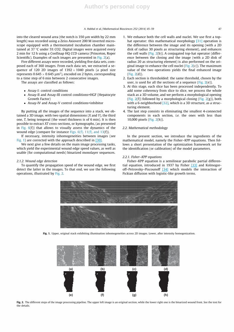
into the cleared wound area (the notch is 350 lm width by 22 mmlength) was recorded using a Zeiss Axiovert 200 M inverted micro-scope equipped with a thermostated incubation chamber main-tained at 37 �C under 5% CO2. Digital images were acquired every2 min for 12 h using a CoolSnap HQ CCD camera (Princeton, RoperScientific). Examples of such images are presented in Fig. 2(a).

Five different assays were recorded, yielding five data sets, com-posed each of 360 images. From each data set, we extracted a se-quence of 120 2D images of 1392� 1040 pixels (a pixel sizerepresents 0:645� 0:645 lm2), encoded on 2 bytes, correspondingto a time step of 6 min between 2 consecutive images.

The assays are classified as follows:

� Assay-I: control conditions� Assay-II and Assay-III control conditions+HGF (Hepatocyte

Growth Factor)� Assay-IV and Assay-V control conditions+inhibitor

By putting all the images of the sequence into a stack, we ob-tained a 3D image, with two spatial dimensions (X and Y), the thirdone, T, being temporal (the voxel thickness is of 6 min). It is thenpossible to extract XT cross-sections, or kymographs, (as presentedin Fig. 6(f)) that allows to visually assess the dynamics of thewound edge (compare for instance Figs. 6(f), 11(f), and 13(f)).

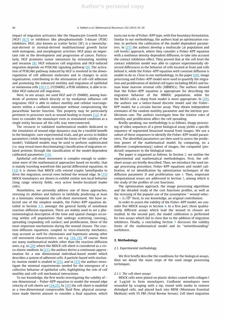
If necessary, intensity inhomogeneities between images (seeFig. 1) are corrected with the approach described in [30].

We next give a few details on the main image processing tasks,which yield the experimental wound edge speed values, as well asusable (for computational needs) binarized monolayer sequences.

2.1.2. Wound edge detectionTo quantify the propagation speed of the wound edge, we first

detect the latter in the images. To that end, we use the followingoperations, illustrated by Fig. 2.

1. We enhance both the cell walls and nuclei. We use first a top-hat operator: this mathematical morphology [31] operation isthe difference between the image and its opening (with a 2Ddisk of radius 30 pixels as structuring element), and enhancesthe cell walls (Fig. 2(b)). A conjugated top-hat operator (differ-ence between the closing and the image (with a 2D disk ofradius 20 as structuring element) is also performed on the ori-ginal image to enhance the cell nuclei (Fig. 2(c)). The maximumvalue of the two operations yields the final enhanced image(Fig. 2(d)).

2. Each section is thresholded: the same threshold, chosen by theuser, is used for all the sections of a sequence (Fig. 2(e)).

3. At this stage, each slice has been processed independently. Toadd some coherency from slice to slice, we process the wholestack as a 3D volume, and we perform a morphological opening(Fig. 2(f)) followed by a morphological closing (Fig. 2(g)), bothwith a 6-neighborhood [32], which is a 3D structure, as a struc-turing element.

4. The last step consists in eliminating the smallest 4-connectedcomponents in each section, i.e. the ones with less than10,000 pixels (Fig. 2(h)).

2.2. Mathematical methodology

In the present section, we introduce the ingredients of themathematical model, namely the Fisher–KPP equations. Then fol-lows a short presentation of the optimization framework set forthe identification (or calibration) of the model parameters.

2.2.1. Fisher–KPP equationsFisher–KPP equation is a semilinear parabolic partial differen-

tial equation, introduced in 1937 by Fisher [33] and Kolmogor-off–Petrovsky–Piscounoff [34] which models the interaction ofFickian diffusion with logistic-like growth terms.

Fig. 1. Upper, original stack exhibiting illumination inhomogeneities across 2D images. Lower, after intensity homogenization.

(a) (b) (c) (d)

(e) (f) (g) (h)

Fig. 2. The different steps of the image processing pipeline. The upper left image is an original section, while the lower right one is the binarized wound front. See the text forthe details.

A. Habbal et al. / Mathematical Biosciences 252 (2014) 45–59 47

Author's personal copy

First, let us introduce the equation in its most classical presen-tation, before discussing its main features and relevance to modelthe wound healing of monolayers.

We denote by X a rectangular domain, typically an image frameof the monolayer, by CD its vertical sides and by CN its horizontalones.

We assume that the monolayer is at confluence initially, andconsider the cell density relatively to the confluent one. TheFisher–KPP equation then reads

@u@t¼ DDuþ ruð1� uÞ in X ð1Þ

where u ¼ uðt;xÞ ¼ cell densitycell density at confluence denotes the relative cell den-

sity at time t and position x ¼ ðx; yÞ 2 X. The parameter D is the dif-fusion coefficient and r is the linear growth rate. The two latterparameters are assumed constant. The operator D ¼ @2

@x2 þ @2

@y2 is theLaplace operator.

To complete the formulation of the Fisher–KPP equation, initialand boundary conditions must be specified. Classically, at t ¼ 0 onehas at hand an initial (binarized) monolayer image u0ðxÞ. Then, onesimply sets:

uð0;xÞ ¼ u0ðxÞ over X: ð2Þ

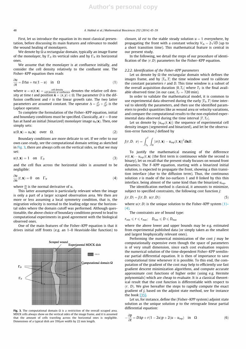
Boundary conditions are more delicate to set. If we refer to ourown case-study, see the computational domain setting as sketchedin Fig. 3, there are always cells on the vertical sides, so that we mayset:

uðt; xÞ ¼ 1 on CD ð3Þ

and the cell flux across the horizontal sides is assumed to benegligible:

@u@nðt;xÞ ¼ 0 on CN ð4Þ

where @u@n is the normal derivative of u.

This latter assumption is particularly relevant when the imageis only a part of a larger scraped observation area. We then aremore or less assuming a local symmetry condition, that is, themigration velocity is normal to the leading edge near the horizon-tal sides where the domain cutoff was performed. Although ques-tionable, the above choice of boundary conditions proved to lead tocomputational experiments in good agreement with the biologicalobserved ones.

One of the main features of the Fisher–KPP equation is that itdrives initial stiff fronts (e.g. an 1–0 Heaviside-like function) to

closure, id est to the stable steady solution u ¼ 1 everywhere, bypropagating the front with a constant velocity Vth ¼ 2

ffiffiffiffiffiffirDp

(up toa short transition time). This mathematical feature is central inour present study.

In the following, we detail the steps of our procedure of identi-fication of the ðr;DÞ parameters for the Fisher–KPP equation.

2.2.2. Identification of the Fisher–KPP parametersLet us denote by X the rectangular domain which defines the

images frame, and by ½T0; T� the time window used to calibratethe constant parameters r and D. This time window is a subset ofthe overall acquisition duration ½0; TF � where TF is the final avail-able observed time (in our case, TF ¼ 720 min).

In order to validate the mathematical model, it is common touse experimental data observed during the early ½T0; T� time inter-val to identify the parameters, and then use the identified param-eters to predict quantities like as wound area or velocity variations,and compare the computational results to the non exploited exper-imental data observed during the time interval ½T; TF �.

Let us denote by uexpðt;xÞ� �

the sequence of experimental celldensity images (segmented and binarized), and let be the observa-tion-error function J defined by

Jðr;D; vÞ ¼Z T

T0

ZXjvðt;xÞ � uexpðt;xÞj2dxdt:

To justify the mathematical meaning of the differencevðt;xÞ � uexpðt;xÞ (the first term is continuous while the second isbinary), let us recall that the present study focuses on wound frontdynamics. The F–KPP equation, starting with a binarized initialsolution, is expected to propagate the front, showing a thin transi-tion interface (due to the diffusion term). Thus, the continuoussolution v is made of the iso-surfaces 1 and 0 linked by this thininterface, being almost of the same kind than the binarized uexp.

The identification method is classical, it amounts to minimize,subject to specified constraints, the following cost function j:

jðr;DÞ ¼ Jðr;D; uðr;DÞÞ ð5Þ

where uðr;DÞ is the unique solution to the Fisher–KPP system (1)–(4).

The constraints are of bound type:

rmin 6 r 6 rmax; Dmin 6 D 6 Dmax

where the above lower and upper bounds may be e.g. estimatedfrom experimental published data (or simply taken as the smallestand largest biophysically relevant ones).

Performing the numerical minimization of the cost j may becomputationally expensive even though the space of parametersis of very small dimension, since each cost evaluation requiresthe numerical solution of the time-dependent Fisher–KPP semilin-ear partial differential equation. It is then of importance to savecomputational time whenever it is possible. To this end, the com-putation of the gradient of the cost may help to efficiently use fastgradient descent minimization algorithms, and compute accurateapproximate cost functions of higher order (using e.g. Hermitepolynomials) which are cheap to evaluate. It is a classical theoret-ical result that the cost function is differentiable with respect toðr; DÞ. We give hereafter the steps to rapidly compute the exactgradient of j, based on the adjoint state method, see for instancethe book [35].

Let us, for instance, define the (Fisher–KPP system) adjoint statesolution as the unique solution p to the retrograde linear partialdifferential equation:

� @p@t¼ DDpþ rð1� 2uÞpþ 2ðu� uexpÞ in X ð6Þ

Fig. 3. The computational domain X is a restriction of the overall scraped area.MDCK cells always show on the vertical sides of the image frame, and it is assumedthat the amount of cells traveling across the horizontal ones is negligible.Dimensions of a typical dish are 350lm width by 22 mm length.

48 A. Habbal et al. / Mathematical Biosciences 252 (2014) 45–59

Author's personal copy

with the following boundary conditions, consistent with the onesstated above for the Fisher–KPP solution u:

pðt; xÞ ¼ 0 over CD@p@nðt; xÞ ¼ 0 over CN ð7Þ

and with a final condition prescribed at t ¼ T:

pðT;xÞ ¼ 0 in X: ð8Þ

The adjoint state formula yields the gradient of the cost func-tion j:

@j@rðr;DÞ ¼

Z T

T0

ZX

uð1� uÞpdxdt; ð9Þ

@j@Dðr;DÞ ¼ �

Z T

T0

ZXrurpdxdt: ð10Þ

To solve the Fisher–KPP system, we used an explicit Euler for-ward finite difference in time, and centered second order fivepoints finite difference in space. The numerical scheme is conver-gent provided a stability condition (the leading condition is ofthe form rDt þ 2DDt maxf1=ðDxÞ2;1=ðDyÞ2g 6 1, where Dt;Dx;Dyare time and space steps). The latter condition is satisfied thanksto the relative small magnitude of the considered diffusion andproliferation coefficients with respect to the typical time and spacesteps used in the present computational experiments. Indeed, spa-tial step is one pixel in both directions, and time step is a fraction(tenth) of the image acquisition lapse time.

We implemented our own finite difference code to solve theFisher–KPP equations, and used the matlab optimization (fmincon)toolbox. Let us underline that the numerical approximation of theretrograde adjoint state Eq. (6) requires careful treatment. In par-ticular, because of the lack of intermediate values of uexp for timesteps used by the numerical scheme that are not acquisition times(time interpolation is necessary). As well, the gradient formulae (9)and (10) have to be handled carefully because of the nature of thesolution u which shows a stiff profile nearby the wound edge,where the whole gradient information is concentrated.

The cost function j has a strongly non-linear implicit depen-dence on the parameters r and D. It is then not straightforwardto draw any conclusion related to the uniqueness of the minima(which do exist in the compact set defined by the bounds). Thus,in order to perform efficient numerical optimization, it is usefulif not mandatory to lead a preliminary study of the profile of thecost functions.

3. Preliminary analysis

We first list the parameters, experimentally estimated or com-puted, which are involved in the model validation method. Then,we lead a detailed study of the profiles of the cost functions com-monly used to identify the parameters. In the final part of the pres-ent section, we address the relevance of the assumption whichstates that experimental wound edge velocity should be a prioriim-posed as equal to the theoretical wavefront velocity.

3.1. Experimental and computed variables

On original images, 1 pixel ¼ 0:416 lm2 ¼ ð0:645 lmÞ2, but dueto computational restrictions on the image size, original imagessize is reduced by a rescaling factor of 8� 8. On resized images,1 pixel ¼ 8� 8� 0:416 lm2, so the leading edge velocity and diffu-sion parameters units must be rescaled accordingly:

� Diffusion unit: 1 pixel �min�1 ¼ 1:6 10�3mm2 � h�1 ¼ 1600lm2 � h�1

� Velocity unit: 1 pixel1=2 �min�1 ¼ 309:10�3mm � h�1

The bounds for the proliferation and diffusion parameters areset as follows, for the preliminary study as well as for the mainidentification calculations:

rmin ¼ 10�6; rmax ¼ 0:5 ðmin�1Þ Dmin ¼ 10�8;

Dmax ¼ 0:15 ðpixel �min�1Þ

½T0 � T� (increments of 6 min) is the subset of images used tocalibrate the model parameters r and D;r ðmin�1Þ and D (pixel/min) are the proliferation rate and diffu-sion coefficient;J is the optimal cost function. Otherwise specified, we usedJ ¼ JU=w0 where w0 is the initial wound area (see Section 3.2for the definition of JU);Vexp (pixel1=2

=min) is the experimental wound closure speeddefined as the slope of the linear regression w.r.t. time of theleading-edge (averaged in the i-coordinates) velocities;Vcomp (pixel1=2

=min) is the computed wound closure speeddefined as for Vexp, using the PDE model leading-edge evolution;Vth ¼ 2

ffiffiffiffiffiffirDp

(pixel1=2=min) is the theoretical wavefront velocity

of the Fisher–KPP model;MRexpðpixel=minÞ is the experimental migration rate defined asthe slope of the linear regression w.r.t. time of the experimentalwound area;MRcompðpixel=minÞ is the computed migration rate defined asfor MRexp, using the PDE model area evolution.

Notice that, throughout the paper, the experimental and com-putational velocities we refer to are the horizontal componentsof the velocity vectors, which are approximately the componentsperpendicular to the wound edge. Considering an Eulerian viewof the wound edge rather than a Lagrangian one, the assumptionis reasonable. We do not take into account the mechanical strainsthat are experienced by the cell rows behind the edge, so that theedge tangential velocity does not affect the wound edge geometry.

3.2. Profile of the cost functions

For a given assay, we denote by uexpðt;xÞ� �

the sequence ofexperimental cell monolayer images, segmented and binarized,and by ðWexpðtÞÞ the corresponding experimental wound area.

We have considered as cost functions to be minimized thefollowing:

Cell density error : JUðr;DÞ ¼Z½T0 ;T�

ZXjuðt; xÞ � uexpðt;xÞj2dxdt ð11Þ

Wound area error : JAðr;DÞ ¼Z½T0 ;T�jWðtÞ �WexpðtÞj2dt ð12Þ

where u is the computed solution of the Fisher–KPP equations for agiven pair of parameters ðr;DÞ and WðtÞ ¼

RXð1� uðt; xÞÞdx is the

computed wound area.The cost function JA is introduced in order to study its relevance

to be used as an error-function, that is, its ability to yield correctmodel parameters at its minimal value.

We performed the computation of the cost functions surfacesfor several assays. The results were all similar. We present hereone that corresponds to an inhibited migration, a case which illus-trates a pathological behavior of the cost JA.

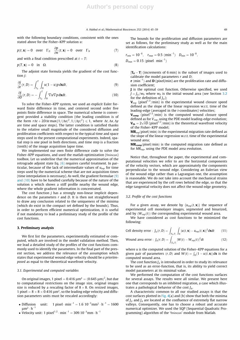
A characteristic common to all our studied assays is that thecost surfaces plotted in Fig. 4(a) and (b) show that both the minimaof JU and JA are located at the confluence of extremely flat narrowvalleys. Consequently, one has to choose a robust and accuratenumerical optimizer. We used the SQP (Sequential Quadratic Pro-gramming) algorithm of the ‘fmincon’ module from Matlab.

A. Habbal et al. / Mathematical Biosciences 252 (2014) 45–59 49

Author's personal copy

We plotted in Fig. 4(c) the profile of ðJAðr;DÞ; JUðr;DÞÞ for a uni-form 40� 40 sampling of ½rmin; rmax� � ½Dmin;Dmax�. Globally, the twocosts JA and JU show some correlated variation; Interestingly, closeto their minima, which is the region of interest for our study, thesetwo functions are quite antagonistic (increasing one decreases theother and conversely). In order to help us answer the question:which cost function is the most relevant for the parameter identi-fication? we led different studies, essentially numerical because of

the intricate implicit relation satisfied by the two functions withrespect to the parameters r and D.

Indeed, many authors (see e.g. [24]) assume that the experi-mentally measured leading edge velocities are close toVth ¼ 2

ffiffiffiffiffiffirDp

, the theoretical velocity of the Fisher–KPP wavefront,and then use the latter to compute the diffusion coefficient D giventhe cell proliferation rate r (doubling time tables obtained frompublished data) through the formula Vexp � 2

ffiffiffiffiffiffirDp

. So, we found it

0

0.1

0.2

0.3

0.4

0.5 0

0.05

0.1

0.15

0.2

024

x 105

Diffusion coefficient

Surface of Upde−Uexp function

Proliferation Rate

0

0.1

0.2

0.3

0.4

0.5 0

0.05

0.1

0.15

0.2

024

x 105

Diffusion coefficient

Surface of Area−Cost function

Proliferation Rate

0 1 2 3 4 5 6 7 8x 104

0

1

2

3

4

5

6

7

x 104 Area−Cost versus (Uexp−Upde) Cost

Cost JA

Cos

t JU

(a) (b) (c)

Fig. 4. Surface plot of costs (a) JU and (b) JA as function of the parameters ðr;DÞwhere r 2 ½rmin; rmax� and D 2 ½Dmin;Dmax �. The colors correspond to the cost function magnitude(high cost areas are in red and lowest are in dark blue) (c) Values of ðJAðr;DÞ; JUðr;DÞÞ are plotted for exhaustive pairs ðr;DÞ. The costs show globally some correlated variation.Close to their minima, the relative position of the values located at the image set boundary indicates that indeed they are conflicting (decrease in one increases the other andconversely). (For interpretation of the references to color in this figure caption, the reader is referred to the web version of this article.)

0 0.5 1 1.5 2 2.5 3x 105

−16

−14

−12

−10

−8

−6

−4

−2

0

2JU Cost versus relative (Vexp−Vth) Gap

Cost JU

(Vex

p−Vt

h)/V

exp

0 0.5 1 1.5 2 2.5 3 3.5x 105

−16

−14

−12

−10

−8

−6

−4

−2

0

2JA Cost versus relative (Vexp−Vth) Gap

Cost JA

(Vex

p−Vt

h)/V

exp

(a) (b)

1 2 3 4 5 6 7 8x 104

−2.5

−2

−1.5

−1

−0.5

0

0.5

1

1.5

JU Cost versus relative (Vexp−Vth) Gap

Cost JU

(Vex

p−Vt

h)/V

exp

1 2 3 4 5 6 7 8x 104

−2.5

−2

−1.5

−1

−0.5

0

0.5

1

1.5

JA Cost versus relative (Vexp−Vth) Gap

Cost JA

(Vex

p−Vt

h)/V

exp

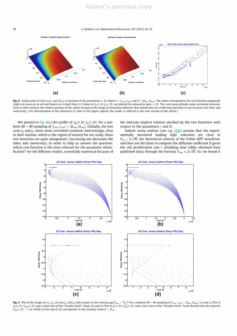
(c) (d)Fig. 5. Plot of the image set ðJU ; JAÞ of costs JU and JA with respect to the velocity gap Vgap ¼ Vexp�Vth

Vexpfor a uniform 40� 40 sampling of ½rmin; rmax � � ½Dmin;Dmax�. (a) and (c) Plot of

ðJUðr;DÞ;Vgapðr;DÞÞ and a close view of the ‘‘Paradise bird’s’’ head. (b) and (d) Plot of ðJAðr;DÞ;Vgapðr;DÞÞ and a close view of the ‘‘Paradise bird’s’’ head. Remark that the segmentVgapðr;DÞ ¼ 1 as visible on the top of (d) corresponds to the minimal value D ¼ Dmin .

50 A. Habbal et al. / Mathematical Biosciences 252 (2014) 45–59

Author's personal copy

interesting to investigate the dependance of the considered costswith respect to the difference in velocities Vgap ¼ Vexp�Vth

Vexpwhere

Vexp is the experimentally measured one using the sequence ofbinarized images.

The study of the dependence of the wound area cost JA and celldensity one JU with respect to the parameter Vgap led us to the fol-lowing observations, see Fig. 5:

(i) for all assays, the global minimum of JA as a function offfiffiffiffiffiffirDp

always occurred at Vgapðr;DÞ � 1, id est at D ¼ Dmin.(ii) for inhibited migration assays, the assumption Vgap � 0 wasirrelevant to yield the optimal values of the model parameters.

Thus, we abandoned the recourse to the wound area cost func-tion JA (and convex combination with the cost JU turned out to beuseless), and as well we abandoned thea prioriconstraining ofVgapðr;DÞ to zero. Remarkably, we nevertheless observed, fromour numerical results, that for migration assays, which are neitheractivated nor inhibited, the approximation Vexp � Vth holds a poste-riori, see Table 1.

4. Results

We performed the assessment of the validity of the F–KPPmathematical model on five MDCK monolayer assays: a reference

one, two activated and two inhibited migration conditions. Twodifferent situations are considered, depending on the success orfailure of the wound closure.

4.1. Wound closure occurs

In the following, the results of three different MDCK cell-sheetassays are discussed. They have in common that the scrapedwound closed. The first one referred to as Assay-I is a referenceone, also known as control assay, where no migration activatorsor inhibitors were used. In the two other assays, Assay-II and As-say-III, HGF (Hepatocyte Growth Factor) a well known migrationactivator of epithelial cells is added to the control (Assay-I) setting.

For the three assays, we first comment in a few words the pro-files computed by exploiting the experimental data, using the seg-mented and binarized image sequences. Then, we compare theexperimental profiles and parameters to the corresponding com-puted ones.

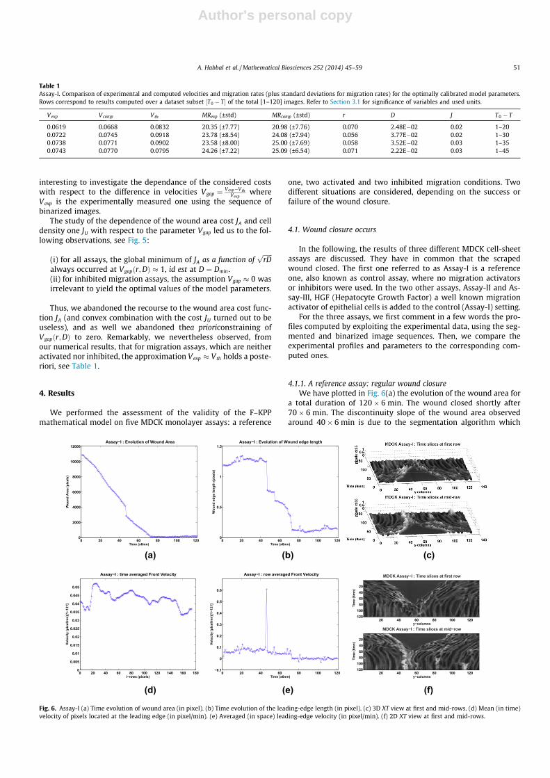
4.1.1. A reference assay: regular wound closureWe have plotted in Fig. 6(a) the evolution of the wound area for

a total duration of 120� 6 min. The wound closed shortly after70� 6 min. The discontinuity slope of the wound area observedaround 40� 6 min is due to the segmentation algorithm which

Table 1Assay-I. Comparison of experimental and computed velocities and migration rates (plus standard deviations for migration rates) for the optimally calibrated model parameters.Rows correspond to results computed over a dataset subset ½T0 � T� of the total [1–120] images. Refer to Section 3.1 for significance of variables and used units.

Vexp Vcomp Vth MRexp (±std) MRcomp (±std) r D J T0 � T

0.0619 0.0668 0.0832 20.35 (±7.77) 20.98 (±7.76) 0.070 2.48E�02 0.02 1–200.0722 0.0745 0.0918 23.78 (±8.54) 24.08 (±7.94) 0.056 3.77E�02 0.02 1–300.0738 0.0771 0.0902 23.58 (±8.00) 25.00 (±7.69) 0.058 3.52E�02 0.03 1–350.0743 0.0770 0.0795 24.26 (±7.22) 25.09 (±6.54) 0.071 2.22E�02 0.03 1–45

0 20 40 60 80 100 1200

2000

4000

6000

8000

10000

12000 Assay−I : Evolution of Wound Area

Time (x6mn)

Wou

nd A

rea

(pix

els)

0 20 40 60 80 100 1200

0.5

1

1.5 Assay−I : Evolution of Wound edge length

Time (x6mn)

Wou

nd e

dge

leng

th (p

ixel

s)

(c)(b)(a)

0 20 40 60 80 100 120 140 160 1800

0.005

0.01

0.015

0.02

0.025

0.03

0.035

0.04

0.045

0.05

Assay−I : time averaged Front Velocity

i−rows (pixels)

Velo

city

(pix

el/m

n)[1

−121

]

0 20 40 60 80 100 120−0.1

0

0.1

0.2

0.3

0.4

0.5

0.6

Assay−I : row averaged Front Velocity

Time (x6mn)

Velo

city

(pix

el/m

n)[1

−121

]

y−columns

Tim

e (6

mn)

MDCK Assay−I : Time slices at first row

20 40 60 80 100 120

20406080

100120

y−columns

Tim

e (6

mn)

MDCK Assay−I : Time slices at mid−row

20 40 60 80 100 120

20406080

100120

(f)(e)(d)

Fig. 6. Assay-I (a) Time evolution of wound area (in pixel). (b) Time evolution of the leading-edge length (in pixel). (c) 3D XT view at first and mid-rows. (d) Mean (in time)velocity of pixels located at the leading edge (in pixel/min). (e) Averaged (in space) leading-edge velocity (in pixel/min). (f) 2D XT view at first and mid-rows.

A. Habbal et al. / Mathematical Biosciences 252 (2014) 45–59 51

Author's personal copy

performs poorly when the opposite wound edges touch each otherat some point.

The discontinuity observed in Fig. 6b) and the peak observed inFig. 6(e) (they occur around T ¼ 48� 6 mm) correspond also to thefirst contact between wound opposite edges. The edge mean veloc-ity profile in Fig. 6(e) is rather constant until the opposite parts ofthe wound edge enter into contact (until the peak).

Fig. 6(d) shows that if one records the time-averaged speed ofthe pixels located at the wound edge, then some cells (that is, somecollection of neighbor pixels) exhibit higher speeds, in more pre-cisely three distinct locations. This observation may have a linkwith the so-called leader cells, see [15].

In Fig. 6(c), we have plotted the XT slices (kymographs) with as3rd dimension the pixel intensity in order to picture how far thecell-sheet migration is from a pure scattering dynamics. Indeed,without mitosis, apoptosis and maybe some videoscopy defocal-

ization, we would observe lines of continuous smooth ridges. Weproject the 3D view in a 2D one in Fig. 6(f), to get a visual represen-tation of the speed profile for first and mid-range rows of the imagesequences.

Assay-I: Computational results compared to experimental dataTable 1 and Fig. 7 show a very good accordance between the ob-

served biological parameters and the model predicted ones, nota-bly the Fisher–KPP model accurately predicted total closure time(shortly after 70� 6 min).

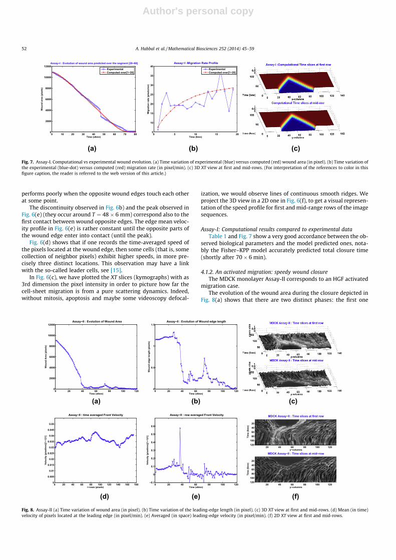
4.1.2. An activated migration: speedy wound closureThe MDCK monolayer Assay-II corresponds to an HGF activated

migration case.The evolution of the wound area during the closure depicted in

Fig. 8(a) shows that there are two distinct phases: the first one

0 10 20 30 40 50 60 70 800

2000

4000

6000

8000

10000

12000

Time (x6mn)

Wou

nd a

rea

(pix

els)

Assay−I : Evolution of wound area predicted over the segment [20−80]

ExperimentalComputed over[1−20]

0 5 10 15 205

10

15

20

25

30

35

40

Time (6mn)

Mig

ratio

n ra

te (p

ixel

s/m

n)

Assay−I :Migration Rate Profile

ExperimentalComputed over[1−20]

(c)(b)(a)

Fig. 7. Assay-I. Computational vs experimental wound evolution. (a) Time variation of experimental (blue) versus computed (red) wound area (in pixel). (b) Time variation ofthe experimental (blue-dot) versus computed (red) migration rate (in pixel/min). (c) 3D XT view at first and mid-rows. (For interpretation of the references to color in thisfigure caption, the reader is referred to the web version of this article.)

0 20 40 60 80 100 1200

2000

4000

6000

8000

10000

12000 Assay−II : Evolution of Wound Area

Time (x6mn)

Wou

nd A

rea

(pix

els)

0 20 40 60 80 100 1200

0.5

1

1.5 Assay−II : Evolution of Wound edge length

Time (x6mn)

Wou

nd e

dge

leng

th (p

ixel

s)

(c)(b)(a)

0 20 40 60 80 100 120 140 160 1800

0.005

0.01

0.015

0.02

0.025

0.03

0.035

0.04

0.045

0.05

Assay−II : time averaged Front Velocity

i−rows (pixels)

Velo

city

(pix

el/m

n)[1

−121

]

0 20 40 60 80 100 120−0.1

0

0.1

0.2

0.3

0.4

0.5

0.6

Assay−II : row averaged Front Velocity

Time (x6mn)

Velo

city

(pix

el/m

n)[1

−121

]

y−columns

Tim

e (6

mn)

MDCK Assay−II : Time slices at first row

20 40 60 80 100 120

20406080

100120

y−columns

Tim

e (6

mn)

MDCK Assay−II : Time slices at mid−row

20 40 60 80 100 120

20406080

100120

(f)(e)(d)

Fig. 8. Assay-II (a) Time variation of wound area (in pixel). (b) Time variation of the leading-edge length (in pixel). (c) 3D XT view at first and mid-rows. (d) Mean (in time)velocity of pixels located at the leading edge (in pixel/min). (e) Averaged (in space) leading-edge velocity (in pixel/min). (f) 2D XT view at first and mid-rows.

52 A. Habbal et al. / Mathematical Biosciences 252 (2014) 45–59

Author's personal copy

occurs roughly speaking during the image interval [1–20], and thesecond one occurs around [20–36] with a larger slope. The woundedge mean velocity plotted in Fig. 8(e) corroborates this distinc-tion, and one may observe that the velocity magnitude is slightlygreater than 0:10 during the [20–36] interval, 36 being the imageat which opposite edges come into contact.

Compared to the reference assay, the topology of the ridgesshown in Fig. 8(c) look more jerky, and the 2D projected imageFig. 8(f) shows a velocity profile (the contour of the homoge-neously gray region) which is not a rectilinear triangle as observedin Fig. 6(f).

The total length of the leading edges Fig. 8(b) seems to havelower fluctuation than in the reference case, except close to theoccurrence of the fronts contact.

The distribution of the mean (time-averaged) front velocitywith respect to the pixels location is plotted in Fig. 8(d). Cells lo-cated at the mid and bottom rows tend to be faster, but no obviouslocalized leading regions, except the middle, arises from theprofile.

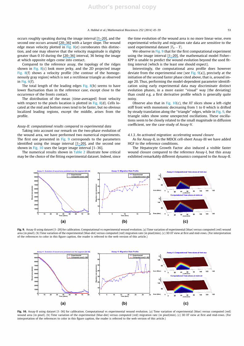
Assay-II: computational results compared to experimental dataTaking into account our remark on the two-phase evolution of

the wound area, we have performed two numerical experiments.The first one presented in Fig. 9 corresponds to the parametersidentified using the image interval [1–20], and the second oneshown in Fig. 10 uses the larger image interval [1–36].

The numerical results shown in Table 2 illustrate how criticalmay be the choice of the fitting experimental dataset. Indeed, since

the time evolution of the wound area is no more linear-wise, evenexperimental velocity and migration rate data are sensitive to theused experimental dataset ½T0 � T�.

We observe in Fig. 9 that for the first computational experimentusing the image interval [1–20], the mathematical model Fisher–KPP is unable to predict the wound evolution beyond the used fit-ting interval (which is the least one should expect).

Interestingly, the computational area profile does howeverdeviate from the experimental one (see Fig. 9(a)), precisely at theinitiation of the second faster phase cited above, that is, around im-age 20. Thus, performing the model-dependent parameter identifi-cation using early experimental data may discriminate distinctevolution phases, in a more easier ‘‘visual’’ way (the deviating)than could e.g. a first derivative profile which is generally quitenoisy.

Observe also that in Fig. 10(c), the XT slices show a left–rightstiff front with monotonic decreasing from 1 to 0 which is driftedby steady translation along the ‘‘triangle’’ edges, while in Fig. 9, thetriangle sides show some unexpected oscillations. These oscilla-tions seem to be closely related to the small magnitude in diffusioncoefficient, see the case-study of Assay-V.

4.1.3. An activated migration: accelerating wound closureAs for Assay-II, in the MDCK cell-sheet Assay-III we have added

HGF to the reference conditions.The Hepatocyte Growth Factor also induced a visible faster

wound closure compared to the reference Assay-I, but this assayexhibited remarkably different dynamics compared to the Assay-II.

0 10 20 30 40 50 60 70 800

1000

2000

3000

4000

5000

6000

7000

8000

9000

10000

Time (x6mn)

Wou

nd a

rea

(pix

els)

Assay−II : Evolution of wound area predicted over the segment [20−80]

ExperimentalComputed over[1−20]

0 5 10 15 205

10

15

20

25

30

35

Time (6mn)

Mig

ratio

n ra

te (p

ixel

s/m

n)

Assay−II :Migration Rate Profile

ExperimentalComputed over[1−20]

(c)(b)(a)

Fig. 9. Assay-II using dataset [1–20] for calibration. Computational vs experimental wound evolution. (a) Time variation of experimental (blue) versus computed (red) woundarea (in pixel). (b) Time variation of the experimental (blue-dot) versus computed (red) migration rate (in pixel/min). (c) 3D XT view at first and mid-rows. (For interpretationof the references to color in this figure caption, the reader is referred to the web version of this article.)

0 10 20 30 40 50 60 70 800

1000

2000

3000

4000

5000

6000

7000

8000

9000

10000

Time (x6mn)

Wou

nd a

rea

(pix

els)

Assay−II : Evolution of wound area predicted over the segment [36−80]

ExperimentalComputed over[1−36]

0 5 10 15 20 25 30 350

10

20

30

40

50

60

70

Time (6mn)

Mig

ratio

n ra

te (p

ixel

s/m

n)

Assay−II :Migration Rate Profile

ExperimentalComputed over[1−36]

(c)(b)(a)

Fig. 10. Assay-II using dataset [1–36] for calibration. Computational vs experimental wound evolution. (a) Time variation of experimental (blue) versus computed (red)wound area (in pixel). (b) Time variation of the experimental (blue-dot) versus computed (red) migration rate (in pixel/min). (c) 3D XT view at first and mid-rows. (Forinterpretation of the references to color in this figure caption, the reader is referred to the web version of this article.)

A. Habbal et al. / Mathematical Biosciences 252 (2014) 45–59 53

Author's personal copy

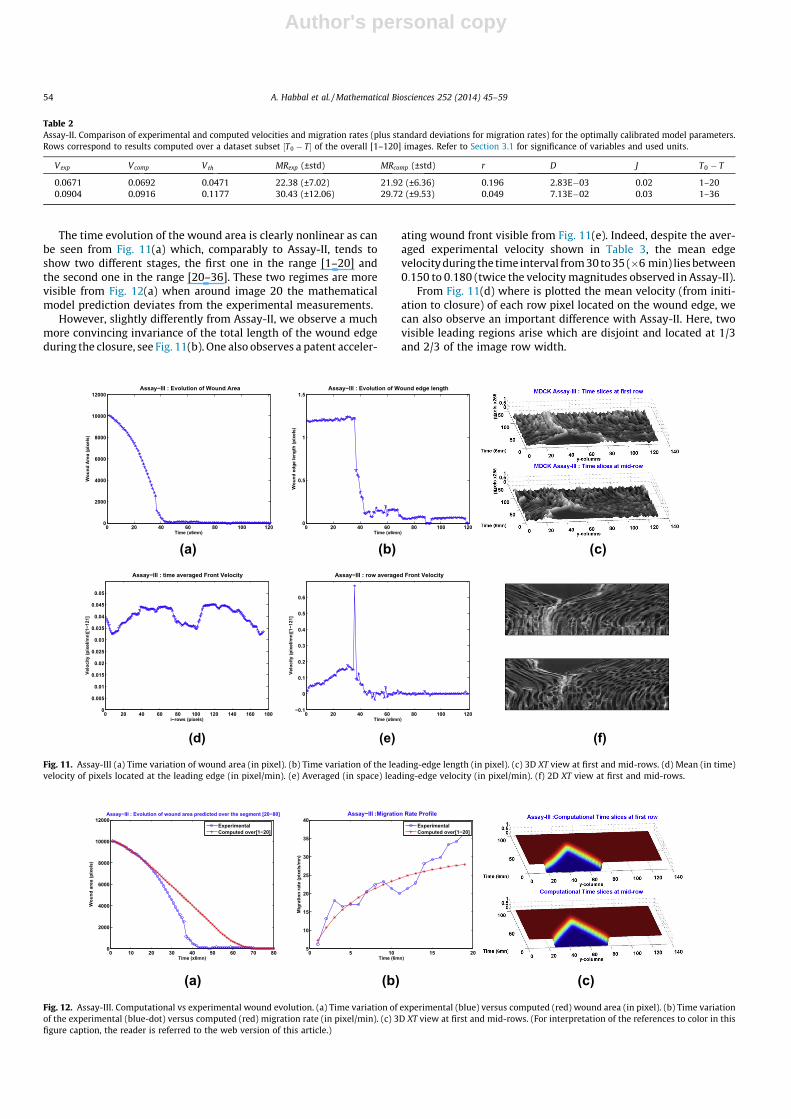
The time evolution of the wound area is clearly nonlinear as canbe seen from Fig. 11(a) which, comparably to Assay-II, tends toshow two different stages, the first one in the range [1–20] andthe second one in the range [20–36]. These two regimes are morevisible from Fig. 12(a) when around image 20 the mathematicalmodel prediction deviates from the experimental measurements.

However, slightly differently from Assay-II, we observe a muchmore convincing invariance of the total length of the wound edgeduring the closure, see Fig. 11(b). One also observes a patent acceler-

ating wound front visible from Fig. 11(e). Indeed, despite the aver-aged experimental velocity shown in Table 3, the mean edgevelocity during the time interval from 30 to 35 (�6 min) lies between0:150 to 0:180 (twice the velocity magnitudes observed in Assay-II).

From Fig. 11(d) where is plotted the mean velocity (from initi-ation to closure) of each row pixel located on the wound edge, wecan also observe an important difference with Assay-II. Here, twovisible leading regions arise which are disjoint and located at 1/3and 2/3 of the image row width.

Table 2Assay-II. Comparison of experimental and computed velocities and migration rates (plus standard deviations for migration rates) for the optimally calibrated model parameters.Rows correspond to results computed over a dataset subset ½T0 � T� of the overall [1–120] images. Refer to Section 3.1 for significance of variables and used units.

Vexp Vcomp Vth MRexp (±std) MRcomp (±std) r D J T0 � T

0.0671 0.0692 0.0471 22.38 (±7.02) 21.92 (±6.36) 0.196 2.83E�03 0.02 1–200.0904 0.0916 0.1177 30.43 (±12.06) 29.72 (±9.53) 0.049 7.13E�02 0.03 1–36

0 20 40 60 80 100 1200

2000

4000

6000

8000

10000

12000 Assay−III : Evolution of Wound Area

Time (x6mn)

Wou

nd A

rea

(pix

els)

0 20 40 60 80 100 1200

0.5

1

1.5 Assay−III : Evolution of Wound edge length

Time (x6mn)

Wou

nd e

dge

leng

th (p

ixel

s)

(c)(b)(a)

0 20 40 60 80 100 120 140 160 1800

0.005

0.01

0.015

0.02

0.025

0.03

0.035

0.04

0.045

0.05

Assay−III : time averaged Front Velocity

i−rows (pixels)

Velo

city

(pix

el/m

n)[1

−121

]

0 20 40 60 80 100 120−0.1

0

0.1

0.2

0.3

0.4

0.5

0.6

Assay−III : row averaged Front Velocity

Time (x6mn)

Velo

city

(pix

el/m

n)[1

−121

]

(f)(e)(d)

Fig. 11. Assay-III (a) Time variation of wound area (in pixel). (b) Time variation of the leading-edge length (in pixel). (c) 3D XT view at first and mid-rows. (d) Mean (in time)velocity of pixels located at the leading edge (in pixel/min). (e) Averaged (in space) leading-edge velocity (in pixel/min). (f) 2D XT view at first and mid-rows.

0 10 20 30 40 50 60 70 800

2000

4000

6000

8000

10000

12000

Time (x6mn)

Wou

nd a

rea

(pix

els)

Assay−III : Evolution of wound area predicted over the segment [20−80]

ExperimentalComputed over[1−20]

0 5 10 15 205

10

15

20

25

30

35

40

Time (6mn)

Mig

ratio

n ra

te (p

ixel

s/m

n)

Assay−III :Migration Rate Profile

ExperimentalComputed over[1−20]

(c)(b)(a)

Fig. 12. Assay-III. Computational vs experimental wound evolution. (a) Time variation of experimental (blue) versus computed (red) wound area (in pixel). (b) Time variationof the experimental (blue-dot) versus computed (red) migration rate (in pixel/min). (c) 3D XT view at first and mid-rows. (For interpretation of the references to color in thisfigure caption, the reader is referred to the web version of this article.)

54 A. Habbal et al. / Mathematical Biosciences 252 (2014) 45–59

Author's personal copy

The 3D XT view in Fig. 11(c) and its 2D projection in Fig. 11(f)visually show even more jerky ridges than for the Assay-II, butwe did not assess it quantitatively.

Assay-III: computational results compared to experimental dataWe observe that as for Assay-II, and contrarily to the reference

Assay-I, the optimal model parameters strongly depend on the por-tion of data used for the identification process, and also are, but toa lesser extent, the mean velocities and migration rates, as can beseen from Table 3.

The comparison of experimental versus computational woundareas, as plotted in Fig. 12(a), show that the Fisher–KPP modelusing the optimal parameters sticks on the experiment only duringthe time used for the calibration. The model is unable to render thenon-linear wound area evolution as it enters an accelerated phase.Indeed, Fisher–KPP equation with the logistic growth term canonly propagate with constant velocity the initial front (so with lin-ear area profile), as tend to show the rectilinear-sided triangles inFig. 12(c).

4.2. Wound closure fails

We present in this section two assays, Assay-IV and Assay-V,where we added to the control conditions an inhibitor of thecell-sheet migration, the LY 294002 (more precisely, LY29 inhibitsPI3-kinase). For the two assays, both experimental and model-computed mean front velocities, migration rates and wound areaprofiles are to some extent comparable. A noticeable difference lies

in the range of the calibrated model parameters. Wound edgemean velocity is, for both Assay-IV and Assay-V, two to five timessmaller than the reference assay; but for Assay-IV the diffusioncoefficient D is comparable in order to the reference ones, whileit is two to three orders less in the case of Assay-V.

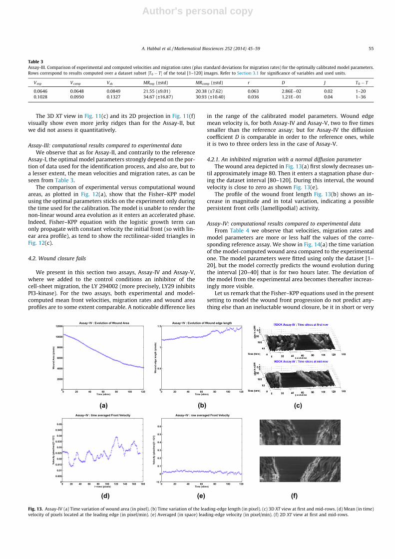
4.2.1. An inhibited migration with a normal diffusion parameterThe wound area depicted in Fig. 13(a) first slowly decreases un-

til approximately image 80. Then it enters a stagnation phase dur-ing the dataset interval [80–120]. During this interval, the woundvelocity is close to zero as shown Fig. 13(e).

The profile of the wound front length Fig. 13(b) shows an in-crease in magnitude and in total variation, indicating a possiblepersistent front cells (lamellipodial) activity.

Assay-IV: computational results compared to experimental dataFrom Table 4 we observe that velocities, migration rates and

model parameters are more or less half the values of the corre-sponding reference assay. We show in Fig. 14(a) the time variationof the model-computed wound area compared to the experimentalone. The model parameters were fitted using only the dataset [1–20], but the model correctly predicts the wound evolution duringthe interval [20–40] that is for two hours later. The deviation ofthe model from the experimental area becomes thereafter increas-ingly more visible.

Let us remark that the Fisher–KPP equations used in the presentsetting to model the wound front progression do not predict any-thing else than an ineluctable wound closure, be it in short or very

Table 3Assay-III. Comparison of experimental and computed velocities and migration rates (plus standard deviations for migration rates) for the optimally calibrated model parameters.Rows correspond to results computed over a dataset subset ½T0 � T� of the total [1–120] images. Refer to Section 3.1 for significance of variables and used units.

Vexp Vcomp Vth MRexp (±std) MRcomp (±std) r D J T0 � T

0.0646 0.0648 0.0849 21.55 (±9.01) 20.38 (±7.62) 0.063 2.86E�02 0.02 1–200.1028 0.0950 0.1327 34.67 (±16.87) 30.93 (±10.40) 0.036 1.21E�01 0.04 1–36

0 20 40 60 80 100 1200

2000

4000

6000

8000

10000

12000 Assay−IV : Evolution of Wound Area

Time (x6mn)

Wou

nd A

rea

(pix

els)

0 20 40 60 80 100 1200

0.5

1

1.5 Assay−IV : Evolution of Wound edge length

Time (x6mn)

Wou

nd e

dge

leng

th (p

ixel

s)

(c)(b)(a)

0 20 40 60 80 100 120 140 160 1800

0.005

0.01

0.015

0.02

0.025

0.03

0.035

0.04

0.045

0.05

Assay−IV : time averaged Front Velocity

i−rows (pixels)

Velo

city

(pix

el/m

n)[1

−121

]

0 20 40 60 80 100 120−0.1

0

0.1

0.2

0.3

0.4

0.5

0.6

Assay−IV : row averaged Front Velocity

Time (x6mn)

Velo

city

(pix

el/m

n)[1

−121

]

(f)(e)(d)

Fig. 13. Assay-IV (a) Time variation of wound area (in pixel). (b) Time variation of the leading-edge length (in pixel). (c) 3D XT view at first and mid-rows. (d) Mean (in time)velocity of pixels located at the leading edge (in pixel/min). (e) Averaged (in space) leading-edge velocity (in pixel/min). (f) 2D XT view at first and mid-rows.

A. Habbal et al. / Mathematical Biosciences 252 (2014) 45–59 55

Author's personal copy

long time. So, the use of mathematical models of the Fisher–KPPkind for inhibited migration assays must be carefully handled.We show here and for the next assay, that the Fisher–KPP modelis unable to render the whole story, because of the inhibition effect.If a given inhibitor has an effect of only slowing the migrationspeed without freezing it at some point, then the parameter iden-tification process for the Fisher–KPP model should yield computedresults (e.g. area evolution) in better accordance with the biological

experiments. As illustrated by Assay-II and Assay-III, the same re-mark holds as is for the activation case.

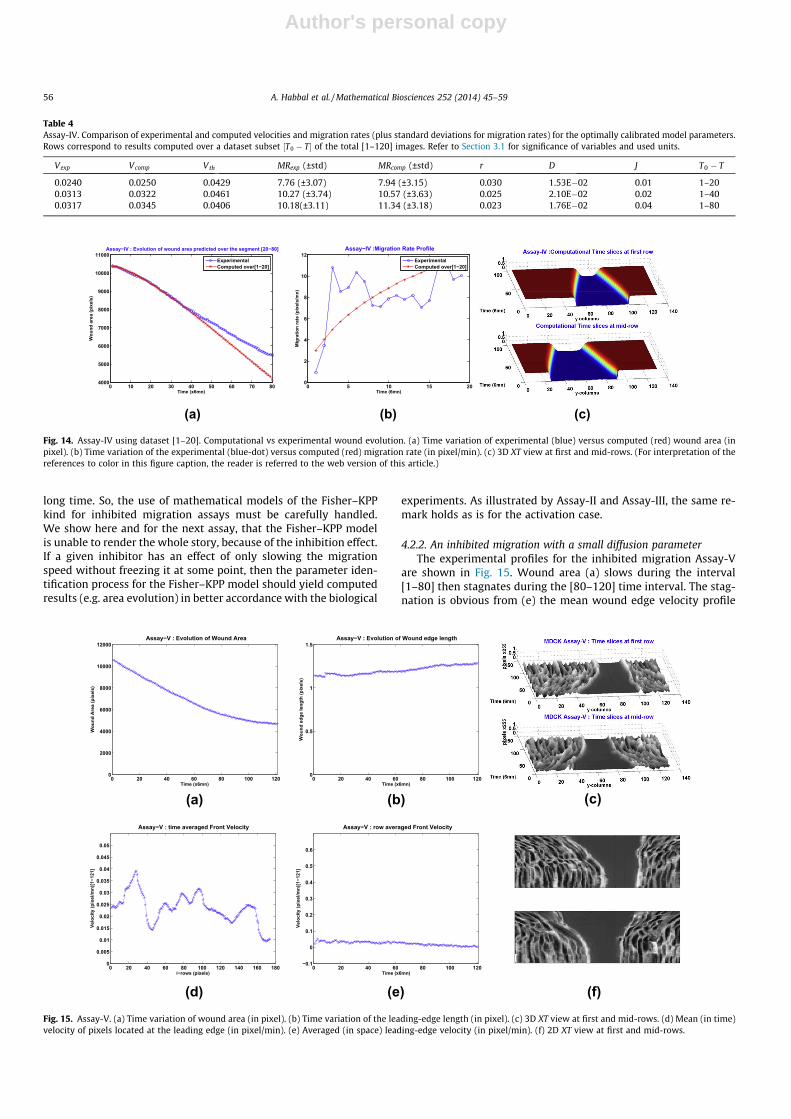
4.2.2. An inhibited migration with a small diffusion parameterThe experimental profiles for the inhibited migration Assay-V

are shown in Fig. 15. Wound area (a) slows during the interval[1–80] then stagnates during the [80–120] time interval. The stag-nation is obvious from (e) the mean wound edge velocity profile

Table 4Assay-IV. Comparison of experimental and computed velocities and migration rates (plus standard deviations for migration rates) for the optimally calibrated model parameters.Rows correspond to results computed over a dataset subset ½T0 � T� of the total [1–120] images. Refer to Section 3.1 for significance of variables and used units.

Vexp Vcomp Vth MRexp (±std) MRcomp (±std) r D J T0 � T

0.0240 0.0250 0.0429 7.76 (±3.07) 7.94 (±3.15) 0.030 1.53E�02 0.01 1–200.0313 0.0322 0.0461 10.27 (±3.74) 10.57 (±3.63) 0.025 2.10E�02 0.02 1–400.0317 0.0345 0.0406 10.18(±3.11) 11.34 (±3.18) 0.023 1.76E�02 0.04 1–80

0 10 20 30 40 50 60 70 804000

5000

6000

7000

8000

9000

10000

11000

Time (x6mn)

Wou

nd a

rea

(pix

els)

Assay−IV : Evolution of wound area predicted over the segment [20−80]

ExperimentalComputed over[1−20]

0 5 10 15 200

2

4

6

8

10

12

Time (6mn)

Mig

ratio

n ra

te (p

ixel

s/m

n)

Assay−IV :Migration Rate Profile

ExperimentalComputed over[1−20]

(c)(b)(a)

Fig. 14. Assay-IV using dataset [1–20]. Computational vs experimental wound evolution. (a) Time variation of experimental (blue) versus computed (red) wound area (inpixel). (b) Time variation of the experimental (blue-dot) versus computed (red) migration rate (in pixel/min). (c) 3D XT view at first and mid-rows. (For interpretation of thereferences to color in this figure caption, the reader is referred to the web version of this article.)

0 20 40 60 80 100 1200

2000

4000

6000

8000

10000

12000 Assay−V : Evolution of Wound Area

Time (x6mn)

Wou

nd A

rea

(pix

els)

0 20 40 60 80 100 1200

0.5

1

1.5 Assay−V : Evolution of Wound edge length

Time (x6mn)

Wou

nd e

dge

leng

th (p

ixel

s)

(c)(b)(a)

0 20 40 60 80 100 120 140 160 1800

0.005

0.01

0.015

0.02

0.025

0.03

0.035

0.04

0.045

0.05

Assay−V : time averaged Front Velocity

i−rows (pixels)

Velo

city

(pix

el/m

n)[1

−121

]

0 20 40 60 80 100 120−0.1

0

0.1

0.2

0.3

0.4

0.5

0.6

Assay−V : row averaged Front Velocity

Time (x6mn)

Velo

city

(pix

el/m

n)[1

−121

]

(f)(e)(d)

Fig. 15. Assay-V. (a) Time variation of wound area (in pixel). (b) Time variation of the leading-edge length (in pixel). (c) 3D XT view at first and mid-rows. (d) Mean (in time)velocity of pixels located at the leading edge (in pixel/min). (e) Averaged (in space) leading-edge velocity (in pixel/min). (f) 2D XT view at first and mid-rows.

56 A. Habbal et al. / Mathematical Biosciences 252 (2014) 45–59

Author's personal copy

which vanishes during the latter interval. The length of the leadingedge (b) does barely increase in the course of the assay. As for As-say-IV, we observe in (d) localized -roughly speaking, three- lead-ing regions of pixels.

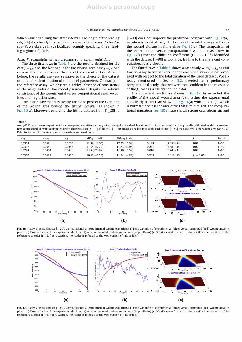
Assay-V: computational results compared to experimental dataThe three first rows in Table 5 are the results obtained for the

cost J ¼ JU , and the last one is for the wound area cost J ¼ JA. Wecomment on the last row at the end of the current section. As seenbefore, the results are very sensitive to the choice of the datasetused for the identification of the model parameters. Contrarily tothe reference assay, we observe a critical absence of consistencyin the magnitudes of the model parameters, despite the relativeconsistency of the experimental versus computational mean veloc-ities and migration rates.

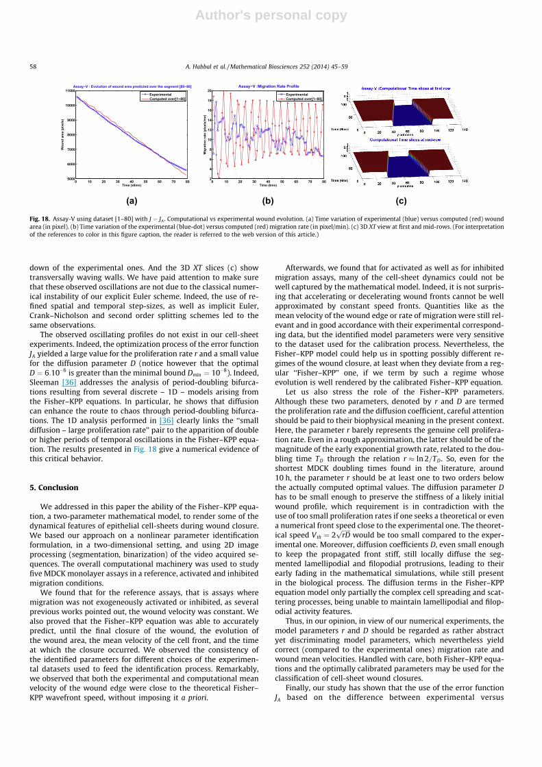
The Fisher–KPP model is clearly unable to predict the evolutionof the wound area beyond the fitting interval, as shown inFig. 16(a). Moreover, enlarging the fitting dataset from [1–20] to

[1–90] does not improve the prediction, compare with Fig. 17(a).As already pointed out, the Fisher–KPP model always achievesthe wound closure in finite time Fig. 17(c). The comparison ofthe experimental versus computational wound areas show inFig. 17(a) that the diffusion coefficient (D ¼ 3:7 10�2) identifiedwith the dataset [1–90] is too large, leading to the irrelevant com-putational early closure.

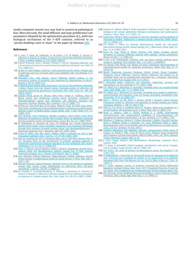
The fourth row in Table 5 shows a case study with J ¼ JA as costfunction (gap between experimental and model wound areas, aver-aged with respect to the total duration of the used dataset). We al-ready mentioned in Section 3.2, devoted to a preliminarycomputational study, that we were not confident in the relevanceof the JA cost as a calibration indicator.

The numerical results are shown in Fig. 18. As expected, theprofile of the model wound area (a) matches the experimentalone clearly better than shown in Fig. 16(a) with the cost JU whichis normal since it is the area error that is minimized. The computa-tional migration Fig. 18(b) rate shows strong oscillations up and

Table 5Assay-V. Comparison of experimental and computed velocities and migration rates (plus standard deviations for migration rates) for the optimally calibrated model parameters.Rows correspond to results computed over a dataset subset ½T0 � T� of the total [1–120] images. The last row, with used dataset [1–80] the used cost is the wound area gap J ¼ JA .Refer to Section 3.1 for significance of variables and used units.

Vexp Vcomp Vth MRexp (±std) MRcomp (±std) r D J T0 � T

0.0354 0.0381 0.0205 11.69 (±3.65) 12.23 (±3.58) 0.148 7.05E�04 0.01 1–200.0337 0.0351 0.0058 11.54 (±2.72) 11.73 (±3.98) 0.231 3.68E�05 0.02 1–400.0294 0.0360 0.0486 9.86 (±2.89) 11.86 (±3.59) 0.016 3.74E�02 0.07 1–90

0.0307 0.0330 0.0026 10.43 (±2.50) 11.24 (±4.83) 0.268 6.41E�06 JA ¼ 0:05 1–80

0 10 20 30 40 50 60 70 803000

4000

5000

6000

7000

8000

9000

10000

11000

Time (x6mn)

Wou

nd a

rea

(pix

els)

Assay−V : Evolution of wound area predicted over the segment [20−80]

ExperimentalComputed over[1−20]

0 5 10 15 206

8

10

12

14

16

18

Time (6mn)

Mig

ratio

n ra

te (p

ixel

s/m

n)

Assay−V :Migration Rate Profile

ExperimentalComputed over[1−20]

(c)(b)(a)

Fig. 16. Assay-V using dataset [1–20]. Computational vs experimental wound evolution. (a) Time variation of experimental (blue) versus computed (red) wound area (inpixel). (b) Time variation of the experimental (blue-dot) versus computed (red) migration rate (in pixel/min). (c) 3D XT view at first and mid-rows. (For interpretation of thereferences to color in this figure caption, the reader is referred to the web version of this article.)

0 20 40 60 80 100 1201000

2000

3000

4000

5000

6000

7000

8000

9000

10000

11000

Time (x6mn)

Wou

nd a

rea

(pix

els)

Assay−V : Evolution of wound area predicted over the segment [90−120]

ExperimentalComputed over[1−90]

0 10 20 30 40 50 60 70 80 900

2

4

6

8

10

12

14

16

18

Time (6mn)

Mig

ratio

n ra

te (p

ixel

s/m

n)

Assay−V :Migration Rate Profile

ExperimentalComputed over[1−90]

(c)(b)(a)

Fig. 17. Assay-V using dataset [1–90]. Computational vs experimental wound evolution. (a) Time variation of experimental (blue) versus computed (red) wound area (inpixel). (b) Time variation of the experimental (blue-dot) versus computed (red) migration rate (in pixel/min). (c) 3D XT view at first and mid-rows. (For interpretation of thereferences to color in this figure caption, the reader is referred to the web version of this article.)

A. Habbal et al. / Mathematical Biosciences 252 (2014) 45–59 57

Author's personal copy

down of the experimental ones. And the 3D XT slices (c) showtransversally waving walls. We have paid attention to make surethat these observed oscillations are not due to the classical numer-ical instability of our explicit Euler scheme. Indeed, the use of re-fined spatial and temporal step-sizes, as well as implicit Euler,Crank–Nicholson and second order splitting schemes led to thesame observations.

The observed oscillating profiles do not exist in our cell-sheetexperiments. Indeed, the optimization process of the error functionJA yielded a large value for the proliferation rate r and a small valuefor the diffusion parameter D (notice however that the optimalD ¼ 6:10�6 is greater than the minimal bound Dmin ¼ 10�8). Indeed,Sleeman [36] addresses the analysis of period-doubling bifurca-tions resulting from several discrete – 1D – models arising fromthe Fisher–KPP equations. In particular, he shows that diffusioncan enhance the route to chaos through period-doubling bifurca-tions. The 1D analysis performed in [36] clearly links the ‘‘smalldiffusion – large proliferation rate’’ pair to the apparition of doubleor higher periods of temporal oscillations in the Fisher–KPP equa-tion. The results presented in Fig. 18 give a numerical evidence ofthis critical behavior.

5. Conclusion

We addressed in this paper the ability of the Fisher–KPP equa-tion, a two-parameter mathematical model, to render some of thedynamical features of epithelial cell-sheets during wound closure.We based our approach on a nonlinear parameter identificationformulation, in a two-dimensional setting, and using 2D imageprocessing (segmentation, binarization) of the video acquired se-quences. The overall computational machinery was used to studyfive MDCK monolayer assays in a reference, activated and inhibitedmigration conditions.

We found that for the reference assays, that is assays wheremigration was not exogeneously activated or inhibited, as severalprevious works pointed out, the wound velocity was constant. Wealso proved that the Fisher–KPP equation was able to accuratelypredict, until the final closure of the wound, the evolution ofthe wound area, the mean velocity of the cell front, and the timeat which the closure occurred. We observed the consistency ofthe identified parameters for different choices of the experimen-tal datasets used to feed the identification process. Remarkably,we observed that both the experimental and computational meanvelocity of the wound edge were close to the theoretical Fisher–KPP wavefront speed, without imposing it a priori.

Afterwards, we found that for activated as well as for inhibitedmigration assays, many of the cell-sheet dynamics could not bewell captured by the mathematical model. Indeed, it is not surpris-ing that accelerating or decelerating wound fronts cannot be wellapproximated by constant speed fronts. Quantities like as themean velocity of the wound edge or rate of migration were still rel-evant and in good accordance with their experimental correspond-ing data, but the identified model parameters were very sensitiveto the dataset used for the calibration process. Nevertheless, theFisher–KPP model could help us in spotting possibly different re-gimes of the wound closure, at least when they deviate from a reg-ular ‘‘Fisher–KPP’’ one, if we term by such a regime whoseevolution is well rendered by the calibrated Fisher–KPP equation.

Let us also stress the role of the Fisher–KPP parameters.Although these two parameters, denoted by r and D are termedthe proliferation rate and the diffusion coefficient, careful attentionshould be paid to their biophysical meaning in the present context.Here, the parameter r barely represents the genuine cell prolifera-tion rate. Even in a rough approximation, the latter should be of themagnitude of the early exponential growth rate, related to the dou-bling time TD through the relation r � ln 2=TD. So, even for theshortest MDCK doubling times found in the literature, around10 h, the parameter r should be at least one to two orders belowthe actually computed optimal values. The diffusion parameter Dhas to be small enough to preserve the stiffness of a likely initialwound profile, which requirement is in contradiction with theuse of too small proliferation rates if one seeks a theoretical or evena numerical front speed close to the experimental one. The theoret-ical speed Vth ¼ 2

ffiffiffiffiffiffirDp

would be too small compared to the exper-imental one. Moreover, diffusion coefficients D, even small enoughto keep the propagated front stiff, still locally diffuse the seg-mented lamellipodial and filopodial protrusions, leading to theirearly fading in the mathematical simulations, while still presentin the biological process. The diffusion terms in the Fisher–KPPequation model only partially the complex cell spreading and scat-tering processes, being unable to maintain lamellipodial and filop-odial activity features.

Thus, in our opinion, in view of our numerical experiments, themodel parameters r and D should be regarded as rather abstractyet discriminating model parameters, which nevertheless yieldcorrect (compared to the experimental ones) migration rate andwound mean velocities. Handled with care, both Fisher–KPP equa-tions and the optimally calibrated parameters may be used for theclassification of cell-sheet wound closures.

Finally, our study has shown that the use of the error functionJA based on the difference between experimental versus

0 10 20 30 40 50 60 70 805000

6000

7000

8000

9000

10000

11000

Time (x6mn)

Wou

nd a

rea

(pix

els)

Assay−V : Evolution of wound area predicted over the segment [80−80]

ExperimentalComputed over[1−80]

0 10 20 30 40 50 60 70 802

4

6

8

10

12

14

16

18

20

Time (6mn)

Mig

ratio

n ra

te (p

ixel

s/m

n)

Assay−V :Migration Rate Profile

ExperimentalComputed over[1−80]

(c)(b)(a)

Fig. 18. Assay-V using dataset [1–80] with J ¼ JA . Computational vs experimental wound evolution. (a) Time variation of experimental (blue) versus computed (red) woundarea (in pixel). (b) Time variation of the experimental (blue-dot) versus computed (red) migration rate (in pixel/min). (c) 3D XT view at first and mid-rows. (For interpretationof the references to color in this figure caption, the reader is referred to the web version of this article.)

58 A. Habbal et al. / Mathematical Biosciences 252 (2014) 45–59

Author's personal copy

model-computed wound area may lead to numerical pathologicalbias. More precisely, the small diffusion and large proliferation rateparameters obtained by the optimization procedure of JA yield nonbiological oscillations of the F–KPP solution, referred to as‘‘period-doubling route to chaos’’ in the paper by Sleeman [36].

References

[1] A. Saez, E. Anon, M. Ghibaudo, O. du Roure, J.-M. Di Meglio, P. Hersen, P.Silberzan, A. Buguin, B. Ladoux, Traction forces exerted by epithelial cell sheets,J. Phys.: Condens. Matter 22 (19) (2010) 194119.

[2] Gabriel Fenteany, Paul A. Janmey, Thomas P. Stossel, Signaling pathways andcell mechanics involved in wound closure by epithelia cell sheets, Curr. Biol. 10(14) (2000) 831.

[3] Qi Bao, R. Colin Hughes, Galectin-3 and polarized growth within collagen gelsof wild-type and ricin-resistant mdck renal epithelial cells, Glycobiology 9 (5)(1999) 489.

[4] Alexandre Saez, Axel Buguin, Pascal Silberzan, Benoı�t Ladoux, Is themechanical activity of epithelial cells controlled by deformations or forces?,Biophys J. 89 (6) (2005) L52.

[5] Sri Ram Krishna Vedula, Man Chun Leong, Tan Lei Lai, Pascal Hersen, AlexandreJ. Kabla, Chwee Teck Lim, Benoît Ladoux, Emerging modes of collective cellmigration induced by geometrical constraints, Proc. Natl. Acad. Sci. 109 (32)(2012) 12974.

[6] Qinghui Meng, James M. Mason, Debra Porti, Itzhak D. Goldberg, Eliot M.Rosen, Saijun Fan, Hepatocyte growth factor decreases sensitivity tochemotherapeutic agents and stimulates cell adhesion, invasion, andmigration, Biochem. Biophys. Res. Commun. 274 (3) (2000) 772.

[7] Jui-Fen Lai, Shu-Chen Kao, Si-Tse Jiang, Ming-Jer Tang, Po-Chao Chan, Hong-Chen Chen, Involvement of focal adhesion kinase in hepatocyte growth factor-induced scatter of Madin–Darby canine kidney cells, J. Biol. Chem 275 (11)(2000) 7474.

[8] Esko Kankuri, Dana Cholujova, Monika Comajova, Antti Vaheri, Jozef Bizik,Induction of hepatocyte growth factor/scatter factor by fibroblast clusteringdirectly promotes tumor cell invasiveness, Cancer Res. 65 (21) (2005) 9914.

[9] M. Delehedde, N. Sergeant, M. Lyon, P.S. Rudland, D.G. Fernig, Hepatocytegrowth factor/scatter factor stimulates migration of rat mammary fibroblaststhrough both mitogen-activated protein kinase and phosphatidylinositol 3-kinase/akt pathways, Eur. J. Biochem. 268 (16) (2001) 4423.

[10] Claire M. Wells, Arie Abo, Anne J. Ridley, Pak4 is activated via pi3k in hgf-stimulated epithelial cells, J. Cell Sci. 115 (Pt 20) (2002) 3947.

[11] Mao Ye, Danning Hu, Lili Tu, Xiangtian Zhou, Fan Lu, Bin Wen, Wencan Wu, YiLin, Zhonglou Zhou, Jia Qu, Involvement of pi3k/akt signaling pathway inhepatocyte growth factor-induced migration of uveal melanoma cells, Invest.Ophthalmol. Vis. Sci. 49 (2) (2008) 497.

[12] Anne L. Pollack, Gerard Apodaca, Keith E. Mostov, Hepatocyte growth factorinduces mdck cell morphogenesis without causing loss of tight junctionfunctional integrity, Am. J. Physiol. Cell Physiol. 286 (3) (2004).

[13] Luis Almeida, Patrizia Bagnerini, Abderrahmane Habbal, Stéphane Noselli,Fanny Serman, A mathematical model for dorsal closure, J. Theor. Biol. 268 (1)(2011) 105.

[14] Rizwan Farooqui, Gabriel Fenteany, Multiple rows of cells behind an epithelialwound edge extend cryptic lamellipodia to collectively drive cell-sheetmovement, J. Cell Sci. 118 (Pt 1) (2005) 51.

[15] M. Poujade, E. Grasland-Mongrain, A. Hertzog, J. Jouanneau, P. Chavrier, B.Ladoux, A. Buguin, P. Silberzan, Collective migration of an epithelial monolayerin response to a model wound, Proc. Natl. Acad. Sci. 104 (41) (2007) 15988.

[16] Eamonn A. Gaffney, Philip K. Maini, Jonathan A. Sherratt, Paul D. Dale, Woundhealing in the corneal epithelium: Biological mechanisms and mathematicalmodels, J. Theor. Med. 1 (1) (1997) 13.

[17] Luke Olsen, Philip K. Maini, Jonathan A. Sherratt, Spatially varying equilibria ofmechanical models: Application to dermal wound contraction, Math. Biosci.147 (1) (1998) 113.

[18] P.K. Maini, L. Olsen, J.A. Sherratt, Mathematical models for cell-matrixinteractions during dermal wound healing, Int. J. Bifurcation Chaos Appl. Sci.Eng. 12 (9) (2002) 2021.

[19] Karen M. Page, Philip K. Maini, Nicholas A.M. Monk, Complex patternformation in reaction–diffusion systems with spatially varying parameters,Physica D 202 (1-2) (2005) 95.

[20] P. Lee, C.W. Wolgemuth, Crawling cells can close wounds without pursestrings or signaling, PLoS Comput. Biol. 7 (3) (2011) (e1002007).

[21] J.A. Fozard, H.M. Byrne, O.E. Jensen, J.R. King, Continuum approximations ofindividual-based models for epithelial monolayers, Math. Med. Biol. 27 (1)(2010) 39.

[22] Nestor Sepulveda, Laurence Petitjean, Olivier Cochet, Erwan Grasland-Mongrain, Pascal Silberzan, Vincent Hakim, Collective cell motion in anepithelial sheet can be quantitatively described by a stochastic interactingparticle model, PLoS Comput. Biol. 9 (3) (2013).

[23] J. Alexandre Kabla, Collective cell migration: leadership, invasion andsegregation, J. R. Soc. Interface 9 (77) (2012) 3268.

[24] P.K. Maini, D.L.S. McElwain, D. Leavesley, Traveling waves in a wound healingassay, Appl. Math. Lett. 17 (5) (2004) 575.

[25] P.K. Maini, D.L.S. McElwain, D. Leavesley, Traveling wave model to interpret awound-healing cell migration assay for human peritoneal mesothelial cells,Tissue Eng. 10 (3–4) (2004) 475.

[26] Julia C. Arciero, Qi Mi, Maria F. Branca, David J. Hackam, David Swigon,Continuum model of collective cell migration in wound healing and colonyexpansion, Biophys. J. 100 (3) (2011) 535.

[27] Anna Q. Cai, Kerry A. Landman, Barry D. Hughes, Multi-scale modeling of awound-healing cell migration assay, J. Theor. Biol. 245 (3) (2007) 576.

[28] Bram G. Sengers, Colin P. Please, Richard O. C Oreffo, Experimentalcharacterization and computational modelling of two-dimensional cellspreading for skeletal regeneration, J. R. Soc. Interface 4 (17) (2007) 1107.

[29] Matthew J. Simpson, Katrina K. Treloar, Benjamin J. Binder, Parvathi Haridas,Kerry J. Manton, David I. Leavesley, D.L. Sean McElwain, Ruth E. Baker,Quantifying the roles of cell motility and cell proliferation in a circular barrierassay, J. R. Soc. Interface 10 (82) (2013).

[30] Grégoire Malandain, Eric Bardinet, Intensity compensation within series ofimages, in: Randy E. Ellis, Terry M. Peters (Eds.), Medical Image Computingand Computer-assisted Intervention (MICCAI 2003), LNCS, vol. 2879, SpringerVerlag, Montreal, Canada, 2003, p. 41.

[31] J. Serra, Image Analysis and Mathematical Morphology, Academic Press,London, 1982.

[32] T.Y. Kong, A. Rosenfeld, Digital topology: introduction and survey, Comput.Vision Graphics Image Process. 48 (3) (1989) 357.

[33] R.A. Fisher, The wave of advance of advantageous genes, An. Eugenics 7 (4)(1937) 355.

[34] A. Kolmogoroff, I. Petrovsky, N. Piscounoff, Étude de l’équation de la diffusionavec croissance de la quantité de matière et son application à un problèmebiologique, Bull. Univ. Etat Moscou, Ser. Int., Sect. A, Math. et Mecan. 1 (Fasc. 6)(1937) 1.

[35] J.-L. Lions, Optimal Control of Systems Governed by Partial DifferentialEquations, Springer-Verlag, New York, 1971 (Translated from the French byS.K. Mitter, Die Grundlehren der mathematischen Wissenschaften, Band 170).

[36] B.D. Sleeman, Period-doubling bifurcations leading to chaos in discrete modelsof biology, IMA J. Math. Appl. Med. Biol. 5 (1) (1988) 21.

A. Habbal et al. / Mathematical Biosciences 252 (2014) 45–59 59