Assessing Supervised Machine Learning Techniques for Predicting Student Learning Preferences

Assessing Supervised Machine Learning Techniques for Predicting Student Learning

Preferences

S. B. Kotsiantis ([email protected])

I. D. Zaharakis ([email protected])

P. E. Pintelas ([email protected])

Educational Software Development Laboratory, Department of Mathematics University of Patras, Hellas

ABSTRACT The preferences and the learning styles of different students can vary greatly. The same learning material can be boring for a student and at the same time quite interesting for another. The use of Machine Learning (ML) in adaptive educational systems can construct systems that are automatically improved by experience. Key characteristics of the learning material and the learning habits of a student may constitute the training set for a supervised learning algorithm. The learning algorithm will then create a model of the student's decision making process that can be used to emulate the students's decisions on future instances (learning units). This paper aims to fill the gap between empirical student profiling and the existing ML techniques To this end it introduces the issues involved in predicting student learning preferences, briefly describes the different supervised learning algorithms and investigates the pros and cons of each algorithm in the context of student modeling in order to recommend the most suitable algorithms to be used within an integrated educational environment.

KEYWORDS: supervised machine learning, student preferences, adaptive educational systems

INTRODUCTION In distance learning, it is desirable that learners with different learning style view different

presentations of the educational material. The objective is to support learners, following their preferred way of studying. Adaptive educational systems depend on student’s model, a model of student characteristics, as the basis for their adaptation decisions. The models of students can be generated by hand or through machine learning techniques. In the past, student models were often created by hand, constructing stereotypes with which to classify students. Rules for interaction with students were also often constructed manually. A straightforward way of using ML for preferences profiles is to assume that learning units can be divided into a number of classes (e.g., for "interesting" and "not interesting") and the students provide, directly or indirectly, instances for all classes in the initial training phase (see next section for more details). A Learning Unit (LU) is considered to be the smallest complete educational material, which will be displayed by the educational software.

ML algorithms reason from externally supplied instances (input set) to produce general hypotheses, which will make predictions about future instances. Generally, every instance is represented by using the same set of attributes and the attributes’ values can be continuous, categorical or binary. The externally supplied instances are usually referred to as training set. If

«ICTs in Education», Volume I, A. Dimitracopoulou (Ed), Proceedings of 3rd Congress HICTE, 26-29/9/2002, University of Aegean, Rhodes, Greece, KASTANIOTIS Editions Inter@ctive 639

training instances are given with known labels (the corresponding correct outputs) then the learning is called supervised, in contrast to unsupervised learning where training instances are unlabeled. In detail, unsupervised learning deals with instances, which have not been pre-classified in any way and thus they do not have a class attribute associated with them. In our case, the LUs are divided into classes and therefore unsupervised learning algorithms are excluded from our study. To induce a hypothesis from a given training set, a learning system needs to make assumptions about the hypothesis to be learned. A learning system without any assumptions cannot generate a useful hypothesis since the number of hypotheses that are consistent with the training set is usually huge.

This paper aims to fill the gap between empirical student profiling and the existing ML techniques, which could be useful for further advances in the area of adaptive educational systems. Particularly, the scope of this work is to discuss the pros and cons of each supervised learning algorithm in the context of student modeling. In the next section, we introduce the issues involved in predicting student learning preferences. In section 3, we briefly describe the categories of supervised learning algorithms and comment on the possible use of them in the prediction of student learning preferences. Some of them can handle more and some others less the special difficulties of the application of ML in student modeling. The final section ends up in useful conclusions.

PREDICTING STUDENT LEARNING PREFERENCES At first glance, it may be tempting to consider the learning of student preferences as

straightforward standard classification task; however, it is not so trivial (Webb, Pazzani & Billsus, 2001). One important limitation of the straightforward application of ML is that the learning algorithm does not build a classifier (mapping from unlabeled instances to classes) with acceptable accuracy until it sees a relatively large number of examples. Another difficulty confronting direct application of ML is that the supervised ML approaches require explicitly labeled data, but the proper labels may not be readily apparent from simple observation of the student's behavior (such as printing a LU or copy a subset of the LU in the clipboard). One simpler solution is to require the student to explicitly label the data, but the student must perform additional work.

The most well-known classifier criterion in ML community is the rate of correct predictions made by the classifier over a data set. However, from the perspective of student modelling, an algorithm that recommends favourite LUs with a predictive accuracy of 80% might be preferred over an algorithm that achieves 82%, if the former algorithm requires considerably less time. This efficiency criterion arises from the requirement that a classifier of LUs should use only reasonable amounts of time and memory for training and application. In addition, student modeling focuses on a system that refines on-line its behaviour over time, incorporating new training instances or new knowledge about the student, without having to halt and re-process all data. This means that accurate and descriptive classifier should be generated from small sets of training cases and that it should be updated each time a student interaction occurs or at least before the next session. Moreover, student modeling is known to be a very dynamic modeling task – student preferences are likely to change over time. Therefore, it is important the learning algorithms to be capable of adjusting to changes quickly.

The process of applying supervised ML to an adaptive educational system starts with the suggestions of the domain expert about which fields (attributes) are the most informative for the description of a LU. The careful choice of the attributes could help the learning algorithm to build an efficient classifier. Unfortunately, the most informative attributes are not specified in the bibliography so some irrelevant attributes could be among them (some of the possible attributes with their values are presented in the Table 1). Since the domain expert offers the list with the useful attributes, the next step is the collection of the data set (the attribute values among with their

640

corresponding output) by the observation or the feedback of the student (content-based learning). In addition, since some students may exhibit similar behaviours, these similar instance spaces could be combined into larger sets, providing more evidence for prediction (collaboration learning). The choice of which algorithm is most appropriate for learning student preferences is a critical step. After a successful training, the classifier can be used to emulate the student's decisions on future LUs to personalize the educational process.

LU attributes Values Media Type {Text, Video, Presentation, Other} Instructional Type {Example, Description, Definition, Other} Size {Small, Medium, Large} Language {English, Greek, Other} Level of Difficulty {Too Easy, Easy, Medium, Difficult, Very Difficult}

Table 1. Some possible LU attributes

The goal of the classifier could be to support the student in hyperspace orientation and navigation in the learning material by changing the appearance of visible links that lead to the LUs. In particular, the system could adaptively sort, annotate, or partly hide the links of the current page to make easier the choice of the next link (LU) to proceed. In general, adaptive navigation helps students to find an "optimal path" through the learning material. At the same time, adaptive navigation support is less directive than traditional sequencing since such a method guides students implicitly and leaves the choice of the next knowledge item to them (Brusilovsky, 1998).

SUPERVISED MACHINE LEARNING METHODS There are many categories of supervised learning algorithms and each category has its own

characteristics but some issues are more or less generally applicable (Kotsiantis S., Zaharakis I., Pintelas P., 2002). From statistical point of view, instances with irrelevant input attributes provide less information. Hence, it is wise to carefully choose which attributes to provide to the learning algorithm with (Wettschereck et al., 1997). Moreover, a reduction in attribute values is usually not harmful and it leads to a major decrease in computational complexity of the learning algorithm.

Decision Trees A well known and broadly used category of supervised learning is the decision trees. Murthy

(1998) provides a recent overview of existing work in decision trees. Decision trees are tree structures that classify instances by sorting them based on attribute values. Each node in a decision tree represents an attribute of an instance to be classified and each branch represents a value that a node can take. Instances are classified starting at the root node and sorting them based on their attribute values. The problem of constructing optimal binary decision trees is an NP-complete problem and thus scientists research for efficient heuristics for constructing near-optimal decision trees. Mitchell (1997) gives a detailed description of the ID3 algorithm, which exemplifies its well-known successors C4.5 and C5.0. The attribute that best divides the training data would be the root node of the tree. Then the algorithm is repeated on each partition of the divided data, creating sub trees until the training data are divided into subsets of the same class. At each level of the partitioning process a statistical property, known as information gain, is used to determine which attribute best divides the training instances (Mitchell, 1997).

ID3 and many other learning algorithms don’t take as input numeric data, so data preprocessing is necessary for handling the continuous attributes. An approach dealing with numerical attributes is to discrete them using a multi-splitting procedure such as the one suggested by (Elomaa & Rousu, 1999). The ID3 algorithm was improved to accommodate incremental learning by a series of algorithms (Murthy, 1998).

641

In the context of the student modelling, the decision trees can start training with few instances. In addition, the training speed is acceptable and the classification process is very rapid. However, in order to enable a decision tree algorithm to respond to changes (concept drift), it is necessary to decide which old training instances should be deleted. Neural Networks

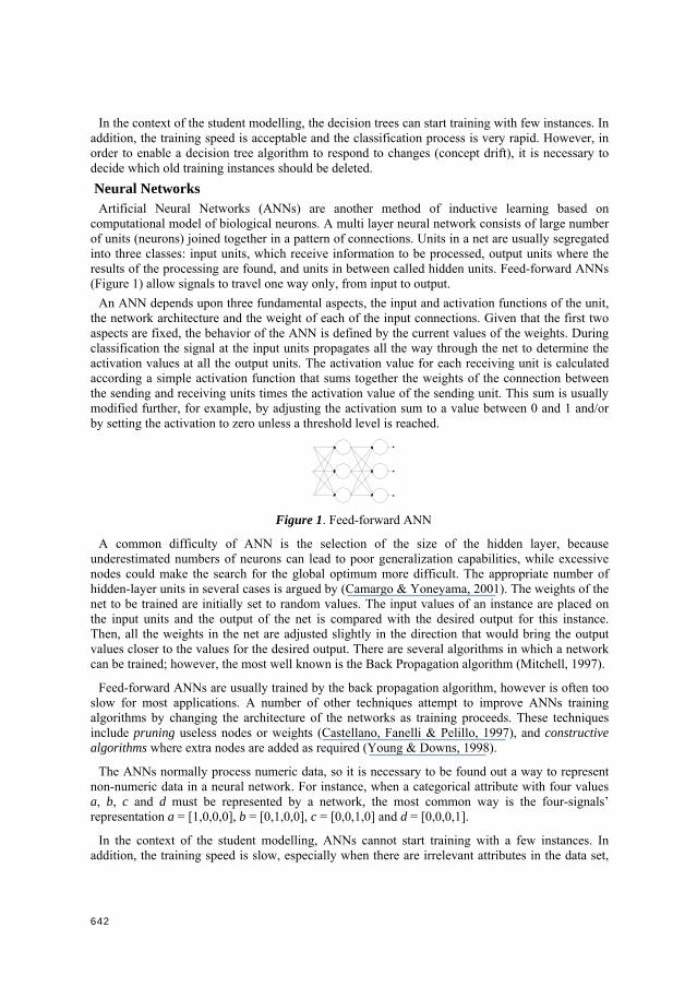
Artificial Neural Networks (ANNs) are another method of inductive learning based on computational model of biological neurons. A multi layer neural network consists of large number of units (neurons) joined together in a pattern of connections. Units in a net are usually segregated into three classes: input units, which receive information to be processed, output units where the results of the processing are found, and units in between called hidden units. Feed-forward ANNs (Figure 1) allow signals to travel one way only, from input to output.

An ANN depends upon three fundamental aspects, the input and activation functions of the unit, the network architecture and the weight of each of the input connections. Given that the first two aspects are fixed, the behavior of the ANN is defined by the current values of the weights. During classification the signal at the input units propagates all the way through the net to determine the activation values at all the output units. The activation value for each receiving unit is calculated according a simple activation function that sums together the weights of the connection between the sending and receiving units times the activation value of the sending unit. This sum is usually modified further, for example, by adjusting the activation sum to a value between 0 and 1 and/or by setting the activation to zero unless a threshold level is reached.

Figure 1. Feed-forward ANN

A common difficulty of ANN is the selection of the size of the hidden layer, because underestimated numbers of neurons can lead to poor generalization capabilities, while excessive nodes could make the search for the global optimum more difficult. The appropriate number of hidden-layer units in several cases is argued by (Camargo & Yoneyama, 2001). The weights of the net to be trained are initially set to random values. The input values of an instance are placed on the input units and the output of the net is compared with the desired output for this instance. Then, all the weights in the net are adjusted slightly in the direction that would bring the output values closer to the values for the desired output. There are several algorithms in which a network can be trained; however, the most well known is the Back Propagation algorithm (Mitchell, 1997).

Feed-forward ANNs are usually trained by the back propagation algorithm, however is often too slow for most applications. A number of other techniques attempt to improve ANNs training algorithms by changing the architecture of the networks as training proceeds. These techniques include pruning useless nodes or weights (Castellano, Fanelli & Pelillo, 1997), and constructive algorithms where extra nodes are added as required (Young & Downs, 1998).

The ANNs normally process numeric data, so it is necessary to be found out a way to represent non-numeric data in a neural network. For instance, when a categorical attribute with four values a, b, c and d must be represented by a network, the most common way is the four-signals’ representation a = [1,0,0,0], b = [0,1,0,0], c = [0,0,1,0] and d = [0,0,0,1].

In the context of the student modelling, ANNs cannot start training with a few instances. In addition, the training speed is slow, especially when there are irrelevant attributes in the data set,

642

so it is proposed an attribute reduction pre-processing to be applied first. However, if the training process has been terminated the classification process is very rapid and quite accurate.

Bayesian Classification A Bayesian Network is a graphical model for probabilistic relationships among a set of variables

(attributes). The Bayesian network structure S is a directed acyclic graph (DAG) and the nodes in S are in one-to-one correspondence with the variables X. The arcs represent casual influences among the variables while the lack of possible arcs in S encodes conditional independencies. Moreover, a variable is conditionally independent of its non-descendants given its parents (X1 is conditionally independent of X2 given X3 if P(X1|X2,X3)=P(X1|X3) for all possible values of X1, X2, X3).

Commonly, the task of learning a Bayesian Network (BN) is divided into two subtasks: one of learning the DAG structure of the network, and the second of determining the parameters (Jensen, 1996). Within the general framework of inducing Bayesian networks, there are two broad scenarios: known structure and unknown structure. In the first scenario, the structure of the network is given (e.g. by an expert) and assumed to be correct. The task is then to learn the parameters of the network from data and it is fairly straightforward (a function of the relative frequencies of occurrences of the values of the variable). However, the computational difficulty of exploring a previously unknown network is an inherent limitation. Given a problem described by n variables, the number of possible structure hypotheses is more than exponential in n. In the case that the structure is unknown, the most common approach is to introduce a scoring function (or a score) that evaluates the “fitness” of networks with respect to the training data, and then to search for the best network (according to this score).

The most general learning scenario is when the structure of the network is unknown and there are hidden variables – attributes that are not inserted in the model. Friedman (1997) has proposed a technique to learn the structure of a network with hidden variables; however, it requires the number of hidden variables to be pre-specified. Using the suitable method of the previous, one can induce a Bayesian Network from a given training set. The classifier based on the network and on the given set of attributes X1,X2, . . . , Xn, returns the label c that maximizes the posterior probability p(c | X1,X2, . . . , Xn).

An important property of BNs is that they support the combination of the collaborative and the content-based approach. The collaborative approach may be used to obtain the conditional probability tables and the initial beliefs of a BN. These beliefs can then be updated in a content-based manner by the student feedback. This mode of operation enables the predictive model to overcome the data collection problem of the content-based approach (which requires large amounts of data to be gathered from a single student). However, the training speed is acceptable only in the case that the structure of the network is known. Moreover, even though the classification process is rapid, BNs delay a little to respond to changes (concept drift).

Naive Bayes classifier is the simplest form of BN. In this acyclic graph, there is no edge between attributes and edges only exist between the class variable and attributes. This network captures the assumption that every attribute (every node in the network) is independent from the rest of the attributes, given the state of the class variable (the starting node). The independence model (Naive

Bayes) is based on estimating R=( )( )

( ) ( )( ) ( )

( ) ( )( ) ( )

| |

| |

r

r

P i X P i P X i P i P X i

P j X P j P X j P j P X j= =

|

|

∏∏

. Comparing

these two probabilities, the larger probability indicates the class label value that is more likely to be the actual label (if R > 1: predict i else predict j).

The assumption of independence is clearly almost always incorrect and for this reason naive Bayes classifier is usually less accurate than other more sophisticated learning algorithms (such

643

ANNs). However, Domingos & Pazzani (1997) performed a large-scale comparison of naive Bayes classifier with state-of-the-art algorithms for decision tree induction, instance-based learning and rule induction on standard benchmark datasets, and found it sometimes to be superior from the other learning schemes even on datasets with substantial attribute dependencies.

Naive Bayes classifiers provide some benefits to the field of learning student preferences. They do not require large amounts of data before learning process and they are computationally fast during training and decision making. However, they delay to respond to changes (concept drift).

Instance-Based Learning Instance-based learning algorithms belong to the category of lazy-learning algorithms (Mitcell,

1997), as they defer in the induction or generalization process until classification is performed. The lazy-learning algorithms require less computation time during the training phase than eager-learning algorithms (such as decision trees, neural and BNs) but more computation time during the classification process. The time to classify the query instance is a function of the number of stored instances and the number of attributes that are used to describe each instance. One of the most straightforward instance-based learning algorithms is the nearest neighbour algorithm (Aha, 1997). k-Nearest Neighbour (kNN) is based on the principle that the instances within a data set will generally exist in close proximity with other instances that have similar properties. If the instances are tagged with a classification label, then the value of the label of an unclassified instance can be determined by observing the class of its nearest neighbours. The kNN locates the k nearest instances in the query instance and determines its class by identifying the single most frequent class label. The relative distance is determined using a distance metric. Ideally, the distance metric must minimize the distance between two similarly classified instances, while maximizing the distance between instances of different classes. Many different metrics are presented in (Wilson & Martinez, 2000).

The power of kNN has been demonstrated in a number of real domains, however, there are some objections about the power of kNN, such as: 1) they have large storage requirements, 2) they are sensitive to the choice of the similarity function that is used to compare instances, 3) they lack of a principled way to choose k. Wettschereck et al. (1997) investigated the behavior of the kNN. They found that for small values of k, the kNN algorithm was more robust than the single nearest neighbour algorithm (1NN) for the majority of large data sets tested. However, the performance of the kNN was inferior to that achieved by the 1NN on small data sets.

As the instances multiply, the classification time multiplies too, so the application of kNN in the student modeling is useful only with k=1 and in the initial phase (the student is new to the system). When the training instances pass a number, another algorithm must be selected.

Genetic Algorithms Genetic algorithms (GAs) are inspired by natural evolution. In the natural world, organisms that

are poorly suited for an environment die off, while those well suited for it prosper. In order to apply GAs to a particular problem is needed to select an internal representation of the space to be searched and define an external evaluation function, which assigns utility to candidate solutions. Potential solutions to the problem must be encoded as strings of characters (chromosomes) drawn from some alphabet. Often the characters are binary, but it is also possible to draw them from larger alphabets (Banzhaf, Nordin, Keller & Francone, 1998). For a classification task, a natural way to express complex concepts is as a disjunctive set of (possibly overlapping) classification rules. Assuming two binary attributes X1, X2 and the binary target value c, the rule representation to chromosomes could be:

IF X1=True /\ X2=False THEN c=True, IF X1= False /\ X2=True THEN c=False 10 01 1 01 10 0

644

Note that there is a fixed length bit-string representation for each rule. The task of the genetic algorithm is to find good chromosomes. The goodness of a chromosome is represented by some function, which is called fitness function. In the canonical genetic algorithm, fitness is defined by fi / f where fi is the evaluation associated with chromosome i and f is the average evaluation of all the chromosomes in the population. At the heart of the algorithm are operations, which take the population at the present generation, and produce the population at the next time step in such a way that the overall fitness of the population is increased. These operations (selection, crossover, and mutation) are repeated until some stopping criterion is met, such as a given number of chromosomes been processed or a chromosome of given quality has been produced.

Selection is applied to the current population to create an intermediate population. There are a lot of selection schemes: 1) Remainder stochastic sampling, for each string i where fi / f is greater than 1 the integer portion of this number indicates how many copies of that string are directly placed in the intermediate population, 2) Elitism, the best members of the population are put into the next generation at each time step, 3) Tournament Selection, two members of the population are chosen at random. The least fit is removed and replaced by a copy of the most fit.

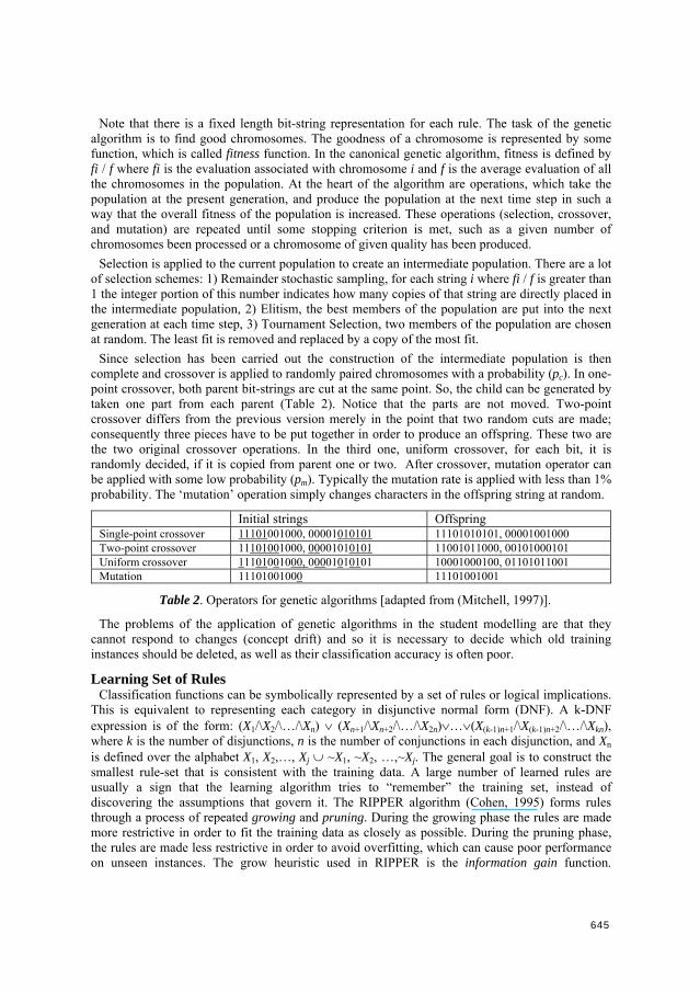
Since selection has been carried out the construction of the intermediate population is then complete and crossover is applied to randomly paired chromosomes with a probability (pc). In one-point crossover, both parent bit-strings are cut at the same point. So, the child can be generated by taken one part from each parent (Table 2). Notice that the parts are not moved. Two-point crossover differs from the previous version merely in the point that two random cuts are made; consequently three pieces have to be put together in order to produce an offspring. These two are the two original crossover operations. In the third one, uniform crossover, for each bit, it is randomly decided, if it is copied from parent one or two. After crossover, mutation operator can be applied with some low probability (pm). Typically the mutation rate is applied with less than 1% probability. The ‘mutation’ operation simply changes characters in the offspring string at random.

Initial strings Offspring Single-point crossover 11101001000, 00001010101 11101010101, 00001001000 Two-point crossover 11101001000, 00001010101 11001011000, 00101000101 Uniform crossover 11101001000, 00001010101 10001000100, 01101011001 Mutation 11101001000 11101001001

Table 2. Operators for genetic algorithms [adapted from (Mitchell, 1997)].

The problems of the application of genetic algorithms in the student modelling are that they cannot respond to changes (concept drift) and so it is necessary to decide which old training instances should be deleted, as well as their classification accuracy is often poor.

Learning Set of Rules Classification functions can be symbolically represented by a set of rules or logical implications.

This is equivalent to representing each category in disjunctive normal form (DNF). A k-DNF expression is of the form: (X1/\X2/\…/\Xn) ∨ (Xn+1/\Xn+2/\…/\X2n)∨…∨(X(k-1)n+1/\X(k-1)n+2/\…/\Xkn), where k is the number of disjunctions, n is the number of conjunctions in each disjunction, and Xn is defined over the alphabet X1, X2,…, Xj ∪ ~X1, ~X2, …,~Xj. The general goal is to construct the smallest rule-set that is consistent with the training data. A large number of learned rules are usually a sign that the learning algorithm tries to “remember” the training set, instead of discovering the assumptions that govern it. The RIPPER algorithm (Cohen, 1995) forms rules through a process of repeated growing and pruning. During the growing phase the rules are made more restrictive in order to fit the training data as closely as possible. During the pruning phase, the rules are made less restrictive in order to avoid overfitting, which can cause poor performance on unseen instances. The grow heuristic used in RIPPER is the information gain function.

645

Generally, rule-based methods generate a small set of rules; however, finding these rules is usually computationally expensive. Thus, for the task of student modeling, they are not so suitable, at least for on line operation.

The earlier learning methods can learn hypotheses that are expressed in propositional logic. Inductive Logic Programming (ILP) classifiers use framework of first order predicate logic (Raedt, 1996). The generic ILP algorithm can be considered as decision tree, where each node of the decision tree is itself a sub-decision tree and each sub-decision tree consists of nodes that make binary splits on several variables using the background relations. FOIL (Mitchell, 1997) is an algorithm designed to learn a set of first order rules to predict a predicate to be true. Since ILP methods are searching a much larger space of possible rules in a more expressive language, they are computationally more demanding and inappropriate for student modeling.

Linear Threshold Classifiers The WINNOW algorithm (Littlestone & Warmuth, 1994) is a linear threshold algorithm for two-

class problems with binary (that is, 0/1 valued) input attributes. In more detail, it classifies a new instance x into class 2 if

i i

i

x w θ>∑ and into class 1 otherwise. WINNOW is an online algorithm

that accepts instances one at a time and updates the weights wi as necessary (Littlestone & Warmuth, 1994). A solution in order to handle WINNOW categorical attributes is to convert multiple categorical attributes into binary attributes (using 0 and 1 to represent either a category is absent or present). Generally, WINNOW is an example of an exponential update algorithm. The weights of the relevant attributes grow exponentially but the weights of the irrelevant attributes shrink exponentially. For this reason, WINNOW can also adapt rapidly to changes in the target function. The drawback of WINNOW in the context of student modelling is its poor classification accuracy with a few training instances and generally the classification accuracy regardless the number of training instances in comparison with more sophisticated methods such as ANNs.

Support Vector Machines The Support Vector Machines (SVM) revolve around the notion of a ‘margin’ on either side of a

hyperplane that separates two data classes. Maximising the margin and thereby creating the largest possible distance between the separating hyperplane and the instances on either side of it, is proven to reduce an upper bound on the expected generalisation error. An excellent survey of SVMs can be found in (Burges, 1998).

In the case of the linear separable data, once the optimum separating hyperplane is found, data points that lie on its margin are known as support vector points and the solution is represented as a linear combination of only these points. Thus, model complexity of an SVM is unaffected by the number of attributes encountered in the training data (the number of support vectors is usually small). Even though the maximum margin allows the SVM to select among multiple candidate hyperplanes, for data sets that contain misclassified instances the SVM may not be able to find any separating hyperplane at all. The problem can be addressed by using a soft margin that accepts some misclassifications of the training instances (Cristianini & Taylor, 2000).

Nevertheless, most problems involve non-separable data for which there does not exist any hyperplane that successfully separates the positive from negative instances in the training set. A solution to the inseparability problem is to map the data into a higher-dimensional space and define a separating hyperplane there. This higher-dimensional space is called the feature space, as opposed to the input space occupied by the training instances. The mapping is never explicitly carried out by using kernels. Kernels are a special class of functions that allow the inner products

646

to be calculated directly in feature space without performing the mapping (Scholkopf, Burges & Smola, 1999). Genton (2001) described several classes of kernels.

A limitation of SVMs is the low speed of the training; however as long as the kernel function is legitimate, a SVM will operate correctly even if the designer does not know exactly what attributes of the training data are being used in the kernel-induced feature space. The remarks upon the use of SVMs in learning student preferences are sinilar to those on ANNs except for SVMs can learn even if the number of attributes is large with respect to the number of training instances.

CONCLUSIONS Modeling student preferences can be considered as a learning problem where the aim is to learn

the so-called preference function for a certain student. Combining collaboration and content-based learning can help increase the accuracy of student models. Content-based learning can be complemented with collaboration-based learning in situations where there is inadequate information available about an individual. In the present study, the most well known supervised machine learning techniques were described. In the context of prediction of student learning preferences we summarize the followings.

Generally, decision trees are not as computational cheap as Naive Bayes, but they have shorter training times than neural networks. However, in order to enable a decision tree algorithm to respond to changes (concept drift), it is necessary to decide which of the old training instances should be deleted. The majority of ANN algorithms require more time for training and more instances than other ML methods. However, in many cases they have better accuracy, so their use could be useful in off-line collaboration learning. Bayesian networks on the other hand have the advantage of being easier to give prior knowledge if the domain experts can give the correct structure of the network. Moreover, even though Bayesian Networks delay a little to respond to changes, it is not necessary to remove the old instances, as is the case with decision trees. Naive Bayes classifier is the simplest form of Bayesian network and it has a major simplifying assumption of independence among the attributes. The advantage of naive Bayes classifier is the short computational time for training and classification. Furthermore, it can start training with few instances for the content-based learning of student preferences.

Usually, nearest neighbor algorithms can be fairly accurate if the new instances are very similar to the training instances. However, as the instances multiply, the classification time multiplies, too. Thus, the application of the 1NN algorithm in the student modeling is only useful in the initial phase. When the training instances reach an upper bound, another algorithm must be selected. Genetic algorithms rely least on information and assumptions, and most on blind search to find solutions. The problems of the application of genetic algorithms in the student modelling are that they cannot respond to changes and so it is necessary to decide which of the old training instances should be deleted, as well as their classification accuracy is often poor.

Rule-based methods are usually computationally expensive so for the task of student modeling, rules are not recommended, at least for on line operation. The WINNOW algorithm behaves well in student modeling but its classification accuracy is low with a few training data. SVMs are well suited to deal with learning tasks where the number of attributes is large with respect to the number of training instances. A limitation of SVMs is the low speed of the training so their use could be useful only in off-line collaboration learning.

Thus, our study suggests that an adaptive educational system which is about to employ ML techniques for student modelling reasons, should apply one algorithm from the set {1NN, Naive Bayes Classifier , WINNOW} for on-line content-based learning and one from the {decision trees, ANNs, SVMs} for off-line collaboration learning. At this time, we are experimenting with these

647

algorithms in an attempt to identify the most appropriate couple of algorithms to be used within the X-Genitor (Triantis et al., 2001) integrated educational environment, which produces agent-based tutoring applications suitable for distance learning. Early results of the experimentations indicate that the most probable pair of algorithms is Naive Bayes Classifier and SVM. However, this is only an indication and is definitely not conclusive yet.

REFERENCES Aha D. (1997), Lazy Learning, Dordrecht: Kluwer Academic Publishers. Banzhaf, W., Nordin P., Keller R. E., & Francone, F. D. (1998), Genetic programming: An

introduction, San Francisco, CA: Morgan Kaufman Publishers, Inc. Brusilovsky (1998), Adaptive Educational Systems on the World-Wide-Web: A Review of

Available Technologies, ITS'98. Burges C.J.C. (1998), A tutorial on support vector machines for pattern recognition, Data Mining

and Knowledge Discovery, 2(2):1-47, 1998. Camargo L. S., Yoneyama T. (2001), Specification of Training Sets and the Number of Hidden

Neurons for Multilayer Perceptrons. Neural Computation 13, 2673–2680 (2001). Castellano, G., Fanelli, A., & Pelillo, M. (1997), An iterative pruning algorithm for feedforward

neural networks. IEEE Transactions on Neural Networks, 8, 519–531. Cohen W. W. (1995), Fast Effective Rule Induction. In Proc. ICML-95. 1995. 115-123. Cristianini N., Shawe-Taylor J. (2000), An Introduction to Support Vector Machines and Other

Kernel-Based Learning Methods, Cambridge University Press, Cambridge, 2000. De Raedt, L. (1996), Advances in Inductive Logic Programming. IOS Press. Domingos P. & Pazzani M. (1997), On the optimality of the simple Bayesian classifier under zero-

one loss, Machine Learning, 29, 103-130. Elomaa T., Rousu J. (1999), General and Efficient Multisplitting of Numerical Attributes, Machine

Learning, 36, 201–244 (1999), Kluwer Academic Publishers. Friedman, N. (1997), Learning belief networks in the presence of missing values and hidden

variables, In Proceedings of the Fourteenth International Conference on Machine Learning. Genton M. G. (2001), Classes of Kernels for Machine Learning: A Statistics Perspective, Journal

of Machine Learning Research, 2 (2001) 299-312. Jensen, F. (1996), An Introduction to Bayesian Networks. Springer. Kotsiantis S., Zaharakis I., Pintelas P. (2002), Supervised Machine Learning, TR-02-02,

Department of Mathematics, University of Patras, Hellas, pp 28. Littlestone, N., & Warmuth, M. K. (1994), The weighted majority algorithm. Information and

Computation, 108(2), 212–261. Mitchell Τ. (1997), Machine Learning, McGraw Hill, 1997. Murthy (1998), Automatic Construction of Decision Trees from Data: A Multi-Disciplinary

Survey, Data Mining and Knowledge Discovery, 2, 345–389 (1998), Kluwer Academic. Scholkopf, C., Burges, J. C., and Smola, A. J. (1999), Advances in Kernel Methods. MIT Press. Triantis A., Kameas A., Pintelas P. (2001). Application of agent technology in distance, network –

based education: the X-GENITOR architecture. In proceeding of Workshop on "Advanced systems for teaching and learning over the world wide web", 2001, Samos, Hellas, p. 53-77.

Webb G. I., Pazzani M. J. and Billsus D. (2001), Machine Learning for User Modeling, User Modeling and User-Adapted Interaction, 11: 19-29, 2001, Kluwer Academic Publishers.

Wettschereck, D.; Aha, D. W.; and Mohri, T. (1997), A Review and Empirical Evaluation of Feature Weighting Methods for a Class of Lazy Learning Algorithms. AI Review 10:1–37.

Wilson D. R., Martinez T. R. (2000), Reduction Techniques for Instance-Based Learning Algorithms, Machine Learning, 38, 257–286, 2000. Kluwer Academic Publishers.

Young, S., & Downs, T. (1998), CARVE—A constructive algorithm for real valued examples. IEEE Transactions on Neural Networks, 9(6), 1180–1190.

648