Highlights Using property taxes as an instrument for house prices, we show the causal effect of house prices on unemployment dynamics across time and countries. A 10% appreciation in house prices yields to a 3.4% decrease in the unemployment rate. If house prices drive employment fluctuations in construction, they impact also total employment through their effects on labour demand. Housing booms impact specifically the tradable sector as they lead to real exchange rate appreciations that affect manufacturing activity. Assessing House price Effects on Unemployment dynamics No 2014-25 – December Working Paper François Geerolf & Thomas Grjebine

Welcome message from author
This document is posted to help you gain knowledge. Please leave a comment to let me know what you think about it! Share it to your friends and learn new things together.
Transcript
Highlights
Using property taxes as an instrument for house prices, we show the causal effect of house prices on unemployment dynamics across time and countries.
A 10% appreciation in house prices yields to a 3.4% decrease in the unemployment rate.
Ifhousepricesdriveemploymentfluctuationsinconstruction,theyimpactalsototalemploymentthroughtheir effects on labour demand.
Housingboomsimpactspecificallythetradablesectorastheyleadtorealexchangerateappreciationsthataffect manufacturing activity.
Assessing House price Effects on Unemployment dynamics
No 2014-25 – DecemberWorking Paper
François Geerolf & Thomas Grjebine
CEPII Working Paper Assessing House price Effects on Unemployment dynamics
Abstract We investigate the causal effect of house price movements on unemployment dynamics. Using a dataset of 34 countries over the last 40 years, we show the large and significant impact of house prices on unemploymentfluctuationsusingproperty taxesasan instrument forhouseprices. A10%(instrumented)appreciation inhouseprices yields to a 3.4% decrease in the unemployment rate. These results are very robust to the inclusion of the variables commonly used to explain unemployment rate developments. If house prices directly impact employment in construction,jobvolatilityinthissectorresultinginlargeemploymentfluctuations,theyimpactalsototalemploymentthrough their effects on non-residential investment and consumption, two determinants of labour demand. Housing boomshaveaspecificeffectonemploymentinthetradablesectorastheyleadtorealexchangerateappreciationsthat affect manufacturing activity.
KeywordsUnemployment, House Prices.
JELJ60, E29, R32.
CEPII (Centre d’Etudes Prospectives etd’InformationsInternationales)isaFrenchinstitutededicated to producing independent, policy-oriented economic research helpful to understand the international economic environment and challenges in the areas of trade policy, competitiveness, macroeconomics, international financeandgrowth.
CEPII Working PaperContributing to research in international economics
© CEPII, PARIS, 2014
All rights reserved. Opinions expressed in this publication are those of the author(s)alone.
Editorial Director: Sébastien Jean
Production: Laure Boivin
No ISSN: 1293-2574
CEPII113, rue de Grenelle75007 Paris+33 1 53 68 55 00
www.cepii.frPress contact: [email protected]
Working Paper

CEPII Working Paper Assessing House price Effects on Unemployment dynamics
Assessing House price Effects on Unemployment dynamics1
François Geerolf∗ and Thomas Grjebine†
Introduction
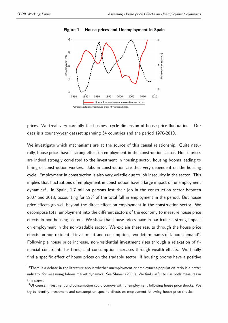
Many commentators have noted a close link between house price busts and rising unemploy-ment rates. In Spain, for example, there is a striking symmetrical evolution between houseprices and unemployment over the last 30 years (Figure 1). Following the housing bust in 2007,the unemployment rate increased from 8.3% to 26% at the end of 2012. Unemployment hadpreviously decreased from 24% to 8.3% during the housing boom period (1995-2007). Thenegative relationship between house prices and unemployment can however accommodate verydifferent interpretations: house prices comove positively and unemployment negatively withthe business cycle, so whatever drives the cycle could explain their comovement. Moreover,house prices could decline when unemployment goes up in the case of reduced consumptionon all goods, and on housing services in particular. However, in this paper we investigate theopposite causal effect: the effects of house price movements on unemployment dynamics.
Following Geerolf and Grjebine (2013), we use property taxes as an instrument for houseprices. Our identification strategy relies on the fact that property tax changes are driven bylocal politics rather than macroeconomics, so that they are orthogonal to macroeconomicfactors which might otherwise determine the business cycle. We show that house prices havea causal effect on unemployment: a 10% (instrumented) increase in house prices yields to a3.4% decrease in the unemployment rate. This is economically a very large effect2. It wouldfor example account for one third of the unemployment rate decline in the US during the recentboom period (2003-2007), and for half of the unemployment rate decline in Spain during theperiod 1995-2007. To show the robustness of our instrumental strategy, we check throughalternative methods whether our instrument introduces purely exogenous variations in house
1We thank Benjamin Carton, Linda Goldberg, Jean Imbs, Sébastien Jean, Philippe Martin, Thierry Mayer,Cédric Tille, Natacha Valla, seminar participants at CEPII, AFSE, and especially Fabien Tripier for theircomments and remarks.∗UCLA ([email protected])†CEPII ([email protected])2The standard deviation of house prices is 9% in the whole sample, while that of unemployment is 1.3% ofactive population. Descriptive statistics are fully described in online appendix C.
3
CEPII Working Paper Assessing House price Effects on Unemployment dynamics
Figure 1 – House prices and Unemployment in Spain
-.5
0.5
Hou
se p
rices
(gr
owth
)
510
1520
25U
nem
ploy
men
t rat
e
1980 1985 1990 1995 2000 2005 2010 2015
Unemployment rate House prices
Authors'calculations. Real house prices (4-year growth rate).
prices. We treat very carefully the business cycle dimension of house price fluctuations. Ourdata is a country-year dataset spanning 34 countries and the period 1970-2010.
We investigate which mechanisms are at the source of this causal relationship. Quite natu-rally, house prices have a strong effect on employment in the construction sector. House pricesare indeed strongly correlated to the investment in housing sector, housing booms leading tohiring of construction workers. Jobs in construction are thus very dependent on the housingcycle. Employment in construction is also very volatile due to job insecurity in the sector. Thisimplies that fluctuations of employment in construction have a large impact on unemploymentdynamics3. In Spain, 1.7 million persons lost their job in the construction sector between2007 and 2013, accounting for 52% of the total fall in employment in the period. But houseprice effects go well beyond the direct effect on employment in the construction sector. Wedecompose total employment into the different sectors of the economy to measure house priceeffects in non-housing sectors. We show that house prices have in particular a strong impacton employment in the non-tradable sector. We explain these results through the house priceeffects on non-residential investment and consumption, two determinants of labour demand4.Following a house price increase, non-residential investment rises through a relaxation of fi-nancial constraints for firms, and consumption increases through wealth effects. We finallyfind a specific effect of house prices on the tradable sector. If housing booms have a positive
3There is a debate in the literature about whether unemployment or employment-population ratio is a betterindicator for measuring labour market dynamics. See Shimer (2005). We find useful to use both measures inthis paper.4Of course, investment and consumption could comove with unemployment following house price shocks. Wetry to identify investment and consumption specific effects on employment following house price shocks.
4

CEPII Working Paper Assessing House price Effects on Unemployment dynamics
effect on total employment, they seem to affect negatively employment in the manufacturingsector. This could be explained by a mechanism reminiscent of a Dutch disease phenomenon.An increase in house prices tends indeed to lead to a real exchange rate appreciation thataffects manufacturing activity.
Related literature. We will not review here the very vast literature on unemployment dy-namics. In particular a large number of articles have sought the source of differences in labourmarket outcomes in differences in labour market institutions. Blanchard and Wolfers (2000)showed that the interaction between shocks and institutions is crucial to explaining unemploy-ment patterns. Nickell et al. (2005) emphasized that broad movements in unemployment canbe explained by shifts in labour market institutions. Bassanini and Duval (2006) looked atthe existence of complementarities between labour market policies. The first contribution ofthis article is to show the strong explanatory power of house prices relative to labour marketinstitutions to explain unemployment dynamics.
A limited number of papers has started to look at the issue empirically. Bover and Jimeno(2008) presented for example evidence regarding the relationship between house prices andrelative employment in construction on a sample of nine OECD countries over the period1980-2003. They showed that countries with more building possibilities tend to display largerelasticities of labour demand in the construction sector with respect to house prices than coun-tries with fewer building possibilities. Byun (2010) tried to estimate the impact on employmentof the recent housing bubble in the US. Using input-output tables, the bubble is estimatedto have contributed somewhere between 1.2 million and 1.7 million jobs in 2005, accountingfor 0.8 percent to 1.2 percent of total U.S. employment. Using our IV, we get a very closeestimate of the house price impact on US employment in construction.
In this paper, we also investigate more fully the house price effects on unemployment. Moreimportantly, we address the issue of causality between house prices and unemployment dynam-ics. We finally test different channels through which house prices could impact unemploymentpatterns. Note that if we study the macroeconomic consequences of house prices, we do notinvestigate specifically the effects of home-ownership rates on residential mobility. FollowingOswald (1996) and more recently Blanchflower and Oswald (2013), a different strand of theliterature has indeed looked at the role of home-ownership rates as a friction in the labourmarket5.5More theoretical papers have also address this question. Recently, Rupert and Wasmer (2012) presenteda model where the interconnection between two frictional markets (housing and labour) can be used tounderstand differences in the functioning of labour markets. In this paper, we do not focus specifically on theeffects of housing on residential mobility. In the robustness checks, we test the hypothesis that home-ownership
5
CEPII Working Paper Assessing House price Effects on Unemployment dynamics
Outline. The rest of the paper is organized as follows. In Section 1, we develop our estimationstrategy and we present our OLS results, controlling for the determinants which have beenpreviously used in the literature. In Section 2, we present our instrumental variable approach.We treat very carefully the business cycle dimension of house price movements and we answerpotential endogeneity issues. The main result is that a 10% (instrumented) increase in houseprices leads to a 3.4% decrease in the unemployment rate. In Section 3, we try to understandthe channels through which house prices impact unemployment. We decompose employmentinto the different sectors of the economy. If house prices have a strong impact on employmentin construction, house price effects go beyond the construction sector. House prices impactalso total employment through their effects on labour demand. In Section 4, we performa simulation exercise to understand how far one can go towards explaining unemploymentdynamics with changes in house prices. Finally, in the Appendices, we model the capitalizationmechanism (A), we show descriptive statistics (B), and we present our robustness checks (C).We show in particular that our results are robust using VAR techniques.
1. Estimation methodology and OLS results
1.1. Data and estimation technique
Data. House price data are taken from Geerolf and Grjebine (2013). We use annual data for34 countries for the period 1970-2010 6. To build this database, we notably used the propertyprice statistics from the Bank for International Settlements which cover a large number ofcountries but only for a short period of time. We then completed this database with datafrom various national sources (central banks, national statistical agencies, etc.). Data forunemployment are taken from the OECD Labour Market statistics. Employment variables arebuilt as a percentage of active population. In the robustness checks, we show also results withvariables taken as percentage of working age population. Sectoral employment variables arein addition measured as a percentage of total employment. Other variables used in this articleare described at the end of the paper, in Table C.1.
Stationarity problems and estimation technique. Due to data limitation on house prices,most of the economies we consider are advanced economies. House prices have an upward trendin the period we consider. Unemployment series contain also a unit root7. We detrend our datacould play as a friction in the labour market.6Our sample comprises Australia, Austria, Belgium, Canada, China, Czech republic, Denmark, Estonia, Fin-land, France, Germany, Greece, Hungary, Iceland, Indonesia, Ireland, Israel, Italy, Japan, Korea, Mexico, TheNetherlands, New Zealand, Norway, Poland, Portugal, Slovak Republic, Slovenia, South Africa, Spain, Sweden,Switzerland, United Kingdom, the United States.7Using augmented Dickey-Fuller, Phillips-Perron tests or panel-data unit root tests, we cannot reject the
6
CEPII Working Paper Assessing House price Effects on Unemployment dynamics
by using a HP-filter with a smoothing parameter of 400 to remove the very low frequencies.We show in the robustness checks that our results are robust to several specifications of theHP parameter (Table C.2). Our results are also robust when taking first differences instead ofa HP filter. Using augmented Dickey-Fuller and Phillips-Perron tests, we can then reject thehypothesis that our series contain a unit root. Moreover, after regressing unemployment onhouse prices, we can reject the null hypothesis that residuals contain a unit root at reasonableconfidence intervals, for all series in which we have a sufficiently large sample (online appendixA). Since house prices and unemployment are serially correlated, we are careful to use robustestimation procedures to not overestimate the precision of our coefficients. In this paper,we only present standard errors which are robust to heteroscedasticity and autocorrelation(HAC). We use the Bartlett kernel-based (or nonparametric) estimator, also known as theNewey and West (1987) estimator. We use a bandwith of 2, which leads to the inclusion ofautocovariances up to 1 lag. Our results are robust to different choices, for example inclusionof 2 lags8.
1.2. OLS Results
The main specification of our paper is:
Uit = αHit + βXit + δi + νt + uit. (1)
Uit and Hit are unemployment and house prices of country i in year t respectively. Moreprecisely, Uit denotes the share of unemployment over active population. Hit denotes anindex of real house prices (that is, deflated by the CPI), in base 1 = 2005. Xit are controlsfor unemployment. δi and νt are country and year fixed-effects. Country-fixed effects areincluded in all the regressions of this article, and enable us to identify the effect of houseprices on unemployment from the time-series dimension9. We also add year fixed-effects inthe robustness checks.hypothesis that our series are non-stationary. The high persistence in unemployment rates observed in thedeveloped world since the first oil shock has led to a vivid debate over which paradigm can better explain thebehavior of unemployment rates. The hysteresis hypothesis has been formulated in particular as a unit rootor non-stationary process. Empirical evidence tends to support the hypothesis of hysteresis for the EuropeanUnion economies and is mixed for the United States (Romero-Ávila and Usabiaga (2007), León-Ledesma(2002)). We show in the robustness checks that our results are also robust without filtering unemploymentrate series (Tables C.5, C.6 and C.7).8Automatic lag selection as in West (1994) is not available here since we use panel data. See Hayashi (2000)for more on GMM estimation with serial correlation.9Country-fixed effect also control for the fact that house price indices may not be comparable across countries,so that we are only left with interpreting the difference from the country-mean.
7

CEPII Working Paper Assessing House price Effects on Unemployment dynamics
Table 1 – House Prices and Unemployment. OLS regressions.
(1) (2) (3) (4) (5)U U U U U
(OLS) (OLS) (OLS) (OLS) (OLS)House Prices -7.734*** -7.247*** -5.006*** -4.517***
(0.902) (0.879) (0.913) (1.094)GDP growth -2.030*** -2.075*** -1.283*
(0.488) (0.741) (0.680)Min. vs. Av. wage 5.577 4.931
(4.986) (4.747)LME 1.741 1.140
(1.478) (1.480)Employment protection 0.0816 -0.479
(0.651) (0.651)Tax Wedge 0.00761 0.000717
(0.0338) (0.0319)Trade Union 0.212*** 0.261***
(0.0554) (0.0578)Replacement rate 7.924*** 5.499**
(2.706) (2.532)Observations 630 628 252 220 220R2 0.252 0.279 0.251 0.307 0.373Notes: HAC robust (Heteroscedasticity and AutoCorrelation robust) standard errors are inparentheses (we use Bartlett kernel-based filter with bandpass parameter 2). *** p<0.01, **p<0.05, * p<0.1. Country fixed effects included in the regressions. All series are detrendedusing a HP-filter. U denotes unemployment rate. LME denotes labour market expenditures.
The baseline regression yields the estimates displayed in Table 1. According to the simplestspecification (column (1)), an increase in house prices of 10% is associated with a decrease ofthe unemployment rate of 0.8%. The correlation is very significant and the explanatory powerof this regression is high: R2 = 25% with house prices alone. Adding our house price variableto usual determinants of unemployment dynamics increases the R2 by more than 7 percentagepoints (compare column (5) to column (4)).
In columns (4), (5), and (6) of Table 1, we follow the literature on unemployment to comparethe explanatory power of house prices with other variables usually put forward in the literature(Blanchard and Wolfers (2000), Nickell et al. (2005), Bassanini and Duval (2006), Murtin andRobin (2013)). We add the following variables:
(i) Employment protection. It tends to increase long-term unemployment as employers are
8

CEPII Working Paper Assessing House price Effects on Unemployment dynamics
more reluctant to hire highly protected workers. In the short term, it can reduce unemploymentas workers are fired less easily.
(ii) Minimum versus average wage. This is the minimum wage as a percentage of the medianwage. High minimum wages tend to increase unemployment as they mean higher real labourcosts but not necessarily higher productivity. But the literature does not find a significanteffect of minimum wage on unemployment (Bassanini and Duval (2006)).
(iii) Labour market expenditures. We take the active measures in favour of the labour market.They include notably training, employment incentives or direct job creation. Effects of thesemeasures can be complex as they may entail substitution effects or programmes that are likelyto pay off only in the long-run (training programmes). This explains that macro studies tendnot to find significant effects of these expenditures on unemployment.
(iv) Tax wedge. We define this variable as in Murtin and Robin (2013). It is the sum ofthe payroll, income, and consumption tax rates. Tax wedge is based on a full time workerwith no children. The impact of this variable on unemployment depends on who shouldersthe burden of taxes, and so on the relative bargaining power of the parties. If for exampletaxes cannot be shifted onto wages, then labour demand is likely to be negatively affected andso, employment is likely to be negatively affected as well. High tax wedges on labour largelymay reflect high levels of public expenditure and the important role played by wage-basedcontributions in financing the transfer system.
(v) Trade Union. Higher levels of unionization can give rise to less competition in labourmarkets. In particular, Nickell and others (2001) find that greater unionization tends to increasereal labour costs. de Serres and Murtin (2013) show that the degree of unionisation may eitherraise or lower unemployment cyclical volatility depending on whether unions push for higherreal wages regardless of the unemployment level or seek to preserve current members’ jobs.
(vi) Replacement rate. It captures the degree of generosity of the unemployment insur-ance system. More generous insurance systems may cause unemployment if they reduce theeffectiveness of the search of jobs.
Interestingly, the six policy and institutional determinants of unemployment explain 30% of thevariance (column (4)), almost as much as house prices alone (column (3)). Moreover, addinghouse prices to these institutional variables helps to explain 37% of the variance (column (5)).We control also by real GDP growth which is also endogenously affected by house prices (seesection 3.3). We show in the robustness checks that these results are also robust withoutfiltering our variables but by taking instead house prices in delta-log (Tables C.6 and C.7).
9

CEPII Working Paper Assessing House price Effects on Unemployment dynamics
2. Instrumental approach
There are several issues with the OLS regression which prevent an interpretation of this correla-tion in a causal sense, from house prices to unemployment. The first issue is reverse causality:it could be argued that house prices can decrease when unemployment goes up because ofreduced consumption on all goods10, and on housing services in particular. Second, thereis potentially an omitted variable problem, since many factors could drive both house pricebooms and unemployment patterns. For example, house prices could comove positively andunemployment negatively with the business cycle. Whatever drives the cycle could explain thecomovement. Third, there is a clear problem of measurement errors in house prices.
To address these issues, we use an Instrumental Variable approach. Following Geerolf andGrjebine (2013), we use property taxes as an instrumental variable for house prices. Becauseof capitalization, unexpected increases in property taxes are immediately translated into adecrease of house prices (see the model in Appendix A). A very important element in thechoice of this tax is that it is not endogenously affected by house prices. Indeed, propertytaxation essentially uses fiscal values (as opposed to market values) which are rarely revised toreflect market values. Concerning the construction of our instrument, it is not possible to usemarginal rates as property taxes are highly multidimensional, nonlinear, with several brackets,and exemptions below a certain threshold. We therefore use the share of revenues broughtabout by property taxation in total taxation of a country. This enables to capture variationsin property taxation that keep total tax receipts constant, since changes in total tax couldimpact the business cycle. We discuss the issue of exclusion restriction after presenting the IVresults. Data on property taxes come from OECD Revenue Statistics. We use recurrent taxeson immovable property, a category that covers taxes levied regularly in respect of the use orownership of immovable property11.
2.1. IV results
We use Two stage least squares (2SLS), with exogenous variation of real-estate propertytaxation (Tit) as an instrumental variable for house prices in the first stage. We check in the10For example, in the precautionary savings literature, capital market imperfections and the presence of unin-sured idiosyncratic risk lead agents to save more than they would if there were no uncertainty (notably Carrollet al. (1992), and more recently Mody et al. (2012)).11According to OECD Revenue Statistics, "these taxes are levied on land and building, in the form of apercentage of an assessed property value based on a national rental income, sales price, or capitalised yield;or in terms of other characteristics of real property, such as size, location, and so on, from which are deriveda presumed rent or capital value. Such taxes are included whether they are levied on proprietors, tenants, orboth. Unlike taxes on net wealth, debts are not taken into account in their assessment."
10
CEPII Working Paper Assessing House price Effects on Unemployment dynamics
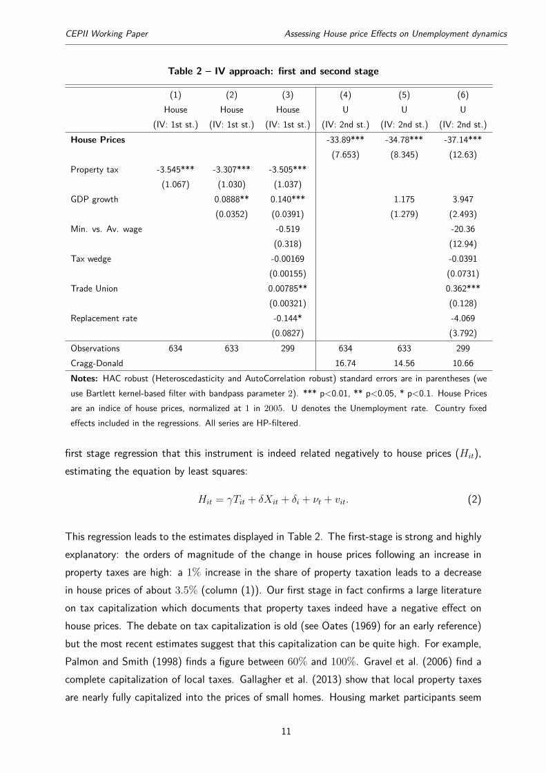
Table 2 – IV approach: first and second stage
(1) (2) (3) (4) (5) (6)House House House U U U
(IV: 1st st.) (IV: 1st st.) (IV: 1st st.) (IV: 2nd st.) (IV: 2nd st.) (IV: 2nd st.)House Prices -33.89*** -34.78*** -37.14***
(7.653) (8.345) (12.63)Property tax -3.545*** -3.307*** -3.505***
(1.067) (1.030) (1.037)GDP growth 0.0888** 0.140*** 1.175 3.947
(0.0352) (0.0391) (1.279) (2.493)Min. vs. Av. wage -0.519 -20.36
(0.318) (12.94)Tax wedge -0.00169 -0.0391
(0.00155) (0.0731)Trade Union 0.00785** 0.362***
(0.00321) (0.128)Replacement rate -0.144* -4.069
(0.0827) (3.792)Observations 634 633 299 634 633 299Cragg-Donald 16.74 14.56 10.66Notes: HAC robust (Heteroscedasticity and AutoCorrelation robust) standard errors are in parentheses (weuse Bartlett kernel-based filter with bandpass parameter 2). *** p<0.01, ** p<0.05, * p<0.1. House Pricesare an indice of house prices, normalized at 1 in 2005. U denotes the Unemployment rate. Country fixedeffects included in the regressions. All series are HP-filtered.
first stage regression that this instrument is indeed related negatively to house prices (Hit),estimating the equation by least squares:
Hit = γTit + δXit + δi + νt + vit. (2)
This regression leads to the estimates displayed in Table 2. The first-stage is strong and highlyexplanatory: the orders of magnitude of the change in house prices following an increase inproperty taxes are high: a 1% increase in the share of property taxation leads to a decreasein house prices of about 3.5% (column (1)). Our first stage in fact confirms a large literatureon tax capitalization which documents that property taxes indeed have a negative effect onhouse prices. The debate on tax capitalization is old (see Oates (1969) for an early reference)but the most recent estimates suggest that this capitalization can be quite high. For example,Palmon and Smith (1998) finds a figure between 60% and 100%. Gravel et al. (2006) find acomplete capitalization of local taxes. Gallagher et al. (2013) show that local property taxesare nearly fully capitalized into the prices of small homes. Housing market participants seem
11

CEPII Working Paper Assessing House price Effects on Unemployment dynamics
to rationally take into account increases in property taxes on the price they should pay fornewly purchased homes.
Using the property tax as an instrument for house prices as a first stage gives the results for thesecond stage in Table 2. Looking at the column (4), we get that a 10% increase in house pricesyields to a decrease of the unemployment rate of 3.4%. As stated in the introduction, thiseffect is large. It would for example account for one third of the unemployment rate declinein the US during the recent boom period (2003-2007), and for half of the unemploymentrate decline in Spain during the period 1995-2007. The IV estimates are substantially greaterthan the OLS estimates; that is, OLS estimates appear to be biased downward significantly12.Comparing column (4) (2nd stage) in Table 2 with column (1) in Table 1, we interpret theincrease in the coefficient with respect to OLS (in absolute value) by the fact that houseprices are mismeasured and that OLS estimates are therefore biased towards 0. This suggestsalso that reverse causality is not at work in the data (higher unemployment does not generatelower house prices). The lower coefficient in the OLS case could also be explained by the useof housing as a precautionary saving asset in times of uncertainty. For example during therecent crisis in France, increase in the demand for housing could partly be due to an increasein uncertainty (correlated with higher unemployment rate).
2.2. Exclusion restriction.
Several arguments help to explain why our instrumental variable does not impact unemploy-ment other than through house prices. Property tax changes must not result from an omittedthird factor, like economic conditions. A major argument in favor of our instrument is thatproperty taxes are usually set by local governments, and are not a tool used for macroeco-nomic policy. We check through alternative methods that our instrument introduces purelyexogenous variations in house prices. We first show that variations of our instrument are notdriven by changes in total taxes. We then answer potential endogeneity issues. We finally
12The result that the 2SLS coefficient is larger than the OLS coefficient is a "common empirical finding"(Hahn and Hausman (2005)). In this paper, we check that this is not due to weak identification. For our mainspecification (column (4) of Table 2), the Cragg-Donald Wald F statistic (Weak identification test) is about 17,so our instrument is not a weak instrument. Classical measurement error in an independent variable attenuatestowards zero the OLS estimator. It does not affect the consistency of IV estimation (because the exclusionrestriction holds), neither does it affect the consistency of OLS or IV estimators when the mismeasured variableis the endogenous variable. The fact that the IV estimator does not suffer from attenuation bias from classicalmeasurement error, while the OLS estimator is attenuated, is an explanation for IV estimates usually beinglarger than their OLS counterparts, even when we expect omitted variable bias to go in the opposite direction.Such findings are common in the labour economics literature (Card (2001)).
12
CEPII Working Paper Assessing House price Effects on Unemployment dynamics
propose a narrative approach for identification of property tax shocks.
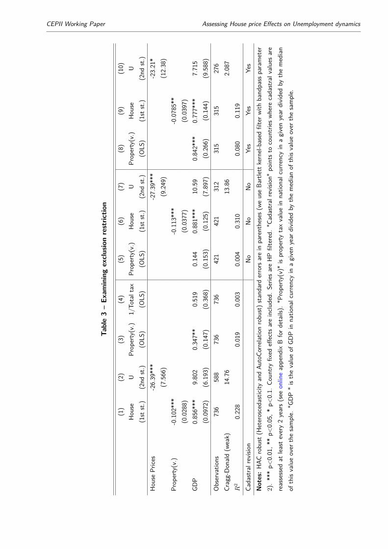
Why choose Property Taxes as a % of Total Taxation? We use property taxes as apercentage of total taxation as our benchmark instrument for house prices. Property taxesbeing expressed in the OECD data as an amount in national currency, we therefore need areference to which we can compare the amount of property taxes levied by the governmentacross countries. Because we want to use unanticipated shocks to property taxes as ourinstrument for house prices, we do not want the increase of property taxes to reflect thegeneral increase of total taxation in the country. Our instrument thus reflects the amount ofproperty taxes levied by the government relative to the general level of taxation in the country.One could be worried that dividing by total taxes would introduce some spurious correlationbetween house prices and our instrument, leading us to an overestimation of the true linkbetween house prices and property taxes in the first stage. However, we show three things toaddress this potential concern. First, we check that our results are not sensitive to the choiceof this normalization rather than to using for example, the value of property taxes in nationalcurrency in a given year13. We call this other instrument "Property taxes (value)". Table 3reports the IV results with this alternative measure of property taxes. Columns (1) and (2)show that using this alternative measure does not change significantly the point estimate ofthe estimated impact of house prices on unemployment14: a 10% increase in house pricesleads to a 2.6% decrease in the unemployment rate (column (2)), against 3.4% in the baselinespecification, column (4) of Table 2. Second, we show in column (4) that the inverse of totaltax is not significantly correlated to GDP, and if anything it is positively correlated to GDP15.Third, we show in Table C.4, that smoothing our denominator does not alter the results inany way. In particular, we take an averaged value of total tax or we smooth total tax takingthe trend component of a HP filter to remove business cycle frequencies. We verify also that
13To normalize this value, we divide it by the median of this value over the sample.14In any case, we think that the alternative instrument is not as well suited to our analysis here, as we donot want to consider mechanic increases in Property Taxation resulting from the increase or the decrease ofthe overall tax shares as "shocks" to property taxes. Referring to the model developed in Appendix A, and inparticular equation (H), it is unexpected shocks to property taxes that have an effect on house prices, not theexpected ones which are already factored in prices. The mechanic increase of property taxes with the trendof general total taxation certainly is incorporated in prices well in advance of actual rises. In contrast, onlywhen the government decides to shift the burden of taxes towards property taxation will we record a "shock"to property taxes. This is why in the following, we will work with property taxes as a percentage of totaltaxation, unless otherwise noted.15The reason for this result is that 1/Total Taxation barely moves over the cycle, and stays roughly equal totwo. Because of the positive correlation between house prices and GDP, the denominator introduces somepositive correlation between house prices and the instrument. This bias is not a problem because it tends toweaken the first stage, and hence go against our conclusions.
13
CEPII Working Paper Assessing House price Effects on Unemployment dynamics
choosing other scaling variables for property taxes does not alter the results either.
Potential Endogeneity Issues. Our instrumental strategy requires that property tax changesbe orthogonal to macroeconomic factors which might otherwise determine unemployment. Wedevelop three arguments to answer potential endogeneity issues.
First, for our instrumental variable strategy to work, it must be that cadastral values are notrevised too frequently, otherwise property taxes would mechanically rise when house pricesincrease (see equation (H) in the model in Appendix A). In that case, we would not be able toidentify the negative relationship that property taxes have on house prices through capitaliza-tion. If property taxes are revised sometimes, then this introduces a positive correlation in therelationship between house prices and property taxes, which go towards weakening our firststage. Consistent with this weakening effect of the revision in property taxes on our estimationstrategy, we show that in countries with no cadastral revision, the correlation between propertytaxes and house prices (column (6) of Table 3) is slightly stronger than using the full sample(column (1)), let alone using the sample with frequent revisions (column (9)). In particular,the explanatory power of the property tax is much higher in the case of no cadastral revision(R2 = 31%, column (6)) than in the case of frequent revisions (R2 = 12%, column (5)).We show also in column (5) of Table 3 that in countries that revise cadastral values relativelymore infrequently (see online appendix B for details), property taxes are not at all correlatedto GDP (this is true for both the instrument we use and property tax values). Property taxesare only very weakly correlated to GDP in the full sample: the explanatory power of GDP onproperty taxes is very low, lower than 2% (column (3)) (by comparison, the R2 with incometax is very large, 45%).
A second argument in favor of our instrument is that the specialized literature on propertytaxes, especially that on the United States, points to the relative stability of property taxationover the cycle as an advantage of this form of taxation over others: see for example Lutz(2008) and Giertz (2006).16 It is all the more remarkable that the United States are takenas having a relatively frequent revision of their property taxes compared to other countries(online appendix B).
As a third argument in favor our instrument, we show that controlling for GDP (through ourvariable of GDP growth) does not alter our results in any significant way (see Table 2). Tofurther alleviate endogeneity problems, we also show that controlling by different measures ofGDP like real GDP or relative income yields similar results (see Table C.3).
16 Lutz (2008) writes: "The relative stability of the property tax over the course of the business cycle is oftencited as one of the primary virtues of property taxation."
14
CEPII Working Paper Assessing House price Effects on Unemployment dynamics
Table3–Ex
aminingexclusionrestric
tion
(1)
(2)
(3)
(4)
(5)
(6)
(7)
(8)
(9)
(10)
Hou
seU
Prop
erty(v.)
1/To
taltax
Prop
erty(v.)
Hou
seU
Prop
erty(v.)
Hou
seU
(1st
st.)
(2nd
st.)
(OLS
)(O
LS)
(OLS
)(1st
st.)
(2nd
st.)
(OLS
)(1st
st.)
(2nd
st.)
Hou
sePrice
s-26.39***
-27.39***
-23.21*
(7.566)
(9.249)
(12.38)
Prop
erty(v.)
-0.102***
-0.113***
-0.0785**
(0.0288)
(0.0377)
(0.0397)
GDP
0.856***
9.802
0.347**
0.519
0.144
0.881***
10.59
0.842***
0.777***
7.715
(0.0972)
(6.193)
(0.147)
(0.368)
(0.153)
(0.125)
(7.897)
(0.266)
(0.144)
(9.588)
Observatio
ns736
588
736
736
421
421
312
315
315
276
Cragg-Don
ald(w
eak)
14.76
13.86
2.087
R2
0.228
0.019
0.003
0.004
0.310
0.080
0.119
Cadastralrevision
No
No
No
Yes
Yes
Yes
Notes:HAC
robu
st(H
eteroscedasticity
andAu
toCo
rrelatio
nrobu
st)standard
errors
arein
parentheses(w
euseBa
rtlet
tkernel-b
ased
filterw
ithband
pass
parameter
2).***p<
0.01,*
*p<
0.05,*
p<0.1.
Coun
tryfixed
effects
areinclu
ded.
Serie
sareHPfiltered.
"Cadastral
revisio
n"po
ints
tocoun
tries
wherecadastralv
aluesare
reassessed
atlea
stevery2years(see
onlineappend
ixB
ford
etails)
."P
roperty
(v)"
isprop
erty
taxvaluein
natio
nalc
urrencyin
agivenyear
dividedby
themedian
ofthisvalueover
thesample.
"GDP"isthevalueof
GDPin
natio
nalc
urrencyin
agivenyear
dividedby
themedianof
thisvalueover
thesample.

CEPII Working Paper Assessing House price Effects on Unemployment dynamics
2.3. A narrative approach: the example of France.
We take the example of France where it is possible to shed light on four different propertytax shocks over the last thirty years (Figures 2 and 3). These shocks are consequences ofdecentralization policies, uncorrelated with unemployment dynamics or the business cycle.They can also be explained by the electoral cycle. The first shock was the result of theDefferre Laws in 1982-1983 that initiated the policy of decentralization in France. Priorto these laws, French municipalities and departments enjoyed very limited autonomy. Thelaws gave territorial collectivities in France separate defined responsibilities and resources. Inparticular, the 1983 laws dating from 7 January and 22 July defined the responsibilities of newbodies (the "Régions") and how they would be financed. If local authorities could set propertytax rates since 1981, it was the need of increasing resources due to the new responsibilities oflocal collectivities that explained the rise of property taxes between 1982 and 1985. Propertytax increases contributed to the gradual decrease of house prices and the increase in theunemployment rate.
Figure 2 – Instrument, house prices and unemployment in France
Def
ferr
e La
ws
of 1
982
The
198
5 ha
lt
Law
of 1
990
The
Tax
exe
mpt
ions
of 1
997
34
56
Inst
rum
ent
68
1012
14U
nem
ploy
men
t
0.5
11.
5H
ouse
Pric
es
1980 1990 2000 2010
House Prices Unemployment
Instrument
Source: OECD and authors' calculations. Series are not filtered.
A second shock was the halt to the decentralization reforms in 1985. That year marked the endof the first phase of decentralization. This started a period of moderation of local taxation. Iflocal authorities enjoyed more autonomy thanks to the decentralization reforms, they becamealso responsible to the electors, in particular of their budget management. Several localelections took place during this period (for the "Départements" in 1985, for the "Régions" in1986, for the municipalities in 1989). This was a major factor explaining the fiscal moderation.
16
CEPII Working Paper Assessing House price Effects on Unemployment dynamics
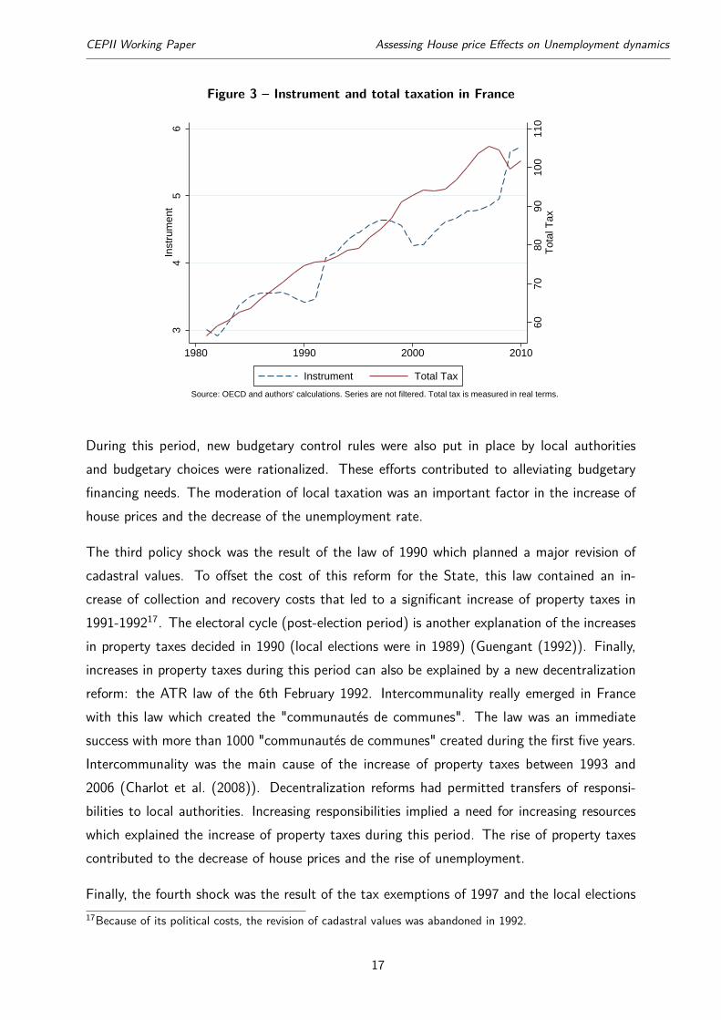
Figure 3 – Instrument and total taxation in France
6070
8090
100
110
Tot
al T
ax
34
56
Inst
rum
ent
1980 1990 2000 2010
Instrument Total Tax
Source: OECD and authors' calculations. Series are not filtered. Total tax is measured in real terms.
During this period, new budgetary control rules were also put in place by local authoritiesand budgetary choices were rationalized. These efforts contributed to alleviating budgetaryfinancing needs. The moderation of local taxation was an important factor in the increase ofhouse prices and the decrease of the unemployment rate.
The third policy shock was the result of the law of 1990 which planned a major revision ofcadastral values. To offset the cost of this reform for the State, this law contained an in-crease of collection and recovery costs that led to a significant increase of property taxes in1991-199217. The electoral cycle (post-election period) is another explanation of the increasesin property taxes decided in 1990 (local elections were in 1989) (Guengant (1992)). Finally,increases in property taxes during this period can also be explained by a new decentralizationreform: the ATR law of the 6th February 1992. Intercommunality really emerged in Francewith this law which created the "communautés de communes". The law was an immediatesuccess with more than 1000 "communautés de communes" created during the first five years.Intercommunality was the main cause of the increase of property taxes between 1993 and2006 (Charlot et al. (2008)). Decentralization reforms had permitted transfers of responsi-bilities to local authorities. Increasing responsibilities implied a need for increasing resourceswhich explained the increase of property taxes during this period. The rise of property taxescontributed to the decrease of house prices and the rise of unemployment.
Finally, the fourth shock was the result of the tax exemptions of 1997 and the local elections17Because of its political costs, the revision of cadastral values was abandoned in 1992.
17
CEPII Working Paper Assessing House price Effects on Unemployment dynamics
of 1998. The increase of property taxes that had started in 1992 with the ATR law wastemporary halted in 1997-1998. Several property tax exemptions were voted in 1996-1997(property tax exemptions for developed property during 5 years in urban free zones with theLaw of the 14th November 1996; property taxes for undeveloped property are removed forthe "Régions" and "Départements" in 1996). In addition, local authorities started in 1997 apolicy of tax moderation, notably because the parliament had secured the state grants to localgovernments with the Financial Stability Pact (integrated into the 1996 Finance Act). Thelocal elections of 1998 (for the "Départements" and "Régions") contributed also to this taxmoderation which was in important factor in the increase of house prices and the decline ofunemployment.
3. Explaining the mechanisms
House prices have a causal effect on the unemployment rate. To understand this effect, wedecompose employment into the different sectors of the economy. Quite naturally, house priceshave a strong impact on employment in construction. House prices impact also total employ-ment through their effects on non-residential investment and consumption, two determinantsof labour demand.
3.1. House price effects on construction
House prices have a strong impact on employment in the construction sector. They are indeedhighly correlated to investment in construction (see Table C.20), housing booms leading tohiring of construction workers. Employment in construction is also very volatile due to jobinsecurity in this sector. This implies that shocks on construction have a large impact onunemployment dynamics.
The magnitude of the direct effect. In average for our sample of 34 countries overthe period 1970-2010, employment in the construction sector and in real estate activitiesrepresents around 8% of total employment18 (7% for the construction sector only, with astandard deviation of 2%). It is Europe’s largest industrial employer, accounting for aboutseven percent of total employment. In particular, employment in construction represented in2005 around 6% of total employment in France or Germany, 7% in the United-Kingdom, 8%in the United States or 12% in Spain (Table B.1 in Appendix B). In addition, the production ofother sectors of the economy may be used as inputs for construction. In table B.2 of AppendixB, we estimate the total share of employment devoted to housing in several countries. To do18Estimations for non-filtered series.
18
CEPII Working Paper Assessing House price Effects on Unemployment dynamics
so, we add employment in the construction sector (column (2)) and in real estate activities(column (3)). We calculate also thanks to OECD Input-Output tables an estimation of thenumber of employees devoted to housing in sectors that are used as inputs of constructionand real estate activities (column (1)). The sum of these 3 columns gives us an estimation ofthe size of employment generated by housing sector activity. The housing sector represented11.7% of total employment in the United States in 2005 (column (4)), 12% in the UnitedKingdom, 11.3% in France, almost 23% in Spain. It is interesting to notice the cases of Japanand Germany which had a housing boom in the nineties. If percentages in theses countries arestill high (13.4% in Japan, around 10% in Germany), they are lower than in the mid-nineties(respectively 16.1% and 14.2% )19.
A volatile sector. Not only the housing sector represents a significant share of total em-ployment, but employment in this sector is also one of the most volatile in the economy. Ifemployment in the construction sector represents in average in our sample 8% of total em-ployment, it explains 56% of the variance of total employment20 (Table C.8, column (2)).This volatility can be explained by job characteristics in the construction sector. Employmentin the construction sector can be characterized by job insecurity, low wages and poor workingconditions (ILO (2001)). The demand for labour in the construction industry tends to changefrom day to day. A large proportion of the construction workforce is employed on a casual andtemporary basis to cope with variations in the contractor’s workload and demand for differentskills. Construction workers are often not protected by social insurance or trade union mem-bership. Construction work also provides a traditional point of entry into the labour marketfor migrants (Wells (2012)). The practice of employing labour through subcontractors hasalso a profound effect upon occupational safety and it has undermined collective bargainingagreements. Amongst European countries, the trend to outsource has been most evidentin the United Kingdom and in Spain (ILO (2001))21. Job volatility in construction helps toexplain that house prices shocks on this sector have a high impact on employment dynamics(see subsection 3.2 for IV results on construction). After the 2007 housing bust, the number
19We calculate also in column (5) of Table B.2 the share of employment devoted to housing in sectors whichuse construction as an input. If employment in these sectors is not directly impacted by a construction boom,it is influenced by changes in house prices (rising input prices impact employment in output sectors). Forinstance, almost 8% of employment in Spain (in 2005) was in sectors which directly use housing as an input(in the sense of an input-output table).20Employment in industry that represents 18% of total employment explains 44% of the variance (column(3)). Volatility is also high in retail services. Employment in retail service activities (hotels, restaurants, ..),that represents in average 24% of total employment, explains 56% of the variance (column (4)).21In 1999, 62 per cent of Spain’s 1.5 million construction workers held temporary contracts (compared with33 per cent in the economy as a whole), ILO (2001).
19

CEPII Working Paper Assessing House price Effects on Unemployment dynamics
of persons employed in construction in Spain was divided by three, 1.7 million persons losttheir job in this sector (2007- 2013), accounting for 52% of the total fall in employment inthe period. In the United States, 2.3 million jobs in construction disappeared between 2007and 2012, accounting for 35% of the total fall in employment in the period.
3.2. House price effects go beyond impacts on construction
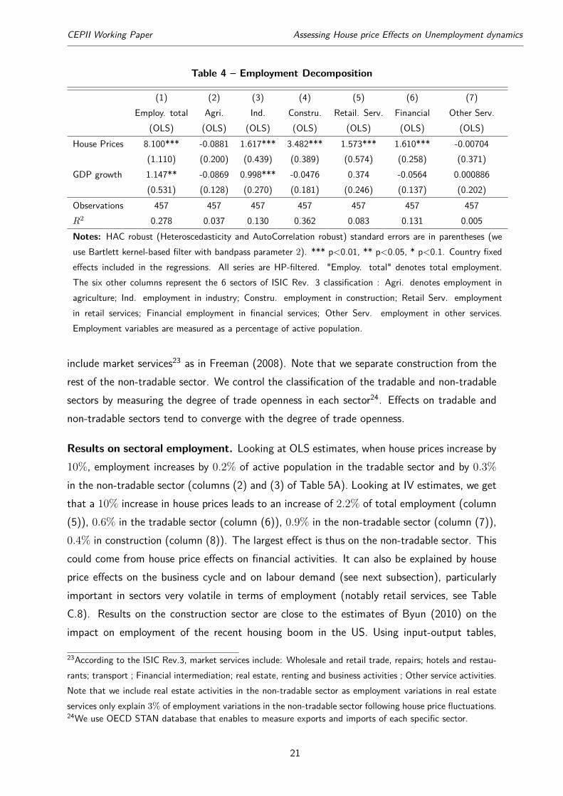
House price effects on unemployment dynamics go beyond the direct effect on the constructionsector. Employment variations in construction explain 43% of the variations of total employ-ment following house price fluctuations (Table 4). This implies that more than half of thevariations comes from other sectors of the economy.
Decomposition of Employment. To measure the effects of house prices on the differ-ent sectors of the economy, we decompose employment into six sectors using ISIC Rev. 3classification: (1) Agriculture, hunting and forestry, fishing ; (2) Industry, including energy ;(3) Construction ; (4) Wholesale and retail trade, repairs; hotels and restaurants; transport; (5) Financial intermediation; real estate, renting and business activities ; (6) Other serviceactivities. Each sectoral variable is measured as a percentage of active population.
Looking at OLS estimates between house prices and employment on these different sectors, weget that an increase of house prices of 10% is associated with an increase of total employmentof 0.8% (column (1) of Table 4). If we decompose this effect, employment increases by0.3% in the construction sector (column (4)), and by around 0.2% in industry (column (3)),in retail services (column (5)), and in financial and business activities (column (6)). Theseresults are robust using the instrumental strategy (Table C.9 B). We discuss in next subsection(3.3) different explanations for the positive correlation between house prices and employmentin industry and in retail services. Concerning financial activities, the result can probably beexplained by the strong links between housing cycles and financial cycles (Claessens et al.(2012)), in particular with the strong dependency of financial products on the development inhousing markets (see Table C.17 for the links between house prices and share prices).
Tradable and non-tradable sectors. To understand better the effects of house prices on thedifferent sectors of the economy, we decompose the economy into tradable and non-tradablesectors. We define industry22 as the tradable sector. For robustness, we show also the resultsrestricting the tradable sector to manufacturing. To represent the non-tradable sector, we
22According to the International Standard Industry Classification (ISIC Rev.3), industry includes: mining andquarrying; manufacturing; and electricity, gas and water supply.
20
CEPII Working Paper Assessing House price Effects on Unemployment dynamics
Table 4 – Employment Decomposition
(1) (2) (3) (4) (5) (6) (7)Employ. total Agri. Ind. Constru. Retail. Serv. Financial Other Serv.
(OLS) (OLS) (OLS) (OLS) (OLS) (OLS) (OLS)House Prices 8.100*** -0.0881 1.617*** 3.482*** 1.573*** 1.610*** -0.00704
(1.110) (0.200) (0.439) (0.389) (0.574) (0.258) (0.371)GDP growth 1.147** -0.0869 0.998*** -0.0476 0.374 -0.0564 0.000886
(0.531) (0.128) (0.270) (0.181) (0.246) (0.137) (0.202)Observations 457 457 457 457 457 457 457R2 0.278 0.037 0.130 0.362 0.083 0.131 0.005Notes: HAC robust (Heteroscedasticity and AutoCorrelation robust) standard errors are in parentheses (weuse Bartlett kernel-based filter with bandpass parameter 2). *** p<0.01, ** p<0.05, * p<0.1. Country fixedeffects included in the regressions. All series are HP-filtered. "Employ. total" denotes total employment.The six other columns represent the 6 sectors of ISIC Rev. 3 classification : Agri. denotes employment inagriculture; Ind. employment in industry; Constru. employment in construction; Retail Serv. employmentin retail services; Financial employment in financial services; Other Serv. employment in other services.Employment variables are measured as a percentage of active population.
include market services23 as in Freeman (2008). Note that we separate construction from therest of the non-tradable sector. We control the classification of the tradable and non-tradablesectors by measuring the degree of trade openness in each sector24. Effects on tradable andnon-tradable sectors tend to converge with the degree of trade openness.
Results on sectoral employment. Looking at OLS estimates, when house prices increase by10%, employment increases by 0.2% of active population in the tradable sector and by 0.3%in the non-tradable sector (columns (2) and (3) of Table 5A). Looking at IV estimates, we getthat a 10% increase in house prices leads to an increase of 2.2% of total employment (column(5)), 0.6% in the tradable sector (column (6)), 0.9% in the non-tradable sector (column (7)),0.4% in construction (column (8)). The largest effect is thus on the non-tradable sector. Thiscould come from house price effects on financial activities. It can also be explained by houseprice effects on the business cycle and on labour demand (see next subsection), particularlyimportant in sectors very volatile in terms of employment (notably retail services, see TableC.8). Results on the construction sector are close to the estimates of Byun (2010) on theimpact on employment of the recent housing boom in the US. Using input-output tables,
23According to the ISIC Rev.3, market services include: Wholesale and retail trade, repairs; hotels and restau-rants; transport ; Financial intermediation; real estate, renting and business activities ; Other service activities.Note that we include real estate activities in the non-tradable sector as employment variations in real estateservices only explain 3% of employment variations in the non-tradable sector following house price fluctuations.24We use OECD STAN database that enables to measure exports and imports of each specific sector.
21
CEPII Working Paper Assessing House price Effects on Unemployment dynamics
the bubble is estimated to have contributed somewhere between 1.2 million and 1.7 millionjobs in 2005, accounting for 0.8 percent to 1.2 percent of total U.S. employment. These arethe residential-construction-related jobs. During the period considered (2002-2005), our IVestimated impact of the house price boom on US employment in construction would be closeto 1% of total employment (as house prices increased by 25%), a very close estimate to theone of Byun (2010).
Note that house price effects on the construction sector are even larger when we take intoaccount the relative size of each sector. In elasticity terms, house price effects are muchstronger in the construction sector than in the rest of the economy25.
Asymmetric effects between booms and busts. Interestingly, house prices have asym-metric effects on employment during booms and busts26. In Table 5B, we show that theemployment effect of house prices is much larger when house prices decrease (columns (1)to (4)) than during housing booms. For example, if house prices increase by 10%, totalemployment increases by 0.6%, while for a decline of house prices of the same magnitude,total employment decreases by 1.3% (column (1)). This asymmetric effect could be explainedby the mismatches created by the labour reallocation following house price shocks. We canmake the hypothesis that as housing busts tend to be more sudden than booms, labour re-allocation effectively needs to be a lost faster during busts than booms, creating mismatchunemployment. Note also that this asymmetric effect could imply higher unemployment overthe housing cycle, each housing cycle leading to a higher unemployment rate level. This couldbe linked to the hysteresis hypothesis. Such an effect would however depend on the structureof the housing cycle and on the duration of booms and busts. If the employment effect ofhouse prices is larger when house prices decrease, the duration of housing busts is also shorterthan booms27. These issues would require further investigation.
A specific effect in the tradable sector: a new Dutch Disease? Contrary to the othersectors of the economy, employment in the tradable sector does not increase during housingbooms (column (2) of Table 5B). This result could be explained by a mechanism reminiscentof a "Dutch Disease" phenomenon28. House price booms lead indeed to rising economy-wide
25In table C.10, a 10% (instrumented) increase in house prices leads to an increase of 8% of employment inconstruction (4% in the tradable sector and 2% in the non-tradable sector).26We measure booms as periods where house prices increase. Similarly, busts are defined as periods wherehouse prices decrease.27Bracke (2011) has calculated for OECD countries an average duration of housing cycle of 10 years withapproximately 6 years of booms and 4 years of busts.28The analogy between housing booms and the Dutch Disease phenomenon was suggested previously. But toour knowledge, no academic paper has investigated this issue before this work. Bover and Jimeno (2008) raised
22

CEPII Working Paper Assessing House price Effects on Unemployment dynamics
Table 5 – House prices and Employment in tradable and non-tradable sectors
(1) (2) (3) (4) (5) (6) (7) (8)E E.T E. NT E. C E. E. T E.NT E. C
Table A (OLS) (OLS) (OLS) (OLS) (IV) (IV) (IV) (IV)House Prices 8.033*** 1.617*** 3.175*** 3.482*** 21.84*** 6.109*** 9.216*** 4.015***
(1.114) (0.439) (0.808) (0.389) (6.803) (2.203) (3.537) (1.557)GDP growth 1.234** 0.998*** 0.318 -0.0476 -0.923 0.296 -0.625 -0.131
(0.532) (0.270) (0.334) (0.181) (1.189) (0.444) (0.643) (0.264)Observations 457 457 457 457 457 457 457 457R2 0.277 0.130 0.131 0.362Cragg-Donald 17.02 17.02 17.02 17.02
(1) (2) (3) (4)Employment Employment T. Employment NT Employment C.
Table B (OLS) (OLS) (OLS) (OLS)House(boom) 5.941*** 0.686 2.316*** 3.039***
(1.200) (0.442) (0.867) (0.452)House(bust) 12.52*** 3.613*** 5.018*** 4.431***
(1.656) (0.729) (1.203) (0.555)GDP growth 1.103** 0.939*** 0.264 -0.0755
(0.500) (0.249) (0.326) (0.181)Observations 457 457 457 457R2 0.310 0.169 0.150 0.374Notes: HAC robust (Heteroscedasticity and AutoCorrelation robust) standard errors arein parentheses (we use Bartlett kernel-based filter with bandpass parameter 2). ***p<0.01, ** p<0.05, * p<0.1. Country fixed effects included. Series are HP-filtered.House denotes house prices. E. denotes total employment. E.T. denotes employment inthe tradable sector; E. NT in the non-tradable sector; E. C employment in construction.Employment variables are constructed as a percentage of active population.
CEPII Working Paper Assessing House price Effects on Unemployment dynamics
wages29 and to real exchange rate appreciations that squeeze profits in the tradable sector (asprices are fixed at the world level) and affect manufacturing exports (Table C.15 and TableC.16). This could have adverse effects on employment in the tradable sector. We do notfocus on sectoral labour reallocation in the core of the paper to concentrate on house priceeffects on unemployment dynamics. In the robustness checks, we show however that housingbooms tend to lead to a reallocation of employment in favor of the construction sector (TableC.13). The share of employment in construction increases during booms while the share ofemployment in the tradable sector decreases30.
3.3. Explaining house price effects on unemployment beyond construction
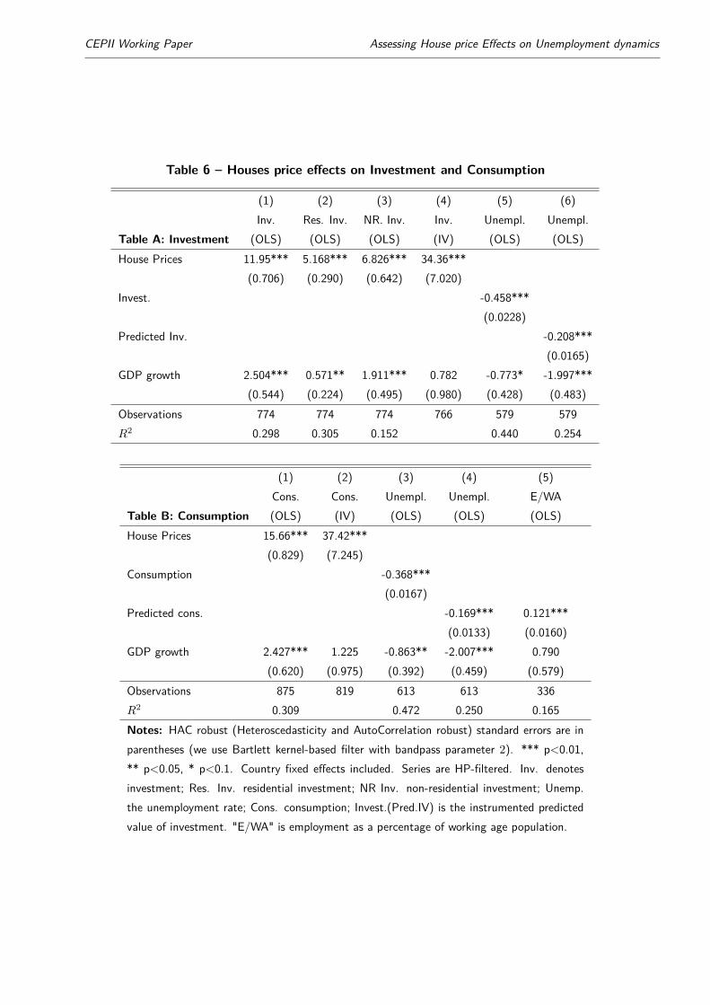
House prices do not only impact employment in the construction sector but also total em-ployment. This could be explained by house price effects on labour demand. We investigatetwo channels to explain these effects: the investment channel and the consumption channel.Following a house price increase, non-residential investment tends to rise through a relax-ation of financial constraints for firms, and consumption increases through wealth effects. Ifthese wealth effects seem to impact labour demand, they do not have a negative effect onlabour supply. Note however that if we can compute with our instrumental strategy houseprice effects on investment and consumption, we cannot precisely identify consumption andinvestment specific effects on employment following house price shocks.
The investment channel. The first channel we investigate is the investment channel. Houseprices could impact the business cycle and labour demand through their effects on investment.House prices have indeed a positive causal effect on investment (Table 6A). A rise of houseprices of 10% leads to an increase of investment of 3.4% of GDP (column (4)). This effectcan be explained both by a rise of construction (column (2)) and non-residential investment(column (3))31. The firm-financing channel could explain the rise of non-residential invest-
the hypothesis that housing booms could have effects close to a Dutch disease but they did not investigatefurther this suggestion. In a speech at the JRC inaugural conference in Princeton, on April 19, 2012, ProfessorGaricano presented stylized facts about what he called the "Spanish Variant of the Dutch Disease" due to thenegative effects of the resource intensive construction growth.29In a recent paper, Carluccio (2014) shows that house prices contributed to differences in wage evolutionsbetween France and Germany during the period 1996-2012.30We can make the assumption that house price booms raise profitability in construction and raise the demandfor labour in construction at a given wage rate. This effect, which raises the wage rate (for a given real exchangerate) thus could cause labour to move out the manufacturing sector.31Note that when looking at elasticity, i.e when we take into account the relative size of each part of invest-ment, the effects of house prices on residential investment are much larger than the effects on non-residentialinvestment (columns (5) and (6) of Table C.20).
24
CEPII Working Paper Assessing House price Effects on Unemployment dynamics
Table 6 – Houses price effects on Investment and Consumption
(1) (2) (3) (4) (5) (6)Inv. Res. Inv. NR. Inv. Inv. Unempl. Unempl.
Table A: Investment (OLS) (OLS) (OLS) (IV) (OLS) (OLS)House Prices 11.95*** 5.168*** 6.826*** 34.36***
(0.706) (0.290) (0.642) (7.020)Invest. -0.458***
(0.0228)Predicted Inv. -0.208***
(0.0165)GDP growth 2.504*** 0.571** 1.911*** 0.782 -0.773* -1.997***
(0.544) (0.224) (0.495) (0.980) (0.428) (0.483)Observations 774 774 774 766 579 579R2 0.298 0.305 0.152 0.440 0.254
(1) (2) (3) (4) (5)Cons. Cons. Unempl. Unempl. E/WA
Table B: Consumption (OLS) (IV) (OLS) (OLS) (OLS)House Prices 15.66*** 37.42***
(0.829) (7.245)Consumption -0.368***
(0.0167)Predicted cons. -0.169*** 0.121***
(0.0133) (0.0160)GDP growth 2.427*** 1.225 -0.863** -2.007*** 0.790
(0.620) (0.975) (0.392) (0.459) (0.579)Observations 875 819 613 613 336R2 0.309 0.472 0.250 0.165Notes: HAC robust (Heteroscedasticity and AutoCorrelation robust) standard errors are inparentheses (we use Bartlett kernel-based filter with bandpass parameter 2). *** p<0.01,** p<0.05, * p<0.1. Country fixed effects included. Series are HP-filtered. Inv. denotesinvestment; Res. Inv. residential investment; NR Inv. non-residential investment; Unemp.the unemployment rate; Cons. consumption; Invest.(Pred.IV) is the instrumented predictedvalue of investment. "E/WA" is employment as a percentage of working age population.

CEPII Working Paper Assessing House price Effects on Unemployment dynamics
ment following house price increases (Chaney et al. (2012)). The relaxation of borrowingconstraints may indeed have caused increasing investment, together with an increased valueof housing collateral (for its collateral services). Table C.21 in the robustness checks tends toconfirm that the house price effect on non-residential investment goes through a relaxation offinancing constraints for firms. Through investment, house prices could impact unemployment.Investment is indeed negatively correlated with unemployment (column (5)). The predictivevalue of investment following house price shocks is also negatively correlated to unemployment(column (6))32. We cannot exclude that unemployment comoves with investment followinghouse price shocks.
The consumption channel. House prices could impact labour demand through a con-sumption channel. We show in Table 6B that house prices have a causal positive impact onconsumption (column (2)). A 10% increase in house prices leads to an increase of consump-tion of 3.7% 33. The much-commented "wealth effects" could explain house price effects onconsumption (Case et al. (2013))34. In the robustness checks, we show that wealth effectsseem indeed to be a feature of our data (Table C.23)35. Through this effect on consump-tion, house prices could impact aggregate labour demand and unemployment. Consumptionis negatively correlated with unemployment (column (3) of Table 6B). The predictive value ofconsumption following house price shocks is also negatively correlated to unemployment36. As
32To try to identify investment effect on unemployment following house price shocks, we can use regression incolumn (2) of Table 6 to estimate the (instrumented) predicted value of investment. This predicted value ofinvestments is negatively correlated with unemployment (column (6)). We can show that the predicted valueof investment tend to granger cause unemployment (columns (5) and (6) of Table C.25). This could indicatea specific effect of investment on unemployment following a house price shock. Identifying properly houseprices effects on labour demand channels would however require further investigation.33In Table C.20, taking the variables in delta-log, we show that house price effects on consumption are higherduring busts than during boom periods (column (1)). For a 10% increase in house prices, consumptionincreases by 1.1%. When house prices decrease by 10%, consumption decreases by 2.2%.34 Wealth effects through increases in housing prices are controversial. This is because they are usually seenas coming from an increase in the expected present value of dividends. In contrast, in a life-cycle model,increases in house prices lead to a transfer from young to old, who have a higher propensity to consume. Notealso that another possible mechanism explaining house price effect on consumption is the consumer-financingchannel. In Geerolf and Grjebine (2013), we show that the relaxation of consumer-financing constraints doesnot cause an increase in consumption in OECD countries.35Note that concerning the effects of house prices on consumption, it is difficult to disentangle two differentchannels. New workers (or increase in wages) in the construction sector, thanks to the housing boom, couldexplain the increase in consumption. The increase in consumption could also be explained by traditional wealtheffects. In Table C.22, we try to disentangle effects directly linked to construction (volume effect) and themore general effects of house price fluctuations (price effects).36We can try to identify consumption effect on unemployment by using IV regression in column (2) of Table 6B
26
CEPII Working Paper Assessing House price Effects on Unemployment dynamics
for investment, we cannot exclude that unemployment comoves with consumption followinghouse price shocks. Note that housing wealth could also impact labour supply as consumersmay partially spend housing wealth gains on both leisure and consumption. Leisure, like con-sumption, is typically thought of as a normal good so we might expect housing wealth gainsdecrease labour supply (Disney and Gathergood (2013)). This effect does not seem howeverto be a feature of our data. An (instrumented) increase of house prices of 10% leads to a 1.5%increase of employment as a percentage of working age population (column (1), Table C.14).House prices seem thus positively correlated with labour market participation. Similarly, weshow in Table 6 that the (IV) predictive value of consumption is positively correlated withemployment as a percentage of working age population (column (5)).
We finally compute house price effects on GDP, and on activity in the tradable and non-tradable sector. Because of their effects on investment and consumption, house prices couldindeed impact total GDP. In Table C.24, we show that house prices seem to have a causalimpact both on total GDP and on tradable and non-tradable activity. "Housing is the businesscycle" according to Leamer (2007).
4. Simulating unemployment
Movements in house prices can be due to many factors -risk aversion, expectational shocks(bubbles), etc. Taking these movements as given, we can recover the unemployment patternswhich would be generated by our very parsimonious IV model. To simulate unemploymentpatterns, we use IV equation in Table 2 (column (4)). The results of this simulation exerciseare summarized in Figure 4. We show the results for six European countries (Spain, France,Germany, Ireland, Portugal and Sweden). Predicted patterns of unemployment match actualones reasonably well.
to estimate the (instrumented) predicted value of consumption following house price shocks. This predictedvalue of consumption is negatively correlated with unemployment (column (4)). This predicted value ofconsumption tends to Granger cause unemployment (columns (3) and (4) of Table C.25).
27

CEPII Working Paper Assessing House price Effects on Unemployment dynamics
Figure 4 – Simulated unemployment fluctuations and actual ones-5
05
10
1980 1990 2000 2010
U (annual data) Predicted U(instrument)
Source: OECD and authors' calculations. Series are HP filtered.
Spain
-4-2
02
4
1980 1990 2000 2010
U (annual data) Predicted U(instrument)
Source: OECD and authors' calculations. Series are HP filtered.
France
-3-2
-10
12
1990 1995 2000 2005 2010
U (annual data) Predicted U(instrument)
Source: OECD and authors' calculations. Series are HP filtered.
Portugal
-50
510
1980 1990 2000 2010
U (annual data) Predicted U(instrument)
Source: OECD and authors' calculations. Series are HP filtered.
Ireland
-2-1
01
2
1995 2000 2005 2010
U (annual data) Predicted U(instrument)
Source: OECD and authors' calculations. Series are HP filtered.
Germany
-4-2
02
4
1980 1990 2000 2010
U (annual data) Predicted U(instrument)
Source: OECD and authors' calculations. Series are HP filtered.
Sweden
Conclusion
In this paper, we establish that house prices have a large causal effect on unemploymentdynamics. A 10% (instrumented) depreciation in house prices yields to a 3.4% increase inthe unemployment rate. Our instrumental variable for house prices allows us to control forpotential reverse causality or omitted variable problems. This result suggests that house pricesare a major factor determining unemployment patterns. Results of the simulation exercise tend
28
CEPII Working Paper Assessing House price Effects on Unemployment dynamics
also to confirm that taking house price shocks as given enables to recover movements in theunemployment rate quite well.
We investigate empirically which mechanisms are at the source of this causal relationship.Quite naturally, house prices impact the construction sector with a large effect on employment,linked to the volatility in this sector. House prices impact also total employment through theireffects on the business cycle. They could in particular affect labour demand through investmentand consumption channels. House prices have finally asymmetric effects on employment duringbooms and busts. This should encourage more research on house price effects in the long run.
If housing booms have a positive effect on total employment, they however tend to affect nega-tively employment in the tradable sector. This could be linked to a Dutch Disease phenomenon:housing booms tend to lead to real exchange rate appreciations that affect manufacturing ac-tivity. More research would be needed to develop further house price effects on competitivenessand the theoretical linkages with a Dutch Disease.
Finally, future research could also investigate the mismatches created by the labour reallocationfollowing house price shocks. We can make the hypothesis that as housing busts tend to bemore sudden than booms, labour reallocation effectively needs to be a lot faster during buststhan booms, creating mismatch unemployment.
29

CEPII Working Paper Assessing House price Effects on Unemployment dynamics
References
Aghion, P., Angeletos, G.-M., Banerjee, A. and Manova, K. (2010), ‘Volatility and growth:Credit constraints and the composition of investment’, Journal of Monetary Economics57(3), 246–265.
Backus, D. K. (1992), ‘International evidence on the historical properties of business cycles’,The American Economic Review 82(4), 864–888.
Bassanini, A. and Duval, R. (2006), ‘The determinants of unemployment across OECD coun-tries: Reassessing the role of policies and institutions’, OECD Economic Studies 42(1), 7.
Beaudry, P. and Portier, F. (2006), ‘Stock prices, news and economic fluctuations’, AmericanEconomic Review 96(4), 1293–1307.
Blanchard, O. and Wolfers, J. (2000), ‘The role of shocks and institutions in the rise ofEuropean unemployment: the aggregate evidence’, The Economic Journal 110(462).
Blanchflower, D. G. and Oswald, A. J. (2013), Does High Home-Ownership Impair the LaborMarket?, Technical report, National Bureau of Economic Research.
Bover, O. and Jimeno, J. F. (2008), ‘House prices and employment reallocation: internationalevidence’.
Bracke, P. (2011), How Long Do Housing Cycles Last?: A Duration Analysis for 19 OECDCountries, Technical report, International Monetary Fund.
Byun, K. J. (2010), ‘The US housing bubble and bust: impacts on employment’, MonthlyLabor Review 133(12).
Card, D. (2001), ‘Estimating the return to schooling: Progress on some persistent econometricproblems’, Econometrica 69(5), 1127–1160.
Carluccio, J. (2014), ‘L’impact de l’evolution des prix immobiliers sur les couts salariauxComparaison France Allemagne’, Bulletin de la Banque de France 196(2e).
Carroll, C. D., Hall, R. E. and Zeldes, S. P. (1992), ‘The buffer-stock theory of saving: Somemacroeconomic evidence’, Brookings papers on economic activity 1992(2), 61–156.
Case, K. E., Quigley, J. M. and Shiller, R. J. (2013), Wealth effects revisited: 1975-2012,Technical report, National Bureau of Economic Research.
Chaney, T., Sraer, D. and Thesmar, D. (2012), ‘The collateral channel: how real estate shocksaffect corporate investment’, American Economic Review .
Charlot, S., Paty, S. and Piguet, V. (2008), ‘Intercommunalit{é} et fiscalit{é} directe locale’,Economie et statistique 415(1), 121–140.
Claessens, S., Kose, M. A. and Terrones, M. E. (2012), ‘How do business and financial cycles
30

CEPII Working Paper Assessing House price Effects on Unemployment dynamics
interact?’, Journal of International Economics 87(1), 178–190.
de Serres, A. and Murtin, F. (2013), Do Policies that Reduce Unemployment Raise its Volatil-ity?: Evidence from OECD Countries, Technical report, OECD Publishing.
Disney, R. and Gathergood, J. (2013), House Prices, Wealth Effects and Labour Supply,Technical report.
Elsby, M. W. L., Hobijn, B. and Aysegul Sahin (2013), ‘Unemployment Dynamics in theOECD’, Review of Economics and Statistics 95(2), 530–548.
Freeman, R. (2008), ‘Labour Productivity Indicators. Comparison of two OECD Databases,Productivity Differentials and the Balassa-Samuelson Effect’, Retrieved from OECD Statis-tics Directorate Web site: http://www. oecd. org/dataoecd/57/15/41354425. pdf .
Gallagher, R. M., Kurban, H. and Persky, J. J. (2013), ‘Small Homes, Public Schools, andProperty Tax Capitalization’, Working Paper pp. 1–28.
Geerolf, F. and Grjebine, T. (2013), ‘House prices drive current accounts: evidence fromproperty tax variations’.
Giertz, J. F. (2006), ‘The Property Tax Bound’, National Tax Journal 59(3), 695–706.
Gravel, N., Michelangeli, A. and Trannoy, A. (2006), ‘Measuring the social value of localpublic goods: an empirical analysis within Paris metropolitan area’, Applied Economics38(16), 1945–1961.
Hahn, J. and Hausman, J. (2005), ‘Estimation with valid and invalid instruments’, Annalesd’Économie et de Statistique pp. 25–57.
Hayashi, F. (2000), Econometrics, Princeton University Press.
ILO (2001), The construction industry in the twentyfirst century: Its image, employmentprospects and skill requirements, Technical report, International Labour Organization.
Leamer, E. E. (2007), Housing is the business cycle, Technical report, National Bureau ofEconomic Research.
León-Ledesma, M. A. (2002), ‘Unemployment hysteresis in the US states and the EU: a panelapproach’, Bulletin of Economic Research 54(2), 95–103.
Lutz, B. F. (2008), ‘The Connection Between House Price Appreciation and Property TaxRevenues’, National Tax Journal 61(3), 555–572.
Mody, A., Ohnsorge, F. and Sandri, D. (2012), ‘precautionary savings in the Great recession’,IMF Economic Review 60(1), 114–138.
Murtin, F. and Robin, J.-M. (2013), ‘Labour Market Reforms and Unemployment Dynamics’.
Newey, W. K. and West, K. D. (1987), ‘Hypothesis Testing with Efficient Method of Moments
31

CEPII Working Paper Assessing House price Effects on Unemployment dynamics
Estimation’, International Economic Review .
Nickell, S., Nunziata, L. and Ochel, W. (2005), ‘Unemployment in the OECD Since the 1960s.What Do We Know?*’, The Economic Journal 115(500), 1–27.
Oates, W. E. (1969), ‘The Effects of Property Taxes and Local Public Spending on PropertyValues : An Empirical Study of Tax Capitalization and the Tiebout Hypothesis’, Journal ofPolitical Economy 77(6), 957–971.
Oswald, A. J. (1996), ‘A conjecture on the explanation for high unemployment in the indus-trialized nations: part 1’.
Palmon, O. and Smith, B. A. (1998), ‘New Evidence on Property Tax Capitalization’, Journalof Political Economy 106(5), 1099–1111.
Ravn, M. O. and Uhlig, H. (1997), ‘On Adjusting the HP-Filter for the Frequency of observa-tions’, Discussion Paper (September), 25–27.
Romero-Ávila, D. and Usabiaga, C. (2007), ‘Unit root tests, persistence, and the unemploy-ment rate of the US states’, Southern Economic Journal pp. 698–716.
Rupert, P. and Wasmer, E. (2012), ‘Housing and the labor market: Time to move and aggre-gate unemployment’, Journal of Monetary Economics 59(1), 24–36.
Shimer, R. (2005), ‘The Cyclical Behavior of Equilibrium Unemployment and Vacancies’, Amer-ican Economic Review 95(1), 25–49.
Tomz, M. and Wright, M. L. J. (2007), ‘Do countries default in "bad times"?’, Journal of theEuropean Economic 5(May), 352–360.
Van Vliet, O. and Caminada, K. (2012), ‘Unemployment Replacement Rates Dataset Among34 Welfare States, 1971-2009: An Update, Extension and Modification of the Scruggs’Welfare State Entitlements Data Set’.
Wells, J. (2012), ‘Relieving chronic poverty among construction workers: An exploration ofpossibilities to improve the quantity and quality of jobs’.
West, K. D. (1994), ‘Automatic lag selection in covariance matrix estimation’, Review ofEconomic Studies .
32

CEPII Working Paper Assessing House price Effects on Unemployment dynamics
Appendix
A. The capitalization mechanism
In our instrumental strategy, we use exogenous variations of real-estate property taxation Titas an instrumental variable for house prices in the first stage37. The price of housing is givenby the iteration equation:
Hit = Hit+1
1 + r+Rit(Tit)− Tit.
The price of housing is the actualized resale price of housing tomorrow Hit+11+r plus the rental
dividend Rit(Tit) (either housing services provided to the owner occupying his home, or rentspaid by the renter), diminished by the tax on property Tit(Hi0) with Tit an increasing function,whose tax base Hi0 was set at the beginning of the period 0, once and for all (as this is thecase for the countries we consider). In the remaining, we drop the dependence in Hi0. Notethat the introduction of a tax Tit may change rents charged by owners, if housing supply is notcompletely elastic. In effect, the real-estate tax reduces the number of homes constructed inequilibrium, as agents want to avoid the burden of the tax, and this increases the equilibriumrents Rit(Tit). More precisely, partial equilibrium tax incidence analysis tells us that if Qd
iτ (Riτ )denotes the demand for housing at time τ as a function of its price (rental price Riτ ), and ifQsiτ (Riτ ) denotes the supply of housing, then denoting the respective demand elasticity and
supply elasticity by
εD = RiτQd′
QεS = RiτQ
s′
Q
then, for small taxes, the net of tax rent is to the first order
Rit(Tit)− Tit = Rit(0)− εSεD + εS
Tit
If housing supply is not completely inelastic that is εS 6= 0, then the tax is not in the endborne by renters only, but also at least partly by proprietors. We indeed find in the data thatour real estate tax has some negative effect on house prices, which means that renters do notbear all the tax. Iterating forward (and ruling out rational bubbles) yields:
Hit = Et
∞∑τ=t
1(1 + r)τ (Riτ (Tiτ )− Tiτ ) = Et
∞∑τ=t
1(1 + r)τ
(Riτ (0)− εS
εD + εSTit
)(H)
For the last equality, we assume that the tax is set once and for all, and that changes areunexpected38 :
∀τ ∈ {t+ 1, t+ 2, ...},EtTiτ = Tit.
37The description of the capitalization mechanism is extracted from Geerolf and Grjebine (2013).38For simplicity, we assume here a random walk for property taxes, but all that we need is that the process fortax changes is somewhat persistent to have an effect on house prices. In practice, we one can see that realworld tax changes do have some persistence.
33
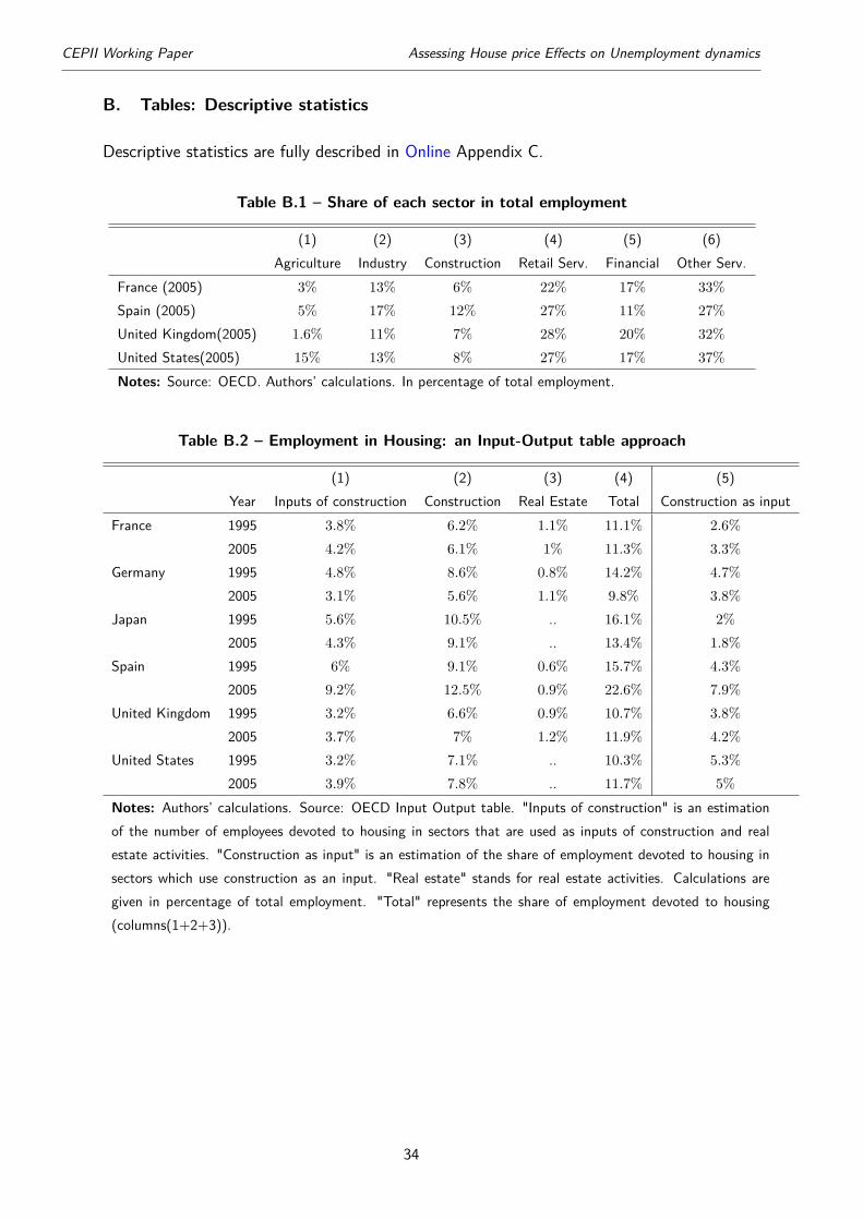
CEPII Working Paper Assessing House price Effects on Unemployment dynamics
B. Tables: Descriptive statistics
Descriptive statistics are fully described in Online Appendix C.
Table B.1 – Share of each sector in total employment
(1) (2) (3) (4) (5) (6)Agriculture Industry Construction Retail Serv. Financial Other Serv.
France (2005) 3% 13% 6% 22% 17% 33%Spain (2005) 5% 17% 12% 27% 11% 27%United Kingdom(2005) 1.6% 11% 7% 28% 20% 32%United States(2005) 15% 13% 8% 27% 17% 37%Notes: Source: OECD. Authors’ calculations. In percentage of total employment.
Table B.2 – Employment in Housing: an Input-Output table approach
(1) (2) (3) (4) (5)Year Inputs of construction Construction Real Estate Total Construction as input
France 1995 3.8% 6.2% 1.1% 11.1% 2.6%2005 4.2% 6.1% 1% 11.3% 3.3%
Germany 1995 4.8% 8.6% 0.8% 14.2% 4.7%2005 3.1% 5.6% 1.1% 9.8% 3.8%
Japan 1995 5.6% 10.5% .. 16.1% 2%2005 4.3% 9.1% .. 13.4% 1.8%
Spain 1995 6% 9.1% 0.6% 15.7% 4.3%2005 9.2% 12.5% 0.9% 22.6% 7.9%
United Kingdom 1995 3.2% 6.6% 0.9% 10.7% 3.8%2005 3.7% 7% 1.2% 11.9% 4.2%
United States 1995 3.2% 7.1% .. 10.3% 5.3%2005 3.9% 7.8% .. 11.7% 5%
Notes: Authors’ calculations. Source: OECD Input Output table. "Inputs of construction" is an estimationof the number of employees devoted to housing in sectors that are used as inputs of construction and realestate activities. "Construction as input" is an estimation of the share of employment devoted to housing insectors which use construction as an input. "Real estate" stands for real estate activities. Calculations aregiven in percentage of total employment. "Total" represents the share of employment devoted to housing(columns(1+2+3)).
34
CEPII Working Paper Assessing House price Effects on Unemployment dynamics
C. Robustness checks
Granger causality. We check in this section that Granger causality tests confirm that houseprices cause unemployment and not the other way around. Table C.1A shows that fittingsimple VAR with 2 lags39 confirm this result: a positive shock to house prices does cause adecrease of unemployment in the period after (columns (2)) while unemployment (a negativeshock to unemployment ) does not cause increases in house prices as can be seen in columns(1), (3). We show also in Table C.1B that Granger causality tests confirm that house pricescause GDP and not the other way round40. A positive shock to house prices does cause anincrease of GDP in the period after (columns (1)) while GDP (a positive shock to GDP) doesnot cause increases in house prices as can be seen in columns (2). We have not pursued thisempirical strategy in the core of the paper, even though it seems to yield the same conclusionsqualitatively, because Granger causality is not strictly causality, and more importantly becausethe coefficients are impossible to interpret quantitatively.
Choice of HP filter parameter. Our results are robust to several specifications of the HPparameter. In Table C.2, we show that any HP-filter parameter in the range 10-1600 yieldsthe same results with very good confidence intervals both for OLS results (A) and IV results(B). There is some disagreement in the literature as to which filter to use for frequenciesdifferent from quarterly data. We have used 400, as in Tomz and Wright (2007). Our resultsare robust to other lower proposed values of 6.25 (Ravn and Uhlig (1997)), 100 in Backus(1992) or higher, such as 1600 (the value commonly use for quarterly data). The choice ofthe parameter is not so important in our case as we are more interested in first moments thansecond moments for which the choice of the parameter is essential (Ravn and Uhlig (1997)).We use 400 as we both want to focus on medium term patterns of the data and to removethe trend of our data for our series to be non-stationary.
Controlling by different measures of GDP. Our results do not depend on the measure ofGDP used. In most tables, we control with real GDP growth. But our results are robust toother measures. In Table C.3, we show that we could have controlled by relative income orreal GDP without changing the results of our instrumental strategy.
Other scaling variables. In Table C.4, we show that using other scaling variables doesnot change our results. In particular, using as an instrumental variable the share of propertytaxation as a percentage of private consumption (column (1)) instead of using the share of
39To determine the number of lags, we use the Akaike Information Criterion (AIC) and the Schwarz’ BayesianInformation Criterion (SIC/BIC/SBIC). For most countries, they indicate 2 lags.40We show the instrumented effect of house prices on GDP in Table C.24.
35

CEPII Working Paper Assessing House price Effects on Unemployment dynamics
this tax as a percentage of total taxes does not change the results. The results are also robustif we measure the property tax with other scaling variables, such as investment (column (2))or GDP (column (3)). We show also that smoothing total tax does not alter the results. Inparticular, we smooth total tax using the trend component of a HP filter (column (4)). Weuse the parameter 6.25 that is recommended by Ravn and Uhlig (1997) to remove businesscycle frequencies with yearly data. We smooth also total tax by taking an averaged value oftotal tax (column (5)).
No filter. In Table C.5, we show that our results are robust even without filtering theunemployment rate. Interestingly, house price effects on unemployment become higher. A10% increase in house prices leads to a decrease of unemployment of 3.8% of active population(column (4)) against 3.4% in the baseline regression (column (4) in table 2). This higher effectcould partly capture a hysteresis phenomenon. In Tables C.6 and C.7, we show that houseprice effects on unemployment we computed in Table 1 are robust even without any filter. Wetake instead house prices in delta-log. In Table C.6, we just measure the unemployment rate inlog terms and house prices in delta log. In Table C.7, we then measure both the unemploymentrate and house prices in delta-log. The effects of house prices on unemployment are very robustboth for OLS and IV regressions, even controlling by the usual determinants of unemployment(columns (1) to (8)) as in Table 2. In Tables C.9, we show that results of Table 4 "Employmentdecomposition" are robust in delta-log, both for OLS (Table A) and for IV (Table B). In TablesC.10, we look at house price effects on employment in the tradable and non-tradable sectors.Results are robust in OLS and IV terms.
Booms and Busts: more. In Table C.12, we show that house price effects on employmentand GDP are still higher during busts than during boom periods when taking the variables indelta-log. Effects on the unemployment rate (column (1) of Table C.12) are also higher thanthe effects on employment (column (2)). When house prices increase by 10%, unemploymentdecreases by 3.8% (column (1)) and employment increases by 0.4% (column (2)). Note thathouse prices are not correlated with employment in the tradable sector during boom periods(column (3)).
Year Fixed effects. We control that house price effects on employment are robust to theinclusion of year fixed-effects (Table C.11). In particular, an instrumented increase in houseprices leads to an increase of employment in the tradable sector (column (5)), in the non-tradable sector (column (6)) and in construction (column (7)).
Other scaling variables : Total Employment and Working age population. In TableC.13, we use as denominator for sectoral employment variables total employment. Housing
36
CEPII Working Paper Assessing House price Effects on Unemployment dynamics
booms tend to lead to a reallocation of employment in favor of the construction sector. Indeed,the share of employment in construction increases during booms while the share of employmentin the tradable sector decreases. House price effects on total employment are also robust whenmeasuring employment variables as a percentage of working age population (Table C.14). A10% (instrumented) increase in house prices leads to a rise of employment of 1.5% (column(1) of Table C.14B). Further research would however be necessary to interpret house priceeffects on inactive persons.
Share prices. Following Beaudry and Portier (2006), we use also share prices as a variablefor capturing changes in agents expectations about future economic growth ("news shock").These changes may drive business cycle fluctuations. In Table C.17A, we show that our resultsboth in OLS and in IV (columns (3) and (5)) are very robust when we control by this variable.In Table C.17B, we show that house prices granger cause share prices.
Home-ownership: a friction in the labour market. Home-ownership could play as afriction in the labour market. Following Oswald (1996), we measure if home-ownership isa constraint for employment, notably because of reduced mobility. We build an interactionvariable between house prices and the home-ownership ratio to capture this friction. Toinvestigate this friction, we look also at unemployment dynamics (Table C.18). Panel data onunemployment dynamics are taken from Elsby et al. (2013). House prices have a significantand positive effect on job findings (column (1)). Interestingly, the effect of house prices onjob findings becomes negative when looking at the interaction variable between house pricesand home-ownership (column (2) of Table C.18): home-ownership seems a constraint in theprocess of finding a job. Concerning employment exits, house prices are negatively correlatedto this variable (column (4)). Note that if home-ownership is not as friction for employmentexits, employment protection tends to decrease employment exits (column (6)).
Beveridge Curve. In Table C.19, we show that job vacancy is indeed negatively correlatedwith unemployment (column (1)). If house prices are negatively correlated with unemployment(column (2)), they are positively correlated with job vacancy (column (3)). Mismatchesinduced by sectoral reallocation could lead to a shift in Beveridge Curve. This issue wouldrequire further investigation.
Dutch Disease. In Table C.15, we show that house prices lead to increases in real labourcosts both in tradable and non-tradable sectors (columns (1) to (3)), and to real exchange rateappreciations (column (4)). They have a negative impact on exports (column (5)). Housingbooms tend to reduce margins in the tradable sector as labour costs increase more thanmanufacturing prices (probably because these prices tend to be fixed at international levels)
37

CEPII Working Paper Assessing House price Effects on Unemployment dynamics
(Table C.16).
The firm-financing channel. The firm-financing channel could explain the rise of non-residential investment following house price increases. Our data allows us to look into whetherthe relaxation of borrowing constraints might have caused increasing investment, togetherwith an increased value of housing collateral (for its collateral services). In Table C.21 , weinvestigate whether house prices could impact investment through firm-financing mechanism.We use as a proxy for the potential tightness of credit constraints, the ratio of private credit toGDP. This is a standard mesure of financial development in the finance-and-growth literature(Aghion et al. (2010)). We construct an interaction variable between house prices and the ratioof private credit to GDP. The simultaneous of the two variables is significant for explaininginvestment and unemployment (columns (1) and (4) of Table C.21), which confirms that theeffect goes through a relaxation of financing constraints for firms. It is interesting to notice thatthe interaction variable is almost not significant in the case of residential investment (column(2)). Since it is not construction firms who are the final investors in residential structures, itdoes not matter whether construction firms are financially constrained. Furthermore, this isconsistent with the fact that houses are much less entrepreneur-specific investments, and thatinformation asymmetries creating the need for collateral are quantitatively very low in housinginvestment.
Construction. In Table C.22, we compare the effects of house prices and the effects ofconstruction volume variations. It is very difficult to disentangle price effects and volumeeffects as house prices are strongly correlated to construction (column (1)). In addition, wecannot use our instrument for construction. We show that the effects of house prices seem tobe larger than the effects of construction (both for estimated coefficients and R2). It is thecase for consumption (columns (2) and (3)), for investment ((4) and (5)), for employment inthe tradable sector ((6) and (7)), and for current account variations ((8) and (9)). This couldindicate that price effects exist in addition to volume effects.
Testing wealth effects. In order to assess whether consumption rises with house pricesbecause of wealth effects, we study the interaction between house prices and homeowneshiprates. The higher is the homeownership rate, the less is the number of households which ownsseveral housing units. Housing units occupied by renters are indeed owned by householdswhich own more than one housing unit (in France in 2010, 96% of private renters occupieda housing unit owned by another household. In the US, individual investors owned 83% ofall rental properties (US Census 2000)). These individual investors, richer in average thanowners of single residential unit, have a lower marginal propensity to consume. In table C.23,we show that the correlation between house prices and consumption is higher in countries
38
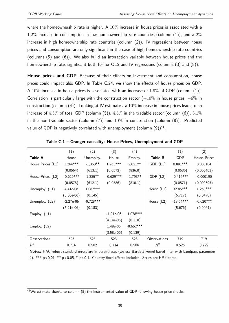
CEPII Working Paper Assessing House price Effects on Unemployment dynamics
where the homeownership rate is higher. A 10% increase in house prices is associated with a1.2% increase in consumption in low homeownership rate countries (column (1)), and a 2%increase in high homeownership rate countries (column (2)). IV regressions between houseprices and consumption are only significant in the case of high homeownership rate countries(columns (5) and (6)). We also build an interaction variable between house prices and thehomeownership rate, significant both for for OLS and IV regressions (columns (3) and (8)).
House prices and GDP. Because of their effects on investment and consumption, houseprices could impact also GDP. In Table C.24, we show the effects of house prices on GDP.A 10% increase in house prices is associated with an increase of 1.9% of GDP (column (1)).Correlation is particularly large with the construction sector (+10% in house prices, +6% inconstruction (column (4)). Looking at IV estimates, a 10% increase in house prices leads to anincrease of 4.3% of total GDP (column (5)), 4.5% in the tradable sector (column (6)), 3.1%in the non-tradable sector (column (7)) and 10% in construction (column (8)). Predictedvalue of GDP is negatively correlated with unemployment (column (9))41.
Table C.1 – Granger causality: House Prices, Unemployment and GDP
(1) (2) (3) (4) (1) (2)Table A House Unemploy. House Employ. Table B GDP House PricesHouse Prices (L1) 1.264*** -1,350** 1.263*** 2,021** GDP (L1) 0.891*** 0.000104
(0.0564) (613.1) (0.0572) (836.0) (0.0636) (0.000403)House Prices (L2) -0.629*** 1,385** -0.629*** -1,793** GDP (L2) -0.414*** -0.000190
(0.0578) (612.1) (0.0586) (810.1) (0.0571) (0.000395)Unemploy. (L1) 4.41e-06 1.087*** House (L1) 32.85*** 1.260***
(5.80e-06) (0.145) (5.717) (0.0478)Unemploy. (L2) -2.27e-06 -0.728*** House (L2) -18.64*** -0.620***
(5.21e-06) (0.183) (5.676) (0.0464)Employ. (L1) -1.91e-06 1.078***
(4.14e-06) (0.110)Employ. (L2) 1.48e-06 -0.652***
(3.58e-06) (0.139)Observations 523 523 523 523 Observations 719 719R2 0.714 0.562 0.714 0.566 R2 0.526 0.729Notes: HAC robust standard errors are in parentheses (we use Bartlett kernel-based filter with bandpass parameter2). *** p<0.01, ** p<0.05, * p<0.1. Country fixed effects included. Series are HP-filtered.
41We estimate thanks to column (5) the instrumented value of GDP following house price shocks.
39
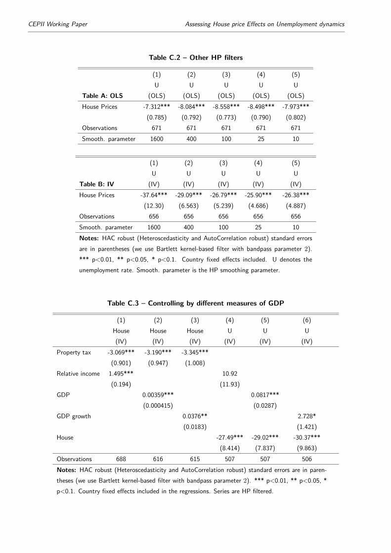
CEPII Working Paper Assessing House price Effects on Unemployment dynamics
Table C.2 – Other HP filters
(1) (2) (3) (4) (5)U U U U U
Table A: OLS (OLS) (OLS) (OLS) (OLS) (OLS)House Prices -7.312*** -8.084*** -8.558*** -8.498*** -7.973***
(0.785) (0.792) (0.773) (0.790) (0.802)Observations 671 671 671 671 671Smooth. parameter 1600 400 100 25 10
(1) (2) (3) (4) (5)U U U U U
Table B: IV (IV) (IV) (IV) (IV) (IV)House Prices -37.64*** -29.09*** -26.79*** -25.90*** -26.38***
(12.30) (6.563) (5.239) (4.686) (4.887)Observations 656 656 656 656 656Smooth. parameter 1600 400 100 25 10Notes: HAC robust (Heteroscedasticity and AutoCorrelation robust) standard errorsare in parentheses (we use Bartlett kernel-based filter with bandpass parameter 2).*** p<0.01, ** p<0.05, * p<0.1. Country fixed effects included. U denotes theunemployment rate. Smooth. parameter is the HP smoothing parameter.
Table C.3 – Controlling by different measures of GDP
(1) (2) (3) (4) (5) (6)House House House U U U(IV) (IV) (IV) (IV) (IV) (IV)
Property tax -3.069*** -3.190*** -3.345***(0.901) (0.947) (1.008)
Relative income 1.495*** 10.92(0.194) (11.93)
GDP 0.00359*** 0.0817***(0.000415) (0.0287)
GDP growth 0.0376** 2.728*(0.0183) (1.421)
House -27.49*** -29.02*** -30.37***(8.414) (7.837) (9.863)
Observations 688 616 615 507 507 506Notes: HAC robust (Heteroscedasticity and AutoCorrelation robust) standard errors are in paren-theses (we use Bartlett kernel-based filter with bandpass parameter 2). *** p<0.01, ** p<0.05, *p<0.1. Country fixed effects included in the regressions. Series are HP filtered.
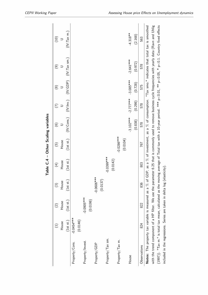
CEPII Working Paper Assessing House price Effects on Unemployment dynamics
TableC.4
–Other
Scalingvaria
bles
(1)
(2)
(3)
(4)
(5)
(6)
(7)
(8)
(9)
(10)
Hou
seHou
seHou
seHou
seHou
seU
UU
UU
(1st
st.)
(1st
st.)
(1st
st.)
(1st
st.)
(1st
st.)
(IV:Con
s.)(IV
:Inv.)
(IV:GDP)
(IV:Tax
sm.)
(IV:Tax
m.)
Prop
erty/C
ons.
-0.0454***
(0.0146)
Prop
erty/Invest.
-0.0905***
(0.0198)
Prop
erty/G
DP
-0.0606***
(0.0137)
Prop
erty/T
axsm
.-0.0399***
(0.0142)
Prop
erty/T
axm.
-0.0286***
(0.0104)
Hou
se-3.102***
-2.777***
-3.085***
-2.641***
-4.318**
(0.838)
(0.298)
(0.728)
(0.972)
(2.168)
Observatio
ns824
822
836
803
767
578
578
575
578
563
Notes:Th
eprop
erty
taxvaria
bleis
measuredas
a%
ofGD
P,as
a%
ofinvestment,
asa
%of
consum
ption.
"Tax
smo."indicatesthat
totaltax
issm
oothed
with
thetrendcompo
nent
ofaHPfilter.
Weusetheparameter
6.25
that
iscommon
lyused
toremovebu
sinesscycle
frequ
encie
swith
yearly
data
(RavnandUh
lig(1997)).
"Tax
m."
istotaltax
mean,
calcu
latedas
themovingaverageof
Totaltax
with
a10-yearp
eriod.
***p<
0.01,*
*p<
0.05,*
p<0.1.
Coun
tryfixed
effects
inclu
dedin
theregressio
ns.Se
riesaretakenin
delta
log(elasticity).
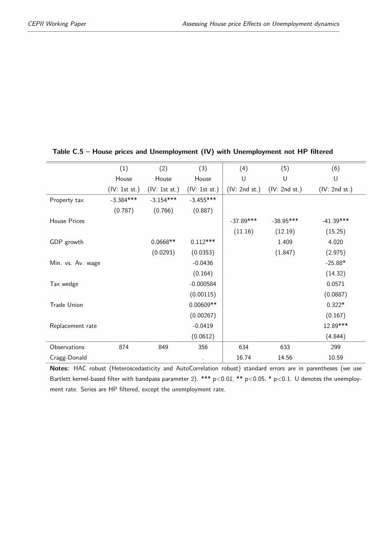
CEPII Working Paper Assessing House price Effects on Unemployment dynamics
Table C.5 – House prices and Unemployment (IV) with Unemployment not HP filtered
(1) (2) (3) (4) (5) (6)House House House U U U
(IV: 1st st.) (IV: 1st st.) (IV: 1st st.) (IV: 2nd st.) (IV: 2nd st.) (IV: 2nd st.)Property tax -3.384*** -3.154*** -3.455***
(0.787) (0.766) (0.887)House Prices -37.89*** -38.95*** -41.39***
(11.16) (12.19) (15.25)GDP growth 0.0668** 0.112*** 1.409 4.020
(0.0293) (0.0353) (1.847) (2.975)Min. vs. Av. wage -0.0436 -25.88*
(0.164) (14.32)Tax wedge -0.000584 0.0571
(0.00115) (0.0887)Trade Union 0.00609** 0.322*
(0.00267) (0.167)Replacement rate -0.0419 12.89***
(0.0612) (4.844)Observations 874 849 356 634 633 299Cragg-Donald . 16.74 14.56 10.59Notes: HAC robust (Heteroscedasticity and AutoCorrelation robust) standard errors are in parentheses (we useBartlett kernel-based filter with bandpass parameter 2). *** p<0.01, ** p<0.05, * p<0.1. U denotes the unemploy-ment rate. Series are HP filtered, except the unemployment rate.
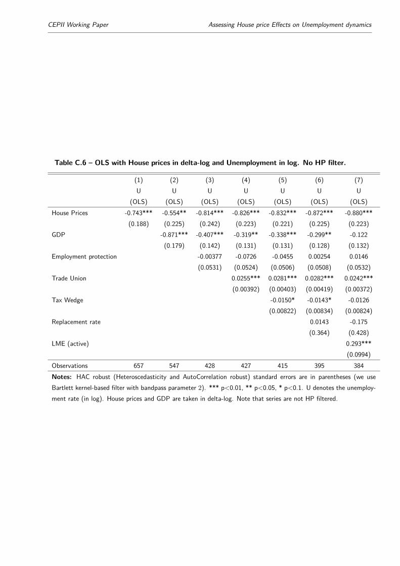
CEPII Working Paper Assessing House price Effects on Unemployment dynamics
Table C.6 – OLS with House prices in delta-log and Unemployment in log. No HP filter.
(1) (2) (3) (4) (5) (6) (7)U U U U U U U
(OLS) (OLS) (OLS) (OLS) (OLS) (OLS) (OLS)House Prices -0.743*** -0.554** -0.814*** -0.826*** -0.832*** -0.872*** -0.880***
(0.188) (0.225) (0.242) (0.223) (0.221) (0.225) (0.223)GDP -0.871*** -0.407*** -0.319** -0.338*** -0.299** -0.122
(0.179) (0.142) (0.131) (0.131) (0.128) (0.132)Employment protection -0.00377 -0.0726 -0.0455 0.00254 0.0146
(0.0531) (0.0524) (0.0506) (0.0508) (0.0532)Trade Union 0.0255*** 0.0281*** 0.0282*** 0.0242***
(0.00392) (0.00403) (0.00419) (0.00372)Tax Wedge -0.0150* -0.0143* -0.0126
(0.00822) (0.00834) (0.00824)Replacement rate 0.0143 -0.175
(0.364) (0.428)LME (active) 0.293***
(0.0994)Observations 657 547 428 427 415 395 384Notes: HAC robust (Heteroscedasticity and AutoCorrelation robust) standard errors are in parentheses (we useBartlett kernel-based filter with bandpass parameter 2). *** p<0.01, ** p<0.05, * p<0.1. U denotes the unemploy-ment rate (in log). House prices and GDP are taken in delta-log. Note that series are not HP filtered.
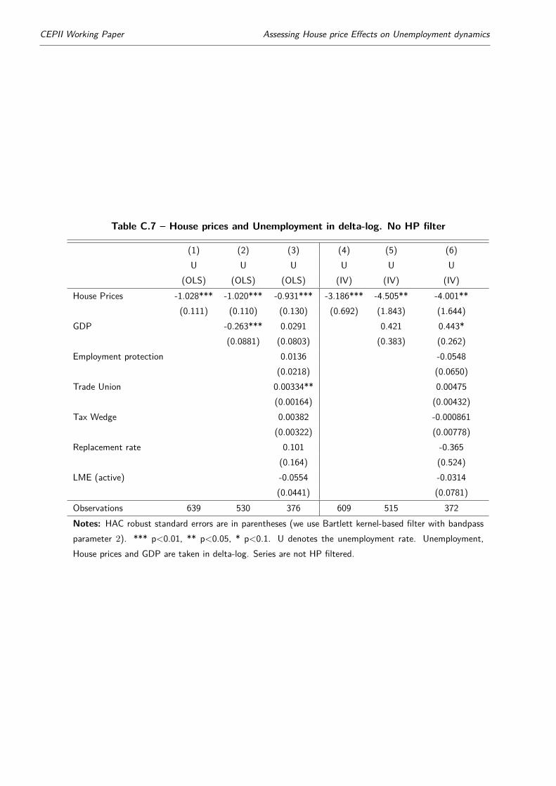
CEPII Working Paper Assessing House price Effects on Unemployment dynamics
Table C.7 – House prices and Unemployment in delta-log. No HP filter
(1) (2) (3) (4) (5) (6)U U U U U U
(OLS) (OLS) (OLS) (IV) (IV) (IV)House Prices -1.028*** -1.020*** -0.931*** -3.186*** -4.505** -4.001**
(0.111) (0.110) (0.130) (0.692) (1.843) (1.644)GDP -0.263*** 0.0291 0.421 0.443*
(0.0881) (0.0803) (0.383) (0.262)Employment protection 0.0136 -0.0548
(0.0218) (0.0650)Trade Union 0.00334** 0.00475
(0.00164) (0.00432)Tax Wedge 0.00382 -0.000861
(0.00322) (0.00778)Replacement rate 0.101 -0.365
(0.164) (0.524)LME (active) -0.0554 -0.0314
(0.0441) (0.0781)Observations 639 530 376 609 515 372Notes: HAC robust standard errors are in parentheses (we use Bartlett kernel-based filter with bandpassparameter 2). *** p<0.01, ** p<0.05, * p<0.1. U denotes the unemployment rate. Unemployment,House prices and GDP are taken in delta-log. Series are not HP filtered.

CEPII Working Paper Assessing House price Effects on Unemployment dynamics
Table C.8 – Volatility of Employment
(1) (2) (3) (4) (5) (6) (7)Employ. Employ. Employ. Employ. Employ. Employ. Employ(OLS) (OLS) (OLS) (OLS) (OLS) (OLS) (OLS)
E.Agriculture 0.00241 0.974***(0.218) (0.0182)
E.Construction 1.936*** 1.011***(0.0736) (0.0113)
E.Industry 1.644*** 0.979***(0.0798) (0.00951)
E.Retail Services 1.949*** 0.977***(0.0747) (0.0116)
E. Financial 2.420*** 1.001***(0.143) (0.0171)
E. Other Services 0.138 0.981***(0.152) (0.0131)
Observations 536 536 536 536 536 536 536R2 0.000 0.563 0.442 0.559 0.349 0.002 0.993Notes: *** p<0.01, ** p<0.05, * p<0.1. Series are HP-filtered. "Employ." denotes total employ-ment."E." represents employment in the 6 sectors of ISIC Rev. 3 classification.
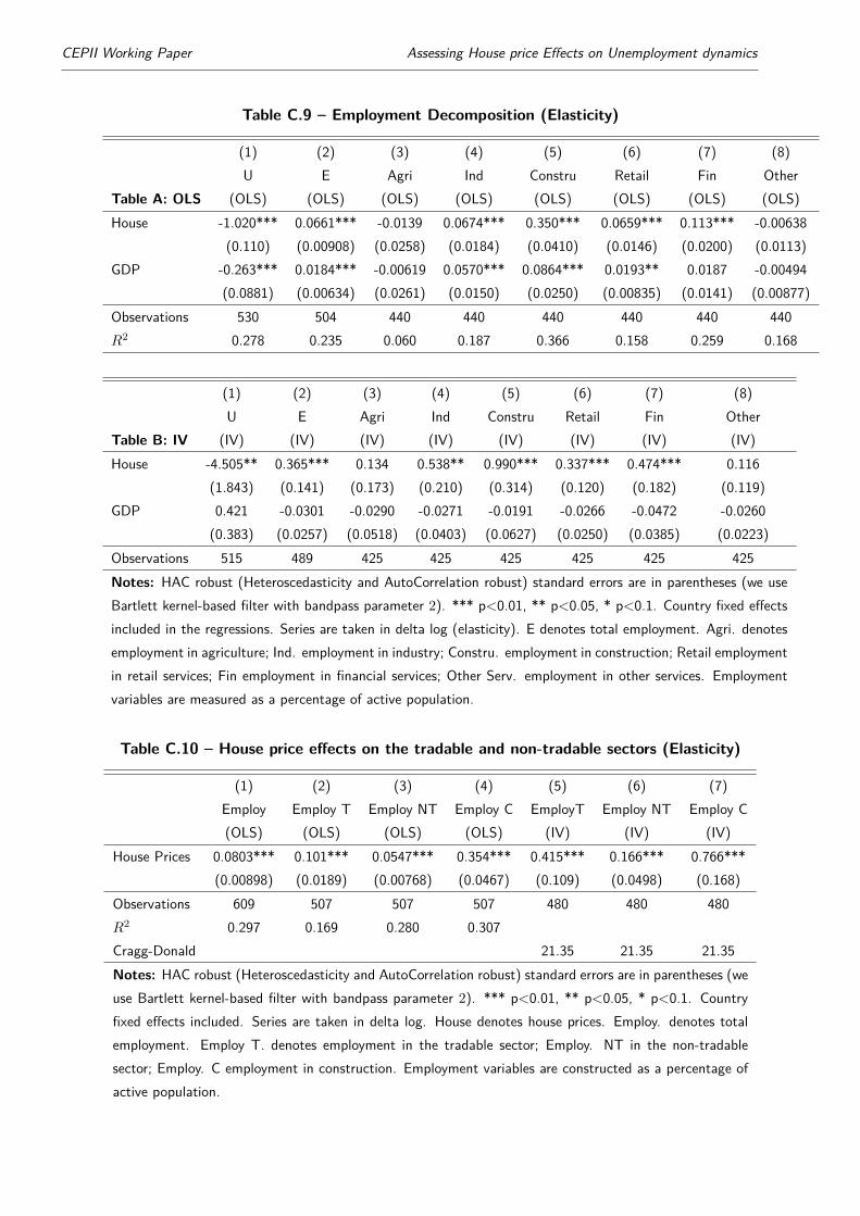
CEPII Working Paper Assessing House price Effects on Unemployment dynamics
Table C.9 – Employment Decomposition (Elasticity)
(1) (2) (3) (4) (5) (6) (7) (8)U E Agri Ind Constru Retail Fin Other
Table A: OLS (OLS) (OLS) (OLS) (OLS) (OLS) (OLS) (OLS) (OLS)House -1.020*** 0.0661*** -0.0139 0.0674*** 0.350*** 0.0659*** 0.113*** -0.00638
(0.110) (0.00908) (0.0258) (0.0184) (0.0410) (0.0146) (0.0200) (0.0113)GDP -0.263*** 0.0184*** -0.00619 0.0570*** 0.0864*** 0.0193** 0.0187 -0.00494
(0.0881) (0.00634) (0.0261) (0.0150) (0.0250) (0.00835) (0.0141) (0.00877)Observations 530 504 440 440 440 440 440 440R2 0.278 0.235 0.060 0.187 0.366 0.158 0.259 0.168
(1) (2) (3) (4) (5) (6) (7) (8)U E Agri Ind Constru Retail Fin Other
Table B: IV (IV) (IV) (IV) (IV) (IV) (IV) (IV) (IV)House -4.505** 0.365*** 0.134 0.538** 0.990*** 0.337*** 0.474*** 0.116
(1.843) (0.141) (0.173) (0.210) (0.314) (0.120) (0.182) (0.119)GDP 0.421 -0.0301 -0.0290 -0.0271 -0.0191 -0.0266 -0.0472 -0.0260
(0.383) (0.0257) (0.0518) (0.0403) (0.0627) (0.0250) (0.0385) (0.0223)Observations 515 489 425 425 425 425 425 425Notes: HAC robust (Heteroscedasticity and AutoCorrelation robust) standard errors are in parentheses (we useBartlett kernel-based filter with bandpass parameter 2). *** p<0.01, ** p<0.05, * p<0.1. Country fixed effectsincluded in the regressions. Series are taken in delta log (elasticity). E denotes total employment. Agri. denotesemployment in agriculture; Ind. employment in industry; Constru. employment in construction; Retail employmentin retail services; Fin employment in financial services; Other Serv. employment in other services. Employmentvariables are measured as a percentage of active population.
Table C.10 – House price effects on the tradable and non-tradable sectors (Elasticity)
(1) (2) (3) (4) (5) (6) (7)Employ Employ T Employ NT Employ C EmployT Employ NT Employ C(OLS) (OLS) (OLS) (OLS) (IV) (IV) (IV)
House Prices 0.0803*** 0.101*** 0.0547*** 0.354*** 0.415*** 0.166*** 0.766***(0.00898) (0.0189) (0.00768) (0.0467) (0.109) (0.0498) (0.168)
Observations 609 507 507 507 480 480 480R2 0.297 0.169 0.280 0.307Cragg-Donald 21.35 21.35 21.35Notes: HAC robust (Heteroscedasticity and AutoCorrelation robust) standard errors are in parentheses (weuse Bartlett kernel-based filter with bandpass parameter 2). *** p<0.01, ** p<0.05, * p<0.1. Countryfixed effects included. Series are taken in delta log. House denotes house prices. Employ. denotes totalemployment. Employ T. denotes employment in the tradable sector; Employ. NT in the non-tradablesector; Employ. C employment in construction. Employment variables are constructed as a percentage ofactive population.
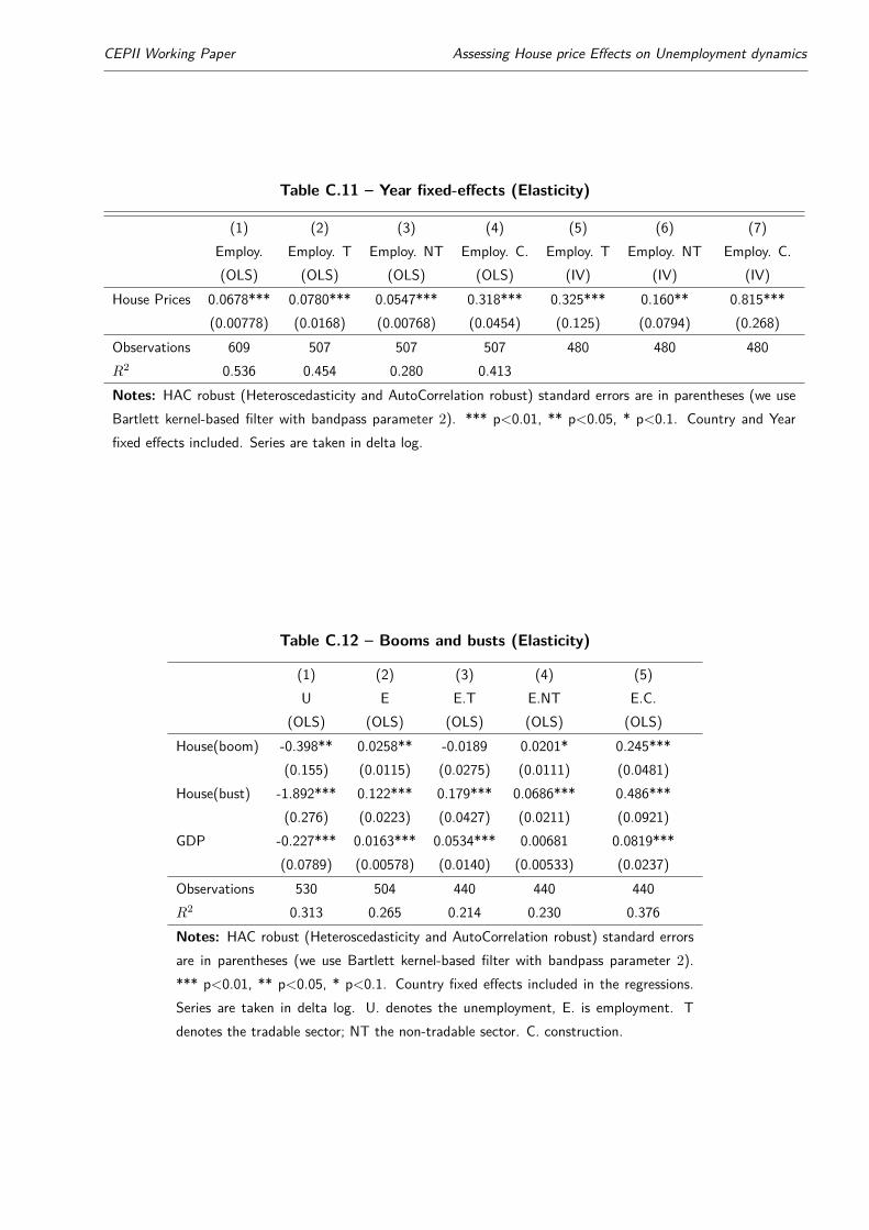
CEPII Working Paper Assessing House price Effects on Unemployment dynamics
Table C.11 – Year fixed-effects (Elasticity)
(1) (2) (3) (4) (5) (6) (7)Employ. Employ. T Employ. NT Employ. C. Employ. T Employ. NT Employ. C.(OLS) (OLS) (OLS) (OLS) (IV) (IV) (IV)
House Prices 0.0678*** 0.0780*** 0.0547*** 0.318*** 0.325*** 0.160** 0.815***(0.00778) (0.0168) (0.00768) (0.0454) (0.125) (0.0794) (0.268)
Observations 609 507 507 507 480 480 480R2 0.536 0.454 0.280 0.413Notes: HAC robust (Heteroscedasticity and AutoCorrelation robust) standard errors are in parentheses (we useBartlett kernel-based filter with bandpass parameter 2). *** p<0.01, ** p<0.05, * p<0.1. Country and Yearfixed effects included. Series are taken in delta log.
Table C.12 – Booms and busts (Elasticity)
(1) (2) (3) (4) (5)U E E.T E.NT E.C.
(OLS) (OLS) (OLS) (OLS) (OLS)House(boom) -0.398** 0.0258** -0.0189 0.0201* 0.245***
(0.155) (0.0115) (0.0275) (0.0111) (0.0481)House(bust) -1.892*** 0.122*** 0.179*** 0.0686*** 0.486***
(0.276) (0.0223) (0.0427) (0.0211) (0.0921)GDP -0.227*** 0.0163*** 0.0534*** 0.00681 0.0819***
(0.0789) (0.00578) (0.0140) (0.00533) (0.0237)Observations 530 504 440 440 440R2 0.313 0.265 0.214 0.230 0.376Notes: HAC robust (Heteroscedasticity and AutoCorrelation robust) standard errorsare in parentheses (we use Bartlett kernel-based filter with bandpass parameter 2).*** p<0.01, ** p<0.05, * p<0.1. Country fixed effects included in the regressions.Series are taken in delta log. U. denotes the unemployment, E. is employment. Tdenotes the tradable sector; NT the non-tradable sector. C. construction.

CEPII Working Paper Assessing House price Effects on Unemployment dynamics
Table C.13 – Employment reallocation during booms and busts
(1) (2) (3)Employ. T (sh.) Employ. NT (sh.) Employ. C. (sh.)
(OLS) (OLS) (OLS)House(boom) -0.0359** -0.00716 0.232***
(0.0179) (0.00739) (0.0358)House(bust) 0.0545** -0.0612*** 0.346***
(0.0250) (0.0116) (0.0589)GDP 0.0332*** -0.00613* 0.0681***
(0.00849) (0.00334) (0.0163)Observations 503 503 503R2 0.179 0.293 0.389Notes: HAC robust (Heteroscedasticity and AutoCorrelation robust)standard errors are in parentheses (we use Bartlett kernel-based filterwith bandpass parameter 2). *** p<0.01, ** p<0.05, * p<0.1. Countryfixed effects included. Series in delta log. Sectoral employment variablesare measured as a share (sh.) of total employment.
Table C.14 – Other scaling variable: Employment in % of working age population
(1) (2) (3) (4) (5) (6) (7)Table A: OLS E.(wa) Agri.(wa) Ind.(wa) Constru.(wa) Retail(wa) Fin.(wa) Other Serv.(wa)House 4.837*** -0.216** 1.082*** 1.958*** 1.152*** 0.827*** 0.274
(0.813) (0.0920) (0.239) (0.274) (0.284) (0.217) (0.211)GDP 0.0257*** 0.000421 0.00681*** 0.00946*** 0.00742*** 0.00342* -0.00395**
(0.00720) (0.000814) (0.00211) (0.00243) (0.00251) (0.00192) (0.00186)Observations 252 252 252 252 252 252 252R2 0.231 0.047 0.169 0.297 0.137 0.098 0.024
(1) (2) (3) (4) (5) (6) (7)Table B: IV E.(/wa) Agri.(/wa) Ind.(/wa) Constru(/wa) Retail(/wa) Fin.(/wa) Other Serv.(/wa)House 14.55*** 0.703 5.178*** 3.815*** 4.529*** 3.598*** -2.716**
(4.193) (0.448) (1.448) (1.229) (1.461) (1.148) (1.164)GDP -0.00377 -0.00237 -0.00562 0.00383 -0.00283 -0.00498 0.00512
(0.0153) (0.00163) (0.00528) (0.00448) (0.00532) (0.00418) (0.00424)Observations 252 252 252 252 252 252 252Notes: HAC robust (Heteroscedasticity and AutoCorrelation robust) standard errors are in parentheses (we useBartlett kernel-based filter with bandpass parameter 2). *** p<0.01, ** p<0.05, * p<0.1. Country fixed effectsincluded. Variables of employment are measured as a percentage of the working age population ("wa").
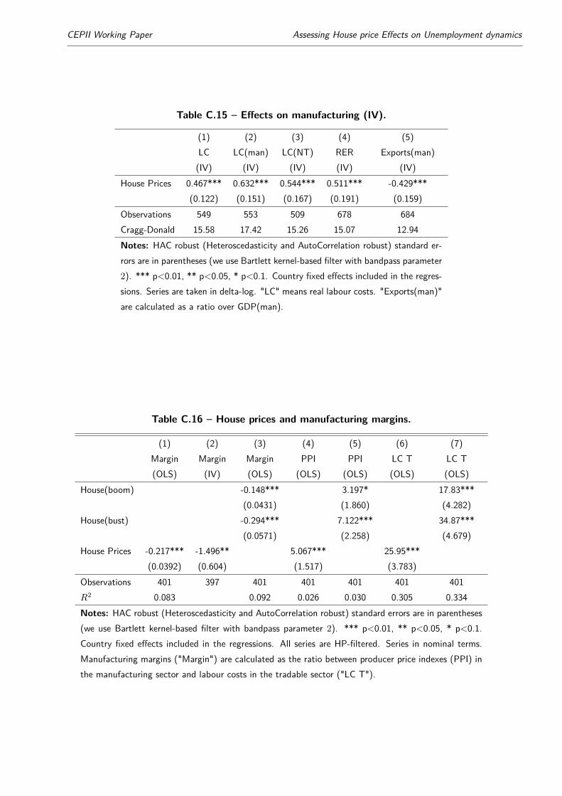
CEPII Working Paper Assessing House price Effects on Unemployment dynamics
Table C.15 – Effects on manufacturing (IV).
(1) (2) (3) (4) (5)LC LC(man) LC(NT) RER Exports(man)(IV) (IV) (IV) (IV) (IV)
House Prices 0.467*** 0.632*** 0.544*** 0.511*** -0.429***(0.122) (0.151) (0.167) (0.191) (0.159)
Observations 549 553 509 678 684Cragg-Donald 15.58 17.42 15.26 15.07 12.94Notes: HAC robust (Heteroscedasticity and AutoCorrelation robust) standard er-rors are in parentheses (we use Bartlett kernel-based filter with bandpass parameter2). *** p<0.01, ** p<0.05, * p<0.1. Country fixed effects included in the regres-sions. Series are taken in delta-log. "LC" means real labour costs. "Exports(man)"are calculated as a ratio over GDP(man).
Table C.16 – House prices and manufacturing margins.
(1) (2) (3) (4) (5) (6) (7)Margin Margin Margin PPI PPI LC T LC T(OLS) (IV) (OLS) (OLS) (OLS) (OLS) (OLS)
House(boom) -0.148*** 3.197* 17.83***(0.0431) (1.860) (4.282)
House(bust) -0.294*** 7.122*** 34.87***(0.0571) (2.258) (4.679)
House Prices -0.217*** -1.496** 5.067*** 25.95***(0.0392) (0.604) (1.517) (3.783)
Observations 401 397 401 401 401 401 401R2 0.083 0.092 0.026 0.030 0.305 0.334Notes: HAC robust (Heteroscedasticity and AutoCorrelation robust) standard errors are in parentheses(we use Bartlett kernel-based filter with bandpass parameter 2). *** p<0.01, ** p<0.05, * p<0.1.Country fixed effects included in the regressions. All series are HP-filtered. Series in nominal terms.Manufacturing margins ("Margin") are calculated as the ratio between producer price indexes (PPI) inthe manufacturing sector and labour costs in the tradable sector ("LC T").
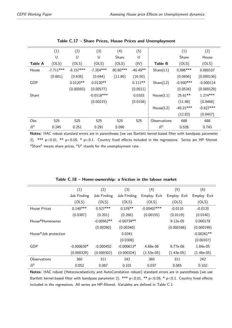
CEPII Working Paper Assessing House price Effects on Unemployment dynamics
Table C.17 – Share Prices, House Prices and Unemployment
(1) (2) (3) (4) (5) (1) (2)U U U Share U Share House
Table A (OLS) (OLS) (OLS) (OLS) (IV) Table B (OLS) (OLS)House -7.711*** -8.157*** -7.204*** 80.80*** -40.49** Share(L1) 0.896*** 0.000107
(0.601) (0.638) (0.644) (11.80) (16.50) (0.0656) (0.000136)GDP 0.0120** 0.0120** 0.111** Share(L2) -0.500*** -0.000114
(0.00593) (0.00577) (0.0511) (0.0534) (0.000129)Share -0.0118*** 0.0183 House(L1) 25.61** 1.274***
(0.00215) (0.0158) (11.88) (0.0468)House(L2) -49.21*** -0.627***
(12.83) (0.0457)Obs. 525 525 525 525 525 Observations 688 688R2 0.245 0.251 0.291 0.090 R2 0.526 0.743Notes: HAC robust standard errors are in parentheses (we use Bartlett kernel-based filter with bandpass parameter2). *** p<0.01, ** p<0.05, * p<0.1. Country fixed effects included in the regressions. Series are HP filtered."Share" means share prices, "U" stands for the unemployment rate.
Table C.18 – Home-ownership: a friction in the labour market
(1) (2) (3) (4) (5) (6)Job Finding Job Finding Job Finding Employ. Exit Employ. Exit Employ. Exit
(OLS) (OLS) (OLS) (OLS) (OLS) (OLS)House Prices 0.148*** 0.527*** 0.576** -0.00407*** -0.0110 -0.0120
(0.0387) (0.201) (0.268) (0.00155) (0.0119) (0.0140)House*Homeowner -0.00562** -0.00734** 9.12e-05 0.000178
(0.00280) (0.00340) (0.000166) (0.000199)House*Job protection 0.0341 -0.00261**
(0.0309) (0.00107)GDP -0.000630* -0.000452 -0.000613* 4.68e-06 6.77e-06 1.84e-05
(0.000329) (0.000302) (0.000324) (1.53e-05) (1.43e-05) (1.46e-05)Observations 360 311 242 360 311 242R2 0.052 0.067 0.101 0.037 0.065 0.102Notes: HAC robust (Heteroscedasticity and AutoCorrelation robust) standard errors are in parentheses (we useBartlett kernel-based filter with bandpass parameter 2). *** p<0.01, ** p<0.05, * p<0.1. Country fixed effectsincluded in the regressions. All series are HP-filtered. Variables are defined in Table C.1.

CEPII Working Paper Assessing House price Effects on Unemployment dynamics
Table C.19 – Beveridge Curve: Unemployment and Vacancy
(1) (2) (3)Unemploy. Unemploy. Job Vacancy(OLS) (OLS) (OLS)
Job Vacancy -3.504***(0.298)
House Prices -6.932*** 1.106***(0.745) (0.118)
Observations 312 312 312R2 0.307 0.217 0.221Notes: HAC robust (Heteroscedasticity and AutoCorrelation robust)standard errors are in parentheses (we use Bartlett kernel-based fil-ter with bandpass parameter 2). *** p<0.01, ** p<0.05, * p<0.1.Country fixed effects included in the regressions. Series are HP fil-tered.
Table C.20 – House prices, Consumption and Investment (Elasticity)
(1) (2) (3) (4) (5) (6)Cons. C. dura. C. Hotels/Rest. I Res. I NR. I(OLS) (OLS) (OLS) (OLS) (OLS) (OLS)
House(boom) 0.115*** 0.239*** 0.128*** 0.273*** 0.461*** 0.201**(0.0208) (0.0870) (0.0235) (0.0687) (0.0785) (0.0845)
House(bust) 0.229*** 0.861*** 0.151*** 0.694*** 1.030*** 0.581***(0.0369) (0.165) (0.0420) (0.108) (0.149) (0.126)
GDP 0.0683*** 0.230*** 0.0602*** 0.142*** 0.142*** 0.151***(0.0104) (0.0499) (0.0127) (0.0279) (0.0426) (0.0369)
Observations 723 489 489 720 691 679R2 0.448 0.375 0.437 0.287 0.317 0.170Notes: HAC robust (Heteroscedasticity and AutoCorrelation robust) standard errors arein parentheses (we use Bartlett kernel-based filter with bandpass parameter 2). ***p<0.01, ** p<0.05, * p<0.1. House Prices are an indice of house prices, normalized at1 in 2005. Country fixed effects included in the regressions. Series are taken in deltalog (Elasticity). Cons. denotes consumption; C. dura consumption of durable goods;C.Hotels/Rest. consumption in hotels and restaurants. I denotes investment ; Res. I isresidential investment; NR. I non-residential investment.
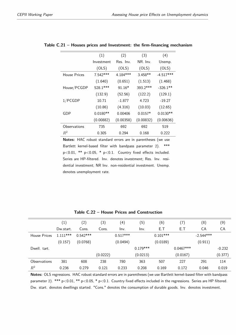
CEPII Working Paper Assessing House price Effects on Unemployment dynamics
Table C.21 – Houses prices and Investment: the firm-financing mechanism
(1) (2) (3) (4)Investment Res. Inv. NR. Inv. Unemp.(OLS) (OLS) (OLS) (OLS)
House Prices 7.542*** 4.184*** 3.458** -4.517***(1.640) (0.651) (1.513) (1.468)
House/PCGDP 528.1*** 91.16* 393.2*** -326.1**(132.9) (52.56) (122.2) (129.1)
1/PCGDP 10.71 -1.877 4.723 -19.27(10.86) (4.316) (10.03) (12.65)
GDP 0.0180** 0.00406 0.0157* 0.0130**(0.00882) (0.00358) (0.00832) (0.00636)
Observations 735 692 692 519R2 0.305 0.294 0.168 0.222Notes: HAC robust standard errors are in parentheses (we useBartlett kernel-based filter with bandpass parameter 2). ***p<0.01, ** p<0.05, * p<0.1. Country fixed effects included.Series are HP-filtered. Inv. denotes investment; Res. Inv. resi-dential investment; NR Inv. non-residential investment. Unemp.denotes unemployment rate.
Table C.22 – House Prices and Construction
(1) (2) (3) (4) (5) (6) (7) (8) (9)Dw.start. Cons. Cons. Inv. Inv. E.T E.T CA CA
House Prices 1.111*** 0.542*** 0.517*** 0.101*** -2.544***(0.157) (0.0768) (0.0494) (0.0189) (0.911)
Dwell. tart. 0.179*** 0.0467*** -0.232(0.0222) (0.0213) (0.0167) (0.377)
Observations 381 608 238 780 363 507 227 291 114R2 0.236 0.279 0.121 0.233 0.208 0.169 0.172 0.046 0.019Notes: OLS regressions. HAC robust standard errors are in parentheses (we use Bartlett kernel-based filter with bandpassparameter 2). *** p<0.01, ** p<0.05, * p<0.1. Country fixed effects included in the regressions. Series are HP filtered.Dw. start. denotes dwellings started. "Cons." denotes the consumption of durable goods. Inv. denotes investment.

CEPII Working Paper Assessing House price Effects on Unemployment dynamics
Table C.23 – Wealth effects
(1) (2) (3) (4) (5) (6) (7)Cons. Cons. Cons. Cons. Cons. Cons. Cons.(OLS) (OLS) (OLS) (IV) (IV) (IV) (IV)
House 12.71*** 19.78*** -10.21 43.21*** 14.91 55.48***(1.884) (1.877) (8.165) (9.699) (13.18) (12.13)
House*Owner 0.407*** 0.540***(0.128) (0.124)
Owner. ratio 0.0216 0.0327(0.0179) (0.0226)
GDP 6.04** 2.95 4.50*** -7.92* 5.04 -11.4** -4.24(2.37) (1.92) (1.68) (4.17) (6.25) (4.87) (3.81)
Observations 334 427 626 738 334 404 613R2 0.402 0.398 0.430Cragg-Donald 16.30 2.541 22.54 17.18Homeownership Low High Low HighNotes: HAC robust (Heteroscedasticity and AutoCorrelation robust) standard errors are in paren-theses (we use Bartlett kernel-based filter with bandpass parameter 2). *** p<0.01, ** p<0.05,* p<0.1. Country-fixed effects are included. "Cons." is real consumption (Index 2005 = 100)."Homeowner" is the homeownership ratio. The homeownership rate lies between 30 and 94. Seriesare HP filtered.
Table C.24 – House prices and GDP
(1) (2) (3) (4) (5) (6) (7) (8) (9)GDP GDP T GDP NT GDP C GDP GDP T GDP NT GDP C Unemp(OLS) (OLS) (OLS) (OLS) (IV) (IV) (IV) (IV) (OLS)
House Prices 19.19*** 15.15*** 15.93*** 61.80*** 42.79*** 44.96*** 30.72*** 106.8***(1.880) (2.579) (1.614) (5.282) (7.601) (16.77) (5.681) (17.18)
GDP(Pred.IV) -0.185***(0.0200)
Observations 820 820 820 820 751 751 751 751 568R2 0.280 0.064 0.277 0.375 0.282Cragg-Donald 20.92 20.92 20.92 20.92Notes: HAC robust (Heteroscedasticity and AutoCorrelation robust) standard errors are in parentheses (we use Bartlettkernel-based filter with bandpass parameter 2). *** p<0.01, ** p<0.05, * p<0.1. Country fixed effects included in theregressions. Series are HP-filtered. GDP denotes total GDP; GDP T denotes GDP in the tradable sector; NT in thenon-tradable sector; C in construction. GDP(Pred.IV) is the instrumented predicted value of GDP.
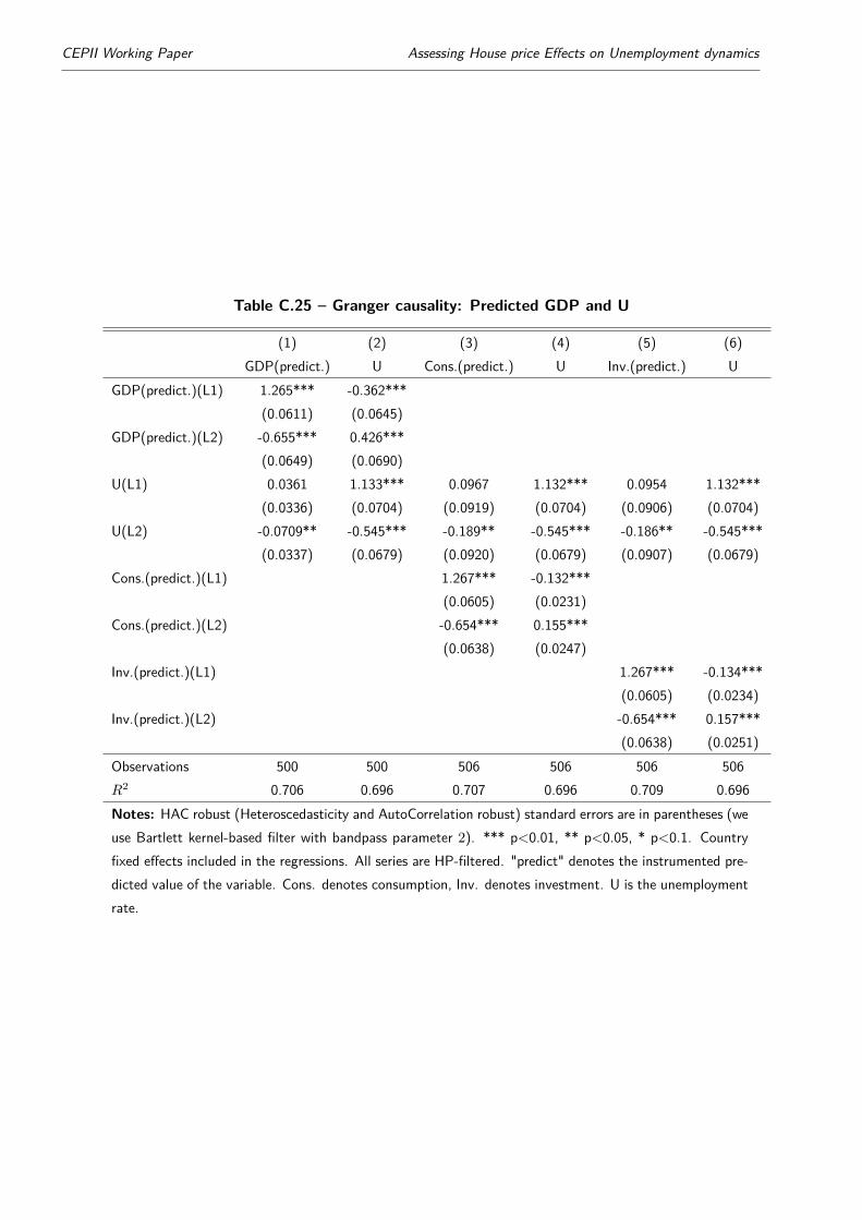
CEPII Working Paper Assessing House price Effects on Unemployment dynamics
Table C.25 – Granger causality: Predicted GDP and U
(1) (2) (3) (4) (5) (6)GDP(predict.) U Cons.(predict.) U Inv.(predict.) U
GDP(predict.)(L1) 1.265*** -0.362***(0.0611) (0.0645)
GDP(predict.)(L2) -0.655*** 0.426***(0.0649) (0.0690)
U(L1) 0.0361 1.133*** 0.0967 1.132*** 0.0954 1.132***(0.0336) (0.0704) (0.0919) (0.0704) (0.0906) (0.0704)
U(L2) -0.0709** -0.545*** -0.189** -0.545*** -0.186** -0.545***(0.0337) (0.0679) (0.0920) (0.0679) (0.0907) (0.0679)
Cons.(predict.)(L1) 1.267*** -0.132***(0.0605) (0.0231)
Cons.(predict.)(L2) -0.654*** 0.155***(0.0638) (0.0247)
Inv.(predict.)(L1) 1.267*** -0.134***(0.0605) (0.0234)
Inv.(predict.)(L2) -0.654*** 0.157***(0.0638) (0.0251)
Observations 500 500 506 506 506 506R2 0.706 0.696 0.707 0.696 0.709 0.696Notes: HAC robust (Heteroscedasticity and AutoCorrelation robust) standard errors are in parentheses (weuse Bartlett kernel-based filter with bandpass parameter 2). *** p<0.01, ** p<0.05, * p<0.1. Countryfixed effects included in the regressions. All series are HP-filtered. "predict" denotes the instrumented pre-dicted value of the variable. Cons. denotes consumption, Inv. denotes investment. U is the unemploymentrate.

CEPII Working Paper Assessing House price Effects on Unemployment dynamics
TableC.1
–DataApp
endix:
Variables
Varia
bles
Abb
reviation
Sources
Varia
bledescrip
tion
Hou
sePrices
Hou
seGeerolfandGrje
bine
(2013)
Real
houseprices
(base1=
2005)
Prop
erty
Tax
Prop
erty
Tax
OEC
DProp
erty
tax(ratio
oftotaltaxation)
CPI
CPI
OEC
DCo
nsum
erPrices,Ind
ex2005=100
Employment
E.OEC
DEm
ployed
popu
latio
n(ET
O)/Ac
tivepo
pulatio
n(PE
ANC)
,(%)
EmploymentIndu
stry
E.Ind.
OEC
DEm
ployed
person
sindu
stry(w
ithenergy)(ET
OCE
)/Ac
tivepo
pulatio
n,(%
)Em
ploymentManufacturin
gE.Manuf.
OEC
DEm
ployed
person
smanufacturin
g(ET
OD)/Ac
tivepo
pulatio
n(PE
ANC)
,(%)
EmploymentCo
nstructio
nE.Co
nstru.
OEC
DEm
ployed
person
sCo
nstructio
n(ET
OF)/A
ctivepo
pulatio
n(PE
ANC)
,(%)
EmploymentX(share)
E.X(share)
OEC
DEm
ployed
popu
latio
nin
X/E
mployed
popu
latio
n(ET
O),(%
)Em
ploymentX(w
orking
age)
E.X(w
a)OEC
DEm
ployed
popu
latio
nin
X/W
orking
agepo
pulatio
n,(%
)Unemployment
UOEC
DUnemployed
popu
latio
n/Ac
tivepo
pulatio
n(PE
ANC)
,(%)
Activ
epo
pulatio
nactiv
epo
pulatio
nOEC
DAc
tivepo
pulatio
n(PE
ANC)
,persons
Working
agepo
pulatio
nwa
OEC
DWorking
agepo
pulatio
n,allp
ersons
Real
labo
urcost
LCOEC
DRe
altotallab
ourcost
(quantity
serie
s),Ind
ex2005=100
EmploymentEx
itEm
ploy.Ex
itElsbyet
al.(
2013)
Rate
ofinflo
wto
unem
ployment
Jobfin
ding
JobFind
ing
Elsbyet
al.(2013)
Rate
ofou
tflow
from
unem
ployment
Jobvacancyrate
Vacancy
OEC
DJobvacancies(totalstock)/Ac
tivepo
pulatio
n(PE
ANC)
Employmentprotectio
nJobprotectio
nOEC
DStric
tnessof
employmentprotectio
nMinim
umversus
averagewage
Min.vs.Av
.wage
OEC
DMinim
umrelativ
eto
medianwages
offull-tim
eworkers
Labo
urmarketexpend
itures
LME
OEC
DPu
blic
expend
iture
(activemeasures)
asapercentage
ofGDP(EXPP
CT)
Taxwedge
Taxwedge
OEC
DAv
eragetaxwedge
(%),Sing
leperson
at10
0%of
averageearnings,n
ochild
TradeUnion
TradeUnion
OEC
DTradeUnion
density
Replacem
entrate
Replacem
entrate
VanVlietandCa
minada(2012)
Net
UnemploymentRe
placem
entRa
teforan
AverageProd
uctio
nWorker,Sing
lePe
rson
Gross
fixed
capitalF
ormation
Investment
OEC
DGross
fixed
capitalF
ormation,
total,ratio
ofGDP
Resid
entia
lInvestm
ent
Res.
Inv.
OEC
DGross
fixed
capitalformation(hou
sing),ratio
ofGDP
Hou
seho
ldfin
alconsum
ption
Consum
ption
WDI
Hou
seho
ldfin
alconsum
ptionexpend
iture,e
tc.(ratio
ofGDP)
Consum
ptiondu
rablego
ods
Cons.du
ra.
OEC
DCo
nsum
ptionof
durablego
ods,Index2005=
100,
real
term
sSh
arePrices
SharePrices
OEC
DSh
areprices,Ind
ex2005
=100
Relativ
eIncome
Relativ
eIncome
WDI
Relativ
eincomeisthetheGDPpercapita
dividedby
theGDPpercapita
fortheUS
GDP
GDP
WDI
Real
GDP,
Index2005=100
GDPgrow
thGDPgrow
thWDI
Real
GDPgrow
thDom
estic
creditto
privatesector
PCGDP,
Financial.Deep.
WDI
Dom
estic
creditto
privatesector
(ratio
ofGDP)
Related Documents