Assessing Foreign Exchange Risk FIN 40500: International Finance

Assessing Foreign Exchange Risk FIN 40500: International Finance.
Dec 22, 2015
Welcome message from author
This document is posted to help you gain knowledge. Please leave a comment to let me know what you think about it! Share it to your friends and learn new things together.
Transcript
Assessing Foreign Exchange Risk
FIN 40500: International Finance


5.PrPr TailsHeads
There is a “true” probability distribution that governs the outcome of a coin toss
Suppose that we were to flip a coin over and over again and after each flip, we calculate the percentage of heads & tails
FlipsTotal
Headsof
#5.
That is, if we collect “enough” data, we can eventually learn the truth!
(Sample Statistic) (True Probability)

Pro
babi
lity
EventMean
Probability distributions identify the chance of each possible event occurring
1 SD
2 SD
3 SD
-1 SD
-2 SD
-3 SD
65%
95%
99%
Continuous distributions
2,N

Sampling
Suppose that you wanted to learn about the temperature in South Bend
Temperature ~ 2,N
We could find this distribution by collecting temperature data for south bend
N
iixN
x1
1
2
1
22 1
N
ii xx
Ns
Sample Mean
(Average)
Sample Variance

Conditional Distributions
Obviously, the temperature in South Bend is different in the winter and the summer. That is, temperature has a conditional distribution
Temp (Summer) ~ 2, ssN
Temp (Winter) ~ 2, WWN
Regression is based on the estimation of conditional distributions
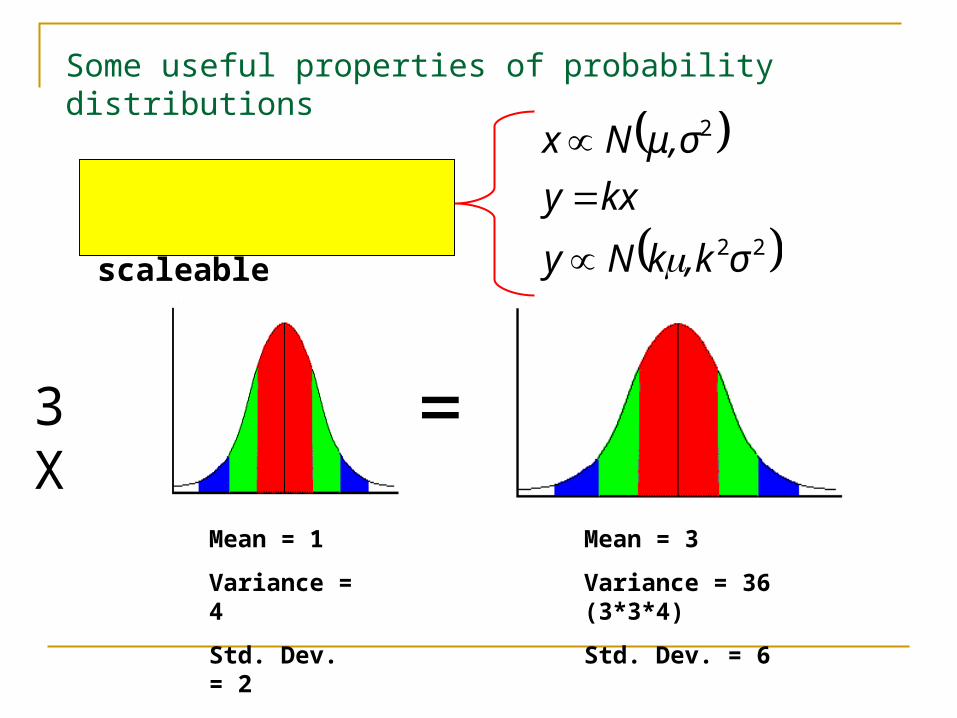
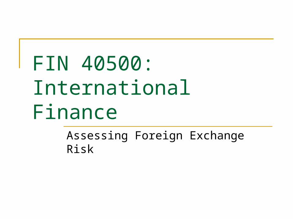
Mean = 1
Variance = 4
Std. Dev. = 2
Probability distributions are scaleable
22
2
σ,kkNy
kxy
μ,σNx
3 X =
Mean = 3
Variance = 36 (3*3*4)
Std. Dev. = 6
Some useful properties of probability distributions
Mean = 1
Variance = 1
Std. Dev. = 1
Probability distributions are additive
xyyxyx
yy
xx
σ,σNyx
,σNy
,σμNx
cov222
2
2
+Mean = 2
Variance = 9
Std. Dev. = 3
COV = 2
=Mean = 3
Variance = 14 (1 + 9 + 2*2)
Std. Dev. = 3.7
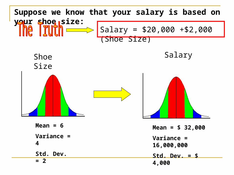
Mean = 6
Variance = 4
Std. Dev. = 2
Mean = $ 32,000
Variance = 16,000,000
Std. Dev. = $ 4,000
Suppose we know that your salary is based on your shoe size:
Salary = $20,000 +$2,000 (Shoe Size)
Shoe Size Salary
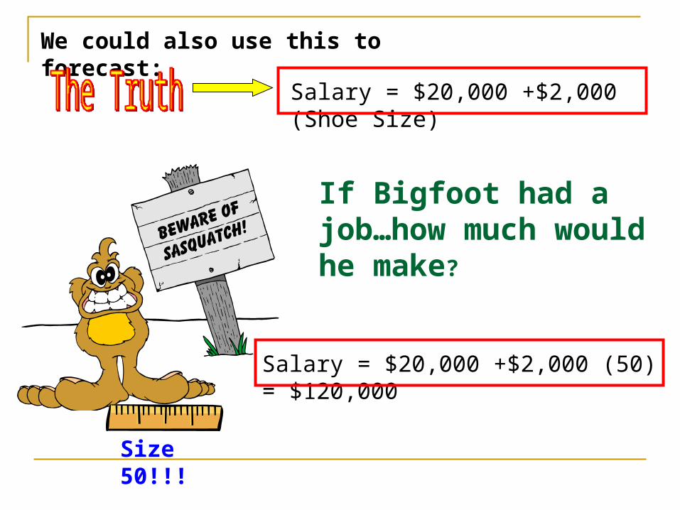
We could also use this to forecast:
Salary = $20,000 +$2,000 (Shoe Size)
If Bigfoot had a job…how much would he make?
Size 50!!!
Salary = $20,000 +$2,000 (50) = $120,000
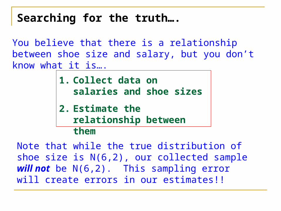
Searching for the truth….
You believe that there is a relationship between shoe size and salary, but you don’t know what it is….
1. Collect data on salaries and shoe sizes
2. Estimate the relationship between them
Note that while the true distribution of shoe size is N(6,2), our collected sample will not be N(6,2). This sampling error will create errors in our estimates!!

0
10000
20000
30000
40000
50000
60000
70000
0 2 4 6 8 10 12 14
Shoe Size
Sala
ry
Salary = a +b * (Shoe Size) + error
a
20,σNerror
Slope = b
We want to choose ‘a’ and ‘b’ to minimize the error!
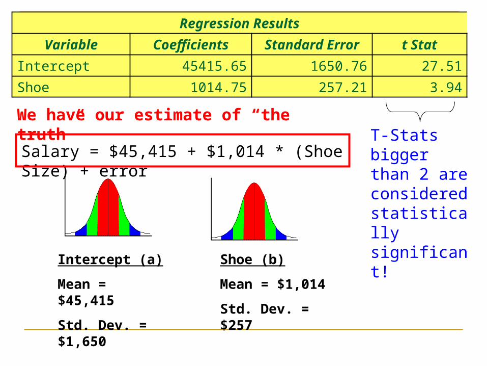
Regression Results
Variable Coefficients Standard Error t Stat
Intercept 45415.65 1650.76 27.51
Shoe 1014.75 257.21 3.94
Salary = $45,415 + $1,014 * (Shoe Size) + error
We have our estimate of “the truth”
Intercept (a)
Mean = $45,415
Std. Dev. = $1,650
Shoe (b)
Mean = $1,014
Std. Dev. = $257
T-Stats bigger than 2 are considered statistically significant!
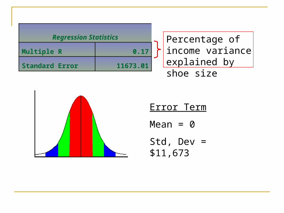
Regression Statistics
Multiple R 0.17
Standard Error 11673.01
Error Term
Mean = 0
Std, Dev = $11,673
Percentage of income variance explained by shoe size

Using regressions to forecast (Remember, Bigfoot wears a size 50)….
Salary = $45,415 + $1,014 * (Shoe Size) + error
50
Mean = $45,415
Std. Dev. = $1,650
Mean = $1,014
Std. Dev. = $ 257
Mean = $0
Std. Dev. = $11,673
Salary Forecast
Mean = $96,115
Std. Dev. = $17,438
438,17$)673,11()257()50()650,1( 2222 StdDev
Given his shoe size, you are 95% sure Bigfoot will earn between $61,239 and $130,991

We’ve looked at several currency pricing models that have potential for being “the truth”
Any combination of these could be “the truth”!!
tt NXe %
*% ttte
*% iiet
1
%%i
itt fEe
Trade Balance Approach
Monetary Approach
Interest Rate Approach
Price Level Approach
1
%%i
itt eEe Technical Approach

-10
-8
-6
-4
-2
0
2
4
6
8
10
-10.0 -5.0 0.0 5.0 10.0 15.0
Inflation Differential
% C
han
ge in
Exch
an
ge R
ate
tttt bae *% Note: PPP implies that a = 0 and b = 1
PPP and the Swiss Franc

Regression Results
Variable Coefficients Standard Error t Stat
Intercept .027 .231 .12
Inflation 1.40 .742 1.89
Regression Results
Variable P-value Lower 95% Upper 95%
Intercept .910 -.49 .43
Inflation .06 -.065 2.86
Regression Statistics
R Squared .02
Standard Error 2.69
Observations 155
For every 1% increase in US inflation over Swiss inflation, the dollar depreciates by 1.40%

-10
-8
-6
-4
-2
0
2
4
6
8
10
1 6 11 16 21 26 31 36 41 46 51 56 61 66 71 76 81 86 91 96 101 106 111 116 121 126 131 136 141 146 151
Predicted Actual
Obviously, we have not explained very much of the volatility in the CHF/USD exchange rate
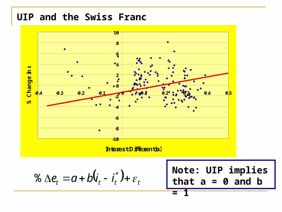
tttt iibae *%Note: UIP implies that a = 0 and b = 1
UIP and the Swiss Franc
-10
-8
-6
-4
-2
0
2
4
6
8
10
-0.4 -0.3 -0.2 -0.1 0 0.1 0.2 0.3 0.4 0.5
Interest Differential
% C
han
ge in
e
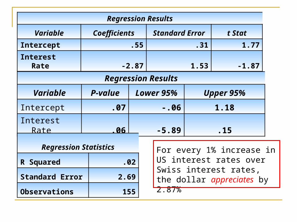
Regression Results
Variable Coefficients Standard Error t Stat
Intercept .55 .31 1.77
Interest Rate -2.87 1.53 -1.87
Regression Results
Variable P-value Lower 95% Upper 95%
Intercept .07 -.06 1.18
Interest Rate .06 -5.89 .15
Regression Statistics
R Squared .02
Standard Error 2.69
Observations 155
For every 1% increase in US interest rates over Swiss interest rates, the dollar appreciates by 2.87%

We still have not explained very much of the volatility in the CHF/USD exchange rate
-10
-8
-6
-4
-2
0
2
4
6
8
10
1 7 13 19 25 31 37 43 49 55 61 67 73 79 85 91 97 103 109 115 121 127 133 139 145 151
Exchange Rate Predicted Exchange Rate
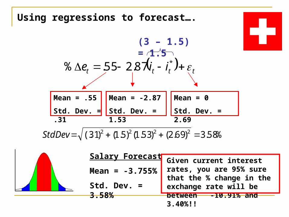
Using regressions to forecast….
(3 – 1.5) = 1.5
Mean = .55
Std. Dev. = .31
Mean = -2.87
Std. Dev. = 1.53
Mean = 0
Std. Dev. = 2.69
Salary Forecast
Mean = -3.755%
Std. Dev. = 3.58%
%58.3)69.2()53.1()5.1()31(. 2222 StdDev
Given current interest rates, you are 95% sure that the % change in the exchange rate will be between -10.91% and 3.40%!!
tttt iie *87.255.%

Technical Analysis Uses prior movements in the exchange rate to predict the future
-10
-8
-6
-4
-2
0
2
4
6
8
10
-10 -8 -6 -4 -2 0 2 4 6 8 10
%Change (t-1)
% C
han
ge (t)
ttt ebae 1%%

Regression Results
Variable Coefficients Standard Error t Stat
Intercept .12 .21 .57
Prior Change .29 .07 3.86
Regression Results
Variable P-value Lower 95% Upper 95%
Intercept .56 -.29 .53
Prior Change .0001 .14 .45
Regression Statistics
R Squared .09
Standard Error 2.59
Observations 154
A 1% depreciation of the dollar is typically followed by a .29% depreciation

BLADES Board & Skate arrived on the action / extreme scene in 1990, and quickly became a trusted source of equipment and service to in-line skaters, skateboarders, and snowboarders.
BLADES got its start in New York and currently operates 15 retail stores in New York, New Jersey, Massachusetts and Pennsylvania.
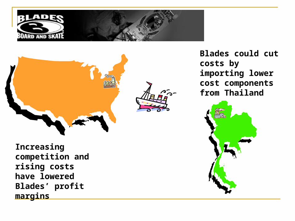
Increasing competition and rising costs have lowered Blades’ profit margins
Blades could cut costs by importing lower cost components from Thailand

Suppose that Blades makes an agreement to buy plastic components sufficient to produce 72,000 pairs of rollerblades from Thai manufacturers at a price of THB 2,870 per pair. ($1 = THB 38.87). Payment is due in one month (72,000*2,870 = THB 206.64 M)
Trend
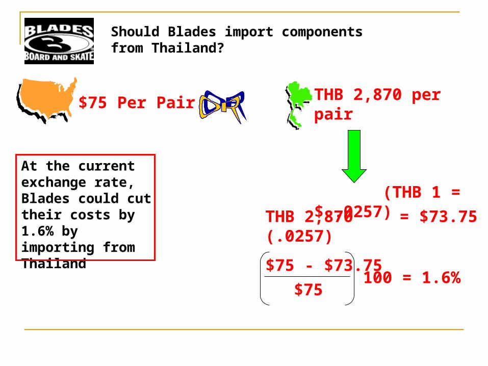
THB 2,870 per pair (THB 1 = $ .0257)
Should Blades import components from Thailand?
$75 Per Pair
THB 2,870 (.0257) = $73.75
$75 - $73.75
$75100 = 1.6%
At the current exchange rate, Blades could cut their costs by 1.6% by importing from Thailand
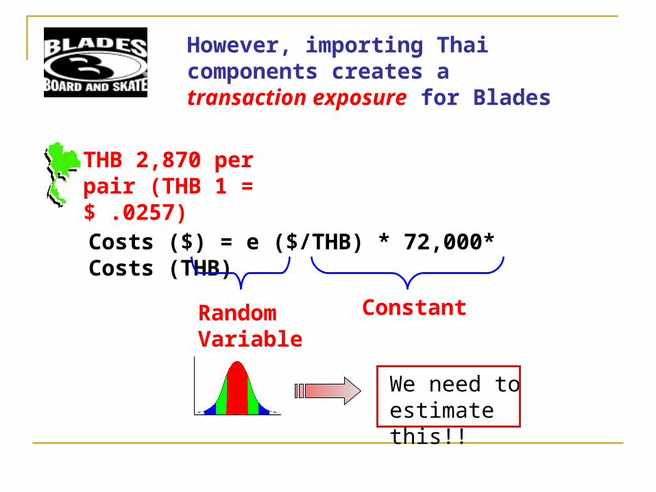
However, importing Thai components creates a transaction exposure for Blades
THB 2,870 per pair (THB 1 = $ .0257)
Costs ($) = e ($/THB) * 72,000* Costs (THB)
ConstantRandom Variable
We need to estimate this!!
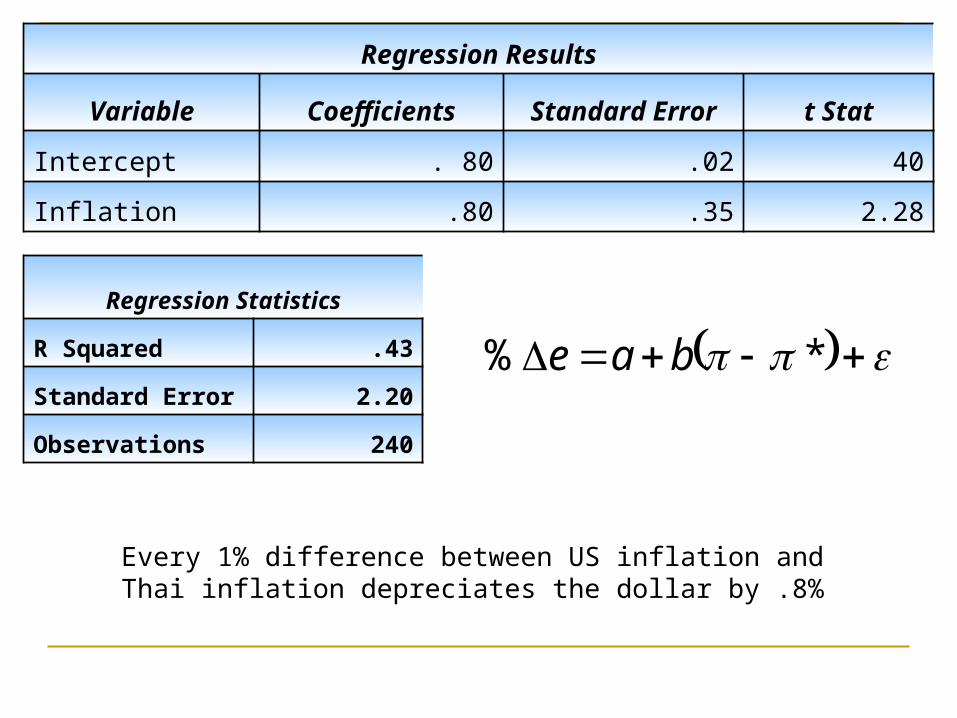
Regression Results
Variable Coefficients Standard Error t Stat
Intercept . 80 .02 40
Inflation .80 .35 2.28
Regression Statistics
R Squared .43
Standard Error 2.20
Observations 240
*% bae
Every 1% difference between US inflation and Thai inflation depreciates the dollar by .8%

US inflation is currently 1% (per month) while inflation in Thailand is 2.25% (per month)
(1 – 2.25) = -1.25
Mean = . 80
Std. Dev. = .02
Mean = .80
Std. Dev. = . 35
Mean = 0
Std. Dev. = 2.20
Forecast
Mean = -.2%
Std. Dev. = 2.25%
%25.2)20.2()25.1()35(.)02(. 2222 StdDev
Your 95% confidence interval for the (monthly) percentage change in the exchange rate is [-4.7% , 4.3% ]
*% bae

Forecast (% Change)
Mean = -.2%
Std. Dev. = 2.25%
Assessing transaction exposure
Costs ($) = e ($/THB) * 72,000*2,870 THB
THB 2,870 per pair (THB 1 = $ .0257)
Costs
Mean = 72,000*2,870*.0257(1-.002)
= $5,300,026
Std. Dev. = .0225*72000*2870*.0256
= $119,250
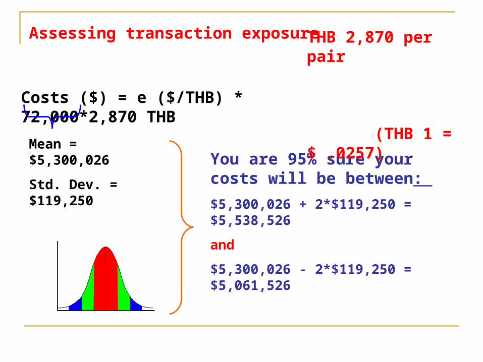
Assessing transaction exposure
Costs ($) = e ($/THB) * 72,000*2,870 THB
You are 95% sure your costs will be between:
$5,300,026 + 2*$119,250 = $5,538,526
and
$5,300,026 - 2*$119,250 = $5,061,526
THB 2,870 per pair (THB 1 = $ .0257)
Mean = $5,300,026
Std. Dev. = $119,250

THB 2,870 per pair (THB 1 = $ .0257)
Should Blades import components from Thailand?
$75 Per Pair
Mean = $5,300,026
Std. Dev. = $119,250
Mean = $5,400,000
Std. Dev. = $0
What do you do?

Blades is also thinking about exporting rollerblades to Thailand
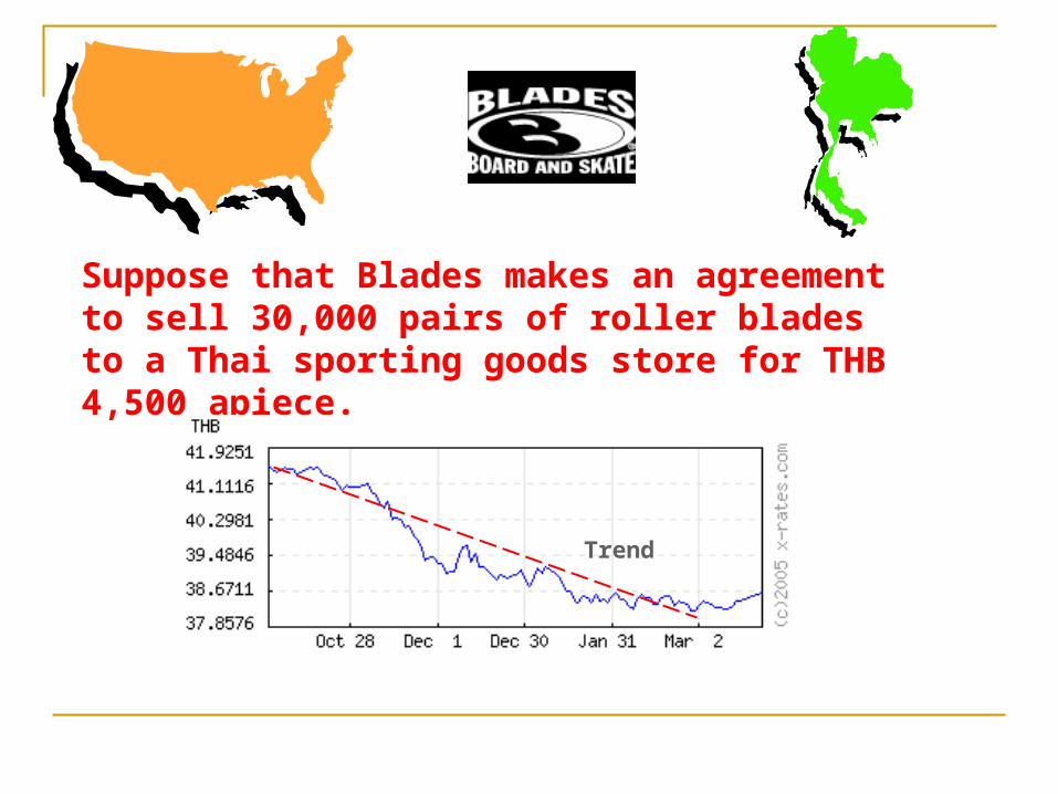
Suppose that Blades makes an agreement to sell 30,000 pairs of roller blades to a Thai sporting goods store for THB 4,500 apiece.
Trend
Forecast (% Change)
Mean = -.2%
Std. Dev. = 2.25%
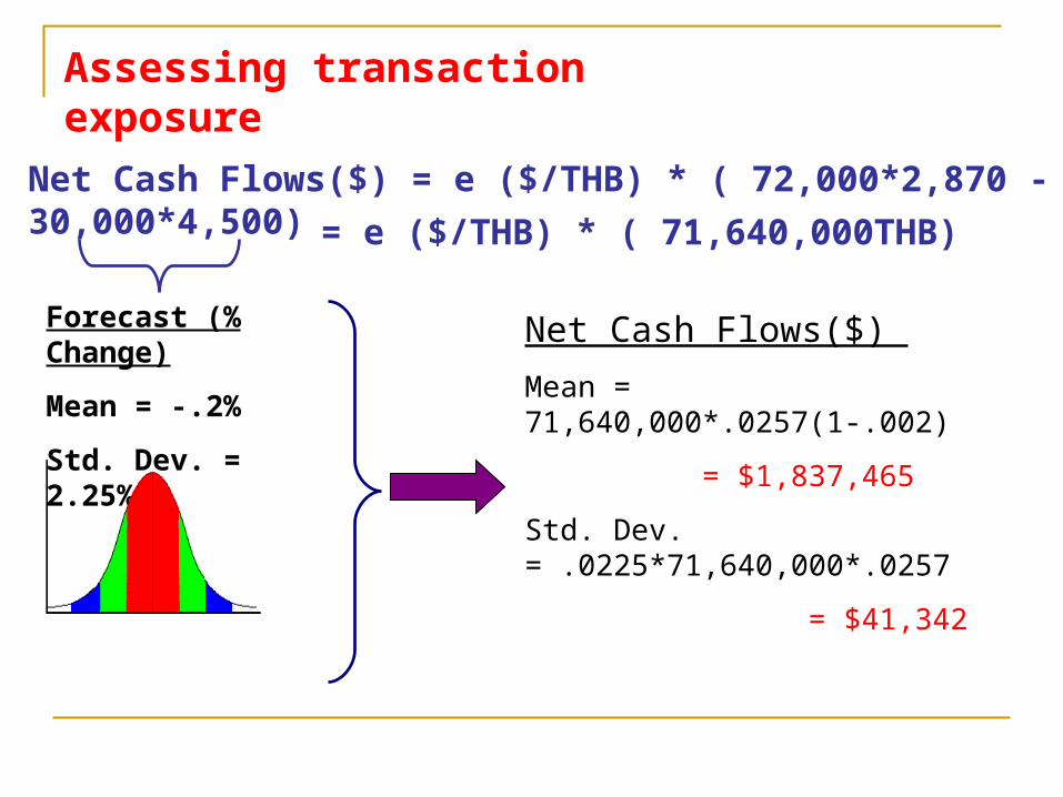
Assessing transaction exposure
Net Cash Flows($) = e ($/THB) * ( 72,000*2,870 - 30,000*4,500)
Net Cash Flows($)
Mean = 71,640,000*.0257(1-.002)
= $1,837,465
Std. Dev. = .0225*71,640,000*.0257
= $41,342
= e ($/THB) * ( 71,640,000THB)
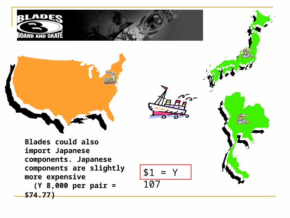
Blades could also import Japanese components. Japanese components are slightly more expensive (Y 8,000 per pair = $74.77) $1 = Y 107
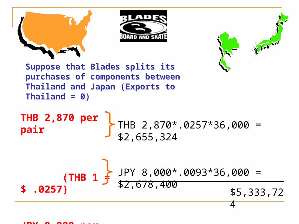
Suppose that Blades splits its purchases of components between Thailand and Japan (Exports to Thailand = 0)
THB 2,870 per pair (THB 1 = $ .0257)
JPY 8,000 per pair (JPY 1 = $ .0093)
THB 2,870*.0257*36,000 = $2,655,324
JPY 8,000*.0093*36,000 = $2,678,400
$5,333,724
$2,678,400
$5,333,724
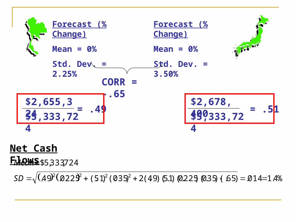
Forecast (% Change)
Mean = 0%
Std. Dev. = 2.25%
Forecast (% Change)
Mean = 0%
Std. Dev. = 3.50%
$2,655,324
$5,333,724= .49 = .51
CORR = -.65
Net Cash Flows
%4.1014.)65.)(035)(.0225)(.51)(.49(.2)035(.)51(.0225.49.
724,333,5$
2222
SD
Mean
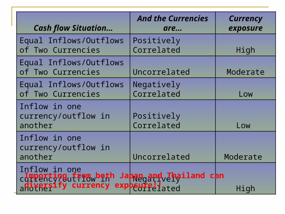
Cash flow Situation…And the Currencies
are…Currency exposure
Equal Inflows/Outflows of Two Currencies Positively Correlated High
Equal Inflows/Outflows of Two Currencies Uncorrelated Moderate
Equal Inflows/Outflows of Two Currencies Negatively Correlated Low
Inflow in one currency/outflow in another Positively Correlated Low
Inflow in one currency/outflow in another Uncorrelated Moderate
Inflow in one currency/outflow in another Negatively Correlated High
Importing from both Japan and Thailand can diversify currency exposure!!

Suppose that Blades is planning to expand sales into England. Should they try and invoice in dollars or Pounds?
Current
GBP 1 = $1.80
Forecast (% Change)
Mean = 0
SD = 2.0%
Contracting sales in GBP creates transaction exposure. However, contracting sales in USD creates economic exposure
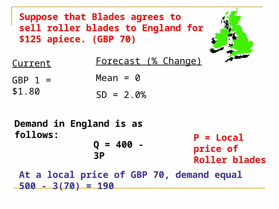
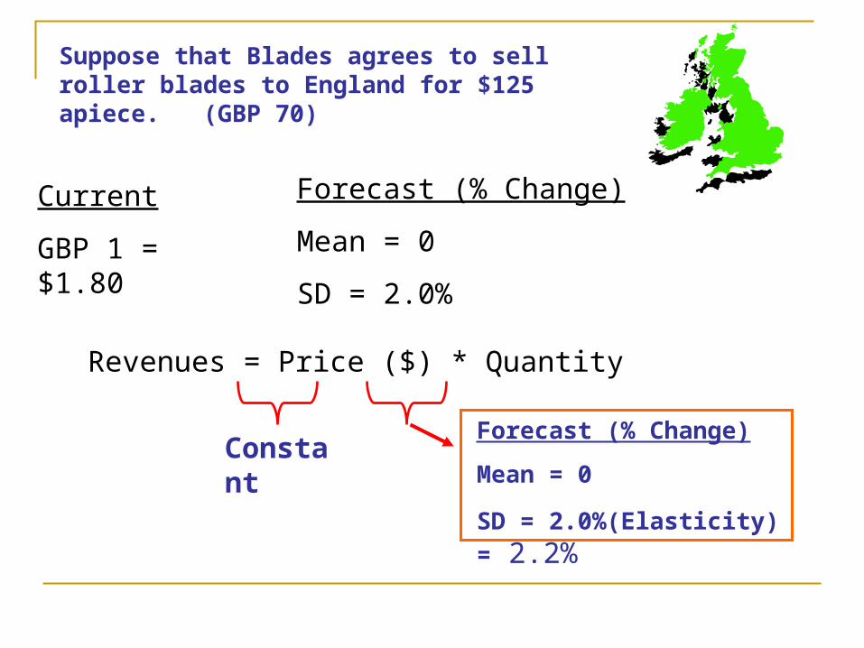
Suppose that Blades agrees to sell roller blades to England for $125 apiece. (GBP 70)
Current
GBP 1 = $1.80
Forecast (% Change)
Mean = 0
SD = 2.0%
Demand in England is as follows:
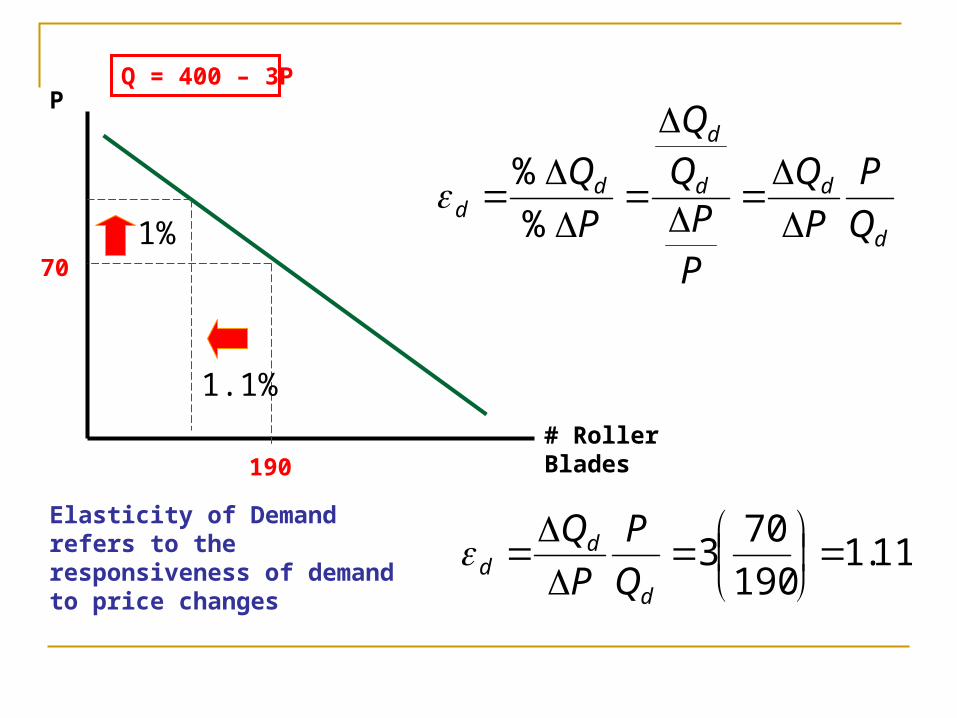
Q = 400 - 3P P = Local price of Roller blades
At a local price of GBP 70, demand equal 500 - 3(70) = 190
11.1190
703
d
dd Q
P
P
QElasticity of Demand refers to the responsiveness of demand to price changes
Q = 400 – 3P
# Roller Blades
P
190
70d
dd
d
dd Q
P
P
Q
PPQ
Q
P
Q
%
%1%
1.1%
Suppose that Blades agrees to sell roller blades to England for $125 apiece. (GBP 70)
Current
GBP 1 = $1.80
Forecast (% Change)
Mean = 0
SD = 2.0%
Revenues = Price ($) * Quantity
ConstantForecast (% Change)
Mean = 0
SD = 2.0%(Elasticity) = 2.2%

Revenues = Price ($) * Quantity
ConstantForecast (% Change)
Mean = 0
SD = 2.0%(Elasticity) = 2.2%
Revenues = e ($/L)* Price (L) * Quantity
Constant
Forecast (% Change)
Mean = 0
SD = 2.0
GBP Pricing (Transaction Exposure)
USD Pricing (Economic Exposure)

Changes in currency prices can have all kinds of economic impacts. A more general way to estimate economic exposure would be as follows:
ttt beaPCF
Percentage change in the exchange rate ($/F)
Percentage change in cash flows (measured in home currency)

Regression Results
Variable Coefficients Standard Error t Stat
Intercept .05 1.5 .03
% Change in Exchange Rate -3.35 .97 -3.45
Regression Statistics
R Squared .63
Standard Error 1.20
Observations 1,000
tt beaPCF
Every 1% depreciation in the dollar relative to the British pound lowers cash flows from England by 3.35%
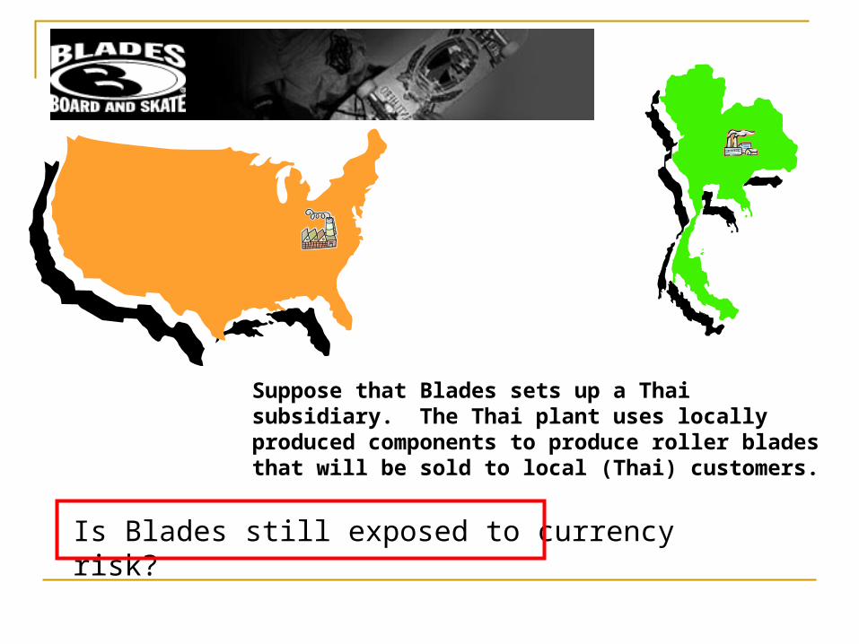
Suppose that Blades sets up a Thai subsidiary. The Thai plant uses locally produced components to produce roller blades that will be sold to local (Thai) customers.
Is Blades still exposed to currency risk?
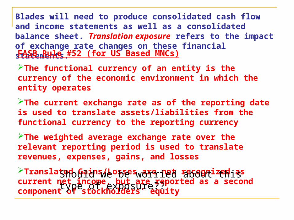
Blades will need to produce consolidated cash flow and income statements as well as a consolidated balance sheet. Translation exposure refers to the impact of exchange rate changes on these financial statements.
FASB Rule #52 (for US Based MNCs)
The functional currency of an entity is the currency of the economic environment in which the entity operates
The current exchange rate as of the reporting date is used to translate assets/liabilities from the functional currency to the reporting currency
The weighted average exchange rate over the relevant reporting period is used to translate revenues, expenses, gains, and losses
Translated Gains/Losses are not recognized as current net income, but are reported as a second component of stockholders’ equity
Should we be worried about this type of exposure??
Related Documents