Assessing Competition with the Panzar-Rosse Model: The Role of … · Assessing Competition with the Panzar-Rosse Model: The Role of Scale, Costs, and Equilibrium Jacob A. Bikker

Assessing Competition with the Panzar-Rosse Model:The Role of Scale, Costs, and Equilibrium

Jacob A. Bikker� Sherrill Shaffer| Laura Spierdijk}

August 5, 2010

Abstract

The Panzar-Rosse test has been widely applied to assess competitive conduct, often in

specifications controlling for firm scale or using a price equation. We show that neither a

price equation nor a scaled revenue function yields a valid measure for competitive conduct.

Moreover, even an unscaled revenue function generally requires additional information about

costs and market equilibrium to infer the degree of competition. Our theoretical findings are

confirmed by an empirical analysis of competition in banking, using a sample containing more

than 100,000 bank-year observations on more than 17,000 banks in 63 countries during the

years 1994 – 2004.

Keywords: Panzar-Rosse test, competition, scale

JEL classification: D40, L11

�Primary affiliation: De Nederlandsche Bank (DNB), Supervisory Policy Division, Strategy Department, P.O. Box98, NL-1000 AB Amsterdam, The Netherlands. Email: [email protected]. Secondary affiliation: Utrecht School ofEconomics, University of Utrecht, Janskerkhof 12, NL-3511 BL Utrecht, the Netherlands.

|Primary affiliation: University of Wyoming, Department of Economics and Finance (Dept. 3985), 1000 East Uni-versity Ave., Laramie, WY 82071, USA. Email: [email protected]. Secondary affiliation: Centre for Applied Macroe-conomic Analysis (CAMA), Australian National University, Australia.

}Laura Spierdijk (corresponding author), University of Groningen, Faculty of Economics & Business, Departmentof Economics & Econometrics, Centre for International Banking, Insurance and Finance, P.O. Box 800, NL-9700 AVGroningen, The Netherlands. Email: [email protected]. The authors are grateful to the participants of the researchseminars at DNB and University of Groningen, and the audiences at the All China Economics International Conferencein Hong Kong, the WEAI conferences in Beijing and Seattle, the VII International Finance Conference in Mexico, theconference of the European Economic Association in Budapest, and the CIBIF Workshop on Financial Systems andMacroeconomics (where earlier versions of this paper have been presented, see Bikker et al., 2006) for their helpfulsuggestions. We would like to thank Tom Wansbeek and three anononymous referees for useful comments and JackBekooij for extensive data support. The usual disclaimer applies. The views expressed in this paper are not necessarilyshared by DNB.

1 Introduction

Empirical estimates of the degree of competition have been significantly refined by two ‘new em-

pirical industrial organization’ (NEIO) techniques, the Bresnahan-Lau method (Bresnahan, 1982,

1989; Lau, 1982) and the Panzar-Rosse reduced-form revenue test (Rosse and Panzar, 1977; Pan-

zar and Rosse, 1982, 1987). The latter method has found particularly widespread application in

the literature due to its modest data requirements, single-equation linear estimation, and robust-

ness to market definition (Shaffer, 2004a,b). Most of these applications have involved the banking

industry, as summarized in Table 1, because of the special importance of banks in the economy

and facilitated by the ready availability of bank-level data.

The current financial and economic crisis has highlighted the crucial position of banks in the

economy. Banks play a pivotal role in the provision of credit, the payment system, the transmis-

sion of monetary policy and maintaining financial stability. The vital role of banks in the economy

makes the issue of banking competition extremely important. The relevance of banking compe-

tition is confirmed by several empirical studies that establish a strong relation between banking

structure and economic growth (see e.g. Jayaratne and Strahan, 1996; Levine, Loayza and Beck,

2000; Collender and Shaffer, 2003). Also, an ongoing debate has emerged in the literature as to

whether banking competition helps or harms welfare in terms of systemic stability (see e.g. Smith,

1998; Allen and Gale, 2004; De Jonghe and Vander Vennet, 2008; Schaeck et al., 2009) or pro-

ductive efficiency (Berger and Hannan, 1998; Maudos and De Guevara, 2007).

Theory suggests that banking competition can be inferred directly from the markup of prices

over marginal cost (Lerner, 1934). In practice, this measure is often hard or even impossible to

implement due to a lack of detailed information on the costs and prices of bank products. The

literature has proposed various indirect measurement techniques to assess the competitive cli-

mate in the banking sector. These methods can be divided into two main streams: structural and

non-structural approaches (see e.g. Bikker, 2004). Structural methods are based on the structure-

conduct-performance (SCP) paradigm of Mason (1939) and Bain (1956), which predicts that more

concentrated markets are more collusive. Competition is proxied by measures of banking concen-

tration, such as the Herfindahl-Hirschman index. However, the empirical banking literature has

1

shown that concentration is generally a poor measure of competition; see e.g. Shaffer (1993, 1999,

2002), Shaffer and DiSalvo (1994), and Claessens and Laeven (2004). Some of these studies find

conduct that is much more competitive than the market structure would suggest, while others find

much more market power than the market structure would imply.1 Since the mismatch can run in

either direction, concentration is an extremely unreliable measure of performance.

The Panzar-Rosse approach and the Bresnahan-Lau method can be formally derived from

profit-maximizing equilibrium conditions, which is their main advantage relative to more heuris-

tic approaches. As shown by Shaffer (1983a,b), their test statistics are systematically related to

each other, as well as to alternative measures of competition such as the Lerner index (Lerner,

1934). In this paper we focus on the Panzar-Rosse (P-R) revenue test, which has been much more

widely used in empirical banking studies, as well as in non-banking studies. This approach esti-

mates a reduced-form equation relating gross revenue to a vector of input prices and other control

variables. The associated measure of competition – usually called the H statistic – is obtained as

the sum of elasticities of gross revenue with respect to input prices. Rosse and Panzar (1977) show

that this measure is negative for a neoclassical monopolist or collusive oligopolist, between 0 and

1 for a monopolistic competitor, and equal to unity for a competitive price-taking bank in long-run

competitive equilibrium. Furthermore, Shaffer (1982a, 1983a) shows that H is negative for a con-

jectural variations oligopolist or short-run competitor and equal to unity for a natural monopoly in

a contestable market or for a firm that maximizes sales subject to a breakeven constraint. More-

over, the H statistic is also equal to unity with free entry equilibrium with full (efficient) capacity

utilization (Vesala, 1995).

There is a striking dichotomy between the reduced-form revenue relation derived in the semi-

nal articles by Panzar and Rosse and the P-R model as estimated in the empirical literature. Many

published P-R studies estimate a revenue function that includes total assets (or another proxy of

scale, such as equity capital) as a control variable. Other articles estimate a price function instead

of a revenue equation, in which the dependent variable is total revenue divided by total assets. In

both cases, the choice to control for scale effects is neither explained nor justified. As far as we1Highly competitive conduct has been found in concentrated banking markets in Canada (Shaffer, 1993), a U.S.

local banking duopoly (Shaffer and DiSalvo, 1994), and a banking monopoly (Shaffer, 2002). Conversely, significantmonopoly power has been found in the U.S. credit card industry, despite thousands of independently pricing issuers ofbank cards (Ausubel, 1991; Calem and Mester, 1995; Shaffer, 1999).

2

know, this inconsistency between the theoretical P-R model and its empirical translation has not

been formally addressed in the economic literature. In line with Vesala (1995), Gischer and Stiele

(2009) intuitively argue that the revenue and price equations will give different estimates of the H

statistic. Goddard and Wilson (2009) use simulation to show that the revenue and price equations

result in different estimates of the H statistic. The present paper provides a formal analysis of

the consequences of controlling for firm scale in the P-R test. We prove that the properties of the

price and revenue equations are identical in the case of long-run competitive equilibrium, but crit-

ically different in the case of monopoly or oligopoly. An important consequence of our findings

is that a price equation and scaled revenue function – which both have been widely applied in the

empirical literature – cannot identify imperfect competition in the same way that an unscaled rev-

enue function can. This conclusion disqualifies a number of studies insofar they apply a P-R test

based on a price function or scaled revenue equation. See e.g. Shaffer (1982a, 2004a), Nathan and

Neave (1989), Molyneux et al. (1994, 1996), De Bandt and Davis (2000), Bikker and Haaf (2002),

Claessens and Laeven (2004), Yildirim and Philippatos (2007), Schaeck et al. (2009), Coccorese

(2009), and Carbo et al. (2009).

Furthermore, we show that the appropriate H statistic, based on an unscaled revenue equation,

generally requires additional information about costs, market equilibrium and possibly market de-

mand elasticity to infer the degree of competition. In particular, because competitive firms can

exhibit H < 0 if the market is in structural disequilibrium, it is important to recognize whether

or not a given sample is drawn from a market or set of markets in equilibrium. We show that the

widely applied equilibrium test (Shaffer, 1982a) is essentially a joint test for competitive conduct

and long-run structural equilibrium, which substantially narrows its applicability. Our findings

lead to the important conclusion that the P-R test is a one-tail test of conduct in a more general

sense than shown in Shaffer and DiSalvo (1994). A positive value of H is inconsistent with stan-

dard forms of imperfect competition, but a negative value may arise under various conditions,

including short-run competition. We illustrate our theoretical results with an empirical analysis of

competition, using data from the banking industry to facilitate comparison with prior literature.

Our sample contains more than 100,000 bank-year observations on more than 17,000 banks in 63

countries during the period 1994 – 2004.

3

Although the P-R test has been applied more often to the banking industry than to any other

sector, the applicability of the P-R model is much broader and not confined to banks only. See

e.g. Rosse and Panzar (1977), Sullivan (1985), Ashenfelter and Sullivan (1987), Wong (1996),

Fischer and Kamerschen (2003), and Tsutsui and Kamesaka (2005), who apply the P-R test to

assess the competitive climate in the newspaper industry, the cigarette industry, the U.S. airline

industry, a sample of physicians, and the Japanese securities industry, respectively. We emphasize

that the aforementioned scale correction is also found in non-banking studies applying the P-R

test to firms of different sizes; see e.g. Ashenfelter and Sullivan (1987) and Tsutsui and Kamesaka

(2005). Hence, the scaling issue that we address in this paper is not confined to empirical banking

studies, but applies to the entire competition literature. For this reason our theoretical analysis is

formulated in terms of generic firms, and as such is not restricted to the special case of banks.

The organization of the remainder of this paper is as follows. Section 2 describes the original

Panzar-Rosse model and the empirical translations found in the competition literature. Next, Sec-

tion 3 analyzes the consequences of controlling for firm size in the P-R test. Section 4 focuses on

the correct P-R test (based on an unscaled revenue equation) and discusses the additional informa-

tion about costs and equilibrium needed to infer the degree of competition. This section also shows

that the widely applied equilibrium test is essentially a test for long-run competitive equilibrium.

Section 5 discusses the empirical translation of the Panzar-Rosse approach. The bank data used for

the empirical illustration of our theoretical findings are described in Section 6. The corresponding

empirical results can also be found in this section. Finally, Section 7 concludes.

2 The Panzar-Rosse model

The Panzar-Rosse (P-R) revenue test is based on a reduced-form equation relating gross revenues

to a vector of input prices and other firm-specific control variables. Assuming an n-input single-

output production function, the empirical reduced-form equation of the P-R model is written as

log TR D ˛ C

nXiD1

ˇi log wi C

JXjD1

j log CFj C "; (1)

where TR denotes total revenue, wi the price of the i -th input factor, and CFj the j -th firm-

specific control factor. Moreover, we assume that IE." j w1; : : : ; wn; CF1; : : : ; CFJ / D 0. Panzar

4

and Rosse (1977) show that the sum of input price elasticities,

H rD

nXiD1

ˇi ; (2)

reflects the competitive structure of the market.

The specification in Equation (1) is similar to what has been commonly used in the empirical

literature, although the choice of dependent and firm-specific control variables varies. For exam-

ple, the empirical banking literature often takes interest income as revenues to capture only the

intermediation activities of banks (e.g. Bikker and Haaf, 2002). Larger firms earn more revenue,

ceteris paribus, in ways unrelated to variations in input prices. Therefore, many studies include

log total assets as a firm-specific control variable in Equation (1). Other studies take the log of

revenues divided by total assets (TA) as the dependent variable in the P-R model, in which case

not log revenues but log(TR/TA) – with TR/TA a proxy of the output price P – is explained from

input prices and firm-specific factors. This results in a log-log price equation instead of a log-log

revenue equations.

In sum, three alternative versions of the empirical P-R model have appeared in the empirical

competition literature. The first one is the P-R revenue equation with log total assets as a control

variable:

log TR D ˛ C

nXiD1

ˇi log wi C

JXjD1

j log CFj C ı log.TA/ C "; (3)

yielding H rs D

PniD1 ˇi (where r refers to ‘revenue’, and s to ‘scaled’). In the empirical banking

literature this version of the P-R model has been used by e.g. Shaffer (1982a, 2004a), Nathan and

Neave (1989), Molyneux et al. (1996), Coccorese (2009), and Carbo et al. (2009). See also Ashen-

felter and Sullivan (1987) and Tsutsui and Kamesaka (2005), who apply the P-R model to assess

the competitive climate in the cigarette industry and the Japanese securities industry, respectively.

Rosse and Panzar (1977) similarly control for scale in the newspaper industry, measured as daily

circulation rather than assets. The second alternative version is the P-R price equation without total

assets as a control variable:

log.TR/TA/ D ˛ C

nXiD1

ˇi log wi C

JXjD1

j log CFj C "; (4)

5

yielding H p DPn

iD1 ˇi (where p refers to ‘price’). See e.g. De Bandt and Davis (2000),

Koutsomanoli-Fillipaki and Staikouras (2005), and Mamatzakis et al. (2005). The last version

is the P-R price equation controlling for firm size:

log.TR/TA/ D ˛ C

nXiD1

ˇi log wi C

JXjD1

j log CFj C ı log.TA/ C "; (5)

yielding Hps D

PniD1 ˇi (where p refers to ‘price’, and s to ‘scaled’). This specification has

been used by e.g. Molyneux et al. (1994), Bikker and Groeneveld (2000), Bikker and Haaf (2002),

Claessens and Laeven (2004), Yildirim and Philippatos (2007), and Schaeck et al. (2009). When

log assets are included, the empirical estimates from a log-log price equation are equivalent to

those of the corresponding log-log revenue equation, with the sole distinction that the coefficient

on log.TA/ will differ by 1. The key issue addressed in this paper is the relation between the

H statistics based on the scaled and unscaled versions of P-R price and revenue equation. Fur-

thermore, several studies estimate a revenue or price equation with another proxy for bank size

as a control variable (such as equity capital), see e.g. Vesala (1995), De Bandt and Davis (2000)

and Gischer and Stiele (2009). This also results in a scale correction. Table 1 provides a detailed

overview of published P-R studies in the field of banking and the type of scaling used in these

studies.

3 Controlling for scale in the P-R model

This section analyzes the consequences of controlling for firm scale in the P-R test. Because elas-

ticities are required to compute the value of the H statistic, and the coefficients in a log-log equa-

tion correspond directly to elasticities, virtually all empirical applications of the P-R test have

relied on the log-log form discussed in Section 2. Accordingly, our analysis below will address

this form exclusively. In addition, the original derivation of the P-R result assumes that produc-

tion technology remains unchanged across the sample, and we likewise maintain that assumption

throughout.

6

3.1 Prerequisites

As a preliminary step, we focus on the unscaled revenue equation and note the basic property that

marginal cost, like total cost, is homogeneous of degree 1 in all input prices.2 That is,

nXiD1

@log MC=@log wi D 1 (6)

for all inputs i and input prices wi . Hence, the summed revenue elasticities of input prices must

equal the elasticity of revenue with respect to marginal cost. That is, we have

@log TR@log MC

D

nXiD1

@TR=@log wi

@log MC=@log wiD

nXiD1

@log TR@log wi

D H r : (7)

Thus, the P-R statistic H r actually represents the elasticity of revenue with respect to marginal

cost, under the assumption of a stable cost function so that all changes in marginal cost are driven

by changes in one or more input prices. We shall make use of this result at various points in this

section by referring interchangeably to H r and @log TR=@log MC. A similar property holds for

H p , the H statistic obtained from the P-R price equation without scaling. Moreover, we have

@log P=@log wi D @log.TR=TA/=@log wi

D @log TR=@log wi � @log.TA/=@log wi : (8)

In the sequel we distinguish between short-run and long-run competitive equilibrium. Short-

run competitive equilibrium occurs before entry and exit have taken place in response to shocks

to cost or demand. In such a situation firms are pricing at marginal cost, but the number of firms

is not in equilibrium, so that entry or exit would be expected to occur subsequently. In case of

positive profits, more competitors will enter the market. Similarly, negative profit will drive some

of them out of the market. By contrast, long-term competitive equilibrium takes place after entry

and exit have fully adjusted to any changes in cost or demand, in which case both the number of

firms and each firm’s output are in equilibrium.

2Rosse and Panzar (1977, page 7) provide a proof of this property.

7

3.2 Revenue equation

First, we address the common practice of including the log of total assets (or similar measure

of scale) as a separate regressor in a reduced-form revenue equation such as Equation (3). This

practice appears ubiquitous in the empirical P-R literature, even going back to the seminal study

by Rosse and Panzar (1977), yet without explicit discussion or analysis. This point is important

because the formal derivation of the H statistic does not include scale as a separate regressor, so

it is necessary to rigorously explore the effects of such inclusion.

Intuitively, controlling for scale makes apparent sense because larger firms earn more revenue,

ceteris paribus, in ways unrelated to variations in input prices. If we estimate a reduced-form rev-

enue equation across firms of different sizes without controlling for scale, the standard measures of

fit will be quite poor. Indeed, this fact has been used to justify the choice of log.P/ D log.TR/TA/

instead of log (TR) as the dependent variable, especially when scale has been omitted as a regressor

in the price equation (see, for example, Mamatzakis et al., 2005).

The main problem arises in the case of imperfectly competitive firms. The standard proof that

H r < 0 for monopoly relies on the monopolist’s quantity adjustment in response to changes in

input prices. If a monopolist faced a perfectly inelastic demand curve, there would be no quantity

adjustment and so total revenue would move in the same direction as P, which is the same direction

as marginal costs. See, for example, Milgrom and Shannon (1994) and Chakravarty (2002). Hence,

total revenue would move in the same direction as input prices, so we would observe H r > 0.3

The condition that rules this out is the firm’s profit-maximizing condition MR D MC > 0 (where

MR stands for marginal revenue), which implies elastic demand at equilibrium output levels. But

if the regression statistically holds the output quantity constant by controlling for log.TA/, then

the coefficients that comprise H rs will represent the response of total revenue to input prices at a

fixed output scale, which is just the change in price times the fixed output. Thus, the estimates will

yield H rs > 0 for any monopoly when the revenue equation controls for scale. The same argument

also applies to oligopoly and to the price equation. This leads to the following result.

Proposition 3.1 Estimates of conduct for monopoly or oligopoly that control for scale, will yield

3The same result also occurs whenever the monopoly demand curve is inelastic, even if imperfectly so.

8

H rs > 0.

Later we will turn back to the P-R revenue equation, but we first discuss the price equation.

3.3 Price equation

A few studies have used log.P/ as the dependent variable without controlling for log.TA/, and this

is the case we address next. Under the standard assumptions of duality theory and the neoclassical

theory of the firm, as used in the original proof of the parametric version of the P-R test (Rosse and

Panzar, 1977), convexity of the production technology implies U-shaped average costs. Then, in

long-run competitive equilibrium, we have @TA=@wi D 0 because the output scale at which aver-

age costs are minimized is not affected by input prices under the assumption of a stable production

technology. Then @log.TA/=@log wi D 0 and so

H pD

nXiD1

@log P=@log wi D

nXiD1

@log TR=@log wi D H r : (9)

Therefore, the price equation and the revenue equation both yield the same result (H r D H p D 1)

in the case of long-run competition with U-shaped average costs, with or without log.TA/ as a

control variable. We thus obtain the following result.

Proposition 3.2 H p D Hps � H r

s D H r D 1 for firms in long-run competitive equilibrium with

U-shaped costs.

Next, we address the sign and magnitude of H p in the monopoly case. We know that the monopoly

price is an increasing function of marginal cost (see, for example, Milgrom and Shannon, 1994,

page 173; Chakravarty, 2002, page 352).4 That is, @P=@MC > 0 and so @log P=@log MC > 0. By

linear homogeneity of MC in input prices,

@log P=@log MC D

nXiD1

@log P=@log wi D H p: (10)

The conclusion here is that H p > 0 for monopoly – a contrasting property to H r < 0 if based

on an unscaled revenue equation. That is, a price equation fitted to data from a monopoly sample

in equilibrium should always yield a positive sum of input price elasticities. Because this result is

4For either monopoly or oligopoly, the condition for profit maximization is MR = MC so we always have@MR=@MC D 1 in equilibrium.

9

also true for a competitive sample, by continuity it also holds for oligopoly. Clearly, this property

holds whether or not log(TA) is included as a separate regressor. This yields the following result.5

Proposition 3.3 H p > 0 and Hps > 0 for monopoly or oligopoly.

Since the scaled price equation is equivalent to the scaled revenue equation, the same conclusion

applies to H rs based on the scaled revenue equation.

Corollary 3.1 H rs > 0 for monopoly or oligopoly.

An important implication of Prop. 3.2 and 3.3 is that the sign of H p and H rs cannot distinguish

between perfect and imperfect competition and thus fails as a test for market power.

3.4 The case of constant marginal and average costs

Next, we address the case of constant MC = AC (where MC stands for marginal cost and AC

for average cost). This case is important to consider separately for two reasons. First, in long-run

competitive equilibrium, the firm’s output quantity is indeterminate within the range over which

the minimum average cost is constant, thus implying potentially different responses to exogenous

shocks than assumed in the traditional P-R derivation. Second, substantial empirical and anecdo-

tal evidence suggests that many firms are in fact characterized by significant ranges of constant

marginal and average cost. Johnston (1960) reports evidence that many industries exhibit con-

stant marginal cost. In banking, several decades of studies have yielded contrasting conclusions

regarding economies or diseconomies of scale, but the market survival test suggests that marginal

and average costs cannot deviate significantly with size, as banks have demonstrated long-term

economic viability over a range of scales on the order of 100,000:1 in terms of total assets.6

5Interestingly, the same property also applies to the value of H rs if the estimated coefficient on log(TA) is unity (in

which case the scaled revenue equation is equivalent to the unscaled price equation), as is often the case empirically.Possible explanations for a unit coefficient on log(TA) could include the law of one price when firms sell homogeneousoutputs within the same market. Then all firms face the same output price, so total revenue is proportional to scale.

6U.S. data from the Federal Reserve Bank of Chicago(http://www.chicagofed.org/webpages/banking/financial institution reports/commercial bank data complete 2001 2009.cfm)indicate that, as of year-end 2008, the smallest long-established general-purpose commercial bank, chartered in 1909,had $ 3.1 million in assets. Another, chartered in 1900, had $ 3.4 million in assets, as did two banks chartered in 1996.Several other established banks were of similar size. By contrast, three U.S. banks reported total assets in excess of $ 1trillion in the same quarter. These cases span a range of about 300,000:1.

10

In the case of monopoly or oligopoly, the imposition of constant average cost will not change

the properties of H p or H r . The reason is that the firm’s output quantity is uniquely determined

under imperfect competition (downward sloping firm demand) even when marginal cost is con-

stant. Appendix A provides full details of the proof.

Proposition 3.4 Constant AC does not alter the sign of H r or H p for monopoly or oligopoly,

compared to the standard case of U-shaped average costs.

Also the case of long-run competition yields the same results for H p whether with constant aver-

age cost or with U-shaped average costs. Again Appendix A explains the details of the proof.

Proposition 3.5 H p D Hps D 1 in long-run competitive equilibrium with constant AC.

However, constant average cost poses a problem for H r in long-run competitive equilibrium.

Proposition 3.6 H r < 1, or even H r < 0, is possible for firms in long-run competitive equilib-

rium with constant AC.

A detailed proof is given in Appendix A. Hence, a unique local minimum average cost (U-shaped

average cost curve) is necessary to ensure that H r D 1 under long-run competitive equilibrium

in the unscaled reduced-form revenue equation. Previous literature has not considered the effect

of alternate cost structures on the P-R test. It should be noted that the standard functional forms

employed in most empirical cost studies (such as translog, flexible Fourier, and minflex Laurent)

are not very useful in testing for constant average cost. If marginal and average cost are constant,

one could contemplate estimating the elasticity of market demand as a further input to properly

interpreting H r (Shaffer, 1982b). However, in that case an overall market must be defined, which

is an extra step that is not necessary in a standard P-R test. We leave this as an important topic for

future research.

3.5 Scaled versus unscaled H statistics

Table 2 summarizes the various conclusions about H r , H rs and H p . In addition to Table 2, we can

draw on theory to predict which types of samples might be likely to generate specific differences

11

across the three measures of H . One possible case would be a sample containing firms of widely

differing sizes in the same market. This case could be evidence of a flat average cost curve, which

suggests that we should observe H r < 1 or perhaps even H r < 0, while also observing H p > 0

or even H p D 1 (if in long-run competitive equilibrium). However, it is also possible that such a

sample could reflect a disequilibrium number of firms, in which case some short-run equilibrium

(but not long-run equilibrium) could exist. In that case, we should observe H r < 0, but H p > 0.

Another possible case would be an industry or market containing only firms of identical or closely

similar size. This case could reflect an equilibrium with a U-shaped average cost curve. Then three

possibilities arise. First, if the sample is in long-run competitive equilibrium, we should observe

H r D H rs � H

ps D H p D 1. Second, if the sample is in an imperfectly competitive equilibrium,

the analysis here indicates that we would expect to see H r < 0, but H rs > 0 and H p > 0.

Finally, the sample might be in short-run but not in long-run competitive equilibrium; then we

should observe H r < 1 or possibly even H r < 0, but H rs > 0 and H p > 0.

4 Assessing competition with the unscaled P-R model

The previous section has made clear that a price or scaled revenue equation cannot be used to

infer the degree of competition. Only the unscaled revenue function can yield a valid measure

for competitive conduct. However, even if the competitive climate is assessed on the basis of the

correct H statistic, there are still some caveats to consider.

4.1 Interpretation of the H statistic

Given an estimate of the H statistic based on the unscaled revenue equation, several situations

may arise. A significantly positive value of H r is inconsistent with standard forms of imperfect

competition, whether the sample is in equilibrium or not.7 Hence, in this case we do not need any

additional information to reject imperfect competition. In particular, if we reject the null hypothesis

H r < 0, then no further tests are required to rule our the possibility of monopolistic, cartel, or

7Panzar and Rosse (1987, p. 447) note the less general result that any positive H r is inconsistent with pure monopolyconduct.

12

profit-maximizing oligopoly conduct.8 Furthermore, H r D 1 reflects either long-run competitive

equilibrium, sales maximization subject to a breakeven constraint, free entry equilibrium with

full (efficient) capacity utilization, or a sample of local natural monopolies under contestability

(Rosse and Panzar, 1977; Shaffer, 1982a; Vesala, 1995).9 A negative value of H r may arise under

various conditions. Table 2 shows that, in addition to the correct H statistic, additional information

about costs is generally needed to infer the degree of competition. A finding of H r < 0 cannot by

itself distinguish reliably between perfect and imperfect competition. First, Shaffer (1982b, 1983a)

showed that, in any profit-maximizing equilibrium in which a firm faces a fixed demand curve with

locally constant elasticity and locally linear cost, H r is negative because it equals 1 plus the firm’s

perceived elasticity of demand, which is less than -1.10 Second, if the firm’s cost curve is flat over

some range within which the firm chooses to produce, it is possible to observe H r < 1 or even

H r < 0 under long-run competitive conduct; that is, a unique local minimum average cost is

necessary to ensure H r D 1 under long-run competitive equilibrium (see Prop. 3.6).11

Only when the hypothesis of constant average cost is ruled out, can we be assured that long-

run competition would generate H r > 0; see Prop. 3.6. Similarly, if we reject H r D 1, this does

not mean that we reject long-run competitive equilibrium. Rather, independent information about

the shape of the cost function is required in addition; see again Prop. 3.6. Since short-run com-

petition may yield H r < 0 as well, even under standard cost conditions (Shaffer, 1982a, 1983a;

Shaffer and DiSalvo, 1994), we also need more information about long-run structural equilibrium

to distinguish between perfect and imperfect competition. In sum, the P-R test boils down to a

one-tail test of conduct, subject to additional caveats.

Some studies, including Bikker and Haaf (2002), Claessens and Laeven (2004), and Coccorese

(2009) have interpreted the H statistic as a continuous monotonic index of conduct. See also the

column captioned ‘continuous measure of competition’ in Table 1. Indeed, for certain market

structures it is possible to show that H r is a monotonic function of the demand elasticity (Panzar

8Panzar and Rosse (1987, p. 447) similarly note that the predictions of H r > 0 for either perfect or monopolisticcompetition ‘depend quite crucially on the assumption that the firms in question are observed in long-run equilibrium.’

9Appendix B shows that H r need not equal unity under fixed markup pricing, in contrast to what is claimed inRosse and Panzar (1977).

10This result is true even with marginal-cost (fully competitive) pricing.11As reported in Table 2, a flat average cost curve does not alter the properties of H r in other, non-competitive

equilibria.

13

and Rosse, 1987; Shaffer, 1983b; Vesala, 1995). If the demand elasticity is constant over time, H r

corresponds to a monotonic function of the degree of competition in these special cases. However,

H r can be either an increasing or a decreasing function of the demand elasticity, depending on

the particular market structure. Consequently, H r is not even an ordinal function of the level of

competition. In particular, smaller values of H r do not necessarily imply greater market power, as

also recognized in previous studies (Panzar and Rosse, 1987; Shaffer, 1983a,b; 2004b).

4.2 Further testing

Because it has been shown that even competitive firms can exhibit H r < 0 if the market is in

structural disequilibrium, it is important to recognize whether or not a given sample is drawn from

a market or set of markets in equilibrium. Empirical P-R studies have long applied a separate test

for market equilibrium in which a firm’s return on assets (ROA) replaces total revenue as the de-

pendent variable in a reduced-form regression equation using the same explanatory variables as the

standard P-R revenue equation (that is, input prices and usually other control variables). The argu-

ment is that, in a free-entry equilibrium among homogeneous firms, market forces should equalize

ROA across firms, so that the level of ROA is independent of input prices (Shaffer, 1982a). That is,

we define an H ROA analogously to H and fail to reject the hypothesis of market equilibrium if we

cannot reject the null hypothesis H ROA D 0. Since its introduction, this test has been widely used,

largely without further scrutiny (see e.g. Bikker and Haaf, 2002; Claessens and Laeven, 2004).

Recall that long-run competitive equilibrium implies P = MC = AC with zero economic profits

for any set of input prices. If accounting profits are sufficiently correlated with economic profits,

then we should observe H ROA D 0 in this case and the test would be valid, subject to similar

caveats and critiques as the original H r test discussed above. However, under imperfect compe-

tition, economic profits are positive and the observed accounting ROA may vary across firms or

over time (think, for instance, of asymmetric Cournot oligopoly or a monopoly with blockaded

entry). In particular, ROA may respond to input prices under imperfect competition, so H ROA

need not (and in general would not) equal zero even if the market is in structural equilibrium. In

Appendix A we prove the following theorem:

14

Proposition 4.1 H ROA < 0 for monopoly, oligopoly, or short-run competitive equilibrium, whether

or not log(TA) is included as a separate regressor.

Therefore, we may think of H ROA as a joint test of both competitive conduct and long-run

structural equilibrium (i.e., a test of long-run competitive equilibrium). Whenever H r D 1 and

H ROA D 0, both the revenue test and the ROA test provide results consistent with long-run

competitive equilibrium. Where H ROA < 0, this would be consistent with monopoly, oligopoly,

or short-run (but not long-run) competition, all of which would also imply H r < 0. Where

H ROA < 0 but H r > 0, the conclusion would be that conduct is largely competitive but some

degree of structural disequilibrium exists in the sample, though not enough to cause H r > 0.

5 Empirical method

We would like to provide an empirical illustration of the theoretical results obtained in Section 3

using bank data. We opt for the banking industry, as there is no other sector to which the P-R

test has been applied so often, which facilitates comparison. This section discusses the empirical

translation of the theoretical Panzar-Rosse model.

To assess bank conduct by means of the P-R model, inputs and outputs need to be specified

according to a banking firm model (Shaffer, 2004a). The model usually chosen for this purpose

is the intermediation model (Klein, 1971; Monti, 1972; Sealey and Lindley, 1977), according

to which a bank’s production function uses labor and physical capital to attract deposits. The

deposits are then used to fund loans and other earning assets. The wage rate is usually measured

as the ratio of wage expenses and the number of employees, the deposit interest rate as the ratio of

interest expense to total deposits, and the price of physical capital as total expenses on fixed assets

divided by the dollar value of fixed assets. In practice, accurate measurement of input prices may

be difficult. For example, the price of physical capital has been shown to be unreliable when based

on accounting data (Fisher and McGowan, 1983).

15

5.1 Dependent variable, input prices and control variables

In the P-R model the dependent variable is the natural logarithm of either interest income (II) or

total income (TI), where the latter includes non-interest revenues (to account for the increase in

revenue coming from fee-based products and off-balance sheet activities, particularly in recent

years). In the P-R price model the dependent variable is either log(II/TA) (with II/TA a proxy of

the lending rate) or log(TI/TA). We use the ratio of interest expense to total funding (IE/FUN) as

a proxy for the average funding rate (w1), the ratio of annual personnel expenses to total assets

(PE/TA) as an approximation of the wage rate (w2), and the ratio of other non-interest expenses

to fixed assets (ONIE/FA) as proxy for the price of physical capital (w3). The ratio of annual

personnel expenses to the number of fulltime employees may be a better measure of the unit

price of labor, but reliable employee figures are only available for a limited number of banks. We

therefore use total assets in the denominator instead, following other studies that use BankScope

data; see e.g. Bikker and Haaf (2002) and Goddard and Wilson (2009). We include (the natural

logarithm of) a number of bank-specific factors as control variables, mainly balance sheet ratios

that reflect bank behavior and risk profile. The ratio of customer loans to total assets (LNS/TA)

represents credit risk. Furthermore, the ratio of other non-earning assets to total assets (ONEA/TA)

reflects certain characteristics of the asset composition. The ratio of customer deposits to the sum

of customer deposits and short term funding (DPS/F) captures important features of the funding

mix. The ratio of equity to total assets (EQ/TA) accounts for the leverage, reflecting differences in

the risk preferences across banks.

The sign of the input prices in the revenue equation will depend on the competitive envi-

ronment as explained in Section 3. The sign of log(LNS/TA) is expected to turn out positive in

the revenue equation. Generally, banks compensate themselves for credit risk by means of a sur-

charge on the prime lending rate, which increases interest income. The variable log(ONEA/TA) is

likely to have a negative influence on interest income, since a higher value of this ratio reflects a

larger share of non-interest earning assets. The influence of log(DPS/F) on interest income is more

difficult to predict. Banks with customer deposits as their main source of funding may behave dif-

ferently from banks that find their funding mainly in the wholesale market. However, the precise

influence of log(DPS/F) on interest income is unclear. Finally, the ratio of equity to total assets

16

log(EQ/TA) is expected to have a negative impact on interest income. A lower equity ratio implies

more leverage and hence more interest income (Molyneux et al., 1994). On the other hand, capital

requirements increase proportionally with the risk on loans and investment portfolios, suggesting

a positive coefficient (Bikker and Haaf, 2002). If total income is the dependent variable in the

revenue equation, the sign of log(ONEA/TA) becomes ambiguous. A larger share of non-interest

earning assets is likely to decrease interest income, but may increase other income. The overall

effect is unclear. Using similar arguments, we expect the influence of log(LNS/TA) on total in-

come to be smaller. We expect the bank-specific control variables to have the same sign in the

scaled revenue and price equations, following similar lines of reasoning. However, we expect the

significance of the explanatory variables to be much higher in the models that control for scale.

It may seem odd to use explanatory variables in the unscaled revenue equation that have total

assets in the denominator. For example, we use log (PE/TA) D log (PE) � log (TA) as a proxy of

the price of labor. By including this variable in the revenue equation, we actually include the log of

total assets in our model (with a restricted coefficient). Our theoretical analysis in Section 3 makes

clear that this may distort the estimates of H . We will address this issue in detail in Section 6.2.

5.2 Estimation method

We use several estimation techniques to estimate the various versions of the P-R model. All models

in this section include year dummies to account for time fixed effects. To deal with any unobserved

bank-specific factors, we include fixed effects in the P-R models of Equations (1), (3), (4), and (5).

We estimate the panel P-R models using the within-group estimator.12 This approach is in line with

e.g. De Bandt and Davis (2000) and Gunalp and Celik (2006). In the unscaled P-R revenue equa-

tion the scale differences in revenues across banks of different sizes affect the error term, which

becomes heteroskedastic with a relatively large standard deviation. This also inflates the standard

errors of the model coefficients and of the resulting H statistic. Imprecise estimates of the H mea-

sure reduce the power of statistical tests for the competitive structure of the market, which is clearly

undesirable. Therefore, we estimate the P-R revenue and price models by means of pooled feasi-

12Throughout, we only use bank-specific fixed effects, as random effects are strongly rejected by a Hausman test inall cases.

17

ble generalized least squares (FGLS) to cope with the heteroskedasticity problem.13 A large part

of the P-R literature applies pooled OLS estimation. Therefore, we also consider this estimation

method. All our specifications include time dummies. We allow for general heteroskedasticity and

cross-sectional correlation in the model errors and use clustered standard errors to deal with this

(Arellano, 1987). In Section 6.6 we will also obtain dynamic panel estimators for the H statistic.

We have to ensure that the use of FGLS does not result in a harmful (implicit) scale correction.

Also the use of bank-specific fixed effects may lead to a correction for scale. That is, if total assets

vary only little over time, the fixed effect could act as a dummy for bank size. We will come back

to this issue in Section 6.3.

6 Empirical results

For each country in our sample we estimate the H statistic using three different versions of the

P-R model: H r based on Equation (1), an unscaled revenue function, H rs based on Equation (3),

a revenue function with total assets as explanatory variable; and H p based on Equation (4), a

price function with total revenue divided by total assets as the dependent variable. In line with

the empirical banking literature, we estimate the P-R model separately for each country, yielding

country-specific H statistics. Since some banks operate in multiple countries, our measure of

competition in a particular country reflects the average level of competition on the markets where

the banks of this country operate. In Section 6.6 we will run a robustness test with respect to the

extent of the market.

6.1 The data

The empirical part of this paper uses an unbalanced panel data set taken from BankScope, cov-

ering the period 1994 – 2004.14 We focus on data from commercial, cooperative and savings

banks. We remove all observations pertaining to other types of financial institutions, such as se-

curities houses, medium and long-term credit banks, specialized governmental credit institutions,

13The FGLS estimator has the same properties as the GLS estimator, such as consistency and asymptotic normality(White, 1980).

14We confine our sample to years prior to the International Financial Reporting Standards.

18

and mortgage banks. The latter types of institutions may be less dependent on the traditional inter-

mediation function and may have a different financing structure compared to our focus group. We

only consider countries for which we have at least 100 bank-year observations (a somewhat arbi-

trary minimum number needed to obtain a sufficiently accurate estimate of a country’s H statistic).

If available, we use consolidated data. About 14% of the banks in our total sample is consolidated.

Our total sample consists of 104,750 bank-year observations on 17,131 different banks in 63 coun-

tries. As in most other such studies, the data have not been adjusted for bank mergers, which means

that merged banks are treated as two separate entities until the point of merger, and thereafter as

a single bank. As also noted by other authors (Kishan and Opiela, 2000; Hempell, 2002), our ap-

proach implicitly assumes that the merged banks’ behavior in terms of their competitive stance

and business mix does not deviate from their behavior before the merger and from that of the other

banks. Since most mergers take place between small cooperative banks that have similar features,

this assumption seems reasonable. We leave further testing of this assumption as a topic for further

research, as it is well beyond the scope of this paper.

Table 3 provides relevant sample statistics for the dependent variables, input prices and control

variables across the major countries, whereas the number of banks and bank-year observations for

each country are given in Tables 4 and 5. All figures in Table 3 (apart from the quantiles) are

averages over time and across banks. Average interest income, total income, and total assets are

expressed in units of millions of US dollars (in year-2000 prices). The sample statistics provide

information on the banking market structure in terms of average balance sheet sizes, levels of credit

and deposit interest rates, relative sizes of other income and lending, type of funding, and bank

solvency (or leverage), reflecting typical differences across the countries considered. The reported

5% and 95% quantiles demonstrate that all variables vary strongly across individual banks. In

particular, bank size – as measured by total assets or revenues – exhibits substantial variation

across banks, explaining the tendency in the economic literature to scale revenues.

6.2 Implicitly controlling for scale

As mentioned in Section 5.1, we have to verify that the explanatory variables have low correlation

with total assets to avoid any implicit scale corrections. For all countries the absolute correlation

19

between the explanatory variables and log(TA) is relatively small; on average below 0.20. Only

the absolute correlation between log(EQ/TA) and log(TA) is relatively high, with an average value

of 0.48 over the 63 countries. Therefore, we only include in the unscaled revenue equation the part

of log(EQ/TA) orthogonal to log(TA).15 In Section 6.6 we will correct all explanatory variables

for any dependence on log(TA) as a robustness test.

6.3 Estimation results for H

Tables 4, 5, 6, 7, 8, and 9 contain the estimation results for the 63 countries in our sample. For

each country, we report H r , H rs and H p and corresponding standard errors. We first consider the

differences in H statistics between various estimation methods (within, pooled FGLS, and pooled

OLS). Regardless of the estimation method, the average H statistics based on the price and scaled

revenue equation are substantially higher than the average H statistic derived from the unscaled

revenue model. For all countries FGLS and OLS yield about the same point estimates of H ; only

their standard errors differ substantially. The use of FGLS reduces the standard errors dramatically.

Apparently, FGLS does not lead to a harmful scale correction, which would result in a substantial

upward bias of H . On average the H statistic based on the within estimator is very close to the H

statistic based on the pooled methods. This holds particularly for the unscaled revenue equation.

The difference between the within and pooled methods is somewhat larger for the price and scaled

revenue equations than for the unscaled revenue model. However, it does not seem likely that the

fixed effects pick up scale differences in these cases, since the scaled revenue and price equation

already correct for scale. On average the H statistics based on within estimation have considerably

lower standard errors than the H measures based on pooled OLS; the use of only within-variation

solves part of the heteroskedasticity problem.

All in all, we consider within estimation as our preferred estimator. Importantly, it corrects for

unobserved bank-specific effects, which are ignored by the pooled methods. Moreover, the use of

only within-group variation solves part of the heteroskedasticity problem. Therefore, we confine

the subsequent analysis to the H statistics based on this method. Nevertheless, we emphasize that

15We do this by regressing log(EQ/TA) on log(TA) and log(TA)2. The resulting error term , i.e. log.EQ/TA/ �

IE.log.EQ/TA/ j log.TA//, in the corresponding regression model is included in the P-R model. By construction theerror term is orthogonal to log(TA).

20

each of the three other estimation methods would yield qualitatively the same result, namely a

substantial difference between the H statistics based on the scaled and unscaled P-R models.

We first consider the P-R model with the dependent variable based on interest income. The

average value of H r over 63 countries equals 0.22 (with average standard error 0.12), versus 0.76

(0.06) and 0.75 (0.06) for H rs and H p , respectively (all based on the within estimator). With total

income as the dependent variable, the averages are very similar. Several other summary statistics

underscore the substantial differences between H r on the one hand, and H rs and H p on the other

hand. For example, the correlation between H r and H rs equals only 0.35. Similarly, the correlation

between H r and H p is 0.39. By contrast, the correlation between H rs and H p is 0.93. We apply

a Wilcoxon signed rank test to the 63 differences between each country’s H r and H rs . This test

rejects the null hypothesis that the median of the differences is zero at each reasonable significance

level, confirming the difference between the two H statistics. We find the same test result for the

differences between H r and H p . Throughout, the differences in H between the P-R models based

on interest income and total income are small. We emphasize that the cross-country averages are

provided to illustrate the differences between the scaled and unscaled P-R models. As is explained

in Section 4.1, these averages do not reflect the average level of competition, or the relative ranking

of the strength of competition, in the countries under consideration.

We estimate ‘aggregate’ H statistics for several world regions.16 It turns out that there are

substantial differences in H r across regions. We establish the following values for H r based

on the within estimator (with the standard error in parentheses): North-America (United States,

Canada and Mexico) 0.43 (0.01), South and Central America 0.38 (0.03), Western Europe 0.22

(0.01), Eastern Europe (including former Soviet Republics) 0.26 (0.04), Australia 0.97 (0.14),

Asia 0.32 (0.02), Middle East (including Turkey) 0.15 (0.06), and Africa 0.48 (0.08).

The significant differences in H between the unscaled revenue equation and the scaled P-R

model confirm our theoretical results. H rs and H p are positively biased relative to H r . To visualize

the differences in H statistic between the three versions of the P-R model, Figure 1 depicts H r in

increasing order for all countries in the sample (‘unscaled P-R’), together with the corresponding

16We divide our sample of countries into world regions. For each world region, we estimate a P-R (unscaled) revenuemodel. This yields a single value of H r for each region.

21

H rs (‘scaled P-R’). H p is not displayed since its values are very close to those of H r .17 Figure 1

illustrates very clearly the positive bias in H rs relative to H r . Figure 1 also shows that, unlike the

unscaled H estimates – which span a range of values, both positive and negative – the scaled H

statistics are always fairly close to unity.

We briefly address the role of the control factors in the unscaled revenue equation. If inter-

est income is the dependent variable, the coefficient of loans to total assets (LNS/TA) turns out

significantly positive (negative) in 36 (2) out of 63 countries. Other non-interest earning assets to

total assets (ONEA/TA) has a significantly negative (positive) effect in 13 (11) countries, while

deposits to funding (DPS/F) have a significantly negative (positive) influence in 16 (12) countries.

Finally, the coefficient of equity to total assets (EQ/TA) is significantly negative (positive) in 29 (8)

countries. For many countries one or more control variables do not turn out significant. With total

income as the dependent variable, the results are very similar. As mentioned in Section 5.1, we

expect the coefficients of the control variables to be much more significant in the scaled revenue

and price equations. Indeed, with interest income as the dependent variable in the price equation,

LNS/TA turns out significantly positive (negative) for 42 (1) countries, ONEA/TA significantly

negative for 21 (3) countries, DPS/F significantly negative (positive) for 15 (10) countries and

EQ/TA significantly positive (negative) for 18 (8) countries. Again the results are similar if the

dependent is based on total income instead of interest income, although in this case ONEA/TA

has a significantly negative (positive) coefficient for 17 (12) countries. The adjusted R2’s are on

average around 0.40 for the unscaled revenue equations and on average about 0.98 for the scaled

revenue and price equations.

Our unscaled estimates of the H statistic are generally lower than the scaled ones found in

the literature, but our scaled estimates are much more in line with previous findings. For example,

Claessens and Laeven (2004) find an average value of H p equal to 0.69, where the average is

taken over 50 countries. Staikouras and Koutsomanoli-Fillipaki (2006) establish a value of H p

equal to 0.54 (0.78) for the EU10 (EU15) during the 1998 – 2002 period. Carbo et al. (2009) find an

average value of H rs equal to 0.70 for 14 EU countries during the period 1995 – 2001. Goddard and

Wilson (2009) use the unscaled revenue to estimate the H statistic for seven developed countries.17Since the coefficient of log(TA) in the revenue equation is virtually equal to unity for all countries in our sample,

the estimates for H rs and H p turn out to be almost identical.

22

Using fixed-effects and dynamic panel estimation, they report average values for H r between 0.18

and 0.37. Delis et al. (2008), who also estimate the unscaled revenue equation using within and

dynamic panel estimation, establish H statistics between �0:12 and 0.45 for Greece, Spain and

Latvia during the 1993 – 2004 period. Clearly, any comparison between our results and the studies

in Table 1 is somewhat loose, given the differences in sample period.

6.4 Statistical tests for market structure

To assess how the bias in H p and H rs impairs assessment of market structures, we follow the

approach generally adopted in existing banking literature. For each country we consider the H

statistic based on either the price or scaled revenue equation and estimated by means of the within

estimator. Subsequently, we draw conclusions about bank conduct on the basis of the theoretical

values of H r . That is, we consider the null hypotheses H r < 0 (corresponding to a neoclas-

sical monopolist, collusive oligopolist, or conjectural-variations short-run oligopolist), H r D 1

(competitive price-taking bank in long-run competitive equilibrium, sales maximization subject

to a breakeven constraint, a sample of local natural monopolies under contestability, or free entry

equilibrium with full (efficient) capacity utilization), and 0 < H r < 1 (monopolistic competitor).

We apply t -tests to test each of the three null hypotheses. We compare the resulting test outcomes

to those based on H rs and H p .

We only discuss the test results for the P-R model in terms of interest income, as we establish

very similar outcomes for the P-R model with total income as dependent variable. The null hy-

potheses H p < 0 and H rs < 0 are rejected for all 63 countries, whereas H r < 0 is rejected for 44

countries only. On the basis of H r and H p monopolistic competition is never rejected, whereas

H r rejects monopolistic competition for 10 countries. The three versions of the P-R model yield

comparable results for the null hypothesis that the H statistic is equal to unity. This hypothesis

is rejected for 56 countries according to the P-R price equation, for 54 (of the same) countries on

the basis of the scaled revenue equation, and for 56 countries on the basis of the unscaled revenue

function. The statistical tests for bank conduct confirm our main theoretical result, namely that

scaling of the P-R equation results in substantially larger estimates of the H statistic in case of

imperfect competition, but not in case of perfect competition. The positive bias in H rs and H p

23

is also apparent from the fact that imperfect competition is rejected more often and monopolistic

competition is rejected less often in the scaled P-R models than in the unscaled ones.

Despite the regional differences in the value of the H statistic as established in Section 6.3, we

cannot rejected the null hypothesis 0 < H r < 1 for any region. By contrast, the null hypotheses

H r < 0 and H r D 1 are rejected for all regions.

6.5 Interpretation of test results

Table 10 provides the outcome of the ROA test as discussed in Section 4.2.18 For 26 countries we

reject H ROA D 0 in favor of H ROA < 0 and reject H r < 0 in favor of H r � 0, suggesting

that there is generally competitive conduct but some structural disequilibrium in these countries.

For 4 countries we cannot reject H ROA D 0 and H r D 1, providing strong evidence for long-run

competitive equilibrium. For 10 other countries we reject H ROA D 0 in favor of H ROA < 0 but

cannot reject H r < 0, both consistent with monopoly, oligopoly, or short-run (but not long-run)

competition. For the remaining 23 countries we cannot reject H ROA D 0, although we reject

H r D 1 in favor of H r < 1. Failure to reject H ROA D 0 could result from large standard errors

without ‘proving’ long-run competition (this interpretation, of course, holds for any hypothesis

that we cannot reject). On the other hand, H r < 1 can also occur in a competitive market and the

outcome of the ROA test, if it rejects structural equilibrium, may be an additional indication for

this.

6.6 Robustness checks

We performed several robustness checks to assess whether the scaling bias remains present if we

use a different model specification. In particular, we estimated the scaled and unscaled P-R model

separately for small and large banks in the countries Germany, France, Italy, Luxembourg, Spain,

Switzerland, and the United States. The data samples for these banks are sizeable enough to create

sufficiently large groups of small and large banks. Similar to Bikker and Haaf (2002), we define

large banks as banks with average total assets (in real terms) during the 1994 – 2004 period in

18We estimate H ROA by regressing ROA on (log) input prices, (log) control variables, log(TA), and year dummies.We use the within estimator, dealing with bank-specific fixed effects. We use clustered standard errors to deal withgeneral heteroskedasticity and cross-sectional correlation in the model errors (Arellano, 1987).

24

excess of the 90% quantile of total assets. Similarly, small banks are defined as banks with average

total assets less than the 50% quantile. The results are displayed in the first part of Table 11. Next,

we assess to what extent the bias in the scaled H statistics depends on the sample period. For

the aforementioned set of seven countries, we estimate separate H statistics for the period 1994

– 1999 and 2000 – 2004 using the within estimator. See the second part of Table 11. As a third

robustness check, we estimate a single P-R revenue and price model for several world regions,

using the within estimator (similar to Section 6.3). Since several banks (e.g. in Switzerland and

the United Kingdom) also operate in other European countries, this can be considered a robustness

check with respect to the extent of the market. The last part of Table 11 displays the estimation

results. Table 11 confirms our main conclusion by consistently highlighting a substantial positive

bias in the H statistics based on price and scaled revenue equations, with the only exception of

large banks in France.19

If log interest income is the dependent variable in the P-R model, it seems theoretically more

correct to take the total of loans, investments in securities, and deposits at other banks as a mea-

sure of scale. However, the empirical banking literature generally uses log total assets to control

for scale. For this reason, our main analysis uses log total assets as a scaling factor. As a robustness

check, we have taken the log of the aforementioned interest earning assets as the scaling factor in

the regressions with log interest income as the dependent variable. This yields virtually identical

results. This can be explained by the fact that the correlation between log interest earning assets

and log total assets is very high for all countries under consideration (the average correlation over

all 63 countries equals 0.84). If log total income is the dependent variable in the P-R model, log

total assets may seem a natural measure of scale. However, certain off-balance sheet (OBS) activ-

ities may result in additional earnings that are included in total income. Hence, a better measure

of scale would be the log of total assets plus OBS items. As a robustness check, we have taken

the log of total assets plus OBS items as a scaling factor for several major countries for which

our data sample remains large enough after deleting the missing values on OBS items. This yields

very similar results. Again this can be explained by looking at the correlation between log total

19Subperiods other than 1994 – 1999 and 2000 – 2004 yield qualitatively the same result: a large positive bias for theH statistics based on the price and scaled revenue equations.

25

assets and the log of total assets plus OBS items. On average this correlation equals 0.71.20

Following Delis et al. (2008) and Goddard and Wilson (2009), we estimate dynamic panel

versions of the models of Equations (1) and (3). We only do this for a selection of countries for

which the number of banks is much larger than the number of years, which is required for the

GMM estimation of the dynamic panel model (Arellano and Bover, 1995; Blundell and Bond,

1998). With relatively few banks, the number of orthogonality conditions will exceed the num-

ber of banks, which may result in biased estimates and other problems (Roodman, 2009). The

countries under consideration are Austria, Denmark, France, Germany, Italy, Japan, Luxembourg,

Spain, Switzerland, and the United States. We use Windmeijer (2005)’s robust standard errors to

account for general heteroskedasticity and autocorrelation in the model residuals. For all countries

under consideration the persistence in the dependent variable is relatively low (below 0.20) and

often insignificant, providing only weak evidence for the need of a dynamic panel approach. Fur-

thermore, the underlying estimation method lacks robustness and the resulting standard errors are

relatively large. Nevertheless, dynamic panel estimation qualitatively yields the same results as

the other estimation methods, namely a positive bias in the H statistic based on the scaled revenue

equation.

Finally, we correct all control factors for any correlation with log(TA), following the approach

of Section 6.2. This hardly affects the estimates of the H statistic.

7 Conclusions

This paper has shown that a Panzar-Rosse price function or scaled revenue equation – which have

both been widely applied in the empirical competition literature – cannot be used to infer the

degree of competition. Only an unscaled revenue equation yields a valid measure for competitive

conduct. Our theoretical findings have been confirmed by an empirical analysis of competition in

the banking industry, based on a sample containing more than 100,000 bank-year observations on

more than 17,000 banks in 63 countries during the 1994 – 2004 period.

Even if the competitive climate is assessed on the basis of an unscaled revenue equation,

20Detailed estimation results in the remainder of this section are available from the authors upon request.

26

there are still some caveats that must be considered. In particular, the Panzar-Rosse H statistic

generally requires additional information about costs, market equilibrium and possibly market

demand elasticity to allow meaningful interpretations. However, it is not a straightforward exercise

to obtain such additional information.

The coexistence of firms of different sizes within the same market is strong evidence either of

disequilibrium or of locally constant average cost. Since constant average cost and disequilibrium

undermine the reliability of the P-R test, a sample of firms of widely differing sizes within a single

market may be intrinsically unsuitable for application of the P-R test. Samples of firms from

multiple markets, by contrast, could exhibit a wide range of sizes without apparent problems in

the P-R test, although then a separate test for market boundaries (which is not otherwise important

in the P-R framework) may be required to rule out a single market for such a sample. If a single

market is found for a sample of different-sized firms, then one should test further for evidence of

a flat average cost curve before estimating a P-R model. We leave this empirical refinement for

future implementation.

Our findings lead to the important overall implication that the unscaled P-R test is a one-tail

test of conduct. A positive value of the H statistic is inconsistent with standard forms of imperfect

competition, but a negative value may arise under various conditions, including short-run or even

long-run competition. In this way, the Panzar-Rosse revenue test results in a non-ordinal statistic

for firm conduct that is less informative than prior literature has suggested.

27

Appendix A Proofs of propositions

In the following analysis, we denote average cost by AC and the output quantity by q.

Proposition 3.4 Constant AC does not alter the sign of H r or H p for monopoly or oligopoly,

compared to the standard case of U-shaped average costs.

Proof: Since MR D MC > 0 in equilibrium, an increase in input prices will drive up marginal

cost by linear homogeneity. The increase in marginal cost will reduce the firm’s equilibrium out-

put quantity by the downward-sloping demand curve. The reduction in output will reduce the

firm’s total revenue by the definition of positive MR. Thus H r < 0. At the same time, however,

the reduction in output quantity will increase the output price by the downward-sloping demand

condition, so H p > 0.

Proposition 3.5 H p D Hps D 1 in long-run competitive equilibrium with constant AC.

Proof: P = MC in long-run competitive equilibrium, so @P=@MC D .MC=P/@P=@MC D 1�1 D 1

and thus, by linear homogeneity of marginal cost in input prices, H p D 1.

Proposition 3.6 H r < 1, or even H r < 0, is possible for firms in long-run competitive equilib-

rium with constant AC.

Proof: To see this, consider separately the cases of increasing and decreasing marginal cost. First,

suppose input prices rise so that marginal cost rises. Starting from an output price equal to the

original marginal cost, firms now find P < MC. But competitive firms are price takers and thus

cannot unilaterally raise price to the new long-run equilibrium level. In the short run, firms will

suffer losses until exit by some firms reduces aggregate production. Since market demand curves

are downward-sloping, the reduction in aggregate production drives up the price. A new equilib-

rium is restored when exit has progressed to the point where the new P equals the new marginal

cost. The indeterminate aspect of firms’ response here is the production quantity chosen by sur-

viving firms. Since MC = AC = constant, firms can mitigate their losses by reducing output. In that

case, a new equilibrium may be restored with little or no exit. Then each firm will be producing

less at the new equilibrium, possibly to the point where total revenue is lower than before despite

28

the higher output price. This scenario would yield an empirical measure of H r < 0, which cannot

be distinguished from the imperfectly competitive outcome.21 Now consider the other possibility,

a decline in input prices causing a decline in marginal cost. At the old output price, P > MC and

positive profits will attract entry. However, with constant MC = AC, incumbent firms are likely to

expand production before entry occurs to take advantage of the incremental profits. Either way,

aggregate output expands and the market price falls. At the new equilibrium (where P = MC), in-

cumbent firms are producing more than before, but by an amount that is indeterminate. Again, it is

possible to observe H r < 0.22 In both cases, H r < 1 if firms make any adjustment of production

quantity in the transition to the new equilibrium. With constant marginal cost, we should expect

some output adjustment in general. Therefore, unless we can rule out constant marginal cost as

a separate hypothesis, a rejection of H r D 1 does necessarily correspond to a rejection of long-

run competitive equilibrium, contrary to the standard results under the assumption of U-shaped

average cost.

Proposition 4.1 H ROA < 0 for monopoly, oligopoly, or short-run competitive equilibrium,

whether or not log(TA) is included as a separate regressor.

Proof: Consider a monopoly facing any demand function that is not perfectly inelastic. If input

prices rise, thus increasing marginal cost, the monopolist reduces production and raises the price

of its output in order to re-equilibrate at the new profit-maximizing condition MC D MR D P C

q@P=@q. But, as market demand is not perfectly inelastic in general (and never perfectly inelastic

at the point of monopoly equilibrium), the monopolist cannot pass along the entire increase in cost

to its customers. That is, �P < �MC. Since the resulting margin P � MC is therefore lower after

this adjustment, ROA is lower, and hence H ROA < 0. This result does not depend on the specific

form of demand or cost, and likewise generalizes to oligopoly. In the case of short-run competitive

equilibrium, firms are output price takers and cannot pass along any increase in input prices in the

short run, so that we would also observe H ROA < 0. If input prices fall, firms in a competitive

market may earn temporary profits until new entry occurs, again implying H ROA < 0. In no case

21It is also possible that the reduction in output may be less severe, in which case 0 < H r < 1. Any reduction in thefirm’s output would cause H r < 1.

22A milder increase in output would cause 0 < H r < 1. Any increase in output by individual firms would causeH r < 1.

29

would we expect to observe H ROA > 0.

Finally, we address the conditions under which our results are valid. We do this by going back

to the seminal work of Rosse and Panzar (1977) and Panzar and Rosse (1987). Since we employ

the same approach to derive our theoretical results, our propositions are valid under the same con-

ditions. The monopoly analysis is valid for any production function satisfying the firm’s second-

order condition. The long-run competitive analysis requires increasing marginal cost; this is a

technical restriction on the existence of long-run competitive equilibrium, rather than a limita-

tion of the Panzar-Rosse test. The static oligopoly analysis is valid for any production function

satisfying the firm’s second-order condition.

Appendix B The administered pricing hypothesis

Rosse and Panzar (1977, page 15-16) erroneously claim that H r D 1 in case of constant markup

pricing (referred to as the Administered Pricing Hypothesis, APH). We first provide a counterex-

ample to H r D 1 under the APH, in the special case of constant marginal and average cost, or

C.q/ D cq, also using the fact that marginal cost is homogeneous of degree 1 in input prices (or

we can think of a single input and constant returns, so c is the input price). Then the APH implies

R.q/ D aC.q/ for some constant a > 1. But in the usual case of linear pricing, R D Pq where

P is the output price and q D q.P / with q0.P / < 0 (downward sloping demand). As we are

showing a counterexample, it suffices to look at the case of linear pricing. Hence, under the APH,

Pq D acq and P D ac. Now

H rD .c=R/@R=@c D .c=Pq/@R=@c D .c=acq/@R=@c D .1=aq/@R=@c (B.1)

and

@R=@c D a.@C=@c/ D aŒq C c.@q=@P /@P=@c� D aŒq C ca.@q=@P /�: (B.2)

So

H rD 1 C Œac=q.P /�@q=@P < 1; (B.3)

since a > 0, c > 0, q > 0, and @q=@P < 0.

30

Next, we consider U-shaped average cost and prove that H r < 1 under APH. Again, as we

are showing a counterexample, it suffices to look at the case of log-quadratic cost (not quadratic

because linear homogeneity must be satisfied). Let

log C.q/ D a C b log q C .c=2/.log q/2C log w; (B.4)

for output quantity q and a single input price w. Note that linear homogeneity in w requires the

unitary coefficient on log w and forbids terms in .log w/2 and log q � log w. This form corre-

sponds to a standard translog cost function with a single input. The associated marginal cost is

not constant unless b D 1 and c D 0. For appropriate combinations of parameter values, this

function represents U-shaped average cost. APH implies Pq D ˛C.q/ for some fixed ˛ > 1, so

P D ˛C.q/=q. Then

log P D log ˛ C a C b log q C .q=2/.log q/2C log w � log q; (B.5)

under APH, so @log P=@log w D 1. Now under linear pricing

H rD @log R=@log w D @log.Pq/=@log w: (B.6)

Moreover, under the APH we have

@log.Pq/=@log w D @Œlog P C log q�=@log w

D @log P=@log w C @log q=@log w D 1 C @log q=@log w

D 1 C .w=q/@q.P /=@w D 1 C .w=q/q0.P /@P=@w

D 1 C .w=q/q0.P /.P=w/@log P=@log w D 1 C Pq0.P /=q:

Finally, we observe that 1 C Pq0.P /=q < 1 since P > 0, q > 0, and q0.P / < 0. Our counterex-

amples for both constant and U-shaped average cost demonstrate that the result H r D 1 under the

APH, as claimed by Rosse and Panzar (1977), does not hold true.

Furthermore, we can show that H p D 1 under the APH. We denote P D aC.q; w/ where a > 1

and w a vector of input prices and wi the i -th input price. Since @P=@wi D [email protected]; w/=@wi , we

find that

.wi=P /P=@wi D Œawi=aC.q; w/�@C.q; w/=@wi D Œwi=C.q; w/�@C.q; w/=@wi : (B.7)

31

Now H p DP

i Œwi=C.q; w/�@C.q; w/=@wi by definition. Moreover, linear homogeneity of the

total cost function in input prices implies

Xi

Œwi=C.q; w/�@C.q; w/=@wi D 1: (B.8)

We can also show that H rs D 1 under the APH. We do this for the special case of constant AC.

The APH implies P D ˛c, where c represents the constant unit cost. Linear homogeneity of the

marginal cost function with respect to input prices implies that H rs D @log.TR/=@log c. Consider

the log-log scaled revenue equation:

log.TR/ D a C b log c C c log.TA/ C X C "; (B.9)

where X is a row vector of (log) control variables, the corresponding column vector of coeffi-

cients and " the error term. Assume TA D ˇq (that is, total assets are proportional to output quan-

tity q, which is roughly implied by the intermediation model of banking) and note that TR D Pq

and log.TA/ D log ˇ C log q. Now Equation (B.9) can be written as:

log P D Œa C d log ˇ� C b log c C .d � 1/ log q C X C ": (B.10)

Substituting P D ˛c from the APH and rearranging terms yields another form of Equation (B.9):

log c D Œa C d log ˇ � log ˛� C b log c C .d � 1/ log q C X C ": (B.11)

Then b D @log c=@log c D 1. Since Equation (B.11) is equivalent to Equation (B.9), we finally

obtain H rs D @log.TR/=@log c D b D 1.

32

References

Allen, F. and Gale, D. (2004). Competition and financial stability. Journal of Money, Credit, andBanking 36, 453-480.Arellano, M. (1987). Computing robust standard errors for within-groups estimators. Oxford Bul-letin of Economics and Statistics 49, 31-34.Arellano, M. and Bover, O. (1995). Another look at the instrumental variable estimation of error-components models. Journal of Econometrics 68, 29-51.Ashenfelter, O. and Sullivan, D. (1987). Nonparametric tests of market structure: An applicationto the cigarette industry. Journal of Industrial Economics 35, 483-498.Ausubel, L.M. (1991). The failure of competition in the credit card market. American EconomicReview 31, 50-81.Bain, J.S. (1956). Barriers to New Competition. Cambridge: Harvard Press.Berger, A. N. and Hannan, T.H. (1998). The efficiency cost of market power in the banking in-dustry: A test of the ’quiet life’ and related hypotheses. Review of Economics and Statistics 8,454-465.Bikker, J.A. and Groeneveld, J.M. (2000). Competition and concentration in the EU banking in-dustry. Kredit und Kapital 30, 62-98.Bikker, J.A and Haaf, K. (2002). Competition, concentration and their relationship: An empiricalanalysis of the banking industry. Journal of Banking & Finance 26, 2191-2214.Bikker, J.A. (2004). Competition and efficiency in a unified European banking market, EdwardElgar.Bikker, J.A., Spierdijk, L., and Finnie, P. (2006). Misspecification in the Panzar-Rosse model:Assessing competition in the banking industry. Working Paper 114, De Nederlandsche Bank.Blundell, R.W. and Bond, S.R. (1998). Initial conditions and moment restrictions in dynamic paneldata models. Journal of Econometrics 87, 115-143.Bresnahan, T.F. (1982). The oligopoly solution concept is identified. Economics Letters 10, 87-92.Bresnahan, T.F. (1989). Empirical studies of industries with market power. In: Schmalensee, R.and Willig, R.D. (eds), Handbook of Industrial Organization, Volume II, 1012-1055.Calem, P. S. and Mester, L. J. (1995). Search, switching costs, and the stickiness of credit cardinterest rates. American Economic Review 85, 1327-1336.Carbo, S., Humphrey, D., Maudos, J., Molyneux, P. (2009). Cross-country comparisons of com-petition and pricing power in European banking. Journal of International Money and Finance 28,115 - 134.Casu, B. and Girardone, G. (2006). Bank competition, concentration and efficiency in the singleEuropean market. The Manchester School 74, 441 - 468.Chakravarty, S.R. (2002). Microeconomics. Allied Publishers.Claessens, S. and Laeven, L. (2004). What drives bank competition? Some international evidence.Journal of Money, Credit, and Banking 36, 563-583.Coccorese, P. (1998). Assessing the competitive conditions in the Italian banking system: someempirical evidence. Banca Nazionale del Lavoro Quarterly Review 51, 171-191.

33

Coccorese, P. (2003). Banking competition and macroeconomic conditions: A disaggregate anal-ysis. Journal of International Financial Markets, Institutions & Money 14, 203-219.Coccorese, P. (2009). Market power in local banking monopolies. Journal of Banking & Finance33, 1196-1210.Collender, R.N. and Sherrill, S. (2003). Local bank office ownership, deposit control, market struc-ture, and economic growth. Journal of Banking & Finance 27, 27-57.De Bandt, O. and Davis, E.P. (2000). Competition, contestability and market structure in Europeanbanking sectors on the eve of EMU. Journal of Banking & Finance 24, 1045-1066.De Jonghe, O. and Vander Vennet, R. (2008). Competition versus efficiency: What drives franchisevalues in European banking. Journal of Banking & Finance 32, 1820-1835.Delis, M.D., Staikouras, K.C. and Varlagas, P.T. (2008) On the Measurement of Market Power inthe Banking Industry. Journal of Business Finance & Accounting 35, 1023-1047.Drakos K. and Konstantinou, P. (2005). Competition and contestability in transition banking: Anempirical analysis. South-Eastern Europe Journal of Economics 2, 183-209.Fischer, T. and Kamerschen, D.R. (2003). Measuring competition in the U.S. airline industry usingthe Rosse-Panzar test and cross-sectional regression analyses. Journal of Applied Economics 6,73-93.Fisher, F. M. and McGowan, J. J. (1983). On the misuse of accounting rates of return to infermonopoly profits. American Economic Review 73, 82-97.Gelos, R.G. and Roldos, J. (2004). Consolidation and market structure in emerging market bankingsystems. Emerging Markets Review 5, 3959.Gischer, H. and Stiele, M. (2009). Competition tests with a non-structural model: the Panzar-Rossemethod applied to Germanys savings banks. German Economic Review 10, 50-70.Goddard, J. and Wilson, J.O.S. (2009). Competition in banking: A disequilibrium approach. Jour-nal of Banking & Finance 33, 2282-2292.Gunalp, B. and Celik, T. (2006), Competition in the Turkish banking industry. Applied Economics38, 1335-1342.Hempell, H. (2002). Testing for competition among German banks. Economic Research Centre ofthe Deutsche Bundesbank. Discussion paper 04/02.Hondroyiannis, L., Lolos, S. and Papapetrou, E. (1999). Assessing competitive conditions in theGreek banking system. Journal of International Financial Markets, Institutions & Money 9, 377-391.Jayaratne, J. and Strahan, P.E. (1996). The finance-growth nexus: evidence from bank branchderegulation. Quarterly Journal of Economics 111, 639-670.Johnston, J. (1960). Statistical Cost Analysis. New York: McGraw-Hill.Kishan, R.P. and Opiela, T.P. (2000), Bank size, bank capital and the bank lending channel. Journalof Money, Credit and Banking 32, 121-141.Klein, M. (1971). A theory of the banking firm. Journal of Money, Credit and Banking 3, 205-218.Lang, G. (1997),Wettbewerbsverhalten deutscher Banken: Eine Panelanalyse auf Basis der Rosse-Panzar Statistik, Jahrbuch fur Wirtschaftswissenschaften. Review of Economics 48, 21-38.Lau, L.J. (1982). On identifying the degree of competitiveness from industry price and output data.Economics Letters 10, 93-99.

34

Lee, M.H. and Nagano, M. (2008). Market competition before and after bank merger wave: Acomparative study of Korea and Japan. Pacific Economic Review 13, 605-619.Levine, R., Loayza, N. and Beck, T. (2000). Financial intermediation and growth: Causality andcauses. Journal of Monetary Economics 46, 31-77.Lerner, A.P. (1934). The concept of monopoly and the measurement of monopoly power. Reviewof Economic Studies 1, 157175.Mason, E. (1939). Price and production policies of large-scale enterprise. American EconomicReview 29, 61-74.Mamatzakis, E., Staikouras, C. and Koutsomanoli-Fillipaki, N. (2005). Competition and concen-tration in the banking sector of the south eastern European region. Emerging Markets Review 6,192-209.Matthews, K., Murinde, V. and Zhao, T. (2007). Competitive conditions among the major Britishbanks. Journal of Banking & Finance 31, 2025-2042.Maudos, J. and Guevara, J.F. (2007). The Cost of Market Power in Banking: Social Welfare Lossvs. Cost Inefficiency. Journal of Banking & Finance 31, 2103-2125.Milgrom, P. and Shannon, C. (1994). Monotone comparative statics. Econometrica 62, 157-180.Mkrtchyan (2005). The evolution of competition in banking in a transition economy: an appli-cation of the Panzar-Rosse model to Armenia. European Journal of Comparative Economics 2,67-82.Molyneux, P., Lloyd-Williams, D.M. and Thornton, J. (1994). Competitive conditions in Europeanbanking. Journal of Banking & Finance 18, 445-459.Molyneux, P., Thornton, J. and Lloyd-Williams, D.M. (1996). Competition and market contesta-bility in Japanese commercial banking. Journal of Economics and Business 48, 33-45.Monti M. (1972). Deposit, credit, and interest rate determination under alternative bank objectivefunctions. In: Mathematical Methods in Investment and Finance, edited by G. P. Szeg and K. Shell.Amsterdam: North-Holland, 431-454.Murjan, W. and Ruza, C. (2002). The competitive nature of the Arab Middle Eastern bankingmarkets. International Advances in Economic Research 8, 267-274.Nathan, A. and Neave, E.H. (1989). Competition and contestability in Canada’s financial system:empirical results. Canadian Journal of Economics 3, 576-594.Panzar, J.C. and Rosse, J.N. (1982). Structure, conduct and comparative statistics. Bell Laborato-ries Economic Discussion Paper.Panzar, J.C. and Rosse, J.N. (1987). Testing for ‘monopoly’ equilibrium. Journal of IndustrialEconomics 35, 443-456.Rime, B. (1999). Mesure de degre de concurrence dans le systeme bancaire Suisse a l’aide dumodele de Panzar et Rosse. Revue Suisse d’Economie Politique et de Statistique 135, 21-40.Roodman, D. (2006). How to do xtabond2: An introduction to ‘difference’ and ‘system’ GMM inStata. Center for Global Development Working Paper 103.Roodman, D. (2009). A note on the theme of too many instruments. Oxford Bulletin of Economicsand Statistics 71, 135-158.Rosse, J. and Panzar, J. (1977). Chamberlin vs Robinson: an empirical study for monopoly rents,Bell Laboratories Economic Discussion Paper.

35

Schaeck, K., Cihak, M., and Wolfe, S. (2009). Are competitive banking systems more stable?Journal of Money, Credit, and Banking 41, 711-734.Sealey, C.W. and Lindley, J.T. (1977). Inputs, outputs, and theory of production cost at depositoryfinancial institutions. Journal of Finance 32, 1251-1266.Shaffer, S. (1982a). A nonstructural test for competition in financial markets. Federal ReserveBank of Chicago, Proceedings of a Conference on Bank Structure and Competition, 225-243.Shaffer, S. (1982b). Competition, conduct, and demand elasticity. Economic Letters 10, 167-171.Shaffer, S. (1983a). Non-structural measures of competition: Toward a synthesis of alternatives.Economics Letters 12, 349-353.Shaffer, S. (1983b). The Rosse Panzar statistic and the Lerner index in the short run. EconomicsLetters 11, 175-178.Shaffer, S. (1993). A test of competition in Canadian banking. Journal of Money, Credit, andBanking 25, 49-61.Shaffer, S. and DiSalvo, J. (1994). Conduct in a banking duopoly. Journal of Banking & Finance18, 1063-1082.Shaffer, S. (1999). The competitive impact of disclosure requirements in the credit card industry.Journal of Regulatory Economics 15, 183-198.Shaffer, S. (2002). Conduct in a banking monopoly. Review of Industrial Organization 20, 221-238.Shaffer, S. (2004a). Patterns of competition in banking. Journal of Economics and Business 56,287-313.Shaffer, S. (2004b). Comment on ‘What drives bank competition? Some international evidence’by Stijn Claessens and Luc Laeven. Journal of Money, Credit and Banking 36, 585-592.Smith, R. Todd (1998). Banking Competition and Macroeconomic Performance. Journal of Money,Credit, and Banking 30, 793-815.Staikouras, C. and Koutsomanoli-Fillipaki, A. (2006). Competition and concentration in the newEuropean banking landscape. European Financial Management 12, 443-482.Sullivan, D. (1985). Testing Hypotheses about Firm Behavior in the Cigarette Industry. Journal ofPolitical Economy 93, 586-598.Tsutsui, Y. and Kamesaka, A. (2005). Degree of competition in the Japanese securities industry.Journal of Economics and Business 57, 360-374.Vesala, J. (1995). Testing for competition in banking: Behavioral evidence from Finland. Bank ofFinland Studies.White, H. (1980). Nonlinear regression on cross-section data. Econometrica 48: 721-746.Windmeijer, F. (2005). A finite sample correction for the variance of linear efficient two-step GMMestimators. Journal of Econometrics 126, 25:51.Wong, H.S. (1996). Market structure and the role of consumer information in the physician ser-vices industry: An empirical test. Journal of Health Economics 15, 39-160.Yildirim, H. S. and Philippatos, G.C. (2007). Restructuring, consolidation, and competition inLatin American banking markets. Journal of Banking & Finance 31, 629-639.

36

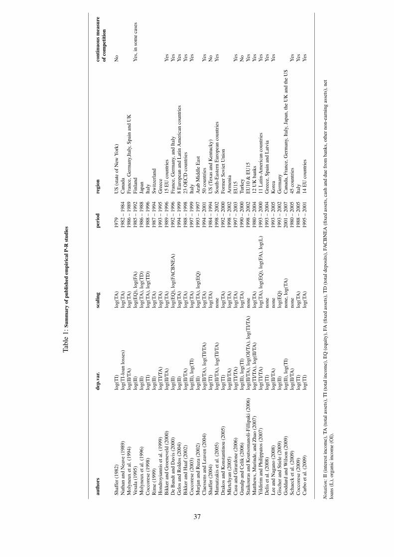
Tabl

e1:

Sum

mar

yof

publ

ishe

dem

piri

calP

-Rst

udie

s

auth

ors

dep.

var.

scal

ing

peri

odre

gion

cont

inuo

usm

easu

reof

com

petit

ion

Shaf

fer(

1982

)lo

g(T

I)lo

g(TA

)19

79U

S(s

tate

ofN

ewY

ork)

No

Nat

han

and

Nea

ve(1

989)

log(

TI-

loan

loss

es)

log(

TA)

1982

–19

84C

anad

aM

olyn

eux

etal

.(19

94)

log(

II/T

A)

log(

TA)

1986

–19

89Fr

ance

,Ger

man

y,It

aly,

Spai

nan

dU

KV

esal

a(1

995)

log(

II)

log(

EQ

),lo

g(FA

)19

85–

1992

Finl

and

Yes

,in

som

eca

ses

Mol

yneu

xet

al.(

1996

)lo

g(II

)lo

g(TA

),lo

g(T

D)

1986

–19

88Ja

pan

Coc

core

se(1

998)

log(

TI)

log(

TA),

log(

TD

)19

88–

1996

Ital

yR

ime

(199

9)lo

g(II

)lo

g(TA

)19

87–

1994

Switz

erla

ndH

ondr

oyia

nnis

etal

.(19

99)

log(

TI/

TA)

log(

TA)

1993

–19

95G

reec

eB

ikke

rand

Gro

enev

eld

(200

0)lo

g(II

/TA

)lo

g(TA

)19

89–

1996

15E

Uco

untr

ies

Yes

De

Ban

dtan

dD

avis

(200

0)lo

g(II

)lo

g(E

Q),

log(

FAC

BN

EA

)19

92–

1996

Fran

ce,G

erm

any,

and

Ital

yY

esG

elos

and

Rol

dos

(200

4)lo

g(II

)lo

g(TA

)19

94–

1999

8E

urop

ean

and

Lat

inA

mer

ican

coun

trie

sY

esB

ikke

rand

Haa

f(20

02)

log(

II/T

A)

log(

TA)

1988

–19

9823

OE

CD

coun

trie

sY

esC

occo

rese

(200

3)lo

g(II

),lo

g(T

I)lo

g(TA

)19

97–

1999

Ital

yY

esM

urja

nan

dR

uza

(200

2)lo

g(II

)lo

g(TA

),lo

g(E

Q)

1993

–19

97A

rab

Mid

dle

Eas

tC

laes

sens

and

Lea

ven

(200

4)lo

g(II

/TA

),lo

g(T

I/TA

)lo

g(TA

)19

94–

2001

50co

untr

ies

Yes

Shaf

fer(

2004

)lo

g(T

I)lo

g(TA

)19

84–

1994

US

(Tex

asan

dK

entu

cky)

No

Mam

atza

kis

etal

.(20

05)

log(

II/T

A),

log(

TI/

TA)

none

1998

–20

02So

uth-

Eas

tern

Eur

opea

nco

untr

ies

Yes

Dra

kos

and

Kon

stan

tinou

(200

5)lo

g(T

I)lo

g(TA

)19

92–

2000

Form

erSo

viet

Uni

onM

krtc

hyan

(200

5)lo

g(II

/TA

)lo

g(TA

)19

98–

2002

Arm

enia

Cas

uan

dG

irar

done

(200

6)lo

g(T

I/TA

)lo

g(TA

)19

97–

2003

EU

15Y

esG

unal

pan

dC

elik

(200

6)lo

g(II

),lo

g(T

I)lo

g(TA

)19

90–

2000

Turk

eyN

oSt

aiko

uras

and

Kou

tsom

anol

i-Fi

llipa

ki(2

006)

log(

II/T

A),

log(

OI/

TA),

log(

TI/

TA)

none

1998

–20

02E

U10

&E

U15

Yes

Mat

thew

s,M

urin

de,a

ndZ

hao

(200

7)lo

g(T

I/TA

),lo

g(II

/TA

)lo

g(TA

)19

80–

2004

12U

Kba

nks

Yes

Yild

irim

and

Phili

ppat

os(2

007)

log(

TI/

TA)

log(

TA),

log(

EQ

),lo

g(FA

),lo

g(L

)19

93–

2000

11L

atin

-Am

eric

anco

untr

ies

Yes

Del

iset

al.(

2008

)lo

g(T

I)no

ne19

93–

2004

Gre

ece,

Spai

nan

dL

atvi

aY

esL

eean

dN

agan

o(2

008)

log(

II/T

A)

none

1993

–20

05K

orea

Yes

Gis

cher

and

Stie

le(2

009)

log(

II)

log(

EQ

)19

93–

2002

Ger

man

yG

odda

rdan

dW

ilson

(200

9)lo

g(II

),lo

g(T

I)no

ne,l

og(T

A)

2001

–20

07C

anad

a,Fr

ance

,Ger

man

y,It

aly,

Japa

n,th

eU

Kan

dth

eU

SSc

haec

ket

al.(

2009

)lo

g(II

/TA

)no

ne19

80–

2005

45co

untr

ies

Yes

Coc

core

se(2

009)

log(

TI)

log(

TA)

1988

–20

05It

aly

Yes

Car

boet

al.(

2009

)lo

g(T

I)lo

g(TA

)19

95–

2001

14E

Uco

untr

ies

Yes

Not

atio

n:II

(int

eres

tinc

ome)

,TA

(tot

alas

sets

),T

I(to

tali

ncom

e),E

Q(e

quity

),FA

(fixe

das

sets

),T

D(t

otal

depo

sits

),FA

CB

NE

A(fi

xed

asse

ts,c

ash

and

due

from

bank

s,ot

hern

on-e

arni

ngas

sets

),ne

tlo

ans

(L),

orga

nic

inco

me

(OI)

.

37

Tabl

e2:

Sum

mar

yof

prop

ertie

soft

heH

stat

istic

unde

ral

tern

ativ

eco

stco

nditi

ons

Hba

sed

on

mar

ketp

ower

AC

func

tion

unsc

aled

rev.

eq.

scal

edre

v.eq

.pr

ice

eq.

long

-run

com

petit

ion

U-s

hape

dR

osse

and

Panz

ar(1

977)

:Hr

D1

Prop

.3.2

:Hr s

D1

Prop

. 3.2

:Hp

D1

long

-run

com

petit

ion

flat

Prop

.3.6

:Hr

<0

or0

<H

r<

1po

ssib

lePr

op.3

.5:H

r sD

1Pr

op.3

.5:H

pD

1sh

ort-

run

com

petit

ion

U-s

hape

dSh

affe

r(19

82a,

1983

a):H

r<

0po

ssib

leby

cont

inui

ty:H

r s>

0by

cont

inui

ty:H

p>

0R

osse

and

Panz

ar(1

977)

:0<

Hr

<1

poss

ible

mon

opol

yU

-sha

ped

Ros

sean

dPa

nzar

(197

7):H

r<

0Pr

op. 3

.1&

Cor

.3.1

:Hr s

>0

Prop

.3.3

:Hp

>0

mon

opol

yfla

tPr

op.3

.4:H

r<

0Pr

op.3

.4:H

r s>

0Pr

op.3

.4:H

p>

0ol

igop

oly

U-s

hape

dR

osse

and

Panz

ar(1

977)

:Hr

<0

Prop

.3.1

&C

or.3

.1:H

r s>

0Pr

op.3

.1:H

p>

0ol

igop

oly

flat

Prop

.3.4

:Hr

<0

Prop

.3.4

:Hr s

>0

Prop

.3.4

:Hp

>0

mon

opol

istic

com

petit

ion

U-s

hape

dR

osse

and

Panz

ar(1

977)

:0<

Hr

<1

unde

rcon

ditio

ns,

byco

ntin

uity

:Hr s

>0

byco

ntin

uity

:Hp

>0

butH

r<

0po

ssib

leco

nsta

ntm

arku

ppr

icin

g(A

PH)

flata

ndU

-sha

ped

App

endi

xB

:Hr

<1

poss

ible

App

endi

xB

:Hr s

D1

App

endi

xB

:Hp

D1

(ass

umin

gfla

tAC

)

Not

e:T

heca

seof

mon

opol

istic

com

petit

ion

cann

otar

ise

with

cons

tant

aver

age

cost

,whi

leth

eze

ro-p

rofit

cons

trai

ntim

plie

sH

p>

0un

derm

onop

olis

ticco

mpe

titio

n.T

here

sult

that

0<

Hr

<1

ispo

ssib

lefo

rsho

rt-r

unco

mpe

titio

nis

base

don

Ros

sean

dPa

nzar

(197

7).T

hey

show

that

Hr

�1

(inc

ludi

ngth

ere

gion

betw

een

0an

d1)

fort

heir

‘Mar

ketE

quili

briu

mH

ypot

hesi

s’,w

hich

they

defin

eas

firm

str

ying

tom

axim

ize

profi

tsin

the

pres

ence

ofm

arke

tfor

ces

oper

atin

gto

elim

inat

eex

cess

profi

ts(w

hich

incl

udes

shor

t-ru

nco

mpe

titio

n).M

ore

gene

rally

and

intu

itive

ly,i

fHr

<0

fora

nypr

ofit-

max

imiz

ing

firm

faci

nga

fixed

dem

and

curv

e(a

ssh

own

inSh

affe

r198

3a)w

hile

Hr

D1

fora

nyfir

min

long

-run

com

petit

ive

equi

libri

um,t

hen

–by

cont

inui

ty–

ther

em

uste

xist

aph

ase

ofpa

rtia

ladj

ustm

entb

etw

een

shor

t-ru

nan

dlo

ng-r

unco

mpe

titio

nfo

rwhi

ch0

<H

r<

1.B

ecau

seH

pis

posi

tive

inth

epo

larc

ases

oflo

ng-r

unco

mpe

titio

nan

dm

onop

oly,

itis

also

posi

tive

inin

term

edia

teca

ses,

incl

udin

gsh

ort-

run

com

petit

ion

and

mon

opol

istic

com

petit

ion.

38

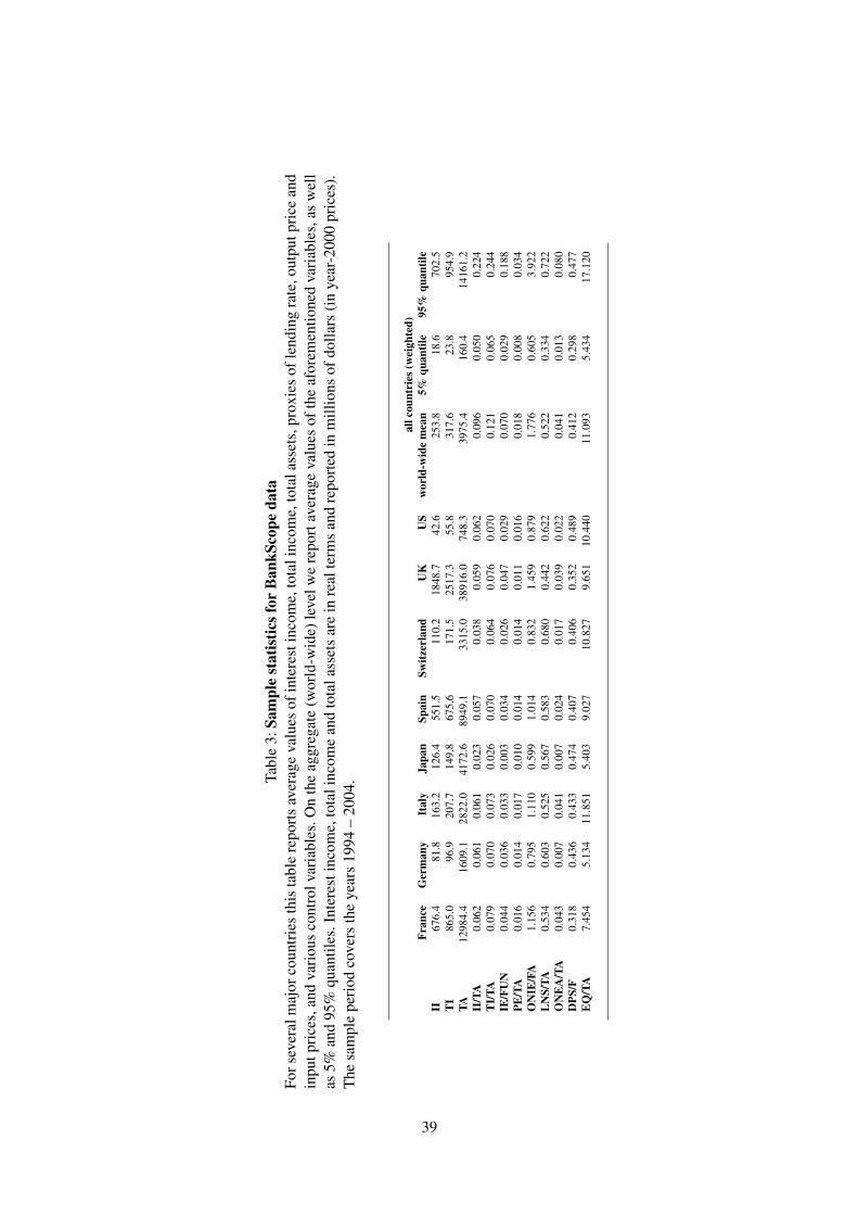
Tabl

e3:

Sam

ple

stat

istic

sfor

Ban

kSco

peda

taFo

rsev

eral

maj

orco

untr

ies

this

tabl

ere

port

sav

erag

eva

lues

ofin

tere

stin

com

e,to

tali

ncom

e,to

tala

sset

s,pr

oxie

sof

lend

ing

rate

,out

putp

rice

and

inpu

tpri

ces,

and

vari

ous

cont

rolv

aria

bles

.On

the

aggr

egat

e(w

orld

-wid

e)le

velw

ere

port

aver

age

valu

esof

the

afor

emen

tione

dva

riab

les,

asw

ell

as5%

and

95%

quan

tiles

.Int

eres

tinc

ome,

tota

linc

ome

and

tota

lass

ets

are

inre

alte

rms

and

repo

rted

inm

illio

nsof

dolla

rs(i

nye

ar-2

000

pric

es).

The

sam

ple

peri

odco

vers

the

year

s19

94–

2004

.

allc

ount

ries

(wei

ghte

d)Fr

ance

Ger

man

yIt

aly

Japa

nSp

ain

Switz

erla

ndU

KU

Sw

orld

-wid

em

ean

5%qu

antil

e95

%qu

antil

eII

676.

481

.816

3.2

126.

455

1.5

110.

218

48.7

42.6

253.

818

.670

2.5

TI

865.

096

.920

7.7

149.

867

5.6

171.

525

17.3

55.8

317.

623

.895

4.9

TA12

984.

416

09.1

2822

.041

72.6

8949

.133

15.0

3891

6.0

748.

339

75.4

160.

414

161.

2II

/TA

0.06

20.

061

0.06

10.

023

0.05

70.

038

0.05

90.

062

0.09

60.

050

0.22

4T

I/TA

0.07

90.

070

0.07

30.

026

0.07

00.

064

0.07

60.

070

0.12

10.

065

0.24

4IE

/FU

N0.

044

0.03

60.

033

0.00

30.

034

0.02

60.

047

0.02

90.

070

0.02

90.

188

PE/T

A0.

016

0.01

40.

017

0.01

00.

014

0.01

40.

011

0.01

60.

018

0.00

80.

034

ON

IE/F

A1.

156

0.79

51.

110

0.59

91.

014

0.83

21.

459

0.87

91.

776

0.60

53.

922

LN

S/TA

0.53

40.

603

0.52

50.

567

0.58

30.

680

0.44

20.

622

0.52

20.

334

0.72

2O

NE

A/T

A0.

043

0.00

70.

041

0.00

70.

024

0.01

70.

039

0.02

20.

041

0.01

30.

080

DPS

/F0.

318

0.43

60.

433

0.47

40.

407

0.40

60.

352

0.48

90.

412

0.29

80.

477

EQ

/TA

7.45

45.

134

11.8

515.

403

9.02

710

.827

9.65

110

.440

11.0

935.

434

17.1

20

39

Tabl

e4:

Est

imat

ion

resu

ltsfo

rP-

Rm

odel

s(w

ithin

estim

ator

)

Thi

sta

ble

repo

rts

estim

ates

ofth

eH

stat

istic

and

corr

espo

ndin

gst

anda

rder

rors

base

don

the

Panz

ar-R

osse

pric

ean

d(u

n-)s

cale

dre

venu

eeq

uatio

n.T

hem

odel

sde

note

dby

‘log

(II)

Clo

g(TA

)’an

d‘l

og(T

I)C

log(

TA)’

refe

rto

the

reve

nue

equa

tion

with

,res

pect

ivel

y,lo

g(II

)and

log(

TI)

asth

ede

pend

entv

aria

ble

and

log(

TA)a

sth

esc

alin

gva

riab

le.T

hew

ithin

estim

ator

has

been

used

toes

timat

eal

lspe

cific

atio

ns.C

lust

ered

stan

dard

erro

rsha

vebe

enus

edto

deal

with

gene

ralh

eter

oske

dast

icity

and

cros

s-se

ctio

nalc

orre

latio

nin

the

mod

eler

rors

(Are

llano

,198

7).

coun

try

#ba

nks

#ob

slo

g(II

)lo

g(T

I)lo

g(PI

)lo

g(PT

)lo

g(II

)+lo

g(TA

)lo

g(PI

)+lo

g(TA

)H

r�

.Hr/

Hr

�.H

r/

Hp

�.H

p/

Hp

�.H

p/

Hr s

�.H

r s/

Hr s

�.H

r s/

Arg

entin

a10

741

80.

377

0.09

20.

225

0.09

20.

851

0.06

20.

686

0.05

60.

881

0.06

70.

777

0.05

9A

ustr

alia

3320

70.

972

0.13

61.

006

0.13

40.

904

0.03

20.

950

0.02

80.

904

0.03

20.

950

0.02

8A

ustr

ia19

412

340.

376

0.05

10.

373

0.05

60.

731

0.02

00.

730

0.02

50.

733

0.02

00.

750

0.02

6B

angl

ades

h33

255

1.12

10.

171

1.09

60.

156

0.98

00.

065

0.95

30.

048

0.93

50.

061

0.92

30.

045

Bel

gium

7851

50.

630

0.09

40.

672

0.09

50.

851

0.02

80.

892

0.03

80.

854

0.02

80.

890

0.03

8B

oliv

ia16

123

-0.0

820.

213

-0.0

570.

200

0.64

70.

059

0.66

80.

055

0.70

20.

060

0.67

80.

058

Bra

zil

167

859

0.46

60.

059

0.52

10.

055

0.70

50.

035

0.76

10.

027

0.70

30.

035

0.75

70.

027

Can

ada

6643

20.

212

0.09

20.

201

0.09

00.

761

0.03

20.

747

0.03

10.

752

0.03

30.

735

0.03

2C

hile

3520

20.

209

0.18

30.

199

0.14

20.

824

0.14

10.

798

0.05

50.

817

0.14

80.

845

0.05

6C

olom

bia

4023

90.

446

0.13

00.

379

0.12

50.

829

0.06

40.

766

0.05

40.

870

0.06

40.

797

0.05

4C

osta

Ric

a39

150

0.21

30.

085

0.24

30.

087

0.81

10.

039

0.84

10.

036

0.76

00.

044

0.80

80.

042

Cro

atia

4727

90.

263

0.15

40.

225

0.16

40.

542

0.06

10.

509

0.06

70.

538

0.06

10.

517

0.06

7C

zech

Rep

ublic

3419

70.

578

0.12

90.

516

0.13

40.

828

0.07

50.

750

0.09

10.

812

0.07

50.

729

0.09

1D

enm

ark

100

881

0.32

70.

054

0.38

90.

065

0.52

60.

028

0.58

80.

038

0.50

30.

027

0.58

30.

038

Dom

inic

anR

epub

lic29

177

1.00

10.

381

0.77

60.

210

1.02

50.

279

0.78

40.

063

1.00

50.

265

0.77

80.

057

Ecu

ador

2911

50.

729

0.13

80.

741

0.12

60.

750

0.09

20.

773

0.08

00.

751

0.09

20.

774

0.07

8Fr

ance

411

2843

0.18

60.

028

0.18

90.

028

0.64

10.

014

0.64

20.

014

0.61

30.

014

0.61

90.

015

Ger

man

y22

9817

260

0.37

30.

018

0.40

00.

018

0.71

60.

005

0.74

20.

006

0.71

90.

005

0.73

90.

006

Gre

ece

2815

2-1

.051

0.20

2-1

.059

0.21

40.

955

0.05

30.

929

0.05

00.

843

0.06

90.

955

0.06

8H

ong

Kon

g38

308

0.41

70.

099

0.44

20.

090

0.85

30.

047

0.87

30.

044

0.87

70.

048

0.86

00.

045

Hun

gary

2613

6-0

.229

0.21

3-0

.290

0.20

60.

710

0.08

50.

647

0.06

70.

694

0.09

60.

636

0.07

6In

dia

7553

60.

820

0.08

90.

849

0.08

80.

708

0.02

70.

738

0.02

20.

712

0.02

70.

742

0.02

1In

done

sia

105

572

0.20

30.

067

0.28

80.

070

0.74

80.

032

0.83

00.

038

0.74

90.

034

0.82

60.

041

Irel

and

3119

70.

108

0.08

70.

122

0.09

60.

673

0.03

90.

680

0.05

20.

667

0.04

50.

698

0.06

0Is

rael

1713

10.

278

0.09

40.

358

0.09

30.

822

0.08

90.

911

0.08

80.

711

0.12

60.

806

0.12

4It

aly

821

5556

0.36

60.

025

0.42

80.

025

0.65

60.

010

0.71

60.

011

0.65

10.

010

0.70

60.

011

Japa

n62

031

970.

098

0.02

60.

157

0.02

90.

473

0.01

50.

532

0.01

90.

429

0.01

60.

502

0.02

0Jo

rdan

1110

0-0

.996

0.24

4-1

.136

0.28

30.

478

0.06

80.

376

0.07

40.

396

0.07

60.

492

0.08

0K

azak

hsta

n24

115

-0.3

820.

204

-0.4

240.

197

0.66

30.

064

0.61

20.

045

0.63

80.

071

0.60

40.

049

Ken

ya38

187

0.44

30.

115

0.26

80.

112

0.67

40.

062

0.49

60.

061

0.67

40.

063

0.49

40.

062

Lat

via

2914

4-0

.422

0.19

4-0

.188

0.18

00.

698

0.10

70.

825

0.09

70.

713

0.12

10.

858

0.11

0L

eban

on59

434

0.09

50.

103

0.07

50.

106

0.71

50.

037

0.69

60.

038

0.71

60.

039

0.71

90.

039

Lux

embo

urg

137

1071

0.19

30.

041

0.14

00.

044

0.84

40.

014

0.79

00.

022

0.82

90.

015

0.78

50.

024

Mal

aysi

a43

335

0.59

10.

068

0.62

00.

070

0.87

40.

025

0.90

10.

030

0.86

60.

026

0.89

60.

031

Mex

ico

3110

90.

791

0.23

90.

603

0.18

21.

220

0.18

31.

009

0.09

81.

236

0.18

61.

020

0.09

9

40

Tabl

e5:

Est

imat

ion

resu

ltsfo

rP-

Rm

odel

s(w

ithin

estim

ator

cont

inue

d)

coun

try

#ba

nks

#ob

slo

g(II

)lo

g(T

I)lo

g(PI

)lo

g(PT

)lo

g(II

)+lo

g(TA

)lo

g(PI

)+lo

g(TA

)H

r�

.Hr/

Hr

�.H

r/

Hp

�.H

p/

Hp

�.H

p/

Hr s

�.H

r s/

Hr s

�.H

r s/

Mon

aco

1412

00.

823

0.15

60.

696

0.15

90.

760

0.05

40.

632

0.06

00.

755

0.05

60.

623

0.06

2N

ethe

rlan

ds51

330

0.17

90.

106

0.06

40.

104

0.90

10.

038

0.77

90.

043

0.92

20.

040

0.77

60.

046

Nig

eria

6431

80.

375

0.11

90.

245

0.11

40.

875

0.05

30.

747

0.03

50.

844

0.05

50.

726

0.03

6N

orw

ay64

370

0.75

10.

072

0.78

30.

073

0.80

70.

030

0.83

80.

033

0.82

10.

029

0.85

10.

033

Paki

stan

2517

80.

769

0.11

90.

622

0.12

00.

651

0.08

00.

503

0.08

40.

664

0.08

00.

518

0.08

3Pa

nam

a45

134

0.53

50.

122

0.46

00.

135

0.88

10.

045

0.80

60.

053

0.88

90.

048

0.84

70.

055

Para

guay

2616

6-0

.110

0.09

2-0

.058

0.11

90.

856

0.04

40.

946

0.07

10.

866

0.05

91.

128

0.09

1Pe

ru26

165

0.40

10.

135

0.23

90.

167

0.78

90.

051

0.66

10.

087

0.79

30.

052

0.69

30.

087

Phili

ppin

es49

308

0.67

10.

127

0.72

40.

126

0.76

40.

044

0.81

40.

040

0.78

10.

043

0.83

30.

039

Pola

nd50

261

-0.8

090.

117

-0.8

400.

126

0.69

10.

052

0.66

90.

047

0.64

50.

068

0.75

90.

062

Port

ugal

3222

70.

344

0.11

30.

596

0.14

10.

771

0.04

71.

022

0.09

40.

777

0.04

91.

049

0.09

7R

oman

ia29

138

-0.3

690.

179

-0.2

590.

178

0.69

40.

072

0.79

10.

074

0.77

40.

079

0.85

10.

082

Rus

sian

Fede

ratio

n20

663

70.

345

0.07

20.

307

0.06

00.

628

0.04

50.

588

0.03

30.

648

0.04

60.

577

0.03

4Sl

ovak

ia21

100

-0.4

150.

230

0.22

10.

262

0.53

80.

107

1.18

30.

177

0.76

40.

124

1.32

30.

217

Slov

enia

2010

7-0

.990

0.16

1-1

.041

0.15

40.

785

0.06

20.

732

0.06

20.

735

0.09

20.

612

0.09

1So

uth

Afr

ica

3113

90.

457

0.13

40.

334

0.12

90.

961

0.03

60.

830

0.03

90.

998

0.03

80.

846

0.04

2Sp

ain

165

1130

0.15

40.

047

0.27

00.

044

0.58

20.

021

0.69

20.

021

0.61

30.

022

0.68

80.

022

Swed

en91

401

-0.0

160.

055

-0.0

060.

063

0.65

10.

033

0.66

50.

033

0.52

90.

036

0.62

40.

039

Switz

erla

nd41

724

250.

107

0.03

30.

019

0.03

50.

559

0.02

00.

470

0.02

20.

559

0.02

10.

475

0.02

4T

haila

nd18

128

0.38

50.

101

0.29

60.

118

0.86

40.

079

0.76

90.

081

0.71

40.

083

0.71

00.

090

Turk

ey51

191

0.61

30.

176

0.48

00.

167

0.81

30.

078

0.67

40.

057

0.81

30.

079

0.67

40.

057

Ukr

aine

4118

4-0

.202

0.14

0-0

.259

0.13

00.

781

0.06

30.

701

0.06

50.

680

0.07

10.

551

0.07

1U

nite

dA

rab

Em

irat

es17

117

-0.5

200.

196

-0.5

580.

210

0.75

60.

060

0.69

60.

066

0.72

90.

074

0.76

70.

080

Uni

ted

Kin

gdom

7340

30.

467

0.07

40.

535

0.07

50.

735

0.03

00.

805

0.02

60.

735

0.03

00.

810

0.02

7U

nite

dSt

ates

9505

5590

40.

426

0.00

90.

474

0.00

90.

684

0.00

30.

732

0.00

30.

692

0.00

30.

745

0.00

3U

rugu

ay32

111

-0.3

330.

133

-0.3

570.

144

0.81

30.

046

0.79

70.

060

0.89

20.

068

0.93

50.

088

Ven

ezue

la56

261

0.33

40.

096

0.32

00.

099

0.78

10.

047

0.76

70.

046

0.77

90.

050

0.78

90.

048

Vie

tnam

2313

1-0

.071

0.22

5-0

.084

0.21

80.

740

0.05

60.

714

0.05

00.

728

0.05

60.

693

0.04

8

aver

age

0.22

30.

122

0.21

50.

120

0.75

90.

055

0.74

90.

051

0.75

20.

060

0.75

70.

056

41

Tabl

e6:

Est

imat

ion

resu

ltsfo

rP-

Rm

odel

s(po

oled

FGL

S)

Thi

sta

ble

repo

rts

estim

ates

ofth

eH

stat

istic

and

corr

espo

ndin

gst

anda

rder

rors

base

don

the

Panz

ar-R

osse

pric

ean

d(u

n-)s

cale

dre

venu

eeq

uatio

n.Po

oled

FGL

Sha

sbe

enus

edto

estim

ate

alls

peci

ficat

ions

.Clu

ster

edst

anda

rder

rors

have

been

used

tode

alw

ithge

nera

lhe

tero

sked

astic

ityan

dcr

oss-

sect

iona

lcor

rela

tion

inth

em

odel

erro

rs(A

rella

no,1

987)

.

coun

try

log(

II)

log(

TI)

log(

PI)

log(

PT)

log(

II)+

log(

TA)

log(

PI)+

log(

TA)

Hr

�.H

r/

Hr

�.H

r/

Hp

�.H

p/

Hp

�.H

p/

Hr s

�.H

r s/

Hr s

�.H

r s/

Arg

entin

a-0

.323

0.03

3-0

.419

0.03

10.

705

0.00

40.

673

0.00

70.

752

0.00

50.

697

0.00

5A

ustr

alia

-0.1

470.

140

0.01

20.

106

0.83

30.

005

0.93

80.

008

0.81

80.

008

0.91

60.

010

Aus

tria

0.22

50.

011

0.42

50.

034

0.60

80.

001

0.82

00.

001

0.59

90.

002

0.81

70.

002

Ban

glad

esh

1.36

20.

078

1.43

50.

077

0.98

90.

008

0.98

80.

016

0.98

10.

013

0.99

40.

014

Bel

gium

0.54

30.

031

0.36

10.

021

0.85

70.

013

0.70

90.

009

0.85

60.

009

0.69

20.

006

Bol

ivia

0.86

30.

056

0.74

00.

047

0.98

50.

034

0.89

20.

025

0.95

40.

049

0.86

20.

011

Bra

zil

0.54

80.

018

0.63

00.

018

0.73

10.

003

0.79

40.

001

0.71

40.

003

0.78

70.

002

Can

ada

0.33

50.

083

0.29

90.

092

0.74

10.

006

0.71

00.

006

0.74

00.

005

0.71

80.

003

Chi

le1.

608

0.11

01.

548

0.11

70.

939

0.02

10.

826

0.00

70.

952

0.01

30.

809

0.00

6C

olom

bia

-1.0

430.

080

-1.0

680.

084

0.80

40.

017

0.77

50.

010

0.78

40.

017

0.75

00.

007

Cos

taR

ica

-0.0

690.

061

-0.0

300.

051

0.75

00.

010

0.78

90.

005

0.74

10.

011

0.78

70.

005

Cro

atia

-1.7

040.

015

-1.7

650.

040

0.47

40.

006

0.34

60.

012

0.51

00.

005

0.40

90.

011

Cze

chR

epub

lic0.

745

0.08

70.

679

0.10

80.

691

0.01

50.

581

0.02

00.

692

0.00

90.

583

0.01

8D

enm

ark

0.49

40.

029

0.71

40.

024

0.36

90.

003

0.59

80.

004

0.39

00.

002

0.61

00.

003

Dom

inic

anR

epub

lic-1

.322

0.13

6-1

.166

0.25

20.

648

0.04

10.

712

0.02

00.

634

0.03

50.

704

0.01

7E

cuad

or0.

513

0.07

10.

973

0.12

60.

342

0.02

30.

884

0.03

20.

340

0.02

30.

878

0.01

9Fr

ance

0.76

60.

006

0.68

10.

007

0.68

40.

001

0.60

30.

001

0.67

10.

001

0.59

10.

000

Ger

man

y0.

841

0.00

10.

893

0.00

20.

605

0.00

00.

661

0.00

00.

597

0.00

00.

653

0.00

0G

reec

e0.

044

0.35

80.

163

0.30

80.

797

0.01

80.

775

0.00

60.

751

0.01

60.

766

0.00

5H

ong

Kon

g-2

.397

0.03

7-2

.407

0.03

70.

594

0.00

90.

633

0.00

70.

568

0.00

60.

628

0.00

3H

unga

ry-0

.584

0.02

7-0

.593

0.01

70.

844

0.00

90.

785

0.01

50.

823

0.00

70.

793

0.01

2In

dia

0.56

50.

082

0.50

40.

098

0.63

70.

005

0.75

00.

006

0.64

00.

001

0.75

10.

005

Indo

nesi

a0.

914

0.01

60.

810

0.01

60.

697

0.00

10.

634

0.00

20.

697

0.00

10.

629

0.00

1Ir

elan

d1.

698

0.08

61.

721

0.10

90.

873

0.00

90.

867

0.00

60.

882

0.00

60.

879

0.00

8Is

rael

-1.7

680.

279

-1.8

090.

268

0.81

80.

019

0.69

00.

018

0.80

20.

021

0.70

20.

013

Ital

y1.

676

0.00

71.

814

0.00

50.

589

0.00

00.

727

0.00

10.

576

0.00

00.

722

0.00

1Ja

pan

-0.5

190.

004

-0.4

380.

006

0.46

00.

001

0.56

00.

001

0.49

30.

001

0.57

70.

001

Jord

an-2

.635

0.19

2-2

.681

0.16

10.

648

0.00

90.

486

0.01

60.

680

0.01

00.

557

0.01

1K

azak

hsta

n-0

.110

0.07

2-0

.023

0.07

10.

599

0.01

50.

591

0.01

30.

619

0.01

30.

587

0.00

9K

enya

0.22

00.

111

0.31

70.

113

0.58

60.

017

0.61

60.

014

0.59

30.

020

0.60

80.

007

Lat

via

0.45

20.

121

0.50

10.

109

0.72

10.

025

0.80

50.

017

0.70

70.

011

0.80

30.

016

Leb

anon

0.15

50.

038

0.17

00.

040

0.63

30.

005

0.58

20.

006

0.63

20.

005

0.57

50.

005

Lux

embo

urg

0.67

50.

008

0.61

50.

010

0.85

70.

001

0.80

10.

001

0.85

50.

001

0.80

20.

001

Mal

aysi

a0.

811

0.03

10.

781

0.01

90.

879

0.00

50.

862

0.00

70.

875

0.00

40.

870

0.00

7M

exic

o1.

223

0.12

31.

183

0.17

40.

999

0.02

30.

928

0.00

70.

957

0.02

50.

934

0.00

8

42

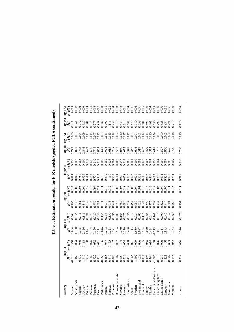
Tabl

e7:

Est

imat

ion

resu

ltsfo

rP-

Rm

odel

s(po

oled

FGL

Sco

ntin

ued)

coun

try

log(

II)

log(

TI)

log(

PI)

log(

PT)

log(

II)+

log(

TA)

log(

PI)+

log(

TA)

Hr

�.H

r/

Hr

�.H

r/

Hp

�.H

p/

Hp

�.H

p/

Hr s

�.H

r s/

Hr s

�.H

r s/

Mon

aco

-0.0

100.

350

0.00

40.

308

0.76

50.

012

0.81

10.

020

0.74

90.

006

0.81

10.

019

Net

herl

ands

1.16

90.

034

1.16

00.

035

0.83

30.

003

0.84

90.

005

0.82

10.

003

0.84

10.

007

Nig

eria

0.33

70.

040

0.37

50.

011

0.78

10.

005

0.75

70.

005

0.78

50.

004

0.77

20.

004

Nor

way

1.94

50.

118

2.12

60.

111

0.84

90.

006

0.92

30.

006

0.84

40.

009

0.92

50.

003

Paki

stan

1.21

90.

130

1.08

10.

081

0.63

70.

022

0.51

10.

012

0.67

20.

012

0.50

10.

014

Pana

ma

0.28

90.

076

0.36

20.

079

0.63

40.

015

0.64

40.

020

0.63

00.

014

0.64

40.

020

Para

guay

-0.6

270.

038

-0.5

790.

029

0.65

90.

006

0.77

00.

019

0.70

20.

007

0.77

50.

016

Peru

-0.1

140.

031

-0.3

110.

039

0.93

10.

023

0.84

70.

011

0.96

50.

015

0.85

80.

010

Phili

ppin

es-0

.068

0.13

6-0

.046

0.15

50.

611

0.01

10.

680

0.00

90.

647

0.00

30.

682

0.00

8Po

land

-0.1

650.

047

-0.2

020.

056

0.93

00.

010

0.83

20.

002

0.92

40.

011

0.79

70.

010

Port

ugal

-0.3

450.

133

0.32

80.

136

0.61

80.

012

1.11

00.

023

0.61

50.

013

1.11

10.

022

Rom

ania

0.48

50.

102

0.57

10.

096

0.74

10.

015

0.75

40.

004

0.73

80.

018

0.75

40.

004

Rus

sian

Fede

ratio

n0.

507

0.00

70.

566

0.00

90.

555

0.00

50.

611

0.00

20.

557

0.00

20.

619

0.00

3Sl

ovak

ia0.

700

0.10

40.

280

0.16

50.

682

0.00

80.

620

0.04

80.

660

0.01

00.

624

0.04

5Sl

oven

ia-0

.210

0.07

4-0

.339

0.07

20.

689

0.01

80.

628

0.01

40.

652

0.01

70.

644

0.01

1So

uth

Afr

ica

0.41

00.

088

0.49

00.

096

0.61

40.

014

0.59

50.

008

0.54

80.

017

0.58

20.

004

Spai

n-0

.045

0.02

10.

113

0.01

70.

454

0.00

30.

575

0.00

10.

452

0.00

30.

579

0.00

1Sw

eden

1.59

20.

059

1.68

90.

024

0.68

50.

004

0.67

60.

006

0.66

40.

004

0.68

00.

004

Switz

erla

nd1.

028

0.00

61.

077

0.00

50.

522

0.00

10.

572

0.00

10.

519

0.00

10.

558

0.00

1T

haila

nd-0

.414

0.13

5-0

.534

0.11

60.

624

0.01

50.

612

0.02

20.

622

0.01

20.

601

0.01

5Tu

rkey

-0.1

960.

058

0.07

00.

065

0.59

20.

016

0.69

30.

008

0.57

90.

013

0.69

30.

008

Ukr

aine

0.56

40.

034

0.46

40.

044

0.57

20.

016

0.49

40.

005

0.55

50.

010

0.49

30.

005

Uni

ted

Ara

bE

mir

ates

-1.6

850.

138

-1.7

130.

141

0.53

40.

014

0.62

20.

026

0.61

80.

024

0.65

00.

018

Uni

ted

Kin

gdom

-0.0

100.

026

0.09

10.

018

0.73

40.

005

0.79

30.

004

0.73

20.

003

0.79

70.

005

Uni

ted

Stat

es0.

210

0.00

00.

314

0.00

00.

522

0.00

00.

631

0.00

00.

527

0.00

00.

628

0.00

0U

rugu

ay1.

121

0.10

00.

995

0.04

50.

944

0.00

60.

824

0.00

70.

960

0.00

50.

834

0.01

0V

enez

uela

0.69

90.

033

0.78

10.

059

0.68

10.

011

0.72

30.

005

0.69

60.

008

0.72

10.

001

Vie

tnam

0.44

50.

052

0.36

20.

060

0.78

00.

015

0.73

10.

009

0.79

00.

016

0.71

90.

008

aver

age

0.21

40.

076

0.24

00.

077

0.70

10.

011

0.71

90.

010

0.70

00.

010

0.72

00.

008

43

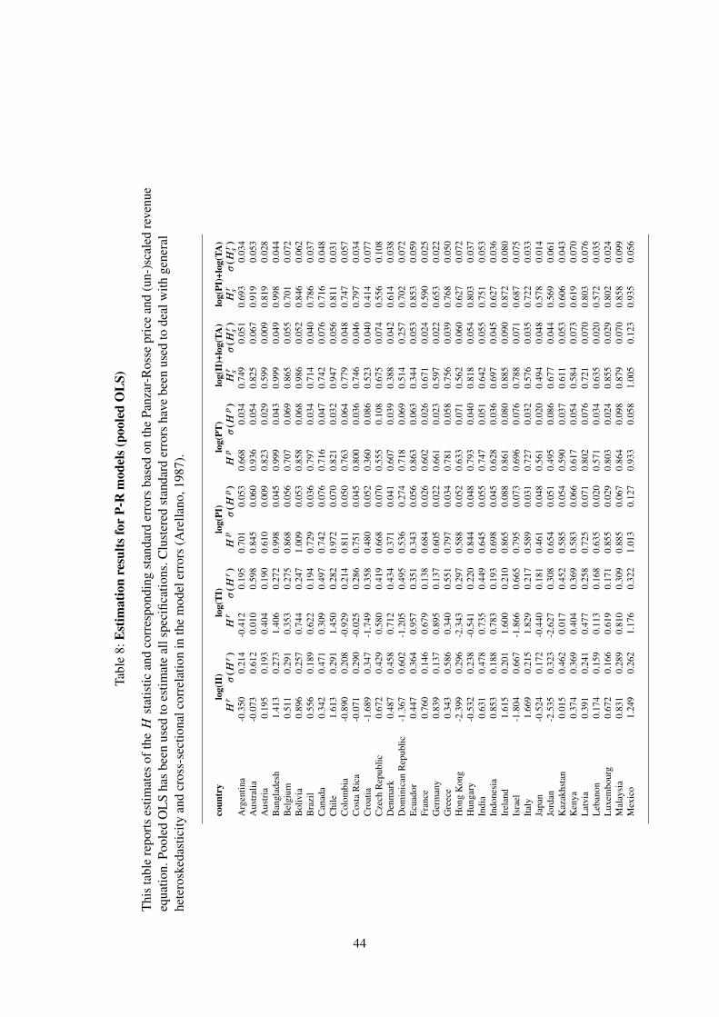
Tabl

e8:

Est

imat

ion

resu

ltsfo

rP-

Rm

odel

s(po

oled

OL

S)

Thi

sta

ble

repo

rts

estim

ates

ofth

eH

stat

istic

and

corr

espo

ndin

gst

anda

rder

rors

base

don

the

Panz

ar-R

osse

pric

ean

d(u

n-)s

cale

dre

venu

eeq

uatio

n.Po

oled

OL

Sha

sbe

enus

edto

estim

ate

alls

peci

ficat

ions

.Clu

ster

edst

anda

rder

rors

have

been

used

tode

alw

ithge

nera

lhe

tero

sked

astic

ityan

dcr

oss-

sect

iona

lcor

rela

tion

inth

em

odel

erro

rs(A

rella

no,1

987)

.

coun

try

log(

II)

log(

TI)

log(

PI)

log(

PT)

log(

II)+

log(

TA)

log(

PI)+

log(

TA)

Hr

�.H

r/

Hr

�.H

r/

Hp

�.H

p/

Hp

�.H

p/

Hr s

�.H

r s/

Hr s

�.H

r s/

Arg

entin

a-0

.350

0.21

4-0

.412

0.19

50.

701

0.05

30.

668

0.03

40.

749

0.05

10.

693

0.03

4A

ustr

alia

-0.0

730.

612

0.01

00.

598

0.84

50.

060

0.93

60.

054

0.82

50.

067

0.91

90.

053

Aus

tria

0.19

50.

193

0.40

40.

190

0.61

00.

009

0.82

30.

029

0.59

90.

009

0.81

90.

028

Ban

glad

esh

1.41

30.

273

1.40

60.

272

0.99

80.

045

0.99

90.

043

0.99

90.

049

0.99

80.

044

Bel

gium

0.51

10.

291

0.35

30.

275

0.86

80.

056

0.70

70.

069

0.86

50.

055

0.70

10.

072

Bol

ivia

0.89

60.

257

0.74

40.

247

1.00

90.

053

0.85

80.

068

0.98

60.

052

0.84

60.

062

Bra

zil

0.55

60.

189

0.62

20.

194

0.72

90.

036

0.79

70.

034

0.71

40.

040

0.78

60.

037

Can

ada

0.34

20.

471

0.30

90.

497

0.74

20.

076

0.71

60.

047

0.74

20.

076

0.71

60.

048

Chi

le1.

613

0.29

11.

450

0.28

20.

972

0.07

00.

821

0.03

20.

947

0.05

60.

811

0.03

1C

olom

bia

-0.8

900.

208

-0.9

290.

214

0.81

10.

050

0.76

30.

064

0.77

90.

048

0.74

70.

057

Cos

taR

ica

-0.0

710.

290

-0.0

250.

286

0.75

10.

045

0.80

00.

036

0.74

60.

046

0.79

70.

034

Cro

atia

-1.6

890.

347

-1.7

490.

358

0.48

00.

052

0.36

00.

086

0.52

30.

040

0.41

40.

077

Cze

chR

epub

lic0.

672

0.42

90.

580

0.41

90.

668

0.07

00.

555

0.10

80.

675

0.07

40.

556

0.10

8D

enm

ark

0.48

70.

458

0.71

20.

434

0.37

10.

041

0.60

70.

039

0.38

80.

042

0.61

40.

038

Dom

inic

anR

epub

lic-1

.367

0.60

2-1

.205

0.49

50.

536

0.27

40.

718

0.06

90.

514

0.25

70.

702

0.07

2E

cuad

or0.

447

0.36

40.

957

0.35

10.

343

0.05

60.

863

0.06

30.

344

0.05

30.

853

0.05

9Fr

ance

0.76

00.

146

0.67

90.

138

0.68

40.

026

0.60

20.

026

0.67

10.

024

0.59

00.

025

Ger

man

y0.

839

0.13

70.

895

0.13

70.

605

0.02

20.

661

0.02

30.

597

0.02

20.

653

0.02

2G

reec

e0.

343

0.58

60.

340

0.55

10.

797

0.03

40.

781

0.05

80.

756

0.03

90.

768

0.05

0H

ong

Kon

g-2

.399

0.29

6-2

.343

0.29

70.

588

0.05

20.

633

0.07

10.

562

0.06

00.

627

0.07

2H

unga

ry-0

.532

0.23

8-0

.541

0.22

00.

844

0.04

80.

793

0.04

00.

818

0.05

40.

803

0.03

7In

dia

0.63

10.

478

0.73

50.

449

0.64

50.

055

0.74

70.

051

0.64

20.

055

0.75

10.

053

Indo

nesi

a0.

853

0.18

80.

783

0.19

30.

698

0.04

50.

628

0.03

60.

697

0.04

50.

627

0.03

6Ir

elan

d1.

615

0.20

11.

600

0.21

00.

865

0.08

80.

861

0.08

00.

885

0.09

00.

872

0.08

0Is

rael

-1.8

040.

667

-1.8

660.

665

0.79

50.

073

0.69

60.

076

0.78

80.

071

0.68

70.

075

Ital

y1.

669

0.21

51.

829

0.21

70.

589

0.03

10.

727

0.03

20.

576

0.03

50.

722

0.03

3Ja

pan

-0.5

240.

172

-0.4

400.

181

0.46

10.

048

0.56

10.

020

0.49

40.

048

0.57

80.

014

Jord

an-2

.535

0.32

3-2

.627

0.30

80.

654

0.05

10.

495

0.08

60.

677

0.04

40.

569

0.06

1K

azak

hsta

n0.

015

0.46

20.

017

0.45

20.

585

0.05

40.

590

0.03

70.

611

0.05

30.

606

0.04

3K

enya

0.37

40.

369

0.40

40.

369

0.58

30.

066

0.61

70.

054

0.58

40.

073

0.61

90.

070

Lat

via

0.39

10.

241

0.47

70.

258

0.72

50.

071

0.80

20.

076

0.72

10.

070

0.80

30.

076

Leb

anon

0.17

40.

159

0.11

30.

168

0.63

50.

020

0.57

10.

034

0.63

50.

020

0.57

20.

035

Lux

embo

urg

0.67

20.

166

0.61

90.

171

0.85

50.

029

0.80

30.

024

0.85

50.

029

0.80

20.

024

Mal

aysi

a0.

831

0.28

90.

810

0.30

90.

885

0.06

70.

864

0.09

80.

879

0.07

00.

858

0.09

9M

exic

o1.

249

0.26

21.

176

0.32

21.

013

0.12

70.

933

0.05

81.

005

0.12

30.

935

0.05

6

44

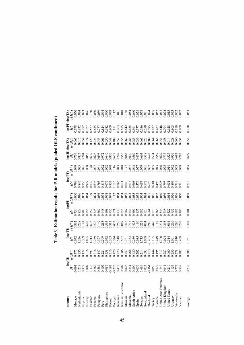
Tabl

e9:

Est

imat

ion

resu

ltsfo

rP-

Rm

odel

s(po

oled

OL

Sco

ntin

ued)

coun

try

log(

II)

log(

TI)

log(

PI)

log(

PT)

log(

II)+

log(

TA)

log(

PI)+

log(

TA)

Hr

�.H

r/

Hr

�.H

r/

Hp

�.H

p/

Hp

�.H

p/

Hr s

�.H

r s/

Hr s

�.H

r s/

Mon

aco

-0.0

910.

375

-0.0

320.

362

0.75

00.

060

0.79

90.

049

0.73

90.

067

0.79

80.

050

Net

herl

ands

1.21

90.

236

1.22

60.

228

0.82

90.

016

0.84

60.

025

0.82

30.

015

0.83

20.

024

Nig

eria

0.37

70.

179

0.36

90.

191

0.78

80.

053

0.75

50.

021

0.78

40.

054

0.77

20.

023

Nor

way

1.80

70.

616

1.88

50.

608

0.85

50.

064

0.92

70.

068

0.85

50.

074

0.92

70.

076

Paki

stan

1.33

30.

597

1.21

30.

635

0.65

20.

129

0.53

20.

178

0.63

90.

129

0.52

70.

180

Pana

ma

0.26

20.

216

0.26

90.

222

0.62

80.

024

0.64

60.

027

0.62

60.

024

0.63

50.

030

Para

guay

-0.5

840.

147

-0.5

270.

149

0.66

90.

056

0.76

30.

061

0.69

80.

045

0.77

70.

059

Peru

-0.1

070.

224

-0.3

090.

213

0.94

80.

074

0.81

30.

072

0.97

20.

061

0.82

40.

064

Phili

ppin

es-0

.087

0.53

8-0

.032

0.56

30.

608

0.06

80.

675

0.07

20.

640

0.05

00.

682

0.06

0Po

land

-0.1

930.

316

-0.3

030.

312

0.93

60.

048

0.83

20.

040

0.92

60.

048

0.80

90.

039

Port

ugal

-0.2

230.

420

0.32

40.

432

0.62

10.

112

1.11

50.

116

0.61

90.

109

1.11

10.

112

Rom

ania

0.47

80.

270

0.51

80.

256

0.73

80.

054

0.76

50.

043

0.74

90.

052

0.76

30.

041

Rus

sian

Fede

ratio

n0.

509

0.08

60.

567

0.08

90.

555

0.05

40.

611

0.01

80.

556

0.05

50.

615

0.01

8Sl

ovak

ia0.

828

0.25

70.

761

0.34

60.

687

0.05

50.

640

0.17

70.

663

0.06

20.

642

0.16

6Sl

oven

ia-0

.341

0.76

6-0

.333

0.74

60.

644

0.07

20.

613

0.06

70.

630

0.08

40.

635

0.05

4So

uth

Afr

ica

0.29

00.

420

0.28

90.

425

0.60

90.

085

0.60

80.

042

0.56

90.

085

0.59

10.

040

Spai

n-0

.059

0.20

20.

085

0.19

00.

455

0.03

80.

576

0.02

70.

457

0.03

90.

577

0.02

8Sw

eden

1.68

90.

214

1.71

50.

221

0.68

20.

064

0.68

70.

059

0.66

40.

063

0.68

60.

058

Switz

erla

nd1.

024

0.09

31.

068

0.07

40.

523

0.02

40.

572

0.03

10.

518

0.02

30.

559

0.03

1T

haila

nd-0

.364

0.21

0-0

.405

0.21

60.

661

0.08

50.

626

0.08

70.

642

0.08

90.

595

0.09

4Tu

rkey

0.05

00.

444

0.16

50.

440

0.57

80.

061

0.68

10.

035

0.57

40.

064

0.67

70.

035

Ukr

aine

0.52

20.

195

0.44

90.

187

0.56

60.

062

0.49

30.

043

0.55

90.

068

0.48

70.

052

Uni

ted

Ara

bE

mir

ates

-1.7

420.

217

-1.7

200.

234

0.54

60.

040

0.62

50.

046

0.62

90.

051

0.64

80.

043

Uni

ted

Kin

gdom

0.04

10.

287

0.09

40.

293

0.73

80.

056

0.79

30.

025

0.73

70.

058

0.79

40.

024

Uni

ted

Stat

es0.

210

0.06

00.

314

0.06

10.

522

0.01

40.

631

0.01

40.

527

0.01

40.

628

0.01

3U

rugu

ay1.

155

0.25

61.

001

0.23

60.

952

0.02

60.

807

0.03

20.

956

0.02

80.

805

0.03

3V

enez

uela

0.77

30.

278

0.81

00.

280

0.68

70.

056

0.71

90.

063

0.68

30.

060

0.71

90.

062

Vie

tnam

0.53

80.

207

0.46

80.

205

0.78

50.

050

0.71

00.

038

0.78

50.

051

0.70

90.

037

aver

age

0.23

20.

308

0.25

10.

307

0.70

10.

058

0.71

80.

054

0.69

90.

058

0.71

80.

053

45

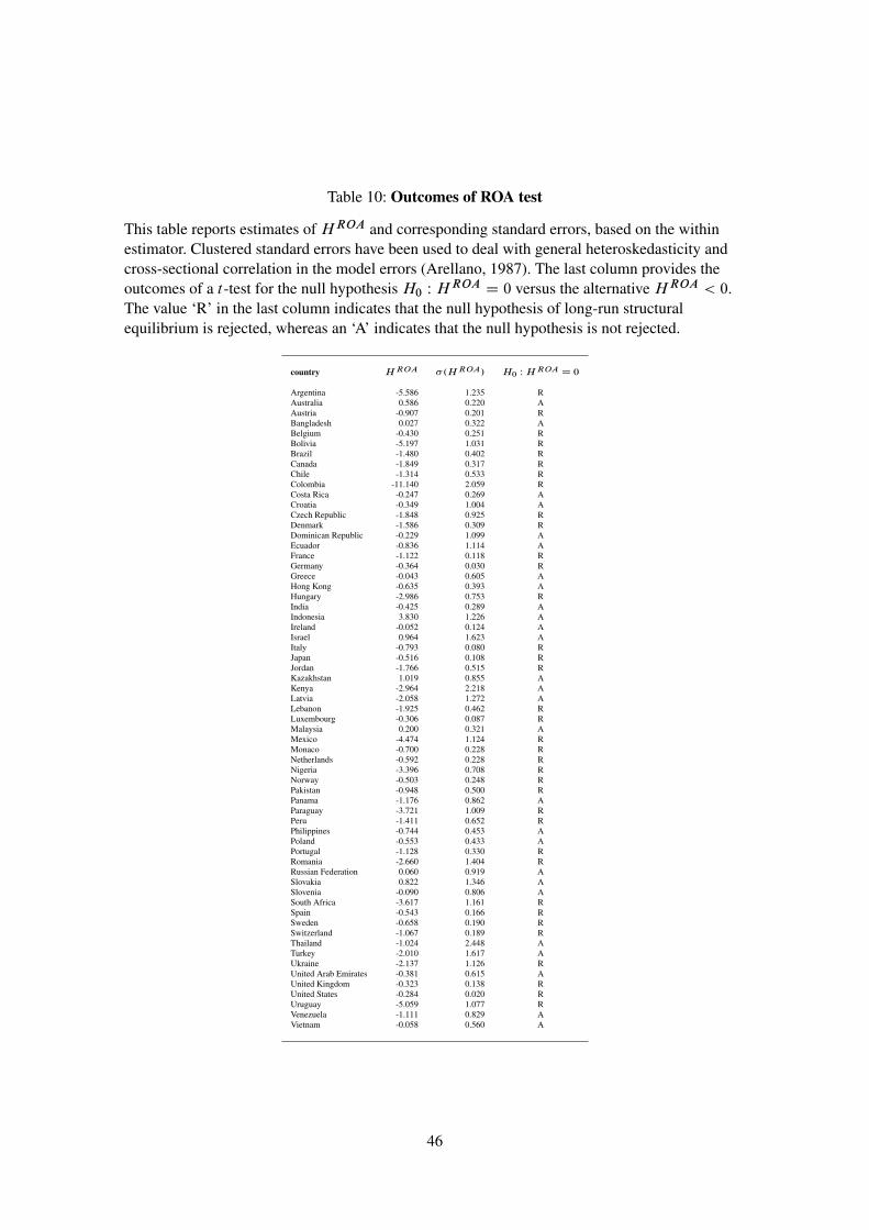
Table 10: Outcomes of ROA test

This table reports estimates of H ROA and corresponding standard errors, based on the withinestimator. Clustered standard errors have been used to deal with general heteroskedasticity andcross-sectional correlation in the model errors (Arellano, 1987). The last column provides theoutcomes of a t -test for the null hypothesis H0 W H ROA D 0 versus the alternative H ROA < 0.The value ‘R’ in the last column indicates that the null hypothesis of long-run structuralequilibrium is rejected, whereas an ‘A’ indicates that the null hypothesis is not rejected.

country H ROA �.H ROA/ H0 W H ROA D 0

Argentina -5.586 1.235 RAustralia 0.586 0.220 AAustria -0.907 0.201 RBangladesh 0.027 0.322 ABelgium -0.430 0.251 RBolivia -5.197 1.031 RBrazil -1.480 0.402 RCanada -1.849 0.317 RChile -1.314 0.533 RColombia -11.140 2.059 RCosta Rica -0.247 0.269 ACroatia -0.349 1.004 ACzech Republic -1.848 0.925 RDenmark -1.586 0.309 RDominican Republic -0.229 1.099 AEcuador -0.836 1.114 AFrance -1.122 0.118 RGermany -0.364 0.030 RGreece -0.043 0.605 AHong Kong -0.635 0.393 AHungary -2.986 0.753 RIndia -0.425 0.289 AIndonesia 3.830 1.226 AIreland -0.052 0.124 AIsrael 0.964 1.623 AItaly -0.793 0.080 RJapan -0.516 0.108 RJordan -1.766 0.515 RKazakhstan 1.019 0.855 AKenya -2.964 2.218 ALatvia -2.058 1.272 ALebanon -1.925 0.462 RLuxembourg -0.306 0.087 RMalaysia 0.200 0.321 AMexico -4.474 1.124 RMonaco -0.700 0.228 RNetherlands -0.592 0.228 RNigeria -3.396 0.708 RNorway -0.503 0.248 RPakistan -0.948 0.500 RPanama -1.176 0.862 AParaguay -3.721 1.009 RPeru -1.411 0.652 RPhilippines -0.744 0.453 APoland -0.553 0.433 APortugal -1.128 0.330 RRomania -2.660 1.404 RRussian Federation 0.060 0.919 ASlovakia 0.822 1.346 ASlovenia -0.090 0.806 ASouth Africa -3.617 1.161 RSpain -0.543 0.166 RSweden -0.658 0.190 RSwitzerland -1.067 0.189 RThailand -1.024 2.448 ATurkey -2.010 1.617 AUkraine -2.137 1.126 RUnited Arab Emirates -0.381 0.615 AUnited Kingdom -0.323 0.138 RUnited States -0.284 0.020 RUruguay -5.059 1.077 RVenezuela -1.111 0.829 AVietnam -0.058 0.560 A

46

Table 11: H statistics in alternative model specifications

This table reports H r , H p and H rs for different model specifications. The first part of the table

reports separate H statistics for small and large banks. The second part of the table displaysseparate H statistics for the 1994 – 1999 and 2000 – 2004 periods. Finally, the third part of thetable reports ‘aggregate’ H statistics for various world regions. All H statistics are based on thewithin estimator. Clustered standard errors have been used to allow for general heteroskedasticityand cross-sectional correlation in the model errors (Arellano, 1987).

# banks # obs ln(II) ln(TI) ln(PI) ln(PT) ln(II)+ln(TA) ln(TI)+ln(TA)H r �.H r / H r �.H r / H p �.H p/ H p �.H p/ H r

s �.H rs / H r

s �.H rs /

SmallDenmark 54 449 0.113 0.070 0.106 0.093 0.203 0.040 0.196 0.068 0.189 0.038 0.187 0.068France 223 1443 0.080 0.039 0.134 0.039 0.628 0.019 0.677 0.020 0.603 0.020 0.650 0.021Germany 1365 8714 0.265 0.028 0.299 0.028 0.594 0.008 0.627 0.009 0.593 0.008 0.622 0.009Italy 454 2782 0.227 0.037 0.243 0.039 0.527 0.016 0.543 0.019 0.527 0.016 0.550 0.019Japan 355 1600 0.149 0.038 0.204 0.043 0.427 0.021 0.483 0.028 0.391 0.021 0.456 0.028Luxembourg 75 553 0.196 0.062 0.151 0.067 0.826 0.022 0.786 0.035 0.818 0.023 0.778 0.037Spain 101 571 -0.026 0.063 0.069 0.060 0.618 0.029 0.702 0.027 0.654 0.031 0.707 0.030Switzerland 246 1214 0.054 0.044 -0.003 0.051 0.439 0.027 0.398 0.032 0.417 0.028 0.417 0.033United States 5026 28022 0.463 0.010 0.495 0.011 0.709 0.005 0.741 0.005 0.724 0.005 0.764 0.005

average 0.169 0.043 0.189 0.048 0.552 0.021 0.572 0.027 0.546 0.021 0.570 0.028

LargeDenmark 9 91 -0.372 0.240 -0.465 0.248 1.007 0.060 0.921 0.079 1.063 0.065 1.014 0.083France 36 279 0.951 0.102 0.876 0.093 0.858 0.057 0.784 0.041 0.880 0.054 0.807 0.036Germany 188 1688 0.619 0.054 0.683 0.054 0.849 0.018 0.912 0.021 0.852 0.019 0.913 0.022Italy 74 557 0.407 0.096 0.435 0.093 0.850 0.025 0.874 0.028 0.852 0.025 0.862 0.028Japan 54 315 0.097 0.092 0.146 0.091 0.768 0.056 0.818 0.051 0.826 0.066 0.899 0.059Luxembourg 12 110 0.178 0.123 0.181 0.135 0.899 0.025 0.902 0.036 0.835 0.027 0.885 0.043Spain 12 106 0.083 0.103 0.036 0.101 0.833 0.023 0.788 0.022 0.813 0.030 0.755 0.028Switzerland 34 254 0.132 0.088 0.071 0.088 0.853 0.040 0.813 0.041 0.841 0.046 0.783 0.047United States 772 5561 0.651 0.035 0.684 0.034 0.715 0.008 0.748 0.009 0.716 0.008 0.747 0.008

average 0.305 0.104 0.294 0.104 0.848 0.035 0.840 0.036 0.853 0.038 0.852 0.039

1994 – 1999Denmark 93 491 0.294 0.062 0.157 0.086 0.693 0.037 0.553 0.065 0.639 0.039 0.540 0.069France 366 1609 0.295 0.036 0.231 0.036 0.789 0.018 0.720 0.019 0.771 0.019 0.694 0.020Germany 2178 10147 0.411 0.020 0.420 0.020 0.757 0.007 0.764 0.008 0.761 0.007 0.761 0.008Italy 699 2636 0.425 0.033 0.423 0.035 0.731 0.014 0.728 0.018 0.712 0.014 0.710 0.019Japan 601 1195 0.051 0.053 0.131 0.056 0.650 0.041 0.731 0.045 0.555 0.047 0.647 0.052Luxembourg 126 651 0.185 0.049 0.171 0.052 0.896 0.012 0.877 0.024 0.900 0.014 0.878 0.027Spain 138 558 0.063 0.060 0.126 0.060 0.531 0.032 0.597 0.030 0.533 0.034 0.611 0.032Switzerland 256 1177 0.089 0.047 0.034 0.049 0.589 0.032 0.533 0.035 0.554 0.035 0.499 0.037United States 8716 12162 0.570 0.040 0.608 0.040 0.837 0.008 0.875 0.010 0.832 0.008 0.868 0.010

average 0.265 0.044 0.256 0.048 0.719 0.022 0.709 0.028 0.695 0.024 0.690 0.030

2000 – 2004Denmark 92 390 0.387 0.061 0.518 0.083 0.472 0.038 0.606 0.052 0.461 0.038 0.617 0.051France 326 1234 0.244 0.043 0.301 0.041 0.623 0.024 0.672 0.023 0.594 0.024 0.627 0.023Germany 1868 7113 0.435 0.027 0.427 0.028 0.750 0.009 0.743 0.011 0.744 0.009 0.739 0.011Italy 748 2920 0.394 0.029 0.439 0.028 0.700 0.015 0.743 0.014 0.704 0.015 0.745 0.015Japan 528 2002 0.017 0.032 0.065 0.037 0.502 0.019 0.549 0.026 0.419 0.020 0.478 0.027Luxembourg 109 420 0.261 0.064 0.155 0.075 0.891 0.029 0.796 0.049 0.875 0.031 0.803 0.052Spain 138 572 0.079 0.068 0.156 0.059 0.614 0.038 0.682 0.035 0.689 0.041 0.658 0.039Switzerland 355 1248 0.219 0.044 0.111 0.044 0.618 0.029 0.518 0.032 0.647 0.033 0.505 0.036United States 9286 43742 0.380 0.008 0.412 0.009 0.697 0.004 0.728 0.004 0.713 0.004 0.753 0.004

average 0.268 0.042 0.287 0.045 0.652 0.023 0.671 0.027 0.650 0.024 0.658 0.029

regional levelNorth America 9602 56439 0.425 0.009 0.470 0.009 0.689 0.003 0.735 0.003 0.697 0.003 0.747 0.003South and Central America 646 3114 0.381 0.034 0.349 0.032 0.795 0.019 0.761 0.015 0.821 0.019 0.787 0.015Western Europe 4849 33947 0.216 0.009 0.237 0.009 0.680 0.003 0.700 0.004 0.676 0.004 0.699 0.004Eastern Europe 484 2106 0.263 0.041 0.247 0.040 0.669 0.020 0.649 0.018 0.681 0.021 0.655 0.018Asia 1029 5937 0.324 0.024 0.364 0.023 0.559 0.013 0.598 0.013 0.556 0.013 0.594 0.013Middle East 155 973 0.148 0.056 0.116 0.056 0.717 0.025 0.682 0.023 0.711 0.027 0.690 0.025Africa 112 601 0.477 0.077 0.342 0.074 0.818 0.036 0.683 0.027 0.799 0.037 0.668 0.028

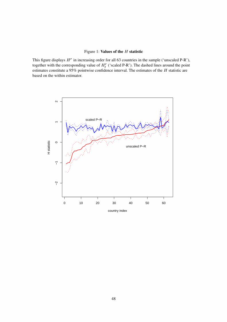
Figure 1: Values of the H statistic

This figure displays H r in increasing order for all 63 countries in the sample (‘unscaled P-R’),together with the corresponding value of H r

s (‘scaled P-R’). The dashed lines around the pointestimates constitute a 95% pointwise confidence interval. The estimates of the H statistic arebased on the within estimator.

0 10 20 30 40 50 60

−2

−1

01

2

country index

H s

tatis

tic

scaled P−R

unscaled P−R

48

Assessing Competition with the Panzar-Rosse Model: The Role of … · Assessing Competition with the Panzar-Rosse Model: The Role of Scale, Costs, and Equilibrium Jacob A. Bikker

Documents