Assessing community variation and randomness in public health indicators

RESEARCH Open Access

Assessing community variation and randomnessin public health indicatorsStephan Arndt1,2,3*, Laura Acion1,2, Kristin Caspers3,4, Ousmane Diallo5,6

Abstract

Background: Evidence-based health indicators are vital to needs-based programming and epidemiologicalplanning. Agencies frequently make programming funds available to local jurisdictions based on need. The use ofobjective indicators to determine need is attractive but assumes that selection of communities with the highestindicators reflects something other than random variability from sampling error.

Methods: The authors compare the statistical performance of two heterogeneity measures applied to communitydifferences that provide tests for randomness and measures of the percentage of true community variation, as wellas estimates of the true variation. One measure comes from the meta-analysis literature and the other from thesimple Pearson chi-square statistic. Simulations of populations and an example using real data are provided.

Results: The measure based on the simple chi-square statistic seems superior, offering better protection againstType I errors and providing more accurate estimates of the true community variance.

Conclusions: The heterogeneity measure based on Pearson’s c2 should be used to assess indices. Methods forimproving poor indices are discussed.

BackgroundEvidence-based health indicators are vital to needs-basedor results-based programming. Agencies frequentlymake programming resources available to local jurisdic-tions based on need. In 2008, the United States Depart-ment of Health and Human Services distributed morethan $421 million in Mental Health Block Grant fundsbased, in part, on the number of people at risk withineach state [1]. Each state then disperses funds to localcommunities. The amount dispersed is often determinedby a demonstrable index of need.The indicators used in public health funding contexts

vary considerably. Common indices include censuscounts within a certain age group or the percentage ofpeople reporting a particular behavior from a popula-tion-based surveillance survey, e.g., the percentage ofpeople reporting binge drinking in the past 30 days.Mortality, arrest, remission, or recidivism rates are alsocommonly used by different funding agencies. US gov-ernment agencies such as the Centers for Disease

Control and Prevention provide yearly datasets such asthe Behavioral Risk Factor Surveillance System (BRFSS)that include prevalence and trend data. State govern-ments and other agencies support various other surveil-lance systems for local assessments. For example, thestate of Iowa supports the administration of the IowaYouth Survey to all 6th, 8th, and 11th graders in the stateevery three years.The use of objective indicators in making funding

decisions can be very attractive for policymakers andfunders. A simple formula to determine which commu-nity receives programming funding is transparent andappears unbiased [2,3]. Targeting areas with high needalso appears to be a rational and evidence-basedapproach. In the United States, there has been a recenteffort to rank the health of counties within states usinga collection of indicators [4,5]. Rankings or “leaguetables” are extremely intuitive and make identification ofthose locales with the greatest need deceptively easy.However, this effort relies on two very basic assump-tions - that the communities differ and that commu-nities with the highest (or lowest) indicators truly reflectthe communities with the greatest need for publichealth funding [6].

* Correspondence: [email protected] of Psychiatry, Carver College of Medicine, University of Iowa,Iowa City, Iowa 52242 USAFull list of author information is available at the end of the article

Arndt et al. Population Health Metrics 2011, 9:3http://www.pophealthmetrics.com/content/9/1/3

© 2011 Arndt et al; licensee BioMed Central Ltd. This is an Open Access article distributed under the terms of the Creative CommonsAttribution License (http://creativecommons.org/licenses/by/2.0), which permits unrestricted use, distribution, and reproduction inany medium, provided the original work is properly cited.

Similar issues arise in the pay-for-performance pro-grams that private health insurers, Medicare, and Medi-caid use in the US and that the National Health Serviceuses in United Kingdom. Pay-for-performance necessa-rily requires using indices, often outcome indicators, forrewards. Whether ranking hospitals or other institutionsor regions, the same assumption is made - that theranking indicators mostly reflect performance ratherthan error.An indicator would show a poor connection with

community needs or outcomes if the differences amongcommunities mainly reflected random variation. Forexample, the BRFSS estimates of the percentage ofadults who drink heavily are based on a sample. Othernonsurvey-based data are incomplete as well - for exam-ple, outcomes of random compliance checks for liquoror tobacco sales to minors. Whenever there is a possiblesampling error, observed differences among commu-nities may be at least partially dictated by random error.The question for policymakers is: How much of thediversity among communities is error, and how much isreal variation?While this question might be answered by reviewing

the communities’ indicator estimates and their standarderrors, this quickly becomes daunting. With more thana few communities or more than two indices, a sum-mary statement quantifying each indicator would beinvaluable in deciding their relative worth. Aside fromlack of convenience, there are other problems with sim-ply relying on the standard errors [6]. One basic issue isthat the standard error of the indicator is not the stan-dard error of the ranking, i.e., knowing the accuracy of asingle measurement does not indicate the accuracy ofthat estimate’s ordering relative to the other commu-nities. The relationship of standard errors of the indivi-dual estimates to the standard errors of the relativerankings is complex [7-9]. From another venue of bios-tatistics, Gauch has noted that the problems of rankingand selection are different statistical questions thanaccuracy of estimation [10,11]. For example, the com-munity with the highest estimated rate of obesity mighthave a relatively large standard error, but that rate maystill be substantially distinguishable from the communitywith the next highest rate. Conversely, the standarderrors might be very small, but the communities mightbe very homogeneous, making the resolution difficult.From a technical perspective, the statistical literature

provides a more formalized treatment. A region’s rankcan be formalized as the number of times a particularregion, say Region d, has a rate (pd) that is larger thanother regions, e.g., ∑(pd ≥ pd’), for all regions d and d’and where the value within the parentheses equals 1when it is true and 0 otherwise. Thus, each region iscompared to all regions, for a total of k2 comparisons,

where k is the total number of regions. Of course,because rates within any region are measured with someamount of error, there is a degree of uncertainty regard-ing any comparison (pd ≥ pd’). One suggestion from thesmall area estimation literature is to replace the rankswith the sum of the estimated probabilities for each esti-mated rate, i.e., [ ( )]’prob d dp p , where the simplerates are replaced by the small area estimates [12,13].This method tends to “shrink” the ranks toward themedian as a function of the spread of the estimates aswell as the size of the estimated standard errors. Each ofthe possible comparisons also has a covariance thatneeds to be considered, again magnifying the complexityof the problem. Furthermore, the resulting sums of theprobabilities are not actually ranks, making interpreta-tion difficult. Rao, in his seminal work on small areaestimation, suggests using triple goal estimators of Shenand Louis when performing Bayesian estimates forregional values [14,15]. Of particular interest is that thetriple goal method explicitly includes the rank orderingand adequate interregional spread in the loss functionsused by the Bayes estimates. More importantly, the tri-ple goal method explicitly attempts to provide good esti-mates of the relative regional ordering rather thansimply good estimators for the rates, goals that are notcompletely overlapping and will not necessarily result inthe same estimates.In actual application, two studies of health indicator

performance (mortality rates and lead poisoning) acrossa variety of geographic levels noted that the degree ofcommunity homogeneity affected how well the indicesperformed [16,17]. The degree of community homoge-neity is not necessarily related to the size of the localpopulation or the corresponding size of the standarderror or estimate. In the context of hospital rankings onperformance measures, one English study noticed con-siderable variation in the rankings, as much as half ofthe league table [18]. A similar result regarding theinstability of rankings is given by O’Brien and Petersonregarding hospital mortality rankings [19]. These consid-erations may also explain inconsistencies in health rank-ings using different indicators across provinces [20] andcommunities [21] in Canada.Both between-community heterogeneity and within-

community homogeneity must be considered simulta-neously when assessing an index’s performance inrankings. The present paper offers two proposed meth-ods for assessing this issue, considering both within-and between-community homogeneity simultaneously.We compare the statistical performance of two het-

erogeneity measures applied to community differenceson a surveyed index. These measures may be useful toscreen indicators for heterogeneity among communitiesdue to true differences versus sampling error. The

Arndt et al. Population Health Metrics 2011, 9:3http://www.pophealthmetrics.com/content/9/1/3

Page 2 of 9

measures, ideally, would be useful for policymakers tochoose appropriate indicators for resource allocation,funding, performance pay, ranking, and reporting. Theseheterogeneity measures would not correct indicators forsampling variability, but they would identify those indi-cators showing more random variation or noise.The two measures, one based on the work of DerSi-

monian and Laird (DL) [22] and one based on a simplePearson’s (P) chi-square, IDL

2 and I P2 , assess the degree

to which the variation among communities correspondsto the variation expected by chance (I2 ≤ 0), or if thevariation exceeds that caused by chance (I2 ® 1). Bothof the I2 measures have associated statistical tests todetermine if the variation is significantly different fromchance expectations. Both measures also provide ameans to estimate the actual range of real differences.For this application, we restrict the discussion to indica-tors or outcomes that are simple proportions, e.g., thepercentage of people who report heavy drinking withinthe last 30 days.

Statistical backgroundA measure of heterogeneity or differences among units,IDL

2 , was recently suggested in a meta-analysis context[23,24]. The main goal of meta-analysis is to combineresults from a variety of studies on a topic and to sum-marize and quantify the combined outcome. In meta-analyses of clinical trials, k independent studies report atreatment effect and its standard error. For the currentapplication, independent communities report an inci-dence or prevalence, pi, where i reflects the ith commu-nity. In a meta-analysis, the presence of heterogeneity isa nuisance that requires specialized statistical treatment.However, in our context, the heterogeneity measure isthe item of interest.

The IDL2 measure used in meta-analysis is based on

Cochran’s Q, [25,26] as modified by DerSimonian andLaird, [22]QDL. First, QDL is calculated; next, QDL is con-verted to IDL

2 ; lastly, the variation among communitiescan be estimated. The Q statistic, used to test for hetero-geneity, is distributed as c2 with k - 1 degrees of freedom(df). Under the null hypothesis that the studies are homo-geneous, the expected value of QDL (i.e., a c2) equals thedf. Thus, QDL is a test that IDL

2 differs from zero.Only a little modification to the meta-analysis notation

is necessary to fit QDL and IDL2 to the present situation.

Weights (wi) used for the calculation of QDL are basedon the inverse of the sampling variance ( si

2 ) within acommunity rather than a study. When the outcomemeasure is binary and estimated from independentobservations, the sampling variance for the ith commu-nity, si

2 , is pi(1 - pi)/ni, where ni is the total number ofobservations within the community and pi is the

proportion of positive cases. Following DerSimonian andLaird [22], we use the weights, w si i 1 2/ , to create apooled estimate across all units, p0 = Σwipi/Σwi. The teststatistic is, QDL =Σwi(pi - p0)

2.The following equation converts QDL to

I I Q df QDL DL DL DL2 2: ( ) / . The QDL value represents

a standardized measure of the observed variance amongthe k communities, and QDL minus the df value repre-sents the degree of variance among communities thatexceeds the chance expectation. Thus, IDL

2 indicates theproportion of true community heterogeneity over thetotal observed variation. An IDL

2 of 0.75 would suggestthat 75% of the variation is not error variation in needor outcome among the communities. This interpretationof I2 led several investigators to point out the resem-blance of IDL

2 to an intraclass correlation coefficientused to assess the reliability [23,27,28]. As noted byShrout and Fleiss, the intraclass correlation can, undercertain conditions, be negative [28]. Similarly, IDL

2 canbe less than zero if the observed variation is less thanexpected. In practice, values less than zero are reportedas zero.Finally, DerSimonian and Laird [22] show that the true

(nonerror) between-community variation can be estimated

using: s Q df w w wcommunities DL i i i2 20 max{ ,( - ) / [ - ( / )]} .

The numerator contrasts the observed Q-value minus itsexpectation (i.e., the df), which reflects the degree that theobserved Q-statistic exceeds the random noise. Thedenominator returns Q to the original metric. Thus, thisvalue is interpretable as the actual variation among theunits, existing beyond random noise, and in the originalunits, the incidence rates.As an alternative to the DL method, we also include a

method based on a simple Pearson’s c2 statistic. Forexample, the k communities would represent the rowsof a two-way frequency table, the two column entrieswould represent the number of people reporting or notreporting a behavior, and the c2-statistic can be calcu-lated in the usual way. An algebraically equivalent formof the c2-statistic is Σwi(pi - p•)

2, where wi is the inverseof that community’s squared standard error si

2 , butnow p• is the overall (marginal) incidence rate across allcommunities [29].

Replacing Q in the formula for IDL2 with Pearson’s c2

gives, I dfP2 2 2 ( ) / . Since I P

2 represents the pro-portion of variance among communities that exceedsthe random noise due to sampling error, and this mea-sure is analogous to the intraclass correlation, i.e.,s s scommunities communities error

2 2 2/ ( ) , the actual varianceamong communities should be approximatelyI sP observed

2 2 , where sobserved2 is the calculated variance

among community rates.

Arndt et al. Population Health Metrics 2011, 9:3http://www.pophealthmetrics.com/content/9/1/3

Page 3 of 9

MethodsSources of dataData from the BRFSS, which involves yearly telephoneinterviews across the nation, were used to illustratethese methods. This is a complex, multistage survey.However, for this application, we only analyzed rawnumbers from 2007 and 2008. The actual county-leveldata we used were summary 30-day prevalence rates forbinge drinking for the 99 counties in Iowa, data avail-able at the county level from the Iowa Department ofPublic Health.The other source of illustrative data came from sum-

mary reports of the 2008 administration of the IowaYouth Survey (IYS) [30]. The IYS is Web-based, in-school survey of all 6th, 8th, and 11th graders in publicand private schools administered by the Iowa Depart-ment of Public Health. Coverage is 83.5% of the enrolledstudent population in Iowa, and 97,741 validated recordswere received from students across the state.Simulation studies. Simulations were performed within

MATLAB. MATLAB calculations for IDL2 and the mod-

ified QDL [22] were validated against the Stata imple-mentation of these statistics [31].To assess the Type I error rates for QDL and Pearson’s

c2 within this context, we randomly generated k inde-pendent binomial proportions representing k commu-nities, each with 200 observations. We chose twoproportions in the simulations: 0.5 and 0.1 to representrelatively common and less common rates. During eachsimulation, the fixed population proportion (0.5 or 0.1)would yield samples (ni = 200) with observed propor-tions varying solely due to sampling error. Simulationsgenerated results for differing numbers of communities(k): 20, 30, 50, and 100. We also used varying numbersof observations within each simulation (ranging from100 to 300). Because these results did not substantiallydiffer from those using the fixed sample size of 200,only the fixed sample sizes are shown. We were inter-ested in the Type I error rate using a nominal alphalevel of 0.05. Using 20,000 replications for each simula-tion provides an (asymptotic) Monte Carlo error [32] of0.0015, with the exact confidence interval of 0.0470 -0.0531.Another simulation assessed the resemblance of the

two I2 measures and the intraclass correlation. For eachof 20,000 iterations, we randomly selected a range ofincidence rates among communities using a uniformdistribution. The population incidence among commu-nities ranged from a single fixed value of 0.5 to 0.5 ±0.4; thus, the spread among communities would be 0(center = 0.5, variance = 0) to 0.8 (center = 0.5, range0.1 - 0.9, variance = 0.0533). Individual community rateswere randomly selected within the span and defined acommunity’s true rate. Using that rate, we generated

two independent samples. This mimics a situationwhere the set of communities was sampled two separatetimes. The two samples from the same population para-meters allowed us to calculate an estimated intraclasscorrelation. The values of IDL

2 , I P2 , and the observed

variance among the communities were recorded.

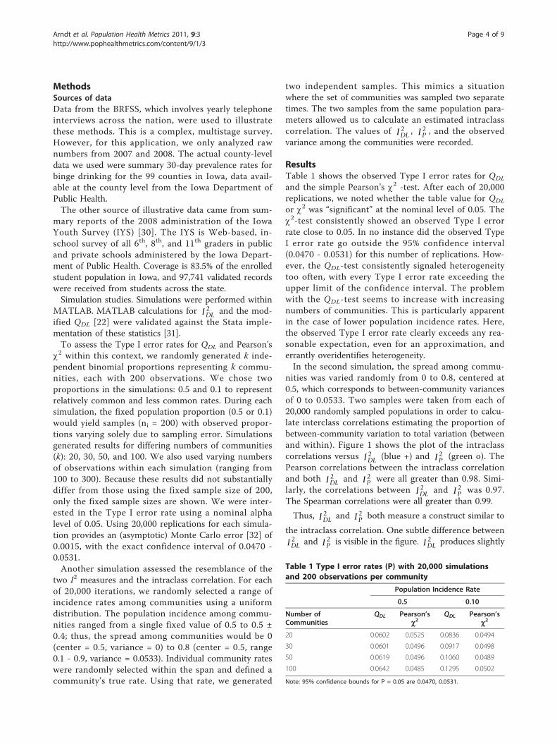
ResultsTable 1 shows the observed Type I error rates for QDL

and the simple Pearson’s c2 -test. After each of 20,000replications, we noted whether the table value for QDL

or c2 was “significant” at the nominal level of 0.05. Thec2-test consistently showed an observed Type I errorrate close to 0.05. In no instance did the observed TypeI error rate go outside the 95% confidence interval(0.0470 - 0.0531) for this number of replications. How-ever, the QDL-test consistently signaled heterogeneitytoo often, with every Type I error rate exceeding theupper limit of the confidence interval. The problemwith the QDL-test seems to increase with increasingnumbers of communities. This is particularly apparentin the case of lower population incidence rates. Here,the observed Type I error rate clearly exceeds any rea-sonable expectation, even for an approximation, anderrantly overidentifies heterogeneity.In the second simulation, the spread among commu-

nities was varied randomly from 0 to 0.8, centered at0.5, which corresponds to between-community variancesof 0 to 0.0533. Two samples were taken from each of20,000 randomly sampled populations in order to calcu-late interclass correlations estimating the proportion ofbetween-community variation to total variation (betweenand within). Figure 1 shows the plot of the intraclasscorrelations versus IDL

2 (blue +) and I P2 (green o). The

Pearson correlations between the intraclass correlationand both IDL

2 and I P2 were all greater than 0.98. Simi-

larly, the correlations between IDL2 and I P

2 was 0.97.The Spearman correlations were all greater than 0.99.

Thus, IDL2 and I P

2 both measure a construct similar to

the intraclass correlation. One subtle difference betweenIDL

2 and I P2 is visible in the figure. IDL

2 produces slightly

Table 1 Type I error rates (P) with 20,000 simulationsand 200 observations per community

Population Incidence Rate

0.5 0.10

Number ofCommunities

QDL Pearson’sc2

QDL Pearson’sc2

20 0.0602 0.0525 0.0836 0.0494

30 0.0601 0.0496 0.0917 0.0498

50 0.0619 0.0496 0.1060 0.0489

100 0.0642 0.0485 0.1295 0.0502

Note: 95% confidence bounds for P = 0.05 are 0.0470, 0.0531.

Arndt et al. Population Health Metrics 2011, 9:3http://www.pophealthmetrics.com/content/9/1/3

Page 4 of 9

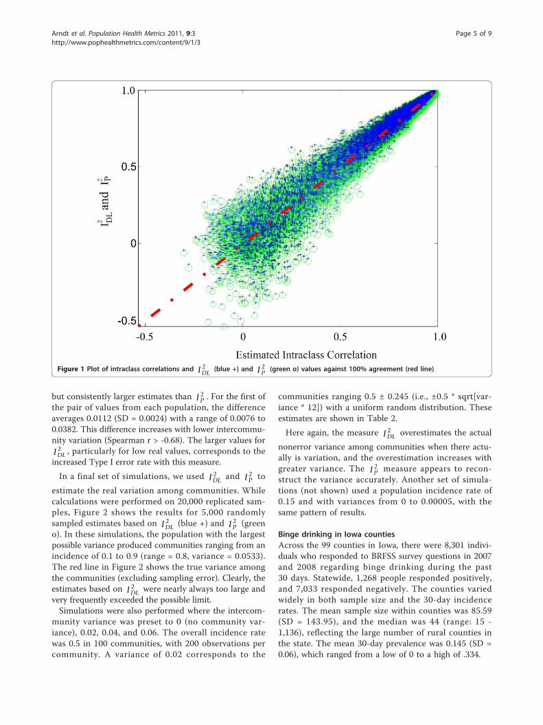
but consistently larger estimates than I P2 . For the first of

the pair of values from each population, the differenceaverages 0.0112 (SD = 0.0024) with a range of 0.0076 to0.0382. This difference increases with lower intercommu-nity variation (Spearman r > -0.68). The larger values forIDL

2 , particularly for low real values, corresponds to theincreased Type I error rate with this measure.

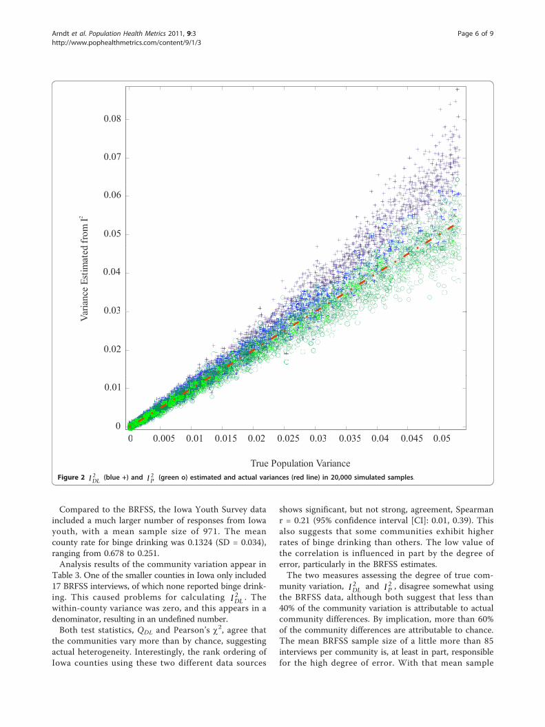
In a final set of simulations, we used IDL2 and I P

2 to

estimate the real variation among communities. Whilecalculations were performed on 20,000 replicated sam-ples, Figure 2 shows the results for 5,000 randomlysampled estimates based on IDL

2 (blue +) and I P2 (green

o). In these simulations, the population with the largestpossible variance produced communities ranging from anincidence of 0.1 to 0.9 (range = 0.8, variance = 0.0533).The red line in Figure 2 shows the true variance amongthe communities (excluding sampling error). Clearly, theestimates based on IDL

2 were nearly always too large andvery frequently exceeded the possible limit.Simulations were also performed where the intercom-

munity variance was preset to 0 (no community var-iance), 0.02, 0.04, and 0.06. The overall incidence ratewas 0.5 in 100 communities, with 200 observations percommunity. A variance of 0.02 corresponds to the

communities ranging 0.5 ± 0.245 (i.e., ±0.5 * sqrt[var-iance * 12]) with a uniform random distribution. Theseestimates are shown in Table 2.

Here again, the measure IDL2 overestimates the actual

nonerror variance among communities when there actu-ally is variation, and the overestimation increases withgreater variance. The I P

2 measure appears to recon-struct the variance accurately. Another set of simula-tions (not shown) used a population incidence rate of0.15 and with variances from 0 to 0.00005, with thesame pattern of results.

Binge drinking in Iowa countiesAcross the 99 counties in Iowa, there were 8,301 indivi-duals who responded to BRFSS survey questions in 2007and 2008 regarding binge drinking during the past30 days. Statewide, 1,268 people responded positively,and 7,033 responded negatively. The counties variedwidely in both sample size and the 30-day incidencerates. The mean sample size within counties was 85.59(SD = 143.95), and the median was 44 (range: 15 -1,136), reflecting the large number of rural counties inthe state. The mean 30-day prevalence was 0.145 (SD =0.06), which ranged from a low of 0 to a high of .334.

Figure 1 Plot of intraclass correlations and IDL2 (blue +) and I P

2 (green o) values against 100% agreement (red line).

Arndt et al. Population Health Metrics 2011, 9:3http://www.pophealthmetrics.com/content/9/1/3

Page 5 of 9

Compared to the BRFSS, the Iowa Youth Survey dataincluded a much larger number of responses from Iowayouth, with a mean sample size of 971. The meancounty rate for binge drinking was 0.1324 (SD = 0.034),ranging from 0.678 to 0.251.Analysis results of the community variation appear in

Table 3. One of the smaller counties in Iowa only included17 BRFSS interviews, of which none reported binge drink-ing. This caused problems for calculating IDL

2 . Thewithin-county variance was zero, and this appears in adenominator, resulting in an undefined number.Both test statistics, QDL and Pearson’s c2, agree that

the communities vary more than by chance, suggestingactual heterogeneity. Interestingly, the rank ordering ofIowa counties using these two different data sources

shows significant, but not strong, agreement, Spearmanr = 0.21 (95% confidence interval [CI]: 0.01, 0.39). Thisalso suggests that some communities exhibit higherrates of binge drinking than others. The low value ofthe correlation is influenced in part by the degree oferror, particularly in the BRFSS estimates.The two measures assessing the degree of true com-

munity variation, IDL2 and I P

2 , disagree somewhat usingthe BRFSS data, although both suggest that less than40% of the community variation is attributable to actualcommunity differences. By implication, more than 60%of the community differences are attributable to chance.The mean BRFSS sample size of a little more than 85interviews per community is, at least in part, responsiblefor the high degree of error. With that mean sample

0.08

0.07

0.08

0.05

0.06

d fr

omI2

0 03

0.04

aria

nce

Estim

ated

0.02

0.03

Va

0 0 005 0 01 0 015 0 02 0 025 0 03 0 035 0 04 0 045 0 050

0.01

0 0.005 0.01 0.015 0.02 0.025 0.03 0.035 0.04 0.045 0.05

True Population VarianceFigure 2 IDL

2 (blue +) and I P2 (green o) estimated and actual variances (red line) in 20,000 simulated samples.

Arndt et al. Population Health Metrics 2011, 9:3http://www.pophealthmetrics.com/content/9/1/3

Page 6 of 9

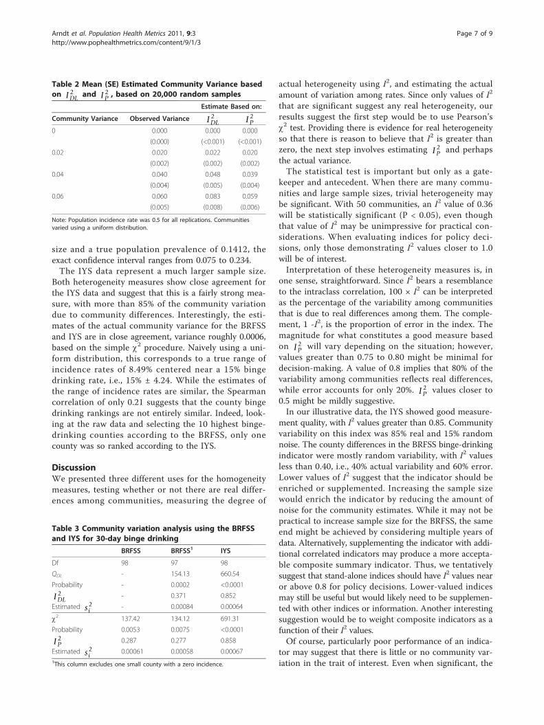
size and a true population prevalence of 0.1412, theexact confidence interval ranges from 0.075 to 0.234.The IYS data represent a much larger sample size.

Both heterogeneity measures show close agreement forthe IYS data and suggest that this is a fairly strong mea-sure, with more than 85% of the community variationdue to community differences. Interestingly, the esti-mates of the actual community variance for the BRFSSand IYS are in close agreement, variance roughly 0.0006,based on the simple c2 procedure. Naively using a uni-form distribution, this corresponds to a true range ofincidence rates of 8.49% centered near a 15% bingedrinking rate, i.e., 15% ± 4.24. While the estimates ofthe range of incidence rates are similar, the Spearmancorrelation of only 0.21 suggests that the county bingedrinking rankings are not entirely similar. Indeed, look-ing at the raw data and selecting the 10 highest binge-drinking counties according to the BRFSS, only onecounty was so ranked according to the IYS.

DiscussionWe presented three different uses for the homogeneitymeasures, testing whether or not there are real differ-ences among communities, measuring the degree of

actual heterogeneity using I2, and estimating the actualamount of variation among rates. Since only values of I2

that are significant suggest any real heterogeneity, ourresults suggest the first step would be to use Pearson’sc2 test. Providing there is evidence for real heterogeneityso that there is reason to believe that I2 is greater thanzero, the next step involves estimating I P

2 and perhapsthe actual variance.The statistical test is important but only as a gate-

keeper and antecedent. When there are many commu-nities and large sample sizes, trivial heterogeneity maybe significant. With 50 communities, an I2 value of 0.36will be statistically significant (P < 0.05), even thoughthat value of I2 may be unimpressive for practical con-siderations. When evaluating indices for policy deci-sions, only those demonstrating I2 values closer to 1.0will be of interest.Interpretation of these heterogeneity measures is, in

one sense, straightforward. Since I2 bears a resemblanceto the intraclass correlation, 100 × I2 can be interpretedas the percentage of the variability among communitiesthat is due to real differences among them. The comple-ment, 1 -I2, is the proportion of error in the index. Themagnitude for what constitutes a good measure basedon I P

2 will vary depending on the situation; however,values greater than 0.75 to 0.80 might be minimal fordecision-making. A value of 0.8 implies that 80% of thevariability among communities reflects real differences,while error accounts for only 20%. I P

2 values closer to0.5 might be mildly suggestive.In our illustrative data, the IYS showed good measure-

ment quality, with I2 values greater than 0.85. Communityvariability on this index was 85% real and 15% randomnoise. The county differences in the BRFSS binge-drinkingindicator were mostly random variability, with I2 valuesless than 0.40, i.e., 40% actual variability and 60% error.Lower values of I2 suggest that the indicator should beenriched or supplemented. Increasing the sample sizewould enrich the indicator by reducing the amount ofnoise for the community estimates. While it may not bepractical to increase sample size for the BRFSS, the sameend might be achieved by considering multiple years ofdata. Alternatively, supplementing the indicator with addi-tional correlated indicators may produce a more accepta-ble composite summary indicator. Thus, we tentativelysuggest that stand-alone indices should have I2 values nearor above 0.8 for policy decisions. Lower-valued indicesmay still be useful but would likely need to be supplemen-ted with other indices or information. Another interestingsuggestion would be to weight composite indicators as afunction of their I2 values.Of course, particularly poor performance of an indica-

tor may suggest that there is little or no community var-iation in the trait of interest. Even when significant, the

Table 2 Mean (SE) Estimated Community Variance basedon IDL

2 and I P2 , based on 20,000 random samples

Estimate Based on:

Community Variance Observed Variance IDL2 I P

2

0 0.000 0.000 0.000

(0.000) (<0.001) (<0.001)

0.02 0.020 0.022 0.020

(0.002) (0.002) (0.002)

0.04 0.040 0.048 0.039

(0.004) (0.005) (0.004)

0.06 0.060 0.083 0.059

(0.005) (0.008) (0.006)

Note: Population incidence rate was 0.5 for all replications. Communitiesvaried using a uniform distribution.

Table 3 Community variation analysis using the BRFSSand IYS for 30-day binge drinking

BRFSS BRFSS1 IYS

Df 98 97 98

QDL - 154.13 660.54

Probability - 0.0002 <0.0001

IDL2 - 0.371 0.852

Estimated si2 - 0.00084 0.00064

c2 137.42 134.12 691.31

Probability 0.0053 0.0075 <0.0001

I P2 0.287 0.277 0.858

Estimated si2 0.00061 0.00058 0.00067

1This column excludes one small county with a zero incidence.

Arndt et al. Population Health Metrics 2011, 9:3http://www.pophealthmetrics.com/content/9/1/3

Page 7 of 9

estimated intercommunity variance, si2 , gives an actual

suggestion of how big the differences are in terms of theraw rates. With a large enough sample size for manycommunities, an indicator may provide a high I2 value,but the actual variation may be epidemiologically orclinically trivial.We contrasted two different methods, one based on

meta-analysis using DerSimonian and Laird’s work [22]and one based on a simple Pearson’s c2. From a purelystatistical perspective in this context, the performance ofthe simple Pearson’s c2 was superior to the DL method.The Pearson c2 method is easy to calculate and offersbetter protection for Type I errors. I P

2 tends to mirrorthe intraclass correlation better and provides more accu-rate estimates of the true community variation in rateswhen compared to IDL

2 . The calculation of IDL2 also

becomes undefined if any of the community rates is zero.Thus, the Pearson-based method has much in its favor.

Zero counts in communities preclude calculation of IDL2

and may cause issues for I P2 , especially if there are more

than a few such counts. Most assessments of the adequacyof Pearson’s c2 in sparse tables are in the context of smal-ler cross-tabulation tables. Even then, these assessmentsfocus on how well the c2 approximation provides adequateprobability estimates for a hypothesis test [29]. The pur-pose of the c2 estimate used here is very different since itis the basis of I P

2 . Furthermore, the number of commu-nities involved tends to produce a table with a larger num-ber of rows than is typical of a cross-tabulation table inmost analytical applications. One early paper suggests thatc2 may still function adequately with low frequencies ofobservations, although perhaps with a correction (i.e.,using df = k - 2 instead of k - 1) [33]. More work may berequired to adequately assess how well I P

2 functions withzero counts, and it may possibly need to be adjusted usingtwo stage models [34], mixture models [35], or a general-ized Poisson distribution [36].The DL technique readily applies to health indices

other than rates. Means of behaviors (e.g., number ofdrinks, miles driven) or other indices are appropriateprovided standard errors are available. For example,many national datasets use complex sampling proce-dures producing data where many basic assumptions(e.g., independence) are violated. These data requireTaylor series or other approximations to produce thestandard errors around means, rates, or quintiles [37].In these more complex situations, the estimated stan-dard errors provide the information required to producethe weights needed for calculating the DL-basedmethod. However, the generalization of the Pearsonmethod is still lacking, and we have only assessed theperformance of these methods when using rates andpercentages in this paper.

Other measures of heterogeneity exist, and we onlyevaluated two. In part, our decision was based on thesemeasures’ ease of interpretation. For example, Higginsand Thompson introduced their statistic, H. Like IDL

2 ,H is based on the Q-statistic; however, it cannot beinterpreted as a percentage of variance due to heteroge-neity. Another study of heterogeneity measures intro-duces a measure similar to I P

2 , but it is based on Qrather than Pearson’s c2 [38]. Sidik and Jonkman [39]recently evaluated seven variants of heterogeneity mea-sures. Further study is clearly needed to assess thesealternatives in the current context.The heterogeneity measures also have some limita-

tions. Both the DL and Pearson methods are large sam-ple approximations; however, for most epidemiologicalapplications, this will not pose problems since the sam-ple size requirements are fairly low, e.g., expected valuesgreater than 5 in 80% or more of the communities [29].Power has been cited as a problem with the Q-test, butthis is more of an issue for meta-analyses of clinicaltrials where the number of studies (here, communities)and the number of subjects is small in terms of typicalepidemiological surveillance standards [40]. For exam-ple, with a true value for I2 = 0.5 and based on a poweranalysis for the Pearson’s c2-test, there is more than89% power to detect it in as few as 10 communities.One limitation of our study is that we used a samplesize of 200 per community for our simulations. We alsoperformed simulations where we allowed the samplesizes to vary (from 100 to 300). This corresponds tobetween one and two years of BRFSS data for US coun-ties. Thus, our results may not generalize to indicesmeasured on fewer numbers of observations. Further-more, we did not assess the adequacy of either of the I2

measures when sample sizes might be grossly imbal-anced. Finally, these measures of heterogeneity andtheir significance tests assume independent observa-tions. In this context, spatial or geographic correlationsamong the communities would violate this assumption.Semi-variograms of the exemplar data used here did notdemonstrate noticeable spatial correlation; however,such checks should be performed before using thesemethods.

ConclusionsWhen using indicators to decide how to target healthresources, the indicator should be assessed for its abilityto reflect true underlying community differences. Actualvariation in health needs, rather than chance variations,should guide decisions about programming and resourceallocation. I P

2 showed good statistical qualities and issuggested as an assessment tool for determining thequality of health indicators.

Arndt et al. Population Health Metrics 2011, 9:3http://www.pophealthmetrics.com/content/9/1/3

Page 8 of 9

AcknowledgementsThis work was supported by the National Institute on Drug Abuse, NationalInstitutes of Health (grant number RO1 DA05821).

Author details1Department of Psychiatry, Carver College of Medicine, University of Iowa,Iowa City, Iowa 52242 USA. 2Department of Biostatistics, College of PublicHealth, University of Iowa, Iowa City, Iowa 52242, USA. 3Iowa Consortium forSubstance Abuse Research and Evaluation, 100 Oakdale Campus M308 OH,University of Iowa, Iowa City, Iowa 52245-5000, USA. 4Department ofEpidemiology, College of Public Health, University of Iowa, Iowa City, Iowa52242, USA. 5Iowa Department of Public Health, Des Moines, Iowa, USA.6Department of Occupational & Environmental Health, College of PublicHealth, University of Iowa, Iowa City, Iowa 52242, USA.

Authors’ contributionsSA conceived the idea, performed analyses, and wrote the first draft. LAworked on and reviewed the statistical development and contributed to thewriting. KC reviewed the statistical development and contributed to thewriting. OD provided data and reviewed the development and writing. Allauthors read and approved the final manuscript.

Competing interestsThe authors declare that they have no competing interests.

Received: 30 June 2010 Accepted: 2 February 2011Published: 2 February 2011

References1. Muhuri PK, Ducrest JL: Block Grants and Formula Grants: A Guide for

Allotment Calculations. United States Department of Health and HumanServices SAMHSA. Office of Applied Studies edition. Rockville, MD: SAMHSA,Office of Applied Studies; 2007.

2. Buehler JW, Holtgrave DR: Challenges in defining an optimal approach toformula-based allocations of public health funds in the United States.BMC Public Health 2007, 7:44.

3. Louis TA, Jabine TB, Gerstein MA: Statistical issues in allocating funds byformula. Washington, D.C.: National Academies Press; 2003.

4. Peppard PE, Kindig DA, Dranger E, Jovaag A, Remington PL: RankingCommunity Health Status to Stimulate Discussion of Local Public HealthIssues: The Wisconsin County Health Rankings. Am J Public Health 2008,98:209-121.

5. Rohan AMK, Booske BC, Remington PL: Using the Wisconsin CountyHealth Rankings to Catalyze Community Health Improvement. Journal ofPublic Health Management and Practice 2009, 15:24-32, 10.1097/PHH.1090b1013e3181903bf3181908.

6. Flowers J, Hall P, Pencheon D: Mini-symposium – Public HealthObservatories: Public health indicators. Public Health 2005, 119:239-245.

7. Goldstein H, Spiegelhalter DJ: League tables and their limitations:Statistical issues in comparisons of institutional performance. J R StatistSoc A 1996, 159:385-443.

8. Hall P, Miller H: Using the bootstrap to quantify the authority of anempirical ranking. The Annals of Statistics 2009, 37:3939-3959.

9. Hall P, Miller H: Modeling the variability of ranks. The Annals of Statistics2010, 38:2652-2677.

10. Gauch HG: Winning the accuracy game. American Scientist 2006,94:133-141.

11. Gauch HG, Zobel RW: Accuracy and selection success in yield trialanalyses. TAG Theoretical and Applied Genetics 1989, 77:473-481.

12. Longford NT: Missing Data and Small-Area Estimation. New York: Springer;2005.

13. Laird N, Louis TA: Empirical Bayes Ranking Methods. J Ed Beh Stat 1989,14:29-46.

14. Rao JNK: Small Area Estimation. New York: Wiley; 2003.15. Shen W, Louis TA: Triple-goal estimates in two-stage hierarchical models.

J R Statist Soc B 1997, 60:455-471.16. Krieger N, Chen JT, Waterman PD, Soobader M-J, Subramanian SV, Carson R:

Geocoding and Monitoring of US Socioeconomic Inequalities inMortality and Cancer Incidence: Does the Choice of Area-based Measureand Geographic Level Matter? American Journal of Epidemiology 2002,156:471-482.

17. Krieger N, Chen JT, Waterman PD, Soobader M-J, Subramanian SV, Carson R:Choosing area based socioeconomic measures to monitor socialinequalities in low birth weight and childhood lead poisoning: ThePublic Health Disparities Geocoding Project (US). J Epidemiol CommunityHealth 2003, 57:186-199.

18. Jacobs R, Goddard M, Smith PC: How Robust Are Hospital Ranks Based onComposite Performance Measures? Med Care 2005, 43:1177-1184.

19. O’Brien SM, Peterson ED: Identifying High-Quality Hospitals: Consult theRatings or Flip a Coin? Arch Intern Med 2007, 167:1342-1344.

20. Kephart G, Asada Y: Need-based resource allocation: different needindicators, different results? BMC Health Services Research 2009, 9:1-22.

21. Page S, Cramer K: Maclean’s Rankings of Health Care Indices in CanadianCommunities, 2000: Comparisons and Statistical Contrivance. CanadianJournal of Public Health 2001, 92:295-298.

22. DerSimonian R, Laird N: Meta-analysis in clinical trials. Control Clin Trials1986, 7:177-188.

23. Higgins JP, Thompson SG: Quantifying heterogeneity in a meta-analysis.Stat Med 2002, 21:1539-1558.

24. Higgins JPT, Thompson SG, Deeks JJ, Altman DG: Measuring inconsistencyin meta-analyses. BMJ 2003, 327:557-560.

25. Cochran WG: Problems Arising in the Analysis of a Series of SimilarExperiments. Supplement to the Journal of the Royal Statistical Society 1937,4:102-118.

26. Cochran WG: Planning and Analysis of Observational Studies. New York:John Wiley & Sons; 1983.

27. Haggard E: Intraclass correlation and the analysis of variance. New York:The Dryden Press, Inc; 1958.

28. Shrout PE, Fleiss JL: Intraclass correlations: Uses in assessing raterreliability. Psychological Bulletin 1979, 86:420-428.

29. Agresti A: Categorical Data Analysis. Hoboken: John Wiley & Sons; 2002.30. 2008 County Youth Survey Reports. [http://www.iowayouthsurvey.org/

counties/county_2008.html].31. Sterne JAC, Harris RJ, Harbord RM, Steichen TJ: Meta-analysis in Stata:

metan, metacum, and metap. In Meta-Analysis in Stata: An UpdatedCollection from the Stata Journal. 2.34 edition. Edited by: Sterne JAC. CollegeStation Stata Press; 2009.

32. Koehler E, Brown E, Haneuse SJ-PA: On the assessment of Monte Carloerror in simulation-based statistical analysis. The American Statistician2009, 63:155-162.

33. Koehler K, K L: An empirical investigation of goodness-of-fit statistics forsparse multinomials. J Am Stat Assoc 1980, 75:336-344.

34. Cunningham RB, Lindenmayer DB: Modeling count data of rare species:Some statistical issues. Ecology 2005, 86:1135-1142.

35. Gilthorpe MS, Frydenberg M, Cheng Y, Baelum V: Modelling count datawith excessive zeros: The need for class prediction in zero-inflatedmodels and the issue of data generation in choosing between zero-inflated and generic mixture models for dental caries data. Statistics inMedicine 2009, 28:3539-3553.

36. Upton G, Fingleton B: Spatial Data Analysis by Example. New York: Wiley;1990.

37. Levy PS, Lemeshow S: Sampling of Populations. New York: John Wiley &Sons; 1999.

38. Mittlböck M, Heinzl H: A simulation study comparing properties ofheterogeneity measures in meta-analyses. Statistics in Medicine 2006,25:4321-4333.

39. Sidik K, Jonkman JN: A comparison of heterogeneity variance estimatorsin combining results of studies. Statistics in Medicine 2007, 26:1964-1981.

40. Hardy RJ, Thompson SG: Detecting and describing heterogeneity inmeta-analysis. Statistics in Medicine 1998, 17:841-856.

doi:10.1186/1478-7954-9-3Cite this article as: Arndt et al.: Assessing community variation andrandomness in public health indicators. Population Health Metrics 20119:3.

Arndt et al. Population Health Metrics 2011, 9:3http://www.pophealthmetrics.com/content/9/1/3

Page 9 of 9