Assessing Benefits of Neighborhood Walkability to Single-Family Property Values A Spatial Hedonic Study in Austin, Texas

Journal of Planning Education and Research 1 –18© The Author(s) 2015Reprints and permissions: sagepub.com/journalsPermissions.navDOI: 10.1177/0739456X15591055jpe.sagepub.com

Research-Based Article

Introduction

Transportation planners and policy makers have been pro-moting neighborhood walkability in pursuit of smart growth goals and carbon-intensive travel reduction, as well as public health promotion. The health and environmental benefits of neighborhood walkability have been documented by many previous studies in multiple disciplines. A number of studies have investigated the effect of built environment on physical activity and public health (Saelens and Handy 2008; Ding et al. 2011; Feng et al. 2010). Walkable neighborhoods with well-connected sidewalks, more street intersections, mixed land use, access to diverse destinations, and smaller block sizes are associated with higher levels of physical activity (Brownson et al. 2001; Frank et al. 2006; Giles-Corti and Donovan 2002, 2003; Handy et al. 2003; Hoehner et al. 2005; Humpel, Owen, and Leslie 2002; Lee and Moudon 2004; Saelens et al. 2003; Moudon et al. 2007), lower prob-ability of being overweight or obese (Sallis et al. 2009; Brown et al. 2009), better mental health (Evans 2003; Renalds, Smith, and Hale 2010), and enhancing social capi-tal (Renalds, Smith, and Hale 2010). In addition, walking, as an active transportation mode, helps individuals increase fit-ness and reduce risks of developing cardiovascular diseases, depression, and even some types of cancers (Killingsworth and Lamming 2001; Litman 2003).

While the health and environmental benefits of walking are now widely known among planners, the links between walkability and economic outcomes, such as residential property values, are less understood. In recent years, there has been a growing market demand for pedestrian- and tran-sit-oriented development in cities, reflecting changing demo-graphics and preferences (Bartholomew and Ewing 2011; McIlwain 2012). Given that these developments are in rela-tively short supply in the U.S. (Leinberger 2009; Levine 2005), homes in neighborhoods with pedestrian-oriented design features should be capitalized into higher sale prices (Landis, Guhathakurta, and Zhang 1994), thereby generating much-needed revenue from property taxes to finance pedes-trian, bicycle, and transit projects. In the current era of fiscal constraints, this provides an incentive for cities to invest in

591055 JPEXXX10.1177/0739456X15591055Journal of Planning Education and ResearchLi et al.research-article2015

Initial submission, November 2013; revised submissions, September 2014 and January 2015; final acceptance, February 2015

1Department of Landscape Architecture and Urban Planning, College of Architecture, Texas A&M University, College Station, TX, USA2Texas A&M Transportation Institute, College Station, TX, USA

Corresponding Author:Wei Li, Department of Landscape Architecture and Urban Planning, College of Architecture, Texas A&M University, 3137 TAMU, College Station, TX 77843-3137, USA. Email: [email protected]

Assessing Benefits of Neighborhood Walkability to Single-Family Property Values: A Spatial Hedonic Study in Austin, Texas

Wei Li1,2, Kenneth Joh1,2, Chanam Lee1, Jun-Hyun Kim1, Han Park1, and Ayoung Woo1

AbstractThis article investigates the impact of neighborhood walkability, measured by Street Smart Walk Score and sidewalk density, on property values by analyzing the 2010–2012 single-family home sale transactions in Austin, Texas. The Cliff-Ord spatial hedonic model (also known as the General Spatial Model, or SAC) is used to control for spatial autocorrelation effects. Results show that improving walkability through increased access to amenities in car-dependent neighborhoods does not appear to increase property values; adding sidewalks in these neighborhoods leads to a minimal increase in property values. Investments in neighborhood amenities and sidewalks will yield a greater home price increase in a walkable neighborhood than in a car-dependent neighborhood.

KeywordsCliff-Ord, General Spatial Model (SAC), property values, walk score, walkable neighborhood, walkability, spatial autocorrelation, spatial hedonic model

at Texas A&M University - Medical Sciences Library on July 23, 2015jpe.sagepub.comDownloaded from

mailto:[email protected]

http://jpe.sagepub.com/

2 Journal of Planning Education and Research

pedestrian infrastructure in addition to promoting active travel. Identifying high-priority areas for investment (such as compact neighborhoods lacking sidewalks) could help cities reap the maximum benefit from walkability premiums in real estate.

This article investigates the impact of walkability on resi-dential property values using spatial hedonic analysis of 2010–2012 single-family home sale transactions in Austin, Texas. Our primary measurement of walkability is Street Smart Walk Score (SSWS) which evaluates accessibility to neighborhood amenities based on walking distances to ame-nities and road connectivity metrics such as intersection den-sity and block length. As a supplement, we also estimate property value impact of sidewalk density (SWD). We evalu-ate how the premiums of SSWS and SWD depend on various sociodemographic factors and local environmental features such as neighborhood safety and pedestrian collision rate.

In order to control for the spatial autocorrelation effects, we employ the spatial Cliff-Ord model.1 The results from this study could help state and local governments better understand the economic consequences of their policies pro-moting neighborhood accessibility and investment in pedes-trian infrastructure.

Literature Review

Research on neighborhood walkability and the built environ-ment is based on objective measures as well as perceived assessments of the built environment (Handy, Cao, and Mokhtarian 2006). Objective measurements use geospatial analysis tools to measure the built environmental character-istics such as density of amenities, proximity to destinations, street connectivity and sidewalk density. In this category, the Walk Score (walkscore.com), which uses accessibility of neighborhood amenities as a proxy for neighborhood walk-ability (Cortright 2009; Litman 2003; Pivo and Fisher 2011; Rauterkus and Miller 2011), is widely used by the public and real estate professionals. The classic Walk Score (CWS) con-siders the Euclidean distances to amenities without account-ing for physical characteristics of the built environment such as street connectivity and sidewalk availability. The algo-rithm of the recently released SSWS considers travel routes and distances, as well as two types of street connectivity met-rics—intersection density and block length. Other research-ers have developed their own objective walkability measures, including land use mix (number of types of establishments within a specified distance), street connectivity (intersection density), and residential density (Handy, Cao, and Mokhtarian 2006; Frank et al. 2005).

Walk Score (CWS and SSWS) offers several advantages over other objective and audit-derived measures and percep-tion surveys, such as its simplicity and ease of access for the public (for instance, Walk Score is currently available for any address in the United States, Canada and Australia). Walkscore.com also offers an app for mobile device users to

get the Walk Score of any location, which further increases its versatility. Despite the simplicity and versatility of Walk Score, it has some limitations as a walkability measure, as it primarily measures neighborhood accessibility to destina-tions; it does not comprehensively represent some built envi-ronment variables that were identified to influence walking travel, such as density, land-use mix, street connectivity, and distance to transit (Cervero and Kockelman 1997; Handy, Cao, and Mokhtarian 2005; Lee and Moudon 2006; Ewing and Cervero 2010). Despite these limitations, SSWS, which incorporates street connectivity metrics such as intersection density and average block length in their algorithm, is still a robust measure of walkability and pedestrian accessibility, given that access to destinations, particularly neighborhood retail and shopping, is a critical determinant of walking travel (Handy and Clifton 2001; Boarnet et al. 2011). To fur-ther bolster our results, we included other measures in our hedonic analysis, such as residential and employment densi-ties, proximities to some neighborhood amenities including transit stations, and site and street design.

The economic benefits of walkability have been over-looked in the literature until recently. Most prior research has focused on impacts of development near transit or economic impacts associated with pedestrian- and transit-oriented development (TOD) (Bartholomew and Ewing 2011). Litman (2003) investigated the value of walkability in one of the first papers that directly addressed this topic. He argued that walkability impacts could be measured in terms of con-sumer cost savings, increased land use efficiency, healthcare cost savings, and increased economic development. Other researchers have followed suit by examining some of these elements in greater detail, such as Guo and Gandavarapu’s (2010) study, which assessed health benefits of built environ-ment investments using a cost-benefit analysis. A recent study by researchers from the Brookings Institution found that walkable neighborhoods provide a multitude of eco-nomic benefits in terms of higher residential and commercial land values, higher retail revenues, and lower transportation costs borne by residents of these neighborhoods (Leinberger and Alfonzo 2012). A recent study by Sohn, Moudon, and Lee (2012) used the hedonic pricing method to study the effects of various pro-walking environmental factors on property values. They found that increased development density could benefit surrounding property values; pedes-trian infrastructure and land use mix contributed to increases in rental property values.

There is a substantial body of literature that uses the hedonic pricing method to analyze the accessibility benefits of TOD (Landis, Guhathakurta, and Zhang 1994; Bowes and Ihlanfeldt 2001; Cervero and Duncan 2002; Song and Knaap 2004). However, most of these studies focus on distance to transit and not on the pedestrian design and land use diver-sity measures that are fundamental to TOD. There are rela-tively few studies to date that use the hedonic pricing method to capture property value impacts of walkability. However, a



Li et al. 3

few previous studies have used this method to capture access to neighborhood destinations; for example, Song and Knapp (2004) found that housing prices increased with proximity to neighborhood commercial centers and stores. There is evi-dence that street designs also influence housing prices; some studies have shown that houses in neighborhoods with grid-pattern and interconnected streets commanded higher prices, especially those proximate to transit (Song and Knaap 2003; M. Duncan 2011).

In terms of previous studies that use Walk Score as a walkability measure, Rauterkus and Miller (2011), Cortright (2009), and Pivo and Fisher (2011) used the hedonic pricing method to understand how variation in Walk Score influ-enced property values. They generally reported point esti-mates that Walk Score had positive effects on values of residential properties (Rauterkus and Miller 2011; Cortright 2009) and commercial properties (Pivo and Fisher 2011). However, results may be subject to biases caused by spatial autocorrelation effects (SAE). Generally speaking, SAE can happen in a housing sample when one house’s value is influ-enced by values or certain characteristics of neighboring properties; omitted variables in a hedonic model can also be spatially correlated with and cause SAE in the error terms (Case 1991). Failure to control for SAE can lead to biased and inconsistent estimation (Anselin 1988). In addition to using an improved version of Walk Score, this research strives to improve the methodology to assess economic ben-efits of walkability by addressing the above modeling issues.

Data

We analyzed 21,686 single-family home sale transactions from January 2010 to November 2012 in the city of Austin, Texas. As the capital of Texas and the eleventh-largest city in the U.S. with a population of 842,592 in 2012, Austin is one of the fastest-growing cities in the U.S. (U.S. Census Bureau 2013). Table 1 presents the summary statistics of variables included in our analysis. We decided to analyze no more than three years of data to avoid the risk of compromising the assumption of market equilibrium, which is required in hedonic analysis (Maclennan 1977).

Housing Data

The housing transaction variables used in this study are based on the Multiple Listing Service (MLS) data provided by the Austin Board of REALTORS®. The original MLS data included 26,107 single-family property records, including detailed information about the properties such as the living area, lot size, built year, numbers of bedrooms, full bath-rooms, half bathrooms, stories, and garage spaces; as well as binary variables about whether a property has a pool, view, and water frontage. We excluded 514 property records with the sale price higher than $1,485,000 (the 99 percentile of the sample) or lower than $63,000 (the 1 percentile of the

sample). Furthermore, 3,907 additional records were excluded due to missing or mistyped values in structural variables (1,252 records), missing values in neighborhood variables (2,452 records), missing Walk Score values (151 records), and having less than three neighboring properties within the same Census Block Group (52 records).

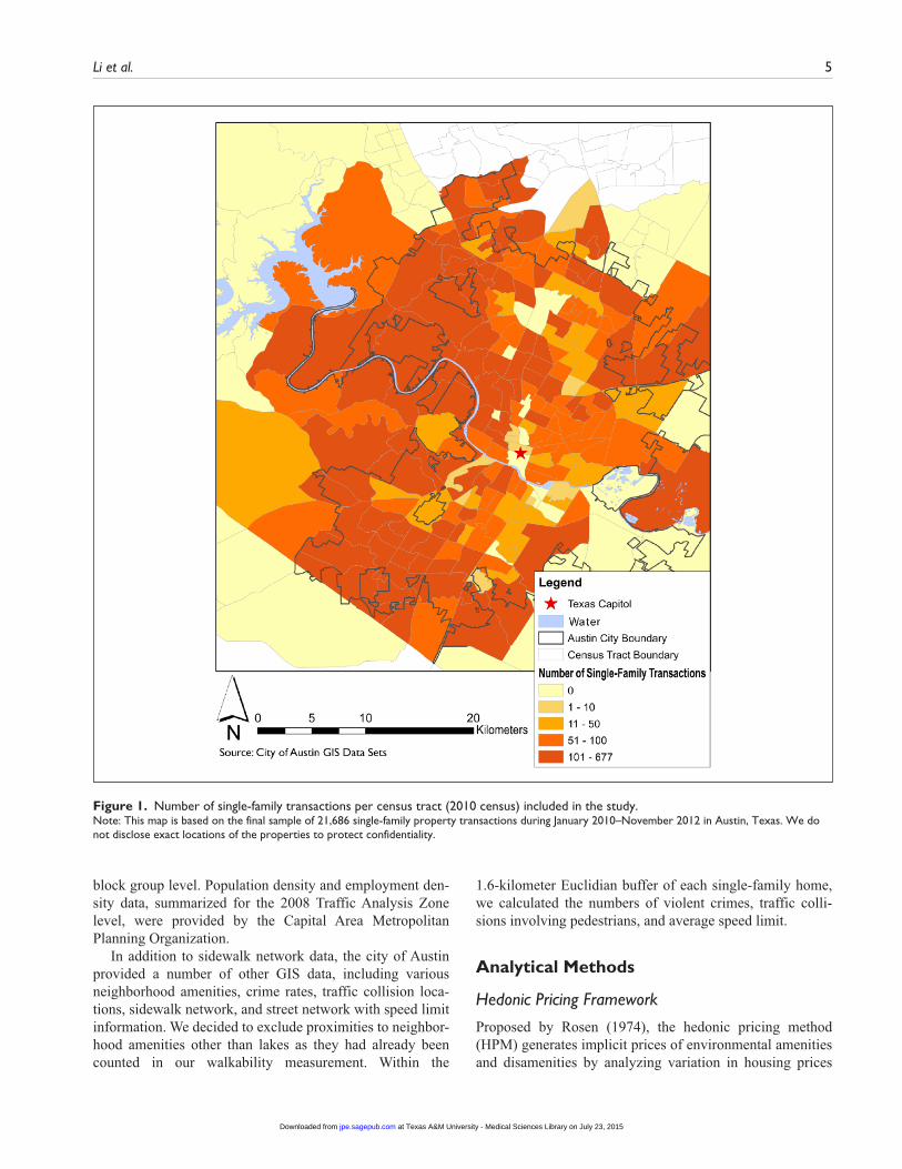
The final sample included 21,686 housing transaction records. The majority of housing records were geocoded with reference to the Geographic Information Systems (GIS) shapefile of parcel locations provided by the Travis Central Appraisal District; the remaining housing records were geo-coded in ArcGIS 10 (ESRI, Redlands, CA) using the address information of the properties. Figure 1 shows the number of housing records per 2010 census tract.2

Walkability Data

Our primary walkability measurement is Street Smart Walk Score, which was collected from walkscore.com for each house in our sample. SSWS for one address is a score between 0 and 100; a higher score indicates that neighbor-hood amenities can be better accessed by walking. The SSWS algorithm considers nine categories of amenities (gro-cery stores, restaurants/bars, shopping, coffee shops, banks, parks, schools, book stores, and entertainment); different weights are assigned to these categories based on empirical findings about their correlates with walking, such as Moudon et al. (2006) and Lee and Moudon (2006). A raw score is determined by counts of amenities, weights of categories, as well as a distance decay function based on travel routes; amenities beyond 1.6 kilometers from the address generally have little effect on the score. The raw score is then normal-ized to the 0–100 scale. Finally, the address can further receive up to 10 percent of the score depending on intersec-tion density and average block length as two street connec-tivity metrics,3 which were found to be positively associated with walking and bicycling (Berrigan, Pickle, and Dill 2010).

From the same website, we also collected the classic Walk Score, which measures availability of amenities, on the 0–100 scale as well, based on straight line distances from an address to the amenities. Although some public health researchers documented favorable evidence about reliability and validity of using CWS to measure neighborhood walk-ability (Carr, Dunsiger, and Marcus 2010, 2011; D. T. Duncan et al. 2013, 2011), we chose to use SSWS as the primary measurement of walkability due to its consideration of travel routes and street connectivity metrics.4

As a supplemental measurement of walkability, we calcu-lated SWD based on GIS data provided by the city of Austin. This variable was defined as the total length of sidewalks within a 1.6-kilometer Euclidean buffer of an address. Such a radius was chosen because our primary walkability mea-surement was determined mainly based on amenities within this radius. Sidewalks are critical elements of pedestrian infrastructure (Tal and Handy 2012), but there have been


www.walkscore.com



Table 1. Summary Statistics.

Variable Definition and Unit MeanStandard Deviation Min Max

Home sale price, $1,000 302.5840 199.4317 63.0000 1,480.0000Structural characteristics Living area, square meters (m2) 199.6537 85.5779 33.1653 809.9951 Lot area, m2 1,119.7210 1,663.3860 141.6400 69,079.83000 House age at the year of sale, year 27.6963 20.9569 0 126 Number of days on market 98.0432 80.5062 1 1253 Number of bedrooms 3.4108 0.7633 1 11 Number of full bathrooms 2.2020 0.7161 1 9 Number of half bathrooms 0.3801 0.5102 0 9 Binary: 1 = Having two or more stories 0.4402 0.4964 0 1 Binary: 1 = Having one or more garage space 0.7678 0.4222 0 1 Binary: 1 = Having pool 0.0939 0.2917 0 1 Binary: 1 = Having view 0.2749 0.4465 0 1 Binary: 1 = Located on the waterfront 0.0137 0.1162 0 1 Binary: 1 = Large/medium tree on parcel 0.8078 0.3940 0 1Neighborhood variables Network distance to state capitol, km 15.0247 7.4016 0.6272 34.7573 Network distance to nearest major road intersection, km 1.8532 1.1500 0.0084 8.0272 Network distance to nearest MetroRail station, m 9.7764 6.2139 0.2516 25.3830 Direct distance to nearest lake, m 753.4717 495.0925 0.0100 2,810.3270 School quality score in the past year, 0–100 75.2822 14.9817 28 96 Binary: 1 = highway within 400 m 0.4887 0.4999 0 1 Binary: 1 = railroad within 400 m 0.0980 0.2974 0 1Street Smart Walk Score, 0–100 29.0486 24.4788 0 99Sidewalk Density (total length within 1.6 km), km 105.9809 42.4135 0.0000 220.2860Covariates interacting with walkability Percent of African American, 0–100 5.4193 7.7488 0.0000 62.7986 Percent of Asian, 0–100 6.4240 6.4229 0.0000 35.4061 Percent of nonwhite Hispanic, 0–100 23.8140 18.3462 1.5649 89.2997 Percent of other nonwhite, 0–100 2.2859 0.7238 0.2899 4.1514 Percent of under eighteen years, 0–100 23.8527 7.3661 1.0863 46.2216 Percent of sixty-five years or older, 0–100 8.6913 5.5518 0.3621 38.0671 Per capita income, $1,000 39.8076 19.1381 6.6320 135.0570 Percent of college degree holders, 0–100 77.4262 18.5765 4.5365 100.0000 Percent of population in poverty, 0–100 4.7148 6.1634 0.0000 69.3527 Number of population per square km, 1,000 1.4254 0.8791 0.0056 8.9504 Number of jobs per square km, 1,000 0.5078 0.7527 0.0015 19.8267 Number of violent crimes within 1.6 km 58.7385 93.6088 0.0000 685.0000 Percent of household with no car, 0–100 3.9561 5.9612 0.0000 52.8395 Number of collisions involving pedestrians within 1.6 km 3.8028 5.3425 0.0000 54.3333 Average speed limit within 1.6 km, km/hour 52.2516 5.1224 40.7340 86.0538

Note: This summary table is based on the final sample of 21,686 single-family property transactions during 2010-2012 in Austin, Texas.

mixed findings about their effects on property values (Mahan, Polasky, and Adams 2000; Hamilton and Schwann 1995).

Neighborhood Data

Roadway and railroad network data were collected from ESRI Inc., the provider of the ArcGIS software. We derived the major road intersections from the roadway network shapefile data. The Capital Metropolitan Transportation

Authority (Capital Metro) provided the locational informa-tion of their commuter rail (MetroRail) stations. The Texas Department of Education provided the school performance data measured by the Texas Assessment of Knowledge and Skills test scores.

Various sociodemographic covariates, such as race/eth-nicity, age, education, poverty level, income, and vehicle ownership, were extracted from the American Community Survey 2007–2011 five-year estimates, at the 2010 census



Li et al. 5

block group level. Population density and employment den-sity data, summarized for the 2008 Traffic Analysis Zone level, were provided by the Capital Area Metropolitan Planning Organization.

In addition to sidewalk network data, the city of Austin provided a number of other GIS data, including various neighborhood amenities, crime rates, traffic collision loca-tions, sidewalk network, and street network with speed limit information. We decided to exclude proximities to neighbor-hood amenities other than lakes as they had already been counted in our walkability measurement. Within the

1.6-kilometer Euclidian buffer of each single-family home, we calculated the numbers of violent crimes, traffic colli-sions involving pedestrians, and average speed limit.

Analytical Methods

Hedonic Pricing Framework

Proposed by Rosen (1974), the hedonic pricing method (HPM) generates implicit prices of environmental amenities and disamenities by analyzing variation in housing prices

Figure 1. Number of single-family transactions per census tract (2010 census) included in the study.Note: This map is based on the final sample of 21,686 single-family property transactions during January 2010–November 2012 in Austin, Texas. We do not disclose exact locations of the properties to protect confidentiality.




within an urban area (Redfearn 2008). Our hedonic pricing framework is as follows:

ln( ) ( , , , ),p fi i i i i= S N R ε (1)

where pi is the sale price of property i; Si andNi are vectors of structural and neighborhood characteristics (see Table 1), respectively, for i; R i is a vector of walkability related vari-ables i; and εi is the error term. We estimated the effects of SSWS and SWD on property values in two separate sets of models which share the same specification other than the selection of walkability variables (see appendix A for meth-odological details). We named the set of models (e.g., ordi-nary least squares [OLS] and spatial regression models) for SSWS as routine A, and those for SWD as routine B. The rest of this subsection introduces the theoretical and empirical considerations of the hedonic pricing framework; routine A and routine B produced consistent results for all statistical tests introduced in this section.

According to Rosen (1974), a valid hedonic framework requires strong assumptions, including perfect competition, continuum of products, market equilibrium, and perfect observability of product characteristics. Bajari & Benkard (2005) provided theoretical insights that perfect competition is unreasonable for many markets and not necessary. Maclennan (1977) found that equilibrium could be generally assumed when there is no severe shock in the market, and Meese and Wallace (1997) further provided evidence that the real estate market could adjust quickly to small shocks. We found no severe shock in the market during our study period of January 2010 to November 2012. The assumption of prod-uct continuum could also be reasonably satisfied because of our large sample. Finally, perfect observability of product characteristics could be approximated as information related to houses could be accessed through the internet and profes-sional realtors and also from home inspections.

Several empirical issues were considered when applying the hedonic pricing framework to this study. In order to determine an appropriate functional form, we conducted a Box-Cox transformation test following Redfearn (2008) and Kuminoff, Parmeter, and Pope (2010). The test suggested logarithm transformations on the sale price as well as the continuous structural and neighborhood variables. Based on adjusted R-squared, Akaike Information Criterion (AIC) and Bayesian Information Criterion (BIC), this Log-Log func-tional form was determined superior to the Log-Linear form in which continuous structural and neighborhood variables are not logarithm-transformed.5 We performed the Variance Inflation Factor (VIF) test to detect the potential threat of multicollinearity and confirmed the threat to be low in our study6 based on Kennedy (2008, 199).

To identify the existence of SAE in the final sample, we performed Moran’s I test using the toolbox provided by LeSage (2010) and obtained highly significant Moran’s I statistics for both routine A and routine B, indicating the

existence of SAE in both cases. We further utilized the Lagrange Multiplier Testing Suite by Lacombe (2013) and detected that SAE existed in both the dependent variable and in the error term.7 Therefore, instead of OLS, we employed the Cliff-Ord spatial hedonic model (Cliff and Ord 1981; Anselin 1988; Arraiz et al. 2010; Saphores and Li 2012) as the optimal modeling approach in order to miti-gate the risk of SAE and omitted neighborhood variables (Pace and LeSage 2008; Brasington and Hite 2005; Anselin 1988).

The Cliff-Ord spatial hedonic model expanded equation 1 by simultaneously adding two terms: a spatial lag term for ln( )pi , which controlled for the influence of neighboring properties’ sale price to its own price; and a spatial lag term for the εi , which improves consistency of estimation by controlling for SAE in εi . Previous empirical studies which tackled SAE usually included only one lag term, either for the dependent variable (through a Spatial Lag Model) or for the error term (through a Spatial Error Model) due to soft-ware limitations or SAE test results.

To mitigate the risk of omitted variable bias, we per-formed extensive data collection; in addition, thirty-four monthly binary variables (February 2010 to November 2012) were included in the models to control for market factors. Following Anderson and West (2006) and Saphores and Li (2012), we added interaction terms to examine syn-ergies between the walkability variable (SSWS and SWD) and other sociodemographic and local environmental covariates listed in Table 1.8 These variables and covariates were normalized through a linear transformation process to simplify the interpretation of results. We also added the quadratic term for the walkability variable, which enabled us to explore whether a higher walkability level increases its premium while keeping other social-demographic and local environmental variables at their average levels. Appendix A presents details of our Cliff-Ord spatial hedonic modelling, including the introduction of the linear transfor-mation process.

Results and Discussions

Table 2 reports the estimation results of the spatial Cliff-Ord model for SSWS (routine A), and Table 3 reports the estimation results of the spatial Cliff-Ord model for SWD (routine B). Our results were generated with the maximum likelihood estimator. The impact of heteroskedasticity on our results was very little, as we obtained very similar results from the generalized spatial two-stage least-squares estimator with the heteroskedastic option. As shown in Tables 2 and 3, both AIC and BIC of the spatial Cliff-Ord models are much lower than their OLS counterparts, indi-cating superiority of this spatial regression approach over OLS for our study.

The spatial Cliff-Ord model generates total effects of structural, neighborhood, and walkability factors on



Li et al. 7

Table 2. Estimation Results for the Spatial Hedonic Model—Street Smart Walk Score (SSWS).

Variable names Coefficients Robust SE Variable names Coefficients Robust SE

Constant term 4.5809*** 0.2868 Binary: 1 = highway within 400 m –0.0013 0.0033Spatial lag coefficient for price 0.0201 0.0420 Binary: 1 = railroad within 400 m –0.0285*** 0.0062Spatial lag coefficient for error term 0.7483*** 0.0172 Walkabilityb Structural characteristicsa Normalized SSWS –0.0215*** 0.0043 Log(living area) 0.5859*** 0.0074 Square of normalized SSWS 0.0243*** 0.0043 Log(lot area) 0.0945*** 0.0033 Log(age) –0.0385*** 0.0010 Log(time on market) –0.0237*** 0.0017 Interaction terms: normalized walkability

with normalized variablesb

Log(number of bedrooms) –0.0281*** 0.0024 Percent of African American, 0–100 –0.0007 0.0033 Log(number of full bathrooms) 0.0694*** 0.0030 Percent of Asian, 0–100 –0.0240*** 0.0042 Log(number of half bathrooms) 0.0221*** 0.0033 Percent of nonwhite Hispanic, 0–100 0.0594*** 0.0108 Binary: 1 = Having two or more

stories–0.0456*** 0.0037 Percent of other nonwhite, 0–100 0.0055 0.0127

Binary: 1 = Having one or more garage space

0.0359*** 0.0041 Percent of under eighteen years, 0–100 0.0017 0.0148

Binary: 1 = Having pool 0.0843*** 0.0045 Percent of sixty-five years or older, 0–100

–0.0067 0.0069

Binary: 1 = Having view 0.0296*** 0.0032 Per capita income, $1,000 0.0045 0.0100 Binary: 1 = Located on the

waterfront0.1191*** 0.0107 Percent of college degree holders,

0–1000.1036*** 0.0341

Binary: 1 = Large/medium tree on parcel

0.0374*** 0.0031 Percent of population in poverty, 0–100

–0.0082*** 0.003

Population per square km 0.0369*** 0.0059Neighborhood variablesa Employment per square km –0.0059*** 0.0022 Log(network distance to state

capitol)–0.3230*** 0.0135 Violent crime rate within 1.6 km –0.0251*** 0.0037

Log(network distance to major road intersection)

0.0172*** 0.0037 Percent of households with no car, 0–100

0.0085*** 0.0028

Log(network distance to MetroRail station)

–0.0028 0.0090 Pedestrian accident rate within 1.6 km

0.0072*** 0.0026

Log(direct distance to lake/reservoir)

–0.0165*** 0.0023 Total length of sidewalk within 1.6 km

–0.0063 0.0119

Log(school quality) 0.0662*** 0.0164 Average speed limit within 1.6 km 0.1046*** 0.0330Number of observations 21,686Akaike Information Criterion (AIC) –13,879.87 (compared to -9,675.57 for the OLS counterpart model)Bayesian Information Criterion

(BIC)–13,161.27 (compared to -8,980.92 for the OLS counterpart model)

Note: The results are based on the final sample of 21,686 single-family property transactions during 2010–2012 in Austin, Texas. The dependent variable is the natural logarithm of the home sale price. Table 1 presents definitions and summary statistics of the relevant variables. For brevity, we do not report estimates of monthly dummy variables and the normalized constitutive terms that form interaction terms with the normalized SSWS.a. The meaning of a coefficient for a logged variable (e.g., 0.5859 for the logged living area) is the elasticity of sale price with respect to the variable; the

coefficient of a binary variable, say b, means when the binary variable changes from 0 to 1, the sale price will change by 100 * ( 1)

variance of b2e

b-- %.

b. The meaning of a coefficient (e.g., 0.0594 for “Percent of nonwhite Hispanic”) is that, keeping all the other variables interacting with Normalized SSWS at their average values, when this variable increases by the amount of its average value (e.g., the average value of the percent of nonwhite Hispanic is 23.81%, and the percent of nonwhite Hispanic population changes from 10% to 33.81%), the elasticity of sale price with respect to SSWS will change by the amount of the coefficient.***Significance level of .01.

property values, as defined by equations 5–7 in appendix A. As the total effects may vary for each individual property, they can be best characterized as a distribution instead of a point estimate. However, in our study, they are very similar to the direct effects9 (defined as a subcomponent of

equations 5–7 in appendix A), which are either estimated coefficients in Tables 2–3 (for the structural and neighbor-hood characteristics) or effects computed by linear opera-tion of the coefficients (for the walkability measurement). We will focus on interpreting direct effects for the structural




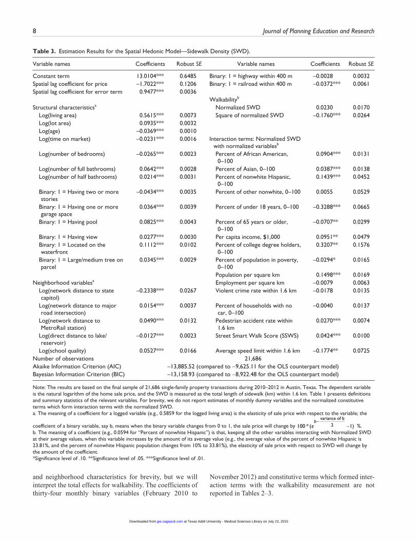
Table 3. Estimation Results for the Spatial Hedonic Model—Sidewalk Density (SWD).

Variable names Coefficients Robust SE Variable names Coefficients Robust SE

Constant term 13.0104*** 0.6485 Binary: 1 = highway within 400 m –0.0028 0.0032Spatial lag coefficient for price –1.7022*** 0.1206 Binary: 1 = railroad within 400 m –0.0372*** 0.0061Spatial lag coefficient for error term 0.9477*** 0.0036 Walkabilityb Structural characteristicsa Normalized SWD 0.0230 0.0170 Log(living area) 0.5615*** 0.0073 Square of normalized SWD –0.1760*** 0.0264 Log(lot area) 0.0935*** 0.0032 Log(age) –0.0369*** 0.0010 Log(time on market) –0.0231*** 0.0016 Interaction terms: Normalized SWD

with normalized variablesb

Log(number of bedrooms) –0.0265*** 0.0023 Percent of African American, 0–100

0.0904*** 0.0131

Log(number of full bathrooms) 0.0642*** 0.0028 Percent of Asian, 0–100 0.0387*** 0.0138 Log(number of half bathrooms) 0.0214*** 0.0031 Percent of nonwhite Hispanic,

0–1000.1439*** 0.0452

Binary: 1 = Having two or more stories

–0.0434*** 0.0035 Percent of other nonwhite, 0–100 0.0055 0.0529

Binary: 1 = Having one or more garage space

0.0364*** 0.0039 Percent of under 18 years, 0–100 –0.3288*** 0.0665

Binary: 1 = Having pool 0.0825*** 0.0043 Percent of 65 years or older, 0–100

–0.0707** 0.0299

Binary: 1 = Having view 0.0277*** 0.0030 Per capita income, $1,000 0.0951** 0.0479 Binary: 1 = Located on the

waterfront0.1112*** 0.0102 Percent of college degree holders,

0–1000.3207** 0.1576

Binary: 1 = Large/medium tree on parcel

0.0345*** 0.0029 Percent of population in poverty, 0–100

–0.0294* 0.0165

Population per square km 0.1498*** 0.0169Neighborhood variablesa Employment per square km –0.0079 0.0063 Log(network distance to state

capitol)–0.2338*** 0.0267 Violent crime rate within 1.6 km –0.0178 0.0135

Log(network distance to major road intersection)

0.0154*** 0.0037 Percent of households with no car, 0–100

–0.0040 0.0137

Log(network distance to MetroRail station)

0.0490*** 0.0132 Pedestrian accident rate within 1.6 km

0.0270*** 0.0074

Log(direct distance to lake/reservoir)

–0.0127*** 0.0023 Street Smart Walk Score (SSWS) 0.0424*** 0.0100

Log(school quality) 0.0527*** 0.0166 Average speed limit within 1.6 km –0.1774** 0.0725Number of observations 21,686Akaike Information Criterion (AIC) –13,885.52 (compared to -9,625.11 for the OLS counterpart model)Bayesian Information Criterion (BIC) –13,158.93 (compared to -8,922.48 for the OLS counterpart model)

Note: The results are based on the final sample of 21,686 single-family property transactions during 2010–2012 in Austin, Texas. The dependent variable is the natural logarithm of the home sale price, and the SWD is measured as the total length of sidewalk (km) within 1.6 km. Table 1 presents definitions and summary statistics of the relevant variables. For brevity, we do not report estimates of monthly dummy variables and the normalized constitutive terms which form interaction terms with the normalized SWD.a. The meaning of a coefficient for a logged variable (e.g., 0.5859 for the logged living area) is the elasticity of sale price with respect to the variable; the

coefficient of a binary variable, say b, means when the binary variable changes from 0 to 1, the sale price will change by 100 * ( 1)

variance of b2e

b-- %.

b. The meaning of a coefficient (e.g., 0.0594 for “Percent of nonwhite Hispanic”) is that, keeping all the other variables interacting with Normalized SWD at their average values, when this variable increases by the amount of its average value (e.g., the average value of the percent of nonwhite Hispanic is 23.81%, and the percent of nonwhite Hispanic population changes from 10% to 33.81%), the elasticity of sale price with respect to SWD will change by the amount of the coefficient.*Significance level of .10. **Significance level of .05. ***Significance level of .01.

and neighborhood characteristics for brevity, but we will interpret the total effects for walkability. The coefficients of thirty-four monthly binary variables (February 2010 to

November 2012) and constitutive terms which formed inter-action terms with the walkability measurement are not reported in Tables 2–3.



Li et al. 9

Structural and Neighborhood Characteristics

The two models (for SSWS and SWD) generate very similar results for structural and neighborhood characteristics. The effects of structural characteristics on property values are highly significant and generally have expected signs. Property values will benefit from an increase in living area, lot size, or the number of full/half bathrooms. Keeping other factors constant, having a garage, a pool, a large/medium tree on the parcel, a view, or a waterfront location positively con-tributes to a property’s value. On the other hand, property values are penalized for an older age or a longer time staying on the market. Interestingly, homes with two or more stories or those having more bedrooms are less desirable if other factors are kept constant. This may be due to regional char-acteristics—for example, single-story homes tend to have lower energy cost for cooling compared to multistory homes in the long and hot Austin summers—however, we do not have a satisfactory explanation for the negative sign on the bedroom variable. Higher school quality and closer proxim-ity to lake or state capitol, which are generally considered as positive neighborhood amenities, significantly benefits prop-erty values.

Proximity to transportation infrastructure can have two contrasting effects on property values: a positive effect because of the convenience and a negative effect because of nuisances such as congestion, air pollution and noise. In our case, the negative effect outweighs the positive effect for proximity to the nearest major road intersection. The current literature includes mixed findings about the effects of com-muter rail proximity on property values (Cervero 2006; Landis, Guhathakurta, and Zhang 1994; Armstrong and Rodriguez 2006). As Dill (2003) found that the actual dis-tance to a transit station was an important factor to determine transit use, we use the street network distance to the nearest MetroRail station to measure proximity. Our study indicates that, controlling for other factors, closer proximity to the nearest MetroRail station has a small but significant damag-ing effect on property values according to the SWD model; but this effect was not significant according to the SSWS model. Both models show that properties within 400 meters of railroad tracks are significantly less valuable than those located at least 400 meters away; this finding is consistent with the study by Armstrong and Rodriguez (2006).

Effects of Walkability on Property Values

The effects of walkability on property values are influenced by various factors. In neighborhoods with higher than sam-ple average Hispanic populations, residents are willing to pay a higher premium for increased SSWS or SWD. As expected, having a higher than average percentage of the population with college degrees significantly enhances the premium for SSWS or SWD; residents with higher level of education may develop better comprehension of benefits

brought by walking. We decided to include both poverty rate and per capita income covariates in our model after confirm-ing that the correlation between these two variables was not very high (the Pearson correlation coefficient was -0.4023). As expected, having a higher than average poverty rate sig-nificantly decreases the SSWS or SWD, as persons in pov-erty may be less willing to pay for walkability due to financial constraints. On the other hand, income has a positive effect on the premium for SWD. While a higher than average popu-lation density significantly increases the elasticities of SSWS or SWD, employment density tends to have an opposite effect on the elasticities.10 The premium of both types of walkability measurement may be compromised in neighbor-hoods with high violent crime rates, consistent with some previous findings that crime rates were negatively associated with walking (Joh, Nguyen, and Boarnet 2012; McDonald 2008).

In neighborhoods where a sizable proportion of house-holds do not own automobiles,11 residents are more willing to pay for neighborhood SSWS since walking is an important transportation mode for zero-vehicle households; however, this factor has no significant effect on the premium for SWD. Interestingly, having a higher than average pedestrian colli-sion rate within 1.6 kilometers significantly increases the premium for SSWS or SWD; this counterintuitive effect may be due to that the collision rate is positively correlated with the total number of active pedestrians. The average speed limit within 1.6 kilometers has a positive effect on the pre-mium for SSWS, while its effect on SWD is negative. The interaction term between SSWS and SWD is also worth dis-cussion: keeping all other variables at their averages, having a higher than average SWD (i.e., 106 kilometers) has no sig-nificant effect on the premium for SSWS; however, having a higher than average SSWS (i.e., 29) can significantly enhance the premium for SWD.

The overall elasticities of property values with respect to walkability (SSWS and SWD) were calculated using the total effects formula (see equation 5 in appendix A). The dis-tribution of the elasticities is shown in Figure 2: panel A for SSWS and panel B for SWD. The average SSWS elasticity of property values is 0.0160 and the median elasticity is -0.0050; for SWD, the average and median values are 0.0087 and 0.0029, respectively.

Following Carr, Dunsiger, and Marcus (2011) and D. T. Duncan et al. (2013), we categorize sample properties into four categories of neighborhoods based on the SSWS elastic-ity of property values. The first category is the car-dependent neighborhoods (SSWS<50), where there are virtually no neighborhood destinations within walking range and resi-dents must drive or take public transportation for most (if not all) of their errands; the second category is the somewhat walkable neighborhoods (50≤SSWS<70), where some ame-nities are within walking distance, but many daily trips rely on modes other than walking; the third category is the very walkable neighborhoods (70≤SSWS<90), where it is




possible to get by without a car; and the fourth category is the “walkers’ paradise” (SSWS≥90), where most errands can be accomplished by walking and many people get by without owning a car.

SSWS benefits 8,175 (37.70%) among the total 21,686 properties in our sample, while SWD benefits 11,193

(51.61%) properties.12 Both the SSWS and SWD elasticities of property values tend to be higher for homes located in more walkable neighborhoods. The average SSWS elasticity is -0.0097 for the car-dependent neighborhoods, but it becomes 0.0587 for somewhat walkable neighborhoods, and increases to 0.1637 and 0.3259 for the very walkable and

Figure 2. Distribution of elasticities.Note: The elasticities in this graph are estimated by equation 5 in appendix A



Li et al. 11

“walkers’ paradise” categories, respectively (see Figure 2A). The average SWD elasticities for the above categories are 0.0015, 0.0058, 0.0650, 0.1925, respectively (see Figure 2B).

In Table 4, we present the average property value impact of walkability in actual dollar values. For a 1 percent increase in SSWS, an average single-family home in the above cate-gories will see its property value change by –$29.56, $155.65, $548.00, and $1,329.20, respectively; for a 1 percent increase in SWD, its property value will increase by only $4.57 if a home is located in a car-dependent neighborhood, compared to $15.38 in a somewhat walkable neighborhood, $217.59 in a very walkable neighborhood, and $785.12 in a “walker’s paradise.” The positive correlations between the premium for walkability and the level of walkability may be partly due to residents’ “self-selection”: that those who prefer to walk value walkability more and may choose to live in more walk-able neighborhoods. While self-selection has been given as a reason by previous researchers to explain the observed cor-relations between the built environment and travel (Handy, Cao, and Mokhtarian 2005, 2006), it does not fully explain residential location choice. Residents’ choices may be sub-ject to other factors such as financial constraints and the sup-ply of housing at different walkability levels. In some cases, there may be a mismatch between a resident’s current resi-dential location and his or her preferences toward a particular neighborhood type and travel mode (Schwanen and Mokhtarian 2005). However, the limited evidence from our housing transaction data precludes us from examining the extent to which self-selection explains the positive correla-tions between the premium for walkability and the level of walkability.

Comparison with Previous Hedonic Studies Using Walk Score

This research reveals a different story from the previous hedonic studies using Walk Score such as Cortright (2009), Rauterkus and Miller (2011), and Pivo and Fisher (2011). We find that increased SSWS benefits only about one-third of the properties analyzed in the sample; the average elasticity for SSWS is positive in neighborhoods that are at least

somewhat walkable (SSWS≥50). For the majority of homes in our sample, the impact of increased walkability on prop-erty values is very small in magnitude.

The difference between our results with the previous stud-ies may be explained from three aspects. First, this study uses an improved version of Walk Score (SSWS was not available before 2012), which considers travel routes and physical features of pedestrian infrastructure including inter-section density and block length; this study also includes a number of other built environmental variables that were not considered in previous studies. Second, previous studies reported the point estimate—an average effect for the whole sample; our analysis considers the potential impact of sociodemographic and built-environment factors on the pre-mium for walkability, and therefore we are able to show the distribution of the premium among different properties (see Figure 2). Third, previous studies relied on the OLS method. We find that OLS overestimates the effects of walkability on property values in our study; our spatial regression approach achieves much better performance than OLS.

Concluding Remarks

In this study, we investigated the effects of neighborhood walkability on property values by analyzing 21,686 single-family home sale transactions in the city of Austin. We used SSWS as the primary walkability measure and SWD as a supplemental measure. In order to control for spatial auto-correlation effects, we employed the Cliff-Ord spatial regres-sion model.

This research shows that improving neighborhood walk-ability has the potential to increase property values for sin-gle-family homes, reflected in higher home sale prices. For cities, this means increased revenues from property taxes that could be used to fund transportation projects, schools, parks, and other municipal services. However, both the SSWS and the SWD model results show that the largest home value (and therefore tax) payoff will be in neighbor-hoods that are already walkable. Improving walkability through increased access to amenities in car-dependent neighborhoods does not appear to increase property values;

Table 4. Effects of 1 Percent Increase in Walkability on Property Values.

Neighborhood walkability level

Street Smart Walk Score (SSWS) Sidewalk Density (SWD)

Actual dollar values

Percentage of average property value

Actual dollar values

Percentage of average property value

SSWS<50 –$29.56 –0.010% $4.57 0.002%50≤SSWS<70 $155.65 0.059% $15.38 0.006%70≤SSWS<90 $548.00 0.164% $217.59 0.065%SSWS≥90 $1,329.20 0.326% $785.12 0.193%

Note: The dollar values in this table represent the effects per house. They were calculated based on the average elasticity in a walkability group (see Figure 2) and the average property value in that group.




additionally, adding sidewalks in these neighborhoods leads to a minimal increase in property values. Therefore, it is likely that an investment in sidewalks and neighborhood amenities will yield a greater home price increase in a walk-able neighborhood than in a car-dependent neighborhood.

The finding that walkability increases have a greater pro-portional impact in areas that are already somewhat walkable have some notable policy implications. If pedestrian infra-structure improvements are only made in areas that are already somewhat walkable, these investments may have limited impacts on pedestrian activity levels. However, we do not directly measure pedestrian activity levels in our study. A more important concern from a planning equity per-spective is the possibility of rising property values to pro-mote gentrification. While increases in property values may bring economic benefits by allowing more funding to be available for pedestrian investments and other municipal ser-vices, it also has the potential to decrease the affordability of housing and to displace existing lower- and middle-income residents. For example, some neighborhoods in Austin, par-ticularly in East Austin, have experienced larger increases in property values compared with the metropolitan region as a whole in recent years, which suggests that some gentrifica-tion is occurring. Based on our evidence, however, it is dif-ficult to assess the magnitude of impact that improving walkability would have on the affordability of housing, as the housing market is impacted by many external factors such as the economic climate. Nevertheless, this is an impor-tant concern for planners and policy makers that should be explored more carefully in future studies.

The housing market has become more diversified in recent years to reflect changing housing preferences. Although home buyers’ preference toward single-family detached homes, the least compact form of housing, still remains strong, the demand and support for compact and walkable communities have been increasing during the past few decades (Myers and Gearin 2001; Handy et al. 2008). The fact that this study found the largest property value effect of walkability for the most walkable neighborhoods suggests that even the walkable communities that are currently avail-able may not be sufficiently walkable to satisfy the expecta-tions of those who prefer walkable communities; in other words, the actual and latent demand for housing in walkable communities likely exceed the supply. The existing zoning regulations need to be reformed in order to create a better policy environment to facilitate the balance of the demand and supply of housing in walkable communities.

Overall, our findings lend credence to policies encourag-ing land use changes that will improve pedestrian infrastruc-ture and reduce distances from where people live to where they shop, work, and play. However, our study suggests that the following two strategies should be pursued in tandem: (1) attract more commercial development (especially neighbor-hood businesses) to residential areas and (2) improve the quality of the walking environment by adding sidewalks

along existing streets and completing pedestrian networks by linking missing segments and constructing off-street paths. The former approach is arguably more difficult as it will likely require zoning changes such as increasing allowable densities and permitting mixed-uses and require a longer time horizon, while the latter approach is more amenable to short-term implementation. Neighborhoods with good com-mercial developments but poor pedestrian infrastructure could potentially become priority areas for implementing the above strategies.

In the case of Austin, there are many areas in the city that could potentially benefit from pedestrian improvements. Examples are those older and compact neighborhoods that lack sidewalks. East Austin (see Figure 3) in particular is undergoing a renaissance with a burgeoning number of res-taurants, retail shops, bars, and mobile food trucks. However, the quality of the pedestrian infrastructure in this part of the city is far from being adequate, characterized by sidewalks that abruptly end or are nonexistent, making walking unpleasant and unsafe. Therefore, targeting pedestrian

Figure 3. Illustration of residential and commercial streets in East Austin.



Li et al. 13

infrastructure improvements in areas like this can lead to benefits in terms of not only increased property values but also more walking travel in the neighborhood.

In summary, we suggest that communities might benefit from aspiring to the goal of improving neighborhood walk-ability. While measures to improve the pedestrian environ-ment of neighborhoods may not result in immediate economic gains in car-dependent neighborhoods, it is an incremental step towards the goal, which is likely to be achieved after a long term effort. Various community sociodemographic char-acteristics should be considered when prioritizing investment strategies for improving neighborhood walkability. Given the fiscal constraints facing municipal governments throughout the nation, promoting walkability solely on environmental and health benefits may not resonate with policy makers as much as the potential for economic benefits through increased prop-erty values. The findings of this research show that allocating funding for pedestrian infrastructure and encouraging mixed-use developments in neighborhoods where walking is a likely result will yield the greatest dividends for cities through increased property tax revenue.

This study may be limited in terms of data and generaliz-ability. Despite the fact that SSWS partially accounts for street connectivity, it provides little information about other physical characteristics of pedestrian infrastructure and land use mixes. Some of the amenity categories considered for its calculation may not be regarded as amenities by residents or profession-als. Generalizability of our study remains untested. Future studies may involve more cities and other types of properties (e.g., multifamily, commercial). Particular attention may be paid to the influences of sociodemographic factors on the pre-mium for walkability, and the possibility to compare results from SSWS with those from other walkability measurements.

Appendix A

Methodological Details of Spatial Hedonic Modeling

For our sample of n = 21,686, we decided to estimate the spatial Cliff-Ord hedonic model (Cliff and Ord 1981; Anselin 1988; Arraiz et al. 2010; Saphores and Li 2012) as follows:

ln(P) = W ln(P) +S +N +R + ,

= W +u,

S N Rλρ

⋅ ⋅ ⋅ ⋅ ⋅⋅ ⋅

ββ ββ ββ εεεε εε

(2)

where

•• ln(P) is a (n × 1) vector of logarithm-transformed sale prices;

•• W is a (n × n) spatial weight matrix;•• S is a (n × 47) matrix of structural characteristics and

monthly binary variables;•• N is a (n × 7) matrix of neighborhood characteristics;•• R is a (n × 32) matrix of the walkability variable

(Street Smart Walk Score [SSWS] for routine A and

sidewalk density [SWD] for routine B), its square term, interaction terms with socio-demographic and local environmental covariates as well as the constitu-tive terms of these covariates.

•• ββS ,ββN , and ββR are vectors of coefficients;•• εε is a (n × 1) vector of error terms;•• u ~ N (0, σ2I

n) is a (n × 1) vector of error terms with-

out spatial autocorrelation effects; and•• λ and ρ are spatial lag coefficients.

The quadratic term for the walkability variable enabled us to explore whether the premium for walkability will be higher for a higher walkability level while keeping other social-demographic and local environmental variables at their average levels. We also estimated the routine A and rou-tine B models in which the quadratic term was deleted. As shown in Table A1, the models with the quadratic term of walkability outperformed their counterparts without the term based on Akaike Information Criterion (AIC) and Bayesian Information Criterion (BIC); according to models without the quadratic terms, the premiums for SSWS and SWD were still higher for areas with higher SSWS.

In order to simplify the interpretation of results, we fol-lowed the linear transformation methods implemented by Anderson and West (2006) and Saphores and Li (2012), and normalized walkability (SSWS for routine A and SWD for routine B) and its covariates as:

rr r

rki

ki k

k

=−

, (3)

where

•• rki is the original value of variable rk for property i , k ∈{ }1 2 3 17, , ,..., ;

•• rk is the sample mean of the variable rk ; and•• rki is the transformed value of variable rk for property

i.

For a property i, the component matrix R R⋅ββ in equation 2 could be written as:

R Z ZR i i⋅( ) = + + +ββ δδ ϕϕ,,i

i ix x β β0 1 (4)

where

•• xi is the quantified walkability measurement (SSWS for routine A and SWD for routine B) for property i;

•• Zi is the ith row of the (n × 16) matrix of sociodemo-graphic and local environmental covariates for prop-erty i; they form interaction terms with the walkability measurement; and13

•• δδ and ϕϕ is are vectors of estimated coefficients.

The elasticity of price with respect to walkability for prop-erty i is




e

v e

i

i ii i

∗

∗ ∗

=

= ≠

, if 0

if 0,

λ

λV , (5)

where

•• e x xi i i∗ = + + + ( )1 20 1 β β Ziδ ; and

•• Vii is the component at the ith row and ith column of matrix V (I W)≡ −−− λ 1 .

Following Saphores and Li (2012), we interpret ei∗ as a

direct effect and vi∗ as the total effect.

For property i, the elasticity of price with respect to a con-tinuous variable j, is

e

v e

j i

j i ii j i

,

, ,

,

,

if 0

if 0.

λλ=

= ≠ V

(6)

The effect of changing a dummy variable j from 0 to 1 on the value of the property i is:

ln( ) ln(p ),

,

,

, ,

pe

v ei i

j i

j i ii j i

1 0− ==

= if 0

if

λV λλ ≠

0.

(7)

For equations 6 and 7:

•• ej i, , as the direct effect, is the coefficient estimated in Table 2; and

•• vj i, is the total effect.

Following Saphores and Li (2012), we constructed a contigu-ity spatial weight matrix so that all neighbors located within the same census block group (2010 Census) have the same weight of impact on one’s property value. The contiguity matrix is doubly stochastic in nature so that the sum of each row or column is equal to 1. According to LeSage and Pace (2009), a doubly stochastic matrix generates the best linear unbiased estimation with smoothing in spatial regression mod-els. Our spatial Cliff-Ord models were estimated using the Stata package of SPPACK developed by Drukker et al. (2011).

Declaration of Conflicting Interests

The author(s) declared no potential conflicts of interest with respect to the research, authorship, and/or publication of this article.

Funding

The author(s) disclosed receipt of the following financial support for the research, authorship, and/or publication of this article: (1) Name of the supporting organization and form of support: Texas Department of Transportation. This study was funded by the Texas Department of Transportation at the direction of the Texas Legislature, under the Mobility Investment Priorities Project. (2) Interests of the supporting organization: The Texas Department of Transportation is a govern-ment agency in the state of Texas. Its stated mission is to “work with others to provide safe and reliable transportation solutions” through-out the state. (3) Funding was used to pay wages for the following contributors: Wei Li, Kenneth Joh, and Han Park.

Notes

1. The spatial Cliff-Ord model is also called the General Spatial Model, or SAC by scholars such as LeSage and Pace (2009).

2. In order to protect the confidentiality of the MLS data pro-vided by the Austin Board of REALTORS®, we decided not to disclose the map showing specific locations of these housing records.

3. Information about the SSWS algorithm was provided by walkscore.com with assistance from an anonymous reviewer.

4. After comparing the modeling results of SSWS and CWS, we concluded that, on average, SSWS had a higher effect on prop-erty values than CWS. SSWS also led to higher model perfor-mance (measured by AIC and BIC) compared to CWS for the same model specification.

5. For routine A: the adjusted R-squared, AIC, and BIC for the OLS model in the Log-Log form were 0.8835, –9,675.57, and -8,980.92, respectively, compared to 0.8663, –6,593.63, and -5,898.98 for its Log-Linear counterpart. The AIC and BIC for the spatial regression model in the Log-Log form (the optimal model) were -13,879.87 and -13,161.27, respectively, com-pared to -9,718.42 and -9,007.81 for its Log-Linear counter-part. Please note that smaller AIC and BIC indicate a better model; the adjusted R-squared was not available for the spatial regression model. The Log-Log form was also found superior to the Log-Linear form for routine B.

6. For routine A: the mean VIF of all the independent variables was 3.27 and the maximum VIF was 8.4; for routine B: the mean VIF of all the independent variables was 3.38 and the maximum VIF was 9.16.

7. For routine A: the Lagrange Multiplier (LM) values for the LM Lag test and LM Error test were 3,503.70 (p-value < .0001)

Table A1. Quadratic Terms of Walkability and Model Performance.

Routine A Routine B

Model specificationOptimal model as

presented in Figure 2AQuadratic term

excludedOptimal model as

presented in Figure 2BQuadratic term

excluded

AIC –13,879.87 –12,595.66 –13,885.52 –13,843.01BIC –13,161.27 –11,885.05 –13,158.93 –13,124.41Average elasticity SSWS<50 –0.0097 0.0078 0.0015 0.0308 50≤SSWS<70 0.0587 0.0337 0.0058 0.0768 70≤SSWS<90 0.1637 0.0445 0.0650 0.2226 SSWS≥90 0.3259 0.0897 0.1925 0.4317



Li et al. 15

and 1,003.48 (p-value < .0001), respectively; their LM values for the robust versions were 3,387.14 (p < .0001) and 900.79 (p-value < .0001), respectively. For routine B: the LM values for the LM Lag test and LM Error test were 3,842.71 (p-value < .0001) and 1,809.86 (p-value < .0001), respectively; their LM values for the robust versions were 3,674.42 (p < .0001) and 1,656.97 (p-value < .0001), respectively.

8. According to Golub, Guhathakurta, and Sollapuram (2012), interaction terms are essential to understanding how the rela-tionship between a dependent variable and an independent variable is influenced by a third variable. We followed their recommendation by including the interaction terms and cor-responding constitutive terms. We found that these interaction terms enhanced model performance. For example, in routine A, the AIC and BIC of the optimal spatial hedonic model were -13,879.87 and -13,161.27, respectively; when exclud-ing the interaction terms with sociodemographic covariates (race/ethnicity, age, income, education, poverty, population and employment density, and car ownership), the AIC and BIC of the reduced spatial hedonic model became -13,054.67 and -12,527.70, respectively; when excluding the local envi-ronmental covariates (crime, pedestrian crash rate, sidewalk density, and speed limit), the AIC and BIC of the reduced spatial hedonic model became -13,826.86 and -13,156.17, respectively.

9. Total effects and direct effects in our study are similar because the values of Vii in equations 5–7 of appendix A range from 1.0001 to 1.0009.

10. The Pearson correlation coefficient between population den-sity and employment density is 0.2541, which is much lower than we expected.

11. The benchmark used here is 3.96 percent, which is the aver-age percentage of carless households for our Austin housing sample.

12. By “benefits,” we mean the elasticity of property value with respect to walkability is greater than zero.

13. In order to mitigate the risk of multicollinearity, the pedestrian accident rate and the sidewalk density were excluded from the constitutive terms in routine A, and the pedestrian accident rate and the SSWS were excluded from the constitutive terms in routine B.

References

Anderson, Soren T., and Sarah E. West. 2006. Open space, residen-tial property values, and spatial context. Regional Science and Urban Economics 36 (6): 773–89.

Anselin, Luc. 1988. Spatial econometrics: Methods and mod-els, studies in operational regional science. Dordrecht, the Netherlands: Kluwer Academic.

Armstrong, Robert J., and Daniel A. Rodriguez. 2006. An evalu-ation of the accessibility benefits of commuter rail in east-ern Massachusetts using spatial hedonic price functions. Transportation 33 (1): 21–43.

Arraiz, Irani, David M. Drukker, Harry H. Kelejian, and Ingmar R. Prucha. 2010. A spatial cliff-ord-type model with heteroske-dastic innovations: Small and large sample results. Journal of Regional Science 50 (2): 592–614.

Bajari, Patrick, and C. Lanier Benkard. 2005. Demand estima-tion with heterogeneous consumers and unobserved product

characteristics: A hedonic approach. Journal of Political Economy 113 (6): 1239–75.

Bartholomew, Keith, and Reid Ewing. 2011. Hedonic price effects of pedestrian-and transit-oriented development. Journal of Planning Literature 26 (1): 18–34.

Berrigan, David, Linda W. Pickle, and Jennifer Dill. 2010. Associations between street connectivity and active transporta-tion. International Journal of Health Geographics 9 (1): 20.

Boarnet, Marlon G., Kenneth Joh, Walter Siembab, William Fulton, and Mai Thi Nguyen. 2011. Retrofitting the suburbs to increase walking: Evidence from a land-use-travel study. Urban Studies 48 (1): 129–59.

Bowes, David R., and Keith R. Ihlanfeldt. 2001. Identifying the impacts of rail transit stations on residential property values. Journal of Urban Economics 50 (1): 1–25.

Brasington, David M., and Diane Hite. 2005. Demand for environ-mental quality: A spatial hedonic analysis. Regional Science and Urban Economics 35 (1): 57–82.

Brown, Barbara B., Ikuho Yamada, Ken R. Smith, Cathleen D. Zick, Lori Kowaleski-Jones, and Jessie X. Fan. 2009. Mixed land use and walkability: Variations in land use measures and relationships with BMI, overweight, and obesity. Health & Place 15 (4): 1130–41. doi:http://dx.doi.org/10.1016/j.health-place.2009.06.008

Brownson, Ross C., Elizabeth A. Baker, Robyn A. Housemann, Laura K. Brennan, and Stephen J. Bacak. 2001. Environmental and policy determinants of physical activity in the United States. American Journal of Public Health 91 (12): 1995–2003.

Carr, Lucas J., Shira I. Dunsiger, and Bess H. Marcus. 2010. Walk Score™ as a global estimate of neighborhood walkability. American Journal of Preventive Medicine 39 (5): 460–63.

Carr, Lucas J., Shira I. Dunsiger, and Bess H. Marcus. 2011. Validation of Walk Score for estimating access to walk-able amenities. British Journal of Sports Medicine 45 (14): 1144–48.

Case, Anne C. 1991. Spatial patterns in household demand. Econometrica 59 (4): 953–65.

Cervero, Robert. 2006. Effects of light and commuter rail transit on land prices: Experiences in San Diego County. Berkeley: University of California Transportation Center.

Cervero, Robert, and Michael Duncan. 2002. Transit’s value-added effects: Light and commuter rail services and commercial land values. Transportation Research Record: Journal of the Transportation Research Board 1805 (1): 8–15.

Cervero, Robert, and Kara Kockelman. 1997. Travel demand and the 3Ds: Density, diversity, and design. Transportation Research Part D: Transport and Environment 2 (3): 199–219.

Cliff, Andrew D., and J. K. Ord. 1981. Spatial processes: Models & applications. Vol. 44. London: Pion.

Cortright, Joe. 2009. Walking the walk: How walkability raises home values in U.S. cities. August. Cleveland, OH: CEOs for Cities.

Dill, Jennifer. 2003. Transit use and proximity to rail: Results from large employment sites in the San Francisco, California, Bay Area. Transportation Research Record: Journal of the Transportation Research Board 1835 (1): 19–24.

Ding, D., J. F. Sallis, J. Kerr, S. Lee, and D. E. Rosenberg. 2011. Neighborhood environment and physical activity among youth: A review. American Journal of Preventive Medicine 40 (4): 442–55.


http://dx.doi.org/10.1016/j.healthplace.2009.06.008

http://dx.doi.org/10.1016/j.healthplace.2009.06.008



Drukker, David M., Hua Peng, Ingmar Prucha, and Rafal Raciborski. 2011. SPPACK: Stata module for cross-section spatial-autoregressive models. Boston: Boston College Department of Economics.

Duncan, Dustin T., Jared Aldstadt, John Whalen, and Steven J. Melly. 2013. Validation of walk scores and transit scores for estimating neighborhood walkability and transit availability: A small-area analysis. GeoJournal 78 (2): 407–16. doi:10.1007/s10708-011-9444-4

Duncan, Dustin T., Jared Aldstadt, John Whalen, Steven J. Melly, and Steven L. Gortmaker. 2011. Validation of Walk Score® for estimating neighborhood walkability: An analysis of four US metropolitan areas. International Journal of Environmental Research and Public Health 8 (11): 4160–79.

Duncan, Michael. 2011. The impact of transit-oriented develop-ment on housing prices in San Diego, CA. Urban Studies 48 (1): 101–27.

Evans, Gary. 2003. The built environment and mental health. Journal of Urban Health 80 (4): 536–55.

Ewing, Reid, and Cervero, Robert. 2010. Travel and the built envi-ronment. Journal of the American Planning Association 76 (3): 265–94.

Feng, Jing, Thomas A. Glass, Frank C. Curriero, Walter F. Stewart, and Brian S. Schwartz. 2010. The built environment and obesity: A systematic review of the epidemiologic evidence. Health & Place 16 (2): 175–90.

Frank, Lawrence D., James F. Sallis, Terry L. Conway, James E. Chapman, Brian E. Saelens, and William Bachman. 2006. Many pathways from land use to health: Associations between neighborhood walkability and active transportation, body mass index, and air quality. Journal of the American Planning Association 72 (1): 75–87. doi:10.1080/01944360608976725

Frank, Lawrence, Thomas Schmid, James Sallis, James Chapman, and Brian Saelens. 2005. Linking objectively measured physi-cal activity with objectively measured urban form: Findings from SMARTRAQ. American Journal of Preventive Medicine 28 (2): 117–25.

Giles-Corti, Billie, and Rob J. Donovan. 2002. The relative influ-ence of individual, social and physical environment deter-minants of physical activity. Social Science and Medicine 54:1793–1812.

Giles-Corti, Billie, and Robert J. Donovan. 2003. Relative influ-ences of individual, social environmental, and physical envi-ronmental correlates of walking. American Journal of Public Health 93 (9): 1583–89.

Golub, Aaron, Subhrajit Guhathakurta, and Bharath Sollapuram. 2012. Spatial and temporal capitalization effects of light rail in phoenix from conception, planning, and construction to operation. Journal of Planning Education and Research 32 (4): 415–29.

Guo, Jessica Y., and Sasanka Gandavarapu. 2010. An economic evaluation of health-promotive built environment changes. Preventive Medicine 50 (Suppl. 1): S44–S49.

Hamilton, Stanley W., and Gregory M. Schwann. 1995. Do high voltage electric transmission lines affect property value? Land Economics 71:436–44.

Handy, L. Susan, Marlon G. Boarnet, Reid Ewing, and Ricahd. E. Killingsworth. 2003. How the built environment affects physi-cal activity: Views from urban planning. American Journal of Preventive Medicine 23 (2): 64–73.

Handy, Susan, Xinyu Cao, and Patricia Mokhtarian. 2005. Correlation or causality between the built environment and travel behavior? Evidence from Northern California. Transportation Research Part D: Transport and Environment 10 (6): 427–44.

Handy, Susan, Xinyu Cao, and Patricia L Mokhtarian. 2006. Self-selection in the relationship between the built environment and walking: Empirical evidence from Northern California. Journal of the American Planning Association 72 (1): 55–74.

Handy, Susan L, and Kelly J. Clifton. 2001. Local shopping as a strategy for reducing automobile travel. Transportation 28 (4): 317–46.

Handy, Susan, James F. Sallis, Deanne Weber, Ed Maibach, and Marla Hollander. 2008. Is support for traditionally designed communities growing? Evidence from two national surveys. Journal of the American Planning Association 74 (2): 209–21.

Hoehner, Christine M., Laura K. Brennan Ramirez, Michael B. Elliott, Susan L. Handy, and Ross C. Brownson. 2005. Perceived and objective environmental measures and physical activity among urban adults. American Journal of Preventive Medicine 28 (2, Suppl. 2): 105–16.

Humpel, Nancy, Neville Owen, and Eva Leslie. 2002. Environmental factors associated with adults’ participation in physical activ-ity: A review. American Journal of Preventive Medicine 22 (3): 188–99.

Joh, Kenneth, Mai Thi Nguyen, and Marlon G. Boarnet. 2012. Can built and social environmental factors encourage walking among individuals with negative walking attitudes? Journal of Planning Education and Research 32 (2): 219–36.

Kennedy, Peter. 2008. A guide to econometrics. 6th ed. Hoboken, NJ: Wiley-Blackwell.

Killingsworth, Richard E., and Jean Lamming. 2001. Development and public health: Could our development patterns be affecting our personal health? Urban Land, July: 12–17.

Kuminoff, Nicolai V., Christopher F. Parmeter, and Jaren C. Pope. 2010. Which hedonic models can we trust to recover the mar-ginal willingness to pay for environmental amenities? Journal of Environmental Economics and Management 60 (3): 145–60. doi:10.1016/j.jeem.2010.06.001

Lacombe, Donald J. 2013. Donald J. Lacombe’s MATLAB code for spatial econometric, p. 2013. Available from http://com-munity.wvu.edu/~djl041/matlab.html (accessed 15 May 2013).

Landis, John, Subhrajit Guhathakurta, and Ming Zhang. 1994. Capitalization of transit investments into single-family home prices: A comparative analysis of five California rail transit systems. Berkeley: University of California Transportation Center.

Lee, Chanam, and Anne Vernez Moudon. 2004. Physical activ-ity and environment research in the health field: Implications for urban and transportation planning practice and research. Journal of Planning Literature 19:147–81.

Lee, Chanam, and Anne Vernez Moudon. 2006. The 3Ds+ R: Quantifying land use and urban form correlates of walking. Transportation Research Part D: Transport and Environment 11 (3): 204–15.

Leinberger, Christopher B. 2009. The option of urbanism: Investing in a new American dream. Washington, DC: Island Press.

Leinberger, Christopher, and Mariela Alfonzo. 2012. Walk this way: The economic promise of walkable places in metropoli-tan Washington, DC. Washington, DC: Metropolitan Policy Program at Brookings.


http://community.wvu.edu/~djl041/matlab.html

http://community.wvu.edu/~djl041/matlab.html


Li et al. 17

LeSage, James P. 2010. Econometrics toolbox 2010. Available from http://www.spatial-econometrics.com/ (accessed 15 May 2013).

LeSage, James P., and Robert K. Pace. 2009. Introduction to spatial econometrics. London: Chapman and Hall/CRC.

Levine, Jonathan. 2005. Zoned out: Regulations, markets, and choices in transportation and metropolitan land use. Washington, DC: RFF Press.

Litman, Todd. 2003. Economic value of walkability. Transportation Research Record: Journal of the Transportation Research Board 1828 (1): 3–11.

Maclennan, D. 1977. Some thoughts on the nature and purpose of house price studies. Urban Studies 14 (1): 59–71.

Mahan, Brent L., Stephen Polasky, and Richard M. Adams. 2000. Valuing urban wetlands: A property price approach. Land Economics 76:100–113.

McDonald, Noreen C. 2008. The effect of objectively measured crime on walking in minority adults. American Journal of Health Promotion 22 (6): 433–36.

McIlwain, John K. 2012. Housing in America: The baby boomers turn 65. Urban Land Institute Report 2012. Available from http://uli.org/wp-content/uploads/ULI-Documents/Housing InAmericaFIN.pdf.

Meese, R., and N. Wallace. 1997. The construction of residential housing price indexes: A comparison of repeat sales, hedonic regression, and hybrid approaches. Journal of Real Estate Finance and Economics 14:51–74.

Moudon, Anne, Chanam Lee, Allen D. Cheadle, Cheza Garvin, Donna B. Johnson, Thomas L. Schmid, and Robert D. Weathers. 2007. Attributes of environments supporting walk-ing. American Journal of Health Promotion 21 (5): 448–59. doi:10.4278/0890-1171-21.5.448

Moudon, Anne V., Chanam Lee, Allen D. Cheadle, Cheza Garvin, Donna Johnson, Thomas L. Schmid, Robert D. Weathers, and Lin Lin. 2006. Operational definitions of walkable neighbor-hood: Theoretical and empirical insights. Journal of Physical Activity & Health 3:S99.

Myers, Dowell, and Elizabeth Gearin. 2001. Current preferences and future demand for denser residential environments. Housing Policy Debate 12:633–59.

Pace, Robert K., and James P. LeSage. 2008. Biases of OLS and spatial lag models in the presence of an omitted variable and spatially dependent variables. Working paper. Available from http://papers.ssrn.com/sol3/papers.cfm?abstract_id= 1133438.

Pivo, Gary, and Jeffrey D. Fisher. 2011. The walkability premium in commercial real estate investments. Real Estate Economics 39 (2): 185–219.

Rauterkus, Stephanie Y., and Norman G. Miller. 2011. Residential land values and walkability. Journal of Sustainable Real Estate 3 (1): 23–43.

Redfearn, Christian L. 2008. How informative are average effects? Hedonic regression and amenity capitalization in com-plex urban housing markets. Regional Science and Urban Economics 39(3). doi:10.1016/j.regsciurbeco.2008.11.001

Renalds, Arlene, Tracey H. Smith, and Patty J. Hale. 2010. A systematic review of built environment and health. Family & Community Health 33 (1): 68–78. doi:10.1097/FCH.0b013e3181c4e2e5

Rosen, Sherwin. 1974. Hedonic prices and implicit markets: Product differentiation in pure competition. Journal of Political Economy 82:34–55.

Saelens, Brian E., and Susan L. Handy. 2008. Built environment correlates of walking: A review. Medicine and Science in Sports and Exercise 40 (7 Suppl.): S550.

Saelens, Brian E., James F. Sallis, Jennifer B. Black, and Diana Chen. 2003. Neighborhood-based differences in physical activ-ity: An environment scale evaluation. American Journal of Public Health 93 (9): 1552–58.

Sallis, James F., Brian E. Saelens, Lawrence D. Frank, Terry L. Conway, Donald J. Slymen, Kelli L. Cain, James E. Chapman, and Jacqueline Kerr. 2009. Neighborhood built environment and income: Examining multiple health outcomes. Social Science & Medicine 68 (7): 1285–93.

Saphores, Jean-Daniel, and Wei Li. 2012. Estimating the value of urban green areas: A hedonic pricing analysis of the single family housing market in Los Angeles, CA. Landscape and Urban Planning 104 (3–4): 373–87.

Schwanen, Tim, and Patricia L. Mokhtarian. 2005. What affects commute mode choice: Neighborhood physical structure or preferences toward neighborhoods? Journal of Transport Geography 13 (1): 83–99.

Sohn, Dong Wook, Anne Vernez Moudon, and Jeasun Lee. 2012. The economic value of walkable neighborhoods. Urban Design International 17 (2): 115–28.

Song, Yan, and Gerrit-Jan Knaap. 2003. New urbanism and hous-ing values: A disaggregate assessment. Journal of Urban Economics 54 (2): 218–38.

Song, Yan, and Gerrit-Jan Knaap. 2004. Measuring the effects of mixed land uses on housing values. Regional Science and Urban Economics 34 (6): 663–80.

Tal, Gil, and Susan L. Handy. 2012. Measuring nonmotorized accessibility and connectivity in a robust pedestrian network. Transportation Research Record: Journal of the Transportation Research Board 2299 (1): 48–56.

U.S. Census Bureau. 2013. Texas cities lead nation in population growth, Census Bureau reports. Available from http://www.census.gov/newsroom/releases/archives/population/cb13-94.html (accessed 30 October 2013).

Author Biographies

Wei Li is an assistant professor in the Department of Landscape Architecture and Urban Planning at Texas A&M University. His research interests include economics of sustainable urbanism, envi-ronmental and health impacts of transportation, travel survey meth-ods, valuation of urban ecosystem services, applied econometrics, and geographical information systems (GIS).

Kenneth Joh is an assistant professor in the Department of Landscape Architecture and Urban Planning at Texas A&M University. His research interests include transportation and the built environment, attitudinal and social environmental factors in nonmotorized travel, accessibility and equity issues in transporta-tion, and the link between transportation and housing.

Chanam Lee is a professor in the Department of Landscape Architecture and Urban Planning at Texas A&M University. Her research interests include urban design and physical planning,


http://www.spatial-econometrics.com/

http://uli.org/wp-content/uploads/ULI-Documents/HousingInAmericaFIN.pdf

http://uli.org/wp-content/uploads/ULI-Documents/HousingInAmericaFIN.pdf

http://papers.ssrn.com/sol3/papers.cfm?abstract_id=1133438

http://papers.ssrn.com/sol3/papers.cfm?abstract_id=1133438

http://www.census.gov/newsroom/releases/archives/population/cb13-94.html





urban form and nonmotorized transportation, physical activity, and public health.

Jun-Hyun Kim is an assistant professor in the Department of Landscape Architecture and Urban Planning at Texas A&M University. His research interests include landscape spatial pat-terns and human behavior, natural environments and public health, landscape ecology and environmental perception, built environ-ment and physical activity, sustainable and healthy community design, low-impact development, and evidence-based design methodology.

Han Park is a doctoral student in the Department of Landscape Architecture and Urban Planning at Texas A&M University. He is interested in affordable housing programs and their association with neighborhood diversity.

Ayoung Woo is a lecturer in the Department of Landscape Architecture and Urban Planning at Texas A&M University. His research interests include housing and community development, subsidized housing policies, equity issues in housing, sustainable transportation, quantitative research methods, and geographic information systems.

