Delft University of Technology Aspects of Source-Term Modeling for Vortex-Generator Induced Flows Florentie, Liesbeth DOI 10.4233/uuid:704d764a-6803-4cad-991f-45dc4ea38f6d Publication date 2018 Document Version Final published version Citation (APA) Florentie, L. (2018). Aspects of Source-Term Modeling for Vortex-Generator Induced Flows. https://doi.org/10.4233/uuid:704d764a-6803-4cad-991f-45dc4ea38f6d Important note To cite this publication, please use the final published version (if applicable). Please check the document version above. Copyright Other than for strictly personal use, it is not permitted to download, forward or distribute the text or part of it, without the consent of the author(s) and/or copyright holder(s), unless the work is under an open content license such as Creative Commons. Takedown policy Please contact us and provide details if you believe this document breaches copyrights. We will remove access to the work immediately and investigate your claim. This work is downloaded from Delft University of Technology. For technical reasons the number of authors shown on this cover page is limited to a maximum of 10.

Welcome message from author
This document is posted to help you gain knowledge. Please leave a comment to let me know what you think about it! Share it to your friends and learn new things together.
Transcript
Delft University of Technology
Aspects of Source-Term Modeling for Vortex-Generator Induced Flows
Florentie, Liesbeth
DOI10.4233/uuid:704d764a-6803-4cad-991f-45dc4ea38f6dPublication date2018Document VersionFinal published versionCitation (APA)Florentie, L. (2018). Aspects of Source-Term Modeling for Vortex-Generator Induced Flows.https://doi.org/10.4233/uuid:704d764a-6803-4cad-991f-45dc4ea38f6d
Important noteTo cite this publication, please use the final published version (if applicable).Please check the document version above.
CopyrightOther than for strictly personal use, it is not permitted to download, forward or distribute the text or part of it, without the consentof the author(s) and/or copyright holder(s), unless the work is under an open content license such as Creative Commons.
Takedown policyPlease contact us and provide details if you believe this document breaches copyrights.We will remove access to the work immediately and investigate your claim.
This work is downloaded from Delft University of Technology.For technical reasons the number of authors shown on this cover page is limited to a maximum of 10.
ASPECTS OF SOURCE-TERM MODELING FORVORTEX-GENERATOR INDUCED FLOWS

ASPECTS OF SOURCE-TERM MODELING FORVORTEX-GENERATOR INDUCED FLOWS
Dissertation
for the purpose of obtaining the degree of doctorat Delft University of Technology,
by the authority of the Rector Magnificus prof. dr. ir. T.H.J.J. van der Hagen,chair of the Board for Doctorates,
to be defended publicly onWednesday 4 April 2018 at 12:30 o’clock
by
Liesbeth FLORENTIE
Master of Science in Aerospace Engineering,Delft University of Technology, the Netherlands
born in Bonheiden, Belgium.
This dissertation has been approved by the promotors.
Composition of the doctoral committee:
Rector Magnificus, chairpersonProf. dr. ir. drs. H. Bijl, Delft University of Technology, promotorDr. S.J. Hulshoff, Delft University of Technology, copromotorDr. ir. A.H. van Zuijlen, Delft University of Technology
Independent members:Prof. dr. S. Hickel, Delft University of TechnologyProf. dr. C.B. Allen, University of BristolProf. dr. A.V. Johansson, KTH Royal Institute of TechnologyProf. dr. N.N. Sørensen, Technical University of DenmarkProf. dr. F. Scarano, Delft University of Technology, reserve member
This work has received funding from the European Union’s Seventh Programme for re-search, technological development and demonstration under grant agreement No FP7-ENERGY-2013-1/no. 608396 Advanced Aerodynamic Tools for Large Rotors (AVATAR).
Front & Back: Simulation result which shows the vortex created by a vortex generatorin a wall-bounded flow.
Copyright © 2018 by L. Florentie
ISBN 978-94-6186-918-0
An electronic version of this dissertation is available athttp://repository.tudelft.nl/.
SUMMARY
Vortex generators (VGs) are a widespread means of passive flow control, capable of yield-ing significant performance improvements to lift-generating surfaces (e.g. wind-turbineblades and airplane wings), by delaying boundary-layer separation. These small vane-type structures, which are typically arranged in arrays, trigger the formation of smallvortices in the boundary layer. The flow circulation induced by these vortices causes thenear-wall flow to be re-energized, thereby reducing the susceptibility of the boundarylayer to separate from the surface.
Predictions of the effect of a VG configuration on a flow are challenging, due to thesmall scale of VGs in combination with the complexity of the generated flow patternsand interactions. Partly-modeled/partly-resolved VG models trigger the formation of asuitable vortex in the flow by local addition of a source term to the governing equations.This type of models is considered a good trade-off between computational effort andaccuracy. Such models do not account for the smallest-scale flow features induced bythe presence of a VG, but the creation and propagation of the main vortex are resolved.
The goal of this thesis consisted of enhancing insight into the use and effectiveness ofsuch source-term models for simulating VG effects in CFD codes. To this end this studyfocused in the first instance on the current industrial standard in this respect, being theBAY and jBAY models. The scope of the analysis was limited to steady RANS simulationsof incompressible wall-bounded flows, using the boundary-layer’s shape factor as pri-mary quantity of interest. Body-fitted mesh (BFM) simulations were used as reference inorder to isolate (as much as possible) the VG modeling error from the RANS errors.
Both the BAY and the jBAY model were implemented in the open-source CFD codeOpenFOAM®, including several options to define the domain in which to apply the sourceterm. The influence of the source-term domain ΩV G was analyzed for different testcases, involving isolated VGs and VG arrays on both flat-plate and airfoil surfaces. Ouranalysis revealed that the results obtained with the BAY model depend strongly on thechoice for ΩV G , and that calibration is therefore essential in order to obtain a reasonablyaccurate flow field with a realistic amount of VG-induced circulation. In the absence ofcalibration data, the cell-selection approach proposed for the jBAY model, which con-sists of a region aligned with the actual VG orientation and a width of 2 cells in crossflowdirection, was found to yield the best calibrated flow field.
Moreover, the effect of mesh refinement on the created flow field was studied by con-sidering both flat-plate and airfoil simulations using 3 different mesh resolutions. Theresults of this study indicated the presence of a model error for the BAY and the jBAYmodel, in the sense that they both create erroneous shape-factor profiles and that theyconsistently under-predict the vortex strength, upon comparison with BFM simulations.Although the jBAY model is typically expected to show reduced mesh dependence com-pared to the BAY model (due to the involved interpolation and redistribution formula-tions), this was not observed in our results. Simulations with the BAY and jBAY mod-
v
vi SUMMARY
els applied for the same ΩV G showed that the effect of the differences in formulationbetween both models is limited, and mainly manifests as a small decrease in vorticitylevels.
Subsequently, the impact of different aspects of the source-term field, that is addedto the governing equations to represent the effect of VGs on the flow, was assessed byformulating several modified source-term formulations. Comparison of uniform andnon-uniform source-term distributions, whether or not calibrated in magnitude and/ordirection with respect to the corresponding VG surface force as obtained from a BFMsimulation, allowed assessment of the source-term’s distribution, magnitude and direc-tion. This analysis revealed that the distribution of the source term over ΩV G seems tohave a lesser influence on the characteristics of the created vortex, and that the resultantsource-term forcing dominates both the strength and shape of the created vortex. It wasfound that the magnitude of the resultant forcing is the main driver in this respect, as itdirectly governs the energy that is added to the system. Small variations in the directionof the imposed forcing were found to have only a limited effect on the created flow field.
The above mentioned analyses were mostly performed on high-resolution meshes.However, practical application of source-term VG models requires the use of coarse mesh-es. To answer the question whether it is possible to achieve sufficiently accurate flowfields when using a source-term model on a coarse mesh, an optimization frameworkwas formulated. This framework allows calculation of the optimal source term for agiven mesh, as well as the achievable accuracy. The goal functional was defined as the l 2-norm of the deviation between the velocity field obtained with a source-term simulationand a high-fidelity reference solution (in this case the projection of a BFM simulation re-sult onto the coarse mesh of interest). By making use of the Lagrange-multiplier methoda set of continuous adjoint equations was formulated which allows the direct calculationof the gradient of the goal functional with respect to the source-term distribution.
The obtained goal-functional gradient was successfully used in a trust-region opti-mization method to calculate the optimal source term for both an isolated VG and a VGarray on flat-plate surfaces. Simulations were performed for different mesh resolutionsand different source-term regions, whereΩV G was either defined as a small region cover-ing the physical VG location, or as a larger rectangular domain. It was found that with anoptimized source term significantly more accurate flow-field results are possible, char-acterized by a decrease in goal functional of almost one order of magnitude, comparedto the jBAY model. Even on very coarse meshes and for small ΩV G , a source term couldbe obtained that yields excellent shape-factor profiles already closely downstream of theVG location. Inspection of the obtained optimized source terms revealed that a closeresemblance with the actual VG reaction force on the flow does not necessarily yield thebest flow-field result.
The concept of replacing a physical VG by a local source term, without mesh adap-tations, was thus proven viable, thereby justifying continued research towards the im-provement of current source-term VG models. The developed source-term optimizationframework can serve as a useful tool in this endeavor.
SAMENVATTING
Wervel generatoren (VGs) zijn een wijd gebruikt middel voor passieve controle van stro-mingen. Het gebruik van VGs kan leiden tot aanzienlijke prestatieverbeteringen voorliftkracht-opwekkende oppervlakken (zoals bijvoorbeeld windturbinebladen en vlieg-tuigvleugels) door het uitstellen van loslating van de grenslaag. Deze kleine opstaandeobjecten, welke typisch met meerdere bij elkaar geplaatst worden, veroorzaken de vor-ming van kleine wervels in de grenslaag. De hierdoor ontstane stromingscirculatie zorgtervoor dat het energieniveau dicht bij het oppervlak toeneemt, waardoor de gevoelig-heid van de grenslaag voor loslating afneemt.
Door de kleine schaal van deze VGs, in combinatie met de complexe stromingsvor-men en interacties, is het een uitdaging om het effect van een bepaalde VG configuratieop de stroming correct te voorspellen. Modellen die de vorming van een wervel in degrenslaag nabootsen door lokale toevoeging van een bronterm aan de stromingsverge-lijkingen, en daarbij de wervel gedeeltelijk modeleren en gedeeltelijk oplossen, wordenbeschouwd als een goed compromis tussen benodigde rekenkracht en nauwkeurigheid.Deze modellen houden geen rekening met de kleinste schalen in de stroming die veroor-zaakt worden door de aanwezigheid van de VG, maar lossen wel de vorming en evolutievan de hoofdwervel op.
In dit proefschrift worden het gebruik en de effectiviteit van dit soort brontermmo-dellen voor de simulatie van de effecten van VGs in numerieke stromingsleer (CFD)codes onderzocht. De focus ligt in eerste instantie op de huidige standaard, namelijkde BAY en jBAY modellen. De gepresenteerde analyse is beperkt tot RANS simulatiesvan onsamendrukbare stromingen over een oppervlak, waarbij de vormfactor van degrenslaag geldt als belangrijkste parameter. Simulaties met een aansluitend rekenroos-ter (BFM), welke de stroming om de VG volledig oplossen, zijn gebruikt als referentie omde fout door het gebruik van een VG brontermmodel te kunnen isoleren van de RANSfout.
Zowel het BAY als het jBAY model zijn geïmplementeerd in de CFD code OpenFOAM®,in combinatie met verschillende opties om het domein van de bronterm te bepalen. Deinvloed van dit domein ΩV G is bestudeerd voor verschillende proefproblemen, waaron-der een enkele VG en VG configuraties op zowel een vlakke plaat als een vleugelprofiel.Uit deze analyse volgt dat de resultaten die verkregen zijn met het BAY model sterk af-hankelijk zijn van de keuze voor ΩV G , en dat kalibratie daarom essentieel is voor hetverkrijgen van een redelijk nauwkeurige stroming met een realistische hoeveelheid cir-culatie (opgewekt door de VG). Als geschikte kalibratiedata ontbreekt, lijkt gebruik vaneen domein zoals voorgesteld in het jBAY model (bestaande uit een regio in de richtingvan de VG van 2 cellen breed) tot het beste resultaat te leiden.
Het effect van roosterverfijning op de gecreëerde stroming is onderzocht door zowelde vlakke plaat als vleugelprofiel problemen te simuleren met 3 verschillende resolu-ties. De resultaten van deze studie duiden op de aanwezigheid van een modelfout in
vii
viii SAMENVATTING
zowel het BAY als het jBAY model, in die zin dat ze beiden tot foutieve vormfactorenleiden en de intensiteit van de gecreëerde wervel onderschatten (in vergelijking met deBFM simulaties). Van het jBAY model wordt over het algemeen een verminderde roos-terafhankelijkheid verwacht in vergelijking met het BAY model (door de interpolatie enherverdeling van parameters tijdens de berekening). Dit is echter niet waargenomen inde resultaten. Simulaties met beide modellen voor hetzelfde domein ΩV G tonen aan dathet effect van dit verschil in formulering minimaal is, en voornamelijk bestaat uit eenkleine afname van de vorticiteit.
Om de invloed van verschillende aspecten van de bronterm op de stroming te onder-zoeken zijn enkele alternatieve brontermen geformuleerd. Het effect van de bronterm-verdeling, -grootte en -richting is bestudeerd door resultaten te vergelijken welke ver-kregen zijn met zowel uniforme als niet-uniforme brontermen, al dan niet gekalibreerdvoor grootte en/of richting aan de hand van BFM simulaties (waaruit de reactiekrachtvan de VG op de stroming afgeleid is). Hieruit volgt dat de verdeling van de brontermover ΩV G minder bepalend is dan de totaal toegevoegde brontermkracht. Deze laatsedomineert zowel de intensiteit als de vorm van de ontstane wervel. De grootte van dezebrontermkracht is de belangrijkste factor in dit opzicht, aangezien deze rechtstreeks deenergie beïnvloed die wordt toegevoegd aan het systeem. Kleine variaties in de richtingvan de brontermkracht hebben slechts een miniem effect op de resulterende stroming.
Voor bovenstaande analyses is voornamelijk gebruik gemaakt van een rekenroos-ter met hoge resolutie. Praktische toepassingen van VG brontermmodellen vereisenechter typisch het gebruik van roosters met een lage resolutie. Om te onderzoeken ofhet mogelijk is om voldoende nauwkeurige resultaten te verkrijgen wanneer een bron-termmodel gebruikt wordt op een grof rooster, is daarom een optimalisatiekader ont-wikkeld. Met deze methode is het mogelijk om de optimale bronterm te berekenenvoor een bepaald (grof) rooster, evenals de hoogst haalbare nauwkeurigheid. De doel-functionaal voor deze optimalisatie is gedefinieerd als de l 2-norm van de afwijking insnelheidsveld tussen de brontermsimulatie en een referentieoplossing (in dit geval deprojectie van een BFM resultaat op het grof rooster). Door middel van de Lagrange-vermenigvuldigingsmethode is een stelsel van continue adjoint vergelijkingen afgeleid,welke de directe berekening van de gradiënt van de doelfunctionaal met betrekking totde bronterm mogelijk maakt.
De op deze manier verkregen gradiënt is succesvol gebruikt in combinatie met een’trust-region’ methode om de optimale bronterm te berekenen voor zowel een enkele VGals voor een VG configuratie op een vlakke plaat. Deze simulaties zijn uitgevoerd voorverschillende resoluties en brontermdomeinen, waarbij ΩV G gedefinieerd is als ofweleen smal domein in de richting van de VG, of als een groter rechthoekig domein. De ver-kregen resultaten tonen aan dat het gebruik van een geoptimaliseerde bronterm kan lei-den tot een aanzienlijk nauwkeuriger stromingsresultaat (gekenmerkt door een afnamein de doelfunctionaal van bijna een ordegrootte), in vergelijking met het jBAY model.Zelfs op een zeer grof rooster en voor kleine ΩV G is een bronterm verkregen welke totuitstekende vormfactorprofielen leidt op korte afstand stroomafwaarts van de VG. Hier-uit volgt dat een goede benadering van de daadwerkelijke reactiekrachtverdeling van deVG op de stroming niet per se leidt tot het meest nauwkeurige resultaat.
Het concept om een VG te vervangen door een lokale bronterm, zonder roosterwij-

SAMENVATTING ix
zigingen t.o.v. de situatie zonder VG, is dus bewezen, en voortgezet onderzoek naar eenverbetering van bestaande VG brontermmodellen is hierom gewenst. Het in dit werkontwikkelde optimalisatiekader kan hierbij dienen als een nuttig hulpmiddel.

CONTENTS
Summary v
Samenvatting vii
1 Introduction 11.1 Motivation . . . . . . . . . . . . . . . . . . . . . . . . . . . . . . . . . 11.2 Objective . . . . . . . . . . . . . . . . . . . . . . . . . . . . . . . . . . 31.3 Outline . . . . . . . . . . . . . . . . . . . . . . . . . . . . . . . . . . . 4
2 Vortex Generator Induced Flows: Background 52.1 A brief history of fluid flow analysis . . . . . . . . . . . . . . . . . . . . . 52.2 On the boundary layer and flow separation . . . . . . . . . . . . . . . . . 82.3 Vortex generators as means of passive flow control . . . . . . . . . . . . . 10
2.3.1 Types of flow control . . . . . . . . . . . . . . . . . . . . . . . . . 102.3.2 Physical principles of vortex generators . . . . . . . . . . . . . . . 112.3.3 Types and lay-outs of vortex generators . . . . . . . . . . . . . . . 14
2.4 Conclusion . . . . . . . . . . . . . . . . . . . . . . . . . . . . . . . . . 16
3 Simulating Vortex Generator Induced Flows: State of the Art 193.1 Analytical methods . . . . . . . . . . . . . . . . . . . . . . . . . . . . . 193.2 Fully-Resolved simulations . . . . . . . . . . . . . . . . . . . . . . . . . 22
3.2.1 Time-resolved VG simulations . . . . . . . . . . . . . . . . . . . . 223.2.2 RANS simulations of flows around VGs . . . . . . . . . . . . . . . 223.2.3 Immersed-boundary methods . . . . . . . . . . . . . . . . . . . . 27
3.3 Fully-modeled simulations . . . . . . . . . . . . . . . . . . . . . . . . . 273.3.1 Three-dimensional approaches . . . . . . . . . . . . . . . . . . . 273.3.2 Two-dimensional approaches . . . . . . . . . . . . . . . . . . . . 293.3.3 An analysis of 3D fully-modeled approaches . . . . . . . . . . . . . 30
3.4 Partly-modeled / Partly-resolved simulations . . . . . . . . . . . . . . . . 333.4.1 Overview. . . . . . . . . . . . . . . . . . . . . . . . . . . . . . . 333.4.2 The BAY and jBAY models . . . . . . . . . . . . . . . . . . . . . . 34
3.5 Conclusion . . . . . . . . . . . . . . . . . . . . . . . . . . . . . . . . . 37
4 Description of Study 394.1 Quantities of interest in the study of VG-induced flows . . . . . . . . . . . 39
4.1.1 Scalar descriptors of vortex properties . . . . . . . . . . . . . . . . 404.1.2 Quantifying the effect of mixing on the boundary layer . . . . . . . 41
4.2 Research scope . . . . . . . . . . . . . . . . . . . . . . . . . . . . . . . 424.2.1 Flow conditions . . . . . . . . . . . . . . . . . . . . . . . . . . . 424.2.2 Scope of the analysis . . . . . . . . . . . . . . . . . . . . . . . . . 43
xi
xii CONTENTS
4.3 Methodology . . . . . . . . . . . . . . . . . . . . . . . . . . . . . . . . 444.4 Test cases . . . . . . . . . . . . . . . . . . . . . . . . . . . . . . . . . . 46
4.4.1 Single VG on a flat plate . . . . . . . . . . . . . . . . . . . . . . . 474.4.2 Flat plate with submerged common-down VG pairs . . . . . . . . . 514.4.3 Airfoil with common-up vortex-generator pairs . . . . . . . . . . . 55
5 Analysis of the BAY and jBAY Models 615.1 Implementation details . . . . . . . . . . . . . . . . . . . . . . . . . . . 61
5.1.1 Addition of the source term to the governing equations . . . . . . . 615.1.2 VG object definition . . . . . . . . . . . . . . . . . . . . . . . . . 625.1.3 Cell selection appoaches . . . . . . . . . . . . . . . . . . . . . . . 635.1.4 Source-term calculation . . . . . . . . . . . . . . . . . . . . . . . 65
5.2 Influence of the source-term domain on the BAY-model result . . . . . . . 665.3 Mesh-sensitivity study . . . . . . . . . . . . . . . . . . . . . . . . . . . 70
5.3.1 BAY model with aligned cell selection . . . . . . . . . . . . . . . . 715.3.2 jBAY model . . . . . . . . . . . . . . . . . . . . . . . . . . . . . 74
5.4 Conclusions. . . . . . . . . . . . . . . . . . . . . . . . . . . . . . . . . 77
6 Influence of Source-Term Parameters 796.1 Rationale of the analysis . . . . . . . . . . . . . . . . . . . . . . . . . . 79
6.1.1 Additional source-term formulations . . . . . . . . . . . . . . . . 806.1.2 Set-up and Implementation . . . . . . . . . . . . . . . . . . . . . 82
6.2 Effects of source-term distribution and total forcing . . . . . . . . . . . . 826.3 Influence of magnitude and direction of the total forcing . . . . . . . . . . 906.4 Conclusions. . . . . . . . . . . . . . . . . . . . . . . . . . . . . . . . . 93
7 Development of a Goal-Oriented Source-Term Optimization Framework 957.1 Formulation of the optimization problem. . . . . . . . . . . . . . . . . . 967.2 Derivation of the continuous adjoint system . . . . . . . . . . . . . . . . 98
7.2.1 Adjoint equations . . . . . . . . . . . . . . . . . . . . . . . . . . 987.2.2 Adjoint boundary conditions . . . . . . . . . . . . . . . . . . . . 100
7.3 Gradient of the objective functional. . . . . . . . . . . . . . . . . . . . . 1027.4 Gradient optimization approach . . . . . . . . . . . . . . . . . . . . . . 102
7.4.1 Overview. . . . . . . . . . . . . . . . . . . . . . . . . . . . . . . 1027.4.2 Details of the trust-region optimization method . . . . . . . . . . . 103
7.5 Implementation . . . . . . . . . . . . . . . . . . . . . . . . . . . . . . 106
8 Accuracy and Distribution of an Optimal Source Term 1098.1 Analysis approach. . . . . . . . . . . . . . . . . . . . . . . . . . . . . . 1098.2 Validation of the adjoint-based gradient of the objective functional. . . . . 1118.3 Achievable accuracy improvement with an optimized source term . . . . . 1128.4 Characteristics of the improved source term . . . . . . . . . . . . . . . . 118
8.4.1 Optimal source term using selection type A (OSTA) . . . . . . . . . 1188.4.2 Optimal source term using selection type B (OSTB) . . . . . . . . . 119
8.5 Conclusion . . . . . . . . . . . . . . . . . . . . . . . . . . . . . . . . . 121

CONTENTS xiii
9 Conclusions & Recommendations 1239.1 Conclusions. . . . . . . . . . . . . . . . . . . . . . . . . . . . . . . . . 123
9.1.1 Effectiveness of source-term models for flow simulationsdownstream of vortex generators . . . . . . . . . . . . . . . . . . 124
9.1.2 Goal-oriented optimization of a source-term representationof vortex generators . . . . . . . . . . . . . . . . . . . . . . . . . 125
9.2 Outlook & Recommendations. . . . . . . . . . . . . . . . . . . . . . . . 126
A Additional results related to the influence of the source-term domain 129
References 135
Acknowledgements 143
List of Publications 145
Curriculum Vitæ 147

1INTRODUCTION
1.1. MOTIVATIONEngineers actively aim to manipulate flows in such a way as to yield maximum benefits.Be it the lift force generated over aircraft wings, the energy conversion in a gas turbine,or the power extracted by a wind turbine, performance largely depends on the specificcharacteristics of the flows involved. Prandtl’s famous notion that the effects of frictionare only experienced very near an object moving through a fluid, thereby introducingthe concept of a boundary layer, has proven key to many developments in this area.
One of the most simple, yet effective, means to influence a local flow field consists ofthe use of passive vortex generators (VGs). These are small vane-type obstacles that canbe mounted on a lift-generating surface, like an airplane wing. Because the fluid (air, inthe case of an airplane) now has to flow around this obstacle, a vortex is created close tothe surface. Due to the swirling motion of this vortex, the fluid particles in the boundarylayer behind the VG are mixed in such a way that energy is added to the region closest tothe surface. This has several potential benefits, one of them being that the susceptibilityof the boundary layer to separate from the surface is reduced. By ensuring an attachedflow over a larger region of the lift-generating surface, the addition of VG arrays has theability to improve the design’s overall performance.
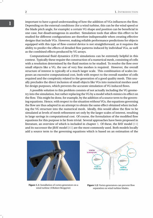
To illustrate the impact of this effect, let us consider the case of a wind turbine. Formaximal power output reduction of flow separation is essential, as those parts of theblade where the flow is separated from the surface adversely affect the power generation.In 1996 the NREL research institute performed a full-scale test in order to investigate theeffectiveness of VGs in this respect [32]. It was found that an array of VGs, distributedalong the root section of the blades (using a configuration similar as illustrated in figures1.1 and 1.2), effectively increased the power output at moderate wind speeds with almost5%. However, the experiment also revealed that the presence of the VGs caused dragpenalties, resulting in a loss in power output at low wind speeds.
From this example, it becomes clear that for the flow alteration to have an overallbeneficial effect, appropriate design and positioning of the VGs is crucial. Therefore it is
1
1
2 1. INTRODUCTION
important to have a good understanding of how the addition of VGs influences the flow.Depending on the external conditions (for a wind turbine, this can be the wind speed orthe blade pitch angle, for example) a certain VG shape and position can be beneficial inone case, but disadvantageous in another. Simulation tools that allow this effect to bestudied for different configurations are therefore indispensable when creating effectivedesigns that include VGs. However, making reliable performance predictions for objectsequipped with this type of flow-control device is not straightforward, as it requires theability to predict the effects of detailed flow patterns induced by individual VGs, as wellas the combined effects produced by VG arrays.
Computational fluid dynamics (CFD) simulations can be extremely helpful in thiscontext. Typically these require the construction of a numerical mesh, consisting of cellswith a resolution determined by the fluid motion to be studied. To resolve the flow oversmall objects like a VG, the use of very fine meshes is required. However, the overallstructure of interest is typically of a much larger scale. This combination of scales im-poses an excessive computational cost, both with respect to the overall number of cellsrequired and the complexity related to the generation of a good quality mesh. This usu-ally precludes the direct inclusion of small objects like VGs into numerical meshes usedfor design purposes, which prevents the accurate simulation of VG induced flows.
A possible solution to this problem consists of not actually including the VG geome-try into the simulation, but rather replacing the VG by a model which mimics its effect onthe flow. This might be done, for example, by the addition of a source term to the govern-ing equations. Hence, with respect to the situation without VGs, the equations governingthe flow are thus adapted in an attempt to obtain the same effect obtained when includ-ing the VG structure into the numerical mesh. Ideally, this would allow the flow to besimulated at levels of mesh refinement set only by the larger scales of interest, resultingin large savings in computational cost. Of course, the formulation of the modified flowequations for this purpose is far from trivial. Several approaches have been proposed inliterature, an overview of which is included in chapter 3. Of these, the BAY model [11]and its successor the jBAY model [41] are the most commonly used. Both models locallyadd a source term to the governing equations which is based on an estimation of the
Figure 1.1: Installation of vortex generators on awind turbine (©Robert Bergqvist)
Figure 1.2: Vortex generators can prevent flowseparation on wind turbine blades.
1.2. OBJECTIVE
1
3
fluid force acting on the VG surface.Despite their widespread use, many essential questions related to the accuracy of the
BAY and jBAY model still remain unanswered. These include the required mesh resolu-tion, and the range of reliable operating conditions. For example, it has been observedthat for airfoil angles of attack close to the stall point, both the BAY and jBAY models areunreliable in their prediction of the effects of VGs on the generated aerodynamic forces[8]. This of course undermines the trustworthiness of the obtained results, and hence theeffectiveness of new VG configuration designs. A better understanding of the principlesgoverning the results obtained with such source-term models is therefore a prerequisitefor their further use. Only when reliable simulation results, and knowledge of their limi-tations, are available, can the addition of VGs be expected to yield large efficiency gains.
1.2. OBJECTIVEConsidering the widespread use of VGs, and of source-term models like the BAY modelto simulate their effect, an urgent need exists for a better understanding of the use of VGmodels in CFD simulations. This dissertation therefore aims to unravel some of thesemysteries, by exploring both the strengths and limitations of existing source-term VGmodels, and the effects of general source term characteristics. For this study we limitour scope to incompressible wall-bounded flows, representative of, for example, wind-turbine applications. The central research question of this work can be formulated as:
How do source-term model formulation and simulation parameters affect theaccuracy of the vortex generator induced flow field obtained when performingCFD simulations of incompressible wall-bounded flows?
To answer this question, it is first of all important to identify the essential flow quan-tities when studying the effects of a VG on a boundary layer. A question which then im-mediately arises is to what level of accuracy these quantities should be reproducible by asource term model for the solution to be reliable. The answer to this question allows as-sessment of the performance of current source-term models, for example, by evaluatinghow well the BAY and jBAY model predict these key quantities.
Moreover, in order to allow for the formulation of improved source-term VG models,a fundamental insight into how specific parameters influence the created flow field is vi-tal. Therefore the current research also investigates the general potential of source-termmodels in this respect. For simulations constrained to suboptimal meshes, the ques-tion arises what is the highest accuracy one can expect to achieve when making use of asource term to reproduce VG induced flow effects. In this work, an inverse approach isconsidered in order to identify those source-term formulations. By starting from a ref-erence high-fidelity flow field, the source term that allows this flow field to be mimickedmost effectively is calculated and studied.
The created body of knowledge presented in this dissertation consists of a synthe-sis of information related to the use of source-term models for simulating VG effects onwall-bounded flows, and serves as a useful addition to the insights already present inliterature. The new approach taken here towards perturbing current source-term mod-els and optimizing their formulation will hopefully serve as an inspiration towards im-proved VG models for CFD simulations.
1
4 1. INTRODUCTION
1.3. OUTLINEThis dissertation begins by revising some fundamental concepts related to wall-boundedflows and boundary-layer separation. This can be found in chapter 2, which also pro-vides an overview of VG working principles and configurations. An overview of the cur-rent state of the art with respect to the simulation of VG-induced flow fields is containedin chapter 3.
Chapter 4 then continues by laying out the scope of the research, including the defi-nition of quantities of interest and the approaches taken to answer the central researchquestion. Furthermore, chapter 4 also contains an overview of the test cases that areconsidered in this study.
Chapter 5 is concerned with the analysis of the BAY and jBAY models. In particular,the effects of mesh resolution and the region where the model is applied are given atten-tion. In order to obtain a better understanding of the factors that influence the resultsobtained, chapter 6 elaborates on the importance of several source-term parameters,including the distribution, total magnitude and direction.
After that, a novel inverse framework, based on a continuous adjoint method, thatallows the calculation of "optimal" source terms is presented in chapter 7. This includesboth derivation and implementation details. A discussion of the obtained results for ourtest problems, and comparison with current VG models, follows in chapter 8.
Finally, chapter 9 presents the findings of this research, focusing on the various as-pects of source-term VG models and how they influence the obtained flow field. The keyparameters arising from the current work are identified, resulting in recommendationsfor further research towards the development of improved VG models.
2VORTEX GENERATOR INDUCED
FLOWS: BACKGROUND
This chapter provides some essential background information for the remainder of thisdissertation. It starts by an historical overview, in which fundamental concepts related tothe description and analysis of fluid flows are revised. This is followed in section 2.2 by adescription of boundary-layer separation for wall-bounded flows. Afterwards, in section2.3, the concept of flow control is introduced. Here, special attention is given to vortexgenerators, including an overview of common configurations and the related physicalprinciples.
2.1. A BRIEF HISTORY OF FLUID FLOW ANALYSISLong before the first scientific theories of fluid flows, people have striven to use thepower of fluids to their advantage. Examples date back to ancient civilizations, usingthe wind as power source for sailing ships. Mentions of wind-powered machines startaround the first century, evolving to widespread use of windmills in the early middleages, when they were primarily used for pumping water or for milling purposes. Effortsto understand the main fluid-dynamic principles were however limited, the only con-tributions of impact being due to two Greek philosophers. Around the 4th century B.C.,Aristotle introduced the concept of a continuum, and even an initial notion of fluid dy-namic drag. These important ideas were soon followed by Archimedes’ reflections onthe pressure in a fluid.
It took several centuries before these fundamental initial thoughts were further de-veloped. During the Renaissance, the rapid rise in importance of naval architecture trig-gered a renewed interest in fluid dynamics. In order to design more efficient ships, it be-came clear that a better understanding of the principles governing fluid flows and powergeneration was indispensable. An important contribution was made by Leonardo DaVinci in the 15th century, who studied the basic characteristics of fluid flow by meansof several experiments. His endeavors led to the important principle of conservation
5
2
6 2. VORTEX GENERATOR INDUCED FLOWS: BACKGROUND
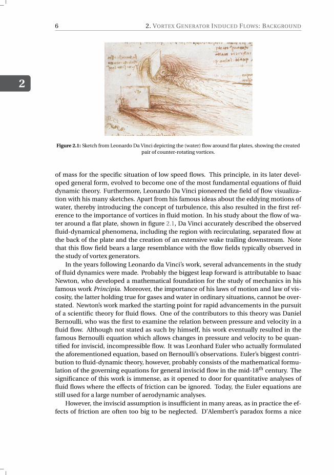
Figure 2.1: Sketch from Leonardo Da Vinci depicting the (water) flow around flat plates, showing the createdpair of counter-rotating vortices.
of mass for the specific situation of low speed flows. This principle, in its later devel-oped general form, evolved to become one of the most fundamental equations of fluiddynamic theory. Furthermore, Leonardo Da Vinci pioneered the field of flow visualiza-tion with his many sketches. Apart from his famous ideas about the eddying motions ofwater, thereby introducing the concept of turbulence, this also resulted in the first ref-erence to the importance of vortices in fluid motion. In his study about the flow of wa-ter around a flat plate, shown in figure 2.1, Da Vinci accurately described the observedfluid-dynamical phenomena, including the region with recirculating, separated flow atthe back of the plate and the creation of an extensive wake trailing downstream. Notethat this flow field bears a large resemblance with the flow fields typically observed inthe study of vortex generators.
In the years following Leonardo da Vinci’s work, several advancements in the studyof fluid dynamics were made. Probably the biggest leap forward is attributable to IsaacNewton, who developed a mathematical foundation for the study of mechanics in hisfamous work Principia. Moreover, the importance of his laws of motion and law of vis-cosity, the latter holding true for gases and water in ordinary situations, cannot be over-stated. Newton’s work marked the starting point for rapid advancements in the pursuitof a scientific theory for fluid flows. One of the contributors to this theory was DanielBernoulli, who was the first to examine the relation between pressure and velocity in afluid flow. Although not stated as such by himself, his work eventually resulted in thefamous Bernoulli equation which allows changes in pressure and velocity to be quan-tified for inviscid, incompressible flow. It was Leonhard Euler who actually formulatedthe aforementioned equation, based on Bernoulli’s observations. Euler’s biggest contri-bution to fluid-dynamic theory, however, probably consists of the mathematical formu-lation of the governing equations for general inviscid flow in the mid-18th century. Thesignificance of this work is immense, as it opened to door for quantitative analyses offluid flows where the effects of friction can be ignored. Today, the Euler equations arestill used for a large number of aerodynamic analyses.
However, the inviscid assumption is insufficient in many areas, as in practice the ef-fects of friction are often too big to be neglected. D’Alembert’s paradox forms a nice
2.1. A BRIEF HISTORY OF FLUID FLOW ANALYSIS
2
7
illustration of this. Upon calculation of the flow over a closed 2D body using the aboveinviscid, incompressible theory, d’Alembert obtained the result of zero drag. This is obvi-ously incorrect, and thus highlights the importance of including friction in the governingfluid-flow equations. At the time, the phenomenon of friction was already appreciatedby scientists, but it was not sufficiently understood to be included in theoretical analysis.
This changed in the 19th century, when both Louis Navier (with an important con-tribution of Jean-Claude Barré de Saint-Venant) and George Stokes independently suc-ceeded in incorporating the internal shear stresses into the description of fluids. In doingso, they managed to derive the governing equations for viscous flow, known widely as theNavier-Stokes equations. The importance of these equations cannot be overstated: theyprovide an excellent description of a wide variety of fluid flows, and belong to the mostfundamental fluid-dynamic equations to date. The Navier-Stokes equations account forconservation of mass and momentum and can be formulated in conservative form as
∂(ρu)
∂t+∇· (ρu) = 0 (2.1)
∂(ρu)
∂t+∇· (ρuu) = −∇p +ρf+∇·τ (2.2)
where u, p andρ represent the primary flow variables, being the (vector) velocity, (scalar)pressure and (scalar) density fields respectively. Viscous effects are included through thestress tensor τ, whose formulation depends on the type of fluid considered, and f ac-counts for external accelerations due to for example gravity. Note that in order to ac-count for compressible (high-speed) flows, the above set of equations needs to be ex-tended with the later formulated energy equation, which is essentially the first law ofthermodynamics.
Despite the fact that the Navier-Stokes equations were formulated more than a cen-tury ago, to date it still remains a challenge to analyze and solve them for arbitrary flows.The nonlinear, coupled, elliptic nature of these partial differential equations does notlend to a general analytical solution. In order to obtain solutions for specific situations,the above equations are therefore often simplified, for example based on particular ge-ometric properties or by assuming some terms to be negligible. For some rare and veryspecific cases exact analytical solutions can be obtained. In general though, engineersrely on numerical methods to obtain solutions of the Navier-Stokes equations for prac-tical situations of interest. In spite of the rapid rise in computing power, which excessedover the last few decades, obtaining numerical solutions for (2.1) and (2.2) remains a de-manding task. Luckily, the burden can often be eased by making use of Prandtl’s famousboundary-layer concept, which revolutionized the analysis of viscous flows and is thetopic of the next section.
In addition to this very brief overview, more information about the historic evolutionof fluid dynamic research can be found in [3], and the first chapter of [44]. For a morein-depth discussion of the fundamental theory of fluid dynamics, the reader is referredto [4] and [44].
2
8 2. VORTEX GENERATOR INDUCED FLOWS: BACKGROUND
2.2. ON THE BOUNDARY LAYER AND FLOW SEPARATIONIn 1904, the field of computational fluid dynamics (CFD) was not yet established andtherefore engineers lacked the tools to solve the Navier-Stokes equations for practicalflow problems. This was a frustrating problem, especially since at that time the first air-planes were being built, of which the lift and drag can be greatly affected by unforeseenflow situations, for example separation. The concepts introduced by Prandtl in that yeartherefore were indispensable for future developments. On a conference in Heidelberg,Ludwig Prandtl was the first to discuss both the boundary layer around a solid body, andthe mechanics governing the phenomenon of flow separation [43, 81].
As defined in [4], "the boundary layer is the region of flow adjacent to a surface,where the flow is retarded by the influence of friction between a solid surface and thefluid". This essentially implies that viscous effects are contained within this layer, andthat friction can be neglected outside this region, where the assumption of inviscid flowis therefore justified. Moreover, Prandtl realized that within the boundary layer and fora sufficiently high Reynolds number, the governing equations can be simplified to theso-called boundary-layer equations, which are parabolic of nature and therefore mucheasier to solve. His pioneering work therefore allowed for reliable, quantitative fluid flowanalyses.
The Reynolds number mentioned above is a dimensionless number which repre-sents the ratio between the characteristic inertial (ρU 2∞) and viscous (µU∞/L) stresses,given by
Re = ρU∞L
µ, (2.3)
where L represents some characteristic length scale and µ is the dynamic viscosity. Forhigh Re the viscous effects are relatively limited, yielding a thin boundary layer. As Redecreases, the viscous effects become relatively large and therefore the thickness of theboundary layer increases. Moreover, when Re is small (for example for low-speed flowsor fluids with a high viscosity), the large viscous effects cause instabilities to be effectivelysuppressed, such that the streamlines remain aligned and smooth. Hence, laminar flowsare characterized by low Re. On the other hand, a high Re typically indicates turbulentflow as these instabilities can no longer be suppressed.
A boundary layer arises in viscous wall-bounded flows, as in such cases friction causesthe flow immediately at the surface to stick to the surface such that the local flow veloc-ity needs to be zero. This is the so-called no-slip condition. When moving away fromthe surface, the local flow velocity gradually increases until at a certain point it (almost)equals the freestream velocity U∞. This point marks the edge of the boundary layer, andthe distance from the surface at which this happens is called the (velocity) boundary-layer thickness, denoted as δ. When the flow moves over a surface, more and more of theflow is affected by friction and therefore δ increases.
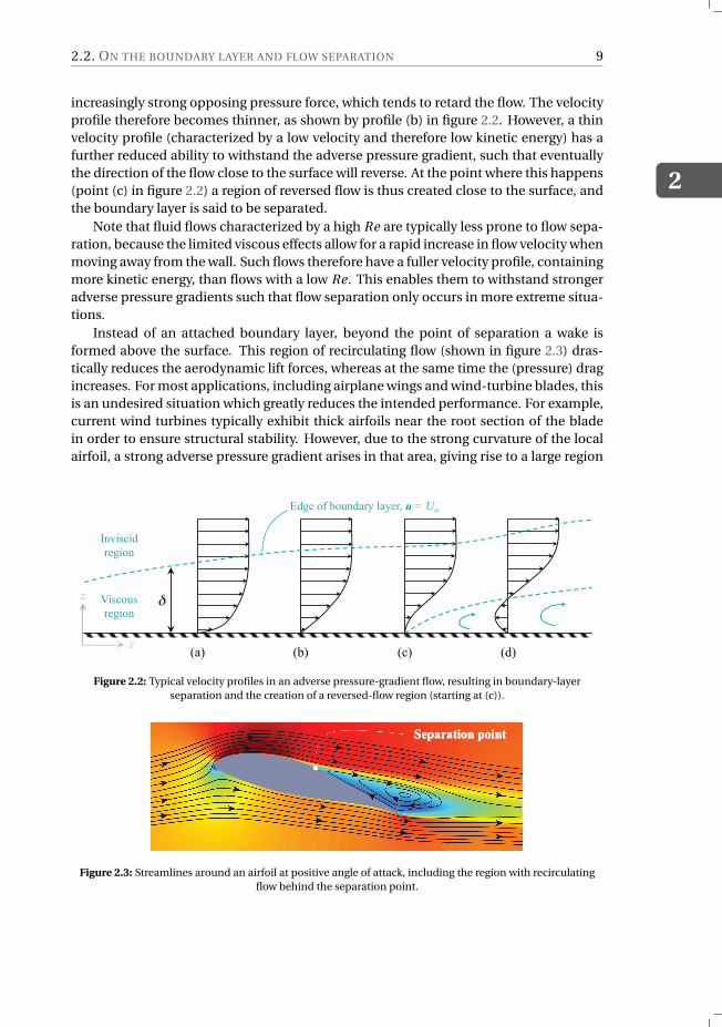
The gradual increase in velocity when moving from the surface towards the edge ofthe boundary layer defines the boundary-layer’s velocity profile, an illustration of whichis shown on the left in figure 2.2. In some situations, for example on the suction (upper)side of an airfoil at a positive angle of attack, the pressure in the boundary layer increasesas the flow moves along the surface, thereby creating a so-called adverse pressure gra-dient (∂p/∂x > 0). This situation is called adverse, because the flow has to overcome an
2.2. ON THE BOUNDARY LAYER AND FLOW SEPARATION
2
9
increasingly strong opposing pressure force, which tends to retard the flow. The velocityprofile therefore becomes thinner, as shown by profile (b) in figure 2.2. However, a thinvelocity profile (characterized by a low velocity and therefore low kinetic energy) has afurther reduced ability to withstand the adverse pressure gradient, such that eventuallythe direction of the flow close to the surface will reverse. At the point where this happens(point (c) in figure 2.2) a region of reversed flow is thus created close to the surface, andthe boundary layer is said to be separated.
Note that fluid flows characterized by a high Re are typically less prone to flow sepa-ration, because the limited viscous effects allow for a rapid increase in flow velocity whenmoving away from the wall. Such flows therefore have a fuller velocity profile, containingmore kinetic energy, than flows with a low Re. This enables them to withstand strongeradverse pressure gradients such that flow separation only occurs in more extreme situa-tions.
Instead of an attached boundary layer, beyond the point of separation a wake isformed above the surface. This region of recirculating flow (shown in figure 2.3) dras-tically reduces the aerodynamic lift forces, whereas at the same time the (pressure) dragincreases. For most applications, including airplane wings and wind-turbine blades, thisis an undesired situation which greatly reduces the intended performance. For example,current wind turbines typically exhibit thick airfoils near the root section of the bladein order to ensure structural stability. However, due to the strong curvature of the localairfoil, a strong adverse pressure gradient arises in that area, giving rise to a large region
δ
Inviscid
region
Viscous
region
(a) (b) (c) (d) x
z
Edge of boundary layer, u = U∞
Figure 2.2: Typical velocity profiles in an adverse pressure-gradient flow, resulting in boundary-layerseparation and the creation of a reversed-flow region (starting at (c)).
Figure 2.3: Streamlines around an airfoil at positive angle of attack, including the region with recirculatingflow behind the separation point.
2
10 2. VORTEX GENERATOR INDUCED FLOWS: BACKGROUND
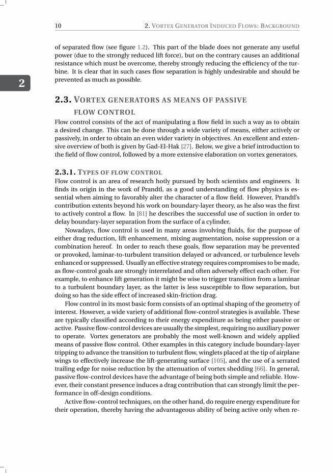
of separated flow (see figure 1.2). This part of the blade does not generate any usefulpower (due to the strongly reduced lift force), but on the contrary causes an additionalresistance which must be overcome, thereby strongly reducing the efficiency of the tur-bine. It is clear that in such cases flow separation is highly undesirable and should beprevented as much as possible.
2.3. VORTEX GENERATORS AS MEANS OF PASSIVE
FLOW CONTROLFlow control consists of the act of manipulating a flow field in such a way as to obtaina desired change. This can be done through a wide variety of means, either actively orpassively, in order to obtain an even wider variety in objectives. An excellent and exten-sive overview of both is given by Gad-El-Hak [27]. Below, we give a brief introduction tothe field of flow control, followed by a more extensive elaboration on vortex generators.
2.3.1. TYPES OF FLOW CONTROLFlow control is an area of research hotly pursued by both scientists and engineers. Itfinds its origin in the work of Prandtl, as a good understanding of flow physics is es-sential when aiming to favorably alter the character of a flow field. However, Prandtl’scontribution extents beyond his work on boundary-layer theory, as he also was the firstto actively control a flow. In [81] he describes the successful use of suction in order todelay boundary-layer separation from the surface of a cylinder.
Nowadays, flow control is used in many areas involving fluids, for the purpose ofeither drag reduction, lift enhancement, mixing augmentation, noise suppression or acombination hereof. In order to reach these goals, flow separation may be preventedor provoked, laminar-to-turbulent transition delayed or advanced, or turbulence levelsenhanced or suppressed. Usually an effective strategy requires compromises to be made,as flow-control goals are strongly interrelated and often adversely effect each other. Forexample, to enhance lift generation it might be wise to trigger transition from a laminarto a turbulent boundary layer, as the latter is less susceptible to flow separation, butdoing so has the side effect of increased skin-friction drag.
Flow control in its most basic form consists of an optimal shaping of the geometry ofinterest. However, a wide variety of additional flow-control strategies is available. Theseare typically classified according to their energy expenditure as being either passive oractive. Passive flow-control devices are usually the simplest, requiring no auxiliary powerto operate. Vortex generators are probably the most well-known and widely appliedmeans of passive flow control. Other examples in this category include boundary-layertripping to advance the transition to turbulent flow, winglets placed at the tip of airplanewings to effectively increase the lift-generating surface [105], and the use of a serratedtrailing edge for noise reduction by the attenuation of vortex shedding [66]. In general,passive flow-control devices have the advantage of being both simple and reliable. How-ever, their constant presence induces a drag contribution that can strongly limit the per-formance in off-design conditions.
Active flow-control techniques, on the other hand, do require energy expenditure fortheir operation, thereby having the advantageous ability of being active only when re-
2.3. VORTEX GENERATORS AS MEANS OF PASSIVE FLOW CONTROL
2
11
quired. However, this makes them also more complex and thereby less reliable. Withinthe category of active flow control, further distinction can be made between predeter-mined techniques and reactive control based on a control loop. The latter categorymakes use of a closed feedback in which the control can be continuously adapted basedon real-time measurements. The suction used by Prandtl [81] is an example of activecontrol, where a pump is used to remove the low-momentum fluid close to the surface,either through a porous surface or a series of slots. Present synthetic jet actuators [2] useperiodic suction and injection to achieve this goal. Furthermore, heating and coolingof a surface can influence the flow via its effect on viscosity and density [60]. Plasmaactuators form another promising type of active flow control [69]. Retractable vortexgenerators also fall within this category.
2.3.2. PHYSICAL PRINCIPLES OF VORTEX GENERATORS
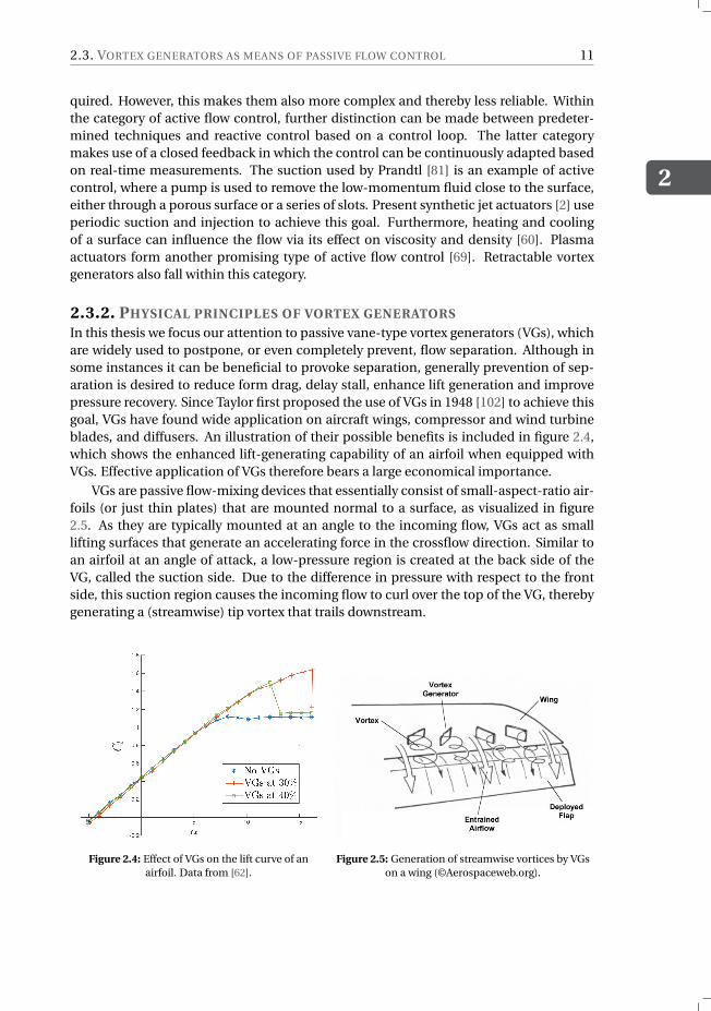
In this thesis we focus our attention to passive vane-type vortex generators (VGs), whichare widely used to postpone, or even completely prevent, flow separation. Although insome instances it can be beneficial to provoke separation, generally prevention of sep-aration is desired to reduce form drag, delay stall, enhance lift generation and improvepressure recovery. Since Taylor first proposed the use of VGs in 1948 [102] to achieve thisgoal, VGs have found wide application on aircraft wings, compressor and wind turbineblades, and diffusers. An illustration of their possible benefits is included in figure 2.4,which shows the enhanced lift-generating capability of an airfoil when equipped withVGs. Effective application of VGs therefore bears a large economical importance.
VGs are passive flow-mixing devices that essentially consist of small-aspect-ratio air-foils (or just thin plates) that are mounted normal to a surface, as visualized in figure2.5. As they are typically mounted at an angle to the incoming flow, VGs act as smalllifting surfaces that generate an accelerating force in the crossflow direction. Similar toan airfoil at an angle of attack, a low-pressure region is created at the back side of theVG, called the suction side. Due to the difference in pressure with respect to the frontside, this suction region causes the incoming flow to curl over the top of the VG, therebygenerating a (streamwise) tip vortex that trails downstream.
Figure 2.4: Effect of VGs on the lift curve of anairfoil. Data from [62].
Figure 2.5: Generation of streamwise vortices by VGson a wing (©Aerospaceweb.org).
2
12 2. VORTEX GENERATOR INDUCED FLOWS: BACKGROUND
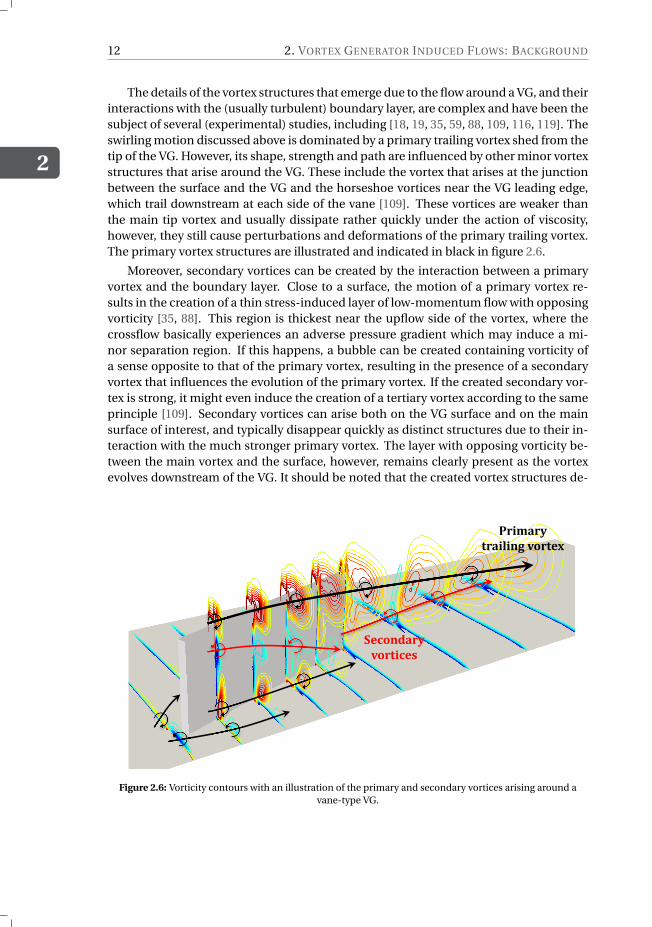
The details of the vortex structures that emerge due to the flow around a VG, and theirinteractions with the (usually turbulent) boundary layer, are complex and have been thesubject of several (experimental) studies, including [18, 19, 35, 59, 88, 109, 116, 119]. Theswirling motion discussed above is dominated by a primary trailing vortex shed from thetip of the VG. However, its shape, strength and path are influenced by other minor vortexstructures that arise around the VG. These include the vortex that arises at the junctionbetween the surface and the VG and the horseshoe vortices near the VG leading edge,which trail downstream at each side of the vane [109]. These vortices are weaker thanthe main tip vortex and usually dissipate rather quickly under the action of viscosity,however, they still cause perturbations and deformations of the primary trailing vortex.The primary vortex structures are illustrated and indicated in black in figure 2.6.
Moreover, secondary vortices can be created by the interaction between a primaryvortex and the boundary layer. Close to a surface, the motion of a primary vortex re-sults in the creation of a thin stress-induced layer of low-momentum flow with opposingvorticity [35, 88]. This region is thickest near the upflow side of the vortex, where thecrossflow basically experiences an adverse pressure gradient which may induce a mi-nor separation region. If this happens, a bubble can be created containing vorticity ofa sense opposite to that of the primary vortex, resulting in the presence of a secondaryvortex that influences the evolution of the primary vortex. If the created secondary vor-tex is strong, it might even induce the creation of a tertiary vortex according to the sameprinciple [109]. Secondary vortices can arise both on the VG surface and on the mainsurface of interest, and typically disappear quickly as distinct structures due to their in-teraction with the much stronger primary vortex. The layer with opposing vorticity be-tween the main vortex and the surface, however, remains clearly present as the vortexevolves downstream of the VG. It should be noted that the created vortex structures de-
!"#$%"&'
("%#)#*+',-"(./
0.1-*2%"&'
,-"(#1.3
Figure 2.6: Vorticity contours with an illustration of the primary and secondary vortices arising around avane-type VG.
2.3. VORTEX GENERATORS AS MEANS OF PASSIVE FLOW CONTROL
2
13
pend strongly on the VG’s geometry and the characteristics of the incoming flow. Thiswill be further elaborated on in the next section.
The overall effect of the created vortical structures is to overturn the near-wall flowvia macro motions, where the primary tip vortex is the main contributor. High-momen-tum fluid particles in the outer part (or outside) of the boundary layer are swept alonga helical path towards the surface, where they mix with the low-momentum (retarded)fluid particles near the wall. This way additional energy is effectively added to the near-wall region, thereby re-energizing the retarded fluid particles such that they can over-come stronger adverse pressure gradients [5, 78, 86]. The presence of a VG thus modifiesthe shape of the local velocity profiles, making them more full. In the sense of separa-tion prevention, the effect of such flow mixing is thus equivalent to a decrease in pressuregradient [86]. As the created vortices evolve downstream, they grow in size and decay instrength due to viscous and turbulent dissipation. Hence, the effect of VGs varies withlocation and only extends a limited distance downstream.
Unfortunately, the favorable flow-mixing properties of VGs come at the cost of a dragpenalty. This is partly due to the skin friction of the VG surface and its induced drag, butthe largest contribution is the form drag caused by the separated flow region on the rearpart of the VG suction side [88]. This drag penalty reduces the efficiency gains obtainedby the use of VGs, and therefore should be kept minimal.
One solution to reduce the drag penalty consists of reducing the size of the VG, and inparticularly its height [55, 83]. Whereas conventional VG designs have a height approxi-mately equal to the boundary layer thickness δ, so-called submerged VGs typically havea height of only δ/3 or less. This size reduction significantly diminishes parasitic drag.Furthermore, it is observed that the tip vortex created over a submerged VG can stretchsuch that it covers nearly the entire device vertically, thereby preventing flow separationover the VG’s suction side [119] and having a favorable effect on the amount of form drag.
Given similar situations, a submerged VG creates a primary tip vortex that is smaller,less circular, situated closer to the surface, and weaker [119], compared to a conventionalVG. The latter is attributed to the fact that the VG now operates in the lower layers of theboundary layer, where the velocity profile is less full and therefore fluid particles are lessenergetic. Apart from being weaker upon formation, the streamwise vortex created bya submerged VG also displays a higher decay rate of vorticity due to its proximity to thesurface, as the resulting higher shear flow enhances the vortex dissipation process.
Over the last decades, research has shown that submerged VGs can be just as ef-fective in postponing flow separation as conventional VGs [56]. However, due to thelower strength and higher decay rate, submerged VGs need to be positioned closer tothe nominal separation point (i.e. in absence of a VG) to generate the same effect as aconventional VG. Moreover, the range in which they are effective is smaller and thereforetheir use is less suitable for situations with a large uncertainty related to the location ofthe separation point. Their practical use thus requires accurate information about theposition of the nominal separation point, and that this separation point is more or lessfixed.
2
14 2. VORTEX GENERATOR INDUCED FLOWS: BACKGROUND
2.3.3. TYPES AND LAY-OUTS OF VORTEX GENERATORS
For a given nominal flow situation, the created vortex structures depend to a large ex-tent on the VG configuration, including geometry and positioning. Generally VGs arecombined in large arrays in order to influence the boundary layer in a wide area. Thearrangement of the individual VGs in such an array has of course a large impact on thedownstream evolution of the streamwise vortices due to interaction effects. Optimaldesign of VG arrays is therefore not straightforward, as geometry, positioning and flowconditions are strongly interrelated. Several studies have been performed in this respect,see for example [31, 57, 59, 77, 78, 86, 115]. An early design guide for VGs is presentedby Pearcey [78], who studied several lay-outs for vane-type VGs. There it is argued thatthe success of a VG configuration depends critically on the strength and position of thevortices in the region near the adverse pressure gradient, and hence on the paths of thevortices as they are convected downstream.
When considering an individual (vane-type) VG, relative height (with respect to δ),aspect ratio, angle with respect to the incoming flow, and the planform area, can be iden-tified as the characteristic geometric parameters. As already discussed in the previoussection, lowering the VG height h has a favorable effect on the drag penalty, but comesat the cost of reduced vortex strength and increased decay rate. Still, submerged VGsare shown to be more effective than VGs with a conventional height of order δ [31, 57].Apart from strength and decay rate, the VG height also determines the size and distancefrom the wall of the vortex core. Furthermore, it is observed that the incidence angle β
directly influences the strength of the main vortex, with the vortex strength increasingmore or less linearly with β [77, 78]. The aspect ratio, defined as the ratio between theVG’s length and height l /h, on the other hand only has minor influence on the VG’s ef-fectiveness. A ratio of l /h = 2 is found to be the minimum requirement [31, 78], withlarger values mainly adding to the drag penalty.
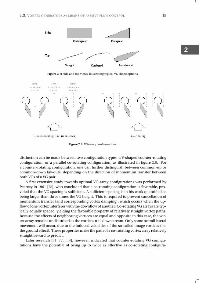
Various VG shapes have been proposed in literature, but the ones most commonlyused in practice consist of straight vane-type VGs with either a rectangular or triangularplanform. Typical shapes are illustrated in figure 2.7, where it should be noted that thereare more possibilities than shown. The use of a triangular VG over a rectangular VG isattractive, since the smaller planform area has a beneficial effect on the drag penalty.Indeed, it was shown by Godard [31], among others, that triangular vanes are more ef-fective than rectangular ones. Although the flow structures around the vane are verysimilar, a stronger vortex is created resulting in a stronger re-energizing effect of the vor-tex. However, a study performed by Velte [107] for a high-Re boundary layer indicatedno notable difference between both shapes. In the same study straight VGs were com-pared with cambered VGs, where the vortices created by the latter shape were observedto be smaller and weaker. Aerodynamically shaped VGs, consisting of an airfoil shapeinstead of a flat plate, on the other hand do effectively improve the VG’s efficiency [33].The choice of a suitable airfoil profile allows the reduction of the separated region on thesuction side of the VG, thereby reducing the form drag.
Probably the most critical design consideration, and the least straightforward to as-sess, is the placement of the individual VGs within an array. The interaction with thevortices created by neighboring VGs determines the location and strength of the vor-tex cores in the region of interest (i.e. near the nominal separation point). Essentially,
2.3. VORTEX GENERATORS AS MEANS OF PASSIVE FLOW CONTROL
2
15
Figure 2.7: Side and top views, illustrating typical VG shape options.
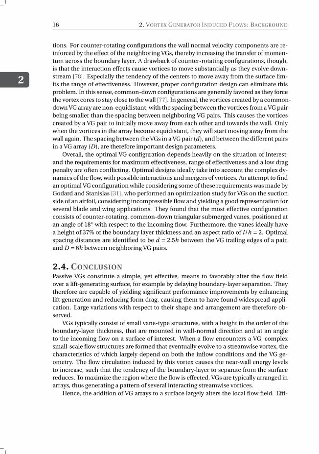
Figure 2.8: VG-array configurations.
distinction can be made between two configuration types: a V-shaped counter-rotatingconfiguration, or a parallel co-rotating configuration, as illustrated in figure 2.8. Fora counter-rotating configuration, one can further distinguish between common-up orcommon-down lay-outs, depending on the direction of momentum transfer betweenboth VGs of a VG pair.
A first extensive study towards optimal VG-array configurations was performed byPearcey in 1961 [78], who concluded that a co-rotating configuration is favorable, pro-vided that the VG spacing is sufficient. A sufficient spacing is in his work quantified asbeing larger than three times the VG height. This is required to prevent cancellation ofmomentum transfer (and corresponding vortex damping), which occurs when the up-flow of one vortex interferes with the downflow of another. Co-rotating VG arrays are typ-ically equally spaced, yielding the favorable property of relatively straight vortex paths.Because the effects of neighboring vortices are equal and opposite in this case, the vor-tex array remains undisturbed as the vortices trail downstream. Only some overall lateralmovement will occur, due to the induced velocities of the so-called image vortices (i.e.the ground effect). These properties make the path of a co-rotating vortex array relativelystraightforward to predict.
Later research [31, 77, 114], however, indicated that counter-rotating VG configu-rations have the potential of being up to twice as effective as co-rotating configura-
2
16 2. VORTEX GENERATOR INDUCED FLOWS: BACKGROUND
tions. For counter-rotating configurations the wall normal velocity components are re-inforced by the effect of the neighboring VGs, thereby increasing the transfer of momen-tum across the boundary layer. A drawback of counter-rotating configurations, though,is that the interaction effects cause vortices to move substantially as they evolve down-stream [78]. Especially the tendency of the centers to move away from the surface lim-its the range of effectiveness. However, proper configuration design can eliminate thisproblem. In this sense, common-down configurations are generally favored as they forcethe vortex cores to stay close to the wall [77]. In general, the vortices created by a common-down VG array are non-equidistant, with the spacing between the vortices from a VG pairbeing smaller than the spacing between neighboring VG pairs. This causes the vorticescreated by a VG pair to initially move away from each other and towards the wall. Onlywhen the vortices in the array become equidistant, they will start moving away from thewall again. The spacing between the VGs in a VG pair (d), and between the different pairsin a VG array (D), are therefore important design parameters.
Overall, the optimal VG configuration depends heavily on the situation of interest,and the requirements for maximum effectiveness, range of effectiveness and a low dragpenalty are often conflicting. Optimal designs ideally take into account the complex dy-namics of the flow, with possible interactions and mergers of vortices. An attempt to findan optimal VG configuration while considering some of these requirements was made byGodard and Stanislas [31], who performed an optimization study for VGs on the suctionside of an airfoil, considering incompressible flow and yielding a good representation forseveral blade and wing applications. They found that the most effective configurationconsists of counter-rotating, common-down triangular submerged vanes, positioned atan angle of 18 with respect to the incoming flow. Furthermore, the vanes ideally havea height of 37% of the boundary layer thickness and an aspect ratio of l/h = 2. Optimalspacing distances are identified to be d = 2.5h between the VG trailing edges of a pair,and D = 6h between neighboring VG pairs.
2.4. CONCLUSIONPassive VGs constitute a simple, yet effective, means to favorably alter the flow fieldover a lift-generating surface, for example by delaying boundary-layer separation. Theytherefore are capable of yielding significant performance improvements by enhancinglift generation and reducing form drag, causing them to have found widespread appli-cation. Large variations with respect to their shape and arrangement are therefore ob-served.
VGs typically consist of small vane-type structures, with a height in the order of theboundary-layer thickness, that are mounted in wall-normal direction and at an angleto the incoming flow on a surface of interest. When a flow encounters a VG, complexsmall-scale flow structures are formed that eventually evolve to a streamwise vortex, thecharacteristics of which largely depend on both the inflow conditions and the VG ge-ometry. The flow circulation induced by this vortex causes the near-wall energy levelsto increase, such that the tendency of the boundary-layer to separate from the surfacereduces. To maximize the region where the flow is effected, VGs are typically arranged inarrays, thus generating a pattern of several interacting streamwise vortices.
Hence, the addition of VG arrays to a surface largely alters the local flow field. Effi-

2.4. CONCLUSION
2
17
cient designs therefore require the ability to make reliable predictions regarding the ef-fect a VG configuration has on the flow. The small scale of VGs in combination with thecomplex flow patterns and interactions, however, poses great challenges in this respect.Moreover, the wide variation in applications precludes the formulation of generally ap-plicable design guidelines. Affordable and accurate analysis techniques are thereforerequired in order to solve these high-dimensional design problems.

3SIMULATING VORTEX
GENERATOR INDUCED FLOWS:STATE OF THE ART
As discussed in chapter 2, the addition of VGs to a boundary layer fundamentally altersthe flow field, locally as well as far downstream. For optimal designs these effects cantherefore not be ignored and need to be carefully considered, from an early design stageon. However, due to the small size of a VG, inclusion of VG arrays in detailed analysesis complex, computationally expensive and time consuming. Even though their influ-ence was known to be large, for this reason VGs were neglected in early-stage analysesfor many years. They were only included in later design stages, for example during ex-perimental testing. Only with the rise of CFD could the effects of VGs on the flow field betaken into account with sufficient accuracy.
In this chapter the state of the art with respect to the simulation of VG effects on aflow field is discussed. We start with an overview of analytical methods in section 3.1,which can be used to obtain initial predictions with respect to the strength and shapeof the generated vortices. This is followed by a more elaborate overview of numericalapproaches, which in general yield results with improved accuracy due to their consid-eration of the entire flow field. Within this category, distinction is made between fullyresolved (section 3.2), fully modeled (section 3.3) and partly resolved / partly modeled(section 3.4) approaches (according to [100]).
3.1. ANALYTICAL METHODSA key concept in the theoretical analysis of the effects of VGs on wall-bounded flowsis the lifting-line theory. This was another major contribution from Ludwig Prandtl tofluid dynamical theory and the first practical method for predicting aerodynamic prop-erties of finite wings. This theory predicts the lift and induced drag generated by a three-dimensional wing by replacing the wing by an infinite number of horseshoe vortices,
19
3
20 3. SIMULATING VORTEX GENERATOR INDUCED FLOWS: STATE OF THE ART
and using the Kutta-Joukowski theorem to relate the sectional lift to the circulation ofthe bound vortex around each airfoil section. This theory, however, is limited to incom-pressible, inviscid flow, and does not account for swept wings, low aspect ratio wings andunsteady effects.
Still, when applied to a VG, which resembles a low-aspect ratio wing protruding theboundary layer, lifting-line theory can be used to obtain a reasonable estimate for thestrength of the vortex shed at the VG tip, as for example done by Jones in 1957 [45]. Inthis first extensive approach to analyze the (counter-rotating) vortex system created bya VG array, Jones developed an analytical model based on potential flow theory. Thismethod assumed two-dimensional inviscid flow, thereby not accounting for the viscousvortex core and variations in the streamwise velocity. The effect of the wall was taken intoaccount by addition of mirror image vortices, causing the surface to become a stream-line of the vortex field. Although qualitatively useful insights were gained, for examplewith respect to the path of the vortices, the predicted minimum height of the createdvortices from the wall was found to be in considerable excess of experimental values.These quantitative deviations limited the practical use of this early analytical model, andclearly indicated that 3D and viscous effects cannot be neglected when studying the flowdownstream of a VG array.
The theory of Jones [45] can be enhanced by considering the swirling velocity andvorticity distribution in the viscous vortex core. Several theoretical descriptions of a sin-gle free vortex have been proposed in literature, see for example [12, 13]. One of thesimplest is due to Rankine [82], who approximates a free vortex as a solid-body like ro-tation within the core, exhibiting a linear increase in swirl velocity from the center to thepoint of maximum swirl velocity, and uses potential theory (similar to Jones [45]) out-side this core region. A more sophisticated model is proposed by Lamb [50] and Oseen[74], which overcomes the discontinuity at the core boundary in the Rankine description,and originates from the one-dimensional (axisymmetric) laminar Navier-Stokes equa-tions. This Lamb-Oseen vortex model assumes zero axial and radial velocity and yields aGaussian distribution for the swirl velocity. Moreover, this theoretical model contains atime-dependent decay, and thereby allows prediction of both the decay in strength andthe vortex growth over time (in the 2D context).
For a trailing vortex, however, the axial velocity is not zero. Squire [97] therefore pro-posed an addition to the Lamb-Oseen model that accounts for this non-zero axial ve-locity. In addition, he also included a viscosity term to account for enhanced diffusionof vorticity due to the effects of turbulence generation. An alternative consists of theBatchelor vortex model [10], which uses a non-uniform axisymmetrical axial velocityand thereby accounts for the axial momentum deficit caused by the vortex. For the caseof vortices generated by a VG in a turbulent wall-bounded flow, the latter model was laterextended by Velte et al. [108] based on the observation of helical symmetry, yielding animproved description of the axial velocity profile.
The above theoretical single-vortex models can yield a good representation of thetotal velocity field of a vortex system generated by a VG array, when using mirror im-age vortices to simulate the wall, and making use of superposition to include the effectsof neighboring vortices. However, several drawbacks are related to these models, limit-ing their use for accurate flow predictions. Firstly, they only describe the vortex system
3.1. ANALYTICAL METHODS
3
21
at a crossplane immediately downstream of the VG, but do not account for the down-stream propagation. Additionally, these vortex descriptions rely on several input quan-tities which are usually unknown. These typically are circulation (and/or peak vorticity)and the vortex core size. For the model of Velte [108] even the helical pitch is a requiredinput parameter. This makes these vortex-profile models by themselves impractical foruse, and additional relations are therefore required.
Probably the simplest estimate for the vortex’s circulation consists of (by Helmholtz’stheorem) equating it to the VG’s bound vortex circulation, which can be approximatedusing the Kutta-Joukowski condition, as done in [34], among others. Furthermore, im-provements of lifting-line theory by means of empirical relations have been proposed toenhance the dependence of the shed vortex’s characteristics on the VG geometry and im-pinging flow conditions. Wendt and Reichert [113, 115], for example, performed an ex-perimental study towards the initial vortex circulation and crossplane peak vorticity forairfoil shaped VGs, assuming that at one VG chord downstream of the VG’s trailing edgethe vortex is fully developed. Circulation in their work was modeled based on Prandtl’slifting-line formula, whereas a correlation for the peak vorticity was derived by equatingthe moment at the airfoil tip to the rate of angular-momentum production of the vortex.Bray [13] used a similar approach to model the vortices shed by vane-type VGs, however,he modified the lifting-line expression for circulation to obtain a quadratic variation withthe incidence angle, in an attempt to account for stall over the VG’s suction side. Addi-tionally, in [13] the peak vorticity was expressed as function of the vortex radius, whichwas modeled by a purely empirical relation.
Recently, Poole et al. [79] proposed a theoretically extended version of lifting-linetheory that accounts for the low aspect ratio of a VG and takes into account the vary-ing velocity profile of the boundary layer. Moreover, they added a vortex-lift componentbased on Polhamus’ suction theory for delta wings, to include the addition of lift gen-erated due to vortex roll-up along the length of the VG. By including these additionalphysics, they managed to derive an expression for circulation that exhibits a significantlyreduced error compared to the empirical model of Wendt.
However, the evolution of the vortex resulting from the above-mentioned theoreticalvortex-profile models is hard to predict analytically, as this requires consideration of vis-cous effects. In contrast to the inviscid potential approach used by Jones [45], Bray [13]attempted to formulate an empirical relation for the viscous decay of vortex strength.Although the latter also yields a reasonable estimate for the growth of the vortex core, itcannot be used to make predictions with respect to interaction effects on the paths ofthe vortices. An analytical viscous analysis has been attempted by Smith [91], but hisapproach only applies to the very specific situation of low-profile triangular vanes notextending beyond the logarithmic layer of the boundary layer. In general, useful resultswith respect to vortex evolution require the use of numerical tools rather than analyticmethods.
Despite their limitations, analytical approaches are particularly suited for getting arough idea about appropriate VG configurations in an early design phase, due to theirlow complexity and low computational cost. Research toward an improved analyticalprediction of the (initial) vortex strength and shape is therefore ongoing, including boththeoretical developments like [79] and enhancements based on (semi-) empirical rela-
3
22 3. SIMULATING VORTEX GENERATOR INDUCED FLOWS: STATE OF THE ART
tions [13, 115]. Moreover, these results can be of value as input for numerical simula-tions, as will be discussed in section 3.3.
3.2. FULLY-RESOLVED SIMULATIONSWhen viscous and 3D flow effects are to be taken into account, analytical methods arelimited and numerical approaches are required. CFD simulations are therefore the pre-ferred method for the study of VG effects, as they can in principle accurately model thephysics associated with the flow patterns induced by individual VGs and their combinedeffects when operating in arrays. When using a finite-volume CFD approach, the regionoccupied by the fluid is divided into discrete cells, constituting the numerical mesh. Inevery cell, the governing flow equations (e.g. (2.1) and (2.2)) are implemented in discreteform, and their residuals used to evolve the flow variables throughout the domain.
A conventional CFD approach to resolving VG-induced flow fields consists of con-structing a body-fitted mesh (BFM) around all solid surfaces, including the surface ofinterest (e.g. a wind-turbine blade) and the VG. Such a fully-resolved approach theoreti-cally possesses the highest achievable accuracy, depending on the choices made for thegoverning equations to be solved, and the related discretization schemes.
3.2.1. TIME-RESOLVED VG SIMULATIONSDirect numerical simulations (DNS) provide a time-resolved solution of the full Navier-Stokes equations, including the smallest scales in the flow, and are thus capable of yield-ing highly-accurate VG-induced flow simulations. This has, for example, been done bySpalart et al. [94] for a periodic array of co-rotating VGs in a supersonic flat-plate bound-ary layer, in the context of an academic study. However, the high accuracy of DNS comesat an enormous computational cost, thereby restricting their use to low Reynolds num-bers and making them unsuitable for typical VG applications.
Large eddy simulations (LES) offer a more affordable alternative for DNS, enablingthe calculation of time-resolved flow fields by modeling instead of resolving the small-est turbulent scales, thereby allowing for less refined meshes outside the boundary layer.This approach has also been used to simulate VG-induced flow fields, yielding highly ac-curate results [14, 106]. Still, the cost of LES is prohibitively expensive for high Reynoldsnumber wall-bounded flows, thereby limiting its applicability for general industrial pur-poses.
3.2.2. RANS SIMULATIONS OF FLOWS AROUND VGSNumerical solution of the Reynolds-averaged Navier-Stokes (RANS) equations is cur-rently the preferred method for resolving the flow over a VG configuration, combining agood accuracy with a reasonable computational cost (see, among others, [1, 24, 47, 117]).
THE REYNOLDS AVERAGED NAVIER STOKES EQUATIONS
The main idea behind the RANS equations consists of using statistical quantities to de-scribe a turbulent flow field, rather than the instantaneous quantities used in (2.1) and(2.2). At the high Re that govern turbulent flows, the evolution of the flow field is ex-tremely sensitive to small changes in, for example, initial and boundary conditions and
3.2. FULLY-RESOLVED SIMULATIONS
3
23
inhomogeneities, yielding a seemingly random behavior of the flow. At the end of the19th century, Osborne Reynolds therefore proposed to describe the flow field in terms ofits mean and fluctuating parts using the decompositions
u = u+u′ (3.1)
p = p +p ′ (3.2)
where, typically, the mean velocity and pressure fields (u and p respectively) are definedas the time-averaged instantaneous fields. By considering the limiting case of averagingover a period much longer than the largest time scale of the turbulent motion, the meanquantities become time independent. Alternatively, unsteady RANS (URANS) methodscan be used, which consider the ensemble rather than the temporal average in order totake into account some of the large-scale unsteadiness in the flow.
Upon substitution of the above decompositions into the Navier Stokes equations,which describe the instantaneous flow field and account for all turbulence effects up tothe smallest (Kolmogorov) scales, equations for the (steady) mean flow and for the fluc-tuating parts can be obtained, see for example [53, 80]. The mean flow RANS equationscan be written in component form, when neglecting external body forces, as
∂ρu j
∂x j= 0, (3.3)
∂ρui u j
∂x j= − ∂p
∂xi+ ∂
∂x j
[µ
(∂ui
∂x j+ ∂u j
∂xi
)−ρu′
i u′j
], (3.4)
where µ denotes the dynamic viscosity. Compared to the steady Navier-Stokes equa-tions, the above RANS equations for the mean flow are very similar, apart from the ad-
dition of an apparent stress term ρu′i u′
j , called the (turbulent) Reynolds stress. The
Reynolds stress tensor stems from momentum transfer by the fluctuating velocity field,and accounts for the effect of the velocity fluctuations on the mean flow, thereby beingcrucial in the description of the turbulent flow field.
For a statistically steady 3D flow, the RANS equations consist of four independentgoverning equations, whereas the number of unknowns is larger: in addition to the threevelocity components and the pressure, the additional Reynolds stress tensor, which issymmetric, introduces 6 additional unknowns. This closure problem prevents a directsolution of (3.3) and (3.4). The Reynolds stresses therefore need to be specified somehowto obtain a solution for the turbulent mean flow.
If an exact representation of the Reynolds stresses would be available, equations (3.3)and (3.4) would yield an exact representation of the turbulent flow field. Unfortunately,such a representation is unavailable, and hence a model must be used. Depending onthe selected model and flow situation, major errors might be introduced to the overallsolution. A significant number of models has been proposed in literature, ranging fromsimple algebraic relations to the solution of full differential transport models. In gen-eral, two main groups of models for the Reynolds stresses can be identified, being eitherbased on the turbulent-viscosity assumption, or on the solution of a modeled transportequation for the stress components.
3
24 3. SIMULATING VORTEX GENERATOR INDUCED FLOWS: STATE OF THE ART
TURBULENT-VISCOSITY MODELS
The turbulent-viscosity hypothesis was formulated by Boussinesq in 1877 (hence it isalso known as the Boussinesq hypothesis) and it states that the deviatoric part of theReynolds stress is proportional to the mean rate of strain Si j . Moreover, it specifies thisrelationship to be linear and determined by a scalar constant, called the turbulent vis-cosity or the eddy viscosity µt , as
ai j =−ρu′i u′
j +2
3ρkδi j = 2µt Si j =µt
(∂ui
∂x j+ ∂u j
∂xi
), (3.5)
with the turbulent kinetic energy
k = 1
2u′
i u′i . (3.6)
This hypothesis reduces the burden significantly, as now only the scalar quantity µt isleft to be determined in order to obtain closure for the RANS equations. A wide varietyof so-called linear eddy-viscosity models is available, typically classified according to thenumber of equations that need to be solved. A comprehensive overview can be found in[53].
The simplest class of linear eddy-viscosity models consists of the algebraic models,which do not require the solution of an additional equation. However, these are typicallytoo simple for use in general situations. In the class of one-equation models, the Spalart-Allmaras model [92] is by far most popular. Despite its simplicity, requiring the solutionof a single transport equation for the kinematic eddy viscosity νt , this model is widelyand successfully used in the study of external aerodynamics.
Within the category of linear eddy-viscosity models, the use of two-equation modelsis most widespread, providing an estimate for νt in combination with a description ofthe turbulent scales by solving transport equations for the turbulent kinetic energy kand the rate of dissipation ϵ (e.g. [46, 52]), or for k and the specific dissipation ω (e.g.[118]). A very successful model is Menter’s k −ω shear-stress transport (SST) model [64],which combines the best of two worlds by blending the k−ωmodel close to the wall, withthe k − ϵ model in the freestream. Moreover, by also including Bradshaw’s assumption(i.e. that the principal shear stress is linearly related to the turbulent kinetic energy) theeffect of the transport of principal turbulent shear stress is partly accounted for. Thisway, the limited performance of k −ϵ models for large mean pressure gradients, and theexcessive sensitivity to the inlet freestream turbulence properties of k −ω models, areboth overcome, yielding improved results for flows exhibiting adverse pressure gradientsand/or separation.
Unfortunately, in its simplicity the Boussinesq hypothesis overlooks the spatial co-herence of turbulent structures. This assumption is reasonable for simple shear flows,where the turbulent characteristics change slowly following the mean flow and there-fore the Reynolds-stress balance is dominated by local processes. This is for examplethe case in channel flows and undisturbed boundary layers. However, for more complexflows governed by high strain rates, like strongly swirling flows or flows with significantstreamline curvature, the hypothesis fails significantly, regardless of the closure approx-imation made to determine the turbulent viscosity [53, 80]. Moreover, the above men-tioned eddy-viscosity models rely heavily on empirical constants, causing additional er-rors for flow situations that fall outside their calibrated range.
3.2. FULLY-RESOLVED SIMULATIONS
3
25
Corrections have been proposed to develop improved eddy-viscosity models, for ex-ample by accounting for streamline curvature [90, 93]. Additionally, a class of nonlineareddy-viscosity models emerged, which no longer assume a linear relation between theturbulent stresses and the mean rate of strain. Instead, a polynomial expansion is con-structed, with the expansion coefficients being based on calibration with experimentalor numerical data [17, 95]. However, none of the above extensions yield generally im-proved flow-field results, as they are all based on empirical functions that are optimizedfor specific flow situations.
REYNOLDS-STRESS MODELS
To overcome the defects of the turbulent-viscosity assumption, closure relations havebeen formulated that determine the Reynolds-stress components directly from the ex-act governing equations. Such Reynolds-stress models typically require the solution of7 coupled nonlinear partial differential equations, in addition to the mean-flow equa-tions, to account for all stress components and the (specific) dissipation. Despite re-taining some exact terms, the resulting transport equations still require models to ac-count for the turbulent dissipation and diffusion, and the pressure-velocity interaction(accounting for the normal-stress redistribution) [53, 80]. By introducing these models,inaccuracies inevitably enter the solution of the turbulent flow field.
As with the turbulent-viscosity models, many different variants to model these ad-ditional unknowns can be found in literature. Widely used examples include the LRRmodel by Launder, Reece and Rodi [51] and the SSG model by Speziale, Sarkar and Gatski[96]. The most important difference between these models consists of the way in whichthe pressure-velocity correlations are approximated. This is the most challenging partto model, as this interaction is highly non-local. Elliptical relaxation allows for non-localeffects to be included [22], thereby offering a higher level of description. However, thesemodels come at the cost of an increased complexity and are strongly affected by theboundary conditions imposed at the wall.
Reynolds-stress models can in general be successfully applied (opposed to turbulent-viscosity models) for flows with significant mean streamline curvature and flows withstrong swirl or mean rotation. However, for very complex flows, for example 3D sepa-rated flow over a curved surface, Reynolds-stress models may give solutions that are nobetter than, or even worse than, turbulent-viscosity models [53]. Moreover, apart fromthe complexity of creating accurate Reynolds-stress models, this approach poses an in-creased computational challenge. The nature of these equations is such that the numer-ical stability of the discretized RANS system is reduced, especially compared to the useof turbulent-viscosity models.
In order to enhance stability and reduce the numerical cost, an additional class ofalgebraic stress models has arisen. Initially implicit relations were extracted based onthe differential Reynolds-stress models discussed above [84]. However, these implicitrelations were found to be lacking computational robustness, resulting in the formula-tion of explicit relations instead. These explicit algebraic stress models are functionallyequivalent to the previously mentioned nonlinear eddy-viscosity models, but differ fun-damentally in the determination of the expansion coefficients, which are now based onthe Reynolds-stress transport equations rather than a calibration process. An overviewof such models can be found in [28].
3
26 3. SIMULATING VORTEX GENERATOR INDUCED FLOWS: STATE OF THE ART
FULLY-RESOLVED RANS SIMULATIONS OF VGS
The RANS equations enable computation of the time-averaged VG-induced flow field,by decomposing the flow into its mean (time-averaged) and fluctuating components.The requirements on the numerical mesh are such that the mean-flow variations canbe resolved, thus posing looser requirements on the mesh resolution than LES and DNSapproaches. By considering steady instead of transient flow, the computational cost isfurther reduced. However, the accuracy of the method depends on the choice for theturbulence model that is used to take into account the influence of the fluctuating com-ponents, corresponding to the small turbulent eddies.
Research indicates that conventional turbulent-viscosity models are able to yield sat-isfactory estimates for the mean-flow features of a single vortex [24, 54], but show re-duced accuracy when vortex interactions are considered [6, 117]. The main observeddeficiencies are underprediction of the streamwise vorticity and deviations with respectto the vortex’s trajectory, where it should be mentioned that strong variations in accuracyare observed depending on the particular turbulent-viscosity model used. For example,the two-equation k−ω SST model has been reported to perform significantly better thanthe one-equation Spalart Allmaras model [1, 14, 117], which shows high diffusion andtypically underestimates the vorticity and therefore the effect of the VG. Especially forflat-plate cases, and depending on the purpose, the k−ω SST model can yield sufficientlyaccurate results [14, 24], similar to those obtained when using an algebraic stress model[14]. However, for more complex situations, for example airfoil flows, the latter categoryclearly outperforms standard turbulent-viscosity models. Reliable pressure distributionscan be obtained with turbulent-viscosity RANS simulations, however, the prediction ofaerodynamic coefficients for high angles of attack (especially near stall) is prone to er-rors [14, 47, 61]. Moreover, comparison with (full) Reynolds-stress models highlights theinherent weakness of conventional turbulent-viscosity models for boundary-layer flowscontaining vortical structures [117].
In [94], Spalart et al. state that in general, flow situations involving vortex interactionsare too complex for RANS methods. However, the formation of the vortex itself is largelyan inviscid process, and therefore RANS errors only become apparent when the vorticesstart aging and interacting. Hence, body-fitted RANS simulations offer a good reliabilityfor studying the vortex-formation process. For highly-accurate results concerning thedownstream evolution, the choice of turbulence model is of large importance.
Effectively capturing and convecting downstream the vortices created by VGs re-quires very high mesh resolutions both around the VG and in its wake. As discussedin section 2.3.2, the physics involved in the vortex-formation process around a VG arecomplex, and studies of grid requirements thus reveal that it is necessary to adequatelyresolve the VG’s boundary layer in order to obtain accurate flow representations [117].Difficulties in the mesh-generation process typically arise due to the combination ofthese high mesh requirements, and the large difference in scale between a VG and thesurface of interest. Inclusion of VGs in body-fitted meshes therefore typically causes alarge increase in the overall mesh size, and hence the related numerical cost. Moreover,creation of a high-quality mesh becomes cumbersome and time-consuming (althoughthe effort can be reduced by making use of the Chimera or overset grid approach, as forexample done in [30]). For these reasons, body-fitted mesh simulations are rarely used
3.3. FULLY-MODELED SIMULATIONS
3
27
for configurations other than those involving a single VG or VG pair.
3.2.3. IMMERSED-BOUNDARY METHODS
In an attempt to reduce the burden of mesh generation, immersed-boundary methodsfor VG simulations are gaining popularity [29, 89, 120]. These methods do not explicitlyinclude the VG geometry into the numerical mesh, but rather simulate the presence of aphysical boundary though the addition of forcing (source) terms in the cells correspond-ing to the VG location. The mesh therefore no longer needs to be locally aligned with theVG surface, thus simplifying the mesh-generation process. However, the same require-ments with respect to mesh resolution still apply, as these simulations still aim to resolvethe full vortex-formation process. An overview of the immersed-boundary method andthe different approaches used to simulate the presence of a solid boundary is given in[65].
Although immersed-boundary methods are typically insufficient when a detailedstudy of the boundary layer is required, You et al. [120] demonstrated the efficacy ofLES in combination with this approach to examine both the temporal and spatial evolu-tion of longitudinal vortex pairs embedded in a turbulent boundary layer. This result wasconfirmed by Shan et al. [89], who successfully used an immersed-boundary method tostudy the flow-separation control with VGs for a NACA0012 airfoil. Moreover, Ghosh etal. [29] used the immersed-boundary technique to simulate the presence of submergedVGs in a compressible RANS study of oblique-shock / turbulent boundary-layer interac-tions. Their study, however, shows that deviations from the body-fitted mesh result oc-cur due to insufficient resolution of the VG boundary layer, mainly resulting in an over-prediction of the momentum sink effect of the VGs. The immersed-boundary methoddoes thus not avoid the requirement for high mesh resolution close to the VG surface.
3.3. FULLY-MODELED SIMULATIONSFully-resolved simulations including VG arrays can deliver the desired accuracy, but at acomputational cost too high to be practical. The analytical methods discussed in section3.1, on the other hand, are computationally cheap but lack the required accuracy. A com-bination of these two approaches therefore constitutes a logical alternative. As definedin [101], these so-called fully-modeled approaches "model the generated structures orthe influence of the modeled VGs".
3.3.1. THREE-DIMENSIONAL APPROACHES
Direct inclusion of a fully-developed vortex into an undisturbed flow field can be a solu-tion to overcome the excessive computational cost related to high-fidelity, fully-resolved,CFD simulations, thereby making VG-induced flow-field information more practical toobtain. These fully-modeled, low-fidelity, approaches do not attempt to resolve all thephysics related to the vortex-formation process. Rather, an analytical model is used topredict the strength and shape of the main vortex created by a VG, and only the down-stream evolution of this vortex is resolved by the numerical method (illustrated in figure3.1). Doing so mitigates the requirements posed on the numerical mesh, as the VG ge-ometry no longer needs to be included into the mesh, and the small-scale flow motions
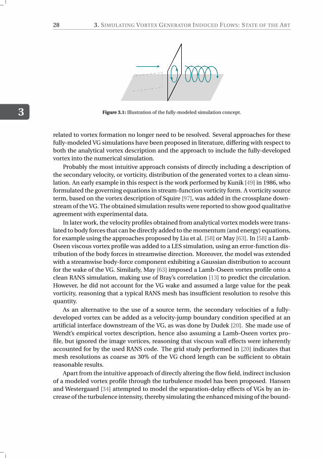
3
28 3. SIMULATING VORTEX GENERATOR INDUCED FLOWS: STATE OF THE ART
Figure 3.1: Illustration of the fully-modeled simulation concept.
related to vortex formation no longer need to be resolved. Several approaches for thesefully-modeled VG simulations have been proposed in literature, differing with respect toboth the analytical vortex description and the approach to include the fully-developedvortex into the numerical simulation.
Probably the most intuitive approach consists of directly including a description ofthe secondary velocity, or vorticity, distribution of the generated vortex to a clean simu-lation. An early example in this respect is the work performed by Kunik [49] in 1986, whoformulated the governing equations in stream-function vorticity form. A vorticity sourceterm, based on the vortex description of Squire [97], was added in the crossplane down-stream of the VG. The obtained simulation results were reported to show good qualitativeagreement with experimental data.
In later work, the velocity profiles obtained from analytical vortex models were trans-lated to body forces that can be directly added to the momentum (and energy) equations,for example using the approaches proposed by Liu et al. [58] or May [63]. In [58] a Lamb-Oseen viscous vortex profile was added to a LES simulation, using an error-function dis-tribution of the body forces in streamwise direction. Moreover, the model was extendedwith a streamwise body-force component exhibiting a Gaussian distribution to accountfor the wake of the VG. Similarly, May [63] imposed a Lamb-Oseen vortex profile onto aclean RANS simulation, making use of Bray’s correlation [13] to predict the circulation.However, he did not account for the VG wake and assumed a large value for the peakvorticity, reasoning that a typical RANS mesh has insufficient resolution to resolve thisquantity.
As an alternative to the use of a source term, the secondary velocities of a fully-developed vortex can be added as a velocity-jump boundary condition specified at anartificial interface downstream of the VG, as was done by Dudek [20]. She made use ofWendt’s empirical vortex description, hence also assuming a Lamb-Oseen vortex pro-file, but ignored the image vortices, reasoning that viscous wall effects were inherentlyaccounted for by the used RANS code. The grid study performed in [20] indicates thatmesh resolutions as coarse as 30% of the VG chord length can be sufficient to obtainreasonable results.
Apart from the intuitive approach of directly altering the flow field, indirect inclusionof a modeled vortex profile through the turbulence model has been proposed. Hansenand Westergaard [34] attempted to model the separation-delay effects of VGs by an in-crease of the turbulence intensity, thereby simulating the enhanced mixing of the bound-
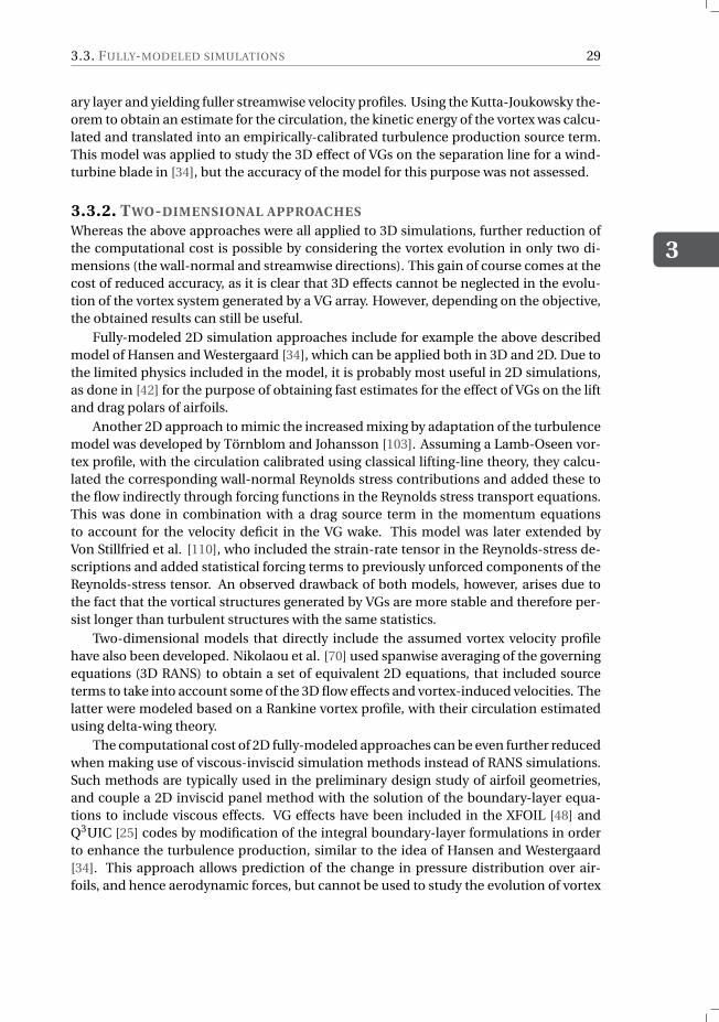
3.3. FULLY-MODELED SIMULATIONS
3
29
ary layer and yielding fuller streamwise velocity profiles. Using the Kutta-Joukowsky the-orem to obtain an estimate for the circulation, the kinetic energy of the vortex was calcu-lated and translated into an empirically-calibrated turbulence production source term.This model was applied to study the 3D effect of VGs on the separation line for a wind-turbine blade in [34], but the accuracy of the model for this purpose was not assessed.
3.3.2. TWO-DIMENSIONAL APPROACHES
Whereas the above approaches were all applied to 3D simulations, further reduction ofthe computational cost is possible by considering the vortex evolution in only two di-mensions (the wall-normal and streamwise directions). This gain of course comes at thecost of reduced accuracy, as it is clear that 3D effects cannot be neglected in the evolu-tion of the vortex system generated by a VG array. However, depending on the objective,the obtained results can still be useful.
Fully-modeled 2D simulation approaches include for example the above describedmodel of Hansen and Westergaard [34], which can be applied both in 3D and 2D. Due tothe limited physics included in the model, it is probably most useful in 2D simulations,as done in [42] for the purpose of obtaining fast estimates for the effect of VGs on the liftand drag polars of airfoils.
Another 2D approach to mimic the increased mixing by adaptation of the turbulencemodel was developed by Törnblom and Johansson [103]. Assuming a Lamb-Oseen vor-tex profile, with the circulation calibrated using classical lifting-line theory, they calcu-lated the corresponding wall-normal Reynolds stress contributions and added these tothe flow indirectly through forcing functions in the Reynolds stress transport equations.This was done in combination with a drag source term in the momentum equationsto account for the velocity deficit in the VG wake. This model was later extended byVon Stillfried et al. [110], who included the strain-rate tensor in the Reynolds-stress de-scriptions and added statistical forcing terms to previously unforced components of theReynolds-stress tensor. An observed drawback of both models, however, arises due tothe fact that the vortical structures generated by VGs are more stable and therefore per-sist longer than turbulent structures with the same statistics.
Two-dimensional models that directly include the assumed vortex velocity profilehave also been developed. Nikolaou et al. [70] used spanwise averaging of the governingequations (3D RANS) to obtain a set of equivalent 2D equations, that included sourceterms to take into account some of the 3D flow effects and vortex-induced velocities. Thelatter were modeled based on a Rankine vortex profile, with their circulation estimatedusing delta-wing theory.
The computational cost of 2D fully-modeled approaches can be even further reducedwhen making use of viscous-inviscid simulation methods instead of RANS simulations.Such methods are typically used in the preliminary design study of airfoil geometries,and couple a 2D inviscid panel method with the solution of the boundary-layer equa-tions to include viscous effects. VG effects have been included in the XFOIL [48] andQ3UIC [25] codes by modification of the integral boundary-layer formulations in orderto enhance the turbulence production, similar to the idea of Hansen and Westergaard[34]. This approach allows prediction of the change in pressure distribution over air-foils, and hence aerodynamic forces, but cannot be used to study the evolution of vortex
3
30 3. SIMULATING VORTEX GENERATOR INDUCED FLOWS: STATE OF THE ART
systems.The above fully-modeled approaches are in general capable of yielding qualitatively
good results, making them suitable for (early) qualitative studies of VG configurations.However, they rely on the inherent assumption that the created vortices satisfy an a pri-ori determined analytical profile, usually in combination with empirical relations thatrequire calibration to obtain quantitatively useful flow-field results. This makes thesemodels less reliable in later design stages when detailed flow information is required.Moreover, as these models fail to take into account the specifics of particular VG geome-tries and/or flow conditions for the situation of interest, they are less suitable for thestudy of new, unconventional designs.
3.3.3. AN ANALYSIS OF 3D FULLY-MODELED APPROACHESFully-modeled approaches have the potential to greatly reduce the numerical cost re-lated to flow simulations involving VGs, however, little information is available regard-ing their general performance. They are typically validated for specific cases which fallwithin the parameter range used to derive their included empirical relations. To date nostudies have been found that yield a conclusive comparative analysis of different fully-modeled approaches.
To provide further insight, a study performed in collaboration with Ana Sofia MoreiraRibeiro is presented here, in which a fully-modeled approach is applied to a test case thatfalls outside its validated range. This case is selected such as to be representative for atypical VG configuration as used for flow control of external aerodynamics applications.It considers the subsonic flow over a counter-rotating common-down VG array attachedto a flat plate, corresponding to the experimental set-up of Baldacchino et al. [9] andin line with the VG configuration design guidelines formulated by Godard and Stanislas[31]. A detailed discussion of this test case, as well as the body-fitted mesh simulationsthat are used as reference, appears in section 4.4.2.
A 3D fully-modeled approach is used in order to include the necessary physics toexpect a sufficiently accurate representation of the vortex paths. Moreover, we desiredto include the effect of the vortex as a mean-flow feature (supported by the evidence of[103]) within a RANS simulation. The fully-modeled approaches proposed by Liu et al.[58], May [63] and Dudek [20] all satisfy these requirements. In this work, it was chosento represent the vortex profile as an artificial boundary condition using the approach ofDudek.
APPLICATION OF DUDEK’S VG-MODELING APPROACH FOR A SAMPLE CASE
The VG-modeling method proposed by Dudek [20] was implemented in the open-sourceCFD code OpenFOAM®. This method makes use of Wendt’s semi-empirical vortex de-scription, describing the secondary velocity profile induced by the presence of a VG asa Lamb (ideal viscous) vortex, as function of the vortex’s total circulation (Γ) and peakvorticity (ωx,max). The model assumes the center of the vortex that is imposed to theundisturbed flow field to be located at the same coordinate in wall-normal and cross-flow direction as the VG tip, but at one VG chord length downstream of the VG’s trailingedge. Our implementation has been verified against the pipe-flow case discussed in [20](see [67] for more information).
3.3. FULLY-MODELED SIMULATIONS
3
31
The chosen VG-flow case of [9] falls partly within and partly outside the parametricrange considered by Wendt; the freestream velocity is significantly lower and the VG in-cidence angle slightly larger than the validated range of the model. For our assessment,Dudek’s modeling approach is compared to both experimental data and a body-fittedmesh (BFM) RANS simulation. Details of the latter can be found in section 4.4.2. Inorder to eliminate mesh-related differences the mesh for the fully-modeled simulation,downstream of the VG location, was equal to that of the body-fitted mesh. Also the samenumerical schemes were used for both simulation approaches.
Our results indicate that the considered fully-modeled approach yields unreliableresults in the sense that the initial circulation and decay rate are underestimated, whilethe vortex shape and position show large deviations. Figure 3.2 shows the total circula-tion levels downstream of the VG (with ∆x/h = 2.5 corresponding to ∆x = l , the locationwhere the vortex profile is imposed). The Q-criterion was used to identify the vortex do-main, as in [9]. Peak vorticity levels are shown in figure 3.3, and vorticity-contour plotsat three locations downstream of the VGs in figure 3.4.
It is observed that Wendt’s circulation approximation yields a significant underesti-mation for our test case, thereby suggesting that use of this model outside its calibratedrange is not advised. The same figure also indicates that, contrary to both experimen-tal and BFM results, the created vortices only start decaying after approximately 15 VGheights. This can be attributed to their large distance from the wall and small size (fig-ure 3.4), both of which minimize the interactions with the viscous layer near the wall.Sufficiently far downstream, the total circulation level and decay rate agree well with thereference data. The underestimated vortex circulation is thus likely counteracted by er-rors with respect to size and location.
Furthermore, our results indicate a rather good result for the peak vorticity, andhence the intensity of the created vortices. Although initially being overestimated withrespect to the BFM result, good agreement with the experimental data is obtained down-stream. The peak vorticity displays a rapid decay, in combination with fast growth of thevortex core, thereby again approaching the BFM results further downstream. However,despite good results with respect to circulation and peak vorticity far downstream, thedeviations with respect to the shape and location of the vortices make predictions of theboundary-layer state questionable, as both the vortex-vortex and vortex-boundary layerinteractions can be expected to be erroneous. Moreover, it cannot be relied upon thatfor all applications the initial errors of the model will be reduced with the convection ofthe vortices.
EFFECT OF PARAMETER CALIBRATION
To explore the effect of parameter errors on the accuracy of Dudek’s fully-modeled ap-proach, simulations were performed with calibrated values for the circulation, peak vor-ticity and location of the vortex center. Due to the large error with respect to the initialtotal circulation, the effect of improving this parameter is of key interest. In Wendt’smodel, however, peak vorticity scales with the circulation cubed. Since in the originalmodel underestimated circulation corresponds to an overestimation of the peak vor-ticity, it was expected that an increase of Γ would yield an unrealistic value for ωx,max.Therefore the initial peak vorticity was calibrated simultaneously with the circulation.
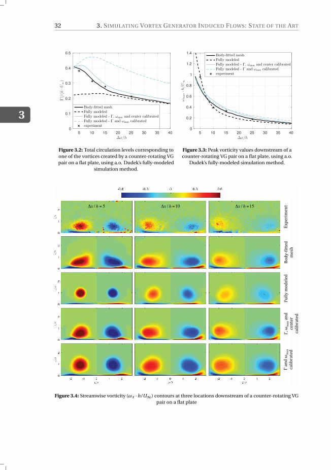
3
32 3. SIMULATING VORTEX GENERATOR INDUCED FLOWS: STATE OF THE ART
5 10 15 20 25 30 35 40
∆x/h
0
0.1
0.2
0.3
0.4
0.5
|Γ|/(h
·U∞)
Body-fitted meshFully modeledFully modeled - Γ, ωmax and center calibratedFully modeled - Γ and ωmax calibratedexperiment
Figure 3.2: Total circulation levels corresponding toone of the vortices created by a counter-rotating VGpair on a flat plate, using a.o. Dudek’s fully-modeled
simulation method.
5 10 15 20 25 30 35 40
∆x/h
0
0.2
0.4
0.6
0.8
1
1.2
1.4
ωmax·h/U∞
Body-fitted mesh
Fully modeled
Fully modeled - Γ, ωmax and center calibrated
Fully modeled - Γ and ωmax calibrated
experiment
Figure 3.3: Peak vorticity values downstream of acounter-rotating VG pair on a flat plate, using a.o.
Dudek’s fully-modeled simulation method.
∆x / h = 5 ∆x / h =10 ∆x / h =15
!"#$%&'$()*
+,-./0&))$-*
'$12*
3455.*',-$5$-*
6*7(-*8
'7"*
975&:%7)$-*
6;*8
'7"*7(-*
9$()$%*
975&:%7)$-*
Figure 3.4: Streamwise vorticity (ωx ·h/U∞) contours at three locations downstream of a counter-rotating VGpair on a flat plate
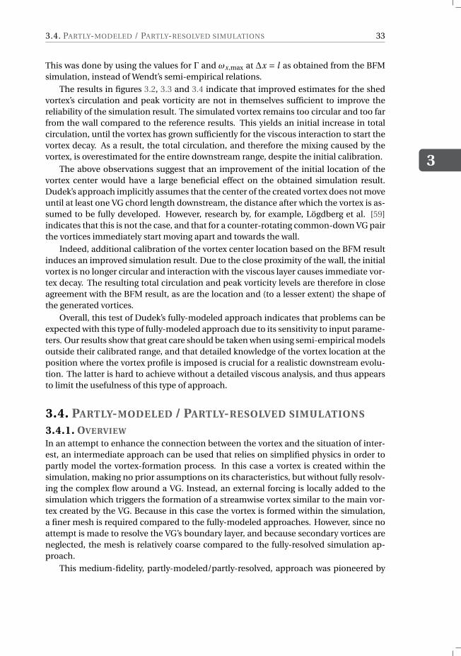
3.4. PARTLY-MODELED / PARTLY-RESOLVED SIMULATIONS
3
33
This was done by using the values for Γ and ωx,max at ∆x = l as obtained from the BFMsimulation, instead of Wendt’s semi-empirical relations.
The results in figures 3.2, 3.3 and 3.4 indicate that improved estimates for the shedvortex’s circulation and peak vorticity are not in themselves sufficient to improve thereliability of the simulation result. The simulated vortex remains too circular and too farfrom the wall compared to the reference results. This yields an initial increase in totalcirculation, until the vortex has grown sufficiently for the viscous interaction to start thevortex decay. As a result, the total circulation, and therefore the mixing caused by thevortex, is overestimated for the entire downstream range, despite the initial calibration.
The above observations suggest that an improvement of the initial location of thevortex center would have a large beneficial effect on the obtained simulation result.Dudek’s approach implicitly assumes that the center of the created vortex does not moveuntil at least one VG chord length downstream, the distance after which the vortex is as-sumed to be fully developed. However, research by, for example, Lögdberg et al. [59]indicates that this is not the case, and that for a counter-rotating common-down VG pairthe vortices immediately start moving apart and towards the wall.
Indeed, additional calibration of the vortex center location based on the BFM resultinduces an improved simulation result. Due to the close proximity of the wall, the initialvortex is no longer circular and interaction with the viscous layer causes immediate vor-tex decay. The resulting total circulation and peak vorticity levels are therefore in closeagreement with the BFM result, as are the location and (to a lesser extent) the shape ofthe generated vortices.
Overall, this test of Dudek’s fully-modeled approach indicates that problems can beexpected with this type of fully-modeled approach due to its sensitivity to input parame-ters. Our results show that great care should be taken when using semi-empirical modelsoutside their calibrated range, and that detailed knowledge of the vortex location at theposition where the vortex profile is imposed is crucial for a realistic downstream evolu-tion. The latter is hard to achieve without a detailed viscous analysis, and thus appearsto limit the usefulness of this type of approach.
3.4. PARTLY-MODELED / PARTLY-RESOLVED SIMULATIONS
3.4.1. OVERVIEW
In an attempt to enhance the connection between the vortex and the situation of inter-est, an intermediate approach can be used that relies on simplified physics in order topartly model the vortex-formation process. In this case a vortex is created within thesimulation, making no prior assumptions on its characteristics, but without fully resolv-ing the complex flow around a VG. Instead, an external forcing is locally added to thesimulation which triggers the formation of a streamwise vortex similar to the main vor-tex created by the VG. Because in this case the vortex is formed within the simulation,a finer mesh is required compared to the fully-modeled approaches. However, since noattempt is made to resolve the VG’s boundary layer, and because secondary vortices areneglected, the mesh is relatively coarse compared to the fully-resolved simulation ap-proach.
This medium-fidelity, partly-modeled/partly-resolved, approach was pioneered by
3
34 3. SIMULATING VORTEX GENERATOR INDUCED FLOWS: STATE OF THE ART
Bender et al. [11], who developed the popular BAY model. This model in essence re-places the VG by the reaction force its presence would impose on the flow, thereby in-troducing an acceleration in crossflow direction which evolves into a streamwise vortex.This model, either in its original form or using the modification proposed by Jirasek (theso-called jBAY model) [41], is often used in industry [21, 30, 47], allowing for reportedmesh-size reductions of 60% - 70% relative to fully-resolved RANS simulations [21, 41].A more detailed discussion of these models follows in section 3.4.2.
The flow-tangency model proposed by Wallin and Eriksson [112] constitutes anotherexample of this simulation approach. In this model, volume forces are applied such thatupon steady-state convergence, flow tangency is satisfied at the virtual VG surface. Toaccomplish this, flow tangency at the virtual VG is linked to the rate of change of the localnormal body forces, yielding a body force equation that is to be solved simultaneouslywith the RANS equations.
More recently, Poole et al. [79] used a partly-modeled/partly-resolved approach basedon the same philosophy as the BAY model. An estimate for the VG’s resultant force wasadded to the momentum equation in the form of an acceleration, enforcing the creationof a streamwise vortex. Their estimate for this resultant force was based on the circu-lation as calculated using the modified lifting-line method presented in the same work.Moreover, the induced drag component was also explicitly taken into account.
3.4.2. THE BAY AND JBAY MODELSAs both the BAY-model and its successor the jBAY-model have been widely adopted byindustry, here a closer look is taken at the details of their performance.
MODEL DETAILS
The BAY model was proposed by Bender et al.[11] in 1999, and since then has beenwidely implemented in CFD codes, see for example [21, 111]. The model mimics theeffect of VGs on the flow by substituting the VG geometry by a volume force, which isrepresentative for the side force (lift force) generated by the VG being modeled. This liftforce is locally approximated as
fi = c AVi
Vtotβρ|ui |2l, (3.7)
where A is the VG planform area, Vi /Vtot is the ratio of the cell volume to the total vol-ume of cells where the source term is applied, ρ is the fluid density and ui the local flowvelocity. The local lift force is assumed to be normal to both the local flow and the spanof the VG, hence the direction l is
l = ui
|ui |×b. (3.8)
Moreover, the angle of incidence of the VG with respect to the incoming flow is assumedsmall, such that
β≈ sinβ= cos(π
2−β
) ui
|ui |·n. (3.9)
Additionally, a factorui
|ui |· t (3.10)
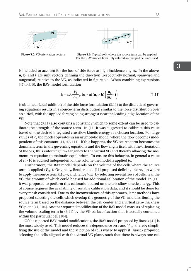
3.4. PARTLY-MODELED / PARTLY-RESOLVED SIMULATIONS
3
35
Figure 3.5: VG orientation vectors. Figure 3.6: Typical cells where the source term can be applied.For the jBAY model, both fully colored and striped cells are used.
is included to account for the loss of side force at high incidence angles. In the above,n, b, and t are unit vectors defining the direction (respectively normal, spanwise andtangential) relative to the VG, as indicated in figure 3.5. When combining expressions3.7 to 3.10, the BAY-model formulation
fi = c AVi
Vtotρ (ui ·n) (ui ×b)
(ui
|ui |· t
)(3.11)
is obtained. Local addition of the side force formulation (3.11) to the discretized govern-ing equations results in a source-term distribution similar to the force distribution overan airfoil, with the applied forcing being strongest near the leading-edge location of theVG.
Note that (3.11) also contains a constant c which to some extent can be used to cal-ibrate the strength of the source term. In [11] it was suggested to calibrate this valuebased on the desired integrated crossflow kinetic energy at a chosen location. For largevalues of c, the model operates in an asymptotic mode, where the flow becomes inde-pendent of this constant [11, 47, 111]. If this happens, the VG source term becomes thedominant term in the governing equations and the flow aligns itself with the orientationof the VG, thus enforcing flow tangency to the virtual VG and thereby allowing the mo-mentum equation to maintain equilibrium. To ensure this behavior, in general a valueof c > 10 is advised independent of the volume the model is applied to.
Furthermore, the BAY model depends on the volume of the cells where the sourceterm is applied (Vtot ). Originally, Bender et al. [11] proposed defining the region whereto apply the source term (ΩV G ), and hence Vtot , by selecting several rows of cells near theVG, the amount of which could be used for additional calibration of the model. In [11],it was proposed to perform this calibration based on the crossflow kinetic energy. Thisof course requires the availability of suitable calibration data, and it should be done forevery mesh considered. Due to the inconvenience of this approach, later methods haveproposed selecting the cells which overlap the geometry of the VG, and distributing thesource term based on the distance between the cell center and a virtual zero-thicknessVG plane[41, 104]. Another reported modification of the BAY model consists of replacingthe volume-scaling term in (3.11) by the VG surface fraction that is actually containedwithin the particular cell [104].
Of the reported BAY-model modifications, the jBAY model proposed by Jirasek [41] isthe most widely used. This model reduces the dependence on c and Vtot , thereby simpli-fying the use of the model and the selection of cells where to apply it. Jirasek proposedselecting the cells aligned with the virtual VG plane, such that there is always one cell
3
36 3. SIMULATING VORTEX GENERATOR INDUCED FLOWS: STATE OF THE ART
center positioned at each side of the VG mean surface (see figure 3.6). Instead of usingthe velocities at the cell centers, the jBAY model calculates the body force using the inter-polated velocity at the intersections of the (virtual) VG surface with the grid edges. Theresulting local source term is then distributed over the surrounding cells. This interpola-tion process keeps the location where flow tangency is enforced consistent, such that thejBAY model can be expected to have improved accuracy and reduced grid dependencecompared to the original BAY model.
REPORTED PERFORMANCE
The BAY and jBAY models have been adopted and implemented in several CFD codes,see for example [21, 25, 47, 111]. This widespread use allows for a good overview of theperformance of this partly-modeled/partly-resolved simulation approach to be obtainedfrom literature.
Most fundamental studies so far have been performed for a single VG on a flat platein a zero-pressure-gradient (ZPG) flow [14, 21, 61, 111]. Overall, the obtained resultsshow a consensus in the observation that both models underestimate the streamwisepeak vorticity, and thereby the intensity, of the created vortex, when compared with bothbody-fitted mesh simulations or experimental data. This behavior is reported for varyingmesh resolutions and regions of application, thereby identifying this underprediction asa weakness inherent to the model. This may be partly due to the absence of VG frictionforces in the BAY and jBAY models, as it was shown in [21] that body-fitted mesh simula-tions with the VG walls modeled as being inviscid produce similar velocity contour plotsas the BAY model.
Less agreement is found between the results with respect to the comparison of thevortex’s shape, trajectory, total circulation and decay rate with reference data. Waithe[111] used the original BAY model and calibrated the model based on experimental databy varying the number of selected rows of cells where the model is applied. For a singleVG on a flat plate, the results seem to indicate a reasonably good agreement in shape,lateral trajectory and total circulation of the modeled vortex. Deviations were observedfor the vortex’s decay rate (which was lower) and the wall-normal location of the vortexcenter (which was further away of the wall). For a pair of counter-rotating VGs, on theother hand, the results obtained with the BAY model by Brunet et al. [14] indicated thatit created vortices that were not only less intense, but also more diffuse than those ofthe body-fitted and experimental references. Moreover, discrepancies in both shape andlateral trajectory were observed, with the modeled vortices being closer together thanthe reference.
For airfoil applications, analysis of BAY/jBAY-model results shows that in general rea-sonable agreement in the pressure distribution can be obtained [41, 61]. However, forairfoils at an angle of attack close to stall, the predictive capabilities of the model fail, aslarge spreads in the aerodynamic coefficients are obtained [8, 47, 61]. This results in alarge uncertainty with respect to both the stall angle and the maximum performance thatcan be expected upon application of a BAY-like model to a particular VG configuration.
Overall, the results from literature seem to indicate that the reliability of BAY-modelresults heavily depends on both mesh resolution and calibration. With respect to meshresolution, however, no conclusive studies can be found that analyze the mesh require-
3.5. CONCLUSION
3
37
ments for specific objectives. In [21], a lateral mesh resolution corresponding to approx-imately 0.2h is used, however, it is unclear whether this resolution is generally sufficient,regardless of the specific objective of the simulation.
As mentioned in the original work of Bender et al. [11], calibration seems to be es-sential in order to obtain the correct amount of flow mixing. To a certain extent this canbe done through the constant c, however, the total cell volume Vtot in which the modelis applied has an equal or even larger influence on the total circulation [11]. In practice,calibration is often not possible due to a lack of available reference data. Therefore theBAY model is usually used without calibration, for example by simply selecting the cellsthat correspond to the actual VG position [14], or by selecting a rectangular domain thatencloses the VG [21]. Use of the jBAY model should eliminate the need for calibration[41], however, studies that identify the impact of cell selection (and hence Vtot ) are lack-ing. The influence of a certain cell-selection approach on the reliability of the simulationresult has thus not been demonstrated, nor has it been shown that the jBAY model doesindeed not require calibration.
This literature survey indicates that there seems to be insufficient knowledge withrespect to the performance of BAY-like models in order to predict the reliability of simu-lation results for specific objectives. It remains unclear how a specific source term affectsthe downstream flow field. Moreover, an understanding of the impact of mesh resolutionand the cell-selection approach on the obtained flow field is required to obtain reliableresults. Further research comparing the original BAY model and the jBAY model, therebyassessing the expected performance improvements of the jBAY model, is also desired.
3.5. CONCLUSIONIn this chapter the results of a literature survey towards different prediction methodswith various levels of fidelity were presented. From an accuracy point of view, fully-resolved (body-fitted mesh) CFD simulations are the method of choice. Unfortunately,time-resolved simulations, like DNS or LES, come at a computational cost that normallyprohibits their use for industrial applications. For high Re-number flows, body-fittedmesh RANS simulations are therefore the standard when high-fidelity results are re-quired. When using RANS, however, care should be taken in choosing the turbulencemodel and interpreting the obtained results, as not all models are able to accurately rep-resent the interactions between the created vortex and the turbulent eddies. Moreover,body-fitted mesh simulations impose a large computational cost since locally very densemeshes are required to fully resolve the VG’s boundary layer and the associated small-scale flow structures. Apart from the large computational effort involved, the creationof a suitable mesh can be a complex task. As an alternative to body-fitted mesh simu-lations, the immersed-boundary method can be an option, as it eliminates the tedioustask of mesh generation. However, the same limitations with respect to mesh resolution(and therefore computational cost) are still present.
On the other end of the spectrum, low-fidelity analytical methods have been pro-posed that, due to their low computational cost, can be of use as a quick assessment toolin initial design phases. These methods mainly attempt to approximate the propertiesof the initial shed vortex. However, their low complexity implies that some fundamentalphysics, like 3D and viscous effects, are neglected. These methods are therefore unreli-
3
38 3. SIMULATING VORTEX GENERATOR INDUCED FLOWS: STATE OF THE ART
able for predictions with respect to the subsequent evolution of the vortices, i.e. their de-cay and interactions. Moreover, the assumptions made during the formulation of thesemodels strongly limit their range of applicability.
Fully-modeled CFD approaches basically attempt to extend an analytical initial vor-tex description with the ability of CFD codes to simulate the downstream convection.Both 2D and 3D approaches have been proposed, typically imposing the analytical vor-tex profile as a source term in either the mean flow or turbulence equations. In gen-eral, qualitatively good results are reported for these type of approaches, however, quan-titative accuracy is less reliable and usually requires calibration. The application of afully-modeled approach shown in this work, illustrated the sensitivity of this modelingapproach to its input parameters. Limitations with respect to the range of applicabilitytherefore also apply here. Moreover, our sample test case suggested that accuracy withrespect to the location of the vortex center is especially important, the accurate predic-tion of which requires 3D and viscous effects to be taken into account.
The category of partly-modeled/partly-resolved simulation methods has the poten-tial of being an effective intermediate solution between the expensive fully-resolved andthe very specific fully-modeled approaches. These simulation methods make use of amodel in the form of a local source term to trigger the formation of a suitable vortex.Hence, the smallest-scale flow features are not accounted for, but the creation and prop-agation of the primary vortex is resolved. By eliminating assumptions with respect to theshape, location and strength of the created vortex, these methods are in theory applica-ble to a wide variety of flow situations. A literature survey has, however, revealed a lackof validation for currently available methods. The effects of mesh resolution and modelparameters on the quantities of interest, are insufficiently understood at this moment.
There thus seems to be a need for a study towards the strengths and limitations ofpartly-modeled/partly-resolved simulation methods, and for the identification of keyparameters that determine their performance. This is of importance for an optimal useof these methods, and the correct interpretation of their results. Moreover, only whenthe effect of specific parameters is clear, can one aim towards the development of modeladaptations which achieve improved accuracy-to-cost ratios. Performing such a study isthe objective of this thesis. The present study focuses in the first instance on the currentindustrial standard in this respect, the BAY and jBAY models. Afterwards, we move onto a more general study of the partly-modeled/partly-resolved modeling concept, andperform a first exploration towards the improvement of these methods.
4DESCRIPTION OF STUDY
Following the overview of the current state of the art in the field of VG design and simula-tion methods (chapters 2 and 3), this chapter lays the foundation for our study towardseffective partly-modeled/partly-resolved source-term models which include the effectof VGs in CFD simulations. To allow for an effective study, the chapter starts with theidentification of the quantities that are of interest when performing simulations of VG-induced flow fields. This is then followed by the outline of our research approach, wherethe applied methodology in section 4.3 is preceded by the definition of our scope (sec-tion 4.2), including an overview of the errors related to source-term CFD simulations.The current chapter concludes with an overview of the test cases that are considered forthe assessment of VG source-term modeling approaches, as presented in the followingchapters, including the presentation of the body-fitted mesh simulation results that willbe used for reference.
4.1. QUANTITIES OF INTEREST IN THE STUDY OF VG-INDUCED
FLOWSBefore assessing the quality of models for simulating VG-induced flow fields, one mustdetermine suitable measures and physical quantities that allow insightful analysis. Ingeneral, distinction can be made between (i) a study of the main vortex generated by aVG, and its downstream evolution, and (ii) an analysis of the effect mixing, due to thisvortex, has on the mean flow and the state of the boundary layer.
In both cases, snapshots of the flow field allow for a quick visual, qualitative analysis.Here the primary and secondary mean-velocity components and the streamwise vortic-ity are of interest, as they show the disturbance of the boundary layer and the topologyof the vortex that causes it.
Vorticity is defined as the curl of the velocity field,
ω=∇×u, (4.1)
39
4
40 4. DESCRIPTION OF STUDY
and can be interpreted as a measure of the level of rotation of the fluid particles. Thestreamwise component of the vorticity vector,
ωx = ∂w
∂y− ∂v
∂z, (4.2)
therefore indicates the rotation in the crossplane (thus perpendicular to the propaga-tion direction of the vortex) due to the secondary-velocity components induced by thepresence of the VG.
Even though a visual analysis of the flow field can provide insight, a thorough quan-titative assessment remains indispensable. The quantities used for this purpose are de-scribed below.
4.1.1. SCALAR DESCRIPTORS OF VORTEX PROPERTIESIn their study of the interaction between a vortex and a turbulent boundary layer, West-phal et al. [116] identified the main descriptors that allow for a quantitative characteriza-tion of vortex properties as being the strength, position, and size of the vortex. These pa-rameters originate from the secondary-velocity field and are generally used in the studyof VG effects [7], although their definition and calculation can change between studies.
Both the absolute value of the overall circulation and peak vorticity are measures typ-ically used to quantify the vortex strength. The peak vorticity ωx,max is the peak value ofthe streamwise vorticity field created by the vortex in a plane downstream of the VG, andis attained in the core of the vortex. This quantity gives an indication for the intensityof the vortex and rapidly attenuates downstream of the VG. Determination of ωx,max isstraightforward, but mesh dependent. If the mesh resolution is insufficient near the vor-tex core, the peak cannot be resolved and ωx,max will be underestimated. In the currentwork, ωx,max is therefore determined as the peak value after performing a spline surfacefit.
The absolute value of the total circulation |Γ| is best suited to assess the overall flowcirculation created by the vortex, and therefore the amount of mixing in the flow. Circu-lation is a scalar integral quantity that is a measure for the rotation in a domain of thefluid, typically calculated as the surface integral of the vorticity field,
Γ=∮
lu · dl =
∫S
(∇×u) · dS =∫
Sω · dS. (4.3)
Circulation is defined in this work as the integral of only the positive streamwise vortic-ity due to the primary vortex, thus including only a single vortex and excluding the layerof negative vorticity occurring close to the wall in these flows. Determination of the do-main over which to perform the integration is not straightforward, as a vortex is typicallysmeared out and therefore no clear boundary can be defined. Several approaches todetermine S have therefore been proposed in literature. In [116] the vortex domain Sconsists of the region where ωx > 0.1ωx,max, thus neglecting the region with lowest vor-ticity where the uncertainty of the results is largest. This filtering is not applied in [1, 119],where the entire positive streamwise vorticity field is considered. Other options for iden-tifying coherent vortex structures can be found in [40], where the λ2- and Q-criteria werefound to be the most accurate. The λ2-method bases the detection of the vortex core on
4.1. QUANTITIES OF INTEREST IN THE STUDY OF VG-INDUCED FLOWS
4
41
the eigenvalues of the velocity gradient tensor, whereas the Q-criterion defines the vor-tex core as the connected fluid region with a positive second invariant of the velocitygradient tensor, and is for example used in [9]. Still, a vortex-core definition based ona cut-off vorticity level is encountered most often in literature, e.g. [47, 62, 115]. In thiswork we therefore chose to use the ωx approach of [116].
A final measure related to the vortex strength consists of the rate with which it decaysas the vortex convects downstream. Due to the nature of the decay process, this can bevisualized as ln(|Γ|/|Γref|), the natural logarithm of the ratio between the circulation anda reference value, the latter typically corresponding to the maximum circulation that isachieved closely downstream of the VG’s trailing edge.
Another important measure used to characterize the vortex created by a VG is theposition of its core, which allows the study of the trajectory of the vortex as it propagatesin the flow and hence to assess whether or not the vortex remains sufficiently close tothe wall. Determination of the position of the vortex core is typically based on the vor-ticity field. In [116] it was determined as the geometric center of the concentric vorticitycontours. However, as vortex cores approach a surface they rarely remain concentric.Considering that the peak vorticity is attained in the vortex core, a more practical ap-proach consists of defining the vortex center as
(yc , zc ) = argmaxy,z
ωx (y, z), (4.4)
with for ωx the spline surface fit, hence as the location where the peak vorticity is found.Finally, a length scale can be determined to quantify the size of a vortex. Often the
edge of the vortex within a cross plane is considered to be the half-life contour, determin-ing the location where the streamwise vorticity has halved compared to its peak value.As in general vortex cores are not circular, due to the interactions with each other and thewall, this measure is ambiguous and different length scales have been proposed in litera-ture. For example, Yao et al. [119] defined the vortex radius as the average of the half-lifedistances in lateral and wall-normal direction. Westphal et al. [116] reported the vortexradius in both these directions separately and, based on this, also defined an ellipticityratio as e = Ry /Rz to indicate the level of flattening of the core. Another approach wasproposed by Ashill et al. [7], who quantified the scale of the vortex by calculating the ra-dius of an equivalent (circular) Rankine vortex based on the vortex strength parameters.
In this work we suggest the use of an alternative quantification of the vortex size,which is based on the area AS of the region S in (4.3), used for the overall circulationcalculation. To prevent a quadratic growth of this parameter with vortex size, we definea vortex radius R as
R =√
AS
π, (4.5)
the radius of an equivalent circular vortex with the same area.
4.1.2. QUANTIFYING THE EFFECT OF MIXING ON THE BOUNDARY LAYERThe analytical, fully-modeled and partly-modeled/partly-resolved approaches discussedin section 3 do not attempt to accurately reproduce the physics related to vortex forma-tion around a VG. Therefore assessing their performance based on the vortex descriptors
4
42 4. DESCRIPTION OF STUDY
identified above may not be the optimal approach. Since the goal of these models con-sists of reproducing the effect the VG has on the mean flow, it is desirable to quantify theeffect of mixing on the boundary layer. A study of integral boundary layer parameters,for example δ∗, θ and H , is suitable for this purpose [48, 86].
The displacement thickness δ∗ is defined based upon the boundary-layer’s velocityprofile as
δ∗ =∫ δ
0
(1− ρU (z)
ρ∞U∞
)dz, (4.6)
with z the wall normal coordinate, and is a length parameter which reflects the distancethrough which the external inviscid flow is displaced by the presence of a boundary layer[4]. Enhanced mixing, for example by the presence of a streamwise vortex, causes themomentum loss being more evenly distributed throughout the boundary layer, resultingin a reduction of δ∗.
In addition, the momentum thickness θ is a measure of the amount of momentumlost by the flow due to the presence of a viscous boundary layer [86]. This quantity isdefined as
θ =∫ δ
0
ρU (z)
ρ∞U∞
(1− U (z)
U∞
)dz. (4.7)
Enhanced flow mixing in this case thus yields an increase in θ, since fluid particles witha higher momentum are transported toward the wall.
The analysis of both above measures can be combined by considering the shape fac-tor H . The shape factor serves as an important indicator for the boundary-layer’s sus-ceptibility to separation and is defined as the ratio between the boundary-layer displace-ment and momentum thicknesses,
H = δ∗
θ. (4.8)
The introduction of a streamwise vortex into the flow causes a decrease in δ∗ and an in-crease in θ, thus reflecting in a reduced value for H . Low values for H therefore typicallyindicate an attached boundary layer, whereas (in general) for H > 4, the flow is sepa-rated from the surface. As H thus is a primary indicator for the tendency of a boundarylayer to separate, and delay of boundary-layer separation is the primal role of VGs, H isconsidered a key parameter when analyzing the performance of VG models.
4.2. RESEARCH SCOPE
4.2.1. FLOW CONDITIONSVG’s are found in a variety of applications, ranging from engine inlets to wind-turbineblades, thereby spanning a wide range of possible flow conditions. To limit the range offlow situations that require consideration in our study, this work is focused on externalaerodynamics applications, where VGs are used as a passive flow-control mechanism todelay boundary-layer separation. Moreover, we limit our scope to incompressible andfully-turbulent flows. These are representative of wind-turbine applications, which con-stitutes the main driver for our research.
In this work the (steady) RANS equations in combination with a turbulent-viscositymodel are used for the numerical simulation of the flows considered. This choice is
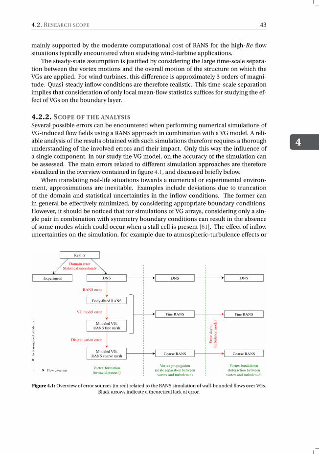
4.2. RESEARCH SCOPE
4
43
mainly supported by the moderate computational cost of RANS for the high-Re flowsituations typically encountered when studying wind-turbine applications.
The steady-state assumption is justified by considering the large time-scale separa-tion between the vortex motions and the overall motion of the structure on which theVGs are applied. For wind turbines, this difference is approximately 3 orders of magni-tude. Quasi-steady inflow conditions are therefore realistic. This time-scale separationimplies that consideration of only local mean-flow statistics suffices for studying the ef-fect of VGs on the boundary layer.
4.2.2. SCOPE OF THE ANALYSISSeveral possible errors can be encountered when performing numerical simulations ofVG-induced flow fields using a RANS approach in combination with a VG model. A reli-able analysis of the results obtained with such simulations therefore requires a thoroughunderstanding of the involved errors and their impact. Only this way the influence ofa single component, in our study the VG model, on the accuracy of the simulation canbe assessed. The main errors related to different simulation approaches are thereforevisualized in the overview contained in figure 4.1, and discussed briefly below.
When translating real-life situations towards a numerical or experimental environ-ment, approximations are inevitable. Examples include deviations due to truncationof the domain and statistical uncertainties in the inflow conditions. The former canin general be effectively minimized, by considering appropriate boundary conditions.However, it should be noticed that for simulations of VG arrays, considering only a sin-gle pair in combination with symmetry boundary conditions can result in the absenceof some modes which could occur when a stall cell is present [61]. The effect of inflowuncertainties on the simulation, for example due to atmospheric-turbulence effects or
Reality
Experiment DNS
Body-fitted RANS
Modeled VG,
RANS fine mesh
Modeled VG,
RANS coarse mesh
VG model error
Discretization error
RANS error
Fine RANS
Coarse RANS
Err
or
due
to
turb
ule
nce
model
DNS
Vortex formation
(inviscid process)
Vortex propagation
(scale separation between
vortex and turbulence)
Vortex breakdown
(Interaction between
vortex and turbulence)
Fine RANS
Coarse RANS
DNS
Flow direction
Incr
easi
ng
lev
el o
f fi
del
ity
Domain error
Statistical uncertainty
Figure 4.1: Overview of error sources (in red) related to the RANS simulation of wall-bounded flows over VGs.Black arrows indicate a theoretical lack of error.
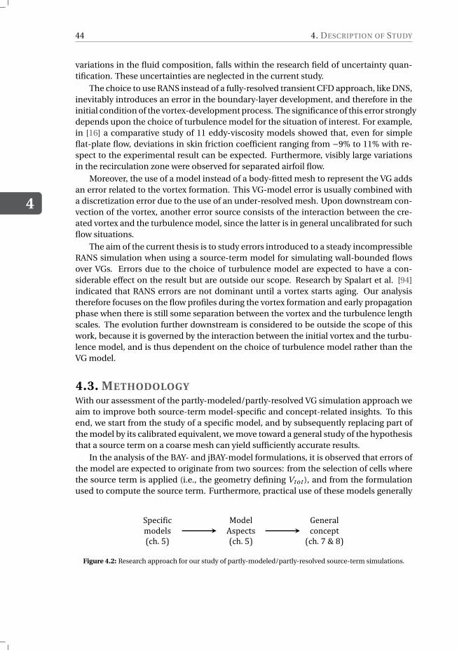
4
44 4. DESCRIPTION OF STUDY
variations in the fluid composition, falls within the research field of uncertainty quan-tification. These uncertainties are neglected in the current study.
The choice to use RANS instead of a fully-resolved transient CFD approach, like DNS,inevitably introduces an error in the boundary-layer development, and therefore in theinitial condition of the vortex-development process. The significance of this error stronglydepends upon the choice of turbulence model for the situation of interest. For example,in [16] a comparative study of 11 eddy-viscosity models showed that, even for simpleflat-plate flow, deviations in skin friction coefficient ranging from −9% to 11% with re-spect to the experimental result can be expected. Furthermore, visibly large variationsin the recirculation zone were observed for separated airfoil flow.
Moreover, the use of a model instead of a body-fitted mesh to represent the VG addsan error related to the vortex formation. This VG-model error is usually combined witha discretization error due to the use of an under-resolved mesh. Upon downstream con-vection of the vortex, another error source consists of the interaction between the cre-ated vortex and the turbulence model, since the latter is in general uncalibrated for suchflow situations.
The aim of the current thesis is to study errors introduced to a steady incompressibleRANS simulation when using a source-term model for simulating wall-bounded flowsover VGs. Errors due to the choice of turbulence model are expected to have a con-siderable effect on the result but are outside our scope. Research by Spalart et al. [94]indicated that RANS errors are not dominant until a vortex starts aging. Our analysistherefore focuses on the flow profiles during the vortex formation and early propagationphase when there is still some separation between the vortex and the turbulence lengthscales. The evolution further downstream is considered to be outside the scope of thiswork, because it is governed by the interaction between the initial vortex and the turbu-lence model, and is thus dependent on the choice of turbulence model rather than theVG model.
4.3. METHODOLOGYWith our assessment of the partly-modeled/partly-resolved VG simulation approach weaim to improve both source-term model-specific and concept-related insights. To thisend, we start from the study of a specific model, and by subsequently replacing part ofthe model by its calibrated equivalent, we move toward a general study of the hypothesisthat a source term on a coarse mesh can yield sufficiently accurate results.
In the analysis of the BAY- and jBAY-model formulations, it is observed that errors ofthe model are expected to originate from two sources: from the selection of cells wherethe source term is applied (i.e., the geometry defining Vtot ), and from the formulationused to compute the source term. Furthermore, practical use of these models generally
!"#$%&%$'
()*#+,
-$./ 01
2)*#+'
3,"#$4,
-$./ 01
5#6#78+'
$)6$#"4
-$./ 9':';1
Figure 4.2: Research approach for our study of partly-modeled/partly-resolved source-term simulations.
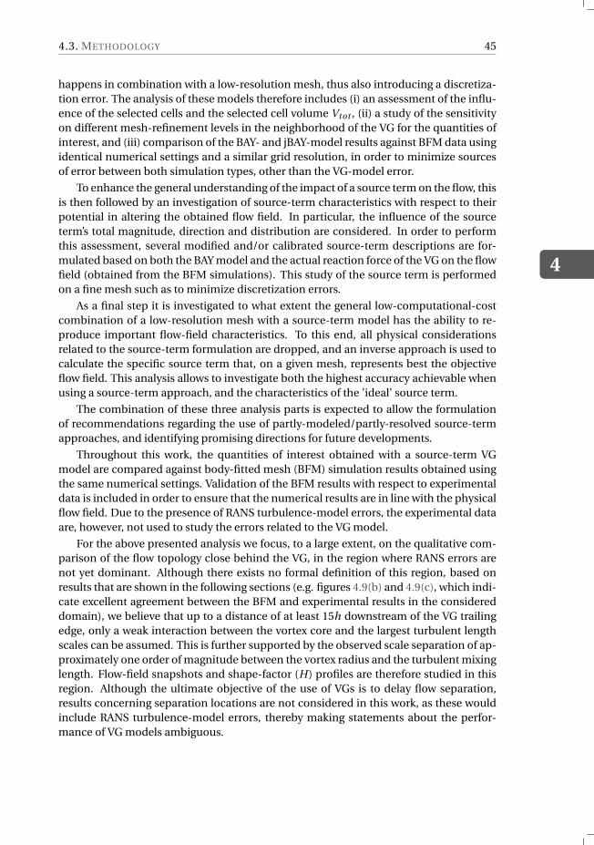
4.3. METHODOLOGY
4
45
happens in combination with a low-resolution mesh, thus also introducing a discretiza-tion error. The analysis of these models therefore includes (i) an assessment of the influ-ence of the selected cells and the selected cell volume Vtot , (ii) a study of the sensitivityon different mesh-refinement levels in the neighborhood of the VG for the quantities ofinterest, and (iii) comparison of the BAY- and jBAY-model results against BFM data usingidentical numerical settings and a similar grid resolution, in order to minimize sourcesof error between both simulation types, other than the VG-model error.
To enhance the general understanding of the impact of a source term on the flow, thisis then followed by an investigation of source-term characteristics with respect to theirpotential in altering the obtained flow field. In particular, the influence of the sourceterm’s total magnitude, direction and distribution are considered. In order to performthis assessment, several modified and/or calibrated source-term descriptions are for-mulated based on both the BAY model and the actual reaction force of the VG on the flowfield (obtained from the BFM simulations). This study of the source term is performedon a fine mesh such as to minimize discretization errors.
As a final step it is investigated to what extent the general low-computational-costcombination of a low-resolution mesh with a source-term model has the ability to re-produce important flow-field characteristics. To this end, all physical considerationsrelated to the source-term formulation are dropped, and an inverse approach is used tocalculate the specific source term that, on a given mesh, represents best the objectiveflow field. This analysis allows to investigate both the highest accuracy achievable whenusing a source-term approach, and the characteristics of the ’ideal’ source term.
The combination of these three analysis parts is expected to allow the formulationof recommendations regarding the use of partly-modeled/partly-resolved source-termapproaches, and identifying promising directions for future developments.
Throughout this work, the quantities of interest obtained with a source-term VGmodel are compared against body-fitted mesh (BFM) simulation results obtained usingthe same numerical settings. Validation of the BFM results with respect to experimentaldata is included in order to ensure that the numerical results are in line with the physicalflow field. Due to the presence of RANS turbulence-model errors, the experimental dataare, however, not used to study the errors related to the VG model.
For the above presented analysis we focus, to a large extent, on the qualitative com-parison of the flow topology close behind the VG, in the region where RANS errors arenot yet dominant. Although there exists no formal definition of this region, based onresults that are shown in the following sections (e.g. figures 4.9(b) and 4.9(c), which indi-cate excellent agreement between the BFM and experimental results in the considereddomain), we believe that up to a distance of at least 15h downstream of the VG trailingedge, only a weak interaction between the vortex core and the largest turbulent lengthscales can be assumed. This is further supported by the observed scale separation of ap-proximately one order of magnitude between the vortex radius and the turbulent mixinglength. Flow-field snapshots and shape-factor (H) profiles are therefore studied in thisregion. Although the ultimate objective of the use of VGs is to delay flow separation,results concerning separation locations are not considered in this work, as these wouldinclude RANS turbulence-model errors, thereby making statements about the perfor-mance of VG models ambiguous.
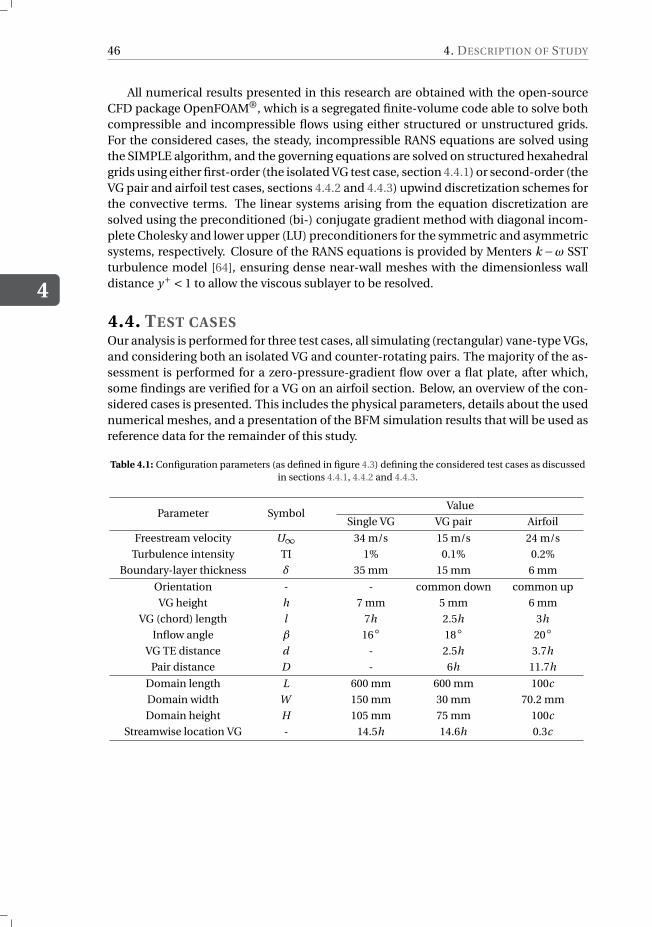
4
46 4. DESCRIPTION OF STUDY
All numerical results presented in this research are obtained with the open-sourceCFD package OpenFOAM®, which is a segregated finite-volume code able to solve bothcompressible and incompressible flows using either structured or unstructured grids.For the considered cases, the steady, incompressible RANS equations are solved usingthe SIMPLE algorithm, and the governing equations are solved on structured hexahedralgrids using either first-order (the isolated VG test case, section 4.4.1) or second-order (theVG pair and airfoil test cases, sections 4.4.2 and 4.4.3) upwind discretization schemes forthe convective terms. The linear systems arising from the equation discretization aresolved using the preconditioned (bi-) conjugate gradient method with diagonal incom-plete Cholesky and lower upper (LU) preconditioners for the symmetric and asymmetricsystems, respectively. Closure of the RANS equations is provided by Menters k −ω SSTturbulence model [64], ensuring dense near-wall meshes with the dimensionless walldistance y+ < 1 to allow the viscous sublayer to be resolved.
4.4. TEST CASESOur analysis is performed for three test cases, all simulating (rectangular) vane-type VGs,and considering both an isolated VG and counter-rotating pairs. The majority of the as-sessment is performed for a zero-pressure-gradient flow over a flat plate, after which,some findings are verified for a VG on an airfoil section. Below, an overview of the con-sidered cases is presented. This includes the physical parameters, details about the usednumerical meshes, and a presentation of the BFM simulation results that will be used asreference data for the remainder of this study.
Table 4.1: Configuration parameters (as defined in figure 4.3) defining the considered test cases as discussedin sections 4.4.1, 4.4.2 and 4.4.3.
Parameter SymbolValue
Single VG VG pair Airfoil
Freestream velocity U∞ 34 m/s 15 m/s 24 m/s
Turbulence intensity TI 1% 0.1% 0.2%
Boundary-layer thickness δ 35 mm 15 mm 6 mm
Orientation - - common down common up
VG height h 7 mm 5 mm 6 mm
VG (chord) length l 7h 2.5h 3h
Inflow angle β 16 18 20VG TE distance d - 2.5h 3.7h
Pair distance D - 6h 11.7h
Domain length L 600 mm 600 mm 100c
Domain width W 150 mm 30 mm 70.2 mm
Domain height H 105 mm 75 mm 100c
Streamwise location VG - 14.5h 14.6h 0.3c
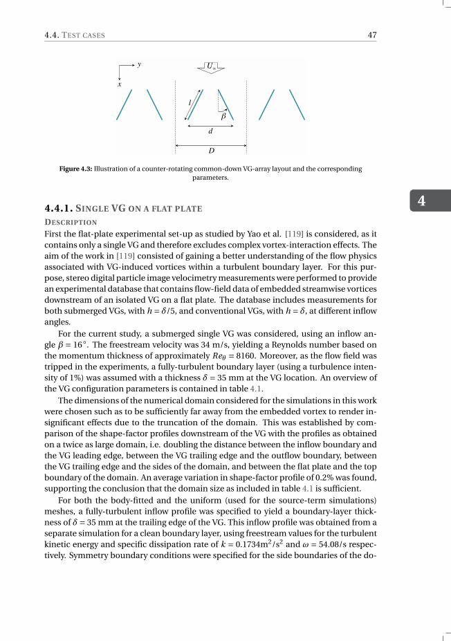
4.4. TEST CASES
4
47
U∞
β
d
D
l
y
x
Figure 4.3: Illustration of a counter-rotating common-down VG-array layout and the correspondingparameters.
4.4.1. SINGLE VG ON A FLAT PLATE
DESCRIPTION
First the flat-plate experimental set-up as studied by Yao et al. [119] is considered, as itcontains only a single VG and therefore excludes complex vortex-interaction effects. Theaim of the work in [119] consisted of gaining a better understanding of the flow physicsassociated with VG-induced vortices within a turbulent boundary layer. For this pur-pose, stereo digital particle image velocimetry measurements were performed to providean experimental database that contains flow-field data of embedded streamwise vorticesdownstream of an isolated VG on a flat plate. The database includes measurements forboth submerged VGs, with h = δ/5, and conventional VGs, with h = δ, at different inflowangles.
For the current study, a submerged single VG was considered, using an inflow an-gle β = 16. The freestream velocity was 34 m/s, yielding a Reynolds number based onthe momentum thickness of approximately Reθ = 8160. Moreover, as the flow field wastripped in the experiments, a fully-turbulent boundary layer (using a turbulence inten-sity of 1%) was assumed with a thickness δ= 35 mm at the VG location. An overview ofthe VG configuration parameters is contained in table 4.1.
The dimensions of the numerical domain considered for the simulations in this workwere chosen such as to be sufficiently far away from the embedded vortex to render in-significant effects due to the truncation of the domain. This was established by com-parison of the shape-factor profiles downstream of the VG with the profiles as obtainedon a twice as large domain, i.e. doubling the distance between the inflow boundary andthe VG leading edge, between the VG trailing edge and the outflow boundary, betweenthe VG trailing edge and the sides of the domain, and between the flat plate and the topboundary of the domain. An average variation in shape-factor profile of 0.2% was found,supporting the conclusion that the domain size as included in table 4.1 is sufficient.
For both the body-fitted and the uniform (used for the source-term simulations)meshes, a fully-turbulent inflow profile was specified to yield a boundary-layer thick-ness of δ= 35 mm at the trailing edge of the VG. This inflow profile was obtained from aseparate simulation for a clean boundary layer, using freestream values for the turbulentkinetic energy and specific dissipation rate of k = 0.1734m2/s2 and ω = 54.08/s respec-tively. Symmetry boundary conditions were specified for the side boundaries of the do-
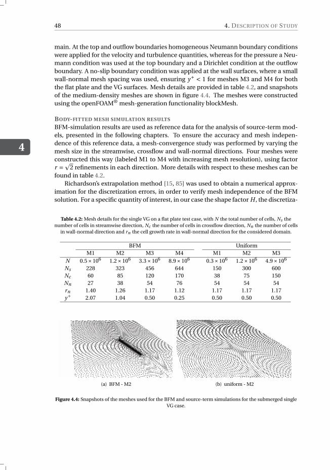
4
48 4. DESCRIPTION OF STUDY
main. At the top and outflow boundaries homogeneous Neumann boundary conditionswere applied for the velocity and turbulence quantities, whereas for the pressure a Neu-mann condition was used at the top boundary and a Dirichlet condition at the outflowboundary. A no-slip boundary condition was applied at the wall surfaces, where a smallwall-normal mesh spacing was used, ensuring y+ < 1 for meshes M3 and M4 for boththe flat plate and the VG surfaces. Mesh details are provided in table 4.2, and snapshotsof the medium-density meshes are shown in figure 4.4. The meshes were constructedusing the openFOAM® mesh-generation functionality blockMesh.
BODY-FITTED MESH SIMULATION RESULTS
BFM-simulation results are used as reference data for the analysis of source-term mod-els, presented in the following chapters. To ensure the accuracy and mesh indepen-dence of this reference data, a mesh-convergence study was performed by varying themesh size in the streamwise, crossflow and wall-normal directions. Four meshes wereconstructed this way (labeled M1 to M4 with increasing mesh resolution), using factorr =p
2 refinements in each direction. More details with respect to these meshes can befound in table 4.2.
Richardson’s extrapolation method [15, 85] was used to obtain a numerical approx-imation for the discretization errors, in order to verify mesh independence of the BFMsolution. For a specific quantity of interest, in our case the shape factor H , the discretiza-
Table 4.2: Mesh details for the single VG on a flat plate test case, with N the total number of cells, Ns thenumber of cells in streamwise direction, Nc the number of cells in crossflow direction, Nn the number of cells
in wall-normal direction and rn the cell growth rate in wall-normal direction for the considered domain.
BFM UniformM1 M2 M3 M4 M1 M2 M3
N 0.5×10⁶ 1.2×10⁶ 3.3×10⁶ 8.9×10⁶ 0.3×10⁶ 1.2×10⁶ 4.9×10⁶
Ns 228 323 456 644 150 300 600Nc 60 85 120 170 38 75 150Nn 27 38 54 76 54 54 54rn 1.40 1.26 1.17 1.12 1.17 1.17 1.17y+ 2.07 1.04 0.50 0.25 0.50 0.50 0.50
(a) BFM - M2 (b) uniform - M2
Figure 4.4: Snapshots of the meshes used for the BFM and source-term simulations for the submerged singleVG case.
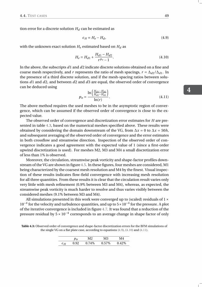
4.4. TEST CASES
4
49
tion error for a discrete solution Hd can be estimated as
ϵH = He −Hd , (4.9)
with the unknown exact solution He estimated based on Hd as
He = Hd1 +Hd1 −Hd2
r po −1. (4.10)
In the above, the subscripts d1 and d2 indicate discrete solutions obtained on a fine andcoarse mesh respectively, and r represents the ratio of mesh spacings, r = ∆d2/∆d1. Inthe presence of a third discrete solution, and if the mesh-spacing ratios between solu-tions d1 and d2, and between d2 and d3 are equal, the observed order of convergencecan be deduced using
po =ln
(Hd3−Hd2Hd2−Hd1
)ln(r )
. (4.11)
The above method requires the used meshes to be in the asymptotic region of conver-gence, which can be assumed if the observed order of convergence is close to the ex-pected value.
The observed order of convergence and discretization error estimates for H are pre-sented in table 4.3, based on the numerical meshes specified above. These results wereobtained by considering the domain downstream of the VG, from ∆x = 0 to ∆x = 50h,and subsequent averaging of the observed order of convergence and the error estimatesin both crossflow and streamwise direction. Inspection of the observed order of con-vergence indicates a good agreement with the expected value of 1 (since a first-orderupwind discretization is used). For meshes M2, M3 and M4 a small discretization errorof less than 1% is observed.
Moreover, the circulation, streamwise peak vorticity and shape-factor profiles down-stream of the VG are shown in figure 4.5. In these figures, four meshes are considered, M1being characterized by the coarsest mesh resolution and M4 by the finest. Visual inspec-tion of these results indicates flow-field convergence with increasing mesh resolutionfor all three quantities. From these results it is clear that the circulation result varies onlyvery little with mesh refinement (0.9% between M3 and M4), whereas, as expected, thestreamwise peak vorticity is much harder to resolve and thus varies visibly between theconsidered meshes (9.1% between M3 and M4).
All simulations presented in this work were converged up to (scaled) residuals of 1×10⁻⁴ for the velocity and turbulence quantities, and up to 5×10⁻⁴ for the pressure. A plotof the iterative convergence is included in figure 4.7. It was found that a reduction of thepressure residual by 5×10⁻⁴ corresponds to an average change in shape factor of only
Table 4.3: Observed order of convergence and shape-factor discretization errors for the BFM simulations ofthe single VG on a flat plate case, according to equations (4.9), (4.10) and (4.11).
po M2 M3 M4ϵH 0.92 0.74% 0.57% 0.42%
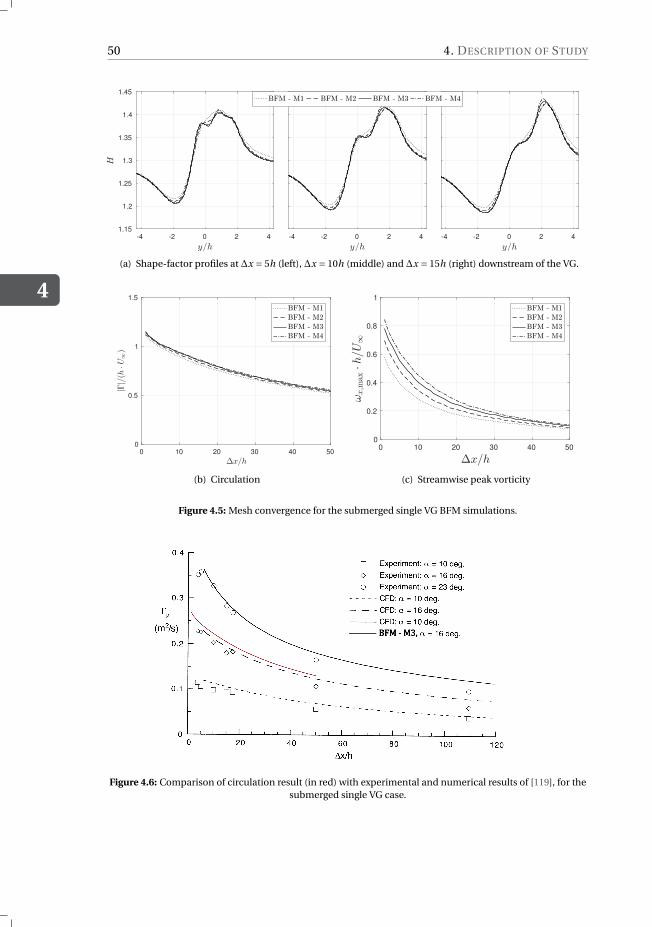
4
50 4. DESCRIPTION OF STUDY
-4 -2 0 2 4
1.15
1.2
1.25
1.3
1.35
1.4
1.45
-4 -2 0 2 4 -4 -2 0 2 4
(a) Shape-factor profiles at ∆x = 5h (left), ∆x = 10h (middle) and ∆x = 15h (right) downstream of the VG.
0 10 20 30 40 50
0
0.5
1
1.5
(b) Circulation
0 10 20 30 40 50
0
0.2
0.4
0.6
0.8
1
(c) Streamwise peak vorticity
Figure 4.5: Mesh convergence for the submerged single VG BFM simulations.
Figure 4.6: Comparison of circulation result (in red) with experimental and numerical results of [119], for thesubmerged single VG case.
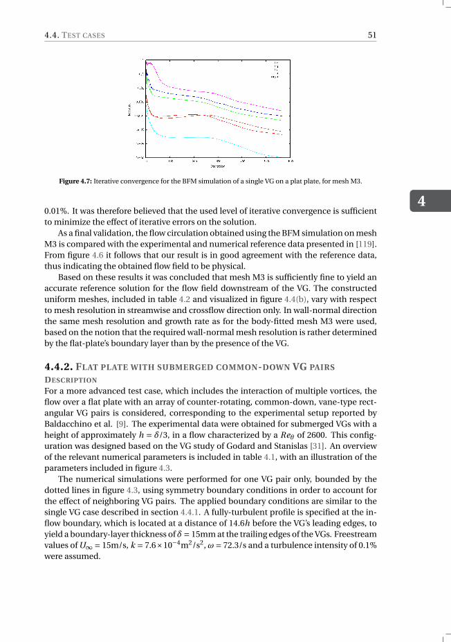
4.4. TEST CASES
4
51
Figure 4.7: Iterative convergence for the BFM simulation of a single VG on a plat plate, for mesh M3.
0.01%. It was therefore believed that the used level of iterative convergence is sufficientto minimize the effect of iterative errors on the solution.
As a final validation, the flow circulation obtained using the BFM simulation on meshM3 is compared with the experimental and numerical reference data presented in [119].From figure 4.6 it follows that our result is in good agreement with the reference data,thus indicating the obtained flow field to be physical.
Based on these results it was concluded that mesh M3 is sufficiently fine to yield anaccurate reference solution for the flow field downstream of the VG. The constructeduniform meshes, included in table 4.2 and visualized in figure 4.4(b), vary with respectto mesh resolution in streamwise and crossflow direction only. In wall-normal directionthe same mesh resolution and growth rate as for the body-fitted mesh M3 were used,based on the notion that the required wall-normal mesh resolution is rather determinedby the flat-plate’s boundary layer than by the presence of the VG.
4.4.2. FLAT PLATE WITH SUBMERGED COMMON-DOWN VG PAIRS
DESCRIPTION
For a more advanced test case, which includes the interaction of multiple vortices, theflow over a flat plate with an array of counter-rotating, common-down, vane-type rect-angular VG pairs is considered, corresponding to the experimental setup reported byBaldacchino et al. [9]. The experimental data were obtained for submerged VGs with aheight of approximately h = δ/3, in a flow characterized by a Reθ of 2600. This config-uration was designed based on the VG study of Godard and Stanislas [31]. An overviewof the relevant numerical parameters is included in table 4.1, with an illustration of theparameters included in figure 4.3.
The numerical simulations were performed for one VG pair only, bounded by thedotted lines in figure 4.3, using symmetry boundary conditions in order to account forthe effect of neighboring VG pairs. The applied boundary conditions are similar to thesingle VG case described in section 4.4.1. A fully-turbulent profile is specified at the in-flow boundary, which is located at a distance of 14.6h before the VG’s leading edges, toyield a boundary-layer thickness ofδ= 15mm at the trailing edges of the VGs. Freestreamvalues of U∞ = 15m/s, k = 7.6×10⁻⁴m2/s2, ω= 72.3/s and a turbulence intensity of 0.1%were assumed.
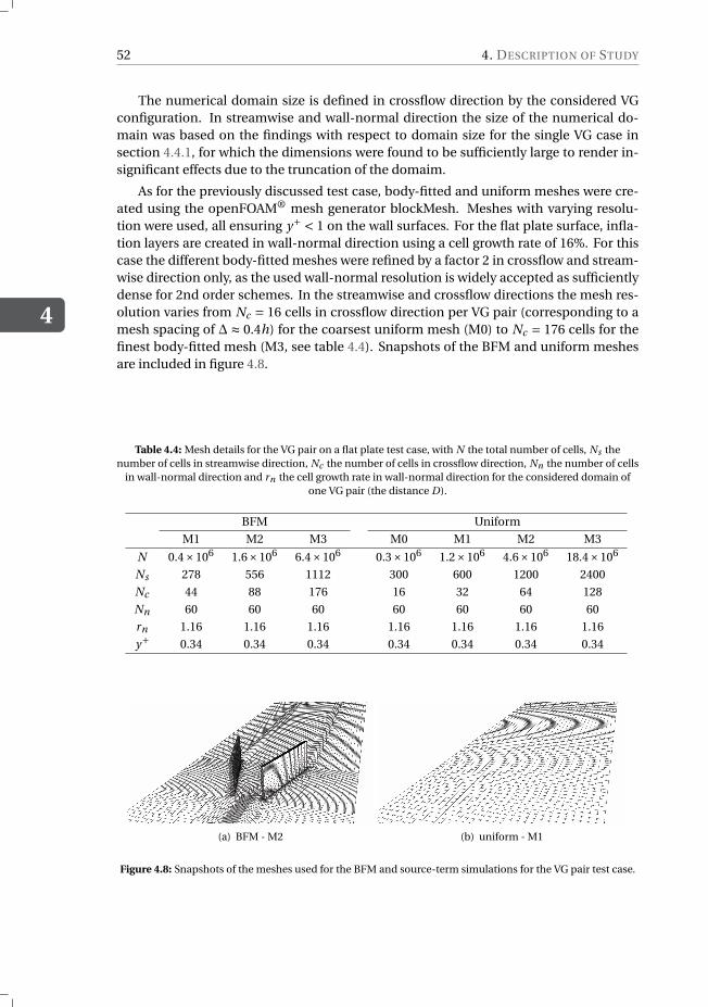
4
52 4. DESCRIPTION OF STUDY
The numerical domain size is defined in crossflow direction by the considered VGconfiguration. In streamwise and wall-normal direction the size of the numerical do-main was based on the findings with respect to domain size for the single VG case insection 4.4.1, for which the dimensions were found to be sufficiently large to render in-significant effects due to the truncation of the domaim.
As for the previously discussed test case, body-fitted and uniform meshes were cre-ated using the openFOAM® mesh generator blockMesh. Meshes with varying resolu-tion were used, all ensuring y+ < 1 on the wall surfaces. For the flat plate surface, infla-tion layers are created in wall-normal direction using a cell growth rate of 16%. For thiscase the different body-fitted meshes were refined by a factor 2 in crossflow and stream-wise direction only, as the used wall-normal resolution is widely accepted as sufficientlydense for 2nd order schemes. In the streamwise and crossflow directions the mesh res-olution varies from Nc = 16 cells in crossflow direction per VG pair (corresponding to amesh spacing of ∆ ≈ 0.4h) for the coarsest uniform mesh (M0) to Nc = 176 cells for thefinest body-fitted mesh (M3, see table 4.4). Snapshots of the BFM and uniform meshesare included in figure 4.8.
Table 4.4: Mesh details for the VG pair on a flat plate test case, with N the total number of cells, Ns thenumber of cells in streamwise direction, Nc the number of cells in crossflow direction, Nn the number of cells
in wall-normal direction and rn the cell growth rate in wall-normal direction for the considered domain ofone VG pair (the distance D).
BFM Uniform
M1 M2 M3 M0 M1 M2 M3
N 0.4×10⁶ 1.6×10⁶ 6.4×10⁶ 0.3×10⁶ 1.2×10⁶ 4.6×10⁶ 18.4×10⁶
Ns 278 556 1112 300 600 1200 2400
Nc 44 88 176 16 32 64 128
Nn 60 60 60 60 60 60 60
rn 1.16 1.16 1.16 1.16 1.16 1.16 1.16
y+ 0.34 0.34 0.34 0.34 0.34 0.34 0.34
(a) BFM - M2 (b) uniform - M1
Figure 4.8: Snapshots of the meshes used for the BFM and source-term simulations for the VG pair test case.
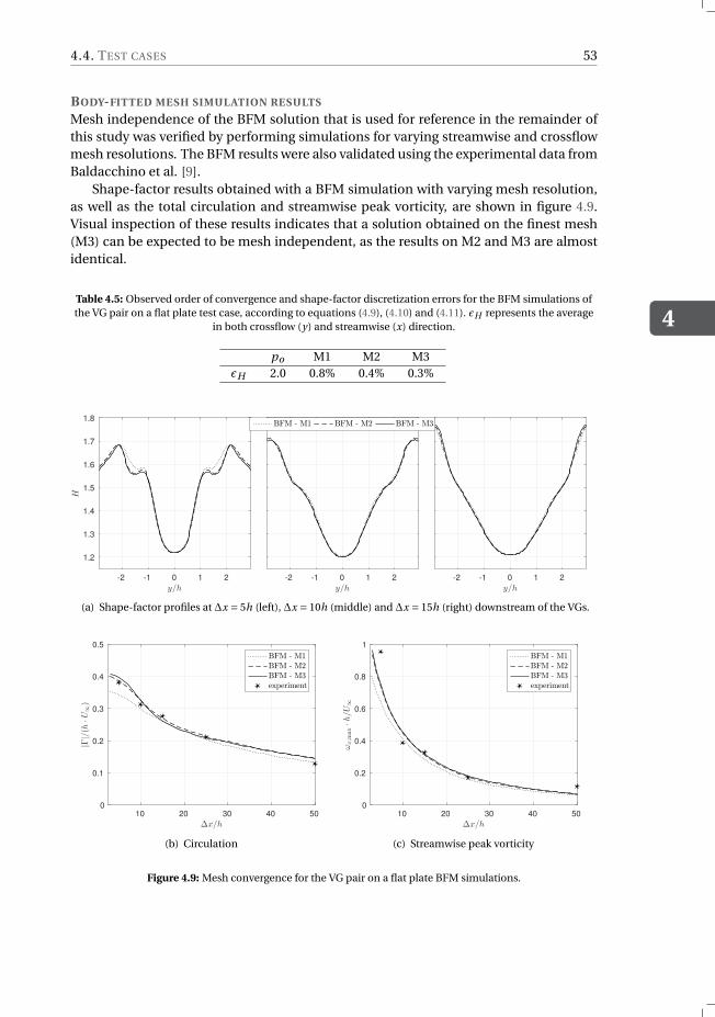
4.4. TEST CASES
4
53
BODY-FITTED MESH SIMULATION RESULTS
Mesh independence of the BFM solution that is used for reference in the remainder ofthis study was verified by performing simulations for varying streamwise and crossflowmesh resolutions. The BFM results were also validated using the experimental data fromBaldacchino et al. [9].
Shape-factor results obtained with a BFM simulation with varying mesh resolution,as well as the total circulation and streamwise peak vorticity, are shown in figure 4.9.Visual inspection of these results indicates that a solution obtained on the finest mesh(M3) can be expected to be mesh independent, as the results on M2 and M3 are almostidentical.
Table 4.5: Observed order of convergence and shape-factor discretization errors for the BFM simulations ofthe VG pair on a flat plate test case, according to equations (4.9), (4.10) and (4.11). ϵH represents the average
in both crossflow (y) and streamwise (x) direction.
po M1 M2 M3ϵH 2.0 0.8% 0.4% 0.3%
-2 -1 0 1 2
y/h
1.2
1.3
1.4
1.5
1.6
1.7
1.8
H
-2 -1 0 1 2
y/h-2 -1 0 1 2
y/h
BFM - M1 BFM - M2 BFM - M3
(a) Shape-factor profiles at ∆x = 5h (left), ∆x = 10h (middle) and ∆x = 15h (right) downstream of the VGs.
10 20 30 40 50
∆x/h
0
0.1
0.2
0.3
0.4
0.5
|Γ|/(h
·U∞)
BFM - M1BFM - M2BFM - M3experiment
(b) Circulation
10 20 30 40 50
∆x/h
0
0.2
0.4
0.6
0.8
1
ωx,m
ax·h/U∞
BFM - M1
BFM - M2
BFM - M3
experiment
(c) Streamwise peak vorticity
Figure 4.9: Mesh convergence for the VG pair on a flat plate BFM simulations.
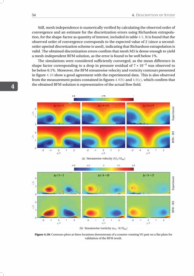
4
54 4. DESCRIPTION OF STUDY
Still, mesh independence is numerically verified by calculating the observed order ofconvergence and an estimate for the discretization errors using Richardson extrapola-tion, for the shape-factor as quantity of interest, included in table 4.5. It is found that theobserved order of convergence corresponds to the expected value of 2 (since a second-order upwind discretization scheme is used), indicating that Richardson extrapolation isvalid. The obtained discretization errors confirm that mesh M3 is dense enough to yielda mesh-independent BFM solution, as the error is found to be well below 1%.
The simulations were considered sufficiently converged, as the mean difference inshape factor corresponding to a drop in pressure residual of 7× 10⁻⁴ was observed tobe below 0.1%. Moreover, the BFM streamwise velocity and vorticity contours presentedin figure 4.10 show a good agreement with the experimental data. This is also observedfrom the measurement points contained in figures 4.9(b) and 4.9(c), which confirm thatthe obtained BFM solution is representative of the actual flow field.
∆x / h = 5 ∆x / h =10 ∆x / h =15
!"#$%&'$()*
+,-*.*-/*
(a) Streamwise velocity (Ux /U∞)
∆x / h = 5 ∆x / h =10 ∆x / h =15!"#$%&'$()*
+,-*.*-/*
(b) Streamwise vorticity (ωx ·h/U∞)
Figure 4.10: Contours plots at three locations downstream of a counter-rotating VG pair on a flat plate forvalidation of the BFM result.
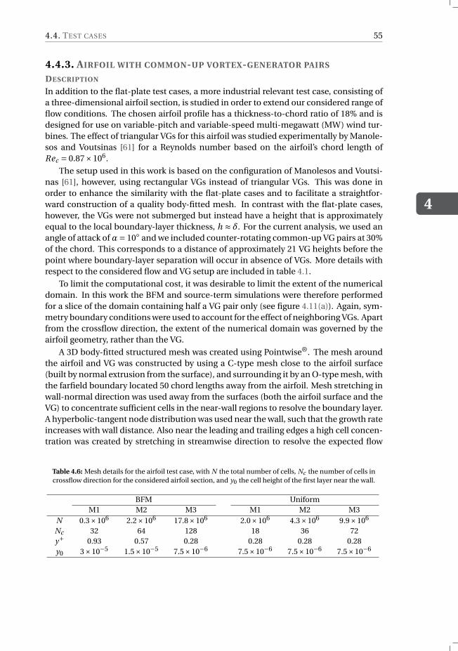
4.4. TEST CASES
4
55
4.4.3. AIRFOIL WITH COMMON-UP VORTEX-GENERATOR PAIRS
DESCRIPTION
In addition to the flat-plate test cases, a more industrial relevant test case, consisting ofa three-dimensional airfoil section, is studied in order to extend our considered range offlow conditions. The chosen airfoil profile has a thickness-to-chord ratio of 18% and isdesigned for use on variable-pitch and variable-speed multi-megawatt (MW) wind tur-bines. The effect of triangular VGs for this airfoil was studied experimentally by Manole-sos and Voutsinas [61] for a Reynolds number based on the airfoil’s chord length ofRec = 0.87×10⁶.
The setup used in this work is based on the configuration of Manolesos and Voutsi-nas [61], however, using rectangular VGs instead of triangular VGs. This was done inorder to enhance the similarity with the flat-plate cases and to facilitate a straightfor-ward construction of a quality body-fitted mesh. In contrast with the flat-plate cases,however, the VGs were not submerged but instead have a height that is approximatelyequal to the local boundary-layer thickness, h ≈ δ. For the current analysis, we used anangle of attack of α= 10 and we included counter-rotating common-up VG pairs at 30%of the chord. This corresponds to a distance of approximately 21 VG heights before thepoint where boundary-layer separation will occur in absence of VGs. More details withrespect to the considered flow and VG setup are included in table 4.1.
To limit the computational cost, it was desirable to limit the extent of the numericaldomain. In this work the BFM and source-term simulations were therefore performedfor a slice of the domain containing half a VG pair only (see figure 4.11(a)). Again, sym-metry boundary conditions were used to account for the effect of neighboring VGs. Apartfrom the crossflow direction, the extent of the numerical domain was governed by theairfoil geometry, rather than the VG.
A 3D body-fitted structured mesh was created using Pointwise®. The mesh aroundthe airfoil and VG was constructed by using a C-type mesh close to the airfoil surface(built by normal extrusion from the surface), and surrounding it by an O-type mesh, withthe farfield boundary located 50 chord lengths away from the airfoil. Mesh stretching inwall-normal direction was used away from the surfaces (both the airfoil surface and theVG) to concentrate sufficient cells in the near-wall regions to resolve the boundary layer.A hyperbolic-tangent node distribution was used near the wall, such that the growth rateincreases with wall distance. Also near the leading and trailing edges a high cell concen-tration was created by stretching in streamwise direction to resolve the expected flow
Table 4.6: Mesh details for the airfoil test case, with N the total number of cells, Nc the number of cells incrossflow direction for the considered airfoil section, and y0 the cell height of the first layer near the wall.
BFM UniformM1 M2 M3 M1 M2 M3
N 0.3×10⁶ 2.2×10⁶ 17.8×10⁶ 2.0×10⁶ 4.3×10⁶ 9.9×10⁶
Nc 32 64 128 18 36 72y+ 0.93 0.57 0.28 0.28 0.28 0.28y0 3×10⁻⁵ 1.5×10⁻⁵ 7.5×10⁻⁶ 7.5×10⁻⁶ 7.5×10⁻⁶ 7.5×10⁻⁶
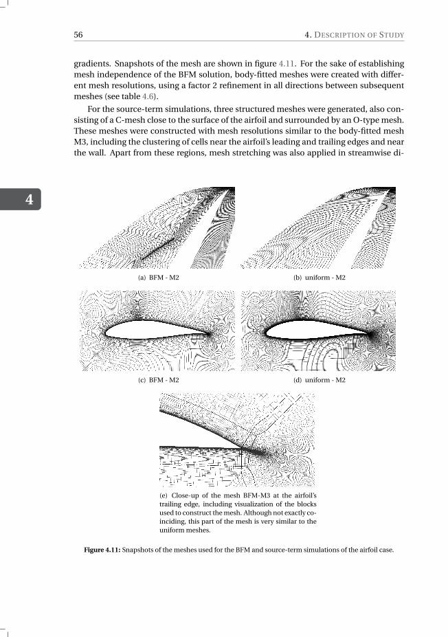
4
56 4. DESCRIPTION OF STUDY
gradients. Snapshots of the mesh are shown in figure 4.11. For the sake of establishingmesh independence of the BFM solution, body-fitted meshes were created with differ-ent mesh resolutions, using a factor 2 refinement in all directions between subsequentmeshes (see table 4.6).
For the source-term simulations, three structured meshes were generated, also con-sisting of a C-mesh close to the surface of the airfoil and surrounded by an O-type mesh.These meshes were constructed with mesh resolutions similar to the body-fitted meshM3, including the clustering of cells near the airfoil’s leading and trailing edges and nearthe wall. Apart from these regions, mesh stretching was also applied in streamwise di-
(a) BFM - M2 (b) uniform - M2
(c) BFM - M2 (d) uniform - M2
(e) Close-up of the mesh BFM-M3 at the airfoil’strailing edge, including visualization of the blocksused to construct the mesh. Although not exactly co-inciding, this part of the mesh is very similar to theuniform meshes.
Figure 4.11: Snapshots of the meshes used for the BFM and source-term simulations of the airfoil case.
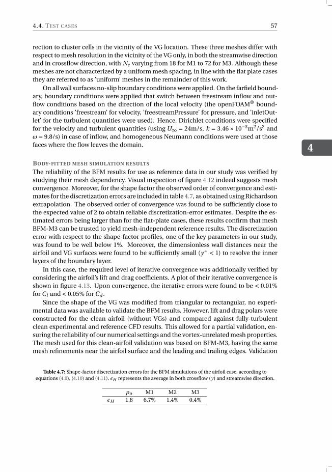
4.4. TEST CASES
4
57
rection to cluster cells in the vicinity of the VG location. These three meshes differ withrespect to mesh resolution in the vicinity of the VG only, in both the streamwise directionand in crossflow direction, with Nc varying from 18 for M1 to 72 for M3. Although thesemeshes are not characterized by a uniform mesh spacing, in line with the flat plate casesthey are referred to as ’uniform’ meshes in the remainder of this work.
On all wall surfaces no-slip boundary conditions were applied. On the farfield bound-ary, boundary conditions were applied that switch between freestream inflow and out-flow conditions based on the direction of the local velocity (the openFOAM® bound-ary conditions ’freestream’ for velocity, ’freestreamPressure’ for pressure, and ’inletOut-let’ for the turbulent quantities were used). Hence, Dirichlet conditions were specifiedfor the velocity and turbulent quantities (using U∞ = 24m/s, k = 3.46×10⁻³m2/s2 andω= 9.8/s) in case of inflow, and homogeneous Neumann conditions were used at thosefaces where the flow leaves the domain.
BODY-FITTED MESH SIMULATION RESULTS
The reliability of the BFM results for use as reference data in our study was verified bystudying their mesh dependency. Visual inspection of figure 4.12 indeed suggests meshconvergence. Moreover, for the shape factor the observed order of convergence and esti-mates for the discretization errors are included in table 4.7, as obtained using Richardsonextrapolation. The observed order of convergence was found to be sufficiently close tothe expected value of 2 to obtain reliable discretization-error estimates. Despite the es-timated errors being larger than for the flat-plate cases, these results confirm that meshBFM-M3 can be trusted to yield mesh-independent reference results. The discretizationerror with respect to the shape-factor profiles, one of the key parameters in our study,was found to be well below 1%. Moreover, the dimensionless wall distances near theairfoil and VG surfaces were found to be sufficiently small (y+ < 1) to resolve the innerlayers of the boundary layer.
In this case, the required level of iterative convergence was additionally verified byconsidering the airfoil’s lift and drag coefficients. A plot of their iterative convergence isshown in figure 4.13. Upon convergence, the iterative errors were found to be < 0.01%for Cl and < 0.05% for Cd .
Since the shape of the VG was modified from triangular to rectangular, no experi-mental data was available to validate the BFM results. However, lift and drag polars wereconstructed for the clean airfoil (without VGs) and compared against fully-turbulentclean experimental and reference CFD results. This allowed for a partial validation, en-suring the reliability of our numerical settings and the vortex-unrelated mesh properties.The mesh used for this clean-airfoil validation was based on BFM-M3, having the samemesh refinements near the airfoil surface and the leading and trailing edges. Validation
Table 4.7: Shape-factor discretization errors for the BFM simulations of the airfoil case, according toequations (4.9), (4.10) and (4.11). ϵH represents the average in both crossflow (y) and streamwise direction.
po M1 M2 M3ϵH 1.8 6.7% 1.4% 0.4%
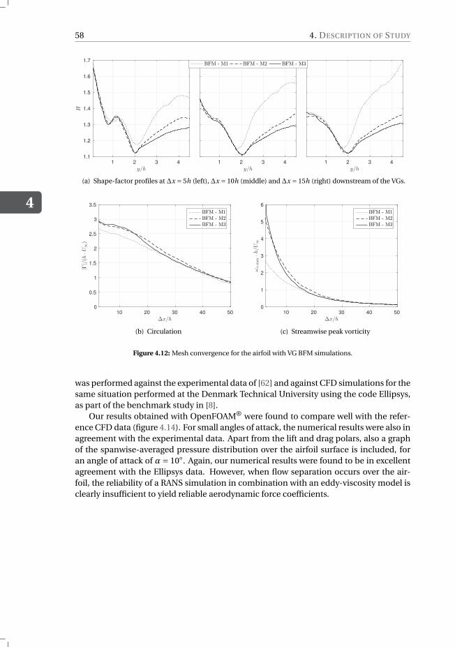
4
58 4. DESCRIPTION OF STUDY
1 2 3 4
y/h
1.1
1.2
1.3
1.4
1.5
1.6
1.7
H
1 2 3 4
y/h1 2 3 4
y/h
BFM - M1 BFM - M2 BFM - M3
(a) Shape-factor profiles at ∆x = 5h (left), ∆x = 10h (middle) and ∆x = 15h (right) downstream of the VGs.
10 20 30 40 50
∆x/h
0
0.5
1
1.5
2
2.5
3
3.5
|Γ|/(h
·U∞)
BFM - M1BFM - M2BFM - M3
(b) Circulation
10 20 30 40 50
∆x/h
0
1
2
3
4
5
6
ωx,m
ax·h/U∞
BFM - M1
BFM - M2
BFM - M3
(c) Streamwise peak vorticity
Figure 4.12: Mesh convergence for the airfoil with VG BFM simulations.
was performed against the experimental data of [62] and against CFD simulations for thesame situation performed at the Denmark Technical University using the code Ellipsys,as part of the benchmark study in [8].
Our results obtained with OpenFOAM® were found to compare well with the refer-ence CFD data (figure 4.14). For small angles of attack, the numerical results were also inagreement with the experimental data. Apart from the lift and drag polars, also a graphof the spanwise-averaged pressure distribution over the airfoil surface is included, foran angle of attack of α= 10. Again, our numerical results were found to be in excellentagreement with the Ellipsys data. However, when flow separation occurs over the air-foil, the reliability of a RANS simulation in combination with an eddy-viscosity model isclearly insufficient to yield reliable aerodynamic force coefficients.
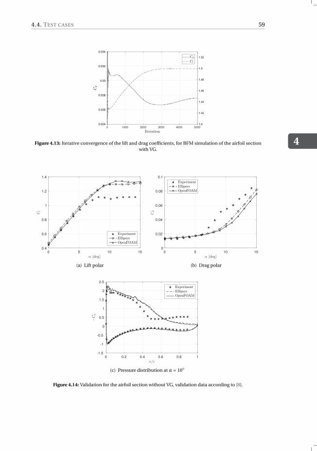
4.4. TEST CASES
4
59
0 1000 2000 3000 4000 5000
0.024
0.026
0.028
0.03
0.032
0.034
1.4
1.42
1.44
1.46
1.48
1.5
1.52
Figure 4.13: Iterative convergence of the lift and drag coefficients, for BFM simulation of the airfoil sectionwith VG.
0 5 10 15
α [deg]
0.4
0.6
0.8
1
1.2
1.4
Cl
ExperimentEllipsysOpenFOAM
(a) Lift polar
0 5 10 15
α [deg]
0
0.02
0.04
0.06
0.08
0.1
Cd
ExperimentEllipsysOpenFOAM
(b) Drag polar
0 0.2 0.4 0.6 0.8 1
x/c
-1.5
-1
-0.5
0
0.5
1
1.5
2
2.5
−C
p
Experiment
Ellipsys
OpenFOAM
(c) Pressure distribution at α= 10
Figure 4.14: Validation for the airfoil section without VG, validation data according to [8].

5ANALYSIS OF THE BAY AND JBAY
MODELS
As was found in chapter 3, the BAY model and its successor, the jBAY model, are cur-rently the most widely used approaches to include VG effects in CFD simulations. Inthe present chapter we evaluate their performance based on the research approach out-lined in chapter 4, in order to enhance the understanding of the potential and limita-tions of both models. The current analysis considers the influence of cell selection (forthe BAY model, section 5.2) and mesh resolution (section 5.3) on the predictive capabil-ities of these models with respect to the created boundary-layer disturbance. Moreover,in section 5.3 the impact of the differences between the jBAY model and the original BAYformulation are assessed.
It is shown that the results of the BAY model strongly depend on the selected source-term region, while the jBAY model does not reduce mesh dependency as expected. Theresults contained in this chapter furthermore highlight that an error is present in bothmodels, which prevents them from accurately reproducing boundary-layer characteris-tics. This chapter concludes with a summary of our findings in section 5.4.
5.1. IMPLEMENTATION DETAILSThe BAY and jBAY models are implemented in the open-source finite-volume CFD codeOpenFOAM®, to allow for the freedom of both analyzing the original formulations aswell as constructing and studying model modifications. A thorough description of thebaseline lay-out and numerical methods of this code, written in C++ and originally de-veloped at Imperial College, can be found in the work of Jasak [39].
5.1.1. ADDITION OF THE SOURCE TERM TO THE GOVERNING EQUATIONSSince the flows of interest considered in this work can be characterized as being steadyand incompressible (see section 4.2), implementation of the BAY and jBAY models isdone by modifying the existing simpleFoam solver. This is a steady-state solver for in-
61
5
62 5. ANALYSIS OF THE BAY AND JBAY MODELS
compressible flows in absence of external forcing, which solves the governing equations
∇·u = 0 (5.1)
∇· (uu)−∇(ν∇u) = −∇p, (5.2)
where the pressure p actually denotes a modified pressure which is scaled by the density.The simpleFoam solver supports both LES and RANS simulations, and makes use of theSIMPLE algorithm (originally described by Patankar [76]) to obtain a discrete solutionfor the above coupled system of partial differential equations.
The SIMPLE method, short for semi-implicit method for pressure-linked equations,is a segregated approach that allows for a discrete solution of the flow field by con-structing explicit discretized equations for both the pressure and the velocity. To do so,(5.2) is first formulated in semi-discrete form (not discretizing the pressure gradient).Upon substitution into (5.1) and by making use of Gauss’s theorem, a Poisson equationfor the pressure is obtained which allows solution for the pressure based on the (non-divergence-free) velocity fluxes at the cell faces. As OpenFOAM® uses a collocated meshapproach, interpolation is used to obtain these face fluxes.
Starting from initial guesses for the pressure and turbulence quantities, the SIM-PLE method thus solves both velocity and pressure equations in an iterative process toimprove p such that u will progressively get closer to satisfying the continuity equa-tion. Note that the iterative process includes a correction step for u such that everysub-solution satisfies conservation of mass. It should furthermore be noted that, as thepressure equation is prone to divergence, in general under-relaxation is required whenupdating the pressure field.
To simulate the effect of VGs on the flow field, the momentum equation (5.2) solvedin the original simpleFoam solver is expanded to include a source term f (the VG model)to become
∇· (uu)−∇(ν∇u)− f =−∇p. (5.3)
This source term f consists of a vector field defined in the entire domain, but which isonly locally non-zero in the neighborhood of the desired VG locations. In the currentimplementation f is added in an explicit fashion to the discretized momentum equation,hence it is lagging in the pressure equation solved in the iterative SIMPLE process. Thisapproach is preferred for stability reasons due to the tendency of the pressure equationtowards divergence. However, as observed by Patankar [76], the converged solution isuninfluenced by any approximations made in the pressure equation. The fact that even-tually the velocity field resulting from the discretized momentum equation (a functionof p) satisfies conservation of mass (5.1), is evidence that we have acquired the correctpressure field.
5.1.2. VG OBJECT DEFINITIONTo enable the easy set-up of simulation cases involving VGs, a class was constructed thatcreates a VG object for every VG within the simulation. These objects are defined by the(private) data members
V G(l ,h1,h2,β, A,p1,p2,b,n,t,δ,Vtot ),
5.1. IMPLEMENTATION DETAILS
5
63
denoting respectively the VG’s length, height at the leading and trailing edges, incidenceangle, planform area, surface locations of the leading and trailing edges, unit directionvectors, the domain where the source term is to be added and the volume of application.Creation of a VG object is done in an external dictionary file by specifying the parametersl , h1, h2 (only if h1 = h2), β and p1, only. The other variables are calculated upon creationof the VG object, which is done as an initialization step before entering the SIMPLE loop.
The VG planform area is defined as
A = 1
2l (h1 +h2), (5.4)
and the trailing edge location as
p2 = p1 + l
cosβsinβ
0
, (5.5)
where the z-coordinates of p1 and p2 are adapted such as to lie on the surface. The unitvector b is defined at the location p1 to be normal to the surface, and
t = p2 −p1
|p2 −p1|and n = t×b
|t×b| . (5.6)
The most elaborate part of the VG-object creation consists of the selection of the cellswhere the source term, representing the VG, is to be applied. Selection of these cellscan be done in several ways, an overview of the implemented options is given in section5.1.3. The outcome of the cell-selection process consists of the characteristic scalar field
δ=
1 in ΩV G
0 in Ω\ΩV G, (5.7)
with ΩV G the considered domain of application, such that the total volume of applica-tion becomes
Vtot =N∑
i=1Viδi . (5.8)
5.1.3. CELL SELECTION APPOACHESSeveral approaches to define the domain ΩV G (and therefore the characteristic scalarfield δ) in which the source-term model is applied (and thus f = 0) were implemented.These different options are illustrated in figure 5.1 and briefly discussed below.
ALIGNED CELL SELECTION
The aligned cell-selection option consists of defining a virtual zero-thickness surface,with the same planform as the actual VG, and selecting all cells that are cut by thissurface. This surface is spanned by the points p1, p2, p3 = p1 + (0 0 h1)T and p4 =p2 + (0 0 h2)T .
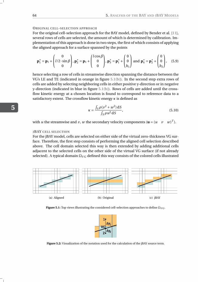
5
64 5. ANALYSIS OF THE BAY AND JBAY MODELS
ORIGINAL CELL-SELECTION APPROACH
For the original cell-selection approach for the BAY model, defined by Bender et al. [11],several rows of cells are selected, the amount of which is determined by calibration. Im-plementation of this approach is done in two steps, the first of which consists of applyingthe aligned approach for a surface spanned by the points
p∗1 = p1 +
0l/2 · sinβ
0
, p∗2 = p1 +
l cosβ00
, p∗3 = p∗
1 + 0
0h1
and p∗4 = p∗
2 + 0
0h2
, (5.9)
hence selecting a row of cells in streamwise direction spanning the distance between theVG’s LE and TE (indicated in orange in figure 5.1(b)). In the second step extra rows ofcells are added by selecting neighboring cells in either positive y-direction or in negativey-direction (indicated in blue in figure 5.1(b)). Rows of cells are added until the cross-flow kinetic energy at a chosen location is found to correspond to reference data to asatisfactory extent. The crossflow kinetic energy κ is defined as
κ=∫
S ρ(v2 +w2)dS∫S ρu2 dS
, (5.10)
with u the streamwise and v , w the secondary velocity components (u = (u v w)T ).
JBAY CELL SELECTION
For the jBAY model, cells are selected on either side of the virtual zero-thickness VG sur-face. Therefore, the first step consists of performing the aligned cell selection describedabove. The cell domain selected this way is then extended by adding additional cellsadjacent to the selected cells on the other side of the virtual VG surface (if not alreadyselected). A typical domain ΩV G defined this way consists of the colored cells illustrated
(a) Aligned (b) Original (c) jBAY
Figure 5.1: Top views illustrating the considered cell-selection approaches to define ΩV G .
Figure 5.2: Visualization of the notation used for the calculation of the jBAY source term.
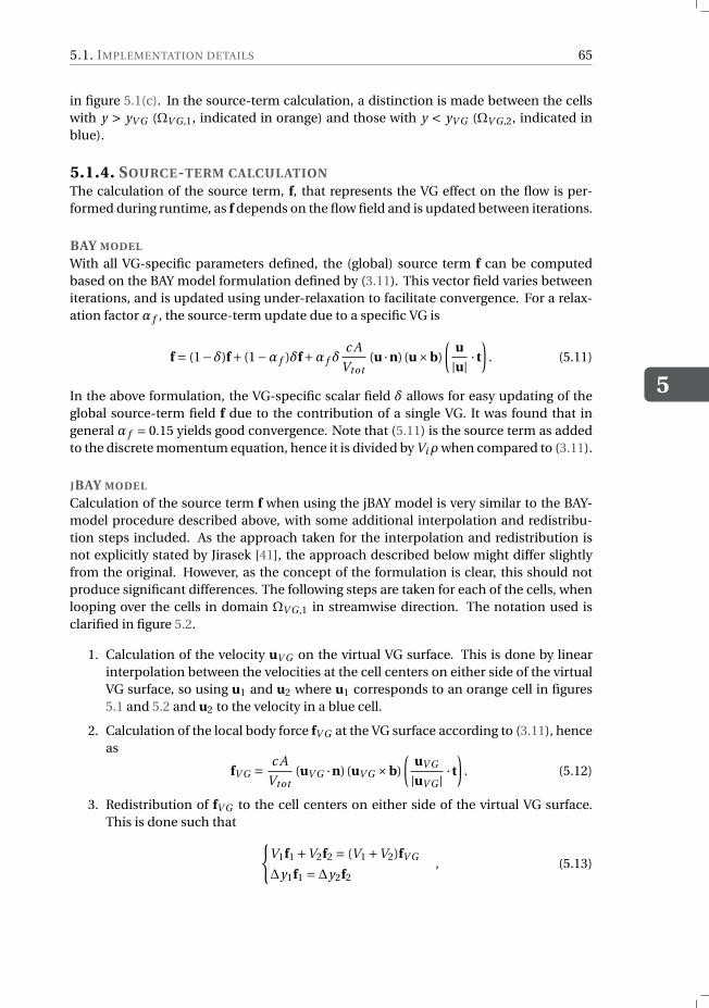
5.1. IMPLEMENTATION DETAILS
5
65
in figure 5.1(c). In the source-term calculation, a distinction is made between the cellswith y > yV G (ΩV G ,1, indicated in orange) and those with y < yV G (ΩV G ,2, indicated inblue).
5.1.4. SOURCE-TERM CALCULATIONThe calculation of the source term, f, that represents the VG effect on the flow is per-formed during runtime, as f depends on the flow field and is updated between iterations.
BAY MODEL
With all VG-specific parameters defined, the (global) source term f can be computedbased on the BAY model formulation defined by (3.11). This vector field varies betweeniterations, and is updated using under-relaxation to facilitate convergence. For a relax-ation factor α f , the source-term update due to a specific VG is
f = (1−δ)f+ (1−α f )δf+α f δc A
Vtot(u ·n) (u×b)
(u
|u| · t)
. (5.11)
In the above formulation, the VG-specific scalar field δ allows for easy updating of theglobal source-term field f due to the contribution of a single VG. It was found that ingeneral α f = 0.15 yields good convergence. Note that (5.11) is the source term as addedto the discrete momentum equation, hence it is divided by Viρ when compared to (3.11).
JBAY MODEL
Calculation of the source term f when using the jBAY model is very similar to the BAY-model procedure described above, with some additional interpolation and redistribu-tion steps included. As the approach taken for the interpolation and redistribution isnot explicitly stated by Jirasek [41], the approach described below might differ slightlyfrom the original. However, as the concept of the formulation is clear, this should notproduce significant differences. The following steps are taken for each of the cells, whenlooping over the cells in domain ΩV G ,1 in streamwise direction. The notation used isclarified in figure 5.2.
1. Calculation of the velocity uV G on the virtual VG surface. This is done by linearinterpolation between the velocities at the cell centers on either side of the virtualVG surface, so using u1 and u2 where u1 corresponds to an orange cell in figures5.1 and 5.2 and u2 to the velocity in a blue cell.
2. Calculation of the local body force fV G at the VG surface according to (3.11), henceas
fV G = c A
Vtot(uV G ·n) (uV G ×b)
(uV G
|uV G |· t
). (5.12)
3. Redistribution of fV G to the cell centers on either side of the virtual VG surface.This is done such that
V1f1 +V2f2 = (V1 +V2)fV G
∆y1f1 =∆y2f2, (5.13)
5
66 5. ANALYSIS OF THE BAY AND JBAY MODELS
where V1 and V2 indicate the cell volumes of the associated cells in domain ΩV G ,1
and ΩV G ,2, and ∆y1 and ∆y2 represent the distance between the cell centers andthe location on the virtual VG surface in between. This step results in the vectorfields f1 and f2, with f1 non-zero in ΩV G ,1 only and f2 non-zero in ΩV G ,2 only.
With f1 and f2 specified, the source-term field can thus be updated for the contributionof a specific VG according to
f = (1−δ)f+ (1−α f )δf+α f (f1 + f2). (5.14)
Note that in the above uV G and fV G are auxiliary variables, which are used for the calcu-lation of f1 and f2. They are not tied to a specific part of the domain and change valuewhile looping over the cells in ΩV G ,1.
5.2. INFLUENCE OF THE SOURCE-TERM DOMAIN ON THE
BAY-MODEL RESULTAs discussed in section 5.1.3, several approaches to define the source-term domain ΩV G
have been implemented. In this section, the influence of ΩV G on the resulting flow fieldis studied. For this analysis, distinction is made between definition of ΩV G oriented inthe direction of the VG (both the "Aligned" and "jBAY" selection methods), hence resem-bling the actual VG lay-out, and in a rectangular domain (the "Original" approach). Notethat, although we are solely considering the BAY model is this section, the jBAY source-term domain is included in this analysis such that other than the direction, also the effectof the width (and hence volume) of the source-term domains can be assessed.
The following test cases, all on a flat plate and varying in mesh resolution and lay-out,were considered: (i) the submerged VG pair (section 4.4.2) using the coarse mesh M0, (ii)the same VG pair case on a finer mesh M2, and (iii) a single submerged VG (section 4.4.1)using mesh M2. Note that the same VG pair case was computed on two different meshes,in order to analyze dependence on the mesh of ΩV G for κ calibration. Scalar vortex-descriptor results and shape-factor profiles are shown in figures 5.3 and 5.4 for the coarsemesh (M0) VG pair case. Similar graphs for the other cases are included in appendixA. Note that for the VG pair cases the circulation results differ slightly from the resultspresented in section 4.4.2, as a different definition of the vortex region S was used, basedon a cut-off value for ωx rather than the Q-criterion. Additionally, table 5.1 presents thevolumes of ΩV G and the scaled streamwise-averaged errors in the vortex parameters forthe considered simulations, which are calculated for a quantity q according to
ϵq = 1
n
n∑i=1
|q∗i −qi ||q∗
i |, (5.15)
with i indicating the streamwise locations, varying from ∆xi = 5h to the end of the con-sidered domain, and the superscript ∗ representing the BFM result.
The obtained results indicate that the source-term domain ΩV G has a large influ-ence on the vortex flow field created with the BAY model. A large spread is especiallypresent in the generated crossflow kinetic energy κ and the vorticity levels (hence in Γ
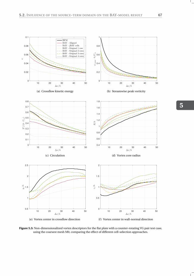
5.2. INFLUENCE OF THE SOURCE-TERM DOMAIN ON THE BAY-MODEL RESULT
5
67
10 20 30 40 50
∆x/h
0
0.02
0.04
0.06
0.08
0.1
κ
BFM
BAY - Aligned
BAY - jBAY cells
BAY - Original 1 row
BAY - Original 2 rows
BAY - Original 3 rows
BAY - Original 4 rows
(a) Crossflow kinetic energy
10 20 30 40 50
∆x/h
0
0.2
0.4
0.6
0.8
1
ωx,m
ax·h/U∞
(b) Streamwise peak vorticity
10 20 30 40 50
∆x/h
0
0.1
0.2
0.3
0.4
0.5
0.6
0.7
0.8
|Γ|/(h
·U∞)
(c) Circulation
10 20 30 40 50
∆x/h
0.4
0.6
0.8
1
1.2
1.4
1.6
1.8
R/h
(d) Vortex core radius
10 20 30 40 50
∆x/h
0.5
1
1.5
2
2.5
y c/h
(e) Vortex center in crossflow direction
10 20 30 40 50
∆x/h
0
0.5
1
1.5
2
z c/h
(f) Vortex center in wall-normal direction
Figure 5.3: Non-dimensionalized vortex descriptors for the flat plate with a counter-rotating VG pair test case,using the coarsest mesh M0, comparing the effect of different cell-selection approaches.
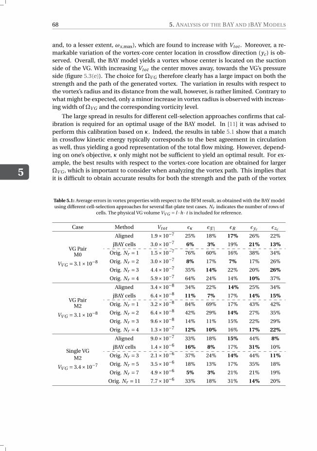
5
68 5. ANALYSIS OF THE BAY AND JBAY MODELS
and, to a lesser extent, ωx,max), which are found to increase with Vtot . Moreover, a re-markable variation of the vortex-core center location in crossflow direction (yc ) is ob-served. Overall, the BAY model yields a vortex whose center is located on the suctionside of the VG. With increasing Vtot the center moves away, towards the VG’s pressureside (figure 5.3(e)). The choice for ΩV G therefore clearly has a large impact on both thestrength and the path of the generated vortex. The variation in results with respect tothe vortex’s radius and its distance from the wall, however, is rather limited. Contrary towhat might be expected, only a minor increase in vortex radius is observed with increas-ing width of ΩV G and the corresponding vorticity level.
The large spread in results for different cell-selection approaches confirms that cal-ibration is required for an optimal usage of the BAY model. In [11] it was advised toperform this calibration based on κ. Indeed, the results in table 5.1 show that a matchin crossflow kinetic energy typically corresponds to the best agreement in circulationas well, thus yielding a good representation of the total flow mixing. However, depend-ing on one’s objective, κ only might not be sufficient to yield an optimal result. For ex-ample, the best results with respect to the vortex-core location are obtained for largerΩV G , which is important to consider when analyzing the vortex path. This implies thatit is difficult to obtain accurate results for both the strength and the path of the vortex
Table 5.1: Average errors in vortex properties with respect to the BFM result, as obtained with the BAY modelusing different cell-selection approaches for several flat-plate test cases. Nr indicates the number of rows of
cells. The physical VG volume VV G = l ·h · t is included for reference.
Case Method Vtot ϵκ ϵ|Γ| ϵR ϵyc ϵzc
VG PairM0
VV G = 3.1×10⁻⁸
Aligned 1.9×10⁻⁷ 25% 18% 17% 26% 22%
jBAY cells 3.0×10⁻⁷ 6% 3% 19% 21% 13%
Orig. Nr = 1 1.5×10⁻⁷ 76% 60% 16% 38% 34%
Orig. Nr = 2 3.0×10⁻⁷ 8% 17% 7% 17% 26%
Orig. Nr = 3 4.4×10⁻⁷ 35% 14% 22% 20% 26%
Orig. Nr = 4 5.9×10⁻⁷ 64% 24% 14% 10% 37%
VG PairM2
VV G = 3.1×10⁻⁸
Aligned 3.4×10⁻⁸ 34% 22% 14% 25% 34%
jBAY cells 6.4×10⁻⁸ 11% 7% 17% 14% 15%
Orig. Nr = 1 3.2×10⁻⁸ 84% 69% 17% 43% 42%
Orig. Nr = 2 6.4×10⁻⁸ 42% 29% 14% 27% 35%
Orig. Nr = 3 9.6×10⁻⁸ 14% 11% 15% 22% 29%
Orig. Nr = 4 1.3×10⁻⁷ 12% 10% 16% 17% 22%
Single VGM2
VV G = 3.4×10⁻⁷
Aligned 9.0×10⁻⁷ 33% 18% 15% 44% 8%
jBAY cells 1.4×10⁻⁶ 16% 8% 17% 31% 10%
Orig. Nr = 3 2.1×10⁻⁶ 37% 24% 14% 44% 11%
Orig. Nr = 5 3.5×10⁻⁶ 18% 13% 17% 35% 18%
Orig. Nr = 7 4.9×10⁻⁶ 5% 3% 21% 21% 19%
Orig. Nr = 11 7.7×10⁻⁶ 33% 18% 31% 14% 20%
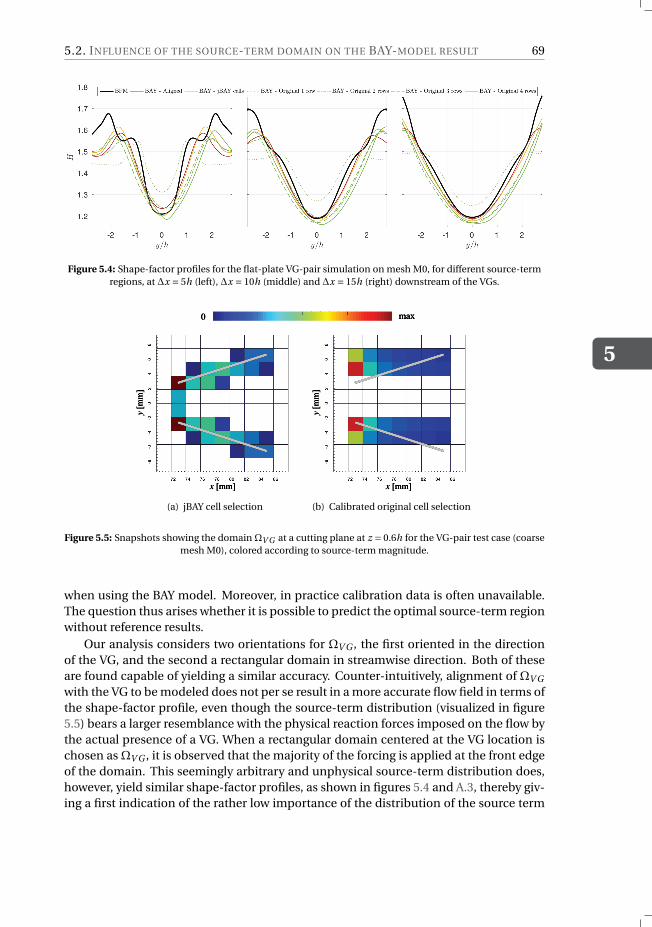
5.2. INFLUENCE OF THE SOURCE-TERM DOMAIN ON THE BAY-MODEL RESULT
5
69
Figure 5.4: Shape-factor profiles for the flat-plate VG-pair simulation on mesh M0, for different source-termregions, at ∆x = 5h (left), ∆x = 10h (middle) and ∆x = 15h (right) downstream of the VGs.
(a) jBAY cell selection (b) Calibrated original cell selection
Figure 5.5: Snapshots showing the domain ΩV G at a cutting plane at z = 0.6h for the VG-pair test case (coarsemesh M0), colored according to source-term magnitude.
when using the BAY model. Moreover, in practice calibration data is often unavailable.The question thus arises whether it is possible to predict the optimal source-term regionwithout reference results.
Our analysis considers two orientations for ΩV G , the first oriented in the directionof the VG, and the second a rectangular domain in streamwise direction. Both of theseare found capable of yielding a similar accuracy. Counter-intuitively, alignment of ΩV G
with the VG to be modeled does not per se result in a more accurate flow field in terms ofthe shape-factor profile, even though the source-term distribution (visualized in figure5.5) bears a larger resemblance with the physical reaction forces imposed on the flow bythe actual presence of a VG. When a rectangular domain centered at the VG location ischosen as ΩV G , it is observed that the majority of the forcing is applied at the front edgeof the domain. This seemingly arbitrary and unphysical source-term distribution does,however, yield similar shape-factor profiles, as shown in figures 5.4 and A.3, thereby giv-ing a first indication of the rather low importance of the distribution of the source term
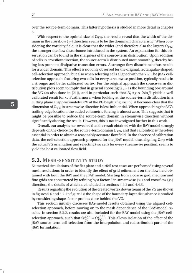
5
70 5. ANALYSIS OF THE BAY AND JBAY MODELS
over the source-term domain. This latter hypothesis is studied in more detail in chapter6.
With respect to the optimal size of ΩV G , the results reveal that the width of the do-main in the crossflow (y-) direction seems to be the dominant characteristic. When con-sidering the vorticity field, it is clear that the wider (and therefore also the larger) ΩV G ,the stronger the flow disturbance introduced in the system. An explanation for this ob-servation can be found in the sharpness of the source-term distribution. Upon additionof cells in crossflow direction, the source-term is distributed more smoothly, thereby be-ing less prone to dissipative truncation errors. A stronger flow disturbance thus resultsfor a wider domain. This effect is not only observed for the original, rectangular-shaped,cell-selection approach, but also when selecting cells aligned with the VG. The jBAY cell-selection approach, featuring two cells for every streamwise position, typically results ina stronger and better calibrated vortex. For the original approach the source-term dis-tribution plots seem to imply that in general choosing ΩV G as the bounding box aroundthe VG (as also done in [21]), and in particular such that Nr∆y ≈ l sinβ, yields a wellcalibrated result for κ. Furthermore, when looking at the source-term distribution in acutting plane at approximately 60% of the VG height (figure 5.5), it becomes clear that thedimension of ΩV G in streamwise direction is less influential. When approaching the VG’strailing-edge location, the added volumetric forcing is almost zero. This suggests that itmight be possible to reduce the source-term domain in streamwise direction withoutsignificantly altering the result. However, this is not investigated further in this work.
Overall, our analysis has revealed that the result obtained with the BAY model stronglydepends on the choice for the source-term domain ΩV G , and that calibration is thereforeessential in order to obtain a reasonably accurate flow field. In the absence of calibrationdata, the cell-selection approach proposed for the jBAY model, thus aligning ΩV G withthe actual VG orientation and selecting two cells for every streamwise position, seems toyield the best calibrated flow field.
5.3. MESH-SENSITIVITY STUDYNumerical simulations of the flat plate and airfoil test cases are performed using severalmesh resolutions in order to identify the effect of grid refinement on the flow field ob-tained with both the BAY and the jBAY model. Starting from a coarse grid, medium andfine grids are constructed by refining by a factor 2 in streamwise (x-) and crossflow (y-)direction, the details of which are included in sections 4.4.2 and 4.4.3.
Results regarding the evolution of the created vortex downstream of the VG are shownin figures 5.6 and 5.7. In figure 5.8 the shape of the boundary-layer disturbance is studiedby considering shape-factor profiles close behind the VG.
This section initially discusses BAY-model results obtained using the aligned cell-selection approach, before moving on to the mesh dependence of the jBAY-model re-sults. In section 5.3.2, results are also included for the BAY model using the jBAY cell-
selection approach, such that ΩB AYV G = Ω
j B AYV G . This allows isolation of the effect of the
jBAY source-term cell selection from the interpolation and redistribution parts of thejBAY formulation.
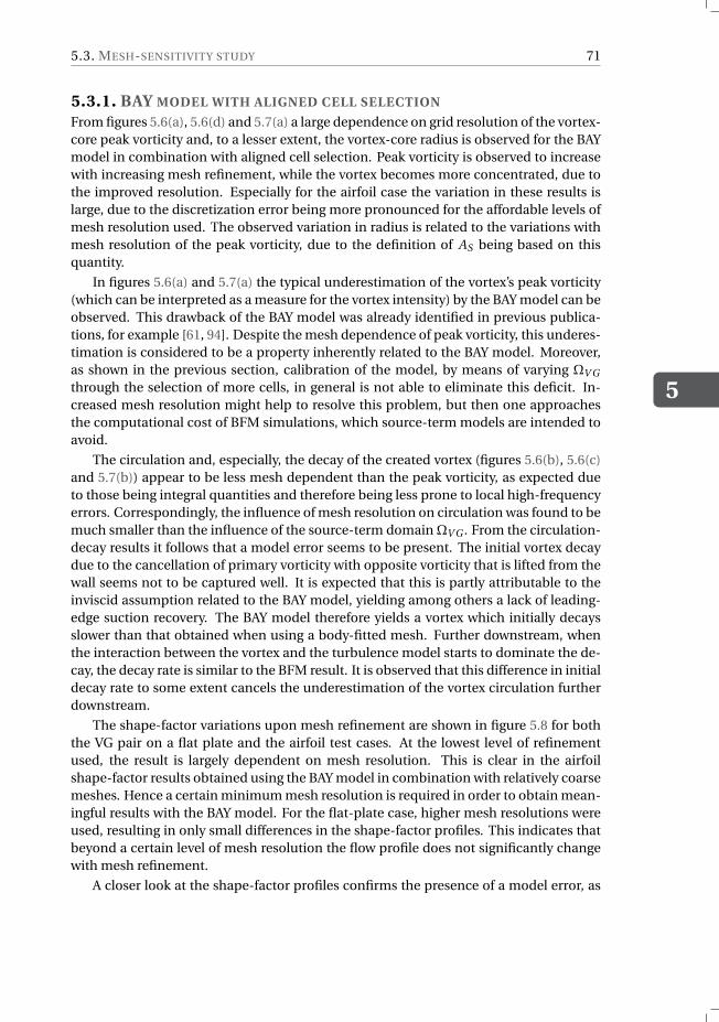
5.3. MESH-SENSITIVITY STUDY
5
71
5.3.1. BAY MODEL WITH ALIGNED CELL SELECTION
From figures 5.6(a), 5.6(d) and 5.7(a) a large dependence on grid resolution of the vortex-core peak vorticity and, to a lesser extent, the vortex-core radius is observed for the BAYmodel in combination with aligned cell selection. Peak vorticity is observed to increasewith increasing mesh refinement, while the vortex becomes more concentrated, due tothe improved resolution. Especially for the airfoil case the variation in these results islarge, due to the discretization error being more pronounced for the affordable levels ofmesh resolution used. The observed variation in radius is related to the variations withmesh resolution of the peak vorticity, due to the definition of AS being based on thisquantity.
In figures 5.6(a) and 5.7(a) the typical underestimation of the vortex’s peak vorticity(which can be interpreted as a measure for the vortex intensity) by the BAY model can beobserved. This drawback of the BAY model was already identified in previous publica-tions, for example [61, 94]. Despite the mesh dependence of peak vorticity, this underes-timation is considered to be a property inherently related to the BAY model. Moreover,as shown in the previous section, calibration of the model, by means of varying ΩV G
through the selection of more cells, in general is not able to eliminate this deficit. In-creased mesh resolution might help to resolve this problem, but then one approachesthe computational cost of BFM simulations, which source-term models are intended toavoid.
The circulation and, especially, the decay of the created vortex (figures 5.6(b), 5.6(c)and 5.7(b)) appear to be less mesh dependent than the peak vorticity, as expected dueto those being integral quantities and therefore being less prone to local high-frequencyerrors. Correspondingly, the influence of mesh resolution on circulation was found to bemuch smaller than the influence of the source-term domain ΩV G . From the circulation-decay results it follows that a model error seems to be present. The initial vortex decaydue to the cancellation of primary vorticity with opposite vorticity that is lifted from thewall seems not to be captured well. It is expected that this is partly attributable to theinviscid assumption related to the BAY model, yielding among others a lack of leading-edge suction recovery. The BAY model therefore yields a vortex which initially decaysslower than that obtained when using a body-fitted mesh. Further downstream, whenthe interaction between the vortex and the turbulence model starts to dominate the de-cay, the decay rate is similar to the BFM result. It is observed that this difference in initialdecay rate to some extent cancels the underestimation of the vortex circulation furtherdownstream.
The shape-factor variations upon mesh refinement are shown in figure 5.8 for boththe VG pair on a flat plate and the airfoil test cases. At the lowest level of refinementused, the result is largely dependent on mesh resolution. This is clear in the airfoilshape-factor results obtained using the BAY model in combination with relatively coarsemeshes. Hence a certain minimum mesh resolution is required in order to obtain mean-ingful results with the BAY model. For the flat-plate case, higher mesh resolutions wereused, resulting in only small differences in the shape-factor profiles. This indicates thatbeyond a certain level of mesh resolution the flow profile does not significantly changewith mesh refinement.
A closer look at the shape-factor profiles confirms the presence of a model error, as
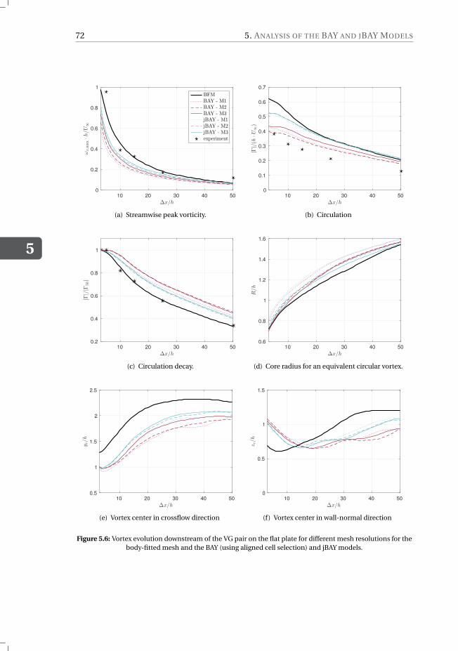
5
72 5. ANALYSIS OF THE BAY AND JBAY MODELS
10 20 30 40 50
∆x/h
0
0.2
0.4
0.6
0.8
1ωx,m
ax·h/U∞
BFM
BAY - M1
BAY - M2
BAY - M3
jBAY - M1
jBAY - M2
jBAY - M3
experiment
(a) Streamwise peak vorticity.
10 20 30 40 50
∆x/h
0
0.1
0.2
0.3
0.4
0.5
0.6
0.7
|Γ|/(h
·U∞)
(b) Circulation
10 20 30 40 50
∆x/h
0.2
0.4
0.6
0.8
1
|Γ|/|Γ
5h|
(c) Circulation decay.
10 20 30 40 50
∆x/h
0.6
0.8
1
1.2
1.4
1.6
R/h
(d) Core radius for an equivalent circular vortex.
10 20 30 40 50
∆x/h
0.5
1
1.5
2
2.5
y c/h
(e) Vortex center in crossflow direction
10 20 30 40 50
∆x/h
0
0.5
1
1.5
z c/h
(f) Vortex center in wall-normal direction
Figure 5.6: Vortex evolution downstream of the VG pair on the flat plate for different mesh resolutions for thebody-fitted mesh and the BAY (using aligned cell selection) and jBAY models.
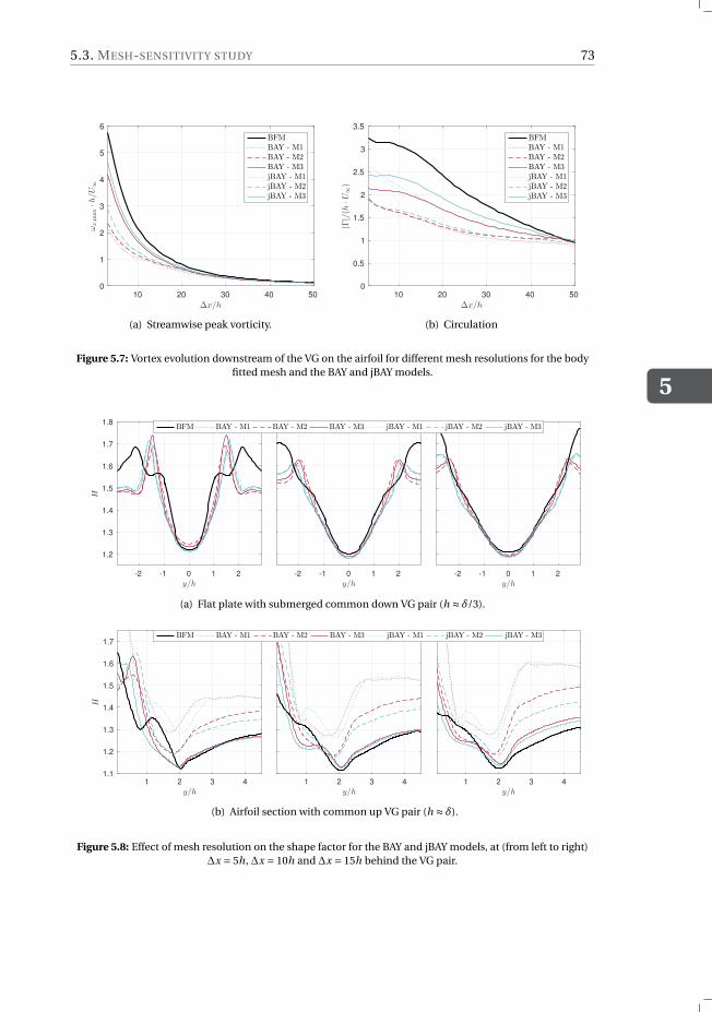
5.3. MESH-SENSITIVITY STUDY
5
73
10 20 30 40 50
∆x/h
0
1
2
3
4
5
6
ωx,m
ax·h/U∞
BFM
BAY - M1
BAY - M2
BAY - M3
jBAY - M1
jBAY - M2
jBAY - M3
(a) Streamwise peak vorticity.
10 20 30 40 50
∆x/h
0
0.5
1
1.5
2
2.5
3
3.5
|Γ|/(h
·U∞)
BFMBAY - M1BAY - M2BAY - M3jBAY - M1jBAY - M2jBAY - M3
(b) Circulation
Figure 5.7: Vortex evolution downstream of the VG on the airfoil for different mesh resolutions for the bodyfitted mesh and the BAY and jBAY models.
-2 -1 0 1 2
y/h
1.2
1.3
1.4
1.5
1.6
1.7
1.8
H
-2 -1 0 1 2
y/h-2 -1 0 1 2
y/h
BFM BAY - M1 BAY - M2 BAY - M3 jBAY - M1 jBAY - M2 jBAY - M3
(a) Flat plate with submerged common down VG pair (h ≈ δ/3).
1 2 3 4
y/h
1.1
1.2
1.3
1.4
1.5
1.6
1.7
H
1 2 3 4
y/h1 2 3 4
y/h
BFM BAY - M1 BAY - M2 BAY - M3 jBAY - M1 jBAY - M2 jBAY - M3
(b) Airfoil section with common up VG pair (h ≈ δ).
Figure 5.8: Effect of mesh resolution on the shape factor for the BAY and jBAY models, at (from left to right)∆x = 5h, ∆x = 10h and ∆x = 15h behind the VG pair.
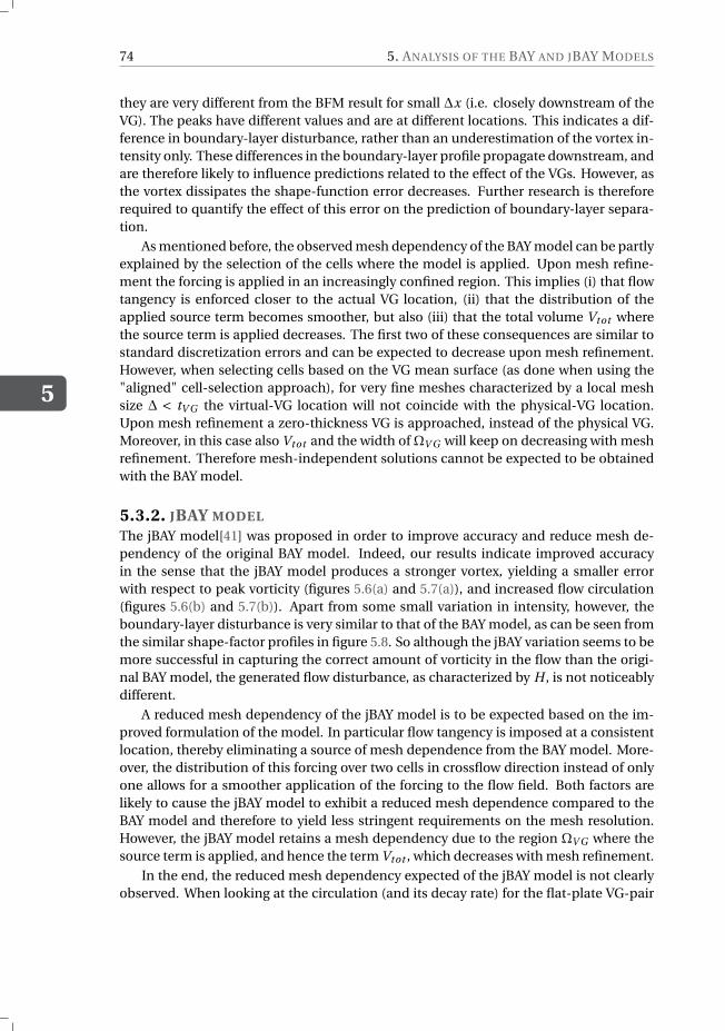
5
74 5. ANALYSIS OF THE BAY AND JBAY MODELS
they are very different from the BFM result for small ∆x (i.e. closely downstream of theVG). The peaks have different values and are at different locations. This indicates a dif-ference in boundary-layer disturbance, rather than an underestimation of the vortex in-tensity only. These differences in the boundary-layer profile propagate downstream, andare therefore likely to influence predictions related to the effect of the VGs. However, asthe vortex dissipates the shape-function error decreases. Further research is thereforerequired to quantify the effect of this error on the prediction of boundary-layer separa-tion.
As mentioned before, the observed mesh dependency of the BAY model can be partlyexplained by the selection of the cells where the model is applied. Upon mesh refine-ment the forcing is applied in an increasingly confined region. This implies (i) that flowtangency is enforced closer to the actual VG location, (ii) that the distribution of theapplied source term becomes smoother, but also (iii) that the total volume Vtot wherethe source term is applied decreases. The first two of these consequences are similar tostandard discretization errors and can be expected to decrease upon mesh refinement.However, when selecting cells based on the VG mean surface (as done when using the"aligned" cell-selection approach), for very fine meshes characterized by a local meshsize ∆ < tV G the virtual-VG location will not coincide with the physical-VG location.Upon mesh refinement a zero-thickness VG is approached, instead of the physical VG.Moreover, in this case also Vtot and the width of ΩV G will keep on decreasing with meshrefinement. Therefore mesh-independent solutions cannot be expected to be obtainedwith the BAY model.
5.3.2. JBAY MODEL
The jBAY model[41] was proposed in order to improve accuracy and reduce mesh de-pendency of the original BAY model. Indeed, our results indicate improved accuracyin the sense that the jBAY model produces a stronger vortex, yielding a smaller errorwith respect to peak vorticity (figures 5.6(a) and 5.7(a)), and increased flow circulation(figures 5.6(b) and 5.7(b)). Apart from some small variation in intensity, however, theboundary-layer disturbance is very similar to that of the BAY model, as can be seen fromthe similar shape-factor profiles in figure 5.8. So although the jBAY variation seems to bemore successful in capturing the correct amount of vorticity in the flow than the origi-nal BAY model, the generated flow disturbance, as characterized by H , is not noticeablydifferent.
A reduced mesh dependency of the jBAY model is to be expected based on the im-proved formulation of the model. In particular flow tangency is imposed at a consistentlocation, thereby eliminating a source of mesh dependence from the BAY model. More-over, the distribution of this forcing over two cells in crossflow direction instead of onlyone allows for a smoother application of the forcing to the flow field. Both factors arelikely to cause the jBAY model to exhibit a reduced mesh dependence compared to theBAY model and therefore to yield less stringent requirements on the mesh resolution.However, the jBAY model retains a mesh dependency due to the region ΩV G where thesource term is applied, and hence the term Vtot , which decreases with mesh refinement.
In the end, the reduced mesh dependency expected of the jBAY model is not clearlyobserved. When looking at the circulation (and its decay rate) for the flat-plate VG-pair
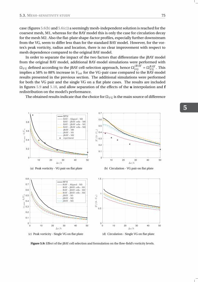
5.3. MESH-SENSITIVITY STUDY
5
75
case (figures 5.6(b) and 5.6(c)) a seemingly mesh-independent solution is reached for thecoarsest mesh, M1, whereas for the BAY model this is only the case for circulation decayfor the mesh M2. Also the flat-plate shape-factor profiles, especially further downstreamfrom the VG, seem to differ less than for the standard BAY model. However, for the vor-tex’s peak vorticity, radius and location, there is no clear improvement with respect tomesh dependence compared to the original BAY model.
In order to separate the impact of the two factors that differentiate the jBAY modelfrom the original BAY model, additional BAY-model simulations were performed with
ΩV G defined according to the jBAY cell-selection approach, hence Ωj B AYV G =ΩB AY
V G . Thisimplies a 58% to 88% increase in Vtot for the VG-pair case compared to the BAY-modelresults presented in the previous section. The additional simulations were performedfor both the VG pair and the single VG on a flat plate cases. The results are includedin figures 5.9 and 5.10, and allow separation of the effects of the u interpolation and fredistribution on the model’s performance.
The obtained results indicate that the choice for ΩV G is the main source of difference
10 20 30 40 50
∆x/h
0
0.2
0.4
0.6
0.8
1
ωx,m
ax·h/U∞
BFM
BAY - Aligned - M2
BAY - jBAY cells - M0
BAY - jBAY cells - M1
BAY - jBAY cells - M2
jBAY - M0
jBAY - M1
jBAY - M2
experiment
(a) Peak vorticity - VG pair on flat plate
10 20 30 40 50
∆x/h
0
0.1
0.2
0.3
0.4
0.5
0.6
0.7
|Γ|/(h
·U∞)
(b) Circulation - VG pair on flat plate
0 10 20 30 40 50
∆x/h
0
0.1
0.2
0.3
0.4
0.5
0.6
0.7
0.8
ωx,m
ax·h/U∞
BFM
BAY - Aligned - M3
BAY - jBAY cells - M1
BAY - jBAY cells - M2
BAY - jBAY cells - M3
jBAY - M1
jBAY - M2
jBAY - M3
(c) Peak vorticity - Single VG on flat plate
0 10 20 30 40 50
∆x/h
0
0.5
1
1.5
|Γ|/(h
·U∞)
(d) Circulation - Single VG on flat plate
Figure 5.9: Effect of the jBAY cell selection and formulation on the flow-field’s vorticity levels.
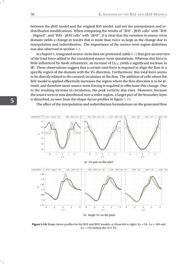
5
76 5. ANALYSIS OF THE BAY AND JBAY MODELS
between the jBAY model and the original BAY model, and not the interpolation and re-distribution modifications. When comparing the results of "BAY - jBAY cells" with "BAY- Aligned", and "BAY - jBAY cells" with "jBAY", it is clear that the variation in source-termdomain yields a change in results that is more than twice as large as the change due tointerpolation and redistribution. The importance of the source-term region definitionwas also observed in section 5.2.
In chapter 6, integrated source-term data are presented (table 6.1) that give an overviewof the total force added to the considered source-term simulations. Whereas this force islittle influenced by mesh refinement, an increase of ΩV G yields a significant increase in|F|. These observations suggest that a certain total force is required to align the flow in aspecific region of the domain with the VG direction. Furthermore, this total force seemsto be directly related to the created circulation in the flow. The addition of cells where theBAY model is applied effectively increases the region where the flow direction is to be al-tered, and therefore more source-term forcing is required to effectuate this change. Dueto the resulting increase in circulation, the peak vorticity also rises. Moreover, becausethe source term is now distributed over a wider region, a larger part of the boundary layeris disturbed, as seen from the shape-factor profiles in figure 5.10.
The effect of the interpolation and redistribution formulations on the generated flow
-2 -1 0 1 2
y/h
1.2
1.3
1.4
1.5
1.6
1.7
1.8
H
-2 -1 0 1 2
y/h-2 -1 0 1 2
y/h
BFM BAY - Aligned - M2 BAY - jBAY cells - M0 BAY - jBAY cells - M1 BAY - jBAY cells - M2 jBAY - M0 jBAY - M1 jBAY - M2
(a) VG pair on flat plate
-4 -2 0 2 4
y/h
1.15
1.2
1.25
1.3
1.35
1.4
1.45
1.5
H
-4 -2 0 2 4
y/h-4 -2 0 2 4
y/h
BFM BAY - Aligned - M3 BAY - jBAY cells - M1 BAY - jBAY cells - M2 BAY - jBAY cells - M3 jBAY - M1 jBAY - M2 jBAY - M3
(b) Single VG on flat plate
Figure 5.10: Shape-factor profiles for the BAY and jBAY models, at (from left to right) ∆x = 5h, ∆x = 10h and∆x = 15h behind the VG’s TE.
5.4. CONCLUSIONS
5
77
field consists of a reduction in overall vorticity levels, and hence the strength of the cre-ated vortex. Both the total circulation and the peak vorticity in the vortex core are clearlydecreased (figure 5.9) in comparison to application of the BAY model on the same ΩV G .This can be explained by observing that the jBAY model aims to align the flow with theVG direction in a smaller region due to the location where flow tangency is evaluated,which is now consistent at the zero-thickness virtual-VG surface. A smaller force andless circulation is thus required to achieve the desired change in flow direction. Due tothis overall decrease in circulation, the peak vorticity also drops. Moreover, the interpo-lation and redistribution procedures of the jBAY model cause the applied source term tobe more concentrated towards the actual VG location, which results in a slightly smallerregion of the boundary layer being disturbed (figure 5.10).
Overall, isolation of the two factors that cause the jBAY model to differ from the BAYmodel, consisting of the mesh-dependent ΩV G selection and the mesh-independent in-terpolation and redistribution, indicates that the former is dominant in both the jBAY’saccuracy and mesh-convergence behavior. Additional interpolation and redistributionto ensure a consistent location of the virtual VG does not affect the results upon meshrefinement. Hence, the remaining source of mesh dependency in the jBAY formula-tion, the variation of Vtot , seems to be dominant and thereby prevents a fully mesh-independent flow field from being achievable. It therefore follows that for the originalBAY model variation of Vtot is also the main source of mesh dependence.
5.4. CONCLUSIONSThe analysis presented in this chapter reveals the presence of model errors in both theBAY and the jBAY models, in the sense that they consistently under-predict the vortexintensity and create erroneous shape-factor profiles when compared with body-fittedmesh simulations. Moreover, the vortex center is typically located too far on the VG’ssuction side.
It is found that both the mesh resolution and the source-term region strongly influ-ence the obtained result, with the effect of the latter being largest. Hence, for the BAYmodel, calibration by means of varying ΩV G is advised in order to achieve an accuraterepresentation of the amount of flow mixing generated by the presence of a VG.
The main modification related to the jBAY model was found to consist of aligning thesource-term domain with the actual VG direction, and using a width of two cells. Thischoice for ΩV G indeed seems to yield the most reliable results in the absence of high-fidelity reference data to perform calibration.
The interpolation and redistribution parts of the jBAY model, however, have not beenobserved to yield the expected reduction in mesh dependency of the model. Our resultsindicate that the effect of this addition on the generated flow field is limited, and mani-fests itself as a small decrease in overall vorticity levels.

6INFLUENCE OF SOURCE-TERM
PARAMETERS
In the previous chapter an analysis of the BAY and jBAY models was presented, whichrevealed shortcomings of these models in representing the boundary-layer disturbancecaused by the presence of a VG. The cause of these deviations was however not identi-fied. In this chapter therefore a closer look is taken at the source term that is added tothe governing equations to represent the VG effect. The effects on the created flow fieldof the total force added to the simulation by the source term and its distribution are in-vestigated (section 6.2), after which the importance of magnitude and direction of thetotal applied forcing are studied in more detail in section 6.3. To this end, first severalmodified source-term formulations are introduced in section 6.1. The main findings ofthis assessment are summarized in section 6.4.
6.1. RATIONALE OF THE ANALYSISThe aim of this part of our investigation consists of assessing the impact of differentaspects of the source-term field that is added to the governing equations in order to rep-resent the effect of VGs on the flow. The aspects that are studied here are the distributionof the source-term field over the selected cells and the resultant total force that is im-posed on the flow by the source term, where the latter is further divided into the effectsof the magnitude and the direction of this resultant force. In particular, with this analy-sis we want to gain insight into which are the most influential parameters of the source-term field, and to improve our understanding of the underlying mechanisms that gov-ern the creation of a vortex by the addition of a source term. Eventually, we expect thisnew insight to be helpful in focusing future research efforts towards the development ofimproved models that minimize (or even eliminate) shortcomings of existing BAY-likemodels, as discussed in chapter 5.
So far, in this work we have focused our attention on existing partly-modeled/partly-resolved reaction-force models that aim to achieve flow tangency in the neighborhood
79
6
80 6. INFLUENCE OF SOURCE-TERM PARAMETERS
of the VG, in particular the BAY and the jBAY model. Assessment of these models is per-formed using body-fitted mesh simulations as reference, which are considered to yieldthe best result achievable within the limitations of the selected numerical framework.
Five additional source-term formulations, based on the BAY model and the actualreaction force a VG imposes on the flow, are now introduced in order to isolate the con-sidered source-term parameters. These formulations are first discussed below, and thenused in the analysis presented in the following sections. The comparisons which will beconsidered are illustrated in figure 6.1.
6.1.1. ADDITIONAL SOURCE-TERM FORMULATIONS
Uniform FBAY In this formulation a uniformly-distributed source term is locally addedto the momentum equation such that the source-term forcing per unit volume is con-stant over the selected cells (ΩV G ), and such that the total applied force equals the totalforce added to the flow by the BAY model. Hence, in the domain ΩV G a source term
fU Bi = Vi
VtotFB AY with FB AY =
N∑i=1
fi (6.1)
is applied, where N equals the number of cells in the source-term region and fi repre-sents the source-term forcing in a single cell according to the BAY-model formulation3.11. Compared to the BAY model, this implies that the applied source term is no longerfocused near the leading edge of the VG.
Uniform Fexact Similar to the uniform FBAY model, a uniformly distributed source termis added to the momentum equation in the selected cells (ΩV G ). In this formulation,however, the magnitude and direction of the resultant applied force are obtained fromthe total surface force acting on the VG in a body-fitted mesh simulation. Hence, theexact total reaction force is imposed on the flow, and the applied source term equals
fU Ei = Vi
VtotFexact with Fexact =
ÓSV G
p ndS, (6.2)
where SV G represents the surface of the VG, p is the stress (pressure and viscous) actingon the VG surface for a BFM VG simulation and n indicates the wall-normal direction.
The main force acting on the VG’s surface is due to pressure, the distribution of whichis shown for the BFM VG-pair case in figure 6.2. It is apparent that the majority of thereaction force due to pressure is focused near the VG’s leading edge.
(Distributed) fexact Given that the force distribution on a VG is non-uniform, formula-tions using non-constant source magnitudes may be advantageous. In this formulationwe therefore not only calibrate the total force added to the system, but also the distri-bution of the source term over the cells is matched as closely as possible to the actualVG surface-force distribution. This is achieved by first calculating the VG force in everyinterior VG cell i of the body-fitted mesh by integration over its faces as
fEi =
ÓSi
pi ni dS. (6.3)
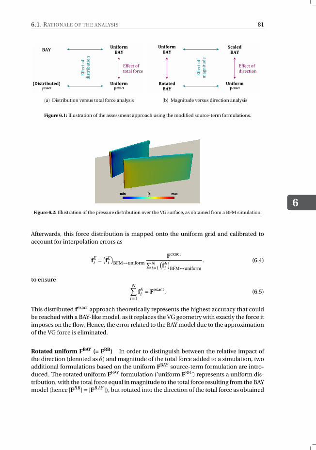
6.1. RATIONALE OF THE ANALYSIS
6
81
!"#$%&'()*+$
!"#$
%&'()*+$
,-./01$
23'41*'561-78$
(-./01$
!""#$%&'"&
%'%()&"'*$#&
!""#$%&'"&
+,-%*,./%,'0&
(a) Distribution versus total force analysis
!"#$%&'
()*'
+,-./01'
2%3#"4'
!""#$%&'"&
()*#$%)'+&
!""#$%&'"&
,-.+)%/(#&
+,-./01'
()*'
5/4#4%&'
()*'
(b) Magnitude versus direction analysis
Figure 6.1: Illustration of the assessment approach using the modified source-term formulations.
Figure 6.2: Illustration of the pressure distribution over the VG surface, as obtained from a BFM simulation.
Afterwards, this force distribution is mapped onto the uniform grid and calibrated toaccount for interpolation errors as
fEi = (
fEi
)BFM 7→uniform
Fexact∑Ni=1
(fE
i
)BFM 7→uniform
. (6.4)
to ensureN∑
i=1fE
i = Fexact. (6.5)
This distributed fexact approach theoretically represents the highest accuracy that couldbe reached with a BAY-like model, as it replaces the VG geometry with exactly the force itimposes on the flow. Hence, the error related to the BAY model due to the approximationof the VG force is eliminated.
Rotated uniform FBAY (= FRB) In order to distinguish between the relative impact ofthe direction (denoted as θ) and magnitude of the total force added to a simulation, twoadditional formulations based on the uniform FBAY source-term formulation are intro-duced. The rotated uniform FBAY formulation (’uniform FRB’) represents a uniform dis-tribution, with the total force equal in magnitude to the total force resulting from the BAYmodel (hence |FRB | = |FB AY |), but rotated into the direction of the total force as obtained
6
82 6. INFLUENCE OF SOURCE-TERM PARAMETERS
from the reference BFM simulation (such that θRB = θexact). The source-term field is thusdefined as
fRBi = Vi
VtotFRB with FRB = |FB AY |
|Fexact|Fexact. (6.6)
Scaled uniform FBAY (= FSB) Similarly, the scaled uniform FBAY formulation (’uniformFSB’) represents a uniform distribution, but now with the total force scaled such that itsmagnitude equals the magnitude of the exact VG reaction force (|FSB | = |Fexact|). Thedirection of the added forcing, however, remains equal to the result of the BAY-modelsimulation, hence θSB = θB AY . Therefore we have
fSBi = Vi
VtotFSB with FSB = |Fexact|
|FB AY | FB AY . (6.7)
6.1.2. SET-UP AND IMPLEMENTATION
The above described uniform source-term formulations were implemented in OpenFOAM®
such that the user need only to specify the total forcing as additional input (hence FBAY,Fexact, FRB and FSB for the first two and the last two formulations respectively). Specifica-tion of the source-term domain ΩV G over which the source term is uniformly distributedwas done as in the BAY model. Note that for these formulations the source-term field washeld constant throughout the simulation.
The (distributed) fexact source-term field, however, was calculated using an addi-tional utility and directly read (without modification) by the modified simpleFoam solver.This utility required the construction of an additional mesh, equal to the body-fittedmesh but including the volume ’within’ the VG, for the calculation of fE
i according to 6.3.This result was then mapped onto the uniform mesh of interest, according to 6.4, usingOpenFOAM®’s mapFields utility.
For the results presented in the following sections, the domain ΩV G was specifiedusing the aligned cell-selection approach. Note that in section 5.2 it was found that ingeneral the jBAY cell-selection approach yields a better calibrated result. However, thealigned approach was chosen for this study because it is the most natural way of impos-ing the exact reaction-force distribution fexact, thus facilitating a convenient comparisonof the relative change in result upon modification of the source-term parameters of in-terest (see figure 6.1), Furthermore, to minimize the effects of discretization errors, alldata presented in this investigation were obtained on the finest meshes considered, un-less specified otherwise.
6.2. EFFECTS OF SOURCE-TERM DISTRIBUTION AND
TOTAL FORCINGTo facilitate discussion of the relative impact of the source-term distribution (f) and totalimposed forcing (F) table 6.1 was constructed, which contains data related to the totalapplied source-term forcing for a range of simulations (as discussed in chapter 5). Thenormal, tangential and wall-normal components (Fn , Ft and Fb respectively) as well asthe magnitude |F| of the resultant total forcing are included, as are the magnitude of the
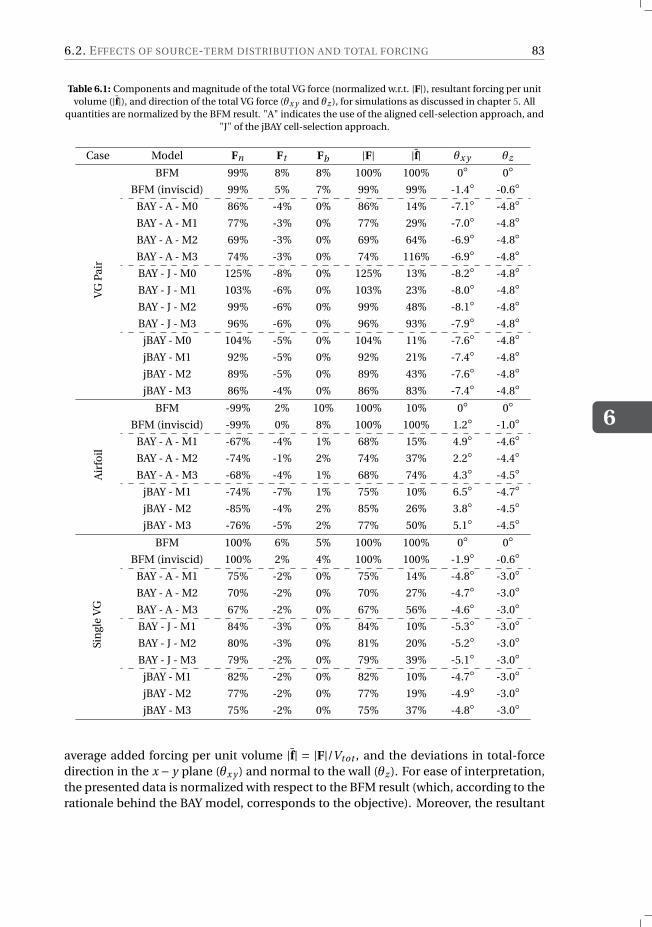
6.2. EFFECTS OF SOURCE-TERM DISTRIBUTION AND TOTAL FORCING
6
83
Table 6.1: Components and magnitude of the total VG force (normalized w.r.t. |F|), resultant forcing per unitvolume (|f|), and direction of the total VG force (θx y and θz ), for simulations as discussed in chapter 5. All
quantities are normalized by the BFM result. "A" indicates the use of the aligned cell-selection approach, and"J" of the jBAY cell-selection approach.
Case Model Fn Ft Fb |F| |f| θx y θz
VG
Pair
BFM 99% 8% 8% 100% 100% 0 0
BFM (inviscid) 99% 5% 7% 99% 99% -1.4 -0.6
BAY - A - M0 86% -4% 0% 86% 14% -7.1 -4.8
BAY - A - M1 77% -3% 0% 77% 29% -7.0 -4.8
BAY - A - M2 69% -3% 0% 69% 64% -6.9 -4.8
BAY - A - M3 74% -3% 0% 74% 116% -6.9 -4.8
BAY - J - M0 125% -8% 0% 125% 13% -8.2 -4.8
BAY - J - M1 103% -6% 0% 103% 23% -8.0 -4.8
BAY - J - M2 99% -6% 0% 99% 48% -8.1 -4.8
BAY - J - M3 96% -6% 0% 96% 93% -7.9 -4.8
jBAY - M0 104% -5% 0% 104% 11% -7.6 -4.8
jBAY - M1 92% -5% 0% 92% 21% -7.4 -4.8
jBAY - M2 89% -5% 0% 89% 43% -7.6 -4.8
jBAY - M3 86% -4% 0% 86% 83% -7.4 -4.8
Air
foil
BFM -99% 2% 10% 100% 10% 0 0
BFM (inviscid) -99% 0% 8% 100% 100% 1.2 -1.0
BAY - A - M1 -67% -4% 1% 68% 15% 4.9 -4.6
BAY - A - M2 -74% -1% 2% 74% 37% 2.2 -4.4
BAY - A - M3 -68% -4% 1% 68% 74% 4.3 -4.5
jBAY - M1 -74% -7% 1% 75% 10% 6.5 -4.7
jBAY - M2 -85% -4% 2% 85% 26% 3.8 -4.5
jBAY - M3 -76% -5% 2% 77% 50% 5.1 -4.5
Sin
gle
VG
BFM 100% 6% 5% 100% 100% 0 0
BFM (inviscid) 100% 2% 4% 100% 100% -1.9 -0.6
BAY - A - M1 75% -2% 0% 75% 14% -4.8 -3.0
BAY - A - M2 70% -2% 0% 70% 27% -4.7 -3.0
BAY - A - M3 67% -2% 0% 67% 56% -4.6 -3.0
BAY - J - M1 84% -3% 0% 84% 10% -5.3 -3.0
BAY - J - M2 80% -3% 0% 81% 20% -5.2 -3.0
BAY - J - M3 79% -2% 0% 79% 39% -5.1 -3.0
jBAY - M1 82% -2% 0% 82% 10% -4.7 -3.0
jBAY - M2 77% -2% 0% 77% 19% -4.9 -3.0
jBAY - M3 75% -2% 0% 75% 37% -4.8 -3.0
average added forcing per unit volume |f| = |F|/Vtot , and the deviations in total-forcedirection in the x − y plane (θx y ) and normal to the wall (θz ). For ease of interpretation,the presented data is normalized with respect to the BFM result (which, according to therationale behind the BAY model, corresponds to the objective). Moreover, the resultant
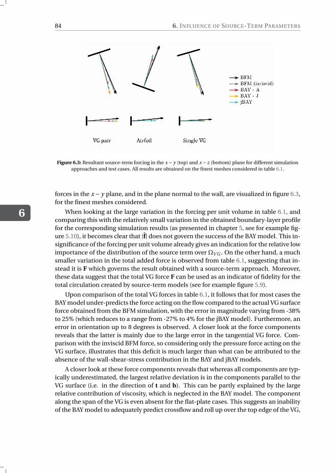
6
84 6. INFLUENCE OF SOURCE-TERM PARAMETERS
Figure 6.3: Resultant source-term forcing in the x − y (top) and x − z (bottom) plane for different simulationapproaches and test cases. All results are obtained on the finest meshes considered in table 6.1.
forces in the x − y plane, and in the plane normal to the wall, are visualized in figure 6.3,for the finest meshes considered.
When looking at the large variation in the forcing per unit volume in table 6.1, andcomparing this with the relatively small variation in the obtained boundary-layer profilefor the corresponding simulation results (as presented in chapter 5, see for example fig-ure 5.10), it becomes clear that |f| does not govern the success of the BAY model. This in-significance of the forcing per unit volume already gives an indication for the relative lowimportance of the distribution of the source term over ΩV G . On the other hand, a muchsmaller variation in the total added force is observed from table 6.1, suggesting that in-stead it is F which governs the result obtained with a source-term approach. Moreover,these data suggest that the total VG force F can be used as an indicator of fidelity for thetotal circulation created by source-term models (see for example figure 5.9).
Upon comparison of the total VG forces in table 6.1, it follows that for most cases theBAY model under-predicts the force acting on the flow compared to the actual VG surfaceforce obtained from the BFM simulation, with the error in magnitude varying from -38%to 25% (which reduces to a range from -27% to 4% for the jBAY model). Furthermore, anerror in orientation up to 8 degrees is observed. A closer look at the force componentsreveals that the latter is mainly due to the large error in the tangential VG force. Com-parison with the inviscid BFM force, so considering only the pressure force acting on theVG surface, illustrates that this deficit is much larger than what can be attributed to theabsence of the wall-shear-stress contribution in the BAY and jBAY models.
A closer look at these force components reveals that whereas all components are typ-ically underestimated, the largest relative deviation is in the components parallel to theVG surface (i.e. in the direction of t and b). This can be partly explained by the largerelative contribution of viscosity, which is neglected in the BAY model. The componentalong the span of the VG is even absent for the flat-plate cases. This suggests an inabilityof the BAY model to adequately predict crossflow and roll up over the top edge of the VG,
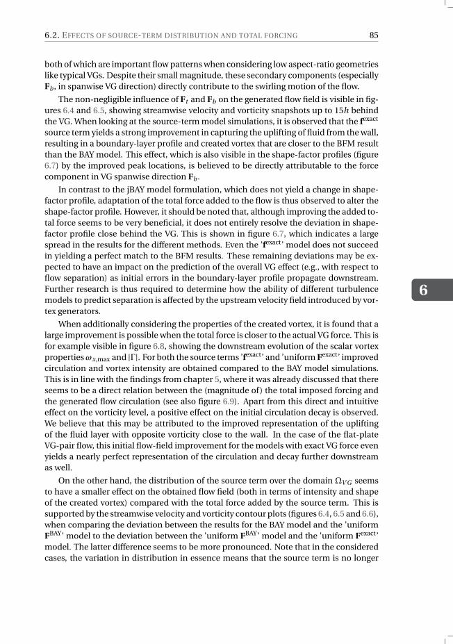
6.2. EFFECTS OF SOURCE-TERM DISTRIBUTION AND TOTAL FORCING
6
85
both of which are important flow patterns when considering low aspect-ratio geometrieslike typical VGs. Despite their small magnitude, these secondary components (especiallyFb , in spanwise VG direction) directly contribute to the swirling motion of the flow.
The non-negligible influence of Ft and Fb on the generated flow field is visible in fig-ures 6.4 and 6.5, showing streamwise velocity and vorticity snapshots up to 15h behindthe VG. When looking at the source-term model simulations, it is observed that the fexact
source term yields a strong improvement in capturing the uplifting of fluid from the wall,resulting in a boundary-layer profile and created vortex that are closer to the BFM resultthan the BAY model. This effect, which is also visible in the shape-factor profiles (figure6.7) by the improved peak locations, is believed to be directly attributable to the forcecomponent in VG spanwise direction Fb .
In contrast to the jBAY model formulation, which does not yield a change in shape-factor profile, adaptation of the total force added to the flow is thus observed to alter theshape-factor profile. However, it should be noted that, although improving the added to-tal force seems to be very beneficial, it does not entirely resolve the deviation in shape-factor profile close behind the VG. This is shown in figure 6.7, which indicates a largespread in the results for the different methods. Even the ’fexact’ model does not succeedin yielding a perfect match to the BFM results. These remaining deviations may be ex-pected to have an impact on the prediction of the overall VG effect (e.g., with respect toflow separation) as initial errors in the boundary-layer profile propagate downstream.Further research is thus required to determine how the ability of different turbulencemodels to predict separation is affected by the upstream velocity field introduced by vor-tex generators.
When additionally considering the properties of the created vortex, it is found that alarge improvement is possible when the total force is closer to the actual VG force. This isfor example visible in figure 6.8, showing the downstream evolution of the scalar vortexpropertiesωx,max and |Γ|. For both the source terms ’fexact’ and ’uniform Fexact’ improvedcirculation and vortex intensity are obtained compared to the BAY model simulations.This is in line with the findings from chapter 5, where it was already discussed that thereseems to be a direct relation between the (magnitude of) the total imposed forcing andthe generated flow circulation (see also figure 6.9). Apart from this direct and intuitiveeffect on the vorticity level, a positive effect on the initial circulation decay is observed.We believe that this may be attributed to the improved representation of the upliftingof the fluid layer with opposite vorticity close to the wall. In the case of the flat-plateVG-pair flow, this initial flow-field improvement for the models with exact VG force evenyields a nearly perfect representation of the circulation and decay further downstreamas well.
On the other hand, the distribution of the source term over the domain ΩV G seemsto have a smaller effect on the obtained flow field (both in terms of intensity and shapeof the created vortex) compared with the total force added by the source term. This issupported by the streamwise velocity and vorticity contour plots (figures 6.4, 6.5 and 6.6),when comparing the deviation between the results for the BAY model and the ’uniformFBAY’ model to the deviation between the ’uniform FBAY’ model and the ’uniform Fexact’model. The latter difference seems to be more pronounced. Note that in the consideredcases, the variation in distribution in essence means that the source term is no longer
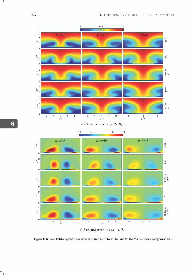
6
86 6. INFLUENCE OF SOURCE-TERM PARAMETERS
∆x / h = 5 ∆x / h =10 ∆x / h =15
!"#$
!%&$
'()*+,-$$
!$!%&$
"$./012 #
'()*+,-$$
!$./012 $
(a) Streamwise velocity (Ux /U∞)
∆x / h = 5 ∆x / h =10 ∆x / h =15
!"#$
!%&$
'()*+,-$$
!"!%&$
#$./012 "
'()*+,-$$
!$./012 $
(b) Streamwise vorticity (ωx ·h/U∞)
Figure 6.4: Flow-field snapshots for several source-term formulations for the VG pair case, using mesh M3.
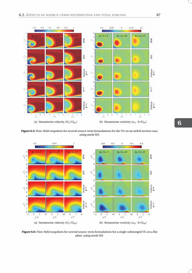
6.2. EFFECTS OF SOURCE-TERM DISTRIBUTION AND TOTAL FORCING
6
87
∆x / h = 5 ∆x / h =10 ∆x / h =15
!"#$
!%&$
'()*+,-$$
!"!%&$
'()*+,-$$
!$./012 $
#$./012 "
(a) Streamwise velocity (Ux /U∞)
∆x / h = 5 ∆x / h =10 ∆x / h =15
!"#$
!%&$
'()*+,-$$
!"!%&$
'()*+,-$$
!$./012 $
#$./012 "
(b) Streamwise vorticity (ωx ·h/U∞)
Figure 6.5: Flow-field snapshots for several source-term formulations for the VG on an airfoil section case,using mesh M3.
∆x / h = 5 ∆x / h =10 ∆x / h =15
!"#
!$%
&'()*+,-
!!$%
&'()*+,-
!./012
(a) Streamwise velocity (Ux /U∞)
∆x / h = 5 ∆x / h =10 ∆x / h =15!"#
!$%
&'()*+,-
!!$%
&'()*+,-
!./012
(b) Streamwise vorticity (ωx ·h/U∞)
Figure 6.6: Flow-field snapshots for several source-term formulations for a single submerged VG on a flatplate, using mesh M3.
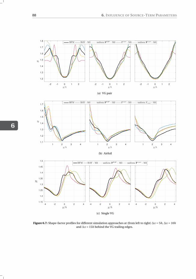
6
88 6. INFLUENCE OF SOURCE-TERM PARAMETERS
-2 -1 0 1 2
y/h
1.2
1.3
1.4
1.5
1.6
1.7
1.8
H
-2 -1 0 1 2
y/h-2 -1 0 1 2
y/h
BFM BAY - M3 uniform FBAY - M3 f
exact - M3 uniform Fexact - M3
(a) VG pair
1 2 3 4
y/h
1.1
1.2
1.3
1.4
1.5
1.6
1.7
H
1 2 3 4
y/h1 2 3 4
y/h
BFM BAY - M3 uniform FBAY - M3 f
exact - M3 uniform Fexact - M3
(b) Airfoil
-4 -2 0 2 4
1.15
1.2
1.25
1.3
1.35
1.4
1.45
1.5
-4 -2 0 2 4 -4 -2 0 2 4
(c) Single VG
Figure 6.7: Shape-factor profiles for different simulation approaches at (from left to right) ∆x = 5h, ∆x = 10hand ∆x = 15h behind the VG trailing edges.
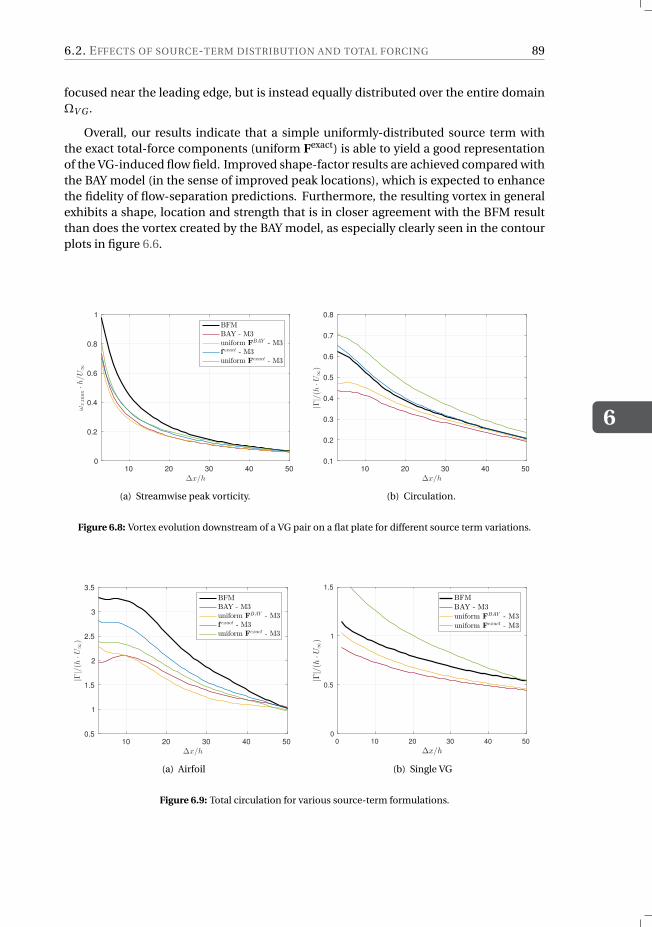
6.2. EFFECTS OF SOURCE-TERM DISTRIBUTION AND TOTAL FORCING
6
89
focused near the leading edge, but is instead equally distributed over the entire domainΩV G .
Overall, our results indicate that a simple uniformly-distributed source term withthe exact total-force components (uniform Fexact) is able to yield a good representationof the VG-induced flow field. Improved shape-factor results are achieved compared withthe BAY model (in the sense of improved peak locations), which is expected to enhancethe fidelity of flow-separation predictions. Furthermore, the resulting vortex in generalexhibits a shape, location and strength that is in closer agreement with the BFM resultthan does the vortex created by the BAY model, as especially clearly seen in the contourplots in figure 6.6.
10 20 30 40 50
∆x/h
0
0.2
0.4
0.6
0.8
1
ωx,m
ax·h/U∞
BFM
BAY - M3
uniform FBAY - M3
fexact - M3
uniform Fexact - M3
(a) Streamwise peak vorticity.
10 20 30 40 50
∆x/h
0.1
0.2
0.3
0.4
0.5
0.6
0.7
0.8|Γ|/(h
·U∞)
(b) Circulation.
Figure 6.8: Vortex evolution downstream of a VG pair on a flat plate for different source term variations.
10 20 30 40 50
∆x/h
0.5
1
1.5
2
2.5
3
3.5
|Γ|/(h
·U∞)
BFMBAY - M3uniform F
BAY - M3fexact - M3uniform F
exact - M3
(a) Airfoil
0 10 20 30 40 50
0
0.5
1
1.5
(b) Single VG
Figure 6.9: Total circulation for various source-term formulations.
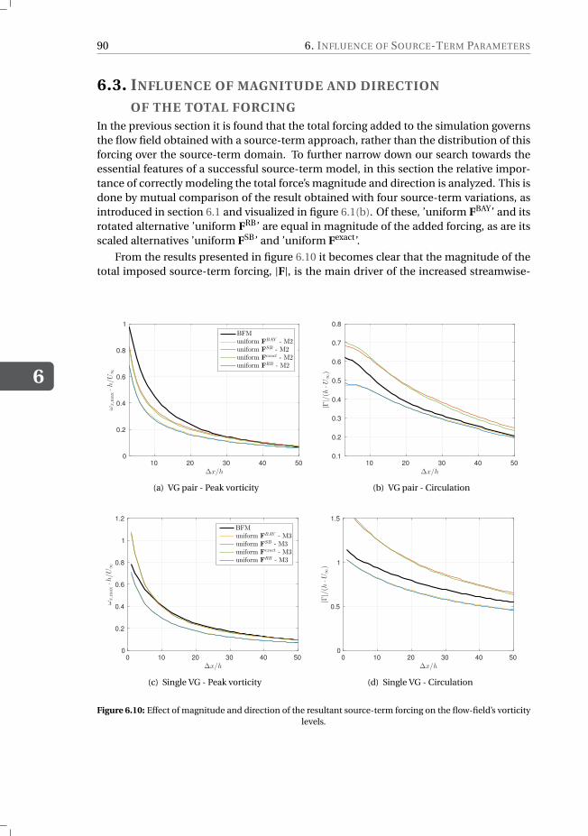
6
90 6. INFLUENCE OF SOURCE-TERM PARAMETERS
6.3. INFLUENCE OF MAGNITUDE AND DIRECTION
OF THE TOTAL FORCINGIn the previous section it is found that the total forcing added to the simulation governsthe flow field obtained with a source-term approach, rather than the distribution of thisforcing over the source-term domain. To further narrow down our search towards theessential features of a successful source-term model, in this section the relative impor-tance of correctly modeling the total force’s magnitude and direction is analyzed. This isdone by mutual comparison of the result obtained with four source-term variations, asintroduced in section 6.1 and visualized in figure 6.1(b). Of these, ’uniform FBAY’ and itsrotated alternative ’uniform FRB’ are equal in magnitude of the added forcing, as are itsscaled alternatives ’uniform FSB’ and ’uniform Fexact’.
From the results presented in figure 6.10 it becomes clear that the magnitude of thetotal imposed source-term forcing, |F|, is the main driver of the increased streamwise-
10 20 30 40 50
∆x/h
0
0.2
0.4
0.6
0.8
1
ωx,m
ax·h/U∞
BFM
uniform FBAY - M2
uniform FSB - M2
uniform Fexact - M2
uniform FRB - M2
(a) VG pair - Peak vorticity
10 20 30 40 50
∆x/h
0.1
0.2
0.3
0.4
0.5
0.6
0.7
0.8|Γ|/(h
·U∞)
(b) VG pair - Circulation
0 10 20 30 40 50
∆x/h
0
0.2
0.4
0.6
0.8
1
1.2
ωx,m
ax·h/U∞
BFM
uniform FBAY - M3
uniform FSB - M3
uniform Fexact - M3
uniform FRB - M3
(c) Single VG - Peak vorticity
0 10 20 30 40 50
∆x/h
0
0.5
1
1.5
|Γ|/(h
·U∞)
(d) Single VG - Circulation
Figure 6.10: Effect of magnitude and direction of the resultant source-term forcing on the flow-field’s vorticitylevels.
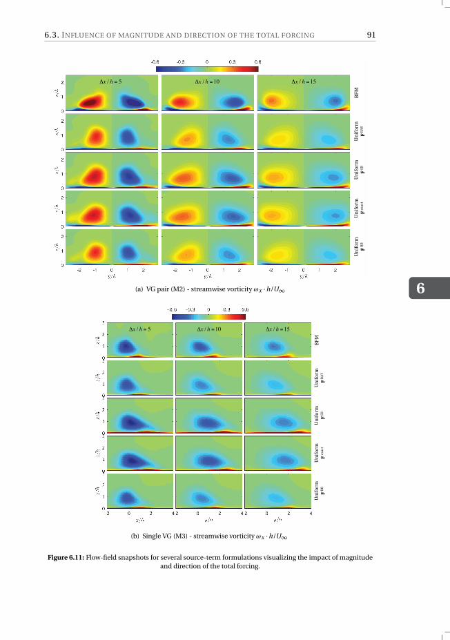
6.3. INFLUENCE OF MAGNITUDE AND DIRECTION OF THE TOTAL FORCING
6
91
∆x / h = 5 ∆x / h =10 ∆x / h =15
!"#$
%&'()*+$$
!",!$
%&'()*+$$
!$-./01 $
%&'()*+$$
!"!23$
%&'()*+$$
!"4!$
(a) VG pair (M2) - streamwise vorticity ωx ·h/U∞
∆x / h = 5 ∆x / h =10 ∆x / h =15
!"#
$%&'()*+
!,!
$%&'()*+
!-./01
$%&'()*+
!!23
$%&'()*+
!4!
(b) Single VG (M3) - streamwise vorticity ωx ·h/U∞
Figure 6.11: Flow-field snapshots for several source-term formulations visualizing the impact of magnitudeand direction of the total forcing.
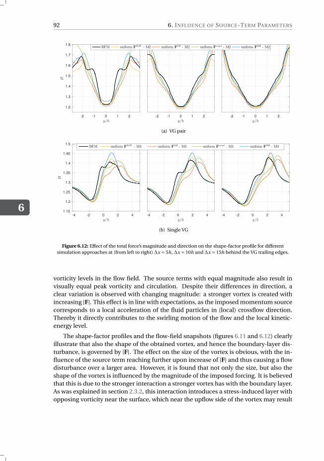
6
92 6. INFLUENCE OF SOURCE-TERM PARAMETERS
-2 -1 0 1 2
y/h
1.2
1.3
1.4
1.5
1.6
1.7
1.8
H
-2 -1 0 1 2
y/h-2 -1 0 1 2
y/h
BFM uniform FBAY - M2 uniform F
SB - M2 uniform Fexact - M2 uniform F
RB - M2
(a) VG pair
-4 -2 0 2 4
y/h
1.15
1.2
1.25
1.3
1.35
1.4
1.45
1.5
H
-4 -2 0 2 4
y/h-4 -2 0 2 4
y/h
BFM uniform FBAY - M3 uniform F
SB - M3 uniform Fexact - M3 uniform F
RB - M3
(b) Single VG
Figure 6.12: Effect of the total force’s magnitude and direction on the shape-factor profile for differentsimulation approaches at (from left to right) ∆x = 5h, ∆x = 10h and ∆x = 15h behind the VG trailing edges.
vorticity levels in the flow field. The source terms with equal magnitude also result invisually equal peak vorticity and circulation. Despite their differences in direction, aclear variation is observed with changing magnitude: a stronger vortex is created withincreasing |F|. This effect is in line with expectations, as the imposed momentum sourcecorresponds to a local acceleration of the fluid particles in (local) crossflow direction.Thereby it directly contributes to the swirling motion of the flow and the local kinetic-energy level.
The shape-factor profiles and the flow-field snapshots (figures 6.11 and 6.12) clearlyillustrate that also the shape of the obtained vortex, and hence the boundary-layer dis-turbance, is governed by |F|. The effect on the size of the vortex is obvious, with the in-fluence of the source term reaching further upon increase of |F| and thus causing a flowdisturbance over a larger area. However, it is found that not only the size, but also theshape of the vortex is influenced by the magnitude of the imposed forcing. It is believedthat this is due to the stronger interaction a stronger vortex has with the boundary layer.As was explained in section 2.3.2, this interaction introduces a stress-induced layer withopposing vorticity near the surface, which near the upflow side of the vortex may result
6.4. CONCLUSIONS
6
93
in the creation of a secondary vortex. Stronger interaction between vortex and bound-ary layer yields a stronger secondary vortex to arise, whose interaction with the primaryvortex influences the (initial) shape of the latter.
The effect of rotation becomes visible when examining the obtained shape-factorprofiles (figure 6.12), which show a variation in peak values upon changing direction ofF. In practice, the presence of a VG creates a region of recirculating flow that is detachedfrom the VG surface on the VG’s suction side. This yields a streamwise momentum deficitwhich reflects into an increase in H . The retarding effect on the flow is captured in theuniform Fexact and uniform FRB simulations by the source-term component acting inopposite streamwise direction. For the uniform FBAY and uniform FRB simulations, how-ever, this streamwise component has decreased, yielding a smaller region with retardedflow, and thus the creation of a smaller wake.
However, the streamwise-vorticity levels are only marginally affected by small vari-ations in the direction of the resultant volumetric forcing. For our investigation direc-tional changes up to 7 in crossflow direction, and up to 5 in wall-normal direction,have been considered without any considerable impact on the vortex strength. Similarly,figure 6.11 indicates that also the shape and location of the created vortex are visuallyunaffected by the considered small variations in the direction of the resultant forcing.
The above observations can be explained by the realization that the calculated stream-wise vorticity is a combination of the flow accelerations in both (freestream) crossflowdirections, in our frame of reference being y and z. The considered directional changesof the resultant source-term forcing are such that an increase in Fy is combined with adecreasing Fz . Even though Fy is the dominant component, its variation upon rotationof the resultant forcing is limited. For small rotations in the x−y plane, it is found that Fy
scales approximately with sinθx y sinβ. Hence, the opposing effects in y- and z-directionpartially cancel each other, thereby yielding only a limited variation in streamwise vor-ticity. It should be noted, however, that this does not imply that the vortex propertiesare insensitive to rotation of the resultant source-term forcing. In reality, variations inthe direction of F will cause the created vortex to be rotated. When studying the impactof rotation in the local crossflow plane (n-b), it is expected that a larger effect will beobserved.
6.4. CONCLUSIONSTwo factors defining the BAY-model source term are investigated in more detail: the dis-tribution of the source term over the selected cells, and the total resultant force added tothe flow, where for the latter further distinction is made between magnitude and direc-tion. The current analysis indicates that the distribution of the source term over ΩV G hasa lesser influence on the characteristics of the created vortex than the resultant source-term forcing, which dominates both the strength and shape of the created streamwisevortex. It is found that the magnitude of the resultant forcing is the main driver in thisrespect, as it directly governs the energy that is added to the system. A larger forcing mag-nitude yields the creation of a larger and stronger vortex. Moreover, due to the strongerinteraction with the boundary layer also the vortex’s shape is influenced. Small varia-tions in the direction of the imposed forcing, however, are found to have only a limitedeffect on the created flow field.
6
94 6. INFLUENCE OF SOURCE-TERM PARAMETERS
In particular, the component in the VG spanwise direction Fb , despite being smallin magnitude, seems to have a significant effect on the shape of the created vortex. Thelarge underestimation of this force component by the BAY model yields a poor predictionfor the uplifting of fluid from the wall close behind the VG, and therefore directly affectsthe flow profile. Furthermore, the BAY model typically yields an erroneous approxima-tion of the VG’s tangential force Ft , resulting in an underestimation of the wake createdbehind the VG and therefore consistently underestimating the shape-factor peaks.
The aforementioned observations with respect to the resultant source-term forceand the source-term distribution are expected to be significant for a possible improve-ment of the BAY model. Whereas previous efforts have mainly focused on approaches toobtaining more realistic and smooth distributions of the source term over the selecteddomain, for example [41], our analysis indicates that a focus on the total force added bythe source term could potentially be more effective in obtaining realistic flow fields witha BAY-like model. It is found that a simple uniformly-distributed source term with theexact total force components is able to yield a fair representation of the VG-induced flowfield. In particular, the source-term’s magnitude seems to be an important parameter tofocus on, governing both the strength and shape of the created vortex.
Although this analysis has shown that for BAY-like source-term models the resultantforcing added to ΩV G is the main driver for the created flow field, it is not likely that animproved estimate for F only, distributed uniformly over ΩV G , will be able to yield opti-mal shape-factor profiles on a coarse mesh. Even though to a lesser extent, the distribu-tion of f over the VG domain also influences the result. It is thus believed that in orderto obtain highly-accurate results on coarse meshes, the combination of an improved es-timate for F with a suitable low-resolution source-term distribution, optimized for useon a coarse mesh, will be required. Based on the presented uniform-distribution results,we envision that it might be possible to derive such a source-term formulation that onlyrequires a low level of spatial resolution, thereby making it resolvable on coarse meshes.The BAY-like models studied in this chapter and in chapter 5 automatically concentratethe majority of the added forcing near the location of the VG’s leading edge. It wouldthus be interesting to investigate whether, when abandoning the BAY-model formula-tion, such a (low-resolution) source-term field indeed exists.
7DEVELOPMENT OF A
GOAL-ORIENTED SOURCE-TERM
OPTIMIZATION FRAMEWORK
The results presented in chapters 5 and 6 suggest that an improvement of current VGmodels is required to accurately simulate VG effects for realistic cases. Our analysis ofthe BAY and jBAY models has shown that these approaches perform reasonably well, cre-ating a vortex with characteristics similar to those of a reference BFM simulation. How-ever, also some deficiencies are observed. It is found that still a rather refined mesh isrequired in the vicinity of the VG, and that the vortex characteristics do not convergeto the BFM results upon refinement of the mesh. Moreover, analysis of the boundary-layer shape factor revealed deviations that could indicate unreliability with respect toseparation prediction. Being constrained by the use of suboptimal meshes, it is unclearwhether and to which extent improvement is possible.
The questions thus arise what is the highest accuracy one can expect to achieve whenmaking use of a source-term model to simulate VG-induced flow effects, on a given mesh?And which source term is able to yield this result? In this chapter an inverse approachis presented that makes it possible to answer both questions. The optimal source-termfield, which recreates the characteristics of a given high-fidelity 3D flow field on a low-resolution mesh, is calculated by means of a goal-oriented optimization, using the con-tinuous adjoint system. The formulation of this optimization problem is presented insection 7.1, followed by the derivation of the related continuous adjoint system in section7.2. The expression for the sensitivity of the objective functional is derived in section 7.3,after which section 7.4 elaborates on the gradient optimization approach that allows forefficient calculation of the optimal source term. The approach presented in this chapteris tested in chapter 8, where results for the considered test cases are discussed.
Note that although the current work is focused on the simulation of VG-induced floweffects, the presented methodology is general. It can in theory also be used to find asuitable source term to replace other missing features in CFD simulations.
95
7
96 7. DEVELOPMENT OF A GOAL-ORIENTED SOURCE-TERM OPTIMIZATION FRAMEWORK
7.1. FORMULATION OF THE OPTIMIZATION PROBLEMThe objective of this part of our research consists of finding a source term that, on aparticular low-resolution mesh, reproduces the flow disturbance caused by the presenceof a VG as accurately as possible. This disturbance consists of a vortex created withinthe boundary layer, propagating downstream and thereby altering the boundary-layerprofile.
As identified in section 4.1, the quantities of interest when analyzing this effect in-clude the streamwise vorticity field, in particular the peak value and the evolution of thelocation of this peak, and its integral measure accounting for the change in overall flowcirculation. If the VG is included for separation control, it is also of primary importanceto accurately represent its effect on the boundary-layer shape factor, which gives an indi-cation of the boundary layer’s ability to withstand adverse pressure gradients (and henceits susceptibility to flow separation).
When looking at the definitions of these quantities in section 4.1, it becomes clearthat these measures are all a function of the (local) velocity field only. This implies that asource term which provides an optimal match to the velocity field, hence without explicitconsideration of other flow properties like pressure and turbulent quantities, would besufficient to yield the highest achievable accuracy with respect to the quantities of in-terest. Goal-oriented optimization using an objective functional J that minimizes thel 2-norm of the deviation between the velocity field obtained with a source-term simula-tion, u, and a high-fidelity reference solution u,
J (u) =∫Ω|u− u|2 dΩ, (7.1)
is therefore expected to be able to yield an optimal source term for representing the effectof a VG on the local flow field. The use of the general goal function u, rather than ourmain quantity of interest H , ensures the flow field created by the optimal source termto be physically relevant. Moreover, the resulting source term can be expected to bemore widely applicable, as it also accounts for applications of VGs other than separationcontrol.
When considering that the velocity field u depends on the imposed source term, theoptimal source term f∗ that minimizes (7.1) can thus be calculated by solving the con-strained optimization problem
f∗ = argminf
J (u) subject to R(u, p,γ, f) = 0 on Ω, (7.2)
with γ denoting the turbulence model variables and R(u, p,γ, f) representing the stateequations and boundary conditions to be satisfied by the flow in the domain Ω. Here,R is defined by the incompressible Reynolds Averaged Navier-Stokes (RANS) equations,which for this purpose are written in the form
Ru = (u ·∇)u+∇p −∇· (2νD(u))+ f = 0 (7.3)
Rp =∇·u = 0, (7.4)
where R = (Ru,Rp )T , ν denotes the kinematic viscosity (comprising both the molecularand turbulent viscosity) and D(u) = 1
2 (∇u+ (∇u)T ) is the strain tensor. The general mo-mentum source f now no longer bears a link with the BAY model, and is instead defined
7.1. FORMULATION OF THE OPTIMIZATION PROBLEM
7
97
in a particular cell as
f =
diag(c) f0 in ΩV G
0 in Ω\ΩV G, (7.5)
where diag(c) is a 3 × 3 coefficient matrix and f0 an initial (uniform) forcing which isnonzero in ΩV G only, such that
f0 =
F0/Vtot in ΩV G
0 in Ω\ΩV G. (7.6)
In (7.6), Vtot denotes the volume of ΩV G and F0 is an initial estimate for the total forcingapplied in ΩV G . Optimization of the source term distribution is achieved by varying thevector of control variables c in each cell contained in ΩV G . This approach is chosen overthe direct optimization of f in order to prevent matrix conditioning problems due to poorscaling of the system.
To solve the constrained optimization problem, equation (7.2) is reformulated asan (easier to solve) unconstrained optimization problem using the Lagrange-multipliermethod. This method implicitly enforces the optimization constraints by introducinga new functional which consists of the objective functional augmented by the prod-uct of the state constraints and their Lagrange multipliers. More information about thismethod, and how to use it for practical optimal-control situations, can be found in forexample the work of Ito and Kunisch [38] and the first part of [72], respectively. Using thecontrol variable c instead of f, the Lagrange-multiplier method requires solving
c∗ = argminc
L (u, p,γ,c,v, q), (7.7)
with the Lagrange functional
L (u, p,γ,c,v, q) = J (u)+λ ·∫Ω
RdΩ (7.8)
=∫Ω|u− u|2 dΩ+
∫Ω
v ·Ru(u, p,γ,c)dΩ+∫Ω
qRp (u)dΩ, (7.9)
where λ= (v, q)T , with v and q the Lagrange multipliers, often denoted as the adjoint ve-locity and adjoint pressure respectively. Note that by rewriting the constrained problemas an unconstrained problem the dimensionality of the system has increased, becausewe now have the adjoint variables λ as additional unknowns.
In order to find the optimal control c∗ which minimizes L , and for R = 0 thereforealso J , the necessary condition for an extremum of the Lagrange functional needs to besatisfied. This implies requiring the first-order variation δL to equal 0, hence
δL = δϕL +δcL +δλL = 0, (7.10)
for the state variables ϕ = (u, p,γ)T . The above first variations can be evaluated usingthe directional derivatives of L with respect to the state, control and adjoint variables.(7.10) therefore yields the equivalent set of optimality conditions
∇ϕLδϕ= 0, (7.11)
∇cLδc = 0, (7.12)
∇λLδλ= 0, (7.13)
7
98 7. DEVELOPMENT OF A GOAL-ORIENTED SOURCE-TERM OPTIMIZATION FRAMEWORK
for arbitrary variations δϕ, δc and δλ. Simultaneously satisfying (7.11), (7.12) and (7.13)constitutes the necessary and sufficient condition for determining a local optimum ofL . It does not, however, yield a global optimum.
Derivation of the expressions corresponding to the above optimality conditions ispresented in the following sections. The expression related to the last optimality condi-tion is however straightforward. Due to linearity of L in λ, (7.13) reduces to the originalconstraint imposed on the objective functional, requiring that the state variables satisfythe state equations. Hence, (7.13) is equivalent to solving R(ϕ) = 0.
7.2. DERIVATION OF THE CONTINUOUS ADJOINT SYSTEM
The first optimality condition, (7.11), is the most complex to solve for. Upon evaluationof the gradient of the Lagrangian with respect to the state variables, an adjoint system ofequations and corresponding boundary conditions is obtained. In this work, the contin-uous adjoint system is derived, so that no initial assumptions with respect to the numer-ical discretization method are made. The applied approach is similar to the one used byOthmer [75], where a continuous adjoint formulation is derived for the purpose of topol-ogy optimization. Furthermore, other examples of the use of an adjoint-based approachfor goal-oriented optimization can be found in literature. These include, for example,airfoil geometry optimization [98], control strategies for active flow control [68] and aposteriori error estimation for adaptive mesh refinement [36].
7.2.1. ADJOINT EQUATIONS
By considering that
δϕL = δuL +δpL +δγL =∇uL δu+∇pL δp +∇γL δγ, (7.14)
and upon substitution of (7.9), the first optimality condition (7.11) becomes
∇ϕLδϕ = ∇u J δu+∇p J δp +∇γ J δγ
+∫Ω
v ·∇uRuδudΩ+∫Ω
v ·∇p Ruδp dΩ+∫Ω
v ·∇γRuδγdΩ
+∫Ω
q ∇uRp δudΩ+∫Ω
q ∇p Rp δp dΩ+∫Ω
q ∇γRp δγdΩ = 0. (7.15)
The directional derivatives in the above expression can be evaluated by assuming Fréchetdifferentiability of L and by making use of the Gâteau derivative, which is defined for afunction f (x) as
∇x f δx = d f |x(δx) = limϵ→0
f (x+ϵδx)− f (x)
ϵ. (7.16)
When furthermore assuming, similar to Taylor’s frozen turbulence hypothesis, that boththe influence of small local variations in the turbulent quantities γ on δϕL and the vari-
7.2. DERIVATION OF THE CONTINUOUS ADJOINT SYSTEM
7
99
ation in γ with small local variations in u and p are negligible, this yields
∇u J δu =∫Ω
2(u− u) ·δu dΩ, (7.17)
∇p J δp = 0, (7.18)
∇γ J δγ = 0, (7.19)
∇uRuδu = (δu ·∇)u+ (u ·∇)δu−∇· (2νD(δu)), (7.20)
∇p Ruδp = ∇δp, (7.21)
∇γRuδγ = 0, (7.22)
∇uRp δu = ∇·δu, (7.23)
∇p Rp δp = 0, (7.24)
∇γRp δγ = 0. (7.25)
Since both the objective functional and the continuity equation do not explicitly dependon the pressure, the second and penultimate terms on the right hand side of (7.15) van-ish. Satisfying the first optimality condition thus requires solving∫
Ω2(u− u) ·δu dΩ+
∫Ω
v · [(δu ·∇)u+ (u ·∇)δu−∇· (2νD(δu))] dΩ
+∫Ω
q∇·δudΩ+∫Ω
v ·∇δp dΩ= 0. (7.26)
Using integration by parts, this can be written in the form∫Ω
[2(u− u)−∇v ·u− (u ·∇)v−2ν∇·D(v)−∇q
] ·δudΩ −∫Ω
(∇·v)δp dΩ
+∫∂Ω
[n(v ·u)+v(u ·n)+2νn ·D(v)+qn
] ·δudS +∫∂Ω
(v ·n)δp dS
−∫∂Ω
2νn ·D(δu) ·vdS = 0, (7.27)
which should hold for arbitrary δu and δp that satisfy the equations of state (7.3) and(7.4). Equation (7.27) thus reduces to the adjoint momentum and continuity equations
∇v ·u+ (u ·∇)v+2ν∇·D(v)−2(u− u) = −∇q (7.28)
∇·v = 0, (7.29)
with the boundary conditions to be defined such as to satisfy∫∂Ω
[n(v ·u)+v(u ·n)+2νn ·D(v)+qn
] ·δudS −∫∂Ω
2νn ·D(δu) ·vdS = 0 (7.30)
and ∫∂Ω
(v ·n)δp dS = 0. (7.31)
Note that the presented derivation assumes the influence of small local variations inthe turbulent quantities (for example the eddy viscosity in many RANS turbulence mod-els) on δϕL to be negligible. This implies an incomplete derivative in (7.15) and there-fore the obtained sensitivities (section 7.3) are no longer exact. However, this comes at
7
100 7. DEVELOPMENT OF A GOAL-ORIENTED SOURCE-TERM OPTIMIZATION FRAMEWORK
the advantage of not having to solve additional equations for the adjoint turbulence vari-ables. Despite the possibility of large sensitivity errors [121], in general this assumptionis valid for cases where the integral scales are sufficiently large compared to the smallerscales [37], hence cases with a low turbulence intensity. For example, in [23] it is shown(for a discrete adjoint approach) that the assumption of a frozen eddy viscosity yieldsexcellent results for a high-lift airfoil case. For the sake of computational expediency, inthe current work we therefore assume the applied assumption to have little impact onthe determined optimum. As will be shown in chapter 8, the accuracy of the obtainedresults indicates that this assumption is indeed valid for our purpose.
7.2.2. ADJOINT BOUNDARY CONDITIONSThe boundary conditions that should be imposed on the adjoint variables v and q whensolving the above derived adjoint equations (7.28) and (7.29) in a domain of interest,are to be extracted from the integral equations (7.30) and (7.31) by substitution of thecorresponding boundary conditions for the state variables u and p. In this section, theseboundary conditions are derived for the different types of boundaries encountered inour considered test problems.
WALLS AND INLET
Both the wall surfaces and the inflow boundaries are typically characterized by a fixedvelocity and a zero-gradient condition for the pressure, hence
u = constant and ∇p = 0. (7.32)
This condition on u implies δu = 0 such that on these boundaries (7.30) reduces to∫Γ
2νn ·D(δu) ·v dS = 0. (7.33)
Furthermore, since (7.31) should hold for arbitrary δp, it immediately follows that alongthe wall and inflow boundaries we have
v ·n = vn = 0. (7.34)
(7.33) thus becomes ∫Γνn · [∇δu+ (∇δu)T ] ·vt dS = 0, (7.35)
which is satisfied for all ∇δu if we require the tangential component of the adjoint veloc-ity, vt , to be zero as well.
For the considered state boundary conditions, the boundary integral equations (7.30)and (7.31) do not yield a necessary condition for the adjoint pressure q . Similar to [75] wetherefore exploit the similarity between the state and adjoint equations, and use ∇q = 0.The adjoint boundary conditions along the wall and inflow boundaries thus become
v = 0 and ∇q = 0. (7.36)
7.2. DERIVATION OF THE CONTINUOUS ADJOINT SYSTEM
7
101
OUTLET
At the outlet of the domains the flow is required to be parallel to the surface, and we pre-scribe a constant value for the pressure. The boundary conditions for the state variablesat the outlets are therefore
(n ·∇)u = 0 and p = constant. (7.37)
The latter implies thatδp = 0 such that (7.31) is automatically satisfied. Furthermore, it isshown in [75] that the terms in (7.30) containing the rate of strain tensor D are equivalentto
2νn · [D(v) ·δu−D(δu) ·v] = ν [(n ·∇)v ·δu+ (n ·∇)δu ·v] , (7.38)
such that (7.30) becomes∫Γ
[n(v ·u)+v(u ·n)+ν(n ·∇)v+qn
] ·δudS −∫Γν(n ·∇)δu ·vdS = 0. (7.39)
Because u+δu should satisfy the boundary condition for u, we also obtain the require-ment (n · ∇)δu = 0, such that the last integral in (7.39) cancels. The adjoint boundaryconditions are thus to be obtained from the requirement
n(v ·u)+v(u ·n)+ν(n ·∇)v+qn = 0. (7.40)
Decomposition of the above expression into its normal and tangential components yields
v ·u+ vnun +νn ·∇vn +q = 0 (7.41)
un vt +νn ·∇vt = 0, (7.42)
from which respectively the adjoint pressure q and the tangential component of the ad-joint velocity, vt , at the outlet boundary can be obtained. The adjoint boundary con-ditions for the outlet are closed by considering the adjoint continuity equation (7.29),which implies that
(n ·∇)vn =−∇·vt . (7.43)
TOP
Along the boundary on the top of the considered domains zero-gradient requirementshold for both state variables, hence
(n ·∇)u = 0 and ∇p = 0. (7.44)
Similar to the outlet boundary, this condition for the velocity implies that the adjointpressure and tangential velocity should satisfy (7.41) and (7.42), respectively. However,in this case the boundary conditions can be closed by the requirement for p, which,similar as for the wall and inlet boundaries, implies from equation (7.31) that
vn = 0 (7.45)
along the top boundary.
7
102 7. DEVELOPMENT OF A GOAL-ORIENTED SOURCE-TERM OPTIMIZATION FRAMEWORK
SIDES
Finally, for all considered cases the side boundaries parallel to the freestream direction(x) act as symmetry planes, thereby simulating the effect of neighbouring VGs in orderto create a VG array. A symmetry condition is also imposed for the adjoint variables.
7.3. GRADIENT OF THE OBJECTIVE FUNCTIONALAs last remaining optimality condition the variation of the Lagrangian with respect to thecontrol variable c is considered. Since (7.12) should be satisfied for arbitrary variationsδc, this reduces to
∇cL = 0. (7.46)
Given that (7.13) is satisfied, it follows that this condition is equivalent to
∇c J = 0, (7.47)
thus yielding an optimum for the objective functional J .With the state and adjoint solutions known, the sensitivity of the objective functional
to changes in the control variable ci in a particular cell i can be calculated as
∇ci J =∇ci L
=∫Ω
v ·∇ci Ru(u, p,c)dΩ
=∫Ω
v ·∇ci
(diag(c) f0
)dΩ
=∫Ω
diag(vi ) f0i dΩ
= diag(vi ) f0i Vi , (7.48)
with Vi the volume of cell i . In combination with a gradient-optimization algorithm(see section 7.4) the above obtained gradient can subsequently be used to calculate theoptimal c∗ that yields a minimum in J .
Despite the cost of having to solve the additional system of adjoint equations, theadvantage of the methodology described in sections 7.1, 7.2 and 7.3 is that it allows forthe direct calculation of the gradient of the objective functional with respect to the con-trol variable. As ∇ci L is inexpensive to calculate, this implies that with only the com-putational cost equivalent to two state equation solves one is able to obtain the neces-sary sensitivity information to use a gradient optimization algorithm to calculate c∗, andtherefore also the optimal source term f∗.
7.4. GRADIENT OPTIMIZATION APPROACH
7.4.1. OVERVIEWThe optimality conditions defined by (7.11), (7.12) and (7.13) must all be satisfied at anoptimum. In [87] a one-shot approach is proposed, solving for all three conditions si-multaneously using a reduced SQP-type method. Despite some promising results, themost straightforward and widely used approach consists of first solving the system of
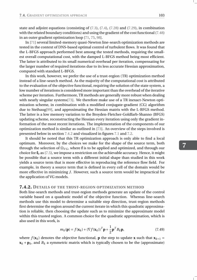
7.4. GRADIENT OPTIMIZATION APPROACH
7
103
state and adjoint equations (consisting of (7.3), (7.4), (7.28) and (7.29), in combinationwith the related boundary conditions) and using the gradient of the cost functional (7.48)in an outer gradient optimization loop [71, 75, 98].
In [71] several limited-memory quasi-Newton line-search optimization methods aretested in the context of DNS-based optimal control of turbulent flows. It was found thatthe L-BFGS approach performed best among the tested methods, requiring the small-est overall computational cost, with the damped L-BFGS method being most efficient.The latter is attributed to its small numerical overhead per iteration, compensating forthe larger number of required iterations due to its less accurate Hessian approximation,compared with standard L-BFGS.
In this work, however, we prefer the use of a trust-region (TR) optimization methodinstead of a line-search method. As the majority of the computational cost is attributedto the evaluation of the objective functional, requiring the solution of the state system, alow number of iterations is considered more important than the overhead of the iterativescheme per iteration. Furthermore, TR methods are generally more robust when dealingwith nearly singular systems[73]. We therefore make use of a TR inexact-Newton opti-mization scheme, in combination with a modified conjugate-gradient (CG) algorithmdue to Steihaug[99], and approximating the Hessian matrix with the L-BFGS method.The latter is a low memory variation to the Broyden-Fletcher-Goldfarb-Shanno (BFGS)updating scheme, reconstructing the Hessian every iteration using only the gradient in-formation of the most recent iterations. The implementation of the components of ouroptimization method is similar as outlined in [73]. An overview of the steps involved ispresented below in section 7.4.2 and visualized in figures 7.1 and 7.2.
It should be noted that this TR optimization approach is only able to find a localoptimum. Moreover, by the choices we make for the shape of the source term, boththrough the selection of ΩV G , where f is to be applied and optimized, and through ourchoice for f0 as (7.5), we impose a restriction on the achievable accuracy. Hence, it mightbe possible that a source term with a different initial shape than studied in this workyields a source term that is more effective in reproducing the reference flow field. Forexample, in theory a source term that is defined in every cell of the domain would bemore effective in minimizing J . However, such a source term would be impractical forthe application of VG models.
7.4.2. DETAILS OF THE TRUST-REGION OPTIMIZATION METHODBoth line-search methods and trust-region methods generate an update of the controlvariable based on a quadratic model of the objective function. Whereas line-searchmethods use this model to determine a suitable step direction, trust-region methodsfirst determine the region around the current iterate in which this quadratic approxima-tion is reliable, then choosing the update such as to minimize the approximate modelwithin this trusted region. A common choice for the quadratic approximation, which isalso used in this work, is
mk (p) = f (xk )+ (∇ f (xk ))T p+ 1
2pT Bk p, (7.49)
where f (xk ) denotes the objective functional, p the step to update x such that xk+1 =xk +pk , and Bk a symmetric matrix which is typically chosen to be the (approximate)
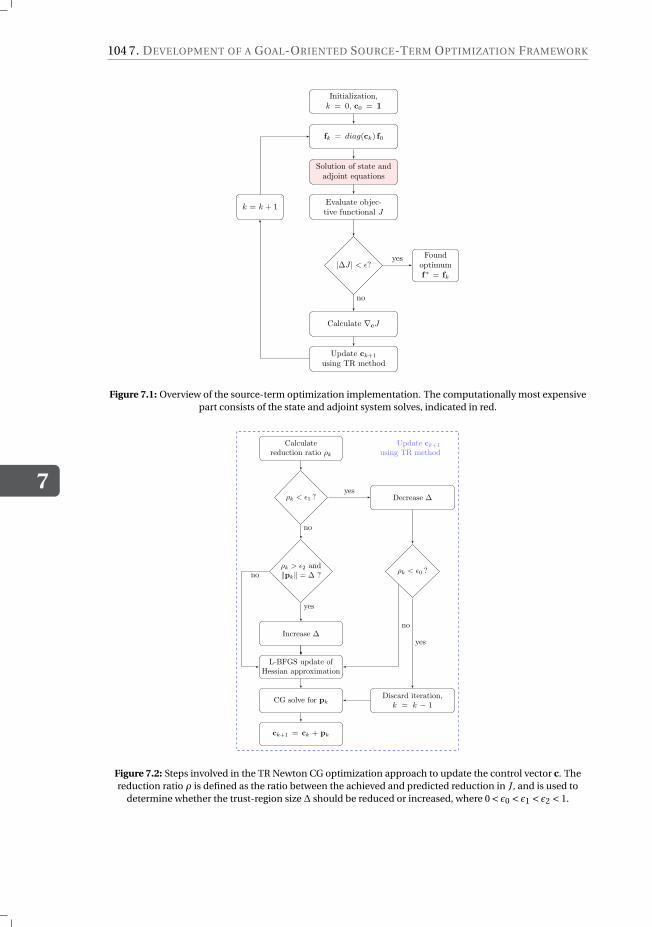
7
104 7. DEVELOPMENT OF A GOAL-ORIENTED SOURCE-TERM OPTIMIZATION FRAMEWORK
Initialization,k = 0, c0 = 1
fk = diag(ck) f0
Solution of state andadjoint equations
Evaluate objec-tive functional J
|∆J | < ε?
Calculate ∇cJ
Update ck+1
using TR method
k = k + 1
Foundoptimumf∗ = fk
yes
no
Figure 7.1: Overview of the source-term optimization implementation. The computationally most expensivepart consists of the state and adjoint system solves, indicated in red.
Calculatereduction ratio ρk
ρk < ε1 ? Decrease ∆
ρk < ε0 ?ρk > ε2 and‖pk‖ = ∆ ?
Increase ∆
L-BFGS update ofHessian approximation
CG solve for pk
ck+1 = ck + pk
Discard iteration,k = k − 1
Update ck+1
using TR method
yes
no
yes
yes
no
no
Figure 7.2: Steps involved in the TR Newton CG optimization approach to update the control vector c. Thereduction ratio ρ is defined as the ratio between the achieved and predicted reduction in J , and is used to
determine whether the trust-region size ∆ should be reduced or increased, where 0 < ϵ0 < ϵ1 < ϵ2 < 1.
7.4. GRADIENT OPTIMIZATION APPROACH
7
105
Hessian. The gradient of the cost functional, ∇ f (xk ), corresponds to the gradient calcu-lated in section 7.3. Using this approximation, the next iterate can thus be constructedusing a step that minimizes the quadratic approximation and falls within the trusted re-gion. Hence,
pk = arg minpk∈Rn
mk (p) such that ∥pk∥ ≤∆k , (7.50)
with ∆k denoting the trust-region radius at iterate k.A crucial step in trust-region methods is the determination of the size of the trust
region, which governs to a large extent the convergence rate. This trust-region radius∆ is based on the agreement between the real and predicted reduction of the objectivefunctional for a certain step, quantified as the reduction ratio
ρk = f (xk )− f (xk +pk )
mk (0)−mk (pk )= f (xk )− f (xk +pk )
−(∇ f (xk ))T pk − 12 pT
k Bk pk. (7.51)
If ρk ≈ 1 the approximate model yields a good representation of the objective functionalwithin the trust region, such that the current trust-region radius can be increased andfast convergence is to be expected. If, on the other hand, ρk is small, mk yields a poorapproximation and the trust region needs to be reduced. Moreover, in the case of anincrease in objective functional, characterized by a negative ρk , the current iterate isdiscarded. This process is visualized in figure 7.2.
Furthermore, the above described process requires a Hessian matrix Bk in order toconstruct the quadratic approximation. As no exact Hessian is available, an approxima-tion to the Hessian is constructed using the BFGS method. When starting from an ini-tial symmetric positive-definite matrix B0, this method produces increasingly accurateHessian approximations, that remain symmetric positive definite, using the updatingformula
Bk+1 = Bk −Bk pk pT
k B Tk
pTk Bk pk
+ yk yYk
yTk pk
, (7.52)
where yk represents the change in gradient between subsequent iterations, hence yk =∇k+1 f −∇k f . The approximate Hessian matrix has size n ×n, with n the total numberof control variables (hence n = 3NV G with NV G the number of cells in the source-termdomain ΩV G ).
Since n quickly grows with mesh refinement and the size of ΩV G , the Hessian updateaccording to 7.52 can become expensive to calculate, thereby slowing down the source-term optimization. It is thus worthwhile to limit the memory requirements by using alow-memory variant of the BFGS updating scheme instead. Following [73], we thereforeconstruct a Hessian approximation using the m most recent iterates for pk and yk as
Bk = δk I − [δk Sk Yk
][δk ST
k Sk Lk
LTk −Dk
]−1 [δk ST
kY T
k
], (7.53)
where
δk = yTk−1yk−1
pTk−1yk−1
, (7.54)
7
106 7. DEVELOPMENT OF A GOAL-ORIENTED SOURCE-TERM OPTIMIZATION FRAMEWORK
Sk and Yk denote the (n ×m)-matrices
Sk = [pk−m . . . pk−1
]and Sk = [
yk−m . . . yk−1]
, (7.55)
and Lk and Dk are respectively the lower-triangular and diagonal (m ×m)-matrices
(Lk )i , j =
pTk−m−1+i yk−m−1+ j if i > j ,
0 otherwise, (7.56)
Dk = diag[pT
k−m yk−m . . . pTk−1yk−1
]. (7.57)
The size of the square matrix in (7.53) therefore becomes 2m × 2m, with m typicallysmall, such that the required matrix inversion is cheap to evaluate. Note that this re-quires pk T yk > 0 for the matrix to be nonsingular.
Once the approximate model mk (p) is updated with the estimate for Bk , a next iteratecan be determined by calculating the step p according to the trust-region subproblem(7.50). When equating the derivative of mk (p) to zero an explicit formula for the step pk
can be obtained, yieldingpN
k =−B−1k ∇ f (xk ), (7.58)
which for Bk = ∇2 f (xk ) corresponds to a step of unit length in the Newton descent di-rection. However, the step pk needs to be chosen such as to be within the trust region,which is not guaranteed for (7.58). Therefore Steihaug’s conjugate-gradient method [99]is used instead, which calculates an inexact Newton step by iteratively varying both the(descent) direction and step length until the residual
rk = Bk pk +∇ f (xk ) < ϵk , (7.59)
with ϵk = min(0.5,
√∥∇ f (xk )∥)∥∇(xk )∥ to enhance convergence speed. The step ob-tained this way is the optimal approximation to the Newton step pN
k that falls withinthe trust region.
For the optimization problem as defined in section 7.1, the above method yields anew iterate ck+1 = ck +pk . Subsequent solution of the state and adjoint equations allowsthe gradient of the objective functional (7.48) to be re-evaluated, until eventually c∗ isfound for which ∇cL = 0 and thus f∗ = diag(c∗) f0 is obtained.
7.5. IMPLEMENTATIONThe described methodology has been implemented in the open-source CFD packageOpenFOAM®. A basic shape-optimization algorithm is already contained in the package[75], which served as the starting point for our goal-oriented source-term optimizationmethod. The steady incompressible RANS equations and their continuous adjoint coun-terpart are solved in a coupled fashion by making use of the SIMPLE algorithm. Once asteady-state solution is obtained, the objective functional is evaluated according to (7.1)and its gradient with respect to the control variable is calculated from (7.48). The sourceterm is then updated using the trust-region approach, as described above in section 7.4,until a local optimum is found. This process is visualized in figure 7.1.

7.5. IMPLEMENTATION
7
107
During the initialization step, ΩV G is defined by a cell-selection method, as discussedin section 5.1.3. In the selected cells an initial forcing per unit volume f0i is defined, ac-cording to 7.6, based on a user defined input vector F0 (for each VG considered), whichrepresents an estimate for the total forcing the presence of the VG would impose on theflow. This estimate does not need to be accurate, however, it is important that all com-ponents are non-zero. Note that the control variables ci are vectors defined for the cellscontained in ΩV G only, yielding a total of 3NV G controls to be optimized, with NV G thenumber of cells in the VG domain ΩV G .

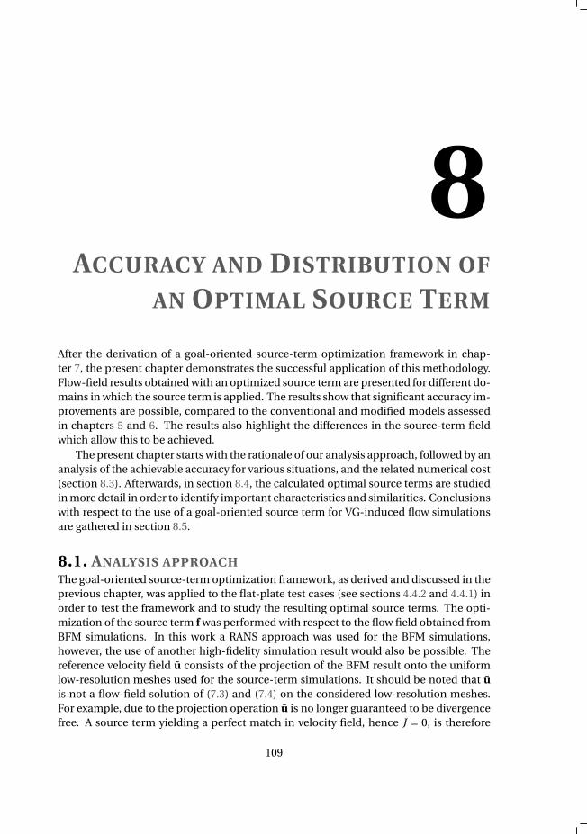
8ACCURACY AND DISTRIBUTION OF
AN OPTIMAL SOURCE TERM
After the derivation of a goal-oriented source-term optimization framework in chap-ter 7, the present chapter demonstrates the successful application of this methodology.Flow-field results obtained with an optimized source term are presented for different do-mains in which the source term is applied. The results show that significant accuracy im-provements are possible, compared to the conventional and modified models assessedin chapters 5 and 6. The results also highlight the differences in the source-term fieldwhich allow this to be achieved.
The present chapter starts with the rationale of our analysis approach, followed by ananalysis of the achievable accuracy for various situations, and the related numerical cost(section 8.3). Afterwards, in section 8.4, the calculated optimal source terms are studiedin more detail in order to identify important characteristics and similarities. Conclusionswith respect to the use of a goal-oriented source term for VG-induced flow simulationsare gathered in section 8.5.
8.1. ANALYSIS APPROACHThe goal-oriented source-term optimization framework, as derived and discussed in theprevious chapter, was applied to the flat-plate test cases (see sections 4.4.2 and 4.4.1) inorder to test the framework and to study the resulting optimal source terms. The opti-mization of the source term f was performed with respect to the flow field obtained fromBFM simulations. In this work a RANS approach was used for the BFM simulations,however, the use of another high-fidelity simulation result would also be possible. Thereference velocity field u consists of the projection of the BFM result onto the uniformlow-resolution meshes used for the source-term simulations. It should be noted that uis not a flow-field solution of (7.3) and (7.4) on the considered low-resolution meshes.For example, due to the projection operation u is no longer guaranteed to be divergencefree. A source term yielding a perfect match in velocity field, hence J = 0, is therefore
109
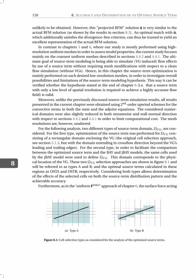
8
110 8. ACCURACY AND DISTRIBUTION OF AN OPTIMAL SOURCE TERM
unlikely to be obtained. However, this "projected BFM" solution u is very similar to theactual BFM solution (as shown by the results in section 8.3). An optimal match with u,which additionally satisfies the divergence-free criterion, can thus be trusted to yield anexcellent representation of the actual BFM solution.
In contrast to chapters 5 and 6, where our study is mostly performed using high-resolution uniform meshes in order to assess model properties, the current study focusesmainly on the coarsest uniform meshes described in sections 4.4.2 and 4.4.1. The ulti-mate goal of source-term modeling is being able to simulate (VG-induced) flow effectsby use of a source term without requiring mesh modifications with respect to a cleanflow simulation (without VGs). Hence, in this chapter the source-term optimization ismainly performed on such desired low-resolution meshes, in order to investigate overallpossibilities and limitations of the source-term modeling hypothesis. This way it can beverified whether the hypothesis stated at the end of chapter 6 (i.e. that a source termwith only a low level of spatial resolution is required to achieve a highly accurate flowfield) is valid.
Moreover, unlike the previously discussed source-term simulation results, all resultspresented in the current chapter were obtained using 2nd-order upwind schemes for theconvective terms in both the state and the adjoint equations. The considered numer-ical domains were also slightly reduced in both streamwise and wall-normal directionwith respect to sections 4.4.2 and 4.4.1 in order to limit computational cost. The meshresolutions are, however, unaltered.
For the following analysis, two different types of source-term domain, ΩV G , are con-sidered. For the first type, optimization of the source term was performed for ΩV G con-sisting of a rectangular domain enclosing the VG (the original cell selection approach,see section 5.1.3, but with the domain extending in crossflow direction beyond the VG’sleading and trailing edges). For the second type, in order to facilitate the comparisonbetween the optimized source term and the BAY and jBAY models, the same cells usedby the jBAY model were used to define ΩV G . This domain corresponds to the physi-cal location of the VG. These two ΩV G selection approaches are shown in figure 8.1 andwill be referred to as types A and B, and the optimal source terms calculated in theseregions as OSTA and OSTB, respectively. Considering both types allows determinationof the effects of the selected cells on both the source-term distribution pattern and theachievable accuracy.
Furthermore, as in the ’uniform Fexact’ approach of chapter 6, the surface force acting
(a) Type A (b) Type B
Figure 8.1: Cell-selection types as considered for the analysis of the optimized source terms.
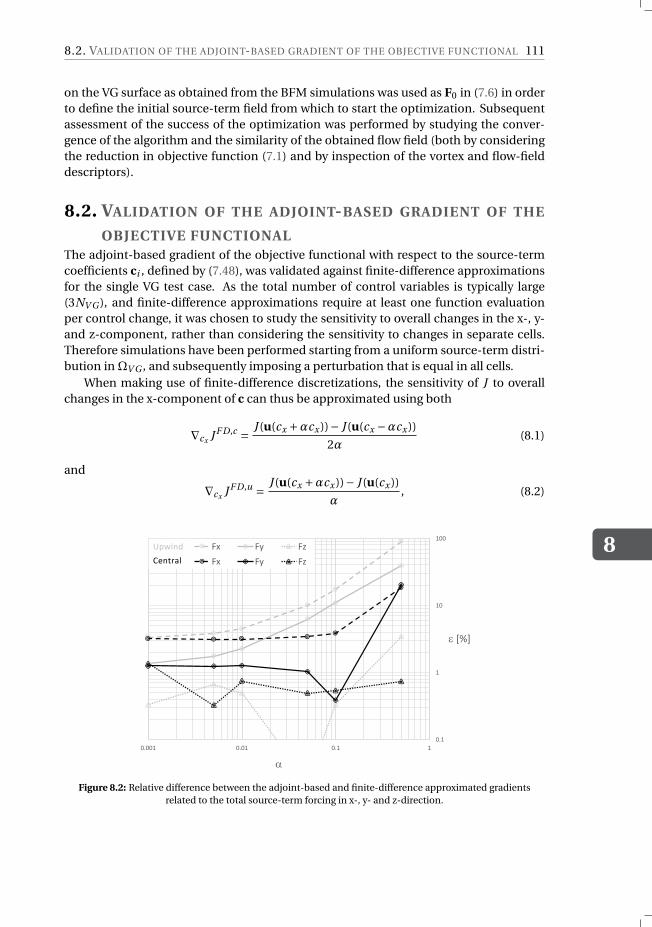
8.2. VALIDATION OF THE ADJOINT-BASED GRADIENT OF THE OBJECTIVE FUNCTIONAL
8
111
on the VG surface as obtained from the BFM simulations was used as F0 in (7.6) in orderto define the initial source-term field from which to start the optimization. Subsequentassessment of the success of the optimization was performed by studying the conver-gence of the algorithm and the similarity of the obtained flow field (both by consideringthe reduction in objective function (7.1) and by inspection of the vortex and flow-fielddescriptors).
8.2. VALIDATION OF THE ADJOINT-BASED GRADIENT OF THE
OBJECTIVE FUNCTIONALThe adjoint-based gradient of the objective functional with respect to the source-termcoefficients ci , defined by (7.48), was validated against finite-difference approximationsfor the single VG test case. As the total number of control variables is typically large(3NV G ), and finite-difference approximations require at least one function evaluationper control change, it was chosen to study the sensitivity to overall changes in the x-, y-and z-component, rather than considering the sensitivity to changes in separate cells.Therefore simulations have been performed starting from a uniform source-term distri-bution in ΩV G , and subsequently imposing a perturbation that is equal in all cells.
When making use of finite-difference discretizations, the sensitivity of J to overallchanges in the x-component of c can thus be approximated using both
∇cx J F D,c = J (u(cx +αcx ))− J (u(cx −αcx ))
2α(8.1)
and
∇cx J F D,u = J (u(cx +αcx ))− J (u(cx ))
α, (8.2)
!"#
#
#!
#!!
!"!!# !"!# !"# #
ε $%&
α
'( ') '*
'( ') '*
+,-./0
12/3456
Figure 8.2: Relative difference between the adjoint-based and finite-difference approximated gradientsrelated to the total source-term forcing in x-, y- and z-direction.
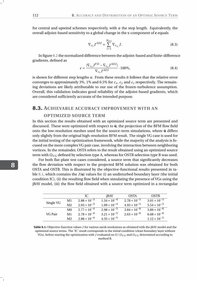
8
112 8. ACCURACY AND DISTRIBUTION OF AN OPTIMAL SOURCE TERM
for central and upwind schemes respectively, with α the step length. Equivalently, theoverall adjoint-based sensitivity to a global change in the x-component of c equals
∇cx J AD J =NV G∑i=1
∇cxiJ . (8.3)
In figure 8.2 the normalized difference between the adjoint-based and finite-differencegradients, defined as
ϵ= |∇cx J F D −∇cx J AD J |∇cx J AD J
·100%, (8.4)
is shown for different step lengths α. From these results it follows that the relative errorconverges to approximately 3%, 1% and 0.5% for cx , cy and cz respectively. The remain-ing deviations are likely attributable to our use of the frozen-turbulence assumption.Overall, this validation indicates good reliability of the adjoint-based gradients, whichare considered sufficiently accurate of the intended purpose.
8.3. ACHIEVABLE ACCURACY IMPROVEMENT WITH AN
OPTIMIZED SOURCE TERMIn this section the results obtained with an optimized source term are presented anddiscussed. These were optimized with respect to u, the projection of the BFM flow fieldonto the low-resolution meshes used for the source-term simulations, where u differsonly slightly from the original high-resolution BFM result. The single VG case is used forthe initial testing of the optimization framework, while the majority of the analysis is fo-cused on the more complex VG pair case, involving the interaction between neighboringvortices. In the remainder, OSTA refers to the result obtained using an optimized sourceterm with ΩV G defined by selection type A, whereas for OSTB selection type B was used.
For both flat-plate test cases considered, a source term that significantly decreasesthe flow deviation with respect to the projected BFM solution was obtained for bothOSTA and OSTB. This is illustrated by the objective-functional results presented in ta-ble 8.1, which contains the J (u) values for (i) an undisturbed boundary layer (the initialcondition IC), (ii) the resulting flow field when simulating the presence of VGs using thejBAY model, (iii) the flow field obtained with a source term optimized in a rectangular
IC jBAY OSTA OSTB
Single VGM1 2.88×10⁻³ 1.34×10⁻⁴ 2.78×10⁻⁵ 3.01×10⁻⁵
M2 2.93×10⁻³ 1.09×10⁻⁴ 4.93×10⁻⁵ 5.54×10⁻⁵
VG PairM0 2.77×10⁻⁴ 2.98×10⁻⁵ 3.84×10⁻⁶ 3.89×10⁻⁶
M1 2.78×10⁻⁴ 3.21×10⁻⁵ 2.63×10⁻⁶ 6.68×10⁻⁶
M2 2.88×10⁻⁴ 4.35×10⁻⁵ - 1.12×10⁻⁵
Table 8.1: Objective-function values J for various mesh resolutions as obtained with the jBAY model and theoptimized source terms. The ’IC’ result corresponds to the initial condition (clean boundary layer without
VGs), before starting the optimization with J evaluated on Ω\ΩV G and ΩV G determined according tomethod B.
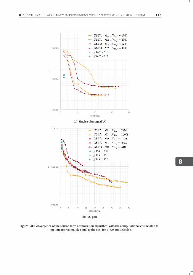
8.3. ACHIEVABLE ACCURACY IMPROVEMENT WITH AN OPTIMIZED SOURCE TERM
8
113
!!"#$"%"
!!"#$"&"
!!"#$"'"
" % (" (% )"
*
+,#-.,+/0
(a) Single submerged VG
!!"#$"%"
!!"#$"&"
!!"#$"'"
" & (" (& )" )& *" *& '"
+
,-#./-,01
(b) VG pair
Figure 8.3: Convergence of the source-term optimization algorithm, with the computational cost related to 1iteration approximately equal to the cost for 1 jBAY model solve.
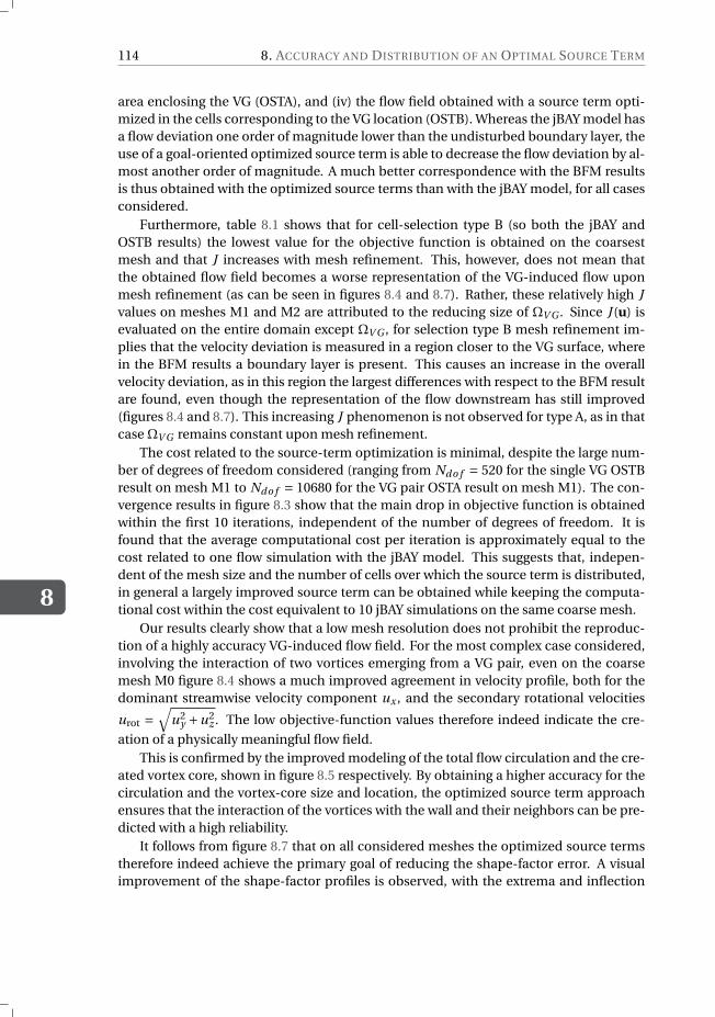
8
114 8. ACCURACY AND DISTRIBUTION OF AN OPTIMAL SOURCE TERM
area enclosing the VG (OSTA), and (iv) the flow field obtained with a source term opti-mized in the cells corresponding to the VG location (OSTB). Whereas the jBAY model hasa flow deviation one order of magnitude lower than the undisturbed boundary layer, theuse of a goal-oriented optimized source term is able to decrease the flow deviation by al-most another order of magnitude. A much better correspondence with the BFM resultsis thus obtained with the optimized source terms than with the jBAY model, for all casesconsidered.
Furthermore, table 8.1 shows that for cell-selection type B (so both the jBAY andOSTB results) the lowest value for the objective function is obtained on the coarsestmesh and that J increases with mesh refinement. This, however, does not mean thatthe obtained flow field becomes a worse representation of the VG-induced flow uponmesh refinement (as can be seen in figures 8.4 and 8.7). Rather, these relatively high Jvalues on meshes M1 and M2 are attributed to the reducing size of ΩV G . Since J (u) isevaluated on the entire domain except ΩV G , for selection type B mesh refinement im-plies that the velocity deviation is measured in a region closer to the VG surface, wherein the BFM results a boundary layer is present. This causes an increase in the overallvelocity deviation, as in this region the largest differences with respect to the BFM resultare found, even though the representation of the flow downstream has still improved(figures 8.4 and 8.7). This increasing J phenomenon is not observed for type A, as in thatcase ΩV G remains constant upon mesh refinement.
The cost related to the source-term optimization is minimal, despite the large num-ber of degrees of freedom considered (ranging from Ndo f = 520 for the single VG OSTBresult on mesh M1 to Ndo f = 10680 for the VG pair OSTA result on mesh M1). The con-vergence results in figure 8.3 show that the main drop in objective function is obtainedwithin the first 10 iterations, independent of the number of degrees of freedom. It isfound that the average computational cost per iteration is approximately equal to thecost related to one flow simulation with the jBAY model. This suggests that, indepen-dent of the mesh size and the number of cells over which the source term is distributed,in general a largely improved source term can be obtained while keeping the computa-tional cost within the cost equivalent to 10 jBAY simulations on the same coarse mesh.
Our results clearly show that a low mesh resolution does not prohibit the reproduc-tion of a highly accuracy VG-induced flow field. For the most complex case considered,involving the interaction of two vortices emerging from a VG pair, even on the coarsemesh M0 figure 8.4 shows a much improved agreement in velocity profile, both for thedominant streamwise velocity component ux , and the secondary rotational velocities
urot =√
u2y +u2
z . The low objective-function values therefore indeed indicate the cre-
ation of a physically meaningful flow field.This is confirmed by the improved modeling of the total flow circulation and the cre-
ated vortex core, shown in figure 8.5 respectively. By obtaining a higher accuracy for thecirculation and the vortex-core size and location, the optimized source term approachensures that the interaction of the vortices with the wall and their neighbors can be pre-dicted with a high reliability.
It follows from figure 8.7 that on all considered meshes the optimized source termstherefore indeed achieve the primary goal of reducing the shape-factor error. A visualimprovement of the shape-factor profiles is observed, with the extrema and inflection
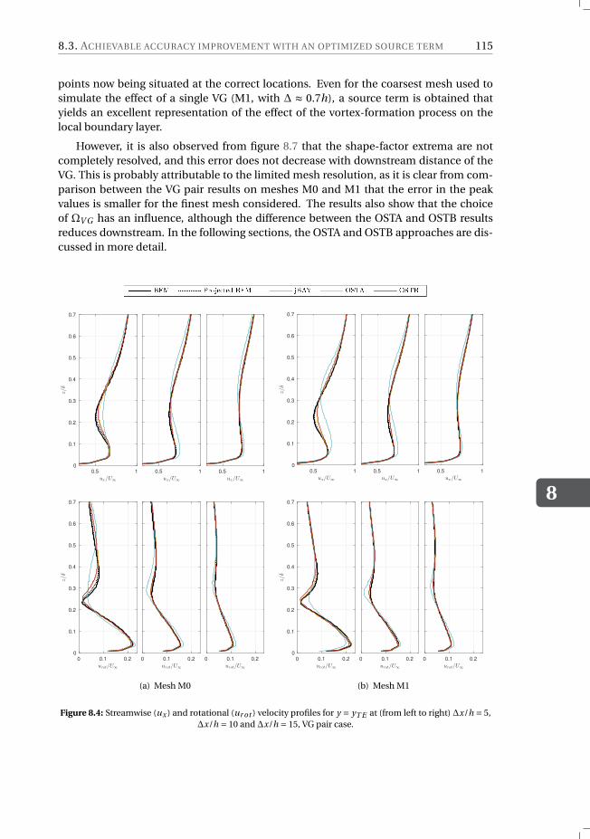
8.3. ACHIEVABLE ACCURACY IMPROVEMENT WITH AN OPTIMIZED SOURCE TERM
8
115
points now being situated at the correct locations. Even for the coarsest mesh used tosimulate the effect of a single VG (M1, with ∆ ≈ 0.7h), a source term is obtained thatyields an excellent representation of the effect of the vortex-formation process on thelocal boundary layer.
However, it is also observed from figure 8.7 that the shape-factor extrema are notcompletely resolved, and this error does not decrease with downstream distance of theVG. This is probably attributable to the limited mesh resolution, as it is clear from com-parison between the VG pair results on meshes M0 and M1 that the error in the peakvalues is smaller for the finest mesh considered. The results also show that the choiceof ΩV G has an influence, although the difference between the OSTA and OSTB resultsreduces downstream. In the following sections, the OSTA and OSTB approaches are dis-cussed in more detail.
0.5 1
ux/U∞
0
0.1
0.2
0.3
0.4
0.5
0.6
0.7
z/δ
0 0.1 0.2
urot/U∞
0
0.1
0.2
0.3
0.4
0.5
0.6
0.7
z/δ
0.5 1
ux/U∞
0 0.1 0.2
urot/U∞
0.5 1
ux/U∞
0 0.1 0.2
urot/U∞
(a) Mesh M0
0.5 1
ux/U∞
0
0.1
0.2
0.3
0.4
0.5
0.6
0.7
z/δ
0 0.1 0.2
urot/U∞
0
0.1
0.2
0.3
0.4
0.5
0.6
0.7
z/δ
0.5 1
ux/U∞
0 0.1 0.2
urot/U∞
0.5 1
ux/U∞
0 0.1 0.2
urot/U∞
(b) Mesh M1
Figure 8.4: Streamwise (ux ) and rotational (ur ot ) velocity profiles for y = yT E at (from left to right) ∆x/h = 5,∆x/h = 10 and ∆x/h = 15, VG pair case.
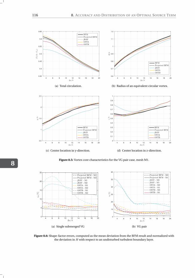
8
116 8. ACCURACY AND DISTRIBUTION OF AN OPTIMAL SOURCE TERM
4 6 8 10 12 14 16 18 20
∆x/h
0.35
0.4
0.45
0.5
0.55
0.6
0.65
|Γ|/(h
·U∞)
BFM
Projected BFM
jBAY
OSTA
OSTB
(a) Total circulation.
4 6 8 10 12 14 16 18 20
∆x/h
0.6
0.7
0.8
0.9
1
1.1
1.2
R/h
BFM
Projected BFM
jBAY
OSTA
OSTB
(b) Radius of an equivalent circular vortex.
4 6 8 10 12 14 16 18 20
∆x/h
0.5
1
1.5
2
2.5
y c/h
BFM
Projected BFM
jBAY
OSTA
OSTB
(c) Center location in y-direction.
4 6 8 10 12 14 16 18 20
∆x/h
0
0.1
0.2
0.3
0.4
0.5
0.6
0.7
0.8
0.9
1
z c/h
BFM
Projected BFM
jBAY
OSTA
OSTB
(d) Center location in z-direction.
Figure 8.5: Vortex core characteristics for the VG pair case, mesh M1.
∆x/h4 6 8 10 12 14 16 18 20
ǫH[%
]
0
5
10
15
20
25
Projected BFM - M1Projected BFM - M2jBAY - M1jBAY - M2OSTA - M1OSTA - M2OSTB - M1OSTB - M2
(a) Single submerged VG
4 6 8 10 12 14 16 18 20
∆x/h
0
10
20
30
40
50
60
ǫH[%
]
Projected BFM - M0
Projected BFM - M1
jBAY - M0
jBAY - M1
OSTA - M0
OSTA - M1
OSTB - M0
OSTB - M1
(b) VG pair
Figure 8.6: Shape-factor errors, computed as the mean deviation from the BFM result and normalized withthe deviation in H with respect to an undisturbed turbulent boundary layer.
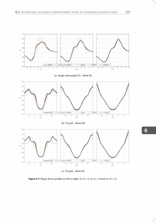
8.3. ACHIEVABLE ACCURACY IMPROVEMENT WITH AN OPTIMIZED SOURCE TERM
8
117
y/h-3 -2 -1 0 1 2 3 4 5
H
1.15
1.2
1.25
1.3
1.35
1.4
1.45
1.5
y/h-3 -2 -1 0 1 2 3 4 5
y/h-3 -2 -1 0 1 2 3 4 5
BFM Projected BFM jBAY OSTA OSTB
(a) Single submerged VG - Mesh M1
-2 -1 0 1 2
y/h
1.1
1.2
1.3
1.4
1.5
1.6
1.7
1.8
H
-2 -1 0 1 2
y/h-2 -1 0 1 2
y/h
BFM Projected BFM jBAY OSTA OSTB
(b) VG pair - Mesh M0
-2 -1 0 1 2
y/h
1.1
1.2
1.3
1.4
1.5
1.6
1.7
1.8
H
-2 -1 0 1 2
y/h-2 -1 0 1 2
y/h
BFM Projected BFM jBAY OSTA OSTB
(c) VG pair - Mesh M1
Figure 8.7: Shape-factor profiles at (left to right) ∆x/h = 5, ∆x/h = 10 and ∆x/h = 15.
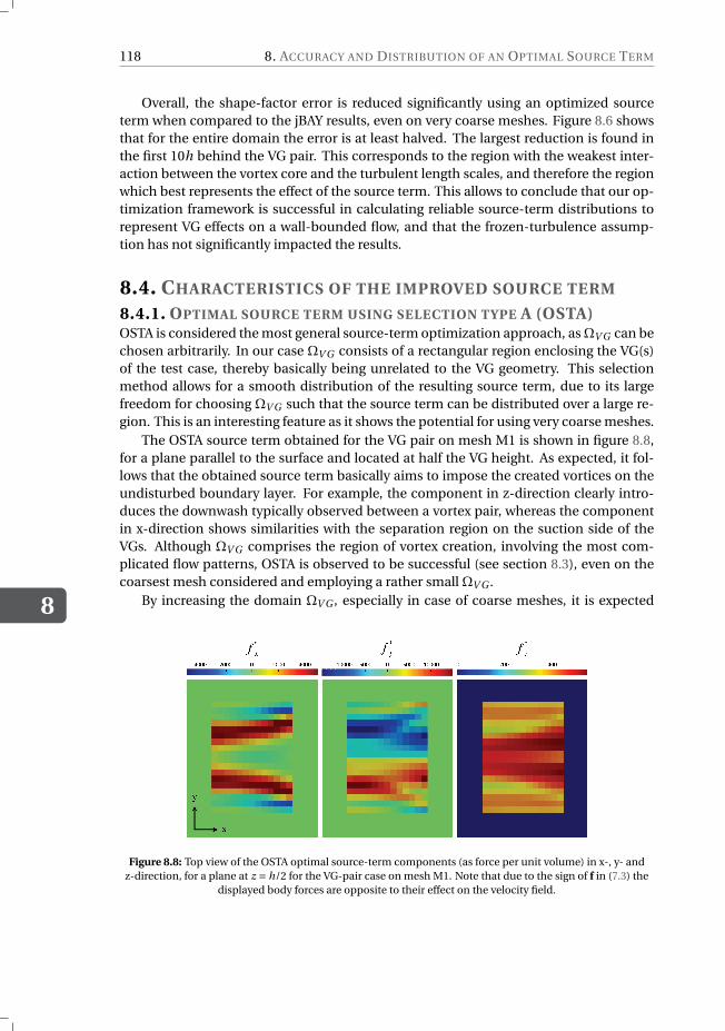
8
118 8. ACCURACY AND DISTRIBUTION OF AN OPTIMAL SOURCE TERM
Overall, the shape-factor error is reduced significantly using an optimized sourceterm when compared to the jBAY results, even on very coarse meshes. Figure 8.6 showsthat for the entire domain the error is at least halved. The largest reduction is found inthe first 10h behind the VG pair. This corresponds to the region with the weakest inter-action between the vortex core and the turbulent length scales, and therefore the regionwhich best represents the effect of the source term. This allows to conclude that our op-timization framework is successful in calculating reliable source-term distributions torepresent VG effects on a wall-bounded flow, and that the frozen-turbulence assump-tion has not significantly impacted the results.
8.4. CHARACTERISTICS OF THE IMPROVED SOURCE TERM
8.4.1. OPTIMAL SOURCE TERM USING SELECTION TYPE A (OSTA)OSTA is considered the most general source-term optimization approach, as ΩV G can bechosen arbitrarily. In our case ΩV G consists of a rectangular region enclosing the VG(s)of the test case, thereby basically being unrelated to the VG geometry. This selectionmethod allows for a smooth distribution of the resulting source term, due to its largefreedom for choosing ΩV G such that the source term can be distributed over a large re-gion. This is an interesting feature as it shows the potential for using very coarse meshes.
The OSTA source term obtained for the VG pair on mesh M1 is shown in figure 8.8,for a plane parallel to the surface and located at half the VG height. As expected, it fol-lows that the obtained source term basically aims to impose the created vortices on theundisturbed boundary layer. For example, the component in z-direction clearly intro-duces the downwash typically observed between a vortex pair, whereas the componentin x-direction shows similarities with the separation region on the suction side of theVGs. Although ΩV G comprises the region of vortex creation, involving the most com-plicated flow patterns, OSTA is observed to be successful (see section 8.3), even on thecoarsest mesh considered and employing a rather small ΩV G .
By increasing the domain ΩV G , especially in case of coarse meshes, it is expected
Figure 8.8: Top view of the OSTA optimal source-term components (as force per unit volume) in x-, y- andz-direction, for a plane at z = h/2 for the VG-pair case on mesh M1. Note that due to the sign of f in (7.3) the
displayed body forces are opposite to their effect on the velocity field.
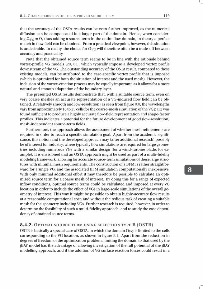
8.4. CHARACTERISTICS OF THE IMPROVED SOURCE TERM
8
119
that the accuracy of the OSTA results can be even further improved, as the numericaldiffusion can be compensated in a larger part of the domain. Hence, when consider-ing ΩV G = Ω, thus adding a source term in the entire flow domain, in theory a perfectmatch in flow field can be obtained. From a practical viewpoint, however, this situationis undesirable. In reality, the choice for ΩV G will therefore often be a trade-off betweenaccuracy and practicality.
Note that the obtained source term seems to be in line with the rationale behindvortex-profile VG models [20, 63], which typically impose a developed vortex profiledownstream of the VG. The outstanding accuracy of the OSTA result, compared to theseexisting models, can be attributed to the case-specific vortex profile that is imposed(which is optimized for both the situation of interest and the used mesh). However, theinclusion of the vortex-creation process may be equally important, as it allows for a morenatural and smooth adaptation of the boundary layer.
The presented OSTA results demonstrate that, with a suitable source term, even onvery coarse meshes an accurate representation of a VG-induced flow field can be ob-tained. A relatively smooth and low-resolution (as seen from figure 8.8, the wavelengthsvary from approximately 10 to 25 cells for the coarse-mesh simulation of the VG pair) wasfound sufficient to produce a highly accurate flow-field representation and shape-factorprofiles. This indicates a potential for the future development of good (low-resolution)mesh-independent source-term fields.
Furthermore, the approach allows the assessment of whether mesh refinements arerequired in order to reach a specific simulation goal. Apart from the academic signifi-cance, this notion and the developed approach may (after additional research) possiblybe of interest for industry, where typically flow simulations are required for large geome-tries including numerous VGs with a similar design (for a wind-turbine blade, for ex-ample). It is envisioned that an OSTA approach might be used as part of a multi-fidelitymodeling framework, allowing for accurate source-term simulations of these large struc-tures with minimal mesh requirements. The construction of a BFM is rather straightfor-ward for a single VG, and the associated BFM simulation computationally inexpensive.With only minimal additional effort it may therefore be possible to calculate an opti-mized source term for a coarse mesh of interest. By doing this for a range of expectedinflow conditions, optimal source terms could be calculated and imposed at every VGlocation in order to include the effect of VGs in large-scale simulations of the overall ge-ometry of interest. This way it might be possible to obtain highly-accurate flow resultsat a reasonable computational cost, and without the tedious task of creating a suitablemesh for the geometry including VGs. Further research is required, however, in order todetermine the feasibility of such a multi-fidelity approach, and to study the case depen-dency of obtained source terms.
8.4.2. OPTIMAL SOURCE TERM USING SELECTION TYPE B (OSTB)OSTB is basically a special case of OSTA, in which the domain ΩV G is limited to the cellscorresponding to the VG location, as shown in figure 8.1. Apart from the reduction indegrees of freedom of the optimization problem, limiting the domain to that used by thejBAY model has the advantage of allowing investigation of the full potential of the jBAYmodelling approach, and if the addition of VG surface reaction forces could result in a
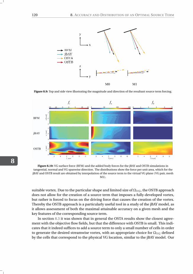
8
120 8. ACCURACY AND DISTRIBUTION OF AN OPTIMAL SOURCE TERM
x
y
y
z
M0 M1
Figure 8.9: Top and side view illustrating the magnitude and direction of the resultant source term forcing.
!"#$$$$$$$$$$!"%$$$$$$$$$$$$$!#$$$$$$$$$$$$$$%$$$$$$$$$$$$$$$#$$$$$$$$$$$$$$$"%$$$$$$$$$$$"#$ % $$$$$$$$$$$$$$#% $$$$$$$$$$$$$$$$$$$$$$$$$$$$"%% $$$$$$$$$$$$$$$$$$$$"#%$ % $" $$& $$$' $$$$$( $$$$$#$
BFM
jBAY
OSTB
ft fn
fb
Figure 8.10: VG surface force (BFM) and the added body forces for the jBAY and OSTB simulations intangential, normal and VG spanwise direction. The distributions show the force per unit area, which for the
jBAY and OSTB result are obtained by interpolation of the source term to the virtual VG plane (VG pair, meshM1).
suitable vortex. Due to the particular shape and limited size of ΩV G , the OSTB approachdoes not allow for the creation of a source term that imposes a fully-developed vortex,but rather is forced to focus on the driving force that causes the creation of the vortex.Thereby the OSTB approach is a particularly useful tool in a study of the jBAY model, asit allows assessment of both the maximal attainable accuracy on a given mesh and thekey features of the corresponding source term.
In section 8.3 it was shown that in general the OSTA results show the closest agree-ment with the objective flow fields, but that the difference with OSTB is small. This indi-cates that it indeed suffices to add a source term to only a small number of cells in orderto generate the desired streamwise vortex, with an appropriate choice for ΩV G definedby the cells that correspond to the physical VG location, similar to the jBAY model. Our
8.5. CONCLUSION
8
121
results therefore demonstrate that even on a coarse mesh, with a resolution too low toresolve the detailed flow patterns related to vortex creation, there exists a specific drivingforce that yields an accurate representation of the desired flow field. This is a favorableoutcome, as it demonstrates the validity behind the jBAY rationale. Furthermore, se-lection method B in theory simplifies the analysis and description of an optimal sourceterm due to the possibility of choosing ΩV G as a 2D plane rather than a 3D volume.
Whereas the jBAY model is observed to be unable to accurately represent the shapefactor, our OSTB results display a largely improved accuracy in this respect. These re-sults suggest that an improvement for the jBAY model is both desired and possible. It istherefore worthwhile to investigate the differences in the applied source term for boththese simulation approaches. For this purpose first the resultant source term is consid-ered, the magnitude and direction of which are visualized in figure 8.9. As expected, itfollows that the OSTB source term adds a resultant forcing that is nicely aligned with theexact VG surface force (as extracted from the BFM simulation). In contrast, the direc-tion of the forcing included by the jBAY model is tilted upstream and downward (as wasalso observed in [26]). Counter-intuitively, the magnitude of the optimal source termis smaller than the exact VG surface force. This suggest that aiming for an exact repre-sentation of the resultant VG surface force is not the optimal approach when using anunder-resolved mesh. This is confirmed by the source-term distributions, show in figure8.10 for the VG pair using mesh M1, which are interpolated to the virtual VG plane anddisplayed as force per unit surface. The jBAY model clearly aims to represent the actualVG force distribution, with the focus being on the leading edge of the VG.
The OSTB result on the other hand shows a more uniform distribution of the normalforce (fn), which is less focused on the leading edge region but spread over the front halfof the virtual VG plane. Furthermore, large differences are observed in the secondarycomponents ft and fb , in the tangential and VG-spanwise directions respectively. Al-though insufficient to draw general conclusions regarding the optimal source-term lay-out, the presented results show that aiming for an exact representation of the VG surface-force distribution seems not to be the optimal approach for coarse meshes.
8.5. CONCLUSIONIn this chapter we presented the successful optimization of the source term added to aCFD simulation in order to represent the flow effects induced by the presence of VGs.The results proved the viability of the idea to replace a physical obstacle by a local sourceterm, for the situation of an incompressible flow over a flat plate with rectangular, vane-type VGs. It was shown that, even on a low-resolution mesh, a nearly perfect representa-tion of the boundary layer can be achieved when only adding a source term to a limitednumber of cells in the neighborhood of the VG location.
Although good results were achieved for all cases considered, comparison of thesource terms optimized in two different domains indicated that extension of the source-term domain ΩV G has a favorable effect on the accuracy of the created flow field. On acoarse mesh a high-gradient source-term distribution is hard to resolve, and its effectsare more subject to truncation errors. A smoother distribution with the same net effect,as is possible on a larger ΩV G , is thus favorable, even if in that case the source term doesno longer yield the closest match possible with the physical VG reaction force on the
8
122 8. ACCURACY AND DISTRIBUTION OF AN OPTIMAL SOURCE TERM
flow. The obtained results indicated that it is not necessary to have a high-frequencysource term, and to resolve all flow details close around the VG, to obtain an accuraterepresentation of the downstream flow field. A low-resolution source-term field, whichis thus resolvable on coarse meshes, may be sufficient to simulate the effect of VGs on aboundary layer.
The value of the presented optimization approach consists of its ability to determinethe source term which yields the highest accuracy that can potentially be achieved witha source-term method on a given (coarse) mesh for a certain situation of interest. It maytherefore be used (i) as a tool for the development of improved VG models, (ii) in order toassess whether or not mesh refinement is required for achieving a specific objective, and(iii) to obtain the specific source term that allows achieving this highly accurate result,even for unconventional VG designs. Apart from an academic point of view, with someadditional research the current method is therefore also expected to be of use for indus-trial applications involving large VG arrays, as valuable information can be obtained bystudying the simplified sub-problem of only a single VG or VG pair.
9CONCLUSIONS &
RECOMMENDATIONS
Vortex generators (VGs) are, and can be expected to remain, one of the most widely usedmeans of passive flow control. Despite this widespread use, making reliable predictionsabout their effect on the local flow field, and on the performance of the object equippedwith VGs, remains far from straightforward. From an accuracy point of view, fully re-solved CFD simulations are preferred to study VG-induced flows. The large scale differ-ence, in combination with the complex flow dynamics observed around a VG, however,imposes an excessive computational cost, thereby precluding this type of simulationsfor other than academic purposes. As an alternative, partly-modeled/partly-resolvedCFD methods are typically used instead. These methods do not resolve the flow detailsaround the VG, but rather add an external forcing locally to the simulation which triggersthe formation of a streamwise vortex similar to the main vortex created by the VG. Forthese methods to be successful, a good understanding of the principles governing theirresult is a prerequisite. Still, many essential questions related to their use and accuracyremained unanswered.
9.1. CONCLUSIONSTo fill this scientific gap, this dissertation has presented a study of the impact of modelformulation and simulation parameters on the VG-induced flow field obtained with partly-modeled/partly-resolved source-term CFD methods. It did so by starting from existingmodels and perturbing their formulation, until eventually arriving at fully optimizedsource-term distributions for specific cases. Given that the primal objective of VGs con-sists of the reduction or elimination of flow separation, the shape factor was identifiedas key parameter in assessing the accuracy of simulations, with accuracy defined relativeto body-fitted mesh simulations.
In this dissertation it was shown that the idea of reproducing VG-induced flows byuse of a coarse mesh in combination with a local source-term model is viable. Current
123
9
124 9. CONCLUSIONS & RECOMMENDATIONS
models were found to posses several shortcomings, causing their accuracy to be uncer-tain and the required mesh resolution to be still rather fine. Improvement of these mod-els is thus desired, and as shown, possible. Case-specific optimized source terms areshown to be capable of yielding highly accurate flow fields on very coarse meshes.
9.1.1. EFFECTIVENESS OF SOURCE-TERM MODELS FOR FLOW SIMULATIONS
DOWNSTREAM OF VORTEX GENERATORSThe effectiveness of the BAY and jBAY models for including VG effects in CFD simula-tions was investigated, which revealed the presence of model errors in both methods.For mesh resolutions approaching the body-fitted mesh resolution, significant devia-tions in the boundary-layer profile were observed, thus suggesting the presence of modelerrors that might result in poor predictions with respect to the VG effect on the flow. Ourresults showed a consistent under-prediction of the vortex strength and errors in theshape-factor profiles for the flow fields obtained with both the BAY and the jBAY models.Moreover, the center of the initiated vortex was found to be too far on the VG suctionside, yielding deviations in the vortex path upon downstream propagation.
Both mesh resolution and the region where the source-term model is applied werefound to have a large impact on the created flow field, with the effect of the latter be-ing largest. The overall vorticity levels in the flow, and therefore the total circulation andhence amount of mixing, increase with the width (and thus size) of the source-term re-gion. For the BAY model, the source-term region can therefore be used to calibrate thegenerated flow circulation, however, this will not improve the overall accuracy of the flowrepresentation. In the absence of calibration data the jBAY source-term region, consist-ing of a 2-cells wide region aligned with the (virtual) VG, was found to yield the mostreliable result.
Mesh dependence was observed for the results of both the BAY and the jBAY model,with a more concentrated vortex being created upon refinement of the mesh. For source-term regions that are aligned with the VG, an important source of mesh dependence wasfound to be the variation of the source-term region with mesh resolution, which be-comes more confined with mesh refinement. The interpolation and redistribution partsof the jBAY model were not observed to yield the expected reduction in mesh depen-dency of the model. Our results indicated that the effect of this addition on the generatedflow field is limited, and manifests mainly as a small decrease in overall vorticity level.
Analysis of factors that can be used to define a source term, indicated that the to-tal resultant source-term forcing dominates both the strength and shape of the createdstreamwise vortex. The distribution of the forcing over the source-term region seems tohave a lesser influence on the characteristics of the created vortex. The magnitude of theresultant forcing was found to be the main driver in this respect, governing directly theenergy that is added to the flow and the strength and size of the created vortex. Also theshape of the boundary-layer profile is influenced most by the source term’s magnitude,as for the same position a stronger vortex yields a stronger interaction with the boundarylayer. Small variations in the direction of the resultant forcing (in the order of the differ-ence between the BAY model’s forcing and the exact VG reaction force), however, werefound to have only a limited effect on the created flow field.
Comparison of the resultant forcing added to the flow by the BAY and jBAY models
9.1. CONCLUSIONS
9
125
with the actual VG reaction force, showed that the largest deviations occur in the tangen-tial and VG spanwise components. The former was found to cause an underestimationof the wake created behind the VG (and therefore an underestimation of the shape-factorpeaks), whereas the latter yields a poor prediction for the uplifting of fluid from the wallclose behind the VG.
Overall, the analysis of modified source-term formulations revealed that a simpleuniformly-distributed source term with the exact total-force components is able to yielda fair representation of the VG-induced flow field in terms of the shape, location andstrength of the created vortex. However, errors with respect to the shape-factor profileswere still observed.
9.1.2. GOAL-ORIENTED OPTIMIZATION OF A SOURCE-TERM
REPRESENTATION OF VORTEX GENERATORSA goal-oriented optimization framework was presented that can be used to calculate thesource term that, on a low-resolution mesh, optimally reproduces a high-fidelity VG-induced velocity field. The proposed method was successfully applied for two flat-platecases using various low-resolution meshes.
The optimized source-term simulations proved the viability of the idea to replace aphysical obstacle by a local source term, for the situation of incompressible flow over aflat plate with rectangular vane-type VGs. It was shown that, even on a low-resolutionmesh, a nearly perfect representation of the boundary layer can be achieved when onlyadding a source term to a limited number of cells in the neighborhood of the VG location.
Distinction was made between source terms added in a region surrounding the VG,thereby imposing a specific vortex profile, and source terms added at exactly the VG lo-cation that aim to introduce a suitable driving force to initiate vortex creation. Althoughthe rationale between these approaches differs, they both prove to be effective, with thefirst approach showing the largest accuracy potential.The optimal source term obtainedthis way was characterized by a low-wavelength distribution, thus indicating that a low-resolution source term (resolvable on coarse meshes) suffices for accurate source-termsimulations of VG-induced flows.
The presented optimization framework allows determination of the source term whichyields the highest accuracy that can potentially be achieved with a source term methodon a given (coarse) mesh for a situation of interest. It may therefore be used (i) as a toolfor the development of improved VG models, (ii) in order to assess whether or not meshrefinement is required for achieving a specific objective, and (iii) to obtain the specificsource term that allows achieving this highly accurate result, even for unconventionalVG designs. Apart from an academic point of view, with some additional research thedeveloped method is therefore also expected to be of use for industrial applications in-volving large VG arrays, as useful information can be obtained by studying the simplifiedsub-problem of only a single VG or VG pair.
Finally, comparison of optimized source-term simulations with flow results obtainedusing the jBAY model indicates that research towards an improvement of the latter modelis justified and desired. Goal-oriented source-term optimization can be useful in thisendeavor, as it allows to quantify the achievable improvement and to identify the devia-tions of the jBAY source term from the optimal one.
9
126 9. CONCLUSIONS & RECOMMENDATIONS
9.2. OUTLOOK & RECOMMENDATIONSAlthough the created body of knowledge presented in this dissertation yields a useful ad-dition to the insights already present in literature, additional research towards efficientand accurate VG-induced flow simulations remains desired. In this view, the followingrecommendations originate from the current work:
• The choice to use a RANS simulation method inevitably introduces an error in theboundary-layer development, and therefore in both the initial condition for thevortex-development process, and the downstream evolution of the created vor-tices. These errors due to the choice of turbulence model were outside the scopeof this dissertation, but are expected to have a considerable effect on the result-ing flow field. Further research towards the effectiveness of different turbulencemodels for VG-induced flows is therefore desired, if necessary followed by the de-velopment of improved turbulence models that feature enhanced capabilities tocapture the interaction between the turbulent eddies and the streamwise vortex.
Moreover, the current study focused on the accuracy with which a source-termmodel can reproduce the vortex created by a VG, such as to contribute to improvedflow-separation predictions. Further research is however required to determinehow the ability of different turbulence models to predict separation is affected bythe upstream velocity field introduced by VGs.
• In this work, reproduction of the shape-factor profile was identified as the key per-formance parameter when assessing the accuracy of a VG model. Especially closedownstream of the VG large deviations from the BFM result were observed. How-ever, as the vortex dissipates the shape-factor error was found to decrease. Furtherresearch is therefore desired to quantify the effect of this error on the prediction ofboundary-layer separation, i.e. to define the region in which it is important to keepthe shape-factor error ϵH low.
• The presented study towards the effectiveness of the BAY and jBAY models, andsource-term models in general, to simulate VG-induced flows was performed for asmall set of cases, all featuring rectangular vane-type VGs and incompressible flow.It would be interesting to extent the considered test matrix in oder to verify ourfindings for a larger spectrum of configurations and flow conditions, including,for example, triangular VGs and compressible flows.
• In chapter 6 it was found that a uniformly-distributed source term that featuresa total forcing equal to the exact VG reaction force yields fair flow-field results.This observation can serve as stimulation for research towards improved predic-tion methods for the total force acting on a VG in a wall-bounded flow. The avail-ability of such predictions would allow for an alternative and simple source-termVG model. In this light, a detailed analysis of the model proposed in [79] would beinteresting.
• The goal-oriented source-term optimization framework in chapter 7 was devel-oped with the objective of obtaining a minimal deviation in the velocity field, withrespect to a high-fidelity reference solution. Enhancement of the objective func-tional with the additional requirement of maximizing pressure-field similarity (on
9.2. OUTLOOK & RECOMMENDATIONS
9
127
the surface of application) is expected to allow for even more accurate solutions.In particular, this can be expected to yield more reliable predictions regarding theeffect of VGs on the aerodynamic forces.
Moreover, the derivation and implementation of a compressible equivalent forthe adjoint equations, which are now derived using the assumption of incompress-ible flow, is required for application to compressible flow cases.
The accuracy of the source-term optimization can be further improved by re-moving the frozen-turbulence assumption in the derivation of the adjoint equa-tions. This would result in an additional set of adjoint turbulence equations. Giventhe good results obtained with the current optimization framework, however, weexpect the related accuracy gain to be limited if the considered conditions are sim-ilar to those used in this work.
• In chapter 8, some preliminary observations with respect to optimal source-termdistributions were discussed, based on two flat-plate cases. The formulation ofgeneral conclusions in this respect requires more VG-induced flow situations tobe studied. In this light, it is also interesting to investigate how optimal source-terms change with varying flow and geometric input parameters, i.e. to study thecase dependency of optimal source-term fields.
• The number of degrees of freedom related to the source-term optimization frame-work could potentially be reduced by parametrization of the source term, for ex-ample by means of modal decomposition, thereby shifting from a fully-discrete to-wards a continuous source-term description. Apart from optimization purposes,this approach can be further extended for the purpose of developing a reduced-order model. Application of the optimization procedure presented in this workto a wide range of cases is, however, required in order to develop a successfulparametrization.
• As an alternative to the construction of (reduced-order) VG models, it is envisionedthat goal-oriented source-term optimization may be of use in a multi-fidelity frame-work for the simulation of complex cases involving multiple VGs. When extractingthe local flow conditions, BFM simulations of isolated VGs could be used to calcu-late the optimal source term for reproduction of the VG effect in the global simu-lation. Especially when only considering a limited domain around the VG (or VGpair) of interest, the cost related to the BFM simulation and subsequent source-term optimization is expected to be limited, compared to a global high-fidelitysimulation. It may be interesting to study the feasibility of such an approach.


AADDITIONAL RESULTS RELATED TO
THE INFLUENCE OF THE
SOURCE-TERM DOMAIN
In this appendix some additional results related to the influence of the source-term do-main on the BAY-model result are contained. The presented figures belong to the dis-cussion in section 5.2.
129
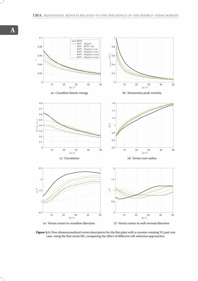
A
130 A. ADDITIONAL RESULTS RELATED TO THE INFLUENCE OF THE SOURCE-TERM DOMAIN
10 20 30 40 50
∆x/h
0
0.02
0.04
0.06
0.08
0.1
κ
BFM
BAY - Aligned
BAY - jBAY cells
BAY - Original 1 row
BAY - Original 2 rows
BAY - Original 3 rows
BAY - Original 4 rows
(a) Crossflow kinetic energy
10 20 30 40 50
∆x/h
0
0.2
0.4
0.6
0.8
1
ωx,m
ax·h/U∞
(b) Streamwise peak vorticity
10 20 30 40 50
∆x/h
0
0.1
0.2
0.3
0.4
0.5
0.6
0.7
0.8
|Γ|/(h
·U∞)
(c) Circulation
10 20 30 40 50
∆x/h
0.4
0.6
0.8
1
1.2
1.4
1.6
R/h
(d) Vortex core radius
10 20 30 40 50
∆x/h
0.5
1
1.5
2
2.5
y c/h
(e) Vortex center in crossflow direction
10 20 30 40 50
∆x/h
0
0.5
1
1.5
2
z c/h
(f) Vortex center in wall-normal direction
Figure A.1: Non-dimensionalized vortex descriptors for the flat plate with a counter-rotating VG pair testcase, using the fine mesh M2, comparing the effect of different cell-selection approaches.
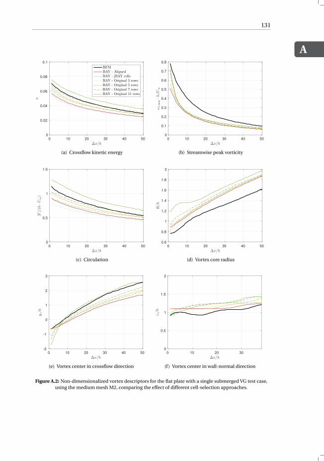
A
131
0 10 20 30 40 50
∆x/h
0
0.02
0.04
0.06
0.08
0.1
κ
BFM
BAY - Aligned
BAY - jBAY cells
BAY - Original 3 rows
BAY - Original 5 rows
BAY - Original 7 rows
BAY - Original 11 rows
(a) Crossflow kinetic energy
0 10 20 30 40 50
∆x/h
0
0.1
0.2
0.3
0.4
0.5
0.6
0.7
0.8
ωx,m
ax·h/U∞
(b) Streamwise peak vorticity
0 10 20 30 40 50
∆x/h
0
0.5
1
1.5
|Γ|/(h
·U∞)
(c) Circulation
0 10 20 30 40 50
∆x/h
0.6
0.8
1
1.2
1.4
1.6
1.8
2
R/h
(d) Vortex core radius
0 10 20 30 40 50
∆x/h
-2
-1
0
1
2
3
y c/h
(e) Vortex center in crossflow direction
0 10 20 30
∆x/h
0
0.5
1
1.5
2
z c/h
(f) Vortex center in wall-normal direction
Figure A.2: Non-dimensionalized vortex descriptors for the flat plate with a single submerged VG test case,using the medium mesh M2, comparing the effect of different cell-selection approaches.
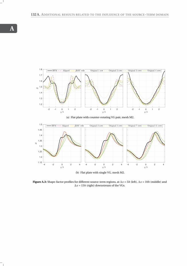
A
132 A. ADDITIONAL RESULTS RELATED TO THE INFLUENCE OF THE SOURCE-TERM DOMAIN
-2 -1 0 1 2
y/h
1.2
1.3
1.4
1.5
1.6
1.7
1.8
H
-2 -1 0 1 2
y/h-2 -1 0 1 2
y/h
BFM Aligned jBAY cells Original 1 row Original 2 rows Original 3 rows Original 4 rows
(a) Flat plate with counter-rotating VG pair, mesh M2.
-4 -2 0 2 4
y/h
1.15
1.2
1.25
1.3
1.35
1.4
1.45
1.5
H
-4 -2 0 2 4
y/h-4 -2 0 2 4
y/h
BFM Aligned jBAY cells Original 3 rows Original 5 rows Original 7 rows Original 11 rows
(b) Flat plate with single VG, mesh M2.
Figure A.3: Shape-factor profiles for different source-term regions, at ∆x = 5h (left), ∆x = 10h (middle) and∆x = 15h (right) downstream of the VGs.
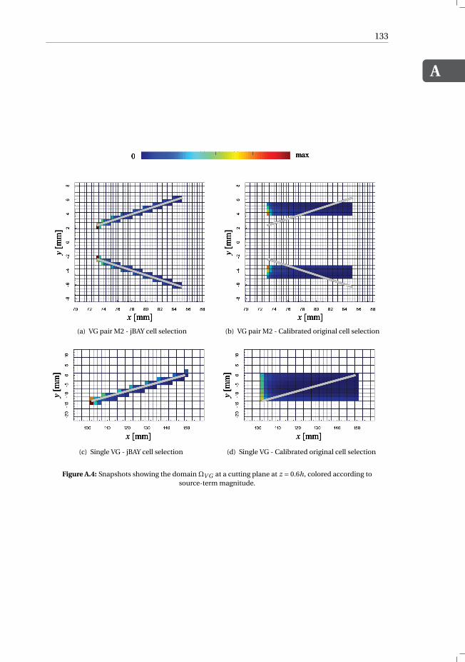
A
133
(a) VG pair M2 - jBAY cell selection (b) VG pair M2 - Calibrated original cell selection
(c) Single VG - jBAY cell selection (d) Single VG - Calibrated original cell selection
Figure A.4: Snapshots showing the domain ΩV G at a cutting plane at z = 0.6h, colored according tosource-term magnitude.

REFERENCES
[1] B. G. Allan, C.-s. Yao, and J. C. Lin. Numerical Simulations of Vortex GeneratorVanes and Jets on a Flat Plate. (June):1–14, 2002.
[2] M. Amitay, D. R. Smith, V. Kibens, D. E. Parekh, and A. Glezer. Aerodynamic FlowControl over an Unconventional Airfoil Using Synthetic Jet Actuators. AIAA J.,39(3):361–370, mar 2001.
[3] J. D. Anderson. A History of Aerodynamics. Cambridge University Press, 1 edition,1997.
[4] J. D. Anderson. Fundamentals of Aerodynamics. McGraw-Hill Education, 4 edition,2006.
[5] K. P. Angele and B. Muhammad-Klingmann. The effect of streamwise vortices onthe turbulence structure of a separating boundary layer. Eur. J. Mech. B/Fluids,24(5):539–554, 2005.
[6] P. Ashill, J. Fulker, and K. Hackett. Research at DERA on Sub Boundary Layer VortexGenerators (SBVGs). Technical Report January, 2001.
[7] P. Ashill, J. L. Fulker, and K. C. Hackett. Studies of flows induced by Sub Boundarylayer Vortex Generators ( SBVGs ). 40th AIAA Aerosp. Sci. Meet. Exhib., (January):13,2002.
[8] D. Baldacchino, M. Manolesos, C. Simao Ferreira, Á. González Salcedo, M. Apari-cio, T. Chaviaropoulos, K. Diakakis, L. Florentie, N. R. García, G. Papadakis, N. N.Sørensen, N. Timmer, N. Troldborg, S. G. Voutsinas, and A. H. van Zuijlen. Exper-imental benchmark and code validation for airfoils equipped with passive vortexgenerators. J. Phys. Conf. Ser., 753:022002, sep 2016.
[9] D. Baldacchino, D. Ragni, C. Simao Ferreira, and G. van Bussel. Towards integralboundary layer modelling of vane-type vortex generators. In 45th AIAA Fluid Dyn.Conf., Reston, Virginia, jun 2015. American Institute of Aeronautics and Astronau-tics.
[10] G. Batchelor. Batchelor, G. K. 1964 Axial flow in trailing line vortices. J. Fluid Mech.20, 645658. J. Fluid Mech.1, 20:645–658, 1964.
[11] E. E. Bender, B. H. Anderson, and P. J. Yagle. Vortex Generator Modeling for Navier-Stokes Codes. In 3rd Jt. ASME/JSME Fluids Eng. Conf., pages 1–7, San Francisco,CA, 1999.
[12] M. J. Bhagwat and J. G. Leishman. Generalized viscous vortex model for applica-tion to free-vortex wake and aeroacoustic calculations. Annu. forum proceedings-American helicopter Soc., 58(2):2042–2057, 2002.
[13] T. P. Bray. A parametric study of vane and air-jet vortex generators. Engineeringdoctorate (engd), Cranfield University, 1998.
135
136 REFERENCES
[14] V. Brunet, C. Francois, E. Garnier, and M. Pruvost. Experimental and NumericalInvestigations of Vortex Generators Effects. In 3rd AIAA Flow Control Conf., num-ber June, pages 1–12, Reston, Virigina, jun 2006. American Institute of Aeronauticsand Astronautics.
[15] C. Burg and T. Erwin. Application of Richardson extrapolation to the numeri-cal solution of partial differential equations. Numer. Methods Partial Differ. Equ.,25(4):810–832, jul 2009.
[16] A. Celic and E. H. Hirschel. Comparison of Eddy-Viscosity Turbulence Models inFlows with Adverse Pressure Gradient. AIAA J., 44(10):2156–2169, 2006.
[17] T. Craft, B. Launder, and K. Suga. Development and application of a cubic eddy-viscosity model of turbulence. Int. J. Heat Fluid Flow, 17(2):108–115, apr 1996.
[18] A. Cutler and P. Bradshaw. Strong vortex/boundary layer interactions - Part I: Vor-tices High. Exp. Fluids, 14(5):321–332, apr 1993.
[19] A. Cutler and P. Bradshaw. Strong vortex/boundary layer interactions - Part II: Vor-tices Low. Exp. Fluids, 14(6):393–401, may 1993.
[20] J. C. Dudek. An Empirical Model for Vane-Type Vortex Generators in a Navier-Stokes Code. pages 1–24, 2005.
[21] J. C. Dudek. Modeling Vortex Generators in a Navier-Stokes Code. AIAA J.,49(4):748–759, 2011.
[22] P. Durbin. Near-wall turbulence closure modeling without damping functions.Theor. Comput. Fluid Dyn., 3(1):1–13, 1991.
[23] R. P. Dwight and J. Brezillon. Effect of Approximations of the Discrete Adjoint onGradient-Based Optimization. AIAA J., 44(12):3022–3031, 2006.
[24] U. Fernandez, C. M. Velte, P.-E. Réthoré, and N. N. Sørensen. Self-similarity andhelical symmetry in vortex generator flow simulations. Proc. Torque 2012, Sci. Mak.torque from Wind, 2012.
[25] C. Ferreira, A. Gonzalez, D. Baldacchino, M. Aparicio, S. Gomez-Iradi, X. Mund-uate, A. Barlas, N. Garcia, N. N. Sorensen, N. Troldborg, G. N. Barakos, E. Jost,S. Knecht, T. Lutz, P. Chassapoyiannis, K. Diakakis, M. Manolesos, S. G. Voutsinas,J. Prospathopoulos, T. Gillebaart, L. Florentie, A. H. van Zuijlen, and M. Reijerk-erk. AVATAR Task 3.2 : Development of aerodynamic codes for modelling of flowdevices on aerofoils and rotors. Technical Report November, AVATAR project, FP7-ENERGY-2013-1/ n 608396, 2015.
[26] L. Florentie, A. H. van Zuijlen, S. J. Hulshoff, and H. Bijl. Effectiveness of SideForce Models for Flow Simulations Downstream of Vortex Generators. AIAA J.,55(4):1373–1384, apr 2017.
[27] M. Gad-el Hak. Flow Control: Passive, Active, and Reactive Flow Management.Cambridge University Press, 2000.
[28] T. B. Gatski and T. Jongen. Nonlinear eddy viscosity and algebraic stress modelsfor solving complex turbulent flows. Prog. Aerosp. Sci., 36(8):655–682, 2000.
REFERENCES 137
[29] S. Ghosh, J.-I. Choi, and J. R. Edwards. Numerical Simulations of Effects of Mi-cro Vortex Generators Using Immersed-Boundary Methods. AIAA J., 48(1):92–103,2010.
[30] T. Gillen, M. Rybalko, and E. Loth. Vortex Generators for Diffuser of AxisymmetricSupersonic Inlets. In 5th Flow Control Conf., pages 1–18, Chicago, Illionois, jul2010. American Institute of Aeronautics and Astronautics.
[31] G. Godard and M. Stanislas. Control of a decelerating boundary layer. Part 1: Op-timization of passive vortex generators. Aerosp. Sci. Technol., 10(3):181–191, apr2006.
[32] D. A. Griffin. Investigation of Vortex Generators for Augmentation of Wind TurbinePower Performance. Technical Report NREL/SR-440-21399, National RenewableEnergy Laboratory, 1996.
[33] M. Hansen, C. M. Velte, S. Øye, R. Hansen, N. N. Sørensen, J. Madsen, andR. Mikkelsen. Aerodynamically shaped vortex generators. Wind Energy, 17(April2013):n/a–n/a, mar 2015.
[34] M. O. Hansen and C. Westergaard. Phenomenological Model of Vortex Genera-tors. In B. Maribo Pedersen, editor, 9th Int. Energy Agency Symp. Aerodyn. WindTurbines, pages 1–7, 1995.
[35] J. K. Harvey and F. J. Perry. Flowfield produced by trailing vortices in the vicinity ofthe ground. AIAA J., 9(8):1659–1660, aug 1971.
[36] J. Hoffman. Adaptive simulation of the subcritical flow past a sphere. J. FluidMech., 568:77, 2006.
[37] D. D. Holm. Taylor’s Hypothesis , Hamilton’s Principle , and the LANS-a Model forComputing Turbulence. Los Alamos Sci., (29):172–180, 2005.
[38] K. Ito and K. Kunisch. Lagrange Multiplier Approach to Variational Problems andApplications. Society for Industrial and Applied Mathematics, jan 2008.
[39] H. Jasak. Error analysis and estimation for the finite volume method with applica-tions to fluid flows. Ph.d. thesis, Imperial College, London, 1996.
[40] J. Jeong and F. Hussain. On the identification of a vortex. J. Fluid Mech., 285(-1):69,feb 1995.
[41] A. Jirasek. Vortex-Generator Model and Its Application to Flow Control. J. Aircr.,42(6):1486–1491, 2005.
[42] J. Johansen, N. N. Sørensen, F. Zahle, S. Kang, I. Nikolaou, E. Politis,P. Chaviaropoulos, and J. Ekaterinaris. KNOW-BLADE Task-2 report ; AerodynamicAccessories. Technical Report October, Risø-R-1482(EN), 2004.
[43] John D Anderson. Ludwig Prandtl ’ s Boundary Layer. Phys. Today, (December):7,2005.
[44] R. W. Johnson. The Handbook of Fluid Dynamics. Crc. Pr. Inc., 1998.
[45] J. Jones. The calculation of the paths of vortices from a system of vortex genera-tors and a comparison with experiment. Technical report, Aeronautical ResearchCouncil, 1957.
138 REFERENCES
[46] W. Jones and B. Launder. The prediction of laminarization with a two-equationmodel of turbulence. Int. J. Heat Mass Transf., 15(2):301–314, feb 1972.
[47] G. Joubert, A. Le Pape, and S. Huberson. Numerical study of flow separation con-trol over a OA209 Airfoil using Deployable Vortex Generator. 49th AIAA Aerosp. Sci.Meet. Incl. New Horizons Forum Aerosp. Expo., (January):1–20, 2011.
[48] M. Kerho and B. Kramer. Enhanced Airfoil Design Incorporating Boundary-LayerMixing Devices. In 41st Aerosp. Sci. Meet. Exhib., Reston, Virigina, jan 2003. Amer-ican Institute of Aeronautics and Astronautics.
[49] W. G. Kunik. Application of a computational model for vortex generators in sub-sonic internal flows. AIAA/ASME/SAE/ASEE 22nd Jt. Propuls. Conf., pages 0–6, 1986.
[50] H. Lamb. Hydrodynamics. Cambridge University Press, Cambridg, 6th ed. edition,1932.
[51] B. Launder, G. Reece, and W. Rodi. Progress in the Development of a Reynolds-Stress Turbulent Closure. J. Fluid Mech., 68(3):537–566, 1975.
[52] B. Launder and B. Sharma. Application of the energy-dissipation model of tur-bulence to the calculation of flow near a spinning disc. Lett. Heat Mass Transf.,1(2):131–137, nov 1974.
[53] M. Leschziner. Statistical Turbulence Modelling for Fluid Dynamics - Demystified.Imperial College Press, 2016.
[54] J. Liandrat, B. Aupoix, and J. Cousteix. Calculation of Longitudinal Vortices Imbed-ded in a Turbulent Boundary Layer. In Turbul. Shear Flows 5, pages 253–265.Springer Berlin Heidelberg, Berlin, Heidelberg, 1987.
[55] J. Lin, F. Howard, D. Bushnell, and G. Selby. Investigation of several passive andactive methods for turbulent flow separation control. In 21st Fluid Dyn. PlasmaDyn. Lasers Conf., Reston, Virigina, jun 1990. American Institute of Aeronauticsand Astronautics.
[56] J. C. Lin. Review of research on low-profile vortex generators to control boundary-layer separation. Prog. Aerosp. Sci., 38(4-5):389–420, 2002.
[57] J. C. Lin, S. K. Robinson, R. J. McGhee, and W. O. Valarezo. Separation control onhigh-lift airfoils via micro-vortex generators. J. Aircr., 31(6):1317–1323, nov 1994.
[58] J. Liu, U. Piomelli, and P. R. Spalart. Interaction between a spatially growing turbu-lent boundary layer and embedded streamwise vortices. J. Fluid Mech., 326:151,nov 1996.
[59] O. Lögdberg, J. H. M. Fransson, and P. H. Alfredsson. Streamwise evolution of lon-gitudinal vortices in a turbulent boundary layer. J. Fluid Mech., 623:27, 2009.
[60] L. Maestrello and L. Ting. Analysis of active control by surface heating. AIAA J.,23(7):1038–1045, jul 1985.
[61] M. Manolesos, G. Papadakis, and S. G. Voutsinas. Assessment of the CFD capa-bilities to predict aerodynamic flows in presence of VG arrays. J. Phys. Conf. Ser.,524:012029, 2014.
REFERENCES 139
[62] M. Manolesos and S. G. Voutsinas. Experimental investigation of the flow past pas-sive vortex generators on an airfoil experiencing three-dimensional separation. J.Wind Eng. Ind. Aerodyn., 142:130–148, 2015.
[63] N. May. A new vortex generator model for use in complex configuration CFDsolvers. In 19th AIAA Appl. Aerodyn. Conf., Reston, Virigina, jun 2001. AmericanInstitute of Aeronautics and Astronautics.
[64] F. R. Menter. Zonal Two Equation k-w Turbulence Models for Aerodynamic Flows.In 24th Fluid Dyn. Conf., Orlando, Florida, 1993.
[65] R. Mittal and G. Iaccarino. Immersed Boundary Methods. Annu. Rev. Fluid Mech.,37(1):239–261, jan 2005.
[66] D. J. Moreau and C. J. Doolan. Noise-Reduction Mechanism of a Flat-Plate SerratedTrailing Edge. AIAA J., 51(10):2513–2522, 2013.
[67] A. S. Moreira Ribeiro. Implementation and Analysis of an Empirical Vortex Gener-ator Model in OpenFOAM. M.sc. thesis, Delft University of Technology, 2017.
[68] A. Nemili and E. Ozkaya. Optimal Control of Unsteady Flows Using Discrete Ad-joints. (June):1–14, 2011.
[69] G. Neretti. Active Flow Control by Using Plasma Actuators. In R. K. Agerwal, editor,Recent Prog. Some Aircr. Technol. InTech, sep 2016.
[70] I. G. Nikolaou, E. S. Politis, and P. K. Chaviaropoulos. Modelling the FlowAround Airfoils Equipped with Vortex Generators Using a Modified 2D Navier-Stokes Solver. J. Sol. Energy Eng., 127(2):223, 2005.
[71] C. Nita, S. Vandewalle, and J. Meyers. On the efficiency of gradient based opti-mization algorithms for DNS-based optimal control in a turbulent channel flow.Comput. Fluids, 125:11–24, 2016.
[72] B. R. Noack, M. Morzynski, and G. Tadmor, editors. Reduced-Order Modelling forFlow Control, volume 528 of CISM International Centre for Mechanical Sciences.Springer Vienna, Vienna, 2011.
[73] J. Nocedal and S. J. Wright. Numerical Optimization. 2 edition, 2006.
[74] C. Oseen. Uber Wirbelbewegung in Einer Reiben- den Flussigkeit. Ark. J. Mat.Astrom. Fys., 7:14–21, 1912.
[75] C. Othmer. A continuous adjoint formulation for the computation of topologicaland surface sensitivities of ducted flows. Int. J. Numer. Methods Fluids, 58(8):861–877, nov 2008.
[76] S. Patankar. The SIMPLE Algorithm. In Numer. heat Transf. fluid flow, chapter 6,pages 126–131. Hemisphere Publishing Corporation, 1980.
[77] W. R. Pauley and J. K. Eaton. Experimental study of the development of longitudi-nal vortex pairs embedded in a turbulent boundary layer. AIAA J., 26(7):816–823,jul 1988.
[78] H. Pearcey. Introduction To Shock-Induced Separation and Its Prevention By Designand Boundary Layer Control. PERGAMON PRESS LTD, 1961.
140 REFERENCES
[79] D. Poole, R. Bevan, C. Allen, and T. Rendall. An Aerodynamic Model for Vane-TypeVortex Generators. 34th AIAA Appl. Aerodyn. Conf., (June):1–18, 2016.
[80] S. B. Pope. Turbulent Flows. Cambridge University Press, 2000.
[81] L. Prandtl. Über Flüssigkeitsbewegung bei sehr kleiner Reibung. In Verhandlungendes III Int. Math. Heidelberg, 1904, pages 484–491, 1905.
[82] W. Rankine. Manual of Applied Mechanics. C. Griffen Co., London, 1858.
[83] D. Rao and T. Kariya. Boundary-layer submerged vortex generators for separationcontrol - An exploratory study. In 1st Natl. Fluid Dyn. Conf., volume 3546, page1988, Reston, Virigina, jul 1988. American Institute of Aeronautics and Astronau-tics.
[84] W. Rodi. A new algebraic relation for calculating the Reynolds stresses. GesellschaftAngew. Math. und Mech. Work. Paris Fr., 56, 1976.
[85] C. Roy. Review of Discretization Error Estimators in Scientific Computing. In 48thAIAA Aerosp. Sci. Meet. Incl. New Horizons Forum Aerosp. Expo., Reston, Virigina,jan 2010. American Institute of Aeronautics and Astronautics.
[86] G. Schubauer and W. Spangenberg. Forced mixing in boundary layers. J. FluidMech., 8:10–32, 1960.
[87] V. Schulz and I. Gherman. One-Shot Methods for Aerodynamic Shape Optimiza-tion. In Notes Numer. Fluid Mech. Multidiscip. Des., pages 207–220. Springer,Berlin, Heidelberg, 2009.
[88] I. M. M. A. Shabaka, R. D. Mehta, and P. Bradshaw. Longitudinal vortices imbeddedin turbulent boundary layers. Part 1. Single vortex. J. Fluid Mech., 155(-1):37, jun1985.
[89] H. Shan, L. Jiang, C. Liu, M. Love, and B. Maines. Numerical study of passive andactive flow separation control over a NACA0012 airfoil. Comput. Fluids, 37(8):975–992, 2008.
[90] P. E. Smirnov and F. R. Menter. Sensitization of the SST Turbulence Model to Rota-tion and Curvature by Applying the SpalartShur Correction Term. J. Turbomach.,131(4):041010, 2009.
[91] F. T. Smith. Theoretical prediction and design for vortex generators in turbulentboundary layers. J. Fluid Mech., 270:91, 1994.
[92] P. Spalart and S. Allmaras. A one-equation turbulence model for aerodynamicflows. In 30th Aerosp. Sci. Meet. Exhib., Reston, Virigina, jan 1992. American In-stitute of Aeronautics and Astronautics.
[93] P. Spalart and M. Shur. On the sensitization of turbulence models to rotation andcurvature. Aerosp. Sci. Technol., 1(5):297–302, jul 1997.
[94] P. Spalart, M. L. Shur, M. K. Strelets, and A. K. Travin. Direct Simulation and RANSModelling of a Vortex Generator Flow. Flow, Turbul. Combust., 95(2-3):335–350,2015.
[95] C. G. Speziale. On nonlinear K-l and K -ϵ models of turbulence. J. Fluid Mech.,178(1):459, may 1987.
REFERENCES 141
[96] C. G. Speziale, S. Sarkar, and T. B. Gatski. Modelling the pressurestrain correlationof turbulence: an invariant dynamical systems approach. J. Fluid Mech., 227:245–272, jun 1991.
[97] H. Squire. The Growth of a Vortex in Turbulent Flow. Aeronaut. Q., 16(3):302–306,1965.
[98] D. N. Srinath and S. Mittal. An adjoint method for shape optimization in unsteadyviscous flows. J. Comput. Phys., 229(6):1994–2008, 2010.
[99] T. Steihaug. The Conjugate Gradient Method and Trust Regions in Large ScaleOptimization. SIAM J. Numer. Anal., 20(3):626–637, jun 1983.
[100] F. V. Stillfried. Computational fluid-dynamics investigations of vortex generatorsfor flow-separation control. PhD thesis, Royal Institute of Technology, Stockholm,2012.
[101] F. V. Stillfried, S. Wallin, and A. V. Johansson. An improved passive vortex generatormodel for flow separation control. 5th Flow Control Conf., (July):1–14, 2010.
[102] H. Taylor. Application of Vortex Generator Mixing Principles to Diffusers. Techni-cal report, United Aircraft Corporation, East Hartford, Connecticut, 1948.
[103] O. Törnblom and A. V. Johansson. A Reynolds stress closure description of sepa-ration control with vortex generators in a plane asymmetric diffuser. Phys. Fluids,19(11), 2007.
[104] N. Troldborg, F. Zahle, and N. N. Sørensen. Simulation of a MW rotor equippedwith vortex generators using CFD and an actuator shape model. 53rd AIAA Aerosp.Sci. Meet., (January):1–10, 2015.
[105] C. P. van Dam, B. J. Holmes, and C. Pitts. Effect of Winglets on Performance andHandling Qualities of General Aviation Aircraft. J. Aircr., 18(7):587–591, jul 1981.
[106] C. Velte, M. Hansen, and D. Cavar. Flow analysis of vortex generators on wingsections by stereoscopic particle image velocimetry measurements. Environ. Res.Lett., 3:015006, 2008.
[107] C. M. Velte, C. Braud, S. Coudert, and J.-m. Foucaut. Vortex Generator InducedFlow in a High Re Boundary Layer. Sci. Mak. Torque from Wind 2012, (Umr 8107),2012.
[108] C. M. Velte, M. O. Hansen, and V. L. Okulov. Helical structure of longitudinal vor-tices embedded in turbulent wall-bounded flow. J. Fluid Mech., 619:167, 2009.
[109] C. M. Velte, V. L. Okulov, and I. V. Naumov. Regimes of flow past a vortex generator.Tech. Phys. Lett., 38(4):379–382, 2012.
[110] F. von Stillfried, S. Wallin, and A. V. Johansson. Vortex-Generator Models for Zero-and Adverse-Pressure-Gradient Flows. AIAA J., 50(4):855–866, 2012.
[111] K. Waithe. Source Term Model for Vortex Generator Vanes in a Navier-Stokes Com-puter Code. In 42nd AIAA Aerosp. Sci. Meet. Exhib., pages 1–11, Reston, Virigina,jan 2004. American Institute of Aeronautics and Astronautics.
[112] F. Wallin and L.-E. Eriksson. A Tuning-free Body-Force Vortex Generator Model. In
142 REFERENCES
44th AIAA Aerosp. Sci. Meet. Exhib., pages 1–12, Reston, Virigina, jan 2006. Ameri-can Institute of Aeronautics and Astronautics.
[113] B. J. Wendt. The Modelling of Symmetric Vortex Generators Airfoil Vortex Genera-tors. Aerosp. Sci. Meet. Exhib. 34th, Reno, NV, pages 15–18, 1996.
[114] B. J. Wendt. Initial Circulation and Peak Vorticity Behavior of Vortices Shed fromAirfoil Vortex Generators. Technical Report August, NASA, 2001.
[115] B. J. Wendt. Parametric Study of Vortices Shed from Airfoil Vortex Generators. AIAAJ., 42(11):2185–2195, nov 2004.
[116] R. V. Westphal, W. R. Pauley, and J. K. Eaton. Interaction between a vortex and aturbulent boundary layer. Part 1: Mean flow evolution and turbulence properties.(January), 1987.
[117] E. Wik and S. Shaw. Numerical Simulation of Micro Vortex Generators. In 2nd AIAAFlow Control Conf., Reston, Virigina, jun 2004. American Institute of Aeronauticsand Astronautics.
[118] D. C. Wilcox. Reassessment of the scale-determining equation for advanced tur-bulence models. AIAA J., 26(11):1299–1310, nov 1988.
[119] C. Yao, J. Lin, and B. Allan. Flow-field measurement of device-induced embeddedstreamwise vortex on a flat plate. In NASA STI/Recon Tech. Rep. . . . , number June,page 16, 2002.
[120] D. You, M. Wang, R. Mittal, and P. Moin. Large-Eddy Simulations of Longitudi-nal Vortices Embedded in a Turbulent Boundary Layer. AIAA J., 44(12):3032–3039,2006.
[121] A. S. Zymaris, D. I. Papadimitriou, K. C. Giannakoglou, and C. Othmer. Continu-ous adjoint approach to the Spalart-Allmaras turbulence model for incompress-ible flows. Comput. Fluids, 38(8):1528–1538, 2009.

ACKNOWLEDGEMENTS
Almost 5 years after getting excited to start my Ph.D. research, it is now time to get ex-cited about finishing it and starting a new adventure. Looking back on those years, I canhonestly say that what people have been telling me is true: it was definitely a path withmany ups and downs, but also, I never regretted starting it! All along my way I foundpeople supporting and encouraging me. So now that I am writing these last words of thisbook, feeling proud of my work and already forgetting the challenges and frustrationsalong the way, I would like to express my gratitude to all of you.
To my supervisors from the start, Hester Bijl and Alexander van Zuijlen, thank you forbelieving in me and for giving me the opportunity to perform this research entirely to myown ideas. Hester, your contagious enthusiasm and optimism have been heartwarming,and Sander, thank you for being there to help me whenever I asked.
Finishing this Ph.D. would not have been possible without the help of my copromo-tor. Steve, even before being an official member of the team you managed to steer meinto the right direction by some casual, yet straight to the point, comments. With justone question during the department’s presentation days you fueled my inspiration foralmost half my research. And you did the same a year later for the other half. I am ex-tremely grateful that you believed in me and that you took on the role as my copromotorat a time when I felt I was stuck. Your eye for detail has been key to raising the quality ofmy work. Thank you for your kindness and for our inspiring and motivating discussions!
I also want to thank Daniel Baldacchino and Carlos Simao Ferreira for our pleasantcollaboration on the AVATAR project. Daniel, thank you also a lot for sharing your exper-imental data with me, they have been of great value to this work.
Over the past years I have had the pleasure of sharing an office with a large group ofgreat fellow Ph.D. students. Thijs, Rogier, Wouter, David, Iliass, Koen, Jan, Paul, Jacopo,Mirja, Theo, Giuseppe, Rakesh, Shaafi, and many others, thank you for the good timesduring lunch, breaks and at conferences! Moreover, I am very grateful to Thijs for helpingme find my way in the OpenFOAM maze. And of course I cannot forget Colette, whosolves any problem related to vague procedures before you can even ask, thank you!
Another group of colleagues that cannot go unmentioned are the people of our fac-ulty’s student and education department. I am very grateful that I had the opportunityto work with you aside of my Ph.D. project. Thank you for the great atmosphere and foryour honest interest and support! Especially Sander, thank you for always being therefor me, I owe you a lot! These last two years you have been a constant source of supportand tranquility, calming me down when I was stressed but also putting me to work whenI was pushing forward work on my dissertation. You have been a great colleague andfriend. I will miss working with you, but let’s hope that moving away from Delft does notmean having to miss our chats.
And as 4 heroes once sang, I get by with a little help from my friends. Indeed, whatwould I be without the love and support from my friends and family? Rui, Eveline,
143

144 ACKNOWLEDGEMENTS
Inge, Nanda, Emma, the Stomwijzer, Victor, thank you for the good times, the chats, thedrinks, the laughs. We should definitely increase their frequency! Vake, moeke, groot-moe, grootva, Pieter, Ellen, Pär, it is heartwarming to have such a loving and caring fam-ily like you! I will always be there for you, just as I know that you are for me.
Finally, to Mirko, my perfect boyfriend, thank you for bringing an endless stream ofhappiness to my life! I am who I am because of you. You inspire me to be ambitious andto chase my dreams, while at the same time making our home a relaxed place where Ican always refuel. Everything feels easier and better with you at my side. Finishing thisdissertation is a milestone which I would never have been able to achieve without yourlove, help and support. I love you and I look forward to the following adventures we willembark on together!
LIST OF PUBLICATIONS
• L. Florentie, S.J. Hulshoff, and A.H. van Zuijlen. Adjoint-Based Optimization ofa Source-Term Representation of Vortex Generators. Computers and Fluids, 162:139-151, 2018.
• L. Florentie, A.H. van Zuijlen, S.J. Hulshoff, and H. Bijl. Effectiveness of Side ForceModels for Flow Simulations Downstream of Vortex Generators. AIAA Journal, 55(4):1373-1384, 2017.
• M. Manolesos, N.N. Sørensen, N. Troldberg, L. Florentie, G. Papadakis, and S.G.Voutsinas. Computing the flow past Vortex Generators: Comparison between RANSSimulations and Experiments. Journal of Physics: Conference Series, 753: 022014,2016.
• D. Baldacchino, M. Manolesos, C.J. Simão Ferreira, A. González Salcedo, M. Apari-cio, T. Chaviaropoulos, K. Diakakis, L. Florentie, N.R. García, G. Papadakis, N.N.Sørensen, N. Timmer, N. Troldborg, S.G. Voutsinas, and A.H. van Zuijlen. Exper-imental benchmark and code validation for airfoils equipped with passive vortexgenerators. Journal of Physics: Conference Series, 753: 022002, 2016.
• L. Florentie, D.S. Blom, T.P. Scholcz, A.H. van Zuijlen, and H. Bijl. Analysis ofSpace Mapping Algorithms for Application to Partitioned Fluid-Structure Interac-tion Problems. International Journal for Numerical Methods in Engineering, 105(2):138-160, 2016.
• L. Florentie, A.H. van Zuijlen, and H. Bijl. Towards a multi-fidelity approach forCFD simulations of vortex generator arrays. 11th World Congress on Computa-tional Mechanics, WCCM 2014, 5th European Conference on Computational Me-chanics, ECCM 2014 and 6th European Conference on Computational Fluid Dy-namics, ECFD 2014, 7187-7198, 2014.
145

CURRICULUM VITÆ
Liesbeth Florentie was born on August 30, 1988 in Bonheiden, Belgium. Her entire child-hood she lived in Haacht, where she attended the Don Bosco secondary school from2000 to 2006.
Following her passion for mathematics and space exploration, Liesbeth moved toDelft to study Aerospace Engineering at Delft University of Technology in September2006. She obtained her Bachelor of Science degree cum laude in 2009. By that time Lies-beth had become intrigued by the beautiful complexity of fluid dynamics, motivating herto combine a master programme in aerodynamics with an honours programme in math-ematics. After a research internship at Cardiff Univerisity, Liesbeth completed her Mas-ter of Science in Aerospace Engineering at Delft University of Technology in 2012, cumlaude, with a thesis on multi-fidelity coupling algorithms for fluid-structure-interactionsimulations.
After graduation, Liesbeth spent one year working as an engineering consultant forDynaflow Research Group. She returned to Delft University of Technology in 2013 to starther Ph.D. research on simulation methods for vortex-generator effects in wall-boundedflows. She performed this research as part of the European project AVATAR, which had asgoal the investigation of simulation methods for application to a next generation of largewind turbines. From 2016 on, Liesbeth combined her Ph.D. research with a part-timejob at the faculty’s student and education office where she worked on getting a selectionprocedure for incoming bachelor students on track.
With the completion of this dissertation comes an end to Liesbeth’s time in Delft. InApril 2018 Liesbeth will start as a researcher at Wageningen University, hoping to con-tribute to a better understanding of (human-produced) greenhouse-gas flows in the at-mosphere.
147
Related Documents