ASPECTS OF INFLATION IN STRING THEORY Daniel Baumann A Dissertation Presented to the Faculty of Princeton University in Candidacy for the Degree of Doctor of Philosophy Recommended for Acceptance by the Department of Physics Advisor: Paul Steinhardt June 2008

Welcome message from author
This document is posted to help you gain knowledge. Please leave a comment to let me know what you think about it! Share it to your friends and learn new things together.
Transcript

ASPECTS OF INFLATION IN STRING THEORY
Daniel Baumann
A Dissertation
Presented to the Faculty
of Princeton University
in Candidacy for the Degree
of Doctor of Philosophy
Recommended for Acceptance
by the Department of Physics
Advisor: Paul Steinhardt
June 2008

c© Copyright by Daniel Baumann, 2008. All rights reserved.

Abstract. In this thesis we make small steps towards the ambitious
goal of a microphysical understanding of the inflationary era in the early
universe. We identify three key questions that require a proper under-
standing of the ultraviolet limit of the theory: i) the delicate flatness
of the inflaton potential, ii) the possibility of observable gravitational
waves and iii) a large non-Gaussianity of the primordial density fluctu-
ations. We study these fundamental aspects of inflation in the context
of string theory.
V (φ): In the first half of the thesis, we give the first fully explicit
derivation of the potential for warped D-brane inflation. The analy-
sis exposes the eta-problem, relates effective parameters in the inflaton
Lagrangian to microscopic string theory input, and illustrates impor-
tant correlations between the parameters of the potential. We show
that compactification constraints significantly limit the possibility of
obtaining inflationary solutions in these scenarios.
r: All inflationary models that predict an observable gravitational
wave signal require that the inflaton field evolves over a super-Planckian
range. In the second half of the thesis, we derive a microscopic bound
on the maximal inflaton field variation for D-brane models. The bound
arises from the compact nature of the extra dimensions and puts a
strong upper limit on the gravitational wave signal.
fNL: Finally, we explain that our limit on the field range also
significantly constrains the parameter space of Dirac-Born-Infeld infla-
tion. In this case the bound strongly restricts the possibility of a large
non-Gaussianity in the primordial fluctuations.
iii

For Anna/Mama
iv

Contents
Acknowledgments viii
Chapter 1. Introduction 2
1. Prelude 2
2. From String Compactification to the Low Energy Lagrangian 3
3. Compactification Effects in D-brane Inflation 5
4. String Theory and Primordial Gravitational Waves 7
5. Outline of the Thesis 8
Part 1. Review of String Cosmology 12
Chapter 2. Aspects of Modern Cosmology 14
1. A Brief History of the Universe 15
2. Status of Observational Cosmology 22
3. Dark Energy 32
4. Inflation 34
Chapter 3. Elements of String Compactifications 46
1. The Moduli-Stabilization Problem 46
2. Flux Compactification 47
3. De Sitter Vacua in String Theory 49
4. Klebanov-Strassler Geometry 51
Chapter 4. Inflation in String Theory 54
1. UV Challenges/Opportunities 55
2. Warped D-brane Inflation 57
3. Models of String Inflation 63
4. Inflation from Explicit String Compactifications 68
Part 2. The Inflaton Potential 70
Chapter 5. On D3-brane Potentials in Compact Spaces 71
1. Introduction 71
2. D3-branes and Volume Stabilization 75
3. Warped Volumes and the Superpotential 79
4. D3-brane Backreaction 82
v

5. Backreaction in Warped Conifold Geometries 86
6. Compactification Effects 93
7. Implications and Conclusion 99
Chapter 6. Compactification Obstacles to D-brane Inflation 102
1. Introduction 102
2. The Compactification 104
3. Towards Fine-Tuned Inflation 105
4. Microscopic Constraints 109
5. Conclusions 109
Chapter 7. Towards an Explicit Model of D-brane Inflation 111
1. Introduction 111
2. D3-brane Potential in Warped Backgrounds 116
3. Case Study: Kuperstein Embedding 123
4. Search for an Inflationary Trajectory 129
5. Comments on Other Embeddings 140
6. Discussion 146
7. Conclusions 149
Part 3. String Theory and Gravitational Waves 154
Chapter 8. A Microscopic Limit on Gravitational Waves 156
1. Introduction 156
2. The Lyth Bound 157
3. Constraint on Field Variation in Compact Spaces 160
4. Implications for Slow-Roll Brane Inflation 164
5. Implications for DBI Inflation 166
6. Conclusions 173
7. Epilogue 176
Chapter 9. Comments on Field Ranges in String Theory 180
1. String Moduli and the Lyth Bound 180
2. Branes 181
3. Axions 189
4. Volume Modulus 190
5. Implications 192
Part 4. Conclusions 193
vi

Chapter 10. Inflationary UV Challenges/Opportunities 194
1. The Inflaton Potential 194
2. Gravitational Waves 196
3. Non-Gaussianity 196
Chapter 11. Epilogue 199
Appendix 201
Appendix A. Primordial Fluctuations from Inflation 203
Appendix B. Green’s Functions on Conical Geometries 212
Appendix C. Computation of Backreaction in the Singular Conifold 216
Appendix D. Computation of Backreaction in Y p,q Cones 224
Appendix E. The F-term Potential 231
Appendix F. Dimensional Reduction 235
Appendix G. Stability in the Angular Directions 244
Appendix H. Stabilization of the Volume 256
Appendix J. Collection of Useful Results 261
Bibliography 268
vii

Acknowledgments
I cannot thank Liam McAllister enough for his contributions to this thesis and
to my understanding of physics in general. Most of all, I owe Liam thanks for
helping me to regain my passion for theoretical physics. Liam came to Princeton
as a post-doc when I was halfway through my PhD. Progress was slow and I had
the canonical depression which grad students feel at that time. Liam reminded me
why theoretical physics is fun. We discussed physics almost every day – on the
blackboard, on the phone or via email. Liam’s infinite patience continues to amaze
me and his research style has become my inspiration. But, above all, Liam has
become a great friend.
I am deeply indebted to my advisor, Paul Steinhardt, for his guidance and sup-
port. Paul’s imagination, passion for science and professionalism are an inspiration
for me. I am grateful for his advice not just on technical aspects, but also on personal
questions on life in science more generally. Finally, I thank Paul for encouraging
my passion for teaching. Paul is an exceptional teacher and co-teaching “physics for
poets” with him was one of my highlights at Princeton.
I am most grateful to Igor Klebanov who has in many ways acted like a second
advisor to me. Igor was closely involved in most of the research in this thesis and
has been very generous with his time and technical knowledge. I admire Igor’s
dedication and careful consideration of computational details (i.e. factors of 2 and π).
Thanks to my scientific hero, Juan Maldacena, for sharing his insights with me
and for inspiring some of the problems in this thesis.
Thanks to David Spergel for sharing his vast knowledge of astrophysics with me.
Thanks to Anatoly Dymarsky for computing the uncomputable (see Appendix D).
viii

Modern theoretical physics is largely a collaborative effort. This dissertation
would not have been possible without the input and guidance of my outstanding
collaborators. The results presented here have been obtained together with Liam
McAllister, Igor Klebanov, Anatoly Dymarsky, Juan Maldacena, Arvind Murugan
and Paul Steinhardt. I also feel very privileged to have worked with Asantha
Cooray, Brett Friedman, Dragan Huterer, Kiyotomo Ichiki, Shamit Kachru, Marc
Kamionkowski, Hiranya Peiris, Keitaro Takahashi, Neil Turok, Devdeep Sarkar,
Paolo Serra, and Kris Sigurdson.
For stimulating discussions about physics I wish to thank: Niayesh Afshordi,
Nima Arkani-Hamed, Daniel Babich, Raphael Bousso, Latham Boyle, Cliff Burgess,
Jim Cline, Joe Conlon, Jo Dunkley, Richard Easther, Alan Guth, Petr Horava, Mark
Jackson, Shamit Kachru, Renata Kallosh, Marc Kamionkowski, Justin Khoury,
Eiichiro Komatsu, Louis Leblond, Eugene Lim, Andrei Linde, Lyman Page, Enrico
Pajer, Hiranya Peiris, Uros Seljak, Leonardo Senatore, Sarah Shandera, Gary Shiu,
Eva Silverstein, Tristan Smith, Michael Strauss, Wati Taylor, Max Tegmark, Andrew
Tolley, Fernando Quevedo, Bret Underwood, Daniel Wesley, Herman Verlinde, and
Matias Zaldarriaga.
Parts of the research described in this thesis were conducted during visits to
the Perimeter Institute and the theory groups at Harvard, MIT, Berkeley, Caltech,
Stanford, Austin and Cornell. I thank these institutions for their kind hospitality
and for providing stimulating research environments.
Thanks to my friends in Jadwin Hall for “sharing the pain”, especially Mihail
Amarie, Latham Boyle, Jo Dunkley, Joel Erickson, Justin Khoury, Katie Mack,
Arvind Murugan, Andrew Tolley, Amol Upadhye, and Daaan Wesley.
I am grateful to Laurel Lerner and Angela Glenn for helping me out on many
administrative emergencies.
I wish to express special thanks to the people who have enriched my personal
life at Princeton, especially my roommates David Hsieh, Mikael Rechtsman, Yuri
Corrigan, and Grunde Jomaas – You have been great! Finally, thanks to Zhi Cheng
for her emotional support.
ix

Going back in time, there have been many people who supported my academic
career:
First, I wish to thank to my father, Fritz Baumann, (who knows little about
physics, but much about everything else) for supporting my earliest interests in sci-
ence. Recognizing my curiosity about physics, my father gave me two inspiring popu-
lar science books (‘The Dancing Wu Li Masters’ and ‘A Brief History of Time’) and a
video documentary on Richard Feynman. After these experiences I started studying
physics. I will always be grateful to my father for his vision and support.
I had two remarkable high school teachers: Rolf Becken and Rainer Gaitzsch. I
thank them for not laughing at me when I wanted to learn relativity and quantum
mechanics. Thanks also to my fellow high school student, Ferdl Kummeth, for many
discussions on physics and mathematics.
At Cambridge I received generous support from the following teachers: Anthony
Challinor, Richard Hills, Neil Turok, Bill Saslaw, as well as Yen Lee and Bernard
Leong. Special thanks to Bernard for teaching me general relativity, for introducing
me to LATEX and Mathematica, and for supporting my first research as an undergrad-
uate.
As a summer student at Caltech I was supervised by Asantha Cooray and Marc
Kamionkowski. I have valued their friendship and support ever since. I am very
grateful for Asantha’s faith in me.
Finally, thanks to all the friends I have neglected over the past five years for their
understanding:
- my friends in Jamaica: Rebecca, David, Ronnie and the Dougalls
- my friends in Germany: especially Markus Twardowitz, David Fassbender,
Molly Donohue and Urs Wien
- my family in Canada: Uncle Andrew, Aunt Marie, and my cousins Asha,
Candice and Leah
- my family in Germany: my late Aunt Annerl, my Uncle Heinz and my cousin
Klaus
- and my family in Jamaica: especially my late grand-parents, Ivan and Monica
Arscott. I wish I had the chance to explain this thesis to Grand-dad Ivan.
x

Der grosste Dank geburt meiner Familie – meinen Eltern, Anna und Fritz Bau-
mann, meinem Bruder, Julian Baumann, und meiner Oma, Anna Baumann. Worte
sind nicht genug um auszudrucken wie viel mir meine Familie bedeutet. Ich habe sie
sehr vermisst in den letzten Jahren.
Julian, Ich bin sehr stolz auf Dich.
Fritz, Danke fur die herzlichen Versuche meine Arbeit zu verstehen.
Anna, Ich schulde Dir alles.
Princeton, June 2008 Daniel Baumann
xi

“I’m astounded by people who want to ‘know’ the Universe
when it’s hard enough to find your way around Chinatown.”
Woody Allen
1

CHAPTER 1
Introduction
1. Prelude
The classical Big Bang theory is incomplete. In particular, it fails to explain
why the universe is so smooth on scales that according to the Big Bang picture have
never been in causal contact. Cosmological inflation solves this ‘horizon problem’
in an elegantly simple way [83]. By hypothesizing an early period of accelerated
expansion the puzzle is solved. In addition, quantum mechanical fluctuations during
inflation are stretched to cosmic scales. Inflation therefore explains both the large-
scale homogeneity of the universe as well as the small primordial fluctuations that
are the seeds for large-scale structure.
However, a period of prolonged inflation requires that the early universe was
dominated by a form of energy whose density stays nearly constant as the universe
expands. This is unlike any physical phenomenon we have ever probed in terrestrial
experiments. The energy densities we are familiar with all dilute with expansion. We
are therefore led to ask: What is the physics of inflation? Can inflation be embedded
in a theory of fundamental physics?
Cosmic inflation is thought to have occurred at extremely high energies (∼ 1015
GeV), far out of reach of terrestrial particle accelerators (∼ 103 GeV). Given that
the inflationary proposal requires a huge extrapolation of the known laws of physics,
it is not surprising that the physics governing this phase of rapid expansion is still
very uncertain. In the absence of a complete theory, a standard practice has been a
2

1. introduction 3
phenomenological approach where an effective potential V (φ) is postulated. Here φ
is an order parameter used to describe the change in the inflationary energy during
inflation. The requirement of slow evolution of the energy density puts constraints on
the shape of V (φ). Ultimately, however, V (φ) should be derived from a fundamental
theory. Since string theory is the leading candidate for a UV-completion of the
Standard Model that consistently unifies gauge and gravitational interactions, it is
natural to search in string theory for a realization of the inflationary paradigm. One
of the main results of this thesis is an explicit derivation of V (φ) for a specific model
of inflation in string theory.
2. From String Compactification to the Low Energy Lagrangian
In this thesis we will be mainly concerned with describing low energy physics from
a top down approach. Our philosophy is illustrated in Figure 1.
String Compactification
Inflationary Lagrangians
4d Lagrangians
Observables
branesfluxes
moduli
geometry of M6
potential V(φ)
Figure 1. From String Compactification Data to Low Energy Lagrangianto Inflation. String theory specifies discrete compactification data C (geom-etry and topology of extra dimensions, amount and types of branes, amountand types of fluxes, etc.) At low energies, four-dimensional physics is de-scribed by an effective field theory with Lagrangian L. In this thesis westudy the correspondence between C and L and search for configurationsthat allow inflationary solutions.

1. introduction 4
Starting from a consistent string theory configuration with given compactification
data C the aim is to derive the low energy 4d Lagrangian L. The input C amounts to
specifying the compactification geometry, the background fluxes and the configuration
of branes. From this the effective four-dimensional physics can in principle be derived.
The parameters in the four-dimensional Lagrangians L will be defined in terms of the
more fundamental input parameters in C. In this thesis we will be investigating this
correspondence between the fundamental parameters of a string compactification and
the effective four-dimensional physics.
Generically, a given string compactification will not lead to low energy Lagrangians
that permit cosmological inflation to occur. An important application of string theory
to early universe cosmology therefore is to identify the subset of Lagrangians that do
allow inflationary solutions. A systematic study of the correspondence C → L should
ultimately allow us to determine which models of inflation are possible in string
theory. One can then search for signatures that are (un)natural or (un)characteristic
in string inflation. This is to be compared to the results for inflation in the context of
quantum field theory. It is hoped that inflationary models derived from string theory
are more restricted and therefore more predictive.
Making explicit the correspondence between higher-dimensional string theory in-
put and four-dimensional effective Lagrangians is highly non-trivial. To study in-
flation requires having exquisite control over classical and quantum contributions to
the inflaton potential. To compute the inflaton mass requires understanding gravity
corrections to the potential up to dimension six, δV = 1M2
plO6. This requires knowing
gs and α′ corrections, backreaction effects, etc. Common approximations like the
classical limit, non-compact or large volume treatments and probe approximations
for D-branes are often insufficient. In addition, as we will see, the inflaton potential
often depends sensitively on the inclusion of moduli stabilization effects.

1. introduction 5
In this thesis we focus on a specific, concrete model of inflation in string theory,
warped D-brane inflation, with the aim of understanding corrections to the inflaton
potential as fully and explicitly as possible. This gives substantial progress towards
an existence proof of an inflationary scenario derived from the microscopic compacti-
fication data of string theory.
3. Compactification Effects in D-brane Inflation
Warped D-brane inflation has received considerable theoretical attention as a
framework where explicit computations can be performed. In particular, the in-
flaton potential is in principle completely computable from string theory. In practice,
computing the D3-brane potential in sufficient detail to determine whether it can be
flat enough for inflation is very challenging.
Kachru, Kallosh, Linde, Maldacena, McAllister and Trivedi (KKLMMT) [95] es-
tablished that the Coulomb part of the brane-antibrane potential in a warped back-
ground is sufficiently flat for inflation. However, they also showed that compactifi-
cation effects induced by the stabilization of moduli fields lead to crucial correction
terms that generically spoil the delicate flatness of the potential and lead to an in-
carnation of the supergravity eta-problem. At the time of Ref. [95], not all terms of
the inflaton potential could be computed explicitly, but the hope was expressed that
the individual contributions to the inflaton mass could cancel in special fine-tuned
configurations. However, this expectation required certain assumptions about the
functional form of a specific unknown correction term which we call the ‘superpoten-
tial correction’. An explicit computation was needed to assess the real status of the
eta-problem for brane inflation models.
In this thesis we compute the missing term in the D3-brane potential [18]. We
are then equipped with the full inflaton Lagrangian. In fact, we find that the missing
term and hence the resulting potential is not of the functional form anticipated in
earlier work. This lends a new perspective to the brane inflation scenario. The

1. introduction 6
warped throat
r
D3D3
r0
0
V(r) bulk Calabi-Yau
Figure 2. The KKLMMT Scenario. The 3-branes are spacetime-fillingand therefore pointlike in the extra dimensions. The net force on the D3-brane is associated with the inflaton potential.
inflaton potential can be flat only locally over a small range of values for the inflaton
field. Fine-tuned inflation is restricted to the region near an inflection point of the
potential.
An important aspect of our analysis is the consistent treatment of compactification
constraints. The higher-dimensional theory determines the following aspects of the
four-dimensional effective theory:
(1) Functional form of correction terms.
As mentioned above and as we will explain in much more detail below
(Chapters 5, 6 and 7), considerations of holomorphicity and the dimension-
ality of the compact space dictate the functional form of the superpotential
correction to the inflaton potential. This severely restricts the possibility of
fine-tuning the shape of the potential.
(2) Range of parameters in the Lagrangian.
After deriving the effective Lagrangian L from explicit string theory data
C it is important to remember the relation been the effective parameters
in the four-dimensional Lagrangian and the higher-dimensional input (this
in contrast to “string-inspired” models where this connection is unknown
or subsequently forgotten). In particular, more often than not there are

1. introduction 7
important compactification constraints on the input parameters in C that
restrict the allowed values of the parameters in L.
For example, in Ref. [21] Liam McAllister and I derived that the range
of the canonical inflaton field in this scenario is bounded by the size of the
compactification manifold
∆φ
Mpl
<2√N 1 . (1.1)
(Here, N is a large integer defined below.) Any parameter in the Lagrangian
that relates to a coordinate on the compact space has to satisfy this con-
straint. In later chapters we explain the relevance of this bound for the
fine-tuning of slow-roll models of brane inflation, for the viability of DBI
inflation and for the amplitude of inflationary gravitational waves.
(3) Correlation of parameters in the Lagrangian.
Knowing the explicit relation between the parameters in L and the data
in C allows us to identify important correlations between the parameters in
L. The effective parameters often cannot be treated independently but are
linked by virtue of having a common origin in the compactification of the
higher-dimensional Lagrangian. This perspective is lost in string-inspired
models without an explicit derivation of the Lagrangian.
4. String Theory and Primordial Gravitational Waves
Some of the simplest inflationary models (V (φ) = m2φ2, λφ4, . . . ) have the inflaton
field evolving over a super-Planckian range, ∆φ > Mpl. In particular, this is required
of all models with an observable gravitational wave signal [122]. So far it has been
challenging to derive such ‘large-field’ models from an explicit string compactification.
It is therefore interesting to ask whether these models can arise from a consistent
string compactification C or if there are any fundamental obstructions. In the context

1. introduction 8
of effective field theory with a Planck scale cutoff Λ = Mpl it has been argued [122] that
the effective potential V (φ) can only be reliably computed over a domain ∆φ < Mpl.
The question of the implications of super-Planckian field excursions is UV-sensitive
and therefore provides an interesting window into microphysics (while inflation usually
hides UV-physics!). In addition, there is the possibility that these considerations
might be forced on us by a future observation of a primordial gravitational wave
signal. To explain such a signal from a microscopic point of view will be an interesting
theoretical challenge. In this thesis we ask whether scalar fields in string theory can
have ∆φ > Mpl and controllably flat potential (i.e. V ′, V ′′ V for ∆φ > Mpl).
5. Outline of the Thesis
The structure of this thesis is as follows:
Part I: Review
In Chapters 2, 3 and 4 we review key aspects of cosmology and string theory. This
sets the stage for the discussion in the following chapters. However, readers with a
background in cosmology and string theory may skip directly to Chapter 5 without
loss of continuity.
Our review of the fundamentals of modern cosmology (Chapter 2) emphasizes
observations and the physical mysteries (dark matter, dark energy, and inflation) that
they reveal. After a discussion of the homogeneous background cosmology we present
an analysis of cosmological fluctuations. An understanding of these fluctuations is
essential for observational tests of the inflationary paradigm. We then describe the
dark energy puzzle and its impact on fundamental physics. Finally, we end our
discussion of cosmology with a review of basic elements of inflation and an assessment
of the future prospects for cosmological observations.
To preface our discussion of string cosmology we then give an overview of recent
techniques of moduli stabilization in string theory (Chapter 3). In particular, we
describe type IIB flux compactifications and the KKLT scenario. Finally, we review
1. introduction 9
the Klebanov-Strassler (KS) geometry as an important example of a warped back-
ground space whose metric is explicitly known. The KS solution will be an important
background for our study of string inflation.
We end our review of string cosmology with an assessment of the state of the
‘art’ of inflation in string theory (Chapter 4). We describe warped D-brane inflation
in some detail, emphasizing the eta-problem and the DBI mechanism. Finally, we
summarize the progress and challenges of other models of string inflation.
Part II: The Inflaton Potential V (φ)
Chapter 5 is a technical calculation of a crucial correction to the non-perturbative
superpotential. This correction depends on the position of any mobile D3-branes in
the compactification geometry and therefore forms a key ingredient for computing the
inflaton potential in warped D-brane inflation (Chapters 6 and 7). We explain how
the gauge theory effect can be translated into a geometric calculation via open-closed
string duality. In particular, we compute the D3-brane backreaction on the warped
volume of the four-cycle wrapped by a stack of D7-branes. We prove that the final
result for the superpotential is then given by the holomorphic embedding condition
of the D7-branes.
Chapter 6 is a summary of the implications of the results of Chapter 5 for models
of D-brane inflation, while Chapter 7 is a long version of Chapter 6 that derives
all results and extends the discussion. First, we derive the D3-brane potential in
warped backgrounds. The multi-field potential depends on the radial coordinate
r and the five real angular coordinates of the KS throat as well as the complex
modulus associated with the overall volume of the compact space. We integrate out
the volume and the angles to get an effective single-field potential V (r). We identify
parameters in the inflaton potential with the microscopic input data of the string
compactification. Imposing all consistency conditions on the compactification, we
search for inflationary solutions in the effective theory. We find that inflationary

1. introduction 10
solutions would be easy to find if compactification constraints were ignored. Imposing
constraints from the compactification geometry significantly restricts the parameter
space of successful models. In particular, the potential can be made flat only locally
and inflation is possible only close to an approximate inflection point of the potential.
This leads to a model that is very sensitive to the model parameters and the initial
conditions. We called this “A Delicate Universe” [20].
Part III: String Theory and Gravitational Waves
Chapter 8 derives a microscopic bound on the field evolution during warped D-brane
inflation. In particular, we show that ∆φ < Mpl. This bound is model-independent
in the sense that it does not depend on the form of the potential and other details
of inflation. Via a result by Lyth [122] this geometric bound on the field range
is translated into a limit on the primordial gravitational wave amplitude. We also
discuss the implications of the field range bound for the viability of DBI inflation on
Calabi-Yau cones. The simplest models of DBI inflation overproduce primordial non-
Gaussianity if the microscopic compactification constraint is imposed on the D3-brane
position.
Chapter 9 speculates about possible generalizations of the result of Chapter 8. We
describe the important challenge of deriving explicit models of string inflation that
predict observable tensors, providing an important connection between microscopic
physics and macroscopic observables.
Part IV: Conclusion
Chapters 10 and 11 offer some conclusions and perspectives.
In Chapter 10 we summarize the three main UV challenges/opportunities of string
inflation: the eta-problem of V (φ), a microscopically consistent realization of large-
field models with observable gravitational wave amplitude r and a microscopically
consistent realization of models with large non-Gaussianity fNL.

1. introduction 11
In Chapter 11 we make some concluding remarks and give a personal perspective
on future directions.
Appendices
The appendices contain many original and new results. We consider them an essential
aspect of this work.
In Appendix A we review Maldacena’s beautiful calculation of the inflationary
two- and three-point functions and cite the corresponding results for more general
inflation models like DBI inflation. These classic results are used throughout the
thesis as they form the basis for all modern comparisons of the inflationary predic-
tions with cosmological data. Appendix B, C and D give technical details of the
computations presented in Chapter 5, while Appendix E, F G and H give technical
details of the computations presented in Chapters 6 and 7. Finally, Appendix J is a
reference of key results used in this dissertation.
Note on collaboration. Modern theoretical physics is largely a collaborative effort.
This thesis would not have been possible without the input and guidance of my
outstanding collaborators. However, I was intimately involved in all the research
reported in this dissertation. Furthermore, in each project the majority of the writing
and rewriting of our results was done by Liam McAllister and myself. At the end my
contributions and those of my collaborators have been woven together and there is
no meaningful way to partition the final product.

Part 1
Review of String Cosmology

3 min
Tim
e [y
ears
] 30
0,00
013
.7 b
illio
n10
-34 s
Reds
hift
02
625
1,10
010
4
Ener
gy
1 meV
1 eV
1 MeV
10 15
GeV
Scal
e a(
t)
?
CMB
Lens
ing
Ia
QSO
Lya
g-wa
ves
B-m
ode
Pola
rizat
ion
21 cm
neut
rinos
reco
mbi
natio
nBB
Nre
heat
ing
Inflation
reio
niza
tion
gala
xy fo
rmat
ion
dark
ene
rgy
LSS
BAO
dark
age
s
13

CHAPTER 2
Aspects of Modern Cosmology
In this chapter we present a review of basic cosmology (see also [62, 130, 160]).
The emphasis is on observations and the physical mysteries that they reveal. Readers
familiar with this background material may skip directly to Chapter 3.
We preface this chapter with a qualitative description of the thermal history of the
universe (§1). In §2 we then give the theoretical background for understanding the
status of observational cosmology. After describing the geometry and dynamics of the
homogeneous background spacetime we define fluctuations around the smooth back-
ground. We focus on fluctuations in the density and the metric (gravitational waves).
We describe how cosmological observations of these fluctuations are related to the
physics of the early universe. Next, we devote two sections to the mystery of cosmic
acceleration. We introduce dark energy and inflation in §3 and §4, respectively. While
we restrict our treatment of dark energy to brief and mostly qualitative remarks, we
discuss inflation in some detail. We explain the Big Bang puzzles and their resolution
by a period of accelerated expansion in the early universe. We then introduce the
inflaton potential V (φ) and the slow-roll conditions. Finally, we make the important
connection between cosmological observables (§2) and quantum fluctuations around
the classical inflationary dynamics (Appendix A).
14

2. aspects of modern cosmology 15
1. A Brief History of the Universe
“Why is the universe big, flat and empty?” “What is the origin of structure?”
These ancient questions have sharpened in recent years as a result of significant the-
oretical advances and high precision cosmological experiments. Remarkably, we now
have quantitative answers to these questions based on fundamental physics applied to
conditions in the early universe. Even more remarkably, for the first time in history
our theories can be tested against cosmological observations. Data from the cosmic
microwave background (CMB) [151] (Figure 1) and the large-scale structure (LSS)
[156] (Figure 2) have given us detailed views of the early universe and its late time evo-
lution. In this section we give a qualitative description of our modern understanding
of the cosmos. We fill in the quantitative details in later sections.
Figure 1. Temperature fluctuations in the cosmic microwave background(CMB). Blue spots represent directions on the sky where the CMB temper-ature is ∼ 10−4 below the mean, T0 = 2.7 K. This corresponds to photonslosing energy while climbing out of the gravitational potentials of overdenseregions in the early universe. Yellow and red indicate hot (underdense)regions. The statistical properties of these fluctuations contain importantinformation about both the background evolution and the initial conditionsof the universe (see Figures 3 and 4).
1.1. Physics in an Expanding Universe. There is undeniable evidence for
the expansion of the universe: the light from distant galaxies is systematically shifted

2. aspects of modern cosmology 16
Figure 2. Distribution of galaxies. The Sloan Digital Sky Survey (SDSS)has measured the positions and distances (redshifts) of nearly a million galax-ies. Galaxies first identified on 2d images, like the one shown above on theright, have their distances measured to create the 3d map. The left imageshows a slice of such a 3d map. The statistical properties of the measureddistribution of galaxies reveal important information about the structureand evolution of the late time universe.
towards the red end of the spectrum [89], the observed abundances of the light ele-
ments (H, He, and Li) matches the predictions of Big Bang Nucleosynthesis (BBN)
[6], and the only explanation for the cosmic microwave background is a relic radiation
from a hot early universe [60].
Two principles characterize thermodynamics and particle physics in an expanding
universe:
(1) interactions between particles freeze out when the interaction rate Γ = σnv
drops below the expansion rate H.
(2) broken symmetries in the laws of physics may be restored at high energies.
Table 1 shows the thermal history of the universe and various phase transitions related
to symmetry breaking events. In the following we will give a qualitative summary of

2. aspects of modern cosmology 17
Table 1. Major Events in the History of the Universe
Time Energy
Planck Epoch? < 10−43 s 1018 GeVString Scale? . 10−43 s . 1018 GeVGrand Unification? ∼ 10−36 s 1015 GeVInflation? . 10−34 s . 1015 GeVSUSY Breaking? > 10−10 s > 1 TeVBaryogenesis? > 10−10 s > 1 TeVElectroweak Unification 10−10 s 1 TeVQuark-Hadron Transition 10−4 s 102 MeVNucleon Freeze-out 0.01 s 10 MeVNeutrino Decoupling 1 s 1 MeVBBN 3 min 0.1 MeV
Redshift
Matter-Radiation Equality 104 yrs 1 eV 104
Recombination 105 yrs 0.1 eV 1,100Dark Ages 105 − 108 yrs > 25Reionization 108 yrs 25− 6Galaxy Formation ∼ 6× 10⁸ yrs ∼ 10Dark Energy ∼ 109 yrs ∼ 2Solar System 8× 10⁹ yrs 0.5Albert Einstein born 14× 109 yrs 1 meV 0
these milestones in the evolution of our universe. We will emphasize which aspects
we consider certain and which are still more speculative.
1.2. From Electroweak Symmetry Breaking to Recombination. From
10−10 seconds to 380, 000 years the history of the universe is based on well under-
stood and tested(!) laws of particle, nuclear and atomic physics. We are therefore
justified to have some confidence about the events shaping the universe during that
time.
Enter the universe at 100 GeV, the time of the electroweak phase transition
(10−10 s). Above 100 GeV the electroweak symmetry is restored and the Z and W±
bosons are massless. Interactions are strong enough to keep quarks and leptons in
thermal equilibrium. Below 100 GeV the symmetry between the electromagnetic and
the weak forces is broken, Z and W± bosons acquire mass and the cross-section of

2. aspects of modern cosmology 18
weak interactions decreases as the temperature of the universe drops. As a result, at
1 MeV, neutrinos decouple from the rest of the matter. Shortly after, at 1 second, the
temperature drops below the electron rest mass and electrons and positrons annihi-
late efficiently. Only an initial matter-antimatter asymmetry of one part in a billion
survives. The resulting photon-baryon fluid is in equilibrium.
Around 0.1 MeV the strong interaction becomes important and protons and neu-
trons combine into the light elements (H, He, Li) during Big Bang Nucleosynthesis
(BBN) (∼ 200 s). The successful prediction of the H, He and Li1 abundances is one
of the most striking consequences of the Big Bang theory.
The matter and radiation densities are equal around 1 eV (1011 s). Charged matter
particles and photons are strongly coupled in the plasma and fluctuations in the
density propagate as cosmic ‘sound waves’. Around 0.1 eV (380,000 yrs) protons
and electrons combine into neutral hydrogen atoms. Photons decouple and form the
free-streaming cosmic microwave background (CMB). 13.7 billion years later these
photons give us the earliest snapshot of the universe (Figure 1).
1.3. Evolution of Cosmic Structure. Small density perturbations in the early
universe, δ ≡ δρρ
, grow via gravitational instability to form the large scale structures
observed in the late universe (Figure 2). During radiation domination the growth is
slow, δ ∼ ln a (where a(t) is the scale factor, see below). Clustering becomes more
1BBN predicts the primordial abundances of the light elements deuterium D, helium-33He, helium-4 4He and lithium-7 7Li as a function of the baryon-to-photon ratio. Thesepredictions are tested by reconstructing the primordial abundances from astronomical ob-servations. To reduce systematic uncertainties the observations are limited to astronomicalobjects in which very little stellar nucleosynthesis has taken place (e.g. dwarf galaxies)or to objects that are very distant and therefore in an early stage of their evolution (e.g.quasars). The agreement between the theory and observations is excellent for deuteriumand helium, but less perfect for lithium [47]. However, because the 7Li abundance in oldPopulation II stars may be depleted, the observed lithium abundance depends both on stel-lar models and the consistency of BBN. We consider it more likely that the ‘Li problem’is explained by systematic errors in the measurements and uncertainties in astrophysicalmodeling than by a fundamental problem with early universe cosmology. It should alsobe noted that the baryon-to-photon ratio preferred by BBN is consistent with the valueinferred independently from CMB measurements.

2. aspects of modern cosmology 19
efficient after matter dominates the background density, δ ∼ a. Small scales become
non-linear first, δ ∼ 1, and form gravitationally bound objects that decouple from
the overall expansion. This leads to a picture of hierarchical structure formation (see
Table 2) with small scale structures (like stars and galaxies) forming first and then
merging into larger structures (clusters and superclusters of galaxies).
Table 2. Typical Length Scales in the Universe
meters
Planck Scale 10−35 mString Scale? ∼ 10−30 m“LHC Scale” 10−18 mQuark, Electron < 10−18 mProton 10−15 mNucleus 10−14 mAtom 10−10 mDNA 10−8 mVirus 10−7 mCell 10−4 m
light years parsec
Earth 108 mEarth-Moon 109 mEarth-Sun 1011 m 8 minEarth-Star 1018 m 100 yrs 30 pcGalaxy 1021 m 105 yrs 10 kpcLocal Group 1022 m 105 yrs 100 kpcVirgo Cluster 1023 m 106 yrs 1 MpcSupercluster 1024 m 107 yrs 10 MpcObservable Universe 4.3× 1026 m 45× 109 yrs 1.4× 10⁴ Mpc
Around redshift z = 25, high energy photons from the first stars begin to ionize
the hydrogen in the inter-galactic medium (IGM). This process of ‘reionization’ is
completed at z ≈ 6. Meanwhile, the most massive stars run out of nuclear fuel and
explode as ‘supernovae’. In these explosions the heavy elements (C, O, . . . ) necessary
for the formation of life are created, leading to the slogan “we are all stardust”.
At z ≈ 1, a negative pressure ‘dark energy’ comes to dominate the universe. The
background spacetime is accelerating and the growth of structure ceases, δ ∼ const.

2. aspects of modern cosmology 20
1.4. The First 10−10 Seconds. The fundamental laws of high energy physics
are well-established up to the energies reached by current particle accelerators (∼
1 TeV). Our ideas about the very early universe on the other hand are based on more
speculative physics. In this section we sketch the implications of physics beyond the
Standard Model for early universe cosmology.
Grand Unification. In the history of physics symmetry principles and unification
have been reliable guides towards the true nature of the world. The giants of physics,
Newton, Maxwell and Einstein, each provided important unifying principles that
revolutionized the way we see the world (physics+astronomy, electricity+magnetism,
space+time). Grand Unified Theories (GUTs) are a set of gauge theories that unify
the electromagnetic force with the strong and the weak nuclear forces at high energies
(∼ 1015 GeV). GUTs have a number of interesting theoretical consequences. Generic
versions of GUTs predict proton decay and the existence of magnetic monopoles.
Neither phenomenon is observed in nature.2 GUTs also predict a phase transition as
the temperature of the universe drops below 1015 GeV. Initially there was some hope
that this might be the physical origin of cosmological inflation (see below). However, it
now seems that this hope cannot be realized when details of the inflationary dynamics
are considered in the context of GUTs.
Finally, at the GUT scale, interactions violate baryon number and CP, while the
GUT phase transition provides out of equilibrium conditions. GUT physics therefore
can provide a plausible explanation for the observed baryon asymmetry of the universe
(alternatively, there are many models in which the baryon asymmetry is produced at
lower energies by electroweak processes).
2Indeed, one of Guth’s original motivations for inflation was to explain the absence of GUTmonopoles. Today, experimental limits on the proton lifetime rule out the simplest versionsof grand unified theories raising some doubts about the idea of the unification of forces atthe GUT scale.

2. aspects of modern cosmology 21
Inflation. The observed expansion of the universe implies serious initial conditions
problems (see §4) unless a period of accelerated expansion3 – inflation – is postulated
to have occurred somewhere between the GUT scale, 1015 GeV, and the electroweak
scale, 1 TeV. The large uncertainty in the energy scale of inflation reflects our lack
of understanding of the fundamental physical origin of the inflationary era. We defer
a detailed discussion of speculations on the “physics of inflation” to the remainder
of this thesis. Here, we would only like to mention that small quantum fluctuations
around the classical inflationary dynamics are stretched by inflation to cosmological
scales and seed primordial density fluctuations. Inflation therefore provides a very
elegant mechanism to explain the initial conditions relevant to the formation of large-
scale structure via gravitational instability.
Quantum Foam. At very very early times (10−43 s), corresponding to high energies
(1018 GeV) and short length scales (10−35 m), quantum mechanics becomes important
for the structure and dynamics of the universe. Classical notions of space and time lose
their familiar meanings. The uncertainty principle allows (virtual) particles to briefly
come into existence, and then annihilate, without violating energy conservation. The
energy of these virtual particles can be large if the space that is considered is small.
Since energy curves spacetime, this suggests that on very small scales space looks
nothing like the smooth large scale spacetime that characterizes the universe today.
On small scales violent quantum fluctuations produce a foam-like structure [161]. A
quantitative understanding of the physics of that era requires applying a theory of
quantum gravity to fluctuations at the Planck scale. The absence of such a theory
limits us to hand-waving and speculation.
3The cyclic model [154] proposes a radically different solution to the initial conditions prob-lems and a very different cosmic history. In the cyclic model the Big Bang singularity wasnot the beginning of time but only marked the transition from a slow contracting universeto an expanding universe. The standard initial conditions problems are solved by a longperiod of dark energy domination followed by slow contraction and a bounce.

2. aspects of modern cosmology 22
String Cosmology. It is now believed that general relativity is only an effective
theory valid at low energies and large distances. As we just sketched heuristically,
at very high energy and short distances, new symmetries and degrees of freedom of
a more fundamental theory are likely to become important. In the context of string
theory some of these qualitative ideas can be made more concrete (for a review see
e.g. [128]). Quantitatively, one expects a treatment based on quantum field theory
(QFT) and general relativity (GR) to break down down, either when the Hubble
scale H increases to the scale of some new physics (like the string scale Ms ≡ 1√α′∼
gsMpl Mpl) or when spatial fluctuations shrink to the string scale ls. In many cases,
string degrees of freedom (characterizing the extended nature of strings) become
important in this limit.4 Perturbative and non-perturbative stringy dynamics has
been suggested as a way to resolve the cosmological Big Bang singularity and to
explain why our universe has three large space dimensions [42]. Due to lack of space
and expertise we cannot do justice to these interesting applications of string theory to
the very early universe in this work. For a recent survey of ideas we refer the reader
to Ref. [128].
2. Status of Observational Cosmology
2.1. ΛCDM. The recent data of fluctuations in the cosmic microwave back-
ground [151] (Figure 1) and the distribution of galaxies [156] (Figure 2) has led to
the emergence of a standard cosmological model. On the largest observed scales the
universe is homogeneous and isotropic, while on small scales tiny primordial fluctua-
tions in the overall density have grown by gravitational instability to form galaxies,
stars, and planets. Galaxies and clusters of galaxies would be unstable if it weren’t
4For the remainder of this thesis it will be important that we assume that the string scaleMs is significantly above the inflation scale Minf ∼ (HinfMpl)1/2. At energies below Ms,string theory reduces to supergravity with corrections that can be treated perturbatively.In practice, we will also assume that the inflation scale is below the compactification (orKaluza-Klein) scale Mc ∼ L−1, where L is a typical length scale of the compactificationmanifold. In that case, an effective four-dimensional description is possible.

2. aspects of modern cosmology 23
for the gravitational effect of cold dark matter (CDM). Finally, the observations show
that the present universe is dominated by a mysterious form of dark energy (Λ) that
causes the expansion of the universe to accelerate.
All the cosmological data can be well fit by a six parameter model: Ωb, Ωdm,
h, τ describes the homogeneous background (§2.2), while As, ns characterizes the
primordial fluctuations (§2.3). In this section we consider the observational evidence
for the ΛCDM model, before discussing the theoretical issues that the model raises
(§3 and §4).
2.2. Homogeneous Background.
Geometry. Averaged over very large scales the universe is nearly homogeneous
and isotropic. The spacetime is then described by the Friedmann-Robertson-Walker
(FRW) metric
ds2 = −dt2 + a(t)2
(dr2
1− kr2+ r2(dθ2 + sin2 θdφ2)
). (2.1)
Here, the scale factor a(t) describes the relative size of spacelike hypersurfaces Σ3 at
different times. The curvature parameter k is +1 for positively curved Σ3, 0 for flat
Σ3, and −1 for negatively curved Σ3. Equation (2.1) uses comoving coordinates –
the universe expands as a(t) increases, but galaxies keep fixed coordinates5 r, θ, φ. If
we define the scale factor to be unity today, a(t0) ≡ 1, then the redshifting of light
between emission at time t and observation today at t0 is given by
1 + z =λobserved
λemitted
=1
a(t). (2.2)
The expansion rate of the universe is characterized by the Hubble parameter H(t) ≡
∂t ln a. This is arguably the most important function in cosmology. It is measured
5This statement only applies to the Hubble flow and ignores the peculiar velocities of galaxiesvpec = (r, θ, φ).

2. aspects of modern cosmology 24
rather indirectly by determining separately the distances and redshifts of astronom-
ical objects. Since measuring distances in cosmology is notoriously difficult (see e.g.
[62, 134]), the value of the Hubble constant has historically been associated with large
uncertainties and fierce debates [134]. In defining cosmological distances a fundamen-
tal quantity is the comoving distance to an object at redshift z6
χ(z) ≡∫ z
0
dz′
H(z′). (2.3)
It relates to two important distance measures: the ‘angular diameter distance’ and
the ‘luminosity distance’. Angular diameter distance is defined as the ratio of an
object’s physical transverse size to its angular size
dA(z) =1
1 + z
sinh[
√ΩkH0χ(z)]
[H0√
Ωk]k = +1
χ(z) k = 0
sin[√
ΩkH0χ(z)]
[H0√
Ωk]k = −1
(2.4)
Observations of cosmic microwave background anisotropies provide a measure of the
angular diameter distance to the last scattering surface7 dA(zCMB). This provides
an accurate measure of the average geometry of the universe8 (see Figures 3 and 4).
Supernova observations on the other hand measure luminosity distances which relate
the observed apparent magnitudes to the absolute luminosity emitted by the stellar
explosion
dL(z) = (1 + z)χ(z) . (2.5)
6This is the distance along radial null geodesics of (2.1).7CMB observations measure the angular diameter of the sound horizon at baryon-photondecoupling. We here point out that the angular size of CMB anisotropies only provides ameasure of the integrated Hubble parameter to the last scattering surface. However, throughbaryon acoustic oscillations in large-scale structure correlations and the Alcock-Paczynskieffect angular diameter distances to objects at lower redshifts can be measured. This mightprovide interesting constraints on the late time evolution of H and the dynamics of darkenergy.8From (2.4) we see that a measurement of Ωk requires an independent estimate of theHubble constant H0.

2. aspects of modern cosmology 25
Multipole moment
Figure 3. Power spectrum of CMB temperature fluctuations. The datais in perfect agreement with the theoretical prediction (solid line) of theΛCDM model with a nearly scale-invariant input spectrum for the primordialdensity perturbations (as predicted by inflation). The position of the firstpeak measures the angular diameter distance to the recombination surface.
This gives a late time measurement of the evolution of the Hubble parameter H(z).
Analysis of data from type IA supernova explosions led to the discovery of the accel-
erating universe [137, 142].
Dynamics. So far we have described the kinematics of the FRW spacetime as
defined by the metric (2.1). To characterize the dynamics we relate the background
spacetime to the energy-momentum tensor of the universe. Einstein’s gravitational
field equations (M2plGµν = Tµν) for a FRW universe (2.1) filled with a perfect fluid,
T µν = diag(−ρ, p, p, p), take the form of the Friedmann equations
H2 =1
3M2pl
ρ− k
a2, (2.6)
a
a= − 1
6M2pl
(ρ+ 3p) . (2.7)
Here, ρ and p are the energy density and the pressure of the fluid, respectively. For a
multi-component fluid, it is convenient to define the density parameter in a species i
2. aspects of modern cosmology 26
0.2 0.4 0.6 0.8
20
40
60
80
100
0.2 0.4 0.6 0.8 1.0
100.02 0.04 0.06
100 1000
20
40
60
80
100
10 100 10000.1 0.2 0.3 0.4 0.5
(a) Curvature (b) Dark Energy
(c) Baryons (d) Matter
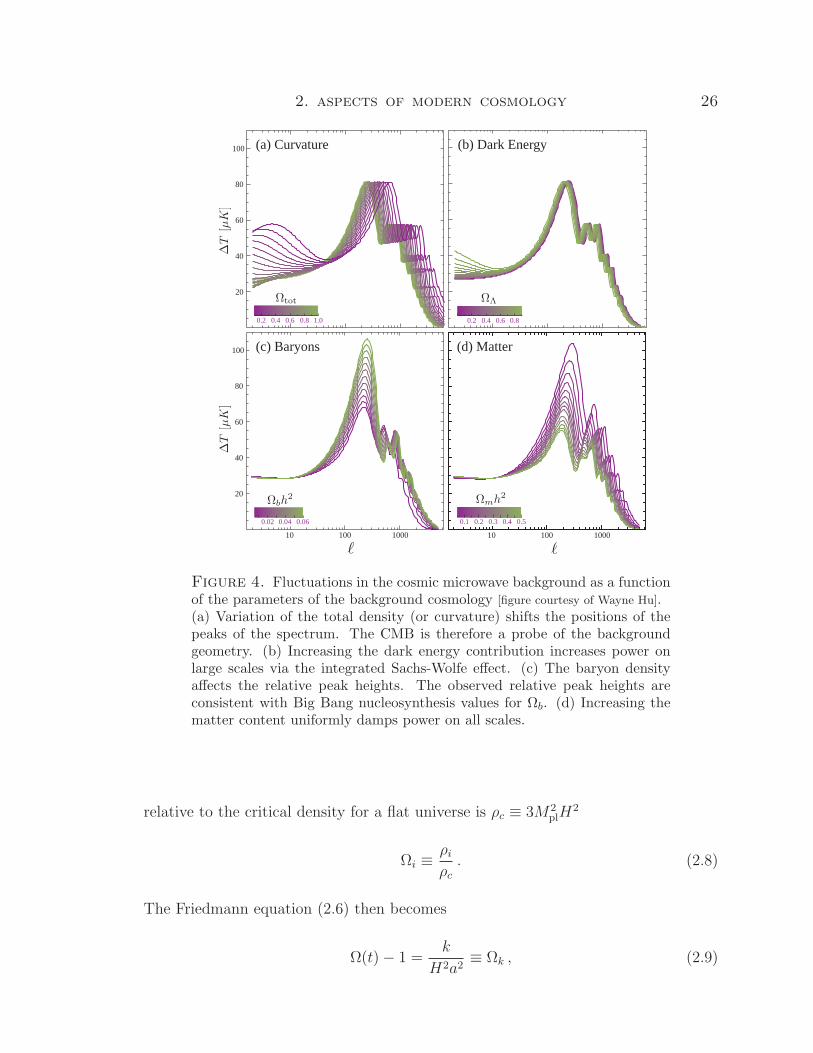
Figure 4. Fluctuations in the cosmic microwave background as a functionof the parameters of the background cosmology [figure courtesy of Wayne Hu].(a) Variation of the total density (or curvature) shifts the positions of thepeaks of the spectrum. The CMB is therefore a probe of the backgroundgeometry. (b) Increasing the dark energy contribution increases power onlarge scales via the integrated Sachs-Wolfe effect. (c) The baryon densityaffects the relative peak heights. The observed relative peak heights areconsistent with Big Bang nucleosynthesis values for Ωb. (d) Increasing thematter content uniformly damps power on all scales.
relative to the critical density for a flat universe is ρc ≡ 3M2plH
2
Ωi ≡ρiρc. (2.8)
The Friedmann equation (2.6) then becomes
Ω(t)− 1 =k
H2a2≡ Ωk , (2.9)

2. aspects of modern cosmology 27
where
Ω =∑i
Ωi = Ωr + Ωb + Ωdm + ΩΛ + · · · . (2.10)
Here, we consider radiation (photons and neutrinos)9 (r), baryons (b), dark matter
(dm) and dark energy (Λ). The CMB+LSS best fit parameters for the composition
of the universe today are [151]
Ωr 8.518× 10⁻⁵
Ωb 0.046± 0.003
Ωdm 0.231± 0.026
Ωm ≡ Ωb + Ωdm 0.277± 0.029
ΩΛ 0.723± 0.029
Ωk −0.0052± 0.0064
Ω ∼ 1± 10−2
This is consistent with a spatially flat universe, a theoretical prejudice inspired by
inflation (see §4). In the remainder of this thesis we will therefore set Ωk ≡ 0.
Notice from the second Friedmann equation (2.7) that accelerated expansion, a >
0, as observed for the late universe (dark energy) and as postulated for the early
universe (inflation), requires a negative pressure component, p < −13ρ. To explain
this from fundamental physics is one of the biggest challenges of theoretical physics.
2.3. Fluctuations. As we mentioned before, galaxies are formed by gravita-
tional instability of minute density fluctuations δρ, i.e. small perturbations of the
homogeneous FRW background (2.1). Observations of the cosmic microwave back-
ground radiation provide the earliest snapshot of these fluctuations. The metric of a
flat FRW universe with small perturbations is
ds2 =[gµν + δgµν
]dxµdxν . (2.11)
9We use Ωr = Ωγ(1 + 0.2271Neff), where Ωγ is the photon density and Neff ≈ 3.04 is theeffective number of relativistic neutrino species.

2. aspects of modern cosmology 28
For the important discussion of the gauge dependence of this split into background
variables (gµν , ρ) and perturbations (δgµν , δρ) we refer the reader to the excellent
treatment in Ref. [130]. Here, we restrict ourselves to a summary of the basic techni-
cal results of first-order cosmological perturbation theory. (Further details are given
in Appendix A.) The metric perturbations δgµν can be decomposed into three dis-
tinct types: scalar, vector and tensor perturbations. This classification describes the
transformation properties of the perturbations under spatial coordinate reparameter-
izations [130]. At linear order scalar, vector and tensor perturbations do not interact.
Scalars. Scalar perturbations are characterized by 4 scalar functions and 2 gauge
degrees of freedom. In Newtonian gauge the perturbed metric takes the following
form
ds2 = −(1 + 2Φ)dt2 + a(t)2(1− 2Ψ)δijdxidxj . (2.12)
In the absence of anisotropic stress (Tij = 0) Φ = Ψ and scalar metric perturbations
are described by a single function, the Newtonian potential Φ(t,x). In Fourier space
the fluctuation amplitude is
Φk(t) =
∫d3x e−ik·xΦ(t,x) . (2.13)
The initial power spectrum of Φ is10
〈Φk(ti)Φk′(ti)〉 ≡ (2π)3δ(k + k′)Ps(k) , Ps(k) ≡ k3
2π2Ps(k) . (2.14)
Assuming a power law, Ps(k) = Askns−1, we define the spectral index of the primordial
power spectrum
ns − 1 ≡ d lnPsd ln k
. (2.15)
10By “initial” we mean any time ti between the end of inflation and the horizon re-entryof a given Fourier mode (see §4). The normalization of Ps(k) is chosen such that the realspace variance of Φ is 〈ΦΦ〉 =
∫∞0 Ps(k) d ln k.

2. aspects of modern cosmology 29
The value ns = 1 corresponds to a scale-invariant Harrison-Zeldovich spectrum. The
scalar metric perturbations Φ are induced by inhomogeneities in the energy density,
ρ(t,x) = ρ(t)[1 + δ(t,x)] . (2.16)
Density perturbations δ and metric perturbations Φ are related by a Poisson equation
on subhorizon scales (k > aH) and by a constant rescaling on superhorizon scales
(k < aH). On subhorizon scales, gravity acts as an amplifier of these fluctuations,
which leads to the formation of the large-scale structure of the universe. The evolution
of density fluctuations is characterized by the growth function gk(t)11
δk(t) ≡ gk(t, ti)
aδk(ti) . (2.17)
CMB and LSS observations measure the density power spectrum at late times (Fig-
ure 5). To relate this to the primordial spectrum one needs to take into account the
post-processing of the spectrum as given by the growth factor gk(t). Assuming va-
lidity of general relativity and using the measured cosmological parameters to fix the
background cosmology we can factor out the cosmological evolution and extract the
spectrum of primordial fluctuations Ps(k). The precise shape of this spectrum pro-
vides an accurate test of inflationary perturbations as the origin of cosmic structure
(see §4 and Figure 6).
Vectors. Vector perturbations are related to rotational motion of the fluid. They
decay with the expansion of the universe and therefore do not affect the late time
properties of the universe. We will not consider them further.
11The function gk(t) depends on theory of gravity and the matter content of the universe.The growth of structure therefore provides an important consistency test for the applica-bility of general relativity on very large scales.

2. aspects of modern cosmology 30
Figure 5. Density fluctuations as a function of scale and relevant obser-vational probes [figure courtesy of Max Tegmark].
Tensors. Tensor perturbations describe gravitational waves, i.e. perturbations to
the spatial metric of the form
ds2 = −dt2 + a(t)2(δij + hij)dxidxj , (2.18)
where ∂ihij = hii = 0. A stochastic background of gravitational waves is a unique
prediction of inflationary cosmology (see §4). At linear order gravitational waves do
not couple to perturbations in the fluid.12 They therefore redshift like radiation and
their amplitudes decays with the expansion of the universe. The tensor perturbation
hij can be written in terms of two polarization modes: hij = h+e+ij + h×e
×ij. The
primordial power spectrum for each polarization mode is
〈hkhk′〉 = (2π)3δ(k + k′)Pt(k) , Pt(k) ≡ k3
2π2Pt(k) . (2.19)
12Second order couplings between scalar and tensor modes have been considered in [8, 23,129], but they are small by virtue of the scalar amplitude being small, Φ ∼ 10−5.

2. aspects of modern cosmology 31
CMB polarization experiments will be sensitive to the tensor-to-scalar ratio
r ≡ PtPs. (2.20)
The data has now reached a precision that allows meaningful constraints to be placed
on ns (2.15) and r (2.20) (see Figure 6).
Figure 6. Constraints on the inflationary parameters ns and r from recentcosmic microwave background and large-scale structure observations [151].
2.4. Summary. This is a golden age of cosmology. New precision data is testing
theoretical ideas about the structure and evolution of the universe. These observations
have revealed three problems that challenge the foundations of theoretical physics:
dark matter, dark energy, and inflation. We now know that 95% of the universe is not
ordinary atoms! However, we have yet to make sense of it! We have some ideas for
what the dark matter might be, but dark energy and inflation lack any explanation
in fundamental physics.

2. aspects of modern cosmology 32
3. Dark Energy
3.1. The Dark Energy Crisis. Explaining the nature of dark energy is one of
the greatest challenges of fundamental physics. Paul Steinhardt calls the discovery
of dark energy “one of the most surprising and profound discoveries in the history of
science” [152], while Steven Weinberg notes that “physics thrives on crisis” [159].
Two questions summarize the dark energy crisis:
Why is the vacuum energy so unnaturally small?
The energy momentum tensor of the universe Tµν is expected to contain
a term Λgµν coming from the quantum mechanical energy density of the vac-
uum. Computations in quantum field theory13 suggest that the natural value
of the constant Λ should be in the range (TeV)4 ≤ Λtheory ≤ (1019 GeV)4.
According to Einstein’s equations, M2plGµν = Tµν , such a term admits de Sit-
ter space as a solution. It is therefore natural to propose vacuum energy as
the cause of the observed acceleration of the universe today. Unfortunately,
the observed value of the cosmological constant Λobs ∼ (meV)4 is some 120
orders of magnitude smaller than its natural value, Λobs/Λtheory = 10−123.
This is the biggest disagreement between theory and experiment in the his-
tory of science. It is the famous cosmological constant problem: “Why is the
vacuum energy density so small?” And, “If it is so small, why is it not zero?”
Why did acceleration start only in the recent past?
To make matters worse, the energy density of dark energy is observed to
be of the same order of magnitude as the present matter density. This is
13The following provides an estimate of the energy density of empty space: Consider sum-ming the zero-point energies of all normal modes of some field of mass m up a wavenumbercutoff Λ1/4 m. This yields the following vacuum energy density
〈ρ〉 =∫ Λ1/4
0
4πk2dk(2π)3
12
√k2 +m2 ≈ Λ
16π2. (2.21)
If Λ1/4 is set to any particle physics scale (Mpl, MSUSY, Λ1/4QCD, me), one gets a version of
the cosmological constant problem.

2. aspects of modern cosmology 33
puzzling since the vacuum energy density ρΛ ∝ a0 remains constant during
the evolution of the universe, whereas the matter energy density ρm ∝ a−3
decreases as the universe expands. The two energy densities being nearly the
same today means that their ratio ρΛ/ρm had to be incredibly small in the
early universe, but fine-tuned to become nearly equal today. In other words,
one might think that we are living at a special epoch when the dark energy
density and the matter density are nearly equal in magnitude. During most
of the history and the future of the universe this is not the case. This has
become known as the cosmic coincidence problem (the “why now?” problem).
3.2. Dark Energy in String Theory. The cosmological constant problem
points to a deep conflict between the physics of the very large and the very small.
Quantum mechanics describes the microscopic world of elementary particles, atoms
and molecules, while Einstein’s general relativity provides an elegant mathematical
formulation for the evolution of the universe on the largest scales. Both theories are
fantastically successful in describing fundamental features of the world. However,
whenever forced to apply quantum mechanics and general relativity simultaneously
one is led to troubling inconsistencies. String theory in contrast is a consistent theory
of quantum gravity and hence has the potential to address fundamental questions
about the initial Big Bang singularity and the center of black holes. It is therefore
justified to imagine that string theory will also give us new insights into the vacuum
energy problem. So far this hope has not been realized, although string theory has
provided some interesting new ideas for addressing the problem. In particular, for-
mulating de Sitter space in string theory has been a challenge that was overcome only
recently by the first explicit constructions of metastable de Sitter solutions (see Chap-
ter 3). The multiplicity of these vacuum solutions can explain the vacuum energy
problem by anthropic reasoning [39].

2. aspects of modern cosmology 34
4. Inflation
“SPECTACULAR REALIZATION:
This kind of supercooling can explain why the universe today is
so incredibly flat and therefore resolve the fine-tuning paradox
pointed out by Bob Dicke in his Einstein day lectures.”
Alan Guth, Dec 7, 1979.
4.1. Shortcomings of the Big Bang Theory. Despite the success of the Big
Bang theory in explaining basic cosmological observations (see §2) it was realized
(e.g. by Dicke) that the uniform expansion of the universe poses serious conceptual
problems.
Homogeneity Problem. The standard model of cosmology assumes that the uni-
verse is homogeneous and isotropic. Indeed observations confirm this. However, the
conventional Big Bang theory does not explain this fact. As we discussed above,
inhomogeneities are gravitationally unstable and therefore tend to grow with time.
Observations of the CMB for instance verify that the fluctuations were much smaller
at the last scattering epoch than today. One thus expects that these inhomogeneities
were still smaller further back in time. How to explain a universe so smooth in its
past?
Flatness Problem. Spacetime in general relativity is dynamical, curving in re-
sponse to matter in the universe. Why then is the universe so closely approximated
by flat Euclidean space? To understand the severity of the problem consider the
Friedmann equation in the form (2.9)
Ω(a)− 1 =k
(aH)2. (2.22)
In the conventional Big Bang theory the comoving Hubble radius (aH)−1 grows with
time and |Ω− 1| hence diverges with time. (A flat universe with Ω = 1 is an unstable

2. aspects of modern cosmology 35
fixed point.) In the context of the standard Big Bang model, the quasi-flatness
observed today, Ω(a0) ∼ 1, therefore requires extreme fine-tuning of Ω near 1 in the
early universe, e.g. the deviation from flatness at BBN, during the GUT era and at
the Planck scale, respectively has to satisfy the following conditions: |Ω(aBBN)− 1| ≤
O(10−16), |Ω(aGUT)− 1| ≤ O(10−55), |Ω(apl)− 1| ≤ O(10−61).
Conformal Time Today
CMBBig Bang
Past Light-Cone
0
causally disconneted @ CMB decoupling
Figure 7. Conformal spacetime of conventional Big Bang cosmology. TheCMB at last scattering consists of 105 causally disconnected regions!
Horizon Problem. Consider radial null geodesics in a flat FRW spacetime (2.1)
dr = ± dt
a(t)≡ dτ . (2.23)
We define the comoving horizon, τ , as the causal horizon, i.e. the distance a light
ray travels between time 0 and time t
τ ≡∫ t
0
dt′
a(t′)=
∫ a
0
da
Ha2=
∫ a
0
d ln a (aH)−1 . (2.24)
During the standard cosmological expansion the increasing comoving Hubble radius,
(aH)−1, is therefore associated with an increasing comoving horizon14, τ , and the
fraction of the universe in causal contact increases with time. However, the near-
homogeneity of the CMB tells us that the universe was quasi-homogeneous at the
14This explains the common practice of often using the terms ‘comoving Hubble radius’ and‘comoving horizon’ interchangeably. Although these terms should conceptually be clearlydistinguished, this inaccurate use of language has become standard.

2. aspects of modern cosmology 36
time of last scattering on a scale encompassing many regions that are a priori causally
independent (see Figure 7). Why then is the CMB uniform on large scales (of order
the present horizon)?
Comment on Initial Conditions. It should be emphasized that the flatness and
horizon problems are not strict inconsistencies of the standard cosmological model.
If one assumes that the initial value of Ω was extremely close to unity and that
the universe began homogeneously (but with just the right level of inhomogeneity
to explain structure formation) then the universe would have continued to evolve
homogeneously in agreement with observations. The flatness and horizon problems
are therefore just severe shortcomings in the predictive power of the Big Bang model.
The dramatic flatness of the early universe cannot be predicted by the standard
model, but must instead be assumed in the initial conditions. Likewise, the striking
large-scale homogeneity of the universe is not explained or predicted by the model,
but instead must simply be assumed. Inflation removes these assumptions about
initial conditions.
4.2. The Basic Idea of Inflation. All the Big Bang puzzles are solved by a
beautifully simple idea: ‘invert the behavior of the comoving Hubble radius’ (aH)−1
i.e. make it decrease sufficiently in the very early universe. A decreasing Hubble
radius corresponds to accelerated expansion
d
dt(aH)−1 < 0 ⇒ d2a
dt2> 0 . (2.25)
A flat universe then becomes an attractor solution (see Equation (2.22)) and the
observed CMB sky was in causal contact in the past (see Figure 8). A period of
acceleration in the early universe therefore very elegantly solves the problems with
the standard Big Bang theory. However, it raises the question: What is the physics
of inflation? Twenty-five years after inflation was introduced by Guth it remains a
paradigm in search of a theory. From the second Friedmann equation (2.7) we see

2. aspects of modern cosmology 37
Conformal Time Today
CMB
Big Bang
Past Light-Cone
Reheating
Inflation
0
Figure 8. Conformal spacetime of the inflationary universe. The horizonproblem is solved by extending conformal time to negative values. In infla-tionary cosmology the Big Bang is at τ = −∞, while without inflation it isat τ = 0 (see Figure 7).
that accelerated inflationary expansion, like dark energy, requires a negative pressure
component to dominate the universe
d2a
dt2> 0 ⇒ ρ+ 3p < 0 . (2.26)
Furthermore, the two Friedmann equations (2.6) and (2.7) may be combined into the
continuity equation
dρ
dt= −3H(ρ+ p) . (2.27)
During inflation p ≈ −ρ, so the inflationary expansion requires that the early universe
was dominated by a nearly constant energy density, ρ ≈ 0. This is unlike any physical
phenomenon we are familiar with.

2. aspects of modern cosmology 38
4.3. Slow-Roll Inflation. In the absence of a better theoretical understanding
of inflation it is standard practice to parameterize our ignorance by a scalar field φ
with potential V (φ) (see Figure 9). Consider therefore the scalar field Lagrangian
L = −1
2gµν∂µφ∂νφ− V (φ) . (2.28)
Computing the energy-momentum tensor associated with L, we find that the homo-
reheating
Figure 9. The Inflaton Potential. Acceleration occurs when the potentialenergy of the field V dominates over its kinetic energy 1
2 φ2. Inflation ends
at φend when the slow-roll conditions are violated, ε→ 1. CMB fluctuationsare created by quantum fluctuations δφ about 60 e-folds before the end ofinflation. At reheating, the energy density of the inflaton is converted intoradiation.Left: A typical small-field potential. Right: A typical large-field potential.
geneous mode φ(t) acts like a perfect fluid with equation of state
w ≡ p
ρ=
12φ2 − V
12φ2 + V
. (2.29)
The equation of motion of the inflaton field in an FRW background is the Klein-
Gordon equation
φ+ 3Hφ+ V ′(φ) = 0 . (2.30)
From equation (2.29) we see that accelerated expansion, w < −13, occurs when the
potential energy density dominates over the kinetic energy, V 12φ2. From the
equation of motion (2.30) we further note that this condition is sustained if φ
V ′. These two conditions for prolonged inflation are summarized by restrictions on

2. aspects of modern cosmology 39
the form of the inflaton potential V (φ) and its derivatives. Quantitatively, inflation
requires smallness of the slow-roll parameters
ε ≡M2
pl
2
(V ′V
)2
, (2.31)
η ≡ M2pl
V ′′
V. (2.32)
The conditions for inflation, ε, |η| 1, constrain the shape of the inflaton potential.
Whether and how naturally such flat potentials are achievable in string theory is an
important open question which we will address in the bulk of this thesis.
4.4. Quantum Origin of Structure. So far we have only discussed the classical
evolution of the inflaton field. Something remarkable happens when one considers
quantum fluctuations of the inflaton: inflation combined with quantum mechanics
provides an elegant mechanism for generating the initial seeds of all structure in the
universe.
Comoving Horizon
Time [log(a)]
Inflation Hot Big Bang
Comoving Scales
horizon exit horizon re-entry
density fluctuation
Figure 10. Creation and evolution of perturbations in the inflationary uni-verse. Fluctuations are created quantum mechanically on sub-horizon scales.While comoving scales remain constant the comoving Hubble radius duringinflation shrinks and the perturbations exit the horizon. Causal physics can-not act on superhorizon perturbations and they freeze until horizon re-entryat late times.

2. aspects of modern cosmology 40
A very intuitive way of understanding how the quantum fluctuations of the inflaton
field δφ(x) translate into density fluctuations δρ(x) is via the time-delay formalism
developed by Guth and Pi [84].15 The basic idea is that φ controls the time at which
inflation ends (see Figure 9). Small quantum fluctuations in the value of the inflaton
field δφ(x) ∼ H translate into differences in the end of inflation (ε ≡ 1) for different
regions of space δt(x). Regions acquiring a negative frozen fluctuation δφ remain
potential-dominated longer than regions where δφ is positive. Hence, fluctuations of
the field φ lead to a local delay of the end of inflation
δt =δφ
φ∼ H
φ. (2.33)
For the field fluctuation we have used the result of the zero-point calculation in de
Sitter space, δφ ∼ H. After reheating, the energy density evolves as ρ = 3M2plH
2
where H ∼ t−1, so that
δρ
ρ∼ 2
δH
H∼ Hδt ∼ H
H
φ. (2.34)
This process therefore induces tiny density variations δρ which via gravitational in-
stability grow to form the observed large-scale structure of the universe. In addition,
quantum fluctuations during inflation excite tensor metric perturbations, δg ∼ HMpl
.
Future experiments hope to detect this stochastic background of gravitational waves
from inflation.
15Strictly speaking the time-delay formalism is only valid when inflation is well-describedby the de Sitter solution and the equation of state is nearly unchanging [158]. We refer thereader to Appendix A for an improved derivation of the inflationary perturbation spectra.

2. aspects of modern cosmology 41
Figure 11. Constraints on inflationary models from recent cosmic mi-crowave background and large-scale structure observations [151].
4.5. Cosmological Observables.
Power Spectra. The computation we just sketched gives the following results for
primordial scalar and tensor power spectra (see Appendix A for details)
Ps =(H
2π
)2(H
φ
)2
≈ 1
24π2M4pl
V
ε(2.35)
Pt =2
π2
( H
Mpl
)2
≈ 2
3π2
V
M4pl
. (2.36)
Here, the r.h.s. should be evaluated when the fluctuation mode freezes after crossing
the horizon, k = aH, (see Figure 10) and the second equality made use of the slow-
roll approximation. In a power law description, Ps = Askns−1 and Pt = Atk
nt , the
spectral indices in terms of the slow-roll parameters are
ns − 1 = 2η − 6ε , (2.37)
nt = −2ε . (2.38)
The deviation from scale-invariance (ns = 1, nt = 0) may be traced to a small time
evolution of the Hubble parameter during inflation. From (2.35) and (2.36) we define

2. aspects of modern cosmology 42
the tensor-to-scalar ratio
r = 16ε . (2.39)
Measurements of ns and r are strong discriminators of inflationary models (see Figure
11).
Inflationary Gravitational Waves. Detection of a stochastic background of primor-
dial gravitational waves is widely regarded as a ‘smoking gun’ signature of inflation.
The best hope for detecting such a signal is via the subtle imprints they leave in the
polarization of the CMB (B-modes).16 It is important to make pre-dictions for the ex-
pected gravitational wave amplitude before the next generation of CMB polarization
experiments comes online. In the context of string theory we discuss this challenge
in Chapters 8, 9 and 10.
LISA
PULSARS
LIGO II
(2013 ?)
(2013)
(2025 ?)
(2030 ?)
inflationary gravitational waves
BBO Corr
BBO I
CMBPol
ΩGW(f )
k (Mpc-1)
WMAP3
10-20
10-15
10-10
10-15
10-10 10
-510
010
5
100
105
1010
1015
1020
Frequency (Hz)
(2020 ?)
Figure 12. Current and future constraints on the inflationary gravita-tional wave background (Figure adapted from Boyle et al. [41]). Shownis the theoretical prediction for “minimally tuned” inflationary models asdefined in [41].
16In the future it might also become feasible to measure inflationary gravitational waves atlate times with direct-detection experiments like the Big Bang Observer (BBO) (see Figure12)

2. aspects of modern cosmology 43
A conservative estimate for the minimal gravitational wave amplitude that is
accessible to future experiments is r > 0.01. Any signal that is much smaller than
this will be very hard to extract from astrophysical foregrounds [150]. A detection of
the primordial tensor-to-scalar ratio r would be truly revolutionary, as r encodes two
crucial pieces of information about the inflationary era:
(1) Energy scale of inflation
The measured amplitude of scalar perturbations Ps ≈ 2.4 × 10⁻⁹ implies a
relation between the energy scale of inflation V 1/4 and the tensor-to-scalar
ratio r
V 1/4 = 1.06× 10¹⁶ GeV( r
0.01
)1/4
. (2.40)
Detecting tensors (r > 0.01) would therefore imply that inflation occurred
at very high energies.
(2) Super-Planckian field variation
There is a one-to-one correspondence between the tensor-to-scalar ratio r
and the evolution of the inflaton during inflation ∆φ ≡ |φCMB − φend| [122]
(see Figure 9 for a definition of ∆φ and Chapter 8 for a derivation of the
Lyth bound)
∆φ
Mpl
> O(1)( r
0.01
)1/2
. (2.41)
Observable gravitational waves (r > 0.01) therefore require super-Planckian
field excursions ∆φ > Mpl while keeping the potential controllably flat. In
Chapters 8 and 9 we discuss whether this is realizable in a consistent micro-
scopic theory like string theory.
Primordial Non-Gaussianity. Gaussian fluctuations are completely described by
their two-point correlation function (or the power spectrum). The primordial fluc-
tuations created during slow-roll inflation are predicted to be highly Gaussian (see

2. aspects of modern cosmology 44
Appendix A) and the CMB power spectrum therefore reveals most of their statis-
tical properties. However, large non-Gaussianity can arise for non-minimal models
with non-trivial kinetic terms and/or multiple fields. This non-Gaussianity is best
extracted from the three-point function (or bi-spectrum)
〈Φk1Φk2Φk3〉 = (2π)3δ(k1 + k2 + k3)F (k1, k2, k3) , (2.42)
where the momentum dependence of the function F contains important clues about
the physics of inflation.
A simple way to characterize the non-Gaussianity of Φ is to assume that it can
be parameterized by a field redefinition of the form
Φ = ΦL + fNLΦ2L , (2.43)
where ΦL is Gaussian and the constant fNL measures the amount of non-Gaussianity
of Φ. Equation (2.43) is often called local non-Gaussianity. For single-field slow-roll in-
flation fNL < 1 (see Appendix A). Since it is generally believed that non-Gaussianity
is only observable if fNL & 1, we conclude that primordial non-Gaussianities from
slow-roll inflation are unobservable. However, the non-Gaussianity can easily be one
or two orders of magnitude bigger in non-minimal models of inflation. The search
for primordial non-Gaussianity is therefore an important aspect of the experimental
efforts to test the physics of inflation.

2. aspects of modern cosmology 45
4.6. What is the Physics of Inflation? Understanding the (micro)physics of
inflation remains one of the most important open problems in modern cosmology
and theoretical physics. Explicit particle physics models of inflation remain elusive,
so that a natural microscopic explanation for inflation has yet to be uncovered.17
Nevertheless, there have recently been interesting efforts to derive inflation from string
theory. The search for inflationary solutions in string compactifications will be the
main focus of this thesis.
17At this point it should be emphasized that the inflationary era in the early universeis an unproven hypothesis. It is therefore important to keep an open mind about creativealternative solutions to the horizon and flatness problems and the generation of cosmologicalperturbations. The most interesting proposals to date are the ekpyrotic/cyclic scenarios[43, 100, 154]. In these models a period of slow contraction before the Big Bang expandingphase replaces inflation.

CHAPTER 3
Elements of String Compactifications
In this chapter we review fundamental aspects of string compactifications. The
formal developments described here form the basis for modern studies of string cos-
mology. We make no attempt at a complete and/or pedagogical introduction to string
theory. For a more thorough treatment of this vast and rapidly evolving subject the
reader may be referred to [27, 79, 138, 164].
After describing the moduli problem in §1 we present flux compactifications and
the KKLT scenario in §2 and §3, respectively. These constructions fix all moduli
and allow metastable de Sitter solutions. In addition, compactifications with fluxes
generically have warped regions whose local geometry we review in §4.
1. The Moduli-Stabilization Problem
Low energy effective actions arising from string theory typically contain many
scalar fields collectively called moduli. In particular, the compact manifolds satis-
fying the string equations of motion generally come in continuous families whose
parameters (controlling the size and shape of the extra dimensions) become scalar
fields in the four-dimensional effective theory. Compactifications containing branes
have additional moduli that parameterize their relative positions and orientations.
Finally, any string compactification always contains the massless dilaton field.
Before considering potentials arising from fluxes and non-perturbative effects,
these string moduli fields are massless and their couplings are of gravitational
46

3. elements of string compactifications 47
strength. the existence of these fields therefore raises generic cosmological problems
– The late time evolution of moduli fields affects low energy observables like the cou-
plings of the Standard Model, Newton’s gravitational constant, and the fine-structure
constant. In addition, light moduli fields can lead to fifth force-type violations of the
equivalence principle. All of these effects are strongly constrained by experiments.
The presence of light moduli fields may also lead to problems in the early universe:
e.g. successful Big Bang nucleosythesis (BBN) requires a moduli mass mχ in excess
of 30 TeV. If mχ . 100 MeV then the energy stored in the moduli fields overcloses the
universe while if 100 MeV . mχ . 30 TeV then the moduli decay dilutes the BBN
products [110]. Phenomenologically viable models of particle physics and cosmology
therefore require a solution to the moduli-stabilization problem.
2. Flux Compactification
The moduli-stabilization problem has been solved only recently in the context of
flux compactifications of type IIB string theory [76], [82], [93]. Here we summarize
the basic elements of this program. For more details we refer the reader to the review
by Douglas and Kachru [63] or the recent Les Houches lectures by Denef [57].
2.1. Basic Ingredients. The basic ingredients of type IIB flux compactifications
are fluxes, branes and warped extra dimensions. The type IIB limit of string theory
contains D3-, D5-, and D7-branes as well as O(rientifold)-planes. The action for a Dp-
brane is the sum of a Dirac-Born-Infeld (DBI) term and a Chern-Simons (CS)-term
[139]
SDp = SDBI + SCS . (3.1)
The DBI action describes the worldvolume of the brane which in string frame is1
SDBI = −Tp∫
dp+1ξ e−Φ√−det(GAB) . (3.2)
1This result is to leading order in α′ and for the case of vanishing worldvolume field strength.

3. elements of string compactifications 48
Here, Tp = (2π)−pg−1s (α′)−(p+1)/2 is the D-brane tension in terms of the string coupling
gs and the fundamental string length√α′. The field Φ is the dilaton and GAB is
the pullback of the metric onto the brane worldvolume. The Chern-Simons-term2
describes the electric coupling of a Dp-brane to the R-R (p+ 1)-form Cp+1
SCS = µp
∫Cp+1 , |µp| = Tpe
−(p−3)Φ/4 . (3.3)
Branes are therefore sources for form-field fluxes Fp+2 = dCp+1. The total flux of these
fields through topologically non-trivial surfaces in the extra dimensions is quantized,
e.g.
1
(2π)2α′
∫A
F3 = M ,1
(2π)2α′
∫B
H3 = −K , (3.4)
where A and B are 3-cycles of the compact manifold, F3 = dC2 and H3 = dB2 are
3-form fluxes and M and K are integers.
Finally, the presence of branes and fluxes sources locally warped spacetime regions,
ds2 = h1/2(y) gµνdxµdxν︸ ︷︷ ︸
4D
+h−1/2(y) gijdyidyj︸ ︷︷ ︸
6D
. (3.5)
These regions are important backgrounds for quantitative studies of string cosmology
(see §4 and Chapter 4).
2.2. Moduli Potential. In the following we provide a lightning review of the
four-dimensional low-energy effective description of the KKLT proposal. We work in
the limit of N = 1 supergravity, where the moduli potential VF is characterized by a
superpotential W and a Kahler potential K
VF = eK/M2pl
[KiDiWDjW −
3
M2pl
|W |2], (3.6)
where DiW ≡ ∂iW + 1M2
pl(∂iK)W and Ki ≡ ∂i∂K. The compactification typically
contains 3-form flux G3 ≡ F3 − τH3 which contributes to the superpotential via the
2More general forms of the Chern-Simons term may be found in [139].

3. elements of string compactifications 49
Gukov-Vafa-Witten (GVW) term [82]
Wflux =
∫G3 ∧ Ω , (3.7)
where Ω denotes the holomorphic three-form on the Calabi-Yau three-fold and τ ≡
C0 + ie−Φ is the axio-dilaton. The Kahler potential for the complex structure moduli
and the dilaton is
K = −M2pl ln
[∫Ω ∧ Ω
]−M2
pl ln[τ + τ ] . (3.8)
Turning on generic G3-flux induces a potential VF that usually fixes all the complex
structure moduli (χα) and the dilaton (τ) [76]. The potential (3.6) is minimized for
DχαWflux = DτWflux = 0.
3. De Sitter Vacua in String Theory
3.1. Non-perturbative Effects. The (classical) flux background fixes the shape
(complex structure moduli) of the extra dimensions, but leaves the overall size (Kahler
moduli ρ) unfixed [76] (see Figure 1). Recently, Kachru, Kallosh, Linde and Trivedi
(KKLT) [93] provided a framework for stabilizing the overall size of the compact
manifold by including non-perturbative (quantum) effects e.g. gaugino condensation
on D7-branes or Euclidean D3-instantons. These effects are parameterized by the
following superpotential
Wnp = Ae−aρ , (3.9)
for a constant. With K = −3M2pl ln[ρ+ ρ] the F-term potential (3.6) then leads to
supersymmetric anti-de Sitter (SUSY AdS) vacua, DρW = Dρ(Wflux +Wnp) = 0, with
stabilized Kahler modulus. The compactification is stabilized at large volume, ρ? 1,
iff the flux superpotential is a small negative constant Wflux(χ?α, τ?) ≡ W0 ∼ −10−4
(in units where Mpl ≡ 1).

3. elements of string compactifications 50
3.2. de Sitter Space. Having negative cosmological constant, these solutions
cannot yet describe our universe, VF = − 3M2
pl|W |2eK/M2
pl . KKLT therefore uplifted the
AdS minima to positive energies by adding anti-D3-branes. This ‘D-term’ uplifting
adds the following term to the moduli potential
VD =D
(ρ+ ρ)2, (3.10)
where D is a constant that depends on the D3-brane tension and the warping of
the background. The final potential for the volume modulus σ ≡ Re(ρ) is shown in
Figure 1
V (σ) =aA
2M2pl
e−aσ
σ2
(1
3aσAe−aσ +W0 + Ae−aσ
)+
1
4
D
σ2. (3.11)
Notice that the de Sitter minimum is metastable. The magnitude of the cosmological
12 16 18 20
-2
-1
1
2
3
no-scale
SUSY-AdS
dS
volume
V (σ)
σ ≡ Re(ρ)
Figure 1. KKLT compactification: Potential for the volume modulusσ = Re(ρ). Fluxes fix the complex structure and the dilaton field, but leavethe overall volume modulus unfixed (green curve). Non-perturbative effectsstabilize the volume in a supersymmetric minimum with negative cosmolog-ical constant (blue curve). Anti-D3 branes provide the uplifting energy to ametastable de Sitter minimum (red curve).
constant associated with the minimum depends on the choice of flux quanta (3.4) and
is therefore tunable. The discretuum of vacua in type IIB flux compactifications has
been employed for an anthropic solution to the cosmological constant problem [39].

3. elements of string compactifications 51
4. Klebanov-Strassler Geometry
The moduli spaces of compact Calabi-Yau spaces generically contain conifold sin-
gularities. The local description of these singularities is called the conifold, a non-
compact Calabi-Yau three-fold whose geometry is given by a cone. In contrast to
general Calabi-Yau backgrounds the metric data for the conifold is explicitly known.
This makes these backgrounds very interesting for detailed studies of string cosmology
and particle phenomenology.
In this section we cite basic geometrical facts about the conifold (for more details
we refer the reader to the recent Les Houches lectures by Benna and Klebanov [29]).
4.1. Singular Conifold. The (singular) conifold is defined by the complex equa-
tion4∑i=1
z2i = 0 , zi ∈ C . (3.12)
The constraint equation (3.12) describes a cone over X5 = S2 × S3. To see this note
that if zi is a solution to (3.12) then so is λzi with λ ∈ C. Also, letting zi ≡ xi + iyi,
the complex equation (3.12) may be recast into three real equations
~x · ~x =1
2ρ2 , ~y · ~y =
1
2ρ2 , ~x · ~y = 0 . (3.13)
The first equation defines a 3-sphere S3 with radius ρ/√
2.3 The last two equations
then describe a 2-sphere S2 fibred over the S3. The Calabi-Yau metric on the conifold
is
ds26 = dr2 + r2ds2
T 1,1 , (3.14)
if we define the radial coordinate r ≡√
3/2ρ2/3 or r3 ≡∑4
i=1 |zi|2.
3Here, the variable ρ is of course not to be confused with the Kahler modulus introducedin §3.

3. elements of string compactifications 52
The base of the cone is the T 1,1 coset space [SU(2)A× SU(2)B]/U(1)R which has
the topology S2×S3. The metric of T 1,1 in angular coordinates θi ∈ [0, π], φi ∈ [0, 2π],
ψ ∈ [0, 4π] is
ds2T 1,1 =
1
6
(dψ +
2∑i=1
cos θidφi
)2
+1
6
2∑i=1
(dθ2i + sin2 θidφ
2i ) . (3.15)
4.2. Deformed Conifold. The space defined by (3.12) is singular at the tip
of the cone, r = 0. Various prescriptions exist for removing this singularity – e.g.
consider the deformed conifold defined by
4∑i=1
z2i = ε2 , (3.16)
where ε ∈ C. By a phase rotation of the zi coordinates we can always choose ε ∈
R+. This defines a one-dimensional moduli space. For large r the deformed conifold
geometry reduces to the singular conifold with ε = 0. Moving from large r towards
the origin, the sizes of the S2 and the S3 both decrease. Decomposing the zi into real
and imaginary parts we now find
ε2 = ~x · ~x− ~y · ~y , (3.17)
and
ρ2 = ~x · ~x+ ~y · ~y . (3.18)
This shows that the range of ρ (or r) is limited by
ε2 ≤ ρ2 <∞ (3.19)
and the singularity at r = 0 is avoided for ε2 > 0. It also shows that as ρ2 → ε2 the
S2 disappears (~y · ~y → 0) leaving just an S3 with finite radius.

3. elements of string compactifications 53
4.3. Warped Throat. A stack of N D3-branes placed at the singularity zi = 0
backreacts on the geometry, producing a warped background with the following ten-
dimensional line element
ds2 = h1/2(z)gµνdxµdxν + h−1/2(z)gidz
idz , (3.20)
where gi is the metric (3.14) and the warp factor is
h(r) =R4
r4, R4 ≡ 27π
4gsN(α′)2 . (3.21)
This AdS background is an explicit realization of the Randall-Sundrum scenario [140,
141] in string theory. In the spirit of AdS/CFT [124] the AdS5×T 1,1 geometry (3.20)
has a dual gauge theory interpretation. The dual N = 1 supersymmetric conformal
gauge theory was constructed in [107]. It is an SU(N)×SU(N) gauge theory coupled
to bifundamental chiral superfields. If one further adds M D5-branes wrapped over
the S2 inside T 1,1, then the gauge group becomes SU(N + M) × SU(N), giving
a cascading gauge theory [105, 106]. The three-form flux induced by the wrapped
D5-branes (fractional D3-branes) satisfies
1
(2π)2α′
∫S3
F3 = M . (3.22)
The warp factor h(r) for this case was found by Klebanov and Strassler (KS) [105].
For large r it is [106]
h(r) =27π(α′)2
4r4
[gsN +
3
2π(gsM)2 ln
( rr0
)+
3
8π(gsM)2
], (3.23)
where r0 ∼ ε2/3e2πN/(3gsM).
The Klebanov-Strassler warped conifold background (also refered to as the warped
throat) is the basis for our explicit studies of warped D-brane inflation.

CHAPTER 4
Inflation in String Theory
Understanding the physics of inflation is one of the main challenges of fundamen-
tal physics and modern cosmology. Since string theory remains the most promising
candidate for a UV-completion of the Standard Model that unifies gauge and gravita-
tional interactions in a consistent quantum theory, it seems natural to search within
string theory for an explicit realization of the inflationary scenario. This search has
so far revealed two distinct classes of inflationary models which identify the inflaton
field with either open string modes (e.g. brane inflation [64, 95], DBI inflation [4, 147],
assisted M5-brane inflation [26], D3/D7 inflation [56], wrapped brane inflation [148]),
or closed string modes (e.g. Kahler moduli inflation [54], racetrack inflation [35, 36],
N-flation [61, 67]). In this chapter we review these theoretical developments.
We begin in §1 with general remarks about the promise of studying UV-physics
in string theory models of inflation. In §2 we review warped brane inflation with
particular emphasis on the eta-problem [95] and the DBI mechanism [147]. In §3 we
provide a brief survey of other models of string inflation. We describe their prospects
and problems. Finally, in §4 we explain the ambitious goal of deriving inflationary
models from explicit string compactifications.
For more details on these and related aspects of inflation in string theory we refer
the reader to the excellent review by McAllister and Silverstein [128] or the upcoming
review by Liam McAllister and myself [22].
54
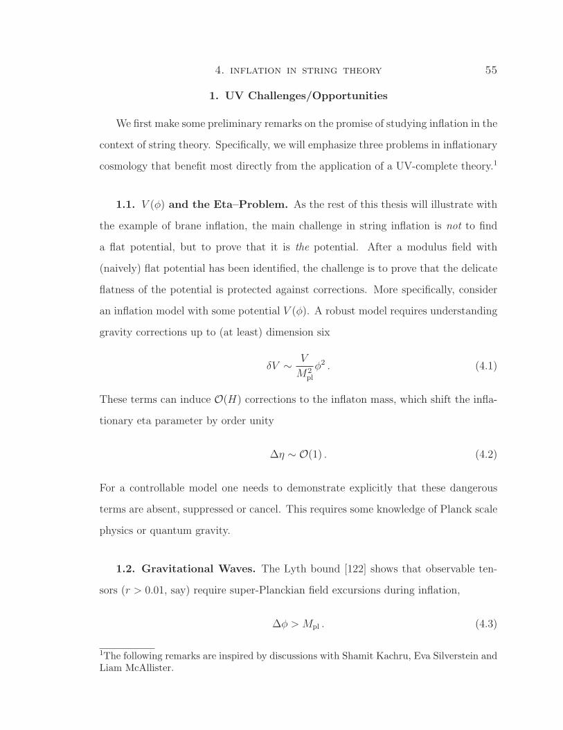
4. inflation in string theory 55
1. UV Challenges/Opportunities
We first make some preliminary remarks on the promise of studying inflation in the
context of string theory. Specifically, we will emphasize three problems in inflationary
cosmology that benefit most directly from the application of a UV-complete theory.1
1.1. V (φ) and the Eta–Problem. As the rest of this thesis will illustrate with
the example of brane inflation, the main challenge in string inflation is not to find
a flat potential, but to prove that it is the potential. After a modulus field with
(naively) flat potential has been identified, the challenge is to prove that the delicate
flatness of the potential is protected against corrections. More specifically, consider
an inflation model with some potential V (φ). A robust model requires understanding
gravity corrections up to (at least) dimension six
δV ∼ V
M2pl
φ2 . (4.1)
These terms can induce O(H) corrections to the inflaton mass, which shift the infla-
tionary eta parameter by order unity
∆η ∼ O(1) . (4.2)
For a controllable model one needs to demonstrate explicitly that these dangerous
terms are absent, suppressed or cancel. This requires some knowledge of Planck scale
physics or quantum gravity.
1.2. Gravitational Waves. The Lyth bound [122] shows that observable ten-
sors (r > 0.01, say) require super-Planckian field excursions during inflation,
∆φ > Mpl . (4.3)
1The following remarks are inspired by discussions with Shamit Kachru, Eva Silverstein andLiam McAllister.

4. inflation in string theory 56
An effective field theory (EFT) description of inflation integrates out all heavy fields
above a cutoff M and only retains the light inflaton degree of freedom. It is argued
(e.g. [123]) that this procedure generically gives a tree-level potential of the following
form
V (φ) = V0 +1
2m2φ2 +
1
4λφ4 + φ4
4∑n=1
λn
( φM
)n. (4.4)
Here we have separated the potential in a renormalizable part and an infinite series
of irrelevant terms which are supressed by the cut-off scale M . Since it is usually
assumed that λn ∼ O(1) and M . Mpl, this suggests a breakdown of the EFT
for φ > Mpl. Of course, this argument does not prove the impossibility of super-
Planckian vevs, but it suggests that capturing the dynamics over a super-Planckian
range requires going beyond EFT. Whether large-field models of inflation are under
(microphysical) theoretical control can therefore be addressed unambiguously only in
a UV-complete theory such as string theory.
1.3. Non-Gaussianity. In single-field slow-roll models of inflation the primor-
dial fluctuations are very nearly Gaussian with the amount of non-Gaussianity sup-
pressed by powers of the slow-roll parameters [125]. To obtain observable non-
Gaussianity during inflation requires extensions of the simplest models by including
multiple fields and/or non-trivial kinetic effects. In single-field models with higher-
derivative corrections to the canonical kinetic term the non-Gaussianity can be large
if and only if these operators are important to the inflationary background dynamics
[55]. From an effective field theory point of view this means living dangerously close
to the limit of control with a large number of higher-derivative corrections all being
simultaneously important. Such models therefore cry for UV-completion. String the-
ory has recently provided a number of interesting realizations for such models, e.g.
DBI inflation [147] (see §2).

4. inflation in string theory 57
2. Warped D-brane Inflation
2.1. Setup. Warped D-brane inflation is arguably the most developed inflation-
ary scenario in string theory. In this setup inflation is described by the motion of
a D3-brane in a warped background (like the Klebanov-Strassler throat [105] intro-
duced in the previous chapter). The D3-brane fills four-dimensional spacetime and is
pointlike in the compact extra dimensions (see Figure 1). The position of the brane
in the extra dimensions serves as the inflaton field.
warped throat
r
D3D3
r0
0
V(r) bulk Calabi-Yau
Figure 1. The KKLMMT Scenario. The 3-branes are spacetime-fillingand therefore pointlike in the extra dimensions. The net force on the D3-brane is associated with the inflaton potential.
The kinetic term for the motion of the brane arises from the Dirac-Born-Infeld
(DBI) action (3.2) in the background (3.20)
LDBI = −f−1(φ)√
1− 2f(φ)X + f−1(φ) . (4.5)
Here, X ≡ −12gµν∂µφ∂νφ, where φ2 = T3r
2 parameterizes the inflaton field, and
f−1 = T3h−1 is the warped tension of the brane. In the slow-roll limit (fX 1) we
recover the familiar canonical kinetic term LDBI ≈ X.
The original brane inflation proposal by Dvali and Tye [64] considered a brane-
antibrane pair in an unwarped background (e.g. a torus). The brane then feels a
Coulomb-like force from the anti-brane that acts as a potential for the inflaton. How-
ever, in the scenario of Dvali and Tye this force is too strong to allow slow-roll

4. inflation in string theory 58
inflation. In addition, the moduli stabilization problem had not been addressed.
Kachru, Kallosh, Linde, Maldacena, McAllister and Trivedi (KKLMMT) made the
important observation that a brane in a warped background feels a much weaker
force. Warping suppresses the brane-antibrane force sufficiently to make slow-roll
possible. In addition, KKLMMT showed how to embed the model into a concrete
KKLT compactification with fixed moduli. However, in the process they discovered
that compactification effects add correction terms to the potential that generically
spoil slow-roll.
2.2. The Eta–Problem. Consider a KKLT compactification with an additional
mobile D3-brane. As argued by Ganor [71], the non-perturbative superpotential (3.9)
now depends on the D3-brane position φ ∝ r
Wnp = A(φ)e−aρ . (4.6)
At this point A(φ) is an unknown function. The Kahler potential in such a setup was
given by DeWolfe and Giddings [58]
K = −3M2pl ln[ρ+ ρ− k(φ, φ)] ≡ −3M2
pl lnU(ρ, φ) , (4.7)
where k(φ, φ) ≈ φφ is the Kahler potential on the moduli space of the D3-brane
(e.g. a warped throat region). The inflaton potential may then be computed from the
F- and D-term potentials
V (φ) = VF (φ) + VD(φ) . (4.8)
Here, VF (φ) is the moduli potential (3.6) and VD(φ) = DU−2 parameterizes the the
energy of the brane-antibrane pair (see (3.10)). To arrive at a single field potential
for φ the volume modulus ρ has been integrated out. The slow-roll eta parameter
corresponding to (4.8) is
η =2
3+ ∆η(φ) , (4.9)

4. inflation in string theory 59
where ∆η(φ) has isolated the terms that arise from the dependence of the superpo-
tential on φ (4.6) . Notice that if A = constant then η = 23
and inflation is impossible.
However, we know that it is inconsistent to assume that A is a pure constant inde-
pendent of the brane position φ. KKLMMT therefore expressed the hope that the
functional form of A(φ) would be such that it allowed a fine-tuned cancellation of the
23
in (4.9). Since at the time the function A(φ) was not known, this expectation re-
mained only a hope that had to be checked against an explicit computation. In other
words, to assess the true status of warped D-brane inflation one needed to compute
A(φ) (Chapter 5) and determine ∆η(φ) (Chapters 6 and 7). The first computation of
A(φ) [18] is one of the main results of this thesis. We find that inflation is harder to
achieve than was generally assumed.
KKLMMT
BDKM
Dvali+Tye (+warping)
2.0
1.5
1.0
0.5
0.0 0.2 0.4 0.6 0.8 1.0 1.2 1.4
Figure 2. Computations of the brane potential.a) Dvali+Tye (+warping) [64, 95]: VCoulomb(φ) = V0(1− cφ−4).b) KKLMMT [95]: VKKLMMT(φ) = VCoulomb(φ) + βφ2.c) BDKM [19]: VBDKM(φ) = VCoulomb(φ) + λ1(φ− φ0) + λ3(φ− φ0)3.

4. inflation in string theory 60
2.3. Physical Interpretation of the Brane Potential. We digress briefly to
give a more physical interpretation of the different contributions to the brane potential
(see Figure 2). A brane experiences (at least) three forces in a KKLT background:
(1) Coulomb interaction with the anti-D3:
The Coulomb-like interaction between the brane-antibrane pair may be
understood as follows: The energy density of the branes perturbs the warp
factor of the background geometry. Schematically, the perturbation δhi sat-
isfies the following equation of motion
∇2δhi = C δ(r − ri) ⇒ δhi ∝1
|r − ri|4, (4.10)
where ri parameterizes the positions of the D3-brane and the anti-D3-brane.
The D3-brane hence feels a 1/r4 force from the perturbed geometry sourced
by the anti-brane. The force is suppressed by warping and gives a negligible
contribution to the inflationary η-parameter.
(2) D3-brane backreaction on the volume:
Similarly, the D3-brane energy backreacts on the overall compactification
volume, so that the physical volume becomes dependent on the brane position
V(r). Since powers of the volume appear in the rescaling of the action from
string frame to Einstein frame2
LEinstein =1
Vn(r)Lstring , n ∈ Z , (4.11)
this gravitational interaction between the D3-brane and the compact space
induces a force on the D3-brane (first computed by KKLMMT [95]). This is
the physical origin of the 23-term in equation (4.9).
2Strictly speaking, only a breathing mode appears in the dimensional reduction (see Ap-pendix F).

4. inflation in string theory 61
(3) D3/D7 interaction:
In a KKLT compactification the overall volume is stabilized by non-
perturbative effects on wrapped D7-branes. One therefore is obliged to in-
clude the force between the D3-brane and the D7-branes. The effect can be
small if the D7-branes are far from the throat region (in which case inflation
will be impossible) or it can be large if the D7-branes are in or near the
throat. In the hope of deriving inflationary solutions, we therefore consider
D7-branes wrapping a 4-cycle reaching into the throat. The presence of the
D3-brane changes the (warped) volume of the 4-cycle. A change in the 4-cycle
volume in turn changes the effective gauge coupling on the D7-brane world-
volume, g(r), and hence modifies the strength of the non-perturbative effect
in a way that depends on the location of the D3-brane, Wnp ∝ exp(1/g2(r))
(see (4.6)). This induces a force on the mobile D3-brane (first computed
by BDKMMM [18]; Chapter 5). We discuss the D3/D7 interaction in more
detail in the bulk of this thesis. It produces the ∆η(φ)-contribution in (4.9).
2.4. DBI Inflation. Silverstein and Tong [147] recently proposed an interest-
ing mechanism that potentially obviates the eta-problem of slow-roll brane inflation.
Their model (called DBI inflation) is driven by non-linear kinetic effects exhibited by
the action (4.5) and does not rely on the delicate flatness of the inflaton potential.
While slow-roll brane inflation corresponds to non-relativistic brane motion, the
non-linearities of the DBI action become important in the relativistic limit. The
relativistic limit of brane motion in a warped background may be characterized by
the parameter γ (defined in analogy to the Lorentz factor of relativistic particle
dynamics)3
γ ≡ 1√1− f(φ)φ2
. (4.12)
3For simplicity we here restrict the discussion to the homogeneous mode φ(t).

4. inflation in string theory 62
Positivity of the argument of the square-root in (4.12) imposes a local speed limit on
the brane motion, φ2 ≤ f−1(φ) = T3h−1(φ) (in units where c = 1). The presence of
strong warping in the throat, h−1 1, can make this maximal speed of the brane
much smaller than the speed of light. The parameter γ is large when φ is close to
this speed limit.
From the inflaton action L = LDBI − V we find the homogeneous energy density
in the field
ρ = 2XL,X − L = (γ − 1)f−1 + V , (4.13)
while the pressure is
p = L = (1− γ−1)f−1 − V . (4.14)
The energy and pressure of the inflaton source the dynamics of the homogeneous
background spacetime, ds2 = −dt2 + a(t)2dx2, as described by the Friedmann equa-
tions
3M2plH
2 = ρ , 2M2plH = −(ρ+ p) . (4.15)
Inflation requires that the variation of the Hubble parameter H is small
ε ≡ − H
H2=
3
2(1 + w) < 1 , (4.16)
where
w ≡ p
ρ=
(1− γ−1)f−1 − V(γ − 1)f−1 + V
. (4.17)
From the expression for the equation of state parameter (4.17) we see that although
the brane moves relativistically in the DBI limit, γ 1, inflation still requires that
the potential energy V dominates over the kinetic energy of the brane (γ − 1)T3h−1.
This is possible because the kinetic energy of the brane is suppressed by the large
warping of the internal space, h−1 1.
In addition to providing an elegant solution to the eta-problem, DBI inflation
makes exciting phenomenological predictions. The primordial fluctuations produced

4. inflation in string theory 63
during DBI inflation are highly non-Gaussian (fNL ∝ γ2 1) at a level easily de-
tectable by near future experiments [147]. This makes DBI inflation very falsifiable.
In fact, as we will show in Chapter 8, DBI inflation on Calabi-Yau cones is already
very constrained by a combination of experimental and microscopic considerations
[21].
3. Models of String Inflation
Models of inflation in string theory can be divided into two categories: models
where the inflaton is an open string or closed string degree of freedom.
3.1. Open String Models. Crudely speaking, open string moduli parameterize
the positions and orientations of D-branes. Using these moduli, many variants and
complements of brane-antibrane inflation and DBI inflation have been constructed
(e.g. assisted M5-brane inflation [26], D3/D7 inflation [56], wrapped brane inflation
[148], etc.). We refer the reader to the original papers and recent reviews [96] for
a more comprehensive summary of these developments. Since we described brane
inflation in some detail in the previous section we here restrict ourselves to a few
comments on models of inflation coming from the closed string sector.
3.2. Closed String Models. Closed string moduli are the Kahler moduli, the
complex structure moduli, the dilaton and the corresponding axions. The associated
inflationary models include racetrack inflation [35, 36], Kahler moduli inflation [54],
Roulette inflation [38], and N-flation [61, 67]. For no reason other than personal
taste we here select to describe Kahler moduli inflation and N-flation in more detail.
Kahler moduli inflation by Conlon and Quevedo [54] is an interesting at-
tempt to embed inflation in the LARGE volume compactifications of [15]. An at-
tractive feature of these models is that most corrections to the inflaton potential are
suppressed by factors of the exponentially large volume.

4. inflation in string theory 64
Let the Kahler potential for three Kahler moduli ρi be
K = −2M2pl ln
[λ1(ρ1 + ρ1)3/2 + λ2(ρ2 + ρ2)3/2 + λ3(ρ3 + ρ3)3/2 + ξ
](4.18)
≡ −2M2pl ln[V(φ)] , (4.19)
where ξ parameterizes α′ corrections. The superpotential has the same structure as
in KKLT (see Chapter 3)
W = W0 +3∑i=1
Aieaiρi . (4.20)
For W0 = O(1)M4pl this leads to a minimum at exponentially large volume V? ∼
O(1014). (Recall that the KKLT solution corresponds to the limit W0 ≈ −10−4M4pl.)
At least three Kahler moduli are required to stabilize the overall volume V during
inflation. ρ1 and ρ2 are fixed, while a blow-up four-cycle ρ3 plays the role of the
evolving inflaton φ. In [54] the axion Im(ρ3) was frozen at its minimum and the
inflaton reduced to Re(ρ3). The more general case was considered in [38]. There, the
two complex fields ρ1 and ρ2 are again fixed, but in ρ3 ≡ φ + iθ, both the volume
modulus φ and the axion θ evolve during inflation. The resulting potential is periodic
in θ and exponentially flat in φ. In this multi-field case, the inflationary trajectories
are of course not unique, but depend on the initial conditions.
To date, it has not been proven rigorously that the eta-problem is really absent
in Kahler moduli inflation. Most corrections to the potential are suppressed by
factors of the overall (exponentially large) volume. However, as noted in [38, 54],
there are additional corrections to the Kahler potential of the form f(φ)V−n that
could depend on the inflaton. For generic functions f(φ) this gives an eta-problem.
Proving the absence of these terms remains an important step towards establishing
the viability of models of Kahler moduli inflation.
N-flation [61, 67] is unique amongst inflationary models in string theory in
that it predicts an observable amplitude of gravitational waves. As we explained in

4. inflation in string theory 65
Chapter 2, observable gravity waves are associated with super-Planckian field excur-
sions during inflation. In Chapters 8, 9 and 10 we explain why we think it may be
very challenging to embed large-field models of inflation in a consistent string com-
pactification. This makes it particularly interesting to discuss whether N-flation is a
serious exception to this general expectation.
N-flation overcomes the super-Planckian problem by the mechanism of assisted
inflation [115]. Let us first describe assisted inflation in effective field theory and
then present its string theoretic realization. We consider N fields φi with separable
potentials V (φ) =∑
i Vi(φi). The individual fields do not exceed Planckian vevs. The
crucial point of the assistance effect is that each individual field feels the combined
Hubble friction of all fields, 3M2plH
2 =∑
i Vi, but only the force from its own potential
φi + 3Hφi = −∂iVi . (4.21)
(Note that cross-couplings between the fields can easily destroy the assistance effect).
Imagine a large number of fields with small initial displacements away from the min-
ima of their potentials, ∆φi Mpl. The potentials Vi are then approximated by a
quadratic expansion about the minima Vi ≈ 12m2iφ
2i . For simplicity, we also take all
masses to be equal mi = m [61] (the case of a distribution of different masses was
considered by Easther and McAllister [67]). The effective inflaton potential then be-
comes, V = 12m2 [φ2
1 + φ22 + · · ·+ φ2
N ] ≡ 12m2Φ2. Here, we have defined the effective
inflaton as the Pythagorean sum of the individual fields Φ2 ≡∑
i φ2i . If the initial field
displacements are equal, φi ≡ φ, we can write Φ =√Nφi. If the number of fields N
is large enough, then the effective inflaton can have a super-Planckian displacement
∆Φ > Mpl even if ∆φi Mpl. For string theory axions the required number of field
turns out to be N ≥ O(1000) [61, 67, 102].
We now come to the concrete realization of this idea using the many axions of
string theory – our treatment parallels that of Ref. [67]. A large number of axions

4. inflation in string theory 66
are generically present in string compactifications. The axion Lagrangian is
L =1
2M2
plKij∇µφi∇µφj − V , (4.22)
where
V = exp
(KM2
pl
)[KABDAWDBW − 3
|W |2
M2pl
]. (4.23)
Here A,B run over the dilaton τ , the complex structure moduli χα and the Kahler
moduli ρi ≡ σi − iφi. The Kahler potential only depends on the real part of the
Kahler moduli and in particular is independent of the axions φi. Meanwhile, in the
KKLT superpotential the dependence on the axions is as follows
Wi = Aie−2πσie2πiφi ≡ Cie
2πiφi . (4.24)
Assuming that the complex structure moduli and the volume cycles σi have relaxed
to their minima, we focus on the evolution of the axion fields φi (we discuss this
assumption below). The complete superpotential from fluxes and nonperturbative
effects is
W = W0(τ ?, χ?α) +∑i
Wi(σ?i , φi) . (4.25)
Substituting (4.25) into (4.23) and performing a Taylor expansion around φi = 0 one
finds [67] (using F-flatness DAW |φi=0 = 0)
V = (2π)2Mijφiφj +O(φ3) , (4.26)
where
Mij ≡1
M2pl
eK/M2P(KABDACiDBCj − 3CiCj
). (4.27)
At this point, neither the kinetic terms, nor the mass matrix are diagonal. Hence, the
potential does not take the uncoupled form required for the assistance effect described
above. However, Ref. [67] showed that the cross-couplings in Mij are suppressed for
statistical reasons (see Appendix A of [67]). Furthermore, the metric Kij can be

4. inflation in string theory 67
diagonalized by an orthogonal rotation
O ki KklO l
j =f 2i
M2pl
δij . (4.28)
The eigenvalues fi are the axion decay constants. Finally, after absorbing the fi into
a rescaling of the φi to make the kinetic terms canonical, the Lagrangian becomes
L =1
2∂µφi∂
µφi −Mijφiφj , (4.29)
where
Mij = (2π)2 eK
fifjO ki
(DACkD
ACl − 3CkCl)O lj . (4.30)
In the limit where only the quadratic terms in (4.26) are retained a further orthogonal
rotation diagonalizes Mij. The eigenvalues of Mij are the masses mi of N canonically
normalized, uncoupled axions
L =1
2∂µφi∂
µφi −∑i
1
2m2iφ
2i . (4.31)
(Ref. [67] went further and characterized the statistical properties of these eigenvalues
using random matrix theory). This seems to establish the Lagrangian assumed for
assisted N axion inflation. However, the devil is in the details. Are the cross-couplings
really small enough to allow the assistance effect? What happens when higher-order
corrections to the quadratic approximations for the potentials are included? Most
importantly there is a question of initial conditions: is it consistent to assume that
the real parts of the Kahler moduli have all relaxed to their minima before the axionic
counterparts? This assumption requires that the mass in the σi-directions is much
larger than in the φi-directions. Finally, the string compactifications of N-flation are
at the limit of control of the α′ and gs expansions [61]. Unknown higher corrections in
α′ and gs could spoil the success of the scenario. It therefore remains to be established

4. inflation in string theory 68
explicitly whether N-flation is a consistent realization of large-field inflation in string
theory.4
4. Inflation from Explicit String Compactifications
None of the models in §3 have been derived from an explicit string compactification
that includes a computation of all relevent correction terms. In this thesis we make
important steps towards this goal.
String Compactification
Inflationary Lagrangians
4d Lagrangians
Observables
branesfluxes
moduli
geometry of M6
potential V(φ)
Figure 3. From String Compactification Data to Low Energy Lagrangianto Inflation. String theory specifies discrete compactification data C (geom-etry and topology of extra dimensions, amount and types of branes, amountand types of fluxes, etc.) At low energies, four-dimensional physics is de-scribed by an effective field theory with Lagrangian L. In this thesis westudy the correspondence between C and L and search for configurationsthat allow inflationary solutions.
In the following chapters, we formulate the standard that we would like to require
from an explicit model of string inflation. We illustrate this program with a concrete
computation of the inflaton potential for models of warped D-brane inflation. We
draw conclusions about the possibilities and impossibilities of effective field theories
derivable from this setup. We will find that although naively these scenarios lead to
4At the time of writing the most detailed discussions of these issues can be found in [80]and [98] .

4. inflation in string theory 69
effective Lagrangians that should easily allow inflationary solutions, the parameter
space of successful models is dramatically reduced by microphysical constraints arising
from the compactification geometry.

Part 2
The Inflaton Potential

CHAPTER 5
On D3-brane Potentials in Compact Spaces
We begin our study of D-brane motion in warped background spacetimes by com-
puting a crucial ingredient to the D3-brane potential.1 Technical details of the com-
putations presented in this chapter are relegated to Appendices B, C and D.
1. Introduction
1.1. Motivation. As we emphasized in Part I of this thesis, a truly satisfac-
tory model of inflation in string theory should include a complete specification of a
string compactification, together with a reliable computation of the resulting four-
dimensional effective theory. While some models come close to this goal, we have seen
that very small corrections to the potential can spoil the delicate flatness conditions
required for slow-roll inflation [153]. In particular, gravitational corrections typically
induce inflaton masses of order the Hubble parameter H, which are fatal for slow-roll.
String theory provides a framework for a systematic computation of these corrections,
but so far it has rarely been possible, in practice, to compute all the relevant effects.
However, there is no obstacle in principle, and one of our main goals in this work is
to improve the status of this problem.
It is well-known that a D3-brane probe of a ‘no-scale’ compactification [76] with
imaginary self-dual three-form fluxes experiences no force: gravitational attraction
1The material of this chapter is based on Daniel Baumann, Anatoly Dymarsky, Igor Kle-banov, Juan Maldacena, Liam McAllister and Arvind Murugan, “On D3-brane Potentialsin Compactifications with Fluxes and Wrapped D-branes”, JHEP 0611, 031 (2006).
71

5. on d3-brane potentials in compact spaces 72
and Ramond-Ramond repulsion cancel, and the brane can sit at any point of the
compact space with no energy cost. This no-force result is no longer true, in general,
when the volume of the compactification is stabilized. The D-brane moduli space
is lifted by the same nonperturbative effect that fixes the compactification volume.
This has particular relevance for inflation models involving moving D-branes.
In the warped brane inflation model of Kachru et al. [95] (see Chapter 4) it
was established that the interaction potential of a brane-antibrane pair in a warped
throat geometry is exceptionally flat, in the approximation that moduli-stabilization
effects are neglected. However, incorporating these effects yielded a potential that
generically was not flat enough for slow roll. That is, certain correction terms to the
inflaton potential arising from the Kahler potential2 and from volume-inflaton mixing
[95] could be computed in detail, and gave explicit inflaton masses of order H.3
One further mass term, arising from a one-loop correction to the volume-stabilizing
nonperturbative superpotential, was known [71] to be present, but was not computed.
The authors of [95] argued that in some small percentage of possible models, this one-
loop mass term might take a value that approximately canceled the other inflaton
mass terms and produced an overall potential suitable for slow-roll. This was a
fine-tuning, but not an explicit one: lacking a concrete computation of the one-loop
correction, it was not possible to specify fine-tuned microscopic parameters, such as
fluxes, geometry, and brane locations, in such a way that the total mass term was
known to be small. In this chapter we give an explicit computation of this key,
missing inflaton mass term for brane motion in general warped throat backgrounds.
Applications of our results to brane inflation will be discussed in Chapters 6 and 7.
2These terms are those associated with the usual supergravity eta problem.3Similar problems are expected to affect other warped throat inflation scenarios, such as[65]. Indeed, concerns about the Hubble-scale corrections to the inflaton potential of [65]have been raised in [44], but the effects of compactification were not considered there.

5. on d3-brane potentials in compact spaces 73
1.2. Method. The inflaton mass problem described in [95] appears in any model
of slow-roll inflation involving D3-branes moving in a stabilized flux compactification.
Thus, it is necessary to search for a general method for computing the dependence
of the nonperturbative superpotential on the D3-brane position. Ganor [71] stud-
ied this problem early on, and found that the correction to the superpotential is a
section of a bundle called the ‘divisor bundle’, which has a zero at the four-cycle
where the wrapped brane is located. The problem was addressed more explicitly
by Berg, Haack, and Kors (BHK) [32], who computed the threshold corrections to
gaugino condensate superpotentials in toroidal orientifolds. This gave a substantially
complete4 potential for brane inflation models in such backgrounds. However, their
approach involved a challenging open-string one-loop computation that is difficult to
generalize to more complicated Calabi-Yau geometries and to backgrounds with flux
and warping, such as the warped throat backgrounds relevant for a sizeable fraction
of current models. Moreover, KKLT-type volume stabilization often proceeds via a
superpotential generated by Euclidean D3-branes [163], not by gaugino condensation
or other strong gauge dynamics; this requires computing semiclassical corrections
around the instanton background.
Following work by Giddings and Maharana [77], we overcome these difficulties
by viewing the correction to the mobile D3-brane potential as arising from a distor-
tion, sourced by the D3-brane itself, of the background near the four-cycle wrapped
by the D7-branes or Euclidean D3-brane responsible for the non-perturbative effect.
This corrects the warped volume of the four-cycle, changing the magnitude of the
nonperturbative effect. Specifically, we assume that the Kahler moduli are stabilized
by nonperturbative effects, arising either from Euclidean D3-branes or from strong
gauge dynamics (such as gaugino condensation) on D7-branes. In either case, the
4Corrections to the Kahler potential provide one additional effect; see [33, 75].

5. on d3-brane potentials in compact spaces 74
nonperturbative superpotential is associated with a particular four-cycle, and has ex-
ponential dependence on the warped volume of this cycle. Inclusion of a D3-brane
in the compact space slightly modifies the supergravity background, changing the
warped volume of the four-cycle and hence the gauge coupling in the D7-brane gauge
theory. Due to gaugino condensation this in turn changes the superpotential of the
four-dimensional effective theory. The result is an energy cost for the D3-brane that
depends on its location.
This method may be viewed as the closed-string dual of the open-string computa-
tion of BHK [32]. In §4.2 we compute the correction for a toroidal compactification,
where an explicit comparison is possible, and verify that the closed-string method
exactly reproduces the result of [32]. We view this as a highly nontrivial check of the
closed-string method.
Employing the closed-string perspective allows us to study the potential for a
D3-brane in a warped throat region, such as the warped deformed conifold [105]
or its generalizations [48, 65], glued into a flux compactification. This is a case of
direct phenomenological interest. To model the four-cycle bearing the most relevant
nonperturbative effect, we compute the change in the warped volume of a variety of
holomorphic four-cycles, as a function of the D3-brane position. We find that most
of the details of the geometry far from the throat region are irrelevant. Note that
the supergravity method is applicable provided that the internal manifold has large
volume.
The distortion produced by moving a D3-brane in a warped throat corresponds to
a deformation of the gauge theory dual to the throat by expectation values of certain
gauge-invariant operators [108]. Hence, it is possible, and convenient, to use methods
and perspectives from the AdS/CFT correspondence [124] (see [2, 103] for reviews).

5. on d3-brane potentials in compact spaces 75
1.3. Outline. The organization of this chapter is as follows. In §2 we recall the
problem of determining the potential for a D3-brane in a stabilized flux compactifi-
cation. We stress that a consistent computation must include a one-loop correction
to the volume-stabilizing nonperturbative superpotential. In §3 we explain how this
correction may be computed in supergravity, as a correction to the warped volume of
each four-cycle producing a nonperturbative effect. We present the Green’s function
method (cf. Ref. [77]) for determining the perturbation of the warp factor at the loca-
tion of the four-cycle in §4. We argue that supersymmetric four-cycles provide a good
model for the four-cycles producing nonperturbative effects in general compactifica-
tions, and in particular in warped throats. In §5 we compute in detail the corrected
warped volumes of certain supersymmetric four-cycles in the singular conifold. We
also give results for corrected volumes in some other asymptotically conical spaces.
In §6 we give an explicit and physically intuitive solution to the ‘rho problem’ [32],
i.e. the problem of defining a holomorphic volume modulus in a compactification with
D3-branes. We also discuss the important possibility of model-dependent effects from
the bulk of the compactification. We conclude in §7.
Technical details of the computations in this chapter are relegated to a number
of appendices. In Appendix B we present some facts about Green’s functions on
conical geometries, as needed for the computation of §5. Details of our computation
for warped conifolds are given in Appendix C. The equivalent calculation for Y p,q
cones is presented in Appendix D.
2. D3-branes and Volume Stabilization
2.1. Nonperturbative Volume Stabilization. For realistic applications to
cosmology and particle phenomenology, it is important to stabilize all the moduli.
The flux-induced superpotential [82] stabilizes the dilaton and the complex structure
moduli [76], but is independent of the Kahler moduli. However, nonperturbative
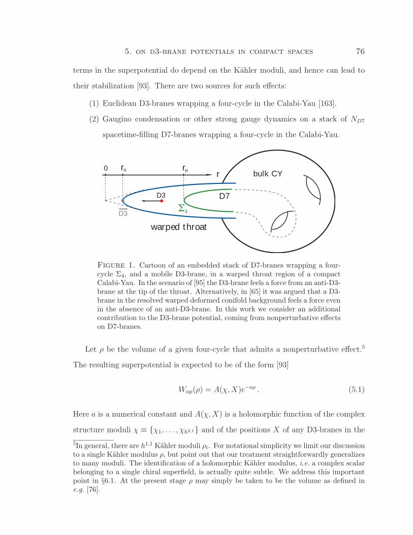
5. on d3-brane potentials in compact spaces 76
terms in the superpotential do depend on the Kahler moduli, and hence can lead to
their stabilization [93]. There are two sources for such effects:
(1) Euclidean D3-branes wrapping a four-cycle in the Calabi-Yau [163].
(2) Gaugino condensation or other strong gauge dynamics on a stack of ND7
spacetime-filling D7-branes wrapping a four-cycle in the Calabi-Yau.
bulk CY
warped throat
D7
r
D3
D3
rμr00
4Σ
Figure 1. Cartoon of an embedded stack of D7-branes wrapping a four-cycle Σ4, and a mobile D3-brane, in a warped throat region of a compactCalabi-Yau. In the scenario of [95] the D3-brane feels a force from an anti-D3-brane at the tip of the throat. Alternatively, in [65] it was argued that a D3-brane in the resolved warped deformed conifold background feels a force evenin the absence of an anti-D3-brane. In this work we consider an additionalcontribution to the D3-brane potential, coming from nonperturbative effectson D7-branes.
Let ρ be the volume of a given four-cycle that admits a nonperturbative effect.5
The resulting superpotential is expected to be of the form [93]
Wnp(ρ) = A(χ,X)e−aρ . (5.1)
Here a is a numerical constant and A(χ,X) is a holomorphic function of the complex
structure moduli χ ≡ χ1, . . . , χh2,1 and of the positions X of any D3-branes in the
5In general, there are h1,1 Kahler moduli ρi. For notational simplicity we limit our discussionto a single Kahler modulus ρ, but point out that our treatment straightforwardly generalizesto many moduli. The identification of a holomorphic Kahler modulus, i.e. a complex scalarbelonging to a single chiral superfield, is actually quite subtle. We address this importantpoint in §6.1. At the present stage ρ may simply be taken to be the volume as defined ine.g. [76].
5. on d3-brane potentials in compact spaces 77
internal space.6 The functional form of A will depend on the particular four-cycle in
question.
The prefactor A(χ,X) arises from a one-loop correction to the nonperturbative
superpotential. For a Euclidean D3-brane superpotential, A(χ,X) represents a one-
loop determinant of fluctuations around the instanton. In the case of D7-brane gauge
dynamics the prefactor comes from a threshold correction to the gauge coupling on
the D7-branes.
In the original KKLT proposal, the complex structure moduli acquired moderately
large masses from the fluxes, and no probe D3-brane was present. Thus, it was
possible to ignore the moduli-dependence of A(χ,X) and treat A as a constant, albeit
an unknown one. In the case of present interest (as in [95]), the complex structure
moduli are still massive enough to be negligible, but there is at least one mobile D3-
brane in the compact space, so we must write A = A(X). (See [71] for a very general
argument that no prefactor A can be independent of a D3-brane location X.)
The goal of this chapter is to compute A(X). As we explained in the introduction,
this has already been achieved in certain toroidal orientifolds [32], and the relevance
of A(X) for brane inflation has also been recognized [32, 95]. Here we will use a
closed-string channel method for computing A(X), allowing us to study more general
compactifications. In particular, we will give the first concrete results for A(X) in
the warped throats relevant for many brane inflation models.
2.2. D3-brane Potential After Volume Stabilization. The F-term part of
the supergravity potential is
VF = eκ2K[KijDiWDjW − 3κ2|W |2
], κ2 = M−2
pl = 8πG . (5.2)
6Strictly speaking, there are three complex fields, corresponding to the dimensionality ofthe internal space, but we will refer to a single field for notational convenience.

5. on d3-brane potentials in compact spaces 78
DeWolfe and Giddings [58] showed that the Kahler potential K in the presence of
mobile D3-branes is
κ2K = −3 ln[ρ+ ρ− γk(X, X)
]≡ −2 lnV , (5.3)
where k(X, X) is the Kahler potential for the Calabi-Yau metric, i.e. the Kahler
potential on the putative moduli space of a D3-brane probe, V is the physical volume
of the internal space, and γ is a constant.7 We address this volume-inflaton mixing in
more detail in §6.1. For clarity we have assumed here that there is only one Kahler
modulus, but our later analysis is more general.
The superpotential W is the sum of a constant flux term [82] Wflux(χ?) =∫G3 ∧
Ω ≡ W0 at fixed complex structure χ? and a term Wnp (5.1) from nonperturbative
effects,
W = W0 + A(X)e−aρ . (5.4)
Equations (7.13) to (7.14) imply three distinct sources for corrections to the po-
tential for D3-brane motion:
(1) mK: The X-dependence of the Kahler potential K leads to a mass term
familiar from the supergravity eta problem.
(2) mD: Sources of D-term energy, if present, will scale with the physical volume
V and hence depend on the D3-brane location. This leads to a mass term
for D3-brane displacements.
(3) mA: The prefactor A(X) in the superpotential (7.14) leads to a mass term8
via the F-term potential (7.13).
7In §6.1 we will find that γ ≡ 13κ
2T3, where T3 is the D3-brane tension.8After the appearance of [18] (Chapter 5) we realized in [19] (Chapter 7) that A(X) cannever lead to a pure mass term. We should therefore imagine a local definition of the massmA(X) as the second derivative of the potential. As indicated here (and proven in [19]) this‘mass’ will depend on the field value X. This is to be contrasted with mK and mD whichare constants.
5. on d3-brane potentials in compact spaces 79
The masses mK and mD were calculated explicitly in [95] and shown to be of
order the Hubble parameter H. On the other hand, mA has been computed only
for the toroidal orientifolds of [32]. It has been suggested [95] that there might exist
non-generic configurations in which mA cancels against the other two terms. It is in
these fine-tuned situations that D3-brane motion could produce slow-roll inflation.
By computing mA explicitly, one can determine whether or not this hope is realized
[19].
3. Warped Volumes and the Superpotential
3.1. The Role of the Warped Volume. The nonperturbative effects discussed
in §2.1 depend exponentially on the warped volume of the associated four-cycle: the
warped volume governs the instanton action in the case of Euclidean D3-branes, and
the gauge coupling in the case of strong gauge dynamics on D7-branes. To see this,
consider a warped background with the line element
ds2 = Gµνdxµdxν +GijdY
idY j ≡ h−1/2(Y )gµνdxµdxν + h1/2(Y )gijdY
idY j , (5.5)
where Y i and gij are the coordinates and the unwarped metric on the internal space,
respectively, and h(Y ) is the warp factor.
The Yang-Mills coupling g7 of the 7+1 dimensional gauge theory living on a stack
of D7-branes is given by9
g27 ≡ 2(2π)5gs(α
′)2 . (5.6)
The action for gauge fields on D7-branes that wrap a four-cycle Σ4 is
S =1
2g27
∫Σ4
d4ξ√gind h(Y ) ·
∫d4x√−g gµαgνβ TrFµνFαβ , (5.7)
where ξi are coordinates on Σ4 and gind is the metric induced on Σ4 from gij. A key
point is the appearance of a single power of h(Y ) [77]. Defining the warped volume
9In the notation of [139], g27 = 2g2
D7.

5. on d3-brane potentials in compact spaces 80
of Σ4,
V wΣ4≡∫
Σ4
d4ξ√gind h(Y ) , (5.8)
and recalling the D3-brane tension
T3 ≡1
(2π)3gs(α′)2, (5.9)
we read off the gauge coupling of the four-dimensional theory from (5.7):
1
g2=V w
Σ4
g27
=T3V
wΣ4
8π2. (5.10)
InN = 1 super-Yang-Mills theory, the Wilsonian gauge coupling is the real part of
a holomorphic function which receives one-loop corrections, but no higher perturba-
tive corrections [7, 143–145]. The modulus of the gaugino condensate superpotential
in SU(ND7) super-Yang-Mills with ultraviolet cutoff MUV is given by
|Wnp| = 16π2M3UV exp
(− 1
ND7
8π2
g2
)∝ exp
(−T3V
wΣ4
ND7
). (5.11)
The mobile D3-brane adds a flavor to the SU(ND7) gauge theory, whose mass m is a
holomorphic function of the D3-brane coordinates. In particular, the mass vanishes
when the D3-brane coincides with the D7-brane. In such a gauge theory, the superpo-
tential is proportional to m1/ND7 [91]. Our explicit closed-string channel calculations
will confirm this form of the superpotential.
In the case that the nonperturbative effect comes from a Euclidean D3-brane, the
instanton action is
S = T3
∫Σ4
d4ξ√Gind = T3
∫Σ4
d4ξ√gind h(Y ) ≡ T3V
wΣ4, (5.12)
so that, just as in (5.7), the action depends on a single power of h(Y ). The modulus
of the nonperturbative superpotential is then
|Wnp| ∝ exp(−T3V
wΣ4
). (5.13)

5. on d3-brane potentials in compact spaces 81
3.2. Corrections to the Warped Volumes of Four-Cycles. The displace-
ment of a D3-brane in the compactification creates a slight distortion δh of the warped
background, and hence affects the warped volumes of four-cycles. The correction takes
the form
δV wΣ4≡∫
Σ4
d4Y√gind(X;Y ) δh(X;Y ) . (5.14)
By computing this change in volume we will extract the dependence of the superpo-
tential on the D3-brane location X. In the non-compact throat approximation, we
will calculate δV wΣ4
explicitly, and find that it is the real part of a holomorphic func-
tion ζ(X).10 Its imaginary part is determined by the integral of the Ramond-Ramond
four-form perturbation δC4 over Σ4 (we will not compute this explicitly, but will be
able to deduce the result using the holomorphy of ζ(X)).
The nonperturbative superpotential of the form (5.1), generated by the gaugino
condensation, is then determined by
A(X) = A0 exp(−T3 ζ(X)
ND7
). (5.15)
We have introduced an unimportant constant A0 that depends on the values at which
the complex structure moduli are stabilized, but is independent of the D3-brane posi-
tion. As remarked above, computing (5.15) is equivalent to computing the dependence
of the threshold correction to the gauge coupling on the mass m of the flavor coming
from strings that stretch from the D7-branes to the D3-brane.
In the case of Euclidean D3-branes, the change in the instanton action is propor-
tional to the change in the warped four-cycle volume. Hence, the nonperturbative
10In the compact case, it is no longer true that δV wΣ4
is the real part of a holomorphicfunction. This is related to the ‘rho problem’ [32], and in fact leads to a resolution ofthe problem, as we shall explain in §6.1 (see also [77]). The result is that in terms of anappropriately-defined holomorphic Kahler modulus ρ (5.62), the holomorphic correction tothe gauge coupling coincides with the holomorphic result of our non-compact calculation.

5. on d3-brane potentials in compact spaces 82
superpotential is of the form (5.1) with
A(X) = A0 exp(−T3 ζ(X)
). (5.16)
In this case, computing (5.14) is equivalent to computing the D3-brane dependence
of an instanton fluctuation determinant.
Finally, we can write a unified expression that applies to both sources of nonper-
turbative effects:
A(X) = A0 exp(−T3 ζ(X)
n
), (5.17)
where n = ND7 for the case of gaugino condensation on D7-branes and n = 1 for the
case of Euclidean D3-branes.
4. D3-brane Backreaction
4.1. The Green’s Function Method. A D3-brane located at some position X
in a six-dimensional space with coordinates Y acts as a point source for a perturbation
δh of the geometry:
−∇2Y δh(X;Y ) = C
[δ(6)(X − Y )√
g(Y )− ρbg(Y )
]. (5.18)
That is, the perturbation δh is a Green’s function for the Laplace problem on the back-
ground of interest. Here C ≡ 2κ210T3 = (2π)4gs(α
′)2 ensures the correct normalization
of a single D3-brane source term relative to the four-dimensional Einstein-Hilbert ac-
tion. A consistent flux compactification contains a background charge density ρbg(Y )
which satisfies ∫d6Y√g ρbg(Y ) = 1 (5.19)
to account for the Gauss’s law constraint on the compact space [76].
To solve (5.18), we first solve
−∇2Y ′Φ(Y ;Y ′) = −∇2
Y Φ(Y ;Y ′) =δ(6)(Y − Y ′)√g
− 1
V6
, (5.20)

5. on d3-brane potentials in compact spaces 83
where V6 ≡∫
d6Y√g. The solution to (5.18) is then
δh(X;Y ) = C[Φ(X;Y )−
∫d6Y ′√gΦ(Y ;Y ′)ρbg(Y
′)]. (5.21)
We note for later use that
−∇2Xδh(X;Y ) = C
[δ(6)(X − Y )√
g(X)− 1
V6
]. (5.22)
This relation is independent of the form of the background charge ρbg.
To compute A(X) from (7.15), we simply solve for the Green’s function δh obeying
(5.18) and then integrate δh over the four-cycle of interest, according to (5.14).
4.2. Comparison with the Open-String Approach. Let us show that this
supergravity (closed-string channel) method is consistent with the results of BHK
[32], where the correction to the gaugino condensate superpotential was derived via
a one-loop open-string computation.11
The analysis of [32] applied to configurations of D7-branes and D3-branes on
certain toroidal orientifolds, e.g. T 2 × T 4/Z2. We introduce a complex coordinate X
for the position of the D3-branes on T 2, as well as a complex structure modulus τ
for T 2, and without loss of generality we set the volume of T 4/Z2 to unity. Let us
consider the case where all the D7-branes wrap T 4/Z2 and sit at the origin X = 0 in
T 2.
The goal is to determine the dependence of the gauge coupling on the position X
of a D3-brane. (The location of the D3-brane in the T 4/Z2 wrapped by the D7-branes
is immaterial.) For this purpose, we may omit terms computed in [32] that depend
only on the complex structure and not on the D3-brane location. Such terms will
only affect the D3-brane potential by an overall constant.
11Analogous pairs of closed-string and open-string computations exist in the literature,e.g. [17].

5. on d3-brane potentials in compact spaces 84
Then, the relevant terms from equation (44) of [32], in our notation12, are
δ(8π2
g2
)=
1
4π Im(τ)
[Im(X)
]2
− 1
2ln
∣∣∣∣ϑ1
(X
2π
∣∣∣τ)∣∣∣∣2 + . . . . (5.23)
Let us now compare (5.23) to the result of the supergravity computation. In
principle, the prescription of equation (5.14) is to integrate the Green’s function on
a six-torus over the wrapped four-torus. However, we notice that this procedure of
integration will reduce the six-dimensional Laplace problem to the Laplace problem
on the two-torus parametrized by X,
−∇2Xδh(X; 0) = C
[δ(2)(X)− 1
VT 2
], (5.24)
where VT 2 = 8π2 Im(τ). The correction to the gauge coupling, in the supergravity
approach, is then proportional to δh(X; 0). Solving (5.24) and using (5.10), we get
exactly (5.23). We conclude that our method precisely reproduces the results of [32],
at least for those terms that directly enter the D3-brane potential.
4.3. A Model for the Four-Cycles. The closed-string channel approach to
calculating A(X) is well-defined for any given background, but further assumptions
are required when no complete metric for the compactification is available. Fortu-
nately, explicit metrics are available for many non-compact Calabi-Yau spaces, and
at the same time, the associated warped throat regions are of particular interest
for inflationary phenomenology. For a given warped throat geometry, our approach
is to compute the D3-brane backreaction on specific four-cycles in the non-compact,
asymptotically conical space. We will demonstrate that this gives an excellent approx-
imation to the backreaction in a compactification in which the same warped throat
is glued into a compact bulk. In particular, we will show in §6.2 that the physical
effect in question is localized in the throat, i.e. is determined primarily by the shape
12After the replacement X → w, our definitions of the theta functions and torus coordinatescorrespond to those of [139]; our X differs from the A of [32] by a factor of 2π.

5. on d3-brane potentials in compact spaces 85
of the four-cycle in the highly warped region.13 The model therefore only depends on
well-known data, such as the specific warped metric and the embedding equations of
the four-cycles, and is insensitive to the unknown details of the unwarped bulk. In
principle, our method can be extended to general compact models for which metric
data is available.
It still remains to identify the four-cycles responsible for nonperturbative effects
in this model of a warped throat attached to a compact space. Such a space will in
general have many Kahler moduli, and hence, assuming that stabilization is possible
at all, will have many contributions to the nonperturbative superpotential. The most
relevant term, for the purpose of determining the D3-brane potential, is the term
corresponding to the four-cycle closest to the D3-brane. For a D3-brane moving in
the throat region, this is the four-cycle that reaches farthest down the throat. In
addition, the gauge theory living on the corresponding D7-branes should be making
an important contribution to the superpotential.
The nonperturbative effects of interest are present only when the four-cycle sat-
isfies an appropriate topological condition [163], which we will not discuss in detail.
This topological condition is, of course, related to the global properties of the four-
cycle, whereas the effect we compute is dominated by the part of the four-cycle in
the highly-warped throat region, and is insensitive to details of the four-cycle in the
unwarped region. That is, our methods are not sensitive to the distinction between
four-cycles that do admit nonperturbative effects, and those that do not. We therefore
propose to model the four-cycles producing nonperturbative effects with four-cycles
that are merely supersymmetric, i.e. can be wrapped supersymmetrically by D7-
branes. Many members of the latter class are not members of the former, but as
13To be precise, the physical effect is localized near the D3-brane, which may be taken to befar from the bulk, in the region where the throat is well-approximated by the non-compactmetric. This is also the region where the background warping is large.

5. on d3-brane potentials in compact spaces 86
the shape of the cycle in the highly-warped region is the only important quantity, we
expect this distinction to be unimportant.
We are therefore led to consider the backreaction of a D3-brane on the volume
of a stack of supersymmetric D7-branes wrapping a four-cycle in a warped throat
geometry. The simplest configuration of this sort is a supersymmetric ‘flavor brane’
embedding of several D7-branes in a conifold [9, 99, 133].
5. Backreaction in Warped Conifold Geometries
We now recall some relevant geometry. The singular conifold14 is a non-compact
Calabi-Yau threefold defined as the locus
4∑i=1
z2i = 0 (5.25)
in C4. After a linear change of variables (w1 = z1 + iz2, w2 = z1 − iz2, etc.), the
constraint (5.25) becomes
w1w2 − w3w4 = 0 . (5.26)
The Calabi-Yau metric on the conifold is
ds26 = dr2 + r2ds2
T 1,1 . (5.27)
The base of the cone is the T 1,1 coset space (SU(2)A×SU(2)B)/U(1)R whose metric
in angular coordinates θi ∈ [0, π], φi ∈ [0, 2π], ψ ∈ [0, 4π] is
ds2T 1,1 =
1
9
(dψ +
2∑i=1
cos θi dφi
)2
+1
6
2∑i=1
(dθ2
i + sin2 θi dφ2i
). (5.28)
14The KS geometry [105] and its generalizations [48] are warped versions of the deformedconifold, defined by
∑4i=1 z
2i = ε2. When the D3-branes and D7-branes are sufficiently far
from the tip of the deformed conifold, it will suffice to consider the simpler case of thewarped singular conifold constructed in [106].

5. on d3-brane potentials in compact spaces 87
A stack of N D3-branes placed at the singularity wi = 0 backreacts on the geom-
etry, producing the ten-dimensional metric
ds210 = h−1/2(r)dx2
4 + h1/2(r)ds26 , (5.29)
where the warp factor is
h(r) =27πgsN(α′)2
4r4. (5.30)
This is the AdS5 × T 1,1 background of type IIB string theory, whose dual N =
1 supersymmetric conformal gauge theory was constructed in [107]. The dual
is an SU(N) × SU(N) gauge theory coupled to bifundamental chiral superfields
A1, A2, B1, B2, each having R-charge 1/2. Under the SU(2)A × SU(2)B global sym-
metry, the superfields transform as doublets. If we further add M D5-branes wrapped
over the two-cycle inside T 1,1, then the gauge group changes to SU(N+M)×SU(N),
giving a cascading gauge theory [105, 106]. The metric remains of the form (5.29),
but the warp factor is modified to [106]
h(r) =27π(α′)2
4r4
[gsN + b(gsM)2 ln
( rr0
)+
1
4b(gsM)2
], (5.31)
with b ≡ 32π
, and r0 ∼ ε2/3e2πN/(3gsM). If an extra D3-brane is added at small r, it
produces a small change of the warp factor, δh = 27πgs(α′)2
4r4 + O(r−11/2). A precise
determination of δh on the conifold, using the Green’s function method, is one of
our goals in this chapter. As discussed above, this needs to be integrated over a
supersymmetric four-cycle.

5. on d3-brane potentials in compact spaces 88
5.1. Supersymmetric Four-Cycles in the Conifold. The complex coordi-
nates wi can be related to the real coordinates (r, θi, φi, ψ) via
w1 = r3/2ei2
(ψ−φ1−φ2) sinθ1
2sin
θ2
2, (5.32)
w2 = r3/2ei2
(ψ+φ1+φ2) cosθ1
2cos
θ2
2, (5.33)
w3 = r3/2ei2
(ψ+φ1−φ2) cosθ1
2sin
θ2
2, (5.34)
w4 = r3/2ei2
(ψ−φ1+φ2) sinθ1
2cos
θ2
2. (5.35)
It was shown in [9] that the following holomorphic four-cycles admit supersymmetric
D7-branes:15
f(wi) ≡4∏i=1
wpii − µP = 0 . (5.36)
Here pi ∈ Z, P ≡∑4
i=1 pi, and µ ∈ C are constants defining the embedding of the
D7-branes. In real coordinates the embedding condition (5.36) becomes
ψ(φ1, φ2) = n1φ1 + n2φ2 + ψs , (5.37)
r(θ1, θ2) = rmin
[x1+n1(1− x)1−n1y1+n2(1− y)1−n2
]−1/6, (5.38)
where
r3/2min ≡ |µ| , (5.39)
1
2ψs ≡ arg(µ) +
2πs
P, s ∈ 0, 1, . . . , P − 1 . (5.40)
We have defined the coordinates
x ≡ sin2 θ1
2, y ≡ sin2 θ2
2(5.41)
15This is not an exhaustive list: another holomorphic embedding was used in [114].

5. on d3-brane potentials in compact spaces 89
and the rational winding numbers
n1 ≡p1 − p2 − p3 + p4
P, n2 ≡
p1 − p2 + p3 − p4
P. (5.42)
To compute the integral over the four-cycle we will need the volume form on the
wrapped D7-brane, which is
dθ1dθ2dφ1dφ2
√gind =
VT 1,1
16π3r4 G(x, y) dxdydφ1dφ2 , (5.43)
where
G(x, y) ≡ (1 + n1)2
2
1
x(1− x)− 2n1
1
1− x
+(1 + n2)2
2
1
y(1− y)− 2n2
1
1− y− 1 . (5.44)
In (5.43) we defined the volume of T 1,1
VT 1,1 ≡∫
d5Ψ√gT 1,1 =
16π3
27, (5.45)
with Ψ standing for all five angular coordinates on T 1,1.
For applications to brane inflation, we are interested in four-cycles that do not
reach the tip of the conifold (|ni| ≤ 1). This condition is obeyed when the pi are
nonnegative, and we shall restrict to this case for the remainder of the chapter. Two
particularly simple special cases of (5.36) are:
Ouyang embedding [133]: w1 = µ .
Karch-Katz embedding [99]: w1w2 = µ2 .
Analogous supersymmetric four-cycles are known [50] in some more complicated
asymptotically conical spaces, such as cones over Y p,q manifolds. We will consider
this case in §5.4 and in Appendix D.

5. on d3-brane potentials in compact spaces 90
5.2. Relation to the Dual Gauge Theory Computation. The calculation of
δh and its integration over a holomorphic four-cycle is not sensitive to the background
warp factor. Let us discuss a gauge theory interpretation of the calculation when
we choose the background warp factor from (5.30), i.e. we ignore the effect of M
wrapped D5-branes. Here the gauge theory is exactly conformal, and we may invoke
the AdS/CFT correspondence to give a simple meaning to the multipole expansion
of δh,
δh =27πgs(α
′)2
4r4
[1 +
∑i
cifi(θ1, θ2, φ1, φ2, ψ)
r∆i
]. (5.46)
In the dual gauge theory, the ci are proportional to the expectation values of gauge-
invariant operators Oi determined by the position of the D3-brane [108]. Among
these operators a special role is played by the chiral operators of R-charge k,
Tr[Aα1Bβ1Aα2Bβ2
. . . AαkBβk], symmetric in both the dotted and the undotted indices.
These operators have exact dimensions ∆chirali = 3k/2 and transform as (k/2, k/2) un-
der the SU(2)A×SU(2)B symmetry. In addition to these operators, many non-chiral
operators, whose dimensions ∆i are not quantized [81], acquire expectation values
and therefore affect the multipole expansion of the warp factor. But remarkably, all
these non-chiral contributions vanish upon integration over a holomorphic four-cycle.
Therefore, the contributing terms in δh have the simple form [108]
δhchiral =27πgs(α
′)2
4r4
[1 +
∞∑k=1
(fa1...ak za1...ak + c.c.)
r3k/2
], (5.47)
where fa1...ak ∼ εa1 εa2 . . . εak for a D3-brane positioned at za = εa. Above, za1...ak are
the normalized spherical harmonics on T 1,1 that transform as (k/2, k/2) under the
SU(2)A × SU(2)B. The normalization factors are defined in Appendix B.
The leading term in (5.46), which falls off as 1/r4, gives a logarithmic divergence
at large r when integrated over a four-cycle. We note that this term does not appear if
we define δh as the solution of (5.18) with√g ρbg(Y ) = δ(6)(Y −X0). This corresponds
to evaluating the change in the warp factor, δh, created by moving the D3-brane to

5. on d3-brane potentials in compact spaces 91
X from some reference point X0. If we choose the reference point X0 to be at the tip
of the cone, r = 0, then (5.46) is modified to
δh =27πgs(α
′)2
4r4
[∑i
cifi(θ1, θ2, φ1, φ2, ψ)
r∆i
]. (5.48)
An advantage of this definition is that now there is a precise correspondence between
our calculation and the expectation values of operators in the dual gauge theory.
5.3. Results for the Conifold. We are now ready to compute the D3-brane-
dependent correction to the warped volume of a supersymmetric four-cycle in the
conifold. Using the Green’s function on the singular conifold (B.9), which we derive
in Appendix B, and the explicit form of the induced metric√gind (5.43), we carry
out integration term by term and find that most terms in (5.14) do not contribute.
We relegate the details of this computation to Appendix C. As we demonstrate
in Appendix C, the terms that do not cancel are precisely those corresponding to
(anti)chiral deformations of the dual gauge theory.
Integrating (5.48) term by term as prescribed in (5.14), we find that the final
result for a general embedding (5.36) is
T3 δVw
Σ4= T3 Re (ζ(wi)) = −Re
(ln
[µP −
∏4i=1 w
pii
µP
]), (5.49)
so that
A = A0
(µP −
∏4i=1 w
pii
µP
)1/n
. (5.50)
Comparing to (5.36), we see that A is proportional to a power of the holomorphic
equation that specifies the embedding. For n = ND7 coincident D7-branes, this power
is 1/n. This behavior agrees with the results of [71]; note in particular that when
n = 1, (5.50) has a simple zero everywhere on the four-cycle, as required by [71].
Finally, let us specialize to the two cases of particular interest, the Ouyang [133]
and Karch-Katz [99] embeddings in which the four-cycle does not reach all the way

5. on d3-brane potentials in compact spaces 92
to the tip of the throat. For the Ouyang embedding we find
A(w1) = A0
(µ− w1
µ
)1/n
, (5.51)
whereas for the Karch-Katz embedding we have
A(w1, w2) = A0
(µ2 − w1w2
µ2
)1/n
. (5.52)
5.4. Results for Y p,q Cones. Recently, a new infinite class of Sasaki-Einstein
manifolds Y p,q of topology S2×S3 was discovered [73, 74]. TheN = 1 superconformal
gauge theories dual to AdS5 × Y p,q were constructed in [30]. These quiver theories,
which live on N D3-branes at the apex of the Calabi-Yau cone over Y p,q, have gauge
groups SU(N)2p, bifundamental matter, and marginal superpotentials involving both
cubic and quartic terms. Addition of M D5-branes wrapped over the S2 at the
apex produces a class of cascading gauge theories whose warped cone duals were
constructed in [86]. A D3-brane moving in such a throat could also serve as a model
of D-brane inflation [65].
Having described the calculation for the singular conifold in some detail, we now
cite the results of an equivalent computation for cones over Y p,q manifolds. More
details can be found in Appendix D.
Supersymmetric four-cycles in Y p,q cones are defined by the following embedding
condition [50]
f(wi) ≡3∏i=1
wpii − µ2p3 = 0 , (5.53)
where the complex coordinates wi are defined in Appendix D. Integration of the
Green’s function over the four-cycle leads to the following result for the perturbation
to the warped volume
T3 δVw
Σ4= T3 Re (ζ(wi)) = −Re
(ln
[µ2p3 −
∏3i=1w
pii
µ2p3
]), (5.54)

5. on d3-brane potentials in compact spaces 93
so that
A = A0
(µ2p3 −
∏3i=1w
pii
µ2p3
)1/n
. (5.55)
5.5. General Compactifications. The arguments in [71], which were based on
studying the change in the theta angle as one moves the D3-brane around the D7-
branes, indicate that the correction is a section of a bundle called the ‘divisor bundle’.
This section has a zero at the location of the D7-branes. The correction has to live
in a non-trivial bundle since a holomorphic function on a compact space would be
a constant. In the non-compact examples we considered above we can work in only
one coordinate patch and obtain the correction as a simple function, the function
characterizing the embedding. Strictly speaking, the arguments in [71] were made
for the case that the superpotential is generated by wrapped D3-instantons. But the
same arguments can be used to compute the correction for the gauge coupling on
D7-branes.
In summary, we have explicitly computed the modulus of A, and found a result
in perfect agreement with the analysis of the phase of A in [71]. One has a general
answer of the form
A(wi) = A0
(f(wi)
)1/n
, (5.56)
where f is a section of the divisor bundle and f(wi) = 0 specifies the location of the
D7-branes.
6. Compactification Effects
6.1. Holomorphy of the Gauge Coupling. In compactifications with mobile
D3-branes, the identification of holomorphic Kahler moduli and holomorphic gauge
couplings is quite subtle. This has become known as the ‘rho problem’ [32].16 Let us
recall the difficulty. In the internal metric gij appearing in (5.5), we can identify the
16Similar issues were discussed in [162].

5. on d3-brane potentials in compact spaces 94
breathing mode of the compact space via
ds2 = h−1/2(Y )e−6ugµνdxµdxν + h1/2(Y )e2ugijdY
idY j . (5.57)
Here gij is a fiducial metric for the internal space, e2u is the breathing mode, and gµν is
the four-dimensional Einstein-frame metric. In the following, all quantities computed
from gij will be denoted by a tilde. The Born-Infeld kinetic term for a D3-brane,
expressed in Einstein frame and in terms of complex coordinates X, X on the brane
configuration space, is then
Skin = −T3
∫d4x√−ge−4u∂µX
i∂µX j gij . (5.58)
DeWolfe and Giddings argued in [58] that to reproduce this volume scaling, as well as
the known no-scale, sequestered property of the D3-brane action in this background,
the Kahler potential must take the form
κ2K = −3 ln e4u , (5.59)
with the crucial additional requirement that
∂i∂je4u ∝ gij , (5.60)
so that e4u contains a term proportional to the Kahler potential k(X, X) for the
fiducial Calabi-Yau metric. Comparing (5.58) to the kinetic term derived from (5.59),
we find in fact
∂i∂je4u = −
(κ2T3
3
)k,ij . (5.61)
We can now define the holomorphic volume modulus ρ as follows. The real part of ρ
is given by
ρ+ ρ ≡ e4u +
(κ2T3
3
)k(X, X) (5.62)

5. on d3-brane potentials in compact spaces 95
and the imaginary part is the axion from the Ramond-Ramond four-form potential.
As explained in [95], this is consistent with the fact that the axion moduli space is a
circle that is non-trivially fibered over the D3-brane moduli space.
Next, the gauge coupling on a D7-brane is easily seen to be proportional to the
breathing mode of the metric, e4u ≡ ρ + ρ −(
13κ2T3
)k(X, X), which is not the real
part of a holomorphic function on the brane moduli space. However, supersymmetry
requires that the gauge kinetic function is a holomorphic function of the moduli. This
conflict is the rho problem.
We can trace this problem to an incomplete inclusion of the backreaction due to
the D3-brane. Through (5.62), the physical volume modulus e4u has been allowed to
depend on the D3-brane position. That is, the difference between the holomorphic
modulus ρ and the physical modulus e4u is affected by the D3-brane position. This
was necessary in order to recover the known properties of the brane/volume moduli
space. Notice from (5.62) that the strength of this open-closed mixing is controlled
by κ2T3, and so is manifestly a consequence of D3-brane backreaction in the compact
space. However, as we explained in §3, the warp factor h also depends on the D3-
brane position, again via backreaction. To include the effects of the brane on the
breathing mode, but not on the warp factor, is not consistent.17 One might expect
that consideration of the correction δh to the warp factor would restore holomorphy
and resolve the rho problem. This was suggested in [77], and we now carry out an
explicit calculation that confirms this.
What we find is that the uncorrected warped volume (V wΣ4
)0, as well as the cor-
rection δV wΣ4
, are both non-holomorphic, but their non-holomorphic pieces precisely
cancel, so that the corrected warped volume V wΣ4
is the real part of a holomorphic
function of the moduli ρ and X.
17Let us point out that this is precisely the closed-string dual of the resolution found in [32]:careful inclusion of the open-string one-loop corrections to the gauge coupling resolved therho problem. In that language, the initial inconsistency was the inclusion of only some ofthe one-loop effects.

5. on d3-brane potentials in compact spaces 96
First, we separate the constant, zero-mode, piece of the warp factor:
h(X;Y ) = h0 + δh(X;Y ) . (5.63)
By definition δh(X;Y ) integrates to zero over the compact manifold,∫d6Y
√g(Y ) δh(X;Y ) = 0 . (5.64)
This implies that the factor of the volume that appears in the four-dimensional New-
ton constant is unaffected by δh. Thus we have κ−2 = κ−210 h0V6. We define the
uncorrected warped volume via
(V wΣ4
)0 ≡∫
Σ4
d4ξ√gind h0 = e4u(X,X) h0 VΣ4 . (5.65)
This is non-holomorphic because of the prefactor e4u(X,X). In particular, using (5.62),
we have
(V wΣ4
)0 = −(κ2T3
3
)VΣ4 h0 k(X, X) + [hol.+ antihol.] . (5.66)
We next consider δh. When the D3-brane is not coincident with the four-cycle of
interest, we find from (5.22) that δh obeys
∇2Xδh(X;Y ) =
CV6
(5.67)
where C ≡ 2κ210T3 = 2κ2T3h0V6. Hence, δh is not the real part of a holomorphic
function of X. The source of the deviation from holomorphy is the term 1V6
in (5.22).
Although this term is superficially similar to a constant background charge density, it
is independent of the density ρbg(Y ) of physical D3-brane charge in the internal space,
which has coordinates Y . Instead, 1V6
may be thought of as a ‘background charge’
on the D3-brane moduli space, which has coordinates X. From this perspective,
it is the Gauss’s law constraint on the D3-brane moduli space that forces δh to be
non-holomorphic.
5. on d3-brane potentials in compact spaces 97
In complex coordinates, using the metric g, and noting that V6 = V6 e−6u, (5.67)
may be written as
gij∂i∂jδh = κ2T3 h0 e−4u , (5.68)
where because the compact space is Kahler, we can write the Laplacian using partial
derivatives. It follows that, to leading order in κ2,
δh =
(κ2T3
3
)h0 e
−4uk(X, X) + [hol.+ antihol.] . (5.69)
The omitted holomorphic and antiholomorphic terms are precisely those that we
computed in the preceding sections. Furthermore, recalling the definition (5.14), we
have
δV wΣ4
=
(κ2T3
3
)h0 VΣ4k(X, X) + [ζ(X) + ζ(X)] . (5.70)
The non-holomorphic first term in (5.70) precisely cancels the non-holomorphic term
in (V wΣ4
)0 (5.66), so that
V wΣ4
= (V wΣ4
)0 + δV wΣ4
= VΣ4 h0 (ρ+ ρ) + [ζ(X) + ζ(X)] . (5.71)
We conclude that V wΣ4
can be the real part of a holomorphic function.18 This sup-
ports the role of the warped four-volume in the definition of holomorphic coordinates
proposed in [77].
To summarize, we have seen that the background charge term in (5.22), which
was required by a constraint analogous to Gauss’s law on the D3-brane moduli space,
causes δV wΣ4
to have a non-holomorphic term proportional to k(X, X). Furthermore,
the DeWolfe-Giddings Kahler potential produces a well-known non-holomorphic term,
also proportional to k(X, X), in the uncorrected warped volume (V wΣ4
)0. We found
that these two terms precisely cancel, so that the total warped volume V wΣ4
= (V wΣ4
)0 +
18Strictly speaking, we have shown only that V wΣ4
is in the kernel of the Laplacian; ther.h.s. of (5.69) and (5.71) could in principle contain extra terms that are annihilated by theLaplacian but are not the real parts of holomorphic functions. However, the obstruction toholomorphy presented by k(X, X) has disappeared, and we expect no further obstructions.

5. on d3-brane potentials in compact spaces 98
δV wΣ4
can be holomorphic. Thus, the corrected gauge coupling on D7-branes, and the
corrected Euclidean D3-brane action, are holomorphic.19
Note that, as a consequence of this discussion, the holomorphic part of the correc-
tion to the volume changes under Kahler transformations of k(X, X). This implies
that the correction is in a bundle whose field strength is proportional to the Kahler
form.
6.2. Model-Dependent Effects from the Bulk. In §2.2, we listed three con-
tributions to the potential for D3-brane motion. The first two were given explicitly in
[95], and we have computed the third. It is now important to ask whether this is an
exhaustive list: in other words, might there be further effects that generate D3-brane
mass terms of order H? In particular, could coupling of the throat to a compact bulk
generate corrections to our results, and hence adjust the brane potential?20
First, let us justify our approach of using noncompact warped throats to model
D3-brane potentials in compact spaces with finite warped throat regions. The idea
is that the effect of the D3-brane on a four-cycle is localized in that portion of the
four-cycle that is deepest in the throat. Comparing (5.43) to (5.48), we see that all
corrections to the warped volume scale inversely with r, and are therefore supported
in the infrared region of the throat. Hence, as anticipated in §4.3, the effects of interest
are automatically concentrated in the well-understood region of high warping, far from
the model-dependent region where the throat is glued into the rest of the compact
space. This is true even though a typical four-cycle will have most of its volume in
the bulk, outside the highly warped region. The perturbation due to the D3-brane
already falls off faster than r−4 in the throat, where the measure factor is r4, and
in the bulk the perturbation will diminish even more rapidly. Except in remarkable
19To complete the identification of the holomorphic variable, we note that the constant aappearing in (5.1) is a ≡ 2T3VΣ4h0/n. The resulting dependence on gs could be absorbedby a redefinition of ρ, as in [93].20The bulk corrections considered in [1] are generically smaller than those we consider here.

5. on d3-brane potentials in compact spaces 99
cases, the diminution of the perturbation will continue to dominate the growth of
the measure factor. A similar argument reinforces our assertion that the dominant
effect on a D3-brane comes from whichever wrapped brane descends farthest into the
throat.
We conclude that the effects of the gluing region, where the throat meets the bulk,
and of the bulk itself, produce negligible corrections to the terms we have computed.
Fortunately, the leading effects are concentrated in the highly warped region, where
one has access to explicit metrics and can do complete computations.
We have now given a complete account of the nonperturbative superpotential.
However, the Kahler potential is not protected against perturbative corrections, which
could conceivably contribute to the low-energy potential for D3-brane motion. Ex-
plicit results are not available for general compact spaces (see, however, [33, 75]);
here we will simply argue that these corrections can be made subleading. Recall
that the DeWolfe-Giddings Kahler potential provides a mixing between the volume
and the D3-brane position that generates brane mass terms of order H. Any fur-
ther corrections to the Kahler potential, whether from string loops or sigma-model
loops, will be subleading in the large-volume, weak-coupling limit, and will therefore
generically give mass terms that are small compared to H. In addition, the results of
[70] give some constraints on α′ corrections to warped throat geometries. We leave a
systematic study of this question for the future.
7. Implications and Conclusion
We have used a supergravity approach (see also [77]) to study the D3-brane cor-
rections to the nonperturbative superpotential induced by D7-branes or Euclidean
D3-branes wrapping four-cycles of a compactification. This has been a key, unknown
element of the potential governing D3-brane motion in such a compactification. We
integrated the perturbation to the background warping due to the D3-brane over
the wrapped four-cycle. The resulting position-dependent correction to the warped

5. on d3-brane potentials in compact spaces 100
four-cycle volume modifies the strength of the nonperturbative effect, which in turn
implies a force on the D3-brane. This computation is the closed-string channel dual
of the threshold correction computation of [32], and we showed that the closed-string
method efficiently reproduces the results of [32].
We then investigated the D3-brane potential in explicit warped throat back-
grounds with embedded wrapped branes. We showed that for holomorphic embed-
dings, only those deformations corresponding to (anti)chiral operators in the dual
gauge theory contribute to correcting the superpotential. This led to a strikingly
simple result: the superpotential correction is given by the embedding condition for
the wrapped brane, in accord with [71].
An important application of our results is to cosmological models with moving
D3-branes, particularly warped brane inflation models [95]. It is well-known that
these models suffer from an eta problem and hence produce substantial inflation
only if the inflaton mass term is fine-tuned to fall in a certain range. Our result
determines a ‘missing’ contribution to the inflaton potential that was discussed in
[95], but was not computed there. Equipped with this contribution, one can quantify
the fine-tuning in warped brane inflation by considering specific choices of throat
geometries and of embedded wrapped branes, and determining whether prolonged
inflation occurs [19]. This amounts to a microscopically justified method for selecting
points or regions within the phenomenological parameter space described in [69]. This
approach was initiated in [32], but the open-string method used there does not readily
extend beyond toroidal orientifolds, and is especially difficult for warped throats in
flux compactifications. In contrast, our concrete computations were performed in
warped throat backgrounds, and thus apply directly to warped brane inflation models,
including backgrounds with fluxes.
Our approach also led to an explicit solution of the ‘rho problem’, i.e. the apparent
non-holomorphy of the gauge coupling on wrapped D7-branes in backgrounds with

5. on d3-brane potentials in compact spaces 101
D3-branes. This problem arises from incomplete inclusion of D3-brane backreaction
effects, and in particular from omission of the correction to the warped volume that
we computed in this work. We observed that the correction is itself non-holomorphic,
as a result of a Gauss’s law constraint on the D3-brane moduli space. Moreover,
the non-holomorphic correction cancels precisely against the non-holomorphic term
in the uncorrected warped volume, leading to a final gauge kinetic function that is
holomorphic.
Let us emphasize that the problem of fine-tuning in D-brane inflation models has
not disappeared, but can now be made more explicit. A detailed analysis of this will
be presented in Chapters 6 and 7.

CHAPTER 6
Compactification Obstacles to D-brane Inflation
We proceed by analyzing the cosmological implications of the results of the pre-
vious chapter. This chapter summarizes our findings,1 while in the next chapter we
present more technical aspects of our computations.
1. Introduction
String theory is a promising candidate for the theoretical underpinning of the
inflationary paradigm [3, 83, 120], but explicit and controllable models of inflation in
string theory have remained elusive. In this chapter we ask whether explicit working
models are possible in the setting of slow-roll warped D-brane inflation [64, 95], in
which the inflaton field is identified with the location of a mobile D3-brane in a warped
throat region [105] of the compactification manifold. As explained in Chapter 5,
moduli stabilization introduces potentially fatal corrections to the inflaton potential
in this scenario. Some of these corrections arise from complicated properties of the
compactification [32] and have been computed only recently [18].
The attitude taken in most of the literature on the subject (cf. [95, 118]) is that
because of the vast number and complexity of string vacua, in some nonzero fraction
of them it should be the case that the different corrections to the inflaton potential
cancel to high precision, leaving a suitable inflationary model. This expectation or
1This chapter is based on Daniel Baumann, Anatoly Dymarsky, Igor Klebanov, Liam McAl-lister and Paul Steinhardt, “A Delicate Universe: Compactification Obstacles to D-braneInflation”, Phys. Rev. Lett. 99, 141601 (2007).
102

6. compactification obstacles to d-brane inflation 103
hope has never been rigorously justified, and there is no guarantee that the correction
terms can ever cancel: for example, it may be the case that the correction terms
invariably have the same sign, so that no cancellation can occur. In this chapter
we report the results of a systematic investigation into whether or not this hope of
fine-tuned cancellation can in fact be realized. While this chapter is a non-techincal
summary of our conclusions, all the technical subtleties that we had to consider are
carefully spelt out in Chapter 7.
The new ingredient that makes this work possible is the result of [18] for a correc-
tion to the volume-stabilizing nonperturbative superpotential. As explained in Chap-
ter 5, this effect corresponds to the interaction between the inflationary D3-brane and
the moduli-stabilizing wrapped branes, i.e. D7-branes or Euclidean D3-branes wrap-
ping a four-cycle of the Calabi-Yau. The location of these wrapped branes therefore
becomes a crucial parameter in the D3-brane potential.
In a recent paper [45], Burgess et al. showed that for a particular embedding of
the D7-branes, the Ouyang embedding [133], the correction to the inflaton potential
from the term computed in [18] vanishes identically. In this case the potential is al-
ways too steep for inflation, independent of fine-tuning. Here, we consider a different
holomorphic embedding due to Kuperstein [114]. For fine-tuned values of the micro-
physical parameters, the potential for radial motion of a D3-brane in this background
contains an approximate inflection point around which slow-roll inflation can occur.
This potential is not of the form anticipated by previous authors: the D7-brane has
no effect whatsoever on the quadratic term in the inflaton potential, but instead
causes the potential to flatten in a small region far from the tip of the conifold. We
emphasize that arranging for this inflection point to occur inside the throat region,
where the metric is known and our construction is self-consistent, imposes a severe
constraint on the compactification parameters. Moreover, inflation only occurs for

6. compactification obstacles to d-brane inflation 104
a bounded range about the inflection point, which requires a high degree of control
over the initial conditions of the inflaton field.
2. The Compactification
Our setting is a flux compactification [63, 76] of type IIB string theory on an
orientifold of a Calabi-Yau threefold, or, more generally, an F-theory compactification.
We suppose that the fluxes are chosen so that the internal space has a warped throat
region, and that n > 1 D7-branes supersymmetrically wrap a four-cycle that extends
into this region (see Figure 1 in Chapter 5). As a concrete example of this local
geometry, we consider the warped version [105] of the deformed conifold∑z2i = ε2,
where zi are coordinates on C4. Assuming that the D3-brane is far from the tip of the
conifold, we may neglect the deformation ε. We choose zα = (z1, z2, z3) as the three
independent complex D3-brane coordinates, and use the conifold constraint to express
z4 in terms of them. We suppose that this throat is glued into a compact space, as in
[76], and for simplicity we take this space to have a single Kahler modulus ρ. Moduli
stabilization [93] relies on the fact that strong gauge dynamics on suitable D7-branes
generates a nonperturbative superpotential, Wnp = A(zα) exp[−aρ], where a = 2πn
.
The D7-brane embedding is specified by a single holomorphic equation, f(zα) = 0,
and the result of [18] is that
A(zα) = A0
(f(zα)
f(0)
)1/n
, (6.1)
whereA0 is independent of the D3-brane position zα. Including the flux superpotential
[82] Wflux =∫G3 ∧ Ω ≡ W0, the total superpotential is W = W0 + A(zα) exp[−aρ].
The DeWolfe-Giddings Kahler potential [58] is2
K(ρ, ρ, zα, zα) = −3 ln[ρ+ ρ− γk] ≡ −3 lnU , (6.2)
2In this chapter, we employ natural units where M−2pl = 8πG ≡ 1.

6. compactification obstacles to d-brane inflation 105
where k(zα, zα) is the Kahler potential of the Calabi-Yau space, and γ is a constant
[19]. Well inside the throat but far from the tip, we may use the Kahler potential of
the conifold [49],
k =3
2
(4∑i=1
|zi|2)2/3
=3
2r2 . (6.3)
Then the F-term potential is [19, 45]
VF =1
3U2
[(ρ+ ρ)|W,ρ|2 − 3(WW,ρ + c.c.)
+3
2(W,ρz
αW,α + c.c.) +1
γkαβW,αW,β
], (6.4)
where
kαβ = r
[δαβ +
1
2
zαzβr3− zβ zα
r3
]. (6.5)
To this we add the contribution of an anti-D3-brane at the tip of the deformed conifold
[95],
VD = D(r)U−2 , D(r) ≡ D
(1− 3D
16π2
1
(T3r2)2
), (6.6)
where D = 2T3/h0, T3 is the D3-brane tension, and h0 is the KS warp factor at the tip.
3. Towards Fine-Tuned Inflation
To derive the effective single-field potential, we consider radial trajectories that
are stable in the angular directions, so that the dynamics of the angular fields be-
comes trivial. We also integrate out the massive volume modulus, incorporating the
crucial fact that the volume shifts as the D3-brane moves [19]. Then the canonically
normalized inflaton field φ = r√
32T3 parameterizes the motion along the radial di-
rection of the throat. To investigate the possibility of sustained inflation, we consider
the slow-roll parameter η = V ′′/V . We find η = 23
+ ∆η(φ), where ∆η arises from
the dependence (6.1) of the superpotential on φ. Slow-roll inflation is possible near

6. compactification obstacles to d-brane inflation 106
φ = φ0 if ∆η(φ0) ≈ −23. Here, using the explicit result of [18] for A(φ), we compute
∆η and determine whether the full potential can be flat enough for inflation.3
A reasonable expectation implicit in prior work on the subject is that there exist
fine-tuned values of the microphysical parameters for which ∆η(φ) ≈ −23, i.e. the
correction to the inflaton potential arising from A(φ) includes a term quadratic in φ,
which, for a fine-tuned value of its coefficient, causes η to be small for a considerable
range of φ. However, we make the important observation that the functional form
of (6.1) implies that there is actually no purely quadratic correction. To see this we
note that A is a holomorphic function of the zα coordinates, which, by (6.3), scale
with radius as zα ∝ φ3/2. Thus, the presence of A(φ) in the form (6.1) does not lead
to new quadratic terms in (7.13). This is concrete evidence against the hope of a
fine-tuned cancellation of the inflaton mass over an extended range of φ.
However, as we now explain, there exists a simple example in which a different
sort of cancellation can occur. Kuperstein [114] studied the D7-brane embedding
z1 = µ, where we may assume that µ ∈ R+. This embedding, and the potential in this
background, preserve an SO(3) subgroup of the SO(4) global symmetry acting on the
zi coordinates of the deformed conifold. To find a purely radial trajectory that is stable
in the angular directions, we consider the variation δz1 while keeping the radius r fixed.
We then require the first variation of the potential δV = V (z1 + δz1, r, ρ)−V (z1, r, ρ)
to vanish for all r and the second variation δ2V to be non-negative. The extremality
constraint δV = 0 specifies the radial trajectory z1 = ± 1√2r3/2, z2 = ±iz1. A detailed
study of the angular mass matrix δ2V reveals that the trajectory along z1 = + 1√2r3/2
is unstable, while the potential along the negative axis, z1 = − 1√2r3/2, is stable in all
angular directions. After integrating out the imaginary part of the Kahler modulus
3For the special case of the Ouyang embedding, z1 + iz2 = µ, Burgess et al. proved asimple no-go result for fine-tuned brane inflation [45]. They found that for this particularexample, ∆η vanishes along the angularly stable trajectory. We have found similar ‘delta-flat’ trajectories [19] for all embeddings in the infinite class studied in [9]. These trajectoriescannot support slow-roll inflation, no matter how the parameters of the potential are tuned.Here, we study an embedding for which there is no delta-flat direction.

6. compactification obstacles to d-brane inflation 107
ρ, the potential is given in terms of the radius r (or the canonical inflaton φ) and the
real-valued volume modulus σ ≡ 12(ρ+ ρ), as [19]
V (φ, σ) =a|A0|2
3
e−2aσ
U2(φ, σ)g(φ)2/n
[2aσ + 6− 6eaσ
|W0||A0|
1
g(φ)1/n+
3c
n
φ
φµ
1
g(φ)2
− 3
n
1
g(φ)
φ3/2
φ3/2µ
]+
D(φ)
U2(φ, σ). (6.7)
Here g(φ) ≡ f(φ)f(0)
= 1 +(φφµ
)3/2, and φ2
µ ≡ T3(2µ2)2/3 denotes the minimal radial
location of the D7-branes. We have also introduced c−1 ≡ 4πγ(2µ2)2/3, used [19]
γ = σ0T3/3, and defined U(φ, σ) ≡ 2σ − σ0
3φ2. The parameter σ0 is the stabilized
value of the Kahler modulus in the absence of the D3-brane (or when the D3-brane is
near the bottom of the throat). Now, for each value of φ we carry out a constrained
minimization of the potential to find σ?(φ), i.e. we find σ?(φ) such that ∂V∂σ
∣∣σ?(φ)
= 0.
The function σ?(φ) may either be computed numerically or fitted to high accuracy
by the approximate expression [19]
σ?(φ) ≈ σ0
[1 +
1
n aσ0
(1− 1
2aσ0
)(φ
φµ
)3/2]. (6.8)
Substituting σ?(φ) into (6.7), we find the effective single-field potential V(φ) ≡
V (φ, σ?(φ)).
For generic values of the compactification parameters, V has a metastable min-
imum at some distance from the tip. In fact, one can show that the potential has
negative curvature near the tip and positive curvature far away, so that by continuity,
η vanishes at some intermediate value φ0. Then, one can find fine-tuned values of the
D7-brane position φµ for which this minimum is lifted to become an inflection point
(see Figure 2). This transition from metastability to monotonicity guarantees that
ε = 12(V ′/V )2 can be made extremely small, so that prolonged slow-roll inflation is
possible. In our scenario, then, the potential contains an approximate inflection point
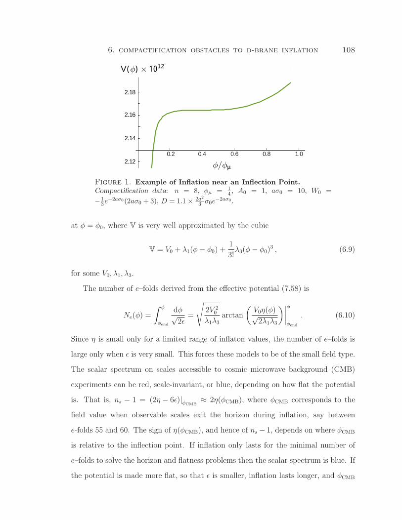
6. compactification obstacles to d-brane inflation 108
2.18
2.16
2.14
2.12 0.2 0.4 0.6 0.8 1.0
V(φ) × 1012
φ/φµ
Figure 1. Example of Inflation near an Inflection Point.Compactification data: n = 8, φµ = 1
4 , A0 = 1, aσ0 = 10, W0 =−1
3e−2aσ0(2aσ0 + 3), D = 1.1× 2a2
3 σ0e−2aσ0 .
at φ = φ0, where V is very well approximated by the cubic
V = V0 + λ1(φ− φ0) +1
3!λ3(φ− φ0)3 , (6.9)
for some V0, λ1, λ3.
The number of e–folds derived from the effective potential (7.58) is
Ne(φ) =
∫ φ
φend
dφ√2ε
=
√2V 2
0
λ1λ3
arctan
(V0η(φ)√
2λ1λ3
)∣∣∣∣φφend
. (6.10)
Since η is small only for a limited range of inflaton values, the number of e–folds is
large only when ε is very small. This forces these models to be of the small field type.
The scalar spectrum on scales accessible to cosmic microwave background (CMB)
experiments can be red, scale-invariant, or blue, depending on how flat the potential
is. That is, ns − 1 = (2η − 6ε)|φCMB≈ 2η(φCMB), where φCMB corresponds to the
field value when observable scales exit the horizon during inflation, say between
e-folds 55 and 60. The sign of η(φCMB), and hence of ns− 1, depends on where φCMB
is relative to the inflection point. If inflation only lasts for the minimal number of
e–folds to solve the horizon and flatness problems then the scalar spectrum is blue. If
the potential is made more flat, so that ε is smaller, inflation lasts longer, and φCMB

6. compactification obstacles to d-brane inflation 109
is reduced, the spectrum can be red. This sensitivity to the details of the potential
reduces the predictivity of the scenario.
4. Microscopic Constraints
A crucial consistency requirement is that the inflationary region around φ0, and
the location φµ of the tip of the wrapped D7-branes, should fit well inside the throat,
where the metric is known. As shown in [21] (see Chapter 8), the range of φ in Planck
units is geometrically limited,
∆φ <2√N, (6.11)
where N 1 is the background D3-brane charge of the throat. When combined
with the Lyth bound [122], this yields a sharp upper bound on the tensor signal in
these models [21]. Here we find that this same bound actually poses an obstacle to
inflation itself: for an explicit inflationary model with the Kuperstein embedding of
D7-branes, φµ and φ0 must obey (6.11). Although one can find examples [19] in which
this requirement is met, this imposes significant restrictions on the compactification.
In particular, N cannot be too large, implying that corrections to the supergravity
approximation could be significant.
5. Conclusions
We have assessed the prospects for an explicit model of warped D-brane inflation
by including the known dangerous corrections to the inflaton potential. In particular,
we have studied whether the hope of fine-tuning superpotential corrections to the
inflaton potential to reduce the slow-roll parameter η can be justified. For a large
class [9] of holomorphic embeddings of wrapped D7-branes there are trajectories where
the potential is too steep for inflation, with no possibility of fine-tuning to avoid this
conclusion [45], [19]. For the Kuperstein embedding [114], fine-tuning is possible

6. compactification obstacles to d-brane inflation 110
in principle, and inflation can occur in a small region near an inflection point of
the potential. The requirement (6.11) that this inflection point lies well inside the
throat provides stringent constraints on the compactification. Detailed construction
of compactifications where such constraints are satisfied remains an open problem.
This study illustrates the care that must be taken in assessing the prospects for
inflationary cosmology in string theory. It appeared that warped D-brane inflation
involved many adjustable parameters, including the D7-brane embedding and other
compactification data, and so it was reasonable to expect that working examples
would exist. However, the compactification geometry constrains these microphysical
parameters so that there is much less freedom to adjust the shape of the potential
than simple parameter counting would suggest.
The problem of constructing a fully explicit model of inflation in string theory
remains important and challenging. Diverse corrections to the potential that are neg-
ligible for many other purposes can be fatal for inflation, and one cannot reasonably
claim success without understanding all these contributions. We have made consider-
able progress towards this goal, but have not yet succeeded: a truly exhaustive search
for further corrections to the inflaton potential remains necessary.
Finally, there is a pressing need for a more natural model of string inflation than
the one we have presented here.

CHAPTER 7
Towards an Explicit Model of D-brane Inflation
For the dedicated reader this chapter presents the technical details behind the
results presented in Chapter 6.1 Appendices E, F, G, and H are an integral part of
this work.
1. Introduction
1.1. Review and Motivation. In this chapter we will be concerned with mak-
ing progress towards an explicit model of inflation in string theory, by which we mean
a model in which the fields and parameters in the low-energy Lagrangian are derived
from the data of a string compactification. In such a scenario, questions about the
structure of the inflaton potential can be resolved by concrete string theory compu-
tations. This should be contrasted with string-inspired models constructed directly
in effective field theory, for which naturalness is the final arbiter of the form of the
potential. We will not quite reach the ambitious goal of an entirely explicit model of
inflation derived from string theory, and indeed one main point of this work is that
truly explicit models of string inflation can be rather intricate, involving multiple
nontrivial microscopic constraints that are surprising from the low-energy perspec-
tive.
As before, we will work in the setting of D-brane inflation [64, 95], a promising
framework that has attracted considerable interest, but in which concrete, working
1This chapter is based on Daniel Baumann, Anatoly Dymarsky, Igor Klebanov and LiamMcAllister, “Towards an Explicit Model of D-brane Inflation”, JCAP 0801, 024 (2008).
111

7. towards an explicit model of d-brane inflation 112
models remain scarce. In previous chapters we reviewed that moduli stabilization
gives rise to corrections to the inflaton potential. Some of these corrections arise from
complicated properties of the compactification and have been computed only recently
[18].2
The attitude taken in most of the literature on the subject (see e.g. [95, 118])
is that because of the vast number and complexity of string vacua, in some nonzero
fraction of them it should be the case that the corrections to the inflaton potential
cancel to high precision, leaving a suitable inflationary model. However, there is
no guarantee that this hope can be realized: for example, the correction terms may
invariably have the same sign so that no cancellation can ever occur. Moreover, the
precise nature of the cancellation will affect the detailed predictions of the model. In
this chapter we will systematically address the question of whether or not this hope
of fine-tuned cancellation can in fact be realized. The new ingredient that makes
this investigation possible is the result of Chapter 5 for the one-loop correction to
the volume-stabilizing nonperturbative superpotential. As we explained in Chapter
5, this effect is due to the interaction [32, 77] between the inflationary D3-brane and
the moduli-stabilizing wrapped branes, i.e. D7-branes wrapping a four-cycle within
the Calabi-Yau threefold.3 The location of these wrapped branes therefore becomes
a crucial parameter in the D3-brane potential.
With this theoretical input we ask whether the known correction terms to the
inflaton potential can indeed cancel for specific values of the microphysical input
parameters. To investigate this, we study D3-brane motion in warped conifold back-
grounds [105, 106] for a large class of wrapped brane embeddings. By identifying
radial trajectories that are stable in the angular directions, we integrate out the an-
gular degrees of freedom and arrive at an effective two-field potential for the inflaton –
2For important earlier work, see [32, 71, 77].3Alternatively, one could consider Euclidean D3-branes wrapping this four-cycle. Theireffect on the nonperturbative superpotential is very similar to that of the D7-branes.

7. towards an explicit model of d-brane inflation 113
corresponding to the radial direction in the throat – and the compactification volume.
Because we work in a framework with explicitly stabilized moduli, the compactifica-
tion volume has a positive mass-squared. However, this mass is not so large that
the volume remains fixed at a single value during inflation. Instead, the minimum
of the potential for the volume shifts as the D3-brane moves: the compact space
shrinks slightly as the D3-brane falls down the throat. Properly incorporating this
phenomenon leads to a nontrivial change in the effective single-field inflaton potential.
Thus, we find that an approximation that keeps the volume fixed at its KKLT [93]
minimum during inflation is not sufficiently accurate for a D-brane inflation model.
Our improved approximation is that the volume changes adiabatically, remaining in
an inflaton-dependent minimum, as the D3-brane moves.
Equipped with the effective single-field potential, we ask whether the trajectories
that are stable in the angular directions can enjoy flat potentials. For the large class
of holomorphic wrapped brane embeddings described in [9], we find trajectories that
are too steep to permit inflation, even with an arbitrary amount of fine-tuning of the
compactification parameters: the functional form of the leading corrections to the
potential makes fine-tuning impossible. (Our conclusions are consistent with those
reached in [45] for the special case of the Ouyang embedding [133].) This illustrates
a key virtue of the explicit, top-down approach: by direct computation we can refute
the very reasonable expectation that fine-tuning is generically possible.
Undeterred by this no-go result for a wide class of D3-brane trajectories, we devote
a large portion of this paper to showing that in a particularly simple and symmetric
embedding due to Kuperstein [114], the stable trajectory is not necessarily steep.
We then establish that for fine-tuned values of the microphysical parameters, a D3-
brane following this stable trajectory leads to sustained slow-roll inflation near an
inflection point of the potential. Finally, we derive nontrivial constraints, due to
the consistency of the embedding of the warped throat in a flux compactification,

7. towards an explicit model of d-brane inflation 114
that relate the microscopic parameters of the inflaton Lagrangian. These constraints
sharply restrict the parameter space of the model, and in fact exclude most, but not
all, of the parameter space that permits sustained inflation.
Our result provides evidence for the existence of successful warped D-brane infla-
tion models based on concrete microscopic data of a flux compactification. However,
we emphasize that inflation is non-generic in this class of D-brane models. In fact, be-
cause of the geometric constraints, it is surprisingly difficult, though not impossible,
to achieve inflation.
1.2. Outline. The outline of this chapter is as follows: In §2 we briefly review
D-brane inflation in warped backgrounds. We then provide results for the complete
D3-brane potential in a warped throat region of the compactification. This includes
an important correction to the volume-stabilizing nonperturbative superpotential first
computed in [18]. In §3 we present a detailed study of a simple example, the case
of the Kuperstein embedding [114] of the wrapped branes. By integrating out the
complex Kahler modulus and the angular positions of the D3-brane, we derive effec-
tive single-field potentials for different brane trajectories. In §4 we then prove the
existence of a stable inflationary trajectory, but also discuss important constraints on
microscopic parameters that make inflation challenging to achieve. In §5 we comment
on generalizations to other embeddings. We then take the opportunity, in §6, to make
some general remarks about the problem of relating string compactification data to
the low energy Lagrangian. We conclude in §7.
In order to make this chapter more readable, we have relegated a number of more
technical results to a series of appendices. Although most of these results are new,
they could be omitted on a first reading. Appendix E gives details of the conifold
geometry and of the supergravity F-term potential. In Appendix F we dimensionally
reduce the ten-dimensional string action and derive microscopic constraints on the
inflaton field range and the warped four-cycle volume. In particular, we explain how

7. towards an explicit model of d-brane inflation 115
to generalize the field range bound of [21] to a compactification with a nontrivial
breathing mode. We also derive a new constraint that relates the field range and the
volume of the wrapped four-cycle. Appendix G provides more technical aspects of
the proof that the inflationary trajectory is stable against angular fluctuations. In
Appendix H we derive the dependence of the compactification volume on the D3-
brane position. This is an important improvement on the typical approach of keeping
the volume fixed as the D3-brane moves.

7. towards an explicit model of d-brane inflation 116
2. D3-brane Potential in Warped Backgrounds
2.1. The Compactification. Our setting is a flux compactification [76] (see
Chapter 3 or Ref. [63] for a review) of type IIB string theory on an orientifold of a
Calabi-Yau threefold (or an F-theory compactification on a Calabi-Yau fourfold). We
suppose that the fluxes are chosen so that the internal space has a warped throat
region. As a simple, concrete example of this local geometry, we consider the warped
deformed conifold [105]. The deformed conifold is a subspace of complex dimension
three in C4 defined by the constraint equation
4∑i=1
z2i = ε2 , (7.1)
where zi, i = 1, 2, 3, 4 are complex coordinates in C4. The deformation parameter
ε can be made real by an appropriate phase rotation. The region relevant to our
modeling of D-brane inflation lies far from the bottom of the throat, where the right
hand side of (7.1) can be ignored and the metric of the deformed conifold is well-
approximated by that of the singular conifold,
ds26 = dr2 + r2ds2
T 1,1 , (7.2)
where ds2T 1,1 is the metric of the Einstein manifold T 1,1, the base of the cone (see
Appendix A). This Calabi-Yau metric is obtained from the Kahler potential [49]
k =3
2
(4∑i=1
|zi|2)2/3
=3
2r2 = r2 . (7.3)
The warping is achieved by turning on M units of F3 flux through the A-cycle
of the deformed conifold (the three-sphere at the bottom) and −K units of H3 flux
through the dual B-cycle. The resulting warped deformed conifold background is
given in [87, 105]. If rUV is the maximum radial coordinate where the throat is

7. towards an explicit model of d-brane inflation 117
glued into a compact manifold, then for ε2/3 r rUV the background is well-
approximated by the warped conifold [106]
ds210 = h−1/2(r)ds2
4 + h1/2(r)ds26 , (7.4)
with the warp factor [87, 106]
h(r) =L4
r4ln
r
ε2/3, L4 =
81
8(gsMα′)2 . (7.5)
We also have [76, 87]
lnrUV
ε2/3≈ 2πK
3gsM. (7.6)
The scale of supersymmetry breaking associated with an anti-D3-brane at the bottom
of the throat is D = 2T3h−10 , where h0 is the warp factor there. The approximation
(7.5) is not accurate enough to determine the warp factor at the bottom of the throat;
its value is [87, 105]
h0 = a0(gsMα′)222/3ε−8/3 , a0 ≈ 0.71805 , (7.7)
which is approximately h0 ≈ e8πK/3gsM [76].
Following [93], we require that all the closed string moduli are stabilized,4 by a
combination of fluxes and nonperturbative effects. Each nonperturbative effect may
arise either from Euclidean D3-branes wrapping a four-cycle, or from strong gauge
dynamics, such as gaugino condensation, on a stack of n > 1 D7-branes wrapping a
four-cycle. Finally, as in [18], we require that at least one of the four-cycles bearing
nonperturbative effects descends a finite distance into the warped throat. For sim-
plicity of presentation we will refer to the nonperturbative effects on this cycle as
originating on D7-branes, but all our results apply equally well to the case in which
Euclidean D3-branes are responsible for this effect.
4This condition is necessary for a realistic model, and amounts to a nontrivial selectioncriterion on the space of compactifications.

7. towards an explicit model of d-brane inflation 118
bulk CY
warped throat
D7D3
D3
0 φµφ
Figure 1. Cartoon of an embedded stack of D7-branes wrapping a four-cycle Σ4, and a mobile D3-brane, in a warped throat region of a compactCalabi-Yau. The D3-brane feels a force from the D7-branes and from ananti-D3-brane at the tip of the throat.
An embedding is specified by the number n = ND7 > 1 of D7-branes and the
minimal radial coordinate rµ reached by the D7-branes. The stabilization of rµ is
a potentially confusing issue, so we pause to explain it. In the construction [114]
of supersymmetric wrapped D7-branes in the noncompact KS throat, rµ is a free
parameter. One might therefore think that the wrapped D7-branes are not stabilized,
and that there is a massless field corresponding to changes in rµ. However, in the F-
theory picture, rµ is determined by the complex structure of the fourfold. For generic
choices of four-form fluxes, this complex structure is entirely fixed [121] (see also
[78]), just as the threefold complex structure is fixed in type IIB compactifications
with generic three-form fluxes [76]. Moreover, the scale of the associated mass terms
(see e.g. [94]), mflux ∼ α′√V6
, with V6 the volume of the compact space, is considerably
higher than the (warped) energy scale associated with the brane–antibrane pair under
consideration. Hence, for our purposes the D7-brane moduli are massive enough to
be ignored. Next, the stabilized value of rµ is determined by the fluxes in the bulk
of the fourfold. In a generic compactification the number of choices of such fluxes
is vast, so we expect that for a given compactification and for any desired value r?µ,
there exist choices of flux that fix the D7-brane to a location rµ ≈ r?µ.

7. towards an explicit model of d-brane inflation 119
2.2. D3-brane Potential from Moduli Stabilization. The effect of moduli
stabilization on the D3-brane is captured by the F-term potential of N = 1 super-
gravity,
VF = eκ2K[DΣWKΣΩDΩW − 3κ2WW
], κ2 = M−2
pl ≡ 8πG , (7.8)
where ZΣ ≡ ρ, zα;α = 1, 2, 3 and DΣW = ∂ΣW + κ2(∂ΣK)W . The combined
Kahler potential for the volume modulus, ρ, and the three open string moduli (D3-
brane positions), zα, is of the form postulated by DeWolfe and Giddings [58]5
κ2K(ρ, ρ, zα, zα) = −3 ln[ρ+ ρ− γk(zα, zα)] ≡ −3 lnU , (7.9)
where in general k(zα, zα) denotes the Kahler potential of the Calabi-Yau manifold.
The normalization constant γ in (7.9) is derived in Appendix F and may be expressed
as
γ ≡ σ0
3
T3
M2pl
, (7.10)
where 2σ0 ≡ 2σ?(0) = ρ?(0) + ρ?(0) is the stabilized value of the Kahler modulus
when the D3-brane is near the tip of the throat.
The Kahler metric KΩΣ ≡ K,ΩΣ assumes the form
KΩΣ =3
κ2U2
1 −γkβ−γkα Uγkαβ + γ2kαkβ
, (7.11)
where kαβ ≡ ∂α∂βk is the Calabi-Yau metric, and kα ≡ k,α.
5In [46] it was suggested that this result may receive corrections in strongly-warped sce-narios. However, the proposed corrections do not affect the metric on the Kahler modulispace, and thus are irrelevant for most of the considerations presented here. However, atruly thorough search for possible effects of such corrections on our analysis must await amore complete understanding of the structure of corrections to the Kahler potential.

7. towards an explicit model of d-brane inflation 120
The problem of finding the inverse metric, K∆ΓKΓΩ = δ∆Ω, was solved in [45]:
K∆Γ =κ2U
3
U + γkγkγδkδ kγk
γβ
kαδkδ1γkαβ
. (7.12)
After some calculation, these results lead to the F-term potential
VF (ρ, zα) =κ2
3U2
[(ρ+ ρ+ γ(kγk
γδkδ − k)
)|W,ρ|2 − 3(WW,ρ + c.c.)
+ (kαδkδW,ρW,α + c.c.) +1
γkαβW,αW,β︸ ︷︷ ︸
∆VF
]. (7.13)
The label ∆VF has isolated the terms in F-term potential (7.13) that arise exclusively
from the dependence of the nonperturbative superpotential on the brane position [18].
The remainder of (7.13) is the standard KKLT F-term potential [93].
The superpotential W is the sum of the constant Gukov-Vafa-Witten flux super-
potential [82], Wflux =∫G3 ∧ Ω ≡ W0, and a term from nonperturbative effects,
Wnp = A(zα)e−aρ,
W (ρ, zα) = W0 + A(zα)e−aρ , a ≡ 2π
n. (7.14)
By a choice of phases we can arrange that W0 is real and negative. The nonper-
turbative term Wnp arises either from strong gauge dynamics on a stack of n > 1
D7-branes or from Euclidean D3-branes (with n = 1 ). We assume that either sort of
brane supersymmetrically wraps a four-cycle in the warped throat that is specified by
a holomorphic embedding equation f(zα) = 0. The warped volume of the four-cycle
governs the magnitude of the nonperturbative effect, by affecting the gauge coupling
on the D7-branes (equivalently, the action of Euclidean D3-branes) wrapping this
four-cycle. The presence of a D3-brane gives rise to a perturbation to the warp fac-
tor, and this leads to a correction to the warped four-cycle volume. This correction
depends on the D3-brane position and is responsible for the prefactor A(zα) [77]. In

7. towards an explicit model of d-brane inflation 121
[18], in collaboration with J. Maldacena and A. Murugan, we computed the D3-brane
backreaction on the warped four-cycle volume. This gave the result6
A(zα) = A0
(f(zα)
f(0)
)1/n
. (7.15)
See [18] for a derivation of this result, and for a more complete discussion of the setup,
which we have only briefly reviewed here.
2.3. Potential in the Warped Conifold Throat. In this section we apply
the general formulae of the previous section to the case of a D3-brane moving in a
warped deformed conifold. We will assume that both the mobile D3-brane and the
fixed D7-branes are located far enough from the tip that the deformation parameter
ε may be neglected. If we use zα = z1, z2, z3 as the three independent variables, the
conifold constraint allows us to express z4 = ±i(∑3
α=1 z2α)1/2. Using this basis, and
the Kahler potential (7.3), we obtain the conifold metric
kαβ =3
2
∂2
∂zα∂zβ
(3∑
γ=1
|zγ|2 +
∣∣∣∣∣3∑
γ=1
z2γ
∣∣∣∣∣)2/3
(7.16)
=1
r
[δαβ +
zαzβ|z4|2
− 1
3r3
(zαzβ + zβzα −
z4
z4
zαzβ −z4
z4
zαzβ
)]. (7.17)
Its inverse assumes the simple form
kαβ = r
[δαβ +
1
2
zαzβr3− zβzα
r3
]. (7.18)
Expression (7.13) for the F-term potential simplifies significantly when we substitute
(7.18) and note that
U(ρ, r) = ρ+ ρ− 3γ
2r2 , kγδkδ =
3
2zγ , kγk
γδkδ = k . (7.19)
6The D3-brane-independent factor A0 in (7.15) arises from threshold corrections that dependon the complex structure moduli. This quantity is not known except in special cases, butis a relatively unimportant constant in our scenario, because the complex structure moduliare stabilized by the flux background, and because, as we shall see, A0 appears in the finalpotential only as an overall constant prefactor.
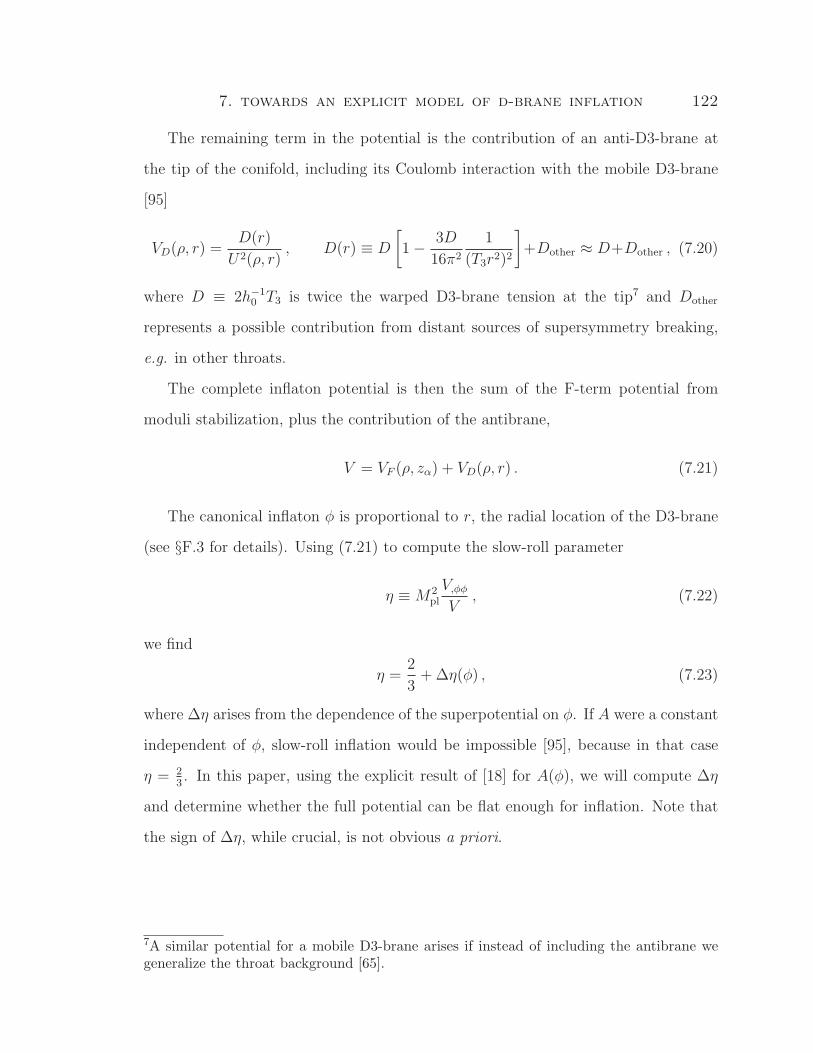
7. towards an explicit model of d-brane inflation 122
The remaining term in the potential is the contribution of an anti-D3-brane at
the tip of the conifold, including its Coulomb interaction with the mobile D3-brane
[95]
VD(ρ, r) =D(r)
U2(ρ, r), D(r) ≡ D
[1− 3D
16π2
1
(T3r2)2
]+Dother ≈ D+Dother , (7.20)
where D ≡ 2h−10 T3 is twice the warped D3-brane tension at the tip7 and Dother
represents a possible contribution from distant sources of supersymmetry breaking,
e.g. in other throats.
The complete inflaton potential is then the sum of the F-term potential from
moduli stabilization, plus the contribution of the antibrane,
V = VF (ρ, zα) + VD(ρ, r) . (7.21)
The canonical inflaton φ is proportional to r, the radial location of the D3-brane
(see §F.3 for details). Using (7.21) to compute the slow-roll parameter
η ≡M2pl
V,φφV
, (7.22)
we find
η =2
3+ ∆η(φ) , (7.23)
where ∆η arises from the dependence of the superpotential on φ. If A were a constant
independent of φ, slow-roll inflation would be impossible [95], because in that case
η = 23. In this paper, using the explicit result of [18] for A(φ), we will compute ∆η
and determine whether the full potential can be flat enough for inflation. Note that
the sign of ∆η, while crucial, is not obvious a priori.
7A similar potential for a mobile D3-brane arises if instead of including the antibrane wegeneralize the throat background [65].

7. towards an explicit model of d-brane inflation 123
3. Case Study: Kuperstein Embedding
Let us consider a particularly simple and symmetric holomorphic embedding due
to Kuperstein [114], which is defined by the algebraic equation
f(z1) = µ− z1 = 0 , (7.24)
where, without loss of generality, we will consider the case in which µ ∈ R+. This
embedding preserves an SO(3) subgroup of the SO(4) global symmetry acting on
the zi coordinates of the deformed conifold. Kuperstein showed that this is a super-
symmetric embedding not just for the singular conifold, but also in the full warped
deformed conifold background with three-form fluxes. (For comparison, the embed-
dings of [9, 133] have so far been studied explicitly only in the AdS5 × T 1,1 back-
ground). Adding just a mobile D3-brane does not break supersymmetry in the case
of the non-compact throat. Therefore, the interaction between the D3-branes and
D7-branes must vanish in that limit. When the throat is embedded in a compactifi-
cation, the D3-brane potential can receive a contribution from the nonperturbative
superpotential (7.14).
The inflaton potential V (ρ, r, zi) is in general a complicated function of the Kahler
modulus and of the radial and angular coordinates of the D3-brane. In this section
we systematically integrate out all fields except the radial coordinate, leading to an
effective single-field potential for the radial inflaton.

7. towards an explicit model of d-brane inflation 124
3.1. Multi-field Potential.
F-term potential. By the results of [18], equation (7.24) implies
A(z1) = A0
(1− z1
µ
)1/n
, (7.25)
and the F-term potential (7.13) is
VF =κ2a|A(z1)|2e−a(ρ+ρ)
3U(ρ, r)2
[(a(ρ+ ρ) + 6
)+ 6W0 Re
( eaρ
A(z1)
)
− 3 Re(αz1z1) +r
aγ
(1− |z1|2
2r3
)|αz1 |2
], (7.26)
where
αz1 ≡Az1A
= − 1
n(µ− z1), (7.27)
and
Re(αz1z1) = − 1
2n
µ(z1 + z1)− 2|z1|2
|µ− z1|2. (7.28)
Note that the potential (7.26) depends only on r, z1, and ρ. Therefore, it is invariant
under the SO(3) that acts on z2, z3, z4.
Angular degrees of freedom.
Imaginary part of the Kahler modulus. First, to reduce the complexity of the
multi-field potential, we integrate out the imaginary part of the Kahler modulus.
Setting ρ ≡ σ + iτ , equation (7.26) becomes
VF =κ2a|A|2e−2aσ
3U2
[(2aσ + 6
)+ 6W0e
aσ Re(eiaτA
)
− 3 Re(αz1z1) +r
aγ
(1− |z1|2
2r3
)|αz1|2
]. (7.29)
We see that only the underlined term depends on τ , and the potential for τ is mini-
mized when this term is as small as possible. Because W0 is negative, integrating out

7. towards an explicit model of d-brane inflation 125
τ(z1, r) = Im(ρ) then amounts to the replacement
eiaτ
A→ 1
|A|. (7.30)
Notice that this is not the same as setting τ ≡ 0. In particular, τ(z1, r) might be a
complicated function, but all we need to know is (7.30).
Angular directions. The D3-brane position is described by the radial coordinate
r and five angles Ψi on the base of the cone. The angles are periodic coordinates on
a compact space, so the potential in Ψi is either constant or else has discrete minima
at some values Ψ?i . We are interested in trajectories that are stable in the angular
directions, so that the motion occurs purely along the radial direction.
We can therefore reduce the number of degrees of freedom by fixing the angular
coordinates to the positions that minimize the potential. In Appendix G we show that
for any Kuperstein-like embedding f(z1) = 0, these extrema in the angular directions
occur only for trajectories satisfying
z1 = ±r3/2
√2, ⇔ ∂V
∂Ψi
= 0 . (7.31)
Furthermore, in Appendix G we examine the matrix of second derivatives, ∂2V∂Ψi∂Ψj
,
and find the conditions under which these extrema are stable minima. For the present
discussion we only need one result from that section: for small r, the trajectory (7.31)
is stable against angular fluctuations for negative z1 and unstable for positive z1. In
Appendix F we show that the canonical inflaton field φ is well-approximated by a
constant rescaling of the radial coordinate r,
φ2 ≡ T3r2 =
3
2T3r
2 . (7.32)
An important parameter of the brane potential is the minimal radial coordinate of
the D7-brane embedding [18, 114], r3µ ≡ 2µ2, or φ2
µ = 32T3(2µ2)2/3. The potential

7. towards an explicit model of d-brane inflation 126
along the trajectory (7.31) may then be written as
V (φ, σ) = VF (φ, σ) + VD(φ, σ) , (7.33)
where
VF (φ, σ) =κ2a|A0|2
3
exp(−2aσ)
U(φ, σ)2g(φ)2/n
[2aσ + 6− 6 exp(aσ)
|W0||A0|
1
g(φ)1/n
+3
n
(cφ
φµ±(φ
φµ
)3/2
−(φ
φµ
)3)
1
g(φ)2
], (7.34)
VD(φ, σ) =D(φ)
U(φ, σ)2, (7.35)
and
g(φ) ≡
∣∣∣∣∣1∓(φ
φµ
)3/2∣∣∣∣∣ , U(φ, σ) ≡ 2σ − σ0
3
φ2
M2pl
. (7.36)
Here we have introduced the constant
c ≡ 1
4πγr2µ
=9
4n aσ0φ2µ
M2pl
. (7.37)
This two-field potential is the input for our numerical study in §4.3.
3.2. Effective Single-Field Potential.
Real part of the Kahler modulus. Having reduced the potential to a function of
two real fields, φ and σ, we integrate out σ by assuming8 that it evolves adiabatically
while remaining in its instantaneous minimum σ?(φ), which is defined implicitly by
∂σV |σ?(φ) = 0 . (7.38)
8We are assuming that σ is much more massive than φ. This may not be valid for a trulygeneric configuration of a D3-brane in a compact space, but we are specifically interestedin cases in which the potential for φ has been fine-tuned to be flat. Thus, when slow-rollinflation is possible at all, the adiabatic approximation is justified. See also [135].

7. towards an explicit model of d-brane inflation 127
This leads to the effective single-field potential
V(φ) ≡ V (σ?(φ), φ) . (7.39)
In general, we are not able to solve equation (7.38) analytically for σ?(φ), so we
perform this final step numerically (§4.3). Nevertheless, in Appendix H we derive
useful approximate analytical solutions for the stabilized volume modulus and its
dependence on φ (similar results were derived independently in [113]). Here, we cite
the basic results of that section. First, the critical value σF of the Kahler modulus
before uplifting is determined by DρW |φ=0, σF= 0, or equivalently [93],
3|W0||A0|
eaσF = 2aσF + 3 ⇒ ∂VF∂σ
∣∣∣∣σF
= 0 . (7.40)
We now show how the Kahler modulus is shifted away from σF by the inclusion of a
brane-antibrane pair.
(1) Shift induced by the uplifting
Adding an anti-D3-brane to lift the KKLT AdS minimum to a dS mini-
mum induces a small shift in the stabilized volume, σF → σF +δσ ≡ σ?(0) ≡
σ0, where
δσ ≈ s
a2σF 1 σF . (7.41)
Here we found it convenient to define the ratio of the antibrane energy to
the F-term energy before uplifting, i.e. when σ = σF ,
s ≡ (D +Dother)U−2(0, σF )
|VF (0, σF )|, (7.42)
where stability of the volume modulus in a metastable de Sitter vacuum
requires 1 < s . O(3). Although δσ is small, it appears in an exponent in
(7.34), so that its effect there has to be considered,
3|W0||A0|
eaσ0 ≈ 2aσ0 + 3 + 2s . (7.43)

7. towards an explicit model of d-brane inflation 128
When the D3-brane is near the tip, φ ≈ 0, the Kahler modulus remains at
σ0. Using this constant value even when the brane is at finite φ suffices for
understanding the basic qualitative features of the potential (7.34). How-
ever, important quantitative details of the potential depend sensitively on
the dependence of σ? on φ; see Appendix D and Ref. [135].
(2) Shift induced by D3-brane motion
In Appendix H we derive the following analytic approximation to the
dependence of the stabilized volume on the D3-brane position:
σ?(φ) ≈ σ0
[1 + c3/2
(φ
φµ
)3/2], (7.44)
where
c3/2 ≈1
n
1
aσF
[1− 1
2aσF
]. (7.45)
This expression is valid along z1 = − r3/2√
2, which we argue below is the inter-
esting case in which the potential is stable in the angular directions.
Analytic single-field potential. Along the trajectory z1 = − r3/2√
2, the inflaton po-
tential is
V(φ) =κ2a|A0|2
3
exp(−2aσ?(φ))
U(φ, σ?(φ))2g(φ)2/n
[2aσ?(φ) + 6− 6 exp(aσ?(φ))
|W0||A0|
1
g(φ)1/n
+3c
n
φ
φµ
1
g(φ)2− 3
n
(φ
φµ
)3/21
g(φ)
]+
D(φ)
U(φ, σ?(φ))2, (7.46)
where σ?(φ) can be determined numerically or approximated analytically by (7.44).
Using the analytic result (7.44) in (7.46) captures the basic qualitative features of the
potential, but is insufficient to assess detailed quantitative questions. In particular, by
using (7.44) one systematically underestimates the total number of e-folds supported
by the potential (see Appendix D and Ref. [135]).
The inflaton potential (7.46) is one of our main results.

7. towards an explicit model of d-brane inflation 129
4. Search for an Inflationary Trajectory
In the preceding section, we derived the inflaton potential (7.46) along the
angularly-stable trajectory z1 = − r3/2√
2. We will now explore this potential and es-
tablish that slow roll inflation is possible for a certain range of parameters. First, in
§4.1, we present a few analytic results about the curvature of the potential. Then,
in §4.2, we describe the constraints on the parameters of the model that are dictated
by the structure of the compactification. Finally, in §4.3, we present the results of a
numerical study of the potential.
4.1. Analytic Considerations. Let us briefly recall the reason for computing
the effect of A(φ) on the inflaton potential. Kachru et al. [95] derived η = 23
for the
case A = const., and suggested that the inflaton-dependence of the nonperturbative
superpotential, A(φ), could contribute corrections to the inflaton mass, which, if of
the right sign, could accidentally make η small. This reasonable expectation hinges
on the presence of quadratic corrections to the inflaton potential.
We now argue that in view of the result (7.15), wrapped D7-branes give no purely
quadratic corrections to the inflaton potential. To see this, we note that the holo-
morphic coordinates on the conifold scale as fractional powers of φ, |zi| ∝ φ3/2, and
A(zi) is a holomorphic function of the zi coordinates [18]. This observation implies
that the inflaton potential is of the form
V(φ)
V(0)= 1 +
1
3
φ2
M2pl
+ v(φ) , (7.47)
where v(φ) contains no quadratic terms. The slow roll parameter η, which needs to
be very small for sustained slow roll inflation, is
η ≡M2pl
V,φφ
V=
2
3+M2
plv,φφ . (7.48)

7. towards an explicit model of d-brane inflation 130
Because v,φφ contains no constant term, there is no possibility of cancelling the 23
uniformly, for the entire range of φ. Instead, we can at best hope to cancel the 23
at
some special point(s) φ0 obeying v,φφ(φ0) = −23.
Using the explicit form (7.46) and expanding for small φ/φµ, we find
η =2
3− η−1/2
(φ
φµ
)−1/2
+ · · · , (7.49)
where
η−1/2 ≈M2
pl
φ2µ
3(4s− 3)
8n(s− 1)
1
aσ0
> 0 . (7.50)
Hence, η < 0 sufficiently close to the tip. On the other hand, we find that for φ φµ,
η > 0. By continuity, η must vanish at some intermediate location φ0.
The precise location of φ0 is a parameter-dependent question. For this purpose,
the most important parameter is the minimal radius φµ of the D7-branes. Notice that
(7.48) can be written as
η =2
3+M2
pl
φ2µ
v,xx , (7.51)
where x ≡ φφµ
and vxx is insensitive to φµ (see (7.46)). From (7.49) we see that the
second term in (7.51) dominates near the tip, giving a large negative η. This implies
the opportunity for a small η by cancellation against the positive 23. However, only if
φµ is not too small can this cancellation be achieved inside the throat. Otherwise, η
remains negative throughout the regime of interest. We conclude that for small φµ,
φ0 is outside the throat, and hence outside the validity of our construction.
4.2. Parameters and Microscopic Constraints. Let us describe the micro-
scopic parameters that determine the inflaton potential (7.46). In view of (7.42), the
D-term Dother + 2T3h−10 and W0 are represented by s and by ωF = aσF , respectively.
Next, the prefactor A0 only appears as an overall constant rescaling the height of
the potential, so we set A0 ≡ 1. The shape of the inflaton potential is therefore
determined by n, ωF , s and φµ. As we now explain, microscopic constraints lead to

7. towards an explicit model of d-brane inflation 131
important restrictions on the allowed parameter ranges and induce non-trivial corre-
lations among the above parameters.
First, the range of the radial coordinate r affects the four-dimensional Planck mass,
because a longer throat makes a larger contribution to the volume of the compact
space. In [21] Liam McAllister and I showed that this creates a strong constraint on
the allowed field range of the inflaton field φ (see also Appendix F)
∆φ
Mpl
<2√N. (7.52)
Here we use the field range bound (7.52) to constrain the microscopically viable range
of φµ, the minimal radial extent of the D7-branes in canonical units. For this purpose
we find it convenient to write the bound in the form
φ2µ
M2pl
=1
Q2µ
1
B6
4
N, (7.53)
where B6 ≡ V w6(V w6 )throat
> 1 parameterizes the relative contribution of the throat to the
total (warped) volume of the compact space, and
Qµ ≡rUV
rµ(7.54)
is a measure of how far into the throat the four-cycle extends. Applicability of the
results of [18] requires Qµ = φUV
φµ> 1.
Second, the warped volume V wΣ4
of the wrapped four-cycle Σ4 is bounded below
by the warped volume in the throat region,
V wΣ4
= (V wΣ4
)throat + (V wΣ4
)bulk ≥ (V wΣ4
)throat . (7.55)
In Appendix F.2 we compute (V wΣ4
)throat for the Kuperstein embedding
T3(V wΣ4
)throat =3
2N lnQµ . (7.56)

7. towards an explicit model of d-brane inflation 132
In §2 we explained how the unperturbed warped four-cycle volume relates to the
Kahler modulus of the compactification (more details can be found in Refs. [18,
77] and Appendix F). If we use B4 ≡V wΣ4
(V wΣ4)throat
> 1 to parameterize the relative
contribution of the throat to the total warped volume of the four-cycle wrapped by
the D7-branes, then we can relate the vev of the Kahler modulus to microscopic
parameters of the compactification
ωF ≈ ω0 ≈3
2
N
nB4 lnQµ . (7.57)
We require ω0 < O(30), because otherwise the inflation scale will be too low – see
Appendix F.
The constraints (7.53), (7.57) will play an essential role in our analysis. We will
find that inflationary configurations are rather easy to find if these constraints are
neglected, but imposing them dramatically decreases the parameter space suitable
for inflation.
Bulk contributions to the volume. We have just introduced two parameters, B4 =V wΣ4
(V wΣ4)throat
and B6 =V w6
(V w6 )throat, that represent ratios of total volumes to throat volumes.
In the throat, we have access to an explicit Calabi-Yau metric and can compute the
volumes directly. This metric data in the throat is one of the main reasons that
warped D-brane inflation can be studied explicitly. In contrast, we have very little
data about the bulk, so we cannot compute B4 and B6.
Fortunately, these parameters do not directly enter the potential. Instead, they
appear in the compactification constraints (7.53) and (7.57), and thereby affect the
microscopically allowable ranges of the other parameters, such as φµ and Qµ. In
particular, when B6 is large, the range of φµ is reduced, because the throat is shorter
in four-dimensional Planck units. In the numerical investigation of §4.3, we find that
inflation is possible inside the throat, and our construction is self-consistent, provided
that B4/B6 & 2. For concreteness, we take B4 ∼ 9, B6 ∼ 1.5 in the remainder. This

7. towards an explicit model of d-brane inflation 133
means that the throat contributes a greater share of the total six-volume than it does
of the wrapped four-cycle volume: in other words, the wrapped four-cycle only enters
the upper reaches of the throat. Although we expect that such a configuration can
be realized, it will be valuable to find a fully explicit construction. We note, however,
that a very large value of B4, implying that the D7-brane is hardly in the throat
at all, would mean that the result of [18] is inapplicable, because the correction to
the four-cycle volume is then dominated by the correction to the uncomputable bulk
portion of the volume.
Parameter choices. Although a systematic study of the full multi-dimensional
parameter space would undoubtedly be instructive, we here employ a simpler and
more transparent strategy that we believe nevertheless accurately portrays the range
of possibilities. To this end, we set some of the discrete parameters to reasonable
values and then scan over the remaining parameters. Let us emphasize that although
the precise values chosen here are not important, it is important that we were able
to find regions in parameter space where all our approximations are valid and all the
compactification constraints are satisfied.
First, we fix n → 8. This helps to reduce the degree to which the volume shifts
during inflation, as from (7.45), c3/2 ∝ n−1. Numerical study of the case n = 2 yields
results qualitatively similar to those we present here, but the analytical treatment is
more challenging. To ignore backreaction of the wrapped branes on the background
geometry, we require that the background D3-brane charge exceeds the number of
wrapped branes, Nn> 1. For concreteness, we use N = 32. Finally, as previously
stated, we take B4 ∼ 5, B6 ∼ 2.
This allows us to impose the microscopic constraints (7.53), (7.57) on the compact-
ification volume ωF and the wrapped brane location φµ in terms of a single parameter
Qµ. The remaining parameters that determine the potential are then Qµ (7.54) and
s (7.42).

7. towards an explicit model of d-brane inflation 134
To search for inflationary solutions, we scanned over Qµ and s, treating both as
continuous parameters, although they are in principle determined by discrete flux
input. Here, for simplicity of presentation, we will fix Qµ to a convenient value, Qµ =
1.2, and only exhibit the scanning over s. To interpret this scanning in microphysical
terms, we recall that, for fixed F-term potential and for fixed supersymmetry breaking
(corresponding to the parameter Dother) outside the throat, s is determined by D =
2T3h−10 , where h0 is given in (7.7) and is of order h0 ≈ exp
(8πK3gsM
). The values of h0
we will consider can be achieved for reasonable values of K,M, gs.
In summary, we have arranged that all consistency conditions are satisfied, and all
parameters except for the amount of uplifting, s, are fixed. As we vary the uplifting,
the shape of the potential (7.46) will change. As we shall now see, for a certain range
of values of s the potential becomes flat enough for prolonged inflation.
2.18
2.16
2.14
2.12 0.2 0.4 0.6 0.8 1.0
V(φ) × 1012
φ/φµ
Figure 2. Inflaton potential V(φ).Compactification data: n = 8, ωF = 10, N = 32, Qµ = 1.2, B6 = 1.5,B4 = 9, s = 1.1, which implies φµ = 0.25, W0 = −3.432×10⁻⁴, D+Dother =1.2× 10⁻⁸, ω0 ≈ 10.1.
4.3. Numerical Results. The first observation we make about (7.46) is that,
near the parameter values we have indicated, it is generically non-monotonic. In fact,
the potential has a metastable minimum9 at some distance from the tip. We are
9A D3-brane located in this metastable minimum contributes to the breaking of super-symmetry. It would be extremely interesting to use a configuration of a D3-brane and a

7. towards an explicit model of d-brane inflation 135
confident that this is a minimum and not a saddle point, because we have explicitly
shown in the Appendices that the curvature of the potential in the angular directions
is non-negative. (The curvature is zero along directions protected by the unbroken
SO(3) symmetry of the background, and positive in the other directions.) Moreover,
we have shown that the potential is stable with respect to changes in the Kahler
modulus.
Next, we notice that as we vary s, the metastable minimum grows more shallow,
and the two zeroes of V ′, the local maximum and the local minimum, approach each
other. A zero of V ′′ is trapped in the shrinking range between these two zeroes of V ′.
For a critical value of s, the zero of V ′′ and the two zeroes of V ′ coincide, and the
potential has an inflection point. As s changes further, the potential becomes strictly
monotonic.
We therefore find that there exists a range of s for which both the first and second
derivatives of the potential approximately vanish. This is an approximate inflection
point. In the next section we discuss a phenomenological model that captures the
essential features of (7.46) in the vicinity of this inflection point.
4.4. Phenomenological Model: Cubic Inflation. We have shown that in-
flationary solutions in the Kuperstein embedding arise near an inflection point at
φ = φ0, where the potential is very well approximated by the cubic form [88, 123]10
V = V0 + λ1(φ− φ0) +1
3!λ3(φ− φ0)3 . (7.58)
moduli-stabilizing D7-brane stack to uplift to a de Sitter vacuum. Here we have not quiteaccomplished this: we have, of course, included an anti-D3-brane as well, which is well-known to accomplish the uplifting by itself [93]. If this antibrane is removed, the structureof the potential changes, and it is not clear from our results so far that a remaining D3-branewould suffice to uplift to a de Sitter vacuum. We leave this as a promising direction forfuture work.10Ref. [5] has developed an inflation model within the minimal supersymmetric standardmodel (MSSM) that has a similar cubic phenomenology. We thank Justin Khoury forbringing this model to our attention. Inflection point inflation in the context of stringtheory, with the inflaton corresponding to the compactification volume, has been consideredin [92].
7. towards an explicit model of d-brane inflation 136
0.2 0.4 0.6 0.8
2.28
2.27
2.26
2.25
2.29
0.2 0.4 0.6 0.8
7.84
7.83
7.82
7.81
7.85
0.2 0.4 0.6 0.8
5.46
5.45
5.44
5.43
5.47
0.2 0.4 0.6 0.8
15.70
15.69
15.68
15.67
15.71
V(φ) × 1012
φ/φµ
φ/φµ
φ/φµ
φ/φµV(φ) × 1012
V(φ) × 1012 V(φ) × 1012
s = 1.5
s = 1.15s = 1.35
s = 2.0
Figure 3. The inflaton potential V(φ) as a function of s.The transition from metastability to monotonicity is shown; old inflationand new inflation are continuously connected.
Prolonged inflation requires smallness of the slow roll parameters, ε, η 1. From
(7.58) we find11
ε ≡ 1
2
(V,φ
V
)2
≈ 1
2
(λ1 + 1
2λ3(φ− φ0)2
V0
)2
, (7.59)
η ≡ V,φφ
V≈ λ3
V0
(φ− φ0) . (7.60)
The number of e–folds between some value φ and the end of inflation φend is then
Ne(φ) =
∫ φ
φend
dφ√2ε
=Ntot
πarctan
(η(φ)
2πN−1tot
)∣∣∣∣φφend
, (7.61)
where
Ntot ≡∫ ∞−∞
dφ√2ε
= π
√2V 2
0
λ1λ3
. (7.62)
11In this section we set Mpl ≡ 1.

7. towards an explicit model of d-brane inflation 137
In (7.59) and (7.60) we have set V(φ) ≈ V0 in the denominators, while in (7.62) we
extended the integral from the range where |η| < 1 to infinity. These approximations
are very good in the regime
V0
λ3
1 ,V0√λ1λ3
1 . (7.63)
The first of these conditions guarantees that inflation is of the small-field type, while
the second implies that Ntot 1. We will be interested in Ntot ≥ NCMB ∼ 60.
Ntot
Ne
η
end of inflation
near scale-invariance
ns < 1
ns > 1
Figure 4. η(φ) as a function of the number of e-folds of inflation,Ne. In the green band, |η| < 2πN−1
tot .
Equation (7.61) shows that there are 12Ntot e–folds during which |η| < 2πN−1
tot ; see
Figure 4. For large Ntot this implies that there is a large range of e–folds where η is
small and the scalar perturbation spectrum is nearly scale-invariant. Predicting the
scalar spectral index in these models is non-trivial:
ns − 1 = (2η − 6ε)|φCMB≈ 2η(φCMB) . (7.64)
The scalar spectral index on CMB scales can be red, blue or even perfectly scale-
invariant depending on where φCMB is relative to the inflection point. If inflation only

7. towards an explicit model of d-brane inflation 138
lasts for the minimal number of e-folds to solve the horizon and flatness problems
then the scalar spectrum is blue. If the potential is flatter than this, so that ε is
smaller, inflation lasts longer and φCMB is more likely to be smaller than φ0. The
spectrum is then red, since η(φCMB < φ0) < 0.
200 400 600 800 100 50
1.20
1.15
1.10
1.05
0.95
0.90
1.0Ntot
ns
Figure 5. Spectral index ns, evaluated on CMB scales, as a functionof the total number of e-folds of inflation, Ntot. The light band gives theWMAP3 2σ limit on ns (for r ≡ 0) [151].
More concretely, we can evaluate ns by inverting (7.61) at φCMB whereNe(φCMB) ≡
NCMB ∼ 60, and using η(φend) = −1. This gives
ns − 1 =4π
Ntot
tan
(πNCMB
Ntot
− arctan
(Ntot
2π
)). (7.65)
Using arctanx = π2− x−1 +O(x−3) we furthermore find
ns − 1 =4π
Ntot
tan
(πNCMB + 2
Ntot
− π
2+O(N−3
tot )
). (7.66)
Using NCMB + 2 ≈ NCMB 1, we may simplify this to
ns − 1 ≈ − 4π
Ntot
cot
(πNCMB
Ntot
), (7.67)

7. towards an explicit model of d-brane inflation 139
which has the expansion
ns − 1 ≈ − 4
NCMB
+4π2
3
NCMB
N2tot
+O(N3
CMB
N4tot
). (7.68)
Equation (7.67) is plotted in Figure 5. We note the following properties of this
result. For Ntot not much greater than NCMB the spectrum is strongly blue and the
model is hence ruled out by recent observations [151] (in this regime the slow-roll
formulae we have used are not good approximations, but a more exact treatment
gives similar results). For Ntot ≈ 2NCMB the spectrum on CMB scales is exactly
scale-invariant. For Ntot & 2NCMB the spectrum is red and asymptotes to the lower
limit ns → 1 − 4/NCMB ≈ 0.93 for Ntot NCMB. This asymptotic limit, which has
been noted in studies of inflation near an inflection point [5, 92], is more strongly red
than is typical in single-field inflation models.
Given the explicit expression (7.67) for the spectral index ns(Ne) we can compute
its scale-dependence or ‘running’:
αs ≡dnsd ln k
= − dnsdNe
∣∣∣∣Ne=NCMB
= − 4π2
N2tot
sin−2
(πNCMB
Ntot
), (7.69)
≈ − 4
N2CMB
− 4π2
3
1
N2tot
+O(N2
CMB
N4tot
). (7.70)
The running can be large for models with blue spectral tilt (Ntot ∼ NCMB), but
is small for models with red spectra. The asymptotic value for Ntot NCMB is
αs → −4/N2CMB ≈ −10−3. Notice that because both the tilt ns − 1 and the running
αs are determined by Ntot alone (for fixed NCMB), this phenomenological model is
predictive.
It is possible to arrange for the magnitude of scalar perturbations on CMB scales
to be small,
∆2R =
1
24π2
Vε
∣∣∣∣φCMB
≈ 2.4× 10⁻⁹ , (7.71)
by adjusting the overall scale of inflation V0.

7. towards an explicit model of d-brane inflation 140
Let us comment briefly on some general difficulties in inflection point inflation.
Since inflation is restricted to a small region around the inflection point, an immediate
concern is the question of initial conditions. In particular, how sensitive is the present
scenario to the initial position and velocity of the D3-brane? What fraction of initial
conditions lead to overshoot rather than to inflation? These questions have recently
been analyzed by Bret Underwood [157] who finds that including the effects of the
DBI kinetic term dramatically improves naive estimates on the amount of fine-tuning
of initial conditions necessary for inflation.
Since this is a small-field model, it is sensitive to small corrections in the slope
of the potential (see §6). These corrections are important for both the background
evolution, i.e. the number of e–folds of inflation, and for the perturbation spectrum.
Finally, we note that the appearance of the inflection point feature depends sen-
sitively on the use of the adiabatic approximation for integrating out the volume
modulus. One might therefore be worried about cases in which the exact two-field
evolution is not well captured by this approximation and a more detailed numerical
study of the two-field evolution is required.12
5. Comments on Other Embeddings
The previous two sections contained a detailed discussion of the D3-brane poten-
tial for the Kuperstein embedding. We derived important microscopic constraints,
analyzed the fine-tuning problem involved in realizing inflationary solutions, and stud-
ied the resulting cosmological dynamics.
In this section we will make some brief remarks about other embeddings. When
applicable we will emphasize the differences and similarities to the Kuperstein case.
This will illustrate the special status of the Kuperstein embedding.
12This important problem has been explored in the subsequent work [135] where the validityof the adiabatic approximation is explicitly confirmed.

7. towards an explicit model of d-brane inflation 141
First, we give a simple proof that for an infinite class of D7-brane embeddings, the
ACR embeddings, there always exist trajectories for which no amount of fine-tuning
can flatten the inflaton potential. Arean, Crooks and Ramallo (ACR) [9] studied
supersymmetric four-cycles in the conifold described by the embedding equations
f(wi) = µP −4∏i=1
wpii = 0 , (7.72)
where pi ∈ Z, P ≡∑4
i=1 pi and µP ∈ C are constants defining the embedding.
Here wi ∈ C are alternative coordinates on the conifold that follow from the zi
coordinates by a linear transformation (see Appendix E). The conifold constraint in
these coordinates is w1w2 − w3w4 = 0. By requiring that the pi are non-negative we
can restrict attention to four-cycles that do not reach the tip of the conifold. Two
simple special cases of the ACR embeddings (7.72) are the Ouyang embedding [133],
w1 = µ, and the Karch-Katz embedding [99], w1w2 = µ2.
To study the ACR embeddings in a unified way we define a collective coordinate
Φ
ΦP ≡4∏i=1
wpii , (7.73)
such that
A(ΦP ) = A0
(1− ΦP
µP
)1/n
, (7.74)
and ∑i
wiαwi =∑i
piΦPαΦP = PΦPαΦP , (7.75)
where
αΦP ≡1
A
∂A
∂ΦP= − 1
n
1
µP − ΦP. (7.76)
Next, we consider the part of the F-term potential that depends on derivatives of the
superpotential with respect to the brane coordinates
∆VF = −κ2a|A|2e−2aσ
U2
[3 Re(wiαwi)−
1
aγkiwαwiαwj
], (7.77)

7. towards an explicit model of d-brane inflation 142
where
Re(wiαwi) = P Re(ΦPαΦP ) (7.78)
and
1
γkiwαwiαwj =
1
γr2|αΦP |2
∣∣ΦP∣∣2 1
2P 2 + (p1 − p2)2 + (p3 − p4)4 + Z(wi)
. (7.79)
Here, we found it convenient to write the Kahler metric kiw in SO(4)–invariant form
(see Appendix E) and defined the function
Z ≡ +
∣∣∣∣p1w4
w1
+ p3w2
w3
∣∣∣∣2 +
∣∣∣∣p1w3
w1
+ p4w2
w4
∣∣∣∣2+
∣∣∣∣p2w3
w2
+ p4w1
w4
∣∣∣∣2 +
∣∣∣∣p2w4
w2
+ p3w1
w3
∣∣∣∣2 . (7.80)
5.1. Delta-flat Directions. We now show that there is always a radial trajec-
tory, Φ = 0, along which ∂W/∂wi is orthogonal to wi and lies in the null direction of
kiw. The term ∆VF in (7.77) then vanishes and the prefactor A of the superpotential
becomes independent of the brane position. We call this a delta-flat direction. For
the Ouyang embedding this trajectory was first found by Burgess et al. [45]. As noted
in [45], delta-flat directions are noteworthy because they have ∆η = 0 and therefore
imply a well-known no-go result for inflation [95].
More concretely, we see that for (7.78) to vanish one requires
Φ = 0 , (7.81)
i.e. at least one of the wi that enter the embedding must vanish. In fact, we
notice that (7.78) vanishes whenever (7.79) does, so we can restrict our atten-
tion to (7.79). If any pi > 1, then we see immediately from the overall factor
|ΦP |2 = |w1|2p1|w2|2p2|w3|2p3|w4|2p4 that (7.79) vanishes on wi = 0. For pi ≤ 1 there
are only a few distinct cases: Φ = w1, Φ2 = w1w2, Φ2 = w1w3, Φ3 = w1w2w3, and

7. towards an explicit model of d-brane inflation 143
Φ4 = w1w2w3w4. In the next section we will illustrate the argument for the impor-
tant case of the Ouyang embedding, Φ = w1; the proof is easily generalized to the
remaining cases. This completes the proof that all ACR embeddings have delta-flat
trajectories.
5.2. Comparison of the Ouyang and Kuperstein Embeddings. Recently
the result of [18] has been applied [45, 113] to compactifications involving the Ouyang
embedding w1 = µ. In this case, the correction to the F-term potential is
∆VF =κ2
3U2
[3
2(W,ρw1W,w1 + c.c.) +
1
γk11w W,w1W,w1
], (7.82)
where
k11w = r
(1 +|w1|2
2r3− |w2|2
r3
). (7.83)
There are two kinds of radial extremal trajectories: the delta-flat trajectory w1 =
w3 = w4 = 0, for which ∆VF = 0 [45], and also a trajectory w2 = w3 = w4 = 0,
w1 ∈ R used in [113].
The Kuperstein scenario is closely related to the Ouyang scenario except for two
subtle differences which we now discuss:
(1) There exists no delta-flat direction for the Kuperstein embedding.
(2) The single-field potential along the non-delta-flat direction for the Ouyang
embedding is identical in shape to that along the corresponding Kuperstein
trajectory. However, the angular stability is different (see Appendix G).
This trajectory in the Kuperstein embedding is stable for small r, while in
the Ouyang embedding it is unstable in that regime.
To see this compare the correction to the F-term potential for the Ouyang embedding,
(7.82), with the corresponding term for the Kuperstein embedding,
∆VF =κ2
3U2
[3
2(W,ρz1W,z1 + c.c.) +
1
γk11W,z1W,z1
], (7.84)

7. towards an explicit model of d-brane inflation 144
where
k11 = r(
1− 1
2
|z1|2
r3
). (7.85)
This shows immediately that the Kuperstein embedding does not have a delta-flat
direction, since k11 cannot vanish for r > 0. This is to be viewed in contrast to the
Ouyang case for which (7.83) vanishes on w1 = 0.
Considering k11, k11w for each case one may further show that the trajectories
2|z1|2 = r3 and |w1|2 = r3 lead to identical shapes for the single-field potential.
However, ‘off-shell’, i.e. away from the extremal path, k11w for the Ouyang embedding
is of a different form from k11 for the Kuperstein embedding. It is for this reason that
the angular stability of the two scenarios is different (see Appendix G for details). In
particular, while for the Kuperstein embedding the trajectory is stable for the regime
of interest, for the Ouyang embedding it is unstable.
To discuss the issue of stability in simple terms, we consider θ1 = θ2 = θ and
ψ ≡ ψ − φ1 − φ2, so that w1 = ei2ψr3/2 sin2(θ/2). Then, as shown in [45] for n = 1,
VF (θ) = V1 sin2(θ/2) + V2 sin4(θ/2) + const. , (7.86)
where
V1 =κ2|A0|2e−2aσ
3U2
r
γµ2
(2− aµγ
√r cos
ψ
2
(9 + 4aσ + 6W0
eaσ
|A0|
)), (7.87)
V2 =1
4
κ2|A0|2e−2aσ
3U2
r
γµ2
(− 2 + aγr2(12 + 8aσ)
). (7.88)
We see that ∂VF∂θ
vanishes for θ = 0 or π.
The θ = 0 trajectory is delta-flat [45]. For this trajectory, ∂2VF∂θ2 = 1
2V1 which
is clearly positive for small r and stays positive up to some critical radius rc. To
compute rc we evaluate V1 at σ = σ0 using
4aσ0 + 9− 6W0eaσ0
|A0|≈ 3− 4s . (7.89)

7. towards an explicit model of d-brane inflation 145
We find
V1 ≈κ2|A0|2e−2aσ0
3U2
r
γµ2
(2 + aµγ(4s− 3)
√r cos
ψ
2
). (7.90)
For s > 3/4 and for real positive µ, the potential is minimized at ψ = 2π, where
V1 ≈κ2|A0|2e−2aσ0
3U2
r
γµ2
(2− aµγ(4s− 3)
√r
), (7.91)
This is positive as long as r is less than rc, where
rcrµ
=1
(4s− 3)2
(9
aσ0
)2 M4pl
φ4µ
. (7.92)
Applying the field range bound in the formφ2µ
M2pl< 4
None finds
rcrµ
>N2
42
1
(4s− 3)2
(9
aσ0
)2
. (7.93)
For typical parameters we therefore conclude that rc ≥ rµ and the delta-flat direction
is hence stable from the tip to at least the location rµ of the D7-branes.
For the θ = π trajectory, ∂2VF∂θ2 = −1
2V1. This is negative for r < rc and the θ = π
trajectory is therefore unstable in this regime. This analysis was carried out for n = 1
but it illustrates the essential qualitative point (for a more general analysis with the
same conclusion, see Appendix C.2).
In Appendix G.4 we show that for all ACR embeddings there are alternative
trajectories with Φ 6= 0 that are not delta-flat. This is important because it implies
that, for a D3-brane moving along such a trajectory, η can be different from 23.
We postpone a more general treatment of such trajectories for the future (but see
Appendix G.4 for some preliminary remarks).

7. towards an explicit model of d-brane inflation 146
6. Discussion
In this section we will briefly take stock of our progress towards an explicit model of
D-brane inflation. For this purpose, it is useful to consider the more general problem
of deriving a low-energy Lagrangian from the data of a string compactification.
In principle, the data of a compactification – such as the background geometry,
brane positions, and fluxes – determine the low-energy effective Lagrangian in full.
In practice, one typically begins by deriving the leading-order effective Lagrangian,
which follows from dimensional reduction of the classical ten-dimensional supergravity
action, including the effect of fluxes but treating D-branes as probes. Then, one can
include corrections to this action, including such things as nonperturbative terms in
the superpotential, D-brane backreaction effects, string loop corrections to the Kahler
potential, and α′ corrections to the Kahler potential. Except in cases with extended
supersymmetry, it is typically impossible to obtain results beyond leading order in
either series of corrections to the Kahler potential.
For the present purpose, an instructive way to organize these corrections is ac-
cording to their effects on the slow-roll parameter η, as follows. The leading order
classical four-dimensional Lagrangian we denote L0. Correction terms are well-known
to give rise to inflaton masses of order H, and hence corrections of order unity to η.
When all such effects, from any source whatsoever, have been added to L0, we denote
this corrected Lagrangian L1. By definition, this is the Lagrangian whose inflaton
mass term is a good approximation to the ‘true’ mass term that would follow from
a dimensional reduction incorporating corrections of arbitrarily high degree. (Notice
that the leading-order classical Lagrangian L0 may itself contain large inflaton mass
terms.) Finally, if to L1 we add the leading terms that give corrections to η that
are parametrically small compared to unity, we call the resulting Lagrangian L2. In
sum, we propose to organize corrections to the Lagrangian according to the degree of

7. towards an explicit model of d-brane inflation 147
their effects on η, even though such an organization does not correspond to a literal
expansion parameter such as the string coupling.
To determine whether a given model gives rise to prolonged slow-roll inflation, one
needs to know L1. However, it is rarely true that all the required results are available.
For example, in the warped brane inflation model of [95], the inflaton-dependence of
the threshold factor A(φ) of the nonperturbative superpotential was not known until
recently [18, 32]. Similarly, in Kahler moduli inflation [54], a particular term in the
Kahler potential that could give ∆η ∼ 1 has not yet been computed (though it has
been conjectured that this term might vanish.) Although such partial data is generally
insufficient to determine whether a model is successful, even this degree of detail is
relatively rare: a fair fraction of proposed models of string inflation include only the
L0 data, without any corrections at all.
In this chapter, we have made progress towards a full understanding of the La-
grangian L1 for the warped brane inflation models of [95]. However, as we will now
explain, further work is necessary.
First, let us briefly recall the best-understood correction terms. The D3-brane po-
tential receives contributions from the mixing between the volume and the D3-brane
position in the DeWolfe-Giddings Kahler potential (7.9). Moreover, the nonpertur-
bative superpotential receives the correction (7.15) sourced by the backreaction of
the D3-brane on the warp factor. Holomorphy of the gauge kinetic function ensures
that this correction, which corresponds to a one-loop threshold factor, is the only
perturbative correction to the superpotential. The only additional contributions to
the superpotential come from multi-instantons, which give a negligibly small effect.
The Kahler potential, however, is not protected by holomorphy, and in general
receives α′ and gs corrections. In the large-volume, weak-coupling limit, these cor-
rections are suppressed relative to the leading terms in the DeWolfe-Giddings Kahler
potential, and so generate mass terms that are generically smaller than H by powers

7. towards an explicit model of d-brane inflation 148
of the inverse volume or powers of the string coupling. Hence, by our above defi-
nition, these corrections correspond to terms in L2. Although complete results for
these terms are not available for a general compactification, the work of Berg, Haack,
and Kors [33, 34] in the toroidal orientifold case gives substantial guidance. These
authors found that the leading D3-brane-dependent corrections to K are of two types,
one suppressed by an additional power of ρ compared to the DeWolfe-Giddings result,
and the other suppressed by one power of gs. For ρ 1, gs 1, these terms give a
parametrically small correction to the D3-brane potential, and so belong to what we
have called L2. Even better, in some cases [33] the expectations of naive dimensional
analysis are borne out, and the numerical prefactors of these higher-order terms are
moderately small.13
Corrections due to the fluxes are a further possibility. The best-understood α′
corrections arise from the term (α′)3R4 in ten dimensions, with R4 standing for an
appropriate contraction of four powers of the Riemann tensor. In the presence of
three-form flux G3, there are additional terms from (G3)2R3, and it is less clear how
these correct the Kahler potential [25]. However, it has been argued that at large
volume, hence low flux density, this effect is subleading [15].
Finally, and perhaps most importantly, perturbations of the background fields in
the throat, which can arise from sources in the bulk, can give substantial corrections
to the D3-brane potential.14 It was argued in [59] (see also [113]) that in special cases
these effects may be small compared to the forces from the D7-brane. However, lack-
ing a more complete understanding of these effects, we do not claim that the potential
we have presented is completely general. Instead, our construction is representative
of a particulay tractable class of situations in which the bulk effects are small.
13We thank M. Berg for helpful discussions of this point.14We thank S. Kachru for explanations of this point.

7. towards an explicit model of d-brane inflation 149
7. Conclusions
In this chapter we have systematically studied the potential for a D3-brane in
a warped throat containing holomorphically-embedded D7-branes. This system is a
promising candidate for an explicit model of inflation in string theory. However, the
warped brane inflation model of [95] is well-known to suffer from an inflaton mass
problem, in that corrections from moduli stabilization tend to curve the potential
and make slow-roll inflation impossible. The true severity of this problem – and,
correspondingly, the status of the model – have remained unclear, because the func-
tional form of one particular correction term, arising from a threshold correction to
the nonperturbative superpotential, was unavailable before the recent result of [18].
In this work, building on [18], we have studied the corrected potential in detail. This
equipped us to assess the true status of the warped brane inflation model [95] and to
ascertain whether prolonged slow-roll inflation is indeed possible.
Our method for analyzing the potential involved several nontrivial improvements
over existing approximations. First, we systematically identified stable minima in the
angular directions of the conifold, and showed how the radial potential depends on
the choice of angular minimum. Second, we showed that the common assumption
that the compactification volume remains stabilized at its minimum during inflation
is inadequate: the volume shrinks slightly as the D3-brane falls down the throat, and
this leads to non-negligible corrections to the effective D3-brane potential. We gave
an analytic expression for the volume as a function of the D3-brane position and
showed that this is an excellent approximation to the full result.
For a large class of embeddings of the wrapped branes, the ACR embeddings, we
showed that the radial potential for a D3-brane at a particular angular extremum is
necessarily too steep to support inflation, because the contributions computed in [18]
vanish along the trajectory, and so the no-go result of [95] applies. This was first
explained in [45] for a special ACR embedding, the Ouyang embedding [133]. Our

7. towards an explicit model of d-brane inflation 150
results here generalize this to the full ACR class. It follows that these trajectories
in throats containing wrapped branes with ACR embeddings do not permit slow roll
D-brane inflation, even if one allows an arbitrary degree of fine-tuning: there is simply
no parameter that can be varied to flatten the potential in such a case. However, we
also showed that all ACR embeddings have alternative trajectories, corresponding to
other choices of the angular extremum, for which this no-go result does not apply.
Our main result was an analysis of a very simple and symmetric embedding,
the Kuperstein embedding, that does allow a flat D3-brane potential. We found
that for certain fine-tuned ranges of the compactification parameters, the potential
is flat enough to allow prolonged inflation. However, the resulting potential is not as
simple as that conjectured in [95] and further elaborated in [68]: moduli stabilization
gives rise to a potential that is much more complicated than a mass term for radial
motion. Furthermore, adjusting the potential by varying microscopic parameters
changes features in the potential instead of just rescaling the mass term. In particular,
one can fine-tune to arrange for a flat region suitable for inflation, but we found
that this will occur around an inflection point away from the origin. Hence, when
inflation occurs, it does so near an approximate inflection point, rather than in a
shallow quadratic potential centered on the origin. In short, we found that a low-
order Taylor expansion of the potential around the minimum at the tip of the throat
does not properly describe those regions of the potential where inflation is possible.
Instead, one is obliged to use the complete potential presented here. Our result
implies that the phenomenology of some classes of warped D-brane inflation models
is well-described by an effective single-field potential with a constant and cubic term.
As we explained, models of this sort (see [5] for an analogous example in the MSSM)
are particularly sensitive to the initial conditions. Moreover, the tilt of the scalar
spectrum is exquisitely sensitive to the slope of the potential near the approximate
inflection point.

7. towards an explicit model of d-brane inflation 151
One important, general lesson of our work is that there is considerably less freedom
to adjust the parameters of this system than one might expect from the low-energy
effective action. First, the functional form of A(φ) derived in [18] is rather special:
most importantly, A(φ) contains no quadratic term, and does not lead to any new
quadratic terms in the inflaton potential. This implies that the potential cannot be
flattened uniformly, and η can only be small in a limited region. Second, the range
of φ is limited by the microscopic constraint of [21]. Finally, the field range is linked
to the scale of inflation, because of a new geometric constraint linking the size of the
wrapped four-cycle and the length of the throat. Using these results, we found that
although this system depends on many microscopic parameters, in many cases it is
nevertheless impossible to choose these parameters in such a way that the slow-roll
parameter η is fine-tuned to vanish. This occurs because constraints originating in
the geometry of the compactification correlate the microscopic quantities, so that the
true number of adjustable parameters is much smaller than a naive estimate would
suggest.
An important direction for future work is a more comprehensive understanding
of any additional corrections to the potential, such as α′ corrections, string loop
corrections, and perturbations of the throat metric due to bulk sources. We have
argued that in some cases the presence of such effects is not fatal for inflation, but
precise observational predictions will certainly depend on these effects.

7. towards an explicit model of d-brane inflation 152
Symbols used in this Chapter
Table 1. Definitions of symbols and notation used in this chapter andin Appendices E, F, G, and H.
Variable Description Definition
zi complex conifold coordinates∑
i z2i = 0, (E.4)–(E.7)
wi complex conifold coordinates w1w2 − w3w4 = 0, (E.8)–(E.11)ε conifold deformation parameter
∑i z
2i = ε, equation (7.1)
r radial coordinate on the conifold r3 =∑
i |zi|2r radial coordinate on the conifold r2 = 3
2r2, ds2 = dr2 + . . .
r radial coordinate on the conifold r = eureu breathing mode equation (F.1)gαβ fiducial metricgαβ physical metric gαβ = e2ugαβk Kahler potential gαβ = k,αβ, k = 3
2(∑
i z2i )
2/3
φi, θi, ψ angular coordinates on T 1,1 equations (E.4)–(E.7)h(r) warp factor equation (7.4)rUV radius at the UV end ln rUV/ε
2/3 = 2πK/(3gsM)φ inflaton field φ2 = T3r
2
ϕ canonical inflaton field Appendix F, ϕ2 ≈ σ(0)c
σ(φ)φ2
K Kahler potential κ2K = −3 lnUW superpotentialU argument of Kahler potential [58] U = ρ+ ρ− γkρ complex Kahler modulusσ real part of ρ 2σ = ρ+ ρτ imaginary part of ρ 2i τ = ρ− ρσ? stabilized volume modulus ∂σV |σ? = 0ω? rescaled volume modulus ω? ≡ aσ?W0 GVW-flux superpotential W0 =
∫G ∧ Ω
Wnp non-perturbative superpotential Wnp = A(zi)e−aρ
f(zi) embedding equation A(zi) ∝ (f(zi))1/n
g(zi) embedding equation g(zi) = f(zi)/f(0)A0 prefactor of Wnp A0 = A(zi = 0)VF F-term potential equation (7.8)VD D-term potential VD = DU−2; equation (7.20)D scale of D-term energy D ≡ 2h−1
0 T3
ε, η slow-roll parameters ε = 12(V ′/V )2, η = V ′′/V
gs string couplingT3 D3-brane tension T−1
3 = (2π)3gs(α′)2

7. towards an explicit model of d-brane inflation 153
Variable Description Definition
µ embedding parameter z1 = µn # of embedded D7’sa parameter in Wnp a = 2π/nrµ minimal radius of D7 r3
µ = 2µ2
φµ rescaled rµ φ2µ = 3
2T3r
2µ
M , K flux on the A and B cycleN five-form flux N ≡MKL AdS radius equation (F.21)Mpl 4d Planck mass M2
pl = 1π(T3)2V w
6
V w6 warped 6-volumeV w
Σ4warped 4-cycle volume Appendix F
s ratio of D- and F-termx ratio of r and rµ x = r/rµx0 location of η = 0Qµ ratio of rUV and rµ Qµ = rUV/rµ > 1B6 bulk contribution to V w
6 (V w6 )bulk = B6(V w
6 )throat
B4 bulk contribution to V wΣ4
(V wΣ4
)bulk = B4(V wΣ4
)throat
ωF Kahler modulus before uplifting equation (H.2)ω0 Kahler modulus after uplifting ω0 ≈ ωF + s/ωFΓ factor in K Γ = 2σ0
Γ factor in K Γ ≡ Γe4u = Uγ prefactor in the Kahler potential γ = Γ
6T3
M2pl
= σ0
3T3
M2pl
c factor in VF c−1 = 4πγr2µ
c3/2 factor in volume shift equation (7.45)X, X + Y eigenvalues of Hessian Appendix G
P degree of ACR embeddings∏
iwpii = µP
pi embedding parameter pi ∈ ZΦ collective coordinate for ACR ΦP ≡
∏iw
pii

Part 3
String Theory and Gravitational Waves

“I never thought that anybody would ever actually measure these things.
I thought we were just calculating for the fun of it.”
Alan Guth
155

CHAPTER 8
A Microscopic Limit on Gravitational Waves
We conclude our analysis of D-brane inflation by exposing a geometric limit on
the maximal amplitude of gravitational waves attainable in these models.1
1. Introduction
In the foreseeable future it may be possible to detect primordial gravitational
waves [37] produced during inflation [3, 83, 120]. This would be a spectacular oppor-
tunity to reveal physics at energy scales that are unattainable in terrestrial experi-
ments. In light of this possibility, it is essential to understand the predictions made
by various inflationary models for gravitational wave production. As we shall review,
a result of Lyth [122] connects detectably large gravitational wave signals to motion
of the inflaton over Planckian distances in field space. It is interesting to know when
suitably flat potentials over such large distances are attainable in string compactifica-
tions, allowing a potentially observable tensor signal in the associated string inflation
models. In this chapter we analyze this issue for the case of warped D-brane inflation
models [64, 95], and use compactification constraints to derive a firm upper bound
on the inflaton field range in Planck units.
1This chapter is based on Daniel Baumann and Liam McAllister, “A Microscopic Limiton Gravitational Waves from D-brane Inflation,” Phys. Rev. D 75, 123508 (2007). Thecomputation was originally suggested to us by Juan Maldacena and we received importantinitial input from Igor Klebanov.The numerical estimates of Ref. [21] have been updated to the WMAP 5-year data [111]. Thesign of fNL for DBI inflation has been corrected. These changes strengthen the conclusionsof Ref. [21].
156

8. a microscopic limit on gravitational waves 157
For slow-roll warped brane inflation, our result implies that the gravitational wave
signal is undetectably small. This constraint is model-independent and holds for any
slow-roll potential. For DBI inflation [4, 147], the limit on the field range forces the
tensor signal to be much smaller than the current observational bound. Detection
in a future experiment may be possible only if r decreases rapidly soon after scales
observable in the cosmic microwave background exit the horizon. This does occur in
some models, but it has a striking correlate: the scalar spectrum will typically have
a strong blue tilt and/or be highly non-Gaussian during the same epoch.
We also consider compactification constraints on the special case of DBI inflation
with a quadratic potential. We find that observational constraints, together with our
bound on the field range, exclude scenarios with a large amount of five-form flux. For
a DBI model realized in a warped cone over an Einstein manifold X5, this translates
into a very strong requirement on the volume of X5 at unit radius. However, we
show that manifolds obeying this constraint do exist, at least in noncompact models.
This translates the usual problem of accommodating a large flux into the problem of
arranging that X5 has small volume.
2. The Lyth Bound
In slow-roll inflation2 the tensor fluctuation two-point function is3
Pt =2
π2
(H
Mpl
)2
, (8.1)
where H is the Hubble expansion rate. The scalar fluctuation two-point function is
Ps =
(H
2π
)2(H
ϕ
)2
. (8.2)
The first factor in (8.2) represents the two-point function of the scalar field, while
the second factor comes from the conversion of fluctuations of the scalar field into
2By slow-roll inflation we mean standard single-field inflation with canonical kinetic term.3See Chapter 2 and Appendix A for details of the results cited in this section.

8. a microscopic limit on gravitational waves 158
fluctuations of the scale factor in the metric (or scalar curvature fluctuations). The
ratio between the tensor and scalar two-point functions is
r ≡ PtPs
= 8( ϕ
HMpl
)2
= 8( dϕdN
1
Mpl
)2
, (8.3)
where dN = Hdt represents the differential of the number of e-folds. This implies
that the total field variation during inflation is
∆ϕ
Mpl
=1
81/2
∫ Nend
0
dN r1/2 , (8.4)
where Nend ∼ 60 is the total number of e-folds from the time the CMB quadrupole
(N ≡ 0) exits the horizon to the end of inflation.
In any given model of inflation, r is determined as a function of N . As a measure
of the evolution of r we define the following quantity
Neff ≡∫ Nend
0
dN( r
rCMB
)1/2
, (8.5)
so that
∆ϕ
Mpl
=(rCMB
8
)1/2
Neff . (8.6)
Here rCMB denotes the tensor-to-scalar ratio r evaluated on CMB scales, 0 < N <
NCMB ≈ 4. We use Neff to parameterize how far beyond NCMB the support of
the integral in (8.4) extends. If r is precisely constant then Neff = Nend, if r is
monotonically increasing then Neff > Nend, and if r decreases then Neff < Nend. For
a detailed discussion of related issues, see [66].
Equation (8.6) relates the amount of gravitational waves observable in CMB po-
larization experiments to the field variation ∆ϕ during inflation
rCMB =8
(Neff)2
(∆ϕ
Mpl
)2
. (8.7)

8. a microscopic limit on gravitational waves 159
To make use of the relation (8.7), we need to estimate Neff , which amounts to deter-
mining r(N ). In slow-roll inflation r is proportional to the slow-roll parameter
ε ≡ −d lnH
dN. (8.8)
We can define a second slow roll parameter η as the fractional variation of ε during
one e-fold. Then we have
d ln r
dN=d ln ε
dN= η . (8.9)
Equivalently, we can write (8.9) in terms of the spectral indices of the scalar and
tensor power spectra
d ln r
dN= nt − (ns − 1)
= −[(ns − 1) +
r
8
], (8.10)
where we have used the usual single-field consistency condition, nt = −r/8. Hence,
observational constraints on ns and r give limits on the evolution of r to first order
in slow-roll.
We notice that Neff < Nend only if η is negative. Present observations [151, 156]
indicate that |ηCMB| is very small on scales probed by CMB (N . 4) and large-scale
structure observations (N . 10). In particular, ηCMB & −0.03. Since the variation
of η is second order in slow-roll we may assume that η remains small throughout
inflation. Integrating (8.9), we find a range Neff ∼ 30 − 60 in (8.7). Nearly all of
the range for ηCMB allowed by WMAP3+SDSS [151, 156] actually corresponds to
Neff & 50. To get a conservative bound, we have considered the most negative values
of ηCMB allowed at the 2σ-level, corresponding to the largest allowed values of ns− 1
and r. This gives Neff ∼ 30. Direct observation of gravitational waves by some
futuristic gravitational wave detector such as the Big Bang Observer (BBO) would
put a similar lower bound on Neff (see e.g. [40]).

8. a microscopic limit on gravitational waves 160
With this input, the Lyth bound [122] for slow-roll inflation becomes
rCMB .8
302
(∆ϕ
Mpl
)2
. (8.11)
This bound implies that a model producing a detectably large quantity of gravita-
tional waves necessarily involves field variations of order the Planck mass. We will
now determine whether such large field variations are possible in a class of string
inflation models.
3. Constraint on Field Variation in Compact Spaces
In this section we determine the maximum field range of the inflaton in warped
D-brane inflation. By (8.7) or (8.11), this will imply an upper limit on gravitational
wave production in this scenario. As we will show, this geometrical restriction leads
to a strong, model-independent constraint.
3.1. Warped Throat Compactifications. Consider a warped flux compacti-
fication of type IIB string theory to four dimensions [63], with the line element
ds2 = h−1/2(y)gµνdxµdxν + h1/2(y)gijdy
idyj , (8.12)
where µ, ν ∈ 0 . . . 3 are spacetime indices and i, j ∈ 4 . . . 9 are internal space indices.
We will be interested in the case that the internal space has a conical throat, i.e.
a region in which the metric is locally of the form4
gijdyidyj = dρ2 + ρ2ds2
X5, (8.13)
for some five-manifold X5. The metric on this cone is Calabi-Yau provided that X5
is a Sasaki-Einstein space. If the background contains suitable fluxes, the metric in
the throat region can be highly warped.
4We use ρ to denote the radial direction, because the conventional symbol r is already inuse.

8. a microscopic limit on gravitational waves 161
Many such warped throats can be approximated locally, i.e. for a small range of
ρ, by the geometry AdS5 ×X5, with the warp factor
h(ρ) =(Rρ
)4
, (8.14)
where R is the radius of curvature of the AdS space. In the case that the background
flux is generated entirely by N dissolved D3-branes placed at the tip of the cone, we
have the relation [81]
R4
(α′)2= 4πgsN
π3
Vol(X5). (8.15)
Here Vol(X5) denotes the dimensionless volume of the space X5 with unit radius.5
Generically, we expect this volume to obey Vol(X5) = O(π3), e.g. Vol(S5) = π3,
Vol(T 1,1) = 1627π3. However, very small volumes are possible, for example by perform-
ing orbifolds.
Warped throats have complicated behavior both in the infrared and the ultravio-
let. For almost all X5, no smooth tip geometry, analogous to that of the Klebanov-
Strassler throat [105], is known. Furthermore, the ultraviolet end of the throat, where
the conical metric is supposed to be glued into a compact bulk, is poorly understood.
These regions are geometric realizations of what are called the ‘IR brane’ and ‘Planck
brane’ in Randall-Sundrum models. In this note we study constraints that are largely
independent of the properties of these boundaries. We take the throat to extend from
the tip at ρ = 0 up to a radial coordinate ρUV, where the ultraviolet end of the throat
is glued into the bulk of the compactification. Background data, in particular three-
form fluxes, determine ρUV, but we will find that ρUV cancels from the quantities of
interest.
To summarize our assumptions: we consider a throat that is a warped cone over
some Einstein space X5, but may have complicated modifications in the infrared and
5An equivalent definition of Vol(X5), which may be more clear when it is difficult to definea radius, is as the angular factor in the integral defining the volume of a cone over X5.

8. a microscopic limit on gravitational waves 162
ultraviolet. This very large class of geometries includes the backgrounds most often
studied for warped brane inflation, but it would be interesting to understand even
more general warped throats.
conifold
0 IR UV
bulk
ρρ ρ
Figure 1. Conifold geometry. The throat volume (bounded by ρIR andρUV) gives a lower limit on the total compactification volume. This providesa lower limit on the four-dimensional Planck mass.
3.2. A Lower Bound on the Compactification Volume. Standard dimen-
sional reduction gives the following relation between the four-dimensional Planck mass
Mpl, the warped volume of the compact space V w6 , the inverse string tension α′, and
the string coupling gs:
M2pl ≡
V w6
κ210
, (8.16)
where κ210 ≡ 1
2(2π)7g2
s(α′)4. The warped volume of the internal space is
V w6 =
∫d6y√g h . (8.17)
Formally this may be split into separate contributions from the bulk and the throat
region
V w6 ≡ (V w
6 )bulk + (V w6 )throat . (8.18)
The throat contribution is
(V w6 )throat ≡ Vol(X5)
∫ ρUV
0
dρ ρ5h(ρ)
=1
2Vol(X5)R4ρ2
UV
= 2π4gsN(α′)2 ρ2UV . (8.19)
8. a microscopic limit on gravitational waves 163
A key point is that the warped throat volume is independent of Vol(X5).
The result (8.19) is rather robust. To confirm that (8.14) is a suitable approxi-
mation for the warp factor, we note that in the Klebanov-Tseytlin regime [106] of a
Klebanov-Strassler throat, the warp factor may be written as
h(ρ) =(Lρ
)4
lnρ
ρs, (8.20)
where L4 ≡ 32π
gsM2
NR4, ln ρUV
ρs≈ 2π
3KgsM
and N ≡MK. Integrating (8.20) one finds
(V w6 )throat =
1
2Vol(T 1,1)R4ρ2
UV , (8.21)
in agreement with equation (8.19).
The bulk volume is model-dependent, but we can impose a very conservative lower
bound on the total warped volume by omitting the bulk volume,
V w6 > (V w
6 )throat . (8.22)
This implies a lower limit on the four-dimensional Planck mass in string units
M2pl >
(V w6 )throat
κ210
. (8.23)
3.3. An Upper Bound on the Field Range. Let us now consider inflation
driven by the motion of a D3-brane in the background (8.12). The canonically-
normalized inflaton field is
ϕ2 = T3ρ2 , T3 ≡
1
(2π)3
1
gs(α′)2. (8.24)
The maximal radial displacement of the brane in the throat is the length of the
throat, from the tip ρIR ≈ 0 to the ultraviolet end, ρUV, so that ∆ρ . ρUV. Naively
one could think that the range of the inflaton could be made arbitrarily large by
increasing the length of the throat. However, what is relevant is the field range in

8. a microscopic limit on gravitational waves 164
four-dimensional Planck units, which is
(∆ϕ
Mpl
)2
<T3ρ
2UV
M2pl
<T3κ
210ρ
2UV
(V w6 )throat
. (8.25)
Substituting equation (8.19) gives the following important constraint on the maximal
field variation in four-dimensional Planck units:
(∆ϕ
Mpl
)2
<4
N. (8.26)
Two comments on this result are in order. First, the field range in Planck units
only depends on the background charge N and is manifestly independent of the choice
of X5, so our result is the same for any throat that is a warped cone over some X5.
Second, the size of the throat, and hence the validity of a supergravity description
of the throat, increases with N . In the same limit, the field range in Planck units
decreases, because the large throat volume causes the four-dimensional Planck mass
to be large in string units. Because N = 0 corresponds to an unwarped throat, we
require at the very least N ≥ 1; in practice, N 1 is required for a controllable
supergravity description.
The bound (8.26) is extremely conservative, because we have neglected the bulk
volume, which in many cases will actually be larger than the throat volume. Mod-
ifications of the geometry at the tip of the throat, where ρ R, provide negligible
additional field range. One might also try to evade this bound by considering a stack
of n D3-branes moving down the throat, which increases the effective tension. How-
ever, the backreaction from such a stack is important unless n N , so this will not
produce a bound weaker than (8.26) with N = 1.
4. Implications for Slow-Roll Brane Inflation
Via the Lyth relation (8.7), the bound (8.26) translates into a microscopic con-
straint on the maximal amount of gravitational waves produced during warped brane

8. a microscopic limit on gravitational waves 165
inflation
rCMB
0.009≤ 1
N
( 60
Neff
)2
. (8.27)
As explained in §2, for slow-roll inflation, recent observations [151, 156] imply
30 . Neff . Nend ≈ 60 . (8.28)
Let us stress that the lower part of this range is occupied only by models with a large,
positive scalar running or a blue scalar spectrum and a large tensor fraction.
This implies
rCMB
0.009.
4
N. (8.29)
Near-future CMB polarization experiments [37] will probe6 rCMB & O(10−2). Detec-
tion of gravitational waves in such an experiment would therefore imply that N < 4.
This implies that the space is effectively unwarped, and that the supergravity descrip-
tion is uncontrolled. We therefore find that warped D-brane inflation can be falsifed
by a detection of gravitational waves at the level rCMB & 0.01.
One might have anticipated this result on the grounds that D-brane inflation mod-
els are usually considered to be of the ‘small-field’ type, and are typically thought
to predict an unobservably small tensor fraction. Let us stress, however, that ex-
tracting precise predictions from D-brane inflation scenarios is rather involved, and
requires careful consideration, and fine-tuning, of the potential introduced by moduli
stabilization [18]. It is quite unlikely that the fully corrected potential will enjoy the
same exceptional flatness as the uncorrected potential given in [95] (see Chapter 7).
As moduli stabilization effects increase ε, they increase r, and a priori this may be
expected to lead to observable gravitational waves. Indeed, it has been argued in the
context of more general single-field inflation that minimally tuned models correlate
with maximal gravitational wave signals [41]. Nevertheless, our result implies that
6The ultimate detection limit is probably around r ∼ 10−3 − 10−4. Measuring even lower ris prohibited by the expected magnitude of polarized dust foregrounds and by the lensingconversion of primordial E-modes to B-modes [150].

8. a microscopic limit on gravitational waves 166
even the maximal signal in warped D-brane inflation is undetectably small. We have
thus excluded the possibility of detectable tensors on purely kinematic grounds, i.e.
by using only the size of the field space.
5. Implications for DBI Inflation
A very interesting alternative to standard slow-roll inflation arises when nontrivial
kinetic terms drive inflationary expansion [12]. The DBI model [4, 147] is a string
theory realization of this possibility in which a D3-brane moves rapidly in a warped
background of the form (8.12). The resulting Dirac-Born-Infeld action is [147]
LDBI = −f−1(ϕ)√
1− 2f(ϕ)X + f−1(ϕ)− V (ϕ) , (8.30)
where X ≡ −12gµν∂µϕ∂νϕ, f−1(ϕ) ≡ T3h
−1(ϕ) is the rescaled warp factor, and ϕ2 ≡
T3ρ2. As was true in our earlier discussion, the warp factor is determined by solving
the supergravity equations of motion in a given background. The potential for the
brane motion, V (ϕ), arises from more subtle interactions of the D3-brane with the
rest of the compactification [18]. For the present discussion we will treat V (ϕ) as
a phenomenological potential, but ultimately it should of course be derived from an
explicit string theory compactification [18].
We will now combine the Lyth bound with our field range bound (8.26) to con-
strain the tensor signal in DBI inflation.7
5.1. A Generalized Lyth Bound. We will first present the Lyth bound in a
theory with a general kinetic term, then specialize to the DBI case. Consider the
action [72]
S =1
2
∫d4x√−g[M2
plR+ 2P (X,ϕ)], (8.31)
7Further constraints on the reletivistic limit of brane inflation was obtained in interestingfollow-up work by Lidsey and Huston [116]. We summarize their results in §7.

8. a microscopic limit on gravitational waves 167
where P (X,ϕ) is a general function of the inflaton ϕ and of X. For slow-roll inflation
with canonical kinetic term,
P (X,ϕ) ≡ X − V (ϕ) . (8.32)
while DBI inflation may be parameterized by
P (X,ϕ) ≡ −f−1(ϕ)√
1− 2f(ϕ)X + f−1(ϕ)− V (ϕ) . (8.33)
From (8.31) we find the energy density in the field to be ρ = 2XP,X − P . We also
define the speed of sound as
c2s ≡
dP
dρ=P,Xρ,X
=P,X
P,X + 2XP,XX. (8.34)
One can define slow-variation parameters in analogy with the standard slow-roll pa-
rameters
ε ≡ − H
H2=
XP,XM2
PH2, η ≡ ε
εH, s ≡ cs
csH. (8.35)
To first order in these parameters the basic cosmological observables are [72]
Ps =1
8π2M2pl
H2
csε, (8.36)
Pt =2
π2
H2
M2pl
, (8.37)
ns − 1 = −2ε− η − s , (8.38)
nt = −2ε . (8.39)
The tensor-to-scalar ratio in these generalized inflation models is
r = 16 csε . (8.40)

8. a microscopic limit on gravitational waves 168
This nontrivial dependence on the speed of sound implies a modified consistency
relation
r = −8 csnt . (8.41)
As discussed recently by Lidsey and Seery [117], equation (8.41) provides an inter-
esting possibility for testing DBI inflation (see also [149]). The standard slow-roll
predictions are recovered in the limit cs = 1.
Restricting to the homogeneous mode ϕ(t) we find from (8.35) that
dϕ
Mpl
=
√2ε
P,XdN (8.42)
and hence
∆ϕ
Mpl
=
∫ Nend
0
√r
8
1
csP,XdN . (8.43)
Notice the nontrivial generalization of the slow-roll result (8.4) through the factor
csP,X . For DBI inflation (8.33) this factor happens to be
csP,X = 1 , (8.44)
where
c2s = 1− 2f(ϕ)X ≡ 1
γ2(ϕ), (8.45)
so that the Lyth bound remains the same as for slow-roll inflation.8
The variation of r during inflation follows from (8.40)
d ln r
dN=d ln ε
dN+d ln csdN
= η + s . (8.46)
While the observed near scale-invariance of the density perturbations restricts the
magnitude of s = d ln cs/dN in the range 0 ≤ N . 10, outside that window s can
in principle become large and negative. By (8.46) this would source a rapid decrease
in r. Note, however, that the results given in this section are first order in s and
8This result has been obtained independently by S. Kachru and by H. Tye.

8. a microscopic limit on gravitational waves 169
receive important corrections when s is large. Furthermore, omission of terms in the
DBI action involving two or more derivatives of ϕ may not be consistent when s is
sufficiently large.
Constraints on the evolution of r may also be understood by rewriting equation
(8.46) as
d ln r
dN= nt − (ns − 1) = −
[(ns − 1) +
r
8cs
]. (8.47)
This implies that r can decrease significantly only if the scalar spectrum becomes
very blue (ns − 1 > 0) and/or the speed of sound becomes very small, so that r/cs
is large. During the time when observable scales exit the horizon this possibility is
significantly constrained, but outside that window r may decrease rapidly in some
models.
5.2. Constraints on Tensors. Just as in slow-roll inflation we can write
rCMB
0.009≤ 1
N
( 60
Neff
)2
. (8.48)
However, in DBI inflation we have to allow for the possibility that a nontrivial evo-
lution of the speed of sound allows Neff to be considerably smaller than Nend, which
weakens the Lyth bound. The precise value of Neff will be highly model-dependent.
In light of the constraint (8.48), constructing a successful DBI model with de-
tectable tensors is highly nontrivial. First of all, such a model must produce a spec-
trum of scalar perturbations consistent with observations, i.e. with the appropriate
amplitude and with a suitably small level of non-Gaussianity. Then, the model should
include each of the following additional elements related to the large tensor signal:
(1) A consistent compactification in which
(V w6 )bulk (V w
6 )throat , (8.49)

8. a microscopic limit on gravitational waves 170
so that the inequality in (8.26) may be nearly saturated.
(2) A small five-form flux N , together with a demonstration that the super-
gravity corrections and brane backreaction are under control in this difficult
limit.
(3) A decrease in r that is rapid enough to ensure that Neff 30. In this situ-
ation the slow-variation parameters η, s cannot both be small, substantially
complicating the analysis.
It would be extremely interesting to find a system that satisfies all these con-
straints, especially because this would be a rare example of a complete string inflation
model with detectable tensors.9
5.3. Constraints on Quadratic DBI Inflation. In this section we illustrate
our considerations for one important class of DBI models,10 those with a quadratic
potential, i.e. we consider an action of the form (8.30), with
V (ϕ) =1
2m2ϕ2 . (8.50)
Such a potential might be generated by moduli-stabilization effects, which often drive
D3-branes toward the tip of the throat. This particular example is a ‘large-field’
model, and so it should come as no surprise that it is strongly constrained by our
upper limit (8.26) on the field range. At sufficiently late times, the Hubble parameter
is [147]
H(ϕ) = c ϕ , (8.51)
9We should mention one promising string inflation scenario, N-flation [61, 67], that doespredict observable tensors. It would be very interesting to understand whether this modelcan indeed be realized in a string compactification [80].10We consider the so-called ‘UV model’, i.e. with a D3-brane moving toward the tip of thethroat; cf. [51] for an interesting alternative.

8. a microscopic limit on gravitational waves 171
for some constant c. Using this in (8.35), one finds
ε γ(ϕ) = 2M2pl
(Hϕ
H
)2
= 2
(Mpl
ϕ
)2
. (8.52)
This relates the DBI Lorentz factor γ to the slow-roll parameter ε < 1 and to the
inflaton field value.
Microscopic Constraint from Limits on Non-Gaussianity. Observational tests of
the non-Gaussianity of the primordial density perturbations are most sensitive to the
three-point function of the comoving curvature perturbations. It is usually assumed
that the three-point function has a form that would follow from the field redefinition
ζ = ζL +3
5fNLζ
2L , (8.53)
where ζL is Gaussian. The scalar parameter fNL quantifies the amount of non-
Gaussianity. It is a function of three momenta which form a triangle in Fourier
space. Here we cite results for the limit of an equilateral triangle. Slow-roll models
predict |fNL| 1 [125], which is far below the detection limit of present and future
observations. For generalized inflation models represented by the action (8.31) one
finds [52]
fNL = − 35
108
( 1
c2s
− 1)
+5
81
( 1
c2s
− 1− 2Λ), (8.54)
where
Λ ≡X2P,XX + 2
3X3P,XXX
XP,X + 2X2P,XX. (8.55)
For the case of DBI inflation (8.30), the second term in (8.54) is identically zero
[52], so that the prediction for the level of non-Gaussianity (8.54) is11
fNL = − 35
108
( 1
c2s
− 1)≈ − 35
108γ2 , (8.56)
11Notice that this result is generic to DBI inflation and is independent of the choice of thepotential and the warp factor. This is in contrast to other observables like ns, Ps, etc.

8. a microscopic limit on gravitational waves 172
where the second relation holds when cs 1. This result leads to an upper bound
on γ from the observed limit on the non-Gaussianity of the primordial perturbations.
The recent analysis of the WMAP 5-year data [111] gives −151 < fNL < 253 (95%
confidence level), which implies
γ . 22 . (8.57)
Using the expressions (8.40) and (8.52), we have
N < 4(Mpl
ϕ
)2
=rγ2
8=
27
70r|fNL| . (8.58)
Combining the observational bound on gravitational waves [111], r < 0.2, with the
bound on non-Gaussianity, we find
N . 12 . (8.59)
Quadratic DBI inflation with a larger amount of five-form flux is hence excluded by
current observations. The Planck satellite may be sensitive enough to give the limits
|fNL| < 50 and r < 0.05. Non-observation at these levels would give the bound N < 1,
excluding quadratic DBI inflation.
Microscopic Constraint from the Amplitude of Primordial Perturbations. We can
derive an additional constraint on this scenario by requiring the proper normalization
of the scalar perturbation spectrum. Using the result (8.36) [72] for the scalar spec-
trum, along with the relation c−1s = γ(ϕ) =
√1 + 4M4
plf(ϕ)(Hϕ)2 for DBI inflation,
we find [4, 147]
Ps =16
π2
γ2(γ2 − 1)
(rγ2)2
1
M4plf
. (8.60)
For the AdS5 warp factor (8.14)
M4plf(ϕ) = λ
(Mpl
ϕ
)4
= λ(rγ2
32
)2
, (8.61)

8. a microscopic limit on gravitational waves 173
where
λ ≡ T3R4 =
π
2
N
Vol(X5), (8.62)
we find
Ps =(32
π
)3
× γ2(γ2 − 1)
(rγ2)4
Vol(X5)
N. (8.63)
In the relativistic limit we have γ2(γ2 − 1) ∼ γ4 = 9f 2NL and (8.63) becomes
Ps =( 32
3π
)3 3
r4f 2NL
Vol(X5)
N& 3.2
Vol(X5)
N, (8.64)
where the last relation comes from the current observational bounds on r and fNL on
CMB scales. COBE or WMAP give the normalization Ps ≈ 2.4 × 10⁻⁹, so that we
arrive at the condition
N & 109 Vol(X5) . (8.65)
The requirements (8.59) and (8.65) are clearly inconsistent for the generic case,
Vol(X5) ∼ O(π3). We conclude that quadratic DBI inflation in warped throats12
cannot simultaneously satisfy the observational constraints on the amplitude and
Gaussianity of the primordial perturbations unless Vol(X5) . 10−8. In particular,
this excludes realization of this scenario in a cut-off AdS model or in a Klebanov-
Strassler [105] throat. Cones with very small values of Vol(X5) can be constructed by
taking orbifolds or considering Y p,q spaces in the limit that q is fixed and p→∞ [73].
However, it seems rather unlikely that one could embed these spaces into a string
compactification.
6. Conclusions
We have established a firm upper bound on the canonical field range in Planck
units for a D3-brane in a warped throat. This range can never be large, and can be
of order one only in the limit of an unwarped throat attached to a bulk of negligible
12Throats that are not cones over Einstein manifolds could evade this constraint, and maybe a more natural setting for realizing the DBI mechanism. We thank E. Silverstein forexplaining this to us.
8. a microscopic limit on gravitational waves 174
volume. Combined with the Lyth relationship [122] between the variation of the infla-
ton field during inflation and the gravitational wave signal, this implies a constraint
on the tensor fraction in warped D-brane inflation. The tensor signal is undetectably
small in slow-roll warped D-brane inflation, regardless of the form of the potential.
In DBI inflation, detectable tensors may be possible only in a poorly-controlled limit
of small warping, moderately low velocity, rapidly-changing speed of sound, and sub-
stantial backreaction. In this case, the scalar spectrum will typically have a strong
blue tilt and/or become highly non-Gaussian shortly after observable scales exit the
horizon.
We have also presented stronger constraints for the case of DBI inflation with a
quadratic potential, finding that combined observational constraints on tensors and
non-Gaussianity imply an upper bound N . 12 on the amount of five-form flux. Near-
future improvements in the experimental limits could imply N < 1 and thus exclude
the model. For models realized in a warped cone over a five-manifold X5, current
limits imply that the dimensionless volume of X5, at unit radius, is smaller than
10−8. Manifolds of this sort do exist; extremely high-rank orbifolds and cones over
special Y p,q manifolds are examples, but it is not clear that these can be embedded
in a string compactification.
Although our result resonates with some well-known effective field theory ob-
jections (see e.g. [123]) to controllably flat inflaton potentials involving large field
ranges, we stress that our analysis was entirely explicit and did not rely on notions
of naturalness or of fine-tuning.
Our microscopic limit on the evolution of the inflaton implies that a detection of
primordial gravitational waves would rule out most models of warped D-brane infla-
tion, and place severe pressure on the remainder. We expect that compactification
constraints on canonical field ranges imply similar bounds in many other string in-
flation models [54]. In this sense, current models of string inflation do not readily

8. a microscopic limit on gravitational waves 175
provide detectable gravitational waves. However, this is not yet by any means a
firm prediction of string theory, and it is more important than ever to search for a
compelling model of large-field string inflation that overcomes this obstacle. Given
the apparent difficulty of achieving super-Planckian field variations with controllably
flat potentials for scalar fields in string theory, a detection of primordial gravitational
waves would provide a powerful selection principle for string inflation models and give
significant clues about the fundamental physics underlying inflation.

8. a microscopic limit on gravitational waves 176
7. Epilogue
Our result for the maximal field range in brane inflation models [21] has inspired
interesting subsequent work e.g. [28, 90, 97, 109, 112, 116, 136, 148]. In this section
we briefly describe some of these recent developments.
7.1. Bound in the Relativistic DBI Limit. Lidsey and Huston [116] derived
an interesting generalization of our field range bound [21] that is useful in the rel-
ativistic DBI limit (|fNL| 1). First, one notes that for an arbitrary warp factor
h(ϕ) = T3f(ϕ) the geometric bound on the field range may be written as follows(∆ϕ
Mpl
)2
<4
Nthroat
, (8.66)
where
Nthroat ≡4 Vol(X5)
π ϕ2UV
∫ ϕUV
ϕIR
dϕϕ5f(ϕ) . (8.67)
If one defines ∆ϕ? to be the field variation when observable scales are generated dur-
conifold
bulk
∆ϕ!
ϕ! ϕUVIRϕ
CMB
Figure 2. Conifold geometry. Lidsey and Huston [116] use a slice of thethroat to bound the compactification volume.
ing inflation (this corresponds to ∆N? ≤ 4 e-foldings of inflationary expansion or the
CMB multipole range 2 ≤ ` < 100), then the integral in (8.67) can be approximated
as follows ∫ ϕUV
ϕIR
dϕϕ5f(ϕ) > ∆ϕ?ϕ5?f? > (∆ϕ?)
6f? . (8.68)

8. a microscopic limit on gravitational waves 177
Here, we have bounded the integral by a small part of the Riemann sum, defined
f? ≡ f(ϕ?) and used ∆ϕ? < ϕ?. Equation (8.66) then becomes(∆ϕ?Mpl
)6
<π
Vol(X5)(f?M
4pl)−1 . (8.69)
Next, we express the warped tension f−1 in terms of the scalar power spectrum Ps,
the tensor-to-scalar ratio r, and the non-Gaussianity parameter fNL. This relates f?
to observables
(f?M4pl)−1 =
π2
16P ?s r
2?
(1 +
1
3|fNL|
), (8.70)
and hence gives (∆ϕ?Mpl
)6
<π3
16Vol(X5)P ?s r
2?
(1 +
1
3|fNL|
). (8.71)
For slow-roll models with |fNL| 1 this is not a very useful constraint. However, for
relativistic DBI models with |fNL| 1 the bound (8.71) is independent of fNL. Since
P ?s ∼ 2.4×10⁻⁹, r? < 0.4 (from observations) and Vol(X5) = O(π3) (from theory) we
conclude that super-Planckian field variation is inconsistent with observations (unless
Vol(X5) is made unnaturally small). The Lyth bound (8.7) can now be written as(∆ϕ?Mpl
)2
≈ r?8
(∆N?)2 . (8.72)
Substituting this into (8.71) we find [116]
r? <32P ?
s
(∆N?)6
π3
Vol(X5)∼ 10−10
Vol(X5). (8.73)
We have used P ?s = 2.4 × 10⁻⁹ and ∆N? ≈ 4. The tensor amplitude is therefore
unobservably small for relativistic DBI models. We emphasize that the bound (8.73)
does not apply to slow-roll models since |fNL| > 1 has been assumed in its derivation.

8. a microscopic limit on gravitational waves 178
Interestingly, Lidsey and Huston also derived a lower limit on r for models of UV
DBI inflation with |fNL| 1 and ns < 1 [116]
r? >4(1− ns)√
3|fNL|. (8.74)
The limits (8.73) and (8.74) are clearly inconsistent unless Vol(X5) is very small,
cf. (8.59) and (8.65).
With the work of [21], [136], [24] and [116] there is now a growing body of evidence
that the theoretically best-motivated models of relativistic (UV) DBI inflation are in
tension with the data if microscopic constraints are applied consistently. In [136] and
[24] it was shown numerically that these problems persist even if considerable freedom
is allowed for the functional form of the brane potential V (ϕ) and the background
warp factor f(ϕ).
7.2. Relaxing the Bound?
Wrapped Branes. Becker et al. [28] and independently Kobayashi et al. [109] sug-
gested an interesting way to potentially relax the field range bound of [21]. Both
papers showed that the bound weakens if the analysis of [21] is generalized to Dp-
branes wrapping (p− 3)-cycles in the throat. Recall that for D3-branes the maximal
field range is bounded by N−1/2
(∆ϕ
Mpl
)D3< 2N−1/2 . (8.75)
For branes of higher dimensionality the relation between the radial coordinate ρ and
canonical field ϕ changes and the field range bound scales only as N−1/4 for D5-branes
and is independent of N for D7-branes,
(∆ϕ
Mpl
)D5
< 2Cg−1/4s N−1/4 (8.76)(∆ϕ
Mpl
)D7
< 2CN0 (8.77)

8. a microscopic limit on gravitational waves 179
where
C ≡( pgs
Vol(X5)
)1/2
. (8.78)
Here, p is the winding number of the wrapped brane. However, as Becker et al. [28]
explain, inflationary models with wrapped branes suffer from significant backreaction
(we discuss these problems and their generalizations in the next chapter).
Multiple Coincident Branes. Above we extended the Lyth bound to general
P (X,φ) actions [21]
∆ϕ
Mpl
=
∫ Nend
0
√r
8
1
csP,XdN . (8.79)
For both slow-roll inflation (cs = P,X = 1) and DBI inflation (cs = 1/γ, P,X = γ) we
find that csP,X = 1. For slow-roll inflation and DBI inflation there is therefore a one-
to-one correspondence between r and ∆ϕ. However, from (8.79) one sees immediately
that the Lyth bound is weakened for models with csP,X 1. Huston et al. [90] suggest
that such an action can arise as the non-Abelian effective action of multiple coincident
branes. However, their paper also exposes that models with observable gravitational
wave amplitude can hardly be made consistent with non-Gaussianity constraints.

CHAPTER 9
Comments on Field Ranges in String Theory
1. String Moduli and the Lyth Bound
It is a fascinating open question whether super-Planckian fields can be realized in
a consistent microscopic theory of inflation. At the same time, the Lyth bound [122]
and the advent of CMB polarization experiments makes the answer to this question
timely. In Chapter 8 we proved the impossibility of super-Planckian field variation
for D3-brane inflation in warped throats. In this chapter we broaden our scope and
make some general remarks about the sizes of the moduli spaces for large classes of
models of string inflation.
More concretely, we speculate about the following two constraints on moduli fields
in string theory:
• C1: Kinematical Constraints on the Field Range: (∆ϕ)kin < Mpl?
Some fields in string theory are restricted by “pure geometry”. In these cases
very strong statements can be made about the impossibility of using those
fields to construct inflationary models with observable tensors.
• C2: Dynamical Constraints on the Field Range: (∆ϕ)dyn < Mpl?
For the fields that violate the first condition (i.e. (∆ϕ)kin > Mpl) we consider
whether flat potentials can extend over super-Planckian distances. This re-
quires careful study of backreaction effects and corrections to the inflaton
potential.
180

9. comments on field ranges in string theory 181
In the following sections we describe simple examples for the constraints C1 and
C2. Elementary examples for C1 are: branes on a torus, D3-branes in a warped
throat and string axions. Wrapped higher-dimensional branes provide nice examples
of C2. We also discuss possible counter-examples to C2 [61, 148].
2. Branes
2.1. Branes on T 6. The first system we study is D-branes on a isotropic six-
torus.1 We compute a limit on the kinematical range of the brane coordinates.
Field Range. The Dp-branes are spacetime-filling and wrap a (p−3)–cycle on the
torus. Let the volume of the torus and the volume of the cycle be V6 = (2πL)6 and
Vp−3 = (2πL)p−3, respectively. Dimensional reduction of the ten-dimensional Einstein
and Dirac-Born-Infeld actions defines the canonical field,
ϕ2 = TpVp−3r2 , (9.1)
and the four-dimensional Planck mass,
M2pl = κ−2
10 V6 , κ210 ≡
1
2(2π)7g2
s(α′)4 . (9.2)
Generically, the brane coordinate is limited by the size of the torus r < 2πL. We
then get the following result for the maximal field variation in Planck units(∆ϕ
Mpl
)2
Dp
<gs2
(L
ls
)p−7
1 , (9.3)
where L ls ≡√α′ and gs < 1 in the controlled theoretical regime. Branes on
an isotropic torus therefore provide a sharp example for the conjecture C1: the field
range is kinematically limited to be sub-Planckian.
1For the case of an anisotropic torus some of the constraints presented here may be relaxed[127], [85].

9. comments on field ranges in string theory 182
2.2. Branes on AdS5 ×X5.
Field Range. String compactifications with a local throat region (0 < r < rmax,
h(r) ∼ R4
r4 ) satisfy the following constraint on the compactification volume (see Chap-
ter 8)
V6 > (V6)throat = Vol(X5)
∫ rmax
0
dr r5h(r) (9.4)
=1
2r2
maxR4Vol(X5) . (9.5)
As before, this implies a lower bound on the four-dimensional Planck mass. For a
wrapped Dp-brane the maximal field range inside the throat is (see (9.1))
∆ϕ2 < TpVp−3r2max . (9.6)
Using Vp−3 ∼ Rp−3 and T3R4Vol(X5) = π
2N we therefore find(
∆ϕ
Mpl
)2
Dp
< 4TpR
p−3
NT3
≡(
∆ϕ
Mpl
)2
max
. (9.7)
For the case of D3-branes we showed in Chapter 8 that (∆ϕ)kin ≤ (∆ϕ)max =
2√NMpl Mpl. However, for higher-dimensional wrapped branes (∆ϕ)kin can in
principle be large [28, 109].
Backreaction. The above analysis leading to the bound (9.7) assumes that the
wrapped branes can be treated as a probe of the background geometry. Quantita-
tively, this requires that the (local) curvature induced by the energy of the branes is
much less than the curvature of the background space. This backreaction constraint
takes the following form [28]
γTpRp−3 NT3 . (9.8)
Together with equation (9.7) this implies(∆ϕ
Mpl
)2
max
1
γ≤ 1 . (9.9)

9. comments on field ranges in string theory 183
We therefore conclude that, although the kinematical range (9.7) can be large, the
field range is bounded by dynamical considerations (9.9). This is an example where
C1 does not hold, but C2 limits the field range to be sub-Planckian.
2.3. D8-branes on S1/Z2 × X5. A very elegant example for a field that can
have large kinematical range but sub-Planckian dynamical range was related to me by
Maldacena2 [126]. He considers a spacetime-filling D8-brane wrapping five dimensions
of the compact space. The brane is pointlike in the sixth compact dimension (see
Figure 1).
0 L
R3,1
X5
D8y0
Figure 1. Wrapped D8-brane on (R3,1 × S1/Z2)×X5.
Field Range. Using the above methods one easily finds the canonical range of the
D8-brane in the sixth dimension (cf. equation (9.3))(∆ϕ
Mpl
)2
D8
=gs2
(Lls
). (9.10)
This can be arbitrarily large for L ls. Notice that the field range for D8-branes
(9.10) becomes parametrically larger in the controlled regime L ls. This is in
contrast to the case for Dp-branes with p < 7 for which by (9.3) the field range
decreases parametrically for L ls. This observation makes D8-branes moving along
a long interval naively a promising system for super-Planckian field variation.
2I thank Juan Maldacena for the permission to reproduce his argument here.

9. comments on field ranges in string theory 184
Backreaction. Maldacena, however, argues that although the kinematical range
(9.10) is unbounded, backreaction restricts the brane motion to be sub-Planckian.3
To see this, one considers backreaction of the D8-brane in the spacetime R3,1 ×
S1/Z2. Orientifold planes at y = 0, L bound the interval S1/Z2. For a D8-brane at
y = y0 in the extra dimension the metric is
ds2 = h−1/2dx2 + h1/2dy2 , (9.11)
where the warp factor h(y) obeys
∂2yh = −gδ(y − y0) . (9.12)
Equation (9.12) has the following solution
h = 1− (gL)Θ(z − z0) · (z − z0) , z ≡ y
L, (9.13)
where Θ is the Heaviside function. Hence, the spacetime is flat for z < z0 and curved
AdS space for z > z0. Notice that
h(z = 1) = 1− (gL)(1− z0) (9.14)
becomes singular at (1 − z0) = (gL)−1. The maximum value of (1 − z0) therefore
is the minimum of 1 and (gL)−1. For (gL)−1 < 1 the warped geometry becomes
singular at z = 1 for (1− z0) > (gL)−1. This singularity dynamically limits the range
of controlled motion of the brane.
The four-dimensional Planck mass in the perturbed geometry is
M2pl =
V6
g2=
1
g2V5
∫ L
0
dy h =V5L
g2
(1− gL
2(1− z0)2
). (9.15)
3In this example we ignore factors of π and focus our attention on the parametric dependenceof the result.

9. comments on field ranges in string theory 185
0 1D8
z0 (1 − z0)max
h(z)
Figure 2. Warp factor induced by the D8-brane. For (gL)−1 < 1 a singu-larity appears at z = 1 for (1− z0) > (gL)−1.
Given that the maximum of (1 − z0) is the minimum of 1 and (gL)−1, we get the
following constraints
M2pl > V5L
g2
(1− 1
21gL
)> V5L
2g2 , (gL)−1 < 1 ,
M2pl > V5L
g2
(1− gL
2
)> V5L
2g2 , (gL) < 1 .(9.16)
The canonical field range, ϕ2 = V5L2
gz2, is limited by backreaction to
∆ϕ2 = V5L2
g· (gL)−2 = V5
g3 , (gL)−1 < 1 ,
∆ϕ2 = V5L2
g· 12 = V5L2
g, (gL) < 1 .
(9.17)
In Planck units we therefore find
∆ϕ2
M2pl
< 2(gL)−1 , (gL)−1 < 1 , (9.18)
∆ϕ2
M2pl
< 2(gL) , (gL) < 1 . (9.19)
This proves that although the kinematical range (9.10) can be parametrically large,
backreaction of the D8-brane on the background geometry restricts its dynamical field
range to be sub-Planckian, (∆ϕ)dyn < Mpl.

9. comments on field ranges in string theory 186
2.4. Monodromies. Eva Silverstein and Alexander Westphal recently proposed
a very interesting idea for realizing large-field inflation in string theory [148] using a
monodromy4 mechanism.
Their particular model considers a D4-brane wrapping a 1-cycle with monodromy
in the Nil compactifications of Ref. [146]. The specific model is less important here
than the general idea of using monodromy to extend the field range probed by the
brane. We therefore focus on the general idea rather than the specific realization.
Nil Geometry. The Nil geometry
ds2Nil
α′= L2
u1du2
1 + L2u2
du22 + L2
x(dx′ +Mu1du2)2︸ ︷︷ ︸
T 2
(9.20)
compactified by the following projections
tx : (x′, u1, u2)→ (x′ + 1, u1, u2) (9.21)
tu1 : (x′, u1, u2)→ (x′ −Mu2, u1 + 1, u2) (9.22)
tu2 : (x′, u1, u2)→ (x′, u1, u2 + 1) (9.23)
gives the manifold N3. We consider type IIA string theory on an orientifold of the
product space N3 × N3. For the moment it suffices to consider a single N3. For each
u1 there is a 2-torus T 2 in u2 and x′
ds2T 2(u1)
α′= L2
u2du2
2 + L2x(dx
′ +Mu1du2)2 . (9.24)
Going once around the circle S1 defined by the u1-direction the complex structure
of the torus shift by M units, i.e. τ → τ + M as u1 → u1 + 1. The projection tu1
(9.22) identifies these equivalent tori. At M special locations around the u1-circle,
4In complex analysis, functions may fail to be single-valued as one goes around a pathencircling a singularity, e.g. consider f(z) = ln z where z = |z|eiθ – because ez+2πin = ez
one finds that f(z) → f(z) + 2πin as the origin is encircled n times. In this example thecovering space is a helicoid.

9. comments on field ranges in string theory 187
Mu1 = j ∈ Z, the tori are equivalent to rectangular tori
ds2T 2
α′= L2
xdy21 + L2
u2dy2
2 , (9.25)
where
y1 ≡ x′ + ju2 , y2 ≡ u2 . (9.26)
Wrapped Branes and Monodromy. Silverstein and Westphal consider a D4-brane
wrapped on the 1-cycle defined by u2 = λ or (y1, y2) = (jλ, λ). It is proposed that
transverse motion in the u1-direction may be the source of inflation. The crucial point
is the following: as the brane circles in the u1-direction the fibred torus returns to an
equivalent torus but the 1-cycle does not, e.g. at u1 = 0, the brane wraps (y1, y2) =
(0, λ), while at u1 = 1, the brane wraps (y1, y2) = (Mλ, λ). This monodromy is the
key to extending the field range.
0 1 2
. . .
Figure 3. Wrapped D4-brane with Monodromy.
Field Range. As before, the four-dimensional Planck mass Mpl is fixed by the
compactification volume V6 = (α′)3L6, where L3 ≡ Lu1Lu2Lx, i.e.
M2pl =
2
(2π)7
L6
g2s
1
α′. (9.27)
However, now, as a result of the monodromy, the brane field space is not constrained
by the compactification volume. The monodromy effect implies that the D-brane
moduli space lives on a subspace of the covering of the compactification, i.e. on the

9. comments on field ranges in string theory 188
space obtained by undoing the projection tu1 . At fixed Mpl, the field range in the
u1-direction can be large by moving around the S1 many times (see Figure 3).
To quantify this one considers the DBI-action for the wrapped D4-brane
SD4 =−1
(2π)4(α′)5/2
∫d5ξ e−Φ
√detG(X)(∂X)2 (9.28)
=−1
(2π)4gs(α′)5/2
∫R3,1×u2
d5ξ√−g4gu2u2(1− α′gu1u1u
21) (9.29)
≈ −1
(2π)4gs(α′)2
∫d4x√−g4
√L2u2
+ L2xM
2u21
(1− 1
2α′L2
u1u2
1
). (9.30)
For large u1 (LxMu1 Lu2), this gives
SD4 =
∫d4x√−g4
(1
2ϕ2 − µ10/3ϕ2/3
), (9.31)
where
ϕ2
M2pl
= α2u31 . (9.32)
Here we have defined
α2 ≡ 2
9(2π)3gs
M
L3
Lu1
Lu2
(9.33)
and
µ10
M10pl
≡(Ms
Mpl
)10
· 9
4
M2
(2π)8g2s
(LxL
)3Lu2
Lu1
. (9.34)
For ∆u1 = k 1, the field range
∆ϕ2
M2pl
=2
9(2π)3gs
Mk3
L3
Lu1
Lu2
(9.35)
can be super-Planckian for Mk3 > L3 and Lu1 Lu2 .
Backreaction. Silverstein and Westphal [148] studied various backreaction effects
and concluded that the field range can be super-Planckian even if dynamical con-
straints are taken into account. This makes their model very interesting and worthy
of further investigation.

9. comments on field ranges in string theory 189
3. Axions
3.1. Field Ranges for String Theory Axions.
Natural Inflation. In the context of inflationary model building, axions have the
attractive feature that their potential is protected by a shift symmetry ϕ→ ϕ+δ. This
symmetry guarantees that to first approximation the axion is massless. However, non-
perturbative corrections break the shift symmetry and generically lead to a potential
of the form
V (ϕ) = Λ4(
1 + cos(ϕ/fa)). (9.36)
For fa > Mpl this gives a successful and (technically) natural inflation model.
Axions in String Theory. String theory contains many axion fields (both model-
independent and model-dependent). However, systematic studies by Banks et al. [16]
and recently by Svrcek and Witten [155] suggest that string theory does not allow
(parametrically) super-Planckian values for fa as required for inflation from a single
axion field.
Field Range. We give a sketch of the argument in Ref. [16]. Consider the complex
modulus field ρ = σ+ iα (for concreteness the reader may imagine the dilaton or the
overall volume). The associated Lagrangian is
L = cM2pl
(∂σ)2 + (∂α)2
4σ2− V (σ, α) , (9.37)
where c = 1 for the dilaton and c = 3 for the total volume. Instanton corrections
induce a potential for the axion field α
V ∼ Λ4 cosα . (9.38)
Let σ be stabilized at σ?. The canonical axion field is then ϕ2 = c4α2
σ2?
and
V ∼ Λ4 cos(ϕ/fa) , wherefaMpl
≡√c/2
σ?. (9.39)

9. comments on field ranges in string theory 190
Backreaction. We notice that the axion decay constant fa can only be large if σ?
1. However, the non-perturbative axion potential (generated e.g. from Euclidean
branes wrapped over some cycle of size σ?) scales as e−σ? . For σ? 1, the factor e−σ?
is not very small and therefore n-instanton corrections proportional to e−nσ? cannot be
ignored. This presents a serious obstruction to the possibility of having parametrically
large axion decay constants in string theory, since the multi-instanton corrections will
destroy the desired large periodicity of the single instanton contribution, reducing the
“effective” fa by a factor of n.
3.2. N-flation: Assisted Axion Inflation. As we have just seen, there seem to
be fundamental obstructions to getting single axion fields with super-Planckian field
range. However, as we reviewed in Chapter 4, the N-flation model of Dimopoulos
et al. [61] (see also [67]) suggests that the effective field related to the Pythagorean
sum of N axions, Φ2 ≡∑
i ϕ2i , can have super-Planckian range, (∆Φ)kin > Mpl,
even if all individual axions have sub-Planckians fa’s, ∆ϕi < Mpl. However, this
requires N ≥ 1000 and it remains unclear whether the potential is radiatively stable
or whether dynamical effects limit the effective field range (∆Φ)dyn. N-flation remains
an interesting candidate for large-field inflation that deserves further study.
4. Volume Modulus
So far we have considered the effective four-dimensional fields associated with
localized energy densities (branes) moving through the compact extra dimensions.
The moduli space was compact and it was natural to expect geometrical restrictions
on the canonical field range.
In the search for super-Planckian field excursions it is therefore natural to look for
fields with non-compact moduli spaces. An immediate example is the overall volume
of the compactification manifold. The moduli space associated with the volume is
non-compact with decompactification corresponding to infinite range.

9. comments on field ranges in string theory 191
Single Field. The volume (Kahler) modulus ρ has a logarithmic Kahler potential
K = −3M2pl ln(ρ+ ρ) ≡ −3M2
pl lnσ . (9.40)
Typical energy sources in string theory all scale as inverse powers of the volume σ
V =∑i
aiσci
, (9.41)
where ci are constants of order unity. The canonical field associated with σ is ϕ =
Mpl lnσ. The potential for the canonical field is therefore a sum of steep potentials
V ∼∑i
aie−ciφ/Mpl . (9.42)
This can never be sufficiently flat for inflation over a super-Planckian range (at best
the potential can be flat for a small field range near an inflection point in the potential
[92, 119]).
Multiple Fields. One may wonder whether models with multiple Kahler moduli
can enjoy flat potentials of super-Planckian range even though individually each field
has a steep exponential potential. In the absence of a general no-go result for large-
field inflation from multiple Kahler moduli, it is instructive to consider the explicit
examples discussed in the literature. In Chapter 4 we reviewed Conlon and Quevedo’s
model for Kahler moduli inflation in the context of LARGE volume compactifications
[15]. Elementary considerations [53] show that in this example the field range during
inflation is always small. The same conclusion applies to any other realization of
Kahler moduli inflation that we are aware of. No existing model has a flat potential
over a super-Planckian range.

9. comments on field ranges in string theory 192
5. Implications
We caution the reader not to overinterpret the results of this chapter. We have
given various examples for limits on the field range for moduli in string theory. Often
we found that fields which naively have a large kinematical range, are dynamically
limited to a sub-Planckian range by backreaction constraints. However, given that
we have not identified a physical principle for why super-Planckian vevs should be
censored by string theory, the examples we have given in this chapter can at best be
viewed as illustrative for the challenges one faces when trying to embed large-field
inflation in string theory.

Part 4
Conclusions

CHAPTER 10
Inflationary UV Challenges/Opportunities
In this thesis we have discussed aspects of inflation that benefit most directly
from the application of a UV-complete theory. In this chapter we summarize the
main physics points that we learned from the analysis of D-brane inflation. We
believe these conclusions to be more general than the particular example we studied.
1. The Inflaton Potential
The major challenge for a microphysical understanding of the inflationary era of
the early universe is obtaining the requisite slow variation of the inflationary energy
density. Typically, this is described in terms of an inflaton field with very flat potential
V (φ) and quantified by the smallness of the slow-roll parameters ε and η. Many
models suffer from an eta-problem, meaning that corrections to V (φ) shift the eta
parameter by order unity
∆η ∼ 1 . (10.1)
In this thesis, we have proposed a useful classification for corrections to the inflaton
potential in terms of their contribution to the η–parameter. To establish a robust
model and prove that slow-roll can occur requires theoretical control over all possible
order one corrections to η. Corrections whose contributions to η are parametrically
suppressed can be ignored to first order (i.e. when treating the background evolution).
194

10. inflationary uv challenges/opportunities 195
KKLMMT
BDKM
Dvali+Tye (+warping)
2.0
1.5
1.0
0.5
0.0 0.2 0.4 0.6 0.8 1.0 1.2 1.4
Figure 1. Computations of the brane potential.a) Dvali+Tye (+warping) [64, 95]: VCoulomb(φ) = V0(1− cφ−4).b) KKLMMT [95]: VKKLMMT(φ) = VCoulomb(φ) + βφ2.c) BDKM [19]: VBDKM(φ) = VCoulomb(φ) + λ1(φ− φ0) + λ3(φ− φ0)3.
In Figure 1 we illustrate this scheme for the example of warped D-brane inflation.
In a warped background the Coulomb attraction between a D3-brane and an anti-D3-
brane is of the following form: VCoulomb(φ) = V0(1 − cφ−4). Warping suppression of
the interaction makes the potential exponentially flat, ε, η 1. If this were the end
of the story, this would be the perfect inflationary model. However, as we discussed in
the bulk of this thesis, moduli stabilization effects give dangerous ∆η ∼ 1 corrections
to VCoulomb. This is the origin of the eta-problem for these models. KKLMMT [95]
showed that D3-brane backreaction on the compactification volume resulted in the
following potential (see Chapter 4): VKKLMMT(φ) = VCoulomb + βφ2. Generically, the
potential is then too steep for inflation. In the first half of this thesis, we derived
a crucial further correction to the potential arising from interaction of the D3-brane
with D7-branes involved in the non-perturbative stabilization of the compactification
volume. As we show in Figure 1 this allows a fine-tuned solution of the eta-problem
close to a locally flat plateau around an inflection point. We also argued that all
further corrections to the potential are parametrically suppressed (∆η 1), so that
we can claim a robust model. However, the model is very sensitive to the values of

10. inflationary uv challenges/opportunities 196
the microscopic input parameters and the initial conditions (such as the initial brane
position and velocity).
2. Gravitational Waves
One of the most exciting observational signatures of inflation is a spectrum of
primordial gravitational waves. Interestingly, all inflationary models that predict
an observable gravitational wave signal require that the inflaton field evolves over a
super-Planckian range
r
0.01= O(1)
(∆φ
Mpl
)2
. (10.2)
So far it has been challenging to derive such ‘large-field’ models from an explicit and
controllable string compactification. For D-brane inflation Liam McAllister and I
derived following bound on the field range
∆φ
Mpl
<2√N 1 . (10.3)
Similar field range bounds exist for most models of string inflation. However, a
deeper physical principle behind these theoretical observations hasn’t been established
(although there have been some interesting proposals [11, 131, 132]). In particular,
there is no general no-go result for gravitational waves from string inflation. Also, it
should be noted that N-flation [61, 67] and the monodromy mechanism of Ref. [148]
may be interesting exceptions that deserve further investigation.
3. Non-Gaussianity
In single-field slow-roll models of inflation the primordial density fluctuations are
Gaussian to a very high degree [125]. Non-Gaussianity can only be large if higher-
derivative terms, Xn ≡ (12(∂φ)2)n, play a crucial role during inflation. One is then
faced with the problem of providing a plausible UV-completion of the theory. The
relativistic limit of D-brane inflation (DBI inflation) is an interesting example where

10. inflationary uv challenges/opportunities 197
higher-derivative terms are important and non-Gaussianities can be large in a con-
trolled setting.
DBI inflation falls under the general category of higher-derivative theories first
studied by Mukhanov and Garriaga [72]. The effective field theory action for these
theories may be parameterized by an infinite series of higher-derivative terms Xn
suppressed by a cutoff scale Λ2n
P (X,φ) = P0(φ) + P1(φ)X
Λ2+
1
2P2(φ)
X2
Λ4+
1
3!P3(φ)
X3
Λ6+ . . . , (10.4)
where PnΛ2n = dnP
dXn
∣∣X=0∼ O(1). Considering the special case of a X2
Λ4 correction to the
slow-roll action, Creminelli [55] showed that the non-Gaussianity can only be large
(fNL > 1) if XΛ2 > 1. One then worries about the UV-convergence of (10.4).
DBI inflation is a special type of higher-derivative action
PDBI(X,φ) = −f−1√
1− 2fX + f−1 − V (φ) (10.5)
or
PDBI = −V (φ) + f−1
∞∑n=1
λn(fX)n , λn ≡ (2n− 3)!! . (10.6)
In a generic effective field theory one would typically assume uncorrelated coefficients
λn in (10.6). In the relativistic limit 2fX ∼ O(1) one might then worry about
the validity of (10.6). However, string theory does the sum! The coefficients λn
for the terms in (10.6) are not independent, but correlated by their string theoretic
origin in the square-root DBI action (10.5). Any inflationary model with large non-
Gaussianities arising from non-canonical kinetic effects requires a similiar degree of
UV-completeness as DBI inflation.

“I have deep faith that the principle of the universe will be beautiful and simple.”
Albert Einstein
“Of two equivalent theories or explanations, all other things being equal,
the simpler one is to be preferred.”
Occam’s Razor
198

CHAPTER 11
Epilogue
“It doesn’t matter how beautiful your theory is, it doesn’t matter how
smart you are or what your name is. If it doesn’t agree with experiment,
it’s wrong.”
Richard Feynman
Cosmological observations are, for the first time, precise enough to allow detailed
tests of theories of the early universe. This has established inflation [3, 83, 120] as
the leading explanation for the origin of structure in the universe. In this thesis we
described the search for the microphysical origin of inflation. The physics of inflation
is in principle very simple – a universe dominated by the energy density of a uniform
scalar field1 that satisfies the slow-roll conditions leads to exponential expansion. The
simplest scenario furthermore has the advantage that it is very predictive: canoni-
cal single-field inflation predicts a homogeneous and flat universe with small density
perturbations that are nearly scale-invariant, adiabatic and Gaussian. These predic-
tions are consistent with recent measurements of anisotropies in the cosmic microwave
background temperature [151]. Inflation further predicts a stochastic background of
gravitational waves which leaves subtle imprints in the polarization of the CMB and
can therefore potentially be detected by future experiments. Involving two or more
1This can be a fundamental scalar or an effective scalar condensate.
199

11. epilogue 200
scalar fields extends the possibilities, but also diminishes the predictive power of in-
flation. At present, the data does not require any extensions of the simplest models
beyond single-field slow-roll.
The observational evidence for ‘simple’ inflation is strong and rapidly growing
[111], and in the near future it will be possible to falsify a large fraction of existing
models. This presents a remarkable opportunity for inflationary model-building, and
it intensifies the need for a more fundamental description of inflation than current
phenomenological models can provide. At the same time, theoretical advances in
string theory (moduli stabilization, SUSY breaking, etc.) have led to the first reliable
models of string inflation. This research is still in its infancy but it holds the promise
to give an improved understanding of key UV-sensitive predictions of inflation (eta-
problem, gravitational waves, non-Gaussianity). We have come to appreciate that
understanding the universe on the largest scales depends crucially on insights about
the physics of the very small. The future therefore holds much promise for cosmology
and its connection to fundamental physics.

Appendix

Reading Guide for the Appendices
The following appendices are an integral part of this work and contain many
original results and important theoretical additions to the main body of the thesis:
Appendix A reviews the calculation of the two- and three-point functions for
quantum fluctuations created during inflation. These classic results are used
throughout the thesis as they form the basis for all modern comparisons of
the inflationary predictions with the cosmological data.
Appendices B, C and D complement the computations of Chapter 5.
Appendices E, F, G, and H give important technical details of the arguments
presented in Chapter 7.
Finally, Appendix J collects frequently used results from early universe cos-
mology and string theory.
202

APPENDIX A
Primordial Fluctuations from Inflation
In this appendix we review Maldacena’s beautiful calculation of the two- and
three-point functions for quantum fluctuations created during inflation [125]. The
analysis shows that primordial non-Gaussianities are unobservably small for slow-
roll models of inflation. Large non-Gaussianities, however, arise if inflation is driven
by a scalar field with non-minimal kinetic term. We cite results for the two- and
three-point functions for inflationary models with general speed of sound [52].
We use the classic results of this appendix throughout this thesis as they form the
theoretical basis for comparing inflationary predictions to observational data.
A.1. Slow-Roll Inflation
Background. Slow-roll models of inflation are described by a canonical scalar field
φ minimally coupled to gravity
S =1
2
∫d4x√−g
[R− (∇φ)2 − 2V (φ)
], M−2
pl ≡ 8πG = 1 . (A.1)
We consider a flat background metric
ds2 = −dt2 + a(t)2δijdxidxj = a2(τ)(−dτ 2 + δijdx
idxj) (A.2)
with scale factor a(t) and Hubble parameter H(t) ≡ ∂t ln a satisfying the Friedmann
equations
3H2 =1
2φ2 + V (φ) , H = −1
2φ2 . (A.3)
203

A. primordial fluctuations from inflation 204
The scalar field satisfies the Klein-Gordon equation
φ+ 3Hφ+ V ′(φ) = 0 . (A.4)
The standard slow-roll parameters are
ε =1
2
(V ′V
)2
≈ 1
2
φ2
H2, η =
V ′′
V≈ − φ
Hφ+
1
2
φ2
H2. (A.5)
ADM Formalism. We treat fluctuations in the ADM formalism [13] where space-
time is sliced into three-dimensional hypersurfaces
ds2 = −N2dt2 + gij(dxi +N idt)(dxj +N jdt) . (A.6)
Here, the lapse function N(x) and the shift function Ni(x) are non-dynamical La-
grange multipliers. The action (A.1) becomes
S =1
2
∫d4x√−g[NR(3) − 2NV +N−1(EijE
ij − E2) +
N−1(φ−N i∂iφ)2 −Ngij∂iφ∂jφ− 2V], (A.7)
where
Eij ≡1
2(gij −∇iNj −∇jNi) , E = Ei
i . (A.8)
Eij is related to the extrinsic curvature of the three-dimensional spacetime slices
Kij = N−1Eij. To fix time and spatial reparameterizations we choose a gauge for the
dynamical fields gij and φ [125]
δφ = 0 , gij = a2[(1 + 2ζ)δij + hij] , ∂ihij = hii = 0 . (A.9)
In this gauge the inflaton field is unperturbed and all scalar degrees of freedom are
parameterized by the metric fluctuation ζ(t,x). Geometrically, ζ measures the spatial
curvature of constant-φ hypersurfaces, (3)R = −4∇2ζ/a2. An important property of
ζ is that it remains constant outside the horizon. We can therefore restrict our

A. primordial fluctuations from inflation 205
computation to correlation functions at horizon crossing. The ADM action (A.7)
implies the following constraint equations for the Lagrange multipliers N and N i
∇i[N−1(Ei
j − δijE)] = 0 , (A.10)
R(3) − 2V −N−2(EijEij − E2)−N−2φ2 = 0 . (A.11)
A.1.1. Two-Point Function.
Scalar Perturbations. Maldacena solved for N and N i in equations (A.10) and
(A.11) and substituted the result back into the action. After integrations by parts
and using the background equations of motion he finds [125]
S =1
2
∫d4x a3 φ
2
H2
[ζ2 − a−2(∂iζ)2
]≡∫
d4x a3 εζ . (A.12)
For H ∼ const. this corresponds to the action for a massless field ψ ≡ φHζ in de Sitter
space
S =1
2
∫d4x a3
[(ψ)2 − a−2(∂iψ)2
](A.13)
=1
2
∫d4x (Hτ)−2
[(∂τψ)2 − (∂iψ)2
]. (A.14)
We define the following Fourier expansion of the field ψ
ψ(τ,x) =
∫d3k
(2π)3ψk(τ)eik·x . (A.15)
The Fourier components ψk are promoted to operators and expressed via the following
decomposition
ψk = v∗k(τ)a−k + v−k(τ)a+−k , (A.16)
where the creation and annihilation operators a+−k and a−k satisfy the canonical com-
mutation relation
[a−k , a+−k′ ] = (2π)3δ(k + k′) (A.17)
A. primordial fluctuations from inflation 206
if and only if the mode functions are normalized as follows
Im(v′−kv∗k) = 1 , (...)′ ≡ ∂τ (...) . (A.18)
The Bunch-Davies vacuum, a−k |0〉 = 0, corresponds to
vk =H√2k3
(1− ikτ)eikτ . (A.19)
On small scales, kτ 1, this reduces to the Minkowski vacuum. We then compute
the power spectrum of ψ
〈ψk(τ)ψk′(τ)〉 = (2π)3δ(k + k′)|vk(τ)|2 (A.20)
= (2π)3δ(k + k′)H2
2k3(1 + k2τ 2) . (A.21)
On super-horizon scales, kτ 1, this approaches a constant
〈ψk(τ)ψk′(τ)〉 ∼ (2π)3δ(k + k′)H2
2k3. (A.22)
The de Sitter result for ψ (A.22) allows us to compute the power spectrum of ζ = Hφψ
at horizon crossing, a(t?)H(t?) ∼ k,
〈ζk(t)ζk′(t)〉 = (2π)3δ(k + k′)H2?
2k3
H2?
φ2?
. (A.23)
We define the dimensional power spectrum Ps(k) by
〈ζkζk′〉 = (2π)3δ(k + k′)Ps(k) , Ps(k) ≡ k3
2π2Ps(k) , (A.24)
such that the real space variance of ζ is 〈ζζ〉 =∫∞
0Ps(k) d ln k. This gives
Ps(k) =H2?
(2π)2
H2?
φ2?
. (A.25)
Since ζ approaches a constant on super-horizon scales the spectrum at horizon crossing
determines the future spectrum until a given fluctuation mode re-enters the horizon.

A. primordial fluctuations from inflation 207
The scale dependence of the spectrum follows from the time-dependence of the Hubble
parameter and is quantified by the spectral index
ns − 1 ≡ d lnPsd ln k
=1
H?
d
dt?lnH4?
φ2?
= 2η? − 6ε? . (A.26)
Tensor Perturbations. The action for tensor fluctuations is
S =1
8
∫dx4a3
[(hij)
2 − a−2(∂lhij)2]. (A.27)
We define the following Fourier expansion
hij =
∫d3k
(2π)3
∑s=+,×
εsij(k)hsk(t)eik·x , (A.28)
where εii = kiεij = 0 and εsij(k)εs′ij(k) = 2δss′ . The two polarization modes of gravita-
tional waves, hsk ≡ h+,×k , correspond to massless scalars in de Sitter space for which
the power spectrum is given by (A.22)
〈hkhk′〉 = (2π)3δ(k + k′)1
2k3
H2?
M2pl
. (A.29)
The dimensionless power spectrum of tensor fluctuations therefore is
Pt(k) =2
π2
H2?
M2pl
. (A.30)
From (A.25) and (A.30) we get the tensor-to-scalar ratio
r ≡ PtPs
= 16ε? . (A.31)
The tensor spectral index is
nt ≡d lnPtd ln k
= −2ε? . (A.32)

A. primordial fluctuations from inflation 208
We see that single-field slow-roll models satisfy a consistency condition between the
tensor-to-scalar ratio r and the tensor tilt nt
r = −8nt . (A.33)
A.1.2. Three-Point Function and Non-Gaussianity. Using the same for-
malism (but fighting with considerably more algebra) Maldacena also derived the
bispectrum (three-point function) of scalar fluctuations [125]
〈ζk1ζk2ζk3〉 = (2π)3δ(∑
ki
)H4?
φ4?
H4?
M4pl
1∏i(2k
3i )A? (A.34)
where
A? ≡ 2φ?
φ?H?
∑i
k3i +
φ2?
H2?
[1
2
∑i
k3i +
1
2
∑i 6=j
kik2j + 4
∑i>j k
2i k
2j∑
i ki
]︸ ︷︷ ︸
≡(Pi k
3i )f(k)
. (A.35)
Shape of Non-Gaussianity. A simple way to characterize the non-Gaussianity of
ζ is to assume that it can be parameterized by a field redefinition of the form
ζ = ζL +3
5fNLζ
2L , (A.36)
where ζL is Gaussian and the constant fNL measures the amount of non-Gaussianity
of ζ. Equation (A.36) is often called local non-Gaussianity. This leads to a momentum
dependence of the three-point functions that is close to (but not exactly the same
as) the momentum dependence found in (A.35). One may, however, define a weakly
k-dependent fNL parameter
fNL ∼5
3
A?(4∑
i k3i )
= − 5
12[(ns − 1) + f(k)nt] (A.37)
where 0 ≤ f(k) ≤ 56. This shows that fNL 1 due to the near scale-invariance of the
primordial spectra, ns−1, nt 1. Since it is generally believed that non-Gaussianity

A. primordial fluctuations from inflation 209
is only observable if fNL & 1, we conclude that primordial non-Gaussianities from
slow-roll inflation are unobservable.
A.2. Models with General Speed of Sound
While primordial fluctuations are highly Gaussian for slow-roll models of inflation,
non-Gaussianities can be significant for models with non-canonical kinetic effects.
Chen et al. [52] studied such models using the following parameterization for the
inflaton action
S =1
2
∫d4x√−g [R+ 2P (X,φ)] , (A.38)
where X ≡ −12gµν∂µφ∂νφ. Examples of inflation models with actions of the type
(A.38) are K-inflation [12], DBI inflation [147] and ghost inflation [10]. The function
P corresponds to the pressure of the scalar fluid, while its energy density is
ρ = 2XP,X − P . (A.39)
Furthermore, the models are characterized by a non-trivial speed of sound
c2s ≡
dP
dρ=
P,XP,X + 2XP,XX
. (A.40)
Finally, it proves convenient to define parameters for the time-variation of the expan-
sion rate H(t) and the speed of sound cs(t)
ε = − H
H2=XP,XH2
, η =ε
εH, (A.41)
s =cscsH
. (A.42)
A.2.1. Two-Point Function.
Scalar Perturbations. A calculation similar to that of the previous section gives
the power spectrum of scalar fluctuations
Ps(k) =1
8π2M2pl
H2?
cs?ε?. (A.43)

A. primordial fluctuations from inflation 210
The r.h.s. of (A.43) is evaluated at the time of (sound) horizon exit at a?H? = csk.
The scale-dependence of the spectrum is
ns − 1 = −2ε? − η? − s? . (A.44)
Tensor Perturbations. The tensor fluctuation spectrum is the same as for slow-roll
models
Pt(k) =2
π2
H2?
M2pl
(A.45)
nt = −2ε? . (A.46)
The r.h.s. of (A.45) and (A.46) is evaluated at a?H? = k. We see that for models
with cs 6= 1 the consistency relation between r and nt, equation (A.33), is modified
r = −8csnt . (A.47)
A.2.2. Three-Point Function and Non-Gaussianity. To present the results
for the calculation of the three-point function it is useful to define two more param-
eters
Σ ≡ XP,X + 2X2P,XX =H2ε
c2s
, (A.48)
λ ≡ X2P,XX +2
3X3P,XXX . (A.49)
Following Maldacena [125], Chen et al. [52] derived the three-point function of super-
horizon curvature fluctuations
〈ζk1ζk2ζk3〉 = (2π)7δ(k1 + k2 + k3) (Ps)2 1∏
i k3i
A? , (A.50)

A. primordial fluctuations from inflation 211
where
A? ⊃(
1
c2s
− 1− 2λ
Σ
)3k2
1k22k
23
2K3
+
(1
c2s
− 1
)(− 1
K
∑i>j
k2i k
2j +
1
2K2
∑i 6=j
k2i k
3j +
1
8
∑i
k3i
). (A.51)
Here, we defined K ≡ k1 + k2 + k3.
Shape of Non-Gaussianity. We notice that the momentum dependence of (A.51)
is significantly different from the local shape of non-Gaussianity (A.35). While for
(A.35) the signal is largest when one of the momenta is very small, k1 k2 ∼ k3,
(A.51) peaks when the magnitude of all momenta is the same, k1 ∼ k2 ∼ k3. For
obvious reasons this is called the equilateral shape [14]. One may define the parameter
f equilNL =
5
3
A?(4∑
i k3i ), (A.52)
where A? is now evaluated for equilateral triangles in momentum space. From (A.51)
one then finds
f equilNL = − 35
108
( 1
c2s
− 1)
+5
81
( 1
c2s
− 1− 2Λ), (A.53)
where
Λ ≡ λ
Σ=X2P,XX + 2
3X3P,XXX
XP,X + 2X2P,XX. (A.54)
DBI Inflation. For the Lagrangian of DBI inflation [147]
PDBI(X,φ) = −f−1(φ)√
1− 2f(φ)X + f−1(φ)− V (φ) , (A.55)
one finds that the second term in (A.53) is identically zero and
fDBINL = − 35
108
( 1
c2s
− 1). (A.56)

APPENDIX B
Green’s Functions on Conical Geometries
In this appendix we give mathematical details on the Green’s functions used in
Chapter 5. Further details may be found in Ref. [104].
B.1. Green’s Function on the Singular Conifold
The D3-branes that we consider throughout this thesis are point sources in the
six-dimensional internal space. The backreaction they induce on the background
geometry can therefore be related to the Green’s functions for the Laplace problem
on conical geometries (see Chapter 5)
−∇2XG(X;X ′) =
δ(6)(X −X ′)√g(X)
. (B.1)
In the following we present explicit results for the Green’s function on the singular
conifold. In the large r limit, far from the tip, the Green’s functions for the resolved
and deformed conifold reduce to those of the singular conifold [104].
In the singular conifold geometry (5.27), the defining equation (B.1) for the
Green’s function becomes
1
r5
∂
∂r
(r5 ∂
∂rG)
+1
r2∇2
ΨG = − 1
r5δ(r − r′)δT 1,1(Ψ−Ψ′) , (B.2)
where ∇2Ψ and δT 1,1(Ψ−Ψ′) are the Laplacian and the normalized delta function on
T 1,1, respectively. Ψ stands collectively for the five angular coordinates of the base
and X ≡ (r,Ψ). An explicit solution for the Green’s function is obtained by a series
212

B. green’s functions on conical geometries 213
expansion of the form
G(X;X ′) =∑L
Y ∗L (Ψ′)YL(Ψ)HL(r; r′) . (B.3)
The YL’s are eigenfunctions of the angular Laplacian,
∇2ΨYL(Ψ) = −ΛLYL(Ψ) , (B.4)
where the multi-index L represents a set of discrete quantum numbers related to the
symmetries of the base of the cone. The angular eigenproblem is worked out in detail
in §B.2. If the angular wavefunctions are normalized as∫d5Ψ√gT 1,1 Y ∗L (Ψ)YL′(Ψ) = δLL′ , (B.5)
then ∑L
Y ∗L (Ψ′)YL(Ψ) = δT 1,1(Ψ−Ψ′) , (B.6)
and equation (B.2) reduces to the radial equation
1
r5
∂
∂r
(r5 ∂
∂rHL
)− ΛL
r2HL = − 1
r5δ(r − r′) , (B.7)
whose solution away from r = r′ is
HL(r; r′) = A±(r′)rc±L , c±L ≡ −2±
√ΛL + 4 . (B.8)
The constants A± are uniquely determined by integrating equation (B.7) across r = r′.
The Green’s function on the singular conifold is
G(X;X ′) =∑L
1
2√
ΛL + 4× Y ∗L (Ψ′)YL(Ψ)×
1r′4
(rr′
)c+Lr ≤ r′ ,
1r4
(r′
r
)c+Lr ≥ r′ ,
(B.9)
where the angular eigenfunctions YL(Ψ) are given explicitly in §B.2.

B. green’s functions on conical geometries 214
B.2. Eigenfunctions of the Laplacian on T 1,1
In this section we complete the Green’s function on the singular conifold (B.9) by
solving for the eigenfunctions of the Laplacian on T 1,1
∇2ΨYL =
1√g∂m(gmn
√g∂nYL) = (6∇2
1 + 6∇22 + 9∇2
R)YL (B.10)
= −ΛLYL ,
where
∇2iYL ≡
1
sin θi∂θi(sin θi∂θiYL) +
( 1
sin θi∂φi − cot θi∂ψ
)2
YL , (B.11)
∇2RYL ≡ ∂2
ψYL . (B.12)
The solution to equation (B.10) is obtained through separation of variables
YL(Ψ) = Jl1,m1,R(θ1)Jl2,m2,R(θ2) eim1φ1+im2φ2 ei2Rψ , (B.13)
where
1
sin θi∂θi(sin θi∂θiJli,mi,R(θi))−
( mi
sin θi− R
2cot θi
)2
Jli,mi,R(θi) = −Λli,RJli,mi,R(θi) .
(B.14)
The eigenvalues are Λli,R ≡ li(li + 1)− R2
4. Explicit solutions for equation (B.14) are
given in terms of hypergeometric functions 2F1(a, b, c;x)
JΥli,mi,R
(θi) = NΥL (sin θi)
mi(
cotθi2
)R/2×
2F1
(−li +mi, 1 + li +mi, 1 +mi −
R
2; sin2 θi
2
), (B.15)
JΩli,mi,R
(θi) = NΩL (sin θi)
R/2(
cotθi2
)mi×
2F1
(−li +
R
2, 1 + li +
R
2, 1−mi +
R
2; sin2 θi
2
), (B.16)

B. green’s functions on conical geometries 215
where NΥL and NΩ
L are determined by the normalization condition (B.5). If mi ≥ R/2,
solution Υ is non-singular. If mi ≤ R/2, solution Ω is non-singular. When mi = R/2,
the solutions coincide. The full wavefunction corresponds to the spectrum
ΛL = 6(l1(l1 + 1) + l2(l2 + 1)− R2
8
). (B.17)
The eigenfunctions transform under SU(2)1×SU(2)2 as the spin (l1, l2) representation
and under the U(1)R with charge R. The multi-index L has the data:
L ≡ (l1, l2), (m1,m2), R .
The following restrictions on the quantum numbers correspond to the existence of
single-valued regular solutions:
• l1 and l2 are both integers or both half-integers.
• m1 ∈ −l1, · · · , l1 and m2 ∈ −l2, · · · , l2 .
• R ∈ Z with R2∈ −l1, · · · , l1 and R
2∈ −l2, · · · , l2.
As discussed in §5.2, chiral operators in the dual gauge theory correspond to l1 =
R2
= l2.

APPENDIX C
Computation of Backreaction in the Singular Conifold
This appendix computes the gravitational backreaction of a D3-brane on the vol-
ume of a four-cycle in the singular conifold.
C.1. Correction to the Four-Cycle Volume
Recall from Chapter 5 the definition (5.14) of the (holomorphic) correction to the
warped volume of a four-cycle Σ4
δV wΣ4
= Re(ζ(X ′)) =
∫Σ4
d4X√gind(X) δh(X;X ′) , (C.1)
where δh(X;X ′) = CG(X;X ′) and T3C = 2π.
Embedding, Induced Metric and a Selection Rule. The induced metric on
the four-cycle, gind, is determined from the background metric and the embedding
constraint. In §5 of Chapter 5 we introduced the class of supersymmetric embeddings
(5.36). Equation (5.37) and the form of the angular eigenfunctions of the Green’s
function (see §B.2 of Appendix B) imply that (C.1) is proportional to
ei2Rψs
(2π)2
∫ 2π
0
dφ1 ei(m1+R
2n1)φ1
∫ 2π
0
dφ2 ei(m2+R
2n2)φ2 = e
i2Rψs δm1,−R2 n1
δm2,−R2 n2. (C.2)
We may therefore restrict the computation to values of the R-charge that satisfy
m1 = −R2n1 , m2 = −R
2n2 . (C.3)
216

C. computation of backreaction in the singular conifold 217
The winding numbers ni (5.42) are rational numbers of the form
ni ≡niq, ni ∈ Z , (C.4)
where ni and q do not have a common divisor. Therefore the requirement that
the magnetic quantum numbers mi be integer or half-integer leads to the following
selection rule for the R-charge
R = q · k , k ∈ Z . (C.5)
Green’s Function and Reduced Angular Eigenfunctions. The Green’s
function on the conifold (§B.1) is
G(X;X ′) =∑L
Y ∗L (Ψ′)YL(Ψ)HL(r; r′) , (C.6)
where it is important that the angular eigenfunctions (§B.2) are normalized correctly
on T 1,1 ∫d5Ψ√gT 1,1|YL(Ψ)|2 = 1 , (C.7)
or
VT 1,1
∫ 1
0
dx [Jl1,m1,R(x)]2∫ 1
0
dy [Jl2,m2,R(y)]2 = 1 . (C.8)
The coordinates x and y are defined in (5.41). Next, we show that the hypergeometric
angular eigenfunctions reduce to Jacobi polynomials if we define
l1 ≡R
2+ L1 , l2 ≡
R
2+ L2 , L1, L2 ∈ Z . (C.9)
This parameterization is convenient because chiral terms are easily identified by L1 =
0 = L2. Non-chiral terms correspond to non-zero L1 and/or L2. Without loss of
generality we define chiral terms to have R > 0 and anti-chiral terms to have R < 0.

C. computation of backreaction in the singular conifold 218
With these restrictions the angular eigenfunctions of §B.2 simplify to
JR2
+L1,−R2 n1,R(x) = x
R4
(1+n1)(1− x)R4
(1−n1) PL1,R,n1(x) , (C.10)
JR2
+L2,−R2 n2,R(y) = y
R4
(1+n2)(1− y)R4
(1−n2) PL2,R,n2(y) , (C.11)
where
PL1,R,n1(x) ≡ NL1,R,n1PR2
(1+n1),R2
(1−n1)
L1(1− 2x) , (C.12)
PL2,R,n2(y) ≡ NL2,R,n2PR2
(1+n2),R2
(1−n2)
L2(1− 2y) . (C.13)
The Pα,βN are Jacobi polynomials and the normalization constants NL1,R,n1 and
NL2,R,n2 can be determined from (C.8).
Main Integral. Assembling the ingredients of the previous subsections (induced
metric, embedding constraint, Green’s function) we find that (C.1) may be expressed
as
T3 δVw
Σ4= (2π)3
∫ 1
0
dxdy√gind(x, y)
∑L,ψs
Y ∗L (x′, y′)YL(x, y)HL(r; r′)
=VT 1,1
2
∑L,ψs
Y ∗L (r′)c+L × e
i2Rψ′s r
−c+Lmin ×
InK(Q+L)√
ΛL + 4, (C.14)
where
InK(Q+L) ≡
∫ 1
0
dxdy G(x, y)
(r(x, y)
rmin
)−6Q+L
PL1,R,n1(x)PL2,R,n2(y) . (C.15)
Here K ≡ (L1, L2, R), n ≡ (n1, n2) and
Q±L ≡c±L6
+R
4, c±L ≡ −2±
√ΛL + 4 . (C.16)
The sum in equation (C.14) is restricted by the selection rules (C.3) and (C.5). Equa-
tion (C.15) is the main result of this section.

C. computation of backreaction in the singular conifold 219
In the following we will show that the integral (C.15) vanishes for all non-chiral
terms and reduces to a simple expression for (anti)chiral terms.
C.2. Non-Chiral Contributions
In this section we prove that
InK(Q) ≡∫ 1
0
dxdy PL1,R,n1(x)PL2,R,n2(y)×
×xQ(1+n1)(1− x)Q(1−n1)yQ(1+n2)(1− y)Q(1−n2) ×
×[
(1 + n1)2
2
1
x(1− x)− 2n1
1
1− x
+(1 + n2)2
2
1
y(1− y)− 2n2
1
1− y− 1
](C.17)
vanishes for Q→ Q+L iff L1 6= 0 or L2 6= 0. This proves that non-chiral terms do not
contribute to the perturbation δV wΣ4
to the warped four-cycle volume.
The Jacobi polynomial Pα,βN (x) satisfies the following differential equation
−N(N + α + β + 1)Pα,βN (1− 2x) =
= x−α(1− x)−βd
dx
(x1+α(1− x)1+β d
dxPα,βN (1− 2x)
). (C.18)
Multiplying both sides by xqα(1− x)qβ and integrating over x gives
−N(N + α + β + 1)
∫ 1
0
dxPα,βN (1− 2x)xqα(1− x)qβ =
=
∫ 1
0
dxPα,βN (1− 2x)xqα(1− x)qβ × (C.19)
×[(qα + qβ + 1)(α + β − qα − qβ) +
qα(α− qα)− qβ(β − qβ)
(1− x)+qα(qα − α)
x(1− x)
],
where we have used integration by parts.

C. computation of backreaction in the singular conifold 220
In the case of interest, (C.17), we make the following identifications: N ≡ L1, α ≡R2
(1 + n1), β ≡ R2
(1− n1), qα ≡ Q(1 + n1), qβ ≡ Q(1− n1). This gives∫ 1
0
dxPR2
(1+n1),R2
(1−n1)
L1(1− 2x)xQ(1+n1)(1− x)Q(1−n1) ×
((1 + n1)2
2x(1− x)− 2n1
(1− x)
)=
= XL1,R,Q
∫ 1
0
dxPR2
(1+n1),R2
(1−n1)
L1(1− 2x) xQ(1+n1)(1− x)Q(1−n1) , (C.20)
where
XL1,R,Q ≡(2Q+ 4Q2 − L2
1 − L1R−R− 2L1 − 2RQ)
Q(2Q−R). (C.21)
The corresponding identity for the y-integral follows from the above expression and
the replacements L1 → L2 and n1 → n2. We then notice that the integral (C.17) is
InK(Q) = (XL1,R,Q + YL2,R,Q − 1)× ΛL1,R,n1,Q ΛL2,R,n2,Q
=6(Q−Q+
L)(Q−Q−L)
Q(2Q−R)× ΛL1,R,n1,Q ΛL2,R,n2,Q , (C.22)
where
ΛL1,R,n1,Q ≡∫ 1
0
dxPL1,R,n1(x) xQ(1+n1)(1− x)Q(1−n1) , (C.23)
ΛL2,R,n2,Q ≡∫ 1
0
dy PL2,R,n2(y) yQ(1+n2)(1− y)Q(1−n2) . (C.24)
Since InK(Q) ∝ (Q − Q+L) it just remains to observe that the integrals (C.23) and
(C.24) are finite to conclude that
limQ→Q+
L
InK = 0 iff Q+L 6=
R
2. (C.25)
This proves that non-chiral terms do not contribute corrections to the warped volume
of any holomorphic four-cycle of the form (5.36).

C. computation of backreaction in the singular conifold 221
C.3. Chiral Contributions
Finally, let us consider the special case Q+L = R
2which corresponds to chiral
operators (L1 = L2 = 0) in the dual gauge theory. In this case,
IchiralR ≡ lim
Q→R2
InK =3R + 4
2
1
R× Λ0,R,n1,
R2× Λ0,R,n2,
R2, (C.26)
where
Λ0,R,n1,R2≡
∫ 1
0
dxP0,R,n1(x) xR2
(1+n1)(1− x)R2
(1−n1) , (C.27)
Λ0,R,n2,R2≡
∫ 1
0
dy P0,R,n2(y) yR2
(1+n2)(1− y)R2
(1−n2) . (C.28)
Notice that P0,R,ni = N0,R,ni = (N0,R,ni)−1(P0,R,ni)
2. Hence,
Λ0,R,n1,R2≡ (N0,R,n1)−1
∫ 1
0
dx(P0,R,n1(x)
[x(1+n1)(1− x)(1−n1)
]R/4)2
(C.29)
Λ0,R,n2,R2≡ (N0,R,n2)−1
∫ 1
0
dy(P0,R,n2(y)
[y(1+n2)(1− y)(1−n2)
]R/4)2
(C.30)
and
Λ0,R,n1,R2× Λ0,R,n2,
R2
=1
VT 1,1N0,R,n1N0,R,n2
(C.31)
by the normalization condition (C.8) on the angular wave function. Therefore, we
get the simple result
IchiralR√
ΛchiralR + 4
=1
VT 1,1N0,R,n1N0,R,n2
× 1
R. (C.32)
We substitute this into equation (C.14) and get
T3 (δV wΣ4
)chiral =1
2
∑s
∑R=q·k
1
R×(∏
i
(w′i)pi)R/P
× 1
µR× ei
RP
2πs , (C.33)
where we used
(r′)3R/2 Y ∗R(Ψ′)
N0,R,n1N0,R,n2
=(∏
i
(w′i)pi)R/P
(C.34)

C. computation of backreaction in the singular conifold 222
and
eiarg(µ)R r−3R/2min =
1
µR. (C.35)
The sum over s in (C.33) counts the P different roots of equation (5.36):
P−1∑s=0
eq·kP
2πs = P δ q·kP,j , j ∈ Z . (C.36)
Dropping primes, we therefore arrive at the following sum
T3 (δV wΣ4
)chiral =1
2
∞∑j=1
1
j×(∏
i
wpii
)j× 1
µP ·j, (C.37)
which gives
T3 (δV wΣ4
)chiral = −1
2ln
[1−
∏i w
pii
µP
]. (C.38)
For the anti-chiral terms (R < 0) an equivalent computation gives the complex
conjugate of this result.
The R = 0 term formally gives a divergent contribution that needs to be
regularized by introducing a UV cutoff at the end of the throat. Alternatively, as
discussed in §5.2, this term does not appear if we define δh as the solution of (5.18)
with√g ρbg(Y ) = δ(6)(Y −X0). This choice amounts to evaluating the change in the
warp factor, δh, created by moving the D3-brane from some reference point X0 to
X. We may choose the reference point X0 to be at the tip of the cone, r = 0, and
thereby remove the divergent zero mode.
The total change in the warped volume of the four-cycle is therefore
δV wΣ4
= (δV wΣ4
)chiral + (δV wΣ4
)anti−chiral (C.39)
and
T3 Re(ζ) = T3 δVw
Σ4= −Re
(ln
[µP −
∏iw
pii
µP
]). (C.40)

C. computation of backreaction in the singular conifold 223
Finally, the prefactor of the nonperturbative superpotential is
A(wi) = A0 e−T3ζ/n = A0
(µP −∏iwpii
µP
)1/n
. (C.41)

APPENDIX D
Computation of Backreaction in Y p,q Cones
This appendix computes the gravitational backreaction of a D3-brane on the vol-
ume of four-cycles in Y p,q cones.
D.1. Setup
Metric and Coordinates on Y p,q. Cones over Y p,q manifolds have the following
metric
ds2 = dr2 + r2ds2Y p,q , (D.1)
where the Sasaki-Einstein metric on the Y p,q base is given by [73, 74]
ds2Y p,q =
1− y6
(dθ2 + sin2 θ dφ2) +1
v(y)w(y)dy2 +
v(y)
9(dψ + cos θ dφ)2
+w(y)[dα + f(y) (dψ + cos θ dφ)
]2. (D.2)
The following functions have been defined
v(y) ≡ b− 3y2 + 2y3
b− y2, w(y) ≡ 2(b− y2)
1− y, f(y) ≡ b− 2y + y2
6(b− y2), (D.3)
with
b ≡ 1
2− p2 − 3q2
4p3
√4p2 − 3q2 . (D.4)
The parameters p and q are two coprime positive integers. The zeros of v(y) are
y1,2 =1
4p
(2p ∓ 3q −
√4p2 − 3q2
), y3 =
3
2− (y1 + y2) . (D.5)
224

D. computation of backreaction in Y p,q cones 225
It is convenient to introduce
x ≡ y − y1
y2 − y1
. (D.6)
The angular coordinates θ, φ, ψ, x, and α span the ranges
0 ≤ θ ≤ π , 0 < φ ≤ 2π , 0 < ψ ≤ 2π ,
0 ≤ x ≤ 1 , 0 < α ≤ 2π` , (D.7)
where ` ≡ − q4p2y1y2
.
Green’s Function. The Green’s function on the Y p,q cone is
G(X;X ′) =∑L
1
4(λ+ 1)× Y ∗L (Ψ′)YL(Ψ)×
1r′4
(rr′
)2λ
r ≤ r′ ,
1r4
(r′
r
)2λ
r ≥ r′ .
(D.8)
Here L is again a complete set of quantum numbers and Ψ represents the set of angular
coordinates (θ, φ, ψ, x, α). The eigenvalue of the angular Laplacian is ΛL ≡ 4λ(λ+2).
The spectrum of the scalar Laplacian on Y p,q, as well as the eigenfunctions YL(Ψ),
were calculated in [31, 101]. We do not review this treatment here, but simply present
an explicit form of YL(Ψ)
YL(Ψ) = NL ei(mφ+nψψ+nα
`α)Jl,m,2nψ(θ)Rnα,nψ ,l,λ(x) , (D.9)
where
Rnα,nψ ,l,λ(x) = xα1(1− x)α2(a− x)α3h(x) , a ≡ y1 − y3
y1 − y2
. (D.10)
The parameters αi depend on nψ and nα (see [101]), and the function h(x) satisfies
the following differential equation[d2
dx2+
(γ
x+
δ
x− 1+
ε
x− a
)d
dx+
αβx− kx(1− x)(a− x)
]h(x) = 0 . (D.11)

D. computation of backreaction in Y p,q cones 226
The parameters α, β, γ, δ, ε, k depend on p, q and on the quantum numbers of the
Y p,q base. Explicit expressions may be found in [101].
Finally, we introduce the normalization condition that fixes NL in (D.9). If we
define z ≡ sin2 θ2
then the normalization condition∫d5Ψ√gY p,q |YL(Ψ)|2 = 1 (D.12)
becomes
N2L
∫ 1
0
dz dx√g(x, z) J2R2 =
1
(2π)3`, (D.13)
where √g(x, z) =
√g(x) =
q(2p+ 3q +√
4p2 − 3q2 − 6qx)
24p2. (D.14)
Embedding, Induced Metric and a Selection Rule. The holomorphic em-
bedding of four-cycles in Y p,q cones is described by the algebraic equation [50]
3∏i=1
wpii = µ2p3 , (D.15)
where
w1 ≡ tanθ
2e−iφ , (D.16)
w2 ≡1
2sin θ x
12y1 (1− x)
12y2 (a− x)
12y3 ei(ψ+6α) , (D.17)
w3 ≡1
2r3 sin θ [x(1− x)(a− x)]1/2eiψ . (D.18)
This results in the following embedding equations in terms of the real coordinates
ψ =1
1 + n2
(n1φ− 6n2α)− ψs , (D.19)
r = rmin
[z1+n1+n2(1− z)1−n1+n2
]−1/6 [x2e1(1− x)2e2(a− x)2e3
]−1/6
≡ rminrzrx , (D.20)

D. computation of backreaction in Y p,q cones 227
where
ψs ≡ arg(µ) +2πs
p2 + p3
, s ∈ 0, 1, . . . , (p2 + p3)− 1 (D.21)
r3/2min ≡ |µ| , (D.22)
and
ei ≡1
2
(1 +
n2
yi
), (D.23)
n1 ≡p1
p3
, (D.24)
n2 ≡p2
p3
. (D.25)
Integration over φ and α together with the embedding equation (D.19) dictates
the following selection rules for the quantum numbers of the angular eigenfunctions
(D.9),
m = −n1
2QR , nα = 3`n2QR , nψ =
1 + n2
2QR , (D.26)
where QR is the R-charge defined as QR ≡ 2nψ − 13`nα. In this case αi = ei
QR2
.
Finally, we need the determinant of the induced metric on the four-cycle
dθdx√gind =
r4
z(1− z)x(1− x)(a− x)G(x, z) dzdx . (D.27)
G(x, z) is a polynomial of order 3 in x and of order 2 in z.
Main Integral. The main integral (the analog of (C.15)) is therefore given by
IL =
∫dxdz G(x, z)N2
L
z(1− z)x(1− x)(a− x)
(r
rmin
)−6Q+L
P a,bA=l−nψ(1− 2z)hL(x) , (D.28)
with a ≡ (1+n1 +n2)QR2
, b ≡ (1−n1 +n2)QR2
and 6Q+L ≡ 2λ+ 3
2QR. We will calculate
this integral for a general 6Q+L = 2w + 3
2QR and then take the limit w → λ.

D. computation of backreaction in Y p,q cones 228
First we compute the integral over z in complete analogy to the treatment of
Appendix C. The Jacobi polynomial satisfies
r3QRz
d
dz
(r−3QRz z(1− z)
d
dzP a,bA (1− 2z)
)+A(A+ 1 + a+ b)P a,b
A (1− 2z) = 0 . (D.29)
Let us multiply this equation by r−(2w+ 3
2QR)
z and integrate over z. It can be shown
that there is a third order polynomial G(x) which is implicitly defined by the following
relation
G(x, z)
z(1− z)−G(x) =
G(x, z = 0)
(1 + n1 + n2)2(w2
92 −Q2R
16
) ××[r
2w+ 32Qr
zd
dz
(z(1− z)r−3QR
z
d
dz
(r
32QR−2w
z
))+ A(A+ 1 + a+ b)
]. (D.30)
The right-hand side vanishes after multiplying by r−6Q+
Lz P a,b
A (1− 2z) and integrating,
and we get
IL =
∫dxG(x)N2
L
x(1− x)(a− x)r−6Q+
Lx hL(x)
∫dz r
−6Q+L
z P a,bA (1− 2z) . (D.31)
D.2. Non-Chiral Contributions
To evaluate (D.31) we make use of the differential equation (D.11). We multiply
(D.11) by r−2w− 3
2QR
x and integrate over x. There exists a first order polynomial
M√g(x) such that
G(x)
x(1− x)(a− x)−M
√g(x) =
=144 G(x = 0)
(1− n2)(3QR + 4λ)(18QRn2 + 8λn2 − 9QR − 4λ− 24)×[(αβx− k)−
− r2w+ 32QR
xd
dx
(r−2w− 3
2QR
x (γ(1− x)(a− x) + δx(x− a) + εx(x− 1)))
+ r2w+ 3
2QR
xd2
dx2
(x(1− x)(a− x)r
−2w− 32QR
x
)], (D.32)

D. computation of backreaction in Y p,q cones 229
where we defined
M ≡ 48(λ− w)(λ+ w + 2)
(1 + n2)(16w2 − 9Q2R)
. (D.33)
After multiplying by r−6Q+
Lx h(x) and integrating over x, the right-hand side vanishes
and we have
IL = MN2L
∫dxdz
√g(x, z)
(r
rmin
)−6Q+L
P a,bA (1− 2z)h(x) (D.34)
= MNL
∫dzdx
√g
(r
rmin
)−2λ
J(z)R(x) . (D.35)
Since limw→λM = 0, this immediately implies that limw→λ IL = 0 ‘on-shell’, i.e. for
all operators except for the chiral ones. Just as for the singular conifold case, we have
therefore proven that non-chiral terms do not contribute to the perturbation to the
warped four-cycle volume.
D.3. Chiral Contributions
For the chiral operators one finds
λ =3
4QR , (D.36)
and both the numerator and the denominator of M (D.33) vanish. Chiral operators
also require A = l − nψ to be equal to zero. Taking the chiral limit we therefore find
IL =(3QR + 4)
(1 + n2)QR
N2L
∫dx q(2p+ 3q +
√4p2 − 3q2 − 6qx)
24p2
(r
rmin
)−3QR
(D.37)
=(3QR + 4)
(1 + n2)QR
1
(2π)3`, (D.38)
since A = 0 implies P a,bA (1 − 2z) = 1 and h(x) = 1. The integral in (D.37) reduces
to the normalization condition (D.13). Finally, we use the identity for chiral wave-
functions r32QRYL(Ψ) = (wn1
1 wn22 w3)
QR2 and the relation between T3 (δV w
Σ4)chiral and IL
(an analog of (C.14)). Note that the (2π)3 in (C.14) should be changed to (2π)3` as

D. computation of backreaction in Y p,q cones 230
α runs from 0 to 2π`. We hence arrive at the analog of (C.33)
T3 (δV wΣ4
)chiral =1
2
∑QR,s
2
(1 + n2)QR
(wn11 wn2
2 w3)QR2 ei
(1+n2)2
QRψs , (D.39)
where we recall that ψs = 2πsp2+p3
. The summation over s effectively picks out nψ =
(1+n2)2
QR to be of the form (p2+p3)s′ with natural s′, or QR = 2p3s′. After summation
over s′ we have
T3 (δV wΣ4
)chiral = −1
2ln
[µ2p3 −
∏i w
pii
µ2p3
]. (D.40)
A similar calculation for the anti-chiral contributions gives the complex conjugate
of (D.40).
The final result for the perturbation of the warped volume of four-cycles in cones
over Y p,q manifolds is then
T3 δVw
Σ4= −Re
(ln
[µ2p3 −
∏iw
pii
µ2p3
]), (D.41)
so that
A(wi) = A0
(µ2p3 −∏
iwpii
µ2p3
)1/n
. (D.42)
APPENDIX E
The F-term Potential
In this appendix we derive the F-term potential for D3-branes and wrapped D7-
branes in the conifold.
E.1. The Singular Conifold
The conifold constraint,∑4
i=1 z2i = 0, for complex coordinates zi; i = 1, 2, 3, 4
may be written as det(W ) = 0 where
W =1√2
z3 + iz4 z1 − iz2
z1 + iz2 −z3 + iz4
≡ w3 w2
w1 w4
. (E.1)
The Kahler potential (7.3) is chosen such that the Kahler metric on the conifold,
kαβ ≡ ∂α∂βk, is Calabi-Yau (Ricci-flat)
ds2 = ∂α∂βk duαduβ
= k′′ |Tr(W †dW )|2 + k′Tr(dWdW †) , (E.2)
where (. . . )′ ≡ d(... )dr3 and uα;α = 1, 2, 3 are three complex coordinates on the coni-
fold, e.g. uα = zα. The metric on the conifold (E.2) may be cast in the form (7.2)
where
ds2T 1,1 =
1
9
(dψ +
2∑i=1
cos θidφi
)2
+1
6
2∑i=1
(dθ2i + sin2 θidφ
2i ) , (E.3)
is the metric on the Einstein space T 1,1.
231

E. the f-term potential 232
The complex coordinates zi are related to the real coordinates r ∈ [0,∞], θi ∈
[0, π], φi ∈ [0, 2π], ψ ∈ [0, 4π] via
z1 =r3/2
√2ei2ψ
[cos(θ1 + θ2
2
)cos(φ1 + φ2
2
)+ i cos
(θ1 − θ2
2
)sin(φ1 + φ2
2
)], (E.4)
z2 =r3/2
√2ei2ψ
[− cos
(θ1 + θ2
2
)sin(φ1 + φ2
2
)+ i cos
(θ1 − θ2
2
)cos(φ1 + φ2
2
)], (E.5)
z3 =r3/2
√2ei2ψ
[− sin
(θ1 + θ2
2
)cos(φ1 − φ2
2
)+ i sin
(θ1 − θ2
2
)sin(φ1 − φ2
2
)], (E.6)
z4 =r3/2
√2ei2ψ
[− sin
(θ1 + θ2
2
)sin(φ1 − φ2
2
)− i sin
(θ1 − θ2
2
)cos(φ1 − φ2
2
)]. (E.7)
The complex coordinates wi are related to the real coordinates r, θi, φi, ψ via
w1 = r3/2ei2
(ψ−φ1−φ2) sinθ1
2sin
θ2
2, (E.8)
w2 = r3/2ei2
(ψ+φ1+φ2) cosθ1
2cos
θ2
2, (E.9)
w3 = r3/2ei2
(ψ+φ1−φ2) cosθ1
2sin
θ2
2, (E.10)
w4 = r3/2ei2
(ψ−φ1+φ2) sinθ1
2cos
θ2
2. (E.11)
E.2. Making SO(4) Symmetry Manifest
It is sometimes convenient to write the F-term potential (7.13) in terms of the
four homogeneous coordinates zi of the embedding space C4 which makes the SO(4)
symmetry of the conifold transparent. For that reason we define a new metric KAB
which depends on zi in such a way that for any function W (zi) the following identity
is satisfied
DAW KABDBW ≡ DΣWKΣΩDΩW , (E.12)
where ZA ≡ ρ, zi; i = 1, 2, 3, 4 and ZΣ ≡ ρ, zα;α = 1, 2, 3. In this equation
the conifold constraint, z24 = z2
4(zα) = −∑3
α=1 z2α, is substituted after differentiation
on the left-hand side and before differentiation on the right-hand side. The metric
KAB(zi) defined through (E.12) is not unique and the choice of one over another is a

E. the f-term potential 233
matter of convenience. We construct KAB with the help of the auxiliary matrix JAΣ
KAB = JAΣKΣΩ JBΩ, (E.13)
where JAΣ is defined as follows
DΣW =∂ZA
∂ZΣDAW ≡ JAΣ DAW , JAΣ =
1 0
0 δiα
0 −zα√−
P3γ=1 z
2γ
. (E.14)
This gives KAB as a function of zα. To find it as a function of zi guess a KAB(zi)
such that it reduces to KAB(zα) after substituting the conifold constraint. This step
and hence KAB(zi) is not unique. Nevertheless finding an SO(4)–invariant KAB(zi)
is not difficult, e.g. replacing(−∑3
γ=1 z2γ
)1/2
by z4 everywhere in KAB(zα) and JAΣ
we find
KAB =κ2U
3
U + γklklmkm klk
l
kimkm1γki
, (E.15)
where
ki =zir, (E.16)
and
ki = J iα kαβ J
β= r
[δi +
1
2
zizjr3− zizj
r3
]. (E.17)
Notice that ki is not the inverse of ki = 1r
[δi− 1
3
zizjr3
], which is ki = r
[δi + 1
2
zizjr3
].
From (E.16) and (E.17) one then finds
klkl =
3
2zj , klk
lmkm =3
2r2 = r2 = k , (E.18)
and hence,
KAB =κ2U
3
ρ+ ρ 32zj
32zi
rγ
[δi + 1
2
zizjr3 − zizj
r3
] . (E.19)

E. the f-term potential 234
Using the above results we arrive at the F-term potential
VF =κ2
3U2
[(ρ+ ρ)|W,ρ|2 − 3(WW,ρ + c.c.) +
3
2(W,ρz
iW,i + c.c.) +1
γkiW,iW,j
].
(E.20)
The result (E.20) is essential for the main analysis presented in Chapter 7. In terms
of the wi-coordinates the F-term potential (E.20) is
VF =κ2
3U2
[(ρ+ ρ)|W,ρ|2 − 3(WW,ρ + c.c.) +
3
2(W,ρw
iW,i + c.c.) +1
γkiW,iW,j
],
(E.21)
where
ki = r
[δi +
1
2
wiwjr3−ci′i c
j′
j wi′wj′
r3
]. (E.22)
The matrix ci′j has only four non-zero elements c1
2 = c21 = 1 and c3
4 = c43 = −1.

APPENDIX F
Dimensional Reduction
As explained in detail in Chapters 5 and 7, D7-branes wrapping certain four-cycles
in the compactification source nonperturbative effects that stabilize the volume mod-
ulus. In §F.1 we identify the real part of the Kahler modulus with the warped volume
of the four-cycle and give a detailed derivation of the DeWolfe-Giddings Kahler po-
tential. These results are well known, but our goal here is to fix notation with enough
care to permit precise discussions in Chapter 7. §F.2 computes the throat contribution
to the warped four-cycle volume for our setup and relates it to microscopic compact-
ification data. We also explain how this relates microscopic input to the energy scale
of inflation. Finally, in §F.3, we present an improved derivation of the field range
bound of [21] that includes a non-trivial breathing mode of the compactification.
F.1. Kahler Modulus and Kahler Potential
We consider the line element
ds2 = h−1/2(y)e−6ugµνdxµdxν + h1/2(y)e2ugαβdyαdyβ , (F.1)
where gµν is the four-dimensional Einstein frame metric, h is the warp factor, gαβ is a
fiducial metric on the internal space, and the factor eu extracts the breathing mode.
Before proceeding, let us explain the division of the metric gαβ ≡ e2ugαβ into a
fiducial metric g and a breathing mode e2u. These two objects do play different roles:
235

F. dimensional reduction 236
note in particular that although g affects the four-dimensional Planck mass
M2pl =
1
π(T3)2
∫d6y√g h ≡ 1
π(T3)2V w
6 , (F.2)
the breathing mode does not, because of the factor e−6u in the spacetime term of
(F.1).
For any fixed location Y ≡ Yα of the D3-brane, there is a minimum ρ?(Y ) of
the nonperturbatively-generated potential for the Kahler modulus ρ. (We will soon
come to a precise definition of ρ in terms of the fields in (F.1).) We argued in §3 for
an adiabatic approximation in which, as the D3-brane moves and hence the location
ρ?(Y ) of the instantaneous minimum changes, ρ moves to remain in this instantaneous
minimum ρ?(Y ). In terms of the fields in (F.1), this is most conveniently represented1
by fixing the fiducial metric once and for all, but allowing the breathing mode eu(Y,Y )
to keep track of the change in the volume that is due to the displacement of the
D3-brane.
To this end, we normalize the fiducial metric g to correspond to ρ?(0), i.e. so that
the volume computed with g is precisely the physical volume of the internal space
when the D3-brane sits at the tip of the throat, Y ≈ 0. Then, eu(Y,Y ) represents the
change in the volume that is due to the displacement of the D3-brane away from the
tip, and by this definition, u(0) = 0. In the throat region, the fiducial metric takes
the form
gαβdyαdyβ = dr2 + r2ds2T 1,1 . (F.3)
The non-perturbative superpotential arising from strong gauge dynamics on n
D7-branes (or Euclidean D3-instantons) wrapping a four-cycle Σ4 in the background
(F.1) is [18]
|Wnp|2 ∝ exp
[−
2T3Vw
Σ4e4u
n
], (F.4)
1At the end of this section we will verify that choosing a different normalization of thefiducial metric does not affect any physical quantities.

F. dimensional reduction 237
where V wΣ4≡∫
d4ξ√gind h. Before the mobile D3-brane enters the throat region, the
(warped) four-cycle volume is (V wΣ4
)0. When the D3-brane is in the throat, it induces
a perturbation in the warp factor, δh, which sources a change in the warped four-cycle
volume, δV wΣ4
(Y ). (This change in the warped volume is logically distinct from the
shift in the stabilized value of the Kahler modulus studied in Appendix H.) Hence,
|Wnp|2 ∝ exp
[−
2T3δVw
Σ4(Y )e4u(Y,Y )
n
]exp
[−
2T3(V wΣ4
)0e4u(Y,Y )
n
](F.5)
≡ |A(Y )|2e−a(ρ+ρ) . (F.6)
We now define a ≡ 2πn
and identify the Kahler modulus [18]
ρ+ ρ ≡ Γe4u(Y,Y ) + γk(Y, Y ) , Γ ≡T3(V w
Σ4)0
π. (F.7)
Here k is the little Kahler potential for the fiducial metric on the conifold, ∂α∂βk ≡
gαβ. The term proportional to k in (F.7) has to be added to make ρ holomorphic; see
[18, 77] for extensive discussions of this issue. Because u(0) = k(0) = 0, we may relate
the parameter Γ to the value of the stabilized Kahler modulus ρ when the D3-brane
is at the tip of the throat,
Γ ≡ ρ?(0) + ρ?(0) = 2σ?(0) ≡ 2σ0 . (F.8)
The range of allowed values for σ0 is constrained by the throat contribution to the
warped four-cycle volume, which we will compute in the next section.
With these definitions the DeWolfe-Giddings Kahler potential is
K = −3M2pl ln
[ρ+ ρ− γk(Y, Y )
]= −3M2
pl ln[Γe4u(Y,Y )
]. (F.9)
To determine the constant γ, we compare the kinetic terms derived from the DBI
action,
LDBIkin = −1
2T3e
−4ugαβ∂µYα∂µY β , (F.10)

F. dimensional reduction 238
with the kinetic terms2 derived from (F.9),
LKkin = −Kαβ∂µY α∂µY β
≈ 3M2ple−4u∂α∂βe
4u∂µYα∂µY β , (F.11)
where
∂α∂βe4u = −γ
Γ∂α∂βk = −γ
Γgαβ . (F.12)
Equations (F.10) and (F.11) are consistent if we define
γ ≡ Γ
6
T3
M2pl
=1
6
(V wΣ4
)0
V w6
. (F.13)
Using equation (F.8) this may be written in the useful form
γ =σ0
3
T3
M2pl
. (F.14)
We now notice that the physical quantities of interest, such as ρ and γk, are inde-
pendent of the split into breathing mode eu(0) and fiducial metric g in (F.1). For
2Of course, the complete kinetic terms for the D3-brane coordinates and the volume modulusare
Lkin ≡ −Kρρ∂µρ∂µρ−KYαYβ∂µYα∂µY β −
(KρYβ∂µρ∂
µY β + c.c.)
= 3M2pl
γkαβ∂µYα∂µY β
U
−3M2pl
∣∣∣∣∂µρU∣∣∣∣2 + 3M2
pl
∣∣∣∣γkα∂µY α
U
∣∣∣∣2 + 3M2pl
(∂µρ
U
γkβ∂µY β
U+ c.c.
)
≈3M2
plγkαβ∂µYα∂µY β
U,
In the final relation we have focused attention on a subset of the kinetic terms for theD3-brane coordinates. This is justified for several reasons. First, in Chapter 7 we arespecifically searching for (fine-tuned) configurations in which the D3-brane potential isunusually flat. In such a case, it is consistent to use an adiabatic approximation for themotion of the volume modulus, and omit the kinetic terms for ρ. Next, the term involving|kα∂µY α|2 is suppressed, relative to the term we have retained, by U−1 1. Furthermore,kα vanishes at the tip of a singular conifold, and is correspondingly very small at the tip ofthe deformed conifold we are considering. Finally, from the explicit form of k we learn thatthe term |kα∂µY α|2 is suppressed by the small quantity (φ/Mpl)2 relative to the term wehave retained.

F. dimensional reduction 239
example,
γk =1
6
T3
[M2ple
6u]
T3[(V wΣ4
)0e4u]
π[e2uk] =
1
6
(V wΣ4
)0
V w6
k ≡ γk , (F.15)
where we have defined
k ≡ e2uk = e2ur2 = r2 , (F.16)
and
γ ≡ e−2uγ =Γ
6
T3
[M2ple
6u]=
1
6
(V wΣ4
)0
V w6
, (F.17)
where
Γ ≡ Γe4u = 2σ0e4u . (F.18)
This shows that γk is invariant under the change of conventions
e2u(0) → λe2u(0) , gαβ → λ−1gαβ . (F.19)
One easily sees that ρ+ ρ is likewise invariant. We have therefore justified our original
choice of the convenient value u(0) = 0.
F.2. Warped Four-Cycle Volume
The four-cycle Σ4 wrapped by the D7-branes is, in principle, compact. The vol-
ume of the four-cycle receives contributions both from the throat region and the bulk,
(V wΣ4
)0 = (V wΣ4
)0,throat +(V wΣ4
)0,bulk. Since we have access to explicit metric information
only in the throat region we cannot evaluate (V wΣ4
)0,bulk. However, we can still make
progress by deriving results that are largely independent of the unknown bulk region.
In the remainder of this section we compute (V wΣ4
)0,throat for various embeddings and
use (V wΣ4
)0 ≡ B4(V wΣ4
)0,throat, with B4 > 1, to parameterize the unknown bulk contri-
bution. In the non-compact limit, (V wΣ4
)0,throat diverges. Here we identify the leading
order divergence and regularize the throat volume by introducing the UV cutoff rUV,
where the throat attaches to the bulk and h(rUV) ≈ 1.

F. dimensional reduction 240
We use the following approximation to the warp factor [87, 106],
h ≈ L4
r4ln
r
ε2/3, (F.20)
where
2T3L4 =
27
16π2
(3gsM
2πK
)N , lnQ0 ≡ ln
rUV
ε2/3≈ 2πK
3gsM. (F.21)
At large radius r the D7-brane wraps an S3 and the metric on the four-cycle is
ds2Σ4→ dr2 + r2ds2
S3 . (F.22)
The warped four-cycle volume then becomes
(V wΣ4
)0 ≡∫
d4ξ√gindh = B4L
4Vol(S3)
∫ rUV
rµ
dr
rln
r
ε2/3(F.23)
= B4L4Vol(S3) lnQµ
[lnQ0 −
1
2lnQµ
], (F.24)
where Qµ ≡ rUV
rµ> 1. The numerical value of Vol(S3) depends on the specific embed-
ding. For the Kuperstein embedding we have [114]
Vol(S3) =16π2
9, (F.25)
and hence, by (F.7),
Γ =3
2πB4N lnQµ
[1− 1
2
lnQµ
lnQ0
]. (F.26)
This implies
ω0 ≡ aσ0 =3
2B4
(N
n
)lnQµ
[1− 1
2
lnQµ
lnQ0
], (F.27)
≈ 3
2B4
(N
n
)lnQµ . (F.28)
Since, B4 > 1, N/n > 1 and Qµ > 1, this can assume a range of values, with
ω0 = O(10) being easily achievable. The value of ω0 is important as it determines

F. dimensional reduction 241
the scale of inflation
VdSM4
pl
∼ e−2ω0
2ω0
. (F.29)
In particular, for B4 = O(1) and lnQµ = O(1), constraints on the minimal phe-
nomenologically viable inflation scale, VdS > O(TeV4) ∼ 10−60M4pl or ω0 . 150,
translate into an upper limit on the background five form flux
N
n< O(102) . (F.30)
This can be a serious constraint on nonperturbative volume stabilization by the KKLT
mechanism.
Finally, the ACR [9] embeddings,∏4
i=1wpii = µP , satisfy
Vol(S3) =16π2
9P , (F.31)
and hence
ω0 ≈3
2PB4
(N
n
)lnQµ . (F.32)
F.3. Canonical Field Range
F.3.1. Canonical Inflaton. The inflaton action includes the kinetic term
Lkin = −1
2T3e
−4u(r)(∂µr)2 ≡ −1
2(∂µϕ)2 , (F.33)
so the canonical inflaton field is
ϕ =
∫ (T3
Γ
Γ(r)
)1/2
dr . (F.34)
For analytical considerations the following approximation is often sufficient (see Ap-
pendix H for more accurate analytical results)
ϕ2 ≈ Γ
Γ(r)T3r
2 ≈ 2σ0
ρ+ ρT3r
2 ≈ T3r2 ≡ φ2 . (F.35)

F. dimensional reduction 242
This is independent of the split into breathing mode and fiducial metric in (F.1):
ϕ2
M2pl
=[Γe4u]
Γ
T3[e2ur2]
[M2ple
6u]=
r2
1πT3V w
6
. (F.36)
This implies
γk
ρ+ ρ=
Γ
ρ+ ρ
T3r2
6M2pl
≈ Γ
Γ
T3r2
6M2pl
=1
6
ϕ2
M2pl
(F.37)
and the DeWolfe-Giddings Kahler potential becomes separable
κ2K ≈ −3 ln(ρ+ ρ)− 3 lnu , u ≡ 1− 1
6
ϕ2
M2pl
. (F.38)
F.3.2. Bound on the Field Range. We now derive the microscopic bound on
the inflaton field range in four-dimensional Planck units [21]. Recall that the Planck
mass depends on the warped volume of the internal space as
M2pl =
1
π(T3)2V w
6 , (F.39)
where V w6 is computed from the fiducial metric excluding the breathing mode. The
warped volume of the internal space receives contributions both from the throat and
from the bulk, V w6 = (V w
6 )throat +(V w6 )bulk. Since the bulk metric is not known we use
the parametrization V w6 ≡ B6(V w
6 )throat, with B6 > 1, to characterize the unknown
bulk contribution. Using the warp factor (F.20), we find that the leading contribution
to the throat volume is
(V w6 )throat =
π
T3
N
4r2
UV . (F.40)
This implies that the range of the inflaton is bounded by [21]
ϕ2
M2pl
≤ ϕ2UV
M2pl
=4
e4u(rUV)NB6
, (F.41)
where
e4u(rUV) =σ(rUV)
σ(0). (F.42)

F. dimensional reduction 243
In Chapter 8 we explained that this relation sharply limits the amount of gravitational
waves that can be expected in D-brane inflation models. One of the main results of the
present paper is that the bound (F.41) also provides a surprisingly strong constraint
on the possibility of fine-tuning the inflaton potential, even in cases where the energy
scale of inflation is too low for gravitational waves to be relevant.
The bound (F.41) is written in a slightly stronger and more general form than the
bound given in Chapter 8,
ϕ2
M2pl
≤ 4
N. (F.43)
The factor B6 > 1 is simply an explicit representation of the unknown bulk contribu-
tion to V w6 and hence to M2
pl. The breathing mode factor requires further explanation.
Recall that we have used the convention eu(0) = 1, so that the breathing mode factor
is unity when the D3-brane is at the tip of the throat. We will now argue that in
the configurations of interest, the variation of the breathing mode as the D3-brane
is displaced from the tip is characterized by the condition e4u(r) = σ(r)σ(0)≥ 1. The
D3-brane potential from moduli stabilization is minimized when the D3-brane is at
the tip of the throat, in all the configurations studied in this paper (see also [59]).
Displacing the D3-brane from the tip increases the potential, and so tends to increase
the compactification volume, because positive energy causes a runaway potential for
the volume. (We have confirmed this expectation by explicit numerical analysis in
§4.3, and by analytical arguments in Appendix H.) Thus, moving the D3-brane up
the throat dilates the space, and leads to e4u(r) = σ(r)σ(0)
> 1 for r > 0. This effect goes
in the direction of making the bound (F.41) stronger than (F.43), but the effect is
very small in practice: in the cases we considered, 1 < σ(rUV)σ(0)
< 1.1. Such a factor is a
negligible correction in comparison to the uncertainties in B6, so it is very reasonable
to omit it, as in Chapter 8.

APPENDIX G
Stability in the Angular Directions
In this appendix we study the angular stability of the radial inflationary trajectory
proposed in Chapter 7.
G.1. Kuperstein Embedding
The following analysis complements our Kuperstein case study of §3 and §4 in
Chapter 7. In §G.1.1 we derive the condition for extremal trajectories z1 = ± r3/2√
2
whose angular stability we investigate in §G.1.2.
G.1.1. Extremal Trajectories. Recall that the Kuperstein potential (7.26) de-
pends only on the following dynamical fields: |z1|2, z1 + z1, r, and σ = Re(ρ). Along
a trajectory that extremizes the potential in the angular directions we must have
∂V∂Ψi
= 0 for all r, so we aim to find points in T 1,1 that satisfy
∂|z1|2
∂Ψi
= 0 =∂(z1 + z1)
∂Ψi
. (G.1)
We examine (G.1) by introducing local coordinates in the vicinity of a fiducial point
z0 ≡ (z′1, z′2, z′3, z′4). The coordinates around this point are given by the five generators
of SO(4) acting nontrivially on z0
z(r,Ψi) = exp(T) z0 . (G.2)
The Kuperstein embedding, z1 = µ, breaks the global SO(4) symmetry of the conifold
down to SO(3), and the D3-brane potential preserves this SO(3) symmetry. We will
244

G. stability in the angular directions 245
find that the actual trajectory breaks this SO(3) down to SO(2) which we take to
act on z3 and z4. The coordinates that make this SO(2) stability group manifest are
given by
T ≡
0 α2 α3 α4
−α2 0 β3 β4
−α3 −β3 0 0
−α4 −β4 0 0
, (G.3)
where Ψi ≡ αi, βi ∈ R are the local coordinates of the base of the cone. We aim
to find z0 such that the potential V (z1 + z1, |z1|2) is extremal along z0. We here find
trajectories along which the linear variation of z1 + z1 and |z1|2 vanishes. First, we
observe from (G.2) and (G.3) that for arbitrary z0 we have
δz1 =4∑i=2
αiz′i , αi ∈ R . (G.4)
and, hence,
δ|z1|2 =4∑i=2
αi(z′iz′1 + z′1z
′i) ≡ 0 . (G.5)
To satisfy (G.5) for all αi one requires
z′i = iρiz′1 , ρi ∈ R . (G.6)
We may use SO(3) to set ρ3 = ρ4 = 0, while keeping ρ2 finite. The conifold constraint,
z21 + z2
2 = 0 then implies ρ2 = ±1, while the requirement
δ(z′1 + z′1) = a2(z′2 + z′2) = 0 , (G.7)
makes z′2 purely imaginary and z′1 real. This proves that the following is an extremal
trajectory of the brane potential for the Kuperstein potential
z′1 = ± 1√2r3/2 , z′2 = ±iz′1 . (G.8)

G. stability in the angular directions 246
G.1.2. Stability. Let us now study the stability of the potential along the path
(G.8). From (G.2) one finds
z1 = z′1
[1− 1
2(α2
2 + α23 + α2
4) +i
2ρ2(2α2 − α3β3 − α4β4) + · · ·
], (G.9)
and
z1 + z1 = 2z′1
[1− 1
2(α2
2 + α23 + α2
4) + · · ·], (G.10)
|z1|2 = (z′1)2[1− (α2
3 + α24) + · · ·
]. (G.11)
Since the Kuperstein potential (7.26) depends only on r, z1 + z1, and z1z1, and
∂|z1|2
∂Ψi
∣∣∣∣0
=∂(z1 + z1)
∂Ψi
∣∣∣∣0
= 0 (G.12)
where(. . .)∣∣
0denotes evaluation at z0, we find
∂V
∂Ψi
∣∣∣∣0
= 0 , (G.13)
and
∂2V
∂Ψi∂Ψj
∣∣∣∣0
=
[∂V
∂|z1|2∂2|z1|2
∂Ψi∂Ψj
+∂V
∂(z1 + z1)
∂2(z1 + z1)
∂Ψi∂Ψj
]∣∣∣∣0
, (G.14)
where
∂i∂j|z1|2∣∣0
= ±r3/2
√2∂i∂j(z1 + z1)|0 + r3δi2δj2 = −r3δi3δj3 − r3δi4δj4 . (G.15)
Hence, the angular mass matrix at z0 has the form
∂2V
∂Ψi∂Ψj
∣∣∣∣0
=
X 0 0 0 0
0 X + Y 0 0 0
0 0 X + Y 0 0
0 0 0 0 0
0 0 0 0 0
∣∣∣∣∣∣∣∣∣∣∣∣∣∣∣∣
α2
α3
α4
β3
β4
(G.16)

G. stability in the angular directions 247
where
X ≡ ∓√
2r3/2 ∂V
∂(z1 + z1)
∣∣∣∣0
, (G.17)
Y ≡ −r3 ∂V
∂|z1|2
∣∣∣∣0
. (G.18)
The flat-directions in the β–angles parameterize the symmetry group SO(3)/SO(2)
that leaves the Kuperstein embedding z1 = µ invariant. The α3 and α4–angles have
degenerate eigenvalues.
To calculate the eigenvalues X and Y we note that the F-term potential (7.26)
may be written as
VF = C(r, σ)G1/n
[(2aσ + 6)− 6 eaσ|W0|
|A0|G−1/2n
+3
2n
( 1
µ(z1 + z1)− 2
µ2|z1|2
)G−1 +
4c
n
r
rµ
(1− |z1|2
2r3
)G−1
], (G.19)
and the D-term potential (7.20) depends only on r and is independent of the angles
(at least far from the tip [59]). In (G.19) we have defined the functions
C(r, σ) ≡ κ2a|A0|2e−2aσ
3U2> 0 , ∂z1+z1C = ∂|z1|2C = 0 , (G.20)
G ≡ |A||A0|
=
∣∣∣∣1− z1
µ
∣∣∣∣2 , ∂z1+z1G =−1
µ, ∂|z1|2G =
1
µ2, (G.21)
G0 ≡ G|0 = |1∓ x3/2|2 = g(x)2 , (G.22)
and the variable
x ≡ sign(z1)r
rµ=
φ
φµ. (G.23)

G. stability in the angular directions 248
After a lengthy but straightforward computation we find
X = ±2Cn
x3/2
|1∓ x3/2|2(1−1/n)
[2aσ +
9
2− 3 eaσ|W0|
|A0|1
|1∓ x3/2|1/n
∓ 3(
1− 1
n
)x3/2(1∓ x3/2)
|1∓ x3/2|2− 3c
(1− 1
n
) x
|1∓ x3/2|2
], (G.24)
and
X + Y =(1∓ x3/2
)X +
2Ccn
x
|1∓ x3/2|2(1−1/n)
(1 +
3
2cx2
), (G.25)
where
c ≡ 9
4n aσ0φ2µ
M2pl
. (G.26)
Notice that stability of the trajectory z1 = ± 1√2r3/2 for both positive and negative real
z1 only requires thatX > 0 (from (G.25) this automatically impliesX+Y > 0; at least
for the regime of interest: r < rµ). Hence, from equation (G.24) a simple numerical
check can decide whether a specific scenario is stable in the angular directions. For
all potential inflationary trajectories we have performed this stability test.
Analytical approximation. In Appendix H we explain how the position of the
Kahler modulus in the AdS vacuum, σF , shifts to σ0 when the minimum gets uplifted
to de Sitter
aσ0 ≈ aσF +s
aσF, s ≡ VD(0, σF )
|VF (0, σF )|, (G.27)
where 3|W0||A0| e
aσF = 2aσF + 3 and 3|W0||A0| e
aσ0 ≈ 2aσ0 + 3 + 2s. Substituting this into
(G.24) we find
X = ±2Cn
x3/2
|1∓ x3/2|2(1−1/n)
[3
2− 2s
|1∓ x3/2|1/n+ 2aσ0
(1− 1
|1∓ x3/2|1/n)
+ 3(
1− 1
|1∓ x3/2|1/n)∓ 3(
1− 1
n
)x3/2(1∓ x3/2)
|1∓ x3/2|2
−3c(
1− 1
n
) x
|1∓ x3/2|2
]. (G.28)

G. stability in the angular directions 249
In the limit x→ 0 this becomes
limx→0
X = ∓Cnx3/2 [4s− 3] . (G.29)
Hence, the near tip region is stable on the negative axis and unstable on the positive
axis. Notice that it was essential to include the shift from uplifting to realize this.
G.2. Ouyang Embedding
G.2.1. Extremal Trajectories. For the Ouyang embedding, w1 = µ, the brane
potential depends on w1 + w1, |w1|2 and |w2|2. To find extremal trajectories of the
potential we therefore require
∂|w1|2
∂Ψi
=∂|w2|2
∂Ψi
=∂(w1 + w1)
∂Ψi
= 0 . (G.30)
We introduce local coordinates by applying generators of SU(2) to the generic point
W0
W = eiT1W0e−iT2 , W0 ≡
w′3 w′2
w′1 w′4
, (G.31)
where
Ti ≡
αi βi + iγi
βi − iγi −αi
. (G.32)
This implies
δw1 = −i(α1 + α2)w′1 + (−β1 + iγ1)w′3 + (β2 − iγ2)w′4 + · · · (G.33)
and δ(w1 + w1) = 0 gives w′1 ∈ R, w′3 = w′4 = 0. We find that δ|w1|2 = 0 and
δ|w2|2 = 0 if w′2 ∈ R. The conifold constraint w′1w′2 = 0 then restricts the solution to
the following two options:
w′1 = 0 , |w′2| = r3/2 , ⇔ θ1 = θ2 = 0 , (G.34)

G. stability in the angular directions 250
or
w′1 = ±r3/2 , w′2 = 0 , ⇔ θ1 = θ2 = π . (G.35)
Delta-flat direction. For w′1 = 0 the superpotential correction to the potential
vanishes and inflation is impossible, as noted in [45] and reviewed in §5 of Chapter 7.
Non-delta-flat direction. For w′2 = 0 the superpotential correction to the potential
does not vanishes. In fact, along this extremal trajectory the potential can be shown
to be identical to the potential for the Kuperstein case. Stability for Ouyang and
Kuperstein however is different as we discuss next.
G.2.2. Stability.
Delta-flat direction. Near w′1 = 0, w′2 6= 0 we have
w1 = w′2 [β1β2 − γ1γ2 − i(β1γ2 + β2γ1)] (G.36)
w2 = w′2
[1 + i(α1 + α2)− 1
2(α1 + α2)2 − 1
2(β2
1 + β22 + γ2
1 + γ22)
](G.37)
and (to second order)
w1 + w1 = 2w′2 [β1β2 − γ1γ2] (G.38)
|w1|2 = 0 (G.39)
|w2|2 = (w′2)2[1− (β2
1 + β22 + γ2
1 + γ22)]. (G.40)
The mass matrix in these coordinates is non-diagonal, but may easily be diagonalized
by the transformation
β1,2 =u1 ± v1√
2, γ1,2 =
v2 ± u2√2
, U2 ≡ u21 + u2
2 , V 2 ≡ v21 + v2
2 . (G.41)
This gives
w1 + w1 = w′2[U2 − V 2
], |w2|2 = (w′2)2
[1− (U2 + V 2)
]. (G.42)

G. stability in the angular directions 251
A lengthy but straightforward computation gives the eigenvalues of the angular mass
matrix of the potential along the delta-flat direction
XU =2Ccn
x
[1∓ 1
4cx1/2
(4aσ + 9− 6eaσ|W0|
|A0|
)], (G.43)
XV =2Ccn
x
[1± 1
4cx1/2
(4aσ + 9− 6eaσ|W0|
|A0|
)]. (G.44)
We confirmed that these stability criteria are precisely what was found for the delta-
flat direction in Burgess et al. [45] (cf. their equation (3.15)). Equation (G.43) and
(G.44) show that the delta-flat direction is angularly stable if x < xc and unstable if
x > xc, where
xc ≡(
4c
4s− 3
)2
=1
(4s− 3)2
(9
aσ0
)21
n2
M4pl
φ4µ
. (G.45)
Equation (G.45) is the generalization of (7.92) to general n. Applying the field range
bound in the formφ2µ
M2pl< 4
None finds
xc >1
(4s− 3)2
(9
aσ0
)2N2
(4n)2≥ 1 . (G.46)
For typical parameters the delta-flat direction is hence stable from the tip to at least
the location of the D7-branes.
Non-delta-flat direction. The non-delta-flat trajectory of the Ouyang embedding
is very closely related to the extremal trajectories of the Kuperstein embedding. In
fact, the shape of the potential is identical for the two cases. However, the stability
analysis reveals subtle, but important differences.
Near w′2 = 0, w′1 6= 0 we have
w1 + w1 = 2w′1
[1− 1
2(U2 + V 2)
], |w1|2 = (w′1)2
[1− V 2
], (G.47)
where we have defined
U2 ≡ (α1 + α2)2 , V 2 ≡ β21 + β2
2 + γ21 + γ2
2 . (G.48)

G. stability in the angular directions 252
Computing the eigenvalues of the angular mass matrix we find results that are almost
identical to the Kuperstein results (G.24) and (G.25) except for one crucial sign
difference:
XU = X , (G.49)
XV =(1∓ x3/2
)X +
2Ccn
x
|1∓ x3/2|2(1−1/n)
(− 1 +
3
2cx2
), (G.50)
where X is the Kuperstein result (G.24). Since the leading term in (G.50) now
comes with the opposite sign (cf. (G.25)), the non-delta-flat trajectory for Ouyang
is typically unstable for small x whereas the corresponding trajectory for Kuperstein
is stable
XV ≈ −2Ccn
x
|1∓ x3/2|2(1−1/n)< 0 . (G.51)
This is consistent with the results of [45].
G.3. Stability for small r
To summarize our discussion of stability for the Kuperstein scenario and the
Ouyang scenario we now give an intuitive explanation of angular stability in the
limit of small r.
For either the Kuperstein or the Ouyang embedding, stability near the tip r → 0
is controlled by the term in the potential proportional to k11. We first focus on the
Kuperstein embedding. Since k11 contains a term proportional to r−3, its contribution
to the second derivative of the potential with respect to an angular variable Ψi,∂2V∂Ψ2
i,
grows as r. All other terms grow at least as r3/2 (this follows from ∂∂Ψ
= ∂zi∂Ψ
∂∂zi
+ c.c.
and ∂zi∂Ψ∼ r3/2). A parallel consideration confirms that k11 is responsible for the
leading contribution to the stability analysis in the case of the Ouyang embedding as
well.
Now, the trajectories z1 = ± r3/2√
2maximize |z1|2 for a given r, and any variation
of angles may only increase k11 = r(
1− |z1|2
2r3
). Hence the trajectories in question

G. stability in the angular directions 253
are stable at small r under fluctuations of any angles that affect |z1|2. So far, this
analysis does not include the phase of z1, which of course leaves |z1|2 invariant. The
leading correction to the potential from fluctuations of this phase comes not through
k11 but through terms in V proportional to z1 + z1. These terms change sign when
z1 does; thus, one of the signs in z1 = ± r3/2√
2corresponds to the stable trajectory,
while the other sign corresponds to an unstable trajectory. We showed above that
the stable trajectory in fact corresponds to z1 < 0 (careful consideration of the shift
of the volume, cf. Appendix H, is required for that argument.)
The analysis for the Ouyang embedding is very similar. The delta-flat trajectory
|w2|2 = r3 (θ1 = θ2 = 0) maximizes the ratio |w2|2r3 . Thus, any angular fluctuation
can only decrease the ratio |w2|2r3 , without affecting |w1|2
r3 (cf. (G.39)). This is easily
checked with the help of the angular coordinates θi (E.8). On the other hand, the
trajectory |w1|2 = r3 (θ1 = θ2 = π) maximizes |w1|2r3 , and angular fluctuations away
from this trajectory decrease the ratio |w1|2r3 , without affecting |w2|2
r3 . As a result,
k11 = r(
1 + |w1|22r3 − |w2|2
r3
)cannot decrease in the case of the delta-flat trajectory
|w2|2 = r3, but necessarily has a negative mode along the non-delta-flat trajectory
|w2|2 = r3. Hence, the non-delta-flat trajectory is unstable for small r. No further
consideration is needed to show that the delta-flat trajectory |w2|2 = r3 is stable.
Since angular fluctuations around w1 = 0 can not affect w1 + w1 term the leading
contribution always comes from k11.
We have therefore demonstrated that near the tip, the trajectory |z1|2 = 2r3 is
stable for the Kuperstein embedding, whereas the trajectory |w1|2 = r3 in the Ouyang
embedding is unstable.
G.4. Higher-degree ACR Embeddings
We conclude this appendix with a derivation of the non-delta flat trajectory for
higher degree ACR embeddings. As before, to find an extremal radial direction we
need to satisfy the equations ∂V∂Ψi
= 0 for any r. Since the potential for a general ACR

G. stability in the angular directions 254
embedding depends only on |Φ|2P , Re(ΦP ) and
Z ≡∣∣∣∣p1
w4
w1
+ p3w2
w3
∣∣∣∣2 +
∣∣∣∣p1w3
w1
+ p4w2
w4
∣∣∣∣2+
∣∣∣∣p2w3
w2
+ p4w1
w4
∣∣∣∣2 +
∣∣∣∣p2w4
w2
+ p3w1
w3
∣∣∣∣2 , (G.52)
we will consider these terms separately. Extremizing Re(ΦP ) with respect to the
phase of Φ selects real ΦP . For any non-zero Φ we can use equations (G.31) and
(G.32) to show that
Re
[δΦP
ΦP
]= Re
[∑i
piδwiwi
]= 0 (G.53)
for ∣∣∣∣w1
w3
∣∣∣∣2 = tan2 θ1
2=p1 + p4
p2 + p3
, (G.54)∣∣∣∣w1
w4
∣∣∣∣2 = tan2 θ2
2=p1 + p3
p2 + p4
, (G.55)
and
ΦP = ±λP r3P/2 , (G.56)
where
λP ≡ (p1 + p3)12
(p1+p3)(p1 + p4)12
(p1+p4)(p2 + p3)12
(p2+p3)(p2 + p4)12
(p2+p4)
P P. (G.57)
Notice that this point trivially extremizes |Φ|2P since
δ|Φ|2P = |Φ|2PRe
[δΦP
ΦP
]= 0 . (G.58)
In addition, since ΦP is real, equation (G.53) also implies δRe(ΦP ) = 0. Finally,
surprisingly enough, (G.54, G.55) also extremize (G.52) with respect to the angular
directions. Therefore (G.56) is an extremal radial trajectory which exists for a generic
case in addition to the delta-flat direction, Φ = 0. For P = 1 this reproduces the
non-delta-flat direction for the Ouyang embedding, cf. §G.2. For P = 2, p1 = p2 = 1

G. stability in the angular directions 255
we find that the Karch-Katz embedding has a non-delta-flat direction given by Φ2 =
w1w2 = w3w4 = ±14r3.
Although every ACR embedding contains non-delta flat directions (G.56), we now
argue that these higher degree embeddings (P > 1) are not promising settings for flat
potentials. Recall that for the P = 1 Kuperstein an inflection point could be arranged
on the negative z1–axis (modulo consistency with microscopic constraints) basically
because a x3/2-term in the potential led to a negative divergence of η for small x,
which could be balanced against the x2–term from the η-problem for intermediate x
(see §4.1). For P > 1 embeddings this possibility disappears since there are then no
terms of lower order in x than the x2–term. Hence,
limx→0
η =2
3. (G.59)
This is suggestive evidence that fine tuning in higher degree ACR embeddings cannot
give inflation, at least not at x < 1 (cf. [113]).

APPENDIX H
Stabilization of the Volume
In this appendix we discuss subtleties in the stabilization of the compactification
volume.
In the AdS minimum of a KKLT compactification, the stabilized value of the
Kahler modulus ωF ≡ aσF is given by the SUSY condition
DρW |r=0, ωF= 0 ⇒ ∂VF
∂ω
∣∣∣∣ωF
= 0 , (H.1)
which in terms of the flux superpotential is [93]
3|W0||A0|
eωF = 2ωF + 3 . (H.2)
Adding an antibrane to lift the KKLT AdS minimum to a dS minimum induces a
small shift in the stabilized volume, ω0 = ωF + δω. We compute this shift in §H.1.
This gives the value of the Kahler modulus in the absence of a mobile D3-brane (or
when the brane is near the tip of the throat). The presence of a D3-brane away from
the tip induces a further shift of the volume that depends on the brane position,
which we denote ω?(r). We compute this dependence of the Kahler modulus on the
D3-brane position in §H.2. (See also [113].)
256
H. stabilization of the volume 257
H.1. Shift Induced by Uplifting
The stabilized value of the Kahler after uplifting, ω0 = ωF + δω, is determined
from
∂V
∂ω
∣∣∣∣ω0
= 0 ≈ ∂2VF∂ω2
∣∣∣∣ωF
δω +∂VD∂ω
∣∣∣∣ω0
, (H.3)
where, from (7.20),
∂VD∂ω
∣∣∣∣ω0
=−2VDω
∣∣∣∣ω0
≈ −2VDωF
∣∣∣∣ωF
[1− 3
δω
ωF
]. (H.4)
Solving (H.3) and (H.4) for δω we find
δω =ωF
3 + ω2
2VD
∂2VF∂ω2
∣∣∣ωF
. (H.5)
From equation (7.34) we have
VF (0, ω) = Ce−2ω
(2ω)2
[(2ω + 6)− 6eω
|W0||A0|
](H.6)
VD(0, ω) = D1
(2ω)2(H.7)
and
∂VF∂ω
= −ω + 2
ω
[VF + C
e−2ω
2ω
]. (H.8)
Since
VF (0, ωF ) = −Ce−2ωF
2ωF, (H.9)
equation (H.8) vanishes at ωF , confirming equation (H.1). The second derivative of
the F-term potential at ωF is
∂2VF∂ω2
∣∣∣∣ωF
= − 2
(ωF )2
[(ωF )2 +
5
2ωF + 1
]VF (0, ωF )
≈ +2 |VF (0, ωF )| , (H.10)

H. stabilization of the volume 258
where ωF 1. It proves convenient to define the ratio of the antibrane energy to the
F-term energy before uplifting,
s ≡ VD(0, ωF )
|VF (0, ωF )|, (H.11)
where stability of the volume modulus in a metastable de Sitter vacuum typically
requires 1 . s . O(3). Using (ωF )2
s 1 in equation (H.5), we find
ω0 ≈ ωF +s
ωF. (H.12)
Although δω is small, it appears in an exponent in the potential (7.34), so that its
effect there has to be considered:
3|W0||A0|
eω0 = 3|W0||A0|
eωF eδω ≈ (2ωF + 3)
(1 +
s
ωF
)≈ 2ωF + 3 + 2s ,
≈ 2ω0 + 3 + 2s . (H.13)
H.2. Shift Induced by Brane Motion
Adding a mobile D3-brane to the compactification induces a further shift of the
Kahler modulus that depends on the radial position of the brane, ω?(r). The function
ω?(r) is determined by the solution of a transcendental equation,
∂ωV |ω?(r) = 0 . (H.14)
Although equation (H.14) does not have an exact analytic solution, here we derive
a simple, but very accurate approximate solution. (See also [113].) The precise
form of the solution we give here is only valid for the trajectory z1 = − r3/2√
2of the
Kuperstein potential (see Chapter 7). While these results can easily be generalized
to the trajectory z1 = r3/2√
2and to more general embeddings, we have argued in the

H. stabilization of the volume 259
main body of the paper that the trajectory z1 = − r3/2√
2in the Kuperstein embedding
is of primary interest as far as the possibility of inflationary solutions is concerned.
First, we notice that ω? appears both in polynomial terms and exponential terms
in (H.14). Letting ω? → ω0 = ωF + sωF
(see equation (H.12)) in all polynomial terms,
but not in the exponentials, we transform the transcendental equation (H.14) into a
quadratic equation for eω?(r). Solving this we obtain the dependence of the Kahler
modulus on the brane position as an expansion in x
ω?(r) = ω0
[1 + c1x+ c3/2x
3/2 + c2x2 + . . .
], (H.15)
where
ω0 = ωF +s
ωF+s(3s− 5)
2ω2F
+O(ω−3F ) , (H.16)
and
c1 =
(27
8n2
M2pl
φ2µ
)1
ω3F
+O(ω−4F ) , (H.17)
c3/2 =1
n
1
ωF
[1− 1
2ωF
]+O(ω−3
F ) , (H.18)
c2 =
(s− 1
6
φ2µ
M2pl
)1
ω2F
+O(ω−3F ) . (H.19)
As we can see from this, typically c3/2 c1, c2, so that the following expression is a
good approximation
ω?(r) ≈ ω0
[1 + c3/2x
3/2]. (H.20)
In fact, in the cases we studied numerically this proved to be a remarkably accurate
approximation to the exact result. Notice also that c1, c3/2, c2 are all positive – the
volume shrinks as the D3-brane moves towards the tip.

H. stabilization of the volume 260
2.29
2.28
2.27
2.26
0.2 0.4 0.6 0.8
2.25
0.2 0.4 0.6 0.8
7.84
7.83
7.82
7.81
7.85
Figure 1. D3-brane potential V(φ).Shown are the analytic potential derived from (H.20)(dashed line) and theexact numerical result (solid line).
H.3. Canonical Inflaton Revisited
Equipped with (H.20) for the evolution of the volume modulus, we may obtain a
more accurate analytical result for the canonical inflaton field (F.34),
ϕ(r) =
∫ ( 3σ0T3
U(r, σ?(r))
)1/2
dr , (H.21)
where
3σ0T3
U(r, σ?(r))=
3
2T3
(ω?(r)
ω?(0)−
32T3r
2
6M2pl
)−1
. (H.22)
This implies
ϕ(r) =
∫ [1 + c3/2
(φ
φµ
)3/2
− φ2
6M2pl
]−1/2
dφ (H.23)
≈ φ
[1−
c3/2
5
(φ
φµ
)3/2
+φ2
36M2pl
], (H.24)
≈ φ . (H.25)

APPENDIX J
Collection of Useful Results
In this appendix we cite key results of early universe cosmology and string theory.
As these results are used throughout the thesis, we collect them here for easy reference.
J.1. Early Universe Cosmology
J.1.1. Primordial Fluctuations.
Scalar Fluctuations. We define scalar metric perturbations ζ(t,x) by the following
line element
ds2 = −dt2 + e2ζ(t,x)a2(t)δijdxidxj . (J.1)
The power spectrum of ζ is
〈ζkζk′〉 = (2π)3δ(k + k′)Ps(k) , (J.2)
where ζk(t) =∫
d3xζ(t,x)e−ik·x. By convention we define the following dimensionless
power spectrum
Ps(k) ≡ k3
2π2Ps(k) . (J.3)
This is normalized such that the variance of ζ is 〈ζζ〉 =∫∞
0Ps(k) d ln k. The scale-
dependence of the power spectrum is defined by the scalar spectral index
ns − 1 ≡ d lnPsd ln k
. (J.4)
Scale-invariance corresponds to ns = 1.
261

J. collection of useful results 262
We may also define the running of the spectral index by
αs ≡dnsd ln k
. (J.5)
If ζ is Gaussian then the power spectrum contains all the statistical information.
Non-Gaussianity is encoded in higher-order correlation functions of ζ. Local non-
Gaussianity is parameterized by the following field redefinition
ζ = ζL +3
5fNLζ
2L , (J.6)
where ζL is Gaussian.
Tensor Fluctuations. We define tensor metric perturbations hij(t,x) by the fol-
lowing line element
ds2 = −dt2 + a2(t)(δij + hij(t,x))dxidxj , ∂ihij = hii = 0 . (J.7)
The power spectrum of h is
〈hkhk′〉 = (2π)3δ(k + k′)Pt(k) , (J.8)
where hk is the Fourier transform of the two polarization modes of hij (see Appendix
A). The dimensionless power spectrum is
Pt(k) ≡ k3
2π2Pt(k) . (J.9)
Its scale-dependence is encoded in the tensor spectral index
nt ≡d lnPtd ln k
. (J.10)
Scale-invariance corresponds to nt = 0. We define the tensor-to-scale ratio
r ≡ PtPs. (J.11)

J. collection of useful results 263
J.1.2. Inflationary Predictions.
Slow-roll Models. We use the standard slow-roll parameters
ε = − H
H2≈M2
pl
2
(V ′V
)2
, η ≈M2pl
V ′′
V, ξ(2) = M4
pl
V ′V ′′′
V 2. (J.12)
Inflation predicts a nearly scale-invariant spectrum of scalar perturbations
Ps(k) =1
8π2M2pl
H2
ε
∣∣∣∣∣k=aH
≈ 1
24π2M4pl
V
ε
∣∣∣∣∣k=aH
. (J.13)
At first-order in slow-roll there is a small scale-dependence
ns − 1 = 2η − 6ε . (J.14)
The spectrum is very nearly Gaussian, with
fNL ≈ −5
12(ns − 1) . (J.15)
Running of the spectral index is second-order in slow-roll
αs ≈ 16εη − 24ε2 − 2ξ(2) . (J.16)
Inflation also predicts a nearly scale-invariant spectrum of tensor perturbations
Pt(k) =2
π2
H2
M2pl
∣∣∣∣∣k=aH
. (J.17)
At first-order in slow-roll there is a small scale-dependence
nt = −2ε . (J.18)
The tensor-to-scalar ratio is
r = 16ε , (J.19)

J. collection of useful results 264
and the single-field slow-roll consistency relation is
r = −8nt . (J.20)
Models with General Speed of Sound. The action
S =
∫d4x√−g[M2
pl
2R+ P (X,φ)
], X ≡ −1
2gµν∂µφ∂νφ , (J.21)
describes a fluid with pressure P , energy density ρ = 2XP,X −P , and speed of sound
c2s ≡
dP
dρ=
P,XP,X + 2XP,XX
. (J.22)
Such a fluid can source inflation if the following slow-variation parameters
ε = − H
H2, η =
ε
εH, s =
cscsH
(J.23)
are small. The non-trivial speed of sound modifies the scalar spectrum
Ps(k) =1
8π2M2pl
H2
csε
∣∣∣∣∣csk=aH
. (J.24)
Its scale-dependence becomes
ns − 1 = −2ε− η − s . (J.25)
For cs 1 the spectrum can be highly non-Gaussian
f equilNL = − 35
108
( 1
c2s
− 1)
+5
81
( 1
c2s
− 1− 2Λ), (J.26)
where
Λ ≡X2P,XX + 2
3X3P,XXX
XP,X + 2X2P,XX. (J.27)
The tensor spectrum is the same as for slow-roll models (J.17).

J. collection of useful results 265
J.2. String Theory
In the following we find it convenient to define the fundamental string scale and
the string length as follows
M2s =
1
α′= l−2
s . (J.28)
We used the reduced four-dimensional Planck scale
M2pl =
1
8πG= (2.43× 10¹⁸ GeV)2 . (J.29)
J.2.1. Dimensional Reduction. The ten-dimensional Einstein action dimen-
sionally reduced to four dimensions leads to the following correspondence
M810
2
∫d10X
√−GR10 →
M2pl
2
∫d4x√−gR4 + . . . , (J.30)
where M810 = 2
(2π)7g2sM8
s and
M2pl
M2s
=2
(2π)7g2s
V6
l6s. (J.31)
J.2.2. Warped Compactification. A warped compactification has the follow-
ing generic line element
ds2 = h−1/2(y)gµνdxµdxν + h1/2(y)gijdy
idyj . (J.32)
The compactification volume that enters the dimensional reduction (J.31) then is
V6 =
∫d6y√g h(y) . (J.33)
Locally, the internal metric is often taken to be a cone, gijdyidyj = dr2 + r2ds2
X5,
with radial coordinate r and base manifold X5.
AdS5 ×X5. The warp factor for AdS5 ×X5 on the interval rIR < r < rUV is
h(r) =R4
r4,
R4
l4s≡ 4πgsN
π3
Vol(X5), (J.34)
where e.g. Vol(S5) = π3, Vol(T 1,1) = 16π3
27.

J. collection of useful results 266
Conifold. The warp factor in the large radius limit of the Klebanov-Strassler so-
lution is
h(r) =R4
r4
[1 + c ln
( rr0
)+c
4
], c ≡ 3
2π
gsM2
N. (J.35)
J.2.3. D-branes.
Dp-brane Tension. The tension of a Dp-brane is
Tp =Mp+1
s
(2π)pgs. (J.36)
Dp-brane Action in Warped Background. Dimensional reduction in the back-
ground (J.32) leads to the following effective action for a Dp-brane
SDp =
∫d4ξ√−gLDp , LDp = −f−1(φ)
√1− 2f(φ)X − f−1(φ) , (J.37)
where X ≡ −12gµν∂µφ∂νφ and
φ2 = (TpVp−3)r2 , f−1(φ) = (TpVp−3)h−1 , Vp−3 =
∫dp−3ξ
√g . (J.38)
J.2.4. Supergravity.
F-term Potential. The potential for complex superfields Φi is
VF = eK/M2pl
[KABDAWDBW −
3
M2pl
|W |2]. (J.39)
Here, K(Φi, Φi) and W (Φi) are the Kahler potential and the superpotential, respec-
tively. We defined the covariant derivative, DAW = ∂AW + 1M2
pl(∂AK)W , and the
Kahler metric, KAB = ∂A∂BK.
D3s and D7s in the Conifold. In this thesis we consider D3-branes on the (sin-
gular) conifold. The D3-brane position is given by the complex coordinates zi which
satisfy ∑z2i = 0 and
∑|zi|2 = r3 . (J.40)

J. collection of useful results 267
Moduli stabilization requires a stack of n D7-branes that wrap a four-cycle in the
compact space. This four-cycle is defined by the embedding condition f(zi) = 0. The
volume of the four-cycle relates to the Kahler modulus ρ.
The system of D3-branes and wrapped D7-branes corresponds to the following
superpotential
W = W0 + A(zi)e−aρ , A(zi) = f(zi)
1/n . (J.41)
The Kahler potential is
K = −3M2pl ln [ρ+ ρ− γk(zi, zi)] ≡ −3M2
pl lnU , (J.42)
where γ is a constant and k is the Kahler potential of the conifold
k(zi, zi) =3
2
(∑i
|zi|2)2/3
. (J.43)
Equations (J.41) and (J.42) lead to the following potential (J.39)
VF =1
3M2plU
2
[(ρ+ ρ)|W,ρ|2 − 3(WW,ρ + c.c.) +
3
2(W,ρz
iW,i + c.c.) +1
γkiW,iW,j
],
(J.44)
where
ki ≡ r
[δi +
1
2
zizjr3− zizj
r3
]. (J.45)
Bibliography
[1] O. Aharony, Y. E. Antebi and M. Berkooz, Open String Moduli in KKLT Com-pactifications, Phys. Rev. D72, 106009 (2005), [hep-th/0508080].
[2] O. Aharony, S. S. Gubser, J. M. Maldacena, H. Ooguri and Y. Oz, Large NField Theories, String Theory and Gravity, Phys. Rept. 323, 183 (2000), [hep-th/9905111].
[3] A. Albrecht and P. J. Steinhardt, Cosmology for Grand Unified Theories withRadiatively Induced Symmetry Breaking, Phys. Rev. Lett. 48, 1220 (1982).
[4] M. Alishahiha, E. Silverstein and D. Tong, DBI in the Sky, Phys. Rev. D70,123505 (2004), [hep-th/0404084].
[5] R. Allahverdi, K. Enqvist, J. Garcia-Bellido and A. Mazumdar, Gauge-invariantMSSM Inflaton, Phys. Rev. Lett. 97, 191304 (2006), [hep-ph/0605035].
[6] R. A. Alpher, H. Bethe and G. Gamow, The Origin of Chemical Elements, Phys.Rev. 73, 803 (1948).
[7] D. Amati, K. Konishi, Y. Meurice, G. C. Rossi and G. Veneziano, Nonper-turbative Aspects in Supersymmetric Gauge Theories, Phys. Rept. 162, 169(1988).
[8] K. N. Ananda, C. Clarkson and D. Wands, The Cosmological GravitationalWave Background from Primordial Density Perturbations, Phys. Rev. D75,123518 (2007), [gr-qc/0612013].
[9] D. Arean, D. E. Crooks and A. V. Ramallo, Supersymmetric Probes on theConifold, JHEP 11, 035 (2004), [hep-th/0408210].
[10] N. Arkani-Hamed, P. Creminelli, S. Mukohyama and M. Zaldarriaga, GhostInflation, JCAP 0404, 001 (2004), [hep-th/0312100].
[11] N. Arkani-Hamed, L. Motl, A. Nicolis and C. Vafa, The String Landscape,Black Holes and Gravity as the Weakest Force, JHEP 06, 060 (2007), [hep-th/0601001].
[12] C. Armendariz-Picon, T. Damour and V. F. Mukhanov, k-Inflation, Phys. Lett.B458, 209 (1999), [hep-th/9904075].
[13] R. Arnowitt, S. Deser and C. W. Misner, The Dynamics of General Relativity,gr-qc/0405109.
[14] D. Babich, P. Creminelli and M. Zaldarriaga, The Shape of Non-Gaussianities,JCAP 0408, 009 (2004), [astro-ph/0405356].
[15] V. Balasubramanian, P. Berglund, J. P. Conlon and F. Quevedo, Systematicsof Moduli Stabilisation in Calabi-Yau Flux Compactifications, JHEP 03, 007(2005), [hep-th/0502058].
[16] T. Banks, M. Dine, P. J. Fox and E. Gorbatov, On the Possibility of LargeAxion Decay Constants, JCAP 0306, 001 (2003), [hep-th/0303252].
268

Bibliography 269
[17] T. Banks, M. R. Douglas and N. Seiberg, Probing F-theory with Branes, Phys.Lett. B387, 278 (1996), [hep-th/9605199].
[18] D. Baumann, A. Dymarsky, I. R. Klebanov, J. Maldacena, L. McAllister andA. Murugan, On D3-brane Potentials in Compactifications with Fluxes andWrapped D-branes, JHEP 11, 031 (2006), [hep-th/0607050].
[19] D. Baumann, A. Dymarsky, I. R. Klebanov and L. McAllister, Towards anExplicit Model of D-brane Inflation, JCAP 0801, 024 (0600), [arXiv:0706.0360[hep-th]].
[20] D. Baumann, A. Dymarsky, I. R. Klebanov, L. McAllister and P. J. Steinhardt,A Delicate Universe: Compactification Obstacles to D-brane Inflation, Phys.Rev. Lett. 99, 141601 (0500), [arXiv:0705.3837 [hep-th]].
[21] D. Baumann and L. McAllister, A Microscopic Limit on Gravitational Wavesfrom D-brane Inflation, Phys. Rev. D75, 123508 (2007), [hep-th/0610285].
[22] D. Baumann and L. McAllister, Inflation in String Theory, Ann. Rev. Nucl.Part. Sci. (2009).
[23] D. Baumann, P. J. Steinhardt, K. Takahashi and K. Ichiki, Gravitational WaveSpectrum Induced by Primordial Scalar Perturbations, Phys. Rev. D76, 084019(0300), [hep-th/0703290].
[24] R. Bean, S. E. Shandera, S. H. Henry Tye and J. Xu, Comparing Brane Inflationto WMAP, JCAP 0705, 004 (2007), [hep-th/0702107].
[25] K. Becker, M. Becker, M. Haack and J. Louis, Supersymmetry Breakingand α′-Corrections to Flux-induced Potentials, JHEP 06, 060 (2002), [hep-th/0204254].
[26] K. Becker, M. Becker and A. Krause, M-theory Inflation from Multi M5-braneDynamics, Nucl. Phys. B715, 349 (2005), [hep-th/0501130].
[27] K. Becker, M. Becker and J. H. Schwarz, String Theory and M-theory: A ModernIntroduction (Cambridge University Press, 2007).
[28] M. Becker, L. Leblond and S. E. Shandera, Inflation from Wrapped Branes,Phys. Rev. D76, 123516 (2007), [arXiv:0709.1170 [hep-th]].
[29] M. K. Benna and I. R. Klebanov, Gauge-String Dualities and Some Applica-tions, arXiv:0803.1315 [hep-th].
[30] S. Benvenuti, S. Franco, A. Hanany, D. Martelli and J. Sparks, An InfiniteFamily of Superconformal Quiver Gauge Theories with Sasaki-Einstein Duals,JHEP 06, 064 (2005), [hep-th/0411264].
[31] D. Berenstein, C. P. Herzog, P. Ouyang and S. Pinansky, Supersymmetry Break-ing from a Calabi-Yau Singularity, JHEP 09, 084 (2005), [hep-th/0505029].
[32] M. Berg, M. Haack and B. Kors, Loop Corrections to Volume Moduli andInflation in String Theory, Phys. Rev. D71, 026005 (2005), [hep-th/0404087].
[33] M. Berg, M. Haack and B. Kors, String Loop Corrections to Kahler Potentialsin Orientifolds, JHEP 11, 030 (2005), [hep-th/0508043].
[34] M. Berg, M. Haack and B. Kors, On Volume Stabilization by Quantum Correc-tions, Phys. Rev. Lett. 96, 021601 (2006), [hep-th/0508171].
[35] J. J. Blanco-Pillado et al., Racetrack Inflation, JHEP 11, 063 (2004), [hep-th/0406230].

Bibliography 270
[36] J. J. Blanco-Pillado et al., Inflating in a Better Racetrack, JHEP 09, 002 (2006),[hep-th/0603129].
[37] J. Bock et al., Task Force on Cosmic Microwave Background Research, astro-ph/0604101.
[38] J. R. Bond, L. Kofman, S. Prokushkin and P. M. Vaudrevange, Roulette In-flation with Kahler Moduli and their Axions, Phys. Rev. D75, 123511 (2007),[hep-th/0612197].
[39] R. Bousso and J. Polchinski, Quantization of Four-Form Fluxes and Dynami-cal Neutralization of the Cosmological Constant, JHEP 06, 006 (2000), [hep-th/0004134].
[40] L. A. Boyle, Probing the Early Universe with Gravtiational Waves, PhD thesis,Princeton University (2006).
[41] L. A. Boyle, P. J. Steinhardt and N. Turok, Inflationary Predictions Reconsid-ered, Phys. Rev. Lett. 96, 111301 (2006), [astro-ph/0507455].
[42] R. H. Brandenberger and C. Vafa, Superstrings in the Early Universe, Nucl.Phys. B316, 391 (1989).
[43] E. I. Buchbinder, J. Khoury and B. A. Ovrut, New Ekpyrotic Cosmology, Phys.Rev. D76, 123503 (2007), [hep-th/0702154].
[44] A. Buchel, Inflation on the Resolved Warped Deformed Conifold, Phys. Rev.D74, 046009 (2006), [hep-th/0601013].
[45] C. P. Burgess, J. M. Cline, K. Dasgupta and H. Firouzjahi, Uplifting and Infla-tion with D3 branes, JHEP 03, 027 (2007), [hep-th/0610320].
[46] C. P. Burgess et al., Warped Supersymmetry Breaking, JHEP 04, 053 (2006),[hep-th/0610255].
[47] S. Burles, K. M. Nollett and M. S. Turner, Big-Bang Nucleosynthesis Predictionsfor Precision Cosmology, Astrophys. J. 552, L1 (2001), [astro-ph/0010171].
[48] A. Butti, M. Grana, R. Minasian, M. Petrini and A. Zaffaroni, The BaryonicBranch of Klebanov-Strassler Solution: A Supersymmetric Family of SU(3)Structure Backgrounds, JHEP 03, 069 (2005), [hep-th/0412187].
[49] P. Candelas and X. C. de la Ossa, Comments on Conifolds, Nucl. Phys. B342,246 (1990).
[50] F. Canoura, J. D. Edelstein, L. A. P. Zayas, A. V. Ramallo and D. Vaman,Supersymmetric Branes on AdS5 × Y p,q and their Field Theory Duals, JHEP03, 101 (2006), [hep-th/0512087].
[51] X. Chen, Inflation from Warped Space, JHEP 08, 045 (2005), [hep-th/0501184].[52] X. Chen, M.-x. Huang, S. Kachru and G. Shiu, Observational Signatures and
Non-Gaussianities of General Single Field Inflation, JCAP 0701, 002 (2007),[hep-th/0605045].
[53] J. Conlon and L. McAllister, private communication (2007).[54] J. P. Conlon and F. Quevedo, Kahler Moduli Inflation, JHEP 01, 146 (2006),
[hep-th/0509012].[55] P. Creminelli, On Non-Gaussianities in Single-Field Inflation, JCAP 0310, 003
(2003), [astro-ph/0306122].[56] K. Dasgupta, C. Herdeiro, S. Hirano and R. Kallosh, D3/D7 Inflationary Model
and M-theory, Phys. Rev. D65, 126002 (2002), [hep-th/0203019].

Bibliography 271
[57] F. Denef, Les Houches Lectures on Constructing String Vacua, arXiv:0803.1194[hep-th].
[58] O. DeWolfe and S. B. Giddings, Scales and Hierarchies in Warped Compactifi-cations and Brane Worlds, Phys. Rev. D67, 066008 (2003), [hep-th/0208123].
[59] O. DeWolfe, L. McAllister, G. Shiu and B. Underwood, D3-brane Vacua inStabilized Compactifications, JHEP 09, 121 (2007), [hep-th/0703088].
[60] R. Dicke, P. J. E. Peebles, P. Roll and D. Wilkinson, Cosmic Black-Body Ra-diation, Astrophys. J. 142, 414 (1965).
[61] S. Dimopoulos, S. Kachru, J. McGreevy and J. G. Wacker, N-flation, hep-th/0507205.
[62] S. Dodelson, Modern Cosmology (Amsterdam, Netherlands: Academic Press,2003).
[63] M. R. Douglas and S. Kachru, Flux Compactification, Rev. Mod. Phys. 79, 733(2007), [hep-th/0610102].
[64] G. R. Dvali and S. H. H. Tye, Brane Inflation, Phys. Lett. B450, 72 (1999),[hep-ph/9812483].
[65] A. Dymarsky, I. R. Klebanov and N. Seiberg, On the Moduli Space of theCascading SU(M + p) × SU(p) Gauge Theory, JHEP 01, 155 (2006), [hep-th/0511254].
[66] R. Easther, W. H. Kinney and B. A. Powell, The Lyth Bound and the End ofInflation, JCAP 0608, 004 (2006), [astro-ph/0601276].
[67] R. Easther and L. McAllister, Random Matrices and the Spectrum of N-flation,JCAP 0605, 018 (2006), [hep-th/0512102].
[68] H. Firouzjahi and S. H. H. Tye, Closer towards Inflation in String Theory, Phys.Lett. B584, 147 (2004), [hep-th/0312020].
[69] H. Firouzjahi and S. H. H. Tye, Brane Inflation and Cosmic String Tension inSuperstring Theory, JCAP 0503, 009 (2005), [hep-th/0501099].
[70] S. Frolov, I. R. Klebanov and A. A. Tseytlin, String Corrections to the Holo-graphic RG Flow of Supersymmetric SU(N)×SU(N+M) Gauge Theory, Nucl.Phys. B620, 84 (2002), [hep-th/0108106].
[71] O. J. Ganor, On Zeroes of Superpotentials in F-theory, Nucl. Phys. Proc. Suppl.67, 25 (1998).
[72] J. Garriga and V. F. Mukhanov, Perturbations in k-Inflation, Phys. Lett. B458,219 (1999), [hep-th/9904176].
[73] J. P. Gauntlett, D. Martelli, J. Sparks and D. Waldram, Sasaki-Einstein Metricson S2 × S3, Adv. Theor. Math. Phys. 8, 711 (2004), [hep-th/0403002].
[74] J. P. Gauntlett, D. Martelli, J. Sparks and D. Waldram, Supersymmetric AdS5
Solutions of M-theory, Class. Quant. Grav. 21, 4335 (2004), [hep-th/0402153].[75] G. von Gersdorff and A. Hebecker, Kahler Corrections for the Volume Modulus
of Flux Compactifications, Phys. Lett. B624, 270 (2005), [hep-th/0507131].[76] S. B. Giddings, S. Kachru and J. Polchinski, Hierarchies from Fluxes in String
Compactifications, Phys. Rev. D66, 106006 (2002), [hep-th/0105097].[77] S. B. Giddings and A. Maharana, Dynamics of Warped Compactifications and
the Shape of the Warped Landscape, Phys. Rev. D73, 126003 (2006), [hep-th/0507158].

Bibliography 272
[78] L. Gorlich, S. Kachru, P. K. Tripathy and S. P. Trivedi, Gaugino Condensationand Nonperturbative Superpotentials in Flux Compactifications, JHEP 12, 074(2004), [hep-th/0407130].
[79] M. B. Green, J. H. Schwarz and E. Witten, Superstring Theory. Vol. 1: Intro-duction (Cambridge University Press, 1987).
[80] T. W. Grimm, Axion Inflation in Type II String Theory, arXiv:0710.3883 [hep-th].
[81] S. S. Gubser, Einstein Manifolds and Conformal Field Theories, Phys. Rev.D59, 025006 (1999), [hep-th/9807164].
[82] S. Gukov, C. Vafa and E. Witten, CFT’s from Calabi-Yau Four-Folds, Nucl.Phys. B584, 69 (2000), [hep-th/9906070].
[83] A. H. Guth, The Inflationary Universe: A Possible Solution to the Horizon andFlatness Problems, Phys. Rev. D23, 347 (1981).
[84] A. H. Guth and S. Y. Pi, Fluctuations in the New Inflationary Universe, Phys.Rev. Lett. 49, 1110 (1982).
[85] M. Haack et al., Update of D3/D7-Brane Inflation on K3× T 2/Z2, 0804.3961.[86] C. P. Herzog, Q. J. Ejaz and I. R. Klebanov, Cascading RG Flows from New
Sasaki-Einstein Manifolds, JHEP 02, 009 (2005), [hep-th/0412193].[87] C. P. Herzog, I. R. Klebanov and P. Ouyang, Remarks on the Warped Deformed
Conifold, hep-th/0108101.[88] R. Holman, P. Ramond and G. G. Ross, Supersymmetric Inflationary Cosmol-
ogy, Phys. Lett. B137, 343 (1984).[89] E. Hubble, A Relation between Distance and Radial Velocity among Extra–
galactic Nebulae, Proc. Nat. Acad. Sci. 15, 168 (1929).[90] I. Huston, J. E. Lidsey, S. Thomas and J. Ward, Gravitational Wave Constraints
on Multi-Brane Inflation, arXiv:0802.0398 [hep-th].[91] K. A. Intriligator and N. Seiberg, Lectures on Supersymmetric Gauge Theories
and Electric-Magnetic Duality, Nucl. Phys. Proc. Suppl. 45BC, 1 (1996), [hep-th/9509066].
[92] N. Itzhaki and E. D. Kovetz, Inflection Point Inflation and Time DependentPotentials in String Theory, JHEP 10, 054 (2007), [arXiv:0708.2798 [hep-th]].
[93] S. Kachru, R. Kallosh, A. Linde and S. P. Trivedi, de Sitter Vacua in StringTheory, Phys. Rev. D68, 046005 (2003), [hep-th/0301240].
[94] S. Kachru, J. McGreevy and P. Svrcek, Bounds on Masses of Bulk Fields inString Compactifications, JHEP 04, 023 (2006), [hep-th/0601111].
[95] S. Kachru et al., Towards Inflation in String Theory, JCAP 0310, 013 (2003),[hep-th/0308055].
[96] R. Kallosh, On Inflation in String Theory, hep-th/0702059.[97] R. Kallosh and A. Linde, Testing String Theory with CMB, JCAP 0704, 017
(2007), [arXiv:0704.0647 [hep-th]].[98] R. Kallosh, N. Sivanandam and M. Soroush, Axion Inflation and Gravity Waves
in String Theory, Phys. Rev. D77, 043501 (2007), [arXiv:0710.3429 [hep-th]].[99] A. Karch and E. Katz, Adding Flavor to AdS/CFT, JHEP 06, 043 (2002),
[hep-th/0205236].

Bibliography 273
[100] J. Khoury, B. A. Ovrut, P. J. Steinhardt and N. Turok, The Ekpyrotic Universe:Colliding Branes and the Origin of the Hot Big Bang, Phys. Rev. D64, 123522(2001), [hep-th/0103239].
[101] H. Kihara, M. Sakaguchi and Y. Yasui, Scalar Laplacian on Sasaki-Einsteinmanifolds Y p,q, Phys. Lett. B621, 288 (2005), [hep-th/0505259].
[102] S. A. Kim and A. R. Liddle, N-flation: Multi-field Inflationary Dynamics andPerturbations, Phys. Rev. D74, 023513 (2006), [astro-ph/0605604].
[103] I. R. Klebanov, TASI Lectures: Introduction to the AdS/CFT Correspondence,hep-th/0009139.
[104] I. R. Klebanov and A. Murugan, Gauge / Gravity Duality and Warped ResolvedConifold, JHEP 03, 042 (2007), [hep-th/0701064].
[105] I. R. Klebanov and M. J. Strassler, Supergravity and a Confining Gauge Theory:Duality Cascades and chiSB-Resolution of Naked Singularities, JHEP 08, 052(2000), [hep-th/0007191].
[106] I. R. Klebanov and A. A. Tseytlin, Gravity Duals of Supersymmetric SU(N)×SU(N +M) Gauge Theories, Nucl. Phys. B578, 123 (2000), [hep-th/0002159].
[107] I. R. Klebanov and E. Witten, Superconformal Field Theory on Threebranes ata Calabi-Yau Singularity, Nucl. Phys. B536, 199 (1998), [hep-th/9807080].
[108] I. R. Klebanov and E. Witten, AdS/CFT Correspondence and Symmetry Break-ing, Nucl. Phys. B556, 89 (1999), [hep-th/9905104].
[109] T. Kobayashi, S. Mukohyama and S. Kinoshita, Constraints on Wrapped DBIInflation in a Warped Throat, JCAP JCAP01, 028 (2007), [arXiv:0708.4285[hep-th]].
[110] E. W. Kolb and M. S. Turner, The Early Universe (Reading, MA: Addison-Wesley, 1990).
[111] E. Komatsu et al., Five-Year Wilkinson Microwave Anisotropy Probe Observa-tions: Cosmological Interpretation, 0803.0547.
[112] A. Krause, Large Gravitational Waves and Lyth Bound in Multi Brane Inflation,arXiv:0708.4414 [hep-th].
[113] A. Krause and E. Pajer, Chasing Brane Inflation in String-Theory,arXiv:0705.4682 [hep-th].
[114] S. Kuperstein, Meson Spectroscopy from Holomorphic Probes on the WarpedDeformed Conifold, JHEP 03, 014 (2005), [hep-th/0411097].
[115] A. R. Liddle, A. Mazumdar and F. E. Schunck, Assisted Inflation, Phys. Rev.D58, 061301 (1998), [astro-ph/9804177].
[116] J. E. Lidsey and I. Huston, Gravitational Wave Constraints on Dirac-Born-Infeld Inflation, JCAP 0707, 002 (2007), [arXiv:0705.0240 [hep-th]].
[117] J. E. Lidsey and D. Seery, Primordial Non-Gaussianity and GravitationalWaves: Observational Tests of Brane Inflation in String Theory, Phys. Rev.D75, 043505 (2007), [astro-ph/0610398].
[118] A. Linde, Inflationary Cosmology, Lect. Notes Phys. 738, 1 (2008),[arXiv:0705.0164 [hep-th]].
[119] A. Linde and A. Westphal, Accidental Inflation in String Theory, JCAP 0803,005 (2008), [arXiv:0712.1610 [hep-th]].

Bibliography 274
[120] A. D. Linde, A New Inflationary Universe Scenario: A Possible Solution of theHorizon, Flatness, Homogeneity, Isotropy and Primordial Monopole Problems,Phys. Lett. B108, 389 (1982).
[121] D. Lust, P. Mayr, S. Reffert and S. Stieberger, F-theory Flux, Destabilizationof Orientifolds and Soft Terms on D7-branes, Nucl. Phys. B732, 243 (2006),[hep-th/0501139].
[122] D. H. Lyth, What would we learn by detecting a gravitational wave signal inthe cosmic microwave background anisotropy?, Phys. Rev. Lett. 78, 1861 (1997),[hep-ph/9606387].
[123] D. H. Lyth and A. Riotto, Particle Physics Models of Inflation and the Cosmo-logical Density Perturbation, Phys. Rept. 314, 1 (1999), [hep-ph/9807278].
[124] J. M. Maldacena, The Large N Limit of Superconformal Field Theories andSupergravity, Adv. Theor. Math. Phys. 2, 231 (1998), [hep-th/9711200].
[125] J. M. Maldacena, Non-Gaussian Features of Primordial Fluctuations in SingleField Inflationary Models, JHEP 05, 013 (2003), [astro-ph/0210603].
[126] J. M. Maldacena, private communication (2007).[127] L. McAllister, private communication (2007).[128] L. McAllister and E. Silverstein, String Cosmology: A Review, Gen. Rel. Grav.
40, 565 (2007), [arXiv:0710.2951 [hep-th]].[129] S. Mollerach, D. Harari and S. Matarrese, CMB Polarization from Secondary
Vector and Tensor Modes, Phys. Rev. D69, 063002 (2004), [astro-ph/0310711].[130] V. Mukhanov, Physical Foundations of Cosmology (Cambridge University
Press, 2005).[131] A. Nicolis, On Super-Planckian Fields, arXiv:0802.3923 [hep-th].[132] H. Ooguri and C. Vafa, On the Geometry of the String Landscape and the
Swampland, Nucl. Phys. B766, 21 (2007), [hep-th/0605264].[133] P. Ouyang, Holomorphic D7-branes and Flavored N = 1 Gauge Theories, Nucl.
Phys. B699, 207 (2004), [hep-th/0311084].[134] D. Overbye, Lonely Hearts of the Cosmos (Back Bay Books, 1999).[135] S. Panda, M. Sami and S. Tsujikawa, Prospects of Inflation in Delicate D-brane
Cosmology, Phys. Rev. D76, 103512 (2007), [arXiv:0707.2848 [hep-th]].[136] H. V. Peiris, D. Baumann, B. Friedman and A. Cooray, Phenomenology of D-
Brane Inflation with General Speed of Sound, Phys. Rev. D76, 103517 (0600),[arXiv:0706.1240 [astro-ph]].
[137] S. Perlmutter et al. (Supernova Cosmology Project), Measurements of Omegaand Lambda from 42 High-Redshift Supernovae, Astrophys. J. 517, 565 (1999),[astro-ph/9812133].
[138] J. Polchinski, String Theory. Vol. 1: An Introduction to the Bosonic String(Cambridge University Press, 1998).
[139] J. Polchinski, String Theory. Vol. 2: Superstring Theory and Beyond (Cam-bridge University Press, 1998).
[140] L. Randall and R. Sundrum, An Alternative to Compactification, Phys. Rev.Lett. 83, 4690 (1999), [hep-th/9906064].
[141] L. Randall and R. Sundrum, A Large Mass Hierarchy from a Small Extra Di-mension, Phys. Rev. Lett. 83, 3370 (1999), [hep-ph/9905221].

Bibliography 275
[142] A. G. Riess et al. (Supernova Search Team), Type Ia Supernova Discoveries atz > 1 From the Hubble Space Telescope: Evidence for Past Deceleration andConstraints on Dark Energy Evolution, Astrophys. J. 607, 665 (2004), [astro-ph/0402512].
[143] N. Seiberg, Naturalness versus Supersymmetric Nonrenormalization Theorems,Phys. Lett. B318, 469 (1993), [hep-ph/9309335].
[144] M. A. Shifman and A. I. Vainshtein, On Gluino Condensation in Supersymmet-ric Gauge Theories. SU(N) and O(N) Groups, Nucl. Phys. B296, 445 (1988).
[145] M. A. Shifman and A. I. Vainshtein, On Holomorphic Dependence and InfraredEffects in Supersymmetric Gauge Theories, Nucl. Phys. B359, 571 (1991).
[146] E. Silverstein, Simple de Sitter Solutions, 0712.1196.[147] E. Silverstein and D. Tong, Scalar Speed Limits and Cosmology: Acceleration
from D-cceleration, Phys. Rev. D70, 103505 (2004), [hep-th/0310221].[148] E. Silverstein and A. Westphal, Monodromy in the CMB: Gravity Waves and
String Inflation, arXiv:0803.3085 [hep-th].[149] Y.-S. Song and L. Knox, The Detectability of Departures from the Inflationary
Consistency Equation, Phys. Rev. D68, 043518 (2003), [astro-ph/0305411].[150] D. Spergel and L. Page, private communication (2007).[151] D. N. Spergel et al. (WMAP), Wilkinson Microwave Anisotropy Probe (WMAP)
three year results: Implications for Cosmology, Astrophys. J. Suppl. 170, 377(2007), [astro-ph/0603449].
[152] P. J. Steinhardt, A Quintessential Introduction to Dark Energy, Phil. Trans.Roy. Soc. Lond. A361, 2497 (2003).
[153] P. J. Steinhardt and M. S. Turner, A Prescription for Successful New Inflation,Phys. Rev. D29, 2162 (1984).
[154] P. J. Steinhardt and N. Turok, A Cyclic Model of the Universe, Science 296,1436 (2002).
[155] P. Svrcek and E. Witten, Axions in String Theory, JHEP 06, 051 (2006), [hep-th/0605206].
[156] M. Tegmark et al., Cosmological Constraints from the SDSS Luminous RedGalaxies, Phys. Rev. D74, 123507 (2006), [astro-ph/0608632].
[157] B. Underwood, Brane Inflation is Attractive, arXiv:0802.2117 [hep-th].[158] L.-M. Wang, V. F. Mukhanov and P. J. Steinhardt, On the problem of predicting
inflationary perturbations, Phys. Lett. B414, 18 (1997), [astro-ph/9709032].[159] S. Weinberg, The Cosmological Constant Problem, Rev. Mod. Phys. 61, 1
(1989).[160] S. Weinberg, Cosmology (Oxford University Press, 2008).[161] J. A. Wheeler and K. Ford, Geons, Black Holes, and Quantum Foam: A Life
in Physics (Norton, 1998).[162] E. Witten, Dimensional Reduction of Superstring Models, Phys. Lett. B155,
151 (1985).[163] E. Witten, Non-Perturbative Superpotentials In String Theory, Nucl. Phys.
B474, 343 (1996), [hep-th/9604030].[164] B. Zwiebach, A First Course in String Theory (Cambridge, UK: Univ. Pr.,
2004).
Related Documents