ADBI Working Paper Series The Persistence of Current Account Balances and its Determinants: The Implications for Global Rebalancing Erica Clower and Hiro Ito No. 400 December 2012 Asian Development Bank Institute

Welcome message from author
This document is posted to help you gain knowledge. Please leave a comment to let me know what you think about it! Share it to your friends and learn new things together.
Transcript

ADBI Working Paper Series
The Persistence of Current Account Balances and its Determinants: The Implications for Global Rebalancing
Erica Clower and Hiro Ito
No. 400 December 2012
Asian Development Bank Institute

The Working Paper series is a continuation of the formerly named Discussion Paper series; the numbering of the papers continued without interruption or change. ADBI’s working papers reflect initial ideas on a topic and are posted online for discussion. ADBI encourages readers to post their comments on the main page for each working paper (given in the citation below). Some working papers may develop into other forms of publication.
Suggested citation:
Clower, E. and H. Ito. 2012 The Persistence of Current Account Balances and its Determinants: The Implications for Global Rebalancing. ADBI Working Paper 400. Tokyo: Asian Development Bank Institute. Available: http://www.adbi.org/working-paper/2012/12/13/5386.persistence.current.acct.bal.determinants/ Please contact the author for information about this paper.
Email: [email protected]; [email protected]
Erica Clower is a Ph.D. candidate at the Department of Economics, University of Washington. Hiro Ito is associate professor of economics at Portland State University.
The views expressed in this paper are the views of the authors and do not necessarily reflect the views or policies of ADBI, the Asian Development Bank (ADB), its Board of Directors, or the governments they represent. ADBI does not guarantee the accuracy of the data included in this paper and accepts no responsibility for any consequences of their use. Terminology used may not necessarily be consistent with ADB official terms.
Asian Development Bank Institute Kasumigaseki Building 8F 3-2-5 Kasumigaseki, Chiyoda-ku Tokyo 100-6008, Japan Tel: +81-3-3593-5500 Fax: +81-3-3593-5571 URL: www.adbi.org E-mail: [email protected] © 2012 Asian Development Bank Institute

ADBI Working Paper 400 Clower and Ito
Abstract
This paper examines the statistical nature of the persistency of current account balances and its determinants. With the assumption that stationary current account series ensures the long-run budget constraint while countries may experience “local non-stationarity” in current account balances, we examine the dynamics of current account balances across a panel of 70 countries. We find that once we allow current account series to take regime shifts by applying a Markov-switching (MS) process, we are able not only to reject the unit root null hypothesis for a much increased number of countries than with standard linear unit root tests, but also to identify notable cross-country differences in the timing and duration of stationary and locally non-stationary regimes. Armed with the structural break dates the MS-ADF testing provides, we investigate the determinants of the different degrees of current account persistence. We find that emerging market countries with fixed exchange rate regime or countries with greater financial openness are more likely to enter a random walk regime, which is more evident among countries with current account deficits. For countries with all levels of income, trade openness decreases the likelihood of entering the random walk regime, presumably reducing the cost of current account adjustments. Also, countries with budget deficits tend to stay in stationary regimes, so do those with current account deficits, implying that markets force these countries to rebalance their current account imbalances. When we examine the determinants of various degrees of current account persistence, the type of exchange rate regimes no longer affects the extent of current account persistence. However, countries with greater trade or financial openness, or those with mounting pressure from real exchange rate misalignment tend to have a smaller degree of current account persistence while international reserves holding seems to contribute to a larger degree of persistence.
JEL Classification: F32, F41

ADBI Working Paper 400 Clower and Ito
Contents
1. Introduction ........................................................................................................................ 3
2. Current Account Persistency: Facts and Theory ............................................................... 5
2.1 Facts: Current Account Divergence and Persistency .............................................. 5 2.2 Current Account Stationarity: Theory ...................................................................... 8
3. Stationarity of Current Account Balances and Regime Shifts ......................................... 10
3.1 Linear Unit Root Tests and Current Account Balances ......................................... 10 3.2 Markov-Switching (MS) Stationarity Analysis ........................................................ 14
4. Determinants of Current Account Persistence ................................................................ 21
4.1 Probit Estimation ................................................................................................... 21 4.2 Further Analysis on the Degree of Current Account Persistence – OLS Analysis 27
5. Concluding Remarks ....................................................................................................... 30
References .................................................................................................................................. 32
Appendix 1: Summary statistics by country for current account (% GDP) .................................. 35
Appendix 2: Tests for parameter stability and nonlinearities ...................................................... 36
Appendix 3: Unit Root Tests for Individual Countries ................................................................. 37
Appendix 4: Candidate Determinants of the Current Account Persistency ................................. 39

ADBI Working Paper 400 Clower and Ito
3
1. INTRODUCTION
Since the breakout of the global financial crisis in 2008 and the European debt crisis that followed, sustainability of country debt has been an important policy consideration for policy makers, especially those in developed economies. Concerns of debt sustainability, often alarmed by downgrades of or speculative attacks on government bonds, have made many advanced economies, including the United States (US) and a number of southern European countries, face severe constraints on fiscal policy despite the urgent need for large stimulus expenditures. Unable to meet those constraints, some countries have already sought out international bail-outs to ensure solvency or short-term liquidity. Yet, while these countries struggle to meet their debt obligations, others are amassing savings to send abroad.
The undercurrent of the global crisis and the debt crisis of advanced economies is the state of “global imbalances”—profligacy of several advanced economies, including the US, has been financed by excess savings of emerging market economies, most notably the People’s Republic of China (PRC), and oil exporting countries. It is the imbalanced capital flows that enabled some countries to run persistent and massive current account deficits, financed by persistent current account surpluses of other countries. Researchers have investigated the causes of the global imbalances (such as Chinn et al. 2011) and found that many factors are intricately intertwined, creating “up-hill” flows of excess savings from developing countries with high rates of return to rich countries with low rates of return but with more developed financial markets (the “Lucas paradox”). However, the global financial crisis in 2008–09 and the European debt crisis have revealed that the world economy stands on a delicate balancing act with regard to capital flows; while a change in the world economic conditions can change the directions of capital flows suddenly, possibly disrupting real economies, persistent capital flows on the other hand may put the world economy in a crisis-prone situation akin to the one in the pre-crisis period. Given such a fragile environment, examining the country specific determinants of persistent current account deficits or surpluses can provide a deeper understanding of the global imbalances as well as the financing of countries with massive debt.
The recent sovereign debt issues are by no means the first time capital flows have received notable attention in the international macroeconomics literature. We know from the literature that sovereign debt and current account persistency are essentially both sides of a coin. That is, theoretically, current account balances of a country should evolve in such a way that it meets the long-run intertemporal national budget constraint (LRBC). In reference to the Feldstein and Horioka puzzle (1980), Taylor (2002) argues that the LRBC implies that savings and investment must be highly correlated as countries approach long-run steady-state. This does not preclude short-run deviations from the LRBC, however, since these can be caused by macroeconomic and institutional policy changes related to savings and investment such as capital market liberalizations.
The stationarity of the current account to gross domestic product (GDP) ratio is a sufficient condition for the LRBC to hold, and many researchers have confirmed it (Trehan and Walsh, 1991; Taylor, 2002). This view involves important economic implications. Firstly, the results of such empirical exercises help to test the validity of various intertemporal, representative agent models. Under the assumption of perfect capital mobility and consumption-smoothing behavior, the intertemporal budget constraint implies that the current account to GDP balance must be stationary. Secondly, as Trehan and Walsh (1991) suggest, current account stationarity directly implies that external debt is finite and sustainable. In other words, countries are strictly bound by the intertemporal budget constraints, and the presumed lack of Ponzi games ensures international investors for the repayment of the debt. Of course, the reality we face tells us that
ADBI Working Paper 400 Clower and Ito
4
that may not be the case, at least in the short time horizon. Countries do face the risk of default, as we observed in the developing world in the 1980s and 1990s and are observing now in Europe.
It is difficult to draw conclusions on current account sustainability from the past literature, however, because it is full of inconsistent, or inconclusive at best, evidence on the sustainability or stationary of current account balances. This may arise, in part, from inconsistencies in testing methodologies. However, it may also represent a failure to appropriately distinguish long-run sustainability from short-run dynamics. As Taylor (2002) argues, even within the context of the LRBC, countries may run “unsustainable” current account imbalances for short periods of time while not necessarily violating the long-run constraint. Hence, it is important to distinguish long-run sustainability from short-run deviations from the intertemporal constraint, and not to falsely reject long-run current account sustainability based on some evidence of short-run non-stationarity of current account balances.
Once current account balances are found to be stationary, either globally or locally, the degree of current account persistency can vary not just across countries but also over time. As we will show later on, in the period leading to the financial crisis of 2008–09, we witnessed both current account surplus and deficit countries experience persistent current account imbalances. Persistent current account imbalances do not have to lead immediately to the question of external debt sustainability because the speed of reversion can differ across countries and time periods depending on their macroeconomic policies and other institutional characteristics. Recently, the PRC’s persistent current account surplus and its quasi-fixed exchange rate policy raises a question of whether and how exchange rate regimes affect current account persistency. Chinn and Wei (forthcoming) have investigated this issue and found no significant or systematic relationship between exchange rate regimes and the degree of current account persistency contrary to a common, anecdotal belief that flexible exchange rate should lead to current account adjustments. Not just restricted to exchange rate regimes, it is important to investigate what kind of fundamentals contribute to different degrees of current account persistency.
Given this background, this paper will take a closer look at the dynamics of current account balances with particular focus on the persistency of current account balances and its determinants. Firstly, we will re-examine the stationarity of current account balances for about 70 countries. A number of stationarity tests using standard linear unit root testing procedures confirm that the time series of current account balances (as a share of GDP) are not stationary for many countries contrary to what theory predicts. Secondly, we will investigate whether the lack of statistical evidence for the stationarity of current account balances is driven by the existence of regime shifts in the time series of current account balances, following a recent strand of the literature that tests structural breaks in current account dynamics (Taylor 2002; Raybaudi et al. 2004; Chen 2011). Lastly, we will examine whether the probability of entering a non-stationary current account regimes and the degree of current account persistence among different regimes can be explained by variations, both cross-sectional and over-time, in policies, institutions, and macroeconomic fundamentals of the countries.
The remainder of this paper is as follows. Section 2 provides a preliminary analysis on the persistency of current accounts. This section also briefly reviews the theory of current account balances and the long-run intertemporal budget constraint. In Section 3, we conduct a series of unit root tests employing conventional linear models. In this section, we also employ the Markov-Switching (MS) stationarity analysis and show that we reject the unit root for a larger number of countries once we allow for regime shifts in the current account series. Section 4 builds on the MS results to examine the determinants of current account persistence. We present concluding remarks in Section 5.
ADBI Working Paper 400 Clower and Ito
5
2. CURRENT ACCOUNT PERSISTENCY: FACTS AND THEORY
2.1 Facts: Current Account Divergence and Persistency
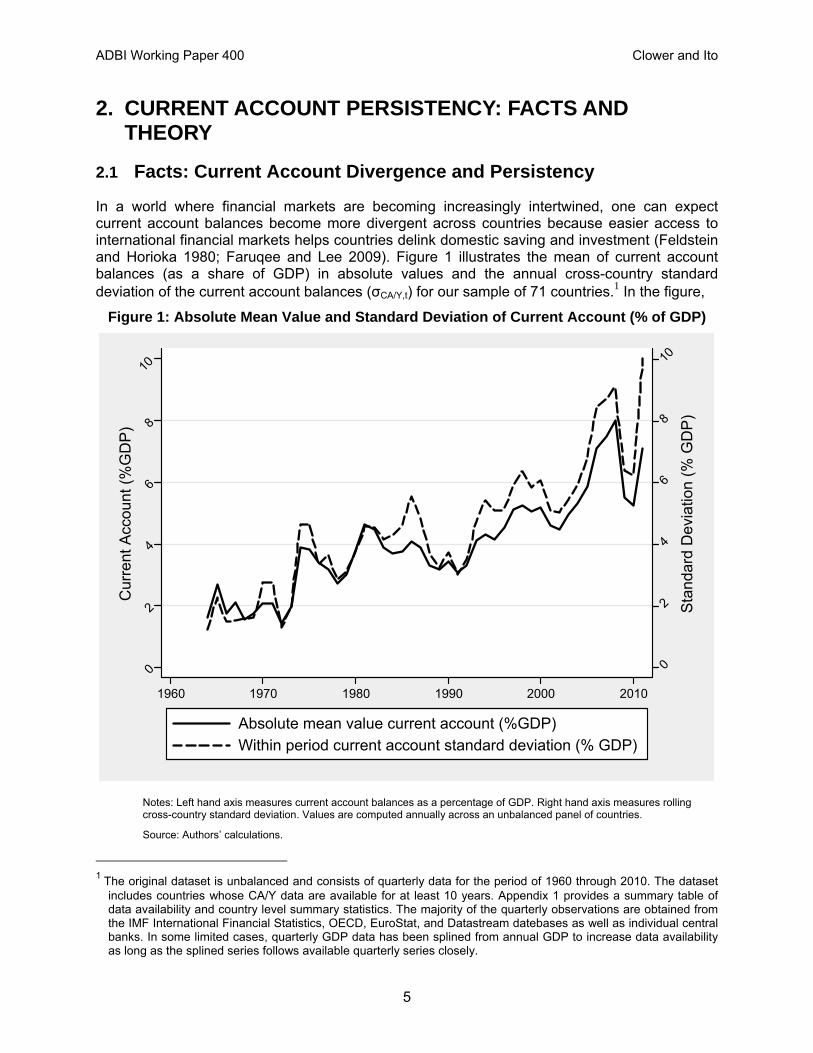
In a world where financial markets are becoming increasingly intertwined, one can expect current account balances become more divergent across countries because easier access to international financial markets helps countries delink domestic saving and investment (Feldstein and Horioka 1980; Faruqee and Lee 2009). Figure 1 illustrates the mean of current account balances (as a share of GDP) in absolute values and the annual cross-country standard deviation of the current account balances (σCA/Y,t) for our sample of 71 countries.1 In the figure,
Figure 1: Absolute Mean Value and Standard Deviation of Current Account (% of GDP)
0
2
4
6
8
10
Sta
ndar
d D
evia
tion
(% G
DP
)0
2
4
6
8
10
Cur
rent
Acc
ount
(%
GD
P)
1960 1970 1980 1990 2000 2010
Absolute mean value current account (%GDP)
Within period current account standard deviation (% GDP)
Notes: Left hand axis measures current account balances as a percentage of GDP. Right hand axis measures rolling cross-country standard deviation. Values are computed annually across an unbalanced panel of countries.
Source: Authors’ calculations.
1 The original dataset is unbalanced and consists of quarterly data for the period of 1960 through 2010. The dataset
includes countries whose CA/Y data are available for at least 10 years. Appendix 1 provides a summary table of data availability and country level summary statistics. The majority of the quarterly observations are obtained from the IMF International Financial Statistics, OECD, EuroStat, and Datastream datebases as well as individual central banks. In some limited cases, quarterly GDP data has been splined from annual GDP to increase data availability as long as the splined series follows available quarterly series closely.

ADBI Working Paper 400 Clower and Ito
6
we can observe a rising trend for both the mean absolute value and standard deviation of current account balances. Especially in the years of global imbalances, i.e., the mid-2000s, we observe wider cross-country variations in current accounts as well as higher degree of imbalances, implying higher degrees of current account persistency.
While the financial crisis of 2008 seems to have contributed to rebalancing, its effect appears to be only temporary, possibly suggesting that the financial crisis did not lead to corrections of the global imbalances (as is argued in Chinn et al. 2011). However, we must also note that part of the short-lived impact of the financial crisis on current account balances may be masked by the fact that we view current account balances as a fraction of GDP; the crisis may have shrunk both current account balances and nominal GDP with its impact possibly larger on the latter.
When we divide our sample into subgroups based on income levels or geographical regions, which is displayed in Figure 2, we still observe that both the levels and the standard deviations of current account balances rose in the last decade for most of the country groups until the breakout of the 2008–09 crisis. As many researchers have noted, the groups of industrialized countries, emerging market economies, and Asian economies have experienced persistent rises in the size of current account imbalances.
Figure 2: Mean Absolute Current Account (% of GDP) and Cross-Sectional Standard Deviation by Country Subsamples
0
5
10
15
02468
10
1960 1970 1980 1990 2000 2010
Industrialized Countries
0
5
10
15
02468
10
1960 1970 1980 1990 2000 2010
Less Developed Countries
0
5
10
15
02468
10
1960 1970 1980 1990 2000 2010
Emerging Countries
0
5
10
15
02468
10
1960 1970 1980 1990 2000 2010
East Asian and Pacific Countries
0
5
10
15
02468
10
1960 1970 1980 1990 2000 2010
Latin American Countries
0
5
10
15
02468
10
1960 1970 1980 1990 2000 2010
Euro 12 Countries
Absolute mean value current account (%GDP)
Within period current account standard deviation (% GDP)
Notes: Left hand axis measures current account balances as a percentage of GDP. Right hand axis measures rolling cross-sectional standard deviation. Values are computed annually across an unbalanced panel of countries.
Source: Authors’ calculations.

ADBI Working Paper 400 Clower and Ito
7
As another way of looking at the degree of current account persistence, Figure 3 shows the cross-country average and standard deviation of the AR(1) coefficient from the following autoregressive model applied to each of our sample countries in a rolling window of 20 quarters:
, (1)
.
The figure shows that after experiencing a high level of current account persistence in the early 1970, the persistence level gradually declined until the end of the 1990s. After the early 2000s, however, the average level of persistence has been on a moderately rising trend again. In contrast, the cross-country standard deviation of persistence has been on a cyclically declining trend since its peak in the early 1990s, though the cross-country variation does seem to have moderately increased in the mid-2000s.
Figure 3: Current Account Persistence
.1.2
.3.4
.5C
ross
Sec
tion
Sta
ndar
d D
evia
tion
0
.2
.4
.6
.8
1
AR
(1)
Coe
ffici
ent
1960 1970 1980 1990 2000 2010
AR(1) Coefficient
Within period standard deviation of AR(1) estimates
Notes: All regressions include a constant and use a rolling window of 20 quarters. The figure shows annual averages across an unbalanced panel of countries. All coefficients greater than one are set to one and all coefficients less than negative one are set to negative one.
Source: Authors’ calculations.

ADBI Working Paper 400 Clower and Ito
8
This figure allows us to make two observations. First, the behavior of the AR(1) coefficient’s standard deviations confirms the differences in the changes of persistence levels across the countries in any given time period, suggesting increasing idiosyncratic shocks to country level persistence. Second, the relatively stable standard deviations in the last three decades suggest that country level changes in persistence are not driven solely by global factors.2
In fact, more formal tests for parameter stability provide support for the presence of non-linearities in current account dynamics. We apply the Elliot-Muller (2006) quasi-local-level (QLL) test, a robust parameter stability test, allowing for singular or multiple structural breaks, parameter instability, and heteroskedasticity (Baum 2001).3 The QLL tests the null hypothesis that regression coefficients are stable within the sample period. When applying the QLL test to the AR(1) regression for current account balances, we reject the null hypothesis of parameter stability at the 10% significance level for 52% of the countries, 70% of industrialized countries, and 50% of developing countries. When we use the Hansen (1992) parameter stability test as a robustness check to test the stability of the constant, persistence, variance, and a joint stability in the AR(1) model, we reject the null hypothesis of stability with significantly large values of the test statistic.4
Overall, these stability tests generally support the instability of AR(1) coefficients for the data generating process of current account balances, suggesting that linear models may not be well-fit to investigate the stationarity of current account series.
2.2 Current Account Stationarity: Theory
With a simple theoretical framework with the infinitely-lived, consumption-smoothing representative agent, we can make theoretical predictions on current account sustainability (Trehan and Walsh 1991; Hakkio and Rush 1991). In this framework, stationarity of current account balances is warranted as the representative agent optimizes her consumption with the long-run intertemporal budget constraint (LRBC).
When we assume that the economy-wide budget constraint is given as:
, (2)
where Ct , It , Gt , Bt , Yt , and rt represent consumption, private investment, government spending, net foreign assets, output, and the world real interest rate, respectively. We can isolate net foreign asset as:
(3).
2 An obvious counterexample is the turbulence in the standard deviation in the early 1970s that must have been
associated with a global event, i.e., the collapse of the Bretton Woods system. 3 Complete results are found in Appendix 2. 4 The distribution of the test statistic is non-standard and depends directly on the number of regressors. These tests
statistics are valid even in the presence of non-stationary movements in the model regressors and/or variance (Hansen 1991).

ADBI Working Paper 400 Clower and Ito
9
This can be further simplified to:
(4)
or
(5)
where . Hence, the current account balance is composed of the net flow of income from the domestic economy to the rest of the world in exchange for goods and services and capital.
Following Taylor (2002), we can consider eq. (4) at the steady state in a stochastic setting. Defining Rt = 1 + rt such that E(Rt + i | Ωt-1)=R for all t and i≥0, given the information set Ω from the previous period, leads us to obtain the long-run behavior of current account as:
(6).
The LRBC is conditional on:
(7).
This condition holds as long as the world interest rate is above zero and the current account is stationary.
Even when adjusted to allow for stochastic growth, the intertemporal framework yields a similar condition for sustainability. Allowing the world economy to grow at rate of gt with E(gt) =g > 0, we can show that in the case with growth and stochastic shocks, the LRBC implies that
(8)
where and . This will hold as long as is greater than one and the current account as a fraction of output is stationary.
ADBI Working Paper 400 Clower and Ito
10
3. STATIONARITY OF CURRENT ACCOUNT BALANCES AND REGIME SHIFTS
3.1 Linear Unit Root Tests and Current Account Balances
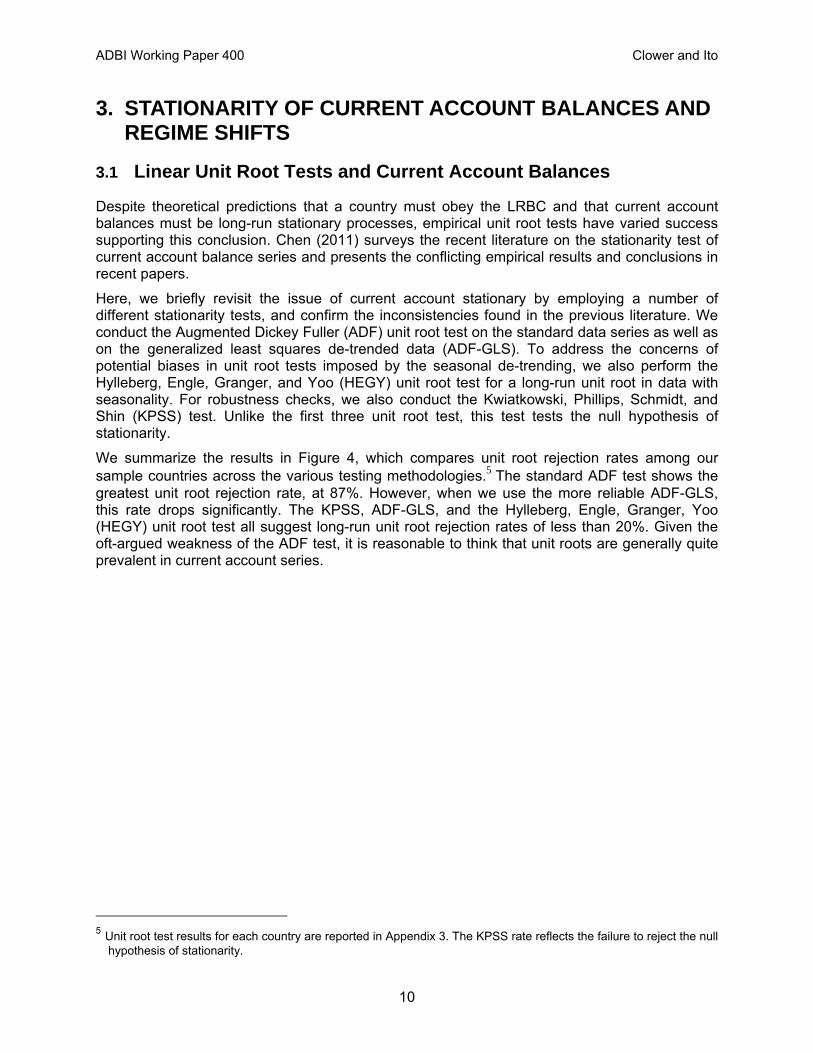
Despite theoretical predictions that a country must obey the LRBC and that current account balances must be long-run stationary processes, empirical unit root tests have varied success supporting this conclusion. Chen (2011) surveys the recent literature on the stationarity test of current account balance series and presents the conflicting empirical results and conclusions in recent papers.
Here, we briefly revisit the issue of current account stationary by employing a number of different stationarity tests, and confirm the inconsistencies found in the previous literature. We conduct the Augmented Dickey Fuller (ADF) unit root test on the standard data series as well as on the generalized least squares de-trended data (ADF-GLS). To address the concerns of potential biases in unit root tests imposed by the seasonal de-trending, we also perform the Hylleberg, Engle, Granger, and Yoo (HEGY) unit root test for a long-run unit root in data with seasonality. For robustness checks, we also conduct the Kwiatkowski, Phillips, Schmidt, and Shin (KPSS) test. Unlike the first three unit root test, this test tests the null hypothesis of stationarity.
We summarize the results in Figure 4, which compares unit root rejection rates among our sample countries across the various testing methodologies.5 The standard ADF test shows the greatest unit root rejection rate, at 87%. However, when we use the more reliable ADF-GLS, this rate drops significantly. The KPSS, ADF-GLS, and the Hylleberg, Engle, Granger, Yoo (HEGY) unit root test all suggest long-run unit root rejection rates of less than 20%. Given the oft-argued weakness of the ADF test, it is reasonable to think that unit roots are generally quite prevalent in current account series.
5 Unit root test results for each country are reported in Appendix 3. The KPSS rate reflects the failure to reject the null
hypothesis of stationarity.

ADBI Working Paper 400 Clower and Ito
11
Figure 4: Unit Root Rejection Rates
0.873
0.197 0.197
0.155
0.465
0
.1
.2
.3
.4
.5
.6
.7
.8
.9
1
ADF KPSS DFGLS HEGY Zivot-Andrews
Notes: The ADF, HEGY, and DFGLS results report unit root rejection rates across all countries. The KPSS results report the failure to reject stationarity rate across all countries. The original ADF is run using no constant, no time trends, and no lags. The second bar reports the ADF tests using lag lengths chosen by the Schwartz Criteria. The KPSS test is run without a time trend and results reported are for zero lags, though longer lag lengths are tested and yield similar results. All DFGLS tests are run without a trend, use the reported Schwartz Criteria lag lengths, and the Elliot, Rothenberg, and Stock critical values. The chart reports the Hylleberg, Engle, Granger, Yoo (HEGY) test long-run unit roots using no lags.
Source: Authors’ calculations.
We can consider a number of possible explanations for the failure of rejection of the unit root in current account series. First, such results could arise if current account balances do have a true long-run unit root. This conclusion is somewhat troublesome, because it opposes theoretical predictions on current account sustainability. A second possible explanation is that the current account balance as a portion of GDP may have structural breaks in the levels or trends. If that is the case, simple linear stationarity tests could fail to reject the null hypothesis of unit roots. Finally, these results may result from parameter instabilities. Given the change in both domestic and international environment that countries face, it is possible that the degree of persistence (captured by α in equation (1)) can vary over time. Depending on the nature of structural breaks, parameter instabilities, or regime switches, the power of standard unit root tests can vary significantly (Perron 1989; Nelson et al. 2001). As such, it is reasonable that recent literature often incorporates non-linear models to test the stationarity of current account balances.
The use of non-linear models of current account balances does not hinge solely on the empirical finding of unit root tests, but also has backing in economic intuition. Taylor (2002) argues that structural breaks in either or both of savings and investment in the private and government

ADBI Working Paper 400 Clower and Ito
12
sectors could lead to breaks in current account balances. This suggests that regime shifts in current account balances can be caused by changes in the global financial market, changes in regulatory controls on cross-border capital flows, changes in credit worthiness of a country, or changes in domestic and foreign countries’ policies and institutions for savings and investment (Taylor 2002).6
When we apply unit root tests with a single or double structural breaks in the trend and/or intercept to our current account balance data, we get results with increased rates of unit root rejection. The unit root rejection rate for the Zivot-Andrews (1992) test for a single break in the intercept is 46.5% (Figure 4). Table 1 provides country level results for unit root testing with structural breaks and shows similar results using the Zivot-Andrews or Clemente-Montanes-Reyes unit root test with structural breaks (Clemente et al. 1998). The unit root rejection rates hardly increases when we move from a single break test and a double break test. Although these increases in the unit root rejection rates should not be used as the sole motivation for including structural breaks, they do offer support for inclusion of structural breaks. More broadly, these results suggest that non-rejection of the unit root in linear tests should not be too quickly interpreted as non-sustainability of current account balances.
6 Furthermore, when measuring the current account relative to GDP structural breaks can arise from sudden changes
in GDP behavior. For example, sudden stop growth, regime shifting or “plucking” in GDP growth (Friedman 1964) have been supported in a number of previous papers.

ADBI Working Paper 400 Clower and Ito
13
Table 1: Unit Root Tests with Single Structural Breaks
Country Zivot Andrews Break Date
T-Stat CMR AO Break Date
T-Stat CMR IO Break Date
T-Stat N Start Date End Date
1 Argentina 2001q2 -4.999** 2000q3 -0.948 2000q4 -4.011 61 1993q1 2011q1 2 Armenia 2008q1 -5.503*** 2000q3 -0.553 2000q1 -1.754 58 1994q1 2011q1 3 Australia 1980q3 -4.937** 1979q2 -3.785** 1980q1 -4.195 189 1960q1 2010q4 4 Austria 2001q3 -2.761 2001q1 -1.743 2001q2 -2.846 151 1970q1 2011q1 5 Belarus 2008q4 -7.015*** 2008q1 -2.262 2008q2 -2.288 50 1996q1 2011q1 6 Belgium 2007q4 -9.063*** 2004q4 -0.602 2005q1 -1.204 53 1995q1 2010q4 7 Bolivia 2003q2 -3.674 2003q4 -3.836** 2003q1 -3.145 68 1990q1 2009q4 8 Brazil 1994q4 -3.672 1985q1 -3.417 1982q4 -3.364 121 1978q1 2011q2 9 Bulgaria 2008q3 -7.146*** 2004q1 -2.336 2004q2 -2.949 58 1994q1 2011q1 10 Cambodia 2007q2 -5.984*** 2007q3 -2.869 2006q4 -3.529 53 1994q1 2009q4 11 Canada 1994q2 -3.131 1994q4 -2.484 1995q1 -3.150 186 1961q1 2011q1 12 Chile 2007q4 -3.717 2003q1 -4.205** 2003q2 -2.956 68 1991q1 2010q4 13 PRC 2004q3 -3.559 2003q3 -3.579** 2003q4 -3.734 65 1991q1 2010q1 14 Colombia 1998q4 -6.751*** 1998q1 -1.631 1998q2 -4.173 49 1996q1 2010q4 15 Costa Rica 2009q1 -7.655*** 2007q4 -2.576 2008q1 -5.117** 38 1999q1 2010q4 16 Croatia 2000q2 -18.445*** 2007q4 -2.164 2008q1 -2.093 54 1994q4 2010q4 17 Czech Republic 2005q1 -7.410*** 2003q2 -4.101** 2004q2 -4.429** 61 1993q1 2011q1 18 Denmark 1987q1 -3.062 1989q2 -2.437 1989q4 -2.427 124 1977q1 2011q1 19 El Salvador 2009q1 -5.822*** 2001q1 -2.848 2002q1 -3.714 38 1999q1 2010q4 20 Estonia 2008q1 -3.461 2008q4 -1.724 2008q4 -2.143 60 1993q1 2010q4 21 Finland 1993q3 -4.787** 1994q3 -3.343 1992q4 -3.922 131 1975q1 2011q1 22 France 2004q2 -2.591 2006q3 -1.722 1982q4 -1.228 130 1975q1 2010q4 23 Georgia 2005q3 -3.836 2004q4 -1.853 2005q1 -3.497 46 1997q1 2011q1 24 Germany 1990q2 -3.598 2002q4 -2.186 2003q2 -3.036 147 1971q1 2011q1 25 Greece 1986q1 -3.515 2005q1 -2.884 2005q2 -2.644 127 1976q1 2011q1 26 Guatemala 1987q2 -3.759 2008q2 -3.505 1986q4 -3.830 123 1977q1 2010q4 27 Hong Kong, China 2009q2 -6.642*** 2003q4 -5.767** 2004q1 -5.767** 38 1999q1 2011q1 28 Hungary 2007q3 -2.360 1991q3 -2.344 1992q2 -3.368 73 1989q4 2010q4 29 Iceland 2004q4 -4.954** 2004q1 -3.395 2004q2 -4.621** 127 1976q1 2011q1 30 India 1980q1 -3.724 1973q3 -2.838 1973q4 -2.849 189 1960q1 2010q4 31 Indonesia 1997q4 -5.041** 1997q1 -3.267 1997q2 -6.593** 107 1981q1 2010q4 32 Ireland 2004q2 -3.298 1999q4 -3.430 2004q1 -3.203 72 1990q1 2010q4 33 Israel 1984q4 -3.830 1984q1 -2.106 1984q2 -5.888** 143 1972q1 2011q1 34 Italy 1993q1 -2.673 2004q1 -4.158** 2004q2 -3.279 151 1970q1 2011q1 35 Japan 1983q2 -3.808 1982q3 -5.222** 1979q4 -3.877 124 1977q1 2011q1 36 Kazakhstan 2001q2 -5.935*** 2008q4 -5.461** 2008q2 -5.607** 53 1995q1 2010q4 37 Korea, Rep. 1983q2 -4.332 1982q3 -3.746** 1982q4 -4.702** 127 1976q1 2011q1 38 Kyrgyz Republic 2006q4 -6.700*** 2006q1 -0.495 2006q2 -6.584** 34 2000q1 2010q4 39 Latvia 2008q2 -4.766** 2008q4 -1.936 2008q3 -3.257 61 1993q1 2011q1 40 Lithuania 2008q2 -3.929 2009q1 -3.115 2008q4 -3.147 61 1993q1 2011q1 41 Luxembourg 2003q3 -8.129*** 2007q4 -3.897** 2008q1 -4.116 53 1995q1 2010q4 42 Malaysia 2005q1 -4.214 2004q2 -3.421 2004q3 -2.062 35 1999q1 2010q1 43 Mauritius 2005q2 -5.966*** 2004q3 -2.674 2004q4 -2.887 34 2000q1 2010q4 44 Mexico 1988q2 -3.969 1981q3 -2.800 1981q4 -3.618 116 1979q1 2011q1 45 Moldova 2000q3 -7.154*** 2002q3 -2.172 1998q4 -3.287 53 1995q1 2010q4 46 Netherlands 1998q1 -2.897 2003q1 -3.392 2002q1 -3.965 124 1977q1 2011q1 47 New Zealand 1988q1 -3.338 1987q2 -2.537 1987q3 -4.532** 112 1980q1 2011q1 48 Norway 1985q3 -5.066** 1998q2 -4.200** 1998q3 -4.228 131 1975q1 2011q1 49 Paraguay 2002q2 -5.147** 2002q1 -7.809** 2001q4 -2.617 34 2000q1 2010q4 50 Peru 1998q3 -4.916*** 1999q4 -5.782** 1998q1 -5.769** 115 1979q1 2010q4 51 Philippines 1989q2 -3.888 2002q1 -6.348** 2003q1 -6.251** 109 1977q2 2011q1 52 Poland 1991q4 -4.410 1989q4 -7.420** 1990q1 -5.440** 91 1985q1 2010q4 53 Portugal 1983q3 -3.817 1997q1 -2.093 1995q2 -2.934 124 1977q1 2011q1 54 Romania 2003q4 -4.460 2003q3 -3.023 2002q4 -2.746 68 1991q1 2010q4 55 Russian Federation 1998q4 -6.494*** 1999q1 -3.543 1998q1 -4.103 58 1994q1 2011q1 56 Slovak Republic 1996q1 -4.887** 1995q1 -4.370** 1995q2 -5.737** 60 1993q1 2010q4 57 Slovenia 2004q2 -6.347*** 2005q1 -2.953 2005q2 -4.746** 54 1995q1 2011q1 58 South Africa 1977q1 -4.869** 1979q3 -2.749 1979q4 -4.849** 190 1960q1 2011q1 59 Spain 1998q4 -2.606 2003q2 -4.314** 2003q3 -4.475** 131 1975q1 2011q1 60 Sri Lanka 1984q1 -5.143*** 1983q1 -5.199** 1983q3 -5.694** 123 1977q1 2010q4 61 Sweden 1994q1 -3.235 1996q2 -3.118 1994q3 -2.869 131 1975q1 2011q1 62 Switzerland 1979q2 -4.248 1996q1 -4.628** 1991q3 -3.692 142 1972q1 2010q4 63 Taipei,China 1987q4 -4.412 1988q2 -2.817 1987q2 -4.010 108 1981q1 2011q1 64 Thailand 1997q3 -4.261 1996q4 -3.193 1997q1 -5.052** 126 1976q1 2010q4 65 Turkey 1994q2 -6.509*** 2003q1 -5.628** 2002q2 -2.434 85 1987q1 2011q1 66 Ukraine 1999q2 -6.551*** 2006q1 -1.913 2004q4 -2.291 57 1994q1 2010q4 67 United Kingdom 1986q2 -3.419 1986q3 -4.111** 1985q3 -4.283** 189 1960q1 2010q4 68 United States 1998q2 -2.249 1998q4 -2.750 1997q4 -3.005 189 1960q1 2010q4 69 Uruguay 2002q1 -6.460*** 2007q4 -2.825 2001q3 -5.556** 38 1999q1 2010q4 70 Venezuela, RB 2008q4 -7.487*** 2003q3 -2.170 2002q4 -2.972 46 1997q1 2011q1 71 Viet Nam 1999q1 -5.589*** 2007q3 -1.920 2006q4 -3.338 49 1996q1 2010q4
***, **, * denotes rejection of the null unit root hypothesis at the 1%, 5%, and 10% level
Source: Authors’ calculations.

ADBI Working Paper 400 Clower and Ito
14
While the Zivot-Andrews and CMR unit root tests allow the incorporation of certain non-linearities, they are not robust for all types of non-linear adjustment. For example, these tests restrict the number and types of breaks. Hence, the Zivot-Andrews and CMR unit root tests are invalid for any form of non-linearities that fall outside those restrictions (Nelson et al. 2001). As such, these tests fail to address the primary observations we made in a previous section: time variations in current account persistence. One particularly concerning limitation is that if the series switches from stationary to non-stationary regimes, standard unit root tests are not valid, even if they account for structural breaks (Kim 2000). This gives rise to the questionable validity of these standard tests when they are applied to current account balances exhibiting persistence switches, and possible periods of “local” non-stationarity (Chen 2011).
Local non-stationarity in current account balances is intuitively plausible. Such switches in persistence imply that current account accumulation occurs in some short-run regimes at rates that violate the LRBC but eventually switches back to a rate that is in accordance with the LRBC. Hence, an appropriate empirical model of current account balances may need to allow for more general parameter instabilities than just breaks in the trend or the mean, which gives rise to a need to employ a Markov-Switching unit root test.
3.2 Markov-Switching (MS) Stationarity Analysis
3.2.1 MS-ADF Estimation
We now take a more general unit root testing approach and employ a Markov-Switching unit root test following Raybaudi et al. (2004) and Chen (2011). The MS-ADF testing framework is based on the standard ADF testing framework but distinguishes periods of locally explosive behavior from global unit roots (Hall et al. 1999). This testing procedure allows for the dynamics of the tested variable to depend on an unobserved, stochastic state variable.
Estimation of the model requires maximum likelihood estimation of the parameter vector θ according to
(9)
with and .
We allow for the constant and serial correlation coefficient to take two different regimes while maintaining constant variance.7 Furthermore, we restrict one regime to a random walk regime (state 0) while the second regime is a standard AR(1) mean-reverting regime (state 1). This allows for the distinction between local non-stationarity that occurs within a regime and global non-stationarity that occurs across the entire sample (Raybaudi et al. 2004). In light of cross-sectional differences in current account dynamics, we estimate the model for each of our
7 We allow switching variances for Belgium, Georgia, Greece, Indonesia, and Israel, however, as exceptions. For
these countries, data visualization, model fit, and parameter stability tests confirm that the MS-ADF model with switching variances perform significantly better than the model shown in Equation 9. In the model with switching variances, the variance takes two regimes, ? , ? in accord with the regime changes in the constant and the AR(1) coefficient.
ADBI Working Paper 400 Clower and Ito
15
sample countries individually. This will provide greater insight on whether and to what extent cross-sectional differences drive differences in current account dynamics.8
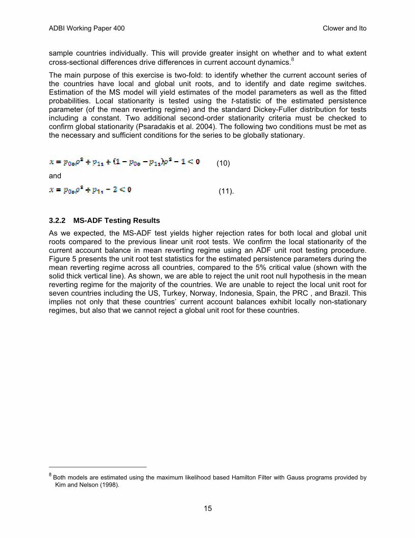
The main purpose of this exercise is two-fold: to identify whether the current account series of the countries have local and global unit roots, and to identify and date regime switches. Estimation of the MS model will yield estimates of the model parameters as well as the fitted probabilities. Local stationarity is tested using the t-statistic of the estimated persistence parameter (of the mean reverting regime) and the standard Dickey-Fuller distribution for tests including a constant. Two additional second-order stationarity criteria must be checked to confirm global stationarity (Psaradakis et al. 2004). The following two conditions must be met as the necessary and sufficient conditions for the series to be globally stationary.
(10)
and
(11).
3.2.2 MS-ADF Testing Results
As we expected, the MS-ADF test yields higher rejection rates for both local and global unit roots compared to the previous linear unit root tests. We confirm the local stationarity of the current account balance in mean reverting regime using an ADF unit root testing procedure. Figure 5 presents the unit root test statistics for the estimated persistence parameters during the mean reverting regime across all countries, compared to the 5% critical value (shown with the solid thick vertical line). As shown, we are able to reject the unit root null hypothesis in the mean reverting regime for the majority of the countries. We are unable to reject the local unit root for seven countries including the US, Turkey, Norway, Indonesia, Spain, the PRC , and Brazil. This implies not only that these countries’ current account balances exhibit locally non-stationary regimes, but also that we cannot reject a global unit root for these countries.
8 Both models are estimated using the maximum likelihood based Hamilton Filter with Gauss programs provided by
Kim and Nelson (1998).

ADBI Working Paper 400 Clower and Ito
16
Figure 5: MS-ADF Mean Reverting Regime Test Statistics
ZAFVNMVEN
USAURY
UKRTWNTUR
THASWE
SVN SVKSLV
RUSROM PRY
PRTPOL
PHLPERNZL
NORNLD MYS
MUSMEX
MDA LVALUX
LTULKA KOR
KGZKAZ
JPNITAISR
ISLIRLIND
IDNHUN
HRV HKGGTM
GRCGEOGBR
FRAFIN ESTESP
DNKDEUCZE
CRICOL
CHNCHECAN
BRABOL
BLR BGRBEL
AUTAUSARM
ARG
-10 -8 -6 -4 -2 0
Notes: The thick solid line represents 5% ADF critical value for the case with a constant and no trend. The econometric model for this figure allows for switching constant and persistence parameter across regimes. One regime is restricted to a random walk model. We are unable to reject the unit root in the first regime for seven countries: the US, Turkey, Norway, Indonesia, Spain, The PRC, and Brazil.
Source: Authors’ calculations.
For those countries in which we can reject the unit root in the mean reverting regime, this is not sufficient to reject global nonstationarity, and one must also consider the second-order conditions for global stationarity (Psaradakis et al. 2004). Using these conditions, we find that we are also unable to reject the global unit root for Venezuela. With the MS-ADF testing framework, we are now able to reject the unit root for 88% of the countries, a substantial increase compared to linear unit root tests.
3.2.3 Random Walk Episodes
The random walk regime represents time spans during which a country runs an “explosive,” or non-mean reverting, current account balance. These locally non-stationary periods of current account balance would be unsustainable if it continued in the long-run. In other words, these periods can be interpreted as those with a “red signal” (Raybaudi et al. 2004) that the country of concern would violate the long-run budget constraint unless there is a drastic change in its current account balances.
ADBI Working Paper 400 Clower and Ito
17
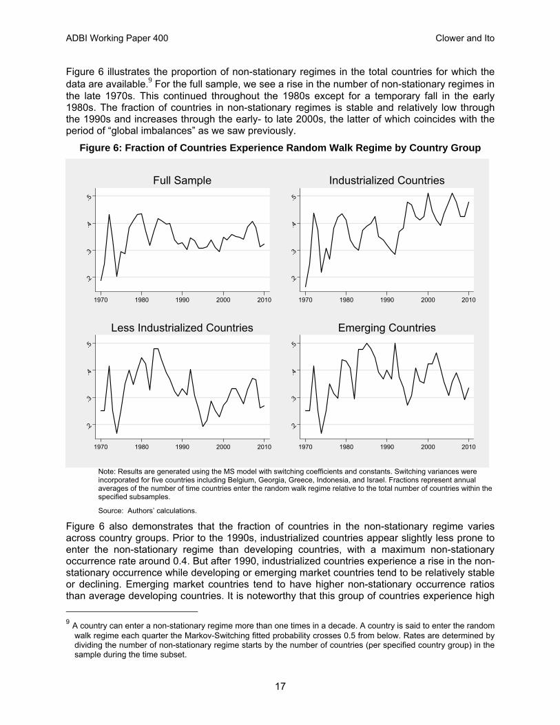
Figure 6 illustrates the proportion of non-stationary regimes in the total countries for which the data are available.9 For the full sample, we see a rise in the number of non-stationary regimes in the late 1970s. This continued throughout the 1980s except for a temporary fall in the early 1980s. The fraction of countries in non-stationary regimes is stable and relatively low through the 1990s and increases through the early- to late 2000s, the latter of which coincides with the period of “global imbalances” as we saw previously.
Figure 6: Fraction of Countries Experience Random Walk Regime by Country Group
.2
.3
.4
.5
1970 1980 1990 2000 2010
Full Sample
.2
.3
.4
.5
1970 1980 1990 2000 2010
Industrialized Countries
.2
.3
.4
.5
1970 1980 1990 2000 2010
Less Industrialized Countries
.2
.3
.4
.5
1970 1980 1990 2000 2010
Emerging Countries
Note: Results are generated using the MS model with switching coefficients and constants. Switching variances were incorporated for five countries including Belgium, Georgia, Greece, Indonesia, and Israel. Fractions represent annual averages of the number of time countries enter the random walk regime relative to the total number of countries within the specified subsamples.
Source: Authors’ calculations.
Figure 6 also demonstrates that the fraction of countries in the non-stationary regime varies across country groups. Prior to the 1990s, industrialized countries appear slightly less prone to enter the non-stationary regime than developing countries, with a maximum non-stationary occurrence rate around 0.4. But after 1990, industrialized countries experience a rise in the non-stationary occurrence while developing or emerging market countries tend to be relatively stable or declining. Emerging market countries tend to have higher non-stationary occurrence ratios than average developing countries. It is noteworthy that this group of countries experience high
9 A country can enter a non-stationary regime more than one times in a decade. A country is said to enter the random
walk regime each quarter the Markov-Switching fitted probability crosses 0.5 from below. Rates are determined by dividing the number of non-stationary regime starts by the number of countries (per specified country group) in the sample during the time subset.
ADBI Working Paper 400 Clower and Ito
18
non-stationary regime ratios in the 1980s, a time period many emerging market countries experienced debt crisis. Both developing and emerging market country groups experience a fall in the rate in the late 1980s and the mid-1990s. Interestingly, the (unreported) euro 12 countries’ ratios rapidly rise in the second half of the 2000s, suggesting a possible link with the debt crisis that started in 2010.
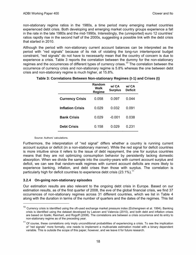
Although the period with non-stationary current account balances can be interpreted as the period with “red signals” because of its risk of violating the long-run intertemporal budget constraint, “red signals” do not have to necessarily mean that the country of concern is due to experience a crisis. Table 3 reports the correlation between the dummy for the non-stationary regimes and the occurrences of different types of currency crises.10 The correlation between the occurrence of currency crisis and non-stationary regime is 5.8% whereas the one between debt crisis and non-stationary regime is much higher, at 15.8%.
Table 3: Correlations Between Non-stationary Regimes (t-1) and Crises (t)
Random Walk
Regime
w/ CA Surplus
w/ CA Deficit
Currency Crisis 0.058 0.097 0.044
Inflation Crisis 0.029 0.032 0.091
Bank Crisis 0.029 -0.001 0.038
Debt Crisis 0.158 0.029 0.231
Source: Authors’ calculations.
Furthermore, the interpretation of “red signal” differs whether a country is running current account surplus or deficit (in a non-stationary manner). While the red signal for deficit countries is more intuitive since it refers to the issue of debt repayment, the one for surplus countries means that they are not optimizing consumption behavior by persistently lacking domestic absorption. When we divide the sample into the country-years with current account surplus and deficit, we can see that random-walk regimes with current account deficits are more likely to experience banking, inflation, and debt crises than those with surplus. The correlation is particularly high for deficit countries to experience debt crisis (23.1%).11
3.2.4 On-going non-stationary episodes
Our estimation results are also relevant to the ongoing debt crisis in Europe. Based on our estimation results, as of the first quarter of 2008, the eve of the global financial crisis, we find 37 occurrences of non-stationary regimes across 31 different countries, which we list in Table 4 along with the duration in terms of the number of quarters and the dates of the regimes. This list 10 Currency crisis is identified using the oft-used exchange market pressure index (Eichengreen et al. 1994). Banking
crisis is identified using the dataset developed by Laeven and Valencia (2010), and both debt and inflation crises are based on Ilzetki, Reinhart, and Rogoff (2008). The correlations are between a crisis occurrence and its entry to non-stationary regime as of the preceding year.
11 Of course, these correlations only imply unconditional probabilities of experiencing a crisis. To see the implication of “red signals” more formally, one needs to implement a multivariate estimation model with a binary dependent variable. This is outside the scope of this paper, however, and we leave it for future research.

ADBI Working Paper 400 Clower and Ito
19
is quite suggestive of the current euro debt crisis; we find Greece, Ireland, Portugal, and Spain as locally non-stationary regimes (with current account deficit). Interestingly, the US also falls on this list with two non-stationary regimes, one ending in 2008q3 and another currently on-going.12 These findings suggest that concerns about debt sustainability are not empirically unfounded.
12 We must remind that we cannot reject the global non-stationarity of current account balances of the US. This
finding may be interpreted as evidence for the country’s “exorbitant privilege,” which may exempt the country from the binding of the intertemporal budget constraint.

ADBI Working Paper 400 Clower and Ito
20
Table 4: Countries Recently Experiencing Locally Non-stationary Episodes (as of 2008q1)
Country Start End Duration Average CA
Armenia 2001q1 - - 39 -8.7%
Austria 2006q4 - - 16 3.6%
Belarus 2008q3 - - 9 -15.1%
Bolivia 2003q2 2009q3 25 8.3%
Bulgaria 2005q4 2009q1 13 -21.7%
Canada 1996q1 2008q2 49 1.0%
PRC 2007q4 2008q4 4 6.1%
Colombia 2007q2 2008q3 5 -2.4%
2009q3 2010q3 4 -2.6%
El Salvador 2002q4 2008q3 23 -4.9%
Estonia 2006q3 2010q3 16 -6.5%
Georgia 2006q1 2008q4 11 -20.5%
Germany 1985q4 - - 100 2.3%
Greece 2005q4 2011q1 20 -12.2%
Hungary 2009q1 2010q3 6 1.4%
Indonesia 2006q4 2010q3 15 1.5%
Ireland 2005q1 2010q3 22 -3.9%
Israel 1997q2 - - 54 0.9%
Lithuania 2007q1 2011q1 15 -5.2%
Mexico 2007q2 2008q3 5 -0.8%
Norway 2007q1 2008q3 6 15.3%
2009q3 - - 5 12.2%
Peru 2008q1 2009q3 6 -2.5%
Portugal 1997q3 - - 53 -9.3%
Romania 2007q1 2008q4 7 -13.2%
Slovenia 2007q3 2008q3 4 -6.6%
Spain 2003q2 2008q4 22 -7.5%
2009q3 - - 5 -4.8%
Sweden 1995q1 - - 63 5.6%
Switzerland 2009q1 2010q3 6 12.6%
Thailand 2005q3 2008q3 12 2.7%
2009q3 2010q3 4 5.1%
United States 1993q2 2008q3 61 -3.6%
2009q2 2010q3 5 -3.1%
Venezuela, RB 2006q4 2008q2 6 10.1%
2008q4 2009q4 4 1.1%
Viet Nam 2009q2 2010q2 4 -10.1%
Notes: “--” means the non-stationary regime is still in place as of the end of the sample period. For the countries with “--”, the duration refers to the duration of non-stationary regime up to the last available period.
Source: Authors’ calculations.

ADBI Working Paper 400 Clower and Ito
21
4. DETERMINANTS OF CURRENT ACCOUNT PERSISTENCE
We now know that the data generation process for current account balances entails different regimes, either stationary or non-stationary, and also that the degree of current account persistence can differ across countries and over time. These findings raise a natural question: what kind of economic fundamentals or policy regimes can affect the nature of current account persistence? More specifically, what kind of factors would lead a country to enter a non-stationary regime for its current account process? And how do they affect the degree of current account persistence? We now explore these questions.
4.1 Probit Estimation
As a first exploration, we examine how the economic fundamentals contribute to the probability of countries entering non-stationary regimes. This exercise may help us identify factors that would prevent countries from rebalancing their current accounts, which might evolve into a violation of the long-run budget constraint (“red signal”).13
We estimate the probit model with the dependent variable indicating non-mean reverting regimes as:
(12)
where Ii,t is an indicative variable that takes the value of one if country i is in a locally non-stationary regime in year t, and 0, otherwise. Xi,t is a vector of economic fundamentals and policy regimes for country i in year t. To avoid bidirectional causality or simultaneous bias, we lag all the explanatory variables by one year. Also, to control for external, or global, common shocks, we include global factors in the vector Wt (that is invariant across countries, but is variant over time).
A number of factors can be potential determinants of the probability of entering non-stationary regimes, encompassing a wide range of related literature from sudden-stop and twin crises, to the savings and investment integration puzzle. Despite this span, we test a list of candidate determinants that recursively appear in the literature. Specifically, we include in vector X the dummies for flexible and fixed exchange rate regimes; real exchange rate misalignment; financial development; financial and trade openness; per capita income levels; international reserves holding; net foreign asset positions; budget balances (as a proxy for government debt); absolute values of current account balances; and the dummies for commodity exporters, manufacturing exporters, current account deficit countries; currency crisis; and the euro countries. We describe the rationales and theoretical predictions as well as the data sources of the explanatory variables in Appendix 4. We conduct estimations for the full sample as well as the subsamples of industrialized countries, developing countries, and emerging market economies.14
13 Again, the situation is more of concern when a country runs current account deficits persistently in a non-stationary
regime. However, a surplus country in a non-stationary regime can be also a subject of concern since it is not optimizing its consumption and financing behavior in the context of the intertemporal budget constraint.
14 The emerging market economies are defined as the economies classified as either emerging or frontier during 1980–1997 by the International Financial Corporation plus Hong Kong, China; and Singapore.
ADBI Working Paper 400 Clower and Ito
22
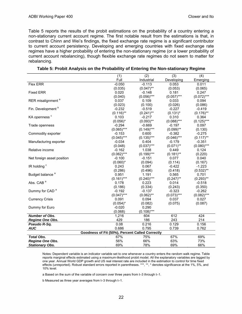
Table 5 reports the results of the probit estimations on the probability of a country entering a non-stationary current account regime. The first notable result from the estimations is that, in contrast to Chinn and Wei’s findings, the fixed exchange rate regime is a significant contributor to current account persistency. Developing and emerging countries with fixed exchange rate regimes have a higher probability of entering the non-stationary regime (or a lower probability of current account rebalancing), though flexible exchange rate regimes do not seem to matter for rebalancing.
Table 5: Probit Analysis on the Probability of Entering the Non-stationary Regime
(1) (2) (3) (4) Full Industrial Developing Emerging Flex ERR -0.050 -0.113 0.053 0.011 (0.035) (0.047)** (0.053) (0.065) Fixed ERR 0.020 -0.148 0.181 0.247 (0.040) (0.056)*** (0.057)*** (0.072)*** RER misalignment a 0.037 0.109 0.033 0.094 (0.023) (0.100) (0.026) (0.086) Fin. Development b -0.232 -0.519 -0.227 -0.419 (0.116)** (0.241)** (0.131)* (0.176)** KA openness c 0.103 -0.217 0.310 0.364 (0.056)* (0.093)** (0.088)*** (0.125)*** Trade openness -0.294 -0.669 -0.197 0.097 (0.065)*** (0.149)*** (0.099)** (0.130) Commodity exporter -0.153 0.600 -0.382 -0.275 (0.045)*** (0.135)*** (0.046)*** (0.117)** Manufacturing exporter -0.034 0.404 -0.179 -0.351 (0.048) (0.037)*** (0.071)** (0.080)*** Relative income -0.162 1.038 0.449 0.124 (0.062)*** (0.199)*** (0.181)** (0.220) Net foreign asset position -0.100 -0.151 0.077 0.040 (0.060)* (0.094) (0.114) (0.167) IR holding c 0.243 0.067 -0.422 -1.223 (0.286) (0.496) (0.418) (0.532)** Budget balance a 0.951 1.191 0.565 0.701 (0.161)*** (0.240)*** (0.247)** (0.293)** Abs. CAB a 0.178 0.223 0.014 -0.518 (0.186) (0.334) (0.243) (0.350) Dummy for CAD a -0.192 -0.137 -0.323 -0.262 (0.047)*** (0.062)** (0.073)*** (0.082)*** Currency Crisis 0.091 0.094 0.037 0.027 (0.054)* (0.082) (0.075) (0.087) Dummy for Euro -0.020 0.290 (0.068) (0.108)*** Number of Obs. 1,216 604 612 424 Regime One Obs. 429 186 243 214 Pseudo R-Sq. 0.08 0.216 0.129 0.156 AUC 0.686 0.795 0.739 0.762
Goodness of Fit (50%), Percent Called CorrectlyTotal Obs. 67% 75% 67% 69% Regime One Obs. 56% 66% 63% 73% Stationary Obs. 69% 78% 69% 66%
Notes: Dependent variable is an indicator variable set to one whenever a country enters the random walk regime. Table reports marginal effects estimated using a maximum-likelihood probit model. All the explanatory variables are lagged by one year. Annual World GDP growth and US real interest rate are included in the estimation to control for time fixed effects (unreported). Robust standard errors reported in parentheses. ***, **, * denotes significance at the 1%, 5%, and 10% level.
a Based on the sum of the variable of concern over three years from t–3 through t–1.
b Measured as three year averages from t–3 through t–1.

ADBI Working Paper 400 Clower and Ito
23
c Measured as deviations from the sample mean.
Source: Authors’ calculations.
The group of industrialized countries has significantly negative coefficients for both flexible and fixed exchange rate regimes, but given that we also include the dummy for the euro countries, we can think of these effects to be those of non-euro countries. For the euro countries, the fact that they belong to a currency union raises the probability of entering the non-stationary regime by 14% (= 29% – 14.8%). Non-Euro countries are less likely to enter the random-walk regime when adopting a flexible exchange rate regime (by 11%).
A higher level of financial development increases the probability of current account rebalancing, and is significant for all country groups. This is consistent with the Caballero-Farhi-Gourinchas (2008) hypothesis that countries with less developed financial markets seek external sources of safe financial assets (surplus countries) or continue to rely on foreign saving (deficit countries), thereby running more persistent current account imbalances. This finding also means that those countries with more developed financial markets would face lower transaction costs for current account adjustments, possibly making the US an outlier. We further test if the effect of financial development can be non-linear because, strictly speaking, the Caballero, et al. hypothesis predicts both financial developed and financial underdeveloped countries should experience persistent current account imbalances. To do so, we instead include the dummies for highly-developed and under-developed financial markets (both in terms of private credit creation), but we do not detect such nonlinearity in the effect of financial development.15
The role of financial openness in current account persistence, on the other hand, varies across country groups. We find that for developing and emerging countries, financial openness increases the likelihood of entering the random walk while the opposite is true for industrialized countries. Hence, among industrialized countries, financial openness may primarily transmit global shocks towards current account rebalancing. For developing and emerging market countries, however, greater financial openness may lead countries to run imbalanced current accounts more persistently. This result may indicate an increased likelihood for developing or emerging market countries to experience persistent excessive borrowing from or lending to overseas, again consistent with the Caballero, et al. hypothesis. Also, the effect of financial opening can depend upon the level of institutional development (Chinn and Ito 2006). We will come back to this issue when we divide the sample into the subgroups of deficit and surplus countries.
Although accumulated pressure from the real exchange rate misalignment does not seem to matter, trade openness is found to facilitate current account adjustment; it decreases the likelihood of entering the random walk regime for both industrial and developing country groups. Both commodity and manufacturing exporters also are less likely to enter non-stationary regimes if they are either developing or emerging countries. This result may reflect the effect of terms of trade shocks.16
International reserves (IR) holding is found to help rebalancing, which may be contradictory given that international reserve holdings may help developing countries shield against both real exchange rate volatility and terms of trade shocks (as found in Aizenman 2008). However, we need to see how the results differ between surplus and deficit countries.
15 The results are not reported. The dummy for highly-developed financial markets takes the value of one when the
level of private credit creation is above the 70th percentile and zero, otherwise. The dummy for under-developed financial markets takes the value of one when the level of private credit creation is below the 30th percentile and zero, otherwise. We include these dummies instead of the variable of private credit creation.
16 However, when we include the variable for terms of trade shocks, the results were consistently insignificant.

ADBI Working Paper 400 Clower and Ito
24
Budget surplus as a percent of GDP, included as accumulated balances over three years, decreases the probability of current account rebalancing across all country groups. This means that countries with accumulated budget deficits are more likely to rebalance current accounts while countries with budget surpluses can afford to run more persistent current account imbalances in the short run.
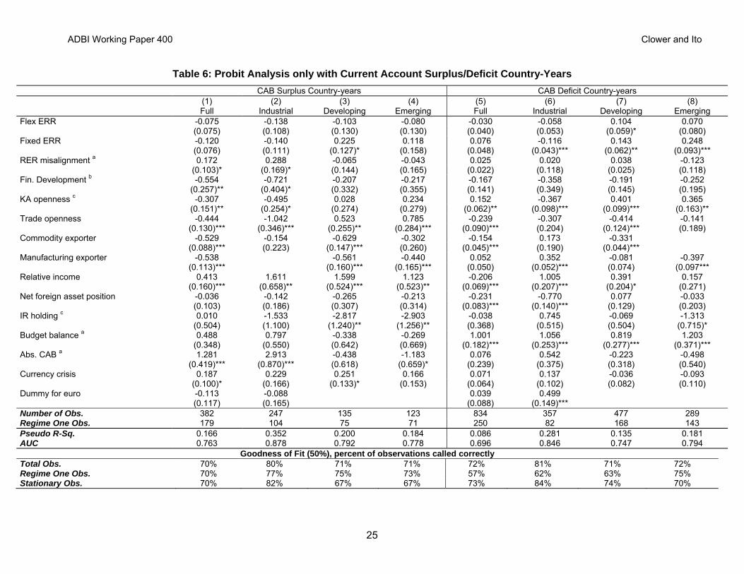
History is full of episodes where international monetary systems faced severe stress caused by the asymmetry between current account deficit and surplus countries. As we see a significantly negative coefficient on the current account deficit dummy in Table 5, in general, deficit countries are in general more likely to face market pressure for corrections and, therefore, are at greater risk for crises than surplus countries. To shed more light on the asymmetry between surplus and deficit countries, we repeat the same exercise across the subsamples of country-years with current account surpluses and those with deficits, and report the results in Table 6.17
The results reported in Table 6 show that the positive correlation between fixed exchange rate regime and current account persistence we found in Table 5 seems to reflect more of the behavior of deficit countries. In particular, when an emerging market country with a fixed exchange rate is running a current account deficit, the likelihood of entering the random walk regime rises significantly. We can surmise that while exchange rate stability ensures stable inflow of capital, the risk of failing to meet the intertemporal budget may increase. We can make the same observation about the euro deficit countries, which very much reflect the current debt crisis in the region.
Furthermore, a similar observation can be made about the effect of financial openness. A developing or emerging market country with current account deficit is more likely to enter the “red signal” regime if it pursues greater openness for their financial markets. These positive impacts of financial openness and fixed exchange rate regimes on the probability of experiencing a “red signal” state are consistent with the experiences of developing and emerging market economies that experienced crises in the 1980s and 1990s.
Better net foreign asset positions on the other hand would help countries with current account deficit to remain in the stationary regime. In the context of intertemporal budget constraint, it is quite reasonable. However, international reserves holding continue to present somewhat puzzling results. While the negative coefficient of the international reserves holding for deficit countries is understandable, significantly negative coefficients for both developing and emerging market countries groups with surplus appear somewhat counter-intuitive. One way of interpreting the result is through the liquidity effect of large volumes of international reserves; given price rigidities, more provision of liquidity through foreign exchange interventions by surplus countries would help increase domestic absorption, possibly contributing to a shrinkage of the surplus. 18 This interpretation implies that surplus countries with high volumes of international reserves holding such as the PRC and Singapore are experiencing more persistent surplus mainly because of other reasons than their massive IR holding, such as high levels of trade openness.
17 A country-year is classified as a current account deficit country-year if the three year accumulation of the current
account deficit across t-3 to t-1is negative. 18 Keep in mind that international reserves are included as deviations from the annual world average.
ADBI Working Paper 400 Clower and Ito
25
Table 6: Probit Analysis only with Current Account Surplus/Deficit Country-Years
CAB Surplus Country-years CAB Deficit Country-years (1) (2) (3) (4) (5) (6) (7) (8) Full Industrial Developing Emerging Full Industrial Developing Emerging Flex ERR -0.075 -0.138 -0.103 -0.080 -0.030 -0.058 0.104 0.070 (0.075) (0.108) (0.130) (0.130) (0.040) (0.053) (0.059)* (0.080) Fixed ERR -0.120 -0.140 0.225 0.118 0.076 -0.116 0.143 0.248 (0.076) (0.111) (0.127)* (0.158) (0.048) (0.043)*** (0.062)** (0.093)*** RER misalignment a 0.172 0.288 -0.065 -0.043 0.025 0.020 0.038 -0.123 (0.103)* (0.169)* (0.144) (0.165) (0.022) (0.118) (0.025) (0.118) Fin. Development b -0.554 -0.721 -0.207 -0.217 -0.167 -0.358 -0.191 -0.252 (0.257)** (0.404)* (0.332) (0.355) (0.141) (0.349) (0.145) (0.195) KA openness c -0.307 -0.495 0.028 0.234 0.152 -0.367 0.401 0.365 (0.151)** (0.254)* (0.274) (0.279) (0.062)** (0.098)*** (0.099)*** (0.163)** Trade openness -0.444 -1.042 0.523 0.785 -0.239 -0.307 -0.414 -0.141 (0.130)*** (0.346)*** (0.255)** (0.284)*** (0.090)*** (0.204) (0.124)*** (0.189) Commodity exporter -0.529 -0.154 -0.629 -0.302 -0.154 0.173 -0.331 (0.088)*** (0.223) (0.147)*** (0.260) (0.045)*** (0.190) (0.044)*** Manufacturing exporter -0.538 -0.561 -0.440 0.052 0.352 -0.081 -0.397 (0.113)*** (0.160)*** (0.165)*** (0.050) (0.052)*** (0.074) (0.097*** Relative income 0.413 1.611 1.599 1.123 -0.206 1.005 0.391 0.157 (0.160)*** (0.658)** (0.524)*** (0.523)** (0.069)*** (0.207)*** (0.204)* (0.271) Net foreign asset position -0.036 -0.142 -0.265 -0.213 -0.231 -0.770 0.077 -0.033 (0.103) (0.186) (0.307) (0.314) (0.083)*** (0.140)*** (0.129) (0.203) IR holding c 0.010 -1.533 -2.817 -2.903 -0.038 0.745 -0.069 -1.313 (0.504) (1.100) (1.240)** (1.256)** (0.368) (0.515) (0.504) (0.715)* Budget balance a 0.488 0.797 -0.338 -0.269 1.001 1.056 0.819 1.203 (0.348) (0.550) (0.642) (0.669) (0.182)*** (0.253)*** (0.277)*** (0.371)*** Abs. CAB a 1.281 2.913 -0.438 -1.183 0.076 0.542 -0.223 -0.498 (0.419)*** (0.870)*** (0.618) (0.659)* (0.239) (0.375) (0.318) (0.540) Currency crisis 0.187 0.229 0.251 0.166 0.071 0.137 -0.036 -0.093 (0.100)* (0.166) (0.133)* (0.153) (0.064) (0.102) (0.082) (0.110) Dummy for euro -0.113 -0.088 0.039 0.499 (0.117) (0.165) (0.088) (0.149)*** Number of Obs. 382 247 135 123 834 357 477 289 Regime One Obs. 179 104 75 71 250 82 168 143 Pseudo R-Sq. 0.166 0.352 0.200 0.184 0.086 0.281 0.135 0.181 AUC 0.763 0.878 0.792 0.778 0.696 0.846 0.747 0.794
Goodness of Fit (50%), percent of observations called correctlyTotal Obs. 70% 80% 71% 71% 72% 81% 71% 72% Regime One Obs. 70% 77% 75% 73% 57% 62% 63% 75% Stationary Obs. 70% 82% 67% 67% 73% 84% 74% 70%
ADBI Working Paper 400 Clower and Ito
26
Notes: Dependent variable is an indicator variable set to one whenever a country enters the random walk regime. Table reports marginal effects estimated using a maximum-likelihood probit model. All the explanatory variables are lagged by one year. Time fixed effects are proxied using annual World GDP growth and US real interest rate in the estimation. Robust standard errors reported in parentheses. ***, **, * denotes significance at the 1%, 5%, and 10% level.
a Based on the sum of the variable of concern over three years from t–3 through t–1.
b Measured as three year averages from t–3 through t–1.
c Measured as deviations from the sample mean.
Source: Authors’ calculations.

ADBI Working Paper 400 Clower and Ito
27
The positive effect of budget surplus on the probability of entering the random walk regime is found across all country groups with current account deficits. This reinforces our conjecture that deficit countries would face more market pressure to correct imbalances especially when they are running budget deficits.19
We provide a number of tests of goodness-of-fit measures for the probit estimations. Considering that the pseudo R-squared (or McFadden’s R2) does not provide useful information for cross-sample comparison,20 a better statistic for model comparison is the “area under the ROC curve” (AUC).21 The AUC ranges from 0 to 1, with higher AUC values representing an improved ability for the model to discriminate correct predictions from false alarms. We find the AUC statistics for our estimations ranging at relative high values, from 0.686 to 0.878. In addition, the AUC statistics are higher in subsample regressions than in the full sample regression, supporting the hypothesis that stages of development matter for variations in the degree of current account persistence. A similar conclusion can be made about the sample division for the groups of current account surplus and deficit countries, supporting asymmetries in determinants between surplus and deficit countries. We also report the proportions of regimes that are correctly called in total observations, regime one observations, and stationary regime observations (using the predicted probability of 50% as a cut-off). Across different subsamples, the percent of correct predictions appears to be relatively high, indicating that the model has a good level of goodness-of-fit. Overall, these statistics indicate that our models do a good job in predicting the probabilities.
As a robustness check, we repeat the exercises using updated Reinhart and Rogoff (2004) exchange rate regime classifications (results not reported). There is little change in the magnitude, signs, or significance of the estimated coefficients when we use the Reinhart and Rogoff index, with the notable exception of the significance of the flexible exchange rate regime. In the probit analysis, the Reinhart and Rogoff index flexible exchange rate regime is significant for developing and emerging countries especially when they are running current account deficits. The positive impact of fixed exchange rate regimes is found to be robust even when we use the different index.
4.2 Further Analysis on the Degree of Current Account Persistence—OLS Analysis
A higher level of current account persistence, or a higher value of the serial correlation coefficient in the current account series, means that the country takes more time to revert to its long-time mean and therefore maintains longer periods of either (above-average) current account deficits or surplus. By allowing current account series to take different regimes, the nature of the reversion can differ across regimes, and it should be affected by the country’s economic fundamentals, policy regimes, and other institutional factors.
19 This result may be contradictory to the previous finding that both the US and southern European countries have
been in the non-stationary regime in the last few years since these countries have been experiencing “twin deficits.” However, the significantly negative coefficient of net foreign asset positions explains especially the case of southern euro countries that have been taking negative positions for the last decade (even to a larger extent than the US). Furthermore, and more importantly, these European countries are under the fixed exchange rate regime).
20 Comparisons of the pseudo R-squared are valid only if the regressions utilize the exact same sample, not across different samples.
21 The ROC curve reflects the trade-off between sensitivity and specificity in the underlying model (Candelon, et al., 2009).

ADBI Working Paper 400 Clower and Ito
28
We now take a more nuance analysis on the determinants of current account rebalancing and examine the determinants of the degree of current account persistence. For this analysis, we first measure the extent of current account persistence by applying the AR(1) estimation model, as specified as below, to each of the regimes of current account series previously identified with the MS unit root analysis.
, (13)
for where tj and Tj indicate the beginning and ending dates of regime j, respectively.22
We treat the estimated serial autocorrelation coefficient, , as the measure of the degree of current account persistence, then regress it collectively against a vector of candidate determinants by applying the OLS estimation to a semi-panel dataset composed of cross-country regimes as:23
(14)
Where Zj is a vector of fundamental variables for regime j. Zj includes a similar set of explanatory variables to what we used for the probit analysis, though we drop persistently insignificant variables from the estimations. Namely, Zj includes the dummies for flexible and fixed exchange rate regimes; real exchange rate misalignment; relative income; financial development; financial and trade openness; IR holding; the dummies for current account deficit regimes; and the dummy for developing countries. All the variables except for the dummies for the exchange rate regimes and real exchange rate misalignment are included as of the first year of a regime.24 More explanations on the explanatory variables are provided in Appendix 4.
The essence of this exercise is similar to the work by Chinn and Wei who focused on the impact of exchange rate regimes on current account balance persistence while controlling for other characteristic variables. However, while Chinn and Wei’s framework looks into the average behavior of current account persistence (by looking at for each of the sample countries), we add more nuance to the estimation by allowing current account dynamics to take different regimes and thereby different degrees of current account persistence not just across countries but over time.
Table 7 reports the results of the OLS estimations, in which we regress the regime-specific degrees of current account persistence on a set of candidate determinants. Unlike the previous probit exercise, the number of observations drops significantly because the regressions use the
22 One regime must be at least 12 quarters long. 23 A country can take more than one regime as we report in Table 2. 24 The variables for financial openness and IR holding are converted to deviations from the world averages before
their regime averages are calculated. The real exchange rate misalignment variable is included as the sum of the absolute values of deviations from the annual trend over three years from t–3 through t–1. The dummies for the exchange rate regimes are based on the regime-averages of the original dummies. If the average of the dummies is greater than 0.50, the value of one is assigned for the particular type of exchange rate regime.

ADBI Working Paper 400 Clower and Ito
29
estimated autocorrelation coefficients for the regimes identified by the Markov-switching estimation. Furthermore, we restrict our samples to include only the estimates for the stationary regimes. This is because the autocorrelation coefficient of the non-stationary regimes may not be trustworthy. Table 7 reports the estimation results for the full sample as well as the subsamples of developed (IDC), developing countries’ (LDC) regimes, and current account surplus (CAS) and deficit (CAD) regimes.
Table 7: OLS Analysis of Current Account Persistence—Stationary Regimes Only
FULL IDC LDC CAS CAD (1) (2) (3) (4) (5)
Flexible ERR 0.152 -0.330 0.279 0.043 0.108 (0.114) (0.158)* (0.144)* (0.188) (0.096)
Fixed ERR 0.139 0.260 0.114 0.711 -0.002 (0.107) (0.180) (0.177) (0.217)*** (0.121)
RER misalignment a -0.060 0.993 -0.078 0.406 -0.061 (0.029)** (0.323)*** (0.030)** (0.210)* (0.020)***
Relative income -0.336 0.127 -0.607 -1.626 -0.084 (0.299) (0.572) (0.358) (0.873)* (0.248)
Fin. Development b 0.195 0.320 0.233 0.889 -0.129 (0.169) (0.164)* (0.265) (0.346)** (0.214)
KA openness c -0.250 -0.109 -0.120 0.009 -0.199 (0.119)** (0.133) (0.158) (0.394) (0.124)
Trade openness -0.353 -0.510 -0.292 -0.547 -0.418 (0.090)*** (0.171)*** (0.173) (0.144)*** (0.147)***
IR holding c 0.745 -1.291 0.551 -0.092 0.509 (0.411)* (1.665) (0.775) (1.013) (0.731)
Dummy for CAD -0.099 0.123 -0.236 (0.103) (0.106) (0.127)*
Developing countries -0.060 0.023 -0.130 (0.156) (0.228) (0.193)
Number of Obs. 65 27 38 23 42 Adj. R-Squared 0.30 0.30 0.38 0.38 0.25
Notes: The dependent variable is the serial correlation coefficient on the AR(1) estimation on current account balance series. All regressors are averages over regime unless otherwise noted. Standard errors reported in brackets. ***, **, * denotes significance at the 1%, 5%, and 10% level. The estimate on the constant term is omitted from presentation.
a Based on the sum of the variable of concern over three years from t–3 through t–1.
b Measured as three year averages from t–3 through t–1.
c Measured as deviations from the sample mean.
Source: Authors’ calculations.
Unlike the previous probit exercise, the OLS regressions fail to find a consistent relationship between the exchange rate regime and current account persistence. Although the sign of the fixed exchange rate regime dummy is positive as was in the case of the probit estimation, only the estimate for the surplus regimes is statistically significant; current account surplus regimes tend to have higher degrees of current account persistence while retaining stationary data generation process.
Both trade openness and financial openness are found to reduce adjustment costs for current account balances. However, the results of trade openness are more significant and persistent among subsamples while we do not have evidence for financial openness among the subsamples.
Countries with mounting pressure from real exchange rate misalignment tend to find it hard to maintain persistent current account imbalances. We find some contradictory results for the group of industrialized countries and surplus countries. But the number of observations for these
ADBI Working Paper 400 Clower and Ito
30
groups is so small that we may need to take the results for these subgroups with some grain of salt.
Lastly, we find evidence that higher levels of IR holding would lead to more persistent (but stationary) current account imbalances. But we do not have any evidence among subsample estimations.25
5. CONCLUDING REMARKS
This paper aims to provide a closer look at the dynamics of current account balances with particular focus on the statistical nature of the persistency of current account balances and its determinants.
In doing so, we first re-examine the stationarity of current account balances for about 70 countries. A number of stationarity tests we conduct confirm that the time series of current account balances (as a share of GDP) are not stationary for many countries contrary to what theory predicts. However, once we allow current account series to have structural breaks and use a nonlinear, Markov-Switching unit-root tests, we significantly improve the rejection rate of unit root, verifying that current account dynamics are driven by the existence of regime shifts in the current account balances series.
Armed with these findings, we examine whether the degree of current account persistence among different regimes can be explained by variations, both cross-sectional and over-time, in policies, institutions, and macroeconomic fundamentals of the countries. By doing so, we offer important insight into the bigger picture of current account sustainability and the country-specific factors that allow some countries to run persistent current account imbalances while forcing others to make current account readjustments.
Several findings are noteworthy. In the examination of the determinants of forcing countries to enter non-stationary, or “explosive” regimes, we find that exchange rate regimes do play a role unlike the finding of Chinn and Wei; fixed exchange rate regime can increase the probability of an emerging market country to enter a random walk regime. This finding, along with the finding that financial openness can also increase the probability, suggests that emerging market countries may tend to enter a state of financial instability, particularly emerging countries running current account deficits.
For countries with all levels of income, trade openness is found to decrease the likelihood of entering the random walk regime, presumably reducing the cost of current account adjustments. We find a similar effect in net foreign assets as well. Countries with budget deficits tend to stay in stationary regimes, so do those with current account deficits. These results imply that markets force these countries to rebalance their current accounts.
We shed more nuanced light on the issue of current account persistency by examining the determinants of degrees of current account persistence which we measure by the autocorrelation coefficients for the regimes we identified by the Markov-switching analysis.
In this analysis, the type of exchange rate regimes does not affect the extent of current account persistence. However, countries with greater trade or financial openness, or those with mounting pressure from real exchange rate misalignment tend to have a smaller degree of
25 If we do the estimations using the samples that also include the autocorrelation coefficients of non-stationary
regimes, the results are qualitatively similar for the group of industrialized countries, but the level of statistical significance drops significantly for other subsamples. However, trade openness continues to be a significantly negative contributor to current account persistence.

ADBI Working Paper 400 Clower and Ito
31
current account persistence while IR holding seems to contribute to a larger degree of persistence.

ADBI Working Paper 400 Clower and Ito
32
REFERENCES
Aizenman, J. 2008. International reserve management and the current account. Central Banking, Analysis, and Economic Policies Book Series. In: Current Account and External Financing, edition 1, volume 12, chapter 11, edited by K. Cowan, S. Edwards, R. O. Valdés, N. Loayza (series editors), and K. Schmid (ed.), Central Bank of Chile.
Aizenman, J., and R. Glick. 2009. Sterilization, Monetary Policy, and Global Financial Integration. Review of International Economics 17(4): 816–840.
Aizenman, J., and J. Lee. 2007. International reserves: precautionary versus mercantilist views, theory and evidence. Open Economies Review 18(2): 191–214.
Aizenman, J., and N. Marion. 2004. International reserves holdings with sovereign risk and costly tax collection. Economic Journal 114: 569–91.
Aizenman, J., M. Chinn, and H. Ito. 2012. The 'Impossible Trinity' Hypothesis in an Era of Global Imbalances: Measurement and Testing. Mimeo. Forthcoming in Review of International Economics.
Aizenman, J., M. Chinn, and H. Ito. 2010. The Emerging Global Financial Architecture: Tracing and Evaluating New Patterns of Trilemma Configuration. International Journal of Money and Finance 29(4): 615–641.
Baum, C. 2001. Stata: The language of choice for time series analysis? The Stata Journal 1: 1–16.
Bernanke, B. 2005. The Global Saving Glut and the U.S. Current Account. Remarks at the Sandridge Lecture. Virginia Association of Economics. Richmond, VA. 10 March.
Caballero, R, E. Farhi, and P. Gourinchas. 2008. An Equilibrium Model of ‘Global Imbalances’ and Low Interest Rates. American Economic Review 98(1) (March): 358–393.
Candelon, B., E. I. Dumitrescu, and C. Hurlin. 2009. How to evaluate an early warning system? Towards a unified statistical framework for assessing financial crises forecasting methods, Working Paper.
Chen, S. 2011. Current account deficits and sustainability: Evidence from the OECD countries. Economic Modelling. doi:10.10.1016/j.econmod.2011.01.011.
Chinn, M., and H. Ito. 2006. What matters for financial development? Capital controls, institutions, and interactions. Journal of Development Economics 81(1): 163–192.
Chinn, M. D., B. Eichengreen, and H. Ito. 2011. A Forensic Analysis of Global Imbalances. NBER Working Paper Series No. 17513 (October). Cambridge, MA: NBER.
Chinn, M., and S. J. Wei. Forthcoming. A faith-based initiative meets the evidence: Does a flexible exchange rate regime really facilitate current account adjustment? Review of Economics and Statistics.
Clemente, J., A. Montanes, and M. Reyes. 1998. Testing for a unit root in variables with a double change in the mean. Economic Letters 59: 175–182.
Eichengreen, B., A. Rose, and C. Wyplosz. 1995. Exchange Market Mayhem: The Antecedents and Aftermaths of Speculative Attacks. Economic Policy 21 (October): 249−312.
Eichengreen, B., A. Rose, and C. Wyplosz. 1996. Contagious Currency Crises: First Tests. Scandinavian Journal of Economics 98(4): 463−484.

ADBI Working Paper 400 Clower and Ito
33
Elliot, G., and U. K. Muller. 2006. Efficient tests for persistent time variations in regression coefficients. The Review of Economic Studies 73(4): 907–940.
Faruqee, H., and J. Lee. 2009. Global dispersion of current accounts: Is the universe expanding? IMF Staff Papers 56: 574–595.
Feldstein, M., and C. Horioka. 1980. Domestic saving and international capital flows. Economic Journal 90(2): 314–329.
Freund, C., and F. Warnock. 2007. Current Account Deficits in Industrial Countries: The Bigger They Are, The Harder They Fall? In: G7 Current Account Imbalances: Sustainability and Adjustment, edited by R. H. Clarida. Cambridge, MA: University of Chicago Press.
Friedman, M. 1964. Monetary Studies of the National Bureau. The National Bureau Enters Its 45th Year, 44th Annual Report, 7–25; Reprinted in M. Friedman. 1969. The Optimum Quantity of Money and Other Essays. Chicago, IL: Aldine.
Hall, S. F., Z. Psaradakis, and M. Sola. 1999. Detecting periodically collapsis bubbles: a Markov-switching unit root test. Journal of Applied Econometrics 14: 143–154.
Hakkio, C., and M. Rush. 1991. Is the budget deficit too large. Economic Inquiry 29(3): 429–445.
Hansen, B. 1992. Testing for parameter instability in linear models. Journal of Policy Modeling 14(4): 517–533.
Ilzetzki, E., C. Reinhart, and K. Rogoff. 2008. Exchange rate arrangements entering the 21st century: Which anchor will hold? Quarterly Journal of Economics 119(1): 1–48.
Kim, J. Y. 2000. Detection of change in persistence of a linear time series. Journal of Econometrics 95: 97–116.
Kim, C.-J., and C. R. Nelson. 1998. State-Space models with Markov-Switching: Classical and Gibbs-sampling approproaches with applications. Cambridge, MA: MIT Press.
Lane, P. R., and G. M. Milesi-Ferretti. 2007. The external wealth of nations mark II: Revised and extended estimates of foreign assets and liabilities, 1970–2004. Journal of International Economics 73(November): 223–250.
Matsubayashi, Y. 2005. Are US current account deficits unsustainable? Testing for the private and government interremporal budget contraints. Japan and the World Economy 17: 223–237.
Nelson, C., J. Piger, and E. Zivot. 2001. Markov regime switching and unit-root tests. Journal of Business & Economic Statistics 19(4): 404–415.
Perron, P. 1989. The great crash, the oil price shock and the unit root hypothesis. Econometrica 57: 1361–1401.
Psaradakis, Z., M. Sola, and F. Spagnolo. 2004. On Markov error-correction models, with an application to stock prices and dividends. Journal of Applied Econometrics 19: 69–88.
Ramsey, J. 1969. Tests for specification errors in classical linear least squares regression analysis. Journal of the Royal Statistical Society 31(2): 350–371.
Raybaudi, M., M. Sola, and F. Spagnolo. 2004. Red Signals: current account deficits and sustainability. Economic Letters (84): 217–223.
Taylor, A. M. 2002. A century of current account dynamics. Journal of International Money and Finance 21: 725–742.

ADBI Working Paper 400 Clower and Ito
34
Trehan, B., and C. Walsh. 1991. Testing intertemporal budget constraints: Theory and applications to U.S. federal budget and current account deficits. Journal of Money, Credit and Banking 23(2): 206–223.
Zivot, E., and D. Andrews. 1992. Further evidence on the great crash, the oil-price shock, and the unit-root hypothesis. Journal of Business & Economic Statistics 10: 251–270.
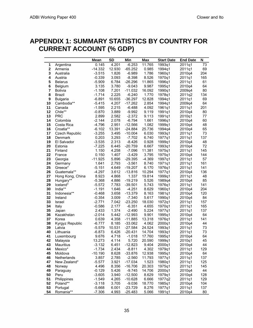
ADBI Working Paper 400 Clower and Ito
35
APPENDIX 1: SUMMARY STATISTICS BY COUNTRY FOR CURRENT ACCOUNT (% GDP)
Mean SD Min Max Start Date End Date N 1 Argentina 0.145 4.201 -6.253 11.765 1993q1 2011q1 73 2 Armenia -14.332 12.930 -65.252 0.985 1994q1 2011q1 69 3 Australia -3.515 1.826 -6.989 1.786 1960q1 2010q4 204 4 Austria -0.339 3.093 -8.398 8.526 1970q1 2011q1 165 5 Belarus -5.909 6.784 -26.296 11.865 1996q1 2011q1 61 6 Belgium 3.135 3.780 -9.043 9.987 1995q1 2010q4 64 7 Bolivia -1.108 7.201 -11.032 16.092 1990q1 2009q4 80 8 Brazil -1.714 2.225 -6.240 1.770 1978q1 2011q2 134 9 Bulgaria -6.891 10.655 -36.297 12.828 1994q1 2011q1 69
10 Cambodia** -5.415 4.207 -17.262 2.854 1994q1 2009q4 64 11 Canada -1.595 2.215 -6.488 4.092 1961q1 2011q1 201 12 Chile** -0.870 3.889 -9.992 9.119 1991q1 2010q4 80 13 PRC 2.899 2.582 -2.372 9.113 1991q1 2010q1 77 14 Colombia -2.144 2.078 -6.794 1.661 1996q1 2010q4 60 15 Costa Rica -4.796 2.951 -12.566 1.082 1999q1 2010q4 48 16 Croatia** -6.102 13.391 -24.884 25.736 1994q4 2010q4 65 17 Czech Republic -3.255 3.495 -10.004 6.030 1993q1 2011q1 73 18 Denmark 0.203 3.293 -7.702 6.740 1977q1 2011q1 137 19 El Salvador -3.535 2.313 -8.426 0.928 1999q1 2010q4 48 20 Estonia -7.225 6.445 -20.759 6.667 1993q1 2010q4 72 21 Finland 1.150 4.258 -7.096 11.381 1975q1 2011q1 145 22 France 0.150 1.407 -3.429 3.795 1975q1 2010q4 144 23 Georgia -11.925 5.896 -29.395 -4.369 1997q1 2011q1 57 24 Germany 1.641 2.793 -3.561 8.740 1971q1 2011q1 161 25 Greece* -5.151 4.649 -19.207 6.170 1976q1 2011q1 141 26 Guatemala** -4.297 3.612 -13.816 10.294 1977q1 2010q4 136 27 Hong Kong, China 8.923 4.868 1.337 19.814 1999q1 2011q1 48 28 Hungary** -5.368 4.886 -19.219 5.526 1989q4 2010q4 85 29 Iceland* -5.572 7.783 -39.501 5.743 1976q1 2011q1 141 30 India** -1.191 1.646 -4.251 8.629 1960q1 2010q4 204 31 Indonesia** -0.468 3.658 -13.379 8.163 1981q1 2010q4 120 32 Ireland -0.354 3.009 -7.340 5.617 1990q1 2010q4 84 33 Israel -2.771 7.042 -23.250 18.030 1972q1 2011q1 157 34 Italy -0.586 2.177 -6.351 4.655 1970q1 2011q1 165 35 Japan 2.433 1.374 -2.490 5.224 1977q1 2011q1 137 36 Kazakhstan -2.014 5.442 -12.993 9.901 1995q1 2010q4 64 37 Korea 0.639 4.358 -11.885 13.318 1976q1 2011q1 141 38 Kyrgyz Republic -6.777 8.185 -33.062 4.062 2000q1 2010q4 44 39 Latvia -5.579 10.531 -27.584 24.524 1993q1 2011q1 73 40 Lithuania -6.873 6.426 -20.431 14.704 1993q1 2011q1 73 41 Luxembourg 9.676 4.718 -1.018 17.760 1995q1 2010q4 64 42 Malaysia 13.273 4.114 5.720 20.590 1999q1 2010q1 45 43 Mauritius -3.132 6.451 -12.823 9.404 2000q1 2010q4 44 44 Mexico* -1.734 2.434 -8.811 4.302 1979q1 2011q1 129 45 Moldova -10.190 8.628 -33.876 12.938 1995q1 2010q4 64 46 Netherlands 3.857 2.785 -2.560 11.793 1977q1 2011q1 137 47 New Zealand* -5.577 3.921 -17.034 1.523 1980q1 2011q1 125 48 Norway 4.496 8.356 -16.706 20.303 1975q1 2011q1 145 49 Paraguay -0.129 5.426 -9.745 14.706 2000q1 2010q4 44 50 Peru -3.605 3.940 -12.500 8.629 1979q1 2010q4 128 51 Philippines -1.549 4.265 -10.628 6.666 1977q2 2011q1 129 52 Poland** -3.118 3.705 -9.036 18.770 1985q1 2010q4 104 53 Portugal -5.668 6.001 -23.729 8.276 1977q1 2011q1 137 54 Romania** -7.306 4.993 -25.483 5.066 1991q1 2010q4 80

ADBI Working Paper 400 Clower and Ito
36
55 Russian Federation 7.288 5.524 -3.830 21.337 1994q1 2011q1 69 56 Slovak Republic -5.259 4.935 -16.344 7.286 1993q1 2010q4 72 57 Slovenia -1.676 2.714 -9.501 3.273 1995q1 2011q1 65 58 South Africa -1.003 4.036 -11.448 14.432 1960q1 2011q1 205 59 Spain -2.845 3.124 -10.924 4.327 1975q1 2011q1 145 60 Sri Lanka** -5.231 5.330 -21.095 6.283 1977q1 2010q4 136 61 Sweden* 1.727 4.029 -5.926 10.174 1975q1 2011q1 145 62 Switzerland 6.416 4.346 -5.180 17.463 1972q1 2010q4 156 63 Taipei,China 7.043 5.065 -7.202 22.761 1981q1 2011q1 121 64 Thailand** -1.527 6.412 -13.209 15.505 1976q1 2010q4 140 65 Turkey -2.121 3.395 -11.862 5.583 1987q1 2011q1 97 66 Ukraine** 0.349 7.008 -17.651 21.729 1994q1 2010q4 68 67 United Kingdom -1.042 1.771 -5.800 4.223 1960q1 2010q4 204 68 United States -1.508 2.054 -6.848 1.426 1960q1 2010q4 204 69 Uruguay** -1.295 3.175 -9.551 5.054 1999q1 2010q4 48 71 Venezuela 5.411 6.682 -6.652 24.883 1997q1 2011q1 57 72 Viet Nam** -3.657 7.736 -32.045 12.684 1996q1 2010q4 60
* Data uses IMF GDP projections, **GDP data splined from annual data
Source: Authors’ calculations.
APPENDIX 2: TESTS FOR PARAMETER STABILITY AND NONLINEARITIES
QLL Hansen Parameter Stability Test Country Persistence Constant Joint 1 Argentina -9.429 0.301 0.472** 1.706*** 2 Armenia -21.037*** 0.028 0.585** 1.444*** 3 Australia -14.951** 0.399* 0.602** 1.096** 4 Austria -46.183*** 0.876*** 1.944*** 2.990*** 5 Belarus -18.498*** 0.765*** 0.64 1.121** 6 Belgium -16.319** 0.647** 1.374*** 2.222*** 7 Bolivia -8.478 0.118 0.417* 0.798 8 Brazil -16.327** 0.152 0.136 0.729 9 Bulgaria -18.423*** 0.486** 0.848*** 1.274** 10 Cambodia -8.862 0.153 0.203 1.955*** 11 Canada -23.737*** 0.31 0.457* 1.967*** 12 Chile -13.506* 0.048 0.71** 0.954** 13 PRC -10.425 0.191 0.286 0.471 14 Colombia -11.301 0.191 0.117 0.728 15 Costa Rica -7.860 0.146 0.084 0.629 16 Croatia -6.203 0.021 0.045 1.209** 17 Czech Republic -15.711** 0.679** 0.171 1.351*** 18 Denmark -26.713*** 0.606** 1.181*** 2.033*** 19 El Salvador -13.627* 0.159 0.242 1.347** 20 Estonia -17.623*** 0.457* 0.16 1.140** 21 Finland -26.919*** 0.326 0.709** 3.684*** 22 France -29.525*** 0.534** 0.257 1.431** 23 Georgia -8.779 0.234 0.28 0.442 24 Germany -13.638* 0.79*** 0.322 1.194** 25 Greece -29.521*** 1.718*** 1.551*** 2.667*** 26 Guatemala -7.985 0.199 0.147 1.254** 27 Hong Kong, China -9.608 0.16 0.326 0.470 28 Hungary -10.231 0.064 0.139 1.474*** 29 Iceland -16.031 0.217 0.872*** 2.330*** 30 India -18.263*** 0.169 0.225 0.475 31 Indonesia -10.881 0.018 0.75*** 0.960* 32 Ireland -18.316*** 0.575** 0.503** 1.347**

ADBI Working Paper 400 Clower and Ito
37
33 Israel -36.377*** 0.134 1.972*** 5.090*** 34 Italy -17.015** 0.417* 0.255 1.708*** 35 Japan -11.321 0.0637 0.317 1.165** 36 Kazakhstan -8.010 0.047 0.085 0.384 37 Korea, Rep. -8.216 0.055 0.181 0.505 38 Kyrgyz Republic -10.092 0.252 0.299 0.475 39 Latvia -12.856* 0.316 0.108 0.678 40 Lithuania -24.965*** 0.743** 0.159 2.873*** 41 Luxembourg -9.374 0.319 0.364* 0.665 42 Malaysia -12.028 0.366* 0.501** 0.765 43 Mauritius -11.740 0.086 0.59** 0.841 44 Mexico -6.623 0.064 0.082 1.267** 45 Moldova -14.282* 0.147 0.219 0.560 46 Netherlands -18.368*** 0.795*** 0.972*** 1.318** 47 New Zealand -12.412 0.395* 0.203 0.582 48 Norway -6.434 0.071 0.387* 0.675 49 Paraguay -8.172 0.06 0.148 0.272 50 Peru -8.792 0.041 0.403* 2.400*** 51 Philippines -21.223*** 0.285 0.77*** 1.310** 52 Poland -8.273 0.205 0.454* 1.016** 53 Portugal -11.363 0.415 0.522** 1.626*** 54 Romania -17.810*** 0.766*** 0.272 1.122** 55 Russian Federation -10.262 0.164 0.119 1.029** 56 Slovak Republic -15.798** 0.206 0.203 1.583*** 57 Slovenia -17.287** 0.781*** 0.388* 0.990* 58 South Africa -9.577 0.071 0.15 1.102** 59 Spain -26.068*** 2.073*** 0.699** 2.592*** 60 Sri Lanka -26.685*** 1.021*** 0.495* 1.725*** 61 Sweden -9.353 0.436* 0.548** 1.173** 62 Switzerland -10.737 0.224 0.731** 2.621*** 63 Taipei,China -18.573*** 0.297 0.375* 0.878* 64 Thailand -14.087* 0.299 0.648** 1.160** 65 Turkey -16.534** 0.713** 0.866*** 1.256** 66 Ukraine -18.681*** 0.454* 0.252 0.753 67 United Kingdom -15.397** 0.103 0.808*** 1.209** 68 United States -7.899 0.14 0.349 1.244** 69 Uruguay -9.353 0.095 0.126 0.309 70 Venezuela, RB -20.323*** 0.022 0.535** 2.054*** 71 Viet Nam -11.250 0.042 0.316 1.588***
Notes: ***, **, * denotes rejection of the null hypothesis of parameter stability at the 1%, 5%, and 10% level, respectively.
Source: Authors’ calculations.
APPENDIX 3: UNIT ROOT TESTS FOR INDIVIDUAL COUNTRIES
Country ADF KPSS HEGY DFGLS MAIC lags
N Start Date End Date
1 Argentina -2.326 3.235††† -2.245 -0.846 11 61 1993q1 2011q1 2 Armenia -6.182*** 1.650††† -1.506 -0.288 8 58 1994q1 2011q1 3 Australia -5.180*** 4.838††† -3.751** -1.674* 14 189 1960q1 2010q4 4 Austria -9.194*** 3.458††† -1.094 -1.125 13 151 1970q1 2011q1 5 Belarus -4.269*** 1.275††† -0.002 -0.159 3 50 1996q1 2011q1 6 Belgium -7.294*** 1.614††† -1.209 -0.288 7 53 1995q1 2010q4 7 Bolivia -1.887 5.405††† -1.245 -1.067 2 68 1990q1 2009q4 8 Brazil -1.394 2.084††† -2.372 -1.871 8 121 1978q1 2011q2 9 Bulgaria -4.727*** 1.900††† -1.163 -1.093 7 58 1994q1 2011q1
10 Cambodia -6.318*** 0.316 -1.853 -0.654 3 53 1994q1 2009q4
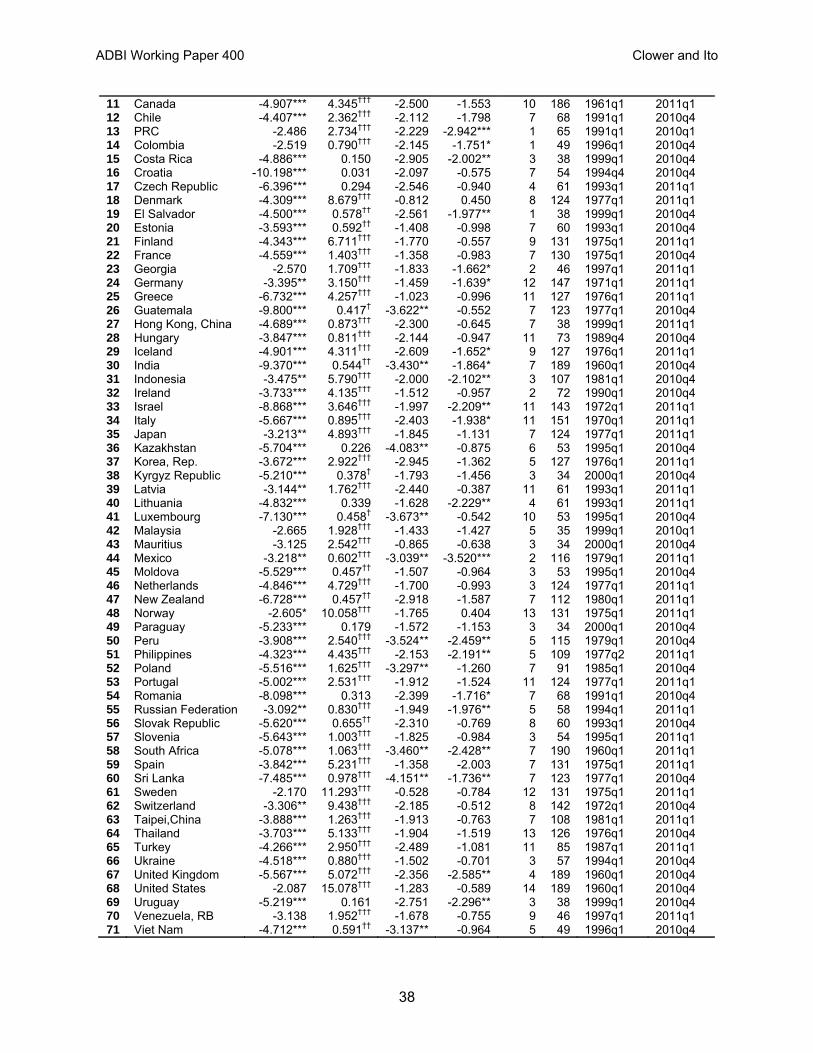
ADBI Working Paper 400 Clower and Ito
38
11 Canada -4.907*** 4.345††† -2.500 -1.553 10 186 1961q1 2011q1 12 Chile -4.407*** 2.362††† -2.112 -1.798 7 68 1991q1 2010q4 13 PRC -2.486 2.734††† -2.229 -2.942*** 1 65 1991q1 2010q1 14 Colombia -2.519 0.790††† -2.145 -1.751* 1 49 1996q1 2010q4 15 Costa Rica -4.886*** 0.150 -2.905 -2.002** 3 38 1999q1 2010q4 16 Croatia -10.198*** 0.031 -2.097 -0.575 7 54 1994q4 2010q4 17 Czech Republic -6.396*** 0.294 -2.546 -0.940 4 61 1993q1 2011q1 18 Denmark -4.309*** 8.679††† -0.812 0.450 8 124 1977q1 2011q1 19 El Salvador -4.500*** 0.578†† -2.561 -1.977** 1 38 1999q1 2010q4 20 Estonia -3.593*** 0.592†† -1.408 -0.998 7 60 1993q1 2010q4 21 Finland -4.343*** 6.711††† -1.770 -0.557 9 131 1975q1 2011q1 22 France -4.559*** 1.403††† -1.358 -0.983 7 130 1975q1 2010q4 23 Georgia -2.570 1.709††† -1.833 -1.662* 2 46 1997q1 2011q1 24 Germany -3.395** 3.150††† -1.459 -1.639* 12 147 1971q1 2011q1 25 Greece -6.732*** 4.257††† -1.023 -0.996 11 127 1976q1 2011q1 26 Guatemala -9.800*** 0.417† -3.622** -0.552 7 123 1977q1 2010q4 27 Hong Kong, China -4.689*** 0.873††† -2.300 -0.645 7 38 1999q1 2011q1 28 Hungary -3.847*** 0.811††† -2.144 -0.947 11 73 1989q4 2010q4 29 Iceland -4.901*** 4.311††† -2.609 -1.652* 9 127 1976q1 2011q1 30 India -9.370*** 0.544†† -3.430** -1.864* 7 189 1960q1 2010q4 31 Indonesia -3.475** 5.790††† -2.000 -2.102** 3 107 1981q1 2010q4 32 Ireland -3.733*** 4.135††† -1.512 -0.957 2 72 1990q1 2010q4 33 Israel -8.868*** 3.646††† -1.997 -2.209** 11 143 1972q1 2011q1 34 Italy -5.667*** 0.895††† -2.403 -1.938* 11 151 1970q1 2011q1 35 Japan -3.213** 4.893††† -1.845 -1.131 7 124 1977q1 2011q1 36 Kazakhstan -5.704*** 0.226 -4.083** -0.875 6 53 1995q1 2010q4 37 Korea, Rep. -3.672*** 2.922††† -2.945 -1.362 5 127 1976q1 2011q1 38 Kyrgyz Republic -5.210*** 0.378† -1.793 -1.456 3 34 2000q1 2010q4 39 Latvia -3.144** 1.762††† -2.440 -0.387 11 61 1993q1 2011q1 40 Lithuania -4.832*** 0.339 -1.628 -2.229** 4 61 1993q1 2011q1 41 Luxembourg -7.130*** 0.458† -3.673** -0.542 10 53 1995q1 2010q4 42 Malaysia -2.665 1.928††† -1.433 -1.427 5 35 1999q1 2010q1 43 Mauritius -3.125 2.542††† -0.865 -0.638 3 34 2000q1 2010q4 44 Mexico -3.218** 0.602††† -3.039** -3.520*** 2 116 1979q1 2011q1 45 Moldova -5.529*** 0.457†† -1.507 -0.964 3 53 1995q1 2010q4 46 Netherlands -4.846*** 4.729††† -1.700 -0.993 3 124 1977q1 2011q1 47 New Zealand -6.728*** 0.457†† -2.918 -1.587 7 112 1980q1 2011q1 48 Norway -2.605* 10.058††† -1.765 0.404 13 131 1975q1 2011q1 49 Paraguay -5.233*** 0.179 -1.572 -1.153 3 34 2000q1 2010q4 50 Peru -3.908*** 2.540††† -3.524** -2.459** 5 115 1979q1 2010q4 51 Philippines -4.323*** 4.435††† -2.153 -2.191** 5 109 1977q2 2011q1 52 Poland -5.516*** 1.625††† -3.297** -1.260 7 91 1985q1 2010q4 53 Portugal -5.002*** 2.531††† -1.912 -1.524 11 124 1977q1 2011q1 54 Romania -8.098*** 0.313 -2.399 -1.716* 7 68 1991q1 2010q4 55 Russian Federation -3.092** 0.830††† -1.949 -1.976** 5 58 1994q1 2011q1 56 Slovak Republic -5.620*** 0.655†† -2.310 -0.769 8 60 1993q1 2010q4 57 Slovenia -5.643*** 1.003††† -1.825 -0.984 3 54 1995q1 2011q1 58 South Africa -5.078*** 1.063††† -3.460** -2.428** 7 190 1960q1 2011q1 59 Spain -3.842*** 5.231††† -1.358 -2.003 7 131 1975q1 2011q1 60 Sri Lanka -7.485*** 0.978††† -4.151** -1.736** 7 123 1977q1 2010q4 61 Sweden -2.170 11.293††† -0.528 -0.784 12 131 1975q1 2011q1 62 Switzerland -3.306** 9.438††† -2.185 -0.512 8 142 1972q1 2010q4 63 Taipei,China -3.888*** 1.263††† -1.913 -0.763 7 108 1981q1 2011q1 64 Thailand -3.703*** 5.133††† -1.904 -1.519 13 126 1976q1 2010q4 65 Turkey -4.266*** 2.950††† -2.489 -1.081 11 85 1987q1 2011q1 66 Ukraine -4.518*** 0.880††† -1.502 -0.701 3 57 1994q1 2010q4 67 United Kingdom -5.567*** 5.072††† -2.356 -2.585** 4 189 1960q1 2010q4 68 United States -2.087 15.078††† -1.283 -0.589 14 189 1960q1 2010q4 69 Uruguay -5.219*** 0.161 -2.751 -2.296** 3 38 1999q1 2010q4 70 Venezuela, RB -3.138 1.952††† -1.678 -0.755 9 46 1997q1 2011q1 71 Viet Nam -4.712*** 0.591†† -3.137** -0.964 5 49 1996q1 2010q4

ADBI Working Paper 400 Clower and Ito
39
Note: ADF is run using a constant, no time trends, and no lags. The KPSS test is run without a time trend and results reported are for zero lags, though longer lag lengths are tested and yield similar results. All DFGLS tests are run without a trend, using the reported MAIC lag lengths, and the Elliot, Rothenberg, and Stock critical values. The table reports the Hylleberg, Engle, Granger, Yoo (HEGY) test long-run unit roots using no lags. ***, **, * denotes rejection of the unit root hypothesis at the 1%, 5%, and 10% level, respectively. †††,††,† denotes rejection of the null hypothesis of stationarity at a 1%, 5%, and 10% level, respectively.
Source: Authors’ calculations.
APPENDIX 4: CANDIDATE DETERMINANTS OF THE CURRENT ACCOUNT PERSISTENCY
Our choice of candidate determinants for both probit and OLS estimations is based on the past literature. We summarize the theoretical rationales and predictions of the candidate determinants and describe data sources below. Most of the data are extracted from the IMF’s International Financial Statistics (IFS) and World Economic Outlook (WEO), the World Bank’s World Development Indicator (WDI), and OECD’s Economic Outlook database, unless mentioned otherwise.
Exchange Rate Regime: A certain type of exchange rate regime may allow a country to run current account imbalances persistently. While a country with a fixed, undervalued currency may be able to maintain current account surplus persistently, a deficit country with a fixed, but overvalued exchange rate could end up experiencing a balance of payments crisis, suggesting that a fixed exchange rate regime may not allow a greater degree of current account persistency.26 A flexible exchange rate regime on the other hand may facilitate current account adjustments, but it may also allow countries to run persistent current account imbalances because of the lack of forceful market corrections. As such, the impact of exchange rate regimes is expected to have an ambiguous impact on current account persistence. The fact that Chinn and Wei do not find any evidence for the link between exchange rate regimes and current account persistency may reflect the ambiguity.
For the estimation, we use the dummies for fixed and flexible exchange rate regimes based on the index of exchange rate stability from the Aizenman, Chinn, and Ito (2012) “trilemma indexes.”27 For robustness checks, we also use the Reinhart and Rogoff (2004) exchange rate regime index.28
Trade Openness: Greater trade openness should reduce the cost of current account adjustment by transmitting real exchange rate changes to the trade balance as argued in Chinn and Wei. Therefore, we can expect greater levels of trade openness help decrease current account persistence. We measure trade openness using the ratio of the sum of exports and imports divided by GDP.
Financial Openness: A more financially open country may be susceptible to the transmission of financial shocks across countries and therefore tends to experience weaker current account 26 A surplus country with an undervalued currency, even with sterilization efforts, should eventually experience a
correction in the form of rising expected inflation (Aizenman and Glick 2009). 27 The original Aizenman et al. index of exchange rate stability ranges from zero to one. We assign the value of one
for the fixed exchange rate regime dummy if the index is above .70 and assign the value of one for the flexible exchange rate regime if the index is below .30.
28 We aggregate the Reinhart and Rogoff coarse grid indexes and assign dummies for fixed and flexible regimes. Fixed regime countries include those with Reinhart and Rogoff indexes ranging from no legal tender to de facto peg. Flexible regime countries include those ranging from managed float to freely floating.

ADBI Working Paper 400 Clower and Ito
40
persistence. Feldstein and Horioka (1980) and Faruqee and Lee (2009) argue, on the other hand, that countries with more open financial markets should be able to delink saving and investment, which may help sustain more persistent current account imbalances. We use the Chinn and Ito (2006, 2008) index of financial openness and include it as deviations from the world average.
Size of Current Account: Freund and Warnock (2007) find that current account adjustments could depend on the size of the current account balance. We can also expect that market pressures to rebalance current account would respond to trends of accumulating current account imbalances. To test this, we include the three-year total accumulation of current account balances. We also examine if regimes with current account deficits perform inherently differently from others by including a dummy for the regime with current account deficits based on three-year current account balance accumulation.
Exchange Rate Misalignment: Regardless of exchange rate regimes, the exchange rate can deviate from the equilibrium exchange rate, but persistent deviations from the equilibrium rate can also create pressure on the current account movement. Hence, we calculate the real exchange rate deviation from the time trend using the nominal exchange rate between country i and the base country and the CPIs of the two countries.29 We use the sum of the absolute values of the deviations over t – 3 through t – 1 as the measure of exchange rate misalignment.
Budget Balance: The government debt may affect the extent of current account persistence, especially if it is financed by foreign investors. As the debt accumulates, pressure from the international financial markets may amount in the form of higher government bond yield or lower credit rating. This will, in turn, make it harder for the government of concern to continue to borrow from the markets, thus making the degree of current account persistence fall. We include a variable for three-year budget balance accumulation as a proxy for the government’s debt since the debt data are often quite limited but highly correlated with the trend in budget balances. We use the data from the IMF’s World Economic Outlook and IFS and the World Bank’s WDI.
Financial Development: The level of financial development may also matter for the degree of persistency. The proponents of the “saving glut” argument (such as Bernanke, 2005) have argued that it is the sophisticated financial markets of the US that keep attracting capital flowing into the country, thereby causing persistent current account deficits. This argument may also help explain the persistent current account surplus of the PRC which is often argued to lack sophisticated financial markets (Caballero et al. 2008). We use private the long-run, HP-filtered trend of credit creation (as a ratio to GDP) as a measure of financial development. The original data are obtained from the World Bank’s financial structure database.
International Reserves Holding: Holding ample international reserves can give ammunition to central banks to defend the country’s currency value, and that may help slow down current account adjustments. We use international reserves relative to GDP and include it as deviations from the world mean.
Income Level: More developed countries are usually equipped with more sophisticated socio-economic institutions, which may help them to maintain better access to international financial markets and thereby experience more persistent current account imbalances. We include the relative per capita income level (to the US) in the estimation using the data from the Penn World Table. We also include the growth rate of real GDP as a proxy for (future) productivity growth.
29 See Aizenman et al. (2012) for the base countries.

ADBI Working Paper 400 Clower and Ito
41
Net Foreign Asset Position: A country with more net foreign assets may be able to run more persistent current account imbalances, especially deficits, compared to a country with small net foreign assets or debt. We use the data from Lane and Milesi-Ferretti (2007).
Currency Crisis: It may be necessary to control for the correlation between currency crisis and current account readjustments because a crisis can occur to correct current account imbalances. Therefore, we include a currency crisis dummy based on the exchange market pressure index (Eichengreen et al. 1995, 1996). However, our EMP index is calculated against the base country in the sense of Aizenman et al. (2012).
Commodity or Manufacturing Exporter: Current account balance of countries can behave differently depending upon their different industrial structures. We assign the value of one for the countries if the average share of food and fuel in their exports during the period 1995 through 2010 is greater than 40%, and zero, otherwise. Similarly, if manufacturing exports comprise 50% or greater of total exports, the dummy of manufacturing exporter takes the value of one.
Related Documents