Computer Physics Communications 155 (2003) 244–259 www.elsevier.com/locate/cpc ASEP/MD: A program for the calculation of solvent effects combining QM/MM methods and the mean field approximation ✩ I. Fdez Galván, M.L. Sánchez,M.E. Martín, F.J. Olivares del Valle, M.A. Aguilar ∗ Dpto Química Física, Univ. de Extremadura, Avda de Elvas s/n, 06071 Badajoz, Spain Received 28 March 2003 Abstract ASEP/MD is a computer program designed to implement the Averaged Solvent Electrostatic Potential/Molecular Dynamics (ASEP/MD) method developed by our group. It can be used for the study of solvent effects and properties of molecules in their liquid state or in solution. It is written in the FORTRAN90 programming language, and should be easy to follow, understand, maintain and modify. Given the nature of the ASEP/MD method, external programs are needed for the quantum calculations and molecular dynamics simulations. The present version of ASEP/MD includes interface routines for the GAUSSIAN package, HONDO, and MOLDY, but adding support for other programs is straightforward. This article describes the program and its usage. Program summary Title of program: ASEP/MD Catalogue identifier: ADSF Program Summary URL: http://cpc.cs.qub.ac.uk/summaries/ADSF Program obtainable from: CPC Program Library, Queen’s University of Belfast, N. Ireland Computer for which the program is designed: it has been tested on Intel-based PC and Sun Operating systems under which the program has been tested: Red Hat Linux 7.2 and SunOS 5.6 Programming language used: FORTRAN90 Memory required to execute with typical data: greatly depends on the system No. of processors used: 1 Has the code been vectorized or parallelized?: no No. of bytes in distributed program, including test data, etc.: 44 544 Distribution format: tar gzip file Keywords: Solvent effects, QM/MM methods, mean field approximation, geometry optimization Nature of physical problem: The study of molecules in solution with quantum methods is a difficult task because of the large number of molecules and configurations that must be taken into account. The quantum mechanics/molecular mechanics methods proposed to date either require massive computational power or oversimplify the solute quantum description. ✩ This paper and its associated computer program are available via the Computer Physics Communications homepage on ScienceDirect (http://www.sciencedirect.com/science/journal/00104655 ). * Corresponding author. E-mail address: [email protected] (M.A. Aguilar). 0010-4655/$ – see front matter 2003 Elsevier B.V. All rights reserved. doi:10.1016/S0010-4655(03)00351-5

Welcome message from author
This document is posted to help you gain knowledge. Please leave a comment to let me know what you think about it! Share it to your friends and learn new things together.
Transcript
c
n
ynamicss in theirrstand,tions andackage,and its
larges methods
ienceDirect
Computer Physics Communications 155 (2003) 244–259
www.elsevier.com/locate/cp
ASEP/MD: A program for the calculation of solvent effectscombining QM/MM methods and the mean field approximatio✩
I. Fdez Galván, M.L. Sánchez, M.E. Martín, F.J. Olivares del Valle, M.A. Aguilar∗
Dpto Química Física, Univ. de Extremadura, Avda de Elvas s/n, 06071 Badajoz, Spain
Received 28 March 2003
Abstract
ASEP/MD is a computer program designed to implement the Averaged Solvent Electrostatic Potential/Molecular D(ASEP/MD) method developed by our group. It can be used for the study of solvent effects and properties of moleculeliquid state or in solution. It is written in the FORTRAN90 programming language, and should be easy to follow, undemaintain and modify. Given the nature of the ASEP/MD method, external programs are needed for the quantum calculamolecular dynamics simulations. The present version of ASEP/MD includes interface routines for the GAUSSIAN pHONDO, and MOLDY, but adding support for other programs is straightforward. This article describes the programusage.
Program summary
Title of program: ASEP/MDCatalogue identifier:ADSFProgram Summary URL:http://cpc.cs.qub.ac.uk/summaries/ADSFProgram obtainable from:CPC Program Library, Queen’s University of Belfast, N. IrelandComputer for which the program is designed:it has been tested on Intel-based PC and SunOperating systems under which the program has been tested:Red Hat Linux 7.2 and SunOS 5.6Programming language used:FORTRAN90Memory required to execute with typical data:greatly depends on the systemNo. of processors used:1Has the code been vectorized or parallelized?:noNo. of bytes in distributed program, including test data, etc.:44 544Distribution format: tar gzip fileKeywords: Solvent effects, QM/MM methods, mean field approximation, geometry optimizationNature of physical problem:The study of molecules in solution with quantum methods is a difficult task because of thenumber of molecules and configurations that must be taken into account. The quantum mechanics/molecular mechanicproposed to date either require massive computational power or oversimplify the solute quantum description.
✩ This paper and its associated computer program are available via the Computer Physics Communications homepage on Sc(http://www.sciencedirect.com/science/journal/00104655).
* Corresponding author.E-mail address:[email protected] (M.A. Aguilar).
0010-4655/$ – see front matter 2003 Elsevier B.V. All rights reserved.doi:10.1016/S0010-4655(03)00351-5
I.F. Galván et al. / Computer Physics Communications 155 (2003) 244–259 245
lassicald by theeld. Thisnd for the
cule)ble for
external
dy ofiption ofed fromsolvent
ty of the(number
meanolute–
on the); thissolved.
severalnergy orethods,
ons.tions andent im-re accus-written.
a shortsolute
Method of solution:A non-traditional QM/MM method based on the mean field approximation was developed where a cmolecular dynamics simulation is coupled with a quantum calculation. The average electrostatic potential generatesolvent over the solute is calculated from the simulation and introduced into the quantum calculation as an external fiprocess can be performed iteratively. Standard external programs are used for the molecular dynamics simulations aquantum calculations. The present program acts as an interface and controls the flow of the calculation.Restrictions on the complexity of the problem:At present, only pure liquids and binary dilute solutions (a single solute molecan be studied. For the molecular dynamics only MOLDY is implemented, while GAUSSIAN and HONDO are availathe quantum calculations. Restrictions of the aforementioned programs apply.Typical running time: Running time depends on the nature of the chemical system and the options passed to theprograms, which are usually by far the longest part of the calculations.Unusual features of the program:Uses SYSTEM and GETARG calls. 2003 Elsevier B.V. All rights reserved.
1. Introduction
Quantum Mechanics/Molecular Mechanics (QM/MM) methods [1] are now widely used in the stumolecules in solution. The main advantage of these methods is that they combine a quantum descrthe solute, allowing chemical processes to be studied, with a detailed description of the solvent, obtainsimulation techniques. In most QM/MM methods the solute Schrödinger equation has to be solved for eachconfiguration, which implies several thousand quantum calculations. This imposes a limitation on the qualiquantum description of the solvent (basis set and calculation level) and on the significance of the resultsof configurations considered).
In previous papers [2] we have developed a non-traditional QM/MM method that makes use of thefield approximation [3] (MFA). In this approximation, the average value of the energies of the different ssolvent configurations is replaced by the energy of the average configuration. Our method is basedcalculation of the Average Solvent Electrostatic Potential (ASEP) from Molecular Dynamics data (MDaverage potential is introduced into the molecular Hamiltonian of the solute and the Schrödinger equation isThis approximation, named ASEP/MD, reduces drastically the number of quantum calculations fromthousands to half a dozen, and introduces no significant inaccuracies [3] in the solute–solvent interaction ethe solute dipole moment. This reduced number of quantum calculations permits one to use higher quality mwhile having an adequate sampling of the solvent configurations through the molecular dynamics simulati
This paper presents of the computer program developed to implement our method. The quantum calculathe molecular dynamics simulations are performed by external programs, intentionally left out of the presplementation. This dependence on external programs allows the users to employ whatever program they atomed to or that is best suited to their needs, although specific subroutines for the purpose may have to be
2. Method
The main characteristics of the ASEP/MD method have been discussed elsewhere [2]. The following isdescription. As in traditional QM/MM methods, in ASEP/MD the energy and wavefunction of the solvatedmolecule are obtained by solving the effective Schrödinger equation
(1)(HQM + HQM/MM
)|Ψ 〉 = E|Ψ 〉.The interaction term,HQM/MM , takes the following form:
(2)HQM/MM = H electQM/MM + H vdw
QM/MM ,
(3)H electQM/MM =
∫ρ⟨Vs(r;ρ)
⟩dr,
246 I.F. Galván et al. / Computer Physics Communications 155 (2003) 244–259
scalnard-
y, Eqs. (1)namics
nted beimate it ishen, foralculatedolute areng tooectrostatictains theFinally,erated byalues are
ges
of pointd, fartherformeds.lectronit the
rizables done,lculated
les ofn the restbtained,
radient
whereρ is the solute charge density, obtained from a quantum calculation, and the term〈Vs(r;ρ)〉 is the averageelectrostatic potential generated by the solvent (ASEP) at the positionr, and is obtained from MD calculationwhere the solute molecule has fixed geometry and charge distributionρ—the angle brackets denote a statistiaverage. The termH vdw
QM/MM is the Hamiltonian for the van der Waals interaction, usually represented by a LenJones potential. Since the solvent structure, and hence the ASEP, is a function of the solute charge densitand (3) have to be solved iteratively. In general, only a few cycles of quantum calculation/molecular dysimulations are needed for convergence.
In order to facilitate its implementation in a standard quantum program package, the ASEP is represemeans of a set of point charges. The method used to obtain the ASEP and the point charges that approxas follows. First a three-dimensional grid of points is created inside the volume occupied by the solute. Tevery solvent configuration considered, the electrostatic potential created by the solvent at these points is cand averaged over all the configurations. The solvent charges inside a certain cut-off radius around the sexplicitly kept (their values divided by the total number of configurations considered) and, to avoid havimany charges, they are grouped together if the distance between them is less than a certain value. The elpotential created by these explicit charges is subtracted from the one calculated before. In this way one obcontribution of the solvent molecules placed outside the cut-off radius. We named this contribution ASEP1.an external set of point charges, arranged in two spherical shells, is obtained such that the potential genthem is the closest to the calculated ASEP1. The positions of these charges are set previously and their vobtained through a least squares fit, so that
(4)∑
i
(V ′
i − Vi
)2,
(5)V ′i =
∑a
qa
rai
is minimized, whereVi is the ASEP1 calculated at pointi andV ′i is the potential generated by the fitted char
at the same point,qa is the value of the chargea andrai is the distance between chargea and pointi. These pointcharges are then introduced into the solute Hamiltonian. In this way, the solvent is represented by two setscharges, one closer to the solute and keeping some information about the solvent structure and a seconfrom the solute, completing the fit to the ASEP. In the current implementation the molecular dynamics is perwith the MOLDY program [4] and the quantum calculation with the GAUSSIAN [5] or HONDO [6] package
In some cases it is desirable to make a calculation with polarizable solvent, for example to study etransitions in the solute, which are too rapid to allow a reorganization of the solvent nuclei but permpolarization of the electron clouds of the solvent molecules. In this case, instead of performing a full polamolecular dynamics—which would be too expensive—the polarization is calculated after the simulation iusing the obtained solute–solvent configurations. In each configuration, the induced dipole moment is cafor every solvent molecule,
(6)µ′i = αiEi,
whereµ′i is the induced dipole moment of moleculei, αi its polarizability tensor, andEi the total electric field in
the center of mass of the moleculei, including contributions from the solute and the charges and induced dipothe other solvent molecules. Since the dipole moment on each molecule depends on the dipole moments oof molecules, the calculation is done iteratively until convergence. Once the dipole moments have been othe ASEP is calculated as above.
To perform a geometry optimization of the solute with the ASEP/MD method [7] we use the free energy g(FEG) method [8], in which the forces on the nuclei are
(7)F(x) = −∂G(x)
∂x= −
⟨∂V (x)
∂x
⟩
I.F. Galván et al. / Computer Physics Communications 155 (2003) 244–259 247
teect it and
iven bygeometry
g tasksns), codea single
ich willeviously).OLDY
olecular
put filenumber
xternaloptions
o extract
insertedNext, aaverageseveral
tion, thisenergy,
reached,.o otherometry
and the Hessian
(8)H(x) = ∂F (x)
∂x=
⟨∂2V (x)
∂x2
⟩− β
(⟨F(x)2⟩ − ⟨
F(x)⟩2)
,
whereG(x) is the free energy associated with the solute geometryx, V (r) the potential energy of the soluincluding the interaction with the solvent molecules, andβ = 1/RT . The last term in Eq. (8) is related to ththermal fluctuation of the force and, since the Hessian is not essential for geometry optimization, we negleassume
(9)F(x) = −∂〈V (x)〉∂x
,
(10)H(x) = −∂2〈V (x)〉∂x2
,
where we replace the statistical average of the gradient by the gradient of the “average configuration” gthe ASEP, and similarly for the Hessian. Once the gradient and Hessian have been obtained, a standardoptimization (steepest descent, Newton-like methods, RFO) is performed in each cycle of the process.
3. Program description
The ASEP/MD program is written with readability in mind. Since most processor and memory consuminare those performed by the external programs (quantum calculations and molecular dynamics simulatiooptimization was considered as only secondary. Once compiled and linked, the program is available asexecutable file. To launch ASEP/MD the user needs to provide a general input file and “template” files, whbe used as input for the external programs (obviously, these external programs must have been installed prThe external programs currently supported are GAUSSIAN and HONDO for quantum calculations and Mfor molecular dynamics simulations.
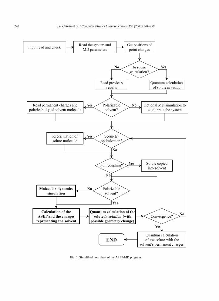
Fig. 1 shows the simplified flow chart of the program. The most important steps are those in bold face: mdynamics simulation, calculation of the ASEP, and the quantum calculation.
In a typical run, the first thing the program does is to read the values of some variables from the insupplied by the user. It then reads the system definition from the molecular dynamics template (nature andof solvent and solute molecules, interaction potential, etc.). With this information, and if needed, the equantum calculation program is called to perform a calculation of the isolated solute molecule, using thegiven in the quantum calculation template (method, basis set, etc.). The output of this calculation is read tthe energy, dipole moment and atomic charges of the solutein vacuo.
Now the main ASEP/MD cycle is carried out. The solute and solvent geometry and atomic charges areinto the molecular dynamics input file and the appropriate program is called to perform the simulation.set of solvent–solute configurations is read from the output of the molecular dynamics program and theelectrostatic potential created by the solvent over the solute (ASEP) is calculated from them, as well asinteraction energies. The ASEP is then approximated by a set of point charges. A new quantum calculatime with the external point charges representing the solvent, is performed. The output gives again thedipole moment, and atomic charges of the solute. A check for convergence is made and, if it has not beenthe solute charges are inserted again into the molecular dynamics input file and the main cycle starts anew
So far, the program flow has been described when a basic calculation is requested. There are twmain types of calculations which require some modifications of this scheme: polarizable solvent and geoptimization.
248 I.F. Galván et al. / Computer Physics Communications 155 (2003) 244–259
Fig. 1. Simplified flow chart of the ASEP/MD program.
I.F. Galván et al. / Computer Physics Communications 155 (2003) 244–259 249
amplen of theolecularreviousitse soluterom theated by
tributione.t of sol-, which
lectrons.
t (FEG)ilibriumobtained,[9]. Inon. The
program,ASEP/MD
rocess,r partialationary
nitionsable. The
ram.
3.1. Polarizable solvent
In the current implementation [2], the solvent polarization calculation is performed after an equilibrium sof solvent–solute configurations has been obtained with a non-polarizable solvent. Once a normal ruprogram, as described above, has finished, another calculation is carried out. This time no more mdynamics simulations are made, but the solvent configurations are read from the final simulation of the prun. An additional input is given with the permanentin vacuoatomic charges of the solvent molecule andpolarizability tensor. Then, for each one of the configurations, all the solvent molecules are polarized by thcharge distribution and by the other solvent molecules. The calculated ASEP now includes contributions fpermanent charges and the induced dipole moments of the solvent molecules. This potential is approximthe two sets of point charges explained above and introduced into the quantum calculation. The charge disof the solute is used to obtain the solvent polarization again, and this process is repeated until convergenc
This whole calculation can performed for different solute electronic states, keeping always the same sevent configurations. In this way, it is possible to study the solvent effect on electronic transitions in the solutetake place without appreciable reordering of the solvent nuclei, but with a major response of the solvent e
3.2. Geometry optimization
The geometry optimization method implemented in this program is based on the Free Energy Gradienmethod [8], in which the effective forces on the nuclei are taken as the average force over a set of equsolvent–solute configurations. Once the molecular dynamics simulation has been made and the ASEPa geometry optimization calculation is performed using the rational function optimization (RFO) methodthis way, a new solute geometry is obtained, which is introduced into the next molecular dynamics simulatiprocess is repeated until convergence.
The gradient and Hessian, needed for the optimization process, are given by the quantum calculationbut the appropriate van der Waals components have to be added. These components are calculated by theprogram as an average over all the solute–solvent configurations considered.
There are a number of options affecting the optimization method used. In each cycle of the ASEP/MD pthe optimization may be complete (a stationary point is found and this geometry is used in the next cycle) o(a fixed number of optimization steps is performed, and while the geometry used in the next cycle is not a stpoint, it is closer to one). Other options are related to the algorithm of the optimization procedure.
4. Program organization
The ASEP/MD source code is divided into different files, each of them containing subroutines and defigrouped according to the subject. The program uses modules to make variables and arrays globally availfollowing is a short description of the contents of the different files:
Main.f90
This file contains the main program, global definitions, and subroutines related directly to the main prog
– Module definitions.– ASEP_MD: This is the main program that controls the flow of the calculations.– LeerEntrada: This subroutine reads the input provided by the user.– LeerContinuacion: If a calculation is resumed, this subroutine reads the “continue” file.– EscribePrin: Writes the output of the main program.
250 I.F. Galván et al. / Computer Physics Communications 155 (2003) 244–259
uantumpendent:
)
OLDY.
ogram
NDO.
trostatic
olvent
es that
.olute–
Execute.f90
The subroutines in this file are related to the external programs used by ASEP/MD to perform the qmechanics calculations and molecular dynamics simulations. Most of these subroutines are program-indethey simply call the appropriate subroutine or process depending on the specific program used.
– LeerSistema: Calls another subroutine to read the system definition (solute, solvent, force field, etc.– LeerAbinitio: Calls another subroutine to read the output of a quantum calculation.– EjecutarAbInitio: Runs the appropriate quantum calculation through a SYSTEM call.– EjecutarDinamica: Runs the appropriate MD simulation through a SYSTEM call.– LeerConfig: Extracts a solute–solvent configuration from the output of the MD program.
MoldySubroutines.f90
The subroutines included in this file deal with the input and output of the molecular dynamics program M
– LeerControlMoldy: Reads the MOLDY control file for some necessary parameters.– LeerSistemaMoldy: Reads the system definition from the MOLDY input file.– ModificarMoldy: Modifies the MOLDY input files to run a new simulation.
GaussianSubroutines.f90
The subroutines included in this file deal with the input and output of the quantum calculation prGAUSSIAN.
– ModificarGaussian: Modifies the GAUSSIAN input file to perform a new quantum calculation.– LeerSalidaGaussian: Reads the output of GAUSSIAN.
HondoSubroutines.f90
The subroutines included in this file deal with the input and output of the quantum calculation program HO
– ModificarHondo: Modifies the HONDO input file to perform a new quantum calculation.– LeerSalidaHondo: Reads the output of HONDO.
Calculations.f90
This file is the core of the program. It contains the subroutines that calculate the average solvent elecpotential and the point charges that reproduce it. It also contains some other auxiliary subroutines.
– PosicionesCargas: Gets the positions of the outer point charges representing the average selectrostatic potential.
– CalcularCargas: This subroutine calls other subroutines to calculate the values of the point chargwill represent the solvent in the quantum calculations.
– PuntosPotencial: Calculates a grid of points inside the solute in which the ASEP will be calculated– CalcularPotencial: Calculates the electrostatic potential and interaction energies for a given s
solvent configuration.– ReducirCapa: Reduces the number of point charges in the solvent representation.
I.F. Galván et al. / Computer Physics Communications 155 (2003) 244–259 251
the
t and
to the
It acceptsfferentpend on
uantumtemplateitationsodifying
cycle ofdicated
e
– CalcularCampo: Calculates the fluctuations of the solvent electric field.– AjusteLagrange: Fits the outer point charges by the Lagrange multipliers method.– ResolverLU: Solves a system of linear equations by the LU factorization method.– GirarMolecula: Rotates a molecule (solute or solvent) to orient it along its main inertia axes.
Optim.f90
This file contains all the subroutines needed to perform a geometry optimization.
– OptimizarGeometria: This is the main subroutine for geometry optimization. It controls the flow ofprogram in this section.
– CalcularGradHessPot: Calculates the contribution of the van der Waals potential to the gradienHessian.
– BuscarMinimo: Performs a linear search to find a minimum.– EnergPunto: This is a function that returns the total energy for a given solute geometry.– ActualizarHessiana: Updates the Hessian using an appropriate formula.– CalcularIncremento: Calculates the increment to obtain the new solute geometry.– EscribeOptim: Writes output related to the optimization process.
5. Usage
The compilation of this program is straightforward. Just feed the names of the different source filescompiler. For example, withpgf90 use (this is a single line):
[user@localhost]$ pgf90 Main.f90 Execute.f90 MoldySubroutines.f90GaussianSubroutines.f90 HondoSubroutines.f90 Calculations.f90Optim.f90 -o asepmd
No makefile or configure script is needed.Once the program has been successfully compiled and linked, the resulting binary file can be executed.
a single command-line option: the name of the global input file. This file contains the values of the dioptions affecting the calculation. The input is formatted as a namelist called Input, whose syntax may dethe compiler and platform.
In addition to the global input file, the user must have access to suitable external programs for the qcalculations and for the molecular dynamics simulations. For these external programs the user must supplyfiles from which ASEP/MD can build the appropriate input files as needed. Currently, there are some limon the options and units that can be used in the template files, but they can be easily circumvented by mthe launching scripts or the parser subroutines. Future versions may eliminate these limitations.
As the calculation progresses, input and output files for the external programs will be created for eachthe process. All files will be created in the current working directory, so it is recommended to create a dedirectory for each calculation and run the program from there.
5.1. Input
The following is a short description of the different options in theInput namelist. For each option, its typ(string, integer, or float) is indicated:
252 I.F. Galván et al. / Computer Physics Communications 155 (2003) 244–259
out a
ram.a
ram.a
alues
tions.LDY’
readexternalmethod
m used.
e will
readformat
e will
micsystem.o such
rence
imum
. The
’ forthe
ber is
ation
– DirDynamics: String. Must point to the directory where the molecular dynamics binaries reside, withtrailing slash.
– ProgAbInitio: String. Location of a script or binary file that will run the quantum calculation progIt will be launched as ‘ProgAbInitio input-file output-file’, so the user is advised to writescript that runs the program in this way. The value of this option should include the full path.
– ProgDynamics: String. Location of a script or executable that will run the molecular dynamics progIt will be launched as ‘ProgDynamics input-file output-file’, so the user is advised to writescript that runs the program in this way. The value of this option should include the full path.
– AbInitio: String. This option specifies the program that will be used for quantum calculations. Valid vare ‘GAUSS’ for GAUSSIAN and ‘HONDO’ for HONDO.
– Dynamics: String. This option specifies the program that will be used for molecular dynamics simulaSince the only molecular dynamics program supported in this version is MOLDY, the value must be ‘MO
– MainOutput: String. Name of the file where the general output will be written in text format.– ContFile: String. Name of the file where the resume information will be written to and/or read from.– AbInitioFile: String. Name of the template file for the quantum calculation input. This file will be
and used as a template for each quantum calculation performed. The system definition (solute andpoint charges) will be added by ASEP/MD as needed, so only such options as basis set and quantumhave to be specified here. This file should be in the format expected by the quantum calculation prograIt will not be overwritten.
– AbInitioOutput: String. This is the generic name for the quantum calculation output files. The nambe modified for each cycle by appending ‘.cic.#’, where # is the cycle number.
– DynamicsFile: String. Name of the template file for the molecular dynamics input. This file will beand used as a template for each molecular dynamics simulation performed. This file should be in theexpected by the molecular dynamics program used, it will not be overwritten.
– DynamicsOutput: String. This is the generic name for the molecular dynamics output files. The nambe modified for each cycle by appending ‘.cic.#’, where # is the cycle number.
– InitialDynamics: String. Sometimes the user may want to perform an initial molecular dynacalculation with different conditions (smaller time step, lower temperature, etc.) to equilibrate the sIn that case the name of the input file for this simulation is specified here. If this option is left blank, nequilibration dynamics will be performed.
– EnergyConv: Float. Value of the convergence criterium for the energy. If the solute energy diffebetween two consecutive cycles is less thanEnergyConv, the energy is considered as converged.
– ChargesConv: Float. Value of the convergence criterion for the solute atomic charges. If the maxdifference in the atomic charges of the solute between two consecutive cycles is less thanChargesConv, thesolute atomic charges are considered to have converged.
– MaxDiffCharges: Float. Maximum allowed variation in the solute atomic charges from cycle to cyclecharges’ variation is damped if it is larger thanMaxDiffCharges.
– ChargesType: String. Type of atomic charges calculated for the solute. Allowed values are: ‘MULMulliken type, ‘CHE’ for CHELP calculated by the quantum program, ‘POT’ for charges fitted toelectrostatic potential by the ASEP/MD program.
– MaxIter: Integer. Maximum number of molecular dynamics + quantum calculation cycles. If this numreached, the program terminates.
– MaxIterPol: Integer. Maximum number of solvent polarization cycles if a solvent polarization calculis requested.
– Start: Integer. Initial cycle for the ASEP/MD calculation. IfStart = 0, the program will start with aquantum calculation of the isolated solute. For other values, the file specified inContFile should containvalid data for the previous cycles.
I.F. Galván et al. / Computer Physics Communications 155 (2003) 244–259 253
ling,verals
ntumynamics
n
hen
imum
dered
t be
e, they
used
ggers
. Ifnds,
n the
If the
ocess.
anewula. If
ations.
n the
will be
– Coupling: String. Type of coupling between solute and solvent. Allowed values are: ‘NON’ for no coupa single quantum calculation for the solute in solution will be performed; ‘PAR’ for partial coupling, secycles are made until convergence is achieved orMaxIter is reached; ‘TOT’ for full coupling, the solute icopied into the solvent (this is only for pure liquids).
– Polarization: String. ‘YES’ if a solvent polarization calculation should be made; ‘NO’ otherwise.– DoDynamics: String. The ASEP/MD cycles start with a molecular dynamics simulation, then a qua
calculation, and then another cycle begins. If a previous run is being resumed and the next molecular dsimulation has already been done, settingDoDynamics = ‘NO’ will skip the first molecular dynamics runand start with the following quantum calculation. This only skips thefirst molecular dynamics simulationeeded. The following cycles will be made normally. If all simulations are to be performed,DoDynamicsshould be ‘YES’.
– NumConfig: Integer. Number of solute–solvent configurations considered for obtaining the ASEP.– NumIniConfig: Integer. First configuration to consider in obtaining the ASEP.– RadiiFactor: Float. Factor by which the van der Waals radii of the solute atoms will be multiplied w
getting the grid of points to calculate the ASEP.– GridDiv: Integer. Number of points in each dimension where the ASEP will calculated. The max
number of grid points is thusGridDiv [3], but it will typically be far less.– FirstShell: String. If ‘YES’, the charges of the solvent molecules closest to the solute will be consi
explicitly. If ‘NO’, they will not.– ShellRadius: Float. Cut-off radius around the solute beyond which solvent molecules will no
considered explicitly.– Proximity: Float. Minimum distance between point charges. If two charges are closer than this valu
will be added together.– PermCharges: String. Name of the file with the solvent atomic charges and polarizability. This is only
when a solvent polarization calculation is performed.– IndDip: String. Type of calculation for the induced dipole moments in the solvent molecules. ‘NOR’ tri
a one-pass calculation, ‘CON’ triggers a self-consistent polarization process until convergence.– MaxIterOpt: Integer. Maximum number of optimization iterations within each ASEP/MD cycleMaxIterOpt = 0, optimization is turned off. If this number of iterations is reached, the optimization ebut the ASEP/MD program continues normally.
– GradientConv: Float. Convergence criterion for the gradient in the optimization process. Whegradient’s magnitude is less than this value, the optimization ends.
– MinStep: Float. Convergence criterion for the geometry variation in the optimization process.magnitude of the predicted change in geometry is less than this value, the optimization ends.
– MaxStep: Float. Maximum allowed change in the geometry between iterations of the optimization prIf the geometry change is larger, it will be damped accordingly.
– CalcHessian: Integer. Number of optimization iterations after which the Hessian will be calculatedby the quantum calculation program; in other iterations it will just be updated by the appropriate formCalcHessian= 1, the Hessian will be calculated in every iteration. IfCalcHessian= 0, the Hessian willnever be calculated; the identity matrix will be taken as the initial Hessian and updated in following iterIf CalcHessian= 10, for example, the Hessian will be calculated again every 10 cycles.
– LinearSearch: String. ‘YES’ turns on the linear search algorithm to locate a minimum of the energy isearch direction. ‘NO’ turns it off.
The input file can be specified as an argument when running the program. If no extension is given, ‘.dat’assumed and appended to the name:
254 I.F. Galván et al. / Computer Physics Communications 155 (2003) 244–259
s,A short
nt areurations
ent
edonly be
lated
ss,
an
d just
rgymselves.
sical, asarges that
olvent
nent
te–
ent
the
– asepmd will launch ASEP/MD and ask for an input file.– asepmd water will launch ASEP/MD usingwater.dat as input.– asepmd water.input will launch ASEP/MD usingwater.input as input.
5.2. Output
The output of this program, stored inMainOutput, will show, for each cycle of the ASEP/MD procesthe values of the solute–solvent interaction energy, solvent dipole moment, and other useful energies.description of this output follows:
MM ENERGIES: Energies and properties calculated from the MD data only; the solute and the solvetreated classically. The MM solute–solvent interaction energy is averaged over all the considered configand split into three components.
– Charge(solute)-charge(solvent) interaction: Interaction energy between the permancharges of the solvent and the atomic charges of the solute.
– Dipole(solvent)-charge(solvent) interaction: Interaction energy between the inducdipoles of the solvent and the atomic charges of the remaining solvent molecules. This energy willnon-zero if a polarizable solvent calculation has been made.
– Van der Waals interaction: Van der Waals interaction energy between solvent and solute, calcuby using the same potential (typically Lennard-Jones) given in the molecular dynamics input.
– Electric field fluctuation: Fluctuation of the electric field at the solute’s center of macalculated as the difference between the mean squared field and the squared mean field.
– Dipole-electric field interaction: Solute dipole–electric field interaction energy. This isoversimplification of the electrostatic solute–solvent interaction energy.
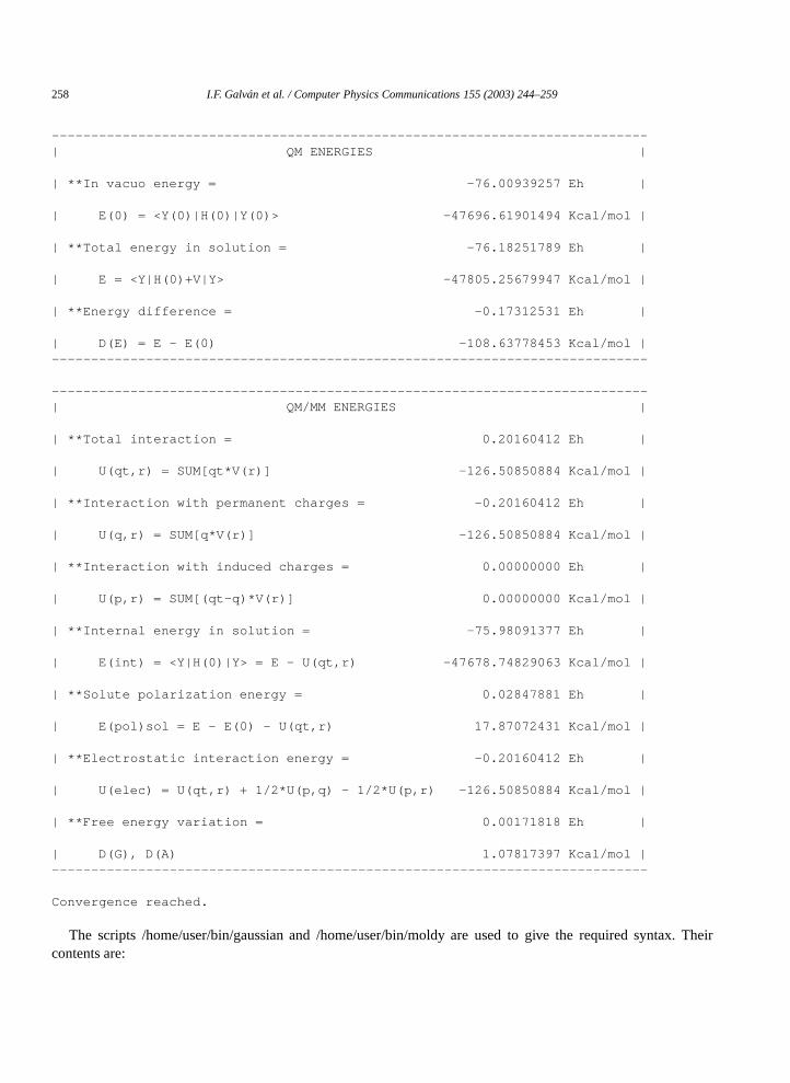
QM ENERGIES: Solute energies given by the quantum calculation program.
– In vacuo energy: Vacuum energy of the solute, this will be the same for all cycles, as it is calculateonce.
– Total energy in solution: Total solute energy in “solution”, including the interaction enebetween the solute and the solvent charges, but not including the self-energy of the external charges the
– Energy difference: Energy difference between the two previous values.
QM/MM ENERGIES: Solute–solvent interaction energies where the solute is quantum and the solvent claswell as some energies derived from these. The solvent representation for these energies is the set of chwas introduced into the quantum calculation.
– Total interaction: Total electrostatic solute–solvent interaction, calculated as the product of the scharges and the electrostatic potential generated by the solute over these charges.
– Interaction with permanent charges: Same as above, but considering only the permasolvent charges (and not the contribution of the induced dipoles).
– Interaction with induced charges: Contribution of the solvent induced dipoles to the solusolvent interaction energy, calculated as the difference between the two previous values.
– Internal energy in solution: Solute internal energy in solution, without the solute–solvinteraction energy.
– Solute polarization energy: Solute polarization or distortion energy: the difference betweeninternal energy in solution and the vacuum energy.
I.F. Galván et al. / Computer Physics Communications 155 (2003) 244–259 255
ded
one,
d output,
to
ually theuantum
een
– Electrostatic interaction energy: Electrostatic interaction energy including the energy neeto polarize the solvent molecules.
– Free energy variation: Free energy variation between the previous cycle and the currentcalculated by the free energy perturbation method.
Some of this data, as well as short messages about what the program is doing, will be written to standarbut this can be redirected to a file. For example:
asepmd water > water.std will launch ASEP/MD usingwater.dat as input and writing messageswater.std. The output file specified inMainOutput will still be generated.
Apart from errors in the input, the most common errors are those occurring in the external programs, so usfirst thing to do when the program stops unexpectedly is to check the output of the molecular dynamics or qcalculation program. The last lines inMainOutput and in the standard output (or the file to which it has bredirected) can also help in finding the errors.
5.3. Example
This example shows a simple calculation for pure water. Input files arewater.dat, water.g (input forGAUSSIAN),water.ctr, andwater.in (input files for MOLDY). Output file, as specified byMainOutput,is water.out.
water.dat
&Input
DirDynamics = ’/usr/local/MOLDY/’ProgAbInitio = ’/home/user/bin/gaussian’ProgDynamics = ’/home/user/bin/moldy’
AbInitio = ’GAUSSIAN’Dynamics = ’MOLDY’MainOutput = ’water.out’ContFile = ’water.con’AbInitioFile = ’water.g’AbInitioOutput = ’water.ogau’DynamicsFile = ’water.ctr’DynamicsOutput = ’water.omol’
EnergyConv = 0.005ChargesConv = 0.01MaxDiffCharges = 10.0ChargesType = ’CHELP’MaxIter = 50Start = 0Coupling = ’TOTAL’Polarization = ’NO’DoDynamics = ’YES’
NumConfig = 500NumIniConfig = 1
256 I.F. Galván et al. / Computer Physics Communications 155 (2003) 244–259
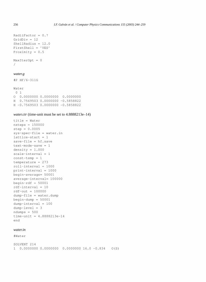
RadiiFactor = 0.7GridDiv = 12ShellRadius = 12.0FirstShell = ’YES’Proximity = 0.5
MaxIterOpt = 0/
water.g
#P HF/6-311G
Water0 1
O 0.0000000 0.0000000 0.0000000H 0.7569503 0.0000000 -0.5858822H -0.7569503 0.0000000 -0.5858822
water.ctr(time-unit must be set to 4.8888213e–14)
title = Waternsteps = 150000step = 0.0005sys-spec-file = water.inlattice-start = 1save-file = hf.savetext-mode-save = 1density = 1.000scale-interval = 1const-temp = 1temperature = 273roll-interval = 1000print-interval = 1000begin-average= 50001average-interval= 100000begin-rdf = 50001rdf-interval = 10rdf-out = 100000dump-file = water.dumpbegin-dump = 50001dump-interval = 100dump-level = 3ndumps = 500time-unit = 4.8888213e-14end
water.in
#Water
SOLVENT 2141 0.0000000 0.0000000 0.0000000 16.0 -0.834 O(S)
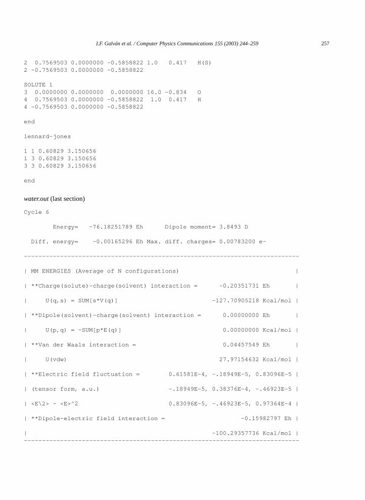
I.F. Galván et al. / Computer Physics Communications 155 (2003) 244–259 257
2 0.7569503 0.0000000 -0.5858822 1.0 0.417 H(S)2 -0.7569503 0.0000000 -0.5858822
SOLUTE 13 0.0000000 0.0000000 0.0000000 16.0 -0.834 O4 0.7569503 0.0000000 -0.5858822 1.0 0.417 H4 -0.7569503 0.0000000 -0.5858822
end
lennard-jones
1 1 0.60829 3.1506561 3 0.60829 3.1506563 3 0.60829 3.150656
end
water.out(last section)
Cycle 6
Energy= -76.18251789 Eh Dipole moment= 3.8493 D
Diff. energy= -0.00165296 Eh Max. diff. charges= 0.00783200 e-
----------------------------------------------------------------------------
| MM ENERGIES (Average of N configurations) |
| **Charge(solute)-charge(solvent) interaction = -0.20351731 Eh |
| U(q,s) = SUM[s*V(q)] -127.70905218 Kcal/mol |
| **Dipole(solvent)-charge(solvent) interaction = 0.00000000 Eh |
| U(p,q) = -SUM[p*E(q)] 0.00000000 Kcal/mol |
| **Van der Waals interaction = 0.04457549 Eh |
| U(vdw) 27.97154632 Kcal/mol |
| **Electric field fluctuation = 0.61581E-4, -.18949E-5, 0.83096E-5 |
| (tensor form, a.u.) -.18949E-5, 0.38376E-4, -.46923E-5 |
| <E\2> - <E>^2 0.83096E-5, -.46923E-5, 0.97364E-4 |
| **Dipole-electric field interaction = -0.15982797 Eh |
| -100.29357736 Kcal/mol |----------------------------------------------------------------------------
258 I.F. Galván et al. / Computer Physics Communications 155 (2003) 244–259
x. Their
----------------------------------------------------------------------------| QM ENERGIES |
| **In vacuo energy = -76.00939257 Eh |
| E(0) = <Y(0)|H(0)|Y(0)> -47696.61901494 Kcal/mol |
| **Total energy in solution = -76.18251789 Eh |
| E = <Y|H(0)+V|Y> -47805.25679947 Kcal/mol |
| **Energy difference = -0.17312531 Eh |
| D(E) = E - E(0) -108.63778453 Kcal/mol |----------------------------------------------------------------------------
----------------------------------------------------------------------------| QM/MM ENERGIES |
| **Total interaction = 0.20160412 Eh |
| U(qt,r) = SUM[qt*V(r)] -126.50850884 Kcal/mol |
| **Interaction with permanent charges = -0.20160412 Eh |
| U(q,r) = SUM[q*V(r)] -126.50850884 Kcal/mol |
| **Interaction with induced charges = 0.00000000 Eh |
| U(p,r) = SUM[(qt-q)*V(r)] 0.00000000 Kcal/mol |
| **Internal energy in solution = -75.98091377 Eh |
| E(int) = <Y|H(0)|Y> = E - U(qt,r) -47678.74829063 Kcal/mol |
| **Solute polarization energy = 0.02847881 Eh |
| E(pol)sol = E - E(0) - U(qt,r) 17.87072431 Kcal/mol |
| **Electrostatic interaction energy = -0.20160412 Eh |
| U(elec) = U(qt,r) + 1/2*U(p,q) - 1/2*U(p,r) -126.50850884 Kcal/mol |
| **Free energy variation = 0.00171818 Eh |
| D(G), D(A) 1.07817397 Kcal/mol |----------------------------------------------------------------------------
Convergence reached.
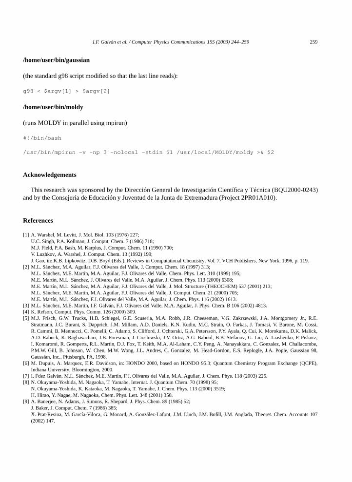
The scripts /home/user/bin/gaussian and /home/user/bin/moldy are used to give the required syntacontents are:
I.F. Galván et al. / Computer Physics Communications 155 (2003) 244–259 259
0-0243)
9.
Jr., R.E.Cossi,alick,
Piskorz,ombe,sian 98,
(QCPE),
nts 107
/home/user/bin/gaussian
(the standard g98 script modified so that the last line reads):
g98 < $argv[1] > $argv[2]
/home/user/bin/moldy
(runs MOLDY in parallel using mpirun)
#!/bin/bash
/usr/bin/mpirun -v -np 3 -nolocal -stdin $1 /usr/local/MOLDY/moldy >& $2
Acknowledgements
This research was sponsored by the Dirección General de Investigación Científica y Técnica (BQU200and by the Consejería de Educación y Juventud de la Junta de Extremadura (Project 2PR01A010).
References
[1] A. Warshel, M. Levitt, J. Mol. Biol. 103 (1976) 227;U.C. Singh, P.A. Kollman, J. Comput. Chem. 7 (1986) 718;M.J. Field, P.A. Bash, M. Karplus, J. Comput. Chem. 11 (1990) 700;V. Luzhkov, A. Warshel, J. Comput. Chem. 13 (1992) 199;J. Gao, in: K.B. Lipkowitz, D.B. Boyd (Eds.), Reviews in Computational Chemistry, Vol. 7, VCH Publishers, New York, 1996, p. 11
[2] M.L. Sánchez, M.A. Aguilar, F.J. Olivares del Valle, J. Comput. Chem. 18 (1997) 313;M.L. Sánchez, M.E. Martín, M.A. Aguilar, F.J. Olivares del Valle, Chem. Phys. Lett. 310 (1999) 195;M.E. Martín, M.L. Sánchez, J. Olivares del Valle, M.A. Aguilar, J. Chem. Phys. 113 (2000) 6308;M.E. Martín, M.L. Sánchez, M.A. Aguilar, F.J. Olivares del Valle, J. Mol. Structure (THEOCHEM) 537 (2001) 213;M.L. Sánchez, M.E. Martín, M.A. Aguilar, F.J. Olivares del Valle, J. Comput. Chem. 21 (2000) 705;M.E. Martín, M.L. Sánchez, F.J. Olivares del Valle, M.A. Aguilar, J. Chem. Phys. 116 (2002) 1613.
[3] M.L. Sánchez, M.E. Martín, I.F. Galván, F.J. Olivares del Valle, M.A. Aguilar, J. Phys. Chem. B 106 (2002) 4813.[4] K. Refson, Comput. Phys. Comm. 126 (2000) 309.[5] M.J. Frisch, G.W. Trucks, H.B. Schlegel, G.E. Scuseria, M.A. Robb, J.R. Cheeseman, V.G. Zakrzewski, J.A. Montgomery
Stratmann, J.C. Burant, S. Dapprich, J.M. Millam, A.D. Daniels, K.N. Kudin, M.C. Strain, O. Farkas, J. Tomasi, V. Barone, M.R. Cammi, B. Mennucci, C. Pomelli, C. Adamo, S. Clifford, J. Ochterski, G.A. Petersson, P.Y. Ayala, Q. Cui, K. Morokuma, D.K. MA.D. Rabuck, K. Raghavachari, J.B. Foresman, J. Cioslowski, J.V. Ortiz, A.G. Baboul, B.B. Stefanov, G. Liu, A. Liashenko, P.I. Komaromi, R. Gomperts, R.L. Martin, D.J. Fox, T. Keith, M.A. Al-Laham, C.Y. Peng, A. Nanayakkara, C. Gonzalez, M. ChallacP.M.W. Gill, B. Johnson, W. Chen, M.W. Wong, J.L. Andres, C. Gonzalez, M. Head-Gordon, E.S. Replogle, J.A. Pople, GausGaussian, Inc., Pittsburgh, PA, 1998.
[6] M. Dupuis, A. Marquez, E.R. Davidson, in: HONDO 2000, based on HONDO 95.3; Quantum Chemistry Program ExchangeIndiana University, Bloomington, 2000.
[7] I. Fdez Galván, M.L. Sánchez, M.E. Martín, F.J. Olivares del Valle, M.A. Aguilar, J. Chem. Phys. 118 (2003) 225.[8] N. Okuyama-Yoshida, M. Nagaoka, T. Yamabe, Internat. J. Quantum Chem. 70 (1998) 95;
N. Okuyama-Yoshida, K. Kataoka, M. Nagaoka, T. Yamabe, J. Chem. Phys. 113 (2000) 3519;H. Hirao, Y. Nagae, M. Nagaoka, Chem. Phys. Lett. 348 (2001) 350.
[9] A. Banerjee, N. Adams, J. Simons, R. Shepard, J. Phys. Chem. 89 (1985) 52;J. Baker, J. Comput. Chem. 7 (1986) 385;X. Prat-Resina, M. García-Viloca, G. Monard, A. González-Lafont, J.M. Lluch, J.M. Bofill, J.M. Anglada, Theoret. Chem. Accou(2002) 147.
Related Documents