Ascenso Titular - Universidad de Carabobo

Universidad de Carabobo

Facultad de Experimental de Ciencias y Tecnologıa

Departamento de Fısica

Influencia de la topologıa en la distribucion de riquezaen un modelo determinista de intercambio economico

Transition from Pareto to Boltzmann-Gibbs behavior ina deterministic economic model

Synchronization induced by intermittent versus partial drivesin chaotic systems

Global interactions, information flow, and chaos synchronization

Produccion Intelectual Acreditada presentada ante la Ilustre

Universidad de Carabobo

como merito para ascender a la categorıa de:

Profesor Titular

Dr. Orlando Alvarez Llamoza

Valencia, Abril de 2014

Hay quien se pasa la vida entera leyendo sin conseguir nunca ir mas alla de la lectura,se quedan pegados a la pagina, no entienden que las palabras son solo piedras puestas

atravesando la corriente de un rıo, si estan allı es para que podamos llegar a la otramargen, la otra margen es lo que importa.

Jose Saramago

Ningun hombre es una isla, algo completo en sı mismo;todo hombre es un fragmento del continente, una partede un conjunto.

John Donne

Agradecimientos

Mi desarrollo academico e intelectual y en especial, la produccion intelectual acre-ditada presentada a continuacion y toda la elaborada a lo largo de mi permanencia enla Universidad de Carabobo, no se hubiera podido realizar sin el apoyo de personas einstituciones, que de una u otra manera me han brindado su respaldo en estos anos devida universitaria.

Agradezco a mi familia, mi esposa Manuela y a mi hijo Adrian, que me han apo-yado y estado siempre conmigo, en mis estudios y en mi trabajo. A mi madre, misherman@s, mis ti@s, mi abuela† y a mi suegra. A mis segundas familias los Lopes-Moura, Echeverrıa-Calderon, Gonzalez-Mendez, Alvarez-Suescun, Marino-Antunes yLopes-Mackenzie. Puedo decir que a mi familia le debo todo, desde mis fracasos hastamis triunfos.

Agradezco a mis amigos y colaboradores del grupo de los “caoticos” de la ULA, a mitutor eterno Mario Cosenza, a mi compadre Carlos Echeverrıa, mi buen amigo JavierGonzalez, a Gilberto Paredes, Kay Tucci, Antonio Parravano, Juan Carlos Gonzalez,Jose Luis Herrera, Miguel Pineda y Miguel Escalona. Citando a John Bardeen “ laciencia es un esfuerzo de colaboracion. Los resultados combinados de varias personasque trabajan juntas es a menudo mucho mas eficaz de lo que podrıa ser el de un cientıficoque trabaja solo ”

Agradezco a mis companeros de la Universidad de Carabobo, los del Departamentode Fısica Eber Orozco, Damarys Serrano, Luciana Scarioni, Rolando Gaitan, MiguelAngel Suarez, Jose J. Rodrıguez, Juan Mateu, Richard Barrios, Miguel Rodrıguez, OttoRendon, Angel Rivas, Rafael Munoz, Aaron Munoz, Jose Albornoz, Alfredo Macıas,Freddy Narea, Oscar Sucre y Nelson Falcon. Y a los que no son del Departamento,Nancy Salinas, Jose Marcano, Saba Infante, Jose Guaregua, Pedro Linares, CarolinaCorao, Renny Pacheco, Eucandis Fuentes, y a muchos otros que por no estar en estabreve lista debido a mi descuido y/o mala memoria no implica que les tenga unaspalabras de agradecimiento, ya que todos, de una u otra forma colaboraron e influyeronen mi desempeno en la UC.

i

Al personal administrativo del Departamento, Luis Matos, Jower Ruiz y DayanaParra. Al personal del decanato en especial de la Oficina de Asuntos Profesorales, alpersonal de Control de Estudios y al de Telematica

Y finalmente dentro de las personas debo reconocer a mis estudiantes, sobre todoa mis tesistas David Romero, Vianney Gimenez, Wilder Iglesias, Aquilez Gonzalez,Jose Luis Casa Diego, Gustavo HArgenis Lopez, Linmar Pina y Douglas Avendano.“Con mis maestros he aprendido mucho; con mis colegas, mas; con mis alumnos todavıamas” proverbio hindu.

Dentro de las instituciones agradezco a mi Alma Mater, La ilustre Universidadde Los Andes, gracias a ella soy profesionalmente lo que soy hoy. Mi paso por esainstitucion, desde mi Licenciatura, Maestrıa y Doctorado cambio mi forma de ver yapreciar el mundo y me dio las herramientas para ser un profesional competitivo ycabal.

Por ultimo agradezco a la ilustre Universidad de Carabobo, que me acogio dandometrabajo y proporciono el campo para aplicar lo que he aprendido y sigo aprendiendoen el mundo academico. Dicha institucion me apoyo economicamente en mis estudiosdoctorales, conjuntamente con la OPSU, y son responsables tambien de mi desarrollointelectual.

A tod@s ell@s muchas gracias!

Departamento de Fısica ii FACYT-UC

El cientıfico encuentra su recompensa en lo que HenriPoincare llama el placer de la comprension, y no en lasposibilidades de aplicacion que cualquier descubrimien-to pueda conllevar.

Albert Einstein

PresentacionLa siguiente Produccion Intelectual Acreditada presentada como credencial de meri-

to para el ascenso a la categorıa de Profesor Titular, consta de cuatro publicacionestipo A, segun el artıculo 196 del Estatuto del Personal Docente y de Investigacion de laUniversidad de Carabobo (EPDI-UC). Estos trabajos de investigacion estan enmarca-dos dentro de las lıneas de investigacion del Departamento de Fısica, Grupo de FısicaComputacional, en el area de Sistemas Dinamicos y Sistemas Complejos.

Todos los trabajos fueron publicados luego de mi ascenso a la categorıa de ProfesorAsociado, realizado el 06 de octubre de 2008 y no han sido utilizados para otro finacademico, segun reza el artıculo 190 del EPDI-UC.

Las publicaciones fueron realizadas conjuntamente con algunos de los siguientes cola-boradores; Dr. Mario Cosenza, Universidad de Los Andes, Merida; Dr. Javier Gonzalez,Universidad Nacional Experimental del Tachira, San Cristobal; Gilberto Paredes, Uni-versidad Nacional Experimental del Tachira, San Cristobal y Ricardo Lopez Ruiz, Uni-versidad de Zaragoza, Espana.

Para los artıculos publicados en revistas internacionales en idioma ingles, se presentaun condensado en idioma castellano, segun ordena el artıculo 198 del EPDI-UC. Estoscondensados, si bien no son una traduccion completa de los trabajos, van mas alla deun simple resumen y representan casi todo el contenido del trabajo original. Al final decada condensado se incluye el artıculo original publicado.

En el capıtulo 1 se presenta el trabajo Influencia de la topologıa en la distribucionde riqueza en un modelo determinista de intercambio economico, publicado en la RevistaCientıfica de la UNET (Universidad Nacional del Tachira), en el volumen 23, numero 1,desde la pagina 61 hasta la 68, en el ano 2011. La Revista Cientıfica de la UNET esta indi-zada en Latindex-Catalogo, Latindex-Directorio y Revencyt (Registro de PublicacionesCientıficas y Tecnologicas Venezolanas).

El capıtulo 2 corresponde al artıculo Transition from Pareto to Boltzmann-Gibbsbehavior in a deterministic economic model, publicado en la revista Physica A, en el

iii

volumen 388, numero 17, desde la pagina 3521 hasta la 3526, en el ano 2009. La re-vista Physica A esta indizada en Science Citation Index, Science Citation Index Ex-panded, El Compendex Plus, INSPEC, Scopus, Astrophysics Data System, y CurrentContents/Physics, Chemical & Earth Sciences, entre otros.

En el capıtulo 3 se presenta el trabajo Synchronization induced by intermittent ver-sus partial drives in chaotic systems, publicado en la Revista International Journal ofBifurcation and Chaos, en el volumen 20, numero 2, desde la pagina 323 hasta la 330,en el ano 2010. La revista International Journal of Bifurcation and Chaos esta indiza-da en Science Citation Index, Science Citation Index Expanded, Compendex, Scopus,INSPEC, y Current Contents/Physics, Chemical & Earth Sciences, entre otros.

Finalmente, en el capıtulo 4 se presenta el artıculo Global interactions, informationflow and chaos synchronization, publicado en la revista Physical Review E, en el volumen88, 042920, desde la pagina 042920-1 hasta la 042920-8, en el ano 2013. La revistaPhysical Review E esta indizada en Current Physics Index, INSPEC, Medline, PhysicsAbstracts y Science Citation Index Expanded entre otros.

Departamento de Fısica iv FACYT-UC

Indice

Agradecimientos I

Presentacion III

1. Influencia de la topologıa en la distribucion de riqueza en un modelodeterminista de intercambio economico 1

Artıculo publicado . . . . . . . . . . . . . . . . . . . . . . . . . . . . . . . . 2

2. Transition from Pareto to Boltzmann-Gibbs behavior in a determinis-tic economic model 10

2.1. Modelo determinıstico economico es una red bidimensional . . . . . . . 11

2.2. Transicion de comportamiento Pareto a Boltzmann-Gibbs . . . . . . . . 13

2.3. Conclusiones . . . . . . . . . . . . . . . . . . . . . . . . . . . . . . . . . 14


3. Synchronization induced by intermittent versus partial drives in chao-tic systems 21

3.1. Sistema de mapas forzados intermitentemente . . . . . . . . . . . . . . 22

3.2. Sistema de mapas forzados parcialmente . . . . . . . . . . . . . . . . . 24

3.3. Redes dinamicas . . . . . . . . . . . . . . . . . . . . . . . . . . . . . . 25

3.4. Conclusiones . . . . . . . . . . . . . . . . . . . . . . . . . . . . . . . . . 25


4. Global interactions, information flow and chaos synchronization 34

4.1. Campos globales de interaccion . . . . . . . . . . . . . . . . . . . . . . 35

4.1.1. Estados sincronizados . . . . . . . . . . . . . . . . . . . . . . . . 36

4.2. Interaccion global homogenea . . . . . . . . . . . . . . . . . . . . . . . 37

v

4.2.1. Sincronizacion completa . . . . . . . . . . . . . . . . . . . . . . 37

4.2.2. Sincronizacion generalizada . . . . . . . . . . . . . . . . . . . . 38

4.3. Interacciones globales heterogeneas . . . . . . . . . . . . . . . . . . . . 39

4.3.1. Sincronizacion completa . . . . . . . . . . . . . . . . . . . . . . 39

4.4. Conclusiones . . . . . . . . . . . . . . . . . . . . . . . . . . . . . . . . . 40


Departamento de Fısica vi FACYT-UC

¿No es extrano? Los mismos que se rıen de los adivinosse toman en serio a los economistas.

Anonimo

1Influencia de la topologıa en la

distribucion de riqueza en un modelodeterminista de intercambio

economico

Artıculo publicado en La Revista Cientıfica de la UNET (Universidad Nacional delTachira), en el volumen 23, numero 1, desde la pagina 61 hasta la 68, ano 2011.

La Revista Cientıfica de la UNET, ISSN 1316-869X, es una publicacion periodicasemestral que se encuentra indizada en Latindex-Catalogo, Latindex-Directorioy Revencyt (Registro de Publicaciones Cientıficas y Tecnologicas Venezolanas).http://www.latindex.unam.mx/buscador/ficRev.html?opcion=1&folio=15384.Ver apendice.

1

http://www.latindex.unam.mx/buscador/ficRev.html?opcion=1&folio=15384

We investigate a deterministic model of coupled maps lattices in one and two dimensions to describe the economicinteraction of a set of agents. The dynamics of each map or agent is controlled by two parameters. The first one isassociated to an agent's growth capacity and the other is a control term that represents the local environment pressurethat inhibits an exponential increase. The probability distribution of wealth in the system is calculated as a function of theseparameters. It is found that these distributions can exhibit an exponential (Boltzmann-Gibbs) or a power-law (Pareto) behaviorin different regions of parameters. Such distributions are typical of real economic systems. These probability distributions alsodepend on the dimensionality of the lattice and on the number of neighbors that participate in the local interactions. Tocharacterize the inequality of the wealth distribution in the system, we calculate the Gini coeficient as a function of theparameters. Our results show that entirely deterministic processes can lead to the phenomenology observed in real societies.

Econophysics, computational models, coupled map lattices, Pareto and Boltzmann-Gibbs distributions.Key Words:

INFLUENCIA DE LA TOPOLOGÍA EN LADISTRIBUCIÓN DE RIQUEZA EN UN

MODELO DETERMINISTA DEINTERCAMBIO ECONÓMICO

(Influence of topology on the wealth distribution in adeterministc model of economic exchange)

González-Estévez, J.; Cosenza, M. G.; López-Ruíz, R.; Alvarez-Llamoza, O.1, 2 2 3 4, 2

1

2

3

4

Laboratorio de Fí ca Aplicada y Computacional,Universidad Nacional Experimental del Táchira, San Cristóbal, Venezuela,

Centro de Física Fundamental, Universidad de Los Andes, Mérida,Venezuela,DIIS y BIFI, Facultad de Ciencias, Universidad de Zaragoza, 50009 Zaragoza, España,

Departamento de Fí ca, FACyT, Universidad de Carabobo, Valencia, Venezuela,Correo Electrónico:

si

[email protected]

Se investiga un modelo determinista de mapas acoplados en redes de una y de dos dimensiones para describir la interacción económica de unconjunto de agentes. La dinámica de cada mapa o agente está controlada por dos parámetros. El primero está asociado con la capacidad decrecimiento del agente y el otro es un término de control que representa la presión del ambiente local que evita un crecimiento exponencial.Se calcula la probabilidad de distribución de riqueza en el sistema en función de estos parámetros. Se encuentran distribuciones de tipoexponencial (Boltzmann-Gibbs) o de tipo de ley de potencia (Pareto) en diferentes regiones de parámetros. Estas distribuciones sontí icas de sistemas económico reales. Se encuentra que las distribuciones de probabilidad también dependen de la dimensionalidad de la red ydel número de vecinos que participan en la interacción local. Se calcula el coeficiente de Gini para caracterizar la desigualdad en ladistribución de la riqueza en el sistema en función de los parámetros. Nuestros resultados muestran que procesos completamentedeterministas pueden dar lugar a fenomenologí observadas en sociedades reales.

Econofí ca, modelos computacionales, redes de mapas acoplados, distribuciones de Pareto y Boltzmann-Gibbs.

p

as

siPalabras Clave:

RESUMEN

ABSTRACT

VOL.23(1):61-68. 2011.61

Recibido:19/05/2008Aprobado:07/07/2009

Versión Final: 15/07/2009

Cs. Exactas

Departamento de Fısica 2 FACYT-UC

INTRODUCCIÓN

MÉTODO

La desigualdad en la distribución de la riqueza es unhecho bien documentado de la actividad económica. Elorigen de este fenómeno está relacionado con lainteracción de la macroeconomía en la microeconomía,lo que conlleva, en muchos casos, la intervención decircunstancias aleatorias fuera del control de los agenteseconómicos. Así, está reportado que el ingreso dealrededor del 95% del total de la sociedad, justamenteaquel colectivo conformado por agentes con ingresosmedios y bajos, siguen una distribución exponencial(comportamiento Boltzmann-Gibbs; BG para abreviarde aquí en adelante), mientras que el 5% restante de lasociedad, asociada a los altos ingresos, se distribuyesegún una función potencial, que en el contextoeconómico se conoce como ley de Pareto (Dragulescu yYakovenko, 2003; Yakovenko, 2007). Diferentesmodelos (Dragulescu yYakovenko, 2000; Chakraborti yChakrabarti, 2000; Chatterjee 2004; Angle, 2006)con ingredientes aleatorios han sido propuestos parareproducir estas distribuciones de ingresos que seencuentran comunmente en datos económicos reales(Levy y Solomon, 1997, Dragulescu y Yakovenko2001a; Dragulescu yYakovenko, 2001b; Souma, 2001).

Por otro lado, en muchos casos no es suficienteinvocar mecanismos aleatorios para la distribución de lariqueza en las sociedades humanas, puesto que éste no esun proceso completamente fortuito, sino que presentaelementos de racionalidad y determinismo. El objeto deeste trabajo consiste en demostrar la viabilidad de estepunto de vista determinista y, por tanto, presentar unaalternativa frente a la aleatoriedad como característicapredominante en la dinámica de intercambio económicoque conduce a las distribuciones de riqueza observadasen las sociedades. Específicamente, estudiamos unmodelo determinista y conceptualmente simple basadoen agentes interactivos donde la interacción de cadaagente se realiza con sus vecinos más próximos en elespacio. El modelo dispone de pocos parámetros, loscuales al variar pueden conducir a distribuciones deprobabilidad de riqueza de tipo BG o Pareto.

El modelo consiste en un sistema dinámico espaciotemporal representado por mapas ubicados en una red(unidimensional o bidimensional), con interaccioneslocales y con condiciones de contorno periódicas. Cadamapa representa un agente económico: una compañía,un país u otra entidad económica. El estado de cadaagente, identificado por un coeficiente ( = 1, 2,..., ),

está caracterizado por un grado de libertad,denotando la fuerza, abundancia o riqueza

del agente en el tiempo discreto . El sistema evolucionaen el tiempo de forma síncrona, es decir, los estados detodos los agentes se actualizan simultáneamente encada paso de tiempo.

Cada agente actualiza su estado de acuerdo a suestado presente y a los estados de su vecindad. De estaforma el valor del estado está dado por el productode dos factores: 1) el crecimiento natural del agente

con un tasa local positiva (cuyo valor es igual omayor a 1, para garantizar el crecimiento de estetérmino), y 2) un término de control que limita elcrecimiento del agente con respecto al ambiente o suentorno local, . De esta manera, la dinámica delsistema esta descrito por el siguiente conjunto deecuaciones

(1)

El

Por motivos de simplicidad, estudiaremos escenarioscon distribución homogénea de los parámetros. Así,reescribimos los parámetros como (suponiendo que losagentes poseen la misma capacidad de crecimiento) y(que corresponde a una presión de selección localhomogénea). Consideramos un sistema descrito por lasEcs. (1) y (2), formado por 10 mapas concondiciones iniciales completamente aleatoriasdistribuidas uniformemente en el intervalo (1, 100).

En general, el comportamiento colectivo del sistemapuede ser caracterizado mediante el campo medioinstantáneo de la red o actividad del sistema, definidocomo:

(2)

et al.

N

i N

t

ra

N=

,

sistema (1) corresponde a una red de mapasacoplados, donde indica el estado del agente parael tiempo discreto , ( ) es el conjunto de agentes en lared acoplados con el agente y ( ) es la cardinalidad deeste conjunto; el parámetro a mide la intensidad delacoplamiento del agente con su vecindad; que tambiénpuede ser interpretado como la presión ambiental localejercida sobre el agente (Ausloos 2003). Lafunción exponencial negativa actúa como un inhibidorque limita este crecimiento con respecto al campo local(Sánchez y López-Ruiz, 2005; Sánchez . 2007;López-Ruiz 2007a; López-Ruiz 2007b;González 2008).

it i

i n i

i

i et al.

et alet al. et al.

et al.

5

Influencia de la topología en la distribución de riqueza en un modelo...

62 VOL.23(1):61-68. 2011.

,

.

.


A d i c i o n a l m e n t e , e l c o e f i c i e n t e d e G i n i(Rodríguez-Achach y Huerta-Quintanilla, 2006),

(3)

mide el grado de desigualdad relativa en la distribuciónde riqueza en el instante . Este coeficiente esta acotadoentre los valores = 0 (todos los elementos tienenla misma riqueza; esto es, perfecta equidad, ) y

(un elemento posee toda la riqueza delsistema ; es decir, máxima desigualdad). Enconsecuencia, cuanto menor es el valor del coeficienteGini, menor es la desigualdad y viceversa (Bouchaud yPotters, 2000; Mantegna y Stanley, 2000; Voit, 2002).

Para examinar las condiciones en que el sistemapuede exhibir los comportamientos estadísticos tipo BGo Pareto, son realizadas cien simulaciones para cadavalor de barrido en el parámetro , con el fin de disminuirlas fluctuaciones estadísticas en los cálculo (Reed,2002).

Una distribución de probabilidad tipo exponencial, oBoltzmann-Gibbs (BG), de una variable presenta la

forma funcional , donde es el exponente quecaracteriza esta distribución. Por otro lado,una distribución de probabilidad tipo ley depotencia, o Pareto (P), se comporta como

donde es un exponente característico.La figura 1 muestra las distribuciones de probabilidad

( ) resultantes para el sistema (1) unidimensional en untiempo asintótico donde el sistema es estadísticamenteestacionario, para distintos valores de los parámetros y. Encontramos ambos tipos de distribuciones, con

exponentes característicos calculados a partir de laspendientes de las gráficas por el método de mínimoscuadrados en una regresión semilogarítmica obilogarítmica, según corresponda.

Para garantizar la confiabilidad de los resultadosobtenidos para las distribuciones tipo BG o P,requeriremos que el valor de la correlación en elcálculo de las pendientes correspondientes satisfaga elcriterio | | 0,96.

Las figuras 2 y 3 muestran los valores de lacorrelación del ajuste exponencial y potencial , enfunción del parámetro , para distintos tipos de redes enuna y en dos dimensiones, para un valor fijo = 10. Estopermite seleccionar aquellas regiones de parámetros condistribuciones tipo BG y Pareto, que satisfagan el criterio

t

a

x

P x

ar

ar

RESULTADOS

Régimen Boltzmann-Gibbs y Régimen Pareto

μ

β

β

β

β

≥

| | 0,96.≥

González-Estévez,J.; Cosenza, M. G.; López-Ruiz, R.; Alvarez-Llamoza, O.

Figura 1. Distribuciones de probabilidad ( ) para diferentes valores de parámetros en un sistema (1) unidimensional con= 10 , para = 10000. (a) Comportamiento BG, con = 0,60 y = 4; el exponente es −0,2593 y coeficiente

de correlación es = −0,9943. (b) Ley de potencia (P), con = 0,92 y = 8; el exponente es = −2,8469, con= −0,9849.

P x

N t a ra r

5μ

β=

α

β

63VOL.23(1):61-68. 2011.

μ


En el caso unidimensional con interacción con losdos vecinos más cercanos, se encuentra una región BG

(0,179 − 0,342) y dos regiones Pareto (0,434 −0,993) y (1,025−1,893). En el caso bidimensionalcon cuatro vecinos (o vecindad de Von Neumann) existeuna región BG a (0,219−0,546) con dos regionesPareto (0,611 − 0,994) y (1,015 − 1,887).Finalmente, en el caso bidimensional, pero con ochovecinos (vecindad tipo Moore) se encuentra una zonaBG (0,300−0,800) y una región Pareto para(0,962 − 2,1). Estos valores son el resultado de haberpromediado cien realizaciones en cada barrido delparámetro , de tal forma que nos referimos a valorespromedios.

Una vez delimitadas las regiones de parámetros queexhiben comportamientos tipo BG y Pareto, según elcriterio establecido, mostramos en la figura 4 los valoresde los exponentes característicos y en función delparámetro .

En datos reales se ha encontrado que la economíadel Reino Unido presenta una distribución de Paretopara un rango de ingresos altos con un valor de = 1,9en el año 1996; mientras que para la economía deEE.UU. se obtiene = 1,7 para 1997. Pareto, en su obraclásica (Pareto 1897), estableció este exponente como

= 1,5 para varios paises, siendo este el valor promediode los resultados obtenidos en su trabajo. Levy ySolomon, 1997; Klass 2006; Klass 2007indican un valor promedio = 1,49, tomando los datosde la lista “Forbes 400” (las cuatrocientas personas másricas sobre el planeta) durante los años 1988 al 2003; ySouma reporta un valor de = 2,05 dentro de losingresos más altos en Japón (Souma, 2001; Souma,2002). Los resultados de la figura 4 muestran que esposible obtener un amplio rango de valores de esteexponente, incluyendo valores realistas, mediante lavariación continua de un parámetro en nuestro modelodeterminista de mapas acoplados.

a

a

a

a a

a a

a

a

et al. et al.

Є Є

Є

Є

Є Є

Є Є

α

α

α

α

α

α

μ

Figura 2. Coeficiente de correlación en función del parámetro en la región de comportamiento BG para distintos tipos deredes, con = y = 10 fijo. El cálculo corresponde a = 10000. La línea punteada horizontal corresponde al valor= −0,96.

a

N r t

β

β105

Figura 3. Coeficiente de correlación en función del parámetro en la región de comportamiento tipo ley de potencia (Pareto)para distintos tipos de redes, con N = y = 10 fijo. El cálculo corresponde a = 10000. La línea punteada horizontalcorresponde al valor −0,96.

a

r t

β

β10

=

5


64 VOL.23(1):61-68. 2011.


Riqueza promedio

El campo medio ofrece información acerca delvalor medio promedio de la riqueza en el sistema. En lafigura 5 encontramos que los valores máximos ymínimos en las regiones BG son para el casounidimensional: (mín)=2,471 y (máx)=2,597, en elcaso bidimensional con cuatro vecinos se obtiene que

(mín) = 2,222 y (máx) = 2,644 y finalmente en dosdimensiones y un entorno local de ocho vecinos sepresenta un (mín) = 1,901 y (máx) = 2,640.

Para las regiones cuyo comportamiento sigue la leyde Pareto, y tomando como referencia dicha zona antesde = 1, en el caso unidimensional se tiene que

(mín)=1,294 y (máx) = 2,339 y con dos dimensiones

y una interacción local de 4 vecinos, se obtiene(mín) = 1,223 y (máx) = 2,136. Posterior a = 1 en el

caso unidimensional se tiene que (mín)=1,213 y(máx)=1,393 y con dos dimensiones y una interacción

local de cuatro vecinos, se obtiene (mín)=1,109 y(máx) = 1,200.

En contraste, para el modelo bidimensional convecindad de Moore (8 vecinos), se encuentra únicamenteuna región tipo Pareto cuya riqueza mínima promedio es

(mín)=1,041 y la riqueza máxima promedioencontrada es (máx) = 1,701.

Nótese que la riqueza promedio en el sistema puedeser afectada, tanto por los valores de los parámetros,como por la geometría del sustrato espacial dondeocurren las interacciones.

H

H H

H H

H H

a

a

t

t t

t t

t t

H H

H H

H

H

H

H

H

H

t t

t t

t

t

t

t

t

t

Figura 4. Exponentes característicos en las distribuciones tipo BG (línea continua) y tipo P (línea punteada) en función delparámetro . (a) red unidimensional; (b) red bidimensional con 4 vecinos; (c) red bidimensional con 8 vecinos. Entodos los casos = , = , = 10000. Las regiones BG y Pareto que no cumplen con el criterio | | 0,96 estánacotadas.

a

r N t10 105β ≥

Figura 5. Campo medio en función del parámetro . (a) red unidimensional; (b) red bidimensional con 4 vecinos; c) redbidimensional con 8 vecinos. En todos los casos = 10, = , t = 10000. Las regiones BG y Pareto que no cumplencon el criterio están acotadas.

Ht a

r N 10| | 0,96

5

β ≥

65VOL.23(1):61-68. 2011.



Coeficiente de Gini

DISCUSIÓN DE RESULTADOS

La figura 6 muestra el coeficiente de Gini, ,calculado con la ecuación (3), en función del parámetro

, para distintas redes. Se aprecia que el comportamientodel coeficiente de Gini es cualitativamente muy similaren el rango (0 − 0,82).

Separando la influencia de la topología en lasdistintas redes, se observa en la figura 7 que los valoresmáximos y mínimos del coeficiente de Gini, en lasregiones BG son para el caso unidimensional: (mín) =0,479 y (máx) = 0,633, en el caso bidimensional concuatro vecinos se obtiene que (mín)=0,507 y

(máx)=0,723 y finalmente en dos dimensiones y unentorno local de ocho vecinos se presenta un

(mín)=0,576 y (máx)= 0,783.Para las regiones cuyo comportamiento sigue la ley

de Pareto, y tomando como referencia dicha zona antesde =1, en el caso unidimensional se tiene que

(mín)=0,688 y (máx)=0,703 y, con dos dimensionesy una interacción local de cuatro vecinos, se obtiene

(mín) = 0,678 y (máx)=0,742. Posterior a = 1 en elcaso unidimensional se tiene que (mín)=0,691 y

(máx)=0,780 y con dos dimensiones y una interacciónlocal de cuatro vecinos, se obtiene (mín)=0,683 y

(máx)=0,714.

De la figura 2 se obtiene una distribución exponencialdel tipo BG, con un exponente característico

= 0,2593. Haciendo una analogía termodinámica paraeste tipo de comportamiento exponencial, se puededefinir una especie de “temperatura”, = 1/ , que paraeste caso particular, toma el valor = 3,84.

Como ya se ha mostrado en la figura 3, es posibleencontrar regiones cuyo comportamiento obedece a unaley de potencia ( )~ en el espacio de parámetros ( ,). El exponente de esta distribución, para este caso en

concreto, resulta ser = 2,84, el cual está en acuerdo conlos exponentes característicos de Pareto derivados dedatos económicos reales.

G

a

a

G

G

G

G

G

G G

aG G

G G a

G

G

G

G

TT

P x ar

t

t

t

t

t

t

t t

t t

t t

t

t

t

t

Є

μ

μ

α

x-α

α

Figura 6. Coeficiente de Gini vs. para = 10 , calculado sobre el promedio de 100 realizaciones para cadavalor de , para distintas redes, con = 10, = 10

a t

a r N

4

5


66 VOL.23(1):61-68. 2011.

.


Se observa en términos cualitativos que la riquezamedia promedio (Figura 5) y el coeficiente de Gini(Figura 7) están relacionados. En las regiones decomportamiento BG se manifiesta que la riqueza mediapromedio es mayor con respecto a las zonas Pareto, y loscorrespondientes coeficientes de Gini indican que lariqueza está mejor distribuida en las regiones BG que ensu contraparte, resultado que está acorde con loreportado en la literatura. En lo que respecta a ladimensionalidad, se encuentra en la distribución tipoBG, un desplazamiento de esta región hacia valoresmayores del parámetro , y un ensanchamiento en lamedida que la dimensionalidad y el número de vecinosinteractivos aumenta.

Nuestros resultados muestran que es posible, con unmodelo determinista de mapas acoplados, obtenerdistribuciones de probabilidad de riquezas similares a lasencontradas en sociedades reales.

Hemos estudiado un modelo determinista, local yhomogéneo, conceptualmente simple y con ingredientesmínimos, que permite capturar la fenomenología básicade interacciones económicas y que conduce de un modonatural a las distribuciones de riqueza observadas ensociedades reales. Este modelo consiste en un sistemadinámico espaciotemporal descrito por una red de mapasacoplados en una o dos dimensiones.

En contraste con modelos previos que involucranaleatoriedad y heterogeneidad en los agenteseconómicos, en nuestro modelo las interacciones locales(la “microeconomía”) determina completamente lascaracterísticas macroscópicas del sistema; es decir, lamacroeconomía constituye un comportamientocolectivo emergente. Como consecuencia, fenómenoscomo la desigualdad en la distribución de riqueza en elsistema surgen como resultado de procesos dinámicosque tienen lugar a nivel local.

Nuestros resultados sugieren que en sistemas deagentes económicos interactivos se pueden conseguirdistintas regiones de parámetros en las cuales ladistribución de riqueza manifiesta comportamientos tipoexponencial (BG) o leyes de potencia (Pareto), los cualeshan sido observados en sistemas económicos reales. Porotro lado, se evidencia el rol que juega la conectividad decada agente con su entorno en el surgimiento decomportamientos colectivos en el sistema.

Entre las futuras extensiones de este modelo está laposibilidad de modificar la regla de acoplamiento entrelos mapas para encontrar los dos tipos de distribución deriqueza coexistiendo para los mismos valores deparámetros, con una distribución exponencial BG paralos agentes con ingresos bajos y medios, y unadistribución de Pareto para aquellos con ingresos altos,tal como se observa en datos económicos reales(Yakovenko, 2007).

a

CONCLUSIONES

Figura 7. Coeficiente de Gini vs. , indicando las regiones BG y Pareto. (a) red unidimensional; (b) red bidimensional con 4vecinos; c) red bidimensional con 8 vecinos. En todos los casos = 10, = . Las regiones BG y Pareto que nocumplen con el criterio

a

r N 105

| | 0,96.β ≥

67VOL.23(1):61-68. 2011.



AGRADECIMIENTOS

REFERENCIAS BIBLIOGRÁFICAS

Este trabajo ha sido financiado por el Decanato deInvestigación de la Universidad Nacional Experimentaldel Táchira (UNET), mediante los proyectos 04-001-2006 y 04-002-2006. J.G.-E. agradece al Decanato deInvestigación y Vicerrectorado Académico de la UNETpor el financiamiento obtenido para viajes. J.G-E. y R.L-R. agradecen el apoyo del BIFI, Universidad deZaragoza, y de la Asociación Iberoamericana dePostgrado (AUIP), y del proyecto DGICYTFIS2006-12781-C02-01, España. M.G.C agradece el apoyo delConsejo de Desarrollo, Científico, Tecnológico yHumanístico y de las Artes, Universidad de los Andes,Mérida, a través del proyecto C-1692-10-05-B.

ANGLE, J. The inequality process as a wealthmaximizing process, Physica A. 367, 388-414,2006.

AUSLOOS, M.; CLIPPE, P. y PEKALSKI, A. PhysicaA. 324, 330-337, 2003.

BOUCHAUD, J. P. y POTTERS, M. Theory ofFinancial Risk, Cambridge Univ. Press, 2000.

CHAKRABORTI,A. y CHAKRABARTI, B. Statisticalmechanics of money: How saving propensity affectsits distribution, Eur. Phys. J. B 17:167-170. 2000.

CHATTERJEE, A., CHAKRABARTI, B. y MANNA,S. Pareto law in a kinetic model of market withrandom saving propensity, Physica A. 335:155-163.2004.

DRAGULESCU, A. y YAKOVENKO, V. Modeling ofComplex Systems:Seventh Granada Lectures, AIPConference Proceedings 661, New York. pp. 180-183. 2003.

DRAGULESCU, A. y YAKOVENKO,V. Statisticalmechanics of money, Eur. Phys. J. B. 17. 723-729,2000.

DRAGULESCU, A. y YAKOVENKO, V. Exponentialand power-law probability distributions of wealthand income in the United Kingdom and the UnitedStates, PhysicaA. 299. 213-221. 2001a.

DRAGULESCU, A. y YAKOVENKO, V. Evidence forthe exponential distribution of income in the USA,Eur. Phys. J. B. 20. 585-589. 2001b.

GONZÁLEZ-ESTÉVEZ, J.; COSENZA, M.; LÓPEZ-RUIZ, R. y SÁNCHEZ, J. Pareto andBoltzmann-Gibbs behaviors in a deterministicmultiagent system,Physica A. 2387/18 pp. 4637-4642.2008.

KANEKO, K. Ed., Coupled map lattices, focus issue ofChaos 2. 279-407.1992.

KLASS, O.; BIHAM, O.; LEVY, M.; MALCAI, O. ySOLOMON, S. The Forbes 400 and the Paretowealth distribution, Econ. Lett. 90:290-295. 2006.

KLASS, O.; BIHAM, O.; LEVY, M.; MALCAI, O. ySOLOMON, S. The Forbes 400, the Pareto power-law and efficient markets, Eur. Phys. J. B 55:143-147. 2007.

LEVY, M. y SOLOMON, S., New evidence for thepower-law distribution of wealth, PhysicaA242, 90-94,1997.

LÓPEZ-RUIZ, R.; SAÑUDO, J. y CALBET, X.Geometrical derivation of the Boltzmann factor,arXiv:0707.4081, para aparecer en Am. J. Phys76,780-781. 2008.

LÓPEZ-RUIZ, R.; GONZÁLEZ-ESTÉVEZ, J.;COSENZA, M. y SÁNCHEZ, J. An economicmodel of coupled exponential maps, Proceedings ofthe NOMA’07 Conference, Organizer LATTIS-INSA, Toulouse University. 2007b.

MANTEGNA, R. y STANLEY, H. An introduction toEconophysics, Cambridge Univ. Press, 2000.

PARETO, V. Cours d’Economie Politique, Vol. 2, F.Pichou, Lausanne, 1897.

REED, W. Econ. Lett. 74. 15- 19. 2001.R O D R Í G U E Z - A C H A C H y H U E R T A

QUINTANILLA, R. The distribution of wealth inthe presence of altruism in simple economic models,PhysicaA. 361:309-318. 2006.

SÁNCHEZ, J. y LÓPEZ-RUIZ, R. A model of coupledmaps for economic dynamics, Arxiv.nlin.0507054,2005.

SÁNCHEZ, J.; GONZÁLEZ-ESTÉVEZ, J.; LÓPEZ -RUIZ, R. y COSENZA, M. A model of coupledmaps for economic dynamics, Eur. Phys. J. SpecialTopics. 143: 241-243. 2007.

SOUMA, W. Universal structure of the personal incomedistribution, Fractals 9:463-470, 2001.

SOUMA, W. Physics of Personal Income. In: Takayasu,H. (Ed.) Empirical Science of FinancialFluctuations: The Advent of Econophysics.Springer-Verlag, Tokyo. pp. 343-352. 2002.

VOIT, J. The statistical mechanics of Financial Markets,Springer Verlag. 2002.

YAKOVENKO, V. Econophysics, statistical mechanicsapproach to, preprintArxiv:0709.3662. 2007.

pp. 54-56,


68 VOL.23(1):61-68. 2011.


La igualdad de la riqueza debe consistir en que ningunciudadano sea tan opulento que pueda comprar a otro,nininguno tan pobre que se vea necesitado de venderse.

Jean Jacques Rousseau

2Transition from Pareto to

Boltzmann-Gibbs behavior in adeterministic economic model

Transicion de comportamiento tipo Pareto a comportamientoBoltzmann-Gibbs en un modelo economico determinıstico

Artıculo publicado en la Revista Physica A, en el volumen 388, numero 17, desde lapagina 3521 hasta la 3526, ano 2009. doi: 10.1016/j.physa.2009.04.031

La Revista Physica A, ISSN 0378-4371, de Elsevier Science, se encuentra indiza-da en Science Citation Index, Science Citation Index Expanded, El CompendexPlus, INSPEC, Scopus, Astrophysics Data System, y Current Contents/Physics,Chemical & Earth Sciences, entre otros.

Resumen

El modelo determinıstico economico unidimensional recientemente estudiado porGonzalez-Estevez et al. es considerado sobre una red bidimensional cuadrada con con-diciones de fronteras periodicas. En este modelo, la evolucion de cada agente es descritapor un mapa acoplado con sus vecinos mas cercanos. El mapa tiene 2 factores: untermino lineal que da cuenta a la tendencia propia del agente a crecer economicamentey un termino exponencial que satura su crecimiento a traves de un efecto de controldel entorno. Las regiones en el espacio de los parametros donde el sistema exhibe es-tadısticas de Pareto y Boltzmann-Gibbs son calculadas para los casos de vecindad von

10

http://www.sciencedirect.com/science/article/pii/S0378437109003355

Newmann y vecindad de Moore. Se encuentra que, cuando los parametros en el sistemase mantienen fijos, una transicion desde el comportamiento tipo Pareto a Boltzmann-Gibbs puede ocurrir cuando el numero de vecinos de los agentes se incrementa.

2.1. Modelo determinıstico economico es una red bidi-mensional

El sistema consiste en N agentes colocados en los nodos de una red. Aquı la red esuna malla cuadrada con condiciones de contorno periodicas. Cada agente representandoun individuo, companıa, paıs u otra entidad economica se identifica por un par deındices (i, j), con i, j = 1, . . . , N . La dinamica de cada agente es descrita por un mapau aplicacion de tiempo discreto que expresa la competencia entre entre su tendenciaindividual de crecer y la influencia de un medio ambiente que controla su crecimiento.La dinamica del sistema es descrita por las ecuaciones de mapas acoplados

xi,jt+1 = ri,jxi,jt exp(−|xi,jt − ai,jΨ i,jt |),

Ψ i,jt = 1η(i,j)

∑i,j∈ν(i,j)

xi,jt ,2.1

donde xi,j ≥ 0 da el estado del agente (i, j) en el tiempo discreto t, y puede representarla riqueza de este agente; el factor ri,jx

i,jt representa la capacidad de auto-crecimiento

del agente (i, j), caracterizado por el parametro ri,j; Ψi,jt representa la accion del campo

local actuando en el sitio (i, j), en el tiempo t; ν(i, j) es el conjunto de agentes en lared que estan acolados con el agente (i, j) y η(i, j) es la cardinalidad de este conjunto;y finalmente ai,j mide el acoplamiento del agente (i, j) con su vecindad; ello puede serinterpretado como la presion ambiental local ejercida sobre el agente (i, j). La funcionexponencial negativa actua como un factor de control que limita este crecimiento conrespecto al campo local. Con la dinamica descrita por la ecuacion (2.1), la mas grandeposibilidad de crecimiento para el agente (i, j) es obtenida cuando xi,j ' ai,jΨ

i,jt , es

decir, cuando el agente ha alcanzado algun tipo de adaptacion con su ambiente local.Ası nuestro modelo implıcitamente conecta el crecimiento individual con la prosperidadsocial, un dilema encontrado comunmente en modelos de teorıa de juegos evolutiva.

Se consideran dos tipos de interaccion de primeros vecinos en la malla rectangular.Una vecindad von Neumann de 4 vecinos y otra de vecindad de Moore de 8 vecinos.

Nos enfocamos en un sistema homogeneo donde todos los agentes poseen la mismacapacidad de crecimiento, ri,j = r, y estan sujetos a una presion uniforme de su ambienteai,j = a. El valor a = 1 implica una tendencia a estar totalmente balanceado con lavecindad. El caso a < 1 corresponde a un bajo nivel de expectacion entre los agentes querestringe las posibilidades para mejorar su riqueza relativa. Cuando a > 1 los agentesposeen un gran estımulo para superar a sus vecinos locales.


Se estudia el comportamiento colectivo del sistema descrito por las ecuaciones (2.1)en el espacio de parametros (a, r). Para todas las simulaciones mostradas el tamanodel sistema es 316 × 316 (N ' 104) y los valores de las condiciones iniciales fuerondistribuidas aleatoriamente de manera uniforma en el intervalo xi,j0 ∈ [1, 100]. Tambien,un transitorio de 104 iteraciones fueron descartadas llegando al regimen asintotico.donde todos los calculos fueron llevados a cabo. Cuando es indicado, los promediostemporales fueron hechos sobre las 100 iteraciones siguientes a los transitorios, y esteresultado es nuevamente promediado sobre 100 realizaciones con diferentes condicionesiniciales con los mismos valores de los parametros.

La figura 1 del artıculo muestra la probabilidad de distribucion P (x) que exhibecomportamiento de Boltzmann-Gibbs (BG), P (x) ∼ e−µx, y comportamiento de Pare-to, P (x) ∼ x−α, en el espacio de parametros (a, r) para el sistema dado por la ecuacion(2.1). Los parametros a y r son variados en intervalos de tamano ∆a = 0.02 y ∆r = 1,respectivamente. Para cada par (a, r) y despues de someterse al proceso de promedioarriba descrito, regresiones lineales semilog y log-log fueron usadas para calcular losexponentes µ y α para las distribuciones correspondientes, y solamente aquellos resul-tados que tienen un coeficiente de correlacion mayor que 0.96 son mostrados en la figura1.

En comparacion con el caso unidimensional (referencia [14] del artıculo), las regio-nes BG y las de Pareto en el espacio de los parametros son mas grandes para la mallacuadrada. En ambos casos, el comportamiento BG ocurre para valores pequenos delparametro a, pero en 2 dimensiones hay tambien una region BG angosta para grandesvalores de a. En general, cuando el valor de a se incrementa, la poblacion entra en unregimen competitivo que provoca la aparicion del comportamiento de Pareto. Los ex-ponentes de escala obtenidos para ambas regiones son similares al caso unidimensional.Esos exponentes, que corresponden al comportamiento de Pareto, estan en el rangoα ∈ [2.4, 3.0], en concordancia con la data economica actual encontrada (referencias[7],[17] y [13] del artıculo).

La figura 2(a) y 2(c) del artıculo muestra un valor asintotico del campo medioo promedio de la riqueza del sistema Ht en el espacio de parametros (a, r), donde elcomportamiento BG y el de Pareto son observados para 4 y 8 vecinos. Aunque los valoresiniciales de la riqueza estan distribuidos en el intervalo [0,100], el sistema evoluciona aun estado asintotico de Ht toma valores pequenos en el intervalo [0.6,3.25]. Se observaque la region de BG presenta un promedio de riqueza mas alto que la region de Pareto,esto significa que en este modelo la distribucion BG serıa mas deseable para el beneficiogeneral del grupo. En la misma lınea, las regiones BG y las de Pareto con 8 vecinosexhiben una media de riqueza ligeramente mas grande que para la vecindad de 4 celdasy el caso unidimensional.

Aparte de calcular la desviacion estandar del sistema (figuras 2(b) y 2(d)) de lariqueza en los sistemas, se determino el coeficiente de Gini para caracterizar el gradode desigualdad en distribucion de la misma. El coeficiente de Gini viene dado por la


ecuacion

Gt =1

2N2Ht

N∑

i,j,k,l=1

|xi,j − xk,l|. 2.2

Una distribucion equitativamente perfecta de riqueza en un tiempo t, donde xi,j =xk,l∀i, j, k, l conduce a un valor de Gt = 0. La situacion opuesta, donde un agente tienetoda la riqueza tiene una valor Gt = 1. La figura 3 del artıculo muestra el valor asintoticodel coeficiente de Gini en el plano de parametros (a, r). Note que el coeficiente de Ginialcanza grandes valores, es decir, Gt ∈ [0.65, 0.85] y Gt ∈ [0.7, 1] para vecindades de 4 y8 vecinos, respectivamente, en las regiones asociadas al regimen de Pareto, mientras quetoma valores pequenos Gt ∈ [0.35, 0.65] en la region correspondiente al comportamientode BG.

2.2. Transicion de comportamiento Pareto a Boltzmann-Gibbs

Como se evidencio en la realizacion unidimensional de este modelo economico es-tudiado en la referencia [14], es posible producir una transicion de comportamiento dePareto a BG (o viceversa) manteniendo la configuracion estructural y haciendo sola-mente variaciones en los parametros (a, r) del sistema. En los casos bi-dimensionales,como se puede apreciar en la figura 1, es posible realizar tal transicion, por ejemplo,cambiando r y manteniendo un valor fijo de a. Llamamos a la transicion de Pareto aBG (o viceversa) inducida por cambios en los parametros la estrategia de transicion I.

La figura 4 revela otro mecanismo capaz de provocar un cambio en las propiedadesestadısticas de este modelo economico. Lo denominamos estrategia de transicion II.Ello consiste en desarrollar una reconfiguracion de la conexion local de los agentes. Lafigura 4(a) muestra la region en el espacio de los parametros (a, r) donde un cambioen la topologıa del sistema desde un arreglo unidimensional a una red cuadrada en2 dimensiones con 4 vecinos lleva al sistema de Pareto a una distribucion asintoticade BG. La misma transicion puede ser alcanzada en la region graficada en la figura4(b) transformando un arreglo unidimensional a una red bidimensional de 8 vecinos.La figura 4(c) muestra la region en el espacio de parametros donde una modificaciondel numero de vecinos, de 4 vecinos a 8 vecinos, genera una transicion Pareto-BG en elarreglo bidimensional.

La figura 4(d) muestra que la transicion en comportamiento estadıstico logrado atraves de ambos tipos de estrategias producen una disminucion del coeficiente de Giniy, por lo tanto, una distribucion mas equitativa de la riqueza en el sistema.


2.3. Conclusiones

Actualmente, el comportamiento estadıstico exponencial y el de ley de potencias enlas economıas de paıses del oeste estan bien documentadas. Diferentes modelos para lainteraccion de agentes economicos han sido reportados en la literatura. La mayorıa delos modelos con una inspiracion probabilista deben aplicar una reconfiguracion fuerteen las propiedades estructurales del sistema para poder obtener una transicion de ladistribucion de BG a una distribucion de Pareto en su estado asintotico.

En este artıculo se ha caracterizado en detalle un modelo economico deterministaimplementado en un red cuadrada con condiciones de frontera periodicas. El sistemadepende solamente de dos parametros: el parametro a da informacion acerca de lapresion ambiental local, mientras r expresa la capacidad de auto-crecimiento de cadaagente. Variando los valores de esos parametros, el modelo puede exhibir distribucionesde riqueza asintoticas de BG o de Pareto. El hecho llamativo es que solamente un cambioen cualquiera de esos parametros es suficiente para hacer que el sistema experimenteun cambio desde un tipo de comportamiento estadıstico a otro diferente. Se ha llamadoa este proceso Estrategia de Transicion I.

Otra situacion que puede producir una transicion de comportamiento de Pareto aBG ha sido encontrada en este trabajo. Se ha llamado a esta, Estrategia de TransicionII. En este escenario, una variacion de los valores de los parametros no es necesaria;la transicion en el tipo de comportamiento estadıstico asintotico es una consecuenciade la nueva disposicion de los vecinos de cada agente. En particular, se observa que unincremento del numero de vecinos de cada agente conduce al sistema a traves de unestado asintotico donde la riqueza es distribuida mas equitativamente, esto es, con unvalor menor del coeficiente de Gini. Las regiones especıficas en el espacio de parametrosdonde esta transicion puede tomar lugar han sido delimitadas.

Para nuestro conocimiento, esta es la primera vez en el campo de los sistemaseconomicos donde este tipo de transicion es reportada. Se espera que este trabajo puedaayudar al esclarecimiento del mecanismo que opera en el complejo mundo de las transac-ciones economicas entre individuos, companıas, paıses u otras entidades economicas.


Physica A 388 (2009) 3521–3526

Contents lists available at ScienceDirect

Physica A

journal homepage: www.elsevier.com/locate/physa

Transition from Pareto to Boltzmann–Gibbs behavior in a deterministiceconomic modelJ. González-Estévez a,b,∗, M.G. Cosenza b, O. Alvarez-Llamoza b,c, R. López-Ruiz da Laboratorio de Física Aplicada y Computacional, Universidad Nacional Experimental del Táchira, San Cristóbal, Venezuelab Centro de Física Fundamental, Universidad de Los Andes, Mérida, Venezuelac Departamento de Física, FACYT, Universidad de Carabobo, Valencia, Venezuelad DIIS and BIFI, Facultad de Ciencias, Universidad de Zaragoza, E-50009 Zaragoza, Spain

a r t i c l e i n f o

Article history:Received 6 November 2008Received in revised form 25 February 2009Available online 3 May 2009

PACS:89.75.-k87.23.Ge05.90.+m

Keywords:Multi-agent systemsEconomic modelsPareto and Boltzmann–Gibbs distributions

a b s t r a c t

The one-dimensional deterministic economic model recently studied by González-Estévezet al. [J. González-Estévez, M.G. Cosenza, R. López-Ruiz, J.R. Sanchez, Physica A 387(2008) 4637] is considered on a two-dimensional square lattice with periodic boundaryconditions. In thismodel, the evolution of each agent is described by amap coupledwith itsnearest neighbors. Themap has two factors: a linear term that accounts for the agent’s owntendency to grow and an exponential term that saturates this growth through the controleffect of the environment. The regions in the parameter space where the system displaysPareto and Boltzmann–Gibbs statistics are calculated for the cases of the von Neumann andtheMoore neighborhood. It is found that, evenwhen the parameters in the system are keptfixed, a transition from Pareto to Boltzmann–Gibbs behavior can occur when the numberof neighbors of each agent increases.

© 2009 Elsevier B.V. All rights reserved.

1. Introduction

In the last few years, different probabilistic models [1–5] have been proposed to explain wealth distribution in westernsocieties [6–10], namely the Boltzmann–Gibbs distribution grouping about 95% of individuals, corresponding to thosebelonging to the low and middle economic classes, and the Pareto distribution consisting of 5% of individuals possessingthe highest wealth. The majority of these models explain wealth distribution as a consequence of random processes. Forexample, coexistence of Gamma and Pareto distributions has been found in a probabilistic kinetic exchange model [11].Otherworks assume that economic agents oftenmake irrational, although not randomchoices, rather based on physiologicalfactors [12]. However, most classical economic theories assume that economic transactions are carried out under therationale force of some interest or some final profit, and only occasionally this is conducted by chance. Thus, in order to shedlight on the problem of how wealth is distributed in human society, it is important to dispose of other economic modelsincorporating different degrees of determinism in the interaction among the agents.One of these models was recently proposed [13] and studied in detail for the one-dimensional case in Ref. [14]. This is a

completely deterministicmodel that reproduces realisticwealth distributions, i.e., the Pareto and the Boltzmann–Gibbs (BG)distributions, for different values of parameters. Moreover, it is possible to produce a transition from Pareto to BG behaviorby only modifying one parameter. This means that it is possible to bring the system from a particular wealth distribution toanother one with a lower inequality by making only a small change in the system configuration. This is an advantage withrespect to other random models where it is necessary to perform a structural reconfiguration of the system in order to getthis type of transition [2,3].

∗ Corresponding author at: Laboratorio de Física Aplicada y Computacional, Universidad Nacional Experimental del Táchira, San Cristóbal, Venezuela.E-mail address: [email protected] (J. González-Estévez).

0378-4371/$ – see front matter© 2009 Elsevier B.V. All rights reserved.doi:10.1016/j.physa.2009.04.031


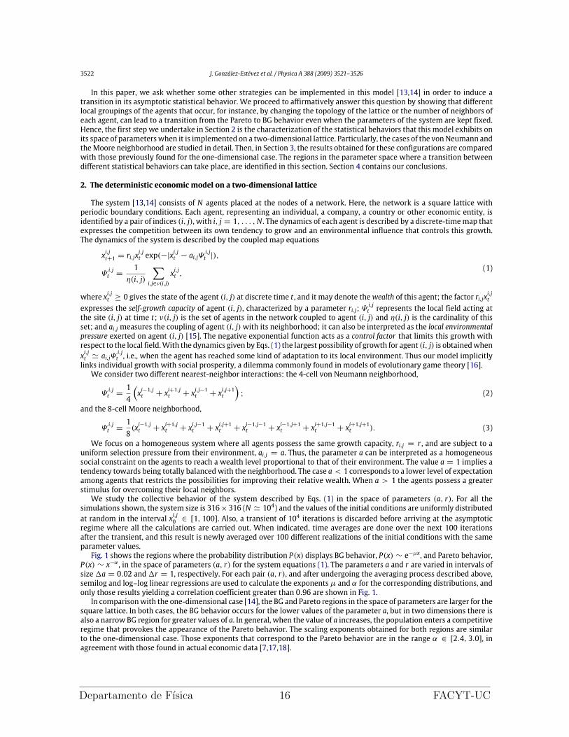
3522 J. González-Estévez et al. / Physica A 388 (2009) 3521–3526

In this paper, we ask whether some other strategies can be implemented in this model [13,14] in order to induce atransition in its asymptotic statistical behavior. We proceed to affirmatively answer this question by showing that differentlocal groupings of the agents that occur, for instance, by changing the topology of the lattice or the number of neighbors ofeach agent, can lead to a transition from the Pareto to BG behavior even when the parameters of the system are kept fixed.Hence, the first step we undertake in Section 2 is the characterization of the statistical behaviors that this model exhibits onits space of parameterswhen it is implemented on a two-dimensional lattice. Particularly, the cases of the vonNeumann andtheMoore neighborhood are studied in detail. Then, in Section 3, the results obtained for these configurations are comparedwith those previously found for the one-dimensional case. The regions in the parameter space where a transition betweendifferent statistical behaviors can take place, are identified in this section. Section 4 contains our conclusions.

2. The deterministic economic model on a two-dimensional lattice

The system [13,14] consists of N agents placed at the nodes of a network. Here, the network is a square lattice withperiodic boundary conditions. Each agent, representing an individual, a company, a country or other economic entity, isidentified by a pair of indices (i, j), with i, j = 1, . . . ,N . The dynamics of each agent is described by a discrete-timemap thatexpresses the competition between its own tendency to grow and an environmental influence that controls this growth.The dynamics of the system is described by the coupled map equations

xi,jt+1 = ri,jxi,jt exp(−|x

i,jt − ai,jΨ

i,jt |),

Ψi,jt =

1η(i, j)

∑i,j∈ν(i,j)

xi,jt ,(1)

where xi,jt ≥ 0 gives the state of the agent (i, j) at discrete time t , and it may denote thewealth of this agent; the factor ri,jxi,jt

expresses the self-growth capacity of agent (i, j), characterized by a parameter ri,j; Ψi,jt represents the local field acting at

the site (i, j) at time t; ν(i, j) is the set of agents in the network coupled to agent (i, j) and η(i, j) is the cardinality of thisset; and ai,j measures the coupling of agent (i, j)with its neighborhood; it can also be interpreted as the local environmentalpressure exerted on agent (i, j) [15]. The negative exponential function acts as a control factor that limits this growth withrespect to the local field.With the dynamics given by Eqs. (1) the largest possibility of growth for agent (i, j) is obtainedwhenxi,jt ' ai,jΨ

i,jt , i.e., when the agent has reached some kind of adaptation to its local environment. Thus our model implicitly

links individual growth with social prosperity, a dilemma commonly found in models of evolutionary game theory [16].We consider two different nearest-neighbor interactions: the 4-cell von Neumann neighborhood,

Ψi,jt =

14

(xi−1,jt + xi+1,jt + xi,j−1t + xi,j+1t

); (2)

and the 8-cell Moore neighborhood,

Ψi,jt =

18(xi−1,jt + xi+1,jt + xi,j−1t + xi,j+1t + xi−1,j−1t + xi−1,j+1t + xi+1,j−1t + xi+1,j+1t ). (3)

We focus on a homogeneous system where all agents possess the same growth capacity, ri,j = r , and are subject to auniform selection pressure from their environment, ai,j = a. Thus, the parameter a can be interpreted as a homogeneoussocial constraint on the agents to reach a wealth level proportional to that of their environment. The value a = 1 implies atendency towards being totally balanced with the neighborhood. The case a < 1 corresponds to a lower level of expectationamong agents that restricts the possibilities for improving their relative wealth. When a > 1 the agents possess a greaterstimulus for overcoming their local neighbors.We study the collective behavior of the system described by Eqs. (1) in the space of parameters (a, r). For all the

simulations shown, the system size is 316×316 (N ' 104) and the values of the initial conditions are uniformly distributedat random in the interval xi,j0 ∈ [1, 100]. Also, a transient of 10

4 iterations is discarded before arriving at the asymptoticregime where all the calculations are carried out. When indicated, time averages are done over the next 100 iterationsafter the transient, and this result is newly averaged over 100 different realizations of the initial conditions with the sameparameter values.Fig. 1 shows the regions where the probability distribution P(x) displays BG behavior, P(x) ∼ e−µx, and Pareto behavior,

P(x) ∼ x−α , in the space of parameters (a, r) for the system equations (1). The parameters a and r are varied in intervals ofsize1a = 0.02 and1r = 1, respectively. For each pair (a, r), and after undergoing the averaging process described above,semilog and log–log linear regressions are used to calculate the exponentsµ and α for the corresponding distributions, andonly those results yielding a correlation coefficient greater than 0.96 are shown in Fig. 1.In comparisonwith the one-dimensional case [14], the BG and Pareto regions in the space of parameters are larger for the

square lattice. In both cases, the BG behavior occurs for the lower values of the parameter a, but in two dimensions there isalso a narrow BG region for greater values of a. In general, when the value of a increases, the population enters a competitiveregime that provokes the appearance of the Pareto behavior. The scaling exponents obtained for both regions are similarto the one-dimensional case. Those exponents that correspond to the Pareto behavior are in the range α ∈ [2.4, 3.0], inagreement with those found in actual economic data [7,17,18].


J. González-Estévez et al. / Physica A 388 (2009) 3521–3526 3523

Fig. 1. Left panels: Regions where Boltzmann–Gibbs behavior P(x) ∼ e−µx appears on the space of parameters (a, r), indicated by the label BG, for the(a) 4-cell and (c) 8-cell neighborhood cases. The grey code on the right indicates the values of the scaling exponentµ. Right panels: Regions where Paretobehavior P(x) ∼ x−α occurs on the plane (a, r), labeled by P, for the (b) 4-cell and (d) 8-cell neighborhood cases. The grey code on the right indicates thevalues of the exponent α.

Fig. 2. Left panels:Mean fieldHt of the system at t = 104 for the Boltzmann–Gibbs (BG) and Pareto (P) regions for the (a) 4-cell and (c) 8-cell neighborhoodcases. The grey code on the right indicates the values taken by Ht . Right panels: The quantity 〈σ 〉 on the space of parameters (a, r), for the (b) 4-cell and(d) 8-cell neighborhood cases, with the grey code indicated on the right.

The mean field of the system or average wealth per agent at a time t is defined as

Ht =1N

N∑i,j=1

xi,jt . (4)

Similarly to the results reported in Ref. [14] for the one-dimensional case, Fig. 2(a–c) shows the asymptotic value of theglobalmean field for the regionswhere BG and Pareto behaviors are observed on the space of parameters (a, r), for the 4-cell



Fig. 3. (a) The Gini coefficient at t = 104 as a function of the parameters a and r for the (a) 4-cell and (b) 8-cell neighborhood cases. The labels BG and Pindicate the regions with Boltzmann–Gibbs and Pareto behaviors. The grey code on the right indicates the values taken by the Gini coefficient.

and 8-cell neighborhood cases. Note that, although the values of the initial states of the agents are randomly distributed onthe interval [1, 100], the system evolves to an asymptotic state where Ht takes values on the smaller interval [0.6, 3.25].Let us observe that the BG region presents a higher mean wealth than the Pareto one, telling us that in this model the BGbehavior would be desirable for the general benefit of the ensemble. In the same line, the BG and Pareto regions with 8-cell neighborhood display a slightly bigger mean wealth than the 4-cell neighborhood and the one-dimensional cases. Thisseems to indicate that the increasing number of the local neighbors of each agent can generate more richness in the system.On the other hand, for some values of the parameters a and r , the states of agents in the system at a given time exhibit

a large dispersion. For those parameters, the values of the state of any agent present large fluctuations over long times. Tocharacterize these fluctuations, we define the instantaneous standard deviation of the mean field as

σt =

(1N

N∑i,j=1

[xi,jt − Ht

]2)1/2. (5)

After discarding 104 transients, we calculate the mean value of σt over 100 iterations, and then average this result over 100realizations of initial conditions. The resulting average dispersion, denoted by 〈σ 〉, is shown in Fig. 2(b–d) on the plane (a, r).Note that for some regions of parameters the quantity 〈σt〉 can be much greater than the value of the mean field.The large dispersions observed in Fig. 2 (b–d) reflect the inequality in wealth distribution among agents in this system.

To characterize the degree of inequality in wealth distribution we use the Gini coefficient defined at a time t as [19]

Gt =1

2N2Ht

N∑i,j,k,l=1

|xi,jt − xk,lt |. (6)

A perfectly equitable distribution of wealth at time t , where xi,jt = xk,lt ∀ i, j, k, l, yields a value Gt = 0. The opposite

situation, where one agent has the total wealth∑Ni,j=1 x

i,jt , has a value of Gt = 1. Fig. 3 shows the asymptotic value of the

Gini coefficient on the plane of parameters (a, r). Note that the Gini coefficient reaches larger values, i.e. Gt ∈ [0.65, 0.85]andGt ∈ [0.7, 1] for the 4-cell and the 8-cell neighborhood, respectively, in the regions associated to Pareto regimes, while ittakes lower values, i.e.Gt ∈ [0.35, 0.65], in the region corresponding to BG behavior. These results agreewith our qualitativeunderstanding that equity is more favored in the presence of a larger middle economic class in a society, as expressed by aBG distribution.

3. Transition from Pareto to Boltzmann–Gibbs behavior

As was evident in the one-dimensional realization of this economic system studied in Ref. [14], it is possible to produce atransition from a Pareto to a BG behavior (or vice versa) maintaining its structural configuration andmaking only a variationin the parameters (a, r) of the system. In the two-dimensional case, as can be seen in Fig. 1, it is also possible to make suchtransition, for example, by changing r with a fixed value of a. We call the transition from Pareto to BG behavior (or viceversa) induced by varying the parameters the Transition Strategy I.Fig. 4 reveals another mechanism capable of provoking a change in the statistical properties of this economic model. We

call it the Transition Strategy II. It consists in performing a reconfiguration of the local connectivity of the agents. Fig. 4(a)shows the region of the parameter space (a, r)where a change in the topology of the system froma one-dimensional array toa two-dimensional square lattice with 4-cell neighborhood takes the system from a Pareto to a BG asymptotic distribution.The same transition can be reached in the region plotted in Fig. 4(b) by transforming the one-dimensional array to a two-dimensional lattice with 8-cell neighborhood. Fig. 4(c) displays the region of parameter space where a modification of thenumber of neighbors, from a 4-cell von Neumann neighborhood to an 8-cell Moore neighborhood, generates a Pareto-BGtransition in the two-dimensional array.As shown in Fig. 4(d), the transitions in statistical behaviors achieved through either type of strategy produce a decrease

of the Gini coefficient and, therefore, a more equitable wealth distribution in the system.


J. González-Estévez et al. / Physica A 388 (2009) 3521–3526 3525

G

0.78

0.76

0.74

0.72

0.70

0.68

0.66

a0.4 0.45 0.5 0.55 0.6 0.65 0.7 0.75 0.8

Fig. 4. Regions in the parameter space (a, r) where the deterministic model displays a transition from Pareto to Boltzmann–Gibbs statistical behaviorthrough a reconfiguration of the local neighborhood. (a) The system changes its topology from a one-dimensional array to a two-dimensional squarelattice with a 4-cell neighborhood. (b) The topology changes from a one-dimensional array to a two-dimensional square lattice to an 8-cell neighborhood.(c) Changing from a 4-cell neighborhood to an 8-cell neighborhood in a two-dimensional square lattice. (d) Graphical evidence that the Gini coefficientdecreases in the transitions described in (a), (b), and (c): one-dimensional array (circle points, upper line); two-dimensional latticewith 4-cell neighborhood(square points, middle line); 8-cell neighborhood (triangle down points, lower line). Fixed r = 10.

4. Conclusions

Nowadays, both the exponential and power law statistical behaviors in the economies of western countries are welldocumented [10]. Different models for the interaction of the economic agents have been reported in the literature. Mostmodels with a probabilistic inspiration must apply a strong reconfiguration in the structural properties of the system inorder to obtain a transition from a BG to a Pareto distribution in its asymptotic state.In this paper we have characterized in detail a deterministic economicmodel implemented on a two-dimensional square

lattice with periodic boundary conditions. The system depends only on two parameters; the parameter a gives informationabout the local environmental pressure while r expresses the self-growth capacity of each agent. By varying the valuesof these parameters, the model can exhibit asymptotic BG or Pareto distributions of wealth. The striking fact is that onlya change in either one of these parameters is enough to make the system undergo a change from one type of statisticalbehavior to a different one. We have called this process Transition Strategy I.Another situation that can produce a transition fromPareto to BG behavior in this systemhas been found in thiswork.We

have called it Transition Strategy II. In this scenario, a variation of the values of the parameters is not necessary; the transitionin the type of asymptotic statistical behavior is a consequence of the rearrangement of the neighborhood of each agent. Inparticular, it is observed that an increase in the number of neighbors of each agent drives the system toward asymptoticstates where wealth is distributed more equitably, that is, with a lower value of the Gini coefficient. The specific regions ofthe parameter space where this transition can take place have been delimited.To our knowledge this is the first time in the field of economic systems where this kind of transition is reported. We

hope that this work can help in enlightening the mechanisms that operate in the complex world of economical transactionsamong individuals, companies, countries or other economic entities.

Acknowledgments

This work was supported in part by Decanato de Investigación of the Universidad Nacional Experimental del Táchira(UNET), under grants 04-001-2006 and 04-002-2006. R.L.-R. acknowledges financial support from Postgrado de FísicaFundamental, Universidad de Los Andes (ULA), Venezuela, and by grant DGICYT-FIS2006-12781-C02-01, Spain. He alsowants to thank ULA and UNET for their kind hospitality during his stay there in July 2008. M.G.C. and O.A.-L. acknowledgesupport from Consejo de Desarrollo, Científico, Tecnológico y Humanístico, ULA, under grant C-1579-08-05-B.



References

[1] A. Dragulescu, V.M. Yakovenko, Eur. Phys. J. B 17 (2000) 723.[2] A. Chakraborti, B.K. Chakrabarti, Eur. Phys. J. B 17 (2000) 167.[3] A. Chatterjee, B.K. Chakrabarti, S.S. Manna, Physica A 335 (2004) 155.[4] J. Angle, Physica A 367 (2006) 388.[5] R. López-Ruiz, J. Sañudo, X. Calbet, Amer. J. Phys. 76 (2008) 780.[6] A. Dragulescu, V.M. Yakovenko, Eur. Phys. J. B 20 (2001) 585.[7] A. Dragulescu, V.M. Yakovenko, Physica A 299 (2001) 213.[8] A. Chatterjee, S. Yarlagadda, B.K. Chakrabarti (Eds.), Econophysics of Wealth Distributions, Springer Verlag, Milan, 2005.[9] B.K. Chakrabarti, A. Chakraborti, A. Chatterjee (Eds.), Econophysics and Sociophysics, Wiley-VCH, Berlin, 2006.[10] V.M. Yakovenko. Preprint arXiv:0709.3662, 2007. Review article for Encyclopedia of Complexity and System Science, to be published by Springer,

2009.[11] A. Chatterjee, B.K. Chakrabarti, Eur. Phys. J. B 60 (2007) 135.[12] D. Kahneman, A. Tversky, Econometrica 47 (1979) 263.[13] J.R. Sánchez, J. González-Estévez, R. López-Ruiz, M.G. Cosenza, Eur. Phys. J. ST 143 (2007) 241.[14] J. González-Estévez, M.G. Cosenza, R. López-Ruiz, J.R. Sanchez, Physica A 387 (2008) 4637.[15] M. Ausloos, P. Clippe, A. Pekalski, Physica A 324 (2003) 330.[16] G. Szabó, G. Fáth, Phys. Rep. 446 (2007) 97.[17] M. Levy, S. Solomon, Physica A 242 (1997) 90.[18] W. Souma, Fractals 9 (2001) 463.[19] M. Rodríguez-Achach, R. Huerta-Quintanilla, Physica A 361 (2006) 309.


La ciencia natural, no se limita a describir y explicar lanaturaleza, sino que es parte de la interaccion entre lanaturaleza y nosotros mismos.

Werner Heisenberg

3Synchronization induced by

intermittent versus partial drives inchaotic systems

Sincronizacion inducida por forzamiento intermitente frente a forzamientoparcial en sistemas caoticos

Artıculo publicado en la Revista International Journal of Bifurcation and Chaos, en elvolumen 20, numero 2, desde la pagina 323 hasta la 330, ano 2010.doi: 10.1142/S0218127410025776

La Revista International Journal of Bifurcation and Chaos, ISSN edicion impresa:0218-1274, ISSN edicion online: 1793-6551, de World Scientific, se encuentra indi-zada en Science Citation Index, Science Citation Index Expanded, Compendex,Scopus, INSPEC, y Current Contents/Physics, Chemical & Earth Sciences, entreotros.

Resumen

Se demuestra que los estados sincronizados de dos sistemas de mapas caoticos identi-cos, uno sujeto a un forzamiento comun que actua con una probabilidad p en el tiempo,u otro sujeto al mismo forzamiento actuando sobre una fraccion p de los mapas del sis-tema, son similares. El comportamiento de sincronizacion de ambos sistemas puede serinferido considerando la dinamica de un mapa solo forzado con una probabilidad p en eltiempo. El estado sincronizado para estos sistemas esta caracterizado sobre su espaciocomun de parametros. Los resultados demuestran que la presencia de un forzamiento

21

http://www.worldscientific.com/doi/abs/10.1142/S0218127410025776

externo comun en todo momento no es esencial para alcanzar la sincronizacion en unsistema de osciladores caoticos, ni tampoco aplicar dicho forzamiento simultaneamen-te a todos los elementos en el sistema. Mas bien, una condicion crucial para obtenersincronizacion es compartir una mınima informacion promedio por los elementos delsistema para tiempos largos.

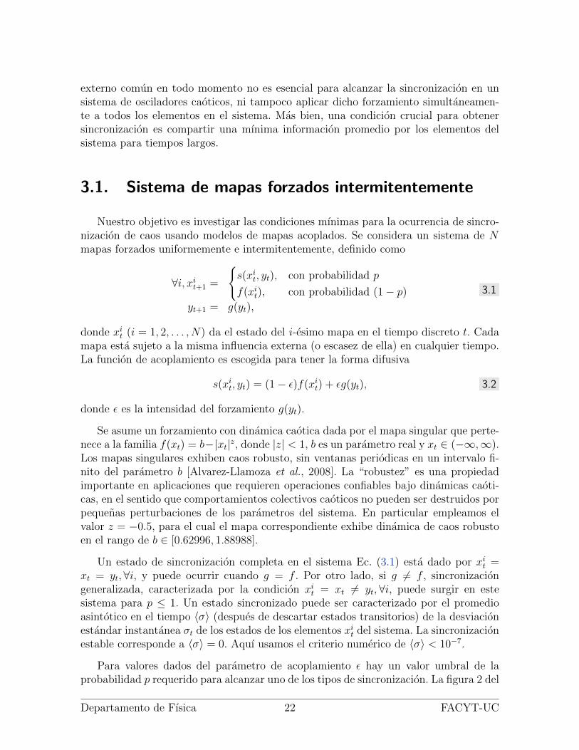
3.1. Sistema de mapas forzados intermitentemente

Nuestro objetivo es investigar las condiciones mınimas para la ocurrencia de sincro-nizacion de caos usando modelos de mapas acoplados. Se considera un sistema de Nmapas forzados uniformemente e intermitentemente, definido como

∀i, xit+1 =

{s(xit, yt), con probabilidad p

f(xit), con probabilidad (1− p)yt+1 = g(yt),

3.1

donde xit (i = 1, 2, . . . , N) da el estado del i-esimo mapa en el tiempo discreto t. Cadamapa esta sujeto a la misma influencia externa (o escasez de ella) en cualquier tiempo.La funcion de acoplamiento es escogida para tener la forma difusiva

s(xit, yt) = (1− ε)f(xit) + εg(yt), 3.2

donde ε es la intensidad del forzamiento g(yt).

Se asume un forzamiento con dinamica caotica dada por el mapa singular que perte-nece a la familia f(xt) = b−|xt|z, donde |z| < 1, b es un parametro real y xt ∈ (−∞,∞).Los mapas singulares exhiben caos robusto, sin ventanas periodicas en un intervalo fi-nito del parametro b [Alvarez-Llamoza et al., 2008]. La “robustez” es una propiedadimportante en aplicaciones que requieren operaciones confiables bajo dinamicas caoti-cas, en el sentido que comportamientos colectivos caoticos no pueden ser destruidos porpequenas perturbaciones de los parametros del sistema. En particular empleamos elvalor z = −0.5, para el cual el mapa correspondiente exhibe dinamica de caos robustoen el rango de b ∈ [0.62996, 1.88988].

Un estado de sincronizacion completa en el sistema Ec. (3.1) esta dado por xit =xt = yt,∀i, y puede ocurrir cuando g = f . Por otro lado, si g 6= f , sincronizaciongeneralizada, caracterizada por la condicion xit = xt 6= yt,∀i, puede surgir en estesistema para p ≤ 1. Un estado sincronizado puede ser caracterizado por el promedioasintotico en el tiempo 〈σ〉 (despues de descartar estados transitorios) de la desviacionestandar instantanea σt de los estados de los elementos xit del sistema. La sincronizacionestable corresponde a 〈σ〉 = 0. Aquı usamos el criterio numerico de 〈σ〉 < 10−7.

Para valores dados del parametro de acoplamiento ε hay un valor umbral de laprobabilidad p requerido para alcanzar uno de los tipos de sincronizacion. La figura 2 del


artıculo muestra las regiones para los estados de sincronizacion completa en el sistemadado por la Ec. (3.1), dentro del espacio de los parametros del sistema (p, ε), paradiferentes orbitas de un forzamiento g = f . En particular, cuando g = f , sincronizacioncompleta en una orbita inestable de perıodo m del mapa f , definida por f (m)(xn)y satisfaciendo

∏mn=1 |f ′(xn)| > 1, donde {x1, x2, . . . , xm} son el conjunto de puntos

consecutivos de la orbita, pueden ser tambien logrados en el sistema dado por la Ec.(3.1), como se muestra en la figura 2.

La figura 3 del artıculo muestra las regiones para los estados de sincronizaciongeneralizada del sistema dedo por la Ec. (3.1), dentro del espacio de parametros (p, ε),con un forzamiento g 6= f .

Puesto que cada mapa en el sistema forzado intermitentemente, Ec. (3.1), experi-menta la misma influencia externa (o ninguna) en algun tiempo, las propiedades de estesistema puede ser analizado por el comportamiento de la dinamica local individual. Ası,consideramos un solo mapa intermitentemente forzado

xt+1 =

{s(xt, yt), con probabilidad p

f(xt), con probabilidad (1− p)yt+1 = g(yt),

3.3

donde xt es la variable forzada, yt es el forzamiento y s(xt, yt) tiene la misma formafuncional de la Ec. (3.2). El enfoque de sistema auxiliar [Abarbanel et al., 1996] implicaque un mapa forzado puede sincronizarse en orbitas identicas con otro mapa forzadoidentico.

El mapa forzado dado la Ec. (3.3) puede ser considerado como un sistema bidi-mensional. La condicion de estabilidad lineal para la sincronizacion requiere del conoci-miento del exponente de Lyapunov. Estos son definidos por Λx = lımT−→∞ lnLx y Λy =

lımT−→∞ lnLy, donde Lx y Ly son las magnitudes de los autovalores de [∏T−1

t=0 J(xt, yt)]1/T

y J(xt, yt) es la matriz Jacobiana para el sistema de la Ec. (3.3), calculado a lo largode una orbita.

La sincronizacion ocurre si el exponente de Lyapunov correspondiente al mapa for-zado es negativo [Rulkov et al., 1995], es decir, Λx < 0. La figura 4 del artıculo muestraa Λx y Λy como funcion de p para el mapa forzado Ec. (3.3) para diferentes g.

Cuando g = f , la condicion Λx < 0 implica sincronizacion completa, donde xt = yt.En este caso se obtiene

Λy = λyΛx = p ln |1− ε|+ λy,

3.4

donde λy es el exponente de Lyapunov del mapa f . La figura 2 muestra las fronterasde estabilidad, dadas por Λx = 0, para los estados de sincronizacion completa delsistema Ec. (3.3) dentro del espacio de los parametros (p, ε) para diferentes orbitas delforzamiento.


Por otro lado, si g 6= f , la condicion Λx < 0 corresponde a sincronizacion gene-ralizada, caracterizado por xt 6= yt. La figura 3 muestra las fronteras de estabilidad,dadas por Λx = 0, para los estados de sincronizacion generalizada del sistema Ec. (3.3)dentro del espacio de los parametros (p, ε) para diferentes forzamientos g(yt). En amboscasos, Figuras 2 y 3, las curvas Λx = 0 coinciden con las fronteras de estabilidad desincronizacion completa y generalizada, respectivamente, para el sistema extendido Ec.(3.1).

3.2. Sistema de mapas forzados parcialmente

La equivalencia entre un solo mapa y un sistema de mapas similares forzados de-muestra que, bajo algunas circunstancias, el comportamiento colectivo de un sistemaextendido de elementos interactuantes puede ser inferido considerando la dinamica deun solo mapa a nivel local. Como una aplicacion de esta idea, consideramos un sistemade mapas parcialmente forzado, definido como

xit+1 =

{s(xit, yt), con probabilidad p

f(xit), con probabilidad (1− p)yt+1 = g(yt).

3.5

El parametro p es la probabilidad de interaccion de un mapa con el forzamiento g enel tiempo t. Los elementos forzados son escogidos aleatoriamente con una probabilidadp, ası, no todos los mapas reciben la misma influencia externa al mismo tiempo. Deesta manera la fraccion promedio de elementos forzados en el sistema (3.5) en cualquiermomento dado es p.

Cuando el sistema de la ecuacion (3.5) alcanza la sincronizacion. se tiene xit = xt.Sin embargo, la solucion sincronizada existe solamente si g = f . De esta forma, solosincronizacion completa puede ocurrir en este sistema.

A nivel local, cada mapa en el sistema parcialmente acoplado Ec. (3.5), esta sujeto enpromedio, a un forzamiento externo g con una probabilidad p. Ası, el comportamientode este sistema puede tambien ser estudiado por el comportamiento del mapa solo,intermitentemente forzado de la Ec. (3.3). La condicion Λx < 0 para la sincronizacioncompleta en el mapa forzado de la Ec. (3.3), que implica sincronizacion estable en elsistema intermitente de la Ec. (3.1), es tambien equivalente a la condicion de estabilidadde sincronizacion completa del sistema parcialmente forzado dado por Ec. (3.5). Estose demuestra adicionalmente con el empleo de la matriz de acoplamiento Gt, que surgede expresar el sistema de la Ec. (3.5) en forma vectorial.

Aunque la sincronizacion completa de caos en ambos casos, ecuaciones (3.1) y (3.5),puede ser caracterizada por el conocimiento de la dinamica de un solo mapa forzado, elcomportamiento transitorio para alcanzar tal estado es diferente en cada caso. La figura


5 del artıculo muestra el tiempo promedio Ts requerido para alcanzar la sincronizacioncomo funcion de p en ambos casos. Los tiempos Ts son mas grandes en el segundo caso,es decir, el forzamiento uniforme es mas eficiente que el no uniforme para alcanzar lasincronizacion completa.

3.3. Redes dinamicas

Por ultimo se corroboran estos resultados al extender el sistema a redes de mapasen una dimension mas un forzamiento aplicado uniformente sobre todo el sistema conprobabilidad p y una red de mapas en una dimension mas un forzamiento aplicado auna fraccion p de mapas del sistema elegidos aleatoriamentes en un tiempo t.

3.4. Conclusiones

En resumen, hemos demostrado que el comportamiento sincronizado en un sistemade mapas caoticos sujetos a un forzamiento externo puede ser inferido desde el com-portamiento de un solo elemento del sistema. La dinamica local puede ser vista comoun solo mapa forzado; cuando este sistema master-esclavo alcanza sincronizacion, elenfoque del sistema auxiliar implica que un grupo de mapas identicos sujetos a un for-zamiento similar deberıa tambien sincronizarse. Hemos demostrado que las regiones desincronizacion completa estable en el espacio de parametros de dos sistemas de mapascaoticos identicos sujetos al mismo forzamiento, uno actuando intermitentemente enel tiempo, y el otro parcialmente en el espacio, coinciden. A nivel local, las dinamicaslocales de ambos sistemas, para grandes tiempos, pueden ser caracterizados por un so-lo mapa caotico forzado con una probabilidad p. En adicion, hemos demostrado quela sincronizacion completa en redes de elementos interactuantes sujetos a forzamientointermitente, o parcial, pueden tambien ser similares. Este resultado sugiere que esossistemas poseen la propiedad de ergodicidad.

Para el sistema forzado intermitentemente, el compartir de la influencia externa porlos elementos toma lugar solamente una fraccion del tiempo. En el caso del sistemaparcialmente forzado, la influencia externa es compartida solamente por una fraccionde los elementos en algun tiempo. Ası, ni la presencia de una influencia comun todoel tiempo, ni el compartir simultaneo de la misma influencia por todos los elementos,parece esencial para alcanzar la sincronizacion en un sistemas de osciladores caoticos. Loque se es crucial para establecer la sincronizacion en ambos sistemas es compartir algunmınimo de informacion promedio por los elementos sobre largos tiempos. Extensionesfuturas de este trabajo deberıan incluir la investigacion de alguna cantidad, tal como laentropıa transferida [Schreiber, 2000], para medir la cantidad mınima de informacionrequerida para ambos tipos de sincronizacion, y la consideracion de otras formas decomportamiento colectivo observado en redes dinamicas ademas de la sincronizacion.


March 3, 2010 14:31 WSPC/S0218-1274 02577

International Journal of Bifurcation and Chaos, Vol. 20, No. 2 (2010) 323–330c© World Scientific Publishing CompanyDOI: 10.1142/S0218127410025776

SYNCHRONIZATION INDUCED BY INTERMITTENTVERSUS PARTIAL DRIVES IN CHAOTIC SYSTEMS

O. ALVAREZ-LLAMOZA∗ and M. G. COSENZACentro de Fısica Fundamental,

Universidad de Los Andes, Merida, Venezuela∗Departamento de Fısica, FACYT,

Universidad de Carabobo, Valencia, Venezuela

Received November 11, 2008; Revised March 18, 2009

We show that the synchronized states of two systems of identical chaotic maps subject to either,a common drive that acts with a probability p in time or to the same drive acting on a fractionp of the maps, are similar. The synchronization behavior of both systems can be inferred byconsidering the dynamics of a single chaotic map driven with a probability p. The synchronizedstates for these systems are characterized on their common space of parameters. Our resultsshow that the presence of a common external drive for all times is not essential for reachingsynchronization in a system of chaotic oscillators, nor is the simultaneous sharing of the driveby all the elements in the system. Rather, a crucial condition for achieving synchronization isthe sharing of some minimal, average information by the elements in the system over long times.

Keywords : Generalized synchronization; chaotic dynamical systems; coupled map lattices.

Chaos synchronization has attracted much inter-est from both scientists and engineers by providinginsights into natural phenomena and motivationfor practical applications in communications andcontrol [Pecora & Carroll, 1990; Boccaletti et al.,2002; Uchida et al., 2005; Argyris et al., 2005;Pikovsky et al., 2002]. This phenomenon is com-monly observed in unidirectionally coupled sys-tems, where a distinction can be made between adrive or forcing subsystem and another driven orresponse subsystem that possesses chaotic dynam-ics [Pikovsky et al., 2002]. Complete synchroniza-tion occurs when the state variables of the drivingand the response subsystems converge to a sin-gle trajectory in phase space. On the other hand,generalized synchronization of chaos arises whena functional relation different from the identity isestablished between the drive and the response sub-systems [Rulkov et al., 1995; Abarbanel et al., 1996;Kapitaniak et al., 1996; Hunt et al., 1997; Parlitz &Kokarev, 1999; Zhou & Roy, 2007].

Periodic, chaotic, or stochastic drives havebeen shown to induce generalized synchroniza-tion in chaotic systems [Maritan & Banavar,1994; Pikovsky et al., 2002]. The auxiliary systemapproach [Abarbanel et al., 1996] shows that when aresponse and a replica subsystems are driven by thesame signal, then the orbits in the phase spaces ofthe response and replica subsystems become iden-tical and they can evolve on identical attractors,if their initial conditions lie on the same basin ofattraction of the driven-response system. By exten-sion, an ensemble of identical chaotic oscillatorscan also be synchronized by a common drive. Thespecific functional form of the drive is not essen-tial; the basic mechanism that leads to synchro-nization is the sharing of the same information bythe oscillators for all times. In fact, it has recentlybeen shown that the source of the common influ-ence being received by the elements in an extendedsystem is irrelevant; it could consist of an exter-nal drive, or an autonomous global interaction field

323


March 3, 2010 14:31 WSPC/S0218-1274 02577

324 O. Alvarez-Llamoza & M. G. Cosenza

[Alvarez-Llamoza & Cosenza, 2008]. At the locallevel, each element in the system is subject to asource that eventually induces complete or gener-alized synchronization between the source and theelement.

In this paper, we explore another mechanismfor synchronization of a system of driven chaoticelements. We consider a system of chaotic elementswhere the external drive acts intermittently on allthe elements with a probability p. From the anal-ysis of the dynamics at the local level, we extendthe auxiliary system approach to a situation wherethe drive is applied only to a fraction p of randomlychosen elements in a system. We show that the com-plete synchronized states in both, the intermittentlyand the partially driven systems, are equivalent.Our results show that the presence of a commondrive for all times is not indispensable for reachingsynchronization in an extended system of chaoticoscillators, nor is the simultaneous sharing of thedrive by all the elements in the system. Our workis motivated by the practical aspect of searching forminimal requirements for the emergence of synchro-nization in dynamical systems.

We search for minimal conditions for the occur-rence of synchronization of chaos by using modelsof coupled maps. Let us consider a system of Nuniformly, intermittently driven maps, defined as

∀i, xit+1 =

{s(xit, yt), with probability p

f(xit), with probability (1− p)

yt+1 = g(yt),

(1)

where xit (i = 1, 2, . . . , N) gives the state of theith map at discrete time t, ε is the strength of thecoupling to the drive g(yt). Each map is subject tothe same external influence (or lack of it) at anytime. The coupling function is chosen to have thediffusive form

s(xit, yt) = (1− ε)f(xit) + εg(yt) . (2)

We assume a chaotic driven dynamics given bya singular map belonging to the family f(xt) =b − |xt|z, where |z| < 1, b is a real parameter andxt ∈ (−∞,∞). These singular maps exhibit robustchaos, with no periodic windows in a finite intervalof the parameter b [Alvarez-Llamoza et al., 2008].Robustness is an important property in applica-tions that require reliable operation under chaosin the sense that the chaotic behavior cannot bedestroyed by small perturbations of the system

parameters. In particular, we employ the valuez = −0.5 for which the corresponding map dis-plays robust chaotic dynamics in the range b ∈[0.62996, 1.88988].

A completely synchronized state in the systemEq. (1) is given by xit = xt = yt, ∀i, and it can occurwhen g = f . On the other hand, if g �= f , gener-alized synchronization, characterized by the condi-tion xit = xt �= yt, may also arise in this system forp ≤ 1. A synchronized state can be characterized bythe asymptotic time-average 〈σ〉 (after discarding anumber of transients) of the instantaneous standarddeviations σt of the distribution of map variables xit,defined as

σt =

[1

N

N∑

i=1

(xit − 〈xt〉)2]1/2

, (3)

where 〈xt〉 is the instantaneous mean of the val-ues xit, ∀i. Stable synchronization corresponds to〈σ〉 = 0. Here we use the numerical criterion 〈σ〉 <10−7. Figure 1 shows σt as a function of time for

(a)

(b)

Fig. 1. σt versus t for the system of driven maps Eq. (1)with N = 104 and f(x) = 1.2 − |x|−0.5, for different formsof the drive g(yt). Initial conditions were randomly and uni-formly distributed such that xi0 ∈ [0, 10]. The drive g(yt)is applied with probability p starting at t = 1000. (a)g(yt) = 1.2 − |yt|−0.5, ε = 0.7, p = 0.6 (complete synchro-nization). (b) g(yt) = 1 − 2y2t , ε = 0.8, p = 0.8 (generalizedsynchronization).


March 3, 2010 14:31 WSPC/S0218-1274 02577

Synchronization Induced by Intermittent versus Partial Drives in Chaotic Systems 325

Fig. 2. Regions for completely synchronized (CS) states(〈σ〉 < 10−7, after discarding 104 iterates) on the plane (p, ε)for the system of intermittently driven maps, Eq. (1) withf(x) = 1.2 − |x|−0.5, N = 104. Dashed line: g(yt) = x1 =−0.393713; solid line: g(yt) = 1.2 − |yt|−0.5; dotted line:g(yt) = {x1 = 0.204805, x2 = −1.00968}. The boundariesalso indicate the onset of stability of those same completesynchronized states in the partially driven system, Eq. (9).The boundaries that separate the stable from the unstableregions are given by the corresponding curve Λx = 0 [Eq. (8)]for the driven single map, Eq. (4).

the intermittently driven system Eq. (1) subject todifferent chaotic drives g.

For a given value of the coupling strength ε,there is a threshold value of the probability prequired to reach either type of synchronization.Figure 2 shows the regions for the complete syn-chronized states of the system [Eq. (1)] within thespace of parameters (p, ε) for different orbits of adrive g = f . In particular, when g = f , completesynchronization into an unstable period-m orbit ofthe map f , defined by f (m)(xn) = xn and sat-isfying

∏mn=1 |f ′(xn)| > 1, where {x1, x2, . . . , xm}

are the set of consecutive points on this orbit, canalso be achieved in the system Eq. (1), as shownin Fig. 2.

Figure 3 shows the regions for the generalizedsynchronized states of the system Eq. (1) within thespace of parameters (p, ε), with a drive g �= f .

Since each map in the intermittently driven sys-tem Eq. (1) experiences the same external influence(or none) at any time, the properties of this systemcan be analyzed from the behavior of the individuallocal dynamics. Thus, we consider a single, intermit-tently driven map

Fig. 3. Region for generalized synchronized (GS) states(〈σ〉 < 10−7, after discarding 104 iterates) for the systemof maps Eq. (1), with f(x) = 1.2− |x|−0.5, N = 104, subjectto the intermittent drive g(yt) = 1− 2y2t , on the plane (p, ε).This same region corresponds to generalized synchronization(satisfying Λx < 0) for the single driven map Eq. (4) withg(yt) = 1− 2y2t .

xt+1 =

{s(xt, yt), with probability p

f(xt), with probability (1− p),

yt+1 = g(yt),

(4)

where xt is the driven or response variable, yt is thedrive and s(xt, yt) has the same functional form asin Eq. (2). The auxiliary system approach [Abar-banel et al., 1996] implies that a driven map cansynchronize on identical orbits with another, iden-tically driven map. Thus, the occurrence of stablesynchronization in the single map Eq. (4) shouldlead to synchronization in the extended system ofmaps Eq. (1), even when the drive acts intermit-tently in both cases.

The single driven map Eq. (4) can be regardedas a two-dimensional system. The linear stabilitycondition for synchronization requires the knowl-edge of the Lyapunov exponents for such a sys-tem. These are defined as Λx = limT→∞ lnLx andΛy = limT→∞ lnLy, where Lx and Ly are the

magnitude of the eigenvalues of [∏T−1

t=0 J(xt, yt)]1/T ,

and J(xt, yt) is the Jacobian matrix for the sys-tem Eq. (4), calculated along an orbit. A givenorbit {xt, yt} from t = 0 to t = T − 1 canbe separated in two subsets, according to thesource of the xt variable, either coupled or uncou-pled to the drive, that we respectively denote as


March 3, 2010 14:31 WSPC/S0218-1274 02577


A = {{xt, yt} : xt = s(xt−1, yt−1)} possessing pT elements, and B = {{xt, yt} : xt = f(xt−1)} having(1− p)T elements. We get

(T−1∏

t=0

J

)1/T

=

∏

t: xt∈Asx

∏

t: xt∈Bf ′(xt) K

0T−1∏

t=0

g′(yt)

1/T

, (5)

where sx = ∂s/∂x = (1− ε)f ′(x), and K is a polynomial whose terms contain products of sx, ε, and g′(yt)to be evaluated along time. Then Lx = [

∏xt∈A sx

∏xt∈B f ′(xt)]1/T and Ly = [

∏T−1t=0 g′(yt)]1/T . Thus, we get

Λx = p ln |1− ε|+ limT→∞

1

T

[ln∏

xt∈A|f ′(xt)|+ ln

∏

xt∈B|f ′(xt)|

](6)

Λy = limT→∞

1

T

T−1∑

t=0

ln |g′(yt)| = λg , (7)

where λg is the Lyapunov exponent of the mapg(yt). Synchronization occurs if the Lyapunov expo-nent corresponding to the driven map is negative[Rulkov et al., 1995]; i.e. Λx < 0. For a given set ofparameter values, there is a definite value of theprobability p at which the exponent Λx changesits sign, from positive to negative, signaling theonset of synchronization in the dynamics of the two-dimensional system Eq. (4).

Figure 4 shows Λx and Λy as a function of p forthe driven map Eq. (4) for different drives g.

When g = f , the condition Λx < 0 implies com-plete synchronization, where xt = yt. In this casewe get

Λy = λf ,

Λx = p ln |1− ε|+ λf ,(8)

where λf is the Lyapunov exponent of the mapf . Figure 2 shows the stability boundaries, givenby Λx = 0, for the completely synchronized statesof the system Eq. (4) within the space of param-eters (p, ε) for different orbits of a drive g(yt).

(a) (b)

Fig. 4. Lyapunov exponents Λx and Λy as functions of p for the single driven map Eq. (4) with f(x) = 1.2 − |x|−0.5,calculated over 5 × 104 iterates after discarding 5 × 103 transients for each value of p. (a) g(yt) = 1.2 − |yt|−0.5, ε = 0.6(complete synchronization). (b) g(yt) = 1− 2y2t , ε = 0.8 (generalized synchronization).


March 3, 2010 14:31 WSPC/S0218-1274 02577


On the other hand, if g �= f , the conditionΛx < 0 corresponds to generalized synchroniza-tion, characterized by xt �= yt. Figure 3 showsthe stability boundaries, given by Λx = 0, forthe generalized synchronized states of the sys-tem Eq. (4) within the space of parameters (p, ε)for different drives g(yt). In both, Figs. 2 and3, the curves Λx = 0 coincide with the bound-aries for stability of complete and generalized syn-chronization, respectively, in the extended systemEq. (1). Thus, the condition Λx < 0 for gener-alized or complete synchronization in the singledriven map Eq. (4) is equivalent to the conditionfor the stability of the synchronized state xit = xt,∀i, in the intermittently driven system of mapsEq. (1).

The above results are a consequence of theauxiliary system approach. Furthermore, the equiv-alence between a single driven map and a sys-tem of driven similar maps also shows that, undersome circumstances, the collective behavior of anextended system of interacting elements can beinferred by considering the dynamics on a singleelement at the local level. As an application of thisidea, we consider a partially driven system of mapsdefined as

xit+1 =

{s(xit, yt), with probability p

f(xit), with probability (1− p)

yt+1 = g(yt) .

(9)

The parameter p is the probability of interactionof a map with the drive g at a time t. The drivenelements are randomly chosen with a probabilityp, so that not all the maps in the system receivethe same external influence at all times. Thus, theaverage fraction of driven elements in the systemEq. (9) at any given time is p. In comparison, theforcing of the elements in the intermittently drivensystem Eq. (1) is simultaneous and uniform; eachmap receives the same influence from the drive g atany t with probability p.

When system Eq. (9) gets synchronized, wehave xit = xt. However, the synchronized solutionexists only if g = f . Therefore, only completesynchronization xit = xt = yt can occur in thissystem.

At the local level, each map in the partiallydriven system Eq. (9) is subject, on the average, toan external forcing g with probability p. Thus, thebehavior of system Eq. (9) can also be studied from

the behavior of the single, intermittently drivenmap Eq. (4). In particular, if the system of mapsEq. (9) driven with g = f reaches a complete syn-chronized state for some values of parameters, thenfor this same set of parameters the single drivenmap Eq. (4) subject to the same drive should even-tually exhibit a synchronized state similar to thatof system Eq. (9). Thus, the condition Λx < 0 forcomplete synchronization in the single driven mapEq. (4), that implies stable synchronization in theintermittently driven system Eq. (1), is also equiv-alent to the condition for the stability of the com-plete synchronized state xit = xt = yt, ∀i, in thepartially driven system Eq. (9). To see this, wheng = f we express the system Eq. (9) in vectorform as

xt+1 = Gtf(xt) (10)

where the (N +1)-dimensional vectors xt and f(xt)have components [xt]i = xit and [f(xt)]i = f(xit),respectively, for i = 1, . . . , N , while [xt]N+1 = ytand [f(xt)]N+1 = g(yt). The (N + 1) × (N + 1)matrix Gt expresses the coupling between the Nmaps and the drive at time t. The matrix Gt attime t possesses pN randomly chosen rows, eachhaving its components Gi,j (i, j = 1, 2, . . . , (N +1))equal to 0, except Gi,i = ε and Gi,N+1 = ε. Theremaining N − pN rows, and the row (N +1), havetheir components Gi,j = 0, except Gi,i = 1. Thus,at time t, the matrix Gt has the form

Gt =

(1− ε) 0 · · · · · · ε

0 1 0 · · · ...

... 0. . . · · · ...

...... 0 (1− ε) ε

0 · · · · · · 0 1

. (11)

The long-time evolution of the vector state xt

is given by

xt+1 = Gf(xt), (12)

where the matrix G is the geometric mean of theproducts of all possible configurations of Gt over along time T ,

G =

[T−1∏

t=0

Gt

]1/T. (13)


March 3, 2010 14:31 WSPC/S0218-1274 02577


We get

G =

(1− ε)pT 0 · · · · · · K

0 (1− ε)pT 0 · · · K

... 0. . . · · · ...

...... 0 (1− ε)pT K

0 · · · · · · 0 1

1/T

,

(14)

where K is a polynomial whose terms contain prod-ucts of (1− ε) and ε.

The linear stability analysis [Waller & Kapral,1984; Kaneko, 1990] of the complete synchronizedstate f(xit) = f(xt) yields

|αkeλf | < 1 , (15)

where αk (k = 0, 1, . . . , N) are the set of eigenval-ues of the matrix G, with α0 = 1 and αk = (ε− 1)p

for k > 0, having N -fold degeneracy. The eigenvec-tor corresponding to k = 0 is homogeneous. Thusperturbations of xt along this eigenvector do notdestroy the coherence, and the stability conditionassociated with k = 0 is irrelevant for a synchro-nized state. The other eigenvectors correspondingto k �= 0 are not homogeneous. Thus, conditionEq. (15) with k �= 0 becomes

p ln|1− ε|+ λf < 0, (16)

which is the same condition for stability of com-plete synchronized states in the single driven map,Eq. (8), when g = f . Thus, the stability boundaryΛx = 0 in Fig. 2 for the driven map with g = fcoincides with both, the boundary that separatesthe region where complete synchronization occurson the space of parameters (p, ε) for the partiallydriven system Eq. (9), and the boundary for com-plete synchronization in the intermittently drivensystem Eq. (1). However, generalized synchroniza-tion cannot occur in the former system.

Although complete synchronization of chaos inboth classes of driven systems, Eqs. (1) and (9), canbe characterized from the knowledge of the dynam-ical response of a single driven map, the transientbehavior to reach such a state is different in eachcase. Figure 5 shows the average time Ts requiredto attain complete synchronization as a function ofp in both, a partially driven system and an inter-mittently driven system of maps. The times Ts arelarger in the first case, i.e. a spatially uniform forc-ing on a system is more efficient than a nonuniformone for achieving complete synchronization.

Fig. 5. Average time Ts to reach complete synchronizationas a function of the probability p for both, the intermittentlydriven system Eq. (1) (bottom curve) and the partially drivensystem Eq. (9) (top curve). For both systems, f = 1.2 −|x|−0.5, ε = 0.7, N = 104, and g = f . The error bars on eachcurve correspond to standard deviations resulting from 100realizations of random initial conditions for each value of p.

Complete synchronization in networks of cou-pled oscillators subject to either a uniform driveg with a probability p, or to a drive g applied ona random fraction p of the elements at all times,may also be equivalent. As an illustration, considera uniformly, intermittently driven one-dimensionallattice,

∀i, xit+1 =

(1− ε− γ)f(xit)

+γ

2

[f(xi+1

t ) + f(xi−1t )

]+ εg(yt),

with probability p;

(1− γ)f(xit) +γ

2

[f(xi+1

t ) + f(xi−1t )

],

with probability (1− p);

(17)

where γ is the local coupling parameter. The anal-ogy can be established with a similar lattice subjectto a drive g(yt) acting on a randomly chosen frac-tion p of maps,

xit+1 =

(1− ε− γ)f(xit)

+γ

2

[f(xi+1

t ) + f(xi−1t )

]+ εg(yt),

with probability p;

(1− γ)f(xit) +γ

2

[f(xi+1

t ) + f(xi−1t )

],

with probability (1− p).

(18)


March 3, 2010 14:31 WSPC/S0218-1274 02577


(a)

(b)

Fig. 6. σt versus t for (a) the intermittently driven latticeEq. (17) and (b) the partially driven lattice Eq. (18). In bothcases, f(x) = 1.2−|x|−0.5, ε = 0.8, γ = 0.2, p = 0.5, N = 103,and the drive g = f is applied starting at t = 1000. Randominitial conditions are used.

Periodic boundary conditions are assumed for bothlattices. Figure 6 shows σt as a function of timefor both systems, Eqs. (17) and (18), for a givenexample.

In summary, we have shown that the synchro-nization behavior of a system of chaotic maps sub-ject to an external forcing can be inferred from thebehavior of a single element in the system. Thelocal dynamics can be seen as a single driven map;when this drive-response system reaches synchro-nization, the auxiliary system approach implies thatan ensemble of identical maps subject to a similardrive should also synchronize. We have shown thatthe regions of stable complete synchronization inparameter space of two systems of identical chaoticmaps subject to the same drive acting either inter-mittently in time, or partially in space, coincide. Atthe local level, the long-time dynamics of both sys-tems can be characterized by a single chaotic mapdriven with a probability p. In addition, we haveshown that complete synchronization in networksof interacting elements subject to either intermit-tent or partial drives can also be similar. This resultsuggests that these systems possess an ergodicityproperty.

For the intermittently driven system, the shar-ing of the external influence by the elements takesplace only a fraction of the time. In the case ofthe partially driven system, the external drive isshared only by a fraction of elements at any time.Thus, neither the presence of a common influencefor all times, or the simultaneous sharing of thesame influence by all the elements, seem essentialfor reaching synchronization in systems of chaoticoscillators. What becomes crucial for achieving syn-chronization in both systems is the sharing of someminimal, average information by the elements overlong times. Future extensions of this work shouldinclude the investigation of some quantity, such asthe transfer entropy [Schreiber, 2000], for measur-ing this minimal amount of information required forboth types of synchronization, and the considera-tion of other forms of collective behaviors observedin dynamical networks, besides synchronization.

Acknowledgments

This work was supported by Consejo de DesarrolloCientıfico, Humanıstico y Tecnologico, Universidadde Los Andes, Venezuela, through grant C-1579-08-05-B.

References

Abarbanel, H. D. I., Rulkov, N. F. & Sushchik, M.M. [1996] “Generalized synchronization of chaos: Theauxiliary system approach,” Phys. Rev. E 53, 4528–4535.

Alvarez-Llamoza, O. & Cosenza, M. G. [2008] “Gener-alized synchronization of chaos in autonomous sys-tems,” Phys. Rev. E 78, 046216-1–046216-6.

Alvarez-Llamoza, O., Cosenza, M. G. & Ponce, G. A.[2008] “Critical behavior of the Lyapunov exponent intype-III intermittency,” Chaos Solit. Fract. 36, 150–156.

Argyris, A., Syvridis, D., Larger, L., Annovazzi-Lodi, V.,Colet, P., Fischer, I., Garcia-Ojalvo, J., Mirasso, C.R., Pesquera, L. & Shore, K. A. [2005] “Chaos-basedcommunications at high bit rates using commercialfibre-optic links,” Nature (London) 438, 343–346.

Boccaletti, S., Kurths, J., Osipov, G., Valladares, D. L.& Zhou, C. S. [2002] “The synchronization of chaoticsystems,” Phys. Rep. 366, 1–101.

Hunt, B. R., Ott, E. & Yorke, J. A. [1997] “Differentiablegeneralized synchronization of chaos,” Phys. Rev. E55, 4029–4034.

Kaneko, K. [1990] “Clustering, coding, switching, hier-archical ordering, and control in networks of chaoticelements,” Physica D 41, 137–172.


March 3, 2010 14:31 WSPC/S0218-1274 02577


Kapitaniak, T., Wojewoda, J. & Brindley, J.[1996] “Synchronization and desynchronization inquasi-hyperbolic chaotic systems,” Phys. Lett. A 210,283–289.

Maritan, A. & Banavar, J. R. [1994] “Chaos, noise andsynchronization,” Phys. Rev. Lett. 72, 1451–1454.

Parlitz, U. & Kokarev, L. [1999]Handbook of Chaos Con-trol, ed. Schuster, H. (Wiley-VCH, Weinheim), p. 271.

Pecora, L. M. & Carroll, T. L. [1990] “Synchronizationin chaotic systems,” Phys. Rev. Lett. 64, 821–824.

Pikovsky, A., Rosenblum, M. & Kurths, J. [2002] Syn-chronization: A Universal Concept in Nonlinear Sci-ences (Cambridge University Press, Cambridge).

Rulkov, N. F., Sushchik, M. M., Tsimring, L. S. & Abar-banel, H. D. I. [1995] “Generalized synchronization of

chaos in directionally coupled systems,” Phys. Rev. E51, 980–994.

Schreiber, T. [2000] “Measuring information transfer,”Phys. Rev. Lett. 85, 461–464.

Uchida, A., Rogister, F., Garcia-Ojalvo, J. & Roy,R. [2005] “Synchronization and communication withchaotic laser systems,” Prog. Opt. 48, 203–341.

Waller, I. & Kapral, R. [1984] “Spatial and temporalstructure in systems of coupled nonlinear oscillators,”Phys. Rev. A 30, 2047–2055.

Zhou, B. B. & Roy, R. [2007] “Isochronal synchronyand bidirectional communication with delay-couplednonlinear oscillators,” Phys. Rev. E 75, 026205-1–026205-5.


Informacion: el valor recıproco negativo de la probabi-lidad.

Claude Shannon

No hay globalidad que sirva, sin localidad que valga.

Carlos Fuentes 4Global interactions, information flow

and chaos synchronization

Interacciones globales, flujo de informacion y sincronizacion caotica

Artıculo publicado en la Revista Physical Review E, en el volumen 88, 042920, desdela pagina 042920-1 hasta la 042920-8, ano 2013. doi: 10.1103/PhysRevE.88.042920

La Revista Physical Review E, ISSN edicion impresa: 1539-3755, ISSN ediciononline: 1550-2376, de la American Physical Society, se encuentra indizada enCurrent Physics Index, INSPEC, Medline, Physics Abstracts y Science CitationIndex Expanded entre otros.

Resumen

Se investiga la relacion entre la emergencia de sincronizacion caotica y el flujo dela informacion en sistemas dinamicos que poseen interacciones globales homogeneas oheterogeneas, y cuyo origen puede ser externo (sistemas forzados) e internos (sistemasautonomos). Empleando un modelo general de mapas caoticos globalmente acopladospara tal sistema, se demuestra que la presencia de un campo global homogeneo, sea ex-terno o interno, aplicado todo el tiempo, no es indispensable para lograr sincronizacioncompleta o generalizada en un sistema de elementos caoticos. Sincronizacion completapuede aparecer tambien en sistemas con campo global heterogeneo; no se requiere com-partir simultaneamente la informacion por todos los elementos del sistema. Se utiliza lainformacion mutua normalizada y la transferencia de la informacion entre las variablesglobales y locales para caracterizar la sincronizacion completa y la generalizada. Se de-muestra que esas medidas de informacion pueden caracterizar ambos tipos de estados

34

http://journals.aps.org/pre/abstract/10.1103/PhysRevE.88.042920

sincronizados y tambien permite discernir el origen del campo de interaccion global. Unestado sincronizado emerge cuando una cantidad suficiente de informacion provista porel campo, es compartida por todos los elementos del sistema, en promedio para largostiempos. Ası, el valor maximo valor de la informacion transferida de arriba hacia abajopuede ser usada como un predictor de sincronizacion en un sistema, a medida que unparametro es variado.

4.1. Campos globales de interaccion

Describimos una interaccion global como un campo que puede influenciar a todoslos elementos de un sistema. Como un modelo simple de un sistema dinamico sujeto auna interaccion global, se considera un sistema de N mapas acoplados de la forma

xit+1 = w(xit, yt)

yt+1 = φ(yt, xjt),

4.1

donde xit (i = 1, 2, . . . , N) representa la variable de estado del i-esimo mapa en elsistema en el tiempo discreto t, yt es el campo de interaccion global que puede afectara cada mapa en el tiempo t, y j ∈ Q donde Q es un subconjunto de los elementos enel sistema. La ecuacion (4.1) describe un sistema de elementos interactuando con unaambiente dinamico comun que puede recibir una retroalimentacion del sistema. Porsimplicidad, nos enfocaremos en la presencia de interacciones globales que no incluyeninteracciones locales.

Un campo externo global yt que posee su propia dinamica, independientemente dela dinamica de los elementos, viene dado por

φ(yt, xjt) = g(yt). 4.2

Luego la Ec. (4.1) con la dinamica del campo Ec. (4.2) describe un sistema sujetoa un forzamiento global, es decir, un sistema acoplado unidireccionalmente. Por otrolado, un campo global interno yt puede ser representado por

φ(yt, xjt) = h(xjt | j ∈ Q), 4.3

donde h es una funcion de los estados de un subconjunto dado Q de elementos en elsistema en un tiempo t. La funcion de acoplamiento h podrıa representar una restricciono una ley de conservacion sobre el sistema. En este caso, Ec. (4.1) con el campo Ec. (4.3)corresponde a un sistema dinamico autonomo globalmente acoplado.

Se considerara el acoplamiento debido al campo de interaccion global en la formadifusiva

w(xit, yt) = (1− ε)f(xit) + εφ(yt, xjt), 4.4


donde f describe la dinamica local de los mapas, y el parametro ε la fuerza del acopla-miento del campo global. Puesto que estamos interesados en la sincronizacion de caos,hemos escogido para la dinamica local el mapa logıstico f(xit) = 4xit(1−xit), de maneraque f(xit) es totalmente caotico para xit ∈ [0, 1].

4.1.1. Estados sincronizados

La sincronizacion en el sistema Ec. (4.1) en un tiempo t corresponde al estadoxit = xjt ∀ i, j. Ası, un estado sincronizado puede ser descrito por la condicion xit = xt,∀i,donde xt es el campo medio instantaneo del sistema (media aritmetica o promediode xit). Para caracterizar la sincronizacion se considera el promedio asintotico en eltiempo 〈σ〉, despues de descartar transitorios, de la desviacion estandar instantaneaσt de la distribucion de los estados de xit. La sincronizacion corresponde a 〈σ〉 = 0.Adicionalmente, se define el promedio asintotico en el tiempo 〈δ〉 (despues de descartarlos transitorios) de la cantidad δt = |xt − yt|.

Dos formas de sincronizacion pueden tomar lugar en el sistema Ec. (4.1) en relacional campo global yt: (i) sincronizacion completa, dado por la condicion xit = xt = yt,es decir, todos los elementos estan sincronizados con el campo, y se caracteriza por〈σ〉 = 0 y 〈δ〉 = 0; y (ii) sincronizacion generalizada, correspondiente a la condicionxit = xt 6= yt, es decir, los elementos estan sincronizados entre ellos pero no con elcampo, y descrito por 〈σ〉 = 0 y 〈δ〉 6= 0.

Para caracterizar el intercambio de la informacion entre el campo global y la dinami-ca local en el sistema, se consideran las siguientes cantidades: (1) La informacion mutuanormalizada entre dos variables yt y xt, basado en la mutua informacion de Shanon (re-ferencia 30 del artıculo):

My,x = −

∑xt,yt

P (xt, yt) log

(P (xt, yt)

P (xt)P (yt)

)

∑xtP (xt) logP (xt)

; 4.5

(2) la transferencia de la informacion de la variable yt a la variable xt, definida como

Ty,x =∑

xt+1,xt,yt

P (xt+1, xt, yt) log

(P (xt+1, xt, yt)P (xt)

P (xt, yt)P (xt+1, xt)

), 4.6

donde P (xt) es la distribucion de probabilidad de la serie de tiempo de la variable xt,P (xt, yt) es la probabilidad conjunta de xt y yt, etc. La cantidad Mx,y mide el sola-pamiento del contenido de la informacion de las variables yt y xt; representa cuantaincertidumbre de xt decrece si yt es conocida. La cantidad Ty,x mide el grado de de-pendencia de xt sobre la variable yt; es decir, la informacion requerida para representarel valor xt+1 a partir del conocimiento de yt. Note que Ty,x 6= Tx,y, en cambio Mx,y essimetrica Mx,y = My,x. Cuando las variables xt y yt se sincronizan Mx,y = 1 y Ty,x = 0.


4.2. Interaccion global homogenea

Se describe una interaccion global homogenea como un campo compartido simultanea-mente por todos los elementos en el sistema. Puesto que, en general, la interaccion conel campo podrıa no ocurrir para todos los tiempos, consideramos un sistema de mapasacoplados sujetos a una interaccion homogenea intermitente. Un sistema sujeto a uncampo externo homogeneo corresponde a

∀i, xit+1 =

{(1− ε)f(xit) + εg(yt), con probabilidad p

f(xit), con probabilidad (1− p),yt+1 = g(yt).

4.7

La sincronizacion completa en el sistema Ec. (4.7) viene dada por xit = xt = yt, ∀ i,y puede ocurrir cuando el campo externo es igual a la dinamica local, g = f . Si g 6= f ,la sincronizacion generalizada, caracterizada por la condicion xit = xt 6= yt, ∀ i, podrıasurgir en el sistema.

Por otro lado, un sistema sujeto a un campo global homogeneo autonomo puede serdescrito por

∀i, xit+1 =

{(1− ε)f(xit) + εh(xjt | j ∈ Qt), con probabilidad p,

f(xit), con probabilidad (1− p), 4.8

donde Qt es un subconjunto de q ≤ N elementos del sistema escogidos aleatoriamenteen cada tiempo t. La sincronizacion completa en el sistema Ec. (4.8) ocurre cuandof(xit) = f(xt) = h, mientras que la sincronizacion generalizada aparece si f(xit) =f(xt) 6= h,∀i.

4.2.1. Sincronizacion completa

Se considera el sistema forzado dado por la Ec. (4.7) con g = f , y el sistemaautonomo Ec. (4.8) sujeto a una funcion de campo medio parcial definida como

h(xjt | j ∈ Qt) =1

q

q∑

j=1

f(xjt), 4.9

donde q ≤ N mapas son elegidos aleatoriamente en cada tiempo t. Para esos sistemas,la condicion 〈δ〉 implica que 〈σ〉 y, por lo tanto, sincronizacion completa.

La figura 2(a) del artıculo muestra la cantidad 〈δ〉 como funcion del parametro deacoplamiento ε, para ambos sistemas: sistema forzado homogeneo y sistema autonomohomogeneo, para valores fijos de p y q/N . La sincronizacion completa en ambos sistemastoma lugar en el valor crıtico εc = 0.579, para el cual 〈δ〉 < 10−7. La figura 2(b) y 2(c)


muestran, respectivamente, la informacion mutua normalizada Myt,xity la informacion

transferida Tyt,xit entre el campo global homogeneo y un mapa, promediado sobre 50mapas elegidos aleatoriamente, para ambos sistemas como funcion de ε. Esas cantidadespromediadas dan practicamente los mismos resultados que para solo un mapa elegidoaleatoriamente.

4.2.2. Sincronizacion generalizada

Si la forma funcional del campo global es diferente a la dinamica local, sincronizaciongeneralizada podrıa ocurrir en un sistema sujeto a interaccion global homogenea. Porejemplo, se considera un campo externo en el sistema forzado Ec. (4.7) como

g(yt) =µ

2(1− |2yt − 1|) , 4.10

con µ = 1.98 y yt ∈ [0, 1]. Luego, en la sincronizacion del sistema forzado Ecs. (4.7)-(4.10), se tiene xit = xt 6= yt. Similarmente, en un sistema autonomo como el de laEc. (4.8), se considera una interaccion global diferente al campo medio, tal como lafuncion de acoplamiento

h(xjt | j ∈ Qt) =µ

2

[1−

∣∣∣∣∣2(

1

q

q∑

j=1

xjt

)− 1

∣∣∣∣∣

], 4.11

con µ = 1.98, donde q ≤ N elementos son elegidos aleatoriamente en cada tiempo t.Luego un estado sincronizado en el sistema autonomo dado por las Ecs. (4.8)-(4.11)corresponde a f(xit) = f(xt) 6= h.

La figura 3(a) muestra la cantidad 〈σ〉 como funcion del parametro de acoplamientoε para ambos sistemas con interaccion global homogenea, el forzado y el autonomo cong y h dados por Ec. (4.10) y Ec. (4.11) respectivamente. Los sistemas obtienen sincro-nizacion generalizada en diferentes valores de ε, para el cual 〈σ〉 < 10−7. La pequenafigura insertada muestra que la cantidad 〈δ〉 para ambos sistemas no se hace cero cuan-do ε es variado, indicando que en ambos casos el estado sincronizado corresponde asincronizacion generalizada.

La figura 3(b) muestra a Myt,xitpara ambos sistemas como funcion de ε. En contras-

te con el valor Myt,xit= 1 exhibido para el caso de la sincronizacion completa, figura

2(b), el comportamiento de Myt,xiten el regimen de sincronizacion generalizada es di-

ferente para cada sistema. Myt,xiten un estado de sincronizacion generalizada para el

sistema autonomo alcanza casi un valor constante Myt,xit= 0.695 < 1, puesto que la

funcion de acoplamiento h y los mapas locales no son identicos. Para el sistema forzadoMyt,xit

se incrementa monotonamente a medida que ε se incrementa, pero los valoresde Myt,xit

estan por debajo que los del sistema autonomo en la region de sincronizaciongeneralizada.


La figura 3(c) muestra la transferencia de informacion Tyt,xit versus ε para ambossistemas. Similar al comportamiento de observado para la sincronizacion completa,a medida que el acoplamiento se aproxima al valor crıtico εc para la emergencia desincronizacion generalizada, la transferencia de la informacion en el sistema autonomollega a un maximo. Tambien, los valores de Tyt,xit para el sistema forzado son masgrandes que para el sistema autonomo. Sin embargo, en la sincronizacion generalizadade caos, para ε > εc, la transferencia de la informacion en ambos sistemas no se anula; ylos valores de Tyt,xit para el sistema forzado son mayores que para el sistema autonomo.

4.3. Interacciones globales heterogeneas

El concepto de campo global puede ser extendido mas alla del concepto de homo-geneidad espacial. En relacion a esto se considera el sistema forzado con interaccionheterogenea como sigue:

xit+1 =

{(1− ε)f(xit) + εg(yt), si i ∈ Rt

f(xit), si i /∈ Rt,

yt+1 = g(yt),

4.12

donde Rt es un subconjunto de pN elementos en el sistema, elegidos aleatoriamenteen cada tiempo t con una probabilidad p ≤ 1. Ası, la fraccion promedio de elementosacoplados con el campo en la Ec. (4.12), en cualquier tiempo es p. De igual manera, elsistema autonomo con interaccion heterogenea viene dado por

xit+1 =

{(1− ε)f(xit) + εh(xjt : j ∈ Qt), si i ∈ Rt,f(xit), si i /∈ Rt,

4.13

donde otra vez, Qt es un subconjunto que consiste en q ≤ N elementos del sistema queson elegidos aleatoriamente en cada tiempo t.

4.3.1. Sincronizacion completa

Cuando el sistema forzado heterogeneo Ec. (4.12) alcanza sincronizacion, se tienexit = xt. Sin embargo, la solucion sincronizada existe solamente si g = f . Por lo tanto,solamente sincronizacion completa xit = xt = yt puede tomar lugar en el sistema. Porotro lado, un estado sincronizado en el sistema autonomo heterogeneo Ec. (4.13) ocurrecuando f(xit) = f(xt). Sin embargo, esta solucion existe solamente si h = f(xt). Porlo tanto, como en el caso forzado, solamente sincronizacion completa, donde f(xit) =f(xt) = h, puede emerger en el sistema autonomo heterogeneo Ec. (4.13).

Las figuras 5(a)-5(c) muestra a las cantidades 〈δ〉, Myt,xity Tyt,xit respectivamente,

como funcion de ε para ambos sistemas. Estos alcanza la sincronizacion completa en elvalor crıtico εc = 0.579.


Tyt,xit en 5(c) alcanza un valor maximo previo al umbral para la sincronizacion,similarmente al comportamiento observado en los sistemas homogeneos. Ası, un va-lor maximo en la transferencia de informacion en el espacio de los parametros puedeser considerado como un precursor del estado de sincronizacion, sea esta completa ogeneralizada.

4.4. Conclusiones

Se ha utilizado la informacion mutua normalizada Myt,xity la transferencia de in-

formacion Tyt,xit entre las variables globales y locales para caracterizar la sincronizacionen modelos de mapas caoticos acoplados. Se encontro que la presencia de un campoglobal homogeneo, sea externo o interno, aplicado en todo momento, no es indispensa-ble para alcanzar sincronizacion completa o generalizada en un sistema de elementoscaoticos. La sincronizacion completa puede tambien aparecer con campo global hete-rogeneo; ella no requiere que todos los elementos del sistema compartan la interaccionglobal simultaneamente. Ademas, el campo global en sistemas autonomos no necesitadepender de todas las variables internas para alcanzar sincronizacion y, en particularsu forma funcional no es determinante para la sincronizacion generalizada.

En ambos sistemas, con campo global homogeneo o heterogeneo, a nivel local cadaelemento es sujeto, en promedio, a un campo que eventualmente induce alguna formade sincronizacion entre el elemento y el campo, de manera similar a un solo sistemamaestro-esclavo. Lo que resulta esencial para la emergencia de un cierto tipo de estadode sincronizacion es que todos los elementos del sistema compartan en promedio unacantidad suficiente de informacion provista por el campo en el tiempo. Esta cantidades caracterizada por el maximo de Tyt,xit previo al valor crıtico del parametro para elestablecimiento de sincronizacion, sea esta completa o generalizada. Por lo tanto lacantidad Tyt,xit podrıa ser empleada para anticipar la ocurrencia de un estado de sin-cronizacion en el espacio de parametros de un sistema que posee campo de interaccionglobal. Ademas, la forma en la cual la informacion fluye de escalas macroscopica haciaescalas microscopicas, medida mediante Myt,xit

y Tyt,xit , difiere entre un sistema forzadoy un sistema autonomo con interacciones globales, aun si ellos tiene formas funcio-nales similares para sus dinamicas locales o para sus campos globales. En resumense ha encontrado que (i) cerca del establecimiento de sincronizacion completa cuandoun parametro es variado, el maximo de la transferencia de la informacion Tyt,xit paraun sistema forzado es mas grande que para un sistema autonomo; (ii) cerca del esta-blecimiento de sincronizacion generalizada, la informacion mutua normalizada Myt,xity Tyt,xit exhiben cambios agudos para un sistema autonomo, mientras que esas canti-dades exhiben un comportamiento suave para sistemas forzados; y (iii) en un estadode sincronizacion generalizada Tyt,xit es mas grande para un sistema forzado que paraun sistema autonomo y Myt,xit

es mas pequeno para un sistema forzado que para unoautonomo.


PHYSICAL REVIEW E 88, 042920 (2013)

Global interactions, information flow, and chaos synchronization

G. Paredes,1 O. Alvarez-Llamoza,2 and M. G. Cosenza3

1LFAC, Universidad Nacional Experimental del Tachira, San Cristobal, Venezuela2Departamento de Fısica, FACYT, Universidad de Carabobo, Valencia, Venezuela

3Centro de Fısica Fundamental, Universidad de los Andes, Merida, Venezuela(Received 6 July 2013; published 22 October 2013)

We investigate the relationship between the emergence of chaos synchronization and the information flow indynamical systems possessing homogeneous or heterogeneous global interactions whose origin can be external(driven systems) or internal (autonomous systems). By employing general models of coupled chaotic maps forsuch systems, we show that the presence of a homogeneous global field, either external or internal, for all timesis not indispensable for achieving complete or generalized synchronization in a system of chaotic elements.Complete synchronization can also appear with heterogeneous global fields; it does not requires the simultaneoussharing of the field by all the elements in a system. We use the normalized mutual information and the informationtransfer between global and local variables to characterize complete and generalized synchronization. We showthat these information measures can characterize both types of synchronized states and also allow us to discernthe origin of a global interaction field. A synchronization state emerges when a sufficient amount of informationprovided by a field is shared by all the elements in the system, on the average over long times. Thus, themaximum value of the top-down information transfer can be used as a predictor of synchronization in a system,as a parameter is varied.

DOI: 10.1103/PhysRevE.88.042920 PACS number(s): 05.45.Xt, 89.75.−k, 05.50.+q

I. INTRODUCTION

Global interactions in a system occur when all its elementsare subject to a common influence or field. Global interac-tions appear naturally in the description of many physical,biological, and social systems, such as coupled oscillators[1,2], Josephson junction arrays [3], charge density waves[4], multimode lasers [5], parallel electric circuits, neuraldynamics, ecological systems, evolution models [6], economicexchange [7], social networks [8], mass media models [9],cross-cultural interactions [10], etc. A global interaction fieldmay consist of an external environment acting on the elements,as in a driven dynamical system; or it may originate fromthe interactions between the elements, in which case, we talkof autonomous dynamical systems. In many cases, globalinteraction fields coexist with local or short-range interactions.

Although systems with global interactions possess asimple topological connectivity structure—a fully connectednetwork—they can exhibit a variety of collective behaviors,such as chaos synchronization, dynamical clusters, nontrivialcollective behavior, chaotic itineracy [6,11], quorum sensing[12], etc. These behaviors have been studied in models ofglobally coupled maps [13] and have been experimentallyinvestigated in globally coupled oscillators in chemical,physical, and biological systems [14–17].

In particular, chaos synchronization is a fundamental phe-nomenon in dynamical systems [18,19]. Its investigation hasprovided insights into many natural processes and motivationfor practical applications such as secure communications andcontrol of nonlinear systems [20–22]. Complete synchro-nization in a system of dynamical elements subject to aglobal interaction field, either external or autonomous, occurswhen the state variables of all the elements and the globalfield converge to a single orbit in phase space. Generalizedchaos synchronization, originally discovered in driven chaoticsystems, arises when all the state variables of the elements

in the system get synchronized into an orbit that is differentfrom that of the drive [23,24]. The concept of generalizedsynchronization of chaos has also been extended to the contextof autonomous systems [25]. This means that the chaotic statevariables in a dynamical system can synchronize to each otherbut not to a coupling function containing information fromthose variables.

The occurrence of both forms of chaos synchronization indriven and in autonomous systems with global interactionssuggests that the nature, either external or endogenous, of theglobal field acting on the elements in a system is irrelevant. Atthe local level, each element in the system is subject to a fieldthat eventually induces some form of synchronization betweenthat field and the element. In general, the local dynamics insystems with global interactions can be seen as a single drive-response system [11,26]. In particular, if the time evolution ofan external global field acting on a system is identical to thatof an autonomous global field acting on a replica system, thecorresponding local drive-response dynamics in both systemsshould be indistinguishable, and therefore the correspondingsynchronized states are equivalent; i.e., they occur for the sameparameter values in both systems [27].

In many systems it is important not only to detect syn-chronized or other collective states, but also to understandthe relationships between global and local scales that lead tosuch behaviors. For example, it has recently been argued thattop-down causation—where information flows from higherlevels to lower levels in complex systems—may be a majorcontributor to evolutionary transitions and to the emergenceof behaviors in living systems [28], and synchronization inneural systems has been described as a top-down informationprocessing driven by a stimulus [29].

The above results suggest that the emergence of collectivebehaviors, such as a synchronized state, in a system isassociated with the reception by its elements of some amount

042920-11539-3755/2013/88(4)/042920(8) ©2013 American Physical Society


G. PAREDES, O. ALVAREZ-LLAMOZA, AND M. G. COSENZA PHYSICAL REVIEW E 88, 042920 (2013)

of information provided by a source, either external orendogenous to the system. In this article we investigate therelationship between information flow between the global andlocal variables and the emergence of complete and general-ized synchronization of chaos in dynamical networks withglobal interactions of different types. We employ informationmeasures [30,31] that have been widely applied to quan-tify drive-response causal relationships between subsystemsand interdependences between data sets in many fields ofscience, including linguistics [32], electroencephalographicsignals [33], neuroscience [34], communication systems [35],dynamical systems [36], and climate networks [37]. We showthat these information measures can characterize complete andgeneralized synchronized states and also allow us to discern theorigin, either external or endogenous, of a global interactionfield. A given synchronization state emerges when a sufficientamount of the information transmitted by a field is sharedby all the elements in the system, on the average over longtimes. Thus, the maximum value of the top-down informationtransfer can be employed as a predictor of synchronization asa parameter in the system, such as the coupling strength to thefield, is varied.

In Sec. II we present a general coupled map model forsystems with external or endogenous global interactions.and define the quantities to characterize synchronized statesand information flow in such systems. Homogeneous globalinteraction fields, which may act intermittently, are consideredin Sec. III. We extend the concept of a global field toinclude heterogeneous global interactions in Sec. IV. Section Vcontains the conclusions of this work.

II. GLOBAL INTERACTION FIELDS

We describe a global interaction in a system as a fieldthat can influence all the elements in the system. As a simplemodel of a dynamical system subject to a global interaction,we consider a system of N coupled maps of the form

xit+1 = w

(xi

t ,yt

),

yt+1 = φ(yt ,x

jt

),

(1)

where xit (i = 1,2, . . . ,N ) represents the state variable of the

ith map in the system at discrete time t , yt is a global interactionfield that can affect each map at time t , and j ∈ Q where Q

is a subset of elements in the system. Equation (1) describesa system of elements interacting with a common dynamicalenvironment that can receive feedback from the system. Forsimplicity, we shall focus on the presence of global interactionsand will not include local interactions.

An external global field yt possesses its own dynamics,independent from the dynamics of the elements, given by

φ(yt ,x

jt

) = g(yt ). (2)

On the other hand, an internal global field yt can be representedby

φ(yt ,x

jt

) = h(x

jt

∣∣j ∈ Qt

), (3)

where h is a function of the states of a given subset Qt ofelements in the system at time t . The coupling function h mayrepresent a constraint or a conservation law in the system.

p

g(yt)

xit

xit

p

(a) (b)

xit

g(yt)

(c) (d)

xit

ht(xjt : j ∈ Qt)

ht(xjt : j ∈ Qt)

FIG. 1. Top panels: homogeneous global interactions. (a) Exter-nal field g(yt ) acting with probability p on all elements. (b) Internalfield h(xj

t |j ∈ Qt ) acting with probability p on all elements. Bottompanels: heterogeneous global interactions. (c) External field g(yt )acting on a fraction p of elements chosen at random at every time. (d)Internal field h(xj

t |j ∈ Qt ) acting on a fraction p of elements chosenat random at every time.

We shall consider the coupling of the maps to the globalinteraction field in the diffusive form

w(xi

t ,yt

) = (1 − ε)f(xi

t

) + εφ(yt ,x

jt

), (4)

where f describes the local dynamics of the maps, and theparameter ε is the strength of the coupling to the global field.Since we are particularly interested in chaos synchronization,we choose for the local dynamics the logistic map f (xi

t ) =4xi

t (1 − xit ), so that f (xi

t ) is fully chaotic for xit ∈ [0,1]. In

this paper, we consider both driven and autonomous systems,subject to global interactions, whose schemes are illustrated inFig. 1.

A. Synchronization states

Synchronization in the system Eq. (1) at a time t corre-sponds to a state xi

t = xjt , ∀ i,j . Thus, a synchronized state

can be described by the condition xit = xt , ∀ i, where xt is the

instantaneous mean field of the system,

xt = 1

N

N∑i=1

xit . (5)

To characterize the occurrence of synchronization, we shallconsider the asymptotic time average 〈σ 〉 (after discarding anumber of transients) of the instantaneous standard deviationsσt of the distribution of state variables xi

t , defined as

σt =[

1

N

N∑i=1

(xi

t − xt

)2

]1/2

. (6)

A synchronization state corresponds to 〈σ 〉 = 0. In addition,we define the asymptotic time average 〈δ〉 (after discarding anumber of transients) of the quantity

δt = |xt − yt |. (7)

Two forms of synchronization can take place in thesystem Eq. (1) in relation to the global field yt : (i) complete

042920-2


GLOBAL INTERACTIONS, INFORMATION FLOW, AND . . . PHYSICAL REVIEW E 88, 042920 (2013)

synchronization, given by the condition xit = xt = yt , i.e., all

elements are synchronized to the field, and characterized by〈σ 〉 = 0 and 〈δ〉 = 0; and (ii) generalized synchronization,corresponding to the condition xi

t = xt �= yt , i.e., all elementsare synchronized to each other but not the field, and describedby 〈σ 〉 = 0 and 〈δ〉 �= 0. It has been shown that both types ofsynchronization can occur in systems with global interactions,for either autonomous or driven systems [25]. In this paper weshall use the numerical criteria 〈σ 〉 < 10−7 and 〈δ〉 < 10−7 forcharacterizing the zero values of these quantities.

In order to characterize the information exchange betweenthe global field and the local dynamics in the system, weconsider the following quantities:

(1) the normalized mutual information between two vari-ables yt and xt , based on Shanon’s mutual information [30],

My,x = −∑

xt ,ytP (xt ,yt ) log

(P (xt ,yt )

P (xt )P (yt )

)∑

xtP (xt ) log P (xt )

; (8)

(2) the information transfer from a variable yt to a variablext , defined as [31]

Ty,x =∑

xt+1,xt ,yt

P (xt+1,xt ,yt ) log

(P (xt+1,xt ,yt )P (xt )

P (xt ,yt )P (xt+1,xt )

), (9)

where P (xt ) means the probability distribution of the timeseries of the variable xt , P (xt ,yt ) is the joint probabilitydistribution of xt and yt , and so on. The quantity My,x measuresthe overlap of the information content of the variables yt and xt ;it represents how much the uncertainty about xt decreases if yt

is known. The quantity Ty,x measures the degree of dependenceof xt on the variable yt ; i.e., the information required torepresent the value xt+1 from the knowledge of yt . Note thatthe information transfer is nonsymmetrical, i.e., Ty,x �= Tx,y .The normalized mutual information My,x is symmetrical, i.e.,My,x = Mx,y , and does not indicate the direction of the flow ofinformation between two interacting dynamical variables, asTy,x does. When the two variables are synchronized, xt = yt .Then we obtain My,x = 1 and Ty,x = 0.

III. HOMOGENEOUS GLOBAL INTERACTIONS

We describe a homogeneous global interaction as a fieldshared simultaneously by all the elements in a system. Since,in general, the interaction with the field may not occur forall times, we consider a coupled map system subject to ahomogeneous, intermittent, global interaction of the form

∀ i, xit+1 =

{w

(xi

t ,yt

)with probability p,

f(xi

t

)with probability (1 − p).

(10)

Each map in the system Eq. (10) is subject to the presence(or absence) of the same influence at any time. Then,the occurrence of complete or generalized synchronizationbetween a local map and the global field yt implies thesame form of synchronization between the mean field of thesystem xt and yt , regardless of the nature, either external orendogenous, of the global field yt .

A system subject to a homogenous external field [Fig. 1(a)],corresponds to

∀ i,xit+1 =

{(1 − ε)f

(xi

t

) + εg(yt ) with probability p,

f(xi

t

)with probability (1 − p),

yt+1 = g(yt ). (11)

The auxiliary system approach introduced in Ref. [24] impliesthat a driven map can synchronize on identical orbits withanother, identically driven map. The system Eq. (11) can beregarded as one of multiple realizations for different initialconditions of a single, intermittently driven map. Thus, byextension, the elements in this system should synchronize withthe external field in the same form as a single local map drivenby that field does.

A complete synchronized state in the system Eq. (11)is given by xi

t = xt = yt , ∀ i, and it can occur when theexternal field is equal to the local dynamics, g = f . If g �= f ,generalized synchronization, characterized by the conditionxi

t = xt �= yt , ∀ i, may also arise in this system.On the other hand, a system subject to an autonomous

homogeneous global field [Fig. 1(b)] can be described as

∀ i, xit+1

={

(1 − ε)f(xi

t

) + εh(x

jt

∣∣ j ∈ Qt

)with probability p,

f(xi

t

)with probability (1−p),

(12)

where Qt is a subset consisting of q � N elements of thesystem that may be chosen at random at each time t . Eachmap receives the same input from the endogenous global fieldyt = h at any t with probability p. Complete synchronizationin the system Eq. (12) occurs when f (xi

t ) = f (xt ) = h,while generalized synchronization appears if f (xi

t ) = f (xt ) �=h, ∀ i.

A. Complete synchronization

As examples of complete chaotic synchronization in sys-tems having homogeneous global interactions, we considerthe driven system Eq. (11) with g = f , and the autonomoussystem Eq. (12) subject to a partial mean field couplingfunction defined as

h(x

jt

∣∣j ∈ Qt

) = 1

q

q∑j=1

f(x

jt

), (13)

where q � N maps are randomly chosen at each time t . Forthese systems, the condition 〈δ〉 = 0 implies 〈σ 〉 = 0 and,therefore, complete synchronization.

Figure 2(a) shows the quantity 〈δ〉 as a function of thecoupling parameter ε, for both the homogeneous driven systemand the homogeneous autonomous system, with fixed values ofp and q/N . Complete synchronization for both systems takesplace at a critical value εc = 0.579, for which 〈δ〉 < 10−7.

Figures 2(b) and 2(c) show, respectively, the normalizedmutual information Myt ,x

it

and the information transfer Tyt ,xit

between the homogeneous global field and one map, averagedover 50 randomly chosen maps, for both systems as functionsof ε. These averaged quantities give practically the same

042920-3



0

0.1

0.2

0.3

0.4

0 0.2 0.4 0.6 0.8 1

δ

(a)

0

0.2

0.4

0.6

0.8

1

0 0.2 0.4 0.6 0.8 1

Myt,xit

(b)

0

0.5

1

1.5

2

2.5

3

3.5

0 0.2 0.4 0.6 0.8 1

Tyt,xit

(c)

FIG. 2. Complete chaos synchronization in systems with homo-geneous global fields. (a) 〈δ〉 vs ε, (b) mutual information Myt ,x

it

vs ε,and (c) information transfer Tyt ,x

it

vs ε. On each panel, the continuousline corresponds to the homogeneous driven system Eq. (11) with g =f and the dashed line corresponds to the homogeneous autonomoussystem Eqs. (12) and (13). Both information measures are calculatedwith 2 × 105 points in the time series, after discarding transients, andaveraged over 50 randomly chosen maps. The number of states usedto calculate the corresponding probability distributions is 100. Thesame conditions are used in Figs. 3 and 5. Fixed parameters: p = 0.8,N = 104, q/N = 0.4.

result as for just one randomly chosen map. The resultsshown are also independent of q for large enough systemsystem size N . We observe that, as the coupling strengthε increases, the global field and the local variables becomemore correlated, and the normalized mutual information forboth systems increases until Myt ,x

it= 1 at the value εc. In the

complete synchronization region ε � εc, we find the constantvalues Myt ,x

it= 1 and Tyt ,x

it= 0 for both systems, signaling

complete synchronization in each case. Once complete chaossynchronization is established, the evolution of the globalfield, regardless of its source, is identical to that of the maps.Thus, the mutual or the transfer information cannot distinguishbetween the driven and the autonomous systems in a regimeof complete synchronization.

On the other hand, just before vanishing at the criticalvalue εc, the information transfer for both systems becomesmaximum. This indicates that, as the critical values of theparameters for the onset of complete chaos synchronizationare approached, the flow of information from the global field

to the local maps must be large. Figure 2(c) shows that themaximum value of the information transfer for the drivensystem is greater than the corresponding maximum value forthe autonomous system. Thus, in the vicinity of parametervalues for the emergence of complete synchronization, anautonomous global field needs to convey less information tothe local maps than an external driving field. This suggeststhat the information transfer Tyt ,x

it

can serve as a predictorof a state of complete synchronization in the parameterspace of driven and autonomous systems with homogenousglobal interactions. Moreover, this quantity can distinguishbetween these two types of systems near the onset of completesynchronization.

B. Generalized synchronization

If the functional form of the global field is different from thatof the local dynamics, generalized synchronization may occurin a system subject to a homogeneous global interaction. Forexample, consider an external field in a driven system Eq. (11)such as

g(yt ) = μ

2(1 − |2yt − 1|), (14)

with μ = 1.98 and yt ∈ [0,1]. Then at synchronization inthe driven system Eqs. (11) and (14), we have xi

t = xt �= yt .Similarly, in an autonomous system Eqs. (12), consider ahomogeneous global interaction different from a mean field,such as the coupling function

h(x

jt

∣∣j ∈ Qt

) = μ

2

[1 −

∣∣∣∣∣2(

1

q

q∑j=1

xjt

)− 1

∣∣∣∣∣], (15)

with μ = 1.98, where q � N elements are chosen at randomat each time t . Then, a synchronized state in the autonomoussystem Eqs. (12) and (15) corresponds to f (xi

t ) = f (xt ) �= h.For the fields chosen above, the functional form of theautonomous field in a synchronized state is similar to thatof the drive, h = g(xt ). However, the time evolution of h atsynchronization is not necessarily identical to that of g(yt ).

Figure 3(a) shows the quantity 〈σ 〉 as a function of thecoupling parameter ε for both systems with homogeneousglobal interactions, the driven system with g given by Eq. (14)and the autonomous system with h given by Eq. (15). Thesesystems get synchronized at different values of ε for which〈σ 〉 < 10−7. The inset in Fig. 3(a) shows that the quantity 〈δ〉for both systems does not vanish when ε is varied, indicatingthat the synchronized state in both cases corresponds togeneralized synchronization.

Figure 3(b) shows Myt ,xit

for both systems, as a functionof ε. In contrast to the constant value Myt ,x

it= 1 exhibited

by the normalized mutual information for both systems in astate of complete synchronization [Fig. 2(b)], the behaviorof Myt ,x

it

in the regime of generalized synchronization isdifferent for each system. The normalized mutual informationfor the autonomous system in a generalized synchronized statereaches an almost constant value Myt ,x

it= 0.695 < 1, since

the time series of the local maps and the coupling functionh are not identical. For the driven system, Myt ,x

it

increasesmonotonically with increasing ε, but the values of Myt ,x

it

arebelow the value of this quantity for the autonomous system

042920-4



0

0.1

0.2

0.3

0.4

0 0.2 0.4 0.6 0.8 1

σ

(a)

0

0.2

0.4

0 0.5 1

δ

0

0.2

0.4

0.6

0.8

1

0 0.2 0.4 0.6 0.8 1

Myt,xit

(b)

0

0.5

1

1.5

2

2.5

3

3.5

0 0.2 0.4 0.6 0.8 1

Tyt,xit

(c)

FIG. 3. Generalized chaos synchronization in systems with ho-mogeneous global fields. (a) 〈σ 〉 vs ε (inset: 〈δ〉 vs ε); (b) Myt ,x

it

vsε; and (c) Tyt ,x

it

vs ε. On each panel, the continuous line correspondsto a homogeneously driven system Eq. (11) with g given in Eq. (14)and the dashed line corresponds to the homogeneous autonomoussystem Eqs. (12) and (15). Fixed parameters are p = 0.8, N = 104,q/N = 0.4.

in the region of generalized synchronization. Therefore, in ageneralized synchronization state, the amount of informationshared between the field h and the local maps in theautonomous system is greater than that between the externalfield g and the maps in the driven system.

Figure 3(c) shows the information transfer Tyt ,xitversus ε for

both systems. Similarly to the behavior observed for completesynchronization, as the coupling strength approaches the criti-cal value εc for the emergence of generalized synchronization,the information transfer in the autonomous system becomesmaximum. Also, the values of Tyt ,x

it

for the driven system aregreater than the values of this quantity for the autonomoussystem. However, in the generalized chaos synchronizationregime, for ε > εc, the information transfer in both systemsdoes not vanish; and the values of Tyt ,x

it

for the driven systemare greater than the values of this quantity for the autonomoussystem. This means that the autonomous field must provideless information to the local maps than an external drive forsustaining generalized synchronization. This behavior shouldbe expected since the autonomous field h already containsinformation about the dynamics of the elements in the system.At the onset of generalized synchronization, both Tyt ,x

it

and

0

0.2

0.4

0.6

0.8

1

0 0.2 0.4 0.6 0.8 1

p

CS

(a)

0

0.2

0.4

0.6

0.8

1

0 0.2 0.4 0.6 0.8 1

p

GS

(b)

FIG. 4. Regions for chaos synchronization on the plane (p,ε)for systems with homogeneous global interactions. (a) Completesynchronization (CS) for both the homogeneous driven systemEq. (11) with g = f = 4x(1 − x), and the homogeneous autonomoussystem Eqs. (12) and (13). The boundary of the region where completesynchronization takes place is given by ε = 1 − e−λf /p , with λf =ln 2 for the map f . (b) Generalized synchronization (GS) for both thehomogeneously driven system Eqs. (11) and (14) (continuous line)and for the homogeneous autonomous system Eqs. (12) and (15)(dashed line), with N = 104, q/N = 0.4.

Myt ,xit

for the driven system are continuous while they arediscontinuous for the autonomous system. Thus, the quantitiesMyt ,x

it

and Tyt ,xit

can distinguish between the driven and theautonomous systems in a state of generalized synchronization,in contrast to the case of complete synchronization.

C. Dynamics at the local level

At the local level in a system with a homogeneous globalfield, each element is subject to a field that eventually inducessome form of synchronization between that element andthe field, similarly to a single master-slave system. Thus,the local dynamics can be seen as a single drive-responsemap system where a drive g acts with probability p ona map f . In particular, the linear stability analysis of thecomplete synchronized state for the single driven map yieldsthe condition [25]

p ln |1 − ε| + λf < 0, (16)

where λf is the Lyapunov exponent of the map f . A stablecompletely synchronized state occurs when this condition isfulfilled. On the other hand, a stable generalized synchronizedstate in both kinds of homogeneous system can be numericallydetermined with the criterion 〈σ 〉 < 10 < −7 on the space ofparameters (p,ε).

Figure 4 shows the regions where complete and generalizedsynchronization can be found on the plane (p,ε) for thesystems with homogeneous global interactions consideredhere. The region of parameters for complete synchronization isthe same for both the autonomous and the driven systems. Theregions corresponding to generalized synchronization are notidentical for these systems with the chosen functional formsof their global fields.

IV. HETEROGENEOUS GLOBAL INTERACTIONS

The concept of a global field can be extended beyond theconcept of spatial homogeneity. In this respect, we consider a

042920-5



system with heterogeneous global interactions, as follows:

xit+1 =

{w

(xi

t ,yt

)if i ∈ Rt,

f(xi

t

)if i /∈ Rt .

(17)

where Rt is a subset containing pN elements of the system,with p � 1, which may be chosen at random at each time t .Thus, the average fraction of elements coupled to the field inEq. (17) at any given time is p, so that not all the maps in thesystem receive the same influence at all times. In comparison,the coupling of the elements to the field in systems withhomogeneous global interactions, Eq. (10), is simultaneousand uniform; each map receives the same influence from thefield yt at any t with probability p. At the local level, each mapin the system with heterogeneous global interactions, Eq. (17),is subject, on the average, to the global field yt with probabilityp over long times. For p = 1, the homogeneous systemEq. (10) and the heterogeneous system Eq. (17) are identical.

In the case of an external field [Fig. 1(c)], Eq. (17) takesthe form

xit+1 =

{(1 − ε)f (xi

t ) + εg(yt ) if i ∈ Rt,

f (xit ) if i /∈ Rt,

yt+1 = g(yt ).

(18)

For an autonomous field [Fig. 1(d)], the coupled map systemEq. (17) becomes

xit+1 =

{(1 − ε)f

(xi

t

) + εh(x

jt : j ∈ Qt

)if i ∈ Rt,

f(xi

t

)if i /∈ Rt,

(19)

where, again, Qt is a subset consisting of q � N elementsof the system that may be chosen at random at each time t .Each map in Eq. (19) is subject, on the average, to the samecoupling function h with probability p over long times. Thesame condition holds for each map with respect to the driveg in the heterogeneously driven system Eq. (18). Then, if g

exhibits the same temporal evolution as h, the synchronizationbehavior of the autonomous system Eq. (19) should be similarto the behavior of the driven system Eq. (18) over long times.

A. Complete synchronization

When the heterogeneously driven system Eq. (18) getssynchronized, we have xi

t = xt . However, the synchronizedsolution exists only if g = f . Therefore, only completesynchronization xi

t = xt = yt can take place in this system.On the other hand, a synchronized state in the heterogeneousautonomous system Eq. (19) occurs when f (xi

t ) = f (xt ).However, this synchronized solution exists only if h = f (xt ).Therefore, as in the case of the heterogeneous driven system,only complete synchronization, where f (xi

t ) = f (xt ) = h, canemerge in the heterogeneous autonomous system Eq. (19). Asan example of a coupling function h(xj

t : j ∈ Qt ) leading tocomplete synchronization in the heterogeneous autonomoussystem Eq. (19), we choose the partial mean field Eq. (13).

Figures 5(a)–5(c) show the quantities 〈δ〉, Myt ,xit, and Tyt ,x

it,

respectively, as functions of ε for both heterogeneous systems,driven and autonomous, with global interactions. Both systems

0

0.1

0.2

0.3

0.4

0 0.2 0.4 0.6 0.8 1

δ

(a)

0

0.2

0.4

0.6

0.8

1

0 0.2 0.4 0.6 0.8 1

Myt,xit

(b)

0

0.5

1

1.5

2

2.5

3

3.5

0 0.2 0.4 0.6 0.8 1

Tyt,xit

(c)

FIG. 5. Complete chaos synchronization in systems with hetero-geneous global fields. (a) 〈δ〉 vs ε; (b) Myt ,x

it

vs ε; and (c) Tyt ,xit

vs ε. Oneach panel, the continuous line corresponds to the heterogeneouslydriven system Eq. (18) with g = f , and the dashed line correspondsto the heterogeneous autonomous system Eqs. (19) and (13). Fixedparameters: p = 0.8, N = 104, q/N = 0.4.

reach complete chaos synchronization at the critical valueεc = 0.579.

The information transfer in Fig. 5(c) becomes maximalprevious to the synchronization threshold, similarly to the be-havior observed in homogeneous systems. Thus, a maximumin the information transfer Tyt ,x

it

in the space of parameterscan be regarded as a precursor to a state of synchronization,either complete or generalized. Figures 2(c), 3(c), and 5(c)reveal that a lesser amount of information flow from theglobal field to the local maps is necessary for the emergenceof synchronization in autonomous systems, in comparison tothat required for synchronization in driven systems possessingsimilar functional forms of their global fields and identicalparameter values.

In either homogeneous or heterogeneous autonomoussystems, complete synchronization occurs independently ofthe number q of elements randomly chosen in the function h,or if the q chosen elements are always the same. Thus, thereinjection of an autonomous coupling function h, althoughcontaining partial information about the system, to a fractionof randomly selected elements suffices to achieve completesynchronization. If the elements in subset Rt receiving thecoupling function h or the drive g are always the same, then

042920-6



only elements in this subset reach complete synchronization,since only those elements share the same information, on theaverage.

V. CONCLUSIONS

We have investigated the relationship between the emer-gence of synchronization and the information flow in dynam-ical systems possessing global interactions. We have used thenormalized mutual information Myt ,x

it

and the informationtransfer Tyt ,x

it

between global and local variables to charac-terize complete and generalized synchronization in models ofcoupled chaotic maps for such systems.

We have found that the presence of a homogeneous globalfield, either external or internal, for all times is not indispens-able for achieving complete or generalized synchronizationin a system of chaotic elements. Complete synchronizationcan also appear with heterogeneous global fields; it does notrequires the simultaneous sharing of a global field by allthe elements in the system. Furthermore, the global couplingfunction in autonomous systems does not need to depend onall the internal variables for reaching synchronization and,in particular, its functional form is not determinantal forgeneralized synchronization.

In both systems with homogeneous or heterogeneous globalfields, at the local level each element is subject, on the average,to a field that eventually induces some form of synchronizationbetween that element and the field, similarly to a singledrive-response system. Then, a set of elements identical tothe response and subject to a global field that behaves as thedrive also synchronizes in a similar manner.

What becomes essential for the emergence of a givensynchronization state is that all the elements in the systemshare a sufficient amount of information provided by a field,on the average, over time. This amount is characterized by themaximum value of the information transfer Tyt ,x

it

previousto the critical values of parameters for either complete or

generalized synchronization. Therefore, the quantity Tyt ,xit

could be employed to anticipate the occurrence of a stateof synchronization in the space of parameters of a systempossessing a global interaction field. Furthermore, the formin which information flows from macroscopic to microscopicscales for the emergence of synchronization, as measured bythe quantities Myt ,x

it

and Tyt ,xit, differs between a driven and

an autonomous system with global interactions, even if theyhave similar functional forms for their local dynamics or fortheir global fields. In summary, we have found that (i) nearthe onset of complete synchronization when a parameter isvaried, the maximum of the information transfer Tyt ,x

it

for adriven system is greater than that for an autonomous system;(ii) near the onset of generalized synchronization, the nor-malized mutual information Myt ,x

it

and Tyt ,xit

exhibit sharpchanges for an autonomous system, while these quanti-ties exhibit a smooth behavior for a driven system; and(iii) in a state of generalized synchronization, Tyt ,x

it

is greaterfor a driven system than for an autonomous system andMyt ,x

it

is smaller for a driven system than for an autonomoussystem.

Our results suggest that these information measures couldbe used to characterize, and possibly also to predict, otherforms of collective behaviors observed in dynamical systemshaving global interactions. Further extensions of this workinclude the investigation of the relationship between top-downinformation flow between global and local scales, and theemergence of collective behaviors and structures in morecomplex dynamical networks.

ACKNOWLEDGMENTS

This work was supported by Project No. C-1827-13-05-Bfrom CDCHTA, Universidad de Los Andes, Venezuela.M.G.C. is grateful for support from the Senior Associates Pro-gram of the Abdus Salam International Centre for TheoreticalPhysics, Trieste, Italy.

[1] Y. Kuramoto, Chemical Oscillations, Waves and Turbulence(Springer, Berlin, 1984).

[2] N. Nakagawa and Y. Kuramoto, Physica D 75, 74 (1994).[3] K. Wiesenfeld and P. Hadley, Phys. Rev. Lett. 62, 1335 (1989).[4] G. Gruner, Rev. Mod. Phys. 60, 1129 (1988).[5] K. Wiesenfeld, C. Bracikowski, G. James, and R. Roy,

Phys. Rev. Lett. 65, 1749 (1990).[6] K. Kaneko and I. Tsuda, Complex Systems: Chaos and Beyond

(Springer, Berlin, 2001).[7] V. M. Yakovenko, in Encyclopedia of Complexity and System

Science, edited by R. A. Meyers (Springer, New York, 2009).[8] M. Newman, A. Barabasi, and D. J. Watts, The Structure and

Dynamics of Networks (Princeton University Press, Princeton,NJ, 2006).

[9] J. C. Gonzalez-Avella, V. M. Eguiluz, M. G. Cosenza, K. Klemm,J. L. Herrera, and M. San Miguel, Phys. Rev. E 73, 046119(2006).

[10] J. C. Gonzalez-Avella, M. G. Cosenza, and M. San Miguel,PLoS ONE 7, e51035 (2012).

[11] S. C. Manrubia, A. S. Mikhailov, and D. H. Zanette, Emergenceof Dynamical Order: Synchronization Phenomena in ComplexSystems (World Scientific, Singapore, 2004).

[12] J. Garcia-Ojalvo, M. B. Elowitz, and S. H. Strogatz, Proc. Natl.Acad. Sci. USA 101, 10955 (2004).

[13] K. Kaneko, Physica D 41, 137 (1990).[14] W. Wang, I. Z. Kiss, and J. L. Hudson, Chaos 10, 248 (2000).[15] S. De Monte, F. d’Ovidio, S. Danø, and P. G. Sørensen,

Proc. Natl. Acad. Sci. USA 104, 18377 (2007).[16] A. F. Taylor, M. R. Tinsley, F. Wang, Z. Huang, and K. Showalter,

Science 323, 614 (2009).[17] A. M. Hagerstrom, T. E. Murphy, R. Roy, P. Hovel,

I. Omelchenko, and E. Scholl, Nat. Phys. 8, 658 (2012).[18] L. M. Pecora and T. L. Carroll, Phys. Rev. Lett. 64, 821 (1990).[19] A. Pikovsky, M. Rosenblum, and J. Kurths, Synchronization:

A Universal Concept in Nonlinear Sciences (CambridgeUniversity Press, Cambridge, UK, 2002).

[20] S. Boccaletti, J. Kurths, G. Osipov, D. L. Valladares, and C. S.Zhou, Phys. Rep. 366, 1 (2002).

042920-7



[21] A. Argyris, D. Syvridis, L. Larger, V. Annovazzi-Lodi, P. Colet,I. Fischer, J. Garcia-Ojalvo, C. R. Mirasso, L. Pesquera, andK. A. Shore, Nature (London) 438, 343 (2005).

[22] A. Uchida, F. Rogister, J. Garcia-Ojalvo, and R. Roy, Prog. Opt.48, 203 (2005).

[23] N. F. Rulkov, M. M. Sushchik, L. S. Tsimring, and H. D. I.Abarbanel, Phys. Rev. E 51, 980 (1995).

[24] H. D. I. Abarbanel, N. F. Rulkov, and M. M. Sushchik,Phys. Rev. E 53, 4528 (1996).

[25] O. Alvarez-Llamoza and M. G. Cosenza, Phys. Rev. E 78,046216 (2008).

[26] A. Parravano and M. G. Cosenza, Phys. Rev. E 58, 1665 (1998).[27] M. G. Cosenza, O. Alvarez-Llamoza, and G. Paredes, J. Phys.:

Conf. Series 246, 012009 (2010).[28] S. I. Walker and P. C. W. Davies, J. R. Soc., Interface 10,

20120869 (2013).

[29] M. Benedek, S. Bergner, Tanja Konen, A. Fink, and A. C.Neubauer, Neuropsychologia 49, 3505 (2011).

[30] C. E. Shanon and W. Weaver, The Mathematical Theory ofInformation (University of Illinois Press, Urbana, IL, 1949).

[31] T. Schreiber, Phys. Rev. Lett. 85, 461 (2000).[32] K. W. Church and P. Hanks, Comput. Linguist. 16, 22

(1990).[33] M. Palus, V. Komarek, Z. Hrncır, and K. Sterbova, Phys. Rev. E

63, 046211 (2001).[34] S. P. Strong, R. Koberle, R. R. de Ruyter van Steveninck, and

W. Bialek, Phys. Rev. Lett. 80, 197 (1998).[35] S. Haykin, Communication Systems (Wiley, New York, 2001).[36] M. S. Baptista, R. M. Rubinger, E. R. Viana, J. C. Sartorelli,

U. Parlitz, and C. Grebogi, PLoS ONE 7, e46745 (2012).[37] J. F. Donges, Y. Zou, N. Marwan, and J. Kurths, Europhys. Lett.

87, 48007 (2009).

042920-8


Ascenso Titular - Universidad de Carabobo

Documents