arXiv:nucl-ex/0402004v1 5 Feb 2004 Parity-violating electroweak asymmetry in ep scattering K. A. Aniol 1 , D. S. Armstrong 34 , T. Averett 34 , M. Baylac 27 , 12 , E. Burtin 27 , J. Calarco 20 , G. D. Cates 24 , 33 , C. Cavata 27 , Z. Chai 19 , C. C. Chang 17 , J.-P. Chen 12 , E. Chudakov 12 , E. Cisbani 11 , M. Coman 4 , D. Dale 14 , A. Deur 12 , 33 , P. Djawotho 34 , M. B. Epstein 1 , S. Escoffier 27 , L. Ewell 17 , N. Falletto 27 , J. M. Finn 34 , ∗ K. Fissum 19 , A. Fleck 25 , B. Frois 27 , S. Frullani 11 , J. Gao 19 , † F. Garibaldi 11 , A. Gasparian 7 , G. M. Gerstner 34 , R. Gilman 26 , 12 , A. Glamazdin 15 , J. Gomez 12 , V. Gorbenko 15 , O. Hansen 12 , F. Hersman 20 , D. W. Higinbotham 33 , R. Holmes 29 , M. Holtrop 20 , T.B. Humensky 24 , 33 , ‡ S. Incerti 30 , M. Iodice 10 , C. W. de Jager 12 , J. Jardillier 27 , X. Jiang 26 , M. K. Jones 34 , 12 , J. Jorda 27 , C. Jutier 23 , W. Kahl 29 , J. J. Kelly 17 , D. H. Kim 16 , M.-J. Kim 16 , M. S. Kim 16 , I. Kominis 24 , E. Kooijman 13 , K. Kramer 34 , K. S. Kumar 24 , 18 , M. Kuss 12 , J. LeRose 12 , R. De Leo 9 , M. Leuschner 20 , D. Lhuillier 27 , M. Liang 12 , N. Liyanage 19 , 12 , 33 , R. Lourie 28 , R. Madey 13 , S. Malov 26 , D. J. Margaziotis 1 , F. Marie 27 , P. Markowitz 12 , J. Martino 27 , P. Mastromarino 24 , K. McCormick 23 , J. McIntyre 26 , Z.-E. Meziani 30 , R. Michaels 12 , B. Milbrath 3 , G. W. Miller 24 , J. Mitchell 12 , L. Morand 5 , 27 , D. Neyret 27 , C. Pedrisat 34 , G. G. Petratos 13 , R. Pomatsalyuk 15 , J. S. Price 12 , D. Prout 13 , V. Punjabi 22 , T. Pussieux 27 , G. Qu´ em´ ener 34 , R. D. Ransome 26 , D. Relyea 24 , Y. Roblin 2 , J. Roche 34 , G. A. Rutledge 34 , 32 , P. M. Rutt 12 , M. Rvachev 19 , F. Sabatie 23 , A. Saha 12 , P. A. Souder 29 , § M. Spradlin 24 , 8 , S. Strauch 26 , R. Suleiman 13 , 19 , J. Templon 6 , T. Teresawa 31 , J. Thompson 34 , R. Tieulent 17 , L. Todor 23 , B. T. Tonguc 29 , P. E. Ulmer 23 , G. M. Urciuoli 11 , B. Vlahovic 21 , K. Wijesooriya 34 , R. Wilson 8 , B. Wojtsekhowski 12 , R. Woo 32 , W. Xu 19 , I. Younus 29 , and C. Zhang 17 (The HAPPEX Collaboration) 1 California State University - Los Angeles, Los Angeles, California 90032, USA 2 Universit´ e Blaise Pascal/IN2P3, F-63177 Aubi` ere, France 3 Eastern Kentucky University, Richmond, Kentucky 40475, USA 4 Florida International University, Miami, Florida 33199, USA 5 Universit´ e Joseph Fourier, F-38041 Grenoble, France 6 University of Georgia, Athens, Georgia 30602, USA 1

Welcome message from author
This document is posted to help you gain knowledge. Please leave a comment to let me know what you think about it! Share it to your friends and learn new things together.
Transcript

arX
iv:n
ucl-
ex/0
4020
04v1
5 F
eb 2
004
Parity-violating electroweak asymmetry in ~ep scattering
K. A. Aniol1, D. S. Armstrong34, T. Averett34, M. Baylac27 ,12, E. Burtin27,
J. Calarco20, G. D. Cates24 ,33, C. Cavata27, Z. Chai19, C. C. Chang17, J.-P. Chen12,
E. Chudakov12, E. Cisbani11, M. Coman4, D. Dale14, A. Deur12 ,33, P. Djawotho34,
M. B. Epstein1, S. Escoffier27, L. Ewell17, N. Falletto27, J. M. Finn34,∗ K. Fissum19,
A. Fleck25, B. Frois27, S. Frullani11, J. Gao19,† F. Garibaldi11, A. Gasparian7,
G. M. Gerstner34, R. Gilman26 ,12, A. Glamazdin15, J. Gomez12, V. Gorbenko15,
O. Hansen12, F. Hersman20, D. W. Higinbotham33, R. Holmes29, M. Holtrop20,
T.B. Humensky24,33,‡ S. Incerti30, M. Iodice10, C. W. de Jager12, J. Jardillier27, X. Jiang26,
M. K. Jones34 ,12, J. Jorda27, C. Jutier23, W. Kahl29, J. J. Kelly17, D. H. Kim16,
M.-J. Kim16, M. S. Kim16, I. Kominis24, E. Kooijman13, K. Kramer34, K. S. Kumar24
,18, M. Kuss12, J. LeRose12, R. De Leo9, M. Leuschner20, D. Lhuillier27, M. Liang12,
N. Liyanage19,12,33, R. Lourie28, R. Madey13, S. Malov26, D. J. Margaziotis1, F. Marie27,
P. Markowitz12, J. Martino27, P. Mastromarino24, K. McCormick23, J. McIntyre26,
Z.-E. Meziani30, R. Michaels12, B. Milbrath3, G. W. Miller24, J. Mitchell12, L. Morand5
,27, D. Neyret27, C. Pedrisat34, G. G. Petratos13, R. Pomatsalyuk15, J. S. Price12,
D. Prout13, V. Punjabi22, T. Pussieux27, G. Quemener34, R. D. Ransome26,
D. Relyea24, Y. Roblin2, J. Roche34, G. A. Rutledge34,32, P. M. Rutt12, M. Rvachev19,
F. Sabatie23, A. Saha12, P. A. Souder29,§ M. Spradlin24,8, S. Strauch26, R. Suleiman13
,19, J. Templon6, T. Teresawa31, J. Thompson34, R. Tieulent17, L. Todor23,
B. T. Tonguc29, P. E. Ulmer23, G. M. Urciuoli11, B. Vlahovic21, K. Wijesooriya34,
R. Wilson8, B. Wojtsekhowski12, R. Woo32, W. Xu19, I. Younus29, and C. Zhang17
(The HAPPEX Collaboration)
1 California State University - Los Angeles,
Los Angeles, California 90032, USA
2 Universite Blaise Pascal/IN2P3, F-63177 Aubiere, France
3 Eastern Kentucky University, Richmond, Kentucky 40475, USA
4 Florida International University, Miami, Florida 33199, USA
5 Universite Joseph Fourier, F-38041 Grenoble, France
6 University of Georgia, Athens, Georgia 30602, USA
1

7 Hampton University, Hampton, Virginia 23668, USA
8 Harvard University, Cambridge, Massachusetts 02138, USA
9 INFN, Sezione di Bari and University of Bari, I-70126 Bari, Italy
10 INFN, Sezione di Roma III, 00146 Roma, Italy
11 INFN, Sezione Sanita, 00161 Roma, Italy
12 Thomas Jefferson National Accelerator Laboratory,
Newport News, Virginia 23606, USA
13 Kent State University, Kent, Ohio 44242, USA
14 University of Kentucky, Lexington, Kentucky 40506, USA
15 Kharkov Institute of Physics and Technology, Kharkov 310108, Ukraine
16 Kyungpook National University, Taegu 702-701, Korea
17 University of Maryland, College Park, Maryland 20742, USA
18 University of Massachusetts Amherst,
Amherst, Massachusetts 01003, USA
19 Massachusetts Institute of Technology,
Cambridge, Massachusetts 02139, USA
20 University of New Hampshire, Durham, New Hampshire 03824, USA
22 Norfolk State University, Norfolk, Virginia 23504, USA
21 North Carolina Central University,
Durham, North Carolina 27707, USA
23 Old Dominion University, Norfolk, Virginia 23508, USA
24 Princeton University, Princeton, New Jersey 08544, USA
25 University of Regina, Regina, Saskatchewan S4S 0A2, Canada
26 Rutgers, The State University of New Jersey,
Piscataway, New Jersey 08855, USA
27 CEA Saclay, DAPNIA/SPhN, F-91191 Gif-sur-Yvette, France
28 State University of New York at Stony Brook,
Stony Brook, New York 11794, USA
29 Syracuse University, Syracuse, New York 13244, USA
30 Temple University, Philadelphia, Pennsylvania 19122, USA
2

31 Tohoku University, Sendai 9890, Japan
32 TRIUMF, Vancouver, British Columbia V6T 2A3, Canada
33 University of Virginia, Charlottesville, Virginia 22901, USA and
34 College of William and Mary, Williamsburg, Virginia 23187, USA
(Dated: May 7, 2019)
Abstract
We have measured the parity-violating electroweak asymmetry in the elastic scattering of po-
larized electrons from protons. Significant contributions to this asymmetry could arise from
the contributions of strange form factors in the nucleon. The measured asymmetry is A =
−15.05 ± 0.98(stat) ± 0.56(syst) ppm at the kinematic point 〈θlab〉 = 12.3 and 〈Q2〉 = 0.477
(GeV/c)2. Based on these data as well as data on electromagnetic form factors, we extract the
linear combination of strange form factors GsE + 0.392Gs
M = 0.014 ± 0.020 ± 0.010 where the first
error arises from this experiment and the second arises from the electromagnetic form factor data.
This paper provides a full description of the special experimental techniques employed for pre-
cisely measuring the small asymmetry, including the first use of a strained GaAs crystal and a
laser-Compton polarimeter in a fixed target parity-violation experiment.
PACS numbers: 13.60.Fz; 11.30.Er; 13.40.Gp; 14.20.Dh
∗Electronic address: [email protected]†Now at: Duke University, Durham, North Carolina 27708 USA‡Now at: University of Chicago, IL, 60637, USA§Electronic address: [email protected]
3

I. INTRODUCTION
In recent years, the role of strange quarks in nucleon structure has been a topic of great
interest. Data from the European Muon Collaboration (EMC) [1] showed that valence
quarks contribute less than half of the proton spin and also suggested that significant spin
may be carried by the strange quarks. Based on these observations, Kaplan and Manohar [2]
pointed out that strange quarks might also contribute to the magnetic moment and charge
radius of the proton, i.e. to the vector matrix elements. It turns out that a practical way to
measure these strange vector matrix elements is by measuring the electroweak asymmetry
in polarized electron scattering [3, 4, 5].
In the work presented here, we have measured the parity-violating asymmetry A =
(σR − σL)/(σR + σL) where σR(L) is the differential cross section for elastic scattering of
right(R) and left(L) handed longitudinally polarized electrons from protons. The kinemat-
ics 〈θlab〉 = 12.3 and 〈Q2〉 = 0.477 (GeV/c)2 correspond to the smallest angle and largest
energy possible with the available spectrometers. Under reasonable assumptions for the Q2
dependence of the strange form factors, these kinematics maximize the figure of merit for
a first measurement. Results were obtained in two separate data-taking runs, in 1998 and
1999 in Hall A at the Thomas Jefferson National Accelerator Facility (Jefferson Lab). The
experimental conditions were somewhat different in the two runs, here referred to as the
“1998 run” and “1999 run”. In the 1998 run we used a 100 µA beam with 38% polarization
produced from a bulk GaAs crystal. In the 1999 run we ran with a strained GaAs crystal
with polarization P=70% and I=35 µA. This gave an improvement in P 2I, providing a
greater effective rate of taking data, but also creating new challenges in controlling system-
atic errors. The 1999 run was subdivided into two periods of several weeks each, the primary
difference being the availability of the Compton polarimeter, which provided an independent
measurement of the beam polarization, for the latter part.
Brief reports of these results have been published [6, 7]; the present paper presents the
experimental technique, data analysis, and physics implications in much more detail. Further
details can be found in several dissertations [8, 9, 10, 11, 12, 13].
This paper is organized as follows. In section II we explain the motivation for this exper-
iment. Section III covers the experimental method used to measure such small asymmetries
of order 10 parts-per-million (ppm) in electron scattering. A crucial aspect of the measure-
4

ment is the control of systematic errors, as described in section IV. Section V discusses the
data analysis of the asymmetries, the sensitivities to beam parameters, and the resulting he-
licity correlated systematic corrections due to the beam. In section VI the extracted physics
asymmetry is presented with all corrections to the data including the beam polarization,
backgrounds, Q2 measurements, radiative corrections, kinematics, and acceptance. Section
VII presents the results and their interpretation, which requires corrections for form fac-
tors. Section VIIB provides the physics interpretation in the context of models of nucleon
strangeness. Finally, VIII draws the conclusions of this work.
II. MOTIVATION
Measurements of the contribution of strange quarks to nucleon structure provide a unique
window on the quark-antiquark sea and make an important impact on our understanding of
the low-energy QCD structure of nucleons. Since the mass of the strange quark is compara-
ble to the strong interaction scale it is reasonable to expect that strangeness qq pairs should
make observable contributions to the properties of nucleons, for instance the mass, spin, mo-
mentum, and the electromagnetic form factors. Indeed, charm production in deep inelastic
neutrino scattering [14] has shown that strange quarks carry about 3% of the momentum
of the proton at Q2 = 2 (GeV/c)2. Much of the interest in the strangeness content of the
nucleon originates from the EMC experiment [1] and related recent experiments [15, 16]
which studied the spin structure functions of the proton and neutron in deep inelastic scat-
tering. These experiments have established that the Ellis-Jaffe sum rule [17] is violated and
that relatively little of the proton’s spin is carried by the valence quarks. The initial paper
also suggested that significant spin was carried by strange quarks. More recent work has
indicated that this latter conclusion is difficult to establish convincingly [18]; see also the
recent reviews by Kumar and Souder[19], Beck and McKeown [20], Beck and Holstein [21],
and Musolf et al. [22].
In the aftermath of the EMC results, it was suggested[2] that strange quarks might
contribute to the vector matrix elements of the nucleon. Indeed, numerous calculations
of strange matrix elements have been computed in the context of various models. The
theoretical approaches include dispersion relations [23, 24, 25, 26], vector dominance models
with ω−φ mixing [27], the chiral bag model [28], unquenched quark model [29], perturbative
5

chiral quark model [30], light-cone diquark model [31], chiral quark model [32, 33], Skyrme
model [34, 35], Nambu-Jona-Lasinio soliton model [36], meson-exchange models [37], kaon
loops [38, 39, 40], an SU(3) chiral quark-soliton model [41], heavy baryon chiral perturbation
theory [42, 43], quenched chiral perturbation theory [45], as well as lattice QCD calculations
[44, 45]. These calculations have elucidated the physics behind strange matrix elements and
have provided numerical estimates of the size of possible effects that have served for the
design goals of our experiment.
Parity violating electron scattering is a practical method to measure the strange vector
matrix elements [3, 4, 5]. Purely electromagnetic scattering at a given kinematics can
measure only two linear combinations of the Sachs form factors:
GγpE,M =
2
3Gu
E,M − 1
3Gd
E,M − 1
3Gs
E,M (1)
GγnE,M =
2
3Gd
E,M − 1
3Gu
E,M − 1
3Gs
E,M (2)
where GfE,M is the electric (E) or magnetic (M) form factor for quark flavor f in the proton.
Here it is assumed that the quark flavors u, d, and s contribute. Charge symmetry between
proton p and neutron n is also assumed, so that for the quark form factors
Gup = Gd
n ; Gdp = Gu
n ; Gsp = Gs
n (3)
where now the subscripts p and n are for proton and neutron.
Additional information is needed to determine whether or not there is a contribution from
the strangeness form factors GsE,M . This is provided by parity violation in the scattering
from protons, measuring a new pair of linear combinations
GZpE,M =
(1
4− 2
3sin2 θW
)Gu
E,M +
(−1
4+
1
3sin2 θW
)×[Gd
E,M +GsE,M
](4)
where Z stands for the Z0 boson of the neutral weak interaction.
Thus by measuring these neutral weak form factors, in conjunction with the electromag-
netic form factors, we can extract the strange quark contribution. The explicit dependence
of the parity violating asymmetry on the strangeness content is written as follows in terms
of the Sachs form factors introduced above, the neutral weak axial form factor GZpA , the
6
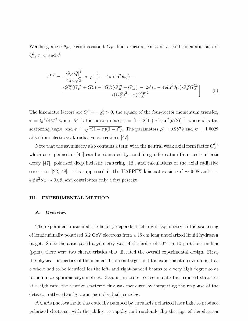
Weinberg angle θW , Fermi constant GF , fine-structure constant α, and kinematic factors
Q2, τ , ǫ, and ǫ′
APV = −GF |Q|2
4πα√2
× ρ′[(1− 4κ′ sin2 θW )−
ǫGγpE (Gγn
E +GsE) + τGγp
M (GγnM +Gs
M) − 2ǫ′ (1− 4 sin2 θW )GγpMG
ZpA
ǫ(GγpE )2 + τ(Gγp
M )2
](5)
The kinematic factors are Q2 = −q2µ > 0, the square of the four-vector momentum transfer,
τ = Q2/4M2 where M is the proton mass, ǫ = [1 + 2(1 + τ) tan2(θ/2)]−1
where θ is the
scattering angle, and ǫ′ =√τ(1 + τ)(1− ǫ2). The parameters ρ′ = 0.9879 and κ′ = 1.0029
arise from electroweak radiative corrections [47].
Note that the asymmetry also contains a term with the neutral weak axial form factor GZpA
which as explained in [46] can be estimated by combining information from neutron beta
decay [47], polarized deep inelastic scattering [16], and calculations of the axial radiative
correction [22, 48]; it is suppressed in the HAPPEX kinematics since ǫ′ ∼ 0.08 and 1 −4 sin2 θW ∼ 0.08, and contributes only a few percent.
III. EXPERIMENTAL METHOD
A. Overview
The experiment measured the helicity-dependent left-right asymmetry in the scattering
of longitudinally polarized 3.2 GeV electrons from a 15 cm long unpolarized liquid hydrogen
target. Since the anticipated asymmetry was of the order of 10−5 or 10 parts per million
(ppm), there were two characteristics that dictated the overall experimental design. First,
the physical properties of the incident beam on target and the experimental environment as
a whole had to be identical for the left- and right-handed beams to a very high degree so as
to minimize spurious asymmetries. Second, in order to accumulate the required statistics
at a high rate, the relative scattered flux was measured by integrating the response of the
detector rather than by counting individual particles.
A GaAs photocathode was optically pumped by circularly polarized laser light to produce
polarized electrons, with the ability to rapidly and randomly flip the sign of the electron
7
beam polarization. The asymmetry was extracted by generating the incident electron beam
as a pseudorandom time sequence of helicity “windows” at 30 Hz and then measuring the
fractional difference in the integrated scattered flux over window pairs of opposite helicity.
The elastically scattered electrons with θlab ∼ 12.5 were focused by two high-resolution
spectrometers (HRS) onto detectors consisting of lead-lucite sandwich calorimeters. The
Cerenkov light from each detector was collected by a photomultiplier tube, integrated over
the duration of each helicity window and digitized by analog to digital converters (ADCs).
The HRS pair has sufficient resolution to spatially separate the elastic electrons from in-
elastic electrons at the π0 threshold. The amount of background was measured in separate
calibration runs using conventional drift chambers, resulting in a small correction with neg-
ligible systematic errors.
The experiment was carefully designed to minimize the impact of random as well as of
helicity-correlated fluctuations of the measured scattered flux. The electrical environment
around the ADCs in particular and the data acquisition and control system as a whole were
configured so that the observed fluctuations in the integrated scattered flux were dominated
by counting statistics.
Apart from random jitter, an important class of potential false asymmetries might arise
from helicity-correlated fluctuations in the physical properties of the beam, such as intensity,
energy and trajectory. The helicity-correlated intensity asymmetry was maintained to be
less than 1 ppm by an active feedback loop. The physical properties of the electron beam
were monitored with high precision by beam monitors. The sensitivity of the scattered
flux to fluctuations in the beam parameters was evaluated continuously and accurately by
modulating judiciously placed corrector coils in the beam line leading to the hydrogen target.
Separate data runs under different conditions determined that target density fluctuations
were negligible for our kinematics.
The electron beam polarization was measured by three different techniques at varying
intervals: Mott scattering, Møller scattering and Compton scattering. Figure 1 shows a
schematic diagram of the important components of the HAPPEX experiment. In the fol-
lowing sections we elaborate on the above considerations in detail.
8

targethydrogen
polarimeterSteering CoilsPosition MonitorsIntensity Monitors
source
spectrometers
CEBAF
polarized
all
periment
rotonarity
detectors
dataacquisition& control
Hall A
HAPPEX
FIG. 1: Schematic Overview of the HAPPEX Experiment.
B. Polarized Electron Beam
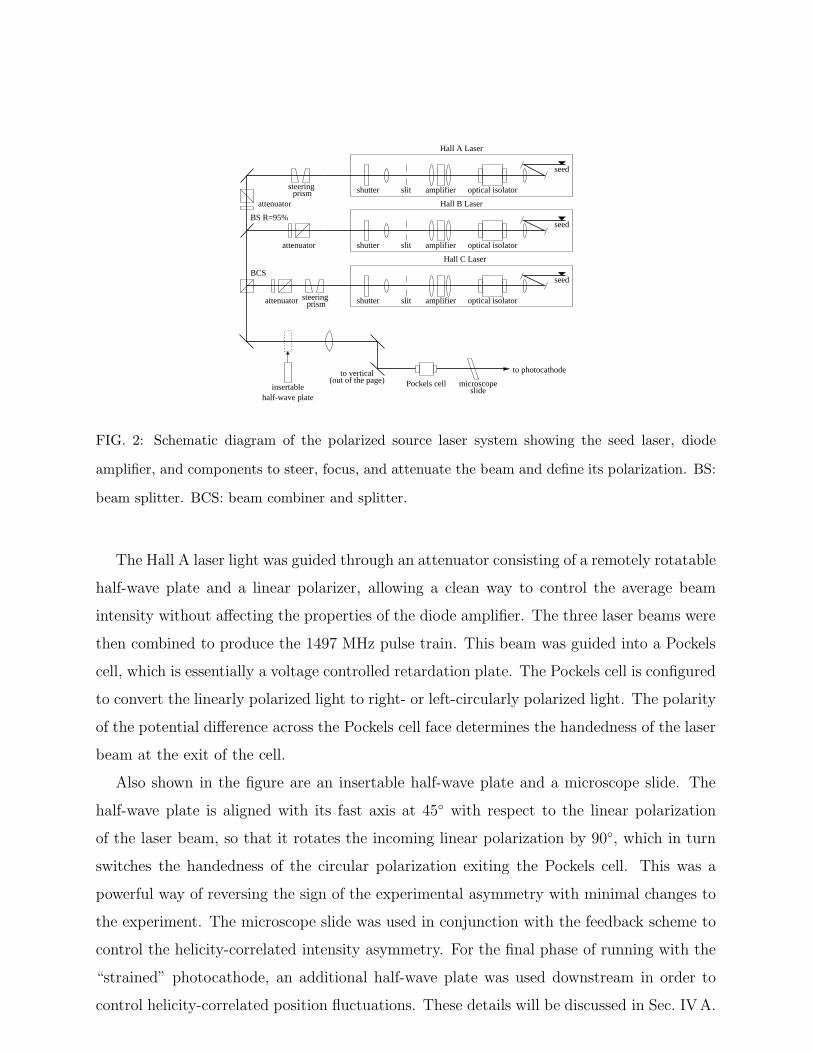
1. The Polarized Source and Laser Optics
The longitudinally-polarized electron beam at Jefferson Lab is produced by illuminating
a GaAs photocathode with circularly polarized laser light. For the 1998 run, a “bulk” GaAs
photocathode was used, which delivered a beam intensity up to 100 µA with a polarization
∼ 38%. For the 1999 run, a “strained” GaAs photocathode was used, which produced a
beam intensity of ∼ 40 µA with a polarization of ∼ 70%. This experiment was the first to
use a strained GaAs photocathode to measure a parity-violating asymmetry in fixed-target
electron scattering.
The source laser system provided laser light with the 1497 MHz microstructure of the JLab
electron beam. A diagram of the source laser system is shown in Fig. 2. There were three
lasers, which provided beams to the three different experimental halls, allowing individual
control of beam intensities. Each laser system consisted of a gain-switched diode seed laser
and a single-pass diode optical amplifier. Each seed laser was driven at 499 MHz, 120 out
of phase with the others. The seed laser light was focused into a diode optical amplifier,
whose respective drive current controllers allowed precise control of the beam intensity into
each experimental hall.
9
microscopeslide
Pockels cell
to photocathodeto vertical(out of the page)
insertablehalf-wave plate
steering prismattenuator
steering prism
attenuator
optical isolator
optical isolator
optical isolator
Hall A Laser
Hall B Laser
Hall C Laser
BCS
attenuator
BS R=95%
seed
slitshutter amplifier
seed
slitshutter
seed
slitshutter
amplifier
amplifier
FIG. 2: Schematic diagram of the polarized source laser system showing the seed laser, diode
amplifier, and components to steer, focus, and attenuate the beam and define its polarization. BS:
beam splitter. BCS: beam combiner and splitter.
The Hall A laser light was guided through an attenuator consisting of a remotely rotatable
half-wave plate and a linear polarizer, allowing a clean way to control the average beam
intensity without affecting the properties of the diode amplifier. The three laser beams were
then combined to produce the 1497 MHz pulse train. This beam was guided into a Pockels
cell, which is essentially a voltage controlled retardation plate. The Pockels cell is configured
to convert the linearly polarized light to right- or left-circularly polarized light. The polarity
of the potential difference across the Pockels cell face determines the handedness of the laser
beam at the exit of the cell.
Also shown in the figure are an insertable half-wave plate and a microscope slide. The
half-wave plate is aligned with its fast axis at 45 with respect to the linear polarization
of the laser beam, so that it rotates the incoming linear polarization by 90, which in turn
switches the handedness of the circular polarization exiting the Pockels cell. This was a
powerful way of reversing the sign of the experimental asymmetry with minimal changes to
the experiment. The microscope slide was used in conjunction with the feedback scheme to
control the helicity-correlated intensity asymmetry. For the final phase of running with the
“strained” photocathode, an additional half-wave plate was used downstream in order to
control helicity-correlated position fluctuations. These details will be discussed in Sec. IVA.
10
Pockels cell
+HVSupply
-HVSupply
+/-
HV
HV Switcher
+H
V
-HV
+H
V S
etpo
int
-HV
Set
poin
t
GeneratorHV Setpoint
PITA Offset
GeneratorHelicity
30 Hz Trigger
15 Hz Pair-Sync
Delayed Helicity
fibe
r-op
tic li
nes
to H
all A
DA
Q
Helicity ControlElectronics
Hel
icit
y
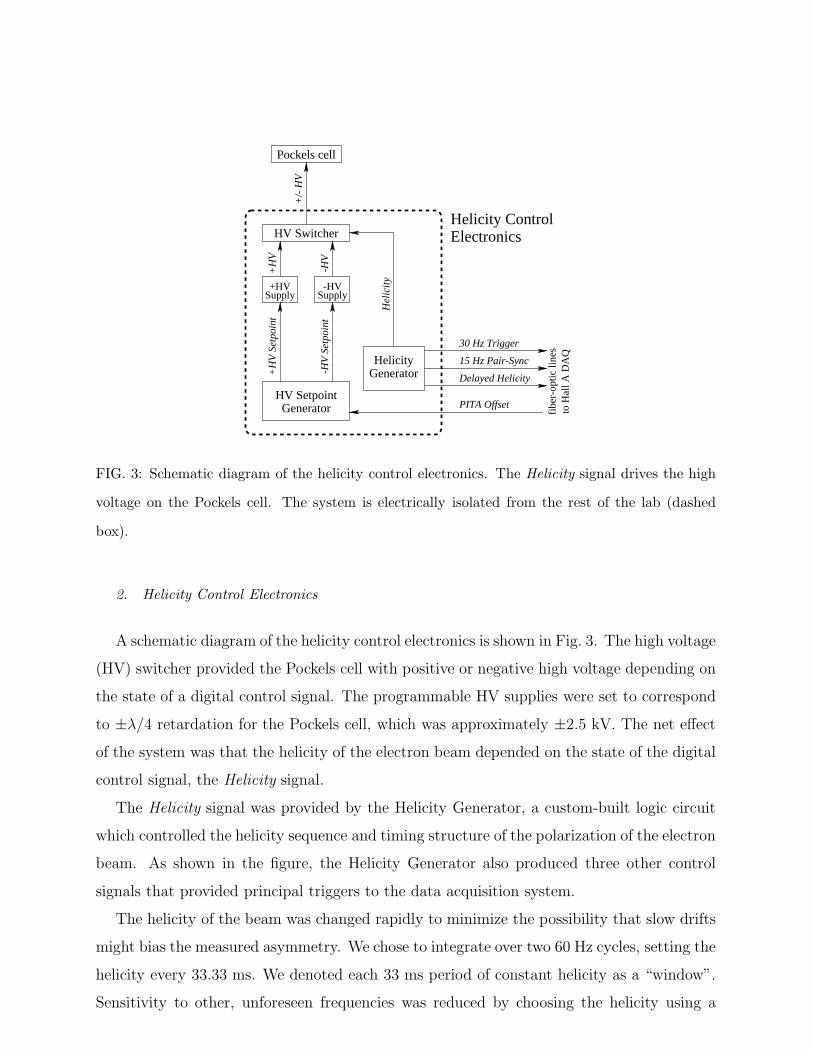
FIG. 3: Schematic diagram of the helicity control electronics. The Helicity signal drives the high
voltage on the Pockels cell. The system is electrically isolated from the rest of the lab (dashed
box).
2. Helicity Control Electronics
A schematic diagram of the helicity control electronics is shown in Fig. 3. The high voltage
(HV) switcher provided the Pockels cell with positive or negative high voltage depending on
the state of a digital control signal. The programmable HV supplies were set to correspond
to ±λ/4 retardation for the Pockels cell, which was approximately ±2.5 kV. The net effect
of the system was that the helicity of the electron beam depended on the state of the digital
control signal, the Helicity signal.
The Helicity signal was provided by the Helicity Generator, a custom-built logic circuit
which controlled the helicity sequence and timing structure of the polarization of the electron
beam. As shown in the figure, the Helicity Generator also produced three other control
signals that provided principal triggers to the data acquisition system.
The helicity of the beam was changed rapidly to minimize the possibility that slow drifts
might bias the measured asymmetry. We chose to integrate over two 60 Hz cycles, setting the
helicity every 33.33 ms. We denoted each 33 ms period of constant helicity as a “window”.
Sensitivity to other, unforeseen frequencies was reduced by choosing the helicity using a
11

pair pair pair
15 Hz Pair-Sync:
30 Hz Trigger:
Helicity:
Delayed Helicity:
FIG. 4: Timing diagram of important control signals related to the beam helicity.
pseudo-random number generator sequence at 15 Hz. The helicity sequence was thus a train
of “window pairs”: the helicity of the first window was chosen pseudo-randomly, while the
second window was chosen to be the corresponding complement.
All signals to and from the Helicity Generator were routed via fiberoptic cable, thus
allowing complete ground isolation of the helicity generator circuit from the rest of the
experiment. This was a powerful way to reduce the possibility of helicity-correlated crosstalk
and ground loops in the rest of the experiment, which could lead to spurious asymmetries.
As a further precaution to suppress crosstalk, the true helicity of each window was fed into
an 8-bit shift register, and the helicity that was transmitted to the data stream of the data
acquisition system arrived 8 windows later, breaking any correlation with the helicity of the
event. The timing signals described above are depicted in Fig. 4.
The system had one important input from the online analyzer of the data acquisition
system: a DC level that allowed for small changes to the precise high voltages of the HV
power supplies. This signal, labeled as “PITA offset” in Fig. 3, allowed for precise control
of the helicity-correlated intensity asymmetry of the electron beam, and will be described
in detail in section IVA2. In order to preserve the ground isolation, the DC level was
transmitted as a frequency over fiberoptic cable and then converted to an analog signal by
a frequency-to-voltage converter.
C. Beam Fluctuations
The detected scattered flux D in each spectrometer, and the beam current I, were
measured independently for every window. From these we obtained the normalized flux
di ≡ Di/Ii and the cross section asymmetry (Ad)i for the ith window pair. The raw asym-
12

metry was then obtained by appropriate averaging of N measurements:
(Ad)i ≡(d+ − d−
d+ + d−
)
i
≡(∆d
2d
)
i
δ(Ad) = σ(Ad)/√N. (6)
where + and − denote the two helicity states in a pair. One goal of the experimental design
was that σ(Ad) should be dominated by the counting statistics in the scattered flux, greatly
minimizing potential problems in the averaging procedure. As will be seen in Section VB,
this goal was met. This is a result of the extraordinary characteristics of the electron beam
and the associated beam instrumentation, which we discuss in this section.
The RMS noise in the asymmetry σ(Ad) was found to be 3.8 × 10⁻³ at a beam current
of approximately 100 µA, which implied that roughly 70,000 electrons were recorded in the
detectors during each beam window for a total rate of 2 MHz which was the expected rate
and consistent with the rate extrapolated from lower currents. Since the experimental cross
section is a function of the physical parameters of the beam, fluctuations in these parameters
may contribute significantly to σ(Ad). All electronic signals in the experiments are designed
so that electronic noise is small compared to σ(Ad).
There are two key parameters for each experimentally measured quantity M , such as
detector rate, beam intensity etc. The first is σ(∆M), the size of the relative window pair-
to-window pair fluctuations in ∆M ≡ M+ − M−, which is affected by real fluctuations
in the electron flux. The second is δ(∆M), the relative accuracy with which the window
pair differences in M can be measured compared to the true value, which is dominated by
instrumentation noise.
If σ(∆M) is large enough, it might mean that there are non-statistical contributions
to σ(Ad) so that the latter is no longer dominated by counting statistics. In this case, it
is crucial that δ(∆M) ≪ σ(∆M) so that window pair to window pair corrections for the
fluctuations in ∆M can be made.
1. Random Fluctuations
As stated in IIIC, we desire that σ(Ad) be dominated by counting statistics. An example
of possible non-statistical contributions is window-to-window relative beam intensity fluctu-
ations, σ(A(I)) ≡ σ(∆I/2I), which were observed to vary between 2 × 10⁻⁴ and 2 × 10⁻³,
13
depending on the quality of the laser and the beam tune. This is remarkable and a unique
feature of the beam at Jefferson lab, since σ(AI) < σ(Ad). Nevertheless, the detector-
intensity correlation can be exploited to remove the dependence of beam charge fluctuations
on the measured asymmetry:
(Ad)i ≃(∆D
2D− ∆I
2I
)
i
≡ (AD −AI)i. (7)
(This is equation 6 to first order.)
Similarly, σ(Ad) might be affected by random beam fluctuations in energy, position and
angle. The corrections can be parameterized as follows:
(Acorrd )i =
(∆D
2D− ∆I
2I
)
i
−∑
j
(αj(∆Xj)i). (8)
Here, Xj are beam parameters such as energy, position and angle and αj ≡ ∂D/∂Xj are
coefficients that depend on the kinematics of the specific reaction being studied, as well as
the detailed spectrometer and detector geometry of the experiment.
By judicious choices of beam position monitoring devices (BPMs) and their respective
locations, several measurements of beam position can be made from which the average
relative energy, position, and angle of approach of each ensemble of electrons in a helicity
window on target can be inferred. One can then write
(Acorrd )i =
(∆D
2D− ∆I
2I
)
i
−∑
j
(βj(∆Mj)i). (9)
HereMi are a set of 5 BPMs that span the parameter space of energy, position, and angle on
target, and βi ≡ ∂D/∂Mi. It is worth noting that this approach of making corrections win-
dow by window automatically accounts for occasional random instabilities in the accelerator
(such as klystron failures) that are characteristic of normal running conditions.
During HAPPEX running, we found that σ(∆Mj) varied between 1 and 10 µm and σ(AE)
was typically less than 10−5. These fluctuations were small enough that their impact on
σ(Ad) was negligible. Indeed, we believe that a significant contribution to the fluctuations in
each monitor difference ∆M was the intrinsic measurement precision δ(∆Mi). We elaborate
on this in section IIIC 2, where we discuss the monitoring instrumentation.
Another important consideration is the accuracy with which the coefficients βi are mea-
sured. As mentioned earlier, these coefficients were evaluated using beam modulation, and
will be discussed in Sect. IVB.
14

Pre
dict
ed P
osit
ion
(µm
)
Measured Position (µm)
FIG. 5: Window-to-window beam jitter as measured by a BPM is plotted along the x axis. On
the y axis is plotted the beam position as predicted by nearby BPMs. The residuals are smaller
than 1 µm.
2. Beam Monitoring
The above discussion regarding measurement accuracy and its impact on σ(Ad) is par-
ticularly relevant in the monitoring of the electron beam properties such as beam intensity,
trajectory and energy.
At Jefferson Lab, the beam position is measured by “stripline” monitors [49], each of
which consists of a set of four plates placed symmetrically around the beam pipe. The
plates act as antennae that provide a signal (modulated by the microwave structure of the
electron beam) proportional to the beam position as well as intensity. Figure 5 shows the
correlation between the measured position at a BPM near the target compared with the
predicted position using neighboring BPMs for a beam current of 100 µA (2×10¹³ electrons
per window). A precision for δ(∆Xi) close to 1 µm was obtained for the average beam
position for a beam window containing 2× 10¹³ electrons.
To measure the beam intensity, microwave cavity BCMs have been developed at Jefferson
15

Lab [50]. The precision δ(AI) that has been achieved for a 30 ms beam window at 100 µA
is 4× 10⁻⁵. This superior resolution is a result of good radiofrequency (rf) instrumentation
as well as a high resolution 16-bit ADC, which will be discussed in section IIIG.
The absolute calibration of the beam current was performed with a parametric current
transformer, the ‘Unser monitor’ [51]. Although the absolute calibration was not important
for HAPPEX, the Unser monitor was useful to establish the pedestals and understand the
linearity of the cavity current monitors.
3. Systematic Fluctuations
Assuming that σ(Ad) has negligible contributions from window-to-window beam fluctua-
tions and instrumentation noise, there is still the possibility that there are helicity-correlated
systematic effects at the sub-ppm level. If one considers the cumulative corrected asymmetry
Acorrd over many window pairs, one can write
Acorrd ≡ 〈(Acorr
d )i〉 =⟨(∆D
2D
)
i
⟩−⟨(
∆I
2I
)
i
⟩−∑
j
βj 〈(∆Mj)i〉
= AD − AI −∑
j
AMj . (10)
For most of the running conditions during data collection, Acorrd ≃ AD ≃ 10 ppm, which
meant that all corrections were negligible. The cumulative average for AI was maintained
below 0.1 ppm. For AMj, the cumulative averages were found to be below 0.1 ppm during
the run with the “bulk” GaAs photocathode. This resulted from the fact that the accelerator
damped out position fluctuations produced at the source by a large factor (section IVA4).
The averaged position differences on target were kept below 10 nm.
However, during data collection with “strained” GaAs, position differences as large as
several µm were observed in the electron beam at a point in the accelerator where the
beam energy is 5 MeV. Continuous adjustment of the circular polarization of the laser beam
was required to reduce the differences to about 0.5 µm. This resulted in observed position
differences on target ranging from 10 nm to 100 nm, which in turn resulted in AMj in the
range from 0.1 to 1 ppm.
The control of the asymmetry corrections within the aforementioned constraints was one
of the central challenges during data collection. A variety of feedback techniques on the laser
16
and electron beam properties were employed in order to accomplish this; these methods are
discussed in Sec. IVA.
D. Target
The Hall A cryogenic target system [50] was used for this experiment. The target sys-
tem consists of three separate cryogenic target loops in an evacuated scattering chamber,
along with subsystems for cooling, temperature and pressure monitoring, target motion,
gas-handling, controls, and a solid and dummy target ladder. Of the three cryogenic loops
(hydrogen, deuterium, and helium), only the hydrogen loop was used in this experiment and
will be described here. The hydrogen loop has two separate target cells, of 15 cm and 4 cm
in length, respectively; only the 15 cm cell was used here.
The liquid hydrogen loop was operated at a temperature of 19 K and a pressure of ∼ 26
psia, leading to a density of about 0.0723 g/cm3. The Al-walled target cells were 6.48 cm in
diameter, and were oriented horizontally, along the beam direction. The upstream window
thickness was 0.071 mm, the downstream window thickness was 0.094 mm, and the side
wall thickness was 0.18 mm. Also mounted on the target ladder were solid thin targets of
carbon, and aluminum dummy target cells, for use in background and spectrometer studies.
The target was mounted in a cylindrical scattering chamber of 104 cm diameter, centered
on the pivot for the spectrometers. The scattering chamber was maintained under a 10−6
torr vacuum. The spectrometers view exit windows in the scattering chamber that were
made of 0.406 mm thick Al foil.
The target coolant, 4He gas at 15 K, was provided by the End Station Refrigerator
(ESR), with a flow rate controlled using Joule-Thompson valves, which could be adjusted
either locally or remotely. At the beam currents used here (up to 100 µA) the beam heating
load was of order 600 W. Including the heating from the target circulation fans, and a small
(∼ 45 W) target heater, the load could reach 1 kW, which could be adequately supplied
by the ESR. In addition to the 45 W target heater, used in a feedback system in order
to stabilize the target temperature, a high power heater (up to 1 kW) was automatically
switched on when the beam dropped out suddenly. This target has achieved a luminosity
of 5× 1038 cm−2s−1.
The target temperature was monitored continuously using 1) radiation hard
17
semiconductor-based sensors, Lakeshore CERNOX [52], 2) Allen-Bradley resistive sensors
[53], and 3) vapor-pressure transducers. The temperature control system was computer
controlled using a PID (proportion, integral and derivative) feedback system. The control
system was based on the EPICS [54] system.
The normal electron beam spot size of about 50 µm is small enough to potentially damage
the target cells at full beam current, as well as to cause local boiling in the target even at
reduced currents. A beam rastering system was used to distribute the heat load throughout
the target cell. The beam was rastered at 20 kHz by two sets of steering magnets 23 m
upstream of the target. These magnets deflected the beam by up to ±2.5 mm in x and y
at the target. For the 1998 run, a rectangular raster pattern was used, while for the 1999
run a helical pattern was adopted, which provided a more uniform distribution of heat load.
Local target boiling would manifest itself as an increase in fluctuations in the measured
scattering rate, which would lead to an increase in the standard deviation of the pulse-pair
asymmetries in the data, above that expected from counting statistics. Studies of the pulse-
pair asymmetries for various beam currents and raster sizes were performed, at a lower Q2
and thus at a higher scattering rate. Figure 6 shows the standard deviation of the pulse-
pair asymmetries, extrapolated to full current values, for various beam currents and raster
sizes. A significant increase over pure counting statistics, indicating local boiling effects, was
observed only for the combination of a small raster (1.0 mm) size and large beam current
(94 µA). During the experiment we used larger raster sizes for which there was little boiling
noise.
E. High Resolution Spectrometers in JLab Hall A
The Hall A high resolution spectrometers (HRS) at Jefferson Lab consist of a pair of
identical spectrometers of QQDQ design, together with detectors for detecting the scattered
particles [50]. For HAPPEX, the spectrometer and their standard detector package served
the following purposes: 1) to suppress background from inelastics and low-energy secon-
daries; 2) to study the backgrounds in separate runs at or near the HAPPEX kinematics;
3) to measure the momentum transfer Q2; 4) to measure and monitor the attenuation in the
HAPPEX detector through the use of tracking; and 5) to measure the detector amplitude
weighting factors for fine bins in Q2 (section VIC).
18
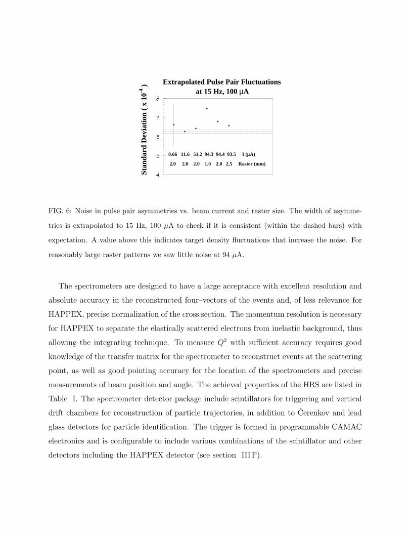
Extrapolated Pulse Pair Fluctuationsat 15 Hz, 100 µA
Stan
dard
Dev
iati
on (
x 1
0-4 )
0.66 11.6 51.2 94.3 94.4 93.5 I (µA)
2.0 2.0 2.0 1.0 2.0 2.5 Raster (mm)
FIG. 6: Noise in pulse pair asymmetries vs. beam current and raster size. The width of asymme-
tries is extrapolated to 15 Hz, 100 µA to check if it is consistent (within the dashed bars) with
expectation. A value above this indicates target density fluctuations that increase the noise. For
reasonably large raster patterns we saw little noise at 94 µA.
The spectrometers are designed to have a large acceptance with excellent resolution and
absolute accuracy in the reconstructed four–vectors of the events and, of less relevance for
HAPPEX, precise normalization of the cross section. The momentum resolution is necessary
for HAPPEX to separate the elastically scattered electrons from inelastic background, thus
allowing the integrating technique. To measure Q2 with sufficient accuracy requires good
knowledge of the transfer matrix for the spectrometer to reconstruct events at the scattering
point, as well as good pointing accuracy for the location of the spectrometers and precise
measurements of beam position and angle. The achieved properties of the HRS are listed in
Table I. The spectrometer detector package include scintillators for triggering and vertical
drift chambers for reconstruction of particle trajectories, in addition to Cerenkov and lead
glass detectors for particle identification. The trigger is formed in programmable CAMAC
electronics and is configurable to include various combinations of the scintillator and other
detectors including the HAPPEX detector (see section III F).
19

TABLE I: Properties of the Hall A Spectrometers
Magnet Configuration QQDQ
Luminosity 1038cm−2sec−1
Momentum Range (spectrometer 1) 0.2 - 4.3 GeV/c
Momentum Range (spectrometer 2) 0.2 - 3.2 GeV/c
Bend Angle 45
Optical Length 23.4 m
Dispersion 12.4 cm/%
Momentum Acceptance ± 4.5%
Momentum Resolution (FWHM) 2×10⁻⁴
Solid Angle Acceptance 6 msr
Horizontal Angle Acceptance ± 28 mrad
Vertical Angle Acceptance ± 60 mrad
Target Length Acceptance (90) 10 cm
Transverse Position Resolution (FWHM) 1.5 mm
Missing Energy Resolution (FWHM) 1.3 MeV
F. Focal Plane Detector
A total absorption shower counter was located in the focal plane of each spectrometer
to detect the elastically scattered electrons. These detectors were based on a layered lead-
acrylic geometry. Cerenkov light in the shower propagates along the acrylic and is detected
at one end using a single photomultiplier tube (PMT); see Fig. 7.
These simple focal plane detectors were chosen over, for example, lead glass, because of
their superior resistance to radiation damage. The radiation dose expected per detector was
approximately 40 Gy in a 30 day data-taking run, which would cause significant decrease
in optical transmission for a lead glass detector. Acrylic is significantly less susceptible to
radiation damage. The insensitivity of such a detector to low-energy backgrounds was also
an important design criterion.
The detectors were made up of 4 layers of 6.4 mm thick lead sheets sandwiched between
5 layers of 1.27 cm thick acrylic (Bicron BC-800 UVT Lucite). Each layer of acrylic was
20

FIG. 7: Schematic of the focal plane detector. The scattered electrons strike a lead-acrylic shower
counter whose light is collected by a PMT and integrated over a helicity period.
wrapped with a Teflon sheet, which does not adhere to the surface, thereby preserving
internal reflection from the acrylic-air interface. The incident electrons first passed through
a 1.9 cm Teflon spacer and 2 layers of 6.4 mm lead sheets acting as a pre-radiator. The
segmentation was chosen in order to provide a sufficiently good energy resolution (15% σ)
with the use of commercially available thicknesses of acrylic while maintaining mechanical
simplicity. The detector energy resolution affects the error on the physics asymmetry via
δA ∼ 1√N
√
1 +
(∆E
〈E〉
)2
(11)
where N is the number of window pairs, ∆E is the energy resolution of the detector, and
〈E〉 is the average detected energy. The width (10 cm) and length (150 cm) of the sandwich
stack was chosen in order to contain the entire image of the elastically scattered electrons in
the focal plane, as well as much of the radiative tail, and yet not detect events from inelastic
scattering. The width of the distribution of elastic events on the focal plane was 3 cm, so
edge effects were small.
The detector sandwich was viewed at one end by a single 12.7 cm diameter Burle 8854
photomultiplier tube. A pair of blue LEDs was mounted in the middle acrylic layer, at the
opposite end from the PMT, for use in study of detector linearity and attenuation. Tests
using the LEDs indicated that the non-linearity of the detector was less than 1.5% at typical
operating voltages.
Bench tests of the detectors using cosmic rays showed that the signal output was a strong
21

function of the incident particle’s position along the detector’s length, due primarily to bulk
absorption of light in the acrylic. While the Bicron BC-800 UVT Lucite acrylic is transparent
to wavelengths shorter than for ordinary acrylic, it has a strong attenuation for wavelengths
shorter than about 350 nm. Given that the PMT used has significant sensitivity down to
250 nm, and given the short wavelengths of typical Cerenkov light, the bulk attenuation
in the acrylic led to a measured decrease in the light output of 50%/m. To decrease this
attenuation, a single sheet of Plexiglass was installed directly in front of the PMT to filter
out the UV light. After installation of this filter the dependence of light output on position
along the detector was reduced to 9%/m, at the cost of a reduction in the total gain, which
was acceptable for this experiment.
The detector, as expected, also exhibited a strong sensitivity to the angle of the incident
particles, with a maximum output when the angle was such that part of the Cerenkov cone
pointed directly at the PMT (see Fig. 8). This angular sensitivity was an advantage. Since
the elastic electrons arrive at the focal plane at well-known angles, the detector orientation
can then be adjusted to maximize the sensitivity to the elastically scattered events while
minimizing the sensitivity to backgrounds that arrive at other angles.
Due to the optics of the spectrometer, the incident angle of the elastically-scattered
electrons varies with their position along the detector’s length. Thus the crossing angle
sensitivity leads to an additional variation of the detector’s response with position along the
detector. The total effect of variation along the detector position was measured periodically
during data-taking and was (17.3±0.5)%/m. This value was stable during the run, indicating
no significant degradation of the optical properties of the detector due to radiation damage.
The detector was mounted in a light-tight aluminum box with 1 cm thick walls and
was supported over the vertical drift chambers in a frame that allowed adjustment of the
horizontal location, as well as the pitch, roll and yaw angle of the detector. The detector’s
strong sensitivity to the incident angle of the incoming electron necessitated the ability
to orient the detector precisely. All material used in the detector box and support frame
near the active region was chosen to be non-ferric in order to reduce the possibility of false
asymmetries due to Møller scattering of electrons off magnetized material. More information
on the detectors is available in [8].
22
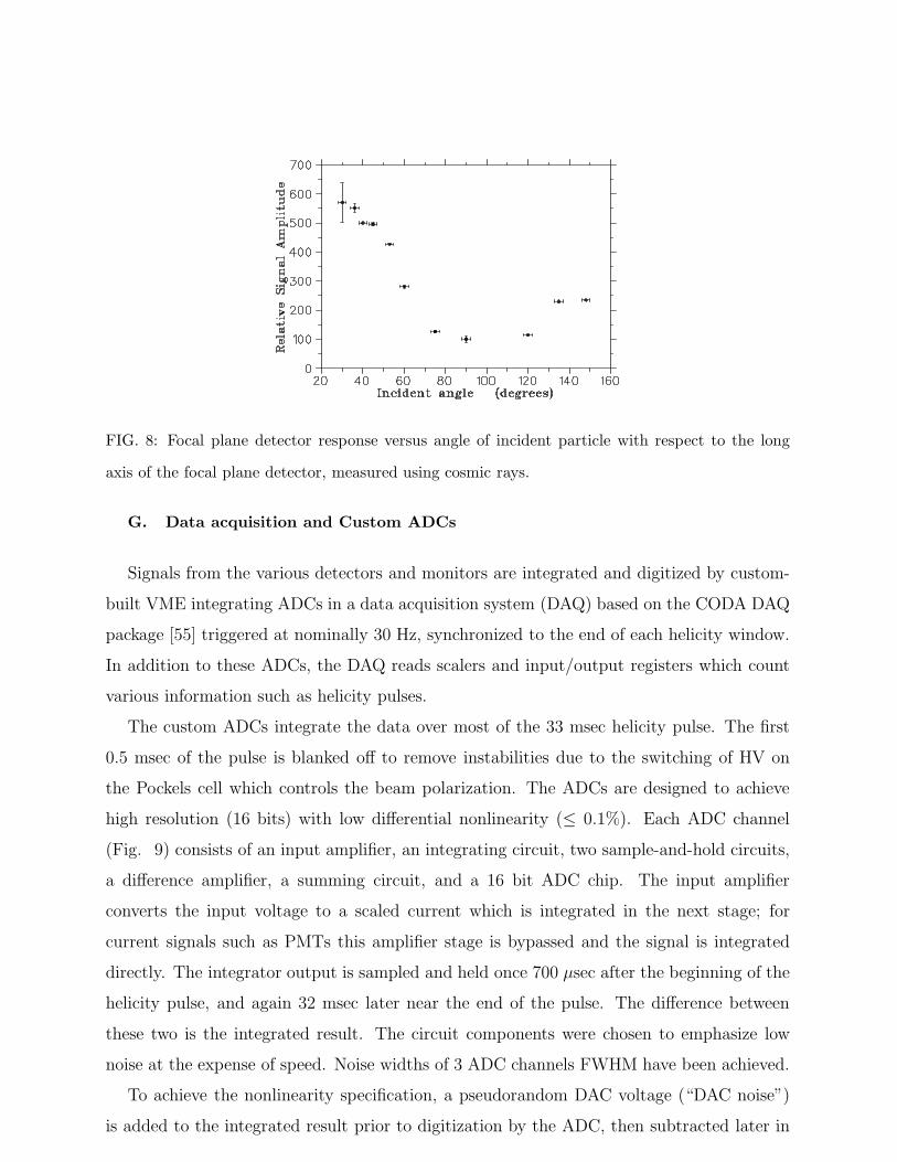
FIG. 8: Focal plane detector response versus angle of incident particle with respect to the long
axis of the focal plane detector, measured using cosmic rays.
G. Data acquisition and Custom ADCs
Signals from the various detectors and monitors are integrated and digitized by custom-
built VME integrating ADCs in a data acquisition system (DAQ) based on the CODA DAQ
package [55] triggered at nominally 30 Hz, synchronized to the end of each helicity window.
In addition to these ADCs, the DAQ reads scalers and input/output registers which count
various information such as helicity pulses.
The custom ADCs integrate the data over most of the 33 msec helicity pulse. The first
0.5 msec of the pulse is blanked off to remove instabilities due to the switching of HV on
the Pockels cell which controls the beam polarization. The ADCs are designed to achieve
high resolution (16 bits) with low differential nonlinearity (≤ 0.1%). Each ADC channel
(Fig. 9) consists of an input amplifier, an integrating circuit, two sample-and-hold circuits,
a difference amplifier, a summing circuit, and a 16 bit ADC chip. The input amplifier
converts the input voltage to a scaled current which is integrated in the next stage; for
current signals such as PMTs this amplifier stage is bypassed and the signal is integrated
directly. The integrator output is sampled and held once 700 µsec after the beginning of the
helicity pulse, and again 32 msec later near the end of the pulse. The difference between
these two is the integrated result. The circuit components were chosen to emphasize low
noise at the expense of speed. Noise widths of 3 ADC channels FWHM have been achieved.
To achieve the nonlinearity specification, a pseudorandom DAC voltage (“DAC noise”)
is added to the integrated result prior to digitization by the ADC, then subtracted later in
23

SUM OUT
INT OUT
10.00 K
10.00 K
10.00 K
10.00 K 33 pF
33 pF470
470 pFPEAK
Peak Sample-and-Hold
470
470 pFBASELINE
Baseline Sample-and-Hold
R1
240 K
11.00 K
10.00 K
1.100 K
1.000 K
V IN
AD7884
Integrator
2 K
1 KRESET
C2
C1
RANGE
Summing Amplifier
2.5 K
2.5 K
5 K
100 pF10 K
DAC+5.000 V
Difference Amplifier
I
Input Stage
ADC Chip
FIG. 9: Circuit diagram of one channel of the custom 16 bit integrating ADC.
analysis. DAC noise solves a problem of nonlinearity that arises generally in the digitization
of data which leads to a systematic error in the asymmetry that can be estimated as follows.
Consider a signal of average value S (ADC channels) and RMS width σ, and let the deviation
from ideal linear response be denoted D which is typically the least count bit. Denote the
helicity correlated asymmetry in the signal by A. Then if AS ≪ σ the relative systematic
error in the asymmetry will be dA/A ≈ KD/σ with K ≃ 1. (For Gaussian signals K =
2/√2π.) Thus, the DAC noise smears the data over many ADC channels, which reduces
systematic errors from bit resolution. Since the noise is later subtracted it does not increase
the statistical error.
The data acquisition software is based on the CODA 1.4 package [55]. The trigger in-
terrupt service routine in the VME controller assembles the following data into an event
record: ADC data, ADC flags, scaler data, trigger controller data, VME flags, beam modu-
lation data, and Pockels cell high voltage offsets. The ADC data include the digitized ADC
outputs and the value of the DAC noise that had been added to the ADC signal. The ADC
flags govern various options for each ADC board. Data from the trigger controller include a
flag indicating the helicity of the first window of the pair, and a flag indicating whether the
window is the first or the second of a pair. As described in section IIIB 2, the helicity flag
is delayed at the polarized source and applies to the eighth window preceding the one with
which it is collected. The VME flags govern various options for the VME controller. Beam
modulation data describe the state of the beam modulation system including the object
being modulated, the size of its offset, and flags indicating whether the object’s state was
stable during the event.
24
The complete event record is then sent over the network to the data acquisition worksta-
tion, where the data files are written to disk and are processed by an online analyzer.
A separate process on the VME controller is able to handle requests via a TCP/IP socket
to change or report various system parameters, including the ADC and VME flags, beam
intensity feedback parameters, and the Pockels cell high voltage offset, and to enable or
disable the beam modulation system.
The online analyzer verifies the integrity of the data, determines where cuts due to beam
off or computer dead time are required, associates the delayed helicity information with its
proper window, groups windows into opposite-helicity pairs, subtracts DAC noise from each
ADC signal, computes x and y positions from the BPM data, and packages the data into
files in the PAW ntuple format for further analysis.
Another function of the online analyzer is to handle beam intensity feedback. Beam
intensity asymmetries are averaged over a user-defined interval, typically 2500 pairs, termed
a “minirun”. At the end of each minirun the change to the Pockels cell high voltage offset
required to null the observed intensity asymmetry is computed. The analyzer then issues a
request for the VME controller to make the appropriate change to the offset.
H. Polarimetry
The experimental asymmetry Aexp is related to the corrected asymmetry by
Aexp = Acorrd /Pe (12)
where Pe is the beam polarization. Three beam polarimetry techniques were available at
JLab for the HAPPEX experiment: A Mott polarimeter in the injector, and both a Møller
and a Compton polarimeter in the experimental hall.
1. Mott Polarimeter
A Mott polarimeter [57] is located near the injector to the first linac, where the electrons
have reached 5 MeV in energy. Mott polarimetry is based on the scattering of polarized
electrons from unpolarized high-Z nuclei. The spin-orbit interaction of the electron’s spin
with the magnetic field it sees due to its motion relative to the nucleus causes a differential
25

cross section
σ(θ) = I(θ)[1 + S(θ)~Pe · n
], (13)
where S(θ), known as the Sherman function, is the analyzing power of the polarimeter, and
I(θ) is the spin-averaged scattered intensity
I(θ) =Z2e4
4m2β4c4 sin4(θ/2)
[1− β2 sin2(θ/2)
](1− β2) . (14)
The unit vector n is normal to the scattering plane, defined by n = (~k × ~k′)/|~k × ~k′| where~k and ~k′ are the electron’s momentum before and after scattering, respectively. Thus σ(θ)
depends on the electron beam polarization Pe. Defining an asymmetry
A(θ) =NL −NR
NL +NR, (15)
where NL and NR are the number of electrons scattered to the left and right, respectively,
we have
A(θ) = Pe S(θ) , (16)
and so knowledge of the Sherman function S(θ) allows Pe to be extracted from the measured
asymmetry.
The 5 MeV Mott polarimeter employs a 0.1 µm gold foil target, and four identical plastic
scintillator total-energy detectors, located symmetrically around the beam line at a scat-
tering angle of 172, the maximum of the analyzing power. This configuration allows a
simultaneous measurement of the two components of polarization transverse to the beam
momentum direction. A Wien filter upstream of the polarimeter is used to rotate the elec-
tron’s spin from longitudinal to transverse polarization for the Mott measurement. Multiple
scattering in the foil target leads to substantial uncertainty in the analyzing power which is
evaluated by measurements for a range of target foil thicknesses and an extrapolation to zero
thickness. It is believed [56] that the theoretically calculated single-atom analyzing power
(Sherman function) is the correct number to use for zero target thickness extrapolation. The
primary systematic errors of the device were the extrapolation to zero target foil thickness
(5% relative) and background subtraction (3%) [57], see section VIA1.
26

2. Møller Polarimeter
A Møller polarimeter measures the beam polarization via measuring the asymmetry in
~e, ~e scattering, which depends on the beam and target polarizations P beam and P target, as
well as on the analyzing power Athm of Møller scattering:
Aexpm =
∑
i=X,Y,Z
(Athmi · P targ
i · P beami ), (17)
where i = X, Y, Z defines the projections of the polarizations (Z is parallel to the beam,
while X − Z is the scattering plane). The analyzing powers Athmi depend on the scattering
angle θCM in the center-of-mass (CM) frame and are calculable in QED. The longitudinal
analyzing power is
AthmZ = −sin2 θCM(7 + cos2 θCM)
(3 + cos2 θCM)2 . (18)
The absolute values of AthmZ reach the maximum of 7/9 at θCM = 90. At this angle the
transverse analyzing powers are AthmX = −Ath
mY = AthmZ/7.
The polarimeter target is a ferromagnetic foil magnetized in a magnetic field of 24 mT
along its plane. The target foil can be oriented at various angles in the horizontal plane
providing both longitudinal and transverse polarization measurements. The asymmetry
is measured at two target angles (±20) and the average taken, which cancels transverse
contributions and reduces the uncertainties of target angle measurements. At a given target
angle two sets of measurements with oppositely signed target polarization are made which
cancels some false asymmetries such as beam current asymmetries. The target polarization
was (7.95 ± 0.24)%.
The Møller-scattered electrons were detected in a magnetic spectrometer (see Fig. 10)
consisting of three quadrupoles and a dipole [50].
The spectrometer selects electrons in a bite of 75 ≤ θCM ≤ 105 and −5 ≤ φCM ≤ 5
where φCM is the azimuthal angle. The detector consists of lead-glass calorimeter modules in
two arms to detect the electrons in coincidence. More details about the Møller polarimeter
are published in [50]. The total systematic error that can be achieved is 3.2% which is
dominated by uncertainty in the foil polarization.
27

-80
-60
-40
-20
0
20
40
0 100 200 300 400 500 600 700 800Z cm
Y cm
(a)
Tar
get
Co
llim
ato
r
Coils Quad 1 Quad 2 Quad 3 Dipole
Detector
non-scatteredbeam
-20
-15
-10
-5
0
5
10
15
20
0 100 200 300 400 500 600 700 800Z cm
X cm
(b)
B→
FIG. 10: Layout of the Hall A Møller polarimeter.
3. Compton Polarimeter
The Compton polarimeter performed its first measurements during the second HAPPEX
run in July 1999 [58]. It is installed on the beam line of Hall A (see Fig.11). The electron
beam interacts with a polarized “photon target” in the center of a vertical magnetic chicane
that aims at separating the scattered electrons and photons from the primary beam. The
backscattered photons are detected in a matrix of 25 PbWO4 crystals [59].
The experimental asymmetry Aexpc = (N+−N−)/(N++N−) is measured, where N+ (N−)
refers to Compton counting rates for right (left) electron helicity, normalized to the beam
intensity. This asymmetry is related to the electron beam polarization via
Pe =Aexp
c
PγAthc
(19)
where Pγ is the photon polarization and Athc the analyzing power. At typical JLab energies
(a few GeV), the Compton cross-section asymmetry is only a few percent. An original
way to compensate this drawback is the implementation of a Fabry-Perot cavity [60] which
amplifies the photon density of a standard low-power laser at the integration point. An
average power of 1200 W is accumulated inside the cavity with a photon beam waist of the
order of 150 µm and a photon polarization above 99%, monitored online at the exit of the
cavity [61].
Since less than 10−9 of the beam undergoes Compton scattering, and thanks to the zero
total field integral of the magnetic chicane, the primary beam is delivered unchanged to the
28

FIG. 11: Oblique view of the Compton polarimeter. The beam enters from the left and is bent
down into a chicane where it intersects the laser cavity. The cavity is on the bench in the middle
of the chicane. The photon detector for backscattered photons is on the bench just upstream of
the last chicane magnet.
experimental target. These features make Compton polarimetry an attractive alternative to
other techniques, as it provides a non-invasive measurement simultaneous with the running
experiment.
The quality of the polarization measurement is driven by the tuning of the electron
beam in the center of the magnetic chicane. In the early tests a large background rate was
generated in the photon detector by the halo of the electron beam scraping on the narrow
apertures of the ports in the mirrors of the cavity. Extra focusing in the horizontal plane,
induced by an upstream quadrupole dramatically reduces this background. Then a fine
adjustment of the electron beam vertical position optimizes the luminosity at the Compton
interaction point. Figure 12 illustrates that beyond maximizing the luminosity, standing
near the optimum position also reduces our sensitivity to electron beam position differences
correlated with the helicity.
In the data-taking procedure, periods of cavity ON (resonant) and cavity OFF (unlocked)
are alternated in order to monitor the background level and asymmetry. A typical signal
over background ratio of 5 is achieved and the associated errors are small.
The photon polarization is reversed for each ON period, reducing the systematic errors
29

y (µ)
Rat
e (k
Hz/
µA)
0.6
0.8
1
1.2
1.4
1.6
1.8
2
2.2
400 500 600 700 800 900 1000
FIG. 12: Counting rate normalized to beam current versus vertical position of the electron beam
for the Compton polarimeter. The sensitivity to beam position differences is proportional to the
derivative of this curve. The arrow points to where we run.
due to electron helicity correlations. These correlations are already minimized by our controls
at the source (see Sec. IVA). By summing the Compton asymmetries of the right and left
photon polarization states with the proper statistical weights we expect the effects of helicity
correlations to cancel out to first order and the residual effects to be small. Nevertheless,
extra slow drifts in time of the beam parameters can occur and increase the sensitivity to
helicity correlations. In order to select stable running conditions we apply cuts of ±3 µA on
the beam current and reject all the coil-modulation periods in the analysis. This leads to the
loss of 1/3 of the events. In the end the residual helicity correlated luminosity asymmetry
AF still contributed 1.2% to the experimental Compton asymmetry and remained its main
source of systematic error (cf. Table II).
An optical setup allows us to monitor the photon polarization at the exit of the cavity.
The connection with the “true” polarization Pγ at the Compton interaction point is given
by a transfer function measured once during a maintenance period. Polarizations for right
and left handed photons are found to be stable in time and given by PR,Lγ = ±99.3+0.7
−1.1%.
The last ingredient of Eq. 19 is the analyzing power Athc . The response function of the
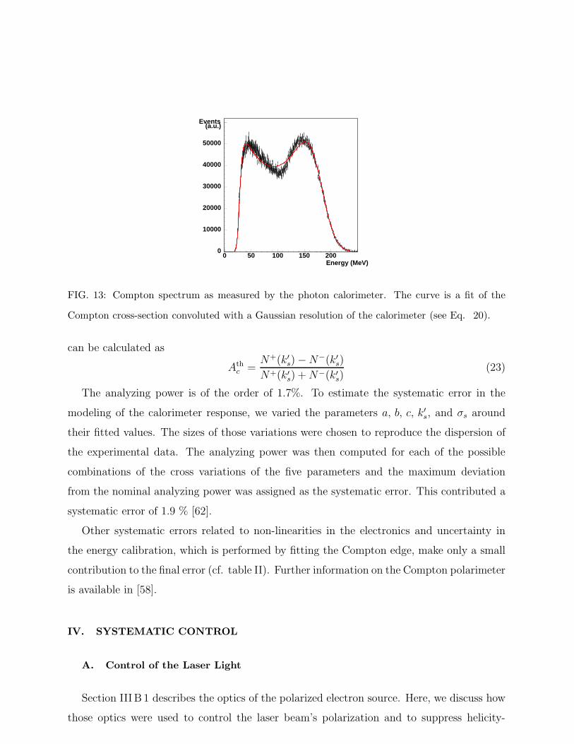
photon detector (see Fig. 13) is parametrized by a Gaussian resolution g(k′) of width
σres(k′) =
√a+
b
k′+
c
(k′)2, (20)
30

TABLE II: Average relative error budget for the beam polarization measured using the Compton
polarimeter, based on 40 measurements in the 1999 run. S and B refer to signal and background,
AB is the asymmetry in the background, and AF is the helicity correlated luminosity asymmetry.
Source Systematic Statistical
Pγ 1.1%
Aexpc Statistical 1.4%
B/S 0.5%
AB 0.5% 1.4%
AF 1.2%
Athc Non-linearities 1%
Calibration 1%
Efficiency/Resolution 1.9% 2.4%
Total 3.3%
where k′ is the backscattered photon energy. A Gaussian was used because the complete
study of the calorimeter response wasn’t available at the time of this analysis; the corre-
sponding errors in the calibration, efficiency, and resolution are shown in Table II and
explained here. The coefficients (a, b, c) are fitted to the data (Fig. 13). A “smeared” cross
section is then obtained
dσ±smeared
dk′r=
∫ ∞
o
dσ±c
dk′g(k′ − k′r) dk
′ (21)
where k′r is the energy deposited in the calorimeter and dσ±c /dk
′ the helicity-dependent
Compton cross section. Experimentally, the energy spectrum has a finite width at the
threshold (see Fig. 13) which is modeled by an error function p(k′s, k′r) = erf((k′r − k′s)/σs)
where σs is fitted to the data as well. This width can be due either to the fact that the
threshold level itself is unstable, or to the fact that a given k′r can correspond to different
voltages at the discriminator level.
Finally, the observed counting rates can be expressed as
N±(k′s) = L×∫ ∞
0
p(k′s, k′r)dσ±
smeared
dk′rdk′r (22)
where L stands for the interaction luminosity and the analyzing power of the polarimeter
31
0
10000
20000
30000
40000
50000
Events (a.u.)
0 50 100 150 200Energy (MeV)
FIG. 13: Compton spectrum as measured by the photon calorimeter. The curve is a fit of the
Compton cross-section convoluted with a Gaussian resolution of the calorimeter (see Eq. 20).
can be calculated as
Athc =
N+(k′s)−N−(k′s)
N+(k′s) +N−(k′s)(23)
The analyzing power is of the order of 1.7%. To estimate the systematic error in the
modeling of the calorimeter response, we varied the parameters a, b, c, k′s, and σs around
their fitted values. The sizes of those variations were chosen to reproduce the dispersion of
the experimental data. The analyzing power was then computed for each of the possible
combinations of the cross variations of the five parameters and the maximum deviation
from the nominal analyzing power was assigned as the systematic error. This contributed a
systematic error of 1.9 % [62].
Other systematic errors related to non-linearities in the electronics and uncertainty in
the energy calibration, which is performed by fitting the Compton edge, make only a small
contribution to the final error (cf. table II). Further information on the Compton polarimeter
is available in [58].
IV. SYSTEMATIC CONTROL
A. Control of the Laser Light
Section IIIB 1 describes the optics of the polarized electron source. Here, we discuss how
those optics were used to control the laser beam’s polarization and to suppress helicity-
32
correlated beam asymmetries.
1. Laser Polarization and the PITA Effect
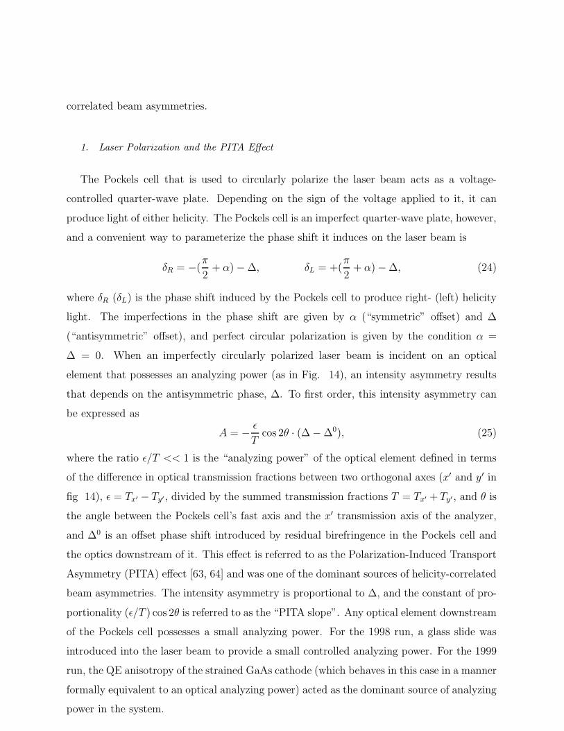
The Pockels cell that is used to circularly polarize the laser beam acts as a voltage-
controlled quarter-wave plate. Depending on the sign of the voltage applied to it, it can
produce light of either helicity. The Pockels cell is an imperfect quarter-wave plate, however,
and a convenient way to parameterize the phase shift it induces on the laser beam is
δR = −(π
2+ α)−∆, δL = +(
π
2+ α)−∆, (24)
where δR (δL) is the phase shift induced by the Pockels cell to produce right- (left) helicity
light. The imperfections in the phase shift are given by α (“symmetric” offset) and ∆
(“antisymmetric” offset), and perfect circular polarization is given by the condition α =
∆ = 0. When an imperfectly circularly polarized laser beam is incident on an optical
element that possesses an analyzing power (as in Fig. 14), an intensity asymmetry results
that depends on the antisymmetric phase, ∆. To first order, this intensity asymmetry can
be expressed as
A = − ǫ
Tcos 2θ · (∆−∆0), (25)
where the ratio ǫ/T << 1 is the “analyzing power” of the optical element defined in terms
of the difference in optical transmission fractions between two orthogonal axes (x′ and y′ in
fig 14), ǫ = Tx′ − Ty′ , divided by the summed transmission fractions T = Tx′ + Ty′ , and θ is
the angle between the Pockels cell’s fast axis and the x′ transmission axis of the analyzer,
and ∆0 is an offset phase shift introduced by residual birefringence in the Pockels cell and
the optics downstream of it. This effect is referred to as the Polarization-Induced Transport
Asymmetry (PITA) effect [63, 64] and was one of the dominant sources of helicity-correlated
beam asymmetries. The intensity asymmetry is proportional to ∆, and the constant of pro-
portionality (ǫ/T ) cos 2θ is referred to as the “PITA slope”. Any optical element downstream
of the Pockels cell possesses a small analyzing power. For the 1998 run, a glass slide was
introduced into the laser beam to provide a small controlled analyzing power. For the 1999
run, the QE anisotropy of the strained GaAs cathode (which behaves in this case in a manner
formally equivalent to an optical analyzing power) acted as the dominant source of analyzing
power in the system.
33
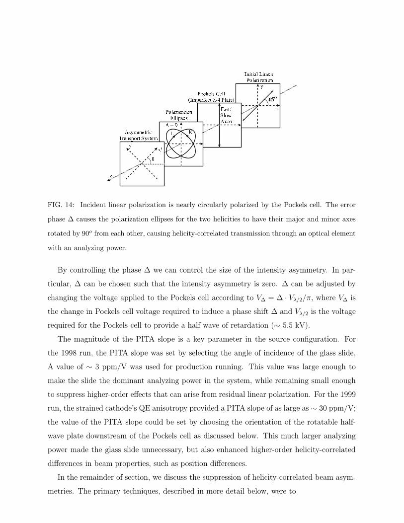
FIG. 14: Incident linear polarization is nearly circularly polarized by the Pockels cell. The error
phase ∆ causes the polarization ellipses for the two helicities to have their major and minor axes
rotated by 90o from each other, causing helicity-correlated transmission through an optical element
with an analyzing power.
By controlling the phase ∆ we can control the size of the intensity asymmetry. In par-
ticular, ∆ can be chosen such that the intensity asymmetry is zero. ∆ can be adjusted by
changing the voltage applied to the Pockels cell according to V∆ = ∆ · Vλ/2/π, where V∆ is
the change in Pockels cell voltage required to induce a phase shift ∆ and Vλ/2 is the voltage
required for the Pockels cell to provide a half wave of retardation (∼ 5.5 kV).
The magnitude of the PITA slope is a key parameter in the source configuration. For
the 1998 run, the PITA slope was set by selecting the angle of incidence of the glass slide.
A value of ∼ 3 ppm/V was used for production running. This value was large enough to
make the slide the dominant analyzing power in the system, while remaining small enough
to suppress higher-order effects that can arise from residual linear polarization. For the 1999
run, the strained cathode’s QE anisotropy provided a PITA slope of as large as ∼ 30 ppm/V;
the value of the PITA slope could be set by choosing the orientation of the rotatable half-
wave plate downstream of the Pockels cell as discussed below. This much larger analyzing
power made the glass slide unnecessary, but also enhanced higher-order helicity-correlated
differences in beam properties, such as position differences.
In the remainder of section, we discuss the suppression of helicity-correlated beam asym-
metries. The primary techniques, described in more detail below, were to
34

1. Suppress the intensity asymmetry via an active feedback, the “PITA feedback.”
2. For the 1999 run, suppress position differences at the source by rotating an additional
half-wave plate located downstream of the helicity-flipping Pockels cell (Fig. 2) to an
orientation at which position differences appeared to be intrinsically small.
3. Gain additional suppression of position differences by properly tuning the accelerator
to take advantage of “adiabatic damping” (section IVA4).
4. For the 1999 run, suppress the intensity asymmetry of the Hall C beam by use of a
second intensity-asymmetry feedback system.
5. Gain some additional cancellation of beam asymmetries by using the insertable half-
wave plate (located just upstream of the Pockels cell in Fig. 2) as a means of slow
helicity reversal.
2. PITA Feedback
The linear relationship between the intensity asymmetry and the phase ∆ allowed us to
establish a feedback loop. The intensity asymmetry was measured by a BCM located near
the target and the phase ∆ was corrected to zero the asymmetry by adjusting the high
voltage applied to the Pockels cell by small amounts. This feedback loop was called the
“PITA Feedback.” The algorithm worked as follows. The initial Pockels cell voltages for
right- and left-helicity (V 0R and V 0
L , respectively, with V 0R ≈ −V 0
L ) were determined while
aligning the Pockels cell. We measured the PITA slope M approximately every 24 hours, a
time scale on which it was reasonably stable. During physics running, the DAQ monitored
the intensity asymmetry in real time and, every 2500 window pairs (approximately every
three minutes), adjusted the Pockels cell voltages to null the intensity asymmetry measured
on the preceding 2500 pairs. We referred to each set of 2500 pairs as a “minirun.” The
feedback is initialized with the offset voltage set to zero and the voltages for right and left
helicity set to their default values:
V 1∆ = 0,
V 1R = V 0
R, (26)
V 1L = V 0
L .
35

Using the measured value of M , we apply a correction for the nth minirun according to the
following algorithm. For minirun n, the Pockels cell voltages were
V n∆ = V n−1
∆ −(An−1
I /M),
V nR = V 0
R + V n∆ , (27)
V nL = V 0
L + V n∆ .
The HAPPEX DAQ was responsible for calculating the intensity asymmetry and the
required correction to the Pockels cell voltages for each minirun. The correction voltage V n∆
was transmitted back to the Injector over a fiber-optic line as indicated in Fig. 2. This
algorithm worked effectively; the intensity asymmetry averaged over the entire 1999 run was
below one ppm, an order of magnitude smaller than the physics asymmetry.
The virtue of the PITA feedback lies in the fact that the dominant cause of intensity
asymmetry is the residual linear polarization in the laser beam. By adjusting the phase ∆
to suppress the intensity asymmetry, we are either minimizing the residual linear polarization
or at least arranging the Stokes-1 and Stokes-2 components such that their effects cancel
out.
3. The Rotatable Half-Wave Plate
The rotatable half-wave plate gives us control over the orientation of the laser beam’s
polarization ellipse with respect to the cathode’s strain axes. To describe its utility, we
extend Eq. 25 to include effects due to the half-wave plate and the vacuum window at the
entrance to the polarized gun. We assume that the half-wave plate is imperfect and induces
a retardation of π + γ, where γ ≪ 1. In addition, we assume that the vacuum window
possesses a small amount of stress-induced birefringence β ≪ 1. The result, to first order, is
AI = − ǫ
T[(∆−∆0) cos(2θ − 4ψ)− (28)
γ sin(2θ − 2ψ)− β sin(2θ − 2ρ)]
where ψ and ρ are orientation angles for the half-wave plate and the vacuum window fast
axes, respectively, as measured from the horizontal axis. In Eq. 25, the contributions
36
from the half-wave plate and the vacuum window were included in the term ∆0. This new
expression has three terms:
1. The first term, proportional to ∆, is now modulated by the orientation of the half-wave
plate with a 90o period.
2. The second term, proportional to γ, arises from using an imperfect half-wave plate
and also depends on the half-wave plate’s orientation but with a 180o period.
3. The third term, proportional to β, arises from the vacuum window and is independent
of the half-wave plate’s orientation because the vacuum window is downstream of the
half-wave plate. This term generates a constant offset to the intensity asymmetry.
Figure 15 shows a measurement of intensity asymmetry as a function of half-wave plate
orientation angle from the 1999 run. The function fit to the data allowed us to extract
the relative contributions of the half-wave plate error, the vacuum window, and the Pockels
cell. The three terms contributed at roughly the same magnitude, though the offset was
large enough that the curve did not pass through zero intensity asymmetry. In addition, we
found, as discussed more below, that the PITA slope was usually maximized at the extrema
of this curve. These facts motivated us to choose to operate at an extremum (in this case,
at 1425o) in order to minimize the voltage offset required to null the intensity asymmetry.
Figure 16 shows the results of a study conducted prior to the start of the 1999 run in
which the position differences were also measured using BPMs located at the 5 MeV point in
the injector. We observed a fairly strong correlation between the intensity asymmetry and
the position differences. It was not clear what the underlying cause of this correlation was,
but it was certainly clear that by minimizing the intensity asymmetry we simultaneously
suppressed position differences. For this reason, during the 1999 run our strategy was to
measure the intensity asymmetry as a function of half-wave plate orientation using a Hall
A BCM and to choose an orientation angle which minimized the intensity asymmetry; this
orientation angle would also minimize the position differences. It would have been preferable
to measure the position difference in the Injector and choose a half-wave plate orientation
that minimized them directly, but such a study would have required interrupting beam
delivery to Hall C for several hours, and that level of interference with an experiment running
in another Hall was unacceptable. Using this strategy, we achieved position differences below
37

FIG. 15: Intensity asymmetry as a function of rotatable half-wave plate orientation. The error
bars on some points are smaller than the symbols.
500 - 1000 nm at the 5-MeV BPMs. The position differences were further suppressed in the
accelerator via adiabatic damping (section IVA4) and some additional cancellation was
achieved via the insertable half-wave plate used for slow helicity reversal.
4. Adiabatic Damping
If the sections of the accelerator are well matched and free of XY coupling, the helicity-
correlated position differences become damped as√(A/P ) where A is a constant and P is
the momentum. This is due to the well-known adiabatic damping of phase space area for
a beam undergoing acceleration [65]. The beam emittance, defined as the invariant phase
space area based on the beam density matrix, varies inversely as the beam momentum. The
projected beam size and divergence, and thus the difference orbit amplitude (defined as the
size of the excursion from the nominally correct orbit), are proportional to the square root of
the emittance multiplied by the beta function at the point of interest. Ideally therefore the
position differences become reduced by a factor of√
(3.3 GeV/5 MeV) ∼ 25 between the 5
MeV region and the target. This also implies that the 5 MeV region is a sensitive location
to measure and apply feedback on these position differences, if signals from the beams of
38

FIG. 16: Dependence of position differences measured by two BPMs at the 5 MeV point in the
Injector (a-d) on the orientation of the rotatable half-wave plate. The position differences show
a strong correlation with the intensity asymmetry (e). The error bars on some data points are
smaller than the symbols.
the different halls could be measured separately.
Deviations from this ideal reduction factor can however occur mainly due to two effects.
The presence of XY coupling can potentially lead to growth in the emittance in both X and
Y planes, while a mismatched beam line often results in growth in the beta function. Both
effects, as can be seen from the previous paragraph, can translate into growth in difference
orbit amplitude and a reduction in adiabatic damping actually derived. The Courant-Snyder
parameters [66] calculated at different sections of the accelerator based on such difference
orbits are an effective measure of the quality of betatron matching, with a constant value at
all sections for all orbits indicating perfect betatron matching.
Imperfections or deviations from design in the magnetic elements at the 10−3 level dis-
tributed across the magnet lattice, or 10−2 at one point in the lattice, can lead to large
coupling between position and angle, or growth in one or more dimensions of phase space,
and consequent amplification of the position differences. Matching the sections of the accel-
erator is an empirical procedure in which the Courant-Snyder parameters (or equivalently the
39
transfer matrices) are measured by making kicks in the beam orbit, and the quadrupoles are
adjusted to fine-tune the matrix elements. This adjustment procedure is being automated
[67] for future experiments.
5. Suppressing the Hall C Intensity Asymmetry
During the 1999 run, experiments were running in Hall C that required a high beam
current (50 - 100 µA). While the PITA feedback suppressed the intensity asymmetry in Hall
A, it was possible for a large intensity asymmetry to develop on the Hall C beam. Cross
talk between the beams in the accelerator allowed the intensity asymmetry in the Hall C
beam to induce intensity, energy, and position asymmetries in the Hall A beam.
A second feedback system on the laser power was used to control the Hall C intensity
asymmetry. This feedback was based on helicity-correlated modulation of Hall C’s laser
intensity rather than its polarization. The modulation was introduced by adding an offset
to the current driving its seed laser. We found that by manually adjusting the offset once
per hour to null the Hall C intensity asymmetry, we could maintain the asymmetry at the
10 ppm level, small enough to make its effects on the Hall A beam negligible.
While adequate for a non-parity experiment, the laser-power feedback suffered from two
flaws that prevented it from replacing the PITA feedback. First, the laser beam’s pointing
was correlated with its drive current. Thus, changing the current in a helicity-correlated
way induced position differences. Second, the laser-power feedback removed the intensity
asymmetry directly without correcting the underlying problem of residual linear polarization
in the circularly polarized light.
B. Beam modulation
Modulation of beam parameters calibrated the response of the detectors to the beam
and permitted us to measure online the helicity-correlated beam parameter differences. The
beam modulation system intentionally varied beam parameters concurrently with data tak-
ing. The relevant parameters were the beam position in x and y at the target, angle in x
and y at the target, and energy. We measured position differences in x and y at two points
1.3 and 7.5 m upstream of the target in a field free region, and at a point of high dispersion
40

in the magnetic arc leading into Hall A, as well as several other locations for redundancy.
False asymmetries due to these differences were found to be negligible.
The energy of the beam is varied by applying a control voltage to a vernier input on a
cavity in the accelerator’s South Linac. To vary beam positions and angles, we installed
seven air-core corrector coils in the Hall A beam line upstream of the dispersive arc. These
coils are interspersed with quadrupoles in the beam line; their positions are chosen based on
beam transport simulations intended to verify that we could span the space of two positions
and two angles at the target using four of the seven coils. The additional coils are for
redundancy, since a change in beam tune could change our ability to span the required
space. The coils are driven by power supply cards with a control voltage input to govern
their excitation. Control voltages for the seven coils and energy vernier are supplied by a
VME DAC module in response to requests sent from the HAPPEX DAQ.
The coils and vernier are modulated in sequence. A modulation cycle consists of three
steps up, six down, and three up, forming a stepped sawtooth pattern. Each step is 200 ms
in duration. Typically the total peak-to-peak amplitude of the coil modulation is 800 mA
corresponding to a beam deflection at the BPMs in the hall on the order of ±100 µm; for
the vernier the typical amplitude is 900 keV, resulting in a deflection of similar size at the
dispersion point BPM. After stepping through all seven coils and the vernier the modulation
system is inactive for 38 sec, resulting in a duty factor of ∼33%.
Individual modulation cycles are evident in the BPM data (Fig. 17). It should be em-
phasized that these data are integrated at a subharmonic of the 60 Hz line frequency, which
eliminates any 60 Hz noise in the beam position. Typically the 60 Hz noise is significantly
larger than the modulations we impose. Figure 17 also shows that the response of our de-
tectors to the beam modulation is small compared to the window-to-window noise, which
is dominated by counting statistics. Only by averaging over many modulation cycles can
the effects of modulation be seen in the detectors; therefore the modulation system does
not add significantly to our experimental error. Section VD details how the sensitivities to
beam differences are extracted from the modulation data.
41
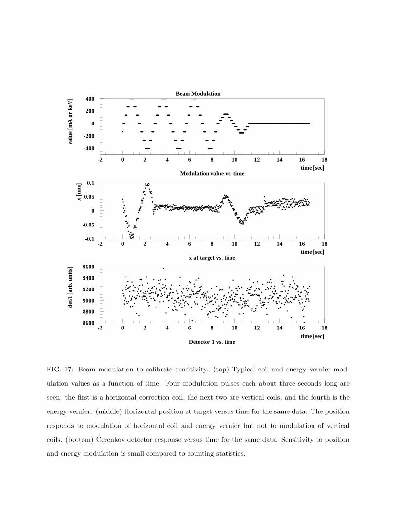
Beam Modulation
Modulation value vs. timetime [sec]
valu
e [m
A o
r ke
V]
x at target vs. timetime [sec]
x [m
m]
Detector 1 vs. timetime [sec]
det/
I [a
rb. u
nits
]
-400
-200
0
200
400
-2 0 2 4 6 8 10 12 14 16 18
-0.1
-0.05
0
0.05
0.1
-2 0 2 4 6 8 10 12 14 16 18
8600
8800
9000
9200
9400
9600
-2 0 2 4 6 8 10 12 14 16 18
FIG. 17: Beam modulation to calibrate sensitivity. (top) Typical coil and energy vernier mod-
ulation values as a function of time. Four modulation pulses each about three seconds long are
seen: the first is a horizontal correction coil, the next two are vertical coils, and the fourth is the
energy vernier. (middle) Horizontal position at target versus time for the same data. The position
responds to modulation of horizontal coil and energy vernier but not to modulation of vertical
coils. (bottom) Cerenkov detector response versus time for the same data. Sensitivity to position
and energy modulation is small compared to counting statistics.
42
V. ASYMMETRIES
In this section we describe how data are selected for analysis, how raw asymmetries are
extracted from the data, and how these raw asymmetries are corrected for systematic effects
due to helicity-correlated differences in beam parameters and to pedestals and nonlinearities
in the measured signals.
A. Data selection
The 1998 production quality data were generated by 78 Coulombs of electrons striking
the target; in 1999, 92 C struck the target. These totals exclude runs taken for diagnostic
purposes and a small number of runs in which equipment malfunctions serious enough to
compromise the quality of the entire run occurred; a typical run was about one hour.
We define a ‘data set’ as a group of consecutive runs taken with the same state (in or
out) of the insertable half-wave plate; the state of the half-wave plate was changed typically
after 24–48 hours of data-taking.
In our analysis of the production data, we impose a minimal set of cuts to reject unus-
able or compromised data. Our philosophy was never to cut on asymmetries (or helicity-
correlated differences), rather only to cut on absolute quantities. We reject any data in
which:
• The integrated current monitor signal falls below a value corresponding to 2% of the
maximum current. In practice the threshold value was not critical since the beam was
almost always either close to fully on or off.
• Any of several redundant checks for synchronization between ADC data and helicity
information fails. Since the helicity state arrives in the data stream eight windows
after the window it applied to, incorrect helicity assignment could result if one or more
windows are missing from the data stream due to DAQ deadtime. We therefore check
that the second window of each pair has helicity opposite the first; that the sequence of
helicity values read in hardware matches the prediction of a software implementation
of the same pseudorandom bit generator; and that the scaler used to count windows
increments by one at each window.
43
Whenever one or more consecutive windows fail one of these cuts, we also reject some
windows before and after the ones that failed. For example, when the current monitor
threshold cut is imposed, we also reject 10 windows before the BCM drops below threshold
and 50 windows after it comes back above threshold. This procedure eliminates not only
beam-off data but also conditions where the beam was ramping or the gains of our devices
were recovering from a beam trip.
Additional cuts are applied depending on what is being calculated. In effect there are five
different measurements being made using the same data: raw asymmetries in each of the
two detectors, helicity-correlated differences in beam parameters, and sensitivities of each of
the two detectors to changes in beam parameters. The additional cuts appropriate to each
measurement are discussed in the following subsections.
Integrated signals for each event include: D1 and D2, the Cerenkov detectors in the
two arms; I1, I2, IU , three beam current monitors (the two cavity monitors and the Unser
monitor); X1, Y1, X2, and Y2, two pairs of beam position monitors (BPMs) measuring
horizontal and vertical positions 7.5 and 1.3 m, respectively, upstream of the target; and
XE , a horizontal BPM located in a region of high dispersion 72.6 m upstream of the target.
(These five BPMs are also denoted Bi, where i = 1..5.) The analysis uses detector signals
normalized to the beam current, d1(2) ≡ D1(2)/I1.
B. Calculation of raw asymmetries
For each window pair of each run we compute asymmetries for various signals S,
A(S) =S+ − S−
S+ + S−(29)
Superscripts + and − refer to the two states of the Helicity signal originating at the
polarized electron source; a change in this signal corresponds to a helicity reversal of the
source laser beam. The relationship of this signal to the sign of the polarization of the
electron beam in the experimental hall depends on a number of factors: whether the half-
wave plate is present or not in the laser table optics, the beam energy (due to precession in the
accelerator arcs and the Hall A line), and the setup of the helicity Pockels cell electronics.
We use the Hall A polarimeters to determine the actual polarization sign relative to the
Helicity signal. For our 1998 and July 1999 data, with the half-wave plate in (out), the +
44

Helicity state corresponds to left (right) polarized electrons while the − state corresponds to
right (left) polarized electrons; for the April-May 1999 data the correspondence is opposite.
A change in the Pockels cell configuration between May and July accounts for the latter
difference, the small energy change having been compensated by adjustment of the Wien
filter at the source.
For example, we compute asymmetries for each Cerenkov detector normalized by the
beam current, A1(2) ≡ A(d1(2)); the summed normalized detectors, As ≡ A(d1 + d2); the
average value from the two detectors Aa ≡ (A(d1) + A(d2))/2; and the beam current, AI ≡A(I1). We also compute asymmetries for various non helicity-correlated voltage and current
sources as a check for electronic crosstalk.
In addition to the cuts on beam current and data acquisition dead time, cuts are applied
to reject data taken during a malfunction of the beam current monitor. For calculation of
A1(2) and As we also reject data taken during a malfunction of the magnets or detector in
that arm, or during times when there was significant boiling in the target.
For each run, we then compute averages of these asymmetries weighted by beam currents,
〈A(S)〉 =∑
k wkA(Sk)∑k wk
(30)
where the index k denotes pulse pair in the run and wk = I+1k+I−1k. Errors on these averages,
denoted δ〈A(S)〉, are estimated from widths of the distributions of A(S).
Finally, we compute average asymmetries over all runs in the data set
〈〈A(S)〉〉 =∑
j ǫjWj(S)〈A(S)〉j∑j Wj(S)
(31)
where the index j denotes the run, ǫj = ±1 depending on the sign of the measured beam
polarization, and Wj(S) = 1/δ2〈A(S)〉j.Figure 18 shows the asymmetries for the 1999 running periods broken down into data sets.
As expected, the asymmetry changed sign when the half-wave plate was inserted, but the
magnitude of the asymmetry is statistically compatible for all data sets. Similar behavior is
seen for the 1998 data [6].
Our analysis assumes the asymmetry distributions are Gaussian with widths dominated
by counting statistics. To check this, in Fig. 19 we plot the distribution of the quantity
((As)jk−〈As〉)/√2(I1)jk for the 1999 running periods. If counting statistics dominate, then
the distribution of this quantity should be Gaussian. We see that this is indeed the case,
45

FIG. 18: Raw asymmetries for 1999 running period, in ppm, broken down by data set. The circles
are for the left spectrometer, triangles for the right spectrometer. The step pattern represents the
effect of insertion/removal of the half-wave plate between data sets combined with a Pockels cell
reconfiguration between data sets 16 and 17; see text. The amplitude of the step is the average
value of the asymmetry over the entire run.
over seven orders of magnitude with no tails. Likewise, the run averages behave statistically
as can be seen in Fig. 20 where we plot the distribution of the quantity ((As)j−〈As〉)/δ(As)j
for the 1999 running periods; the distribution is Gaussian with unit width. The 1998 data
show similar behavior.
C. Calculation of helicity-correlated beam differences
For calculation of helicity-correlated beam position and energy differences, cuts are ap-
plied to reject data taken during a malfunction of the position monitors and data taken
while a beam modulation device was ramping. The difference in the ith BPM is denoted
∆Bi = B+i − B−
i .
Averages over each run 〈∆Bi〉 and over all runs in the data set 〈〈∆Bi〉〉 are computed
similarly to the asymmetry averages. For the latter, differences are weighted in the average
by Wj = 1/δ2〈As〉j , not by 1/δ2〈∆Bi〉j. The reason is that in a computation of an average
corrected asymmetry 〈〈As〉corr〉 = 〈〈As〉−∑
j aj〈∆Bj〉〉 (sec VD) the dominant error is δ〈As〉and the average over multiple runs of 〈∆Bj〉 weighted by 1/δ2〈As〉 is the relevant quantity.
46

Pair asymmetry residuals (normalized to current)
65,135,968pair entries
Normalized difference from average
1
10
10 2
10 3
10 4
10 5
10 6
-60000 -40000 -20000 0 20000 40000 60000
FIG. 19: Window pair asymmetries for 1999 running period, normalized by square root of beam
intensity, with mean value subtracted off, in ppm.
Run asymmetry residuals (normalized to error)
827 runentries
σ = 0.98
Fraction of sigma from average
0
20
40
60
80
100
120
-6 -4 -2 0 2 4 6
FIG. 20: Run asymmetries for 1999 running period, with mean subtracted off and normalized by
statistical error.
47

TABLE III: Beam position differences in nm, corrected for sign of beam polarization.
∆X1 ∆Y1 ∆X2 ∆Y2 ∆XE
1998 half-wave out −2.7± 2.9 1.9 ± 1.9 −1.9± 3.2 1.3± 2.8 20.9 ± 8.5
1998 half-wave in −2.3± 2.9 −1.1± 1.9 −2.9± 3.2 −0.1± 3.0 −0.8± 8.5
All 1998 data −2.5± 2.0 0.4 ± 1.4 −2.4± 2.3 0.7± 2.0 10.0 ± 6.0
Apr/May 1999 half-wave out −20.9 ± 3.1 −12.6 ± 1.5 −15.3± 5.2 12.7± 0.7 −47.3 ± 4.6
Apr/May 1999 half-wave in −1.0± 3.4 −5.9± 1.8 −5.8± 5.7 −3.7± 0.8 18.6 ± 5.1
All Apr/May 1999 data −11.9 ± 2.3 −9.8± 1.2 −11.0± 3.8 5.2± 0.5 −17.5 ± 3.4
Jul 1999 half-wave out −9.5± 5.5 −44.8± 10.4 87.2 ± 12.4 0.3± 3.2 −77.0± 10.6
Jul 1999 half-wave in 13.9 ± 4.6 11.4 ± 8.4 −53.8 ± 11.3 −5.8± 2.4 60.2 ± 9.6
All Jul 1999 data 4.3 ± 3.5 −10.8 ± 6.6 10.2 ± 8.4 −3.6± 1.9 −1.2± 7.1
The BPM differences for the three running periods and two half-wave plate settings are
given in Table III. Note that the differences for the two different half-wave plate states
tend to have opposite sign and thus partially cancel, reducing the size of their effect on the
experimental asymmetry.
D. Calculation of sensitivities to beam parameters
The helicity-correlated differences in beam parameters originate in the polarized source
and can give rise to differences in rates in the detectors and therefore false contributions
to the asymmetries. We compute normalized detector asymmetries corrected for beam
differences using
〈A〉corr = 〈A〉 − 〈∆A〉. (32)
The asymmetry correction ∆A is calculated by
〈∆A〉 = 1
2〈d〉
(5∑
j=1
(∂d
∂Bj
)〈∆Bj〉
)(33)
where 〈d〉 is the average normalized signal for the detector. We assume that the cross
section is a linear function of (x, y, θx, θy, E). Then ∂d/∂Bj is a quantity which describes the
sensitivity of the detector signal to changes in a combination of beam parameters measured
48
by the BPM. We obtain these partial derivatives by starting with the system of linear
equations
∂d
∂Ci
=5∑
j=1
∂d
∂Bj
∂Bj
∂Ci
(34)
and solving by matrix inversion
∂d
∂Bj=
5∑
i=1
∂d
∂Ci
(∂Bj
∂Ci
)−1
(35)
The slopes ∂d/∂Ci and ∂Bj/∂Ci describe the sensitivities of the normalized detectors
and the BPMs to changes in the beam modulation devices; the index i refers to the five
devices (four coils and one vernier). These slopes are calculated in offline analysis using
the beam modulation data. For each modulation cycle the BPM and detector data versus
coil or vernier offset value, Ci, are fit to straight lines, and the resulting slopes are averaged
over each run. Values for these slopes ∂d/∂Bj averaged over each run period are given in
Table IV.
We can write 〈∆A〉 =∑5
j=1 aj〈∆Bj〉 where aj = (∂d/∂Bj)/2〈d〉. The coefficients aj are
stable against changes in the gains of the detectors and BCMs, as shown in Fig. 21. The
helicity-correlated position differences in the beam monitors are shown in Fig. 22. Assuming
negligible correlations between these coefficients and the BPM differences, we may compute
corrections to asymmetries averaged over multiple runs using
TABLE IV: Summary of the detector asymmetry dependence on BPMs for the 1998 and 1999 runs.
All values are given in units of ppm/µm.
BPM Detector 1 Detector 2
1998 1999 1998 1999
XE −0.2± 0.05 −0.39± 0.02 0.5± 0.05 −0.32 ± 0.02
X1 −5.0± 0.7 −3.59± 0.09 3.5± 0.6 3.43 ± 0.09
X2 10.4 ± 0.9 9.07 ± 0.03 −4.8± 0.8 −3.04 ± 0.03
Y1 −0.50 ± 0.06 −0.51± 0.06 0.10 ± 0.05 0.61 ± 0.06
Y2 4.7 ± 0.03 2.48 ± 0.12 0.90 ± 0.03 −1.88 ± 0.12
49

Data Set Number0 2 4 6 8 10 12 14 16 18 20
m)
µ (
pp
m/
EX∂/ 1d∂ -1.2
-1-0.8-0.6-0.4-0.2
Data Set Number0 2 4 6 8 10 12 14 16 18 20
m)
µ (
pp
m/
EX∂/ 2d∂
-0.6
-0.4
-0.2
0
Data Set Number0 2 4 6 8 10 12 14 16 18 20
m)
µ (
pp
m/
1X∂/ 1d∂ -5
-4-3-2-101
Data Set Number0 2 4 6 8 10 12 14 16 18 20
m)
µ (
pp
m/
1X∂/ 2d∂ 1
234567
Data Set Number0 2 4 6 8 10 12 14 16 18 20
m)
µ (
pp
m/
2X∂/ 1d∂
9
10
11
12
Data Set Number0 2 4 6 8 10 12 14 16 18 20
m)
µ (
pp
m/
2X∂/
2d∂ -3.5
-3
-2.5
-2
-1.5
Data Set Number0 2 4 6 8 10 12 14 16 18 20
m)
µ (
pp
m/
1Y∂/ 1d∂ -1.5
-1
-0.5
0
Data Set Number0 2 4 6 8 10 12 14 16 18 20
m)
µ (
pp
m/
1Y∂/
2d∂ -0.5
0
0.5
1
Data Set Number0 2 4 6 8 10 12 14 16 18 20
m)
µ (
pp
m/
2Y∂/ 1d∂ 1
2
3
4
Data Set Number0 2 4 6 8 10 12 14 16 18 20
m)
µ (
pp
m/
2Y∂/ 2d∂
-3
-2
-1
0
1
FIG. 21: Representative sensitivity coefficients aj = (∂d/∂Bj)/2〈d〉 vs. data set for 1999 run, for
energy-sensitive position (top row), horizontal positions at locations on the beamline 7.5 m and
1.3 m upstream of the target (second and third rows), and vertical positions at 7.5 m and 1.3 m
(fourth and fifth rows). Left and right columns correspond to the two detectors. Units in all cases
are ppm/µm. Coefficients are seen to be stable at the level of estimated errors.
50
〈〈∆A〉〉 =5∑
j=1
〈aj〉〈〈∆Bj〉〉 . (36)
The corrections for each detector as a function of the data set are shown in Fig. 23. The
overall averages of the corrections are shown in Table V. The corrections are negligibly
small, as are their contribution to our systematic error.
TABLE V: Asymmetry corrections in parts per billion (ppb), 1999 data.
half-wave Detector 1 Detector 2 Average
plate state (ppb) (ppb) correction (ppb)
out 69± 49 −45± 21 14± 27
in 151 ± 51 −39± 21 60± 28
combined −36± 35 −3± 15 −20± 20
E. Pedestals and linearity
The signals produced by the beam monitors and Cerenkov detectors ideally are propor-
tional to the actual rates in those devices. In reality, however, these signals can deviate from
linearity over the full dynamic range and in general do not extrapolate to a zero pedestal.
For illustrative purposes, suppose a measured signal, Smeas, is a quadratic function of the
true rate, S:
Smeas = s0 + s1S + s2S2. (37)
Then in the approximation where |s0| ≪ |s1S| and |s2S2| ≪ |s1S|, the measured asymmetry
is
A(Smeas) ≈ A(S)
(1 +
s2S2
s1S− s0s1S
), (38)
i.e. the measured asymmetry is the true asymmetry, A(S), increased by the size of the
quadratic piece relative to the linear piece, and decreased by the size of the pedestal relative
to the linear piece (in the case where all the coefficients are positive).
51
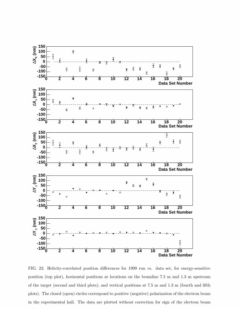
Data Set Number0 2 4 6 8 10 12 14 16 18 20
(n
m)
EX∆
-150-100
-500
50100150
Data Set Number0 2 4 6 8 10 12 14 16 18 20
(n
m)
1X∆
-150-100
-500
50100150
Data Set Number0 2 4 6 8 10 12 14 16 18 20
(n
m)
2X∆
-150-100
-500
50100150
Data Set Number0 2 4 6 8 10 12 14 16 18 20
(n
m)
1Y∆
-150-100
-500
50100150
Data Set Number0 2 4 6 8 10 12 14 16 18 20
(n
m)
2Y∆
-150-100
-500
50100150
FIG. 22: Helicity-correlated position differences for 1999 run vs. data set, for energy-sensitive
position (top plot), horizontal positions at locations on the beamline 7.5 m and 1.3 m upstream
of the target (second and third plots), and vertical positions at 7.5 m and 1.3 m (fourth and fifth
plots). The closed (open) circles correspond to positive (negative) polarization of the electron beam
in the experimental hall. The data are plotted without correction for sign of the electron beam
polarization. 52
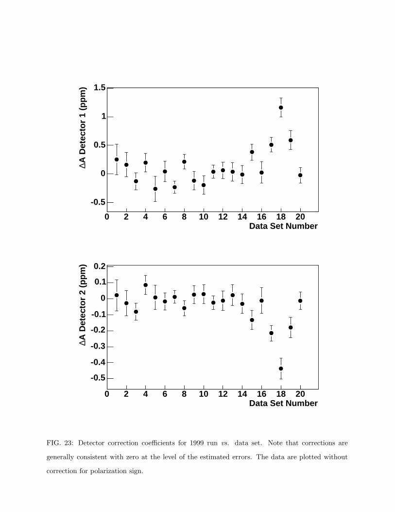
Data Set Number0 2 4 6 8 10 12 14 16 18 20
A D
etec
tor
1 (p
pm
)∆
-0.5
0
0.5
1
1.5
Data Set Number0 2 4 6 8 10 12 14 16 18 20
A D
etec
tor
2 (p
pm
)∆
-0.5
-0.4
-0.3
-0.2
-0.1
0
0.1
0.2
FIG. 23: Detector correction coefficients for 1999 run vs. data set. Note that corrections are
generally consistent with zero at the level of the estimated errors. The data are plotted without
correction for polarization sign.
53
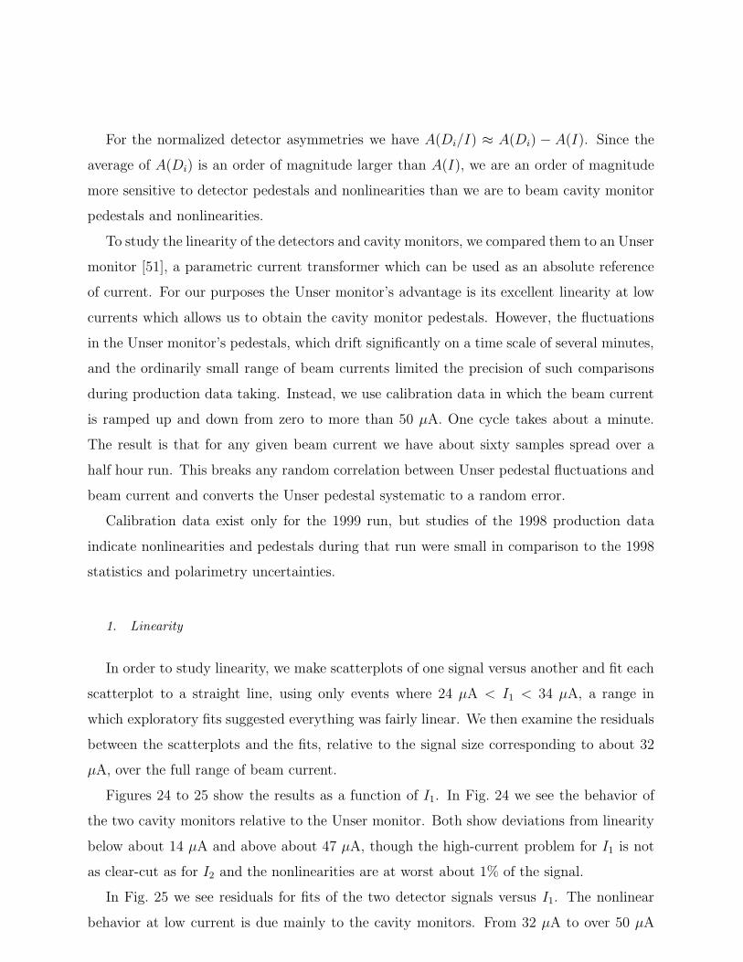
For the normalized detector asymmetries we have A(Di/I) ≈ A(Di) − A(I). Since the
average of A(Di) is an order of magnitude larger than A(I), we are an order of magnitude
more sensitive to detector pedestals and nonlinearities than we are to beam cavity monitor
pedestals and nonlinearities.
To study the linearity of the detectors and cavity monitors, we compared them to an Unser
monitor [51], a parametric current transformer which can be used as an absolute reference
of current. For our purposes the Unser monitor’s advantage is its excellent linearity at low
currents which allows us to obtain the cavity monitor pedestals. However, the fluctuations
in the Unser monitor’s pedestals, which drift significantly on a time scale of several minutes,
and the ordinarily small range of beam currents limited the precision of such comparisons
during production data taking. Instead, we use calibration data in which the beam current
is ramped up and down from zero to more than 50 µA. One cycle takes about a minute.
The result is that for any given beam current we have about sixty samples spread over a
half hour run. This breaks any random correlation between Unser pedestal fluctuations and
beam current and converts the Unser pedestal systematic to a random error.
Calibration data exist only for the 1999 run, but studies of the 1998 production data
indicate nonlinearities and pedestals during that run were small in comparison to the 1998
statistics and polarimetry uncertainties.
1. Linearity
In order to study linearity, we make scatterplots of one signal versus another and fit each
scatterplot to a straight line, using only events where 24 µA < I1 < 34 µA, a range in
which exploratory fits suggested everything was fairly linear. We then examine the residuals
between the scatterplots and the fits, relative to the signal size corresponding to about 32
µA, over the full range of beam current.
Figures 24 to 25 show the results as a function of I1. In Fig. 24 we see the behavior of
the two cavity monitors relative to the Unser monitor. Both show deviations from linearity
below about 14 µA and above about 47 µA, though the high-current problem for I1 is not
as clear-cut as for I2 and the nonlinearities are at worst about 1% of the signal.
In Fig. 25 we see residuals for fits of the two detector signals versus I1. The nonlinear
behavior at low current is due mainly to the cavity monitors. From 32 µA to over 50 µA
54

Fit of BCM1 to Unser current monitorCurrent [µΑ]
Res
idua
l [pe
rcen
t]
Fit of BCM2 to Unser current monitorCurrent [µΑ]
Res
idua
l [pe
rcen
t]
-1
-0.75
-0.5
-0.25
0
0.25
0.5
0.751
0 10 20 30 40 50 60
-1.2-1
-0.8-0.6-0.4-0.2
00.2
0 10 20 30 40 50 60
FIG. 24: (top) Residuals from fit of BCM1 to Unser data, as a fraction of the BCM1 pulse height
at 32 µA, versus beam current. (bottom) Same for fit of BCM2 to Unser.
the detectors are linear to well under 0.2%.
We may conclude that the detectors and cavity monitors are linear to well within the
required tolerances.
2. Pedestals
Detector pedestals were measured easily, by averaging the detector signals during times
when the beam is off. The resulting pedestals were always less than 0.3% of the signal
corresponding to the lowest stable beam current in the production data set, and typically
less than 0.06%; these pedestals are negligible.
The cavity monitor pedestals cannot be measured this way, since the cavity signals are
meaningless when the beam is off. Instead, we fit I1(2) to IU in the calibration data and
extrapolate to zero current. Such an extrapolation requires knowledge of the average Unser
55

Fit of Det1 to BCM1Current [µΑ]
Res
idua
l [pe
rcen
t]
Fit of Det2 to BCM1Current [µΑ]
Res
idua
l [pe
rcen
t]
-0.4-0.2
00.20.40.60.8
11.21.4
0 10 20 30 40 50 60
-0.5
0
0.5
1
1.5
0 10 20 30 40 50 60
FIG. 25: (top) Residuals from fit of detector 1 to BCM1 data, as a fraction of the detector 1 pulse
height at 32 µA, versus beam current. (bottom) Same for fit of detector 2 to BCM1.
pedestal, which is obtained from the beam-off data in the same run. The resulting pedestals
are less than 2% of the signal corresponding to the lowest stable beam current in the pro-
duction data set.
Are the cavity monitor pedestals obtained in the calibration data typical of the 1999
data? In order to answer this, we must make the reasonable assumption that the cavity
monitor linearities are stable at the negligible level seen in the calibration data. If that is
the case, then with negligible pedestals and nonlinearities for the detectors, a straight line
fit to a scatterplot of A(Dmeas) vs. A(Imeas) should give a slope equal to 1.0 if A(Imeas) is
computed with a corrected BCM signal in which the pedestal measured in the calibration
data is subtracted off. Any residual pedestals would give a deviation from unity equal to
the size of the pedestal relative to the size of the signal. We find that such deviations are
negligible.
56
3. Pedestal and linearity conclusions
No corrections for pedestals or nonlinearities need to be applied. The nonlinearities of the
detectors and cavity monitors were negligible over the dynamic range of the beam current
we ran. The pedestals for detectors and cavity monitors were negligible.
VI. NORMALIZATION
To extract physics results from the raw measured asymmetry, one needs to correct the
beam polarization, estimate and correct for any contributions from background processes,
and determine the average Q2 of the elastically-scattered electrons, weighted by the response
of the detectors. In addition one must apply radiative corrections and correct for the finite
acceptance. This section describes each of these steps of the data analysis.
A. Beam polarization
Transverse components of the beam polarization are a negligible source of systematic
error; the maximum analyzing power for a point nucleus is < 10−8 [68] and the trans-
verse component bounded by Møller polarimetry results was ≤ PZ sin(10) where PZ is the
longitudinal polarization. Explicit calculations of the vector analyzing power arising from
two-photon exchange diagrams, including proton structure effects, yield an analyzing power
of less than 0.1 ppm [69] for our kinematics. At different kinematics, a larger analyzing
power, (−15.4 ± 5.4)ppm, was measured in the SAMPLE experiment [70], in reasonable
agreement with the predicted value [69]; the much smaller value expected for our kinematics
is a consequence of the higher beam energy and small scattering angle. The left-right sym-
metry of the apparatus further suppresses our sensitivity to transverse components. The
determination of the magnitude of the polarization proceeded differently in the two running
periods, and is described below.
1. 1998 Run
For the 1998 running period, we used the Mott and Møller measurements to determine
the absolute beam polarization, averaged over the entire running period. This average was
57

used to correct the asymmetry averaged over the running period. The Compton polarimeter
was not yet available. The average of 16 Mott measurements yielded a polarization of
(40.5± 2.8)%. The quoted error is dominated by the systematic error due to extrapolation
to zero target foil thickness (5% relative error), background subtraction (3%), and observed
variations in the measured Pe with beam current (3%).
The average of several Møller measurements yielded 〈Pe〉 = (36.1± 2.5)%, in reasonable
agreement with the Mott results (note that the Møller results are 3% lower than those
reported in [6], due to a subsequent recalibration of the polarization of the target foil). The
uncertainty was dominated by knowledge of the foil polarization (5% relative error).
Averaging the Mott and Møller results we obtain the final result for the 1998 run of
〈Pe〉 = (38.2 ± 2.7)%. Note that we conservatively choose not to reduce the error by√2
when averaging the results.
2. 1999 Run
For the 1999 running periods, we used the Møller measurements to determine the absolute
beam polarization for each of the 20 data sets. These averages were used to correct the
asymmetries averaged over each data set. Typically there were between one and three
Møller measurements during each data set; these measurements were averaged to determine
〈Pe〉 for that data set. For two data sets there were no Møller measurements and 〈Pe〉 wasset to the average of 〈Pe〉 for the preceding and following data sets. The polarization average
over all the data sets was (68.8± 2.2)%.
At the time of this run, the Møller was fully commissioned, and the systematic errors were
reduced by more than a factor of two. Thus we did not make regular Mott measurements,
however those that were done were in reasonable agreement with the Møller results.
The Møller measurement is invasive, as it involves significantly reducing the beam current
and inserting the Møller target in the beam, and so these measurements were only made
at intervals. A possible concern is that the polarization may be varying between Møller
measurements, and thus a non-invasive, continuous measurement of the beam polarization
was desirable. This was provided in the 1999 run by the Compton polarimeter.
58

FIG. 26: Polarization of the JLab electron beam measured by the Møller (solid squares) and the
Compton (open circles) polarimeters during the entire 1999 run (upper plot) and July portion
(lower plot) where the Compton polarimeter was available. The error bar on the left-most Møller
point in the upper plot is its total error (dominated by systematic error 3.2% relative) while all
other points show only the statistical error, which for Møller data is smaller than the symbol (0.2%
relative).
3. Compton Polarimeter: 1999 Run Results
Under the conditions of the 1999 run (electron beam energy of 3.3 GeV and current of
40 µA) the measured Compton rate was 58 kHz and the experimental asymmetry was 1.3%.
Due to the high gain of the Fabry-Perot cavity coupled to a standard 300 mW laser, a
relative statistical accuracy of 1.4% was achieved within an hour, inside the analysis cuts.
All the systematic errors of the measurement discussed above in section IIIH 3 are listed in
Table II and lead to a total uncertainty of 3.3%.
Forty polarization measurements were performed by the Compton polarimeter in July
1999 in good agreement with measurements from the Møller polarimeter (see Fig. 26). They
provide, for the first time, an essentially continuous monitoring of the electron beam polar-
59
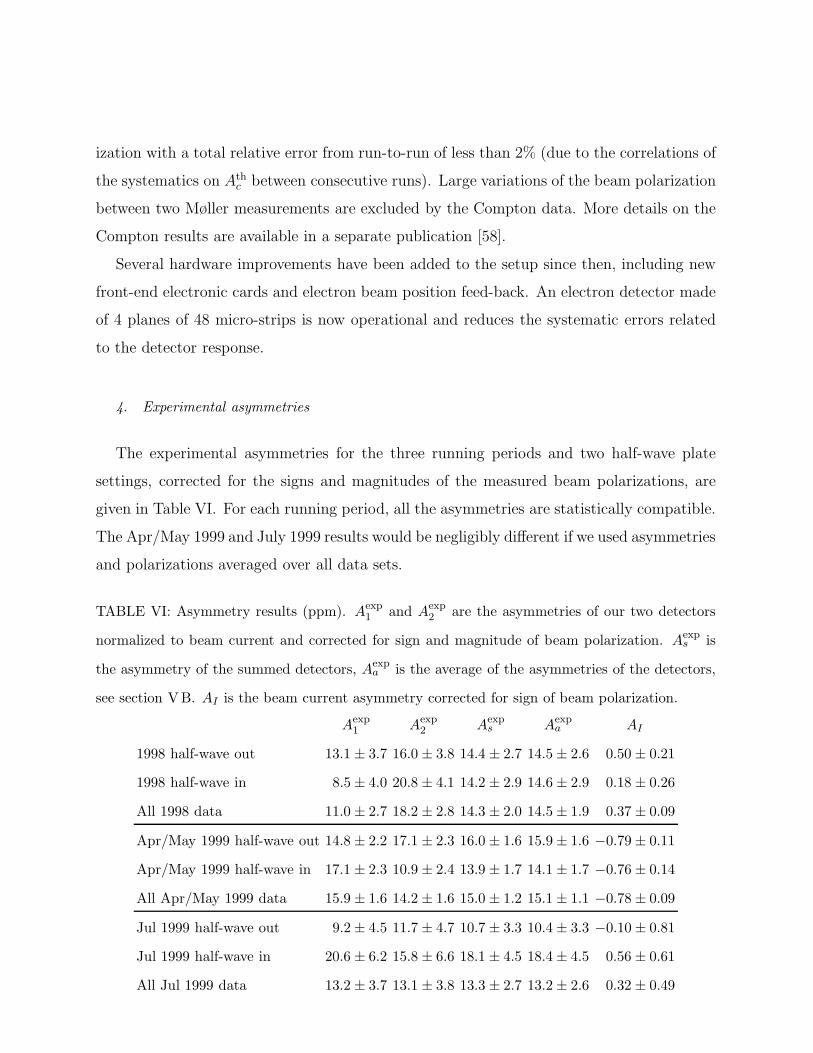
ization with a total relative error from run-to-run of less than 2% (due to the correlations of
the systematics on Athc between consecutive runs). Large variations of the beam polarization
between two Møller measurements are excluded by the Compton data. More details on the
Compton results are available in a separate publication [58].
Several hardware improvements have been added to the setup since then, including new
front-end electronic cards and electron beam position feed-back. An electron detector made
of 4 planes of 48 micro-strips is now operational and reduces the systematic errors related
to the detector response.
4. Experimental asymmetries
The experimental asymmetries for the three running periods and two half-wave plate
settings, corrected for the signs and magnitudes of the measured beam polarizations, are
given in Table VI. For each running period, all the asymmetries are statistically compatible.
The Apr/May 1999 and July 1999 results would be negligibly different if we used asymmetries
and polarizations averaged over all data sets.
TABLE VI: Asymmetry results (ppm). Aexp1 and Aexp
2 are the asymmetries of our two detectors
normalized to beam current and corrected for sign and magnitude of beam polarization. Aexps is
the asymmetry of the summed detectors, Aexpa is the average of the asymmetries of the detectors,
see section VB. AI is the beam current asymmetry corrected for sign of beam polarization.
Aexp1 Aexp
2 Aexps Aexp
a AI
1998 half-wave out 13.1 ± 3.7 16.0 ± 3.8 14.4 ± 2.7 14.5± 2.6 0.50 ± 0.21
1998 half-wave in 8.5± 4.0 20.8 ± 4.1 14.2 ± 2.9 14.6± 2.9 0.18 ± 0.26
All 1998 data 11.0 ± 2.7 18.2 ± 2.8 14.3 ± 2.0 14.5± 1.9 0.37 ± 0.09
Apr/May 1999 half-wave out 14.8 ± 2.2 17.1 ± 2.3 16.0 ± 1.6 15.9± 1.6 −0.79± 0.11
Apr/May 1999 half-wave in 17.1 ± 2.3 10.9 ± 2.4 13.9 ± 1.7 14.1± 1.7 −0.76± 0.14
All Apr/May 1999 data 15.9 ± 1.6 14.2 ± 1.6 15.0 ± 1.2 15.1± 1.1 −0.78± 0.09
Jul 1999 half-wave out 9.2± 4.5 11.7 ± 4.7 10.7 ± 3.3 10.4± 3.3 −0.10± 0.81
Jul 1999 half-wave in 20.6 ± 6.2 15.8 ± 6.6 18.1 ± 4.5 18.4± 4.5 0.56 ± 0.61
All Jul 1999 data 13.2 ± 3.7 13.1 ± 3.8 13.3 ± 2.7 13.2± 2.6 0.32 ± 0.49
60

Note that, for all the groups of data, Aexps (asymmetry of the summed signal from the two
detectors) and Aexpa (average asymmetry from the two detectors) are essentially identical,
with identical widths. This indicates that the two detectors are statistically independent,
demonstrating that both false asymmetries and target density fluctuations are negligibly
small.
B. Backgrounds
The two backgrounds that we observed were: 1) electrons that scattered inelastically
and then rebounded into the detector; and 2) electrons from the target aluminum walls. In
addition, we put an upper limit on the contribution from magnetized iron in the spectrom-
eter, based on measurements using a “proton tagging” technique, which was confirmed by
simulation. In this section we describe the corrections and systematic errors due to these
backgrounds.
1. Electrons from Inelastic Scattering
The main background to proton elastic scattering in the Hall A spectrometers near the
HAPPEX kinematics comes from electrons that scattered inelastically and then re-scattered
inside the spectrometer after the dipole. Much of this re-scattered debris is in the form of
low energy charged or neutral particles which contribute little to the integrated signal in our
calorimeter detector. The validity of this “re-scattering model” was studied with simulation
of the optics, as well as with a data set of e-P elastic scattering runs with energies and angles
nearby the HAPPEX running conditions. The energies varied from 3.2 to 4.0 GeV and angles
from 12.5 to 35. Several observables of background were studied from this data set, to
verify that they tracked with our model. The model was applied to the HAPPEX kinematics
to obtain the correction and systematic error for re-scattering from the π threshold through
the ∆ resonance region.
The re-scattering model is based on the assumption that the background, as a fraction of
the elastic scattering signal, is given by the following integral over the energy of the scattered
electron:
B =
∫ Emax
Ethr
dE Prs(E)×R(E) (39)
61
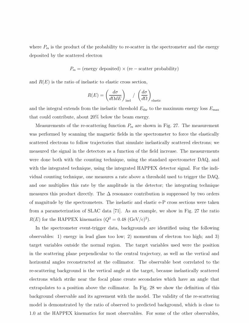
where Prs is the product of the probability to re-scatter in the spectrometer and the energy
deposited by the scattered electron
Prs = (energy deposited) × (re− scatter probability)
and R(E) is the ratio of inelastic to elastic cross section,
R(E) =
(dσ
dΩdE
)
inel
/
(dσ
dΩ
)
elastic
and the integral extends from the inelastic threshold Ethr to the maximum energy loss Emax
that could contribute, about 20% below the beam energy.
Measurements of the re-scattering function Prs are shown in Fig. 27. The measurement
was performed by scanning the magnetic fields in the spectrometer to force the elastically
scattered electrons to follow trajectories that simulate inelastically scattered electrons; we
measured the signal in the detectors as a function of the field increase. The measurements
were done both with the counting technique, using the standard spectrometer DAQ, and
with the integrated technique, using the integrated HAPPEX detector signal. For the indi-
vidual counting technique, one measures a rate above a threshold used to trigger the DAQ,
and one multiplies this rate by the amplitude in the detector; the integrating technique
measures this product directly. The ∆ resonance contribution is suppressed by two orders
of magnitude by the spectrometers. The inelastic and elastic e-P cross sections were taken
from a parameterization of SLAC data [71]. As an example, we show in Fig. 27 the ratio
R(E) for the HAPPEX kinematics (Q2 = 0.48 (GeV/c)2).
In the spectrometer event-trigger data, backgrounds are identified using the following
observables: 1) energy in lead glass too low; 2) momentum of electron too high; and 3)
target variables outside the normal region. The target variables used were the position
in the scattering plane perpendicular to the central trajectory, as well as the vertical and
horizontal angles reconstructed at the collimator. The observable best correlated to the
re-scattering background is the vertical angle at the target, because inelastically scattered
electrons which strike near the focal plane create secondaries which have an angle that
extrapolates to a position above the collimator. In Fig. 28 we show the definition of this
background observable and its agreement with the model. The validity of the re-scattering
model is demonstrated by the ratio of observed to predicted background, which is close to
1.0 at the HAPPEX kinematics for most observables. For some of the other observables,
62

FIG. 27: Results of scan of spectrometer magnetic fields to measure the probability to re-scatter
into the detector vs. the fractional difference from the nominal momentum setting. Inset: the ratio
of inelastic to elastic cross sections at the HAPPEX kinematics, (dσ/dΩdE)inel/(dσ/dΩ)elast.
the ratio was less than one since the observables measure only part of the background. Note
that for this comparison, instead of using the energy-weighted re-scattering function, we use
the probability to re-scatter into the focal plane which is measured by the magnet scan using
the individual counting technique.
Above Q2 = 2 (GeV/c)2 the model under-predicts the observed backgrounds and there
was a growing rate of pions seen with particle identification cuts that use the Cerenkov and
lead glass detectors. However, the model works fairly well within the range Q2 = 0.5 to 1.0
(GeV/c)2 where there are no pions. We conclude that re-scattering in the spectrometer is
the main source of background to e-P elastic scattering and is B = (0.20± 0.05)% of our
detected signal (Eq. 39).
The background is mainly due to the ∆ resonance (see Fig. 27). To compute the correction
63

FIG. 28: Top: Reconstructed vertical angle at the target, from triggered data; background from
re-scattering of inelastic electrons indicated by hatched area. Bottom: The ratio of observed to
predicted re-scattering background vs. Q2; the ratio is 1 in the region of our kinematics (Q2 = 0.48
(GeV/c)2). The line is a guide to the eye.
to our data, we use the predicted parity-violating asymmetry from the ∆ resonance [72]
APV∆ ≈ −GF |Q2|
2√2πα
(1− 2sin2θW ) (40)
The asymmetry is (−47±10) ppm at our Q2 which is 3 times as large as the asymmetry for
elastic scattering. In Ref. [72], various small additional terms and theoretical uncertainties
are discussed in detail, including non-resonant hadronic vector current background, axial
vector coupling, and hadronic contributions to electroweak radiative corrections. The extra
terms are typically 4% and have opposite signs that tend to cancel. We therefore ascribe a
conservative error of 20% to the asymmetry and arrive at a correction to our experimental
asymmetry of (0.06 ± 0.02) ppm, where the error includes the estimated systematic error
of the re-scattering model.
64

2. Quasielastic Scattering from the Target Walls
Scattering from the target aluminum windows contributed (1.4 ± 0.1)% to our detected
signal. This background can be observed in the reconstructed target position in the region
of momentum above the elastic peak, where one sees an enhancement in the target window
regions which is due to quasielastic scattering. A more direct measure of this background
was performed by inserting into the beam an empty aluminum target cell, similar to the one
used to contain liquid hydrogen, and measuring the signal in our detector. The thickness of
the empty target cell walls is about 10 times that of the walls used in the hydrogen cell, in
order to compensate for the radiative losses in the hydrogen cell.
The correction to our data arises from the neutrons in the aluminum target. The kine-
matic setup of the spectrometer selects electrons which have scattered quasielastically from
protons and neutrons in the aluminum. For quasielastic scattering from a nucleus with Z
protons and N neutrons, the expected parity-violating asymmetry is [73]
APVQE =
−GF |Q2|4√2πα
WPV
WEM(41)
where, following the notation of [73],
WEM = ǫ[Z(GpE)
2+N(Gn
E)2] + τ [Z(Gp
M )2+N(Gn
M)2]
and
WPV = ǫ[ZGpEG
pE +NGn
EGnE] + τ [ZGp
M GpM +NGn
MGnM ]
where the G’s are nucleon electromagnetic form factors, the G’s are the weak nucleon
form factors, ǫ, τ are the usual kinematic quantities (see definitions after Eq. 5) and we
have neglected small axial vector and radiative correction terms. The predicted asymmetry
for quasielastic aluminum scattering is -24 ppm at our Q2. We obtain a correction (0.12 ±0.04) ppm, where we have assumed that the asymmetry from this process is known with a
relative accuracy of 30%.
3. Magnetized Iron in the Spectrometer
Scattering from the magnetized iron in the spectrometer is a potential source of systematic
error because of the polarization dependent asymmetry in ~e, ~e scattering (Møller scattering).
In this section we describe the analysis which led to an upper bound for this effect.
65
Using the two HRS spectrometers we performed “proton tagging” measurements in which
we used protons from elastic e-P scattering to tag the trajectories of electrons. We set up
the two spectrometers slightly mispointed, so that for electrons that come close to the edge
of the acceptance, the corresponding protons are well within the proton arm acceptance.
Thus, the protons can tag electrons which might hit the magnetized iron of the pole tips.
To measure the backgrounds in the electron spectrometer we use the lead glass detector,
which is read out in a bias–free way for every proton trigger or other triggers. In the
low-energy tail of the energy spectrum, which contains backgrounds, we measure the excess
energy for events in which the electrons come closest to the pole tips. The excess is measured
relative to the energy spectra for electrons in the middle of the acceptance. No enhancement
was seen for the “poletip scattering” candidate events, and we placed an upper bound that
≪ 10−4 of the energy in our detector arises from poletip scattering.
Simulations of the magnetic optics confirmed these observations. The acceptance of
the spectrometer is defined primarily by the collimators, and secondarily by the first two
quadrupoles in the QQDQ design. Practically no high-energy rays strike magnetized iron. In
addition, secondaries from reactions in which particles which have struck the first elements
of the spectrometer tend to be low energy and get swept away before hitting the detector.
The correction to our data from poletip scattering is
dA = f Pe1 Pe2 A (42)
where f is the fraction of our signal (f ≪ 10−4), Pe1, Pe2 are the polarizations of the
scattered electron and the electron in the iron (Pe1 ∼ 0.8 and Pe2 ∼ 0.03), and A is the
analyzing power A ≤ 0.11. The result is conservatively dA ≪ 0.26 ppm and we make no
correction for this effect.
4. Backgrounds in HAPPEX Triggered Data
Backgrounds could be studied under the conditions of the experiment by using the
HAPPEX detector to define the trigger. A signal above a discriminator threshold was
used to trigger the spectrometer DAQ and read out the drift chambers and other detectors.
One small source of backgrounds was electron scattering from the aluminum frame of
the HAPPEX detector, observed in a correlation between the amplitude in the detector
66

and the track position. At the location of the detector frame a small enhancement ∼ 10−3
in low energy background was seen which in addition should have the same asymmetry
and is therefore a negligible systematic. The neutral particle component of background
from the HRS was measured as the energy-weighted sample of events which had no track
activity, and was a ≤ 0.2% background. For the charged particle component, the method
of analyzing the background was similar to what was described above for the e-P runs.
We reconstructed tracks and traced them back through the spectrometer to the collimator.
The percentage of tracks that miss an aperture is a measure of the background as well as
other problems including mis-reconstruction. One complication of placing the HAPPEX
detector near the drift chambers was that secondaries from showers splashed back into the
chambers, causing confusion in the reconstruction. In event displays such events were often
ambiguous with other background candidate events and could not be easily subtracted by
a pattern recognition algorithm. Other chamber problems included inefficiency, scattering
inside a chamber, two-track confusion due to overlap of two events, and events in which an
abnormal array of hits with bad fit χ2 existed in only one of the four chambers. This latter
category was easily eliminated. We eliminated many of the two-track events by rejecting
events in which one of the tracks had a good fit and was within 0.2 GeV of the elastic
peak. From the remaining sample, we obtained an upper bound ≤ 0.5% background which
is a weaker upper bound than that obtained from the re-scattering model. Because of the
limitations in reconstructing events at the 10−3 level we consider the re-scattering model to
be a more accurate assessment of our background.
5. Summary on Backgrounds
Table VII lists the backgrounds, the correction to our data, and the systematic error.
The total correction was +(0.18± 0.04) ppm, which represents a (1.2± 0.3)% correction to
the experimental asymmetry.
C. Measurement of Q2
The square of the four-momentum transfer is Q2 = 2EE ′(1− cos(θ)) where the three in-
gredients needed are the incident energy E, final energy of the electron E ′, and the scattering
67

TABLE VII: Backgrounds and Corrections.
Source Fraction Events A (ppm) Correction (ppm)
Inelastic e− 0.2 % -47 0.06 ± 0.02
Al walls (1.4 ± 0.1)% -24 0.12 ± 0.04
Magn. Iron ≪ 10−4 ≤ 2700 none
angle θ. For elastic scattering one may eliminate one of the three variables, which provides
a consistency check. The kinematics were E ∼ 3.3 GeV, θ = 12.5 (see table Table VIII).
The beam energy is measured by two methods to an accuracy of about 1 MeV. One
apparatus, called the arc method [74], measures the deflection of the beam in the arc of
magnets that lead into the experimental hall, for which the integral of the field is precisely
known. A second apparatus, called the e-P method [75], measures the kinematics in e-P
coincidences on hydrogen. When we assumed that beam energy was correctly measured in
the 1999 run, we found that an −8 MeV (−0.2%) adjustment was needed for the Q2 in
the 1998 run to be consistent with elastic scattering after known corrections for angle and
momentum calibration of the scattered electron. Based on this, and based on the history
of comparisons of the two energy apparatus, we have assigned a very conservative 10 MeV
error to our energy measurement.
A second ingredient required for the Q2 determination is the momentum of the scattered
electron. We adjusted the momentum scale by a few tenths of a percent in order to satisfy
the missing mass constraint for elastic scattering. Subsequently, the magnet constants were
measured by an independent group and found to agree within 0.1% of our values.
The largest error in Q2 comes from the scattering angle. There are two ingredients
here: 1) surveys measure the angle of the spectrometer’s optic axis relative to the incident
beam direction; and 2) the spectrometer reconstruction code reconstructs the horizontal
and vertical angles at the target relative to the optic axis using tracking detectors in the
focal plane. Calibration of the optical transfer matrix for the spectrometers is performed by
sieve slit runs in which the optical transfer matrix of the spectrometers is calibrated in the
following way. A 0.5 cm thick tungsten plate with a rectangular pattern of holes covering
the acceptance (sieve slit) is placed at the entrance of the spectrometers, and tracks in the
focal plane are used to reproduce the hole pattern through a χ2 minimization procedure.
68
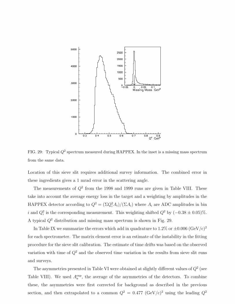
FIG. 29: Typical Q2 spectrum measured during HAPPEX. In the inset is a missing mass spectrum
from the same data.
Location of this sieve slit requires additional survey information. The combined error in
these ingredients gives a 1 mrad error in the scattering angle.
The measurements of Q2 from the 1998 and 1999 runs are given in Table VIII. These
take into account the average energy loss in the target and a weighting by amplitudes in the
HAPPEX detector according to Q2 = (ΣQ2iAi)/(ΣAi) where Ai are ADC amplitudes in bin
i and Q2i is the corresponding measurement. This weighting shifted Q2 by (−0.38 ± 0.05)%.
A typical Q2 distribution and missing mass spectrum is shown in Fig. 29.
In Table IX we summarize the errors which add in quadrature to 1.2% or±0.006 (GeV/c)2
for each spectrometer. The matrix element error is an estimate of the instability in the fitting
procedure for the sieve slit calibration. The estimate of time drifts was based on the observed
variation with time of Q2 and the observed time variation in the results from sieve slit runs
and surveys.
The asymmetries presented in Table VI were obtained at slightly different values ofQ2 (see
Table VIII). We used Aexpa , the average of the asymmetries of the detectors. To combine
these, the asymmetries were first corrected for background as described in the previous
section, and then extrapolated to a common Q2 = 0.477 (GeV/c)2 using the leading Q2
69
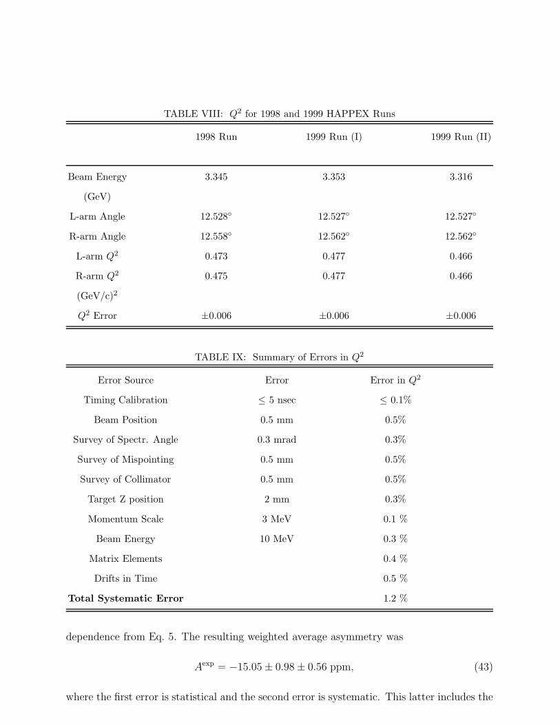
TABLE VIII: Q2 for 1998 and 1999 HAPPEX Runs
1998 Run 1999 Run (I) 1999 Run (II)
Beam Energy 3.345 3.353 3.316
(GeV)
L-arm Angle 12.528 12.527 12.527
R-arm Angle 12.558 12.562 12.562
L-arm Q2 0.473 0.477 0.466
R-arm Q2 0.475 0.477 0.466
(GeV/c)2
Q2 Error ±0.006 ±0.006 ±0.006
TABLE IX: Summary of Errors in Q2
Error Source Error Error in Q2
Timing Calibration ≤ 5 nsec ≤ 0.1%
Beam Position 0.5 mm 0.5%
Survey of Spectr. Angle 0.3 mrad 0.3%
Survey of Mispointing 0.5 mm 0.5%
Survey of Collimator 0.5 mm 0.5%
Target Z position 2 mm 0.3%
Momentum Scale 3 MeV 0.1 %
Beam Energy 10 MeV 0.3 %
Matrix Elements 0.4 %
Drifts in Time 0.5 %
Total Systematic Error 1.2 %
dependence from Eq. 5. The resulting weighted average asymmetry was
Aexp = −15.05± 0.98± 0.56 ppm, (43)
where the first error is statistical and the second error is systematic. This latter includes the
70

errors in the beam polarization, background subtraction, helicity-correlated beam properties,
and Q2.
D. Finite Acceptance
To interpret the experimental asymmetry given in Eq. 43, one must correct for the effect
of averaging over the finite acceptance of the detectors and the effect of radiation on the
effective kinematics of the measurement. A Monte Carlo simulation was developed for this
purpose, and is described below.
1. Monte Carlo
As the acceptance of the HRS spectrometers is dictated by their entrance collimators, the
simulation involved generating elastically scattering electrons along the length of the target,
with realistic account of the materials in the target region, and tracking the events to the
collimators. First-order magnetic optics of the spectrometers were then used to determine
the location and momentum of the electrons at the focal plane detectors. The measured
analog response of the focal plane detectors, as a function of the position of the hit along
the detector, was taken as a weighting factor on the asymmetry (this weighting had a ∼ 1%
effect compared to pure counting statistics). Account was taken of ionization energy loss in
the target, both before and after the scattering.
Bremsstrahlung was included in the simulation in both the initial and final state. In the
extreme relativistic limit, hard photon radiation is strongly peaked in the forward angle,
and so the angle peaking approximation [76] was adopted.
The radiated cross section σradwas calculated as a convolution of integrals along the
incident and scattered electron directions [77]. With Es the incident electron energy, Ep the
final electron energy, t the location of the scattering along the target of length T , t1(t) and
t2(t) the material thickness in radiation lengths before and after the scattering respectively,
we have
σrad(Es, Ep) = (1 + δf )
∫ T
0
dT
T
∫ 1
0
dy1I1(y1, t1)
∫ 1
0
dy2I2(y2, t2)σ(E′s, E
maxp )Θ(Ep −Ecut) (44)
71

where y1 and y2 are the fractional radiative energy losses before and after the scattering,
σ(E ′s, E
maxp ) is the unradiated cross section for elastic scattering of electrons of energy E ′
s =
ES(1− y1) into energy Emaxp , where
Emaxp =
E ′s
1 + 2(E ′s/M) sin2(θ/2)
(45)
with M the proton mass and θ the scattering angle; the final electron energy is therefore
Ep = Emaxp (1 − y2). The lower-energy cutoff in the spectrometer acceptance is Ecut. The
intensity factors I1(y1, t1) and I2(y2, t2) are given by
I(y, t) =Φ(y, t)
yexp
(∫ y
1
dy′Φ(y′, t)
y′
)(46)
with
Φ(y, t) = tv(1− y) +4
3t
(1− y +
3
4y2)
. (47)
The first term represents the effect of internal bremsstrahlung, which was dealt with using
an equivalent virtual radiator [77] of thickness
tv =α
π
[ln
(Q2
m2
)− 1
]. (48)
The second term in Eq. 47 represents the ‘complete screening approximation’ [78] calculation
of external bremsstrahlung.
Finally, the factor (1+δf ) in Eq. 44 is the lowest order correction to the running coupling
constant α2(Q2),
δf(Q2) ≈ 2α
π
[13
12ln
(Q2
m2
)− 28
18
]. (49)
The primary effect of bremsstrahlung was to radiate about 20% of the elastic events out
of the detector acceptance, and to lower the effective Q2 by about 0.1%, a negligible amount.
2. Effective Kinematics
Due to both the finite acceptance of the spectrometer and radiative energy losses, the
measured asymmetry represents a convolution over a range of Q2. To account for this, and to
present a value of the asymmetry for a single Q2, we calculated an average incident electron
energy and effective scattering angle for the experiment, and then used the simulation to
calculate the factor needed to correct the acceptance-averaged asymmetry to that from point
scattering at the effective kinematics.
72
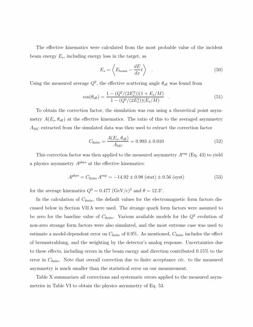
The effective kinematics were calculated from the most probable value of the incident
beam energy Es, including energy loss in the target, as
Es =
⟨Ebeam − dE
dxt
⟩. (50)
Using the measured average Q2, the effective scattering angle θeff was found from
cos(θeff) =1− (Q2/(2E2
s ))(1 + Es/M)
1− (Q2/(2E2s ))(Es/M)
. (51)
To obtain the correction factor, the simulation was run using a theoretical point asym-
metry A(Es, θeff) at the effective kinematics. The ratio of this to the averaged asymmetry
AMC extracted from the simulated data was then used to extract the correction factor
Cfinite =A(Es, θeff)
AMC= 0.993± 0.010 (52)
This correction factor was then applied to the measured asymmetry Aexp (Eq. 43) to yield
a physics asymmetry Aphys at the effective kinematics:
Aphys = CfiniteAexp = −14.92± 0.98 (stat)± 0.56 (syst) (53)
for the average kinematics Q2 = 0.477 (GeV/c)2 and θ = 12.3.
In the calculation of Cfinite, the default values for the electromagnetic form factors dis-
cussed below in Section VIIA were used. The strange quark form factors were assumed to
be zero for the baseline value of Cfinite. Various available models for the Q2 evolution of
non-zero strange form factors were also simulated, and the most extreme case was used to
estimate a model-dependent error on Cfinite of 0.9%. As mentioned, Cfinite includes the effect
of bremsstrahlung, and the weighting by the detector’s analog response. Uncertainties due
to these effects, including errors in the beam energy and direction contributed 0.15% to the
error in Cfinite. Note that overall correction due to finite acceptance etc. to the measured
asymmetry is much smaller than the statistical error on our measurement.
Table X summarizes all corrections and systematic errors applied to the measured asym-
metries in Table VI to obtain the physics asymmetry of Eq. 53.
73
TABLE X: Asymmetry corrections and systematic errors.
Source Correction δA/A(%) δA/A(%)
(1998) (1999)
Statistics − 13.3 7.2
Pe − 7.0 3.2
Q2 − 1.8 1.8
Backgrounds 1.2 0.6 0.6
Radiative corrections -0.1 0.1 0.1
Finite acceptance 0.7 0.9 0.9
VII. RESULTS AND INTERPRETATION
A. Electromagnetic and Axial Form Factors
The extraction of the strange quark form factors GsE and Gs
M from the measured asym-
metry (Eq. 53) requires knowledge of the other form factors entering into Eq. 5: the purely
electromagnetic form factors GγpE , Gγp
M , GγnE , and Gγn
M , as well as the neutral weak axial
form factor GZpA . Uncertainties in these form factors contribute significantly to the total
uncertainty in the extracted strange form factors.
In the time since our initial publications [6, 7], there has been considerable progress made
on precision measurements of these form factors (see [79] for a review). In the following we
describe how values for the form factors, interpolated to our Q2, were extracted from world
data, and we reassess our extraction of the strange form factors in light of the recent data.
1. GZpA
As mentioned earlier, the contribution of the neutral weak axial form factor GZpA to the
measured asymmetry is suppressed for our kinematics (forward-angle scattering, where ǫ′ is
small). This form factor can be decomposed into terms involving the well-known charged-
current axial form factor and ∆s, the first moment of the strange quark momentum distri-
butions. The latter, as measured in deep inelastic scattering, while not precisely measured,
is small for our purposes [16]. The former at Q2 = 0 is the axial vector coupling constant
74
gA, which is well measured [47], and the Q2 evolution of the form factor is well reproduced
with a dipole form. However, GZpA suffers from large electroweak radiative corrections, which
include hadronic uncertainties, and which are problematic to calculate. These corrections
have been calculated by Zhu et al. [87], and lead to a predicted effect on our measured
asymmetry of 0.56± 0.23 ppm (the hadronic uncertainties in the axial radiative correction
dominate the error on this prediction).
This prediction was cast into some doubt with the results from the SAMPLE collabora-
tion on backward-angle parity-violating quasielastic scattering from a deuterium target [81].
When combined with their measurement on a hydrogen target [82, 83], they extracted a
value for GZpA in significant disagreement with the calculation of Zhu et al., leading to specu-
lation of large ‘anapole moment’ contributions. However, more recent data from SAMPLE,
along with a reanalysis of the earlier data [84] now yields excellent agreement with the Zhu
et al. calculation, and so there is no longer reason to doubt that the axial contribution is
under adequate control.
2. GγpM
The proton’s magnetic form factor is quite precisely known at our kinematics, and it
deviates only slightly from the dipole form factor GD = [1 +Q2/(0.71 (GeV/c)2)]−2. We
adopt the value GγpM/µpGD = 0.9934 at Q2 = 0.477 (GeV/c)2 using the recent fit of Brash
et al. [85]. This fit is a reanalysis of the magnetic form factor obtained from Rosenbluth
separation data, using as an additional constraint the results on GγpE /G
γpM obtained with
polarization transfer techniques. An almost identical value GγpM/µpGD = 0.9940 at Q2 =
0.477 (GeV/c)2 was found from the empirical fits of Friedrich and Walcher [86]. The value
also agrees within 0.3% with the one we adopted in our earlier publication [7].
As the other electromagnetic form factors are often measured relative to GγpM , we will
express them relative to this value, and subsume its small uncertainty in the errors assigned
to the other form factors.
75
3. GγpE
The situation with regard to the proton’s electric form factor is unsettled at present. The
recent high-precision measurements from Jefferson Lab of the ratio GγpE /G
γpM using recoil
polarization techniques [93, 94] differ significantly from older results that used Rosenbluth
separation techniques (see [95] for a review of the situation). There are recent suggestions
that this discrepancy could be the result of contributions from two-photon exchange [96, 97]
which may have a large effect on the Rosenbluth separation data at large Q2. We note,
however, that at our lower Q2 the difference between the values of GγpE extracted from the
recoil polarization data and those from the Rosenbluth data is small. Adopting the empirical
fit of Friedrich and Walcher [86], which is based on both polarization data and Rosenbluth
data at lower Q2, yields GγpE /(G
γpM/µp) = 0.98 at Q2 = 0.477 (GeV/c)2; a similar value of
GγpE /(G
γpM/µp) = 0.97 is obtained from the empirical fit of Arrington [95]. We adopt the
former value with a 2% uncertainty, which is essentially the same as we used previously [7].
4. GγnE
In our previous publications [6, 7] the largest uncertainty arising from an electromagnetic
form factor was that due to the electric form factor of the neutron, GγnE . Since those
publications appeared, the situation for GγnE has improved dramatically, due to new precise
results using polarization techniques now available from Jefferson Lab [87, 88, 89] and Mainz
[90], as well as a new analysis that obtained GγnE from data on the quadrupole form factor in
elastic electron-deuteron scattering [92]. Individual measurements now have uncertainties
at roughly the 10% level, and the recent results, which conveniently bracket our Q2, are
satisfactorily consistent.
To extract the value of GγnE at our Q2, we use the fit to a Galster form [91] provided by
Madey et al. [88], which gives µpGγnE /G
pM = 0.161 ± 0.006 at Q2 = 0.477 (GeV/c)2. This
fit was based on the world data from polarization measurements as well as the analysis of
the deuteron quadrupole form factor. It did not include the very recently reported result of
Warren et al. [89], however the fit agrees with the Warren et al. datum at Q2 = 0.5 within
1σ. A similar fit was presented by Warren at al., which did not include the Madey et al.
datum, but nevertheless agreed with the Madey et al. result at their Q2 = 0.447 (GeV/c)2.
76
That fit also gave a value consistent within 3.6% with that from the Madey et al. fit at our
Q2. To be conservative, we enlarge the error from the Madey fit to 5% and thus adopt the
value µpGγnE /G
pM = 0.161± 0.008 at Q2 = 0.477 (GeV/c)2. The central value is essentially
unchanged from that used previously [7], however the error bar has been reduced by almost
a factor of 4. The contribution to the error in APV due to the uncertainty in GγnE is now less
than those due to other form factors (GγnM and Gγp
E ); see Table XI.
5. GγnM
The largest contribution to our error due to electromagnetic form factors is that due to
the neutron’s magnetic form factor, GγnM . Results from two new experiments have appeared
since our earlier publications [6, 7]. These are the measurements from Mainz of Kubon et
al. [98] and from JLab of Xu et al. [99]. The former span a range of Q2 from 0.071 to 0.894
GeV2, and the later, while somewhat less precise, report data for Q2 ranging from 0.3 to 0.6
GeV2, including points (Q2 = 0.4, 0.5 (GeV/c)2) close to our own kinematics.
Kubon et al. [98] provide an empirical fit to their data along with other recent data onGγnM
[100, 101, 102]. While the recent results of Xu et al. [99] were not included in the fit, the fit
does an excellent job of reproducing them, with agreement to better than 2%. We note that
this agreement exhibits the compatibility of results obtained from very different experimental
techniques, with different model dependences, and thus builds confidence in the values of
GγnM extracted. Thus we adopt the Kubon et al. fit to interpolate to Q2 = 0.477 (GeV/c)2
and extract the value (GγnM )/µn)/(G
γpM/µp) = 1.004± 0.040 (in order to be conservative, we
have inflated the uncertainty in the fit from Kubon et al. by a factor of 3). This new value
is somewhat lower than the value of 1.05± 0.02 adopted previously by us [7].
A different fit for GγnM , using a somewhat different database of results, and a very dif-
ferent functional form, was obtained by Friedrich and Walter [86], and it yields the value
(GγnM )/µn)/(G
γpM/µp) = 1.039 at Q2 = 0.477 (GeV/c)2, in reasonable agreement with the fit
of Kubon et al..
We note, however, that both fits discard the results of Bruins et al. [103] and Markowitz et
al. [104]. The former has been criticized [105] due to potential difficulties with the extraction
of their neutron detection efficiency, however a direct measurement of that efficiency is
planned [106]. If the results from Bruins et al. are adopted at face value, this would have a
77

very significant effect on our extracted strange form factors. Finally, we note that there are
new data from the CLAS at JLab presently under analysis, which should help clarify the
situation [107].
In summary, the two significant changes that recent data have made to the information on
the electromagnetic form factors, compared to that of our previous result [7], are the signifi-
cantly improved precision on GγnE (without a change in the central value) and a change in the
best estimate of GγnM . The latter causes a shift in the extracted strange quark contribution
compared to that presented in Ref. [7] (the shift is small compared to the statistical error).
The effect of the form factors on the predicted asymmetry is summarized in Table XI.
TABLE XI: Electromagnetic form factors at the present Q2, normalized to (GγpM/µp), and their
contribution to the error in ppm on the theoretical asymmetry APV.
Form Factor Value δA (ppm)
GγpE /(Gγp
M/µp) 0.98 ± 0.02 0.33
GγnE /(Gγp
M/µp) 0.161 ± 0.008 0.15
(GγnM )/µn)/(G
γpM/µp) 1.004 ± 0.040 0.48
B. Strange Quark Form Factors
Using Eq. 5 and the result in Eq. 53, along with the calculated GZpA and the known values
of the proton and neutron form factors in Table XI, we may solve for the linear combination
of strange form factors GsE + βGs
M where β = τGγpM/ǫG
γpE = 0.392 at our kinematics. We
obtain
GsE + βGs
M = 0.014± 0.020± 0.010 (54)
where the first error is the total experimental error (statistical and systematic errors added
in quadrature) and the second error is the error due to the “ordinary” electromagnetic form
factors and is dominated by GnM . Since [7] the central value has reduced slightly, though
less than the error bar, and the error due to electromagnetic form factors has reduced. This
result is consistent with zero strangeness contribution to the vector matrix elements of the
proton. However, the result could also be zero due to a cancellation of GsE and Gs
M at our
78

-0.4 -0.2 0 0.2 0.4
-0.2
-0.1
0
0.1
0.2
G sM
Gs
E
(24)
(36)
(35)
(44)
(25)
(25)
(30)
(45)(41)
FIG. 30: Plot of GsE vs Gs
M at Q2 = 0.477(GeV/c)2. The band is the allowed region derived
from our results. The width of the band is the total error computed in quadrature. The points
are estimates from various models that make predictions at our Q2. The numbers in ref. [25] are
plotted twice due to an ambiguity in the predicted sign. This plot is similar to Fig. 4 in [7] except
that the central value and error bars have both reduced slightly, and three new models shown in
circles have since been published.
Q2. The SAMPLE experiment [46, 83, 108], which is sensitive to GsM at Q2 = 0.1(GeV/c)2
as well as the axial form factor GZpA , also found a very small strangeness contribution which
is consistent with zero.
Numerous theoretical models have been formulated to predict the strangeness form fac-
tors. The problem is one of nonperturbative QCD since ms ≃ ΛQCD. In some cases the
models are considered to be only an order of magnitude estimate, and in other cases only
an upper bound to the strangeness effects. The large variety of models with very different
physics assumptions is indicative of the difficulty in making solid predictions. See also the
discussion in section II and refs [23, 24, 25, 26, 27, 28, 29, 30, 31, 32, 33, 34, 35, 36, 37, 38,
39, 40, 41, 42, 43, 44, 45].
Most models focus on predictions of the static moments ρs and µs at Q2 = 0. A subset
of the models attempt to predict the form factors at our Q2, shown as points in Fig. 30,
together with our result for GsM + βGs
M displayed as a line with an error band representing
the two errors in Eq. 54 added in quadrature. The numbers near the points in Fig 30 are
79

the references for those models. The square points are the models displayed in Fig. 4 of our
previous publication [7]. The circle points are from three models published since [7] which
predict relatively small strangeness form factors that are in good agreement with our data.
In two of the models [41, 45] the authors predicted a likely range (1σ) of form factors which
is indicated by the error bars in the figure for those two points.
Several of the models make predictions which will be tested by future measurements,
including the HAPPEX-2 experiment [109], He4 parity [110], G0 [111], and the Mainz A4
parity experiments [112]. These measurements will be necessary to separate GsE and Gs
M
and determine their Q2 dependence.
VIII. CONCLUSIONS
The HAPPEX results reported in this paper have provided a stringent test of strange
qq contributions to the vector matrix elements of the proton. Our results still allow for
strangeness effects of a few percent or the possibility of accidental cancellation at our kine-
matics. It will be important to complete the program of approved parity experiments at
Jefferson Lab [109, 110, 111] and elsewhere [112] to quantify the strangeness effects over
a range of kinematics and over various distance scales in the nucleon. These experiments
should yield a detailed mapping of the spatial dependence of ss contributions to nucleon
structure.
In this paper we have reported details of the experimental technique and data analysis.
We have described methods for minimizing helicity correlations of the polarized electron
beam from a strained GaAs crystal. Because of the highly stable beam at Jefferson Lab
we were able to acquire precise data that were nearly free of systematic error. This bodes
well for future applications of parity violating electron scattering to various physics topics
including future searches for strange sea effects [109, 110, 111, 112], precision studies of the
standard model [113, 114] and measurements of neutron densities in nuclei [115, 116, 117].
IX. ACKNOWLEDGMENTS
We wish to thank the entire staff at Jefferson Lab for their exemplary effort in devel-
oping and operating the facility, and particularly C. K. Sinclair and M. Poelker for their
80

essential work on the polarized source. This work was supported by DOE contract DE-
AC05-84ER40150 under which the Southeastern Universities Research Association (SURA)
operates the Thomas Jefferson National Accelerator Facility, and by the Department of
Energy, the National Science Foundation, the Korean Science and Engineering Foundation
(Korea), the Istituto Nazionale di Fisica Nucleare (Italy), the Natural Sciences and Engi-
neering Research Council of Canada, the Commissariat a l’Energie Atomique (France), and
the Centre National de Recherche Scientifique (France).
[1] J. Ashman et al., Phys. Lett. B 206 (1988) 364; Nucl. Phys. B 328 (1988) 527. Nucl. Phys.
B 328 (1989) 1.
[2] D. B. Kaplan and A. Manohar, Nucl. Phys. B 310 (1988) 527.
[3] R. D. McKeown, Phys. Lett. B 219 (1989) 140.
[4] E. J. Beise and R. D. McKeown, Comments Nucl. Part. Phys. 20 (1991) 105.
[5] D. H. Beck, Phys. Rev. D 39 (1989) 3248.
[6] K. Aniol et al., [HAPPEX Collaboration], Phys. Rev. Lett. 82, 1096 (1999).
[7] K. Aniol et al., [HAPPEX Collaboration], Phys. Lett. B509, 211 (2001).
[8] G.A. Rutledge, Ph.D. thesis, College of William and Mary, 2001.
[9] G.W. Miller, Ph.D. thesis, Princeton U., 2001.
[10] J. Jardiller, Ph.D. thesis (in French), U. Blaise Pascal, 2001.
[11] W.E. Kahl, Ph.D. thesis, Syracuse U., 2000.
[12] T.B. Humensky, Ph.D. thesis, Princeton U., 2003.
[13] B.T. Tonguc, Ph.D. thesis, Syracuse U., 2003.
[14] A. O. Bazarko et al., Z. Phys. C 65 (1995) 189; M. Gonchorov et al., Phys. Rev. D64 (2001)
112006.
[15] B. Adeva et al., Phys. Lett. B 302, (1993) 533; P.L. Anthony et al., Phys. Rev. Lett. 71
(1993) 959; D. Adams et al., Phys. Lett. B 329 (1994) 399.
[16] K. Abe et al., Phys. Rev. Lett 74 (1995) 346.
[17] J. Ellis and R.L. Jaffe, Phys. Rev. D 9 (1974) 1444; 10 (1974) 1669.
[18] B. Adeva et al., Phys. Rev. D 58 (1998) 112002.
[19] K.S. Kumar and P.A. Souder, Prog. Part. Nucl. Phys. 45 (2000) S333.
81

[20] D.H. Beck and R.D. McKeown, Ann. Rev. Nucl. Part. Sci. 51 (2001) 189.
[21] D.H. Beck and B.R. Holstein, Int. J. Mod. Phys. E10 (2000) 1.
[22] M.J. Musolf et al., Phys. Rep. 239 (1994) 1.
[23] R.L. Jaffe, Phys. Lett. B 229, 275 (1989).
[24] H.-W. Hammer, U.-G. Meissner, and D. Drechsel, Phys. Lett. B 367, 323 (1996).
[25] H.-W. Hammer and M.J. Ramsey-Musolf, Phys. Rev. C 60, 045204 (1999); ibid 60, 045205
(1999); erratum ibid 62, 049902 (2000); 63, 049903 (2000).
[26] H. Forkel, Phys. Rev. C 56, 510 (1997)..
[27] H. Forkel, M. Nielsen, X. Jin, and T. Cohen, Phys. Rev. C 50, 3108 (1994).
[28] S.-T. Hong, B.-Y. Park, and D.-P. Min, Phys. Lett. B 414, 229 (1997).
[29] P. Geiger and N. Isgur, Phys. Rev. D 55. 299 (1997).
[30] V. E. Lyubovitskij, P. Wang, Th. Gutsche, and A. Faessler, Phys. Rev. C 66, 055204 (2002).
[31] B.-Q. Ma, Phys. Lett. B 408, 387 (1997).
[32] D.O. Riska, Nucl. Phys. A 678, 79 (2000).
[33] L. Hannelius, D.O. Riska, and L.Ya. Glozman, Nucl. Phys. A 665, 353 (2000).
[34] N.W. Park, J. Schechter, and H. Weigel, Phys. Rev. D 43, 869 (1991).
[35] N.W. Park and H. Weigel, Nucl. Phys. A 541, 453 (1992).
[36] H. Weigel et al., Phys. Lett. B 353, 20 (1995).
[37] U.-G. Meissner, V. Mull, J. Speth, J.W. Van Orden, Phys. Lett. B 408, 381 (1997).
[38] W. Koepf, E.M. Henley, and J.S. Pollock, Phys. Lett. B 288, 11 (1992).
[39] M.J. Musolf and M. Burkhardt, Z. Phys. C 61, 433 (1994).
[40] H. Ito, Phys. Rev. C 52, R1750 (1995).
[41] A. Silva, H.-C. Kim, and K. Goeke, Phys. Rev. D 65, 014016 (2002), Erratum-ibid. D 66,
039902 (2002).
[42] T. Hemmert, U.-G. Meissner, and S. Steininger, Phys. Lett. B 437, 184 (1998).
[43] T. Hemmert, B. Kubis, and U.-G. Meissner, Phys. Rev. C 60, 045501 (1999).
[44] S.J. Dong, K.F.Liu, and A.G. Williams, Phys. Rev. D 58, 074504 (1998).
[45] R. Lewis, W. Wilcox, and R.M. Woloshyn, Phys. Rev. D 67, 013003 (2003).
[46] B. Mueller et al., Phys. Rev. Lett 78 (1997) 3824.
[47] Particle Data Group, R.M. Barnet et al., Phys. Rev. D 54 (1996) 1.
[48] M.J. Musolf and B.R. Holstein, Phys. Rev. Lett B 242 (1990) 461.
82
[49] T. Powers, L. Doolittle, R. Ursic, and J. Wagner, Proc. 7th Workshop on Beam Instrumen-
tation, AIP Conf.Proc. 390, Ed. A.. Lumpkin and C.E. Eyberger (1997); JLAB-TN-96-021.
[50] J. Alcorn et al., accepted by Nucl. Instrum. Methods (2003).
[51] K. Unser, IEEE Trans. Nucl. Sci. NS-28 (1981) 2344. T. Powers, L. Doolittle, R. Ursic, and
J. Wagner, Proc. 7th Workshop on Beam Instrumentation, AIP Conf.Proc. 390, Ed. A.
Lumpkin and C.E. Eyberger (1997); JLAB-TN-96-021.
[52] CERNOX resistor, Lakeshore Cryogenics.
[53] Allen-Bradley, http://www.ab.com.
[54] Experimental physics and industrial control system (EPICS),
http://www.aps.anl.gov/epics/.
[55] W.A. Watson et al., CODA: A Scalable, Distributed Data Acquisition System, in Proc. of
the Real Time 1993 Conference, p. 296; G. Heyes et al., The CEBAF Online Data Acqui-
sition System, in Proc. of the CHEP Conference, 1994, p. 122; D.J. Abbott et al., CODA
Performance in the Real World, 11th IEEE NPSS Real Time 199 Conference, JLab-TN-99-12
(1999).
[56] C.K. Sinclair, “Electron Beam Polarimetry”, Tech Note JLAB-ACC-98-04; T.J. Gay and
F.B. Dunning, Rev. Sci. Instrum. 63 (1992) 1635; T.J. Gay et al., Rev. Sci. Instrum. 63
(1992) 114. S. Mayer et al., Rev. Sci. Instrum. 64 (1993) 952.
[57] J.S. Price et al., Proc. 13th Symposium on High Energy Spin Physics (SPIN98) Protvino,
Russia, 8-12 September 1998, Ed. N.E. Tyurin, V.L. Solovianov, S.M. Troshin, and A . G.
Ufimtsev, (World Scientific) 1999; JLab Technical Note ACC-97-27, 1997 (unpublished).
[58] M. Baylac et al., Phys. Lett. B 539, 8 (2002).
[59] D. Neyret et al., Nucl. Instrum. Methods A 443, 231 (2000).
[60] J.P. Jorda et al., Nucl. Instrum. Methods A 412, 1 (1998).
[61] N. Falletto et al., Nucl. Instrum. Methods A 459, 412 (2001).
[62] M. Baylac, Ph.D. thesis, U. Claude Bernard Lyon I, # 212-2000 ; Report
CEA/DSM/DAPNIA/SPhN-00-05-T (unpublished).
[63] G. D. Cates et al., Nucl. Instrum. Methods, A 278 (1989) 293-317.
[64] T. B. Humensky et al., SLAC-PUB-9381. Submitted to Nucl. Instrum. Methods A (2002).
[65] D.A. Edwards and M.J. Syphers, An Introduction to the Physics of High Energy Accelerators,
Wiley Interscience (1993).
83

[66] E.D. Courant and H.S. Snyder, Annals of Physics 3(1) (1958) 1.
[67] Y. Chao, “Measuring and Matching Transport Optics at Jefferson Lab”, Proceedings of the
2003 Particle Accelerator Conference, Portland, Oregon, 2003.
[68] N.F. Mott, Proc. R. Soc. London, Ser A 135, 429 (1932); ibid. 124, 425 (1929).
[69] A. Afanasev, I. Akushevic, N.P. Merenkov, Workshop on Exclusive Process at High Momen-
tum Transfer, Jefferson Lab, May 15-18, 2002; hep-ph/0208260.
[70] S.P. Wells et al., Phys. Rev. C 63, 064001 (2001).
[71] L.W. Whitlow et al., Phys. Lett. B 282 (1992) 475; Phys. Lett. B 250 (1990) 193.
[72] N.C. Mukhopadhyay et al., Nucl. Phys. A 633, 481 (1998).
[73] M.J. Musolf and T.W. Donnelly, Nucl. Phys. A 546, 509 (1992); Erratum-ibid A 550, 564
(1992).
[74] D. Marchand, Ph.D. Thesis, U. Clermont-Ferrand, 1998.
[75] O. Ravel et al., Nucl. Instrum. Methods, A 409, 611 (1998).
[76] S. Stein et al., Phys. Rev. D 12, 1884 (1975).
[77] L.W. Mo and Y.S. Tsai, Rev. Mod. Phys. 41, 205 (1969).
[78] Y.S. Tsai, Rev. Mod. Phys. 46, 815 (1974).
[79] H. Gao, Int. J. Mod. Phys E 12, 1 (2003).
[80] S.L. Zhu, S.J. Puglia, B.R. Holstein, and M.J. Ramsey-Musolf. Phys. Rev. D 62, 033008
(2000); M.J. Musolf and B.R. Holstein, Phys. Lett. B 242, 461 (1990).
[81] R. Hasty et al., Science, 290, 2117 (2000).
[82] B. Mueller et al., Phys. Rev. Lett. 78, 3824 (1997).
[83] D.T. Spayde et al., Phys. Rev. Lett. 84, 1106 (2000).
[84] T.M. Ito et al., nucl-ex/03100001; E. Beise, private communication (2003).
[85] E.J. Brash, A. Kozlov, Sh. Li, and G.M. Huber, Phys. Rev. C 65, 051001(R) (2002).
[86] J. Friedrich and Th. Walcher, Eur. Phys. J A 17, 607 (2003).
[87] H. Zhu et al., Phys. Rev. Lett. 87, 081801 (2001).
[88] R. Madey et al., Phys. Rev. Lett. 91, 122002 (2003).
[89] G. Warren et al., nucl-ex/0308021
[90] J. Bermuth et al., Phys. Lett B 564, 199 (2003).
[91] S. Galster, H. Klein, K.H. Scmidt, D. Wegener, and J. Bleckwenn, Nucl. Phys. B 32, 221
(1971).
84

[92] R. Schiavilla and I. Sick, Phys. Lett C 64, 041002(R) (2001).
[93] M.K. Jones at al., Phys. Rev. Lett. 84, 1398 (2000).
[94] O. Gayou at al., Phys. Rev. Lett. 88, 092301 (2002).
[95] J. Arrington, Phys. Rev. C 68, 034325 (2003).
[96] P.A.M. Guichon and M. Vanderhaeghen Phys. Rev. Lett. 91, 142303 (2003).
[97] P.G. Blunden, W. Melnitchouk, J.A. Tjon, Phys. Rev. Lett. 91, 142304 (2003).
[98] G. Kubon et al., Phys. Lett. B 524, 26 (2002).
[99] W. Xu et al., Phys. Rev. C 67, 012201(R) (2003).
[100] H. Anklin et al., Phys. Lett. B 336, 313 (1994); H. Anklin et al. Phys. Lett B 428, 248
(1998).
[101] H. Gao et al., Phys. Rev. C 50, R546 (1994).
[102] W. Xu et al., Phys. Rev. Lett. 85, 2900 (2000).
[103] E.E.W. Bruins et al, Phys. Rev. Lett. 75, 21 (1995).
[104] P. Markowitz et al., Phys. Rev. C 48, R5 (1993).
[105] J. Jourdan, I. Sick, J. Zhao, Phys. Rev. Lett. 79, 5186 (1997).
[106] E.E.W. Bruins et al., Phys. Rev. Lett. 79, 5187 (1997).
[107] Jefferson Lab Expt. 94-017, W. Brooks and M. Vineyard, spokespersons; W. Brooks, private
communication (2003).
[108] E.J. Beise nucl-ex/0309008; R. Hasty et al., Science 290 (2000) 2117
[109] HAPPEX-II Experiment E99-115, K.S. Kumar and D. Lhuillier, spokespersons.
[110] He4 Parity Experiment E00-114, D. Armstrong and R. Michaels, spokespersons.
[111] G0 Experiment E00-006, D.H. Beck, spokesperson.
[112] Mainz A4 Parity Experiment, D. von Harrach, spokesperson.
[113] The Qweak Experiment, J. Bowman, R. Carlini, J.M. Finn, S. Kowalski, and S. Page,
spokespersons.
[114] Letter of Intent to Measure Parity Violating DIS from Deuterium, X. Zheng, spokesperson.
[115] C. J. Horowitz, Phys. Rev. C 57, 3430 (1998).
[116] C. J. Horowitz, S. Pollock, P. Souder, and R. Michaels, Phys. Rev. C 63, 025501 (2001).
[117] The PREX Experiment, JLab proposal E03-011, P. Souder, G. Urciuoli, R. Michaels,
spokespersons
85
Related Documents

![arXiv:0910.5768v3 [hep-ex] 5 Feb 2010](https://static.cupdf.com/doc/110x72/586a291d1a28aba47b8bc050/arxiv09105768v3-hep-ex-5-feb-2010.jpg)

![arXiv:0902.3231v1 [nucl-ex] 18 Feb 2009](https://static.cupdf.com/doc/110x72/62088c2dbf2696302d3f4db2/arxiv09023231v1-nucl-ex-18-feb-2009.jpg)


![arXiv:2102.12228v1 [nucl-ex] 24 Feb 2021](https://static.cupdf.com/doc/110x72/624d6761eb03bc30ff735e31/arxiv210212228v1-nucl-ex-24-feb-2021.jpg)