arXiv:hep-th/0412081v2 25 Feb 2005 N = 4 “Fake” Supergravity

arX

iv:h

ep-t

h/04

1208

1v2

25

Feb

2005

SU-ITP-05/003hep-th/0412081

N = 4 “Fake” Supergravity

Marco Zagermann

Department of Physics, Stanford University,Varian Building, Stanford, CA 94305-4060, USA.

Abstract

We study curved and flat BPS-domain walls in 5D, N = 4 gauged supergravity and show thattheir effective dynamics along the flow is described by a generalized form of “fake supergravity”.This generalizes previous work in N = 2 supergravity and might hint towards a universal behav-ior of gauged supergravity theories in supersymmetric domain wall backgrounds. We show thatBPS-domain walls in 5D, N = 4 supergravity can never be curved if they are supported by thesupergravity scalar only. Furthermore, a purely Abelian gauge group or a purely semisimple gaugegroup can never lead to a curved domain wall, and the flat walls for these gaugings always exhibita runaway behavior.

e-mail: [email protected]

Contents

1 Introduction 1

2 True and fake 5D, N = 2 supergravity 32.1 5D, N = 2 gauged supergravity . . . . . . . . . . . . . . . . . . . . . . . . . 42.2 Curved and flat BPS-domain walls . . . . . . . . . . . . . . . . . . . . . . . 62.3 The relation to (N = 2) “fake” supergravity . . . . . . . . . . . . . . . . . . 8

3 BPS-domain walls in N = 4 fake and true supergravity 133.1 Ungauged 5D, N = 4 supergravity . . . . . . . . . . . . . . . . . . . . . . . 143.2 5D, N = 4 gauged supergravity . . . . . . . . . . . . . . . . . . . . . . . . . 173.3 BPS-domain walls . . . . . . . . . . . . . . . . . . . . . . . . . . . . . . . . . 183.4 Consistency conditions and domain wall curvature . . . . . . . . . . . . . . . 233.5 Special cases . . . . . . . . . . . . . . . . . . . . . . . . . . . . . . . . . . . . 25

4 Conclusions 27

A The flatness condition 28

1 Introduction

Domain wall solutions of (d + 1)-dimensional supergravity theories have received a lot of

attention during the past few years. This interest was largely driven by applications in

the context of holographic renormalization group flows and certain brane world models. In

most of these applications, the domain walls of interest preserve a fraction of the original

supersymmetry of the supergravity theory they are embedded in. A domain wall of this type

can be either Minkowski-sliced or AdS-sliced,

ds2 = e2U(r)gmn(x) dxm dxn + dr2, (1.1)

depending on whether, respectively, gmn is the metric of d-dimensional Minkowski- or Anti-

de Sitter space. A non-trivial warp factor U(r) (i.e., one that does not give rise to (d + 1)-

dimensional Minkowski- or Anti-de Sitter space) requires a nontrivial scalar profile φx(r)

(x = 1, . . . , m), as dictated by the Einstein equations. A domain wall thus defines a curve

φx(r) on the scalar manifold.

The allowed scalar manifolds in supergravity theories are in general highly constrained

and strongly depend upon the spacetime dimension, the amount of supersymmetry, as well

as on the type of multiplet the scalars are sitting in. The geometrical constraints on the

scalar manifolds also leave their trace in the BPS-equations of the scalar fields, which are

likewise highly spacetime-, supersymmetry- and multiplet dependent.

1

It came therefore as quite a surprise when it was found in [1] that one can reformulate

the BPS-conditions for domain walls in 5D, N = 2 supergravity in such a way that their

naive strong multiplet dependence effectively disappears. The same is true for the scalar

potential, which, in this simplified reformulation, also contains the scalar fields from vector

and hypermultiplets in a symmetric way. In order to achieve this simplification, one has

to restrict one’s attention to the effective dynamics along the curve φx(r) of a given BPS-

domain wall and properly “integrate out” the orthogonal scalar fields. Interestingly, this

also exactly reproduces the equations of “fake supergravity” that were introduced in ref. [2]

to prove the stability of domain walls in certain scalar/gravity theories that, despite some

superficial similarities, are not necessarily supersymmetric1. The fake supergravity formalism

in [2] was tailor-made to describe curved domain walls and generalizes and refines the earlier

work [4–6]. It was worked out in [2] in detail for theories with only one scalar field, and

it is this scalar field that one has to identify with the scalar direction along the flow curve

φx(r) in 5D, N = 2 supergravity. The fake supergravity equations were also generalized to

several scalar fields in [2], but only for a very particular type of scalar potential. One of the

lessons of [1], however, is that a generalization and covariantization to more than one scalar

field can go along various different lines, and it seems that only the effective one-scalar field

formulation is universal.

The results of [1] are by no means of only formal interest. On the contrary, it was

found that the simplified reformulation of true supergravity a la fake supergravity provides

a very handy tool for studying true BPS-domain walls themselves. For example, using the

simplified language of “fake” supergravity, it is fairly easy to prove that BPS-domain walls

that are only supported by scalars from vector multiplets can at most be Minkowski-sliced.

An AdS-sliced BPS-domain wall thus must involve non-trivial hypermultiplet scalars. This

fact had gone unnoticed before.

In this paper, we will go one step beyond the work of [1] and study domain walls in

5D, N = 4 supergravity along similar lines. That is, we will try to similarly recast the

BPS-equations and the scalar potential in a generalized “fake” supergravity form. This

generalization is highly nontrivial due to the following reasons:

• The BPS-constraints are stronger, as there are now twice as many supersymmetries to

preserve.

• The N = 4 theory is Usp(4) ∼= SO(5) instead of Usp(2) ∼= SU(2) covariant, i.e.,

several peculiarities of the group SU(2) no longer hold.

• The scalar manifolds in theN = 4 theory are of the type SO(1, 1)× SO(5, n)/(SO(5)×1Some related work appeared in [3].

2

SO(n)), which are, in general, neither very special nor quaternionic manifolds. Con-

trary to what happens in rigid supersymmetry, the N = 4 theory can therefore not be

viewed as a special case of the N = 2 theory.

Given these differences, it is all the more intriguing that only few features of the N = 2

formulation are identified as SU(2) artifacts and that one finds an exactly analogous picture:

The effective BPS-equations and the scalar potential can again be brought to a simple,

generalized “fake” supergravity-type form, no matter whether the running scalar field sits

in the N = 4 supergravity multiplet or in an N = 4 vector or tensor multiplet. Just as

in the N = 2 analogue [1], we can also use this simplified language in order to study the

domain walls themselves. It is found that BPS-domain walls that are supported by the

supergravity scalar only are necessarily flat. Similarly, if the gauge group is purely Abelian

or purely semisimple, the domain wall can at most be flat, no matter by which type of scalar

field they are supported. Any flat domain wall for these gaugings, however, has a runaway

behaviour. These results could prove very useful for studies of holographic renormalization

group flows [7] in the setup of, e.g., [8] or for domain walls in gauged supergravities that

derive from flux compactifications (see e.g., [9–11] for some recent work in this direction).

Moreover, the present work suggests that the language of “fake supergravity” is far more

universal than previously thought and that it might well be applicable to a much wider range

of gauged supergravity theories, perhaps, if properly formulated, even to all of them. Fake

supergravity might thus turn out to be not that fake after all!

The organization of this paper is as follows: In section 2, we briefly recapitulate the

structure of BPS-domain walls in 5D, N = 2 gauged supergravity and the relation to the

fake supergravity formalism developed in [2]. In section 3, we then discuss the structure of

5D, N = 4 gauged and ungauged supergravity and study its 1/2-supersymmetric domain

wall solutions. This is done by rewriting the BPS-equations and the scalar potential in a

generalized, “N = 4” fake supergravity form. In this simplified version, several general state-

ments about possible BPS-domain walls are easily derived. We end with some conclusions

in section 4. Appendix A proves the equivalence of two flatness conditions.

2 True and fake 5D, N = 2 supergravity

In this section, we briefly summarize the key results of [1] on BPS-domain walls in true and

fake, 5D, N = 2 supergravity. For earlier work on (smooth) flat and curved BPS-domain

walls in these theories, see [12–22] and [23–27], respectively.

3

2.1 5D, N = 2 gauged supergravity

Five-dimensional, N = 2 supergravity can be coupled to vector-, tensor- and hypermultiplets.

The precise form of these theories was derived in the original references [28–34], to which we

refer the reader for further details. As was emphasized already in [17, 35], all the terms in

the theory that are due to the presence of tensor multiplets have to vanish on a BPS-domain

wall background, and we can thus restrict ourselves to the coupling of nV vector multiplets

and nH hypermultiplets to supergravity.

The bosonic field content of such a theory consists of the funfbein emµ , (nV + 1) vector

fields AIµ (I = 0, 1, . . . , nV ) and (nV + nH) real scalar fields (ϕx, qX), with x = 1, . . . , nV

and X = 1, . . . , 4nH . Here, we have combined the graviphoton of the supergravity multiplet

with the nV vector fields of the nV vector multiplets to form a single (nV + 1)-plet AIµ.

The nV scalar fields ϕx of the vector multiplets parameterize a “very special” real man-

ifold MVS, i.e., an nV -dimensional hypersurface of an auxiliary (nV + 1)-dimensional space

spanned by coordinates hI (I = 0, 1, . . . , nV ) :

MVS = hI ∈ R(nV +1) : CIJKh

IhJhK = 1, (2.1)

where the constants CIJK appear in a Chern-Simons-type coupling of the Lagrangian. On

MVS, the hI become functions of the nV physical scalar fields, ϕx. The metric, gxy, on the

very special manifold is determined via

gxy = −3CIJK(∂xhI)(∂yh

J)hK . (2.2)

The scalars qX (X = 1, . . . , 4nH) of nH hypermultiplets, on the other hand, take their

values in a quaternionic-Kahler manifoldMQ [36], i.e., a manifold of real dimension 4nH with

holonomy group contained in SU(2)×USp(2nH). The vielbein on this manifold is denoted by

f iAX , where i = 1, 2, and A = 1, . . . , 2nH refer to an adapted SU(2)×USp(2nH) decomposition

of the tangent space. The hypercomplex structure is (−2) times the curvature of the SU(2)

part of the holonomy group, denoted as RrZX (r = 1, 2, 3), so that the quaternionic identity

reads

RrXYRsY Z = −1

4δrs δX

Z − 12εrstRt

XZ . (2.3)

The vector fields AIµ can be used to gauge up to (nV + 1) isometries of the quaternionic

manifold MQ (provided such isometries exist)2.

The quaternionic Killing vectors, KXI (q), that generate these isometries on MQ can be

expressed in terms of the derivatives of SU(2) triplets of Killing prepotentials (or “moment

2A non-Abelian gauge group also has to leave the CIJK invariant, which implies that the gauge groupalso has to be a subgroup of the isometry group of MV S [29, 31, 34, 37].

4

maps”) P rI (q) (r = 1, 2, 3) via

DXPrI = Rr

XYKYI , ⇔

KYI = −4

3RrY XDXP

rI

DXPrI = −εrstRs

XYDY P t

I ,(2.4)

where DX denotes the SU(2) covariant derivative, which contains the SU(2) connection ωrX

with curvature RrXY :

DXPr = ∂XP

r + 2 εrstωsXP

t, RrXY = 2 ∂[Xω

rY ] + 2 εrstωs

XωtY . (2.5)

The prepotentials have to satisfy the constraint

1

2Rr

XYKXI K

YJ − εrstP s

I PtJ +

1

2fIJ

KP rK = 0, (2.6)

where fIJK are the structure constants of the gauge group. In this section, we will frequently

switch between the above vector notation for su(2)-valued quantities such as P rI , and the

usual (2× 2) matrix notation,

PI =(

PIij)

, PIij ≡ i σri

jP rI , (2.7)

where boldface expressions such as PI refer to the (2 × 2)-matrices with the indices i, j

suppressed. Turning on only the metric and the scalars, the Lagrangian of such a gauged

supergravity theory is

e−1L = −1

2R− 1

2gxy∂µϕ

x∂µϕy − 1

2gXY ∂µq

X∂µqY − g2V(ϕ, q), (2.8)

whereas the supersymmetry transformation laws of the fermions are given by

δψµi = ∇µǫi − ωµijǫj −

i√6g γµP

ji ǫj , (2.9)

δλxi = − i

2γµ(∂µϕ

x)ǫi − g Pijxǫj , (2.10)

δζA =i

2f iAX γµ(∂µq

X)ǫi − gN iAǫi. (2.11)

Here, ψiµ, λ

xi , ζ

A are the gravitini, gaugini and hyperini, respectively, g denotes the gauge

coupling, the SU(2) connection ωµ is defined as ωµij = (∂µq

X)ωXij, and

P r = hI(ϕ)P rI (q), (2.12)

P rx = −√

3

2gxy∂yP

r (2.13)

N iA =

√6

4f iAX (q)hI(ϕ)KX

I (q). (2.14)

5

As usual, the potential is given by the sum of “squares of the fermionic shifts” (the scalar

expressions in the above transformations of the fermions):

V = −4P rP r + 2P xrP yrgxy + 2N iAN jBεijCAB, (2.15)

where CAB is the (antisymmetric) symplectic metric of USp(2nH). Using (2.4) and the

quaternionic identity (2.3), the scalar potential for vector and hypermultiplets can be written

in the form

V 2 = 4P2 − 3(∂xP)(∂xP)− (DXP)(DXP). (2.16)

One clearly sees that the scalars of the vector- and hypermultiplets enter the supersymmetry

transformations and the scalar potential in a rather different way.

2.2 Curved and flat BPS-domain walls

In this paper, we are interested in Minkowski-sliced (“flat”) and AdS-sliced (“curved”) do-

main walls of the form

ds2 = e2U(r)gmn(x) dxm dxn + dr2 (2.17)

with gmn(x) being either the 4D Minkowski-metric or a metric of AdS4 with curvature scale

L4. In a curved domain wall background of the form (2.17), when the scalar fields only

depend on the radial coordinate r, the vanishing of the supersymmetry variations (2.9)-

(2.11) implies

[

∇AdS4

m + γm

(

1

2U ′γ5 −

ig√6P

)]

ǫ = 0, (2.18)

[

Dr + γ5

(

− ig√6P

)]

ǫ = 0, (2.19)

[

γ5ϕx′ + ig

√6 gxy∂yP

]

ǫ = 0, (2.20)

f iAX

[

γ5qX′ − ig

√

8

3RrXYDY P

r

]

ǫi = 0, (2.21)

where

Drǫi ≡ ∂rǫi − qX′ωXijǫj (2.22)

has been introduced. The gaugino variation suggests a spinor projector of the form 3

ǫi = −γ5Θijǫj ⇔ ( 2 + γ5Θ) ǫ = 0, (2.23)

3As it turns out to be more convenient for the N = 4 case, our Θ differs by a factor i from the one usedin [1]: Θhere = iΘthere.

6

where Θ2 = 2 ⇔ ΘrΘr = −1. Using this projector, the gaugino and hyperino BPS-

conditions can be brought to the following form [1]

igyx ϕx′Θ+

√6 g ∂yP = 0, (2.24)

i gY XqX′Θ+ iqX′[RY X ,Θ] +

√6 g DYP = 0. (2.25)

The hyperino BPS-equation (2.25) can be written in the equivalent form

√6 g KY + 2i qX′RY X ,Θ = 0 (2.26)

by contracting (2.25) with the SU(2)-curvature.

Contracting now (2.24) and (2.25) with, respectively, ϕy′ and qY ′, one can solve for the

projector Θ: [23, 25, 26]

Θ = ig√6ϕx′∂xP

ϕy′ϕz′gyz(2.27)

Θ = ig√6qX′DXP

qY ′qZ′gY Z

. (2.28)

When both vector multiplet scalars and hyper-scalars are non-trivial, consistency of (2.28)

and (2.27) obviously requires

qX′DXP

qY ′qZ′gY Z=

ϕx′∂xP

ϕy′ϕz′gyz. (2.29)

Squaring (2.27) and (2.28) finally yields the equations of motion for the scalar fields,

ϕx′ϕy′gxy = ±g√6√

−(ϕx′∂xP)2 (2.30)

qX′qY ′gXY = ±g√6√

−(qX′DXP)2. (2.31)

As for the warp factor U(r), a first order equation can be obtained from the integrability

condition of (2.18), which yields

(U ′)2 = −e−2U

L24

− 2

3g2P2. (2.32)

However, the compatibility condition of (2.18) and (2.23) also implies a first order equation

for U(r):

U ′ = − ig√6Θ,P. (2.33)

Consistency of (2.32) and (2.33) then implies an algebraic equation for the warp factor:

6e−2U

g2L24

2 = Θ,P2 − 4P2. (2.34)

7

This is an important equation, because it tells us that the domain wall is flat (corresponding

to L4 → ∞) if and only if P and Θ are proportional to one another, P = cΘ.

There is yet one other important consistency condition, which follows from the compat-

ibility of (2.19) and (2.23). It reads

[

Θ , DrΘ+ i

√

2

3gP

]

= 0. (2.35)

Since eqs. (2.27) and (2.28) imply that Θ is proportional to DrP:

DrP ≡ ϕ′x∂xP+ q′XDXP = − i√6ggΛΣφ

Λ′φΣ′Θ, (2.36)

where φΛ = ϕx, qX, the consistency condition (2.35) can be rewritten in the form

[

DrP, DrDrP+1

3gΛΣφ

Λ′φΣ′P

]

= 0. (2.37)

Obviously, (2.37) is a constraint on the possible field dependence of P on a supersymmet-

ric domain wall solution. As was shown in [1], this constraint is only partially compatible

with the geometric constraints from very special geometry. More precisely, if the domain

wall is supported only by vector multiplet scalars, (2.37) can only be satisfied if Θ and P

are proportional to one another. But, according to (2.34), this means that the domain wall

then has to be flat. Thus, any BPS-domain wall that is supported by vector multiplet scalars

only has to be flat, and curved domain walls require non-trivial hyperscalar profiles [1].

2.3 The relation to (N = 2) “fake” supergravity

The BPS-domain wall solutions reviewed in the previous subsection are classically stable

solutions of the underlying gauged supergravity theories. This follows from standard argu-

ments based on the existence of Killing spinors and the first order form of the field equations

along the lines of [38, 39]. In [4–6], these stability arguments were formalized and general-

ized to flat domain wall solutions of a broader class of theories which, while having some

superficial similarities with true supergravity theories, do not necessarily have to be super-

symmetric and can live in any space-time dimension D = (d + 1). In ref. [2], such theories

were dubbed “fake” supergravity theories, and the formalism was further generalized and

refined to include also curved domain walls. More precisely, the theories studied in ref. [2]

are gravitational theories with a single scalar field φ and an action

S =

∫

dd+1x√−g

[

1

2κ2R− 1

2∂µφ∂

µφ− V (φ)

]

, (2.38)

8

with a scalar potential V (φ) given by

V (φ) =2(d− 1)2

κ2

(

1

2Tr

)[

1

κ2(∂φW)2 − d

d− 1W2

]

. (2.39)

Here, W(φ) is an su(2)-valued (2×2)-matrix, which implies that quadratic expressions such

as W2, (∂φW)2 or W, ∂φW are proportional to the unit matrix. This allows one to write

the potential in an equivalent form without explicitly taking the trace:

V (φ) 2 =2(d− 1)2

κ2

[

1

κ2(∂φW)2 − d

d− 1W2

]

. (2.40)

The matrix W also enters some “fake” Killing spinor equations for an SU(2)-doublet

spinor ǫ,[

∇AdSd

m + γm

(

1

2U ′γ5 +W

)]

ǫ = 0, (2.41)

[∂r + γ5W] ǫ = 0, (2.42)[

γ5φ′ − 2(d− 1)

κ2∂φW

]

ǫ = 0. (2.43)

In this expression, U(r) is the warp factor of a (d+1)-dimensional metric of the form (2.17),

and ∇AdSd

m denotes the covariant derivative for the AdSd background metric gmn(x). The

prime means a derivative with respect to r, which we have chosen, for all d, to be the fifth

coordinate x5. These fake Killing spinor equations can be thought of as arising from some

“fake” supersymmetry transformation rules in a domain wall background (2.17),

[∇µ + γµW] ǫ = 0,[

γµ∇µφ− 2(d− 1)

κ2∂φW

]

ǫ = 0, (2.44)

where ∇µǫ =(

∂µ +14ωµ

νργνρ)

ǫ.

It is shown in [2] that the system (2.41)-(2.43) reproduces the second order field equations

for the warp factor U(r) and the scalar field φ(r) that follow from (2.38) and (2.39) with

e−2U(r)

L2d

=2TrW2Tr(∂φW)2 − TrW, ∂φW2

Tr(∂φW)2(2.45)

(where L2d = −12/RAdS is determined by the scalar curvature of the AdS space) provided

that the “superpotential” W(φ) satisfies the constraint[

∂φW,d− 1

κ2∂φ∂φW +W

]

= 0, (2.46)

9

which is a compatibility condition of (2.42) and (2.43).

As there are some obvious similarities with the analogous equations in sections 2.1 and

2.2, one might wonder what exactly the relation between fake and real supergravity is, and

how far-reaching the similarities are. As was found in [1], the answer to this question turns

out to be surprisingly simple. In order to see this, three cases should be distinguished:

(i) The domain wall is supported only by scalar fields ϕx that sit in vector multiplets.

(ii) The domain wall is supported only by scalar fields qX that sit in hypermultiplets.

(iii) The domain wall is supported by both types of scalar fields, ϕx and qX .

Let us first consider case (i). In this case, a supersymmetric domain wall solution is given

by profile functions U(r) and ϕx(r) that solve the BPS-equations (2.18)-(2.20), where now

Drǫi = ∂rǫi, because qX′ = 0:

[

∇AdS4

m + γm

(

1

2U ′γ5 −

ig√6P

)]

ǫ = 0, (2.47)

[

∂r + γ5

(

− ig√6P

)]

ǫ = 0, (2.48)

[

γ5ϕx′ + ig

√6 gxy∂yP

]

ǫ = 0. (2.49)

Obviously, the two gravitino equations (2.47) and (2.48) are now exactly of the fake super-

gravity form (2.41) and (2.42) if we identify

W = − ig√6P. (2.50)

Upon this identification, the gaugino equation (2.49) also assumes the form (2.43), the

only difference being the different number of scalar fields in these two expressions. There

are now two attitudes one could take. One could, for example, simply view (2.49) as a

suggestion for a generalized form of fake supergravity which involves several scalar fields.

As we will see, however, running hypermultiplet scalars in cases (ii) and (iii) suggest quite

a different generalization to several scalar fields. We will therefore, at this point, choose the

interpretation adopted in [1] and bring (2.49) and (2.43) to exact agreement, by reducing

(2.49) effectively to an equation for one scalar field. In order to do this, one recalls that a

given domain wall solution defines a curve on the scalar manifold M, which in the case at

hand lies entirely in MV S. As the coordinates ϕx on MV S can be chosen at will, one can,

at least locally, choose “adapted” coordinates ϕx(r) = (ϕ(r), ϕx), where ϕ(r) is aligned with

the flow curve, and the other scalars ϕx correspondingly do not depend on r. It is convenient

(and locally always possible) to choose these r-independent coordinates ϕx to be orthogonal

10

MVS MVS

ϕ1

ϕ2

ϕx

ϕ

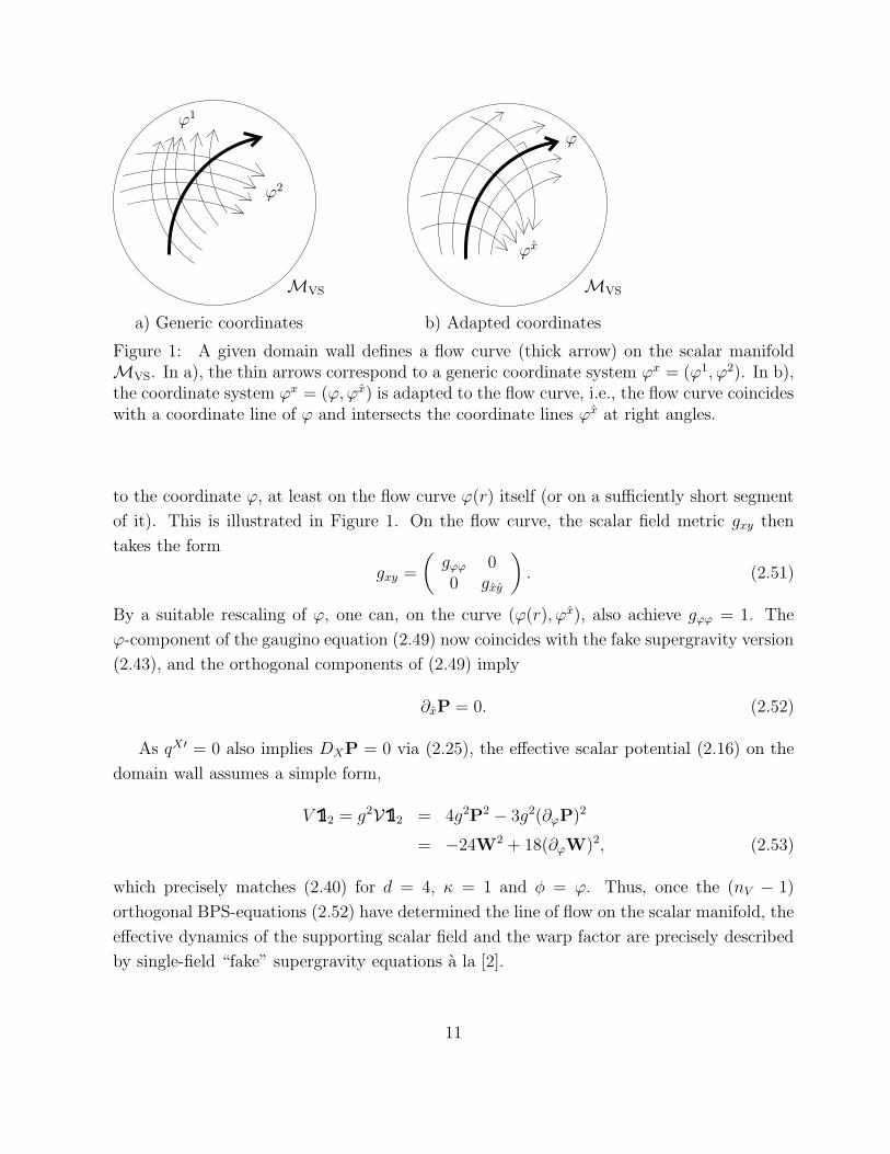
a) Generic coordinates b) Adapted coordinates

Figure 1: A given domain wall defines a flow curve (thick arrow) on the scalar manifoldMVS. In a), the thin arrows correspond to a generic coordinate system ϕx = (ϕ1, ϕ2). In b),the coordinate system ϕx = (ϕ, ϕx) is adapted to the flow curve, i.e., the flow curve coincideswith a coordinate line of ϕ and intersects the coordinate lines ϕx at right angles.

to the coordinate ϕ, at least on the flow curve ϕ(r) itself (or on a sufficiently short segment

of it). This is illustrated in Figure 1. On the flow curve, the scalar field metric gxy then

takes the form

gxy =

(

gϕϕ 00 gxy

)

. (2.51)

By a suitable rescaling of ϕ, one can, on the curve (ϕ(r), ϕx), also achieve gϕϕ = 1. The

ϕ-component of the gaugino equation (2.49) now coincides with the fake supergravity version

(2.43), and the orthogonal components of (2.49) imply

∂xP = 0. (2.52)

As qX′ = 0 also implies DXP = 0 via (2.25), the effective scalar potential (2.16) on the

domain wall assumes a simple form,

V 2 = g2V 2 = 4g2P2 − 3g2(∂ϕP)2

= −24W2 + 18(∂ϕW)2, (2.53)

which precisely matches (2.40) for d = 4, κ = 1 and φ = ϕ. Thus, once the (nV − 1)

orthogonal BPS-equations (2.52) have determined the line of flow on the scalar manifold, the

effective dynamics of the supporting scalar field and the warp factor are precisely described

by single-field “fake” supergravity equations a la [2].

11

Let us now turn to case (ii) and assume the domain wall is supported by hypermultiplet

scalars only. In that case, the gaugino BPS-equation (2.20) implies

∂xP = 0, (2.54)

because we now have ϕx′ = 0. The gravitino equations (2.18) and (2.19) are again of the

same form as the corresponding fake supergravity equations (2.41) and (2.42) provided that

we again make the identification (2.50) and gauge away the SU(2) connection along the flow

line:

qX′ωXij = 0 (SU(2) gauge choice), (2.55)

which is locally always possible, as explained in [1]. However, due to the explicit appearance

of the SU(2) curvature tensor, the hyperino BPS-condition (2.21), or its equivalent version

(2.25),

i gY XqX′Θ + iqX′[RY X ,Θ] +

√6 g DYP = 0, (2.56)

clearly differs from the corresponding fake supergravity analogue (2.43). Likewise, the scalar

potential (2.16) now reads (remembering (2.54))

V 2 = 4P2 − (DXP)(DXP), (2.57)

which seems to have the “wrong” prefactor in front of the derivative term when compared

to (2.40). In order to make contact between the two formulations, one again has to interpret

fake supergravity as the effective theory along the flow line. More precisely, for a given

domain wall solution, one again chooses adapted coordinates qX(r) = (q(r), qX) such that,

on the flow curve,

gXY =

(

gqq 00 gXY

)

, (2.58)

where gqq(q(r), qX) can again be chosen to be equal to one. The supersymmetry condition

(2.56) now splits into two equations:

q′Θ− i g√6DqP = 0, (2.59)

q′[RXq,Θ]− i g√6DXP = 0. (2.60)

In view of (2.23), the first equation (2.59) is easily seen to be equivalent to the fake super-

gravity equation (2.43) provided the SU(2) gauge (2.55) is imposed. The second equation

should again be viewed as a set of constraint equations that determines the position of the

flow curve in the full scalar manifold MQ as a co-dimension one hypersurface. Note that

(2.60) is different from the analogous equation (2.52) in the case of running vector multiplet

12

scalars, as it no longer implies that the hatted derivatives of P have to vanish. In fact, one

can show that (2.60) implies that, on a BPS-domain wall solution [1],

DXPDXP = 2DqPD

qP, (2.61)

showing that at least some components of DXP have to be non-zero. Luckily, this is precisely

as it should be, because (2.61) exactly corrects the “wrong” prefactor (−1) in the potential

(2.57) to (−3), so that, using the SU(2) gauge (2.55),

V 2 = g2V 2 = 4g2P2 − 3g2(∂qP)2

= −24W2 + 18(∂qW)2, (2.62)

i.e., exactly as in “fake” supergravity.

Let us finally mention the last case (iii) of running vector- and hypermultiplet scalars.

The flow curve now has non-trivial projections ϕx(r) and qX(r) on both scalar manifold com-

ponents, MV S and MQ. One can then, in a first step, choose separate adapted coordinates

ϕx(r) = (ϕ(r), ϕx) and qX(r) = (q(r), qX) on MV S and MQ, respectively. In the SU(2)-

gauge (2.55), the BPS-equations and the scalar potential then look the same for both types

of scalars ϕ and q. One can then employ a coordinate transformation in the (ϕ, q)-plane,

(ϕ(r), q(r)) → (φ(r), φ), (2.63)

such that, locally, ∂r = q′∂q + ϕ′∂ϕ = φ′∂φ. In this new, totally adapted coordinate system,

the BPS-equation for φ and the scalar potential as a function of φ(r) then take the standard

“fake” supergravity form [1].

The lesson we learn from this is that a generalization of the single-field formalism of

fake supergravity to several scalar fields is not so straightforward, as the prefactors in the

scalar potential can be different and non-trivial connections and curvatures might come into

play. However, interpreting single-field fake supergravity as an effective theory along the

flow curve seems to make sense in all cases. It is this latter interpretation that we will now

try to generalize to the N = 4 case.

3 BPS-domain walls in N = 4 fake and true supergrav-

ity

In this section, we study curved and flat BPS-domain walls in 5D,N = 4 gauged supergravity

and verify to what extend one can generalize “N = 2” fake supergravity to “N = 4” fake

supergravity. We begin with a brief summary of 5D,N = 4 ungauged [40] and gauged [41,42]

supergravity. Our notation follows that of ref. [42], to which the reader is referred for further

details.

13

3.1 Ungauged 5D, N = 4 supergravity

In the previous section, the index i = 1, 2 was used to denote the fundamental representation

of the R-symmetry group Usp(2) ∼= SU(2) of the 5D, N = 2 Poincare superalgebra. In this

section,

i = 1, . . . , 4 (3.1)

will instead denote the fundamental representation of the N = 4 R-symmetry group Usp(4),

which is locally isomorphic to SO(5).

In ungauged 5D supergravity, vector fields and antisymmetric tensor fields are equivalent,

and the most general ungauged N = 4 theory describes the coupling of n vector multiplets

to supergravity.

The supergravity multiplet,

(

eµm , ψi

µ , Aijµ , aµ , χ

i , σ)

, (3.2)

contains the graviton eµm, four gravitini ψi

µ, six vector fields (Aijµ , aµ), four spin 1/2 fermions

χi and one real scalar field σ. The vector field aµ is USp(4) inert, whereas the vector fields

Aijµ transform in the 5 of USp(4), i.e.,

Aijµ = −Aji

µ , Aijµ Ωij = 0, (3.3)

with Ωij being the symplectic metric of USp(4).

An N = 4 vector multiplet is given by

(

Aµ , λi , ϕij

)

, (3.4)

where Aµ is a vector field, λi denotes four spin 1/2 fields, and the ϕij are scalar fields

transforming in the 5 of USp(4), similar to eq. (3.3). Coupling n vector multiplets to

supergravity, the field content of the theory can then be summarized as follows

(

eµm , ψi

µ , AIµ , aµ , χ

i , λia , σ , ϕx)

. (3.5)

Here, a = 1, . . . , n counts the number of vector multiplets whereas I = 1, . . . , (5 + n) collec-

tively denotes the Aijµ and the vector fields of the vector multiplets. Similarly, x = 1, . . . , 5n

is a collective index for all the scalar fields in the vector multiplets. We will further adopt

the following convention to raise and lower USp(4) indices:

T i = Ωij Tj , Ti = T j Ωji, (3.6)

14

whereas a, b are raised and lowered with δab. Before we proceed, we note that, in a more

familiar language, quantities such as Aµij in the 5 of Usp(4) ∼= SO(5) can be expressed as

Aµij = Aα

µΓαij, where α = 1, . . . , 5, and Γαi

j denote SO(5) gamma matrices,

ΓαijΓβj

k + (α↔ β) = 2δαβδki . (3.7)

As was shown in [40], the manifold spanned by the (5n+ 1) scalar fields is

M =SO(5, n)

SO(5)× SO(n)× SO(1, 1), (3.8)

where the SO(1, 1) part corresponds to the USp(4)-singlet σ of the supergravity multiplet.

The theory therefore has a global symmetry group SO(5, n)×SO(1, 1) and a local composite

SO(5) × SO(n) invariance. The coset part of the scalar manifold M can be described in

two different ways:

(i) Standard sigma model description:

As in (3.5) one can simply choose a parameterization in terms of 5n independent real

coordinates ϕx on the coset space. The vielbeins on the coset space can then be chosen

to be of the form

f ijax = −f jia

x , f ijax Ωij = 0, (3.9)

where [ij] and a refer to the natural (5,n) tangent space decomposition with respect

to the holonomy group H = SO(5)× SO(n). The inverse vielbein, fxaij , is defined by

faijx fxb

kl = 4(

δ[ik δ

j]l − 1

4ΩijΩkl

)

δab. (3.10)

The non-linear σ-model metric gxy on the coset part of M is then given by

gxy =1

4f ijax fa

yij , (3.11)

and the kinetic term for the scalar fields takes the standard form 12gxy∂µϕ

x∂µϕy. This

way of describing M is particularly useful for discussing geometrical properties of the

theory.

(ii) Coset representatives:

The parametrization that makes the symmetries of the theory as manifest as possible

is in terms of coset representatives, i.e., (5+n)×(5+n) matrices LIA ⊂ G ≡ SO(5, n)

that are subject to local (“composite”) H = SO(5)× SO(n) transformations (acting

on the index A) and admit the action of global G = SO(5, n) transformations (acting

15

on the index I). The index A = 1, . . . , (5 + n) naturally decomposes into A = (ij, a),

and so do the coset representatives, LIA = (Lij

I, La

I), where Lij

Itransforms in the 5 of

SO(5), just as in (3.3). Denoting the inverse of LIA by LA

I (i.e., LIA LB

I = δAB),

the vielbeins on G/H and the composite H-connections are determined from the G-invariant 1-form:

L−1dL = Qab Tab +Qij Tij + P aij Taij, (3.12)

where (Tab,Tij) are the generators of the Lie algebra h of H, and Taij denotes the

generators of the coset part of the Lie algebra g of G. More precisely,

Qab = LIadLIb and Qij = LIikdLIk

j (3.13)

are the composite SO(n) and USp(4) connections, respectively, and

P aij = LIadLIij = −1

2faijx dϕx (3.14)

describes the space-time pull-back of the G/H vielbein. Note that Qabµ is antisymmetric

in the SO(n) indices, whereas Qijµ is symmetric in i and j. Denoting by Dx the

corresponding USp(4) and SO(n) covariant derivative, one has the following differential

realations for the coset representatives [40]:

DxLIij = −1

2LaIfaxij , (3.15)

DxLIij =

1

2LI afa

xij , (3.16)

DxLaI

= −1

2faxijL

ij

I, (3.17)

DxLIa =

1

2f ijax LI

ij , . (3.18)

We finally note the identities (see [40, 42])

δIJ = Lij

ILJij + La

ILJa , CIJ = Lij

ILJij − La

ILaJ, (3.19)

where CI J is the (constant) SO(5, n) metric.

In the following, we will frequently switch between these two formulations, which is easily

done using eq. (3.14). The Lagrangians and supersymmetry transformation rules can be

found in [40, 42].

16

3.2 5D, N = 4 gauged supergravity

The above ungauged supergravity theories cannot support domain walls, because their scalar

potentials vanish identically, as enforced by supersymmetry. As is typical for extended super-

gravity, non-trivial scalar potentials are related to non-trivial local gauge groups, K. These

gauge groups cannot be chosen at will, but have to be subgroups of the global symmetry

group G = SO(1, 1)×SO(5, n) of the ungauged supergravity. As is explained in more detail

in [42], the SO(1, 1) factor in G cannot be gauged, and all gauge groups, K, actually have to

be suitable subgroups of G = SO(5, n). Under G = SO(5, n), the vector fields AIµ transform

in the defining representation (5+ n), whereas aµ is SO(5, n)-inert. If some of these vector

fields are promoted to gauge fields of a local gauge group K ⊂ SO(5, n) under which some

of the other fields are charged, the general equivalence between vector and tensor fields is

broken [42]. Instead, one now has to distinguish carefully between vector and tensor fields

and pay attention to their transformation properties under the gauge group K ⊂ SO(5, n).

The result of the analysis in ref. [42] is as follows 4:

(i) If the gauge group K is a direct product of an Abelian factor KA and a (possibly

trivial) non-Abelian factor KS, the Abelian factor KA has to be one-dimensional (i.e.,

either U(1) or SO(1, 1), but no higher powers/products thereof). The gauge field of

this Abelian factor is aµ. Decomposing the vector fields AIµ into KA singlets, AI

µ, and

non-singlets, AMµ , the non-singlets AM

µ have to be converted to tensor fields BMµν for

the gauging to be possible:

AIµ → (AI

µ, BMµν) (3.20)

(ii) A possible non-Abelian factor, KS, is gauged by the remaining vector fields AIµ. The

tensor fields BMµν are inert under KS.

Turning on only the metric and the scalars, the corresponding Lagrangian is of the form

e−1 L = −1

2R− 1

2(∂µσ)

2 − 1

2gxy∂µϕ

x∂µϕy − V (3.21)

4In [42], particular attention was paid to gauge groups of the form K = Abelian × semi-simple ,but all results of [42] equally apply to all gauge groups K ⊂ SO(5, n) under which the (5+ n) of SO(5, n)decomposes into a completely reducible representation so that tensor fields and vector fields are not connectedby K-transformations (see also [34]). We only consider such gauge groups in this paper. They include, inparticular, the gauge groups encountered in [43] and [44].

17

whereas the supersymmetry transformations of the fermions are

δψµi = Dµǫi − iγµ(

gAUij + gSSi

j)

ǫj (3.22)

δχi = − i

2∂/σǫi + 3∂σ

(

gAUij + gSSi

j)

ǫj (3.23)

δλai =i

2faxi

j(∂/ϕx)ǫj −(

gAVaij + gST

aij)

ǫj . (3.24)

Here, gA and gS are the gauge couplings of, respectively, the Abelian and the non-Abelian

gauge group, and

Uij = Uji =

√2

6e2σ/

√3ΛN

MLNikLMk

j (3.25)

Sij = Sji = −2

9e−σ/

√3LJ

ikfKJIL

klKL

Ilj , (3.26)

V aij = −V a

ji =1√2e2σ/

√3ΛN

MLNijLMa (3.27)

T aij = T a

ji = −e−σ/√3LJaLK

ikf I

JKLIkj , (3.28)

denote the “fermionic shifts” with the structure constants, fKJI , of KS and the KA trans-

formation matrix, ΛNM , of the tensor fields BM

µν . The fermionic shifts also enter the scalar

potential,

V =1

2

[

g2AV aijV

aij − 36 gAgS UijSij + g2

S

(

T aijT

aij − 9SijSij) ]

, (3.29)

which is obtained from the trace of the “Ward identity” [42]

1

4δji V =

1

2g2AV aikV a

kj + gAgS

[

9(SikUk

j + UikSk

j) +1

2(V a

ikT a

kj − T a

ikV a

kj)]

−1

2g2S

[

T aikT a

kj − 9Si

kSkj]

. (3.30)

3.3 BPS-domain walls

Our goal is to study domain walls of the form (2.17) that are supported by nontrivial scalar

profiles σ(r) and/or ϕx(r) and preserve one-half of the N = 4 supersymmetry. This anal-

ysis would be considerably simplified if one could bring the BPS-equations and the scalar

potential into a “fake supergravity” form similar to (2.39) and (2.41) – (2.43) for the N = 2

case. In N = 2 supergravity, the gravitino shift W = −(ig/√6)P was a usp(2) ∼= su(2)-

valued (2 × 2)-matrix (cf. eq. (2.50)). For N = 4 supergravity, the gravitino shift is a

usp(4) ∼= so(5)-valued (4 × 4)-matrix, −i(gAUij + gSSi

j), (see eq. (3.22)). In analogy with

the N = 2 case, we choose to call this gravitino shift Wij :

Wij := −i

(

gAUij + gSSi

j)

. (3.31)

18

Furthermore, we will, from now on, suppress the usp(4) indices i, j = 1, . . . , 4 by using

boldface expressions such as

W =Wij , WW = Wi

jWjk etc., (3.32)

just as we did in Section 2 for the analogous (2 × 2)-matrices. Note that, in this boldface

notation, the position of the indices is always assumed to be of the form shown in (3.32),

which differs for example by a minus sign from expressions such as WijWjk due to the

convention (3.6). In a domain wall background, the gravitino and dilatino BPS-equations

(3.22) and (3.23) then take the form[

∇AdS4

m + γm

(

1

2U ′γ5 +W

)]

ǫ = 0, (3.33)

[Dr + γ5W] ǫ = 0, (3.34)

[γ5σ′ − 6∂σW] ǫ = 0, (3.35)

which are precisely of the same form as the fake supergravity equations (2.41) – (2.43), except,

that W is now a (4×4)-matrix instead of a (2×2)-matrix. Adding 0 = 6g2AU2− 9

2g2A(∂σU)2

to the right hand side of (3.30), the scalar potential reads

1

4V 4 = −6W2 +

9

2(∂σW)2 +

1

2

[

g2AVaVa + gAgS[V

a,Ta]− g2STaTa

]

. (3.36)

Thus, if the domain wall is supported by σ(r) only (i.e., if ϕx′ = 0 and hence Va = Ta = 0

via eq. (3.24)), the BPS-equations (3.33) – (3.35) and the scalar potential (3.36) generalize

the N = 2 fake supergravity equations (2.40) – (2.43) to what one might call “N = 4

fake supergravity”. The interesting question now is: Can a non-trivial profile ϕx(r) also be

incorporated in this formalism? This obviously requires two things:

(i) The gaugino/tensorino BPS-condition (3.24) has to be brought into a form in which

Va and Ta are expressed in terms of derivatives of W with respect to ϕx with the

same relative prefactors as in (3.35).

(ii) The term in brackets in the scalar potential (3.36) should likewise be re-expressed in

terms of ϕx-derivatives of W with the prefactor 9/2, just as for the (∂σW)2-term.

As we will see, the rewriting of the vector- and tensor multiplet sector along these lines bears

many similarities with the hypermultiplet sector of N = 2 supergravity, but also shows some

novel features. Let us start with the BPS-equation (3.24). In the domain wall background

(2.17) it reads, after using a projector of the form (2.23) (now with (4× 4)-matrices),

− i

2ϕx′faxΘ− gAV

a − gSTa = 0. (3.37)

19

Multiplying by fay from the left and using [40, 42]

fay fax = gyx 4 + 4Ryx, (3.38)

this becomes

− i

2ϕx′gyxΘ− 2iϕx′RyxΘ− fay (gAV

a + gSTa) = 0. (3.39)

Decomposing (3.39) into symmetric and antisymmetric part, one obtains

− i

2ϕx′gyxΘ− iϕx′[Ryx,Θ]− gA

2[fay ,V

a]− gS2fay ,Ta = 0 (3.40)

−iϕx′Ryx,Θ − gA2fay ,Va − gS

2[fay ,T

a] = 0. (3.41)

Using (3.15) – (3.19) and the invariance conditions for the structure constants fKIJ and the

transformation matrices ΛNM ,

CIJfIKL + CILf

IKJ = 0 (3.42)

ΛPMCPN + ΛP

NCMP = 0, (3.43)

one derives [42]

DyU =1

6[fay ,V

a] (3.44)

DyS =1

6fay ,Ta, (3.45)

so that (3.40) becomes

ϕx′gyxΘ+ 2ϕx′[Ryx,Θ] + 6DyW = 0. (3.46)

If one now switches to adapted coordinates (ϕ(r), ϕx), with ϕx constant and perpendicular

to ϕ along a given flow curve, one obtains for the (canonically normalized) ϕ-component of

(3.46)

ϕ′Θ+ 6DϕW = 0. (3.47)

Gauging away the composite Usp(4) connection,

ϕx′Qxij = 0 (Usp(4)-gauge choice) (3.48)

and taking into account (2.23), this assumes the desired fake supergravity form (cf. (3.35)).

The other BPS-equations can again be viewed as constraints that determine the position of

20

the flow curve on the full scalar manifold. Let us now turn to the scalar potential. Using

(3.44) and (3.45) as well as (3.10), one derives

DxUDxU = −4

9VaVa (3.49)

DxS, DxU =

1

3[Ta,Va] (3.50)

DxSDxS =

1

9

[

TaTa +1

2Tr(TaTa) 4

]

. (3.51)

These relations allow one to re-express the term in brackets in (3.36) in terms of derivatives

of U and S:

1

4V 4 = −6W2 +

9

2(∂σW)2 − 9

8g2ADxUD

xU− 3

2gAgSDxS, D

xU

−9

2g2S

(

DxSDxS− 1

6Tr(DxSD

xS) 4

)

(3.52)

We note three interesting features of this expression:

(i) In contrast to the N = 2 analogue (2.16), the Ward identity (3.52) can, in general, not

be written without taking some traces.

(ii) Even after taking the trace of (3.52), the prefactor of the (DxU)2-term is different

from the prefactor of the DxS, DxU-term and the (DxS)

2-term. This means that, as

long as gA and gS are both non-vanishing, one cannot write these terms as something

proportional to (DxW)2, i.e., in terms of derivatives of the full gravitino shift W.

Again, this is different from the N = 2 case (2.16).

(iii) If gS = 0, or if gA = 0, the scalar potential can be written as the full gravitino shift

and its derivatives, but in none of these two special cases, the ϕx-derivatives appear

with the “right” cofficient 9/2 required by fake supergravity.

Properties (i) and (ii) are clearly different from the N = 2 case. These differences can

in part be traced to the fact that the adjoint of Usp(4) is no longer equivalent to the

vector representation of SO(5), as was the case for SU(2) and SO(3). This implies, in

particular, that symmetric products of usp(4)-valued matrices such as DxSDxS are no longer

automatically proportional to the unit matrix, as was the case for su(2)-valued matrices such

asDXPDXP in the N = 2 case due to the anticommutation properties of the Pauli-matrices,

i.e., the Clifford algebra of SO(3). On the other hand, even the N = 2 hypermultiplet sector

did not fall into the N = 2 fake supergravity framework before the BPS-equations and

adapted coordinates were imposed (see eqs. (2.16) vs. (2.62)). Thus, there is still some

hope that imposing the BPS-equations (3.40) – (3.41) and using the adapted coordinates

21

ϕx(r) = (ϕ(r), ϕx) miraculously transforms the last three terms in (3.52) into 9/2(DϕW)2

and removes at least some of the above-mentioned differences to the N = 2 case. To see

whether this works, let us go back to the BPS-condition (3.46) and its ϕ-component (3.47),

which we rearrange as (normalizing gϕϕ = 1)

DyW = −1

6ϕx′gxyΘ− 1

3ϕx′[Ryx,Θ] (3.53)

=⇒ DϕW = −1

6ϕ′Θ (y = ϕ) (3.54)

Squaring (3.54) gives

DϕWDϕW =1

36(ϕ′)2 4 (3.55)

On the other hand, squaring (3.53) and using (3.41) as well as the identity

RxyRxz = −1

4gyz 4 −

3

4Ryz, (3.56)

one derives

DyWDyW =5

36ϕx′ϕz′gxz 4 −

g2A36

fay ,Vaf by,Vb

−gAgS36

(

fay ,Va[f by,Tb] + [fay ,Ta]f by,Vb

)

−g2S

36[fay ,T

a][f by,Tb]. (3.57)

Using (3.10), the vielbeins can be eliminated, and (3.57) becomes

DyWDyW =5

36ϕx′ϕz′gxz 4 −

g2A9VaVa − gAgS

9[Va,Ta] +

g2S18

Tr(TaTa) 4. (3.58)

However, (DxW)2 can be computed directly from (3.49) – (3.51) and the definition (3.31):

DyWDyW =4

9g2AV

aVa − gAgS3

[Ta,Va]− g2S9

(

TaTa +1

2Tr(TaTa) 4

)

. (3.59)

Consistency of (3.58) and (3.59) then implies

5

4ϕx′ϕz′gxz 4 = 5g2AV

aVa + 4gAgS[Va,Ta]− g2S

(

TaTa + Tr(TaTa) 4

)

, (3.60)

or, after taking the trace,

ϕx′ϕz′gxz = g2ATr(VaVa)− g2STr(T

aTa) (3.61)

Switching to adapted coordinates, (3.55) then becomes

DϕWDϕW =1

36

(

g2ATr(VaVa)− g2STr(T

aTa))

4, (3.62)

22

and we finally obtain for the scalar potential (3.36)

V = −6TrW2 +9

2Tr(∂σW)2 +

9

2Tr(DϕW)2. (3.63)

Thus, after employing the Usp(4) gauge choice (3.48), the ϕ-sector and the σ-sector enter

the theory symmetrically and with the “right” prefactors. If both ϕ and σ are running,

one can, just as in N = 2 supergravity, go over to a total adapted coordinate φ(r) with

σ′∂σ + ϕ′∂ϕ = φ′∂φ so as to obtain N = 4 single-field fake supergravity equations (see the

discussion around (2.63)).

3.4 Consistency conditions and domain wall curvature

Let us summarize what we have shown so far. In 5D, N = 4 supergravity, the gravitino

BPS-equations in a 12-supersymmetric domain wall background read

[

∇AdS4

m + γm

(

1

2U ′γ5 +W

)]

ǫ = 0, (3.64)

[Dr + γ5W] ǫ = 0. (3.65)

Subjecting the spinor ǫ to

γ5ǫ = −Θǫ, (3.66)

the dilatino equation becomes

σ′Θ+ 6∂σW = 0, (3.67)

and the gaugino/tensorino BPS-equation can be decomposed as follows

ϕx′gyxΘ + 2ϕx′[Ryx,Θ] + 6DyW = 0 (3.68)

2ϕx′Ryx,Θ − igAfay ,Va − igS[fay ,T

a] = 0. (3.69)

In adapted coordinates, ϕx(r) = (ϕ(r), ϕx), the scalar potential reads

V = −6TrW2 +9

2Tr(∂σW)2 +

9

2Tr(DϕW)2, (3.70)

and (3.68) splits further into

ϕ′Θ+ 6DϕW = 0 (3.71)

2ϕ′[Ryϕ,Θ] + 6DyW = 0. (3.72)

Eqs. (3.67) and (3.68) can be solved for Θ:

Θ = −6∂σW

σ′(3.73)

Θ = −6ϕy′DyW

ϕx′ϕz′gxz= −6

DϕW

ϕ′. (3.74)

23

If both σ and ϕx are running, consistency of these two expressions requires

∂σW

σ′=ϕy′DyW

ϕx′ϕz′gxz=DϕW

ϕ′. (3.75)

Eqs. (3.73) and (3.74) also imply

DrW ≡ (σ′∂σ + ϕx′Dx)W = −1

6((σ′)2 + ϕx′gxyϕ

y′)Θ. (3.76)

Squaring (3.73) and (3.74) gives the first order equation for the scalars,

σ′ = ±6√

(∂σW)2 (3.77)

ϕx′gxyϕy′ = ±6

√

(ϕx′DxW)2 ⇒ ϕ′ = ±6√

(DϕW)2 (3.78)

Let us now turn to the warp factor. Just as in section 2.2, the integrability condition of

(3.64), yields

(U ′)2 = 4W2 − e−2U

L24

. (3.79)

On the other hand, the compatibility condition between (3.64) and (3.66) gives

U ′ = Θ,W, (3.80)

which, when combined with (3.79), gives

−e−2U

L24

4 = Θ,W2 − 4W2, (3.81)

just as in (2.34). Hence, a BPS-domain wall is flat if and only if

Θ,W2 = 4W2 (flatness condition). (3.82)

It is shown in Appendix A that this is equivalent to

[Θ,W] = 0 ⇔ [DrW,W] = 0 (equivalent flatness condition), (3.83)

where we have used (3.76). Finally, there is the N = 4 analogue of eq. (2.35), namely the

compatibility condition of (3.65) and (3.66),

[Θ, DrΘ− 2W] = 0, (3.84)

or, using (3.76),[

DrW, DrDrW +1

3((σ′)2 + ϕxϕygxy)W

]

= 0. (3.85)

24

3.5 Special cases

In this subsection, we will take a closer look at the implications of the equations listed in

section 3.4 and apply them to a number of special cases.

Case 1: The gauging is purely Abelian:

gS = 0. (3.86)

In this case, W = −igAU, and (3.67) implies

σ′Θ = −4√3W. (3.87)

Thus, σ′ = 0 would imply W = 0 along the flow, and, hence, because of (3.80), also

U(r) = const., i.e., a trivial domain wall. In other words, for a non-trivial Abelian BPS-

domain wall, σ′ has to be non-zero. Now, a running σ(r), however, means that (3.87) can

be solved for Θ:

Θ = −4√3W

σ′. (3.88)

This implies that the domain wall has to be flat because of (3.83). On the other hand, due

to the simple σ-dependence, (3.77) can be readily solved:

σ(r) = a ln(r − ro) + b (3.89)

with some constants a and b. Hence, σ(r) always approaches infinity, which is not surprising

in view of the simple runaway behaviour of the scalar potential in the σ-direction when

gS = 0.

Case 2: The gauging is purely Non-Abelian:

gA = 0. (3.90)

In this case, W = −igSS, and the simple exponential behaviour of W leads to similar

conclusions as in the purely Abelian case: Just as in (3.87), one concludes that σ(r) has

to have a non-trivial r-dependence for the domain wall to be non-trivial. This, however,

also implies that Θ is always proportional to W, and any domain wall must be flat, due to

(3.83). Again, the runaway behavior of the potential leads to a logarithmic r-dependence of

the scalar field σ(r).

Case 3: The mixed gauging:

gAgS 6= 0. (3.91)

25

When both the Abelian part and the non-Abelian part are gauged, the σ-dependence of W

no longer factors out and neither does the scalar potential have a simple runaway behaviour

in the σ-direction. Nevertheless, the structure of domain walls that are solely supported by

the supergravity scalar σ are still quite limited. In order to see this, consider the consistency

condition (3.85), which, for ϕx′ = 0, simplifies to[

∂σW, ∂2σW +1

3W

]

= 0. (3.92)

Using (3.31) and the σ-dependence of U and S, (3.25) – (3.26), one easily sees that (3.92)

implies

[U,S] = 0. (3.93)

But this also implies [∂σW,W] = 0, and hence, via (3.83), the flatness of the domain wall.

Thus, taking into account our observations in the purely Abelian and purely non-Abelian

case, we find that a domain wall supported by σ(r) only can never be curved. Obviously,

the condition [U,S] = 0 is automatically satisfied if either gA or gS vanishes. One way

to satisfy [U,S] = 0 for gAgS 6= 0 is as follows: Suppose, the gauge group K contains the

obvious SO(3)×SO(2) subgroup of SO(5) ⊂ SO(5, n) as a factor. More generally, one could

take the SO(2) factor of the gauge group to be a diagonal subgroup of the SO(2) ⊂ SO(5)

and some product of SO(2)’s that are contained in SO(n) ⊂ SO(5, n) such that, under

KA-transformations, the tensors charged under SO(2) ⊂ SO(5) do not mix with the tensors

charged under the other SO(2)-subgroups of SO(n). These gaugings are precisely the ones

that occur in the N = 4 orbifold compactifications [45] in the AdS/CFT-correspondence [8].

In such a gauging, the five vector fields A1,...,5µ of the ungauged supergravity multiplet split

into a triplet of SO(3)-gauge fields, which we take to be A1,2,3µ , and a doublet of tensor fields,

B4,5µν , charged under the SO(2). Suppose further that the scalar fields ϕx of the vector- and

tensor multiplets all sit at the “origin” of the symmetric space SO(5, n)/SO(5) × SO(n):

LAI= δA

I. Since, by assumption, the tensor field transformation matrix ΛN

M does not mix

the supergravity tensors B4,5µν with the other tensor fields (provided such additional tensor

fields exist), and since the SO(3) part of the gauge group is supposed to be a direct factor,

it is easy to see that V aij and T a

ij from eqs. (3.27) and (3.28) vanish at this critical point,

which is consistent with the BPS-conditions (3.40) – (3.41) and ϕx′ = 0. Using SO(5)-

gamma matrices (see eq. (3.7)) to convert Usp(4)-indices i, j = 1, . . . , 4 into SO(5) indices

α, β = 1, . . . 5, it is easy to see that

U ∼ e2σ√

3Γ45 (3.94)

S ∼ e− σ

√

3Γ123 ∼ e− σ

√

3Γ45 (3.95)

and hence [U,S] = 0. In fact, if the scalars ϕx are frozen as described, the model becomes

effectively the Romans model [41]. The BPS-conditions for the general case of running

26

scalars ϕx(r) and σ(r) can be analyzed along similar lines using the equations (3.44), (3.45)

as well as [42]

DxVa =

( e2σ√

3

2√2ΛN

MLaNL

Mb)

f bx +3

2[fax ,U] (3.96)

DxTa =

(e− σ

√

3

2f IJKL

JaLbI

)

[LK , f bx] +3

2fax ,S, (3.97)

but the results are in general model-dependent and beyond the scope of this paper.

4 Conclusions

In this paper, we have shown that the BPS-equations and the scalar potentials for 1/2-BPS-

domain walls in 5D, N = 4 gauged supergravity can be cast into a generalized form of “fake”

supergravity. In many respects, this parallels the situation in N = 2 supergravity in five

dimensions, but there are also important differences. Most importantly, the gravitino shift

is now a usp(4)-valued (4× 4)-matrix instead of a su(2)-valued (2× 2)-matrix. This means

that some peculiarities of the group SU(2) are no longer valid, which makes it all the more

surprising that the simple form of the fake supergravity equations remains largely unaltered

(in fact, the only immediately visible difference is that the scalar potential in N = 4 fake

supergravity can no longer be written in terms of the gravitino shift W without taking the

trace). Furthermore, due to the doubled amount of supersymmetry, there are now twice as

many BPS-conditions to satisfy. It should also be noted that the scalar manifolds are no

longer of the type encountered in N = 2 supergravity, but are subject to completely different

geometrical constraints. The fact that nevertheless the full dynamics along the flow line is

captured by almost identical equations suggests that possibly all BPS-domain walls in all

spacetime dimensions and for all amounts of supersymmetry can be described in terms of an

appropriately generalized form of fake supergravity. This could, for instance, be due to some

general properties of gauged supergravities in the spirit of [46]. The results of this paper

should help distinguish N = 2 artifacts from this general formulation.

Recasting domain wall equations of supergravity theories into a “fake” supergravity lan-

guage greately simplifies their study. This was already demonstrated in [1], and in this paper

we saw that also N = 4 domain walls can be studied quite efficiently in this language. For

example, we could easily rule out curved BPS-domain walls if the gauge group is purely

Abelian or purely semisimple. In both of these cases, domain walls furthermore show a

runaway behavior in the σ-direction. In the mixed gauging, curved domain walls are ruled

out if they are supported by σ(r) only.

27

It might be interesting to apply the results of this paper to the study of holographic

renormalization group flows along the lines of [8] or in the context of domain wall solutions

in flux compactifications, which single out certain types of gauge groups [9–11]. Another

interesting further direction concerns a generalization to 1/4-BPS-domain walls [8], which are

impossible in N = 2 supergravity. One might also wonder whether other types of solutions

such as charged black holes or cosmic strings have a similar description in terms of some

other form of “fake” supergravity, in which all scalars are treated equally, independently of

the spacetime dimension or the amount of supersymmetry.

A The flatness condition

As shown in section 3.3, a 1/2-BPS domain wall in 5D, N = 4 supergravity is flat if and

only if (cf. eq. (3.82))

Θ,W2 = 4W2. (A.1)

A sufficient condition for this to hold is obviously

[Θ,W] = 0. (A.2)

We will now show that this condition is also necessary. Both Θ and W are usp(4) ∼= so(5)-

valued, so they can be expressed in terms of the SO(5) gamma matrices (3.7) via

Θ = ΘαβΓαβ , W =W αβΓαβ. (A.3)

Without loss of generality, we can assume Θ = 2Θ12Γ12. Using

Γαβ,Γγδ = 2Γαβγδ + 2δαδδβγ − 2δβδδαγ, (A.4)

one finds that Θ2 = 4 implies (Θ12)2 = −1/4. (A.4) now implies

Θ,W2 = [2ΘαβW γδΓαβγδ − 4ΘαβW αβ4]

2. (A.5)

Isolating the part of (A.5) that is proportional to the unit matrix, one easily sees that this

is (remembering Θ = 2Θ12Γ12 and (Θ12)2 = −1/4)

−16[(W 12)2 + (W 34)2 + (W 35)2 + (W 45)2]. (A.6)

In 4W2, on the other hand, the part proportional to the unit matrix is easily seen to be

−8W αβW αβ, so that (A.1) implies that all components except W 12,W 34,W 45,W 35 have to

vanish. This implies (A.2).

28

Acknowledgements: I have benefitted from earlier discussions with A. Celi, A. Ceresole,

G. Dall’Agata, C. Herrmann and A. Van Proeyen on the material of refs. [1,42]. This work is

supported by the German Research Foundation (DFG) within the Emmy Noether Program

(ZA 279/1-1).

References

[1] A. Celi, A. Ceresole, G. Dall’Agata, A. Van Proeyen and M. Zagermann, On the

fakeness of fake supergravity, Phys. Rev. D71 (2005) 045009, hep-th/0410126

[2] D. Z. Freedman, C. Nunez, M. Schnabl and K. Skenderis, Fake supergravity and

domain wall stability, Phys. Rev. D69 (2004) 104027, hep-th/0312055

[3] D. Bak, M. Gutperle, S. Hirano and N. Ohta, “Dilatonic repulsons and confinement

via the AdS/CFT correspondence,” Phys. Rev. D 70 (2004) 086004

[arXiv:hep-th/0403249].

[4] P. K. Townsend, Positive energy and the scalar potential in higher dimensional

(super)gravity theories, Phys. Lett. B148 (1984) 55

[5] K. Skenderis and P. K. Townsend, Gravitational stability and renormalization-group

flow, Phys. Lett. B468 (1999) 46–51, hep-th/9909070

[6] O. DeWolfe, D. Z. Freedman, S. S. Gubser and A. Karch, Modeling the fifth dimension

with scalars and gravity, Phys. Rev. D 62, 046008 (2000) [arXiv:hep-th/9909134].

[7] L. Girardello, M. Petrini, M. Porrati and A. Zaffaroni, Novel local CFT and exact

results on perturbations of N = 4 super Yang-Mills from AdS dynamics, JHEP 9812,

022 (1998) [arXiv:hep-th/9810126]; J. Distler and F. Zamora, Non-supersymmetric

conformal field theories from stable anti-de Sitter spaces, Adv. Theor. Math. Phys. 2,

1405 (1999) [arXiv:hep-th/9810206]; D. Z. Freedman, S. S. Gubser, K. Pilch and

N. P. Warner, Renormalization group flows from holography supersymmetry and a

c-theorem, Adv. Theor. Math. Phys. 3, 363 (1999) [arXiv:hep-th/9904017].

[8] R. Corrado, M. Gunaydin, N. P. Warner and M. Zagermann, Orbifolds and flows from

gauged supergravity Phys. Rev. D 65, 125024 (2002) [arXiv:hep-th/0203057].

[9] C. Mayer and T. Mohaupt, Domain walls, Hitchin’s flow equations and G2-manifolds,

hep-th/0407198

[10] T. House and A. Lukas, G(2) domain walls in M-theory, arXiv:hep-th/0409114.

29

[11] J. Louis and S. Vaula, in preparation

[12] K. Behrndt and M. Cvetic Supersymmetric domain wall world from D = 5 simple

gauged supergravity Phys. Lett. B 475, 253 (2000) [arXiv:hep-th/9909058].

[13] R. Kallosh and A. D. Linde, Supersymmetry and the brane world, JHEP 0002, 005

(2000) [arXiv:hep-th/0001071].

[14] K. Behrndt and M. Cvetic, Anti-de Sitter vacua of gauged supergravities with 8

supercharges Phys. Rev. D 61, 101901 (2000) [arXiv:hep-th/0001159].

[15] G. W. Gibbons and N. D. Lambert, Domain walls and solitons in odd dimensions

Phys. Lett. B 488, 90 (2000) [arXiv:hep-th/0003197].

[16] K. Behrndt, C. Herrmann, J. Louis and S. Thomas, Domain walls in five dimensional

supergravity with non-trivial hypermultiplets, JHEP 01 (2001) 011, hep-th/0008112

[17] A. Ceresole, G. Dall’Agata, R. Kallosh and A. Van Proeyen, Hypermultiplets, domain

walls and supersymmetric attractors, Phys. Rev. D64 (2001) 104006, hep-th/0104056

[18] D. V. Alekseevsky, V. Cortes, C. Devchand and A. Van Proeyen, Flows on

quaternionic-Kahler and very special real manifolds, Commun. Math. Phys. 238

(2003) 525–543, hep-th/0109094

[19] K. Behrndt and G. Dall’Agata, Vacua of N = 2 gauged supergravity derived from

non-homogeneous quaternionic spaces, Nucl. Phys. B627 (2002) 357–380,

hep-th/0112136

[20] L. Anguelova and C. I. Lazaroiu, Domain walls of N = 2 supergravity in five

dimensions from hypermultiplet moduli spaces, JHEP 0209 (2002) 053

[arXiv:hep-th/0208154].

[21] S. L. Cacciatori, D. Klemm and W. A. Sabra, Supersymmetric domain walls and

strings in D = 5 gauged supergravity coupled to vector multiplets JHEP 0303, 023

(2003) [arXiv:hep-th/0302218].

[22] A. Celi, Toward the classification of BPS solutions of N = 2, d = 5 gauged

supergravity with matter couplings, hep-th/0405283, Ph.D. thesis, Milano

[23] G. Lopes Cardoso, G. Dall’Agata and D. Lust, Curved BPS domain wall solutions in

five-dimensional gauged supergravity, JHEP 07 (2001) 026, hep-th/0104156

30

[24] A. H. Chamseddine and W. A. Sabra, Einstein brane-worlds in 5D gauged

supergravity, Phys. Lett. B517 (2001) 184–190, hep-th/0106092, Erratum-ibid. B537

(2002) 353

[25] G. L. Cardoso, G. Dall’Agata and D. Lust, Curved BPS domain walls and RG flow in

five dimensions, JHEP 03 (2002) 044, hep-th/0201270

[26] K. Behrndt and M. Cvetic, Bent BPS domain walls of D = 5 N = 2 gauged

supergravity coupled to hypermultiplets, Phys. Rev. D65 (2002) 126007,

hep-th/0201272

[27] G. L. Cardoso and D. Lust, The holographic RG flow in a field theory on a curved

background, JHEP 09 (2002) 028, hep-th/0207024

[28] M. Gunaydin, G. Sierra and P. K. Townsend, The geometry of N = 2

Maxwell–Einstein supergravity and Jordan algebras, Nucl. Phys. B242 (1984) 244

[29] M. Gunaydin, G. Sierra and P. K. Townsend, Gauging the d = 5 Maxwell–Einstein

supergravity theories: more on Jordan algebras, Nucl. Phys. B253 (1985) 573

[30] G. Sierra, N=2 Maxwell Matter Einstein Supergravities In D = 5, D = 4 And D = 3

Phys. Lett. B 157, 379 (1985).

[31] M. Gunaydin and M. Zagermann, The gauging of five-dimensional, N = 2

Maxwell–Einstein supergravity theories coupled to tensor multiplets, Nucl. Phys. B572

(2000) 131–150, hep-th/9912027

[32] A. Ceresole and G. Dall’Agata, General matter coupled N = 2, D = 5 gauged

supergravity, Nucl. Phys. B585 (2000) 143–170, hep-th/0004111

[33] M. Gunaydin and M. Zagermann, Gauging the full R-symmetry group in

five-dimensional, N = 2 Yang-Mills/Einstein/tensor supergravity Phys. Rev. D 63,

064023 (2001) [arXiv:hep-th/0004117].

[34] E. Bergshoeff, S. Cucu, T. de Wit, J. Gheerardyn, S. Vandoren and A. Van Proeyen,

N = 2 supergravity in five dimensions revisited, Class. Quant. Grav. 21 (2004)

3015–3041, hep-th/0403045

[35] A. Ceresole and G. Dall’Agata, Five-dimensional gauged supergravity and the brane

world, Nucl. Phys. Proc. Suppl. 102 (2001) 65–70

31

[36] J. Bagger and E. Witten, Matter couplings in N = 2 supergravity, Nucl. Phys. B222

(1983) 1

[37] J. R. Ellis, M. Gunaydin and M. Zagermann, Options for gauge groups in

five-dimensional supergravity, JHEP 11 (2001) 024, hep-th/0108094

[38] E. Witten, A simple proof of the positive energy theorem, Commun. Math. Phys. 80

(1981) 381

[39] J. M. Nester, A new gravitational expression with a simple positivity proof, Phys. Lett.

83A (1981) 241

[40] M. Awada and P. K. Townsend, N=4 Maxwell-Einstein Supergravity In

Five-Dimensions And Its SU(2) Gauging Nucl. Phys. B 255, 617 (1985).

[41] L. J. Romans, Gauged N=4 Supergravities In Five-Dimensions And Their Magnetovac

Backgrounds Nucl. Phys. B 267, 433 (1986).

[42] G. Dall’Agata, C. Herrmann and M. Zagermann, General matter coupled N = 4 gauged

supergravity in five dimensions Nucl. Phys. B 612, 123 (2001) [arXiv:hep-th/0103106].

[43] J. Louis and A. Micu, Heterotic string theory with background fluxes Nucl. Phys. B

626, 26 (2002) [arXiv:hep-th/0110187].

[44] G. Villadoro and F. Zwirner, The minimal N = 4 no-scale model from generalized

dimensional reduction JHEP 0407, 055 (2004) [arXiv:hep-th/0406185].

[45] S. Kachru and E. Silverstein, 4d conformal theories and strings on orbifolds, Phys.

Rev. Lett. 80, 4855 (1998) [arXiv:hep-th/9802183].

[46] R. D’Auria and S. Ferrara, On fermion masses, gradient flows and potential in

supersymmetric theories JHEP 0105, 034 (2001) [arXiv:hep-th/0103153].

32