arXiv:cond-mat/9806038v2 12 Oct 1998

arX

iv:c

ond-

mat

/980

6038

v2 1

2 O

ct 1

998

Theory of Bose-Einstein condensation in trapped gases

Franco Dalfovo,1 Stefano Giorgini,1 Lev P. Pitaevskii,1,2,3 and Sandro Stringari11 Dipartimento di Fisica, Universita di Trento, and

Istituto Nazionale per la Fisica della Materia, I-38050 Povo, Italy2 Department of Physics, TECHNION, Haifa 32000, Israel

3 Kapitza Institute for Physical Problems, ul. Kosygina 2, 117334 Moscow

The phenomenon of Bose-Einstein condensation of dilute gases in traps is reviewed from a the-oretical perspective. Mean-field theory provides a framework to understand the main features ofthe condensation and the role of interactions between particles. Various properties of these systemsare discussed, including the density profiles and the energy of the ground state configurations, thecollective oscillations and the dynamics of the expansion, the condensate fraction and the thermo-dynamic functions. The thermodynamic limit exhibits a scaling behavior in the relevant length andenergy scales. Despite the dilute nature of the gases, interactions profoundly modify the static aswell as the dynamic properties of the system; the predictions of mean-field theory are in excellentagreement with available experimental results. Effects of superfluidity including the existence ofquantized vortices and the reduction of the moment of inertia are discussed, as well as the conse-quences of coherence such as the Josephson effect and interference phenomena. The review alsoassesses the accuracy and limitations of the mean-field approach.

Preprint, October 6, 1998. For publication in Reviews of Modern Physics.

I. INTRODUCTION

Bose-Einstein condensation (BEC) (Bose, 1924; Einstein, 1924) was observed in 1995 in a remarkable series ofexperiments on vapors of rubidium (Anderson et al., 1995) and sodium (Davis et al., 1995) in which the atoms wereconfined in magnetic traps and cooled down to extremely low temperatures, of the order of fractions of microkelvins.The first evidence for condensation emerged from time of flight measurements. The atoms were left to expand byswitching off the confining trap and then imaged with optical methods. A sharp peak in the velocity distribution wasthen observed below a certain critical temperature, providing a clear signature for BEC. In Fig. 1, we show one of thefirst pictures of the atomic clouds of rubidium. In the same year, first signatures of the occurrence of BEC in vaporsof lithium were also reported (Bradley et al., 1995).

Though the experiments of 1995 on the alkalis should be considered a milestone in the history of BEC, the experi-mental and theoretical research on this unique phenomenon predicted by quantum statistical mechanics is much olderand has involved different areas of physics (for an interdisciplinary review of BEC see Griffin, Snoke and Stringari,1995). In particular, from the very beginning, superfluidity in helium was considered by London (1938) as a possiblemanifestation of BEC. Evidences for BEC in helium have later emerged from the analysis of the momentum distri-bution of the atoms measured in neutron scattering experiments (Sokol, 1995). In recent years, BEC has been alsoinvestigated in the gas of paraexcitons in semiconductors (see Wolfe, Lin and Snoke, 1995, and references therein),but an unambiguous signature for BEC in this system has proven difficult to find.

Efforts to Bose condense atomic gases began with hydrogen more than 15 years ago. In a series of experimentshydrogen atoms were first cooled in a dilution refrigerator, then trapped by a magnetic field and further cooled byevaporation. This approach has come very close to observing BEC, but is still limited by recombination of individualatoms to form molecules (Silvera and Walraven, 1980 and 1986; Greytak and Kleppner, 1984; Greytak, 1995; Silvera,1995). At the time of this review, first observations of BEC in spin polarized hydrogen have been reported (Fried et

al., 1998). In the ’80s laser-based techniques, such as laser cooling and magneto-optical trapping, were developed tocool and trap neutral atoms [for recent reviews, see Chu (1998), Cohen-Tannoudji (1998) and Phillips (1998)]. Alkaliatoms are well suited to laser-based methods because their optical transitions can be excited by available lasers andbecause they have a favourable internal energy-level structure for cooling to very low temperatures. Once they aretrapped, their temperature can be lowered further by evaporative cooling [this technique has been recently reviewedby Ketterle and van Druten (1996a) and by Walraven (1996)]. By combining laser and evaporative cooling for alkaliatoms, experimentalists eventually succeeded in reaching the temperatures and densities required to observe BEC.It is worth noticing that, in these conditions, the equilibrium configuration of the system would be the solid phase.Thus, in order to observe BEC, one has to preserve the system in a metastable gas phase for a sufficiently long time.This is possible because three-body collisions are rare events in dilute and cold gases, whose lifetime is hence longenough to carry out experiments. So far BEC has been realized in 87Rb (Anderson et al., 1995; Han et al., 1998;Kasevich, 1997; Ernst et al., 1998a; Esslinger et al., 1998; Dalibard et al., 1998), in 23Na (Davis et al., 1995; Hau,

1

1997 and 1998; Lutwak et al., 1998) and in 7Li (Bradley et al., 1995 and 1997). The number of experiments on BECin vapors of rubidium and sodium is now growing fast. In the meanwhile, intense experimental research is currentlycarried out also on vapors of caesium, potassium and metastable helium.

One of the most relevant features of these trapped Bose gases is that they are inhomogeneous and finite-sizedsystems, the number of atoms ranging typically from a few thousands to several millions. In most cases, the confiningtraps are well approximated by harmonic potentials. The trapping frequency, ωho, provides also a characteristic lengthscale for the system, aho = [h/(mωho)]

1/2, of the order of a few microns in the available samples. Density variationsoccur on this scale. This is a major difference with respect to other systems, like for instance superfluid helium,where the effects of inhomogeneity take place on a microscopic scale fixed by the interatomic distance. In the caseof 87Rb and 23Na, the size of the system is enlarged as an effect of repulsive two-body forces and the trapped gasescan become almost macroscopic objects, directly measurable with optical methods. As an example, we show in Fig. 2a sequence of “in situ” images of an oscillating condensate of sodium atoms taken at the Massachusetts Institute ofTechnology (MIT), where the mean axial extent is of the order of 0.3 mm.

The fact that these gases are highly inhomogeneous has several important consequences. First BEC shows up notonly in momentum space, as happens in superfluid helium, but also in co-ordinate space. This double possibility ofinvestigating the effects of condensation is very interesting from both the theoretical and experimental viewpoints andprovides novel methods of investigation for relevant quantities, like the temperature dependence of the condensate,energy and density distributions, interference phenomena, frequencies of collective excitations, and so on.

Another important consequence of the inhomogeneity of these systems is the role played by two-body interactions.This aspect will be extensively discussed in the present review. The main point is that, despite the very dilutenature of these gases (typically the average distance between atoms is more than ten times the range of interatomicforces), the combination of BEC and harmonic trapping greatly enhances the effects of the atom-atom interactionson important measurable quantities. For instance, the central density of the interacting gas at very low temperaturecan be easily one or two orders of magnitude smaller than the density predicted for an ideal gas in the same trap, asshown in Fig. 3. Despite the inhomogeneity of these systems, which makes the solution of the many-body problemnontrivial, the dilute nature of the gas allows one to describe the effects of the interaction in a rather fundamental way.In practice a single physical parameter, the s-wave scattering length, is sufficient to obtain an accurate description.

The recent experimental achievements of BEC in alkali vapors have renewed a great interest in the theoreticalstudies of Bose gases. A rather massive amount of work has been done in the last couple of years, both to interpretthe initial observations and to predict new phenomena. In the presence of harmonic confinement, the many-bodytheory of interacting Bose gases gives rise to several unexpected features. This opens new theoretical perspectivesin this interdisciplinary field, where useful concepts coming from different areas of physics (atomic physics, quantumoptics, statistical mechanics and condensed matter physics) are now merging together.

The natural starting point for studying the behavior of these systems is the theory of weakly interacting bosonswhich, for inhomogeneous systems, takes the form of the Gross-Pitaevskii theory. This is a mean-field approach forthe order parameter associated with the condensate. It provides closed and relatively simple equations for describingthe relevant phenomena associated with BEC. In particular, it reproduces typical properties exhibited by superfluidsystems, like the propagation of collective excitations and the interference effects originating from the phase of theorder parameter. The theory is well suited to describing most of the effects of two-body interactions in these dilutegases at zero temperature and can be naturally generalized to explore also thermal effects.

An extensive discussion of the application of mean-field theory to these systems is the main basis of the presentreview article. We also give, whenever possible, simple arguments based on scales of length, energy and density, inorder to point out the relevant parameters for the description of the various phenomena.

There are several topics which are only marginally discussed in our paper. These include, among others, collisionaland thermalization processes, phase diffusion phenomena, light scattering from the condensate and analogies withsystems of coherent photons. In this sense our work is complementary to other recent review articles (Burnett, 1996;Parkins and Walls, 1998). Furthermore in our paper we do not discuss the physics of ultracold collisions and thedetermination of the scattering length which have been recently the object of important experimental and theoreticalstudies in the alkalis (Heinzen, 1997; Weiner et al., 1998).

The plan of the paper is the following:In Sec. II we summarize the basic features of the noninteracting Bose gas in harmonic traps and we introduce the

first relevant length and energy scales, like the oscillator length and the critical temperature. We also comment onfinite size effects, on the role of dimensionality and on the possible relevance of anharmonic traps.

In Sec. III we discuss the effects of the interaction on the ground state. We develop the formalism of mean-fieldtheory, based on the Gross-Pitaevskii equation. We consider the case of gases interacting with both repulsive andattractive forces. We then discuss in detail the large N limit for systems interacting with repulsive forces, leading tothe so called Thomas-Fermi approximation, where the ground state properties can be calculated in analytic form. Inthe last part, we discuss the validity of the mean-field approach and give explicit results for the first corrections, beyond

2

mean-field, to the ground state properties, including the quantum depletion of the condensate, i.e., the decrease inthe condensate fraction produced by the interaction.

In Sec. IV we investigate the dynamic behavior of the condensate using the time dependent Gross-Pitaevskiiequation. The equations of motion for the density and the velocity field of the condensate in the large N limit, wherethe Thomas-Fermi approximation is valid, are shown to have the form of the hydrodynamic equations of superfluids.We also discuss the dynamic behavior in the nonlinear regime (large amplitude oscillations and free expansion), thecollective modes in the case of attractive forces and the transition from collective to single-particle states in thespectrum of excitations.

In Sec. V we discuss thermal effects. We show how one can define the thermodynamic limit in these inhomogeneoussystems and how interactions modify the behavior compared to the noninteracting case. We extensively discuss theoccurrence of scaling properties in the thermodynamic limit. We review several results for the shift of the criticaltemperature and for the temperature dependence of thermodynamic functions, like the condensate fraction, thechemical potential and the release energy. We also discuss the behavior of the excitations at finite temperature.

In Sec. VI we illustrate some features of these trapped Bose gases in connection with superfluidity and phasecoherence. We discuss in particular the structure of quantized vortices and the behavior of the moment of inertia, aswell as interference phenomena and quantum effects beyond mean-field theory, like the collapse-revival of collectiveoscillations.

In Sec. VII we draw our conclusions and we discuss some further future perspectives in the field.The overlap between current theoretical and experimental investigations of BEC in trapped alkalis is already wide

and rich. Various theoretical predictions, concerning the ground state, dynamics and thermodynamics are foundto agree very well with observations; others are stimulating new experiments. The comparison between theory andexperiments then represents an exciting feature of these novel systems, which will be frequently emphasized in thepresent review.

II. THE IDEAL BOSE GAS IN A HARMONIC TRAP

A. The condensate of noninteracting bosons

An important feature characterizing the available magnetic traps for alkali atoms is that the confining potentialcan be safely approximated with the quadratic form

Vext(r) =m

2(ω2

xx2 + ω2

yy2 + ω2

zz2) . (1)

Thus the investigation of these systems starts as a textbook application of nonrelativistic quantum mechanics foridentical point-like particles in a harmonic potential.

The first step consists in neglecting the atom-atom interaction. In this case, almost all predictions are analyticaland relatively simple. The many-body Hamiltonian is the sum of single-particle Hamiltonians whose eigenvalues havethe form

εnxnynz =

(

nx +1

2

)

hωx +

(

ny +1

2

)

hωy +

(

nz +1

2

)

hωz , (2)

where nx, ny, nz are non-negative integers. The ground state φ(r1, .., rN ) of N noninteracting bosons confined bythe potential (1) is obtained by putting all the particles in the lowest single-particle state (nx = ny = nz = 0), namelyφ(r1, .., rN ) =

∏

i ϕ0(ri), where ϕ0(r) is given by

ϕ0(r) =(mωho

πh

)3/4

exp[

−m

2h(ωxx

2 + ωyy2 + ωzz

2)]

, (3)

and we have introduced the geometric average of the oscillator frequencies:

ωho = (ωxωyωz)1/3 . (4)

The density distribution then becomes n(r) = N |ϕ0(r)|2 and its value grows with N . The size of the cloud is insteadindependent of N and is fixed by the harmonic oscillator length

aho =

(

h

mωho

)1/2

(5)

3

which corresponds to the average width of the Gaussian (3). This is the first important length scale of the system.In the available experiments, it is typically of the order of aho ≈ 1 µm. At finite temperature only part of theatoms occupy the lowest state, the others being thermally distributed in the excited states at higher energy. Theradius of the thermal cloud is larger than aho. A rough estimate can be obtained by assuming kBT ≫ hωho andapproximating the density of the thermal cloud with a classical Boltzmann distribution ncl(r) ∝ exp[−Vext(r)/kBT ].If Vext(r) = (1/2)mω2

hor2, the width of the Gaussian is RT = aho(kBT/hωho)

1/2, and hence larger than aho. The useof a Bose distribution function does not change significantly this estimate.

The above discussion reveals that Bose-Einstein condensation in harmonic traps shows up with the appearanceof a sharp peak in the central region of the density distribution. An example is shown in Fig. 4, where we plot theprediction for the condensate and thermal densities of 5000 noninteracting particles in a spherical trap at a temperatureT = 0.9T 0

c , where T 0c is the temperature at which condensation occurs (see discussion in the next section). The curves

correspond to the column density, namely the particle density integrated along one direction, n(z) =∫

dx n(x, 0, z);this is a typical measured quantity, the x direction being the direction of the light beam used to image the atomiccloud. By plotting directly the density n(r), the ratio of the condensed and noncondensed densities at the centerwould be even larger.

By taking the Fourier transform of the ground state wave function, one can also calculate the momentum distributionof the atoms in the condensate. For the ideal gas, it is given by a Gaussian centered at zero momentum and havinga width proportional to a−1

ho . The distribution of the thermal cloud is, also in momentum space, broader. Using

a classical distribution function one finds that the width is proportional to (kBT )1/2. Actually, the momentumdistributions of the condensed and noncondensed particles of an ideal gas in harmonic traps have exactly the sameform as the density distributions n0 and nT shown in Fig. 4.

The appearence of the condensate as a narrow peak in both co-ordinate and momentum space is a peculiar featureof trapped Bose gases having important consequences in both the experimental and theoretical analysis. This isdifferent from the case of a uniform gas where the particles condense into a state of zero momentum, but BEC cannotbe revealed in co-ordinate space, since the condensed and noncondensed particles fill the same volume.

Indeed, the condensate has been detected experimentally as the occurrence of a sharp peak over a broader dis-tribution, in both the velocity and spatial distributions. In the first case, one lets the condensate expand freely, byswitching-off the trap, and measures the density of the expanded cloud with light absorption (Anderson et al., 1995).If the particles do not interact, the expansion is ballistic and the imaged spatial distribution of the expanding cloudcan be directly related to the initial momentum distribution. In the second case, one measures directly the density ofthe atoms in the trap by means of dispersive light scattering (Andrews et al., 1996). In both cases, the appearence of asharp peak is the main signature of Bose-Einstein condensation. An important theoretical task consists of predictinghow the shape of these peaks is modified by the inclusion of two-body interactions. As anticipated in Fig. 3, theinteractions can change the picture drastically. This effect will be deeply discussed in Sec. III.

The shape of the confining field fixes also the symmetry of the problem. One can use spherical or axially symmetrictraps, for instance. The first experiments on rubidium and sodium were carried out with axial symmetry. In this caseone can define an axial co-ordinate z and a radial co-ordinate r⊥ = (x2 +y2)1/2 and the corresponding frequencies, ωz

and ω⊥ = ωx = ωy. The ratio between the axial and radial frequencies, λ = ωz/ω⊥, fixes the asymmetry of the trap.For λ < 1 the trap is cigar-shaped while for λ > 1 is disk-shaped. In terms of λ the ground state (3) for noninteractingbosons can be rewritten as

ϕ0(r) =λ1/4

π3/4a3/2⊥

exp

[

− 1

2a2⊥

(r2⊥ + λz2)

]

. (6)

Here a⊥ = (h/mω⊥)1/2 is the harmonic oscillator length in the x-y plane and, since ω⊥ = λ−1/3ωho, one has alsoa⊥ = λ1/6aho.

The choice of an axially symmetric trap has proven useful for providing further evidence of Bose-Einstein conden-sation from the analysis of the momentum distribution. To understand this point, let us take the Fourier transform ofthe wave function (6): ϕ0(p) ∝ exp[−a2

⊥(p2⊥ + λ−1p2

z)/2h2]. From this one can calculate the average axial and radial

widths. Their ratio,√

〈p2z〉/〈p2

⊥〉 =√λ , (7)

is fixed by the asymmetry parameter of the trap. Thus, the shape of the expanded cloud in the x-z plane is anellipse, the ratio between the two axis (aspect ratio) being equal to

√λ. If the particles, instead of being in the lowest

state (condensate), were thermally distributed among many eigenstates at higher energy, their distribution functionwould be isotropic in momentum space, according to the equipartition principle, and the aspect ratio would be equalto 1. Indeed, the occurrence of anisotropy in the condensate peak has been interpreted from the very beginning as

4

an important signature of BEC (Anderson et al., 1995; Davis et al., 1995; Mewes et al., 1996a). In the case of the

experiment at the Joint Institute for Laboratory Astrophysics (JILA) in Boulder, the trap is disk-shaped with λ =√

8.

The first measured value of the aspect ratio was about 50% larger than the prediction,√λ, of the noninteracting

model (Anderson et al., 1995). Of course, a quantitative comparison can be obtained only including the atom-atominteraction, which affects the dynamics of the expansion (Holland and Cooper, 1996; Dalfovo and Stringari, 1996;Holland et al., 1997; Dalfovo et al., 1997c). However, the noninteracting model already points out this interestingeffect due to anisotropy.

B. Trapped bosons at finite temperature: thermodynamic limit

At temperature T , the total number of particles is given, in the grand-canonical ensemble, by the sum

N =∑

nx,ny,nz

exp[β(εnxnynz − µ)] − 1−1

, (8)

while the total energy is given by

E =∑

nx,ny,nz

εnxnynz

exp[β(εnxnynz − µ)] − 1−1

, (9)

where µ is the chemical potential and β = (kBT )−1. Below a given temperature the population of the loweststate becomes macroscopic and this corresponds to the onset of Bose-Einstein condensation. The calculation of thecritical temperature, the fraction of particles in the lowest state (condensate fraction) and the other thermodynamicquantities, starts from Eqs. (8) and (9) with the appropriate spectrum εnxnynz (de Groot, Hooman and Ten Seldam,1950; Bagnato, Pritchard and Kleppner, 1987). Indeed the statistical mechanics of these trapped gases is less trivialthan expected at first sight. Several interesting problems arise from the fact that these systems have a finite size andare inhomogeneous. For example, the usual definition of thermodynamic limit (increasing N and volume with theaverage density kept constant) is not appropriate for trapped gases. Moreover the traps can be made very anisotropic,reaching the limit of quasi-2D and quasi-1D systems, so that interesting effects of reduced dimensionality can be alsoinvestigated.

As in the case of a uniform Bose gas, it is convenient to separate out the lowest eigenvalue ε000 from the sum (8)and call N0 the number of particles in this state. This number can be macroscopic, i.e., of the order of N , when thechemical potential becomes equal to the energy of the lowest state,

µ→ µc =3

2hω , (10)

where ω = (ωx + ωy + ωz)/3 is the arithmetic average of the trapping frequencies. Inserting this value in the rest ofthe sum, one can write

N −N0 =∑

nx,ny,nz 6=0

1

exp[βh(ωxnx + ωyny + ωznz)] − 1. (11)

In order to evaluate this sum explicitly, one usually assumes that the level spacing becomes smaller and smaller whenN → ∞, so that the sum can be replaced by an integral:

N −N0 =

∫ ∞

0

dnxdnydnz

exp[βh(ωxnx + ωyny + ωznz)] − 1. (12)

This assumption corresponds to a semiclassical description of the excited states. Its validity implies that the relevantexcitation energies, contributing to the sum (11), are much larger than the level spacing fixed by the oscillatorfrequencies. The accuracy of the semiclassical approximation (12) is expected to be good if the number of trappedatoms is large and kBT ≫ hωho. It can be tested a posteriori by comparing the integral (12) with the numericalsummation (11).

The integral (12) can be easily calculated by changing variables (βhωxnx = nx, etc.). One finds

N −N0 = ζ(3)

(

kBT

hωho

)3

, (13)

5

where ζ(n) is the Riemann ζ-function and ωho is the geometric average (4). From this result one can also obtain thetransition temperature for Bose-Einstein condensation. In fact, by imposing that N0 → 0 at the transition, one gets

kBT0c = hωho

(

N

ζ(3)

)1/3

= 0.94 hωho N1/3 . (14)

For temperatures higher than T 0c the chemical potential is less than µc and becomesN -dependent, while the population

of the lowest state is of the order of 1 instead of N . The proper thermodynamic limit for these systems is obtainedby letting N → ∞ and ωho → 0, while keeping the product Nω3

ho constant. With this definition the transitiontemperature (14) is well defined in the thermodynamic limit. Inserting the above expression for T 0

c into Eq. (13) onegets the T -dependence of the condensate fraction for T < T 0

c :

N0

N= 1 −

(

T

T 0c

)3

. (15)

The same result can be also obtained by rewriting (12) as an integral over the energy, in the form

N −N0 =

∫ ∞

0

ρ(ε) dε

exp(βε) − 1(16)

where ρ(ε) is the density of states. The latter can be calculated by using the spectrum (2) and turns out to bequadratic in ε: ρ(ε) = (1/2)(hωho)

−3ε2. Inserting this value into (16), one finds again result (13). The integralE =

∫∞

0dερ(ε)ε/[exp(βε) − 1] gives instead the total energy of the system (9) for which one finds the result

E

NkBT 0c

=3ζ(4)

ζ(3)

(

T

T 0c

)4

. (17)

Starting from the energy one can calculate specific heat, entropy and the other thermodynamic quantities.These results can be compared with the well known theory of uniform Bose gases (see, for example, Huang, 1987).

In this case, the eigenstates of the Hamiltonian are plane waves of energy ε = p2/(2m), with the density of states givenby ρ(ε) = (2π)−2V (2m/h2)3/2

√ε, where V is the volume. The sum (8) gives N0/N = 1 − (T/T 0

c )3/2 and kBT0c =

(2πh2/m)[n/ζ(3/2)]2/3, with n = N/V , while the energy is given by E/(NkBT0c ) = 3ζ(5/2)/[2ζ(3/2)](T/T 0

c )5/2.Another quantity of interest, which can be easily calculated using the semiclassical approximation, is the density

of thermal particles nT (r). The sum of nT (r) and the condensate density, n0(r) = N0|ϕ0(r)|2, gives the total densityn(r) = n0(r) + nT (r). At T < T 0

c and in the thermodynamic limit, the thermal density is given by the integral overmomentum space nT (r) =

∫

dp(2πh)−3[exp(βε(p, r)) − 1]−1, where ε(p, r) = p2/2m + Vext(r) is the semiclassicalenergy in phase space. The result is

nT (r) = λ−3T g3/2

(

e−βVext(r))

, (18)

where λT = [2πh2/(mkBT )]1/2 is the thermal wavelength. The function g3/2(r) belongs to the class of functions

gα(z) =∑∞

n=1 zn/nα [see, for example, Huang (1987)]. By integrating nT (r) over space one gets again the number

of thermally depleted atoms N − N0 = N(T/T 0c )3, consistently with Eq. (15). In a similar way one can obtain the

distribution of thermal particles in momentum space: nT (p) = (λTmωho)−3g3/2(exp(−βp2/2m)).

The above analysis points out the existence of two relevant scales of energy for the ideal gas: the transitiontemperature, kBT

0c , and the average level spacing, hωho. From expression (14), one clearly sees that kBT

0c can be

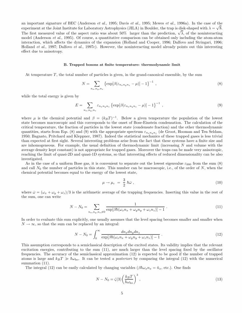
much larger than hωho. In the available traps, with N ranging from a few thousand to several millions, the transitiontemperature is 20 to 200 times larger than hωho. This also means that the semiclassical approximation is expectedto work well in these systems on a wide and useful range of temperatures. The frequency ωho/(2π) is fixed by thetrapping potential and ranges typically from tens to hundreds of Hertz. This gives hωho of the order of a few nK.In one of the first experiments at JILA (Ensher et al., 1996) for example, the average level spacing was about 9 nK,corresponding to a critical temperature [see Eq. (14)] of about 300 nK with 40000 atoms in the trap. We also notethat, for the ideal gas, the chemical potential is of the same order of hωho, as shown by Eq. (10). However, as wewill see later on, its value depends significantly on the atom-atom interaction and shall consequently provide a thirdimportant scale of energy.

The noninteracting harmonic oscillator model has guided experimentalists to the proper value of the critical tem-perature. In fact, the measured transition temperature was found to be very close to the ideal gas value (14), theoccupation of the condensate becoming macroscopically large below the critical temperature as predicted by (15). As

6

an example, in Fig. 5 we show the first experimental results obtained at JILA (Ensher et al., 1996). The occurrenceof a sudden transition at T/T 0

c ∼ 1 is evident. Similar results have been obtained also at MIT (Mewes et al., 1996a).Apart from problems related to temperature calibration, a more quantitative comparison between theory and exper-iments requires the inclusion of two main effects: the fact that these gases have a finite number of particles and thatthey are interacting. The role of interactions will be analysed extensively in the next sections. Here we briefly discussthe relevance of finite size corrections.

C. Finite size effects

The number of atoms that can be put into the traps is not truly macroscopic. So far experiments have been carriedout with a maximum of about 107 atoms. As a consequence, the thermodynamic limit is never reached exactly. Afirst effect is the lack of discontinuities in the thermodynamic functions. Hence Bose-Einstein condensation in thesetrapped gases is not, strictly speaking, a phase transition. In practice, however, the macroscopic occupation of thelowest state occurs rather abruptly as temperature is lowered and can be observed, as clearly shown in Fig. 5. Thetransition is actually rounded with respect to the predictions of the N → ∞ limit, but this effect, though interesting,is small enough to make the words transition and critical temperature meaningful even for finite-sized systems. Itis also worth noticing that, instead of being a limitation, the fact that N is finite makes the system potentiallyricher, because new interesting regimes can be explored even in cases where there is no real phase transition in thethermodynamic limit. An example is BEC in 1D, as we will see in Sec. II D.

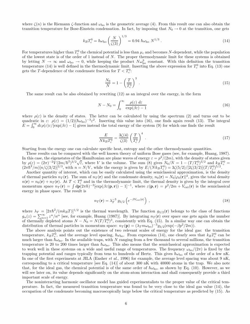
In order to work out the thermodynamics of a noninteracting Bose gas, all one needs is the spectrum of singleparticle levels entering the Bose distribution function. Working in the grand-canonical ensemble for instance, theaverage number of atoms is given by the sum (8) and it is not necessary to take the N → ∞ limit. In fact, the explicitsummation can be carried out numerically (Ketterle and van Druten, 1996b) for a fixed number of particles and agiven temperature, the chemical potential being a function of N and T . The condensate fraction N0(T )/N , obtainedin this way, turns out to be smaller than the thermodynamic limit prediction (15) and, as expected, the transition isrounded off. An example of an exact calculation of the condensate fraction for 1000 noninteracting particles is shownin Fig. 6 (circles). With their numerical calculation, Ketterle and van Druten (1996b) found that finite size effectsare significant only for rather small values of N , less than about 104. They calculated also the occupation of the firstexcited levels, finding that the fraction of atoms in these states vanishes for N → ∞ and is very small already for Nof the order of 100.

The first finite size correction to the law (15) for the condensate fraction can be evaluated analytically by studyingthe large N limit of the sum (8) (Grossmann and Holthaus, 1995; Ketterle and van Druten, 1996b; Kirsten and Toms1996; Haugerud, Haugset and Ravndal, 1997). The result for N0(T )/N is given by

N0

N= 1 −

(

T

T 0c

)3

− 3ωζ(2)

2ωho[ζ(3)]2/3

(

T

T 0c

)2

N−1/3 . (19)

To the lowest order, finite size effects decrease as N−1/3 and depend on the ratio of the arithmetic (ω) and geometric(ωho) averages of the oscillator frequencies. For axially symmetric traps this ratio depends on the deformationparameter λ = ωz/ω⊥ as ω/ωho = (λ + 2)/(3λ1/3). For N = 1000 prediction (19) is already indistinguishable fromthe exact result obtained by summing explicitly over the excited states of the harmonic oscillator Hamiltonian, apartfrom a narrow region near T 0

c where higher order corrections should be included to get the exact result. This is wellillustrated in Fig. 6, where we plot the prediction (19) (solid line) together with the exact calculation obtained directlyfrom (8) (circles). Both predictions are also compared with the thermodynamic limit, N0/N = 1 − (T/T 0

c )3.Finite size effects reduce the condensate fraction and thus result in a lowering of the transition temperature as

compared to the N → ∞ limit. By setting the left hand side of Eq. (19) equal to zero one can estimate the shift ofthe critical temperature to order N−1/3 (Grossmann and Holthaus, 1995; Ketterle and van Druten, 1996b; Kirstenand Toms, 1996):

δT 0c

T 0c

= − ωζ(2)

2ωho[ζ(3)]2/3N−1/3 ≃ − 0.73

ω

ωhoN−1/3 . (20)

Another problem, which deserves to be mentioned in connection with the finite size of the system, is the equivalencebetween different statistical ensembles and the problem of fluctuations. In the thermodynamic limit the grand canon-ical, canonical and microcanonical ensembles are expected to provide the same results. However, their equivalence isno longer ensured when N is finite. Rigorous results concerning the ideal Bose gas in a box and, in particular, thebehavior of fluctuations, can be found in Ziff et al. (1977), and Angelescu et al. (1996). In the case of a trapped

7

gas, Gajda and Rzazewski (1997) have shown that the differences between the predictions of the micro- and grandcanonical ensembles for the temperature dependence of the condensate fraction are small already at N ∼ 1000. Thefluctuations of the number of atoms in the condensate are instead much more sensitive to the choice of the ensemble(Navez et al., 1997; Wilkens and Weiss, 1997; see also Holthaus, Kalinowski and Kirsten, 1998, and references therein).Inclusion of two-body interactions can, however, change the scenario significantly (Giorgini, Pitaevskii and Stringari,1998).

D. Role of dimensionality

So far we have discussed the properties of the ideal Bose gas in three-dimensional space. Though the trappingfrequencies in each direction can be quite different, nevertheless the relevant results for the temperature dependenceof the condensate have been obtained assuming that kBT is much larger than all the oscillator energies hωx, hωy, hωz.In order to observe effects of reduced dimensionality, one should remove such a condition in one or two directions.

The statistical behavior of 2D and 1D Bose gases exhibits very peculiar features. Let us first recall that in auniform gas Bose-Einstein condensation cannot occur in 2D and 1D at finite temperature because thermal fluctuationsdestabilize the condensate. This can be seen by noting that, for an ideal gas in the presence of BEC, the chemicalpotential vanishes and the momentum distribution, n(p) ∝ [exp(βp2/2m)−1]−1, exhibits an infrared 1/p2 divergence.In the thermodynamic limit, this yields a divergent contribution to the integral

∫

dp n(p) in 2D and 1D, therebyviolating the normalization condition. The absence of BEC in 1D and 2D can be also proven for interacting uniformsystems, as shown by Hohenberg (1967).

In the presence of harmonic trapping, the effects of thermal fluctuations are strongly quenched due to the differentbehavior exhibited by the density of states ρ(ε). In fact, while in the uniform gas ρ(ε) behaves as ε(d−2)/2, whered is the dimensionality of space, in the presence of an harmonic potential one has instead the law ρ(ε) ∼ εd−1 and,consequently, the integral (16) converges also in 2D. The corresponding value of the critical temperature is given by

kBT2D = hω2D

(

N

ζ(2)

)1/2

, (21)

where ω2D = (ωxωy)1/2 (see, for example, Mullin, 1997, and references therein). One notes first that in 2D thethermodynamic limit corresponds to taking N → ∞ and ω2D → 0 with the product Nω2

2D kept constant. In orderto achieve 2D Bose-Einstein condensation in real 3D traps, one should choose the frequency ωz in the third directionlarge enough to satisfy the condition hω2D ≪ kBT2D < hωz; this implies rather severe conditions on the deformationof the trap. The main features of BEC in 2D gases confined in harmonic traps and, in particular, the applicability ofthe Hohenberg theorem and of its extensions to nonuniform gases, have been discussed in details by Mullin (1997).

In 1D the situation is also very interesting. In this case, Bose-Einstein condensation cannot occur even in thepresence of harmonic confinement because of the logarithmic divergence in the integral (16). This means that thecritical temperature for 1D Bose-Einstein condensation tends to zero in the thermodynamic limit if one keeps theproduct Nω1D fixed. In fact, in 1D the critical temperature for the ideal Bose gas can be estimated to be (Ketterleand van Druten, 1996b)

kBT1D = hω1DN

ln(2N)(22)

with ω1D ≡ ωz. Despite the fact that one cannot have BEC in the thermodynamic limit, nevertheless for finite valuesof N the system can exhibit a large occupation of the lowest single-particle state in a useful interval of temperatures.Furthermore, if the value ofN and the parameters of the trap are chosen in a proper way, one observes a new interestingphenomenon associated with the macroscopic occupation of the lowest energy state, taking place in two distinct steps(van Druten and Ketterle, 1997). This happens when the relevant parameters of the trap satisfy simultaneously theconditions T1D < T3D and hω⊥ < kBT3D, where T3D coincides with the usual critical temperature given in Eq. (14)and ω⊥ is the frequency of the trap in the x-y plane. In the interval T1D < T < T3D, only the radial degrees offreedom are frozen, while no condensation occurs in the axial degrees of freedom. At lower temperatures, below T1D,also the axial variables start being frozen and the overall ground state is occupied in a macroscopic way. An exampleof this two-step BEC is shown in Fig. 7. It is also interesting to notice that the conditions for the occurrence oftwo-step condensation in harmonic potentials are peculiar of the 1D geometry. In fact, it is easy to check that thecorresponding conditions T2D < T3D and hωz < kBT3D, which would yield two-step BEC in 2D, cannot be easilysatisfied because of the absence of the lnN factor.

8

It is finally worth pointing out that the above discussion concerns the behavior of the ideal Bose gas. Effects oftwo-body interactions are expected to modify in a deep way the nature of the phase transition in reduced dimension-ality. In particular, interacting Bose systems exhibit the well known Berezinsky-Kosterlitz-Thouless transition in 2D(Berezinsky, 1971; Kosterlitz and Thouless, 1973). The case of trapped gases in 2D has been recently discussed byMullin (1998) and is expected to become an important issue in future investigations.

E. Non harmonic traps and adiabatic transformations

A crucial step to reach the low temperatures needed for BEC in the experiments realized so far is evaporative cooling.This technique is intrinsically irreversible since it is based on the loss of hot particles from the trap. New interestingperspectives would open if one could adiabatically cool the system in a reversible way (Ketterle and Pritchard, 1992;Pinkse et al., 1997). Reversible cooling of the gas is achieved by adiabatically changing the shape of the trap at arate slow compared to the internal equilibration rate.

An important class of trapping potentials for studying the effects of adiabatic changes is provided by power-lawpotentials of the form

Vext(r) = A rα , (23)

where, for simplicity, we assume spherical symmetry. The critical temperature for Bose-Einstein condensation in thetrap (23) has been calculated by Bagnato, Pritchard and Kleppner (1987) and is given by

kBT0c =

[

Nh3

(2m)3/2

6√πAδ

Γ(1 + δ)ζ(3/2 + δ)

]

1(3/2+δ)

. (24)

Here we have introduced the parameter δ = 3/α, while Γ(x) is the usual gamma function. By setting δ = 3/2 andA = mω2

ho/2, one recovers the result for the transition temperature in an isotropic harmonic trap. The result for arigid box is instead obtained by letting δ → 0.

It is straightforward to work out the thermodynamics of a noninteracting gas in the confining potential (23)(Bagnato, Pritchard and Kleppner, 1987; Pinkse et al. 1997). For example, for the condensate fraction one finds:N0/N = 1−(T/T 0

c )3/2+δ. More relevant to the discussion of reversible processes is the entropy which remains constantduring the adiabatic change. Above Tc the system can be approximated by a classical Maxwell-Boltzmann gas andthe entropy per particle takes the simple form

S

NkB=

(

5

2+ δ − ln ζ(3/2 + δ)

)

+

(

3

2+ δ

)

ln

(

T

T 0c

)

. (25)

From this equation one sees that the entropy depends on the parameter A of the external potential (23) only throughthe ratio T/T 0

c . Thus, for a fixed power-law dependence of the trapping potential (δ fixed), an adiabatic change ofA, like for example an adiabatic expansion of the harmonic trap, does not bring us closer to the transition, since theratio T/T 0

c remains constant. A reduction of the ratio T/T 0c is instead obtained by increasing adiabatically δ, that

is, changing the power-law dependence of the trapping potential (Pinkse et al. 1997). For example, in going from a

harmonic (δ1 = 3/2) to a linear trap (δ2 = 3), one gets the relation t2 ≃ 0.7t2/31 between the initial and final reduced

temperature t = T/T 0c . In this case a system at twice the critical temperature (t1 = 2) can be cooled down to nearly

the critical point (t2 ≃ 1.1). Using this technique it should be possible, by a proper change of δ, to cool adiabaticallythe system from the high temperature phase without condensate down to temperatures below Tc with a large fractionof atoms in the condensate state.

The possibility of reaching BEC using adiabatic transformations has been recently successfully explored in anexperiment carried out at MIT (Stamper-Kurn et al., 1998b).

III. EFFECTS OF INTERACTIONS: GROUND STATE

A. Order parameter and mean-field theory

The many body Hamiltonian describing N interacting bosons confined by an external potential Vext is given, insecond quantization, by:

9

H =

∫

dr Ψ†(r)

[

− h2

2m∇2 + Vext(r)

]

Ψ(r) +1

2

∫

drdr′ Ψ†(r)Ψ†(r′)V (r − r′)Ψ(r′)Ψ(r) (26)

where Ψ(r) and Ψ†(r) are the boson field operators that annihilate and create a particle at the position r, respectively,and V (r − r′) is the two-body interatomic potential.

The ground state of the system as well as its thermodynamic properties can be directly calculated starting fromthe Hamiltonian (26). For instance, Krauth (1996) has used a Path Integral Monte Carlo method to calculate thethermodynamic behavior of 104 atoms interacting with a repulsive “hard-sphere” potential. In principle, this proceduregives exact results within statistical errors. However, the calculation can be heavy or even impracticable for systemswith much larger values of N . Mean-field approaches are commonly developed for interacting systems in order toovercome the problem of solving exactly the full many-body Schrodinger equation. Apart from the convenience ofavoiding heavy numerical work, mean-field theories allow one to understand the behavior of a system in terms of aset of parameters having a clear physical meaning. This is particularly true in the case of trapped bosons. Actuallymost of the results reviewed in this paper show that the mean-field approach is very effective in providing quantitativepredictions for the static, dynamic and thermodynamic properties of these trapped gases.

The basic idea for a mean-field description of a dilute Bose gas was formulated by Bogoliubov (1947). The key pointconsists in separating out the condensate contribution to the bosonic field operator. In general, the field operatorcan be written as Ψ(r) =

∑

α Ψα(r)aα, where Ψα(r) are single-particle wave functions and aα are the correspondingannihilation operators. The bosonic creation and annihilation operators a†α and aα are defined in Fock space throughthe relations

a†α | n0, n1, . . . , nα, . . .〉 =√nα + 1 | n0, n1, . . . , nα + 1, . . .〉 (27)

aα | n0, n1, . . . , nα, . . .〉 =√nα | n0, n1, . . . , nα − 1, . . .〉 (28)

where nα are the eigenvalues of the operator nα = a†αaα giving the number of atoms in the single-particle α-state.They obey the usual commutation rules:

[

aα, a†β

]

= δα,β ,[

aα, aβ

]

= 0 ,[

a†α, a†β

]

= 0 . (29)

Bose-Einstein condensation occurs when the number of atoms n0 of a particular single-particle state becomes verylarge: n0 ≡ N0 ≫ 1 and the ratio N0/N remains finite in the thermodynamic limit N → ∞. In this limit the stateswith N0 and N0 ± 1 ≃ N0 correspond to the same physical configuration and, consequently, the operators a0 and

a†0 can be treated like c-numbers: a0 = a†0 =√N0. For a uniform gas in a volume V , where BEC occurs in the

single-particle state Ψ0 = 1/√V having zero momentum, this means that the field operator Ψ(r) can be decomposed

in the form Ψ(r) =√

N0/V + Ψ′(r). By treating the operator Ψ′ as a small perturbation, Bogoliubov developed the“first-order” theory for the excitations of interacting Bose gases.

The generalization of the Bogoliubov prescription to the case of nonuniform and time dependent configurations isgiven by

Ψ(r, t) = Φ(r, t) + Ψ′(r, t) , (30)

where we have used the Heisenberg representation for the field operators. Here Φ(r, t) is a complex function defined

as the expectation value of the field operator: Φ(r, t) ≡ 〈Ψ(r, t)〉. Its modulus fixes the condensate density throughn0(r, t) = |Φ(r, t)|2. The function Φ(r, t) possesses also a well-defined phase and, similarly to the case of uniformgases, this corresponds to assuming the occurrence of a broken gauge symmetry in the many-body system.

The function Φ(r, t) is a classical field having the meaning of an order parameter and is often called “wave function ofthe condensate”. It characterizes the off-diagonal long-range behavior of the one-particle density matrix ρ1(r

′, r, t) =

〈Ψ†(r′, t)Ψ(r, t)〉. In fact the decomposition (30) implies the following asymptotic behavior (Ginzburg and Landau,1950; Penrose, 1951; Penrose and Onsager, 1956):

lim|r′−r|→∞

ρ1(r′, r, t) = Φ∗(r′, t)Φ(r, t) . (31)

Notice that, strictly speaking, in a finite-sized system neither the concept of broken gauge symmetry, nor the one ofoff-diagonal long-range order can be applied. The condensate wave function Φ has nevertheless still a clear meaning: itcan be in fact determined through the diagonalization of the one-body density matrix,

∫

dr′ρ1(r′, r)Φi(r

′) = NiΦi(r),and corresponds to the eigenfunction, Φi, with the largest eigenvalue, Ni. This procedure has been used, for example,to explore Bose-Einstein condensation in finite drops of liquid helium by Lewart et al. (1988). The connectionbetween the condensate wave function, defined through the diagonalization of the density matrix and the concept

10

of order parameter commonly used in the theory of superfluidity, is an interesting and nontrivial problem in itself.Another important question concerns the possible fragmentation of the condensate, taking place when two or moreeigenstates of the density matrix ρ1(r

′, r) are macroscopically occupied. One can show (Nozieres and Saint James,1982; Nozieres, 1995) that, due to exchange effects, in uniform gases interacting with repulsive forces the fragmentationcosts a macroscopic energy. The behavior can be however different in the presence of attractive forces and almostdegenerate single-particle states (Nozieres and Saint James, 1982; Kagan, Shlyapnikov and Walraven, 1996; Wilkin,Gunn and Smith, 1998).

The decomposition (30) becomes particularly useful if Ψ′ is small, i.e., when the depletion of the condensate is

small. Then, an equation for the order parameter can be derived by expanding the theory to the lowest orders in Ψ′

as in the case of uniform gases. The main difference is that here one gets also a nontrivial “zeroth-order” theory forΦ(r, t).

In order to derive the equation for the condensate wave function Φ(r, t), one has to write the time evolution of the

field operator Ψ(r, t) using the Heisenberg equation with the many-body Hamiltonian (26):

ih∂

∂tΨ(r, t) = [Ψ, H]

=

[

− h2∇2

2m+ Vext(r) +

∫

dr′ Ψ†(r′, t)V (r′ − r)Ψ(r′, t)

]

Ψ(r, t) . (32)

Then one has to replace the operator Ψ with the classical field Φ. In the integral containing the atom-atom interactionV (r′ − r), this replacement is, in general, a poor approximation when short distances (r′− r) are involved. In a diluteand cold gas, one can nevertheless obtain a proper expression for the interaction term by observing that, in this case,only binary collisions at low energy are relevant and these collisions are characterized by a single parameter, thes-wave scattering length, independently of the details of the two-body potential. This allows one to replace V (r′ − r)in (32) with an effective interaction

V (r′ − r) = gδ(r′ − r) (33)

where the coupling constant g is related to the scattering length a through

g =4πh2a

m. (34)

The use of the effective potential (33) in (32) is compatible with the replacement of Ψ with Φ and yields the followingclosed equation for the order parameter:

ih∂

∂tΦ(r, t) =

(

− h2∇2

2m+ Vext(r) + g|Φ(r, t)|2

)

Φ(r, t) . (35)

This equation, known as Gross-Pitaevskii (GP) equation, was derived independently by Gross (1961 and 1963) andPitaevskii (1961). Its validity is based on the condition that the s-wave scattering length be much smaller thanthe average distance between atoms and that the number of atoms in the condensate be much larger than 1. TheGP equation can be used, at low temperature, to explore the macroscopic behavior of the system, characterized byvariations of the order parameter over distances larger than the mean distance between atoms.

The Gross-Pitaevskii equation (35) can also be obtained using a variational procedure:

ih∂

∂tΦ =

δE

δΦ∗, (36)

where the energy functional E is given by

E[Φ] =

∫

dr

[

h2

2m|∇Φ|2 + Vext(r)|Φ|2 +

g

2|Φ|4

]

. (37)

The first term in the integral (37) is the kinetic energy of the condensate Ekin, the second is the harmonic oscillatorenergy Eho, while the last one is the mean-field interaction energy Eint. Notice that the mean-field term, Eint,corresponds to the first correction in the virial expansion for the energy of the gas. In the case of non-negative andfinite-range interatomic potentials, rigorous bounds for this term have been obtained by Dyson (1967) and Lieb andYngvason (1998).

11

The dimensionless parameter controlling the validity of the dilute-gas approximation, required for the derivation ofEq. (35), is the number of particles in a “scattering volume” |a|3. This can be written as n|a|3, where n is the averagedensity of the gas. Recent determinations of the scattering length for the atomic species used in the experiments onBEC give: a = 2.75 nm for 23Na (Tiesinga et al., 1996), a = 5.77 nm for 87Rb (Boesten et al., 1997) and a = −1.45nm for 7Li (Abraham et al., 1995). Typical values of density range instead from 1013 to 1015 cm−3, so that n|a|3 isalways less than 10−3.

When n|a|3 ≪ 1 the system is said to be dilute or weakly interacting. However, one should better clarify themeaning of the words “weakly interacting”, since the smallness of the parameter n|a|3 does not imply necessarily thatthe interaction effects are small. These effects, in fact, have to be compared with the kinetic energy of the atoms in thetrap. A first estimate can be obtained by calculating the interaction energy, Eint, on the ground state of the harmonicoscillator. This energy is given by gNn, where the average density is of the order of N/a3

ho, so that Eint ∝ N2|a|/a3ho.

On the other hand, the kinetic energy is of the order of Nhωho and thus Ekin ∝ Na−2ho . One finally finds

Eint

Ekin∝ N |a|

aho. (38)

This is the parameter expressing the importance of the atom-atom interaction compared to the kinetic energy. It canbe easily larger than 1 even if n|a|3 ≪ 1, so that also very dilute gases can exhibit an important nonideal behavior,as we will discuss in the following sections. In the first experiments with rubidium atoms at JILA (Anderson et al.,1995) the ratio |a|/aho was about 7 × 10−3, with N of the order of a few thousands. Thus Na/aho is larger than1. In the experiments with 7Li at Rice University (Bradley et al., 1997; Sackett et al., 1997) the same parameteris smaller than 1, since the number of particles is of the order of 1000 and |a|/aho ≈ 0.5 × 10−3. Finally, in theexperiments with sodium at MIT (Davis et al., 1995) the number of atoms in the condensate is very large (106 − 107)and N |a|/aho ∼ 103 − 104.

Due to the assumption Ψ′ ≡ 0, the above formalism is strictly valid only in the limit of zero temperature, whenall the particles are in the condensate. The dynamic behavior and the generalization to finite temperatures will bediscussed in Secs. IV and V, respectively. Here we present the results for the stationary solution of the Gross-Pitaevskii(GP) equation at zero temperature.

B. Ground state

For a system of noninteracting bosons in a harmonic trap, the condensate has the form of a Gaussian of averagewidth aho [see Eq. (3)], and the central density is proportional to N . If the atoms are interacting, the shape of thecondensate can change significantly with respect to the Gaussian. The scattering length entering the Gross-Pitaevskiiequation can be positive or negative, its sign and magnitude depending crucially on the details of the atom-atompotential. Positive and negative values of a correspond to an effective repulsion and attraction between the atoms,respectively. The change can be dramatic when the interaction energy is much greater than the kinetic energy, thatis, when N |a|/aho ≫ 1. The central density is lowered (raised) by a repulsive (attractive) interaction and the radiusof the atomic cloud consequently increases (decreases). This effect of the interaction has important consequences, notonly for the structure of the ground state, but also for the dynamics and thermodynamics of the system, as we willsee later on.

The ground state can be easily obtained within the formalism of mean-field theory. For this, one can write thecondensate wave function as Φ(r, t) = φ(r) exp(−iµt/h), where µ is the chemical potential and φ is real and normalizedto the total number of particles,

∫

dr φ2 = N0 = N . Then the Gross-Pitaevskii equation (35) becomes

(

− h2∇2

2m+ Vext(r) + gφ2(r)

)

φ(r) = µφ(r) . (39)

This has the form of a “nonlinear Schrodinger equation”, the nonlinearity coming from the mean-field term, propor-tional to the particle density n(r) = φ2(r). In the absence of interactions (g = 0), this equation reduces to the usualSchrodinger equation for the single-particle Hamiltonian −h2/(2m)∇2 + Vext(r) and, for harmonic confinement, the

ground state solution coincides, apart from a normalization factor, with the Gaussian function (3): φ(r) =√Nϕ0(r).

We note, in passing, that a similar nonlinear equation for the order parameter has been also considered in connectionwith the theory of superfluid helium near the λ-point (Ginzburg and Pitaevskii, 1958); in that case, however, theingredients of the equation have a different physical meaning.

The numerical solution of the GP equation (39) is relatively easy to obtain (Edwards and Burnett, 1995; Ruprechtet al., 1995; Edwards et al., 1996b; Dalfovo and Stringari, 1996; Holland and Cooper, 1996). Typical wave functions

12

φ, calculated from Eq. (39) with different values of the parameter N |a|/aho, are shown in Figs. 8 and 9 for attractiveand repulsive interaction, respectively. The effects of the interaction are revealed by the deviations from the Gaussianprofile (3) predicted by the noninteracting model. Excellent agreement has been found by comparing the solution ofthe GP equation with the experimental density profiles obtained at low temperature (Hau et al., 1998), as shown inFig. 3. The condensate wave function obtained with the stationary GP equation has been also compared with theresults of an ab initio Monte Carlo simulation starting from Hamiltonian (26), finding a very good agreement (Krauth,1996).

The role of the parameter N |a|/aho, already discussed in the previous section, can be easily pointed out, in theGross-Pitaevskii equation, by using rescaled dimensionless variables. Let us consider a spherical trap with frequencyωho and use aho, a

−3ho and hωho as units of length, density and energy, respectively. By putting a tilde over the rescaled

quantities, Eq. (39) becomes

[

−∇2 + r2 + 8π(Na/aho)φ2(r)

]

φ(r) = 2µφ(r) . (40)

In these new units the order parameter satisfies the normalization condition∫

dr|φ|2 = 1. It is now evident that theimportance of the atom-atom interaction is completely fixed by the parameter Na/aho.

It is worth noticing that the solution of the stationary GP equation (39) minimizes the energy functional (37) fora fixed number of particles. Since the ground state has no currents, the energy is a functional of the density only,which can be written in the form

E[n] =

∫

dr

[

h2

2m|∇

√n|2 + nVext(r) +

gn2

2

]

= Ekin + Eho + Eint . (41)

The first term corresponds to the quantum kinetic energy coming from the uncertainty principle; it is usually named“quantum pressure” and vanishes for uniform systems. In general, for a nonstationary order parameter, the kineticenergy in (37) includes also the contribution of currents in the form of an additional term containing the gradient ofthe phase of Φ.

By direct integration of the GP equation (39) one finds the useful expression

µ = (Ekin + Eho + 2Eint)/N (42)

for the chemical potential in terms of the different contributions to the energy functional (41). Further importantrelationships can be also found by means of the virial theorem. In fact, since the energy (37) is stationary for anyvariation of φ around the exact solution of the GP equation, one can choose scaling transformations of the formφ(x, y, z) → (1 + ν)1/2φ((1 + ν)x, y, z), and insert them in (37). By imposing the energy variation to vanish at firstorder in ν, one finally gets

(Ekin)x − (Eho)x +1

2Eint = 0 , (43)

where (Ekin)x = 〈∑

i p2ix〉/2m and (Eho)x = (m/2)ω2

x〈∑

i x2i 〉. Analogous expressions are found by choosing similar

scaling transformations for the y and z co-ordinates. By summing over the three directions one finally finds the virialrelation:

2Ekin − 2Eho + 3Eint = 0 . (44)

The above results are exact within Gross-Pitaevskii theory and can be used, for instance, to check the numericalsolutions of Eq. (39).

In a series of experiments the gas has been imaged after a sudden switching-off of the trap and the kinetic energyof the atoms has been measured by integrating over the observed velocity distribution. This energy, which is alsocalled release energy, coincides with the sum of the kinetic and interaction energies of the atoms at the beginning ofthe expansion:

Erel = Ekin + Eint . (45)

During the first phase of the expansion both the quantum kinetic energy (quantum pressure) and the interactionenergy are rapidly converted into kinetic energy of motion. Then the atoms expand at constant velocity. Sinceenergy is conserved during the expansion, its initial value (45), calculated with the stationary GP equation, canbe directly compared with experiments. This comparison provides clean evidences for the crucial role played by

13

two-body interactions. In fact, the noninteracting model predicts a release energy per particle given by Erel/N =(1/2)(1 + λ/2)hωho, independent of N . Conversely, the observed release energy per particle depends rather stronglyon N , in good agreement with the theoretical predictions for the interacting gas. In Figs. 10 and 11, we show theexperimental data obtained at JILA (Holland et al.,1997) and MIT (Mewes et al., 1996a), respectively.

Finally, we notice that the balance between the quantum pressure and the interaction energy of the condensatefixes a typical length scale, called the healing length, ξ. This is the minimum distance over which the order parametercan heal. If the condensate density grows from 0 to n within a distance ξ, the two terms in Eq. (39) coming from thequantum pressure and the interaction energy are ∼ h2/(2mξ2) and ∼ 4πh2an/m, respectively. By equating them,one finds the following expression for the healing length:

ξ = (8πna)−1/2 . (46)

This is a well known result for weakly interacting Bose gases. In the case of trapped bosons, one can use the centraldensity, or the average density, to get an order of magnitude of the healing length. This quantity is relevant forsuperfluid effects. For instance, it provides the typical size of the core of quantized vortices (Gross, 1961; Pitaevskii,1961). Note that in condensed matter physics the same quantity is often named “coherence length”, but the name“healing length” is preferable here in order to avoid confusion with different definitions of coherence length used inatomic physics and optics.

C. Collapse for attractive forces

If forces are attractive (a < 0), the gas tends to increase its density in the center of the trap in order to lower theinteraction energy, as seen in Fig. 8. This tendency is contrasted by the zero point kinetic energy which can stabilisethe system. However, if the central density grows too much, the kinetic energy is no longer able to avoid the collapseof the gas. For a given atomic species in a given trap, the collapse is expected to occur when the number of particlesin the condensate exceeds a critical value Ncr, of the order of aho/|a|. It is worth stressing that in a uniform gas,where quantum pressure is absent, the condensate is always unstable.

The critical number Ncr can be calculated at zero temperature by means of the Gross-Pitaevskii equation. Thecondensates shown in Fig. 8 are metastable, corresponding to local minima of the energy functional (37) for differentN . When N increases, the depth of the local minimum decreases. Above Ncr the minimum no longer exists and theGross-Pitaesvkii equation has no solution. For a spherical trap this happens at (Ruprecht et al., 1995)

Ncr|a|aho

= 0.575 . (47)

For the axially symmetric trap with 7Li used in the experiments at Rice University (Bradley et al., 1995 and 1997;Sackett et al., 1997), the GP equation predicts Ncr ≃ 1400 (Dalfovo and Stringari, 1996; Dodd et al., 1996); this valueis consistent with recent experimental measurements (Bradley et al., 1997; Sackett et al., 1997). The same problemhas been investigated theoretically by several authors (Kagan, Shlyapnikov and Walraven, 1996; Houbiers and Stoof,1996; Shuryak, 1996; Pitaevskii, 1996; Bergeman,1997).

A direct insight into the behavior of the gas with attractive forces can be obtained by means of a variationalapproach based on Gaussian functions (Baym and Pethick, 1996). For a spherical trap one can minimize the energy(37) using the ansatz

φ(r) =

(

N

w3a3hoπ

3/2

)1/2

exp

(

− r2

2w2a2ho

)

, (48)

where w is a dimensionless variational parameter which fixes the width of the condensate. One gets

E(w)

Nhωho=

3

4(w−2 + w2) − (2π)−1/2N |a|

ahow−3 . (49)

This energy is plotted in Fig. 12 as a function of w, for several values of the parameter N |a|/aho. One clearlysees that the local minimum disappears when this parameter exceeds a critical value. This can be calculated byrequiring that the first and second derivative of E(w) vanish at the critical point (w = wcr and N = Ncr). One findswcr = 5−1/4 ≈ 0.669 and Ncr|a|/aho ≈ 0.671. The last formula provides an estimate of the critical number of atoms,for given trap and atomic species, reasonably close to the value (47) obtained by solving exactly the GP equation.The Gaussian ansatz has been used by several authors in order to explore both static and dynamic properties of

14

the trapped gases. The stability of a gas with a < 0 has been explored in details, for instance, by Stoof (1997),Perez-Garcıa et al. (1997), Shi and Zheng (1997a), Parola, Salasnich and Reatto (1998). The variational functionproposed by Fetter (1997), which interpolates smoothly between the ideal gas and the Thomas-Fermi limit for positivea, also reduces to a Gaussian for a < 0.

The behavior of the gas close to collapse could be significantly affected by mechanisms not included in the Gross-Pitaevskii theory. Among them, inelastic two- and three-body collisions can cause a loss of atoms from the condensatethrough, for instance, spin exchange or recombination (Hijmans et al., 1993; Edwards et al., 1996b; Moerdijk et al.,1996; Fedichev et al., 1996). This is an important problem not only for attractive forces but also for repulsive forceswhen the density of the system becomes large.

Recent discussions about the collapse, including quantum tunneling phenomena, can be found, for instance, inSackett, Stoof and Hulet (1998), Kagan, Muryshev and Shlyapnikov (1998), Ueda and Leggett (1998), Ueda andHuang (1998).

D. Large N limit for repulsive forces

In the case of atoms with repulsive interaction (a > 0), the limit Na/aho ≫ 1 is particularly interesting, since thiscondition is well satisfied by the parameters N , a and aho used in most of current experiments. Moreover, in thislimit the predictions of mean-field theory take a rather simple analytic form (Edwards and Burnett 1995; Baym andPethick 1996).

As regards the ground state, the effect of increasing the parameter Na/aho is clearly seen in Fig. 9: the atomsare pushed outwards, the central density becomes rather flat and the radius grows. As a consequence, the quantumpressure term in the Gross-Pitaevskii equation (39), proportional to ∇2

√

n(r), takes a significant contribution onlynear the boundary and becomes less and less important with respect to the interaction energy. If one neglectscompletely the quantum pressure in (39), one gets the density profile in the form

n(r) = φ2(r) = g−1[µ− Vext(r)] (50)

in the region where µ > Vext(r), and n = 0 outside. This is often referred to as Thomas-Fermi (TF) approximation.The normalization condition on n(r) provides the relation between chemical potential and number of particles:

µ =hωho

2

(

15Na

aho

)2/5

. (51)

Note that the chemical potential depends on the trapping frequencies, entering the potential Vext given in (1), onlythrough the geometric average ωho [see Eq. (4)]. Moreover, since µ = ∂E/∂N , the energy per particle turns out tobe E/N = (5/7)µ. This energy is the sum of the interaction and oscillator energies, since the kinetic energy gives avanishing contribution for large N . Finally, in the same limit, the release energy (45) coincides with the interactionenergy: Erel/N = (2/7)µ.

The chemical potential, as well as the interaction and oscillator energies obtained by solving numerically the GPequation (39) become closer and closer to the Thomas-Fermi values when N increases (see for instance, Dalfovo andStringari, 1996). For sodium atoms in the MIT traps, where N is larger than 106, the Thomas-Fermi approximationis practically indistinguishable from the solution of the GP equation. The release energy per particle measured byMewes et al. (1996a) is indeed well fitted with a N2/5 law, as shown in Fig. 11. The same agreement is expected tooccur for rubidium atoms in the most recent JILA traps, having N larger than 105 (Matthews et al., 1998).

The density profile (50) has the form of an inverted parabola, which vanishes at the classical turning point R

defined by the condition µ = Vext(R). For a spherical trap, this implies µ = mω2hoR

2/2 and, using result (51) for µ,one finds the following expression for the radius of the condensate

R = aho

(

15Na

aho

)1/5

(52)

which grows with N . For an axially symmetric trap, the widths in the radial and axial directions are fixed by theconditions µ = mω2

⊥R2⊥/2 = mω2

zZ2/2. It is worth mentioning that, in the case of the cigar-shaped trap used at

MIT, with a condensate of about 107 sodium atoms, the axial width becomes macroscopically large (Z ∼ 0.3 mm),allowing for direct in situ measurements.

The value of the density (50) in the center of the trap is nTF(0) = µ/g. It is worth stressing that this density ismuch lower than the one predicted for noninteracting particles. In the latter case, using Eq. (3) one gets nho(0) =N/(π3/2a3

ho). The ratio between the central densities in the two cases is then

15

nTF(0)

nho(0)=

152/5π1/2

8

(

Na

aho

)−3/5

, (53)

and decreases with N . For the available traps with 23Na and 87Rb, where Na/aho ranges from about 10 to 104, theatom-atom repulsion reduces the density by one or two orders of magnitude, which is a quite remarkable effect forsuch a dilute systems. An example was already shown in Fig. 3; in that case, the number of particles is about 80000and Na/aho ∼ 300.

In Fig. 13a we show the density profile for a gas in a spherical trap with Na/aho = 100. The comparison with theexact solution of the GP equation (39) shows that the TF approximation is very accurate except in the surface regionclose to R. In part b of the same figure, we plot the column density, n(z) =

∫

dx n(x, 0, z), which is the measuredquantity when the atomic cloud is imaged by light absorption or dispersive light scattering. Using the TF density (50)with Vext = (1/2)mω2

hor2, one finds n(z) = (4/3)[2/(mω2

ho)]1/2g−1[µ− (1/2)mω2

hoz2]3/2. One notes that the accuracy

of the Thomas-Fermi approximation is even better in the case of the column density, because the extra integrationmakes the cusp in the outer part of the condensate smoother.

The only region where the Thomas-Fermi density (50) is inadequate is close to the classical turning point. Thisregion plays a crucial role for the calculation of the kinetic energy of the condensate. The shape of the outer part ofthe condensate is fixed by the balance of the zero point kinetic energy and the external potential. In particular, thisbalance can be used to define an effective surface thickness, d. For a spherical trap, for instance, one can assume thetwo energies to have the form h2/(2md2) and mω2

hoRd, respectively. One then gets (Baym and Pethick, 1996)

d

R= 2−1/3

(aho

R

)4/3

; (54)

this ratio is small when TF approximation is valid, i.e., when R ≫ aho. It is interesting to compare the surfacethickness d with the healing length (46). In terms of the ratio aho/R one can write ξ/R = (aho/R)2, showing thatthe healing length decreases with N more rapidly than the surface thickness d.

A good approximation for the density in the region close to the classical turning point, can be obtained by a suitableexpansion of the GP equation (39). In fact, when |r − R| ≪ R, the trapping potential Vext(r) can be replaced witha linear ramp, mω2

hoR(r − R), and the GP equation takes a universal form (Dalfovo, Pitaevskii and Stringari, 1996;Lundh, Pethick and Smith, 1997), yielding the rounding of the surface profile.

Using the above procedure it is possible to calculate the kinetic energy which, in the case of a spherical trap, isfound to follow the asymptotic law

Ekin

N≃ 5h2

2mR2ln

(

R

Caho

)

(55)

where C ≃ 1.3 is a numerical factor. Analogous expansions can be derived for the harmonic potential energy, Eho,and interaction energy, Eint, in the same large N limit (Fetter and Feder, 1997). A straightforward derivation isobtained by using nontrivial relationships among the various energy components Ekin, Eho and Eint of Eq. (41). Afirst relation is given by the virial theorem (44). A second one is obtained by using expression (42) for the chemicalpotential and the thermodynamic definition µ = ∂E/∂N . These two relationships, together with the asymptoticlaw (55) for the kinetic energy, allow one to obtain the expansions Eho/N = (3/7)µTF + h2/(mR2) ln[R/(Caho)] andEint/N = (2/7)µTF − h2/(mR2) ln[R/(Caho)]. From them one gets the useful results

µ = µTF

[

1 + 3a4ho

R4ln

(

R

Caho

)]

(56)

and

E =5

7NµTF

[

1 + 7a4ho

R4ln

(

R

Caho

)]

(57)

for the chemical potential and the total energy, respectively. In these equations µTF and R are the Thomas-Fermivalues (51) and (52) of the chemical potential and the radius of the condensate. Equations (55)-(57), which apply tospherical traps, clearly show that the relevant small parameter in the large N expansion is aho/R = (15Na/aho)

−1/5.The Thomas-Fermi approximation (50) for the ground state density of trapped Bose gases is very useful not only

for determining the static properties of the system, but also for dynamics and thermodynamics, as we will see inSecs. IV and V. It is worth noticing that this approximation can be derived more directly using local density theoryas we are going to discuss in the next section.

16

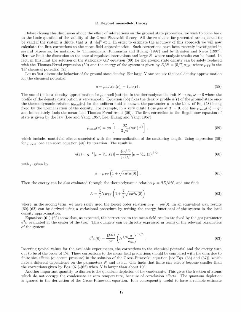
E. Beyond mean-field theory

Before closing this discussion about the effect of interactions on the ground state properties, we wish to come backto the basic question of the validity of the Gross-Pitaevskii theory. All the results so far presented are expected tobe valid if the system is dilute, that is, if n|a|3 ≪ 1. In order to estimate the accuracy of this approach we will nowcalculate the first corrections to the mean-field approximation. Such corrections have been recently investigated inseveral papers as, for instance, by Timmermans, Tommasini and Huang (1997) and by Braaten and Nieto (1997).Here we limit the discussion to the case of repulsive interactions and large N , where analytic results can be found. Infact, in this limit the solution of the stationary GP equation (39) for the ground state density can be safely replacedwith the Thomas-Fermi expression (50) and the energy of the system is given by E/N = (5/7)µTF, where µTF is theTF chemical potential (51).

Let us first discuss the behavior of the ground state density. For large N one can use the local density approximationfor the chemical potential:

µ = µlocal[n(r)] + Vext(r) . (58)

The use of the local density approximation for µ is well justified in the thermodynamic limit N → ∞, ω → 0 where theprofile of the density distribution is very smooth. Equation (58) fixes the density profile n(r) of the ground state oncethe thermodynamic relation µlocal(n) for the uniform fluid is known, the parameter µ in the l.h.s. of Eq. (58) beingfixed by the normalization of the density. For example, in a very dilute Bose gas at T = 0, one has µlocal(n) = gnand immediately finds the mean-field Thomas-Fermi result (50). The first correction to the Bogoliubov equation ofstate is given by the law (Lee and Yang, 1957; Lee, Huang and Yang, 1957)

µlocal(n) = gn

[

1 +32

3√π

(na3)1/2

]

, (59)

which includes nontrivial effects associated with the renormalization of the scattering length. Using expression (59)for µlocal, one can solve equation (58) by iteration. The result is

n(r) = g−1 [µ− Vext(r)] −4m3/2

3π2h3 [µ− Vext(r)]3/2

, (60)

with µ given by

µ = µTF

(

1 +√

πa3n(0))

. (61)

Then the energy can be also evaluated through the thermodynamic relation µ = ∂E/∂N , and one finds

E =5

7NµTF

(

1 +7

8

√

πa3n(0)

)

(62)

where, in the second term, we have safely used the lowest order relation µTF = gn(0). In an equivalent way, results(60)-(62) can be derived using a variational procedure by writing the energy functional of the system in the localdensity approximation.

Equations (61)-(62) show that, as expected, the corrections to the mean-field results are fixed by the gas parametera3n evaluated at the center of the trap. This quantity can be directly expressed in terms of the relevant parametersof the system:

a3n(0) =152/5

8π

(

N1/6 a

aho

)12/5

. (63)

Inserting typical values for the available experiments, the corrections to the chemical potential and the energy turnout to be of the order of 1%. These corrections to the mean-field predictions should be compared with the ones due tofinite size effects (quantum pressure) in the solution of the Gross-Pitaevskii equation [see Eqs. (56) and (57)], whichhave a different dependence on the parameters N and a/aho. One finds that finite size effects become smaller thanthe corrections given by Eqs. (61)-(62) when N is larger than about 106.

Another important quantity to discuss is the quantum depletion of the condensate. This gives the fraction of atomswhich do not occupy the condensate at zero temperature, because of correlation effects. The quantum depletionis ignored in the derivation of the Gross-Pitaevskii equation. It is consequently useful to have a reliable estimate

17

of its value in order to check the validity of the theory. Also in this case we can use local density approximation(Timmermans, Tommasini and Huang, 1997) and write the density of atoms out of the condensate, nout(r), usingBogoliubov’s theory for uniform gases at density n = n(r) (see for example Huang, 1987). One gets nout(r) =(8/3)[n(r)a3/π]1/2. Integration of nout yields the result:

Nout

N=

5√π

8

√

a3n(0) . (64)

for the quantum depletion of the condensate. Similarly to the correction to the mean-field energy (62), this effect isvery small (less than 1%) in the presently available experimental conditions.

The above results justify a posteriori the use of the Bogoliubov prescription for the Bose field operators and theperturbative treatment of the noncondensed part at zero temperature. We recall that this situation is completelydifferent from the one of superfluid 4He where quantum depletion amounts to about 90% (Griffin, 1993; Sokol, 1995).

IV. EFFECTS OF INTERACTIONS: DYNAMICS

A. Excitations of the condensate and time dependent GP equation

The study of elementary excitations is a task of primary importance of quantum many-body theories. In the caseof Bose fluids, in particular, it plays a crucial role in the understanding of the properties of superfluid liquid heliumand was the subject of pioneering work by Landau, Bogoliubov and Feynman (for a recent discussion on the dynamicbehavior of interacting Bose superfluids see, for instance, Griffin, 1993).

After the experimental realization of BEC in trapped Bose gases, there has been an intensive study of the excitationsin these systems. Measurements of the frequency of the lowest modes have soon become available and the directobservation of the propagation of wave packets has been also obtained. In the meanwhile, on the theoretical side, avariety of papers has been written to explore several interesting features exhibited by the dynamic behavior of trappedBose gases.

Let us start our discussion recalling that for dilute Bose gases an appropriate description of the excitations canbe obtained from the time dependent GP equation (35) for the order parameter. This equation has been alreadyused in Sec. III for evaluating the stationary solution φ(r) characterizing the ground state. In the low temperaturelimit, where the properties of the excitations do not depend on temperature, the excited states can be found from the“classical” frequencies ω of the linearized GP equation. Namely, one can look for solutions of the form

Φ(r, t) = e−iµt/h[

φ(r) + u(r)e−iωt + v∗(r)eiωt]

(65)

corresponding to small oscillations of the order parameter around the ground state value. By keeping terms linear inthe complex functions u and v, Eq. (35) becomes

hωu(r) = [H0 − µ+ 2gφ2(r)]u(r) + gφ2(r)v(r) (66)

−hωv(r) = [H0 − µ+ 2gφ2(r)]v(r) + gφ2(r)u(r) . (67)

where H0 = −(h2/2m)∇2 +Vext(r). These coupled equations allow one to calculate the eigenfrequencies ω and hencethe energies ε = hω of the excitations. This formalism was introduced by Pitaevskii (1961), in order to investigatethe excitations of vortex lines in a uniform Bose gas.

This procedure is also equivalent to the diagonalization of the Hamiltonian in Bogoliubov approximation, in which

one expresses the field operator Ψ′ in terms of the quasiparticle operators αj and α†j through (Fetter, 1972 and 1996)

Ψ′(r) =∑

j

[uj(r)αj(t) + v∗j (r)α†j(t)] . (68)

By imposing the Bose commutation rules to the operators αj and α†j , one finds that the quasiparticle amplitudes u

and v must obey the normalization condition∫

dr [u∗i (r)uj(r) − v∗i (r)vj(r)] = δij . (69)

In a uniform gas, the amplitudes u and v are plane waves and the resulting dispersion law takes the most famousBogoliubov form (Bogoliubov, 1947)

18

(hω)2 =

(

h2q2

2m

)(

h2q2

2m+ 2gn

)

(70)

where q is the wavevector of the excitation and n = |φ|2 is the density of the gas. For large momenta the spectrumcoincides with the free-particle energy h2q2/2m. At low momenta Eq. (70) instead yields the phonon dispersionω = cq, where

c =

√

gn

m(71)

is the sound velocity. It is worth noticing that this velocity coincides with the hydrodynamic expression c =[(1/m)∂P/∂n]1/2 for a gas with equation of state P = (1/2)gn2 [see also the discussion after Eq. (78)].

In the case of harmonic trapping, an important role is played by the ratio Na/aho, and one expects differentbehaviors in the two opposite limits Na/aho ≪ 1 and Na/aho ≫ 1. In the first case, one recovers the excitationspectrum ω = nxωx + nyωy + nzωz of the noninteracting harmonic potential [see Eq. (2)]. In the second case, oneobtains a different dispersion law for the excitations of the system which are the analog of phonons [see Eq. (80)below].

The coupled equations (66)-(67) were first used to calculate numerically the excitations of trapped gases by Burnettand co-workers (Ruprecht et al., 1996; Edwards et al, 1996a and 1996c). Similar calculations have been also performedby other authors, for both spherical and anisotropic configurations (Singh and Rokhsar, 1996; Esry, 1997; Hutchinson,Zaremba and Griffin, 1997; Hutchinson and Zaremba, 1997; You, Hoston and Lewenstein,1997; Dalfovo et al., 1997a).

For spherical traps, the solutions of Eqs. (66)-(67) are characterized by the quantum numbers nr, ℓ and m, wherenr is the number of radial nodes, ℓ is the angular momentum of the excitation and m its z component. For axiallysymmetric traps the third component m of angular momentum is still a good quantum number. In Fig. 14 we reportthe lowest solutions of even parity with m = 0 and m = 2, obtained for a gas of rubidium atoms confined in anaxially symmetric trap (ωx = ωy = ω⊥). The asymmetry parameter of the trap (λ = ωz/ω⊥ =

√8) corresponds to

the experimental conditions of Jin et al. (1996) and values of N up to 104 are considered. Actually the results are

reported as a function of the dimensionless parameterNa/a⊥ where a⊥ =√

h/(mω⊥). The theoretical predictions arecompared with the experimental results. In the experiments these oscillations are observed by shaking the condensatethrough the modulation of the trapping magnetic fields. The general agreement between theory and experiments isgood and reveals the important role played by two-body interactions. In fact, in the absence of interactions, theeigenfrequencies would be the ones predicted by the ideal harmonic oscillator, which gives ω = 2ω⊥ for both modes.

Among the various excitations exhibited by these trapped gases, special attention should be devoted to the dipolemode. This oscillation corresponds to the motion of the center of mass of the system which, due to the harmonicconfinement, oscillates with the frequency of the harmonic trap (this frequency can of course be different in the threedirections). Two-body interactions cannot affect this mode because, in the presence of harmonic trapping, the motionof the center of mass is exactly decoupled from the internal degrees of freedom of the system. This is best understoodby considering Eq. (35) and looking for solutions of the form

eizβ(t) Φ(x, y, z + α(t)) , (72)

where, for simplicity, we have considered only oscillations along the z-axis. By a proper change of variables, z → z+α,one finds that (72) corresponds to an exact solution of the time dependent equation (35) oscillating with frequencyωz. This property holds not only in the context of the Gross-Pitaevskii equation, but is valid for any interactingsystem confined in a harmonic potential at zero as well as finite temperature, and is independent of statistics (Fermior Bose). For example, such a decoupling is a well known property of shell model theory in nuclear physics (Elliottand Skyrme, 1955; Brink, 1957). It also exhibits interesting analogies with Kohn’s theorem for electrons in a staticmagnetic field, stating that the cyclotron frequency is not affected by interactions (Kohn, 1961) [see also Dobson(1994) and references therein for discussions about the generalization of Kohn’s theorem to the case of electronsconfined in harmonic traps].

The fact that the dipole frequency is not affected by two-body interactions offers a direct test on the numericalaccuracy of the various methods used to solve the equations of motion. On the other hand the experimental deter-mination of the dipole frequency turns out to be a very useful procedure to check the harmonicity of the trap and todetermine accurately the value of the trapping frequencies. The properties of the dipole excitation in the frameworkof Bogoliubov theory have been discussed in detail by Fetter and Rokhsar (1998) [see also Kimura and Ueda (1998)].

Of course the coupled equations (66)-(67) provide a full series of solutions, with different values of the correspondingquantum numbers. So far experiments have provided direct information only on the low energy modes which can bedirectly excited by suitable modulation of the harmonic trap. These excitations will be further discussed in the next

19

section using the formalism of collisionless hydrodynamic equations. States at higher energy and multipolarity arealso important, since they characterize the thermodynamic behavior of the system, as we will see later on.

Finally, we note that, starting from the solutions of Eqs. (66)-(67), one can also evaluate the density of particles outof the condensate at zero temperature (quantum depletion) by summing the square modulus of the “hole” amplitudev over all the excited states: nout(r) =

∑

j |vj(r)|2 (Fetter, 1972). The results (Hutchinson, Zaremba and Griffin,

1997; Dalfovo et al., 1997a) are in agreement with the local density estimate (64).

B. Large Na/aho limit and collisionless hydrodynamics

When the number of atoms in the trap increases, the eigenfrequencies of the coupled equations (66)-(67) approach anasymptotic value. The new regime is achieved when the condition Na/aho ≫ 1 is satisfied. In this limit the excitationsare properly described by the hydrodynamic theory of superfluids in the collisionless regime at zero temperature. In adilute gas this theory can be explicitly derived starting from the time dependent GP equation (35). To this purpose,it is convenient to write the complex order parameter Φ in terms of a modulus and a phase, as follows:

Φ(r, t) =√

n(r, t) eiS(r,t) . (73)

The phase fixes the velocity field

n(r, t)v(r, t) =h

2im(Φ∗

∇Φ − Φ∇Φ∗) , (74)

so that

v(r, t) =h

m∇S(r, t) . (75)

The GP equation (35) can hence be rewritten in the form of two coupled equations for the density and the velocityfield:

∂

∂tn+ ∇ · (vn) = 0 (76)

and

m∂

∂tv + ∇

(

Vext + gn− h2

2m√n∇2√n+

mv2

2

)

= 0 . (77)

Equation (76) is the equation of continuity, while (77) establishes the irrotational nature of the superfluid motion. Itis worth noticing that, at this stage, Eqs. (76) and (77) do not involve any approximation with respect to the GPequation (35) and can be used in the linear as well as nonlinear regimes.

If the repulsive interaction among atoms is strong enough, then the density profiles become smooth and one cansafely neglect the kinetic pressure term, proportional to h2, in the equation for the velocity field, which then takesthe form

m∂

∂tv + ∇

(

Vext + gn+mv2

2

)

= 0 . (78)

This result corresponds to the equation of potential flow for a fluid whose pressure and density are related by theequation of state P = (1/2)gn2. Equations (76) and (78) have the typical structure of the dynamic equations ofsuperfluids at zero temperature (see, for example, Pines and Nozieres, 1966, Vol.II) and can be viewed as a particularcase of the more general Landau’s theory of superfluidity. According to this theory, which is valid if the relevantphysical quantities change slowly on distances larger than the healing length, a complete description of the dynamicsof the fluid is obtained by coupling the equation for the superfluid velocity field with a Boltzmann-type equationfor the distribution function of elementary excitations [see, Lifshitz and Pitaevskii, 1981, §77]. At high temperature,when the mean free path of elementary excitations is short, one gets a system of two-fluid hydrodynamics equations.Conversely, at low temperature, where the role of thermally excited states is negligible, the same equations reduce tothe hydrodynamic-type equations (76) and (78) involving only the superfluid velocity. In this sense, equations canbe referred to as the hydrodynamic equations of superfluids. They should not be confused with the hydrodynamicequations valid in the collisional regime at high temperature.

20

The stationary solution of Eq. (78) coincides with the Thomas-Fermi density (50) while the time dependent equations(76) and (78), after linearization, take the following simplified form:

∂2

∂t2δn = ∇ ·

[

c2(r)∇δn]

(79)

where mc2(r) = ∂P/∂n = µ− Vext(r), the quantity c having the meaning of a local sound velocity.The validity of the equation (79) is based on the assumption that the spatial variations of the density are smooth

not only in the ground state, but also during the oscillation. In a uniform system (Vext ≡ 0) this is equivalent toimposing that the collective frequencies be much smaller than the chemical potential. In this case, the solutions of(79) are sound waves propagating with the Bogoliubov velocity (71). Sound waves can propagate also in nonuniformmedia, provided we look for solutions varying rapidly with respect to the size of the system, so that one can assumea locally uniform sound velocity (Landau and Lifshitz, 1987, §67). This is possible if both the conditions qL≫ 1 andhq ≪ mc are satisfied, where L is the size of the condensate and q is the wavevector of the sound wave. Furthermore, ifthe system is highly deformed and cigar-shaped, one can simultaneously satisfy the conditions qZ ≫ 1 and qR⊥ ≪ 1,characterizing one-dimensional waves propagating in the z direction. Here Z and R⊥ are the radii of the condensatein the axial and radial directions, respectively. In this case, one can show (Zaremba, 1998) that the sound velocity

in the central region of the trap is given by√

µ/2m, instead of the usual Bogoliubov value√

µ/m, where µ = gn(0)and n(0) is the value of the central density. The occurrence of the extra factor 2 follows from the fact that, in the“one-dimensional” geometry, the sound velocity is fixed by the density averaged over the radial direction, which is ofcourse smaller than its central value.

In the experiments of Andrews, Kurn et al. (1997), one-dimensional sound waves are generated by focusing a laserpulse in the center of the trap. A wave packet forms in this way, propagating outwards. It is then imaged at differenttimes so that the value of the sound velocity can be directly measured. In Fig. 15 we show the observed values of cat different densities. The agreement with the theoretical predictions is reasonably good especially at high density.Possible sources of inaccuracy at low density are discussed by the same authors. The theoretical analysis of thepropagation of wave packets and sound waves in the elongated geometry has been the object of several recent works(Zaremba, 1998; Kavoulakis and Pethick, 1998; Stringari, 1998).

In these nonuniform condensates, as already said, oscillations having wavelength much smaller than the size of thesystem or, equivalently, frequency much larger than the trapping frequency ωho, propagate as usual sound waves.Conversely, solutions of (79) at lower frequency, of the order of ωho, involve a motion of the whole system (Baym andPethick, 1996). They coincide with the low energy solutions of Eqs. (66)-(67) discussed in the previous section. For a

spherical trap these solutions are defined in the interval 0 ≤ r ≤ R and have the form δn(r) = P(2nr)ℓ (r/R) rℓ Yℓm(θ, φ)

where P(2n)ℓ are polynomials of degree 2n, containing only even powers. The dispersion law of the discretized normal

modes is given by the formula (Stringari, 1996b)

ω(nr, ℓ) = ωho(2n2r + 2nrℓ+ 3nr + ℓ)1/2 . (80)

This result can be compared with the prediction for noninteracting particles in harmonic potential:

ω(nr, ℓ) = ωho(2nr + l) (81)

with 2nr + l = nx +ny +nz [see Eq. (2)]. Of particular interest is the case of the so called surface excitations (nr = 0)

for which Eq. (80) predicts the dispersion law ω =√ℓ ωho. The frequency of these modes is systematically smaller

than the harmonic oscillator result ℓωho. Notice that in the dipole case (nr = 0, ℓ = 1) the prediction (80) coincideswith the oscillator frequency, in agreement with the general considerations discussed in the previous section.

As concerns compressional modes (nr 6= 0), the lowest solution of (79) is the monopole oscillation, also called the

breathing mode, characterized by the quantum numbers nr = 1 and ℓ = 0. The formula (80) gives the result√

5 ωho,higher than the corresponding prediction of the noninteracting model, which gives 2ωho.

For a fixed value of N the accuracy of prediction (80) is expected to become lower and lower as nr and ℓ increase.In fact, for large nr and ℓ the oscillations of the density have shorter wavelength and neglecting the kinetic energypressure in (77) is no longer justified. In analogy with the case of uniform Bose gases, the condition for the applicabilityof the hydrodynamic theory of superfluids is expected to be hω < µ. However, as discussed in Sec. IVE, more severerestrictions are imposed when one considers surface excitations.

The result (80) reveals that, in the Thomas-Fermi limit Na/aho ≫ 1, the dispersion relation of the normal modes ofthe condensate has changed significantly from the noninteracting behavior, as a consequence of two-body interactions.However it might appear surprising that in this limit the dispersion does not depend any more on the value of theinteraction parameter a. This differs from the uniform case where the dispersion law, in the corresponding phonon

21

regime, is given by ω = cq and depends explicitly on the interaction through the velocity of sound. The behaviorexibited in the harmonic trap is well understood if one notes that the values of q are fixed by the boundary and varyas 1/L where L is the size of the system. While in the box this size is fixed, in the case of harmonic confinementit increases with N due to the repulsive effect of two-body interactions: L ∼ (Na/aho)

2/5(mωho)−1/2. On the other

hand the value of the sound velocity, calculated at the center of the trap, is given by c = (Na/aho)2/5(ωho/m)1/2 and

also increases with N . One finally finds that in the product cq both the interaction parameter and the number ofatoms in the trap cancel out, so that the collective frequency is proportional to the oscillator frequency ωho.

The results for the spherical trap can be generalized to the case of anisotropic configurations. Let us consider thecase of a harmonic oscillator trap with axial symmetry along the z axis. In this case the differential equation (79)takes the form

m∂2

∂t2δn = ∇ ·

[

µ− m

2

(

ω2⊥r

2⊥ + ω2

zz2)

]

∇δn

(82)

where we have used mc2(r) = µ−Vext(r). [We notice, in passing, that the corresponding Eq. (21) in Stringari (1996b)was misprinted, since it contains the chemical potential counted twice.]

Because of the axial symmetry of the trap the third component m of the angular momentum is a good quantumnumber. However, in contrast to the spherical case, the dispersion law depends on m. Explicit results are available insome particular cases. For example, quadrupole solutions of the form δn = r2Y2m(θ, φ) satisfy Eq. (82) for m = ±2and m = ±1. The resulting dispersion laws are:

ω2(ℓ = 2,m = ±2) = 2ω2⊥ (83)

and

ω2(ℓ = 2,m = ±1) = ω2⊥ + ω2

z . (84)

Conversely the ℓ = 2,m = 0 mode is coupled to the monopole ℓ = 0 excitation and the dispersion law of the twodecoupled modes is given by (Stringari, 1996b)

ω2(m = 0) = 2ω2⊥ +

3

2ω2

z ∓ 1

2

√

9ω4z − 16ω2

zω2⊥ + 16ω4

⊥ . (85)

When ωz = ω⊥ one recovers the solutions for the quadrupole and monopole excitations in the spherical trap. Theoccurrence of analytic solutions for the excitation spectrum, like Eqs. (80) and (82)-(85), is the result of nontrivialunderlying symmetries of the Hamiltonian that have been exploited by Fliesser et al. (1997). The result (85) canbe generalized to a triaxially deformed trap of the form (1). In this case, the collective frequencies are given by thesolution of the equation

ω6 − 3ω4(ω2x + ω2

y + ω2z) + 8ω2(ω2

xω2y + ω2

yω2z + ω2

zω2x) − 20ω2

zω2yω

2z = 0 . (86)

From Fig. 14 one can see that the experiments at JILA do not fully fall in the asymptoticNa/aho ≫ 1 regime, wherethe frequencies are given by Eqs. (83-85). Conversely the experimental results obtained on sodium vapors at MIT(Stamper-Kurn et al., 1998c) represent a very clear example of excitations belonging to the Thomas-Fermi regime.In this experiment the magnetic trap is highly asymmetric, with λ = ωz/ω⊥ = 17/230 (cigar-shaped geometry).Furthermore the number of atoms is very high, so that the condition Na/aho ≫ 1 is well satisfied and the energiesof the collective oscillations along the axial direction are much smaller than the chemical potential, µ ≈ 200ωz. Thisexplains the excellent agreement between the observed frequency for the lowest axial m = 0 mode of even parity(ω/ωz = 1.569(4)) and the theoretical prediction (ω/ωz =

√

5/2 = 1.581) given by Eq. (85) with ωz ≪ ω⊥. InFig. 16 we show the oscillations observed in the MIT experiment (see also Fig. 2). These measurements correspondto nondestructive in situ images of the oscillating condensate, while the ones at JILA (Jin et al., 1996 and 1997), aswell as the first experiments carried out at MIT (Mewes et al., 1996b) were taken after switching-off the trap andletting the gas expand.

For highly deformed traps it is possible to obtain simple analytic results also for the excitations with higher quantumnumbers. For example, in the case of cigar-shaped traps (ωz ≪ ω⊥) one finds the dispersion law (Fliesser et al., 1997;Stringari, 1998)

ω2(k) =1

4k(k + 3)ω2

z . (87)

where k is the relevant quantum number characterizing the spatial shape of the density oscillation δn(z) = (zk +αzk−1 + . . .). Equation (87) is valid if ω(k) ≪ ω⊥. It includes, as special cases, the dipole (k = 1, ω = ωz) and

22

“quadrupole” (k = 2, ω =√

5/2 ωz) modes already discussed. It also permits one to understand the transitionbetween the discretized (small k) and “continuum” (k ≫ 1) regimes, through the identification k ≡ qz where q is

the wave vector of “one-dimensional” phonons propagating with sound velocity√

µ/2m. As already discussed, thesephonons can be considered one-dimensional only if the conditions qZ ≫ 1 and qR⊥ ≪ 1 are satisfied. The firstcondition implies large values of k, the second one is equivalent to imposing ω ≪ ω⊥.

Analogously for disk-shaped traps (ω⊥ ≪ ωz) the dispersion law of the lowest modes takes the analytic form(Stringari, 1998)

ω2(nr,m) =

(

4

3n2

r +4

3nrm+ 2nr +m

)

ω2⊥ , (88)

where nr = 0, 1, .. is the number of radial nodes and m is the z-component of the angular momentum.

C. Sum rules and collective excitations

In the previous section we have discussed the excitations of the condensate when atoms interact with repulsiveforces (a > 0). In the opposite case of attractive interactions (a < 0), one expects a different behavior. For example,interesting effects can originate from the fact that the system becomes more and more compressible when approachingthe critical number, Ncr, for collapse. In terms of the excitation spectrum, this means a lowering of the frequency ofthe monopole oscillation. For repulsive forces, we have previously discussed the Thomas-Fermi Na/aho ≫ 1 limit, inwhich the time dependent GP equation takes the form of the zero temperature hydrodynamic theory of superfluids.When the interaction is attractive, the large N limit is never reached, since the collapse occurs at Na/aho of theorder of 1, and one has to solve numerically the GP equation (see, for example, Dodd et al., 1996) or use differenttheoretical schemes, as shown in the following.

A useful physical insight on the behavior of collective oscillations for both positive and negative a can be obtainedusing the formalism of linear response and sum rules [see, for instance, Bohigas, Lane and Martorell (1979), Lippariniand Stringari (1989)]. This approach allows one to evaluate the energy weighted moments, mp =

∫∞

0SF (E)EpdE, of

the strength distribution function (dynamic form factor) associated with a given operator F :

SF (E) =∑

j

|〈j|F |0〉|2δ(E − Ej0) (89)

where the quantity Ej0 = (Ej − E0) is the excitation energy of the eigenstate |j〉 of the Hamiltonian. Consequently,

the method provides information on the dynamic behavior of the system. Quantities like mp+1/mp or (mp+2/mp)1/2

correspond to rigorous upper bounds for the energy of the lowest state excited by the operator F . They are close tothe exact energy when this state is highly collective, that is, when the strength distribution is almost exhausted by asingle mode. This is often true in the case of trapped gases, as we will see below.

A major advantage of sum rules is that they can be often evaluated in a direct way, avoiding the full solution of theSchrodinger equation for the eigenstates of the Hamiltonian. For example, using the completeness of the eigenstates|j〉, the energy weighted moment, m1, can be easily transformed into the calculation of commutators involving theoperator F and the Hamiltonian:

m1 =1

2〈0|[F †, [H,F ]]|0〉 . (90)

Furthermore, if the operator F depends only on spatial co-ordinates then only the kinetic energy gives a contributionto m1, whose calculation becomes straightforward. In a similar way, one can write the cubic energy weighted moment,m3, in the form m3 = 1

2 〈[[F †, H ], [H, [H,F ]]]〉. Unlike m1 and m3, the inverse energy weighted moment, m−1, cannotbe expressed in terms of commutators; it can be however written in the useful form

m−1 =1

2χ , (91)

where χ is the linear static response of the system.Let us first consider the case of compressional modes. The natural monopole operator is given by the choice

F =∑N

i r2i and, from (90), one gets the result m1 = 2Nh2〈r2〉/m for the energy weighted sum rule. Furthermore, inthe monopole case one can easily evaluate also the inverse energy weighted sum rule through Eq. (91). In fact, thestatic response χM (monopole compressibility) is fixed by the linear change δ〈r2〉 = ǫχM of the mean square radius

23

induced by the external field −ǫr2. Adding this field to the Hamiltonian is equivalent to renormalizing the trappingharmonic potential and hence, for isotropic confinement, one can write

χM = −2N

m

∂〈r2〉∂ω2

ho

. (92)

where ωho is the frequency of the harmonic oscillator. Using the properties of the Gross-Pitaevskii equation (35), onecan express exactly the derivative ∂〈r2〉/∂ω2

ho in terms of the square radius, 〈r2〉, and its derivative with respect toN . One finds (Zambelli, 1998)

χM =N

mω2ho

[

〈r2〉 − N

2

∂

∂N〈r2〉

]

(93)

where the term depending on the derivative arises from two-body interactions; in the case of an ideal gas, this termvanishes and the mean square radius, 〈r2〉 = (3/2)a2

ho, is independent of N .Using the moments m1 and m−1 one can define an average excitation energy, hω, through the ratio

(hω)2 =m1

m−1, (94)

yielding the useful result (Zambelli, 1998)

ω2M = 4ω2

ho

〈r2〉〈r2〉 − N

2∂

∂N 〈r2〉. (95)

In the noninteracting case, one recovers ωM = 2ωho. When Na/aho is large and positive, the Thomas-Fermi ap-proximation (50) for the density provides the analytic behavior of the radius, 〈r2〉 ∝ N2/5, and hence the result

ωM =√

5 ωho already discussed in the previous section. For negative a and close to the critical size Ncr, themonopole frequency goes to zero because the compressibility of the system becomes larger and larger. Actually theN -dependence of ωM near Ncr can be determined analytically. For example, using the Gaussian variational proceduredeveloped in Sec. III C, one finds the result (〈r2〉 − 〈r2〉cr) = 〈r2〉cr

√

8/5(1 − N/Ncr)1/2, where 〈r2〉cr is the square

radius of the condensate at the critical value Ncr. As a consequence of this peculiar N dependence, the monopolecompressibility diverges near Ncr and the monopole frequency vanishes as (Singh and Rokhsar, 1996; Zambelli, 1998;Ueda and Leggett, 1998)

ωM = ωho(160)1/4

(

1 − N

Ncr

)1/4

. (96)

By using the numerical solution of the Gross-Pitaevskii equation to calculate the N -dependence of the square radiusone finds a slightly smaller value for the numerical coefficient in (96), namely 3.43 instead of 3.56. It has been suggestedthat the behavior of the monopole frequency near Ncr might play an important role in the decay mechanism of thecondensate for N very close to Ncr, due to quantum tunneling (Ueda and Leggett, 1998).

In Fig. 17 we show the frequency ωM obtained from Eq. (95) as a function of the parameter Na/aho (solid line).The square radius 〈r2〉 has been calculated by solving numerically the stationary GP equation (39) in a sphericaltrap. As already said, the ratio (94) between moments of the strength distribution function SF (ω) provides a rigorousupper bound to the lowest monopole frequency. The comparison with the numerical solutions of the time dependentGP equation (circles) shows that the sum rule estimate actually gives an excellent approximation to the collectivefrequency for both positive and negative values of a, practically indistinguishable from the exact result. This meansthat the strength distribution of the monopole operator F almost coincides with a δ-function located at the energyof the lowest compressional mode. For the same reason, also the ratio m3/m1 turns out to be very close to m1/m−1

(Zambelli, 1998).Unlike the monopole frequency, the quadrupole frequency increases with N when a < 0, due to the increase of the

kinetic energy of the condensate. This behavior is well understood by calculating the quadrupole frequency throughthe ratio (hω)2 = m3/m1, where m1 and m3 are the energy and cubic energy weighted moments for the natural

quadrupole operator F =∑N

i=1 r2Y2m. By explicitly working out the commutators of the two sum rules one finds the

following result for the quadrupole frequency (Stringari, 1996b):

ω2Q = 2ω2

ho

(

1 +Ekin

Eho

)

. (97)

24

In the noninteracting gas one has Ekin = Eho and (97) gives the harmonic oscillator result ωQ = 2ωho. In the

Thomas-Fermi limit Na/aho ≫ 1, the kinetic energy term is negligible and one finds the value ωQ =√

2 ωho, whilefor negative a the kinetic energy term is larger than Eho and one finds an enhancement of the quadrupole frequency.The numerical results are reported in Fig. 17. Also in the quadrupole case the sum rule estimate (97) turns out to bevery close to the exact numerical solution of the linearized time dependent GP equations (66)-(67), indicating thatthe lowest quadrupole mode almost exhausts the strength distribution of F , as already found for the monopole mode.

We have here applied the sum rule approach to the case of spherical traps, but the same analysis can be easilygeneralized to more complex geometries, the main physical arguments remaining unchanged. Calculations of sumrules for axially symmetric traps have been carried out by Kimura and Ueda (1998), finding accurate predictions forthe collective frequencies.

D. Expansion and large amplitude oscillations

So far we have discussed the behavior of normal modes of the condensate and sound propagation. It is also interestingto investigate nonlinear features associated, for example, with the dynamics of the expansion of the gas, following theswitching-off of the trap, as well as with the frequency shifts of large amplitude oscillations. The dynamics of theexpansion is an important issue because much information on these Bose condensed gases is obtained experimentallyfrom images of the expanded atomic cloud. This includes in particular the temperature of the gas (which is extractedfrom the tail of the thermal component), the release energy and the aspect ratio of the velocity distribution. Nonlinearphenomena are also crucial in the analysis of the large amplitude oscillations which are produced and detected incurrent experiments. Phenomena like mode coupling, harmonic generation, frequency shifts and stochastic behaviormay become interesting subjects of research in these systems.

From the theoretical viewpoint one can again attack the problem starting from the time dependent Gross-Pitaevskiiequation. Indeed, the GP equation (35) for the order parameter of the condensate can be applied to the nonlinearregime and it is important to check the validity of its predictions through a direct comparison with experiments. InSec. IVA we have linearized this equation in order to obtain the coupled equations (66)-(67) for the excitations. Thenumerical solution in the nonlinear regime is also feasible (Holland and Cooper, 1996; Holland et al., 1997; Ruprechtet al., 1996; Smerzi and Fantoni, 1997; Morgan et al., 1998; Brewczyk et al., 1998). For instance, Holland et al.

(1997) obtained results for the density and energy of the expanding gas of 87Rb in good agreement with the firstmeasurements at JILA. In the inset of Fig. 10 their results for the axial and radial widths are plotted as a functionof expansion time.

When the number of atoms in the trap is large, the time dependent GP equation (35) reduces to the equationsof continuity (76) for the density and the Euler equation (78) for the velocity field. These equations can be usedto investigate nonlinear phenomena in a simplified way. Let us write the external potential in the form Vext(r) =(m/2)

∑

i ω2i r

2i , with ri ≡ x, y, z. In general, the trapping frequencies can depend on time, ωi = ωi(t); their static

values, ω0i = ωi(0), fix the initial equilibrium configuration of the system, corresponding to the Thomas-Fermi density(50). One can easily prove that the equations of motion admit a class of analytic solutions having the density in theform

n(r, t) = a0(t) − ax(t)x2 − ay(t)y2 − az(t)z2 , (98)

within the region where n(r, t) is positive and n(r, t) = 0 elsewhere, and the velocity field as

v(r, t) =1

2∇[αx(t)x2 + αy(t)y2 + αz(t)z

2] . (99)

These results, combined with Eq. (75), allow one to obtain an explicit expression for the order parameter (73). Inparticular, its phase S takes the form

S(r, t) =m

2h[αx(t)x2 + αy(t)y2 + αz(t)z

2] . (100)

Notice that, while the velocity field (99) is governed by the classical equations (76) and (78), the phase of the orderparameter depends explicitly on the Planck constant h.

The results (98) and (99) include the ground state solution (50) in the Thomas-Fermi limit. This is recovered byputting αi ≡ 0 and ai ≡ mω2

0i/(2g), with i = x, y, z, while a0 = µ/g. In general, one can insert expressions (98) and(99) into the equations (76)-(78), getting six coupled differential equations for the time dependent coefficients ai(t)and αi(t), while the relation a0 = (15N/8π)2/5(axayaz)

1/5 is fixed, at any time, by the normalization of the density

25

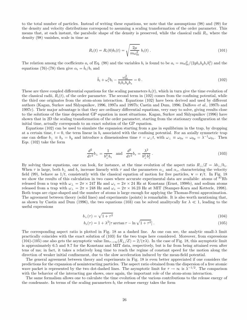
to the total number of particles. Instead of writing these equations, we note that the assumptions (98) and (99) forthe density and velocity distributions correspond to assuming a scaling transformation of the order parameter. Thismeans that, at each instant, the parabolic shape of the density is preserved, while the classical radii Ri, where thedensity (98) vanishes, scale in time as

Ri(t) = Ri(0)bi(t) =

√

2µ

mω20i

bi(t) . (101)

The relation among the coefficients ai of Eq. (98) and the variables bi is found to be ai = mω20i/(2gbxbybzb

2i ) and the

equations (76)-(78) then give αi = bi/bi and

bi + ω2i bi −

ω20i

bibxbybz= 0 . (102)

These are three coupled differential equations for the scaling parameters bi(t), which in turn give the time evolution ofthe classical radii, Ri(t), of the order parameter. The second term in (102) comes from the confining potential, whilethe third one originates from the atom-atom interaction. Equations (102) have been derived and used by differentauthors (Kagan, Surkov and Shlyapnikov, 1996, 1997a and 1997b; Castin and Dum, 1996; Dalfovo et al., 1997b and1997c). Their major advantage is that they are ordinary differential equations, very easy to solve, giving results closeto the solutions of the time dependent GP equation in most situations. Kagan, Surkov and Shlyapnikov (1996) haveshown that in 2D the scaling transformation of the order parameter, starting from the stationary configuration at theinitial time, actually corresponds to an exact solution of the GP equation.

Equations (102) can be used to simulate the expansion starting from a gas in equilibrium in the trap, by droppingat a certain time, t = 0, the term linear in bi associated with the confining potential. For an axially symmetric trapone can define b⊥ ≡ bx = by and introduce a dimensionless time τ = ω⊥t, with ω⊥ ≡ ω0x = ω0y = λ−1ω0z . ThenEqs. (102) take the form

d2

dτ2b⊥ =

1

b3⊥bzand

d2

dτ2bz =

λ2

b2⊥b2z

. (103)

By solving these equations, one can look, for instance, at the time evolution of the aspect ratio R⊥/Z = λb⊥/bz.When τ is large, both b⊥ and bz increase linearly with τ and the parameters α⊥ and αz, characterizing the velocityfield (99), behave as 1/t, consistently with the classical equation of motion for free particles, v = r/t. In Fig. 18we show the results of this calculation in two cases where accurate experimental data are available: atoms of 87Rbreleased from a trap with ω⊥ = 2π × 247 Hz and ωz = 2π × 24 Hz at Konstanz (Ernst, 1998b), and sodium atomsreleased from a trap with ω⊥ = 2π × 248 Hz and ωz = 2π × 16.23 Hz at MIT (Stamper-Kurn and Ketterle, 1998).Both traps are cigar-shaped and the number of atoms is large enough for applying the Thomas-Fermi approximation.The agreement between theory (solid lines) and experiments (points) is remarkable. It is also worth mentioning that,as shown by Castin and Dum (1996), the two equations (103) can be solved analitycally for λ ≪ 1, leading to theuseful expressions

b⊥(τ) =√

1 + τ2 (104)

bz(τ) = 1 + λ2[τ arctan τ − ln√

1 + τ2] . (105)

The corresponding aspect ratio is plotted in Fig. 18 as a dashed line. As one can see, the analytic small-λ limitpractically coincides with the exact solution of (103) for the two traps here considered. Moreover, from expressions(104)-(105) one also gets the asymptotic value limτ→∞(R⊥/Z) = 2/(πλ). In the case of Fig. 18, this asymptotic limitis approximately 6.5 and 9.7 for the Konstanz and MIT data, respectively, but is far from being attained even aftertens of ms; in fact, it takes a relatively long time to reach the regime of constant speed for the motion along thedirection of weaker initial confinement, due to the slow acceleration induced by the mean-field potential.

The general agreement between theory and experiments in Fig. 18 is even better appreciated if one considers thepredictions for the expansion of noninteracting particles. The aspect ratio obtained from the dispersion of a free atomicwave packet is represented by the two dot-dashed lines. The asymptotic limit for τ → ∞ is λ−1/2. The comparisonwith the behavior of the interacting gas shows, once again, the important role of the atom-atom interaction.

The same formalism allows one to calculate the time evolution of the various contributions to the release energy ofthe condensate. In terms of the scaling parameters bi the release energy takes the form

26

Erel =2µ

7

(

1

bxbybz+

1

2

∑

i

b2iω2

0i

)

. (106)

This quantity is conserved during the expansion. At t = 0, when bi = 1 and bi = 0, the release energy is equal to(2/7)µ. During the expansion the mean-field energy (first term in the bracket) is converted into kinetic energy (secondterm). After a certain time, which can be estimated using Eq. (106), the mean-field energy becomes negligible, sincethe system is more and more dilute, and the expansion proceeds at constant speed in each direction.

The same Eqs. (102) allow one also to study the effects of a sinusoidal driving force which simulates the modulationof the confining potential used in experiments to generate collective modes in the trap. In the small amplitude limit,Eqs. (102) yields the frequencies of the normal modes in the regime of collisionless hydrodynamics already discussedin Sec. IVB. In particular for axially symmetric traps, expression (98) includes the lowest m = 0 and m = 2 modes,which have been measured experimentally, while other modes could be investigated by adding terms in xy, xz andyz. When the amplitude of the oscillations grows, the frequency of the modes can shift and the modes themselves cancouple. For the experiments carried out at JILA and MIT (Jin et al., 1996 and 1997; Stamper-Kurn et al., 1998c) boththe frequency shift and the mode coupling are small. An example is given in Fig. 19, where we show the frequencyof the lowest m = 0 mode, observed in the cigar-shaped MIT trap (Stamper-Kurn et al., 1998c; Stamper-Kurn andKetterle, 1998), as a function of its amplitude. The solid line is the prediction of Eqs. (102). The overall agreementis good for both the zero amplitude frequency and its shift. It is worth recalling that the theory has no fittingparameters.

An effect which deserves to be mentioned is the large enhancement of nonlinear effects for special values of theasymmetry parameter λ. First, one notes that the frequencies of the collective modes depend on the shape of thetrapping potential and hence on λ. For certain values of this parameter, it may happen that different modes havethe same frequency; this has been shown to occur, in the linear regime, for |m| > 2 by Ohberg et al. (1997) anda systematic investigation of the level crossing has been done by Hutchinson and Zaremba (1997). In the nonlinearregime, one finds strong mode-coupling via harmonic generation when the frequency of a mode becomes equal tothe one of the second harmonics of other modes (Dalfovo et al., 1997b; Graham et al., 1998). The conditions forthis degeneracy can be found numerically from Eqs. (102). In the limit of small amplitude one can also expand thesolutions finding analytical results (Dalfovo et al., 1997b). In particular, one gets a quadratic shift in the form

ω(A) = ω(0)[1 + δ(λ)A2] (107)

where A is the relative amplitude of the oscillation and δ(λ) is an analytic coefficient depending on the anisotropy ofthe trapping potential and on the mode considered. For instance, in the case of the m = 2 mode, one finds:

δ(λ) =(16 − 5λ2)

4(16 − 7λ2). (108)

The divergence at λ =√

16/7 is due to the degeneracy between the frequencies of the high-lying m = 0 mode andthe second harmonic of the m = 2 mode. In this case, it is difficult to drive the system in a pure mode and, evenfor relatively small amplitudes, the motion is rather complex and the resulting trajectories can exhibit a chaotic-likebehavior. The coefficient δ(λ) can be calculated also for other modes. For the low-lying m = 0 mode, for instance,

similar divergences are found when λ = (√

125 ±√

29)/√

72 (i.e., λ ≈ 0.683 and λ ≈ 1.952). They occur because thefrequency of the high-lying mode becomes equal to the second harmonics of the low-lying mode. It would be veryinteresting to study experimentally the system in these conditions.

As a final remark we note that, by means of a variational approach based on Gaussian wave functions, Perez-Garcıaet al. (1996, 1997) have derived equations of motion of the form (102), but with an additional term included, propor-tional to 1/b3i , accounting for the quantum pressure in the Gross-Pitaevskii equation. Even though the equilibriumconfiguration in the Thomas-Fermi regime Na/aho ≫ 1 is not exactly recovered, because of the Gaussian ansatz,these equations represent a good approximation to the GP equation for finite N , interpolating between the noninter-acting and strongly interacting systems. The frequencies of the lowest m = 0 and m = 2 modes, calculated with theparameter of the JILA trap, differ from the exact solutions of (66)-(67) by less than 1% over all the relevant rangeof N . Since this method includes quantum pressure effects, it can be used to explore the nonlinear dynamics of thegas also in the case of attractive forces (Perez-Garcıa et al., 1997).

E. Density of states: collective vs. single-particle excitations

In the previous sections we have discussed several features of collective excitations pointing out the crucial role playedby two-body interactions. We may ask whether these collective modes are relevant for the statistical properties of

27

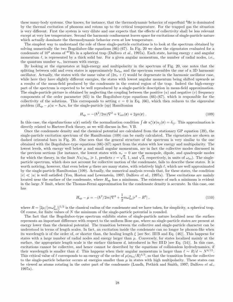
these many-body systems. One knows, for instance, that the thermodynamic behavior of superfluid 4He is dominatedby the thermal excitation of phonons and rotons up to the critical temperature. For the trapped gas the situationis very different. First the system is very dilute and one expects that the effects of collectivity shall be less relevantexcept at very low temperature. Second the harmonic confinement leaves space for excitations of single-particle naturewhich actually dominate the thermodynamic behavior even at low temperature.

The simplest way to understand the role of these single-particle excitations is to look at the spectrum obtained bysolving numerically the two Bogoliubov-like equations (66)-(67). In Fig. 20 we show the eigenstates evaluated for acondensate of 104 atoms of 87Rb in a spherical trap (Dalfovo et al., 1997a). Each state, having energy ε and angularmomentum ℓ, is represented by a thick solid bar. For a given angular momentum, the number of radial nodes, i.e.,the quantum number nr, increases with energy.

By looking at the eigenstates at high-energy and multipolarity in the spectrum of Fig. 20, one notes that thesplitting between odd and even states is approximately hωho and the spectrum resembles the one of a 3D harmonicoscillator. Actually, the states with the same value of (2nr + ℓ) would be degenerate in the harmonic oscillator case,while here they have slightly different energies, the states with lowest angular momentum being shifted upwards asa results of the mean-field produced by the condensate in the central region of the trap. Indeed the high-energypart of the spectrum is expected to be well reproduced by a single-particle description in mean-field approximation.The single-particle picture is obtained by neglecting the coupling between the positive (u) and negative (v) frequencycomponents of the order parameter (65) in the Bogoliubov-type equations (66)-(67), which is responsible for thecollectivity of the solutions. This corresponds to setting v = 0 in Eq. (66), which then reduces to the eigenvalueproblem (Hsp − µ)u = hωu, for the single-particle (sp) Hamiltonian

Hsp = −(h2/2m)∇2 + Vext(r) + 2gn(r) . (109)

In this case, the eigenfunctions u(r) satisfy the normalization condition∫

dr u∗i (r)uj(r) = δij . This approximation isdirectly related to Hartree-Fock theory, as we will discuss in Sec. VB.

Once the condensate density and the chemical potential are calculated from the stationary GP equation (39), thesingle-particle excitation spectrum of the Hamiltonian (109) can be easily calculated. The eigenstates are shown asdashed orizontal bars in Fig. 20. One sees that the general structure of the spectrum is very similar to the oneobtained with the Bogoliubov-type equations (66)-(67) apart from the states with low energy and multipolarity. Thelowest levels, with energy well below µ and small angular momentum, are in fact the collective modes discussed inthe previous sections (for instance, the lowest states with nr = 0 are the monopole, dipole, and quadrupole modes

for which the theory, in the limit Na/aho ≫ 1, predicts ε =√

5, 1, and√

2, respectively, in units of ωho). The single-particle spectrum, which does not account for collective motion of the condensate, fails to describe these states. It isworth noticing, however, that even below µ there are many states, with relatively high ℓ, which are well approximatedby the single-particle Hamiltonian (109). Actually, the numerical analysis reveals that, for these states, the condition|v| ≪ |u| is well satisfied (You, Hoston and Lewenstein, 1997; Dalfovo et al., 1997a). These excitations are mainlylocated near the surface of the condensate, where Hsp has a minimum. The existence of such a minimum is evidentin the large N limit, where the Thomas-Fermi approximation for the condensate density is accurate. In this case, onehas

Hsp − µ = −(h2/2m)∇2 +1

2mω2

ho|r2 −R2| , (110)

where R = [2µ/(mω2ho)]

1/2 is the classical radius of the condensate and we have taken, for simplicity, a spherical trap.Of course, for finite values of N the minimum of the single-particle potential is rounded.

The fact that the Bogoliubov-type spectrum exhibits states of single-particle nature localized near the surfacerepresents an important difference with respect to the uniform Bose gas, where no single-particle states are present atenergy lower than the chemical potential. The transition between the collective and single-particle character can beunderstood in terms of length scales. In fact, an excitation inside the condensate can no longer be phonon-like whenits wavelength is of the order of, or shorter than, the healing length ξ [see Sec. III B and Eq. (46)]. This happens forstates with a large number of radial nodes and energy larger than µ. Conversely, for states localized mainly at thesurface, the appropriate length scale is the surface thickness d, introduced in Sec III D [see Eq. (54)]. In this case,excitations cannot be collective, and hence cannot be described by the equations of collisionless hydrodynamics, iftheir wavelength is smaller than d. This happens when their angular momentum is larger than ℓ ∼ R/d ∼ N4/15.This critical value of ℓ corresponds to an energy of the order of µ(aho/R)4/3, so that the transition from the collectiveto the single-particle behavior occurs at energies smaller than µ in states with high multipolarity. These states canbe viewed as atoms rotating in the outer part of the condensate (Lundh, Pethick and Smith, 1997; Dalfovo et al.,1997a).

28

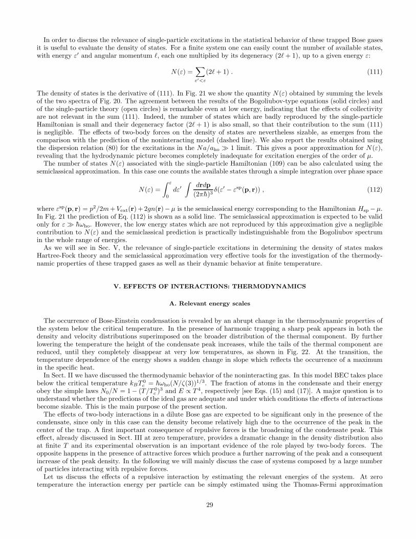
In order to discuss the relevance of single-particle excitations in the statistical behavior of these trapped Bose gasesit is useful to evaluate the density of states. For a finite system one can easily count the number of available states,with energy ε′ and angular momentum ℓ, each one multiplied by its degeneracy (2ℓ+ 1), up to a given energy ε:

N(ε) =∑

ε′<ε

(2ℓ+ 1) . (111)

The density of states is the derivative of (111). In Fig. 21 we show the quantity N(ε) obtained by summing the levelsof the two spectra of Fig. 20. The agreement between the results of the Bogoliubov-type equations (solid circles) andof the single-particle theory (open circles) is remarkable even at low energy, indicating that the effects of collectivityare not relevant in the sum (111). Indeed, the number of states which are badly reproduced by the single-particleHamiltonian is small and their degeneracy factor (2ℓ + 1) is also small, so that their contribution to the sum (111)is negligible. The effects of two-body forces on the density of states are nevertheless sizable, as emerges from thecomparison with the prediction of the noninteracting model (dashed line). We also report the results obtained usingthe dispersion relation (80) for the excitations in the Na/aho ≫ 1 limit. This gives a poor approximation for N(ε),revealing that the hydrodynamic picture becomes completely inadequate for excitation energies of the order of µ.

The number of states N(ε) associated with the single-particle Hamiltonian (109) can be also calculated using thesemiclassical approximation. In this case one counts the available states through a simple integration over phase space

N(ε) =

∫ ε

0

dε′∫

drdp

(2πh)3δ(ε′ − εsp(p, r)) , (112)

where εsp(p, r) = p2/2m+Vext(r) +2gn(r)−µ is the semiclassical energy corresponding to the Hamiltonian Hsp −µ.In Fig. 21 the prediction of Eq. (112) is shown as a solid line. The semiclassical approximation is expected to be validonly for ε≫ hωho. However, the low energy states which are not reproduced by this approximation give a negligiblecontribution to N(ε) and the semiclassical prediction is practically indistinguishable from the Bogoliubov spectrumin the whole range of energies.

As we will see in Sec. V, the relevance of single-particle excitations in determining the density of states makesHartree-Fock theory and the semiclassical approximation very effective tools for the investigation of the thermody-namic properties of these trapped gases as well as their dynamic behavior at finite temperature.

V. EFFECTS OF INTERACTIONS: THERMODYNAMICS

A. Relevant energy scales

The occurrence of Bose-Einstein condensation is revealed by an abrupt change in the thermodynamic properties ofthe system below the critical temperature. In the presence of harmonic trapping a sharp peak appears in both thedensity and velocity distributions superimposed on the broader distribution of the thermal component. By furtherlowering the temperature the height of the condensate peak increases, while the tails of the thermal component arereduced, until they completely disappear at very low temperatures, as shown in Fig. 22. At the transition, thetemperature dependence of the energy shows a sudden change in slope which reflects the occurrence of a maximumin the specific heat.

In Sect. II we have discussed the thermodynamic behavior of the noninteracting gas. In this model BEC takes placebelow the critical temperature kBT

0c = hωho(N/ζ(3))1/3. The fraction of atoms in the condensate and their energy

obey the simple laws N0/N = 1− (T/T 0c )3 and E ∝ T 4, respectively [see Eqs. (15) and (17)]. A major question is to

understand whether the predictions of the ideal gas are adequate and under which conditions the effects of interactionsbecome sizable. This is the main purpose of the present section.

The effects of two-body interactions in a dilute Bose gas are expected to be significant only in the presence of thecondensate, since only in this case can the density become relatively high due to the occurrence of the peak in thecenter of the trap. A first important consequence of repulsive forces is the broadening of the condensate peak. Thiseffect, already discussed in Sect. III at zero temperature, provides a dramatic change in the density distribution alsoat finite T and its experimental observation is an important evidence of the role played by two-body forces. Theopposite happens in the presence of attractive forces which produce a further narrowing of the peak and a consequentincrease of the peak density. In the following we will mainly discuss the case of systems composed by a large numberof particles interacting with repulsive forces.

Let us discuss the effects of a repulsive interaction by estimating the relevant energies of the system. At zerotemperature the interaction energy per particle can be simply estimated using the Thomas-Fermi approximation

29

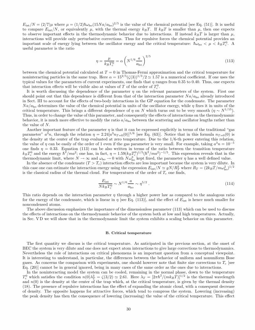
Eint/N = (2/7)µ where µ = (1/2)hωho(15Na/aho)2/5 is the value of the chemical potential [see Eq. (51)]. It is useful

to compare Eint/N , or equivalently µ, with the thermal energy kBT . If kBT is smaller than µ, then one expectsto observe important effects in the thermodynamic behavior due to interactions. If instead kBT is larger than µ,interactions will provide only perturbative corrections. Thus for repulsive forces the chemical potential provides animportant scale of energy lying between the oscillator energy and the critical temperature: hωho < µ < kBT

0c . A

useful parameter is the ratio

η =µ

kBT 0c

= α

(

N1/6 a

aho

)2/5

(113)

between the chemical potential calculated at T = 0 in Thomas-Fermi approximation and the critical temperature fornoninteracting particles in the same trap. Here α = 152/5(ζ(3))1/3/2 ≃ 1.57 is a numerical coefficient. If one uses thetypical values for the parameters of current experiments, one finds that η ranges from 0.35 to 0.40. Thus, one expectsthat interaction effects will be visible also at values of T of the order of T 0

c .It is worth discussing the dependence of the parameter η on the relevant parameters of the system. First one

should point out that this dependence is different from that of the interaction parameter Na/aho already introducedin Sect. III to account for the effects of two-body interactions in the GP equation for the condensate. The parameterNa/aho determines the value of the chemical potential in units of the oscillator energy, while η fixes it in units of thecritical temperature. This brings a different dependence of η on N which turns out to be very smooth (η ∼ N1/15).Thus, in order to change the value of this parameter, and consequently the effects of interactions on the thermodynamicbehavior, it is much more effective to modify the ratio a/aho between the scattering and oscillator lengths rather thanthe value of N .

Another important feature of the parameter η is that it can be expressed explicitly in terms of the traditional “gasparameter” a3n, through the relation η = 2.24[a3nT=0(0)]1/6 [see Eq. (63)]. Notice that in this formula nT=0(0) isthe density at the center of the trap evaluated at zero temperature. Due to the 1/6-th power entering this relation,the value of η can be easily of the order of 1 even if the gas parameter is very small. For example, taking a3n = 10−5

one finds η = 0.33. Equation (113) can be also written in terms of the ratio between the transition temperaturekBT

0c and the energy h2/ma2; one has, in fact, η = 1.59(kBT

0c )1/5(h2/ma2)−1/5. This expression reveals that in the

thermodynamic limit, where N → ∞ and ωho → 0 with Nω3ho kept fixed, the parameter η has a well defined value.

In the absence of the condensate (T > Tc) interaction effects are less important because the system is very dilute. Inthis case one can estimate the interaction energy using the expression Eint/N ≃ gN/R3

T where RT = (2kBT/mω2ho)

1/2

is the classical radius of the thermal cloud. For temperatures of the order of Tc one finds,

Eint

NkBT 0c

∼ N1/6 a

aho∼ η5/2 . (114)

This ratio depends on the interaction parameter η through a higher power law as compared to the analogous ratiofor the energy of the condensate, which is linear in η [see Eq. (113)], and the effect of Eint is hence much smaller fornoncondensed atoms.

The above discussion emphasizes the importance of the dimensionless parameter (113) which can be used to discussthe effects of interactions on the thermodynamic behavior of the system both at low and high temperatures. Actually,in Sec. VD we will show that in the thermodynamic limit the system exhibits a scaling behavior on this parameter.

B. Critical temperature

The first quantity we discuss is the critical temperature. As anticipated in the previous section, at the onset ofBEC the system is very dilute and one does not expect atom interactions to give large corrections to thermodynamics.Nevertheless the role of interactions on critical phenomena is an important question from a conceptual viewpoint.It is interesting to understand, in particular, the differences between the behavior of uniform and nonuniform Bosegases. As concerns the comparison with experiments, one should however note that finite size corrections to Tc [seeEq. (20)] cannot be in general ignored, being in many cases of the same order as the ones due to interactions.

In the noninteracting model the system can be cooled, remaining in the normal phase, down to the temperatureT 0

c which satisfies the condition n(0)λ3T = ζ(3/2) ≃ 2.61. Here λT = [2πh2/(mkBT )]1/2 is the thermal wavelength

and n(0) is the density at the center of the trap which, at the critical temperature, is given by the thermal density(18). The presence of repulsive interactions has the effect of expanding the atomic cloud, with a consequent decreaseof density. The opposite happens for attractive forces, which tend to compress the system. Lowering (increasing)the peak density has then the consequence of lowering (increasing) the value of the critical temperature. This effect

30

is absent in the case of a uniform gas where the density is kept fixed in the thermodynamic limit. It consequentlyrepresents a typical feature of trapped Bose gases that is worth discussing in some detail.

The shift in the critical temperature due to the mechanism described above can be easily estimated by treatingthe interaction in mean-field approximation. The simplest scheme is Hartree-Fock (HF) theory, which consists inassuming the atoms to behave as “noninteracting” bosons moving in a self-consistent mean-field:

HHF = − h2∇2

2m+ Veff(r)

= − h2∇2

2m+ Vext(r) + 2gn(r) , (115)

where the last term, 2gn(r) is a mean-field generated by the interactions with the other atoms. This method hasbeen first applied to the study of trapped Bose gases by Goldman, Silvera and Leggett (1981) and Huse and Siggia(1982) and it has since been adopted in many papers (Bagnato, Pritchard and Kleppner, 1987; Oliva, 1989; Giorgini,Pitaevskii and Stringari, 1996, 1997a and 1997b ; Chou, Yang and Yu, 1996; Minguzzi, Conti and Tosi, 1997; Shi andZheng, 1997b).

In Eq. (115) the quantity n(r) is the total density of the system, the sum of the density of both the condensate andthermal components. The single-particle energies and the density n(r) are obtained by solving a Schrodinger equationwith a density-dependent effective potential. In the presence of Bose-Einstein condensation, the equations for thesingle-particle excitations are coupled to the equation for the order parameter and the whole set of equations must besolved using a self-consistent procedure. At zero temperature the Hamiltonian HHF coincides with the single-particleHamiltonian (109), which describes the excitations of time dependent Gross-Pitaevskii theory after neglecting thequasi-particle amplitude vj in the equations of motion (see discussion in Sec. IVE ).

In the semiclassical approximation (see Sec. II B) one can easily calculate the thermal averages over the eigenstatesof the Hamiltonian (115). The thermal density of the system is given by the ideal gas formula (18)

nT (r) = λ−3T g3/2

(

e−[Veff (r)−µ]/kBT)

, (116)

where we have replaced Vext with [Veff − µ]. Bose-Einstein condensation starts at the temperature for which thenormalization condition

N =

∫

dr nT (r, Tc, µc) (117)

can be satisfied with the value of the chemical potential µc corresponding to the minimal eigenvalue of the Hamiltonian(115). For large systems the leading contribution arises from interaction effects

µc = 2gn(0) , (118)

where, working to the lowest order in g, one can calculate the central density n(0) using the noninteracting model.Equation (118) ignores finite size effects, given by (10) for the ideal gas.

By expanding the right hand side of (117) around µc = 0 and Tc = T 0c one obtains the following result for the shift

δTc = Tc − T 0c of the critical temperature (Giorgini, Pitaevskii and Stringari, 1996)

δTc

T 0c

= −1.3a

ahoN1/6 . (119)

Equation (119) shows that, to lowest order in the coupling constant, the shift of Tc is linear in the scattering lengthand is negative for repulsive interactions (a > 0). In this case, the ratio (119) can be expressed in terms of theparameter η defined in (113), and one has δTc/T

0c = −0.43 η5/2. For a typical configuration with η = 0.4, the shift

is ∼ 4%; this can be compared with the shift (20) arising from the finite size correction. Unlike the shift (119) dueto interactions, the finite size effect (20) depends on the anisotropy of the trap and decreases with N . Taking, for

example, N = 105 and λ =√

8 one finds that finite size effects provide a negative correction of ∼ 2%. For largervalues of N these corrections become negligible and one can safely use prediction (119). For attractive interactions(a < 0), equation (119) predicts instead a positive shift. However, in this case, finite size effects are always importantbecause the value of N cannot be large.

First measurements of the critical temperature (Ensher et al., 1996), as shown in Fig. 5, indicate the occurrenceof a negative shift with respect to T 0

c by about 6%, in agreement with the theoretical predictions. However theexperimental uncertainties are at present too large to draw definitive conclusions from this comparison.

31

Let us conclude this section by recalling that in the mean-field approach discussed above the relation between Tc andthe critical density in the center of the trap remains the same as for the noninteracting model: n(0)λ3

Tc= ζ(3/2) = 2.61

[see Eq. (116)] and it is interesting to look for effects which violate this relation. These can be either finite size ormany-body effects beyond mean-field theory. These latter effects have been recently calculated in the uniform gasthrough a Path Integral Monte Carlo simulation of the homogeneous hard-sphere Bose gas (Gruter, Ceperley andLaloe, 1997). This work has shown that the critical temperature Tc as a function of the gas parameter na3 firstincreases from the noninteracting value T 0

c = (2πh2/mkB)[n/ζ(3/2)]2/3, reaches a maximum for na3 ≃ 0.01 whereTc/T

0c ≃ 1.06 and finally decreases for larger values of na3. For the densities relevant for the experiments in traps the

effects on Tc calculated by these authors are much smaller than the mean-field correction (119).

C. Below Tc

Below the critical temperature Tc, Bose-Einstein condensation results in a sharp enhancement of the density inthe central region of the trap. This makes interaction effects much more important than above Tc, as discussed inSec. VA. In this section we will be dealing only with systems interacting with repulsive forces and we will considerthe limit of large N where finite size effects can be ignored. The main purpose is to develop a perturbative schemewhich permits one to obtain simple analytic formulas for the temperature dependence of the condensate fraction andof the energy of the system, providing a useful guide to understand the role of two-body interactions. We will use thefinite temperature Hartree-Fock scheme already presented in the previous section. An important result emerging fromthis analysis is that, to lowest order in the coupling constant, the corrections to the thermodynamic quantities dueto interaction effects are linear in the parameter η defined in (113). A more complete analysis of the thermodynamicbehavior, based on self-consistent numerical calculations will be presented in Sec. VD.

A first important problem concerns the temperature dependence of the order parameter and of the chemical po-tential. As long as N0(T )a/aho ≫ 1 and one ignores the interaction with the thermal component, the Thomas-Fermiapproximation (50) to the GP equation provides a good description for the condensate also at T > 0. Equation(51) then permits one to estimate the temperature dependence of the chemical potential whose value is fixed by thenumber of atoms in the condensate. One can write

µ(N0, T )

kBT 0c

≃ µ(N,T = 0)

kBT 0c

(

N0

N

)2/5

= η(1 − t3)2/5 . (120)

In order to express the condensate fraction in terms of the reduced temperature t = T/T 0c we have used the non-

interacting prediction N0 = N(1 − t3). Inclusion of corrections to this law would yield higher order effects in theinteraction parameter. Equation (120) provides a useful estimate of µ, which is expected to be accurate in the rangeµ < T < T 0

c . For smaller temperatures, Eq. (120) misses the thermal contributions arising from collective excitations.These effects represent however very small corrections and will be ignored in the present discussion.

Concerning the uncondensed atoms, at high temperature they can be treated as free particles governed by theeffective mean-field potential Veff(r) given by (115). The form of this potential can be simplified by ignoring thecontribution to the density n(r) due to the dilute thermal component and by evaluating the condensate density in theThomas-Fermi approximation. This yields the simple result Veff(r)−µ = |Vext(r)−µ| [see also Eq. (115)]. In practicemost of the thermal atoms occupy regions of space lying outside the condensate where Vext > µ and Veff = Vext. As aconsequence, to a first approximation the effective potential felt by thermal atoms is the same as without interaction.However, this does not mean that interaction effects are negligible. In fact, these atoms have a chemical potential(120) quite different from the noninteracting value and the corresponding contribution to the thermodynamic averagesis modified.

Let us first discuss the problem of thermal depletion. Using the semiclassical picture one can write

NT =

∫

drdp

(2πh)3

exp[(p2/2m+ Veff(r) − µ)/kBT ]− 1−1

. (121)

Explicit integration of (121), using the Thomas-Fermi approximation for the effective mean-field potential, Veff(r)−µ =|Vext(r) − µ|, leads to the result

N0

N= 1 − t3 − ζ(2)

ζ(3)ηt2(1 − t3)2/5 , (122)

valid to the lowest order in the interaction parameter η.

32

Equation (122) shows that the effects of the interaction depend linearly on η and are consequently expected to bemuch larger than the ones in the shift of the critical temperature (119) which behave like η5/2. For example, takingη = 0.4 and t = 0.6 one finds that interactions reduce the value of N0 by 20% as compared to the prediction ofthe noninteracting model. It is worth noting that the quenching of the condensate represents a peculiar behavior oftrapped Bose gases and takes place because the thermal component of the gas is, in large part, spatially separatedfrom the condensate. In a uniform system one has an opposite mechanism. In fact, in this case, the condensate andthe thermal components completely overlap and the effective potential is enhanced due to the interaction term 2gn[see Eq. (115)]. This effect is only partially compensated by the presence of the chemical potential and the final resultis a suppression of the thermal component.

In a similar way one can calculate the energy of the system. The main effects of temperature and interactions aretwofold: on the one hand the number of atoms in the condensate is reduced at finite temperature and the densityin the central region of the trap decreases. As a consequence the atom cloud becomes larger but more dilute andthe interaction energy is reduced as compared to the zero temperature case. On the other hand the particles out ofthe condensate are thermally distributed with a modified Bose factor as in (121). By explicitly calculating the twocontributions, one finds that the total energy of the system exhibits the following temperature dependence:

E

NkBT 0c

=3ζ(4)

ζ(3)t4 +

1

7η(1 − t3)2/5(5 + 16t3) . (123)

Notice that the contribution of the interaction, which is again linear in η, can be obtained directly starting from result(120) for the chemical potential, through the use of general relations of thermodynamics. Analogously to Eqs. (120)and (122), expression (123) is valid in the temperature regime µ < T < Tc and to the lowest order in the parameterη.

Another useful quantity is the release energy, which corresponds to the energy of the system after switching off thetrap. Using the same approximations as discussed above, one can easily calculate also this quantity, for which onefinds the result

Erel

NkBT 0c

≡ E − Eho

NkBT 0c

=3ζ(4)

2ζ(3)t4 +

1

7η(1 − t3)2/5

(

2 +17

2t3)

. (124)

The release energy can be extracted from time of flight measurements and, consequently, equation (124) provides auseful formula to check the effects of two-body interactions directly from experiments.

The formulas presented in this section account for first order effects in the coupling constant η. Their validity isensured only for relatively high temperatures and weakly interacting gases. In order to appreciate the accuracy ofthese predictions, in Fig. 23 we compare the energy predicted in (123) with the one obtained by means of a self-consistent calculation based on the Popov approximation (see Sec. VE). The agreement is excellent over a wide rangeof temperatures except, of course, very close to T 0

c where higher orders in η give the leading contribution of two-bodyinteractions to thermodynamics.

Expansions similar to the ones discussed in this section can be carried out also in the opposite limit of low tem-perature t < η, which is the analog of the phonon regime of uniform superfluids. Though this regime is not easilyreachable in current experiments, its theoretical investigation is rather interesting. The low temperature propertiesof trapped Bose gases are deeply influenced by the thermal excitation of the single-particle states localized near thesurface of the condensate, already discussed in Section IVE (see also, Giorgini, Pitaevskii and Stringari, 1997b).

D. Thermodynamic limit and scaling

The thermodynamic limit for the noninteracting gas confined in harmonic traps has been discussed in Sec. II B.This limit is reached by letting the total number of particles N increase to infinity and the oscillator frequency ωho

decrease to zero, with the product ωhoN1/3 kept fixed. Here ωho is the geometrical average of the three frequencies.

This procedure provides a natural extension of the usual thermodynamic limit used in uniform systems where onetakes N → ∞, V → ∞, and keeps the density n = N/V fixed. In harmonic traps the quantity ωhoN

1/3 represents,together with T , the relevant thermodynamic parameter of the system and replaces the role played by the densityin uniform systems. In particular it fixes the value of the critical temperature kBT

0c = hωhoN

1/3/(ζ(3))1/3. In thethermodynamic limit all the thermodynamic properties of the noninteracting model can be expressed in terms ofthe critical temperature T 0

c and the reduced temperature t = T/T 0c . Of course dimensionless quantities, like the

condensate fraction or the entropy per particle, will depend only on t.The thermodynamic limit discussed above applies also in the presence of repulsive interactions. As discussed in

Sec. VA the parameter η depends on N and ωho only through the transition temperature T 0c and is consequently

33

well defined in the thermodynamic limit. It is also worth noticing that the dimensionless parameter Na/aho, whichcharacterizes the effects of two-body interactions in the Gross-Pitaevskii equation for the ground state behaves asNa/aho ∼ N5/6η5/2. Thus, in the thermodynamic limit, the condition N0a/aho ≫ 1 which ensures the validity of theThomas-Fermi approximation for the condensate, is always guaranteed below Tc.

The above discussion suggests that in the thermodynamic limit the relevant functions of the system will dependon T 0

c , t and η (Giorgini, Pitaevskii and Stringari, 1997a). In the previous section we have already anticipated sucha behavior by calculating some relevant thermodynamic functions to the lowest order in η, as done in Eqs. (120),(122)-(124). This points out a scaling behavior exhibited by these systems. Different configurations, corresponding todifferent values of N , m, trapping frequencies and scattering length, will be characterized by the same thermodynamicbehavior provided they correspond to the same value of η.

The scaling behavior can be proved in a general way by noting that in the limit ωho → 0 the size of the systemincreases and the density n(r) changes very slowly. As a consequence in the thermodynamic limit the density is fixedby the condition (58) of local equilibrium, µ(T ) = µlocal(n, T ) + Vext(r), where µlocal(n, T ) is the chemical potentialof an interacting uniform system at density n = n(r). By inverting the above condition one can write the densityof the gas in the form n(r) = n(µ − Vext(r), T ), where n(µ, T ) is the density of the uniform gas as a function ofchemical potential and temperature. Notice that the inversion of the function µlocal(n) requires that µlocal be amonotonous function of the density. This condition is satified by interacting systems where the stability conditionimplies ∂µ/∂n > 0. The total number of atoms N is obtained by integrating the density over space co-ordinates.Introducing the new variable ξ = Vext(r), one can write

N = 2π

(

2

mω2ho

)3/2 ∫ ∞

0

dξ n(µ− ξ, T )√

ξ . (125)

The parameters of the trap enter the above equation through the combination ωhoN1/3 ∝ T 0

c . On the other hand theintegral on the right hand side requires the knowledge of the density of the uniform system as a function of chemicalpotential and T . Equation (125) shows that the knowledge of the thermodynamic behavior of the interacting uniformsystem would permit one, in principle, to determine the thermodynamics of the trapped gas (Damle et al., 1996).For a dilute Bose gas, where the interaction is accounted for by a single parameter (the scattering length a), theintegral (125) depends on the quantities µ, T and h2/ma2, the latter being the only energy one can construct with themass m and the scattering length a. As a consequence, inversion of (125) yields the following general dependence forthe chemical potential µ = µ(T, T 0

c , h2/ma2). Due to dimensionality arguments the above expression can be always

written in the form

µ = kBT0c f(t, η) . (126)

Here f is a dimensionless function depending on the reduced temperature t = T/T 0c and on the scaling parameter η,

fixed by the ratio between kBT0c and h2/ma2 [see discussion after Eq. (113)]. A similar scaling behavior applies to

the other thermodynamic functions.The above discussion applies to the thermodynamic limit where N → ∞. An important question is to understand

whether in the available experimental conditions, where N ranges between 104 and 107, this limit is reached in practiceor finite size effects are still significant. In Fig. 24 we show, as an example, the behavior of the condensate fraction.This quantity depends, in the thermodynamic limit, only on the variables t and η. In the figure we plot the numericalresults obtained from a self-consistent mean-field calculation based on the Popov approximation (see Sec. VE) fortwo very different configurations, both corresponding to the same value of η = 0.4. Open squares correspond toN = 5 × 104 rubidium atoms in a trap with a/aho = 5.4 × 10−3 and λ =

√8, while solid squares correspond to

N = 5 × 107 sodium atoms in a trap with a/aho = 1.7 × 10−3 and λ = 0.05. One sees that both set of data coincidewith the asymptotic scaling function (solid line), calculated with the same value of η, by taking the thermodynamiclimit in the equations of the Popov approximation (Giorgini, Pitaevskii and Stringari, 1997b). The figure pointsout, in an explicit way, how very different configurations can give rise to the same thermodynamic behavior, if thecorresponding scaling parameter η is the same. It is also interesting to notice that the scaling behavior is reachedfaster in the presence of two-body interactions than for noninteracting particles. In the latter case, in fact, finite sizeeffects, which are responsible for the deviations from the scaling law (1− t3) (dashed line), are more visible (open andsolid circles).

The scaling behavior is very well reproduced also by the other thermodynamic quantities. For this reason, in thenext section, we will discuss the behavior of interacting Bose gases confined in harmonic traps calculating directly thevarious physical quantities in the thermodynamic limit.

34

E. Results for the thermodynamic functions

In Sec. VC we have used Hartree-Fock theory to estimate the temperature dependence of the chemical potential,condensate fraction, release energy to lowest order in the scaling parameter η. The full equations of Hartree-Focktheory can be solved numerically in a self-consistent way (Minguzzi, Conti and Tosi, 1997; Shi and Zheng 1997b;Giorgini, Pitaevskii and Stringari, 1997b) going beyond the perturbative scheme. Hartree-Fock theory is expected tobe quite accurate at high temperature except, of course, very close to Tc, where mean-field theories are inadequate(Shi, 1997; Shi and Griffin, 1998). The accuracy of Hartree-Fock at high T is justified by the crucial role played bysingle-particle excitations, as we have already seen in Sec. IVE for the density of states. This theory is instead lessaccurate at low T , since it ignores the effects of collectivity which characterize the low energy part of the excitationspectrum. Such collective effects are instead properly included in time dependent Gross-Pitaevskii theory, as discussedin Sec. IVA. A mean-field scheme, describing correctly both the high and low temperature regimes, is provided bythe so called Popov approximation (Popov, 1965 and 1987; Griffin, 1996; Shi, 1997) whose application to interactingbosons in harmonic traps has been considered by several authors in the last few years. This mean-field scheme isbased, on the one hand, on a finite T extension of the Gross-Pitaevskii equation, in which the interaction betweencondensed and noncondensed atoms is explicitly accounted for, and, on the other hand, on Bogoliubov-type equationsfor the excitations of the system. The corresponding equations have the form

(

− h2∇2

2m+ Vext(r) + g[n0(r) + 2nT (r)]

)

φ = µφ (127)

and

εiui(r) =

(

− h2∇2

2m+ Vext(r) − µ+ 2gn(r)

)

ui(r) + gn0(r)vi(r) (128)

−εivi(r) =

(

− h2∇2

2m+ Vext(r) + µ+ 2gn(r)

)

vi(r) + gn0(r)ui(r) (129)

where n0(r) = |φ(r)|2 is the condensate density, while the thermal density nT is calculated through the relationnT =

∑

j(|u|2j +|v|2j)[exp(βεj)−1]−1 with uj , vj and εj solutions of (128)-(129). These quantities are now temperature

dependent. The sum n(r) = n0(r) + nT (r) is the total density. The functions ui, vi entering Eqs. (128)-(129) arenormalized according to condition (69). Notice that in this approximation the thermal component is treated as athermal bath generating an additional static external field in the equation for the condensate. One also ignores herethe T = 0 quantum depletion nout(r) =

∑

j |vj(r)|2 which has been shown to be very small in these trapped gases

(see Sec. III E). Finally, at low temperature, when nT is negligible compared with n0, equation (127) coincides withthe stationary GP equation (39), while Eqs. (128)-(129) reduce to (66)-(67).

From the solution of Eqs. (127)-(129) one obtains density profiles in good agreement with experimental data. Asan example, we take two of the density profiles already shown in Fig. 22 and we plot them again in Fig. 25 togetherwith the theoretical prediction from Eqs. (127)-(129), using the number of particles, N , and the temperature, T , asfitting parameters. The same equations have been used also for fitting the experimental data by Hau et al. (1998).

Using the distribution function of the excited states, fj = [exp(βεj) − 1]−1, and the combinatorial expression forthe entropy, S = kB

∑

jβεjfj − ln[1 − exp(−βεj)], one can work out all the thermodynamic quantities (Giorgini,

Pitaevskii and Stringari, 1997b). The comparison between the predictions of Hartree-Fock and Popov theories hasrevealed that there are no significant differences between the two approaches for most thermodynamic quantities.Only increasing the value of the interaction parameter η one can observe some differences. This is a further evidenceof the negligible role played in thermodynamics by the collective modes of the condensate, which are ignored in theHartree-Fock scheme. This behavior, in accordance with the analysis of the density of states made in Sec. IV E,represents a significant difference with respect to the case of uniform superfluids.

In the following we present results for various thermodynamic quantities (chemical potential, condensate fractionand release energy) obtained using the Popov approximation in the thermodynamic limit. As discussed in thepreceeding section, this limit is well achieved in the configurations realized in present experiments. The results areconsequently presented as a function of the reduced temperature t for different values of the scaling parameter η. Wehave considered the value η = 0.4, which corresponds to the typical configurations realized in actual experiments, andthe value η = 0.6, which would correspond to a more correlated gas.

First, in Fig. 26, we show the chemical potential in units of kBT0c as a function of the reduced temperature t.

Notice that for t→ 0 the plotted quantity coincides, by definition, with the parameter η [see definition (113)]. In theclassical limit, T ≫ T 0

c , the chemical potential approaches the ideal gas value µ/kBT0c = t ln(ζ(3)/t3).

35

The results for the condensate fraction N0/N are given in Fig. 27. The open circles are the experimental points(Ensher et al., 1996). In the experiment the number of atoms N varies with t and the corresponding value of η rangesfrom 0.39 to 0.45. The data are compared with the predictions of the mean-field theory for η = 0.4 (solid line) andthe noninteracting gas model (dotted line). The experimental points are shifted from the noninteracting case to lowertemperature, but not as much as predicted by mean-field theory. However, the experimental uncertainties are stilltoo large to draw any definitive conclusion.

In Fig. 28 we show the results for the release energy. The dots are the experimental data (Ensher et al., 1996)which, below Tc, lie well above the noninteracting curve, showing again a clear evidence for the effects of two-bodyinteractions. We notice that, by differentiating the total energy with respect to T , one could calculate the specific heat.In the present experiments however, this quantity is not directly available because only the release energy is measured.What one can see from a fit to the experimental data of the release energy is the occurrence of a characteristic bumpin the derivative near the transition temperature (Ensher et al., 1996); this behavior is in good agreement with theprediction obtained by taking the derivative of the theoretical curves in Fig. 28.

Finally, the above results of the mean-field theory at finite temperature can be also compared with the ones ofQuantum Monte Carlo calculations (Krauth, 1996; Holzmann, Krauth and Naraschewski, 1998). It is worth noticingthat the possibility of making a close comparison between exact Monte Carlo simulations, experimental data andmean-field calculations is a rather rare event in the context of interacting many-body systems and represents a furthernice feature of BEC in traps. In Fig. 27, the condensate fraction obtained with path integral Monte Carlo calculationsby Krauth (1996) is represented by solid circles with error bars. The simulation has been done with 10000 atomsinteracting through an hard-core potential, and corresponds to η = 0.35. The results are very close to the mean-fieldprediction. The value of η used for the solid curve is actually 0.4, since this value is closer to the experimentalsituation, but the same calculation for η = 0.35 gives an even better agreement, crossing precisely the three MonteCarlo data at high temperature. A detailed comparison between Monte Carlo results and mean-field theory has beenrecently performed by Holzmann, Krauth and Naraschewski (1998), including the analysis of the density profiles ofthe gas at different temperatures.

F. Collective modes at finite temperature

In Sec. IV we have studied the collective excitations of a trapped Bose gas at zero temperature. In this case, all theatoms are in the condensate and there are no collisions. In the collisionless regime the force acting on a given particlecomes from the mean-field created by the other particles; this field generates a collective oscillation of the system,which is sometimes called Bogoliubov sound and is the analog of zero sound for normal Fermi liquids.

At finite temperature the situation is more complicated. On the one hand both the condensate and the thermalcloud can oscillate. On the other hand collisions between excitations can play an important role and one mustdistinguish between a collisional and a collisionless regime.

So far the temperature dependence of these oscillations has been analysed experimentally both at JILA and MIT. Inthe first case, Jin et al. (1997) investigated the m = 0 and m = 2 modes for a system of ∼ 104 Rb atoms in a trap with

asymmetry parameter λ =√

8. At low temperatures (T<∼ 0.4T 0

c ) they found that the oscillations of the condensatehave frequencies in good agreement with the predictions of the T = 0 Gross-Pitaevskii equation (see Sec. IV), whileat higher temperatures the frequency exhibits an unexpected temperature dependence with very different behaviorfor the two modes. In the second case, Stamper-Kurn et al. (1998c) studied the low-lying m = 0 mode for a muchlarger system (N ∼ 107 Na atoms) in a cigar-shaped trap with λ ≪ 1. Similarly to the JILA group, they observeda shift of the collective frequency with respect to the T = 0 value. Both groups measured also the damping of thecollective modes of the condensate, finding a rather strong T -dependence. They also observed the oscillations of thethermal cloud below and above the critical temperature.

Mean-field approaches have been used to predict the properties of the collective excitations in the collisionless regime.This regime is achieved at low temperatures and for low densities of the thermal cloud. In this case, the oscillationsof the condensate behave similarly to the T = 0 case and can still be called Bogoliubov’s sound modes. Severalauthors have used finite T extensions of the time-dependent Gross-Pitaevskii equation in the Popov approximation[see Eqs. (127)-(129)] (Hutchinson, Zaremba and Griffin, 1997; Dodd et al., 1998a and 1998b). This approach, inwhich the thermal component is treated as a static thermal bath, does not account for any damping mechanism. Inorder to include damping, a dynamic description of the oscillations of both the condensate and the thermal cloud isneeded (Minguzzi and Tosi, 1997; Giorgini, 1998). The dynamic coupling between the motion of the two componentsmight also be important in the determination of the temperature dependence of the frequency shift. There are stillopen questions on this problem and several aspects of the theory are expected to be clarified in the next future.

Damping processes in the collisionless regime have been investigated using perturbative approaches (Liu and Shieve,

36

1997; Pitaevskii and Stringari, 1997; Liu, 1997; Fedichev, Shlyapnikov and Walraven, 1998). An important mechanismof collisionless damping is provided by the Landau damping. In Fermi liquids, Landau damping originates from thecoupling between single-particle excitations and zero sound at T = 0 (Lifshitz and Pitaevskii, 1981, §30; Pinesand Nozieres, 1966, Vol.I). In a Bose gas, an analogous damping occurs because the thermal bath of elementaryexcitations can absorb quanta of the collective oscillation. Landau damping increases with temperature, becauseof the larger number of elementary excitations available at thermal equilibrium. For temperatures larger than thechemical potential it increases linearly with T and for a uniform system the ratio between the imaginary, γ = −Im(ω),and real, Re(ω), parts of the collective frequency takes the analytic form (Szepfalusy and Kondor, 1974; Shi, 1997;Pitaevskii and Stringari, 1997)

γ

Re(ω)=

3π

8

kBTa

hc. (130)

This equation is valid for excitations with energy hRe(ω) ≪ µ ≪ kBT , which in a uniform system are phononspropagating with the sound velocity c. Equation (130) can be used for a rough estimate of the damping of collectiveexcitations in traps by taking for c the value of the sound velocity in the center of the trap. As an example, in Fig. 29we show the damping rate, γ, measured for the m = 0 and m = 2 modes by Jin et al. (1997), compared with thetheoretical estimate (130). Taking into account that this estimate, which is expected to apply at high temperatures,is very rough and that the effects of geometry and multipolarity are completely neglected, the agreement betweentheory and experiment can be considered reasonable. Recently Fedichev, Shlyapnikov and Walraven (1998) haveindeed argued that Landau damping is strongly influenced by the geometry of the traps, being particularly effectivein anisotropic traps, due to the randomness of the excitation spectrum.

At high temperature and/or high density, collisions are more important and can affect the nature of collectiveexcitations. In Bose superfluids the collisional regime is described by the equations of two-fluid hydrodynamics andis characterized by the occurrence of two distinct oscillations: first and second sound. In liquid 4He, first sound isa density wave with in phase oscillations of the superfluid and normal components, while second sound is an almostpure entropy wave with opposite phase motion of the two components. For a dilute Bose gas the situation is differentbecause the interaction between the condensate and the thermal cloud is very weak. In particular, except at verylow temperature, first sound mainly involves the thermal cloud and reduces to the usual hydrodynamic sound aboveTc; conversely, second sound is essentially the oscillation of the condensate and disappears above Tc (Lee and Yang,1959; Griffin and Zaremba, 1997). Similar features have been pointed out also in the presence of harmonic trapping(Zaremba, Griffin and Nikuni, 1997; Shenoy and Ho, 1998).

An important limiting case is represented by the collective motion of the gas above the critical temperature,where the gas exhibits an almost classical behavior. In the collisional regime, one can then use the equations ofhydrodynamics for classical gases in order to obtain explicit results for the collective frequencies. For example thecoupled quadrupole and monopole modes with m = 0 obey the following dispersion law (Griffin, Wu and Stringari,1997; Kagan, Surkov and Shlyapnikov, 1997a):

ω2 =1

3[5ω2

⊥ + 4ω2z ± (25ω4

⊥ + 16ω4z − 32ω2

⊥ω2z)1/2] . (131)

If the trap is spherical (ω⊥ = ωz = ωho), the two solutions have frequency ω =√

2 ωho (quadrupole) and ω = 2ωho

(monopole). Notice that the frequency of the surface (quadrupole) mode is equal to the one of the oscillation of thecondensate at zero temperature, given by Eq. (83). In the limit of highly deformed cigar-shaped traps (ωz ≪ ω⊥),

the lowest frequency of (131) becomes ω =√

12/5 ωz.This collisional regime, yielding the dispersion law (131), is achieved if ωτ ≪ 1, where τ is a typical collision time.

In the opposite limit (ωτ ≫ 1) one finds the collisionless regime, where the gas oscillates with frequencies fixed bythe trapping potential, corresponding to the predictions of the noninteracting model. Oscillations of this type havebeen observed by Jin et al. (1997) for both the gas above Tc and the thermal component below Tc; the frequency ofthe m = 0 and m = 2 modes was found to be roughly twice the trap frequency, in agreement with the prediction forthe ideal gas.

In the intermediate regime where ωτ ∼ 1 one expects a smooth cross-over from collisionless to collisional hydrody-namic modes. A useful interpolation formula is provided by the law (Kavoulakis, Pethick and Smith, 1998)

ω2 = ω2C +

ω2HD − ω2

C

1 − iωτ, (132)

predicted by general theory of relaxation phenomena (Landau and Lifshitz, 1987, §81). Here ωC and ωHD are thefrequencies of the mode in the collisionless and collisional hydrodynamic regimes respectively.

37

An estimate of the collisional time τ can be obtained by considering again a classical picture of the system. Onefinds τ ≃ lmfp/vT , where vT =

√

2kBT/m is the thermal velocity and lmfp = (nTσ)−1 is the mean free path which isfixed by the s-wave cross section σ = 8πa2 and by the density. For frequencies of the order of the oscillator frequencythe condition ωτ ≪ 1 is equivalent to requiring that the mean free path be much smaller than the thermal radiusRT =

√

2kBT/mω2ho. Near Tc one finds that the collisional frequency 1/τ behaves like η5kBTc/h where η is the

scaling parameter defined in (113). Despite the smallness of the factor η5, the collisionless frequency can be of thesame order of the collective frequencies of the system because of the factor N1/3 contained in Tc, so that increasingN favours the achievement of the collisional hydrodynamic regime. Notice that the multipolarity of the excitationcan play an important role in characterizing the relaxation of the collective oscillation. For example the dipole modecannot have any relaxation mechanism in the presence of harmonic trapping. The same happens in the case of themonopole excitation if the harmonic trap is isotropic. In both cases the collisionless (ωC) and hydrodynamic (ωHD)frequencies coincide.

In Fig. 30 we plot the imaginary part of ω against the real part, as given in (132), for the case of the low-lyingm = 0 mode observed in the cigar-shaped trap at MIT (Stamper-Kurn et al., 1998c). In this experiment, the thermal

cloud is found to oscillate with a frequency of 1.78ωz, which is larger than the hydrodynamic prediction√

12/5 ωz,but lower than the noninteracting value 2ωz. A damping rate of about 20 s−1 was also observed, corresponding to−Im(ω) = 0.19ωz. In Fig. 30 the experimental results are represented by the solid circle with error bars, which turnsout to be reasonably close to the theoretical curve, the difference being of the order of the experimental uncertainty.The part of the curve near the maximum corresponds to values of collision time such that Re(ω)τ ∼ 1 and thissuggests that, differently from the JILA experiment (Jin et al., 1997), the motion of the thermal cloud in the MITexperiment is affected by collisions.

Finally, we mention that Stamper-Kurn et al. (1998c) observed also the opposite phase dipolar oscillation of thethermal cloud and the condensate, occurring below Tc (Zaremba, Griffin and Nikuni, 1998). This mode exhibitsstrong damping.

VI. SUPERFLUIDITY AND COHERENCE PHENOMENA

Superfluidity is one of the most spectacular consequences of Bose-Einstein condensation. However, the explicitconnection between superfluidity and BEC is not trivial and has been the object of a longstanding and deep investi-gation in the last decades, mainly for its importance in understanding the physics of liquid helium. In macroscopicbodies superfluidity shows up with many peculiar features: absence of viscosity, reduction of the moment of inertia,occurrence of persistent currents, new collective phenomena (second sound, third sound, etc.), quantized vortices,and others. Several properties are usually interpreted as coherence effects associated with the phase, S, of the or-der parameter whose gradient fixes the velocity of the superfluid through vs = (h/m)∇S. A major question is tounderstand whether some of these effects can be observed also in trapped gases. Of course in a mesoscopic systemone expects the manifestations of superfluidity to be different from the ones exhibited by macroscopic bodies. In par-ticular, traditional experiments based on the study of transport phenomena are not easily feasible in trapped gases.On the other hand, interference patterns, associated with phase coherence, have been already observed (Andrews,Townsend et al., 1997) and successfully compared with theory. This opens a promising field of research based on theinvestigation of coherence phenomena, including the realization of the so-called “atom laser” (Ketterle, 1998).

A. Rotational properties: vortices and moment of inertia

Among the several properties exhibited by superfluids, the occurrence of quantized vortices and the strong reductionof the moment of inertia represent effects of primary importance.

In a dilute Bose gas the structure of quantized vortices can be investigated starting from the Gross-Pitaevskiiequation. Indeed one of the primary motivations of the GP theory was the study of vortex states in weakly interactingbosons (Gross, 1961 and 1963; Pitaevskii, 1961). These studies were further developed by Fetter (1972) includinghigher order effects in the interaction.

A quantized vortex along the z-axis can be described by writing the order parameter in the form

φ(r) = φv(r⊥, z) exp[iκϕ] (133)

where ϕ is the angle around the z-axis, κ is an integer, and φv(r⊥, z) =√

n(r⊥, z). This vortex state has tangentialvelocity

38

v =h

mr⊥κ . (134)

The number κ is the quantum of circulation and the angular momentum along z is Nκh. The equation for themodulus of the order parameter is obtained from the GP equation (39). The kinetic energy brings a new centrifugalterm arising from the velocity flow which pushes the atoms away from the z-axis. The GP equation then takes theform

[

− h2∇2

2m+

h2κ2

2mr2⊥+m

2(ω2

⊥r2⊥ + ω2

zz2) + gφ2

v(r⊥, z)

]

φv(r⊥, z) = µφv(r⊥, z) . (135)

Due to the presence of the centrifugal term, the solution of this equation for κ 6= 0 has to vanish on the z-axis. Anexample is shown in Fig. 31, where the solid line represents the condensate wave function, φv(x, 0, 0), for a gas of 104

rubidium atoms in a spherical trap and with vorticity κ = 1. In the inset, we give the contour plot for the density inthe xz-plane, n(x, 0, z) = |φv(x, 0, z)|2.

For noninteracting systems the solution of Eq. (135) is analytic and, for κ = 1, has the form

φv(r⊥, z) ∝ r⊥ exp[

−m

2h

(

ω⊥r2⊥ + ωzz

2)

]

. (136)

In this case, the vortex state corresponds to putting all the atoms in the m = 1 single-particle state. Its energy isthen Nhω⊥ plus the ground state energy. In Fig. 31, the corresponding wave function is shown as a dashed line.Similarly to what happens for the ground state without vortices, the presence of repulsive forces reduces dramaticallythe density with respect to the noninteracting gas, the condensate wave function becoming much broader.

The structure of the core of the vortex is fixed by the balance between the kinetic energy and the two-bodyinteraction term. For a uniform Bose gas the size of the core is of the order of the healing length ξ = (8πna)−1/2,already introduced in Sec. III.B, where n is the density of the system. For the trapped gas, an estimate of the coresize can be obtained using for n the central value of the density in the absence of vortices. If the trap is spherical,as in the case of Fig. 31, the ratio between ξ and the radius R of the condensate takes the form (Baym and Pethick,1996)

ξ

R=(aho

R

)2

. (137)

where we have used the Thomas-Fermi approximation for the central density and the radius R. For the condensatein the figure, the radius is about 4.1 in units of aho and the ratio ξ/R is then ∼ 0.06. The actual core size depends,obviously, also on the position on the z-axis and becomes larger when the vortex line reaches the outer part of thecondensate, where the density decreases. This can be clearly seen in the inset of Fig. 31.

The energy of the vortex can be evaluated through the energy functional (37). The difference between the energyof the vortex state and the one of the ground state allows one to calculate the critical frequency needed to create avortex. In fact, in a frame rotating with angular frequency Ω, the energy of a system carrying angular momentum Lz

is given by (E−ΩLz), where E and Lz are defined in the laboratory frame. At low rotational frequencies this energyis minimal without the vortex. If Ω is large enough the creation of a vortex can become favourable due to the term−ΩLz. This happens at the critical frequency

Ωc = (hκ)−1[(E/N)κ − (E/N)0] . (138)

where Eκ is the energy of the system in the presence of a vortex with angular momentum Nhκ. In Fig. 32 we plotthe critical frequency for the creation of a vortex with κ = 1 as a function of the number of atoms, for rubidium in aspherical trap. As shown in the figure, the predicted critical frequency is a fraction of the oscillator frequency and, intypical experimental conditions, corresponds to a few Hz. It decreases when N increases, because for large systemsthe energy cost associated with the occurrence of a vortex increases as lnN , while the gain in ΩLz is always linearin N . This behavior is similar to the one exhibited by uniform systems where, approximating the vortex core as acylindrical hole of radius ξ, one can calculate explicitly the critical frequency; one finds Ωc = (h/mR2) ln(R/ξ), whereR is the radius of the region occupied by the vortex flow. Analogous expressions can be derived also in the presenceof harmonic trapping for large N . Baym and Pethick (1996) and Sinha (1997) have shown that the critical frequency,in units of ωho, goes as ∼ (aho/R)2 ln(R/ξ). Using the asymptotic solution of the GP equation in the large N limit,Lundh, Pethick and Smith (1997) have found a useful analytic expression for the critical velocity in the case of axiallysymmetric traps:

Ωc =5h

2mR2⊥

ln0.671R⊥

ξ(139)

39

where R⊥ is the Thomas-Fermi radius of the cloud in the xy-plane, orthogonal to the vortex line, while the healinglength is defined by ξ = (8πna)−1/2, with n equal to the central density of the gas without vortex. This formula givesa critical frequency which differs significantly from the numerical result shown in Fig. 32 only for N smaller thanabout 2000, while for larger N it becomes more and more accurate.

The above discussion regards the structure of vortices for repulsive interactions. An intriguing problem is how theangular momentum is distributed in systems with attractive forces. This question was recently addressed by Wilkin,Gunn and Smith (1998), who showed that the lowest eigenstates of fixed angular momentum do not exhibit vortexconfigurations.

A major question concerning vortices in trapped Bose gases is whether they can be observed in experiments. Sofar no evidence about their existence has been reported. In principle, it should not be difficult to produce them ina steadily rotating trap. The value of the critical frequency is in fact easy to achieve in the laboratory. However,when one stops the rotation it is not obvious whether the vortex remains stable. The problem of stability of vorticesis rather complex even in uniform superfluids, like 4He, where it has been the object of much experimental andtheoretical work (Donnelly, 1991). In a recent paper, Rokhsar (1997) has argued that a vortex placed at the center ofa nonrotating harmonic trap is unstable. Other discussions about the stability of vortex configurations can be foundin Fetter (1998), Benakli et al. (1997), Isoshima and Machida (1998).

Creating a vortex is only part of the problem. A second important problem is its detection. The excitation energyassociated with a vortex is too small to be observed with measurements of the release energy. In fact the increase inthe energy per particle is hΩc, a quantity much smaller than the energy per particle in the ground state, given by(5/7)µ. However, imaging the core of the vortex during the expansion, after switching-off the trap, should be feasible,as recently suggested by Lundh, Pethick and Smith (1998). Promising perspectives are also given by the effects ofvortices on the shift of the collective frequencies of the condensate. These can be measured with high precision andthe observation of a breaking of degeneracy between states of opposite angular momentum would represent a ratherunambiguous evidence of the presence and the quantization of the vortex. The shift of the collective frequencieshas been already investigated by several authors. Sinha (1997) used a large N semiclassical expansion in the Gross-Pitaevskii equation, Dodd et al. (1997a) carried out a direct numerical solution of the same equation. Very recentlyZambelli and Stringari (1998) have developed a sum rule approach yielding an explicit analytic expression for thesplitting of the quadrupole modes, while Svidzinsky and Fetter (1998) have developed a perturbative solution of thecollisionless hydrodynamic equations. One should also recall that the existence of vortices gives rise to a new series ofcollective excitations localized near the vortex core. Similar modes are found in uniform superfluids. In that case, thecorresponding dispersion law of the lowest mode is ω = (hk2

z/2m) ln(kzξ), where kz is the wavevector associated witha periodic motion of the vortex line along the z-axis. The effects of thermally excited vortex waves in trapped gaseshave been explored by Barenghi (1996). Another explicit proof of the existence of vortices would be the observationof an asymmetry in the velocity of sound when one considers wave packets propagating in the same, or in the oppositedirection with respect to the vortex flow. Such a test on the quantization of the superfluid flow requires a ring-typegeometry for the confinement of the atomic cloud. The quantization of the superfluid flow in the ring could be alsorevealed using interference experiments (see next section). By letting the condensate expand one should in fact observeinterference fringes associated with the modulations of the phase produced by the quantization of the circulation inthe ring. In a similar way, one could detect a quantized vortex by looking at the phase slip in the interference fringesproduced by two expanding condensates (Bolda and Walls, 1998).

We have already pointed out that if we induce at zero temperature rotations on an axially symmetric system withangular frequency smaller than Ωc, then the system remains in its ground state. In fact only the normal (nonsuperfluid)part of the system can participate in the rotational motion and, consequently, axially symmetric Bose systems canpossess a moment of inertia only at finite temperature. A deviation of the moment of inertia from the rigid valuerepresents an important manifestation of superfluidity. In liquid 4He such deviation has been directly observed belowthe lambda temperature, where the system becomes superfluid (Donnelly, 1991). Measuring the moment of inertia ofa trapped gas is actually a challenging problem, because direct measurements of angular momentum are difficult toobtain.

The moment of inertia Θ relative to the z axis can be defined as the linear response of the system to a rotationalfield Hext = −ωLz, according to the definition

〈Lz〉 = ωΘ , (140)

where Lz =∑

i(xipyi − yip

xi ) is the z component of the angular momentum and the average is taken on the state

perturbed by Hext. For a classical system the moment of inertia takes the rigid value

Θrig = mN〈r2⊥〉 . (141)

Vice versa, the quantum mechanical determination of Θ is much less trivial. It involves a dynamic calculation and,according to perturbation theory, can be written as

40

Θ =2

Z∑

i,j

|〈j|Lz|i〉|2Ei − Ej

exp

(

− Ej

kBT

)

, (142)

where |j〉 and |i〉 are eigenstates of the unperturbed Hamiltonian, Ej and Ei are the corresponding eigenvalues, andZ is the partition function.

The moment of inertia can be easily calculated if one considers the simplest case of an ideal gas trapped by aharmonic potential. The result is (Stringari, 1996a)

Θ = ǫ20m〈r2⊥〉0N0(T ) +m〈r2⊥〉TNT (T ) , (143)

where the indices 〈〉0 and 〈〉T mean average taken over the densities of the Bose condensed and noncondensed com-ponents of the system, respectively. The quantity

ǫ0 =〈x2 − y2〉0〈x2 + y2〉0

(144)

is the deformation parameter of the condensate given by (ωy − ωx)/(ωy + ωx). This quantity vanishes for an axiallysymmetric trap.

The physics contained in (143) is very clear. In fact, the first term in the moment of inertia arises from theatoms in the condensate, which contribute with their irrotational flow and can be hence interpreted as the superfluidcomponent. The second term arises instead from the particles out of the condensate which rotate in a rigid way(normal component). These two distinct contributions are at the origin of an interesting T -dependence of Θ. In fact,above Tc, where N0 = 0, the moment of inertia takes the classical rigid value (141), while at T = 0, where all theatoms are in the condensate, it is given by the irrotational value Θirrot = ǫ20Θrig. In the limit of small deformation(i.e., small ǫ0), the deviation of the moment of inertia from its rigid-body value is given by the useful expression:

Θ

Θrig=

NT 〈r2⊥〉TN0〈r2⊥〉0 +NT 〈r2⊥〉T

. (145)

It is worth discussing the behavior of the moment of inertia in the thermodynamic limit N → ∞, with Nω3ho kept

constant. In this limit, the ratio 〈r2⊥〉0/〈r2⊥〉T tends to zero. In fact the square radius of the condensate increases as1/ω⊥, while the one of the thermal cloud as kBT/ω

2⊥. In this limit, one then finds Θ/Θrig → 1 everywhere except at

T ≃ 0 where NT ≃ 0. This behavior is not surprising. In fact if the radius of the condensate is much smaller thanthe one of the thermal component then there is no distinction between Θ and Θrig since in both cases the leadingcontribution is given by the thermal component. For finite values of N the ratio Θ/Θrig goes smoothly to zero astemperature decreases. An example is shown in Fig. 33 for a spherical trap and two different values of N (dashed anddot-dashed lines).

How do two-body interactions change the above picture? Result (145) is expected to be valid also in the presenceof interactions, to the extent that the relevant excitations are well described by a single-particle picture and thecondensate can be still identified with the superfluid component. For example in Hartree-Fock theory one obtainscoupled equations for the condensate wave function and the single-particle excited states. The irrotational flow for thecondensate follows from the definition of the superfluid velocity as the gradient of the phase of the order parameter.On the other hand, the flow of the atoms out of the condensate is rigid-like if one treats the thermally excited statesin semiclassical approximation, as done in Sec. V [see Eq. (121)]. Only at very low temperature, where the effects ofcollectivity can be important and the superfluid component must be distinguished from the condensate, expression(145) for the moment of inertia is no longer correct.

Interactions can affect the value of the moment of inertia by changing the temperature dependence of the condensateas well as the value of the square radii 〈r2⊥〉. The change in the radii is particularly significant at large N . In fact,unlike for the noninteracting case, the ratio 〈r2⊥〉0/〈r2⊥〉T does not vanish in the thermodynamic limit and is fixed bythe value of the scaling parameter η. As a consequence interactions have the important effect of reducing the valueof the moment of inertia with respect to the rigid value in the whole range of temperatures below Tc. This behavioris explicitly shown by the solid line in Fig. 33.

B. Interference and Josephson effect

An important consequence of phase coherence in Bose-Einstein condensates is the occurrence of interference phe-nomena. A beautiful example is the experiment carried out at MIT (Andrews, Townsend et al., 1997), where a laser

41

beam was used to cut a cigar-shaped atomic cloud into two spatially separated parts. After switching off the confiningpotential and the laser, the two independent atomic clouds expand and eventually overlap. Clean interference patternshave been observed in the overlapping region (see Fig. 34b).

From a qualitative viewpoint, one can imagine the initial condensates as two point-like pulsed sources placed atdistance d on the z-axis. Let us consider the interference taking place in the region of space where the density ofthe gas is small enough and hence the condensate wave function is a linear superposition of two de Broglie waves.By using result (100) for the phase of each expanding condensate, one finds that the relative phase of the two wavesbehaves as [S(x, y, z + d/2) − S(x, y, z − d/2)] = (m/h)αz(t)zd. If the time delay, t, between the switching off of thetrap and observation is large, one has αz(t) → 1/t. One then finds straight interference fringes, orthogonal to thez-axis, with wavelength given by

λ =ht

md. (146)

Using the spacing between the two initial condensates as an estimate of the distance d one gets fringe periods inreasonable agreement with the observed patterns (Andrews, Townsend et al., 1997). Typical values are t ≃ 40 ms,d ≃ 40 µm, and λ ≃ 20µm.

Gross-Pitaevskii theory is a natural framework for investigating interference phenomena in a quantitative way. Inthis theory, the phase coherence of the condensate is assumed from the very beginning. The interference patterns canbe obtained by solving numerically the GP equation (35) for two condensates. This has been done for instance byHoston and You (1996), Naraschewski et al. (1996), Rohrl et al. (1997), Wallis et al. (1997a and 1997b). Interferencephenomena have been investigated also without using the concept of broken gauge symmetry by Javanainen andYoo (1996). In Fig. 34 the experimental results are plotted together with the theoretical calculations by Rohrl et al.

(1997). The good agreement between theory and experiment reveals that the concept of phase coherence, as assumedin GP theory, works very well. This was not obvious a priori, since the system is finite-sized and interacting andhence phase coherence is expected to be only approximate.

Another interesting manifestation of phase coherence in trapped condensates is the possible occurrence of Josephson-type effects, in analogy with well known properties of Josephson junctions in superconductors and superfluids. Thephysical idea consists of considering a double-well trap, with a barrier between the two condensates. If the chemicalpotential in the two traps is different, a flux of atoms is generated. In Fig. 35 we show a simplified scheme. If oneassumes the barrier between the two wells to be high enough, then Eq. (39) has two natural solutions, φ1(r) and φ2(r),localized in each potential well, 1 and 2, and having chemical potentials µ1 and µ2. A difference between the chemicalpotentials in the two traps can be achieved by filling them with a different number of atoms. The overlap betweenthe condensates occurs only in the classically forbidden region, where the wave function is small and nonlinear effectsdue to interactions can be ignored. Thus in this region the linear combination

φ(r, t) = φ1(r) exp(−iµ1t

h) + φ2(r) exp(−iµ2t

h) (147)

is still a solution of the time dependent equation (35). If the two condensates are elongated in the z-direction, thecurrent through the barrier can be written as

I(z, t) =ih

2m

∫

dxdy

(

φ(r, t)∂

∂zφ∗(r, t) − φ∗(r, t)

∂

∂zφ(r, t)

)

(148)

Using the wave function (147), the current can be easily calculated and takes the typical Josephson form

I = I0 sin[(µ1 − µ2)t/h] (149)

with I0 = (h/m)∫

dxdy(φ1φ′2−φ2φ

′1). The calculation of the critical current I0 is a difficult task, since it corresponds

to a nonlinear 3D tunneling problem. If µ1 and µ2 differ from the average value µ by a small quantity δµ andone treats the motion under the barrier in WKB semiclassical approximation, the estimated current I0 turns out

to be proportional to exp(−S0), where S0 =∫ 2

1 dz[2m(Vext(0, 0, z) − µ)/h2]1/2 and the integral is taken betweenthe points 1 and 2 located as in Fig. 35 (Dalfovo, Pitaevskii and Stringari, 1996). Zapata, Sols and Leggett (1998)have recently applied the same formalism to realistic 3D configurations, deriving the Josephson current in the formI ∼ (kBT

0c /h) exp(−S0). Their results suggest that Josephson effects might be indeed observed in experiments. At

finite temperatures one should also include possible contributions arising from the incoherent flux of thermally excitedatoms; this “normal” current is expected to be proportional to δµ. In order to observe the Josephson effect one mustconsequently work at low enough temperatures where the system is fully superfluid. It is also worth noticing that thegeometry of the trapped gases allows one to realize qualitatively new Josephson-type effects, as suggested by Smerzi

42

et al. (1997), Raghavan et al. (1997) and Williams et al. (1998). The propagation of density solitons across regionsof phase discontinuity in the collision of two condensates has been also considered as an analogue of a Josephson-likeeffect (Reinhardt and Clark, 1997).

An open problem concerns the possible decoherence mechanisms, which could affect, or even destroy, the phasecoherence in interference and Josephson-like experiments through phase diffusion processes. The fluctuations of thephase can have either a thermal or a quantum origin. Actually, even at T = 0 the phase of the condensate mustdiffuse since having a fixed phase is inconsistent with atom number conservation. Many authors have investigatedthe problem of the quantum diffusion of the phase by describing the system as a coherent superposition of stateswith different N . This yields fluctuations in the chemical potential and hence in the phase of the order parameter.Discussions about this effect and on the general problem of phase coherence can be found in: Lewenstein and You(1996), Barnett, Burnett and Vaccarro (1996), Wright, Walls and Garrison (1996), Castin and Dalibard (1997), Walliset al. (1997b), Imamoglu, Lewenstein and You (1997), and Dodd et al. (1997b), Javanainen and Wilkens (1998),Leggett and Sols (1998) [see also Parkins and Walls (1998) for more discussions and references].

C. Collapse and revival of collective oscillations

In trapped gases one can predict another interesting “mesoscopic” phenomenon having no classical analog, namelythe collapse and revival of collective excitations. This process should not be confused with the decay of coherence in themany-body wave function, which corresponds to the phase diffusion mentioned at the end of the previous section andwhich is also sometimes called “collapse” of the condensate. Conversely, the collapse-revival of collective excitationsoriginates from a dephasing of an oscillation due to the quantum fluctuation of the number of quanta. Indeed, aclassical oscillation of the condensate can be viewed as a coherent superposition of stationary states with differentnumbers of quanta of the oscillator. Fluctuations in the number of quanta cause a dephasing and a consequentdecrease in the amplitude (collapse) of the oscillation. Since there is no dissipation of energy in this process, theoscillation can eventually reappear (revival) after a certain time interval. A schematic picture is shown in Fig. 36.Similar processes of collapse-revival of coherent quantum states have been already observed in atomic Rydberg wavepackets (Yeazell and Stroud, 1991; Meacher et al., 1991), molecular vibrations (Vrakking et al., 1996) as well as atomsand ions interacting with an electromagnetic field (Meekhof et al., 1996; Brune et al., 1996).

Let E be the energy associated with a classical oscillation of the system induced, for example, by some externalsinusoidal drive. By classical oscillation we mean that the number n of quanta of oscillation is very large. Let usfurther suppose the frequency ω to be weakly dependent on the amplitude as in Eq. (107). The energy of the oscillationis proportional to the square of the amplitude, E ∝ A2, and the coefficient of proportionality can be calculated, forinstance, by solving the time dependent GP equation (35). Thus one can rewrite Eq. (107) as

ω = ω0(1 + κE) , (150)

with |κ|E ≪ 1. Now, one can use the semiclassical approximation in order to express the energy E in terms of thenumber of quanta of oscillation, through hω = (∂En/∂n). One finds En/h = nω0 + n2(hω2

0κ/2). The wave functiondescribing the coherent state of the oscillator can be written in the form ψ =

∑

n cnψn exp(−iEnt/h). The coefficients

|cn|2 ≈ 1√2πn

exp

[

− (n− n)2

2n

]

. (151)

characterize a coherent gaussian distribution, and n is the average value of quanta, which is supposed to be much largerthan 1. Given a generic oscillator co-ordinate ξ(t), its average over this Gaussian superposition of states can be easilyestimated; it takes contributions from n→ n± 1 transitions and the result is 〈ξ(t)〉 ∝∑n | cn |2 cos[(ω0 + hω2

0κn)t].For small enough values of t, one can replace the summation over n by an integral and one gets a Gaussian damping,or collapse, of the oscillation according to 〈ξ〉 ∝ exp[−(t/τc)

2], where

τ−1c = ω0(Ehω0/2)1/2 | κ | (152)

defines the collapse time. The periodicity of 〈ξ(t)〉 gives also the revival time, τr = 2π/(hω20κ). One finds τc ≈

√

(1/n) τr ≪ τr. These expressions for the time scales were derived by one of us (Pitaevskii, 1997), and the theoryof collapse-revival has been also developed by Kuklov et al. (1997) and Graham et al. (1998). The revival time is inagreement with the theory of Averbukh and Perelman (1989).

An explicit estimate of the collapse time (152) can be obtained, for instance, using Gross-Pitaevskii theory withinthe collisionless hydrodynamic scheme of Sec. IVD. One can solve the equations of motion for the lowest m = 0

43

and m = 2 modes in an axially symmetric trap and find the relation between the coefficients κ and δ(λ) entering theexpansions (150) and (107), respectively (Dalfovo et al., 1997b). For the m = 2 mode in the first JILA trap, withabout 5000 rubidium atoms, one finds a collapse time of the order of 5 s, if the relative amplitude is about 20%. Thistime is much larger than the lifetime reported in the experiment by Jin et al. (1996, 1997), which is of the orderof 100 ms and hence clearly originates from other damping mechanisms. The collapse time would be even longerfor larger N and this makes the collapse rather difficult to observe. It is not hopeless, however, to observe such aneffect at very low temperatures where other damping processes, like Landau damping, become much less effective,and looking for special values of the anisotropy parameters, where nonlinear effects and frequency shifts are larger,as suggested in Sec. IVD.

VII. CONCLUSIONS AND OUTLOOK

In this paper we have provided an introductory description of the properties of Bose condensed gases confinedin harmonic traps. The main message emerging from our analysis is that, despite the dilute nature of these gases,two-body interactions have crucial consequences on most measurable quantities. This is the combined effect of Bose-Einstein condensation and of the nonuniform nature of the system. In particular the ground state (Sec. III) and thedynamic (Sec. IV) properties are affected by two-body forces in an essential way. Interactions can be included usingfundamental many-body theories for the order parameter, depending on a single interaction parameter, the s-wavescattering length. Direct measurements of the density profiles, release energy and collective frequencies have alreadyprovided very accurate tests of the theoretical predictions. Concerning thermodynamics (Sec. V) our analysis haspointed out the possibility of defining the thermodynamic limit for these nonuniform systems including the effects oftwo-body interactions. Such effects are less important than those of the ground state since at finite temperature thesystem is more dilute. Nevertheless significant corrections to the critical temperature and to the T -dependence of therelease energy can be predicted and in some cases compared with experiments. In Sec. VI we have discussed possiblesuperfluid and coherence phenomena exhibited by trapped Bose gases. This discussion could not be exhaustive becausethe evolution of current research in this field is very rapid.

The mean-field picture of these interacting Bose gases turns out to be quite accurate in describing most of theavailable experimental results. Deviations from the mean-field predictions are expected to arise from “correlation”effects beyond Bogoliubov theory, when the gas parameter n|a|3 is not very small. They can also originate from“mesoscopic” effects associated with the fact that the concepts of order parameter and gauge symmetry breaking areonly approximate in finite systems and, in particular, the fluctuations of the phase are not always negligible. Thereare no experimental evidences so far for these effects, but accurate theoretical predictions concerning both correlationand mesoscopic effects might stimulate new important experiments in the future.

In our review we have been able to cover only part of the huge body of literature which arose after the experimentaldiscovery of Bose-Einstein condensation in 1995. We would like to mention here some important issues that we havenot discussed and that have been recently at the center of significant theoretical and/or experimental research.

Kinetics of the condensate: An important question, not yet fully understood, is the kinetics of the condensatenucleation. The process of condensation of a uniform ideal gas was considered by Semicoz and Tkachev (1995) onthe basis of the Boltzmann equation. They assumed that the distribution function depends only on the energy of theatoms and found that this function exhibits a divergence at zero energy after a finite time interval, corresponding tothe onset of Bose-Einstein condensation. In previous investigations the mechanism of condensation was predicted tooccur only asymptotically. The next stage of the process is the growth of the condensate. This was considered recentlyby Gardiner et al. (1997) and Jaksch et al. (1997) on the basis of quantum kinetic master equations. The kinetics ofthe Bose gas near critical conditions for condensation has also been studied by Monte Carlo simulations taking intoaccount the Bose statistics under the random phase approximation (Wu, Arimondo and Foot, 1997). In a very recentexperiment at MIT (Miesner et al., 1998) the formation and growth of the condensate has been investigated by meansof imaging techniques. This work has shown clear evidence for a behavior known as “bosonic stimulation”, whichcorresponds to an enhancement of the condensation rate induced by the condensate itself. Explicitly, if N atoms arein the condensate the condensation rate is proportional to (N + 1). This gain mechanism is familiar in the physics ofoptical lasers and, in the case of trapped atoms, can lead to matter-wave amplification. Another important questionrecently investigated experimentally is the decay of the trapped gas due to three-body recombination, yielding forma-tion of molecules and loss of atoms from the trap (Burt el al., 1997; Stamper-Kurn et al., 1998a). The correspondingrate turns out to be different for a condensate and a thermal cloud, confirming the theoretical predictions by Kagan,Svitsunov and Shlyapnikov (1985).

Mixtures of condensates: Binary mixtures of condensates can be obtained experimentally by trapping at the sametime two different atomic species (different isotopes or different alkalis), or two different spin states of the same atoms.

44

The confining potential of the two condensates may be centered at the same point, or not. Ground state and dynamiccalculations of two interacting condensates have been carried out by Ho and Shenoy (1996b) using the Thomas-Fermiapproximation and by Esry et al. (1997) by solving the GP equations. Similar calculations have also been done byGraham and Walls (1998) and by Pu and Bigelow (1998). Interesting behaviors can be predicted depending on thevalues of the intraspecies and interspecies scattering lengths. Hydrodynamic equations have been recently derived byHo and Shenoy (1998). From the experimental viewpoint, mixtures of this kind have been created and observed atJILA (Myatt et al., 1997) with different spin states of 87Rb. In a very recent experiment (Matthews et al., 1998) allthe atoms have been converted, via two-photon transitions, into a different hyperfine state. The system in the finalconfiguration is no longer in equilibrium and will start oscillating. From the analysis of the subsequent oscillations(see Fig. 37) it has been possible to determine with high precision the ratio of the intraspecies scattering lengthrelative to the final and initial states. Using the same apparatus with a mixture of the |F = 1,mF = −1〉 and|F = 2,mF = 1〉 spin states, it was also possible to measure the relative phase of two condensates, thus realizing a“condensate interferometer” (Hall et al., 1998). Suggestions have been made to use the same mixture of states inorder to observe nonlinear Josephson-type oscillations (Williams et al., 1998).

Fermions: The study of degenerate Fermi gases in traps is expected to be an important issue of future research.Trapping of fermionic species has been reported for 6Li (McAlexander et al., 1995) and 40K (Cataliotti et al., 1998).Sympathetic cooling of fermions by bosons might yield low temperature regimes overcoming the problem of thesuppression of collisional processes exhibited by polarized Fermi gases at low temperature. Degenerate Fermi gasesbehave quite differently from bosonic sytems. Effects of Fermi statistics can be observed in the behavior of therelease energy below the Fermi temperature; for an ideal gas of N fully polarized atoms, the latter is given bykBTF = (6Nλ)1/3hω⊥, with the usual definition λ = ωz/ω⊥. Figure 38 shows how the release energy of an idealFermi gas compares with the corresponding behavior of an ideal Bose gas confined in the same harmonic potential andwith the same number of atoms. At very low temperatures interacting Fermi gases can undergo a phase transition toa superfluid phase. The resulting behavior in the presence of a harmonic trap has been the object of several studies[see, for instance, Baranov et al. (1996), Stoof et al. (1996), Houbiers et al. (1997) and references therein].

Optical confinement: The recent realization of Bose-Einstein condensation in optical traps (Stamper-Kurn et al.,1998a) is also expected to open important perspectives. On the one hand one can obtain higher densities, useful,for example, to study three-body decay processes and more correlated configurations. On the other hand differentgeometrical configurations can be achieved, like for example quasi 1D structures. Finally, by releasing the conditionof spin polarization imposed by magnetic trapping, this new method of confinement will permit one to study in asystematic way the magnetic properties of these gases, including the spinor nature of the order parameter (Ho andShenoy, 1996a; Ho, 1998; Ohmi and Machida, 1998). Spin domains in condensates of sodium, made by three hyperfinestates of the F = 1 multiplet, have been recently observed by Stenger et al. (1998), who have demostrated the anti-ferromagnetic character of the spin-dependent interaction. A further advantage of the optical traps is that they allowone to observe Feshbach resonances for strong-field seeking states, as already done by Inouye et al. (1998) withsodium. Feshbach resonances are strong variations of the scattering length, induced by an external field, which occurwhen a quasibound molecular state has nearly zero energy and couples resonantly to the free states of the collidingatoms. The possibility of tuning the scattering length with external magnetic fields provides new perspectives in themanipulation of Bose condensates.

ACKNOWLEDGMENTS

An important part of the material presented in this review is the result of fruitful collaborations with the othermembers of the Trento team on Bose-Einstein condensation (M. Guilleumas, C. Minniti, L. Ricci, L. Vichi and F.Zambelli). It is a pleasure to thank them. We are indebted to E.A. Cornell, L.V. Hau, W. Ketterle, D.M. Stamper-Kurn, and C.E. Wieman for stimulating discussions and for sending us experimental data prior to publication. Wealso gratefully thank E. Arimondo, D. Brink, M. Chiofalo, A.L. Fetter, A. Griffin, M. Inguscio, F. Laloe, A. Minguzzi,L. Reatto, G. Tino, M.P. Tosi, M. Ueda and P. Zoller for many fruitful discussions. One of us (S.G.) would like tothank the European Centre for Theoretical Studies in Nuclear Physics and Related Areas (ECT*, Trento) where hedid part of this work. This research was supported by the Istituto Nazionale per la Fisica della Materia through theAdvanced Research Project on BEC and, partly, by the National Science Foundation under Grant N. PHY94-07194.

45

− Abraham, E.R.I., W.I. Mc Alexander, C.A. Sackett, and R.G. Hulet, 1995, Phys. Rev. Lett. 74, 1315.− Anderson, M.H., J. R. Ensher, M.R. Matthews, C.E. Wieman, and E.A. Cornell, 1995, Science 269, 198.− Andrews, M.R., D.M. Kurn, H.-J. Miesner, D.S. Durfee, C.G. Townsend, S. Inouye, and W. Ketterle, 1997, Phys. Rev. Lett.

79, 553 and Erratum, 1998, Phys. Rev. Lett. 80, 2967.− Andrews, M.R., M.-O. Mewes, N.J. van Druten, D.S. Durfee, D.M. Kurn, and W. Ketterle, 1996, Science 273, 84.− Andrews, M.R., C.G. Townsend, H.-J. Miesner, D.S. Durfee, D.M. Kurn and W. Ketterle, 1997, Science 275, 637.− Angelescu, N., J.G. Brankov and A. Verbeure, 1996, J. Phys. A 29, 3341.− Averbukh, I. Sh., and N. F. Perelman, 1989, Phys. Lett. A 139, 449.− Bagnato, V., D.E. Pritchard and D. Kleppner, 1987, Phys. Rev. 35, 4354.− Baranov, M.A., Yu. Kagan and M. Yu. Kagan, 1996, JETP Lett. 64, 301.− Barenghi, C.F., 1996, Phys. Rev. A 54, 5445.− Barnett, S.M., K. Burnett, and J.A. Vaccarro, 1996, J. Res. Natl. Inst. Stand. Technol. 101, 593.− Baym, G., and C. Pethick, 1996, Phys. Rev. Lett. 76, 6.− Benakli, M., S. Raghavan, A. Smerzi, S. Fantoni, and S.R. Shenoy, 1997, e-print cond-mat/9711295.− Berezinsky, V.L., 1971, Zh. Eksp. Teor. Fiz. 61, 1144 [Sov. Phys. JETP 34, 610 (1972)].− Bergeman, T., 1997, Phys. Rev. A 55, 3658.− Boesten, H.M.J.M., C.C. Tsai, J.R. Gardner, D.J. Heinzen, and B.J. Verhaar, 1997, Phys. Rev. A 55, 636.− Bogoliubov, N., 1947, J. Phys. USSR 11, 23.− Bohigas, O., A.M. Lane and J. Martorell, 1979, Phys. Rep. 51, 267.− Bolda, E.L., and D.F. Walls, e-print cond-mat/9807345.− Bose, S.N., 1924, Z. Phys. 26, 178.− Braaten, E., and A. Nieto, 1997, Phys. Rev. B 56, 14745.− Bradley, C.C., C.A. Sackett, and R.G. Hulet, 1997, Phys. Rev. Lett. 78, 985.− Bradley, C.C., C.A. Sackett, J.J. Tollett, and R.G. Hulet, 1995, Phys. Rev. Lett. 75, 1687.− Brewczyk, M., K. Rzazewski and C.W. Clark, 1998, Phys. Rev. A 57 488.− Brink, D.M., 1957, Nucl. Phys. 4, 213.− Brune, M., F. Schmidt-Kaler, A. Maali, J. Dreyer, E. Hagley, J. M. Raimond, and S. Haroche, 1996, Phys. Rev. Lett. 76,

1800.− Burnett, K., 1996, Contemp. Phys. 37, 1.− Burt, E.A., R.W. Ghrist, C.J. Myatt, M.J. Holland, E.A. Cornell, and C.E. Wieman, 1997, Phys. Rev. Lett. 79, 337.− Castin, Y., and J. Dalibard, 1997, Phys. Rev. A 55, 4330.− Castin, Y., and R. Dum, 1996, Phys. Rev. Lett. 77, 5315.− Cataliotti, F.S., E.A. Cornell, C. Fort, M. Inguscio, F. Marin, M. Prevedelli, L. Ricci, and G.M. Tino, 1998, Phys. Rev. A

57, 1136.− Chou, T.T., C.N. Yang and L.H. Yu, 1996, Phys. Rev. A 53, 4257.− Chu, S., 1998, Rev. Mod. Phys. 70, 685.− Cohen-Tannoudji, C., 1998, Rev. Mod. Phys. 70, 707.− Cornell, E., J. Res. Natl. Stand. Technol. 101, 419 (1996)− Dalfovo, F., S. Giorgini, M. Guilleumas, L.P. Pitaevskii and S. Stringari, 1997a, Phys. Rev. A. 56, 3840.− Dalfovo, F., C. Minniti, and L.P. Pitaevskii, 1997b, Phys. Rev. A 56, 4855.− Dalfovo, F., C. Minniti, S. Stringari, L. Pitaevskii, 1997c, Phys. Lett. A 227, 259.− Dalfovo, F., L. Pitaevskii, and S. Stringari, 1996, Phys. Rev. A 54, 4213.− Dalfovo, F., and S. Stringari, 1996, Phys. Rev. A 53, 2477.− Dalibard, J., et al., 1998, to be published.− Damle, K., T. Senthil, S.N. Majumdar and S. Sachdev, 1996, Europhys. Lett. 36, 7.− Davis, K.B., M.-O. Mewes, M.R. Andrews, N.J. van Druten, D.S. Durfee, D.M. Kurn, and W. Ketterle, 1995, Phys. Rev.

Lett. 75, 3969.− de Groot, S.R., G.J. Hooman, and C.A. Ten Seldam, 1950, Proc. R. Soc. (London) A 203, 266.− Dobson, J.F., 1994, Phys. Rev. Lett. 73, 2244.− Dodd, R.J., K. Burnett, Mark Edwards, C. W. Clark, 1997a, Phys. Rev. A 56, 587.− Dodd, R.J., C.W. Clark, M. Edwards, and K. Burnett, 1997b, Optics Express 1, 284.− Dodd, R.J., M. Edwards, C.W. Clark and K. Burnett, 1998a, Phys. Rev. A 57, R32.− Dodd, R.J., K. Burnett, M. Edwards, and C.W. Clark, 1998b, Acta Physica Polonica 93, 45.− Dodd, R.J., M. Edwards, C.J. Williams, C.W. Clark, M.J. Holland, P.A. Ruprecht, and K. Burnett, 1996, Phys. Rev. A 54,

661.

46

− Donnelly, R. J., 1991, Quantized Vortices in Helium II (Cambridge University Press, Cambridge, U.K.)− Dyson, F.J., 1967, J. Math. Phys. (N.Y.) 8, 1538.− Edwards, M., and K. Burnett, 1995, Phys. Rev. A 51, 1382.− Edwards, M., R.J. Dodd, C.W. Clark, and K. Burnett, 1996a, J. Res. Natl. Inst. Stand. Technol. 101, 553.− Edwards, M., R.J. Dodd, C.W. Clark, P.A. Ruprecht, and K. Burnett, 1996b, Phys. Rev. A 53, R1950.− Edwards, M., P.A. Ruprecht, K. Burnett, R. J. Dodd, and C. W. Clark, 1996c, Phys. Rev. Lett. 77, 1671.− Einstein, A., 1924, Sitzber. Kgl. Preuss. Akad. Wiss., p. 261; and 1925, p.3− Elliott, J., and T. Skyrme, 1955, Proc. Roy. Soc. A 232, 561.− Ensher, J.R., D.S. Jin, M.R. Matthews, C.E. Wieman, and E.A. Cornell, 1996, Phys. Rev. Lett. 77, 4984.− Ernst, U., A. Marte, F. Schreck, J. Schuster, and G. Rempe, 1998a, Europhys. Lett. 41, 1.− Ernst, U., J. Schuster, F. Schreck, A. Marte, A. Kuhn, and G. Rempe, 1998b, submitted to Appl. Phys. B.− Esry, B.D., 1997, Phys. Rev. A 55, 1147.− Esry, B.D., C.H. Greene, J.P. Burke Jr. and J.L. Bohn, 1997, Phys. Rev. Lett. 78, 3594.− Esslinger, T., Bloch I., and T.W. Hansch, 1998, unpublished.− Fedichev, P. O., M.W. Reynolds and G. V. Shlyapnikov, 1996, Phys. Rev. Lett. 77, 2921.− Fedichev, P. O., G. V. Shlyapnikov, J. T. M. Walraven, 1998, Phys. Rev. Lett. 80, 2269.− Fetter, A.L., 1972, Ann. Phys. (N.Y.) 70, 67.− Fetter, A.L., 1996, Phys. Rev. A 53, 4245.− Fetter, A.L., 1997, J. Low Temp. Phys. 106, 643.− Fetter, A.L., 1998, contributed paper to QFS Symposium, Amherst, to be published in J. Low Temp. Phys.− Fetter, A.L., and D.L. Feder, 1997, e-print cond-mat/9704173.− Fetter, A.L., and D. Rokhsar, 1998, Phys. Rev. A 57, 1191.− Fliesser, M., A. Csordas, P. Szepfalusy and R. Graham, 1997, Phys. Rev. A 56, R2533.− Fried, D.G., T.C. Killian, L. Willmann, D. Landhuis, S.C. Moss, D. Kleppner, and T.J. Greytak, e-print physics/9809017.− Gajda, M., and K. Rzazewski, 1997, Phys. Rev. Lett. 78, 2686.− Gardiner, C.W., P. Zoller, R.J. Ballagh, and M.J. Davis, 1997, Phys. Rev. Lett. 79, 1793.− Ginzburg V.L., and L.D. Landau, 1950, Zh. Eksp. Teor. Fiz. 20, 1064.− Ginzburg V.L., and L.P. Pitaevskii, 1958, Sov. Phys. JETP 7, 858.− Giorgini, S., 1998, Phys. Rev. A 57, 2949.− Giorgini, S., L. Pitaevskii, and S. Stringari, 1996, Phys. Rev. A 54, 4633.− Giorgini, S., L. Pitaevskii, and S. Stringari, 1997a, Phys. Rev. Lett. 78, 3987.− Giorgini, S., L. Pitaevskii, and S. Stringari, 1997b, J. Low Temp. Phys. 109, 309.− Giorgini, S., L. Pitaevskii, and S. Stringari, 1998, Phys. Rev. Lett. 80, 5040.− Goldman, V.V., I.F. Silvera, and A.J. Leggett, 1981, Phys. Rev. B 24, 2870.− Graham, R., and D. F. Walls, 1998, Phys. Rev. A 57, 484.− Graham, R., D. F. Walls and M. J. Collett, M. Fliesser and E. M. Wright, 1998, Phys. Rev. A 57, 503.− Greytak, T.J., 1995, in Bose-Einstein Condensation, Griffin A., D.W. Snoke and S. Stringari, eds. (Cambridge Univ. Press,

Cambridge), p. 131− Greytak, T.J., and D. Kleppner, 1984, in New Trends in Atomic Physics, G. Grynberg and R. Stora, eds. (North Holland,

Amsterdam)− Griffin, A., 1993, Excitations in a Bose-Condensed Liquid (Cambridge University Press, New York).− Griffin, A., 1996, Phys. Rev. B 53, 9341.− Griffin, A., D.W. Snoke and S. Stringari, eds., 1995, Bose-Einstein Condensation (Cambridge Univ. Press, Cambridge).− Griffin, A., W.-C. Wu and S. Stringari, 1997, Phys. Rev. Lett. 78, 1838.− Griffin, A., and E. Zaremba, 1997, Phys. Rev. A 56, 4839.− Gross, E.P., 1961, Nuovo Cimento 20, 454.− Gross, E.P., 1963, J. Math. Phys. 4, 195.− Grossmann, S., and M. Holthaus, 1995, Zeit. f. Naturforsch. 50a, 921; Phys. Lett. A 208, 188.− Gruter, P., D. Ceperley and F. Laloe, 1997, Phys. Rev. Lett. 79, 3549.− Hall, D.S., M.R. Matthews, C.E. Wieman and E.A. Cornell, 1998, Phys. Rev. Lett. 81, 1543.− Han, D.-J., R.H. Wynar, Ph. Courteille, and D.J. Heinzen, 1998, Phys. Rev. A 57, R4114.− Hau, L.V., B.D. Busch, C. Liu, M.M. Burns, and J.A. Golovchenko, 1997, in Photonic, Electronic and Atomic Collisions,

vol.1, edited by F. Aumayr and H.P. Winter (World Scientific, Singapore) p.41.− Hau, L.V., B.D. Busch, C. Liu, Z. Dutton, M.M. Burns and J.A. Golovchenko, 1998, Phys. Rev. A 58, R54.− Haugerud, H., T. Haugset and F. Ravndal, 1997, Phys. Lett. A 225, 18.− Heinzen, D.J., 1997, Int. J. Mod. Phys. B 11, 3297.− Hijmans, T.W., Y. Kagan, G.V. Shlyapnikov, and J.T.M. Walraven, 1993, Phys. Rev. B 48, 12886.− Ho, T.-L., 1998, Phys. Rev. Lett. 81, 742.− Ho, T.-L., and V.B. Shenoy, 1996a, Phys. Rev. Lett. 77, 2595.− Ho, T.-L., and V.B. Shenoy, 1996b, Phys. Rev. Lett. 77, 3276.

47

− Ho, T.-L., and V.B. Shenoy, 1998, J. Low. Temp. Phys. 111, 937.− Hohenberg, P.C., 1967, Phys. Rev. 158, 383.− Holland, M.J., and J. Cooper, 1996, Phys. Rev. A 53, R1954.− Holland, M.J., D. Jin, M.L. Chiofalo, and J. Cooper, 1997, Phys. Rev. Lett. 78, 3801.− Holthaus, M., E. Kalinowski, and K. Kirsten, 1998, e-print cond-mat/9804171.− Holzmann, M., W. Krauth, and M. Naraschewski, e-print cond-mat/9806201.− Hoston, W., L. You, 1996, Phys. Rev. A 53, 4254.− Houbiers, M., and H.T.C. Stoof, 1996, Phys. Rev. A 54, 5055.− Houbiers, M., R. Ferwerda, H.T.C. Stoof, W.I. McAlexander, C.A. Sackett and R.G. Hulet, 1997, Phys. Rev. A 56, 4864.− Huang, K., 1987, Statistical Mechanics, Second Edition (John Wiley and Sons, New York).− Huse, D.A., and E.D. Siggia, 1982, J. Low Temp. Phys. 46, 137.− Hutchinson, D.A.W., E. Zaremba, 1997, Phys. Rev. A 57, 1280.− Hutchinson, D.A.W., E. Zaremba, and A. Griffin, 1997, Phys. Rev. Lett. 78, 1842.− Imamoglu, A., M. Lewenstein and L. You, 1997, Phys. Rev. Lett. 78, 2511.− Inouye, S., M.R. Andrews, J. Stenger, H.-J. Miesner, D.M. Stamper-Kurn, and W. Ketterle, 1998, Nature 392, 151.− Isoshima, T., and K. Machida, 1998, e-print cond-mat/9807250.− Jaksch, D., C.W. Gardiner, K.M. Gheri and P. Zoller, 1997, e-print cond-mat/9712206.− Javanainen, J. and S.M. Yoo, Phys. Rev. Lett. 76, 161 (1996).− Javanainen, J., and M. Wilkens, 1998, Phys. Rev. Lett. 78, 4675.− Jin, D.S., J. R. Ensher, M. R. Matthews, C. E. Wieman, and E. A. Cornell, 1996, Phys. Rev. Lett. 77, 420.− Jin, D.S., M.R. Matthews, J.R. Ensher, C.E. Wieman, E.A. Cornell, 1997, Phys. Rev. Lett. 78, 764.− Kagan, Yu., A.E. Muryshev, and G.V. Shlyapnikov, 1998, Phys. Rev. Lett. 81, 933.− Kagan, Yu., G.V. Shlyapnikov, and J.T.M. Walraven, 1996, Phys. Rev. Lett. 76, 2670.− Kagan, Yu., E.L. Surkov and G.V. Shlyapnikov, 1996, Phys. Rev. A 54, R1753.− Kagan, Yu., E.L. Surkov and G.V. Shlyapnikov, 1997a, Phys. Rev. A 55, R18.− Kagan, Yu., E.L. Surkov and G.V. Shlyapnikov, 1997b, Phys. Rev. Lett. 79, 2604.− Kagan, Yu., B.V. Svitsunov and G.V. Shlyapnikov, 1985, JETP Lett. 42, 209.− Kasevich, M., 1997, talk at the IV. Workshop on Optics and Interferometry with Atoms, St. John’s College, Oxford, July

21-23.− Kavoulakis, G.M. and C. J. Pethick, 1998, Phys. Rev. A 58, 1563.− Kavoulakis, G.M., C. J. Pethick and H. Smith, 1998, Phys. Rev. A 57, 2938.− Ketterle, W., 1998, preprint.− Ketterle, W., and D.E. Pritchard, 1992, Phys. Rev. A 46, 4051.− Ketterle, W., and N.J. van Druten, 1996a, in Advances in Atomic, Molecular and Optical Physics, vol. 37, edited by B.

Bederson and H. Walther (Academic Press, San Diego) p.181.− Ketterle, W., and N.J. van Druten, 1996b, Phys. Rev. A 54, 656.− Kimura, T., and M. Ueda, e-print cond-mat/9803130.− Kirsten, K., and D.J. Toms, 1996, Phys. Rev. A 54, 4188.− Kohn, W., 1961, Phys. Rev. 123, 1242.− Kosterlitz, J.M., and D.J. Thouless, 1973, J. Phys. C 6, 1181.− Krauth, W., 1996, Phys. Rev. Lett. 77, 3695.− Kuklov, A. B. , N. Chencinski, A. M. Levine, W. M. Schreiber and J. L. Birman, 1997, Phys. Rev. A 55, 488.− Landau, L.D., and E.M. Lifshitz, 1987, Fluid Mechanics (Pergamon Press, Oxford).− Lee, T.D., K. Huang and C.N. Yang, 1957, Phys. Rev. 106, 1135.− Lee, T.D., and C.N. Yang, 1957, Phys. Rev. 105, 1119.− Lee, T.D., and C.N. Yang, 1959, Phys. Rev. 113, 1406.− Leggett, A.J., and F. Sols, 1998, Phys. Rev. Lett. 81, 1344.− Lewart, D.S., V.R. Pandharipande and S.C. Pieper, 1988, Phys. Rev. B 37, 4950.− Lewenstein, M., and L. You, 1996, Phys. Rev. Lett. 77, 3489.− Lieb, E.H, and J. Yngvason, 1998, Phys. Rev. Lett. 80, 2504.− Lifshitz E.M., and L.P. Pitaevskii, 1981, Physical Kinetics (Pergamon Press, Oxford).− Lipparini, E., and S. Stringari, 1989, Phys. Rep. 175, 103.− Liu, W.V., 1997, Phys. Rev. Lett. 79, 4056.− Liu W.V., and W.C. Shieve, 1997, e-print cond-mat/9702122.− London, F., 1938, Nature 141, 643.− Lundh, E., C.J. Pethick, and H. Smith, 1997, Phys. Rev. A 55, 2126.− Lundh, E., C.J. Pethick, and H. Smith, 1998, e-print cond-mat/9805351.− Lutwak, R., et al., 1998, to be published− Matthews, M.R., D.S. Hall, D.S. Jin, J.R. Ensher, C.E. Wieman, E.A. Cornell, F. Dalfovo, C. Minniti, and S. Stringari,

1998, Phys. Rev. Lett. 81, 243.

48

− McAlexander, W.I., E.R.I. Abraham, N.W.M. Ritchie, C.J. Williams, H.T.C. Stoof, and R.G. Hulet, Phys. Rev. A 51, R871(1995).

− Meacher, D.R., P.E. Meyler, I.G. Hughes, and P. Ewart, 1991, J. Phys. B 24, L63.− Meekhof, D. E., C. Monroe, B. E. King, W. M. Itano, and D. J. Wineland, 1996, Phys. Rev. Lett. 76, 1796.− Mewes, M.-O., M. R. Andrews, N. J. van Druten, D. M. Kurn, D. S. Durfee, and W. Ketterle, 1996a, Phys. Rev. Lett. 77,

416.− Mewes, M.-O., M. R. Andrews, N. J. van Druten, D. M. Kurn, D. S. Durfee, C. G. Townsend, and W. Ketterle, 1996b, Phys.

Rev. Lett. 77, 988.− Miesner, H.-J., D.M. Stamper-Kurn, M.R. Andrews, D.S. Durfee, S. Inouye, and W. Ketterle, 1998, Science 279, 1005.− Minguzzi, A., S. Conti and M.P. Tosi, 1997, J. Phys.: Condens. Matter 9, L33.− Minguzzi, A., and M.P. Tosi, 1997, J. Phys.: Condens. Matter 9, 10211.− Moerdijk, A.J., H.M.J.M. Boesten and B.J. Verhaar, 1996, Phys. Rev. A 53, 916.− Morgan, S.A., S. Choi, K. Burnett and M. Edwards, 1998, Phys. Rev. A 57, 3818.− Mullin, W.J., 1997, J. Low Temp. Phys. 106, 615.− Mullin, W.J., 1998, J. Low Temp. Phys. 110, 167.− Myatt, C.J., E.A. Burt, R.W. Ghrist, E.A. Cornell and C.E. Wieman, 1997, Phys. Rev. Lett. 78, 586.− Naraschewski, M., H. Wallis, A. Schenzle, J.I. Cirac and P. Zoller, 1996, Phys. Rev. A 54, 2185.− Navez, P., D. Bitouk, M. Gajda, Z. Idziaszek and K. Rzazewski, 1997, Phys. Rev. Lett. 79, 1789.− Nozieres, Ph., 1995, in Bose Einstein Condensation, Griffin A., D.W. Snoke and S. Stringari, eds. (Cambridge Univ. Press,

Cambridge), p. 15.− Nozieres, Ph., and D. Saint James, 1982, J. Phys. (Paris) 43, 1133.− Ohberg, P., E.L. Surkov, I. Tittonen, S. Stenholm, M. Wilkens, and G.V. Shlyapnikov, 1997, Phys. Rev. A 56, R3346.− Ohmi, T., and K. Machida, 1998, J. Phys. Soc. Jpn. 67, in press.− Oliva, J., 1989, Phys. Rev. B 39, 4197.− Parkins, A.S., and D.F. Walls, 1998, Phys. Rep. 303, 1.− Parola, A., L. Salasnich and L. Reatto, 1998, Phys. Rev. A 57, R3180.− Penrose, O., 1951, Phyl. Mag. 42, 1373.− Penrose, O., and L. Onsager, 1956, Phys. Rev. 104, 576 (1956).− Perez-Garcıa, V.M., H. Michinel, J.I. Cirac, M. Lewenstein, and P. Zoller, 1996, Phys. Rev. Lett. 77, 5320.− Perez-Garcıa, V.M., H. Michinel, J.I. Cirac, M. Lewenstein, and P. Zoller, 1997, Phys. Rev. A 56, 1424.− Pines, D., and Ph. Nozieres, 1966, The Theory of Quantum Liquids (Benjamin, New York), Vol. I; Ph. Nozieres and D. Pines,

The Theory of Quantum Liquids (Addison-Wesley, 1990), Vol. II.− Pinkse, P.W.H., A. Mosk, M. Weidemuller, M.W. Reynolds, T.W. Hijmans and J.T.M. Walraven, 1997, Phys. Rev. Lett.

78, 990.− Pitaevskii, L.P., 1961, Zh. Eksp. Teor. Fiz. 40, 646 [Sov. Phys. JETP 13, 451 (1961)]− Pitaevskii, L.P., 1996, Phys. Lett. A 221, 14.− Pitaevskii, L.P., 1997, Phys. Lett A 229, 406.− Pitaevskii, L.P., and S. Stringari, 1997, Phys. Lett. A 235, 398.− Phillips, W.D., 1998, Rev. Mod. Phys. 70, 721.− Popov, V.N., 1965, Sov. Phys. JETP 20, 1185.− Popov, V.N., 1987, Functional integrals and collective excitations (Cambridge University Press, Cambridge).− Pu, H., and N.P. Bigelow, 1998, Phys. Rev. Lett. 80, 1130 and 1134.− Raghavan, S., A. Smerzi, S. Fantoni, and S.R. Shenoy, 1997, e-print cond-mat/9706220− Reinhardt, W.P., and C.W. Clark, 1997, J. Phys. B: At. Mol. Opt. Phys. 30, L785.− Rohrl, A., M. Naraschevski, A. Schenzle, and H. Wallis, 1997, Phys. Rev. Lett. 78, 4143.− Rokhsar, D., 1997, Phys. Rev. Lett. 79, 2164.− Ruprecht, P.A., M. Edwards, K. Burnett, and C. W. Clark, 1996, Phys. Rev. A 54, 4178.− Ruprecht, P.A., M.J. Holland, K. Burnett and M. Edwards, 1995, Phys. Rev A 51, 4704.− Sackett, C.A., C.C. Bradley, M. Welling and R.G. Hulet, 1997, Appl. Phys. B 65, 433.− Sackett, C.A., H.T.C. Stoof and R.G. Hulet, 1998, Phys. Rev. Lett. 80, 2031.− Semicoz, D.V., and I.I. Tkachev, 1995, Phys. Rev. Lett. 74, 3093.− Shenoy, V.B., and T.-L. Ho, 1998, Phys. Rev. Lett. 80, 3895.− Shi, H., 1997, Finite Temperature Excitations in a Dilute Bose-Condensed Gas, Ph.D. Thesis, University of Toronto.− Shi, H., and A. Griffin, 1998, Phys. Rep. 304, 1.− Shi, H., and W.-M. Zheng, 1997a, Phys. Rev. A 55, 2930.− Shi, H., and W.-M. Zheng, 1997b, Phys. Rev. A 56, 1046.− Shuryak, E.V., 1996, Phys. Rev. A 54, 3151.− Silvera, I.F., 1995, in Bose Einstein Condensation, Griffin A., D.W. Snoke and S. Stringari, eds. (Cambridge Univ. Press,

Cambridge), p. 160− Silvera, I.F., and J.T.M. Walraven, 1980, Phys. Rev. Lett. 44, 164.

49

− Silvera, I.F., and J.T.M. Walraven, 1986, Progress in Low Temp. Physics, Vol. X, D.F. Brewer, ed. (Elsevier, Amsterdam),p. 139

− Singh, K.G., and D.S.Rokhsar, 1996, Phys. Rev. Lett. 77, 1667.− Sinha, S., 1997, Phys. Rev. A 55, 4325.− Smerzi, A., and S. Fantoni, 1997, Phys. Rev. Lett. 78, 3589.− Smerzi, A., S. Fantoni, S. Giovannazzi and S.R. Shenoy, 1997, Phys. Rev. Lett. 79, 4950.− Sokol, P., 1995, in Bose Einstein Condensation, Griffin A., D.W. Snoke and S. Stringari, eds. (Cambridge Univ. Press,

Cambridge), p. 51− Stamper-Kurn, D.M., M.R. Andrews, A.P. Chikkatur, S. Inouye, H.-J. Miesner, J. Stenger and W. Ketterle, 1998a, Phys.

Rev. Lett. 80, 2027.− Stamper-Kurn, D.M., H.-J. Miesner, A.P. Chikkatur, S. Inouye, J. Stenger and W. Ketterle, 1998b, Phys. Rev. Lett. 81,

2194.− Stamper-Kurn, D.M., H.-J. Miesner, S. Inouye, M.R. Andrews, and W. Ketterle, 1998c, Phys. Rev. Lett. 81, 500.− Stamper-Kurn, D.M., W. Ketterle, 1998, private communication− Stenger, J., S. Inouye, D.M. Stamper-Kurn, H.-J. Miesner, A.P. Chikkatur, and W. Ketterle, 1998, preprint.− Stoof, H.T.C., 1997, J. Stat. Phys. 87 1353.− Stoof, H.T.C., M. Houbiers, C.A. Sackett, and R.G. Hulet, 1996, Phys. Rev. Lett. 76, 10.− Stringari, S., 1996a, Phys. Rev. Lett. 76, 1405.− Stringari, S., 1996b, Phys. Rev. Lett. 77, 2360.− Stringari, S., 1998, Phys. Rev. A 58, 2385.− Svidzinsky, A., and A. Fetter, 1998, e-print cond-mat/9803181− Szepfalusy, P.,and I. Kondor, 1974, Ann. Phys. (N.Y.) 82, 1.− Tiesinga E., C.J. Williams, P.S. Julienne, K.M. Jones, P.D. Lett, and W.D. Phillips, 1996, J. Res. Natl. Inst. Stand. Technol.

101, 505.− Timmermans, E., P. Tommasini and K. Huang, 1997, Phys. Rev. A 55, 3645.− Ueda, M., and K. Huang, e-print cond-mat/9807359.− Ueda, M., A.J. Leggett, 1998, Phys. Rev. Lett. 80, 1576.− van Druten, N.J., and W. Ketterle, 1997, Phys. Rev. Lett 79, 549.− Vrakking, M.J.J., D.M. Villeneuve and A. Stolow, 1996, Phys. Rev. A 54, R37.− Wallis, H., A. Rohrl, M. Naraschewski, and A. Schenzle, 1997a, Phys. Rev. A 55, 2109.− Wallis, H., A. Rohrl, M. Naraschewski, A. Schenzle, and H.J. Miesner, 1997b, J. Mod. Optics 44, 1751.− Walraven, J.T.M., 1996, in Quantum Dynamics of Simple Systems, edited by G.L. Oppo, S.M. Barnett, E. Riis and M.

Wilkinson (Institute of Physics Publ., London) p.315.− Weiner, J., V.S. Bagnato, S. Zilio, and P.S. Julienne, Rev. Mod. Phys., in press.− Wilkens, M., and C. Weiss, 1997, J. Mod. Opt. 44, 1801.− Wilkin, N.K., J.M.F. Gunn, and R.A. Smith, 1998, Phys. Rev. Lett. 80, 2265.− Williams, J., R. Walser, J. Cooper, E. Cornell, and M. Holland, 1998, e-print cond-mat/9806337.− Wolfe, J.P., J.L. Lin, and D.W. Snoke, 1995, in Bose-Einstein Condensation, Griffin A., D.W. Snoke and S. Stringari, eds.

(Cambridge Univ. Press, Cambridge), p. 281− Wright, E.M., D.F. Walls, and J.C. Garrison, 1996, Phys. Rev. Lett. 77, 2158.− Wu, H., E. Arimondo and C.J. Foot, 1997, Phys. Rev. A 56, 560.− Yeazell, J.A. and C.R. Stroud, 1991, Phys. Rev. A 43, 5153.− You, L., W. Hoston and M. Lewenstein, 1997, Phys. Rev. A 55, R1581.− Zambelli, F., 1998, Thesis, Universita di Trento.− Zambelli, F., and S. Stringari, 1998, Phys. Rev. Lett. 81, 1754.− Zapata, I., F. Sols, and A.J. Leggett, 1998, Phys. Rev. A 57, R28.− Zaremba, E., 1998, Phys. Rev. A 57, 518.− Zaremba, E., A. Griffin and T. Nikuni, 1997, Phys. Rev. A 57, 4695.− Ziff, R.M., G.E. Uhlenbeck, and M. Kac, 1977, Phys. Rep. 32, 169.

50

FIG. 1. Images of the velocity distribution of rubidium atoms in the experiment by Anderson et al. (1995), taken bymeans of the expansion method. The left frame corresponds to a gas at a temperature just above condensation; the centerframe, just after the appearance of the condensate; the right frame, after further evaporation leaves a sample of nearly purecondensate. The field of view is 200µm ×270µm, and corresponds to the distance the atoms have moved in about 1/20 s. Thecolor corresponds to the number of atoms at each velocity, with red being the fewest and white being the most. From Cornell(1996). [note: this is B/W version of reduced quality for e-archive only; the original is a color jpeg file]

FIG. 2. Collective excitations of a Bose-Einstein condensate. Shown are in-situ repeated phase-contrast images taken ofa “pure” condensate. The excitations were produced by modulating the magnetic fields which confine the condensate, andthen letting the condensate evolve freely. Both the center-of-mass and the shape oscillations are visible, and the ratio of theiroscillation frequencies can be accurately measured. The field of view in the vertical direction is about 620µm, correspondingto a condensate width of the order of 200-300µm. The time step is 5 ms per frame. From Stamper-Kurn and Ketterle (1998).[note: this is B/W version of reduced quality for e-archive only; the original is a color jpeg file]

51

FIG. 3. Density distribution of 80000 sodium atoms in the trap of Hau et al. (1998) as a function of the axial co-ordinate.The experimental points correspond to the measured optical density, which is proportional to the column density of the atomcloud along the path of the light beam. The data well agree with the prediction of mean-field theory for interacting atoms (solidline) discussed in Sec. III. Conversely, a noninteracting gas in the same trap would have a much sharper Gaussian distribution(dashed line). The same normalization is used for the three density profiles. The central peak of the Gaussian is found at about5500µm−2. The figure points out the role of atom-atom interaction in reducing the central density and enlarging the size ofthe cloud.

FIG. 4. Column density for 5000 noninteracting bosons in a spherical trap at temperature T = 0.9T 0c . The central peak is the

condensate, superimposed on the broader thermal distribution. Distance and density are in units of aho and a−2ho

, respectively.The density is normalized to the number of atoms. The same curves can be identified with the momentum distribution of thecondensed and noncondensed particles, provided the abscissa and the ordinate are replaced with pz, in units of a−1

ho , and themomentum distribution, in units of a2

ho, respectively.

52

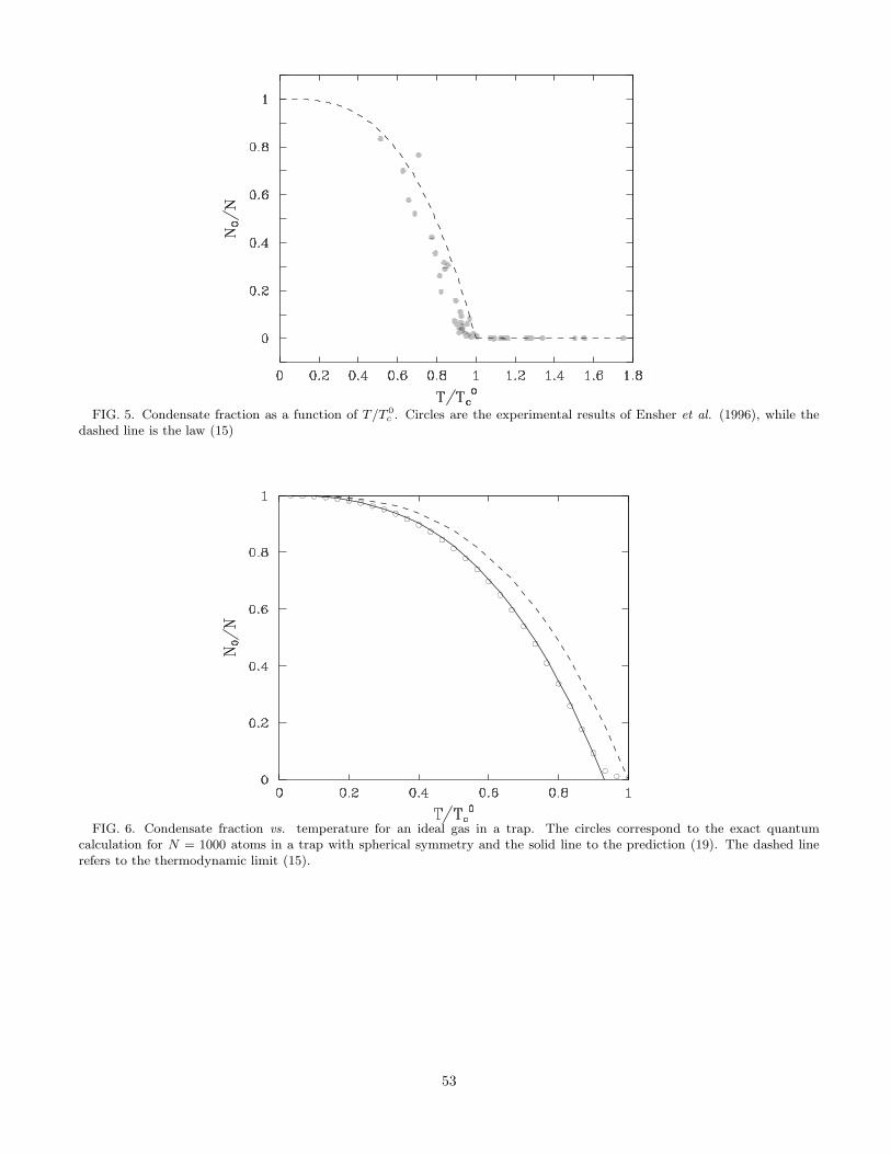
FIG. 5. Condensate fraction as a function of T/T 0c . Circles are the experimental results of Ensher et al. (1996), while the

dashed line is the law (15)

FIG. 6. Condensate fraction vs. temperature for an ideal gas in a trap. The circles correspond to the exact quantumcalculation for N = 1000 atoms in a trap with spherical symmetry and the solid line to the prediction (19). The dashed linerefers to the thermodynamic limit (15).

53

FIG. 7. Behavior of an ideal gas with N = 106 particles in a highly anisotropic trap: ω⊥ = 5.6 × 104ωz, corresponding toT3D = 2T1D. Solid line: fraction of atoms in the ground state (nx = 0, ny = 0, nz = 0), dashed line: fraction of atoms in thelowest radial state (nx = 0, ny = 0).

FIG. 8. Condensate wave function, at T = 0, obtained by solving numerically the stationary GP equation (39) in a sphericaltrap and with attractive interaction among the atoms (a < 0). The three solid lines correspond to N |a|/aho = 0.1, 0.3, 0.5.The dashed line is the prediction for the ideal gas. Here the radius, r, is in units of the oscillator length aho and we plot(a3

ho/N)1/2φ(r), so that the curves are normalized to 1 [see also Eq. (40)].

54

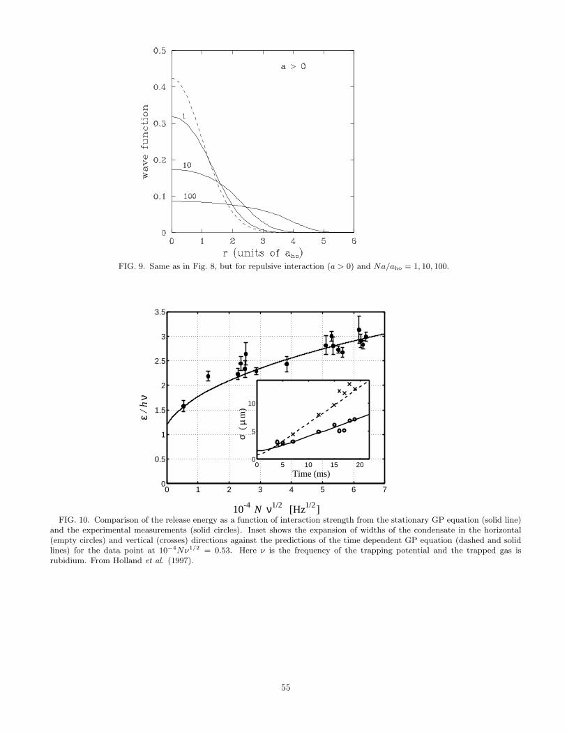
FIG. 9. Same as in Fig. 8, but for repulsive interaction (a > 0) and Na/aho = 1, 10, 100.

0 1 2 3 4 5 6 70

0.5

1

1.5

2

2.5

3

3.5

0 5 10 15 200

5

10

µm

)/ hε

ν

10

σ

N

Time (ms)

-4 ν1/2 [Hz1/2]

(

FIG. 10. Comparison of the release energy as a function of interaction strength from the stationary GP equation (solid line)and the experimental measurements (solid circles). Inset shows the expansion of widths of the condensate in the horizontal(empty circles) and vertical (crosses) directions against the predictions of the time dependent GP equation (dashed and solidlines) for the data point at 10−4Nν1/2 = 0.53. Here ν is the frequency of the trapping potential and the trapped gas isrubidium. From Holland et al. (1997).

55

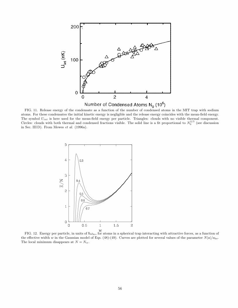
FIG. 11. Release energy of the condensate as a function of the number of condensed atoms in the MIT trap with sodiumatoms. For these condensates the initial kinetic energy is negligible and the release energy coincides with the mean-field energy.The symbol Uint is here used for the mean-field energy per particle. Triangles: clouds with no visible thermal component.Circles: clouds with both thermal and condensed fractions visible. The solid line is a fit proportional to N

2/5

0 (see discussionin Sec. III D). From Mewes et al. (1996a).

FIG. 12. Energy per particle, in units of hωho, for atoms in a spherical trap interacting with attractive forces, as a function ofthe effective width w in the Gaussian model of Eqs. (48)-(49). Curves are plotted for several values of the parameter N |a|/aho.The local minimum disappears at N = Ncr.

56

FIG. 13. Density profile for atoms interacting with repulsive forces in a spherical trap, with Na/aho = 100. Solid line:solution of the stationary GP equation (39). Dashed line: Thomas-Fermi approximation (50). In the upper part the atomdensity is plotted in arbitrary units, while the distance from the center of the trap is in units of aho. The classical turning pointis at R ≃ 4.31aho. In the lower part the column density for the same system is reported.

FIG. 14. Frequency of the lowest collective modes of even parity, m = 0 and m = 2, for rubidium atoms in the JILA trap(λ =

√8). The abscissa is the dimensionless parameter Na/a⊥, with a⊥ = [h/(mω⊥)]1/2, while the frequency is given in units

of ω⊥. Points are taken from the experimental data of Jin et al. (1996). Solid lines are the predictions of the mean-fieldequations (66)-(67) [see, for instance, Edwards et al. (1996c); Esry, (1997); You, Hoston and Lewenstein (1997)]. Dashed linesare the asymptotic results for Na/a⊥ → ∞ (Stringari, 1996b), as discussed in Sec. IVB.

57

10

5

0

Spe

ed o

f Sou

nd (

mm

/s)

86420

Density (1014 cm-3)

FIG. 15. Speed of sound, c, versus condensate peak density, n(0), for waves propagating along the axial direction in thecigar-shaped condensate at MIT. The experimental points are compared with the theoretical prediction c = [gn(0)/2m]1/2

(solid line). From Andrews, Kurn et al. (1997).

Time After Drive (ms)

Con

dens

ate

Leng

th (

µm)

3002001000

T < 0.5 µKa) ∆νrf = 30 kHz

T = 0.95 µKrf = 250 kHzb) ∆ν320

280

240

360

320

280

FIG. 16. Oscillations of the axial width of the condensate in the cigar-shaped trap at MIT. The excited collective motionis the low-lying m = 0 mode. Oscillations are shown at low (a) and high (b) temperature. Points show the axial widthdetermined from fits to phase-contrast images, similar to the ones in Fig. 2. Lines are fits to a damped sinusoidal oscillation.From Stamper-Kurn et al., (1998c).

58

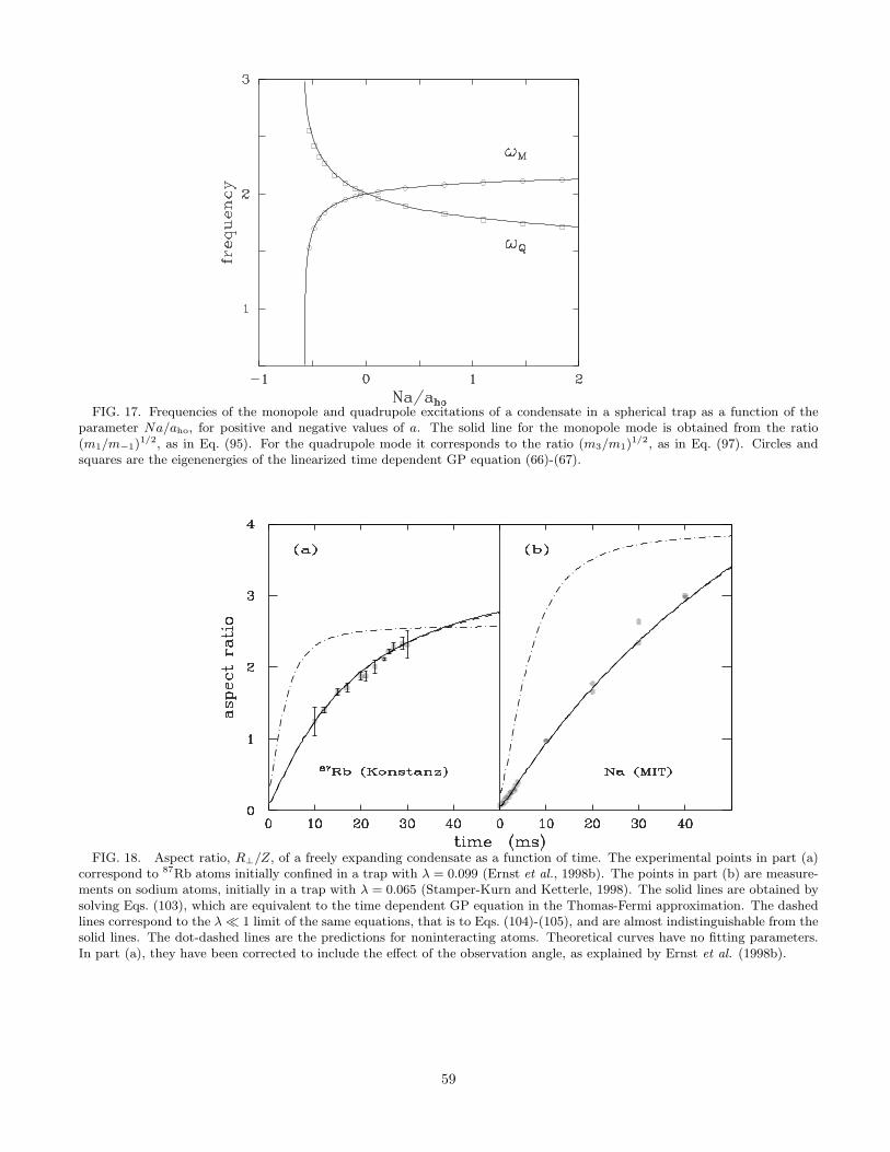
FIG. 17. Frequencies of the monopole and quadrupole excitations of a condensate in a spherical trap as a function of theparameter Na/aho, for positive and negative values of a. The solid line for the monopole mode is obtained from the ratio(m1/m−1)

1/2, as in Eq. (95). For the quadrupole mode it corresponds to the ratio (m3/m1)1/2, as in Eq. (97). Circles and

squares are the eigenenergies of the linearized time dependent GP equation (66)-(67).

FIG. 18. Aspect ratio, R⊥/Z, of a freely expanding condensate as a function of time. The experimental points in part (a)correspond to 87Rb atoms initially confined in a trap with λ = 0.099 (Ernst et al., 1998b). The points in part (b) are measure-ments on sodium atoms, initially in a trap with λ = 0.065 (Stamper-Kurn and Ketterle, 1998). The solid lines are obtained bysolving Eqs. (103), which are equivalent to the time dependent GP equation in the Thomas-Fermi approximation. The dashedlines correspond to the λ ≪ 1 limit of the same equations, that is to Eqs. (104)-(105), and are almost indistinguishable from thesolid lines. The dot-dashed lines are the predictions for noninteracting atoms. Theoretical curves have no fitting parameters.In part (a), they have been corrected to include the effect of the observation angle, as explained by Ernst et al. (1998b).

59

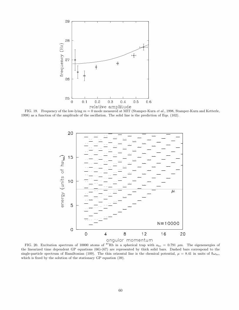
FIG. 19. Frequency of the low-lying m = 0 mode measured at MIT (Stamper-Kurn et al., 1998, Stamper-Kurn and Ketterle,1998) as a function of the amplitude of the oscillation. The solid line is the prediction of Eqs. (102).

FIG. 20. Excitation spectrum of 10000 atoms of 87Rb in a spherical trap with aho = 0.791 µm. The eigenenergies ofthe linearized time dependent GP equations (66)-(67) are represented by thick solid bars. Dashed bars correspond to thesingle-particle spectrum of Hamiltonian (109). The thin orizontal line is the chemical potential, µ = 8.41 in units of hωho,which is fixed by the solution of the stationary GP equation (39).

60

FIG. 21. Number of states N(ε) vs. energy. Solid circles are obtained by counting the Bogoliubov-type states in the spectrumshown in Fig. 20 (thick solid bars). Open circles corresponds to counting the single-particle states in the same figure (dashedbars). Both calculations are compared with the predictions of the semiclassical approximation (112) (solid line), as well aswith the ones of the noninteracting harmonic oscillator (dashed line) and of the collisionless hydrodynamic equations in theThomas-Fermi regime (dot-dashed line). Chemical potential is µ = 8.41 in this scale.

FIG. 22. Column density of atomic clouds from phase-contrast images at several values of temperature in the MIT trap.From Stamper-Kurn and Ketterle (1998).

61

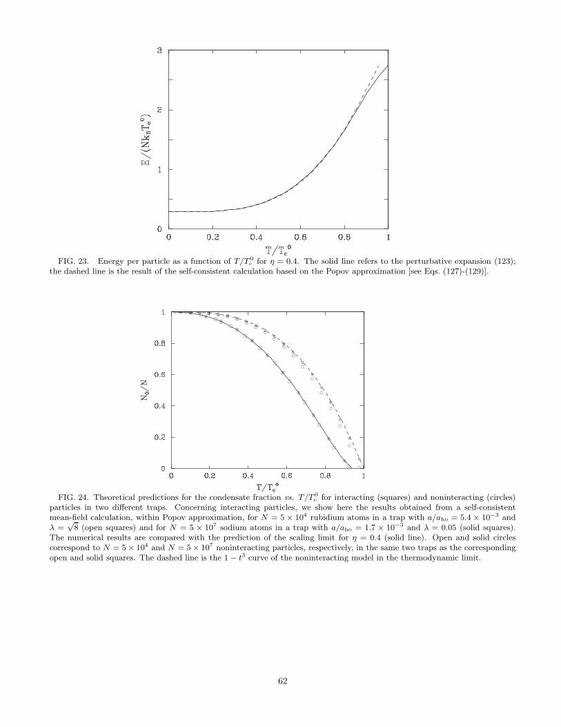
FIG. 23. Energy per particle as a function of T/T 0c for η = 0.4. The solid line refers to the perturbative expansion (123);

the dashed line is the result of the self-consistent calculation based on the Popov approximation [see Eqs. (127)-(129)].

FIG. 24. Theoretical predictions for the condensate fraction vs. T/T 0c for interacting (squares) and noninteracting (circles)

particles in two different traps. Concerning interacting particles, we show here the results obtained from a self-consistentmean-field calculation, within Popov approximation, for N = 5 × 104 rubidium atoms in a trap with a/aho = 5.4 × 10−3 andλ =

√8 (open squares) and for N = 5 × 107 sodium atoms in a trap with a/aho = 1.7 × 10−3 and λ = 0.05 (solid squares).

The numerical results are compared with the prediction of the scaling limit for η = 0.4 (solid line). Open and solid circlescorrespond to N = 5 × 104 and N = 5 × 107 noninteracting particles, respectively, in the same two traps as the correspondingopen and solid squares. The dashed line is the 1 − t3 curve of the noninteracting model in the thermodynamic limit.

62

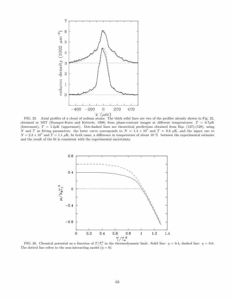
FIG. 25. Axial profiles of a cloud of sodium atoms. The thick solid lines are two of the profiles already shown in Fig. 22,obtained at MIT (Stamper-Kurn and Ketterle, 1998) from phase-contrast images at different temperatures: T = 0.7µK(lowermost), T = 1.2µK (uppermost). Dot-dashed lines are theoretical predictions obtained from Eqs. (127)-(129), usingN and T as fitting parameters: the lower curve corresponds to N = 1.4 × 107 and T = 0.8 µK, and the upper one toN = 2.3 × 107 and T = 1.1 µK. In both cases, a difference in temperature of about 10 % between the experimental estimateand the result of the fit is consistent with the experimental uncertainty.

FIG. 26. Chemical potential as a function of T/T 0c in the thermodynamic limit. Solid line: η = 0.4, dashed line: η = 0.6.

The dotted line refers to the non-interacting model (η = 0).

63

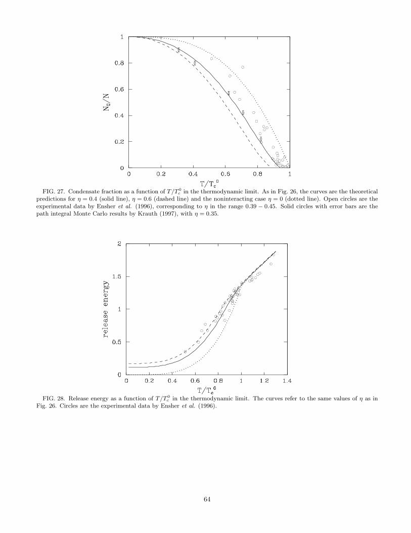
FIG. 27. Condensate fraction as a function of T/T 0c in the thermodynamic limit. As in Fig. 26, the curves are the theoretical

predictions for η = 0.4 (solid line), η = 0.6 (dashed line) and the noninteracting case η = 0 (dotted line). Open circles are theexperimental data by Ensher et al. (1996), corresponding to η in the range 0.39 − 0.45. Solid circles with error bars are thepath integral Monte Carlo results by Krauth (1997), with η = 0.35.

FIG. 28. Release energy as a function of T/T 0c in the thermodynamic limit. The curves refer to the same values of η as in

Fig. 26. Circles are the experimental data by Ensher et al. (1996).

64

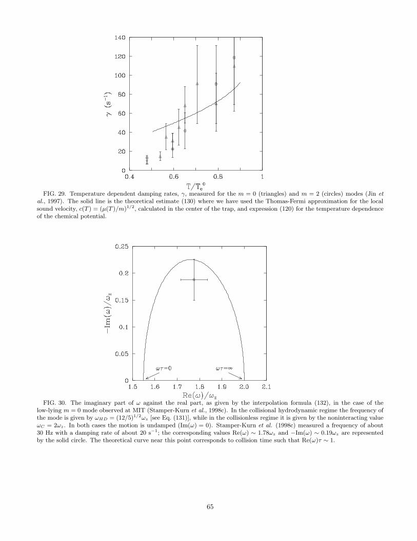
FIG. 29. Temperature dependent damping rates, γ, measured for the m = 0 (triangles) and m = 2 (circles) modes (Jin et

al., 1997). The solid line is the theoretical estimate (130) where we have used the Thomas-Fermi approximation for the localsound velocity, c(T ) = (µ(T )/m)1/2, calculated in the center of the trap, and expression (120) for the temperature dependenceof the chemical potential.

FIG. 30. The imaginary part of ω against the real part, as given by the interpolation formula (132), in the case of thelow-lying m = 0 mode observed at MIT (Stamper-Kurn et al., 1998c). In the collisional hydrodynamic regime the frequency ofthe mode is given by ωHD = (12/5)1/2ωz [see Eq. (131)], while in the collisionless regime it is given by the noninteracting valueωC = 2ωz. In both cases the motion is undamped (Im(ω) = 0). Stamper-Kurn et al. (1998c) measured a frequency of about30 Hz with a damping rate of about 20 s−1; the corresponding values Re(ω) ∼ 1.78ωz and −Im(ω) ∼ 0.19ωz are representedby the solid circle. The theoretical curve near this point corresponds to collision time such that Re(ω)τ ∼ 1.

65

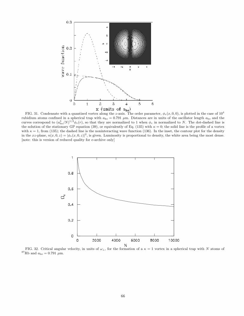
FIG. 31. Condensate with a quantized vortex along the z-axis. The order parameter, φv(x, 0, 0), is plotted in the case of 104

rubidium atoms confined in a spherical trap with aho = 0.791 µm. Distances are in units of the oscillator length aho and thecurves correspond to (a3

ho/N)1/2φv(r), so that they are normalized to 1 when φv in normalized to N . The dot-dashed line isthe solution of the stationary GP equation (39), or equivalently of Eq. (135) with κ = 0; the solid line is the profile of a vortexwith κ = 1, from (135); the dashed line is the noninteracting wave function (136). In the inset, the contour plot for the densityin the xz-plane, n(x, 0, z) = |φv(x, 0, z)|2, is given. Luminosity is proportional to density, the white area being the most dense.[note: this is version of reduced quality for e-archive only]

FIG. 32. Critical angular velocity, in units of ω⊥, for the formation of a κ = 1 vortex in a spherical trap with N atoms of87Rb and aho = 0.791 µm.

66

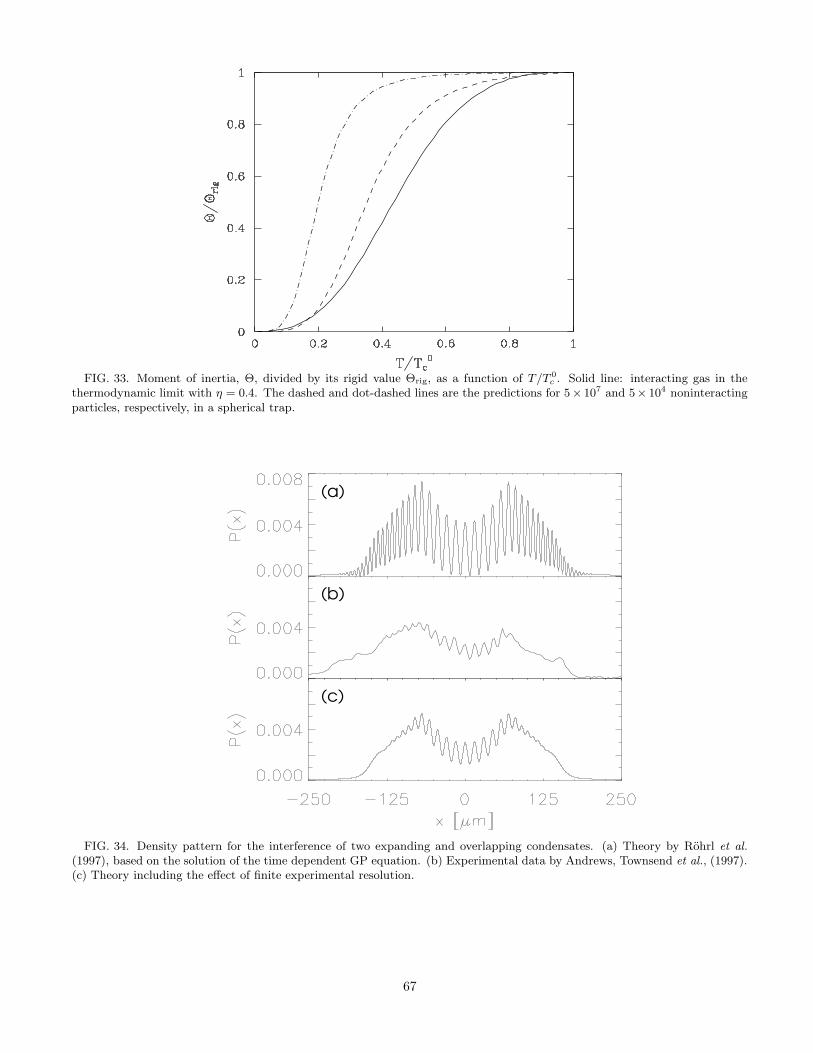
FIG. 33. Moment of inertia, Θ, divided by its rigid value Θrig, as a function of T/T 0c . Solid line: interacting gas in the

thermodynamic limit with η = 0.4. The dashed and dot-dashed lines are the predictions for 5× 107 and 5× 104 noninteractingparticles, respectively, in a spherical trap.

(a)

(b)

(c)

FIG. 34. Density pattern for the interference of two expanding and overlapping condensates. (a) Theory by Rohrl et al.

(1997), based on the solution of the time dependent GP equation. (b) Experimental data by Andrews, Townsend et al., (1997).(c) Theory including the effect of finite experimental resolution.

67

FIG. 35. Schematic geometry of a double-well trapping potential, Vext, for the Josephson effect.

FIG. 36. Schematic picture for collapse-revival of collective excitations. The quantity ξ is a generic oscillator co-ordinateand the symbol 〈ξ〉 means an average over different replica of the system prepared in the same conditions.

68

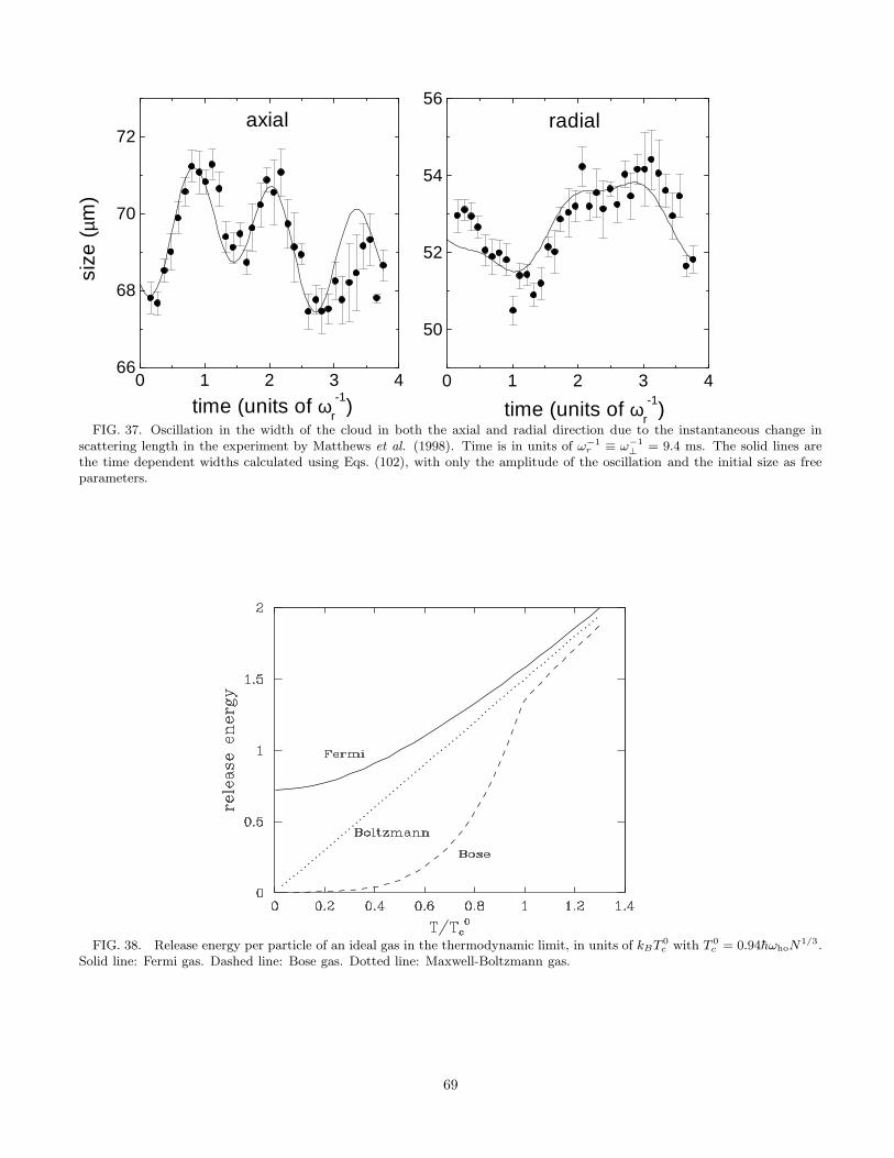
0 1 2 3 466

68

70

72

axial

time (units of ωr

-1)

siz

e (µ

m)

time (units of ωr

-1)

0 1 2 3 4

50

52

54

56

radial

FIG. 37. Oscillation in the width of the cloud in both the axial and radial direction due to the instantaneous change inscattering length in the experiment by Matthews et al. (1998). Time is in units of ω−1

r ≡ ω−1⊥

= 9.4 ms. The solid lines arethe time dependent widths calculated using Eqs. (102), with only the amplitude of the oscillation and the initial size as freeparameters.

FIG. 38. Release energy per particle of an ideal gas in the thermodynamic limit, in units of kBT 0c with T 0

c = 0.94hωhoN1/3.

Solid line: Fermi gas. Dashed line: Bose gas. Dotted line: Maxwell-Boltzmann gas.

69