arXiv:astro-ph/0105506v1 29 May 2001 · arXiv:astro-ph/0105506v1 29 May 2001 ... We also look for patterns of cluster ... We used the IRAF2 tasks GEOMAP and GEOTRAN to

arX

iv:a

stro

-ph/

0105

506v

1 2

9 M

ay 2

001

Identification and Analysis of Young Star Cluster Candidates in

M311

Benjamin F. Williams

University of Washington

Astronomy Dept. Box 351580, Seattle, WA 98195-1580

[email protected]

Paul W. Hodge

University of Washington

Astronomy Dept. Box 351580, Seattle, WA 98195-1580

[email protected]

ABSTRACT

We present a method for finding clusters of young stars in M31 using

broadband WFPC2 data from the HST data archive. Applying our

identification method to 13 WFPC2 fields, covering an area of ∼60 arcmin2,

has revealed 79 new candidate young star clusters in these portions of the

M31 disk. Most of these clusters are small (∼<5 pc) young (∼10-200 Myr) star

groups located within large OB associations. We have estimated the reddening

values and the ages of each candidate individually by fitting isochrones to the

stellar photometry. We provide a catalog of the candidates including rough

approximations of their reddenings and ages. We also look for patterns of cluster

formation with galactocentric distance, but our rough estimates are not precise

enough to reveal any clear patterns.

Subject headings: galaxies: M31; spiral; stellar populations; star clusters; OB

associations.

1Based on observations with the NASA/ESA Hubble Space Telescope obtained at the Space Telescope

Science Institute, which is operated by the Association of Universities for Research in Astronomy, Inc., under

NASA contract NAS5-26555.

– 2 –

1. Introduction

Observations of extragalactic young star clusters are essential for understanding

how star formation affects galaxy evolution. The young stellar population is responsible

for many of the characteristics which give spiral galaxies their current morphological

classification. Although massive young stars constitute only a very small percentage of

the stellar population of most spiral galaxies, they trace the most recent star formation,

produce and disperse most of the heavy elements, and illuminate the spiral arms. Open

clusters are the typical birthplaces of bright massive stars. Since these clusters contain the

youngest stars in the galaxy, their identification and examination is crucial for learning how

star formation has progressed within the galaxy, resulting in its current appearance. The

most detailed information about these clusters comes from studies of their constituent stars.

The study of extragalactic OB associations has been an ongoing struggle for 5 decades,

going back to studies of the properties of the very conspicuous associations of bright stars

in the Large Magellanic Cloud (LMC) in the 1950s (e.g. Buscombe, Gascoigne, & de

Vaucouleurs 1955, Shapley 1956). Decades of research have resulted in catalogs of OB

associations in nearby galaxies (e.g. Lucke & Hodge 1970 (LMC), van den Bergh 1964

(M31), Hodge 1977 (NGC 6822)). These catalogs have provided excellent starting points for

studying the young stellar populations of other galaxies; however, these samples were not

ideal for further statistical analysis because they were obtained through subjective analysis

of low-resolution, non-uniform data.

More recently, high-resolution photometric data and advances in computational

analysis techniques have allowed more objective identification of OB associations in galaxies

(e.g. Wilson, Scoville, & Rice (1991)), creating more uniform samples on which to perform

statistical analyses. These objective samples have resulted in significant advances in our

understanding of the properties of extragalactic OB associations. The similarity of their size

distributions and stellar luminosity functions across different galaxy types (Bresolin et al.

1998), and their similar luminosity function across galaxy types (Battinelli et al. 2000)

have suggested that massive star formation occurs by similar processes in all galaxies. At

the same time, OB associations’ average population sizes appear to differ between galaxies

of different morphological type (Bresolin & Kennicutt 1997), showing that environment has

some effect on massive star formation.

M31 has been an excellent laboratory for the study of massive star formation due to its

proximity and its many active spiral arms. These arms contain hundreds of OB associations

that have been studied extensively from the ground and from space. Our distant view

of M31 has allowed ground-based studies of young clusters on a wide range of size scales.

Due to the crowding of stars and variable reddening in the disk, the optical ground based

– 3 –

data was used mainly for identification and studies of the structure of OB associations.

These studies have shown, for example, that massive star formation appears hierarchical

(Battinelli, Efremov, & Magnier 1996): the large complexes contain many smaller clusters,

possibly with related physical properties. In the infrared, the crowding and reddening

effects are reduced. Recent infrared work has succeeded in finding evidence for episodic star

formation which occurred in different subregions during each spiral wave passage (Kodaira

et al. 1999). Space-based observations are allowing more detailed analysis of these regions

of recent star formation. Magnier et al. (1997) have used Hubble Space Telescope (HST)

photometric data to determine the reddening distribution and ages of a handful of OB

associations.

While studies of the well-known OB associations in M31 have been instrumental to

our understanding of massive star formation, there has been very little work done on the

small, young and compact star clusters in the spiral arms of M31. These clusters have

been difficult to identify from the ground since they require very high resolution to resolve.

Hodge (1979) discovered several hundred open cluster candidates in M31, but these objects

were larger than typical Galactic clusters and may actually be small OB associations. In

this study, we use the resolving power of HST in order to probe the size scales of typical

open clusters in M31. We create a cluster finding algorithm fine-tuned to find small young

clusters in the M31 disk and identify their most likely member stars. We then use the

photometry from these stellar populations to estimate reddening and age values for our

sample of young cluster candidates.

2. Data Acquisition and Reduction

We searched the HST archive for all exposures of longer than 60 seconds which were

taken through the broadband B (F439W) and V (F555W) filters pointing within 1.5 degrees

of the M31 nucleus. Using this narrow radius kept our data contained within the disk,

avoiding significant halo contamination. Any fields in the bulge were later excluded by eye.

We acquired and reduced 13 WFPC2 fields from the HST archive, each observed through at

least the B and V broad-band filters. U band (F336W) images were also available for most

of these fields, providing useful information about the reddening of our cluster candidates.

Table 1 gives the RA, DEC, dates, bandpasses, and exposure times of the data taken from

the HST archive in order to put together each of these fields. The positions of these fields

on the galaxy are shown in Figure 1. The figure shows an Hα mosaic of the M31 disk

(Winkler & Williams 1995) with the positions of the 13 fields marked with squares showing

the positions of each chip in the field. Each field is labeled with the number given in Table

– 4 –

1. The PC chip position is not shown because it was excluded from our analysis. Since

the PC portions of the images often contained special regions of the galaxy (e.g. globular

clusters) and since the area covered by the PC is small, we decided to exclude all of the PC

data in order to keep the data set as unbiased as possible. The exposure times for these

fields were generally quite short, and therefore they are relatively shallow.

We determined instrumental magnitudes for each of these fields using the automated

programs DAOPHOT II and ALLSTAR (Stetson, Davis, & Crabtree 1990). An object

was considered a real star if it was detected as a point source at 4σ above the noise level

in 2 bandpasses with centroids separated by less than 0.7 pixels. Therefore, some of the

objects under consideration may be misclassified background galaxies and foreground

stars; however, in fields of these angular sizes at this galactic latitude (-21.57deg) and

these depths, the average number of foreground galactic stars per field should be less than

10. Background galaxies will typically not be detected as they will not appear as point

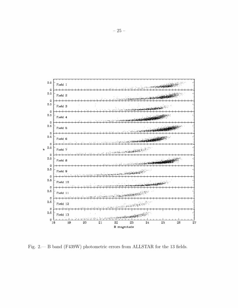
sources. Figures 2 and 3 show the typical photometric errors, determined by ALLSTAR,

as a function of B and V magnitude for each of the 13 fields. The errors tended to be

approximately at the 10% level near the bright magnitudes (mV < 24), mostly due to the

fluctuating surface brightness of the background. The M31 disk is a complex background

with which to work and therefore limits the accuracy of the photometry by increasing

the uncertainty of the local background level. This uncertainty is partially due to the

poisson noise of the higher background levels, but it is also due to actual structure in

the background on spatial scales relevant to stellar photometry. These surface brightness

fluctuations come from structure in the stellar disk which cannot be resolved by HST.

Point Spread Function (PSF) magnitudes were checked against aperture photometry of

the most isolated stars with the highest signal to noise in order to determine if there was an

offset between the PSF photometry and the more standard aperture photometry. We found

small offsets of our PSF photometry from the aperture photometry on the WF3 chip in the

V band and in the WF4 chip in the B band. We applied small corrections (+0.03 mags for

stars measured in the V band on the WF3 chip, and +0.05 mags for stars measured in the

B-band on the WF4 chip) to our photometry in these cases in order to make the mean offset

between the aperture and PSF photometry zero. In all other cases, the offsets were zero.

We then obtained standard U, B, and V magnitudes from our instrumental magnitudes

using the methods, zero points, and transformation coefficients given in Holtzman et al.

(1995). We first determined instrumental magnitudes for the F336W, F439W, and F555W

filter as

mfilter = −2.5× log(ADU/t) +X + ZPfilter (1)

where ADU is the number of counts, t is the exposure time, X is the small offset computed

from the aperture photometry mentioned above, and ZPfilter is the zero point of the

– 5 –

WFPC-2 chip for the bandpass. Since the transformation to U, B, and V is a function

of color, we used the F336W - F439W as a first approximation of the U-B color and the

F439W - F555W color as a first approximation of the B-V color and iteratively solved the

transformation equations.

As a further test to the accuracy of our photometry, we took advantage of the fact that

two of our fields were overlapping. The WF3 chip in field 7 was covering the same region of

space as the WF2 chip in field 9. We used the IRAF2 tasks GEOMAP and GEOTRAN to

determine a rotational and translational conversion between the coordinates of the stars in

one frame to their coordinates in the other frame. We were then able to convert all of the

pixel coordinates of the stars in one frame to the coordinates of the same star in the other

frame. By comparing the star lists, we found every star which was detected in both frames.

Then we were able to compare independent measurements of the same stars as determined

in different locations on the chips, on different chips and in different frames.

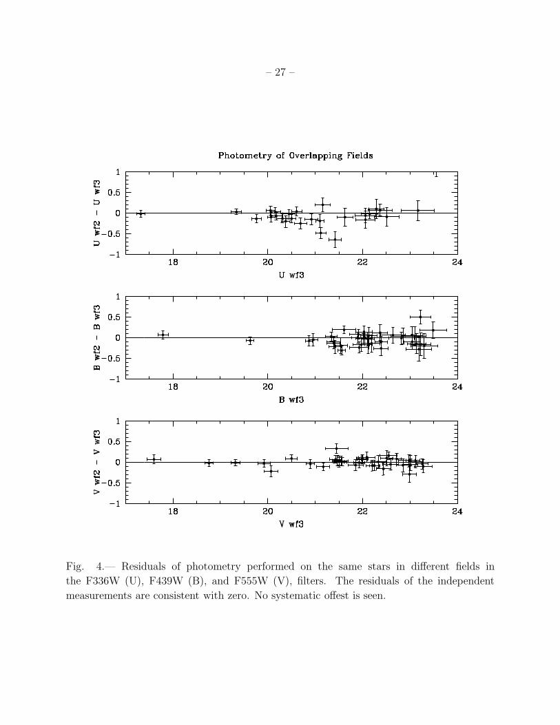
The easiest way to see the accuracy of our photometry is by looking at the residuals

after subtracting the magnitudes of the stars determined on the WF3 chip from the same

stars observed with the WF2 chip. These residuals are shown in Figure 4. No systematic

differences between the chips are seen, and the residuals are consistent with zero in nearly

all cases. With this reinforcement that we understood our errors, and with the knowledge

that our photometry and errors were accurate, we could apply our young cluster finding

algorithm to the stellar photometry.

3. Identification of Young Clusters of Stars

In order to explore the many open clusters and young stellar associations, we created

an objective method for detecting the clusters within the fields. Using our stellar positions

and photometry from DAOPHOT II and ALLSTAR, the mean surface density of bright

(mV < 24.5, MV ∼< 0.1) blue (B − V < 0.45) stars is determined. Then the standard

deviation from the mean density (σ) on a size scale specified by the user is calculated. This

calculation is performed by comparing the density of bright blue stars in regions of the

specified size around every bright blue star detected in the field with the mean density. This

calculation of the mean stellar density and the standard deviation of the stellar density is

followed by a search for regions containing at least 4 bright blue stars and having surface

2IRAF is distributed by the National Optical Astronomy Observatories, which are operated by the

Association of Universities for Research in Astronomy, Inc., under cooperative agreement with the National

Science Foundation.

– 6 –

densities of bright blue stars 3σ above the mean.

We found the user specified size must be chosen carefully. Large values will often

find overdensities which contain more than one cluster, unnecessarily reducing the spatial

resolution of the data. Small values will often lead to single clusters being divided into

several stellar overdensities of the size requested. We found the best way to overcome these

problems was to run the algorithm using two size scales, one corresponding to the sizes of

a few of the smaller clusters visible in the images and one corresponding to the sizes a few

of the larger clusters visible in the images. If a cluster was found at both size scales, we

had to choose which of the detections was most appropriate to use for follow-up work. If

the cluster appeared small and populous we would use the detection from the small search

radius in order to avoid field contamination in our star sample. If the cluster was large,

and it had been detected as more than one cluster with the small search radius, we would

use the detection from the large search radius in order to maximize the number of stars in

our sample and in order to avoid making multiple age and reddening measurements for the

same cluster.

Finally, in order to remove statistical anomalies from our sample, we ran each cluster

candidate through a surface brightness test. In this test, we measure the surface brightness

around the center of each cluster candidate. This test was a bit more complex since, due to

completeness issues, the centers of the stellar overdensities were not always aligned exactly

with the high surface brightness regions. Therefore we allowed overdensities with very

nearby high surface brightness regions to pass. This step required great care for the larger

clusters since the chance of one bright star entering the surface brightness calculation and

enhancing the surface brightness near the center of the overdensity was higher for the large

clusters. We found the number of these single bright star contaminants was reduced when

we removed candidates with substantial (>2 mag arcsec−2) increases in surface brightness

away from the center. These large jumps in surface brightness were usually bright single

point sources, which were likely foreground stars. Any stellar overdensity whose measured

surface brightness characteristics did not pass our objective criteria was not likely part of an

underlying cluster of unresolved stars. These low surface brightness regions were removed

from the sample.

We ran this algorithm on our star lists for all of the WFPC2 chips for each field in

our sample. We did one run looking for small scale associations (radius ∼5 pc), and we

did a second run looking for larger associations (radius ∼15 pc). We compared our results

with published catalogs of clusters and associations, and with previously performed eye

searches in order to learn our method’s strengths and weaknesses. The only previously

known blue cluster in the survey region was G42 (Sargent et al. 1977), and it was found

– 7 –

by our algorithm. Since these regions had not been observed for young clusters with this

resolution before, all of the other coincident cataloged objects were either individual bright

stars within the clusters or coincident emission nebulae within the confused northeast spiral

arm. No other previously known star clusters were found. There were, however, a few

distinct clusters found within objects which had been previously cataloged from the ground

as a single cluster. For example, the previously cataloged H81 B-202 (Hodge 1981), which

was an open cluster as seen from the ground contains three of these cluster candidates

at high resolution: M31SCC J004205+405714, M31SCC J004204+405826, and M31SCC

J004205+405659. This discovery may indicate that many open clusters found with ground

based data could in fact be small OB associations containing multiple young clusters. The

other clusters which were found to be part of previously cataloged clusters are listed in

Table 3.

Due to the size of the fields we were using, we were not able to find large (>40 pc) OB

associations previously discovered from the ground, but we were able to identify smaller

sub-clusters within these larger associations which were not previously identified as separate

clusters. This selection bias against large associations should be avoidable in other data sets

by looking for stellar overdensities on larger scales, but we did not have wide enough fields

to run such a test. We also found that our method did not detect the smallest, densest

clusters seen by eye, most likely due to the low completeness in these areas. It also missed

several obvious red clusters, including a few known globulars. These clusters were either

heavily extincted or much older than the clusters found by our algorithm. In either case,

due to severe crowding, age, or extinction, there were too few detected blue stars in these

clusters to separate the cluster stars from the field in order to study the stellar population.

Succinctly, the algorithm tended to miss many possible clusters that could be seen

by eye. These clusters tended to be dense red clusters which were likely older than our

sample and/or heavily reddened. Using different color criteria, it could be possible to

obtain a sample of red cluster candidates; however, we limit our discussion here to the

blue cluster candidates which were the most straight-forward to statistically separate from

the background population. The clusters the algorithm did not find were too red or too

dense to easily obtain photometry of a sample of member stars. The member stars did not

stand out statistically in color, or due to completeness, they did not stand out in stellar

density. The algorithm found only one previously known blue cluster in the images as well

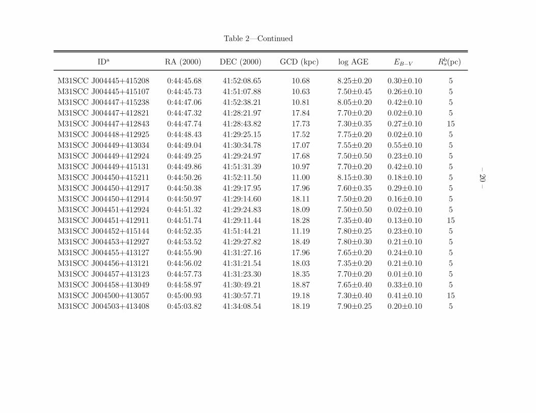
as many new clusters which were found previously by eye. Five of the fields had been

previously scrutinized by eye looking for extended objects which may be clusters. Table 3

lists which of the star clusters found by the algorithm in these five fields were also found by

eye, and which were not. Roughly 75 percent of the objects found by the algorithm had

been previously discovered by eye on the test fields. The other 25 percent were comparable

– 8 –

to M31SCC J004455+413127 or M31SCC J004206+405649 (see Figure 5). They did not

contain obvious compact cores and are not as likely to be real clusters.

We also checked the overlapping fields to see which clusters were found independently

by the algorithm using photometry from different observations of the same region. Table 4

lists the clusters which were in the overlapping regions of two fields, along with the fields

in which they were found. There were clusters found in overlapping regions of fields 9 and

10. Only 3 of 7 cluster candidates in the overlapping regions were found independently in

both frames. This result reveals the dependence of our method upon the stellar density of

the field observed. The non-overlapping regions of the overlapping fields sample different

regions, and if these non-overlapping regions of the fields have significantly different mean

stellar densities or significantly different stellar density fluctuations, then the algorithm

will pick out some different cluster candidates for the overlapping regions of the fields. For

example, the WF2 chip of field 10 overlaps the WF4 chip of field 9. The non-overlapping

portion of the WF2 chip of field 10 contains a very active region. This active region raises

the stellar density threshold for finding a cluster on the field 10 chip. Therefore the clusters

found on the field 9 chip are not as convincing due to the very low average stellar density,

and, in fact, these clusters are not picked out on the field 10 chip, even though field 10 is

deeper. Exactly the inverse situation occurs for the non-overlapping portions of the WF3

chip of fields 9 and 10. Here the non-overlapping section of field 9 contains a very active

region, raising the threshold for finding a cluster. This inconsistency would likely be less

severe for wider field data sets, as the mean stellar densities and density fluctuations should

be more stable if sampled over larger regions. The good news about these inconsistencies

between overlapping regions is that they provide a very nice ranking of candindates in

these regions. The candidates that were found in both data sets of the same area are much

stronger than the candidates that were not.

We show a random subset of 9 of the objects detected by the algorithm in Figure 5.

These 9 images are through the F439W filter and are 12 arcsec across. The example set

shows a variety of objects from large obvious clusters like M31SCC J004000+403325 to very

marginal detections such as M31SCC J004455+413127. There were several of these types

of objects in our sample, which do not look like obvious clusters to the eye. These make up

close to half of the sample. Generally, the properties of these cluster candidates are right at

the limits of our criteria. The candidates that were not found independently when observed

in two fields were comparable to these candidates, as were the candidates that were not

seen by eye. Nevertheless these star populations contain well above the mean density of

bright blue stars and have enhanced surface brightness compared to the rest of the region

sampled in that field. There was no simple objective way to remove these objects from the

sample without also removing many of our best candidates in the process. Though these

– 9 –

objects are less likely bona fide clusters, we have included them for completeness.

4. Determining Physical Parameters for the Clusters

4.1. Deprojected Galactocentric Distance

Using the coordinates of the clusters in the HST fields, RA=00:42:44.31 DEC=41:16:09.4

for the center of M31, the inclination angle of the disk (77 degrees) (Brinks & Burton 1984),

and the position angle of the disk (38 degrees), we corrected the projected galactocentric

distances of each of our fields. First we determined the major and minor axis coordinates

using:

x2 = P 2∗ cos2(φ− θ)

y2 = (P 2− x2)

where x is the coordinate of the object along the major axis of M31, y is the coordinate of

the object along the minor axis, φ is the anglular position of the object east of north, θ is

the M31 position angle east of north, and P is the projected galactocentric distance of the

field. Then, we corrected the minor axis coordinate for the disk inclination using:

y2c = y2/cos2(I)

where yc is the minor axis coordinate corrected to its face-on value. Together, these

transformations allow a direct transformation from P to the galactocentric distance using:

G2 = x2 + y2c = P 2(cos2(φ− θ) + (1− cos2(φ− θ))/cos2(I))

where G is the deprojected galactocentric distances for the clusters. Calculated values are

given in Table 2.

4.2. Reddening and Age Determinations

Once we had determined the positions of the clusters and the photometry of the most

likely member stars, the next step was to correct the stellar photometry for the extinction

between us and each of the clusters. The reddening was likely to be significant since these

– 10 –

clusters were all within the M31 disk where we expect there to be relatively thick dust.

Open clusters tend to contain upper main sequence stars. These stars are virtually the

same intrinsic color in B-V, and they tend to lie along a narrow sequence in the U-B, B-V

plane. Since extinction makes these stars appear to be to the red of this sequence, it is

possible to estimate the extinction values of these clusters using photometry of just a few

of the brightest cluster members.

Since the clusters were found on the basis of the grouping of just a handful of detected

bright blue stars, we were limited in our confidence for determining accurate reddening and

age values for them. Since there was not a statistical overdensity of red stars in the clusters,

we could not confidently assume the red stars were cluster members. Therefore we had very

few stars from each cluster with which to work, and it was not practical or informative to

run a detailed fit of synthetic color-magnitude diagrams to the observed color-magnitude

diagram. With so few stars, it proved more useful and faster to assume that the over-dense

population of blue stars we detected represented the main sequence turnoff of the cluster.

Simulations described in section 4.3 show this to be a reasonable assumption to estimate

the age to ∼50% accuracy. This assumption allowed us to determine reddening values by

fitting model U-B and B-V star colors to model main sequence colors when possible. We

determined the reddening by doing a least-squares fit of the U-B and B-V colors of the stars

to the U-B and B-V colors of the theoretical main sequence from Girardi et al. (2000). We

occasionally adjusted this value in cases where the B-V colors of the full cluster sample did

not appear to follow the isochrones due to one outlier which had polluted the least-squares

fit. In cases where there were no U band data available, the reddening was determined by

fitting the B-V colors to the theoretical upper main sequence. The reddening values for the

whole sample determined by this method are given in Table 2.

Figure 6 shows a sample of one of our reddening determination fits. The figure shows

the data after applying the our best reddening correction overplotted with the theoretical

stellar colors from Girardi et al. (2000). In some cases, only one star was detected in all

three bands due to the sensitivity of WFPC2 in the UV. These single star fits often had to

be adjusted by eye since they often resulted in poor fits to the B-V color for the rest of the

stars detected in the cluster candidate. These adjustments pushed the stars slightly off the

best fit to the theoretical line in these cases. Our findings show that these clusters have a

wide range of reddening values, indicating that they are likely at different depths within

the disk. In the cases where U band data was not available, the reddening had to be fit

assuming that all of the stars were still on the upper main sequence, and therefore were

not red in B-V due to evolution. Two examples of these fits are shown in Figure 6 as well.

We assume that all of the stars within a single cluster are reddened by the same amount.

It is possible that some of these clusters contain dust which would produce differential

– 11 –

reddening within individual clusters. If differential reddening is affecting our data, it is

possible that the brightest stars are over-corrected. Such an over correction would cause an

under-estimation of the cluster age as determined by the method described below.

After correcting the photometry using these reddening values, we produced simple

least-squares fits of the stellar photometry to single age model isochrones in order to

approximate the age of the cluster. This procedure was performed on all of our cluster

candidates. We used all of the stars in the overdensity, without subtracting any possible

field stars. We justify the lack of correcting for field contamination by pointing out that

the average number of these bright blue stars in areas the size that we were sampling

was generally ∼<1. Randomly throwing out a single star from each cluster would not have

have been useful in case of our data because there was no reason to throw out one star as

opposed to another. On the contrary, these stars had already been selected on the basis

that they were grouped, bright blue stars of which the density in the field was very low.

Therefore, our field contamination was minimized without doing a second contamination

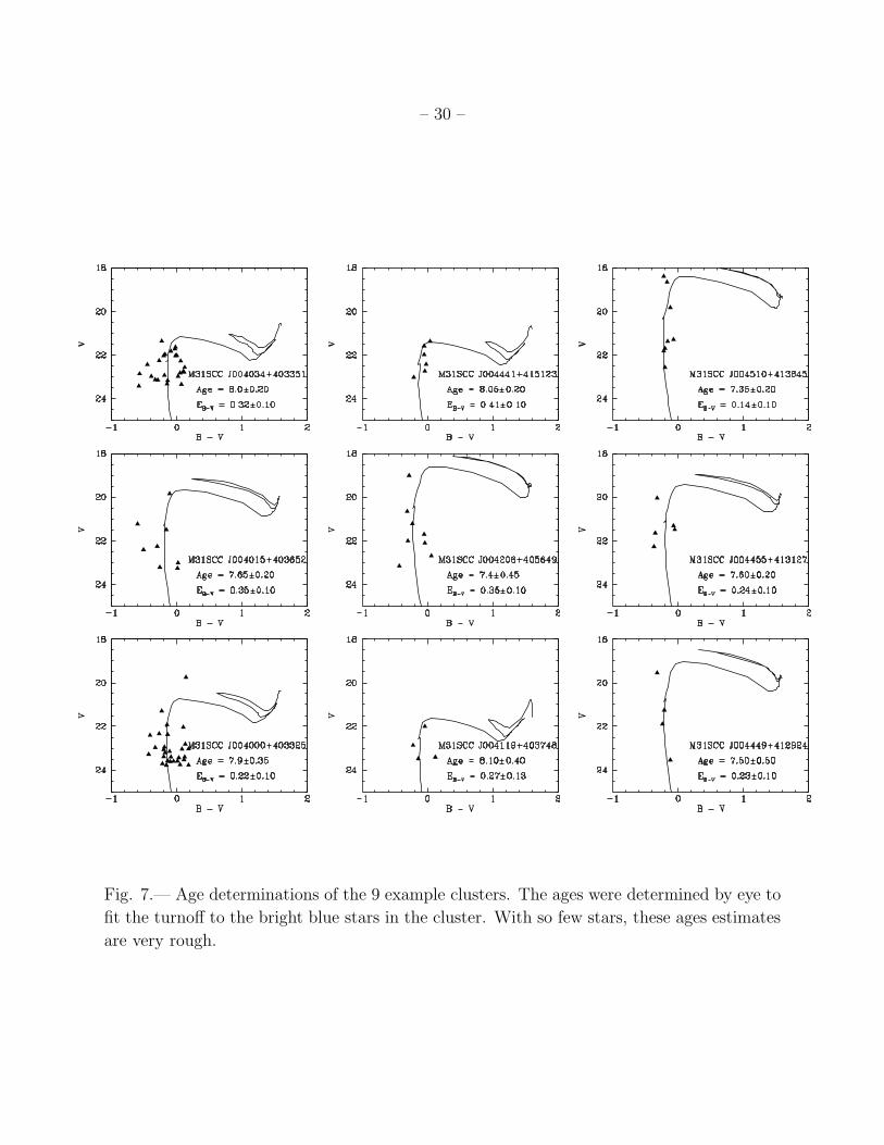
correction. All of the age fits were inspected by eye and adjusted in cases where the fitting

procedure produced inferior fits. The inferior fits were obvious because they did not fit

the main sequence turnoff of the cluster due to the measured color of the brightest star

in the cluster. If this color was measured to be bluer than the theoretical main sequence

due to photometry errors, then the least squares method could not fit a turnoff. In these

cases, ages were determined using by-eye fits to the isochrones. Therefore, about half of

our age determinations were done by eye, and the fitting procedure was only used as a first

approximation. Some typical fits are shown in Figure 7. The ages for the whole sample

determined by this method are given in Table 2.

4.3. Error Estimates: Simulation Tests

We determined the errors of our subjective age and reddening determination technique

through several experiments. First, we simulated our data using higher resolution PC data

of well-studied massive young clusters. By comparing the results from our crude method

to the robust results from the high resolution data, we were able to estimate how accurate

our results were for the most populated clusters. Then we experimented with the clusters

themselves. By removing data points and iterating our analysis routine, we were able

to assess the stability of our results. Lower stability resulted in errors larger than those

determined by the resolution simulation.

As a test of our age and reddening determination method, we simulated our low

resolution wide field data using our data from the PC. Since we had previously obtained

– 12 –

robust ages from the high resolution PC data of four previously know blue globular-like

clusters (Williams & Hodge 2001), we binned these data 2 by 2 in order to simulate the

resolution of the WF chips (∼0.1 arcsec/pixel). We then ran the binned data through the

same photometry routine and cluster finding algorithm as the wide field data. This exercise

was further confirmation that the algorithm was finding clusters, as it found all four clusters

and nothing else in the frames. Finally, we put the stars which the algorithm provided as

the most likely cluster members through the same reddening and age determination routine

in order to check the accuracy of our method. We found that the ages determined were all

under-estimated. The turn-off was found at a brighter magnitude than we had determined

it from the PC. These brighter turnoff stars were always found very near the cluster center,

and therefore were very likely blended stars at the lower resolution. These massive and

dense clusters show the worst case scenario for this kind of blending, so that we hope our

less populous clusters will not suffer as badly from this effect.

A summary of the results of the low resolution simulation is shown in Table 5. The

ages are systematically under estimated by a mean of 0.2 dex. Since the vast majority of

the new cluster candidates were not this dense and massive, we did not feel that it would

be appropriate to simply add 0.2 dex to all of our ages. Rather, this result was useful for

determining our error bars. The test showed that ±0.2 dex was the best we could do for

our age determinations. The test result also showed that error determination by throwing

out the brightest few stars at the turnoff and redetermining the reddening and age was

reasonable.

In order to assess the errors of our reddening and age estimates for each cluster

candidate individually, we removed the brightest star from each small cluster and the

brightest four stars from every large cluster. We then measured the reddening and age

again using the same method. This experiment allowed us to find the stability of our

estimate as well as to account for the effect of field stars, and/or blends on our results. The

errors given are the difference between the reddening and age values determined with the

full sample of stars and the values determined with the manipulated sample. If this error

value was less than 0.1 in EB−V or 0.2 in log age, the error was set to 0.1 in EB−V or 0.2 in

log age because our low resolution simulation had shown that our errors had to be at least

this large. We therefore would not allow these reddening and age values, determined using

a much smaller number of stars, to have smaller quoted errors. These small experimental

errors were quite common, mostly due to the high sensitivity of the turnoff to the age at

these young ages (2 mag between 30 Myr and 100 Myr). It was encouraging to find that

most of our experiments showed our results to be quite stable against removal of the turnoff

data points.

– 13 –

5. Results and Conclusions

All of our measurements are given in Table 2. With this table, we have provided

an objective collection of young star cluster candidates in the M31 disk along with their

reddenings and ages as determined from the photometry of their constituent stars. With

our crude age approximations, it was possible to look for statistical patterns in the age

distribution. While the precision of our ages is clearly low, and in fact we cannot even

quote reliable errors on our age measurements, our data is most sensitive to bright blue

stars which define the main sequence turnoff of these clusters. Assuming the detected

stars do mark the turnoff, and that our data set was equally sensitive to them for all of

the clusters detected, we believe that we have done the best job possible to preserve their

relative ages by reducing all of the data identically and determining all ages with the same

model isochrones.

We looked for correlations between the reddening of the clusters and their galactocentric

distances and between the ages of the clusters and their galactocentric distances. These

plots are shown in Figure 8. No correlation is seen within the large errors in our

measurements. Apparently, more accurate age determinations are needed in order to

dicipher the propagation of recent cluster formation in these regions of the M31 disk. We

also checked for a correlation between ages and reddening which would have been indicative

of observational biases within the sample. As seen in Figure 9, there appears to be a lack

of older clusters with high reddening values, confirming that our selection method is bias

against such clusters. There is also a lack of older clusters with very low reddening. This

effect was not expected, and it may be an effect of field contaminants. It is possible that

the six clusters with very low reddening have field contaminants causing them to appear

less reddened and younger.

We have created an automated routine for finding young star clusters amoung stellar

populations in nearby galaxies. This method requires the clusters to be resolved into

individual stars, so that the positions and photometric properties of the stars can be used to

distinguish the star cluster candidate from the field. From comparisons between overlapping

data sets and comparisons between the automated routine and independent searches by

eye, we expect at least half of these candidates are real, young star clusters. The method is

not effective for finding small compact clusters whose stellar populations cannot be studied

in detail with the survey data. Unfortunately, the algorithm misses clusters that could

be useful when higher resolution data are obtainable, and the algorithm finds some very

loose associations which are likely not real clusters. On the other hand, the method is quite

effective at finding star clusters whose populations can be further studied with the survey

data. The algorithm only finds clusters whose stellar photometry is statistically different

– 14 –

from the surrounding stellar population. This statistical difference provides a sample of

stars from each cluster candidate which can be used to constrain the age and reddening.

We have objectively detected 80 blue cluster candidates in the M31 disk using

HST/WFPC2 archival data of 13 fields. Of these clusters, 79 are newly discovered as

individual clusters, though many lie within previously known OB associations. We have

determined rough ages and extinction estimates from the stellar photometry. The ages

and reddening values for these clusters span the full range of our sensitivity and are

consistent with the range of ages and reddening values of the OB associations determined

by Magnier et al. (1997) in the fields common to both studies. The precision of our

approximations is too low to look for cluster formation patterns; however, future, more

accurate determinations of these values could significantly advance our understanding of

the propagation of cluster formation in the M31 disk.

6. Acknowledgments

Support for this work was provided by NASA through grant number GO-06459.01-95A

from the Space Telescope Science Institute, which is operated by the Association of

Universities for Research in Astronomy, Incorporated, under NASA contract NAS5-26555.

REFERENCES

Battinelli, P., Capuzzo-Dolcetta, R., Hodge, P. W., Vicari, A., & Wyder, T. K. 2000, A&A,

357, 437

Battinelli, P., Efremov, Y., & Magnier, E. A. 1996, A&A, 314, 51

Bresolin, F., & Kennicutt, R. C. 1997, AJ, 113, 975

Bresolin, F., et al. 1998, AJ, 116, 119

Brinks, E., & Burton, W. B. 1984, A&A, 141, 195

Buscombe, W., Gascoigne, S. C. B., & de Vaucouleurs, G. 1955, Suppl. Australian J. Sci.,

17

Girardi, L., Bressan, A., Bertelli, G., & Chiosi, C. 2000, A&AS, 141, 371

Hodge, P. W. 1977, ApJS, 33, 69

– 15 –

Hodge, P. W. 1979, AJ, 84, 744

Hodge, P. W. 1981, Atlas of the Andromeda galaxy (Seattle/London: University of

Washington Press, 1981)

Holtzman, J. A., Burrows, C. J., Casertano, S., Hester, J. J., Trauger, J. T., Watson, A. M.,

& Worthey, G. 1995, PASP, 107, 1065

Kodaira, K., Vansevicius, V., Tamura, M., & Miyazaki, S. 1999, ApJ, 519, 153

Lucke, P. B., & Hodge, P. W. 1970, AJ, 75, 171

Magnier, E. A., Hodge, P., Battinelli, P., Lewin, W. H. G., & van Paradijs, J. 1997,

MNRAS, 292, 490

Sargent, W. L. W., Kowal, C. T., Hartwick, F. D. A., & van den Bergh, S. 1977, AJ, 82, 947

Shapley, H. 1956, Am. Sci., 44, 73

Stetson, P. B., Davis, L. E., & Crabtree, D. R. 1990, in ASP Conf. Ser. 8: CCDs in

astronomy, 289

van den Bergh, S. 1964, ApJS, 9, 65

Williams, B. F., & Hodge, P. W. 2001, ApJ, 548, 190

Wilson, C. D., Scoville, N., & Rice, W. 1991, AJ, 101, 1293

Winkler, P. F., & Williams, B. F. 1995, in American Astronomical Society Meeting, Vol.

186, 4910

This preprint was prepared with the AAS LATEX macros v4.0.

– 16 –

Table 1. Data obtained from the HST data archive used for the cluster survey.

Field Prop. # Obs. date RA (2000) DEC (2000) Filter Exp. (sec)

1 8296 Oct 15 1999 0:39:47.35 40:31:57.9 F336W 1000

1 8296 Oct 15 1999 0:39:47.35 40:31:57.9 F336W 800

1 8296 Oct 15 1999 0:39:47.35 40:31:57.9 F336W 1200

1 8296 Oct 15 1999 0:39:47.35 40:31:57.9 F336W 600

1 8296 Oct 15 1999 0:39:47.35 40:31:57.9 F439W 800

1 8296 Oct 15 1999 0:39:47.35 40:31:57.9 F439W 800

1 8296 Oct 15 1999 0:39:47.35 40:31:57.9 F555W 600

1 8296 Oct 15 1999 0:39:47.35 40:31:57.9 F555W 600

2 8296 Oct 30 1999 0:40:01.58 40:34:14.7 F336W 1000

2 8296 Oct 30 1999 0:40:01.58 40:34:14.7 F336W 800

2 8296 Oct 30 1999 0:40:01.58 40:34:14.7 F336W 1200

2 8296 Oct 30 1999 0:40:01.58 40:34:14.7 F336W 600

2 8296 Oct 30 1999 0:40:01.58 40:34:14.7 F439W 800

2 8296 Oct 30 1999 0:40:01.58 40:34:14.7 F439W 800

2 8296 Oct 30 1999 0:40:01.58 40:34:14.7 F555W 600

2 8296 Oct 30 1999 0:40:01.58 40:34:14.7 F555W 600

3 6038 Jan 23 1996 0:40:14.10 40:37:11.3 F336W 900

3 6038 Jan 23 1996 0:40:14.10 40:37:11.3 F336W 900

3 6038 Jan 23 1996 0:40:14.10 40:37:11.3 F439W 600

3 6038 Jan 23 1996 0:40:14.10 40:37:11.3 F555W 160

4 6431 Dec 9 1997 0:40:39.54 40:33:25.4 F439W 350

4 6431 Dec 9 1997 0:40:39.54 40:33:25.4 F439W 350

4 6431 Dec 9 1997 0:40:39.54 40:33:25.4 F555W 260

4 6431 Dec 9 1997 0:40:39.54 40:33:25.4 F555W 260

4 6431 Dec 9 1997 0:40:39.54 40:33:25.4 F814W 260

4 6431 Dec 9 1997 0:40:39.54 40:33:25.4 F814W 260

5 8296 Oct 30 1999 0:41:22.08 40:37:06.7 F336W 600

5 8296 Oct 30 1999 0:41:22.08 40:37:06.7 F336W 1000

5 8296 Oct 30 1999 0:41:22.08 40:37:06.7 F336W 800

5 8296 Oct 30 1999 0:41:22.08 40:37:06.7 F336W 1200

5 8296 Oct 30 1999 0:41:22.08 40:37:06.7 F439W 800

5 8296 Oct 30 1999 0:41:22.08 40:37:06.7 F439W 800

5 8296 Oct 30 1999 0:41:22.08 40:37:06.7 F555W 600

5 8296 Oct 30 1999 0:41:22.08 40:37:06.7 F555W 600

– 17 –

Table 1—Continued

Field Prop. # Obs. date RA (2000) DEC (2000) Filter Exp. (sec)

6 6431 Dec 9 1997 0:42:05.27 40:57:33.9 F439W 350

6 6431 Dec 9 1997 0:42:05.27 40:57:33.9 F439W 350

6 6431 Dec 9 1997 0:42:05.27 40:57:33.9 F555W 260

6 6431 Dec 9 1997 0:42:05.27 40:57:33.9 F555W 260

6 6431 Dec 9 1997 0:42:05.27 40:57:33.9 F814W 260

6 6431 Dec 9 1997 0:42:05.27 40:57:33.9 F814W 260

7 5911 Oct 3 1995 0:44:44.17 41:27:33.8 F336W 400

7 5911 Oct 3 1995 0:44:44.23 41:27:33.8 F439W 160

7 5911 Oct 3 1995 0:44:44.23 41:27:33.8 F555W 140

8 8296 Oct 31 1999 0:44:46.19 41:51:33.3 F336W 1000

8 8296 Oct 31 1999 0:44:46.19 41:51:33.3 F336W 800

8 8296 Oct 31 1999 0:44:46.19 41:51:33.3 F336W 1200

8 8296 Oct 31 1999 0:44:46.19 41:51:33.3 F336W 600

8 8296 Oct 31 1999 0:44:46.19 41:51:33.3 F439W 800

8 8296 Oct 31 1999 0:44:46.19 41:51:33.3 F439W 800

8 8296 Oct 31 1999 0:44:46.19 41:51:33.3 F555W 600

8 8296 Oct 31 1999 0:44:46.19 41:51:33.3 F555W 600

9 5911 Oct 8 1995 0:44:49.28 41:28:59.0 F336W 400

9 5911 Oct 8 1995 0:44:49.34 41:28:59.0 F439W 160

9 5911 Oct 8 1995 0:44:49.34 41:28:59.0 F555W 140

10 6038 Jan 1 1996 0:44:51.22 41:30:03.7 F336W 900

10 6038 Jan 1 1996 0:44:51.22 41:30:03.7 F336W 900

10 6038 Jan 1 1996 0:44:51.22 41:30:03.7 F439W 600

10 6038 Jan 1 1996 0:44:51.22 41:30:03.7 F555W 160

11 5911 Oct 4 1995 0:44:57.57 41:30:51.6 F336W 400

11 5911 Oct 4 1995 0:44:57.63 41:30:51.6 F439W 160

11 5911 Oct 4 1995 0:44:57.63 41:30:51.6 F555W 140

12 5911 Oct 15 1995 0:45:09.20 41:34:30.5 F336W 400

12 5911 Oct 15 1995 0:45:09.25 41:34:30.7 F439W 160

12 5911 Oct 15 1995 0:45:09.25 41:34:30.7 F555W 140

13 5911 Oct 15 1995 0:45:11.89 41:36:56.8 F336W 400

13 5911 Oct 15 1995 0:45:11.95 41:36:57.0 F439W 160

13 5911 Oct 15 1995 0:45:11.95 41:36:57.0 F555W 140

–18

–

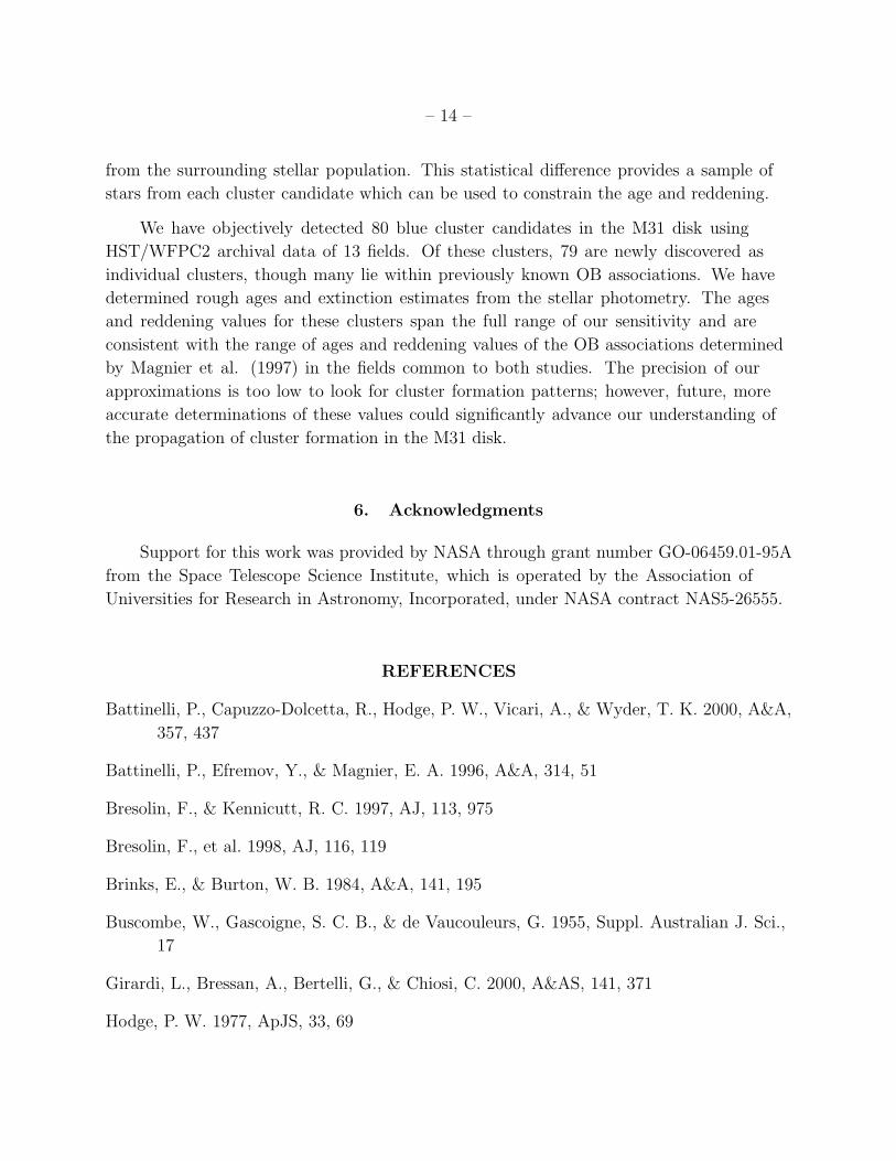
Table 2. Catalog of positions, galactocentric distances, age estimates, reddening values, and search radii for M31

young star cluster candidates.

IDa RA (2000) DEC (2000) GCD (kpc) log AGE EB−V Rbs(pc)

M31SCC J003952+403141 0:39:52.43 40:31:41.27 15.21 8.00±0.20 0.28±0.10 5

M31SCC J004000+403325 0:40:00.03 40:33:25.02 14.52 7.90±0.35 0.22±0.10 15

M31SCC J004000+403406 (G42) 0:40:00.83 40:34:06.64 14.49 7.75±0.45 0.21±0.10 15

M31SCC J004001+403420 0:40:01.54 40:34:20.06 14.44 8.25±0.30 0.20±0.20 5

M31SCC J004004+403440 0:40:04.66 40:34:40.51 14.11 8.10±0.20 0.23±0.10 5

M31SCC J004006+403508 0:40:06.78 40:35:08.41 13.92 7.30±0.85 0.25±0.10 15

M31SCC J004010+403624 0:40:10.36 40:36:24.16 13.63 7.75±0.60 0.01±0.10 5

M31SCC J004012+403632 0:40:12.01 40:36:32.62 13.46 7.70±0.50 0.24±0.10 5

M31SCC J004012+403617 0:40:12.97 40:36:17.32 13.33 7.90±0.45 0.17±0.10 15

M31SCC J004013+403815 0:40:13.68 40:38:15.54 13.46 7.70±0.40 0.43±0.10 5

M31SCC J004015+403652 0:40:15.42 40:36:52.85 13.11 7.90±0.20 0.35±0.10 5

M31SCC J004032+403320 0:40:32.93 40:33:20.45 12.10 7.90±0.20 0.16±0.10 5

M31SCC J004033+403308a 0:40:33.28 40:33:08.64 12.13 7.75±0.20 0.31±0.10 5

M31SCC J004033+403326 0:40:33.46 40:33:26.93 12.06 7.85±0.20 0.30±0.10 5

M31SCC J004033+403319 0:40:33.48 40:33:19.15 12.09 7.75±0.40 0.30±0.10 5

M31SCC J004033+403308b 0:40:33.51 40:33:08.39 12.12 8.00±0.20 0.24±0.10 5

M31SCC J004033+403346 0:40:33.70 40:33:46.69 11.99 8.00±0.20 0.34±0.10 5

M31SCC J004034+403351 0:40:34.62 40:33:51.59 11.95 8.00±0.20 0.32±0.10 15

M31SCC J004035+403420 0:40:35.45 40:34:20.24 11.83 7.90±0.20 0.28±0.10 5

M31SCC J004035+403251 0:40:35.51 40:32:51.18 12.15 7.85±0.20 0.22±0.10 5

M31SCC J004039+403210 0:40:39.35 40:32:10.79 12.32 8.15±0.35 0.31±0.18 5

M31SCC J004040+403223 0:40:40.43 40:32:23.50 12.26 7.85±0.20 0.27±0.10 5

–19

–

Table 2—Continued

IDa RA (2000) DEC (2000) GCD (kpc) log AGE EB−V Rbs(pc)

M31SCC J004040+403256 0:40:40.67 40:32:56.98 12.10 8.10±0.40 0.37±0.10 5

M31SCC J004041+403222 0:40:41.35 40:32:22.88 12.27 7.90±0.30 0.22±0.10 5

M31SCC J004117+403720 0:41:17.21 40:37:20.57 11.92 7.85±0.20 0.34±0.11 5

M31SCC J004119+403748 0:41:19.57 40:37:48.79 11.89 8.10±0.40 0.27±0.13 5

M31SCC J004121+403638 0:41:21.37 40:36:38.84 12.65 7.45±0.40 0.45±0.10 5

M31SCC J004123+403726 0:41:23.89 40:37:26.98 12.47 7.85±0.70 0.02±0.10 5

M31SCC J004125+403723 0:41:25.92 40:37:23.66 12.71 8.20±0.45 0.29±0.28 5

M31SCC J004158+405738 0:41:58.57 40:57:38.48 5.40 7.80±0.30 0.50±0.10 5

M31SCC J004204+405826 (H81 B-202) 0:42:04.85 40:58:26.44 5.47 7.95±0.20 0.43±0.11 5

M31SCC J004205+405714 (H81 B-202) 0:42:05.59 40:57:14.26 6.15 7.30±0.20 0.22±0.10 5

M31SCC J004205+405659 (H81 B-202) 0:42:05.80 40:56:59.06 6.31 7.75±0.45 0.37±0.10 5

M31SCC J004206+405649 0:42:06.23 40:56:49.38 6.45 7.40±0.45 0.35±0.10 5

M31SCC J004207+405801 0:42:07.11 40:58:01.27 5.89 7.25±0.55 0.35±0.10 15

M31SCC J004441+412701 0:44:41.19 41:27:01.37 17.32 7.45±0.20 0.38±0.10 5

M31SCC J004441+415136 0:44:41.35 41:51:36.86 10.37 8.05±0.20 0.24±0.10 5

M31SCC J004441+415239 0:44:41.61 41:52:39.22 10.50 7.75±0.30 0.29±0.10 5

M31SCC J004441+415123 0:44:41.79 41:51:23.15 10.37 8.05±0.20 0.41±0.10 5

M31SCC J004442+415237 0:44:42.09 41:52:37.45 10.52 7.95±0.20 0.34±0.10 5

M31SCC J004442+415153 0:44:42.48 41:51:53.42 10.46 7.85±0.20 0.35±0.10 5

M31SCC J004444+412749 0:44:44.86 41:27:49.32 17.63 7.40±0.60 0.22±0.10 5

M31SCC J004445+412800 0:44:45.07 41:28: 0.48 17.58 7.95±0.20 0.41±0.14 5

M31SCC J004445+415121 0:44:45.39 41:51:21.42 10.61 7.75±0.20 0.35±0.10 5

–20

–

Table 2—Continued

IDa RA (2000) DEC (2000) GCD (kpc) log AGE EB−V Rbs(pc)

M31SCC J004445+415208 0:44:45.68 41:52:08.65 10.68 8.25±0.20 0.30±0.10 5

M31SCC J004445+415107 0:44:45.73 41:51:07.88 10.63 7.50±0.45 0.26±0.10 5

M31SCC J004447+415238 0:44:47.06 41:52:38.21 10.81 8.05±0.20 0.42±0.10 5

M31SCC J004447+412821 0:44:47.32 41:28:21.97 17.84 7.70±0.20 0.02±0.10 5

M31SCC J004447+412843 0:44:47.74 41:28:43.82 17.73 7.30±0.35 0.27±0.10 15

M31SCC J004448+412925 0:44:48.43 41:29:25.15 17.52 7.75±0.20 0.02±0.10 5

M31SCC J004449+413034 0:44:49.04 41:30:34.78 17.07 7.55±0.20 0.55±0.10 5

M31SCC J004449+412924 0:44:49.25 41:29:24.97 17.68 7.50±0.50 0.23±0.10 5

M31SCC J004449+415131 0:44:49.86 41:51:31.39 10.97 7.70±0.20 0.42±0.10 5

M31SCC J004450+415211 0:44:50.26 41:52:11.50 11.00 8.15±0.30 0.18±0.10 5

M31SCC J004450+412917 0:44:50.38 41:29:17.95 17.96 7.60±0.35 0.29±0.10 5

M31SCC J004450+412914 0:44:50.97 41:29:14.60 18.11 7.50±0.20 0.16±0.10 5

M31SCC J004451+412924 0:44:51.32 41:29:24.83 18.09 7.50±0.50 0.02±0.10 5

M31SCC J004451+412911 0:44:51.74 41:29:11.44 18.28 7.35±0.40 0.13±0.10 15

M31SCC J004452+415144 0:44:52.35 41:51:44.21 11.19 7.80±0.25 0.23±0.10 5

M31SCC J004453+412927 0:44:53.52 41:29:27.82 18.49 7.80±0.30 0.21±0.10 5

M31SCC J004455+413127 0:44:55.90 41:31:27.16 17.96 7.65±0.20 0.24±0.10 5

M31SCC J004456+413121 0:44:56.02 41:31:21.54 18.03 7.35±0.20 0.21±0.10 5

M31SCC J004457+413123 0:44:57.73 41:31:23.30 18.35 7.70±0.20 0.01±0.10 5

M31SCC J004458+413049 0:44:58.97 41:30:49.21 18.87 7.65±0.40 0.33±0.10 5

M31SCC J004500+413057 0:45:00.93 41:30:57.71 19.18 7.30±0.40 0.41±0.10 15

M31SCC J004503+413408 0:45:03.82 41:34:08.54 18.19 7.90±0.25 0.20±0.10 5

–21

–Table 2—Continued

IDa RA (2000) DEC (2000) GCD (kpc) log AGE EB−V Rbs(pc)

M31SCC J004504+413451 0:45:04.52 41:34:51.60 17.99 7.95±0.20 0.25±0.30 5

M31SCC J004506+413406 0:45:06.32 41:34:06.96 18.68 7.70±0.20 0.45±0.10 5

M31SCC J004506+413545 0:45:06.73 41:35:45.78 17.99 8.00±0.50 0.21±0.20 15

M31SCC J004509+413643 0:45:09.82 41:36:43.31 18.14 7.80±0.20 0.10±0.10 5

M31SCC J004509+413649 0:45:09.82 41:36:49.79 18.09 7.30±0.50 0.31±0.10 5

M31SCC J004510+413645 0:45:10.33 41:36:45.47 18.22 7.25±0.20 0.14±0.10 5

M31SCC J004511+413711 0:45:11.82 41:37:11.86 18.30 7.90±0.30 0.24±0.10 5

M31SCC J004512+413715 0:45:12.31 41:37:15.78 18.36 7.95±0.20 0.11±0.10 5

M31SCC J004512+413716 0:45:12.48 41:37:16.82 18.38 7.70±0.40 0.33±0.10 5

M31SCC J004512+413723 0:45:12.78 41:37:23.45 18.39 8.00±0.50 0.23±0.10 5

M31SCC J004512+413727 0:45:12.87 41:37:27.80 18.38 7.80±0.20 0.25±0.10 5

M31SCC J004513+413735 0:45:13.40 41:37:35.08 18.42 7.30±0.20 0.46±0.10 5

M31SCC J004514+413743 0:45:14.13 41:37:43.72 18.49 7.35±0.20 0.39±0.10 5

M31SCC J004514+413724 0:45:14.22 41:37:24.31 18.66 7.70±0.20 0.36±0.10 5

aM31SCC is an IAU registered acronym; G42 refers to the globular cluster catalog of Sargent et al. (1977); [H81]

B-202 is identified in Hodge (1981)

bSearch radius given to the automated search routine. Using this radius the algorithm searched for overdensities over

areas of (πR2

s).

– 22 –

Table 3. Comparison of 5 fields searched both by eye and by algorithm. About 75 percent

of the cluster candidates were found by both methods. Many of the candidates are parts of

previously known associations.

Field Cluster Found by eye? Associationa

7 M31SCC J004441+412701 N

7 M31SCC J004444+412749 Y

7 M31SCC J004445+412800 N

7 M31SCC J004447+412821 Y

9 M31SCC J004447+412843 Y Part of [H81] B-298

9 M31SCC J004451+412911 Y Part of [H81] B-301

9 M31SCC J004453+412927 N

11 M31SCC J004455+413127 Y Part of [H81] B-306

11 M31SCC J004456+413121 Y Part of [H81] B-306

11 M31SCC J004457+413123 Y

11 M31SCC J004458+413049 Y

11 M31SCC J004500+413057 Y

12 M31SCC J004503+413408 Y

12 M31SCC J004504+413451 N

12 M31SCC J004506+413406 N

12 M31SCC J004506+413545 N

13 M31SCC J004509+413643 Y Part of [H81] B-310

13 M31SCC J004509+413649 Y Part of [H81] B-310

13 M31SCC J004510+413645 Y Part of [H81] B-310

13 M31SCC J004511+413711 Y

13 M31SCC J004512+413715 Y Part of [H81] B-312

13 M31SCC J004512+413716 Y Part of [H81] B-312

13 M31SCC J004512+413723 N Part of [H81] B-312

13 M31SCC J004512+413727 Y

13 M31SCC J004513+413735 Y

13 M31SCC J004514+413743 Y

13 M31SCC J004514+413724 Y

aM31SCC is an IAU registered acronym; the [H81] B prefix is identified in Hodge (1981)

table B.

– 23 –

Table 4. Comparison of detection cluster candidates appearing in more than one field.

Cluster Fields Observed Fields Found

M31SCC J004448+412925 9,10 10

M31SCC J004449+412924 9,10 10

M31SCC J004450+412914 9,10 9,10

M31SCC J004450+412917 9,10 9,10

M31SCC J004451+412924 9,10 9,10

M31SCC J004451+412911 9,10 9

M31SCC J004453+412927 9,10 9

Table 5. Comparison of ages determined by isochrone fitting on high and low resolution

WFPC2 photometry.

Name log Agehires (yr) log Agelowres (yr) E(B-V)hires E(B-V)lowres

G38 8.00±0.15 7.75±0.20 0.31±0.11 0.26±0.10

G44 8.00±0.15 7.90±0.20 0.23±0.10 0.21±0.10

G94 8.20±0.15 7.80±0.20 0.20±0.10 0.39±0.10

G293 7.80±0.10 7.65±0.20 0.20±0.10 0.35±0.10

– 24 –

11.5 11.0 10.5 10.0RA (deg)

40.6

40.8

41.0

41.2

41.4

41.6

41.8

42.0

DE

C (

deg)

8

1312111097

6

54

32

1

Fig. 1.— Positions of the HST fields taken from the HST archive. Shown are the fields

that were observed through blue filters allowing detailed studies of the young main sequence

population.

– 25 –

Fig. 2.— B band (F439W) photometric errors from ALLSTAR for the 13 fields.

– 26 –

Fig. 3.— V band (F555W) photometric errors from ALLSTAR for the 13 fields.

– 27 –

Fig. 4.— Residuals of photometry performed on the same stars in different fields in

the F336W (U), F439W (B), and F555W (V), filters. The residuals of the independent

measurements are consistent with zero. No systematic offest is seen.

– 28 –

Fig. 5.— A random selection of 9 of our open cluster candidates. These B band (F439W)

images are 12” by 12”.

– 29 –

Fig. 6.— Reddening estimates of the 9 example clusters. The stellar colors and magnitudes

have been corrected by the reddening values shown on the figures. These values gave the best

fits to model upper main sequence colors. In cases where we did not have U band photometry,

we relied on the B-V colors alone to determine reddening. Due to the sensitivity of WFPC2

in the U band, we occasionally were forced to make our first estimate of the reddening based

on the colors of a single star detected in all three bands.

– 30 –

Fig. 7.— Age determinations of the 9 example clusters. The ages were determined by eye to

fit the turnoff to the bright blue stars in the cluster. With so few stars, these ages estimates

are very rough.

– 31 –

Fig. 8.— Plots of reddening and age vs. galactocentric distances for the cluster candidates.

No patterns are seen with these rough estimates.

– 32 –

Fig. 9.— Reddening vs. age for the cluster candidates. Our algorithm was not sensitive to

red clusters of stars so that there is a lack of high extinction, old clusters. The very low

extinction clusters are likely to have field contaminants.