artigo1

A model for the corrosion of steel subjected to synthetic produced watercontaining sulfate, chloride and hydrogen sulfide

Peter Smith a,n, Sudipta Roy a, David Swailes b, Stephen Maxwell c, David Page d, John Lawson d

a Chemical Engineering and Advanced Materials, Newcastle University, Newcastle upon Tyne, NE1 7RU, United Kingdomb Mechanical and Systems Engineering, Newcastle University, Newcastle upon Tyne, NE1 7RU, United Kingdomc Commercial Microbiology Limited, Kettock Lodge, Campus 2, Aberdeen Science Park, Bridge of Don, Aberdeen, AB22 8GU, United Kingdomd Chevron North Sea Limited, Chevron House, Hill of Rubislaw, Aberdeen, AB15 6XL, United Kingdom

a r t i c l e i n f o

Article history:Received 17 January 2011Received in revised form11 July 2011Accepted 24 July 2011Available online 6 August 2011

Keywords:CorrosionElectrochemistryMathematical modelingKineticsMass transferProduced water

a b s t r a c t

A model was developed for the prediction of corrosion rates associated with steel subjected to syntheticproduced water. The corrosive species included in the model, identified through water analysisconducted in the field, are sulfate, chloride and hydrogen sulfide. The effect on corrosion of thesespecies was examined through polarization experimentation using a three electrode glass corrosion celland potentiostat. Samples of carbon steel, used in sub-sea pipeline systems, were used at the workingelectrode and the experiments were carried out at similar physicochemical conditions observed inpipeline systems in the field. The model was based on heterogeneous reactions at the metal surface,with electrochemical parameters determined through experimentation employed in the model todescribe the anodic and cathodic processes involved in the corrosion of steel. The model consists of asystem of equations with Butler–Volmer kinetics describing the charge transfer and the Nernstdiffusion model the mass transfer processes occurring in the corrosion system. The solution is basedon a charge balance between the reduction and the oxidation processes which occur at the steelsurface. Current density convergence criteria were used in the model to solve the system of equationsfor corrosion potential, surface species concentration and component current densities. The corrosionrate is determined as the rate of oxidation of iron at the surface and model results have been validatedusing experimental data. The model demonstrates a reasonable qualitative match with corrosion datacollected in the potential region close to the corrosion potential in general, with good qualitative matchin the anodic region near the corrosion potential. Some deviation occurs between model andexperimental values where overpotentials become large but the model is shown to respond well tochanges in input parameter values and predicts the corrosion potential and corrosion rate for eachsystem within experimental variability and the accepted standards of accuracy.

& 2011 Elsevier Ltd. All rights reserved.

1. Introduction

Corrosion mitigation in the oilfield industry has traditionallybeen performed by combining methods for measuring corrosionrates such as corrosion coupons and regular pipeline inspectionswith prevention strategies such as cathodic protection and thedeployment of corrosion inhibiting chemicals. In more recenttimes, these methods have been enhanced by the employment ofintelligent pigs which are able to detect the severity of corrosionat particular sites and more effective in-situ corrosion probes forcorrosion measurement. Corrosion models and corrosion predic-tion models are now proving to be increasingly important in theoilfield industry to further enhance the performance of corrosion

mitigation strategies and provide non-invasive methods for cor-rosion assessment of oilfield assets.

Several corrosion models have been developed for specificcorrosion mechanisms such as carbon dioxide (Nesic et al., 1996;NORSOK, 2005) for which predictive modeling guidelines in thefield have also been published (Nyborg, 2009). Work towardscorrosion modeling for other corrosion mechanisms such as thatassociated with microbiologically influenced corrosion (MIC)(Maxwell, 2006; Pots et al., 2002) have also been conducted andapplied to oilfield systems in the field. More complex investiga-tive models for MIC (Picioreanu and Loosdrecht, 2002) andother more generalized corrosion mechanisms such as galvaniccorrosion (Morris and Smyrl, 1988, 1989) and differential aerationof surfaces subjected to moisture films (Alkire and Nicolaides,1974) have proven successful at exploring the respectivecorrosion mechanisms in more detail.

The motivation for this current work is based on recentactivity in the oilfield industries to develop corrosion models that

Contents lists available at ScienceDirect

journal homepage: www.elsevier.com/locate/ces

Chemical Engineering Science

0009-2509/$ - see front matter & 2011 Elsevier Ltd. All rights reserved.doi:10.1016/j.ces.2011.07.033

n Corresponding author.E-mail address: [email protected] (P. Smith).

Chemical Engineering Science 66 (2011) 5775–5790

Possante

Possante

www.elsevier.com/locate/ces

dx.doi.org/10.1016/j.ces.2011.07.033

mailto:[email protected]

dx.doi.org/10.1016/j.ces.2011.07.033

more effectively predict corrosion rates in oilfield systems com-pared to the models that are currently used. Corrosion mechan-isms in oilfield systems are complex and have been studiedwidely showing high degrees of interaction between corrosion

species, products and oilfield metallurgies. The interactions ofsulfate and chloride are of interest in this work since a presence ofsulfate in oilfield produced water systems also facilitates furthercorrosion mechanisms such as MIC by sulfate reducing bacteriaand chloride due to its catalytic action on corrosion. Abioticcorrosion experimentation in this work as was conducted toinvestigate the interaction between a sample of pipeline steeland two main species, sodium sulfate and sodium chloride,identified in the field water analysis data presented in Table 1.Firstly, it was determined if abiotic interactions could be mea-sured in the system for these components. Then the effect ofsynthetic hydrogen sulfide in addition to these two componentswas investigated. Presented within are the experimental proce-dures and results of abiotic experimentation along with themodel development steps. The model is validated using corrosiondata collected in the experimental work.

By examination of the physicochemical data of produced waterencountered in a typical pipeline fluid, presented in Table 1, anumber of abiotic corrosion influencing components can beinitially identified based on knowledge of their corrosive proper-ties and their concentration. The main abiotic corrosion para-meter in Table 1 can be identified as sodium chloride. This ispresent in higher concentrations as compared to the othercomponents present and is well known to have a significantinfluence on the corrosion of steel. Another abiotic parameter ofinterest in Table 1 is sulfate due to its influence on the corrosionmechanism of chloride and its potential to facilitate furthercorrosion mechanisms. A sodium salt was chosen as a source ofsulfate to ensure any influence observed on the corrosion system

Table 2Summary of model species, parameters and reactions used in the model.

Model parameters Reactions

Kinetic Mass transport Heterogeneous Homogeneous

E1 V vs. SCE ni aai aci Cbi (mol m!3) Di (m2 s!1) dNi (m)

Deaerated water systemFe2" !0.681 2 0.4 0.6 7.98#10!10 7.23#10!6 Fe-Fe2""2e!

H" !0.241 1 0.6 0.4 7.4# 10!3 9.47#10!9 1.67#10!5 H""e!-1/2H2

0.01 M Sulfate systemFe2" !0.681 2 0.4 0.6 7.98#10!10 7.23#10!6 Fe-Fe2""2e!

H" !0.241 1 0.6 0.4 2.5# 10!3 9.47#10!9 1.67#10!5 H""e!-1/2H2

SO42! !1.177 2 1.0# 10!5 1.0#10!9 7.87#10!6 SO4

2!"2e!"H2O-SO32!"OH!

SO32! !0.817 4 5.6#10!10 6.49#10!6 2SO3

2!"4e!"3H2O-S2O32!"6OH!

S !0.900 4 SO32!"4e!"3H2O-S"6OH!

S2! !0.688 2 S"2e!-S2!

0.01 M Sulfate, 0.2 M chloride sSystemFe2" !0.681 2 0.25 0.75 7.98#10!10 7.23#10!6 Fe-Fe2""2e!

H" !0.241 1 0.6 0.4 0.013 9.47#10!9 1.67#10!5 H""e!-1/2H2

SO42! !1.177 2 1# 10!5 1.0#10!9 7.87#10!6 SO4

2!"2e!"H2O-SO32!"OH!

SO32! !0.817 4 5.6#10!10 6.49#10!6 2SO3

2!"4e!"3H2O-S2O32!"6OH!

S !0.900 SO32!"4e!"3H2O-S"6OH!

S2! !0.688 2 S"2e!-S2!

0.01 M Sulfate, 0.2 M chloride system, 18% saturated hydrogen sulfideFe2" !0.681 2 0.25 0.75 7.98#10!10 7.23#10!6 Fe-Fe2""2e!

H" !0.241 1 0.6 0.4 6.2# 10!3 9.47#10!9 1.67#10!5 H""e!-1/2H2

SO42! !1.177 2 1# 10!5 1.0#10!9 7.87#10!6 SO4

2!"2e!"H2O-SO32!"OH!

SO32! !0.817 4 5.6#10!10 6.49#10!6 2SO3

2!"4e!"3H2O-S2O32!"6OH!

S !0.900 4 SO32!"4e!"3H2O-S"6OH!

H2S H2S(aq)-H""HS!

HS! HS!-H""S2!

S2! !0.688 2 2.5# 10!6 5.6#10!10 6.49#10!6 S"2e!-S2! HS!-H""S2!

1. The dissociation of water to protons and hydroxyl ions is included implicitly in the pH.2. Cl! is assumed to change reactions parameters as mentioned in the text, and therefore homogeneous or heterogeneous specific to Cl! species are not mentioned inTable 2.3. Values for j0 are not mentioned in Table 2 as they are calculated in the model using Eq. (7) and model predicted values of Cs for each component.4. Parameters written in italics refer to experimentally calculated values, others refer to literature values.

Table 1Physicochemical data for produced water collected at a North Sea sub-sea asset.

Element M Concentration

mg/l mol/l

Barium Ba2" 137.327 31 0.0002Boron B 10.8 6 0.0006Calcium Ca2" 40.08 284 0.0071Iron Fe3" 55.85 8 0.0001Magnesium Mg2" 24.31 161 0.0066Phosphorous P3! 30.97 1 0.0000Potassium K" 39.1 50 0.0013Sodium Na" 22.99 4770 0.2075Strontium Sr2" 87.62 83 0.0009Chloride Cl! 35.45 7480 0.2110Bromide Br! 79.9 20 0.0003Sulphate SO4

2! 96 21 0.0002Nitrate NO3! 62 0.5 0.0000Hydroxyl OH! 17 0 0.0000Carbonate CO3

2! 60 0 0.0000Bicarbonate HCO3

! 61.02 500 0.0082Dissolved CO2 CO2 44 92.4 0.0021Specific gravity 1.014pH 6.58Resistivity 0.4405 OmTotal dissolved solids 13,453 mg/l

P. Smith et al. / Chemical Engineering Science 66 (2011) 5775–57905776

was due to the presence of sulfate and not the presence of adifferent cationic components compared to sodium chloride. Acorrosion rate model based on these components can beexpressed conceptually as a function of the corrosion rates fromeach of the contributing parameters as presented in

CR$ f %CRCl! ,CRSO2!4

CRH2S& %1&

The abiotic corrosion model presented within this studyreflects a modeling strategy that would allow the inclusion offurther processes in the future. The model is based on causalelectrochemical processes that describe the charge and masstransfer processes occurring at the steel surface. Similar methodshave been implemented in several of the models cited within, butthis model is based on parameters which can be easily measuredin the field allowing the model to be tailored to individual oilfieldsystems and implemented effectively within corrosion mitigationstrategies. This holistic modeling strategy allows the inclusion offurther corrosion parameters specific to individual corrosionsystems. This concept may also provide a basis for the futureenhancement of current MIC models used in pipeline systems bymodeling together the synergistic relationship (Crolet, 2005;Hamilton, 2002; Hardy and Bown, 1984; Lee and Characklis,1993) between abiotic corrosion parameters measured in thefield and those contributing to MIC.

2. Experimental

Polarization experiments have been employed in this study toexamine processes occurring in the corrosion system with the useof a three electrode corrosion cell and a potentiostat. A Radio-meter EDI101 rotating disk electrode (RDE) was employed as theworking electrode (WE) in this system with the tip containing asample of pipeline steel. The tip was manufactured by setting acylindrical sample of pipeline steel within a cylindrical PTFE

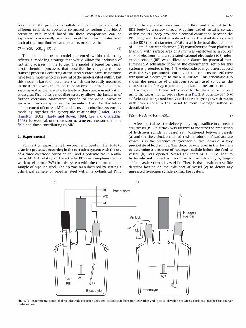
collar. The tip surface was machined flush and attached to theRDE body by a screw thread. A spring loaded metallic contactwithin the RDE body provided electrical connection between theRDE body and the steel sample in the tip. The steel disk exposedat the RDE tip had diameter of 0.6 cm with the total disk diameterof 1.1 cm. A counter electrode (CE) manufactured from platinisedtitanium with surface area of 3 cm2 was employed as a source/sink of electrons, and a saturated calomel electrode (SCE) refer-ence electrode (RE) was utilized as a datum for potential mea-surement. A schematic showing the experimental setup for thissystem is presented in Fig. 1. The electrode configuration adoptedwith the WE positioned centrally in the cell ensures effectivetransport of electrolyte to the RDE surface. This schematic alsoshows the presence of a nitrogen sparger used to purge thecorrosion cell of oxygen prior to polarization measurements.

Hydrogen sulfide was introduced to the glass corrosion cellusing the experimental setup shown in Fig. 2. A quantity of 1.0 Msulfuric acid is injected into vessel (a) via a syringe which reactswith iron sulfide in the vessel to form hydrogen sulfide asdescribed by

FeS"H2SO4-H2S"FeSO4 %2&

A feed port allows the delivery of hydrogen sulfide to corrosioncell, vessel (b). An airlock was utilized to monitor the productionof hydrogen sulfide in vessel (a). Positioned between vessels(a) and (b), the airlock contained a white solution of lead acetatewhich is in the presence of hydrogen sulfide forms of a grayprecipitate of lead sulfide. This detector was used in this locationto determine a presence of hydrogen sulfide before the feed tovessel (b) was opened. Vessel (c) contains a 1.0 M sodiumhydroxide and is used as a scrubber to neutralize any hydrogensulfide passing through vessel (b). There is also a hydrogen sulfidedetector located on the exit port of vessel (c) to detect anyunreacted hydrogen sulfide exiting the system.

PotentiostatRE

WE

CE

REWE

CE

Electrolyte

WE

N2

Electrolyte

Air lockNitrogen sparger

Fig. 1. (a) Experimental setup of three electrode corrosion cells and potentiostat from front elevation and (b) side elevation showing airlock and nitrogen gas spargerconfiguration.

P. Smith et al. / Chemical Engineering Science 66 (2011) 5775–5790 5777

2.1. Electrolyte preparation

Electrolytes have been prepared using water analysis data ofthe produced water presented in Table 1. The major corrosionparameters present in this field sample includes 0.2 M sodiumchloride and 0.0002 M sodium sulfate. It was necessary to prepareelectrolytes containing individual and then mixed components toassess the influence of each component on corrosion.

The corrosion cell was setup with the RE, CE, gas sparger andair lock in position. The WE orifice was utilized as a fill hole withthe aid of funnel. Using low conductivity water produced in aPurite select 300 unit, the corrosion cell was then filled to a level2 cm above the RE electrode tip, approximately 50 cm3. A glassstopper was used to seal the fill hole. An air lock containing lowconductivity water was then placed at the top of the cell as inFig. 1(b). Each of the ground glass joints in the cell were coatedwith silicone grease prior to sparing to ensure that an airtight cellis established. The sparger connected to a nitrogen supply wassubmerged to the base of the corrosion cell and used to gentlysparge nitrogen through the electrolyte. Sparging was maintainedfor 20 min to allow full evacuation of oxygen from the cell. Thesparger was then raised to just below the electrolyte surface. TheWE, set to a rotation speed of 800 rpm, was then lowered intoposition. This rotation minimizes the chance of nitrogen bubblesadhering to the surface of the WE during positioning. Spargingwas maintained for a further 5 min to ensure that any oxygenentered during the WE positioning is removed. The gas spargerwas raised to just above the electrolyte level during data collec-tion and a nitrogen atmosphere was maintained throughout theexperiment to prevent any oxygen influx.

2.2. Corrosion data collection

E–j data was collected for this corrosion system by employingpotentiodynamic polarization in order to deduce parameters forthe model. The corrosion potential, Ecorr, of the corrosion systemwas initially measured during a 30 s stabilization period prior toimposing a potential on the system. A potential scan was theninitiated at a sweep rate of 0.01 V s!1 from a cathodic over-potential potential of !1.5 V w.r.t. Ecorr to an anodic overpotential

of "5.0 V w.r.t. Ecorr. The potential was then reversed at the samerate back to the start potential. This procedure was performedthree times for each corrosion system using a freshly preparedRDE tip and fresh electrolyte for each replicate.

Ohmic drop compensation was applied to the data collectedfor this system, retrospectively (Oelßner et al., 2006), usingmeasured values of electrolyte conductivity and the interelec-trode gap between the WE and the RE. Ohmic drop compensateddata have been presented for each system.

2.3. Materials characterization

Prior to experimental work the sample of steel was standar-dised and characterized by assessing the microstructure and itselemental composition. A sample of carbon steel used as the WEin this corrosion system was encapsulated in Struers Epofix resinand the surface was mechanically ground using grades P#500,P#1200, P#2400 and P#4000 silicone carbide grit paper consecu-tively lubricated with 96% ethanol. The sample was washed with96% ethanol after each paper grade to reduce contamination offine grit paper with larger grit particles. After the grinding stages,the sample was ultrasonicated in ethanol for 3 min to remove anyfurther surface particulates. The sample was then chemicallyetched using 2% nital for 60 s, washed in 96% ethanol and driedin a flow of nitrogen.

Energy dispersive X-ray analysis (EDX), optical microscopy andscanning electron microscopy (SEM) were employed to assess theelemental and microstructure properties of the steel samplesused in experimental work. The steel was determined to containlow concentrations of carbon, a small fraction of manganese withfew other alloying components. The microstructure showedcharacteristics of ferrite and pearlite grain structure with grainsin the 2–12 mm diameter range.

3. Experimentation results

The effect of sodium chloride and sodium sulfate on the abioticcorrosion system have been investigated to establish the con-tribution that each of these components have on the overall

Electrolyte

FeS Powder

Lead Acetate for detection of H2S

H2SO4

Lead Acetate for detection oH2S

NaOHH2S

H2S

H2S

H2S

WE

Fig. 2. A schematic showing the experimental setup used to quantify the influence of synthetic hydrogen sulfide. (a) H2S production vessel, (b) corrosion cell and (c) H2Sneutralisation.


corrosion rate. Since the mechanism of corrosion due to chlorideand the inhibition effects observed with sulfate are widelystudied, and respective concentrations in field water are wellknown, only a small range of concentrations were investigated inthese experiments. Since the electrolytes have been preparedusing low conductivity water and have then been deaerated, thecorrosion effects due to deaerated water have also been examinedin this work.

3.1. Deaerated low conductivity water system

The initial corrosion system under investigation was a systemof steel subjected to an electrolyte of pure deaerated lowconductivity water. This system represents the most simplecorrosion system where the oxidation of iron from steel isbalanced by the reduction of protons in the electrolyte to formhydrogen at the surface. The concentration of dissolved carbondioxide in the electrolyte was assumed to be common across allsystems and its affect on corrosion rate was indirectly taken intoaccount in the model through measurement of the pH andconductivity for each system. The electrolyte conductivity in thissystem was measured for all three replicates and ranges from65.4 to 104 mS cm!1. Ohmic drop was calculated using the RDEradius, knowledge of the conductivity and the interelectrode gapbetween the RE and WE. For this system the Ohmic drop wascalculated to be 9669 kO. Due to the Ohmic drop, an appliedpotential of 4.5 V w.r.t. the open circuit potential (OCP) isrequired in polarization experiments to impose an anodic polar-ization of 1.5 V at the working electrode in the experimentalsystem.

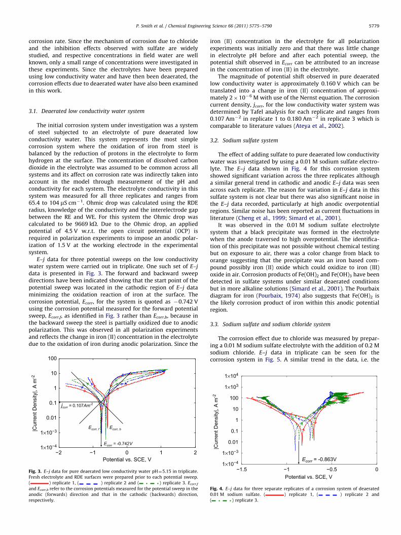
E–j data for three potential sweeps on the low conductivitywater system were carried out in triplicate. One such set of E–jdata is presented in Fig. 3. The forward and backward sweepdirections have been indicated showing that the start point of thepotential sweep was located in the cathodic region of E–j dataminimizing the oxidation reaction of iron at the surface. Thecorrosion potential, Ecorr, for the system is quoted as !0.742 Vusing the corrosion potential measured for the forward potentialsweep, Ecorr,f, as identified in Fig. 3 rather than Ecorr,b, because inthe backward sweep the steel is partially oxidized due to anodicpolarization. This was observed in all polarization experimentsand reflects the change in iron (II) concentration in the electrolytedue to the oxidation of iron during anodic polarization. Since the

iron (II) concentration in the electrolyte for all polarizationexperiments was initially zero and that there was little changein electrolyte pH before and after each potential sweep, thepotential shift observed in Ecorr can be attributed to an increasein the concentration of iron (II) in the electrolyte.

The magnitude of potential shift observed in pure deaeratedlow conductivity water is approximately 0.160 V which can betranslated into a change in iron (II) concentration of approxi-mately 2#10!6 M with use of the Nernst equation. The corrosioncurrent density, jcorr, for the low conductivity water system wasdetermined by Tafel analysis for each replicate and ranges from0.107 Am!2 in replicate 1 to 0.180 Am!2 in replicate 3 which iscomparable to literature values (Ateya et al., 2002).

3.2. Sodium sulfate system

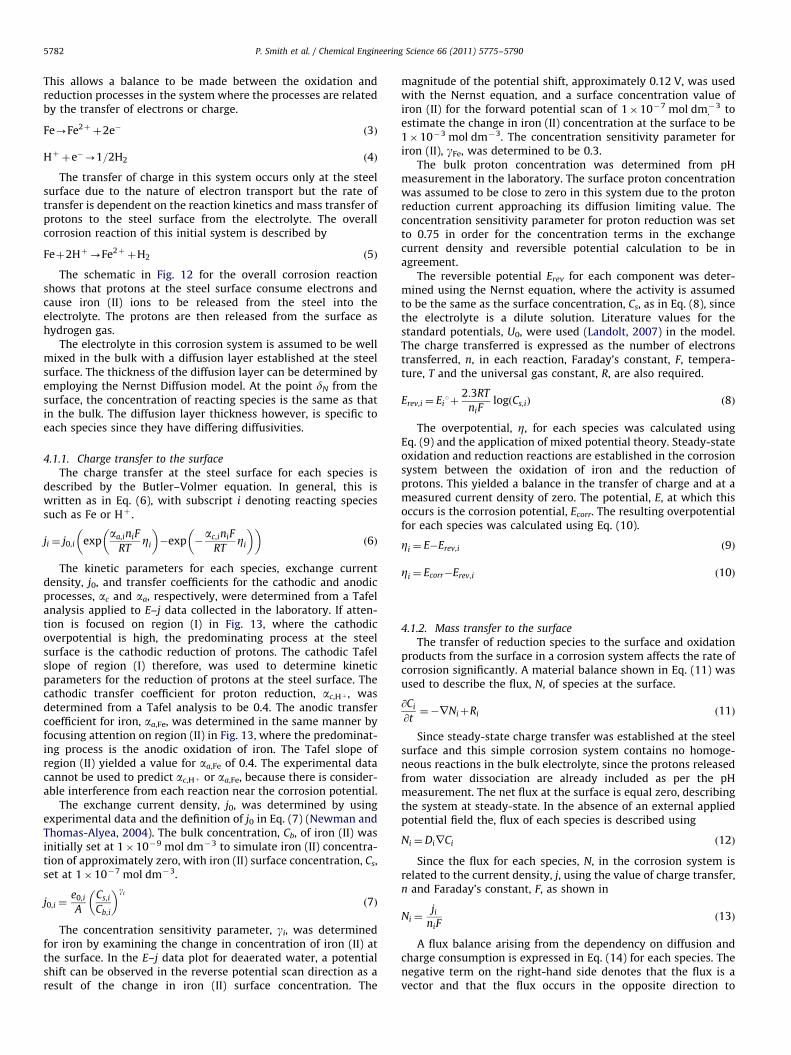
The effect of adding sulfate to pure deaerated low conductivitywater was investigated by using a 0.01 M sodium sulfate electro-lyte. The E–j data shown in Fig. 4 for this corrosion systemshowed significant variation across the three replicates althougha similar general trend in cathodic and anodic E–j data was seenacross each replicate. The reason for variation in E–j data in thissulfate system is not clear but there was also significant noise inthe E–j data recorded, particularly at high anodic overpotentialregions. Similar noise has been reported as current fluctuations inliterature (Cheng et al., 1999; Simard et al., 2001).

It was observed in the 0.01 M sodium sulfate electrolytesystem that a black precipitate was formed in the electrolytewhen the anode traversed to high overpotential. The identifica-tion of this precipitate was not possible without chemical testingbut on exposure to air, there was a color change from black toorange suggesting that the precipitate was an iron based com-pound possibly iron (II) oxide which could oxidize to iron (III)oxide in air. Corrosion products of Fe(OH)2 and Fe(OH)3 have beendetected in sulfate systems under similar deaerated conditionsbut in more alkaline solutions (Simard et al., 2001). The Pourbaixdiagram for iron (Pourbaix, 1974) also suggests that Fe(OH)2 isthe likely corrosion product of iron within this anodic potentialregion.

3.3. Sodium sulfate and sodium chloride system

The corrosion effect due to chloride was measured by prepar-ing a 0.01 M sodium sulfate electrolyte with the addition of 0.2 Msodium chloride. E–j data in triplicate can be seen for thecorrosion system in Fig. 5. A similar trend in the data, i.e. the

!2 !1 0 1 21!10!4

1!10!3

0.01

0.1

1

10

100

Potential vs. SCE, V

|Cur

rent

Den

sity

|, A

m-2

Ecorr = -0.742V

jcorr = 0.107Am-2

Ecorr, f Ecorr, b

Fig. 3. E–j data for pure deaerated low conductivity water pH$5.15 in triplicate.Fresh electrolyte and RDE surfaces were prepared prior to each potential sweep.( ) replicate 1, ( ) replicate 2 and ( ) replicate 3. Ecorr,f

and Ecorr,b refer to the corrosion potentials measured for the potential sweep in theanodic (forwards) direction and that in the cathodic (backwards) direction,respectively.

!1.5 !1 !0.5 01!10!4

1!10!3

0.01

0.1

1

10

100

1!103

1!104


|Cur

rent

Den

sity

|, A

m-2

Ecorr = -0.863V

Fig. 4. E–j data for three separate replicates of a corrosion system of deaerated0.01 M sodium sulfate. ( ) replicate 1, ( ) replicate 2 and( ) replicate 3.


shift in potential between the forward and backward potentialsweep directions, to that of the low conductivity water andsulfate system, can be observed. The magnitude of the potentialshift, however, in this system is considerably greater and equal to0.3 V compared to 0.151 V in the 0.01 M sulfate system.

The corrosion potential recorded for the forward potentialsweep is also observed to shift in the cathodic direction by0.104 V with the addition of 0.2 M sodium chloride, from!0.863 V measured in the 0.01 M sulfate system, to !0.967 Vmeasured in the 0.2 M chloride and 0.01 M sulfate system. Anincrease in the corrosion current density, jcorr, was also measuredwith a jcorr of 3.0 Am!2 for the 0.2 M chloride and 0.01 M sulfatesystem which is comparable to literature (Ateya et al., 2002) andan order of magnitude greater than that of the 0.01 M sulfatesystem with jcorr of 0.5 Am!2. The shift in corrosion potential andincrease in corrosion current density can be attributed to theaddition of 0.2 M chloride in the system, since chloride is wellknown to facilitate film breakdown at the surface of steel(Al-Kharafi et al., 2002; Ateya et al., 2002; El-Egamy and Badaway,2004; Laycock and Newman, 1997; Meguid and Latif, 2004).

A plateau in the current response can be seen in the anodicregion of the forward potential sweep between the potentials!0.967 and !0.650 V. This plateau suggests that the corrosionpotential falls within the passivation region of the anodic character-istics of iron. The current plateau can be attributed to the develop-ment of a metal oxide at the surface, or due to the deaerated natureof the electrolyte and low alloying content of the steel, a protectivesalt film (Landolt, 2007). The potential, EF, which is called the Fladepotential, at !0.650 V, denotes where the film begins to break downand suggests the onset of localized corrosion which increases in rateas the anodic overpotential increases.

The effect of sodium sulfate concentration was examined usingdeaerated low conductivity water electrolytes containing 0.2 Msodium chloride and two different concentrations of sodiumsulfate; 0.0002 and 0.01 M against the 0.2 M sodium sulfate onlysolution. The effect of sulfate concentration can be seen in the E–jdata for the two systems of different sulfate concentrations andthe control presented in Fig. 6. It can be seen that the increase insodium sulfate concentration causes the equilibrium potential toshift in the cathodic direction from !0.882 V in the control,to !0.900 V in the system containing 0.0002 M sulfate, and then to!0.946 V with sulfate concentration of 0.01 M. A cathodic shift incorrosion potential correspondingly results in an increase in jcorr.

E–j data showing the effect of increasing sodium chlorideconcentration can be seen in Fig. 13. Three 0.0002 M sodium

sulfate electrolytes with increasing sodium chloride concentra-tions of 0.025, 0.2 and 0.8 M have been examined. An increase injcorr with increasing chloride concentration can be initiallyobserved, as can be slight but consistent anodic shift in thecorrosion potential with increasing chloride concentration. ThepH measured for these corrosion systems of increasing chlorideconcentration also increases with values of 5.03, 5.36 and 5.70 for0.025, 0.2 and 0.8 M chloride, respectively. As proton reduction isa primary cathodic process in this system it is expected that thecathodic reaction also increases in rate to balance the increase inthe anodic corrosion process. It appears that the plateau in anodicE–j data depicting a salt film is more prominent in where thechloride concentration is greater. This may also be due to theincreased dissolution rate of iron (II) from the surface which inturn facilitates the formation of a salt film (Landolt, 2007). TheFlade potential, EF, for this system is observed at !0.560 V,beyond which pitting is expected to occur, along with a sharpincrease in current density, as shown in Fig. 7.

3.4. Hydrogen sulfide system

The effect of synthetically produced hydrogen sulfide on acorrosion system was examined by the addition of hydrogen

"1.5 "1 "0.5 01!10!4

1!10!3

0.01

0.1

1

10

100

1!103

1!104


|Cur

rent

Den

sity

|, A

m-2

Increasing sulfate concentration

Ecorr (3) = -0.946V(3)(2)(1)

Ecorr (2) = -0.900VEcorr (1) = -0.882V

Fig. 6. E–j data for two corrosion systems of increasing sulfate concentration.( ) 0.2 M sodium chloride, pH$5.61 ( ) 0.0002 M and sodiumsulfate 0.2 M sodium chloride, pH$5.36 and ( ) 0.01 M sodium sulfate0.2 M and sodium chloride, pH$4.99.

"1.5 "1 "0.5 01!10!4

1!10!3

0.01

0.1

1

10

100

1!103

1!104


|Cur

rent

Den

sity

|, A

m-2

EF = -0.650VEcorr = -0.967V

Fig. 5. E–j data for three separate replicates of a corrosion system of steelsubjected to an electrolyte of deaerated 0.01 M sodium sulfate and 0.2 M sodiumchloride in triplicate. pH$4.99. ( ) replicate 1, ( ) replicate 2 and( ) replicate 3.

"1.5 "1 "0.5 01!10!4

1!10!3

0.01

0.1

1

10

100

1!103

1!104


|Cur

rent

Den

sity

|, A

m-2

Increasing chloride concentration

EF = -0.560VEcorr (3) = -0.891V(2) (3)

Ecorr (2) = -0.904VEcorr (1) = -0.916V

(1)

Fig. 7. E–j data for three corrosion systems of increasing sodium chloride concentra-tion. ( ) 0.0002 M sodium sulfate and 0.025 M sodium chloride, pH$5.03( ) 0.0002 M sodium sulfate 0.2 M and sodium chloride, pH$5.36 and( ) 0.0002 M sodium sulfate and 0.8 M sodium chloride, pH$5.70.


sulfide to a deaerated low conductivity water electrolyte contain-ing 0.01 M sodium sulfate and 0.2 M sodium chloride. E–j data forthis system can be seen in triplicate in Fig. 8 and shows thepresence of noise in current values and greater deviation betweenmeasured corrosion potentials, Ecorr, of each replicate. The rangein Ecorr measured for the three replicates was 0.123 V with meanEcorr of !0.912 V. Although noisy data were observed in thesodium sulfate system, the magnitude of noise and variation inEcorr is greater in the presence of hydrogen sulfide, which showsthe formation of unstable surface films. In fact a dark gray/blackprecipitate was observed to develop in each corrosion systemboth with and without added hydrogen sulfide. In the systemwith hydrogen sulfide, however, the precipitate adhered to thesurface and was resistant to removal by ultrasonication suggest-ing the precipitate had changed into an adherent protective filmat the surface.

A study conducted to determine the corrosion products of ironwith hydrogen sulfide (Shoesmith et al., 1980) reported large varia-tion in corrosion potential measurement of over 0.030 V conductinggalvanostatic potentiometry experiments. The corrosion potentialwas observed to shift in the initial 10 min of their experiments byup to 0.150 V which is comparable to ours. In that study X-raydiffractometry was used (Shoesmith et al., 1980) to characterise thecorrosion products at the surface yielding three ferrous monosulfidephases, mackinawite, troilite (FeS) and cubic ferrous sulfide. It wasconcluded (Shoesmith et al., 1980) that mackinawite and cubicferrous sulfide form unpassivating layers at the surface which allowlocal corrosion attack until more stable slowly forming troilite forms astable passive layer at the surface protecting the surface from furthercorrosion. A similar study (Huang et al., 1996) identified that sulfidefilm morphology is dependent on time.

Fig. 9 shows a comparison in E–j data between deaerated lowconductivity water sodium sulfate–sodium chloride electrolyteswith added hydrogen sulfide. It can be seen that the jcorr for thecorrosion system containing hydrogen sulfide, measured atapproximately 4.0 Am!2, is approximately twice that of thecorrosion system with no hydrogen sulfide, measured at2.1 Am!2. The current density response at high overpotentialshowever, in the anodic potential region of E–j data, indicateshydrogen sulfide decreases the rate of corrosion. It is also evidentthat an oxidation peak, Eox, is present in the anodic region for thecorrosion system containing hydrogen sulfide which is not pre-sent in systems without hydrogen sulfide. This suggests that aprotective film forms on the surface when overpotential is high inthe presence of hydrogen sulfide, which can be oxidized as wasobserved by Shoesmith et al. (1980).

The effect of lowering the sulfate concentration in the pre-sence of hydrogen sulfide was examined by using a deaerated lowconductivity water electrolyte containing 0.2 M sodium chloridewith synthetic hydrogen sulfide but in the absence of sodiumsulfate. There was significant noise in the E–j data for this system.The standard deviation in the corrosion potential for this systemis calculated to be 0.021 V which is low compared to 0.050 V forthe corrosion system containing 0.01 M sodium sulfate but showsthat significant variation remains present and confirms that thisvariation is due to the presence of aqueous hydrogen sulfide.

The notable item was that the oxidation peak observed at!0.700 V, in E–j data for the corrosion system containing 0.01 Msodium sulfate and 0.2 M sodium chloride with the addition ofhydrogen sulfide, was also present in E–j data for this system. Themagnitude of the peak, however, was lower. E–j data presented inliterature (Shoesmith et al., 1978) show a similar oxidation peakto the one observed in our study but at a more anodic potential of!0.405 V, in alkaline conditions of pH 9–12. Black precipitates ofblack iron sulfide similar to those in our study, shown in Fig. 11,were also reported to form at the surface in their experimentswhere X-ray diffractometry was used to deduce that the pre-cipitates were mackinawite.

The corrosion potential measured for the experimental systemcontaining hydrogen sulfide appeared to occur in a more anodicposition compared to that of the system without sulfide which isconsistent with experimental studies presented in literature(Videm and Kvarekval, 1995). A dark gray/black precipitate wasobserved to form in this system and a dark gray/black filmdeveloped at the RDE surface. The current density response forthe system containing hydrogen sulfide showed little deviationfrom the system without hydrogen sulfide in the region close toEcorr. At high overpotentials however, the current density waslower suggesting that the film formed offered protection againstcorrosion which has also been observed in literature (Shoesmithet al., 1978; Shoesmith et al., 1980).

4. Model development

4.1. Corrosion model: deaerated water

In this corrosion system, the steel surface is in contact withlow conductivity water electrolyte forming a solid–liquid inter-face. It is assumed that the electrons formed in iron oxidationprocess in this system described by Eq. (3) are consumed bythe proton reduction process at the surface described by Eq. (4).

"1.5 "1 "0.5 01!10!4

1!10!3

0.01

0.1

1

10

100

1!103

1!104


|Cur

rent

Den

sity

|, A

m-2

EF = -0.657V

Fig. 8. E–j data for the corrosion system of deaerated 0.01 M sodium sulfate and0.2 M sodium chloride and H2S in triplicate. ( ) replicate 1, ( )replicate 2 and ( ) replicate 3.

"1.5 "1 "0.5 01!10!4

1!10!3

0.01

0.1

1

10

100

1!103

1!104


|Cur

rent

Den

sity

|, A

m-2

Eox = -0.700V

Current density is greater in the system with no hydrogen sulfide at high anodic overpotential

Oxidation peak

Fig. 9. A comparison between a corrosion system containing ( ) 0.01 Msodium sulfate and 0.2 M sodium chloride, and a system containing ( )0.01 M sodium sulfate and 0.2 M sodium chloride and hydrogen sulfide.


This allows a balance to be made between the oxidation andreduction processes in the system where the processes are relatedby the transfer of electrons or charge.

Fe-Fe2" "2e! %3&

H" "e!-1=2H2 %4&

The transfer of charge in this system occurs only at the steelsurface due to the nature of electron transport but the rate oftransfer is dependent on the reaction kinetics and mass transfer ofprotons to the steel surface from the electrolyte. The overallcorrosion reaction of this initial system is described by

Fe"2H"-Fe2" "H2 %5&

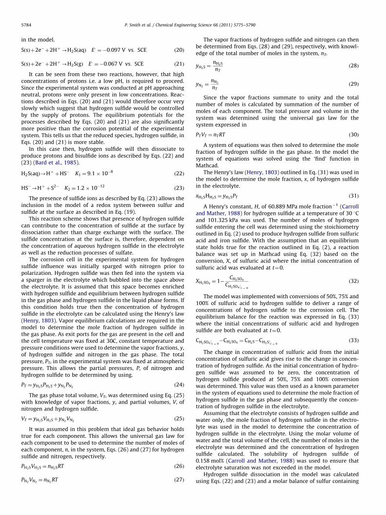
The schematic in Fig. 12 for the overall corrosion reactionshows that protons at the steel surface consume electrons andcause iron (II) ions to be released from the steel into theelectrolyte. The protons are then released from the surface ashydrogen gas.

The electrolyte in this corrosion system is assumed to be wellmixed in the bulk with a diffusion layer established at the steelsurface. The thickness of the diffusion layer can be determined byemploying the Nernst Diffusion model. At the point dN from thesurface, the concentration of reacting species is the same as thatin the bulk. The diffusion layer thickness however, is specific toeach species since they have differing diffusivities.

4.1.1. Charge transfer to the surfaceThe charge transfer at the steel surface for each species is

described by the Butler–Volmer equation. In general, this iswritten as in Eq. (6), with subscript i denoting reacting speciessuch as Fe or H" .

ji $ j0,i expaa,iniF

RTZi

! "!exp !

ac,iniFRT

Zi

! "! "%6&

The kinetic parameters for each species, exchange currentdensity, j0, and transfer coefficients for the cathodic and anodicprocesses, ac and aa, respectively, were determined from a Tafelanalysis applied to E–j data collected in the laboratory. If atten-tion is focused on region (I) in Fig. 13, where the cathodicoverpotential is high, the predominating process at the steelsurface is the cathodic reduction of protons. The cathodic Tafelslope of region (I) therefore, was used to determine kineticparameters for the reduction of protons at the steel surface. Thecathodic transfer coefficient for proton reduction, ac,H" , wasdetermined from a Tafel analysis to be 0.4. The anodic transfercoefficient for iron, aa,Fe, was determined in the same manner byfocusing attention on region (II) in Fig. 13, where the predominat-ing process is the anodic oxidation of iron. The Tafel slope ofregion (II) yielded a value for aa,Fe of 0.4. The experimental datacannot be used to predict ac,H" or aa,Fe, because there is consider-able interference from each reaction near the corrosion potential.

The exchange current density, j0, was determined by usingexperimental data and the definition of j0 in Eq. (7) (Newman andThomas-Alyea, 2004). The bulk concentration, Cb, of iron (II) wasinitially set at 1#10!9 mol dm!3 to simulate iron (II) concentra-tion of approximately zero, with iron (II) surface concentration, Cs,set at 1#10!7 mol dm!3.

j0,i $e0,i

ACs,i

Cb,i

! "gi

%7&

The concentration sensitivity parameter, gi, was determinedfor iron by examining the change in concentration of iron (II) atthe surface. In the E–j data plot for deaerated water, a potentialshift can be observed in the reverse potential scan direction as aresult of the change in iron (II) surface concentration. The

magnitude of the potential shift, approximately 0.12 V, was usedwith the Nernst equation, and a surface concentration value ofiron (II) for the forward potential scan of 1#10!7 mol dm!3

, toestimate the change in iron (II) concentration at the surface to be1#10!3 mol dm!3. The concentration sensitivity parameter foriron (II), gFe, was determined to be 0.3.

The bulk proton concentration was determined from pHmeasurement in the laboratory. The surface proton concentrationwas assumed to be close to zero in this system due to the protonreduction current approaching its diffusion limiting value. Theconcentration sensitivity parameter for proton reduction was setto 0.75 in order for the concentration terms in the exchangecurrent density and reversible potential calculation to be inagreement.

The reversible potential Erev for each component was deter-mined using the Nernst equation, where the activity is assumedto be the same as the surface concentration, Cs, as in Eq. (8), sincethe electrolyte is a dilute solution. Literature values for thestandard potentials, U0, were used (Landolt, 2007) in the model.The charge transferred is expressed as the number of electronstransferred, n, in each reaction, Faraday’s constant, F, tempera-ture, T and the universal gas constant, R, are also required.

Erev,i $ Ei1"2:3RT

niFlog%Cs,i& %8&

The overpotential, Z, for each species was calculated usingEq. (9) and the application of mixed potential theory. Steady-stateoxidation and reduction reactions are established in the corrosionsystem between the oxidation of iron and the reduction ofprotons. This yielded a balance in the transfer of charge and at ameasured current density of zero. The potential, E, at which thisoccurs is the corrosion potential, Ecorr. The resulting overpotentialfor each species was calculated using Eq. (10).

Zi $ E!Erev,i %9&

Zi $ Ecorr!Erev,i %10&

4.1.2. Mass transfer to the surfaceThe transfer of reduction species to the surface and oxidation

products from the surface in a corrosion system affects the rate ofcorrosion significantly. A material balance shown in Eq. (11) wasused to describe the flux, N, of species at the surface.

@Ci

@t$!rNi"Ri %11&

Since steady-state charge transfer was established at the steelsurface and this simple corrosion system contains no homoge-neous reactions in the bulk electrolyte, since the protons releasedfrom water dissociation are already included as per the pHmeasurement. The net flux at the surface is equal zero, describingthe system at steady-state. In the absence of an external appliedpotential field the, flux of each species is described using

Ni $DirCi %12&

Since the flux for each species, N, in the corrosion system isrelated to the current density, j, using the value of charge transfer,n and Faraday’s constant, F, as shown in

Ni $ji

niF%13&

A flux balance arising from the dependency on diffusion andcharge consumption is expressed in Eq. (14) for each species. Thenegative term on the right-hand side denotes that the flux is avector and that the flux occurs in the opposite direction to


concentration gradient.

ji

niF$!Di

Cb,i!Cs,i

dNi

! "%14&

4.1.3. Solution technique and convergence criteriaThe model was set up to seek the corrosion potential based on

the calculation of surface concentrations for each species and byemploying convergence criteria. Since the number of electronscreated in the oxidation process is equal to the number ofelectrons consumed by the reduction process, and each reactioncan be expressed as current, the total current in the system i.e.sum of the current due to oxidation and reduction, must equate tozero. This is expressed in Eq. (15) in terms of the oxidation andreduction component current densities.

jT $ jFe" jH" %15&

where jT$0, or smaller than a tolerance or residual. This was usedas a convergence criterion in the model to locate the corrosionpotential of the system. The model calculates the partial currentsbased on the surface concentrations required to meet the con-vergence criteria. The corrosion rate was then equal to the currentdensity for iron oxidation.

This solution technique was written using a commercial soft-ware package, Mathcad 14. The Solve block facility was employedin the workspace for the input of modeling equations andspecification of convergence criteria. The function ‘Find’ was thenconfigured to solve the set of non-linear equations to determinethe corrosion potential and component currents in the corrosionsystem. Initial values in the model solution were based onestimates of corrosion potential and surface concentration ofcomponents in the model. The convergence tolerance for thesolution algorithm in Mathcad 14 (which controls the precision towhich differentials and integrals are evaluated) was fixed at avalue of 0.001.

4.2. Reaction system: sulfate

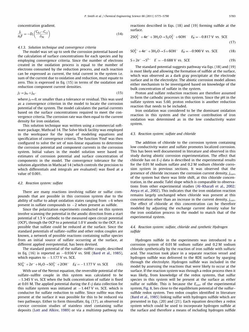
There are many reactions involving sulfate or sulfur com-pounds that are possible in this corrosion system due to theability of sulfur to adopt oxidation states ranging from "6 whenpresent in sulfate compounds to !2 when present as sulfide.

Since the polarization experiments conducted on this systeminvolve scanning the potential in the anodic direction from a startpotential of 1.5 V cathodic to the measured open circuit potential(OCP), through the OCP to a potential 1.0 V anodic to the OCP, it ispossible that sulfate could be reduced at the surface. Since thestandard potentials of sulfate–sulfite and other redox couples areknown, a network of possible reactions containing sulfur speciesfrom an initial source of sulfate occurring at the surface, atdifferent applied overpotential, has been devised.

The standard potential of the sulfate–sulfite couple, describedin Eq. (16) is reported as !0.936 V vs. SHE (Bard et al., 1985),which equates to !1.177 V vs. SCE.

SO2!4 "2e!"H2O-SO2!

3 "2OH! EB1$!1:177 V vs: SCE %16&

With use of the Nernst equation, the reversible potential of thesulfate–sulfite couple in this system was calculated to be!1.345 V vs. SCE when the bulk concentration of sulfate is fixedat 0.01 M. The applied potential during the E–j data collection forthis sulfate system was initiated at !1.447 V vs. SCE. which isconducive for sulfate reduction to sulfite. Since sulfite was thenpresent at the surface it was possible for this to be reduced viatwo pathways. Either to form thiosulfate, Eq. (17), as observed increvice corrosion studies of stainless steel containing sulfurdeposits (Lott and Alkire, 1989) or via a multistep pathway via

reactions described in Eqs. (18) and (19) forming sulfide at thesurface.

2SO2!3 "4e!"3H2O-S2O2!

3 "6OH! EB1 $!0:817 V vs: SCE

%17&

SO2!3 "4e!"3H2O-S"6OH! EB

1 $!0:900 V vs: SCE %18&

S"2e!-S2! E1 $!0:688 V vs: SCE %19&

The standard potential suggests pathway via Eqs. (18) and (19)is most likely and allowing the formation of sulfide at the surface,which was observed as a dark gray precipitate at the electrodesurface and in the electrolyte. The abiotic corrosion model allowseither mechanism to be investigated based on knowledge of thebulk concentration of sulfate in the system.

Proton and sulfate reduction reactions are therefore assumedto form the cathodic processes in this system. Since the pH in thesulfate system was 5.60, proton reduction is another reductionreaction that needs to be included.

Iron oxidation was considered to be the dominant oxidationreaction in this system and the current contribution of ironoxidation was determined as in the low conductivity watersystem.

4.3. Reaction system: sulfate and chloride

The addition of chloride to the corrosion system containinglow conductivity water and sulfate promotes localized corrosion.This has been well documented in literature and observed in thisstudy during abiotic corrosion experimentation. The effect thatchloride has on E–j data is described in the experimental resultsfor the 0.01 M sodium sulfate and 0.2 M sodium chloride corro-sion system in previous sections. It was observed that thepresence of chloride increases the corrosion current density, jcorr,of the system but there was little shift, at this chloride concen-tration, in the anodic Tafel slope which is comparable to observa-tions from other experimental studies (Al–Kharafi et al., 2002;Ateya et al., 2002). This indicates that the iron oxidation reactionremains largely unchanged when chloride was present at thisconcentration other than an increase in the current density, jcorr.The effect of chloride at this concentration can be thereforemodeled by adjusting the exchange current density value forthe iron oxidation process in the model to match that of theexperimental system.

4.4. Reaction system: sulfate, chloride and synthetic Hydrogensulfide

Hydrogen sulfide in the experiments was introduced to acorrosion system of 0.01 M sodium sulfate and 0.2 M sodiumchloride synthetically by the reaction of iron sulfide with sulfuricacid. The reaction took place in a separate reaction vessel andhydrogen sulfide was delivered to the RDE surface by spargingthrough the electrolyte. Hydrogen sulfide was included in themodel by assessing the reactions that were likely to occur at thesurface. If the reaction system was through a redox process then itwas likely, from knowledge of the redox systems, that sulfurspecies in this system will be present at the surface as eithersulfur or sulfide. This is because the Ecorr of the experimentalsystem, Fig. 8, lies close to the equilibrium potential of the sulfur–sulfide redox system. Two redox couples identified in literature(Bard et al., 1985) linking sulfur with hydrogen sulfide which arepresented in Eqs. (20) and (21). Each equation describes a redoxsystem which could be used to incorporate hydrogen sulfide atthe surface and therefore a means of including hydrogen sulfide


in the model.

S%s&"2e!"2H"-H2S%aq& E3 $!0:097 V vs: SCE %20&

S%s&"2e!"2H"-H2S%g& E3 $!0:067 V vs: SCE %21&

It can be seen from these two reactions, however, that highconcentrations of protons i.e. a low pH, is required to proceed.Since the experimental system was conducted at pH approachingneutral, protons were only present in low concentrations. Reac-tions described in Eqs. (20) and (21) would therefore occur veryslowly which suggest that hydrogen sulfide would be controlledby the supply of protons. The equilibrium potentials for theprocesses described by Eqs. (20) and (21) are also significantlymore positive than the corrosion potential of the experimentalsystem. This tells us that the reduced species, hydrogen sulfide, inEqs. (20) and (21) is more stable.

In this case then, hydrogen sulfide will then dissociate toproduce protons and bisulfide ions as described by Eqs. (22) and(23) (Bard et al., 1985).

H2S%aq&-H" "HS! K1 $ 9:1# 10!8 %22&

HS!-H" "S2! K2 $ 1:2# 10!12 %23&

The presence of sulfide ions as described by Eq. (23) allows theinclusion in the model of a redox system between sulfur andsulfide at the surface as described in Eq. (19).

This reaction scheme shows that presence of hydrogen sulfidecan contribute to the concentration of sulfide at the surface bydissociation rather than charge exchange with the surface. Thesulfide concentration at the surface is, therefore, dependent onthe concentration of aqueous hydrogen sulfide in the electrolyteas well as the reduction processes of sulfate.

The corrosion cell in the experimental system for hydrogensulfide influence was initially sparged with nitrogen prior topolarization. Hydrogen sulfide was then fed into the system viaa sparger in the electrolyte which bubbled into the space abovethe electrolyte. It is assumed that this space becomes enrichedwith hydrogen sulfide and equilibrium between hydrogen sulfidein the gas phase and hydrogen sulfide in the liquid phase forms. Ifthis condition holds true then the concentration of hydrogensulfide in the electrolyte can be calculated using the Henry’s law(Henry, 1803). Vapor equilibrium calculations are required in themodel to determine the mole fraction of hydrogen sulfide inthe gas phase. As exit ports for the gas are present in the cell andthe cell temperature was fixed at 30C, constant temperature andpressure conditions were used to determine the vapor fractions, y,of hydrogen sulfide and nitrogen in the gas phase. The totalpressure, PT, in the experimental system was fixed at atmosphericpressure. This allows the partial pressures, P, of nitrogen andhydrogen sulfide to be determined by using.

PT $ yH2SPH2S"yN2PN2

%24&

The gas phase total volume, VT, was determined using Eq. (25)with knowledge of vapor fractions, y, and partial volumes, V, ofnitrogen and hydrogen sulfide.

VT $ yH2SVH2S"yN2VN2

%25&

It was assumed in this problem that ideal gas behavior holdstrue for each component. This allows the universal gas law foreach component to be used to determine the number of moles ofeach component, n, in the system, Eqs. (26) and (27) for hydrogensulfide and nitrogen, respectively.

PH2SVH2S $ nH2SRT %26&

PN2VN2$ nN2

RT %27&

The vapor fractions of hydrogen sulfide and nitrogen can thenbe determined from Eqs. (28) and (29), respectively, with knowl-edge of the total number of moles in the system, nT.

yH2S $nH2S

nT%28&

yN2$

nN2

nT%29&

Since the vapor fractions summate to unity and the totalnumber of moles is calculated by summation of the number ofmoles of each component. The total pressure and volume in thesystem was determined using the universal gas law for thesystem expressed in

PT VT $ nT RT %30&

A system of equations was then solved to determine the molefraction of hydrogen sulfide in the gas phase. In the model thesystem of equations was solved using the ‘find’ function inMathcad.

The Henry’s law (Henry, 1803) outlined in Eq. (31) was used inthe model to determine the mole fraction, x, of hydrogen sulfidein the electrolyte.

xH2SHH2S $ yH2SPT %31&

A Henry’s constant, H, of 60.889 MPa mole fraction!1 (Carrolland Mather, 1988) for hydrogen sulfide at a temperature of 30 1Cand 101.325 kPa was used. The number of moles of hydrogensulfide entering the cell was determined using the stoichiometryoutlined in Eq. (2) used to produce hydrogen sulfide from sulfuricacid and iron sulfide. With the assumption that an equilibriumstate holds true for the reaction outlined in Eq. (2), a reactionbalance was set up in Mathcad using Eq. (32) based on theconversion, X, of sulfuric acid where the initial concentration ofsulfuric acid was evaluated at t$0.

XH2SO4$ 1!

CH2SO4

CH2SO49t $ 0

%32&

The model was implemented with conversions of 50%, 75% and100% of sulfuric acid to hydrogen sulfide to deliver a range ofconcentrations of hydrogen sulfide to the corrosion cell. Theequilibrium balance for the reaction was expressed in Eq. (33)where the initial concentrations of sulfuric acid and hydrogensulfide are both evaluated at t$0.

CH2SO49t $ 0!CH2SO4

$ CH2S!CH2S9t $ 0%33&

The change in concentration of sulfuric acid from the initialconcentration of sulfuric acid gives rise to the change in concen-tration of hydrogen sulfide. As the initial concentration of hydro-gen sulfide was assumed to be zero, the concentration ofhydrogen sulfide produced at 50%, 75% and 100% conversionwas determined. This value was then used as a known parameterin the system of equations used to determine the mole fraction ofhydrogen sulfide in the gas phase and subsequently the concen-tration of hydrogen sulfide in the electrolyte.

Assuming that the electrolyte consists of hydrogen sulfide andwater only, the mole fraction of hydrogen sulfide in the electro-lyte was used in the model to determine the concentration ofhydrogen sulfide in the electrolyte. Using the molar volume ofwater and the total volume of the cell, the number of moles in theelectrolyte was determined and the concentration of hydrogensulfide calculated. The solubility of hydrogen sulfide of0.158 mol% (Carroll and Mather, 1988) was used to ensure thatelectrolyte saturation was not exceeded in the model.

Hydrogen sulfide dissociation in the model was calculatedusing Eqs. (22) and (23) and a molar balance of sulfur containing


species expressed in.

CH2S9t $ 0$ CHS! "CH2S%aq& "CS2! %34&

A species charge constraint expressed in Eq. (35) was alsoincluded to maintain electroneutrality in the electrolyte.

CH" $ CHS! "CS2! %35&

The concentration of protons and sulfide were then included inthe bulk concentrations of corresponding redox processes occur-ring at the surface.

5. Model results

5.1. Deaerated water

The corrosion model for a system of deaerated water wasbased on a charge balance between the oxidation of iron withinsteel, releasing iron (II) to the electrolyte and the reduction ofprotons to hydrogen at the surface. Mass transport effects in themodel have been included by calculating the Nernst diffusionlayer thickness using literature values and measured values fordiffusion coefficients of reduction species in the electrolyte.Corrosion parameters collected during the potential scan in theanodic direction of the E–j data collected for this system havebeen used in model development, it is important to note there-fore, that model validation has been conducted using the para-meters collected from potential the scan in the cathodic directionand then to test the performance of the model under differentconditions. This means that the model fit will be examinedagainst the corrosion potential (the value measured on the back-ward potential scan i.e. the more anodic corrosion potentialpresented in the experimental data).

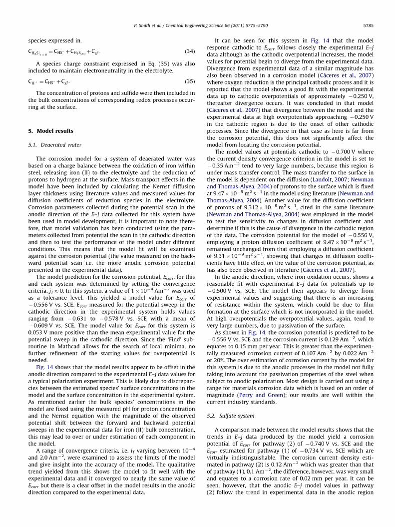
The model prediction for the corrosion potential, Ecorr, for thisand each system was determined by setting the convergencecriteria, jTE0. In this system, a value of 1#10!4 Am!2 was usedas a tolerance level. This yielded a model value for Ecorr of!0.556 V vs. SCE. Ecorr measured for the potential sweep in thecathodic direction in the experimental system holds valuesranging from !0.631 to !0.578 V vs. SCE with a mean of!0.609 V vs. SCE. The model value for Ecorr for this system is0.053 V more positive than the mean experimental value for thepotential sweep in the cathodic direction. Since the ‘Find’ sub-routine in Mathcad allows for the search of local minima, nofurther refinement of the starting values for overpotential isneeded.

Fig. 14 shows that the model results appear to be offset in theanodic direction compared to the experimental E–j data values fora typical polarization experiment. This is likely due to discrepan-cies between the estimated species’ surface concentrations in themodel and the surface concentration in the experimental system.As mentioned earlier the bulk species’ concentrations in themodel are fixed using the measured pH for proton concentrationand the Nernst equation with the magnitude of the observedpotential shift between the forward and backward potentialsweeps in the experimental data for iron (II) bulk concentration,this may lead to over or under estimation of each component inthe model.

A range of convergence criteria, i.e. iT varying between 10!4

and 2.0 Am!2, were examined to assess the limits of the modeland give insight into the accuracy of the model. The qualitativetrend yielded from this shows the model to fit well with theexperimental data and it converged to nearly the same value ofEcorr but there is a clear offset in the model results in the anodicdirection compared to the experimental data.

It can be seen for this system in Fig. 14 that the modelresponse cathodic to Ecorr follows closely the experimental E–jdata although as the cathodic overpotential increases, the modelvalues for potential begin to diverge from the experimental data.Divergence from experimental data of a similar magnitude hasalso been observed in a corrosion model (Caceres et al., 2007)where oxygen reduction is the principal cathodic process and it isreported that the model shows a good fit with the experimentaldata up to cathodic overpotentials of approximately !0.250 V,thereafter divergence occurs. It was concluded in that model(Caceres et al., 2007) that divergence between the model and theexperimental data at high overpotentials approaching !0.250 Vin the cathodic region is due to the onset of other cathodicprocesses. Since the divergence in that case as here is far fromthe corrosion potential, this does not significantly affect themodel from locating the corrosion potential.

The model values at potentials cathodic to !0.700 V wherethe current density convergence criterion in the model is set to!0.35 Am!2 tend to very large numbers, because this region isunder mass transfer control. The mass transfer to the surface inthe model is dependent on the diffusion (Landolt, 2007; Newmanand Thomas-Alyea, 2004) of protons to the surface which is fixedat 9.47#10!9 m2 s!1 in the model using literature (Newman andThomas-Alyea, 2004). Another value for the diffusion coefficientof protons of 9.312#10!9 m2 s!1, cited in the same literature(Newman and Thomas-Alyea, 2004) was employed in the modelto test the sensitivity to changes in diffusion coefficient anddetermine if this is the cause of divergence in the cathodic regionof the data. The corrosion potential for the model of !0.556 V,employing a proton diffusion coefficient of 9.47#10!9 m2 s!1,remained unchanged from that employing a diffusion coefficientof 9.31#10!9 m2 s!1, showing that changes in diffusion coeffi-cients have little effect on the value of the corrosion potential, ashas also been observed in literature (Caceres et al., 2007).

In the anodic direction, where iron oxidation occurs, shows areasonable fit with experimental E–j data for potentials up to!0.500 V vs. SCE. The model then appears to diverge fromexperimental values and suggesting that there is an increasingof resistance within the system, which could be due to filmformation at the surface which is not incorporated in the model.At high overpotentials the overpotential values, again, tend tovery large numbers, due to passivation of the surface.

As shown in Fig. 14, the corrosion potential is predicted to be!0.556 V vs. SCE and the corrosion current is 0.129 Am!2, whichequates to 0.15 mm per year. This is greater than the experimen-tally measured corrosion current of 0.107 Am!2 by 0.022 Am!2

or 20%. The over estimation of corrosion current by the model forthis system is due to the anodic processes in the model not fullytaking into account the passivation properties of the steel whensubject to anodic polarization. Most design is carried out using arange for materials corrosion data which is based on an order ofmagnitude (Perry and Green); our results are well within thecurrent industry standards.

5.2. Sulfate system

A comparison made between the model results shows that thetrends in E–j data produced by the model yield a corrosionpotential of Ecorr for pathway (2) of !0.740 V vs. SCE and theEcorr estimated for pathway (1) of !0.734 V vs. SCE which arevirtually indistinguishable. The corrosion current density esti-mated in pathway (2) is 0.12 Am!2 which was greater than thatof pathway (1), 0.1 Am!2, the difference, however, was very smalland equates to a corrosion rate of 0.02 mm per year. It can beseen, however, that the anodic E–j model values in pathway(2) follow the trend in experimental data in the anodic region


more closely than that of pathway (1) which provides greatercredibility to pathway (2).

The model results appear to under predict the current densityin the cathodic region compared to the E–j data collected for theexperimental sulfate system. This suggests that the cathodicreactions in the experimental system occur at a greater rate thandescribed by the model. The E–j data collected for the experi-mental systems containing sulfate, however, showed significantnoise and variation in both the current density and Ecorr values foreach replicate suggesting that the interaction processes at thesurface are complex and metastable Fig. 15.

5.3. Sulfate and chloride system

The model configuration for the corrosion system containing0.01 M sodium sulfate and 0.2 M sodium chloride was similar tothat of the system containing only sulfate. Since chloride facil-itates iron oxidation (Al-Kharafi et al., 2002; Ateya et al., 2002;El-Egamy and Badaway, 2004; Laycock and Newman, 1997;Meguid and Latif, 2004), the addition of chloride was incorporatedin the model by increasing the exchange current density of theiron oxidation process at the surface. The model for this systemalso included the effect of each reaction pathway for the reduc-tion of sulfate, Eqs. (16)–(19).

The model matches well with the experimental E–j for thissystem up to anodic potentials of !0.500 V. The divergence athigher potentials may be due to the assumption that onlyoxidation of iron from the steel surface is included. It is possibleat the high overpotentials that other anodic processes are occur-ring. It was also shown in a previous corrosion modeling study(Caceres et al., 2007) that the iron (II) anodic transfer coefficientcan decrease with increasing concentration of chloride in thesystem. Fig. 16 shows the model data with the anodic transfercoefficient for iron (II) set to 0.25 as opposed to 0.4 which wasinitially used in the low conductivity water system. The model fitin the anodic region is considerably better at high overpotentialsusing an aFe2" value of 0.25 as compared to 0.4.

The model prediction for Ecorr in this system with aFe2" of 0.4 is!0.702 V vs. SCE which is 0.061 V cathodic to the experimentallymeasured Ecorr. The model implemented with aFe2" of 0.25 yieldsa corrosion potential prediction of !0.721 V vs. SCE which is0.080 V cathodic to the experimentally measured value, whichshows that the transfer coefficient is an important parameter.

It should be noted that value of the anodic transfer coefficientfor iron dissolution in earlier experimental work has also beenreported with values of 0.70 and even approaching 1.0 (Morriset al., 1980). In the presence of chloride, since iron dissolution iscatalyzed, there may be a variation of j0 with time and the anodictransfer coefficient may also vary. Since this is difficult toquantify, the results from our model can be considered to be inreasonable agreement.

The model response in the cathodic region for this systemshows that calculated values of Icorr are approximately one orderof magnitude lower than the experimental E–j data. This may bedue to the catalytic effects and film forming nature of chlorideand sulfate system which are not described in the model. Theexperimental E–j data also showed variation of a similar magni-tude in the cathodic region for this system.

5.4. Sulfate, chloride and hydrogen sulfide system

Three corrosion scenarios were developed to assess the modelpredictions for a corrosion system containing hydrogen sulfide.An equilibrium calculation was set up in the model to determinethe concentration of protons and sulfide produced by hydrogen

sulfide for three conversions of 50%, 75% and 100% for the reactionpresented in Eq. (2) which equates to hydrogen sulfide saturationlevels of 18%, 30% and 35% in the electrolyte, respectively. Themodel results for the case of 18% hydrogen sulfide saturation areshow in Fig. 17. The trend in the data fit for the other conversionswas very similar.

The model response in the anodic region shows a reasonablefit with the experimental data until overpotentials of !0.600 Vare reached, thereafter a divergence was observed. However,there was significant noise and variation in the experimentaldata, Fig. 8, suggesting that the processes occurring at the surfaceare unsystematic due to formation of surface films. These E–jmeasurements coincide with other studies (Videm and Kvarekval,1995) showing the unsystematic effects of aqueous hydrogensulfide on E–j data. The divergence is attributed to the limiteddescription of passivity and film formation in the model whichhas been identified as the cause of increased resistance at thesurface (Huang et al., 1996). The model values for the cathodicregion in this system show similar characteristics to the othersystems presented in this work, where the cathodic currentdensities are somewhat lower than the experimental data

6. Discussion

The results for the abiotic model systems have been presentedhere which show that the qualitative trend in the model was inbroad agreement with the experimental data. There is also goodquantitative agreement with potentials higher than Ecorr for up to0.500 V. It has been shown that the model responds effectively tochanges in the input parameters such as the anodic transfercoefficient for iron. The model response in the region cathodicto Ecorr shows limited agreement which suggesting that waterreduction and reduction of dissolved carbon dioxide mayberequired for more accurate predictions. The model was also usedto assess reaction pathways for the abiotic reduction of sulfate.Although there was little difference in the model response for thetwo different pathways, pathway (2) showed somewhat betteragreement. Further assessment of these differences could beaddressed in future work.

The initial deaerated water corrosion system was utilized todemonstrate the most simple corrosion system containing theanodic dissolution of iron to form iron (II) and the cathodicreduction of protons to form hydrogen at the steel surface. TheE–j data collected from this system allowed the corrosion currentof approximately 0.14 Am!2 to be determined along with acorrosion potential of !0.742 V vs. SCE. Corrosion current densityvalues of this magnitude represent corrosion rates of 0.16 mmy!1

which is relatively low when the threshold corrosion rate of0.1 mmy!1 (Crolet, 2005) for mitigated corrosion systems isconsidered.

The E–j data for the deaerated water system presented forthree replicate potential sweep experiments, shows that thecorrosion potential measured at !0.742 V vs. SCE was fairlyconstant but there was variation in the current response betweeneach of the three replicates. This variation in current response isdue to the effect of low conductivity in the electrolyte whichvaries from 65.4 to 104 mS cm!1 and may reflect a systematicerror in the data accumulated through the electrolyte prepara-tion. A variation in conductivity of 38.6 mS cm!1 measured forbetween replicates induces a change in Ohmic drop up to4000 O(Oelßner et al., 2006) for electrodes of 0.6 cm diameterused here. This range in Ohmic drop between replicates may bereflected in the variation observed in the E–j data.

The addition of 0.01 M sodium sulfate to the corrosion systemgave rise to an increase in the corrosion current density to


0.50 Am!2 which equates to 0.58 mm y!1 and is comparable toother corrosion systems of similar pH and sulfate concentration(Hernandez-Espejel et al., 2010). A significant level of noise wasalso recorded in the anodic current response in the presence ofsodium sulfate. Noise of similar character was also observed inseveral studies presented in literature (Cheng et al., 1999; Simardet al., 2001) where it was attributed to the formation and break-ing of passive films on the surface due to the presence of saltprecipitates. It is reasonable to draw similar conclusions in thedata for the sulfate corrosion system presented in this study asblack precipitates were also observed to form at the surface andin the electrolyte. The formation of precipitates at the surface inthis system was also reflected by the large variation in corrosionpotential of each replicate which was also observed in similarstudies (Hernandez-Espejel et al., 2010). Since it is known thatsulfate is able to form many species in solution (Bard et al., 1985)it is likely that these species and their varying morphologiesinteract with the surface giving rise to the variance in potentialobserved in the experimental measurement. It was shown in onestudy (Hernandez-Espejel et al., 2010) that the variation in opencircuit potential was dependent on immersion time of steel in anelectrolyte prepared to induce sulfate based film formation at thesurface, there was, however, no obvious trends reported.

Experimental work in this study was also conducted to assessthe effect of chloride addition to the corrosion system. Since theoverall objective was to assess the corrosion influence due tocomponents in the produced water, presented in Table 1, anelectrolyte of 0.01 M sodium sulfate and 0.2 M sodium chloridewas used. The effects on corrosion of this electrolyte wereobserved as an increase in corrosion current density from0.5 Am!2 measured in the sulfate system to 3.0 Am!2 with theinclusion of chloride which is comparable to corrosion currentsmeasured in other corrosion studies (Caceres et al., 2007).

There was also evidence in the E–j data of pitting corrosionwhich is widely understood to be facilitated by the presence ofchloride ions at the steel surface (Al-Kharafi et al., 2002; Ateyaet al., 2002; El-Egamy and Badaway, 2004; Laycock and Newman,1997; Meguid and Latif, 2004). The characteristic film breakdowneffect which causes pitting can be seen in the E–j data plotscontaining chloride. A plateau can be observed in the anodiccurrent response close to the corrosion potential in both plotswhich, as the overpotential is increased, suddenly gives rise to anincrease in current density. The potential at which this occurs iscalled the Flade potential and pitting is expected to occur atvalues of overpotential greater than this. The Flade potential forthe corrosion system containing 0.01 M sodium sulfate and 0.2 Msodium chloride was recorded at !0.650 V and for the systemcontaining 0.0002 M sodium sulfate and 0.8 M sodium chloridewas !0.560 V. These values for the Flade potential are morenegative than several published in literature (Ateya et al., 2002;Videm and Kvarekval, 1995) but this is likely to reflect differencesin the nature of the films at the surface and their ability to resistpitting induced by chloride at the surface.

It was clear that a presence of hydrogen sulfide in theelectrolyte induced major changes in the interactions at thesurface compared to corrosion systems in the absence of hydro-gen sulfide. Figs. 8–10 show experimental E–j data for thehydrogen sulfide systems where there is evidence of film forma-tion at the surface through the development of an oxidation peakat !0.700 V vs. SCE and noise in the current density response.This E–j data also show that the films formed at the surface areprotective in nature due to the reduced magnitude in currentresponse as reported in several other studies (Hernandez-Espejelet al., 2010; Shoesmith et al., 1978; Shoesmith et al., 1980).

The E–j data for the hydrogen sulfide system shows a two-foldincrease in corrosion current density from 2.1 to 4.0 Am!2. This

reflects an increase in corrosion activity at the surface due toincreased presence of aggressive species in the electrolyte but theE–j data also describes an increase in the resistance at the surfacewith increases in overpotential in both the cathodic and anodicdirections compared to the sulfate-chloride system. This showsthe development of a protective film at the surface of the RDEduring polarization, which were observed optically (Smith, 2010).

The modeling method is, however, different in the otherelectrochemical corrosion models where experimental E–j datais required in the model calculation or calibration. These requiredsteps may limit the usage of these models where experimental E–jis not available. One benefit of the model presented in this paperis that an estimation of corrosion potential and corrosion currentdensity can be made without the need of collection of newexperimental data. Providing that estimation of the Tafel coeffi-cients is available, the model will provide a prediction of corro-sion rate. The accuracy of this method, however, is dependent onthe components included in the model. It is necessary to ensurethat all components in the corrosion system under investigationare included in the model before predictions are sought.

"1.5 "1 "0.5 01!10!4

1!10!3

0.01

0.1

1

10

100

1!103

1!104


|Cur

rent

Den

sity

|, A

m-2

EF = -0.629V

Fig. 10. E–j data for three separate replicates of a corrosion system of deaerated0.2 M sodium chloride and H2S. The standard deviation in the corrosion potentialmeasured for this system was 0.021 V. The Flade potential, EF, showing filmbreakdown at the surface during the potential sweep in the anodic direction canbe seen at a potential of !0.629 V vs. SCE.

Dark Area

DarkArea

Light Area

Fig. 11. Optical micrograph of RDE tip after exposure to a deaerated lowconductivity water electrolyte containing 0.01 M sodium sulfate electrolyte andpolarization experimentation at rotation speed of 800 rpm. Dark areas outlinedshow areas of film formation on the surface.


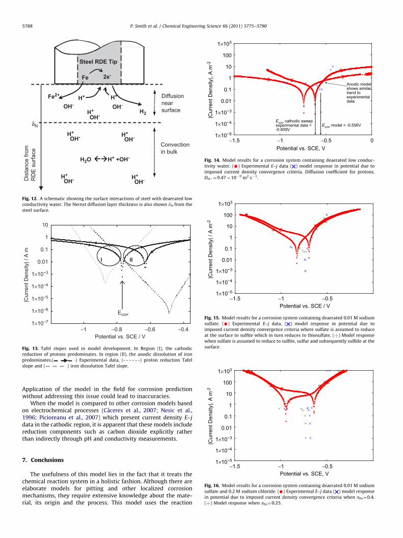
Application of the model in the field for corrosion predictionwithout addressing this issue could lead to inaccuracies.

When the model is compared to other corrosion models basedon electrochemical processes (Caceres et al., 2007; Nesic et al.,1996; Picioreanu et al., 2007) which present current density E–jdata in the cathodic region, it is apparent that these models includereduction components such as carbon dioxide explicitly ratherthan indirectly through pH and conductivity measurements.

7. Conclusions

The usefulness of this model lies in the fact that it treats thechemical reaction system in a holistic fashion. Although there areelaborate models for pitting and other localized corrosionmechanisms, they require extensive knowledge about the mate-rial, its origin and the process. This model uses the reaction

I II

"1 "0.8 "0.6 "0.41!10!7

1!10!6

1!10!5

1!10!4

1!10!3

0.01

0.1

1

10

Potential vs. SCE / V

|Cur

rent

Den

sity

| / A

m

I II

Ecorr

Fig. 13. Tafel slopes used in model development. In Region (I), the cathodicreduction of protons predominates. In region (II), the anodic dissolution of ironpredominates.( ) Experimental data, (- - - - - -) proton reduction Tafelslope and ( ) iron dissolution Tafel slope.

"1.5 "1 "0.5 01!10!5

1!10!4

1!10!3

0.01

0.1

1

10

100

1!103


|Cur

rent

Den

sity

|, A

m-2

Ecorr model = -0.556VEcorr cathodic sweep experimental data = -0.609V

Anodic model shows similar trend to experimental data

Fig. 14. Model results for a corrosion system containing deaerated low conduc-tivity water. ( ) Experimental E–j data ( ) model response in potential due toimposed current density convergence criteria. Diffusion coefficient for protons,DH" $9.47#10!9 m2 s!1.

"1.5 "1 "0.51!10!5

1!10!4

1!10!3

0.01

0.1

1

10

100

1!103

Potential vs. SCE / V

|Cur

rent

Den

sity

| / A

m-2

Fig. 15. Model results for a corrosion system containing deaerated 0.01 M sodiumsulfate. ( ) Experimental E–j data, ( ) model response in potential due toimposed current density convergence criteria where sulfate is assumed to reduceat the surface to sulfite which in turn reduces to thiosulfate. ( ) Model responsewhen sulfate is assumed to reduce to sulfite, sulfur and subsequently sulfide at thesurface.


|Cur

rent

Den

sity

|, A

m-2

"1.5 "1 "0.51!10!5

1!10!4

1!10!3

0.01

0.1

1

10

100

1!103

Fig. 16. Model results for a corrosion system containing deaerated 0.01 M sodiumsulfate and 0.2 M sodium chloride. ( ) Experimental E–j data ( ) model responsein potential due to imposed current density convergence criteria when aFe$0.4.( ) Model response when aFe$0.25.

H+

OH-

H+OH-

H+

OH-

H+OH-

H2O H+ +OH-

H+OH-

H+OH-

H2

H+OH-

Fe2+

2e-Fe

Diffusion nearsurface

Convection in bulk

Dis

tanc

e fro

m

RD

E su

rface

#N

Steel RDE Tip

Fig. 12. A schematic showing the surface interactions of steel with deaerated lowconductivity water. The Nernst diffusion layer thickness is also shown dN from thesteel surface.


network data with process parameters and provides reasonableagreement with corrosion rates measured experimentally.

A model was developed based on experimental data collectedfor corrosion systems containing sulfate, chloride and hydrogensulfide. Using the mixed potential theory the corrosion modelaimed to balance the charge transferred in reduction and oxida-tion reactions at the surface and calculate the corrosion currentdensity. Mass transport of reduction species to the surface in theabiotic model, is described by using the Nernst diffusion modelwith knowledge of diffusion coefficients and the Nernst diffusionlayer thickness. Charge transfer at the surface is described usingButler–Volmer kinetics. The rate of the iron oxidation reaction isdependent on the sum of rates for all the reduction reactionsoccurring at the surface. The abiotic corrosion model outputs, E–jdata, corrosion potential and corrosion current density, for themodel system are determined in the abiotic corrosion modelsubject to current density convergence criteria.

The E–j data predicted by the abiotic model developed in thiswork was found in general to match well with qualitative trendsobserved in the experimental E–j data for the corrosion systems.The quantitative fit of the model to experimental data, however,was variable over the range of E–j data. There was a good matchof Ecorr and Icorr (within experimental variability) and small over-potentials in the anodic region. There was a poor quantitative fitin general between the model and experimental E–j data in thecathodic region. Deviations between the model and experimentalE–j data were recorded at high anodic overpotentials but inseveral systems these deviations were eliminated through adjust-ment of the anodic Tafel slope values used by the model.

Nomenclature

List of symbols

A electrode surface area (m2)CR corrosion rate (mm y!1)C concentration of species (mol m!3)D diffusion coefficient (m2 s!1)e0 exchange current density transfer parameterE potential (V)Ecorr free corrosion potential (V)EF flade PotentialErev reversible potential for species (V)E0 equilibrium potential (V)

E1 standard electrode potential (V)F Faraday constant 96485 C mol!1

H Henry’s coefficientj current density (A m!2)j0 exchange current density (A m!2)M molar mass (g mol!1)N flux of reaction speciesn number of electrons transferred in the processn number of moles of species (moles)P system or partial species pressure (Pa)R universal gas constant$8.314 J K!1 mol!1

R rate of homogeneous production (mol m!3 s!1)T temperature /(K)t time (s)V system or partial volume (m3)X conversionx mole fraction in the liquid phasey mole fraction in the vapor phasea transfer function for redox processg concentration sensitivity parameterdN Nernst diffusion layer thickness (m)Z overpotential (V)

List of subscripts

a anodic process parameterc cathodic process parameteri reaction speciesT total system pressure, volume, moles parameter

References

Al-Kharafi, F.M., Ateya, B.G., Abdallah, R.M., 2002. Electrochemical behaviour oflow carbon steel in concentrated carbonate chloride brines. Journal of AppliedElectrochemistry 32, 1363–1370.

Alkire, R., Nicolaides, G., 1974. Differential aeration corrosion of a passivatingmetal under a moist film of locally variable thickness. Journal of the Electro-chemical Society: Electrochemical Science and Technology 121, 183–190.

Ateya, B.G., Kharafi, F.M.A., Abdalla, R.M., 2002. Electrochemical behavior of low carbonsteel in slightly acidic brines. Materials Chemistry and Physics 78, 534–541.

Bard, A.J., Parsons, R., Jordan, J., 1985. Standard Potentials in Aqueous Solution,1st Edition, CRC Press.

Caceres, L., Vargas, T., Herrera, L., 2007. Determination of electrochemical para-meters and corrosion rate for carbon steel in un-buffered sodium chloridesolutions using a superposition model. Corrosion Science 49, 3168–3184.

Carroll, J.J., Mather, A.E., 1988. The solubility of hydrogen sulfide in water from 0 to90 1C and pressures to 1 MPa. Geochimica et Cosmochimica Acta 53, 1163–1170.

Cheng, Y.F., Wilmott, M., Luo, J.L., 1999. Transition criterion of metastable pittingtowards stability for carbon steel in chloride solutions. British CorrosionJournal 34, 280–284.

Crolet, J.-L., 2005. Microbial Corrosion in the Oil Industry: A Corrosionist’s View,Petroleum Mircobiology. ASM Press, Washington, DC, pp. 143–169.

El-Egamy, S.S., Badaway, W.A., 2004. Passivity and passivity breakdown of 304stainless steel in alkaline sodium sulphate solutions. Journal of AppliedElectrochemistry 34, 1153–1158.

Hamilton, W.A., 2002. Microbially influenced corrosion as a model system for thestudy of metal microbe interactions: A unifying electron transfer hypothesis.Biofouling 19, 65–76.

Hardy, J.A., Bown, J.L., 1984. The corrosion of mild steel by biogenic sulphide filmsexposed to air. Corrosion 40, 650–654.

Henry, W., 1803. Experiments on the quantity of gasses absorbed by water, atdifferent temperatures, and under different pressures. Philosophical Transac-tions of the Royal Society London 93 (29–43), 274–275.

Hernandez-Espejel, A., Dominguez-Crespo, M.A., Cabrera-Sierra, R., Rodrigues-Meneses, C., Arce-Estrada, E.M., 2010. Investigations of corrosion films formedon API-X52 pipeline steel in acid sour media. Corrosion Science 52,2258–2267.

Huang, H.H., Tsai, W.T., Lee, J.T., 1996. Electrochemical behaviour of A516 carbonsteel in solutions containing hydrogen sulfide. Corrosion 52, 708–713.

Landolt, D., 2007. Corrosion and Surface Chemistry of Metals, Translated from therevised second French edition ed EPFL Press.

Laycock, N.J., Newman, R.C., 1997. Localised dissolution kinetics, salt films andpitting potentials. Corrosion Science 39, 1771–1790.

"1.5 "1 "0.5 01!10!5

1!10!4

1!10!3

0.01

0.1

1

10

100

1!103


|Cur

rent

Den

sity

|, A

m-2

Fig. 17. Model results for a corrosion system containing deaerated 0.01 M sodiumsulfate and 0.2 M sodium chloride and 18% hydrogen sulfide saturation. ( )Experimental E–j data ( ) Model response in potential due to imposed currentdensity convergence criteria.


Lee, W., Characklis, W.G., 1993. Corrosion of mild steel under anaerobic biofilm.Corrosion 49, 186–199.

Lott, S.E., Alkire, R.C., 1989. The role of inclusions on initiation of crevice corrosionof stainless steel. Journal of the Electrochemical Society 136, 973–979.

Maxwell, S., 2006. Monitoring the mitigation of MIC risk in pipelines. NACE, 2006.Meguid, E.A.A.E., Latif, A.A.A.E., 2004. Electrochemical and SEM study on type 254

SMO stainless steel in chloride solutions. Corrosion Science 46, 2431–2444.Morris, D.R., Sampaleanu, L.P., Veysey, D.N., 1980. The corrosion of steel by

aqueous solutions of hydrogen sulfide. Journal of The Electrochemical Society127, 1228–1235.

Morris, R., Smyrl, W., 1988. Galvanic interactions on periodically regular hetero-geneous surfaces. AIChE Journal 34, 723–732.

Morris, R., Smyrl, W., 1989. Galvanic interactions on random heterogeneoussurfaces. Journal of the Electrochemical Society 136, 3237–3248.

Nesic, S., Postlethwaite, J., Olsen, S., 1996. An electrochemical model for predictionof corrosion of mild steel in aqueous carbon dioxide solutions. Corrosion 52,280–294.

Newman, J., Thomas-Alyea, K.E., 2004. Electrochemical Systems, Third ed. JohnWiley & Sons, Inc.

NORSOK, 2005. CO2 corrosion rate calculation model.Nyborg, R., 2009. Guidelines for Prediction of CO2 Corrosion in Oil and Gas

Production Systems. Institute for Energy Technology.Oelßner, W., Berthold, F., Guth, U., 2006. The iR Drop—Well-known but often

underestimated in electrochemical polarisation measurements and corrosiontesting. Materials and Corrosion 57, 455–466.

Perry, R.H., Green, D.W., Perry’s Chemical Engineers’ Handbook. McGraw-Hill.

Picioreanu, C., Head, I.M., Katuri, K.P., Loosdrect, M.C.M.v., Scott, K., 2007.A computational model for biofilm-based microbial fuel cells. Water Research41, 2921–2940.

Picioreanu, C., Loosdrecht, M.C.M.v., 2002. A mathematical model for initiation ofmicrobiologically influenced corrosion by differential aeration. Journal of TheElectrochemical Society 149, B211–B223.

Pots, B.F., John, R.C., Rippon, I.J., Thomas, M.J.J.S., Kapusta, S.D., Girgis, M.M.,Whitman, T., 2002. Improvements on De Waard-Milliams corrosion predictionand applications to corrosion management. NACE, 2002.

Pourbaix, 1974. Atlas of Electrochemical Equilibria in Aqueous Solutions.Shoesmith, D.W., Bailey, M.G., Ikeda, B., 1978. Electrochemical formation of

Mackinawite in alkaline sulfide solutions. Electrochimica Acta 23, 1329–1339.Shoesmith, D.W., Taylor, P., Bailey, M.G., Owen, D.G., 1980. The formation of ferrous

monosulfide polymorphs during the corrosion of iron by aqueous hydrogensulfide at 21 1C. Journal of the Electrochemical Society 127, 1007–1015.

Simard, S., Odziemkowski, M., Irish, D.E., Brossard, L., Menard, H., 2001. In situmicro-Ramen spectroscopy to investigate pitting corrosion product of 1024mild steel in phosphate and bicarbonate solutions containing chloride andsulfate ions. Journal of Applied Electrochemistry 31, 913–920.

Smith, P.J., 2010. A Predictive Model for Microbiologically Influenced Corrosion(MIC) in Sub-Sea Production Pipelines, School of Chemical Engineering andAdvanced Materials. Newcastle University, Newcastle upon Tyne.

Videm, K., Kvarekval, J., 1995. Corrosion of carbon steel in carbon dioxidesaturated solutions containing small amounts of hydrogen sulfide. CorrosionScience 51, 260–269.
