Artificial Intelligence in Medicine HCA 590 (Topics in Health Sciences) Rohit Kate 8. Machine Learning, Support Vector Machines of the slides have been adapted from Ray Mooney’s Machine Learning Austin.

Artificial Intelligence in Medicine HCA 590 (Topics in Health Sciences) Rohit Kate 8. Machine Learning, Support Vector Machines Many of the slides have.
Dec 14, 2015
Welcome message from author
This document is posted to help you gain knowledge. Please leave a comment to let me know what you think about it! Share it to your friends and learn new things together.
Transcript

Artificial Intelligence in MedicineHCA 590 (Topics in Health Sciences)
Rohit Kate
8. Machine Learning, Support Vector Machines
Many of the slides have been adapted from Ray Mooney’s Machine Learning courseat UT Austin.
Reading
• Chapter 3, Computational Intelligence in Biomedical Engineering by Rezaul Begg, Daniel T.H. Lai, Marimuthu Palaniswami, CRC Press 2007.

3
What is Learning?
• Herbert Simon: “Learning is any process by which a system improves performance from experience.”
• What is the task?– Classification– Problem solving / planning / control
4
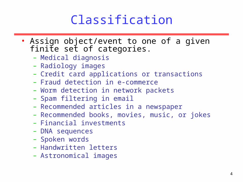
Classification
• Assign object/event to one of a given finite set of categories.– Medical diagnosis– Radiology images– Credit card applications or transactions– Fraud detection in e-commerce– Worm detection in network packets– Spam filtering in email– Recommended articles in a newspaper– Recommended books, movies, music, or jokes– Financial investments– DNA sequences– Spoken words– Handwritten letters– Astronomical images

5
Problem Solving / Planning / Control
• Performing actions in an environment in order to achieve a goal.– Solving calculus problems
– Playing checkers, chess, or backgammon
– Balancing a pole
– Driving a car or a jeep
– Flying a plane, helicopter, or rocket
– Controlling an elevator
– Controlling a character in a video game
– Controlling a mobile robot

6
Measuring Performance
• Classification Accuracy
• Solution correctness
• Solution quality (length, efficiency)
• Speed of performance

7
Why Study Machine Learning?Engineering Better Computing Systems
• Develop systems that are too difficult/expensive to construct manually because they require specific detailed skills or knowledge tuned to a specific task (knowledge engineering bottleneck).
• Develop systems that can automatically adapt and customize themselves to individual users.– Personalized news or mail filter– Personalized tutoring
• Discover new knowledge from large databases (data mining).– Market basket analysis (e.g. diapers and beer)– Medical text mining (e.g. drugs and their adverse effects)

8
Why Study Machine Learning?Cognitive Science
• Computational studies of learning may help us understand learning in humans and other biological organisms.– Hebbian neural learning
• “Neurons that fire together, wire together.”– Human’s relative difficulty of learning disjunctive
concepts vs. conjunctive ones.– Power law of practice
log(# training trials)
log(
perf
. tim
e)

9
Why Study Machine Learning?The Time is Ripe
• Many basic effective and efficient algorithms available.
• Large amounts of on-line data available.
• Large amounts of computational resources available.

10
Related Disciplines
• Artificial Intelligence• Data Mining• Probability and Statistics• Information theory• Numerical optimization• Computational complexity theory• Control theory (adaptive)• Psychology (developmental, cognitive)• Neurobiology• Linguistics• Philosophy
11
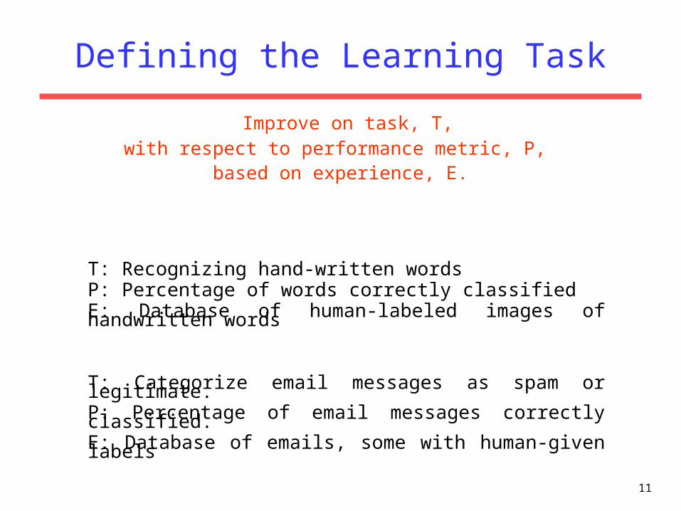
Defining the Learning Task
Improve on task, T, with respect to performance metric, P,
based on experience, E.
T: Recognizing hand-written wordsP: Percentage of words correctly classifiedE: Database of human-labeled images of handwritten words
T: Categorize email messages as spam or legitimate.P: Percentage of email messages correctly classified.E: Database of emails, some with human-given labels

12
Designing a Learning System
• Choose the training experience– Training examples– Features
• Choose exactly what is too be learned, i.e. the target function.• Choose how to represent the target function.• Choose a learning algorithm to infer the target function from
the experience.

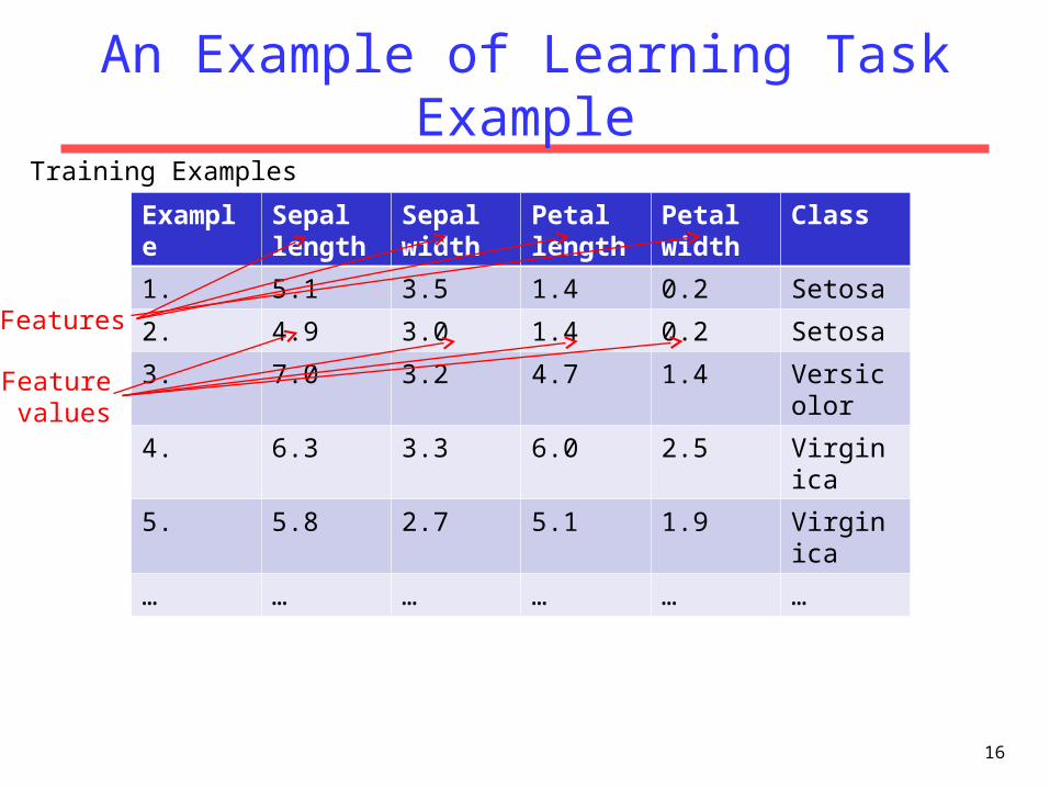
An Example of Learning Task
• Task: Predict the class of Iris plant (Iris Setosa, Iris Versicolor, Iris Vriginica) from the dimensions of its sepals and petals– http://archive.ics.uci.edu/ml/datasets/Iris
• Features: – Sepal length in cm– Sepal width in cm– Petal length in cm– Petal width in cm
• Manually (expert) label some examples which become the training examples
13
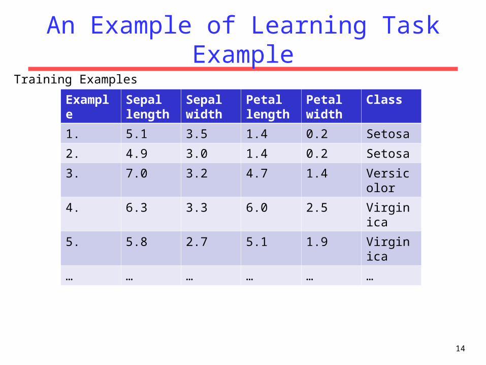
An Example of Learning Task Example
14
Example Sepal length
Sepal width
Petal length
Petal width
Class
1. 5.1 3.5 1.4 0.2 Setosa
2. 4.9 3.0 1.4 0.2 Setosa
3. 7.0 3.2 4.7 1.4 Versicolor
4. 6.3 3.3 6.0 2.5 Virginica
5. 5.8 2.7 5.1 1.9 Virginica
… … … … … …
Training Examples

An Example of Learning Task Example
15
Example Sepal length
Sepal width
Petal length
Petal width
Class
1. 5.1 3.5 1.4 0.2 Setosa
2. 4.9 3.0 1.4 0.2 Setosa
3. 7.0 3.2 4.7 1.4 Versicolor
4. 6.3 3.3 6.0 2.5 Virginica
5. 5.8 2.7 5.1 1.9 Virginica
… … … … … …
Training Examples
Features
An Example of Learning Task Example
16
Example Sepal length
Sepal width
Petal length
Petal width
Class
1. 5.1 3.5 1.4 0.2 Setosa
2. 4.9 3.0 1.4 0.2 Setosa
3. 7.0 3.2 4.7 1.4 Versicolor
4. 6.3 3.3 6.0 2.5 Virginica
5. 5.8 2.7 5.1 1.9 Virginica
… … … … … …
Training Examples
Features
Feature values

An Example of Learning Task Example
17
Example Sepal length
Sepal width
Petal length
Petal width
Class
1. 5.1 3.5 1.4 0.2 Setosa
2. 4.9 3.0 1.4 0.2 Setosa
3. 7.0 3.2 4.7 1.4 Versicolor
4. 6.3 3.3 6.0 2.5 Virginica
5. 5.8 2.7 5.1 1.9 Virginica
… … … … … …
Training Examples
Features
Feature values
Expertlabels

An Example of Learning Task Example
18
Example Sepal length
Sepal width
Petal length
Petal width
Class
1. 5.1 3.5 1.4 0.2 Setosa
2. 4.9 3.0 1.4 0.2 Setosa
3. 7.0 3.2 4.7 1.4 Versicolor
4. 6.3 3.3 6.0 2.5 Virginica
5. 5.8 2.7 5.1 1.9 Virginica
… … … … … …
Training Examples
Test ExamplesExample Sepal
lengthSepal width
Petal length
Petal width
Class
1. 6.4 2.7 5.3 1.9 ??
2. 6.9 3.2 5.7 2.3 ??
3. 5.0 3.3 1.4 0.2 ??
Unknownlabels
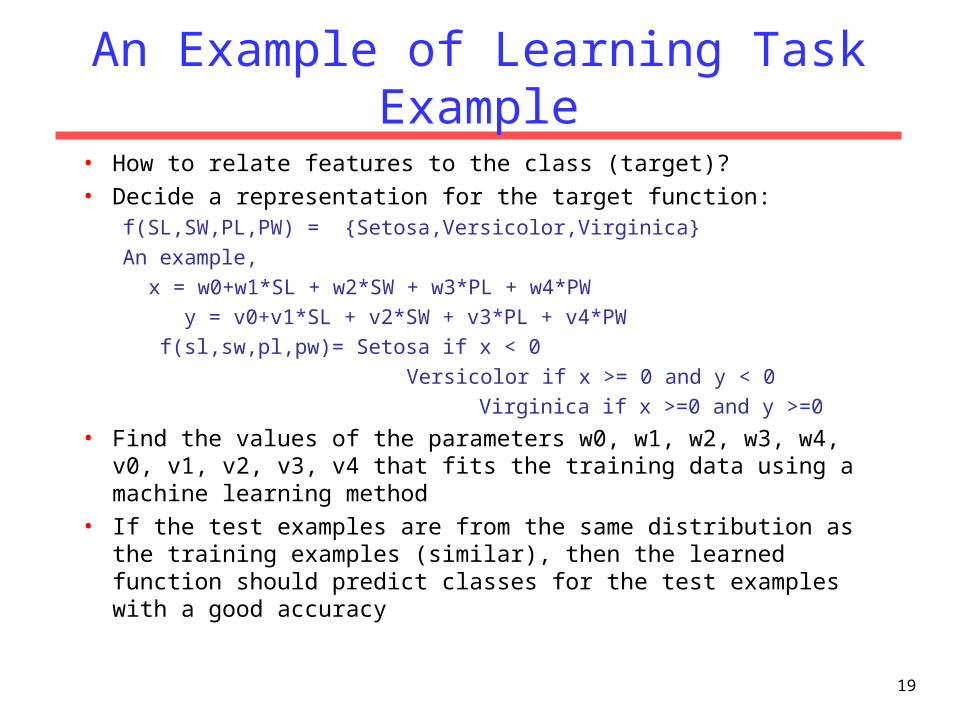
An Example of Learning Task Example
• How to relate features to the class (target)?
• Decide a representation for the target function:f(SL,SW,PL,PW) = {Setosa,Versicolor,Virginica}
An example,
x = w0+w1*SL + w2*SW + w3*PL + w4*PW
y = v0+v1*SL + v2*SW + v3*PL + v4*PW
f(sl,sw,pl,pw)= Setosa if x < 0
Versicolor if x >= 0 and y < 0
Virginica if x >=0 and y >=0
• Find the values of the parameters w0, w1, w2, w3, w4, v0, v1, v2, v3, v4 that fits the training data using a machine learning method
• If the test examples are from the same distribution as the training examples (similar), then the learned function should predict classes for the test examples with a good accuracy
19

Classification and Regression
• Most learning tasks fall under two categories
• Classification: The value to be predicted is a nominal value, for example, class of the plant, positive or negative diagnosis
• Regression: The value to be predicted is a numerical value, for example, stock prices, energy expenditure
• Most machine learning methods have both classification and regression versions
20
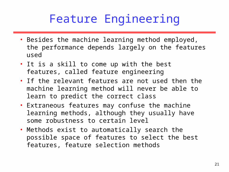
Feature Engineering
• Besides the machine learning method employed, the performance depends largely on the features used
• It is a skill to come up with the best features, called feature engineering
• If the relevant features are not used then the machine learning method will never be able to learn to predict the correct class
• Extraneous features may confuse the machine learning methods, although they usually have some robustness to certain level
• Methods exist to automatically search the possible space of features to select the best features, feature selection methods
21
22
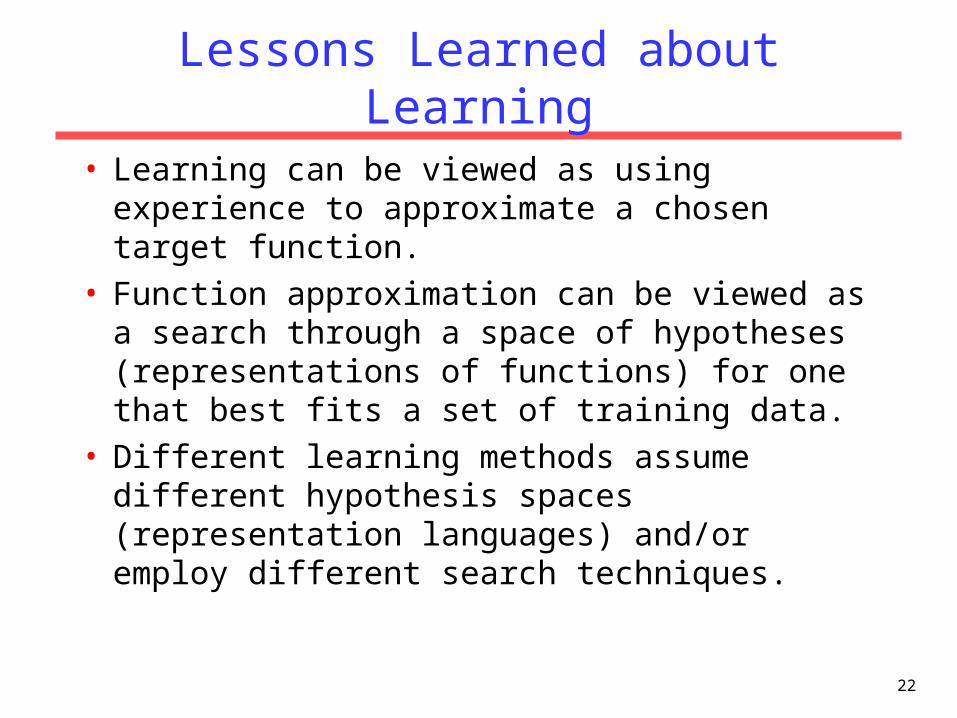
Lessons Learned about Learning
• Learning can be viewed as using experience to approximate a chosen target function.
• Function approximation can be viewed as a search through a space of hypotheses (representations of functions) for one that best fits a set of training data.
• Different learning methods assume different hypothesis spaces (representation languages) and/or employ different search techniques.
23
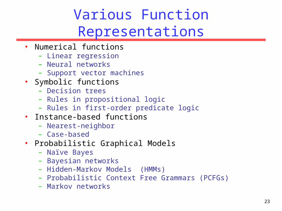
Various Function Representations
• Numerical functions– Linear regression– Neural networks– Support vector machines
• Symbolic functions– Decision trees– Rules in propositional logic– Rules in first-order predicate logic
• Instance-based functions– Nearest-neighbor– Case-based
• Probabilistic Graphical Models– Naïve Bayes– Bayesian networks– Hidden-Markov Models (HMMs)– Probabilistic Context Free Grammars (PCFGs)– Markov networks
24
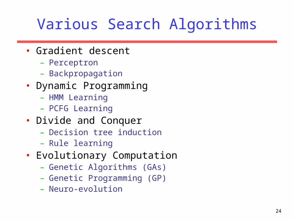
Various Search Algorithms
• Gradient descent– Perceptron– Backpropagation
• Dynamic Programming– HMM Learning– PCFG Learning
• Divide and Conquer– Decision tree induction– Rule learning
• Evolutionary Computation– Genetic Algorithms (GAs)– Genetic Programming (GP)– Neuro-evolution

25
Evaluation of Learning Systems
• Experimental– Conduct controlled cross-validation experiments to
compare various methods on a variety of benchmark datasets.
– Gather data on their performance, e.g. test accuracy, training-time, testing-time.
– Analyze differences for statistical significance.• Theoretical
– Analyze algorithms mathematically and prove theorems about their:
• Computational complexity (how fast the algorithm runs)• Ability to fit training data• Sample complexity (number of training examples needed to
learn an accurate function)

26
History of Machine Learning
• 1950s– Samuel’s checker player– Selfridge’s Pandemonium
• 1960s: – Neural networks: Perceptron– Pattern recognition – Learning in the limit theory– Minsky and Papert prove limitations of Perceptron
• 1970s: – Symbolic concept induction– Winston’s arch learner– Expert systems and the knowledge acquisition bottleneck– Quinlan’s ID3– Michalski’s AQ and soybean diagnosis– Scientific discovery with BACON– Mathematical discovery with AM

27
History of Machine Learning (cont.)
• 1980s:– Advanced decision tree and rule learning– Explanation-based Learning (EBL)– Learning and planning and problem solving– Utility problem– Analogy– Cognitive architectures– Resurgence of neural networks (connectionism, backpropagation)– Valiant’s PAC Learning Theory– Focus on experimental methodology
• 1990s– Data mining– Adaptive software agents and web applications– Text learning– Reinforcement learning (RL)– Inductive Logic Programming (ILP)– Ensembles: Bagging, Boosting, and Stacking– Bayes Net learning

28
History of Machine Learning (cont.)
• 2000s– Support vector machines– Kernel methods– Graphical models– Statistical relational learning– Transfer learning– Sequence labeling– Collective classification and structured outputs– Computer Systems Applications
• Compilers• Debugging• Graphics• Security (intrusion, virus, and worm detection)
– E mail management– Personalized assistants that learn– Learning in robotics and vision
29University of Texas at Austin
Machine Learning Group
Support Vector Machine (SVM)

30University of Texas at Austin
Machine Learning Group
Linear Separators
• Binary classification can be viewed as the task of separating classes in feature space:
wTx + b = 0
wTx + b < 0wTx + b > 0
f(x) = sign(wTx + b)

31University of Texas at Austin
Machine Learning Group
Linear Separators
• Which of the linear separators is optimal?
32University of Texas at Austin
Machine Learning Group
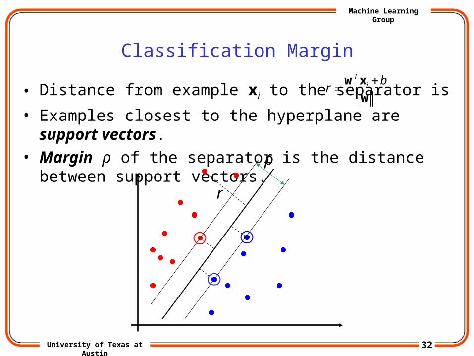
Classification Margin
• Distance from example xi to the separator is
• Examples closest to the hyperplane are support vectors.
• Margin ρ of the separator is the distance between support vectors.
w
xw br i
T
r
ρ
33University of Texas at Austin
Machine Learning Group
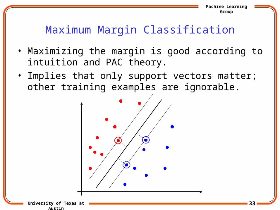
Maximum Margin Classification
• Maximizing the margin is good according to intuition and PAC theory.
• Implies that only support vectors matter; other training examples are ignorable.
34University of Texas at Austin
Machine Learning Group
Linear SVMs Mathematically
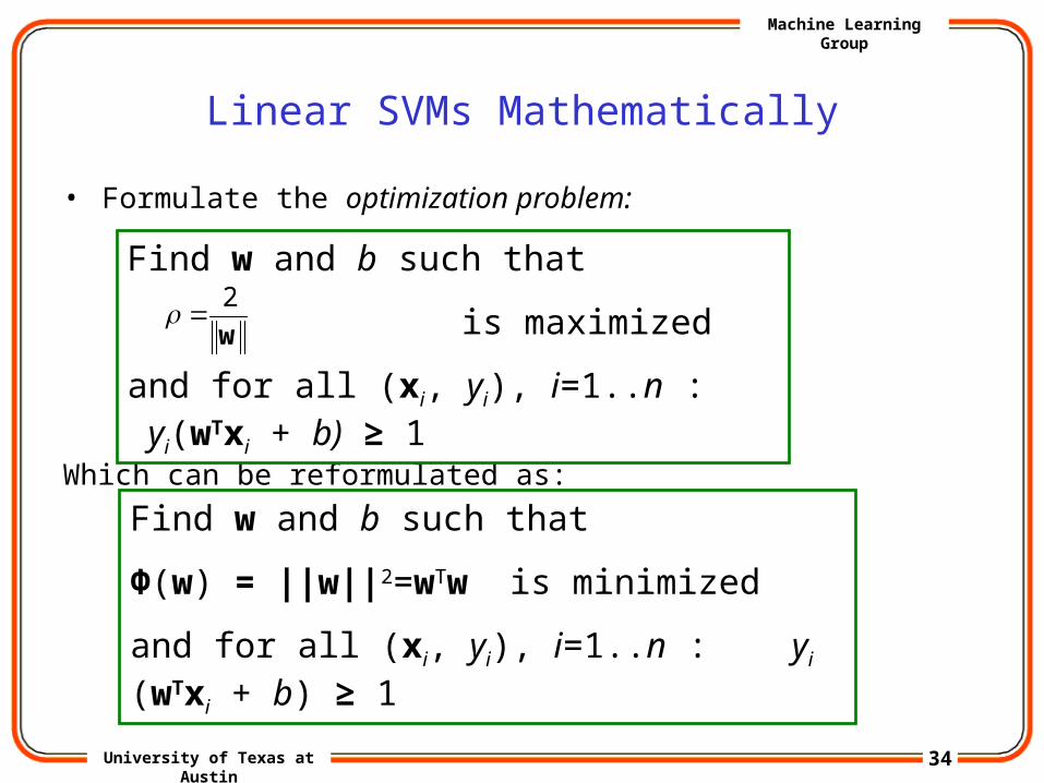
• Formulate the optimization problem:
Which can be reformulated as:
Find w and b such that
is maximized
and for all (xi, yi), i=1..n : yi(wTxi + b) ≥ 1
w
2
Find w and b such that
Φ(w) = ||w||2=wTw is minimized
and for all (xi, yi), i=1..n : yi (wTxi + b) ≥ 1

35University of Texas at Austin
Machine Learning Group
Solving the Optimization Problem
• Need to optimize a quadratic function subject to linear constraints.
• Quadratic optimization problems are a well-known class of mathematical programming problems for which several (non-trivial) algorithms exist.
• The solution involves constructing a dual problem where a Lagrange multiplier αi is associated with every inequality constraint in the primal (original) problem:
Find w and b such thatΦ(w) =wTw is minimized and for all (xi, yi), i=1..n : yi (wTxi + b) ≥ 1
Find α1…αn such that
Q(α) =Σαi - ½ΣΣαiαjyiyjxiTxj is maximized and
(1) Σαiyi = 0(2) αi ≥ 0 for all αi
36University of Texas at Austin
Machine Learning Group
Soft Margin Classification
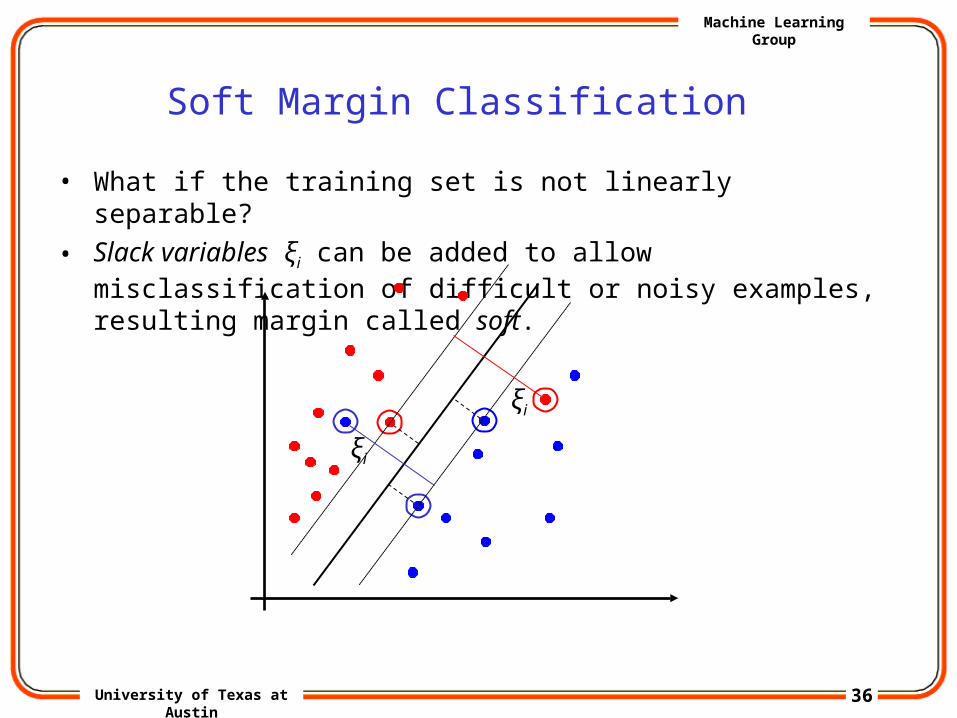
• What if the training set is not linearly separable?
• Slack variables ξi can be added to allow misclassification of difficult or noisy examples, resulting margin called soft.
ξi
ξi
37University of Texas at Austin
Machine Learning Group
Soft Margin Classification Mathematically
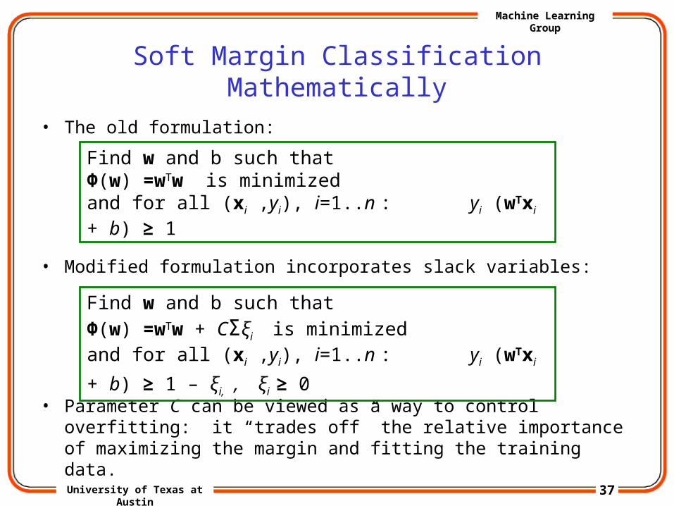
• The old formulation:
• Modified formulation incorporates slack variables:
• Parameter C can be viewed as a way to control overfitting: it “trades off” the relative importance of maximizing the margin and fitting the training data.
Find w and b such thatΦ(w) =wTw is minimized and for all (xi ,yi), i=1..n : yi (wTxi + b) ≥ 1
Find w and b such that
Φ(w) =wTw + CΣξi is minimized
and for all (xi ,yi), i=1..n : yi (wTxi + b) ≥ 1 – ξi, , ξi ≥ 0

38University of Texas at Austin
Machine Learning Group
Linear SVMs: Overview
• The classifier is a separating hyperplane.
• Most “important” training points are support vectors; they define the hyperplane.
• Quadratic optimization algorithms can identify which training points xi are support vectors with non-zero Lagrangian multipliers αi.
• Both in the dual formulation of the problem and in the solution training points appear only inside inner products:
Find α1…αN such that
Q(α) =Σαi - ½ΣΣαiαjyiyjxiTxj is maximized and
(1) Σαiyi = 0(2) 0 ≤ αi ≤ C for all αi
f(x) = ΣαiyixiTx + b
39University of Texas at Austin
Machine Learning Group
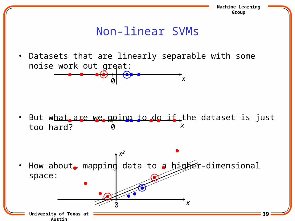
Non-linear SVMs
• Datasets that are linearly separable with some noise work out great:
• But what are we going to do if the dataset is just too hard?
• How about… mapping data to a higher-dimensional space:
0
0
0
x2
x
x
x

40University of Texas at Austin
Machine Learning Group
Non-linear SVMs: Feature spaces
• General idea: the original feature space can always be mapped to some higher-dimensional feature space where the training set is separable:
Φ: x → φ(x)
41University of Texas at Austin
Machine Learning Group
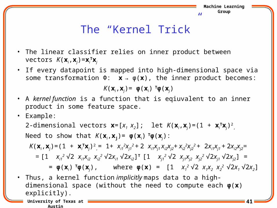
The “Kernel Trick”
• The linear classifier relies on inner product between vectors K(xi,xj)=xiTxj
• If every datapoint is mapped into high-dimensional space via some transformation Φ: x → φ(x), the inner product becomes:
K(xi,xj)= φ(xi) Tφ(xj)
• A kernel function is a function that is eqiuvalent to an inner product in some feature space.
• Example:
2-dimensional vectors x=[x1 x2]; let K(xi,xj)=(1 + xiTxj)2
,
Need to show that K(xi,xj)= φ(xi) Tφ(xj):
K(xi,xj)=(1 + xiTxj)2
,= 1+ xi12xj1
2 + 2 xi1xj1 xi2xj2+ xi2
2xj22 + 2xi1xj1 + 2xi2xj2=
= [1 xi12 √2 xi1xi2 xi2
2 √2xi1 √2xi2]T [1 xj12 √2 xj1xj2 xj2
2 √2xj1 √2xj2] =
= φ(xi) Tφ(xj), where φ(x) = [1 x1
2 √2 x1x2 x22 √2x1 √2x2]
• Thus, a kernel function implicitly maps data to a high-dimensional space (without the need to compute each φ(x) explicitly).

42University of Texas at Austin
Machine Learning Group
Examples of Kernel Functions
• Linear: K(xi,xj)= xiTxj
– Mapping Φ: x → φ(x), where φ(x) is x itself
• Polynomial of power p: K(xi,xj)= (1+ xiTxj)p
– Mapping Φ: x → φ(x), where φ(x) has dimensions
• Gaussian (radial-basis function): K(xi,xj) =– Mapping Φ: x → φ(x), where φ(x) is infinite-dimensional: every point is
mapped to a function (a Gaussian); combination of functions for support vectors is the separator.
• Higher-dimensional space still has intrinsic dimensionality d, but linear separators in it correspond to non-linear separators in original space.
2
2
2ji
exx
p
pd

43University of Texas at Austin
Machine Learning Group
Non-linear SVMs Mathematically
• Dual problem formulation:
• The solution is:
• Optimization techniques for finding αi’s remain the same!
Find α1…αn such that
Q(α) =Σαi - ½ΣΣαiαjyiyjK(xi, xj) is maximized and
(1) Σαiyi = 0(2) αi ≥ 0 for all αi
f(x) = ΣαiyiK(xi, xj)+ b

44University of Texas at Austin
Machine Learning Group
SVM applications
• SVMs were originally proposed by Boser, Guyon and Vapnik in 1992 and gained increasing popularity in late 1990s.
• SVMs are currently among the best performers for a number of classification tasks ranging from text to genomic data.
• SVMs can be applied to complex data types beyond feature vectors (e.g. graphs, sequences, relational data) by designing kernel functions for such data.
• SVM techniques have been extended to a number of tasks such as regression [Vapnik et al. ’97], principal component analysis [Schölkopf et al. ’99], etc.
• Most popular optimization algorithms for SVMs use decomposition to hill-climb over a subset of αi’s at a time, e.g. SMO [Platt ’99] and [Joachims ’99]
• Tuning SVMs remains a black art: selecting a specific kernel and parameters is usually done in a try-and-see manner.
Related Documents