Artifact characterization and removal for in vivo neural recording

Page 1

C

A

Ma

b

h

•••••

a

ARRA

KIANW

1

poeA2

0h

Journal of Neuroscience Methods 226 (2014) 110–123

Contents lists available at ScienceDirect

Journal of Neuroscience Methods

jo ur nal home p age: www.elsev ier .com/ locate / jneumeth

omputational Neuroscience

rtifact characterization and removal for in vivo neural recording

d Kafiul Islama,∗, Amir Rastegarniaa,b, Anh Tuan Nguyena, Zhi Yanga

Department of Electrical and Computer Engineering, National University of Singapore, Singapore 117583, SingaporeDepartment of Electrical Engineering, Malayer University, Malayer 95863-65719, Iran

i g h l i g h t s

We characterize labeled artifacts in neural recording experiments.An algorithm for automatic artifact detection and removal is proposed.A modified universal-threshold value is proposed to make the algorithm robust under different recording conditions.Both real and synthesized data have been used for testing the proposed algorithm in comparison with other available algorithms.Quantitative results show that the proposed algorithm can outperform the others in removing artifacts reliably without distorting neural signals.

r t i c l e i n f o

rticle history:eceived 19 August 2013eceived in revised form 22 January 2014ccepted 23 January 2014

eywords:n vivo neural recordingrtifact characterizationeural signal spectraavelet transform

a b s t r a c t

Background: In vivo neural recordings are often corrupted by different artifacts, especially in a less-constrained recording environment. Due to limited understanding of the artifacts appeared in the invivo neural data, it is more challenging to identify artifacts from neural signal components comparedwith other applications. The objective of this work is to analyze artifact characteristics and to develop analgorithm for automatic artifact detection and removal without distorting the signals of interest.New method: The proposed algorithm for artifact detection and removal is based on the stationary wavelettransform with selected frequency bands of neural signals. The selection of frequency bands is based onthe spectrum characteristics of in vivo neural data. Further, to make the proposed algorithm robust underdifferent recording conditions, a modified universal-threshold value is proposed.Results: Extensive simulations have been performed to evaluate the performance of the proposed algo-rithm in terms of both amount of artifact removal and amount of distortion to neural signals. Thequantitative results reveal that the algorithm is quite robust for different artifact types and artifact-to-signal ratio.Comparison with existing methods: Both real and synthesized data have been used for testing the pro-

posed algorithm in comparison with other artifact removal algorithms (e.g. ICA, wICA, wCCA, EMD-ICA,and EMD-CCA) found in the literature. Comparative testing results suggest that the proposed algorithmperforms better than the available algorithms.Conclusion: Our work is expected to be useful for future research on in vivo neural signal processing andeventually to develop a real-time neural interface for advanced neuroscience and behavioral experiments.

. Introduction

Extracellularly recorded neural data from in vivo experimentsrovide higher spatio-temporal resolution and SNR compared withther non-invasive brain signal recordings; e.g. EEG, MEG, fMRI,

tc. (Eichenbaum, 2001; Foffani and Moxon, 2003; Dayan andbbott, 2005; Lytton, 2002; Mitra and Bokil, 2008; Buzsáki et al.,012). While the recorded data can be corrupted by artifacts and

∗ Corresponding author. Tel.: +65 93986197.E-mail addresses: kafiul [email protected], [email protected] (M.K. Islam).

165-0270/$ – see front matter © 2014 Elsevier B.V. All rights reserved.ttp://dx.doi.org/10.1016/j.jneumeth.2014.01.027

© 2014 Elsevier B.V. All rights reserved.

interferences, especially under a less constrained recording proto-col. Hence as a part of neural data preprocessing procedure, thedetection and removal of artifacts without distorting the signals ofinterest play an important role. Compared with other applications,artifact detection and removal for in vivo neural recordings havethe following application related challenges:

• The signal characteristics: Many other physiological signal

recordings mostly contain narrow-band neural data (e.g. band-widths of EEG, ECG, and EMG in general range from sub Hz tono more than a few hundred Hz); while in vivo neural recordingshave a broad spectral band, i.e. from sub-1 Hz to several kHz. Thus,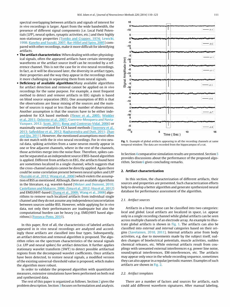

Page 2

oscience Methods 226 (2014) 110–123 111

•

•

aiar(srhot

ma

p

M.K. Islam et al. / Journal of Neur

spectral overlapping between artifacts and signals of interest forin vivo recordings is larger. Apart from the wide bandwidth, thepresence of different signal components (i.e. Local Field Poten-tials (LFP), neural spikes, synaptic activities, etc.) and their highlynon-stationary properties (Tomko and Crapper, 1974; Lewicki,1998; Kaneko and Suzuki, 2007; Bar-Hillel and Spiro, 2005) com-pared with other recordings, make it more difficult for identifyingartifacts.The artifact characteristics: When dealing with other physiolog-ical signals, often the appeared artifacts have certain stereotypewaveforms or the artifact source itself can be recorded by a ref-erence channel. This is not the case for in vivo neural recordings.In fact, as it will be discussed later, the diversity in artifact types,their properties and the way they appear in the recordings makeit more challenging in separating them from neural signals.Deficiency of available algorithms:Many available algorithmsfor artifact detection and removal cannot be applied on in vivorecordings for the same purpose. For example, a most frequentmethod to detect and remove artifacts in EEG signals is basedon blind source separation (BSS). One assumption of BSS is thatthe observations are linear mixing of the sources and the num-ber of sources is equal or less than the number of observations.Another assumption is that the sources have to be either inde-pendent for ICA based methods (Flexer et al., 2005; Winkleret al., 2011; Delorme et al., 2007; Guerrero-Mosquera and Navia-Vazquez, 2012; Scott, 2011; Rong and Contreras-Vidal, 2006) ormaximally uncorrelated for CCA based methods (Sweeney et al.,2013; Safieddine et al., 2012; Raghavendra and Dutt, 2011; Zhaoand Qiu, 2011). However, the mentioned assumptions most oftendo not match with the in vivo neural recordings. For in vivo neu-ral data, spiking activities from a same neuron mostly appear inone or few adjacent channels, where in the rest of the channels,those activities merge into the noise floor. Therefore, spikes can-not be separated as an independent source if BSS-based algorithmis applied. Different from artifacts in EEG, the artifacts found hereare sometimes localized in a single channel, which suggests thatthe cross-channel analysis cannot be directly applied. Again therecould be some correlation present between neural spikes and LFP(Buzsáki et al., 2012; Wang et al., 2006) which violets the assump-tion of BSS as mentioned. Although, there are available algorithmsin the literature, e.g. wavelet-based (Molavi and Dumont, 2010;Castellanos and Makarov, 2006; Zima et al., 2012; Hsu et al., 2012)and EMD/HHT-based (Zhang et al., 2009; Wang et al., 2008) algo-rithms to remove such localized artifacts from individual singlechannel and they do not assume any independence/uncorrelationbetween sources unlike BSS. However, while applying for in vivodata, not only their performances are inadequate but also thecomputational burden can be heavy (e.g. EMD/HHT based algo-rithms) (Fonseca-Pinto, 2010).

In this paper, first of all, the characteristics of labeled artifactsppeared in in vivo neural recordings are analyzed and accord-ngly those artifacts are classified into four types. Subsequently,n artifact detection and removal algorithm is proposed. The algo-ithm relies on the spectrum characteristics of the neural signalsi.e. LFP and neural spikes) for artifact detection. It further appliestationary wavelet transform (SWT) to detect possible artifactualegions from the decomposed wavelet coefficients. Once artifactsave been detected, to restore neural signals, a modified versionf the existing universal-threshold value is proposed, which makeshe algorithm more robust.

In order to validate the proposed algorithm with quantitative

easures, extensive simulations have been performed on both real

nd synthesized data.The rest of this paper is organized as follows. Section 2 gives the

roblem description. Section 3 focuses on formulation and analysis.

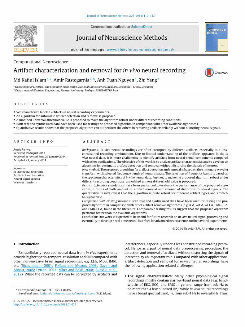
Fig. 1. Example of global artifacts appearing in all the recording channels at sametemporal window. The data are recorded from the hippocampus of a rat.

In Section 4 comparative simulation results are presented. Section 5provides discussions about the performance of the proposed algo-rithm. Section 6 gives concluding remarks.

2. Artifact characterization

In this section, the characterization of different artifacts, theirsources and properties are presented. Such characterization effortshelp to develop a better algorithm and generate synthesized neuraldatabase for performance assessment of the algorithm.

2.1. Artifact sources

Artifacts in a broad sense can be classified into two categories:local and global. Local artifacts are localized in space, i.e. appearonly in a single recording channel while global artifacts can be seenacross multiple channels of an electrode array. An example to illus-trate global artifacts is shown in Fig. 1. The artifacts can also beclassified into external and internal categories based on their ori-gins (Savelainen, 2010, 2011). Internal artifacts arise from bodyactivities, e.g. due to movements made by the subject itself, sud-den changes of bioelectrical potentials, muscle activities, suddenchemical releases, etc. While external artifacts result from cou-plings with unwanted external interferences e.g. power line noise,sound/optical interferences, EM-interferences, etc. The artifactsmay appear only once in the whole recording sequence, sometimesthey can also appear in a regular/periodic manner. Examples of suchartifacts are shown in Fig. 2.

2.2. Artifact templates

There are a number of factors and sources for artifacts, eachcould add different waveform signatures. After manual labeling,

Page 3

112 M.K. Islam et al. / Journal of Neuroscien

Fzh

tbwd

riad

ttdtn

ig. 2. Illustration of rarely appeared (top) and periodic (bottom) artifacts withoom-in view on the right side. The appeared data have been recorded from theippocampus of a rat.

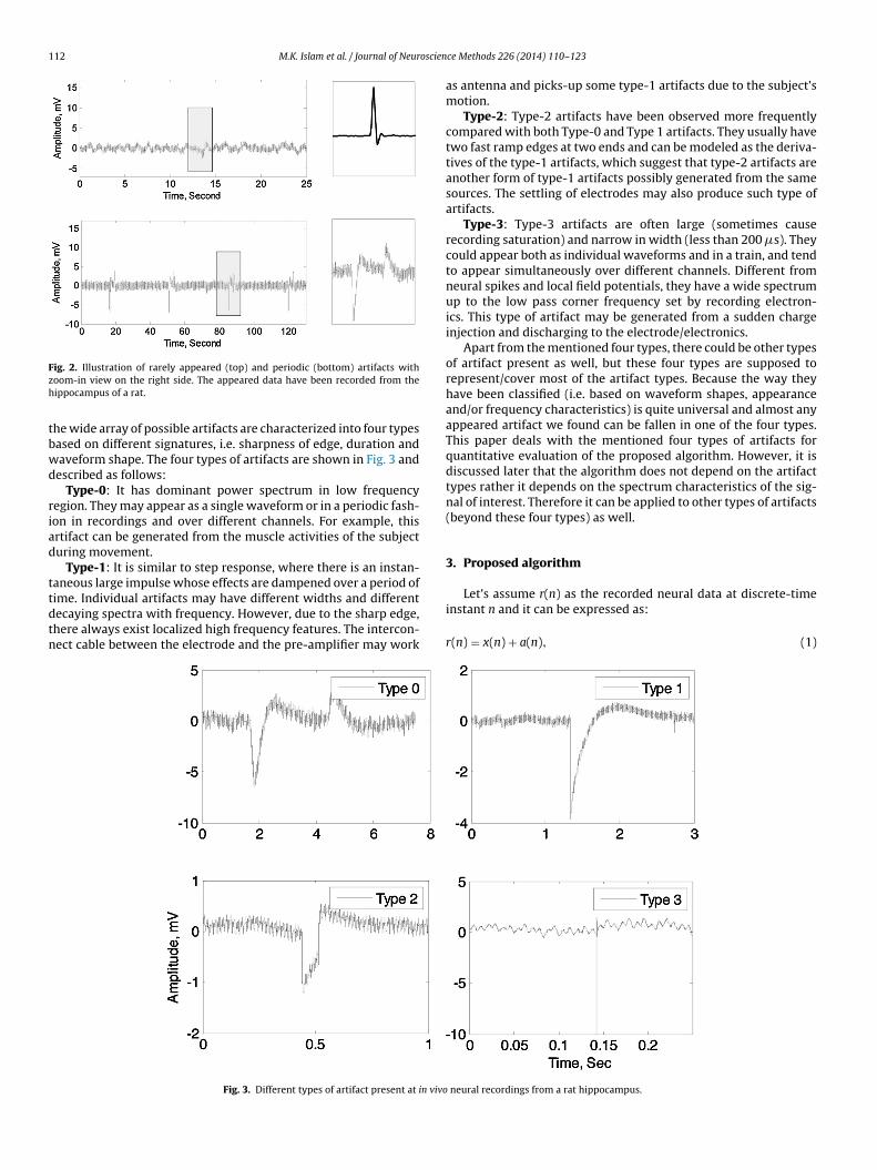
he wide array of possible artifacts are characterized into four typesased on different signatures, i.e. sharpness of edge, duration andaveform shape. The four types of artifacts are shown in Fig. 3 andescribed as follows:

Type-0: It has dominant power spectrum in low frequencyegion. They may appear as a single waveform or in a periodic fash-on in recordings and over different channels. For example, thisrtifact can be generated from the muscle activities of the subjecturing movement.

Type-1: It is similar to step response, where there is an instan-aneous large impulse whose effects are dampened over a period of

ime. Individual artifacts may have different widths and differentecaying spectra with frequency. However, due to the sharp edge,here always exist localized high frequency features. The intercon-ect cable between the electrode and the pre-amplifier may work

Fig. 3. Different types of artifact present at in vivo

ce Methods 226 (2014) 110–123

as antenna and picks-up some type-1 artifacts due to the subject’smotion.

Type-2: Type-2 artifacts have been observed more frequentlycompared with both Type-0 and Type 1 artifacts. They usually havetwo fast ramp edges at two ends and can be modeled as the deriva-tives of the type-1 artifacts, which suggest that type-2 artifacts areanother form of type-1 artifacts possibly generated from the samesources. The settling of electrodes may also produce such type ofartifacts.

Type-3: Type-3 artifacts are often large (sometimes causerecording saturation) and narrow in width (less than 200 �s). Theycould appear both as individual waveforms and in a train, and tendto appear simultaneously over different channels. Different fromneural spikes and local field potentials, they have a wide spectrumup to the low pass corner frequency set by recording electron-ics. This type of artifact may be generated from a sudden chargeinjection and discharging to the electrode/electronics.

Apart from the mentioned four types, there could be other typesof artifact present as well, but these four types are supposed torepresent/cover most of the artifact types. Because the way theyhave been classified (i.e. based on waveform shapes, appearanceand/or frequency characteristics) is quite universal and almost anyappeared artifact we found can be fallen in one of the four types.This paper deals with the mentioned four types of artifacts forquantitative evaluation of the proposed algorithm. However, it isdiscussed later that the algorithm does not depend on the artifacttypes rather it depends on the spectrum characteristics of the sig-nal of interest. Therefore it can be applied to other types of artifacts(beyond these four types) as well.

3. Proposed algorithm

Let’s assume r(n) as the recorded neural data at discrete-timeinstant n and it can be expressed as:

r(n) = x(n) + a(n), (1)

neural recordings from a rat hippocampus.

Page 4

M.K. Islam et al. / Journal of Neuroscience Methods 226 (2014) 110–123 113

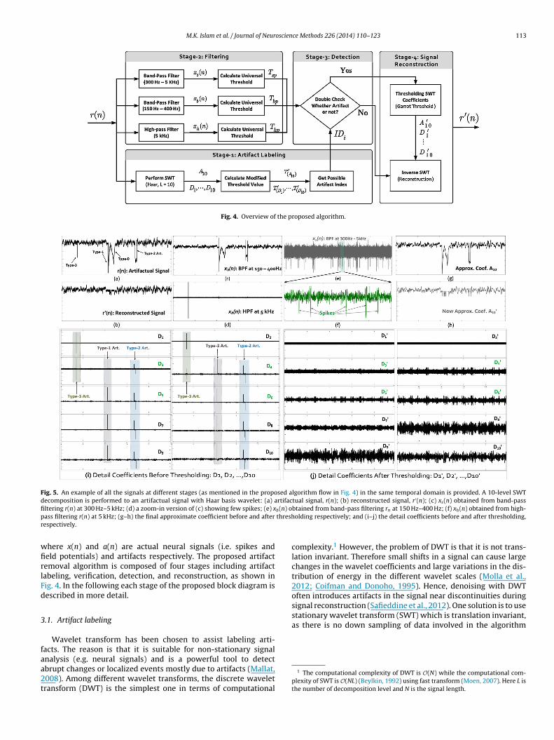
Fig. 4. Overview of the proposed algorithm.

Fig. 5. An example of all the signals at different stages (as mentioned in the proposed algorithm flow in Fig. 4) in the same temporal domain is provided. A 10-level SWTdecomposition is performed to an artifactual signal with Haar basis wavelet: (a) artifactual signal, r(n); (b) reconstructed signal, r′(n); (c) xs(n) obtained from band-passfi b(n) op threshr

wfirlFd

3

faa2t

stationary wavelet transform (SWT) which is translation invariant,as there is no down sampling of data involved in the algorithm

ltering r(n) at 300 Hz–5 kHz; (d) a zoom-in version of (c) showing few spikes; (e) xass filtering r(n) at 5 kHz; (g–h) the final approximate coefficient before and afterespectively.

here x(n) and a(n) are actual neural signals (i.e. spikes andeld potentials) and artifacts respectively. The proposed artifactemoval algorithm is composed of four stages including artifactabeling, verification, detection, and reconstruction, as shown inig. 4. In the following each stage of the proposed block diagram isescribed in more detail.

.1. Artifact labeling

Wavelet transform has been chosen to assist labeling arti-acts. The reason is that it is suitable for non-stationary signal

nalysis (e.g. neural signals) and is a powerful tool to detectbrupt changes or localized events mostly due to artifacts (Mallat,008). Among different wavelet transforms, the discrete waveletransform (DWT) is the simplest one in terms of computational

btained from band-pass filtering rn at 150 Hz–400 Hz; (f) xh(n) obtained from high-olding respectively; and (i–j) the detail coefficients before and after thresholding,

complexity.1 However, the problem of DWT is that it is not trans-lation invariant. Therefore small shifts in a signal can cause largechanges in the wavelet coefficients and large variations in the dis-tribution of energy in the different wavelet scales (Molla et al.,2012; Coifman and Donoho, 1995). Hence, denoising with DWToften introduces artifacts in the signal near discontinuities duringsignal reconstruction (Safieddine et al., 2012). One solution is to use

1 The computational complexity of DWT is O(N) while the computational com-plexity of SWT is O(NL) (Beylkin, 1992) using fast transform (Moen, 2007). Here L isthe number of decomposition level and N is the signal length.

Page 5

114 M.K. Islam et al. / Journal of Neuroscience Methods 226 (2014) 110–123

Table 1The frequency bands of the respective SWT coefficients and corresponding signal components for a 10-level decomposition. Here two typical sampling frequencies forextracellular neural recordings are considered (i.e. 40 kHz and 30 kHz) and the maximum recording bandwidth is assumed to be half of the sampling frequency.

(2

3

waaTcfisncdcp0ifitdsod

3

fdose

T

wfe

˛

Il

tsrdpads

Molla et al., 2012; Coifman and Donoho, 1995; Safieddine et al.,012).

.1.1. SWT decompositionThe SWT is performed on the artifactual signal r(n) at level L = 10

ith Haar as basis wavelet function.2 Thus, two types of coefficientsre generated: approximate and detail coefficients that contain lownd high frequency information respectively as shown in Fig. 5.he generated wavelet coefficients at different levels denote theorrelation coefficients between artifactual signal and the waveletunction. The artifactual events will have larger coefficient valuesf they have higher correlation with the wavelet function whilemaller coefficients will be generated corresponding to the actualeural activities. In order to perform thresholding, the selectedoefficients are the final approximate coefficient, A10 and all theetail coefficients i.e. D1, . . ., D10. A10 consists of all low frequencyomponents (from 0 Hz to 19.5 Hz), such as electrode offset, someart of information from LFPs, neuron noise and artifacts (e.g. type-, type-1 and type-2). While, D1, . . ., D10 contain the high frequency

nformation such as neural spikes, type-3 artifacts and sharp edgesrom artifacts of type-1 or type-2. A plot is shown in Table 1 tollustrate the frequency bands of different level of coefficients andhe corresponding neural signal bands. It reveals that even in theecomposed coefficients, the artifacts can overlap with the neuralignals of interest. Therefore the threshold is chosen carefully inrder to detect and suppress possible artifactual activities from theecomposed coefficients.

.1.2. Threshold calculationThe next step is to calculate a threshold value to detect the arti-

acts in the wavelet domain. The choice of threshold value willecide both the amount of artifact suppression and the amountf distortion to the neural signal at the same time. One possibleolution is to use the universal threshold proposed by (Safieddinet al., 2012) which is given as follows:

j = ˛j

√2 ln N, (2)

here N is the signal length and ˛j is the estimated noise varianceor Wj which is usually calculated by following formula (Safieddinet al., 2012)

= median(|Wj|). (3)

j 0.6745

n (3) Wj is the wavelet coefficients at the jth decompositionevel (Wj = Aj for approximation coefficient and, Wj = Dj for detail

2 A majority of motion artifacts appear in the form of abrupt changes in the ampli-ude of the signal. Therefore, Haar is used as basis wavelet since due to its waveformhape, it can possibly detect and localize such artifactual events and they appear withelatively high amplitudes in the decomposed coefficients. The choice of level-10ecomposition is done empirically by considering two facts: (i) the no. of signal com-onents present in the raw recordings and (ii) the trade-off between latency/storagend amount of detail information extraction. Less than level-10 would give lessetail information and more than level-10 would consume unnecessary time andtorage.

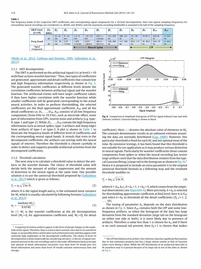
Fig. 6. Comparison in amplitude histogram of LFP for signal without (top) and with(bottom) artifacts. Gaussian fitting is shown in black.

coefficient). Here, | · | denotes the absolute value of elements in Wj.The constant denominator results in an unbiased estimate assum-ing the data are normally distributed (Gao, 1998). However, thisparticular threshold is fixed for each Wj and not optimal most of thetime. By extensive testings, it has been found that this threshold isnot suitable for our application as it may produce serious distortionto neural signals. Particularly for wavelet coefficients those containcomponents from spikes or when the neural recording has severelarge artifacts such that the data distribution violates from the typi-cal Gaussian fitting (a large tail in the histogram as shown in Fig. 6).3

Hence it is proposed to include an extra parameter k to the originaluniversal threshold formula in a following way and the resultantthreshold modifies to

T ′j = k˛j

√2 ln N, (4)

where k = {kA, kD}, 0 < kA < 1, 1 < kD < 5, which comes from the empir-ical observations (see Appendix A). More precisely, k = kA is selectedfor thresholding approximate coefficient at final level, here it is A10and select k = kD to threshold all the detail coefficients (Dj, j = 1, 2,. . ., 10).

The tuning of parameter kA depends on the data distributionas shown in Fig. 6. Since A10 contains both the LFP and some low-frequency artifacts, so when the histogram of the data has largedeviation from the standard deviation (large tail on the histogramon either one side or both), it is more likely due to presence ofartifacts. Therefore a value less than 1 is chosen for kA and if thereis no such unusual tail present, then kA = 1 is chosen that makes

3 The LFP distribution of an artifact-free reference data has significant fluctuationsdue to non-stationary property but has a shape almost similar to that of Gaussianwhen curve fitting is done. While the LFP distribution of an artifactual data fails tofit anywhere near to Gaussian because of its large tail at one of the sides as shownin Fig. 6.

Page 6

oscien

tT

k

wbttf

c4niwo

k

wppsnt

3

crrunbppb5ra

fixat

T

auf

3

to

M.K. Islam et al. / Journal of Neur

he threshold exactly same as the original universal threshold, i.e.′i= T1. The criterion for the choice of kA is given below:

A ={

1 if max(|A10|) > m × sd(A10),

0 ≤ kA < 1 otherwise,(5)

here sd denotes the standard deviation of A10. The value of m isased on the parameter tuning and can be obtained from some ini-ial several seconds of incoming raw in vivo data samples to updatehe threshold value. From the empirical studies, the value of m isound as minimum of 5, i.e. 5< m < ∞ (see Appendix A).

In order to decide the value of kD, power spectra of all detailoefficients are studied and it is found that coefficients at level 3,, 5 and 6, i.e. D3, D4, D5 and D6 have highest power around theeural spikes’ spectra and hence these three level contains spike

nformation along with artifacts. Therefore it is chosen to put moreeight (kD > 1) on these coefficients and less on the rest of the level

f coefficients (i.e. D1, D2, D3, D7, D8, D9 and D10) as follows:

D ={

1 < ki ≤ 5 i = 3, 4, 5 and 6,

1 otherwise,(6)

here i denotes the detail decomposition level and the constantarameter kD is chosen from the spike data histogram. The spikesresent in neural data with very large amplitudes influence theelection of kD towards higher value while if the spike amplitude isormal, then from empirical studies it is found that the value of kD

o be 2–3.

.2. Filtering

Once the time indices are obtained from the decomposedoefficients after applying modified threshold function, T ′

i; it is

equired to double check possible artifactual segments to sepa-ate artifacts from signals of interest, especially from spikes. These of filtering is inspired from the spectrum characteristics ofeural signal components: LFP and spikes. Although the spectraland of in vivo recordings has a wide spectrum, there are tworospective bands, i.e. 150–400 Hz and >5 kHz, where both LFPower and spike power are relatively low (Islam et al., 2012). Thus,and pass and high pass filtering are performed at 150–400 Hz and

kHz, respectively, for artifact detection. It is assumed here that theecording do not contain ripple band oscillations, which appearsround 100–300 Hz, is ignored (Molle et al., 2006).

In order to detect spikes, the raw data is usually band-passltered from 300 Hz to 5 kHz (Belitski et al., 2008). Denoted byb(n), xh(n) and xs(n) as the band-pass filtered, high-pass filterednd spike signals respectively and their corresponding universalhreshold values are calculated by:

bp,hp,sp =(

median(|xb,h,s|)0.6745

)√2 ln N, (7)

These threshold values Tbp, Thp and Tsp with the time indices ofrtifactual segments (provided by artifact labeling stage 3.1) aresed to make the decision of whether artifacts or signals (stage 2rom Fig. 4).

.3. Detection

Denote IDi the time index for artifactual segment at decomposi-ion level i found from the earlier stage, the condition for separationf artifact from neural signals is given by the following pseudo code:

ce Methods 226 (2014) 110–123 115

Separation of artifacts from signals

If (|xb(IDi)| < Tbp) or (|xh(IDi)| < Thp)If (|xs(IDi)| > Tsp)

IDi is not artifact indexelse

IDi is artifact indexend

elseIDi is artifact index

end

3.4. Signal reconstruction

In the final stage, in order to reconstruct the signal, at first thecoefficients are thresholded once it is confirmed as artifacts fromstage-3. Thus a new set of coefficients, i.e. A′

10, and D′1, . . ., D′

10are generated. Finally, inverse stationary wavelet transform isapplied to the new coefficients to restore artifact-reduced neuralsignals.

The choice of threshold function is very important, as it influ-ences the amount of attenuation to the SWT coefficients. A mostpopular thresholding function is hard threshold that has a dis-continuity which may produce large variance to the reconstructedsignal or in other words, output estimate is very sensitive to smallchanges in the input data (Gao, 1998). On the other hand, thereis soft threshold function that is continuous but has larger biasin the estimated signal which results in larger errors. In order toovercome the disadvantages of these two threshold functions, thenon-negative garrote shrinkage function is proposed in (Gao, 1998)which is a nice trade-off between hard and soft threshold functionand is given by:

ıGi=

⎧⎨⎩

0 |x| ≤ T ′i

x − T ′i2

x|x| > T ′

i.

(8)

where ıGiis the garrote threshold function at each decomposi-

tion level of i. This function is less sensitive to input change, lowerbias and more importantly continuous. Therefore garrote thresholdfunction is chosen for our application.

4. Experiments

To validate the proposed algorithm, extensive testings havebeen performed on both real and synthesized data to facilitate bothqualitative and quantitative measurements and compared withother algorithms in the literature. The data recording protocol isdescribed below:

Neural recording data from in vivo preparations are providedby Edward Keefer at Plexon Inc./University of Texas SouthwestMedical Institute and Victor Pikov at Huntington Medical ResearchInstitute. For Keefer’s data, the protocols are similar to (Keeferet al., 2008; Yang et al., 2009), where the subjects (rats) have beenanesthetized for acute experiments. CNT electrodes, microwire,and electrode array have been used in experiments and connectedto Plexon OmniPlex neural data acquisition system. For Pikov’sdata: the 16-channel electrode arrays with a nominal geomet-ric area of exposed electrode tips were purchased from BlackrockMicrosystems. The array was chronically implanted in the sensori-motor cortex and connected to a percutaneous connector mountedin the animal’s (monkey) head. The experiment protocols are inaccordance with the Institutional Animal Care and in compliance

with the United States Department of Agriculture (USDA) Ani-mal Welfare Act. We have been authorized by Edward Keefer andVictor Pikov to utilize the recorded data for research and publica-tion.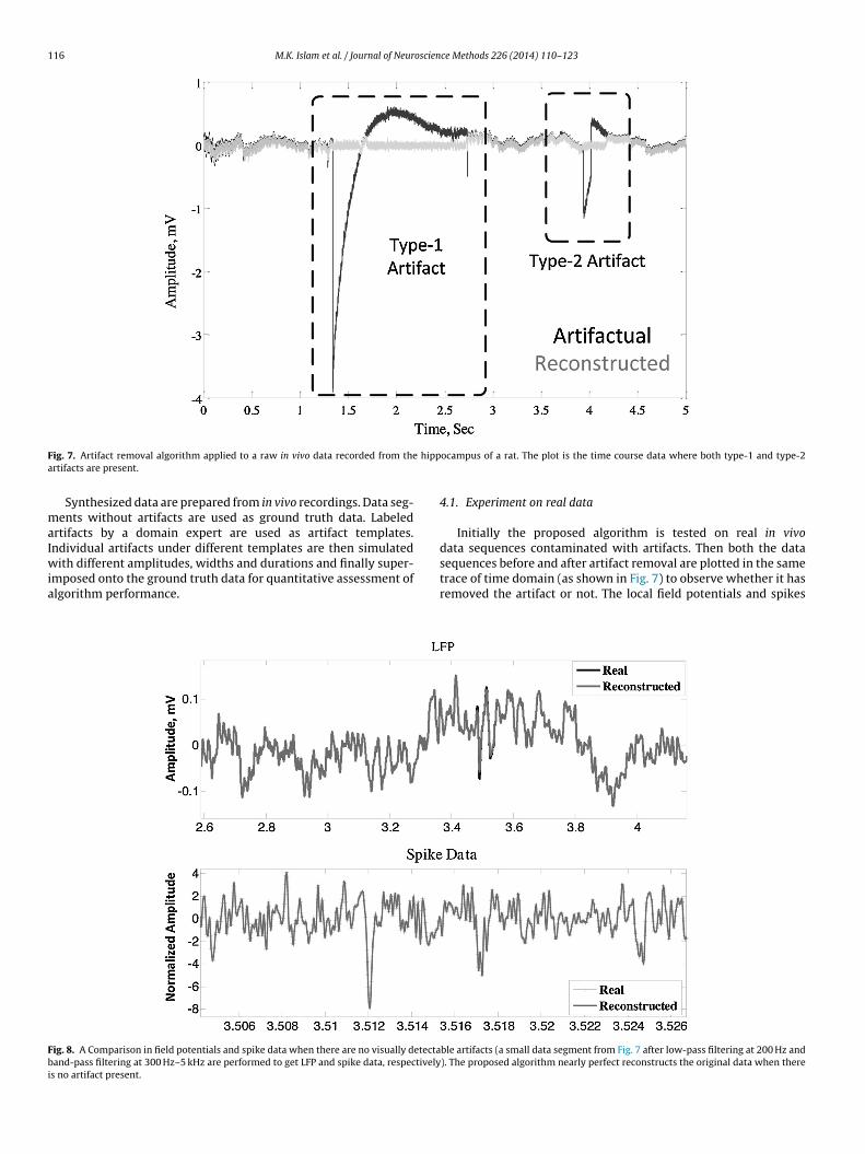

Page 7

116 M.K. Islam et al. / Journal of Neuroscience Methods 226 (2014) 110–123

F hippa

maIwia

Fbi

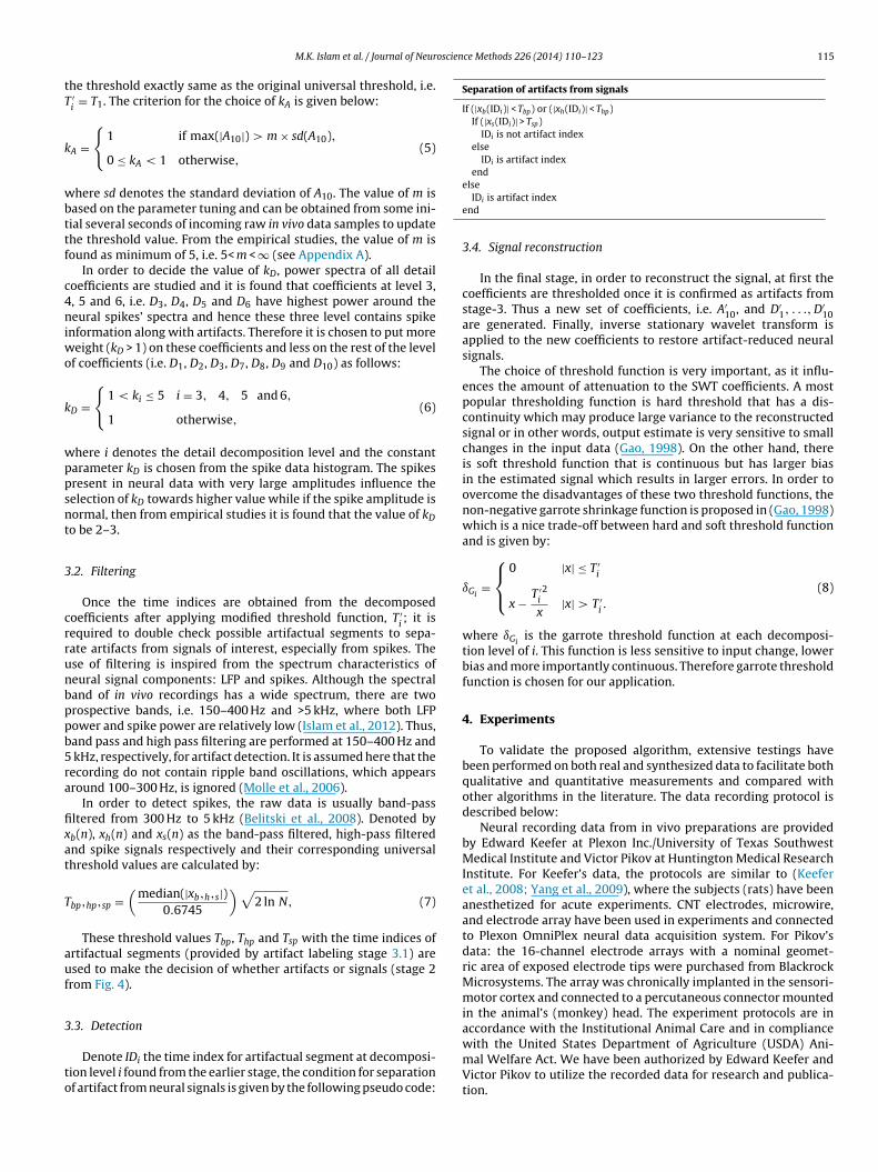
ig. 7. Artifact removal algorithm applied to a raw in vivo data recorded from thertifacts are present.

Synthesized data are prepared from in vivo recordings. Data seg-ents without artifacts are used as ground truth data. Labeled

rtifacts by a domain expert are used as artifact templates.ndividual artifacts under different templates are then simulated

ith different amplitudes, widths and durations and finally super-mposed onto the ground truth data for quantitative assessment oflgorithm performance.

ig. 8. A Comparison in field potentials and spike data when there are no visually detectaand-pass filtering at 300 Hz–5 kHz are performed to get LFP and spike data, respectively

s no artifact present.

ocampus of a rat. The plot is the time course data where both type-1 and type-2

4.1. Experiment on real data

Initially the proposed algorithm is tested on real in vivodata sequences contaminated with artifacts. Then both the data

sequences before and after artifact removal are plotted in the sametrace of time domain (as shown in Fig. 7) to observe whether it hasremoved the artifact or not. The local field potentials and spikes

ble artifacts (a small data segment from Fig. 7 after low-pass filtering at 200 Hz and). The proposed algorithm nearly perfect reconstructs the original data when there

Page 8

M.K. Islam et al. / Journal of Neuroscience Methods 226 (2014) 110–123 117

a(p

4

(dotpinertcdatetar

4

irbiaiamsmqdRbs

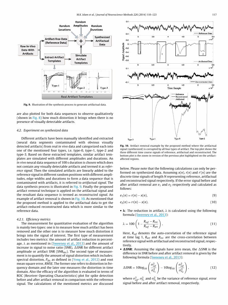
Fig. 10. Artifact removal example by the proposed method where the artifactualsignal (synthesized) is corrupted by all four types of artifact. The top plot shows the

Fig. 9. Illustration of the synthesis process to generate artifactual data.

re also plotted for both data sequences to observe qualitativelyshown in Fig. 8) how much distortion it brings when there is noresence of visually detectable artifacts.

.2. Experiment on synthesized data

Different artifacts have been manually identified and extractedneural data segments contaminated with obvious visuallyetected artifacts) from real in vivo data and categorized each intone of the mentioned four types, i.e. type-0, type-1, type-2 andype-3. Based on these extracted templates, similar artifact tem-lates are simulated with different amplitudes and durations. An

n vivo neural data sequence of 100 s duration is chosen which doesot contain any visually detectable artifacts and termed it as refer-nce signal. Then the simulated artifacts are linearly added to theeference signal in different random positions with different ampli-udes, edge widths and durations to form a data sequence that isontaminated with artifacts, it is referred to artifactual signal. Theata synthesis process is illustrated in Fig. 9. Finally the proposedrtifact removal technique is applied on the artifactual signal andhe resultant data sequence is termed as reconstructed signal. Anxample of artifact removal is shown in Fig. 10. As mentioned thathe proposed method is applied to the artifactual data to get thertifact-reduced reconstructed data which is more similar to theeference data.

.2.1. Efficiency metricsThe measurement for quantitative evaluation of the algorithm

s mainly two types: one is to measure how much artifact has beenemoved and the other one is to measure how much distortion itrings into the signal of interest. The first type of measurement

ncludes two metrics: the amount of artifact reduction in percent-ge, � as mentioned in (Sweeney et al., 2013) and the amount ofncrease in signal to noise ratio (SNR), �SNR for different artifactmplitude or artifact SNR (SNRArt). The second type of measure-ent is to quantify the amount of signal distortion which includes:

pectral distortion, Pdis as defined in (Yong et al., 2012) and rootean square error, RMSE. The former one refers to distortion in fre-

uency domain and the later one measures the distortion in time

omain. Also the efficacy of the algorithm is evaluated in terms ofOC (Receiver Operating Characteristics) plot for spike detectionefore and after artifact removal in comparison with the referenceignal. The calculations of the mentioned metrics are discussed

three different time course signals of reference, artifactual and reconstructed. Thebottom plot is the zoom-in version of the previous plot highlighted on the artifact-affected regions.

below. Please note that the following calculations can only be per-formed on synthesized data. Assuming x(n), r(n) and r′(n) are thediscrete time signals of length N representing reference, artifactualand reconstructed signal respectively. If the error signal before andafter artifact removal are e1 and e2 respectively and calculated asfollows:

e1(n) = r(n) − x(n), (9)

e2(n) = r′(n) − x(n). (10)

• �: The reduction in artifact, � is calculated using the followingformula (Sweeney et al., 2013):

� = 100

(1 − Rref − Rrec

Rref − Rart

), (11)

Here, Rref denotes the auto-correlation of the reference signalat time lag 1, Rart and Rrec are the cross-correlation betweenreference signal with artifactual and reconstructed signal, respec-tively.

• �SNR: Assuming the signals have zero mean, the �SNR is thedifference in SNR before and after artifact removal is given by thefollowing formula (Sweeney et al., 2013):

�SNR = 10log10

(�2

ref

�2

)− 10log10

(�2

ref

�2

), (12)

e1 e2

where �2ref

, �2e1

and �2e2

be the variance of reference signal, errorsignal before and after artifact removal, respectively.

Page 9

1 oscience Methods 226 (2014) 110–123

•

•

•

•

•

•

5

5

(doiptctwl

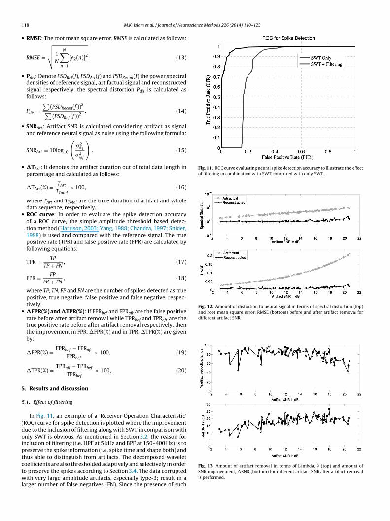
Fig. 11. ROC curve evaluating neural spike detection accuracy to illustrate the effectof filtering in combination with SWT compared with only SWT.

Fig. 12. Amount of distortion to neural signal in terms of spectral distortion (top)and root mean square error, RMSE (bottom) before and after artifact removal fordifferent artifact SNR.

18 M.K. Islam et al. / Journal of Neur

RMSE: The root mean square error, RMSE is calculated as follows:

RMSE =

√√√√ 1N

N∑n=1

[e2(n)]2. (13)

Pdis: Denote PSDRef(f), PSDArt(f) and PSDRecon(f) the power spectraldensities of reference signal, artifactual signal and reconstructedsignal respectively, the spectral distortion Pdis is calculated asfollows:

Pdis =∑

(PSDRecon(f ))2∑(PSDRef (f ))2

. (14)

SNRArt: Artifact SNR is calculated considering artifact as signaland reference neural signal as noise using the following formula:

SNRArt = 10log10

(�2

e1

�2ref

). (15)

�TArt: It denotes the artifact duration out of total data length inpercentage and calculated as follows:

�TArt(%) = TArt

TTotal× 100, (16)

where TArt and TTotal are the time duration of artifact and wholedata sequence, respectively.ROC curve: In order to evaluate the spike detection accuracyof a ROC curve, the simple amplitude threshold based detec-tion method (Harrison, 2003; Yang, 1988; Chandra, 1997; Snider,1998) is used and compared with the reference signal. The truepositive rate (TPR) and false positive rate (FPR) are calculated byfollowing equations:

TPR = TP

TP + FN, (17)

FPR = FP

FP + TN, (18)

where TP, TN, FP and FN are the number of spikes detected as truepositive, true negative, false positive and false negative, respec-tively.�FPR(%) and �TPR(%): If FPRbef and FPRaft are the false positiverate before after artifact removal while TPRbef and TPRaft are thetrue positive rate before after artifact removal respectively, thenthe improvement in FPR, �FPR(%) and in TPR, �TPR(%) are givenby:

�FPR(%) = FPRbef − FPRaft

FPRbef× 100, (19)

�TPR(%) = TPRaft − TPRbef

TPRbef× 100, (20)

. Results and discussion

.1. Effect of filtering

In Fig. 11, an example of a ‘Receiver Operation Characteristic’ROC) curve for spike detection is plotted where the improvementue to the inclusion of filtering along with SWT in comparison withnly SWT is obvious. As mentioned in Section 3.2, the reason fornclusion of filtering (i.e. HPF at 5 kHz and BPF at 150–400 Hz) is toreserve the spike information (i.e. spike time and shape both) andhus able to distinguish from artifacts. The decomposed wavelet

oefficients are also thresholded adaptively and selectively in ordero preserve the spikes according to Section 3.4. The data corruptedith very large amplitude artifacts, especially type-3; result in a

arger number of false negatives (FN). Since the presence of such

Fig. 13. Amount of artifact removal in terms of Lambda, � (top) and amount ofSNR improvement, �SNR (bottom) for different artifact SNR after artifact removalis performed.

Page 10

M.K. Islam et al. / Journal of Neuroscience Methods 226 (2014) 110–123 119

Fi

atsOtd

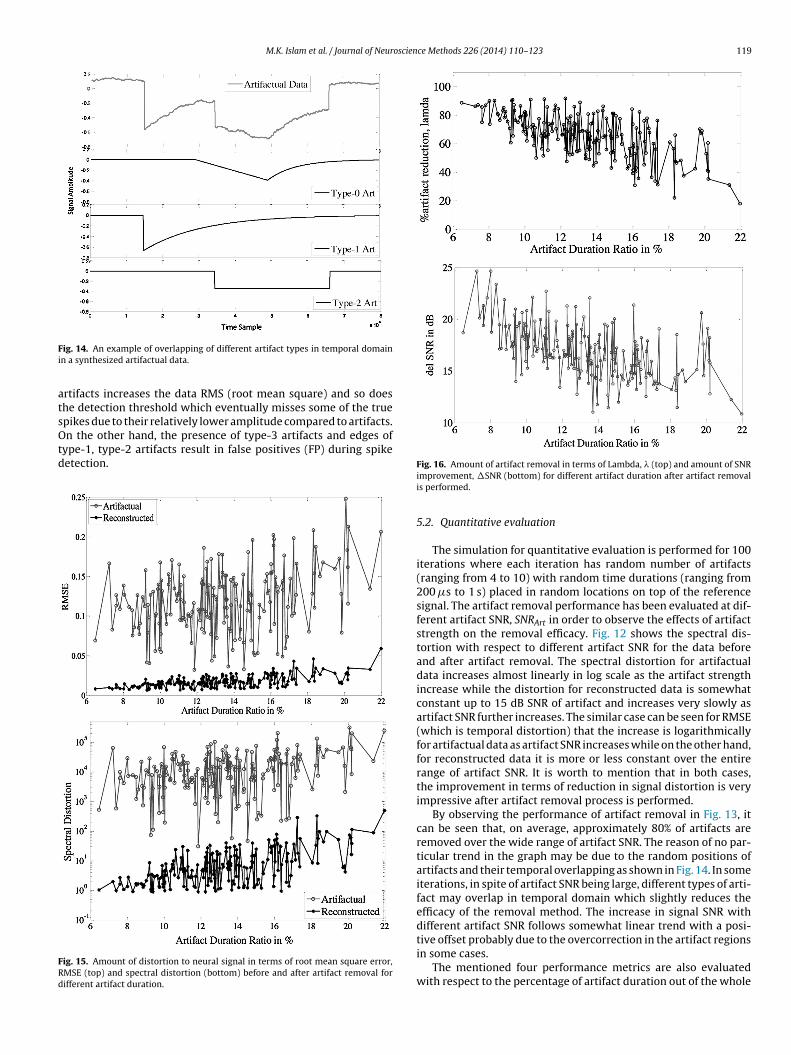
FRd

ig. 14. An example of overlapping of different artifact types in temporal domainn a synthesized artifactual data.

rtifacts increases the data RMS (root mean square) and so doeshe detection threshold which eventually misses some of the true

pikes due to their relatively lower amplitude compared to artifacts.n the other hand, the presence of type-3 artifacts and edges of

ype-1, type-2 artifacts result in false positives (FP) during spikeetection.

ig. 15. Amount of distortion to neural signal in terms of root mean square error,MSE (top) and spectral distortion (bottom) before and after artifact removal forifferent artifact duration.

Fig. 16. Amount of artifact removal in terms of Lambda, � (top) and amount of SNRimprovement, �SNR (bottom) for different artifact duration after artifact removalis performed.

5.2. Quantitative evaluation

The simulation for quantitative evaluation is performed for 100iterations where each iteration has random number of artifacts(ranging from 4 to 10) with random time durations (ranging from200 �s to 1 s) placed in random locations on top of the referencesignal. The artifact removal performance has been evaluated at dif-ferent artifact SNR, SNRArt in order to observe the effects of artifactstrength on the removal efficacy. Fig. 12 shows the spectral dis-tortion with respect to different artifact SNR for the data beforeand after artifact removal. The spectral distortion for artifactualdata increases almost linearly in log scale as the artifact strengthincrease while the distortion for reconstructed data is somewhatconstant up to 15 dB SNR of artifact and increases very slowly asartifact SNR further increases. The similar case can be seen for RMSE(which is temporal distortion) that the increase is logarithmicallyfor artifactual data as artifact SNR increases while on the other hand,for reconstructed data it is more or less constant over the entirerange of artifact SNR. It is worth to mention that in both cases,the improvement in terms of reduction in signal distortion is veryimpressive after artifact removal process is performed.

By observing the performance of artifact removal in Fig. 13, itcan be seen that, on average, approximately 80% of artifacts areremoved over the wide range of artifact SNR. The reason of no par-ticular trend in the graph may be due to the random positions ofartifacts and their temporal overlapping as shown in Fig. 14. In someiterations, in spite of artifact SNR being large, different types of arti-fact may overlap in temporal domain which slightly reduces theefficacy of the removal method. The increase in signal SNR withdifferent artifact SNR follows somewhat linear trend with a posi-

tive offset probably due to the overcorrection in the artifact regionsin some cases.

The mentioned four performance metrics are also evaluatedwith respect to the percentage of artifact duration out of the whole

Page 11

120 M.K. Islam et al. / Journal of Neuroscien

Fig. 17. SNDR comparison between signals before (artifactual) and after (recon-s

dtd(sswpt

channels capture the global artifactual events, they fail in identify-ing the in vivo artifacts which could also be local. The distortions

Fs5

tructed) artifact removal. The SNDR values are averaged over 200 interactions.

ata segment duration in temporal domain in order to observehe algorithm’s response or sensitivity to the amount of artifacturation. It is expected that, the higher the duration of artifactsi.e. higher temporal overlapping with signals) present in a dataequence, the more difficult to remove them without distorting theignal of interest. The relevant plots are shown in Fig. 15 and Fig. 16here the distortions in both temporal and spectral domain are

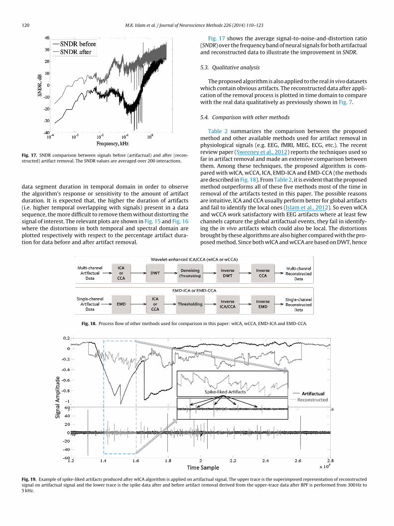
lotted respectively with respect to the percentage artifact dura-ion for data before and after artifact removal.

Fig. 18. Process flow of other methods used for comparison

ig. 19. Example of spike-liked artifacts produced after wICA algorithm is applied on artiignal on artifactual signal and the lower trace is the spike data after and before artifact

kHz.

ce Methods 226 (2014) 110–123

Fig. 17 shows the average signal-to-noise-and-distortion ratio(SNDR) over the frequency band of neural signals for both artifactualand reconstructed data to illustrate the improvement in SNDR.

5.3. Qualitative analysis

The proposed algorithm is also applied to the real in vivo datasetswhich contain obvious artifacts. The reconstructed data after appli-cation of the removal process is plotted in time domain to comparewith the real data qualitatively as previously shown in Fig. 7.

5.4. Comparison with other methods

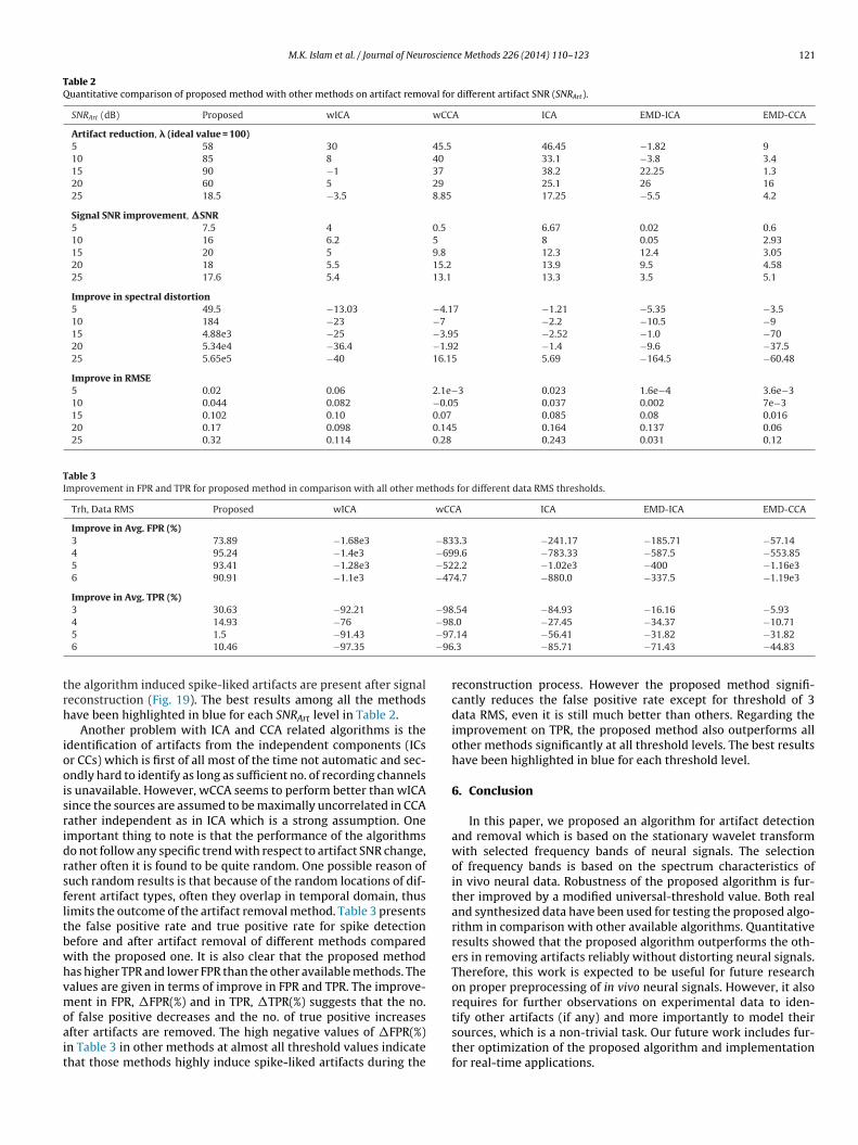
Table 2 summarizes the comparison between the proposedmethod and other available methods used for artifact removal inphysiological signals (e.g. EEG, fMRI, MEG, ECG, etc.). The recentreview paper (Sweeney et al., 2012) reports the techniques used sofar in artifact removal and made an extensive comparison betweenthem. Among these techniques, the proposed algorithm is com-pared with wICA, wCCA, ICA, EMD-ICA and EMD-CCA (the methodsare described in Fig. 18). From Table 2, it is evident that the proposedmethod outperforms all of these five methods most of the time inremoval of the artifacts tested in this paper. The possible reasonsare intuitive, ICA and CCA usually perform better for global artifactsand fail to identify the local ones (Islam et al., 2012). So even wICAand wCCA work satisfactory with EEG artifacts where at least few

brought by these algorithms are also higher compared with the pro-posed method. Since both wICA and wCCA are based on DWT, hence

in this paper: wICA, wCCA, EMD-ICA and EMD-CCA.

factual signal. The upper trace is the superimposed representation of reconstructed removal derived from the upper-trace data after BPF is performed from 300 Hz to

Page 12

M.K. Islam et al. / Journal of Neuroscience Methods 226 (2014) 110–123 121

Table 2Quantitative comparison of proposed method with other methods on artifact removal for different artifact SNR (SNRArt).

SNRArt (dB) Proposed wICA wCCA ICA EMD-ICA EMD-CCA

Artifact reduction, � (ideal value = 100)5 58 30 45.5 46.45 −1.82 910 85 8 40 33.1 −3.8 3.415 90 −1 37 38.2 22.25 1.320 60 5 29 25.1 26 1625 18.5 −3.5 8.85 17.25 −5.5 4.2

Signal SNR improvement, �SNR5 7.5 4 0.5 6.67 0.02 0.610 16 6.2 5 8 0.05 2.9315 20 5 9.8 12.3 12.4 3.0520 18 5.5 15.2 13.9 9.5 4.5825 17.6 5.4 13.1 13.3 3.5 5.1

Improve in spectral distortion5 49.5 −13.03 −4.17 −1.21 −5.35 −3.510 184 −23 −7 −2.2 −10.5 −915 4.88e3 −25 −3.95 −2.52 −1.0 −7020 5.34e4 −36.4 −1.92 −1.4 −9.6 −37.525 5.65e5 −40 16.15 5.69 −164.5 −60.48

Improve in RMSE5 0.02 0.06 2.1e−3 0.023 1.6e−4 3.6e−310 0.044 0.082 −0.05 0.037 0.002 7e−315 0.102 0.10 0.07 0.085 0.08 0.01620 0.17 0.098 0.145 0.164 0.137 0.0625 0.32 0.114 0.28 0.243 0.031 0.12

Table 3Improvement in FPR and TPR for proposed method in comparison with all other methods for different data RMS thresholds.

Trh, Data RMS Proposed wICA wCCA ICA EMD-ICA EMD-CCA

Improve in Avg. FPR (%)3 73.89 −1.68e3 −833.3 −241.17 −185.71 −57.144 95.24 −1.4e3 −699.6 −783.33 −587.5 −553.855 93.41 −1.28e3 −522.2 −1.02e3 −400 −1.16e36 90.91 −1.1e3 −474.7 −880.0 −337.5 −1.19e3

Improve in Avg. TPR (%)3 30.63 −92.21 −98.54 −84.93 −16.16 −5.93

−98−97−96

trh

iooisridrsfltbwhvmoait

4 14.93 −76

5 1.5 −91.43

6 10.46 −97.35

he algorithm induced spike-liked artifacts are present after signaleconstruction (Fig. 19). The best results among all the methodsave been highlighted in blue for each SNRArt level in Table 2.

Another problem with ICA and CCA related algorithms is thedentification of artifacts from the independent components (ICsr CCs) which is first of all most of the time not automatic and sec-ndly hard to identify as long as sufficient no. of recording channelss unavailable. However, wCCA seems to perform better than wICAince the sources are assumed to be maximally uncorrelated in CCAather independent as in ICA which is a strong assumption. Onemportant thing to note is that the performance of the algorithmso not follow any specific trend with respect to artifact SNR change,ather often it is found to be quite random. One possible reason ofuch random results is that because of the random locations of dif-erent artifact types, often they overlap in temporal domain, thusimits the outcome of the artifact removal method. Table 3 presentshe false positive rate and true positive rate for spike detectionefore and after artifact removal of different methods comparedith the proposed one. It is also clear that the proposed methodas higher TPR and lower FPR than the other available methods. Thealues are given in terms of improve in FPR and TPR. The improve-ent in FPR, �FPR(%) and in TPR, �TPR(%) suggests that the no.

f false positive decreases and the no. of true positive increasesfter artifacts are removed. The high negative values of �FPR(%)n Table 3 in other methods at almost all threshold values indicatehat those methods highly induce spike-liked artifacts during the

.0 −27.45 −34.37 −10.71

.14 −56.41 −31.82 −31.82

.3 −85.71 −71.43 −44.83

reconstruction process. However the proposed method signifi-cantly reduces the false positive rate except for threshold of 3data RMS, even it is still much better than others. Regarding theimprovement on TPR, the proposed method also outperforms allother methods significantly at all threshold levels. The best resultshave been highlighted in blue for each threshold level.

6. Conclusion

In this paper, we proposed an algorithm for artifact detectionand removal which is based on the stationary wavelet transformwith selected frequency bands of neural signals. The selectionof frequency bands is based on the spectrum characteristics ofin vivo neural data. Robustness of the proposed algorithm is fur-ther improved by a modified universal-threshold value. Both realand synthesized data have been used for testing the proposed algo-rithm in comparison with other available algorithms. Quantitativeresults showed that the proposed algorithm outperforms the oth-ers in removing artifacts reliably without distorting neural signals.Therefore, this work is expected to be useful for future researchon proper preprocessing of in vivo neural signals. However, it alsorequires for further observations on experimental data to iden-

tify other artifacts (if any) and more importantly to model theirsources, which is a non-trivial task. Our future work includes fur-ther optimization of the proposed algorithm and implementationfor real-time applications.

Page 13

1 oscien

A

iIp

AA6

A

rbrsissa

f((p

••

b(f

k

l

k

d

m

R

B

B

B

B

C

C

C

22 M.K. Islam et al. / Journal of Neur

cknowledgments

The experiment data are provided by Victor Pikov at Hunt-ngton Medical Research Institute and Edward Keefer at Plexonnc./University of Texas Southwest Medical Institute and with theirermission to use.

The authors would like to acknowledge the funding support by*STAR PSF Grant R-263-000-699-305, NUS YIA Grant R-263-000-29-133, A*STAR-CIMIT R-263-000-A47-112 and MOE R-263-000-19-133.

ppendix A. Calculation of threshold parameters

The threshold parameters kA and kD are chosen based on artifactemoval results from few initial trial/training cycles. If we sweepoth these two parameters and evaluate the corresponding artifactemoval performance in terms of the correlation value betweenignals before and after artifact removal, then we can get a roughdea of choosing the optimal values for kA and kD. In order to doo, we assume that the correlations between artifactual and recon-tructed signals are higher in non-artifactual regions and lower inrtifact-contaminated regions.

If RXYArtand RXYNon−Art

are the correlation values between arti-actual and reconstructed signals for artifact-contaminated regionsi.e. IDi is artifact index) and non-artifact-contaminated regionsi.e. IDi is not artifact index) respectively, then the optimizationroblem will be as follows:

Find kA for maximum RXYNon−Artand minimum RXYArt

.Find kD for maximum RXYNon−Art

and minimum RXYArt.

Now if kAmax be the value when RXYNon−Artis maximum and kAmin

e the value when RXYArtis minimum, then the optimal value of kA

i.e. kAopt ) is chosen as the average of these two values as given byollowing equation:

Aopt = kAmax + kAmin

2(21)

Similarly the optimal value of kD, (i.e. kDopt ) is calculated as fol-ows:

Dopt = kDmax + kDmin

2(22)

The value of m can be averaged over few initial trials of 1-secata segment from the following equation:

= 1N

N∑j=1

max(|A10|j)(sd(A10)j

. (23)

eferences

elitski A, Gretton A, Magri C, Murayama Y, Montemurro MA, LogothetisNK, Panzeri S. Low-frequency local field potentials and spikes in primaryvisual cortex convey independent visual information. Journal of Neuroscience2008];28(22):5696–709.

ar-Hillel A, Spiro ASE. Spike sorting: Bayesian clustering of non-stationary data.Advances in Neural Information Processing Systems 2005];17:105–12.

eylkin G. On the representation of operators in bases of compactly supportedwavelets. SIAM Journal on Numerical Analysis 1992];29(6):1716–40.

uzsáki G, Anastassiou CA, Koch C. The origin of extracellular fields and currents –EEG, ECoG, LFP and spikes. Nature Reviews Neuroscience 2012];13(6):407–20.

astellanos NP, Makarov VA. Recovering EEG brain signals: artifact suppression withwavelet enhanced independent component analysis. Journal of NeuroscienceMethods 2006];158(2):300–12.

handra ROL. Detection, classification, and superposition resolution of action poten-tials in multiunit single-channel recordings by an on-line real-time neuralnetwork. IEEE Transactions on Biomedical Engineering 1997];44(5):403.

oifman RR, Donoho DL. Translation-invariant denoising. Berlin, Germany:Springer-Verlag; 1995]. p. 125–50.

ce Methods 226 (2014) 110–123

Dayan P, Abbott LF. Theoretical neuroscience: computational and mathematicalmodeling of neural systems. Cambridge, MA, USA: MIT Press; 2005].

Delorme A, Sejnowski T, Makeig S. Enhanced detection of artifacts in EEG datausing higher-order statistics and independent component analysis. NeuroImage2007];34(4):1443–9.

Eichenbaum H. The hippocampus and declarative memory: cognitive mechanismsand neural codes. Behavioural Brain Research 2001];127(12):199–207.

Flexer A, Bauer H, Pripfl J, Dorffner G. Using ICA for removal of ocular artifacts in EEGrecorded from blind subjects. Neural Networks 2005];18(7):998–1005.

Foffani G, Moxon K. Decoding the spatio-temporal localization of behavioral eventsin populations of neurons. In: Conference proceedings. First international IEEEEMBS conference on neural engineering; 2003]. p. 24–7.

Fonseca-Pinto R. A new tool for nonstationary and nonlinear signals: The Hilbert-Huang transform in biomedical applications. In: Laskovski AN, editor. Chapter inbiomedical engineering, trends, researches and technologies. Croatia: In-Tech;2010].

Gao H-Y. Wavelet shrinkage denoising using the non-negative garrote. Journal ofComputational and Graphical Statistics 1998];7(4):469–88.

Guerrero-Mosquera C, Navia-Vazquez A. Automatic removal of ocular artefacts usingadaptive filtering and independent component analysis for electroencephalo-gram data. IET Signal Processing 2012];6(2):99–106.

Kaneko H, Suzuki HT. Tracking spike-amplitude changes to improve the qualityof multineuronal data analysis. IEEE Transactions on Biomedical Engineering2007];54(2):262–72.

Hsu W-Y, Lin C-H, Hsu H-J, Chen P-H, Chen I-R. Wavelet-based envelope featureswith automatic {EOG} artifact removal: application to single-trial EEG data.Expert Systems with Applications 2012];39(3):2743–9.

Islam MK, Tuan NA, Zhou Y, Yang Z. Analysis and processing of in vivo neural signalfor artifact detection and removal. In: BMEI 2012 – 5th international conferenceon biomedical engineering and informatics; 2012]. p. 437–42.

Keefer EW, Botterman BR, Romero MI, Rossi FA, Gross GW. Carbon nanotube-coatedelectrodes improve brain readouts. Nature Nanotechnology 2008];39:434–9.

Lewicki M. A review of methods for spike sorting: the detection and classifi-cation of neural action potentials. Network: Computation in Neural Systems1998];9:53–78.

Lytton W. From computer to brain: foundations of computational neuroscience. NewYork: Springer; 2002].

Mallat S. A Wavelet tour of signal processing: the sparse way. 3rd ed. California,USA: Academic Press; 2008].

Mitra P, Bokil H. Observed brain dynamics. New York: Oxford University Press;2008].

Moen H. Wavelet transforms and efficient implementation on the GPU. Departmentof Informatics, University of Oslo; 2007], Master Thesis.

Molavi B, Dumont G. Wavelet based motion artifact removal for functional nearinfrared spectroscopy. In: Engineering in medicine and biology society (EMBC),2010 annual international conference of the IEEE; 2010]. p. 5–8.

Molla MKI, Islam MR, Tanaka T, Rutkowski TM. Artifact suppression from EEG signalsusing data adaptive time domain filtering. Neurocomputing 2012];97:297–308.

Molle M, Yeshenko O, Marshall L, Sara SJ, Born J. Hippocampal sharp wave-rippleslinked to slow oscillations in rat slow-wave sleep. Journal of Neurophysiology2006];96(1):62–70.

Raghavendra BS, Dutt DN. Wavelet enhanced CCA for minimization of ocular andmuscle artifacts in EEG. World Academy of Science, Engineering and Technology2011];57(6 Dec):1027–32.

Rong F, Contreras-Vidal JL. Magnetoencephalographic artifact identification andautomatic removal based on independent component analysis and categoriza-tion approaches. Journal of Neuroscience Methods 2006];157(2):337–54.

Harrison RR. A low-power integrated circuit for adaptive detection of action poten-tials in noisy signals. In: Annual international conference of the IEEE engineeringin medicine and biology proceedings; 2003]. p. 3325–8.

Safieddine D, Kachenoura A, Albera L, Birot G, Karfoul A, Pasnicu A, Biraben A,Wendling F, Senhadji L, Merlet I. Removal of muscle artifact from EEG data:comparison between stochastic (ICA and CCA) and deterministic (EMD andwavelet-based) approaches. EURASIP Journal of Advances in Signal Processing2012];2012:127.

Savelainen A. An introduction to EEG artifacts. In: Independent research project inapplied mathematics. Finland: School of Science – Aalto University; 2010].

Savelainen A. Movement artifact detection from electroencephalogram utilizingaccelerometer. Helsinki, Finland: School of Science and Technology, Aalto Uni-versity; 2011], M.S. Thesis.

Scott B. Developments in EEG analysis, protocol selection, and feedback delivery.Journal of Neurotherapy 2011];15(3):262–7.

Snider RBA. Classification of non-stationary neural signals. Journal of NeuroscienceMethods 1998];84(1–2):155–6.

Sweeney KT, McLoone SF, Ward TE. The use of ensemble empirical mode decompo-sition with canonical correlation analysis as a novel artifact removal technique.IEEE Transactions on Biomedical Engineering 2013];60(1):97–105.

Sweeney KT, Ward TE, McLoone SF. Artifact removal in physiological signals –practices and possibilities. IEEE Transactions on Information Technology inBiomedicine 2012];16(3):488–500.

Tomko G, Crapper D. Neuronal variability: non-stationary responses to identical

visual stimuli. Brain Research 1974];79(3):405–18.

Wang YL, Liu JH, Liu YC. Automatic removal of ocular artifacts from elec-troencephalogram using Hilbert-Huang transform. In: ICBBE 2008 – The 2ndinternational conference on bioinformatics and biomedical engineering; 2008].p. 2138–41.

Page 14

oscien

W

W

Y

Y

M.K. Islam et al. / Journal of Neur

ang Y, Sanchez JC, Principe JC, Mitzelfelt JD, Gunduz A. Analysis of the correlationbetween local field potentials and neuronal firing rate in the motor cortex. In:Annual international conference of the IEEE engineering in medicine and biologyproceedings; 2006]. p. 6185–8.

inkler I, Haufe S, Tangermann M. Automatic classification of artifactual ICA-components for artifact removal in EEG signals. Behavioral and Brain Functions2011];7(1):1–15.

ang Z, Zhao Q, Keefer E, Liu W. Noise characterization, modeling, and reductionfor in vivo neural recording. In: Bengio Y, Schuurmans D, Lafferty JD, Williams

CKI, Culotta A, editors. NIPS. New York, USA: Curran Associates Inc.; 2009]. p.2160–8.

ang XSS. A totally automated system for the detection and classification ofneural spikes. IEEE Transactions on Biomedical Engineering 1988];35(10):806–16.

ce Methods 226 (2014) 110–123 123

Yong X, Fatourechi M, Ward R, Birch G. Automatic artifact removal in a self-paced hybrid brain–computer interface system. Journal of Neuroengineeringand Rehabilitation 2012];9(1):1–20.

Zhang L, Wu D, Zhi L. Method of removing noise from EEG signals based on hhtmethod. In: ICISE 2009 – 1st International Conference on Information Scienceand Engineering; 2009]. p. 596–9.

Zhao C, Qiu T. An automatic ocular artifacts removal method based on wavelet-enhanced canonical correlation analysis. In: Engineering in Medicine andBiology Society, EMBC 2011 – Annual International Conference of the IEEE;

2011]. p. 4191–4.

Zima M, Tichavsk P, Paul K, Krajca V. Robust removal of short-duration arti-facts in long neonatal EEG recordings using wavelet-enhanced ICA andadaptive combining of tentative reconstructions. Physiological Measurement2012];33(8):N39.