Article Modeling Categorical Random Fields via Linear ...

Article

Modeling Categorical Random Fields via Linear Bayesian Updating Xiang Huang and Zhizhong Wang *

Department of Statistics, Central South University, Changsha 410012, China; [email protected] * Correspondence: [email protected]; Tel.: +86-136-2731-1056

Abstract: Categorical variables are common in spatial data analysis. Traditional analytical methods for deriving probabilities of class occurrence, such as kriging-family algorithms, have been hindered by the discrete characteristics of categorical fields. This study introduces the theoretical backgrounds of linear Bayesian updating (LBU) approach for spatial classification through expert system. Transition probabilities are interpreted as expert opinions for updating the prior marginal probabilities of categorical response variables. The main objective of this paper is to present the solid theoretical foundations of LBU and provide a categorical random field prediction method which yields relatively higher classification accuracy compared with conventional Markov chain random field (MCRF) approach. A real-world case study has also been carried out to demonstrate the superiority of our method. Since the LBU idea is originated from aggregating expert opinions and not restricted to conditional independent assumption (CIA), it may prove to be reasonably adequate for analyzing complex geospatial data sets, like remote sensing images or area-class maps.

Keywords: Bayesian updating; expert opinion; spatial classification; transition probability

PACS: 02.50.Sk

1. Introduction

Categorical spatial data, such as lithofacies, land-use/land-cover (LULC) classifications, mineralization phases, are widely investigated geographical and geological data sources. They are typically represented by mutually exclusive and collectively exhaustive (MECE) classes and visualized as area-class maps [1]. Traditionally, indicator variograms or indicator covariances are commonly used in geostatistics to measure spatial continuity in categorical fields [2]. Different from (but related to) those two indicator approaches, transition probabilities [3], or equivalently, transiograms [4], are naturally designed to quantify spatial variability of categorical variables. The advantages of transition probability-based methods over indicator covariances or variograms had been well discussed [3]. The critical and most challenging step here is to model the data redundancy between these elementary probabilities or interactions among multiple variables. Several methods have been developed in consideration of data interaction, e.g., Tau ( )τ model [5,6], Nu ( )υ expression [7], generalized linear mixed model (GLMM) [8], etc. The paradigm of latent random fields and spatial covariance functions used in GLMM was also discussed in [9], the results show that the class occurrence probability at a target location can be formulated as a multinomial logistic function of spatial variable covariances between the target and sampled locations. The interaction terms were included into logistic regression models in [10] to account for data dependency in terms of Markov random fields [11,12]. In the Geo-information context, the Rao’s quadratic diversity was used in [13] to measure the scale-dependent landscape structure. In the geological counterpart, a spatial hidden Markov chain model was employed in [14] for estimation of petroleum reservoir categorical variables. Most often, the step of considering data interaction is avoided, or at least simplified, by assuming some form of conditional independent assumption (CIA), such as the Markov chain random field (MCRF) method, introduced by [15]. The recently proposed MCRF co-located

Preprints (www.preprints.org) | NOT PEER-REVIEWED | Posted: 14 July 2016 doi:10.20944/preprints201607.0030.v1

http://dx.doi.org/10.20944/preprints201607.0030.v1

2 of 13

cosimulation algorithm [16] is an enrichment of the previous MCRF theory by integrating auxiliary data.

Generally speaking, the spatial classification problem can be regarded as combing two-point transition probabilities into a multi-point conditional probability. A formal review of most of the available techniques to aggregate probability distributions in geoscience can be found in [17]. What we focus on is to use probability aggregation method for spatial classification based on the pioneering work of [18] and [19]. This paper is organized as follows. We start by introducing the basic forms of the linear Bayesian updating (LBU) method in Section 2. We then make detailed proofs in Section 3 for some propositions introduced by [18] and [19] while have not yet been proven. Finally, to further investigate the performance of the proposed method in real cases, the lithology types in the well-known Jura data set [20] are used for case study (Section 4). The contribution is completed by conclusions and acknowledgments in Section 5.

2. Linear Bayesian updating model

We use A and nDD ,,1 to represent the events in sample spaces of categorical random variable ( )0xC and ( ) ( )nxCxC ,,1 respectively and A denotes the complementary event of A . We wish to assess

the probability of an event A , conditional on the occurrence of a set of data events iD , ni ,,2,1 = . For

categorical events, the formal probabilistic set-up is the following. We need to consider a sample space Ω such that all events A and iD are subsets of Ω . In the case of categorical data, letA be the finite set of events in Ω such that the events KAAA ,, 21 ofA are MECE, that isA forms a finite partition of

Ω . Obviously,

( ))1(

otherwise.0,2,1,if1 0

==

=KjjxC

Aj

Without loss of generality, we will use A as a short notation for jA . The event A can for example

be a lithofacies category at a specified location 0x , while the data iD can represent information provided by core samples at surrounding wells nxxx ,, 21 . This means that we wish to approximate the probability ( )nDDDAP ,,,| 21 on the basis of the simultaneous knowledge. This multi-point posterior probability can be obtained by combining prior probability ( )AP0 with the two-point transition probabilities ( ) niDAP i ,,2,1,| = . This prior probability is independent on any other probabilities ( )iDAP | . It can be thought of as arising from an abstract and never specified information

0D with ( )0| DAPp = . In geoscience, such a prior probability could be for example the proportion of a kind of lithofacies varying in space [17]. The n neighboring events nDDD ,,, 21 are regarded as experts, thus the conditional probability ( )iDAP | can be considered as expert opinion iQ for the

occurrence of A , an event of interest.

We then examine the situation in which a decision maker (DM) uses the opinions of 1≥n expert individual ( )nn qQqQqQ ==== ,,, 2211 Q to revise his/her own prior probability ( )AP0 , denoted p ,

for the occurrence of A , and it is desired to use this information to form the DM’s posterior probability for A . This process is called Bayesian updating. The experts’ opinions are treated as random variables

iQ whose values niqi ≤≤1, , are to be revealed to the DM. The posterior probability of A given qQ =

is then ( )q∗p .



3 of 13

The LBU method was proposed by [18] of the form

( ) ( ) =−+=

ni iii qpp

1* μλq (2)

with possibly negative weights, iλ , expressing the amounts of correlation between each iQ and A . iμ denotes the mathematical expectation of iQ . When pn === μμ 1 and 0≥iλ for all i , (2) reduces to

the linear opinion pool [21]

( ) 1tosubject*010 =+= ==

ni i

ni iiqpp λλλq (3)

where the DM is considered as one of the experts, thereby lending support to a supposition of [22] to the effect that (3) sometimes corresponds to an application of Bayes’ theorem. To obtain a legitimate probability, iλ must obey a number of inequalities [18]. If, for example, the DM feels that all iλ are

positive, the most common case, then they must be chosen so that

( ) ( ) ,11/1,/max11

≤

−− ==

ni ii

ni ii pp μλμλ (4)

which can be considered as a sufficient but not necessary condition for LBU model. The proof of (4) is given in Section 3.1.

The LBU method presented above has some parameters that need either to be estimated or specified by the DM. In the context of aggregating expert opinion, [23] introduced four ways of assessing the weights for the linear pool: the first suggestion is to set equal weights when there is no element which allows to prefer one source of information to another, or when symmetry of information justifies it; the second and third propositions are setting weights proportional to a ranking based on expert’s advice and self-rating, respectively. The last suggestion is to set weights based on some comparison of previously assessed distributions with actual outcomes. An algorithm [24] is based on the minimization of a Kullback-Leibler distance for selecting weighting factors in logarithmic opinion pools. The optimal weights are found by solving a quadratic programming problem. We can also find approach based on ordinary kriging, a well-known framework for accounting for data interaction in a spatial context [25]. In their discussion, information interaction between iD and 1−iD is encapsulated by the exponent weight factor iτ , but the concept of distance

between source of information and that of variogram of probabilities is not obvious [17]. Our derivation provides an interpretation of the coefficients iλ in LBU (2) as the linear regression

coefficients of pp −∗ on μQ − so long as the experts are not linearly dependent. The proof of this

proposition can be found in Section 3.2. As in multiple regression, each iλ can thus be thought of as a

measure of the additional information that the i th expert provides over and above the other experts and what the DM already knows.

3. Theoretical foundations of linear Bayesian updating model

3.1. Parameter ranges for linear Bayesian updating

Since ( )q∗p is a probability, it must satisfy ( ) 10 ≤≤ ∗ qp , that is to say,



4 of 13

( )

( )

≤−+

≥−+

=

=

.1

0

1

1ni iii

ni iii

qp

qp

μλ

μλ (5)

Through algebra transformation, (5) can be simplified as

≤−

−

≥+

==

==

.11

1

11

11

p

q

pp

q

ni ii

ni ii

ni ii

ni ii

μλλ

μλλ

(6)

Suppose that all iλ are positive, since 10 ≤≤ iq , as long as

( )

≤−

−

≤

=

=

,11

1

1

1

1

p

pni ii

ni ii

μλ

μλ

(7)

(6) can be satisfied. Therefore, (7) can be considered as a sufficient but not necessary condition for LBU model (2). Only when (7), or equivalently (4), is satisfied, can (2) be a valid probability model.

3.2. Interpreting parameters as regression coefficients for linear Bayesian updating

Let QΣ denote the covariance matrix ofQ andQ∗pσ be the vector of covariances between ∗p and

Q . Let t denote matrix transposition and

( ) ( ) ( )tnnn ,λ,,λλ,μ,,μμ,Q,,QQ 212121 === λμQ ,

using the definition of expectation, it is

( ) ( )( ) ( ) ( ) ppEAEAEEpAE ==== ** |,| QQ .

In addition, (2) can be given as

( ) ( )QμλμQ Epp =⋅−+=∗ and ,

i.e.,

( ) ( )tnnn ,λ,,λλμ,Q,μ,QμQpp 212211 ⋅−−−+=∗ .

Taking the expectations on both sides of the equation after transformation yields



5 of 13

( ) ( )[ ] ( ) ( )[ ] ( )( ) ( )λ

μQ

Q ⋅Σ=⋅=

⋅−−−⋅−−−=−⋅− ∗

tnn

tnnn

tnn

t

,λ,,λλ,Q,,QQ

,λ,,λλμ,Q,μ,QμQμ,Q,μ,QμQEppE

2121

2122112211

cov

we have

qpQλ ∗−Σ= σ1

provided that the covariance matrix QΣ is invertible.

Suppose we havem samples in the training set, consider the regression model

εBXY +⋅=

where

=

=

−−

−−−−

=

−

−

−

=

∗

∗

∗

mnnmnm

nn

nn

mb

bb

qq

qqqq

pp

pp

pp

ε

εε

μμ

μμμμ

2

1

1

0

11

2121

1111

2

1

1

11

εBXY ,

( )tmεεε ,,, 11 =ε denotes the random errors. As long as the experts are not linearly dependent, the

least squares estimation of the regression coefficients is

( ) ( )YXXXB tt 1ˆ −= ,

which can be written in its matrix form

( ) ( )( ) ( ) ( )( )

( ) ( )( ) ( )( )

( ) ( )( ) ( )

( )( )

( )( )

( )( )

.

11

1

11

111

ˆ

1

*

122

*

111

*

1

1

2

111

1 122112222

1 111

21111

11

2

1

1

22212

11111

1

11

2121

1111

21

22222212

11121111

−−

−−

−−

−

⋅

−−−−

−−−−−

−−−−

−−

=

−

−

−

⋅

−−

−−−−

⋅

−−

−−−−

⋅

−−−

−−−−−−

=

=

=

=

∗−

==

= =

= =

∗

∗

∗−

m

inini

m

iii

m

iii

m

inin

m

iininnn

m

i

m

ininiii

m

i

m

ininii

nn

mnmnnn

m

m

nmnm

nn

nn

nmnnnnn

m

m

qpp

qpp

qpp

mppm

qqqQm

qqqqQm

qqqQm

QmQmm

pp

pp

pp

qq

qqqq

qq

qqqq

qqq

qqqqqq

μ

μ

μ

μμμμ

μμμμμ

μμμμ

μμ

μμ

μμμμ

μμ

μμμμ

μμμ

μμμμμμ

B



6 of 13

When the sample size is large enough, the sample mean is approximately equal to the total expectation, we have

( ) ( ) ( )( ) ( )[ ] ( )( )[ ]( ) ( )( )[ ] ( )( )[ ]

( ) ( )( )[ ] ( )[ ]

( )( )( )[ ]( )( )[ ]( )( )[ ]

( ) ( ) ( )( )( ) ( )

( )

( )

( ).

0

,,cov

1

1

1

1ˆ

11

1

1

2122

11

2211

22

11

1

211

22112222

112

1111

2211

×+

−

∗

−

∗

∗

∗

∗−

⋅Σ=

−⋅⋅

−

−−

−−−

⋅=

−−

−−

−−

−

⋅⋅

−−−−

−−−−−−−−−

−−−

⋅=

∗

∗

np

p

nn

n

nn

nnnnnnnn

nn

nn

nn

ppEm

QE

QQQQEQE

QEQEQE

m

QppE

QppE

QppE

ppE

m

QEQQEQE

QQEQQEQEQQEQEQE

QEQEQE

m

QQ

Q

B

σ

σ

μ

μμ

μμμ

μ

μ

μ

μμμμ

μμμμμμμμμ

μμμ

Therefore, the parameters λ in LBU model can be interpreted as the linear regression coefficients B

of pp −∗ on μQ − .

4. Case study

To investigate the performance of LBU method in real cases, the lithology types in the well-

known Swiss Jura data set [20] are used, in which four rock types are sampled in a 14.5 2km area and 259 samples are selected as training data set (Figure 1). The class proportions of these four categories are [20.46%, 32.82%, 24.32%, 22.39%], respectively. We consider 10 nearest

Figure 1. Jura lithology data set with four classes.

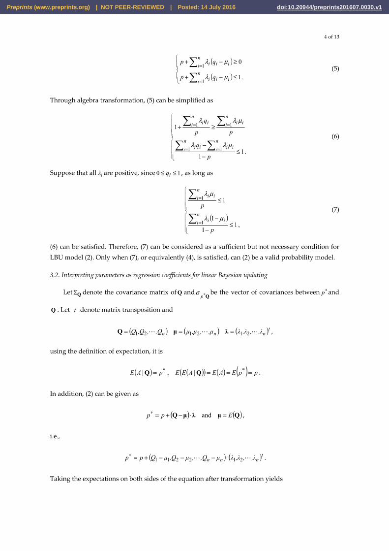
samples as the neighbors of target locations, thus we have 10 experts for consultation. Correlation analysis (Figure 2) shows that the 10 experts are mutual correlated to some extent. The two nearest neighbors have the highest correlation coefficient (greater than 0.9). Therefore, a variable-reduction



7 of 13

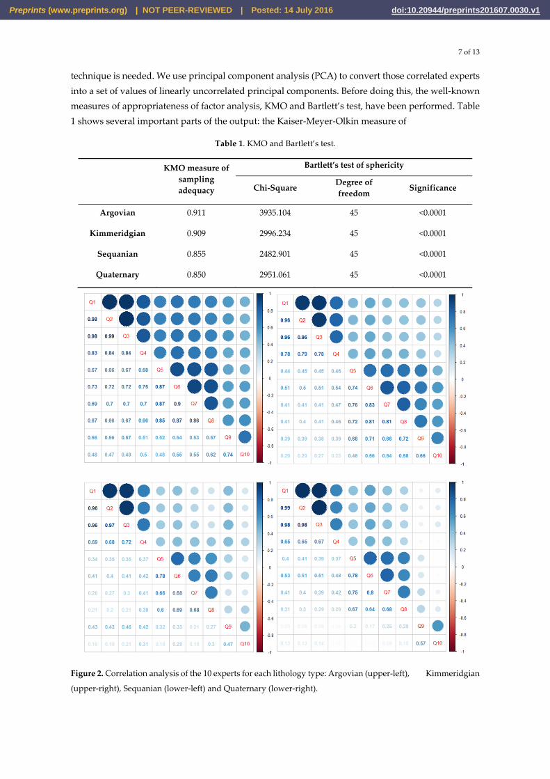
technique is needed. We use principal component analysis (PCA) to convert those correlated experts into a set of values of linearly uncorrelated principal components. Before doing this, the well-known measures of appropriateness of factor analysis, KMO and Bartlett’s test, have been performed. Table 1 shows several important parts of the output: the Kaiser-Meyer-Olkin measure of

Table 1. KMO and Bartlett’s test.

KMO measure of sampling adequacy

Bartlett’s test of sphericity

Chi-Square Degree of freedom

Significance

Argovian 0.911 3935.104 45 <0.0001

Kimmeridgian 0.909 2996.234 45 <0.0001

Sequanian 0.855 2482.901 45 <0.0001

Quaternary 0.850 2951.061 45 <0.0001

Figure 2. Correlation analysis of the 10 experts for each lithology type: Argovian (upper-left), Kimmeridgian

(upper-right), Sequanian (lower-left) and Quaternary (lower-right).



8 of 13

sampling adequacy and Barlett’s test of sphericity. The KMO statistic of each lithology type is greater than 0.5, so we should be confident that PCA is appropriate for these data. Bartlett’s measure tests the null hypothesis that the original correlation matrix is an identity matrix. For these data, Bartlett’s test is highly significant ( 0001.0<p ), and therefore PCA is appropriate. Combined, components 1

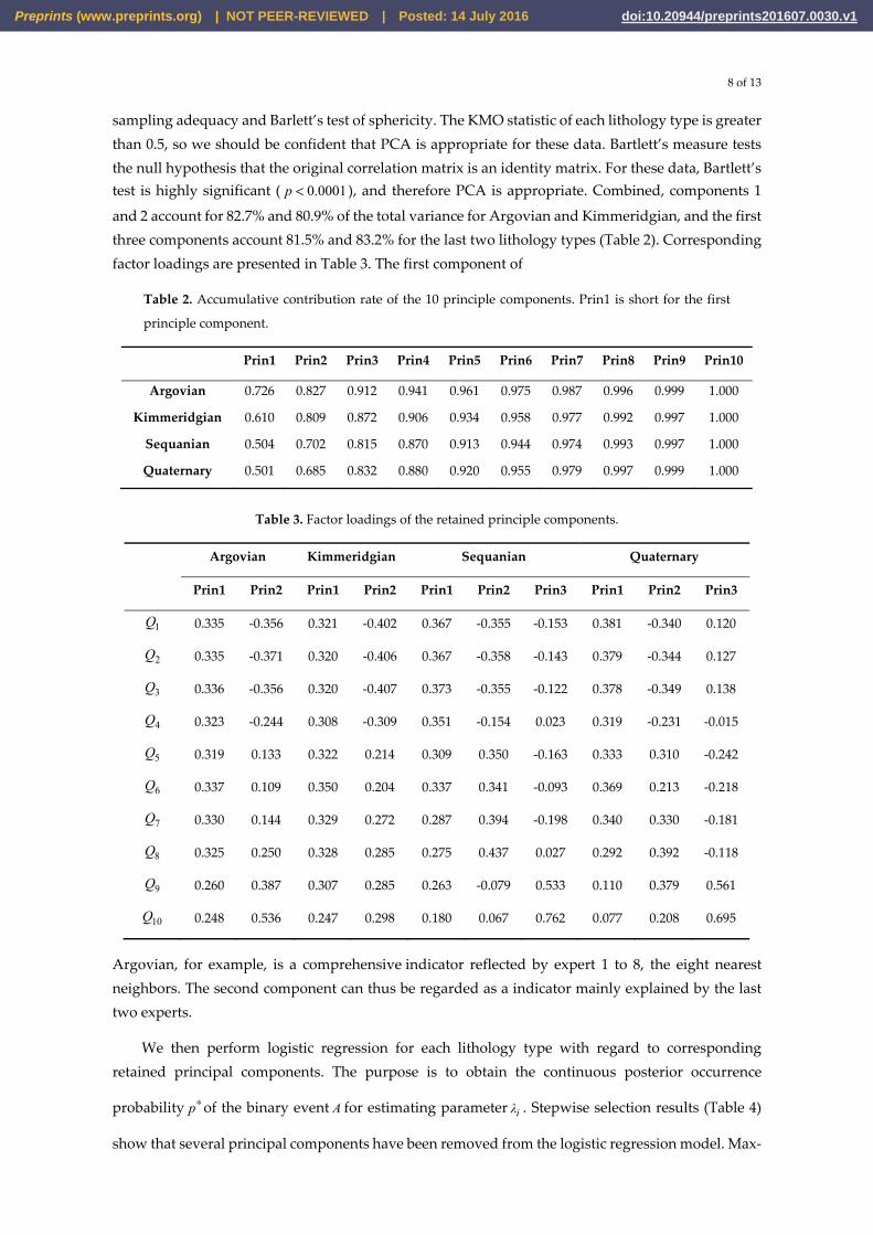
and 2 account for 82.7% and 80.9% of the total variance for Argovian and Kimmeridgian, and the first three components account 81.5% and 83.2% for the last two lithology types (Table 2). Corresponding factor loadings are presented in Table 3. The first component of

Table 2. Accumulative contribution rate of the 10 principle components. Prin1 is short for the first

principle component.

Prin1 Prin2 Prin3 Prin4 Prin5 Prin6 Prin7 Prin8 Prin9 Prin10

Argovian 0.726 0.827 0.912 0.941 0.961 0.975 0.987 0.996 0.999 1.000

Kimmeridgian 0.610 0.809 0.872 0.906 0.934 0.958 0.977 0.992 0.997 1.000

Sequanian 0.504 0.702 0.815 0.870 0.913 0.944 0.974 0.993 0.997 1.000

Quaternary 0.501 0.685 0.832 0.880 0.920 0.955 0.979 0.997 0.999 1.000

Table 3. Factor loadings of the retained principle components.

Argovian Kimmeridgian Sequanian Quaternary

Prin1 Prin2 Prin1 Prin2 Prin1 Prin2 Prin3 Prin1 Prin2 Prin3

1Q 0.335 -0.356 0.321 -0.402 0.367 -0.355 -0.153 0.381 -0.340 0.120

2Q 0.335 -0.371 0.320 -0.406 0.367 -0.358 -0.143 0.379 -0.344 0.127

3Q 0.336 -0.356 0.320 -0.407 0.373 -0.355 -0.122 0.378 -0.349 0.138

4Q 0.323 -0.244 0.308 -0.309 0.351 -0.154 0.023 0.319 -0.231 -0.015

5Q 0.319 0.133 0.322 0.214 0.309 0.350 -0.163 0.333 0.310 -0.242

6Q 0.337 0.109 0.350 0.204 0.337 0.341 -0.093 0.369 0.213 -0.218

7Q 0.330 0.144 0.329 0.272 0.287 0.394 -0.198 0.340 0.330 -0.181

8Q 0.325 0.250 0.328 0.285 0.275 0.437 0.027 0.292 0.392 -0.118

9Q 0.260 0.387 0.307 0.285 0.263 -0.079 0.533 0.110 0.379 0.561

10Q 0.248 0.536 0.247 0.298 0.180 0.067 0.762 0.077 0.208 0.695

Argovian, for example, is a comprehensive indicator reflected by expert 1 to 8, the eight nearest neighbors. The second component can thus be regarded as a indicator mainly explained by the last two experts.

We then perform logistic regression for each lithology type with regard to corresponding retained principal components. The purpose is to obtain the continuous posterior occurrence

probability ∗p of the binary event A for estimating parameter iλ . Stepwise selection results (Table 4)

show that several principal components have been removed from the logistic regression model. Max-



9 of 13

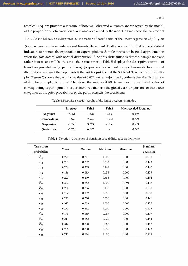
rescaled R-square provides a measure of how well observed outcomes are replicated by the model, as the proportion of total variation of outcomes explained by the model. As we know, the parameters

λ in LBU model can be interpreted as the vector of coefficients of the linear regression of pp −∗ on

μQ − , so long as the experts are not linearly dependent. Firstly, we want to find some statistical

indicators to estimate the expectation of expert opinions. Sample means can be good approximation when the data accord with normal distribution. If the data distribution is skewed, sample medians rather than means will be chosen as the estimator ofμ . Table 5 displays the descriptive statistics of

transition probabilities (expert opinions). Jarque-Bera test is used for goodness-of-fit to a normal distribution. We reject the hypothesis if the test is significant at the 5% level. The normal probability plot (Figure 3) shows that, with a p-value of 0.002, we can reject the hypothesis that the distribution of 11P , for example, is normal. Therefore, the median 0.201 is used as the estimated value of

corresponding expert opinion’s expectation. We then use the global class proportions of these four categories as the prior probabilities p , the parameters λ is the coefficients

Table 4. Stepwise selection results of the logistic regression model.

Intercept Prin1 Prin2 Max-rescaled R-square

Argovian -5.361 4.328 -2.683 0.849

Kimmeridgian -3.662 2.924 -3.244 0.729

Sequanian -3.959 3.263 -3.053 0.699

Quaternary -6.770 6.667 - 0.792

Table 5. Descriptive statistics of transition probabilities (expert opinions).

Transition

probability Mean Median Maximum Minimum

Standard

deviation

11P 0.270 0.201 1.000 0.000 0.250

12P 0.290 0.292 0.632 0.000 0.173

13P 0.254 0.239 0.769 0.000 0.140

14P 0.186 0.193 0.436 0.000 0.123

21P 0.227 0.239 0.563 0.000 0.134

22P 0.332 0.282 1.000 0.091 0.198

23P 0.254 0.256 0.436 0.000 0.090

24P 0.187 0.192 0.387 0.000 0.088

31P 0.220 0.200 0.636 0.000 0.141

32P 0.313 0.309 1.000 0.000 0.155

33P 0.294 0.262 1.000 0.000 0.203

34P 0.173 0.185 0.469 0.000 0.119

41P 0.219 0.182 0.720 0.000 0.154

42P 0.312 0.318 0.562 0.000 0.142

43P 0.256 0.238 0.586 0.000 0.123

44P 0.213 0.184 1.000 0.000 0.208



10 of 13

of stepwise regression in LBU model. All the estimated iλ are greater than zero, which means that iQ

is more likely to be high (and less likely to be low) when 1=A than when 0=A .

We also use MCRF method for comparison. As a non-linear and parameter-free method, the MCRF is based on the product of probabilities, which will dramatically amplify higher probability and reduce lower probability close to zero. The lithology types of corresponding 259 locations can be predicted based on the maximum a posterior (MAP) probability criterion (Figure 4). Together with Table 6, we find that LBU is superior to MCRF in overall prediction accuracy by comparing the prediction results of MCRF with LBU model.

5. Conclusions

In this work, we consummate the theoretical foundations of LBU method for the prediction of categorical spatial data. The philosophy underlying this approach is originated from combining probability distributions in expert system. The Bayesian argument embodied in LBU is both normative and logical. With a linear expression, the probabilities of class occurrence of target locations can be assessed by neighboring sample types. Weights in this model are interpreted as linear regression coefficients. We have enriched our previous findings [19] by adding some rigorous theoretical proofs of the LBU method. Experimental results show that our method performs better



11 of 13

Figure 3. Normal probability plot and Jarque-Bera test for goodness-of-fit to a normal distribution.

Table 6. Prediction accuracy comparison.

Argovian Kimmeridgian Sequanian Quaternary overall

LBU 86.79% (46/53) 85.88% (73/85) 73.02% (46/63) 84.48% (49/58) 82.63% (214/259)

MCRF 88.68% (47/53) 78.82% (67/85) 77.78% (49/63) 82.76% (48/58) 81.47% (211/259)

in terms of classification accuracy compared with traditional MCRF method. As pointed out by [19], our method can also be generalized to nonlinear cases, where more confident probability forecasting results can be obtained.

Acknowledgments: This study is supported by the Fundamental Research Funds for the Central Universities of Central South University (No. 2016zzts011). The authors are indebted to Ying Chen, Danhua Chen, Ruizhi Zhang and Wuyue Shen for their critical reviews of the paper.

Author Contributions: Xiang Huang and Zhizhong Wang conceived and designed the experiments; Xiang Huang performed the experiments; Zhizhong Wang analyzed the data; Xiang Huang wrote the paper.

Conflicts of Interest: The authors declare no conflicts of interest.



12 of 13

Figure 4. Predicted lithology types of corresponding 259 locations based on MAP probability criterion.

References

1. Cao, G.; Kyriakidis, P.C.; Goodchild, M.F. Combining spatial transition probabilities for stochastic simulation of categorical fields. Int. J. Geogr. Inf. Sci. 2011, 25, 1773-1791.

2. Deutch, C.V.; Journel, A.G. GSLIB: geostatistical software library and user’s guide. Oxford University Press, New York, 1992.

3. Carle, S.F.; Fogg, G.E. Transition probability-based indicator geostatistics. Math. Geol. 1996, 28, 453-476. 4. Li, W. Transiogram: A spatial relationship measure for categorical data. Int. J. Geogr. Inf. Sci. 2006, 20, 693-

699. 5. Journel, A. Combining knowledge from diverse sources: an alternative to traditional data independence

hypotheses. Math. Geol. 2002, 34, 573-596. 6. Krishnan, S. The tau model for data redundancy and information combination in earth sciences: theory and

application. Math. Geosci. 2008, 40, 705-727. 7. Polyakova, E.I.; Journel, A.G. The Nu expression for probabilistic data integration. Math. Geol. 2007, 39, 715-

733. 8. Cao, G.; Kyriakidis, P.C.; Goodchild, M.F. A multinomial logistic mixed model for the prediction of

categorical spatial data. Int. J. Geogr. Inf. Sci. 2011, 25, 2071-2086. 9. Cao, G.; Yoo, E.-H.; Wang, S. A statistical framework of data fusion for spatial prediction of categorical

variables. Stoch. Env. Res. Risk. A. 2014, 28, 1785-1799. 10. Schaeben, H. A mathematical view of weights-of-evidence, conditional independence, and logistic

regression in terms of Markov random fields. Math. Geosci. 2014, 46, 691-709. 11. Besag, J. Spatial interaction and the statistical analysis of lattice systems. J. Roy. Stat. Soc. B 1974, 2, 192-236. 12. Norberg, T.; Rosén, L.; Baran, A.; Baran, S. On modelling discrete geological structures as Markov random

fields. Math. Geol. 2002, 34, 63-77. 13. Ricotta, C.; Carranza, M.L. Measuring scale-dependent landscape structure with Rao’s quadratic diversity.

ISPRS Int. J. Geo-Inf. 2013, 2, 405-412. 14. Huang, X.; Li, J.; Liang, Y.; Wang, Z.; Guo, J.; Jiao, P. Spatial hidden Markov chain models for estimation of

petroleum reservoir categorical variables. J. Petrol. Explor. Prod. Technol. 2016, doi: 10.1007/s13202-016-0251-9.

15. Li, W. Markov chain random fields for estimation of categorical variables. Math. Geol. 2007, 39, 321-335. 16. Li, W.; Zhang, C.; Willig, M.R.; Dey, D.K.; Wang, G.; You, L. Bayesian Markov Chain Random Field

Cosimulation for Improving Land Cover Classification Accuracy. Math. Geosci. 2015, 47, 123-148. 17. Allard, D.; Comunian, A.; Renard, P. Probability aggregation methods in geoscience. Math. Geosci. 2012, 44,

545-581. 18. Genest, C.; Schervish, M.J. Modeling expert judgments for Bayesian updating. Ann. Stat. 1985, 13, 1198-

1212. 19. Huang, X.; Wang, Z.; Guo J. Prediction of categorical spatial data via Bayesian updating, Int. J. Geogr. Inf.

Sci. 2016, 30, 1426-1449. 20. Goovaerts, P. Geostatistics for natural resources evaluation. Oxford university press, New York, 1997. 21. Stone, M. The opinion pool. Ann. Math. Stat. 1961, 32, 1339-1342.



13 of 13

22. French, S. Consensus of opinion. Eur. J. Oper. Res. 1981, 7, 332-340. 23. Winkler, R.L. The consensus of subjective probability distributions. Manage. Sci. 1968, 15, B-61-B-75. 24. Heskes, T. Selecting weighting factors in logarithmic opinion pools, in: Jordan, M., Kearns, M., Solla, S.

(Eds.), Advances in neural information processing systems. MIT Press, Cambridge, 1998, pp. 266-272. 25. Cao, G.; Kyriakidis, P.; Goodchild, M. Prediction and simulation in categorical fields: a transition

probability combination approach, Proceedings of the 17th ACM SIGSPATIAL International Conference on Advances in Geographic Information Systems. ACM, New York, 2009, pp. 496-499.

© 2016 by the authors; licensee Preprints, Basel, Switzerland. This article is an open access article distributed under the terms and conditions of the Creative Commons by Attribution (CC-BY) license (http://creativecommons.org/licenses/by/4.0/).



Article Modeling Categorical Random Fields via Linear ...

Documents