Artificialneural networksand modeling for determination of

Page 1

Artificial neural networks and physical modeling for determination of

baseline consumption of CHP plants

Francesco Rossi a,⇑, David Velázquez a, Iñigo Monedero b, Félix Biscarri b

a Department of Energy Engineering, Universidad de Sevilla, Spain b Electronic Technology Department, Universidad de Sevilla, Spain

⇑ Corresponding author. Tel.: +34 647004965.E-mail addresses: [email protected], [email protected] (F. Rossi).

Keywords:Baseline energy consumptionIndustryCogenerationANN modelingThermodynamic modeling

a b s t r a c t

An effective modeling technique is proposed for determining baseline energy consumption in the industry.A CHP plant is considered in the study that was subjected to a retrofit, which consisted of the implemen-tation of some energy-saving measures. This study aims to recreate the post-retrofit energy consumptionand production of the system in case it would be operating in its past configuration (before retrofit) i.e., thecurrent consumption and production in the event that no energy-saving measures had been implemented.Two different modeling methodologies are applied to the CHP plant: thermodynamic modeling and artifi-cial neural networks (ANN). Satisfactory results are obtained with both modeling techniques. Acceptableaccuracy levels of prediction are detected, confirming good capability of the models for predicting plantbehavior and their suitability for baseline energy consumption determining purposes. High level of robust-ness is observed for ANN against uncertainty affecting measured values of variables used as input in themodels. The study demonstrates ANN great potential for assessing baseline consumption in energy-intensive industry. Application of ANN technique would also help to overcome the limited availability ofon-shelf thermodynamic software for modeling all specific typologies of existing industrial processes.

1. Introduction

The industry represents about 20% of the European Union (EU)’sprimary energy consumption. Although 30% improvement in en-ergy intensity has been achieved in this sector during the lasttwo decades, relevant potential remains for energy efficiencyenhancement (Energy Efficiency Plan, 2011).

The European Commission is developing systematic plansaimed at rational energy use, like regular and mandatory energyaudits in large industrial sites and incentives that EU membercountries should establish for companies to implement energymanagement systems. Intensification of high-efficiency cogenera-tion plants is also included as an effective potential contributorto the energy efficiency of European industry.

In this scenario, energy studies acquire a decisive role in thecompetitiveness of the industrial sector, the main objective of en-ergy audits being the identification of measures aimed at increas-ing equipment efficiency and reduction of energy consumption.Once the saving measures proposed in the energy audit have beenimplemented, an issue of relevant importance is the assessment ofreal benefits generated by the changes. Although it is to be hoped

that the actual effects are not too different from the anticipatedsavings, a significant margin of error exists due to, among otherfactors, the reference conditions which the study was based onand the variability of those conditions in the real operation ofthe production process. The new consumption of the factory afterthe retrofit can be easily obtained, provided that adequate measur-ing instruments are installed and functioning properly. The energysaving achieved, on the contrary, cannot be measured, since thiswould suppose being able to measure the current consumptionof industry in its past configuration (before retrofit). For these rea-sons, the impact of programs and projects for improving energyefficiency in the industry can only be estimated, as the differencebetween the current energy consumption (directly measurable)and consumption that would occur in the same period in the eventthat no saving measures had been implanted. This second term isoften called by the name of baseline energy consumption.

The International Performance Measurement and VerificationProtocol (Efficiency Valuation Organization (EVO), IPMVP Volume1, 2012) can be considered as the international reference text onmeasurement and verification (M&V) of energy savings from pro-jects aimed at improving energy efficiency and reducing energycosts. One of the aspects highlighted in the protocol is that a keyfactor in the planning phase of a program of M&V of savings isthe selection of the method that aims to solve the problem of

Page 2

determining the baseline consumption. The need for a clear for-malization of the baseline development process is also stressedin the interesting work of (Reichl & Kollmann, 2011). Among thevarious approaches proposed for determining the baseline con-sumption (U.S. EPA State Clean Energy, 2009), the most easilyapplicable is the engineering method, based on the use of standardformulas and assumptions for calculating the energy use beforeretrofit. However, the simplicity and practicality guaranteed byits implementation involves an associated level of uncertainty(Kelly Kissock & Eger, 2008) that makes it unsuitable for systematicuse in the industrial field. Statistical analyses are also contem-plated, but this general term is actually used to refer to modelsof limited complexity aimed at determining ‘‘before’’ and ‘‘after’’consumption taking into consideration few factors like changesin weather, facility occupancy and factory operating hours. Othersuggested methods contemplate computer simulation for deter-mining system energy performance. Finally, integrative methodscan be used, combining some of the aforementioned approaches.

As evidenced by the literature survey (discussed below), no rel-evant applications of ANN modeling technique were detected forthe determination of the energy consumption baseline in CHP sys-tems, intended as the consumption of the system before the imple-mentation of the efficiency enhancement measures. The objectiveof this paper is to present a valid modeling technique allowingan answer to the problem of determining the baseline energy con-sumption in the industry. The ANN approach is proposed, as aneffective way of recognizing complex non-lineal patterns govern-ing energy consumption in industrial production sites. Achievablelevels of accuracy and suitability of ANNs in predicting the behav-ior of the system are also discussed, by comparing the ANNapproach with the thoroughly tested thermodynamic modelingtechnique. A combined heat and power (CHP) plant is consideredfor the application of the proposed methodology. The extensivehistorical operating dataset available from the existing monitoringsystem is used to generate and validate both ANN and thermody-namic models. Cogeneration plants are often present in industrialsites and represent an efficient solution for electricity and heatsupply to energy-intensive processes. According to the objectiveof this work, a CHP system can also be considered as an indepen-dent industrial unit, products of which are electricity and heat,e.g., in the form of steam delivered to the productive process.

Below is a brief summary of the literature consulted, statingsome of the latest applications of ANN modeling to industrialand cogeneration plants.

Simplified methodologies have been proposed for determiningbaseline consumption and for verification of energy savings in theindustry, based on lineal regression and multi-regression analysis(Dalgleish & Grobler, 2003; Kelly Kissock & Eger, 2008). Other moredeveloped methods have been applied, like lineal combinations ofinfluence variables and subsequent regression modeling for generat-ing the baseline efficiency in industrial refining sites (Velázquez et al.,2013).

The ANN modeling approach is not a novelty in the industry, asevidenced by the applications for optimization of distillation pro-cesses and control of wastewater treatment units (Liau, Yang, & Tsai,2004; Mingzhi, Yongwen, Jinquan, & Yan, 2009; Motlaghi, Jalali, &Nili Ahmadabadi, 2008). Olanrewaju and Jimoh (2014) propose ahybrid approach based on Index Decomposition Analysis (IDA),ANN modeling and Data Envelopment Analysis (DEA), to predictthe expected energy consumption in the industry and subsequentlyoptimize the present energy use with reference to the predicted val-ues. Monedero et al. (2012) apply ANN approach to model the bestpast operation of a petrochemical site, for comparison with presentoperation and efficiency optimizations purposes. ANN modeling hasbeen frequently proposed also for cogenerations, combined cyclesand power plants, with multiple objectives:

- Power prediction of the plant (Smrekar, Pandit, Fast, Assadi, &De, 2010).

- Prediction and monitoring of thermal efficiency and pollutantemissions of the plant (Fantozzi & Desideri, 1998; Flynn,Ritchie, & Cregan, 2005; Lu & Hogg, 2000; Pan, Flynn, & Cregan,2007; Tronci, Baratti, & Servida, 2002).

- Adjustment of power generation to demand profile of theindustry (Moghavvemi, Yang, & Kashem, 1998).

- Reproducing the behavior of plant components (boilers, steamturbines, and superheaters) (Bekat, Erdogan, Inal, & Genc,2012; De, Kaiadi, Fast, & Assadi, 2007; Du et al., 2011; Jia &Xu, 2010; Ma, Wang, & Ma, 2008; Olausson, Häggståhl, Arriag-ada, Dahlquist, & Assadi, 2003).

- Optimization of load distribution and load disconnection forstability purposes in the case of fault of the system (Hsu, Chu-ang, & Chen, 2011; Romero & Shan, 2005).

- Optimization of operating parameters for plant efficiency max-imization, in some cases through combined implementation ofANN and other optimization techniques, e.g., genetic algorithm(Arslan, 2011; Hajabdollahi, Hajabdollahi, & Hajabdollahi, 2012;Rashidi, Galanis, Nazari, Basiri Parsa, & Shamekhi, 2011; Suresh,Reddy, & Kolar, 2011).

The main power generation unit of the CHP plant considered inthis study is constituted by a gas turbine. Many examples exist inthe literature of the ANN modeling approach applied to gas turbines,for condition monitoring and performance estimation (Asgari, Chen,Menhaj, & Sainudiin, 2013; Barad, Ramaiahb, Giridhara, & Krishna-iahb, 2012; Fast, Assadi, & De, 2009a; Fast, Palmé, & Genrup, 2009b;Lazzaretto & Toffolo, 2001; Nikpey, Assadi, Breuhaus, & Mørkved,2014; Palme, Breuhaus, Assadi, Klein, & Kim, 2011), fault detection(Kong, Ki, Kang, & Kho, 2004; Kong, Park, & Kim, 2008; Simani & Fant-uzzi, 2000; Volponi, DePold, Ganguli, & Daguang, 2003), controlenhancement (Sisworahardjo, El-Sharkh, & Alamb, 2008), and turbinediagnostics (Bettocchi, Pinelli, Spina, Venturini, & Burgio, 2004).

Other examples of ANN methodology applied to industry for onlinemonitoring, performance estimation and diagnostic purposes are rep-resented by modeling of boilers (Arriagada, Costantini, Olausson,Assadi, & Torisson, 2003; Chong, Wilcox, & Ward, 2000; Chu et al.,2003; Hao, Kefa, & Jianbo, 2001; Rusinowski & Stanek, 2007; Teruel,Cortes, Diez, & Arauzo, 2005), furnaces (Calisto, Martins, & Afgan,2008), circulating fluidized bed boilers (Liukkonen et al., 2011), com-pressors (Ghorbanian & Gholamrezaei, 2009), refrigerating and heat-ing systems (Kizilkan, 2011; Esen and Inalli; 2009), and fluidized beddryers (Chen, Tsutsumi, Lin, & Otawara, 2005; Satish & Setty, 2005).

Other industrial applications of ANN involve more specific areassuch as control of nuclear power plants (Oliveira & Soares de Almei-da, 2013), performance prediction of internal combustion engines(Canakci, Ozsezen, Arcaklioglu, & Erdil, 2009; Oguz, Saritas, &Baydan, 2010; Tasdemir, Saritas, Ciniviz, & Allahverdi, 2011; Yap &Karri, 2013), modeling and control of fuel cells (Chávez-Ramírezet al., 2010; Hatti & Tioursi, 2009), performance prediction and opti-mization of solar systems (Kalogirou, 2004; Sözen & Akçayol, 2004),power output forecasting of wind power plants (Yeh, Yeh, Chang, Ke,& Chung, 2014), control of hybrid wind-diesel power generators(Vargas-Martínez, Minchala Avila, Zhang, Garza-Castañón, & CalleOrtiz, 2013), and prediction performance of photovoltaic panels(Karamirad, Omid, Alimardani, Mousazadeh, & Navid Heidari, 2013).

2. Description of CHP plant, implemented energy-savingmeasures and preliminary data processing

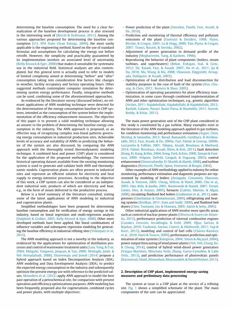
The system at issue is a CHP plant at the service of a refiningsite. Fig. 1 shows a simplified schematic of the plant. The maincomponents of the unit can be appreciated:

Page 3

Evaporator

Deaerator

Heat Recovery Steam Generator

Stack

Economizer

Gas Turbine

Superheater

Process

Steam Turbine

LP steam

MP steam

Exhaustgases

Boilerfeedwater

New low-NOx burners

Preheating of deaerator feedwater

New economizer

Ambientair

Fuel (post-combustion)

Fuel

Treatedwater

Returnedcondensates

Fig. 1. Simplified diagram of the CHP plant and areas subject to energy-saving measures.

� Gas turbine (GT). Generates electricity from fuel burned inthe combustion chamber, both for refinery use and forexport to the grid of the production which exceeds demand.

� Heat recovery steam generator (HRSG). Equipment consti-tuted by heat exchangers the function of which is to recoverthe heat contained in the flue gases at the outlet of the GTand contemporary steam generation. Post-combustion isalso used to increase steam generation and meet the ther-mal demand of the refinery.

� Steam turbine (ST). Used for additional generation of elec-tricity from steam generated in the HRSG. Part of the steamis extracted from the turbine before it completes its expan-sion, to be supplied to refinery at the proper pressure levelrequired by the process. The remaining steam completesthe expansion in the turbine to be delivered to the processat a lower pressure level.

From April to November 2008 a number of energy-saving pro-jects were implemented in the CHP unit, by which the economicbenefit of the plant was increased significantly. Fig. 1 evidencesareas of implementation of projects, which were:

� Replacement of existing burners with Low-NOx burners inthe GT combustion chamber. It allowed the cessation ofsteam injection into the combustion chamber, performeduntil meeting the emission levels required by legislation.

� Preheating of deaerator feed water and installation of a neweconomizer in the HRSG. A new heat exchanger wasinstalled that preheats the water fed to the deaerator, con-temporarily cooling HRSG feed water. The first effect of thismeasure was the reduction of steam consumption in thedeaerator. A new heat exchanger was also installed in theHRSG (new economizer), to compensate the lower HRSGfeed water temperature. As a second effect of the project,exploitation was thus enhanced of the GT gases heat contentand stack gas temperature was reduced from 190 to 130 �C.

The main effect of all implemented measures was a significantreduction in steam self-consumption of the plant, which explainsthe subsequent increase of CHP plant profit. Moreover, saving pro-jects impacted on other consumptions and productions, which also

contribute significantly to the operating profit of cogeneration. Theparameters directly affected by the projects, for which the con-struction of the baseline is required, are:

� Electricity production and fuel (natural gas) consumption in theGT.� Medium pressure (MP) steam injected into the GT.� Low pressure (LP) steam consumed in the deaerator.

As mentioned above, two different modeling methodologieswere applied to the CHP plant, i.e., thermodynamic modeling andANN modeling. Prior to that, a filtering of the collected data wasnecessary so that a valid database could be obtained for develop-ment of both models. A comprehensive data collection was con-ducted for most of the process variables. Records were obtainedfrom distributed control system (DCS), through specific softwarethat allows downloading historical data in Excel format. Plantmonitoring is very exhaustive, and hourly data were collected for134 variables, comprised between 02-16-2007 18:00 and 05-07-2009 00:00. These variables include the main operating parame-ters of all the components of the plant:

� GT: electricity generation, GT regulation parameters (e.g.,inlet guide vane opening angle), pressure drop in air filters,properties of fuel, inlet air, exhaust gases and injectedsteam.

� HRSG: conditions of fuel fed to post-combustion, propertiesof exhaust gases and water/steam in the economizer, evap-orator and superheaters, blowdown rate and stack exhaustgas temperature.

� Deaerator: operating pressure, properties of fed steam andboiler feed water.

� ST: electricity generation, properties of inlet live steam,extraction steam and steam to condenser.

� Other components: properties of streams in the existingheat exchangers of the plant for boiler feed water preheat-ing, steam de-superheating stations, etc.

Previous data treatment was performed and anomalous regis-ters were eliminated, associated with measurement faults or infor-matics errors in the acquisition process. A valid database for the

Page 4

following modeling phase was subsequently selected. The effec-tiveness and the outcome of this selection process are stronglybound to the level of knowledge of the operation of the plant. Adeep mastery of the philosophy of operation and control of the sys-tem is fundamental to the purpose, and it always derives not onlyfrom the prior knowledge of the system, but also from the observa-tion of the same recorded data. A good understanding of the sys-tem is thus necessary, whatever the method of modeling elected.

3. ANN modeling

ANN is an adaptive non-linear statistical data modeling tech-nique consisting of interconnected artificial neurons processingdata in parallel. Exhaustive introductions to ANN modeling areprovided in most of the above-referenced works. The multi-layerperceptron (MLP) network type was employed in this study, andthe supervised learning process was used for adjustment of net-work parameters. Before the training, the dataset was randomizedand divided into training and test data subsets. The training set isused for weight adjustment and the test set is used after the train-ing to assess the performance i.e., prediction capability of ANN bycomparing calculated and desired values for a set of unknown data.

3.1. ANN setup and training

A multi-layer feed-forward structure was chosen for the ANN. Aspecific ANN was generated for each output variable (GT electricityproduction, GT fuel consumption, MP and LP steam consumptions)and IBM SPSS Modeler 14.1.0 software package was used to setupand train the models. Input variables in the models were selectedby the authors, based on the knowledge of system physics. Inputused for GT electricity production and GT fuel consumption werethe ambient conditions (temperature, atmospheric pressure andhumidity), the density and the lower heating value of the fuel,NOx emissions and a counter representing the aging status of theGT. The same inputs were used for GT steam injection, except forfuel density, which has not a significant influence over it. Thesteam consumption of deaerator was modeled as a function of itsoperating pressure, the ambient temperature, the steam produc-tion of the HRSG and the hot condensate mass flow returned fromthe process for preheating of deaerator feed water.

For each of the generated ANN, the output layer is representedby one neuron, while the number of hidden layers and neurons isnot fixed, being two the maximum number of hidden layers con-templated in the study. The final architecture of the network wasdetermined by a trial-and-error process, in which different train-ings were performed with varying numbers of hidden layers andneurons, until the network with best prediction accuracy was se-lected. A first set of trainings was performed, observing the behav-ior of one-layered ANN with increasing number of neurons from 1to 15, fixed as the maximum limit of neurons in the analysis. Fur-ther increase of ANN complexity was considered unnecessary; asobserved by Calisto et al. (2008), an excessive number of neurons,rather than having beneficial effects, may facilitate the overtrain-ing and reduce the generalization capability of the network. ANNstructures presenting local maxima in prediction performancewere selected and the effect was observed of introducing a secondhidden layer. The number of neurons in the second layer was in-creased for each selected ANN, from one to the same number ofneurons of the first hidden layer. As suggested by Kong and Goo(2011), hyperbolic tangent sigmoid function and identity functionwere used as transfer functions in the hidden and output layersrespectively. Range fields of data were rescaled before training tohave values between 0 and 1, to match the range of the activationfunction of the first hidden layer. The common and well proven

back-propagation algorithm proposed by Rumelhart, Hinton, andWilliams (1986) was applied to train the ANN and update theweights associated with neurons. Data are processed in the for-ward direction at each iteration (epoch) and output values are gen-erated in the output layer. The calculated error between thedesired output and the model prediction subsequently propagatesin the backward direction by means of Gradient Descent algorithmwith Momentum, a computationally efficient technique that allowsminimizing the error by updating the connection weights. Thismethod, widely explained in Moghavvemi et al. (1998), contem-plates the use of two coefficients referred to as learning rate (g)and momentum rate (m). Coefficient g is used to control the inten-sity of the weights modification: fast learning is obtained with highg values, but it may lead to instability problems. Momentum isused to correct the current weight variation with a term thatreflects the impact of past weight change. The weight vector isupdated using the formula

wkþ1 ¼ wk � gkgk þmDwk

where k refers to the number of epochs and g is the gradient of theerror function E(w) with respect to the weights, in turn defined as

EðwÞ ¼XNR

r¼1

EðrÞðwÞ

being

EðrÞðwÞ ¼ 12

XN

n¼1

tðrÞn � pðrÞn

� �2

where NR is the number of records, N is the number of network out-puts, tn is the target output value for output n and pn is the corre-sponding prediction generated by the network. The initial value ofg was set to 0.4 and m was fixed to 0.9. As proposed by Liang-yu,Jian-qiang, and Bing-shu (2002) and Kong and Goo (2011), dynamicvariation of learning rate was used to increase stability of trainingprocess. Variable adjustments were applied to learning rate factordepending on the error behavior: no correction was used for errordecrease and strong reduction is applied for error increase (0.5 fac-tor of correction), to prevent network unsteady problems. The factorm was kept constant, except for the situations in which

gkjgkj � mjDwkj

In these cases m value is set at

m ¼ 0:9gkjgkjjDwkj

This correction being necessary to make sure that the weightchange takes place in the right direction for error decrease.

3.2. Prediction capability of the model

A total of 6405 records were used for the training of the net-work. Data were pre-randomized and subsequently grouped intwo different sets: 70% of data were used for training and theremaining 30% were used for testing at each epoch. The recordsof the training set were internally divided into a model buildingset and an overfit prevention set, which is used to track errors dur-ing training in order to avoid overtraining of the network, i.e., toprevent the network from becoming overly ‘‘specialized’’ in recog-nizing the patterns which it was trained with, thereby losing itsgeneralization capability. The percentages of training data em-ployed for model building and overfit prevention were 85% and15%, respectively, corresponding to 59.5% and 10.5% of total re-cords. The criteria selected for performance evaluation was theaccuracy coefficient defined by the formula:

Page 5

Accuracy ¼ 1NR

XNR

r¼1

1� jtr � prjmax

iðtiÞ �min

iðtiÞ

0@

1A

where NR is the number of records, tr is the target output value ofrecord r and pr is the corresponding prediction generated by thenetwork. The terms max(ti) and min(ti) in the denominator referto the maximum and minimum values among all the targets, andsubscript i was used to indicate that they do not vary with the indexr. Mean absolute error (MAE), root mean square error (RMSE), andcoefficient of determination R2 (square of the Pearson product mo-ment correlation coefficient R) were also calculated, to completeprediction capability analysis of the generated models:

MAE ¼ 1NR

XNR

r¼1

tr � pr

tr

��������

RMSE ¼

ffiffiffiffiffiffiffiffiffiffiffiffiffiffiffiffiffiffiffiffiffiffiffiffiffiffiffiffiffiffiffiffiffiffiffiffiffi1

NR

XNR

r¼1

tr � pr

tr

� �2vuut

R ¼

XNR

r¼1ðtr � �tÞðpr � �pÞffiffiffiffiffiffiffiffiffiffiffiffiffiffiffiffiffiffiffiffiffiffiffiffiffiffiffiffiffiffiXNR

r¼1ðtr � �tÞ2

q�ffiffiffiffiffiffiffiffiffiffiffiffiffiffiffiffiffiffiffiffiffiffiffiffiffiffiffiffiffiffiffiffiXNR

r¼1ðpr � �pÞ2

q

Table 1 summarizes the accuracy levels achieved for GT electricpower in the selection process of the final structure of the ANNmodel. Limited obtained variations of predictive capability confirmthe slight influence of hidden neurons number on ANN perfor-mance observed by Bettocchi, Pinelli, Spina, and Venturini (2007)when data are affected by measurement errors. Local maximacan be observed for 3, 6 and 8 neurons in the first hidden layer.Maximum accuracy is calculated for 8 neurons and no furtherimprovements are obtained augmenting neurons number. For thatreason 3, 6 and 8-layer structures are selected for checking the ef-fect of introducing a second hidden layer. As it may be observed,second hidden layer has no benefit for the case of 3 neurons,whereas slight improvements can be observed for any two-layerstructures containing 6 and 8 neurons in the first hidden layer.The final configuration selected for ANN contains 8 neurons inthe first layer and 3 neurons in the second, although the accuracyenhancement achieved with the second layer introduction is notrelevant.

Table 1Selection of ANN structure for modeling of GT electricity production. Obtained prediction

No. of neurons in the firsthidden layer

1 2 3 4 5 6 7 8

Obtained accuracy (%) 94,557 94,715 95,400 95,070 94,912 95,330 94,880 95,837

No. of neurons in the first-second hidden layer

3-1 3-2 3-3

Obtained accuracy (%) 94,768 95,399 95,341

No. of neurons in the first-second hidden layer

6-1 6-2 6-3 6-4 6-5 6-6

Obtained accuracy (%) 95,150 95,268 95,493 95,393 95,495 95,485

No. of neurons in the first-second hidden layer

8-1 8-2 8-3 8-4 8-5 8-6 8-7 8-8

Obtained accuracy (%) 95,310 95,532 95,850 95,338 95,508 95,254 95,091 95,600

One-layer feed-forward structure

Two-layer feed-forward structure

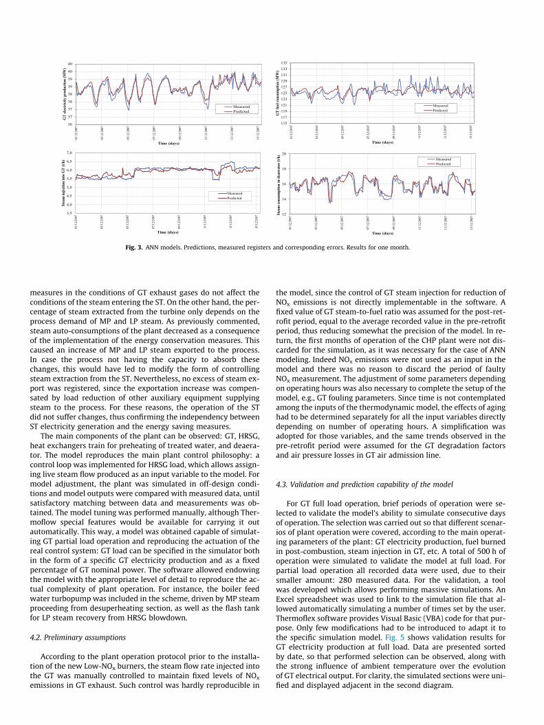
Fig. 2 shows obtained results for all generated ANN models. Asit can be observed, the initial date of the modeling period does notcoincide with the aforementioned one. Indeed the elimination ofregisters corresponding to the first months of operation was re-quired, due to a prolonged faulty measurement of NOx. The finaldataset was so reduced to data comprised between 06-12-200707:00 and 04-21-2008 17:00 (6405 data). The first column ofFig. 2 contains the simultaneous plots of ANN predictions and mea-sured registers, along with corresponding errors for each datapoint. The same information is presented in the second column,in the form of cross plots of predicted values against measured val-ues. Good agreement between predicted and actual values can beobserved from the first column, and correct random (and not sys-tematic) behavior of deviations from the diagonal in the secondcolumn. A strong smoothening tendency is observed in the deaer-ator steam consumption for high steam flow rates (bottom leftgraph of Fig. 2). This is mainly due to the low number of availabledata for training the model in that period, which does not reflectthe normal operation of the plant. The plant in its original pre-ret-rofit configuration includes a heat exchanger for preheating ofdeaerator feed water with hot condensates returned from the pro-cess. During the period at issue the heat exchanger was not receiv-ing condensates, thus augmenting the steam consumption in thedeaerator. Apart from these aspects, the relative errors calculatedin that zone are still acceptable and comparable with those ob-tained in the rest of the modeled period.

Additional graphs are also presented in Fig. 3, showing the sameresults of Fig. 2 but for a smaller period of time (two weeks). Thismay be useful to observe the graphical correspondence betweenthe values of accuracy and R2 achieved and the capacity of themodels to reproduce the registered profiles, in terms of flexibilityand ability to follow the tendencies and fluctuations of measureddata.

With reference to Table 2, satisfactory values of all calculatedperformance parameters may be observed in GT electricity produc-tion, demonstrating high model capability in predicting the out-puts. Almost 89% of the points present errors lower than 1.0%and only 0.9% are higher than 2%. Lower accuracy was obtainedfrom GT fuel consumption. The tendency of the model to smoothenfluctuations of registered data may be observed in the generatedplots and is also reflected by the low value of R2. The strong influ-ence of input data quality over model performance has to be con-sidered in this specific case. Indeed the fluctuations of registered

accuracies.

9 10 11 12 13 14 15

95,150 95,663 95,523 95,524 95,605 95,722 95,620

Page 6

-5,0

-2,5

0,0

2,5

5,0

7,5

10,0

12,5

15,0

32

33

34

35

36

37

38

39

40

12/0

6/20

07

10/0

7/20

07

07/0

8/20

07

04/0

9/20

07

02/1

0/20

07

30/1

0/20

07

27/1

1/20

07

25/1

2/20

07

22/0

1/20

08

19/0

2/20

08

18/0

3/20

08

15/0

4/20

08

Erro

r (%

)

GT

elec

tric

ity p

rodu

ctio

n (M

W)

Time (days)

MeasuredPredicted

33

34

35

36

37

38

39

40

41

34 35 36 37 38 39 40

GT

elec

tric

ity p

rodu

ctio

n (M

W) p

reci

ted

GT electricity production (MW) measured

-9,0-6,0-3,00,03,06,09,012,015,018,021,024,0

90

95

100

105

110

115

120

125

130

135

12/0

6/20

07

10/0

7/20

07

07/0

8/20

07

04/0

9/20

07

02/1

0/20

07

30/1

0/20

07

27/1

1/20

07

25/1

2/20

07

22/0

1/20

08

19/0

2/20

08

18/0

3/20

08

15/0

4/20

08

Erro

r (%

)

GT

fuel

cons

umpt

ion

(MW

)

Time (days)

MeasuredPredicted

100

105

110

115

120

125

130

135

140

110 114 118 122 126 130 134

GT

fuel

cons

umpt

ion

(MW

) pre

cited

GT fuel consumption (MW) measured

-20,0

-10,0

0,0

10,0

20,0

30,0

40,0

50,0

0

1

2

3

4

5

6

7

12/0

6/20

07

10/0

7/20

07

07/0

8/20

07

04/0

9/20

07

02/1

0/20

07

30/1

0/20

07

27/1

1/20

07

25/1

2/20

07

22/0

1/20

08

19/0

2/20

08

18/0

3/20

08

15/0

4/20

08

Erro

r (%

)

Stea

m in

ject

ion

into

GT

(t/h)

Time (days)

MeasuredPredicted

1

2

3

4

5

6

7

8

2 3 4 5 6 7 8

Stea

m in

ject

ion

into

GT

(t/h)

prec

ited

Steam injection into GT (t/h) measured

-20,0

-10,0

0,0

10,0

20,0

30,0

40,0

50,0

60,0

70,0

0

5

10

15

20

25

12/0

6/20

07

10/0

7/20

07

07/0

8/20

07

04/0

9/20

07

02/1

0/20

07

30/1

0/20

07

27/1

1/20

07

25/1

2/20

07

22/0

1/20

08

19/0

2/20

08

18/0

3/20

08

15/0

4/20

08

Erro

r (%

)

Stea

m co

nsum

ptio

n in

dea

erat

or (t

/h)

Time (days)

MeasuredPredicted

2

6

10

14

18

22

26

30

9 12 15 18 21 24 27

Stea

m co

ns. i

n de

aera

tor (

t/h) p

recit

ed

Steam cons. in deaerator (t/h) measured

Fig. 2. ANN models. Predictions, measured registers and corresponding errors.

data are not representative of the real GT operation. They aremainly due to the different frequencies of data acquisition for thetwo parameters, product of which gives GT fuel consumption inMW: fuel mass flow rate and fuel heating value. The first is mea-sured on an hourly basis and the latter proceeds from the daily lab-oratory analysis. Nevertheless model prediction capability is stillacceptable, since almost 86% of the calculated errors are lower than2.0% and only 0.4% are higher than 5%. Models generated for GTsteam injection and steam consumption of deaerator reproducecorrectly tendencies of registered data, as confirmed by the calcu-lated values of R2 and accuracy. As it was expected, higher MAE andRMSE values were calculated for these two models, due to the rel-evant error level commonly associated with on-line measurementof steam flow rates. On average, 85% of errors are lower than 5.0%for these two modeled parameters.

Summarizing, obtained accuracy levels and errors allow assert-ing that the generated ANN models captured correctly the behaviorof the CHP plant. The generalization capability is regarded assatisfactory for baseline energy consumption determiningpurposes, since the order of magnitude of the obtained errors iscomparable with the uncertainty associated with measuringinstruments.

4. Thermodynamic modeling

The same energy consumption and generation parameters weremodeled using a thermodynamic simulator. The model wasperformed with Thermoflex (release 23.0), (Thermoflow Inc.,2013) a specific software for thermal systems modeling speciallyconceived for power generation and CHP plants.

4.1. Model description

The generated model reproduces the CHP plant configuration inthe period prior to the implementation of saving projects. Fig. 4shows the diagram of the model used for the simulation. As itcan be observed, ST was not included in the model, due to the factthat the operation and electricity production of ST was not affectedby energy saving measures. Indeed, the electricity generated by theST is determined by the conditions (mass flow, temperature andpressure) of inlet live steam and the amount of steam extracted.The production and conditions of live steam entering the turbineare continuously controlled by means of the post-combustion fuelregulation system. It implies that the changes caused by saving

Page 7

36

37

37

38

38

39

39

40

40

01/1

2/20

07

03/1

2/20

07

05/1

2/20

07

07/1

2/20

07

09/1

2/20

07

11/1

2/20

07

13/1

2/20

07

15/1

2/20

07

GT

elect

ricity

pro

duct

ion

(MW

)

Time (days)

MeasuredPredicted

115117119121123125127129131133135

01/1

2/20

07

03/1

2/20

07

05/1

2/20

07

07/1

2/20

07

09/1

2/20

07

11/1

2/20

07

13/1

2/20

07

15/1

2/20

07

GT

fuel

cons

umpt

ion

(MW

)

Time (days)

MeasuredPredicted

3,5

4,0

4,5

5,0

5,5

6,0

6,5

7,0

01/1

2/20

07

03/1

2/20

07

05/1

2/20

07

07/1

2/20

07

09/1

2/20

07

11/1

2/20

07

13/1

2/20

07

15/1

2/20

07

Stea

m in

ject

ion

into

GT

(t/h)

Time (days)

MeasuredPredicted

12

14

16

18

20

01/1

2/20

07

03/1

2/20

07

05/1

2/20

07

07/1

2/20

07

09/1

2/20

07

11/1

2/20

07

13/1

2/20

07

15/1

2/20

07

Stea

m co

nsum

ptio

n in

dea

erat

or (t

/h)

Time (days)

MeasuredPredicted

Fig. 3. ANN models. Predictions, measured registers and corresponding errors. Results for one month.

measures in the conditions of GT exhaust gases do not affect theconditions of the steam entering the ST. On the other hand, the per-centage of steam extracted from the turbine only depends on theprocess demand of MP and LP steam. As previously commented,steam auto-consumptions of the plant decreased as a consequenceof the implementation of the energy conservation measures. Thiscaused an increase of MP and LP steam exported to the process.In case the process not having the capacity to absorb thesechanges, this would have led to modify the form of controllingsteam extraction from the ST. Nevertheless, no excess of steam ex-port was registered, since the exportation increase was compen-sated by load reduction of other auxiliary equipment supplyingsteam to the process. For these reasons, the operation of the STdid not suffer changes, thus confirming the independency betweenST electricity generation and the energy saving measures.

The main components of the plant can be observed: GT, HRSG,heat exchangers train for preheating of treated water, and deaera-tor. The model reproduces the main plant control philosophy: acontrol loop was implemented for HRSG load, which allows assign-ing live steam flow produced as an input variable to the model. Formodel adjustment, the plant was simulated in off-design condi-tions and model outputs were compared with measured data, untilsatisfactory matching between data and measurements was ob-tained. The model tuning was performed manually, although Ther-moflow special features would be available for carrying it outautomatically. This way, a model was obtained capable of simulat-ing GT partial load operation and reproducing the actuation of thereal control system: GT load can be specified in the simulator bothin the form of a specific GT electricity production and as a fixedpercentage of GT nominal power. The software allowed endowingthe model with the appropriate level of detail to reproduce the ac-tual complexity of plant operation. For instance, the boiler feedwater turbopump was included in the scheme, driven by MP steamproceeding from desuperheating section, as well as the flash tankfor LP steam recovery from HRSG blowdown.

4.2. Preliminary assumptions

According to the plant operation protocol prior to the installa-tion of the new Low-NOx burners, the steam flow rate injected intothe GT was manually controlled to maintain fixed levels of NOx

emissions in GT exhaust. Such control was hardly reproducible in

the model, since the control of GT steam injection for reduction ofNOx emissions is not directly implementable in the software. Afixed value of GT steam-to-fuel ratio was assumed for the post-ret-rofit period, equal to the average recorded value in the pre-retrofitperiod, thus reducing somewhat the precision of the model. In re-turn, the first months of operation of the CHP plant were not dis-carded for the simulation, as it was necessary for the case of ANNmodeling. Indeed NOx emissions were not used as an input in themodel and there was no reason to discard the period of faultyNOx measurement. The adjustment of some parameters dependingon operating hours was also necessary to complete the setup of themodel, e.g., GT fouling parameters. Since time is not contemplatedamong the inputs of the thermodynamic model, the effects of aginghad to be determined separately for all the input variables directlydepending on number of operating hours. A simplification wasadopted for those variables, and the same trends observed in thepre-retrofit period were assumed for the GT degradation factorsand air pressure losses in GT air admission line.

4.3. Validation and prediction capability of the model

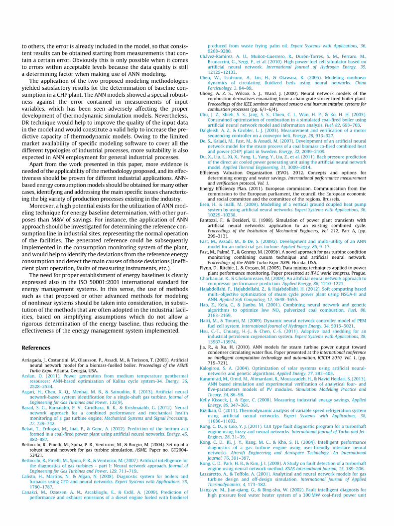
For GT full load operation, brief periods of operation were se-lected to validate the model’s ability to simulate consecutive daysof operation. The selection was carried out so that different scenar-ios of plant operation were covered, according to the main operat-ing parameters of the plant: GT electricity production, fuel burnedin post-combustion, steam injection in GT, etc. A total of 500 h ofoperation were simulated to validate the model at full load. Forpartial load operation all recorded data were used, due to theirsmaller amount: 280 measured data. For the validation, a toolwas developed which allows performing massive simulations. AnExcel spreadsheet was used to link to the simulation file that al-lowed automatically simulating a number of times set by the user.Thermoflex software provides Visual Basic (VBA) code for that pur-pose. Only few modifications had to be introduced to adapt it tothe specific simulation model. Fig. 5 shows validation results forGT electricity production at full load. Data are presented sortedby date, so that performed selection can be observed, along withthe strong influence of ambient temperature over the evolutionof GT electrical output. For clarity, the simulated sections were uni-fied and displayed adjacent in the second diagram.

Page 8

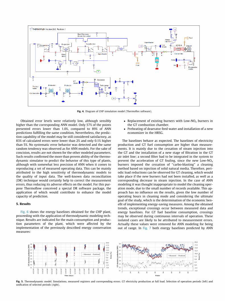
Fig. 4. Diagram of CHP simulation model (Thermoflex software).

Obtained error levels were relatively low, although sensiblyhigher than the corresponding ANN model. Only 57% of the pointspresented errors lower than 1.0%, compared to 89% of ANNpredictions fulfilling the same condition. Nevertheless, the predic-tion capability of the model may be still considered satisfactory, as83% of calculated errors were lower than 2% and only 0.1% higherthan 5%. No systematic error behavior was detected and the samerandom tendency was observed as for ANN models. For the sake ofconcision, results are not shown for the other modeled parameters.Such results confirmed the more than proven ability of the thermo-dynamic simulator to predict the behavior of this type of plants,although with somewhat less precision of ANN when it comes toreproducing a set of measured operating data. This can be mainlyattributed to the high sensitivity of thermodynamic models tothe quality of input data. The well-known data reconciliation(DR) technique would certainly help to correct the measurementerrors, thus reducing its adverse effects on the model. For this pur-pose Thermoflow conceived a special DR software package, theapplication of which would contribute to enhance the modelcapacity of prediction.

5. Results

Fig. 6 shows the energy baselines obtained for the CHP plant,proceeding with the application of thermodynamic modeling tech-nique. Results are indicated for the main consumption and produc-tion parameters of the plant, which were affected by theimplementation of the previously described energy conservationmeasures:

-5,0-2,50,02,55,07,510,012,515,017,520,0

31

32

33

34

35

36

37

38

39

16/0

2/20

07

16/0

3/20

07

13/0

4/20

07

11/0

5/20

07

08/0

6/20

07

06/0

7/20

07

03/0

8/20

07

31/0

8/20

07

28/0

9/20

07

26/1

0/20

07

23/1

1/20

07

21/1

2/20

07

18/0

1/20

08

15/0

2/20

08

14/0

3/20

08

11/0

4/20

08

Erro

r (%

)

GT

elect

ricity

pro

duct

ion

(MW

)

Time (days)

Measured Predicted

Fig. 5. Thermodynamic model. Simulations, measured registers and corresponding errounification of selected periods (right).

� Replacement of existing burners with Low-NOx burners inthe GT combustion chamber.

� Preheating of deaerator feed water and installation of a neweconomizer in the HRSG.

The baselines behave as expected. The baselines of electricityproduction and GT fuel consumption are higher than measure-ments. It is mainly due to the cessation of steam injection intothe GT and the installation of a new stage of filtration in the GTair inlet line; a second filter had to be integrated in the system toprevent the acceleration of GT fouling, since the new Low-NOx

burners imposed the cessation of ‘‘carbo-blasting’’ a cleaningmethod based on injection of solid natural media. Therefore, peri-odic load reductions can be observed for GT cleaning, which wouldtake place if the new burners had not been installed, as well as acorresponding decrease in steam injection. In the case of ANNmodeling it was thought inappropriate to model the cleaning oper-ation mode, due to the small number of records available. This ap-proach has no influence on the results, given the low number ofoperating hours in cleaning mode and considering the ultimategoal of the study, which is the determination of the economic ben-efit of implementing energy-saving measures. Among the obtainedtrends, exceptional crossings occur between measured data andenergy baselines. For GT fuel baseline consumption, crossingsmay be observed during continuous intervals of operation. Theseisolated cases are likely to be attributed to measurement errors.Actually these values were removed for ANN modeling for beingout of range. In Fig. 7 both energy baselines predicted by ANN

-5,0

-2,5

0,0

2,5

5,0

7,5

10,0

12,5

15,0

17,5

20,0

31

32

33

34

35

36

37

38

39

0

100

200

300

400

500

600

700

800

Erro

r (%

)

GT

elect

ricity

pro

duct

ion

(MW

)

Points

Measured Predicted

rs. GT electricity production at full load. Selection of operation periods (left) and

Page 9

30

32

34

36

38

40

4217

/11/

2008

07/1

2/20

08

27/1

2/20

08

16/0

1/20

09

05/0

2/20

09

25/0

2/20

09

17/0

3/20

09

06/0

4/20

09

26/0

4/20

09

GT

elect

ricity

pro

duct

ion

(MW

)

Time (days)

Actual Baseline

0,00,51,01,52,02,53,03,54,04,55,0

17/1

1/20

08

07/1

2/20

08

27/1

2/20

08

16/0

1/20

09

05/0

2/20

09

25/0

2/20

09

17/0

3/20

09

06/0

4/20

09

26/0

4/20

09

Stea

m in

ject

ion

into

GT

(t/h)

Time (days)

Actual Baseline

100,0

106,0

112,0

118,0

124,0

130,0

136,0

17/1

1/20

08

07/1

2/20

08

27/1

2/20

08

16/0

1/20

09

05/0

2/20

09

25/0

2/20

09

17/0

3/20

09

06/0

4/20

09

26/0

4/20

09

GT

fuel

cons

umpt

ion

(MW

)

Time (days)

Actual Baseline

0

3

6

9

12

15

18

21

17/1

1/20

08

07/1

2/20

08

27/1

2/20

08

16/0

1/20

09

05/0

2/20

09

25/0

2/20

09

17/0

3/20

09

06/0

4/20

09

26/0

4/20

09

Stea

m co

nsum

ptio

n in

dea

erat

or (t

/h)

Time (days)

Actual Baseline

Fig. 6. Predicted and measured energy production and consumptions of CHP in the post-retrofit period.

and thermodynamic models are represented, together with thepercentage differences between them.

The results for predicted GT electricity production and fuel con-sumption indicate relatively low differences between generatedbaselines, in the order of 3–5%. Predictions obtained from ANNmodeling for these two parameters show a tendency to exceedthermodynamic baseline in the second part of the observed period.A source of inaccuracy which the differences could be addressed tois the approximate approach that was adopted to reproduce GTaging in thermodynamic modeling. On the one hand, aging param-eters were used as an adjustable input to better reproduce mea-sured data when validating the thermodynamic model for preretrofit period. On the other hand, those parameters generate anenvironment of uncertainty in the post retrofit period: the sametrends were reproduced as for the pre retrofit period and there isno warranty that it corresponds to the real CHP operation. Another

-3,0%

0,0%

3,0%

6,0%

9,0%

12,0%

15,0%

18,0%

25

27

29

31

33

35

37

39

41

17/1

1/20

08

07/1

2/20

08

27/1

2/20

08

16/0

1/20

09

05/0

2/20

09

25/0

2/20

09

17/0

3/20

09

06/0

4/20

09

26/0

4/20

09

GT

elect

ricity

pro

duct

ion

(MW

)

Time (days)

Baseline_ANN model Baseline_Termodynamical model Difference (%)

-40,0%

-20,0%

0,0%

20,0%

40,0%

60,0%

80,0%

100,0%

120,0%

140,0%

160,0%

0,0

1,0

2,0

3,0

4,0

5,0

6,0

7,0

17/1

1/20

08

07/1

2/20

08

27/1

2/20

08

16/0

1/20

09

05/0

2/20

09

25/0

2/20

09

17/0

3/20

09

06/0

4/20

09

26/0

4/20

09

Stea

m in

ject

ion

into

GT

(t/h)

Time (days)

Baseline_ANN model Baseline_Termodynamical model Difference (%)

Fig. 7. Energy baselines obtained with A

possible cause of the discrepancies could be associated with thefuel feed temperature, not contemplated in the ANN model. Afterthe implementation of energy saving measures, fuel preheatingwas introduced as a practice in plant operation. This resulted in aslight reduction of GT fuel consumption and electricity production.Fuel temperature could not be included as an input to ANN models,since fuel was supplied to GT at ambient temperature in pre retro-fit period and the slight fluctuations registered were not sufficientto appreciate its effects. More relevant differences between themodels were detected for steam injected into the GT, the differ-ences ranging up to 30–35%. In this case better results wereachieved with the ANN modeling approach. The discrepancies aremainly associated with the limitations of thermodynamic modelwhen reproducing the real plant control for NOx emissions reduc-tion, as discussed above. Concerning the effect of the second savingproject (pre-heating of deaerator feed water), the differences are

-6,00%

-3,00%

0,00%

3,00%

6,00%

9,00%

12,00%

15,00%

18,00%

80,00

90,00

100,00

110,00

120,00

130,00

17/1

1/20

08

07/1

2/20

08

27/1

2/20

08

16/0

1/20

09

05/0

2/20

09

25/0

2/20

09

17/0

3/20

09

06/0

4/20

09

26/0

4/20

09

GT

fuel

cons

umpt

ion

(MW

)

Time (days)

Baseline_ANN model Baseline_Termodynamical model Difference (%)

-15,0%

0,0%

15,0%

30,0%

45,0%

60,0%

75,0%

90,0%

105,0%

02468

10121416182022

17/1

1/20

08

07/1

2/20

08

27/1

2/20

08

16/0

1/20

09

05/0

2/20

09

25/0

2/20

09

17/0

3/20

09

06/0

4/20

09

26/0

4/20

09

Stea

m co

nsum

ptio

n in

dea

erat

or (t

/h)

Time (days)

Baseline_ANN model Baseline_Termodynamical model Difference (%)

NN and thermodynamic modeling.

Page 10

Table 2Final structure and prediction performance of the generated ANN models.

Modeledparameter

No. ofinputneurons

No. of neurons inthe first hiddenlayer

No. of neurons in thesecond hidden layer

No. of neurons in the second hidden layer MAE(%)

RMSE(%)

R2 Accuracy(%)

Below0.1%

0.1�0.5% 0.5�1.0% 1.0�2.0% 2.0�5.0% 5.0�10.0% Above10.0%

GT electricityproduction

7 8 3 13.5 45.8 29.3 10.5 0.9 0.0 0.0 0.51 0.67 0.95 95.85

GT fuelconsumption

7 7 2 6.6 24.5 26.0 28.4 14.1 0.4 0.0 1.08 1.41 0.74 93.29

MP steaminjection intoGT

6 12 5 2.2 9.7 11.2 20.8 35.9 17.4 2.8 3.16 4.32 0.94 96.90

LP steamconsumed indeaerator

4 3 / 3.1 11.5 15.2 25.0 34.6 8.7 1.9 2.45 3.58 0.94 97.22

relevant again: steam consumption in the deaerator predicted bythermodynamic simulation is significantly lower, due to the highmeasurement uncertainty of treated water flow, which induces er-ror propagation in the simulation of the water preheating line.Hence, the differences are smaller for the hours of operation inwhich the implanted saving measure is not active, i.e., the new ex-changer installed is out of service and LP steam consumption ishigher. Discussed results reflect the main problem associated withenergy baseline assessment, i.e., the great uncertainty environmentand the absence of reference data for comparison characterizingthe post-retrofit period. Limiting this uncertainty was indeed themain objective of this study, aimed at developing advanced andreliable modeling techniques for determination of credible base-line energy profiles. As regards the fidelity of the models, it is log-ical that it cannot be appreciated from the generated baselines, butprediction accuracy is to be rather detected during the validationprocess of the models. In this sense, the reader can refer to the pre-vious sections of this paper discussing the validation results ofboth ANN and thermodynamic models.

6. Conclusions

Two different modeling approaches were used to determine thebaseline of energy consumption and production in a CHP plant.ANN modeling and thermodynamic simulation were compared,both showing satisfactory levels of accuracy and suitability forbaseline construction. The main potentials and inconveniencesassociated with each one of the analyzed methodologies were de-tected during the study.

Concerning ANN modeling, the potential versatility and utilityof this technique was demonstrated. High accuracy was observedin the results, being the error levels obtained comparable withthe uncertainty of measured data. The models showed satisfactoryrobustness against the errors contained in measured values of in-put variables. Another detached feature of ANN models is theirpracticality, which make them easily usable on different media likespreadsheets, programming, etc.

However, in the course of work, the main drawback associatedwith the ANN modeling arose, i.e., the vulnerability to changes inoperating parameters outside the range for which the model wastrained. A common feature to statistical models in general is theneed for input data to contain fluctuations representative of sys-tem operation. ANNs do not guarantee accuracy outside the rangesfor which they were generated and the effects cannot be repro-duced of the variables for which no changes were recorded. Also,when records for output variables are erroneous, the error is insur-mountable by ANN models since they were trained through theserecords. A clarification is also necessary, with respect to the sim-plicity of development and application of ANN models. Although

the ‘‘black box’’ philosophy of ANN modeling technique might sug-gest the contrary, the presented analysis shows that ANN approachcannot elude a deep knowledge of the physics of the system. This isa factor of paramount importance, since the selected databaseinevitably affects the result of the ANN training. In the case of ther-modynamic modeling the problem of system knowledge is ratherrelated to the construction of the model, being the selection of dataless critical. Indeed, deviations of thermodynamic simulationsfrom measured registers can even be a valuable aid for the revisionof the selected database.

Regarding thermodynamic modeling, obtained results as well asprevious experience in the use of the simulator confirmed itsremarkable ability to predict the behavior and performance ofCHP plants with satisfactory level of accuracy. Also, thermody-namic modeling is not conditioned by the richness of historicaldata available, since it is not based on statistics. This can be a greatadvantage, given the problems involved in the acquisition of reli-able measurements in almost any industrial plant.

On the other hand, the high sensitivity to measurement errorsemerged for this modeling method: faulty meters impact adverselyon the variables which are calculated from these measurements.This directly affects the simulation, which solves the mass and en-ergy balances based on these inputs, contrary to what happens toANN models. Some limitations were also detected when perform-ing a complete modeling of the plant, and some simplifyingassumptions had to be introduced, thus reducing the fidelity ofreproduction of plant operation. It is the case of the steam flowinjection into the GT, which cannot be directly predicted as a func-tion of NOx emission levels. A second case is represented by theinability to include operating hours as input variables to the model.It makes necessary the adjustment of equipment aging parameters,which complicates the simulation if the aim is reproducing contin-uous time intervals of plant operation.

With respect to the times required for computation, during thevalidation phase the problem arose of long waiting times for thesimulation of continuous periods of operation. However this isnot a problem for the construction of the baseline, since its deter-mination is performed periodically and response times of the sim-ulator are more than acceptable for the intended purpose.

Some aspects are also worth noting related to the behavior ofthe models against uncertainty. The modeling of a system by ther-modynamic simulation is based on the physical behavior of plantequipment. This is advantageous, since detection is possible ofmeasurement errors and therefore the model, by means of its re-sults, may provide more reliable values for those parameters withhigh uncertainties in their measurements. However, if these errorsoccur in the input variables, risk of propagation exists and adjust-ments or complementary calculations are necessary. ANN model-ing may help to overcome this problem due to the ‘‘black box’’treatment that it implies; when modeling variables with respect

Page 11

to others, the error is already included in the model, so that consis-tent results can be obtained starting from measurements that con-tain a certain error. Obviously this is only possible when it comesto errors within acceptable levels because the data quality is stilla determining factor when making use of ANN modeling.

The application of the two proposed modeling methodologiesyielded satisfactory results for the determination of baseline con-sumption in a CHP plant. The ANN models showed a special robust-ness against the error contained in measurements of inputvariables, which has been seen adversely affecting the properdevelopment of thermodynamic simulation models. Nevertheless,DR technique would help to improve the quality of the input datain the model and would constitute a valid help to increase the pre-dictive capacity of thermodynamic models. Owing to the limitedmarket availability of specific modeling software to cover all thedifferent typologies of industrial processes, more suitability is alsoexpected in ANN employment for general industrial processes.

Apart from the work presented in this paper, more evidence isneeded of the applicability of the methodology proposed, and its effec-tiveness should be proven for different industrial applications. ANN-based energy consumption models should be obtained for many othercases, identifying and addressing the main specific issues characteriz-ing the big variety of production processes existing in the industry.

Moreover, a high potential exists for the utilization of ANN mod-eling technique for energy baseline determination, with other pur-poses than M&V of savings. For instance, the application of ANNapproach should be investigated for determining the reference con-sumption line in industrial sites, representing the normal operationof the facilities. The generated reference could be subsequentlyimplemented in the consumption monitoring system of the plant,and would help to identify the deviations from the reference energyconsumption and detect the main causes of those deviations (ineffi-cient plant operation, faults of measuring instruments, etc.).

The need for proper establishment of energy baselines is clearlyexpressed also in the ISO 50001:2001 international standard forenergy management systems. In this sense, the use of methodssuch as that proposed or other advanced methods for modelingof nonlinear systems should be taken into consideration, in substi-tution of the methods that are often adopted in the industrial facil-ities, based on simplifying assumptions which do not allow arigorous determination of the energy baseline, thus reducing theeffectiveness of the energy management system implemented.

References

Arriagada, J., Costantini, M., Olausson, P., Assadi, M., & Torisson, T. (2003). Artificialneural network model for a biomass-fuelled boiler. Proceedings of the ASMETurbo Expo. Atlanta, Georgia, USA.

Arslan, O. (2011). Power generation from medium temperature geothermalresources: ANN-based optimization of Kalina cycle system-34. Energy, 36,2528–2534.

Asgari, H., Chen, X. Q., Menhaj, M. B., & Sainudiin, R. (2013). Artificial neuralnetwork-based system identification for a single-shaft gas turbine. Journal ofEngineering for Gas Turbines and Power, 135(9).

Barad, S. G., Ramaiahb, P. V., Giridhara, R. K., & Krishnaiahb, G. (2012). Neuralnetwork approach for a combined performance and mechanical healthmonitoring of a gas turbine engine. Mechanical Systems and Signal Processing,27, 729–742.

Bekat, T., Erdogan, M., Inal, F., & Genc, A. (2012). Prediction of the bottom ashformed in a coal-fired power plant using artificial neural networks. Energy, 45,882–887.

Bettocchi, R., Pinelli, M., Spina, P. R., Venturini, M., & Burgio, M. (2004). Set up of arobust neural network for gas turbine simulation. ASME. Paper no. GT2004-53421.

Bettocchi, R., Pinelli, M., Spina, P. R., & Venturini, M. (2007). Artificial intelligence forthe diagnostics of gas turbines – part I: Neural network approach. Journal ofEngineering for Gas Turbines and Power, 129, 711–719.

Calisto, H., Martins, N., & Afgan, N. (2008). Diagnostic system for boilers andfurnaces using CFD and neural networks. Expert Systems with Applications, 35,1780–1787.

Canakci, M., Ozsezen, A. N., Arcaklioglu, E., & Erdil, A. (2009). Prediction ofperformance and exhaust emissions of a diesel engine fueled with biodiesel

produced from waste frying palm oil. Expert Systems with Applications, 36,9268–9280.

Chávez-Ramírez, A. U., Muñoz-Guerrero, R., Durón-Torres, S. M., Ferraro, M.,Brunaccini, G., Sergi, F., et al. (2010). High power fuel cell simulator based onartificial neural network. International Journal of Hydrogen Energy, 35,12125–12133.

Chen, W., Tsutsumi, A., Lin, H., & Otawara, K. (2005). Modeling nonlineardynamics of circulating fluidized beds using neural networks. ChinaParticuology, 3, 84–89.

Chong, A. Z. S., Wilcox, S. J., Ward, J. (2000). Neural network models of thecombustion derivatives emanating from a chain grate stoker fired boiler plant.Proceedings of the IEEE seminar advanced sensors and instrumentation systems forcombustion processes (pp. 6/1–6/4).

Chu, J. Z., Shieh, S. S., Jang, S. S., Chien, C. I., Wan, H. P., & Ko, H. H. (2003).Constrained optimization of combustion in a simulated coal-fired boiler usingartificial neural network model and information analysis. Fuel, 82, 693–703.

Dalgleish, A. Z., & Grobler, L. J. (2003). Measurement and verification of a motorsequencing controller on a conveyor belt. Energy, 28, 913–927.

De, S., Kaiadi, M., Fast, M., & Assadi, M. (2007). Development of an artificial neuralnetwork model for the steam process of a coal biomass co-fired combined heatand power (CHP) plant in Sweden. Energy, 32, 2099–2109.

Du, X., Liu, L., Xi, X., Yang, L., Yang, Y., Liu, Z., et al. (2011). Back pressure predictionof the direct air cooled power generating unit using the artificial neural networkmodel. Applied Thermal Engineering, 31, 3009–3014.

Efficiency Valuation Organization (EVO). 2012. Concepts and options fordetermining energy and water savings. International performance measurementand verification protocol, Vol. 1.

Energy Efficiency Plan. (2011). European commission. Communication from thecommission to the European parliament, the council, the European economicand social committee and the committee of the regions. Brussels.

Esen, H., & Inalli, M. (2009). Modelling of a vertical ground coupled heat pumpsystem by using artificial neural networks. Expert Systems with Applications, 36,10229–10238.

Fantozzi, F., & Desideri, U. (1998). Simulation of power plant transients withartificial neural networks: application to an existing combined cycle.Proceedings of the Institution of Mechanical Engineers, Vol. 212, Part A, (pp.299–313).

Fast, M., Assadi, M., & De, S. (2009a). Development and multi-utility of an ANNmodel for an industrial gas turbine. Applied Energy, 86, 9–17.

Fast, M., Palmé, T., & Genrup, M. (2009b). A novel approach for gas turbine conditionmonitoring combining cusum technique and artificial neural network.Proceedings of the ASME Turbo Expo 2009. Florida, USA.

Flynn, D., Ritchie, J., & Cregan, M. (2005). Data mining techniques applied to powerplant performance monitoring. Paper presented at IFAC world congress, Prague.

Ghorbanian, K., & Gholamrezaei, M. (2009). An artificial neural network approach tocompressor performance prediction. Applied Energy, 86, 1210–1221.

Hajabdollahi, F., Hajabdollahi, Z., & Hajabdollahi, H. (2012). Soft computing basedmulti-objective optimization of steam cycle power plant using NSGA-II andANN. Applied Soft Computing, 12, 3648–3655.

Hao, Z., Kefa, C., & Jianbo, M. (2001). Combining neural network and geneticalgorithms to optimize low NOx pulverized coal combustion. Fuel, 80,2163–2169.

Hatti, M., & Tioursi, M. (2009). Dynamic neural network controller model of PEMfuel cell system. International Journal of Hydrogen Energy, 34, 5015–5021.

Hsu, C.-T., Chuang, H.-J., & Chen, C.-S. (2011). Adaptive load shedding for anindustrial petroleum cogeneration system. Expert Systems with Applications, 38,13967–13974.

Jia, R., & Xu, H. (2010). ANN models for steam turbine power output towardcondenser circulating water flux. Paper presented at the international conferenceon intelligent computation technology and automation, ICICTA 2010, Vol. 1, (pp.719–721).

Kalogirou, S. A. (2004). Optimization of solar systems using artificial neural-networks and genetic algorithms. Applied Energy, 77, 383–405.

Karamirad, M., Omid, M., Alimardani, R., Mousazadeh, H., & Navid Heidari, S. (2013).ANN based simulation and experimental verification of analytical four- andfive-parameters models of PV modules. Simulation Modelling Practice andTheory, 34, 86–98.

Kelly Kissock, J., & Eger, C. (2008). Measuring industrial energy savings. AppliedEnergy, 85, 347–361.

Kizilkan, Ö. (2011). Thermodynamic analysis of variable speed refrigeration systemusing artificial neural networks. Expert Systems with Applications, 38,11686–11692.

Kong, C. D., & Goo, Y. J. (2011). GUI type fault diagnostic program for a turboshaftengine using fuzzy and neural networks. International Journal of Turbo and Jet-Engines, 28, 31–39.

Kong, C. D., Ki, J. Y., Kang, M. C., & Kho, S. H. (2004). Intelligent performancediagnostics of a gas turbine engine using user-friendly interface neuralnetworks. Aircraft Engineering and Aerospace Technology. An InternationalJournal, 76, 391–397.

Kong, C. D., Park, H. B., & Kim, J. I. (2008). A Study on fault detection of a turboshaftengine using neural network method. KSAS International Journal, 15, 189–206.

Lazzaretto, A., & Toffolo, A. (2001). Analytical and neural network models for gasturbine design and off-design simulation. International Journal of AppliedThermodynamics, 4, 173–182.

Liang-yu, M., Jian-qiang, G., & Bing-shu, W. (2002). Fault intelligent diagnosis forhigh pressure feed water heater system of a 300 MW coal-fired power unit

Page 12

based on improved BP neural network. IEEE Transactions on Neural Networks,1535–1539.

Liau, L. C.-K., Yang, T. C.-K., & Tsai, M.-T. (2004). Expert system of a crude oildistillation unit for process optimization using neural networks. Expert Systemswith Applications, 26, 247–255.

Liukkonen, M., Heikkinen, M., Hiltunen, T., Hälikkä, E., Kuivalainen, R., & Hiltunen, Y.(2011). Artificial neural networks for analysis of process states in fluidized bedcombustion. Energy, 36, 339–347.

Lu, S., & Hogg, B. W. (2000). Dynamic and nonlinear modelling of power plant byphysical principles and neural networks. International Journal of Electrical Power& Energy Systems, 22, 67–78.

Ma, J., Wang, B.-S., & Ma, Y.-G. (2008). ANN-based real-time parameter optimizationvia GA for superheater model in power plant simulator. Proceedings of the 7thInternational Conference on Machine Learning and Cybernetics, ICMLC, Vol. 4, (pp.2269–2273).

Mingzhi, H., Yongwen, M., Jinquan, W., & Yan, W. (2009). Simulation of a paper millwastewater treatment using a fuzzy neural network. Expert Systems withApplications, 36, 5064–5070.

Moghavvemi, M., Yang, S. S., & Kashem, M. A. (1998). A practical neural networkapproach for power generation automation. Proceedings of Energy Managementand Power Delivery. 1998 International Conference, Vol. 1, (pp. 305–310).

Monedero, I., Biscarri, F., León, C., Guerrero, J. I., González, R., & Pérez-Lombard, L.(2012). Decision system based on neural networks to optimize the energyefficiency of a petrochemical plant. Expert Systems with Applications, 39,9860–9867.

Motlaghi, S., Jalali, F., & Nili Ahmadabadi, M. (2008). An expert system design for acrude oil distillation column with the neural networks model and the processoptimization using genetic algorithm framework. Expert Systems withApplications, 35, 1540–1545.

Nikpey, H., Assadi, M., Breuhaus, P., & Mørkved, P. T. (2014). Experimentalevaluation and ANN modeling of a recuperative micro gas turbine burningmixtures of natural gas and biogas. Applied Energy, 117, 30–41.

Oguz, H., Saritas, I., & Baydan, H. E. (2010). Prediction of diesel engine performanceusing biofuels with artificial neural network. Expert Systems with Applications,37, 6579–6586.

Olanrewaju, O. A., & Jimoh, A. A. (2014). Review of energy models to thedevelopment of an efficient industrial energy model. Renewable andSustainable Energy Reviews, 30, 661–671.

Olausson, P., Häggståhl, D., Arriagada, J., Dahlquist, E., & Assadi, M. (2003). Hybridmodel of an evaporative gas turbine power plant utilizing physical models andartificial neural network. Proceedings of the ASME Turbo Expo. Atlanta, Georgia,USA.

Oliveira, M. V., & Soares de Almeida, J. C. (2013). Application of artificial intelligencetechniques in modeling and control of a nuclear power plant pressurizersystem. Progress in Nuclear Energy, 63, 71–85.

Palme, T., Breuhaus, P., Assadi, M., Klein, A., & Kim, M. (2011). New Alstommonitoring tools leveraging artificial neural network technologies. ASME TurboExpo. Paper no. GT2011-45990.

Pan, L., Flynn, D., & Cregan, M. (2007). Statistical model for power plantsperformance monitoring and analysis. Universities Power EngineeringConference, 2007. UPEC 2007, 121–126. 42nd International Conference.

Rashidi, M. M., Galanis, N., Nazari, F., Basiri Parsa, A., & Shamekhi, L. (2011).Parametric analysis and optimization of regenerative Clausius and organicRankine cycles with two feedwater heaters using artificial bees colony andartificial neural network. Energy, 36, 5728–5740.

Reichl, J., & Kollmann, A. (2011). The baseline in bottom-up energy efficiency andsaving calculations – a concept for its formalization and a discussion of relevantoptions. Applied Energy, 88, 422–431.

Romero, C. E., & Shan, J. (2005). Development of an artificial neural network-basedsoftware for prediction of power plant canal water discharge temperature.Expert Systems with Applications, 29, 831–838.

Rumelhart, D. E., Hinton, G. E., & Williams, R. J. (1986). Learning internalrepresentations by error propagation. Parallel distributed processing:explorations in the microstructure of cognition, Vol. 1(1), (pp. 318–362).Cambridge, MA: MIT Press.

Rusinowski, H., & Stanek, W. (2007). Neural modelling of steam boilers. EnergyConversion and Management, 48, 2802–2809.

Satish, S., & Setty, Y. P. (2005). Modeling of a continuous fluidized bed dryer usingartificial neural networks. International Communications in Heat and MassTransfer, 32, 539–547.

Simani, S., & Fantuzzi, C. (2000). Fault diagnosis in power plant using neuralnetworks. Information Sciences, 127, 125–136.

Sisworahardjo, N. S., El-Sharkh, M. Y., & Alamb, M. S. (2008). Neural networkcontroller for microturbine power plants. Electric Power Systems Research, 78,1378–1384.

Smrekar, J., Pandit, D., Fast, M., Assadi, M., & De, S. (2010). Prediction of poweroutput of a coal-fired power plant by artificial neural network. NeuralComputing & Applications, 19, 725–740.

Sözen, A., & Akçayol, M. A. (2004). Modelling (using artificial neural-networks) theperformance parameters of a solar-driven ejector-absorption cycle. AppliedEnergy, 79, 309–325.

Suresh, M. V. J. J., Reddy, K. S., & Kolar, A. K. (2011). ANN–GA based optimization of ahigh ash coal-fired supercritical power plant. Applied Energy, 88, 4867–4873.

Tasdemir, S., Saritas, I., Ciniviz, M., & Allahverdi, N. (2011). Artificial neural networkand fuzzy expert system comparison for prediction of performance andemission parameters on a gasoline engine. Expert Systems with Applications,38, 13912–13923.

Teruel, E., Cortes, C., Diez, L. I., & Arauzo, I. (2005). Monitoring and prediction offouling in coal-fired utility boilers using neural networks. Chemical EngineeringScience, 60, 5035–5048.

Thermoflow Inc., (2013). 2 Willow Street, Suite 100, Southborough, MA 01745-1020, USA. <http://www.thermoflow.com>.

Tronci, S., Baratti, R., & Servida, A. (2002). Monitoring pollutant emissions in a4.8 MW power plant through neural network. Neurocomputing, 43, 3–15.

U.S. EPA State Clean Energy and Climate Program. (2009). Clean energy lead byexample guide: Strategies, resources, and action steps for state programs,prepared by Joanna Pratt and Joe Donahue. Stratus Consulting Inc.

Vargas-Martínez, A., Minchala Avila, L. I., Zhang, Y., Garza-Castañón, L. E., & CalleOrtiz, E. R. (2013). Model-based fault-tolerant control to guarantee theperformance of a hybrid wind-diesel power system in a microgridconfiguration. Procedia Computer Science, 19, 712–719.

Velázquez, D., González-Falcón, R., Pérez-Lombard, L., Gallego, L. M., Monedero, I., &Biscarri, F. (2013). Development of an energy management system for anaphtha reforming plant: A data mining approach. Energy Conversion andManagement, 67, 217–225.

Volponi, A. J., DePold, H., Ganguli, R., & Daguang, C. (2003). The use of Kalman filterand neural network methodologies in gas turbine performance diagnostics: Acomparative study. Journal of Engineering for Gas Turbines and Power, 125,917–924.

Yap, W. K., & Karri, V. (2013). Comparative analysis of artificial neural networks anddynamic models as virtual sensors. Applied Soft Computing, 13, 181–188.

Yeh, W.-C., Yeh, Y.-M., Chang, P.-C., Ke, Y.-C., & Chung, V. (2014). Forecasting windpower in the Mai Liao wind farm based on the multi-layer perceptron artificialneural network model with improved simplified swarm optimization.International Journal of Electrical Power and Energy Systems, 55, 741–748.