The copyright in this document is vested in JOANNEUM RESEARCH. This document may only be reproduced in whole or in part, or stored in a retrieval system, or transmitted in any form, or by any means electronic, mechanical, photocopying or otherwise, either with the prior permission of JOANNEUM RESEARCH or in accordance with the terms of ESTEC Contract no 4000114810/15/UK/ND. ARTES 5.1: ADVANCED AIR INTERFACE DEMONSTRATOR FOR FUTURE MOBILE INTERACTIVE NETWORKS (FuMIN) Final Report ESTEC Contract Number 4000114810/15/UK/ND ESA Technical Officer(s): Nikolaos Toptsidis, ESTEC, Noordwijk Johannes Ebert, Harald Schlemmer, Barbara Süsser-Rechberger JOANNEUM RESEARCH, Graz, Austria Date: 4 th April, 2019 Document ref. no. FuMIN-FR-v1.0 EUROPEAN SPACE AGENCY CONTRACT REPORT The work described in this report was done under ESA contract. Responsibility for the contents resides in the author or organisation that prepared it.

Welcome message from author
This document is posted to help you gain knowledge. Please leave a comment to let me know what you think about it! Share it to your friends and learn new things together.
Transcript

The copyright in this document is vested in JOANNEUM RESEARCH. This document may only be reproduced in whole or in part, or stored in a retrieval system, or transmitted in any form, or by any means electronic, mechanical, photocopying or otherwise, either with the prior permission of JOANNEUM RESEARCH or in accordance with the terms of ESTEC Contract no 4000114810/15/UK/ND.
ARTES 5.1: ADVANCED AIR INTERFACE DEMONSTRATOR FOR FUTURE MOBILE
INTERACTIVE NETWORKS (FuMIN)
Final Report
ESTEC Contract Number 4000114810/15/UK/ND
ESA Technical Officer(s): Nikolaos Toptsidis, ESTEC, Noordwijk
Johannes Ebert, Harald Schlemmer, Barbara Süsser-Rechberger
JOANNEUM RESEARCH,
Graz, Austria
Date: 4th April, 2019
Document ref. no. FuMIN-FR-v1.0
EUROPEAN SPACE AGENCY
CONTRACT REPORT
The work described in this report was done under ESA contract. Responsibility for the
contents resides in the author or organisation that prepared it.

FuMIN FR v1.0 page 2 of 282
ABSTRACT
In the activity, an advanced air interface demonstrator for future mobile interactive networks in the Ka-band was implemented as simulation model and as HW solution on a software defined radio platform. The air interface is based on DVB-S2x and DVB-RCS2 for forward and return link respectively. The full range of DVB-S2x modcods up to 32APSK and RCS2 waveforms up to 16QAM-5/6 are supported. Very-low operational points down to -10dB SNR for both forward and return link have been realized. A full modem implementation with carrier synchronization, FEC-codecs, ACM and a link-layer FEC (staircase LDPC) has been done. The demonstrator includes also a channel emulation with realistic impairments (AWGN, TWTA, Phase Noise, IMUX, OMUX, co & adjacent channel interferences, multi carrier operation, frequency & timing offsets) as well as a mobile channel model that includes effects from the troposphere, the mobile antenna, multi-paths and blockages. The realized scenarios include vehicular, train and aeronautic use-cases, and for each use-case an adequate mobile channel model was developed.

FuMIN FR v1.0 page 3 of 282
Document History
Version NOTES DATES
1.0 First Release. April 4th, 2019

FuMIN FR v1.0 page 4 of 282
Table of Contents
1. Introduction ........................................................................................................................ 20
1.1. Reference Documents ..................................................................................................... 20
1.2. Acronyms ........................................................................................................................ 26
2. System Requirements and Applicable Scenarios ...... 29
2.1. Future Satellite Systems.................................................................................................. 29
2.1.1. Introduction............................................................................................................... 29
2.1.2. Baseline Satellite System Architecture ..................................................................... 30
2.2. Definition of Reference Scenarios for Mobile Interactive Satellite Systems ..................... 31
3. End-to-End Air Interface .............................................. 34
3.1. Introduction ..................................................................................................................... 34
3.2. DVB-S2x ......................................................................................................................... 34
3.2.1. Overview .................................................................................................................. 34
3.2.2. Encapsulation ........................................................................................................... 35
3.2.3. Framing .................................................................................................................... 37
3.2.4. FEC .......................................................................................................................... 37
3.2.5. Modulation ................................................................................................................ 41
3.2.6. Modcod Performance ............................................................................................... 44
3.2.7. Super-frames ............................................................................................................ 53
3.2.8. DVB-S2x Synchronization and Channel Estimation .................................................. 61
3.3. DVB-RCS2 ...................................................................................................................... 88
3.3.1. Overview .................................................................................................................. 88
3.3.2. Encapsulation ........................................................................................................... 88
3.4. Burst Assembly ........................................................................................................... 90
3.4.1. FEC .......................................................................................................................... 90
3.4.2. Modulation ................................................................................................................ 92
3.4.3. Waveform Performance ............................................................................................ 92
3.4.4. RCS2 Synchronization and SNR Estiamtion ............................................................. 95
3.4.5. VL-SNR for the Return Link .................................................................................... 100
3.5. Forward Error Correction for Counter-Measuring Blockages ......................................... 115
3.5.1. Link Layer-FEC and Interleaving for Mobile Applications ........................................ 116
3.5.2. PL Interleaver ......................................................................................................... 125
3.6. ACM .............................................................................................................................. 130
3.6.1. Introduction............................................................................................................. 130
3.6.2. ACM signalling channel .......................................................................................... 131
3.6.3. ACM controller ........................................................................................................ 131

FuMIN FR v1.0 page 5 of 282
3.6.4. Measurement of the channel condition ................................................................... 133
3.7. Air-Interface and Techniques Selection for the Implementation of the Demonstrator ..... 136
4. Mobile Channel Model ................................................ 138
4.1. Introduction ................................................................................................................... 138
4.2. Channel Models ............................................................................................................ 139
4.3. Modeling the Doppler effects ......................................................................................... 140
4.4. Modeling of Tropospheric Effects .................................................................................. 142
4.4.2. Generating synthetic tropospheric channel time-series ........................................... 151
4.5. Modeling of Local Effects .............................................................................................. 156
4.5.1. State-based railroad and vehicular channels models .............................................. 157
4.5.2. Railroad scenarios with periodic features ............................................................... 166
4.5.3. The aeronautical channel ....................................................................................... 168
4.6. Modelling of Antenna Pointing Errors ............................................................................ 169
4.6.1. Second-order statistics (SoSt) ................................................................................ 175
4.6.2. Comparison of a Gaussian distribution and a Laplace distribution .......................... 179
4.7. Mobile Channel Implementation .................................................................................... 180
4.7.1. Land Mobile Channel .............................................................................................. 180
4.7.2. Aeronautical Channel ............................................................................................. 181
4.7.3. Railway Channel with periodic features .................................................................. 181
4.7.4. RICE Channel ........................................................................................................ 182
4.7.5. Antenna Pointing Error ........................................................................................... 184
5. Demonstrator Architecture ........................................ 186
5.1. Architecture of the Demonstrator ................................................................................... 186
5.1.1. Functional Architecture ........................................................................................... 186
5.1.2. HW/SW Split ........................................................................................................... 190
5.2. Demonstrator Hardware Architecture ............................................................................ 192
5.2.1. Overall HW Architecture ......................................................................................... 192
5.2.2. SDR Platform Evaluation ........................................................................................ 194
5.2.3. Host PC .................................................................................................................. 202
5.3. Demonstrator Software Architecture .............................................................................. 203
6. End-to-End Performance Assessment ...................... 204
6.1. Introduction ................................................................................................................... 204
6.2. Scenarios with linear Channel ....................................................................................... 205
6.2.1. Test P1: Line of sight - Fixed Terminal with ACM ................................................... 205
6.2.2. Test P2: Line of Sight – Moving Terminal with ACM ............................................... 216
6.2.3. Test P3: Vehicular Scenario with ACM, clear sky conditions .................................. 231
6.2.4. Test P4: Vehicular Scenario with ACM, rain conditions .......................................... 238

FuMIN FR v1.0 page 6 of 282
6.2.5. Test P5: Train Scenario with ACM, clear sky conditions ......................................... 247
6.2.6. Test P6: Train Scenario with ACM, rain conditions ................................................. 251
6.2.7. Test P7: Airplane Scenario with ACM ..................................................................... 257
6.3. Scenarios with Impaired Channel .................................................................................. 263
6.3.1. Test P7: Line of Sight – Moving Terminal with ACM ............................................... 263
6.3.2. Test P8: Vehicular Scenario with ACM and Channel Impairments .......................... 265
6.3.3. Test P9: Train Scenario with ACM and Channel Impairments ................................ 267
6.3.4. Test P10: Airplane Scenario with ACM and Channel Impairments .......................... 269
7. Conclusions and Tradeoffs ....................................... 271
7.1. Air Interface Aspects ..................................................................................................... 271
7.1.1. Forward Link ........................................................................................................... 271
7.1.2. Return Link ............................................................................................................. 271
7.2. ACM .............................................................................................................................. 272
7.3. FEC of Blockages.......................................................................................................... 274
7.4. Application, QoS and Higher Layer Aspects .................................................................. 274
7.4.1. Impacts to QoS ....................................................................................................... 274
7.4.2. TCP and HTTP Issues ............................................................................................ 275
7.4.3. Impacts to Traffic .................................................................................................... 276
7.5. Summary from the System Performance Analyses ........................................................ 277
8. Roadmap to a Product ............................................... 281
8.1. Technological Challenges ............................................................................................. 281
8.2. Technological Roadmap ................................................................................................ 281

FuMIN FR v1.0 page 7 of 282
Table of Figures Figure 3-1: Building blocks of the DVB-S2x air interface ............................................................ 35
Figure 3-2: Schematics of Encapsulation, and Framing ............................................................. 36
Figure 3-3: An example for GSE packets ................................................................................... 36
Figure 3-4: BBheader ................................................................................................................. 37
Figure 3-5: DVB-S2X data format before interleaving................................................................. 38
Figure 3-6: FER performance with and without outer BCH codec (short frames, 2/3) ................. 39
Figure 3-7: Tanner graph ........................................................................................................... 40
Figure 3-8: 8PSK and 8APSK constellations .............................................................................. 41
Figure 3-9: 16APSK constellations ............................................................................................. 42
Figure 3-10: 32APSK constellations ........................................................................................... 42
Figure 3-11: 64APSK constellations ........................................................................................... 43
Figure 3-12: 256APSK constellations ......................................................................................... 43
Figure 3-13: DVB-S2 short frame MODCODs ............................................................................ 46
Figure 3-14: DVB-S2 MODCDOS, QPSK, normal frame ............................................................ 47
Figure 3-15: DVB-S2 MODCDOS, 8APSK, normal frame .......................................................... 47
Figure 3-16: DVB-S2 MODCDOS, 16APSK, normal frame ........................................................ 48
Figure 3-17: DVB-S2 MODCDOS, 32APSK, normal frame ........................................................ 48
Figure 3-18: QPSK short frames, single carrier (from simulation) ............................................... 49
Figure 3-19: 8PSK short frames, single carrier (from simulation) ............................................... 50
Figure 3-20: 16APSK short frames, single carrier (from simulation) ........................................... 50
Figure 3-21: 32APSK short frame, single carrier (from simulation) ............................................. 51
Figure 3-22: General SF format ................................................................................................. 53
Figure 3-23: Two-way scrambling .............................................................................................. 54
Figure 3-24: SF format 2 ............................................................................................................ 55
Figure 3-25: Examples of long bundled PLFRAMEs using different modulation formats ............ 56
Figure 3-26: SF format 3 ............................................................................................................ 57
Figure 3-27: Examples of short bundled PLFRAMEs using different modulation formats ........... 58
Figure 3-28: Flexible SF format with VL-SNR tracking ............................................................... 59
Figure 3-29: PLH structures ....................................................................................................... 60
Figure 3-30: PLH structures ....................................................................................................... 60
Figure 3-31: XFECFRAME spreading ........................................................................................ 61
Figure 3.32: Architecture of correlation and timing recovery ....................................................... 62
Figure 3.33: Architecture of frequency and phase recovery....................................................... 62
Figure 3.34: Quadricorrelator frequency tracker ......................................................................... 63
Figure 3.35: Impulse response of RCOS and convolution of RRCOS and DMF for roll-off=0.2 .. 63
Figure 3.36: Detector characteristic for roll-off 0.2 and a filter length of 20 symbols ................... 64
FuMIN FR v1.0 page 8 of 282
Figure 3.37: Detector characteristic for roll-off 0.05 and a filter lengths of 20, 80 symbols ......... 64
Figure 3.38: Settling of the second order loop with blt=10-3 ........................................................ 65
Figure 3.39: QC variance under ideal conditions (no timing error), QPSK modulation and normalized frequency error up to 20 percent .............................................................................. 65
Figure 3.40: QC variance timing error tau=0.2, QPSK modulation and normalized frequency error up to 20 percent ......................................................................................................................... 66
Figure 3.41: QC variance timing error timing drift of 10-4 (100ppm), QPSK modulation and normalized frequency error up to 20 percent .............................................................................. 66
Figure 3.42: QC variance timing error tau=0.2, 32-APSK modulation and normalized frequency error up to 20 percent................................................................................................................. 67
Figure 3.43: QC variance ideal conditions (no timing error) QPSK modulation and normalized frequency error up to 10 percent ................................................................................................ 67
Figure 3.44: QC variance timing error tau=0.2, QPSK modulation and normalized frequency error up to 10 percent ......................................................................................................................... 68
Figure 3.45: QC variance timing error timing drift of 10-4 (100ppm), 32-APSK modulation and normalized frequency error up to 10 percent .............................................................................. 68
Figure 3.46: QC blt=10-4, Dopper-rate dfTs=0.0001/s, SNR=0dB .............................................. 69
Figure 3.47: Zoom to one ramp, QC blt=10-4, Dopper rate = 1000Hz/s, SNR=0dB .................... 69
Figure 3.48: QC blt=10-4, Dopper rate = 1000Hz/s, SNR=-10dB ............................................... 70
Figure 3.49: Zoom QC blt=10-4, Dopper rate = 1000Hz/s, SNR=-10dB ..................................... 70
Figure 3.50: CRLB and variance for frequency estimation and the variance of the LR algorithm for L=256 and L=720 (SoSF and SFFI) ...................................................................................... 71
Figure 3.51: Architecture of combined QC and data aided loop ................................................. 72
Figure 3.52: Initial Settling of QC for blt=10-4 at -10dB SNR ...................................................... 72
Figure 3.53: Characteristic of settled QC for blt=10-4 at -10dB SNR .......................................... 73
Figure 3.54: Characteristic of initial settling of combined frequency tracker at -10dB SNR ......... 73
Figure 3.55: Initial settling of data aided frequency tracker at -10dB SNR (after swiching from QC) .................................................................................................................................................. 73
Figure 3.56: Long term test of data aided frequency tracker at -10dB SNR ................................ 74
Figure 3.57: Long term test Zoom of data aided frequency tracker at -10dB SNR ...................... 74
Figure 3.58: Variance of the DA frequency tracker ..................................................................... 74
Figure 3.59: Variance of the DA frequency tracker for Doppler rates between 100Hz and 1000Hz per second at 10MSymbols/s ..................................................................................................... 75
Figure 3.60: Synchronization state diagram ............................................................................... 76
Figure 3.61: Probability of no detection for Initial Synchronization (dfTs=10-2) ............................ 77
Figure 3.62: Initial Super frame (SF) acquisition time given in number of SFs over SNR ........... 77
Figure 3.63: False Detection Probability for correlation (L=720) on reduced correlation window of +/- four symbols ......................................................................................................................... 78
Figure 3.64: MCRLB for timing estimates roll-off 0.2 .................................................................. 79
Figure 3.65: Variance of timing estimates for os=2, ro=0.2, L=720 ............................................. 79
Figure 3.66: Variance of timing estimates for os=4, ro=0.2 and WH code length L=256 ............. 80

FuMIN FR v1.0 page 9 of 282
Figure 3.67: Standard deviation in degrees for phase estimates ................................................ 80
Figure 3.68: Normalized variance of amplitude estimates L=720 ............................................... 81
Figure 3.69: Separation of rings for 16-APSK ............................................................................ 83
Figure 3.70: Variance of DA SNR estimatior L=720 and NDA SNR estimator L=612540 for QPSK .................................................................................................................................................. 84
Figure 3.71: SER for SOSF, SFFI and PILOTS .......................................................................... 84
Figure 3.72: Variance for 1000 SER samples from -10dB to 10 dB SNR.................................... 85
Figure 3.73: Histogram for SER -10dB 1000 super frames......................................................... 85
Figure 3.74: FER BPSK CR=4/15 short frames .......................................................................... 86
Figure 3.75: FER BPSK-S2 CR=1/5 short frames ...................................................................... 87
Figure 3.76: FER BPSK-S2 CR=11/45 short frames .................................................................. 87
Figure 3-77: Building blocks of the DVB-RCS2 air interface ....................................................... 88
Figure 3-78: RLE Packet ............................................................................................................ 89
Figure 3-79: ALPDU ................................................................................................................... 89
Figure 3-80: PPDU ..................................................................................................................... 89
Figure 3-81: Assembled burst .................................................................................................... 90
Figure 3-82: Turbo-phi encoder block diagram [ETSI EN 301 545-2] ......................................... 91
Figure 3.83: RCS2 demodulator architecture ............................................................................. 96
Figure 3.84: Ö&M performance for QPSK and estimator lengths L=600 and L=800 ................... 97
Figure 3.85: RB frequency estimation performance for WID 13, preamble (32) and all DA symbols (142) ............................................................................................................................ 98
Figure 3.86: STD of DA phase estimation for relevant preamble and post-amble lengths .......... 99
Figure 3.87: Format of the burst for the FEPE and CA-FEPE algorithm. .................................. 101
Figure 3.88: Block diagram of the receiver architecture. ........................................................... 102
Figure 3.89: Normalized correlation magnitude vs. timing and frequency hypotheses illustrated for a burst received at -10 dB SNR. .......................................................................................... 104
Figure 3.90: Architecture of the CA-FEPE algorithm ................................................................ 107
Figure 3.91: Burst error rate vs. normalized frequency error at the input of the CA-FEPE. ....... 108
Figure 3.92: Burst error rate vs. normalized frequency error at the input of the FEPE block. .... 109
Figure 3.93: Computational complexity comparison of modcods BPSK-1/18, BPSK-1/12, BPSK-1/6, BPSK-1/3, QPSK-1/2 and 8PSK-4/5. ................................................................................ 111
Figure 3.94: Burst error rate as function of the upper limit of tested hypothesis........................ 112
Figure 3.95: Average number of tested hypotheses vs. SNR and vs. the total UW lengths (preamble + postamble) for BPSK-1/3. ..................................................................................... 113
Figure 3.96: Burst error rate of the different modcods using the proposed receiver structure processing full carrier synchronization (solid lines) and comparison of the performance over an ideal AWGN channel (dashed lines). ........................................................................................ 114
Figure 3.97: Illustration of the gain for the “CRC-supported” Turbo decoder vs. the Turbo code performance over the ideal AWGN channel. ............................................................................ 115
Figure 3-98: FEC locations in DVB protocol stack [RD35] ........................................................ 116

FuMIN FR v1.0 page 10 of 282
Figure 3-99:DVB-H MPE-FEC Frame ...................................................................................... 117
Figure 3-100:MPE-IFEC encoding process .............................................................................. 118
Figure 3-101: Mapping of datagrams to ADT for DVB-RCS + M LL-FEC [RD35] ..................... 119
Figure 3-102: LL-FEC: Staircase LDPC ................................................................................... 121
Figure 3-103: Example of LDPC-Staircase parity check matrix with k=6 and n=9. ................... 121
Figure 3-104: LDPC-Staircase encoding illustration ................................................................. 122
Figure 3-105: CCDF of the packet delivery latency for LL-FEC block length of k=100 frames .. 124
Figure 3-106: CCDF of the packet delivery latency for LL-FEC block length of k=500 frames .. 124
Figure 3-107: CCDF of the packet delivery latency for LL-FEC block length of k=1000 frames 125
Figure 3-108: Conceptual diagram of the DVB-SH time interleaver .......................................... 126
Figure 3-109: Erasure rate vs. SNR for QSPK modulation and code rates ¼ ........................... 128
Figure 3-110: Erasure rate vs. SNR for BSPK modulation and code rates 1/3 and 1/5............. 129
Figure 3-111: Blockage distribution in frames after interleaving (QPSK 1/4) ............................ 130
Figure 3-112: Illustration of frame losses (hatched area) during a modcod switch at a negative SNR slope. ............................................................................................................................... 132
Figure 3-113: Relation between average codec iterations (Turbo codec of RCS2) and the difference to the SNR threshold (simulation result) .................................................................. 134
Figure 3-114: CDF of the absolute difference at an SNR of 10dB (simulation results) .............. 135
Figure 3-115: CDF of the absolute difference at an SNR of 0dB (simulation results) ................ 135
Figure 4-1: Doppler shift modeling. .......................................................................................... 141
Figure 4-2: Example of three consecutive dry days measured in Vigo, Spain, at 20 GHz (Alphasat experiment) .............................................................................................................................. 143
Figure 4-3: Example of three consecutive rainy days measured in Vigo, Spain, at 20 GHz (Alphasat experiment) .............................................................................................................. 143
Figure 4-4: Europe wide rain attenuation map for an exceedance probability p. Downlink frequency 20 GHz, satellite 13 deg. east. ................................................................................. 145
Figure 4-5: Europe wide rain attenuation map for an exceedance probability p. Downlink frequency 20 GHz, satellite 13 deg. east. ................................................................................. 145
Figure 4-6: Europe wide rain attenuation map for an exceedance probability p. Downlink frequency 20 GHz, satellite 13 deg. east. ................................................................................. 146
Figure 4-7: Europe wide rain attenuation map for an exceedance probability p. Downlink frequency 20 GHz, satellite 13 deg. east. ................................................................................. 146
Figure 4-8: Cumulative distribution of rain attenuation at Vigo, Spain, for the downlink frequency, 20 GHz, and the satellite at 13 deg. east. ................................................................................. 147
Figure 4-9: Cumulative distribution of rain attenuation at Vigo, Spain, for the uplink frequency, 30 GHz, and the satellite at 13 deg. east. ..................................................................................... 147
Figure 4-10: Example of second order statistic......................................................................... 147
Figure 4-11: Distribution of scintillation amplitudes at 20 GHz (downlink), example location, Vigo, Spain. Satellite located at 13 deg east. Assumptions: antenna diameter 0.2 m and efficiency 0.7. ................................................................................................................................................ 148

FuMIN FR v1.0 page 11 of 282
Figure 4-12: Distribution of scintillation amplitudes at 30 GHz (uplink), example location, Vigo, Spain. Satellite located at 13 deg east. Assumptions: antenna diameter 0.2 m and efficiency 0.7. ................................................................................................................................................ 148
Figure 4-13 : Schematic presentation of an Earth-space path giving the parameters to be input into the attenuation prediction process (From [RD9]) ............................................................... 151
Figure 4-14: Ideal rain event power spectrum (from [RD78].) ................................................... 153
Figure 4-15: Average power spectrum for a set of eight rain events recorded in May 2000 at 50 GHz (from [RD80].) .................................................................................................................. 153
Figure 4-16: Block diagram of the rain attenuation time series synthesizer (from [RD65]) ........ 154
Figure 4-17: Block diagram of the scintillation time series synthesizer (from [RD65]). .............. 154
Figure 4-18: Sum of sinusoids approach to generating real and complex time series, replacing the Gaussian noise filtering approach. ..................................................................................... 155
Figure 4-19. Block diagram of the total attenuation and scintillation time series synthesizer (from [RD65].) ................................................................................................................................... 155
Figure 4-20: Overall bock diagram of tropospheric effect synthesizer. .................................... 156
Figure 4-21 : Overall structure of the time-series synthesizer. All lines are duplicated to produce variations at the up and downlink frequencies, 30 and 20 GHz, respectively. ........................... 156
Figure 4-22: Measured time series at Ka-Band ([RD6].) ........................................................... 157
Figure 4-23: Measured pdfs at Ka-Band. A two state behavior can be observed with a third intermediate state that can be merged with the bad state ([RD6]. ............................................ 158
Figure 4-24: Two-state Markov model [RD89]. ......................................................................... 161
Figure 4-25: Simulator of train scenario with periodic features. ................................................ 167
Figure 4-26: Examples of measured attenuation in dB caused by electrical trellises (left), electrical posts with brackets (mid) and catenaries (right) at Ku-band [RD52]. ......................... 168
Figure 4-27: Effect or normal flight and maneuvering conditions in aeronautical channel measurements (from [RD91].) .................................................................................................. 168
Figure 4-28: Aeronautical channel model synthesizer. ............................................................. 169
Figure 4-29: Time series data segments for overall pointing error and antenna gain from the three test terrains. In these examples the elevation angle was 40°. Each segment is one minute in duration, (a) Improved road, (b) Unimproved road, (c) Rough road. (From [RD89]). ................ 171
Figure 4-30: Probability densities for azimuth and elevation error over rough terrain for an elevation angle if 65°. Fitted and measured pdfs. (a) Azimuth, (b) Elevation. (From [RD89]) ... 172
Figure 4-31: CCDFs for the three terrain types and two elevation angles. (From [RD89]) ........ 173
Figure 4-32: Probability density for LOS error and antenna gain in improved terrain, 40° elevation angle, (a) LOS error (b) Antenna gain relative to perfect pointing. (From [RD89]) .................... 174
Figure 4-33: Probability density for LOS error and antenna gain in unimproved terrain, 40° elevation angle, (a) LOS error, (b) Antenna gain relative to perfect pointing. (From [RD89]) .... 174
Figure 4-34: Probability density for LOS error and antenna gain in unimproved terrain, 65° elevation angle, (a) LOS error (b) Antenna gain relative to perfect pointing. (From [RD89]) ..... 174
Figure 4-35: Probability density for LOS error and antenna gain in rough terrain, 40° elevation angle, (a) LOS error (b) Antenna gain relative to perfect pointing. (From [RD89]) .................... 175
Figure 4-36: Probability density for LOS error and antenna gain in rough terrain, 65° elevation angle, (a) LOS error (b) Antenna gain relative to perfect pointing. (From [RD89]) .................... 175

FuMIN FR v1.0 page 12 of 282
Figure 4-37. Average fade and connection durations over the three terrain types, (a) Average connection duration as a function of LOS error (b) Average fade duration as a function of LOS error (c) Average connection duration as a function of UL gain relative to perfect pointing, (d) Average fade duration as a function of UL gain relative to perfect pointing. (From [RD89]) ...... 176
Figure 4-38: Level crossing rates for the three terrain types, (a) Level crossing rate as a function of LOS error (b) Level crossing rate as a function of UL gain relative to perfect pointing. (From [RD89]) .................................................................................................................................... 177
Figure 4-39: Antenna mispointing performance plots for 𝝈𝒂𝒛𝟐 = 𝝈𝒆𝒍𝟐 (From [RD86].) ............ 178
Figure 4-40: Antenna mispointing performance plots for 𝝈𝒂𝒛𝟐 ≠ 𝝈𝒆𝒍𝟐 (From [RD86].) ............ 178
Figure 4-41: Comparison of the Laplace and Gaussian pdfs. ................................................... 180
Figure 4-42: Comparison of the Laplace and Gaussian CDFs. ................................................. 180
Figure 4.43: Example CCDF for semi markov model with lognormal duration .......................... 180
Figure 4.44: Example of the state sequence generator for the given CCDF ............................. 181
Figure 4.45: Flight maneuver of 180 degrees with a sine attenuation characteristic ................. 181
Figure 4.46: Model of electrical trellises ................................................................................... 182
Figure 4.47: Zoom into Figure 4.46 .......................................................................................... 182
Figure 4.48: Example for 10kHz Doppler spread (K=20dB) and AWGN channel with 20 dB SNR for single tone .......................................................................................................................... 183
Figure 4.49: Example for 10kHz doppler spread (K=25dB) no AWGN for a QPSK modulated signal ....................................................................................................................................... 183
Figure 4.50: Codec simulation for a carrier with 1Msymbol/s and 16-APSK short frames using different Doppler spreads (dfTs=0.01,0.1) and Rice factors (K=30,K=20) ................................ 184
Figure 4.51: Antenna Pointing error time series 100Hz resolution ............................................ 185
Figure 5-1: Logical block diagram of the demonstrator for the forward link ............................... 187
Figure 5-2: Logical block diagram of the demonstrator for the forward link ............................... 188
Figure 5-3: Building blocks of the DVB-S2x air interface .......................................................... 189
Figure 5-4: Building blocks of the DVB-RCS2 air interface ....................................................... 190
Figure 5-5: HW architecture of the demonstrator ...................................................................... 192
Figure 5-6: Hardware Demonstrator ......................................................................................... 193
Figure 5-7: End-to-end block diagram of the simulation model ................................................. 194
Figure 5-8: Front Panel Description .......................................................................................... 195
Figure 5-9: Rear Panel Description .......................................................................................... 196
Figure 5-10: Host Interfaces ..................................................................................................... 197
Figure 5-11: Host Interface Configuration................................................................................. 197
Figure 5-12: USRPX-310 architecture ...................................................................................... 198
Figure 5-13: FPGA DSP blocks ................................................................................................ 198
Figure 5-14: FPGA resources .................................................................................................. 199
Figure 5-15: WBX-40MHz board architecture ........................................................................... 200
Figure 5-16: Rx characteristics over Frequency ....................................................................... 201
Figure 5-17: Two Height unit Host PC ...................................................................................... 202

FuMIN FR v1.0 page 13 of 282
Figure 5-18: SW architecture on a computer ............................................................................ 203
Figure 6-1: Attenuation of a slightly (red) and heavy (orange) rain event with 1 m antenna ...... 206
Figure 6-2: FER in 5 s intervals (ACM margin = 0 dB) .............................................................. 206
Figure 6-3: FER in 5 s intervals (ACM margin = 0.2 dB) ........................................................... 207
Figure 6-4: Average spectral efficiency over varying ACM margin values after slightly rain event ................................................................................................................................................ 208
Figure 6-5: Average spectral efficiency over varying ACM margin values after slightly and heavy rain event ................................................................................................................................. 209
Figure 6-6: Service availabilities over varying ACM margin values after slightly rain event....... 209
Figure 6-7: Service availabilities over varying ACM margin values slightly and heavy rain event ................................................................................................................................................ 210
Figure 6-8: FER in 5 s interval (ACM margin = 0 dB) ............................................................... 211
Figure 6-9 : FER in 5 s interval (ACM margin = 0.2 dB)............................................................ 211
Figure 6-10: Average spectral efficiency over varying ACM margin values after clear sky and slightly rain event ..................................................................................................................... 213
Figure 6-11: Average spectral efficiency over varying ACM margin values after clear sky, slightly and heavy rain event ................................................................................................................ 213
Figure 6-12: Service availabilities over varying ACM margin values after clear sky and slightly rain event ................................................................................................................................. 214
Figure 6-13: Service availabilities over varying ACM margin values after clear sky, slightly and heavy rain event ....................................................................................................................... 214
Figure 6-14: Attenuation of a slightly and heavy rain event with 1m-antenna ........................... 217
Figure 6-15: Trace of the current spectral efficiency with 1 m antenna ..................................... 217
Figure 6-16: FER in 5 s interval (ACM margin = 0 dB) ............................................................. 218
Figure 6-17: FER in 5 s interval (ACM margin = 0.5 dB)........................................................... 218
Figure 6-18: FER in 5 s interval (ACM margin =1 dB) .............................................................. 219
Figure 6-19: FER in 5 s interval (ACM margin =1.5 dB) ........................................................... 219
Figure 6-20: Average spectral efficiency over varying ACM margin values after slightly rain event ................................................................................................................................................ 221
Figure 6-21: Average spectral efficiency over varying ACM margin values slightly and heavy rain event ........................................................................................................................................ 221
Figure 6-22: Service availabilities over varying ACM margin values after slightly rain event..... 222
Figure 6-23: Service availabilities over varying ACM margin values after slightly and heavy rain event ........................................................................................................................................ 222
Figure 6-24: Attenuation of a slightly and heavy rain event with 1 m antenna .......................... 224
Figure 6-25: Trace of the current spectral efficiency (ACM margin = 0 dB) .............................. 224
Figure 6-26: FER in 5 s interval (ACM margin = 0 dB) ............................................................. 225
Figure 6-27: FER in 5 s interval (ACM margin = 0.5 dB)........................................................... 225
Figure 6-28: FER in 5 s interval (ACM margin =1 dB) .............................................................. 226
Figure 6-29: Average spectral efficiency over varying ACM margin values after slightly rain event ................................................................................................................................................ 228

FuMIN FR v1.0 page 14 of 282
Figure 6-30: Average spectral efficiency over varying ACM margin values after slightly and heavy rain event ................................................................................................................................. 228
Figure 6-31: Service availabilities over varying ACM margin values slightly rain event............. 229
Figure 6-32: Service availabilities over varying ACM margin values after slightly and heavy rain event ........................................................................................................................................ 229
Figure 6-33: Overall attenuation including clear sky and blockages ......................................... 232
Figure 6-34: FER in 5 s interval, with no LL-FEC ..................................................................... 232
Figure 6-35: FER in 5 s interval, with a LL-FEC = 30 frames (0.19392 s) ................................. 233
Figure 6-36: FER in 5 s interval, with a LL-FEC = 50 frames (0.3232 s) ................................... 233
Figure 6-37: FER in 5 s interval, with a LL-FEC = 100 frames (0.6464 s) ................................. 234
Figure 6-38: FER in 5 s interval, with a LL-FEC of 300 frames (1.9392 s) ................................ 234
Figure 6-39: Service availabilities over varying LL-FEC values for clear sky scenario .............. 235
Figure 6-40: Overall attenuation including slightly and heavy rain event and blockages ........... 239
Figure 6-41: FER in 5 s interval, with no LL-FEC ..................................................................... 240
Figure 6-42: FER in 5 s interval, with a LL-FEC = 30 frames (0.19392 s) ................................. 240
Figure 6-43: FER in 5 s interval, with a LL-FEC = 50 frames (0.3232 s) ................................... 241
Figure 6-44: FER in 5 s interval, with a LL-FEC = 100 frames (0.6464 s) ................................. 241
Figure 6-45: Service availabilities over varying LL-FEC values for a slightly rain event ............ 243
Figure 6-46: Service availabilities over varying LL-FEC values for a slightly and heavy rain event (v = 50 km/h, rural) .................................................................................................................. 243
Figure 6-47:Trace of current spectral efficiency........................................................................ 246
Figure 6-48: Attenuation of a clear sky and blockages ............................................................. 248
Figure 6-49: FER in 5 s interval, with no LL-FEC ..................................................................... 248
Figure 6-50: FER in 5 s interval, with a LL-FEC = 100 frames (0.4309 s) ................................. 249
Figure 6-51: Service availabilities over varying LL-FEC values for clear sky scenario .............. 250
Figure 6-52: Overall attenuation including clear sky, slightly and heavy rain event and blockages ................................................................................................................................................ 252
Figure 6-53: FER in 5 s interval, with a LL-FEC = 50 frames (0.2154 s) ................................... 252
Figure 6-54: : FER in 5 s interval, with a LL-FEC = 300 frames (1.2928 s) ............................... 253
Figure 6-55: Service availabilities over varying LL-FEC values for a slightly rain event ............ 254
Figure 6-56: Service availabilities over varying LL-FEC values for a slightly and heavy rain event (v = 100 km/h) .......................................................................................................................... 255
Figure 6-57: Attenuation of a three minutes maneuver including the 0.6m-antenna ................. 258
Figure 6-58: Attenuation of a three minutes manoeuvre, with a one meter antenna ................. 259
Figure 6-59: FER in 5 s interval, with one meter antenna ......................................................... 260
Figure 7-1: Service availabilities as a function of the LL-FEC block length for the train scenario with train speed of 100km/s...................................................................................................... 280
Figure 7-2: Service availabilities as a function of the LL-FEC block length for the vehicular scenario with vehicular speed of 100km/s ................................................................................ 280

FuMIN FR v1.0 page 15 of 282
FuMIN FR v1.0 page 16 of 282
Table of Tables
Table 2-1: Assumptions from SoW [RD5] including comments. .................................................. 31
Table 2-2: Summary of the satellite link parameters ................................................................... 32
Table 2-3: Summary of the different use cases with parameter settings for ACM and LL-FEC ... 32
Table 3-1: BCHFEC field length ................................................................................................. 38
Table 3-2: Check node update rules .......................................................................................... 41
Table 3-3: Performance for medium frames, 75 iterations, at Quasi Error Free FER =10-5, AWGN .................................................................................................................................................. 44
Table 3-4: Performance for normal frames, 50 iterations, at Quasi Error Free FER =10-5 .......... 45
Table 3-5: Performance for short frames, 75 iterations for π/2BPSK iterations, 50 iterations other
modes , at Quasi Error Free FER =10-5 , AWGN ........................................................................ 46
Table 3-6: Single carrier QPSK MODCOD performance for short frames at PER 1e-5 compared with the DVB-S standard ............................................................................................................ 52
Table 3-7: Single carrier 8PSK MODCOD performance for short frames at PER 1e-5 compared with ............................................................................................................................................ 52
Table 3-8: Single carrier 16APSK MODCOD performance for short frames at PER 1e-5 compared with the DVB-S standard ........................................................................................... 52
Table 3-9: Single carrier 32APSK MODCOD performance for short frames at PER 1e-5 compared with the DVB-S standard ........................................................................................... 53
Table 3-10: DVB-S2x super-frame formats ................................................................................ 53
Table 3-11: PLH protection levels .............................................................................................. 60
Table 3-12: Max-Log-MAP vs. Log-MAP .................................................................................... 92
Table 3-13: Performance of control bursts ................................................................................. 93
Table 3-14: Performance of short bursts .................................................................................... 93
Table 3-15: Performance of long bursts ..................................................................................... 94
Table 3-16: Performance of very short bursts ............................................................................ 94
Table 3-17: Performance of very long bursts .............................................................................. 94
Table 3-18: Bounds on LL-FEC parameter values using extended MPE-FEC for RCS+M ....... 119
Table 3-19: LL-FEC parameter values using extended MPE-FEC for RCS+M ......................... 120
Table 3-20: Minimal achievable code rates using extended MPE-FEC framework ................... 120
Table 3-21: Example for calculation of codeword lengths and related times ............................. 122
Table 3-22: Results for different LLFEC coderates and block lengths of k DVB-S2 frames using the vehicular model .................................................................................................................. 123
Table 3-23: Interleaver parameters for generating reference curves ........................................ 128
Table 3-24: Simulation set up parameters ................................................................................ 129
Table 3-25: Summary of the selected techniques for the forward link ....................................... 136
Table 3-26: Summary of the selected techniques for the return link ......................................... 137

FuMIN FR v1.0 page 17 of 282
Table 3-27: Summary of the selected techniques for ACM and blockage counter-measurement ................................................................................................................................................ 138
Table 4-1: Doppler shift and rate at Ka-band assuming the uplink frequency is 30.0 GHz and the downlink frequency 20.2 GHz (from [RD52]) ............................................................................ 141
Table 4-2: ITU-R recommendations used for each tropospheric attenuation contribution plus time-series generation related. ................................................................................................. 144
Table 4-3: CCDF for rain attenuation at the example location: Vigo, Spain. Satellite located at 13 deg east. .................................................................................................................................. 147
Table 4-4: Gaseous attenuation at the example location, Vigo, Spain. Satellite at 13 deg east. 148
Table 4-5: Cloud attenuation at the example location, Vigo, Spain. Satellite at 13 deg east. .... 148
Table 4-6: Scintillation levels for various exceedance probabilities at Vigo, Spain, satellite 13 deg. east at 20 and 30 GHz. ............................................................................................................ 148
Table 4-7: CCDF of the total attenuation for the example location, Vigo, Spain, for a satellite at 13 deg. east. ................................................................................................................................. 149
Table 4-8: Results for figure of merit degradation. Various probability levels. Location, Vigo, Spain. Satellite 13 deg. east. Downlink frequency 20 GHz. ...................................................... 150
Table 4-9: Summary of best fit for 20 GHz data using the Lutz model [RD86] .......................... 160
Table 4-10: Average Loo model parameters for different orientations and sides of the road (IAS, GRAZ, Ka-BAND) [RD7]. ......................................................................................................... 160
Table 4-11: Run summary for 20 GHz data with a threshold of L= 6 dB/LOS using two state model with a 𝑻𝒔 =1/9600 s (bitrate Rb = 9600 bps) [RD86] ...................................................... 162
Table 4-12: Markov chain matrices [P] AND [W] for various elevations.. France, leaf trees, 30 deg. elevation (IAS, GRAZ, Ka-BAND) [RD7]........................................................................... 164
Table 4-13: Markov chain matrices [P] AND [W] for various elevations. Germany needle trees, 30 elevation (IAS, GRAZ, Ka-BAND) [RD7]. ................................................................................. 164
Table 4-14: Markov chain matrices [P] AND [W] for various elevations.. Austria, tree alley, 30 deg elevation (IAS, GRAZ, Ka-BAND) [RD7]. ................................................................................. 165
Table 4-15: Markov chain matrices [P] AND [W] for various elevations. Germany/Austria, suburban, 30 deg. elevation (IAS, GRAZ, Ka-BAND) [RD7]. .................................................... 165
Table 4-16: Markov chain matrices [P] AND [W] for various elevations.Germany, urban, 30 deg. elevation (IAS, GRAZ, Ka-BAND) [RD7]. ................................................................................. 166
Table 4-17:. Period Time and Obstacle Time for the Railway scenario 4]) ............................... 168
Table 4-18:. Measured RMS pointing error for different road types (After [RD89].) .................. 169
Table 4-19: Azimuth and elevation error pdf parameters from model fitting (From [RD89]) ...... 172
Table 6-1: Service Availabilities for varying ACM margin values .............................................. 207
Table 6-2: Diverse Spectral efficiencies for varying ACM margin values .................................. 208
Table 6-3: Service Availabilities for varying ACM margin values .............................................. 212
Table 6-4: Diverse Spectral efficiencies for varying ACM margin values .................................. 212
Table 6-5: Service availabilities for varying ACM margin values for a 1m-antenna ................... 220
Table 6-6: Diverse spectral efficiencies for varying ACM margin values for a 1m-antenna ....... 220
Table 6-7: Service availabilities for ACM margin = 0.5 dB for a 0.6 m-antenna ........................ 223
Table 6-8: Diverse spectral efficiencies for ACM margin = 0.5 dB for a 0.6 m-antenna ............ 223

FuMIN FR v1.0 page 18 of 282
Table 6-9: Service availabilities for varying ACM margin values ............................................... 226
Table 6-10: Diverse spectral efficiencies for varying ACM margin values ................................. 227
Table 6-11: Service availabilities for ACM margin = 1 dB for a 0.6 m-antenna ......................... 230
Table 6-12: Diverse spectral efficiencies for ACM margin = 1 dB for a 0.6 m-antenna ............. 230
Table 6-13: Service availabilities for varying LL-FEC values .................................................... 235
Table 6-14: Diverse spectral efficiencies for varying LL-FEC values ........................................ 235
Table 6-15: Service availabilities for LL-FEC block length of 4.5248 s ..................................... 237
Table 6-16: Diverse spectral efficiencies for LL-FEC block length of 4.5248 s ......................... 237
Table 6-17: Service availabilities for varying LL-FEC values (v = 50 km/h, rural) ..................... 242
Table 6-18: Diverse spectral efficiencies for varying LL-FEC values (v = 50 km/h, rural) ......... 242
Table 6-19: Service availabilities for LL-FEC block length of 4.5248 s (v = 130 km/h, rural) ..... 243
Table 6-20: Diverse spectral efficiencies for LL-FEC block length of 4.5248 s (v = 130 km/h, rural) ................................................................................................................................................ 244
Table 6-21: Service availabilities for LL-FEC block length of 4.5248 s (v = 30 km/h, suburban) 245
Table 6-22: Diverse spectral efficiencies for LL-FEC block length of 4.5248 s (v = 30 km/h, suburban) ................................................................................................................................. 245
Table 6-23: Service availabilities for LL-FEC block length of 4.5248 s (v = 50 km/h, suburban) 245
Table 6-24: Diverse spectral efficiencies for LL-FEC block length of 4.5248 s (v = 50 km/h, suburban) ................................................................................................................................. 245
Table 6-25: Service availabilities for LL-FEC block length of 4.5248 s (v = 50 km/h, rura) ....... 246
Table 6-26: Diverse spectral efficiencies for LL-FEC block length of 4.5248 s (v = 50 km/h, rural) ................................................................................................................................................ 246
Table 6-27: Service availabilities for varying LL-FEC values (v = 100 km/h)............................. 249
Table 6-28: Diverse spectral efficiencies for varying LL-FEC values (v = 100 km/h) ................. 249
Table 6-29: Service availabilities for LL-FEC block length of 1s (v = 100 km/h) ........................ 250
Table 6-30: Diverse spectral efficiencies for LL-FEC block length of 1.5 s (v = 100 km/h) ........ 250
Table 6-31: Service availabilities for varying LL-FEC values (v = 100 km/h)............................. 253
Table 6-32: Diverse spectral efficiencies for varying LL-FEC values (v = 100 km/h) ................. 254
Table 6-33: Service availabilities for varying LL-FEC values (v = 200 km/h)............................. 255
Table 6-34: Diverse spectral efficiencies for varying LL-FEC values (v = 200 km/h) ................. 255
Table 6-35: Service availabilities for LL-FEC block length of 3.0165 s (v = 100 km/h) .............. 256
Table 6-36: Diverse spectral efficiencies for LL-FEC block length of 3.0165 s (v = 100 km/h) .. 256
Table 6-37: Service availabilities .............................................................................................. 258
Table 6-38: Diverse spectral efficiencies .................................................................................. 258
Table 6-39: Service availabilities .............................................................................................. 259
Table 6-40: Diverse spectral efficiencies .................................................................................. 259
Table 6-41: Service availabilities .............................................................................................. 260
Table 6-42: Diverse spectral efficiencies .................................................................................. 260
Table 6-43: Service availabilities .............................................................................................. 261
FuMIN FR v1.0 page 19 of 282
Table 6-44: Diverse spectral efficiencies .................................................................................. 261
Table 6-45: Service availabilities for LL-FEC block length of 4.5248 s ..................................... 262
Table 6-46: Diverse spectral efficiencies for LL-FEC block length of 4.5248 s ......................... 262
Table 6-47: Service availabilities .............................................................................................. 264
Table 6-48: Diverse spectral efficiencies .................................................................................. 264
Table 6-49: Service availabilities for varying LL-FEC values .................................................... 266
Table 6-50: Diverse spectral efficiencies for varying LL-FEC values ........................................ 266
Table 6-51: Service availabilities for varying LL-FEC values .................................................... 268
Table 6-52: Diverse spectral efficiencies for varying LL-FEC values ........................................ 268
Table 6-53: Service availabilities .............................................................................................. 270
Table 6-54: Diverse spectral efficiencies .................................................................................. 270
Table 7-1: Proprietary waveform IDs added to the implementation of DVB-RCS2 .................... 272
Table 7-2: Summary of the satellite link parameters ................................................................. 277
Table 7-3: Summary of the different use cases with parameter settings for ACM and LL-FEC . 277
Table 7-4: Summary of the resulting SNIR’s and throughputs .................................................. 278

FuMIN FR v1.0 page 20 of 282
1. Introduction
1.1. Reference Documents
[RD1] ETSI TR 102 768, “Digital Video Broadcasting (DVB); Interaction channel for Satellite Distribution Systems; Guidelines for the use of EN 301 790 in mobile scenarios”, v1.1.1, April 2009.
[RD2] “DVB-S2X Channel Models”, TM-S2 Channel Model group, TM-S2 technical contribution, May 2014.
[RD3] E. Casini, R. De Gaudenzi, and A. Ginesi, “DVB-S2 modem algorithms design and performance over typical satellite channels”, Int. J. Satell. Commun. Network., pp. 281 – 318, 2004.
[RD4] R. De Gaudenzi, A. Guillen i Fabregas, and A. Martinez Vicente, “Performance analysis of turbo-coded APSK modulations over nonlinear satellite channels”, IEEE Trans. Wireless Commun., vol. 5, pp. 2396–2407, Sept. 2006.
[RD5] ESA, “ARTES 5.1 Statement of Work, Advanced Air Interface Demonstrator for Future Mobile Interactive Networks”, Ref. 3A.061, Appendix 1 to AO/1-8162/15/NL/ND, Issue Final, 13/03/2014.
[RD6] E. Kubista, F. Perez Fontan, M.A. Vasquez Castro, S. Buonomo, B. Arbesser-Rastburg, J. Pedro et al., “Ka-band propagation measurements and statistics for land mobile satellite applications,” IEEE Trans. Vehic. Technol., vol. 49, no. 3, pp. 973–983, 2000.
[RD7] F. Perez-Fontan, et al., "Statistical modeling of the LMS channel," IEEE Trans. Vehic. Technol., vol. 50, no. 6, pp. 1549-1567, 2001.
[RD8] M. Angelone, A. Ginesi, M. Caus, A. I. Pérez-Neira, J. Ebert “System Performance of an Advanced Multi-User Detection Technique for High Throughput Satellite Systems” Proceedings of 21st Ka and Broadband Communications Conference, 12-14 October 2015, Bologna (Italy).
[RD9] Recommendation ITU-R P. 618-10, Propagation data and prediction methods required for the design of Earth-space telecommunication systems. Geneva, Switzerland, 2009.
[RD10] B. Evans, P. Thompson, “EXTENDING THE SPECTRUM FOR KA-BAND SATELLITE SYSTEMS BY USE OF THE SHARED BANDS”, proc. of 21st Ka and Broadband Communications Conference, 12-14 October 2015, Bologna (Italy).
[RD11] Gerard Maral, Michel Bousquet, Zhili Sun, “Wiley: Satellite Communications Systems: Systems, Techniques and Technology, 5th Edition.” [Online]. Available: http://eu.wiley.com/WileyCDA/WileyTitle/productCd-0470714581.html. [Accessed: 11-Aug-2015].
[RD12] ETSI EN 303 978, “Satellite Earth Stations and Systems (SES); Harmonized EN for Earth Stations on Mobile Platforms (ESOMP) transmitting towards satellites in geostationary orbit in the 27,5 GHz to 30,0 GHz frequency bands covering the essential requirements of article 3.2 of the R&TTE Directive”, V1.1.0, July, 2012.
[RD13] ITU-R Recommendation S.465-6, “Reference radiation pattern for earth station antennas in the fixed-satellite service for use in coordination and interference assessment in the frequency range from 2 to 31 GHz”, January, Geneva, 2010.
[RD14] Intelsat, “Adjacent Satellite Interference in Mobile / VSAT Environments”, 12 March 2015.
[RD15] B. Elbert, M. Schiff, “Simulating the Performance of Communication Links with Satellite
Transponders.”, AN142, Elanix Inc., 2003. (Available from Internet:
http://www.applicationstrategy.com/Communications_simulation.htm)

FuMIN FR v1.0 page 21 of 282
[RD16] Breed G., “An Overview of Common Techniques for Power Amplifier Linearization”, High Frequency Electronics, pp.44-46, February 2010.
http://highfreqelec.summittechmedia.com/Feb10/HFE0210_Tutorial.pdf
[RD17] Ettus X310 Device documentation at: https://kb.ettus.com/X300/X310#Device_Overview
[RD18] WBX daughter-board documentation at : http://files.ettus.com/manual/page_dboards.html#dboards_wbx
[RD19] Digital Video Broadcasting (DVB) Implementation guidelines for the second generation system for Broadcasting, Interactive Services, News Gathering and other broadband satellite applications; Part 2 - S2 Extensions (DVB-S2X), DVB Document A171-2 March 2015
[RD20] ETSI EN 301 545-2 V1.1.1 (2012-01) Digital Video Broadcasting (DVB); Second Generation DVB. Interactive Satellite System (DVBRCS2); Part 2: Lower Layers for Satellite Standard.
[RD21] Digital Video Broadcasting (DVB); Second Generation DVB Interactive Satellite System (DVB-RCS2); Guidelines for Implementation and Use of LLS: EN 301 545-2 DVB Document A162 February 2013
[RD22] U. Mengali and A. N. D’Andrea, Synchronization Techniques for Digital Receivers. New York: Plenum, 1997.
[RD23] L. Giugno and M. Luise, “Carrier frequency and frequency rate-change estimators with preamble-postamble pilot symbol distribution”, in Proc. IEEE Int. Conf. Commun. (ICC), Seoul, Korea, vol. 4, pp.2478–2482, May 2005.
[RD24] Martin Oerder and Heinrich Meyr: “Digital lnterpolation and square timing recovery”, IEEE Transactions on Communications, 1988.
[RD25] K. H. Mueller and M.Müller, “Timing recovery in digital synchronousdata receivers,” IEEE Trans. Commun., vol. 24, no. 5, pp. 516–531,May 1976.
[RD26] Gardner, F. M., “Interpolation in Digital Modems – Part I: Fundamentals”, IEEE Trans. Comm., vol. 41, pp. 501–507, March 1993.
[RD27] Rife, D.; Boorstyn, R.R., "Single tone parameter estimation from discrete-time observations," Information Theory, IEEE Transactions on , vol.20, no.5, pp.591,598, Sep 1974
[RD28] M. Luise and R. Reggiannini, “Carrier frequency recovery in all-digital modems for burst-mode transmissions”, IEEE Trans. Commun., vol. 43, pp. 1169–1178, Feb./Mar./Apr. 1995.
[RD29] Morelli, M., Mengali, U., “Feedforward Frequency Estimation for PSK: a Tutorial Review”, Euro. Trans. Telecomm., vol. 9,pp. 103 – 116, March/April 1998.
[RD30] Imran Ali, Uwe Wasenmüller, Norbert When, “ Hardware Implementation Issues of Carrier Synchronization for Pilot-Symbol Assisted Bursts: A Case Study for DVB-RCS2”
[RD31] A.N. D’Andrea, and U. Mengali, “Design of Quadricorrelators for Automatic FrequencyControl Systems,” IEEE Transactions On Communications, VOL. 41, NO. 6, JUNE 1993
[RD32] W. Gappmair, S. Cioni, G. E. Corazza, and O. Koudelka, “A novel approach for symbol timing estima-tion based on the extended zero-crossing property”, Proc. IEEE 7th Advanced Satellite Multimedia Sys-tems Conf. and 13th Signal Processing for Space Commun. Workshop, Livorno, Italy, pp. 59–65, Sept. 2014.
[RD33] D. R. Pauluzzi and N. C. Beaulieu. A comparison of SNR estimation techniques for the AWGN channel. IEEE Transactions on Communications, 48:pp1681-1691, Oct.2000.
[RD34] P. Marco, F. Rosario, C. Giovanni, and E. V. C. Alessandro, “On the application of MPE-FEC to mobile DVB-S2: Performance evaluation in deep fading conditions,” in Proc. Int. Workshop Satellite Space Commun.,Salzburg, Austria, Sep. 13/14, 2007, pp. 223–227.
[RD35] Jiang Lei, María Ángeles Vázquez-Castro and Thomas Stockhammer, “Layer FEC and Cross-Layer Architecture for DVB-S2 Transmission With QoSin Railway Scenarios”, IEEE TRANSACTIONS ON VEHICULAR TECHNOLOGY, VOL. 58, NO. 8, OCTOBER 2009
[RD36] ETSI EN 301 545-2 Digital Video Broadcasting (DVB); Second Generation DVB Interactive Satellite System (DVB-RCS2);Part 2: Lower Layers for Satellite standard
FuMIN FR v1.0 page 22 of 282
[RD37] ETSI EN 302-307: Digital Video Broadcasting(DVB); Second generation framing structure, channel coding and modulation systems for Broadcasting, Interactive Services, News Gathering and other broadcast satellite applications; Part 2: DVB-S2 Extensions (DVB-S2X)
[RD38] ETSI TS 102 606-1 Digital Video Broadcasting (DVB); Generic Stream Encapsulation (GSE); Part 1: Protocol
[RD39] ETSI TR 101 545-4 Digital Video Broadcasting (DVB); Second Generation DVB Interactive Satellite System (DVB-RCS2); Part 4: Guidelines for Implementation and Use of EN 301 545-2
[RD40] ETSI TS 103 179 Satellite Earth Stations and Systems (SES) Return Link Encapsulation (RLE) Protocol.
[RD41] J. Ebert, H. Schlemmer, E. Tuerkyilmaz, W. Gappmair, J. Rivera-Castro, and S. Cioni, “An Efficient Receiver Architecture for Burst Reception at Very Low SNR”, to be published at ASMS/SPSC in Palma di Mallorca, Sep. 2016.
[RD42] D. Arapoglou, “Antares Link Adaptation Concept”, ESA technical note, April 2013.
[RD43] H. Schemmer et al., “A DVB-S2 signal analyzer for the Alphasat TDP5 communication experiment”, 9th European Conference on Antennas and Propagation (EuCAP), Lisbon, Portugal, April, 2015.
[RD44] J. Ebert el al., “The Alphasat Aldo Paraboni Experiment: Fade Mitigation Techniques in Q/V-Band Satellite Channels, First Results”, 36th IEEE Aerospace Conf., Big Sky, Montana, March 2015.
[RD45] J. Ebert, M. Schmidt, S. Kastner-Puschl, and J. Rivera-Castro, “ACM STRATEGIES FOR THE HIGH FADE DYNAMICS IN Q/V-BAND”, 21st Ka- and Broadband Communications Conference, Bologna, Oct. 2015.
[RD46] L. Giugno and M. Luise, “Carrier frequency and frequency rate-of-change estimators with preamble-postamble pilot symbol distribution”, in Proc. IEEE Int. Conf. Commun. (ICC), Seoul, Korea, vol. 4, pp. 2478–2482, May 2005.
[RD47] J. Ebert., H Schlemmer, and W. Gappmair, “The code-aided FEPE algorithm for joint frequency and phase estimation at low SNR”, in Proc. 7th Advanced Satellite Multimedia Systems Conference (ASMS) and 12th Signal Processing for Space Communications Workshop (SPSC), Baiona, Spain, Sept. 2012.
[RD48] Wilfried Gappmair, Stefano Cioni, Giovanni E. Corazza, “A Novel Approach for Symbol Timing Estimation Based on the Extended Zero-Crossing Property”, ASMS/SPSC 2014
[RD49] Viterbi, A, "Nonlinear estimation of PSK-modulated carrier phase with application to burst digital transmission," Information Theory, IEEE Transactions on , vol.29, no.4, pp.543,551, Jul 1983
[RD50] Pansoo Kim and Deock-Gil Oh, “Low Complexity Carrier Phase Recovery for DVB-RCS2 Standard” , 2012 International Conference on ICT Convergence (ICTC), 15-17 Oct. 2012
[RD51] Lars Erup, Member, IEEE, Floyd M. Gardner, Fellow, IEEE, and Robert A. Harris, Member, IEE “Interpolation in Digital Modems-Part II: Implementation and Performance”
[RD52] ETSI TR 102 768, “Digital Video Broadcasting (DVB); Interaction channel for Satellite Distribution Systems; Guidelines for the use of EN 301 790 in mobile scenarios”
[RD53] ARTES 5.1 Statement of Work. Advanced Air Interface Demonstrator for Future Mobile Interactive Networks. 3A.061. 13/03/2014.
[RD54] K.Plimon, T.Grandits and J.Ebert. Deliverable TN1. ARTES 5.1: ADVANCED AIR INTERFACE DEMONSTRATOR FOR FUTURE MOBILE INTERACTIVE NETWORKS (FuMIN) ESA Contract No. 4000114810/15/UK/ND. System Requirements and Applicable Scenario Consolidation. Reference: FuMIN-TN1-v1.0. March 1, 2016.
[RD55] G. Sciascia, S. Scalise, H. Ernst, R. Mura. Statistical characterization of the railroad satellite channel at Ku-band. Proceedings of the International Workshop COST Action 272 and 280, Noordwijk, The Netherlands, 2003.

FuMIN FR v1.0 page 23 of 282
[RD56] M. Holzbock, E. Lutz, G. Losquadro. Aeronautical Channel Measurements and Multimedia Service Demonstration at K/Ka Band. Proc. 4th ACTS Mobile Communications Summit, Sorrento, Italy, 1999.
[RD57] ESA ITT AO/1-7963/14/NL/LvH. Large Scale assessment of Ka/Q band atmospheric channel using the Alphasat TDP5 propagation beacon. 10/06/2014.
[RD58] ITU-R P.1623-1. Prediction method of fade dynamics on Earth-space paths. Geneva, Switzerland, 2005.
[RD59] ITU-R P.836-5. Water vapor: surface density and total columnar content. Geneva, Switzerland, 2013.
[RD60] ITU-R P.839-4. Rain height model for prediction methods. Geneva, Switzerland. 2013.
[RD61] ITU-R P.837-6. Characteristics of precipitation for propagation modelling. Geneva, Switzerland. 2012.
[RD62] ITU-R P.840-6. Attenuation due to clouds and fog. Geneva. 2013.
[RD63] ITU-R P.676-10. Attenuation by atmospheric gases. Geneva. 2013.
[RD64] ITU-R S.733-2. Determination of the G/T ratio for earth stations operating in the fixed-satellite service. Geneva. 2000.
[RD65] ITU-R P.1853-1. Tropospheric attenuation time series synthesis. Geneva, Switzerland, 2013.
[RD66] ITU-R P.1511. Topography for Earth-to-space propagation modelling. Geneva. Switzerland. 2001.
[RD67] ITU-R P.838-3. Specific attenuation model for rain for use in prediction methods. Geneva. 2005.
[RD68] ITU-R P.841-4. Conversion of annual statistics to worst-month statistics. Geneva. Switzerland. 2005.
[RD69] ITU-R P.678-3. Characterization of the variability of propagation phenomena and estimation of the risk associated with propagation margin. Geneva. Switzerland. 2015.
[RD70] ITU-R P.372-12. Radio noise. Geneva. 2015.
[RD71] ITU-R P.1510. Annual mean surface temperature. Geneva. 2001.
[RD72] ITU-R P.835-5. Reference standard atmospheres. Geneva. 2012.
[RD73] ITU-R P.453-11. The radio refractive index: its formula and refractivity data. Geneva. 2015.
[RD74] T. Maseng and P. M. Bakken. A stochastic dynamic model for rain attenuation. IEEE Trans. Comm., vol. 29, no. 5, pp. 660–669, 1981.
[RD75] F. Lacoste. Modelisation de la dynamique du canal de propagation Terre-Espace dans les bandes Ka et EHF. Ph.D. thesis, University of Toulouse, France.
[RD76] E.Matricciani. Transformation of Rain Attenuation Statistics from Fixed to Mobile Satellite Communication Systems. IEEE transactions on vehicular technology, Vol. 44, No. 3 (1995), p. 565-569, 1995.
[RD77] E.Matricciani. Prediction of Site Diversity Performance in Satellite Communications Systems Affected by Rain Attenuation: Extension of the two Layer Rain Model. European Transactions on Telecommunications. Volume 5, Issue 3, pages 327–336. May/June 1994.
[RD78] A.J. Page, R.J. Watson and P.A. Watson. Time-series of attenuation on EHF and SHF fixed radio links derived from meteorological forecast and radar data. IEE Proc.-Microw. Antennas Propag., Vol. 152, No. 2, April 2005, pp. 124-128.
[RD79] E.Matricciani, M. Mauri, and C.Riva. Scintillation and simultaneous rain attenuation at 49.5 GHz. 9th. Int. Conf. on Antennas and Propagation (Conf. Publ. No. 407). IEE, 1995, Vol. 2, pp. 165–168.
[RD80] P.Garcia-del-Pino, J.M.Riera, and A.Benarroch. Tropospheric Scintillation With Concurrent Rain Attenuation at 50 GHz in Madrid. IEEE Transactions on Antennas and Propagation, Volume:60, Issue: 3, pp. 1578 – 1583. 2011.

FuMIN FR v1.0 page 24 of 282
[RD81] V.I.Tatarskii. Wave propagation in a turbulent medium. McGraw-Hill, 1961.
[RD82] Y. Li, M. Pätzold, U. Killat, and F. Laue. An efficient deterministic simulation model for land mobile satellite channels. Proc. 46th IEEEVeh. Technol. Conf., Atlanta, GA, Apr./May 1996, pp. 1423–1427.
[RD83] E. Lutz et al. The land mobile satellite communications channel - recording, statistics and channel model. IEEE Trans. Vehicular Tech., pp. 375-386, May 1991.
[RD84] F. P. Fontan, A. Mayo, D. Marote, R. Prieto-Cerdeira, P. Mariño, F. Machado, N. Riera. Review of generative models for the narrowband land mobile satellite propagation channel. Int. J. of Satellite Comms and Networking, Vol. 26, No. 4, pp. 291-316. 2008.
[RD85] A.Jahn and M.Holzbock. EHF-Band channel characterization for mobile multimedia satellite systems. IEEE VTC'98.
[RD86] J.B. Schodorf. A Probabilistic Mispointing Analysis for Land Mobile Satellite Communications Systems with Directive Antennas. Proceedings of the 54th IEEE Vehicular Technology Conference, VTC Fall 2001, 7-11 October 2001, Atlantic City, New Jersey, USA. 2001.
[RD87] C. Loo. A statistical model for land mobile satellite link. IEEE Trans. Vehic. Tech., 34, 1985, 122–127.
[RD88] M-Rice, J.Slack, B.Humpherys and D.S.Pinck. K-band land-mobile satellite channel haracterization using ACTS. International Journal of Satellite Communications, Vol. 14, pp. 283-296 (1996).
[RD89] J.B.Schodorf. EHF satellite communications on the move: experimental results. Rechnical Report 1087. Lincoln Lab. MIT. 2003.
[RD90] Lars Erling Bråten and Terje Tjelta. Semi-Markov Multistate Modeling of the Land Mobile Propagation Channel for Geostationary Satellites. IEEE TRANSACTIONS ON ANTENNAS AND PROPAGATION, VOL. 50, NO. 12, DECEMBER 2002 pp.1795-1802.
[RD91] M.J. Agan, D.I. Nakamura, A.D. Campbell, R.H. Sternowski, W.A. Whiting, and L.Shameson. ACTS aeronautical experiments. International Journal Of Satellite Communications, Vol. 14, 233-247, 1996.
[RD92] ITU-R Rec. F.699-7. Reference radiation patterns for fixed wireless system antennas for use in coordination studies and interference assessment in the frequency range from 100 MHz to about 70.
[RD93] Antenna introduction/basics. Viewed 2016/02/25 on http://www.phys.hawaii.edu/~anita/new/papers/militaryHandbook/antennas.pdf.
[RD94] M. Rice, B. J. Mott, and K. D. Wise, A pointing error analysis of the ACTS mobile terminal. Intl. Mob. Satellite Conf, 1997.
[RD95] J.D. Parsons. The Mobile Radio Propagation Channel, 2nd edition. John Wiley & Sons, Ltd, Chichester, UK, 2000.
[RD96] ETSI EN 302 307, “Digital Video Broadcasting (DVB);Second generation framing structure, channel coding and modulation systems for Broadcasting, Interactive Services, News Gathering and other broadband satellite applications (DVB-S2)”, V1.3.1, draft, Nov. 2012.
[RD97] ETSI, “Part II: S2-Extensions (S2-X) Specification (Optional)”, 2013.
[RD98] ETSI TR 102 376, “Digital Video Broadcasting (DVB) User guidelines for the second generation system for Broadcasting, Interactive Services, News Gathering and other broadband satellite applications (DVB-S2)”, V1.1.1, Feb. 2005.
[RD99] TM- ETSI EN 301 790 V1.5.1 (2009-05) Digital Video Broadcasting (DVB). Interaction channel for satellite distribution systems
[RD100] ETSI TR 101 790 V1.4.1 (2009-07) Interaction channel for Satellite Distribution Systems. Guidelines for the use of EN 301 790S2 Channel Model Group, “DVB-S2x Channel Models”, Jan. 2013.
[RD101] FUMIN Deliverable TN2a
FuMIN FR v1.0 page 25 of 282
[RD102] D. R. Pauluzzi and N. C. Beaulieu. “A comparison of SNR estimation techniques for the AWGN channel”, IEEE Transactions on Communications, 48:pp1681-1691, Oct.2000.
[RD103] W. Gappmair, H. Schlemmer, and A. Ginesi, “Joint Synchronization of Symbol Timing and Carrier Frequency Using the Extended Zero-Crossing Property”, 2016 Proceedings of the 8th Advanced Satellite Multimedia Conference and the 14th Signal Processing for Space Communications Workshop. IEEEXplore
[RD104] K. H. Mueller and M.Müller, “Timing recovery in digital synchronous data receivers,” IEEE Trans. Commun., vol. 24, no. 5, pp. 516–531, May 1976.
[RD105] M. Villanti, P. Salmi, and G. E. Corazza, “Differential Post Detection Integration Techniques for Robust Code Acquisition”, IEEE Transactions on Communications, VOL. 55, NO. 11, NOVEMBER 2007, pp. 2172-2184.”
[RD106] C. Rohde, N. Alagha, R. De Gaudenzi, H. Stadali, G. Mocker, “Super-Framing: A Powerful Physical Layer Frame Structure for Next Generation Satellite Broadband Systems”
[RD107] U. Mengali and A. N. D’Andrea, Synchronization Techniques for Digital Receivers . New York: Plenum, 1997.
[RD108] M. Luise and R. Reggiannini: "Carrier Frequency Recovery in All Digital Modems for Burst Mode Transmissions", IEEE Transactions on Communications, COM-43, pp. 1169-1178, Feb./March/Apr. 1995.
[RD109] Viterbi, A. J., Viterbi, A. M., “Nonlinear Estimation of PSK-Modulated Carrier Phase with Application to Burst Digital Transmission”, IEEE Trans. Inf. Theory, vol. 29, pp. 543–551, July 1983.
[RD110] Oerder, M., Meyr, H., “Digital Filter and Square Timing Recovery”, IEEE Trans. Comm., vol. 36, pp.
[RD111] ETSI, “Digital video broadcasting (DVB); second generation framing structure, channel coding and modulation systems for broadcasting, interactive services, news gathering and other broadband satellite applications; part 1: DVB-S2”, EN 302.307-1, Nov. 2014.
[RD112] ETSI, “Digital video broadcasting (DVB); Interaction channel for satellite distribution systems”, EN 301.790, May 2009.
[RD113] ETSI, “Digital video broadcasting (DVB); second generation DVB interactve satellite system; part 2: lower layers for satellite standard”, DVB document A155-2, March 2011.
[RD114] F. Gini, U. Mengali, and R. Reggiannini, “The modified Cramér-Rao bound in vector parameter estimation”, IEEE Trans. Commun., vol. 46, pp. 52–60, Jan. 1998.
[RD115] Y. Ould-Cheikh-Mouhamedou, S. Crozier, K. Gracie, P. Guinand, and P. Kabal, “A method for lowering Turbo Code error flare using correction impulses and repeated decoding“, in Proc. 4th Int. Symp. on Turbo Coding and Related Topics, Munich, Germany, Apr. 2006.
[RD116] SatixFy, Aero stearable antenna, available at: http://www.satixfy.com/product/aero/.
[RD117] SatixFy, SX-3000, SDR Modem SoC ASIC, available at: http://www.satixfy.com/sx-3000-2/.
[RD118] V. V. Zyablov and M. S. Pinsker, “Decoding complexity of low-density codes for transmission in a channel with erasures,” Probl. Peredachi Inf., vol. 48, pp. 18–28, 1974.
[RD119] M. Cunche and V. Roca, “Optimizing the error recovery capabilities of LDPC-staircase codes featuring a Gaussian Elimination decoding scheme,” in 10th IEEE International Workshop on Signal Processing for Space Communications (SPSC’08), Rhodes Island, Greece, Oct. 2008.
[RD120] E. Paolini, M. Varrella, M. Chiani, B. Matuz, and G. Liva, “Lowcomplexity ldpc codes with near-optimum performance over the bec,” in Advanced Satellite Mobile Systems, 2008. ASMS 2008. 4th, aug. 2008.
[RD121] Vincent Roca, Mathieu Cunche, Cedric Thienot, Jonathan Detchart, Jerome Lacan,“RS + LDPC-Staircase Codes for the Erasure Channel:Standards, Usage and Performance”, https://hal.inria.fr/hal00850118/file/wimob13_rs_ldpc_staircase_perf.pdf.

FuMIN FR v1.0 page 26 of 282
1.2. Acronyms
ACI adjacent channel interference
ACM adaptive coding and modulation
ACU antenna control unit
AFR array-fed reflector
AGC automatic gain control
AZ azimuth
BBFRAME Baseband frame
BER bit error rate
BPSK binary phase shift keying
CAN controller area network
CCI co-channel interference
CRC Cyclic redundancy check
CDF cumulative distribution function
CoL crossover level of the antenna pattern
COTS commercial off-the-shelf
CPU central processing unit
CW clockwise
DA data-aided
DF distribution function
DUT device under test
DVB digital video broadcasting
ECMWF European centre for medium-range weather forecasts
EIRP effective isotropic radiated power
EL
ESOMP
elevation
Earth Stations on Mobile Platforms
FEC forward error correction
FER frame error rate
FL forward link
GEO geostationary orbit
GS ground station
GUI graphical user interface
GSE Generic stream encapsulation
HEO highly elliptical orbit
HPA high power amplifier
HPBW half-power beamwidth
HU height unit

FuMIN FR v1.0 page 27 of 282
IBO input back-off
ICD interface communication document
ILWC integrated liquid water content
IMT interference mitigation technique
IP internet protocol
ITU international telecommunication union
IWVC integrated water vapour content
LAN local area network
LEO low earth orbit
LNA low noise amplifier
LNB low-noise block converter
MEO medium-earth orbit
MF matched filter
MIMO multiple-input multiple-output
ML maximum likelihood
MMSE minimum mean-square error
MODCOD modulation and coding scheme
MUD multi-user detection
NDA non-data-aided
NTP network time protocol
OBO output back-off
OEM orbit ephemeris messages
OMM orbit mean-elements messages
OPM orbit parameter messages
PDU Protocol data unit
PCI peripheral component interconnect
PCLW probability of liquid water
PER packet error rate
PLL phase locked loop
RF radio frequency
RL return link
RX receiver
SIC successive interference cancellation
SINR signal-to-interference-plus-noise ratio
SNR signal-to-noise ratio
SoW statement of work
SPC servo simulator PC
STDM satellite trajectory data messages
TCP transmission control protocol

FuMIN FR v1.0 page 28 of 282
TDM time-division multiplex
TDP technology demonstrator payload
TLE two line elements
TX transmitter
UT user terminal
UW unique word
VA Vertex antenna
WID Waveform ID
ZF zero forcing

FuMIN FR v1.0 page 29 of 282
2. System Requirements and Applicable Scenarios
2.1. Future Satellite Systems
2.1.1. Introduction
With the increased demand for satellite capacity new architectures of satellite systems, namely the high throughput satellites (HTS), are envisaged. Eutelsat’s Ka-sat on 9° east launched in 2012 is one of the first HTS and more will follow in the near future.
A significant difference to the “old” satellites is the use of multiple spot beams instead of a single beam radiating a whole continent. We are taking here of hundreds of these spot beams covering an area like Europa [bats]. These spot beams are relatively small, e.g. 200km in diameter with respect to the 3dB contour. Clearly, this relates directly to a larger antenna on the space segment (3.7m antenna assumed e.g. in [RD8]) with a correspondingly higher gain.
The effect of the higher antenna gain is that the downlink EIRP per spot beam and the power flux density on the earth is maintained with respect to the available electrical power on the spacecraft. Thus, ignoring the spectrum limitations, the theoretical data throughput would be simple by the number of spot beams increased. The door to the true terabit-satellite is open.
In fact, the spectrum interesting for the uplink and downlink to the user terminal (the user link) are the Ka-band exclusive bands for satellite at 19.7 to 20.2 GHz in the downlink and 29.5 to 30 GHz on the uplink. In these bands, FSS terminals as well as ESOMPs (if the adjacent system interference is compliant with FSS specifications) can operate in an uncoordinated manner, which means that they do not have to apply for and be granted a license by the national regulators, provided they meet set performance characteristics [RD10].
Without frequency reuse on the spot beams, this 500MHz portion in the Ka-Band would clearly limit the throughput. Currently two different frequency reuse scenarios are under consideration [RD2], the 4-color and the more aggressive 2-color scheme. In the latter one, interfering spot beams are direct neighbors, such that the SNIR at the receiver is significant interference limited. For instance at the spot beam boundary, the user might receive an interferer as strong as the desired carrier.
Advance interference mitigation techniques are required in the 2-color frequency reuse case. Today, mainly two different techniques are considered:
Multi user detection (MUD): Both, desired carrier and interferer are decoded, which allows
to mutually excludes the interfering component.
Precoding: The channel matrix estimated at the terminals is fed back to the gateway,
which applies the inverse channel to the transmitted signals on the interfering spot
beams.
Since signal and interferers are radiated by the same spacecraft and traverse the same path to the user terminal, both techniques could be applied to mobile satellite applications. Note that this scenario is not case of the simulation study and demonstrator development conducted in this project.
For interactive mobile use cases, HTS offers a further interesting property. The higher gain of the satellite antenna results in a significant higher G/T on the satellite, which allows considerable throughputs on the return link even with small mobile antenna dishes.
For the feeder link, i.e. the link between gateway and spacecraft, Ka-band has the disadvantage that the required spectral resources would have to be taken from the user link. To avoid this Q/V and even W-band is considered for feeding. This has, however, no direct impact to the mobile satellite use case considered in this project.

FuMIN FR v1.0 page 30 of 282
2.1.2. Baseline Satellite System Architecture
Baseline for the reference system is given in the statement of work (SoW) [RD5], as well as in [RD1] and [RD2]. In Table 2-1, the list from the SoW, Annex A [RD5] is remarked, which presents additional aspects of the baseline scenario including further comments.
Parameter Value Remark Comments
Satellite Orbit GEO
Feeder Link Frequency Band
Q/V-band 5 GHz of bandwidth per polarization
For high throughput satellites that provide in total a capacity of hundreds of Gbit/s via multiple spot beams, feeder links in the Q/V-band and possible also in the W-band are necessary.
User Link Frequency Band
Ka-band 500 MHz of system bandwidth
19.7-20.2 GHz user downlink
29.5-30.0 GHz user uplink
Ka-band in this frequency band is already established and is of commercial interest presently and in the near future. Q/V-band down to the user especially for airborne use cases is expected in some time as well.
Polarization circular dual polarization at system level
The use of dual polarization is common in order to fully exploit available resources (twice the bandwidth). Circular polarization is to be preferred for mobile application.
Coverage Multibeam, >5 deg. Field-of-View
3.7m satellite antenna assumed.
Multi-beam satellite systems are required for high throughput systems. The number of spot-beams needed to provide a service to a defined coverage area is depended on the antenna beam pattern and the defined spot-beam cross-over levels. Following the assumption in the literature [RD8], a 3.7m antenna is assumed at the spacecraft.
Number of static spot beams
71 beams, # of colours 2
200 beams, # of colours 4
Both scenarios are detailed in the DVB-S2X channel model
document [RD2].
Both reference systems are designed to provide service to a similar coverage area. The advantage of a reduced number of required hardware and the increase in bandwidth for a 2-colouring scheme has to be achieved by the disadvantage of a higher receiver complexity required to mitigate the stronger co-channel interferences.
Colour scheme 2 or 4 250 MHz or 500 MHz per beam depending on the frequency re-use. The more
A more aggressive colouring scheme causes stronger interference levels and therefore requires the utilization of suitable to interference mitigation

FuMIN FR v1.0 page 31 of 282
aggressive freq. re-use of 2 is meant to be used together with interference management techniques.
techniques (IMTs) to observe a gain in the system. Suitable IMTs are for example multi user detection (MUD).
Channelization Multi-carrier per TWTA and high number of colours (negligible co-channel interference) Single carrier per TWTA and 2 colours
Both options are part of [RD10 from SoW].
This again plays into the tradeoff between overall system performance in terms of spectral efficiency and overall system costs. Single carrier per TWTA with 2 colour scheme have a better performance due to better performance in the non-linearity and the use of IMTs. However, the receivers are more complex (more BW to receive, IMT)
Total Cross-Polar Isolation
23 dB
Intra-system co-channel interference
according to [RD2]
Dependent on the colouring scheme, the user position, the defined cross-over level and the antenna pattern different C/I distributions can be observed in the system. Due to the contribution of co-channel interferers the first reference system with a 2 colouring scheme is C/I limited.
Propagation impairments
according to ITU-R Recommendation P.618
As described in ITU-R P.618, attenuation due to rain has most impact on the signal in this frequency range of interest. This ITU recommendation provides models to predict attenuation effects due to rain as well as total attenuation considering clouds, gases and scintillation provided by related ITU recommendations.
Table 2-1: Assumptions from SoW [RD5] including comments.
2.2. Definition of Reference Scenarios for Mobile Interactive Satellite Systems
Railway, aeronautical and institutional vehicular use cases are considered. These use cases are mainly different in terms of antenna size and propagation channel. Railways may carry antennas up to 1m of diameter, whereas aeronautical antennas or antennas for vehicular are in the size of 30-60cm. Following [RD1], the propagation channel for airplanes can be modelled as a LOS channel, with a Rice factor well above 20 dB.
Again following [RD1], the propagation channel for the railway and vehicular use cases can be modelled using a 3-state Markov chain model with the states “LOS”, “shadowed” and “blocked”. The corresponding parameters can be found in [RD6] and [RD7].
Special for the railway use case are periodical blockages due to power arches, which are described in [RD1]. In this case, antenna diversity would be useful assuming the space between

FuMIN FR v1.0 page 32 of 282
the antenna does not correspond to the space between the obstacles. For the other use cases antenna diversity would not increase performance significantly. Also, antenna diversity is not expected to provide significant gains against multipath or most atmospheric fade events.
A summary of the considered satellite link parameters is given in Table 2-2 and in Table 2-3 the use cases are illustrated following the SoW and assumptions.
Table 2-2: Summary of the satellite link parameters
Satellite architecture Multibeam, 4-color
Downlink frequency 20 GHz
Uplink frequency 30 GHz
Forward link BW 50MHz / 41.7Mbaud
Return Link BW 5MHz / 4Mbaud
Satellite EIRP 57dBW @ 50MHz
OBO 1.1 dB Determined from
optimum for APSK
Satellite G/T 17.5 dB/K
Total Interference beam centre (1m
antenna)
22.7 dB From co - and
adjacent satellite
links
Total Interference beam border (1m
antenna)
16.2 dB
Total Interference beam centre (0.6m
antenna)
19.4 dB
Total Interference beam border (0.6m
antenna)
15.2 dB
Table 2-3: Summary of the different use cases with parameter settings for ACM and LL-FEC
Railway Scenario Aeronautical Scenario Vehicular Scenario
Terminal Size 1m 0.6m 0.6m

FuMIN FR v1.0 page 33 of 282
Propagation Channel Clear sky, light and
heavy rain events as
scenarios
No significant
atmospheric effects
Clear sky, light and
heavy rain events as
scenarios
Mobile Channel Line of sight channel,
channel with poles and
overpasses as
scenarios
Airplane maneuver as
scenario
Line of sight channel,
channel with blockages
(rural area) as scenario

FuMIN FR v1.0 page 34 of 282
3. End-to-End Air Interface
3.1. Introduction
The present document describes the DVB-S2x and DVB-RCS2 air interfaces, which are considered here for mobile interactive satellite communication. Following arguments support this consideration:
DVB-S2 is a widely accepted standard for satellite communication, and there are cost
effective consumer products available. DVB-S2x is an extension to DVB-S2 and it can be
expected that the industry will follow this path.
DVB-S2x and RCS2 physical layers are highly optimized, and it can be expected that they
are performing well in the mobile channel.
The link layer of DVB-S2x and RCS2 support ACM.
One missing aspect in both the DVB-S2x and RCS2 standard is a mitigation technique for shadowing and blockages, like link layer FEC or interleaving. Nevertheless such techniques can be amended to DVB-S2x and RCS2 based systems straightforwardly.
In sections 2 and 3, we summarize DVB-S2x and RCS2 covering the physical layer air interface (modulation, coding, frames, bursts) and link layer formats dedicate to the data plane (encapsulation). The control plane aspects of the link layer, especially the relatively complex RCS2 media access control (MAC) are not considered. In addition, we present algorithmic approaches for critical functions at the receiver, which mainly covers synchronization and decoding aspects. Section 4 is then dedicated to shadowing and blockages mitigation techniques, and in section 5, ACM is described. In the ANNEX, end-to-end block diagrams of the air interfaces and of the intended simulation architecture are given.
3.2. DVB-S2x
3.2.1. Overview
Figure 3-1 shows an overview of the building blocks of the DVB-S2x air interface. It consists of the link and physical layer transmit (TX) and receive (RX) processing chains. Details of the different building blocks of the DVB-S2x air interface are given in the subsequent sections of chapter 2.

FuMIN FR v1.0 page 35 of 282
IP packets
Encapsulation
BB-Framing
LL-FEC
Encoder
FEC Encoding
Bit to Symbol
Mapping
Superframing
Baseband
Shaping
Lin
k L
ay
er
TX
Ch
ain
Ph
ys
ica
l L
ay
er
TX
Ch
ain
Samples
IP packets
Encapsulation
BB-Framing
LL-FEC
Decoder
FEC Decoding
Symbol to Bit
Mapping
Superframe
Removal
Fine Sync.
Lin
k L
ay
er
RX
Ch
ain
Ph
ys
ica
l L
ay
er
RX
Ch
ain
Coarse Sync.
Baseband
Shaping
Samples
Figure 3-1: Building blocks of the DVB-S2x air interface
3.2.2. Encapsulation
The main purpose of the encapsulation is to build frames with a constant length from various length IP packets. For encapsulation within the DVB protocol we use Generic Stream Encapsulation [RD38]. The main structure of this process can be seen on Figure 3-2: Schematics of Encapsulation, and Framing

FuMIN FR v1.0 page 36 of 282
Figure 3-2: Schematics of Encapsulation, and Framing
The PDUs (Protocol data units, in our case IP packets) are packed in the GSE packets. In case of need the packets can be truncated to fit in the baseband frames data field. In this case the PDUs have to be protected with a 4 byte CRC to make possible to filter out the packets with possible missing parts caused by a frame loss. Each truncated packet becomes a Frag ID to make the reorganization of the GSE packets possible. The GSE packets optionally can be filtered, or redirected with labels, or protocol types. An example for a fragmented and encapsulated PDU can be found on Figure 3-3: An example for GSE packets
Figure 3-3: An example for GSE packets
GSE-Lite
In order to reduce memory, and processing requirements GSE-Lite has been conceived as a subset of GSE. GSE-Lite reduces the maximum size of a PDU, and gives some restrictions in the possible fragmentations too.

FuMIN FR v1.0 page 37 of 282
3.2.3. Framing
The GSE packets build up the data fields of a DVB baseband frame (BBFrame) [RD37]. Each BBFrame (Figure 3-4: BBheader) starts with a header, which main task in the case of GSE encapsulation is to determine the length of the actual data field (DFL). MATYPE field of the header describes the input streams format. In case of Generic Stream Encapsulation UPL, and SYNC fields are not in use. DFL provides the length of the data field, and SYNCD points to the first bit of the first GSE header in data field. The whole header has to be protected with 8 bit CRC (CRC-8 field)
Figure 3-4: BBheader
Additionally in DVB-RCS standard they propose to give a CRC code to the end of the data field to be able to provide more robustness in case of not quasi error free channel. [RD39]
The possibly remaining space data field has to be padded with zeroes. The resulted BBFrames have to be scrambled before the application of error correction.
3.2.4. FEC
Forward error correction is performed by the combination of outer Bose-Chaudhuri-Hocquenghem (BCH) coding and inner Low Density Parity Check (LDPC) coding. Input to the FEC subsystem consists of BBFRAMES and its output consists of FECFRAMEs. FECFRAMEs are interleaved, which is followed by the baseband (I/Q) modulation. The following figure shows the data format before the interleaver and (I/Q) modulation subsystems.

FuMIN FR v1.0 page 38 of 282
Figure 3-5: DVB-S2X data format before interleaving
LDPC codes are powerful iteratively i.e. soft-decision decodable linear block codes that correct most of the bit errors. The few bit errors that remain after LDPC decoding are corrected by an outer binary BCH code, which is a cyclic hard-decision decodable block code.
3.2.4.1. BCH Codec
As already mentioned, the task of BCH codes is the correction of a small number of bit errors that haven’t been corrected by the much more powerful inner LDPC codec. The number of BCH correctable bit errors in DVB-S2X standard can be 8, 10 or 12 depending on the LDPC code rate and frame length. In order to correct one error using a BCH code over GF(2) the degree of the generator polynomial n-k i.e. the number of parity bits generated by the BCH encoder has to fulfill the following condition:
Lkn 2 , (1)
where L stands for the FEC frame length. Naturally, the standard chooses the minimal number that satisfies the condition thus keeping the overhead as small as possible. In order to enable the correction of t errors, a generator polynomial of t times higher degree is needed. The following table gives an overview of the length of the BCHFEC field in bits depending on the number of correctable errors t and the frame length, which is also expressed in bits.
Frame length NBCH-KBCH (t=12) NBCH-KBCH (t=10) NBCH-KBCH (t=8)
64800 192 160 128
32400 180 150 120
16200 168 140 112
Table 3-1: BCHFEC field length
BCH codes are typically syndrome decoded using the combination of the Berlekamp–Massey algorithm and the Chien Search Algorithm. The following figure depicts the influence of the BCH codec on the overall FER performance over AWGN channel. Short frameS and LDPC code rate of 2/3 are assumed. As for BCH codes in this particular case, t = 10.

FuMIN FR v1.0 page 39 of 282
Figure 3-6: FER performance with and without outer BCH codec (short frames, 2/3)
3.2.4.2. LDPC Codec
As it can be concluded from their name, LDPC codes use sparse parity check matrices. An LDPC
code is completely characterized by its parity check matrix, typically denoted as H(N-K)xN. Each K
bits long information sequence is encoded to a N bits long codeword.
It is not practical to give an example of a low-density matrix on a single sheet of paper, as the matrix dimensions have to be very large so that the sparseness condition can be met. In that sense, the following matrix is not sparse, but it can be used as an example for the representation of LDPC codes.
𝐇 = [
1 01 1
1 10 0
0 10 0
1 00 1
0 01 0
0 11 0
0 11 1
0 11 0
] . (2)
Like with other block codes, every valid code word c is determined by
1,0E-06
1,0E-05
1,0E-04
1,0E-03
1,0E-02
1,0E-01
1,0E+00
2,8 2,9 3,0 3,1 3,2 3,3 3,4 3,5 3,6 3,7 3,8
FER
SNR [dB]
LDPC only
LDPC + BCH

FuMIN FR v1.0 page 40 of 282
𝐜 𝐇T = 𝟎. (3)
Each column of the parity check matrix H corresponds to one code word bit. Parity check equations are defined by the rows of the parity check matrix H, i.e. by their non-zero elements. Each row corresponds to one parity check equation and a non-zero element at the position (i, j) means that j-th bit contributes to the i-th parity check equation. Parity check equations associated with the parity check matrix H from above have the following form:
𝑧1 = 𝑦1 + 𝑦3 + 𝑦4 + 𝑦8
𝑧2 = 𝑦1 + 𝑦2 + 𝑦5 + 𝑦7
𝑧3 = 𝑦2 + 𝑦3 + 𝑦6 + 𝑦8
𝑧4 = 𝑦4 + 𝑦5 + 𝑦6 + 𝑦7
A typical way to represent LDPC codes is using a bipartite graph, called Tanner graph, whose incident matrix is equal to the parity check matrix of the code. A bipartite graph is a graph whose nodes are divided into two disjoint sets such that there is no branch that connects two nodes belonging to the same set. In the Tanner graph, the nodes are divided into check nodes (CN), which represent parity check equations and variable nodes (VN), which represent code bits. The following figure depicts the Tanner graph associated with the parity check matrix from (3)
.
Figure 3-7: Tanner graph
Variable and check nodes communicate with each other in order to determine the values of the transmitted information bits. Each received channel value is assigned to the corresponding variable node and sent to the adjacent check nodes. The check nodes update the variable node information and send it back. The updated soft values are summed by the variable nodes. This sum represents the base for the hard decision. If hard decisions satisfy all parity check equations, a valid codeword has been found and the decoding of the current frame is over. Otherwise, further iteration is performed.
The optimal decoding algorithm for LDPC codes is called the Belief Propagation algorithm and is briefly presented in ETSI EN 302 307-1. The algorithm is highly computationally complex, which is why suboptimal algorithms are often used. The only difference between different algorithms is the way the check node update is performed. The following table gives an overview of the most established algorithms for decoding of LDPC codes.
Belief Propagation 𝛿 = ∏ − tanh
𝑀𝑣′→𝑐
2;
𝑣′∈𝑣𝑐\𝑣
𝑀𝑐→𝑣 = −2 ∗ 𝑎𝑡𝑎𝑛ℎ(𝛿)
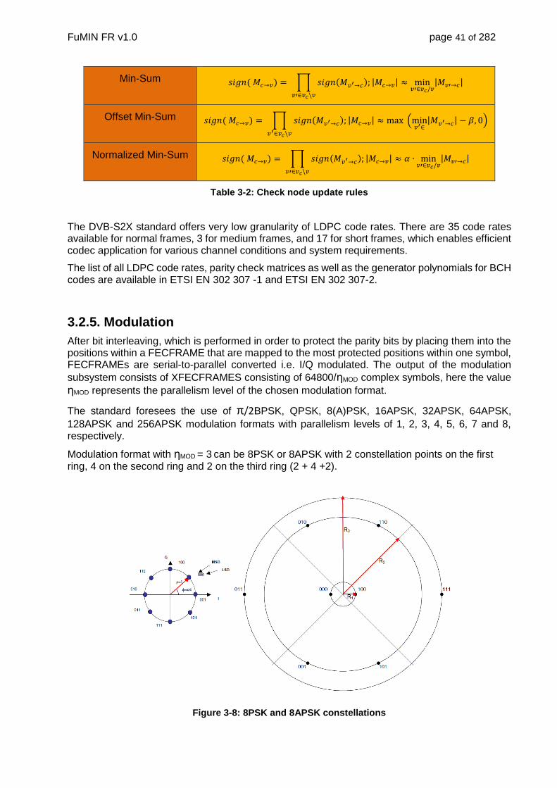
FuMIN FR v1.0 page 41 of 282
Min-Sum 𝑠𝑖𝑔𝑛( 𝑀𝑐→𝑣) = ∏ 𝑠𝑖𝑔𝑛(𝑀𝑣′→𝑐);
𝑣′∈𝑣𝑐\𝑣
|𝑀𝑐→𝑣| ≈ min𝑣′∈𝑣𝑐/𝑣
|𝑀𝑣′→𝑐|
Offset Min-Sum 𝑠𝑖𝑔𝑛( 𝑀𝑐→𝑣) = ∏ 𝑠𝑖𝑔𝑛(𝑀𝑣′→𝑐);
𝑣′∈𝑣𝑐\𝑣
|𝑀𝑐→𝑣| ≈ max (min𝑣′∈
|𝑀𝑣′→𝑐| − 𝛽, 0)
Normalized Min-Sum 𝑠𝑖𝑔𝑛( 𝑀𝑐→𝑣) = ∏ 𝑠𝑖𝑔𝑛(𝑀𝑣′→𝑐);
𝑣′∈𝑣𝑐\𝑣
|𝑀𝑐→𝑣| ≈ 𝛼 ∙ min𝑣′∈𝑣𝑐/𝑣
|𝑀𝑣′→𝑐|
Table 3-2: Check node update rules
The DVB-S2X standard offers very low granularity of LDPC code rates. There are 35 code rates available for normal frames, 3 for medium frames, and 17 for short frames, which enables efficient codec application for various channel conditions and system requirements.
The list of all LDPC code rates, parity check matrices as well as the generator polynomials for BCH codes are available in ETSI EN 302 307 -1 and ETSI EN 302 307-2.
3.2.5. Modulation
After bit interleaving, which is performed in order to protect the parity bits by placing them into the positions within a FECFRAME that are mapped to the most protected positions within one symbol, FECFRAMEs are serial-to-parallel converted i.e. I/Q modulated. The output of the modulation
subsystem consists of XFECFRAMES consisting of 64800/ηMOD complex symbols, here the value
ηMOD represents the parallelism level of the chosen modulation format.
The standard foresees the use of π/2BPSK, QPSK, 8(A)PSK, 16APSK, 32APSK, 64APSK,
128APSK and 256APSK modulation formats with parallelism levels of 1, 2, 3, 4, 5, 6, 7 and 8, respectively.
Modulation format with ηMOD = 3 can be 8PSK or 8APSK with 2 constellation points on the first ring, 4 on the second ring and 2 on the third ring (2 + 4 +2).
Figure 3-8: 8PSK and 8APSK constellations

FuMIN FR v1.0 page 42 of 282
16 APSK can have 4+12 format or 8+8 format. Two versions with different constellation radius ratios of the 8+8 format are defined in the standard.
Figure 3-9: 16APSK constellations
32APSK is used in three variants: 4+12+16 and 4+8+4+16 with two different ring ratios.
Figure 3-10: 32APSK constellations
There three 64APSK variants: 16+16+16+16, 8+16+20+20 and 4+12+20+28

FuMIN FR v1.0 page 43 of 282
Figure 3-11: 64APSK constellations
As for 128APSK and 256APSK modulation formats, only one constellation for each of them is foreseen.
Figure 3-12: 256APSK constellations

FuMIN FR v1.0 page 44 of 282
The standard precisely defines the combinations, called MODCODs, of LDPC code rate, BCH error correcting ability, modulation format and variant of the constellation that can be used.
Exact ring ratios for each constellation are available in ETSI EN 302 307-1 and ETSI EN 302 307-2.
3.2.6. Modcod Performance
The modulation/coding spectral efficiency ranges from 0.5 (QPSK, 1/4 code rate) to 6 (256APSK, code rate 135/180). The following tables show the requirements of new DVB-S2x MODCODs for quasi error free (QEF) operations, which is defined as the point at which FER =10-5, for AWGN and non-linear hard limiter channels.
Table 3-3: Performance for medium frames, 75 iterations, at Quasi Error Free FER =10-5, AWGN
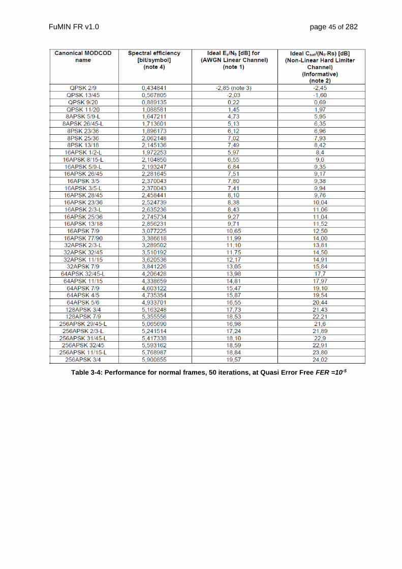
FuMIN FR v1.0 page 45 of 282
Table 3-4: Performance for normal frames, 50 iterations, at Quasi Error Free FER =10-5

FuMIN FR v1.0 page 46 of 282
Table 3-5: Performance for short frames, 75 iterations for π/2BPSK iterations, 50 iterations other
modes , at Quasi Error Free FER =10-5 , AWGN
The performance of the legacy DVB-S2 MODCODs over AWGN channel is presented in the following figures.
Figure 3-13: DVB-S2 short frame MODCODs

FuMIN FR v1.0 page 47 of 282
Figure 3-14: DVB-S2 MODCDOS, QPSK, normal frame
Figure 3-15: DVB-S2 MODCDOS, 8APSK, normal frame

FuMIN FR v1.0 page 48 of 282
Figure 3-16: DVB-S2 MODCDOS, 16APSK, normal frame
Figure 3-17: DVB-S2 MODCDOS, 32APSK, normal frame
The standard provides the QEF SNR values for 50 iterations of the Belief Propagation Algorithm. In the scope of the project, BP Algorithm as well as computationally less complex Min-Sum

FuMIN FR v1.0 page 49 of 282
Algorithm family have been implemented. The results presented in this chapter are produced using the Offset Min Sum Algorithm. At the end of the chapter two exemplary BP curves are provided. When using the Offset Min Sum Algorithm, the maximal number of iterations was set to 200 with the application of early stop criterion, which significantly increases decoder’s throughput. BP curves were produced using 50 iterations and early stop criterion.
Figure 3-18: QPSK short frames, single carrier (from simulation)

FuMIN FR v1.0 page 50 of 282
Figure 3-19: 8PSK short frames, single carrier (from simulation)
Figure 3-20: 16APSK short frames, single carrier (from simulation)

FuMIN FR v1.0 page 51 of 282
Figure 3-21: 32APSK short frame, single carrier (from simulation)
MODCOD Ideal SNR [dB] at FER 1E-5 Simulated SNR
[dB] at FER 1E-5 Simulated vs. ideal
SNR [dB]
QPSK_1_4 -2.15 -2.7 -0.55
QPSK_11_45 -2.5 -2.6 -0.1
QPSK_4_15 -2.24 -2.05 0.19
QPSK_14_45 -1.46 -1.45 0.01
QPSK_1_3 -1.04 -1.2 -0.16
QPSK_2_5 -0.1 -0.15 -0.05
QPSK_1_2 1.2 0.95 -0.25
QPSK_7_15 0.6 0.75 0.15
QPSK_8_15 1.45 1.6 0.15
QPSK_3_5 2.53 2.5 -0.03
QPSK_2_3 3.4 3.4 0
QPSK_32_45 3.66 4 0.34
QPSK_3_4 4.33 4.3 -0.03
QPSK_4_5 4.98 5.1 0.12
QPSK_5_6 5.48 5.75 0.27

FuMIN FR v1.0 page 52 of 282
QPSK_8_9 6.5 6.6 0.1
Table 3-6: Single carrier QPSK MODCOD performance for short frames at PER 1e-5 compared with the DVB-S standard
MODCOD Ideal SNR [dB] at FER
1E-5 Simulated SNR
[dB] at FER 1E-5 Simulated vs. ideal
SNR [dB]
PSK8_7_15 3.83 3.9 0.07
PSK8_8_15 4.71 4.8 0.09
PSK8_26_45 5.52 5.55 0.03
PSK8_3_5 5.8 7.5 1.7
PSK8_2_3 6.92 7 0.08
PSK8_32_45 7.54 7.6 0.06
PSK8_3_4 8.21 8.2 -0.01
PSK8_5_6 9.65 10.2 0.55
PSK8_8_9 10.99 10.95 -0.04
Table 3-7: Single carrier 8PSK MODCOD performance for short frames at PER 1e-5 compared with
the DVB-S standard
MODCOD Ideal SNR [dB] at FER
1E-5 Simulated SNR
[dB] at FER 1E-5 Simulated vs. ideal
SNR [dB]
APSK16_7_15 5.99 6.1 0.11
APSK16_8_15 6.93 7.1 0.17
APSK16_26_45 7.66 8.05 0.39
APSK16_3_5 8.4 8.55 0.15
APSK16_32_45 9.81 9.9 0.09
APSK16_3_4 10.51 10.5 -0.01
APSK16_4_5 11.33 11.3 -0.03
APSK16_5_6 11.91 12.25 0.34
APSK16_8_9 13.19 12.2 -0.69
Table 3-8: Single carrier 16APSK MODCOD performance for short frames at PER 1e-5 compared with the DVB-S standard
MODCOD Ideal SNR [dB] at FER
1E-5 Simulated SNR
[dB] at FER 1E-5 Simulated vs. ideal
SNR [dB]
APSK32_2_3 11.71 12.2 0.49
APSK32_3_4 13.03 13.25 0.22
APSK32_4_5 13.94 14.2 0.26

FuMIN FR v1.0 page 53 of 282
APSK32_5_6 14.58 14.95 0.37
APSK32_8_9 15.99 16.1 0.11
Table 3-9: Single carrier 32APSK MODCOD performance for short frames at PER 1e-5 compared with the DVB-S standard
3.2.7. Super-frames
DVB-S2x introduces super-frames for advanced air interfaces. There are 3 types of theses superframe that are different from DVB-S2 as shown in Table 3-10. For mobile applications, type 4 is important, since it addresses the very low SNR operational points.
Table 3-10: DVB-S2x super-frame formats
Figure 3-22: General SF format
The following rules apply to each SF format:
The super-frame length is fixed to a unique number of symbols (612 540 symbols). The
super-frame length in symbols is independent of pilot settings or hosted content formats.
The SFFI signals the actual super-frame format.
For resource allocation of a content format, a format-individual "capacity unit" (CU) can be

FuMIN FR v1.0 page 54 of 282
specified. It shall provide a grid for mapping the content into the super-frame. Note to
distinguish between a resource allocation grid (based on CUs) and the payload structure
(based on SLOTs). Nevertheless, the CU size can be the same as the SLOT size of 90
symbols.
Pilot fields and pilot structure can be specified for each individual super-frame format. The
first 720 symbols per each super-frame are fixed with the SOSF and SFFI.
The full super-frame can be scrambled, including also SOSF/SFFI, with two different
scrambling sequences,. The scramblers are reset with the first symbol of the SOSF
sequence. SOSF and SFFI have to be scrambled, whereas the applicability of scrambling
the hosted super-frame content is defined in each individual super-frame format.
After super-frame generation and scrambling, baseband shaping and quadrature
modulation is performed as described in EN 302 307-1
SOSF field comprises 270 symbols. The SOSF defining a binary sequence is composed of a 256 bit long Walsh-Hadamard (WH) sequence plus padding of 14 bits. The 14 bits long padding sequence is generated from a 16 bits long WH sequence. The sequence is BPSK modulated.
SFFI field is constructed from 4 bits corresponding to the bit vector bSFFI, which refers to a super-frame format by the means of simplex encoding (code rate 4/14) and repletion of factor 30, which results in 450 long vector X SFFI vector. BPSK modulation of the X SFFI vector results in the SFFI field.
Two way scrambling is applied using two parallel scramblers:
Reference data scrambler with sequence CnRef(iRef) applied at least to the SOSF and
potentially to SF-aligned pilots.
Payload data scrambler with sequence CnPay(iPay)applied at least to the SFFI.
Figure 3-23: Two-way scrambling

FuMIN FR v1.0 page 55 of 282
3.2.7.1. Bundled PLFRAMEs (64800 Payload Size) with SF-Pilots
Figure 3-24: SF format 2
Each bundled PLFRAME comprises multiple XFECFRAMEs with the same MODCODs and a common PLHEADER.
The overall symbol size remains constant, independent of the modulation format
Resource allocation is done by means of a symbol-wise mapping into super-frame. There is no CU definition.
Overhead of this format (incl. SOSF, SFFI, PLH, Pilots) is 5,03 %.
Bundled PLFRAMEs are designed to maintain a constant PLFRAME size (measured in symbols):
PLFRAME payload size: 64 800 symbols.
PLHEADER: 384 symbols (6 replica of identical PLS code to allow decoding down to -10
dB SNR).
Super-frame size is set to 612,540 symbols, identical to that for all other super-frame
formats.
There are 9 bundled frames per each super-frame in this format.
Each bundle contains 384 symbols of the PLHEADER, 64 800 symbols of payload, 180
known modulated symbols (P2) from the payload constellation format, and 71 pilot fields
with 36 symbols in each pilot field. The total bundled frame length is 67 920 symbols.
Modulated pilots symbols are inserted after the PLH and selected from the same
constellation format as the data payload of the corresponding bundled PLFRAME. Any

FuMIN FR v1.0 page 56 of 282
gateway-based payload data pre-processing technique (pre-distortion, pre-coding) shall
be applied to these pilots as well.
Pilots are always present. There are 639 fields of pilots with 36 symbols in each pilot
group and repeated every 956 symbols.
The first pilot field starts at symbol 1 665 with reference to the first symbol in the super-
frame.
Each super frame includes 720 symbols for SOSF and SFFI.
There are 540 dummy symbols at the end of each super-frame
Figure 3-25: Examples of long bundled PLFRAMEs using different modulation formats
PLHEADER for bundled PLFRAME consists of 6 replica of the 64-bit PLS code defined in EN 302 307-1. No SOF is included in the PLHEADER for the bundled PLFRAME. Thus, the PLHEADER has 384 symbols with π/2 BPSK modulation.
Pilot Structure: There are two different types of pilots defined in this super-frame format. The first type is based on pilot fields of 36 symbols repeated throughout the super-frame as per the following specification:
PSF = 36 symbols
Number of pilot fields per super-frame = 639
The pilot fields repeat periodically within each super-frame with a repetition period of 956 symbols. It should be noted that the periodicity of pilot fields is not kept between super-frames. There are 71 pilot fields per each bundled frame (summing up to a total of 639 pilot fields). In this super-frame format, the pilot fields are always present. The pilot fields are determined by a Walsh-Hadamard sequence of size 32 plus padding of 4 bits.
In addition to pilot fields described above, each bundled PLFRAME also includes 180 known symbols inserted after the PLH field. The exact definition of P2 pilots is available in ETSI EN 302 307-2, page 112.
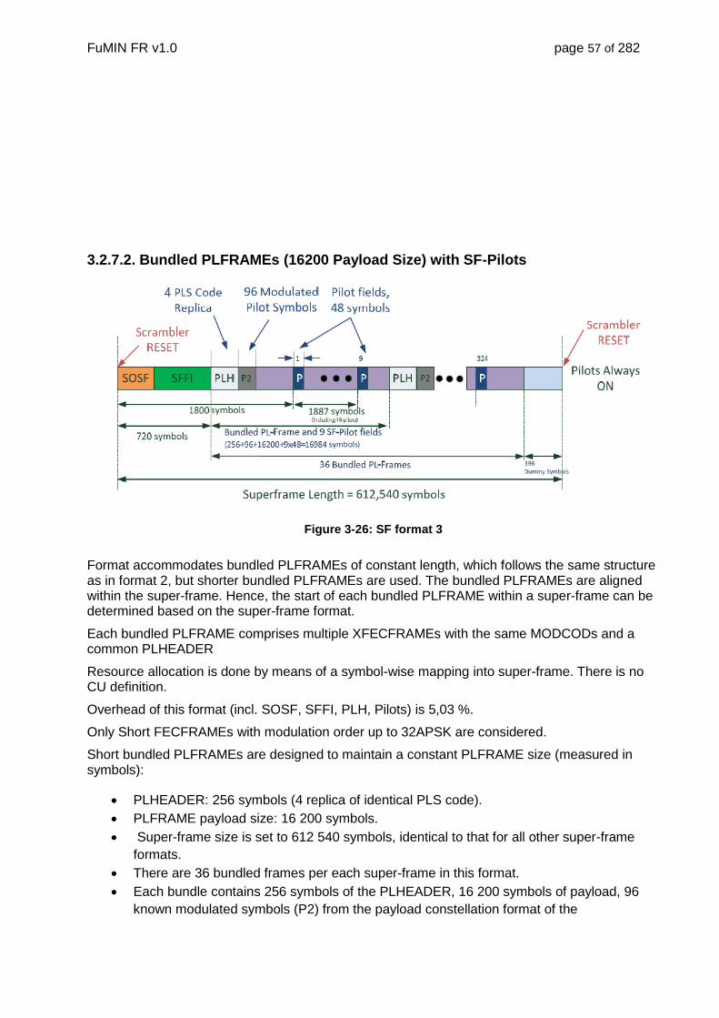
FuMIN FR v1.0 page 57 of 282
3.2.7.2. Bundled PLFRAMEs (16200 Payload Size) with SF-Pilots
Figure 3-26: SF format 3
Format accommodates bundled PLFRAMEs of constant length, which follows the same structure as in format 2, but shorter bundled PLFRAMEs are used. The bundled PLFRAMEs are aligned within the super-frame. Hence, the start of each bundled PLFRAME within a super-frame can be determined based on the super-frame format.
Each bundled PLFRAME comprises multiple XFECFRAMEs with the same MODCODs and a common PLHEADER
Resource allocation is done by means of a symbol-wise mapping into super-frame. There is no CU definition.
Overhead of this format (incl. SOSF, SFFI, PLH, Pilots) is 5,03 %.
Only Short FECFRAMEs with modulation order up to 32APSK are considered.
Short bundled PLFRAMEs are designed to maintain a constant PLFRAME size (measured in symbols):
PLHEADER: 256 symbols (4 replica of identical PLS code).
PLFRAME payload size: 16 200 symbols.
Super-frame size is set to 612 540 symbols, identical to that for all other super-frame
formats.
There are 36 bundled frames per each super-frame in this format.
Each bundle contains 256 symbols of the PLHEADER, 16 200 symbols of payload, 96
known modulated symbols (P2) from the payload constellation format of the
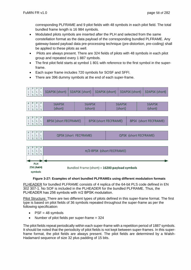
FuMIN FR v1.0 page 58 of 282
corresponding PLFRAME and 9 pilot fields with 48 symbols in each pilot field. The total
bundled frame length is 16 984 symbols.
Modulated pilots symbols are inserted after the PLH and selected from the same
constellation format as the data payload of the corresponding bundled PLFRAME. Any
gateway-based payload data pre-processing technique (pre-distortion, pre-coding) shall
be applied to these pilots as well.
Pilots are always present. There are 324 fields of pilots with 48 symbols in each pilot
group and repeated every 1 887 symbols.
The first pilot field starts at symbol 1 801 with reference to the first symbol in the super-
frame.
Each super frame includes 720 symbols for SOSF and SFFI.
There are 396 dummy symbols at the end of each super-frame.
Figure 3-27: Examples of short bundled PLFRAMEs using different modulation formats
PLHEADER for bundled PLFRAME consists of 4 replica of the 64-bit PLS code defined in EN 302 307-1. No SOF is included in the PLHEADER for the bundled PLFRAME. Thus, the PLHEADER has 256 symbols with π/2 BPSK modulation.
Pilot Structure: There are two different types of pilots defined in this super-frame format. The first type is based on pilot fields of 36 symbols repeated throughout the super-frame as per the following specification:
PSF = 48 symbols
Number of pilot fields per super-frame = 324
The pilot fields repeat periodically within each super-frame with a repetition period of 1887 symbols. It should be noted that the periodicity of pilot fields is not kept between super-frames. In this super-frame format, the pilot fields are always present. The pilot fields are determined by a Walsh-Hadamard sequence of size 32 plus padding of 15 bits.
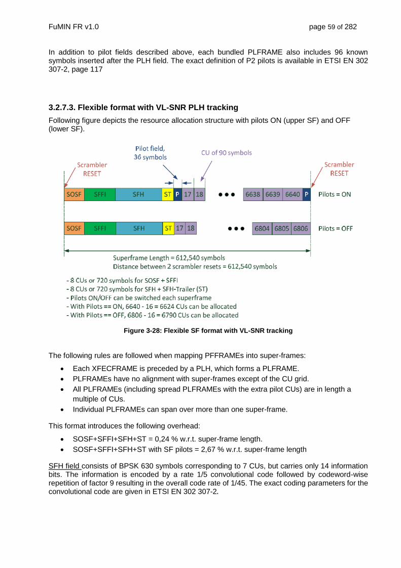
FuMIN FR v1.0 page 59 of 282
In addition to pilot fields described above, each bundled PLFRAME also includes 96 known symbols inserted after the PLH field. The exact definition of P2 pilots is available in ETSI EN 302 307-2, page 117
3.2.7.3. Flexible format with VL-SNR PLH tracking
Following figure depicts the resource allocation structure with pilots ON (upper SF) and OFF (lower SF).
Figure 3-28: Flexible SF format with VL-SNR tracking
The following rules are followed when mapping PFFRAMEs into super-frames:
Each XFECFRAME is preceded by a PLH, which forms a PLFRAME.
PLFRAMEs have no alignment with super-frames except of the CU grid.
All PLFRAMEs (including spread PLFRAMEs with the extra pilot CUs) are in length a
multiple of CUs.
Individual PLFRAMEs can span over more than one super-frame.
This format introduces the following overhead:
SOSF+SFFI+SFH+ST = 0,24 % w.r.t. super-frame length.
SOSF+SFFI+SFH+ST with SF pilots = 2,67 % w.r.t. super-frame length
SFH field consists of BPSK 630 symbols corresponding to 7 CUs, but carries only 14 information bits. The information is encoded by a rate 1/5 convolutional code followed by codeword-wise repetition of factor 9 resulting in the overall code rate of 1/45. The exact coding parameters for the convolutional code are given in ETSI EN 302 307-2.

FuMIN FR v1.0 page 60 of 282
ST field stands for Super-frame header Trailer and is 90 symbols long. It consists of a 64-bit long Walsh-Hadamard sequence with 26 bits appended to it. The 26 bits are constructed from a 32 bits long Walsh-Hadamard sequence. For details see in ETSI EN 302 307-2 page 119 and 120.
Physical layer header (PLH): The PLH is constructed from a concatenation of a SOF of 20 symbols and a PLSCODE. It is closely related to the PLH definition in EN 302 307-1, annex M but without puncturing of the PLSCODE and no pilot bit. Here, four protection levels of the PLH are specified, which use different modulation and spreading.
Table 3-11: PLH protection levels
Different protection levels result in different PLH structures, as shown in the following figure.
Figure 3-29: PLH structures
PLFRAME structure is depicted in the following figure.
Figure 3-30: PLH structures
FuMIN FR v1.0 page 61 of 282
XFECFRAME spreading:
XFECFRAME spreading is signaled via PLH
Spreading factors 1, 2, or 5 are accomplished by frame-wise repetition of the XFECFRAME
XFECFRAMEs with SPREAD > 1 contain additional pilot SLOTs
In case the current PLH indicates a spreading factor > 1 for the actual XFECFRAME, additional CUs are dedicated as pilot sequences in order to achieve robust phase estimation:
Special VL-SNR pilot distance: 15 payload SLOTs
Pilot fields each of 90 symbols length
Constant I/Q symbols with constellation point (1 + 1j)/√2
The following figure depicts an example of super-frame with spreading of XFECFRAME by factor 2.
Figure 3-31: XFECFRAME spreading
3.2.8. DVB-S2x Synchronization and Channel Estimation
3.2.8.1. Synchronization Architecture
Figure 3.32 presents the architecture of super-frame acquisition and timing recovery. Fast coarse frequency estimation is done fully blind with the quadri-correlator [RD103]. In the worst case the residual normalized frequency error is dfTs=10-2. Details can be found in section 3.2.8.2.1. Super frame acquisition based on correlation copes with this residual error using the post detection integration principle (see section 3.2.8.3) [RD105]. The timing drift (maximum 100ppm) is estimated by using the difference of correlation peaks produced on the start of the super-frame (SoSF) field and applied on a cubic interpolator. In this state a correlation window of 61 symbols periods is necessary which is then reduced to +/- 4. The residual timing drift smaller than 1ppm has then to be recovered on per super-frame basis. The cold and warm aquisition time which is essential in the environment of the considered mobile channels (see section 0) will be given in section 3.2.8.3.3.
Now timing recovery is applied on per super-frame basis via interpolation between known fields (SOSF, SFFI, PILOTS). The timing error is estimated on the main lobe of the correlation results with a parabolic interpolator (see section 3.2.8.4).The advantage is that a decoupling of the phase correction is possible (in contrast to the joint phase and timing estimation approach). The data aided timing tracker with the Müller detector [RD104] needs phase recovered samples.
Next fine frequency estimation is done with the LR (Luise Reggiannini) algorithm on the SoSF and SFFI (super frame format indicator) field (see section 3.2.8.2.2). It is now possible to apply the frequency correction on the super-frame (marked with the dotted arrow in Figure 3.33). The other way is to use the data aided (DA) frequency estimates to control the frequency tracker operated up to now with the quadri-correlator detector. The advantages are that the frequency estimation

FuMIN FR v1.0 page 62 of 282
quality improves compared to the LR estimator with L=720 and that shading effects in the mobile channel can be detected with high reliability (see section 3.2.8.2.3)
Phase estimation is again done via interpolation between the pilot fields. For higher order modulation like in DVB-S2 a NDA four quadrant tracker on frame basis will increase the performance in the presence of strong phase noise [RD3]. Now it is possible to decode PLH and/or VLSNR header. The channel quality will be provided via SNR estimation (see section 3.2.8.6). The normalization of signal power will be achieved via a data aided amplitude estimator on the phase corrected SoSF and SFFI field (see section 3.2.8.5).
Matched Filter with
QC
Super-frame acquisition (SoSF,SFFI)
Coarse Estimation of Timing Drift
Cubic IP
d
Samples from Channel
Cubic IP
Timing Est. on (SoSF,SFFI),(Pilots) via
Interpolation
Sample to
Symbol
ip
Pos(SoSF)
()je
f2
DA loop Input Fine FEST
Figure 3.32: Architecture of correlation and timing recovery
LR Fine Frequency Estimation (SoSF,SFFI)
Phase Interpolation (SoSF,SFFI,Pilots)
f2
()je
Pos(SoSF)
Input symbols from timing
synchronization
()je
SER Analyzer
Pos(SoSF)
PLH VLSNR Decoder
PLS(frame)
f2 Input to DA loop
SNR estimation
Carrier Power estimation and normalization
x
Figure 3.33: Architecture of frequency and phase recovery
3.2.8.2. Frequency Estimation
In the sequel coarse and fine frequency estimation taking care of the Doppler rates in mobile environment are presented. In the last section the combined frequency tracker approach is analysed, which uses the quadri-correlator detector for coarse frequency acquisition and then, after super framing is established, switches to a data aided tracker.
3.2.8.2.1. Coarse Frequency Estimation with the Quadricorrelator (QC)
After decimation the large frequency offsets (common to all signals as due to the terminal LNB instabilities) have to be recovered before the signal enters the matched filter (MF). At this stage the estimator has to be operated fully blind (NDA) without recovery of the timing. For that purpose the Quadri-Correlator detector [RD103] implemented as second order tracker with a loop bandwidth of blt=10-4 (see Figure 3.34) shall bring down the normalized frequency error to dfTs=10-2 (5*’sigma) at an SNR of -10 dB. The filter impulse response for the RCOS and convolution of RRCOS and DMF is plotted in Figure 3.35.

FuMIN FR v1.0 page 63 of 282
RRCOS
df
()jeDezimation
from Channel
QCQ(z)
DMF
Correlation and Timing Est.
Figure 3.34: Quadricorrelator frequency tracker
Figure 3.35: Impulse response of RCOS and convolution of RRCOS and DMF for roll-off=0.2
The detector characteristic is given for roll-off factor 0.2 and filter lengths of 20 symbols in Figure 3.36. For roll-off 0.05 Figure 3.39 presents a comparison of filter lengths 20 and 80 symbols. Only for 80 symbols, where the ringing is significantly reduced, the capture of 10% frequency error is possible.

FuMIN FR v1.0 page 64 of 282
Figure 3.36: Detector characteristic for roll-off 0.2 and a filter length of 20 symbols
Figure 3.37: Detector characteristic for roll-off 0.05 and a filter lengths of 20, 80 symbols
The following sections present the variance for roll off factors 0.2 and 0.05. The channel is AWGN. The timing error has significant impact on the performance of the QC, so static timing offsets and timing drifts up to 100ppm are considered. Modulations considered are QPSK and 32-APSK. Figure 3.39 presents the variance of the frequency error under ideal channel conditions (AWGN only) and frequency errors from zero to 20%. In Figure 3.40 20% static timing error is present. A floor at an SNR starting above 5 dB SNR can be observed. A timing drift degrades the variance with increasing frequency error (see Figure 3.41). Figure 3.42 is analogue to Figure 3.39 except that 32-APSK is used as modulation. The performance does not deviate significantly, so there is no impact due to the modulation.
The same plots are done for roll-off factor 0.05 (see Figure 3.43, Figure 3.44 and Figure 3.45). Following literature the save capture range is half the roll-off factor [RD103]. But the QC is also able to lock when the detector is driven into the flat area. A lock could also be achieved up to 10% frequency error. A necessary condition is that sufficient filter taps are used and that’s why ringing in the detector is avoided.
A loop bandwidth of blt=10-4 needs significant settling time. To reduce the settling time an adaptive loop bandwidth starting with blt=10-3 and successive reduction by steps of 10-5 is implemented So after 99 steps with 12000 symbols the QC is operable (two super-frames). The adpative mode is started after two million samples (see Figure 3.38) when the initial settling with blt=10-3 is given.
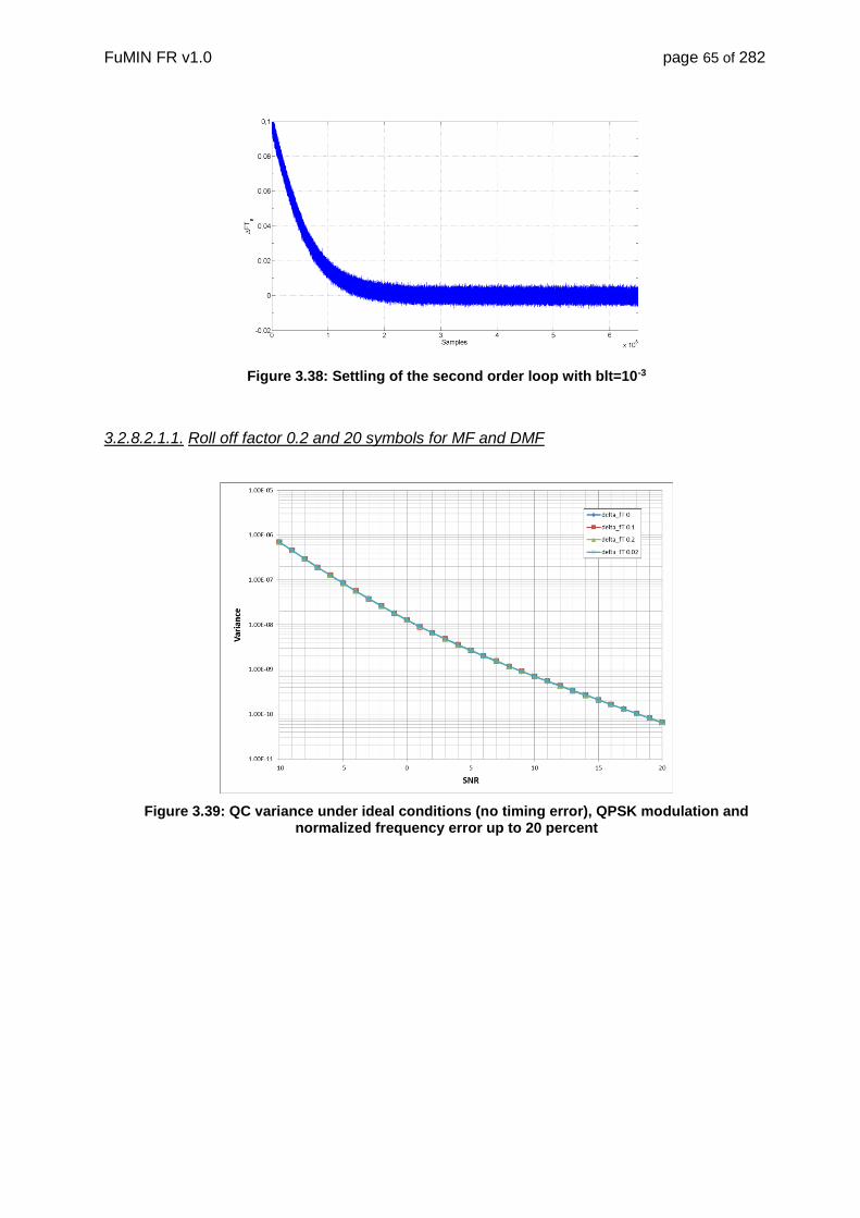
FuMIN FR v1.0 page 65 of 282
Figure 3.38: Settling of the second order loop with blt=10-3
3.2.8.2.1.1. Roll off factor 0.2 and 20 symbols for MF and DMF
Figure 3.39: QC variance under ideal conditions (no timing error), QPSK modulation and normalized frequency error up to 20 percent
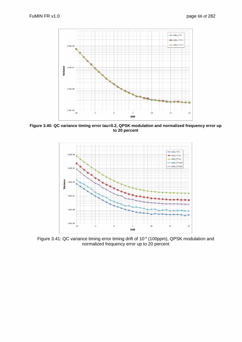
FuMIN FR v1.0 page 66 of 282
Figure 3.40: QC variance timing error tau=0.2, QPSK modulation and normalized frequency error up to 20 percent
Figure 3.41: QC variance timing error timing drift of 10-4 (100ppm), QPSK modulation and normalized frequency error up to 20 percent

FuMIN FR v1.0 page 67 of 282
Figure 3.42: QC variance timing error tau=0.2, 32-APSK modulation and normalized frequency error up to 20 percent
3.2.8.2.1.2. Roll off factor 0.05 and 320 filter taps for MF and DMF
Figure 3.43: QC variance ideal conditions (no timing error) QPSK modulation and normalized frequency error up to 10 percent
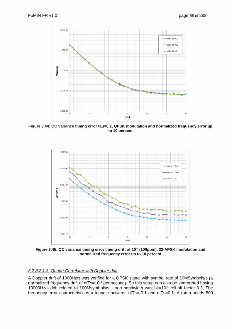
FuMIN FR v1.0 page 68 of 282
Figure 3.44: QC variance timing error tau=0.2, QPSK modulation and normalized frequency error up to 10 percent
Figure 3.45: QC variance timing error timing drift of 10-4 (100ppm), 32-APSK modulation and normalized frequency error up to 10 percent
3.2.8.2.1.3. Quadri-Correlator with Doppler drift
A Doppler drift of 1000Hz/s was verified for a QPSK signal with symbol rate of 10MSymbols/s (a normalized frequency drift of dfTs=10-4 per second). So this setup can also be interpreted having 10000Hz/s drift related to 100Msymbols/s. Loop bandwidth was blt=10-4 roll-off factor 0.2. The frequency error characteristic is a triangle between dfTs=-0.1 and dfTs=0.1. A ramp needs 500

FuMIN FR v1.0 page 69 of 282
seconds, which exaclty matches with the plots. Two SNR scenarios are tested: 0dB and -10dB. The channel was AWGN, further a static timing error of 20% was applied.
The frequency estimation characteristic 0 dB SNR is presented in Figure 3.46 (a zoom can be found in Figure 3.47). The index on the x-axis represents the number of super-frames, the y-axis corresponds to the normalized frequency error. The variance results to var=3*10-8 and matches with the plots for static frequency error (see Figure 3.39).
Figure 3.46: QC blt=10-4, Dopper-rate dfTs=0.0001/s, SNR=0dB
Figure 3.47: Zoom to one ramp, QC blt=10-4, Dopper rate = 1000Hz/s, SNR=0dB

FuMIN FR v1.0 page 70 of 282
The frequency estimation characteristic for -10dB SNR is presented in Figure 3.48 (a zoom can be found in Figure 3.49). The variance results to var=10-6 and matches with the plots for static frequency error (see Figure 3.39).
Figure 3.48: QC blt=10-4, Dopper rate = 1000Hz/s, SNR=-10dB
Figure 3.49: Zoom QC blt=10-4, Dopper rate = 1000Hz/s, SNR=-10dB

FuMIN FR v1.0 page 71 of 282
3.2.8.2.2. Fine Frequency Estimation
The LR algorithm [RD29] is a data aided (DA) maximum likelihood frequency estimator. In Figure 3.50 the variance is plotted for an estimator length of 256. Also for -10dB SNR the variance is close to the CRLB. Taking also the SFFI into account the estimator length can be increased to L=720. The evaluation of the CRLB for 720 symbols results to a sigma of 6.38*10-5 at -10dB SNR (five sigma results to 3.2*10-4). For reliable phase correction on pilot symbols with distance 16 slots (1440 symbols) a residual frequency error of maximal dfTs=10-4 is allowed. So the worst case value at -10dB SNR is slightly above. With the combined frequency tracker presented in the next section this mismatch can be solved.
Figure 3.50: CRLB and variance for frequency estimation and the variance of the LR algorithm for L=256 and L=720 (SoSF and SFFI)
3.2.8.2.3. Combined Frequency Tracking
The Quadri-Correlator ensures fast initial settling and reduces the frequency error in the worst case (-10dB SNR) down to a dfTs=10-2 at which the correlator following the PDI (post detection integration) principle is able to produce reliable results [RD105]. But the following problems arise:
The QC produces at -10dB SNR a volatility in frequency (see Figure 3.53) also over one super-frame, so the fine frequency estimation at the beginning (SoSF+SFFI) may cause problems in the phase estimation module
In the mobile channel shadowing can cause a lock loss, the detection is problematic.
But fine frequency estimation can also be used to take over the QC feedback loop. The LR estimates in combination with the tracker result in a variance superior to LR estimation with L=720. So the proper function of the phase recovery module is save also for -10dB SNR. Further it is possible to get a reliable estimate of shadowing taking the correlation results into account. A threshold detector based on a moving average reference recognizes suspicious peaks. Based on that information the frequency estimates are fed into the loop. For a certain time depending on the Doppler rate the system can survive without losing synchronization.
The architecture of the combined frequency tracker can be found in Figure 3.51.

FuMIN FR v1.0 page 72 of 282
RRCOS
df
()jeDezimation
from Channel
QCQ(z)
DMF
Correlation and Timing
Est.Fine Fest
QDA(z)
Frame Composer
Frame Begin
DVB-S2x Superframes
Thresholddetector
Correlation peak
Suspicious peak
Figure 3.51: Architecture of combined QC and data aided loop
The QC operates in a second order loop with bandwidth blt=10-4. The settling for an initial normalized frequency error of 20% is given in Figure 3.52. Appropriate settling is reached above 100 super-frames which is not applicable in a mobile scenario. For a start blt=10-3 and an adaptive loop bandwidth down to blt=10-4 only three super-frames are necessary (see section 3.2.8.2.1).
Figure 3.52: Initial Settling of QC for blt=10-4 at -10dB SNR
The data aided tracker fed with the LR estimates is operated with loop order one and a loop bandwidth blt=0.1. Figure 3.54 presents the characteristic for adaptive settling of the QC and switch to first order DA loop. Figure 3.55 is a zoom into Figure 3.54 starting at the point where the DA loop takes over. Figure 3.56 and Figure 3.57 confirm that the DA tracker is able to follow the Doppler rate.

FuMIN FR v1.0 page 73 of 282
Figure 3.53: Characteristic of settled QC for blt=10-4 at -10dB SNR
Figure 3.54: Characteristic of initial settling of combined frequency tracker at -10dB SNR
Figure 3.55: Initial settling of data aided frequency tracker at -10dB SNR (after swiching from QC)

FuMIN FR v1.0 page 74 of 282
Figure 3.56: Long term test of data aided frequency tracker at -10dB SNR
Figure 3.57: Long term test Zoom of data aided frequency tracker at -10dB SNR
The performance (variance) for a static normalized frequency error of 20% is given in Figure 3.58
Figure 3.58: Variance of the DA frequency tracker

FuMIN FR v1.0 page 75 of 282
Figure 3.59 considers Doppler rates from 100Hz/s to 1000/Hz/s for 10MSymbols/s. With increasing Doppler rate a bias determines the performance, so the increase of the SNR has only minor effect.
Figure 3.59: Variance of the DA frequency tracker for Doppler rates between 100Hz and 1000Hz per second at 10MSymbols/s
3.2.8.2.3.1. Doppler Drift Tracking
The initial frequency error including the actual doppler frequency is captured by the quadri-correlator. The doppler drift has then to be tracked be the combined frequency tracker. The acceleration of the mobile terminal determines the Doppler-drift. In the RCS2 guidelines the worst case drift results to 2800 Hz/s for aircrafts (or 17m^2/s). Special manoeuvers are explicitly like the start and landing are not considered. With the actual configuration of 10MSymbols/s also this drift can be tracked. Compared to 1000Hz/s the variance is degraded by a factor 3 to 2*10-9. The capability of tracking increases with increasing the symbol rate. If the tracker is optimized for a normalized drift dfTs=0.0001 at 100 Msymbols/s the absolute drift is already 10kHz/s. For RCS2 the Doppler drift is not relevant because the synchronization is done per burst with of limited length. So only the absolute error is relevant and shall be between dfTs=0.005 and dfTs=0.03
3.2.8.3. Super-frame Acquisition
At system start-up or restart due to shadowing in the mobile channel initial super-frame acquisition has to be reliable and fast. Synchronization shall cope with short blockages so that fast re-synchronization is possible for a time defined by the symbol rate, Doppler drift and timing drift. Figure 3.60 presents the state machine details are given in section 3.2.8.3.1, section 3.2.8.3.2 and section 3.2.8.3.3.

FuMIN FR v1.0 page 76 of 282
COLD SF ACQRepeated_SYNC
Switch to DA Freq tracker
Repeated_SYNC FREEZE DA Freq Tracker, open corr window
SYNC
NOT
FOUND
SYN
C F
OU
ND
SYN
C L
OST
D
ete
ctio
n
Drift <=1ppm
QC Acquisition
QC
se
ttle
d
Drift Compensation
SYNC FOUND
SYNC LOST_Timeout
Drift
Averaging
QC tracker
settling
SYNC
Open corr
window
Figure 3.60: Synchronization state diagram
3.2.8.3.1. Initial Acquisition of Super-framing
Initial acquisition has to cope with the residual frequency error of the Quadri-correlator (in the worst case dfTs=10-2 at -10dB SNR. Figure 3.61 shows the probability that the initial synchronization on the super-frame (SF) structure is not able to find a consistent framing structure. For that purpose samples containing at least three SoSF fields are stored. If the search for subsequent peaks corresponding to the distance of three super-frames in the window of 61 symbols (maximum possible drift per super-frame of 100ppm) is successful, the synchronization is established. The simulation of a false detection has so far no result at -10dB and one million trials. The average duration in super-frames to come to a result in dependence of the SNR is given in Figure 3.62. At -10dB SNR in average 3 trials (so 9 super-frames) are necessary for initial synchronization.

FuMIN FR v1.0 page 77 of 282
Figure 3.61: Probability of no detection for Initial Synchronization (dfTs=10-2)
Figure 3.62: Initial Super frame (SF) acquisition time given in number of SFs over SNR
3.2.8.3.2. In Service Super-frame Acquisition
As long the maximal drift of 100ppm is present +/- 61 symbols have to be considered in the correlation. Figure 3.63 presents the probability that the detection in this window was not correct.
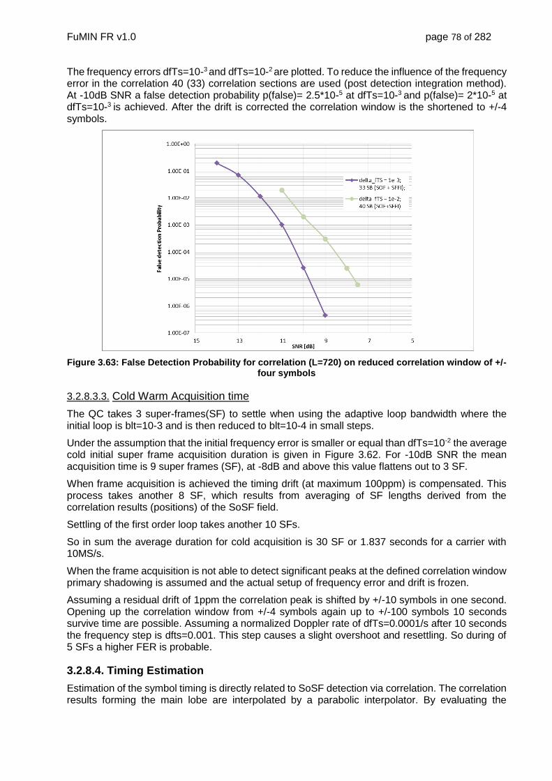
FuMIN FR v1.0 page 78 of 282
The frequency errors dfTs=10-3 and dfTs=10-2 are plotted. To reduce the influence of the frequency error in the correlation 40 (33) correlation sections are used (post detection integration method). At -10dB SNR a false detection probability p(false)= 2.5*10-5 at dfTs=10-3 and p(false)= 2*10-5 at dfTs=10-3 is achieved. After the drift is corrected the correlation window is the shortened to +/-4 symbols.
Figure 3.63: False Detection Probability for correlation (L=720) on reduced correlation window of +/- four symbols
3.2.8.3.3. Cold Warm Acquisition time
The QC takes 3 super-frames(SF) to settle when using the adaptive loop bandwidth where the initial loop is blt=10-3 and is then reduced to blt=10-4 in small steps.
Under the assumption that the initial frequency error is smaller or equal than dfTs=10-2 the average cold initial super frame acquisition duration is given in Figure 3.62. For -10dB SNR the mean acquisition time is 9 super frames (SF), at -8dB and above this value flattens out to 3 SF.
When frame acquisition is achieved the timing drift (at maximum 100ppm) is compensated. This process takes another 8 SF, which results from averaging of SF lengths derived from the correlation results (positions) of the SoSF field.
Settling of the first order loop takes another 10 SFs.
So in sum the average duration for cold acquisition is 30 SF or 1.837 seconds for a carrier with 10MS/s.
When the frame acquisition is not able to detect significant peaks at the defined correlation window primary shadowing is assumed and the actual setup of frequency error and drift is frozen.
Assuming a residual drift of 1ppm the correlation peak is shifted by +/-10 symbols in one second. Opening up the correlation window from +/-4 symbols again up to +/-100 symbols 10 seconds survive time are possible. Assuming a normalized Doppler rate of dfTs=0.0001/s after 10 seconds the frequency step is dfts=0.001. This step causes a slight overshoot and resettling. So during of 5 SFs a higher FER is probable.
3.2.8.4. Timing Estimation
Estimation of the symbol timing is directly related to SoSF detection via correlation. The correlation results forming the main lobe are interpolated by a parabolic interpolator. By evaluating the

FuMIN FR v1.0 page 79 of 282
argument of the maximum, we obtain the required timing estimate. The MRCLB for the relevant estimator lengths is given in Figure 3.64 for roll-off (ro) factor ro=0.2.
Figure 3.64: MCRLB for timing estimates roll-off 0.2
In Figure 3.65 the variance was simulated with an ideal AWGN channel, oversampling factor (os) two, roll-off factor 0.2 and a correlation of length L=720 (SoSF+SFFI). The variance (Figure 3.65) shows a dependence on the timing error with higher SNR values. Reason is an existing bias which is introduced by the interpolator. For os=4 this effect is significantly less (see Figure 3.66).
Figure 3.65: Variance of timing estimates for os=2, ro=0.2, L=720

FuMIN FR v1.0 page 80 of 282
Figure 3.66: Variance of timing estimates for os=4, ro=0.2 and WH code length L=256
As presented in the architecture section 3.2.8.1 timing recovery is done via interpolation on the between SoSF and pilot fields. In the VL-SNR case pilots with 90 symbols are available.
3.2.8.5. Phase and Amplitude Estimation
This section provides performance plots for phase and amplitude estimation. Figure 3.67 presents the MCRLB standard deviation in degrees of relevant estimation lengths.
Figure 3.67: Standard deviation in degrees for phase estimates
Phase recovery on the super-frame is possible after timing recovery and reduction to the symbol. As presented in the architecture section 3.2.8.1 it is done via interpolation between SoSF (SFFI) and pilot fields [RD3]. In the VL-SNR case pilots with 90 symbols are available. The pilot distance is 16 slots or 1440 symbols. Taking the variance of the phase estimates into account the residual frequency error has to be below dfTs=10-4 to avoid phase ambiguities.

FuMIN FR v1.0 page 81 of 282
Amplitude estimation and normalization [RD3] is done per super-frame on SoSF and SFFI. For that purpose the phase error has to be corrected. The performance of the estimator compared to the MCRLB is presented in Figure 3.68. If the synchronization is in operation, the residual frequency error causes a slight offset from the bound.
Note that both in both figures no timing drift has been assumed.
Figure 3.68: Normalized variance of amplitude estimates L=720
3.2.8.6. SNR Estimation
Three SNR estimation methods are considered. Data Aided (DA) estimation on the SoSF and SFFI header fields with in sum a length 720 symbols. Non data aided (NDA) moment based estimaton is executed on a super-frame with length L=612540 for QPSK modulation. Finally SNR estimation via SER (symbol error rate) measurement on known symbols given in the super-frame is analysed.
3.2.8.6.1. DA estimation
For the ACM algorithm a good SNR estimation is essential. Therefore as many as possible
symbols will be used for the estimation The frequency and phase corrected burst symbols kr are
used to calculate a bias corrected DA SNR ML .
1
0
21
0
*2
21
0
*
Re
2
3
1
2
3
1
Re1
ˆK
k
K
k
kkk
K
k
kk
ML
sr
KK
r
K
srK
4
The incoming symbols kr are correlated with the pilot symbols ks . The estimator length is
denoted as K .
The normalized CRLB for the SNR estimation is given by:
0
2
0/
21
1
/ NEKNE
MCRLBNCRLB
ss
5
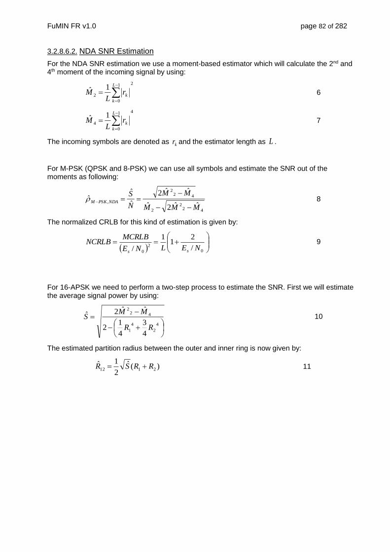
FuMIN FR v1.0 page 82 of 282
3.2.8.6.2. NDA SNR Estimation
For the NDA SNR estimation we use a moment-based estimator which will calculate the 2nd and 4th moment of the incoming signal by using:
21
0
2
1ˆ
L
k
krL
M 6
41
0
4
1ˆ
L
k
krL
M 7
The incoming symbols are denoted as kr and the estimator length as L .
For M-PSK (QPSK and 8-PSK) we can use all symbols and estimate the SNR out of the moments as following:
422
2
422
,ˆˆ2ˆ
ˆˆ2
ˆ
ˆˆ
MMM
MM
N
SNDAPSKM
8
The normalized CRLB for this kind of estimation is given by:
0
2
0/
21
1
/ NELNE
MCRLBNCRLB
ss
9
For 16-APSK we need to perform a two-step process to estimate the SNR. First we will estimate the average signal power by using:
4
2
4
1
422
4
3
4
12
ˆˆ2ˆ
RR
MMS 10
The estimated partition radius between the outer and inner ring is now given by:
)(ˆ2
1ˆ2112 RRSR 11

FuMIN FR v1.0 page 83 of 282
Figure 3.69: Separation of rings for 16-APSK
Then we will only select the symbols from the outer ring and determine the 2nd and 4th order moments of these symbols.
1
0
4
4
1
0
2
2
12
1ˆ
1ˆ
:ˆ
z
z
L
k
k
z
L
k
k
z
kkk
zL
M
zL
M
rzRr
12
Finally we can determine the SNR estimate for the 16-APSK symbols by using:
4
2
22
4
2
2
2
2
,16ˆˆ2ˆ
ˆˆ21ˆ
MMM
MM
RNDAAPSK
13
In Figure 3.70 the NDA SNR estimation for a super-frame with QPSK modulation (ro=0.2) and the DA estimator for L=720 is given from -10db to 20dB SNR. The NDA estimator outperforms the DA estimator but approaches to the DA performance with decreasing SNR. At -5dB SNR the performance is still better by factor 14.

FuMIN FR v1.0 page 84 of 282
Figure 3.70: Variance of DA SNR estimatior L=720 and NDA SNR estimator L=612540 for QPSK
3.2.8.6.3. SNR estimation via Symbol Error Rate (SER)
The SNR can also be estimated by using all available known symbols available in a SF (super frame). In the sequel the know fields SoSF, SFFI and Pilots(90) in sum 720 + 15313 symbols are used to compute the symbol error rate (SER) which is compared to the QPSK reference in Figure 3.71. The variance from -10dB to 10dB SNR is given in Figure 3.72. A histogram for 1000 symbol error rates measeurements at -10dB is given in Figure 3.73. The variance is computed on all known symbols and thats why low compared to the DA estimator. The SER reference which has to be high resolution is essential for the proper function. It has to be based on a ‘realistic’ reference simulation which includes the implementation loss of the system. In the actual variance plot the actual mean value is used and therefore presents the best case.
Figure 3.71: SER for SOSF, SFFI and PILOTS
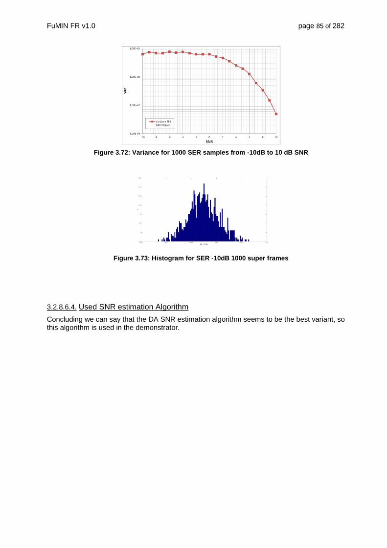
FuMIN FR v1.0 page 85 of 282
Figure 3.72: Variance for 1000 SER samples from -10dB to 10 dB SNR
Figure 3.73: Histogram for SER -10dB 1000 super frames
3.2.8.6.4. Used SNR estimation Algorithm
Concluding we can say that the DA SNR estimation algorithm seems to be the best variant, so this algorithm is used in the demonstrator.

FuMIN FR v1.0 page 86 of 282
3.2.8.7. Performance Verification of selected modCods
Selected modCods for VL-SNR BPSK CR 4/15 (Figure 3.74), BPSK_S2 CR=1/5 (Figure 3.75) and BPSK_S2 CR=11/45 (Figure 3.76) were simulated so far. The reference is the LDPC codec simulation with AWGN channel.
In the following, the min-sum algorithm is used with 50 iteration and early stop criterion for reference curve as well as for the curves with synchronization impairments.
The architecture presented in Figure 3.32 and Figure 3.33 is in operation. The impairments used in all simulations are:
AWGN
Frequency error dfTs=0.2 (or 20%)
Timing drift of 100 ppm
Figure 3.74 presents performance for BPSK CR 4/15 short frames. The implementation loss introduced by the synchronization is below 0.1dB.
Figure 3.74: FER BPSK CR=4/15 short frames
Figure 3.75 presents performance for BPSK-S2 CR 1/5 short frames. Again the implementation loss introduced by the synchronization is about 0.15dB.

FuMIN FR v1.0 page 87 of 282
Figure 3.75: FER BPSK-S2 CR=1/5 short frames
Figure 3.76 presents performance for BPSK-S2 CR=11/45 short frames. Again the implementation loss introduced by the synchronization is about 0.15dB.
Figure 3.76: FER BPSK-S2 CR=11/45 short frames
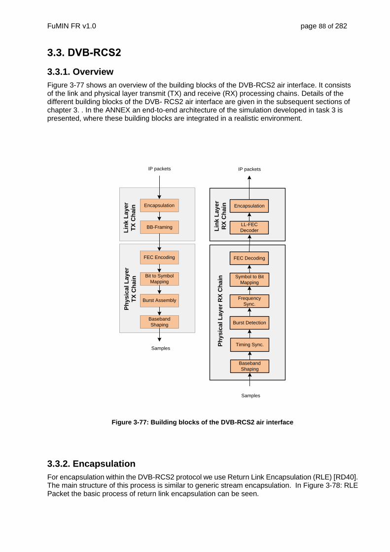
FuMIN FR v1.0 page 88 of 282
3.3. DVB-RCS2
3.3.1. Overview
Figure 3-77 shows an overview of the building blocks of the DVB-RCS2 air interface. It consists of the link and physical layer transmit (TX) and receive (RX) processing chains. Details of the different building blocks of the DVB- RCS2 air interface are given in the subsequent sections of chapter 3. . In the ANNEX an end-to-end architecture of the simulation developed in task 3 is presented, where these building blocks are integrated in a realistic environment.
IP packets
Encapsulation
BB-Framing
FEC Encoding
Bit to Symbol
Mapping
Burst Assembly
Baseband
Shaping
Lin
k L
ay
er
TX
Ch
ain
Ph
ys
ica
l L
ay
er
TX
Ch
ain
Samples
IP packets
Encapsulation
LL-FEC
Decoder
FEC Decoding
Symbol to Bit
Mapping
Frequency
Sync.
Burst Detection
Lin
k L
ay
er
RX
Ch
ain
Ph
ys
ica
l L
ay
er
RX
Ch
ain
Timing Sync.
Baseband
Shaping
Samples
Figure 3-77: Building blocks of the DVB-RCS2 air interface
3.3.2. Encapsulation
For encapsulation within the DVB-RCS2 protocol we use Return Link Encapsulation (RLE) [RD40]. The main structure of this process is similar to generic stream encapsulation. In Figure 3-78: RLE Packet the basic process of return link encapsulation can be seen.

FuMIN FR v1.0 page 89 of 282
Figure 3-78: RLE Packet
Addressed link PDU (ALPDU):
The PDUs (Protocol data units, in our case IP packets) are packed in an ALPDU (Figure 3-79: ALPDU).
Figure 3-79: ALPDU
PRO field is for protection. It has to be provided in case when ALPDU is fragmented.
Payload adapted PDU (PPDU):
ALPDUs shall be transported in one or more PPDUs. The possible structures of the PPDUs can be seen on Figure 3-80: PPDU.
Figure 3-80: PPDU
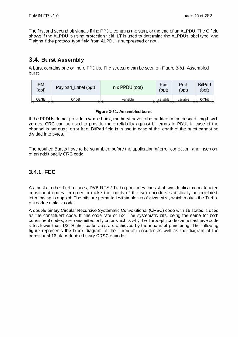
FuMIN FR v1.0 page 90 of 282
The first and second bit signals if the PPDU contains the start, or the end of an ALPDU. The C field shows if the ALPDU is using protection field. LT is used to determine the ALPDUs label type, and T signs if the protocol type field from ALPDU is suppressed or not.
3.4. Burst Assembly
A burst contains one or more PPDUs. The structure can be seen on Figure 3-81: Assembled burst.
Figure 3-81: Assembled burst
If the PPDUs do not provide a whole burst, the burst have to be padded to the desired length with zeroes. CRC can be used to provide more reliability against bit errors in PDUs in case of the channel is not quasi error free. BitPad field is in use in case of the length of the burst cannot be divided into bytes.
The resulted Bursts have to be scrambled before the application of error correction, and insertion of an additionally CRC code.
3.4.1. FEC
As most of other Turbo codes, DVB-RCS2 Turbo-phi codes consist of two identical concatenated constituent codes. In order to make the inputs of the two encoders statistically uncorrelated, interleaving is applied. The bits are permuted within blocks of given size, which makes the Turbo-phi codec a block code.
A double binary Circular Recursive Systematic Convolutional (CRSC) code with 16 states is used as the constituent code. It has code rate of 1/2. The systematic bits, being the same for both constituent codes, are transmitted only once which is why the Turbo-phi code cannot achieve code rates lower than 1/3. Higher code rates are achieved by the means of puncturing. The following figure represents the block diagram of the Turbo-phi encoder as well as the diagram of the constituent 16-state double binary CRSC encoder.

FuMIN FR v1.0 page 91 of 282
Figure 3-82: Turbo-phi encoder block diagram [ETSI EN 301 545-2]
The polynomials that define the way the registers of the constituent CRSC encoder are connected are given in ETSI EN 301 545-2, page 133.
The convolutional codes used are circular i.e. they are able to supply the decoder with the information concerning the final state of the trellis without the use of tail bits, which would degrade the spectral efficiency of the system. The price is the increase in encoding complexity by the factor two (the encoder core is run four times instead of twice). The following steps are performed in the course of encoding:
Circulation of initial state: the encoder core is initialized by the state S=0. The information
sequence is encoded in both natural and interleaved order. The two final states of the
encoder core (after encoding of each sequence) and the block length determine the
circulation states of the interleaved (C2) and the natural order sequence (C1). The
dependency is described in the Table 7-13 of ETSI EN 301 545-2.
Natural order encoding: the encoder is initialized by the circulation state C1 and fed by
the information sequence in the natural order.
Interleaved order encoding: the encoder is initialized by the circulation state C2 and fed
by the information sequence in the interleaved order. Interleaving is performed on the bit
couple level as well as between couples. Exact permutation rules are available in ETSI EN
301 545-2, page 133.
Puncturing: different code rate rates are achieved by selectively deleting the parity bits.

FuMIN FR v1.0 page 92 of 282
The puncturing maps depend on the burst length and the code rate and are the same for
all modulation formats. The same maps are applied for both natural order and interleaved
order sequences. Following code rates are defined: 1/3, 1/2, 2/3, 3/4, 4/5, 5/6, 6/7 and 7/8.
Decoding is performed based on the Trellis structure of the codes using a variant of the Maxim A-Posteriori Probability (MAP) Algorithm. Soft decision decoding is applied, which enables information exchange between the two constituent decoders. In each-half iteration, only one constituent decoder performs actual decoding. At the end of the half-iteration, its extrinsic information i.e. a-posteriori probability (APP) is used as intrinsic information of the other decoder. It is well known, that, in the case of turbo codes, the rate of performance improvement significantly drops with the number of iterations, which is the reason why the maximal number of iterations is typically set to a low number, usually 8, compared to other iteratively decodable codes.
Due to numerical, hardware and computational complexity issues, the Log-MAP algorithm is preferred to the MAP Algorithm in linear domain. It substitutes multiplications by additions, removes exponents and transforms additions into max* operations. A simplified version of the Log-Map Algorithm, called the Max-Log-MAP algorithm introduces a further computational complexity reduction by omitting the correction function from the max* operation.
Log-MAP ln(𝑒𝑥 + 𝑒𝑦) = 𝑚𝑎𝑥(𝑥, 𝑦) + log(1 + 𝑒−|𝑦−𝑥|) = 𝑚𝑎𝑥∗(𝑥, 𝑦)
Max-LOG-MAP ln(𝑒𝑥 + 𝑒𝑦) ≈ 𝑚𝑎𝑥(𝑥, 𝑦)
Table 3-12: Max-Log-MAP vs. Log-MAP
3.4.2. Modulation
Following linear modulation formats are supported in combination with the Turbo-phi codec:
BPSK
QPSK
8-PSK
16-QAM
Exact constellation parameters are not defined by the standard. Prior to I/Q modulation, bit reordering is performed in order to protect the parity bits by placing them into the positions within a burst that are mapped to the most protected positions within one symbol.
3.4.3. Waveform Performance
There is a total of 30 waveforms using linear modulation formats in the DVB-RCS2 standard. A unique waveform ID is assigned to each of them. The following tables show the requirements for PER =10-3 and PER = 10-5 over AWGN channel, as well as the burst length, the code rate and the modulation format of each waveform ID. The tables are taken from the DVB Document A162.

FuMIN FR v1.0 page 93 of 282
Table 3-13: Performance of control bursts
Table 3-14: Performance of short bursts

FuMIN FR v1.0 page 94 of 282
Table 3-15: Performance of long bursts
Table 3-16: Performance of very short bursts
Table 3-17: Performance of very long bursts

FuMIN FR v1.0 page 95 of 282
3.4.4. RCS2 Synchronization and SNR Estiamtion
3.4.4.1. Impairments
The impairments considered for the simulations are listed in the following:
• Frequency Offset dfTs from 0.5% to 3% of the symbol rate
• Random Phase error for reference and interferer signal [-pi,pi]
• Random static timing error for reference and interferer signal (at maximum half a symbol via the RRCOS filter). Timing drift are not considered because the clock is controlled by the DVB(S2x) receiver and the drift is below 1ppm. So considering a symbol rate of 1 Msymbols/s and long bursts with a length of 1616 symbols the timing error at the end of the burst is 0.1%.
• Phase Noise for reference and interferer signal, VSAT-P2 mask
3.4.4.2. Synchronization Procedure
In the sequel the syncronization procedure is given step by step. Figure 3.83 presents the architecture of correlation and timing recovery. The performance (BuErr) plots for all long and short burst waveforms are given in TN4.
Timing Estimation
Under the assumption that the burst begin is known with the uncertainty of the guard time the timing can be estimated in advance to the correlation with a non data aided (NDA) feed forward (FF) timing estimator. The Öerder&Meyer algorithm [RD110] is selected for that purpose. It is spectral based and computable with low complexity if four times oversampling is used because the exonential term simplifies to (1,-1). Further there is only a moderated noise floor at higher SNR. The estimator length for long bursts is 800 symbols, for short bursts 500 symbols. With a cubic interpolator [RD26] the signal is the reduced to one sample per symbol.
Correlation:
The burst format consists of preamble, postamble and single pilots distributed over the burst. For correlation all known symbols are used. To cope frequency errors up to 3% of the symbol rate the PDI (post detection integration) is applied, the correlation is divided into smaller sections. This factor has to be found for each waveform identifier. Up to 1%-2% frequency error this method is successful. The burst error rate does not show a significant floor below BuErr=10-4. Above this threshold correlation failures increase and the performance is dominated by them below BuErr=10-
3.
Frequency Estimation:
Target is to achieve a normalized frequency error of dfTs=2*10-4 which is the target for phase estimation. With modified Rife Boorstyn algorithm [RD27] which takes all known symbols of a burst into account, the required performance is achieved.
Phase Tracking
Next the data aided phase tracker takes into account all known symbols. Because single pilots are distributed over the burst a method which is able to utilize them is necessary. The solution is to compute an accumulated phase in forward (starting at the preamble) and backward direction (starting at the postamble) [RD1]. The forward backward phase values are combined and saved with their according position in the burst. The final step is interpolation over the stored phase values.

FuMIN FR v1.0 page 96 of 282
Symbol to soft bit mapper
Finally the pilots are removed and the burst is fed into the symbol to soft bit module
RRCOSDezimation
fsample =
4* fsymbol
Cubic
Interpolator
Ö&M
CorrelationFrequency
Estimation
Phase
Estimation
(DA Pilots,
tracking)
x
Symbol
To
soft bit
Turbo phi
Decodersds
From
Mixing stage
dfTs
phi
TDMA Timing
Start of Burst
Figure 3.83: RCS2 demodulator architecture
In the sequel the demodulator modules will be described.

FuMIN FR v1.0 page 97 of 282
3.4.4.2.1. Timing Estimation
Figure 3.84 presents the performance of the Oerder&Meyer timing estimator [RD110]. The CRLB and the computed jitter variance for NDA estimation for L=800 and 600 is given for the operatonal range. The measured perfromance is available for the operational range of WID 9,13 and 20 and is slightly above the compute NDA variance.
Figure 3.84: Ö&M performance for QPSK and estimator lengths L=600 and L=800
3.4.4.2.2. Frequency Estimation
For frequency estimation NDA operation is not applicable because of the poor perfromance in the SNR range below 6 dB for QPSK and below 10dB for 8-PSK. Above that threshold the perfronace approximates the bounds. For 16QAM NDA operation is in general not applicable. Further the classical maximum likelyhood frequency estimators like the L&R and M&M algorithm [RD108] are not applicable on single distributed pilots. The perfromance only on preamble and postable is not sufficient. So only FFT based algorithms like the Rife Boorstyn algorithm can cope the required perfromance of a resudual error of at maximum dfTs=2*10-4. The performance is given for WID 13 with all known symbols and only the preamble.
DA estimation is only possible if the start of burst is found via correlation. Correlation is sensitive to frequency errors, the peak is degraded and the detection probability is decreasing. A well known technique is the post detection integration (PDI) technique [RD105], the correlation sequence is divided into smaller pieces and the subresults are then combined to the final result. For RCS2 the WIDs are individually designed and thats why for each WID the optimal factor was found via simulation. Anyway the upper traget of 3% causes a higher degradation in the BuErr. This results from the correlation failures which become significant below a BuErr of 10-3. Especially in the SNR region below 5dB this effect is significant. Above this threshold also 3% frequency error provide appropriate results.

FuMIN FR v1.0 page 98 of 282
Figure 3.85: RB frequency estimation performance for WID 13, preamble (32) and all DA symbols (142)

FuMIN FR v1.0 page 99 of 282
3.4.4.2.3. Phase Estimation
Pre and Postamble are kept short so that the simple FEPE (frequency estimation by phase estimation) approach which interpolates between pre and postamble is not suitable. Figure 3.86 presents the standard deviation for the most used lengths. A non-data aided (NDA) tracker with for instance the V&V detector [RD109] is also not suitable because it is performing well only down to 2dB SNR. Further 16 QAM is a problem because the self-noise due to the nonlinear detector is high. Single pilots are distributed over the burst in defined distance, so method which is able to utilize them is necessary. The solution is to compute an accumulated phase in forward (starting at the preamble) and backward direction (starting at the postamble) [RD1]. The forward backward phase values are combined and saved with their according position in the burst. The final step is interpolation over the stored phase values.
Figure 3.86: STD of DA phase estimation for relevant preamble and post-amble lengths

FuMIN FR v1.0 page 100 of 282
3.4.5. VL-SNR for the Return Link
For very low SNR operation of the return link a proprietary extension to DVB-RCS2 is considered. One of the reasons is that the synchronization tasks have to be achieved on a burst-by-burst basis, since consecutive bursts are in general transmitted by different user terminals with varying conditions. Lengthy averaging algorithms, as it is possible in stream-oriented systems, are therefore not feasible.
Recovery of frequency offsets between transmitter and receiver stations, mainly caused by Doppler shifts due to satellite movements as well as drifts of the local oscillators, is especially difficult. Data-aided (DA) solutions operating on known pilot symbols attached to the bursts, e.g. the Rife-Boorstyn [RD27] or Luise-Reggiannini [RD108] algorithms, exhibit weak and practically insufficient performance at lower SNR values.
This holds also true for non-data aided (NDA) approaches. For instance, the Viterbi-Viterbi phase tracker [RD109] is typically used to compensate the residual frequency errors. But the problem is that the cycle slip rate of the tracker dominates the error performance at lower SNRs, such that a burst error rate of about 10-5, which corresponds to a quasi error-free link, cannot be guaranteed anymore.
To overcome this problem, we used a straight-forward approach using a burst format including preambles and postambles as illustrated in Figure 3.87. In the sequel, two DA phase estimates are calculated, which are then apart in time. The phase difference divided by the time difference between the estimates enables the derivation of the frequency offset. In fact, it turned out that this method performs well at low SNRs. This strategy was already presented in [RD46] and denoted as frequency estimation through phase estimation (FEPE). In our paper, we stick to this terminology. In fact, the FEPE algorithm proposed in [RD46] forms part of our receiver structure.
In [RD47], a code-aware (CA) algorithm has been presented, which extends the FEPE principle insofar as we used an NDA approach jointly with the Turbo decoder in an iterative manner. However, the disadvantage of the FEPE and CA-FEPE methods is the narrow operational range with respect to the frequency offset, which makes these algorithms useful for fine frequency tuning only.
In realistic environments, as it would be expected in the return link of a satellite communication system, frequency offsets in the order of a few percent of the symbol rate might appear, which calls for an additional “coarse” frequency estimation algorithm in order to limit the residual frequency offset to a value the FEPE algorithm can manage.
The approach we follow here is to decode a received burst considering a number of frequency hypotheses and test them by means of a burst payload cyclic redundancy check (CRC), if one of the frequency hypotheses results in a successfully decoded burst. The clue of the proposed “hypotheses testing” algorithm is that we rank the hypotheses by a simple metric, which reduces drastically the number of tested hypotheses on the average.
Burst timing, i.e. the identification of a burst’s reception time, as well as symbol timing aspects have to be solved as well. Although classical solutions, like correlation with a unique word for burst timing or the Oerder and Meyr algorithm for symbol timing recovery [RD110], are in principle applicable under very low SNR conditions, we propose here to integrate timing synchronization into the hypotheses testing algorithm. This can be done straight-forwardly by extending the hypotheses such that frequency and timing offsets are covered.
Over all, our receiver structure combines the aforementioned algorithms, namely the hypotheses testing, the FEPE and the CA-FEPE algorithm, to a very powerful system that shows an excellent robustness against carrier frequency deviations and an impressive performance in terms of burst error rates.

FuMIN FR v1.0 page 101 of 282
3.4.5.1. Air Interface for the VL-SNR Return Link
We consider an (uncoded) burst payload length of 53 byte (424 bit). In addition, the payload incorporates a 32-bit CRC. The Turbo code has a fixed code rate of 1/3.
The modulation scheme is BPSK. The SNR threshold, i.e. the SNR value which allows quasi error-free performance, would then be around -3 dB assuming an AWGN channel. In order to reach lower operational points, we consider a bit-based repetition code in addition to the Turbo code forming a concatenated coding scheme with the repetition code as inner and the Turbo as outer code.
We choose several modcods operating in an SNR range from -3 dB down to -10 dB. In Table I, these modcods are listed with the length of the burst payload in BPSK symbols and the number of pilot symbols for preambles and postambles. The table includes also the overhead due the 32-bit CRC and the pre- and postambles. Note that the code rates lower than 1/3 are achieved by multiplying the code rates of the outer and the inner code. For example, BPSK-1/6 concatenates the 1/3 Turbo code with a rate 1/2 repetition code.
The burst format shown in Figure 3.87 consists of two BPSK modulated unique words (UWs) as preamble and postamble to support the FEPE algorithm. We assume both UWs com-posed by N symbols. The ordering of the bits of the Turbo frame is defined such that the systematic bits are split into two equally sized parts, separated by parity symbols.
Systematic
Bits (part1)
Parity
Bits
Systematic
Bits (part2)
Burst payload = Turbo frame
UW
1
UW
2
TDMA Burst
Phase difference used by CA-FEPE
Phase difference used by FEPE
Figure 3.87: Format of the burst for the FEPE and CA-FEPE algorithm.
TABLE I. SUMMARY OF MODCODS
Modcod
Burst payload
length in
symbols
Total UW
lengths in
symbols
Overhead in
%
BPSK-1/3 1272 80 6.3
BPSK-1/6 2544 160 6.3
BPSK-1/12 5088 240 4.7
BPSK-1/18 7632 320 4.2

FuMIN FR v1.0 page 102 of 282
Similar to DVB-RCS2, we are assuming root-raised cosine filters with roll-off factor 0.2. Further, we assume data transmission over an additive white Gaussian noise (AWGN) channel.
The hypotheses testing algorithm requires the specification of upper limits for deviations in frequency and timing. For the frequency offset this is assumed to be ±1% of the symbol rate,
whereas for the burst timing we foresee an inaccuracy of 2 symbols. Note that a burst timing
accuracy of 1 s is typically achievable in TDMA systems by means of timing control from the hub station. This would mean that the assumed ±2 symbols correspond to a symbol rate of 2 Mbaud.
Moreover, we assume that the timing drift of the clock is limited to 2.5 ppm, which avoids harmful timing drifts even in a worst case scenario with a 125 kbaud carrier and BPSK-1/18. By using 8-times oversampling of the signal, we experienced practically negligible performance losses when using only (integer) sample instances per symbol. Consequently, we did not use an interpolation stage in our receiver structure.
3.4.5.2. Overall Architecture
Our approach for carrier synchronization at very low SNR is to use a combination of several algorithms, as illustrated in Fig 2. The first stage is the hypotheses testing algorithm, which operates on the samples from the root raised cosine (RRCOS) filter. It takes care about the coarse frequency offsets and the burst and symbol timing.
The next stage is the FEPE algorithm, which uses the preamble and postamble to perform fine tuning of the frequency offset along with the estimation of the carrier phase. This has to be done fine enough to enable the CA-FEPE as the final stage to converge.
In the subsequent sections, we discuss the individual algorithmic approaches in the following order: hypotheses testing, FEPE and CA-FEPE algorithm.
3.4.5.3. Synchronization Hypotheses Testing Algorithm
As illustrated in Figure 3.88, the hypotheses testing algorithm consists of a hypothesis selection block and the CRC check operating on the fully decoded burst payload.
Figure 3.88: Block diagram of the receiver architecture.
Its principle is to select a hypothesis with a certain timing/frequency offset, which is then applied to the received samples. In the next step the burst is decoded with respect to the hypothesis and finally the burst payload with a CRC. If the CRC is okay, i.e. no bit error is detected in the burst payload, the burst is correct and it can be passed to the upper layer. Otherwise, the hypothesis
FEPE
(operating on
UWs)
CA-FEPE
(operating on the burst
payload)
Buffer (stores
whole burst)
to
upper
layer
Received
samples
CRC
ok
CRC
not ok
CRC
check
Selection of
promising frequency/
timing hypotheses
Decimation to
symbol (next „best
sample“)
Apply
frequency
offset
Ranked list of
hypotheses
Activate next list entry
Hyphotesis selection
RRCOS

FuMIN FR v1.0 page 103 of 282
selection, decoding and CRC checking is redone with a different frequency offset and/or sample instance.
In order to avoid endless processing of thousands of hypotheses, we use a simple criterion to rank the hypotheses according to the probability of being the right one. The criterion results from the observation that the magnitude A of the correlation function between the received symbols and the pilot symbols is both frequency and timing dependent.
To illustrate the frequency dependency of the correlation magnitude A, we first recall the correlation function as
1
0
*1 L
k
kk rcL
A
with kr denoting the received symbols after proper root-raised cosine filtering and kc being the
transmitted pilot symbols in the unique word with length L. Applying now a frequency hypothesis
hf changes the expression to
1
0
*21 L
k
kk
Tkfj
h rceL
fA Sh
where sT denotes the symbol time. With kn representing the Gaussian-distributed noise from the
AWGN channel, the received symbol can be written as
k
j
kk necr
Multiplying with *
kc gives
k
j
kk nerc *
with kkk ncn * . Substituting (4) into (2) results in
1
0
21
0
21 L
k
Tkfj
k
L
k
Tkfjj
h
ShSh eneeL
fA
Since the noise samples are random and independent from each other, we assumed that the second sum gets much smaller than the first one and can be omitted. After some straightforward manipulations we get
Sh
ShTfLjj
Sh
Sh
hTf
TLf
Lee
Tf
TLf
LfA Sh
sin
sin1
sin
sin1 1
Note that 10 A . By inspection of (6), we find that hfA is a bell-shaped curve around the peak
at 0hf .
Clearly, for burst timing we can observe a similar behavior as it would be expected when applying the correlation function to the received symbols. Denoting the channel impulse response (in our case the raised cosine function) with g (t) and applying a timing hypothesis h , the
relationship in (1) changes to
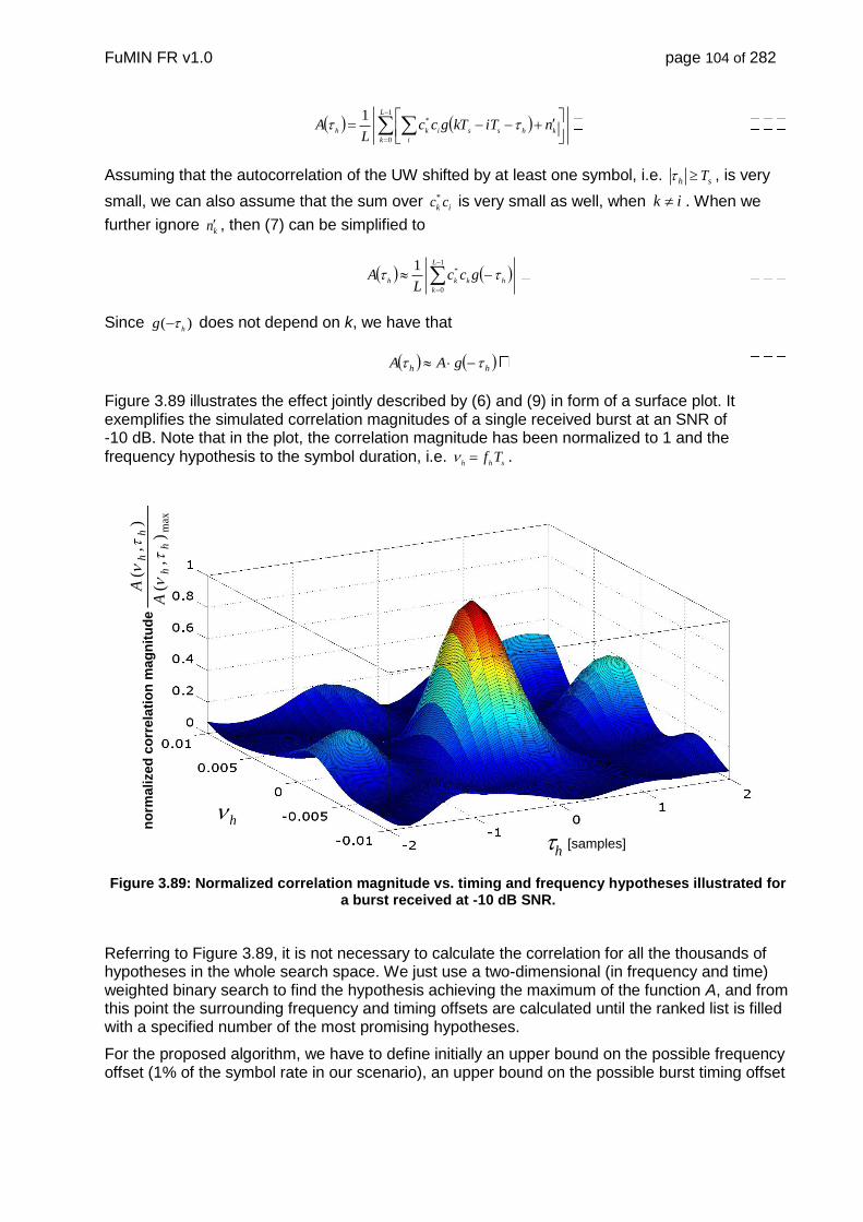
FuMIN FR v1.0 page 104 of 282
1
0
*1 L
k
khss
i
ikhniTkTgcc
LA
Assuming that the autocorrelation of the UW shifted by at least one symbol, i.e. sh T , is very
small, we can also assume that the sum over ik cc* is very small as well, when ik . When we
further ignore kn , then (7) can be simplified to
1
0
*1 L
k
hkkhgcc
LA
Since )(h
g does not depend on k, we have that
hh gAA
Figure 3.89 illustrates the effect jointly described by (6) and (9) in form of a surface plot. It exemplifies the simulated correlation magnitudes of a single received burst at an SNR of -10 dB. Note that in the plot, the correlation magnitude has been normalized to 1 and the
frequency hypothesis to the symbol duration, i.e. shh
Tf .
hh
no
rma
lize
d c
orr
ela
tio
n m
ag
nit
ud
e
[samples]
max
),
(
),
(
hh
hh
A
A
Figure 3.89: Normalized correlation magnitude vs. timing and frequency hypotheses illustrated for a burst received at -10 dB SNR.
Referring to Figure 3.89, it is not necessary to calculate the correlation for all the thousands of hypotheses in the whole search space. We just use a two-dimensional (in frequency and time) weighted binary search to find the hypothesis achieving the maximum of the function A, and from this point the surrounding frequency and timing offsets are calculated until the ranked list is filled with a specified number of the most promising hypotheses.
For the proposed algorithm, we have to define initially an upper bound on the possible frequency offset (1% of the symbol rate in our scenario), an upper bound on the possible burst timing offset
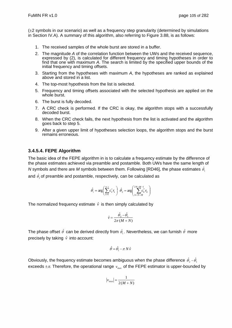
FuMIN FR v1.0 page 105 of 282
(2 symbols in our scenario) as well as a frequency step granularity (determined by simulations in Section IV.A). A summary of this algorithm, also referring to Figure 3.88, is as follows:
1. The received samples of the whole burst are stored in a buffer.
2. The magnitude A of the correlation function between the UWs and the received sequence, expressed by (2), is calculated for different frequency and timing hypotheses in order to find that one with maximum A. The search is limited by the specified upper bounds of the initial frequency and timing offsets.
3. Starting from the hypotheses with maximum A, the hypotheses are ranked as explained above and stored in a list.
4. The top-most hypothesis from the list is selected.
5. Frequency and timing offsets associated with the selected hypothesis are applied on the whole burst.
6. The burst is fully decoded.
7. A CRC check is performed. If the CRC is okay, the algorithm stops with a successfully decoded burst.
8. When the CRC check fails, the next hypothesis from the list is activated and the algorithm goes back to step 5.
9. After a given upper limit of hypotheses selection loops, the algorithm stops and the burst remains erroneous.
3.4.5.4. FEPE Algorithm
The basic idea of the FEPE algorithm in is to calculate a frequency estimate by the difference of the phase estimates achieved via preamble and postamble. Both UWs have the same length of
N symbols and there are M symbols between them. Following [RD46], the phase estimates 1
and 2 of preamble and postamble, respectively, can be calculated as
1
0
*
1argˆ
N
k
kkrc
12*
2 argˆMN
MNk
kk rc
The normalized frequency estimate v is then simply calculated by
)(2
ˆˆˆ 12
NMv
The phase offset can be derived directly from 1 . Nevertheless, we can furnish more
precisely by taking v into account:
vN ˆˆˆ1
Obviously, the frequency estimate becomes ambiguous when the phase difference 12ˆˆ
exceeds . Therefore, the operational range maxv of the FEPE estimator is upper-bounded by
)(2
1max
NMv

FuMIN FR v1.0 page 106 of 282
With s
denoting the SNR, the Cramér-Rao bound (CRB) for DA estimation of the carrier phase,
denoted as )(CRB , is given by [RD47]
s
N
2
1)(CRB
The vector Cramér-Rao bound (VCRB) of a FEPE algorithm for joint estimation of carrier
frequency and phase can be found in [RD114]. We can calculate now the variance 2
v of the
FEPE frequency estimate from the variance 2
of the phase estimate by
2222
22
)(4
1
)(4
2
NMNNM s
v
Simulations show that the measured 2
v is practically very close to (15) even for very low SNRs.
Note that this is also true for 2
, which matches the CRB in (14) very well.
3.4.5.5. CA-FEPE Algorithm
Motivated by the performance of the FEPE algorithm, this frequency estimation approach has been integrated into the Turbo decoder forming a joint synchronization and decoding approach [RD47]. A short summary of the CA-FEPE algorithm is given below and in Figure 3.90.
The idea is to use the soft bits at the output of the Turbo decoder after a single iteration, convert them back to (soft-) estimates kc of the transmitted symbols kc by taking into account the
modulation scheme. The symbols kc are then used in the FEPE algorithm together with the
received symbols kr to produce frequency and phase estimates. These estimates are applied to
the kr and fed into the next iteration of the Turbo decoder. So, as the Turbo decoder converges to
the correct code word, frequency and phase estimates are calculated more and more in a DA-like manner, and they become more and more accurate.
Note that the FEPE algorithm operates now on the burst payload, i.e. on the systematic information of the Turbo frame, and not on the UWs formed by pre- and postambles (see Figure 3.87). Referring to Section III.C, we apply (10), (11) and (12) for the frequency and phase estimates with accordingly modified values for M and N.

FuMIN FR v1.0 page 107 of 282
FEPE
(operating on
burst payload)
,v
Shift
frequency
& phase
Turbo Decoder
(single iteration)
kr
kc
CA-FEPE
Figure 3.90: Architecture of the CA-FEPE algorithm
3.4.5.6. Operational Ranges of FEPE and CA-FEPE
As the first step in our simulation campaign we evaluated the operational range of the fine frequency synchronization steps. For the CA-FEPE algorithm this is shown in Figure 3.91. The graph illustrates the burst error rate performance as a function of the initial frequency offset. It is to be mentioned that the burst error rate is seen here as the figure of merit. Note also that the burst error rates presented here include erroneous and misdetected bursts.
The used SNR values for the modcods are given in Table II. Please note that to speed up simulation time, an operational point just above a burst error rate of 10-5 has been selected, which does not mean that the performance is lower-bounded by this value. The 5th column of Table II summarizes the operational frequency range at the input of the CA-FEPE block taken from Figure 3.91. Of course, this implies that the residual frequency error at the output of the FEPE has to be inside the operational frequency range of the CA-FEPE block.
Taking into account that we want to maintain a burst error rate of 10-5, we took 5 as the effective residual frequency error of the FEPE block (i.e., we discarded the events with probability inferior to 10-6). The values for the different modcods are given in the 4th column of Table II.
By comparing the 4th and 5th column in Table II, we can see that the residual 5 frequency offset of the FEPE is smaller than the operational bound of the CA-FEPE algorithm. Consequently, we conclude that the burst error rate is maintained within the operational range of the FEPE block.
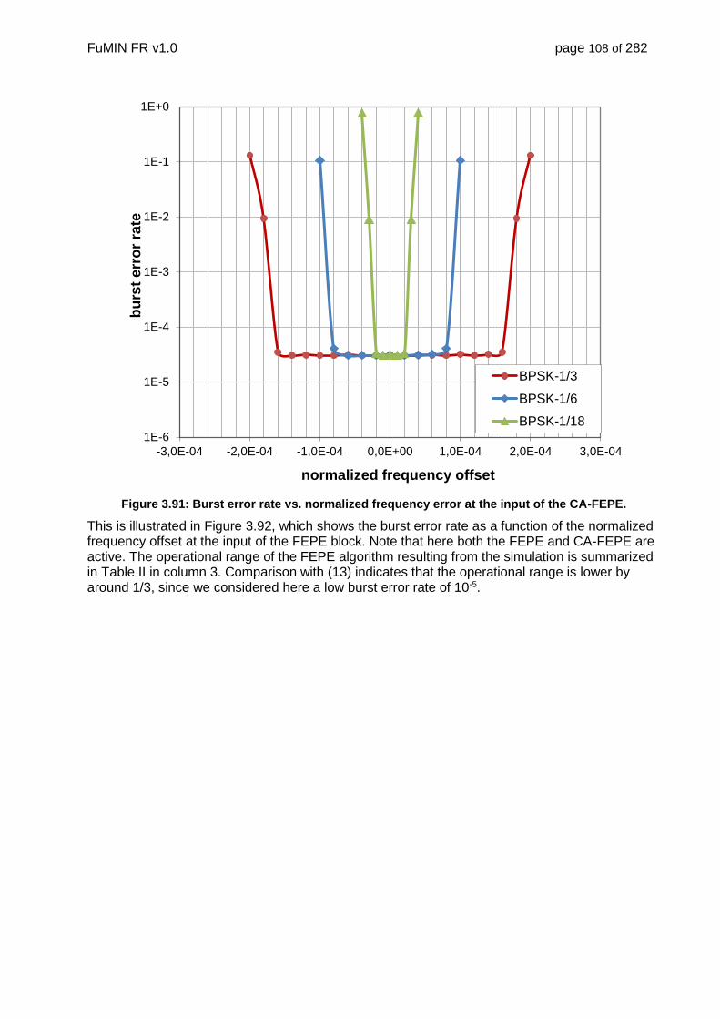
FuMIN FR v1.0 page 108 of 282
Figure 3.91: Burst error rate vs. normalized frequency error at the input of the CA-FEPE.
This is illustrated in Figure 3.92, which shows the burst error rate as a function of the normalized frequency offset at the input of the FEPE block. Note that here both the FEPE and CA-FEPE are active. The operational range of the FEPE algorithm resulting from the simulation is summarized in Table II in column 3. Comparison with (13) indicates that the operational range is lower by around 1/3, since we considered here a low burst error rate of 10-5.
1E-6
1E-5
1E-4
1E-3
1E-2
1E-1
1E+0
-3,0E-04 -2,0E-04 -1,0E-04 0,0E+00 1,0E-04 2,0E-04 3,0E-04
bu
rst
err
or
rate
normalized frequency offset
BPSK-1/3
BPSK-1/6
BPSK-1/18
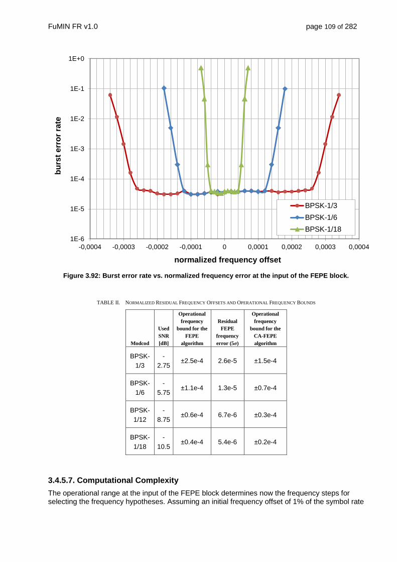
FuMIN FR v1.0 page 109 of 282
Figure 3.92: Burst error rate vs. normalized frequency error at the input of the FEPE block.
TABLE II. NORMALIZED RESIDUAL FREQUENCY OFFSETS AND OPERATIONAL FREQUENCY BOUNDS
Modcod
Used
SNR
[dB]
Operational
frequency
bound for the
FEPE
algorithm
Residual
FEPE
frequency
error (5σ)
Operational
frequency
bound for the
CA-FEPE
algorithm
BPSK-
1/3
-
2.75 ±2.5e-4 2.6e-5 ±1.5e-4
BPSK-
1/6
-
5.75 ±1.1e-4 1.3e-5 ±0.7e-4
BPSK-
1/12
-
8.75 ±0.6e-4 6.7e-6 ±0.3e-4
BPSK-
1/18
-
10.5 ±0.4e-4 5.4e-6 ±0.2e-4
3.4.5.7. Computational Complexity
The operational range at the input of the FEPE block determines now the frequency steps for selecting the frequency hypotheses. Assuming an initial frequency offset of 1% of the symbol rate
1E-6
1E-5
1E-4
1E-3
1E-2
1E-1
1E+0
-0,0004 -0,0003 -0,0002 -0,0001 0 0,0001 0,0002 0,0003 0,0004
bu
rst
err
or
rate
normalized frequency offset
BPSK-1/3
BPSK-1/6
BPSK-1/18

FuMIN FR v1.0 page 110 of 282
and a burst timing inaccuracy of ± 2 symbols with 8 times oversampling, we would end up with a huge number of hypotheses, i.e. between around 5000 (BPSK-1/3) and 25000 (BPSK-1/18) entries. Nevertheless, introducing a ranking as proposed previously, we need to process just a very small fraction of them.
The average number of tested hypotheses has been verified by Monte Carlo simulations. The results for the different modcods are shown in Table III. As illustrated, the average number of tested hypotheses decreases with higher modcods. On the other hand, the transmission time of a single burst is reduced with the spectral efficiency of the modcod. This means that for lower modcods with higher number of hypotheses tests, the available processing time is longer.
TABLE III. MODCODS VS. AVERAGE NUMBER OF TESTED HYPOTHESES
Modcod
Used
SNR
Average number of
tested hypotheses
8PSK-4/5 9.3 1
QPSK-1/2 2.5 1
BPSK-1/3 -2.75 5.9
BPSK-1/6 -5.75 9.6
BPSK-1/12 -8.75 16.1
BPSK-1/18 -10.5 21.8
In order to illustrate this aspect we compared the required processing to a classical decoded (without hypotheses testing loops) QPSK-1/2 and 8PSK-4/5 scheme. The burst rate, i.e. the number of burst per second, is the relation between the symbol rate fsymb of the carrier and the burst payload length Lb
(m) (the number of symbols for a certain modcod m as shown in Table I).

FuMIN FR v1.0 page 111 of 282
Figure 3.93: Computational complexity comparison of modcods BPSK-1/18, BPSK-1/12, BPSK-1/6, BPSK-1/3, QPSK-1/2 and 8PSK-4/5.
Multiplied with the average number of tested hypotheses per burst mloopsn as shown in Table III, we
get the computational complexity mc in form of average loops per second:
mloopsm
b
symbn
L
fc m
Figure 3.93 shows the result for an assumed carrier with 125 kSymb/s. As illustrated, the average number of loops per second of the modcods processed with hypotheses testing loops is higher than the processing requirements for QPSK-1/2. Nevertheless, the complexity of 8PSK-4/5 already exceeds even that one for BPSK-1/3.
Clearly, it is necessary to define an upper limit for the number of tested hypotheses to avoid large processing delays in case of non-decodable bursts. For delay-sensitive applications, even performance in terms of burst error rate can be devoted to control the excess delay as illustrated in Figure 3.93. Note that for the results below, we have set the upper limit to 600 in order to avoid degradations of the performance.
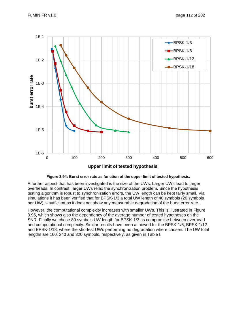
FuMIN FR v1.0 page 112 of 282
Figure 3.94: Burst error rate as function of the upper limit of tested hypothesis.
A further aspect that has been investigated is the size of the UWs. Larger UWs lead to larger overheads. In contrast, larger UWs relax the synchronization problem. Since the hypothesis testing algorithm is robust to synchronization errors, the UW length can be kept fairly small. Via simulations it has been verified that for BPSK-1/3 a total UW length of 40 symbols (20 symbols per UW) is sufficient as it does not show any measurable degradation of the burst error rate.
However, the computational complexity increases with smaller UWs. This is illustrated in Figure 3.95, which shows also the dependency of the average number of tested hypotheses on the SNR. Finally we chose 80 symbols UW length for BPSK-1/3 as compromise between overhead and computational complexity. Similar results have been achieved for the BPSK-1/6, BPSK-1/12 and BPSK-1/18, where the shortest UWs performing no degradation where chosen. The UW total lengths are 160, 240 and 320 symbols, respectively, as given in Table I.
1E-6
1E-5
1E-4
1E-3
1E-2
1E-1
0 100 200 300 400 500 600
bu
rst
err
or
rate
upper limit of tested hypothesis
BPSK-1/3
BPSK-1/6
BPSK-1/12
BPSK-1/18

FuMIN FR v1.0 page 113 of 282
Figure 3.95: Average number of tested hypotheses vs. SNR and vs. the total UW lengths (preamble + postamble) for BPSK-1/3.
3.4.5.8. Burst Error Rate Performance
Finally, the burst error rate of our receiver approach has been determined by means of Monte Carlo simulations over an AWGN channel. The duo-binary Turbo code from DVB-RCS has been used with the max-log-map algorithm and a fixed number of 8 iterations. In order to achieve statistically significant results, each point in the plot incorporates at least 100 erroneous bursts.
For our simulation work, the normalized carrier frequency offset has been randomly chosen
inside a given bound of 1%. Similarly, the burst timing offset was randomly chosen inside a
range of 2 symbols. Of course, the carrier phase was randomly selected as well in the range of
. Note that for each burst all these offsets have been determined independently. The results for the different modcods are shown in Figure 3.96 (solid lines denoted “with sync.”).

FuMIN FR v1.0 page 114 of 282
Figure 3.96: Burst error rate of the different modcods using the proposed receiver structure processing full carrier synchronization (solid lines) and comparison of the performance over an
ideal AWGN channel (dashed lines).
Also shown in Figure 3.96 is the comparison with the simulated performance of the Turbo decoder over an AWGN channel assuming ideal synchronization of carrier and timing parameters (dashed lines labeled “ideal AWGN”).
Interestingly, our receiver based on the hypotheses testing algorithm outperforms the Turbo code performance under ideal AWGN conditions, even with substantial carrier frequency, timing and phase degradations. The reason for this superior behavior is that the Turbo decoder is invoked several times for the same burst, whenever the CRC check fails. There is, loosely spoken, a “second chance” for the Turbo decoder to converge. Such a behavior of a “CRC-supported” Turbo decoder has been already described in [RD115], for instance, although in a different context and with a different way of modification.
Figure 3.97 shows the performance gain in more detail for BPSK-1/3. As we can observe, the effect is quite significant when the Turbo code reaches its error floor region. For this example the gain is with 0.25 dB quite substantial.
1E-6
1E-5
1E-4
1E-3
1E-2
1E-1
1E+0
-12,00 -10,00 -8,00 -6,00 -4,00 -2,00
bu
rst
err
or
rate
SNR [dB]
BPSK-1/3 ideal AWGN BPSK-1/6 ideal AWGNBPSK-1/3 with sync. BPSK-1/6 with sync.BPSK-1/12 ideal AWGN BPSK-1/18 ideal AWGNBPSK-1/12 with sync. BPSK-1/18 with sync.

FuMIN FR v1.0 page 115 of 282
Figure 3.97: Illustration of the gain for the “CRC-supported” Turbo decoder vs. the Turbo code performance over the ideal AWGN channel.
3.5. Forward Error Correction for Counter-Measuring Blockages
1E-6
1E-5
1E-4
1E-3
1E-2
1E-1
1E+0
-4 -3,75 -3,5 -3,25 -3 -2,75 -2,5 -2,25
bu
rst
err
or
rate
SNR [dB]
proposed receiver with allcarrier offsets
Turbo code over idealAWGN channel

FuMIN FR v1.0 page 116 of 282
3.5.1. Link Layer-FEC and Interleaving for Mobile Applications
From the information theoretical point of view, the redundancy introduced by the LL-FEC is better devoted to the PL-FEC i.e. lower PL-FEC code rates and deep- interleaving is theoretically better combination than higher PL-FEC code rate and LL- FEC. However, due to memory issues PL interleaving might not be feasible in low cost terminals, which is why LL-FEC is still being considered.
One of the means of adapting the DVB-S2x for mobile channels is the use of the forward error correction at the link layer (LL). The purpose of LL-FEC is to support system operation during periods of high packet loss ratios, which can occur due to various reasons such as excessive speed of the mobile, low SNR; multipath propagation, blockage etc. DVB family of standards already offers some LL-FEC candidates, e.g. in ETSI TR 102 768. There are three prominent frameworks considering LL-FEC:
Multiple-protocol encapsulation-FEC (MPE/GSE-FEC) from the DVB-H standard
Multiple-protocol interburst FEC (MPE-IFEC) from the DVB-SH STANDARD
Extended MPE-FEC Framework for DVB-RCS+M LL-FEC
Figure 3-98: FEC locations in DVB protocol stack [RD35]
3.5.1.1. MPE/GSE FEC Framework
The MPE sections containing data packets as well as the corresponding MPE-FEC sections are transmitted in a single burst.

FuMIN FR v1.0 page 117 of 282
Figure 3-99:DVB-H MPE-FEC Frame
In [RD17], it is concluded that MPE-FEC is not sufficient for deep fading scenarios, because obstacles may induce the loss of several consecutive bursts. Even if a burst is correctly decoded, it cannot be used for the correction of errors in other bursts. This is especially critical in the case of file delivery services, because typically more than one burst has to be decoded to recover a file.
3.5.1.2. Multiple-protocol interburst FEC Framework
In DVB Bluebook DVB A131, Multiple-protocol interburst FEC has been specified. It supports system operation in the case of erasures that last for several consecutive time slices.
Even though the specified framework is generic and allows for different FEC techniques and system applications, it was mainly designed for video multicasting over time-slice bursts. As such, MPE-IFEC minimizes the channel switching and tune in delays but does not minimize end-to-end delay.

FuMIN FR v1.0 page 118 of 282
Figure 3-100:MPE-IFEC encoding process
3.5.1.3. Extended MPE-FEC Framework for DVB –RCS + M
Due to non-suitability of the MPE-IFEC framework for bidirectional data services, in ETSI TR 102 768, a new LL-FEC framework has been designed. The same MPE data structure, as in the case when no LL-FEC is employed, is used. However, sometimes padding has to be used in order to guarantee that the start of each datagram within the application data table (ADT) is positioned at address which is a multiple of the address granularity. This is shown in the following figure.

FuMIN FR v1.0 page 119 of 282
Figure 3-101: Mapping of datagrams to ADT for DVB-RCS + M LL-FEC [RD35]
The employment of LL-FEC can be separately defined for each elementary stream in the transport stream i.e. for each GSE-FEC stream. Raptor codes can be used for ADT sizes of up to 12 MB, and Reed-Solomon code can be used for the ADT sizes of up to 191KB.
The LL-FEC exhibits the best performance when time diversity is as high as possible. This means that LL-FEC ADT size should be as high as possible. However, there is an upper bound on the LL-FEC ADT size defined as the product of the service bit rate, Rservice and the maximum permitted
latency, ΔSERVICE. This condition also sets a lower bound on the achievable code rate. The following
table shows the allowed values of the LL-FEC parameters.
Table 3-18: Bounds on LL-FEC parameter values using extended MPE-FEC for RCS+M
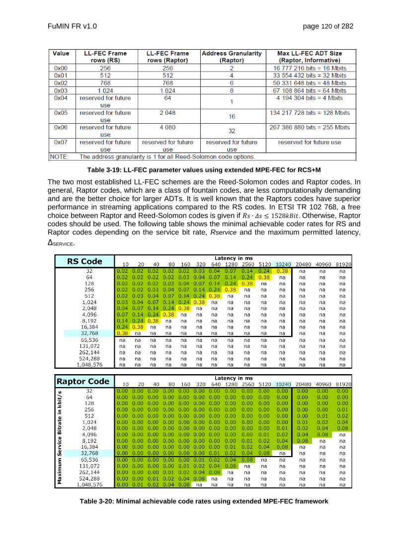
FuMIN FR v1.0 page 120 of 282
Table 3-19: LL-FEC parameter values using extended MPE-FEC for RCS+M
The two most established LL-FEC schemes are the Reed-Solomon codes and Raptor codes. In general, Raptor codes, which are a class of fountain codes, are less computationally demanding and are the better choice for larger ADTs. It is well known that the Raptors codes have superior performance in streaming applications compared to the RS codes. In ETSI TR 102 768, a free
choice between Raptor and Reed-Solomon codes is given if 𝑅𝑠 ∙ 𝛥𝑠 ≤ 1528𝑘𝐵𝑖𝑡. Otherwise, Raptor codes should be used. The following table shows the minimal achievable coder rates for RS and Raptor codes depending on the service bit rate, Rservice and the maximum permitted latency,
ΔSERVICE.
Table 3-20: Minimal achievable code rates using extended MPE-FEC framework

FuMIN FR v1.0 page 121 of 282
3.5.1.4. Staircase LDPC
A LL-FEC provides an effective scheme to mitigate mobile channel blockages for existing solutions. In the sequel the implemented LL-FEC in the simulator, which has been chosen as a Staircase LDPC, is described.
In the simulator LL-FEC encoding and LL-Interleaving are implemented on a BBFrame level. Therefore one “symbol” is equal to a whole BBFrame, rather than a “channel symbol”.
BBFrames
LL-FEC (Staircase
LDPC)
LL
-FE
C
Encoded BBFrames with
LL-FEC Redundancy
1 2 3 kk-1... k+1 k+2 ... k+N
k User Symbols = k BBFrames
N-k Redundancy Symbols =
N-k BBFrames
Figure 3-102: LL-FEC: Staircase LDPC
3.5.1.4.1. Staircase LDPC
Encoding a source object requires this object to be divided into k pieces of equal size, called source symbols. These symbols are then FEC encoded into n encoding symbols, with 𝑛 > 𝑘. The
ratio 𝐶𝑅 = 𝑘𝑛⁄ is represents the code rate.
Low-Density Parity Check (LDPC) codes are characterized by a sparse parity check matrix. The
parity check matrix defines a linear system of 𝑛 − 𝑘 parity check equations. Each column is associated with a symbol and each row represents an equation. What makes Staircase-LDPC codes different than other LDPC codes is the fact that the rightmost part of their parity check matrices, whose columns correspond to repair symbols, have double-diagonal i.e. staircase structure. The figure below shows an example of LDPC-Staircase parity check matrix. The example matrix is too small in dimensions to be considered sparse in the strict sense, but it can be used to highlight the staircase structure.
0 1 11 0 0
𝟏 0 0𝟏 𝟏 0
0 0 00 0 0
0 1 01 0 1
0 𝟏 𝟏0 0 𝟏
0 0 0𝟏 0 0
0 0 11 1 0
0 0 00 0 0
𝟏 𝟏 00 𝟏 𝟏
Figure 3-103: Example of LDPC-Staircase parity check matrix with k=6 and n=9.

FuMIN FR v1.0 page 122 of 282
3.5.1.4.2. Encoding
Encoding of the Staircase-LDPC codes is linear in complexity. This is the case due to the staircase sub-matrix structure which enables sequential creation of the repair symbols. The principle is illustrated in the figure below.
Figure 3-104: LDPC-Staircase encoding illustration
The following code rates and user (=source) symbol lengths are available in the simulator:
Coderates: 3/4; 2/3; 1/2; 1/4
User (=Source) Symbols: 100; 500; 1000
At an assumed symbol-rate of 10 Msymb/s and a QPSK ¼ normal MODCOD the following lengths are given, respecting that one BBFrame equals 16008 bits:
Code Rate
k = User Symbols (1 Symbol = 1
BBFrame) Codeword Length
[kByte] Codeword Length [s]
3/4 100 266.8 0.44
3/4 500 1334.0 2.22
3/4 1000 2668.0 4.44
2/3 100 300.2 0.50
2/3 500 1500.8 2.50
2/3 1000 3001.5 4.99
1/2 100 400.2 0.67
1/2 500 2001.0 3.33
1/2 1000 4002.0 6.66
1/4 100 800.4 1.33
1/4 500 4002.0 6.66
1/4 1000 8004.0 13.31
Table 3-21: Example for calculation of codeword lengths and related times

FuMIN FR v1.0 page 123 of 282
3.5.1.4.3. Decoding
Decoding of the Staircase-LDPC codes comes down to solving a linear system of equations. Naturally, the Maximum Likelihood (ML) approach uses Gaussian Elimination, which guarantees optimal correction capabilities. The price is theoretically cubic complexity. In [RD118], sub-optimal approach (peeling decoder), with linear complexity is proposed. The peeling decoder takes advantage of the double-diagonal structure and uses iterative (IT) approach in which equations are solved one by one where only one variable is unknown. However, some systems cannot be solved in this way, which is why in [RD119],[RD120] it is proposed to start with IT approach which will, in most cases, be able to solve the system. In cases when IT decoding ends up with a system of equations that all have more than one unknown, ML decoding takes over starting from the simplified system of equation and not the original one.
In [RD121] another technique called, Structured Gaussian Elimination (SGE), is proposed. The technique additionally speeds-up the decoding process because it enables us to continue using fast IT decoding even when no weight-one equations are left. The decoding speeds of SGE implemented on the Samsung-Galaxy SII mobile phone as well as the encoding speeds are available in [RD121].
3.5.1.4.4. LL-FEC Block Synchronization
Synchronization of the codewords of the LL-FEC is achieved by numbering the LL-FEC blocks with a consecutive number corresponding to the actual symbol (BBFrame) in the code word. This way in the simulation the beginning of a code word can be found. If in the simulation frames are lost or damaged and its sequence number is missing the next time a valid sequence number is found it will be checked how many lost BBFrames are in-between and the according BBFrames will be marked as erased for the LL-FEC decoder.
3.5.1.4.5. LL-FEC Performance
CR k n FER availability ESR520 [%] availability ESR2010 [%]
1 NA NA 0.161253 0 79
3/4 1000 1333 0.155964 0 81
2/3 1000 1500 0.140134 0 88
1/2 1000 2000 0.08174 33 100
1/4 1000 4000 0.020094 75 100
3/4 500 667 0.15706 0 79
2/3 500 750 0.15223 0 88
1/2 500 1000 0.1258 0 92
1/4 500 2000 0.036844 75 100
3/4 100 133 0.160342 0 79
2/3 100 150 0.160342 0 79
1/2 100 200 0.155374 0 85
1/4 100 400 0.126844 0 100
Table 3-22: Results for different LLFEC coderates and block lengths of k DVB-S2 frames using the vehicular model

FuMIN FR v1.0 page 124 of 282
Figure 3-105: CCDF of the packet delivery latency for LL-FEC block length of k=100 frames
Figure 3-106: CCDF of the packet delivery latency for LL-FEC block length of k=500 frames

FuMIN FR v1.0 page 125 of 282
Figure 3-107: CCDF of the packet delivery latency for LL-FEC block length of k=1000 frames
Conclusions: With the LL-FEC the outages for the user can be significantly reduced. Resynchronization after a longer blockage was no problem throughout the used blockage time series. The blockages had no noticeable influence on the LOS performance. Furthermore, the results are identical between forward and return channel. The LL-FEC show a considerable low latency, since in LOS conditions error free frames / burst can be forwarded immediately. In contrast, the PL-interleaver is not suggested, since the latency is quasi constant in LOS and blocked conditions and therefore simply too high.
3.5.2. PL Interleaver
The physical interleaver is split into two parts:
Intra code word interleaver (FEC frame) is working at bit level called “mixer”.
Inter frame interleaver based on interleaver units (IU) and called “disperser”
3.5.2.1. Interleaver (Disperser)
DVB-SH defines a channel time interleaver used together with Turbo code, thus providing a form of time diversity that mitigates the effects of error bursts over the fading channel. However, it is to note that depending on the link margins and duration of the blockages, time-averaging of the received C/N may even worsen the reception.
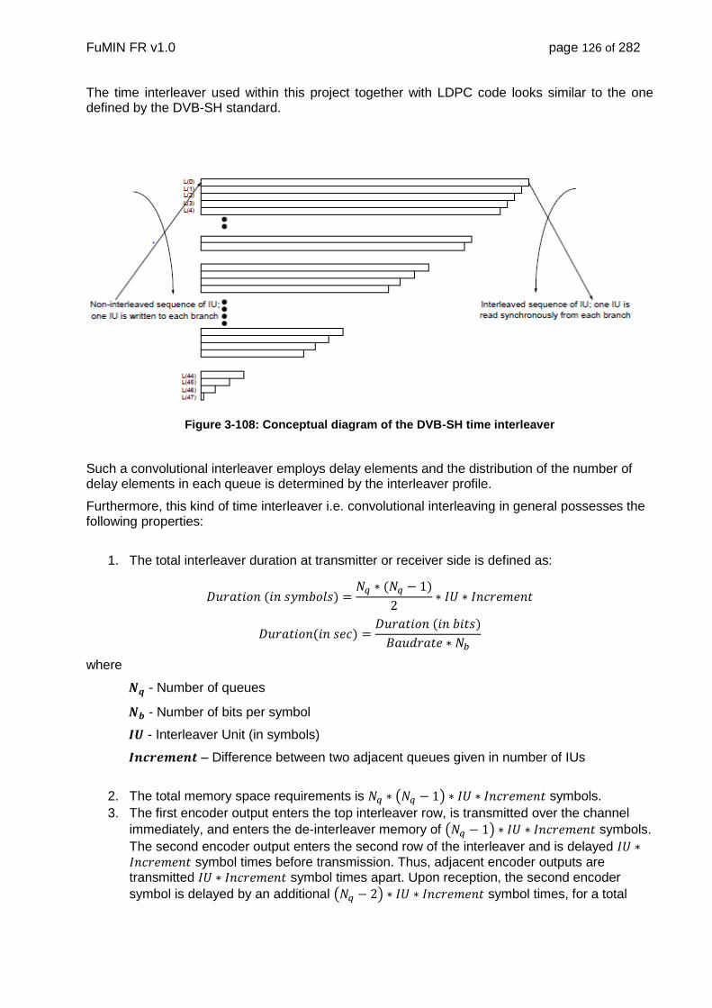
FuMIN FR v1.0 page 126 of 282
The time interleaver used within this project together with LDPC code looks similar to the one defined by the DVB-SH standard.
Figure 3-108: Conceptual diagram of the DVB-SH time interleaver
Such a convolutional interleaver employs delay elements and the distribution of the number of delay elements in each queue is determined by the interleaver profile.
Furthermore, this kind of time interleaver i.e. convolutional interleaving in general possesses the following properties:
1. The total interleaver duration at transmitter or receiver side is defined as:
𝐷𝑢𝑟𝑎𝑡𝑖𝑜𝑛 (𝑖𝑛 𝑠𝑦𝑚𝑏𝑜𝑙𝑠) =𝑁𝑞 ∗ (𝑁𝑞 − 1)
2∗ 𝐼𝑈 ∗ 𝐼𝑛𝑐𝑟𝑒𝑚𝑒𝑛𝑡
𝐷𝑢𝑟𝑎𝑡𝑖𝑜𝑛(𝑖𝑛 𝑠𝑒𝑐) =𝐷𝑢𝑟𝑎𝑡𝑖𝑜𝑛 (𝑖𝑛 𝑏𝑖𝑡𝑠)
𝐵𝑎𝑢𝑑𝑟𝑎𝑡𝑒 ∗ 𝑁𝑏
where
𝑵𝒒 - Number of queues
𝑵𝒃 - Number of bits per symbol
𝑰𝑼 - Interleaver Unit (in symbols)
𝑰𝒏𝒄𝒓𝒆𝒎𝒆𝒏𝒕 – Difference between two adjacent queues given in number of IUs
2. The total memory space requirements is 𝑁𝑞 ∗ (𝑁𝑞 − 1) ∗ 𝐼𝑈 ∗ 𝐼𝑛𝑐𝑟𝑒𝑚𝑒𝑛𝑡 symbols.
3. The first encoder output enters the top interleaver row, is transmitted over the channel
immediately, and enters the de-interleaver memory of (𝑁𝑞 − 1) ∗ 𝐼𝑈 ∗ 𝐼𝑛𝑐𝑟𝑒𝑚𝑒𝑛𝑡 symbols.
The second encoder output enters the second row of the interleaver and is delayed 𝐼𝑈 ∗𝐼𝑛𝑐𝑟𝑒𝑚𝑒𝑛𝑡 symbol times before transmission. Thus, adjacent encoder outputs are transmitted 𝐼𝑈 ∗ 𝐼𝑛𝑐𝑟𝑒𝑚𝑒𝑛𝑡 symbol times apart. Upon reception, the second encoder
symbol is delayed by an additional (𝑁𝑞 − 2) ∗ 𝐼𝑈 ∗ 𝐼𝑛𝑐𝑟𝑒𝑚𝑒𝑛𝑡 symbol times, for a total

FuMIN FR v1.0 page 127 of 282
delay of (𝑁𝑞 − 1) ∗ 𝐼𝑈 ∗ 𝐼𝑛𝑐𝑟𝑒𝑚𝑒𝑛𝑡. All of the symbols have the same delay of
(𝑁𝑞 − 1) ∗ 𝐼𝑈 ∗ 𝐼𝑛𝑐𝑟𝑒𝑚𝑒𝑛𝑡
after passing through both the interleaver and the de-interleaver, so that the decoder input symbols are in the same order as the encoder output symbols with a constant latency. However, that is only on a per branch latency, but, each symbol on each branch also has to wait for a total of 𝑁𝑞 branches, so that the total latency of the interleaver/de-
interleaver pair is
𝑁𝑞 ∗ (𝑁𝑞 − 1) ∗ 𝐼𝑈 ∗ 𝐼𝑛𝑐𝑟𝑒𝑚𝑒𝑛𝑡
4. When choosing an appropriate interleaver profile for particular channel, it is to note that
the total interleaver duration has to be at least duration of the longest erasure in that
channel.
3.5.2.2. Matrix Interleaver (Mixer)
Long convolutional PL interleavers are able to spread the erasures over multiple FEC frames, but fail to disperse them within one FEC frame. One of the reasons for this could be relatively long interleaving units (e.g. 100 bits or more), which are typically used for memory access reasons. Our simulations showed significantly better performance of the DVB-S2 CODEC in the case of dispersed erasures within one FEC frame compared to the case when several erasure bursts occur within one frame. Because of this, we used an intra-block matrix interleaver as a complementary technique to the long convolutional time interleaver.
Matrix interleaving permutes inputs within one period in a block. The matrix is filled with data row by row and then the matrix contents are sent to the output column by column. Block length is predefined with the frame length, i.e. in case of the normal frames, total block (matrix) size is 64800 bits, whereas for the short frames block contains 16200 bits.
In our simulations we used a matrix interleaver with a constant number of columns in symbols, namely 90 symbols, whereas number of rows had been matched to the frame length, i.e.:
In case of QPSK and normal frames:
o Number of columns = 180 bits
o Number of rows = 360 bits
In case of BPSK and short frames:
o Number of columns = 90 bits
o Number of rows = 180 bits
3.5.2.3. PL Interleaver Performance
Table 3-23 lists mixer and disperser parameters used for generating the reference curves. For both QPSK and BPSK modulations, interleaver queue size is set to approximately 30 seconds (memory reserved for 10 MSymbols/s).

FuMIN FR v1.0 page 128 of 282
Table 3-23: Interleaver parameters for generating reference curves
The target frame error rate (FER) was 10-3. Figure 3-109 presents the performance for QPSK ¼, whereas Figure 3-110 shows the performance for BPSK of the code rates 1/3 and 1/5. The deviation from the operational point, i.e. without blockages, represents the margin that is sufficient in order for the interleaver to work properly for a given erasure rate.
Figure 3-109: Erasure rate vs. SNR for QSPK modulation and code rates ¼
QPSK (Normal frames)
Disperser
Profile Type Uniform
Number of Queues 210
Increment (in IU) 150
IU (in symbols) 90
Duration (in sec) 29.6257
Mixer
Number of columns (bits) 180
Number of rows (bits) 360
BPSK (Short frames)
Disperser
Profile Type Uniform
Number of Queues 135
Increment (in IU) 390
IU (in symbols) 90
Duration (in sec) 31.74795
Mixer
Number of columns (bits) 90
Number of rows (bits) 180

FuMIN FR v1.0 page 129 of 282
Figure 3-110: Erasure rate vs. SNR for BSPK modulation and code rates 1/3 and 1/5
For testing the interleaver performance in suburban scenario, we used uniform interleaver with duration of approximately 120 seconds. Disperser parameters are set to the values listed in the Table 3-24.
Table 3-24: Simulation set up parameters
Disperser
Profile Type Uniform
Number of Queues 360
Increment (in IU) 210
IU (in symbols) 90
Duration (in sec) 122.132
Memory Usage (Tx) 4885272000 bits
Memory Usage (Rx) 39082176000 bits
Modulation QPSK
Code Rate 1/4
PLS 5
Baud rate 10 MSym/s
SNR -0.85 dB
SNR QEF -2.32 dB
Margin 1.45 dB

FuMIN FR v1.0 page 130 of 282
Figure 3-111: Blockage distribution in frames after interleaving (QPSK 1/4)
After simulation of 10 million states that are equivalent to the total duration of 32400 seconds, the results showed a FER of 0.000460004. Therefore, physical interleaver with parameters given in the Table 3-24 may be appropriate for the suburban scenario.
In fact , the physical layer interleaver can remove the frame errors from blockages on the channel. However, it has a practically constant latency, which is for interactive scenarios too high. Consequently, the PL-Interleaver is not recommended for this type of service, and is therefore not used in the further evaluation of the performance.
3.6. ACM
3.6.1. Introduction
Adaptive coding and modulation (ACM) is one of the strategies applied to countermeasure high fade dynamics on the communication channel, as they appear at Ka-band. ACM is in principle a simple control loop. At the receiver side, the instantaneous channel condition is measured and signaled back to the transmitter. There, the modulation and coding scheme (modcod in DVB-S2x, waveform in RCS2) is switched with respect to this channel condition. An ACM system consists of following functional components:
Measurement of the channel condition, i.e. the channel condition indicator (CCI)
An “ACM signalling channel” that can be used to signal the CCI back to the transmitter
An instance at the transmitter (ACM controller) that decides and controls the modcod
switching
In the following, possible approaches to these functional components are discussed.

FuMIN FR v1.0 page 131 of 282
3.6.2. ACM signalling channel
ACM is required in both the forward and return channel. In a DVB-RCS2 system, the forward channel is DVB-S2x TDM carrier, whereas the return channel we have the RCS2 TDMA system. Clearly, the ACM signalling channels for a certain direction (forward or return) is the other direction. The ACM signalling channel for the DVB-S2x forward link is the RCS2 link and vice versa.
The interesting question is the resulting latency, which is significantly determined by the signalling channel. For ACM the latency shall be the time between the detection of the fade event and the reception of data with the new modcod. In the following latency budgets are given. For the calculation we assume that the ACM controlled link constantly transmits data.
ACM latency budget for the forward link:
CCI measurement time at terminal: depends on the measurement method, can be 20ms
to several seconds
Terminal waits until transmit opportunity (TxOP): depends on the RCS configuration,
typically 300ms to 1s on the average, if terminal has no traffic to send.
Tx to hub: a single satellite hop, e.g. 260ms
Switch of modcod at DVB-S2x modem: negligible
Transmit of frames with the new modcod: a single satellite hop, e.g. 260ms
Realistic values are in the order of 1s. However, the “observation of PER” measurement method may result in significantly larger latencies.
ACM latency budget for the return link:
Wait time on the hub for a burst to receive: Small, since we assume an ongoing burst
transmission. For a voice over IP traffic this time could be 20ms.
CCI measurement time at hub: depends on the measurement method, since bursts from
a distinct terminal might be rare, a single burst should be sufficient. In this case the
measurement time is negligible.
Calculation of new allocation plan (AP) and wait time to transmit the AP: Since AP are
transmitted frequently this time is low, e.g. 20ms.
Tx AP to terminal: a single satellite hop, e.g. 260ms
Execution of AP + Tx burst to hub: 300ms
Realistic values are in the order of 700ms to 1s.
3.6.3. ACM controller
The ACM controller executes the “ACM algorithm”, which decides when to switch to a different modcod/waveform. Overall, the target is to keep the spectal efficiency as high as possible, while maintain the FER/PER to a certain value.
Based on our experience with the ACM experiment that has been conducted over the Q/V-band
channel in the Austrian Alphasat Q/V-band communication experiment using the Aldo Paraboni

FuMIN FR v1.0 page 132 of 282
payload [RD44], we concluded that the overall FER was practically dominated by frame losses
during rain fade events. This was the case, when the ACM control loop was not able to follow steep
fade slopes. An additional margin, called here ACM margin, on top of the modcod SNR thresholds
mitigates this problem. However, this is clearly at the cost of spectral efficiency.
Figure 3-112 illustrates the frame loss property of an ACM control loop in more detail. As already
mentioned above, ACM switches between modcods according to the channel condition. The
individual modcods M are associated with an SNR threshold MSNRT (in dB). The transmission
is quasi error-free, as long as the SNR at the receiver is higher than MSNRT , otherwise the frame
loss probability increases.
negative SNR
slope
SNR
time
SNRT(M1)
MACM
SNRT(M2)
Tdetect Texecute
TACM
frame losses
Figure 3-112: Illustration of frame losses (hatched area) during a modcod switch at a negative SNR slope.
Variation of the channel due to, e.g. a rain cloud passing through the slant path, changes the SNR
at the receiver. We propose to use the wording SNR-slopes here as to express the difference to
fade slopes, which describe the signal attenuation on the propagation path. In the ACM system,
modcod switching to lower modcods is done during negative SNR-slopes and vice versa to higher
modcods at positive SNR-slopes.
The latency between the detection of a SNR degradation and the execution of the switched
MODCOD at the receiver leads in combination with a negative SNR-slope SNRs (in dB/s) to frame
losses. To avoid or reduce these frame losses, a margin, called here ACM margin ACMM (in dB),
is added to MSNRT . modcod switching is initiated, if ACMT MMSNRSNR (in dB).
Figure 3-112 shows a negative SNR-slope crossing the 1MSNRT . Switching from modcod 1M to
2M is initiated at time detectT , which becomes effective at executeT . The time in between is called
here ACM deadtime ACMT . As illustrated in Figure 3-3, there might appear frame errors in the
hatched area, since here MSNRSNR T .
In the first phase of our Alphasat Aldo Paraboni experiments, the same fixed ACM margins have
been used for all MODCODs. Since obviously the slope of rain fades gradually increases with the
strength of rain events, different margins for the different MODCODs have been applied on the
experiment to optimize the spectral efficiency while maintaining a given FER.
An ad hoc choice of these different margins did not lead to an optimized system targeting a
requested FER. Consequently, a more detailed research on this aspect has been undertaken and
is reported in [RD45]. The idea is to derive the optimal margins for a certain FER rate directly from

FuMIN FR v1.0 page 133 of 282
the fade slope statistics of the channel conditioned by the different fade strengths corresponding
with the modcods.
Although the Alphasat experiments and the results in [RD45] are derived from a fixed ground station, the calculation method for variable margins could be probably used in mobile channels as well.
3.6.4. Measurement of the channel condition
Basically there are three ways to measure the channel condition:
(i) Observation of the PER of the received signal
(ii) Observation of the BER of a pilot sequence
(iii) Observation of the average iteration of the LDPC decoder
(iv) Observation of the SNR at the carrier
(i): Observation of the PER is used for instance in the Antares link adaptation concept [RD42]. The idea in this concept is to measure the PER after a reduced number of iterations of the LDPC codec. For instance, instead of observing the PER after 50 iterations, we do it after 2 iterations. Here we can observe a PER in the order of e.g. 1e-2 over a sliding window of 1000 packets, whereas after 50 iterations the PER is still better than 1e-5. As such a certain definable margin can be introduced in the ACM system.
(ii): Observation of the BER of a pilot sequence is a very simple method. We just have to count the relation between the correctly received (and decided) pilot symbols and the known transmitted symbols. Via a mapping table we can conclude to the related PER.
(iii): When using early stop criteria, the required number of iterations is on the average depending on the distance to the SNR threshold of the currently active modcod. This way the SNR can be estimated via a mapping table that stores the relation between number of iterations and SNR. An example of the relation between SNR and the average iterations of the RCS2 Turbo decoder is shown in Figure 3-113.
(iv): Alternatively we can measure the SNR and conclude to the PER by a known relation between SNR and PER. SNR measurement methods are well established. For instance a DA SNR estimation can be done with the squared signal-to-noise variance estimator (SNV) based on the maximum likelihood (ML) principle [RD33]. Denoting kr as the received and ks as the sent (known)
pilot symbols, the formula for this DA SNR estimator is
1
0
21
0
*2
21
0
*
Re
2
3
1
2
3
1
Re1
ˆK
k
K
k
kkk
K
k
kk
sr
KK
r
K
srK
, (14)
where K is the estimation length and the estimated SNR in linear scale. SNR estimation can be
done NDA as well. More details can be found in [RD43]. Performance results of the SNR estimation method derived from the simulation study are shown in Figure 3-114 and Figure 3-115.
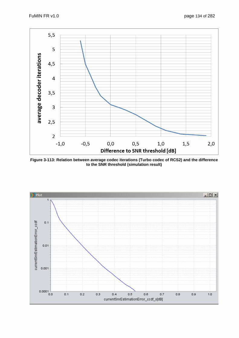
FuMIN FR v1.0 page 134 of 282
Figure 3-113: Relation between average codec iterations (Turbo codec of RCS2) and the difference to the SNR threshold (simulation result)

FuMIN FR v1.0 page 135 of 282
Figure 3-114: CDF of the absolute difference at an SNR of 10dB (simulation results)
Figure 3-115: CDF of the absolute difference at an SNR of 0dB (simulation results)
In order to decide which method is suitable for the mobile satellite communication application, the distinct advantages and disadvantages of the different are shown in the following table.
Advantages Disadvantages
Observation of the PER
In mobile fading channels there is no necessarily unique relation between SNR and PER. By measuring the PER directly this problem does not play a role.
A comparable long observation time is required. For a mobile channel that has rapid fluctuations this might be too slow. This could result in significant service interruptions. Also, the information if a packet is corrupted or not, appears on higher layers, e.g. TCP, and might not be accessible by the modem.
Observation of the BER of a pilot sequence
The method is simple and potentially fast.
If there is a unique relation between the pilot sequence BER and the PER is unclear. The accuracy of the measurement could be rather weak, such that again lengthy averaging would be necessary.

FuMIN FR v1.0 page 136 of 282
Observation of the average iteration of the LDPC decoder
Average iterations of the LDPC codec can be measured very simple. There is a direct relation between PER and iterations in the AWGN channel.
Early stop criterion required for FEC decoder. The accuracy of the measurement could be rather weak, such that again lengthy averaging would be necessary.
Observation of the SNR
The method is very fast and very accurate.
As mentioned already above, the relation between SNR and PER could be unclear.
We have also to take into account that the ACM margin, which turned out to be in the order of 0.5 to 2.5dB, requires the detection of the switching point significantly above the modcod operational point at a FER of 1e-5.
Therefore it can be immediately concluded the method (i), i.e. observation of the PER, would not work. Method (ii) is also not applicable, since especially at higher spectral efficiency, the BER is by far not accurate enough, and also the average iterations of the FEC decoders is at this operational point not significant enough.
Therefore, we concluded to go for the direct SNR measurement method, which proves to be good working throughput al the test cases.
3.7. Air-Interface and Techniques Selection for the Implementation of the Demonstrator
For implementation the HW demonstrator, pre-selection of methods has been performed after the design phase and the simulation study. A summary is given in Table 3-25, Table 3-26 and Table 3-27.
Table 3-25: Summary of the selected techniques for the forward link
Waveform DVB-S2x
Frame format DVB-S2x superframe
mode 0 with short frames
For support of VL-
SNR modcods
Encapsulation GSE-Lite
Modcods DVB-S2 and DVB S2x
modcods from BPSK-
1/3_S2 to 18APSK-8/9
32APSK is for
mobile application
typically not feasible
regarding link
budget
Channel FEC LDPC, BCH According the DVB-
S2x standard

FuMIN FR v1.0 page 137 of 282
LDPC decoder Offset min-sum with
maximum 50 iterations
and early stop criterion.
Carrier frequency synchronization Quadri-Correlator (coarse)
Luise Regiannini (fine)
Carrier timing synchronization Correlation with SoSF and
SFFI fields (coarse)
Mueller&Mueller algorithm
(fine)
Table 3-26: Summary of the selected techniques for the return link
Waveform DVB-RCS2
Burst format RCS2 compliant long
bursts (wid13 – wid22),
additional waveforms
supporting VL-SNR
The VL-SNR WIDs
arecompliant to the
RCS2 burst format,
but not listed in the
standard waveform
tables.
Waveform IDs DVB-RCS2 WIDs from
QPSK-1/3 to QAM-5/6,
VL-SNR WIDs from
BPSK-1/3 to BPSK1/18
Channel FEC Turbo-Phi, for VL-SNR
Turbo phi is concatenated
with a repetition code and
a CRC in the payload.
Compliant to RCS2
format.
LDPC decoder Max-log-map Turbo
decoder algorithm with
maximum 8 iterations and
early stop criterion.
Carrier frequency synchronization Modified Rife-Boorstyn
Carrier timing synchronization Correlation with burst pre-
and postamble and
Oerder&Meyer algorithm

FuMIN FR v1.0 page 138 of 282
Table 3-27: Summary of the selected techniques for ACM and blockage counter-measurement
Channel estimation method DA SNR estimation
ACM margin Fixed between 0.5 and
2.5dB depending on the
Scenario.
Blockage counter-measurement LL-FEC with code-rates
between 0.5 and 0.75 and
block lengths between
100ms and 5s depending
on the scenario.
Staircase –LDPC
has been selected
as algorithm.
4. Mobile Channel Model
4.1. Introduction
In this section, we present the principles of a channel model and its implementation onto a time-series synthesizer which accurately represents the dynamics of the various phenomena affecting a Ka-Band link: 20 GHz for the downlink and 30 GHz for the uplink.
Here we concentrate on the identification of the actual physical phenomena: rain, scintillation, Doppler, shadowing, etc. and choose the relevant models as well as their associated time-series generators. We also pay special attention to model parameterization. In this respect we start off with the use scenarios identified in Table 4-1 of Annex A in the Statement of Work [RD53], reproduced in part below.
It is important to point out that the channel is influenced by both the troposphere and the local environment (shadowing and multipath). Both effects together with the possibility of incurring in pointing errors will be accounted for.
We can see that the usage table indicated in the SoW include for each channel/operational scenario two antenna types with different gains.
The possibility of implementing diversity will be investigated. This implies further requirements on the time-series generators:
(a) for space diversity schemes, at least two simultaneous time series will be synthesized incorporating realistic cross-correlation properties, and
(b) in each time series the autocorrelation properties present in real signals must be captured.
For accounting for the channel's autocorrelation we must take into consideration the fading channel dynamics.
For the three classes of use scenarios, two antenna sizes are indicated:
(a) a nominal one of medium size and
(b) a smaller one for commercial appeal.

FuMIN FR v1.0 page 139 of 282
Antenna size has twofold implications, for one the carrier-to-multipath ratio changes and for the other the pointing errors are different. A minor influence is expected in the tropospheric effects, only very slight variations in the scintillation intensity are to be expected.
Coming to the fading channel modeling, for railway applications, multipath reflections can originate on terrain elements around the terminal, and cannot be ignored, particularly the periodic blocking by power arches [RD55]. Section 11 of the DVB-RCS+M guidelines [RD52] includes a proposed model of the railway channel based on an ESA-sponsored study. We will take this as starting point in our analysis.
For aeronautical applications at Ka-band the antennas have high directivity, hence multipath effects are assumed insignificant. A relevant measurement campaign is reported in [RD56].
4.2. Channel Models
Channel modelling for satellite mobile millimeter wave scenarios must account for the two traversed layers by the transmitted signals: the troposphere and the local environment. The ionosphere can be safely disregarded. In addition, the movement of the terminal has to be taken into account while the satellite is assumed to be fixed (GEO).
Thus, three main categories of channel effects need to be considered, namely, tropospheric, local (shadowing and multipath) and pointing.
Two modeling levels are necessary: one considering "long-term conditions" as in classic link budget calculations, and an "instantons approach" based on producing time-series of the received signal for performing physical layer simulations. We can also call the long term analysis a static approach (which should provide an indication of the link's nominal working point) while the instantaneous level analysis could also be called a dynamic approach.
In the case of tropospheric effects, the static approach (determination of working point, link margin, etc.) is based on the use of average year or worst month cumulative distributions, CDFs. We propose to provide this long-term information, CDF-based, as a reference for initial link budget calculations. They could also represent the conditions of a nomadic terminal. A CDF or its complementary, CCDF, provide the probability or percentage of time that a given threshold level is/is not exceeded.
The instantaneous approach involves generating time-series to be played back at the same time as the physical layer simulator is generating transmitted symbols. The approach proposed is to produce channel simulator runs and store their results. We can then pick out segments of interest for interfacing the Demonstrator. This will allow us to subject the transmission chain to realistic events and learn on the reaction of the receiver terminal to such channel events and dynamics.
The terminal movement gives rise to two types of effects: changing conditions of the channel as the terminal travels, e.g., displacements of the terminal relative to a rain cell or varying shadowing conditions (movement with respect to obstacles) and, mispointing errors, for an antenna with a given beamwidth, due to inaccurate tracking of the satellite due to road turns and unevenness, and an inadequate, slow response of the pointing system. We can also consider here the maneuvers of an aircraft. Terminal movement (and satellite movement) also give rise to Doppler shifts which have to be incorporated in the channel modeling.
There is one first point to be addressed which is how to combine these three kinds of events: local effects and pointing errors are normally modeled on a short-term basis whereas tropospheric effects are normally referred to the so called average year (or, sometimes, to the so called worst month). This latter information is normally used in link budget calculations for a yearly availability calculation, typically specifying many nines, e.g. 99.99%, availability levels, meaning system accumulated outage times amounting to a few tens of minutes in a year. However, nothing is said about how these outages are distributed throughout the year: in small interruptions or in longer
FuMIN FR v1.0 page 140 of 282
ones, or all in one single event. Models are available, especially at the ITU-R, for second order statistics which take care of the characterization of durations of fades and fade slopes.
In the case of the aeronautical channel, the troposphere may not play a significant role during the en-route phase of a flight as the aircraft flies above the rain.
In the case of local effects shadowing and multipath we can also follow a similar two-level approach: one considering an overall CDF of the attenuation for a given type of environment, e.g., urban, suburban, wooded, open fields, highway, etc. The other, again, generating time-series for use in physical layer simulations. One further simplification is to consider the channel at millimeter waves as presenting an on-off or brick-wall behavior: all (0 dB excess attenuation) or nothing at all (infinite excess attenuation). In tis case, there is no need to specify a threshold, any obstacle will give rise to an outage.
Specific "local effects" models are required for each of the channels to be analyzed: aeronautical, train and vehicular. It must be pointed out that the CDFs of local effects do not translate directly into availabilities once a threshold is set. Availability depends very much on the vehicle speed relative to the obstacle sizes and the coding and interleaving scheme employed. However, a coverage probability level should provide a relevant, first-order indication of the availability likely to be obtained.
In the case of rain and other tropospheric effects, the user speed with respect to the extent of rain cells, etc., will not have such a significant impact on fade event durations.
Local effects, given the size of the various obstacles and the length of the platform carrying the terminal can in part be overcome using two antennas at the from and rear ends. We will deal with diversity issues in this way.
Finally, we can say the same for the mispointing errors. We can define a CDF for the pointing error and generate time-series for simulation purposes. In both levels of analysis, different parameters are envisaged at least as a function of antenna beam-width and type of road: winding, straight, flat/even, rough.
4.3. Modeling the Doppler effects
Doppler shifts are generated when the distance between the ends of the radio link varies with time. Here we consider a geostationary satellite (GSO) at one end which apparently is fixed in its orbital position (we later consider further effects). Thus, the shift would be fundamentally due to the movement of the terminal. The Doppler shift is then
𝑓𝐷 =𝑉
𝜆(𝐫 ∙ 𝐯) =
𝑉
𝜆cos 𝛾
where 𝑉 is the velocity of the terminal, 𝐯 is the unit velocity vector (direction of travel) and 𝐫 is the unit vector from the terminal to the satellite (Figure 4-1).

FuMIN FR v1.0 page 141 of 282
Figure 4-1: Doppler shift modeling.
We will be using the above expression to set the order of magnitude of the bulk of the Doppler shift present in the link. However, there are other related effects: Doppler shift (already mentioned) and rate. Values for these parameters have been proposed for different types of terminals in Ku-band and Ka-band in [RD52], based on geometrical considerations.
The maximum offset and drift rates are both important for acquisition. For tracking, the drift rate is the most important, as any constant Doppler has presumably been compensated.
In [RD52] it is proposed to model the carrier frequency offset as a sinusoidal variation with an amplitude corresponding to the maximum given in Table 4-1, and a period that results in the maximum rate of change quoted in the table, which correspond to the case where the terminal was moving in a circular pattern with the satellite at low elevation angle.
Table 4-1: Doppler shift and rate at Ka-band assuming the uplink frequency is 30.0 GHz and the downlink frequency 20.2 GHz (from [RD52])
Terminal type
Speed (km/h)
Acceleration (m/s2)
Doppler rate
Uplink Doppler frequency shift
(Hz)
Downlink Doppler frequency shift (Hz)
Time drift
(ns/s)
Uplink frequency drift (Hz/s)
Downlink frequency drift (Hz/s)
Pedestrian 5 1 4.6 E9 139 94 4.6 100 67
Maritime 25 5 2.3 E8 694 468 23.1 500 337
Vehicular 120 10 1.1 E7 3,333 2,244 111 1,000 673
Train 350 5 3.2 E7 9,722 6,546 324 500 337
Aeronautical 1188 17 1.1 E6 33,000 22,220 1,100 1,700 1,145
GSO satellite 10.8 0 1.0 E8 300 202 10 10 6.7
The frequency offset is given by [RD52]
Δ𝑓(𝑡) = Δ𝑓,max cos (2𝜋𝑡
𝑃)

FuMIN FR v1.0 page 142 of 282
where Δ𝑓,max is the value from Table 4-1 (e.g. 22,220 Hz for an aeronautical terminal at 20.2
GHz) and P is the period of the variation. P can be determined by differentiating the previous equation,
𝜕
𝜕𝑡 Δ𝑓(𝑡) = −
2𝜋Δ𝑓,max
𝑃sin (
2𝜋𝑡
𝑃)
Maximizing we get [RD52]
max (𝜕
𝜕𝑡 Δ𝑓(𝑡)) =
2𝜋Δ𝑓,max
𝑃= 𝐷max
where 𝐷max is the maximum drift from the table (e.g. 1,145 Hz/s for an aeronautical terminal at 20.2 GHz). We get [RD52]
𝑃 =2𝜋Δ𝑓,max
𝐷max
For the example, 𝑃 = 2𝜋22200/1145 = 121.82 s.
The implementation of the Doppler effects into the time-series synthesizer can be performed by multiplying the resulting series by a phasor (Figure 4-1) containing the shift and frequency drift discussed in this section.
4.4. Modeling of Tropospheric Effects
We start by summarizing the tropospheric effects encountered in millimeter waves and prioritize their contributions. The main effects are the following (according to ITU-R Rec. 618 [RD9]):
• Rain attenuation
• Cloud attenuation
• Gaseous absorption (water vapor)
• Scintillation, both during dry and rainy periods.
In Figure 4-2 and Figure 4-3 we illustrate two, three day-long series corresponding to dry days and rainy days, measured at 20 GHz in Vigo, Spain, as part of the Alphasat experiment [RD57]. We can observe how, even during dry days, there is always a small signal variability present due to scintillation. In addition, gaseous absorption and cloud losses may impair the received signal although they show a much slower time variability.

FuMIN FR v1.0 page 143 of 282
Figure 4-2: Example of three consecutive dry days measured in Vigo, Spain, at 20 GHz
(Alphasat experiment)
Figure 4-3: Example of three consecutive rainy days measured in Vigo, Spain, at 20 GHz
(Alphasat experiment)
From the models contained in ITU-R Rec. P.618 [RD9], the long-term, CDF-based link analysis can be implemented. We also obtain duration of fade distributions derived from the relevant recommendation (ITU-R Rec. P.1623 [RD58]). These models are all developed for static receivers. This means that our reference margins and other relevant information relative to the selected working points will be provided assuming static receivers. However, in the time-series simulation modules, the terminal movement is accounted for. The CDFs provided by the models correspond to the so-called "average year". "Worst month" statistics can also be considered.
Since tropospheric effects are strongly dependent on the climatic zone of interest, we can specify different CDFs for different areas where the markets of interest are located. The elevation angle also plays a role, especially linked to the length of the radio path through the rain cells. This depends both on the orbital position of the satellite with respect to the location of the terminal and on the altitude of this location above sea level.
Worldwide tropospheric parameterizations for the relevant models can be found in the ITU-R recommendations in the form of digital gridded maps, e.g. [RD59], [RD60] or [RD61]. In Table 4-2 we enumerates the main ITU-R recommendations used in the static analysis to identify the links' working points. We have also added the recommendation on time-series generation which we have in part followed in the implementation of the synthesizer.
0 0.5 1 1.5 2 2.5 3-2
-1.5
-1
-0.5
0
0.5
1
1.5
2
2.5
Time (Days)
Sig
nal le
vel (d
B)
20 GHz beacon receiver measurements at Vigo. DRY DAYS
0 0.5 1 1.5 2 2.5 3-30
-25
-20
-15
-10
-5
0
520 GHz beacon receiver measurements at Vigo. RAINY DAYS
Sig
nal le
vel (d
B)
Time (Days)
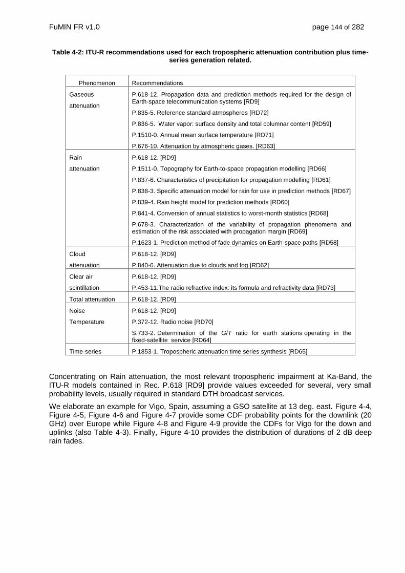
FuMIN FR v1.0 page 144 of 282
Table 4-2: ITU-R recommendations used for each tropospheric attenuation contribution plus time-series generation related.
Phenomenon Recommendations
Gaseous
attenuation
P.618-12. Propagation data and prediction methods required for the design of Earth-space telecommunication systems [RD9]
P.835-5. Reference standard atmospheres [RD72]
P.836-5. Water vapor: surface density and total columnar content [RD59]
P.1510-0. Annual mean surface temperature [RD71]
P.676-10. Attenuation by atmospheric gases. [RD63]
Rain
attenuation
P.618-12. [RD9]
P.1511-0. Topography for Earth-to-space propagation modelling [RD66]
P.837-6. Characteristics of precipitation for propagation modelling [RD61]
P.838-3. Specific attenuation model for rain for use in prediction methods [RD67]
P.839-4. Rain height model for prediction methods [RD60]
P.841-4. Conversion of annual statistics to worst-month statistics [RD68]
P.678-3. Characterization of the variability of propagation phenomena and estimation of the risk associated with propagation margin [RD69]
P.1623-1. Prediction method of fade dynamics on Earth-space paths [RD58]
Cloud
attenuation
P.618-12. [RD9]
P.840-6. Attenuation due to clouds and fog [RD62]
Clear air
scintillation
P.618-12. [RD9]
P.453-11.The radio refractive index: its formula and refractivity data [RD73]
Total attenuation P.618-12. [RD9]
Noise
Temperature
P.618-12. [RD9]
P.372-12. Radio noise [RD70]
S.733-2. Determination of the G/T ratio for earth stations operating in the fixed-satellite service [RD64]
Time-series P.1853-1. Tropospheric attenuation time series synthesis [RD65]
Concentrating on Rain attenuation, the most relevant tropospheric impairment at Ka-Band, the ITU-R models contained in Rec. P.618 [RD9] provide values exceeded for several, very small probability levels, usually required in standard DTH broadcast services.
We elaborate an example for Vigo, Spain, assuming a GSO satellite at 13 deg. east. Figure 4-4, Figure 4-5, Figure 4-6 and Figure 4-7 provide some CDF probability points for the downlink (20 GHz) over Europe while Figure 4-8 and Figure 4-9 provide the CDFs for Vigo for the down and uplinks (also Table 4-3). Finally, Figure 4-10 provides the distribution of durations of 2 dB deep rain fades.

FuMIN FR v1.0 page 145 of 282
Figure 4-4: Europe wide rain attenuation map for an exceedance probability p. Downlink frequency 20 GHz, satellite 13 deg. east.
Figure 4-5: Europe wide rain attenuation map for an exceedance probability p. Downlink frequency 20 GHz, satellite 13 deg. east.

FuMIN FR v1.0 page 146 of 282
Figure 4-6: Europe wide rain attenuation map for an exceedance probability p. Downlink frequency 20 GHz, satellite 13 deg. east.
Figure 4-7: Europe wide rain attenuation map for an exceedance probability p. Downlink frequency 20 GHz, satellite 13 deg. east.

FuMIN FR v1.0 page 147 of 282
Figure 4-8: Cumulative distribution of rain attenuation at Vigo, Spain, for the downlink
frequency, 20 GHz, and the satellite at 13 deg. east.
Figure 4-9: Cumulative distribution of rain attenuation at Vigo, Spain, for the uplink
frequency, 30 GHz, and the satellite at 13 deg. east.
Figure 4-10: Example of second order statistic.
Duration distribution of rain fades below 2 dB at Vigo, Spain.
Table 4-3: CCDF for rain attenuation at the example location: Vigo, Spain. Satellite located at 13 deg east.
Link 𝑝% 1.0 0.7 0.5 0.3 0.2 0.1 0.05 0.02 0.01 0.001
Downlink 1.36 1.73 2.15 2.96 3.76 5.52 7.85 11.91 15.73 31.61
Uplink 2.97 3.73 4.60 6.22 7.81 11.23 15.66 23.13 29.95 56.30
Now we go on to tabulate the gaseous absorption and cloud attenuation levels. We give the zenith values for oxygen and water vapor, and the overall combination for the slant path for various exceedance probability levels, Table 4-4 and Table 4-5.
0 5 10 15 20 25 30 3510
-3
10-2
10-1
100
Attenuation (dB)
Pro
babili
ty (
%)
CCDF - 20 GHz
0 10 20 30 40 50 6010
-3
10-2
10-1
100
Attenuation (dB)
Pro
babili
ty (
%)
CCDF - 30 GHz

FuMIN FR v1.0 page 148 of 282
Table 4-4: Gaseous attenuation at the example location, Vigo, Spain. Satellite at 13 deg east.
Zenith Zenith Gas total,
Link O2 WV 1% slant path, 1%
Downlink 0.10 0.37 0.80
Uplink 0.19 0.23 0.71
Table 4-5: Cloud attenuation at the example location, Vigo, Spain. Satellite at 13 deg east.
Link 𝑝% 1.0 0.7 0.5 0.3 0.2 0.1 0.05 0.02 0.01 0.001
Downlink 0.42 0.47 0.52 0.53 0.58 0.69 0.69 0.69 0.69 0.69
Uplink 0.90 1.01 1.11 1.15 1.25 1.49 1.49 1.49 1.49 1.49
Finally, we can consider the dry scintillation. The down and uplink CCDF for Vigo, Spain, are presented in Figure 4-11 and Figure 4-12 and in Table 4-6. These levels can be taken into consideration to assess the clear air conditions.
Figure 4-11: Distribution of scintillation amplitudes at 20 GHz (downlink), example
location, Vigo, Spain. Satellite located at 13 deg east. Assumptions: antenna diameter 0.2 m and
efficiency 0.7.
Figure 4-12: Distribution of scintillation amplitudes at 30 GHz (uplink), example location,
Vigo, Spain. Satellite located at 13 deg east. Assumptions: antenna diameter 0.2 m and
efficiency 0.7.
Table 4-6: Scintillation levels for various exceedance probabilities at Vigo, Spain, satellite 13 deg. east at 20 and 30 GHz.
Link 𝑝% 1.0 0.7 0.5 0.3 0.2 0.1 0.05 0.02 0.01 0.001
Downlink 0.22 0.24 0.25 0.28 0.31 0.35 0.40 0.46 0.52 0.75
Uplink 0.25 0.27 0.29 0.33 0.35 0.40 0.46 0.53 0.60 0.87
To estimate the total attenuation due to multiple sources of simultaneously occurring atmospheric effects ITU-Rec P618 [RD9] provides the following guidelines. The total
0.2 0.3 0.4 0.5 0.6 0.7 0.8 0.910
-3
10-2
10-1
100
Sintillation amplitude (dB)
Pro
babili
ty (
%)
Vigo 20 GHz
0.2 0.3 0.4 0.5 0.6 0.7 0.8 0.9 110
-3
10-2
10-1
100
Sintillation amplitude (dB)
Pro
babili
ty (
%)
Vigo 30 GHz

FuMIN FR v1.0 page 149 of 282
attenuation (dB) represents the combined effect of rain, gas, clouds and scintillation and requires one or more of the following input parameters: 𝐴𝑅(𝑝), the attenuation due to rain for a fixed probability (dB)
𝐴𝐶(𝑝), the attenuation due to clouds for a fixed probability (dB) (Rec. ITU-R P.840 [RD62])
𝐴𝐺(𝑝), the gas attenuation due to water vapor and oxygen for a fixed probability (dB), (Rec. ITU-R P.676 [RD63])
𝐴𝑆(𝑝), the attenuation due to tropospheric scintillation for a fixed probability (dB).
A general method for calculating total attenuation for a given probability, AT ( p), is given by
)()()()()( 22pApApApApA SCRGT
where
AC ( p) = AC (1%) for p < 1.0%
AG ( p) = AG (1%) for p < 1.0%
The above two equations take account of the fact that a large part of the cloud attenuation and gaseous attenuation is already included in the rain attenuation prediction for time percentages below 1%. The obtained results are summarized in Table 4-7.
Table 4-7: CCDF of the total attenuation for the example location, Vigo, Spain, for a satellite at 13 deg. east.
Link 𝐴𝑇(𝑝%) 1.0 0.7 0.5 0.3 0.2 0.1 0.05 0.02 0.01 0.001
Downlink 2.59 2.96 3.38 4.19 4.99 6.74 9.07 13.13 16.96 32.83
Uplink 4.58 5.35 6.21 7.83 9.42 12.85 17.27 24.75 31.57 57.92
4.4.1.1. External noise and degradation of the G/T parameter during rain events
We further need to assess the degradation in the receiver's figure of merit due to tropospheric attenuation. When we have atmospheric losses, the figure of merit is degraded in two ways [RD64]:
- directly through a decrease in the signal level
- indirectly through an increase in the noise temperature
Thus, the two values we can quote on the figure of merit is a clear air value and a value affected by tropospheric losses and noise temperature increment specified for a given probability
exceedance level, 𝑝, hence we have
𝐺
𝑇1
and
𝐺
𝑇2− 𝐿atm
respectively. The various elements intervening in the calculation of the two figure of merit values are as follows,
𝑇𝐴 =𝑇𝑐 + 𝑇𝑠
𝛼+
𝛼 − 1
𝛼𝑇phys
where 𝑇𝐴is antenna noise temperature in clear-sky conditions and
𝑇𝑐 is antenna noise temperature due to clear sky

FuMIN FR v1.0 page 150 of 282
𝑇𝑠 is the antenna noise temperature due to ground contributions and
𝑇phys is the physical temperature of the non-radiating elements of the antenna and
𝛼 ≥ 1 is resistive losses due to non-radiating elements of the antenna
The system's noise temperature for clear air conditions, 𝑇1, is given by
𝑇1 = 𝑇𝐴 + 𝑇𝑅
where 𝑇𝑅is the receiving equipment noise temperature.
Now, the figure of merit when the transmission is affected by tropospheric attenuation for a given
exceedance probability, 𝑝, is
𝐺
𝑇2(𝑝)− 𝐿atm(𝑝)
where Latm(p) the the attenuation due to clouds and rain exceeded p% of the time and T2(p) is
the system's noise teperature exceeded p % of the time due to atmospheric loss. This parameter is given by
𝑇2(𝑝) =𝑙atm(𝑝) − 1
𝛼 𝑙atm(𝑝)(𝑇atm + 𝑇𝐶) +
1
𝛼[𝑇𝐶 + 𝑇𝑆 + (𝛼 − 1)𝑇phy] + 𝑇𝑅 [𝐾]
where
𝑇atm is the physical temperature of atmosphere and precipitations, typically T = 275 K for both clouds and for rain.
Latm(p)[dB] = 10 log(latm(p)) is the atmospheric loss due to clouds and rain, both in dB
and in linear for an exceedance probability p %.
The above expression can be broken down into three terms,
𝑇2(𝑝) = 𝑇𝐴 + ∆𝑇𝐴(𝑝) + 𝑇𝑅
where ∆TA(p) is the additional antenna noise temperature caused by atmospheric and precipitation losses, given by
∆𝑇𝐴(𝑝) =𝑙atm(𝑝) − 1
𝛼 𝑙atm(𝑝)(𝑇atm + 𝑇𝐶)
Assuming a clear sky system noise temperature of 25 dBK or equivalently, TSYS = T1= 316 K, which
could be allocated as follows, TA = TC = 40 K and TR= 276 K (FR 2 dB), simplifying the expressions
above, we get that
∆𝑇𝐴(𝑝) =𝑙atm(𝑝) − 1
𝑙atm(𝑝)(𝑇atm + 𝑇𝐶)
where we have disregarded the Ohm losses and made α = 1. For the example location (Vigo) we
get a degradation as shown in Table 4-8 where we have kept the scintillation loss as it is almost
negligible with respect to the contribution from rain.
Table 4-8: Results for figure of merit degradation. Various probability levels. Location, Vigo, Spain. Satellite 13 deg. east. Downlink frequency 20 GHz.
𝑝 (%) 𝐴𝑇 (dB) ∆𝑇𝐴(𝑝) (K) 𝑇2(𝑝) (K) 10 log(𝑇2/𝑇1) (dB) Total degrad. (dB)
1.0 2.59 141.67 457.67 1.61 4.20
0.7 2.96 155.78 471.78 1.74 4.70
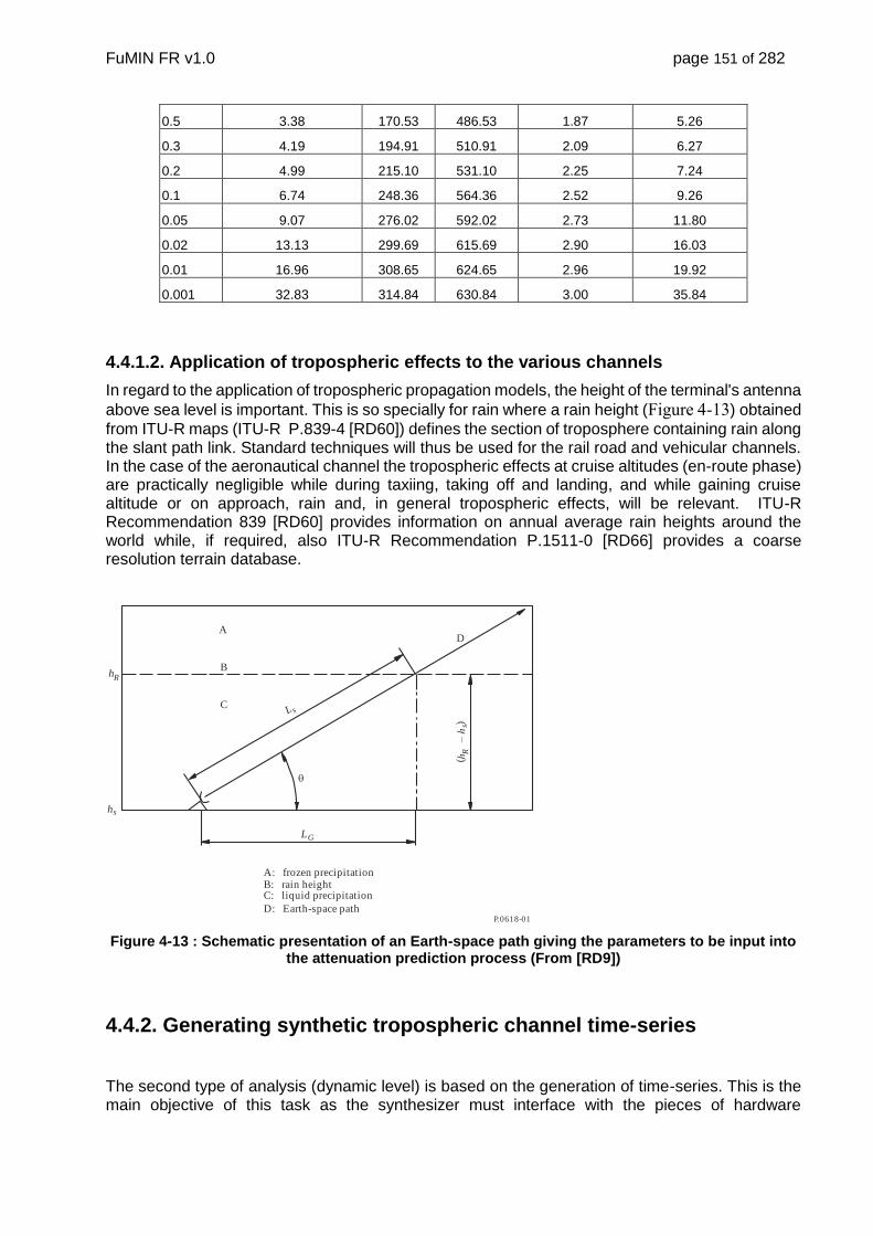
FuMIN FR v1.0 page 151 of 282
0.5 3.38 170.53 486.53 1.87 5.26
0.3 4.19 194.91 510.91 2.09 6.27
0.2 4.99 215.10 531.10 2.25 7.24
0.1 6.74 248.36 564.36 2.52 9.26
0.05 9.07 276.02 592.02 2.73 11.80
0.02 13.13 299.69 615.69 2.90 16.03
0.01 16.96 308.65 624.65 2.96 19.92
0.001 32.83 314.84 630.84 3.00 35.84
4.4.1.2. Application of tropospheric effects to the various channels
In regard to the application of tropospheric propagation models, the height of the terminal's antenna
above sea level is important. This is so specially for rain where a rain height (Figure 4-13) obtained
from ITU-R maps (ITU-R P.839-4 [RD60]) defines the section of troposphere containing rain along the slant path link. Standard techniques will thus be used for the rail road and vehicular channels. In the case of the aeronautical channel the tropospheric effects at cruise altitudes (en-route phase) are practically negligible while during taxiing, taking off and landing, and while gaining cruise altitude or on approach, rain and, in general tropospheric effects, will be relevant. ITU-R Recommendation 839 [RD60] provides information on annual average rain heights around the world while, if required, also ITU-R Recommendation P.1511-0 [RD66] provides a coarse resolution terrain database.
P.0618-01
A: frozen precipitationB: rain heightC: liquid precipitation
D: Earth-space path
B
AD
C
hR
hs
LG
L s
()
h
– h
Rs
Figure 4-13 : Schematic presentation of an Earth-space path giving the parameters to be input into the attenuation prediction process (From [RD9])
4.4.2. Generating synthetic tropospheric channel time-series
The second type of analysis (dynamic level) is based on the generation of time-series. This is the main objective of this task as the synthesizer must interface with the pieces of hardware

FuMIN FR v1.0 page 152 of 282
implementing the Demonstrator, object of this Activity. In the case of tropospheric effects, we are mainly interested in rain attenuation and scintillation series so that we can study the response of the receiver (the various possible system settings to be studied) under realistic dynamic conditions. Generating cloud and gaseous attenuation series is deemed not required since their rate of change is far slower that those of rain and scintillation. Thus, a constant level will be assumed based on the static analysis in preceding sections.
For the selected climatic area we can define various types of events. There is no need to produce year-long simulations which would be unfeasible. To study the response of the receiver to specific events, which must be sufficiently long and representative of the conditions to be encountered. For example a mild event, a bad event or an extreme event. Such issues can be later decided upon after running the simulator and choosing the appropriate events or sequences of events.
Tropospheric effects can be considered as narrowband. This means that the channel will be represented by a complex time-series, sufficiently well sampled to capture the relevant features in the signal. The fastest tropospheric effects have to do with dry and wet scintillation. The required sampling rate has to do with the speed of the terminal.
On the other hand, we must be aware of the rate of change of the various phenomena. For example, rain attenuation and associated wet scintillation are relatively fast. Rain events, especially the stronger ones, have durations of minutes to tens of minutes. Wet scintillation is faster with cut-off frequencies that have to account for the terminal speed. Clear air scintillation also has similar spectral characteristics as wet scintillation. However, cloud attenuation is much slower and, even slower is the time evolution of water vapor giving rise to (gaseous) absorption loss.
We propose to set the cloud and gaseous absorption losses to fixed values (depending on the test cases to be agreed upon) during system simulations, selecting the appropriate levels as a function of the local yearly/worst month statistics. On the other hand, the other effects need to be simulated using time-series synthesizers.
For rain attenuation, we propose to use the enhanced Masen-Baken (M&B) [RD74][RD75] model included in ITU-R Rec. P.1853 [RD65], which targets fixed terminals, but introducing the effect of terminal mobility. In this respect the Synthetic Strom Technique (SST) model [RD76] was extended to the mobility case in [RD77] and [RD78] taking into consideration the relative vectors of translation of the storm and the terminal: angles and speeds. In [RD78], the SST model was used to model the fade slope due to rain for LEO satellites.
Similarly, wet scintillation has to be introduced and the mobile terminal translation movement incorporated in the model. To include the terminal mobility effects, changes to the low pass filter introducing the autocorrelation effects in the time-series synthesizer have to be implemented.
For clear air, scintillation induced signal variations are fairly small but will be included since they can tip the availability-outage balance in low margin systems. Again, the synthesizer proposed in ITU-R Rec. P.1853 [RD65] seems to be the best, most agreed upon option. However, little information on the effect of the coloring filter bandwidth extension due to terminal mobility is available. An increase of the cut-off frequency of the filter is expected. We propose to use techniques proposed for links with LEO satellites [RD79] for assessing this issue.
EHF fading caused by the effects of rain, cloud, water vapor and scintillations typically shows three spectral regimes [RD80][RD6]. The developed time-series synthesizer is capable of reproducing the on-average power spectrum mask during rain shown in Figure 4-14. An example of an spectrum observed by averaging numerous rain event spectra is illustrated in Figure 4-15[RD82].
The lower part of the spectrum (𝑓 < 𝑓𝐿) rolls-off at 20 dB/decade during rain or remains stationary in clear air. Above 𝑓𝐿 the spectrum represents scintillation caused by atmospheric
turbulence along the path. Between (𝑓𝐿 < 𝑓 < 𝑓𝐶) the spectrum depends on how the turbulence is created and has no describing formula (it is usually seen to be flat). Finally the region (𝑓 > 𝑓𝐶) rolls-
off at 80/3 dB/dec as predicted by the theory of turbulence [RD6].

FuMIN FR v1.0 page 153 of 282
In [RD80] radar observations were used. The spectrum up to the radar sampling frequency 𝑓1, is determined from the physical evolution of rain over time. In our case, we have modeled the event duration and its slower dynamics using the M&B model [RD73] [RD74].
Theoretically, the corner frequency of turbulence 𝑓𝐶, can be related to the transverse wind
velocity 𝑣𝑛(m/s). Typical values of 𝑓𝐿 and 𝑓𝐶 are in the order of 0.07 and 0.3Hz respectively. These values correspond to static terminal conditions which have to be modified to account for different terminal speeds.
During dry periods, the only part remaining in the spectral model is that corresponding to scintillation keeping the same spectral slope.
Figure 4-14: Ideal rain event power spectrum (from [RD78].)
Figure 4-15: Average power spectrum for a set of eight rain events recorded in May 2000 at 50 GHz
(from [RD80].)
There is no well recognized method evaluating the instantaneous frequency scaling between the up and down link. Frequency scaling is important as the attenuation measured at one end of the link can be used for making decisions on the application of adaptive transmit power control and/or adaptive coding and modulation. The appearance of partial decorrelation with respect to the long term scaling factor can lead to wrong decisions on the application of such techniques.
In the generation of time series, in the up and downlink simultaneously, we devised a mechanism for using two Gaussian random generators producing partially correlated series according to a coefficient, 𝜌, which, in principle is set to 1 but can be modified to any valid value as desired. This is implemented in this way both for rain and scintillation effects.
One final word on the scintillation time series, they not only depends on the frequency (up- and downlink) but also the antenna gain plays a role through the so called antenna averaging factor ([RD9].
The rain attenuation time-series synthesis method assumes that the long-term statistics of rain attenuation is a log-normal distribution which is not exactly the case in ITU-R P.618 [RD9], however, these distributions are well-approximated by a log-normal distribution over the most significant range of exceedance probabilities.
The Earth-space rain attenuation prediction method predict non-zero rain attenuation for exceedance probabilities greater than the probability of rain [RD65]; however, the time-series synthesis method adjusts the series so the rain attenuation corresponding to exceedance probabilities greater than the probability of rain is 0 dB.
The time-series synthesis method generates a time series that reproduces the spectral characteristics, fade slope and fade duration statistics of rain attenuation events. Inter-fade duration statistics are also reproduced but only within individual attenuation events.

FuMIN FR v1.0 page 154 of 282
In the ITU-R method, illustrated in Figure 4-16, the rain attenuation time series, A(t), is synthesized from the discrete white Gaussian noise process, n(t). The white Gaussian noise is low-pass filtered, transformed from a normal distribution to a log-normal distribution in a memoryless non-linearity, and calibrated to match the desired rain attenuation statistics.
Figure 4-16: Block diagram of the rain attenuation time series synthesizer (from [RD65])
The time series synthesizer uses five input parameters, namely,
m: mean of the log-normal rain attenuation distribution
: standard deviation of the log-normal rain attenuation distribution
p: probability of rain
: parameter that describes the time dynamics (s–1)
Aoffset: offset that adjusts the time series to match the probability of rain (dB)
Similarly, the scintillation time series synthesis method is based on the filtering of another Gaussian
noise source according to Figure 4-17 [RD65]. A scintillation time series, tsci , is generated by
filtering white Gaussian noise, n(t), such that the asymptotic power spectrum of the filtered time series has an f–8/3 roll-off and a cut-off frequency, fc, of 0.1 Hz. In the case of wet scintillation, the standard deviation of the scintillation increases as the rain attenuation increases and its mean is also dependent on the rain attenuation.
Figure 4-17: Block diagram of the scintillation time series synthesizer (from [RD65]).
In our implementation, we have tried to relieve the strain of achieving the spectrum illustrated in Figure 4-14 by using two generators, each taking care of the components above 𝑓1while a secon
generator for achieving the 20 dB/decade specification occurring after 𝑓1. This is better achieved by performing the first filtering process at a lower sampling frquency and then interpolating. Finally, a third generator implements the -80/3 dB/decade characteristic of scinitillation, both dry and wet.
One further modification introduced is that we replace the filtered noise approach which requires discarding the first output samples by the sum of sinusoids, SoS, approach [RD6] (Figure 4-18). The approach uses two sets of sinusoids, sines and cosines. When the resulting signal is merely real, we need only to use the cosine branches.
Low-pass filter Memoryless non-linear device Calibration
Whitegaussian noise
X t( )exp( + ( ))m X t ´ Aoffset
A t( )
Rain attenuation (dB)
k
p +
n t( )
Whitegaussian noise
n t( )
Low-pass filter
Mag
nit
ude
(dB
)
Frequency¦c
–80/3 dB/decade
sci( )Scintillation (dB)
t
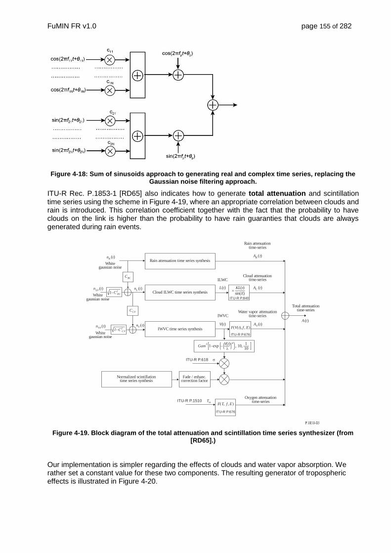
FuMIN FR v1.0 page 155 of 282
Figure 4-18: Sum of sinusoids approach to generating real and complex time series, replacing the Gaussian noise filtering approach.
ITU-R Rec. P.1853-1 [RD65] also indicates how to generate total attenuation and scintillation time series using the scheme in Figure 4-19, where an appropriate correlation between clouds and rain is introduced. This correlation coefficient together with the fact that the probability to have clouds on the link is higher than the probability to have rain guaranties that clouds are always generated during rain events.
Figure 4-19. Block diagram of the total attenuation and scintillation time series synthesizer (from [RD65].)
Our implementation is simpler regarding the effects of clouds and water vapor absorption. We rather set a constant value for these two components. The resulting generator of tropospheric effects is illustrated in Figure 4-20.
Rain attenuation time series synthesis
Cloud ILWC time series synthesis
IWVC time series synthesis
Normalized scintillation time series synthesis
Fade / enhanc.correction factor
Cloud attenuation time-series
Water vapor attenuation time-series
Total attenuation time-series
Whitegaussian noise
Whitegaussian noise
Whitegaussian noise
Rain attenuation time-series
ILWC
IWVC
L t( )
V t( )
A tC ( )
A tV ( )
A tR ( )
A t( )
n tR ( )
CRC
CCV
n tL0 ( )
n tV0 ( )
n tL ( )
n tV ( )1–C2
CV
1 C– 2RC
Oxygen attenuationtime-series
ITU-R P.618
ITU-R P.1510 Tm
KL t( )
sin( )E´
ITU-R P.840
F V t E( ( ),ƒ, )
ITU-R P.676
F T E( , ƒ, )
ITU-R P.676
Gam-1
1–exp –V t( )
l
k
, 10, 110

FuMIN FR v1.0 page 156 of 282
Figure 4-20: Overall bock diagram of tropospheric effect synthesizer.
4.5. Modeling of Local Effects
Three use cases/channels are discussed in this section, namely, a state-based vehicular/railroad, an aeronautical and a special train channel with periodic features. The overall structure of the implemented synthesizer is shown in Figure 4-21. All models assume Ricean channels: direct signal plus diffuse multipath. The multipath power parameter is rather small in all cases but it still depends on the antenna beamwidth. The direct signal may be affected by signal drops duet to shadowing (including parts of the aircraft, in the aeronautical case). Superposed, there may be slow, lower level variations due to pointing errors. We are interested in producing two simultaneous time-series, one for each link direction and frequency (20 and 30 GHz). Some degree of frequency scaling needs to be introduced including the differences in antenna gains.
Figure 4-21 : Overall structure of the time-series synthesizer. All lines are duplicated to produce variations at the up and downlink frequencies, 30 and 20 GHz, respectively.

FuMIN FR v1.0 page 157 of 282
4.5.1. State-based railroad and vehicular channels models
Local effects are mainly due to shadowing/blockage and multipath phenomena. Shadowing and blockage are due to natural and man-made features intercepting the direct satellite-terminal path. Mobility naturally induces the appearance of such events which may lead to a total loss of the connection (tunnels, overpasses, buildings ...) or a reduction of the fade margin (trees ...). The extent of the obstacle and the terminal speed play an important role in system parameters like interleaving depths, etc. Similarly, more or less gentle transitions from line-of-sight (LOS) to blocked or shadowed conditions together with the terminal speed, play an important role when analyzing the response of the receive modem.
On the other hand, multipath effects will be smaller in comparison to those found at the lower frequency bands (L, S, etc.). This is due to the need for higher gain antennas. The narrower the beamwidth the smaller the multipath will be. In the time-series synthesizer to be implemented, we will be considering a small multipath contribution in addition to the direct (sometimes shadowed) signal.
Shadowing/blockage may cause severe problems for train and vehicular usage. Signal blockage by buildings, overpasses, tunnels etc. if too long in size or the speed is too small cannot be overcome by physical layer techniques alone. We present a generator capable of reproducing space diversity features especially if the antennas are located at both ends of the platform. The autocorrelation features in the received signals are also properly captured by the use of state-based modeling techniques.
In the same way as for the troposphere, a two-level analysis approach is proposed. The different models/experimental results identified will be the source of the needed CDFs for the static analyses and for the time-series generator to be used in the dynamic level analyses.
In the same way as with pointing errors and tropospheric effects, the synthesizer can be implemented out of a complex random Gaussian generator and a Doppler coloring filter with cutoff frequency dependent on the terminal's mobility [RD84] or, alternatively, starting from a sum of phasors or sinusoids weighted with the adequate Doppler spectral characteristics..
Given the narrow beamwidths expected, the excess path lengths of the multipath components present will not be large enough to cause time dispersion. Thus, only the narrowband case will be considered. A single complex-valued time series will be generated (only one tap in a tapped delay-line, TDL, model).
We illustrate in Figure 4-22 and Figure 4-23 ([RD6]) the behavior of the Ka-Band channel for tree-alleys. We see that the channel behaves pretty much like an on-off device. The side of the street relative to the satellite and the orientation of the road have an impact but, roughly speaking, the percentage of locations the signal is under a threshold basically corresponds to the percentage of optical shadowing, (POS) characterizing the traversed scenario.
Figure 4-22: Measured time series at Ka-Band ([RD6].)
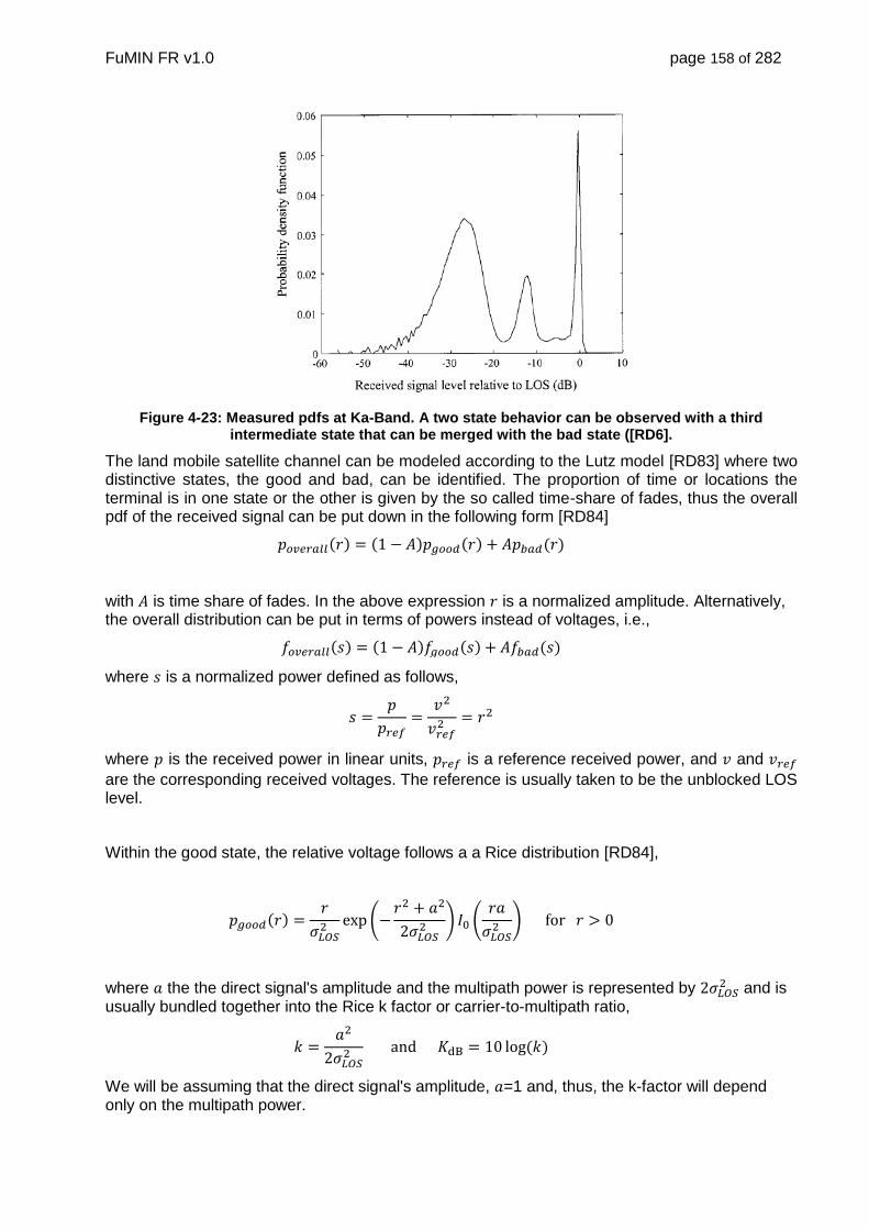
FuMIN FR v1.0 page 158 of 282
Figure 4-23: Measured pdfs at Ka-Band. A two state behavior can be observed with a third intermediate state that can be merged with the bad state ([RD6].
The land mobile satellite channel can be modeled according to the Lutz model [RD83] where two distinctive states, the good and bad, can be identified. The proportion of time or locations the terminal is in one state or the other is given by the so called time-share of fades, thus the overall pdf of the received signal can be put down in the following form [RD84]
𝑝𝑜𝑣𝑒𝑟𝑎𝑙𝑙(𝑟) = (1 − 𝐴)𝑝𝑔𝑜𝑜𝑑(𝑟) + 𝐴𝑝𝑏𝑎𝑑(𝑟)
with 𝐴 is time share of fades. In the above expression 𝑟 is a normalized amplitude. Alternatively, the overall distribution can be put in terms of powers instead of voltages, i.e.,
𝑓𝑜𝑣𝑒𝑟𝑎𝑙𝑙(𝑠) = (1 − 𝐴)𝑓𝑔𝑜𝑜𝑑(𝑠) + 𝐴𝑓𝑏𝑎𝑑(𝑠)
where 𝑠 is a normalized power defined as follows,
𝑠 =𝑝
𝑝𝑟𝑒𝑓=
𝑣2
𝑣𝑟𝑒𝑓2 = 𝑟2
where 𝑝 is the received power in linear units, 𝑝𝑟𝑒𝑓 is a reference received power, and 𝑣 and 𝑣𝑟𝑒𝑓
are the corresponding received voltages. The reference is usually taken to be the unblocked LOS level.
Within the good state, the relative voltage follows a a Rice distribution [RD84],
𝑝𝑔𝑜𝑜𝑑(𝑟) =𝑟
𝜎𝐿𝑂𝑆2 exp (−
𝑟2 + 𝑎2
2𝜎𝐿𝑂𝑆2 ) 𝐼0 (
𝑟𝑎
𝜎𝐿𝑂𝑆2 ) for 𝑟 > 0
where 𝑎 the the direct signal's amplitude and the multipath power is represented by 2𝜎𝐿𝑂𝑆2 and is
usually bundled together into the Rice k factor or carrier-to-multipath ratio,
𝑘 =𝑎2
2𝜎𝐿𝑂𝑆2 and 𝐾dB = 10 log(𝑘)
We will be assuming that the direct signal's amplitude, 𝑎=1 and, thus, the k-factor will depend only on the multipath power.

FuMIN FR v1.0 page 159 of 282
In the bad state practical disappearance of the direct signal is assumed and, locally, a Rayleigh behavior is considered,
𝑝𝑏𝑎𝑑(𝑟|2𝜎2) =𝑟
𝜎2exp (−
𝑟2
2𝜎2) =2𝑟
𝑠0exp (−
𝑟2
𝑠0) for 𝑟 > 0
Again the multipath power is represented by 2𝜎2. We can rename this parameter as 𝑠0 = 2𝜎2 which is assumed to be log-normally distributed [RD84],
𝑓𝑏𝑎𝑑(𝑠0) =10
𝜎dB ln(10) √2𝜋
1
𝑠0exp (−
(10 log(𝑠0) − 𝜇dB)2
2𝜎dB2 ) for 𝑟 > 0
with parameters 𝜇dB and 𝜎dB in dB.
𝑓𝑏𝑎𝑑(𝑠0) =10
𝜎dB ln(10) √2𝜋
1
𝑠0exp (−
(10 log(𝑠0) − 𝜇dB)2
2𝜎dB2 ) for 𝑟 > 0
Below parameter sets from two sources are collated. It must be pointed out that normally the antennas used were directive but with different beamwidths. This has an impact on the multipath power parameter, especially in the good state. It is clear that the wider the beamwidth the larger the multipath power will be. The only source where simultaneous measurements were made at high frequencies (40 GHz) was in [RD85] where going from a 25 deg BW directive antenna to an omnidirectional one meant a reduction in the K factor of 3.5 dB. A geometry based multipath utility is currently under development.
This simplified methodology based on geometrical and radiation pattern assumptions linked to the antenna's BW will be developed to convert the k-factor reported for one antenna to another with a different beamwidth. For the time being it will suffice to use the CDF curve for a different k factor (corrected by a few dB).
In [48] the measurement runs were classified in three categories such that
Category I: (freeway) a limited access multi-lane freeway.
Category II: (suburban) a broad suburban thoroughfare lined with trees and buildings. The tree canopies cause intermittent blockage and the buildings are either too far removed from the roadside or not tall enough to cause significant blockage.
Category III: (rural) a small, two-lane roadway lined with trees and buildings. The tree canopies often cover the entire roadway and buildings are close enough to contribute to the fading process.
In Table 4-9 we reproduce most of the values provided in [RD86].

FuMIN FR v1.0 page 160 of 282
Table 4-9: Summary of best fit for 20 GHz data using the Lutz model [RD86]
Run Cat. 𝐴 𝐾dB 𝜇dB 𝜎dB
020201 070905 070907 071016 071017 072405 072406 072407 072408 072410 072411 072412 070903 070906 070912 070914
I II II II II II II II II II II Il III III III III
0.000 0.582 0.219 0.016 0.032 0.231 0.124 0.343 0.145 0.548 0.010 0.213 0.433 0.188 0.406 0.394
28.8 21.5 23.0 18.2 17.7 16.2 20.3 22.3 27.1 19.0 19.2 19.8 21.1 23.2 20.9 4.0
-- -23.2 -1.6 -19.9 -13.1 -13.7 -2.7 -21.0 -19.8 -16.3 -12.7 -11.9 -20.8 -24.4 -19.1 -20.3
-- 7.37 10.59 1.13 6.67 11.14 10.38 1.48 13.99 8.69 6.07 3.83 0.09 9.01 17.49 0.13
Table 4-10 reproduces results presented in [RD7]. These results correspond to a 3 state model where all states are modeled with the Loo distribution [RD87] using different parameter sets. Equivalences between these parameter sets and those of the Lutz model [RD83] adopted here can be readily obtained by first collapsing the states II and III into a single bad state. The results supplied are very much in line with those in [RD86].
Table 4-10: Average Loo model parameters for different orientations and sides of the road (IAS, GRAZ, Ka-BAND) [RD7].
With the parameters quoted above we can already carry out a static approach and provide relevant CDFs for inclusion in link budget calculations. For time series generation additional information is required, including the modeling at state level and within the states, basically Doppler spectra or, alternatively, autocorrelation functions, discussed in subsequent sections.
4.5.1.1. Two-State Markov Model
The situation is depicted in Figure 4-24 [RD88] [RD89] [RD90]. When the channel is in the good state, g, there is a probability, 𝑝𝑔𝑔, associated with remaining in that state and a crossover
probability, 𝑝𝑔𝑏, associated with the transition to the bad state, b, such that 𝑝𝑔𝑔 + 𝑝𝑔𝑏 = 1. Likewise,
there is a probability, 𝑝𝑏𝑏, associated with remaining in the bad state and a probability, 𝑝𝑏𝑔,
associated with switching from the bad state to the good state such that 𝑝𝑏𝑏 + 𝑝𝑏𝑔 = 1.

FuMIN FR v1.0 page 161 of 282
Figure 4-24: Two-state Markov model [RD89].
We can use a matrix representation of the two-state model,
𝐌 = [𝑝𝑔𝑔 𝑝𝑔𝑏
𝑝𝑏𝑔 𝑝𝑏𝑏]
The model has several various properties of interest. The steady state probability describes the average time spent in each state and can be calculated by solving the equation system below
𝛑𝐌 = 𝛑𝛑𝟏 = 𝟏
with 𝛑 a 1x2 row vector with the steady state probabilities and 1 a 2 x 1 column vector of ones. The solution is
𝛑 = [𝜋𝑔 𝜋𝑏] = [𝑝𝑏𝑔
𝑝𝑔𝑏 + 𝑝𝑏𝑔
𝑝𝑔𝑏
𝑝𝑔𝑏 + 𝑝𝑏𝑔] = [
𝐷𝑔
𝐷𝑔 + 𝐷𝑏
𝐷𝑏
𝐷𝑔 + 𝐷𝑏
]
𝐷𝑔 and 𝐷𝑏
are the mean dwell times in the good and bad states. The dwell time for each state
can be described by a geometric random variable with a probability mass function [RD90] such that
𝑃𝑟{𝐷𝑔 = 𝑛} = 𝑝𝑔𝑏𝑝𝑔𝑔𝑛−1 = (1 − 𝑝𝑔𝑔)𝑝𝑔𝑔
𝑛−1 𝑛 = 1,2, …
𝑃𝑟{𝐷𝑏 = 𝑛} = 𝑝𝑏𝑔𝑝𝑏𝑏𝑛−1 = (1 − 𝑝𝑏𝑏)𝑝𝑏𝑏
𝑛−1 𝑛 = 1,2, …
𝐷𝑔 and 𝐷𝑏 are the dwell times for the good and bad states. Given these mass functions, the
mean dwell times are,
𝐷𝑔 = ∑ 𝑛𝑝𝑔𝑏𝑝𝑔𝑔
𝑛−1
∞
𝑛=1
=1
𝑝𝑔𝑏=
1
1 − 𝑝𝑔𝑔
𝐷𝑏 = ∑ 𝑛𝑝𝑏𝑔𝑝𝑏𝑏
𝑛−1
∞
𝑛=1
=1
𝑝𝑏𝑔=
1
1 − 𝑝𝑏𝑏
The CCDFs for the duration of each state are [RD90]
𝑃𝑟{𝐷𝑔 > 𝑛} = (1 − 𝑝𝑔𝑏)𝑛
= 𝑝𝑔𝑔𝑛
𝑃𝑟{𝐷𝑏 > 𝑛} = (1 − 𝑝𝑏𝑔)𝑛
= 𝑝𝑏𝑏𝑛
The Markov model can be used in a generative time-series synthesizer by drawing a random
number with each sampling interval 𝑇𝑠 s. conversion from times to meters can be carried out defining the mobile terminal speed, 𝑉. In this case, the distance sampling interval is 𝑑𝑠 = 𝑉𝑇𝑠 m.
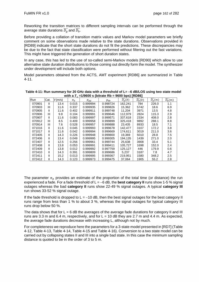
FuMIN FR v1.0 page 162 of 282
Reworking the transition matrices to different sampling intervals can be performed through the
average state durations 𝐷𝑔 and 𝐷𝑏
.
Before providing a collation of transition matrix values and Markov model parameters we briefly comment on some observations made relative to the state durations. Observations provided in [RD89] indicate that the short state durations do not fit the predictions. These discrepancies may be due to the fact that state classification were performed without filtering out the fast variations. This might have triggered the generation of short duration states.
In any case, this has led to the use of so-called semi-Markov models [RD90] which allow to use alternative state duration distributions to those coming out directly form the model. The synthesizer under development will include both options.
Model parameters obtained from the ACTS, AMT experiment [RD86] are summarized in Table 4-11.
Table 4-11: Run summary for 20 GHz data with a threshold of L= 6 dB/LOS using two state model
with a 𝑻𝒔 =1/9600 s (bitrate Rb = 9600 bps) [RD86]
Run Cat. 𝑉(m/s) 𝜋𝑏 𝑝𝑔𝑔 𝑝𝑏𝑏 𝐷𝑔 (𝑏) 𝐷𝑏
(𝑏) 𝐷𝑔 (𝑚) 𝐷𝑏
(𝑚)
070901 070903 070905 070906 070907 070912 070914 071016 071017 072405 072406 072407 072408 072409 072410 072411 072412
II III II III II III III II II II II II II II II II II
13.4 11.6 11.6 9.8
11.6 8.5 7.6
11.6 11.6 14.3 13.4 12.5 13.8 13.8 14.3 15.2 14.3
0.015 0.337 0.402 0.104 0.083 0.409 0.528 0.045 0.042 0.226 0.049 0.256 0.053 0.012 0.391 0.013 0.123
0.999994 0.999935 0.999911 0.999991 0.999997 0.999958 0.999957 0.999993 0.999994 0.999948 0.999995 0.999961 0.999991 0.999992 0.999809 0.999995 0.999973
0.998724 0.999826 0.999748 0.999646 0.999571 0.999899 0.999888 0.999678 0.999669 0.999800 0.999305 0.999744 0.999411 0.997759 0.999686 0.999367 0.999475
162,241 15,362 11,204
112,979 337,618 325,418 23,435
142,477 174,611 19,369
194,135 25,638
105,727 125,127 5,237
219,951 37,064
784 5742 3971 2824 2334 9892 8933 3107 3019 5010 1439 3908 1698 446
3187 1580 1905
226.0 18.6 13.5
115.3 408.0 288.1 18.5
172.2 211.0 28.8
271.0 33.4
152.0 179.9
7.8 348.2 55.2
1.1 6.9 4.8 2.9 2.8 8.8 7.1 3.8 3.6 7.5 2.0 5.1 2.4 0.6 4.7 2.5 2.8
The parameter 𝜋𝑏 provides an estimate of the proportion of the total time (or distance) the run
experienced a fade. For a fade threshold of L = 6 dB, the best category II runs show 1-5 % signal outages whereas the bad category II runs show 22-49 % signal outages. A typical category III run shows 33-52 % signal outage.
If the fade threshold is dropped to L = 10 dB, then the best signal outages for the best category II runs range from less than 1 % to about 3 %, whereas the signal outages for typical category III runs drop below 50 %.
The data shows that for L = 6 dB the averages of the average fade durations for category II and III runs are 3.3 m and 6.4 m, respectively, and for L = 10 dB they are 2.7 m and 4.4 m. As expected, the average fade durations decrease with increasing L, although not by much.
For completeness we reproduce here the parameters for a 3-state model presented in [RD7] (Table 4-12, Table 4-13, Table 4-14, Table 4-15 and Table 4-16). Conversion to a two state model can be carried out by collapsing states II and III into a single bad state. In this case the minimum sampling distance is quoted to be in the order of 3 to 5 m.

FuMIN FR v1.0 page 163 of 282
We can choose between the various combinations of parameters both for the vehicular and the train channels. Identification of the parameter set will be done at a later time. For the time being we concentrate on the modeling aspects.

FuMIN FR v1.0 page 164 of 282
Table 4-12: Markov chain matrices [P] AND [W] for various elevations.. France, leaf trees, 30 deg. elevation (IAS, GRAZ, Ka-BAND) [RD7].
Table 4-13: Markov chain matrices [P] AND [W] for various elevations. Germany needle trees, 30 elevation (IAS, GRAZ, Ka-BAND) [RD7].

FuMIN FR v1.0 page 165 of 282
Table 4-14: Markov chain matrices [P] AND [W] for various elevations.. Austria, tree alley, 30 deg elevation (IAS, GRAZ, Ka-BAND) [RD7].
Table 4-15: Markov chain matrices [P] AND [W] for various elevations. Germany/Austria, suburban, 30 deg. elevation (IAS, GRAZ, Ka-BAND) [RD7].
FuMIN FR v1.0 page 166 of 282
Table 4-16: Markov chain matrices [P] AND [W] for various elevations.Germany, urban, 30 deg. elevation (IAS, GRAZ, Ka-BAND) [RD7].
Multipath. For train applications, multipath reflections can originate from terrain elements around the terminal, and cannot be ignored. Clause 11 of the DVB-RCS + M guidelines [RD52] has a proposed model. According to that study, the fading is again Ricean; with a typical K-factor of about 17 dB.
The same clause also provides expressions for the shape of the Doppler spectrum, conditioned on the antenna beam width. The shape of the Doppler spectrum however also depends on the angle between the direction of travel and the LOS to the satellite. With these conditions, the relative spectral densities provided in [RD52] can be integrated and scaled to represent the desired K-factor.
Non-LOS Scenarios [RD52] Railway. The mobility effects, such as multipath, shadowing and blockage, encountered due to the local environment in the vicinity of the mobile, such as adjacent buildings, vegetation, bridges, and tunnels, result in sporadic severe fading.
4.5.2. Railroad scenarios with periodic features
Figure 4-25 illustrates the implemented simulator for special train scenarios with periodic features. The implementation is in line with the Markov based model. In this case we are always in the Good state and periodic features appear affecting the direct signal.
In [RD52] a special channel for railroad usage is presented where preriodic features are observed Following is a list of signal attenuations associated with different obstacles:
• Catenaries: typically attenuation of 2 dB to 3 dB.

FuMIN FR v1.0 page 167 of 282
• Electrical trellises: up to 15 dB to 20 dB attenuation (depending on the geometry and layout of the obstacles and on the orientation of the railway with respect to the position of the satellite): length ~0,5 m, distance between two consecutive trellises ~43 m.
• Bridges: high signal loss for a length between a few meters up to tens of meters -50 m.
• Tunnels: long-term interruptions.
The railway channel can be modelled by superimposing this kind of deterministic and (space) periodic fades on a statistical model accounting for unpredictable obstacles (such as the state based Markov models with parameters similar to the land mobile highway channel).
The railroad satellite channel is in LOS state most of the time. However, short blockages due to power arches as well as long blockages due to obstacles, such as buildings, vegetation, bridges, and tunnels, are also present leading to non-LOS effects. Figure 4-26 illustrates such features.
Figure 4-25: Simulator of train scenario with periodic features.
The interruption caused by short bridges can last from 0,6 s (at 300 km/h) to 9 s for (20 km/h), Table 4-17.
In the proposed implementation, the electromagnetic responses to several obstacle types will be generated using modeling tools taking into account the frequency scaling effects.
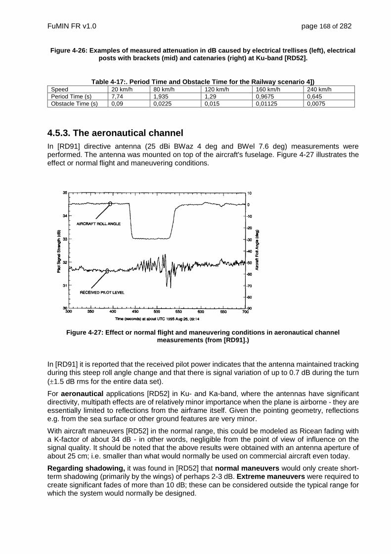
FuMIN FR v1.0 page 168 of 282
Figure 4-26: Examples of measured attenuation in dB caused by electrical trellises (left), electrical posts with brackets (mid) and catenaries (right) at Ku-band [RD52].
Table 4-17:. Period Time and Obstacle Time for the Railway scenario 4]) Speed 20 km/h 80 km/h 120 km/h 160 km/h 240 km/h
Period Time (s) 7,74 1,935 1,29 0,9675 0,645
Obstacle Time (s) 0,09 0,0225 0,015 0,01125 0,0075
4.5.3. The aeronautical channel
In [RD91] directive antenna (25 dBi BWaz 4 deg and BWel 7.6 deg) measurements were performed. The antenna was mounted on top of the aircraft's fuselage. Figure 4-27 illustrates the effect or normal flight and maneuvering conditions.
Figure 4-27: Effect or normal flight and maneuvering conditions in aeronautical channel measurements (from [RD91].)
In [RD91] it is reported that the received pilot power indicates that the antenna maintained tracking during this steep roll angle change and that there is signal variation of up to 0.7 dB during the turn
(1.5 dB rms for the entire data set).
For aeronautical applications [RD52] in Ku- and Ka-band, where the antennas have significant directivity, multipath effects are of relatively minor importance when the plane is airborne - they are essentially limited to reflections from the airframe itself. Given the pointing geometry, reflections e.g. from the sea surface or other ground features are very minor.
With aircraft maneuvers [RD52] in the normal range, this could be modeled as Ricean fading with a K-factor of about 34 dB - in other words, negligible from the point of view of influence on the signal quality. It should be noted that the above results were obtained with an antenna aperture of about 25 cm; i.e. smaller than what would normally be used on commercial aircraft even today.
Regarding shadowing, it was found in [RD52] that normal maneuvers would only create short-term shadowing (primarily by the wings) of perhaps 2-3 dB. Extreme maneuvers were required to create significant fades of more than 10 dB; these can be considered outside the typical range for which the system would normally be designed.

FuMIN FR v1.0 page 169 of 282
Regarding the modelling of the LOS channel conditions encountered in the aeronautical scenario, experimental results at 18,6 GHz [RD52] show that the channel behaves like Ricean during normal flight situations and maneuvers, with a Rice factor well above 20 dB. Light fades in the order of 3 dB were observed for maneuvers with roll angles up to 20°, whereas only in case of extreme maneuvers, with roll angles up to 45°, the influence of the aircraft structure resulted in deep fades in the order of 15 dB. In conclusion, in aeronautical scenarios, LOS conditions can be assumed and the channel can be fairly approximated by a AWGN channel for most of the time.
Our implementation will follow the above guidelines implementing LOS state Ricean conditions with high K-factor. We will also include slow direct signal losses due to maneuvering conditions as illustrated in Figure 4-28.
Figure 4-28: Aeronautical channel model synthesizer.
4.6. Modelling of Antenna Pointing Errors
We model the pointing errors in degree and convert them to antenna gain loss (dB) for the receive antenna options discussed in other sections. The statistical model and an associated time-series generator to be used in the Activity are based on [RD89] and [RD86].
A Laplace distribution was found to match the azimuth and elevation pointing errors. No model was provided for the second order statistics, SoSt, which are necessary for generating synthetic time-series. We will perform model parameter identification for matching the SoSt measurements provided in [RD89].
We now quote the values provided in [RD89]. In the rough terrain measurements the error rarely exceeded 0.5° with an RMS value of 0.11° at a 40° elevation angle and 0.14° at a 65° elevation angle. Table 4-18 summarizes RMS values obtained for different road types.
Table 4-18:. Measured RMS pointing error for different road types (After [RD89].)

FuMIN FR v1.0 page 170 of 282
Environment/elevation angle RMS pointing error (deg.) Mobile speed (mph)
improved/40° 0.04° 25 to 55
unimproved/40° 0.09° 15 to 35
unimproved/65° 0.12°
rough/40° 0.11° 10 to 35
rough/65° 0.14°
The quoted overall or LOS pointing errors (degree) are a combination of the azimuth and elevation mispointing errors. Such combination can be performed using
𝜃 ≈ √𝜃𝑎𝑧2 + 𝜃𝑒𝑙
2
where 𝜃 is the overall error in degree, 𝜃𝑎𝑧 is the azimuth error, and 𝜃𝑒𝑙 is the elevation error. The
loss in antenna gain can be approximated by [RD92]
𝛼(dB) = −2.5 × 10⁻³ (𝐷
𝜆𝜃)
2= −12.25 (
𝜃
𝜃3dB)
2 for 0° < 𝜃 < 𝜃𝑚
(1)
where 𝜃3dB is the 3 dB-beamwidth, BW, of the antenna, and 𝜃 is the off-axis angle (deg.) and
deg.20
1GGD
maxm l
with 𝐺1 = 2 + 15 log𝐷
𝜆
which is the gain of the first side-lobe [RD92]. These approximations are valid for small errors.
As a reference, for a reflector antenna this parameter can be approximated by
𝜃3dB ≈70𝜆
𝐷
where 𝜆 is the wavelength and 𝐷 the antenna diameter.
𝐺(dBi) ≈ 44.5 − 20 log 𝜃3dB(deg. )
For the 30.5 cm reflector (𝐴 = 0.073 m2) used in [RD89], 𝜃3dB ≈ 3.5° at 20 GHz (𝐺 ≈ 33.5 dBi) and 𝜃3dB ≈ 2.3° at 30 GHz (𝐺 ≈ 37 dBi). The gain of a parabolic dish can be approximated by
𝐺 = 10 log 𝑔 with 𝑔 = 𝜂 (𝜋𝐷
𝜆)
2
with 𝜂 ≈ 0.55 being the efficiency for circular apertures and 𝜂 ≈ 0.7 for rectangular apertures [RD93]. The above expressions come from the gain and area, 𝐴, of the aperture relation, i.e.,
𝑔 = 𝜂4𝜋𝐴
𝜆2
An alternative expression for an ellipsoidal aperture is given by
𝑔 = 10𝐺(dBi)/10 =4𝜋 𝜂
Ω𝐴=
4𝜋 𝜂
𝜃3dB(rad)𝜙3dB(rad)=
52525 𝜂
𝜃3dB(deg)𝜙3dB(deg)
where 𝜂=0.55. Another approximation for rectangular apertures is
𝑔 = 10𝐺(dBi)/10 =4𝜋 𝜂
Ω𝐴=
4𝜋 𝜂
𝜃3dB(rad)𝜙3dB(rad)=
41253 𝜂
𝜃3dB(deg)𝜙3dB(deg)
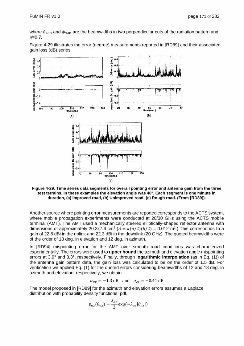
FuMIN FR v1.0 page 171 of 282
where 𝜃3dB and 𝜙3dB are the beamwidths in two perpendicular cuts of the radiation pattern and 𝜂=0.7.
Figure 4-29 illustrates the error (degree) measurements reported in [RD89] and their associated gain loss (dB) series.
Figure 4-29: Time series data segments for overall pointing error and antenna gain from the three test terrains. In these examples the elevation angle was 40°. Each segment is one minute in
duration, (a) Improved road, (b) Unimproved road, (c) Rough road. (From [RD89]).
Another source where pointing error measurements are reported corresponds to the ACTS system, where mobile propagation experiments were conducted at 20/30 GHz using the ACTS mobile terminal (AMT). The AMT used a mechanically steered elliptically-shaped reflector antenna with dimensions of approximately 20.3x7.6 cm2 (𝐴 = 𝜋(𝑎/2)(𝑏/2) = 0.012 m2.) This corresponds to a gain of 22.8 dBi in the uplink and 22.3 dBi in the downlink (20 GHz). The quoted beamwidths were of the order of 18 deg. in elevation and 12 deg. in azimuth.
In [RD94] mispointing error for the AMT over smooth road conditions was characterized experimentally. The errors were used to upper bound the azimuth and elevation angle mispointing errors at 3.9° and 3.3°, respectively. Finally, through logarithmic interpolation (as in Eq. (1)) of the antenna gain pattern data, the gain loss was calculated to be on the order of 1.5 dB. For verification we applied Eq. (1) for the quoted errors considering beamwidths of 12 and 18 deg. in azimuth and elevation, respectively, we obtain
𝛼𝑎𝑧 = −1.3 dB and 𝛼𝑒𝑙 = −0.41 dB
The model proposed in [RD89] for the azimuth and elevation errors assumes a Laplace distribution with probability density functions, pdf,
𝑝𝑎𝑧(𝜃𝑎𝑧) =𝜆𝑎𝑧
2exp(−𝜆𝑎𝑧|𝜃𝑎𝑧|)

FuMIN FR v1.0 page 172 of 282
𝑝𝑒𝑙(𝜃𝑒𝑙) =𝜆𝑒𝑙
2exp(−𝜆𝑒𝑙|𝜃𝑒𝑙|)
where 𝜆𝑎𝑧 and 𝜆𝑒𝑙 are the azimuth and elevation parameters, respectively, which are not necessarily equal. Figure 4-30.a and b illustrate the azimuth and elevation mispointing pdfs for the rough terrain course with an elevation angle of 65°.
Parameter 𝜆 is related to the standard deviation of the distribution as follows,
std(𝜃) = √2/𝜆
In the case of pointing error modeling the mean of the distributions for azimuth and elevation is zero.
The expression for the cumulative distribution, CDF, is
𝐹(𝜃) = ∫𝜆
2exp(−𝜆|𝜃|) 𝑑𝜃
𝜃
−∞
=1
2+
1
2sgn(𝜃)[1 − exp(−𝜆|𝜃|)]
Similarly, the complementary CDF, CCDF, is given by
𝐹−1(𝑝) = −1
𝜆sgn(𝑝 − 0.5) ln(1 − 2|𝑝 − 0.5|)
An the algorithm for generating random Laplace distributed numbers is
𝑋 = −1
𝜆sgn(𝑈) ln(1 − 2|𝑈|)
where a random variable U drawn from a uniform distribution in the interval (−1/2, 1/2], is used. The method is based on the inverse distribution method.
It was also observed that the random variables that describe the azimuth and elevation pointing error are almost completely uncorrelated. Table 4-19 summarizes the findings in [RD89].
Figure 4-30: Probability densities for azimuth and elevation error over rough terrain for an elevation angle if 65°. Fitted and measured pdfs. (a) Azimuth, (b) Elevation. (From [RD89])
Table 4-19: Azimuth and elevation error pdf parameters from model fitting (From [RD89]) density parameters Correlation coefficient
Environment/elevation angle 𝜆𝑎𝑧 𝜆𝑒𝑙 𝜌
improved/40° 52.74 32.05 0.103
unimproved/40° 30.70 23.00 0.095
unimproved/65° 18.73 20.10 0.155
rough/40° 22.66 17.90 0.105

FuMIN FR v1.0 page 173 of 282
rough/65° 14.80 16.47 0.168
The measured complementary CDFs [RD89] are depicted in Figure 4-31 and the pdfs are shown in Figures 34-38, including the gain losses as well.
In [RD89] a model was proposed assuming that the azimuth and elevation errors are
independent, thus the pdf of the overall pointing error, 𝜃 ≈ √𝜃𝑎𝑧2 + 𝜃𝑒𝑙
2 , is given by
𝑝𝐿𝑂𝑆(𝜃) =𝜆𝑎𝑧𝜆𝑒𝑙
4∫ exp (−𝜆𝑎𝑧√𝜃2 − 𝜔2) exp(−𝜆𝑒𝑙𝜔)
𝜃
0
𝜃
√𝜃2 − 𝜔2𝑑𝜔 =
=𝜃𝜆𝑎𝑧𝜆𝑒𝑙
4∫ exp (−𝜃√𝜆𝑎𝑧
2 + 𝜆𝑒𝑙2 ) cos(𝜙 − 𝜙0)
𝜋/2
0
𝑑𝜙
where
𝜙0 = COS−1 (𝜆𝑎𝑧/√𝜆𝑎𝑧2 + 𝜆𝑒𝑙
2 )
The evaluation of the above equation can be performed numerically.
From Figure 4-32, Figure 4-33, Figure 4-34, Figure 4-35 and Figure 4-36, the heavier tails coincide with the rougher terrain and higher elevation angles. Also, the difference in UL (30 GHz) and DL (20 GHz) gain due to mispointing manifests itself as a heavier distribution tail due to the narrower beamwidth on the UL [RD89].
Figure 4-31: CCDFs for the three terrain types and two elevation angles. (From [RD89])

FuMIN FR v1.0 page 174 of 282
Figure 4-32: Probability density for LOS error and antenna gain in improved terrain, 40° elevation angle, (a) LOS error (b) Antenna gain relative to perfect pointing. (From [RD89])
Figure 4-33: Probability density for LOS error and antenna gain in unimproved terrain, 40° elevation angle, (a) LOS error, (b) Antenna gain relative to perfect pointing. (From [RD89])
Figure 4-34: Probability density for LOS error and antenna gain in unimproved terrain, 65° elevation angle, (a) LOS error (b) Antenna gain relative to perfect pointing. (From [RD89])

FuMIN FR v1.0 page 175 of 282
Figure 4-35: Probability density for LOS error and antenna gain in rough terrain, 40° elevation angle, (a) LOS error (b) Antenna gain relative to perfect pointing. (From [RD89])
Figure 4-36: Probability density for LOS error and antenna gain in rough terrain, 65° elevation angle, (a) LOS error (b) Antenna gain relative to perfect pointing. (From [RD89])
4.6.1. Second-order statistics (SoSt)
Second-order statistics, SoSt, are time dependent and are indispensable for generating realistic time-series. Average fade and connection durations as a function of overall pointing error and antenna gain loss were estimated from the data, Figure 4-37. Only the UL gain (worst case) is shown. Connection durations increase (decrease) to their maxima (minima) as a function of LOS error (gain relative to perfect pointing). Fade durations decrease (increase) to their minima (maxima) as a function of LOS error (gain relative to perfect pointing).
Conversion to durations in meters can be performed using the average vehicle speeds for each measurement run (Table 4-18). No model is provided in [RD89] for the SoSt. We propose here a model for generating time series and model paramours will be extracted by fitting the curves provided. Model parameterization will be carried out at a later time.

FuMIN FR v1.0 page 176 of 282
Figure 4-37. Average fade and connection durations over the three terrain types, (a) Average connection duration as a function of LOS error (b) Average fade duration as a function of LOS error
(c) Average connection duration as a function of UL gain relative to perfect pointing, (d) Average fade duration as a function of UL gain relative to perfect pointing. (From [RD89])
Another SoSt is the level crossing rate, lcr. Results for each of the experiments are shown in Figure 4-38. The peak lcr was approximately 7 Hz and occurred between 0.02° and 0.1°, depending on the terrain and elevation angle. As overall pointing error increases and antenna gain decreases, the lcr decreases, reflecting the fact that these thresholds are crossed less frequently [RD89].

FuMIN FR v1.0 page 177 of 282
Figure 4-38: Level crossing rates for the three terrain types, (a) Level crossing rate as a function of LOS error (b) Level crossing rate as a function of UL gain relative to perfect pointing. (From [RD89])
We will finally replace the Laplace distributions by Gaussians with the same variance. For the parameters presented in [RD89] the difference is very small and facilitates the time-series synthesis tasks based on filtered Gaussian distributions or on the sum of sinusoids, SumOS, technique.
For that, we follow an alternative mispointing model proposed in [RD86]. This model is simpler since it allowed providing closed form overall pointing and gain loss distributions and is more amenable for generating time-series which can be used for fitting SoSt to the measurements (curves above).
Two cases were considered in [RD86]: (1) when the variances of the azimuth and elevation mispointing errors are equal, and (2) the more general case when they are not equal.
Case 1. Equal variances. Defining 𝜃𝑎𝑧 and 𝜃𝑒𝑙 as the azimuth and elevation mispointing angles, respectively. Under the assumption that they are independent Gaussian distributed random
variables, each with mean 𝜇 = 0 and variance 𝜎𝑎𝑧2 = 𝜎𝑒𝑙
2 = 𝜎2 , the total mispointing error, defined
as
𝜃 ≈ √𝜃𝑎𝑧2 + 𝜃𝑒𝑙
2
has a Rayleigh pdf given by
𝑓𝜃(𝜃) =𝜃
𝜎2exp (−
𝜃2
2𝜎2) for 𝜃 ≥ 0
Figure 4-39 illustrates this pdf for several values of 𝜎2 .

FuMIN FR v1.0 page 178 of 282
Figure 4-39: Antenna mispointing performance
plots for 𝝈𝒂𝒛𝟐 = 𝝈𝒆𝒍
𝟐 (From [RD86].)
Figure 4-40: Antenna mispointing performance
plots for 𝝈𝒂𝒛𝟐 ≠ 𝝈𝒆𝒍
𝟐 (From [RD86].)
Case 2. Unequal Variances. This is the case in situations where the antenna gain pattern is not
symmetric. In this case 𝜎𝑎𝑧2 ≠ 𝜎𝑒𝑙
2 . For determining 𝑓𝜃(𝜃) the random variable 𝜁 is defined,
𝜁 = 𝜎𝑎𝑧2 + 𝜎𝑒𝑙
2
𝜎𝑎𝑧2 and 𝜎𝑒𝑙
2 are each chi-square random variables with one degree of freedom. However, because
they do not have the same variance, their sum is not necessarily chi-square [RD86]. To determine the pdf of 𝜁, characteristic functions must be used, which for a chi-square random variable is given by
Ψ(𝑗𝜔) =1
√1 − 2𝑗𝜔𝜎2
The characteristic function of a sum of random variables is the product of the individual characteristic functions,
Ψ𝜁(𝑗𝜔) =1
√1 − 2𝑗𝜔𝜎𝑎𝑧2 √1 − 2𝑗𝜔𝜎𝑒𝑙
2
The pdf of 𝜁 is found by taking the inverse of the characteristic function [RD86],
𝑓𝜁(𝜁) =1
2𝜋∫ Ψ𝜁(𝑗𝜔) exp(−𝑗𝜔𝜁) 𝑑𝜔
∞
0
=
=1
2𝜎𝑎𝑧𝜎𝑒𝑙
exp [−𝜁(𝜎𝑎𝑧
2 + 𝜎𝑒𝑙2 )
4𝜎𝑎𝑧2 𝜎𝑒𝑙
2 ] 𝐼0 (𝜁(𝜎𝑎𝑧
2 − 𝜎𝑒𝑙2 )
4𝜎𝑎𝑧2 𝜎𝑒𝑙
2 ) for 𝜁 ≥ 0
where 𝐼0(∙) is a zeroth order modified Bessel function. Finally, using the relationship 𝜃 = √𝜁, the
pdf of 𝜃 is found with a simple change of variables,
𝑓𝜃(𝜃) =𝜃
𝜎𝑎𝑧𝜎𝑒𝑙
exp [−𝜃2(𝜎𝑎𝑧
2 + 𝜎𝑒𝑙2 )
4𝜎𝑎𝑧2 𝜎𝑒𝑙
2 ] 𝐼0 (𝜃2(𝜎𝑎𝑧
2 − 𝜎𝑒𝑙2 )
4𝜎𝑎𝑧2 𝜎𝑒𝑙
2 ) for 𝜃 ≥ 0
Figure 4-40 illustrates the density for several values of the ratio 𝜎𝑎𝑧2 /𝜎𝑒𝑙
2 In each of the plots, 𝜎𝑒𝑙2 =
0.01 [RD86].
In our implementations, we have modeled the gain losses separately for azimuth and elevation pointing errors and combined them by simple dB addition, i.e.,

FuMIN FR v1.0 page 179 of 282
𝐺error(dB) = 𝐺error_az(dB) + 𝐺error_el(dB)
This is a perfectly valid operation when we remain well within the main lobe as is the case in the calculations presented later on.
4.6.2. Comparison of a Gaussian distribution and a Laplace distribution
Here we provide a comparison between the Laplace and Gaussian distributions for a value of 𝜆 in the range of those in Table 4-19 to demonstrate that that one can be safely approximated by the other. The Gaussian distribution is more amenable for generating random time-series and there is an ample literature to draw from.
The probability density function of the Gaussian distribution is given by
2
σ2
1exp
π2σ
1)(
mxxp
and its corresponding cumulative distribution is
xmx
tmt
xF2σ
erf12
1d
σ2
1exp
π2σ
1)(
2
where erf is the error function, m is the mean and the standard deviation. It is helpful to normalize the random variable x i.e., σ/)( mxk , where k is a normalized Gaussian of zero mean and
unity standard deviation. Another useful function is
k
dkQ λ)2/λ(exp2π
1)( 2
Function Q(k) provides an easy way of calculating the probability that random variable x fulfills that
σkmx . This is equivalent to calculating the area under the tail of the pdf. Function Q is easily
related to the error function or its complementary through
2erfc
2
1
2erf
2
1
2
1)(
kkkQ
In Figure 4-41 we show a comparison of the Laplace for 𝜆 = 40 and Gaussian pdf with the same standard deviation. In Figure 4-42 we show a comparison of the CDFs. the differences are assumed to be acceptable for our application.
-0.2 -0.15 -0.1 -0.05 0 0.05 0.1 0.15 0.20
2
4
6
8
10
12
14
16
18
20Laplace and Gaussian CDFs for a l = 40
Azimuth or Elevation pointing error, deg.
Pro
babili
ty d
ensity f
unction
Laaplace
Gaussian
-0.2 -0.15 -0.1 -0.05 0 0.05 0.1 0.15 0.20
0.1
0.2
0.3
0.4
0.5
0.6
0.7
0.8
0.9
1Laplace and Gaussian CDFs for a l = 40
Azimuth or Elevation pointing error, deg.
Pro
babili
ty t
he a
bscis
sa is n
ot
exceeded
Laaplace
Gaussian

FuMIN FR v1.0 page 180 of 282
Figure 4-41: Comparison of the Laplace and Gaussian pdfs.
Figure 4-42: Comparison of the Laplace and Gaussian CDFs.
4.7. Mobile Channel Implementation
In the following section the implementation of the Land Mobile, Railway and Aeronautic channel is given. Basis is the work from University Vigo, deliverable TN2a [RD101] and the according Matlab implementations. Finally a simulation is presented which quantifies the performance degradation of selected RICE factors and Doppler spreads.
4.7.1. Land Mobile Channel
The Good and Bad state sequence generator is based on a CCDF (see Figure 4.43) representing a Semi-Markov model with lognormal durations generated from a Matlab file delivered by University of Vigo with parameters:
MeanDurationGood = 15 % m, Mean Dur. of Good State (LogN % Exp) MeanDurationBad = 32 % m, Mean Duration of Bad State (LogN & Exp) STD_durationGood = 55 % m, for semiMarkov LogNormal case STD_durationBad = 45 % m, for semiMarkov LogNormal case
For the good state LOS conditions represented by a RICE (K factor 30dB) channel are assumed. In the bad state the Suzuki Model (lognormal distribution) is applied.
A realisation of the CCDF in Figure 4.43 is given in Figure 4.44 (plotted with the simulator GUI)
Figure 4.43: Example CCDF for semi markov model with lognormal duration
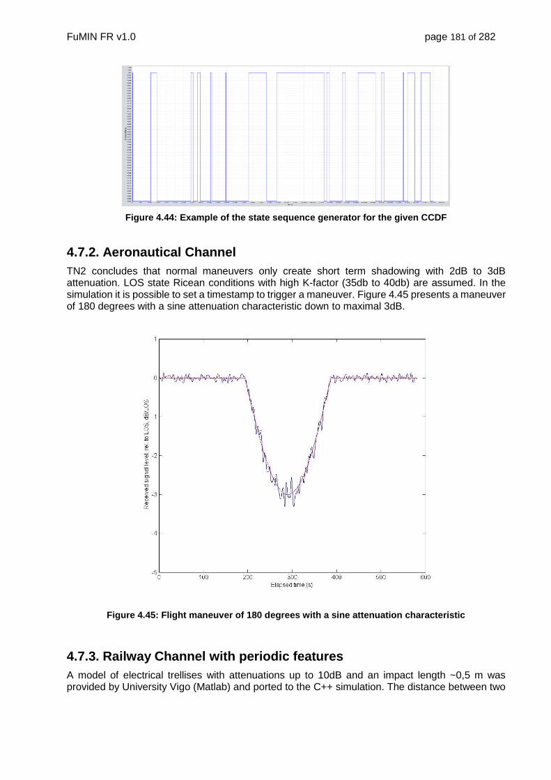
FuMIN FR v1.0 page 181 of 282
Figure 4.44: Example of the state sequence generator for the given CCDF
4.7.2. Aeronautical Channel
TN2 concludes that normal maneuvers only create short term shadowing with 2dB to 3dB attenuation. LOS state Ricean conditions with high K-factor (35db to 40db) are assumed. In the simulation it is possible to set a timestamp to trigger a maneuver. Figure 4.45 presents a maneuver of 180 degrees with a sine attenuation characteristic down to maximal 3dB.
Figure 4.45: Flight maneuver of 180 degrees with a sine attenuation characteristic
4.7.3. Railway Channel with periodic features
A model of electrical trellises with attenuations up to 10dB and an impact length ~0,5 m was provided by University Vigo (Matlab) and ported to the C++ simulation. The distance between two
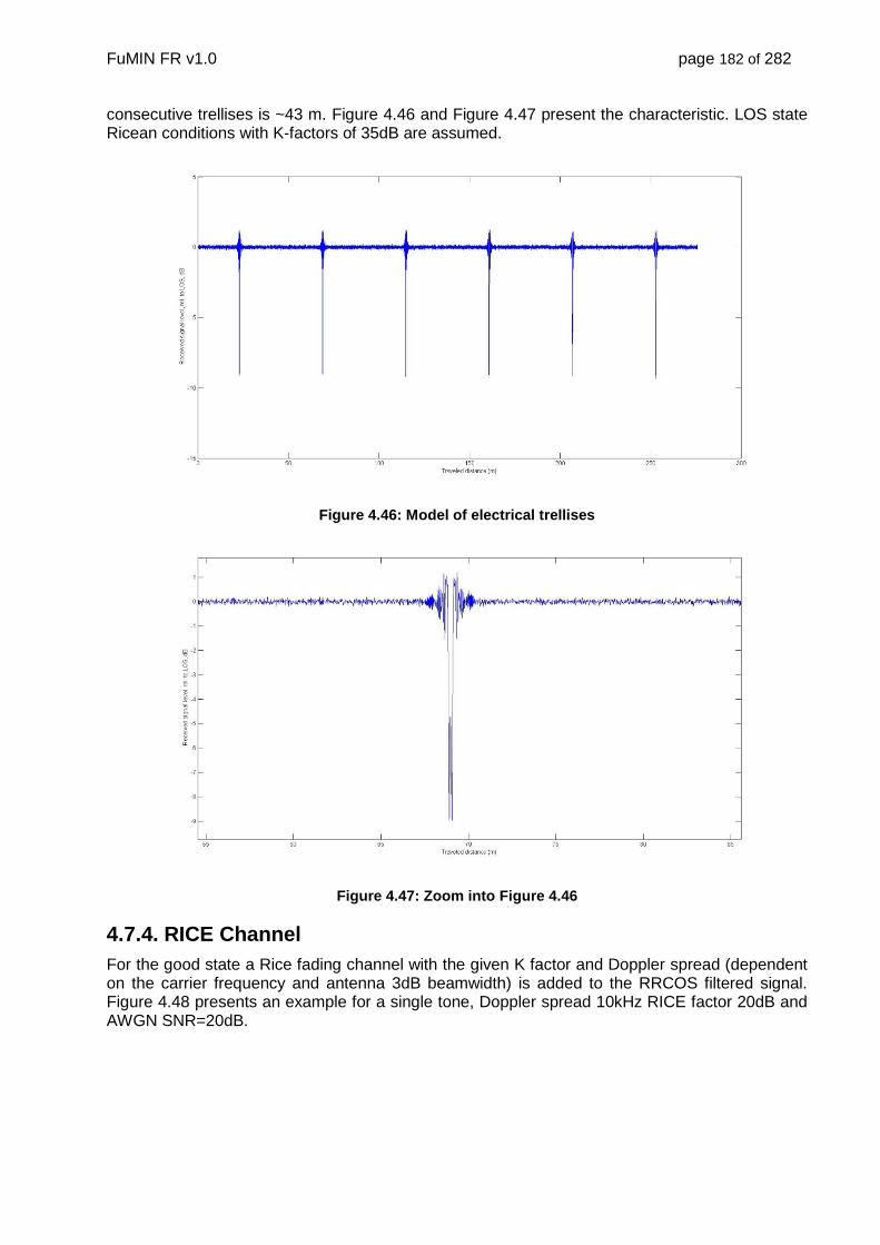
FuMIN FR v1.0 page 182 of 282
consecutive trellises is ~43 m. Figure 4.46 and Figure 4.47 present the characteristic. LOS state Ricean conditions with K-factors of 35dB are assumed.
Figure 4.46: Model of electrical trellises
Figure 4.47: Zoom into Figure 4.46
4.7.4. RICE Channel
For the good state a Rice fading channel with the given K factor and Doppler spread (dependent on the carrier frequency and antenna 3dB beamwidth) is added to the RRCOS filtered signal. Figure 4.48 presents an example for a single tone, Doppler spread 10kHz RICE factor 20dB and AWGN SNR=20dB.

FuMIN FR v1.0 page 183 of 282
Figure 4.48: Example for 10kHz Doppler spread (K=20dB) and AWGN channel with 20 dB SNR for single tone
The get a view of the impact on the modulation constellation a scatter plot is given in Figure 4.49
Figure 4.49: Example for 10kHz doppler spread (K=25dB) no AWGN for a QPSK modulated signal
Figure 4.50 presents the influence of Doppler spread and RICE factor (K) on a 16-APSK signal (CR=3/4) with 1 MSymbol/s. For K=30dB and a worst case Doppler spread of 100kHz (dfTs=0.1) the degradation is below 0.1dB. In the models of University Vigo the smallest RICE factor is 30dB. Due to the directed antenna the Doppler spreads are below 10kHz in all considered mobile channels. For K=20dB and a Doppler spread of 10kHz (dfTs=0.01) the loss is 0.3dB.

FuMIN FR v1.0 page 184 of 282
Figure 4.50: Codec simulation for a carrier with 1Msymbol/s and 16-APSK short frames using different Doppler spreads (dfTs=0.01,0.1) and Rice factors (K=30,K=20)
4.7.5. Antenna Pointing Error
The antenna pointing error time series is generated with a Laplace distribution. The parameter set is:
fs = 100; % Hz, Sampling frequency lambV = 14; % Laplace parameter, elev. lambH = 14; % Laplace parameter, azim. f1 = 7; % Rate ov variations. Filter specs f2 = 20; W1 = 3; W2 = 70; BW_V = 2.3; % deg. Recieve antenna HPBW in vertical plane BW_H = 2.3; % deg. Recieve antenna HPBW in horizontal plane
An example time series is given in Figure 4.51.

FuMIN FR v1.0 page 185 of 282
Figure 4.51: Antenna Pointing error time series 100Hz resolution

FuMIN FR v1.0 page 186 of 282
5. Demonstrator Architecture
5.1. Architecture of the Demonstrator
5.1.1. Functional Architecture
The high level architecture of the simulation is shown in Figure 5-1 and Figure 5-2. It represents the mobile satellite communication simulation for the forward (DVB-S2x) and return (DVB-RCS2) channel. The transmitter and receiver functions are represented by the green blocks, which are detailed in Figure 5-3 and Figure 5-4 for DVB-S2x and DVB-RCS respectively.
In the figures, the transmitters of the forward and return link are at the top, whereas both receivers are at the bottom. The demonstrator is dedicated to operate just one direction at one time, i.e. either the forward or the return channel. Reloading and restarting the SW switches between the forward and return channel.
The functions inside the building blocks are practically identical to the simulation SW. Therefore it is here explicitly referenced to deliverable TN2 and TN3, which provides a more detailed view into the blocks. Nevertheless we provide in Figure 5-3 and Figure 5-4, a more detailed functional architecture as a copy.
Figure 5-1 and Figure 5-2 also show a return channel from the receiver to the transmitter, which is necessary for ACM. In the simulation, the return channel was realized by a SW hook, whereas here we use a network link, i.e. a UDP connection. The associated UDP socket has been added in Figure 5-3 and Figure 5-4.
The CXM device is realized by the IZT C3040. It provides the necessary functions for the satellite channel, i.e. IMUX, OMUX filters, non-linear distortion, phase noise and AWGN.
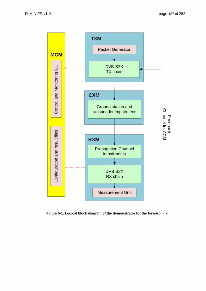
FuMIN FR v1.0 page 187 of 282
CXM
DVB-S2X
TX chain
Ground station and
transponder impairments
TXM
DVB-S2X
RX chain
RXM
MCMC
on
tro
l a
nd
Mo
nito
rin
g G
UI
Measurement Unit
Co
nfig
ura
tio
n a
nd
re
su
lt file
s
Fe
ed
ba
ck
Ch
an
ne
l for A
CM
Packet Generator
Propagation Channel
impairments
Figure 5-1: Logical block diagram of the demonstrator for the forward link

FuMIN FR v1.0 page 188 of 282
CXM
DVB-RCS2
TX chain
Ground station and
transponder impairments
TXM
DVB-RCS2
RX chain
RXM
MCM
Co
ntr
ol a
nd
Mo
nito
rin
g G
UI
Measurement Unit
Co
nfig
ura
tio
n a
nd
re
su
lt file
s
Sig
na
lling
Ch
an
ne
l for
Allo
ca
tion
Pla
n
Packet Generator
Propagation Channel
impairments
Figure 5-2: Logical block diagram of the demonstrator for the forward link

FuMIN FR v1.0 page 189 of 282
IP packets
Encapsulation
BB-Framing
LL-FEC
Encoder
FEC Encoding
PHY
Interleaving
Superframing
Baseband
Shaping
Lin
k L
ay
er
TX
Ch
ain
Ph
ys
ica
l L
ay
er
TX
Ch
ain
Samples
IP packets
Encapsulation
BB-Framing
LL-FEC
Decoder
FEC Decoding
Symbol to Bit
Mapping
Superframe
Removal
Fine freq. &
phase recovery
Lin
k L
ay
er
RX
Ch
ain
Ph
ys
ica
l L
ay
er
RX
Ch
ain
Timing
recovery
Baseband
Shaping
Samples
Bit to Symbol
Mapping
PHY
Deinterleaving
Channel
Estimation
to ACM
controller
Coarse freq.
recovery
UDP
socket
Figure 5-3: Building blocks of the DVB-S2x air interface
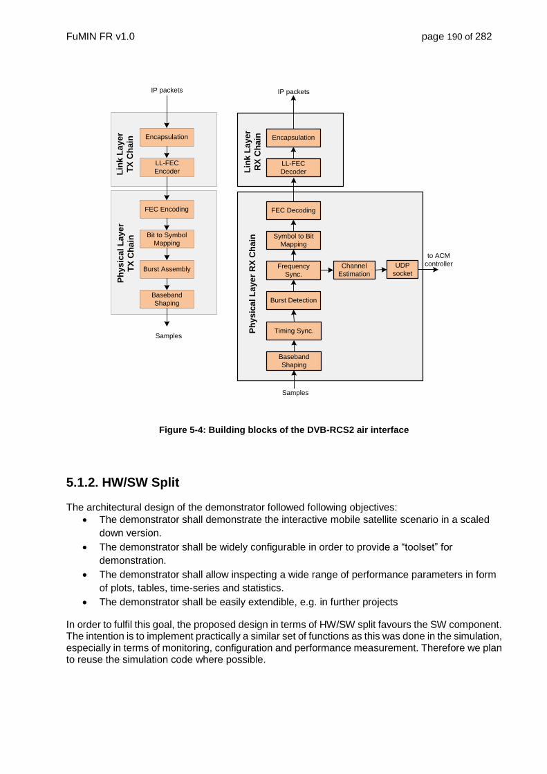
FuMIN FR v1.0 page 190 of 282
IP packets
Encapsulation
LL-FEC
Encoder
FEC Encoding
Bit to Symbol
Mapping
Burst Assembly
Baseband
Shaping
Lin
k L
ay
er
TX
Ch
ain
Ph
ys
ica
l L
ay
er
TX
Ch
ain
Samples
IP packets
Encapsulation
LL-FEC
Decoder
FEC Decoding
Symbol to Bit
Mapping
Frequency
Sync.
Burst Detection
Lin
k L
ay
er
RX
Ch
ain
Ph
ys
ica
l L
ay
er
RX
Ch
ain
Timing Sync.
Baseband
Shaping
Samples
Channel
Estimation
to ACM
controllerUDP
socket
Figure 5-4: Building blocks of the DVB-RCS2 air interface
5.1.2. HW/SW Split The architectural design of the demonstrator followed following objectives:
The demonstrator shall demonstrate the interactive mobile satellite scenario in a scaled
down version.
The demonstrator shall be widely configurable in order to provide a “toolset” for
demonstration.
The demonstrator shall allow inspecting a wide range of performance parameters in form
of plots, tables, time-series and statistics.
The demonstrator shall be easily extendible, e.g. in further projects
In order to fulfil this goal, the proposed design in terms of HW/SW split favours the SW component. The intention is to implement practically a similar set of functions as this was done in the simulation, especially in terms of monitoring, configuration and performance measurement. Therefore we plan to reuse the simulation code where possible.

FuMIN FR v1.0 page 191 of 282
In fact, the simulation code has been already written C++ using efficient libraries and implementations. Time critical code, as for instance the LDPC-decoder, has been written in the performant AVX instruction set.
Therefore, we propose to use following approach:
The HW consists out of COTS SDR platforms, i.e. the Ettus X310 board, and COTS
computers, i.e. a 6-core XEON servers.
The SDR platforms provide just the first stage of signal processing, e.g. mixing,
decimation and equalization. The data on the interface to the computers are samples.
The C++ SW takes care about the next processing steps like carrier synchronization,
decoding or link layer handling.
To achieve the envisaged throughput, a sufficient amount of computational resources are
used.
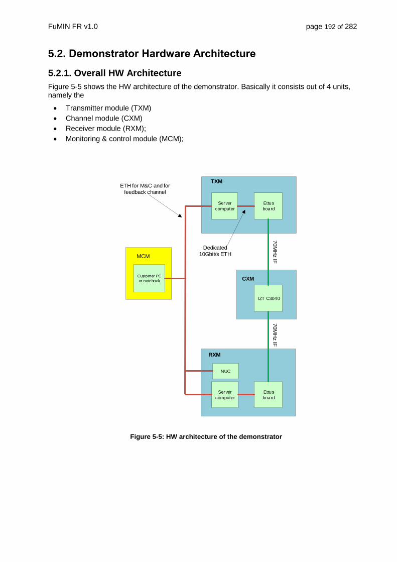
FuMIN FR v1.0 page 192 of 282
5.2. Demonstrator Hardware Architecture
5.2.1. Overall HW Architecture
Figure 5-5 shows the HW architecture of the demonstrator. Basically it consists out of 4 units, namely the
Transmitter module (TXM)
Channel module (CXM)
Receiver module (RXM);
Monitoring & control module (MCM);
Server
computer
TXM
Ettus
board
MCM
Customer PC
or notebook
ETH for M&C and for feedback channel
CXM
IZT C3040
Server
computer
RXM
Ettus
board
70M
Hz IF
Dedicated 10Gbit/s ETH
70M
Hz IF
NUC
Figure 5-5: HW architecture of the demonstrator
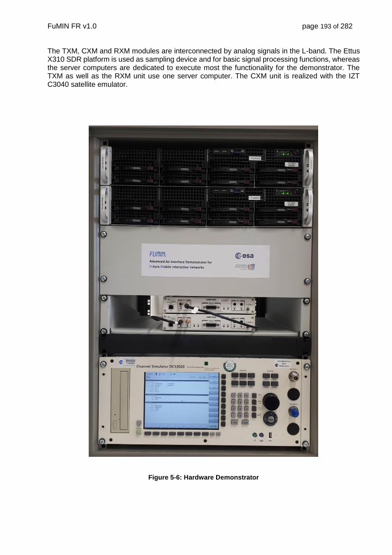
FuMIN FR v1.0 page 193 of 282
The TXM, CXM and RXM modules are interconnected by analog signals in the L-band. The Ettus X310 SDR platform is used as sampling device and for basic signal processing functions, whereas the server computers are dedicated to execute most the functionality for the demonstrator. The TXM as well as the RXM unit use one server computer. The CXM unit is realized with the IZT C3040 satellite emulator.
Figure 5-6: Hardware Demonstrator

FuMIN FR v1.0 page 194 of 282
5.2.2. SDR Platform Evaluation
5.2.2.1. The USRP X310
The USRP X310 provides a high-performance and scalable software defined radio platform (SDR). The in-built ADC (analogue to digital converter) supports sample rates of up to 200 MS/s (14 bits) and the DAC (digital to analogue converter) sampling rates of up to 800 MS/s (16 bits). The X310 is powered by a Xilinx Kintex FPGA running at a clock rate of 200 MHz. Detailed documentation can be found at the links given in [RD17] and [RD18]. In the sequel the specifications are given:
Figure 5-7: End-to-end block diagram of the simulation model
Specifications:
Power
DC Input 12 V
Power Consumption 45 Watts
Physical
Dimensions 27.7 x 21.8x 3.9 cm
Weight 1.7kg
Conversion Performance and Clocks
14 bit 200 MS/s ADC
16 bit 800 MS/s DAC
Internal 10MHz Clock Reference accuracy +/- 2.5 ppm
Optional OCXO +/- 20 ppb
Optional GPSDO (GPS disciplined oscillator) +/- 0.01 ppb
SMA connector for external 10 MHz clock with maximum input power of 15dBm
FPGA (Digital Signal Processing),
Xilinx Kintex-7 XC7K410T FPGA including DSP blocks

FuMIN FR v1.0 page 195 of 282
Daughterboard slots (RF Capabilities)
Two wideband RF daughterboard slots, up to 120MHz bandwidth per channel from DC to
6 GHz (dependent on daughter board)
Host Interfaces:
Dual 1/10Gbit Ethernet,
PCIe Express,)
Figure 5-8 and Figure 5-9 present the Layout of Front and Rear Panel with the according description of connectors and LEDs.
Figure 5-8: Front Panel Description

FuMIN FR v1.0 page 196 of 282
Figure 5-9: Rear Panel Description
5.2.2.2. Host Interface
The interface to the host PC is provided via multiple high-speed interface options (see Figure 5-10) which comprise PCIe, dual 10 GigEth and 2x 1 GigEth. With the according the following data rates can be achieved, where 1 Sample = 2 (I and Q) x 16bit = 4 byte:
Dual 10 Gigabit Ethernet: 200 MS/s Full Duplex
PCIe x4 (Desktop): 200 MS/s Full Duplex
ExpressCard (Laptop): 50 MS/s Full Duplex
Dual 1 Gigabit Ethernet: 25 MS/s Full Duplex
The PCIx interface is optimized for the NI (National instruments) Labview framework. That is why the 10Gbit/s Ethernet interface was selected (recommended by ETTUS).Figure 5-11 presents the configuration of the ETH Interfaces on Host-PC and USRP-X310. For each setup the according FPGA Image has to be burned. This can be easily done via Ethernet.

FuMIN FR v1.0 page 197 of 282
Figure 5-10: Host Interfaces
Figure 5-11: Host Interface Configuration
5.2.2.3. Detailed Architecture
Figure 5-12 presents the architecture of the USRPx-310. The clocking part offers various possibilities of accuracy. The frequency accuracy of the internal TCXO (Temperature controlled crystal oscillator) is +/- 2.5ppm. Considering optional hardware of an OCXO (Oven controlled crystal oscillator) the accuracy is 20ppb is possible. The GPS disciplined OCXO offers the best performance of 0.01ppb. In the project we will supply all USRPs with an external 10MHz clock with OCXO quality.
The ADC supports sample rates of up to 200 MS/s (14 bits) and the DAC sampling rates of up to 800 MS/s (16 bits). Two independent direct conversion channels can be processed. For that purpose two slots for daughter-boards (see next section) are available.
The X310 is powered by a Xilinx Kintex FPGA running at a clock rate of 200 MHz. In Figure 5-13 the DSP blocks which are available in the basic FPGA image are given. Up and down-sampling with CIC (Cascaded integrator comb) and halfband-filters allow a factor of 512. In addition a digital mixer is available which can be programmed via the UHD driver (universal hardware device). The FPGA source code is provided as open source and can therefore be user programmed.
The internal architecture of the FPGA hosts beside DSP cores, a soft processor (ZPU), interface IP blocks, and a memory interface to an internal 1GB DDR3 RAM. The modules used by the X310

FuMIN FR v1.0 page 198 of 282
FPGA source code are reused from older platforms (N210) and therefore are well known. The on-board memory supplements the FPGA resources with buffering and data storage memory.
Figure 5-12: USRPX-310 architecture
FPGA
Figure 5-13: FPGA DSP blocks
Two versions of FPGA are available, the resources are listed in Figure 5-14.

FuMIN FR v1.0 page 199 of 282
Figure 5-14: FPGA resources
5.2.2.4. WBX daughter board
To fulfill the requirement to operate on L-Band frequencies the WBX daughter board was selected.
The features are:
Direct conversion
Independent receive and transmit LO's and synthesizers
Full-duplex operation on different transmit and receive frequencies
Frequency Range: 50 MHz to 2.2 GHz
Transmit gain range: 0-25dB
Receive gain range: 0-31.5dB
Two Bandwidths are available:
o WBX-40: 40 MHz, RX & TX
o WBX-120: 120 MHz, RX & TX
Sensor for LO lock state

FuMIN FR v1.0 page 200 of 282
The RF specifications are:
LO supression between -35dbc and -50dbc dependent on frequency
Phase Noise at 1.8 GHz
- 10kHz -80 dBc/Hz
- 100kHz -100 dBc/Hz
- 1MHz -137 dBc/Hz
Noise Figure
- 2 - 4 dB @ (50MHz ~ 1.2GHz)
- 4 - 8 dB @ (1.2GHz ~ 2.2GHz)
RX IIP3 (Max) 10 - 18 dBm
Maximum RX power -15 dBm
RX IQ Imbalance -30 dBc
TX Power (Max)
- 18 - 20 dBm @ (50MHz ~ 1.4 GHz)
- 12 - 18dBm @ (1.4GHz ~ 2.2 GHz)
TX OIP3
- 30 - 32 dBm @ (50MHz ~ 800MHz)
- 25 - 30 dBm @ (800MHz ~ 2.2GHz)
TX IQ Imbalance
- -30 dBc @ (50MHz ~ 1.9GHz)
- -24 dBc @ (1.9GHz ~ 2.2GHz)
RF Ports are matched to 50 Ohm with a return loss < -10dB
The USPRX-310 provides two quadrature frontends. So two independent transmit and receive chains can be processed. The Architecture of the WBX-40 board is given in Figure 5-15. The RX gain of 25dB is achieved by two amplifiers with an attenuator network between (0.5 dB steps). The LO frequency ADL5387 IQ mixer is input from the ADF4350 a wideband synthesizer with integrated LO. The mixed signal is filtered by a 6th order Chebyshef filter with 20 MHz corner frequency. The level adaption (ADA493) and AAL (Anti alias filter) filtering is done before the ADC converter located on the USRPX310 main board is interfaced.
Figure 5-15: WBX-40MHz board architecture

FuMIN FR v1.0 page 201 of 282
Figure 5-16presents the figure of merits at 30.5dB receive gain over the operational frequency range:
Gain flatness
I/Q imbalance
DC offset
3rd order Input Intersection point (IIP)
2nd order Input Intersection point (IIP)
Noise figure
Figure 5-16: Rx characteristics over Frequency

FuMIN FR v1.0 page 202 of 282
5.2.3. Host PC
For rack mount we propose the following Host PC (see Figure 5-17), which has a similar performance specification as the Tower PC used for the performance verification. To achieve real-time like behaviour with low latencies, the CPU clock speed is favoured over the number of cores. Alternative CPU’s, e.g. XEONs with 8 cores and more, have typically lower clock speeds, and are therefore less attractive, even if the total number of instruction per second is higher.
Typ: Desktop CPU
EAN: 5032037087193
Manufacturer-Nr.: BX80671I76850K
CPU-Typ: Core i7
Socket: 2011-3
Processor: Core i7 6xxx (Broadwell E)
Cores: 6
Micro-architecture: Broadwell-E
Structure: 14 nm
Frequency: 3600 MHz
Turbo-Modes: up to 3800 MHz
Cache Level 1: 6x 64 KB, Level 2: 6x 256 KB, Level 3: 15360 KB
Memory Controller 4 Channels
Supported DDR4-1600, DDR4-1866, DDR4-2133, DDR4-2400
Power Consumption (TDP) max 140 Watt
Figure 5-17: Two Height unit Host PC

FuMIN FR v1.0 page 203 of 282
5.3. Demonstrator Software Architecture
Figure 5-18 shows the overall SW architecture as it appears on each of the computers. The computers are equipped with a Linux operating system. To enable quasi real time behavior, a real time patch is used, which includes also a preemptive scheduler. This ensures fast reaction of dedicated threads.
As shown two Ethernet cards, and therefore two Ethernet drivers are present. ETH2 is dedicated for the access of the MCM unit. ETH2 is used as the interconnection to the SDR platform. Note that ETH2 must be a dedicated 10Gbit/s Ethernet to cope with the high data rate from the SDR platform.
In the user space, a single application is executed. This application is based on the SpaceCommSIMU software, which provides a SW framework used to execute the FuMIN functions. The SW framework is subdivided mainly into two parts, the Core SW, which integrates the MCM interface and the universal hardware driver (UHD), which is used for data exchange with the SDR platform. The second part is the FuMIN SW modules. These modules represent the FuMIN functions, similar to the functions realized for the simulator. In additions the SW framework links two libraries extensively used by the modules, namely the Intel Performance Primitives (IPP) and the Boost-library.
.
SW Framework
UHD
Boost
IPP
FuMIN
SW Modules
Core SW
ETH2
Linux Kernel with
real time patch
ETH1
Real Time
Threads
To
C&MTo
SDR
C&M IF
Figure 5-18: SW architecture on a computer

FuMIN FR v1.0 page 204 of 282
6. End-to-End Performance Assessment
6.1. Introduction
Performance assessment has been performed on the demonstrator on selected scenarios for vehicular, train and aeronautic. Results have been derived with respect to different traffic classes that are different in terms of latency and packet error rates. The QoS criteria for the selected service classes are:
Traffic class 1: 1-way latency < 2.5s, PER < 1e-3
Traffic class 2: 1-way latency < 0.5s, PER < 1e-2
Traffic class 3: no latency requirement, PER < 5%
These QoS parameters are measured in 5s intervals, and for each interval it is assessed, if the specified QoS was satisfied or no, and if not, the service is considered as not available. In addition, the overall frame error rate (FER), and derived from that the good-put, i.e. 1-FER, is derived.
Regarding throughput performance, the spectral efficiency of the used modcods / wid is measured. Please note that these spectral efficiencies do not include the code rate of the LL-FEC.
In total, the measured parameters are as follows:
Service Availability per traffic class: total time service was available / total time
FER: Defined as 1-(total received / total sent packets).
Goodput: 1-FER
Average spectral efficiency
Peak spectral efficiency
Minimum spectral efficiency per traffic class, when service was available
Average one-way packet latency per interval.

FuMIN FR v1.0 page 205 of 282
6.2. Scenarios with linear Channel
6.2.1. Test P1: Line of sight - Fixed Terminal with ACM
Purpose:
This test is for assessment of the performance of a fixed terminal under rain conditions with ACM.
Setup: DVB-S2x Setup DVB-RCS2 Setup For DVB-S2x the SNR at clear sky = 15.7 dB For DVB-RCS2 the SNR at clear sky = 13.2 dB
Test procedure: Switch ACM on Select propagation model off. Switch Rain on (Tropospheric model on) Switch Antenna off (Model off, but used SNR of 1 m antenna) Switch LL-FEC off Run the simulation with DVB-S2x. Run the simulation with DVB-RCS2. Record following traces:
Attenuation
Current spectral efficiency
FER in interval
Record for each simulation following performance figures:
FER
Service Availabilities (1-FER, Traffic class 1, Traffic class 2 and Traffic class 3)
Average spectral efficiency
Peak spectral efficiency
Minimum spectral efficiency when services (Traffic class 1, Traffic class 2 and Traffic
class 3) were available
Output:
Performance figures and curves as defined in the test procedure.
6.2.1.1. DVB-S2X with 1m-Antenna
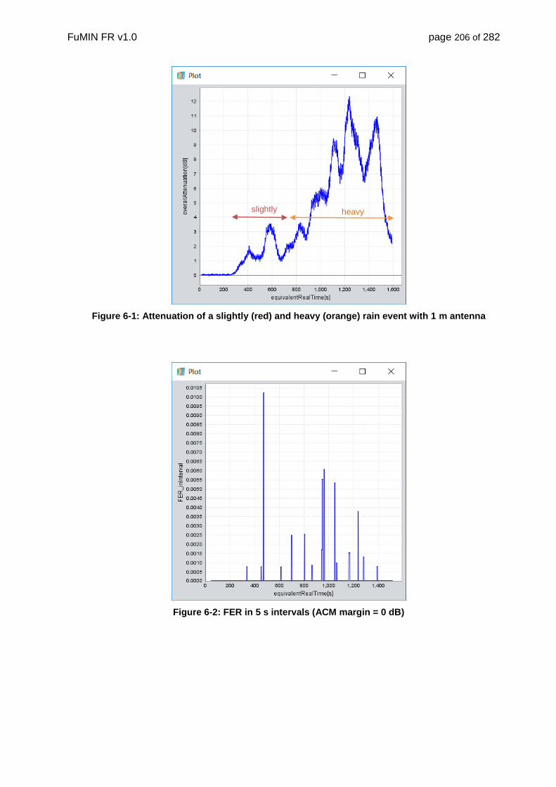
FuMIN FR v1.0 page 206 of 282
Figure 6-1: Attenuation of a slightly (red) and heavy (orange) rain event with 1 m antenna
Figure 6-2: FER in 5 s intervals (ACM margin = 0 dB)
slightly heavy

FuMIN FR v1.0 page 207 of 282
Figure 6-3: FER in 5 s intervals (ACM margin = 0.2 dB)
Table 6-1: Service Availabilities for varying ACM margin values
Rain events
ACM margin
FER 1-FER Traffic class 1
Availability Traffic class 2
Availability Traffic class 3
Availability
[dB] [ × 1e-5] [%] [%] [%] [%]
light 0 9.79 99.99 99.17 99.16 100
light 0.2 0 100 100 100 100
light 0.5 0 100 100 100 100
light 1 0 100 100 100 100
heavy 0 16.9 99.98 96.14 99.65 100
heavy 0.2 1.44 99.99 99.65 100 100
heavy 0.5 0.29 99.99 100 100 100
heavy 1 0 100 100 100 100
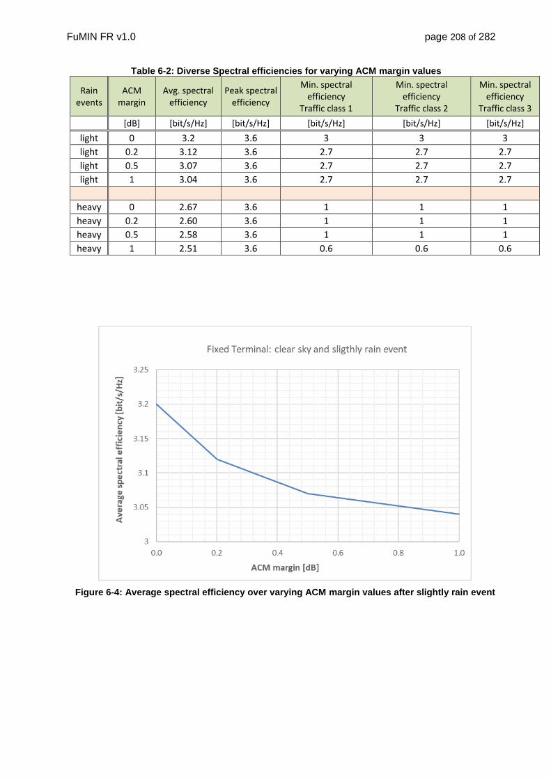
FuMIN FR v1.0 page 208 of 282
Table 6-2: Diverse Spectral efficiencies for varying ACM margin values
Rain events
ACM margin
Avg. spectral efficiency
Peak spectral efficiency
Min. spectral efficiency
Traffic class 1
Min. spectral efficiency
Traffic class 2
Min. spectral efficiency
Traffic class 3
[dB] [bit/s/Hz] [bit/s/Hz] [bit/s/Hz] [bit/s/Hz] [bit/s/Hz]
light 0 3.2 3.6 3 3 3
light 0.2 3.12 3.6 2.7 2.7 2.7
light 0.5 3.07 3.6 2.7 2.7 2.7
light 1 3.04 3.6 2.7 2.7 2.7
heavy 0 2.67 3.6 1 1 1
heavy 0.2 2.60 3.6 1 1 1
heavy 0.5 2.58 3.6 1 1 1
heavy 1 2.51 3.6 0.6 0.6 0.6
Figure 6-4: Average spectral efficiency over varying ACM margin values after slightly rain event
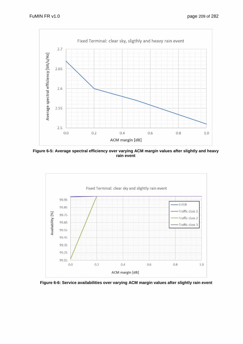
FuMIN FR v1.0 page 209 of 282
Figure 6-5: Average spectral efficiency over varying ACM margin values after slightly and heavy rain event
Figure 6-6: Service availabilities over varying ACM margin values after slightly rain event

FuMIN FR v1.0 page 210 of 282
Figure 6-7: Service availabilities over varying ACM margin values slightly and heavy rain event

FuMIN FR v1.0 page 211 of 282
6.2.1.2. RCS2 with 1m-Antenna
Figure 6-8: FER in 5 s interval (ACM margin = 0 dB)
Figure 6-9 : FER in 5 s interval (ACM margin = 0.2 dB)

FuMIN FR v1.0 page 212 of 282
Table 6-3: Service Availabilities for varying ACM margin values
Rain events
ACM margin
FER 1-FER Traffic class 1
Availability Traffic class 2
Availability Traffic class 3
Availability
[dB] [ × 1e-5] [%] [%] [%] [%]
light 0 0.00E+00 100 100 100 100
light 0.2 0 100 100 100 100
light 0.5 0 100 100 100 100
light 1 0 100 100 100 100
heavy 0 43.5 99.96 93.12 98.915 100
heavy 0.2 5.7 99.99 98.55 100 100
heavy 0.5 0.57 99.99 100 100 100
heavy 1 0 100 100 100 100
Table 6-4: Diverse Spectral efficiencies for varying ACM margin values
Rain events
ACM margin
Avg. spectral efficiency
Peak spectral efficiency
Min. spectral efficiency
Traffic class 1
Min. spectral efficiency
Traffic class 2
Min. spectral efficiency
Traffic class 3
[dB] [bit/s/Hz] [bit/s/Hz] [bit/s/Hz] [bit/s/Hz] [bit/s/Hz]
light 0 2.48 2.5 1.33 1.33 1.33
light 0.2 2.48 2.5 1 1 1
light 0.5 2.47 2.5 1 1 1
light 1 2.44 2.5 1 1 1
heavy 0 2.15 2.5 1 1 1
heavy 0.2 2.13 2.5 0.67 0.67 0.67
heavy 0.5 2.11 2.5 0.67 0.67 0.67
heavy 1 2.05 2.5 0.67 0.67 0.67

FuMIN FR v1.0 page 213 of 282
Figure 6-10: Average spectral efficiency over varying ACM margin values after clear sky and slightly rain event
Figure 6-11: Average spectral efficiency over varying ACM margin values after clear sky, slightly and heavy rain event

FuMIN FR v1.0 page 214 of 282
Figure 6-12: Service availabilities over varying ACM margin values after clear sky and slightly rain event
Figure 6-13: Service availabilities over varying ACM margin values after clear sky, slightly and heavy rain event

FuMIN FR v1.0 page 215 of 282
Conclusions: As illustrated in the test, an ACM margin of 0.5dB leads to a quasi-error free performance. Note that in this scenario, the antenna is fixed, and so there are no SNR variations from the antenna. The ACM result is therefore practically independent from the antenna size.

FuMIN FR v1.0 page 216 of 282
6.2.2. Test P2: Line of Sight – Moving Terminal with ACM
Purpose:
This test is for assessment of the performance of a moving terminal under rain conditions with ACM.
Setup: DVB-S2x Setup DVB-RCS2 Setup For DVB-S2x and 1m-antenna the SNR at clear sky = 15.7 dB For DVB-S2x and 0.6m-antenna the SNR at clear sky = 9.7 dB For DVB-RCS2 and 1m-antenna the SNR at clear sky = 13.2 dB For DVB-RCS2 and 0.6m-antenna the SNR at clear sky = 9.7 dB
Test procedure: Switch ACM on Select propagation model off. Switch Rain on (Tropospheric model on) Switch antenna on Switch LL-FEC off Run the simulation with DVB-S2x. Run the simulation with DVB-RCS2. Record following traces:
Attenuation
Current spectral efficiency
FER in interval
Record for each simulation following performance figures:
FER
Service Availabilities (1-FER, Traffic class 1, Traffic class 2 and Traffic class 3)
Average spectral efficiency
Peak spectral efficiency
Minimum spectral efficiency when services (Traffic class 1, Traffic class 2 and Traffic
class 3) were available
Output:
Performance figures and curves as defined in the test procedure.

FuMIN FR v1.0 page 217 of 282
6.2.2.1. DVB-S2X with 1m-Antenna
Figure 6-14: Attenuation of a slightly and heavy rain event with 1m-antenna
Figure 6-15: Trace of the current spectral efficiency with 1 m antenna
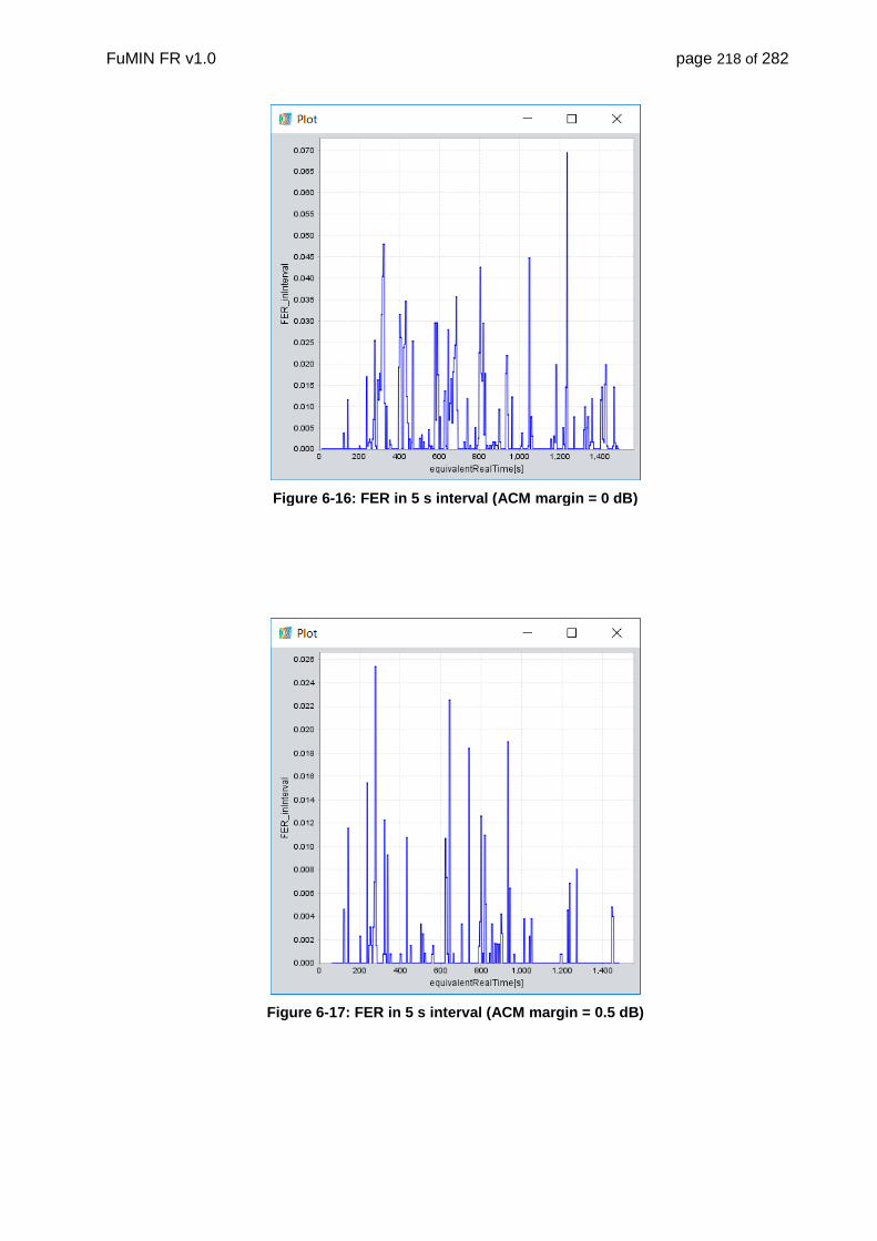
FuMIN FR v1.0 page 218 of 282
Figure 6-16: FER in 5 s interval (ACM margin = 0 dB)
Figure 6-17: FER in 5 s interval (ACM margin = 0.5 dB)

FuMIN FR v1.0 page 219 of 282
Figure 6-18: FER in 5 s interval (ACM margin =1 dB)
Figure 6-19: FER in 5 s interval (ACM margin =1.5 dB)
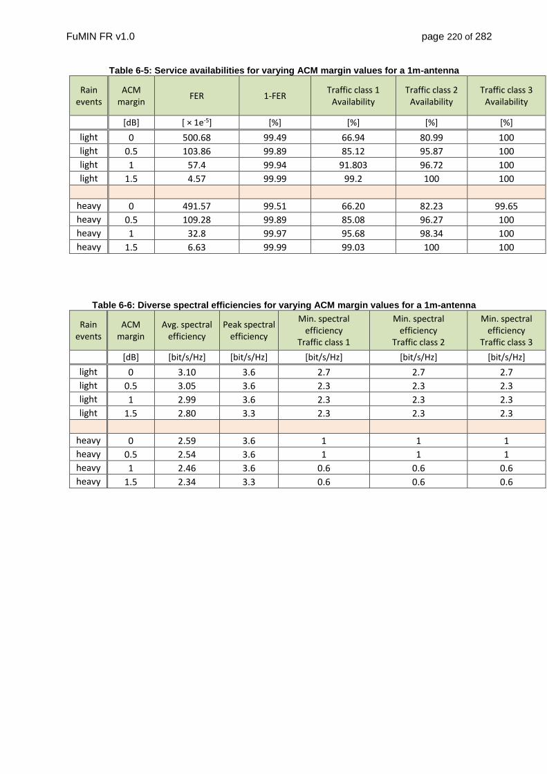
FuMIN FR v1.0 page 220 of 282
Table 6-5: Service availabilities for varying ACM margin values for a 1m-antenna
Rain events
ACM margin
FER 1-FER Traffic class 1
Availability Traffic class 2
Availability Traffic class 3
Availability
[dB] [ × 1e-5] [%] [%] [%] [%]
light 0 500.68 99.49 66.94 80.99 100
light 0.5 103.86 99.89 85.12 95.87 100
light 1 57.4 99.94 91.803 96.72 100
light 1.5 4.57 99.99 99.2 100 100
heavy 0 491.57 99.51 66.20 82.23 99.65
heavy 0.5 109.28 99.89 85.08 96.27 100
heavy 1 32.8 99.97 95.68 98.34 100
heavy 1.5 6.63 99.99 99.03 100 100
Table 6-6: Diverse spectral efficiencies for varying ACM margin values for a 1m-antenna
Rain events
ACM margin
Avg. spectral efficiency
Peak spectral efficiency
Min. spectral efficiency
Traffic class 1
Min. spectral efficiency
Traffic class 2
Min. spectral efficiency
Traffic class 3
[dB] [bit/s/Hz] [bit/s/Hz] [bit/s/Hz] [bit/s/Hz] [bit/s/Hz]
light 0 3.10 3.6 2.7 2.7 2.7
light 0.5 3.05 3.6 2.3 2.3 2.3
light 1 2.99 3.6 2.3 2.3 2.3
light 1.5 2.80 3.3 2.3 2.3 2.3
heavy 0 2.59 3.6 1 1 1
heavy 0.5 2.54 3.6 1 1 1
heavy 1 2.46 3.6 0.6 0.6 0.6
heavy 1.5 2.34 3.3 0.6 0.6 0.6
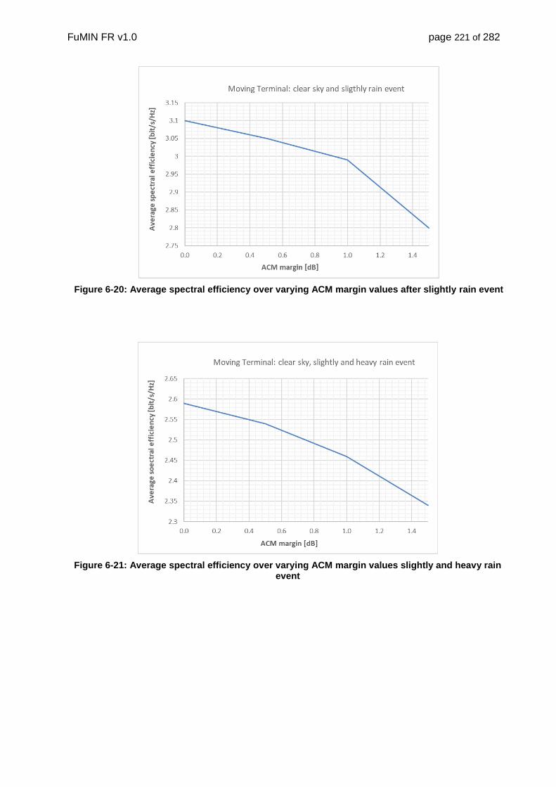
FuMIN FR v1.0 page 221 of 282
Figure 6-20: Average spectral efficiency over varying ACM margin values after slightly rain event
Figure 6-21: Average spectral efficiency over varying ACM margin values slightly and heavy rain event

FuMIN FR v1.0 page 222 of 282
Figure 6-22: Service availabilities over varying ACM margin values after slightly rain event
Figure 6-23: Service availabilities over varying ACM margin values after slightly and heavy rain event

FuMIN FR v1.0 page 223 of 282
6.2.2.2. DVB-S2X with 0.6m-Antenna
For the 0.6m-antenna the ACM margin is less important, since the main lobe is broader than with the 1m-antenna. An ACM margin of 0.5dB shows already quasi-error free performance and is taken therefore.
Table 6-7: Service availabilities for ACM margin = 0.5 dB for a 0.6 m-antenna
Rain events
ACM margin
FER 1-FER Traffic class 1
Availability Traffic class 2
Availability Traffic class 3
Availability
[dB] [ × 1e-6] [%] [%] [%] [%]
light 0.5 1.0 99.99 100 100 100
heavy 0.5 6.0 99.99 100 100 100
Table 6-8: Diverse spectral efficiencies for ACM margin = 0.5 dB for a 0.6 m-antenna
Rain events
ACM margin
Avg. spectral efficiency
Peak spectral efficiency
Min. spectral efficiency
Traffic class 1
Min. spectral efficiency
Traffic class 2
Min. spectral efficiency
Traffic class 3
[dB] [bit/s/Hz] [bit/s/Hz] [bit/s/Hz] [bit/s/Hz] [bit/s/Hz]
light 0.5 1.79 2.3 1.5 1.5 1.5
heavy 0.5 1.52 2.3 0.1 0.1 0.1 Conclusions: It was obvious that for an antenna size of 0.6 meter, an ACM margin of 0.5 dB is sufficient, but for 1m-antenna good results are achieved with an ACM margin of 1.5 dB. Note that when an LL-FEC is used, an ACM margin of 0.5 dB is also sufficient for the 1m-antenna. However, when no LL-FEC is used, a 1.5 dB ACM margin for quasi-error free FER performance is necessary.

FuMIN FR v1.0 page 224 of 282
6.2.2.3. RCS2 with 1m-Antenna
Figure 6-24: Attenuation of a slightly and heavy rain event with 1 m antenna
Figure 6-25: Trace of the current spectral efficiency (ACM margin = 0 dB)

FuMIN FR v1.0 page 225 of 282
Figure 6-26: FER in 5 s interval (ACM margin = 0 dB)
Figure 6-27: FER in 5 s interval (ACM margin = 0.5 dB)

FuMIN FR v1.0 page 226 of 282
Figure 6-28: FER in 5 s interval (ACM margin =1 dB)
Table 6-9: Service availabilities for varying ACM margin values
Rain events
ACM margin
FER 1-FER Traffic class 1
Availability Traffic class 2
Availability Traffic class 3
Availability
[dB] [ × 1e-4] [%] [%] [%] [%]
light 0 74.88 99.25 71.67 83.33 95
light 0.5 28.12 99.72 74.17 88.33 100
light 1 21.932 99.78 75 91.67 100
light 1.5 16.96 99.83 79.17 92.5 100
light 2 9.36 99.91 88.33 96.67 100
light 2.5 4.41 99.96 92.5 98.33 100
light 3 4.15 99.96 95.04 98.35 100
light 3.5 1.62 99.98 98.36 100 100
light 4 0.84 99.99 99.18 100 100
heavy 0 224.11 97.76 35.63 47.64 82.55
heavy 0.5 94.66 99.05 45.65 63.77 98.19
heavy 1 45.82 99.54 60.51 80.79 100
heavy 1.5 22.57 99.77 73.91 90.94 100
heavy 2 11.17 99.89 86.74 95.34 100
heavy 2.5 6.05 99.94 91.79 97.5 100

FuMIN FR v1.0 page 227 of 282
heavy 3 3.52 99.96 96.15 98.60 100
heavy 3.5 1.80 99.98 98.29 99.66 100
heavy 4 0.89 99.99 98.99 99.33 100
Table 6-10: Diverse spectral efficiencies for varying ACM margin values
Rain events
ACM margin
Avg. spectral efficiency
Peak spectral efficiency
Min. spectral efficiency
Traffic class 1
Min. spectral efficiency
Traffic class 2
Min. spectral efficiency
Traffic class 3
[dB] [bit/s/Hz] [bit/s/Hz] [bit/s/Hz] [bit/s/Hz] [bit/s/Hz]
light 0 2.47 2.5 1.33 1.33 1.33
light 0.5 2.45 2.5 1 1 1
light 1 2.44 2.5 1 1 1
light 1.5 2.43 2.5 1 1 1
light 2 2.35 2.5 0.67 0.67 0.67
light 2.5 2.29 2.5 0.67 0.67 0.67
light 3 2.24 2.5 0.67 0.67 0.67
light 3.5 2.08 2.25 0.67 0.67 0.67
light 4 2.03 2.25 0.67 0.67 0.67
heavy 0 2.11 2.5 0.67 0.67 0.67
heavy 0.5 2.05 2.5 0.67 0.67 0.67
heavy 1 1.99 2.5 0.67 0.67 0.67
heavy 1.5 1.93 2.5 0.17 0.17 0.17
heavy 2 1.86 2.5 0.17 0.17 0.17
heavy 2.5 1.78 2.5 0.17 0.17 0.17
heavy 3 1.69 2.5 0.17 0.17 0.17
heavy 3.5 1.58 2.25 0.17 0.17 0.17
heavy 4 1.52 2.25 0.17 0.17 0.17

FuMIN FR v1.0 page 228 of 282
Figure 6-29: Average spectral efficiency over varying ACM margin values after slightly rain event
Figure 6-30: Average spectral efficiency over varying ACM margin values after slightly and heavy rain event

FuMIN FR v1.0 page 229 of 282
Figure 6-31: Service availabilities over varying ACM margin values slightly rain event
Figure 6-32: Service availabilities over varying ACM margin values after slightly and heavy rain event
Conclusions:

FuMIN FR v1.0 page 230 of 282
With RCS2, the antenna main lobes are smaller resulting in higher SNR variations. Therefore the ACM Margins have to be larger in order to reach quasi-error free performance. For an antenna size of 0.6 meter, an ACM margin of 1 dB is recommended, whereas for 1m-antenna the this value is 2.5 dB. With such a margin, the FER is still in order of 1e-4. To reach 1e-5 the ACM margin must be larger than 4dB, and therefore the 2.5 dB are a tradeoff vs. spectral efficiency.
6.2.2.4. RCS2 with 0.6m-Antenna
Table 6-11: Service availabilities for ACM margin = 1 dB for a 0.6 m-antenna
Rain events
ACM margin
FER 1-FER Traffic class 1
Availability Traffic class 2
Availability Traffic class 3
Availability
[dB] [ × 1e-4] [%] [%] [%] [%]
light 1 4.05 99.96 92.5 99.17 100
heavy 1 11.79 99.88 78.29 97.86 100
Table 6-12: Diverse spectral efficiencies for ACM margin = 1 dB for a 0.6 m-antenna
Rain events
ACM margin
Avg. spectral efficiency
Peak spectral efficiency
Min. spectral efficiency
Traffic class 1
Min. spectral efficiency
Traffic class 2
Min. spectral efficiency
Traffic class 3
[dB] [bit/s/Hz] [bit/s/Hz] [bit/s/Hz] [bit/s/Hz] [bit/s/Hz]
light 1 2.28 2.5 1 1 1
heavy 1 1.73 2.5 0.17 0.17 0.17

FuMIN FR v1.0 page 231 of 282
6.2.3. Test P3: Vehicular Scenario with ACM, clear sky conditions
Purpose:
This test is for assessment of the performance on an ideal transponder of a vehicular under clear sky conditions.
Setup: DVB-S2x Setup DVB-RCS2 Setup For DVB-S2x the SNR at clear sky = 11.4 dB For DVB-RCS2 the SNR at clear sky = 9.5 dB
0.6 m antenna
ACM margin = 0.5 dB
LL-FEC rate = 0.5
Test procedure: Switch ACM on Select propagation model to vehicular. Switch Antenna on Switch Rain off (Tropospheric model off) Switch Synchronization on Switch random timing, frequency and phase error on. Select different Modcods / Waveforms and matching SNR. Run the simulation with DVB-S2x. Run the simulation with DVB-RCS2. Record following traces:
Attenuation
Current spectral efficiency
FER in interval
Record for each simulation following performance figures:
FER
Service Availabilities (1-FER, Traffic class 1, Traffic class 2 and Traffic class 3)
Average spectral efficiency
Peak spectral efficiency
Minimum spectral efficiency when services (Traffic class 1, Traffic class 2 and Traffic
class 3) were available
Output:

FuMIN FR v1.0 page 232 of 282
6.2.3.1. DVB-S2X
Figure 6-33: Overall attenuation including clear sky and blockages
Figure 6-34: FER in 5 s interval, with no LL-FEC
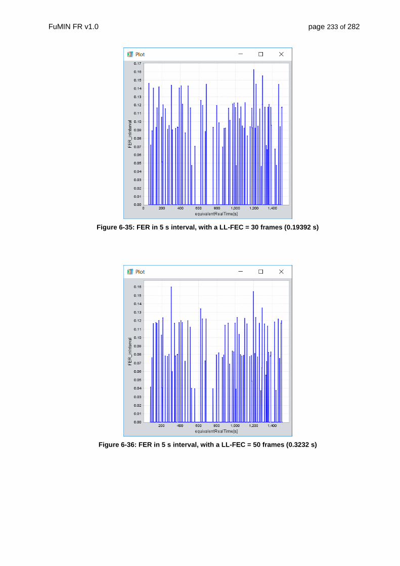
FuMIN FR v1.0 page 233 of 282
Figure 6-35: FER in 5 s interval, with a LL-FEC = 30 frames (0.19392 s)
Figure 6-36: FER in 5 s interval, with a LL-FEC = 50 frames (0.3232 s)
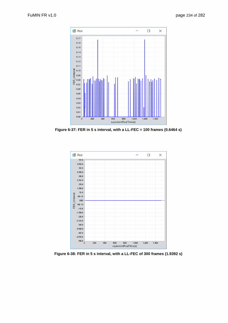
FuMIN FR v1.0 page 234 of 282
Figure 6-37: FER in 5 s interval, with a LL-FEC = 100 frames (0.6464 s)
Figure 6-38: FER in 5 s interval, with a LL-FEC of 300 frames (1.9392 s)

FuMIN FR v1.0 page 235 of 282
Table 6-13: Service availabilities for varying LL-FEC values
Rain events
LL-FEC Block
Length FER 1-FER
Traffic class 1 Availability
Traffic class 2 Availability
Traffic class 3 Availability
[s] [ × 1e-2] [%] [%] [%] [%]
no 0 3.89 96.11 1.66 70.43 74.42
no 0.19 2.69 97.30 74.42 74.42 75.75
no 0.32 2.42 97.58 74.42 74.42 77.41
no 0.65 1.39 98.61 82.39 82.39 83.06
no 1.94 0 100 100 50.49 100
no 4.52 0 100 99.00 1.66 100
Table 6-14: Diverse spectral efficiencies for varying LL-FEC values
Rain events
LL-FEC Block
Length
Avg. spectral efficiency
Peak spectral efficiency
Min. spectral efficiency
Traffic class 1
Min. spectral efficiency
Traffic class 2
Min. spectral efficiency
Traffic class 3
[s] [bit/s/Hz] [bit/s/Hz] [bit/s/Hz] [bit/s/Hz] [bit/s/Hz]
no 0 2.8 3 2.3 2.3 2.3
no 0.19 2.8 3 2.3 2.3 2.3
no 0.32 2.8 3 2.3 2.3 2.3
no 0.65 2.8 3 2.3 2.3 2.3
no 1.94 2.8 3 2.3 2.3 2.3
no 4.52 2.8 3 2.3 2.3 2.3
Figure 6-39: Service availabilities over varying LL-FEC values for clear sky scenario

FuMIN FR v1.0 page 236 of 282
Conclusions: In any case, the Traffic class 2 availability is rather small due to the latencies introduced by the required LL-FEC countermeasuring the blockage losses. So practically, this type of traffic would be not recommended for that kind of mobile satellite service.
For other types of traffic a LL-FEC of 2-3 seconds block length will lead to an acceptable behavior. Note that the vehicular scenarios was rural in the sense that blockages are quite rare and mostly short. For urban or even suburban locations, this approach would not lead to an acceptable user experience.

FuMIN FR v1.0 page 237 of 282
6.2.3.2. RCS2
Table 6-15: Service availabilities for LL-FEC block length of 4.5248 s
Rain events
LL-FEC Block
Length FER 1-FER
Interactive Availability
Phone Availability
Video Availability
[s] [ × 1e-2] [%] [%] [%] [%]
no 4.52 0 100 100 7.2 100
Table 6-16: Diverse spectral efficiencies for LL-FEC block length of 4.5248 s
Rain events
LL-FEC Block
Length
Avg. spectral efficiency
Peak spectral efficiency
Min. spectral efficiency Interactive
Min. spectral efficiency Phone
Min. spectral efficiency Video
[s] [bit/s/Hz] [bit/s/Hz] [bit/s/Hz] [bit/s/Hz] [bit/s/Hz]
no 4.52 2.51 2.5 1 1.33 1
Conclusions: RCS2 shows the same behavior as DVB-S2x.

FuMIN FR v1.0 page 238 of 282
6.2.4. Test P4: Vehicular Scenario with ACM, rain conditions
Purpose:
This test is for assessment of the performance on an ideal transponder of a vehicular under rain conditions.
Setup: DVB-S2x Setup DVB-RCS2 Setup For DVB-S2x the SNR at clear sky = 11.4 dB For DVB-RCS2 the SNR at clear sky = 9.5 dB
0.6 m antenna
ACM margin = 0.5 dB
LL-FEC rate = 0.5
Test procedure: Switch ACM on Select propagation model to vehicular. Switch antenna on Switch Rain on (Tropospheric model on) Switch Synchronization on Switch random timing, frequency and phase error on. Switch LL-FEC off/on Run the simulation with DVB-S2x. Run the simulation with DVB-RCS2. Record following traces:
Attenuation
Current spectral efficiency
FER in interval
Record for each simulation following performance figures:
FER
Service Availabilities (1-FER, Traffic class 1, Traffic class 2 and Traffic class 3)
Average spectral efficiency
Peak spectral efficiency
Minimum spectral efficiency when services (Traffic class 1, Traffic class 2 and Traffic
class 3) were available

FuMIN FR v1.0 page 239 of 282
Output:
6.2.4.1. DVB-S2X
Figure 6-40: Overall attenuation including slightly and heavy rain event and blockages

FuMIN FR v1.0 page 240 of 282
Figure 6-41: FER in 5 s interval, with no LL-FEC
Figure 6-42: FER in 5 s interval, with a LL-FEC = 30 frames (0.19392 s)

FuMIN FR v1.0 page 241 of 282
Figure 6-43: FER in 5 s interval, with a LL-FEC = 50 frames (0.3232 s)
Figure 6-44: FER in 5 s interval, with a LL-FEC = 100 frames (0.6464 s)

FuMIN FR v1.0 page 242 of 282
Table 6-17: Service availabilities for varying LL-FEC values (v = 50 km/h, rural)
Rain events
LL-FEC Block
Length FER 1-FER
Traffic class 1 Availability
Traffic class 2 Availability
Traffic class 3 Availability
[s] [ × 1e-2] [%] [%] [%] [%]
light 0 3.52 96.48 20.93 61.24 75.97
light 0.19 2.35 97.65 77.52 77.52 79.85
light 0.32 2.06 97.94 76.74 76.74 81.39
light 0.65 1.36 98.64 82.17 82.17 82.18
light 1.94 0 100 100 22.48 100
light 4.52 0 100 99.22 20.16 100
heavy 0 3.28 96.72 31.70 63.69 76.37
heavy 0.19 2.19 97.81 77.52 77.52 80.98
heavy 0.32 1.75 98.25 80.12 80.12 83.29
heavy 0.65 1.04 98.96 88.47 88.18 88.47
heavy 1.94 0 100 100 32.56 100
heavy 4.52 0 100 98.56 29.11 100
Table 6-18: Diverse spectral efficiencies for varying LL-FEC values (v = 50 km/h, rural)
Rain events
LL-FEC Block
Length
Avg. spectral efficiency
Peak spectral efficiency
Min. spectral efficiency
Traffic class 1
Min. spectral efficiency
Traffic class 2
Min. spectral efficiency
Traffic class 3
[s] [bit/s/Hz] [bit/s/Hz] [bit/s/Hz] [bit/s/Hz] [bit/s/Hz]
light 0 2.47 3 1.78 1.78 1.78
light 0.19 2.46 3 1.78 1.78 1.78
light 0.32 2.46 3 1.78 1.78 1.78
light 0.65 2.45 3 1.78 1.78 1.78
light 1.94 2.44 3 1.78 1.78 1.78
light 4.52 2.43 3 1.78 1.78 1.78
heavy 0 1.94 3 0.5 0.5 0.5
heavy 0.19 1.94 3 0.5 0.5 0.5
heavy 0.32 1.93 3 0.5 0.5 0.5
heavy 0.65 1.93 3 0.5 0.5 0.5
heavy 1.94 1.92 3 0.5 0.5 0.5
heavy 4.52 1.92 3 0.5 0.5 0.5

FuMIN FR v1.0 page 243 of 282
Figure 6-45: Service availabilities over varying LL-FEC values for a slightly rain event
(v = 50 km/h, rural)
Figure 6-46: Service availabilities over varying LL-FEC values for a slightly and heavy rain event (v = 50 km/h, rural)
Table 6-19: Service availabilities for LL-FEC block length of 4.5248 s (v = 130 km/h, rural)

FuMIN FR v1.0 page 244 of 282
Rain events
LL-FEC Block
Length FER 1-FER
Traffic class 1 Availability
Traffic class 2 Availability
Traffic class 3 Availability
[s] [ × 1e-2] [%] [%] [%] [%]
light 4.52 0 100 96.8 16.08 97.6
heavy 4.52 0 100 98.71 23.33 99.03
Table 6-20: Diverse spectral efficiencies for LL-FEC block length of 4.5248 s (v = 130 km/h, rural)
Rain events
LL-FEC Block
Length
Avg. spectral efficiency
Peak spectral efficiency
Min. spectral efficiency
Traffic class 1
Min. spectral efficiency
Traffic class 2
Min. spectral efficiency
Traffic class 3
[s] [bit/s/Hz] [bit/s/Hz] [bit/s/Hz] [bit/s/Hz] [bit/s/Hz]
light 4.52 1.81 2 1.33 1.33 1.33
heavy 4.52 1.35 2 0.5 0.5 0.5

FuMIN FR v1.0 page 245 of 282
Table 6-21: Service availabilities for LL-FEC block length of 4.5248 s (v = 30 km/h, suburban)
Rain events
LL-FEC Block
Length FER 1-FER
Traffic class 1 Availability
Traffic class 2 Availability
Traffic class 3 Availability
[s] [ × 1e-2] [%] [%] [%] [%]
light 4.52 1.82 98.18 93.08 4.62 93.08
heavy 4.52 2.38 97.62 93.03 9.39 93.63
Table 6-22: Diverse spectral efficiencies for LL-FEC block length of 4.5248 s (v = 30 km/h, suburban)
Rain events
LL-FEC Block
Length
Avg. spectral efficiency
Peak spectral efficiency
Min. spectral efficiency
Traffic class 1
Min. spectral efficiency
Traffic class 2
Min. spectral efficiency
Traffic class 3
[s] [bit/s/Hz] [bit/s/Hz] [bit/s/Hz] [bit/s/Hz] [bit/s/Hz]
light 4.52 1.82 2 1 1 1
heavy 4.52 1.35 2 0.5 0.5 0.5
Table 6-23: Service availabilities for LL-FEC block length of 4.5248 s (v = 50 km/h, suburban)
Rain events
LL-FEC Block
Length FER 1-FER
Traffic class 1 Availability
Traffic class 2 Availability
Traffic class 3 Availability
[s] [ × 1e-2] [%] [%] [%] [%]
light 4.52 0 100 94.94 4.04 95.95
heavy 4.52 0.22 99.78 91.84 3.67 93.47
Table 6-24: Diverse spectral efficiencies for LL-FEC block length of 4.5248 s (v = 50 km/h, suburban)
Rain events
LL-FEC Block
Length
Avg. spectral efficiency
Peak spectral efficiency
Min. spectral efficiency
Traffic class 1
Min. spectral efficiency
Traffic class 2
Min. spectral efficiency
Traffic class 3
[s] [bit/s/Hz] [bit/s/Hz] [bit/s/Hz] [bit/s/Hz] [bit/s/Hz]
light 4.52 1.92 2 1 1 1
heavy 4.52 1.51 2 0.5 0.5 0.5

FuMIN FR v1.0 page 246 of 282
6.2.4.2. RCS2
Figure 6-47:Trace of current spectral efficiency
Table 6-25: Service availabilities for LL-FEC block length of 4.5248 s (v = 50 km/h, rura)
Rain events
LL-FEC Block
Length FER 1-FER
Traffic class 1 Availability
Traffic class 2 Availability
Traffic class 3 Availability
[s] [ × 1e-2] [%] [%] [%] [%]
light 4.52 0 100 100 na 100
heavy 4.52 0 100 100 na 100
Table 6-26: Diverse spectral efficiencies for LL-FEC block length of 4.5248 s (v = 50 km/h, rural)
Rain events
LL-FEC Block
Length
Avg. spectral efficiency
Peak spectral efficiency
Min. spectral efficiency
Traffic class 1
Min. spectral efficiency
Traffic class 2
Min. spectral efficiency
Traffic class 3
[s] [bit/s/Hz] [bit/s/Hz] [bit/s/Hz] [bit/s/Hz] [bit/s/Hz]
light 4.52 1.79 2 1.33 na 1.33
heavy 4.52 1.33 2 0.17 na 0.17
Conclusions:
With rain, there is practically the same behavior as in Test P3, as it is determined by the blockages.

FuMIN FR v1.0 page 247 of 282
6.2.5. Test P5: Train Scenario with ACM, clear sky conditions
Purpose:
This test is for assessment of the performance on an ideal transponder of a train under clear sky conditions.
Setup: DVB-S2x Setup DVB-RCS2 Setup For DVB-S2x the SNR at clear sky = 15.7 dB For DVB-RCS2 the SNR at clear sky = 13.2 dB
1 m antenna
ACM margin = 0.5 dB
LL-FEC rate = 0.75
Test procedure: Switch ACM on Select propagation model to train (mast, overpasses and tunnel) Switch antenna on Switch Rain off (Tropospheric model off) Switch Synchronization on Switch random timing, frequency and phase error on. Switch LL-FEC off/on Select different Modcods / Waveforms and matching SNR. Run the simulation with DVB-S2x. Run the simulation with DVB-RCS2. Record following traces:
Attenuation
Current spectral efficiency
FER in interval
Record for each simulation following performance figures:
FER
Service Availabilities (1-FER, Traffic class 1, Traffic class 2 and Traffic class 3)
Average spectral efficiency
Peak spectral efficiency
Minimum spectral efficiency when services (Traffic class 1, Traffic class 2 and Traffic
class 3) were available
Output:
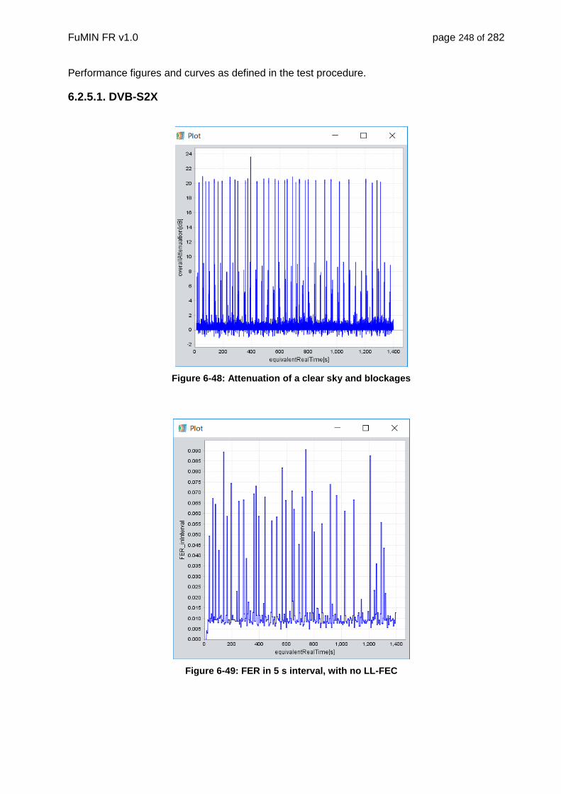
FuMIN FR v1.0 page 248 of 282
Performance figures and curves as defined in the test procedure.
6.2.5.1. DVB-S2X
Figure 6-48: Attenuation of a clear sky and blockages
Figure 6-49: FER in 5 s interval, with no LL-FEC

FuMIN FR v1.0 page 249 of 282
Figure 6-50: FER in 5 s interval, with a LL-FEC = 100 frames (0.4309 s)
Table 6-27: Service availabilities for varying LL-FEC values (v = 100 km/h)
Rain events
LL-FEC Block
Length FER 1-FER
Traffic class 1 Availability
Traffic class 2 Availability
Traffic class 3 Availability
[s] [ × 1e-3] [%] [%] [%] [%]
no 0 16.28 98.37 0.74 63.57 89.59
no 0.13 5.84 99.41 84.76 86.25 95.91
no 0.22 4.66 99.53 87.73 87.73 96.65
no 0.43 3.82 99.62 91.08 91.08 97.03
no 1.29 2.23 99.78 96.65 0 96.65
no 3.02 0 100 100 0 100
Table 6-28: Diverse spectral efficiencies for varying LL-FEC values (v = 100 km/h)
Rain events
LL-FEC Block
Length
Avg. spectral efficiency
Peak spectral efficiency
Min. spectral efficiency
Traffic class 1
Min. spectral efficiency
Traffic class 2
Min. spectral efficiency
Traffic class 3
[s] [bit/s/Hz] [bit/s/Hz] [bit/s/Hz] [bit/s/Hz] [bit/s/Hz]
no 0 3.5 3.6 3.3 3.3 3.3
no 0.13 3.5 3.6 3.3 3.3 3.3
no 0.22 3.5 3.6 3.3 3.3 3.3
no 0.43 3.5 3.6 3.3 3.3 3.3
no 1.29 3.5 3.6 3.3 na 3.3
no 3.02 3.5 3.6 3.3 na 3.3

FuMIN FR v1.0 page 250 of 282
Figure 6-51: Service availabilities over varying LL-FEC values for clear sky scenario
6.2.5.2. RCS2
Table 6-29: Service availabilities for LL-FEC block length of 1s (v = 100 km/h)
Rain events
LL-FEC Block
Length FER 1-FER
Traffic class 1 Availability
Traffic class 2 Availability
Traffic class 3 Availability
[s] [ × 1e-2] [%] [%] [%] [%]
no 1.5 0 100 100 na 100
Table 6-30: Diverse spectral efficiencies for LL-FEC block length of 1.5 s (v = 100 km/h)
Rain events
LL-FEC Block
Length
Avg. spectral efficiency
Peak spectral efficiency
Min. spectral efficiency
Traffic class 1
Min. spectral efficiency
Traffic class 2
Min. spectral efficiency
Traffic class 3
[s] [bit/s/Hz] [bit/s/Hz] [bit/s/Hz] [bit/s/Hz] [bit/s/Hz]
no 1.5 2.49 2.5 1 na 1
Conclusions: For the train scenario a short LL-FEC of around 200-300ms would necessary to countermeasure blockages from poles while maintaining the latency for the Traffic class 2 service. However, this leads still to a weak behaviour of the Traffic class 1 service (90% availability). Therefore a LL-FEC length of around 1s would be recommended.
FuMIN FR v1.0 page 251 of 282
6.2.6. Test P6: Train Scenario with ACM, rain conditions
Purpose:
This test is for assessment of the performance on an ideal transponder of a train under rain conditions.
Setup: DVB-S2x Setup DVB-RCS2 Setup For DVB-S2x the SNR at clear sky = 15.7 dB For DVB-RCS2 the SNR at clear sky = 13.2 dB
1 m antenna
ACM margin = 0.5 dB
LL-FEC rate = 0.75
Test procedure: Switch ACM on Select propagation model to train (mast, overpasses and tunnel). Switch antenna on Switch Rain on (Tropospheric model on) Switch Synchronization on Switch random timing, frequency and phase error on. Switch LL-FEC off/on Run the simulation with DVB-S2x. Run the simulation with DVB-RCS2. Record following traces:
Attenuation
Current spectral efficiency
FER in interval
Record for each simulation following performance figures:
FER
Service Availabilities (1-FER, Traffic class 1, Traffic class 2 and Traffic class 3)
Average spectral efficiency
Peak spectral efficiency
Minimum spectral efficiency when services (Traffic class 1, Traffic class 2 and Traffic
class 3) were available
Output:
Performance figures and curves as defined in the test procedure.

FuMIN FR v1.0 page 252 of 282
6.2.6.1. DVB-S2X
Figure 6-52: Overall attenuation including clear sky, slightly and heavy rain event and blockages
Figure 6-53: FER in 5 s interval, with a LL-FEC = 50 frames (0.2154 s)

FuMIN FR v1.0 page 253 of 282
Figure 6-54: : FER in 5 s interval, with a LL-FEC = 300 frames (1.2928 s)
Table 6-31: Service availabilities for varying LL-FEC values (v = 100 km/h)
Rain events
LL-FEC Block
Length FER 1-FER
Traffic class 1 Availability
Traffic class 2 Availability
Traffic class 3 Availability
[s] [ × 1e-3] [%] [%] [%] [%]
light 0 21.06 97.89 1.65 45.45 86.78
light 0.13 7.09 99.29 82.64 83.47 94.21
light 0.22 5.66 99.43 83.47 83.47 97.52
light 0.43 5.41 99.46 86.78 86.78 96.69
light 1.29 1.17 99.88 98.35 0 99.17
light 3.02 0 100 100 0 100
heavy 0 21.54 97.85 1.01 40.88 89.19
heavy 0.13 6.18 99.38 85.47 86.49 94.59
heavy 0.22 5.14 99.49 86.82 86.82 95.61
heavy 0.43 4.13 99.59 90.88 90.88 96.62
heavy 1.29 2.27 99.77 97.29 0 97.63
heavy 3.02 0 100 100 0 100

FuMIN FR v1.0 page 254 of 282
Table 6-32: Diverse spectral efficiencies for varying LL-FEC values (v = 100 km/h)
Rain events
LL-FEC Block
Length
Avg. spectral efficiency
Peak spectral efficiency
Min. spectral efficiency
Traffic class 1
Min. spectral Efficiency
Traffic class 2
Min. spectral efficiency
Traffic class 3
[s] [bit/s/Hz] [bit/s/Hz] [bit/s/Hz] [bit/s/Hz] [bit/s/Hz]
light 0 3.51 3.56 3 3 3
light 0.13 3.51 3.56 3 3 3
light 0.22 3.51 3.56 3 3 3
light 0.43 3.50 3.56 3 3 3
light 1.29 3.50 3.56 3 na 3
light 3.02 3.49 3.56 2.47 na 2.47
heavy 0 2.92 3.56 1 1 1
heavy 0.13 2.91 3.56 1 1 1
heavy 0.22 2.91 3.56 1 1 1
heavy 0.43 2.90 3.56 1 1 1
heavy 1.29 2.89 3.56 1 na 1
heavy 3.02 2.89 3.56 1 na 1
Figure 6-55: Service availabilities over varying LL-FEC values for a slightly rain event
(v = 100 km/h)

FuMIN FR v1.0 page 255 of 282
Figure 6-56: Service availabilities over varying LL-FEC values for a slightly and heavy rain event (v = 100 km/h)
Table 6-33: Service availabilities for varying LL-FEC values (v = 200 km/h)
Rain events
LL-FEC Block
Length FER 1-FER
Traffic class 1 Availability
Traffic class 2 Availability
Traffic class 3 Availability
[s] [ × 1e-2] [%] [%] [%] [%]
light 0 1.69 98,31 5 50 100
light 1.29 0 100 100 0 100
light 3.02 0 100 100 0 100
heavy 0 2.00 97.99 2.18 38.18 93.1
heavy 1.29 0 100 1 0 100
heavy 3.02 0 100 99.64 0 99.64
Table 6-34: Diverse spectral efficiencies for varying LL-FEC values (v = 200 km/h)
Rain events
LL-FEC Block
Length
Avg. spectral efficiency
Peak spectral efficiency
Min. spectral Efficiency
Traffic class 1
Min. spectral efficiency
Traffic class 2
Min. spectral efficiency
Traffic class 3
[s] [bit/s/Hz] [bit/s/Hz] [bit/s/Hz] [bit/s/Hz] [bit/s/Hz]
light 0 2.73 3 3 2 2
light 1.29 2.69 3 1 1 1
light 3.02 2.70 3 1 1 1
heavy 0 2.08 3 0.5 0.5 0.5

FuMIN FR v1.0 page 256 of 282
heavy 1.29 2.07 3 0.5 0.5 0.5
heavy 3.02 2.0703332 3 0.5 0.5 0.5
6.2.6.2. RCS2
Table 6-35: Service availabilities for LL-FEC block length of 3.0165 s (v = 100 km/h)
Rain events
LL-FEC Block
Length FER 1-FER
Traffic class 1 Availability
Traffic class 2 Availability
Traffic class 3 Availability
[s] [ × 1e-2] [%] [%] [%] [%]
light 3.02 0 100 100 1.67 100
heavy 3.02 0 100 100 0.72 100
Table 6-36: Diverse spectral efficiencies for LL-FEC block length of 3.0165 s (v = 100 km/h)
Rain events
LL-FEC Block
Length
Avg. spectral efficiency
Peak spectral efficiency
Min. spectral efficiency
Traffic class 1
Min. spectral efficiency
Traffic class 2
Min. spectral efficiency
Traffic class 3
[s] [bit/s/Hz] [bit/s/Hz] [bit/s/Hz] [bit/s/Hz] [bit/s/Hz]
light 3.02 2.45 2.5 1 1 1
heavy 3.02 2.04 2.5 0.5 1 0.5
Conclusions:
With rain, there is practically the same behavior as in Test P5, as it is determined by the blockages.
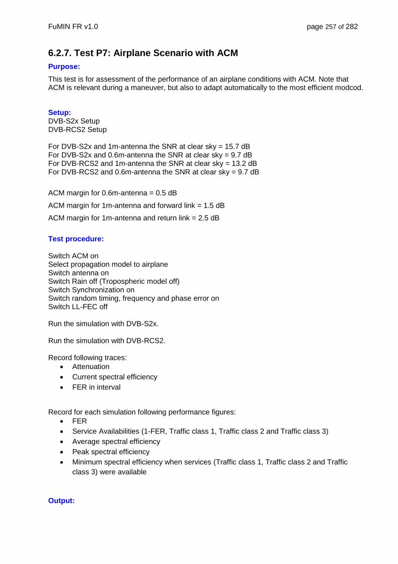
FuMIN FR v1.0 page 257 of 282
6.2.7. Test P7: Airplane Scenario with ACM
Purpose:
This test is for assessment of the performance of an airplane conditions with ACM. Note that ACM is relevant during a maneuver, but also to adapt automatically to the most efficient modcod.
Setup: DVB-S2x Setup DVB-RCS2 Setup For DVB-S2x and 1m-antenna the SNR at clear sky = 15.7 dB For DVB-S2x and 0.6m-antenna the SNR at clear sky = 9.7 dB For DVB-RCS2 and 1m-antenna the SNR at clear sky = 13.2 dB For DVB-RCS2 and 0.6m-antenna the SNR at clear sky = 9.7 dB
ACM margin for 0.6m-antenna = 0.5 dB
ACM margin for 1m-antenna and forward link = 1.5 dB
ACM margin for 1m-antenna and return link = 2.5 dB
Test procedure: Switch ACM on Select propagation model to airplane Switch antenna on Switch Rain off (Tropospheric model off) Switch Synchronization on Switch random timing, frequency and phase error on Switch LL-FEC off Run the simulation with DVB-S2x. Run the simulation with DVB-RCS2. Record following traces:
Attenuation
Current spectral efficiency
FER in interval
Record for each simulation following performance figures:
FER
Service Availabilities (1-FER, Traffic class 1, Traffic class 2 and Traffic class 3)
Average spectral efficiency
Peak spectral efficiency
Minimum spectral efficiency when services (Traffic class 1, Traffic class 2 and Traffic
class 3) were available
Output:
FuMIN FR v1.0 page 258 of 282
Performance figures and curves as defined in the test procedure.
6.2.7.1. DVB-S2X with 0.6m-antenna
Figure 6-57: Attenuation of a three minutes maneuver including the 0.6m-antenna
Table 6-37: Service availabilities
Rain events
FER 1-FER Traffic class 1
Availability Traffic class 2
Availability Traffic class 3
Availability
[ × 1e-3] [%] [%] [%] [%]
no 0 100 100 100 100
Table 6-38: Diverse spectral efficiencies
Rain events
Avg. spectral efficiency
Peak spectral efficiency
Min. spectral efficiency
Traffic class 1
Min. spectral efficiency
Traffic class 2
Min. spectral efficiency
Traffic class 3
[bit/s/Hz] [bit/s/Hz] [bit/s/Hz] [bit/s/Hz] [bit/s/Hz]
no 2.62 3 1.5 1.5 1.5

FuMIN FR v1.0 page 259 of 282
6.2.7.2. DVB-S2X with 1m-antenna
Figure 6-58: Attenuation of a three minutes manoeuvre, with a one meter antenna
Table 6-39: Service availabilities
Rain events
FER 1-FER Traffic class 1
Availability Traffic class 2
Availability Traffic class 3
Availability
[ × 1e-3] [%] [%] [%] [%]
no 0 100 100 100 100
Table 6-40: Diverse spectral efficiencies
Rain events
Avg. spectral efficiency
Peak spectral efficiency
Min. spectral efficiency
Traffic class 1
Min. spectral efficiency
Traffic class 2
Min. spectral efficiency
Traffic class 3
[bit/s/Hz] [bit/s/Hz] [bit/s/Hz] [bit/s/Hz] [bit/s/Hz]
no 3.4 3.6 2.3 2.3 2.3
Conclusions: This scenario shows also for a 1 m and 0.6 m antenna an error free behaviour, with a 100% availability for all services.
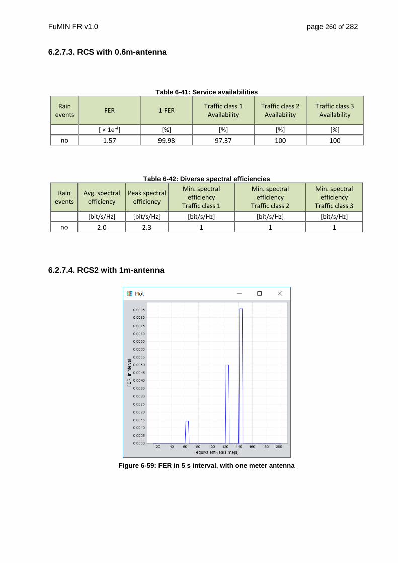
FuMIN FR v1.0 page 260 of 282
6.2.7.3. RCS with 0.6m-antenna
Table 6-41: Service availabilities
Rain events
FER 1-FER Traffic class 1
Availability Traffic class 2
Availability Traffic class 3
Availability
[ × 1e-4] [%] [%] [%] [%]
no 1.57 99.98 97.37 100 100
Table 6-42: Diverse spectral efficiencies
Rain events
Avg. spectral efficiency
Peak spectral efficiency
Min. spectral efficiency
Traffic class 1
Min. spectral efficiency
Traffic class 2
Min. spectral efficiency
Traffic class 3
[bit/s/Hz] [bit/s/Hz] [bit/s/Hz] [bit/s/Hz] [bit/s/Hz]
no 2.0 2.3 1 1 1
6.2.7.4. RCS2 with 1m-antenna
Figure 6-59: FER in 5 s interval, with one meter antenna
FuMIN FR v1.0 page 261 of 282
Table 6-43: Service availabilities
Rain events
FER 1-FER Traffic class 1
Availability Traffic class 2
Availability Traffic class 3
Availability
[ × 1e-4] [%] [%] [%] [%]
no 4.04 99.96 92.31 100 100
Table 6-44: Diverse spectral efficiencies
Rain events
Avg. spectral efficiency
Peak spectral efficiency
Min. spectral efficiency
Traffic class 1
Min. spectral efficiency
Traffic class 2
Min. spectral efficiency
Traffic class 3
[bit/s/Hz] [bit/s/Hz] [bit/s/Hz] [bit/s/Hz] [bit/s/Hz]
no 2.1 2.5 1 1 1
Conclusions: In the return link, the antenna lobes are smaller due to the higher frequency, which leads to a slightly lower FER than in the forward link. Nevertheless just the Traffic class 1 service was affected in the end. For the 1m-antenna this effect was higher, such that the ACM margin was increased to 2dB.
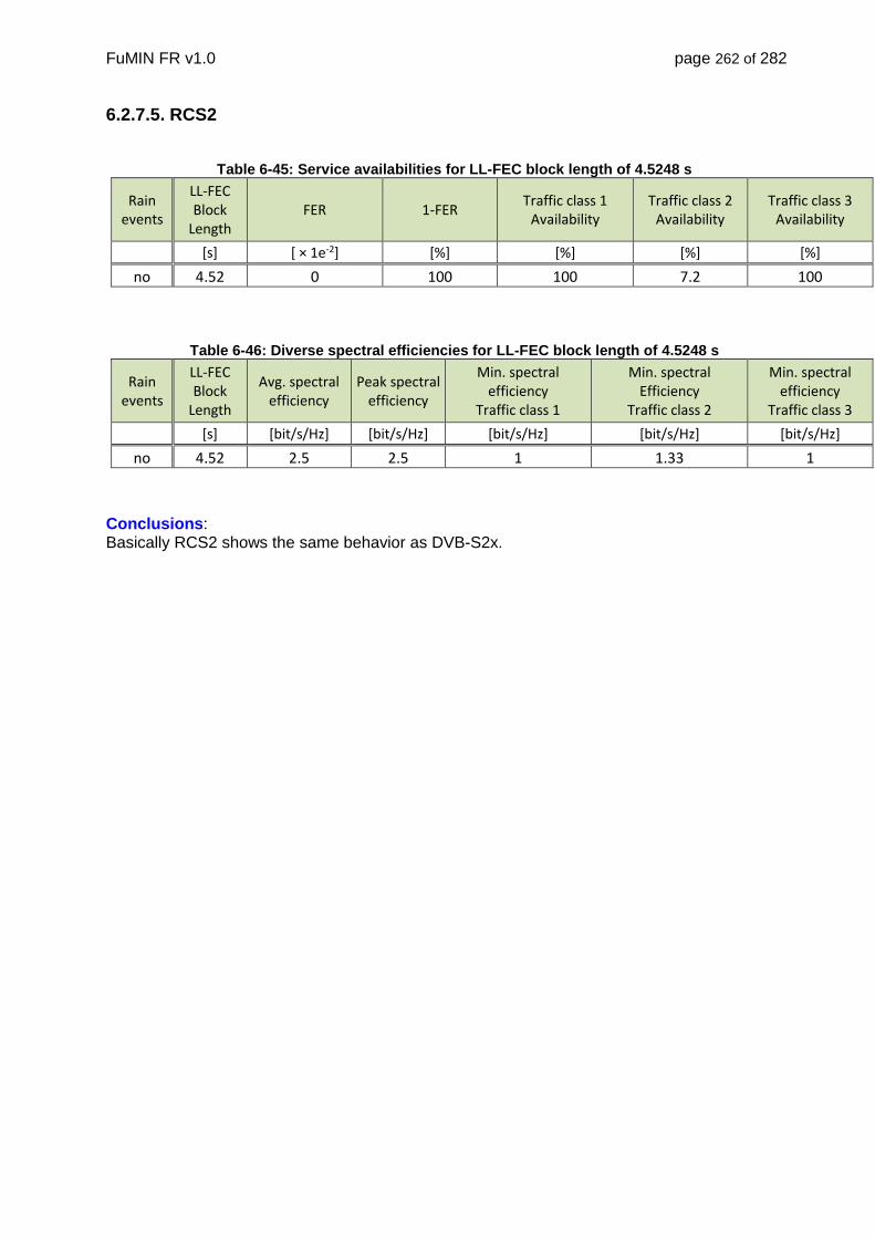
FuMIN FR v1.0 page 262 of 282
6.2.7.5. RCS2
Table 6-45: Service availabilities for LL-FEC block length of 4.5248 s
Rain events
LL-FEC Block
Length FER 1-FER
Traffic class 1 Availability
Traffic class 2 Availability
Traffic class 3 Availability
[s] [ × 1e-2] [%] [%] [%] [%]
no 4.52 0 100 100 7.2 100
Table 6-46: Diverse spectral efficiencies for LL-FEC block length of 4.5248 s
Rain events
LL-FEC Block
Length
Avg. spectral efficiency
Peak spectral efficiency
Min. spectral efficiency
Traffic class 1
Min. spectral Efficiency
Traffic class 2
Min. spectral efficiency
Traffic class 3
[s] [bit/s/Hz] [bit/s/Hz] [bit/s/Hz] [bit/s/Hz] [bit/s/Hz]
no 4.52 2.5 2.5 1 1.33 1
Conclusions: Basically RCS2 shows the same behavior as DVB-S2x.

FuMIN FR v1.0 page 263 of 282
6.3. Scenarios with Impaired Channel
In this section, the tests from section 3.1 are repeated to assess the degradation from the channel non-linear effects and the phase noise. The degradation for RCS2 due to non-linear effects on the transponder effect the feeder link and this has not been considered in the project.
The phase noise contribution from the terminal for the return link is with BPSK, QPSK and 8PSK rather low (<0.4dB). Note that 16QAM is not used in any of the scenarios. Consequently, the results for RCS2 are quasi identical to the Tests from section 3.1, and are therefore not repeated.
Note also that the configuration of the clear sky SNR is made identical with the value in the Tests from section 3.1, such that the degradation due phase noise and non-linear distortions can be assessed. With other words, the OBO is identical in the present section and section 3.1. As given in the link budget (section 4), the OBO is set to 1.1 dB, which is optimal for APSK operation.
6.3.1. Test P7: Line of Sight – Moving Terminal with ACM
Purpose:
This test is for assessment of the performance of a moving terminal under rain conditions with ACM.
Setup: DVB-S2x Setup 1m antenna For DVB-S2x and 1m-antenna the SNR at clear sky = 15.7 dB ACM margin =1.5dB
Test procedure: Switch ACM on Select propagation model off. Switch Rain on (Tropospheric model on) Switch LL-FEC off Run the simulation with DVB-S2x. Record following traces:
Attenuation
Current spectral efficiency
FER in interval
Record for each simulation following performance figures:
FER
Service Availabilities (1-FER, Traffic class 1, Traffic class 2 and Traffic class 3)
Average spectral efficiency
Peak spectral efficiency
Minimum spectral efficiency when services (Traffic class 1, Traffic class 2 and Traffic

FuMIN FR v1.0 page 264 of 282
class 3) were available
Output:
Performance figures and curves as defined in the test procedure.
Table 6-47: Service availabilities
Rain events
FER 1-FER Traffic class 1
Availability Traffic class 2
Availability Traffic class 3
Availability
[ × 1e-5] [%] [%] [%] [%]
light 0.76 99.99 100 100 100
heavy 1.22 99.99 100 100 100
Table 6-48: Diverse spectral efficiencies
Rain events
Avg. spectral efficiency
Peak spectral efficiency
Min. spectral efficiency
Traffic class 1
Min. spectral efficiency
Traffic class 2
Min. spectral efficiency
Traffic class 3
[bit/s/Hz] [bit/s/Hz] [bit/s/Hz] [bit/s/Hz] [bit/s/Hz]
light 2.94 3 2.47 2.47 2.47
heavy 2.37 3 0.89 0.89 0.89
Conclusions: The service availabilities were, with an ACM margin of 1.5dB for the 1m-antenna, practically 100% similar to Test P2. The spectral efficiency is slightly smaller (around 10%) according to the channel degradations. Note that the clear sky SNR was identical to test P2.

FuMIN FR v1.0 page 265 of 282
6.3.2. Test P8: Vehicular Scenario with ACM and Channel Impairments
Purpose:
This test is for assessment of the performance on an ideal transponder of a vehicular under clear sky conditions.
Setup: DVB-S2x Setup 0.6m antenna For DVB-S2x and 0.6m-antenna the SNR at clear sky = 9.7 dB ACM margin =0.5dB
Test procedure: Switch ACM on Select propagation model to vehicular. Switch Rain on (Tropospheric model on) Switch Synchronization on Switch random timing, frequency and phase error on. Switch LL-FEC on Switch phase noise and non-linearity on. Run the simulation with DVB-S2x. Record following traces:
Attenuation
Current spectral efficiency
FER in interval
Record for each simulation following performance figures:
FER
Service Availabilities (1-FER, Traffic class 1, Traffic class 2 and Traffic class 3)
Average spectral efficiency
Peak spectral efficiency
Minimum spectral efficiency when services (Traffic class 1, Traffic class 2 and Traffic
class 3) were available
Output:
Performance figures and curves as defined in the test procedure.

FuMIN FR v1.0 page 266 of 282
Table 6-49: Service availabilities for varying LL-FEC values
Rain events
LL-FEC Block
Length FER 1-FER
Traffic class 1 Availability
Traffic class 2 Availability
Traffic class 3 Availability
[s] [ × 1e-2] [%] [%] [%] [%]
light 1.94 0 100 98.43 21.50 98.43
heavy 1.94 0 100 98.58 30.96 98.87
Table 6-50: Diverse spectral efficiencies for varying LL-FEC values
Rain events
LL-FEC Block
Length
Avg. spectral efficiency
Peak spectral efficiency
Min. spectral efficiency
Traffic class 1
Min. spectral efficiency
Traffic class 2
Min. spectral efficiency
Traffic class 3
[s] [bit/s/Hz] [bit/s/Hz] [bit/s/Hz] [bit/s/Hz] [bit/s/Hz]
light 1.94 2.3 2.7 1.5 1.5 1.5
heavy 1.94 1.9 2.7 0.3 0.3 0.3
Conclusions: The results are similar to Test P4, with a reduction of the spectral efficiencies. For train a LL-FEC length of around 2-3s was recommended in Test P6 and is therefore used here.

FuMIN FR v1.0 page 267 of 282
6.3.3. Test P9: Train Scenario with ACM and Channel Impairments
Purpose:
This test is for assessment of the performance of a train under rain conditions with ACM.
Setup: DVB-S2x Setup 1m antenna For DVB-S2x and 1m-antenna the SNR at clear sky = 15.7 dB ACM margin =0.5dB
Test procedure: Switch ACM on Select propagation model to train. Switch Rain on Switch Synchronization on Switch random timing, frequency and phase error on. Switch LL-FEC on Switch phase noise and non-linearity on. Run the simulation with DVB-S2x. Record following traces:
Attenuation
Current spectral efficiency
FER in interval
Record for each simulation following performance figures:
FER
Service Availabilities (1-FER, Traffic class 1, Traffic class 2 and Traffic class 3)
Average spectral efficiency
Peak spectral efficiency
Minimum spectral efficiency when services (Traffic class 1, Traffic class 2 and Traffic
class 3) were available
Output:
Performance figures and curves as defined in the test procedure.

FuMIN FR v1.0 page 268 of 282
Table 6-51: Service availabilities for varying LL-FEC values
Rain events
LL-FEC Block
Length FER 1-FER
Traffic class 1 Availability
Traffic class 2 Availability
Traffic class 3 Availability
[s] [ × 1e-3] [%] [%] [%] [%]
light 1.5 2.34 99.77 96.77 1.61 98.77
heavy 1.5 3.26 99.67 96.10 0.65 96.10
Table 6-52: Diverse spectral efficiencies for varying LL-FEC values
Rain events
LL-FEC Block
Length
Avg. spectral efficiency
Peak spectral efficiency
Min. spectral efficiency
Traffic class 1
Min. spectral efficiency
Traffic class 2
Min. spectral efficiency
Traffic class 3
[s] [bit/s/Hz] [bit/s/Hz] [bit/s/Hz] [bit/s/Hz] [bit/s/Hz]
light 1.5 3.0 3.6 2.7 na 2.7
heavy 1.5 2.4 3.6 1 na 1
Conclusions: The results are similar to Test P6, with a reduction of the spectral efficiencies. For train a LL-FEC length of around 1-2s was recommended in Test P6 and is therefore used here.

FuMIN FR v1.0 page 269 of 282
6.3.4. Test P10: Airplane Scenario with ACM and Channel Impairments
Purpose:
This test is for assessment of the performance of an airplane conditions with ACM. Note that ACM is relevant during a maneuver, but also to adapt automatically to the most efficient modcod.
Setup: DVB-S2x Setup For DVB-S2x and 0.6m-antenna the SNR at clear sky = 9.7 dB
ACM margin for 0.6m-antenna = 0.5 dB
Test procedure: Switch ACM on Select propagation model to airplane Switch antenna on Switch Rain off (Tropospheric model off) Switch Synchronization on Switch random timing, frequency and phase error on Switch LL-FEC off Run the simulation with DVB-S2x. Record following traces:
Attenuation
Current spectral efficiency
FER in interval
Record for each simulation following performance figures:
FER
Service Availabilities (1-FER, Traffic class 1, Traffic class 2 and Traffic class 3)
Average spectral efficiency
Peak spectral efficiency
Minimum spectral efficiency when services (Traffic class 1, Traffic class 2 and Traffic
class 3) were available
Output:
Performance figures and curves as defined in the test procedure.

FuMIN FR v1.0 page 270 of 282
Table 6-53: Service availabilities
Rain events
FER 1-FER Traffic class 1
Availability Traffic class 2
Availability Traffic class 3
Availability
[ × 1e-5] [%] [%] [%] [%]
no 2.11 99.99 100 100 100
Table 6-54: Diverse spectral efficiencies
Rain events
Avg. spectral efficiency
Peak spectral efficiency
Min. spectral efficiency
Traffic class 1
Min. spectral efficiency
Traffic class 2
Min. spectral efficiency
Traffic class 3
[bit/s/Hz] [bit/s/Hz] [bit/s/Hz] [bit/s/Hz] [bit/s/Hz]
no 2.3 2.7 1.5 1.5 1.5
Conclusions: The results are similar to Test P7, with a reduction of the spectral efficiencies.

FuMIN FR v1.0 page 271 of 282
7. Conclusions and Tradeoffs
7.1. Air Interface Aspects
DVB-S2x [RD96]and DVB-RCS2 has been used as protocols for forward and return link respectively. In the following some conclusions from the project are drawn:
7.1.1. Forward Link
For DVB-S2x, the superframe (option E) is recommended [RD37], since very low (VL-) SNR modcod are supported within mode 0. Furthermore, the superframe enables differentiation between mobile and other services by identification of the mobile service utilizing one of the reserved SFFI’s, e.g. SFFI number 5.
However, definition of a new SFFI number is not necessary for mobile services, except a physical layer interleaver would be used. In this case, signalling of the interleaver profile must be supported in addition to the present DVB-S2x standard. Anyhow as outlined below (section 7.3), use of a PL-interleaver is not recommended.
Fast (warm) acquisition to the carrier is very important, since during blockages carrier synchronization will be lost, and after the blockage the communication should be established as fast as possible. With superframes this can be achieved typically within 3 superframes (SF) even at very low operational points, i.e. at -10dB SNR.
Carrier synchronization has been done with a Quadri-Correlator (QC) for coarse frequency. After settling of the QC (3 SF) a DA loop using the LR algorithm takes over the loop for fine frequency synchronization. Timing estimation has been distinguished between coarse and fine timing estimation. Coarse timing estimation has been based on measurement of the distances between adjacent superframes. Initial correction and tracking achieves an accuracy of 1ppm, which is sufficient to apply the Data Aided algorithm using the pilot fields for fine timing estimation.
Over all we achieved with that approach a robustness against timing offsets of 100 ppm as well as 10% of the symbol rate for frequency offsets. The performance degradation with that synchronization approach versus an ideal AWGN channel was typically between 0.1 and 0.3 dB.
In sum the average duration for cold acquisition is 30 SF or 1.837 seconds for a carrier with 10MS/s. When the frame acquisition is not able to detect significant peaks at the defined correlation window primary, shadowing is assumed and the actual setup of frequency error and drift is frozen.
Assuming a residual drift of 1ppm the correlation peak is shifted by +/-10 symbols in one second. Opening up the correlation window from +/-4 symbols again up to +/-100 symbols 10 seconds survive time are possible. Assuming a normalized Doppler rate of dfTs=0.0001/s after 10 seconds the frequency step is dfts=0.001. This step causes a slight overshoot and resettling. So during of 5 SFs a higher FER is probable.
7.1.2. Return Link
Regarding RCS2, the waveform-id’s (WID) defined in the RCS2 standard has been considered. The WID with the lowest operational point that has been used from the standard was QPSK-1/3, which offers quasi error free transmission down to an SNR of 0 dB.

FuMIN FR v1.0 page 272 of 282
Synchronization was done on a burst-by-burst basis. This means that each burst was individually acquired within a frequency offset of 3 % of the symbol range and within a timing offset of +/-0.5 symbols. The algorithmic approach was the modified Rife-Boorstyn algorithm for frequency and the Oerder&Meyer algorithm for timing synchronization.
TDMA framing is established by means of TDMA frame with a fixed duration. The start of the TDMA frame is indicated by a large unique word (800symbols), This allows to perform TDMA-like synchronization, and was necessary as the TDMA access system (MAC-layer) was not implemented in the prototype. Nevertheless, synchronization of the burst position by means of correlation with the burst pilot symbols (preamble, postamble and pilots) was established similar to a complete TDMA system.
For lower operational points down to an SNR of -10dB, a self-designed synchronization approach was implemented. The motivation for that was the fact that especially frequency synchronization at low operational points done on a relatively short burst, leads either to larger synchronization losses or requires a lot of overhead in form of pilot symbols.
The chosen approach is based on BPSK and a Turbo codec with a code-rate of 1/3 concatenated with a repetition code with rate 2, 4 and 6. In addition, a CRC is added to the burst payload. Note that the air interface regarding the burst format is compatible to the RCS2 standard, even if the configuration is not part of the WID list given in Table 7-1: Proprietary waveform IDs added to the implementation of DVB-RCS2.
Reception of a burst is done with a joint synchronization and decoding approach based a CRC-aided frequency scanning. This results in a robust system with good performance and moderate overheads.
Table 7-1: Proprietary waveform IDs added to the implementation of DVB-RCS2
Waveform
Burst payload length
in
symbols
Total UW lengths in
symbols
Overhead in %
BPSK-1/3 1272 80 6.3
BPSK-1/6 2544 160 6.3
BPSK-1/12 5088 240 4.7
BPSK-1/18 7632 320 4.2
7.2. ACM
Considering possible antenna sizes, different satellite EIRP’s, different use cases and atmospheric conditions, a significant dynamic range of the link budget has to be considered. At least an SNR range between +15dB and -5dB for DVB-S2x and +10 to -10dB for RCS2 should be supported by a potential product.

FuMIN FR v1.0 page 273 of 282
Clearly, ACM is required in order to adapt to the varying channel conditions. In principle, ACM is a simple mechanism that performs following steps:
(i) Measure the channel conditions at the receiver
(ii) Signal the value back to the transmitter: This has to be done over the link in the other
direction, which imposes a certain latency to the switching, the so-called ACM dead-time.
The ACM dead-time should be as small as possible, but typically it is around 1s (1 hop back
to the transmitter + 1 hop until the new modcod is active at the receiver).
(iii) Adapt the modcod such that the packet error rate is low: For each modcod, there is a certain
SNR threshold associated with the quasi error free (FER<1e-5) performance. However, the
channel attenuation is varying especially during a fade event. Due to the ACM dead-time,
there would frame errors appear when the SNR is dropping and we would switch exact on
the SNR threshold. To avoid this a certain ACM margin is added to the SNR threshold.
For (i), i.e. measuring of the channel condition, we have considered 3 different methods:
SNR estimation: Data-aided statistical analyses estimates direct the SNR.
Measuring of the LDPC / Turbo iterations: When using early stop criteria, the required
number of iterations is on the average depending on the distance to the SNR threshold of
the currently active modcod. This way the SNR can be estimated via a mapping table that
stores the relation between number of iterations and SNR.
Symbol error detection of pilot symbols: The relation between SNR and symbol error
probability is known for a given modulation scheme. The bit error probability can be
measured on known pilot symbols (e.g. the SoSF + SFFI header) and the SNR can be
estimated
After initial test, the direct SNR estimation method was chosen, as it provides the most accurate results. The problem with the iteration-based method was that the average iteration value is quite insignificant when the real SNR is more than 0.5dB larger than the SNR threshold. Since in many cases an ACM margin has to be added, the performance of this method would is quite low in practice. For the symbol error detection method, the problem is that at high SNR, e.g. in an SNR range suitable for APSK modcods, the symbol error probability of BPSK is quite low (<1e-4). Therefore symbol errors are quite rare, and the accuracy is consequently low.
In contrast, the direct SNR estimation method works sufficiently and with an averaging of 50ms the estimation error was typically below 0.2dB (sigma).
As already mentioned above, blockages leads to synchronization losses and consequently no SNR measurement is possible anymore. Usually the strategy follow in ACM systems when reception is interrupted is to switch to the most robust modcod. It turned out that this approach is not optimal, since it takes some extra time (in the order of the ACM dead-time) to ramp up to the suitable modcod after the blockage.
This can be effectively avoided, when the system, i.e. receiver and transmitter degrades the estimated SNR slowly from the last measured value during a blockage. The estimated SNR reduction rate should follow the possible negative SNR slopes expected on the channel due to the atmospheric events. A suitable value would by 0.5dB/s for Ka-band. So for instance after a blockage of 2s, the data transfer immediately continues with one modcod step lower, which is in practice nearly the same rate as before.

FuMIN FR v1.0 page 274 of 282
7.3. FEC of Blockages
Blockages in the path towards the satellite cut the link completely. In practice, the FER performance is quasi dominated by these blockages. A way to mitigate this effect is to distribute the transmitted information in time (time diversity) in order to enable a forward error correction approach to repair the lost data.
Two approaches of FEC approaches counter-measuring data loss during blockages have been considered, i.e. link layer FEC: and physical layer (PL) interleaver. The PL-interleaver spreads the information bits in time but introduces itself no redundancy in form of check bits. Instead, the channel code performs the corrections. This would be successfully if the errors from the channel and the errors from the blockage together do not exceed the correction capability of the code.
In contrast, the LL-FEC takes the packets on the link layer as basic entities and adds additional redundant parity packets to them, which enable correction of lost packets. Typically, and in our implementation, this is based on erasure decoding. This means that the decoder knows - based on a CRC - beforehand which packet is wrong or missing and which packet is correct.
From the information theoretical point of view, the redundancy introduced by the LL-FEC is better devoted to the PL-interleaver. However, there is an important drawback of the PL-interleaver. In order to enable interleaving at the transmitter side, all the information bits from the interleaver length have to be stored, and so the PL-interleaver adds a constant latency to the transmission. This latency affects the interactive traffic even when there is line of sight, and together with the required length of the PL-interleaver (at least seconds are necessary!), this would be inacceptable for interactive services.
The decoder of a LL-FEC can acts in a different way. When just valid packet enters the decoder they can be transferred immediately to the output, without adding any additional latency. When a corrupt packets are received, the LL-FEC decoder has to wait until enough valid packets are collected until the corrupt packets can be reconstructed. It is not in every case necessary to wait until a complete LL-FEC block has been collected in the LL-FEC decoder.
Consequently, the additional latency depends on the blockage and the LL-FEC block length, and, in case there is currently a blockage on the channel, the latency would be in the order of the blockage duration. Under LOS conditions, the additional latency is quasi zero. A user would expect such a behaviour.
The disadvantage of LL-FEC is the additional redundancy, which reduces the throughput. LL-FEC coderates between 0.5 and 0.75 are necessary to countermeasure effectively blockages as they appear in typical scenarios.
The question, if there should be a LL-FEC present or not, and which LL-FEC block length and coderate is suitable depends on the scenario and the type of traffic, or with other words, there cannot be a general answer.
7.4. Application, QoS and Higher Layer Aspects
7.4.1. Impacts to QoS
Interactive mobile satellite communication is strongly effected by blockages on the channel, e.g. by houses, trees or overpasses that block the line of sight to the satellite. Since the used antenna dishes are directionally, practically no multipaths can be utilized to increase connectivity as common practice with terrestrial communication schemes. As mentioned above, blockages can be made error free by means of a LL-FEC, on the cost of additional latency and throughput.

FuMIN FR v1.0 page 275 of 282
In order to discuss the impact of blockages on different types of traffic, we first have to look at different impacts on the QoS. In fact, we have to differentiate between following aspects:
Singular, uniform distributed frame errors: Such an error distribution appear when the SNR
threshold of the selected modcod is lower than the current SNR on the channel. Since the
codecs used in DVB-S2x and RCS2 are very strong, and with adequate tuning of the ACM
control loop (ACM margin), such errors can be avoided in practice).
Block of frame errors: Such an error behaviour appear during a blockage on the mobile
channel, when there is no LL-FEC, or the LL-FEC is not sufficient.
Latency: A satellite link over a geostationary satellite has a one-way latency of 270ms. As
described in the section before, LL_FEC add during blockages latency to that. In fact, this
latency might be problematic for interactive traffic, and could be a better decision to accept
packet losses instead.
Throughput: DVB-S2x as well as RCS2 have already a Shannon-bound approaching
performance. However, with an LL-FEC the available throughput will be reduced significant.
As a consequence, download times will be reduced accordingly.
7.4.2. TCP and HTTP Issues
In general TCP performance depends on the latency-bandwidth product (long-fat pipe) and on the packet errors. Reason is the limited TCP protocol-windows size and the TCP congestion algorithm, which interprets packet errors as congestions on the channel.
A TCP performance enhancement proxy (PEP) avoids these problems, as it intercepts the TCP connection and transmits the data via a proprietary transport mechanism suitable for the satellite link.
A further problem arise with HTTP tape of traffic, e.g. with web-browsing. Web pages consists of a lot of small files, which are at-least partly loaded sequentially. For instance, the download of a web page starts with a file “main.http”, which contains links on further files, like gif-files for small icons, etc. together with the latency over the geostationary satellite, loading of a web-page appears to be very slow, even if enough bandwidth is available.
Again PEPs are necessary as they organize pre-fetching of web pages. To continue with the aforementioned example, together with the “main.http”, the linked additional files, e.g. the gif’s, are requested immediately with by the PEP that sits on the transmit side of the satellite link.
PEP’s are today state of the art in satellite communication, and clearly recommended for the envisaged mobile use cases. It is also mentioned here that with VPN tunnels, PEPs do not work, since the TCP header is encrypted by IP-SEC. Consequently, VPN tunnels should be avoided or even blocked in the mobile satcom network.
With PEPs, packet error rate and latency is less critical, and instead of heading for 1e-6 packet error rate as mentioned in the DVB-S2x standard, we are happy with 1e-2 to 1e-3 for file transfers. Similar, with latencies of 2-3s the loading of simple web pages is still fast, and it can be expected that interactive web-based applications still work satisfactory, when this latency appears just during blockages and not permanently.

FuMIN FR v1.0 page 276 of 282
7.4.3. Impacts to Traffic
Considering a system following the conclusions given above, as well as the results from the end-to-end performance assessment study given in section 6, we can conclude on the performance and behaviour for different types of traffic.
File transfer without latency requirements: Assuming that a TCP-PEP is used, the most important feature is good-put over the link. The FER is less critical, but should be lower than 0.01 to avoid extensive retransmissions in order to optimize the good-put. Blockages are less critical as retransmissions are done in a continuous block, which minimizes overhead. Consequently, no LL-FEC is recommended.
Interactive data transfer, web browsing: Latency should be low in general. If from time to time, e.g. during a short blockage, latency increases to several seconds, this is not a big problem. If packet errors happen, a retransmission will occur, which increases the latency in addition. So the requirement would be to limit the FER to 1e-3 and the acceptable latency to 2.5s one way. An LL-FEC recommended especially for the train scenario to avoid short blockages from electric poles.
Video streaming (unidirectional): There is practically no latency requirement, and use of a LL-FEC is recommended. The performance of videos is ok, when the ESR5(20) (less than 5% error in a 20s interval) is satisfied.
Interactive Audio: This type of service is very sensitive to latency. A peak one-way latency of 500ms is still working, but already sensed as very low quality by the users. The FER is less critical and should be better than 1e-2. Consequently, if a LL-FEC is considered, the LL-FEC block-length has to be limited to 230ms in order to limit the one-way latency (single hop over the satellite link) to 500ms.

FuMIN FR v1.0 page 277 of 282
7.5. Summary from the System Performance Analyses
During the project, a performance analyses on selected scenarios has been done. Table 7-1: Proprietary waveform IDs added to the implementation of DVB-RCS2summarizes the satellite link parameters, and in Table 7-3 the summary of the mobile scenarios are given. Based on this inputs the SNIR and achievable throughputs are given in Table 7-4.
Table 7-2: Summary of the satellite link parameters
Satellite architecture Multibeam, 4-color
Downlink frequency 20 GHz
Uplink frequency 30 GHz
Forward link BW 50MHz / 41.7Mbaud
Return Link BW 5MHz / 4Mbaud
Satellite EIRP 55dBW @ 50MHz
OBO 1.1 dB Determined from
optimum for APSK
Satellite G/T 17.5 dB/K
Total Interference beam centre (1m
antenna)
22.7 dB From co - and
adjacent satellite
links
Total Interference beam border (1m
antenna)
16.2 dB
Total Interference beam centre (0.6m
antenna)
19.4 dB
Total Interference beam border (0.6m
antenna)
15.2 dB
Table 7-3: Summary of the different use cases with parameter settings for ACM and LL-FEC
Railway Scenario Aeronautical Scenario Vehicular Scenario

FuMIN FR v1.0 page 278 of 282
Terminal Size 1m 0.6m 0.6m
Propagation Channel Clear sky, light and
heavy rain events as
scenarios
No significant
atmospheric effects
Clear sky, light and
heavy rain events as
scenarios
Mobile Channel Line of sight channel,
channel with poles and
overpasses as
scenarios
Airplane maneuver as
scenario
Line of sight channel,
channel with blockages
(rural area) as scenario
ACM Margin forward 1.5 dB 1 dB 0.5 dB
ACM Margin return 2.5 dB 1.5 dB 1 dB
LL-FEC length 0.3 s na 0.7s
LL-FEC coderate 0.75 na 0.5
Table 7-4: Summary of the resulting SNIR’s and throughputs
Railway Scenario Aeronautical Scenario Vehicular Scenario
Forward link, beam
center, clear sky
SNIR/throughput
SNIR=15.7dB
TP=111Mbit/s
SNIR=11.4dB
TP=111Mbit/s
SNIR=11.4dB
TP=55Mbit/s
Forward link, beam
center, light rain
SNIR=10.5dB
TP=70Mbit/s
na SNIR=6.1dB
TP=31Mbit/s
Forward link, beam
center, heavy rain
SNIR/throughput
SNIR=1.9dB
TP=31Mbit/s
na SNIR=-2.5dB
TP=7Mbit/s
Forward link, beam
border, clear sky
SNIR/throughput
SNIR=11.7dB
TP=83Mbit/s
SNIR=8.2dB
TP=83Mbit/s
SNIR=8.2dB
TP=42Mbit/s
Forward link, beam
border, light rain
SNIR/throughput
SNIR=7.2dB
TP=52Mbit/s
na SNIR=3.1dB
TP=21Mbit/s
Forward link, beam
border, heavy rain
SNIR/throughput
SNIR=-1.1dB
TP=17Mbit/s
na SNIR=-5.5dB
TP=2Mbit/s

FuMIN FR v1.0 page 279 of 282
Return link, beam
center, clear sky
SNIR/throughput
SNIR=13.2dB
TP=7.5Mbit/s
SNIR=9.5dB
TP=6.7Mbit/s
SNIR=9.5dB
TP=2.7Mbit/s
Return link, beam
center, light rain
SNIR=7.7dB
TP=5Mbit/s
na SNIR=3.4dB
TP=2Mbit/s
Return link, beam
center, heavy rain
SNIR/throughput
SNIR=2.2dB
TP=2Mbit/s
na SNIR=-3.2dB
TP=0.6Mbit/s
Return link, beam
border, clear sky
SNIR/throughput
SNIR=9.9dB
TP=7Mbit/s
SNIR=6.3dB
TP=6Mbit/s
SNIR=6.3dB
TP=3Mbit/s
Return link, beam
border, light rain
SNIR/throughput
SNIR=4.6dB
TP=3Mbit/s
na SNIR=0.4dB
TP=0.6Mbit/s
Return link, beam
border, heavy rain
SNIR/throughput
SNIR=-0.8dB
TP=1Mbit/s
na SNIR=-5.2dB
TP=0.2Mbit/s
The different mobile scenarios have specific effects on the link. As already mentioned above, blockages determine the channel practically. With respect to the QoS requirements of the different types of traffic, we get service availabilities as shown in Figure 7-1 and Figure 7-2 as examples for the train and vehicular (rural) scenario respectively.
As illustrated phone availability is rather small due to the latencies introduced by the required LL-FEC countermeasuring the blockage losses. So practically, this type of traffic would be not recommended for that kind of mobile satellite service.
For other types of traffic a LL-FEC of 2-3 seconds block length will lead to an acceptable behavior. Note that the vehicular scenarios was rural in the sense that blockages are quite rare and mostly short. For urban or even suburban locations, this approach would not lead to an acceptable user experience.

FuMIN FR v1.0 page 280 of 282
Figure 7-1: Service availabilities as a function of the LL-FEC block length for the train scenario with train speed of 100km/s
Figure 7-2: Service availabilities as a function of the LL-FEC block length for the vehicular scenario
with vehicular speed of 100km/s
FuMIN FR v1.0 page 281 of 282
8. Roadmap to a Product
8.1. Technological Challenges
One potential problem that appears at the way to a product is the antenna of the user terminal. Cost effective terminal antenna that are dedicated for reception only, i.e. for broadcasting services, will be problematic for return link transmission as they potentially violate the off-boresight requirement. It is also a question, if patch arrays as for instance recently developed by Satixfy [RD116] would be suitable regarding these requirements.
Consequently, we end up with a parabolic full motion tracking antenna dish. Such products are available on the market. However, the available solutions are relatively expensive, such that development of a cost-effective tracking antenna would be a key factor for a business plan.
As already mentioned before, DVB-S2x as well as DVB-RCS2 are sufficient as air-interface and a good solution for a product. In addition, the modem has to copy with a number of functions mandatory for the mobile use case, which are:
Support of low operational points, i.e. -10dB SNR
Range of modcods / wids from -10dB to 20dB SNR
ACM
LL-FEC
To our knowledge no off-the-shelf modem is on the market that supports all these functions. Nevertheless, modem development could be based for instance on an available ASIC SX-3000 from Satixfy [RD117] that allow to implement these functions in a software designed way.
8.2. Technological Roadmap
Towards to a successful and future-proof end-user product following steps are recommended:
Step 1: Functional Prototype
System capable to demonstrate mobile services in the field.
Off-the-shelf steerable antenna.
SDR based modem to be developed supporting symbol rates around 10 – 20 Mbaud.
Hub with off-the-shelf equipment and development of additional functions for mobile
services, like LL-FEC, support of low SNR, supporting just a few user terminals
Development / integration of end-user applications and higher layer functions (e.g. PEP)
Step 2: Product Prototype
System that based already on final components.
Development of cost effective mechanical steerable antenna
ASIC-based end-user modem supporting symbol rates up to 250Mbaud
Hub supporting a high number of user terminals
Step 3: Product for terrestrial scenarios
User terminal fully integrated in a design suitable for vehicular, e.g. cars, trucks, trains
Low price

FuMIN FR v1.0 page 282 of 282
Step 4: Product for airborne scenario
Adaptions to reach qualification for airborne application
Development of a cost-effective airborne antenna
Interface for airborne entertainment systems
Step 5: Future developments
Integration of terrestrial 5G systems
Related Documents