arXiv:1102.2457v1 [math.NT] 11 Feb 2011 ARCHIMEDEAN ZETA INTEGRALS ON GL n × GL m AND SO 2n+1 × GL m TAKU ISHII AND ERIC STADE Abstract. In this paper, we evaluate archimedean zeta integrals for automorphic L- functions on GL n × GL n-1+ℓ and on SO 2n+1 × GL n+ℓ , for ℓ = −1, 0, and 1. In each of these cases, the zeta integrals in question may be expressed as Mellin transforms of prod- ucts of class one Whittaker functions. Here, we obtain explicit expressions for these Mellin transforms in terms of Gamma functions and Barnes integrals. When ℓ = 0 or ℓ = 1, the archimedean zeta integrals amount to integrals over the full torus. We show that, as has been predicted by Bump for such domains of integration, these zeta integrals are equal to the corresponding local L-factors – which are simple rational combinations of Gamma functions. In the cases of GL n × GL n-1 and GL n × GL n this has, in large part, been shown previously by the second author of the present work, though the results here are more general in that they do not require the assumption of trivial central characters. (Our techniques here are also quite different. New formulas for GL(n, R) Whittaker functions, obtained recently by the authors of this work, allow for substantially simplifed computations.) For the cases of SO 2n+1 × GL n and SO 2n+1 × GL n+1 , results such as these have been deduced previously only for a few instances of small rank. In the case ℓ = −1, we express our archimedean zeta integrals explicitly in terms of Gamma functions and certain Barnes-type integrals. These evaluations rely on new recursive formulas, derived herein, for GL(n, R) Whittaker functions. Our results concerning these zeta integrals, in these situations, generalize work of Hoffstein and Murty for the case of GL 3 × GL 1 , and parallel similar results, obtained by the first author of the present work and by Moriyama, for the spinor L-function on GSp 2 . Finally, in our appendix, we indicate an approach to certain unramified calculations, on SO 2n+1 × GL n and SO 2n+1 × GL n+1 , that parallels our method in the correspond- ing archimedean situation. While the unramified theory has already been treated using more direct methods, we hope that the connections evoked herein might facilitate future archimedean computations. Introduction In this paper we investigate the behavior, at archimedean places, of zeta integrals associ- ated to certain automorphic forms and L-functions, and develop explicit formulas for these integrals at such places. More specifically: let G and G ′ be reductive algebraic groups; let π and π ′ be automorphic cuspidal representations of G(A) and G ′ (A) respectively, where A denotes the adeles over a global field F . Following Langlands [20], one may define a global L-function L(s,π × π ′ ), for s ∈ C of sufficiently large real part. The Langlands program then predicts that L(s,π × π ′ ) should admit meromorphic continuation in s (with only finitely many poles in C), and a functional equation under (π,π ′ ,s) → (π ∨ , (π ′ ) ∨ , 1 − s) (where π ∨ and (π ′ ) ∨ are the representations contragredient to π and π ′ , respectively). An especially powerful and fruitful approach to the study of L(s,π × π ′ ) is through the zeta-integral method. At the core of this method is the construction of a certain “global zeta Date : February 15, 2011. 1

Welcome message from author
This document is posted to help you gain knowledge. Please leave a comment to let me know what you think about it! Share it to your friends and learn new things together.
Transcript
arX
iv:1
102.
2457
v1 [
mat
h.N
T]
11
Feb
2011
ARCHIMEDEAN ZETA INTEGRALS ON GLn ×GLm AND SO2n+1 ×GLm
TAKU ISHII AND ERIC STADE
Abstract. In this paper, we evaluate archimedean zeta integrals for automorphic L-functions on GLn × GLn−1+ℓ and on SO2n+1 × GLn+ℓ, for ℓ = −1, 0, and 1. In eachof these cases, the zeta integrals in question may be expressed as Mellin transforms of prod-ucts of class one Whittaker functions. Here, we obtain explicit expressions for these Mellintransforms in terms of Gamma functions and Barnes integrals.
When ℓ = 0 or ℓ = 1, the archimedean zeta integrals amount to integrals over the fulltorus. We show that, as has been predicted by Bump for such domains of integration, thesezeta integrals are equal to the corresponding local L-factors – which are simple rationalcombinations of Gamma functions. In the cases of GLn × GLn−1 and GLn × GLn thishas, in large part, been shown previously by the second author of the present work, thoughthe results here are more general in that they do not require the assumption of trivialcentral characters. (Our techniques here are also quite different. New formulas for GL(n,R)Whittaker functions, obtained recently by the authors of this work, allow for substantiallysimplifed computations.) For the cases of SO2n+1×GLn and SO2n+1×GLn+1, results suchas these have been deduced previously only for a few instances of small rank.
In the case ℓ = −1, we express our archimedean zeta integrals explicitly in terms ofGamma functions and certain Barnes-type integrals. These evaluations rely on new recursiveformulas, derived herein, for GL(n,R) Whittaker functions. Our results concerning thesezeta integrals, in these situations, generalize work of Hoffstein and Murty for the case ofGL3 × GL1, and parallel similar results, obtained by the first author of the present workand by Moriyama, for the spinor L-function on GSp2.
Finally, in our appendix, we indicate an approach to certain unramified calculations,on SO2n+1 × GLn and SO2n+1 × GLn+1, that parallels our method in the correspond-ing archimedean situation. While the unramified theory has already been treated usingmore direct methods, we hope that the connections evoked herein might facilitate futurearchimedean computations.
Introduction
In this paper we investigate the behavior, at archimedean places, of zeta integrals associ-ated to certain automorphic forms and L-functions, and develop explicit formulas for theseintegrals at such places.
More specifically: let G and G′ be reductive algebraic groups; let π and π′ be automorphiccuspidal representations of G(A) and G′(A) respectively, where A denotes the adeles overa global field F . Following Langlands [20], one may define a global L-function L(s, π ×π′), for s ∈ C of sufficiently large real part. The Langlands program then predicts thatL(s, π × π′) should admit meromorphic continuation in s (with only finitely many poles inC), and a functional equation under (π, π′, s) → (π∨, (π′)∨, 1 − s) (where π∨ and (π′)∨ arethe representations contragredient to π and π′, respectively).
An especially powerful and fruitful approach to the study of L(s, π × π′) is through thezeta-integral method. At the core of this method is the construction of a certain “global zeta
Date: February 15, 2011.1
2 TAKU ISHII AND ERIC STADE
integral” Z(s, ϕ × ϕ′), which is, typically, an adelic integral involving automorphic formsassociated with π, π′, and s. The specific form taken by Z(s, ϕ × ϕ′) will depend on thechoice of G and G′; see (0.1) below for details, in the cases of concern to us in this article. Inany case, the automorphicity and analytic properties of the various factors in the integrandof Z(s, ϕ × ϕ′) should bestow upon this global integral both a meromorphic continuationand a functional equation in s. To deduce similar properties of L(s, π× π′), one writes boththis global L-function and the global integral Z(s, ϕ× ϕ′) as products of local factors, andthen compares, at each place of F , the local L-function – which will, generally, amount to arational combination of gamma functions involving s and the eigenvalues of ϕ and ϕ′ – withthe local zeta integral.
Let us elaborate, in the situations that will concern us in this article, namely: the cases(G,G′) = (GLn, GLn−1+ℓ) and (G,G′) = (SO2n+1, GLn+ℓ), for ℓ an integer with |ℓ| ≤ 1.(Of course, by symmetry, our investigations will also apply to the cases of (G,G′) =(GLn, GLn+j), for j = 1 or 2.) See, in particular, the works of Jacquet and Shalika [16], [17],and [18], and of Jacquet, Piatetski-Shapiro, and Shalika [15], for those cases where G = GLn;the works of Gelbart, Piatetski-Shapiro, and Rallis [6], of Ginzburg [7], and of Soudry [24],[25] for those cases where G = SO2n+1; and the monograph of Gelbart and Shahidi [5] forgeneral discussions. We summarize some of the relevant points as follows.
The global zeta integral Z(s, ϕ, ϕ′) may be defined by:
Z(s, ϕ, ϕ′)
=
∫
GLn(F )\GLn(A)
ϕ(g)ϕ′(g)E(g, s) dg if (G,G′) = (GLn, GLn),∫
GLm(F )\GLm(A)
ϕN
∣∣GLm
(g)ϕ′(g) |det(g)|s−1/2 dg if (G,G′) = (GLn, GLm)
for m < n,∫
SO2n+1(F )\SO2n+1(A)
ϕ(g)Eϕ′
∣∣G(g, s) dg if (G,G′) = (SO2n+1, GLn+1),
∫
SO2m(F )\SO2m(A)
ϕN
∣∣SO2m
(g)Eϕ′(g, s) dg if (G,G′) = (SO2n+1, GLm)
for m ≤ n.
(0.1)
We explain: in each case, ϕ and ϕ′ are cusp forms in the spaces of π and π′ respectively.Also, E(g, s) denotes a maximal parabolic Eisenstein series on GLn, while Eϕ′(g, s) denotesan Eisenstein series on SO2m, induced from the representation π ⊗ |det|s−1/2 on the Levicomponent Mm
∼= GLm of the Siegel parabolic subgroup Pm of SO2m. Further, in general,f |D denotes restriction of the function f to the subdomain D. (In the cases above, theindicated subdomains must be realized as subgroups of the original domains in suitableways.) Finally, ϕN denotes an averaging of ϕ, weighted by a nondegenerate character ψ,over a certain subgroup N of GLn (in the case of GLn ×GLm) or of SO2n+1 (in the case ofSO2n+1 ×GLm). (In the latter case, N is trivial when m = n.)
Now let us write π = ⊗νπν , with πν a representation of G(Fν) for each place ν of F , andsimilarly write π′ = ⊗νπ
′ν . Then we have the factorization L(s, π × π′) =
∏ν L(s, πν × π′
ν).We will also assume, from now on, that π′ is generic, meaning it admits a nonzero Whit-taker model. (This is automatic in the cases G′ = GLn, GLn+1, and GLn+2 – automorphicrepresentations of GLm are always generic. For this same reason, π will, in our situa-tion, always admit a nonzero Whittaker model.) Then, by the Rankin-Selberg unfolding
ARCHIMEDEAN L-FACTORS 3
method, the global integral Z(s, ϕ, ϕ′) may itself be expressed as a product of local factorsZν(s,Wν ,W
′ν). Here, Wν is a Whittaker function for πν and W ′
ν a Whittaker function forπ′ν , and Zν(s,Wν ,W
′ν) may be seen to amount, essentially, to a certain Mellin transform of
Wν times W ′ν . (More specific details on these local Whittaker functions and zeta integrals
will be provided in the sections to follow.)Again, the program at hand entails the comparison of L(s, πν × π′
ν) to Zν(s,Wν,W′ν), at
each place ν. To this end, it has been shown that, if ν is a nonarchimedean place of F , andπν and π′
ν are unramified, class one principal series representations, then L(s, πν × π′ν) and
Zν(s,Wν ,W′ν) are, in each of the cases delineated above, in fact equal. (See the references
cited in the fourth paragragh of this Introduction.)In the present work we will show that, in certain circumstances, the archimedean places
behave like the unramified nonarchimedean ones, while in other circumstances they behavesomewhat differently. Specifically, let us and assume that ν is real or complex, and thatπν and π′
ν are irreducible class one principal series representations. (Irreducibility of suchrepresentations is automatic for almost all values of ν and ν ′.) We prove that, if theseconditions are met, then in all of the above cases in which ℓ is nonnegative, we have
Zν(s,Wν ,W′ν) = L(s, πν × π′
ν).
These results agree with a conjecture of Bump [Bu3], which states that, in general, archimedeanzeta integrals and L-functions should coincide in cases where the former are defined as inte-grals over the full torus.
Strictly speaking, our computations below will be performed under the assumption thatν is, in fact, real. In the cases where G = GLn+1−ℓ for some ℓ, the real case implies thecomplex case, by straightforward relationships (cf. [28]) between real and complex Whittakerfunctions for GLm. Analogous relationships between real and complex SO2n+1 Whittakerfunctions may be deduced similarly.
We remark that, in the cases (G,G′) = (GLn, GLn−1) and (G,G′) = (GLn, GLn), equal-ity of the archimedean zeta integrals and the corresponding L-functions has already beendemonstrated, under the somewhat more restrictive assumption that the representations inquestion are induced from representations with trivial central characters. See [14] for thecase G × G′ = GL2 × GL2, [2] for the case G × G′ = GL3 × GL2, [29] for the general caseof GLn × GLn−1, and [30] for the general case of GLn × GLn. By expressing Whittakerfunctions corresponding to more general central characters in terms of those arising in thecase of trivial central characters, we obviate, in the present work, the need for such restric-tions. Our proofs herein are further simplified by the use of more recently obtained recursiveformulas, developed by the authors in [12], for archimedean Whittaker functions on GLn.
We also note that, for certain small values of n, the archimedean calculations for SO2n+1×GLn+ℓ have also been developed previously. See [21] for the case of SO5 × GL2, and [10]for the case of SO5 ×GL3. (Results concerning SO3 are subsumed by those regarding GL2,since SO3(R) Whittaker functions may be realized as special cases of GL2(R) Whittakerfunctions. In particular, compare Proposition 1.2, below, in the case n = 2, with Proposition1.3 in the case n = 1.)
In the cases of GLn × GLn−2 and SO2n+1 × GLn−1, the archimedean zeta integrals inquestion are taken over proper subgroups of the full torus. In such situations one doesnot, generally, expect equality of these zeta integrals with the associated local L-functions.Indeed Hoffstein and Murty [8] have shown that, in the case of GL3 × GL1 and for ν real,
4 TAKU ISHII AND ERIC STADE
the quotient
Zν(s,Wν ,W′ν)/L(s, πν × π′
ν)
is expressible as a single-fold Barnes integral (as defined in Section 1.3 below). In this presentwork, we extend the results of Hoffstein and Murty to the case of general n, and give explicitformulas for the Barnes integrals that arise in such cases. Our results here may also be seenas analogous to those of the first author of this work and of Moriyama [11], for the spinorL-function on GSp2.
The present paper will proceed as follows. In Section 1 we recall fundamental notions ofprincipal series representations; we also present a variety of recursive formulas (many of themformerly derived elsewhere, but a number of them new) for class one Whittaker functions,and for Mellin transforms thereof. We also derive some recursive formulas for (multifold)Barnes integrals, which will be critical to our evaluation of archimedean zeta integrals insubsequent sections.
In Section 2 we consider the archimedean zeta integrals for GLn × GLn−1+ℓ, in the casesℓ = −1, 0, 1. We demonstrate that, in the last two of these cases, these zeta integrals coincidewith the associated archimedean L-functions, which are themselves expressible as productsof (n−1+ℓ)n Gamma functions. Again, these results are consistent with Bump’s conjecture[3] concerning archimedean zeta integrals over a full torus. We also show that, in the firstcase (where the integration is not over the full torus), the archimedean zeta integral equalsthe associated L-factor (which is in turn equal to a product of (n− 2)n Gamma functions)times a certain Barnes-type integral (in a single variable of integration). As noted above, thisgeneralizes work of Hoffstein and Murty concerning L-functions on GL3×GL1, and parallelswork of the first author of this work and of Moriyama regarding the spinor L-function onGSp2.
In Section 3 we compute the archimedean zeta integrals for SO2n+1×GLn+ℓ, for ℓ equal to−1, 0, or 1. We demonstrate that, in the last two of these cases, the zeta integral coincideswith the associated archimedean L-factor, which itself equals a product of 2n(n+ ℓ) Gammafactors, divided by a product of n + ℓ such. (These results again reflect Bump’s conjecture,cited directly above, and generalize the work of Niwa [21] in the case of SO5 ×GL2, and ofthe first author of this paper [10] for the case of SO5 ×GL3.) Additionally we demonstratethat, in the case of SO2n+1 × GLn−1 (where the integration is not over the full torus),the archimedean zeta integral equals the associated L-factor (which comprises, in this case,2n(n−1) Gamma factors in the numerator and n−1 in the denominator) times a single-foldintegral of Barnes type.
Finally, in our appendix, we outline an approach to unramified zeta integrals on SO2n+1×GLn and on SO2n+1×GLn+1 that mimics, in number of ways, our treatment of the analogousarchimedean entities. While these unramified calculations have been performed previously,in more direct fashions, we hope that the parallels suggested by our method might helpelucidate other aspects of the archimedean theory.
The authors would like to thank Professor Takayuki Oda for his time, his expertise, hishospitality, and his generosity, all of which greatly facilitated the collaboration that resultedin this work.
1. Explicit formulas for Whittaker functions
In this section, we discuss class one principal series representations and the associatedWhittaker functions. We also recall explicit formulas, obtained by the authors [9], [12], for
ARCHIMEDEAN L-FACTORS 5
Whittaker functions on GLn(R) and SO2n+1(R), and provide some new formulas concerningGLn(R) Whittaker functions.
1.1. Class one Whittaker functions. Let G be the group GLn(R) or SO2n+1(R). HereSO2n+1(R) = SOn+1,n(R) is the split special orthogonal group with respect to the anti-
diagonal matrix
1
· · ·1
of size 2n+1. Denote by X the maximal unipotent subgroup
of G that consists of upper triangular unipotent matrices in G. Let Y be the subgroup of Gdefined by
Y =
{{diag(t1, . . . , tn) | ti > 0} if G = GLn(R),
{diag(t1, . . . , tn, 1, t−1n , . . . , t−1
1 ) | ti > 0} if G = SO2n+1(R).
We introduce coordinates (y1, . . . , yn) (yi > 0) on Y by putting yi = ti/ti+1 for 1 ≤ i ≤ n−1and yn = tn; we then write
α[y1, . . . , yn] = diag(y1 · · · yn, y2 · · · yn, . . . , yn) ∈ GLn(R),
β[y1, . . . , yn] = diag(y1 · · · yn, . . . , yn, 1, y−1n , . . . , (y1 · · · yn)−1) ∈ SO2n+1(R).
We write O(n) = {g ∈ GLn(R) | tgg = 1} and SO(m) = SLm(R) ∩O(m), and take K tobe the maximal compact subgroup of G defined by
K =
{O(n) if G = GLn(R),
SO(2n+ 1) ∩G ∼= SO(n)× SO(n+ 1) if G = SO2n+1(R).
Then the Iwasawa decomposition G = XYK holds.To introduce the notion of a Whittaker function, we define a nondegenerate unitary char-
acter ψ on X by
ψ(x) = exp(2πi
m∑
j=1
xj,j+1
), x = (xj,k) ∈ X.
Here m = n− 1 if G = GLn(R), while m = n if G = SO2n+1(R). Let W(ψ) be the space ofsmooth functions w : G→ C satisfying
w(xg) = ψ(x)w(g), for all (x, g) ∈ X ×G.
By the right regular action, the spaceW(ψ) becomes a G-module. For an irreducible admissi-ble smooth representation π ofG, it is known that the dimension of the space HomG(π,W(ψ))of intertwining operators is at most one. Throughout, we will assume that π is generic, mean-ing this dimension is, in fact, exactly equal to one. (Again, this stipulation is redundant inthe case of GLn(R).)
We denote by W(π, ψ) the image of π in W(ψ). Then, for a vector v ∈ π, we define the(ψ-)Whittaker function attached to v to be the image Wv (uniquely defined up to a scalar)of v in W(π, ψ), under such an intertwining operator.
In this paper we consider Whittaker functions for class one principal series representationsof G, defined as follows. Let H be the Borel subgroup of G with Langlands decomposition
6 TAKU ISHII AND ERIC STADE
H =MYX , where
M =
{{diag(ε1, . . . , εn) | εi ∈ {±1}} if G = GLn(R),
{diag(ε1, . . . , εn, 1, εn, . . . , ε1) | εi ∈ {±1}} if G = SO2n+1(R).
Let
yρ,A =n−1∏
j=1
yj(n−j)/2j , yρ,B =
n∏
j=1
yj(n−j/2)j .
Then for a = (a1, . . . , an), b = (b1, . . . , bn) ∈ Cn, we define characters χAa , χ
Bb of H by
{χAa (myx) = yρ,A
∏nj=1 y
a1+···+ajj if G = GLn(R),
χBb (myx) = yρ,B
∏nj=1 y
b1+···+bjj if G = SO2n+1(R),
where m ∈M , x ∈ X , and
Y ∋ y =
{α[y1, . . . , yn] if G = GLn(R),
β[y1, . . . , yn] if G = SO2n+1(R).
We call the induced representations
πAa = Ind
GLn(R)H (χA
a ) and πBb = Ind
SO2n+1(R)H (χB
b )
the class one principal series representations of GLn(R) and SO2n+1(R), respectively.There is then a vector v0 in πA
a (respectively, πBb ), unique up to constants, satisfying
πAa (k)v0 = v0 (respectively, π
Bb (k)v0 = v0) for all k ∈ K. We call the Whittaker function Wv0
attached to v0 the class one Whittaker function on G. (This Whittaker function is uniquelydefined only up to scalars; it is conventional to normalize our choice of Wv0 by stipulatingthatWv0(e) = 1, where e is the identity in G.) Since the class one Whittaker functionWv0 onG is a right K-invariant function, the Iwasawa decomposition implies thatWv0 is determinedby its restriction Wv0 |Y to Y . Conversely, we can extend a function w on Y to a function onG by defining
w(g) = ψ(x(g))w(y(g)), g ∈ G,(1.1)
where g = x(g)y(g)k(g) (x(g) ∈ X, y(g) ∈ Y, k(g) ∈ K) is the Iwasawa decomposition of g.
1.2. Integral representations of class one Whittaker functions. We now wish topresent explicit formulas for the class one Whittaker functions on G. Since these formulasrelate Whittaker functions onGLn(R) and SO2n+1(R) to those onGLn−1(R) and SO2n−1(R)respectively, we need to first do the same for our class one principal series representations.
Definition 1.1. (1) To the class one principal series representation πAa ofGLn(R), we as-
sociate a class one principal series representation πa (a = (a1, . . . , an−1)) of GLn−1(R)by putting aj = aj+1 + a1/(n− 1) for 1 ≤ j ≤ n− 1.
(2) To the class one principal series representation πBb of SO2n+1(R), we associate a class
one principal series representation πBb
(b = (b1, . . . , bn−1)) of SO2n−1(R) by putting
bj = bj for 1 ≤ j ≤ n− 1.
Note that, if we write
|a| =n∑
j=1
aj, |a| =n−1∑
j=1
aj
ARCHIMEDEAN L-FACTORS 7
for πAa and πA
a , then have |a| = |a|.Our explicit formulas for class one Whittaker functions in terms of the associated class
one principal series representations are given by the following two propositions.
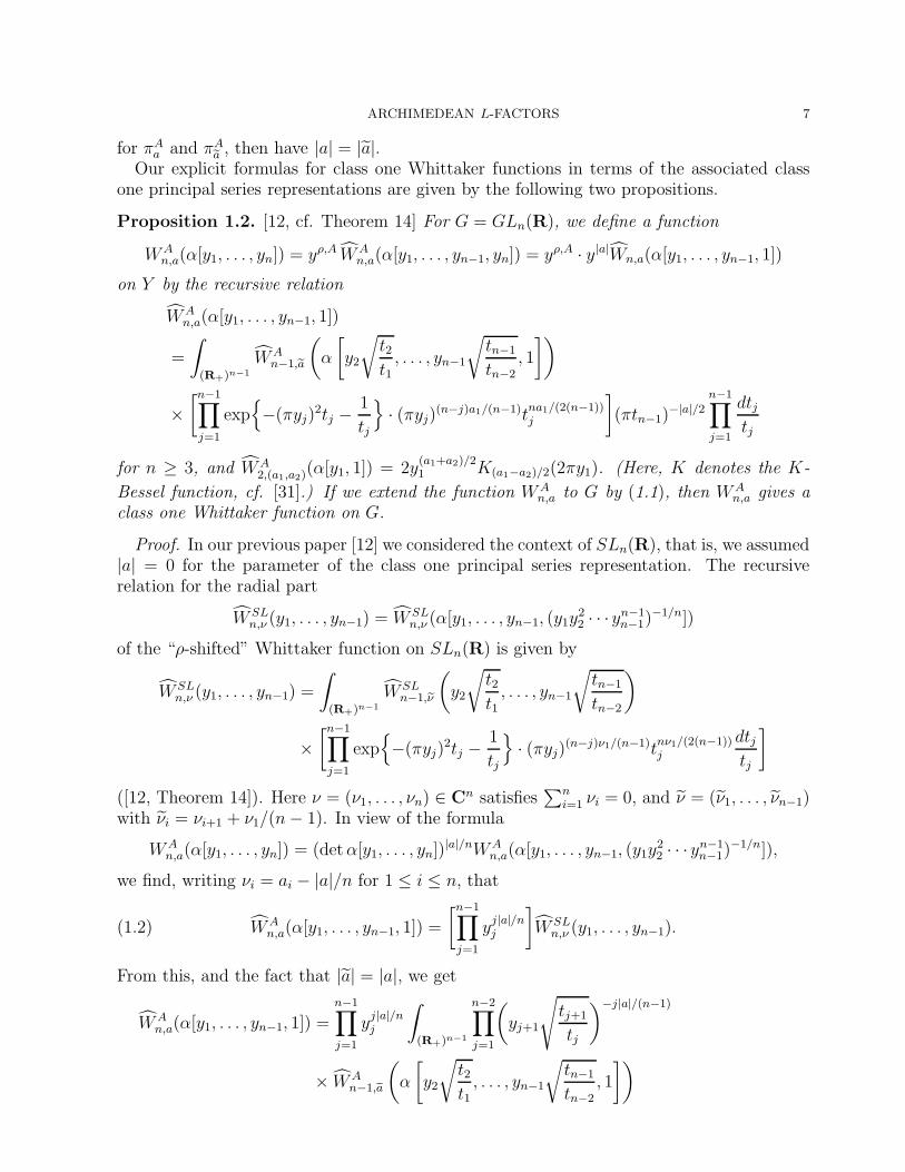
Proposition 1.2. [12, cf. Theorem 14] For G = GLn(R), we define a function
WAn,a(α[y1, . . . , yn]) = yρ,A WA
n,a(α[y1, . . . , yn−1, yn]) = yρ,A · y|a|Wn,a(α[y1, . . . , yn−1, 1])
on Y by the recursive relation
WAn,a(α[y1, . . . , yn−1, 1])
=
∫
(R+)n−1
WAn−1,a
(α
[y2
√t2t1, . . . , yn−1
√tn−1
tn−2, 1
])
×[n−1∏
j=1
exp{−(πyj)
2tj −1
tj
}· (πyj)(n−j)a1/(n−1)t
na1/(2(n−1))j
](πtn−1)
−|a|/2n−1∏
j=1
dtjtj
for n ≥ 3, and WA2,(a1,a2)
(α[y1, 1]) = 2y(a1+a2)/21 K(a1−a2)/2(2πy1). (Here, K denotes the K-
Bessel function, cf. [31].) If we extend the function WAn,a to G by (1.1), then WA
n,a gives aclass one Whittaker function on G.
Proof. In our previous paper [12] we considered the context of SLn(R), that is, we assumed|a| = 0 for the parameter of the class one principal series representation. The recursiverelation for the radial part
W SLn,ν (y1, . . . , yn−1) = W SL
n,ν (α[y1, . . . , yn−1, (y1y22 · · · yn−1
n−1)−1/n])
of the “ρ-shifted” Whittaker function on SLn(R) is given by
W SLn,ν (y1, . . . , yn−1) =
∫
(R+)n−1
W SLn−1,ν
(y2
√t2t1, . . . , yn−1
√tn−1
tn−2
)
×[n−1∏
j=1
exp{−(πyj)
2tj −1
tj
}· (πyj)(n−j)ν1/(n−1)t
nν1/(2(n−1))j
dtjtj
]
([12, Theorem 14]). Here ν = (ν1, . . . , νn) ∈ Cn satisfies∑n
i=1 νi = 0, and ν = (ν1, . . . , νn−1)with νi = νi+1 + ν1/(n− 1). In view of the formula
WAn,a(α[y1, . . . , yn]) = (detα[y1, . . . , yn])
|a|/nWAn,a(α[y1, . . . , yn−1, (y1y
22 · · · yn−1
n−1)−1/n]),
we find, writing νi = ai − |a|/n for 1 ≤ i ≤ n, that
WAn,a(α[y1, . . . , yn−1, 1]) =
[n−1∏
j=1
yj|a|/nj
]W SL
n,ν (y1, . . . , yn−1).(1.2)
From this, and the fact that |a| = |a|, we get
WAn,a(α[y1, . . . , yn−1, 1]) =
n−1∏
j=1
yj|a|/nj
∫
(R+)n−1
n−2∏
j=1
(yj+1
√tj+1
tj
)−j|a|/(n−1)
× WAn−1,a
(α
[y2
√t2t1, . . . , yn−1
√tn−1
tn−2
, 1
])
8 TAKU ISHII AND ERIC STADE
×[n−1∏
j=1
exp{−(πyj)
2tj −1
tj
}· (πyj)(n−j)ν1/(n−1)t
nν1/(2(n−1))j
dtjtj
].
We can check that[n−1∏
j=1
yj|a|/nj
][n−2∏
j=1
(yj+1
√tj+1
tj
)−j|a|/(n−1)][n−1∏
j=1
(πyj)(n−j)ν1/(n−1)t
nν1/(2(n−1))j
]
=
[n−1∏
j=1
(πyj)(n−j)a1/(n−1)t
na1/(2(n−1))j
]· (πtn−1)
−|a|/2.
So our recursive formula in [12] yields the recursive formula in the statement of the presentproposition, and we are done. 2
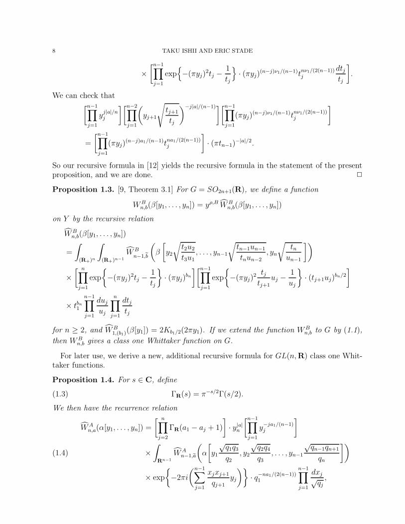
Proposition 1.3. [9, Theorem 3.1] For G = SO2n+1(R), we define a function
WBn,b(β[y1, . . . , yn]) = yρ,B WB
n,b(β[y1, . . . , yn])
on Y by the recursive relation
WBn,b(β[y1, . . . , yn])
=
∫
(R+)n
∫
(R+)n−1
WBn−1,b
(β
[y2
√t2u2t3u1
, . . . , yn−1
√tn−1un−1
tnun−2
, yn
√tnun−1
])
×[ n∏
j=1
exp
{−(πyj)
2tj −1
tj
}· (πyj)bn
][n−1∏
j=1
exp
{−(πyj)
2 tjtj+1
uj −1
uj
}· (tj+1uj)
bn/2
]
× tbn1
n−1∏
j=1
dujuj
n∏
j=1
dtjtj
for n ≥ 2, and WB1,(b1)
(β[y1]) = 2Kb1/2(2πy1). If we extend the function WBn,b to G by (1.1),
then WBn,b gives a class one Whittaker function on G.
For later use, we derive a new, additional recursive formula for GL(n,R) class one Whit-taker functions.
Proposition 1.4. For s ∈ C, define
ΓR(s) = π−s/2Γ(s/2).(1.3)
We then have the recurrence relation
WAn,a(α[y1, . . . , yn]) =
[ n∏
j=2
ΓR(a1 − aj + 1)
]· y|a|n
[n−1∏
j=1
y−ja1/(n−1)j
]
×∫
Rn−1
WAn−1,a
(α
[y1
√q1q3
q2, y2
√q2q4
q3, . . . , yn−1
√qn−1qn+1
qn
])
× exp
{−2πi
(n−1∑
j=1
xjxj+1
qj+1
yj
)}· q−na1/(2(n−1))
1
n−1∏
j=1
dxj√qj,
(1.4)
ARCHIMEDEAN L-FACTORS 9
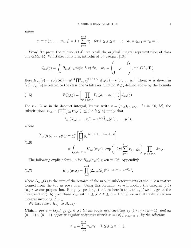
where
qj ≡ qj(x1, . . . , xn−1) = 1 +
n−1∑
p=j
x2p for 1 ≤ j ≤ n− 1; qn = qn+1 = xn = 1.
Proof. To prove the relation (1.4), we recall the original integral representation of classone GL(n,R) Whittaker functions, introduced by Jacquet [13]:
Jn,a(g) =
∫
X
Hn,a(wnxg)ψ−1(x) dx, wn =
1
· · ·1
, g ∈ GLn(R).
Here Hn,a(g) = χa(y(g)) = yρ,A∏n
j=1 ya1+···+ajj if y(g) = α[y1, . . . , yn]. Then, as is shown in
[26], Jn,a(g) is related to the class one Whittaker function WAn,a defined above by the formula
WAn,a(g) =
[ ∏
1≤j<k≤n
ΓR(aj − ak + 1)
]Jn,a(g).(1.5)
For x ∈ X as in the Jacquet integral, let use write x = (xj,k)1≤j,k≤n. As in [26, §3], thesubstitutions xj,k → (
∏k−1p=j yp)xj,k (1 ≤ j < k ≤ n) imply that
Jn,a(α[y1, . . . , yn]) = yρ,AJn,a(α[y1, . . . , yn]),
where
Jn,a(α[y1, . . . , yn]) = y|a|n
[n−1∏
j=1
y−(a1+a2+···+an−j)+|a|j
]
×∫
Rn(n−1)/2
Hn,a(wnx) · exp(−2πi
n−1∑
j=1
xj,j+1yj
) ∏
1≤j<k≤n
dxj,k.
(1.6)
The following explicit formula for Hn,a(wnx) given in [26, Appendix]:
Hn,a(wnx) =n−1∏
m=1
(∆n,m(x))(an−m+1−an−m−1)/2,(1.7)
where ∆n,m(x) is the sum of the squares of the m×m subdeterminants of the m×n matrixformed from the top m rows of x. Using this formula, we will modify the integral (1.6)to prove our proposition. Roughly speaking, the idea here is that that, if we integrate theintegrand in (1.6) over those xj,k with 1 ≤ j < k ≤ n − 1 only, we are left with a certain
integral involving Jn−1,a.We first relate Hn,a to Hn−1,a.
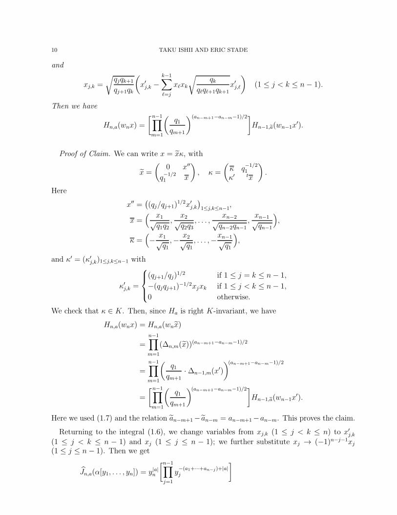
Claim. For x = (xj,k)1≤j,k≤n ∈ X, let introduce new variables xj (1 ≤ j ≤ n − 1), and an(n− 1)× (n− 1) upper triangular unipotent matrix x′ = (x′j,k)1≤j,k≤n−1, by the relations
xj,n =n−1∑
ℓ=j
xj,ℓxℓ (1 ≤ j ≤ n− 1),
10 TAKU ISHII AND ERIC STADE
and
xj,k =
√qjqk+1
qj+1qk
(x′j,k −
k−1∑
ℓ=j
xℓxk
√qk
qℓqℓ+1qk+1x′j,ℓ
)(1 ≤ j < k ≤ n− 1).
Then we have
Hn,a(wnx) =
[n−1∏
m=1
(q1qm+1
)(an−m+1−an−m−1)/2]Hn−1,a(wn−1x
′).
Proof of Claim. We can write x = xκ, with
x =
(0 x′′
q−1/21 x
), κ =
(κ q
−1/21
κ′ tx
).
Here
x′′ =((qj/qj+1)
1/2x′j,k)1≤j,k≤n−1
,
x =( x1√
q1q2,
x2√q2q3
, . . . ,xn−2√qn−2qn−1
,xn−1√qn−1
),
κ =(− x1√
q1,− x2√
q1, . . . ,−xn−1√
q1
),
and κ′ = (κ′j,k)1≤j,k≤n−1 with
κ′j,k =
(qj+1/qj)1/2 if 1 ≤ j = k ≤ n− 1,
−(qjqj+1)−1/2xjxk if 1 ≤ j < k ≤ n− 1,
0 otherwise.
We check that κ ∈ K. Then, since Ha is right K-invariant, we have
Hn,a(wnx) = Hn,a(wnx)
=n−1∏
m=1
(∆n,m(x))(an−m+1−an−m−1)/2
=
n−1∏
m=1
(q1qm+1
·∆n−1,m(x′)
)(an−m+1−an−m−1)/2
=
[n−1∏
m=1
(q1qm+1
)(an−m+1−an−m−1)/2]Hn−1,a(wn−1x
′).
Here we used (1.7) and the relation an−m+1− an−m = an−m+1−an−m. This proves the claim.
Returning to the integral (1.6), we change variables from xj,k (1 ≤ j < k ≤ n) to x′j,k(1 ≤ j < k ≤ n − 1) and xj (1 ≤ j ≤ n − 1); we further substitute xj → (−1)n−j−1xj(1 ≤ j ≤ n− 1). Then we get
Jn,a(α[y1, . . . , yn]) = y|a|n
[n−1∏
j=1
y−(a1+···+an−j)+|a|j
]
ARCHIMEDEAN L-FACTORS 11
×∫
Rn(n−1)/2
Ha(wn−1x) · exp(−2πi
n−2∑
j=1
√qjqj+2
qj+1x′j,j+1yj
)
× exp
{−2πi
(n−1∑
j=1
xjxj+1
qj+1yj
)}
×[n−1∏
j=1
(q1qj+1
)(an−j+1−an−j−1)/2][ ∏
1≤j<k≤n−1
√qjqk+1
qj+1qk
]
×∏
1≤j<k≤n−1
dx′j,k
n−1∏
j=1
dxj .
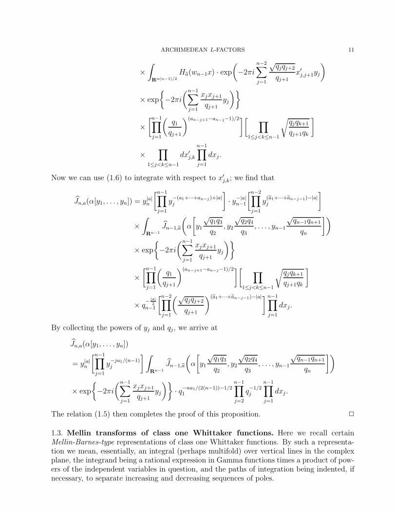
Now we can use (1.6) to integrate with respect to x′j,k; we find that
Jn,a(α[y1, . . . , yn]) = y|a|n
[n−1∏
j=1
y−(a1+···+an−j )+|a|j
]· y−|a|
n−1
[n−2∏
j=1
y(a1+···+an−j−1)−|a|j
]
×∫
Rn−1
Jn−1,a
(α
[y1
√q1q3
q2, y2
√q2q4
q3, . . . , yn−1
√qn−1qn+1
qn
])
× exp
{−2πi
(n−1∑
j=1
xjxj+1
qj+1yj
)}
×[n−1∏
j=1
(q1qj+1
)(an−j+1−an−j−1)/2][ ∏
1≤j<k≤n−1
√qjqk+1
qj+1qk
]
× q−
|a|2
n−1
[n−2∏
j=1
(√qjqj+2
qj+1
)(a1+···+an−j−1)−|a|] n−1∏
j=1
dxj .
By collecting the powers of yj and qj , we arrive at
Jn,a(α[y1, . . . , yn])
= y|a|n
[n−1∏
j=1
y−ja1/(n−1)j
] ∫
Rn−1
Jn−1,a
(α
[y1
√q1q3
q2, y2
√q2q4
q3, . . . , yn−1
√qn−1qn+1
qn
])
× exp
{−2πi
(n−1∑
j=1
xjxj+1
qj+1yj
)}· q−na1/(2(n−1))−1/2
1
n−1∏
j=2
q−1/2j
n−1∏
j=1
dxj .
The relation (1.5) then completes the proof of this proposition. 2
1.3. Mellin transforms of class one Whittaker functions. Here we recall certainMellin-Barnes-type representations of class one Whittaker functions. By such a representa-tion we mean, essentially, an integral (perhaps multifold) over vertical lines in the complexplane, the integrand being a rational expression in Gamma functions times a product of pow-ers of the independent variables in question, and the paths of integration being indented, ifnecessary, to separate increasing and decreasing sequences of poles.
12 TAKU ISHII AND ERIC STADE
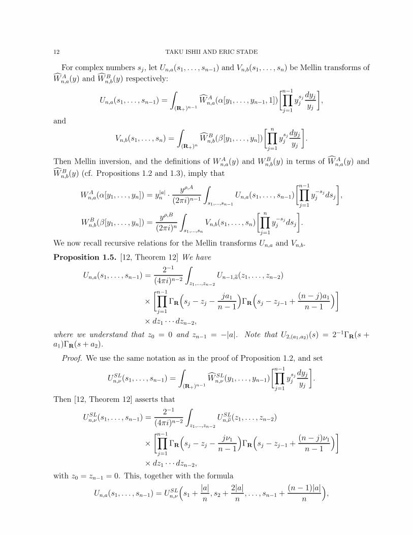
For complex numbers sj , let Un,a(s1, . . . , sn−1) and Vn,b(s1, . . . , sn) be Mellin transforms of
WAn,a(y) and W
Bn,b(y) respectively:
Un,a(s1, . . . , sn−1) =
∫
(R+)n−1
WAn,a(α[y1, . . . , yn−1, 1])
[n−1∏
j=1
ysjj
dyjyj
],
and
Vn,b(s1, . . . , sn) =
∫
(R+)nWB
n,b(β[y1, . . . , yn])
[ n∏
j=1
ysjj
dyjyj
].
Then Mellin inversion, and the definitions of WAn,a(y) and W
Bn,b(y) in terms of WA
n,a(y) and
WBn,b(y) (cf. Propositions 1.2 and 1.3), imply that
WAn,a(α[y1, . . . , yn]) = y|a|n · yρ,A
(2πi)n−1
∫
s1,...,sn−1
Un,a(s1, . . . , sn−1)
[n−1∏
j=1
y−sjj dsj
],
WBn,b(β[y1, . . . , yn]) =
yρ,B
(2πi)n
∫
s1,...,sn
Vn,b(s1, . . . , sn)
[ n∏
j=1
y−sjj dsj
].
We now recall recursive relations for the Mellin transforms Un,a and Vn,b.
Proposition 1.5. [12, Theorem 12] We have
Un,a(s1, . . . , sn−1) =2−1
(4πi)n−2
∫
z1,...,zn−2
Un−1,a(z1, . . . , zn−2)
×[n−1∏
j=1
ΓR
(sj − zj −
ja1n− 1
)ΓR
(sj − zj−1 +
(n− j)a1n− 1
)]
× dz1 · · · dzn−2,
where we understand that z0 = 0 and zn−1 = −|a|. Note that U2,(a1,a2)(s) = 2−1ΓR(s +a1)ΓR(s+ a2).
Proof. We use the same notation as in the proof of Proposition 1.2, and set
USLn,ν(s1, . . . , sn−1) =
∫
(R+)n−1
W SLn,ν (y1, . . . , yn−1)
[n−1∏
j=1
ysjj
dyjyj
].
Then [12, Theorem 12] asserts that
USLn,ν(s1, . . . , sn−1) =
2−1
(4πi)n−2
∫
z1,...,zn−2
USLn,ν(z1, . . . , zn−2)
×[n−1∏
j=1
ΓR
(sj − zj −
jν1n− 1
)ΓR
(sj − zj−1 +
(n− j)ν1n− 1
)]
× dz1 · · · dzn−2,
with z0 = zn−1 = 0. This, together with the formula
Un,a(s1, . . . , sn−1) = USLn,ν
(s1 +
|a|n, s2 +
2|a|n, . . . , sn−1 +
(n− 1)|a|n
),
ARCHIMEDEAN L-FACTORS 13
which follows immediately from (1.2), then yield the desired result. 2
For some investigations below in the case G′ = GLn−2, we present the following resultconcerning the Whittaker function contragredient to Wn,a.
Corollary 1.6. For a ψ-Whittaker function W on GLn(R), we put
W∨(g) =W (wntg−1).
Then we have
(WAn,a)
∨(α[y1, . . . , yn]) = WAn,−a(α[y1, . . . , yn])
and (WAn,a)
∨ ∈ W(πA−a, ψ
−1).
Proof. We first prove
Un,a(sn−1 − |a|, . . . , s1 − |a|) = Un,−a(s1, . . . , sn−1)(1.8)
by induction on n. The case n = 2 follows automatically from the definitions. Now, byProposition 1.5 and the induction hypothesis, we have
Un,a(sn−1 − |a|, . . . , s1 − |a|)
=2−1
(4πi)n−2
∫
z1,...,zn−2
Un−1,−a(zn−2 + |a|, . . . , z1 + |a|)
×[n−1∏
j=1
ΓR
(sn−j − |a| − zj −
ja1n− 1
)ΓR
(sn−j − |a| − zj−1 +
(n− j)a1n− 1
)]
× dz1 · · · dzn−2.
We substitute zj → zn−j−1 − |a| = zn−j−1 − |a|, to find that
Un,a(sn−1 − |a|, . . . , s1 − |a|)
=2−1
(4πi)n−2
∫
z1,...,zn−2
Un−1,−a(z1, . . . , zn−2)
×[n−1∏
j=1
ΓR
(sn−j − zn−j−1 + |a| − ja1
n− 1
)ΓR
(sn−j − zn−j +
(n− j)a1n− 1
)]dz1 · · · dzn−2
=2−1
(4πi)n−2
∫
z1,...,zn−2
Un−1,−a(z1, . . . , zn−2)
×[n−1∏
j=1
ΓR
(sj − zj−1 + |a| − (n− j)a1
n− 1
)ΓR
(sj − zj +
ja1n− 1
)]dz1 · · · dzn−2
= Un,−a(s1, . . . , sn−1).
Thus we obtain (1.8).Now, since WA
n,a is right O(n)-invariant, we have
(WAn,a)
∨(α[y1, . . . , yn])
= (WAn,a)
∨(wntα[y1, . . . , yn]
−1wn)
= (WAn,a)
∨(α[yn−1, yn−2, . . . , y1, (y1 · · · yn)−1])
14 TAKU ISHII AND ERIC STADE
=
[ n∏
j=1
y−|a|j
]yρ,A
(2πi)n−1
∫
s1,...,sn−1
Un,a(s1, . . . , sn−1)
[n−1∏
j=1
y−sjn−j
]ds1 · · · dsn−1.
We substitute sj → sn−j − |a| for 1 ≤ j ≤ n− 1 and use (1.8), to find that
(WAn,a)
∨(α[y1, . . . , yn])
= y−|a|n · yρ,A
(2πi)n−1
∫
s1,...,sn−1
Un,a(sn−1 − |a|, . . . , s1 − |a|)[n−1∏
j=1
y−sjj
]ds1 · · · dsn−1
= WAn,−a(α[y1, . . . , yn]).
Thus we complete our proof. 2
Our recursive relation for Vn,b is given by:
Proposition 1.7. [9, Theorem 4.2] We have
Vn,b(s1, . . . , sn) =2−1
(4πi)2n−2
∫
w1,...,wn−1z1,...,zn−1
Vn−1,b(z1, . . . , zn−1)
×[n−1∏
j=1
ΓR(sj − wj)ΓR(sj − wj−1 − bn)ΓR(wj − zj)ΓR(wj − zj−1 + bn)
]
× ΓR(sn − wn−1 − bn)ΓR(sn − zn−1 + bn) dz1 · · · dzn−1 dw1 · · · dwn−1,
where we understand that w0 = z0 = 0. Note that V1,(b1)(s) = 2−1ΓR(s+ b1)ΓR(s− b1).
Remark 1. Technically, the formula given in the above proposition is of a different formfrom that given in [9, Theorem 4.2]. To show equality of these two formulas, one simplyintegrates with respect to w1, . . . , wn−1 in the above formula, using Barnes’ first lemma (cf.[1]):
1
4πi
∫
z
ΓR(z + a)ΓR(z + b)ΓR(−z + c)ΓR(−z + d) dz
=ΓR(a+ c)ΓR(a+ d)ΓR(b+ c)ΓR(b+ d)
ΓR(a+ b+ c+ d).
(1.9)
1.4. Some identities for Un,a and Vn,b. In this subsection, we present some useful formulasexpressing Un,a (respectively, Vn,b) as a Barnes-type integral of Un,a (respectively Vn,b). Here,by a Barne-type integral, we mean one of Mellin-Barnes type, as described above, but lackingthe “product of powers of the independent variables.” That is, a Barnes-type integral is anintegral of a rational expression in Gamma functions. In our discussions of such Barnes-typeintegrals, Barnes’ first lemma (1.9) will play a fundamental role.
We start with an easy consequence of Barnes’ first lemma.
Lemma 1.8. Let γ, δ, cj and dj (1 ≤ j ≤ n) be complex numbers; also define c0 = d0 = 0.
ARCHIMEDEAN L-FACTORS 15
(1) We have
1
(4πi)n
∫
z1,...,zn
[ n∏
j=1
ΓR(cj−1 + γ + zj)ΓR(cj + zj)ΓR(dj−1 + δ − zj)ΓR(dj − zj) dzj
]
=ΓR(c1 + δ)ΓR(d1 + γ)ΓR(γ + δ)ΓR(cn + dn)
ΓR(γ + δ + cn + dn)· 1
(4πi)n−1
∫
z1,...,zn−1
×[n−1∏
j=1
ΓR(cj + zj)ΓR(cj+1 + δ + zj)ΓR(dj − zj)ΓR(dj+1 + γ − zj) dzj
].
(2) We have
1
(4πi)n−1
∫
z1,...,zn−1
[n−1∏
j=1
ΓR(cj + zj)ΓR(cj+1 + γ + zj)
]
×[n−1∏
j=1
ΓR(dj−1 + δ − zj)ΓR(dj − zj) dzj
]
=ΓR(c1 + δ)ΓR(cn + dn−1 + γ)
ΓR(c1 + γ)ΓR(cn + dn−1 + δ)· 1
(4πi)n−1
∫
z1,...,zn−1
×[n−1∏
j=1
ΓR(cj + zj)ΓR(cj+1 + δ + zj)ΓR(dj−1 + γ − zj)ΓR(dj − zj) dzj
].
Proof. Let first us show (1). Using Barnes’ first lemma (1.9), we can integrate in allvariables on either side. On the left hand side, we get
n−1∏
j=1
ΓR(cj−1 + dj−1 + γ + δ)ΓR(cj−1 + dj + γ)ΓR(cj + dj−1 + δ)ΓR(cj + dj)
ΓR(cj−1 + cj + dj−1 + dj + γ + δ),
while on the right hand side, we get
ΓR(c1 + δ)ΓR(d1 + γ)ΓR(γ + δ)ΓR(cn−1 + dn−1)
ΓR(cn−1 + dn−1 + γ + δ)
×n−2∏
j=1
ΓR(cj + dj)ΓR(cj + dj+1 + γ)ΓR(cj+1 + dj + δ)ΓR(cj+1 + dj+1 + γ + δ)
ΓR(cj + cj+1 + dj + dj+1 + γ + δ).
The two sides are then readily seen to be equal.The latter claim (2) follows similarly from Barnes’ first lemma. 2
We now present some expressions, to be of use to us in the next two sections, for Un,a asintegrals that themselves involve Un,a.
Proposition 1.9. (1) For a complex number σ, we have
Un,a(p1, . . . , pn−1) =ΓR(pn−1 + σ + |a|)∏n
j=1 ΓR(σ + aj)· 1
(4πi)n−1
∫
q1,...,qn−1
Un,a(q1, . . . , qn−1)
×[n−1∏
j=1
ΓR(pj − qj)ΓR(pj−1 − qj + σ)
]dq1 · · · dqn−1.
(1.10)
16 TAKU ISHII AND ERIC STADE
Here we understand that p0 = 0.(2) For a complex number σ, we have
Un,a(p1, . . . , pn−1) =ΓR(p1 + σ)∏nj=1 ΓR(σ − aj)
· 1
(4πi)n−1
∫
q1,...,qn−1
Un,a(q1, . . . , qn−1)
×[n−1∏
j=1
ΓR(pj − qj)ΓR(pj+1 − qj + σ)
]dq1 · · · dqn−1.
(1.11)
Here we understand that pn = −|a|.Proof. Our proof proceeds by induction on n. The case n = 2 amounts to Barnes’ first
lemma (1.9).Now by Proposition 1.5, the right hand side of (1.10) is seen to be equal to
ΓR(pn−1 + σ + |a|)∏nj=1 ΓR(σ + aj)
· 2−1
(4πi)2n−3
∫
q1,...,qn−1r1,...,rn−2
Un−1,a(r1, . . . , rn−2)
×[n−1∏
j=1
ΓR
(qj − rj −
ja1n− 1
)ΓR
(qj − rj−1 +
(n− j)a1n− 1
)]
×[n−1∏
j=1
ΓR(pj − qj)ΓR(pj−1 − qj + σ)
]dr1 · · · drn−2 dq1 · · ·dqn−1,
(1.12)
where r0 = 0 and rn−1 = −|a|. To the integral in the qj ’s in (1.12), we now apply Lemma1.8 (1) with γ = a1; δ = σ; and, for 1 ≤ j ≤ n− 1, cj = −rj − ja1/(n− 1) and dj = pj . Wethereby find that (1.12) equals
ΓR(pn−1 + σ + |a|)∏nj=1 ΓR(σ + aj)
· 2−1
(4πi)2n−4
∫
q1,...,qn−2r1,...,rn−2
Un−1,a(r1, . . . , rn−2)
×ΓR(−r1 − a1
n−1+ σ)ΓR(p1 + a1)ΓR(σ + a1)ΓR(pn−1 − a1 + |a|)ΓR(pn−1 + σ + a1 + · · ·+ an)
×[n−2∏
j=1
ΓR
(qj − rj −
ja1n− 1
)ΓR
(qj − rj+1 + σ − (j + 1)a1
n− 1
)]
×[n−2∏
j=1
ΓR(pj − qj)ΓR(pj+1 − qj + a1)
]dr1 · · · drn−2 dq1 · · ·dqn−2
=1∏n
j=2 ΓR(σ + aj)· 2−1
(4πi)2n−4
∫
q1,...,qn−2r1,...,rn−2
Un−1,a(r1, . . . , rn−2)
× ΓR(pn−1 − a1 + |a|)ΓR(qn−2 + σ − a1 + |a|)ΓR(pn−1 − qn−2 + a1)
×[n−2∏
j=1
ΓR
(qj − rj −
ja1n− 1
)ΓR
(qj−1 − rj −
ja1n− 1
+ σ)]
×[n−2∏
j=1
ΓR(pj − qj)ΓR(pj − qj−1 + a1)
]dr1 · · · drn−2 dq1 · · ·dqn−2.
(1.13)
ARCHIMEDEAN L-FACTORS 17
By the induction hypothesis, we can integrate with respect to the rj’s, to find that (1.13)equals
1∏nj=2 ΓR(σ + aj)
· 2−1
(4πi)n−2
∫
q1,...,qn−2
∏n−1j=1 ΓR(σ − a1
n−1+ aj)
ΓR(qn−2 + σ − a1 + |a|)
× Un,a
(q1 −
a1n− 1
, . . . , qn−2 −(n− 2)a1n− 1
)
× ΓR(pn−1 − a1 + |a|)ΓR(pn−1 − qn−2 + a1)ΓR(qn−2 + σ − a1 + |a|)
×[n−2∏
j=1
ΓR(pj − qj)ΓR(pj − qj−1 + a1)
]dq1 · · · dqn−2
=2−1
(4πi)n−2
∫
q1,...,qn−2
Un,a
(q1 −
a1n− 1
, . . . , qn−2 −(n− 2)a1n− 1
)
×[n−1∏
j=1
ΓR(pj − qj)ΓR(pj − qj−1 + a1)
]dq1 · · · dqn−2.
(1.14)
Here we’ve used the fact that that |a| = |a|; also, we’ve defined qn−1 = a1 − |a|.Finally, after the substitution qj → qj + ja1/(n− 1) for 1 ≤ j ≤ n− 2, we use Proposition
1.5 to find that (1.14) becomes Un,a(p1, . . . , pn−1). Thus we complete the proof of (1.10).
The proof of (1.11) is similar: Again, we use induction on n, with the case n = 2 beingequivalent to Barnes’ first lemma (1.9).
To rearrange the integration over the qj ’s, we first rewrite the identity in Lemma 1.8 (2)slightly, by integrating with respect to zn−1 on the right hand side. We get
1
(4πi)n−1
∫
z1,...,zn−1
[n−1∏
j=1
ΓR(cj + zj)ΓR(cj+1 + γ + zj)ΓR(dj−1 + δ − zj)ΓR(dj − zj) dzj
]
=ΓR(c1 + δ)ΓR(cn + dn−1 + γ)ΓR(cn−1 + dn−2 + γ)
ΓR(c1 + γ)ΓR(cn−1 + cn + dn−2 + dn−1 + γ + δ)
× ΓR(cn−1 + dn−1)ΓR(cn + dn−2 + γ + δ)
× 1
(4πi)n−2
∫
z1,...,zn−2
[n−2∏
j=1
ΓR(cj + zj)ΓR(cj+1 + δ + zj)
]
×[n−2∏
j=1
ΓR(dj−1 + γ − zj)ΓR(dj − zj) dzj
].
Applying this formula with cj = pj (1 ≤ j ≤ n − 1), cn = −|a|, dj = −rj − ja1/(n − 1)(1 ≤ j ≤ n − 2), dn−1 = −a1 + |a|, γ = σ and δ = a1, we find that the right hand side of(1.11) becomes
1∏nj=2 ΓR(σ − aj)
· 2−1
(4πi)2n−4
∫
q1,...,qn−2r1,...,rn−2
Un−1,a(r1, . . . , rn−2)
× ΓR(p1 + a1)ΓR(pn−1 − a1 + |a|)[n−2∏
j=1
ΓR(pj − qj)ΓR(pj+1 − qj + a1)
]
18 TAKU ISHII AND ERIC STADE
× ΓR(q1 + σ)
[n−2∏
j=1
ΓR
(qj+1 − rj −
ja1n− 1
+ σ)ΓR
(qj − rj −
ja1n− 1
)]
× dr1 · · · drn−2 dq1 · · · dqn−2.
Using the induction hypothesis to integrate in the rj ’s, together with Proposition 1.5, weprove our assertion. 2
Our SO2n+1(R)-analog of Proposition 1.9 is as follows.
Proposition 1.10. For a complex number σ, we have
Vn,b(p1, . . . , pn)
=1∏n
j=1 ΓR(σ + bj)ΓR(σ − bj)· 1
(4πi)2n−1
∫
q1,...,qn−1r1,...,rn
Vn,b(r1, . . . , rn)
×[n−1∏
j=1
ΓR(pj − qj)ΓR(qj − rj)
][ n∏
j=1
ΓR(pj − qj−1 + σ)ΓR(qj−1 − rj + σ)
]
× ΓR(pn − rn) dr1 · · ·drn dq1 · · ·dqn−1.
(1.15)
Here we understand that q0 = 0.
Proof. We again proceed by induction on n. The case n = 1 is an immediate consequenceof Barnes’ first lemma (1.9).
We now apply Proposition 1.7, to find that the right hand side of (1.15) equals
1∏nj=1 ΓR(σ + bj)ΓR(σ − bj)
· 2−1
(4πi)4n−3
∫
q1,...,qn−1r1,...,rn
∫
w1,...,wn−1z1,...,zn−1
Vn−1,b(z1, . . . , zn−1)
×[n−1∏
j=1
ΓR(rj − wj)ΓR(rj − wj−1 − bn)ΓR(wj − zj)ΓR(wj − zj−1 + bn)
]
× ΓR(rn − zn−1 + bn)ΓR(rn − wn−1 − bn)
×[n−1∏
j=1
ΓR(pj − qj)ΓR(qj − rj)
][ n∏
j=1
ΓR(pj − qj−1 + σ)ΓR(qj−1 − rj + σ)
]
× ΓR(pn − rn) dz1 · · · dzn−1 dw1 · · · dwn−1 dr1 · · ·drn dq1 · · · dqn−1.
(1.16)
To the integral in the rj’s, in (1.16), we now apply Lemma 1.8 (1), which yields:
1
(4πi)n
∫
r1,...,rn
[n−1∏
j=1
ΓR(rj − wj)ΓR(rj − wj−1 − bn)ΓR(qj − rj)ΓR(qj−1 − rj + σ)
]
× ΓR(rn − zn−1 + bn)ΓR(rn − wn−1 − bn)ΓR(pn − rn)ΓR(qn−1 − rn + σ) dr1 · · · drn
=ΓR(σ − w1)ΓR(q1 − bn)ΓR(σ − bn)ΓR(pn − zn−1 + bn)
ΓR(pn − zn−1 + σ)· 1
(4πi)n−1
∫
r1,...,rn−1
×[n−2∏
j=1
ΓR(rj − wj)ΓR(rj − wj+1 + σ)ΓR(qj − rj)ΓR(qj+1 − rj − bn)
]
× ΓR(rn−1 − wn−1)ΓR(rn−1 − zn−1 + σ + bn)ΓR(qn−1 − rn−1)ΓR(pn − rn−1 − bn)
ARCHIMEDEAN L-FACTORS 19
× dr1 · · · drn−1
=ΓR(σ − bn)ΓR(pn − zn−1 + bn)
ΓR(pn − zn−1 + σ)· 1
(4πi)n−1
∫
r1,...,rn−1
×[n−1∏
j=1
ΓR(rj − wj)ΓR(rj−1 − wj + σ)ΓR(qj − rj)ΓR(qj − rj−1 − bn)
]
× ΓR(rn−1 − zn−1 + σ + bn)ΓR(pn − rn−1 − bn) dr1 · · · drn−1.
Then (1.16) equals
1∏nj=1 ΓR(σ + bj)ΓR(σ − bj)
· 2−1
(4πi)4n−4
∫
q1,...,qn−1r1,...,rn−1
∫
w1,...,wn−1z1,...,zn−1
Vn−1,b(z1, . . . , zn−1)
×[n−1∏
j=1
ΓR(wj − zj)ΓR(wj − zj−1 + bn)ΓR(rj − wj)ΓR(rj−1 − wj + σ)
]
× ΓR(p1 + σ)
[n−1∏
j=1
ΓR(pj − qj)ΓR(pj+1 − qj + σ)ΓR(qj − rj)ΓR(qj − rj−1 − bn)
]
× ΓR(σ − bn)ΓR(pn − zn−1 + bn)ΓR(rn−1 − zn−1 + σ + bn)ΓR(pn − rn−1 − bn)
ΓR(pn − zn−1 + σ)
× dz1 · · · dzn−1 dw1 · · · dwn−1 dr1 · · · drn−1 dq1 · · · dqn−1.
(1.17)
We apply Lemma 1.8 (1) with (cj, dj, γ, δ) = (−zj , rj, νn, σ) to the integratlin the wj’s, andLemma 1.8 (2) with (cj, dj, γ, δ) = (pj,−rj , σ,−ν) to the integral in the qj ’s. Then (1.17)becomes
1∏nj=1 ΓR(σ + bj)ΓR(σ − bj)
· 2−1
(4πi)4n−5
∫
q1,...,qn−1r1,...,rn−1
∫
w1,...,wn−2z1,...,zn−1
Vn−1,b(z1, . . . , zn−1)
× ΓR(σ − z1)ΓR(r1 + bn)ΓR(σ + bn)ΓR(rn−1 − zn−1)
ΓR(rn−1 − zn−1 + σ + bn)
×[n−2∏
j=1
ΓR(wj − zj)ΓR(wj − zj+1 + σ)ΓR(rj − wj)ΓR(rj+1 − wj + bn)
]
× ΓR(p1 − bn)ΓR(pn − rn−1 + σ)
ΓR(p1 + σ)ΓR(pn − rn−1 − bn)
×[n−1∏
j=1
ΓR(pj − qj)ΓR(pj+1 − qj − bn)ΓR(qj − rj)ΓR(qj − rj−1 + σ)
]
× ΓR(σ − bn)ΓR(p1 + σ)ΓR(pn − zn−1 + bn)ΓR(pn − rn−1 − bn)
ΓR(pn − zn−1 + σ)
× ΓR(rn−1 − zn−1 + σ + bn) dz1 · · · dzn−1 dw1 · · · dwn−2 dr1 · · ·drn−1 dq1 · · · dqn−1.
(1.18)
20 TAKU ISHII AND ERIC STADE
We rewrite (1.18) as
1∏n−1j=1 ΓR(σ + bj)ΓR(σ − bj)
· 2−1
(4πi)4n−5
∫
q1,...,qn−1r1,...,rn−1
∫
w1,...,wn−2z1,...,zn−1
Vn−1,b(z1, . . . , zn−1)
×[n−2∏
j=1
ΓR(rj − wj)ΓR(rj − wj−1 + bn)ΓR(qj − rj)ΓR(qj+1 − rj + σ)
]
× ΓR(rn−1 − zn−1)ΓR(rn−1 − wn−2 + bn)ΓR(qn−1 − rn−1)ΓR(pn − rn−1 + σ)
× ΓR(q1 + σ)ΓR(pn − zn−1 + νn)
ΓR(pn − zn−1 + σ)
[n−2∏
j=1
ΓR(wj − zj)
]
×[n−1∏
j=1
ΓR(wj−1 − zj + σ)
][n−1∏
j=1
ΓR(pj − qj)
][ n∏
j=1
ΓR(pj − qj−1 − bn)
]
× dz1 · · · dzn−1 dw1 · · · dwn−2 dr1 · · · drn−1 dq1 · · · dqn−1.
(1.19)
We apply Lemma 1.8 (2) to the integral in r1, . . . , rn−1,to find that (1.19) equals
1∏n−1j=1 ΓR(σ + bj)ΓR(σ − bj)
· 2−1
(4πi)4n−5
∫
q1,...,qn−1r1,...,rn−1
∫
w1,...,wn−2z1,...,zn−1
Vn−1,b(z1, . . . , zn−1)
× ΓR(q1 + bn)
[n−1∏
j=1
ΓR(qj − rj)
][n−2∏
j=1
ΓR(qj+1 − rj + bn)
]ΓR(pn − rn−1 + bn)
×[n−2∏
j=1
ΓR(rj − wj)
]ΓR(rn−1 − zn−1)
[n−1∏
j=1
ΓR(rj − wj−1 + σ)
]
×[n−2∏
j=1
ΓR(wj − zj)
][n−1∏
j=1
ΓR(wj−1 − zj + σ)ΓR(pj − qj)
]
×[ n∏
j=1
ΓR(pj − qj−1 − bn)
]dz1 · · · dzn−1 dw1 · · · dwn−2 dr1 · · · drn−1 dq1 · · · dqn−1.
=1∏n−1
j=1 ΓR(σ + bj)ΓR(σ − bj)· 2−1
(4πi)4n−5
∫
q1,...,qn−1r1,...,rn−1
∫
w1,...,wn−2z1,...,zn−1
Vn−1,b(z1, . . . , zn−1)
×[n−2∏
j=1
ΓR(rj − wj)ΓR(wj − zj)
]
×[n−1∏
j=1
ΓR(wj−1 − zj + σ)ΓR(rj − wj−1 + σ)
]ΓR(rn−1 − zn−1)
×[n−1∏
j=1
ΓR(pj − qj)ΓR(pj − qj−1 − bn)ΓR(qj − rj)ΓR(qj − rj−1 + bn)
]
× ΓR(pn − rn−1 + bn)ΓR(pn − qn−1 − bn)
× dz1 · · · dzn−1 dw1 · · · dwn−2 dr1 · · · drn−1 dq1 · · · dqn−1.
(1.20)
ARCHIMEDEAN L-FACTORS 21
By the induction hypothesis, we can perform the integration over the wj’s and zj ’s. Thus(1.20) becomes
2−1
(4πi)2n−2
∫
q1,...,qn−1r1,...,rn−1
Vn−1,b(r1, . . . , rn−1)
×[n−1∏
j=1
ΓR(pj − qj)ΓR(pj − qj−1 − bn)ΓR(qj − rj)ΓR(qj − rj−1 + bn)
]
× ΓR(pn − rn−1 + bn)ΓR(pn − qn−1 − bn) dr1 · · · drn−1 dq1 · · · dqn−1
= Vn,b(p1, . . . , pn−1).
The last equality follows from Proposition 1.7, and our proof is complete. 2
2. archimedean zeta integrals on GLn ×GLm
In this section, we explicitly calculate archimedean zeta integrals for degree nm L-functionson GLn×GLm when 0 ≤ n−m ≤ 2, by applying some formulas given in the previous section.When m = n or n − 1, and in the case when the class one principal series representationsin question are induced from characters trivial on the center of GLn and GLm, the secondauthor [29] [30] has proved the coincidence of the local zeta integrals and the local LanglandsL-factors, by way of a recursive relation between Un,a and Un−2,a obtained in [29]. Here wegive another proof, which uses a relation between Un,a and Un−1,a, as well as Proposition 1.9in §2.2 below. The present proof will not require the assumption of trivial central charactersthat was stipulated in the earlier proof.
For general n and m, Jacquet and Shalika [18] have proved local functional equationsfor, and non-vanishing of, the ratio of the archimedean zeta integral to the correspondingL-factor. If n > m + 1, it is not generally expected that the archimedean zeta integralsshould coincide with the local L-factors. And indeed Hoffstein and Murty [8], in the case of(n,m) = (3, 1), have expressed the ratio of this local integral to this local L-function as acertain integral of Barnes type.
In this section we generalize the work of Hoffstein and Murty, by expressing this ratio ofarchimedean zeta integral to archimedean L-factor, in the case of GLn × GLn−2 for any n,explicitly as a Barnes-type integral.
2.1. Barnes integral expressions for archimedean zeta integrals. We first recall thearchimedean zeta integrals for the standard L-functions on GLn ×GLm. Let W and W ′ beψ and ψ−1-Whittaker functions on GLn(R) and GLm(R), respectively. Let Xn(R) be thestandard maximal unipotent subgroup of GLn(R) consisting of upper triangular unipotentmatrices. The archimedean zeta integrals we want to study are
Z(s,W,W ′) =
∫
Xn(R)\GLn(R)
W (g)W ′(g)Φ(eng) | det g|s dg if m = n,
∫
Xm(R)\GLm(R)
W
(g
1n−m
)W ′(g) | det g|s−(n−m)/2 dg if m < n.
Here Φ is a Schwartz-Bruhat function on Rn defined by
Φ(x) = exp(−π
n∑
i=1
x2i
)(x = (x1, . . . , xn) ∈ Rn),
22 TAKU ISHII AND ERIC STADE
and en = (0, . . . , 0, 1) ∈ Rn.In the case m ≤ n− 2, the zeta integral
Z∨(s,W,W ′)
=
∫
Mn−m−1,m(R)
∫
Xm(R)\GLm(R)
W
gx 1n−m−1
1
W ′(g) | det g|s−(n−m)/2 dx dg
will also be of interest.Now let us assume thatW and W ′ are class one Whittaker functions. We write W = WA
n,a
and W ′ = WA
m,a′ , where a = (a1, a2, . . . , an) ∈ Cn, a′ = (a′1, a′2, . . . , a
′m) ∈ Cm, and W
A
m,a′
denotes the ψ−1-Whittaker function determined by WA
m,a′(g) = ψ−1(x(g))WAm,a′(y(g)). We
then define
In,m;a,a′(s) = Z(s,WAn,a,W
A
m,a′)
and
I∨n,n−2;a,a′(s) = Z∨(s, (WAn,a)
∨, (WA
n−2,a′)∨).
The goals cited at the outset of this section may now be described more explicitly, as follows:
1. To show that In,m;a,a′(s) equals the corresponding local L-factor, which is a product of(n− j)n Gamma functions, in the cases m = n− j for j = 0 or 1;
2. To show that In,n−2;a,a′(s) equals the corresponding local L-factor, which is a product of(n− 2)n Gamma functions, times a certain Barnes-type integral; that I∨n−2,n;a,a′(s) similarlyequals an L-factor times a Barnes-type integral; and that the former Barnes-type integralbecomes the latter under the replacement of s by 1− s.
The first of these goals will be accomplished in subsection 2.2 below – see Theorem 2.1 –and the second in subsection 2.3 – see Theorems 2.4 and 2.5. In the present subsection, wedevelop some Barnes-type integral expressions for In,m;a,a′(s) and I
∨n,n−2;a,a′(s), to be of use
in what follows.
Proposition 2.1. (1) We have
In,n;a,a′(s) = ΓR(ns+ |a|+ |a′|)
× 2n−1
(2πi)n−1
∫
s1,...,sn−1
Un,a(s− s1, 2s− s2, . . . , (n− 1)s− sn−1)
× Un,a′(s1, . . . , sn−1) ds1 · · · dsn−1.
(2) For m < n,
In,m;a,a′(s) =2m
(2πi)n−2
∫
s1,...,sm−1sm+1,...,sn−1
Un,a(s− s1, 2s− s2, . . . , (m− 1)s− sm−1,
ms + |a′|, sm+1, . . . , sn−1)
× Um,a′(s1, . . . , sm−1) ds1 · · · dsm−1dsm+1 · · · dsn−1.
ARCHIMEDEAN L-FACTORS 23
(3) We have
I∨n,n−2;a,a′(s) =1
4πi
∫
w
In,n−1,−a,a∨
(3
2+w + |a′| − 1
n− 1
)
∏n−1j=2 ΓR(a
∨1 − a∨j + 1)
dw,
where a∨ = (a∨1 , . . . , a∨n−1) with
a∨1 = (n− 2)(−s + 3
2+w + |a′| − 1
n− 1
);
a∨j = −a′j−1 + s− 3
2− w + |a′| − 1
n− 1(2 ≤ j ≤ n− 1).
(2.1)
Proof. We first consider part (1). Since our Whittaker functions WAn,a and W
A
n,a′ are rightO(n) invariant, the Iwasawa decomposition implies that
In,n;a,a′(s) = Z(s,WAn,a,W
A
n,a′)
= 2n∫
(R+)nexp(−πy2n)
×WAn,a(α[y1, . . . , yn])W
An,a′(α[y1, . . . , yn])
[ n∏
j=1
yjs−j(n−j)j
dyjyj
]
= 2n∫
(R+)ny|a|+|a′|n exp(−πy2n)
× WAn,a(α[y1, . . . , yn−1, 1])W
An,a′(α[y1, . . . , yn−1, 1])
[ n∏
j=1
yjsjdyjyj
].
The integral in yn equals 2−1ΓR(ns+ |a|+ |a′|). Applying Mellin inversion and the “convolu-tion theorem” – which says that the Mellin transform of a product equals the convolution ofthe corresponding Mellin transforms – to the integral in y1, y2, . . . , yn−1, above, then yieldsthe stated formula for In,n,a,a′(s).
We now prove part (2). In this case, the Iwasawa decomposition gives us
In,m;a,a′(s) = Z(s,WAn,a,W
A
m,a′)
= 2m∫
(R+)mWA
n,a(α[y1, . . . , ym, 1, . . . , 1])WAm,a′(α[y1, . . . , ym])
[ m∏
j=1
yj(s−(n−m)/2)−j(m−j)j
dyjyj
]
= 2m∫
(R+)mWA
n,a(α[y1, . . . , ym, 1, . . . , 1])WAm,a′(α[y1, . . . , ym])
[ m∏
j=1
yjsjdyjyj
].
(2.2)
Now, for yj ∈ R+ (m+ 1 ≤ j ≤ n− 1), we set
Z(s,WAn,a,W
Am,a′; ym+1, . . . , yn−1)
= 2m∫
(R+)mWA
n,a(α[y1, . . . , ym, ym+1, . . . , yn−1, 1])WAm,a′(α[y1, . . . , ym])
[ m∏
j=1
yjsjdyjyj
],
24 TAKU ISHII AND ERIC STADE
so thatIn,m;a,a′(s) = Z(s,WA
n,a,WAm,a′ ; 1, . . . , 1).
Applying Mellin inversion to the right hand side yields
In,m;a,a′(s) =1
(2πi)n−m−1
∫
sm+1,...,sn−1
Z(sm+1, . . . , sn−1) dsm+1 · · · dsn−1,(2.3)
where
Z(sm+1, . . . , sn−1)
=
∫
(R+)n−m−1
Z(s,WAn,a,W
Am,a′ ; ym+1, . . . , yn−1)
[ n−1∏
j=m+1
ysjj
dyjyj
]
= 2m∫
(R+)n−1
WAn,a(α[y1, . . . , yn−1, 1])W
Am,a′(α[y1, . . . , ym])
[ m∏
j=1
yjsjdyjyj
][ n−1∏
j=m+1
ysjj
dyjyj
]
= 2m∫
(R+)n−1
WAn,a(α[y1, . . . , yn−1, 1])W
Am,a′(α[y1, . . . , ym−1, 1])
[ m∏
j=1
yjsjdyjyj
]y|a
′|m
[ n−1∏
j=m+1
ysjj
dyjyj
]
=2m
(2πi)m−1
∫
s1,...,sm−1
Un,a(s− s1, 2s− s2, . . . , (m− 1)s− sm−1, ms+ |a′|, sm+1, . . . , sn−1)
× Um,a′(s1, . . . , sm−1) ds1 · · · dsm−1,
since, again, the Mellin transform of a product is the convolution of the Mellin transforms.So we conclude from (2.3) that
In,m;a,a′(s) =2m
(2πi)n−2
∫
s1,...,sm−1sm+1,...,sn−1
Un,a(s− s1, 2s− s2, . . . , (m− 1)s− sm−1,
ms+ |a′|, sm+1, . . . , sn−1)
× Um,a′(s1, . . . , sm−1) ds1 · · · dsm−1dsm+1 · · · dsn−1,
(2.4)
as required.Finally, we prove part (3). We have
I∨n,n−2;a,a′(s) = Z∨(s, (WAn,a)
∨, (WA
n−2,a′)∨)
= 2n−2
∫
(R+)n−2
∫
Rn−2
(WAn,a)
∨(M(x1, . . . , xn−2; y1, . . . , yn−2, 1))
× (WA
n−2,a′)∨(α[y1, . . . , yn−2])
[n−2∏
j=1
dxj yj(s−n+j+1)j
dyjyj
],
where
M(x1, . . . , xn−2; y1, . . . , yn−1) =
yx yn−1
1
,
with x = (x1, . . . , xn−2) and y = yn−1 · α[y1, . . . , yn−2]. Then Mellin inversion implies
I∨n,n−2;a,a′(s) =1
2πi
∫
w
I∨n,n−2;a,a′(s, w) dw,
ARCHIMEDEAN L-FACTORS 25
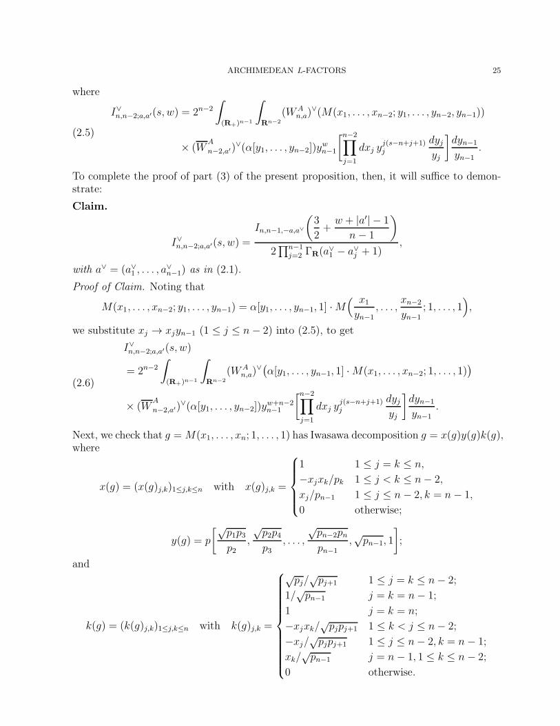
where
I∨n,n−2;a,a′(s, w) = 2n−2
∫
(R+)n−1
∫
Rn−2
(WAn,a)
∨(M(x1, . . . , xn−2; y1, . . . , yn−2, yn−1))
× (WA
n−2,a′)∨(α[y1, . . . , yn−2])y
wn−1
[n−2∏
j=1
dxj yj(s−n+j+1)j
dyjyj
]dyn−1
yn−1.
(2.5)
To complete the proof of part (3) of the present proposition, then, it will suffice to demon-strate:
Claim.
I∨n,n−2;a,a′(s, w) =
In,n−1,−a,a∨
(3
2+w + |a′| − 1
n− 1
)
2∏n−1
j=2 ΓR(a∨1 − a∨j + 1),
with a∨ = (a∨1 , . . . , a∨n−1) as in (2.1).
Proof of Claim. Noting that
M(x1, . . . , xn−2; y1, . . . , yn−1) = α[y1, . . . , yn−1, 1] ·M( x1yn−1
, . . . ,xn−2
yn−1
; 1, . . . , 1),
we substitute xj → xjyn−1 (1 ≤ j ≤ n− 2) into (2.5), to get
I∨n,n−2;a,a′(s, w)
= 2n−2
∫
(R+)n−1
∫
Rn−2
(WAn,a)
∨(α[y1, . . . , yn−1, 1] ·M(x1, . . . , xn−2; 1, . . . , 1)
)
× (WA
n−2,a′)∨(α[y1, . . . , yn−2])y
w+n−2n−1
[n−2∏
j=1
dxj yj(s−n+j+1)j
dyjyj
]dyn−1
yn−1.
(2.6)
Next, we check that g =M(x1, . . . , xn; 1, . . . , 1) has Iwasawa decomposition g = x(g)y(g)k(g),where
x(g) = (x(g)j,k)1≤j,k≤n with x(g)j,k =
1 1 ≤ j = k ≤ n,
−xjxk/pk 1 ≤ j < k ≤ n− 2,
xj/pn−1 1 ≤ j ≤ n− 2, k = n− 1,
0 otherwise;
y(g) = p
[√p1p3
p2,
√p2p4
p3, . . . ,
√pn−2pn
pn−1,√pn−1, 1
];
and
k(g) = (k(g)j,k)1≤j,k≤n with k(g)j,k =
√pj/
√pj+1 1 ≤ j = k ≤ n− 2;
1/√pn−1 j = k = n− 1;
1 j = k = n;
−xjxk/√pjpj+1 1 ≤ k < j ≤ n− 2;
−xj/√pjpj+1 1 ≤ j ≤ n− 2, k = n− 1;
xk/√pn−1 j = n− 1, 1 ≤ k ≤ n− 2;
0 otherwise.
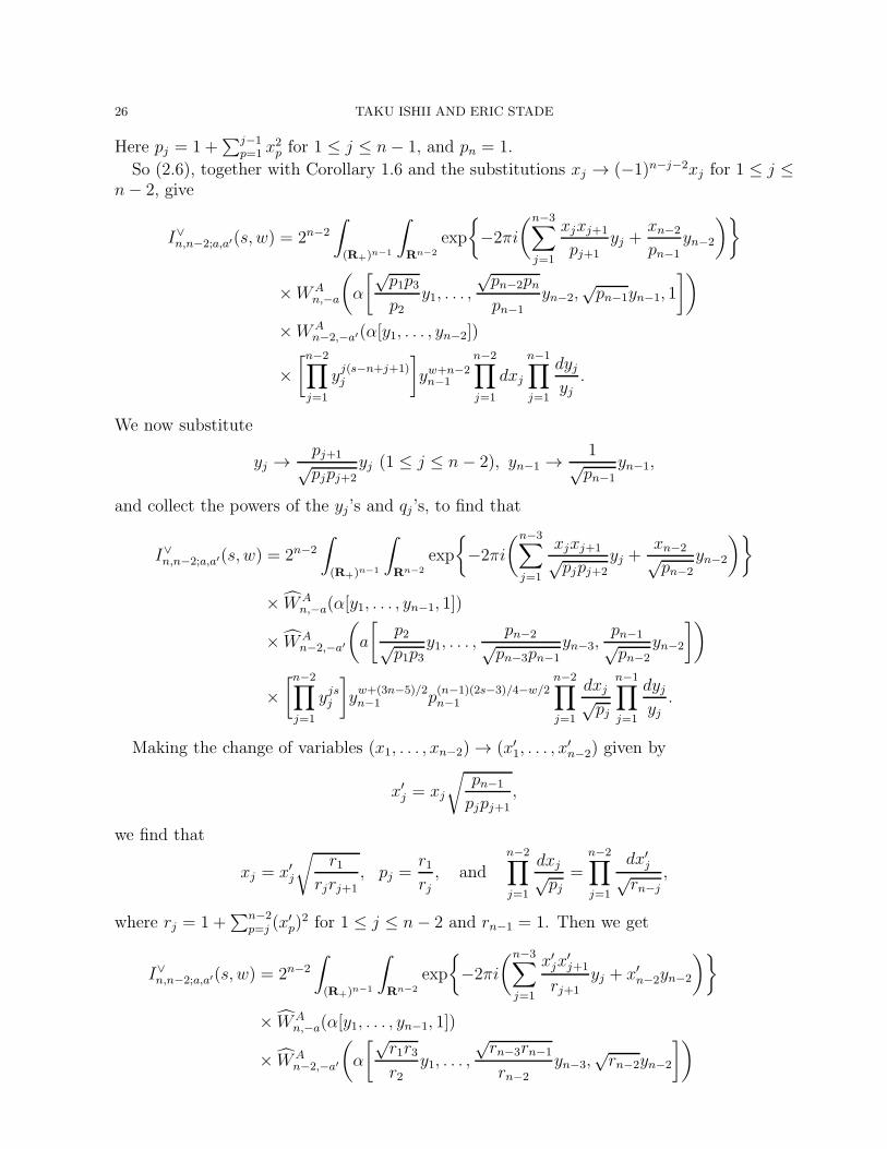
26 TAKU ISHII AND ERIC STADE
Here pj = 1 +∑j−1
p=1 x2p for 1 ≤ j ≤ n− 1, and pn = 1.
So (2.6), together with Corollary 1.6 and the substitutions xj → (−1)n−j−2xj for 1 ≤ j ≤n− 2, give
I∨n,n−2;a,a′(s, w) = 2n−2
∫
(R+)n−1
∫
Rn−2
exp
{−2πi
(n−3∑
j=1
xjxj+1
pj+1
yj +xn−2
pn−1
yn−2
)}
×WAn,−a
(α
[√p1p3
p2y1, . . . ,
√pn−2pn
pn−1
yn−2,√pn−1yn−1, 1
])
×WAn−2,−a′(α[y1, . . . , yn−2])
×[n−2∏
j=1
yj(s−n+j+1)j
]yw+n−2n−1
n−2∏
j=1
dxj
n−1∏
j=1
dyjyj.
We now substitute
yj →pj+1√pjpj+2
yj (1 ≤ j ≤ n− 2), yn−1 →1
√pn−1
yn−1,
and collect the powers of the yj’s and qj ’s, to find that
I∨n,n−2;a,a′(s, w) = 2n−2
∫
(R+)n−1
∫
Rn−2
exp
{−2πi
(n−3∑
j=1
xjxj+1√pjpj+2
yj +xn−2√pn−2
yn−2
)}
× WAn,−a(α[y1, . . . , yn−1, 1])
× WAn−2,−a′
(a
[p2√p1p3
y1, . . . ,pn−2√pn−3pn−1
yn−3,pn−1√pn−2
yn−2
])
×[n−2∏
j=1
yjsj
]yw+(3n−5)/2n−1 p
(n−1)(2s−3)/4−w/2n−1
n−2∏
j=1
dxj√pj
n−1∏
j=1
dyjyj.
Making the change of variables (x1, . . . , xn−2) → (x′1, . . . , x′n−2) given by
x′j = xj
√pn−1
pjpj+1
,
we find that
xj = x′j
√r1
rjrj+1
, pj =r1rj, and
n−2∏
j=1
dxj√pj
=n−2∏
j=1
dx′j√rn−j
,
where rj = 1 +∑n−2
p=j (x′p)
2 for 1 ≤ j ≤ n− 2 and rn−1 = 1. Then we get
I∨n,n−2;a,a′(s, w) = 2n−2
∫
(R+)n−1
∫
Rn−2
exp
{−2πi
(n−3∑
j=1
x′jx′j+1
rj+1yj + x′n−2yn−2
)}
× WAn,−a(α[y1, . . . , yn−1, 1])
× WAn−2,−a′
(α
[√r1r3r2
y1, . . . ,
√rn−3rn−1
rn−2
yn−3,√rn−2yn−2
])
ARCHIMEDEAN L-FACTORS 27
×[n−2∏
j=1
yjsj
]yw+(3n−5)/2n−1 r
(n−1)(2s−3)/4−(w+|a′|)/21
n−2∏
j=2
r−1/2j
n−2∏
j=1
dx′j
n−1∏
j=1
dyjyj.
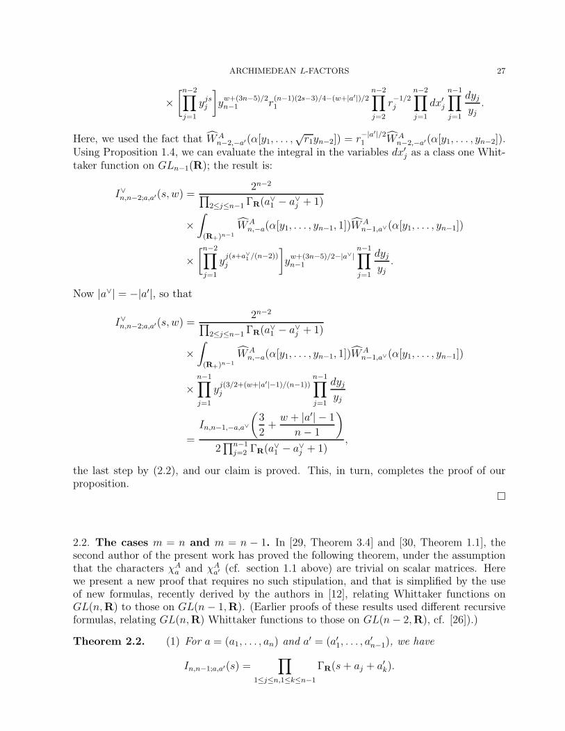
Here, we used the fact that WAn−2,−a′(α[y1, . . . ,
√r1yn−2]) = r
−|a′|/21 WA
n−2,−a′(α[y1, . . . , yn−2]).Using Proposition 1.4, we can evaluate the integral in the variables dx′j as a class one Whit-taker function on GLn−1(R); the result is:
I∨n,n−2;a,a′(s, w) =2n−2
∏2≤j≤n−1 ΓR(a
∨1 − a∨j + 1)
×∫
(R+)n−1
WAn,−a(α[y1, . . . , yn−1, 1])W
An−1,a∨(α[y1, . . . , yn−1])
×[n−2∏
j=1
yj(s+a∨1 /(n−2))j
]yw+(3n−5)/2−|a∨|n−1
n−1∏
j=1
dyjyj.
Now |a∨| = −|a′|, so that
I∨n,n−2;a,a′(s, w) =2n−2
∏2≤j≤n−1 ΓR(a∨1 − a∨j + 1)
×∫
(R+)n−1
WAn,−a(α[y1, . . . , yn−1, 1])W
An−1,a∨(α[y1, . . . , yn−1])
×n−1∏
j=1
yj(3/2+(w+|a′|−1)/(n−1))j
n−1∏
j=1
dyjyj
=
In,n−1,−a,a∨
(3
2+w + |a′| − 1
n− 1
)
2∏n−1
j=2 ΓR(a∨1 − a∨j + 1),
the last step by (2.2), and our claim is proved. This, in turn, completes the proof of ourproposition.
�
2.2. The cases m = n and m = n − 1. In [29, Theorem 3.4] and [30, Theorem 1.1], thesecond author of the present work has proved the following theorem, under the assumptionthat the characters χA
a and χAa′ (cf. section 1.1 above) are trivial on scalar matrices. Here
we present a new proof that requires no such stipulation, and that is simplified by the useof new formulas, recently derived by the authors in [12], relating Whittaker functions onGL(n,R) to those on GL(n− 1,R). (Earlier proofs of these results used different recursiveformulas, relating GL(n,R) Whittaker functions to those on GL(n− 2,R), cf. [26]).)
Theorem 2.2. (1) For a = (a1, . . . , an) and a′ = (a′1, . . . , a
′n−1), we have
In,n−1;a,a′(s) =∏
1≤j≤n,1≤k≤n−1
ΓR(s+ aj + a′k).
28 TAKU ISHII AND ERIC STADE
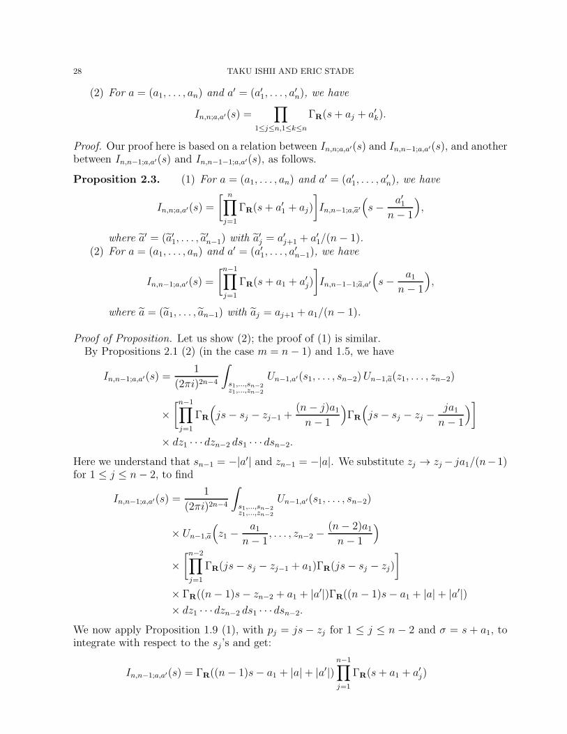
(2) For a = (a1, . . . , an) and a′ = (a′1, . . . , a
′n), we have
In,n;a,a′(s) =∏
1≤j≤n,1≤k≤n
ΓR(s+ aj + a′k).
Proof. Our proof here is based on a relation between In,n;a,a′(s) and In,n−1;a,a′(s), and anotherbetween In,n−1;a,a′(s) and In,n−1−1;a,a′(s), as follows.
Proposition 2.3. (1) For a = (a1, . . . , an) and a′ = (a′1, . . . , a
′n), we have
In,n;a,a′(s) =
[ n∏
j=1
ΓR(s+ a′1 + aj)
]In,n−1;a,a′
(s− a′1
n− 1
),
where a′ = (a′1, . . . , a′n−1) with a
′j = a′j+1 + a′1/(n− 1).
(2) For a = (a1, . . . , an) and a′ = (a′1, . . . , a
′n−1), we have
In,n−1;a,a′(s) =
[n−1∏
j=1
ΓR(s+ a1 + a′j)
]In,n−1−1;a,a′
(s− a1
n− 1
),
where a = (a1, . . . , an−1) with aj = aj+1 + a1/(n− 1).
Proof of Proposition. Let us show (2); the proof of (1) is similar.By Propositions 2.1 (2) (in the case m = n− 1) and 1.5, we have
In,n−1;a,a′(s) =1
(2πi)2n−4
∫
s1,...,sn−2z1,...,zn−2
Un−1,a′(s1, . . . , sn−2)Un−1,a(z1, . . . , zn−2)
×[n−1∏
j=1
ΓR
(js− sj − zj−1 +
(n− j)a1n− 1
)ΓR
(js− sj − zj −
ja1n− 1
)]
× dz1 · · · dzn−2 ds1 · · · dsn−2.
Here we understand that sn−1 = −|a′| and zn−1 = −|a|. We substitute zj → zj − ja1/(n−1)for 1 ≤ j ≤ n− 2, to find
In,n−1;a,a′(s) =1
(2πi)2n−4
∫
s1,...,sn−2z1,...,zn−2
Un−1,a′(s1, . . . , sn−2)
× Un−1,a
(z1 −
a1n− 1
, . . . , zn−2 −(n− 2)a1n− 1
)
×[n−2∏
j=1
ΓR(js− sj − zj−1 + a1)ΓR(js− sj − zj)
]
× ΓR((n− 1)s− zn−2 + a1 + |a′|)ΓR((n− 1)s− a1 + |a|+ |a′|)× dz1 · · · dzn−2 ds1 · · · dsn−2.
We now apply Proposition 1.9 (1), with pj = js− zj for 1 ≤ j ≤ n − 2 and σ = s + a1, tointegrate with respect to the sj’s and get:
In,n−1;a,a′(s) = ΓR((n− 1)s− a1 + |a|+ |a′|)n−1∏
j=1
ΓR(s+ a1 + a′j)
ARCHIMEDEAN L-FACTORS 29
× 2n−2
(2πi)n−2
∫
z1,...,zn−2
Un−1,a′(s− z1, . . . , (n− 2)s− zn−2)
× Un−1,a
(z1 −
a1n− 1
, . . . , zn−2 −(n− 2)a1n− 1
)dz1 · · ·dzn−2.
If we substitute zj → zj + ja1/(n− 1) for 1 ≤ j ≤ n− 2, we find that
In,n−1;a,a(s) =
[n−1∏
j=1
ΓR(s+ a1 + a′j)
]ΓR
((n− 1)
(s− a1
n− 1
)+ |a|+ |a′|
)
× 2n−2
(2πi)n−2
∫
z1,...,zn−2
Un−1,a
((s− a1
n− 1
)− z1, . . . , (n− 2)
(s− a1
n− 1
)− zn−2
)
× Un−1,a(z1, . . . , zn−2) dz1 · · · dzn−2,
and our proposition is proved.
To deduce Theorem 2.2, we use induction. First, we consider part (1) of the theorem: inthe case n = 2, this amounts to Barnes’ first lemma.
Now by Proposition 2.3 (2), we have
In,n;a,a′(s) =
n∏
j=1
ΓR(s+ a′1 + aj)
n−1∏
j=1
ΓR
(s− a′1
n− 1+ a1 + a′j
)
× In−1,n−1;a,a′
(s− a1 + a′1
n− 1
).
By the induction hypothesis applied to In,n;a,a′(s), we find that
In,n;a,a′(s) =
n∏
j=1
ΓR(s+ a′1 + aj)
n−1∏
j=1
ΓR(s+ a1 + a′j+1)
×∏
1≤j≤n−1,1≤k≤n−1
ΓR
(s− a1 + a′1
n− 1+ aj + a′k
)
=n∏
j=1
ΓR(s+ a′1 + aj)n−1∏
j=1
ΓR(s+ a1 + a′j+1)
×∏
1≤j≤n−1,1≤k≤n−1
ΓR(s+ aj+1 + a′k+1)
which is the desired result.We now turn to part (2) of our theorem. The case n = 2 follows from Proposition 2.1
(2) (in the case n = 2, m = 1). The general case then follows by Proposition 2.3 (2) and byinduction (much as in the above proof for the case m = n), and thus we complete our proofof Theorem 2.2. �
2.3. The case m = n− 2. We investigate the zeta integrals Z(s,W,W ′) and Z∨(s,W,W ′),as defined in section 2.1 above, in the case m = n − 2. Note that the case (n,m) = (3, 1)has previously been treated in [8].
30 TAKU ISHII AND ERIC STADE
Theorem 2.4. For a = (a1, . . . , an) and a′ = (a′1, . . . , a
′n−2), we have
In,n−2;a,a′(s) =
[ ∏
1≤j≤n,1≤k≤n−2
ΓR(s+ aj + a′k)
]· 1
4πi
∫
w
∏nj=1 ΓR(w − aj)∏n−2
j=1 ΓR(s+ w + a′j)dw.
Proof. We evaluate the integral (2.4) with m = n − 2. Using Proposition 1.5 to rewriteUn,a, we have
In,n−2;a,a′(s) =2−1
(2πi)2n−4
∫
s1,··· ,sn−3,sn−1z1,...,zn−2
Un−1,a(z1, . . . , zn−2)Un−2,a′(s1, . . . , sn−3)
×[n−3∏
j=1
ΓR
(js− sj − zj −
ja1n− 1
)ΓR
(js− sj − zj−1 +
(n− j)a1n− 1
)]
× ΓR
((n− 2)s+ |a′| − zn−2 −
(n− 2)a1n− 1
)
× ΓR
((n− 2)s+ |a′| − zn−3 +
2a1n− 1
)
× ΓR(sn−1 + |a| − a1)ΓR
(sn−1 − zn−2 +
a1n− 1
)
× dz1 · · · dzn−2 ds1 · · · dsn−3dsn−1.
We apply Proposition 1.9 (1) with σ = s+ a1 to integrate with respect to s1, . . . , sn−3:
In,n−2;a,a′(s) =n−2∏
j=1
ΓR(s+ a1 + a′j) ·2n−4
(2πi)n−1
∫
sn−1,z1,··· ,zn−2
Un−1,a(z1, . . . , zn−2)
× Un−2,a′(s′ − z1, . . . , (n− 3)s′ − zn−3) · ΓR((n− 2)s′ + |a′| − zn−2)
× ΓR(sn−1 + |a| − a1)ΓR
(sn−1 − zn−2 +
a1n− 1
)dz1 · · ·dzn−2 dsn−1.
Here we have defined s′ = s− a1/(n− 1).Next we use Proposition 1.9 (1), with σ = s+ sn−1 + |a|, to rewrite Un−2,a′ ; we find that
In,n−2;a,a′(s) =n−2∏
j=1
ΓR(s+ a1 + a′j) ·2−1
(2πi)2n−4
∫
sn−1,z1,...,zn−2w1,...,wn−3
Un−1,a(z1, . . . , zn−2)
× ΓR((n− 3)s′ − zn−3 + s+ sn−1 + |a|+ |a′|)∏n−2j=1 ΓR(s+ sn−1 + |a|+ a′j)
× Un−2,a′(w1, . . . , wn−3) ·n−3∏
j=1
ΓR(js′ − zj − wj)
×n−3∏
j=1
ΓR((j − 1)s′ − zj−1 − wj + s+ sn−1 + |a|)
× ΓR((n− 2)s′ + |a′| − zn−2)ΓR(sn−1 + |a| − a1)
× ΓR
(sn−1 − zn−2 +
a1n− 1
)dw1 · · · dwn−3 dz1 · · · dzn−2 dsn−1.
ARCHIMEDEAN L-FACTORS 31
If we define wn−2 = −|a′| and wn−1 = (n− 1)s′ + |a|, the above can be rewritten as follows:
In,n−2:a,a′(s) =
n−2∏
j=1
ΓR(s+ a1 + a′j) ·2−1
(2πi)2n−4
∫
sn−1,z1,...,zn−2w1,...,wn−3
Un−1,a(z1, . . . , zn−2)
× Un−2,a′(w1, . . . , wn−3) ·ΓR(sn−1 + |a| − a1)ΓR(s+ sn−1 + |a| − w1)∏n−2
j=1 ΓR(s+ sn−1 + |a|+ a′j)
×n−2∏
j=1
ΓR(js′ − zj − wj)ΓR
((j + 1)s′ − zj − wj+1 + sn−1 +
a1n− 1
+ |a|)
× dw1 · · · dwn−3 dz1 · · · dzn−2 dsn−1.
We can apply Proposition 1.9 (2) with pj = js′−wj (1 ≤ j ≤ n−2) and σ = sn−1+a1/(n−1)+ |a|, to integrate with respect to z1, . . . , zn−2 (note that the condition pn−1 = −|a| = −|a|is satisfied because of the definition of wn−1), and arrive at
In,n−2;a,a′(s) =n−2∏
j=1
ΓR(s+ a1 + a′j) ·2n−3
(2πi)n−2
∫
sn−1,w1,...,wn−3
Un−2,a′(w1, . . . , wn−3)
×ΓR(sn−1 + |a| − a1)
∏n−1j=1 ΓR(sn−1 +
a1n−1
+ |a| − aj)∏n−2j=1 ΓR(s+ sn−1 + |a|+ a′j)
× Un−1,a(s′ − w1, . . . , (n− 3)s′ − wn−3, (n− 2)s′ + |a′|)
× dw1 · · · dwn−3 dsn−1
=
[n−2∏
j=1
ΓR(s+ a1 + a′j)
]· In−1,n−2;a,a′(s
′)
× 1
4πi
∫
sn−1
∏nj=1 ΓR(sn−1 + |a| − aj)∏n−2
j=1 ΓR(s+ sn−1 + |a|+ a′j)dsn−1,
the last step by (2.4). Hence Theorem 2.2 (1) yields our assertion. 2
Now as may be seen, for example, in [18], the GLn ×GLn−2 functional equation at a real
place ν relates Z(s,W,W ′) to Z∨(s, R(wn,n−2)W∨, (W ′)∨). Here wn,m =
(Im
wn−m
)and
R means right translation. In the situation of interest to us here, where W =WAn,a andW
′ =
WA
n−2,a′ as above, we may ignore the R(wn,n−2) in Z∨(s, R(wn,n−2)W∨, (W ′)∨), since WA
n,a
is right O(n)-invariant. The relevant functional equation then relates Z(s,WAn,a,W
A
n−2,a′) =
In,n−2;a,a′(s) to Z∨(s, (WA
n,a)∨, (W
A
n−2,a′)∨) = I∨n,n−2;a,a′(s).
More specifically: the functional equation demonstrated in [18] amounts, in the presentcontext, to the assertion that
In,n−2;a,a′(s)∏1≤j≤n,1≤k≤n−2 ΓR(s+ aj + a′k)
=I∨n,n−2;a,a′(1− s)∏
1≤j≤n,1≤k≤n−2 ΓR(1− s− aj − a′k).
We now wish to show that the above functional equation may also be derived using resultscontained herein. To do so it will suffice, in light of Theorem 2.4, to prove the following:
32 TAKU ISHII AND ERIC STADE
Theorem 2.5. We have
I∨n,n−2;a,a′(s) =
[ ∏
1≤j≤n,1≤k≤n−2
ΓR(s− aj − a′k)
]
× 1
4πi
∫
w
∏1≤j≤n ΓR(w − aj)∏
1≤j≤n−2 ΓR(1− s+ w + a′j)dw.
Proof. By Proposition 2.1 (3),
I∨n,n−2;a,a′(s) =1
4πi
∫
w
In,n−1,−a,a∨
(3
2+w + |a′| − 1
n− 1
)
∏n−1j=2 ΓR(a∨1 − a∨j + 1)
dw,
where a∨ = (a∨1 , . . . , a∨n−1) is as in (2.1). We may now apply Theorem 2.2 (1) to the
archimedean zeta factor inside the integral; we find that
I∨n,n−2;a,a′(s) =1
4πi
∫
w
∏1≤j≤n,1≤k≤n−1 ΓR
(3
2+w + |a′| − 1
n− 1− aj + a∨k
)
∏n−1j=2 ΓR(a∨1 − a∨j + 1)
dw
=
[ ∏
1≤j≤n,2≤k≤n−1
ΓR
(3
2+w + |a′| − 1
n− 1− aj + a∨k
)]
× 1
4πi
∫
w
∏1≤j≤n ΓR
(3
2+w + |a′| − 1
n− 1− aj + a∨1
)
∏n−1j=2 ΓR(a∨1 − a∨j + 1)
dw
=
[ ∏
1≤j≤n,2≤k≤n−1
ΓR(s− aj − a′k−1)
]
× 1
4πi
∫
w
∏1≤j≤n ΓR
(w − aj − (n− 2)s+ |a′|+ 3n− 5
2
)
∏n−1j=2 ΓR
(1 + w + a′j−1 − (n− 1)s+ |a′|+ 3n− 5
2
) dw.
We substitute w → w+(n−2)s−|a′|− 3n− 5
2; we also rearrange the products a bit (letting
k → k + 1 in the product outside the integral; and letting j → j + 1 in the product in thedenominator of the integrand). The result is exactly the statement of Theorem 2.5, and weare done. �
3. archimedean zeta integrals on SO2n+1 ×GLm
Global Rankin-Selberg integrals for L-functions on SO2n+1 ×GLm have been constructedin [6] for the cases m = n and m = n+1, in [7] for the cases m ≤ n, and in [24] for the casesm ≥ n + 1. In this section, we will consider the cases m = n− 1, m = n, and m = n+ 1.
As may be seen from the works cited above, the archimedean zeta integrals Jℓ,n;a,b(s)of interest to us, for the cases of SO2n+1 × GLn+1, SO2n+1 × GLn, and SO2n+1 × GLn−1
ARCHIMEDEAN L-FACTORS 33
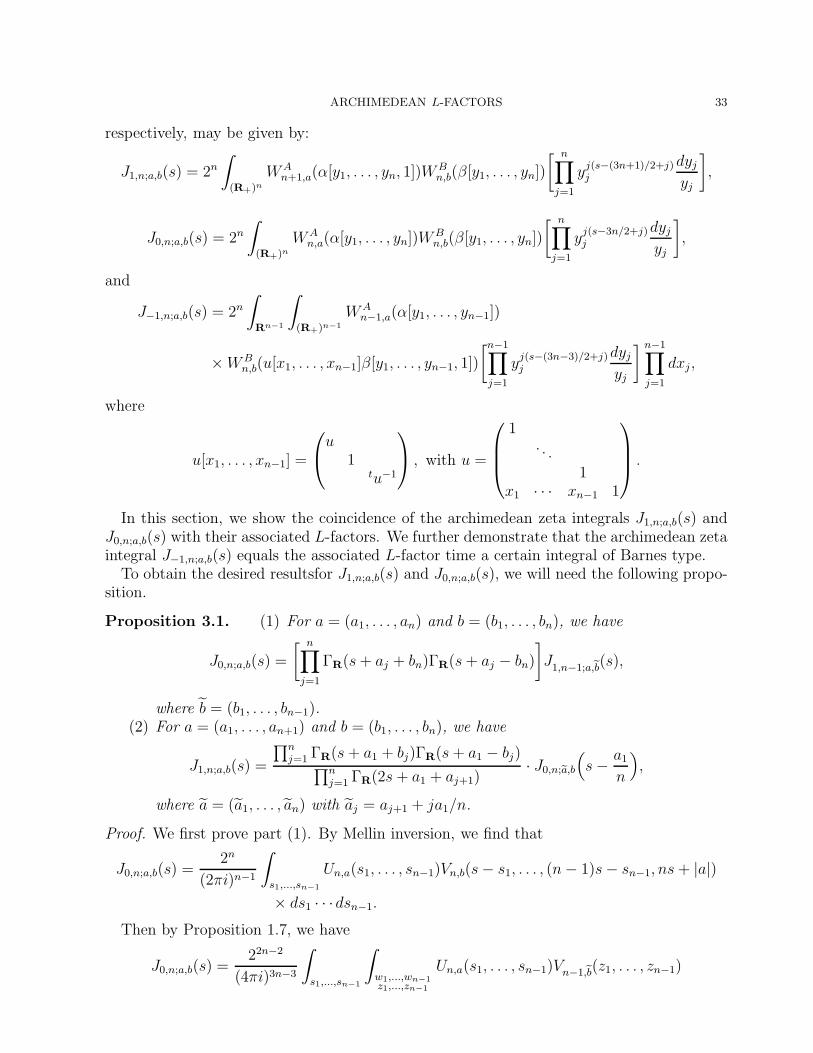
respectively, may be given by:
J1,n;a,b(s) = 2n∫
(R+)nWA
n+1,a(α[y1, . . . , yn, 1])WBn,b(β[y1, . . . , yn])
[ n∏
j=1
yj(s−(3n+1)/2+j)j
dyjyj
],
J0,n;a,b(s) = 2n∫
(R+)nWA
n,a(α[y1, . . . , yn])WBn,b(β[y1, . . . , yn])
[ n∏
j=1
yj(s−3n/2+j)j
dyjyj
],
and
J−1,n;a,b(s) = 2n∫
Rn−1
∫
(R+)n−1
WAn−1,a(α[y1, . . . , yn−1])
×WBn,b(u[x1, . . . , xn−1]β[y1, . . . , yn−1, 1])
[n−1∏
j=1
yj(s−(3n−3)/2+j)j
dyjyj
] n−1∏
j=1
dxj ,
where
u[x1, . . . , xn−1] =
u
1tu−1
, with u =
1. . .
1x1 · · · xn−1 1
.
In this section, we show the coincidence of the archimedean zeta integrals J1,n;a,b(s) andJ0,n;a,b(s) with their associated L-factors. We further demonstrate that the archimedean zetaintegral J−1,n;a,b(s) equals the associated L-factor time a certain integral of Barnes type.
To obtain the desired resultsfor J1,n;a,b(s) and J0,n;a,b(s), we will need the following propo-sition.
Proposition 3.1. (1) For a = (a1, . . . , an) and b = (b1, . . . , bn), we have
J0,n;a,b(s) =
[ n∏
j=1
ΓR(s+ aj + bn)ΓR(s+ aj − bn)
]J1,n−1;a,b(s),
where b = (b1, . . . , bn−1).(2) For a = (a1, . . . , an+1) and b = (b1, . . . , bn), we have
J1,n;a,b(s) =
∏nj=1 ΓR(s+ a1 + bj)ΓR(s+ a1 − bj)∏n
j=1 ΓR(2s+ a1 + aj+1)· J0,n;a,b
(s− a1
n
),
where a = (a1, . . . , an) with aj = aj+1 + ja1/n.
Proof. We first prove part (1). By Mellin inversion, we find that
J0,n;a,b(s) =2n
(2πi)n−1
∫
s1,...,sn−1
Un,a(s1, . . . , sn−1)Vn,b(s− s1, . . . , (n− 1)s− sn−1, ns+ |a|)
× ds1 · · ·dsn−1.
Then by Proposition 1.7, we have
J0,n;a,b(s) =22n−2
(4πi)3n−3
∫
s1,...,sn−1
∫
w1,...,wn−1z1,...,zn−1
Un,a(s1, . . . , sn−1)Vn−1,b(z1, . . . , zn−1)
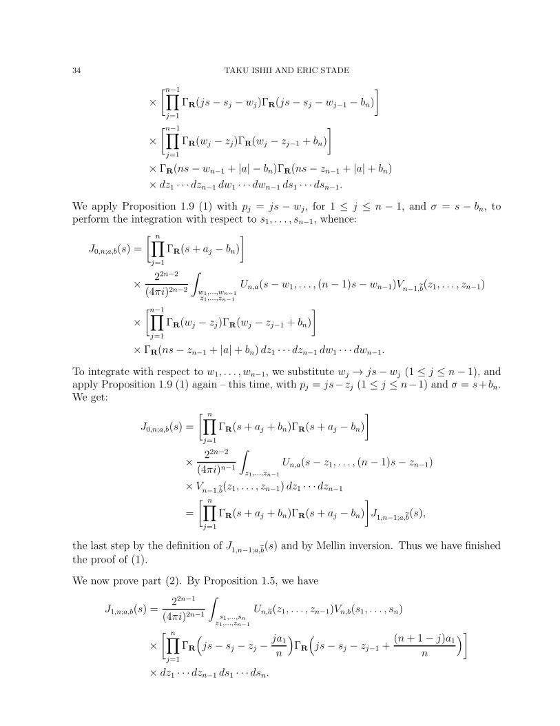
34 TAKU ISHII AND ERIC STADE
×[n−1∏
j=1
ΓR(js− sj − wj)ΓR(js− sj − wj−1 − bn)
]
×[n−1∏
j=1
ΓR(wj − zj)ΓR(wj − zj−1 + bn)
]
× ΓR(ns− wn−1 + |a| − bn)ΓR(ns− zn−1 + |a|+ bn)
× dz1 · · ·dzn−1 dw1 · · ·dwn−1 ds1 · · · dsn−1.
We apply Proposition 1.9 (1) with pj = js − wj, for 1 ≤ j ≤ n − 1, and σ = s − bn, toperform the integration with respect to s1, . . . , sn−1, whence:
J0,n;a,b(s) =
[ n∏
j=1
ΓR(s+ aj − bn)
]
× 22n−2
(4πi)2n−2
∫
w1,...,wn−1z1,...,zn−1
Un,a(s− w1, . . . , (n− 1)s− wn−1)Vn−1,b(z1, . . . , zn−1)
×[n−1∏
j=1
ΓR(wj − zj)ΓR(wj − zj−1 + bn)
]
× ΓR(ns− zn−1 + |a|+ bn) dz1 · · · dzn−1 dw1 · · · dwn−1.
To integrate with respect to w1, . . . , wn−1, we substitute wj → js−wj (1 ≤ j ≤ n− 1), andapply Proposition 1.9 (1) again – this time, with pj = js−zj (1 ≤ j ≤ n−1) and σ = s+bn.We get:
J0,n;a,b(s) =
[ n∏
j=1
ΓR(s+ aj + bn)ΓR(s+ aj − bn)
]
× 22n−2
(4πi)n−1
∫
z1,...,zn−1
Un,a(s− z1, . . . , (n− 1)s− zn−1)
× Vn−1,b(z1, . . . , zn−1) dz1 · · · dzn−1
=
[ n∏
j=1
ΓR(s+ aj + bn)ΓR(s+ aj − bn)
]J1,n−1;a,b(s),
the last step by the definition of J1,n−1;a,b(s) and by Mellin inversion. Thus we have finished
the proof of (1).
We now prove part (2). By Proposition 1.5, we have
J1,n;a,b(s) =22n−1
(4πi)2n−1
∫
s1,...,snz1,...,zn−1
Un,a(z1, . . . , zn−1)Vn,b(s1, . . . , sn)
×[ n∏
j=1
ΓR
(js− sj − zj −
ja1n
)ΓR
(js− sj − zj−1 +
(n+ 1− j)a1n
)]
× dz1 · · · dzn−1 ds1 · · · dsn.
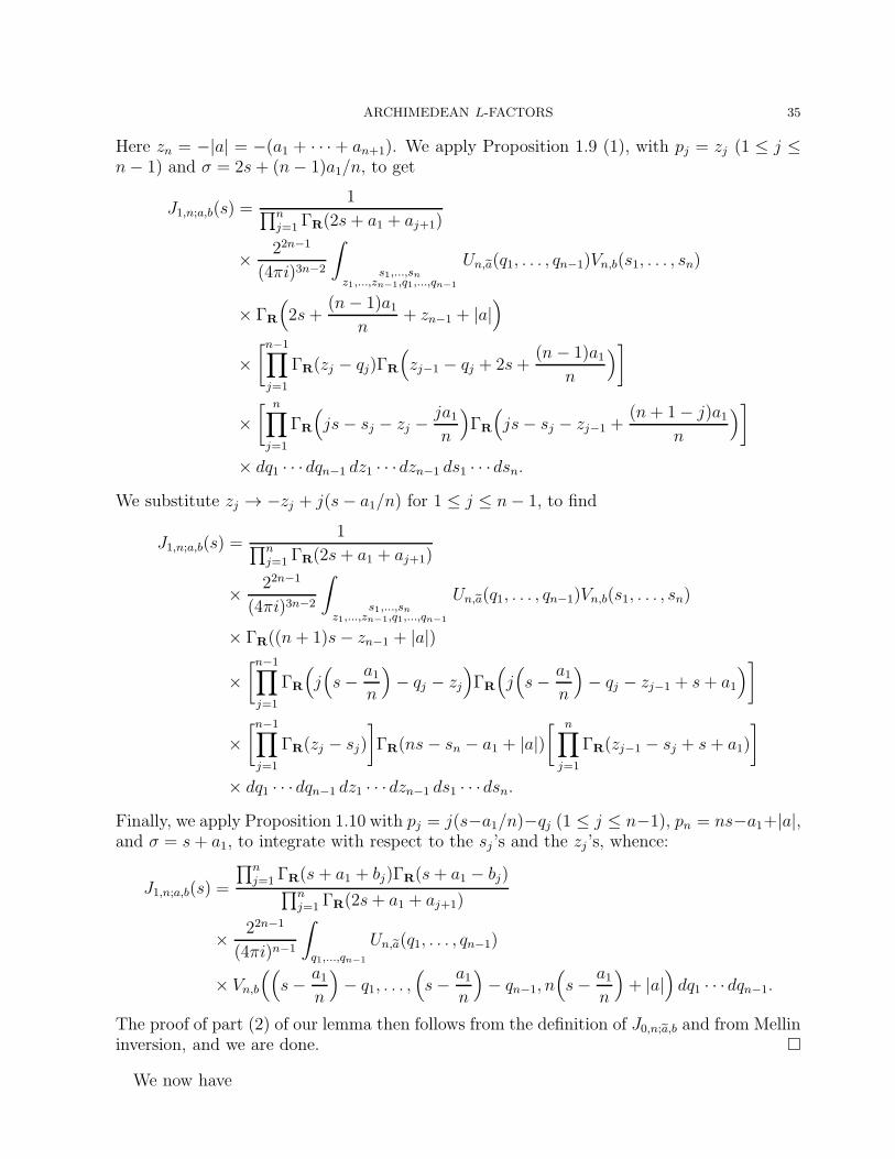
ARCHIMEDEAN L-FACTORS 35
Here zn = −|a| = −(a1 + · · ·+ an+1). We apply Proposition 1.9 (1), with pj = zj (1 ≤ j ≤n− 1) and σ = 2s+ (n− 1)a1/n, to get
J1,n;a,b(s) =1∏n
j=1 ΓR(2s+ a1 + aj+1)
× 22n−1
(4πi)3n−2
∫
s1,...,snz1,...,zn−1,q1,...,qn−1
Un,a(q1, . . . , qn−1)Vn,b(s1, . . . , sn)
× ΓR
(2s+
(n− 1)a1n
+ zn−1 + |a|)
×[n−1∏
j=1
ΓR(zj − qj)ΓR
(zj−1 − qj + 2s+
(n− 1)a1n
)]
×[ n∏
j=1
ΓR
(js− sj − zj −
ja1n
)ΓR
(js− sj − zj−1 +
(n+ 1− j)a1n
)]
× dq1 · · · dqn−1 dz1 · · ·dzn−1 ds1 · · · dsn.
We substitute zj → −zj + j(s− a1/n) for 1 ≤ j ≤ n− 1, to find
J1,n;a,b(s) =1∏n
j=1 ΓR(2s+ a1 + aj+1)
× 22n−1
(4πi)3n−2
∫
s1,...,snz1,...,zn−1,q1,...,qn−1
Un,a(q1, . . . , qn−1)Vn,b(s1, . . . , sn)
× ΓR((n+ 1)s− zn−1 + |a|)
×[n−1∏
j=1
ΓR
(j(s− a1
n
)− qj − zj
)ΓR
(j(s− a1
n
)− qj − zj−1 + s+ a1
)]
×[n−1∏
j=1
ΓR(zj − sj)
]ΓR(ns− sn − a1 + |a|)
[ n∏
j=1
ΓR(zj−1 − sj + s + a1)
]
× dq1 · · · dqn−1 dz1 · · · dzn−1 ds1 · · ·dsn.
Finally, we apply Proposition 1.10 with pj = j(s−a1/n)−qj (1 ≤ j ≤ n−1), pn = ns−a1+|a|,and σ = s+ a1, to integrate with respect to the sj ’s and the zj ’s, whence:
J1,n;a,b(s) =
∏nj=1 ΓR(s+ a1 + bj)ΓR(s+ a1 − bj)∏n
j=1 ΓR(2s+ a1 + aj+1)
× 22n−1
(4πi)n−1
∫
q1,...,qn−1
Un,a(q1, . . . , qn−1)
× Vn,b
((s− a1
n
)− q1, . . . ,
(s− a1
n
)− qn−1, n
(s− a1
n
)+ |a|
)dq1 · · · dqn−1.
The proof of part (2) of our lemma then follows from the definition of J0,n;a,b and from Mellininversion, and we are done. �
We now have
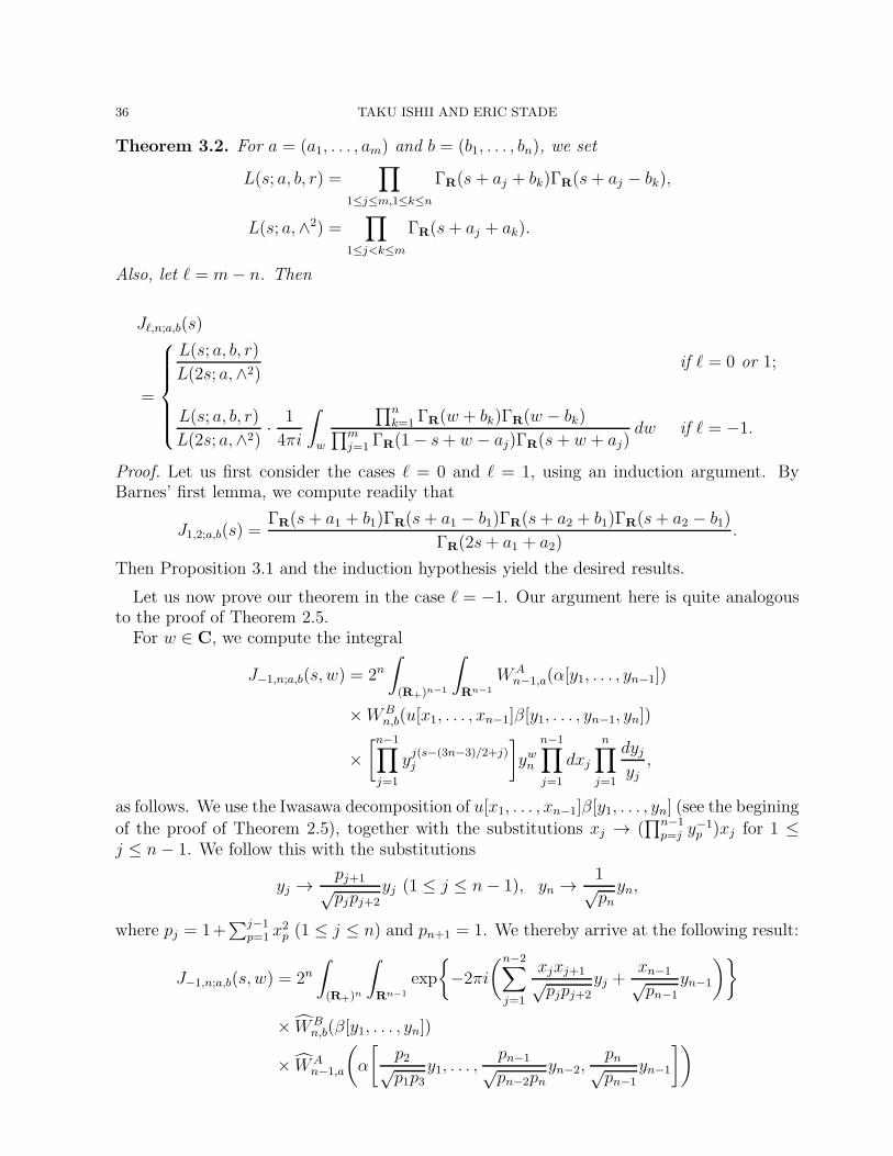
36 TAKU ISHII AND ERIC STADE
Theorem 3.2. For a = (a1, . . . , am) and b = (b1, . . . , bn), we set
L(s; a, b, r) =∏
1≤j≤m,1≤k≤n
ΓR(s+ aj + bk)ΓR(s+ aj − bk),
L(s; a,∧2) =∏
1≤j<k≤m
ΓR(s+ aj + ak).
Also, let ℓ = m− n. Then
Jℓ,n;a,b(s)
=
L(s; a, b, r)
L(2s; a,∧2)if ℓ = 0 or 1;
L(s; a, b, r)
L(2s; a,∧2)· 1
4πi
∫
w
∏nk=1 ΓR(w + bk)ΓR(w − bk)∏m
j=1 ΓR(1− s+ w − aj)ΓR(s+ w + aj)dw if ℓ = −1.
Proof. Let us first consider the cases ℓ = 0 and ℓ = 1, using an induction argument. ByBarnes’ first lemma, we compute readily that
J1,2;a,b(s) =ΓR(s+ a1 + b1)ΓR(s+ a1 − b1)ΓR(s+ a2 + b1)ΓR(s+ a2 − b1)
ΓR(2s+ a1 + a2).
Then Proposition 3.1 and the induction hypothesis yield the desired results.
Let us now prove our theorem in the case ℓ = −1. Our argument here is quite analogousto the proof of Theorem 2.5.
For w ∈ C, we compute the integral
J−1,n;a,b(s, w) = 2n∫
(R+)n−1
∫
Rn−1
WAn−1,a(α[y1, . . . , yn−1])
×WBn,b(u[x1, . . . , xn−1]β[y1, . . . , yn−1, yn])
×[n−1∏
j=1
yj(s−(3n−3)/2+j)j
]ywn
n−1∏
j=1
dxj
n∏
j=1
dyjyj,
as follows. We use the Iwasawa decomposition of u[x1, . . . , xn−1]β[y1, . . . , yn] (see the begining
of the proof of Theorem 2.5), together with the substitutions xj → (∏n−1
p=j y−1p )xj for 1 ≤
j ≤ n− 1. We follow this with the substitutions
yj →pj+1√pjpj+2
yj (1 ≤ j ≤ n− 1), yn → 1√pnyn,
where pj = 1+∑j−1
p=1 x2p (1 ≤ j ≤ n) and pn+1 = 1. We thereby arrive at the following result:
J−1,n;a,b(s, w) = 2n∫
(R+)n
∫
Rn−1
exp
{−2πi
(n−2∑
j=1
xjxj+1√pjpj+2
yj +xn−1√pn−1
yn−1
)}
× WBn,b(β[y1, . . . , yn])
× WAn−1,a
(α
[p2√p1p3
y1, . . . ,pn−1√pn−2pn
yn−2,pn√pn−1
yn−1
])
ARCHIMEDEAN L-FACTORS 37
×[n−1∏
j=1
yjsj
]yw+n2/2n pn(2s−n)/4−(w+1)/2
n
n−1∏
j=1
dxj√pj
n∏
j=1
dyjyj.
Next we change variables from (x1, . . . , xn−1) to (x′1, . . . , x′n−1), with x′j = xj
√pn/(pjpj+1)
for each j, and integrate with respect to variables x′j by way of Proposition 1.4. We findthat
J−1,n;a,b(s, w) =2n∏n−1
j=1 ΓR(w − |a| − aj − n(s− n2) + 1)
×∫
(R+)nWB
n,b(β[y1, . . . , yn])WAn,α(α[y1, . . . , yn])
[ n∏
j=1
yj(n/2+(w−|a|)/n)j
dyjyj
]
=1∏n−1
j=1 ΓR(w − |a| − aj − n(s− n2) + 1)
· J0,n;a,b(n2+w − |a|n
),
where a = (a1, . . . , an) with
a1 = −(n− 1)(s− n
2) +
n− 1
n(w − |a|),
aj = aj−1 + s− n
2− 1
n(w − |a|) (2 ≤ j ≤ n).
Therefore, the case ℓ = 0 of the present theorem implies that
J−1,n;a,b(s, w)
=
∏1≤j≤n−1,1≤k≤n ΓR(s+ aj + bk)ΓR(s+ aj − bk)∏
1≤j<k≤n−1 ΓR(2s+ aj + ak)
×∏n
k=1 ΓR(−(n− 1)s+ n2
2+ w − |a|+ bk)ΓR(−(n− 1)s+ n2
2+ w − |a| − bk)∏n−1
j=1 ΓR(−ns + n2
2+ w − |a| − aj + 1)ΓR(−(n− 2)s+ n2
2+ w − |a|+ aj)
.
Thus Mellin inversion and a change of variable yield our assertion, and we complete theproof of Theorem 3.2. �
Remark 2. The local functional equation for SO2n+1×GLn−1, as described in [25], amounts,at real places, to the assertion that
J−1,n,a,b(s)
/[L(s; a, b, r)
L(2s; a,∧2)
]
is invariant under (s, a, b) → (1 − s,−a,−b). This invariance is readily apparent fromTheorem 3.2 above.
Appendix: Comparison with unramified computations
The well-known Kato-Casselman-Shalika formulas describe unramified (nonarchimedean)Whittaker functions in terms of characters of finite dimensional representations of the corre-sponding L-groups. The unramified computations for SO2n+1 ×GLm can then be achievedby combining these realizations of unramified Whittaker functions with certain facts aboutthe representation theory of GLn(C) and Spn(C), (See [6, Appendix].)
In this appendix, we present an alternative, somewhat roundabout, approach to the un-ramified calculations for SO2n+1 ×GLn and SO2n+1 ×GLn+1. This new approach parallels,
38 TAKU ISHII AND ERIC STADE
in a number of ways, our calculations above in the analogous archimedean cases. We hopethat this suggestion of connections between the unramified and archimedean situations mighthelp enable future computations, particularly in the archimedean context.
The general ideas informing this appendix are as follows. The p-adic analogs of our recur-sive formulas for Mellin transforms of Whittaker functions can be understood as branchinglaws for finite dimensional representation of GLn(C) and Spn(C). Moreover, Pieri’s rule,which gives the decomposition into irreducibles of the tensor product of an irreducible rep-resentation with the symmetric kth power of the standard representation, can be consideredanalogous to our Propositions 1.9 and 1.10. By way of these observations, we may there-fore perform the unramified computationsin a fashion reminescent of that employed above– namely, by reducing the SO2n+1 × GLn+1 (respectively, SO2n+1 × GLn) case to that ofSO2n+1 ×GLn (respectively, SO2n−1 ×GLn).
We begin by recalling explicit formulas for unramified Whittaker functions. Let F bea nonarchimedean local field, O its ring of integers, and p = () its maximal ideal. Weset q = |O/p|. We take a non-trivial additive character ψ of F to be unramified. Let πA
a
(respectively, πBb ) be the unramified principal series representation with Satake paramater
a = diag(a1, . . . , an) ∈ GLn(C) (respectively, b = diag(b1, . . . , bn, b−1n , . . . , b−1
1 ) ∈ Spn(C)).We sometimes write a = (a1, . . . , an) and b = (b1, . . . , bn). We then consider the GLn(O)-(respectively, SO2n+1(O))-fixed Whittaker function WA
n,a ∈ W(πAa , ψ) (respectively, W
Bn,b ∈
W(πBb , ψ)), normalized such that WA
n,a(1n) =WBn,b(12n+1) = 1.
For λ = (λ1, λ2, . . . , λn) ∈ Zn, we put
α[λ] = α[λ1, . . . , λn] = diag(λ1, . . . , λn) ∈ GLn(F ),
β[λ] = β[λ1, . . . , λn] = diag(λ1, . . . , λn, 1, −λn, . . . , −λ1) ∈ SO2n+1(F ).
We set
WAn,a(α[λ]) = δ
1/2A (α[λ])WA
n,a(α[λ]),
WBn,b(β[λ]) = δ
1/2B (β[λ])WB
n,b(β[λ]).
where δA (respectively, δB) is the modulus character for the Borel subgroup of GLn (re-spectively, SO2n+1). According to the formulas of Shintani and Kato-Casselman-Shalika, wehave
WAn,a(α[λ]) =
{χAλ (a) if λ ∈ Pn,
0 otherwise,
WBn,b(β[λ]) =
{χCλ (b) if λ ∈ P+
n ,
0 otherwise,
where χAλ (respectively, χC
λ ) is the character of the irreducible finite dimensional representa-tion πA
λ (respectively, πCλ ) of GLn(C) (respectively, Spn(C)) with highest weight λ. Here
Pn = {λ = (λ1, λ2, . . . , λn) ∈ Zn | λ1 ≥ λ2 ≥ · · · ≥ λn},P+
n = {λ = (λ1, λ2, . . . , λn) ∈ Pn | λn ≥ 0}.We define subsets of P+
n as follows. For a given λ ∈ P+n and a nonnegative integer r, we
set
P+n (λ) = {µ = (µ1, . . . , µn) ∈ P+
n | λ1 ≥ µ1 ≥ λ2 ≥ · · · ≥ µn−1 ≥ λn ≥ µn};
ARCHIMEDEAN L-FACTORS 39
P+n−1(λ) = {µ = (µ1, . . . , µn−1) ∈ P+
n−1 | λ1 ≥ µ1 ≥ λ2 ≥ · · · ≥ λn−1 ≥ µn−1 ≥ λn};P+
n (λ) = {µ ∈ P+n | λ ∈ P+
n (µ)}= {µ = (µ1, . . . , µn) ∈ P+
n | µ1 ≥ λ1 ≥ µ2 ≥ · · · ≥ λn−1 ≥ µn ≥ λn};P+
n,r(λ) = {µ ∈ P+n (λ) | |λ| − |µ| = r};
P+
n,r(λ) = {µ ∈ P+
n (λ) | λ ∈ P+n,r(µ)} = {µ ∈ P+
n (λ) | |µ| − |λ| = r}.Here we write |λ| =
∑ni=1 λi for λ ∈ P+
n .
We first state the nonarchimedean analogs of the recursive formulas in Propositions 1.5and 1.7. Let λ ∈ P+
n . We have the following:
WAn,a(α[λ]) =
∑
µ∈P+n−1(λ)
a|λ|−|µ|n WA
n−1,a(α[µ])(A.1)
and
WBn,b(β[λ]) =
∑
ν∈P+n (λ)
∑
µ∈P+n−1(ν)
b2|ν|−|λ|−|µ|n WB
n−1,b(β[µ]),(A.2)
where a = (a1, . . . , an−1) and b = (b1, . . . , bn−1). These formulas can be interpreted as thebranching laws
πAλ |GLn−1(C) =
⊕
µ∈P+n−1(λ)
πAµ ,
πCλ |Spn−1(C) =
⊕
µ∈P+n−1(λ)
m(λ, µ)πCµ ,
where the mulitiplicity m(λ, µ) is the cardinality of the set {ν ∈ P+n (λ) | µ ∈ P+
n−1(ν)}.To discuss a nonarchimedean analog of the formulas in Propositions 1.9 and 1.10, let us
recall Pieri’s rule. This is a special case of the Littlewood-Richardson rule ([4, §A.1]), whichdescribes how the tensor product πA
λ ⊗ πAκ decomposes:
πAλ ⊗ πA
κ∼= ⊕µM
µλκπ
Aµ .
If we write (k) := (k, 0, . . . , 0) ∈ P+n , then Pieri’s rule ([4, Proposition 15.25]) asserts
Mµλ(k) =
{1 if µ ∈ P+
n,k(λ),
0 otherwise.(A.3)
We denote by Nµλκ the Littlewood-Richardson coefficient for Spn(C):
πCλ ⊗ πC
κ∼= ⊕µN
µλκπ
Cµ .
It is known that Nµλκ may be expressed in terms of Mµ
λκ as follows:
Nµλκ =
∑
ν,σ,τ
MλσνM
µτνM
κστ
([4, §25.3]). From the Littlewood-Richardson rule, we find that
M (k)στ =
{1 if σ = (r) and τ = (k − r) for some 0 ≤ r ≤ k,
0 otherwise.
40 TAKU ISHII AND ERIC STADE
Then Pieri’s rule (A.3) implies a Pieri-type rule for Spn(C):
Nµλ(k) =
∑
0≤r≤k
∑
ν
Mλ(r)νM
µ(k−r)ν
=∑
0≤r≤k
∑
ν∈P+n,r(λ)
∑
µ∈P+n,k−r(ν)
1
= ♯{ν ∈ P+n (λ) ∩ P+
n (µ) | |λ|+ |µ| − 2|ν| = k}.
(A.4)
Let hk denote the kth complete symmetric polynomial in n variables:
hk(x1, . . . , xn) =∑
1≤i1≤···≤ik≤n
xi1 · · ·xik .
If we set
hAk (a) = hr(a1, . . . , an),
hBk (b) = hr(b1, . . . , bn, b−11 , . . . , b−1
n ),
then hAk and hBk give the characters of representations with highest weight (k, 0, . . . , 0) ofGLn(C) and Spn(C), respectively. Thus (A.3) and (A.4) imply that
∑
µ∈P+n,k(λ)
WAn,a(α[µ]) = hAk (a)W
An,a(α[λ])
and ∑
0≤r≤k
∑
ν∈P+n,k−r(λ)
∑
µ∈P+n,r(ν)
WBn,b(β[µ]) = hBk (b)W
Bn,b(β[λ])
for λ ∈ P+n . In light of the formulas
∞∑
k=0
hAk (a)tk =
n∏
j=1
(1− ajt)−1,
∞∑
k=0
hBk (b)tk =
n∏
j=1
{(1− bjt)(1− b−1j t)}−1,
we arrive at our nonarchimedean analogs of Propositions 1.9 and 1.10:
∑
µ∈P+n (λ)
t|µ|−|λ|WAn,a(α[µ]) =
[ n∏
j=1
(1− ajt)−1]WA
n,a(α[λ]),(A.5)
∑
ν∈P+n (λ)
∑
µ∈P+n (ν)
t|λ|+|µ|−2|ν|WBn,b(β[µ]) =
[ n∏
j=1
{(1− bjt)(1− b−1j t)}−1
]WB
n,b(β[λ]).(A.6)
Using the above formulas, we now compute the unramified zeta integrals in a mannersimilar to that employed above, in the archimedean situation. The unramified zeta integralsfor SO2n+1 ×GLn and SO2n+1 ×GLn+1 are given by
J0,n;a,b(s) =∑
λ∈P+n
WAn,a(α[λ])W
Bn,b(β[λ])q
−|λ|s
ARCHIMEDEAN L-FACTORS 41
and
J1,n;a,b(s) =∑
λ∈P+n
WAn+1,a(α[λ, 0])W
Bn,b(β[λ])q
−|λ|s,
respectively. Here we have written α[λ, 0] = α[λ1, . . . , λn, 0].We can relate J0,n;a,b(s) (respectively, J1,n;a,b(s)) to J1,n−1;a,b(s) (respectively, J0,n;a,b(s)) as
follows. From (A.2), we have
J0,n;a,b(s) =∑
λ∈P+n
∑
ν∈P+n (λ)
∑
µ∈P+n−1(ν)
WAn,a(α[λ])W
Bn−1,b
(β[µ])b2|ν|−|λ|−|µ|n q−|λ|s.
We use (A.5) with t = b−1n q−s and t = bnq
−s successively to sum over λ and ν:
J0,n;a,b(s)
=[ n∏
j=1
(1− ajb−1n q−s)−1
] ∑
ν∈P+n
∑
µ∈P+n−1(ν)
WAn,a(α[ν])W
Bn−1,b
(β[µ])b|ν|−|µ|n q−|ν|s
=[ n∏
j=1
{(1− ajbnq−s)(1− ajb
−1n q−s)}−1
] ∑
µ∈P+n−1
WAn,a(α[µ, 0])W
Bn−1,b
(β[µ])q−|µ|s
=[ n∏
j=1
{(1− ajbnq−s)(1− ajb
−1n q−s)}−1
]J1,n−1;a,b(s).
Now, let us consider J1,n;a,b(s). We observe that (A.1) implies
J1,n;a,b(s) =∑
λ∈P+n
∑
µ∈P+n (λ)
WAn,a(α[µ])W
Bn,b(β[λ])a
|λ|−|µ|n+1 q−|λ|s.
Apply (A.5) with t = an+1q−2s to WA
n,a(α[µ]), to get
[ n∏
j=1
(1− ajan+1q−2s)−1
]J1,n;a,b(s)
=∑
λ∈P+n
∑
µ∈P+n (λ)
∑
ν∈P+n (µ)
WAn,a(α[ν])W
Bn,b(β[λ])a
|λ|+|ν|−2|µ|n+1 q−(|λ|+2|ν|−2|µ|)s
=∑
ν∈P+n
WAn,a(α[ν])q
−|ν|s∑
µ∈P+n (ν)
∑
λ∈P+n (µ)
WBn,b(β[λ])(an+1q
−s)|ν|+|λ|−2|µ|.
By (A.6) with t = an+1q−s, we can sum over λ and µ, to get
J1,n;a,b(s) =
∏nj=1{(1− an+1bjq
−s)(1− an+1b−1j q−s)}−1
∏nj=1(1− ajan+1q−2s)−1
J0,n;a,b(s),
and we are done.
References
[1] E.W. Barnes, A new development of the theory of hypergeometric functions, Proc. London Math. Soc.2, # 6 (1908), 141–177.
[2] D. Bump, Barnes’ second lemma and its application to Rankin-Selberg convolutions, American Journalof Mathematics 109 (1987), 179–186.
42 TAKU ISHII AND ERIC STADE
[3] D. Bump, The Rankin-Selberg method: a survey. In: A Symposium in Honor of Atle Selberg, Oslo,Norway, July 14–21, 1987, Academic Press (1989).
[4] W. Fulton and J. Harris, Representation theory. A first course. Graduate Texts in Mathematics, 129.Readings in Mathematics. Springer-Verlag, New York, 1991. xvi+551 pp.
[5] S. Gelbart and F. Shahidi, Analytic properties of automorphic L-functions, Academic Press (1988).[6] S. Gelbart, I.I. Piatetski-Shapiro and S. Rallis, Explicit constructions of automorphic L-functions, Lect.
Note in Math. 1254, Springer-Verlag (1987).[7] D. Ginzburg, L-functions for SOn ×GLk, J. reine angew. Math. 405 (1990), 156–180.[8] J. Hoffstein and M. R. Murty, L-series of automorphic forms on GL(3, R), In: Theorie des nombres
(Quebec, PQ, 1987), de Gruyter, Berlin (1989).[9] T. Ishii, Whittaker functions on orthogonal groups of odd degree, submitted.
[10] T. Ishii, Whittaker functions on real semisimple Lie groups of rank two. Canad. J. Math. 62, #3 (2010),563–581.
[11] T. Ishii and T. Moriyama, Spinor L-functions for generic cusp forms on GSp(2) belonging to principalseries representations, Trans. Amer. Math. Soc. 360 (2008), 5683–5709.
[12] T. Ishii and E. Stade, New formulas for Whittaker functions on GL(n,R), J. Funct. Anal. 244 (2007),289–314.
[13] H. Jacquet, Fonctions de Whittaker associees aux groupes de Chevalley, Bull. Soc. Math. France 95
(1967), 243–309.[14] H. Jacquet, Automorphic Forms on GL(2) Part II, Lecture Notes in Mathematics 278, Springer-Verlag
(1972).[15] H. Jacquet, I. I. Piatetski-Shapiro, and J. Shalika, Rankin-Selberg convolutions, American Journal of
Mathematics 105, #2 (1983), 367–464.[16] H. Jacquet and J. Shalika, On Euler products and the classification of automorphic representations I,
American Journal of Mathematics 103, #3 (1981), 499–558.[17] H. Jacquet and J. Shalika, On Euler products and the classification of automorphic forms II American
Journal of Mathematics103, #4 (1981), 777–815.[18] H. Jacquet and J. Shalika, Rankin-Selberg convolutions: the Archimedean theory. In: Festschrift in
Honor of Piatetski-Shapiro, Part I, American Mathematical Society (1990).[19] B. Kostant, On Whittaker vectors and representation theory, Invent. Math. 48 (1978), 101–184.[20] R.P. Langlands, Euler Products, Yale University Press (1967).[21] S. Niwa, Commutation relations of differential operators and Whittaker functions on Sp2(R), Proc.
Japan Acad. 71, Ser A. (1995), 189–191.[22] I. I. Piatetski–Shapiro, Euler subgroups. In: Lie Groups and their Representations, John Wiley and
Sons (1975).[23] J. Shalika, The multiplicity one theorem for GL(n), Ann. of Math. 100 (1974), 171–193.[24] D. Soudry, Rankin-Selberg covolutions for SO(2l + 1) × GL(n): local theory, Memoirs of the Amer.
Math. Soc. 500, American Mathematical Society (1993).[25] D. Soudry, On the Archimedean theory of Rankin-Selberg convolutions for SO(2l + 1)×GL(n), Ann.
Sci. Ecole Norm. Sup.28, #2 (1995), 161–224.[26] E. Stade, On explicit integral formulas for GL(n,R)-Whittaker functions, Duke Math. J. 60 (1990),
313–362.[27] E. Stade, Hypergeometric series and Euler factors at infinity for L -functions on GL(3,R)×GL(3,R),
American Journal of Mathematics 115, #2 (1993), 371–387.[28] E. Stade, Mellin transforms of Whittaker functions on GL(4,R) and GL(4,C) Manuscripta Mathemat-
ica 87 (1995), 511–526.[29] E. Stade, Mellin transforms of GL(n,R) Whittaker functions, Amer. J. Math. 123 (2001), 121–161.[30] E. Stade, Archimedean L-factors on GL(n) × GL(n) and generalized Barnes integrals, Israel J. Math.
127 (2002), 201-220.[31] E. Whittaker and G. Watson, A Course of Modern Analysis, Cambridge University Press (1902).
ARCHIMEDEAN L-FACTORS 43
Faculty of Science and Technology, Seikei University, 3-3-1 Kichijoji-Kitamachi, Musashino,
Tokyo, 180-8633, Japan
E-mail address : [email protected]
Department of Mathematics, University of Colorado, Boulder, CO 80309, USA
E-mail address : [email protected]
Related Documents