ArcGIS for Desktop Cookbook

Free Sample

In this package, you will find: • The author biography • A preview chapter from the book, Chapter 10 "Working with 3D Analyst" • A synopsis of the book’s content • More information on ArcGIS for Desktop Cookbook

About the Author Daniela Cristiana Docan is currently a lecturer in the Department of Topography and Cadastre at the Faculty of Geodesy in Bucharest, Romania. She obtained her PhD in 2009 from Technical University of Civil Engineering Bucharest with the thesis Contributions to quality improvement of spatial data in GIS. Formerly, she worked for Esri Romania and the National Agency of Cadastre and Land Registration (ANCPI).

While working for Esri Romania, she trained teams (as an authorized instructor in ArcGIS Desktop by Environmental Systems Research Institute, Inc., USA) from state and privately owned companies, such as Romanian Civil Aeronautical Authority, Agency of Payments and Intervention for Agriculture (APIA), Institute of Hydroelectric Studies and Design, and Petrom. She has also trained and assisted the team in charge of quality data control using ArcGIS for Desktop and PLTS GIS Data ReViewer in the Land Parcels Identification System (LPIS) project, in Romania.

For the ANCPI, in 2009, she created the conceptual, logical, and physical data model for the Romanian National Topographic Dataset at the scale 1:5,000 (TOPRO5). She was a member of the workgroup that elaborated TOPRO5 and metadata technical specifications for the ANCPI and the Member State Report for Infrastructure for Spatial Information in the European Community (INSPIRE) in 2010.

I would like to thank Llewellyn Rozario, Mohammed Fahad, Humera Shaikh, Mohita Vyas, and everyone else from Packt Publishing for all their hard work to get this book published.

I would also like to thank the reviewers for their work and practical advice.

A special thanks goes to my friends for their support.

ArcGIS for Desktop Cookbook ArcGIS for Desktop is an important component of the Esri ArcGIS platform. ArcGIS for Desktop allows you to visualize, create, analyze, manage, and distribute geographic data.

ArcGIS for Desktop Cookbook starts with the basics of designing a file geodatabase schema. Using your file geodatabase schema, you will learn to create, edit, and constrain the geometry and attribute values of your data. In this book, you will learn to manage Coordinate Reference System (CRS) issues in the geodatabase context.

This book will also cover the following topics: designing and sharing quality maps, geocoding addresses, creating routes and events, analyzing and visualizing raster data in 3D environments, and exporting/importing different data formats.

Knowing and understanding your data is essential in any spatial analysis and geoprocessing process. Therefore, you will work with two main geodatabase structures that fully support all topics covered by this book's chapters.

ArcGIS for Desktop Cookbook will clearly explain all the basic steps performed in every recipe of the book to help you refine your own workflow.

What This Book Covers Chapter 1, Designing Geodatabase, teaches you how to create a file geodatabase for a topographic map. It shows you, step by step, how to create feature datasets, feature classes, subtypes, and domains. Furthermore, you will create relationship classes and test the relationship behavior.

Chapter 2, Editing Data, teaches you how to add data to your file geodatabase created in Chapter 1, Designing Geodatabase. In addition to this, you will learn to work with Coordinate Geometry (COGO) elements, such as bearings, angles, and horizontal distances. You will identify all invalid attribute values for the newly created or loaded features in accordance with the domains created in the first chapter. You will also constrain and administrate the spatial relationships between features with geodatabase topology.

Chapter 3, Working with CRS, explains how to transform a CRS into another CRS using a predefined ArcGIS Project tool. You will also learn how to georeference a scanned topographic map. Furthermore, you will learn to define a custom CRS and a custom transformation.

Chapter 4, Geoprocessing, guides you through the geoprocessing tools for vector data, such as Spatial Join, Spatial Adjustment, Attribute transfer, Buffer, and Intersect. In addition to this, you will learn to work with the Model Builder application. You will build a geoprocessing workflow for a project named VeloGIS. This small project will

analyze the possible consequences of creating a cycling infrastructure, taking into account the existing road network.

Chapter 5, Working with Symbology, teaches you how to manage a collection of symbols, colors, and map elements into a style format. The chapter also covers the Representation topic that refers to an advanced technique to symbolize geographic features on a map.

Chapter 6, Building Better Maps, teaches you how to create labels with Maplex Label Engine. The chapter also covers the Annotation topic, which refers to an advanced technique to label the geographic features. In addition to this, you will learn to create a quantitative bivariate map, which analyzes two variables from census data: level of education and unemployment rate for a country/region.

Chapter 7, Exporting Your Maps, teaches you how to design, prepare, and export quality maps. Finally, you will publish your maps on ArcGIS Online.

Chapter 8, Working with Geocoding and Linear Referencing, teaches you how to convert the address information into spatial data and how to manage and use these geocoded addresses. The second part of this chapter will show you how to build routes and events for three different bus lines and a complex route for delivering a customer service.

Chapter 9, Working with Spatial Analyst, teaches you how to work with and analyze raster data. It shows you, step by step, how to create a terrain surface, reclassify a raster, work with Map Algebra and statistical functions, generalize a raster, generate density surfaces, and perform a least-cost path analysis.

Chapter 10, Working with 3D Analyst, teaches you how to create 3D features from 2D features and how to create TIN and Terrain surfaces. You will analyze the visibility between buildings and three geodetic points from the ground, using the ArcScene application. Moreover, you will create an animated fly-by tour of your 3D buildings and Digital Terrain Model (DTM) in ArcScene and will export it to a video file.

Chapter 11, Working with Data Interoperability, teaches you how to manage different data formats. You will export and import a fi le geodatabase using the XML interchange format. The second part of this chapter will show you how to import vector data into your geodatabase using the ArcGIS Data Interoperability extension.

10Working with

3D Analyst

In this chapter, we will cover the following topics:

Creating 3D features from 2D features

Creating a TIN surface

Creating a terrain dataset

Creating raster and TIN from a terrain dataset

Intervisibility

Creating a profi le graph

Creating an animation

IntroductionThe 3D Analyst extension allows you to display and analyze your 3D data. 3D data means 3D features, rasters, and Triangulated Irregular Networks (TINs). This 3D data contains a z-value. A z-value refers to an attribute other than the horizontal position (for example, projected x and y coordinates). In this chapter, your z-value will represent the normal heights (gravity-related height) expressed in meters.

The particular term height and the general term elevation are used interchangeably in this chapter because some ArcGIS instruments and parameters use the term: elevation. The term elevation means the height above a given level. In particular, our height term means the height above the local mean sea level.

Working with 3D Analyst

292

According to the international standard ISO 19111:2007 on geographic information—spatial referencing by coordinates:

A gravity-related height is a height dependent on Earth's gravity fi eld.

A normal height (H) is a gravity-related height that approximates the distance of a point above the mean sea level.

A Mean Sea Level (MSL) is the average level of the surface of the sea over all stages of tide and seasonal variations. In the local context, MSL is calculated from observations at one or more points over a given period of time.

For theory about gravity-related height, please refer to Jonathan Iliffe and Roger Lott, Datums and Map Projections 2nd Edition; Whittles Publishing, 2012, pp.30-35 and pp. 135-140.

In this chapter, you will work in the ArcScene 3D environment.

Creating 3D features from 2D featuresA 3D feature is a 2D feature that has elevation (height) values (z-values) stored in its geometry. When you are creating a new feature class in your geodatabase, you have from the fi rst panel Geometry Properties: Coordinate include Z values. Used to store 3D data. In Chapter 1, Designing Geodatabase, you created feature classes that store only 2D features.

In this recipe, you will convert the existing simple features (2D) into 3D features using two methods:

Based on the height values from a raster surface

Based on the height values from the 2D feature's fi eld attribute

Getting readyIn this recipe, you will work with the ArcScene desktop application. ArcScene documents are saved as .sxd fi les. Your scene document will contain:

A raster surface layer created in Chapter 9, Working with Spatial Analyst, in the Analyzing surfaces recipe

Two 2D feature classes: PointElevation and Buildings

Chapter 10

293

How to do it...Follow these steps to convert 2D features into 3D features:

1. Start ArcScene and open an existing scene document 3DFeatures.sxd from <drive>:\PacktPublishing\Data\3DAnalyst.

2. From the Geoprocessing menu, select Environments. Set the geoprocessing environment as follows:

Workspace:

Current Workspace: Data\3DAnalyst\TOPO5000.gdb

Scratch Workspace: Data\3DAnalyst\ScratchTOPO5000.gdb

Output Coordinates: Same as Input

Processing Extent: Same as the Elevation layer

Let's set base heights for the layers and vertical exaggeration for the scene:

1. In the Table Of Contents section, right–click on the Elevation raster layer, and navigate to Properties | Base Heights. Check Floating on a custom surface: Elevation. Click on Raster Resolution. For Base Surface, set Cellsize X to 2.5 and Cellsize Y to 2.5. Notice that the number of Rows and Columns is automatically updated. By decreasing the display resolution, you will improve the display performance. Click on OK.

2. Click on the Rendering tab, check Render layer at all times, and type 0.05 seconds for Draw simpler level of detail if navigation refresh rate exceeds.

The ArcScene redraws or renders the layers every time you make a navigation movement. By decreasing the refresh rate, ArcScene will only have time to draw a blue skeleton of your raster layer while you are exploring the scene with the Navigate tool. When you stop navigating the scene, the raster layer will render normally.

3. In the Effects section, choose 10 for the Select the drawing priority option. The Elevation layer will have the lowest drawing priority in comparison with other layers from the scene document. The highest priority is value 1. Click on Apply and OK.

Working with 3D Analyst

294

4. Set the vertical exaggeration for the scene. From the View menu, navigate to Scene Properties | General. Select 2 for Vertical Exaggeration. Click on OK. Try to navigate around the scene using the Navigate tool, as shown in the following screenshot:

5. In ArcScene, 2D feature layers have their base height set to 0 by default. The PointElevation and Buildings 2D feature layers are displayed below the Elevation layer. Repeat step 3 for the PointElevation feature layer using the same surface base heights. For Select the drawing priority option, type 1. Set the base height for the Buildings feature layer and for the Select the drawing priority option, choose 5.

Your 2D feature layers have been added to the Elevation surface. Turn off the 2D feature layers. Let's convert the PointElevation 2D feature layers to a 3D feature layer:

6. In ArcToolbox, expand 3D Analyst Tools | 3D Features, and double-click on the Feature to 3D by Attributes tool. Click on Show Help to see the meaning of every parameter. Set the following parameters:

Input Features: TOPO5000.gdb\Relief\PointElevation

Output Feature Class: ScratchTOPO5000.gdb\ PointElevation3D

Height Field: Elevation

To Height Field (optional): <none>

7. Click on OK. Notice that the PointElevation3D feature layer is directly displayed in the 3D space based on the z-value in the point geometry. Open its attribute table. The Shape fi eld stores the Point Z geometry.

Let's convert the Building 2D polygon feature layers to a 3D feature layer using the Elevation surface raster, as follows:

Chapter 10

295

8. In ArcToolbox, expand 3D Analyst Tools | Functional Surface, and double-click on the Interpolate Shape tool. Click on Show Help to see the meaning of every parameter. Set the following parameters:

Input Surface: TOPO5000.gdb\Elevation

Input Feature Class: TOPO5000.gdb\Buildings\Buildings

Output Feature Class: ...\3DAnalyst\ScratchTOPO5000.gdb\Buildings3D

Check Interpolate Vertices Only (optional)

9. Accept the default values for all other parameters. Click on OK.

10. Note that the Buildings3D feature layer is directly displayed in the 3D space based on the z-value into the polygon geometry. Open the attribute table of the Buildings3D feature. The Shape fi eld stores the Polygon Z geometry.

Let's improve the 3D appearance of buildings by extruding the polygon features according to the number of levels, as follows:

11. In the Table Of Contents section, right-click on the Buildings3D layer, and navigate to Properties | Extrusion. Set the following parameters:

Check Extrude features in layer

Extrusion value or expression: [Stories]*3

Apply extrusion by: adding it to each feature's minimum height

12. Click on OK and explore the results, as shown in the following screenshot:

13. Save your scene document as My3DFeatures.sxd and close ArcScene.

You can fi nd the fi nal results at <drive>:\PacktPublishing\Data\3DAnalyst\3DFeatures.

Working with 3D Analyst

296

How it works...At step 6, you assigned z-values to point features directly from the Elevation fi eld. The Z from the Shape geometry fi eld confi rms the 3D feature type.

At step 8, the raster cell values were interpolated to the assigned z-values to every vertex of the 3D polygon feature.

For the PointElevation3D and Buildings3D layers, it's not necessary anymore to set the base heights (topographic surface). Note also that subtypes and domains were kept in the new 3D feature classes.

At step 11, you raised the building from the ground using the number of levels multiplied by 3. The value 3 could represent the height of one level expressed in meters. From the Tools toolbar, use Measure tool | Measure Height to measure the reservoir height above the topographic surface, as shown in the following screenshot:

See also To create a 3D surface using 2D features, please refer to the Creating a TIN

surface recipe

Chapter 10

297

Creating a TIN surfaceA Triangulated Irregular Network (TIN) is mesh of non-overlapping triangles that represent a continuous surface. This surface is built by triangulating a set of points that have z-values using the Delaunay triangulation method. This method generates triangles that are as near as possible to an equilateral triangle. The set of points represent the primary source of height values (mass points) and incorporates point features or vertices of the polyline and polygon features.

For theoretical aspects about TIN and Delaunay triangulation, please refer to David O'Sullivan and David Unwin, Geographic Information Analysis, John Wiley & Sons, Inc., 2003, page 28 and 215 to 220.

Getting readyIn this recipe, you will create a TIN surface using 2D feature classes. You will also update the TIN surface with new, upcoming features, such as building footprints and a fi sh pond.

How to do it...Follow these steps to create a TIN surface using the ArcScene environment:

1. Start ArcScene and open an existing scene document TIN.sxd from <drive>:\PacktPublishing\Data\3DAnalyst.

Keep the geoprocessing environment from the previous recipe. From the Geoprocessing menu, select Geoprocessing Options. Check whether Background Processing | Enable is unchecked to ensure that your process will run in the foreground. By selecting this option, you will not allow other work until the tool stops running.

Working with 3D Analyst

298

2. In ArcToolbox, expand 3D Analyst Tools | Data Management | TIN, and double-click on the Create TIN tool. Set the following parameters:

Output TIN: 3DAnalyst\TIN\TOPO5k.gdb

Coordinate System: Pulkovo_1942_Adj_58_Stereo_70

Input Feature Class as shown in the following screenshot:

In the next step, you will create a 3D feature class from the 2D feature class Buildings using this time Topo5k TIN as the height (elevation) source surface:

3. In ArcToolbox, expand 3D Analyst Tools | Functional Surface, and double-click on the Interpolate Shape tool. Set the following parameters:

Input Surface: TOPO5k

Input Feature Class: TOPO5000.gdb\Buildings\Buildings

Output Feature Class: ScratchTOPO5000.gdb\Buildings3DFromTIN

Method (optional): LINEAR

Check Interpolate Vertices Only (optional)

4. Click on OK. In the Table Of Contents section, move the BuildingsFromTIN layer above all layers.

Let's update the TIN with buildings from the BuildingsFromTIN layer and with a fi sh pond from the Lake layer.

5. In ArcToolbox, expand 3D Analyst Tools | Data Management | TIN, and double-click on the Edit TIN tool. Set the following parameters:

Input TIN: 3DAnalyst\TIN\TOPO5k.gdb

Input Feature Class as shown in the following screenshot:

Chapter 10

299

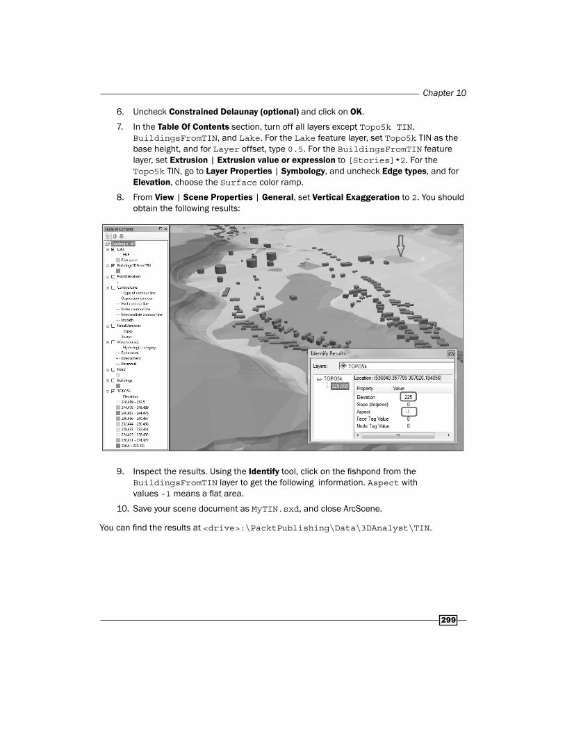
6. Uncheck Constrained Delaunay (optional) and click on OK.

7. In the Table Of Contents section, turn off all layers except Topo5k TIN, BuildingsFromTIN, and Lake. For the Lake feature layer, set Topo5k TIN as the base height, and for Layer offset, type 0.5. For the BuildingsFromTIN feature layer, set Extrusion | Extrusion value or expression to [Stories]*2. For the Topo5k TIN, go to Layer Properties | Symbology, and uncheck Edge types, and for Elevation, choose the Surface color ramp.

8. From View | Scene Properties | General, set Vertical Exaggeration to 2. You should obtain the following results:

9. Inspect the results. Using the Identify tool, click on the fi shpond from the BuildingsFromTIN layer to get the following information. Aspect with values -1 means a fl at area.

10. Save your scene document as MyTIN.sxd, and close ArcScene.

You can fi nd the results at <drive>:\PacktPublishing\Data\3DAnalyst\TIN.

Working with 3D Analyst

300

How it works...The elevation (height) points and vertices of the contour lines will be used as mass points to defi ne the TIN surface. You have used scarps, water courses, and roads as hard lines; therefore, the TIN triangles will not cross the linear features. Leave unchecked the Constrained Delaunay (optional) option; you will allow the Delaunay triangulation process to build multiple triangle edges on the hard lines (breaklines).

At step 5, you updated the TIN surface with fl at areas with constant height values. The fi shpond from the Lake 2D feature layer has the value 225 meters stored in the Elevation fi eld. The building footprints from the BuildingsFromTIN 3D feature layer have z-values incorporated into the polygon geometry or the Shape fi eld.

Creating a terrain datasetA terrain is a multi-resolution surface stored as a feature class in a feature dataset within a geodatabase. A terrain does not actually store the represented surface unlike TINs or rasters, which do. A terrain only references the participating feature classes and derives TINs at various resolutions on the fl y, depending on the display scale. A terrain must be created within a feature dataset together with the feature classes that are used in it. That way, the terrain, terrain surface, and terrain dataset terms are often used interchangeably. You cannot see a terrain surface in the ArcScene environment, but you can use the ArcMap and ArcGlobe applications.

The terrain is used for large amounts of data. In this recipe, you will work with Light Detection and Ranging (LiDAR) data. LiDAR is an optical remote-sensing technology that provides detailed 3D elevation data.

For further research about LiDAR remote-sensing technology, please refer to George Vosselman and Hand-Gerd Maas, Airborne and Terrestrial Laser Scanning, Whittles Publishing, 2010.

Getting readyIn this recipe, you will create a terrain using an ASCII text fi le that stores LiDAR point-cloud data. Your point cloud contains 5 million points. Those points represent a Digital Terrain Model (DTM) or ground data.

In Windows Explorer, go to the <drive>:\PacktPublishing\Data\3DAnalyst\LiDAR folder. Explore the dtm.xyz ASCII fi le with the Notepad application.

Chapter 10

301

How to do it...Follow these steps to create a terrain dataset:

1. Start ArcCatalog and go to Customize | Extensions to check the 3D Analyst extension. In Catalog Tree, go to <drive>:\PacktPublishing\Data\3DAnalyst\TOPO5000.gdb.

2. Your geodatabase already contains an empty feature dataset named Terrain. Right-click on the Terrain feature dataset and choose Properties | XY Coordinate System. The current projected coordinate reference system is Pulkovo_1942_Adj_58_Stereo_70 with the EPSG code as 3844. Click on Z Coordinate System. The vertical coordinate reference system is a national gravity-related height system called Constanta (Black Sea 1975) with the EPSG code as 5781.

In the next steps, you will calculate the basic statistics of dtm.xyz, and convert mass points from the ASCII fi le to a multipoint feature class:

3. In ArcToolbox, expand 3D Analyst Tools | Conversion | From File, and double-click on the Point File Information tool. Set the following parameters:

Point Data Browse for Files: ...\3DAnalyst\LiDAR\dtm.xyz

Output Feature Class: ...\3DAnalyst\TOPO5000.gdb\Terrain\DTMInfo

File Format: XYZ

File Suffix: xyz:

Coordinate System (optional) | XY Coordinate System: National Grids | Europe: Pulkovo_1942_Adj_58_Stereo_70

Z Coordinate System: Europe: Constanta

4. Accept the default values for all other parameters. Click on OK. You have obtained a polygon feature that defi nes the XY extent of your LiDAR data.

5. Open ArcMap. Add the DTMInfo feature class to your map. Save your map document as MyTerrain.mxd in the ...Data\3DAnalyst folder. Open the DTMInfo attribute table to view the following statistical information: Pt_Count: 5,722,782 points; Pt_Spacing: 1.005; Z_Min: 214.77, and Z_Max: 250.85. Close the table and turn off the DTMInfo layer.

6. In ArcToolbox, expand 3D Analyst Tools | Conversion | From File, and double-click on the ASCII 3D to Feature Class tool. Set the following parameters:

Point Data Browse for Files: ...\3DAnalyst\LiDAR\dtm.xyz

File Format: XYZ

Output Feature Class: ...\3DAnalyst\TOPO5000.gdb\Terrain\MassPoints

Working with 3D Analyst

302

Output Feature Class Type: MULTIPOINT

Coordinate System (optional) | XY Coordinate System: National Grids | Europe | Pulkovo_1942_Adj_58_Stereo_70

Z Coordinate System: Europe | Constanta

Average Point Spacing (optional): 1.005

File Suffix (optional): xyz

7. Accept the default values for all other parameters. Click on OK. Use the Zoom In or the Magnifi er tool to look closely at the points, as shown in the following screenshot:

Let's create the terrain surface:

8. In the Catalog window, right-click on the TOPO5000.gdb\Terrain feature dataset and navigate to New | Terrain. Set the following parameters:

Enter a name for your terrain: DTM

Check MassPoints and DTMInfo

Approximate point spacing: 1.005

Chapter 10

303

9. Click on Next. Click on Advanced. Set the Embedded option to Yes. Notice the terrain fi elds. Click on Next and set the following parameters:

Point selection method: Z Mean

Secondary thinning method: Moderate

Secondary thinning threshold: 0.5

10. Click on Next. Click on Calculate Pyramid Properties. Adjust Terrain Pyramid Levels, as shown in the following screenshot:

11. Click on Next. Inspect the parameter's summary. Click on Finish. Click on Yes to build the terrain. Add the DTM terrain to your map. Let's explore the terrain at different scales. Add the Lake feature class in your map document and Zoom In to the fi shpond. Turn off the Lake layer to see the terrain surface. Display and explore the area of interest at different scales, as shown in the following screenshots:

Working with 3D Analyst

304

12. Let's examine the properties of the DTM terrain layer. Right-click on the DTM layer and choose Properties | Display. Let's reduce the default number of points used in the rendering process. From the Apply point limit value, erase a zero to obtain the point 80,000. If you want to see the height when you point to the map, check Show Map Tips. Click on OK. Display and explore the area of interest at the scale 5,000 and 2,500. Apparently, there is no difference. But how about a 1:1,000 scale?

13. Let's display the contour lines for the DTM terrain. Right-click on the DTM layer and choose Properties | Symbology. In the Show section, click on the Add button, and select Contour with the same symbol. Click on Add and Dismiss. Click on the Import button to import the symbol and parameter values from ...\3D Analyst\Terrain\DTM.lyr. You should obtain the following results:

Chapter 10

305

14. Click on OK. Inspect the results. If you add the ContourLine 2D feature class, you can explore the difference between the topographic map surface at the scale 1:5,000 and a new terrain surface, as shown in the following screenshot:

15. In the Table Of Contents section, note that the Window Size label values is updated when you change the display scale. Save your map and close ArcMap.

You can fi nd the results at ...\3DAnalyst\Terrain\Terrain.mxd.

How it works...Before starting to load your LiDAR data into your geodatabase, you evaluated the point density. Because your ACSII fi le contains around fi ve million records, you grouped the LiDAR points into multipoint features. The multipoint geometry reduces the size of the MassPoints output feature class and the number of rows in the attribute table.

The Window Size pyramid will divide the data extent into equal windows and will select the representative points with Z Mean (a z-value closest to the mean). You choose this option because you want to avoid the extreme values. The resultant surface will be integrated in our product, which is a topographic map at the scale 1:5,000.

Working with 3D Analyst

306

From steps 9 to 10, you defi ned the rules for display terrain (scalability). The Moderate secondary thinning method will eliminate irrelevant points but will preserve the linear discontinuities from your surface. If z-values in the window area are within 0.5 meters, then it will be considered a fl at area and will result in a more generalized surface. The 0.5 meters represents twice the vertical accuracy of the LiDAR dataset. We assume that the vendor mentioned a vertical accuracy of 25 centimeters.

At step 10, you defi ned four pyramid levels. Those levels defi ne the vertical accuracy of the terrain, through four ranges of scales. Note that Level 1 of Terrain Pyramid has a Window Size of 1 meter, which means that the full surface resolution will be displayed up to scale 1:1,000.

Creating raster and TIN from a terrain dataset

A terrain dataset can be converted to rasters or TINs using the geoprocessing tools from the 3D Analyst toolbar. Why would we need to convert terrain to raster or TIN?

Starting from large-scale source data, you might want to obtain derivative vector or raster surfaces for small-scale (for example 1:25,000) applications.

You might need a raster surface to use statistical analysis tools from the Spatial Analyst extension.

You might want to refi ne and update the surface with new polygon or polyline features having a precision corresponding to the 1:3,000 scale. You will need a TIN with a vertical accuracy corresponding to that scale.

You might want to visualize your surfaces in ArcScene.

You might want to store the raster and TIN directly onto disk.

Getting readyIn this recipe, you will generate a raster and a TIN based on the DTM terrain surface created in the previous recipe.

You can start from your map document MyTerrain.mxd and skip step 1. Otherwise, you will use the terrain surface from ...\Data\3DAnalyst\Terrain\TOPO5000.gdb.

Chapter 10

307

How to do it...Follow these steps to convert a terrain dataset to raster and TIN using ArcMap:

1. Start ArcMap and open an existing map document, Terrain_ToRasterTIN.mxd, from ...\3DAnalyst\Terrain.

2. For the geoprocessing environment, set Current Workspace and Scratch Workspace: TOPO5000.gdb\Terrain. For Processing Extent, choose Union of Inputs.

3. In ArcToolbox, expand 3D Analyst Tools | Conversion | From Terrain, and double-click on the Terrain to Raster tool. Set the parameters, as shown in the following screenshot:

Working with 3D Analyst

308

4. Click on OK. In the Table Of Contents section, drag the DTM_Raster.tif surface above the DTM terrain surface. Change the symbology from Black to White to Elevation#1 Color Ramp. In the Effects toolbar, select DTM_Raster.tif as the layer drawing. Inspect the result using the Swipe tool, as shown in the following screenshot:

5. In ArcToolbox, expand 3D Analyst Tools | Conversion | From Terrain, and double-click on the Terrain to TIN tool. Set the parameters, as shown in the following screenshot:

Chapter 10

309

6. Click on OK. In the Table Of Contents section, drag the DEM_TIN surface above the DTM raster surface. Inspect the result in the same manner as the step 4 screenshot.

7. Save your map as MyTerrain_ToRasterTIN.mxd and close ArcMap.

You can fi nd the fi nal results at ...\Data\3DAnalyst\Terrain\ ResultsTerrain_ToRasterTIN.mxd.

How it works...At step 3, you converted the terrain surface to a raster surface in the TIFF format. You used the natural neighbors interpolation method to obtain a smoother raster surface. Notice that you have to mention the .tif fi le extension to create a raster in the TIFF format. To defi ne the cell size of your output raster, you mentioned CELLSIZE as 1. You will not improve the accuracy having a cell size smaller than the average point spacing of your initial LiDAR data. You have kept the full resolution of the input terrain by accepting the value 0 for the Pyramid Level Resolution parameter.

At step 5, you converted the terrain surface to a TIN surface. If you keep the value 0 for Pyramid Level Resolution, your geoprocessing tool will fail and display the message, The TIN will be too big. This is because of the allowed number of mass points in a TIN—up to 5,000,000. You chose Level 1 and accepted the default number of nodes.

IntervisibilityIntervisibility refers to the analysis of a sight line between an observer and a target feature through potential obstructions such as 3D surfaces or features.

Getting readyWe continue to plan the topographic survey campaign mentioned in Chapter 9, Working with Spatial Analyst, in the Analyzing surfaces and Analyzing the least-cost path recipes. In this recipe, you will analyze the visibility between three geodetic points and buildings (reservoirs and two churches).

TriangulationPoint3D has an attribute fi eld named SurveyInstruments that stores the normal height (H) of the instrument calculated as the sum of the Height Black Sea'75 fi eld and a constant value of 1.5 meters (height of the survey instrument).

Buildings3D has a fi eld named H_Buildings that stores the height calculated as the sum of the Z_Mean, the normal height (H) fi eld, and the approximate height of the building. The Z_Mean fi eld has been calculated using the Add Z Informative tool.

The Buildings3D feature and the Elevation surface will be used as potential obstructions.

Working with 3D Analyst

310

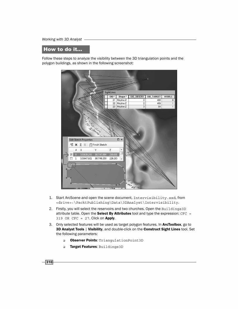
How to do it...Follow these steps to analyze the visibility between the 3D triangulation points and the polygon buildings, as shown in the following screenshot:

1. Start ArcScene and open the scene document, Intervisibility.sxd, from <drive>:\PacktPublishing\Data\3DAnalyst\Intervisibility.

2. Firstly, you will select the reservoirs and two churches. Open the Buildings3D attribute table. Open the Select By Attributes tool and type the expression: CFC = 319 OR CFC = 27. Click on Apply.

3. Only selected features will be used as target polygon features. In ArcToolbox, go to 3D Analyst Tools | Visibility, and double-click on the Construct Sight Lines tool. Set the following parameters:

Observer Points: TriangulationPoint3D

Target Features: Buildings3D

Chapter 10

311

Output: ...\Intervisibility\TOPO5000.gdb\SightLines

Observer Height Field (optional): SurveyInstrument

Target Height Field (optional): H_Building

Join Field (optional): <none>

Sampling Distance (optional): 100

Check Output the Direction (optional)

4. Click on OK. Open the SightLines attribute table to inspect the fi elds. Based on those 33 sight lines, you will analyze the visibility. In ArcToolbox, go to 3D Analyst Tools | Visibility, and double-click on the Intervisibility tool. This tool will modify the input SightLines layer. Set the following parameters:

Sight Lines: SightLines

Obstructions: For this, add the Buildings3D and Elevation layers

5. Accept the default values for Visible Field Name (optional). Click on OK. The SightLines attribute table has been updated with a new fi eld: VISIBLE.

There are 7 sight lines with VISIBLE value 0, which means they are obstructed by the elevation surface or buildings. The remaining 26 sight lines with value 1 are not obstructed, and there is visibility between the observer and target features.

6. Save your scene as MyIntervisibility.sxd and close ArcScene.

You can fi nd the fi nal results at <drive>:\PacktPublishing\Data\3DAnalyst \Intervisibility\Results_Intervisibility.sxd.

How it works...Please note that the result of the Construct Sight Lines tool is a 3D polyline layer. By setting the value 100 for Sampling Distance (optional), we kept only one sight line between the triangulation points and the fi rst vertex of every selected building feature, as shown in the previous image. If you type 0, a sight line will be created for every vertex of a building polygon.

Creating a profi le graphA profi le graph shows the height changes along a given line. A profi le graph can be created from:

3D line graphics (created with the Steepest path and Line of Sight tools)

3D polyline features (for example, geodatabase feature class and shapefi le)

Working with 3D Analyst

312

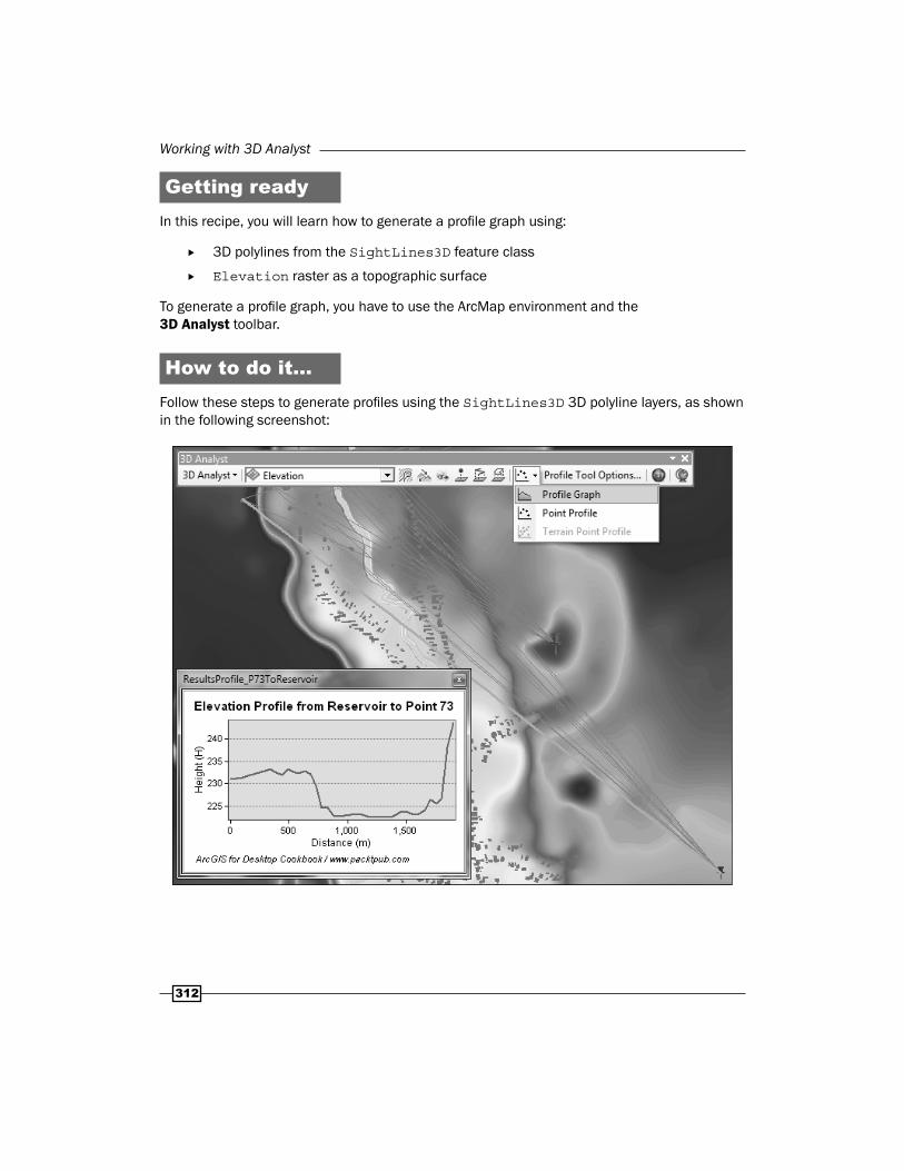
Getting readyIn this recipe, you will learn how to generate a profi le graph using:

3D polylines from the SightLines3D feature class

Elevation raster as a topographic surface

To generate a profi le graph, you have to use the ArcMap environment and the 3D Analyst toolbar.

How to do it...Follow these steps to generate profi les using the SightLines3D 3D polyline layers, as shown in the following screenshot:

Chapter 10

313

1. Start ArcMap and open an existing map document, Profile.mxd, from <drive>:\PacktPublishing\Data\3DAnalyst\ElevationProfile.

2. Load the 3D Analyst extension and add the 3D Analyst toolbar.

3. With the Select Feature tool, select a polyline feature from the SightLines3D layer. Click on the Profi le Graph tool from the 3D Analyst toolbar. The z-value is represented along the Y axis and distance is represented along the X axis.

If you select more polyline features, you will obtain more profiles in the same graph.

4. Right-click on the profi le graph, select the Properties option, and select the Appearance tab. For General graph properties, edit Title and Footer, and for Axis properties, add Title for Left and Bottom, as shown in the preceding screenshot. Click on OK.

5. Right-click on the profi le graph, and select the Save option to save your graph as the MyProfile_P73ToReservoir.grf graph fi le to the ...\3DAnalyst\ElevationProfile folder.

6. Right-click on the profi le graph and select the Export option. In the Picture frame, select the as PDF format and accept the default parameters. Click on Save and go to the previous location. Save the PDF fi le as MyElevationProfile.pdf.

7. Select the Data tab, check Excel Format, and accept the default parameters. Click on Save and repeat the previous step. Inspect the results with the Windows Explorer application.

8. In ArcMap, close the graph window. Go to View | Graphs and select Manage Graphs. If you right-click on ResultsProfile_P73ToReservoir, you will fi nd the same options from steps 5 and 6. To reopen your graph, double-click on the selected graph. Explore by yourself Advanced Properties.

9. Save your map document as MyProfile.mxd and close ArcMap.

You can fi nd the fi nal results at <drive>:\PacktPublishing\Data\3DAnalyst\ ElevationProfile\ResultsProfile.mxd. In the ResultsProfile.mxd map document, please go to View | Graphs, and explore all fi ve profi le graphs.

Working with 3D Analyst

314

How it works...If you want to use the sight lines features created in the Intervisibility recipe, you have to go through the following steps:

1. Recreate the SightLines layer using the Construct Sight Lines tool, with Observer Height Field (optional) with the value Shape.Z and Target Height Field (optional) with the value Shape.Z. You will have a sight line at surface level. Notice that your sight lines have only two vertices along the polyline feature. Only two vertices are not enough for a profi le graph.

2. Use the Densify tool with a DISTANCE of 50—unit as Meters—to add more vertices to the polyline features.

3. Use the Interpolate Shape tool with Interpolate Vertices Only checked. Your new vertices will have interpolated Z-values based on the Elevation surface.

The Profile_P73ToReservoir graph refl ects the direction of polyline features. To change the direction of your path graphic (from point 73 to the reservoir), please follow the next steps: start an edit session, select the polyline with the Edit Vertices tool, right–click on the selected feature to change the polyline direction with Flip, and stop the edit session. Select the polyline and generate a new profi le graph. Note that the direction of the graphic path has been changed.

There's more...You can create profi les from a terrain surface, as shown in the following screenshot:

Chapter 10

315

Open your map document MyProfile.mxd. Add the DTM terrain surface from ...3DAnalyst\ ElevationProfile\TOPO5000.mdb\Terrain.

To activate the Terrain Point Profi le tool, you have to symbolize the terrain surface with one of the three Terrain point renders. For the DTM terrain layer, choose the Terrain point elevation with graduated color ramp render.

In the 3D Analyst toolbar, choose DTM as the surface layer, select the Terrain Point Profi le tool, and click on two locations—the starting and ending points. Change the width for the black selection box, as shown in the preceding image. A new profi le graph will be displayed. From Properties | Appearance of the profi le graph, check the option Graph in 3D view.

Save and export your terrain point profi le using the View | Graphs | Manage Graphs dialog box.

Creating an animationThere are two ways to create an animation:

Capturing keyframes

Recording your navigation through the scene

Keyframes are individual views. When you create an animation by capturing keyframes, you can use the Capture View tool or the Animation Manager dialog from the Animation toolbar. The rest of the views from the animation fi le will be interpolated based on those keyframes to result in a smooth animated picture.

Getting readyIn this recipe, you will create an animated tour of your 3D feature in ArcScene and export it to a video fi le. Before you start working, please watch the movies 3DFeatures_ByKeyFrames.avi and 3DFeatures_ByRecording.avi from the ...\Data\3DAnalyst\Animation folder. These are the two results you should obtain at the end of the exercise. You can use a media player such as Windows Media Player or VLC.

You can start with your scene document My3DFeatures.sxd from the Creating 3D features from 2D features recipe and skip step 1. Otherwise, use a scene document from the Animation folder.

Working with 3D Analyst

316

How to do it...Follow these steps to create an ArcScene animation:

1. Start ArcScene and open an existing scene document 3DFeatures.sxd from ...\Data\3DAnalyst\Animation.

In the next steps, you will create an animation by capturing keyframes:

2. Firstly, you will load seven bookmarks that will help you in capturing camera keyframes. Go to Bookmarks | Manage Bookmarks and click on the Load button to add the KeyFrames_Animation.dat fi le from ...\3DAnalyst\Animation. You will load seven bookmarks, as shown in the following screenshot:

3. Close the Bookmarks Manager dialog. Explore all seven bookmarks and fi nish by choosing the fi rst bookmark.

4. From Customize | Toolbars, add the Animation toolbar. From the Animation toolbar, select the Animation | Animation Manager | Keyframes tab. Move the Animation Manager dialog to the right-hand side of the scene.

Let's capture some keyframes for your animation.

Chapter 10

317

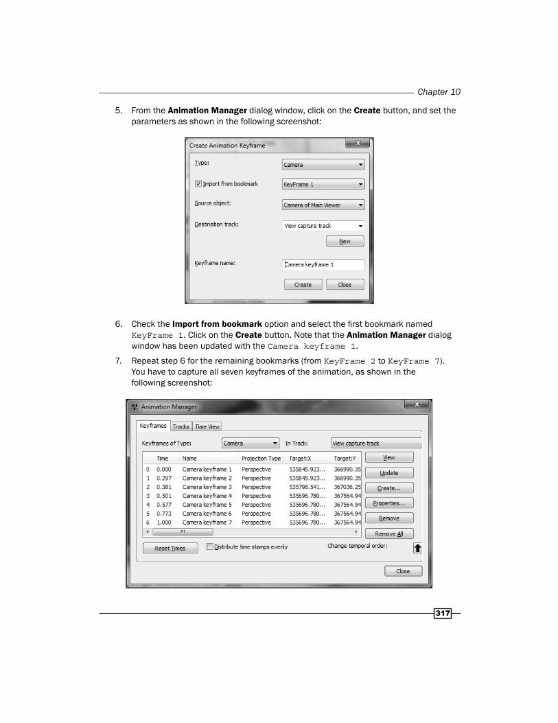
5. From the Animation Manager dialog window, click on the Create button, and set the parameters as shown in the following screenshot:

6. Check the Import from bookmark option and select the fi rst bookmark named KeyFrame 1. Click on the Create button. Note that the Animation Manager dialog window has been updated with the Camera keyframe 1.

7. Repeat step 6 for the remaining bookmarks (from KeyFrame 2 to KeyFrame 7). You have to capture all seven keyframes of the animation, as shown in the following screenshot:

Working with 3D Analyst

318

8. Close the Create animation Keyframe window. Explore all the columns of Keyframes. Select the Time View tab to see the capture track line of your animation. Leave open the Animation Manager dialog window.

9. From the Animation toolbar, select the Open Animation Control button, as shown in the following screenshots:

10. To adjust the default animation duration, click on the Options button, and change Play Options | By duration to 15 seconds. Accept default values for all other parameters. Click on the Options button again to collapse the dialog box. To watch the animation, click on the Play button.

To switch to the fullscreen view, press the F11 key. To leave the fullscreen view, press the F11 key again.

11. While you are watching your animation, notice the capture track line from the Animation Manager dialog window, as shown in the following screenshot:

Chapter 10

319

12. Let's save the animation into an animation fi le with the .asa extension. From the Animation toolbar, select Save Animation File. Save your animation as MyKeyFrames.asa in ...Data\3DAnalyst\Animation. Select the Export Animation option to export your animation fi le to an AVI fi le MyKeyFrames.avi. In the Video Compression dialog window, accept the default Compressor as Microsoft Video 1, and click on OK.

In the next steps, you will create an animation by recording a fl ying through the scene:

13. In the Animation Manager dialog window, select the Keyframes tab, and click on Remove All. From the Animation toolbar, select the Open Animation Control button. From the Bookmarks menu, select KeyFrame 2.

14. To start recording, perform the following steps:

Select the Fly tool from the Tools toolbar.

Click on the Record button from Open Animation Control to start recording.

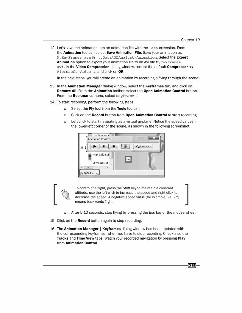
Left-click to start navigating as a virtual airplane. Notice the speed values in the lower-left corner of the scene, as shown in the following screenshot:

To control the fl ight, press the Shift key to maintain a constant altitude, use the left-click to increase the speed and right-click to decrease the speed. A negative speed value (for example, -1, -2) means backwards fl ight.

After 5-10 seconds, stop flying by pressing the Esc key or the mouse wheel.

15. Click on the Record button again to stop recording.

16. The Animation Manager | Keyframes dialog window has been updated with the corresponding keyframes when you have to stop recording. Check also the Tracks and Time View tabs. Watch your recorded navigation by pressing Play from Animation Control.

Working with 3D Analyst

320

17. If you are not satisfi ed with the result, in Animation Manager | Keyframes, click on the Remove All button and start recording once again.

18. Repeat step 30 to save your animation as MyRecording.asa, and to export it as MyRecording.avi. Close the dialog windows and the ArcScene application.

Watch MyKeyFrames.avi and MyRecording.avi using a video player.

How it works...In the Animation Manager | Keyframes dialog window, you can erase and replace any keyframe from your animation by selecting its ID and using the Remove button. Also, you can change the order of keyframes using the Change temporal order arrows.

At step 11, you can change the position or timing of every keyframe (small green square) along the capture-track red line. If your keyframes are too close, your animation will proceed rapidly. If your keyframes are too distant, your animation will move slowly. To improve the timing, click on the Keyframes tab, check Distribute time stamps evenly, and click on Reset Times. These steps will be refl ected in the Time View window and will smoothen the animation.

Where to buy this book You can buy ArcGIS for Desktop Cookbook from the Packt Publishing website. Alternatively, you can buy the book from Amazon, BN.com, Computer Manuals and most internet book retailers.

Click here for ordering and shipping details.

www.PacktPub.com

Stay Connected:

Get more information ArcGIS for Desktop Cookbook