Arbitrage Opportunities in Misspecified Stochastic Volatility ...

arX

iv:1

002.

5041

v3 [

q-fi

n.PR

] 3

0 Se

p 20

11

Arbitrage Opportunities in Misspecified

Stochastic Volatility Models

Rudra P. Jena∗

Peter Tankov∗†

Abstract

There is vast empirical evidence that given a set of assumptions on

the real-world dynamics of an asset, the European options on this asset

are not efficiently priced in options markets, giving rise to arbitrage

opportunities. We study these opportunities in a generic stochastic

volatility model and exhibit the strategies which maximize the arbi-

trage profit. In the case when the misspecified dynamics is a classical

Black-Scholes one, we give a new interpretation of the butterfly and

risk reversal contracts in terms of their performance for volatility ar-

bitrage. Our results are illustrated by a numerical example including

transaction costs.

Key words: stochastic volatility, model misspecification, volatility arbitrage,butterfly, risk reversal, SABR model

2010 Mathematical Subject Classification: 91G20, 60J60

1 Introduction

It has been observed by several authors [1, 3, 12] that given a set of assump-tions on the real-world dynamics of the underlying, the European options

∗Centre de Mathématiques Appliquées, Ecole Polytechnique, 91128 Palaiseau France.E-mail: jena,[email protected]

†Corresponding author

1

Nov 1997 May 20090

10

20

30

40

50

60Realized vol (2−month average)

Implied vol (VIX)

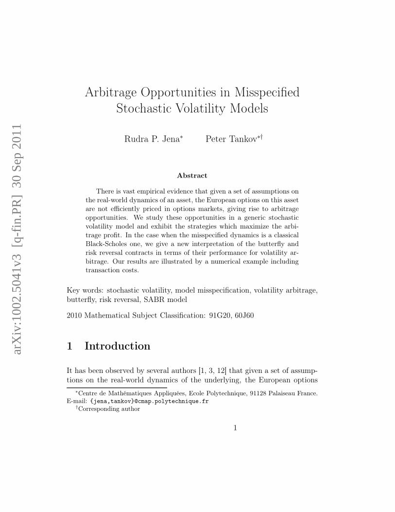
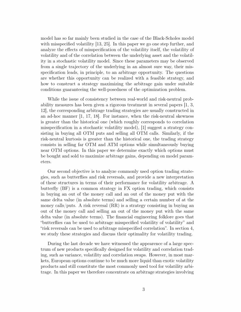
Figure 1: Historical evolution of the VIX index (implied volatility of optionson the S&P 500 index with 1 to 2 month to expiry, averaged over strikes, see[10]) compared to the historical volatility of the S&P 500 index. The factthat the implied volatility is consistently above the historical one by severalpercentage points suggests a possibility of mispricing.

on this underlying are not efficiently priced in options markets. Importantdiscrepancies between the implied volatility and historical volatility levels, asillustrated in Figure 1, as well as substantial differences between historicaland option-based measures of skewness and kurtosis [3] have been docu-mented. These discrepancies could be explained by systematic mispricings /model misspecification in option markets, leading to potential arbitrage op-portunities1. The aim of this paper is to quantify these opportunities within ageneric stochastic volatility framework, and to construct the strategies max-imizing the gain. The arbitrage opportunities analyzed in this paper can becalled statistical arbitrage opportunities, because their presence / absencedepends on the statistical model for the dynamics of the underlying asset.Contrary to model independent arbitrages, such as violation of the call-putparity, a statistical arbitrage only exists in relation to the particular pricingmodel.

The issue of quantifying the gain/loss from trading with a misspecified

1There exist many alternative explanations for why the implied volatilities are con-sistently higher than historical volatilities, such as, price discontinuity [4], market crashfears [5] and liquidity effects such as transaction costs [22, 19, 8, 9], inability to trade incontinuous time [6] and market microstructure effects [24]. The literature is too vast tocite even the principal contributions here

2

model has so far mainly been studied in the case of the Black-Scholes modelwith misspecified volatility [13, 25]. In this paper we go one step further, andanalyze the effects of misspecification of the volatility itself, the volatility ofvolatility and of the correlation between the underlying asset and the volatil-ity in a stochastic volatility model. Since these parameters may be observedfrom a single trajectory of the underlying in an almost sure way, their mis-specification leads, in principle, to an arbitrage opportunity. The questionsare whether this opportunity can be realized with a feasible strategy, andhow to construct a strategy maximizing the arbitrage gain under suitableconditions guaranteeing the well-posedness of the optimization problem.

While the issue of consistency between real-world and risk-neutral prob-ability measures has been given a rigorous treatment in several papers [1, 3,12], the corresponding arbitrage trading strategies are usually constructed inan ad-hoc manner [1, 17, 18]. For instance, when the risk-neutral skewnessis greater than the historical one (which roughly corresponds to correlationmisspecification in a stochastic volatility model), [1] suggest a strategy con-sisting in buying all OTM puts and selling all OTM calls. Similarly, if therisk-neutral kurtosis is greater than the historical one, the trading strategyconsists in selling far OTM and ATM options while simultaneously buyingnear OTM options. In this paper we determine exactly which options mustbe bought and sold to maximize arbitrage gains, depending on model param-eters.

Our second objective is to analyze commonly used option trading strate-gies, such as butterflies and risk reversals, and provide a new interpretationof these structures in terms of their performance for volatility arbitrage. Abutterfly (BF) is a common strategy in FX option trading, which consistsin buying an out of the money call and an out of the money put with thesame delta value (in absolute terms) and selling a certain number of at themoney calls/puts. A risk reversal (RR) is a strategy consisting in buying anout of the money call and selling an out of the money put with the samedelta value (in absolute terms). The financial engineering folklore goes that“butterflies can be used to arbitrage misspecified volatility of volatility” and“risk reversals can be used to arbitrage misspecified correlation”. In section 4,we study these strategies and discuss their optimality for volatility trading.

During the last decade we have witnessed the appearence of a large spec-trum of new products specifically designed for volatility and correlation trad-ing, such as variance, volatility and correlation swaps. However, in most mar-kets, European options continue to be much more liquid than exotic volatilityproducts and still constitute the most commonly used tool for volatility arbi-trage. In this paper we therefore concentrate on arbitrage strategies involving

3

only the underlying asset and liquid European options.

The rest of the paper is structured as follows. In Section 2, we introducethe generic misspecified stochastic volatility model. Section 3 defines theadmissible trading strategies and establishes the form of the optimal arbitrageportfolio. Section 4 is dedicated to the special case when the misspecifiedmodel is the constant volatility Black-Scholes model. This allows us to givea new interpretation of butterfly spreads and risk reversals in terms of theirsuitability for volatility arbitrage. Section 5 presents a simulation study ofthe performance of the optimal arbitrage strategies in the framework of theSABR stochastic volatility model [16]. The purpose of this last section is notto prove the efficiency of our strategies in real markets but simply to providean illustration using simulated data. A comprehensive empirical study usingreal market prices is left for further research.

2 A misspecified stochastic volatility framework

We start with a filtered probabiblity space (Ω,F ,P, (Ft)t≥0) and consider afinancial market where there is a risky asset S, a risk-free asset and a certainnumber of European options on S. We assume that the interest rate is zero,and that the price of the risky asset S satisfies the stochastic differentialequation

dSt/St = µtdt+ σt

√

1− ρ2tdW1t + σtρtdW

2t (1)

where µ, σ and ρ ∈ [−1, 1] are adapted processes such that

ˆ t

0

(1 + S2s )(1 + µ2

s + σ2s )ds < ∞ a.s. for all t,

and (W 1,W 2) is a standard 2-dimensional Brownian motion. This integra-bility condition implies in particular that the stock price process never hitszero P-a.s.

To account for a possible misspecification of the instantaneous volatility,we introduce the process σt, which represents the instantaneous volatilityused by the option’s market for all pricing purposes. In particular, it isthe implied volatility of very short-term at the money options, and in thesequel we call σ the instantaneous implied volatility process. We assume thatσt = σ(Yt), where Y is a stochastic process with dynamics

dYt = atdt+ btdW2t , (2)

4

where at and bt > 0 are adapted processes such that

ˆ t

0

(a2s + b2s)ds < ∞ a.s. for all t,

and σ : R → (0,∞) is a continuously differentiable Lipschitz function with0 < σ ≤ σ(y) ≤ σ < ∞ and σ′(y) > 0 for all y ∈ R;

Further, to account for possible misspecification of the volatility of volatil-ity b and of the correlation ρ, we assume that there exists another probabilitymeasure Q, called market or pricing probability, not necessarily equivalentto P, such that all options on S are priced in the market as if they weremartingales under Q. The measure Q corresponds to the pricing rule usedby the market participants, which may be inconsistent with the real-worlddynamics of the underlying asset (meaning that Q is not necessarily abso-lutely continuous with respect to P). Under Q, the underlying asset and itsvolatility form a 2-dimensional Markovian diffusion:

dSt/St = σ(Yt)√

1− ρ2(Yt, t)dW1t + σ(Yt)ρ(Yt, t)dW

2t (3)

dYt = a(Yt, t)dt+ b(Yt, t)dW2t , (4)

where the coefficients a, b and ρ are deterministic functions and (W 1, W 2)is a standard 2-dimensional Brownian motion under Q. Since σ is bounded,the stock price process never hits zero Q-a.s.

The following assumptions on the coefficients of (3)–(4) will be usedthroughout the paper:

i) There exists ε > 0 such that min(1− ρ(y, t)2, b(y, t)) ≥ ε for all (y, t) ∈R× [0, T ].

ii) The functions a(y, t), b(y, t), ρ(y, t) are twice differentiable with respectto y; these coefficients as well as their first and second derivatives withrespect to y are bounded and Hölder continuous in y, t.

iii) The function σ is twice differentiable; this function as well as its firstand second derivative is bounded and Hölder continuous.

We suppose that a continuum of European options (indifferently calls orputs) for all strikes and at least one maturity is quoted in the market. Theprice of an option with maturity date T and pay-off H(ST ) can be expressedas a deterministic function of St, Yt and t:

P (St, Yt, t) = EQ[H(ST )|Ft].

5

Using standard methods (see e.g. [15]) one can show that under our as-sumptions, for every such option, the pricing function P belongs to the classC2,2,1((0,∞)× R× [0, T )) and satisfies the PDE

a∂P

∂y+ LP = 0, (5)

where we define

Lf =∂f

∂t+

S2σ(y)2

2

∂2f

∂S2+

b2

2

∂2f

∂y2+ Sσ(y)bρ

∂2f

∂S∂y.

In addition (see [26]), the price of any such European option satisfies

∂P

∂y> 0, ∀(S, y, t) ∈ (0,∞)× R× [0, T ). (6)

We shall use the following decay property of the derivatives of call andput prices (see Appendix A for the proof).

Lemma 2.1. Let P be the price of a call or a put option with strike K andmaturity date T . Then

limK→+∞

∂P (S, y, t)

∂y= lim

K→0

∂P (S, y, t)

∂y= 0,

limK→+∞

∂2P (S, y, t)

∂y2= lim

K→0

∂2P (S, y, t)

∂y2= 0,

limK→+∞

∂2P (S, y, t)

∂S2= lim

K→0

∂2P (S, y, t)

∂S2= 0,

and limK→+∞

∂2P (S, y, t)

∂S∂y= lim

K→0

∂2P (S, y, t)

∂S∂y= 0

for all (y, t) ∈ R× [0, T ). All the above derivatives are continuous in K andthe limits are uniform in S, y, t on any compact subset of (0,∞)×R× [0, T ).

3 The optimal arbitrage portfolio

We study the arbitrage from the perspective of the trader, who knows thatthe market is using a misspecified stochastic volatility model to price theoptions. We assume full observation: at every date t, the trader possessesthe information given by the σ-field Ft and knows the deterministic functionsσ, ρ, a and b. In Section 5 we test the robustness of our results with respectto this assumption.

6

To benefit from the market misspecification, our informed trader sets upa dynamic self-financing delta and vega-neutral portfolio Xt with zero initialvalue, containing, at each date t, a stripe of European call or put optionswith a common expiry date T . In addition, the portfolio contains a quantity−δt of stock and some amount Bt of cash.

To denote the quantity of options of each strike, we introduce a pre-dictable process (ωt)t≥0 taking values in the space M of signed measures on[0,∞) equipped with the total variation norm ‖ · ‖V . We refer to [7] fortechnical details of this construction and rigorous definitions of the stochas-tic integral and the self-financing portfolio in this setting. Loosely speaking,ωt(dK) is the quantity of options with strikes between K and K+dK, wherea negative measure corresponds to a short position. We shall see later thatfor the optimal strategies the measure ω is concentrated on a finite numberof strikes.

The quantity of options of each strike is continuously readjusted meaningthat old options are sold to buy new ones with different strikes. In practice,this readjustment will of course happen at discrete dates due to transac-tion costs and we analyze the performance of our strategies under discreterebalancing in section 5. The portfolio is held until date T ∗ < T .

Finally, unless explicitly mentioned otherwise, we assume that at alltimes, the total quantity of options of all strikes in the portfolio is equalto 1:

‖ωt‖V ≡ˆ

|ωt(dK)| ≡ 1 (7)

for all t. This position constraint ensures that the profit maximization prob-lem is well posed in the presence of arbitrage opportunities (otherwise theprofit could be increased indefinitely by increasing the size of positions). Ifthe portfolio is rebalanced completely at discrete equally spaced dates, andthe transaction cost per one unit of option is constant, this assumption im-plies that independently of the composition of the portfolio, the transactioncost paid at each readjustment date is constant, and therefore does not in-fluence the optimization problem. This constraint is also natural from thepoint of view of an option exchange or a market maker who wants to struc-ture standardized option spreads to satisfy a large number of retail clients,because the number of options in such a spread must be fixed.

Remark 3.1. For an individual trader, who is trying to optimize her optionportfolio, it may also be natural to impose a margin constraint, that is, aconstraint on the capital which the trader uses to meet the margin require-ments of the exchange. We discuss option trading under margin constraintin Section 3.1.

7

The value of the resulting portfolio is,

Xt =

ˆ

PK(St, Yt, t)ωt(dK)− δtSt +Bt,

where the subscript K denotes the strike of the option. Together with Lemma2.1, our assumptions ensure (see [7, section 4]) that the dynamics of thisportfolio are,

dXt =

(ˆ

ωt(dK)LPK

)

dt+

(ˆ

ωt(dK)∂PK

∂S

)

dSt

+

(ˆ

ωt(dK)∂PK

∂y

)

dYt − δtdSt

where

Lf =∂f

∂t+

S2t σ

2t

2

∂2f

∂S2+

b2t2

∂2f

∂y2+ Stσtbtρt

∂2f

∂S∂y

To make the portfolio instantaneosly risk-free, we choose,

ˆ

ωt(dK)∂PK

∂y= 0,

ˆ

ωt(dK)∂PK

∂S= δt

to eliminate the dYt and dSt terms. We emphasize that these hedge ratios arealways computed using the market parameters i.e. a, b and ρ. The portfoliodynamics then become

dXt =´

ωt(dK)LPKdt, (8)

and substituting the equation (5) into this formula and using the vega-neutrality, we obtain the risk-free profit from model misspecification:

dXt =

ˆ

ωt(dK)(L− L)PKdt. (9)

or, at the liquidation date T ∗,

XT ∗ =

ˆ T ∗

0

ˆ

ωt(dK)(L− L)PKdt, (10)

where,

(L− L)PK =S2t (σ

2t − σ2(Yt))

2

∂2PK

∂S2+

(b2t − b2t )

2

∂2PK

∂y2

+ St(σtbtρt − σ(Yt)btρt)∂2PK

∂S∂y(11)

8

To maximize the arbitrage profit at each date, we therefore need to solve thefollowing optimization problem:

Maximize Pt =

ˆ

ωt(dK)(L − L)PK (12)

subject to

ˆ

|ωt(dK)| = 1 and

ˆ

ωt(dK)∂PK

∂y= 0. (13)

Remark 3.2. It should be pointed out that in this paper the arbitrage portfo-lio is required to be instantaneously risk-free and the performance is measuredin terms of instantaneous arbitrage profit. This corresponds to the standardpractice of option trading, where the trader is usually only allowed to holddelta and vega netral portfolios and the performance is evaluated over shorttime scales. This rules out strategies which are locally risky but have a.s.positive terminal pay-off, such as the strategies based on strict local martin-gales, which may be admissible under the standard definition of arbitrage.Optimality of arbitrage strategies for an equity market under the standarddefinition of arbitrage has recently been studied in [14].

The following result shows that a spread of only two options (with strikesand weights continuously readjusted) is sufficient to solve the problem (12).

Proposition 3.3. The instantaneous arbitrage profit (12) is maximized by

ωt(dK) = w1t δK1

t(dK)− w2

t δK2t(dK), (14)

where δK(dK) denotes the unit point mass at K, (w1t , w

2t ) are time-dependent

optimal weights given by

w1t =

∂PK2

∂y

∂PK1

∂y+ ∂PK2

∂y

, w2t =

∂PK1

∂y

∂PK1

∂y+ ∂PK2

∂y

,

and (K1t , K

2t ) are time-dependent optimal strikes given by

(K1t , K

2t ) = arg max

K1,K2

∂PK2

∂y(L− L)PK1 − ∂PK1

∂y(L− L)PK2

∂PK1

∂y+ ∂PK2

∂y

. (15)

Proof. Step 1. We first show that the optimization problem (15) is well-posed, that is, the maximum is attained for two distinct strike values. LetF (K1, K2) denote the function to be optimized in (15). From the property(6) and Lemma 2.1 it follows that F is continuous in K1 and K2. Let us show

9

that for every ε > 0 we can find an interval [a, b] such that |F (K1, K2)| ≤ εfor all (K1, K2) /∈ [a, b]2. We introduce the shorthand notation

g(K) =∂PK

∂y, f(K) = (L − L)PK,

F (K1, K2) =g(K2)f(K1)− g(K1)f(K2)

g(K1) + g(K2).

Fix ε > 0. By Lemma 2.1, there exists N > 0 with |f(K)| ≤ ε for allK : K /∈ [e−N , eN ]. Let δ = inf |logK|≤N g(K). Property (6) entails thatδ > 0. Then we can find M > 0 such that g(K) ≤ εδ

sup|logK|≤N |f(K)| for all

K : K /∈ [e−M , eM ] (if the denominator is zero, any M > 0 can be used). It

follows that for all (K1, K2) /∈ [e−N , eN ] × [e−M , eM ],∣

∣

∣

g(K2)f(K1)g(K1)+g(K2)

∣

∣

∣≤ ε. In

the same manner, we can find a rectangle for the second term in F , and,taking the square containing both rectangles, we get the desired result.

Suppose now that for some K1 and K2, F (K1, K2) > 0. Then, by taking εsufficiently small, the above argument allows to find a compact set containingthe maximum of F , and hence the maximum is attained for two strikes whichcannot be equal since F (K,K) ≡ 0. If, on the other hand, F (K1, K2) ≤ 0for all K1, K2, then this means that F (K1, K2) ≡ 0 and any two strikes canbe chosen as maximizers of (15).

Step 2. We now show that the two-point solution suggested by this propo-sition is indeed the optimal one. Let ωt be any measure on R+ satisfying theconstraints (13). Let ωt = ω+

t − ω−t be the Jordan decomposition of ωt and

define ν+t :=

ω+t

ω+t (R+)

and ν−t :=

ω−t

ω−t (R+)

. These measures are well-defined due

to conditions (6) and (13). From the same conditions,

ω−t (R

+) =

´

∂PK

∂ydν+

t´

∂PK

∂ydν+

t +´

∂PK

∂ydν−

t

, ω+t (R

+) =

´

∂PK

∂ydν−

t´

∂PK

∂ydν+

t +´

∂PK

∂ydν−

t

.

The instantaneous arbitrage profit (12) can then be written as

Pt =

ˆ

(L− L)PKdω+t −ˆ

(L − L)PKdω−t

=

´

∂PK

∂ydν−

t

´

(L − L)PKdν+t −´

∂PK

∂ydν+

t

´

(L− L)PKdν−t

´

∂PK

∂ydν+

t +´

∂PK

∂ydν−

t

.

10

Then,

Pt =

´

gdν−t

´

fdν+t −´

gdν+t

´

fdν−t

´

gdν+t +´

gdν−t

,

≤´

ν−t (dK)

g(K) +´

gdν+

supK1

g(K1)´

fdν+t −f(K1)´

gdν+tg(K1)+

´

gdν+t´

gdν+t +´

gdν−t

= supK1

g(K1)´

fdν+t − f(K1)

´

gdν+t

g(K1) +´

gdν+t

≤ supK1

´

ν+t (dK) g(K1) + g(K) supK2

g(K1)f(K2)−f(K1)g(K2)g(K1)+g(K2)

g(K1) +´

gdν+t

= supK1,K2

g(K1)f(K2)− f(K1)g(K2)

g(K1) + g(K2)

Since for the solution (14) the above sup is attained, this solution is indeedoptimal.

The optimal strategy of Proposition 3.3 is adapted, but not necessarilypredictable. In particular, if the maximizer in (15) is not unique, the optimalstrikes may jump wildly between different maximizers leading to strategieswhich are impossible to implement. However, in practice the maximizer isusually unique (see in particular the next section), and the following resultshows that this guarantees the weak continuity, and hence predictability, ofthe optimal strategy.

Proposition 3.4. Let t∗ < T , and assume that the coefficients σt, bt and ρtare a.s. continuous at t∗ and that the maximizer in the optimization problem(15) at t∗ is a.s. unique. Then the optimal strikes (K1

t , K2t ) are a.s. contin-

uous at t∗, and the optimal strategy (ωt) is a.s. weakly continuous at t∗.

Proof. To emphasize the dependence on t, we denote by Ft(K1, K2) the func-tion being maximized in (15). By the continuity of σt, bt ρt, St and Yt,there exists a neighborhood (t1, t2) of t∗ (which may depend on ω ∈ Ω), inwhich these processes are bounded. Since the convergence in Lemma 2.1is uniform on compacts, similarly to the proof of Proposition 3.3, for everyε > 0, we can find an interval [a, b] (which may depend on ω ∈ Ω) such that|Ft(K

1, K2)| ≤ ε ∀(K1, K2) /∈ [a, b]2 and ∀t ∈ (t1, t2). This proves that theoptimal strikes (K1

t , K2t ) are a.s. bounded in the neighborhood of t∗.

Let (tn)n≥1 be a sequence of times converging to t∗ and (K1tn , K

2tn)n≥1

the corresponding sequence of optimal strikes. By the above argument, thissequence is bounded and a converging subsequence (K1

tnk, K2

tnk)k≥1 can be

11

extracted. Let (K1, K2) be the limit of this converging subsequence. Since(K1

tnk, K2

tnk) is a maximizer of Ftnk

and by continuity of F , for arbitrary

strikes (k1, k2),

Ft∗(K1, K2) = lim

k→∞Ftnk

(K1tnk

, K2tnk

) ≥ limk→∞

Ftnk(k1, k2) = Ft∗(k

1, k2).

This means that (K1, K2) is a maximizer of Ft∗(·, ·), and, by the uniquenessassumption, K1 = K1

t∗ and K2 = K2t∗ . By the subsequence criterion we then

deduce that K1t → K1

t∗ and K2t → K2

t∗ a.s. as t → t∗. The weak convergenceof ωt follows directly.

3.1 Trading under margin constraint

Solving the optimization problem (12) under the constraint (7) amounts tofinding the optimal (vega-weighted) spread, that is a vega-neutral combina-tion of two options, in which the total quantity of options equals one. Thisapproach guarantees the well-posedness of the optimization problem and pro-vides a new interpretation for commonly traded option contracts such asbutterflies and risk reversals (see next section).

From the point of view of an individual option trader, an interesting alter-native to (7) is the constraint given by the margin requirements of the stockexchange. In this section, we shall consider in detail the CBOE minimummargins for customer accounts, that is, the margin requirements for retail in-vestors imposed by the Chicago Board of Options Exchange [11, 27]. Underthis set of rules, margin requirements are, by default, calculated individuallyfor each option position:

• Long positions in call or put options must be paid for in full.

• For a naked short position in a call option, the margin requirement attime t is calculated using the following formula [27].

Mt = PKt +max(αSt − (K − St)1K>St, βSt) := PK

t + λKt ,

where PK is the option price, α = 0.15 and β = 0.1.

• The margin requirement for a “long call plus short underlying posi-tion” is equal to the call price plus short sale proceeds plus 50% of theunderlying value.

• The margin requirement for a "short call plus long underlying" is 50%of the underlying value.

12

In addition, some risk offsets are allowed for certain spread options, but weshall not take them into account to simplify the treatment. For the samereason, we shall assume that all options held by the trader are call options.Let ωt = ω+

t − ω−t be the Jordan decomposition of ωt. The value of a delta-

hedged option portfolio can be written as

Xt = Bt +

ˆ

PK − St∂PK

∂S

ωt(dK)

= Bt +

ˆ

PK

(

1− ∂PK

∂S

)

+∂PK

∂S(PK − St)

ω+t (dK)

+

ˆ

−PK

(

1− ∂PK

∂S

)

+∂PK

∂S(St − PK)

ω−t (dK)

The margin requirement for this position is

Mt =

ˆ

PK +∂PK

∂S(1 + γ)St

ω+t (dK)

+

ˆ

(λK + PK)

(

1− ∂PK

∂S

)

+ γSt∂PK

∂S

ω−t (dK)

:=

ˆ

β+t (K)ω+

t (dK) +

ˆ

β−t (K)ω−

t (dK)

with γ = 0.5. Supposing that the trader disposes of a fixed margin account(normalized to 1), the optimization problem (12)–(13) becomes

Maximize Pt =

ˆ

ωt(dK)(L− L)PK

subject to

ˆ

β+t (K)ω+

t (dK) +

ˆ

β−t (K)ω−

t (dK) = 1

and

ˆ

ωt(dK)∂PK

∂y= 0.

This maximization problem can be treated similarly to (12)–(13). Assumethat at time t, the problem

arg supK1,K2

∂PK2

∂y(L− L)PK1 − ∂PK1

∂y(L− L)PK2

β−(K2)∂PK1

∂y+ β+(K1)∂P

K2

∂y

. (16)

admits a finite maximizer (K1t , K

2t ). Then the instantaneous arbitrage profit

is maximized by the two-strike portfolio (14) with

w1t =

β+(K1t )

∂PK2

∂y

β+(K2t )

∂PK1

∂y+ β+(K1

t )∂PK2

∂y

, w2t =

β+(K2t )

∂PK1

∂y

β+(K2t )

∂PK1

∂y+ β+(K1

t )∂PK2

∂y

.

13

However, since β+(K) → 0 as K → +∞, the problem (16) may not admit afinite maximizer for some models. For instance, in the Black-Scholes model,a simple asymptotic analysis shows that β+(K) converges to zero faster than∂PK

∂yas K → +∞, while ∂PK

∂yconverges to zero faster than ∂2PK

∂S∂yand ∂2PK

∂y2.

This means that by keeping K2 fixed and choosing K1 large enough, theinstantaneous arbitrage profit (16) can be made arbitrarily large. In financialterms this means that since the margin constraint does not limit the size ofthe long positions, it may be optimal to buy a large number of far out of themoney options. So the margin constraint alone is not sufficient to guaranteethe well-posedness of the problem and a position constraint similar to (7) isnecessary as well (in particular, the position constraint limits the transactioncosts). If both the margin constraint and the position constraint are imposed,the optimal portfolio will in general be a combination of three options withdifferent strikes.

While our analysis focused on CBOE margining rules for retail investors,a number of other exchanges, for example, CME for large institutional ac-counts, use an alternative margining system called Standard Portfolio Analy-sis of Risk (SPAN). Under this system, the margin requirement is determinedas the worst-case loss of the portfolio over a set of 14 market scenarios. Inthis case, position constraints are also necessary to ensure the well-posednessof the optimization problem. See [2] for a numerical study of optimal optionportfolios under SPAN constraints in the binomial model.

4 The Black-Scholes case

In this section, we consider the case when the misspecified model is the Black-Scholes model, that is, a ≡ b ≡ 0. This means that at each date t the marketparticipants price options using the Black-Scholes model with the volatilityvalue given by the current instantaneous implied volatility σ(Yt). The processYt still has a stochastic dynamics under the real-world probability P. Thisis different from the setting of [13], where one also has a = b = 0, that is,the instantaneous implied volatility is deterministic. In this section, since wedo not need to solve partial differential equations, to simplify notation, weset σt ≡ Yt, that is, the mapping σ(·) is the identity mapping. Recall theformulas for the derivatives of the call/put option price in the Black-Scholes

14

model (r = 0):

∂P

∂σ= Sn(d1)

√τ = Kn(d2)

√τ ,

∂2P

∂S2=

n(d1)

Sσ√τ,

∂2P

∂σ∂S= −n(d1)d2

σ,

∂2P

∂σ2=

Sn(d1)d1d2√τ

σ,

where d1,2 = mσ√τ± σ

√τ

2, τ = T − t, m = log(S/K) and n is the standard

normal density.

We first specialize the general optimal solution (14) to the Black-Scholescase. All the quantities σt, σt, bt, ρt, St are, of course, time-dependent, butsince the optimization is done at a given date, to simplify notation, we omitthe subscript t.

Proposition 4.1. The optimal option portfolio maximizing the instanta-neous arbitrage profit (12) is described as follows:

• The portfolio consists of a long position in an option with log-moneynessm1 = z1σ

√τ− σ2τ

2and a short position in an option with log-moneyness

m2 = z2σ√τ − σ2τ

2, where (z1, z2) is a maximizer of the function

f(z1, z2) =(z1 − z2)(z1 + z2 − w)

ez21/2 + ez

22/2

with w = σbτ+2σρb√τ

.

• The weights of the two options are chosen to make the portfolio vega-neutral.

We define by Popt the instantaneous arbitrage profit realized by the optimalportfolio.

Proof. Substituting the Black-Scholes values for the derivatives of optionprices, and making the change of variable z = m

σ√τ+ σ

√τ

2, the maximization

problem to solve becomes:

maxz1,z2

bSn(z1)n(z2)

n(z1) + n(z2)

b√τ

2σ(z21 − z22)−

bτ

2(z1 − z2)− ρ

σ

σ(z1 − z2)

, (17)

from which the proposition follows directly.

Remark 4.2. A numerical study of the function f in the above propositionshows that it admits a unique maximizer in all cases except when w = 0.

15

Remark 4.3. From the form of the functional (17) it is clear that one shouldchoose options with the largest time to expiry τ for which liquid options areavailable.

Remark 4.4. The gamma term (second derivative with respect to the stockprice) does not appear in the expression (17), because the optimization isdone under the constraint of vega-neutrality, and in the Black-Scholes modela portfolio of options with the same maturity is vega-neutral if and only ifit is gamma neutral (see the formulas for the greeks earlier in this section).Therefore in this setting, to arbitrage the misspecification of the volatilityitself, as opposed to skew or convexity, one needs a portfolio of options withmore than one maturity.

The variable z = log(S/K)σ√τ

+ σ√τ

2introduced in the proof is directly related

to the Delta of the option: for a call option ∆ = N(z). This convenientparameterization corresponds to the current practice in Foreign Exchangemarkets of expressing the strike of an option via its delta. Given a weight-ing measure ωt(dK) as introduced in section 2, we denote by ωt(dz) thecorresponding measure in the z-space. We say that a portfolio of optionsis ∆-symmetric (resp., ∆-antisymmetric) if ωt is symmetric (resp., antisym-metric).

The following result clarifies the role of butterflies and risk reversals forvolatility arbitrage.

Proposition 4.5. Let Popt be the instantaneous arbitrage profit (12) realizedby the optimal strategy of Proposition 4.1

1. Consider a portfolio (RR) described as follows:

• If bτ/2 + ρσ/σ ≥ 0

– buy 12

units of options with log-moneyness m1 = −σ√τ − σ2τ

2,

or, equivalently, delta value N(−1) ≈ 0.16

– sell 12

units of options with log-moneyness m2 = σ√τ − σ2τ

2,

or, equivalently, delta value N(1) ≈ 0.84.

• if bτ/2 + ρσ/σ < 0 buy the portfolio with weights of the oppositesign.

Then the portfolio (RR) is the solution of the maximization problem(12) under the additional constraint that it is ∆-antisymmetric.

2. Consider a portfolio (BF) described as follows

16

• buy x units of options with log-moneyness m1 = z0σ√τ − σ2τ ,

or, equivalently, delta value N(z0) ≈ 0.055, where z0 ≈ 1.6 is auniversal constant, solution to

z202e

z202 = e

z202 + 1

• buy x0 units of options with log-moneyness m2 = −z0σ√τ − σ2τ ,

or, equivalently, delta value N(−z0) ≈ 0.945

• sell 1 − 2x0 units of options with log-moneyness m3 = − σ2τ2

or,equivalently, delta value N(0) = 1

2, where the quantity x0 is chosen

to make the portfolio vega-neutral, that is, x0 =1

2(1+e−z20/2)

≈ 0.39.

Then, the portfolio (BF) is the solution of the maximization problem(12) under the additional constraint that it is ∆-symmetric.

3. Define by PRR the instantaneous arbitrage profit realized by the portfolioof part 1 and by PBF that of part 2. Let

α =|σbτ + 2σρ|

|σbτ + 2σρ|+ 2bK0

√τ

where K0 is a universal constant, defined below in the proof, and ap-proximately equal to 0.459. Then

PRR ≥ αPopt and PBF ≥ (1− α)Popt.

Remark 4.6. In case of a risk reversal, the long/short decision depends onthe sign of ρ + σbτ

2σrather than on the sign of the correlation itself. This

means that when the implied volatility surface is flat and ρ < 0, if b is bigenough, contrary to conventional wisdom, the strategy of selling downsidestrikes and buying upside strikes will yield a positive profit, whereas theopposite strategy will incur a loss. This is because the risk reversal (RR) hasa positive vomma (second derivative with respect to Black-Scholes volatility).Let P x be the price of the risk reversal contract where one buys a call withdelta value x < 1

2and sells a call with delta value 1− x. Then

∂2P x

∂σ2= Sn(d)στd, d = N(1 − x) > 0.

Therefore, from equation (11) it is clear that if b is big enough, the effectof the misspecification of b will outweigh that of the correlation leading to apositive instantaneous profit.

17

Proof. Substituting the Black-Scholes values for the derivatives of optionprices, and making the usual change of variable, the maximization problem(12) becomes:

maxSb2

√τ

2σ

ˆ

z2n(z)ωt(dz)− Sb(bτ/2 + ρσ/σ)

ˆ

zn(z)ωt(dz) (18)

subject to

ˆ

n(z)ωt(dz) = 0,

ˆ

|ωt(dz)| = 1.

1. In the antisymmetric case it is sufficient to look for a measure ω+t on

(0,∞) solution to

max−Sb(bτ/2 + ρσ/σ)

ˆ

(0,∞)

zn(z)ω+t (dz)

subject to

ˆ

(0,∞)

|ωt(dz)| =1

2.

The solution to this problem is given by a point mass at the pointz = argmax zn(z) = 1 with weight −1

2if bτ/2 + ρσ/σ ≥ 0 and 1

2if

bτ/2 + ρσ/σ < 0. Adding the antisymmetric component of ω+t , the

proof of part 1 is complete.

2. In the symmetric case it is sufficient to look for a measure ω+t on [0,∞)

solution to

maxSb2

√τ

2σ

ˆ

[0,∞)

z2n(z)ω+t (dz)

subject to

ˆ

[0,∞)

n(z)ω+t (dz) = 0,

ˆ

[0,∞)

|ω+t (dz)| =

1

2.

By the same argument as in the proof of Proposition 3.3, we get thatthe solution to this problem is given by two point masses at the pointsz1 and z2 given by

(z1, z2) = argmaxn(z1)z

22n(z2)− n(z2)z

21n(z1)

n(z1) + n(z2)= argmax

z22 − z21

ez212 + e

z222

,

from which we immediately see that z1 = 0 and z2 coincides with theconstant z0 introduced in the statement of the proposition. Adding thesymmetric part of the measure ω+

t , the proof of part 2 is complete.

3. To show the last part, observe that the contract (BF) maximizes thefirst term in (18) while the contract (RR) maximizes the second term.The values of (18) for the contract (BF) and (RR) are given by

PBF =Sb2

√τ

σ√2π

e−z20/2, PRR =Sb|bτ/2 + ρσ/σ|√

2πe−

12 .

18

and therefore

PRR

PBF + PRR=

|σbτ + 2σρ||σbτ + 2σρ|+ 2bK0

√τ

with K0 = e12− z20

2 .

Since the maximum of a sum is always no greater than the sum ofmaxima, Popt ≤ PBF + PRR and the proof is complete.

Remark 4.7. Let us sum up our findings about the role of butterflies and riskreversals for arbitrage:

• Risk reversals are not optimal and butterflies are not optimal unlessρ = − bστ

2σ(because α = 0 for this value of ρ).

• Nevertheless there exists a universal risk reversal (16-delta risk reversalin the language of foreign exchange markets, denoted by RR) and auniversal butterfly (5.5-delta vega weighted buttefly, denoted by BF)such that one can secure at least half of the optimal profit by investinginto one of these two contracts. Moreover, for each of these contracts,a precise estimate of the deviation from optimality is available.

• Contrary to the optimal portfolio which depends on model parametersvia the constant w introduced in Proposition 4.1, the contracts (BF)and (RR) are model independent and only the choice of the contract(BF or RR) and the sign of the risk reversal may depend on modelparameters. This means that these contracts are to some extent robustto the arbitrageur using a wrong parameter, which is important sincein practice the volatility of volatility and the correlation are difficult toestimate.

• The instantaneous profit PBF of the contract (BF) does not dependon the true value of the correlation ρ. This means that (BF) is a pureconvexity trade, and it is clear from the above that it has the highestinstantaneous profit among all such trades. Therefore, the contract(BF) should be used if the sign of the correlation is unknown.

• When b → 0, α → 1, and in this case (RR) is the optimal strategy.

5 Simulation study in the SABR model

In this section, we consider the case when, under the pricing probability, theunderlying asset price follows the stochastic volatility model known as SABR

19

model. This model captures both the volatility of volatility and the corre-lation effects and is analytically tractable. The dynamics of the underlyingasset under Q is

dSt = σtSβt (√

1− ρ2dW 1t + ρdW 2

t ) (19)

dσt = bσtdW2t (20)

To further simplify the treatment, we take β = 1, and in order to guaranteethat S is a martingale under the pricing probability [28], we assume that thecorrelation coefficient satisfies ρ ≤ 0. The true dynamics of the instantaneousimplied volatility are

dσt = bσtdW2t , (21)

and the dynamics of the underlying under the real-world measure are

dSt = σtSt(√

1− ρ2dW 1t + ρdW 2

t ). (22)

The SABR model does not satisfy some of the assumptions of section 2,in particular because the volatility is not bounded from below by a positiveconstant. Nevertheless, it provides a simple and tractable framework toillustrate the performance of our strategies. A nice feature of the SABRmodel is that rather precise approximate pricing formulas for vanilla optionsare available, see [16] and [23], which can be used to compute the optimalstrikes of Proposition 3.3. Alternatively, one can directly compute the firstorder correction (with respect to the volatility of volatility parameter b) tothe Black-Scholes optimal values using perturbation analysis. We now brieflyoutline the main ideas behind this approach.

First order correction to option price In the SABR model, the call/putoption price P satisifies the following pricing equation,

∂P

∂t+

S2σ2

2

∂2P

∂S2+

b2σ2

2

∂2P

∂σ2+ Sσ2bρ

∂2P

∂S∂σ= 0

with the appropriate terminal condition. We assume that b is small and lookfor approximate solutions of the form P = P0 + bP1 +O(b2). The zero-orderterm P0 corresponds to the Black Scholes solution:

∂P0

∂t+

S2σ2

2

∂2P0

∂S2= 0

The first order term satisfies the following equation:

∂P1

∂t+

S2σ2

2

∂2P1

∂S2+ Sσ2ρ

∂2P0

∂S∂σ= 0

20

and can be computed explicitly via

P1 =σ2ρ(T − t)

2S∂2P0

∂S∂σ

First order correction to optimal strikes Define

f = (L − L)P

where we recall that

(L − L)P =S2(σ2 − σ2)

2

∂2P

∂S2+

(b2 − b2)σ2

2

∂2P

∂σ2+ S(σσbρ− σ2bρ)

∂P 2

∂S∂σ

For the general case, we are not assuming anything on the smallness of theparameters of the true model. Now to the first order in b, we can expand fas,

f ≈ f0 + bf1

where,

f0 =S2(σ2 − σ2)

2

∂2P0

∂S2+

b2σ2

2

∂2P0

∂σ2+ Sσσbρ

∂P 20

∂S∂σ

and,

f1 =S2(σ2 − σ2)

2

∂2P1

∂S2+

b2σ2

2

∂2P1

∂σ2+ Sσσbρ

∂2P 21

∂S∂σ− Sσ2ρ

∂2P 20

∂S∂σ

Define the expression to be maximized from Proposition 3.3:

F =w2f 1 − w1f 2

w1 + w2

where wi = ∂P i

∂σ. These vegas are also expanded in the same manner: wi ≈

wi0 + bwi

1. Now to first order in b, we can expand F as,

F ≈ F := F0 + b(F1 + F3F0) (23)

where

F0 =w2

0f10 − w1

0f20

w10 + w2

0

F1 =w2

0f11 + w2

1f10 − w1

0f21 − w1

1f20

w10 + w2

0

and F3 =w1

1 + w21

w10 + w2

0

.

21

0.1 0.2 0.3 0.4b

1.39

1.40

1.41

1.42

1.43

k1

1st order perturbation

Black Scholes

SABR model

0.1 0.2 0.3 0.4b

1.055

1.056

1.057

1.058

1.059

1.060

k2

1st order perturbation

Black Scholes

SABR model

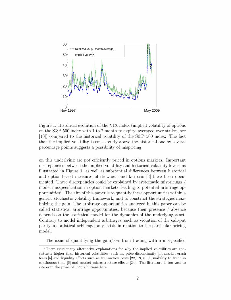
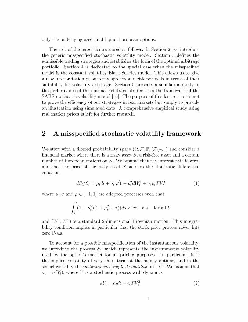
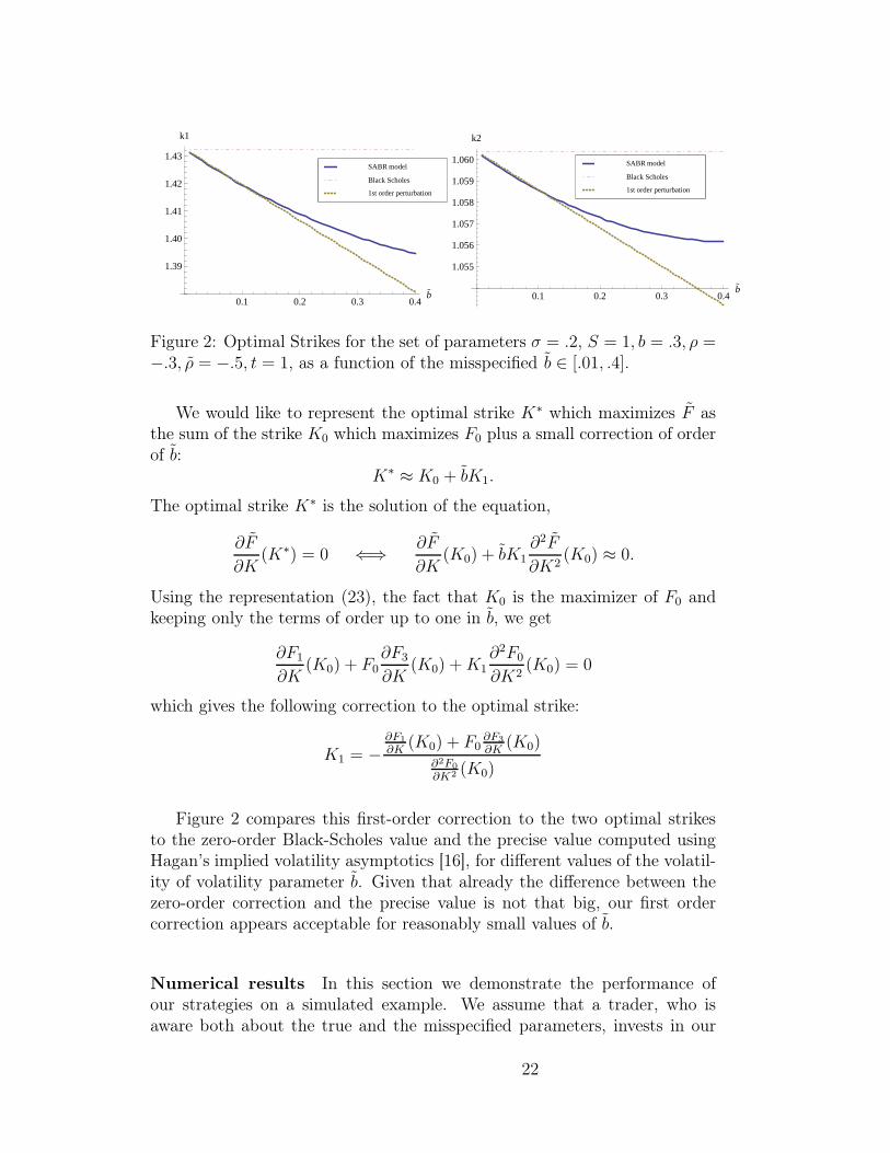
Figure 2: Optimal Strikes for the set of parameters σ = .2, S = 1, b = .3, ρ =−.3, ρ = −.5, t = 1, as a function of the misspecified b ∈ [.01, .4].

We would like to represent the optimal strike K∗ which maximizes F asthe sum of the strike K0 which maximizes F0 plus a small correction of orderof b:

K∗ ≈ K0 + bK1.

The optimal strike K∗ is the solution of the equation,

∂F

∂K(K∗) = 0 ⇐⇒ ∂F

∂K(K0) + bK1

∂2F

∂K2(K0) ≈ 0.

Using the representation (23), the fact that K0 is the maximizer of F0 andkeeping only the terms of order up to one in b, we get

∂F1

∂K(K0) + F0

∂F3

∂K(K0) +K1

∂2F0

∂K2(K0) = 0

which gives the following correction to the optimal strike:

K1 = −∂F1

∂K(K0) + F0

∂F3

∂K(K0)

∂2F0

∂K2 (K0)

Figure 2 compares this first-order correction to the two optimal strikesto the zero-order Black-Scholes value and the precise value computed usingHagan’s implied volatility asymptotics [16], for different values of the volatil-ity of volatility parameter b. Given that already the difference between thezero-order correction and the precise value is not that big, our first ordercorrection appears acceptable for reasonably small values of b.

Numerical results In this section we demonstrate the performance ofour strategies on a simulated example. We assume that a trader, who isaware both about the true and the misspecified parameters, invests in our

22

strategy. We simulate 10000 runs2 of the stock and the volatility during 1year under the system specified by (19)–(22), assuming misspecification ofthe correlation ρ and the volatility of volatility b but not of the volatilityitself (σ = σ). The initial stock value is S0 = 100 and initial volatility isσ0 = .1. The interest rate is assumed to be zero. During the simulation, ateach rebalancing date, the option portfolio is completely liquidated, and anew portfolio of options with the same, fixed, time to maturity and desiredoptimal strikes is purchased.

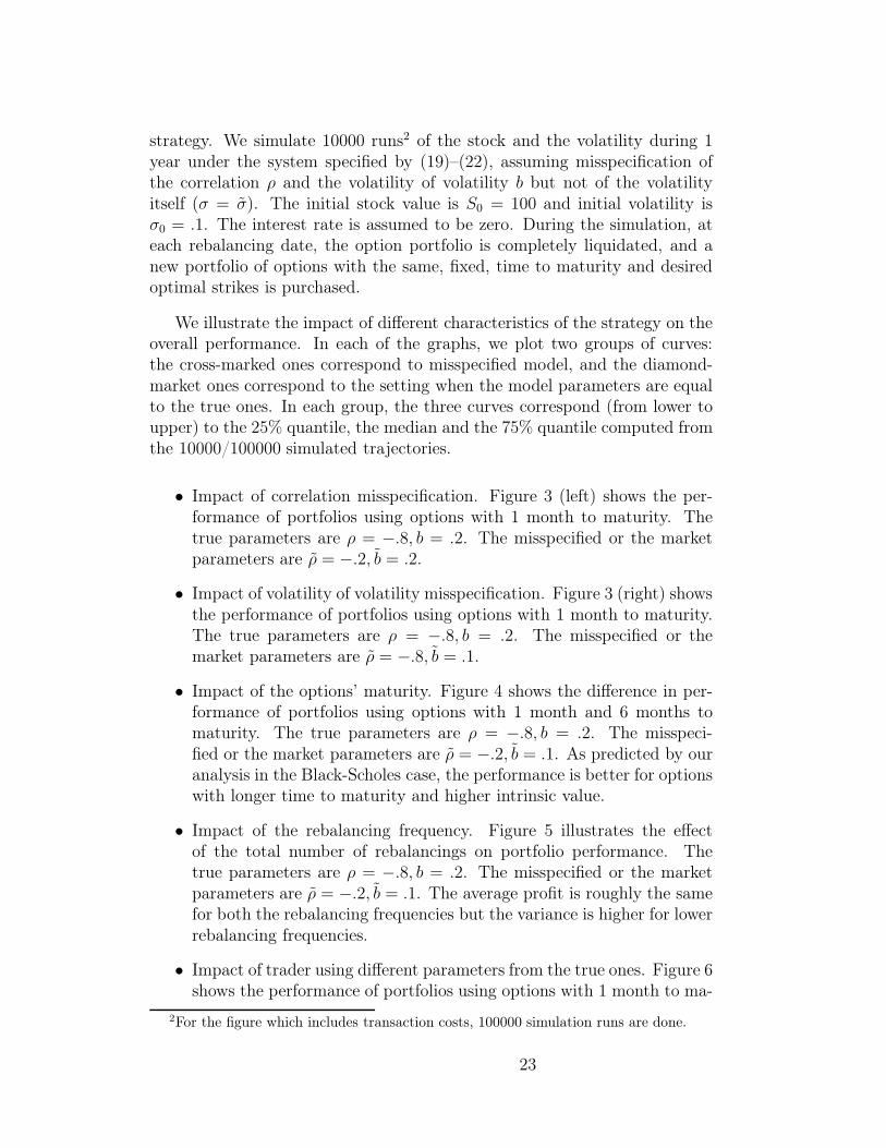
We illustrate the impact of different characteristics of the strategy on theoverall performance. In each of the graphs, we plot two groups of curves:the cross-marked ones correspond to misspecified model, and the diamond-market ones correspond to the setting when the model parameters are equalto the true ones. In each group, the three curves correspond (from lower toupper) to the 25% quantile, the median and the 75% quantile computed fromthe 10000/100000 simulated trajectories.

• Impact of correlation misspecification. Figure 3 (left) shows the per-formance of portfolios using options with 1 month to maturity. Thetrue parameters are ρ = −.8, b = .2. The misspecified or the marketparameters are ρ = −.2, b = .2.

• Impact of volatility of volatility misspecification. Figure 3 (right) showsthe performance of portfolios using options with 1 month to maturity.The true parameters are ρ = −.8, b = .2. The misspecified or themarket parameters are ρ = −.8, b = .1.

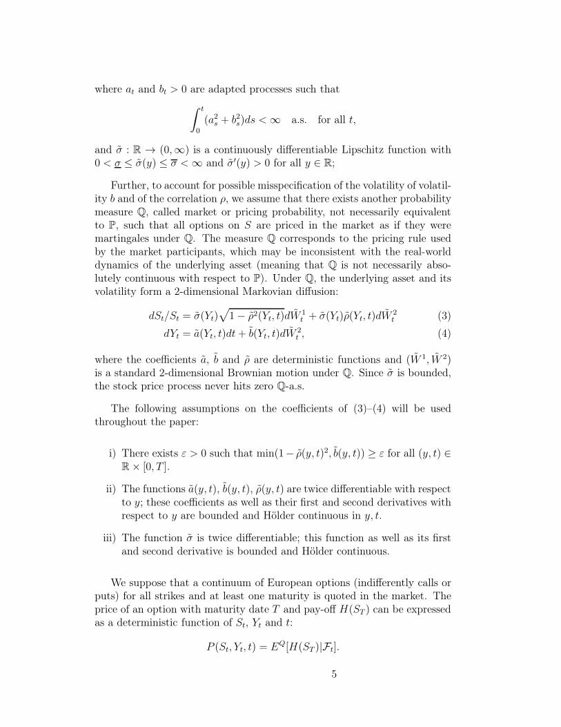
• Impact of the options’ maturity. Figure 4 shows the difference in per-formance of portfolios using options with 1 month and 6 months tomaturity. The true parameters are ρ = −.8, b = .2. The misspeci-fied or the market parameters are ρ = −.2, b = .1. As predicted by ouranalysis in the Black-Scholes case, the performance is better for optionswith longer time to maturity and higher intrinsic value.

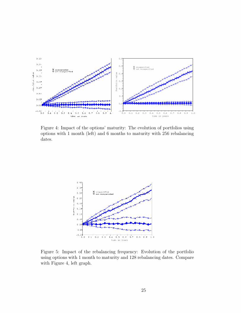
• Impact of the rebalancing frequency. Figure 5 illustrates the effectof the total number of rebalancings on portfolio performance. Thetrue parameters are ρ = −.8, b = .2. The misspecified or the marketparameters are ρ = −.2, b = .1. The average profit is roughly the samefor both the rebalancing frequencies but the variance is higher for lowerrebalancing frequencies.

• Impact of trader using different parameters from the true ones. Figure 6shows the performance of portfolios using options with 1 month to ma-

2For the figure which includes transaction costs, 100000 simulation runs are done.

23

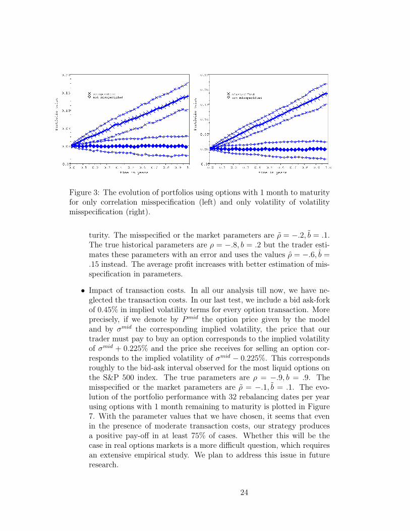
Figure 3: The evolution of portfolios using options with 1 month to maturityfor only correlation misspecification (left) and only volatility of volatilitymisspecification (right).

turity. The misspecified or the market parameters are ρ = −.2, b = .1.The true historical parameters are ρ = −.8, b = .2 but the trader esti-mates these parameters with an error and uses the values ρ = −.6, b =.15 instead. The average profit increases with better estimation of mis-specification in parameters.

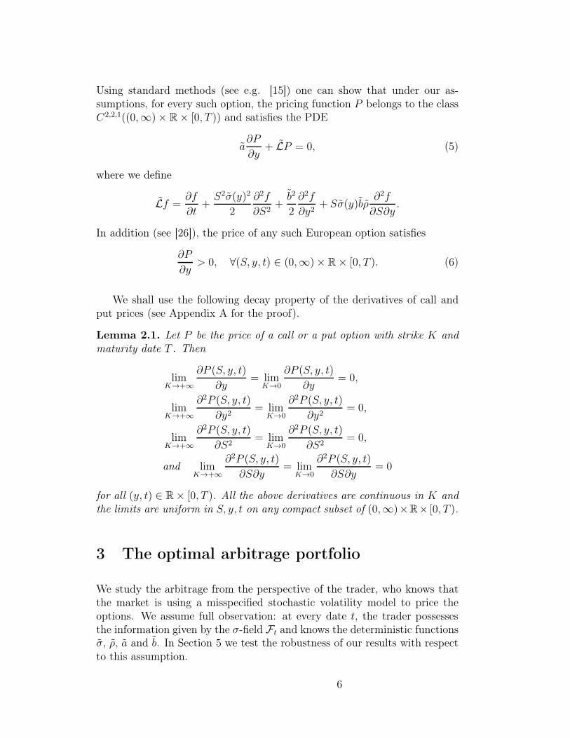
• Impact of transaction costs. In all our analysis till now, we have ne-glected the transaction costs. In our last test, we include a bid ask-forkof 0.45% in implied volatility terms for every option transaction. Moreprecisely, if we denote by Pmid the option price given by the modeland by σmid the corresponding implied volatility, the price that ourtrader must pay to buy an option corresponds to the implied volatilityof σmid + 0.225% and the price she receives for selling an option cor-responds to the implied volatility of σmid − 0.225%. This correspondsroughly to the bid-ask interval observed for the most liquid options onthe S&P 500 index. The true parameters are ρ = −.9, b = .9. Themisspecified or the market parameters are ρ = −.1, b = .1. The evo-lution of the portfolio performance with 32 rebalancing dates per yearusing options with 1 month remaining to maturity is plotted in Figure7. With the parameter values that we have chosen, it seems that evenin the presence of moderate transaction costs, our strategy producesa positive pay-off in at least 75% of cases. Whether this will be thecase in real options markets is a more difficult question, which requiresan extensive empirical study. We plan to address this issue in futureresearch.

24

time in years

0.2 0.3 0.4 0.6 1.00.5 0.9

Portfolio value

0.10.0

0.6

0.5

0.4

0.3

0.2

0.1

0.0

-0.10.80.7

misspecified

not misspecified

Figure 4: Impact of the options’ maturity: The evolution of portfolios usingoptions with 1 month (left) and 6 months to maturity with 256 rebalancingdates.

Figure 5: Impact of the rebalancing frequency: Evolution of the portfoliousing options with 1 month to maturity and 128 rebalancing dates. Comparewith Figure 4, left graph.

25

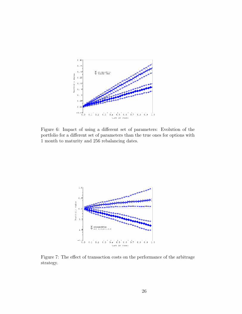
Figure 6: Impact of using a different set of parameters: Evolution of theportfolio for a different set of parameters than the true ones for options with1 month to maturity and 256 rebalancing dates.

Figure 7: The effect of transaction costs on the performance of the arbitragestrategy.

26

Acknowledgements

We would like to thank the participants of the joint seminar of SociétéGénérale, Ecole Polytechnique and Ecole des Ponts et Chaussées, and espe-cially L. Bergomi (Société Générale) for insightful comments on the previousversion of this paper.

This research of Peter Tankov is supported by the Chair Financial Risksof the Risk Foundation sponsored by Société Générale, the Chair Derivativesof the Future sponsored by the Fédération Bancaire Française, and the ChairFinance and Sustainable Development sponsored by EDF and Calyon. Thisresearch of Rudra Jena is supported by the Chair Financial Risks of the RiskFoundation sponsored by Société Générale.

A Proof of Lemma 2.1

First, let us briefly recall some results on fundamental solutions of parabolicPDE [21]. Let

L

(

x, t,∂

∂x,∂

∂t

)

u :=∂

∂t+

1

2

n∑

i,j=1

aij(x, t)∂2u

∂xi∂xj+

n∑

i=1

bi(x, t)∂u

∂xi+ c(x, t).

Assumption A.1. There is a positive constant µ such that

n∑

i,j=1

aij(x, t)ξiξj > µ|ξ|2 ∀(x, t) ∈ Rn × [0, T ], ξ ∈ Rn.

Assumption A.2. There exists α ∈ (0, 1) such that the coefficients of L arebounded and Hölder continuious in x with exponent α and Hölder continuousin t with exponent α

2, uniformly with respect to (x, t) in Rn × [0, T ].

The fundamental solution of the parabolic second-order equation withoperator L is the function Γ(x, t, ξ, T ) which satisfies

L

(

x, t,∂

∂x,∂

∂t

)

Γ(x, t, ξ, T ) = δ(x− ξ)δ(t− T ), t ≤ T.

Under A.1 and A.2, the operator L admits a fundamental solution Γ with

|DrtD

sxΓ(x, t, ξ, T )| ≤ c(T − t)−

n+2r+s2 exp

(

−C|x− ξ|T − t

)

(24)

27

where r and s are integers with 2r + s ≤ 2, t < T and c, C are positive.

Consider now the Cauchy problem,

Lu(x, t) = f(x, t), (x, t) ∈ Rn × [0, T ),

u(x, T ) = φ(x), x ∈ Rn,

where f is Hölder continuous in its arguments, φ is continuous and thesefunction satisfy reasonable growth constraints at infinity. Then the solutionto this problem can be written as

u(x, t) =

ˆ T

t

dτ

ˆ

Rn

dξΓ(x, t, ξ, τ)f(ξ, τ) +

ˆ

Rn

dξΓ(x, t, ξ, T )φ(ξ).

Let us now turn to the proof of Lemma 2.1. We discuss the results forthe put options. The result for calls follows directly by put-call parity. Asdescribed in Section 2, the put option price P (S, y, t) solves the PDE (5).Let x = log S

Kand p(x, y, t) := P (Kex, y, t). Then p solves the PDE

∂p

∂t+Ap = 0, p(x, y, T ) =K(1− ex)+. (25)

where

Ap =1

2σ2

∂2p

∂x2− ∂p

∂x

+ a∂p

∂y+

1

2b2∂2p

∂y2+ ρbσ

∂2p

∂x∂y

The quantities a, b, σ, ρ correspond to market misspecified values, but in thisappendix we shall omit the tilda and often drop the explicit dependence ont and y in model parameters to simplify notation.

Therefore, the option price can be written as

p(x, y, t) =

ˆ

dz

ˆ

dv Γ(x, y, t, z, v, T )K(1− ez)+, (26)

where Γ(x, y, t, z, v, T ) is the fundamental solution of (25). Since the coef-ficients of A do not depend on x, Γ(x, y, t, z, v, T ) ≡ Γ(0, y, t, z − x, v, T ).Coming back to the original variable S, we have

P (S, y, t) =

ˆ

dz γ(y, t, z − logS

K, T )K(1− ez)+ (27)

where we write

γ(y, t, z, T ) :=

ˆ

dv Γ(0, y, t, z, v, T ).

28

Decay of the gamma ∂2P∂S2 By direct differentiation of (27), we get

∂2P

∂S2=

K

S2γ(y, t, log

K

S, T ) (28)

and it follows from (24) that

∣

∣

∣

∣

∂2P

∂S2

∣

∣

∣

∣

≤ CK

S2|T − t| 12exp

(

−c log2 KS

T − t

)

. (29)

This proves the required decay properties, and the continuity of ∂2P∂S2 also

follows from (24).

Decay of the vega ∂P∂y

We denote U(S, y, t) := ∂P (S,y,t)∂y

and u(x, y, t) :=∂p(x,y,t)

∂y. Using the regularity of coefficients and local regularity results for

solutions of parabolic PDE [20, Corollary 2.4.1], we conclude that the deriva-

tives ∂3p∂x2∂y

, ∂3p∂x∂y2

and ∂3p∂y3

exist, and therefore the operator (26) may be dif-ferentiated term by term with respect to y, producing

∂u

∂t+A1u = −σσ′

∂2p

∂x2− ∂p

∂x

, (30)

where

A1 =A+ (ρbσ)′∂

∂x+ bb

′ ∂

∂y+ a′.

All the primes denote the derivative w.r.t. y and the terminal condition isu(S, y, T ) ≡ 0, since the original terminal condition is independent of y.

The right-hand side of (30) satisfies

∂2p

∂x2− ∂p

∂x= Kγ(y, t,−x, T ) (31)

so from (24) we get

∣

∣

∣

∣

∂2p

∂x2− ∂p

∂x

∣

∣

∣

∣

≤ CK

(T − t)12

exp

(

− cx2

T − t

)

. (32)

Let Γ1 denote the fundamental solution of the parabolic equation withthe operator appearing in the left-hand side of (30). Using the estimatesof the fundamental solution in [21, section 4.13] (in particular, the Hölder

29

continuity) and the bound (32), we can show that the solution to (30) isgiven by

u(x, y, t) =

ˆ T

t

dr

ˆ

R2

dz dv Γ1(x, y, t, z, v, r)σ(v)σ′(v)

∂p

∂z− ∂2p

∂z2

(z, v, r).

Using the boundedness of σ and σ′, the bound on the fundamental solutionand (32), and integrating out the variable v, we get

|u(x, y, t)| ≤ˆ T

t

dr

ˆ

dzCK

(T − r)12 (r − t)

12

exp

(

− cz2

T − r− c(x− z)2

r − t

)

.

Explicit evaluation of this integral then yields the bound

|u(x, y, t)| ≤ CK√T − te−

cx2

T−t (33)

|U(S, y, t)| ≤ CK√T − te−

c log2 SK

T−t (34)

from which the desired decay properties follow directly.

Decay of ∂2P∂S∂y

We denote w(x, y, t) = ∂u∂x

and W (S, y, t) = ∂U∂S

= wS

and

differentiate equation (30) with respect to x:

∂w

∂t+A1w = −σσ′

∂3p

∂x3− ∂2p

∂x3

.

From (31) and (24),

∣

∣

∣

∣

∂3p

∂x3− ∂2p

∂x2

∣

∣

∣

∣

≤ CK

T − texp

(

− cx2

T − t

)

. (35)

Similarly to the previous step we now get:

|w(x, y, t)| ≤ˆ T

t

dr

ˆ

dzCK

(T − r)(r − t)12

exp

(

− cz2

T − r− c(x− z)2

r − t

)

and explicit evaluation of this integral yields the bounds

|w(x, y, t)| ≤ CKe−cx2

T−t , |W (S, y, t)| ≤ CK

Se−

c log2 SK

T−t (36)

30

Decay of ∂2P∂y2

We denote v(x, y, t) = ∂u∂y

, V (S, y, t) = ∂U∂y

and differentiate

equation (30) with respect to y:

∂v

∂t+A2v = −σσ′ ∂

∂y

∂2p

∂x2− ∂p

∂x

− a′′u− (ρbσ)′′

w

where

A2 =A1 + bb′ ∂

∂y+ (ρbσ)

′ ∂

∂x+ a′ + (bb′)′.

Once again, from (31) and (24),

∣

∣

∣

∣

∂

∂y

∂2p

∂x2− ∂p

∂x

∣

∣

∣

∣

≤ CK

T − texp

(

− cx2

T − t

)

.

Using this bound together with (36) and (33) and proceding as in previoussteps, we complete the proof.

References

[1] Y. Aït-Sahalia, Y. Wang, and F. Yared, Do option markets cor-rectly price the probabilities of movement of the underlying asset, J.Econometrics, 102 (2001), pp. 67–110.

[2] M. Avriel and H. Reisman, Optimal option portfolios in markets withposition limits and margin requirements, J. Risk, 2 (2000), pp. 57–67.

[3] G. Bakshi, C. Cao, and Z. Chen, Empirical performance of alter-native option pricing models, J. Finance, 52 (1997).

[4] D. Bates, Jumps and stochastic volatility: the exchange rate processesimplicit in Deutschemark options, Rev. Fin. Studies, 9 (1996), pp. 69–107.

[5] D. Bates, Post-87 crash fears in the S&P 500 futures option market,J. Econometrics, 94 (2000), pp. 181–238.

[6] D. Bertsimas, L. Kogan, and A. W. Lo, When is time continuous,J. Financ. Econ., 55 (2000), pp. 173–204.

[7] T. Björk, G. Di Masi, Y. Kabanov, and W. Runggaldier,Towards a general theory of bond markets, Finance Stoch., 1 (1997),pp. 141–174.

31

[8] U. Cetin, R. Jarrow, P. Protter, and M. Warachka, Pricingoptions in an extended Black Scholes economy with illiquidity: Theoryand empirical evidence, Rev. Fin. Studies, 19 (2006), pp. 493–519.

[9] U. Cetin, H. Soner, and N. Touzi, Option hedging for small in-vestors under liquidity costs, Finance Stoch., 14 (2010), pp. 317–341.

[10] Chicago Board of Options Exchange, The CBOEVolatility Index – VIX, CBOE, 2009. Download from:http://www.cboe.com/micro/VIX/vixwhite.pdf.

[11] , CBOE Margin Manual, CBOE, 2000. Download from:www.cboe.com/LearnCenter/pdf/margin2-00.pdf.

[12] B. Dumas, J. Fleming, and R. Whaley, Implied volatility functions:Empirical tests, J. Finance, 53 (1998), pp. 2059–2106.

[13] N. El Karoui, M. Jeanblanc, and S. Shreve, Robustness of theBlack Scholes formula, Math. Finance, 8 (1998), pp. 93–126.

[14] D. Fernholz and I. Karatzas, On optimal arbitrage. preprint, 2008.

[15] A. Friedman, Stochastic Differential Equations and Applications,vol. 1, Academic Press, 1975.

[16] P. Hagan, D. Kumar, A. Lesniewski, and D. Woodward, Man-aging smile risk, Wilmott Magazine, Sep. (2002).

[17] W. Härdle, T. Kleinow, and G. Stahl, Applied Quantitative Fi-nance, Springer-Verlag, 2002.

[18] A. Javaheri, Inside Volatility Arbitrage, Wiley Finance, 2005.

[19] Y. Kabanov and M. Safarian, On Leland’s strategy of option pricingwith transaction costs., Finance Stoch., 1 (1997), pp. 239–250.

[20] N. V. Krylov, Lectures on Elliptic and Parabolic Equations in SobolevSpaces, American Mathematical Society, 2008.

[21] O. A. Ladyzhenskaya, V. A. Solonnikov, and N. N. Uralt-

seva, Linear and Quasilinear Equations of Parabolic Type, AmericanMathematical Society, 1968.

[22] H. E. Leland, Option pricing and replication with transactions costs.,J. Finance, 40 (1985), pp. 1283–1301.

32

[23] Y. Osajima, General asymptotics of Wiener functionalsand application to mathematical finance. Available fromhttp://ssrn.com/abstract=1019587, 2007.

[24] C. Robert and M. Rosenbaum, On the Microstructural Hedging Er-ror, SIAM J. Fin. Math., 1 (2010), pp. 427–453.

[25] S. Romagnoli and T. Vargiolu, Robusness of the Black-Scholesapproach in the case of options on several assets, Finance Stoch., 4(2000), pp. 325–341.

[26] M. Romano and N. Touzi, Contingent claims and market complete-ness in a stochastic volatility model, Math. Finance, 7 (1997), pp. 399–410.

[27] P. Santa-Clara and A. Saretto, Option strategies: Good deals andmargin calls, J. Fin. Markets, 12 (2009), pp. 391–417.

[28] C. A. Sin, Complications with stochastic volatility models, Adv. Appl.Probab., 30 (1998).

33