AQUACULTURE COLLABORATIVE RESEARCH SUPPORT PROGRAM TWENTY-FIFTH ANNUAL TECHNICAL REPORT VOLUME I 1 August 2006 to 31 January 2008 Aquaculture CRSP Program Management Office College of Agricultural Sciences Oregon State University 418 Snell Hall Corvallis, Oregon 97331-1643 USA website: aquafishcrsp.oregonstate.edu Program activities are funded in part by the United States Agency for International Development (USAID) under Grant No. LAG-G-00-96-90015-00. Disclaimers The contents of this document do not necessarily represent an official position or policy of the United States Agency for International Development (USAID). Mention of trade names or commercial products in this report does not constitute endorsement or recommendation for use on the part of USAID or the Aquaculture Collaborative Research Support Program. The accuracy, reliability, and originality of work presented in this report are the responsibility of the individual authors. Acknowledgments The Program Management Office of the Aquaculture CRSP gratefully acknowledges the contributions of Aquaculture CRSP researchers around the world.

Welcome message from author
This document is posted to help you gain knowledge. Please leave a comment to let me know what you think about it! Share it to your friends and learn new things together.
Transcript

AQUACULTURE COLLABORATIVE RESEARCH SUPPORT PROGRAM
TWENTY-FIFTH ANNUAL TECHNICAL REPORT VOLUME I
1 August 2006 to 31 January 2008
Aquaculture CRSP Program Management Office College of Agricultural Sciences Oregon State University 418 Snell Hall Corvallis, Oregon 97331-1643 USA website: aquafishcrsp.oregonstate.edu Program activities are funded in part by the United States Agency for International Development (USAID) under Grant No. LAG-G-00-96-90015-00.
Disclaimers The contents of this document do not necessarily represent an official position or policy of the United States Agency for International Development (USAID). Mention of trade names or commercial products in this report does not constitute endorsement or recommendation for use on the part of USAID or the Aquaculture Collaborative Research Support Program. The accuracy, reliability, and originality of work presented in this report are the responsibility of the individual authors. Acknowledgments The Program Management Office of the Aquaculture CRSP gratefully acknowledges the contributions of Aquaculture CRSP researchers around the world.


AQUACULTURE COLLABORATIVE RESEARCH SUPPORT PROGRAM Twenty-Fifth Annual Technical Report – Volume I Director Dr. Hillary Egna Managing Editor Dr. Laura Morrison Editorial Assistant Lisa Reifke THE TWO VOLUME SET OF THIS PUBLICATION MAY BE CITED AS: Aquaculture Collaborative Research Support Program. 2008. Twenty-Fifth Annual Technical Report. Aquaculture CRSP, Oregon State University, Corvallis, Oregon. Vol I & II.
VOLUME I OF THIS PUBLICATION MAY BE CITED AS: Aquaculture Collaborative Research Support Program. 2008. Twenty-Fifth Annual Technical Report. Aquaculture CRSP, Oregon State University, Corvallis, Oregon. Vol I, 430pp.


i
Contents
INTRODUCTION 1 REPORTS: VOLUME I 5 ENVIRONMENTAL IMPACTS ANALYSIS Impact of Tilapia, Oreochromis niloticus, Introduction on the Indigenous Species
of Bangladesh and Nepal (12EIA3) 7 Building the Capacity of Moi University to Conduct Watershed Assessment (12EIA4) 13 Workshops on Better Practices for Sustainable Aquaculture (12EIA7) 25 Building the Capacity of Moi University to Have a Working GIS Lab and First
Generation GIS Model of the Nzoia River Basin (12EIA8) 30 SUSTAINABLE DEVELOPMENT & FOOD SECURITY Understanding the Aquacultural Knowledge and Information System for Commercial
Tilapia Production in Nicaragua: Economics, Institutions, and Markets (12SDF2) 40 First Annual Sustainable Aquaculture Technology Transfer Workshop (12SDF4) 51 The Eagle of the North and the Condor of the South Aquaculture Exchange
Project (12SDF6 & 12SDF8) 55 Aquaculture Outreach in the Amazon Basin (12SDF7) 62 Sixth International Aquaculture Training Course in the Amazon Region (12SDF9) 69 PRODUCTION SYSTEM DESIGN & INTEGRATION New Paradigm in Farming of Freshwater Prawn (Macrobrachium rosenbergii)
With Closed and Recycle Systems in Thailand (12PSD1a) 74 New Paradigm in Farming of Freshwater Prawn (Macrobrachium rosenbergii)
With Closed and Recycle Systems in Bangladesh (12PSD1b) 84 New Paradigm in Farming of Freshwater Prawn (Macrobrachium rosenbergii)
With Closed and Recycle Systems in Vietnam (12PSD1c) 99 Optimization of Fertilization Regime in Fertilized Nile Tilapia Ponds with
Supplemental Feed (12PSD2) 111 Use of Rice Straw as a Resource for Freshwater Pond Culture: Periphyton
Substrate (12PSD3a) 129 Use of Rice Straw as a Resource for Freshwater Pond Culture: Growth
Performance (12PSD3b) 167 Development of a Recirculating Aquaculture System Module for Family/
Multi-Family Use (12PSD4) 187 Insulin-like Growth Factor-I Gene Expression as a Growth Indicator in Nile
Tilapia (12PSD5) 193
TWENTY-FIFTH ANNUAL TECHNICAL REPORT – VOLUME I
ii
PRODUCTION SYSTEM DESIGN & INTEGRATION (continued) Development of Nile Tilapia Fillets As An Export Product for the
Philippines (12PSD6) 210 Tilapia-Shrimp Polyculture in Negros Occidental, Philippines (12PSD7) 224 Testing Three Styles of Tilapia–Shrimp Polyculture in Tabasco, Mexico (12PSD8) 238 Student Exchange Program to Strengthen Capacity in Chinese Environmental
Studies of Aquaculture: Preliminary Assessment of Integrated Shrimp/Seaweed, Shrimp/Abalone, and Shrimp/Seaweed/Duck Farming Practices in Yinbin Bay, Hainan Province, China (12PSD9a) 246
Student Exchange Program to Strengthen Capacity in Chinese Environmental Studies of Aquaculture: Application of Phytase in Nile Tilapia Feed (12PSD9b) 261
INDIGENOUS SPECIES DEVELOPMENT Controlled Reproduction of an Important Indigenous Species, Spinibarbus
denticulatus, in Southeast Asia (12ISD1) 278 Incorporation of the Native Cichlid Petenia splendida into Sustainable Aquaculture:
Reproduction Systems, Nutrient Requirements and Feeding Strategies (12ISD3) 293 Egg Hatching Quality of Amazonian Fishes (12ISD5) 309 Influence of Dietary Fatty Acid Composition on Reproductive Performance of
Colossoma macropomum (12ISD6) 315
WATER QUALITY & AVAILABILITY Pond Design and Watershed Analyses Training (12WQA1) 321 Elimination of Methyltestosterone from Intensive Masculinization Systems:
Use of Ultraviolet Irradiation of Water (12WQA2) 340 Elimination of Methyltestosterone from Intensive Masculinization Systems:
Use of Solar Irradiation and Bacterial Degradation (12WQA3) 346 Ecological Assessment of Selected Sub-Watersheds of the Nzoia River
Basin (12WQA4) 355 Determination of Hydrologic Baselines for the Nzoia Basin (12WQA5) 371 Student Research to Assess Environmental Impacts of Cage Aquaculture in
the Fujian Province of China (12WQA6) 395 Pelagic (Fish) and Benthic Ecology of Selected Sub-Watersheds of the Nzoia
River Basin (12WQA7) 406 Hydrologic Modeling in the Nzoia River Basin (12WQA8) 418
Introduction
The Aquaculture Collaborative Research Support Program (ACRSP) is funded by the United States Agency for International Development (USAID) under authority of the Foreign Assistance Act of 1961 (PL 87-195) as amended and by ACRSP participating universities and institutions. ACRSP is currently in its final year and will officially close on June 30, 2008. A cohesive program of research has been conducted in selected developing countries and the United States by teams of US and host country researchers, administrators, students, and others. Currently operating under a no-cost extension granted under its fourth USAID grant since 1982, the ACRSP has been guided by the concepts and direction set down in the Continuation Plan 1996 (USAID Grant No. LAG-G-00-96-90015-00). Activities of this multinational, multi-institutional, and multidisciplinary program are administered by Oregon State University (OSU), which functions as the Management Entity (ME) and has technical leadership, programmatic oversight, and fiscal responsibility for the performance of grant provisions.
REPORT SCOPE This report, the Twenty-Fifth Annual Technical Report, describes research and outreach undertaken by the ACRSP during its final year. It includes projects funded in the Twelfth Work Plan (WP12) and its two addenda, available at pdacrsp.oregonstate.edu/pubs/work_plans/. This report is the last in the publication series of project reports for WP12, and for the ACRSP overall.
WP12 RESEARCH PROJECTS The Twenty-Fifth Annual Technical Report contains the final technical reports for the WP12 research projects described in the Twenty-Fifth Annual Administrative Report (published 2007). In setting the conceptual framework for the final stage of ACRSP, WP12 focused research on sustainable aquaculture development in coastal and inland areas. Projects fit into one of three program areas:
• Production Technology • Watershed Management • Human Welfare, Health, and Nutrition
Projects encompass multiple investigations with each investigation focusing on any one of ten scientific themes. For project-level reporting, please refer to the Twenty-Fifth Annual Administrative Report.
WP12 SCIENTIFIC THEMES Each of the ten WP12 scientific themes collectively cover economic growth, food security, and the wise use of natural resources in aquaculture:

TWENTY-FIFTH ANNUAL TECHNICAL REPORT – VOLUME I
2
Environmental Impacts Analysis (EIA) With the rapid growth in aquaculture production, environmental externalities are of increasing concern. Determining the scope and mitigating or eliminating the negative environmental impacts of aquaculture—such as poor management practices and the effects of industrial aquaculture—are primary goals of the ACRSP. Sustainable Development & Food Security (SDF) Aquaculture is increasing in importance as a source for poverty alleviation and food security in developing regions of the world. A focal area of the program is to support efforts related to sustainable aquatic farming systems that can demonstrably ensure a reliable future food supply. Production System Design & Integration (PSD) Aquaculture is an agricultural sector with specific input demands. Systems should be designed to improve efficiency and/or integrate aquaculture inputs and outputs with other agricultural and non-agricultural production systems. Indigenous Species Development (ISD) Domestication of new and indigenous species may contribute positively to the development of local communities as well as protect ecosystems. At the same time, the development of new species for aquaculture must be approached in a responsible manner that diminishes the chance for negative environmental, technical, and social impacts. Efforts that investigate relevant policies and practices are encouraged while exotic species development is not encouraged. Water Quality & Availability (WQA) Aquaculture development that makes wise use of natural resources is at the core of the CRSP. Gaining a better understanding of water and aquaculture is a matter of great interest to the ACRSP. The range of possibilities is broad—from investigations that quantify such things as availability and quality to those that look into the social context of water and aquaculture, including water rights, national and regional policies (or the lack of them), traditional versus industrial uses, and the like. Economic/Risk Assessment & Social Analysis (ERA) Aquaculture is a rapidly growing industry; its risks and impacts on society need to be assessed. Significant issues in this arena include cost, price, and risk relationships; domestic market and distribution needs and trends; the relationships between aquaculture and women/ underrepresented groups; and the availability of financial resources for small farmers. Applied Technology & Extension Methodologies (ATE) Developing appropriate technology and providing technology-related information to end-users are high priorities. The program encourages efforts that result in a better understanding of factors and practices that set the stage for near-term technology implementation and that contribute to the development of successful extension tools and methods. Seedstock Development & Availability (SDA) Procuring reliable supplies of high quality seed for stocking local and remote sites is critical to continued development of the industry. A better understanding of the factors that can contribute to stable seedstock quality and quantity for aquaculture enterprises is essential. Fish Nutrition & Feed Technology (FNF) Ways and methods of increasing the range of available ingredients and improving the technology available to manufacture and deliver feeds is an important theme. Better information about fish nutrition can lead to the development of less expensive and more efficient feeds. Efforts that investigate successful adoption and extension strategies for the nutritional needs of fish are also encouraged.
INTRODUCTION
3
Aquaculture & Human Health Impacts (HHI) Aquaculture can be a crucial source of proteins and micronutrients for improved human health, growth, and development. Conversely, human health can be negatively impacted by aquaculture if it serves as a direct or indirect vector for human diseases. There is also interest in better understanding the interconnectedness of such human health crises as AIDS/HIV and aquaculture production.
TWO VOLUME SET The Twenty-Fifth Annual Technical Report is a 2-volume set with the following coverage of scientific themes: Volume I Volume II • Environmental Impacts Analysis • Economic Risk Assessment & Social Analysis • Sustainable Development & Food Security • Applied Technology & Extension Methodologies • Production System Design & Integration • Seedstock Development & Availability • Indigenous Species Development • Fish Nutrition & Feed Technology • Water Quality & Availability • Aquaculture & Human Health Impacts
CITATION FORMAT
The appropriate citation for a report contained in this volume is, for example: Shameem Ahmad, S.A., A.N. Bart, Md.A. Wahab, M.K. Shrestha, J.E. Rakocy, and J.S. Diana. 2008. Impact of tilapia, Oreochromis niloticus, introduction on the indigenous species of Bangladesh and Nepal. In: L. Morrison and H. Egna (Editors), Twenty-Fifth Annual Technical Report. Aquaculture CRSP, Oregon State University, Corvallis, Oregon, Vol I, pp. 7–12.

TWENTY-FIFTH ANNUAL TECHNICAL REPORT – VOLUME I
4

5
Reports: Volume I
The Twenty-Fifth Annual Technical Report contains final reports for the WP12 research projects described in the Twenty-Fifth Annual Administrative Report (published 2007). The WP12 final technical reports in this volume cover five scientific themes:
• Environmental Impacts Analysis • Sustainable Development & Food Security • Production System Design & Integration • Indigenous Species Development • Water Quality & Availability
INVESTIGATION CODE
Each report is identified by a unique scientific-theme investigation code e.g., 12EIA3. In this code, "12" refers to WP12, the 3-letter acronym (e.g., "EIA") identifies the scientific theme, and the number (e.g., "3") identifies the sequential investigation number assigned within the scientific theme block.
TECHNICAL REPORT FORMAT Although technical reports have been formatted for style, they are published as submitted. Figures and tables that did not follow ACRSP Publication Guidelines may have lost information during formatting. Figures reflect their original condition as submitted. Please contact the authors directly for questions about content, tables, or figures.

TWENTY-FIFTH ANNUAL TECHNICAL REPORT – VOLUME I
ENVIRONMENTAL IMPACTS ANALYSIS
7
IMPACT OF TILAPIA, OREOCHROMIS NILOTICUS, INTRODUCTION ON THE INDIGENOUS SPECIES OF BANGLADESH AND NEPAL
Twelfth Work Plan, Environmental Impacts Analysis 3 (12EIA3)
Final Report Published as Submitted by Contributing Authors
S. A. Shameem Ahmad & Amrit N. Bart Asian Institute of Technology
Pathumthani, Thailand
Md. Abdul Wahab Bangladesh Agricultural University
Mymensingh, Bangladesh
M. K. Shrestha Fisheries & Aquaculture Department
Rampur, Chitwan, Nepal
James E. Rakocy University of Virgin Islands St. Croix, U.S. Virgin Islands
James S. Diana
University of Michigan Ann Arbor Michigan, USA
ABSTRACT Small indigenous species (SIS) of fish are important to rural poor in Bangladesh and Nepal as these species are relatively cheap, consumed whole and contain nutritive values higher than many cultured species. There is concern that introduced tilapia may compete with SIS, causing not only the loss of biodiversity but also affecting health of the rural poor. Therefore, this study was conducted to assess the effect of Nile tilapia on changes in population structure, recruitment and diet with three important indigenous species in simulated natural ponds. Experiments were conducted at Bangladesh Agricultural University and at the Institute of Agriculture and Animal Science in Nepal. In each location, nine earthen ponds of 100 m2 surface area and 1.0 m average depth were used. In each location a completely randomized design with three treatments were used and each treatment had three replicates. The treatments were: mixed-sex tilapia with the three indigenous fish species; mono-sex male tilapia with SIS; and SIS without tilapia. In both sites, gut content analysis and electivity indices indicated that all the fish species were selective in their food habits, and that there was potential competition for food organisms among all species. In Bangladesh, population densities and biomasses of mola (Amblypharyngodon mola), punti (Puntius sophore) and chela (Chela cachius) were significantly higher in the SIS and SIS with monosex-tilapia treatments compared to mixed-sex tilapia with SIS. Total fish biomass in both tilapia treatments was three times higher than in the control. In Nepal, population density and biomass of pothi (Puntius sophore) was significantly higher in the SIS treatment compared to the tilapia treatments, while tilapia did not affect recruitment or biomass of darai (Esomus danricus) or faketa (Barilius barna).
INTRODUCTION Tilapia has been a component of the fish fauna of most of Asia since their first introduction into the region over five decades ago (De Silva, 2005). Culture of tilapia has been promoted for poor farmers as well as a fish with export potential in many parts of Asia. Tilapia is also perceived as
TWENTY-FIFTH ANNUAL TECHNICAL REPORT – VOLUME I
8
an aggressive feeder and prolific breeder even under relatively stressful environments. Despite rapid proliferation of tilapia culture worldwide, several countries continue to remain cautious, as they fear that tilapia may compete with the local indigenous species causing loss of biodiversity and an ecological imbalance. Many of these claims have been based on anecdotal evidence from the pond experience and survey data (Ameen, 1999). The ability of tilapia, even in the static environment, to compete with indigenous, locally well-adapted species has never been established using scientific approaches. Small indigenous species (SIS) of fish are important to rural poor in Bangladesh, India, Nepal, Cambodia and many countries of Asia as these species are relatively cheap, consumed whole and contain nutritive values higher than many cultured species (Hossain, 1998). These indigenous species have many additional advantages, including self-recruitment, fast growth, feeding at low trophic levels, and high content of micronutrients, including calcium and vitamin A (Thilsted and Hassan, 1993). Rural people of Bangladesh consume 56 to 73 species of SIS (Minkin, 1993), among which mola (Amblypharyngodon mola), chela (Chela cachius) and punti (Puntius sophore) are most commonly preferred. Rural people of Nepal consume many species of SIS among which pothi (Puntius sophore), faketa (Barilius barna), darai (Esomus danricus) are most commonly preferred (Shrestha, 1995). Some of these species are similar to tilapia, as they also rely on natural phytoplankton and zooplankton as their primary food sources and some are found to breed in static natural water bodies and abandoned ponds (Shafi and Quddus, 1982; Shrestha, 1994). There is concern that introduced tilapia may compete with SIS, causing not only the loss of biodiversity but also affecting health of the rural poor who derive high quality micronutrients from these indigenous species. Therefore, this study was conducted to assess the effect of mixed-sex and mono-sex tilapia on changes in population structure, recruitment and diet overlap with three important indigenous species in simulated natural ponds.
MATERIALS AND METHODS Experiments were conducted at Bangladesh Agricultural University (BAU), Mymensingh, Bangladesh and at the Institute of Agriculture and Animal Science, Chitwan, Nepal. In each location, nine earthen ponds of 100 m2 surface area and 1.0 m average depth were used. All experimental ponds were drained, dried, and limed (agricultural grade CaCO3) at 250 kg ha-1. Cow dung was applied at 1000 kg ha-1 and the ponds were filled with surface water. A week prior to stocking, ponds were fertilized with urea at 100 kg ha-1 and TSP at 50 kg ha-1. No additional nutrient inputs were made to the ponds after stocking. Experimental fishes were Nile tilapia (Oreochromis niloticus) and small indigenous fish (SIS) in Bangladesh, including mola, chela and punti. In Nepal, experimental fishes were Nile tilapia and the indigenous small fish species, pothi, darai and faketa. In each location a completely randomized design with three treatments were used and each treatment had three replicates. The treatments were:
(i) mixed-sex tilapia with the three indigenous fish species (T1) (ii) mono-sex male tilapia with SIS (T2) (iii) SIS without tilapia (T3-control).
Each species was apportioned equally (25%) with a total stocking rate of 0.56 fish m-2 for the two-tilapia treatments (T1 and T2). Each indigenous species was apportioned equally (33%) with a total stocking rate of 0.42 fish m-2 for the control (T3). The male to female ratio of SIS was 1:1. Juvenile Nile tilapia were stocked 74 days after the SIS were stocked at the Bangladesh site and 30 days after the SIS were stocked at the Nepal site. Individual weights of fishes were determined during stocking. In Bangladesh the initial average weight during stocking of mola, chela, punti and tilapia were 0.68±0.03, 0.73±0.40, 4.54±0.35, 5.12±0.34 g, respectively. This experiment continued for 21 months (December 2004 to September 2006). In Nepal, the initial average weight of pothi, darai, faketa and tilapia were 6.3±0.64, 2.0±0.22, 6.7±0.18, 27.1±0.1.96 g, respectively. This experiment continued for 13 months (June 2005 to July 2006).

ENVIRONMENTAL IMPACTS ANALYSIS
9
Dissolved oxygen (DO), water temperature, pH, and Secchi disc visibility were measured weekly. Total alkalinity, nitrate-nitrogen, nitrite-nitrogen, total ammonia-nitrogen, phosphate-phosphorous and chlorophyll-a concentrations of pond water were analyzed monthly. Standard procedures and methods consistently followed APHA et al. (1999). Plankton samples were collected at monthly intervals and identified to genus level. Monthly sampling of fish was done, and batch and individual weights were measured. All ponds were harvested by draining in early September 2006 in Bangladesh and late July 2006 in Nepal. At harvest, fish from each pond were separated by species, then batch weighed and counted. At the end of experiment, stomach content analysis was performed at each experimental site to determine the Electivity Index and Dietary Overlap of each species using Ivlev electivity index (Ivlev, 1961) and Schoener’s overlap index (Schoener, 1970) respectively. Twenty fish from each species were collected randomly from each pond one-day before the end of experiment. Gut contents were analyzed to identify zooplankton and phytoplankton. Mean values were analyzed statistically by one-way analysis of variance (ANOVA; Ott, 1993) for the abundance of fishes, water quality, and plankton population using SPSS (version 11.5) statistical software (SPSS Inc., Chicago, USA). A Tukey’s Honesty test was used to compare and rank means. Differences among treatment means were considered significant at an alpha level of 0.05. Means were given with ± standard error.
RESULTS In the Bangladesh experiment, gut content analysis and electivity indices indicated that all the fish species were selective in their food habits, and that there was potential competition for food organisms among all species. Significant dietary overlap between the Nile tilapia and SIS and among SIS reflected possible strong competition. In general, the population density and biomass of mola, chela and punti were significantly higher in the SIS and SIS plus male mono-sex tilapia treatments than in the treatment of mixed-sex tilapia with SIS (Table 1). Therefore, mixed-sex tilapia did affect recruitment and biomass of small indigenous species. The population density and biomass of chela was higher in the SIS treatment than in the SIS with male mono-sex tilapia treatment, indicating that recruitment of chela was affected by both mixed-sex and mono-sex male
Table 1. Mean values (±SE) of population numbers and biomass of fish species for each treatment in Bangladesh.
Treatments
Parameters Mixed-sex
Tilapia with SIS (T1)
Male mono-sex Tilapia with SIS
(T2)
SIS-Control (T3)
Mola population density (#/100 m2) 221±21.63b 399±33.34a 358±46.05a
Mola biomass (g/100 m2) 238.33±24.34 496.33±57.44 424.63.00±62.61 Chela population density (#/100 m2) 94±8.11c 157±6.48b 238±7.00a
Chela biomass (g/100 m2) 162.50±8.85b 234.57±19.17b 421±38.62a
Punti population density (#/100 m2) 100±6.66 304±116.03 308±42.92 Punti biomass (g/100 m2) 1009.67±153.10b 1399.67±247.31ab 2052.50±157.50a
Tilapia population density (#/100 m2) 451±24.74a 14±0.0b - Tilapia biomass (kg/100 m2) 7.20±0.329 6.39±0.438 - Total SIS population density (#/100 m2) 415±25.00b 861±109.74a 905±85.35a
Total SIS biomass (kg/100 m2) 1.41±0.121b 2.13 ±0.285ab 2.84 ±0.135a
Total biomass of all species (kg/100 m2) 8.61±0.435a 8.52±0.183a 2.84±0.135b
Mean values with different superscripts in the same row were significantly different P<0.05).
TWENTY-FIFTH ANNUAL TECHNICAL REPORT – VOLUME I
10
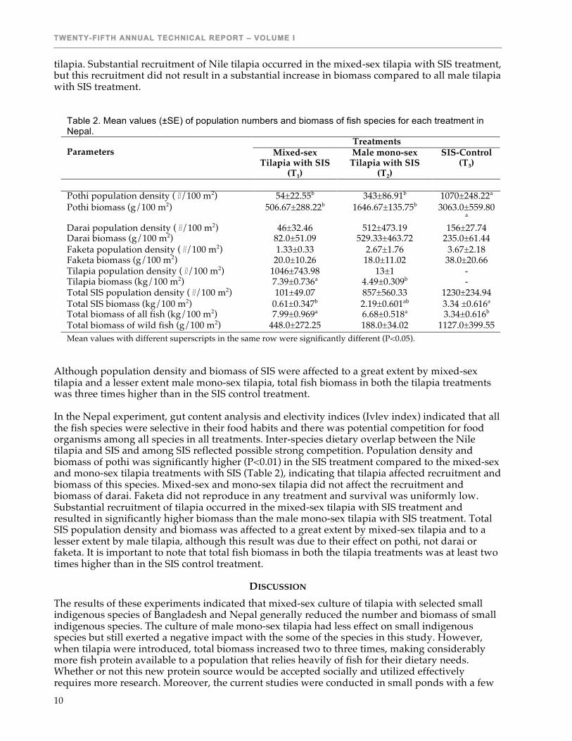
tilapia. Substantial recruitment of Nile tilapia occurred in the mixed-sex tilapia with SIS treatment, but this recruitment did not result in a substantial increase in biomass compared to all male tilapia with SIS treatment.
Table 2. Mean values (±SE) of population numbers and biomass of fish species for each treatment in Nepal.
Treatments Parameters Mixed-sex
Tilapia with SIS (T1)
Male mono-sex Tilapia with SIS
(T2)
SIS-Control (T3)
Pothi population density (#/100 m2) 54±22.55b 343±86.91b 1070±248.22a Pothi biomass (g/100 m2) 506.67±288.22b 1646.67±135.75b 3063.0±559.80
a Darai population density (#/100 m2) 46±32.46 512±473.19 156±27.74 Darai biomass (g/100 m2) 82.0±51.09 529.33±463.72 235.0±61.44 Faketa population density (#/100 m2) 1.33±0.33 2.67±1.76 3.67±2.18 Faketa biomass (g/100 m2) 20.0±10.26 18.0±11.02 38.0±20.66 Tilapia population density (#/100 m2) 1046±743.98 13±1 - Tilapia biomass (kg/100 m2) 7.39±0.736a 4.49±0.309b - Total SIS population density (#/100 m2) 101±49.07 857±560.33 1230±234.94 Total SIS biomass (kg/100 m2) 0.61±0.347b 2.19±0.601ab 3.34 ±0.616a Total biomass of all fish (kg/100 m2) 7.99±0.969a 6.68±0.518a 3.34±0.616b Total biomass of wild fish (g/100 m2) 448.0±272.25 188.0±34.02 1127.0±399.55 Mean values with different superscripts in the same row were significantly different (P<0.05).
Although population density and biomass of SIS were affected to a great extent by mixed-sex tilapia and a lesser extent male mono-sex tilapia, total fish biomass in both the tilapia treatments was three times higher than in the SIS control treatment. In the Nepal experiment, gut content analysis and electivity indices (Ivlev index) indicated that all the fish species were selective in their food habits and there was potential competition for food organisms among all species in all treatments. Inter-species dietary overlap between the Nile tilapia and SIS and among SIS reflected possible strong competition. Population density and biomass of pothi was significantly higher (P<0.01) in the SIS treatment compared to the mixed-sex and mono-sex tilapia treatments with SIS (Table 2), indicating that tilapia affected recruitment and biomass of this species. Mixed-sex and mono-sex tilapia did not affect the recruitment and biomass of darai. Faketa did not reproduce in any treatment and survival was uniformly low. Substantial recruitment of tilapia occurred in the mixed-sex tilapia with SIS treatment and resulted in significantly higher biomass than the male mono-sex tilapia with SIS treatment. Total SIS population density and biomass was affected to a great extent by mixed-sex tilapia and to a lesser extent by male tilapia, although this result was due to their effect on pothi, not darai or faketa. It is important to note that total fish biomass in both the tilapia treatments was at least two times higher than in the SIS control treatment.
DISCUSSION The results of these experiments indicated that mixed-sex culture of tilapia with selected small indigenous species of Bangladesh and Nepal generally reduced the number and biomass of small indigenous species. The culture of male mono-sex tilapia had less effect on small indigenous species but still exerted a negative impact with the some of the species in this study. However, when tilapia were introduced, total biomass increased two to three times, making considerably more fish protein available to a population that relies heavily of fish for their dietary needs. Whether or not this new protein source would be accepted socially and utilized effectively requires more research. Moreover, the current studies were conducted in small ponds with a few

ENVIRONMENTAL IMPACTS ANALYSIS
11
indigenous species for a short time period. Future studies require longer time frames, larger, natural water bodies and a more diverse ecosystem consisting of a wider range of indigenous fish species, including predator species. A comprehensive study will require a multidisciplinary team of researchers including economists and rural sociologists.
ANTICIPATED BENEFITS The protection of native species is an important issue facing several countries in South and Southeast Asia where the introduction of tilapia is viewed with skepticism. Results of this research showed that both mixed-sex and mono-sex Nile tilapia coexisted with small indigenous fish species (SIS) in a static environment, and that both mixed-sex and mono-sex tilapia had higher total fish production in presence of SIS than when only SIS were in ponds. Mixed sex tilapia interfered with the reproduction of SIS, which reduced population recruitment of some SIS. Mixed sex tilapia also showed strong dietary overlap with SIS. Mono-sex male tilapia had less effect on SIS. Mono-sex tilapia could be introduced to allow optimum utilization of the large number of small water bodies, seasonal ponds and ditches. Therefore, mono-sex male tilapia culture could create opportunity for small-scale rural farmers to generate increased income and improve their livelihoods using their scarce resources. It remains unclear whether escape of tilapia to natural waters would create a positive or negative net return of total fish biomass, including SIS.
ACKNOWLEDGMENTS The authors acknowledge with thanks the financial support from the US-AID funded Aquaculture Collaborative Research Support Program (ACRSP) for carrying out this research. They are also grateful to the staffs of Fisheries Field Lab. and Water Quality & Pond Dynamics Lab., BAU, Mymensingh and Fisheries Aquaculture Department, Institute of Agriculture and Animal Science, Rampur Chitwan, Nepal for providing the research field and lab assistance.
LITERATURE CITED Ameen, M., 2000. Development of guiding principles for the prevention of impacts of alien
species. Paper presented at a consultative workshop in Advance of the 4th Meeting of SBSTTA to the CBD. Organized by IUCN-Bangladesh at Dhaka on 25 May 1999.
APHA, AWWA, and WEF, 1999. Standard Methods for the Examination of Water and Wastewater, 20th Edition. American Public Health Association, American Water Works Association and Water Environment Federation, Washington, DC. 1325 pp.
De Silva, S. S., 2005. Book of Abstracts. World Aquaculture 2005. May 09-13, 2005. Nusa Dua, Bali-Indonesia. pp. 155.
Hossain, M. A. 1998. Various aspects of small indigenous species (SIS) of fish in Bangladesh. IFADEP-SP2. Dhaka. Bangladesh. 9 pp.
Ivlev, V. S. 1961. Experimental Ecology of the Feeding of Fish. Yale University Press, New Haven, Connecticut. 302 pp.
Minkin, S., 1989. Flood control and nutritional consequences of biodiversity of fisheries. FAP 16, Environmental Study. 17 pp.
Ott, R. L., 1993. An Introduction to Statistical Methods and Data Analysis. Duxbury Press, Belmont, CA. USA, 1051 pp.
Schoener, T. W., 1970. Non-synchronous spatial overlap of lizards in patchy environments. Ecology, 51:408-418.
Shafi, M. and M. M. A. Quddus., 1982. Bangladesh Mathso Shampad (in Bengali). Bangla Academy, Dhaka, Bangladesh. 444 pp.
Shrestha, J., 1994. Fishes, Fishing Implementation and Methods of Nepal. Craftsman Press. Bangkok. 150pp.
Shrestha, J., 1995. Enumeration of the fishes of Nepal. Biodiversity Profiles Project. Publication No. 10. HMG/N and Government of Netherlands, 417/4308, 2: 63.

TWENTY-FIFTH ANNUAL TECHNICAL REPORT – VOLUME I
12
Thilsted, S., and N. Hassan., 1993. A comparison of the nutritional value of indigenous fish in Bangladesh-the contribution to the dietary intake of essential nutrients. Paper presented at the XV International Congress of Nutrition. Adelaide, Australia.

ENVIRONMENTAL IMPACTS ANALYSIS
13
BUILDING THE CAPACITY OF MOI UNIVERSITY TO CONDUCT WATERSHED ASSESSMENT
Twelfth Work Plan, Environmental Impacts Analysis 4 (12EIA4) Final Report
Published as Submitted by Contributing Authors
E. W. Tollner & Herbert Ssegane University of Georgia Athens, Georgia, USA
Mucai Muchiri Moi University Eldoret, Kenya
Nancy Gitonga
Department of Fisheries Nairobi, Kenya
Geoff Habron
Michigan State University Lansing, Michigan, USA
ABSTRACT A software package was assembled and evaluated for assessing soil erosion potential due to agricultural developments in Nzoia River basin (Kenya). Google Earth Pro was used to define site characteristics. Extensive analysis of components of Universal Soil Loss Equation (USLE) and the US environmental protection agency (USEPA) sediment delivery ratio method was made to determine erosion potential and sediment yield respectively. A paired t-test comparison between GPS and Google Earth derived elevations showed difference between the elevations but the error margin was within the GPS unit’s error margin of 5 meters. The ground truth results obtained from measured data of ten small watersheds yielded mean absolute error of 0.76 tons ha-1 yr-1 with R2 of 0.95. With regard to the field of application of the tools described in this study, the accuracy levels are acceptable. The Moore and Sergoit bridge sites located near Eldoret, Kenya were analyzed. The predicted average soil loss and sediment yield at Moore’s bridge site was 192 and 1.8 tons ha-1 yr-1 respectively while at Sergoit site was 5.3 and 0.05 tons ha-1 yr-1 respectively. It was deduced that Google Earth Pro is useful for initial surveys in extracting site topographic and land use patterns. The Preliminary results suggested that agricultural pollution is not a threat in this particular region but would become as more riparian zones are cleared. Also, the rainfall energy, crops grown, and soils of the region are similar to those of southeast US. Therefore, the US experience would be applicable.
INTRODUCTION The global intensification of agriculture has led to the deterioration of the water quality draining from agricultural catchments to receiving surface waters. Nonpoint source (NPS) pollution from agricultural land runoff, urban areas, and construction sites introduces destructive amounts of sediment, nutrients, bacteria, organic wastes, chemicals, and metals into surface waters. The financial cost due to damage on streams, lakes, and estuaries from NPS pollution in the US was estimated to be about $7 to $9 billion per year in the mid-1980s (Ribaudo, 1986). The monetary implications are due to increased cost of water purification, hydropower generation, increased flood risk (Hansen et al., 2002) and reduction in the fisheries. The fisheries productivity is affected given that sediment clogs up and scrapes fish gills, suffocates fish eggs and aquatic insect larvae, thus causing fish to modify feeding and reproduction behaviors. In addition to mineral soil

TWENTY-FIFTH ANNUAL TECHNICAL REPORT – VOLUME I
14
particles, eroded sediment transports other substances such as plant and animal wastes, nutrients, pesticides, petroleum products, and metals that cause water quality problems (Clark 1985, Neary et al. 1988). The accelerated soil erosion due to water has prompted the global trend of promoting sustainable agriculture and utilization of natural resources (Oldeman, 1994). Target areas for promoting sustainable utilization of natural resources include conservation and restoration of wetlands and riparian buffers as control measures in the reduction of NPS pollutants. Riparian buffers are part of an integrated nutrient management system that includes sediment and erosion control practices to effectively remove excess nutrients and sediment from surface runoff and shallow groundwater. Thus, the riparian buffers act as safeguards such that water quality in nutrient sensitive ecosystems is not contaminated by nutrient enriched sediment from agricultural land and construction sites (Likens and Bormann, 1995). Throughout the African humid tropics are numerous surface water bodies and riparian forests that have provided native people and wildlife with social and economic needs (Leakey, 1998; Okafor and Lamb, 1994). However, the rapid population growth has led to encroachment and destruction of riparian buffers (forests) because of the increased demand of productive agricultural land. This principally explains the increased degradation of the water quality due to sedimentation. Lake Victoria, the second largest source of fresh water on earth is among the affected water bodies. Lake Victoria is shared by three East African countries of Kenya, Uganda, and Tanzania. Massive blooms of algae and water hyacinth are blocking waterways and water supply intakes due to nutrient discharge (LVEMP, 1995, 2001). River Nzoia that drains several western districts of Kenya is a significant pollution contributor to Lake Victoria because of the high discharge of about 118 cubic meters per second. The total suspended solids contributed by Nzoia River are in the magnitude of 2.5 million tons per year (Okungu and Opango, 2001). The river periodically causes flooding of the Budalangi floodplains due to the heavy silt deposits transported from the deforested upper catchment areas. There are environmental laws prohibiting agricultural activities within 30m radius of the rivers. However, the pressure for agricultural land compels small scale farmers specifically on subsistence scale to encroach onto the riparian buffers. The traditional and cultural practice of growing crops alongside rivers and lakes renders the enforcement of environmental laws difficult. Also, the financial and human resource constraints limit the government’s efforts to effectively implement the environmental laws. Therefore, it’s not possible to conserve all areas under the threat of erosion. Consequently, for practical purposes, vulnerable areas under severe conditions are prioritized. The prioritization process requires reasonable assessment of the erosion problem to identify target areas for conservation and implementation of the Environmental laws. Therefore, this study set out to assess the effectiveness of using Google TM Earth Pro as a remote sensing tool for extracting watershed variables. And the integration of the extracted watershed variables into erosion prediction and sediment yield models. Safety Emphasis You are urged to discuss the effects of your research, concept, design, technique, material, etc., on personal safety, if applicable. In what ways did you consider safety in your project? How will your work improve safety? What precautions do you plan or recommend to eliminate the adverse effects?
MATERIALS AND METHODS Basin Reconnaissance Survey The Nzoia basin has three physiographic regions; (1) the highlands (include Mt. Elgon), (2) Upper plateau (include Eldoret valley), (3) the lowlands (include Busia). The reconnaissance survey targeted the Sergoit and Moiben sub-watersheds (upper Nzoia). Both sub-watersheds are located above the Eldoret valley. Sites along the rivers were selected for analysis based on agricultural

ENVIRONMENTAL IMPACTS ANALYSIS
15
intensity, heavy cattle grazing incidences, and water turbidity. The site geographical position system (GPS) coordinates, and elevations were recorded. Also, site photos were taken. Google TM Earth Pro and Basin Characteristics Google TM Earth Pro is a program that maps the earth by pasting images obtained from satellite imagery, aerial photography, and other geographic information system (GIS) over a three dimensional (3D) globe. The degree of resolution for most land is at least 15 meters but some places have a high resolution of 60 – 70 cm. Google TM Earth Pro is currently used to track air freights, used by structural and environmental engineers to visualize 3D buildings at suggested construction sites and in monitoring of forests and other land use forms. This study set out to assess its effectiveness in defining watershed variables. Using the GPS generated coordinates of the selected sites, Google TM Earth Pro was used to locate the same sites and extract: (1) slope length, (2) gradient, (3) identify area under cultivation, (3) riparian buffer width, and (4) elevations for desired site features. Then, Surfer, 3D modeling software was used generate contours and flow direction vital for length, gradient, and slope shape determination. A paired student t – test was carried out to assess the comparison between Google Earth Pro and GPS derived elevations. Estimation of Soil Erosion Using the USLE According to Tiwari et al. (2000) and Oliviera et al. (2004) the USLE model performed better than the WEPP model. However, the USLE model tends to over estimate erosion on plots with low erosion plots and under estimate erosion on plots with high erosion rates. The less parameterization required and simplicity coupled with the world wide acceptance of the USLE, explain the choice of USLE as the soil erosion prediction model for this study. The USLE predicts soil loss (A) as a product of six factors; rainfall factor (R); soil erodibility (K); slope length (L); slope steepness (S); crop management (C); and support practice (P). It’s given by:
RKSLCPA = (1) The rainfall factor quantifies the interrelated erosive forces of rainfall and runoff that are direct results of the rainstorms. For this study the equation used to predict rainfall erosivity was developed by Renard and Freimund (1994) by regressing annual precipitation and the R values for 155 stations in the United States. The equation takes on the form of:
>
≤
+−=
mmPmmP
PPP
R850850
004105.0249.18.5870483.0
2
610.1
(2)
Where R (MJ-mm / ha-hr-yr) and P (mm) is annual precipitation. The soil erodibility factor estimates the long term soil response to rainfall and runoff erosive forces. For this study due to absence of the soil permeability and soil structure data, the global erodibility equation recommended by Torri et al (1997) was used. The equation is given as:
( 3 Where K is in (ton.ha.hr / ha.MJ.mm), Dg is the geometric mean of particle size, OM is percent organic matter, fclay is clay fraction, fsilt is silt fraction, and fsand is sand fraction. In absence of relevant data, tabulated K values were used based on the soil texture. The crop management (C) factor was calculated using the approach proposed by Haan et al. (1994). Tabulated C values were used in absence of detailed rainfall distribution data. Tabulated P values were used. The slope length factor relates the effect of the slope length on soil loss since there is greater
€
K = 0.0293 0.65−Dg +0.24Dg2( )exp −0.0021OM
fclay−0.00037 OM
fclay
2
− 4.02 fclay +1.72 fclay2
(3a)
Dg = −3.5 fclay −2.0 fsilt −0.5 fsand (3b)

TWENTY-FIFTH ANNUAL TECHNICAL REPORT – VOLUME I
16
accumulation of runoff on longer lengths and more runoff volume leads to high runoff velocities, thus more soil loss. According to Renard et al. (1997), it’s calculated as:
Mer
ilL
=22
( ) 05.0sin269.0sinsin*
8.0 ++=
θθ
θRillFactorMer (4)
= −
100tan 1 s
θ
Where, l – length along the slope face (m). if the length is in feet change 22 to 72.16, Mer is Factor relating angle to slope length erosion severity, and RillFactor – Rill erosion susceptibility factor (0.5 – Not susceptible, 1 – Average susceptibility, 2 – Very susceptible ). Renard et al. (1997) recommend different relationships for determining slope steepness factor depending on the slope length and slope steepness (gradient). The equations are:
( ) 56.0sin*3 8.0 += θiS If l < 4m 03.0sin*8.10 += θiS If l > 4m and s < 9% (5) 5.0sin*8.16 −= θiS If l > 4m and s > 9%
Data from several small watersheds in the US and Lake Victoria micro-watershed of Bukora (Uganda) was used for ground-truthing. Determination of Sediment Yield The sediment delivery ratio (SDR) model developed by the US environmental protection agency (USEPA) for the US Forestry Services (USFS) was preferred because the method accounts for more site specific variables than other models. The variables include ground cover, texture of eroded material, surface run-off, slope gradient, surface roughness, delivery distance, and slope shape as depicted on a stiff graph (USEPA, 1980). Figures (1) and (2) are the Stiff diagram and the diagram to convert the percent area from the Stiff diagram to the Sediment delivery ratio. Using Google Earth Pro and the digitized form of the stiff diagram the SDR was predicted. This model is regarded as tentative in that there is little use reported in the literature. However, this model utilizes most of the factors commonly known to affect sediment delivery through riparian zones explaining its use even with limited experimental data. Figures 3, 4, and 5 illustrate the process of extracting the slope length factor and subsequently the slope steepness factor. For a given site, a square grid is overlaid over the site (Google Earth Pro allows for this operation) from which point elevations are extracted. Using Surfer, a 3D modeling software, a vector diagram depicting runoff flow direction (figure 4) and the site contour map (figure 5) are developed. The slope length is defined as the length of the longest flow direction. The assumption is that the longest flow direction defines the direction of concentrated flow which is responsible for the erosive force. The slope steepness (gradient) is determined by the elevation change from the start to the end of the length.

ENVIRONMENTAL IMPACTS ANALYSIS
17
RESULTS AND DISCUSSION
Ground Truthing Results The paired t-test comparison between GPS elevation and Google earth derived elevation showed difference between the elevations. However the error margin of 4 meters was within the GPS unit’s error margin of 5 meters. The ground truth results obtained from measured data for ten small watersheds (Table 1) compared to the predicted values yielded mean absolute errors (MAE) of 0.76 tons ha-1 yr-1 with a coefficient of determination R2 of 0.95 (refer to figure 6). The proximity of the coefficient of determination to one is attributed to the readily available data at the respective sites and high resolution images that allow for accurate assessment using the USLE model. One can argue that the accuracy of two high erosion values at Watkinsville P1 watershed under conventional tillage and at Bukora micro-watershed offset the low accuracy of the other eight watersheds resulting into a high R2 value for the entire dataset. Figure 7 depicts the correlation between the predicted and measured soil erosion values for erosion magnitudes less than 10 tons per hectare per year. The mean absolute error of 0.91 tons ha-1 yr-1 and coefficient of determination of 0.53 fitted datasets of watersheds with erosion values below 10 tons ha-1 yr-1. With regard to the field of application of the tools described in this study, the MAE and R2 values are acceptable. It’s important to note that the overall application of the USLE model, Google Earth Pro, and USEPA – SDR model is the determination of erosion severity at different sites. Table 2 illustrates the different erosion classes with corresponding erosion ranges. From table 1, the predicted and measured soil erosion magnitudes have the same soil erosion class according to Šúri et al. (2002). It’s worth noting that the resolution of the satellite images is poor in some areas such that watershed delineation is impossible. For example, data from three watersheds of WC-1, WC-2, and WC-3 of Holly springs, Mississippi could not be used for ground truthing due to the low and
Table 1. Ground truthing data for small watersheds
Watershed
Latitude (Degrees)
Longitude (Degrees)
Area (ha)
Average annual rainfall mm
Measured soil loss* (tons ha-1
yr-1)
Predicted soil loss* (tons ha-1
yr-1) Chickasha-Oklahoma, C-5 35.033333 -97.909166 5.14 776.5 1.2 (L) 1.1 (L) Coshocton-Ohio,109 40.369722 -81.794166 0.68 976.7 0.3 (VL) 0.6 (VL) Tifton-Georgia, TZ 31.475000 -83.531944 0.34 1205.4 1.1 (L) 1.8 (L) Riesel-Texas, W-12 31.465555 -96.885277 4.01 1026.5 2.6 (L) 3.5 (L) Riesel-Texas, W-13 31.465833 -96.885555 4.57 1026.5 1.8 (L) 1.6 (L) Watkinsville P1, GA conventional tillage 33.887614 -83.420365 2.71 1093.6 23.3 (H) 24.7 (H) Watkinsville P1, GA conservation tillage 33.887614 -83.420365 2.71 1210.0 1.0 (L) 2.2 (L) Watkinsville P2, GA 33.884722 -83.427222 1.29 1434.0 6.1(L) 6.5 (L) Watkinsville P3, GA 33.868888 -83.452777 1.26 1247.0 1.1 (L) 4.0 (L) Watkinsville P4, GA 33.870000 -83.452777 1.40 1325.0 0.8 (L) 2.5 (L) Bukora watershed perennials mixed with annuals
-0.850000 31.483300 … 1250.0 27.4 (H) 23.5 (H)
*Includes erosion potential classification. VL – Very Low, L – Low, H – High. Refer to table 2.

TWENTY-FIFTH ANNUAL TECHNICAL REPORT – VOLUME I
18
poor satellite image resolution. Little data was available to validate the methodology for determining sediment yield. The USEPA – SDR model needs validation with experimental data.
Table 2. Soil erosion ranges and the corresponding soil erosion class
Annual soil erosion (tons ha-1 yr-1) Level of erosion severity
0 – 0.7 None or Very low 0.8 – 7.5 Low
7.6 – 22.5 Moderate 22.6 – 75 High
75.1 – 300 Very high 300.1 – 900 Extreme
> 900 Catastrophic Extracted from Šúri et al. ( 2002)
Selected Site Results The Sergoit and Moore bridge sites were analyzed for erosion in Nzoia basin. The sites are characterized by shrubs, rangeland, forests, and cultivated land. The main crops grown are corn, wheat, and sunflower with corn covering about 80% of the cultivated land. The predicted average soil loss at Moore’s bridge site is 192 tons ha-1 yr-1 with a stream sediment yield of 1.8 tons ha-1 yr-1 (table 3) while at Sergoit site is 5.3 tons ha-1 yr-1 with a stream sediment yield of 0.05 tons ha-1 yr-1 (table 4). The erosion level at Moore’s bridge site is severe though the sediment yield is low. The low sediment yield is attributed to the riparian buffer. Further encroachment into the buffer zone will yield high stream sediment yield. The high soil loss at Moore site is attributed to greater rainfall erosivity and high slope of 5% compared to 1.6% at Sergoit.
Table 3: Moore bridge site analysis results
Plot Erosion (tons / ha yr) Sediment delivery
index (SDR) Sediment yield (tons
/ ha yr) 1 97 0.015 1.455 2 320 0.007 2.240 3 171 0.010 1.710
Average 196 0.011 1.802
Table 4: Sergoit bridge site analysis results
Plot Erosion (tons / ha yr) Sediment delivery index
(SDR) Sediment yield (tons / ha yr)
1 7.8 0.008 0.0624 2 2.7 0.010 0.0270
Average 5.3 0.009 0.0447

ENVIRONMENTAL IMPACTS ANALYSIS
19
Figure 1: Stiff diagram
Figure 2: For converting percent area to the SDR

TWENTY-FIFTH ANNUAL TECHNICAL REPORT – VOLUME I
20
Buffer
Plot 1
Plot 2
873 m
1264 m
224 m
459 m
Sergoit Stre
am
Figure 3: Google Earth Image at Sergoit bridge site with site photos
Figure 4: Sergoit site vector diagram showing the run-off flow direction developed using Surfer software
software

ENVIRONMENTAL IMPACTS ANALYSIS
21
y = 0.9523xR2 = 0.9638
0.0
5.0
10.0
15.0
20.0
25.0
30.0
0.0 5.0 10.0 15.0 20.0 25.0 30.0Measured soil loss (tons / ha-yr)
Pred
icte
d so
il lo
ss (
tons
/ ha
-yr)
Figure 6: Graph of measured against Predicted soil loss for entire data
Figure 5: Sergoit site contour map

TWENTY-FIFTH ANNUAL TECHNICAL REPORT – VOLUME I
22
y = 1.2067xR2 = 0.5349
0.0
1.0
2.0
3.0
4.0
5.0
6.0
7.0
8.0
0.0 1.0 2.0 3.0 4.0 5.0 6.0 7.0
Measured soil loss (tons / ha-yr)
Pred
icte
d so
il lo
ss (
tons
/ ha
-yr)
Figure 7: Graph of measured against Predicted data for soil loss less than 10 tons ha-1 yr-1
CONCLUSION An extensive analysis of the components of the Universal Soil Loss Equation and the US Forest Service sediment delivery ratio method was made. The soil loss at Moore site of 192 tons ha-1 yr-1 is severe while at Sergoit site is low (5.3 tons ha-1 yr-1 ). However, the sediment yield at both sites is low in the magnitudes of 1.8 and 0.05 tons ha-1 yr-1. This depicts the effectiveness of the riparian buffers. Therefore, the buffers should be protected from future encroachment. The rainfall energy of the region is close to that in the US, common crops of the US are in production, and the soils of the region are of the Ultisol and Oxisol classification (southeast US). Therefore, the US experience would be applicable. Using Google Earth Pro, the USLE model coupled with the US Forest Service sediment delivery ratio method, it was determined that topography could be mapped and predictions of erosion potential made. It can be deduced that Google Earth Pro appears useful for the initial surveys in extracting site topographic and land use patterns.
ANTICIPATED BENEFITS There are miles of streams placed on the USEPA 303d impaired streams list in Georgia and the nation in part due to sediment impairments since sediment is the leading pollutant in terms of pollutant mass. The approach developed for Nzoia River in Kenya may be useful in TMDL related assessment in Georgia and US. The combination of Google Earth Pro, sediment prediction, and riparian buffer evaluation may enable the needed fine grained approach to setting workable setbacks that account for parameters affecting erosion and sedimentation compared to the coarse grained approach of dictating via “rule a setback”. This combination of tools may be very useful for assessing areas for receiving agricultural wastes such as poultry liter as part of a
ENVIRONMENTAL IMPACTS ANALYSIS
23
comprehensive nutrient management planning. Thus, this work has much promise for Georgia and the US agriculture as well as for the developing countries. Moi University demonstrated the capacity to perform this type of work at a recent GIS workshop. These tools will help Kenya come to grips with the need for riparian buffers and provide capability to monitor progress.
ACKNOWLEDGMENTS We would like to acknowledge the Pond Dynamics CRSP for funding the work. Also, the Georgia Agricultural Experiment Station contributed funding, which we gratefully acknowledge.
LITERATURE CITED
Haan, C.T., J. C. Hayes, and B.J. Barfield. 1994. Hydrology and Sedimentation of small catchments. Academic press, New York.
LVEMP, 1995. Lake Victoria Environmental Management Project Document, Governments of Kenya, Uganda and the United Republic of TanzaniaReport.
Okungu. J, P. Opango . 2001. Pollution loads into Lake Victoria from Kenyan catchment, Regional Scientific Conference Held at Kisumu, Kenya, 2001
Oldeman, L. R. 1994. The global extent of soil degradation. In: Greenland, D. J. and Szabolcs, I., Eds., Soil Resilience and Sustainable LandUse, CAB International, Wallingford, U.K., 99–118.
Oliveira, F.F. , R.A. Cecílio, R.G. Rodriguez, L.G.N. Baena, F.G. Pruski, A.M. Stephan and J.M.A. Silva. 2004. Analysis of the RUSLE and WEPP models for a small watershed located in Viçosa, Minas Gerais state, Brazil. ISCO 2004 - 13th International Soil Conservation Organisation Conference – Brisbane, July 2004 . Conserving Soil and Water for Society: Sharing Solutions
Renard, K.G., G.R.Foster, G.A.Weesies, D.K. McCool, and D. C. Yoder. 1997. Predicting soil erosion by water: A guide to conservation planning with the revised universal soil loss equation (RUSLE). USDA – ARS Agricultural Handbook 703. U.S. Department of Agriculture, Washington DC
Renard, K. G., and J. R. Freidmund. 1994. Using monthly precipitation data to estimate the R-factor in the revised USLE. J. Hydrology 157: 287-306.
Šúri, M., Cebecauer, T., Hofierka, J., Fulajtár jun., E. 2002. Soil Erosion Assessment of Slovakia at a Regional Scale Using GIS. Ecology (Bratislava), 2002, Vol. 21, No. 4, p. 404-422
Tiwari, A.K.; Risse, L.M. and Nearing, M.A. 2000. Evaluation of WEPP and its comparison with USLE and RUSLE. Transactions of the ASAE 43, 1129-1135.
Torri D, Poesen J, Borselli L. 1997. Predictability and uncertainty of the soil erodibility factor using a global dataset. Catena 31: 1–22.
USEPA, 1980. An Approach to Water Resources Evaluation of Non-Point Silvicultural Sources (A Procedural Handbook). EPA-600/8-80-012, August 1980.
Journal Article Anderson, G. T., C. V. Renard, L. M. Strein, E. C. Cayo, and M. M. Mervin. 1998. A new technique
for rapid deployment of rollover protective structures. Applied Eng. in Agric. 23(2): 34-42. Waladi, W., B. Partek, and J. Manoosh. 1999. Regulating ammonia concentration in swine housing:
Part II. Application examples. Trans. ASAE 43(4): 540-547. Book Allen, J. S. 1988. Agricultural Engineering Applications. New York, N.Y.: John Wiley and Sons.
Coombs, T. R., and F. C. Watson. 1997. Computational Fluid Dynamics. 3rd ed. Wageningen, The Netherlands: Elsevier Science.
Part of a Book ASAE Standards, 36th ed. 1989. S352.1: Moisture measurement -- Grain and seeds. St. Joseph,
Mich.: ASABE. Havemeyer, T. F. 1995. Statistical methods. In Practical Programming Applications, 223-227. Holland,
Mich.: Overstreet Technical Publications.

TWENTY-FIFTH ANNUAL TECHNICAL REPORT – VOLUME I
24
Bulletin or Report CDC. 2000. Infection vectors for E. coli and intervention strategies. CDC Reference No. 9923.
Atlanta, Ga.: Centers for Disease Control and Prevention. Jesperson, D. 1995. United States fruit and vegetable harvest projections: 1996. USDA-1007.
Washington, D.C.: GPO. Published Paper Anthony, W. S. 1998. Performance characteristics of cotton ginning machinery. ASAE Paper No.
981010. St. Joseph, Mich.: ASABE. Miller, F. R., and R. A. Creelman. 1980. Sorghum: A new fuel. In Proc. 12th International Alternative
Fuels Research Conf., 219-232. H. D. Londen and W. Wilkinson, eds. Wageningen, The Netherlands: Elsevier Science.
Dissertation or Thesis Campbell, M. D. 1991. The lower limit of soil water potential for potato growth. Unpublished PhD
diss. Pullman, Wash.: Washington State University, Department of Agricultural Engineering. Lawrence, D. J. 1992. Effect of tillage and crop rotation on soil nitrate and moisture. MS thesis.
Ames, Iowa: Iowa State University, Department of Soil Science. Software SAS. 1990. SAS User's Guide: Statistics. Ver. 6a. Cary, N.C.: SAS Institute, Inc. SPSS. 2000. SigmaPlot for Windows. Ver. 3.2. Chicago, Ill.: SPSS, Inc. Online Source USDA. 1999. Wheat Production in the Upper Plains: 1998-1999. National Agricultural Statistics
Database. Washington, D.C.: USDA National Agricultural Statistics Service. Available at: www.nass.usda.gov. Accessed 23 April 2000.
NSC. 2001. Injury Facts Online. Itasca, Ill.: National Safety Council. Available at: www.nsc.org. Accessed 17 December 2001.
Patent Moulton, R. K. 1992. Method for on-site cleaning of contaminant filters in livestock housing
facilities. U.S. Patent No. 32455986. Richarde, J. 1983. Process for protecting a fluid product and installations for the realization of that
process. French Patent No. 2513087 (in French).

ENVIRONMENTAL IMPACTS ANALYSIS
25
WORKSHOPS ON BETTER PRACTICES FOR SUSTAINABLE AQUACULTURE
Twelfth Work Plan, Environmental Impacts Analysis 7 (12EIA7) Final Report
Published as Submitted by Contributing Authors
Claude E. Boyd & Chhorn Lim Auburn University
Auburn, Alabama, USA
Khalid Salie Stellenbosch University
Stellenbosch, South Africa
Julio Queiroz Embrapa Environment
Jaguariúna, Brazil
Idsariya Wudtisin Kasetsart University Bangkok, Thailand
ABSTRACT Workshops on the development and use of best management practices (BMPs) in aquaculture were held in Brazil, South Africa, and Thailand. In Brazil, the workshop on guidelines for developing aquaculture BMPs was attended by over 250 individuals. A committee was formed to consider BMP adoption in aquaculture licensing in Brazil. In South Africa, the focus was on the use of BMPs to prevent negative environmental impacts of cage culture. The main outcome of the workshop was to promote BMPs for achieving compliance with water quality regulations imposed on aquaculture. This workshop was attended by 33 people representing a wide range of stakeholders. The three workshops in Thailand were primarily for the purpose of presenting pond soil BMPs developed from previous ACRSP research to small-scale fish farmers. Thus, the focus was on using BMPs as a way of extending research results.
INTRODUCTION The ACRSP has previously convened workshops on procedures for developing best management practices (BMPs) for lessening environmental impacts of aquaculture. In addition, it has funded research on pond soil management in Thailand (Boyd and Munsiri, 1997; Thunjai et al., 2004; Wudtisin and Boyd, 2006). As a result of these earlier efforts, a document containing guidelines for developing BMPs for lessening negative environmental impacts of aquaculture was prepared (Boyd et al., unpublished report submitted to ACRSP). A list of pond soil BMPs also was developed (Wudtisin, 2006), and this document was translated into Thai. The ACRSP effort to promote aquaculture BMPs was continued by holding additional workshops in Brazil, South Africa, and Thailand.
MATERIALS AND METHODS The workshop in Brazil was entitled “Water Quality and Best Management Practices for Aquaculture,” and it convened at Amazon State University in Manaus, Brazil from 22 to 25 May 2007. The outline of the workshop follows:
TWENTY-FIFTH ANNUAL TECHNICAL REPORT – VOLUME I
26
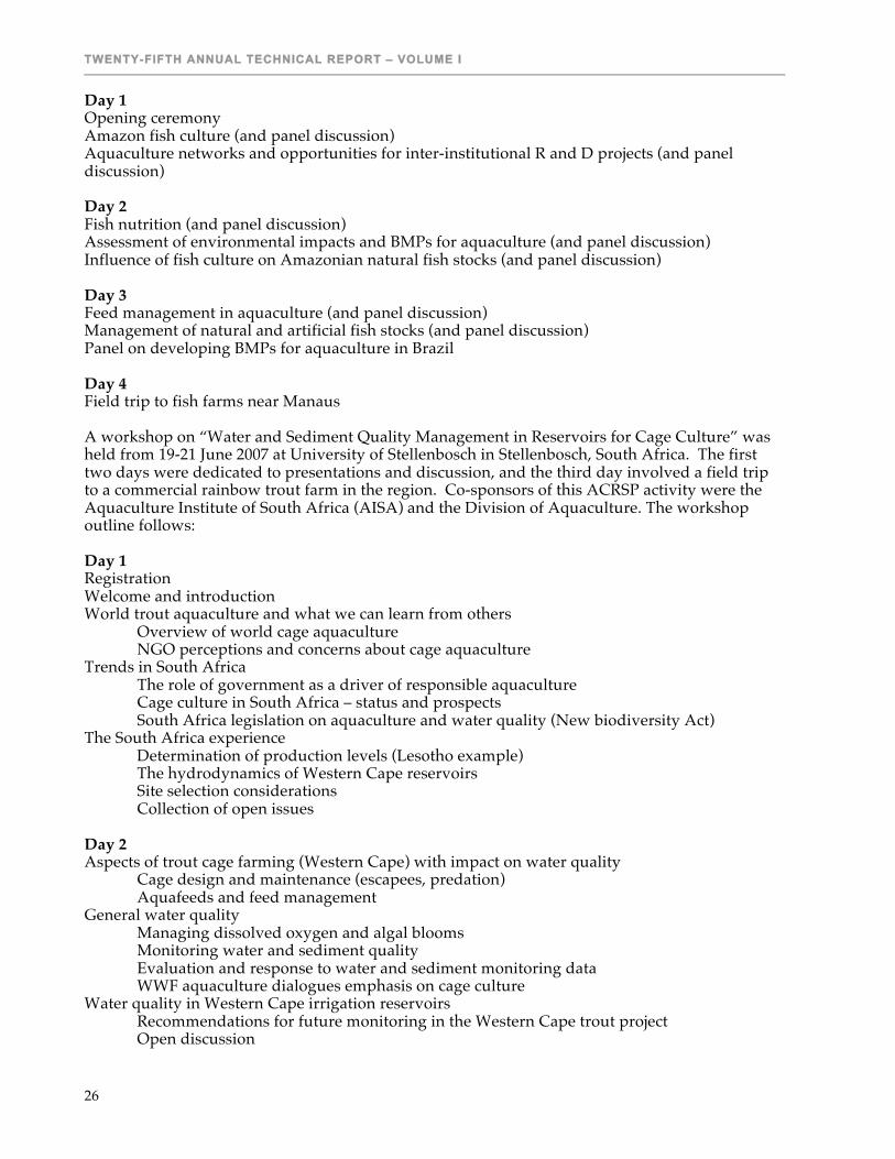
Day 1 Opening ceremony Amazon fish culture (and panel discussion) Aquaculture networks and opportunities for inter-institutional R and D projects (and panel discussion) Day 2 Fish nutrition (and panel discussion) Assessment of environmental impacts and BMPs for aquaculture (and panel discussion) Influence of fish culture on Amazonian natural fish stocks (and panel discussion) Day 3 Feed management in aquaculture (and panel discussion) Management of natural and artificial fish stocks (and panel discussion) Panel on developing BMPs for aquaculture in Brazil Day 4 Field trip to fish farms near Manaus A workshop on “Water and Sediment Quality Management in Reservoirs for Cage Culture” was held from 19-21 June 2007 at University of Stellenbosch in Stellenbosch, South Africa. The first two days were dedicated to presentations and discussion, and the third day involved a field trip to a commercial rainbow trout farm in the region. Co-sponsors of this ACRSP activity were the Aquaculture Institute of South Africa (AISA) and the Division of Aquaculture. The workshop outline follows:
Day 1 Registration Welcome and introduction World trout aquaculture and what we can learn from others
Overview of world cage aquaculture NGO perceptions and concerns about cage aquaculture
Trends in South Africa The role of government as a driver of responsible aquaculture Cage culture in South Africa – status and prospects South Africa legislation on aquaculture and water quality (New biodiversity Act)
The South Africa experience Determination of production levels (Lesotho example) The hydrodynamics of Western Cape reservoirs Site selection considerations Collection of open issues
Day 2 Aspects of trout cage farming (Western Cape) with impact on water quality
Cage design and maintenance (escapees, predation) Aquafeeds and feed management
General water quality Managing dissolved oxygen and algal blooms Monitoring water and sediment quality Evaluation and response to water and sediment monitoring data WWF aquaculture dialogues emphasis on cage culture
Water quality in Western Cape irrigation reservoirs Recommendations for future monitoring in the Western Cape trout project Open discussion

ENVIRONMENTAL IMPACTS ANALYSIS
27
Day 3 Field trip to Somerset West Visit of Lourensford Trout Farm In Thailand, three, one-half day workshops were held to present the pond soil management BMPs. The format of these workshops was:
• Introduction • Importance of pond bottom soil in aquaculture • Management of pond soils • Pond soil BMPs to simplify management decisions • Comments on implementation of BMPs • Questions and answers
The workshops were held at three locations: Kasetsart University, Bangkok; Department of Fisheries Station, Suphan Buri; Department of Fisheries Station, Samut Prakan.
RESULTS The workshop in Brazil was attended by more than 250 individuals including researchers, teachers, extension agents, government officials, fish farmers, feed producers, news media, and students. The panel discussion lead to the formation of a committee that was charged with identifying strategies to incorporate adoption of BMPs in the licensing of aquaculture projects in the Amazon region. The workshop in South Africa was attended by 33 participants from different organizations, including university under- and post-graduate students, small-scale fish farmers, local, provincial and national government representatives, NGO’s and other interest groups such as AISA and a feed manufacturing company, AquaNutro. Emphasis was placed on participatory methods to involve the participants, especially the farmers in dialogue and discussions about challenging aspects of water resource management on their farms. All participants were provided with a CD with copies of the presentation given at the workshop. The workshop proceedings also were posted on-line for wider access. Of specific note were the following comments and feedback from the participants:
• In general all felt that the workshop format was presented the correct way with speaker
sessions followed by open floor discussions. • The fish farmers exclaimed that similar initiatives should be organized in future with
broader participation of fish farmers. • A request was also raised as to ways to increase information dissemination in order to
apply some of the lessons learned. The workshop concluded with a field trip to the Lourensford Trout Farm. The farm is the largest producer in South Africa of rainbow trout in floating net cage systems. The farmer introduced the participant to the aspects of trout farming and facilitated discussions on some of the associated challenges confronting the farm. The workshop at Kasetsart University in Thailand was attended by 61 individuals, most of whom were students, faculty, or aquaculture specialists from the Thai Department of Fisheries. The other two workshops in Thailand were attended by 21 and 29 individuals, respectively, most of whom were farmers. The promotion of pond soil BMPs in Thailand was considered to be a means of disseminating findings of previous ACRSP research to small-scale farmers.

TWENTY-FIFTH ANNUAL TECHNICAL REPORT – VOLUME I
28
DISCUSSION The workshops were received quite well by the participants and much discussion was generated. There was a general consensus that BMPs will be used widely in the future for compliance with government regulations and as requirements for loans. Adoption of BMPs also can be a means of improving environmental performance to allow compliance with standards in aquaculture eco-label certification programs. Several researchers expressed the opinion that BMPs would, in the long run, make aquaculture more profitable. This point of view has been discussed thoroughly by Boyd and Tucker (1995) and Boyd et al. (2007). Participating farmers, however, complained that the adoption of BMPs would increase production costs and probably not lead to greater income. This opinion is based on the observation that current eco-label certification programs for aquaculture ask farmers to implement BMPs to comply with certain standards, but buyers often do not offer farmers more for the certified product.
CONCLUSIONS 1. The workshops were well attended and successful. 2. It was easy to get agreement on BMPs, for producers seem to recognize the better
practices. 3. Voluntary adoption of BMPs is not likely to occur widely because farmers tend to think
that BMPs will increase production costs. 4. Adoption of BMPs probably will result mainly where mandated by government or lending
agencies or where needed for achieving compliance with standards of aquaculture eco-labeling programs.
ANTICIPATED BENEFITS
The activity was beneficial to participants in increasing their awareness of environment issues in aquaculture. In particular, it encouraged a dialogue in which the major concerns of each stakeholder group could be aired. It is expected that there will be further dissemination of information about aquaculture and the environment from the participants to their colleagues. In addition, it is anticipated that the activity will lead to an effort to incorporate BMP adoption into aquaculture licensing in Brazil. A major benefit in South Africa will be that improving practices for cage culture of trout in reservoirs will enhance downstream water quality and avoid violation of water quality standards. The pond soil BMPs were translated to Thai. This should be beneficial in extending previous ACRSP research on pond soil management to Thai farmers.
ACKNOWLEDGMENTS
The collaboration of Vera Maria Fonseca de Almeida e Val and Maria de Nazaré de Paula de Silva of the National Institute of Amazon Research was essential to the success of the conference in Brazil. In addition, the support of the following organizations is greatly appreciated: Amazon State University (UEA), FAPEAM, SECT, SEPROR, Amazon State Government, PPG7, PETROBRAS, National Council for Scientific and Technological Development (CNPq), Special Secretary of Aquaculture and Fisheries-SEAP/PR, and Embrapa Environment. In South Africa, Samantha Ellis of Stellenbosch University kindly made many of the arrangements for the workshop. The participation of Dr. Aaron McNevin of the World Wildlife fund, Washington, D.C. in the workshop was greatly appreciated. The Thailand Department of Fisheries was extremely helpful in selecting farmers to invite to the workshops in Suphan Buri and Samat Prakan.

ENVIRONMENTAL IMPACTS ANALYSIS
29
LITERATURE CITED
Boyd, C. E. and P. Munsiri, 1997. Water quality in laboratory soil-water microcosms with soils from different areas of Thailand. J. World Aquacult. Soc., 28:165-170.
Boyd, C. E. and C. S. Tucker, 1995. Sustainability of channel catfish farming. World Aquacult., 26:45-53.
Boyd, C. E., C. Tucker, A. McNevin, K. Bostick, and J. Clay, 2007. Indicators of resource use efficiency and environmental performance in fish and crustacean aquaculture. Rev. Fish. Science, 15:327-360.
Thunjai, T., C. E. Boyd, and M. Boonyaratpalin, 2004. Bottom soil quality in tilapia ponds of different age in Thailand. Aquacult. Res., 35:698-705.
Wudtisin, I., 2006. Bottom soil quality in ponds for culture of catfish, freshwater prawn, and carp in Thailand. Ph.D. dissertation, Auburn University, Alabama, 89 pp.
Wudtisin, I. and C. E. Boyd, 2006. Physical and chemical characteristics of sediments in catfish, freshwater prawn, and carp ponds in Thailand. Aquacult. Res., 37:1,202-1,214.

TWENTY-FIFTH ANNUAL TECHNICAL REPORT – VOLUME I
30
BUILDING THE CAPACITY OF MOI UNIVERSITY TO HAVE A WORKING GIS LAB AND FIRST GENERATION GIS MODEL OF THE NZOIA RIVER BASIN
Twelfth Work Plan, Environmental Impacts Analysis 8 (12EIA8)
Final Report Published as Submitted by Contributing Authors
Herbert Ssegane & E. W. Tollner University of Georgia Athens, Georgia, USA
Mucai Muchiri Moi University, Eldoret, Kenya
Nancy Gitonga
Department of Fisheries Nairobi, Kenya
Geoff Habron
Michigan State University Lansing, Michigan, USA
ABSTRACT A GIS laboratory was put in place at Moi University in Eldoret, Kenya. A GIS workshop was held that highlighted the process for conducting a GIS analysis and overviewed typical problem areas for which GIS technology can be applied. This workshop demonstrated the capability of the laboratory. One field exercise involved the collection of GPS data on a field excursion. The data was then incorporated into the GIS software in the laboratory. A detailed summary of the workshop is included. Agriculture including aquaculture, natural resource development, business and commercial ventures and governmental functions such as public safety and tax assessment were shown to be major application areas. The GIS lab is continuing to receive many requests and is becoming integrated into the fabric of Moi University. An excerpt of the tutorial document and overview is provided. The workshop format followed the outline as presented by ESRI (1993, 1996). An excerpt of the handout is given in Appendix A. Photos inside the workshop (Figure 1) and in the field collecting GPS data (Figure 2), and a group photograph (Figure 3) are presented. An agenda was provided. The agenda was modified by having four student presentations and discussion of where we are going in the future. Uses computers to relate geography to various human and natural uses. This technology stores information on layers. Where, when how are the main question with location in mind. Make maps by location in a data base. Geography matters to all of us. Land information systems, environmental information systems … are encompassed by GIS. Geography is the science of GIS. GIS allows one to bring social factors, biodiversity, engineering, land use, environmental considerations to provide a modeling platform to enable querrying the database in a space. Measure the integration of parts to get at a description of the whole. Urban planning, resource inventory are example GIS applications. Where, what, when, are major questions. Context is also introduced. GIS becomes a pictorial based language via maps and tables. GIS provides a framework to study very complex systems with a mix of maps, tables and information bubbles.

ENVIRONMENTAL IMPACTS ANALYSIS
31
What is GIS? A system for capturing, checking, storing, manipulating, analyzing and displaying of data which are spatially referenced to the earth. There are 4 subsystems: 1) data input, 2) data storage and retrieval, 3) data manipulation and analyses, 4) output. There ais software, hardware, data, people and methods. Hardware includes a digitizer, scanner, plotter, printer, external storage drives, modems, etc. along with the host computer. GIS software should handle vector and raster data in 3-D. It should incorporate image processing systems, geostatistics and general statistics, surface modeling, desktop mapping and publishing, CAD systems, database management systems. GIS data is made up of geographic features. A feature is any item of interest to a GIS user. GIS features are stored in GIS databases. A feature can be defined based on position, characteristics and relationships. Any GIS dataset can be broken into points, lines, areas and surfaces. The data must be represented in digital format. Postion may defined as vectors, boundary defined by points joined with straight lines. There is a vector polygon data format. Position may be defined by raster, which merge the data file and a data value stored in a cell or pixel. The data may be semantic (name, type, etc.) or numeric(slope, altitude, etc.). Landsat exploits the differential of landscape features via their response to different wavelength. Feature relationship may be proximal, heirarchial (presence of super or subclasses), topological (adjacency, inclusion, connectivity). A GIS features using a topological data structure. Data can be acquired through manually digitizing, scanning, GPS in the field, remote sensing techniques. One must consider spectral resolution, remembering that our eyes do not see all the energy forms involved in GIS imaging. Applications include agriculture, forestry (optimal harvest), mining, petroleum management. Environmental management, transportation, public safety are all applications. Health and human services and law enforcement and criminal justice are further applications. Defense and intelligence along with banking and insurance are mapped with GIS. GIS in research – biologists to track and define species, geologists, environmentalists use GIS; the list keeps expanding. ArcView Introduction – G. Karanja There probably is no ‘best’ software (in response to a question from previous section). The software of choice here is ArcView GIS. It can come as a suite with ArcINFO, ArcEDITOR which provides a powerful package. The arcView GIS is a desktop geographic information system by ESRI. A GIS is a database that links information to location (it connects what to where), allowing you to see and analyze data in new and useful ways. Roads, streets, pipelines, and waterways are examples of line features. In high resolution some of these may be represented as objects. Parks, countries, seas and forests are examples of polygon or area features. Polygons represents objects too large to be depicted as points or lines. Themes -- A GIS links sets of features and their attributes and manages them together in units called themes. A theme consists of a collection of geographic features sucha as rivers, wildlife sightings or parks and the attributes of those features. Themes are found in a view, which is a map display. An ArcView project is a collection of themes. ArcView has tools for managing themes and projects. Views, tables, charts, layouts and scripts are managed as project documents. The layour are documents on which you can arrange views, tables, charts and images as graphic elements. Scripts are programs for customizing ArcView. The script contains the programs that are specific to the project. Tabular information is stored in a database. The lecture continued with two computer exercises given in the course notebook.
TWENTY-FIFTH ANNUAL TECHNICAL REPORT – VOLUME I
32
Data Formats and Map Creation -- T. Esipila Continuation of exercises nearly through exercise 5. Practical experiences continue into the following morning. Bill Tollner and Herbert Ssegane present a practical example showing how one may predict erosion potential over an entire watershed. The methods presented show how one can conduct an assessment over the Nzoia and other watersheds. Field excursion The group was taken to the Moi Fish Research Center. Techniques on GPS were discussed here. The group then visited two reservoirs that supply water to Eldoret. We then traveled to a watershed boundary. The range of elevations sampled with GPS was from 2100 to 2700 meters. The concluding day of the workshop will focus on how to download GPS data to computer and bring it into a GIS model. The workshop will conclude with digitizing issues and data presentation techniques. The workshop will conclude with student presentations related to the CRSP workplan objectives. The workshop resumed with an excellent discussion of approaches for downloading GPS data into computer for editing clean-up and import to ArcView. This is not covered in tutorial and is added as hand-written notes. There was also some good discussion of coordinate systems. One usually downloads as UTM data where one can select the particular UTM system for the locality in question. UTM converts to easting, northing and altitude and enables one to superimpose GPS data over top of topo maps with the UTM system. Digitized UTM maps come with a world coordinate file that enables data registration. Research Presentations related to the ACRSP project that have GIS applications. Mucai gave a nice overview to how the capacity built can lead to participation in larger efforts such as the Nile Basin Initiatives. Why watershed assessment –Muchiri and Tollner This can provide important information to governmental agencies, commodity groups, and community groups. As resources become limited this becomes even more critical. This data is necessary to provide rapid response to policy makers dealing with larger issues such as climate change. Student Presentations (see Figure 4 for a photo of one student, Sainai Bilhai) Frank Masese -- MacroInvertibrate and their contribution as bio-indicators. Worked on the Moiben tributary. Used correspondence analyses to separate variables and their effects on macroinvertibrate specie. The conclusion was that macroinvertibrate specie was affected by water quality along the stations evaluated. As an aside, most sediment appears to come from umpaved roads. Stations were identified based on getting stations in proximity to major land use. Another round of sampling is required to see if changes in landuse can change the specie composition in the river for better or worse. Saina C. Bilha – simulation of suspended solids and phosphorus and in the Moiben River. She used mathematical modeling to model different land use scenarios based on QUAL2E. Excellent discussion of the shortcomings of EXCEL statistical model. Naomi Olerio – Impacts of agricultural chemicals on water quality Atrazine above 0.02 mg/l, nitrate above 50 mg/l as ionic form have well document impacts. Objectives were to determine nitrates and atrazine in the Moiben subwatershed. Intensive wheat and maize farming occur in the region. Both large 1000 ac and small .25 to 20 ac. Did social assessment in the region among farmers and schoolteachers and students. Assessed demographics, pesticide usage and quantity of pesticides used, agricultural practices. Key water quality variables were conducted over 3 parts of the growing season. Results showed some incidents of atrazine toxicity. Demographics included disease. Malaria must important in July

ENVIRONMENTAL IMPACTS ANALYSIS
33
Aug. Pneumea an issue in December. AIDS is there but hard to document. Herbicide handling an issue. Cancer is on the rise. Repugnant practices in food handling were mentioned but not elaborated. About 90% of the groundwater is safe for drinking. Joseph Hitamana – Land use characterization in the Nzoia river basin The work is in preliminary form. Many farm visits have been made. GPS coordinates have been gathered. In the Rift valley section, Cherangani hills area and the Kiptaberr forest have been characterized. Forest of Cupressus, Eucalyptus, pines were noted. Small scale farming also noted. There was some livestock production. Farming and pollution related to lack of erosion control, forest and catchment degradation, substandard management skills, privately owned tree nurseries, nitrogen inorganic fertilizers, farm forestry is not well developed. There are also tea plantations. The Moiben-Sergoit river area was also classified. Unprotected river banks and sand mining contribute also. In Western Kenya, river bank degradation, extensive farming, lack of erosion control and and other problems discussed above. Main problems are as follows. Farming on river banks, lack of protective measures, inorganic fertilizers, siltatin and sedimentation and chemical pollution, horticulture development. There is one example of a well protected area, with natural vegetation in tact. Roads appear to be a major source of soil erosion. There is interest in land use change over time and how that correlate with water quality changes. Maps are to be produced. Watershed assessment of larger basins is encouraging based on the work done on the Nzoia. Plans were initiated to integrate the work done on the Moore’s bridge-Sergoit River region with the larger scale work done by Ssegane-Tollner. A group photograph was made in the afternoon, followed by concluding the exercises in the GIS handout. A course evaluation was completed and certificates of participation were presented.
A GIS TRAINING WORKSHOP FOR RIVER NZOIA WATERSHED MANAGEMENT
FROM 12TH JUNE 2007 TO 14TH JUNE 2007 Held at Chepkoelel Campus, Moi University
Sponsors: USAID through A-CRSP and Moi University p .0. Box 3900 Eldoret, Kenya

TWENTY-FIFTH ANNUAL TECHNICAL REPORT – VOLUME I
34
Figure 1. Workshop in progress in the Moi University GPS Lab.
Figure 2. Field work with the GPS unit at the Moi University Aquaculture Farm.
Figure 3. GIS workshop group photograph.
Figure 4. Ms. Bilha presenting her research summary at the workshop.
ANTICIPATED BENEFITS GIS technology can benefit a myriad of different industries ranging from Agriculture to many governmental functions. DeBarry (2004) provides an excellent protocol which is being followed for additional watershed assessment work. The methods presented therein are easily transposed into other areas as well. The anticipated benefits presented below are being pursued by students and faculty who use the Moi University GIS Laboratory. Aquaculture: A need to document the current status of fish production in Kenya was immediately recognized as a key need. The GIS technology coupled with Global Positioning System (GPS) technology was clearly seen by workshop participants and is currently being pursued. Agriculture: Success in fanning is achieved by obtaining the optimum crop yield. The key to achieving such results is "Precision agriculture" which simply means knowing and responding to the specific conditions of the field.
ENVIRONMENTAL IMPACTS ANALYSIS
35
Forestry: GIS software solutions provide foresters and natural resource managers with powerful tools for better analysis and decision making. It gives you the 'whole picture' about the resource under your care and lets you perform tasks such as developing long term supply strategies, determining harvesting system options, etc. Key applications of GIS in forestry are forest inventory and change mapping. Environmental Management: Since its inception, GIS has been an integral component in Environmental Management. The customization of GIS for various decision makers allow various levels of anagement to view and analyze the data easily. More than 75% of resource managers use GIS. It is therefore clearly evident that GIS is vital to any data creation analysis and assessment of the environmental risks at hand.. A majority of water/wastewater utilities use GIS technology to integrate all kinds of information and applications with a geographic component into one manageable system. GIS lets you organize, manage and distribute geographic information culled from various databases while maintaining data integrity and focusing on project direction. Conservation: GIS is the first analytical tool that allows the users to directly implement the ecological view of reality and to achieve a holistic information management capability, which is why it hold such a promise in the struggle to solve the difficult biological and management that lies ahead. Minerals and Oil: Geography provides the framework to acquire, develop and interpret complex spatial datasets used for mining and earth sciences. Mapping spatial concepts and time/ space operations technology are absolutely essential to effective mining. Where to drill a well, route a pipeline or build a refinery are all in the domain of geography. GIS technology today allows the management of spatial components of petroleum business objects such as wells, pipelines, environmental concerns, facilities and retail outlets, in the corporate database and apply appropriate geographic analysis efficiently in a desktop focused application. Surveying Applications: Surveyors and engineers understand the importance of geographic data. Surveyors use precise instruments, procedures and computations to accurately locate and define geographic features while conducting field surveys that range from cadastral to engineering designs and build structures and infrastructures on geography measured by surveyors. Research: GIS is a valuable tool for displaying and analyzing infonnation that is associated with spatial location. Researchers in numerous disciplines are using GIS to help analyze and display their data in the following ways: biologists to track and define species, geologists to map earth's faults, hydrologists to analyze watersheds and water quality, archeologists to map the locations of artifacts and sites, epidemiologists to track diseases, and many other scientists to analyze data or test models in their fields or integrate data from multiple fields. Other Commercial Applications of GIS: Geography has penetrated through business applications and just no longer for geographers alone! Central part of most business decisions such as locating A TMs close to customers, involves some aspects of GIS. The real estate industry has always known Geography Matters -after all, the real estate practitioners have coined the phrase, "location, location, location". Since location is what GIS is all about, GIS organizations and software developers are actively engaged in implementing GIS-based solutions in all segments of the real estate industry, from map- based contact management to sophisticated investment analysis in Large Real Estate Investment Trusts.

TWENTY-FIFTH ANNUAL TECHNICAL REPORT – VOLUME I
36
Businesses manage a world of information about sales, customers, inventory, Demographic profiles, mailing lists, etc. At the very core of this information, is a geographic location -an address, a service boundary, a sales territory, and a delivery route that can be illustrated and interactively managed on a map. Governmental Applications: The telecommunications industry is changing rapidly, resulting in tough competition and an ever increasing scope of services offered to customers. Solving the many business problems of a telecommunications company requires a good understanding of where your customers and your facilities exist with respect to your competitors' facilities. A GIS provides this information. Geography or terrain matters to the military commander. The commander must understand terrain to make informed decisions in all matters, whether administrative, operational, tactical, or logistical. GIS is one of the hottest new research tools in academia today and one of the fastest growing high-tech career for students. GIS technology provides powerful tools for geographic analysis for almost any academic discipline. A G IS allows students and researchers to ask and answer geographic questions by designing and analyzing maps using user-selected criteria. GIS also allows school administrators to manage campus facilities, develop emergency and safety plans, market programs and track alumni to help conduct the business side of education. Making information accessible and easy to understand is the goal of museums and libraries. GIS links databases to maps, allowing information to be explored and presented visually. Topics such as geology, climate, and population change often are understood more easily through maps than through text of data on spreadsheets. Interactive maps make learning hands-on and fun, sparking greater understanding of places around the globe and close to home. The ability to access and display information quickly in a spatial and visual medium allows agencies to allocate resources quickly and more efficiently. In the 'mission critical" nature of law enforcement, information about the location of a crime, incident, suspect or victim is often crucial in determining the manner and size of the response. Information about the location of an incident or a disaster and its geographic threat is often crucial in knowing how to respond. Most health problems facing the world today such as those caused by environmental, economic, political and social factors, exists in a geographic context, and any analyst must consider that. Understanding issues ranging from epidemiology to access to health care providers require an understanding of the geographic context of these issues. Geographic analysis can be used to monitor rail systems and road conditions, finding the best way to deliver goods and services, tracking fleet vehicles or maintaining deploying or spending resources wisely.
LITERATURE CITED DeBarry, P.A. 2004. Watersheds: Processes, Assessment and Management. John Wiley & Sons,
New York, NY. ESRI. 1993.Understanding GIS. John Wiley & Sons, New York, NY. ESRI. 1996. Introduction to ArcView GIS. Environmental Systems Research Institute. Redlands,
CA.

ENVIRONMENTAL IMPACTS ANALYSIS
37
APPENDIX A. GIS WORKSHOP HANDOUT EXCERPT The following material is an excerpt of the document prepared for workshop participants. WHAT'S GIS? GIS is a computer-based tool for mapping and analyzing features and events on earth. GIS technology integrates common database operations, such as query and statistical analysis, with maps. It is a tool that can be used by organizations such as schools, governments, businesses, research groups, etc, that are seeking innovative ways to solve problems and increase the quality of decision making.

TWENTY-FIFTH ANNUAL TECHNICAL REPORT – VOLUME I
38

ENVIRONMENTAL IMPACTS ANALYSIS
39
…

TWENTY-FIFTH ANNUAL TECHNICAL REPORT – VOLUME I
40
UNDERSTANDING THE AQUACULTURAL KNOWLEDGE AND INFORMATION SYSTEM FOR COMMERCIAL TILAPIA PRODUCTION IN NICARAGUA: ECONOMICS, INSTITUTIONS, AND MARKETS
SMALL AND MEDIUM SCALE TILAPIA CULTURE IN NICARAGUA: ECONOMIC AND FINANCIAL
ANALYSIS1
Twelfth Work Plan, Sustainable Development & Food Security 2 (12SDF2) Final Report
Published as Submitted by Contributing Authors
Pablo Martínez-Mejia Texas Tech University Lubbock, Texas, USA
Joseph J. Molnar
Auburn University Auburn, Alabama, USA
Suyapa Triminio Meyer & Daniel Meyer
Escuela Agrícola Panamericana El Zamorano Zamorano, Honduras
ABSTRACT Small and medium scale tilapia culture in Nicaragua has been practiced for over 20 years. During that period, it went from production systems including mixed-sex culture and the use of animal manures, and/or inorganic fertilizers to implementing more intensive pond and cage production systems. In addition, it went from being a national economic development activity supported heavily by the government, to a localized enterprise, still supported by the government, but at a substantial lower level. This paper provides an economic and financial analysis of several tilapia culture enterprises identified in 2005. The study includes an enterprise budget analysis, a break-even price analysis, the estimation of the internal rate of return of the enterprises, and a sensitivity analysis. The results indicate that fingerling production, as the Nicaraguan government promoted it was not profitable. The three-phase grow-out production systems also promoted by the government yielded low levels of profitability. The members of a cooperative that operate with an 80% subsidy presented the most profitable enterprise. The results also indicate that without the subsidy the members of the cooperative would not be able to stay in businesses. Finally, cage culture seems like a profitable alternative if the proper production parameters are implemented.
INTRODUCTION
When first introduced in Nicaragua, tilapia production systems included mixed-sex culture and the use of animal manures, and/or inorganic fertilizers. At the time of this study, producers were implementing more intensive pond and cage production systems to meet the demand of the market (Engle 1997). More intensive aquaculture production systems require higher investments and better management practices. The decision process faced by aquaculture producers involves a series of economic choices, related to the demand and supply of fish under production that determine the overall profitability of fish culture. As Jolly & Clonts (1993:35) stated, “the decision of what to produce is determined by the questions on whether the product is saleable as well as the individual farmer’s 1 This technical report covers work performed under Objective 4 of WP12. For the technical report on Objectives 1-3, see the 24th Annual Technical Report, pp. 26-30.

SUSTAINABLE DEVELOPMENT & FOOD SECURITY
41
preferences.” If the product is marketable, consumers are willing to pay a given price, and if consumers are willing to pay a certain price, then, producers are willing to grow the fish at a certain cost. Profitability is one of the crucial elements for sustainability, and the ultimate measure of economic success (Molnar et al. 1991). The profitability of tilapia culture determines the degree in which the producers become involved in marketing. Thus, if the profitability of the enterprise is high enough, fish producers will engage in production and marketing of the product. Aquaculture producers, like any other entrepreneurs seek to enhance the profitability of the enterprises, although they are not always successful. The inclusion of economic analysis in aquaculture helps to eliminate non-profitable enterprises (Engle et al. 1997). With that consideration, the general objective of the paper is to conduct an economic and financial analysis of several tilapia culture businesses in Nicaragua. The specific objectives are:
1. To estimate the net returns, break-even prices, internal rates of return, and conduct a sensitivity analysis of fingerling production,
2. To estimate the net returns, break-even prices, internal rates of return, and conduct a sensitivity analysis of pond production.
3. To estimate the net returns, break-even prices, internal rates of return, and conduct a sensitivity analysis of cage tilapia production.
Conceptual Framework In general, fingerlings, feed, chemicals, ponds, equipment, and technical, institutional, and government assistance are the most common inputs in aquaculture (Jolly & Clonts 1993). Keeping control of inputs costs is very important for the profitability of any fish culture enterprise. One important tool to document and keep up to date with input costs and other operating expense is the farm plan. For most small producers the farm plan exists only in their heads (Jolly & Clonts 1993). That practice, although widespread, is not a good one. When producers keep their farm plan in their heads, they do not have reliable means for comparing their real performance against the planned use of resources. Within the farm plan, the planned use of resources is presented in the farm budget. A budget is a plan to coordinate the flow of resources in and out of the farm to achieve a specified set of objectives established in the farm plan (Jolly & Clonts 1993:151). The proper analysis of a budget requires not only some level of knowledge about the production process, but also knowledge of the socioeconomic characteristics of the producers. In aquaculture, an enterprise budget analysis is a procedure of estimating costs and returns for a particular fish culture activity (Jolly & Clonts 1993). In addition to the budget analysis, this study includes a break-even price analysis, the estimation of the internal rate of return for a period of five years, and a sensitivity analysis for a 20% increase and 20% decrease in feed price. Fingerling Economics Fingerlings are an essential input to aquaculture; however, they present several economic and technical challenges to the tilapia industry (Fitzsimmons 1997). Tilapia fingerling production presents some unique characteristics; tilapia can easily produce offspring in ponds without farmer assistance (Molnar et al. 1996). Given favorable conditions, tilapia reach sexual maturity in 6-8 months of hatching, at a size of less than 100 g. When reproduction in the pond occurs, the offspring of the original stock competes for food, resulting in stunted growth and unmarketable fish (Phelps & Popma 2000). Fingerling production is one of the most profitable enterprises in aquaculture, but also the most risky and complex (Molnar et al. 1996). Therefore, the economic analysis of fingerling production is central to the success of tilapia production (Molnar et al. 1996). However, despite its importance, only a few studies have examined tilapia fingerling production costs (Engle 1997).

TWENTY-FIFTH ANNUAL TECHNICAL REPORT – VOLUME I
42
In neighboring Honduras, Triminio & Meyer (2005:257) reported “farmers who have some idea of their costs report that the expense of producing a fingerling is between U.S.$ 0.005 to 0.020.” The authors also reported selling prices ranging from U.S.$ 0.02 to 0.03 for fingerling sizes ranging from 0.05 to 3.00 g. In another study, Lutz (2000) states a purchasing cost of U.S.$ 0.18 per 50 g fingerlings in a budget for pond production in the tropics. Despite its high profitability, the complexity of operation and level of investment necessary to establish a hatchery has proven difficult for most tilapia producers. The reproductive characteristics of tilapia have forced producers to turn to public and private hatcheries for seed of uniform size and gender (faster growing male fingerlings) (Molnar et al. 1996). Furthermore, according to FAO (1996:51) “the cost of constructing and maintaining the required facilities (hatcheries, transport) is considered prohibitive for many producers.” For the previous reasons, public hatcheries play a significant role in supplying tilapia fingerlings at early stages of aquaculture development in a given region. However, at the same time, public hatcheries sometimes create dependency problems for producers, who often believe they should be supplied with subsidized fingerlings. According to FAO (1996) & Molnar et al. (1996) producer expectations for free or low cost fingerlings impede the development of a private market that is crucial for the further expansion of aquaculture. Pond Economics Tilapia is produced using a wide variety of production systems determined by the socioeconomic characteristics of the producer. As Molnar et al. (1996:9) stated, “The kind of technology used is closely linked to the socioeconomic circumstances of the farmer, as the intensity of production often corresponds to the amount of capital investment (Molnar et al. 1996:9).” Consequently, the proper understanding of tilapia culture compels the analysis of the socioeconomic factors using multiple sources of data. However, the task is not easy, since in aquaculture, quantitative and qualitative data usually are unavailable because aquaculture is in its early stages of development (Engle et al. 1997). Despite the limited amount of data, some researchers have documented various basic facts about the economics of tilapia culture. Teichert-Coddington & Green (1997) estimated the average yield (kg/hectare), income above variable costs (U.S.$) and net returns to land and management (U.S.$) of 20 different production systems in Honduras. The authors reported that several production systems with a stocking density of two fingerlings/m2 generated the most profits. The same authors also concluded that feeding was less profitable than fertilization at low stocking rates. In another study, Lutz (2000), in a budget for tilapia culture under assumptions of production in tropical conditions, estimated a production cost of U.S.$ 1.47 per kg of tilapia with an average weight of 800 g. Engle (1987 cited in Engle 1997) reported net returns above total costs of U.S.$ 645 per hectare in monoculture of tilapia in Panama; equivalent to a rate of return of 13%. Head & Zerbi (1995 cited in Engle 1997) reported a breakeven price of U.S.$ 3.86 per kg in an intensive commercial saline pond culture system in Puerto Rico, and an internal rate of return of 18%. Cage Economics Cage production is an intensive management system that facilitates the use of water bodies unsuitable for conventional production systems that require draining or seining for the period of harvest (Lazur 2000). Thus, cage culture makes possible the exploitation of public or communal water reservoirs, lakes, irrigation systems, village ponds, rivers, cooling water discharge canals, and estuaries (McGinty & Rakocy 1989, Watanabe et al. 2002). Other economic advantages of cage production over pond production are that the level of initial capital investment is low compared with open ponds (Watanabe et al. 2002), and that by concentrating fish, the farmer has better control over feeding and harvesting. However, the disadvantages include higher risk of poaching and water quality problems, and reliance on commercial feeds s (Lazur 2000, Watanabe et al. 2002).

SUSTAINABLE DEVELOPMENT & FOOD SECURITY
43
In cage culture, producers rear fish in cages as small as four m3, stocked at 200 to 300 fish/m3, as in cages as large as 100 m3 stocked at 25 to 50 fish/m3. Yields range from 150 kg/m3/crop in four m3 cages to 50 kg/m3/crop in 100 m3 cages (Watanabe et al. 2002). The financial and economic analysis of the different documented enterprises is crucial for the future development of tilapia culture in Nicaragua. The study will help to maintain the profitable enterprises that in the end will determine the future development of tilapia culture in Nicaragua. As Watanabe et al. (2002:484) suggested “in both tropical and temperate zones future development of tilapia aquaculture in the Americas depend on the ability of production systems to produce more fish with less water, less food, and less time to lower costs.” This study will provide specific information about the economic performance of the identified fingerlings and grow-out of tilapia in pond and cage based systems in Nicaragua. The results will present some guidelines that private firms, nongovernmental organizations, and development institutions could utilize to further the practice of tilapia culture in Nicaragua.
METHODS AND MATERIALS Sample and data collection The sampling for this study started when several tilapia producers were approached during a short seminar on tilapia culture and pond construction held by an ACRSP team in Estelí, Nicaragua from November 9 to 12, 2005. During that seminar, the author gave a lecture on budget making and a short presentation about the objectives of the study and how it might benefit tilapia culture in Nicaragua. Subsequently, the researcher requested to the seminar attendees their participation and collaboration. Those who assisted in the short seminar, and agreed to participate in this study led to other stakeholders in their areas. The sampling technique used to identify potential respondents is called network snowball sampling (Neuman 1997). Two types of interviews were used. A total of 13 open-ended interviews were conducted with producers, whereas seven semi-structured interviews were used with other stakeholders. Analysis The data were analyzed using a triangulation research strategy as described by Yin (1994). Triangulation refers to the use of multiple sources of evidence that supply both quantitative and qualitative data to validate the conclusions of the analysis. According to Yin (1994:91), “case studies need not be limited to a single source of evidence. In fact, most of the better case studies rely on a variety of sources.” Once gathered, all sources of evidence are reviewed and analyzed together. The study has several limitations given the nature of the data source. In general, producers do not keep written records of production costs, sales, and in most cases do not verbalize perceptions regarding the opportunity cost of land and other assets. FAO (1996:35) noted, “Because the products of small-scale rural aquaculture are only partially marketed, and objectives relating to the production of fish are only part of the story, quantification is inherently problematic.” Small producers, in fact, only market a fraction of their production and do not keep records of their transactions. Commercial producers, for the most part, do not keep good records either. Instead, patterns of informal cash management, tax avoidance, and rough calculations of profits and losses tend to characterize most types of farm business management including aquaculture (FAO 1996).
RESULTS The economic and financial analysis of the different data sets included first, the estimation of net returns above variable costs and break-even price to cover variable costs, and next the estimation of three Internal Rates of Return (IRR). One for the original data, one for the possible net returns generated by a 20% increase, and one for the possible net returns generated by a 20% decrease in the price of commercial feed (sensitivity analysis). All IRR were estimated for a period of five years.

TWENTY-FIFTH ANNUAL TECHNICAL REPORT – VOLUME I
44
For comparison purposes, the data collected from the different enterprises were used to generate budgets for an area of 1,000 m2. In addition, the IRR from the different enterprises were estimated adjusting the original net returns for inflation to the year 2005. Fingerling Production: ADPESCA Recommendations The fingerling production budget for 26,400, 5-10 g fingerlings (See Martínez-Mejia.(2006) Table 1.1) presented by ADPESCA generated gross receipts of U.S.$ 1,056 and total variable cost of U.S.$ 948, and net returns above variable costs of U.S.$ 107.83. The estimates were calculated using a selling price of U.S.$ 0.04 for 5-10 g fingerlings. The analysis indicated a break-even price to cover variable costs of U.S.$ 0.036, which is 90% of the actual market-selling price. Since the budget presented by ADPESCA ignored fixed costs, the total cost and the break-even price to cover total costs were expected to be higher. The IRR were estimated using an initial investment of U.S.$ 4,000 (See Martínez-Mejia.(2006) Table 1.7). The investment represented the cost of building the tanks and pond necessary to carry out fingerling production as recommended by ADPESCA; it was assumed that the farmers owned the land and a cost of U.S.$ 14/m2 of tank and U.S$ 1.21 for pond construction (EAGE & AECI 1998, Interview 2005). The estimated net returns of U.S.$ 213, 123, and 29 corresponded to a 20% decrease in feed price, original feed price, and a 20% increase in feed price. Those net returns minus the initial investment were equivalent to IRR of -7% and –21%, and less than –21%, respectively. Overall, the estimated IRR suggested that fingerling production was not profitable. Nevertheless, the enterprise could be profitable if the production process presented by ADPESCA were improved in several ways. First, brooders were fed 3% of total biomass; that value is higher that the recommended 1-2% (Phelps & Popma 2000). Second, ADPESCA recommended that only fry equal or less than 12 mm should be sex reversed. According to Phelps and Popma (2000:44) “Grader selectivity should be verified to confirm that 85-90% of the 13 mm fish are able to swim through the grader and no more than 5% of the 15 mm fish are able to swim through.” Third, the stocking density of 500 fry/m2 during sex reversal is significantly lower than the recommended 1000-2000 fry/m2 (Phelps & Popma 2000). All the adjustments would result in either cost reductions or income increases, which would increase net income and profitability. Pond Production: Three-Phases Grow-out- ADPESCA’s Recommendations The grow-out budget offered by ADPESCA generated gross receipts of U.S.$ 3,234, total variable costs of U.S.$ 2,660 for a net return above variable costs of U.S.$ 574. The estimates were calculated using a selling price of U.S.$ 1.54 per kg of fish (See Martínez-Mejia.(2006) Table 1.2). The analysis suggested a break-even price to cover variable costs of U.S.$ 1.27 that represents 82% of the actual market price. Again, since the budget ignored fixed costs, the total cost was expected to be higher. Feed cost represented approximately 66% of total variable cost. As with fingerling production, the information did not indicate the source of commercial feed, but most likely is a national supplier. For this production system the IRR were estimated using an initial investment of U.S.$ 1,200 (See Martínez-Mejia.(2006) Table 1.7). The amount represented the cost of building the ponds, with a useful life of five years, necessary to carry out production as recommended by ADPESCA. It was assumed that the farmers own the land. The results indicated net returns of U.S.$ 1076 for a 20% decrease in the price feed, U.S.$ 655 for the original prices, and U.S.$ 233 for a 20% increase in feed price. The analysis generated IRR of 114%, 65%, and 8% respectively. Even thought, the results indicated that three phases grow-out production was profitable; the recommendations suggested by ADPESCA could be adjusted to obtain even better results. For example, feed conversion during phases II and III were estimated in 3.17 and 3.20 respectively. Those values indicate an unnecessary use of commercial feed. In similar production systems, using organic fertilizer and commercial feed, producers in Honduras reported a significantly lower feed conversion of 0.6 (Martinez et al. 2004). Feed expenses in the production system
SUSTAINABLE DEVELOPMENT & FOOD SECURITY
45
recommended by ADPESCA account for 66% of total variable costs; any significant reduction in this item could result in higher net returns and IRR. Pond Production: Individual Producer This budget was generated in collaboration with a producer who kept partial records of his production costs. The data provided by the producers was used to generate a budget for a 1,000 m2 brick and concrete pond stocked with 15,000, 20 g fingerlings. The production parameters for this production systems included a stocking rate of 15 fingerlings/m2, an ending average weight of 227 g, a 180 day production cycle with a mortality rate of 7%, purchase of 11,486 kg of commercial feed, and utilization of water exchange (See Martínez-Mejia.(2006) Table 1.3). The results (See Martínez-Mejia.(2006) Table 1.3) indicated gross receipts of U.S.$ 7,040, total variable cost of U.S.$ 6,394 that represented approximately 94% of total costs, and fixed cost of U.S.$ 416, for a net return above variable and fixed costs of U.S.$ 646 and 230 respectively. The estimates were calculated using a selling price of U.S.$ 2.20 per kg of fish. The analysis suggested a break-even price to cover variable and fixed costs of U.S.$ 2.00 and 2.13 respectively. The break-even price to cover variable costs and fixed costs were equivalent to 90% and 97% of the actual market price. The results also indicated that feed and fingerlings purchases, each, represented 35% of total costs. The initial investment of the individual producers was estimated in U.S.$ 14,000 (See Martínez-Mejia.(2006) Table 1.7). The amount represented the cost of building and equipping the brick and concrete pond with a useful life of 20 years. The results indicated net returns of U.S.$ 706, 230, and -246 corresponding to a 20% decrease on feed price, original price, and a 20% increase in feed price. Those net returns minus the initial investment per production cycle generated an IRR of –19% for the price reduction. The other two IRR could not be estimated, but would be less than -19%. The economic analysis suggested that tilapia culture for the individual producer was not profitable. Despite the negative results, the profitability of this sort of enterprises could be improved if, the initial investment were lower. The pond built by this producer is very expensive; building a cheaper pond would increase the profitability of the enterprise. The estimated feed conversion with a value of 4 was significantly high. Improvements in feed conversion would increase net returns and profitability. Pond Production: Cooperative COOSEMPROTIR, R.L. excluding the subsidy from IDR. The data for this budget was provided by the members of the cooperative COOSEMPROTIR R.L. located in the Nicaraguan Northern communities of Pueblo Nuevo and Los Horcones, Department of Estelí. These producers received technical assistance and an 80% subsidy on the cost of fingerlings, feed, plastic, and hose from the IDR. However, for this specific budget, the subsidy was ignored to estimate the real production costs. The data provided by the producers was used to average values that then were used to generate the budget for an area of 1,000 m2. The budget was estimated considering the following parameters: fingerlings initial weight of 1 g, a stocking density of 4 fingerlings/m2 for a total of 4,000 fingerlings stocked, a final weight of 340 g, and a production cycle of 195 days with an expected mortality rate of 12.5%. The production system also included the use of animal manure to fertilize the pond and 1,920 kg of commercial feed, and the practice of water exchange as needed. Producers in the cooperative followed the instructions provided by the IDR extension agent who recommends water exchange depending on the color of the water (See Martínez-Mejia.(2006) Table 1.4). The results indicated gross receipts of U.S.$ 2,618, total variable cost of U.S.$ 2,445 for a net return above variable costs of U.S.$ 173; the estimates were calculated using a selling price of U.S.$ 2.20 per kg of tilapia. Fixed costs were estimated at U.S.$ 427, for a total production cost of U.S.$ 2,872.
TWENTY-FIFTH ANNUAL TECHNICAL REPORT – VOLUME I
46
The analysis indicated a break-even price to cover variable and total costs of U.S.$ 2.05 and 2.41 respectively. Those break-even prices represented 91% and 109% of the original market price, correspondingly. The main cost was feed, which represented 41% of total cost. Since the subsidy did not include pond digging, the members of the cooperative had to finance on their own the cost of building the pond (s). The initial investment for a 1,000 m2 pond, the average pond dimensions, was estimated at U.S.$ 950 (See Martínez-Mejia.(2006) Table 1.7). The results indicated net returns of U.S.$ 5 for a 20% decrease in feed price, -254 for the original feed price, and –512.0 for the 20% increase in feed prices. Given that the values were all negative, the corresponding IRR could not be estimated. Nevertheless, the results suggested that without the subsidy tilapia culture was unprofitable. The financial and economic analysis of this budget suggested than tilapia production following the recommendations of the IDR was unsuccessful. However, changes in pond management could reduce feed cost and increase net returns. In Honduras producers running similar production systems obtained 454 g fish with a feed conversion of 0.6 (Martinez et al. 2004). The value of 0.6 is significantly lower than the 1.6 reported by the producers in Nicaragua. It is important to mention that these producers reported labor cost that represented 34% of variable costs, and, since in most cases, producers themselves carried out the labor activities, the reported labor costs represented a source of income as well. Pond Production: Cooperative COOSEMPROTIR, R.L. including the subsidy from IDR. Here, the analysis included the same data and parameter as in the previous budget, except that instead of using the total cost of the inputs, only the 20% of fingerlings, feed, plastic, and hose cost was considered (See Martínez-Mejia.(2006) Table 1.5). The results showed gross receipts of U.S.$ 2,618, total variable cost of U.S.$ 1,371 for a net return above variable costs of U.S.$ 1,277 and total cost of U.S.$ 1,535 giving a net return above total costs of U.S.$ 1,083. The analysis indicated a break-even price to cover variable of U.S.$ 1.13, equivalent to 51% of the actual market price, and a break-even price to cover total costs of U.S.$ 1.29, equivalent to 59% of the market price. With the subsidy feed only represented 15% of total cost (See Martínez-Mejia.(2006) Table 1.5) Other results indicated net returns of U.S.$ 1,135, 1,083, and 1,031 corresponding to a 20% decrease on feed price, original price, and a 20% increase. Those net returns minus the initial investment generated IRR of 214, 204, and 195% for a 20% decrease, original price, and 20% increase (See Martínez-Mejia.(2006) Table 1.7). In all cases, with subsidy, tilapia culture was highly profitable to the members of the cooperative COOSEMPROTIR, R.L. In addition, since producers themselves carried out most labor tasks, a significant portion of labor’ costs, that represented 63% of total costs, was kept by the producers. Cage Production: PDA Budget The next section shows the analysis of a cage culture project carried out by the PDA in Lake Nicaragua (Saavedra 2003). The results showed gross receipts of U.S.$ 3,492 Total variable cost of U.S.$ 2,860 for a net return above variable costs of U.S.$ 632, and total cost of U.S.$ 3,160 producing net returns above all costs of U.S.$ 332. The figures were calculated using a selling price of U.S.$ 1.50 per kg of fish. The analysis suggested a break-even price to cover variable of U.S.$ 1.23, equivalent to 82% of actual prices, and a break-even price to cover total costs of U.S.$ 1.36, equivalent to 91% of the actual price. Feed cost represented approximately 33% of total cost (See Martínez-Mejia.(2006) Table 1.6). The investment for the assembly of 16 cages was estimated in U.S.$ 3,600 (Saavedra 2003). The results indicated net returns of U.S.$ 541 if the price of feed decreases by 20%, U.S.$ 349 for the original price, and U.S.$ 129 if feed costs increase by 20%; the net returns minus initial investment

SUSTAINABLE DEVELOPMENT & FOOD SECURITY
47
generated IRR of 17%, -1%, and <–1%, in that order (See Martínez-Mejia.(2006) Table 1.7). Therefore, only if feed prices decrease by 20%, then tilapia cage culture becomes profitable. Cage culture following PDA’s recommendations could be profitable if some adjustments were made. The stocking densities used during this training were significantly lower than the standard 500 fingerlings/m3. If the stocking rates were increased the profitability of cage culture following similar production parameters would be higher (Saavedra 2003). Additionally, with an estimated cost of U.S.$ 1.36, producers could transport their product to the farmers markets in Managua where consumers are willing to pay up to U.S.$ 2.07per kg. This could be possible given the proximity, 45 minutes, between the area of production and the city of Managua. See Martínez-Mejia.(2006) Table 1. 8 provides a comparison between the average price received by the producers represented in this study and prices reported by Engle & Neira (2003a,b) and Neira & Engle (2003) on whole sale prices paid by supermarkets, open-air market vendors, and restaurants. The comparison showed that the average price received by the producers in this study was 20% higher than the one pay by supermarkets, 84% higher than the one paid by open-air vendors, and 19% higher that the one paid by restaurants. Thus, the producers represented in this study, obtained higher prices for their product, up to some point, because they sold directly to the final consumers through pond bank sales, to neighbors or in farmer markets in their regions. If they were to sell their product to intermediaries, supermarkets, open-air vendors, and restaurants, their profits would be drastically reduced. The profitability of the enterprises analyzed could improve if prices were to increase; however, in perfectly competitive markets, that depends on the forces of supply and demand.
CONCLUSION The information provided by the results of the economic and financial analysis helps to eliminate production systems that are not profitable (Engle et al. 1997), and avoid the waste of resources, since no profits means that production costs exceed selling prices. In some cases, unprofitable enterprises can be turned around and become profitable. That can be achieved if either prices increase or costs decrease. But according to Watanabe et al. (2002) “in both tropical and temperate zones future development of tilapia aquaculture in the Americas depend on the ability of production systems to produce more fish with less water, less food, and less time to lower costs.” Thus, the future of tilapia culture in Nicaragua depends on producers’ ability to lower costs. The results indicated that fingerling production as promoted by the government agency ADPESCA was not profitable. The production process and budget proposed by ADPESCA are flawed. Even though the analysis was conducted considering only the variable costs, all estimated IRR were negative; if fixed costs were included the result would be even poorer. Furthermore, several technical recommendations do not correspond to standard ones published in scientific journals. The promotion of tilapia culture suggesting inappropriate production processes and ignoring real production costs prove the incongruity of the government approach. Grow-out in three phases generated better results. However, if fixed cost were included in the budget analysis, profits would be lower. The estimated IRR indicate that if feed prices increase by 20%, the activity generates low profitability, however, under the two other scenarios the activity was significantly profitable. Again, ADPESCA recommendations are questionable, specifically, regarding feed use. ADPESCA recommendations result in higher that average feed conversion that inflate production costs and reduce profitability. If adjustments in feed use were done, profits would increase. The analysis of the individual producer showed discouraging results. The break-even price to cover total cost was almost equal to the actual market price. Any drop in price or increase in cost would generate negative net returns. Furthermore, all three estimated IRR were negative. High initial investment on the construction of the brick pond and the cost of feed were the main factors

TWENTY-FIFTH ANNUAL TECHNICAL REPORT – VOLUME I
48
why tilapia was unprofitable for this producer. Constructing lower cost ponds and having access to lower price commercial feeds could enhance the economic feasibility of this sort of enterprises. The analysis of the enterprises operated by the members of the cooperative COOSEMPROTIR, R.L. indicated that without the subsidy, tilapia culture was not profitable. If they stayed in business it was because of the generous profits produced by the subsidy. This confirmed why the members of the cooperative were involved in tilapia culture; even if they had to invest in building the ponds the rate of return generated by the subsidy from IDR, was very attractive. At this point it is important to discuss the effects of the subsidy on the market for tilapia in Nicaragua. Given that producers and the members of the cooperative sold their product in the same markets, they received the same price for their products. While the individual producer was losing money, the members of the cooperative were enjoying significant profits. This situation is an example of government market manipulation that illustrates the direct consequence of government intervention in the market. Like in many other countries, in Nicaragua, government interventions in the form of input subsidies have long influenced aquaculture. This sort of intervention is beneficial to producers in the short run, but tend to cause surplus in the market because the real cost of production may be shifted to taxpayers who eventually pay for the subsidy (Jolly & Clonts 1993). This increases the level of income of the producers benefiting from the subsidy and decreases the level of income of those, like the individual producers, who bear the full cost of production. The subsidy provided by the IDR is a short term solution for tilapia culture, but as Jolly & Clonts (1993:290) stated about government interventions in the market “ there should be longer-term solutions planned and short-term policies enacted to guide production and consumption along the lines needed for ultimate social and economic good of the economy.” Without long-term solutions, the future of tilapia culture in Nicaragua is uncertain. In all grow-out production enterprises, producers could attain higher net returns, and levels of profitability by selling tilapia in a different form. In Honduras the members of a cluster involving twelve tilapia farms and four fried tilapia restaurants complement their activity. The owners of the tilapia farms ensured the restaurant a constant supply of fresh tilapia, while the owners of the restaurants were willing to pay a good price (U.S.$ 2.4 / kg in 2002) for pond bank sales, and to share market information with the farmers. Because of the dynamics of the cluster, fresh tilapia producers avoided other marketing strategies with greater uncertainty and inconvenience (Martinez et al. 2004). Small and medium-scale tilapia culture in Nicaragua was adopted and practiced because of the subsidy provided by the government. First, fingerlings supplied to producers were either produced in the fish farm of the UNA-ADPESCA, a public university, or imported by the IDR. In either case, fingerlings were provided to producers at subsidized prices. This was especially important for the members of the cooperative, who are perceived as success story of government support toward tilapia culture. In either case, further development of tilapia culture requires efforts in areas of production and marketing. Producers have a need for more intensive production systems that generate higher profits, and do not require government subsidies. Producers in Nicaragua also need guidance and assistance to explore already existing markets where consumers are willing to pay higher prices for tilapia products.
ANTICIPATED BENEFITS The findings of this study could be used by national or international public or private agents interested in improving tilapia culture in Nicaragua. The results depict a difficult future for small and medium scale tilapia culture in Nicaragua. However, if the proper measures are considered,

SUSTAINABLE DEVELOPMENT & FOOD SECURITY
49
future intervention could avoid making previous mistakes that have impeded the development of a domestic market for tilapia in Nicaragua.
LITERATURE CITED ADPESCA (1999) Producción de Semilla de Tilapia (O. niloticus) y Engorde en Tres Etapas en la
Estación Agroacuícola “Los Chilamates”, Escuela Católica de Agricultura y Ganaderia de Estelí. Presentado al: Proga Regional de Apoyo a la Pesca en el Istmo Centroamericano (PRADEPESCA). Managua, Nicaragua.
Banco Central de Nicaragua (2006) Tazas Mensuales Ponderadas y Deslizamiento Diario del Tipo de Cambio Oficial del Córdova versus U.S. Dolar. [online]. http://www.bcn.gob.ni/estadisticas [cited 13 June 2006].
EAGE & AECI (1998) Componentes y plan de desembolso para la ejecución de la III fase del proyecto agroacuícola “Los Chilamates” EAGE-AECI-FCAA/98/035/XIII. Estelí, Nicaragua.
Engle, Carole R. (1997) Economics of tilapia aquaculture. In: Tilapia aquaculture in the Americas v. 1. (eds B.A. Costa-Pierce & J. E. Rakocy), pp. 229-242. World Aquaculture Society, Baton Rouge, Lousiana, United States.
Engle, Carole R., Balakrishna, Revathi, Hanson, Terry R. & Molnar, Joseph J. (1997) Economic considerations. In: Dynamics of pond aquaculture. (eds. Hillary S. Egna & Claude E. Boyd), pp. 377-393. CRC Lewis Publishers, Boca Raton, Florida, United States.
FAO (1996) Expert Consultation on Small-Scale Rural Aquaculture 28-31 May. FAO Fisheries Report No. 548. Rome, Italy.
Fitzsimmons, Kevin (1997) Tilapia Aquaculture. Proceedings From the Fourth International Symposium of Tilapia in Aquaculture vol. (1). Northeast Regional Agricultural Engineering Service Cooperative Extension. Ithaca, New York, United States.
Jolly, Curtis M. & Clonts, Howard A. (1993) Economics of Aquaculture. Food Products Press, Binghamton, New York.
Lazur, Andrew M. (2000) Management Considerations of Fish Production in Cages. University of Florida, IFAS extension. [online]. http://edis.ifas.ufl.edu/FAO49 [cited 13 June 2006].
Lutz, C. Greg (2000) Production economics and potential competitive dynamics of commercial tilapia culture in the Americas. In: Tilapia aquaculture in the Americas v. 2. (eds B.A. Costa-Pierce & J. E. Rakocy), pp.119-132. World Aquaculture Society, Baton Rouge, Louisiana, United States.
Martinez, Pablo R., Molnar, Joseph, Trejos, Elizabeth, Meyer, Daniel, Triminio Meyer, Suyapa, & Tollner, William (2004) Cluster membership as a competitive advantage in aquaculture development: case study of tilapia producers in Olancho, Honduras. Aquaculture Economics & Management, 8 (5/6) pp. 281-294.
Martínez-Mejia, Pablo Rolando (2006) Understanding Small and Medium Scale Tilapia Culture In Nicaragua. Ph. D. Dissertation, Department of Agricultural Economics and Rural Sociology, Auburn University, Auburn, Alabama, December 15, 2006. [online] http://graduate.auburn.edu/fpdb/AUETD/MARTINEZ-MEJIA_PABLO_53.pdf [cited 6 February 2008].
McGinty, Andrew S., & Rakocy, James E. (1989) Cage Culture of Tilapia. Southern Regional Aquaculture Center, SRAC publication No. 281, Texas, United States.
Molnar, Joseph J., Hanson, Terry R. & Lovshin, Leonard (1996) Social, Economic, and Institutional Impacts of Aquaculture Research on Tilapia: The PD/A CRSP in Rwanda, Honduras, The Philippines, and Thailand. Research and Development Series No. 40, Feb. 1996. International Center for Aquaculture and Aquatic Environments, Alabama Agricultural Experiment Station, Auburn University, Auburn, Alabama.
Neuman, William Lawrence (1997) Social Research Method. Qualitative and Quantitative Approaches, Third Edition. A Viacom company, 160 Gould Street, Needham Heights, MA 02194.
Phelps, Ronald P. & Popma, Thomas J. (2000) Sex reversal of tilapia. In: Tilapia Aquaculture in the Americas, vol. 2. (eds. B. A. Costa-Pierce & J. E. Rakocy), pp. 34-39. World Aquaculture Society, Baton Rouge, Louisiana, United States.

TWENTY-FIFTH ANNUAL TECHNICAL REPORT – VOLUME I
50
Saavedra Martinez, Maria Auxiliadora (2003) Estudio Técnico-Economico, Cultivo de Tilapia (Oreochromis niloticus) en Jaulas de Bajo Volumen en el Lago Cocibolca de Nicaragua. Universidad Centroamericana, Facultad de Ciencia, Tecnología y Ambiente Departamento de Ciencias Ambientales y Agraria, Area Acuicultura, Managua, Nicaragua.
Shang, Yung C. (1981) Aquaculture Economics: Basic Concepts and Methods of Analysis. Westview Press, Inc. Boulder, Colorado, United States.
Shang, Yung C. (1990) Aquaculture Economics Analysis: An Introduction. The World Aquaculture Society, Baton Rouge, Louisiana, United States.
Teichert-Coddington, D.R. & Green, Bartholomew W. (1997) Experimental and commercial culture of tilapia in Honduras. In: Tilapia Aquaculture in the Americas, vol. 1. (eds. B.A. Costa-Pierce & J. E. Rakocy), pp. 142-162. World Aquaculture Society, Baton Rouge, Louisiana, United States.
Triminio, Suyapa & Meyer, Daniel (2003) Evaluation and Improvement of Tilapia Fingerling Production and Availability in Honduras. Aquaculture CRSP 22nd Annual Technical Report.
Veverica, Karen L. & Molnar, Joseph J. (1997) Developing and extending aquaculture technology for producers. In: Dynamics of pond aquaculture. (eds. Hillary S. Egna & Claude E. Boyd), pp. 397-413. CRC Lewis Publishers, Boca Raton, Florida, United States.
Watanabe Wade O., Losordo, Thomas M., Fitzsimmons, Kevin & Hanley, Fred (2002) Tilapia production systems in the Americas: technological advances, trends, and challenges. Reviews in Fisheries Science, 10(3,4) pp. 465-498.
Yin, Robert K. (1994) Case Study Research, Design and Methods, Second Edition. Sage publications, Inc. Thousand Oaks, California 91320.

SUSTAINABLE DEVELOPMENT & FOOD SECURITY
51
FIRST ANNUAL SUSTAINABLE AQUACULTURE TECHNOLOGY TRANSFER WORKSHOP
Twelfth Work Plan, Sustainable Development & Food Security 4 (12SDF4) Final Report
Published as Submitted by Contributing Authors
Michael B. Timmons & Dale Baker Cornell University
Ithaca, New York, USA
ABSTRACT A series of four workshops were conducted over the course of the CRSP project. The first was held in Hermosillo, Sonora, December 2005. Attendance at this workshop exceeded 200 people. This workshop was used also as the lead into the first organizational meeting of CETRA. At this first meeting in December 2005, CETRA set a goal of conducting 3 additional workshops: Boca del Río, Veracruz (March, 2006), Mexico City (July, 2006) and Boca del Río, Veracruz (Pre-ISTA September, 2006). Each of these workshops had its own uniqueness. The Veracruz workshop in September 06 had 140 people attending this 3 day workshop, which was held immediately before the international conference on tilapia at the same site.
INTRODUCTION Large market pressure to supply additional seafood beyond the oceans’ limited fisheries to meet the world’s increasing population demand for healthy nutritious food can lead to hasty and inadequate aquaculture project planning that has limited concern and negative consequences for the environment. The FAO predicts seafood demand to be approximately 150 million tons by 2010 compared to the current ocean supply of approximately 90 million tons and current aquaculture supply of approximately 40 million tons. Inadequate aquaculture project planning can result in environmental degradation, disease outbreaks, and economic failure, such as those experienced in the North/Central/South American and Asian shrimp aquaculture industries during the past 15 years. One of the most recent trends in aquaculture production development is the use of recirculating aquaculture systems (RAS). RAS based aquaculture production is a sustainable form of aquaculture whereby the aquatic environment is all or partially controlled with little or no water exchange with the outside environment. RAS facilities have integrated water treatment devices to remove solids and pollutants and methods for adding oxygen before the water is returned to the production tanks (Timmons and Ebeling 2007). A key aspect of RAS is the ability to control pollutant discharge loading. RAS facilities can thus offer unparalleled control over every aspect of water quality from temperature to oxygen concentration, which can be important aspects for optimized aquatic species growth under disease-free conditions. There are many opportunities for RAS system production in Mexico. Although considered high tech and capital intensive compared to extensive pond production techniques, RAS technology is viewed as a must for commercial aquaculture development where strict environmental control is needed at larval and nursery stage production. This is seen in the international shrimp and salmon production industries where in the wake of diseases such as white spot virus, many farms now demand hatchery-reared rather than pond or wild post larvae or smolt to reduce the risk of disease outbreak in ponds or net pens. (Courtland 1999) In addition to the commercial production, RAS aquaculture is also applicable for sustainable aquaculture when more conventional forms of aquaculture are not possible such as in areas with a lack of land resources, poor water (pond) retention, excessive source water contamination or an inadequate water supply for conventional aquaculture.

TWENTY-FIFTH ANNUAL TECHNICAL REPORT – VOLUME I
52
Increased understanding of the basic premises of recirculating aquaculture system technology will also aid in the application of aquaculture, no matter what system approach is used. Often, there are aspects of RAS such as aeration/gas exchange or biofiltration that are applicable to less intensive aquaculture techniques such as flow through raceways and ponds. Center for Technology Transfer (CETRA) saw part of its central mission as being a leader in providing current technology information for sustainable aquaculture development. Providing this series of workshops was seen as an important contribution towards CETRA’s overall mission of supporting sustainable aquaculture extension. In addition to RAS technology, the Technology Transfer workshop also covered other subjects relative to sustainable aquaculture development such as updates on current CRSP/USAID projects in Mexico and aquaculture entrepreneurship. This project took advantage of the long history of Cornell University being a leader in the development of RAS technology. The project deliverable was to develop a multi-day workshop that teaches the principles of RAS technology with course content specifically developed for Mexico (Project Theme: Sustainable Development and Food Security). The course will be couched in a framework of environmental sustainability and job creation through entrepreneurial ventures.
OBJECTIVES 1. Prepare materials and lectures for aquaculture technology transfer workshop to be hosted
by the Center for Aquaculture Technology Transfer-CETRA(Identify target audience, identify sustainable aquaculture research and extension subjects and presenters, identify location and conference activities, determine synergistic organization meeting potential opportunities).
2. Conduct the 1st Annual Sustainable Aquaculture Technology Transfer Workshop based on Cornell University’s annual Recirculating Aquaculture Short Course.
3. Evaluate effectiveness of workshop (interviews, correspondence, update CATT website).
METHODS AND MATERIALS Activity Plan Activity 1: Prepare Materials and Lectures for Workshop. The first step of this project was to identify the goals, subject areas and presenters of the technology transfer workshop. The target audience of the workshop was current and potential aquaculture producers and extension agents. The central theme upon which the workshop will be based is sustainable aquaculture technology for development. The primary feature of the workshop will be RAS technology. Content will be changed over time based upon need, e.g., application of GIS tools to assist in aquaculture development planning. Based upon current national interest and research that is being performed in Mexico through CRSP/USAID, a strong element of the technical conference was tilapia culture. Holding an aquaculture technology workshop may also provide the opportunity for synergistic organizational meetings. The first workshop was held in Veracruz over 4 days during December 2005. Preparation for the workshop included identifying materials and handouts for the presentations and making local logistics. The text by Timmons and Ebeling (2007) became the primary teaching tool (also used in the Cornell short course). Government and industry sponsorship of the workshop was sought to keep attendance costs as low as possible to allow maximum attendance of the workshop. Attendance and sponsorship fees were used to offset production costs and to make this annual event a self-sustaining program. Activity 2: Conduct the 1st Annual Sustainable Technology Transfer Workshop. The lead presenters of the multi-day workshop was Dr. Michael Timmons of Cornell University, Dr. Raul Piedrahita of UC Davis, and Dr. James Ebeling, Research Director for AST (New Orleans, LA). All

SUSTAINABLE DEVELOPMENT & FOOD SECURITY
53
three of the individuals are recognized leaders in the area of recirculating aquaculture. Dr. Timmons is also the founder/chief organizer of the Cornell University Recirculating Aquaculture Short Course which is held each year in the US or Canada, which has been held consecutively for the last 13 years. The Cornell Short Course is a one-week course consisting of hands-on and classroom instruction that gives a thorough coverage of the design, operation and management of water reuse systems for finfish. Topics covered in Cornell Short Course and ones that will also be presented in the CETRA short course include: overview of recirculation systems engineering; water quality monitoring and measurement; engineering design of individual unit processes; system management; fish health management; and economic and risk evaluation. Other project members that participated in these workshops were Dr. Kevin Fitzsimmons of the University of Arizona and Dr. Martin Hevia of the Fundacion Chile. Activity 3: Evaluate the Aquaculture Technology Transfer Workshop. An important element of this investigation was the evaluation of the efficacy of the workshop. In particular, the investigators sought detailed feedback and information from workshop attendees on the effectiveness and value of this type of activity so as to improve the workshop for the following year (to be an annual event). Feedback from attendees were obtained through written comment forms and personal interviews, both during and following the workshop. Feedback questions were designed for anonymous and objective input (both weighted ranking answers and written comment) and were compiled in electronic form (MS Excel). Compilation of the workshop feedback was performed by the host country PIs Cervantes Trujano and CETRA Director Perez-Sanchez. Additional Workshops and Short Courses 1. Second Sustainable Aquaculture Technology Transfer Workshop (RAS principles) The second workshop was held in Boca del Río from 8 to 10 March and reported a full attendance (30 people) at the Instituto Tecnológico de Boca (ITBoca) (Fig. 1). Dr. Margarita Cervantes-Trujano led the organization of the workshop and participated as instructor along Dr. Raul Piedrahita (UC-Davis), Dr. German Merino (Universidad Catolica de Chile), Dr. Isabel Jímenez-García (ITBoca), Dr. Sergio Ramírez-Gutierrez (ITBoca), Dr. María Castañeda-Chavez (ITBoca) and Dr. Eunice Pérez-Sánchez (UJAT). 50% of participants were undergraduate and graduate students from different Universities and Technological Institutes. 2. Third Sustainable Aquaculture Technology Transfer Workshop (RAS principles) The project’s Third Workshop was held at the Universidad Autonoma Metropolitana Xochimilco Unity (UAM-Xochimilco) from 4 to 7 July. Eduardo Maya-Peña (CATT member) and Dr. Samual Marañon-Herrera from the Aquatic Systems Lab led the organization of this workshop. Instructors were: Dr. Martin Schreibman (Brooklyn College), Dr. Margarita Cervantes-Trujano (ITBoca) and Dr. Eunice Pérez-Sánchez (UJAT). 3. Fourth Sustainable Aquaculture Technology Transfer Workshop (RAS principles) The Fourth Workshop was held in collaboration with ISTA organization committee and Salvador Meza from Panorama Acuícula Magazine. This short course (3-day) was held at ITBoca from 2 to 4 September 2006 with Dr. Margarita Cervantes-Trujano and Dr. Eunice Pérez-Sánchez leading the organizational efforts. The instructors for this short course were Dr. Michael Timmons (Cornell University), Dr. James Ebeling (AST, Baton Rouge, LA) and Dr. Raul Piedrahita (UC-Davis). Salvador Meza and Dr. Kevin Fitzsimmons provided organizational and logistical support.
CONCLUSIONS All four workshops held by CETRA were received enthusiastically. Material presentations centered on recirculating aquaculture principles were on target for participants. There should be

TWENTY-FIFTH ANNUAL TECHNICAL REPORT – VOLUME I
54
continued efforts to hold at least one multi-day workshop if funding can be found to support these efforts.
ANTICIPATED BENEFITS Conducting a sustainable technology transfer workshop has laid a foundation for sustainable aquaculture in Mexico. Conducting these workshops is an effective means of transferring the most current research information into the private sector. The CETRA workshops serve to both a) provide technical knowledge to this audience about RAS techniques and b) link and transfer information from existing aquaculture research being performed throughout Mexico. In addition, conducting these technology transfer workshops will also strengthen the research and extension ties among the various research universities and institutions of Mexico and provide an additional link to U.S. resources.
ACKNOWLEDGMENTS Most of the logistical efforts to conduct the series of four CETRA workshops fell on the shoulders of CETRA Director Dr. Eunice Perez-Sanchez of the Universidad Juarez Autonoma de Tabasco and HC Co-PI Dr. Margarita Cervantes Trujano of the Instituto Tecnologico del Mar. U.S. principal investigators that will assist in the preparation and analysis of the workshop included Dr. Michael Timmons of Cornell University, Dr. Kevin Fitzsimmons of the University of Arizona, and Dr. Martin Schreibmann of Brooklyn College. Dr. Martin Hevia of La Fundacion Chile also made important contributions to these workshops both as a presenter and providing constructive input on how they should be conducted. Dr. Hevia is the director of the Spanish distance learning portion of the Cornell Short Course.
LITERATURE CITED Courtland, Sam. 1999. “Recirculating System Technology for Shrimp Maturation.” The Advocate.
Retrieved from http://www.aquaneer.com/article.pdf on 12/17/04. Timmons, M.B. and J.M. Ebeling 2007. Recirculating Aquaculture. Cayuga Aqua Ventures. Ithaca,
NY.

SUSTAINABLE DEVELOPMENT & FOOD SECURITY
55
THE EAGLE OF THE NORTH AND THE CONDOR OF THE SOUTH AQUACULTURE EXCHANGE PROJECT
Twelfth Work Plan, Sustainable Development & Food Security 6&8 (12SDF6 & 12SDF8) Final Report
Published as Submitted by Contributing Authors
Michael Skladany The University of Tennessee Knoxville, Tennessee, USA
Jim Bowman & Hillary Egna
Aquaculture Collaborative Research Support Program Oregon State University Corvallis, Oregon, USA
ABSTRACT This report provides a brief summary of the Eagle-Condor Aquaculture Exchange Project. Over the course of two years (2005-2007), the Eagle-Condor Exchange Project brought together North American Indian delegates to share information and exchange ideas with their Condor counterparts in Peru (April 2006) and Mexico (March 2007). The focus of these cultural exchanges centered on the water world with an emphasis on aquaculture and interrelated aquatic resource use. The benefits of these two exchanges vastly exceeded expectations and have subsequently stimulated the strengthening of traditional knowledge and practices in relation to the water world and aquatic resource use. This exchange project comes at a critical juncture in the Indigenous World. Many isolated Indigenous groups face threats from encroachment by outside development forces on traditional resources, thereby threatening sustainability of food, livelihoods, and communities. A number of central issues and experiences that demonstrated the environmental interrelatedness of fish, fields, and forests emerged during these two exchanges. Subsequently strong momentum, through a resurgent Indigenous Aquaculture Network, has emerged among participants and the supporting international organizations. The Network seeks to continue developing its vision and approach to revitalizing relations to the water world by applying Indigenous Knowledge and Practice. The Eagle-Condor Exchange was crucial to bringing together these components and rests on the need for economic development combined with traditional cultural practices. This dynamic underlies the fundamental struggle for sustainable livelihoods in the Indigenous World.
INTRODUCTION
The Eagle of North and the Condor of the South Exchange Project integrated a number of important development initiatives—past, present, and future—regarding the standing of Indigenous People and the water world. Although Indigenous People have co-existed in a cosmological, cultural, and usage sense with the water world for millennia, encroachment by colonialists, western development, and more recently globalization has led to the cultural deterioration of traditional ways of life (Beveridge and Little 2002). Eagle observations in Peru and Mexico clearly demonstrate this state of affairs, which has reached crisis proportions. In Peru, Eagles for example encountered numerous instances of illegal forest harvest and heard first hand from Condors about overfishing in the vast Ucayali river system. Likewise, in Mexico industrial oil production in the coastal areas, immigrant encroachment on the rainforest, and insecure land tenure issues threaten traditional livelihoods and the interconnected ecological integrity of these lands, water ways and communities. It is within this developmental context that the Eagle-Condor Exchange Project draws concerted attention to a number of water-based issues that affect Indigenous Peoples. At present there are many Indigenous People’s Organizations (IPOs), both in the North and the South, engaged in a

TWENTY-FIFTH ANNUAL TECHNICAL REPORT – VOLUME I
56
myriad of pressing issues ranging from International Indigenous Rights, Community Forests, Land Claims, Tribal Sovereignty, Alternative Energy Development, Climate Change, Sacred Sites, Food Security, and Environmental Preservation, among others (Vinding and Parellada 2003). These pressing issues are of international, nation, and community concern and in many instances—matters of basic survival. In this broad continuum entailing the struggle for environmental justice, relatively little attention has been focused on the water world and more specifically, fisheries and aquaculture. In essence, the Eagle-Condor Exchange Project is collaboration between North American Indians with Indigenous-ethnic counterparts located in the South. The Project’s point of departure is the water world and related aquatic resource uses in these traditional settings. Two exchanges have taken place thus far—in the Ucayali River Amazon region of Peru in April of 2006, and in the Tabasco-Chiapas region of Mexico in March 2007. This report summarizes the overall exchange project experiences.
MATERIALS AND METHODS The methods used for the Eagle-Condor Exchange Project consisted of three basic approaches; pre-trip planning and coordination, on-site participant observation and recording, and post-trip report writing, follow up, and related activities. Critically important was the requirement for cross-cultural sensitivity and the following of protocols among the different organizations, delegates, and Tribes. Since the Eagle Condor Exchange Project brought together Eagles from a number of different Indian Tribes in North America with often very isolated Condors in Peru and Mexico, enormous planning and coordination requirements demands were placed on the Indigenous Environmental Network (IEN) (http://www.ienearth.org), the Aquaculture Collaborative Research Support Program (A/CRSP) (http://www.pdacrsp.oregonstate.edu/), Heifer International’s Indian People’s Initiative and the ACRSP Host Country PIs. The approach and methods adopted for this extraordinary North-South effort entailed the following; Pre-trip planning, coordination, and logistics The Aquaculture Collaborative Research Support Program (ACRSP) assigned Dr. James Bowman to assist coordination efforts between the two delegations for Peru and Mexico respectively. Dr. Bowman was instrumental in ensuring that communications between the Eagles and ACRSP collaborators, Mr. Fred Chu in Peru and Dr. Wilfrido Contreras-Sanchez in Mexico, took place in a timely manner. Dr. Michael Skladany was hired by the ACRSP through a personal services contract to assist in these efforts and document the exchanges for Peru and Mexico respectively. Heifer International (http://www.heifer.org), a funding partner with the ACRSP, sub-contracted the Indigenous Environmental Network (IEN) to recruit Eagle delegates, arrange all logistical details until arrival in Peru and Mexico, and prepare Eagles with the necessary background information concerning the country and indigenous water-based issues in Peru and Mexico respectively. Throughout the later half of 2005 and into 2006, IEN held frequent conference calls with Eagle delegates, arranged for air tickets and passports, and prepared a background briefing notebook. The notebook was prepared by Ms. Emily Powers, an IEN intern and a recent graduate (Sociology) of Bemidji State University, Bemidji, Minnesota. For the Mexican component of the project, IEN made the strategic decision to invite Eagles from the Peruvian trip to build momentum on experience gained. This proved to be a wise decision. On-site participant observation and recording Upon arrival in Peru and Mexico respectively, the Eagle delegates were escorted throughout their stay by Mr. Fred Chu in Peru and Dr. Wilfrido Contreras-Sanchez and Mr. Ulises Hernandez Vidal in Mexico. Dr. Michael Skladany was responsible for note taking in a participant observation setting. He was greatly assisted by Ms. Brenda Jo McManama, an Eagle delegate, who also took notes and photos. Mr. Jeffery Thomas and Mr. William Simmons also contributed to the Peruvian exchange by taking photos.

SUSTAINABLE DEVELOPMENT & FOOD SECURITY
57
Report Writing and Follow-up with Participants A number of trip reports are currently available at the ACRSP website. Photo reports are available for both Mexico and Peru (http://www.pdacrsp.oregonstate.edu/pubs/featured_titles/eagle-condor.html). Follow up with each Eagle delegate has taken place through a number of conference and individual calls. There have been some notable developments which are further described in the sections below.
RESULTS By any conceivable measure, the beneficial results from these two trips greatly exceeded any preconceived expectations. In the short run, the Eagles and Condors alike were effusive in articulating insights and all were grateful for the opportunity. For the Eagles, the experience of meeting Condor counterparts in Peru elicited a sense of building international relationships, concerns over the present plight of youth, fisheries restoration and a critical consideration of the benefits and costs associated with industrial(Peru) and small (Mexico) scale aquaculture. In Mexico a highly favorable consensus emerged regarding the nascent small-scale aquaculture network in Tabasco. The Eagles drew on their relatively extensive experience with Tribal-U.S. Government relations to call for greater recognition of indigenous rights including the securing of forests for sustainable development. For the Shipibo Condors, a somewhat contrasting set of views were expressed. The Shipibo face relentless developmental pressure from outside corporations and are further burdened by a lack of sovereign rights that sustain traditional livelihoods. As Condor Rafael Lomas Rojas put it to the Eagles; “Talking about your traditions (Eagle) has given me the strength to keep our Shipibo traditions. Through these talks and getting to know you all and your pride in who you are we will carry that back to our young people. They need to know that it is good to be proud of who they are and where they come from. We will be working to save our culture and our traditions for them and their children.” The sentiments expressed by Mr. Rojas best illustrate a cultural approach to the integrated water world and its interconnected forests and fields—as passed through generations (Figure 1). The statement provides an excellent example of the purpose and results associated with the Eagle-Condor Exchange Project. The Mexico Exchange unearthed similar themes but also significant differences. The Eagles as a whole were impressed with what constitutes a highly mobile and resilient Indigenous culture. In sum, the Chontal Condors exhibit a vibrant aquaculture network in the making. At the same time, the Eagles noted an absence of asserted Indigenous-ethnic identity in the specific case of the Chontal, who reside in the Tabasco coastal regions near the city of Villahermosa, Mexico. Subsequently, the Eagles emphasized a collective sense of Indigenous identity at every instance through song, prayer, language use, and culturally oriented interpretations of fisheries and aquaculture activities observed. This effort had a major impact on the Chontal Condors who, by the end of the trip, began their introductions by openly declaring their Chontal identity, first and foremost. The key tipping point in this transformation was a visit to the Lacandonan rain forest and a visit to a sacred site and subsequent ceremony conducted by a Lacandonan spiritual elder in the village of Metzabok. Overall, the Chontal Condors were extremely grateful for this extraordinary opportunity because they had a chance to visit the ancient ruins in Palenque, the Lacondonan rainforest and especially exchange water-resource based ideas with their Condor and Eagle counterparts. Pressing issues included land tenure, improving aquaculture performance, operating and planning for the growth of a co-op run hatchery and remaining vigilant in the face of ever present environmental degradation. In Mexico the Eagle-Condor delegates were

TWENTY-FIFTH ANNUAL TECHNICAL REPORT – VOLUME I
58
accompanied by Mr. Alejandro Musalem, the Country Director for Heifer Mexico. Mr. Musalem’s contribution to this exchange was invaluable as he potentially provides the Condors with an opportunity to develop aquaculture projects, thereby establishing a necessary link for future development activities. This same relationship would be beneficial in Peru, as Heifer has an ongoing program presence there. In May of 2006 articles about the Peru trip were published in Indian Country Today, Native Outreach, and as a supplemental Sunday feature in the Bemidji Pioneer, Bemidji, Minnesota. As of this writing, intermediate results from the Eagle Condor Exchange point to the establishment of a strong collective momentum far beyond the actual trip. First, the Indigenous Aquaculture Network (IAN) (http://www.ienearth.org/ienaqua/) acted as a source for recruiting Eagle delegates. At the time of the Peru Exchange, the Network was relatively inactive and without an organizational base due to some key changes in foundation funding and non-profit support. Fortunately, based on the connections made and enthusiasm developed during the Peru exchange, the Indigenous Environmental Network re-vitalized the dormant IAN and made the necessary arrangements with the former non-profit organizations (The Institute for Agriculture and Trade Policy and the First Nations Development Institute) to house the Network within IEN as a special project. This proved to be an excellent move as the IEN provides strong leadership, oversight and stability. Second, a number of presentations have been made by the Eagles and associated project participants on the Peru experience. Note below that presentations are also forthcoming for Mexico. In July of 2006, Tom Goldtooth, Executive Director of IEN, and Dr. Michael Skladany were invited by Heifer International’s “Indian People’s Initiative” to a strategy meeting attended by senior Heifer “Program of the Americas” personnel. Dr. Skladany detailed the Peru Eagle-Condor exchange which he then used to contextualize the IAN. Later, Mr. Goldtooth discussed how the IAN fits within IEN’s broader mission. A “Project Prospectus” was submitted to attendees outlining IAN’s vision and next steps (http://www.pdacrsp.oregonstate.edu/pubs/featured_titles/eagle-condor.html). As of this writing, further Heifer and other foundation support is pending in the United States and Mexico. Third, in the fall of 2006, IEN’s Advisory Board approved and prioritized their support for moving forward with development of the IAN. The overall vision is to eventually “spin-off” the IAN as an independent 501-(3c) non-profit organization (Tom Goldtooth, personal communication). This strategic move provides the Network with much needed stability, oversight, and extensive linkages to other Indigenous People’s Organizations. IEN has prepared a grant proposal for submission to major foundations during the fall funding cycle. Fourth, Eagle David Vanderhoop (Wampanoag) will be giving a presentation on the Eagle-Condor Exchange Project to the Tribal Council in the Fall of 2007 (David Vanderhoop, personal communication). Likewise, Ms. Brenda Jo McManama (Seneca) will give a presentation on the Eagle-Condor Project to the Eastern Band of Cherokee Tribal Council and to the general Asheville, North Carolina public this summer (Brenda Jo McManama, personal communication). Lastly, Mr. Tom Edwards from Lummi Nation recently hosted four Condors from Peru and assisted in arranging an exchange trip between the National Intercultural University of the Amazon and the Northwest Indian College. Details regarding this exchange are currently being prepared for a press release (Tom Edwards, personal communication).
DISCUSSION The Eagle-Condor Exchange Project successfully galvanized the development of a relatively loose network of American Indian fish-cultural practitioners—the Eagles. In Peru and Mexico, the Condors consisting of Shipibo and Chontal delegates, respectively, were able to forge linkages with their Northern counterparts. That said, the actual trips themselves were enormously successful in achieving the stated purpose of reinforcing Indigenous Knowledge and the

SUSTAINABLE DEVELOPMENT & FOOD SECURITY
59
cosmovision of Indigenous Peoples in the North and the South concerning relations with the water world. The Exchanges provided a setting and activities to further articulate an emerging shared vision: One that is not exclusively technical and geared for economic development or one that exclusively avoids the challenges of modern development. In other words, the Eagle-Condor Exchange Project fostered a balance between economic development and Indigenous Knowledge and Culture. Figure 1 below (adopted from Black 1994) summarizes the overall guiding vision of the Eagle-Condor discussions:
Adopted from Black 1994
Figure 1 conceptually illustrates the substantive and visionary content of Eagle-Condor exchanges and the IAN. Specifically as observations, discussions, and reflection took place on the part of the Eagles and Condors in Peru and Mexico, indirect reference to this “circle of life” informed all responses. This dynamic required the establishment of trust that further informed and enlightened Eagle Condor discussions. A few brief examples here will suffice. In Peru, the Eagles visited a large Paiche (Arapaima gigas) cage culture complex located at Caimito. Among both the Eagles and Condors frank questioning of this Peruvian Government sponsored demonstration project ensued. While diplomatic and understated in their comments, Eagles and Condors raised issues concerning “Control of Assets” and “environmental balance” among other concerns over a project that was simply an outsider-controlled commercial enterprise. In contrast, Eagles and Condors were impressed by a hatchery where work is being conducted to restore Paiche to natural bodies of water utilized by local Shipibo fishers. In Mexico, the major issue of land ownership literally exploded, forming the basis of one critically important exchange between Eagles and Condors. In the village of Tucta (the lack

TWENTY-FIFTH ANNUAL TECHNICAL REPORT – VOLUME I
60
of ) “Control of Assets” once again undermined any Condor effort to maintain a viable livelihood, thereby restricting vision and clouding the future opportunity for subsistence income streams. In this light, the Eagle-Condor Exchange Project has stimulated activity and momentum far beyond any conceivable set of prior expectations. At the same time however, significant gaps exist between Eagles in North America and Condors in Mexico and Peru. The role of Heifer International and the continued and unwavering support of Paul Smith, Director of the Indian People’s Initiative, is critical to any further project development. As of this writing, Heifer was undergoing significant organizational re-alignment and the status of the Initiative (where the IAN would be situated) is uncertain. Notable in this regard, however, was the participation of Mr. Alejandro Musalem, the Country Director for Heifer Mexico. As a result of his participation in the Exchange, Mr. Musalem is now seriously considering investigating aquaculture more carefully and he intended to explore future project development. A similar set of investigations for Peru should be also initiated by Heifer or by another non-profit such as the Pucallpa-based Association for Investigation and Integral Development (AIDER) in conjunction with the Instituto de Investigaciones de la Amazonia Peruana (IIAP).
Consistent follow-up effort is greatly needed as the Exchange is a highly complex undertaking with multiple organizational challenges and levels. First, the recently galvanized IAN remains a loose “network” and as such Eagle participants are often engaged in livelihoods but always volunteer their time and energy, despite a myriad of more immediate tasks at hand. Internal discussion clearly points to the need for one or more FTE’s to staff IAN’s development as a cutting edge Indigenous Initiative and development as an independently based 501 (3c). Along these same lines, IAN’s delegate pool requires expansion and more representation by youth and more inclusion of women are necessary. All of these desired activities will be considered by an IAN Advisory Committee and will require future funding in order to crystallize the effort. While this will be no easy task, the Eagle participants are optimistic that these objectives can be attained given the significant interest and momentum sparked by the Eagle-Condor Exchange Project.
CONCLUSION
In sum, the Eagle-Condor Exchange Project provided the impetus for bringing Eagles from the North and Condors of the South together to meet and exchange experiences and ideas concerning traditional culture-based uses of resources in the water world. The effects of this innovative exchange far exceeded expectations for all participants. An emerging consensus and shared vision concerning aquatic resource use is evident among the delegates. Overall, Eagles and Condors expressed feelings of empowerment and a new-found recognition of their global standing and the challenges they collectively face as Indigenous Peoples in terms of development, both internal and external, in relation to the other participants, communities, and nations. On another organizational level, the IEN’s oversight of the IAN has provided strong momentum for stabilizing the network with the aim of transforming it into an independent entity. Funding support remains the critical factor in the future attainment of these goals.
ANTICIPATED BENEFITS On an immediate level, all participants greatly benefited from the Eagle-Condor Exchange Project. Future benefits are evidenced by a growing momentum that has led to a number of related developments both on the Tribal and International level. As the IAN seeks further funding, the long term development of balancing economic development with cultural resources provides the vision, concepts, and guidelines for practice (Indigenous Standards) necessary to make a very unique contribution to restoring and revitalizing all our relations with the water world.
ACKNOWLEDGMENTS
First and foremost, Acknowledgments are especially due to Drs. Hillary Egna and James Bowman for providing unwavering and consistent professional support throughout this nearly 2-year ACRSP effort. In Peru, Dr. Fred Chu tirelessly acted as our in-country host and coordinator. In Mexico, Dr. Wilfrido Contreras-Sanchez and Mr. Ulises Hernandez Vidal undertook the same

SUSTAINABLE DEVELOPMENT & FOOD SECURITY
61
tasks with a high degree of professionalism. These Host-Country staff did an outstanding job in organizing and providing logistical support throughout both exchanges, despite other pressing professional obligations. Second, Mr. Paul Smith and Mr. Alejandro Musalem played key roles from Heifer’s perspective. Mr. Smith has been committed to this Initiative since it’s inception in 2002. Mr. Musalem’s participation on the Mexican Exchange opened up new project possibilities for the Chontal Condors. Third, Mr. Tom Goldtooth, Executive Director of the Indigenous Environmental Network, worked tirelessly with the Eagles to sort out logistical matters and provide a sound protocol basis for approaching and understanding water-based indigenous issues. There were many other individuals involved in the overall effort behind the Eagle-Condor Exchange Project, ranging from the Shipibo villagers who turned out in numbers to graciously greet the Eagles and perform traditional songs and dances to Lacondonan elders who escorted us to a sacred site and invited all to a Mayan prayer ceremony. Our hosts at the three universities we staged our trips from were all especially warm and gracious. All translators in Peru and Mexico worked to the point of exhaustion. The best acknowledgement to extend to these individuals is to return to their homelands one day. Finally, all of the Eagles and Condors are truly acknowledged for their integrity, insight, and wisdom for becoming truly teachers and students throughout the whole process of this exchange project.
LITERATURE CITED Beveridge, Malcolm C.M. and David C. Little. 2002. “The History of Aquaculture in Traditional
Societies.” In Barry Costa-Pierce (ed.). Ecological Aquaculture: The Evolution of the Blue Revolution. London: Blackwell Publishing. Pp. 3-29.
Black, Sherry Salway. 1994. “Redefining Success in Community development: A New Approach for Determining and Measuring the Impact of development.” The 1994 Richard Schramm Paper on Community Development.
Vinding, Diana and Alejandro Parellada (eds). 2003. The Indigenous World 2002-2003. Copenhagen, International Working group for Indigenous Affairs.
Websites Aquaculture Collaborative Research Support Program (Eagle-Condor Reports)
http://pdacrsp.oregonstate.edu/pubs/featured_titles/eagle-condor.html Heifer International (http://www.heifer.org) Indigenous Aquaculture Network (http://www.ienearth.org/ienaqua/) Indigenous Environmental Network (http://www.ienearth.org) Personal Communications Tom Edwards, personal communication, June 13, 2007 Tom Goldtooth, personal communication, June 18, 2007 Brenda Jo McManama, personal communication, June 14, 2007 David Vanderhoop, personal communication, June 15, 2007

TWENTY-FIFTH ANNUAL TECHNICAL REPORT – VOLUME I
62
AQUACULTURE OUTREACH IN THE AMAZON BASIN
Twelfth Work Plan, Sustainable Development & Food Security 7 (12SDF7) Final Report
Published as Submitted by Contributing Authors
Christopher C. Kohler, Susan T. Kohler & William N. Camargo Southern Illinois University Carbondale, Illinois, USA
Marina Del Aguila & Pedro Ramirez
Universidad Nacional de la Amazonia Peruana Iquitos, Peru
Fernando Alcántara
Instituto de Investigaciones de la Amazonia Peruana Iquitos, Peru
Marle Angélica Villacorta C.
Universidad Federal do Amazônia Manaus, Brazil
Manoel Pereira Filho, Cristhian Castro Pérez, Flávio Leão da Fonseca, Daniel Rabello Ituassú, Fábio Wegbecher & Fábio Soller Dias da Silva
Instituto Nacional de Pesquisas da Amazonia (INPA) Manaus, Brazil
Santiago Dúque, Miguel Angel Landines & Alba Machoa
Universidad Nacional de Colombia Bogotá, Colombia
José Machoa & Linder Isuiza
Comunidad Indígena Sarayaku Rio Pastaza, Ecuador
Luis Arevalo A. & Ricardo Burgos M.
Fundación Arcoiris Macas, Ecuador
Galo Plaza M.
Instituto Tecnológico Saleciano Quito, Ecuador
Karen Graterol, Otto Enrique Castillo G. & Trinidad Urbano S.
Instituto Nacional De Investigaciones Agricolas (INIA) Amazonas, Venezuela
Mabel Magariños, Danny Rejas Alurralde, Francisca Acosta Cárdenas,
Huáscar Muñoz Saravia, Rosmery Ayala Lozada & Mirtha Rivero Lujan Universidad Mayor de San Simón
Cochabamba, Bolivia
Luis Torres Velasco & Rene Vasquez Universidad Autónoma del Beni
Beni, Bolivia

SUSTAINABLE DEVELOPMENT & FOOD SECURITY
63
Guillermo Alvarez Fondo Nacional del Desarrollo Pesquero (FONDEPES)
Iquitos, Peru
Carlos Augusto Pinto Servicio Nacional de Aprendizaje (SENA)
Leticia, Colombia
ABSTRACT Outreach activities significantly benefited over 187 producers and vocational high school students (73 females and 114 males) in the Amazon Basin (Colombia, Ecuador and Peru). Activities provided by the three CRSP-funded extensionists included aquaculture training courses that contained theoretical and/or practical information. Thirty producers (6 females and 24 males) were from the Peruvian communities of Cahuide, Melitón Carbajal, 12 de Octubre, and 28 de Enero. Fourteen producers (1 female and 13 males) lived along the Leticia-Terapaca Road, Columbia. Thirty were members of the Sarayaku indigenous community in Ecuador. Fifty-two high school students (38 females and 14 males) were from Instituto Superior Pedagógico Público de Loreto, Peru. Seventeen producers (5 females and 12 males) were members of the Asociación de Acuicultores de la Región Loreto, Peru. Forty-four high school students (21 females and 23 males) were from the Instituto Superior Tecnológico Pedro A. Del Aguila Hidalgo, Peru. A survey was administered to 35 producers along the Iquitos Nauta Road in the Peruvian Amazon. The producers surveyed were 94% male, 71% from the Iquitos area, 43% between the ages of 45 to 54, and have an average of 2.6 individuals per household. Sixty percent own their farm and most (89%) have lived there for more than 20 years. Thirty-seven percent of the farms are 2 to 4 ha in size and the ponds are irregular in size with clay soils. Fifty-one percent of the ponds are spring fed, 29% use precipitation, and 20% are fed by creek water. In conjunction with the fish production, all farmers raise multiple agriculture crops, such as plantain (14%), anona (13%), pomarosa (11%), yucca (9%), papaya (8%), avocado (8%), pineapple (5%) and other crops (16%), as well as raising terrestrial animals such as hens (32%), pigs (12%), ducks (11%) and cows (3%), among others. The major fish cultured include gamitana Colossoma macropomum (28%), boquichico prochilodus nigricans (20%), paiche Arapaima gigas (19%), sabalo Brycon erythropterus (15%), and paco Piaractus brachypomus (9%). Only 33% feed a balanced diet while 23% feed fruits. Thirty-seven percent responded that fish generate more profit than chickens (20%), fruits (17%) or corn (9%). All producers responded it was advantageous having a fish pond and that it is compatible with other household activities; 98% indicated that fish ponds are a better alternative land usage for their farm. Profitability is the most important factor in fish culture to 51% of those responding and poaching was the greatest threat to the success of 41%. The value of the extensionists is evidenced by the fact that 98% of the producers have contacted them in almost one year. Support included provision of technical assistance, tools, fish, lime, feed and money. The Spanish-language production manual for Colossoma and Piaractus compiled by the WP 10 and WP 11 update was published in November 2007. The Amazonian aquaculture website, developed in WP10, was maintained. This site is an important tool to communicate the work done by research institutions in the USA, many Amazon Basin nations, and elsewhere (over 16,000 hits from Oct. 2006 through Dec. 2007).
INTRODUCTION Fish culture has been practiced for over five decades in the Amazon region. The countries comprising the Amazon region are linked by major river systems, particularly the drainages comprising the Amazon and Orinoco Rivers. The largest diversity of freshwater fishes in the world is contained within these drainages.

TWENTY-FIFTH ANNUAL TECHNICAL REPORT – VOLUME I
64
The addition of South America to the PD/A CRSP in WP 8 provided considerable and unique opportunities to expand the CRSP Central Database. In WP 9, a prime site was established at Iquitos, Peru, which is in the heart of the Peruvian Amazon (Loreto Region). The food security program (PROSEAL) created in 1999 and directed by Terra Nouva (Italian NGO, Marco Colace) and IIAP (Instituto de Investigaciones de Amazonia Peruana) located in Iquitos, provided five extension agents for several communities along the Iquitos-Nauta Road and the Santa Helena and Huayococha indigenous communities in Tigre River (Maynas Province, Loreto Department, Peru). After Terra Nouva completed its prime goals in December 2001, CRSP and IIAP took over this important task through a transitional period in 2001 by retaining 2 of the 5 extension agents, and enrolling a third extension agent in a Ph.D. program at SIUC. Results from research conducted at our host country facilities provided much of the information that PROSEAL extended to farmers. Thus, at the outset in 1999, PROSEAL was a direct beneficiary from the CRSP program in Peru. As a result of the technical support and outreach efforts of the CRSP/IIAP team in WP 9, WP 10 and WP 11, valuable information has been transferred to the Iquitos and Tigre River area fish farmers. In WP 11, and WP 11.5, three new sites, Brazil, Colombia, and Ecuador, were added to expand the project to be more inclusive of the Amazon Basin. The major Brazilian Amazon institutions currently conducting aquaculture outreach and research are the Instituto Nacional de Pesquisas da Amazonia (INPA) and Universidad Federal do Amazonas (UFAM). Both institutions work with Colossoma macropomum and matrinxã or sabalo (Brycon cephalus). In Brazil, a project under the direction of Prof. Marle Villacorta (Universidad Federal Do Amazonas) with the financial support of the Brazilian government, titled: “Family fish culture and food processing in the Sateré-Mawé indigenous communities along the Marau and Urupadi Rivers”, is underway. The main objective is to implement ethno-development activities of the Sateré-Mawé indigenous communities (32 communities with 4,160 inhabitants) to guarantee food security. The Sateré-Mawé indigenous community inhabits the area between the Amazonas and Pará States (middle region of the Amazon River). Fishing is the main source of animal protein for the Sateré-Mawé, but the Marau River is overfished and aquaculture is seen as a means to ensure food security for the rural poor. In the Ecuadorian Amazon, the NGO Arcoiris is the leading aquaculture extension institution in the region. They are producing Colossoma sp., Piaractus sp., and Prochilodus sp. fingerlings, primarily to stock ponds of small-scale producers in the Shuaras, Quichuas and Ashuaras indigenous communities. In the Colombian Amazon, the institutions conducting aquaculture research and/or extension are the Universidad Nacional (UNAL), Instituto de Investigaciones de la Amazonia (SINCHI), Servicio Nacional de Aprendizaje (SENA),(SENA), and Corporación Regional del Amazonas (Corpoamazonia). Colombia fisheries and aquaculture production is 180,440 mt of which 23% was provided by aquaculture (FAO 2001). The species cultured are P. brachypomus, C. macropomum, Arapaima gigas, Prochilodus sp., Brycon sp., Pseudoplatystoma fasciatum, and Cicla oscellaris. In Colombia, a new aquaculture association (Acuiamazonas) was integrated during a visit by one of the Peruvian extensionists. Acuiamazonas has more than 50 members living along the Leticia-Tarapacá Road. Additionally, several indigenous groups also inhabit this road and have demonstrated interest in aquaculture-related activities as part of a food security program. Considerable potential exists to examine other species as the Amazon Basin is home to over 2,000 freshwater species of fish and innumerable invertebrates. A Memorandum of Understanding is currently in place linking UNAP, IIAP, INPA, UFAM, UNAL, Arcoiris, Peace Corps Ecuador, and SIUC (and collaborating US universities) into the CRSP network. For WP 12, four projects were identified: 1) Amazon Aquaculture Outreach, 2) Egg hatching quality of Amazonian fishes, 3) 6th International Aquaculture Training Course with Prominent Amazon Species, and 4) Influence of Dietary Fatty Acid Composition on Reproductive Performance of C. macropomum. These projects are extensions of research and outreach activities initially developed during WP 9. Outreach and networking activities have been greatly expanded during WP 11, WP11.5 and continued in WP 12 to facilitate regionalizing the benefits of the CRSP to nearly every country comprising Amazonia.

SUSTAINABLE DEVELOPMENT & FOOD SECURITY
65
MATERIALS AND METHODS Objective 1. Provide extension services to communities to promote sustainable aquaculture in the Amazonian region. Extension activities continued with the local farmers previously served (WP11.5) in the Cahuide and 12 de Octubre communities, both located in Itaya river (Peru), Leticia (Colombia) and the Sarayaku Indigenous Community along the Pastaza River (Ecuador). These activities facilitated the expansion coverage to other countries of the vast Amazonian region (see list of collaborators). Farmers were provided with knowledge gleaned from the CRSP-sponsored studies with Colossoma and Piaractus conducted in Workplans 8 though 11.5 and with new cultured species (Prochilodus nigricans, Arapaima gigas, Brycon nigricans, Pomacea maculata and Megalobulimus maximus). Specific activities included:
1. Provided workshops to existing and prospective fish farmers, to students from local high schools and to technical (vocational) schools in Colombia, Ecuador and Peru. The Spanish-language production manual was updated for Colossoma and Piaractus compiled by the WP 10 and WP 11 to accompany the reproduction manual completed in Workplan 9. These companion manuals were used in workshops conducted in Leticia (Colombia), El Puyo (Ecuador) and Iquitos (Peru) for teaching prospective farmers the basics for pond culture. The workshops also included orientation on the business aspects of aquaculture.
2. Aquaculture advisement was provided via site visits to local farmers. Bi-monthly site
visits were made to fish farms in the Cahuide and 12 de Octubre communities, both located in Itaya River (Peru), and Leticia (Colombia). Extension activities were initiated in El Puyo (Ecuador). Farms were visited on a rotational basis so that every farm was visited at least once each quarter. Farmers were provided with information on fish husbandry and pond maintenance, as well as with any new developments learned through our research activities. Standard water quality parameters (temperature, dissolved oxygen, pH, total ammonia nitrogen, and nitrite) were measured at representative farms throughout the region as required
3. Extension services were evaluated through a questionnaire pilot tested and administered
by the extensionists to all clientele who received extension services to assess the quality of extension provided and to obtain suggestions on how to improve the program.
Objective 2. Maintain the specialized website developed in WP 10 on Amazonian aquaculture to provide for information exchange and networking. A web site (http://fisheries.siu.edu/amazonia/index.html) on Amazonian aquaculture and species was maintained and expanded to allow for information exchange and networking. The web site contains information on all CRSP-sponsored research and outreach activities in the Amazon region. It provides links to other agency activities in the region such as USAID, World Wildlife Fund, etc. An “AquaForum” allows for discussions on Amazonian aquaculture and species by interested participants. The web site contains a specialized bibliography of publications on research and outreach activities related to Amazonian aquaculture and species. An up-to-date list of announcements concerning related workshops and meetings is maintained on the site. A list-serve was established and is maintained for the purpose of relaying relevant information on Amazonian aquaculture and species. The number of hits to the site were enumerated to determine the site’s exposure.
RESULTS Objective 1. Provide extension services to the community to promote sustainable aquaculture in the Amazonian region. A. Provide workshops to existing and prospective fish farmers, to students from local high schools and to technical (vocational) schools in Colombia, Ecuador and Peru. Specifically, the Spanish-language production manual for Colossoma and Piaractus will be updated.

TWENTY-FIFTH ANNUAL TECHNICAL REPORT – VOLUME I
66
The three CRSP-funded extensionists provided short (one to two day) intensive aquaculture training courses that contained theoretical and/or practical work to 187 producers and vocational high school students (73 females and 114 males) in the Amazon Basin (Brazil, Colombia, Ecuador and Peru). These training activities included the following:
1. Fourteen producers (3 females and 11 males) from the communities of Cahuide, Melitón Carbajal and 28 de Enero received training on Amazon Fish Nutrition, Feeding Strategies, and Amazon Fish Diet Manufacturing in April 2007. Two extensionists from CESVI assisted with the training that took place in Alto Itaya River.
2. Sixteen producers (3 females and 13 males) from the communities of Cahuide, 12 de Octubre, Melitón Carbajal and 28 de Enero communities received training on water quality for aquaculture. This training took place along the Itaya River, Peru on 1 May 2007.
3. Fourteen producers (1 female and 13 males) located along the Leticia-Terapaca Road received training on the marketing of Aquaculture Products. The training took place in Leticia, Colombia on 16 May 2007.
4. Thirty members of the Sarayaku indigenous community (2 females and 28 males) took part in a course on Pond Construction and Management taught by the extensionist in Ecuador. The course took place at the Sarayaku Secondary School in Ecuador on 6 June 2007.
5. Fifty-two high school students (38 females and 14 males) from Instituto Superior Pedagógico Público de Loreto participated in a course on Fish and Mollusks Culture in the Amazon Region. The training took place in Iquitos, Peru, 25 July through 1 August 2007.
6. Seventeen producers (5 females and 12 males) of the Asociación de Acuicultores de la Región Loreto participated in a course in fish diseases prevention. The course took place in Iquitos, Peru in December 2007.
7. Forty-four high school students (21 females and 23 males) from the Instituto Superior Tecnológico Pedro A. Del Aguila Hidalgo participated in a fish culture course. The course was taught in Iquitos, Peru on 19 and 26 September 2007.
B. Provide aquaculture advisement via site visits to local farmers. From 1 October 2006 to 31 December 2007, three CRSP/IIAP extensionists conducted monthly visits to forty-nine producers and their families in the Peruvian Amazon. Sixteen producers (3 females and 13 males) were from four mestizo communities along the Itaya River--Cahuide, 12 de Octubre, 28 de Enero, and Melitón Carbajal. Thirty-three mestizo fish producers (3 females and 30 males) reside along the Iquitos-Nauta road. During the same time period, 38 producers (5 females and 33 males) and their families from both indigenous and mestizo origin located along the Leticia-Tarapaca Road in the Colombian Amazon also benefited from farm visits. A pilot scale food security project with 30 producers (2 females and 28 males) in the Sarayakillu, Kalikali, Chontayaku, Shiwakocha, Centro Pista, and Centro plaza communities, all belonging to the Kichwa Indigenous Nation of the Pastaza Province in the Ecuadorian Amazon, also received extension services. C. Evaluate the extension service through a questionnaire pilot tested and administered by the extensionists themselves to all clientele receiving extension services. A survey was administered to 35 producers along the Iquitos-Nauta Road in the Peruvian Amazon. The producers surveyed were 94% male, 71% from the Iquitos area, 43% between the ages of 45 to 54, and have an average of 2.6 individuals per household. Sixty percent own their farm and most (89%) have lived there for more than 20 years. Thirty-seven percent of the farms are from 2 to 4 ha in size and the ponds are irregular in size with clay soils. Fifty-one percent of the ponds are spring fed; 29% use precipitation, and 20% are fed by creek water. In conjunction with the fish production, all farmers raise multiple agriculture crops, such as plantain (14%), anona (13%), pomarosa (11%), yucca (9%), papaya (8%), avocado (8%), pineapple (5%) and other

SUSTAINABLE DEVELOPMENT & FOOD SECURITY
67
crops (16%), as well as raising terrestrial animals such as hens (32%), pigs (12%), ducks (11%) and cows (3%), among others. The major fish cultured include gamitana Colossoma macropomum (28%), boquichico prochilodus nigricans (20%), paiche Arapaima (19%), sabalo Brycon erythropterus (15%), and paco Piaractus brachypomus (9%). Only 33% feed a balanced diet while 23% feed fruits. Thirty-seven percent responded that fish generate more profit than chickens (20%), fruits (17%) or corn (9%). One hundred percent of the producers responded that it was advantageous having a fish pond, 100% indicated it was compatible with other household activities, and 98% indicated that fish ponds are a better alternative land usage for their farm. Profitability is the most important factor in fish culture to 51% and poaching was the greatest threat to 41%. The value of the extensionists is evidenced by the fact that 98% of the producers have contacted the extensionists in almost one year. Support included technical assistance, tools, fish, lime, feed and money. Objective 2. Maintain the specialized website developed in WP 10 on Amazonian aquaculture to provide for information exchange and networking. Amazon Aqua Forum (Domeus), added in July 2003 to the Amazon website, allowed users to formulate questions to other users. From Oct. 2006 through December 2007, there were 16,042 hits (SurfstatsV.6.0, 2000). Based on registered Domain names and highest registered hits, the following countries visited the site: Switzerland, Brazil, Sweden, Colombia, U.K., Peru, Germany, USA, Norway, Austria, Spain, Belgium, Portugal, Mexico, Chile, Australia, Japan, Taiwan, Argentina, and Canada.
DISCUSSION The three CRSP-funded extensionists provided considerable technical assistance to inhabitants of the Amazon Basin, particularly in Colombia, Ecuador and Peru. Several bilingual indigenous teachers were trained to enable them to provide ongoing assistance to ensure sustainable aquaculture development beyond the life of the aquaculture CRSP. The training courses gave continuity to the channels initially opened by CRSP WP 10 and WP 11 for the creation and support of a network of aquaculturists in the Amazon Basin. Some of these aquaculturists gained expertise to more fully function in extension or production activities. The survey given to the producers was of immense importance by assessing the value of the extension services provided and defined areas in which further technical assistance is required. The expanded website received an ample array of visitors from countries in the Amazon region and throughout the world. This website was used by researchers and scholars to exchange questions and answers with CRSP researchers pertaining to the aquaculture of native species in the Amazon region and elsewhere.
CONCLUSIONS The extension services provided to aquaculture producers in the Amazon Basin have been highly beneficial. By training a number of bilingual indigenous teachers to provide continuous aquaculture extension, we have ensured these benefit will continue to accrue, at least at a modest level, well beyond the life of the Aquaculture CRSP. All training courses gave continuity to the channels initially opened by CRSP WP 10, 11 and 11.5 for the creation and support of a network of aquaculturists in the Amazon Basin. The website has become an important tool to communicate aquaculture research being conducted by institutions in the USA, Amazon nations, and elsewhere.
ANTICIPATED BENEFITS The development of sustainable aquaculture benefited many sectors throughout the Amazon region. Rural farmers and indigenous communities benefited from the addition of an alternative form of agriculture. Aquaculture production requires considerably less land than that needed for cattle ranching. Moreover, ponds can be used year-after-year whereas rain forest lands converted to traditional agricultural practices are rarely productive for more than a couple of seasons. Such lands, once abandoned, usually can no longer support normal jungle growth. Both rural and urban poor benefited by the addition of a steady supply of high quality protein in the
TWENTY-FIFTH ANNUAL TECHNICAL REPORT – VOLUME I
68
marketplace. Aquaculture of Colossoma and Piaractus should relieve some of the fishing pressure on these overharvested, native species. These two frugivorous fishes have been suggested to play a crucial ecological role in disseminating seeds from the flooded forest (Goulding 1980; Araujo-Lima and Goulding 1997). Accordingly, the aquaculture of Colossoma and Piaractus may be ecologically as well as economically and nutritionally beneficial to the inhabitants of the Amazon region. Host country consumers and fish farmers, researchers, extensionists and planners, local and foreign Latin-American governmental organizations and/or NGOs and users of global CRSP- sponsored models and data benefited from this activity. Development of a Latin American network of Amazonian species producers and researchers began to catalyze regional efforts to fortify the growing industry and to explore new aquaculture candidates to diversify production in this highly productive and species-rich region. Specifically, the following quantifies the benefits: 1. Forty-nine producers and their families in the Peruvian Amazon benefited. Sixteen of the
producers (3 females and 13 males) were from four mestizo communities along the Itaya River. Thirty-three mestizo fish producers (3 females and 30 males) resided along the Iquitos-Nauta road.
2. Thirty-eight producers (5 females and 33 males) and their families, both indigenous and of mestizo origin, located along the Leticia-Tarapaca Road in the Colombian Amazon (Leticia), benefited.
3. Thirty producers (2 females and 28 males) belonging to the Kichwa Indigenous Nation, Pastaza Province, in the Ecuadorian Amazon, benefited.
4. Numerous vocational high school students and Aquaculture Cooperative members (73 females and 114 males) in the Amazon Basin of Ecuador, Colombia and Peru benefited.
5. Eight countries from the Amazon Basin received direct benefits through the training of participating students, professionals and farmers.
6. 16,042 hits from over 28 countries and groups occurred on the Amazonian aquaculture website.
ACKNOWLEDGMENTS We would like to acknowledge the assistance received from the star extensionists Pedro Ramirez, Linder Isuiza, Alba Machoa and Yamile Porras, and the Colombian students Adriana Soliris Corredor Castillo and Yudy Sanchez S.
LITERATURE CITED Araujo-Lima, C. and M. Goulding. 1997. So Fruitful a Fish: Ecology, Conservation, and
Aquaculture of the Amazon’s Tambaqui. Columbia University Press, New York. 191pp. Goulding, M. 1980. The Fishes and the Forest. University of California Press. London. 78 pp. Molnar, J. Alcántara, F. and Tello Salvador. 1999. Identifying Goals and Priorities of Fish.
Farmers in the Peruvian Amazon. Workplan 8, Socioeconomic Study3 (8ADR1-3). Final Report. Department of Agricultural Economics and Rural Sociology International Center for Aquaculture and Aquatic Environments. Auburn University. Auburn, USA. Instituto de Investigaciones de la Amazonía Peruana. Iquitos. Perú. 12 pp.

SUSTAINABLE DEVELOPMENT & FOOD SECURITY
69
SIXTH INTERNATIONAL AQUACULTURE TRAINING COURSE IN THE AMAZON REGION
Twelfth Work Plan, Sustainable Development & Food Security 9 (12SDF9) Final Report
Published as Submitted by Contributing Authors
Christopher C. Kohler, Susan T. Kohler & William N. Camargo Southern Illinois University Carbondale, Illinois, USA
Marle Angélica Villacorta C, Ana Lucia Silva G., Márcia Simões dos Santos, Sandro Loris,
Cristian Castro, Fábio Soller Dias, Maria Anete Leite R., Saulo Pereira França, Valdelira Lia Araújo, Rogério Ferreira, Lazaro Luiz Seixas & Lorenzo Soriano Antonaccio
Universidad Federal do Amazônia Manaus, Brazil
Vera Val, Manoel Pereira Filho, Maria de Nazaré Paula & Maria Angélica Correa Laredo
Instituto Nacional de Pesquisas da Amazonia (INPA) Manaus, Brazil
Geraldo Bernadino, Ana Carolina Souza S. & Nívea Geovana Feitosa
Secretaria de Estado da Produção Rural (SEPROR) Manaus, Brazil
Marina Del Aguila & Pedro Ramírez
Universidad Nacional de la Amazonia Peruana Iquitos, Peru
Santiago Dúque
Instituto de Investigaciones IMANI Universidad Nacional
Leticia, Colombia
ABSTRACT The Sixth International Aquaculture Training Course with Amazon Species was part of a series of events taking place since 2002, all having been successfully organized by Southern Illinois University Carbondale (SIUC) in the Amazon region. The outreach activities have been implemented with the collaboration of several Amazon institutions and funded partially by the United States Agency for International Development (USAID) and the Aquaculture Collaborative Research Support Program (A/CRSP). The 6th International Aquaculture Training Course with Amazon Species was held in the city of Balbina (Presidente Figuereido, Amazonas State), Brazil, 4-8 June 2007. The course consisted of two intensive training courses, one for small-scale producers/NGO personnel/indigenous communities and another for large-scale producers/professionals/students of governmental and non-governmental personnel conducting aquaculture research and/or extension activities in the Amazon Basin. A record number of participants, 229, attended (76 females and 153 males). The basic course was presented to 55 producers from indigenous communities. The advanced course was presented to 174 professionals/students. Participants of both courses included members from 33 indigenous communities, 15 small-scale producers, 80 students, 90 professionals and 11 docents. All the participants conduct aquaculture research and/or extension activities with native Amazon species. The following countries, with the number of participants in parentheses, participated:
TWENTY-FIFTH ANNUAL TECHNICAL REPORT – VOLUME I
70
Bolivia (6), Brazil (172), Chile (1), Colombia (13), Ecuador (10), Peru (10), Poland (1), Surinam (3), USA (2) and Venezuela (11). The main objectives of the course were to 1) train participants on the use of technological tools (pond construction, broodstock selection and handling, spawning techniques, incubation, larviculture, grow out, disease prevention and treatment); and 2) facilitate the exchange of strategies, experiences, and learned lessons on rural aquaculture extension for the management and reproduction of native Amazon species (i.e., Colossoma sp., Piaractus sp., Arapaima gigas, Prochilodus sp., Brycon sp., Pseudoplathystoma sp. and Ampularia sp.). A CD-ROM displaying all the course material for the Amazon aquaculture-training course was also produced.
INTRODUCTION The countries comprising the Amazon region are linked by major river systems, particularly the drainages comprising the Amazon and Orinoco Rivers. The largest diversity of freshwater fishes in the world is contained within these drainages. Accordingly, South America offers a special opportunity to develop sustainable technologies to cultivate alternative aquaculture species native to this continent, particularly in Amazonia. The 6th International Aquaculture Extension Course in the Amazon Region was conducted by Southern Illinois University in collaboration with Universidade Federale Do Amazonas (UFAM-Brazil), Instituto Nacional de Pesquisas da Amazónia (INPA-Brazil), Universidad de la Amazonia Peruana (UNAP, Peru), and La Universidad Nacional de Colombia (UNAL, Colombia). The course was part of a series of events successfully organized since 2002 in the Amazon region by the group of institutions. Other courses were offered as follows:
• I International Aquaculture Course for Producers and Extensionists in Amazonia (Curso Internacional de Acuicultura para Productores y extensionistas en la Amazonía). Iquitos, Perú, 25-30 April 2002. Sponsors/organizers included CRSP (USAID), IIAP, UNAP and Gobierno Regional. Participating countries included Brazil, Colombia, Ecuador and Peru. Nineteen people participated.
• II International Aquaculture Course for Producers and Extensionists in Amazonia (Curso
Internacional de Acuicultura para Extensionistas de la Amazonía), Iquitos, Peru, 25-30 August 2002. Sponsors/organizers included CRSP (USAID), IIAP, UNAP and Gobierno Regional. Participating countries included Bolivia, Brazil, Colombia, Ecuador and Peru. Twenty-three people participated.
• III International Aquaculture Course for Producers and Extensionists in Amazonia (Curso
Internacional de Acuicultura para Extensionistas de la Amazonía), Pucallpa, Perú, 18 to 21 August 2003. Sponsors/organizers included CRSP (USAID), IIAP, UNAP, Gobierno Regional, Marina de Guerra. Participating countries included Bolivia, Brazil, Colombia, Ecuador, Peru and Venezuela. Sixty-three people participated.
• I International Nutrition Couse for Tropical Species. (Curso Internacional de Nutrición de
Peces Tropicales), Pucallpa, Perú, 22 August 2003. Sponsors/organizers included CRSP (USAID), IIAP, UNAP, Gobierno Regional, and University of Arkansas-Pine Bluff. Participating countries included Bolivia, Brazil, Colombia, Ecuador, Peru and Venezuela. Sixty-three people participated.
• IV International Aquaculture Course with Promising Amazonia Species. (Curso
Internacional de Acuicultura con Especies Promisorias de la Amazonía), Leticia Colombia, 21 to 24 July 2004. Sponsors/organizers included CRSP (USAID), UNAL, Alcaldía y Gobernación, Sinchi, Acuarios Leticia, INPA, Incoder, Acuiamazonas, and IDAM. Participating countries included Brazil, Colombia, Ecuador, Peru and Venezuela. Fifty-seven people participated.

SUSTAINABLE DEVELOPMENT & FOOD SECURITY
71
• IV International Aquaculture Course with Promising Amazonian Species. (Curso
Internacional de Acuicultura con Especies Promisorias de la Amazonía), Leticia, Colombia, 22 to 24 July 2004. Sponsors/organizers included CRSP (USAID), UNAL, Alcaldía y Gobernación, Sinchi, Acuarios Leticia, INPA, Incoder, Acuiamazonas, and IDAM. Participating countries included Brazil and Colombia. Twenty people participated.
• I International Course in Cultivation of Ornamental Species. (Curso Internacional de
Cultivo de Peces Ornamentales), Leticia, Colombia, 25 to 27 July 2004. Sponsors/organizers included CRSP (USAID), UNAL, Alcaldía y Gobernación, Sinchi, Acuarios Leticia, INPA, Incoder, Acuiamazonas, and IDAM. Participating countries included Brasil and Colombia. Eighteen people participated.
• V International Aquaculture Course with Promising Amazonian Species. (Curso
Internacional de Acuicultura con Especies Promisorias de la Amazonía), Macas, Ecuador, 11-15 April 2006. Sponsors/organizers included SIUC, CRSP-USAID, Fundación Arcoiris, USAID Ecuador, CARE, PSUR, Plan Binacional, Instituto Tecnológico Salesiano de Sevilla Don Bosco, Global Water for Sustainability (GLOWS) Program, Municipio de Huamboya, Peace Corps Ecuador, COMAGA, FUNDACYT, OPIP, Consejos Provinciales de Morona Santiago, Sucumbios y Napo, Alcaldía de Macas, Gobernación, Museo Ecuatoriano de Ciencias Naturales (MECN), Fundación Universitaria San Martín, and Organizaciones de Productores Rurales y Asociaciones/Colegios Profesionales. Participating countries included Colombia, Ecuador, Peru, and United States. Sixty-five people participated.
• V International Aquaculture Course with Promising Amazonian Species. (Curso
Internacional de Acuicultura con Especies Promisorias de la Amazonía), Macas, Ecuador, 11-15 April 2006. Sponsors/organizers included SIUC, CRSP-USAID, Fundación Arcoiris, USAID Ecuador, CARE, PSUR, Plan Binacional, Instituto Tecnológico Salesiano de Sevilla Don Bosco, Global Water for Sustainability (GLOWS) Program, Municipio de Huamboya, Peace Corps Ecuador, COMAGA, FUNDACYT, OPIP, Consejos Provinciales de Morona Santiago, Sucumbios y Napo, Alcaldía de Macas, Gobernación, Museo Ecuatoriano de Ciencias Naturales (MECN), Fundación Universitaria San Martín, Organizaciones de Productores Rurales y Asociaciones/Colegios Profesionales. Participating countries included Bolivia, Brazil, Colombia, Ecuador, Peru, United States and Venezuela. Fifty-nine people participated.
MATERIALS AND METHODS
Objective 1: Train participants on the use of technological tools to facilitate the exchange of strategies, experiences, learned lessons on rural aquaculture extension for the management and reproduction of native Amazon species. The 6th International Aquaculture Training Course with Amazon Species was held in the city of Balbina (Presidente Figuereido, Amazonas State), Brazil, 4-8 June 2007. The course consisted of two intensive training courses, one for small-scale producers/NGO personnel/indigenous communities and another for large-scale producers/professionals/students of governmental and non-governmental personnel conducting aquaculture research and/or extension activities in the Amazon Basin. This training was part of a very successful program that has so far trained over 300 extensionists from Bolivia, Brazil, Colombia, Ecuador and Peru. The courses were conducted by the Southern Illinois University Carbondale Project Coordinator, extensionists, instructors/researchers from Universidad Federal do Amazônia (UFAM, Brazil), Instituto Nacional de Pesquisas da Amazônia (INPA, Brazil), Secretaria da Produção Rural (SEPROR), other HC institutions including Universidad Estadual de Sao Paulo and Universidad de Santa Catarina, local government agencies (Secretaria Especial de Pesca e Aquicultura) and NGO’s.

TWENTY-FIFTH ANNUAL TECHNICAL REPORT – VOLUME I
72
For each course, qualified candidates from Amazon countries were invited to participate. The courses was offered to train aquaculturists, students and experts in aquaculture-related degrees in extension techniques. Topics included pond construction, broodstock selection and handling, spawning, incubation, larviculture, grow out, disease prevention and treatment, all specifically related to native cultured species of Colossoma sp., Piaractus sp., Arapaima sp., Prochilodus sp. and Brycon sp. (fish), and congompe and churo (mollusks). A CD-ROM displaying all the course material for the Amazon aquaculture-training course was produced.
RESULTS
Objective 1: Train participants on the use of technological tools to facilitate the exchange of strategies, experiences, learned lessons on rural aquaculture extension for the management and reproduction of native Amazon species. The Sixth International Aquaculture Training Course with Amazon Region Species was successfully organized by Southern Illinois University Carbondale (SIUC) as the international coordinating institution in collaboration with three Brazilian Amazon regional institutions (Universidad Federal do Amazônia (UFAM), Instituto Nacional de Pesquisas da Amazônia (INPA), and Secretaria da Produção Rural (SEPROR)). The training course was funded partially by the United States Agency for International Development (USAID) and the Aquaculture Collaborative Research Support Program (A/CRSP). A record number of participants, 229, attended (76 females and 153 males). The basic course was presented to 55 producers from indigenous communities. The advanced course was presented to 174 professionals/students. Participants of both courses included members from 33 indigenous communities, 15 small-scale producers, 80 students, 90 professionals and 11 docents. All the participants conduct aquaculture research and/or extension activities with native Amazon species. The following countries, with the number of participants in parentheses, participated: Bolivia (6), Brazil (172), Chile (1), Colombia (13), Ecuador (10), Peru (10), Poland (1), Surinam (3), USA (2) and Venezuela (11).
DISCUSSION The main objective of both courses was accomplished by training participants on the use of practical tools for pond construction, broodstock selection and handling, spawning techniques, incubation, larviculture, grow out, disease prevention and treatment. The international training course provided continuity to the channels initially opened by CRSP WP 10 and 11 for the creation and support of a network of aquaculturists in the Amazon Basin. Some of these aquaculturists gained expertise to function more efficiently in extension or production activities. Both training courses facilitated the exchange of strategies, experiences, and learned lessons on rural aquaculture extension for the management and reproduction of native Amazon species (Colossoma sp., Piaractus sp., Arapaima gigas, Prochilodus sp., Brycon sp., Pseudoplathystoma sp. and Ampularia sp.).
A CD-ROM containing most of the presentations and course material for both (basic and advanced) aquaculture-training courses was produced to refresh the knowledge acquired during the four day training. The CD-ROM will also serve as a training multiplication tool, since it will be used by some participants to train their community members in their respective locations.
ANTICIPATED BENEFITS The development of sustainable aquaculture will benefit many sectors throughout the Amazon region. Rural farmers will benefit from the addition of an alternative form of agriculture. Aquaculture production requires considerably less land than that needed for cattle ranching. Moreover, ponds can be used year-after-year whereas rain forest lands converted to traditional agricultural practices are rarely productive for more than a couple of seasons. Such lands, once abandoned, usually can no longer support normal jungle growth. Both rural and urban poor will

SUSTAINABLE DEVELOPMENT & FOOD SECURITY
73
benefit by the addition of a steady supply of high quality protein in the marketplace. Aquaculture of Colossoma, Piaractus, and Arapaima should relieve some of the fishing pressure on these overharvested, native species. The two former genera have been suggested to play a crucial ecological role in disseminating seeds from the flooded forest (Goulding 1980; Araujo-Lima and Gouling 1997). Accordingly, the aquaculture of Colossoma and Piaractus may be ecologically as well as economically and nutritionally beneficial to the inhabitants of the Peruvian Amazon. Host country consumers and fish farmers, researchers, extensionists and planners, local and foreign Latin-American governmental organizations and/or NGOs and users of global CRSP- sponsored models and data benefited from this activity. Development of a Latin American network of Amazonian species producers and researchers has begun to catalyze regional efforts to fortify the growing industry and to explore new aquaculture candidates to diversify production in this highly productive and species-rich region.
CONCLUSIONS The main objectives of the courses were accomplished by training participants on the use of practical tools applicable to the practice of aquaculture of prominent Amazon species. The International training course provided continuity to the channels initially opened by CRSP WP 10 and 11 for the creation and support of a network of aquaculturists in the Amazon Basin.
ACKNOWLEDGMENTS
We thank all the institutions/companies that financed the organization of the 6th International Training Course with Amazon Species: Collaborative Research Support Program/Aquaculture (CRSP/A), United States Agency for International Development (USAID), Universidad Federal Do Amazonas (UFAM), Instituto Nacional de Pesquisas da Amazônia (INPA), Secretaria de Estado da Produção Agropecuária (SEPROR), Manaus Energia, Secretaria Especial de Aquicultura e Pesca (SEAP/PR), FAPEAM, Fundação Nacional do Índio (FUNAI), Goberno do Estado do Amazonas y Prefeitura de Manaus.
LITERATURE CITED Araujo-Lima, C. and M. Goulding. 1997. So fruitful a fish: Ecology, Conservation, and
Aquaculture of the Amazon’s Tambaqui. Columbia University Press, New York. 191pp. Goulding, M. 1980. The fishes and the forest. University of California Press. London. 78 pp.
TWENTY-FIFTH ANNUAL TECHNICAL REPORT – VOLUME I
74
NEW PARADIGM IN FARMING OF FRESHWATER PRAWN (MACROBRACHIUM ROSENBERGII) WITH CLOSED AND RECYCLE SYSTEMS IN THAILAND
Twelfth Work Plan, Production System Design & Integration 1a (12PSD1a)
Final Report
Vicki Schwantes, James S. Diana & C. Kwei Lin University of Michigan
Ann Arbor, Michigan, USA
Yang Yi & Yuan Derun Asian Institute of Technology
Pathumthani, Thailand
ABSTRACT The objective of this survey was to assess the current state of production for the giant river prawn (Macrobrachium rosenbergii) in Thailand and assess the feasibility for adoption of a nutrient recycling system. A socioeconomic and technical survey of 100 prawn farmers was conducted during 1 May-31 July 2005 in Thailand. The majority of respondents were male (70%) and average age was 46 ± 1. Most farmers (77%) had completed an elementary level of schooling (4 years) and experience on the farm as owner, manager, or both averaged approximately 10 ± 1 years. Most respondents (92.9%) obtained information about prawn culture from their neighbors and only 19% received formal training. Monoculture was the dominant system (96%) while remaining farmers utilized polyculture with prawns and white shrimp (Litopenaeus vannemei). The most common management strategy included nursing postlarvae for 30 to 60 days and harvesting with the combined method, culling only the largest market-sized individuals beginning at 5 months followed by every 30 to 45 days (66% of farmers used this system). Culture practices at the time of this survey were intensive. Most farmers stocked at densities below 20 pieces m-2 and average production was 2,338 kg ha-1 yr-1. However, some farmers utilized stocking densities and obtained production values above those described as semi-intensive. Also, commercially produced, nutritionally complete feed was most common, water exchange and aeration was utilized to maintain suitable water quality, and water quality management throughout the cycle was practiced if respondents had the resources. After the culture period, water was generally discharged directly into canals without treatment. Average net profits were 3,918 US$ ha-1 yr-1. Variables that significantly affected yearly gross prawn production (kg ha-1 year-1) included feed inputs (kg ha-1 year-1), frequent water exchange, and stocking prawns directly (R2 = 0.299). Yearly net profits (US$ ha-1 year-1) were most influenced by gross prawn production (kg ha-1 year-1), feed inputs (kg ha-1 year-1), and years of experience of the respondent (R2 = 0.795). A recycling system that isolates production from the environment and integrates organisms which retain nutrients was simulated for 50 of the surveyed farms. Net profits were lower than average survey results. However, recycling systems do have promise; many farmers seemed to be aware of the environmental effects of current production and attributed multiple problems to water pollution. External pollution was severe for 16% of respondents, moderate for 46%, not an issue for 38%, and was perceived to be caused by multi-user effects. Major problems identified were diseased or poor quality seed supply (67%), disease outbreak within the crop (64%), and external pollution (37%). In 2005 the freshwater prawn industry in Thailand was valued at US$79,096,000 and ranked 3rd behind China and India (FAO 2005). To maintain this level of production, alternative systems are necessary and must balance adequate environmental benefits and economic returns similar to or better than monoculture.
PRODUCTION SYSTEM DESIGN & INTEGRATION
75
INTRODUCTION
Freshwater prawn farming was established in Thailand in 1978 when the Food and Agriculture Organization (FAO) funded the United Nations Development Program (UNDP) working with the Thai Department of Fisheries (DOF) on a project entitled “Expansion of Freshwater Prawn Farming in Thailand”. A large amount of that production has taken place in China and there has been rapid expansion in India and Bangladesh (New 2005). Most recent FAO statistics reported Thai production at 30,000 tons at a value of US$79,096,000, ranking 3rd in producers behind China (99,111 tons) and India (42,820 tons) (FAO 2005). High concentrations of farmers practicing semi-intensive to intensive culture can quickly degrade water quality within an area. Semi-intensive culture has been the most common production system for M. rosenbergii in Southeast Asia (Lee and Wickins 1992; D’Abramo and New 2000). Semi intensive is defined by stocking densities of 4-20 pcs m-2, incorporation of fertilization and feeding, and production of 500-5,000 kg ha-1 year-1 (Lee and Wickins 1992; Valenti and New 2000; New 2002). In Thailand intensive culture is also popular (Derun et. al 2004). Freshwater prawn production takes place on small farms, with 95% of farms under 2 hectares (ha) and few over 5 ha (New 2000). Farmers are concentrated along irrigation canals and most use formulated, protein-rich diets (Derun et al. 2004). This requires frequent water exchange to maintain suitable water quality (New and Singholka 1985) and nutrient rich effluent discharged into public waterways results in eutrophication and poor water quality for multiple users (Derun et al. 2004). Alternative systems would isolate production from the surrounding environment and/or recycle nutrients produced in prawn culture to generate other crops which have market value and will retain nutrients and reduce nutrient discharge (Derun et al. 2004). Closed systems with zero to little water exchange cause less pollution and also reduce the risk of introducing external pollutants and pathogens into culture ponds (Derun et al. 2004). While these systems can reduce environmental impacts and associated effects, farmers must first recognize a problem and adopt the system. The purpose of this survey was to address the following aspects of prawn culture: determine the types of production systems and management strategies utilized for freshwater prawns in Thailand and the level of production and net profits associated; describe the social framework of the industry and the availability of technical assistance and information for farmers; identify variables that have significant influences on production and net profits as these may provide insight into the economic viability of the recycling system as well as inform future research; in addition, determine if farmers perceive environmental effects of culture practices and recognize how they subsequently affect production; finally, assess the sustainability of the industry and feasibility for adoption of environmentally sound culture systems and to offer recommendations for future research.
MATERIALS & METHODS A structured socioeconomic and technical survey was conducted during 1 May through 31 July 2005 in Thailand. The survey was drafted by the project staff at the Asian Institute of Technology in Klong Luang, Pathumthani, Thailand. The survey was initially utilized on prawn farms in Bangladesh and we altered it to better suit responses for conditions in Thailand. The survey consisted of both closed and open ended questions. Open ended questions were concerned with stocking densities, feeding rates, production and corresponding costs; this information was necessary to calculate yearly production rates and net profits. All surveys were conducted in Thai; most were simultaneously translated to English while others were translated later by AIT staff.
Farmers were interviewed on 100 farms that were selected in major prawn producing areas throughout the country. Focus areas were chosen based on 2003 summary data of prawn

TWENTY-FIFTH ANNUAL TECHNICAL REPORT – VOLUME I
76
production and area in each province, collected from farmers registered with DOF (DOF 2004). The proportion of production (tons), number of grow-out farms, and area of grow-out farms (rai, 1 rai = 0.16 ha) was calculated for each province compared to the entire country. These proportions were averaged to determine the number of surveys administered per province. To determine where surveys were conducted within each province, available data were collected from Provincial Fisheries Offices and the number of surveys was broken down proportionally by the number of prawn farmers within districts or sub-districts. All farmers approached for this survey were willing to participate. The majority of farmers that were interviewed did not keep written records of the production cycle, but relied on memory. Calculation of important variables such as stocking, production, and feeding rates was based on water area, not including dykes, water storage ponds, or fish ponds. Nursing ponds were included in water area and all farmers were assumed to continue using nursing ponds for grow-out purposes with prawns stocked at a similar density as grow-out ponds. Production values represent gross production because many farmers stocked postlarvae (PL) of negligible weight, however some stocked juveniles and in these cases we not subtract the initial weight of prawns. Net profits were calculated for cases that included a value for both water area for prawns and the entire area of the farm including dykes and residence. All variables were calculated for a cycle period and extrapolated to yearly values; stocking density was reported on a per cycle basis. A cycle was the period of time from the beginning of pond preparation until final harvest when ponds were drained. Net profits were reported in US dollars (1 dollar = 40 Baht). Data were analyzed using SPSS (version 14.0) statistic software package (SPSS Inc., Chicago, USA). Means were reported with a ± standard error. Multiple linear regression models were created only for monoculture prawn farms so extrinsic factors associated with different management on polyculture farms would not affect the results. Models were created in SPSS using the backward selection method to predict output for two variables of interest, production (kg ha-1 yr-1) and net profits (US$ ha-1 yr-1). Key management decisions chosen as predictor variables for regression included nominal and continuous variables. Nominal variables included those that were descriptive of the management strategy, such as whether the farmer stocked PL or juveniles, stocked directly or nursed, and harvested with the batch or combined method (Table 1). Dichotomous dummy variables were used for nominal data (yes or no answer) to determine the response of the dependent variable to the presence (1) or absence (0) of the independent. The reference case (0) was a well defined category that had a larger number of cases. For example, the presence of aeration was coded 0 and was more common than the absence, coded 1. A theoretical recycling system was simulated for all farms, monoculture and polyculture, in the economic analysis by reducing a proportion of the original prawn stocking and feeding costs and gross profits obtained from harvest. The stocking and production of tilapia and water mimosa were then simulated on that proportion of the farm area. Different proportions were used to find the most economical variation of the recycle system. Feed costs were reduced proportionally assuming that the alternative species would not be fed and that the existing feeding rate for prawns would produce enough nutrients to support them. Aeration was considered unnecessary in all ponds and water exchange rates and all other variables remained constant. It was assumed that each farmer could complete three production cycles (120 days) for tilapia and water mimosa during the year with minimal downtime to drain and dry ponds. The cost of stocking tilapia was calculated using a stocking density of 2 fish m-2 and water mimosa at 0.4 kg m-2, prices were 0.025US$ fish-1 and 0.125US$ kg-1 respectively (Derun et al. 2004). The value used to estimate tilapia production was 12 kg ha-1 day-1 or 1,440 kg ha-1 cycle-1 and water mimosa harvest was estimated with production of 88 kg ha-1 day-1 or 10,560 kg ha-1 cycle-1 (Derun et al. 2004). Market prices used were 0.50US$ kg-1 and 0.125 US$ kg-1 for tilapia and water mimosa, respectively (Derun et al. 2004).
PRODUCTION SYSTEM DESIGN & INTEGRATION
77
RESULTS Prawn farming was predominantly a private business (100%), but the majority of farmers (93%) had local management meetings and most information about prawn culture was acquired from neighbors (92.9%), while government agencies (53.5%) and feed and chemical suppliers (25.3%) were also important. Also, labor at harvest was cooperative in Samut Sakhon, Chachoengsao, and Chonburi where farmers assisted each other at harvest for no cost. The majority of respondents in this survey were male (70%), but it did not seem as though prawn farming was dominated by one gender. While most interviews were conducted with only one person, many were directed toward one person while family members also provided input. The age of respondents (n=98) ranged from 19-72 years, average age 46 ± 1. The majority of farmers (77%) had completed an elementary level of schooling, which requires 4 years in Thailand. High school involved 12 years total and was completed by 16% of respondents; 6% had a vocational or university education while 1 person had no formal education. Experience was measured as the length of time working on the farm as owner (48%), manager (4%), or both (48%). Respondents had as little as 8 months experience and as much as 25 years with average experience approximately 10 ± 1 years. Previous to prawn farming the majority of respondents (63%) participated in some type of agricultural activity such as rice or tiger shrimp culture. Formal training in prawn culture was received by only 19% of interviewees and usually consisted of a day long course, while one farmer had two years of training. Training was often affiliated with the Thai Department of Fisheries, but also Kasetsart University, CP, or a local prawn culture association. There was little variety in the culture systems utilized for freshwater prawn in Thailand, but there were multiple management strategies. Monoculture was most common, practiced by 96% of respondents. Polyculture was utilized in Samut Sakhon and Chachoengsao and consisted of white shrimp cultured with freshwater prawn. These farmers indicated that if this type of polyculture proved to be successful they would continue, however if white shrimp appeared to produce better yields and offer higher economic returns alone they would consider using white shrimp in monoculture. Six management strategies were used by respondents (Table 2). The most common strategy included stocking with postlarvae (PL), 10-25 days old, utilizing a nursing period with high stocking densities in order to use land, water, and labor more efficiently. The nursing period ranged from 30-90 days, most commonly 60-75 days (60%). Alternatively, some farmers chose to directly stock PL or juveniles, ranging from 3-29 grams, into grow-out ponds. Two different harvest methods were used, batch and combined. In the more common combined method farmers culled only marketable sized prawns, beginning 5 months after PL were stocked and 2 months after juveniles were stocked. Prawns stunted by dominants were then allowed to grow and were harvested on a 30-45 day basis. After several months, ponds were drained, harvested entirely, and prepared for the next crop. The less common batch method allowed prawns to grow to a medium market size and then ponds were drained, harvested, and prepared for another crop. A typical farm was less than 5 ha in both total and water area and used ponds with an average pond depth of 1.4 meters (Table 3). Water used for prawn culture was most commonly obtained directly from natural or manmade canals, while two individuals used an area reservoir. Prior to stocking, ponds were dried from 7 to 30 days, soil was tilled and plowed, and dykes were repaired. Ponds were filled and treated most commonly with lime or dolomite and salt was often used in nursing ponds at 0.1 to 1.2% salinity. Prawns were stocked within 1-15 days after ponds had been filled. While some farmers utilized nursing ponds with high stocking densities and others stocked directly into grow-out ponds, most farmers purchased seed to ultimately stock all ponds at low densities, below 20 pcs m-2 (Table 4). Approximately half (54.1%) of respondents stocked ponds with local seed as opposed to seed provided by CP or Kaset Samboon Farms, which charged almost twice the price. Transfer survival values were significantly correlated to stocking density

TWENTY-FIFTH ANNUAL TECHNICAL REPORT – VOLUME I
78
of the nursing pond (slope = 0.580, p < 0.05, R2 = 0.606). The average proportion of prawns that survived to be transferred was 63% (Table 5). This was not related to stocking density in the nursing pond. Once prawns were stocked they were most commonly fed with commercial feed, consisting of 40% crude protein, 15% water, 5% fat, 3% fiber, 1% phosphorus (Table 6). Feeding trays were utilized by many farmers as well as broadcasting feed from the dyke or from a boat. The majority of farmers (94%) fed ad libitum, using their own judgment to modify feeding rates by checking the remaining feed in the feeding tray or on the pond bottom rather than following a feeding table provided by the feed company. Average feed conversion ratio was 2.1 and was not related to feed type. Throughout the cycle farmers either regularly managed water or used treatment only at times of poor water quality. Aeration with paddle wheels was common (78%) and one farmer used an air jet. Water was exchanged every 12 days on average to maintain water quality or topped up to compensate for losses due to evaporation. Generators fueled by diesel were the most common source of energy to power electrical aerators and pumps (97%). Fertilization was not common, only occurring on 6% of farms as many farmers believed it was unnecessary and would cause plankton blooms. Water quality in ponds was measured by 43% of respondents; all of them measured pH on a weekly to monthly basis. A few also measured alkalinity, dissolved oxygen, ammonia, and nitrogen. Periods of poor water quality were experienced by 41%; most common treatments included lime, dolomite, zeolite, or water exchange to control pH. Farmers who did not measure water quality reasoned that they lacked equipment or didn’t know how, and one said it was useless. Those who did not monitor water quality relied on visual inspection to assess pond health. Water treatment after the culture period was not common and the majority of farmers discharged water directly into the drainage canal (90%). Harvest occurred either throughout the cycle or only when ponds were drained and was most commonly done with a beach seine (98%). Yearly prawn production was on average 2,338 kg ha-1 yr-1 (Table 5) and prawns were sold most commonly to a trader at the farmgate either dead or alive (58.7%). Other options included selling prawns at Mahachai market in Samut Sakhon (43.5%) or Chatuchak and other markets in Bangkok (21.7%). Farmers interviewed in the north, northeast, and south sold prawns to local restaurants (2.2%) or hotels (1.1%). Farmgate and market prices were similar and did not differ by region. The price of prawns at market increased with size, females ranged from 1.25-3.75 US$ kg-1 and male prawns (which grow larger) were more profitable at 2-6.25 US$ kg-1. The majority of farms were profitable, making an average US$3,918 ha-1 year-1 (Table 5). Yearly income was 24,160 US$ yr-1 on average (Table 5), quite high compared to the average Thai household. Only 6% of individuals had negative returns. Few farmers subsidized their income, the majority (78%), concentrated only on prawn farming. . Farmers invested in multiple inputs throughout the cycle as described previously. Inputs such as feed and seed were necessary and were the highest proportion of costs, average 56% and 17% respectively (Table 7). Stocking costs were higher for respondents who stocked juveniles and those in the south who had to purchase PL from distant provinces (Suphan Buri and Songkla). In some cases inputs were not necessary or farmers chose not to expend resources on them. For example, farm land was fully owned by 48% of respondents, rented by 30%, and 22% both owned and rented some land. Some farmers rented 25 to 100% of their land at a cost of 5 to 75 dollars ha-
1, on average 40 dollars ha-1 (n=30). The highest proportion of total cost for rent was 18%. At most, labor constituted 13% of cost. However, most farmers relied on family labor which was free, but some hired casual labor for harvest and 14% hired permanent employees. Not all respondents utilized aeration or exchanged water frequently.
PRODUCTION SYSTEM DESIGN & INTEGRATION
79
Prawn production (kg ha-1 yr-1) was positively correlated with feeding (kg ha-1 yr-1) (r2 = 0.151, p < 0.01), lime application throughout the year (kg ha-1 yr-1) (r2 = 0.051, p < 0.05) and stocking directly into grow-out ponds rather than nursing (r2 = 0.069, p < 0.05). It was also negatively correlated with the use of non local seed (r2 = 0.069, p < 0.05). Production (kg ha-1 yr-1) had a strong positive correlation with net profits (US$ ha-1 year-1) (r2 = 0.613, p < 0.01), while stocking directly was less responsible (r2 = 0.208, p < 0.01). Profits were negatively correlated with feed conversion ratio (r2 = 0.118, p < 0.05). A higher proportion of variability in the data was described when using multiple linear regression modeling. In the case of prawn production the models were similar using management predictors and combining them with indirect variables (Table 9, 10). In both cases only one third of the variability in the data was attributed to similar predictor variables. Feeding (kg ha-1 yr-1) and water exchange (days exchanged-1) had the greatest influence on production. Feed and production were positively correlated, while an increase in days before the addition of freshwater or water exchange was negatively correlated. Other important variables positively affecting production were stocking directly, measuring water quality, and use of aeration. Only 23%, of variability in net profits was explained by management decision predictors (Table 11). Both stocking directly and increasing dolomite application throughout the year had positive influences on net profits. Net profits, similar to production, were negatively influenced by an increasing number of days between water exchange and top up events. When using all predictor variables, the R2 was 0.795 and the most influential variables were production and feeding rate, with positive and negative influences respectively (Table 12). Production positively influenced net profits while feeding rate had a negative influence. Other positive influences included the increasing years of experience of the respondent and utilizing the batch harvest method. In this model, profits increased when aeration was absent despite the significant positive influence of aeration on production. A recycling system would reduce feed and aeration costs, but also reduce prawn production, replacing it with organisms of lower market value. Since net profits were positively correlated with prawn production and negatively correlated with feed inputs (the highest proportion of costs), it may be possible to balance the savings from reduced feed costs with profits lost from reduced prawn harvest. In that scenario the recycling system could be economically viable. However, simulation of a theoretical recycle system on 50 monoculture and polyculture prawn farms led to lower average net profits in all combinations (Table 13). If equal proportions of area were devoted to tilapia and water mimosa production for water recycling, the most profitable system utilized only 10% of the water area for these species. This is not suitable for adequate recovery of nutrients, the primary purpose of a recycling system. Another option to increase the recycling area and boost profit was to use a higher proportion of area for tilapia, the more profitable of the two crops. Under this scenario the most profitable combination was prawn, tilapia, and water mimosa at 50%, 40%, and 10% respectively. This combination better balanced profit from harvest and decreased feeding costs compared to the 60%:30%:10% combination. However, the average net profit was still 48% less than the monoculture system. The major problems most commonly identified by respondents were seed supply (67%), disease outbreak (64%), and external pollution (37%). Approximately one third (33%) of respondents cited low production which could be caused by a number of unknown factors. Seed supply problems were caused by poor quality or diseased PL or long waiting periods after ordering and some people reported not receiving what they had ordered. An increase in disease and parasites was reported by 60.6% of respondents and most common was black gill which is protozoan induced (New 2000). Many respondents (57.4%) cited external pollution as the cause of the increase in disease prevalence, followed by seed quality (29.6%), pond water quality (22.2%), and poor soil quality (13%). Most farmers felt they could successfully treat disease by mixing antibiotic with feed (55.4%), but many (31.3%) saw crop failure inevitable and would harvest. Less than 1/3 (26.3%) felt that there had been no change in disease trends.
TWENTY-FIFTH ANNUAL TECHNICAL REPORT – VOLUME I
80
Approximately half (49%) of respondents reported experiencing low production or crop collapse at some time in the past. The causes most frequently reported were disease (46.9%) followed by external pollution (20.4%), lack of water (12.2%) and poor water quality (10.2%). Also commonly reported (45%, n=98) were large fluctuations in production from year to year. Average fluctuations reported were 37.6 ± 2.3%, ranging from 15-65%.
DISCUSSION Intensive monoculture was the primary culture system utilized in Thailand. While stocking and production rates were predominantly semi-intensive as defined by Valenti and New (2000), Thai production would be best described as intensive. Many farmers (31%) stocked prawns at densities greater than 20 pcs m-2 and a small proportion had production greater than 5,000 kg ha-1 yr-1. Most importantly, many aspects of production were intensive as described by Derun et. al (2004) and Valenti and New (2000). In 1999 it was estimated that 50% of feed was still farm made (New 2000), however in this survey most farmers relied solely on nutritionally complete, commercially produced diets rather than using fertilization to produce natural foods within the pond. They also relied on frequent water exchange, aeration, and water treatment with lime and dolomite to maintain water quality. Polyculture systems with Macrobrachium rosenbergii have not previously been described in Thailand, but have been practiced elsewhere with fish (including tilapias, carps, mullet, pacus, and golden shiners) as well as red swamp crayfish (New 2002). Many drivers of prawn production have obvious links, such as feed and lime applications; however simple correlations and multiple linear regression models predicted only a small proportion of the variability in production. From these data one could conclude that higher levels of production could be achieved by stocking directly into grow-out ponds, monitoring water quality, using local seed, aeration, and exchanging water at least every 2 weeks. Production also significantly increased when farmers monitored water quality parameters. The use of non local seed was negatively correlated with production. Many farmers who purchased local and non local seed reported major problems with the seed supply stating that it was diseased, poor quality, or unavailable. According to Correia et al. (2000), poor survival is often caused by errors made during water exchange, waste siphoning, and water quality control, as well as inadequate food at the hatchery. The absence of aeration also had a negative effect on production, and farmers who did not aerate may have had lower production due to low dissolved oxygen events in early morning. In addition to aeration, water exchange was necessary to maintain water quality when utilizing protein rich diets, and in this survey production was negatively linked to the number of days between water exchanges or additions. The model that described the highest proportion of variability in net profits utilized direct and indirect predictor variables. While prawn production had the greatest positive influence on profits, feed which positively influenced production had a substantial negative influence on profits. This was a result of high feed costs and may also be due to overfeeding. Moreover, net profits were negatively correlated with FCR. High feed conversion ratios equate to large quantities of food used for each kilogram of prawns produced, resulting in reduced net profit. Also, while the use of aeration led to increased production; in this case it led to decreased net profits. This also may be due to the cost associated with aeration in contrast to the added profit from prawn production. With more experience individuals were better able to limit unnecessary costs related to overfeeding, excess water treatment, and/or aeration. This was likely why the years of experience of the respondent significantly influenced net profits. A vast majority of respondents did not utilize any type of water treatment prior to discharging water into public canals and waterways. This combined with intensive production that utilizes protein rich diets has the potential to significantly degrade water quality in the natural waterways and canals relied upon by multiple users. While recycling systems could mitigate current and future environmental problems, it is necessary that these systems optimally balance adequate environmental and economic benefits. Also, individuals must perceive that there is a problem in

PRODUCTION SYSTEM DESIGN & INTEGRATION
81
order to change practices. This is vital because an intervention to correct a problem not perceived on a local level, but externally identified will often fail (Rogers 1995, Blanchet 2001). A perception of environmental problems that will ultimately affect production and subsequent profits is evident in Thailand on an individual, community, and national level. In this study a simulated recycling system that reduced feed and aeration costs resulted in lower net profits than monoculture. However, the simulation only considered economic variables and utilized production values for tilapia and water mimosa that may not be realistic for each case as they were obtained under different conditions, such as research conducted by Derun et al. (2004). Unfortunately, in the most economical variation of the recycle system, where average net profits were only 6% lower than the survey average, only 10% of the land was utilized for tilapia and water mimosa. It is likely that the excess nutrients in this scenario would have detrimental effects on the health and survival of these alternative crops and this ratio would be unsuitable for nutrient recovery. On a larger scale, certification programs are ideal to promote environmentally and socially sound production systems as consumers are becoming more conscious of their purchases. Currently there are two certification programs developed by the DOF in Thailand for marine shrimp aquaculture. None exist specifically for prawn farming or freshwater aquaculture, however the Good Aquaculture Practice (GAP) certificate is most commonly applied to prawn operations nationwide and is issued at the farm level. The Code of Conduct (COC) certificate encompasses the whole production line from the hatchery to the processing plant to achieve international quality standards and is only applicable to marine shrimp. Farmers can request an audit from DOF and if they comply with standards receive a one year certification. Both programs predominantly stress good sanitary practices and a safe consumer product absent of chemical or antibiotic residues (Marine Shrimp Culture Research Institute 2003).
ANTICIPATED BENEFITS In Chachoengsao and the southern province of Nakhonsithammarat, farmers turned to prawn culture when local bans prohibited salt water shrimp production. Despite the risk involved, prawn farming yields higher net profits than most other occupations and farmers rarely subsidize their income with other activities. From an environmental standpoint impacts of intensive monoculture will only become exacerbated if the discharge of untreated effluent continues. Once the recycling system is optimized, on farm trials could be conducted in collaboration with DOF within high production provinces such as Nakhon Pathom, Suphanburi, or Ratchaburi. Environmental factors, such as rainfall and temperature, and management differences between farms can have significant affects on experimental results when conducted outside of the research facility.
ACKNOWLEDGMENTS
Claude Boyd and Jim Breck offered technical assistance and insight on different aspects of the data analysis. Shannon Brines and Neil Carter offered their Geographical Information Systems expertise. Arun Agrawal reviewed this manuscript and offered feedback. Staff at the Asian Institute of Technology aided in survey planning and data collection. Without Dr. Supat Ponza and Samrit Tedthong the majority of the survey could not have been completed. Provincial Fisheries Office personnel were vital to locating respondents within each province. We thank Wanwisa Saelee and Zakir Hossain for their valuable assistance and friendship, and the 100 farmers who took part in this survey; their warm reception, generosity, and patience were incomparable.
LITERATURE CITED
Blanchet, K. 2001. Participatory development: between hopes and reality. International Social Science Journal UNESCO 53(4):637-641.

TWENTY-FIFTH ANNUAL TECHNICAL REPORT – VOLUME I
82
Correia, E.S., S. Suwannatous and M.B. New. 2000. Flow-through hatchery systems and management. Pages 52-68 in M.B. New and W.C. Valenti, editors. Freshwater Prawn CultureThe farming of Macrobrachium rosenbergii. Blackwell Science Ltd., Oxford, London.
D’Abramo, L.R., and M.B. New. 2000. Nutrition, feeds and feeding. Pages 203-220 in M.B. New and W.C. Valenti, editors. Freshwater Prawn CultureThe farming of Macrobrachium rosenbergii. Blackwell Science Ltd., Oxford, London.
Department of Fisheries, Thailand (DOF). 2004. Fishery Statistical Division, Information Technology Bureau, Bangkok.
Derun, Y., Y. Yi, J.S. Diana and C.K. Lin. 2004. New paradigm in farming freshwater prawn (Macrobrachium rosenbergii) with closed and recycle systems. Pages 62-80 in J. Burright, C. Flemming, and H. Egna, editors. Aquaculture Collaborative Research Support Program Twenty-Second Annual Technical Report, Corvallis, Oregon.
FAO. 2005. Fisheries Statistical Database, Global Aquaculture Production (Fisheries Global Information System, online query). Available: http://www.fao.org/figis/servlet/ TabLandArea?tb_ds=Aquaculture&tb_mode=TABLE&tb_act=SELECT&tb_grp=COUNTRY. (March 2007).
Lee, D., and J.F. Wickins. 1992. Crustacean Farming. Blackwell Science Publications, Oxford, London.
Marine Shrimp Culture Research Institute, Department of Fisheries,Thailand. 2003. http://www.thaiqualityshrimp.com/eng/standard/home.asp. (July 2006).
New, M.B., and S. Singholka. 1985. Freshwater Prawn Farming: A Manual for the culture of Macrobrachium rosenbergii. FAO Fisheries Technical Paper 225, FAO, Rome.
New, M.B. 2000. Commercial freshwater prawn farming around the world. Pages 290-323 in M.B. New and W.C. Valenti, editors. Freshwater Prawn CultureThe Farming of Macrobrachium rosenbergii. Blackwell Science Ltd., Oxford, London.
New, M.B., 2002. Farming Freshwater Prawns- A Manual for the Culture of the Giant River Prawn (Macrobranchium rosenbergii). FAO Fisheries Technical Paper 428, FAO, Rome.
New, M.B. 2005. Freshwater prawn farming: global status, recent research and a glance at the future. Aquaculture Research 36:210-230.
Rogers, E.M. 1995. Diffusion of Innovations, 4th edition. The Free Press, New York. United Nations Development Program (UNDP). 2006. Available: http://www.undp.or.th/.
(June 2006). Valenti, W.C., and M.B. New. 2000. Grow out systemsmonoculture. Pages 157-173 in M. B.
New and W. C. Valenti, editors. Freshwater Prawn CultureThe Farming of Macrobrachium rosenbergii. Blackwell Science Ltd., Oxford, London.

PRODUCTION SYSTEM DESIGN & INTEGRATION
83
Figure 1. Map of freshwater prawn surveys conducted in Thailand from 1 May-31 July, 2005 organized by region.
Table 1. Variables used in multiple linear regression models of prawn production (kg ha-1 year-1) and net profits (US$ ha-1 year-1) on farms in Thailand.
Management Decisions (16 variables) Indirect Variables (4 variables) Stocking (PL=0, juveniles=1) Education Level (elementary=0, above=1) Nursing (nurse=0, direct=1) Years of Experience (years) Harvest Method (combined=0, batch=1) Previous Training (no=0, yes=1) Stocking Density (pcs m-2 year-1) External Pollution Impact (present=0, absent =1)
Strain Stocked (local=0, CP/Kaset Samboon Farms=1)
Prawn Production (kg ha-1 year-1)a
Lime and Dolomite Used for Pond Preparation (kg ha-1 yr-1)
Lime, Dolomite, and Zeolite Applied Throughout the Cycle (kg ha-1 yr-1)
Aeration (present=0, absent=1) Water Exchange (days exchanged-1) Feeding Rate (kg ha-1 yr-1) Measure Water Quality (no=0, yes=1) a Only used for the net profit model (US$ ha-1 year-1).

TWENTY-FIFTH ANNUAL TECHNICAL REPORT – VOLUME I
84
NEW PARADIGM IN FARMING OF FRESHWATER PRAWN (MACROBRACHIUM ROSENBERGII) WITH CLOSED AND RECYCLE SYSTEMS IN BANGLADESH
Twelfth Work Plan, Production System Design & Integration 1b (12PSD1b)
Final Report Published as Submitted by Contributing Authors
Md. Abdul Wahab & Md. Asaduzzaman
Bangladesh Agricultural University Mymensingh, Bangladesh
Yang Yi & Yuan Derun
Asian Institute of Technology Pathumthani, Thailand
James S. Diana & C. Kwei Lin
University of Michigan Ann Arbor, Michigan, USA
ABSTRACT The study was conducted to understand the status and practices of giant freshwater prawn (Macrobrachium rosenbergii) production systems in four different zones of Bangladesh during January to July 2005. A total of 100 farmers were interviewed, using semi-structured questionnaire and participatory rural appraisal tools. Farmers reared post larvae (PL) at 10 to 37.5 individual m-2 in small ponds or in the trench of ghers with water area averaging 332 m2. About 49.0% farmers stocked hatchery-produced PLs due to shortage on supply and high price of wild PLs. Farmers used urea, triple super phosphate (TSP), and cowdung to produce natural foods. Mean survival of PLs was 67.5%. In grow-out farming systems, farmers reared prawn juveniles in ponds and/or ghers. Many farmers (30%) did not practice integrated culture, 40% integrated prawns with paddy rice, 10% integrated prawns with dike crops, and 20% combined all three. Farmers used processed feed, homemade feed and snail meat, at an average rate of 4.5% body weight per day. The peak season of partial harvesting was from October to January, and small prawns were reared up to next season and harvested in the following year from August to September. The average annual yield of prawn was estimated at 390.2 kg ha-1. There were a large number of problems for prawn farming. For long-term prawn farming in the study areas, adequate bank credit at very low interest, quality seed production and improved management skills are needed.
INTRODUCTION The giant freshwater prawn (Macrobrachium rosenbergii) is indigenous to most Southeast Asian and the South Pacific (New, 1988). Since its successful domestication in late 1960s (Ling, 1969) the culture of freshwater prawn has gained popularity worldwide, mostly in the tropics and subtropical regions (D’Abramo et al., 1996). In recent years, global production of freshwater prawn has increased steadily (FAO, 1997) with the major production in East and South Asian countries. In 2001, China was by far the leader, with over 128,300 tons produced. Vietnam was second with 28,000 tons, India 24,200 tons and Bangladesh 7,000 mt. In Bangladesh, freshwater prawn farming is currently one of the most important sectors of the national economy. During the last two decades, its development has attracted considerable attention for export potential (Ahmed, 2003), creating jobs, earning foreign currency and supplying protein (Rahman, 1994;

PRODUCTION SYSTEM DESIGN & INTEGRATION
85
DFID, 1997). In 2002, total shrimp and prawn production in Bangladesh was 35,534 tons valued about US$347 million of which 15-20% was contributed by freshwater prawns (DOF, 2003). Prawn culture presently practiced in Bangladesh may be categorized broadly into two culture methods: Bheri (gher) culture and polyculture with carps. The cultivation of freshwater prawn is conducted in modified rice fields, locally referred to as “gher,” which is a recent development in Bangladesh (BOBP, 1990; Rosenberry, 1992; Rutherford, 1994). There is considerable potential for freshwater prawn farming in numerous ponds and extensive low-lying agricultural land of Bangladesh. The objectives of the study were:
1. To identify the characteristics of prawn farmers in the study area; 2. To evaluate the nursing technology including season, source of postlarvae (PLs), pre-stocking
management, stocking density, feed and feeding; 3. To evaluate history of grow-out farming, ownership, farm size, experience of farmers, and
training of farming technology; 4. To evaluate the present prawn production system including farming pattern and season, level
of integration, management, culture strategy, stocking density, feeding strategy, water quality and health management, harvesting method, production, marketing and constraints for prawn farming in the study area
In order to complete these objectives, surveys were taken of prawn farming practices.
MATERIALS AND METHODS The study was undertaken over six months from January to June 2005. The study areas were Sadar upazilla of Noakhali district, Sadar and Fakirhat upazillas of Bagerhat district, and Phulpur upazilla of Mymensingh district. Databases of prawn farmers were collected from the relevant Upazilla or District Fisheries Offices, then 100 farmers were selected randomly from the database list (Table 1). The questionnaires were open-ended, and consisted of detailed information about the use of different inputs in connection with current production systems for freshwater prawn. The primary data were collected from the field using formal and informal interviews. We used both standardized questionnaires and an open-ended checklist for interviews, in addition to Participatory Rural Appraisal (PRA) and observations. To accomplish the PRA, 20 focus group discussion sessions were conducted in Mymensingh Phulpur, Noakhali Sadar, Bagerhat Sadar and Fakirhat upazillas, 5 in each upazila. Each focus group included 6 to 12 prawn farmers. The collected information included existing prawn farming systems, problems of prawn farming, its social and economic importance and other issues. After collection, data were coded, converted into international units, summarized and processed for analysis. The processed data were transferred to a master sheet from which classified tables were prepared. Data analyses were done using SPSS (version 10.0) statistical software (SPSS Inc., Chicago, USA).
RESULTS Farmers’ Backgrounds Age of prawn farmers ranged from 24 to 62 years old, of which 28.0% were up to 30 years old, and the majority were less than 40 years old (Table 2). The highest percentage in all areas was the age group of 31 to 40 years old. Among all interviewed farmers, 19% had primary level of education, 36% secondary, 21% secondary school certificate, 8% higher secondary certificate, and only 6% bachelor level (Table 2). There was a notable difference between the occupational status of farmers before and after their involvement in prawn culture (Table 3). More than half (59%) of farmers were involved in

TWENTY-FIFTH ANNUAL TECHNICAL REPORT – VOLUME I
86
agriculture as primary occupation prior to starting prawn farming, with 18% in business, 4% in fish culture and 2% in government jobs. After starting prawn farming, most of the farmers (70%) listed prawn farming as their major occupation (Table 3). The highest percentage of farmers having prawn farming as their major occupation was found in Bagerhat Sadar (93.3%) followed by Bagerhat Fakirhat (73.3%), Mymensingh Phulpur (60.0%) and Noakhali Sadar (46.7%). Nursing Technology The peak season for nursing prawn PLs was from March to June depending on availability of PLs. Most farmers reported that a late start to nursing was due to limited supply and high price of PLs in the early season. Prawn PLs were stocked in nursery ponds or pocket ghers when they became available in March to May, and juveniles were harvested from May to June. The principal water sources were rainfall, ground water and sometimes river water, through canals. Interviewed farmers reared post larvae in small ponds or in the trench of the ghers using water area ranging from 5 to 30 decimals with an average of 8.29 decimals (Table4). The percentage of farmers using hatchery-produced PLs was highest in Mymensingh Phurpul (100%), intermediate in Noakhali Sadar (73.3%), and lowest in Bagerhat Fakirhat and Bagerhat Sadar (30% and 26.7%; Figure 1). On average, half (49%) of interviewed farmers used hatchery produced PLs, 25% used natural or wild PLs, and 26% of farmers used both. The majority of farmers dried their nursery ponds or pocket ghers, repaired their dikes, and removed aquatic weeds during the dry season. They applied lime at rates of 0.5-2.0 kg decimal-1 with an average of 1.0 kg decimal-1 (Table 4). Most farmers (73%) removed undesirable fish species and predators through drying, but 10% used rotenone and 17% used netting when water level was minimal. Most farmers (62%) regularly applied both organic and inorganic fertilizers during preparation of nursery ponds. Fertilizers were applied at average rates of 109.7 ± 52.66 g decimal-1 urea, 117.3 ± 75.82 g decimal-1 triple super phosphate (TSP), and 1.57 ± 0.96 kg decimal-1 cowdung (Table 4). Stocking density of PLs (about 1 cm in size) varied from 400 to 1,500 individuals decimal-1 with an average density of 901 individuals decimal-1. Wheat flour, homemade feed and commercially processed nursery feeds were commonly used for nursing prawn post larvae. Homemade feeds were composed of ingredients such as wheat bran, mustard oil cake, rice bran, wheat flour and fishmeal. About 36% of farmers used wheat flour, 17% used homemade feeds, and 47% used commercially processed nursery feed for nursing prawn PLs. PLs were fed twice daily (morning and evening) at rates of 36.9 g per 1,000 PLs for the first 15 days, 72.1 g for the second 15 days, 125.6 g for the third 15 days, and 205.1 g for the rest of the nursing period (Table 5). After 40-60 days of nursing, farmers harvested PLs for stocking into growout systems. Average survival rate of PLs was 67.5%. Gher or pond farming Freshwater prawn farming first started fat Fakirhat upazilla of Bagerhat district in Bangladesh in late 1970s, but by 1990, the early success of prawn culture in ghers convinced other farmers to adopt this practice, which has become increasingly popular since then (Kamp and Brand, 1994). Twenty-three percent of our surveyed farmers started prawn farming by 1990, 21% from 1991-1995, 18% from 1996-2000, and 38% in 2001 or later (Table 6). In Noakhali Sadar, all farmers had started prawn farming since 2001, while in Bagerhat Fakirhat, 83% started prawn farming before 1995. Most ghers or ponds were owned by the interviewed farmers themselves. Of the 100 interviewed prawn farmers, 71% owned their ghers/ponds, 15% rented from others, and 14% both owned and rented ghers/ponds. The highest percentage (86.7%) of farmers owning ghers/ponds was in Noakhali Sadar, followed by Mymensingh Phurpul (80.0%), Bagerhat Sadar (63.3%), and Bagerhat Fakirhat (63.3%). On average, the rental rate was TK 25,000 to 35,000 ha-1 year-1 in Bagerhat Sadar and Bagerhat Fakirhat, 8,000 to 15,000 Tk ha-1 year-1 in Noakhali Sadar and Mymensingh Phurpul.

PRODUCTION SYSTEM DESIGN & INTEGRATION
87
The average farm size was 1.34 ha, and average farm size was largest in Bagerhat Fakirhat (2.19 ha), followed by Bagerhat Sadar (1.87 ha), Mymensingh Phurpul (0.59 ha) and Noakhali Sadar (0.22 ha). The average individual prawn pond/gher size was 0.53 ha, and pond/gher size was largest in Bagerhat Sadar (0.82 ha), intermediate in Bagerhat Fakirhat (0.68 ha), and smallest in Mymensingh Phurpul (0.28 ha) and Noakhali Sadar (0.18 ha). The freshwater prawn farms were located mainly in beel areas used typically for carp-prawn polyculture. In Bagerhat Sadar and Bagerhat Fakirhat, prawn farming alternated with paddy production. Boro paddy was transplanted in January and harvested by the end of April. In all study areas, peak season of prawn farming was from May to January. Prawn juveniles were stocked from May to July and were harvested during November to January, giving each crop a cycle of 8-9 months. However, many farmers continued culture of smaller prawns on a limited scale through the winter until March or April. For farmers in Bagerhat Fakirhat and Bagerhat Sadar, prawns and shrimp (Penaeus monodon) were often cultured in the same ghers, with a supply of saline water for 1-2 months. Shrimp PLs were stocked from February-March and harvested between May and June. The practice of integrated prawn farming with rice, fish and vegetables has become popular, particularly among small-scale farmers, providing a year-round supply of crops for family subsistence supplemented by a cash crop. The gher/pond design potentially provides good opportunity for diversification with primary dependence on prawn, fish and rice. Most farmers reported that growing vegetables on dykes was low-risk and required little capital investment but enhanced family food security, while income from surplus crops could be used to pay for feeding prawns, repairing ghers, loans and input requirements for the following year. Some farmers (30%) did not integrate prawn farming with other crops, while 40% integrated fish and paddy, 10% fish and dyke crops, and 20% fish, paddy and dike crops. The highest percentage of integrated prawn farming was found in Bagerhat Fakirhat and the lowest in Mymensingh Phurpul (Figure 2). Almost all farmers dried their grow-out ponds or ghers, repaired dikes and removed aquatic weeds during the dry season, particularly after harvesting of boro paddy. Ghers/ponds were limed at rates of 0.5 - 2.0 kg decimal-1 with an average of 1.0 kg decimal-1 (Table 7). Many farmers (73%) removed undesirable fish species and predators through drying, while a few used rotenone, and others used netting when water level was minimum. Fertilization has not been popular for many years, but recently, technical extension from Department of Fisheries (DoF) has focused on the usefulness of lime and fertilizers. In this survey, 62% of farmers regularly used both organic and inorganic fertilizers during pond preparation with the highest percentage (80.0%) in Mymensingh Phurpul and lowest (56.0%) in Noakhali Sadar. The average fertilization rates were 109.8±52.66 g decimal-1 urea, 117.3±75.82 g decimal-1 TSP, and 1.57±0.96 kg decimal-1 cowdung (Table 7). Most farmers (97%) polycultured prawns with other species. Among farmers practicing polyculture, 32% used polyculture for proper utilization of food and feeding niches, 23% for improved financial return, 15% for improved water quality, 10% for reduced disease outbreak, and 20% for overall improved pond productivity. The polycultured fish species included silver carp (Hypophthalmicthys molitrix), catla (Catla catla), rohu (Labeo rohita), mrigal (Cirrhinus mrigala), and grass carp (Ctenopharyngodon idellus). In Bagerhat Sadar and Bagrehat Fakirhat, farmers also stocked black tiger shrimp (Penaeus monodon) in polyculture ghers. Stocking activity depended on rain water supply and availability of prawn juveniles. Most farmers stocked prawn in June-July when ponds/ghers had accumulated about 15-30 cm of water. Farms with a perennial water source were stocked as early as April-May, using overwintered prawn juveniles from the previous year. Fish fingerlings were released to ponds/ghers in June and cultured as long as there was sufficient water. Many farmers (42%) stocked fish and prawn simultaneously, 28% stocked fish one month after stocking prawns, 23% two months afterwards, and only 7% stocked fish one month before stocking prawns. The average stocking density of

TWENTY-FIFTH ANNUAL TECHNICAL REPORT – VOLUME I
88
prawn was 16,921 ha-1 with the highest density in Bagerhat Sadar, and the lowest in Noakhali Sadar (Table 8). Carp fingerlings were stocked at an average density of 3,145 fish ha-1, with the highest density in Noakhali Sadar and the lowest in Bagerhat Sadar. In general, farmers did not attempt to stock any specific ratio of different carp species. In Bagerhat Sadar and Bagerhat Fakirhat, some farmers also stocked black tiger shrimp at 24,462 PLs ha-1 (Table 8). Almost all farmers did not measure water quality parameters in their ghers/ponds. In the study areas, 92% of farmers checked color, odor and transparency of gher/pond water regularly, but only 8% measured dissolved oxygen, pH and some other chemical parameters, and this was mainly done when water quality deteriorated and disease outbreak occurred. Nearly half of farmers (47%) periodically changed water when water quality became poor and disease occurred, while the rest did not ever change water. During prawn culture period, 72% of farmers had experienced oxygen depletion problems, 21% faced low pH problems, and only 5% algal bloom problems. To overcome these problems, different chemicals were used by farmers. On average, 67% of farmers applied lime, 11% disinfectants such as KMnO4, alum and neem extract, 8% salt and lime, and 14% used aquajet (Figure 3). Application rates were 150-500 g lime decimal-1, 250 g salt and lime decimal-1, and 14.8–59.2 g aquajet decimal-1. A number of farmers (26%) applied fertilizer at intervals of 15 to 30 days, while 74% farmers did not fertilize ghers/ponds. The average rates of fertilization were 0.69±0.74 kg cowdung decimal-1, 50.0±34.5 g urea decimal-1, and 63.5±48.6 g TSP decimal-1 (Table 9). Farmers used supplementary feed differently, depending on their experience and culture practices. In general, farmers had very little knowledge on which to base their decisions about feeding, but feeding tables provided by feed companies and DOF were used by some farmers. Prawns farmers used three types of supplementary diets, namely processed feeds, homemade feeds and snail meat. Among the processed feeds, Saudi Bangla Feed, Niribili Feed, CP Feed and Quality Prawn Feed were popular. Homemade feed was composed of oil cakes, rice polish, wheat bran, fish meal, boiled vegetables and other ingredients, while some farmers also directly used oil cake, boiled wheat and boiled rice. Although a variety of feeds were used, the preferred feed was meat of freshwater snails because it was believed to cause the best growth of prawns. Snail meat was the most preferred feed for prawns overall, but was not used in Mymensingh Phurpul and Noakhali Sadar. Farmers first applied snail meat at the juvenile stage, at an average rate of 63.7 kg ha-1 day-1 (range 32.5-78.3 kg ha-1 day-1) during June-October. Almost all farmers fed prawns at an average rate of 4.5% body weight per day (range 3-5%). Most farmers followed disease-preventive measures recommended by extension agencies, including drying, liming, water exchange and mud removal. Regardless, a wide variety of diseases were still found in freshwater prawns. The most common diseases were soft shell, tail and antenna rot, curved rostrum, and black gill. Farmers used a range of chemicals to treat diseases, such as lime, salt +lime, aquajet, aqua-solution and alum. Generally, they applied 250 g to 500 g lime decimal-1, 29.6 – 59.2 kg aquajet acre-1 and 9.9 – 29.6 L decimal-1 of aqua-solution. Most farmers reported that lime was the most effective treatment for controlling diseases. The peak season of partial harvest was from October to January, while small prawns were reared until harvest in August and September the next year. However, some farmers harvested prawns throughout the year. Farmers harvested prawns using cast nets, barrier nets and hand picking at an interval of one to a few weeks, depending on their need for money. Cast nets were generally used for small ghers, while barrier nets were used for big ghers. Most farmers (90%) used partial harvest to sort out marketable size prawns. About 57.5-61.3% of prawns were harvested at the first partial harvest, 20% at the second, and 12% at the third, while the remainder were held for the next year (Figure 5).

PRODUCTION SYSTEM DESIGN & INTEGRATION
89
The average annual yield of prawn was estimated at 390.2 kg ha-1, with the highest in Bagerhat Fakirhat and lowest in Noakhali Sadar (Table 10). The average annual carp yield was 658.5 kg ha-1, and the highest was obtained in Noakhali Sadar, with the lowest in Bagerhat Sadar. In Bagerhat Sadar and Bagerhat Fakirhat, the average annual yield of shrimp was about 124 kg ha-1 (Table 10). Training, marketing, and culture constraints Gher-based prawn farming has been a recent practice, which was developed by farmers in Bagerhat Sadar and Bagerhat Fakirhat (BOBP, 1990; Rosenberry, 1992; Rutherford, 1994). On average, 17% of farmers gained experience by self study, 57% from friends or neighbors, 12% from government (DoF), and 14.0% from GNAEP and NGOs (Table 11). The prawn farmers received training mainly from government and non-government organizations. However, of the interviewed farmers, 44% did not have any technical training (Table 11). Most prawns were sold at local markets, traders or agents from Chittagong or Khulna. In Bagerhat Sadar and Bagerhat Fakirhat, buyers at local markets purchased prawns from farmers and forias, and sent them to processing plants every evening. Sometimes, forias also purchased prawns directly from the farms, carrying them to prawn traders at local markets. About 76% of farmers sold prawns directly to prawn traders, with the rest selling to forias and prawn traders. Prawn price depended on the size of prawns and varied between Tk 130 to 490 (Table 12). Prawn farmers faced a number of problems. These problems were categorized into financial, natural, technical and social. The major constraints of prawn farming included limited access for farmers to institutional credit sources, insufficient supply and high price of prawn PLs, high cost of quality feed, poor technical knowledge, disease, poor marketing, poor water quality, lack of institutional support, natural disasters including floods, droughts and late rains, and social problems such as poaching and poisoning. Lack of capital was the most important constraint to prawn farming in the study areas. Prawn farming operation cost was high due to increasing wage rates and increasing cost of prawn fry and feed. Many farmers also paid high interest rates to get loans from informal money lenders. Cost of processed feeds accounted for about 30-40% of production cost. Homemade feeds were used to some extent, but many farmers lacked knowledge of how to prepare homemade feeds using locally available ingredients.
DISCUSSION The prawn industry supports a thriving local economy and generates important foreign exchange earnings for the country, and many people’s livelihood depends on the prawn industry. Currently, prawn farming is a good business, and there has been a steady increase in the production of prawn by small and marginal farmers. Prawn farming promises to remain a growth and potential sector for the economy of Bangladesh. However, the present study has determined a variety of constraints that act as barriers to the growth of the sector. The backgrounds of prawn farmers are important to planning of development activities, whose nature and extent is influenced largely by such issues. Successful development of prawn farming requires receptive and supportive socioeconomic conditions. Education levels of prawn farmers influenced their ability to absorb new income earning opportunities. Human resource development is largely a function of literacy and education attainment. Amongst farmers, literacy and education attainments help to develop conceptual skills and also facilitate the acquisition of technical skills, which can have direct bearing on income generation, expenditure and savings. Education and farming efficiency are closely related, and education generally has a positive effect on farm productivity (Phillips, 1994), while a high rate of illiteracy results in low farm efficiency (Ali et al., 1982).

TWENTY-FIFTH ANNUAL TECHNICAL REPORT – VOLUME I
90
The age structure of farmers has an important influence on labor as well as their perceptions of the future (Khan and Hashemzadeh, 1985). According to Singh et al. (1972), the age of farmers and the size of cultivated land holdings are key influences on adoption of new farming practices. Assisting farmers to obtain cheap credit for operating costs is the single most important recommendation to reduce the risks of prawn cultivation. The high level of risk that most small and marginal farmers face is the high-interest loans that they must take from local moneylenders and others. The provision of low-interest credit would help ease the debt burden and reduce risks for small and marginal farmers, as well as improve access for poor people to enter prawn farming. Wild prawn post larvae and juveniles are becoming scarce, while the supply of high quality and low-cost PLs from hatcheries is insufficient. This has become one of the major limiting factors for the further development of prawn farming in Bangladesh. To reverse this problem, backyard prawn hatcheries could be established to help produce PLs at low cost. Training would be necessary for interested entrepreneurs to establish new freshwater prawn hatcheries. Private hatchery owners could establish marketing channels in collaboration with NGOs. This would enable hatchery owners to sell PLs to farmers groups via the NGOs’ extension network. In fact, nursing post larvae could be an ideal activity to be taken up by small NGOs, while technical assistance to the hatchery sector could be the responsibility of larger NGOs and agencies. Recently, the scarcity of snail meat and high price of commercial pelleted feeds has created hardships for prawn farmers. Developing appropriate technologies for preparing feeds based on locally available and low-cost ingredients would help to improve farmers declining profit margins and reduce the negative environmental consequences of over-harvesting snails. Some indigenous technologies have been developed in Noakhali and Bagerhat districts to prepare prawn feed with locally available ingredients, and these could be used in other areas. As prawn farming was developed mainly by farmers using trial and error, there is a considerable scope for technical assistance which would ease farmers’ burdens of experimentation on pond/gher prawn farming. Technical assistance such as improved management skills, marketing, training, and supportive government policies are particularly needed for the long-term sustainability of prawn farming. Since prawn is an exportable item, its quality, food safety and animal welfare issues should be addressed in response to the demand of consumers in developed countries.
ANTICIPATED BENEFITS This survey has helped to understand the current status of freshwater prawn farming, and identified constraints for further development of freshwater prawn farming in Bangladesh. The results of this survey will provide useful information for decision-makers for planning and developing sustainable freshwater prawn farming in Bangladesh.
ACKNOWLEDGMENTS The authors would like to acknowledge with thanks to Bangladesh Agricultural University, Mymensingh, Bangladesh, and the Asian Institute of Technology, Thailand for their support in implementation of the project.
LITERATURE CITED Ahmed, N., 2003. Freshwater prawn farming in Southwestern Bangladesh. Bangladesh Journal of
Agricultural Sciences, 30:69-75. Ali, M. I., M. G. Hossain, C. T. Ahasan and M. A. Mazid, 2003. Impact of silver barb (Barbados
gonionotus Bleeker) on growth and survival of prawn (M. rosenbergii) in polyculture system. Journal of Bangladesh Agricultural University, 1:99-104.
BOBP, 1990. Shrimp Seed Collectors of Bangladesh. Bay of Bengal Programme (BOBP), Madras, India, 20 pp.

PRODUCTION SYSTEM DESIGN & INTEGRATION
91
D’Abramo, L. R., J. M. Heinen, H. R. Robbinette and J. S. Collins, 1996. Production of freshwater prawn Macrobrachium rosenbergii stocked as juveniles at different densities in temperate zone ponds. Journal of World Aquaculture Society, 20:81-89.
DFID, 1997. DFID Fisheries Bangladesh, Issue 2–1997. Department for International Development (DFID) of Bangladesh, Dhaka, Bangladesh, 18 pp.
DOF, 2003. A Brief on Department of Fisheries Bangladesh. Department of Fisheries, Dhaka, Bangladesh, 32 pp.
FAO, 1997. Aquaculture Development. FAO Technical Guidelines for Responsible Fisheries, Food and Agricultural Organization of the United Nations, Rome, 40 pp.
Kamp, K. and E. Brand, 1994. Greater Options for Local Development through Aquaculture (GOLDA). CARE GOLDA Project, CARE Bangladesh, Dhaka, Bangladesh, 22 pp.
Khan, A. S., and N. Hashemzadeh, 1985. The Significance of Non-Price Factors to the Economic Survival of Small and Medium Size Farms in North Carolina. Rural Sociological Society (RSS), Radford, VA, 122 pp.
Ling, S. W., 1969. Methods of rearing and culturing Macrobrachium rosenbergii. FAO Fisheries Report 57:589-606.
New, M. B., 1988. Freshwater Prawns: Status of Global Aquaculture, 1987. NACA Technical Manual No. 6. A World Food Day Publication of the Network of Aquaculture Centres in Asia, Bangkok, Thailand, 58 pp.
Phillips, M. J., 1994. Farmer education and farmer efficiency. Economic Development and Cultural Changes, 35:637-641.
Rahman, A .K. A., 1994. The small scale marine fisheries of Bangladesh. In: Socio-Economic Issues in Coastal Fisheries Management. Proceedings of the IPFC Symposium, Bangkok, Thailand, pp. 295-314.
Rosenberry, B., 1992. The post-larvae fishermen of Bangladesh. World Shrimp Farming, 17 (3): 7-9. Rutherford, S., 1994. CARE and Gher: Financing the Small Fry, Investigation of How Freshwater
Prawn Cultivation is Financed. Bangladesh Aquaculture and Fisheries Resources Unit (BAFRU), Dhaka, Bangladesh, 75 pp.
Singh, L. R., J. P. Bhah and S. L. Jain, 1972. Socio-economic factors and the adoptions of improved farm practices. Man in India, 52(4):320-327.
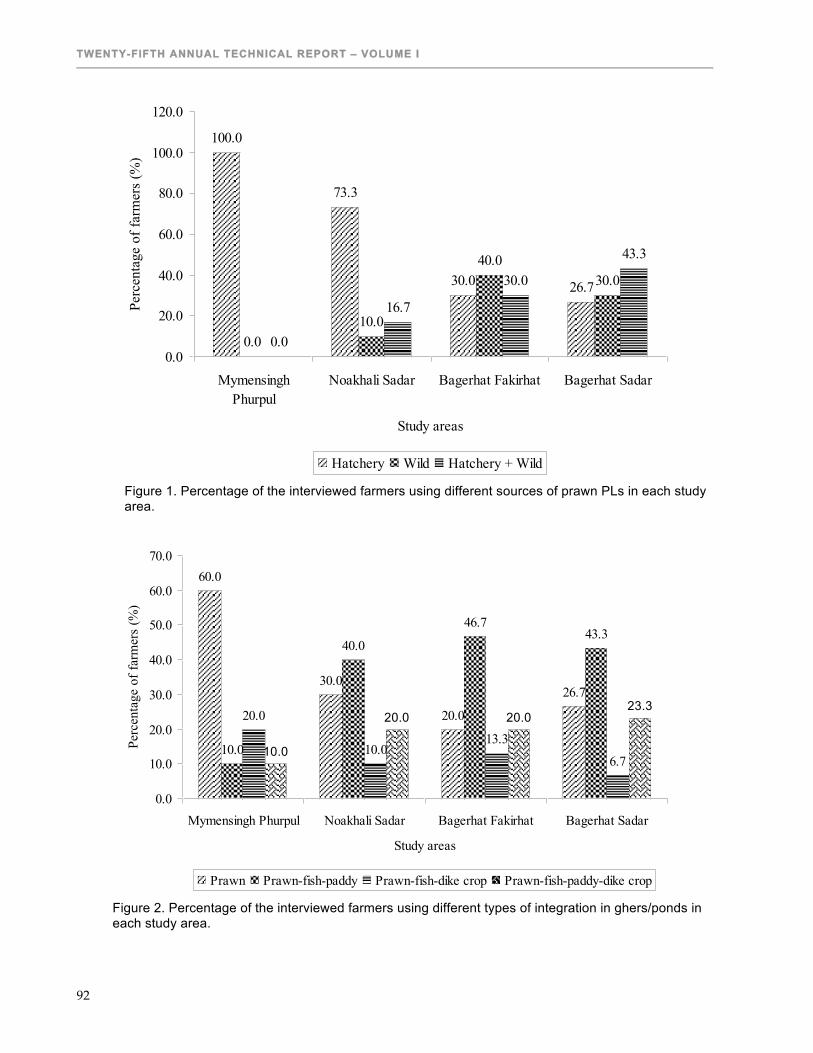
TWENTY-FIFTH ANNUAL TECHNICAL REPORT – VOLUME I
92
100.0
73.3
30.0 26.7
0.010.0
40.030.0
0.0
16.7
30.0
43.3
0.0
20.0
40.0
60.0
80.0
100.0
120.0
MymensinghPhurpul
Noakhali Sadar Bagerhat Fakirhat Bagerhat Sadar
Study areas
Perc
enta
ge o
f far
mer
s (%
)
Hatchery Wild Hatchery + Wild
Figure 1. Percentage of the interviewed farmers using different sources of prawn PLs in each study area.
60.0
30.0
20.0
26.7
10.0
40.0
46.743.3
20.0
10.013.3
6.710.0
20.0 20.023.3
0.0
10.0
20.0
30.0
40.0
50.0
60.0
70.0
Mymensingh Phurpul Noakhali Sadar Bagerhat Fakirhat Bagerhat Sadar
Study areas
Perc
enta
ge o
f far
mer
s (%
)
Prawn Prawn-fish-paddy Prawn-fish-dike crop Prawn-fish-paddy-dike crop
Figure 2. Percentage of the interviewed farmers using different types of integration in ghers/ponds in each study area.

PRODUCTION SYSTEM DESIGN & INTEGRATION
93
70.0
86.7
53.360.0
10.03.3 3.3 6.7
20.0
10.06.7 3.30.0 0.0
26.720.0
0.0
10.0
20.0
30.0
40.0
50.0
60.0
70.0
80.0
90.0
100.0
Mymensingh Phurpul Noakhali Sadar Bagerhat Fakirhat Bagerhat Sadar
Study areas
Perc
enta
ge o
f far
mer
s (%
)
Lime Disinfectant Salt + Lime Aquajet
Figure 3. Percentage of the interviewed farmers using different types of chemicals for improving water quality in each study area.
57.560.3 58.3
61.3
20.0 20.2 20.2 19.7
10.413.5 11.3 10.712.1
6.010.2 8.3
0.0
10.0
20.0
30.0
40.0
50.0
60.0
70.0
Mymensingh Phurpul Noakhali Sadar Bagerhat Fakirhat Bagerhat Sadar
Study areas
Perc
enta
ge o
f har
vete
d pr
awns
(%)
1st harvest 2nd harvest 3rd harvest 2nd year
Figure 4. Average percentage of harvested prawns during the first, second and third partial harvest as well as next year in ghers in each study area.

TWENTY-FIFTH ANNUAL TECHNICAL REPORT – VOLUME I
94
Table 1. Distribution of the randomly selected prawn farmers in each study area.
Study area Sample size Mymensingh Phulpur 10 Noakhali Sadar 30 Bagerhat Sadar 30 Bagerhat Fakirhat 30 Total 100
Table 2. Age and education levels of the interviewed prawn farmers in each study area.
Parameters Mymensingh Phulpur
Noakhali Sadar
Bagerhat Fakirhat
Bagerhat Sadar Total
Age Up to 30 1 (10.0%) 11 (36.7%) 9 (30.0%) 7 (23.7%) 28 (28.0%) 31 to 40 5 (50.0%) 14 (46.7%) 11 (34.6%) 10 (33.3%) 40 (40.0%) 41 to 50 3 (30.0%) 3 (10.0%) 8 (26.7%) 9 (30.0%) 23 (23.0%) > 50 1 (10.0%) 2 (6.7%) 2 (6.7%) 4 (13.3%) 9 (9.0%) Total 10 (100%) 30 (100%) 30 (100%) 30 (100%) 100 (100%) Education No education 1 (10.0%) 6 (20.0%) 2 (6.7%) 1 (3.3%) 10 (10.0%) Primary 1 (10.0%) 13 (43.3%) 1 (3.3%) 4 (13.3%) 19 (19.0%) Secondary 3 (30.0%) 9 (30.0%) 11 (36.7%) 13 (43.3%) 36 (36.0%) S.S.C 5 (50.0%) 2 (6.7%) 7 (23.3%) 7 (23.3%) 21 (21.0%) H.S.C - - 4 (13.3%) 4 (13.3%) 8 (8.0%) Bachelor - - 5 (16.7%) 1 (3.3%) 6 (6.0%) Total 10 (100%) 30 (100%) 30 (100%) 30 (100%) 100 (100%)

PRODUCTION SYSTEM DESIGN & INTEGRATION
95
Table 3. The primary occupations of the interviewed prawn farmers before and after prawn farming in each study area.
Primary occupation Mymensingh Phulpur
Noakhali Sadar
Bagerhat Fakirhat
Bagerhat Sadar Total
Before prawn farming Agriculture 6 (60.0%) 26 (86.7%) 13 (43.3%) 14 (46.7%) 59 (59.0%) Business 3 (30.0%) 2 (6.7%) 9 (30.0%) 4 (13.3%) 18 (18.0%) Fish culture 0 (0.0%) 1 (3.3%) 1 (3.3%) 2 (6.7%) 4 (4.0%) Govt. Job 0 (0.0%) 0 (0.0%) 0 (0.0%) 2 (6.7%) 2 (2.0%) Others 1 (10.0%) 1 (3.3%) 7 (23.3%) 8 (26.7%) 17 (17.0%) Total 10 (100%) 30 (100%) 30 (100%) 30 (100%) 100 (100%)
After prawn farming Prawn farming 6 (60.0%) 14 (46.7%) 22 (73.3%) 28 (93.3%) 70 (70.0%) Agriculture 1 (10.0%) 9 (30.0%) 0 (0.0%) 0 (0.0%) 10 (10.0%) Business 2 (20.0%) 5 (16.7%) 5 (16.7%) 1(3.3%) 13 (13.0%) Fish culture 1 (10.0%) 2 (6.7%) 0 (0.0%) 0 (0.0%) 3 (3.0%) Govt. Job 0 (0.0%) 0 (0.0%) 0 (0.0%) 1 (3.3%) 1 (1%) Others 0 (0.0%) 0 (0.0%) 3 (10.0%) 0 (0.0%) 3 (3.0%) Total 10 (100) 30 (100) 30 (100%) 30 (100%) 100 (100%)
Table 4. Detailed management of prawn post larvae nursing in each study area (1 decimal = 40 m2)
Parameters Study areas Total
Mymensingh Phulpur
Noakhali Sadar
Bagerhat Fakirhat
Bagerhat Sadar
Water area (decimal) 7.48±6.48 10.47±14.76 7.30±3.67 7.91±5.79 8.29±7.67 Nursing duration (days) 46±4 52±7 51±6 51±6 50±6 Rotenone (g decimal-1) 24.0±4.16 - 25.7±5.35 27.5±3.54 25.4±4.58 Lime (kg decimal-1) 1.15±0.36 0.77±0.31 1.23±0.42 1.08±0.35 1.03±0.39
Cowdung (kg decimal-1) 1.9±0.62 2.3±0.77 1.8±0.82 1.6±0.98 1.9±0.86
Urea (g decimal-1) 162.5±64.1 111.9±57.7 82.0±29.0 107.1±41.9 109.7±52.6 TSP (g decimal-1) 109.4±26.5 124.4±63.5 142.7±128.1 93.18±26.9 117.3±75.8 Stocking density (no. decimal-1) 1,000±254 694±171 1,057±259 890±199 901±259
PL length at stocking (cm) 1.0±0.1 1.0±0.1 0.9±0.1 1.1±0.1 1.0±0.1 PL length at harvest (cm) 5.9±0.9 6.1±1 6.0±1.1 6.0±1 6.0±1 Survival rate (%) 68.5±9.73 68.7±6.72 68.3±7.81 65.3±6.94 67.5±7.51 Values are mean ± SD. Mean values with different superscript letters in the same row were significantly different (P<0.05).
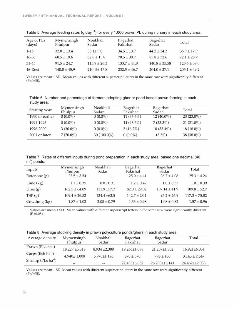
TWENTY-FIFTH ANNUAL TECHNICAL REPORT – VOLUME I
96
Table 5. Average feeding rates (g day -1) for every 1,000 prawn PL during nursery in each study area.
Age of PLs (days)
Mymensingh Phulpur
Noakhali Sadar
Bagerhat Fakirhat
Bagerhat Sadar Total
1-15 32.0 ± 13.4 33.1± 9.0 34.5 ± 13.7 44.2 ± 24.2 36.9 ± 17.9 16-30 60.5 ± 19.6 62.8 ± 15.8 70.5 ± 30.7 85.8 ± 32.6 72.1 ± 28.9 31-45 91.5 ± 24.7 115.9 ± 26.3 133.7 ± 44.8 140.8 ± 35.58 125.6 ± 38.0 46-Rest 140.0 ± 45.9 210 .5± 47.8 232.5 ± 46.7 204.0 ± 27.1 205.1 ± 49.2
Values are mean ± SD. Mean values with different superscript letters in the same row were significantly different (P<0.05).
Table 6. Number and percentage of farmers adopting gher or pond based prawn farming in each study area.
Starting year Mymensingh Phulpur
Noakhali Sadar
Bagerhat Fakirhat
Bagerhat Sadar Total
1990 or earlier 0 (0.0%) 0 (0.0%) 11 (36.6%) 12 (40.0%) 23 (23.0%) 1991-1995 0 (0.0%) 0 (0.0%) 14 (46.7%) 7 (23.3%) 21 (21.0%) 1996-2000 3 (30.0%) 0 (0.0%) 5 (16.7%) 10 (33.4%) 18 (18.0%) 2001 or later 7 (70.0%) 30 (100.0%) 0 (0.0%) 1 (3.3%) 38 (38.0%)
Table 7. Rates of different inputs during pond preparation in each study area, based one decimal (40 m2) ponds.
Inputs Mymensingh Phulpur
Noakhali Sadar
Bagerhat Fakirhat
Bagerhat Sadar Total
Rotenone (g) 22.5 ± 3.54 ---- 25.0 ± 4.41 26.7 ± 4.08 25.3 ± 4.24
Lime (kg) 1.1 ± 0.35 0.8± 0.31 1.2 ± 0.42 1.0 ± 0.35 1.0 ± 0.39 Urea (g) 162.5 ± 64.09 111.9 ±57.7 82.0 ± 29.02 107.14 ± 41.9 109.8 ± 52.7 TSP (g) 109.4 ± 26.52 124.4 ±63.5 142.7 ± 28.1 93.2 ± 26.9 117.3 ± 75.82 Cowdung (kg) 1.87 ± 1.02 2.08 ± 0.79 1.33 ± 0.98 1.08 ± 0.82 1.57 ± 0.96
Values are mean ± SD. Mean values with different superscript letters in the same row were significantly different (P<0.05).
Table 8. Average stocking density in prawn polyculture ponds/ghers in each study area. Average density Mymensingh
Phulpur Noakhali
Sadar Bagerhat Fakirhat
Bagerhat Sadar
Total
Prawn (PLs ha-1) 18,227 ±5,518 8,934 ±2,309 19,266±4,098 21,257±4,302 16,921±6,034 Carps (fish ha-1) 4,940± 1,008 5,970±1,126 870 ± 570 798 ± 430 3,145 ± 2,547 Shrimp (PLs ha-1) -- -- 22,435±6,632 26,200±15,141 24,462±12,033 Values are mean ± SD. Mean values with different superscript letters in the same row were significantly different (P<0.05).

PRODUCTION SYSTEM DESIGN & INTEGRATION
97
Table 9. Average rates of fertilizers, feed and snail meat applied during culture period in each study area.
Activities Mymensingh Phulpur
Noakhali Sadar
Bagerhat Fakirhat
Bagerhat Sadar Total
Fertilizers Cowdung (kg decimal-
1) 1.08 ± 0.86 0.61 ± 0.85 0.68 ± 0.43 0.54 ± 0.29 0.69 ± 0.74 Urea (g decimal-1) 67.9 ± 47.2 31.9 ± 40.0 60.7 ± 13.4 75.0 ± 25.0 50.0 ± 34.5 TSP (g decimal-1) 53.6 ± 39.3 41.7 ± 53.6 87.5 ± 23.2 108.3 ± 20.4 63.5 ± 48.6 Feed and feeding rate Feed (% body weight per day) 4.3±0.67 4.3 ± 0.74 4.6 ± 0.50 4.7 ± 0.48 4.5 ± 0.61 Snail meat (kg ha-1 day-1)
- - 62.0 ± 17.2 65.4 ± 17.2 63.7 ± 17.2
Values are mean ± SD Mean values with different superscript letters in the same row were significantly different (P<0.05).
Table 10. Average annual production of prawn, fish and shrimp in each study area. Average
production (kg ha-1)
Mymensingh Phulpur
Noakhali Sadar
Bagerhat Fakirhat
Bagerhat Sadar Total
Prawn 385.2 ± 60.9 241.2 ±52.5 482.5± 88.7 448.5± 94.0 390.2±127.9 Fish 635.0± 219.9 1,189.2±411.9 406.7±155.0 379.0±113.4 658.5±440.7
Shrimp -- -- 121.7± 31.6 125.7 ± 42.1 123.9 ± 37.0 Values are mean ± SD. Mean values with different superscript letters in the same row were significantly different (P<0.05).

TWENTY-FIFTH ANNUAL TECHNICAL REPORT – VOLUME I
98
Table 11. Means of experience acquisition of the interviewed farmers in each study area. Means of
experience acquisition
Mymensingh Phulpur
Noakhali Sadar
Bagerhat Fakirhat
Bagerhat Sadar Total
Self study 2 (20.0%) 5 (16.8%) 6 (20.0%) 4 (13.3%) 17 (17.0%) Friends or neighbors 6 (60.0%) 13 (43.3%) 19 (63.3%) 19 (63.3%) 57 (57.0%) Govt. (DoF) 2 (20.0%) 1 (3.3%) 4 (13.3%) 5 (16.7%) 12 (12.0%) GNAEP, NGOs 0 (0.0%) 11 (36.6%) 1 (3.3%) 2 (6.7%) 14 (14.0%)
Received training Yes 3 (30.0%) 14 (46.7%) 20 (66.7%) 19 (63.3%) 56 (56.0%) No 7 (70.0%) 16 (53.3%) 10 (33.3%) 11 (36.7%) 44 (44.0%)
Table 12. Prawn size and price in domestic markets.
Prawn size (prawns kg-1)
Average weight
(g prawn-1) Average price
(Tk kg-1) 5 or less 200 475
6-10 100 420 11-20 50 350 21-30 30 275 31-50 20 180
PRODUCTION SYSTEM DESIGN & INTEGRATION
99
NEW PARADIGM IN FARMING OF FRESHWATER PRAWN (MACROBRACHIUM ROSENBERGII) WITH CLOSED AND RECYCLE SYSTEMS IN VIETNAM
Twelfth Work Plan, Production System Design & Integration 1c (12PSD1c)
Final Report Published as Submitted by Contributing Authors
Nguyen Thanh Phuong, Ly Van Khanh Le Quoc Viet & Tran Van Viet
Can Tho University, Can Tho City, Vietnam
Yang Yi & Yuan Derun
Asian Institute of Technology Pathumthani, Thailand
James S. Diana & C. Kwei Lin
University of Michigan, Ann Arbor, Michigan, USA
ABSTRACT Two surveys on giant freshwater prawn (Macrobrachium rosenbergii) farming were conducted in the Mekong delta, Vietnam. The first survey was carried out during March - April 2005 and the second during May - June 2006. These two surveys were conducted in the same locations. Seventy-six prawn farmers were randomly selected during the first survey, among which 15 farmers were from Co Do district and 27 farmers from Thot Not district of Can Tho City, and 34 farmers from Thoai Son district of An Giang province. For the second survey, 21 farmers were selected from Co Do district, 16 from Thot Not district and 22 from Thoai Son district. The selected farmers were interviewed using a structured checklist and open-ended type of questionnaire. The surveys focused on prawn farming in rice paddies to assess changes of giant freshwater prawn farming including development trends aswell as technical, socio-economic and environmental aspects. Prawn farming in the rice-prawn alternative culture model was continuing expansion in the Mekong delta. There were improvements of culture techniques and net return. Average production in 2004 was 1,452 kg ha-1 crop-1, and in 2005 was 1,035 kg ha-1 crop-1. However, average net return in 2005 was 48,788,000 VND, which was 40% higher than that in 2004. Stocking density of prawn in 2005 was lower than that in 2004, and the stocking density of 8-12 post-larvae per square meter would be suitable for the rice-prawn alternative culture model. The technology should be further improved in terms of farm preparation, feed and feeding, stocking and water management.
INTRODUCTION The giant freshwater prawn (Macrobrachium rosenbergii) is the largest of the freshwater crustacean species. It is an indigenous species to South and Southeast Asia, parts of Oceania and some Pacific Islands (New, 2002). This species has an important role in freshwater aquaculture of many countries. FAO (2003) reported that there were 15 top countries producing giant freshwater prawn in 2001, and countries producing over 10,000 tons included China (128,300 tons), Vietnam (28,000 tons, but including other crustacean species), India (24,320 tons), and Thailand (12,067 tons) (New, 2006). In Vietnam, the Mekong delta is the main region for prawn culture, including Can Tho City, An Giang province, Dong Thap province, Vinh Long province and Ben Tre province. The total culture area of 5,680 ha produced 2,760 tons in 2005 (Phuong et al., 2006). Sinh et al. (2006a)

TWENTY-FIFTH ANNUAL TECHNICAL REPORT – VOLUME I
100
estimated that the culture area and production should reach 18,220 ha and 15,910 tons by 2010, bringing the freshwater prawn production of Vietnam to the second in the world (New, 2006). Prawn culture started in early 1980s using wild seed collected from natural water bodies and extensive operation in ponds, garden canals and rice paddies (Hien et al, 1998). However, prawn culture has grown rapidly since 2000, when technology was developed to produce artificial seed (Phuong et. al., 2006). Major models of prawn culture in the Mekong delta include semi-intensive culture in ponds and garden canals, extensive integrated culture in rice paddies (Phuong et al., 2006), and intensive pen culture in rivers (Son et al. 2005). Among these models, the rice-prawn culture model is the most productive and profitable system (Phuong et al., 2006). In freshwater areas, especially flooded areas of An Giang and Dong Thap provinces and Can Tho City, paddy rice has gradually been converted to complete one crop of prawn culture during rainy season and one crop of rice during dry season. This model is called rice-prawn alternative culture. This type of system is more productive and is better than other models (Phuong et. al., 2006). However, one prawn crop during April-December and two rice crops during March-June and December-March have also been completed in many areas of the Mekong delta (Phuong et al., 2006). This model is mainly applied in low flooding areas such as Vinh Long and Ben Tre provinces (Viet and Tuan, 2006). Moreover, addition of prawn to rice paddies has been found to be an ecologically sound method of diversification, and also often increases rice production (New, 1995). Prawns feed on insects, improve soil fertility, and constitute a high-valued cash crop in rice fields (Giap et al., 2005). In the freshwater region of the Mekong delta, rice cultivation areas covered 523,000 ha in Giang province and 229,900 ha in Can Tho City in 2003 (Statistical Office of Can Tho City, 2004; Statistical Office of An Giang Province, 2004). Giant freshwater prawn culture in rice paddies is one of the important innovations for rural development in the two regions. The total areas of rice-prawn alternative culture were 560 ha and 290 ha in 2004, and increased to 747 and 376 ha in 2005 in each locality (Department of Agriculture and Rural Development of An Giang Province, 2005, 2006; Department of Agriculture and Rural Development of Can Tho City, 2005, 2006). There have been great changes in technical and economic performances of rice-prawn culture during its development. Therefore, the objectives of this study were to assess changes in giant freshwater prawn farming for the rice-prawn alternative culture system in technical, socio-economic and environmental terms and to predict the development trend for the rice-prawn alternative culture system.
MATERIALS AND METHODS Two surveys were conducted to collect data from two continuous crops in the same study areas. The first survey was carried out during March-April 2005 to obtain data from 2004, and the second survey during May-June 2006 to obtain data from 2005. Seventy-six prawn farmers were randomly selected during the first survey, from Co Do district, Thot Not district of Can Tho City, and Thoai Son district of An Giang province (Table 1). For the second survey, 59 farmers were selected from the same region. Selected farmers were interviewed using a structured checklist and an open-ended questionnaire. Secondary data were collected from annual reports of the Department of Agriculture and Rural Development of Can Tho City and An Giang province. After data collection, data were coded, summarized and processed for analyses. Data analyses were done using SPSS (version 10.0) statistical software (SPSS Inc., Chicago, USA).
RESULTS Social aspects of prawn farmers The educational level of prawn farmers in the study areas was low, and the survey in 2004 showed that 28.9% and 63.2% farmers had elementary and secondary levels, respectively, while the survey in 2005 indicated that 36.2% of farmers were illiterate, 42.6% had elementary and 21.3%

PRODUCTION SYSTEM DESIGN & INTEGRATION
101
secondary education (Table 2). The lower educational level of farmers in 2005 did not indicate that education status of the region decreased, but that farmers of different educational levels were sampled. About one third of the farmers did not receive training before practicing prawn farming (Table 2). The top sources of the technical information were other farmers (92.1% in 2004 and 55.9% in 2005). In the 2004 survey, many farmers reported that they updated their technical knowledge by public communication, including 86.8% from television and radio and 76.3% from newspapers and technical books, while these percentages were only 20.3% and 22.0% in the 2005 survey. Training courses were important ways for prawn farmers to obtain technical information, and 68.4% and 49.2% farmers participated in training courses from the surveys conducted in 2004 and 2005, respectively. Most prawn farmers (96.1% in 2004 and 93.2% in 2005) had formerly been employed in agriculture (Table 2). Prawn farming practices There were different models of rice-prawn farming in the Mekong delta, including integrated rice-prawn farming and alternative rice-prawn farming (Table 3). The latter form of culture could either start prawn culture in April and produce one rice crop, or start prawn culture in June and produce two rice crops (Phuong et al., 2006). Rice-prawn alternative farming increased from 88.2% of the interviewed farmers in 2004 to 96.6% in 2005, while integrated rice-prawn farming decreased from 11.8% in 2004 to 3.4% in 2005 (Table 4). Most farmers (94.9%) had one rice crop per year compared to 5.1% with two rice crops per year (Table 3). The both Surveys in 2004 and 2005 showed that slightly more than half (55.3% and 55.9%) of the prawn farmers had surrounding for their farms (Table 4). The 2005 survey indicated that 42.4% farms had water supply from the main canal, 28.8% from the secondary canals, 18.6% from the main river, and 10.2% from the secondary river (Table 4). Average farm size was 12,477 m2 in 2004 and 25,000 m2 in 2005, while rice field area was 10,318 m2 in 2004 and 7,000 m2 in 2005 (Table 5).Average water depth above the rice field was 0.6 m in 2004 and 0.7 m in 2005, and the number of gates for water exchange was 2.4 in 2004 and 4.5 in 2005. These differences probably reflect some increase in prawn farming, as well as differences in the farms surveyed each year. Compared to 2004, farms surveyed in 2005 used better farm preparation. The number of farms using fertilization, lime and water intake filtration bag increased from 9.2%, 78.9% and 92.1% in 2004 to 22.0%, 89.8% and 100.0% in 2005, respectively (Table 6). Most farms in Co Do district removed sediment from the surface of rice field to 20-30 cm deep to increase water depth. After harvesting rice, all farmers also burned the rice straw to prevent water pollution when these materials would become submerged and decomposed in water. Most farmers used rotemone to kill predators in water before stocking prawn (Table 6). Most surveyed farms used hatchery-produced post larvae of 10-15 days old for stocking, with only one farmer producing post larvae on farm in 2005 (Table 7). In 2004, no farmers purchased post larvae from local hatcheries, while 33.9% farmers purchased post larvae from local hatcheries in 2005. The percentage of farmers purchasing post larvae from distant hatcheries, either in the same province or from other provinces, was 100% and 64.3% in 2004 and 2005 (Table 8). All farmers nursed post larvae prior to stocking to increase prawn size up to 2-3 cm long, to acclimate prawns to the new water environment, and to improve survival. In 2004, all farmers surveyed nursed post larvae in a diked or net-fenced compartment in the rice field, but only 64.4% of farmers used this method in 2005, while 33.9% nursed post larvae in separate small ponds and 1.7% in hapas installed in surrounding ditches (Table 7). The compartment for nursing post larvae over 20-60 days ranged from 100 to 20,000 m2 with stocking densities of 2-20 PLs/m2 (Table 7). There were two kinds of feed used in rice-prawn culture. Fresh feeds such as freshwater crab, trash fish and golden snail meat were used by more than 80% of farmers. These fresh feeds,
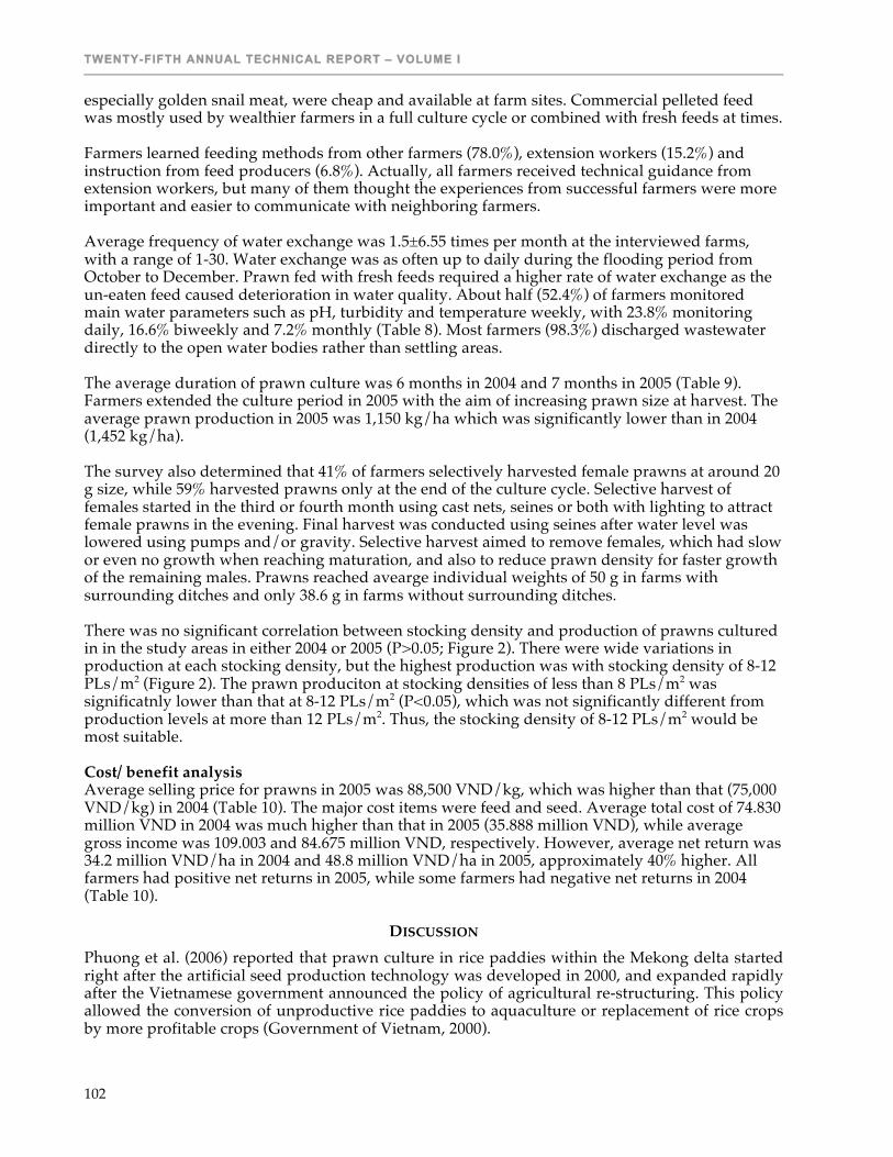
TWENTY-FIFTH ANNUAL TECHNICAL REPORT – VOLUME I
102
especially golden snail meat, were cheap and available at farm sites. Commercial pelleted feed was mostly used by wealthier farmers in a full culture cycle or combined with fresh feeds at times. Farmers learned feeding methods from other farmers (78.0%), extension workers (15.2%) and instruction from feed producers (6.8%). Actually, all farmers received technical guidance from extension workers, but many of them thought the experiences from successful farmers were more important and easier to communicate with neighboring farmers. Average frequency of water exchange was 1.5±6.55 times per month at the interviewed farms, with a range of 1-30. Water exchange was as often up to daily during the flooding period from October to December. Prawn fed with fresh feeds required a higher rate of water exchange as the un-eaten feed caused deterioration in water quality. About half (52.4%) of farmers monitored main water parameters such as pH, turbidity and temperature weekly, with 23.8% monitoring daily, 16.6% biweekly and 7.2% monthly (Table 8). Most farmers (98.3%) discharged wastewater directly to the open water bodies rather than settling areas. The average duration of prawn culture was 6 months in 2004 and 7 months in 2005 (Table 9). Farmers extended the culture period in 2005 with the aim of increasing prawn size at harvest. The average prawn production in 2005 was 1,150 kg/ha which was significantly lower than in 2004 (1,452 kg/ha). The survey also determined that 41% of farmers selectively harvested female prawns at around 20 g size, while 59% harvested prawns only at the end of the culture cycle. Selective harvest of females started in the third or fourth month using cast nets, seines or both with lighting to attract female prawns in the evening. Final harvest was conducted using seines after water level was lowered using pumps and/or gravity. Selective harvest aimed to remove females, which had slow or even no growth when reaching maturation, and also to reduce prawn density for faster growth of the remaining males. Prawns reached avearge individual weights of 50 g in farms with surrounding ditches and only 38.6 g in farms without surrounding ditches. There was no significant correlation between stocking density and production of prawns cultured in in the study areas in either 2004 or 2005 (P>0.05; Figure 2). There were wide variations in production at each stocking density, but the highest production was with stocking density of 8-12 PLs/m2 (Figure 2). The prawn produciton at stocking densities of less than 8 PLs/m2 was significatnly lower than that at 8-12 PLs/m2 (P<0.05), which was not significantly different from production levels at more than 12 PLs/m2. Thus, the stocking density of 8-12 PLs/m2 would be most suitable.
Cost/ benefit analysis Average selling price for prawns in 2005 was 88,500 VND/kg, which was higher than that (75,000 VND/kg) in 2004 (Table 10). The major cost items were feed and seed. Average total cost of 74.830 million VND in 2004 was much higher than that in 2005 (35.888 million VND), while average gross income was 109.003 and 84.675 million VND, respectively. However, average net return was 34.2 million VND/ha in 2004 and 48.8 million VND/ha in 2005, approximately 40% higher. All farmers had positive net returns in 2005, while some farmers had negative net returns in 2004 (Table 10).
DISCUSSION Phuong et al. (2006) reported that prawn culture in rice paddies within the Mekong delta started right after the artificial seed production technology was developed in 2000, and expanded rapidly after the Vietnamese government announced the policy of agricultural re-structuring. This policy allowed the conversion of unproductive rice paddies to aquaculture or replacement of rice crops by more profitable crops (Government of Vietnam, 2000).

PRODUCTION SYSTEM DESIGN & INTEGRATION
103
Generally, the educational level of farmers in the Mekong delta is lower than those in other regions in Vietnam, since the economy is poorer and poor transportation provides limited opportunities for children to attend school. Son et al. (2005) also reported that the educational background of prawn farmers in Dong Thap and An Giang provinces was low, with only 5.77% finishing high school. Thus, most farmers in these two provinces used indigenous knowledge, with only 9% of farmers attending technical training courses. The educational level of prawn farmers in Vinh Long province was similar to those areas, with only 3.3% finishing high school, 43.3% secondary school and 53.4% elementary school (Viet and Tuan, 2006). Chanratchakool and Phillips (2002) also reported that Vietnamese farmers had limited education and little experience in aquaculture. However, the educational level has improved since 2000 (Sinh et al., 2006b). Still, limited education is a constraint in extending new technologies and progress to aquaculture farmers in Vietnam. Public communication plays an important role in updating technical and marketing information for farmers. In the present study, in 2004, 86.8% of farmers obtained such information from television and radio, and 76.3% from newspapers and technical books. However, these percentages were 20.3% and 22.0%, respectively, for the 2005 sample. The much lower percentages in 2005 were at least partially due to the lower education level of farmers sampled that year. Viet and Tuan (2006) reported that 77% of farmers in Vinh Long province obtained technical information from television and radio. In addition, fisheries officers and scientists in academic institutions have also contributed significantly in new technology transfer. Phuong et al. (2006) stated that the development of prawn culture in the Mekong Delta was highly supported by many extension activities and by success in artificial seed production in local hatcheries. Hien (2005) reported that prawn farmers have benefited greatly from scientists in terms of technical progress of prawn farming. Ditches surrounding rice paddies provided space for prawns and relatively stable temperature between day and night. Increased water depth was also important to avoid high temperature, which may cause early maturation of females (Khanh and Phuong, 2005). Hien (2005) reported that the percentage of farms with surrounding ditches varied greatly by location. All prawn farms in Thoai Son district of An Giang province and Vinh Thanh district of Can Tho City had surrounding ditches, but only 21.8% in Co Do district of Can Tho City had ditches. The size and area of surrounding ditches varied by farm, from 20 to 25% of the size of rice paddies. Farms in Mekong delta ranged from 7,000 to 12,000 m2 in size, and were often located near main canals to provide easy water exchange (Hien (2005). This is a key criterion for site selection. High water exchange is required in prawn farming because water quality often deteriorates during the last month of culture, which is most likely caused by the over use of fresh feed. According to Phuong et al. (2006), prawn hatcheries were located mainly in Can Tho City and An Giang and Dong Thap provinces, and produced up to 90 million post-larvae in 2004. However, seed supply did not meet the demand, and was on constraints for further development of prawn farming in the Mekong delta. Thus, wild collected juveniles were still used (Hai et al., 2000), especially for pen culture (Son et al., 2005). However, the stocking of wild collected juveniles has gradually reduced, especially in rice-prawn alternative culture, due mainly to lack of uniformity in size, poor quality, and insufficient numbers. The nursing area for prawn post-larvae was often about 11%-23% of total cultural area, and few farmers stocked post-larvae directly to rice paddies (Hien, 2005). About 82% of farmers in Can Tho City and An Giang province stocked post-larvae at 13-15 days old for nursing at densities of 50-100 PLs/m2 for 25-30 days (Hien, 2005; Khanh, 2005). Stocking density for prawns depends on mainly factors such as feeding practices (pellet and/or fresh food), water quality, capacity of investment, and expected harvest size. The common stocking density is 0.2-4 PLs/m2 in rice-prawn integrated culture and 5-10 PLs/m2 in rice-prawn alternative culture (Hien, 2005). In this study, the average stocking density was 9.7 PLs/m2 in 2004

TWENTY-FIFTH ANNUAL TECHNICAL REPORT – VOLUME I
104
and 8.0 PLs/m2 in 2005, which are within the range reported by Hien (2005). The average prawn production was 1,452 kg/ha in 2004 and 1,150 kg/ha in 2005, which were similar to those (1,081-1,485) reported by Khanh and Phuong (2005) for the rice-prawn alternative model. More than 80% of surveyed farmers used fresh feed instead of commercial pelleted feed. Lan et al. (2006) reported that most farmers used a combination of pellets and fresh feed. Hien (2005) found that pelleted feed was used during the nursing stage or the first month after stocking followed by freshwater crab, golden snail meat and trash fish. The common use of fresh feeds caused deteriorating water quality, thus more water exchange was needed to maintain good water quality, causing environmental problems. Furthermore, most farmers in the present study (98.3%) discharged wastewater directly to open water bodies that may cause environmental problems. However, nutrients accumulating in paddy fields from prawn culture can be utilized by next crop of rice, helping to reduce environmental pollution and to reduce cost of rice production. Average prawn production with the rice-prawn alternative model in Mekong Delta ranged from 600 to 1,000 kg/ha (Phuong, 2003) and 500 to 1,200 kg/ha (Hien, 2005). Average prawn production in the present study areas was 1,452 kg/ha and 1,150 kg/ha in 2004 and 2005, respectively, which was even higher than the upper limit of the above reported prawn production. Most of the surveyed farmers used the alternative prawn method, so these results probably reflect yields for that system. Khanh and Phuong (2005) reported from their experiment that the prawn production in the rice-prawn alternative model varied from 1,081-1,485 kg/ha when stocking post-larvae and 504-599 kg/ha when stocking hatchery-reared juveniles. There were wide variations of production at a given stocking density level, most likely due to factors such as different feeds and feeding practices, farm sites and designs, and water management. Selling price was a main factor affẹcting the profitability of prawn culture in the Mekong Delta. The selling price has wide variation year to year (Khanh and Phuong, 2005). Cost of feed and seed accounted for most of the total production cost for prawn culture, and increased significantly with incresing stocking density (Hien, 2005; Viet and Tuan, 2006). Khanh and Phuong (2005) reported that the cost of seed and feed (both fresh feed and commercial pelleted feed) was 52% and 36%, respectively, of the total cost in the rice-prawn alternative model. However, Lan et al. (2006) reported from their experiment that the cost of feed was 2.5-4 times higher than seed, and also found that a combined feeding regime using both golden snail meat and commercial pelleted feed would reduce total operational cost by 11% and increase net return by 49%, compared to the prawn culture using pelleted feed alone. The profit from rice-prawn culture, especially the alternative model is much higher than that from rice culture alone (Thong et al., 2003). Nguyen (2003) reported that the net profit from rice-prawn alternative culture was 17.9 million VND/ha in 2003, while Khanh and Phuong (2005) reported that the net profit was 54.7 million VND/ha in the rice-prawn alternative culture model and 30.8 million VND/ha in the rice-prawn integrated culture model under experimental conditions. In the present study, the average net return from prawn alone reached 34.2 million VND/ha in 2004 and 48.8 million VND/ha in 2005, and rice would add further to this profit. In conclusion, prawn culture in the Mekong Delta was dominated by the rice-prawn alternative culture model, which most likely will continue to expand. However, the technology should be further improved in farm preparation, feed and feeding, stocking and water management.
ANTICIPATED BENEFITS This survey helped to understand the current status of freshwater prawn farming especially, the rice-prawn alternative culture model in Vietnam. The results of the survey will provide useful information for decision-makers to improve current culture systems, as well as plan and develop sustainable freshwater prawn farming in Vietnam.

PRODUCTION SYSTEM DESIGN & INTEGRATION
105
ACKNOWLEDGMENTS The authors would like to acknowledge with thanks to Can Tho University, Can Tho, Vietnam, and the Asian Institute of Technology, Thailand for their support in the implementation of the project.
LITERATURE CITED Chanratchakool, P., and M.J. Phillips, 2002. Social economic impacts of shrimp disease among
small scale farmers in Thailand and Vietnam. In: J.R. Arthur, M.J. Phillips, R.P. Subasinghe, M.B. Reantaso and I.H. Macrae (Editors). Primary Aquatic Animal Health Care in Rural, Small Scale Aquaculture Development. FAO Fisheries Technical Paper No. 406, pp. 177-189.
Department of Agriculture and Rural Development of An Giang Province, 2005. Annual Report of Agriculture Activities, 12 pp. (in Vietnamese).
Department of Agriculture and Rural Development of An Giang Province, 2006. Annual Report of Agriculture Activities, 14 pp. (in Vietnamese).
Department of Agriculture and Rural Development of Can Tho City Province, 2005. Annual Report of Agriculture Activities, 9 pp. (in Vietnamese).
Department of Agriculture and Rural Development of Can Tho City Province, 2006. Annual Report of Agriculture Activities, 15 pp. (in Vietnamese).
FAO, 2003. Fishstat Plus (v. 2.30). Fisheries Department, FAO, Rome, Italy. Giap, D.H, Y. Yi. and C.K. Lin, 2005. Effects of different fertilization and feeding regimes on the
production of integrated farming of rice and prawn Macrobrachium rosenbergii. Aquaculture Research, 35:292-299.
Government of Vietnam, 1999. Approval of Aquaculture Development Plan Period from 1999–2010, Decree No. 224/1999/QDTTg, Hanoi, 4 pp. (in Vietnamese).
Government of Vietnam, 2000. Restructuring of Agricultural Production and Its Products Consumption, Decree No. 09/2000/NQ-CP, Hanoi, 5 pp. (in Vietnamese).
Hai, T.N, T.T.T. Hien, D.T. Yen, B.T.B. Hang and V.T. Toan, 2000. The growth, spawning, survival rate of freshwater prawn reared under different water exchange rates. Proceedings of the 2000 Annual Workshop of JIRCAS Mekong Delta Project, pp. 89-100.
Hien, T.T.T., T.H. Minh, N.T. Phuong and M.N. Wilder, 1998. Current status of freshwater prawn culture in the Mekong River Delta of Vietnam. JIRCAS Journal, 6: 89-100.
Hien, H.V., 2005. Economic Evaluation of Giant Freshwater Prawn (Macrobrachium rosenbergii) Culture on Paddy Rice in An Giang Province and Can Tho City. Project Report Submitted to Can Tho University, Vietnam, 45 pp. (in Vietnamese).
Khanh, L.V., 2005. Development of Rice and Prawn (Macrobrachium rosenbergii) Culture Models in Tam Binh and Mang Thit Districts, Vinh Long Province. Unpublished Master’s Thesis, Can Tho University, Vietnam, 70 pp. (in Vietnamese).
Khanh, L.V. and N.T. Phuong, 2005. Evaluation of the efficiency of the alternative and integrated rice-prawn (Macrobrachium rosenbergii) farming systems. Scientific Journal of Can Tho University, 4:109-118 (in Vietnamese).
Lan, L.M, D.N. Long and J.C. Micha, 2006. The effects of densities and feed types on the production of Macrobrachium rosenbergii (de Man) in the rotational rice prawn system. Aquaculture Research, 37:1297-1304.
New, M.B., 2002. Farming Freshwater Prawns: A Manual for the Culture of the Giant River Prawn (Macrobrachium rosenbergii). FAO Fisheries Technical Paper No.428, FAO, Rome, Italy, 212 pp.
New, M.B., 1995. Status of freshwater prawn farming: a review. Aquaculture Research, 26:1-54. Nguyen, T.N., 2003. Giant freshwater prawn (Macrobrachium rosenbergii) culture in flood season in
Thot Not district, Can Tho City. A paper presented at the workshop on Economic Development of Agriculture, Fisheries and Forestry in the Flood Region of the Mekong Delta, Vietnam at Can Tho University, (in Vietnamese).
Phuong, N.T., V.N. Son, T.V. Bui, N.A. Tuan and M.N. Wilder, 2003. Research, development and economics of giant freshwater prawns (Macrobrachium rosenbergii) culture in Mekong River

TWENTY-FIFTH ANNUAL TECHNICAL REPORT – VOLUME I
106
Delta, Vietnam: a review. Proceedings of the Final Workshop of JIRCAS Mekong Delta Project, 25-26 November 2003, Can Tho University, pp. 307-318.
Phuong N.T., T.N. Hai, T.T.T. Hien, T.V. Bui, D.T.T. Huong, V.N. Son, Y. Morooka, Y. Fukuda and M.N. Wilder, 2006. Current status of freshwater prawn culture in Vietnam and the development and transfer of seed production technology. Fisheries Science, 72:1-12.
Sinh, L.X, D.M. Chung, P.T.N. Khuyen and T.T. Truyen, 2006a. Social impacts of coastal aquaculture in the Mekong Delta. Scientific Journal of Can Tho University, Special Issue on Aquaculture and Fisheries, 2:220-234 (in Vietnamese).
Sinh, L.X, D.M. Chung, H.V. Hien and T.V. Bui, 2006b. Technical and economic efficiency of giant freshwater prawn (Macrobrachium rosenbergii) hatcheries in the Mekong Delta. Scientific Journal of Can Tho University, Special Issue on Aquaculture and Fisheries, 2:268-279 (in Vietnamese).
Son, V.N, Y. Yi and N.T. Phuong, 2005. River pen culture of giant freshwater prawn (Macrobrachium rosenbergii) in southern Vietnam. Aquaculture Research, 36:284-291.
Statistical Office of An Giang Province, 2004. Statistical Yearbook of An Giang Province. 276 pp. (in Vietnamese).
Statistical Office of Can Tho City, 2004. Statistical Yearbook of Can Tho City, 324 pp. (in Vietnamese).
Thong, N.M., 2003. Application of Prawn (Macrobrachium rosenbergii) Hatchery and Rice and Prawn Culture Models in Thoi Thuan and Thanh Quoi Villages, Thot Not District, Can Tho Province. Unpublished Final Project Report Submitted to Vietnamese Ministry of Science and Technology, 28 pp. (in Vietnamese).
Viet, L.Q., and N.A. Tuan, 2006. Status of giant freshwater prawn (Macrobrachium rosenbergii) farming in pond in Vinh Long province. Scientific Journal of Can Tho University, Special Issue on Aquaculture and Fisheries. 2:280-290 (in Vietnamese).

PRODUCTION SYSTEM DESIGN & INTEGRATION
107
0
500
1000
1500
2000
2500
3000
0 2 4 6 8 10 12 14 16 18 20 22
Stocking density (PLs/m2)
Pro
duction (
kg/h
a)
20042005
Figure 1. Map of the Mekong Delta with highlighted locations of the study areas.
Figure 2. Relationship between stocking density and production of prawns in the surveyed farms in 2004 and 2005.
Table 1. Distribution of surveyed farms in the study areas. Study areas 2004 2005 Can Tho province
- Co Do district - Thot Not district
15 27
21 16
An Giang province - Thoai Son district
34
22
Total 76 59
Table 2. Social aspects of the interviewed prawn farmers in the study area.
2004 Farms 2005 Farms Characteristics Number % Number % Education level
Illiteracy 0 0 17 36.2 Elementary 22 28.9 20 42.5 Secondary 48 63.2 10 21.3 High school 6 7.9 0 0
Training before practice Yes 52 68.4 38 64.4 No 24 31.6 21 36.6
Sources of technical information Self-study 0 0 4 6.8 Television and radio 66 86.8 12 20.3 Newspaper, technical books, 58 76.3 13 22.0 Other farmers 70 92.1 33 55.9 Universities 44 57.9 10 16.9 Demonstration farms 13 17.1 8 13.6 Training courses 52 68.4 29 49.2
PPrevious careers Agriculture 73 96.1 55 93.2 Fish farming 0 0 2 3.4 Business 0 0 1 1.7 Others 3 3.9 1 1.7
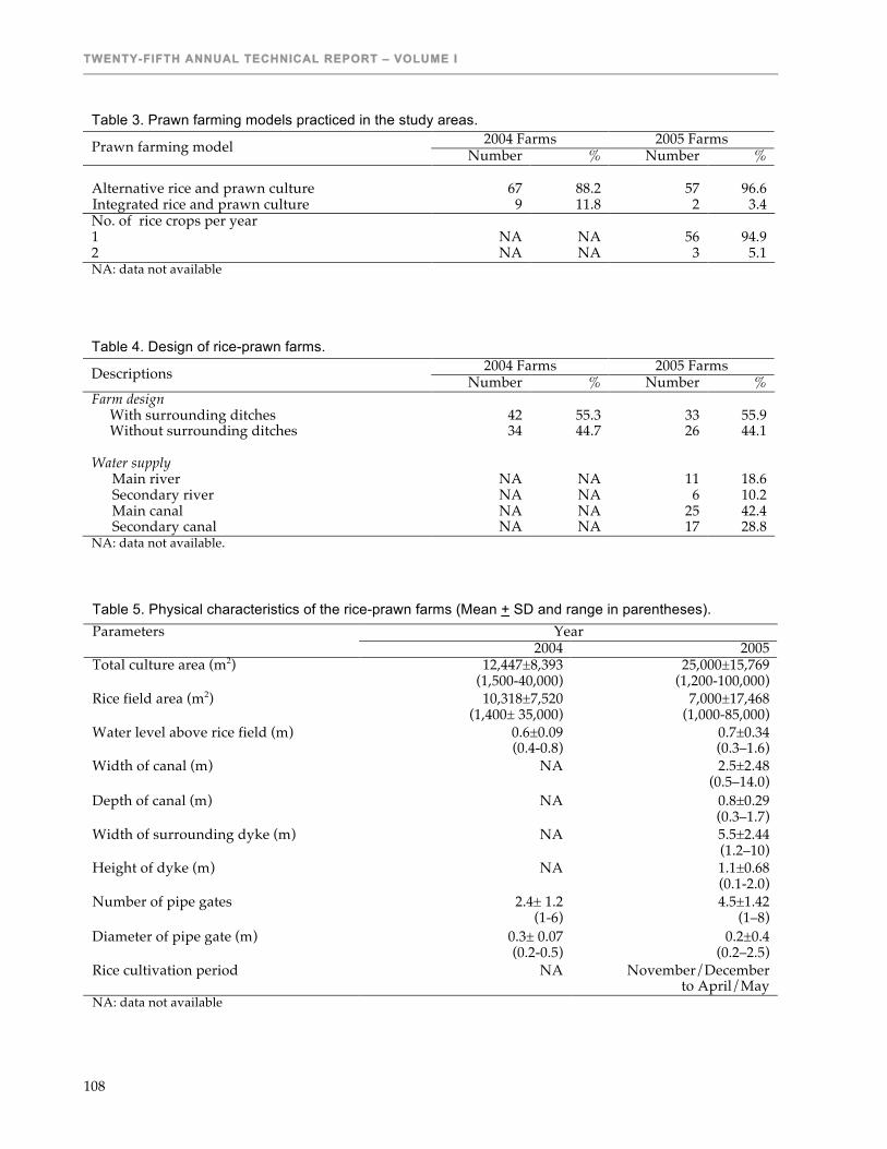
TWENTY-FIFTH ANNUAL TECHNICAL REPORT – VOLUME I
108
Table 3. Prawn farming models practiced in the study areas.
2004 Farms 2005 Farms Prawn farming model Number % Number % Alternative rice and prawn culture 67 88.2 57 96.6 Integrated rice and prawn culture 9 11.8 2 3.4 No. of rice crops per year 1 NA NA 56 94.9 2 NA NA 3 5.1 NA: data not available
Table 4. Design of rice-prawn farms. 2004 Farms 2005 Farms Descriptions Number % Number %
Farm design With surrounding ditches 42 55.3 33 55.9 Without surrounding ditches 34 44.7 26 44.1
Water supply
Main river NA NA 11 18.6 Secondary river NA NA 6 10.2 Main canal NA NA 25 42.4 Secondary canal NA NA 17 28.8
NA: data not available.
Table 5. Physical characteristics of the rice-prawn farms (Mean + SD and range in parentheses). Year Parameters
2004 2005 Total culture area (m2) 12,447±8,393
(1,500-40,000) 25,000±15,769
(1,200-100,000) Rice field area (m2) 10,318±7,520
(1,400± 35,000) 7,000±17,468
(1,000-85,000) Water level above rice field (m) 0.6±0.09
(0.4-0.8) 0.7±0.34 (0.3–1.6)
Width of canal (m) NA 2.5±2.48 (0.5–14.0)
Depth of canal (m) NA 0.8±0.29 (0.3–1.7)
Width of surrounding dyke (m) NA 5.5±2.44 (1.2–10)
Height of dyke (m) NA 1.1±0.68 (0.1-2.0)
Number of pipe gates 2.4± 1.2 (1-6)
4.5±1.42 (1–8)
Diameter of pipe gate (m) 0.3± 0.07 (0.2-0.5)
0.2±0.4 (0.2–2.5)
Rice cultivation period NA November/December to April/May
NA: data not available

PRODUCTION SYSTEM DESIGN & INTEGRATION
109
Table 6. Farm preparation levels for each year. 2004 Farms 2005 Farms Parameters Number % Number %
Burned rice straw 76 100.0 59 100.0 Ploughed rice field surface NA NA 11 18.6 Dried rice field surface 76 100.0 59 100.0 Renovated dykes NA NA 25 42.4 Excavated bottom 67 88.2 39 66.1 Limed 60 78.9 53 89.8 Fertilized 7 9.2 13 22.0 Rotenone treatment 76 100.0 29 92.8 Filtered water intake 70 92.1 59 100.0 NA: data not available
Table 7. Seed sources, stocking procedures and nursing methods in the study areas.
2004 Farms 2005 Farms Items Number % Number % Source of seed supply
Self-production 0 0 1 1.7 Local hatcheries 0 0 20 33.9 Within province 75 98.7 28 47.4 Other provinces 1 1.3 10 16.9
Stocking procedures No nursing 10 13.2 9 15.3 Nursing 66 86.8 50 84.7
Nursing Pond 0 0 20 33.9 Hapa net 0 0 1 1.7 Compartment in rice field 76 100 38 64.4 Area of nursing compartment (m2) 2,093±1,938
(240-10,000) 2,128±3,318 (100–20,000)
Stocking density (PL/m2) 9.7±3.6 (3-20)
8.0±2.91 (2–15)
Nursing duration (day) 30±4 (20-40)
25.6±2.93 (9-60)
Table 8. Water management in the surveyed farms. 2005 Farms Items Number %
Water quality monitoring Daily 10 23.8 Weekly 22 52.4 Biweekly 7 16.6 Monthly 3 7.2
Water discharge To settling rice field 1 1.7 To canal/river 58 98.3

TWENTY-FIFTH ANNUAL TECHNICAL REPORT – VOLUME I
110
Table 9. Mean (+SE) culture cycle duration and production for prawn farmers. Values in parentheses are ranges.
Items 2004 2005 Culture duration (months) 6±0.7
(5-8) 7±0.6 (6–8)
Productivity (kg/ha) 1,452±624 a (66.7-3330)
1,150±471 b (180–2,333)
Mean values with different superscript letters in the same row were significantly different (P<0.05). Table 10. Cost/benefit analysis of rice-prawn alternative farming model in the study areas (1US$=16,000VND). Mean + SD (range in parentheses).
Item 2004 2005 Price of stocked post-larvae (VND/individual)
113± 8.8 (80-120)
110±10.9 (80–120)
Selling price of harvested prawn (VND/kg)
75,000±10,470 (45,000-100,000)
88,500±6,329 (65,000–95,000)
Total cost of production (million VND/ha)
74.830±46.820 (19.904-303.201)
35.888±97.602 (9.537–640.000)
Gross income (million VND/ha)
109.003±49.531 (3.000-262.083)
84.675±171.494 (14.760–1,066.667)
Net return (million VND/ha)
34.173±56.987 (-143.022-154.444)
48.788±77.786 (37.273–426.667)
The values in the parentheses are ranges.

PRODUCTION SYSTEM DESIGN & INTEGRATION
111
OPTIMIZATION OF FERTILIZATION REGIME IN FERTILIZED NILE TILAPIA PONDS WITH SUPPLEMENTAL FEED
Twelfth Work Plan, Production System Design & Integration 2 (12PSD2)
Final Report Published as Submitted by Contributing Authors
Moe Thidar Oo, Dhirendra Prasad Thakur & Yang Yi
Asian Institute of Technology Pathumthani, Thailand
James S. Diana & C. Kwei Lin
University of Michigan Ann Arbor, Michigan, USA
ABSTRACT An experiment was conducted in fifteen 200-m2 earthen ponds at the Asian Institute of Technology, Thailand during September 2005 to January 2006. The objectives of this experiment were to determine effects of different rates of phosphorus fertilizer application on Nile tilapia (Oreochromis niloticus) production, pond water quality parameters and nutrient utilization efficiency under supplemental feeding, and to evaluate the cost and return of Nile tilapia production. Five phosphorus fertilization rates were used as treatments in a randomized completely block design: 100%, 75%, 50%, 25% and 0% of 7 kg P ha-1wk-1. Nitrogen fertilization rate was fixed at 28 kg N ha-1wk-1 for all the treatments throughout the experiment. Sex-reversed all-male Nile tilapia of about 100 g size were stocked at 3 fish m-2, and fed at 50% satiation feeding rate during the culture period. Mean weight, mean weight gain, daily weight gain and net fish yield were not significantly different among treatments (P>0.05). Water quality parameters were not significantly different among treatments, except total Kjeldahl nitrogen, total phosphorus and soluble reactive phosphorus. Nutrient budget showed that higher rates of phosphorus fertilizer input resulted in higher phosphorus sink in the sediment. Economic analysis showed that all the treatments with phosphorus fertilization resulted in positive net returns. Gross income was not affected by different phosphorus fertilization rates. Treatment with 25% phosphorus fertilization might be used as an alternative strategy for Nile tilapia pond culture in terms of economic return and nutrient loss in sediment.
INTRODUCTION Nile tilapia (Oreochromis niloticus) is commonly produced in semi-intensive culture systems in Southeast Asia using fertilization to increase primary production (Boyd, 1976; Diana et al., 1991). In many Asian countries, additions of supplemental feeds into fertilized ponds are becoming more and more popular for tilapia production. Supplemental feeding in fertilized ponds results in a faster fish growth and a higher pond yields at high stocking density compared to the pond that receives only fertilization (Hepher, 1963; Tacon, 1988). There is voluminous literature available on optimization of fertilization rate in fish ponds applied with inorganic or organic fertilizers or their combinations as the sole nutrient inputs (Hickling 1962; Boyd 1976, 1978; Olah 1986; Green et al., 1990; Diana et al., 1991; Knud-Hansen et al., 1991; Edwards, 1994; Lin et al., 1997a). The natural foods in fertilized ponds increase efficiency of supplemental feeds significantly and lead to lower FCR (Diana et al., 1994). Diana et al. (1994) determined that feeding rate of 50% ad libitum was optimal in ponds fertilized at a fixed rate of 28 kg N and 7 kg P ha-1wk-1. Furthermore, Diana et al. (1996) observed that the initiation of supplemental feeding at 50% ad libitum once fish reached 100 g is the most cost-effective way to produce large tilapia.

TWENTY-FIFTH ANNUAL TECHNICAL REPORT – VOLUME I
112
The above recommended fertilization rate is appropriate when fertilizer serves as the sole nutrient input for Nile tilapia culture in the tropics (Knud-Hansen et al. 1991). But the nutrients may become excessive in ponds with supplemental feeding as substantial amounts of nutrients are also released from feeding wastes to pond water and eventually lead to excessive phytoplankton production (Lin, 1990; Lin and Diana, 1995; Yi et al., 1996; Yi and Lin, 2001; Yi et al., 2001). It is ecologically and economically important to maintain adequate production of natural foods in fed ponds with balanced nutrient inputs from both external fertilization and internal wastes. To minimize nutrient wastage the rate of external fertilization needs to be adjusted according to the amount of nutrients derived from feeding wastes. Such practice will result in more efficient utilization of nutrients, better water quality, lower production cost and reduced nutrient load in pond effluents. Previous research has dealt with different combinations of fertilizers and feeds (e.g., Diana et al., 1994; Milstein et al., 1995). However, almost all research to optimize supplemental feeding rate has been conducted in ponds with fixed fertilization rates and none has been reported on optimizing fertilization regimes in fertilized ponds with supplemental feeds. Therefore, it is of interest to carry out study to optimize external fertilization rate for semi-intensive tilapia culture system under supplemental feeding. This study was conducted to optimize phosphorus input in Nile tilapia ponds with supplemental feed, with the following specific objectives: 1. To determine the effect of different rates of phosphorus fertilizer application on Nile Tilapia
production; 2. To evaluate the effect of different rates of phosphorus fertilizer application on pond water
quality; 3. To quantify nutrient budget in supplementary feed fed Nile tilapia ponds with different
phosphorus fertilization rates; 4. To evaluate the cost and return of Nile tilapia production with different rates of phosphorus
fertilization.
MATERIALS AND METHODS The experiment was carried out in 15 earthen ponds of 200 m2 in surface area at the Asian Institute of Technology (AIT), Thailand for 130 days from 01 September 2005 to 09 January 2006. Sex-reversed all-male Nile tilapia of average weights of 93.2-97.0 g were stocked at 3 fish m-2 in all ponds. There were five phosphorus fertilization rates as treatments with three replicates each: 0%, 25%, 50%, 75%, and 100% of 7 kg P ha-1 wk-1, equivalent to 0, 1.75, 3.50, 5.25, and 7 kg P ha-1 wk-1, respectively. All ponds were fertilized with urea at a rate of 28 kg N ha-1 wk-1. The treatments were assigned to the experimental ponds randomly. All ponds were drained completely and dried for 2 weeks prior to the start of the experiment. Pond bottom soil was sampled and analyzed for general soil feature and lime requirement, then the ponds were limed using calcium carbonate at rates of 102-148 kg pond-1, which were determined based on soil pH. Three days after liming, all ponds were filled with water from a nearby canal to a depth of 1 m. A fine mesh screen bag was fixed at the water inlet of each pond while filling water to avoid entry of wild fish and foreign materials. All ponds were fertilized two weeks prior to fish stocking. Throughout the experimental period, pond water level was maintained at 1 meter by adding water weekly to replace water losses due to seepage and evaporation. There was no water exchange during the experimental period. Tilapia in all the experimental treatments were fed at 50% of satiation feeding rates with floating pelleted feed (30% crude protein). To determine satiation feeding rates, fish were fed to satiation during 0900-1000 h and 1500-1600 h once in a week on every Thursday, and total consumption was determined for each pond. The average consumption for each treatment was used to set the satiation feeding rate at 50% of that level for each treatment for the remainder of the week, i.e. from Friday through Wednesday.

PRODUCTION SYSTEM DESIGN & INTEGRATION
113
During the experiment, fish sampling was conducted biweekly using a cast net. About 10-20% of the initially stocked numbers were sampled randomly. Sampled fish were counted and batch weight was determined. Nutrient budget was calculated based on the inputs and outputs of total nitrogen (TN) and total phosphorus (TP) in various components in the ponds. At the beginning and end of the experiment, water, fish, and feed were sampled and analyzed for moisture, TN, and TP. Initial and final soil samples were collected at top 10 cm surface soil from five different locations in each pond by using plastic tubes (10 cm in length and 5 cm in diameter), and were analyzed for bulk density, moisture, TN and TP. Moisture was analyzed by drying the samples in an oven at 103ºC for 24 to 72 h until constant dry weight was achieved. Pond water samples were taken biweekly at 0900-0930 h by using a column sampler and were analyzed for total alkalinity, total ammonia nitrogen (TAN), nitrite nitrogen (nitrite-N), nitrate nitrogen (nitrate-N), total Kjeldahl nitrogen (TKN), soluble reactive phosphorus (SRP), TP, chlorophyll a, total suspended solids (TSS), and total volatile solids (TVS) using standard methods (APHA et al., 1985). Canal water (source water) was sampled every time while filling the ponds and analyzed for TKN, nitrite-nitrate nitrogen and TP by using standard methods (APHA et al., 1985). Temperature, dissolved oxygen (DO) and pH were measured at 25 cm below the water surface, middle and 25 cm above the bottom using a YSI model 58 oxygen meter (Yellow Spring Instrument, Yellow Spring, OH, USA and a pH meter (Model HI 8424, HANNA Instruments, Thailand), and Secchi disk visibility was measured in situ before collecting water samples. In addition, monthly diel measurements of temperature, DO and pH were conducted at 0600, 1000, 1400, 1800, 2200, and 0600 h next day in each pond. A partial budget analysis was conducted to determine economic return of tilapia cultured at different phosphorus fertilization rates during the experiment (Shang, 1990). The analysis was done based on farm-gate prices for harvested tilapia and local market prices for other items expressed in US dollar (1US$ = 39 Baht). Farm-gate price of 300-400 g size tilapia were $0.641 kg-1,
while market prices were $0.026 piece-1 for juvenile sex-reserved tilapia, $0.178 kg-1 for urea, $ 0.298 kg-1 for TSP, and $0.48 kg-1 for feed. The calculation for cost of working capital was based on an annual interest rate of 8%. The profitability for the different phosphorus fertilization regimes was compared in terms of total variable cost (including cost of seed, urea, TSP, feed and cost of working capital), gross revenue (from selling tilapia). Gross return was calculated by deducting total variable cost from total gross revenue. In the analysis, facility cost and labor were not included because the objective was only to compare relative differences in efficiency among treatments. The data for fish growth performance, water quality, nutrient utilization efficiency and economic return were analyzed for significant differences among treatments using one-way analysis of variance (ANOVA) and regression (Steele and Torrie, 1980) using SPSS (version 11.0) statistical software package (SPSS Inc., Chicago, USA). Treatment means were compared using LSD and differences among treatments were considered significant at an alpha level of 0.05. Means were given with ± standard deviation (SD). Data in percentage were arsine transformed prior to analysis.
RESULTS Initial weight of Nile Tilapia ranged from 93.2 to 97 g in all treatment ponds. Fish growth was linear and followed similar trend in all treatments during the experimental period (Figure1). At harvest, mean weights of tilapia reached 372.4, 375.6, 353.7, 352.0, and 355.3 g with daily mean weight gains of 2.15, 2.14, 1.98, 1.97, and 1.99 g fish-1 day -1 in 100%, 75%, 50%, 25%, and 0% P treatments, respectively (Table 1). Mean weights at harvest and mean daily weight gains were not

TWENTY-FIFTH ANNUAL TECHNICAL REPORT – VOLUME I
114
significantly different (P>0.05) among the treatments. High daily weight gains were registered in all the treatments during the early experimental period, and reduced daily weight gains were observed towards the end of the experiment (Figure 1). Survival rates ranged from 90.63% to 95.03% in all the treatments, and was not significantly different among the treatments (P>0.05). Total harvested biomass was also not significantly different among the treatments (P>0.05). Net fish yields were 156.42, 147.15, 134.23,141.64, and 142.35 kg pond-1 crop-1 in 100%, 75%, 50%, 25% and 0% P treatments, respectively (Table 1), and were not significantly different among the treatments (P>0.05). Feed conversion ratio (FCR) ranged from 1.13 to 1.24 in all the treatments, and was not significantly different (P>0.05) among the treatments. Specific growth rate in 100%, 75%, 50%, 25%, and 0% P treatments were 1.06%, 1.04%, 1.00%, 1.00%, and 1.01%, respectively, without significant differences (P>0.05) among the treatments. Final mean weights increased linearly with increasing total feed input (Figure 2). A positive correlation was also found between net fish yields and total feed input during the experimental period (Figure 2). However, mean weight gain and net fish yield was not correlated with the total phosphorous fertilizer inputs during the experimental period (Figure 3). Recruitments were found in all treatments except 75% P treatment, indicating that the sex-reversal was incomplete. However, total weight of recruits did not differ significantly (P>0.05) among the treatments. Nutrient budgets for nitrogen and phosphorus in all the treatments over the experimental period are presented in Tables 2 and 3. In all the treatments, fertilizer was the dominant input of nitrogen followed by feed, water, and stock fish; whereas, feed was the dominant input of phosphorus followed by fertilizer, stock fish, and water. Nitrogen outputs in harvested fish and drained water were not significantly different (P>0.05) among the treatments. Nitrogen and phosphorus outputs in sediment were estimated by subtracting the amount in the sediment before start of the experiment from the amount in the sediment at the harvest, and thus, the gain of nutrient in the sediment in Tables 2 and 3 was described as the outputs. Nitrogen outputs in sediment was significantly different (P<0.05) between 100% and 50% P treatments. Nitrogen outputs in the drained water was not significantly different among the treatments. Unaccounted nitrogen was not significantly different (P<0.05) among the treatments. Phosphorus budget revealed that fertilizer was the dominant input in 100% and 75% P treatments followed by feed and stocked tilapia (Table 3). At the end of experimental period, phosphorus loss through water was 0.08, 0.08, 0.05, 0.06, and 0.06 kg pond-1 in 100%, 75%, 50%, 25% and 0% P treatments, respectively, and was not significantly different (P>0.05) among the treatments. There was no significant difference in phosphorus gain through sediments in 100% and 75% P treatments. Total phosphorus outputs were significantly higher (P<0.05) in 75% and 100% P treatments than those in 0%, 25%, and 50% P treatments. Phosphorus outputs in sediment were significantly higher (P<0.05) in 75% and 100% P treatments than those in 0%, 25%, and 50% P treatments. Unaccounted phosphorus values were not significantly different (P>0.05) among the treatments. Nutrients recovered in harvested fish biomass were 3.67, 3.34, 3.00, 3.32 and 3.33 kg N and, 0.81, 0.78, 0.76, 0.79 and 0.81 kg P in 100%, 75%, 50%, 25% and 0% P treatments, respectively, which were not significantly different (P>0.05) among the treatments. Nitrogen and phosphorus distribution for inputs through fertilizer and feed, and gains in the harvested biomass, water, and sediments over the experimental period are presented in Table 4. Fertilizer was the major source of nitrogen input which accounted for 50.7% – 52.1% of the total added nitrogen in all the treatments. Percentage of phosphorus input through feed increased significantly with the reduced phosphorus fertilization rate. Feed was the only source of phosphorus input in the treatment with 0% P, which accounted for 100% of the total phosphorus input. Percentage of nitrogen gain in the harvested biomass was not significant different (P>0.05) among the treatments. Harvested tilapia removed 18.5% – 44.9% P of the total added phosphorus inputs, which was highest in 0% P treatment, intermediate in 25% P treatment, and lowest in 100%, 75%, and 50% P treatments. Percentage phosphorus recovered in harvested tilapia biomass was not significantly different (P>0.05) among 100%, 75%, and 50% P treatment. Nitrogen and

PRODUCTION SYSTEM DESIGN & INTEGRATION
115
phosphorus gains in water were not significantly different (P>0.05) among the treatments, while nitrogen and phosphorus trapped in sediment accounted for 34.9% to 73.7% of the total added nitrogen and 3.9 to 44.2% of the total added phosphorus. Percentage of nitrogen trapped in sediment was significantly different between 100% and 50% P treatments (P<0.05). There were no significant differences in the percentage of phosphorus trapped in sediments in 100% and 75% P treatments, which were significantly higher (P<0.05) than that in 50%, 25%, and 0% P treatments. Unaccounted nutrients ranged from 3.4% to 49.4% of nitrogen, and from 35.5% to 60.1% of phosphorus of the total added inputs through feed and fertilizer. Unaccounted nitrogen was significantly (P<0.05) lower in 100% P treatment than those in 50%, 25% and 0%P treatments, while no significant difference (P>0.05) was found in unaccounted phosphorus among the treatments. Most of water quality parameters showed no significant difference among the treatments during the experimental period (Table 5). Water quality parameter within replicates of each treatment varied largely during the experimental period. Water temperature fluctuated between 22.3 and 31.9 ºC in all the treatments during the experimental period (Figure 4). Mean and final temperatures in all the treatments ranged from 28.5 to 29.1 ºC and 27.2 to 27.9 ºC, respectively. Mean DO concentrations at early morning (0600 h) in all the treatments ranged from 0.79 to 0.93 mg L-1, which were not significantly different (P>0.05). Mean DO concentrations at 0900 h in all the treatments ranged from 1.92 to 2.58 mg L-1. Final mean DO concentrations at 0900 h in all the treatments ranged from 1.41 to 1.98 mg L-1. DO concentrations in all the treatments fluctuated between 1.00-4.70 mg L-1 throughout the experimental period (Figure 4). The highest DO concentration was recorded at the beginning of the experiment in all the treatments. DO in all treatments showed declining trend with the progress of the experiment and dropped below 2.5 mg L-1 on the 8th week of the experiment. From 8th week onwards, DO values showed relatively stable in all the treatments, and ranged between 1.00 and 3.00 mg L-1 in the later half of the experiment. Values of pH ranged from 6.9 to 7.8 in all treatments during the experimental period (Figure 4), and mean pH values were not significantly different among the treatments (P>0.05). Total alkalinity concentrations in all the treatments ranged from 54.3 to 131.7 mg L-1, and the fluctuation in total alkalinity concentration showed distinct but irregular trend over the experimental period (Figure 5). TAN concentrations in all the treatments ranged from 0.03 to 3.45 mg L-1, and fluctuated over the experimental period (Figure 6). Nitrate-N and nitrite-N concentrations in all treatments fluctuated between 0.15 and 5.08 mg L-1 and between 0.12 and 1.16 mg L-1, respectively throughout the experimental period, without significant differences (P>0.05) among the treatments (Figure 6 and Table 5). Mean TKN concentrations in all treatments ranged from 3.53 to 16.03 mg L-1, reaching peaks around the 70th day of the experimental period then declining towards the end of the experiment (Figure 6). Mean TKN concentration in 0% P treatment was significantly higher than that in other treatments (P<0.05), while there were no significant differences in the final TKN concentrations among the treatments (P>0.05). Mean TP concentrations in all treatments ranged from 0.23 to 1.06 mg L-1, and showed increasing trends over the experimental period (Figure 7). Mean TP concentrations were highest in 100% and 75% P treatments, intermediate in 50% and 25% P treatments, and lowest in 0% P treatment (P<0.05). SRP concentrations in all the treatments showed declining trends towards the end of the experiment (Figure 7). Mean SRP concentration was highest in 25% P treatment, intermediate in 50%, 75% and 100% P treatments, and lowest in 0% P treatment (P<0.05). Concentrations of chlorophyll a, TSS and TVS in all treatments increased towards the end of the experimental period (Figure 8), and did not significantly differ among treatments (P>0.05). Secchi disk visibility decreased towards the end of the experimental period (Figure 8), and mean and final values of Secchi disk visibility were not significantly different among the treatments. The results of the partial budget analysis indicated that there was significant difference in total variable costs, but no significant difference was found in gross revenue as well as gross return among all the treatments (Table 6). All the treatments showed to be profitable, while 25% P seemed to more promising.

TWENTY-FIFTH ANNUAL TECHNICAL REPORT – VOLUME I
116
DISCUSSION The result of the present study showed that under supplementary feeding condition different phosphorus fertilization rates had no effect on Nile tilapia growth performance. Even though fish were fed at 50% satiation level, the total feed amounts were same at all phosphorus fertilization rates. Also, mean daily weight gain (1.97-2.15 g fish-1 day-1) was similar in all the treatments. In the present study physical, chemical and biological parameters did not differ significantly at all phosphorus fertilization rates, indicating that all treatments had the similar culture environment and access to natural foods. Tilapia growth rate observed in the present study is similar to those (1.74-2.15 g fish-1 day-1) in fed alone ponds or fertilized ponds with supplemental feeding reported by Diana et al. (1994). The result of the present study is comparable to the growth rate observed by Truc (2005) under similar culture condition at different nitrogen fertilization rates with supplemental feeding. However, the growth rate observed in the present study is lower than that (3.10 g fish-1 day-1) under fertilization with supplemental feeding (Diana et al. 1996). Thakur et al. (2004) also reported a higher growth rate (2.66 g fish-1 day-1) of Nile tilapia under continued regular pond fertilization in addition to 50% satiation feeding. Daily weight gains in all treatments of the present study fluctuated during the experimental period, but, in general, showed a declining trend with the progress of culture. Furthermore, the relatively slower growth period of tilapia during the experimental period corresponds to the lower DO concentration in water. The result of the present study indicates that the low DO concentration during night time and mainly in the early morning in all the treatments, particularly towards the later half of the culture period, might have slowed down Nile tilapia growth and thus, might have masked the treatment effects in this study. In the present study, FCR was similar in all the treatments and ranged from 1.13 to 1.24. FCR observed in the present study is similar to that obtained under different nitrogen rates with supplemental feeding (Truc, 2005). However, a better FCR (0.87) was reported by Thakur et al. (2004) in fertilized ponds throughout the culture period and feeding starting from day 80. No significant difference in FCR among all treatments in the present study suggests that different phosphorus fertilization rates had no effect on feed utilization efficiency of Nile tilapia. Nile tilapia yield was not significantly different among all treatments in the present study, suggesting that phosphorus fertilization rates had no effect on tilapia growth. The result of the present study is in agreement with the contention of Brunson et al. (1999) who mentioned that it is usually not necessary to fertilize ponds in which the fish are fed regularly, since uneaten feed is a supplemental nutrient source. Zonneveld and Fadhli (1991) mentioned that feed intake in tilapia ponds is influenced by environmental factors. Final mean weights and net yield of tilapia are positively correlated with total feed inputs, but yield of tilapia and mean weight gain are not correlated with total phosphorus fertilizer inputs in the present study. The results of the present study indicate that under supplementary feeding condition growth performance of Nile tilapia is more dependent on the added feed and less on the fertilizer inputs to stimulate natural food. Nutrient budgets revealed that feed and fertilizer are the major sources of nitrogen and phosphorus inputs. The nutrient recovery percentage of nitrogen in harvested tilapia (15.43-18.40%) in the present study is similar to those (15.45-20.04%) previously reported by Lin et al. (1997b). However, Truc (2005) observed a higher nitrogen recovery (19.26-37.14%) in harvested tilapia in an experiment on optimizing nitrogen rates. Phosphorus recovery percentage (18.47-44.90%) in harvested tilapia in the present study is higher than those (10.02-15.10%) reported previously by Lin et al. (1997b). Nitrogen budget showed that a large potion of total nitrogen inputs (34.90-73.70% N) lost to the sediment. But in case of phosphorus the largest proportion of total nutrient inputs (35.53-60.07% P) were unaccounted. The unaccounted phosphorus might have resulted from the mud adsorption, as mud has strong attraction for phosphorus (Boyd, 1985). Higher proportion of total phosphorus outputs in sediment was observed in the treatments with 100% and 75% P than the other treatments. The result indicates that increased phosphorus fertilization rate resulted in higher phosphorus accumulation in the sediment. Masuda and Boyd (1994) emphasized that much of the fertilizer phosphorus not removed in fish but accumulated in

PRODUCTION SYSTEM DESIGN & INTEGRATION
117
sediment. Hickling (1962) also reported that inorganically fertilized ponds often lose phosphorus to sediments. Nitrogen fertilizer not removed in fish was incorporated in sediment as organic nitrogen or lost to the atmosphere through denitrification and ammonia volatilization (Gross et al., 2000). In the present study, nutrients contained in sediment were higher than those in the effluent water. The results are in agreement with the observation of Avnimelech et al. (1984) who found that the sediment layer of few centimeters depth contains more nutrient than the water column. Water temperature during the experimental period ranged from 22.30 to 31.9 ºC, which is suitable for tilapia feeding and growth (Cherviski, 1982). Mean DO concentrations at early morning observed in the present study were much higher than those reported by Truc (2005). Moreover, low growth phase of tilapia in the present study, observed during the later half of the culture, is correspondent with the low DO concentrations. Boyd (1990) also noted that when fish fed ad libitum, the weight gain and feed consumption decline with decreasing DO concentration. In contrary, Liti et al. (2002) observed that low DO concentration at dawn had no significant effect on tilapia growth. Most of the water quality variables are not significantly different among the treatments with the exception of the TP, TKN and SRP in the present study. The results of the present study showed that different phosphorus fertilization rates in all treatments did not significantly affect the major water quality parameters. In the present study, phosphorus concentration in water was not high even in the ponds with the highest fertilizer rate. The result shows that higher phosphorus fertilizer rate not necessarily results in higher phosphorus content in water column as the added phosphorous removed form the water column by other processes possibly sinks to the bottom sediment. Recently, Wudtisin and Boyd (2005) in a study on bluegill also observed that higher rate of fertilizer had no effect on concentration of total nitrogen and phosphorus in pond water. Aquaculture ponds receiving feeds often have total phosphorus concentrations above 0.5 mg L-1 and total nitrogen concentrations of 2 or 3 mg L-1 (Boyd and Tucker, 1998). Total phosphorus and nitrogen concentrations in water in the present study during most of the sampling remained 0.5 mg L-1 and 4 mg L-1, respectively. The result suggests that the system never becomes nutrient limiting during the experimental period. Furthermore, relatively small proportions of total nitrogen and phosphorus inputs were transferred to fish and thus, most of the applied nitrogen and phosphorus were removed from the water by other processes. Mean value of chlorophyll-a concentration in all treatments increased gradually over the experimental period during the present study. Green (1992) also reported similar changes in primary production when fertilization and feeding was done. TSS and TVS were positively correlated with the chlorophyll-a concentration, while the Secchi disk visibility negatively correlated with the chlorophyll-a concentration, indicating that the number of phytoplankton increased with over time during the experiment. The results indicate that in the present study majority of the pond turbidity is from phytoplankton and not from the clay turbidity. The economic analysis showed that the positive gross return was found in all treatments, with the highest at 100% P and followed by 25% P, 75% P, 0% P, and 50% P treatments. Feed costs as a percent of total costs averaged 77.49% to 79.80% for all treatments in the present study. Total production cost in 100% P treatment was higher than that in 50% P, 25% P and 0% P treatments. In the present study, income from the sale of harvested tilapia was similar for all treatments. Among all treatments, 25% P of the standard phosphorus application (7 kg P ha-1 week-1) showed that feed and fertilizer costs about 78.69% and 4.37%, respectively, of the total production costs, which was the lowest among the treatments. Considering both tilapia growth and economic performance as well as environmental aspects, the phosphorus fertilization rate at 25% of the standard phosphorus rate (7 kg P ha-1 week-1), that is, 1.75 kg P ha-1 week-1, may be appropriate in tilapia ponds receiving 50% satiation feeding.
ANTICIPATED BENEFITS Results of this study will help to develop an appropriate fertilization strategy for Nile tilapia production in ponds with supplemental feed. It may benefit fish farmers in Asia and other c,

TWENTY-FIFTH ANNUAL TECHNICAL REPORT – VOLUME I
118
when extended on a large scale. The study itself demonstrated biological and economic efficiency to be gained by adjustments in fertilization rates.
ACKNOWLEDGMENTS The authors wish to acknowledge the Asian Institute of Technology, Thailand, for providing the research filed and laboratory facilities. Mr. Apiyut Siyapan and Mrs. Aye. Aye Mon are greatly appreciated for their field and lab assistance.
LITERATURE CITED APHA, AWWW and WPCF, 1985. Standard Methods for the Examination of Water and
Wastewater, 15th edn. American Public Health Association, American Water Works Association and Water Pollution Control Federation, Washington DC, U.S.A., 1134 p.
Avnimelech, Y., McHenry, J.R. and Ross, D.J., 1984. Decomposition of organic matter in lake sediments. Environment Science and Technology, 18 (1): 5-11.
Boyd, C.E., 1976. Nitrogen fertilizer effects on production of tilapia in ponds fertilized with phosphorus and potassium. Aquaculture, 7:385-390.
Boyd, C.E., 1978. Effluents from catfish ponds during fish harvest. J. Environ. Qual., 7:59-62. Boyd, C. E., 1985. Chemical budgets of channel catfish ponds. Trans. Amer. Fish. Soc., 114:291-298. Boyd, C.E., 1990. Water Quality in Ponds for Aquaculture. Alabama Agricultural Experiment
Station, Auburn University, Alabama. 482 p. Boyd, C.E., and Tucker, C.S., 1998. Pond Aquaculture Water Quality Management. Kluwer
Academic Publishers, Boston, MA, 700 p. Brunson, M.W., Stone, N. and Hargreaves, J., 1999. Fertilization of Fish Ponds. SRAC Publication
No. 471. Chervinski, J., 1982. Environmental physiology of tilapias. In: R.S.V. Pullin and R.H. Lowe-
McConnell (eds.), The Biology and Culture of Tilapias. ICLARM Conference Proceedings 7, International Center for Living Aquatic Resources Management, Manila, Philippines, pp.119-128.
Diana, J.S., Lin, C.K. and Schneeberger, P.J., 1991. Relationships among nutrient inputs, water nutrient concentrations, primary production, and yield of Oreochromis niloticus in ponds. Aquaculture, 92:323-341.
Diana, J.S., Lin. C.K. and Jaiyen. K., 1994. Supplemental feeding of tilapia in fertilized ponds. Journal of the World Aquaculture Society, 25:497-506.
Diana, J.S., Lin, C.K. and Yi, Y., 1996. Timing of supplemental feeding for tilapia production. Journal of the World Aquaculture Society, 27:410-419.
Edwards, P., 1994. An assessment of the role of buffalo manure for pond culture of tilapia. I. On-station experiment. Aquaculture, 126:83-95.
Green, B. W., 1992. Substitution of organic manure for pelleted feed in tilapia production. Aquaculture, 101:213-222.
Green, B.W., Teichert-Coddington, D.R. and Phelps, R.P., 1990. Response of tilapia yield and economics to varying rates of organic fertilization and season in two Central American countries. Aquaculture, 90:279-290.
Gross, A., Boyd, C.E and Wood, C.W., 2000. Nitrogen transformations and balance in channel catfish ponds. Aquacultural Engineering 24: 1-14.
Hepher, B., 1963. The years of research in fish pond fertilization in Israel. II. Fertilizer dose and frequency of fertilization. Bamidgeh, 15:78-92.
Hickling, C.F., 1962. Fish Culture. Faber and Faber, London. 317 p. Knud-Hansen, C.F., McNabb, C.D. and Batterson, T.R., 1991. Application of limnology for efficient
nutrient utilization in tropical pond aquaculture. Proceedings of the International Association of Theoretical and Applied Limnologists, 24:2541-2543.
Lin, C.K., 1990. Integrated culture of walking catfish (Clarias macrocephalus) and tilapia (Oreochromis niloticus). In R. Hirano and I. Hanyu (eds.), The Second Asian Fisheries Forum. Asian Fisheries Society, Manila, Philippines, pp. 209-212.

PRODUCTION SYSTEM DESIGN & INTEGRATION
119
Lin, C.K. and Diana, J.S., 1995. Co-culture of catfish (Clarias macrocephalus x C. gariepinus) and tilapia (Oreochromis niloticus) in ponds. Aquatic Living Resources, 8:449-454.
Lin, C.K., Teichert-Coddington, D.R. Green, B.W. and Veverica, K.L., 1997a. Fertilization regimes. In: H.S. Egna and C.E. Boyd (eds.), Dynamics of Pond Aquaculture. CRC Press, Boca Raton, Florida, pp. 73-107.
Lin, C.K., Yi, Y. and Diana, J.S., 1997b. The effects of pond management strategies on nutrient budgets: Thailand. In: D. Burke, B. Goetze and H.S. Egna (eds.), Fourteenth Annual Technical Report, Pond Dynamics/Aquaculture, Collaborative Research Support Program, Oregon State University, Corvallis, Oregon, USA, pp.19-24.
Liti, D. M., Mac’Were, O. E. and Veverica, K. L., 2002. Growth performance and economic benefits of Oreochromis niloticus/Clarias gariepinus polyculture fed on three supplementary feeds in fertilized tropical ponds. In: K. McElwee, K. Lewis, M. Nidiffer and P. Buitrago (eds), Nineteenth Annual Technical Report. Pond Dynamics/Aquaculture CRSP, Oregon State University, Corvallis, Oregon, pp.11-16.
Masuda, K. and Boyd, C.E., 1994. Phosphorus fractions in soil and water of aquaculture ponds built on clayey ultisols at Auburn, Alabama. Journal of the World Aquaculture Society, 25: 379-395.
Milstein, A., Alkon, A., Karplus, I., Kochba, M. and Avnimelech, Y., 1995. Combined effects of fertilization rate, manuring and feed pellet application on fish performance and water quality in polyculture ponds. Aquaculture Research, 26:55-65.
Olah, J., 1986. Carp production in manured ponds. In: R. Billard and J. Marech (eds.), Aquaculture of Cyprinids. IRNA, Paris, France, pp. 295-303.
Shang, Y.C., 1990. Aquaculture Economic Analysis: An Introduction. The World Aquaculture Society, 211 p.
Steele, R.G.D. and Torrie, J.H., 1980. Principles and Procedures of Statistics, 2nd edn. McGraw-Hill, New York, 633 p.
Tacon, A.G.J., 1988. The Nutrition and Feeding of Farmed Fish and Shrimp - A Training Manual: 3 Feeding Methods. FAO Field Document, Project GPC/RLA/075/ITA. Field Document 7/E, Brazilia, Brazil, 208 p.
Thakur, D.P., Yi, Y., Diana, J. S. and Lin, C. K., 2004. Effects of fertilization and feeding strategy on water quality, growth performance, nutrient utilization and economic return in Nile tilapia (Oreochromis niloticus) ponds. In: R. Bolivar, G.C. Mair, and K. Fitzsimmons (eds.), Proceedings of 6th International Symposium on Tilapia in Aquaculture, pp. 529-543.
Truc, L.T.T., 2005. Optimization of a Nitrogen Fertilization Regime in Fertilized Nile Tilapia (Oreochromis niloticus) Ponds with Supplemental Feed. Unpublished MSc Thesis, Asian Institute of Technology, Thailand, 76 p.
Wudtisin, W. and Boyd, C.E., 2005. Determination of the phosphorus fertilization rate for bluegill ponds using regression analysis. Aquaculture Research, 36: 593-599.
Yi, Y., Lin, C.K. and Diana, J.S., 1996. Influence of Nile tilapia (Oreochromis niloticus) stocking density in cages on their growth and yield in cages and in ponds containing the cages. Aquaculture, 146:205-215.
Yi, Y. and Lin, C.K., 2001. Effects of biomass of caged Nile tilapia (Oreochromis niloticus) and aeration on the growth and yields of all Nile tilapia in an integrated cage-cum-pond system. Aquaculture, 195:253-267.
Yi, Y., Lin, C.K. and Diana, J.S., 2001. Integrated recycle system for catfish and tilapia culture. In: A. Gupta, K. McElwee, D. Burke, J. Burright, X. Cummings and H.S Egna (eds.), Eighteenth Annual Technical Report. Pond Dynamics/Aquaculture CRSP, Oregon State University, Corvallis, Oregon, pp. 87-95.
Zonneveld, N. and Fadholi, R., 1991. Feed intake and growth of red tilapia at different stocking densities in ponds in Indonesia. Aquaculture, 99: 83-94.
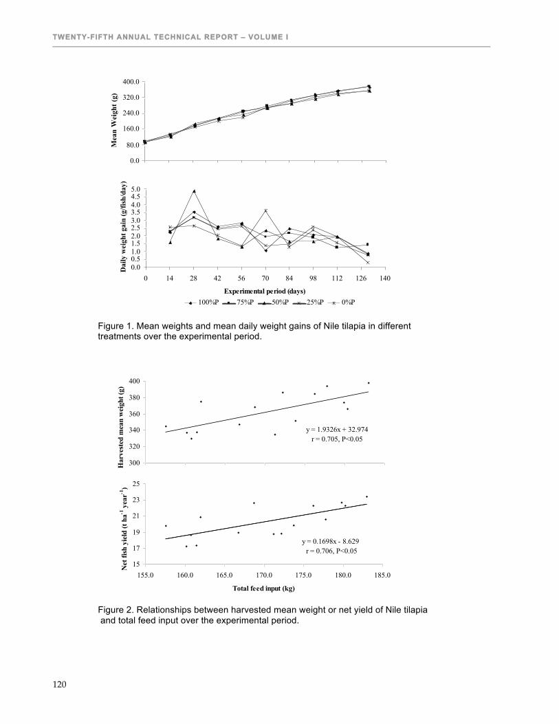
TWENTY-FIFTH ANNUAL TECHNICAL REPORT – VOLUME I
120
y = 1.9326x + 32.974r = 0.705, P<0.05
300
320
340
360
380
400
155 160 165 170 175 180 185
Total feed input (kg)
Har
vest
ed m
ean
wei
ght (
g)
y = 0.1698x - 8.629 r = 0.706, P<0.05
15
17
19
21
23
25
155.0 160.0 165.0 170.0 175.0 180.0 185.0
Total feed input (kg)
Net
fish
yie
ld (t
ha-1
yea
r-1)
Figure 1. Mean weights and mean daily weight gains of Nile tilapia in different treatments over the experimental period.
Figure 2. Relationships between harvested mean weight or net yield of Nile tilapia and total feed input over the experimental period.
0.0
80.0
160.0
240.0
320.0
400.0
0 14 28 42 56 70 84 98 112 126 140
Experimental period (days)
Mea
n W
eigh
t (g)
0.00.51.01.52.02.53.03.54.04.55.0
0 14 28 42 56 70 84 98 112 126 140
Experimental period (days)
Dai
ly w
eigh
t gai
n (g
/fish
/day
)
100%P 75%P 50%P 25%P 0%P

PRODUCTION SYSTEM DESIGN & INTEGRATION
121
y = 5.3399x + 137.67r = 0.343 (P>0.05)
101214161820222426
-0.50 0.00 0.50 1.00 1.50 2.00 2.50 3.00
TP input (kg)
Net
fish
yie
ld (k
g ha
-1ye
ar-1
)
y = 9.7241x + 254.08r = 0.383 (P>0.05)
200
220
240
260
280
300
320
-0.5 0 0.5 1 1.5 2 2.5 3
Total P fertilizer input (kg)
mea
n w
eigh
t gai
n (g
fish
-1)
22.024.0
26.0
28.0
30.032.0
34.0
0 14 28 42 56 70 84 98 112 126 140
Experimental period (days)
Tem
pera
ture
( o C
)
Figure 3. Relationships between net yield or mean weight gain of Nile tilapia and phosphorus input over the experimental period.
Figure 4. Fluctuations in water temperature, DO, and pH measured at 0900 h in different treatments over the experimental period.
0.51.01.52.02.53.03.54.04.55.0
0 14 28 42 56 70 84 98 112 126 140
Experimental period (days)
DO
(mg
L-1)
6.806.907.007.107.207.307.407.507.607.707.807.90
0 14 28 42 56 70 84 98 112 126 140
Experimental period (days)
pH
100%P 75%P 50%P 25%P 0% P

TWENTY-FIFTH ANNUAL TECHNICAL REPORT – VOLUME I
122
50
75
100
125
150
0 14 28 42 56 70 84 98 112 126 140Experimental period (days)
Alk
alin
ity (m
g L-1
)
100%P 75%P 50%P 25%P 0%P
Figure 5. Fluctuations in total alkalinity in different treatments over the experimental period
Figure 6. Fluctuations in TAN, nitrate-N, nitrite-N, and TKN in different treatments over the experimental period.
0.000.501.001.502.002.503.003.504.00
0 14 28 42 56 70 84 98 112 126 140Experimental period (days)
TA
N (m
g L-1
)
0.01.02.03.04.05.06.0
0 14 28 42 56 70 84 98 112 126 140Experimental period (days)
NO
3-N
(mg
L-1)
0.00.2
0.40.60.81.01.2
0 14 28 42 56 70 84 98 112 126 140Experimental period (days)
NO
2-N
(mg
L-1)
2.04.06.08.0
10.012.014.016.018.0
0 14 28 42 56 70 84 98 112 126 140
Experimental period (days)
TK
N (m
g L
-1)
100% P 75% P 50% P 25% P 0% P
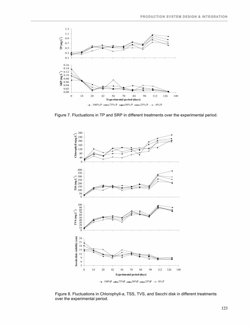
PRODUCTION SYSTEM DESIGN & INTEGRATION
123
0.1
0.3
0.5
0.7
0.9
1.1
1.3
0 14 28 42 56 70 84 98 112 126 140Experimental period (days)
TP (m
g L-1
)
0.000.020.040.060.080.100.120.140.16
0 14 28 42 56 70 84 98 112 126 140Experimental period (days)
SRP
(mg L
-1)
100% P 75% P 50% P 25% P 0% P
Figure 7. Fluctuations in TP and SRP in different treatments over the experimental period.
Figure 8. Fluctuations in Chlorophyll-a, TSS, TVS, and Secchi disk in different treatments over the experimental period.
04080
120160200240280
0 14 28 42 56 70 84 98 112 126 140Experimental period (days)
Chl
orop
hyll
a(µg
L-1)
050
100150200250300350400
0 14 28 42 56 70 84 98 112 126 140Experimental period (days)
TSS
(mg
L-1)
0102030405060708090
100
0 14 28 42 56 70 84 98 112 126 140
Experimental period (days)
TVS
(mg
L-1)
369
1215182124
0 14 28 42 56 70 84 98 112 126 140
Experimental period (days)
Secc
hi d
isk v
isibi
lity
(cm
)
100%P 75%P 50%P 25%P 0% P

TWENTY-FIFTH ANNUAL TECHNICAL REPORT – VOLUME I
124
Table 1. Growth performance (mean ± SD; n=3) of Nile tilapia cultured with different phosphorus fertilization regimes for 130 days in 200-m2 earthen ponds. Mean values with different superscript letters in the same row were significantly different (P<0.05).
Treatment 1 Treatment 2 Treatment 3 Treatment 4 Treatment 5 Parameters (100% P) (75% P) (50% P) (25% P) (0% P)
STOCKING Mean weight (g fish-1) 93.2±0.2 97.0±1.2 96.0±0.3 95.8±1.4 95.6±1.7 Total weight (kg pond-1) 55.9±0.2 58.2±0.7 57.6±0.2 57.5±0.8 57.4±1.0 Stocking density (fish m-2) 3 3 3 3 3 HARVEST Mean weight (g fish-1) 372.4±23.3 375.6±10.1 353.7±35.0 352.0±19.4 355.3±25.9 Total weight (kg pond-1) 212.3±13.4 205.4±12.0 191.8±11.6 199.1±18.8 199.7±13.1 Survival rate (%) 95.0±2.8 91.3±7.8 90.6±5.1 94.2±4.1 93.7±1.8 FCR 1.13±0.09 1.17±0.10 1.24±0.06 1.18±0.11 1.21±0.09 Mean weight gain (g fish-1) 279.2±23.3 278.5±9.6 257.7±35.0 256.2±20.6 259.7±27.6 Daily weight gain (g fish-1 day-1) 2.15±0.18 2.14±0.07 1.98±0.27 1.97±0.16 1.99±0.21 Specific growth rate (%) 1.06±0.05 1.04±0.02 1.00±0.08 1.00±0.05 1.01±0.07 Gross yield (kg pond-1 crop-
1) 212.3±13.4 205.4±12.0 191.8±11.6 199.1±18.8 199.7±13.1 Net fish yield (kg pond-1
crop-1) 156.42±13.29 147.15±12.36 134.23±11.45 141.64±19.52 142.35±14.02 RECRUITMENT Total weight (kg pond-1) 9.7±4.06 0.0±0.0 2.4±1.2 4.5±3.2 3.0±4.2 Mean weight (g fish-1) 13.2±5.0a 0.0±0.0c 10.8±2.6ab 7.5±4.8ac 5.3±7.4bc

PRODUCTION SYSTEM DESIGN & INTEGRATION
125
Table 2. Nitrogen budget (kg pond-1; mean ± S D; n=3) for different treatments over the culture period of 130 days. Notation as in Table 1.
Total Nitrogen (kg) Treatment 1 Treatment 2 Treatment 3 Treatment 4 Treatment 5 Parameters
(100% P) (75% P) (50% P) (25% P) (0% P) INPUTS Tilapia 1.10±0.00 1.15±0.02 1.13±0.01 1.13±0.02 1.13±0.02 Feed 9.84±0.41 9.63±0.52 9.35±0.55 9.30±0.69 9.61±0.27 Water 1.00±0.12 1.28±0.42 1.68±0.45 1.54±0.20 1.91±0.56 Fertilizer 10.10±0.00 10.10±0.00 10.10±0.00 10.10±0.00 10.10±0.00 Total 22.04±0.46 22.16±0.87 22.26±0.37 22.08±0.88 22.75±0.31 OUTPUTS Tilapia 4.77±0.34 4.48±0.24 4.14±0.34 4.45±0.39 4.45±0.17 Water 1.89±0.15 2.04±0.26 1.76±0.28 2.51±0.95 2.05±0.51 Sediment 14.70±1.50a 12.25±1.50ab 6.87±4.66c 12.01±1.84ab 7.91±3.02bc Total 21.33±1.15a 18.80±1.67ab 12.77±5.11c 19.00±1.51ab 14.40±3.64bc GAIN Tilapia 3.67±0.34 3.34±0.25 3.00±0.34 3.32±0.40 3.33±0.18 Water 0.89±0.13 0.75±0.67 0..07±0.73 0.97±1.02 0.14±0.72 Sediment 14.70±1.50a 12.25±1.50ab 6.87±4.66c 12.01±1.84ab 7.91±3.02bc UNACCOUNTED 0.68±0.97c 3.39±2.49bc 9.51±4.91a 3.10±2.41bc 8.33±3.48ab Table 3. Phosphorus budget (kg pond-1; mean ± SD; n=3) for different treatments over the culture period of 130 days. Notation as in Table 1.
Total Phosphorus (kg) Treatment 1 Treatment 2 Treatment 3 Treatment 4 Treatment 5 Parameters
(100% P) (75% P) (50% P) (25% P) (0% P) INPUTS Tilapia 0.25±0.00 0.26±0.00 0.26±0.00 0.26±0.00 0.26±0.00 Feed 1.83±0.08 1.80±0.10 1.76±0.10 1.75±0.13 1.80±0.05 Water 0.08±0.03 0.07±0.04 0.06±0.01 0.06±0.02 0.05±0.02 Fertilizer 2.52±0.00a 1.91±0.00b 1.26±0.00c 0.61±0.00d - Total 4.67±0.06a 4.03±0.06b 3.33±0.06c 2.67±0.12d 2.10±0.00e OUTPUTS Tilapia 1.06±0.12 1.04±0.06 1.02±0.23 1.05±0.10 1.06±0.01 Water 0.16±0.05 0.14±0.04 0.11±0.01 0.12±0.03 0.12±0.03 Sediment 1.92±0.13a 1.48±0.71a 0.42±0.35b 0.09±0.04b 0.07±0.04b Total 3.17±0.06a 2.67±0.74a 1.53±0.60b 1.27±0.15b 1.27±0.06b GAIN Tilapia 0.81±0.12 0.78±0.06 0.76±0.22 0.79±0.11 0.81±0.00 Water 0.08±0.03 0.08±0.02 0.05±0.02 0.06±0.03 0.06±0.02 Sediment 1.92±0.13a 1.48±0.71a 0.42±0.35b 0.09±0.04b 0.07±0.04b UNACCOUNTED 1.55±0.11 1.37±0.67 1.79±0.58 1.41±0.09 0.86±0.07

TWENTY-FIFTH ANNUAL TECHNICAL REPORT – VOLUME I
126
Table 4 Distribution (%; mean ± SD; n=3) of nitrogen and phosphorus in different treatments based on total inputs from fertilizer and feed for the culture period of 130 days. Notation as in Table 1.
Treatment 1 Treatment 2 Treatment 3 Treatment 4 Treatment 5 Parameters (100% P) (75% P) (50% P) (25% P) (0% P)
NITROGEN Inputs Feed 49.30±1.01 48.77±1.31 48.07±1.42 47.90±1.84 48.77±0.70 Fertilizer 50.70±1.01 51.23±1.31 51.93±1.42 52.10±1.84 51.23±0.70 Total 100.00 100.00 100.00 100.00 100.00 Gain Tilapia 18.40±1.66 16.90±0.95 15.43±1.50 17.10±1.45 16.87±0.97 Water 4.50±0.75 3.87±3.50 0.33±3.72 5.07±5.35 0.67±3.61 Sediment 73.70±6.78a 62.23±9.16ab 34.90±22.68c 62.10±11.30ab 40.20±15.60bc Total 96.60±4.99a 83.00±12.49ab 50.63±26.22c 84.27±11.66ab 57.77±17.58bc Unaccounted 3.40±4.99c 17.00±12.49bc 49.37±26.22a 15.73±11.66bc 42.23±17.58ab PHOSPHORUS Inputs Feed 42.06±0.99e 48.51±1.34d 58.19±1.31c 74.00±1.32b 100.00±0.00a Fertilizer 57.94±0.99a 51.49±1.34b 41.81±1.31c 26.00±1.32d 0.00±0.00e Total 100.00 100.00 100.00 100.00 100.00 Gain Tilapia 18.47±2.61c 20.97±1.17c 25.17±7.27c 33.47±3.02b 44.90±1.05a Water 1.80±0.61 2.07±0.51 1.60±0.75 2.63±1.37 3.30±0.95 Sediment 44.17±3.59a 39.50±18.02a 13.77±11.68b 3.87±1.25b 4.20±2.08b Total 64.47±1.79 62.57±18.82 40.53±19.41 39.93±4.63 52.37±3.15 Unaccounted 35.53±1.79 37.43±18.82 59.47±19.41 60.07±4.63 47.63±3.15

PRODUCTION SYSTEM DESIGN & INTEGRATION
127
Table 5. Mean and final values (mean ± SD; n=3) of the water quality parameters measured biweekly in different treatments over the experiment period. Notation as in Table 1.
Treatment 1 Treatment 2 Treatment 3 Treatment 4 Treatment 5 Parameters (100% P) (75% P) (50% P) (25%P) (0% P)
MEAN VALUES Temperature (0C) 28.6±0.1 28.6±0.1 28.9±0.3 28.7±0.2 28.8±0.3 DO at 0600 h (mg L-1) 0.93±0.21 0.86±0.25 0.79±0.25 0.97±0.26 0.90±0.29 DO at 1800 h (mg L-1) 7.03±0.98 6.03±0.60 6.23±1.10 6.27±1.36 5.23±0.64 DO at 0900 h (mg L-1) 2.58±0.28a 2.41±0.22ab 2.33±0.14ab 2.18±0.25bc 1.92±0.09c pH 7.4±0.1 7.4±0.0 7.4±0.0 7.4±0.1 7.3±0.1 Secchi disk visibility (cm) 11±1 11±3 11±2 11±0 12±1 Total alkalinity (mg L-1) 76±26 94±14 76±21 96±4 104±14 TAN (mg L-1) 0.83±0.58 1.05±0.55 1.12±0.91 1.35±0.36 1.97±1.07 Nitrate-N (mg L-1) 1.69±0.84 1.84±0.25 1.44±0.45 1.99±0.78 1.43±0.70 Nitrite-N (mg L-1) 0.43±0.05 0.31±0.05 0.38±0.10 0.52±0.10 0.53±0.11 TKN (mg L-1) 7.30±0.84b 7.89±0.78b 7.94±1.07b 8.51±0.98ab 9.49±1.94a TP (mg L-1) 0.63±0.12a 0.61±0.16a 0.56±0.06ab 0.54±0.10ab 0.47±0.07b SRP (mg L-1) 0.03±0.02ab 0.03±0.01bc 0.03±0.02ab 0.04±0.01a 0.02±0.01c TSS (mg L-1) 188±21 165±52 149±18 161±37 130±31 TVS (mg L-1) 60±7 54±12 54±5 57±3 51±4 Chlo-a (µg L -1) 131±29 132±44 103±31 114±30 84±13 FINAL VALUES Temperature (0C) 27.3±0.1 27.3±0.2 27.6±0.2 27.4±0.1 27.5±0.3 DO at 0600 h (mg L-1) 0.73±0.12 0.97±0.57 0.63±0.06 0.77±0.21 0.80±0.26 DO at 1800 h (mg L-1) 6.07±0.58 5.43±1.47 5.43±0.55 4.40±1.04 4.77±0.49 DO at 0900 h (mg L-1) 1.70±0.19ab 1.61±0.27b 1.98±0.24a 1.41±0.35b 1.56±0.07b pH 7.3±0.2 7.4±0.0 7.6±0.1 7.4±0.2 7.4±0.1 Secchi disk visibility (cm) 9±1 8±1 8±1 8±1 9±1 Total alkalinity (mg L-1) 66±46 75±21 66±43 85±9 110±19 TAN (mg L-1) 0.49±0.72 1.30±1.13 0.05±0.01 0.47±0.76 0.98±0.56 Nitrate-N (mg L-1) 2.94±0.78 3.15±0.55 2.75±0.67 5.08±2.99 2.99±1.43 Nitrite-N (mg L-1) 0.27±0.09 0.35±0.12 0.36±0.14 0.38±0.10 0.46±0.35 TKN (mg L-1) 8.55±0.58 8.52±1.30 7.34±0.48 9.70±2.12 8.77±2.16 TP (mg L-1) 0.99±0.31 0.85±0.25 0.62±0.15 0.76±0.18 0.69±0.16 SRP (mg L-1) 0.00±0.00 0.01±0.01 0.00±0.01 0.00±0.00 0.00±0.00 TSS (mg L-1) 385±150 255±52 205±28 295±117 213±68 TVS (mg L-1) 90±20 75±20 77±12 79±15 81±8 Chlo-a (µg L -1) 262±21 222±78 210±54 192±39 198±88

TWENTY-FIFTH ANNUAL TECHNICAL REPORT – VOLUME I
128
Table 6. Partial budget analysis to compare profit (US$; mean ± SD; n=3) for different treatments over the culture period of 130 days, based on pond area of 200 m2. Notation as in Table 1.
Treatment 1 Treatment 2 Treatment 3 Treatment 4 Treatment 5 Parameters
(100% P) (75% P) (50% P) (25% P) (0% P) GROSS REVENUE Tilapia 136.10±8.58 131.63±7.71 122.97±7.44 127.63±12.02 128.07±8.43 VARIABLE COST Seed cost 15.6±0.0 15.6±0.0 15.6±0.0 15.6±0.0 15.6±0.0 Feed cost 91.23±3.75 89.30±4.81 86.80±5.03 86.40±6.36 89.30±2.45 Urea 3.9±0.0 3.9±0.0 3.9±0.0 3.9±0.0 3.9±0.0 TSP 3.80±0.00a 2.80±0.00b 1.90±0.00c 0.90±0.00d - Cost of working capital 3.27±0.12a 3.17±0.15ab 3.07±0.12b 3.07±0.21b 3.10±0.10b Total cost 117.73±3.85a 114.83±4.96ab 111.23±5.17b 109.80±6.53b 111.90±2.55b GROSS RETURN 18.37±8.03 16.80±7.33 11.73±3.67 17.83±7.41 16.13±6.33 ADDED COST 5.85 2.93 -0.67 -2.07 - ADDED RETURN 2.23 0.69 -4.40 1.68 - ADDED RETURN/ADDED COST 0.38 0.24 6.59 -0.81 -

PRODUCTION SYSTEM DESIGN & INTEGRATION
129
USE OF RICE STRAW AS A RESOURCE FOR FRESHWATER POND CULTURE: PERIPHYTON SUBSTRATE
Twelfth Work Plan, Production System Design & Integration 3a (12PSD3a) Final Report
Published as Submitted by Contributing Authors
Rai Sunila & Yang Yi Asian Institute of Technology
Pathumthani, Thailand
Md. Abdul Wahab Bangladesh Agricultural University
Mymensingh, Bangladesh
James S. Diana & C. Kwei Lin University of Michigan
Ann Arbor, Michigan, USA
ABSTRACT In order to assess the feasibility of rice straw as periphyton substrates for freshwater fish culture, three on station trials were carried out. Experiment one was conducted to determine the appropriate loading level of rice straw in 5-m2 fertilized cement tanks without stocking fish. There were seven different loading rates of rice straw each in triplicate: 0, 625, 1,250, 2,500, 5,000, 10,000 and 20,000 kg ha-1 (dry matter basis). The loading rate of 625 kg ha-1 was best, and water quality deteriorated with increased loading rates of rice straw. Periphyton grown on rice straw surface alone could contribute a maximum fish production of 1,825 kg ha-1 y-1. Experiment two was conducted to optimize the number of rice straw mats used in fertilized 40-m2 ponds stocked with rohu (Labeo rohita), catla (Catla catla), mrigal (Cirrhinus mrigala), common carp (Cyprinus carpio) and silver carp (Hypophthalmichthys molitrix). There were six treatments in triplicate each: a) no rice straw mats (control); b) using rice straw mats to cover pond dikes; c) suspending one (1x 625 kg ha-1) rice straw mat in water column; d) suspending two (2 x 625 kg ha-
1) rice straw mats in water column; e) suspending three (3 x 625 kg ha-1) rice straw mats in water column; and f) suspending four (4 x 625 kg ha-1) rice straw mats in water column. The results showed that three straw mats per pond gave the highest total weight gain of fish (0.44± 0.07 t ha-1 90 days -1) among all treatments (P<0.05). In experiment three, plankton-based carp polyculture system was compared with two periphyton-based carp polyculture systems using rice straw mats (3 straw mats per pond, 3x625 kg ha-1) or kanchi (390 bamboo side shoots per pond) as substrates in fertilized ponds. Rice straw and kanchi treatments gave 38% and 47% higher total weight gains than that in the control (P<0.05), due probably to periphyton and bacterial biofilm from substrates. The rice straw treatment appeared to be more economical than the control and kanchi treatments. This study demonstrated that rice straw which is widely available at low-cost in South Asia can be used to increase fish production through the development of bacterial biofilm and periphyton. The technology is simple, cost effective and appropriate for resource poor farmers.
INTRODUCTION Aquaculture intensification is constrained by increased capital, labor and mechanization (Edwards, 1990). It is not affordable for small-scale farmers to practice intensive aquaculture. Therefore, semi-intensive aquaculture systems like periphyton-based aquaculture have potential

TWENTY-FIFTH ANNUAL TECHNICAL REPORT – VOLUME I
130
in resource poor countries of South Asia, where most farmers are poor, own small ponds, and need technologies that give high production from low input. Since periphyton-based aquaculture can be cost effective and give relatively high fish production, it has potential in rural aquaculture. A variety of materials have been used as periphyton substrates. Among these substrates, bamboo has performed best (Azim et al. 2002b) but it is expensive and prohibitive for small-scale rural farmers. There is a need to explore inexpensive and locally available substrates that enhance fish growth. Rice straw and kanchi (bamboo stick, hereafter kanchi) fall in this category. Rice straw is widely available in farms in South Asia because rice is widely cultivated in this region (FAO, 2004). Since rice straw has low nutritive value due to low crude protein (2.3%) and digestibility, farmers often burn rice straw in fields to use straw ash as fertilizer (Potikanond et al., 1987). Rice straw has potential to enhance fish production in aquaculture ponds through mitigating turbidity (Yi et al., 2003) and developing bacterial biofilm and periphyton (Ramesh et al., 1999). Bundled rice straw in tanks significantly increased the growth of rohu (Labeo rohita) and common carp (Cyprinus carpio; Ramesh et al. 1999; Mridula et al. 2005), and fringed lipped carp (Labeo fimbriatus; Mridula et al., 2003). However, extensive research has not been done to explore the potential and roles of rice straw as substrates in carp polyculture ponds. The purpose of the study is to assess the technical and economical feasibility of rice straw as substrates in carp polyculture ponds.
MATERIALS AND METHODS There were three experiments in the present study. Experiment I was conducted at the Asian Institute of Technology (AIT), Thailand, while experiments II and III were conducted at the Bangladesh Agricultural University (BAU), Mymensingh, Bangladesh.
Experiment I The experiment I was done in 21 cement tanks of 5 m2 (2.5 x 2 x 1.1m) at AIT for 35 days. The experiment had seven treatments each with three replicates: no rice straw mats (T1, control); and rice straw mats at loading rates of 0.0625 kg m-2 (T2), 0.1250 kg m-2 (T3), 0.2500 kg m-2 (T4), 0.5000 kg m-2 (T5), 1.0000 kg m-2 (T6), and 2.0000 kg m-2 (T7) on dry weight basis. Treatments were randomly assigned to tanks. Tanks were drained completely, dried for a week, and filled with water to 1 m deep. Then a rice straw mat (2 m x 1 m) was suspended in each tank using bamboo poles. Tanks were fertilized weekly with urea and triple super phosphate (TSP) at rates of 28 kg N
ha-1 week -1 and 7 kg P ha -1week -1, respectively. Temperature, dissolved oxygen (DO) and pH were monitored at 10, 50 and 70 cm below the water surface daily at 0600 h. Diel DO, temperature and pH were recorded weekly at 0600, 1000, 1400, 1800 and 0600 h of next day. Secchi disk visibility was measured daily at 0900-1000 h. Composite column water samples were collected weekly for the analyses of total alkalinity, total ammonia nitrogen (TAN), nitrite-nitrogen (nitrite-N), nitrate-nitrogen (nitrate-N), total Kjeldahl nitrogen (TKN), soluble reactive phosphorus (SRP), total phosphorus (TP), total suspended solids (TSS), total volatile solids (TVS) and chlorophyll a following APHA et al. (1980). For plankton analyses, five liters of composite water samples were collected from five locations of each tank, and the sampled water was passed through a plankton net (mesh size 25 µm) to concentrate the volume to 50 mL, which was preserved in small plastic bottles containing 6% formalin. Phytoplankton and zooplankton were enumerated using a Sedgewick-Rafter counting cell (S-R cell) under a binocular microscope. Phytoplankton and zooplankton densities were estimated using the following formula (Azim et al., 2001a).

PRODUCTION SYSTEM DESIGN & INTEGRATION
131
N= (PxCx100)/L Where, N= the number of plankton cells or units per litre of original water; P = the number of plankton contained in ten random fields of S-R cell; C = the volume of final concentrated sample (mL); L = the volume (L) of the pond water sample. Periphyton samples were collected starting from the second week after rice straw mat suspension in the water column. Pieces of rice straw were cut by scissors from three different depths (surface, middle and bottom) of each mat, and wrapped in aluminum foil for periphyton analyses. Each sample was then transferred to an Erlenmeyer flask containing 50 mL distilled water, and shaken in a mechanical shaker for 3 hours to detach periphyton from the straw surface. After removing periphyton from rice straw, each straw was dissected longitudinally to measure the surface area of the straw. The number of periphyton units was estimated using following formula:
N = (P x C x 100)/A Where N = Number of periphyton units; P = Number of periphyton units counted in ten random fields of S-R cell; C = Volume of final concentrated sample (mL); A = Area of rice straw (cm2). Identification of phytoplankton, zooplankton and periphyton was done to genus level using keys from Ward and Whipple (1959), Wetzel (1983) and Bellinger (1992). One sample from each replicate was used to determine dry matter and ash content of rice straw after periphyton were removed from rice straw following APHA et al. (1980). Dry matter, ash free dry matter and chlorophyll a were estimated weekly based on surface area of the rice straw. Rice straw samples were kept in sterilized tubes containing phosphate buffer solution and stored in a refrigerator at 4oC for bacteria analyses. Total plate count of bacteria was done following APHA et al. (1980). Bacteria total plate count was determined based on dry weight of rice straw. Experiment II Experiment II was conducted in eighteen 40 m2 (8 x 5m) ponds of 1.5 m deep at the Field Laboratory of BAU during September-December 2005. The experiment included six treatments in triplicate: 1) no straw mat (control, RS0); 2) rice straw mats covering the slope of dikes (RSS); 3) one rice straw mat per pond (RS1, 1 x 625 kg ha-1); 4) two rice straw mats per pond (RS2, 2 x 625 kg ha-1); 5) three rice straw mats per pond (RS3, 3 x 625 kg ha-1); and 6) four rice straw mats per pond (RS4, 4 x 625 kg ha-1). The treatments were allocated randomly to experimental ponds. Ponds were drained and rotenone applied at 8.03 kg ha-1 to kill predatory fish. After 7 days, ponds were limed with CaO at 250 kg ha-1. Five days later, rice straw mats (2 m x 1 m) were placed into the rice straw treatment ponds. Mats were prepared by pressing straw bundles between bamboo splits at a loading rate of 625 kg ha-1 on dry weight basis. The loading rate was derived from experiment I. Then, all ponds were filled to 1.1 m deep, and fertilized next day with urea, TSP and cow dung at rates of 31, 16 and 1,250 kg ha-1, respectively, and fertilization continued every two weeks. DO in the rice straw treatment ponds was monitored for a month until it recovered to 2.2 mg L-1. After DO recovery, 40 fingerlings of rohu (25.5±0.31 g), mrigal (26.2±0.93 g), catla (24.0±0.87 g), common carp (23.5±0.85 g) and silver carp (25.9±0.48 g) were stocked in each pond at a species ratio of 3:2:2:2:1.

TWENTY-FIFTH ANNUAL TECHNICAL REPORT – VOLUME I
132
DO, temperature and pH were recorded weekly at 0600, 1800 and 0600 h of next day. DO concentration was measured at 10 cm, 50 cm and 70 cm below water surface. Secchi disc visibility was monitored weekly at 0900 h. Composite column water samples were collected monthly at 0900-1000 h from three locations in each pond for analyses of total alkalinity, TAN, nitrite-N, nitrate-N, SRP, TP, chlorophyll a, TSS and TVS (APHA et al. 1980). Total nitrogen (TN) was analyzed following Raveh and Avnimelech (1979). Analyses of phytoplankton, zooplankton, periphyton and bacteria followed the methods described in experiment I. At least 30% of each stocked fish species were sampled monthly and weighed individually using an electronic scale. At the end, rice straw mats were removed from the ponds, and fish were seined, counted and weighed individually. Gross margin analysis was done to determine economic returns for all treatments, based on 40-m2 pond surface area and 90-day culture period. The local market prices of all inputs and outputs in Mymensingh were used in the economic analysis. Cost of bamboo was estimated considering three month culture period so that bamboo could be used for 9 crops. Experiment III Experiment III was conducted in nine 40-m2 (8 x 5m) ponds of 1.5 m deep at Field Laboratory of BAU for 90 days from February to May 2006. The experiment had three treatments in triplicate: 1) plankton-based system without substrate (control); 2) using rice straw mats as substrate; and 3) using kanchi as substrate. The treatments were randomly allocated to experimental ponds. Prior to placing substrates, all ponds were drained, dried and limed with CaO at a rate of 250 kg ha-1. The ponds were filled to 0.30 m deep three days later. Afterwards, 390 kanchi (1.5 cm in diameter and 1.8 m in length) and three rice straw mats (2 m x 1 m) were fixed vertically to the bottom of respective treatment ponds. The number of rice straw mats per pond was derived from experiment II. Rice straw mats were prepared as in Experiment I. All ponds were filled to 1.1 m deep and fertilized with urea, TSP and cow dung at rates of 31, 16 and 1,250 kg ha-1, respectively. DO concentrations in rice straw treatment ponds were monitored for two weeks until DO recovered to 2.1 mg L-1. Then 40 fingerlings of rohu (24.5±0.5 g), mrigal (25.1±0.6 g), catla (25.8±0.5 g), silver carp (30.4±0.9 g) and common carp (27.6±0.6 g) were stocked in each pond at 3:2:2:2:1 ratio. Analyses of water quality, phytoplankton, zooplankton, periphyton and bacteria used methods described in experiment II. An Ekman dredge covering an area of 225 cm2 (15 x 15 cm) was used to collect zoobenthic organisms monthly from the bottom of each pond. Sediment samples were collected from three different locations in each pond. The content of the dredge was thoroughly washed through a sieve of 250 µm mesh size. Zoobenthos were separated from sediment and kept in vials containing 10% formalin. Later, zoobenthos were identified using a dissecting microscope (CH40RF200 Model, Olympus, Japan) following keys from Ward & Whipple (1959) and Needham & Needham (1962). The number of benthic animals was estimated using following formula (Rahman et al., 2006):
N = (Y x 10,000)/3A Where, N= number of benthic organisms per square meter (individuals m-2) Y = total number of benthic organisms counted in 3 samples A = area of Ekman dredge (cm2)

PRODUCTION SYSTEM DESIGN & INTEGRATION
133
At harvest, substrates were removed from the ponds, and fish were collected, counted and weighed individually to estimate weight gain and survival rates. Gross margin analysis was done to determine economic returns for the three treatments. Data Analyses Data were statistically analyzed by one-way analysis of variance (ANOVA), regression and student’s t-test, using SPSS (version 11.0) statistical software package (SPSS Inc., Chicago, USA). Tukey’s t-test was performed to compare treatment means if significant differences were found by one-way ANOVA. Differences were considered significant at an alpha level of 0.05. All means were given with ± 1 standard error (S.E.).
RESULTS Experiment I DO (r2=0.60), pH (r2=0.70), and Secchi disk depth (r2=0.55) decreased significantly (P<0.05) with increased rice straw loading rates (Table 1). DO at three depths (10, 50 and 70 cm) and pH values were significantly lower in rice straw treatments than in the control (P<0.05). Secchi disk depth was significantly higher in the 0.25 kg m-2 treatment and lower in the 2.00 kg m-2 treatment (P<0.05). In contrast, total alkalinity (r2=0.97), nitrite-N (r2=0.60), TKN (r2=0.28), TP (r2=0.60), TSS (r2=0.63), TVS (r2=0.62) and chlorophyll a (r2=0.80) increased significantly with increasing rice straw loading rates. Total alkalinity, nitrite-N, TKN, TP, TSS, TVS and chlorophyll-a contents were significantly higher in the 2.00 kg m-2 treatment than in the other treatments (P<0.05). Increasing trends over time were found for alkalinity, TSS, and TVS, while decreasing trends occurred for nitrate, TN and TP There were no significant differences in phytoplankton and zooplankton densities overall among all treatments (P>0.05; Tables 2 and 3). Phytoplankton community was comprised of 8 groups, namely, Bacillariophyceae, Chlorophyceae, Cyanophyceae, Euglenophyceae, Chrysophyceae, Cryptophyceae, Raphidophyceae, and Xanthophyceae. In total, 51-60 phytoplankton genera were identified in the treatments. Zooplankton was comprised of 8 groups, including Sarcodina, Ciliata, Rotifera, Hydrozoa, Siphonophora, Crustacea, Monogononta, and Gastropoda. There were 18-25 zooplankton genera in the treatments. Plankton density fluctuated during the experimental period with a significant increase for Kanchi treatments in week 2. Periphyton density did not differ significantly among treatments (P>0.05; Table 4). The periphyton community was composed of 10 phytoplankton and 6 zooplankton groups. Periphyton found in the treatments with rice straw varied from 32-41 genera, and showed an increasing trend in rice straw treatments. Dry matter and ash free dry matter of periphyton were significantly higher in treatments T2 to T4 than in those with higher rice straw loading rates of (T5 and T6; P<0.05; Table 5). Ash content was significantly higher in the 0.06 kg m-2 treatment than that in the 0.25 and 2.00 kg m-2 treatments (P<0.05), while there were no differences among other treatments. Chlorophyll-a concentration of periphyton was significantly higher in the 0.13 kg m-2 treatment than in the 1.00 and 2.00 kg m-2
treatments (P<0.05). Total plate count of bacteria varied from 28-65 x 106 cfu g-1 in the treatments with rice straw, but were not significantly different among treatments (P>0.05; Table 4). Bacteria number fluctuated over time with peak values in the second week of the experiment. Experiment II Water quality parameters except DO and TN did not differ significantly among treatments (P>0.05, Table 6). DO concentration recorded at 0600 h at 10 cm below the water surface was significantly lower in the dyke-covered treatment (RSS) than in the control (RS0) (P<0.05), while all other treatments were not significantly different from RSS or RS0. TN was significantly higher in RS1, RS2, and RS4 (rice straw mats) than in the control or treatment RS3 (P<0.05), but was not significantly different from the dyke-covered treatment (Table 6). DO, nitrate-N and TSS increased over time, while Secchi disk depth and TAN decreased over time.

TWENTY-FIFTH ANNUAL TECHNICAL REPORT – VOLUME I
134
There were no significant differences in densities of plankton among all treatments (P>0.05; Table 7). Plankton communities were composed of four phytoplankton groups (Bacillariophyceae, Chlorophyceae, Cyanophyceae and Euglenophyceae) and three zooplankton groups (Sarcodina, Rotifera and Crustacea). In total, 55-56 genera were identified in the treatments. Plankton number reached maximum in the fourth month of the experiment in most treatments. Periphyton and bacteria data were based on two monthly samples (n=6) because rice straw was lost from the mats at the end of the second month of the experiment. Periphyton density did not differ significantly among treatments (P>0.05; Table 8). The periphyton community was composed of 40-43 genera in each treatment, belonging to groups of Bacillariophyceae, Chlorophyceae, Cyanophyceae, Euglenophyceae, Sarcodina and Rotifera. Total plate counts of bacteria were 1.0-2.2 (x106 cfu g-1) in the treatments, which did not differ significantly from each other (P>0.05; Table 8). There were no significant differences in individual final weight, daily and total weight gains of all carps except common carp among all treatments (P>0.05; Table 9). Total weight gain of common carp was significantly higher in RS1 than in the control (P<0.05), but was not significantly different from RSS or RS2-4. Combined total weight gain was significantly higher in RS3 than in the control (P<0.05), however, there were no significant differences among the rice straw treatments (P>0.05). Contribution of fish species to the combined total weight gain was in the decreasing order of silver carp , rohu, catla , common carp and mrigal (Figure 1). Survival rates of rohu, mrigal, common carp and silver carp did not differ significantly among all treatments (P>0.05), while survival rate of catla was significantly higher in all rice straw treatments than in the control (P<0.05). Gross margin analysis showed that all treatments were not profitable (Table 10). Gross return was significantly higher in RS3 than in the control (P<0.05), while there were no significant differences among the rice straw treatments. The gross margin was significantly higher in the control than in RS2-4 (P<0.05), while gross margin in RSS and RS1 were not significantly different from the control (Table 10). Experiment III All water quality parameters except DO did not differ significantly (P>0.05) among treatments (Table 11). DO concentrations at 0600 h and 1800 h were significantly higher in the control and kanchi treatment than in the rice straw treatment at all three depths (P<0.05). Total solids (volatile and suspended) increased over time; total nitrogen, nitrite and TP decreased over time, while all other variables showed no distinct trends. Four phytoplankton groups (Bacillariophyceae, Chlorophyceae, Cyanophyceae and Euglenophyceae) and three zooplankton groups (Sarcodina, Rotifera and Crustacea) constituted plankton communities in the experimental ponds (Table 12, 13). All together, 42-45 phytoplankton genera were identified from pond water in the treatments, with Chlorophyceae dominant. Zooplankton genera were same (15) in all three treatments,. There were no significant differences in the densities of phytoplankton and zooplankton in pond water among the treatments (P>0.05). Plankton density peaked in the second month in rice straw treatments, while zooplankton declined over time. There were 6 periphyton groups (Bacillariophyceae, Chlorophyceae, Cyanophyceae, Euglenophyceae, Sarcodina and Rotifera) with 41 genera in the rice straw treatments and 5 periphyton groups (no Sarcodina) with 34 genera in the kanchi treatment (Table 14). There were no significant differences in total density of periphyton between the rice straw and kanchi treatments (P>0.05). Dry matter, ash and chlorophyll-a content of periphyton did not differ between the rice straw and kanchi treatments (P>0.05) however, ash free dry matter was found significantly higher in the kanchi treatment than that in the rice straw treatment (Table 15; P<0.05).

PRODUCTION SYSTEM DESIGN & INTEGRATION
135
Total plate count of bacteria was significantly higher (P<0.05) in the the rice straw treatment than on the kanchi. Periphyton and bacteria increased over time in the rice straw treatment while the trend was reverse in the kanchi treatment. Bacteria increased over time in the rice straw treatment. The abundance of zoobenthos in pond sediment did not differ significantly among the treatments (Table 16; P>0.05). Oligochaete, chironomid, insecta were the major groups in zoobenthos communities. Zoobenthos population decreased over time with minimum at the end of the experiment in all three treatments. Treatments with substrates had higher fish growth. Final sizes of individuals and daily weight gains for rohu and common carp were significantly higher in both treatments than in the control (P<0.05). There was no difference between the two treatments. Final size and daily weight gain of catla were higher in the kanchi treatment than in the control (P<0.05) but were not different from rice straw treatment. Total weight gains of rohu and catla were higher in both treatments than in the control (P<0.05). There were no differences in growth performance of mrigal, common carp and silver carp among treatments. Combined total weight gain was significantly higher in both treatments than in the control (P<0.05) but there were no differences between treatments. Silver carp made the highest contribution (30%-36%) to the total weight gains in all three treatments though they represented only 10% of the total population, while catla contributed the least (7%-10%; Figure 2). There were no differences in survival rates among all five species across treatments. Gross return was significantly higher in the rice straw and kanchi treatments than in the control (P<0.05; Table 18), while there was no significant difference in gross return between the two substrate treatments (P>0.05). All treatments were profitable, however, there was no significant difference in gross margin among all treatments (P>0.05).
DISCUSSION In experiment I, rice straw decomposition released nutrients and brought rapid changes in tank water. Rice straw decomposition took place in two phases. The initial phase of one week was non-microbial and involved physical leaching of soluble organic compounds (Masifwa et al., 2004). The second phase involved microbial decomposition which continued throughout the experiment. Water quality deteriorated at higher loading rates of rice straw (>0.25 kg m-2), especially dissolved oxygen and pH, probably due to intense decomposition (Moriarty, 1997). Similar results were reported for the decomposition of rice straw (Mridula et al., 2003) and water hyacinth (Masifwa et al., 2004). DO content remained below 2 mg/L at loading rates higher than 0.25 kg m-2, but was within safe values at lower loading rates of rice straw. Decomposition released CO2, which reacted with water to produce carbonic acid (H2CO3) to lower pH (Kusakabe et al., 2000). Generally, pH and total alkalinity are interrelated, but increased total alkalinity with rice straw loading rates in this study could be due to increased carbonate (CO3
2-) content in water that contributed to alkalinity (Boyd, 1990). Though the same rate of fertilization was applied, concentrations of nitrite-nitrogen, total Kjeldahl nitrogen and total phosphorus were higher at the highest loading rate of rice straw, probably due to nutrients leaching from rice straw (Kaggwa et al., 2002). The nutrients released from rice straw and fertilizer subsequently increased phytoplankton biomass and hence the concentrations of total suspended solids and total volatile solids. Plankton density did not differ significantly among treatments, indicating that periphyton did not significantly affect plankton growth (Azim et al., 2002b; Azim et al., 2003). This is in contrast to the results obtained by Wahab et al. (1999). Decrease in periphyton density and biomass with increasing rice straw loading rates was probably due to a euphotic layer caused by dense phytoplankton (Kaggwa et al., 2002). Moreover, rice straw strands in the upper layer might also have obstructed light and impeded periphyton growth. Bacteria are the prominent microbial group responsible for decomposition; however, bacteria total plate count number did not vary significantly among treatments.

TWENTY-FIFTH ANNUAL TECHNICAL REPORT – VOLUME I
136
The maximum periphyton production achieved was 0.06 mg AFDM cm-2 day-1. Using an FCR value of 1.22 for periphyton AFDM and 70% utilization of total biomass (Azim et al., 2001c), periphyton alone could contribute fish production of 0.05 mg fresh weight cm-2 day-1, or 1825 kg ha-1 y-1. The estimated production was lower than those reported by Azim et al. (2001c and 2002b) with bamboo substrate. However, the estimated fish production was consistent with earlier results. Ramesh et al. (1999) estimated that periphyton grown on sugarcane contributed 1,343 kg ha-1 y-1 to total fish production in polyculture of rohu and common carp whereas Wahab et al. (1999) reported that periphyton on kanchi contributed just 954 kg ha-1 y-1 to the production of kalbaush. Rice straw decomposition did not have a pronounced influence on water quality in the second experiment. The reasons might be because the actual experiment began a month after mat placement in the ponds, so rice straw was already largely decomposed and influenced water less (Boyd, 1990). Apart from DO and total nitrogen, no other water quality parameters showed significant differences among the treatments. Lower DO concentration in the treatment covering the slope with rice straw mats was probably due to intense decomposition of rice straw at soil-water interface (Wetzel, 2001). DO improved and remained stable in all treatments from six weeks of the experiment indicating the end of decomposition and loss of rice straw from the mat. Higher total nitrogen in the treatment T5 was probably due to run off of soil from the dike. Mean Secchi disk depth was less than 24 cm in all treatments. Since ponds were newly constructed, clay turbidity remained uncontrolled in the ponds. Fish movement could resuspend the clay particles in the water column. Plankton density did not vary among all treatments, and did not increase with increased number of rice straw mats. Plankton density in the present experiment was lower than that reported by Mridula et al. (2003) and Mridula et al. (2005) in their rice straw trials. Low Secchi disk depth caused by clay particles and grazing of planktons by fish in the absence of periphyton probably reduced plankton abundance. Clay particles probably inhibited the light penetration and adsorbed mineral nutrients from the water (Avnimelech et al., 1981; Avnimelech et al., 1982) so that primary production was reduced (Yi et al., 2003). The insignificant variation in periphyton and bacteria number among the rice straw treatments indicated that higher density of rice straw mats did not enhance periphyton and bacteria production. There was no significant effect of the density of rice straw mats on the growth and production of carps except common carp, which grew faster in rice straw treatments, especially at the low density of mats. A marginally higher combined total weight gain in the rice straw treatments could be attributed to the additional food in terms of periphyton and bacteria grown on the rice straw, but total weight gains and combined total weight gain did not vary among different densities of mats. The combined total weight gain of carps in the present experiment was lower than that reported by Ramesh et al. (1999), Mridula et al. (2003) and Mridula et al. (2005). Silver carp was the major contributor to combined fish production, though they represented only 10% of the total population. Silver carp grew better because it is an efficient filter feeder (Milstein et al., 1985, Rai, 1997). Higher survival rate of catla in the rice straw treatments might be due to the provision of shelter and protection from the substrates (Azim et al., 2002b). All treatments did not give positive economic returns in the present experiment, due to the low fish yields. Generally water quality remained within normal range during the experiment. Significantly lower dissolved oxygen in the rice straw treatment was probably due to increased biological oxygen demand (Dharmaraj et al., 2002) which is common in the water with predominate heterotrophic food production (Moriarty, 1997). For experiment III, plankton density did not differ among all treatments, indicating that the added substrates did not affect plankton growth. Plankton densities were comparable to those reported by Azim et al. (2001a). Lower ash-free dry matter of periphyton in the rice straw treatment than that in the kanchi treatment was probably due to mixing of rice straw fragments with the periphyton. Keshavnath et al., (2001) had also reported similar problem using sugarcane bagasse as substrate. The rice straw treatment had more bacteria than the kanchi treatment, probably

PRODUCTION SYSTEM DESIGN & INTEGRATION
137
because that rice straw provided more surface area. Bacteria total plate count in rice straw in the present experiment was higher than that obtained by Ramesh et al. (1999), Dharmaraj et al. (2002) and Mridula et al. (2005) in sugarcane bagasse, paddy straw and Eichhornia. The two substrate treatments gave better fish yield than the control, most likely due to the provision of additional periphyton (Miller and Falace, 2000) and bacterial biofilm (Ramesh, et al. 1999). Total weight gains of rohu and catla increased significantly in substrate treatments compared to the control, similar to findings by Azim et al. (2004). Higher total weight gain of rohu in the substrate treatments could be explained by its common consumption of periphyton (NFEP, 1997), which could indirectly benefit catla because of reduced interspecific competition. In ponds without substrates, rohu and catla tend to compete with each other for planktons (Azim et al., 2002b). Generally, catla is the faster growing than other Indian major carp (Chakrabarti, 1998), but they did not grow faster in this experiment. Higher daily weight gain and larger mean final size of common carp in the rice straw treatment could be attributed to high organic matter (2.0%) deposited to the pond bottom and to its bottom feeding habit. Silver carp grew equally well in all three treatments independent of substrates. The rice straw treatment had the highest economic return, due to low cost of rice straw and high fish yield in the rice straw treatment. Despite the highest gross return, the kanchi treatment was less profitable than the rice straw treatment, due mainly to the relatively higher cost of kanchi. The substrates (rice straw and kanchi) added to the ponds increased fish yield substantially and did not affect the water quality negatively, but they did not increase economic return significantly. The present study suggests that rice straw may serve as a substrate in carp polyculture ponds. However, success of this technology in aquaculture requires improvement of the technology. How to make continuous supply of nutrient rich periphyton and bacteria grown on rice straw surface to fish has been the major concern. There are three possible ways to overcome the problem: i) improving the mat design, ii) biological pre-treatment of the rice straw and application to the fish pond at regular time interval and iii) chop the rice straw and allow to grow periphyton and bacteria over the rice straw surface (Ekpo and Bender, 1989; Phillips et al., 1994). But both rice straw pre-treatment and microbial mat development methods are labor and resource intensive, and might not be convenient to resource poor farmers. In conclusion, using rice straw as substrate indeed increases fish production comparable to kanchi and profit without adversely affecting water quality. Partial harvesting is also easier in rice straw ponds than kanchi ponds. Moreover, the technique is simple to be used by small-scale rural farmers. Thus, rice straw has the potential application in periphyton-based rural aquaculture.
ANTICIPATED BENEFITS Rice straw is an agricultural byproduct and widely found on farms in many Asian countries. Small-scale farmers may benefit from this experiment, for they can utilize their farm byproduct as substrates in the ponds to grow fish. They can have protein and also can earn extra money by selling the surplus fish.
ACKNOWLEDGMENTS The authors would like to thank the support from the Bangladesh Agricultural University, Mymensingh, Bangladesh, and the Asian Institute of Technology, Thailand for their supports to conduct the present study. Authors wish to thank Prof. M. Bahanur Rahman for guiding Microbiology work, Associate Prof. Dr. Zoardar Farukh Ahmed, Mr. Abaidullah Masud, Mr. Md. Asaduzzaman, Mr Shaheen and students of Water Quality and Pond Dynamics Laboratory, Field Lab staffs of Fisheries Faculty and staffs of Central Laboratory, Bangladesh Agricultural University, Mymensingh for their help during this research, and Dr. Tek Bahadur Gurung and Research Scientists Asha Rayamajhi and Nita Pradhan of Fisheries Research Division, Nepal Agriculture Research Council for providing the laboratory facility and help to carry out
TWENTY-FIFTH ANNUAL TECHNICAL REPORT – VOLUME I
138
periphyton analysis. Sincere thanks are also due to Ms. Aye Mon and Hero for helping to carry out AIT experiment.
LITERATURE CITED APHA, AWWA and WPCF, 1980. Standard Methods for the Examination of Water and
Wastewater, 15th edn. American Public Health Association, American Water Work Association and Water Pollution Control Federation, Washington D.C. 1134 pp.
Avinmelech, Y., M. Lacher, A. Raver and O. Zur, 1981. A method of evaluation of conditions in fishpond sediment. Aquaculture, 23:361-365.
Avinmelech, Y., B.W. Troeger and L.W. Reed, 1982. Mutual flocculation of algae and clay evidence and implications. Science, 216:63-65.
M. E. Azim, A. Milstein, M. A. Wahab and M. C. J. Verdegam, 2003. Periphyton–water quality relationships in fertilized fishponds with artificial substrates. Aquaculture 228:169-187.
Azim, M.E., M.A. Wahab, A.A. Van Dam, M.C.M. Beveridge and M.C.J. Verdegem, 2001a. The potential of periphyton based culture of two Indian major carps, rohu, Labeo rohita (Hamilton) and gonia, Labeo gonius (Linnaeus). Aquaculture Research, 32:209-216.
Azim, M.E., M.A. Wahab, A.A. Van Dam, M.C.M. Beveridge, A. Milstein and M.C.J. Verdegem, 2001c. Optimization of fertilization rate for maximizing periphyton production on artificial substrates and implications for periphyton-based aquaculture. Aquaculture Research, 32:749-760.
Azim, M.E., M.C.J. Verdegem, M.M. Rahman, M.A. Wahab, A.A. Van Dam and M.C.M. Beveridge, 2002b. Evaluation of polyculture with Indian major carps in periphyton-based pond. Aquaculture, 213:131-149.
Azim M.E., M.C.J. Verdegem, M. Singh, A.A. Van Dam and M.C.M. Beveridge, 2003. The effects of periphyton substrate and fish stocking density on water quality, phytoplankton, periphyton and fish growth. Aquaculture Research, 34:685-695.
Azim, M.E., M.A. Wahab, P.K. Biswas, T. Asaeda, T. Fujino and M.C.J. Verdegem, 2004a. The effect of periphyton substrate density on production in freshwater polyculture ponds. Aquaculture, 232:441-453.
Bellinger, E.G., 1992. A Key to Common Algae. The Institute of Water and Environmental Management, London.
Boyd, C.E., 1990. Water Quality in Ponds for Aquaculture. Alabama Agricultural Experiment Station, Auburn University, AL, USA.
Chakrabarty, N.M., 1998. Biology, Culture and Production of Indian Major Carp–A review. Narendra Publishing House, Delhi, India.
Dharmaraj, M., J.K. Manissery and P. Keshavnath, 2002. Effects of a biodegradable substrate, sugarcane bagasse and supplementary feed on growth and production of fringe-lipped peninsular carp, Labeo fimbriatus (Bloch). Acta Ichthyologica et Piscatoria, 32:137-144.
Edwards, P., 1990. Wastewater-fed aquaculture, P. Edwards and R.S.V. Pullin (Editors), Proceedings of the International Seminar on Wastewater Reclamation and Reuse for Aquaculture, Calcutta, India, December 6-9, 1988, ENSIC, AIT, Bangkok, pp. 281-91.
Ekpo, I., and J. Bender, 1989. Digestibility of a commercial fish feed, wet algae, and dried algae by Tilapia nilotica and silver carp. The Progressive Fish Culturist, p.p. 83-86.
FAO, 2004. FAOSTAT 2004. Website of Food and Agricultural Organization: http://apps.fao.org/.
Kaggwa, R.C., D. Kasule, A.A. Van Dam and F. Kansiime, 2002. An initial assessment of the use of wetland plant materials as substrates for periphyton production in seasonal wetland fishponds in Uganda. From website: www.aquaticecosystem-cpoof.org.
Keshavnath, P., B. Gangadhar, T.J. Ramesh, J.M. Van Rooij, M.C.M. Beveridge, D.J. Baird, M.C.J. Verdegem and A.A. Van Dam, 2001. Use of artificial substrates to enhance production of freshwater herbivorous fish in pond culture. Aquaculture Research, 32:189-197.
Kusakabe, M., G.Z. Tanyileke, S.A. McCord and S.G. Schladow, 2000. Recent pH and CO2 profiles at Lakes Nyos and Monoun, Cameroon: Implications for the de-gassing strategy and its numerical simulations. Journal of Volcanology Geothermal Research, 97(14):241-260.

PRODUCTION SYSTEM DESIGN & INTEGRATION
139
Masifwa, W.F., H. W.Okello, E. Ocheing and Ganda, 2004. Phosphorus released from decomposing water hyacinth and effects of decomposition on water quality. Uganda Journal of Agricultural Sciences, 9:389-395.
Miller, M.W. and A. Falace, 2000. Evaluation methods for trophic resource factor-nutrients, primary production, and associated assemblages. In: Artificial reef evaluation with application to natural habitats, W. Seaman Jr. (Editor). CRC Press, Florida, USA, pp.95-126.
Milstein, A., B. Hepher, and B. Teltsch, 1985. Interactions between fish species and the ecological conditions in mono and polyculture pond system. Aquaculture and Fisheries Management, 16:305-317.
Moriarty, D.J.W., 1997. The role of microorganisms in aquaculture ponds. Aquaculture, 151:333-349.
Mridula, R.M., J.K. Manissary, P. Keshavnath, K.M. Shankar, M.C. Nandesha and K.M. Rajesh, 2003. Water quality, biofilm production and growth of fringe-lipped carp (Labeo fimbriatus) in tanks provided with two solid substrates. Aquaculture, 87:263-267.
Mridula, R.M., J.K. Manissary, P. Keshavnath, K.M. Shankar, M.C. Nandesha and K.M. Rajesh, 2005. Effects of paddy straw and sugarcane bagasse on water quality, bacterial biofilm production and growth and survival of rohu, Labeo rohita (Hamilton). Aquaculture Research, 36:635-642.
Needham, J.G., and P.R. Needham, 1962. A Guide to the Study of Freshwater Biology. Holden-Day, Inc., San Francisco. 108 pp.
NFEP, 1997. Production enhancement of the Indian major carp, Labeo rohita (Hamilton) using bamboo trimmings as a substrate for the growth of periphyton. NFEP Paper No. 10. Northwest Fisheries Extension Project, Parbatipur, Dinajpur, Bangladesh.
Phillips, P., A. Russell, J. Bender and R. Munoz, 1994. Management plan for fertilization of floating microbial mat with its associated detrital gelatinous layer as a complete tilapia Oreochromis niloticus feed system. Bioresource Technology, 47:239-245.
Potikanond, N., L. Saengchot and B. Cheva-Isarakul, 1987. Crop residues from rice-based cropping systems for large ruminant production. In: Proceedings of the Seventh Annual Workshop of the Australian–Asian Fibrous Agricultural Residues Research Network held at Chiang Mai University, Thailand, 2-4, June 1987.
Rai, S. 1997. Co-culture of walking catfish with Indian major carps. Unpublished M.Sc. Thesis, Asian Institute of Technology, Bangkok, Thailand.
Rahman, M.M., M.C.J. Verdegem, L.A.J. Nagelkerke, M.A. Wahab, A. Milstein and J.A.J. Verreth, 2006. Growth production and food preference of rohu Labeo rohita (H) in monoculture and in polyculture with common carp Cyprinus carpio (L.) under fed and non-fed ponds. Aquaculture, 257:359-372.
Ramesh, M. R., K.M. Shankar, C.V. Mohan and T.J.Varghese, 1999. Comparison of three plant substrates for enhancing carp growth through bacterial biofilm. Aquacultural Engineering 19:119-131.
Raveh A., and Y. Avnimelech, 1979. Total nitrogen analysis in water, soil and plant material with persulfate digestion. Water Research, 13:911-912
Wahab, M.A., M.E. Azim,. M.H. Ali, M.C.M. Beveridge and S. Khan, 1999. The potential of periphyton based culture of the native major carp calbaush, Labeo calbasu (Hamilton). Aquaculture Research, 30:409-419.
Ward, H.B., and G.C. Whipple, 1959. Freshwater Biology. John Willey and Sons Inc., New York. 1248 pp.
Wetzel, R.G., 1983. Attached algal-substrata interactions; fact or myth, and when and how? In: Periphyton of Freshwater Ecosystems, R.G. Wetzel (Editor), Dr. W. Junk publishers, The Hague, pp. 207-215.
Wetzel, R.G., 2001. Limnology: Lake and River Ecosystems. Academic Press, San Diego, California, USA. 1006 pp.
Yi, Y., C.K. Lin and J.S. Diana, 2003. Techniques to mitigate clay turbidity problems in fertilized earthen fish ponds. Aquacultural Engineering, 27:39-51.

TWENTY-FIFTH ANNUAL TECHNICAL REPORT – VOLUME I
140
26 30 32
79
1020
2020
1111 8
36 30 30
0%
20%
40%
60%
80%
100%
Control Rice straw Kanchi
Treatment
Rel
ativ
e co
ntr
ibu
tio
n (
%)
of
tota
l wei
gh
t g
ain
s
Rohu Catla Mrigal Common carp Silver carp
17 23 2316
22 24
15
21 2020
18209
83
98
1416
2021
16 14
14
43
27 33 39 3728
0%
20%
40%
60%
80%
100%
RS0 RSS RS1 RS2 RS3 RS4
Treatment
Rel
ativ
e co
ntrib
utio
n (%
) of s
peci
es
Rohu Catla Mrigal Common carp Silver carp
Figure 1. Relative contribution of carp species to total weight gain in each treatment in experiment II.
Figure 2. Relative contribution of carp species to total weight gain in each treatment in experiment III.

PRODUCTION SYSTEM DESIGN & INTEGRATION
141
Table 1. Summary of water quality parameters in each treatment of rice straw in experiment I.
Rice straw loading rates (kg m-2)
Parameter 0.00 0.06 0.13 0.25 0.5 1.00 2.00
Temperature at 0600 h (0C) 28.4±0.2 28.3±0.1 28.3±0.1 28.3±0.2 28.1±0.1 28.1±0.2 27.8±0.1 DO at 0600 h (mg L-1) 10 cm 9.4±0.5a 8.0±0.5ab 6.5±1.2bc 4.7±0.4c 1.5±0.3d 0.8±0.2d 0.8±0.2d 50 cm 8.3±0.5a 7.2±0.5a 5.9±1.1ab 4.5±0.3b 1.4±0.3c 0.7±0.2c 0.7±0.2c 70 cm 8.1±0.4a 6.9±0.5ab 5.7±1.0bc 4.3±0.3c 1.2±0.2d 0.6±0.2d 0.6±0.1d pH at 0600 h 9.9±0.1a 9.6±0.2ab 9.2±0.3b 8.2±0.2c 7.6±0.1d 7.2±0.1de 6.9±0.0e Secchi disk depth (cm) 60±8abc 63±6abc 58±8bcd 76±4a 53±5bcd 41±3de 31±2e Total alkalinity (mg L-1 as CaCO3) 81±3f 92±2e 99±4de 102±4d 123±4c 145±2b 190±1a Chlo-a (ug L-1) 28±8c 44±9c 49±17c 71±22c 54±4c 134±16b 197±29a Total ammonia nitrogen (mg L-1) 0.23±0.01 0.16±0.04 0.16±0.04 0.09±0.02 0.17±0.04 0.13±0.04 0.23±0.02 Nitrite nitrogen (mg L-1) 0.004±0.001b 0.005±0.002b 0.003±0.001b 0.002±0.000b 0.005±0.002b 0.006±0.000b 0.013±0.001a Nitrate nitrogen (mg L-1) 0.10±0.00 0.13±0.01 0.10±0.02 0.10±0.01 0.11±0.01 0.09±0.02 0.12±0.02 Total Kjeldahl nitrogen (mg L-1) 1.89±0.15bc 2.00±0.16bc 2.35±0.17ab 1.83±0.13bc 1.73±0.04c 2.27±0.36abc 2.61±0.14a Soluble reactive phosphorous (mg L-1) 0.36±0.06 0.41±0.14 0.38±0.13 0.55±0.08 0.62±0.04 0.61±0.05 0.76±0.07 Total phosphorous (mg L-1) 0.83±0.12bc 0.81±0.22c 0.79±0.21c 0.97±0.11bc 1.13±0.03bc 1.25±0.11ab 1.58±0.13a Total suspended solids (mg L-1) 19±4bc 14±2c 18±4bc 10±2c 15±4bc 26±5b 42±4a
Total volatile solids (mg L-1) 17±4bc 12±1c 16±4bc 9±2c 13±3bc 22±4b 36±4a Different superscript letters in the same row are significantly different (P<0.05)
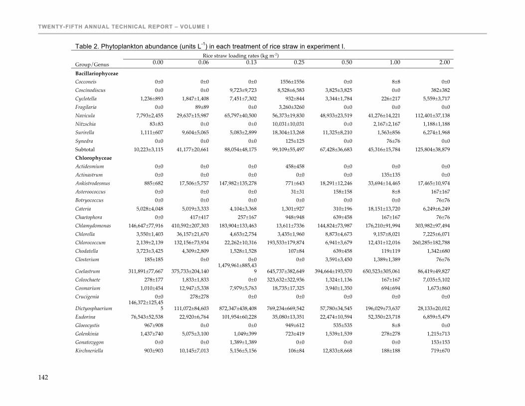
TWENTY-FIFTH ANNUAL TECHNICAL REPORT – VOLUME I
142
Table 2. Phytoplankton abundance (units L-1) in each treatment of rice straw in experiment I. Rice straw loading rates (kg m-2)
Group/Genus 0.00 0.06 0.13 0.25 0.50 1.00 2.00
Bacillariophyceae Cocconeis 0±0 0±0 0±0 1556±1556 0±0 8±8 0±0 Coscinodiscus 0±0 0±0 9,723±9,723 8,528±6,583 3,825±3,825 0±0 382±382 Cyclotella 1,236±893 1,847±1,408 7,451±7,302 932±844 3,344±1,784 226±217 5,559±3,717 Fragilaria 0±0 89±89 0±0 3,260±3260 0±0 0±0 0±0 Navicula 7,793±2,455 29,637±15,987 65,797±40,500 56,373±19,830 48,933±23,519 41,276±14,221 112,401±37,138 Nitzschia 83±83 0±0 0±0 10,031±10,031 0±0 2,167±2,167 1,188±1,188 Surirella 1,111±607 9,604±5,065 5,083±2,899 18,304±13,268 11,325±8,210 1,563±856 6,274±1,968 Synedra 0±0 0±0 0±0 125±125 0±0 76±76 0±0 Subtotal 10,223±3,115 41,177±20,661 88,054±48,175 99,109±55,497 67,428±36,683 45,316±15,784 125,804±38,879 Chlorophyceae Actidesmium 0±0 0±0 0±0 458±458 0±0 0±0 0±0 Actinastrum 0±0 0±0 0±0 0±0 0±0 135±135 0±0 Ankistrodesmus 885±682 17,506±5,757 147,982±135,278 771±643 18,291±12,246 33,694±14,465 17,465±10,974 Asteroococcus 0±0 0±0 0±0 31±31 158±158 8±8 167±167 Botryococcus 0±0 0±0 0±0 0±0 0±0 0±0 76±76 Cateria 5,028±4,048 5,019±3,333 4,104±3,368 1,301±927 310±196 18,151±13,720 6,249±6,249 Chaetophora 0±0 417±417 257±167 948±948 639±458 167±167 76±76 Chlamydomonas 146,647±77,916 410,592±207,303 183,904±133,463 13,611±7336 144,824±73,987 176,210±91,994 303,982±97,494 Chlorella 3,550±1,403 36,157±21,670 4,653±2,754 3,435±1,960 8,873±4,673 9,157±8,021 7,225±6,071 Chlorococcum 2,139±2,139 132,156±73,934 22,262±10,316 193,533±179,874 6,941±3,679 12,431±12,016 260,285±182,788 Chodatella 3,723±3,425 4,309±2,809 1,528±1,528 107±84 639±458 119±119 1,342±680 Closterium 185±185 0±0 0±0 0±0 3,591±3,450 1,389±1,389 76±76
Coelastrum 311,891±77,667 375,733±204,140 1,479,961±885,43
9 645,737±382,649 394,664±193,570 650,523±305,061 86,419±49,827 Coleochaete 278±177 1,833±1,833 0±0 323,632±322,936 1,324±1,136 167±167 7,035±5,102 Cosmarium 1,010±454 12,947±5,338 7,979±5,763 18,735±17,325 3,940±1,350 694±694 1,673±860 Crucigenia 0±0 278±278 0±0 0±0 0±0 0±0 0±0
Dictyosphaerium 146,372±125,45
5 111,072±84,603 872,347±438,408 769,234±669,542 57,780±34,545 196,029±73,637 28,133±20,012 Eudorina 76,543±52,538 22,920±6,764 101,954±60,228 35,080±13,351 22,474±10,594 52,350±23,718 6,859±5,479 Gloeocystis 967±908 0±0 0±0 949±612 535±535 8±8 0±0 Golenkinia 1,437±740 5,075±3,100 1,049±399 723±419 1,539±1,539 278±278 1,215±713 Gonatozygon 0±0 0±0 1,389±1,389 0±0 0±0 0±0 153±153 Kirchneriella 903±903 10,145±7,013 5,156±5,156 106±84 12,833±8,668 188±188 719±670

PRODUCTION SYSTEM DESIGN & INTEGRATION
143
Table 2 (continued) Rice straw loading rates (kg m-2)
Group/Genus 0.00 0.06 0.13 0.25 0.50 1.00 2.00
Lobomonas 0±0 0±0 0±0 733±733 649±460 0±0 167±167 Micractinium 0±0 0±0 208±208 0±0 535±535 2328±1797 0±0 Micrasterias 0±0 0±0 0±0 1,375±1,375 229±229 0±0 0±0 Mougeotia 503±321 5,605±3,119 4,722±3,629 14,109±10,103 8,375±5,556 1,258±1,258 4,236±3,221 Oedogonium 0±0 434±285 819±653 3,177±2,370 1,410±737 45±45 375±375 Onychonema 611±611 1,593±1,027 750±750 811±463 167±167 0±0 125±125 Oocystis 4,563±1,332 43,171±16,239 11,041±8,030 21,230±8,329 1,401±875 504±432 2,433±2,433 Pandorina 14,983±13,483 271,819±266,849 263,358±248,368 254,499±160,711 144,239±83,214 132,010±80,559 20,281±11,241 Pediastrum 694±694 653±493 1,236±656 2,925±1,439 191±191 38±38 0±0 Planktosphaeria 3,038±2,749 6,472±5,447 10,741±7,374 1,927±1,499 618±532 1,149±734 2,333±2,048 Pyrobotrys 34±34 14,155±11,346 10,639±9,043 12,978±11,139 73,388±40,745 168,426±118,357 683,106±451,255 Radiococcus 0±0 7250±7250 2417±2270 382±382 2128±1920 1000±683 0±0 Rivularia 0±0 0±0 0±0 0±0 0±0 62±43 0±0
Scenedesmus 749,190±331,75
2 905,765±331,044 783,619±253,700 103,905±40,506 907,163±317,836 248,109±55,504 36,156±11,936 Selenastrum 0±0 2,778±2,778 764±764 61±61 1,736±1,736 0±0 0±0 Sphaerocystis 63±63 226±226 0±0 0±0 167±167 0±0 0±0 Spirogyra 101±101 278±278 1,389±1,389 76±76 884±884 0±0 38±38 Tetraedron 2,011±2,011 2,182±1,221 2,679±1,025 1,363±1,363 5,423±3,975 1,691±1,173 140±101 Tetraspora 0±0 2,500±2,500 382±382 552,118±551,935 1,157±1,157 0±0 0±0 Ulothrix 434±238 2,421±2,091 1,479±1,128 574±305 1,736±1,736 0±0 892±683 Volvox 139±139 0±0 0±0 38±38 0±0 0±0
Subtotal 1,567,065±385,7
59 2,415,798±660,7
64 3,985,142±1,092,2
58 1,881,518±845,22
0 1,830,989±506,62
1 1,713,152±359,52
3 1,480,225±690,14
0 Chrysophyceae Chrysococcus 0±0 0±0 0±0 0±0 0±0 0±0 4,166±4,166 Uroglenopsis 628±444 392±252 250±250 830±606 0±0 23±23 57,875±57,875 Ochromonas 0±0 0±0 0±0 367±367 0±0 0±0 0±0
Mallomonas 252±252 4722±4722 0±0 199±199 0±0 265±265 0±0
Prymnesium 0±0 0±0 0±0 611±611 0±0 0±0 0±0
Subtotal 880±444 5115±4650 250±250 2006±1757 0±0 288±288 62,041±57,188 Cryptophyceae Chroomonas 0±0 0±0 0±0 3,128±3,128 0±0 84±84 0±0 Cryptomonas 694±452 5,653±5,653 0±0 4,306±3,827 3,150±1,334 35,448±17,550 18,966±12,076 Gonyostomum 2,104±2,079 2,083±2,083 0±0 5,623±3,733 158±158 3,056±1,944 2,777±2,777

TWENTY-FIFTH ANNUAL TECHNICAL REPORT – VOLUME I
144
Table 2 (continued) Rice straw loading rates (kg m
Group/Genus 0.00 0.06 0.13 0.25 0.50 1.00 2.00
Gymnodinium 0±0 0±0 0±0 4,667±4,667 6,764±5,391 6,111±6,111 0±0 Peridinium 456±244 2,494±2,080 48±48 1,455±673 10,024±6,483 1,158±639 790±577 Subtotal 3,254±1,893 10,230±5,310 48±48 19,179±16,029 20,096±7,322 45,857±17,595 22,534±11,356 Cyanophyceae Anabaena 1,042±834 578±454 764±764 306±306 579±579 335±167 4,226±4,155 Anacystis 0±0 1,667±1,667 764±764 692±451 0±0 1,389±1,389 0±0 Aphanocapsa 458±458 36,436±24,846 382±382 11,910±8,184 19,675±19,675 10,417±10,417 43,632±41,488 Chroococcus 531±274 1,269±804 1,722±1,090 260±260 76±76 542±384 0±0 Coelosphaerium 0±0 267±267 3,728±3,655 0±0 977±891 42±42 191±191 Gloecapsa 32±32 0±0 333±333 801±419 904±904 15±15 0±0
Gomphosphaeria 139±139 139±139 382±382 397±397 14,467±14,467 0±0 0±0
Merismopedia 689±663 847±681 115±115 5,420±4,035 167±167 104±104 0±0
Microcystis 4,403±3,618 140,905±85,896 1,701±1,169 2,653±1,738 333±333 57±41 951±833 Nostoc 0±0 0±0 0±0 0±0 76±76 0±0 0±0 Oscillatoria 32,592±7,877 109,482±63,444 81,422±18,132 20,614±4,934 35,490±10,250 32,011±11,675 62,215±33,151 Raphidiopsis 0±0 226±226 0±0 191±191 21±21 292±208 76±76 Spirulina 0±0 972±972 764±764 367±367 579±579 0±0 923±923 Subtotal 39,885±9,851 292,786±167,201 92,077±17,657 43,609±21,281 73,345±44,740 45,203±22,761 112,216±73,559 Euglenophyceae Euglena 17,620±14,878 22,074±14,601 63,496±61,926 4,847±3,218 60,276±53,268 182,182±114,220 118,279±64,733 Euglenopsis 0±0 0±0 0±0 552±552 0±0 8±8 0±0
Lepocinclis 0±0 0±0 0±0 552±552 0±0 283±283 0±0
Phacus 59±59 2,176±2,176 21,215±21,215 428±428 11,539±10,797 5,227±3,428 5,274±5,274 Trachalomonas 476±439 3,125±1,594 0±0 1,348±867 181±181 394±234 0±0 Subtotal 18,155±15,304 27,375±16,475 84,711±83,138 7,727±5,618 71,995±64,029 188,094±117,525 123,553±66,684 Xanthophyceae Botrydium 84±84 0±0 0±0 0±0 0±0 0±0 0±0
Centritractus 0±0 0±0 0±0 92±84 0±0 0±0 0±0
Gloeobotrys 278±278 0±0 0±0 0±0 0±0 0±0 0±0
Subtotal 362±274 0±0 0±0 92±84 0±0 0±0 0±0
Unknown 185±133 926±926 0±0 455±356 1157±1157 833±833 153±153 No. of identified genus 51 55 50 58 60 59 50

PRODUCTION SYSTEM DESIGN & INTEGRATION
145
Table 3. Zooplankton abundance (units L-1) in each treatment of rice straw in experiment I. Rice straw loading rates (kg m-2)
Group/Genus 0.00 0.06 0.13 0.25 0.50 1.00 2.00 Sarcodina Arcella 116±60 97±97 55±35 125±69 132±55 69±45 170±125 Amoeba 0±0 0±0 0±0 0±0 0±0 0±0 11±11 Centropyxis 62±32 145±82 729±389 208±115 167±66 1,464±1,404 18±18 Diffugia 37±37 0±0 108±82 0±0 0±0 0±0 0±0
Euglypha 0±0 0±0 55±35 15±15 0±0 0±0 0±0
Holophyra 37±37 0±0 0±0 0±0 0±0 0±0 0±0
Subtotal 253±84 243±173 946±509 347±184 299±69 1,533±1,425 200±122 Ciliata Cinetochilum 0±0 0±0 83±83 0±0 45±45 138.8889 33±33 Tintinnidium 0±0 0±0 21±21 0±0 0±0 0±0 0±0
Tintinnopsis 196±196 233±233 83±37 265±226 94±52 95±62 105±61 Paramecium 114±96 82±60 692±400 574±358 960±543 4,505±2,008 1,456±812 Subtotal 310±292 315±225 878±483 839±633 1,099±578 4,739±2,056 1,594±868 Rotifera Asplanchna 1,286±638 3,815±2,430 9,493±6,691 1,216±490 1,942±732 1,847±715 522±267 Brachionus 8,061±3,016 9,877±3,066 6,956±2,882 5,762±2,132 5,966±1,764 5,204±1,800 1,361±359 Gastropus 0±0 0±0 0±0 12±12 45±45 0±0 0±0
Hexarthra 38±38 354±354 328±328 258±258 0 19±19 54±54 Filinia 81±81 0±0 0±0 0±0 0±0 0±0 0±0
Keratella 81±81 470±470 89±89 44±44 232±232 47±47 74±53 Lecane 279±110 378±289 620±411 448±221 1,272±845 97±97 252±87 Pedalia 128±91 495±305 317±181 757±280 370±202 317±139 173±106 Polyarthra 0±0 0±0 0±0 97±97 0±0 32±32 0±0 Scaridium 0±0 0±0 57±57 0±0 0±0 0±0 0±0
Trichocerca 409±383 204±53 47±30 363±167 129±60 12±12 167±131 Subtotal 10,364±3,694 15,594±5,286 17,907±7,359 8,956±2,396 9,956±1,980 7,576±2,386 2,602±525 Hydrozoa Gastroblasta 0±0 0±0 0±0 30±22 95±60 0±0 89±59 Stauropora 0±0 41±41 0±0 0±0 0±0 0±0 0±0
Phialidium 0±0 41±41 0±0 0±0 0±0 0±0 0±0
Lensia 37±37 0±0 0±0 0±0 0±0 0±0 200±200 Subtotal 37±37 81±81 0±0 30±22 95±60 0±0 289±251

TWENTY-FIFTH ANNUAL TECHNICAL REPORT – VOLUME I
146
Table 3. (continued)
Rice straw loading rates (kg m-2) Group/Genus 0.00 0.06 0.13 0.25 0.50 1.00 2.00 Siphonophora 794±444 487±241 107±40 367±240 348±221 588±415 239±98 Crustacea Alona 98±98 74±74 0±0 22±22 0±0 0±0 0±0
Cyclops 192±95 339±106 200±116 107±84 176±47 33±33 147±115 Daphnia 41±41 37±37 0±0 0±0 54±54 0±0 0±0
Diaphanosoma 41±41 0±0 0±0 0±0 0±0 0±0 92±92 Moina 265±159 372±160 13271 0±0 467±211 11±11 148±76 Monostyla 0±0 0±0 0±0 0±0 0±0 0±0 11±11 Nauplius 435±176 1121±463 666±281 744±442 631±152 181±120 405±218 Ostracoda 0±0 0±0 0±0 30±30 0±0 0±0 0±0 Cypris 61±61 62±62 30 148±96 188±81 43±28 215±149 Cypridopsis 0±0 37±37 0±0 0±0 0±0 0±0 0±0
Candona 0±0 0±0 0±0 0±0 11±11 0±0 0±0
Subtotal 1,134±427 2,043±669 1,28±364 1,051±569 1,527±437 268±182 1,018±550 Monogononta Anuraeopsis 31±31 50±32 0±0 57±57 379±229 23±23 101±58 Colurella 0±0 0±0 0±0 78±63 25±25 0±0 0±0
Euchlanis 0±0 0±0 0±0 0±0 33±33 0±0 0±0
Mytilina 0±0 37±37 0±0 0±0 0±0 0±0 0±0
Pleosoma 37±37 0±0 0±0 0±0 0±0 0±0 0±0
Subtotal 68±43 87±41 0±0 135±85 437±258 23±23 101±58 Gastropoda Creseis 61±61 0±0 0±0 0±0 0±0 0±0 0±0
Subtotal 61±61 0±0 0±0 0±0 0±0 0±0 0±0
Unknown 170±139 91±73 0±0 12±12 189±189 147±147 0 No. of identified genus 25 22 21 22 22 18 21

PRODUCTION SYSTEM DESIGN & INTEGRATION
147
Table 4. Abundance of periphyton (units cm-2) in each treatment of rice straw in experiment I. Rice straw loading rates (kg m-2) Group/Genus 0.06 0.13 0.25 0.50 1.00 2.00 Phytoplankton Bacillariophyceae Achnanthes 0±0 0±0 0±0 0±0 66±60 0±0 Chodatella 2,072±1815 28±26 117±107 0±0 0±0 0±0 Cocconeis 0±0 0±0 0±0 234±213 0±0 0±0 Coscinodiscus 0±0 420±384 0±0 1,033±943 0±0 1,768±1,614 Cyclotella 437±204 226±127 435±170 3,904±3008 507±397 2,332±1,305 Cymbella 170±155 29±26 422±211 3110±2163 2044±1311 0±0 Fragillaria 0±0 0±0 2354±1322 2582±2357 0±0 0±0 Gyrosigma 0±0 0±0 0±0 0±0 0±0 403±368 Gomphonema 0±0 0±0 0±0 748±683 0±0 29,779±27,074 Melosira 189±173 0±0 0±0 1,173±1,071 0±0 0 Navicula 142,064±41,718 144,396±78,657 277,795±60,869 341,407±85,470 386,721±164,826 192,025±71,631 Nitzschia 0±0 0±0 0±0 414±378 18±16 0±0 Penium 57±52 0±0 0±0 0±0 0±0 0±0 Rhabdonema 0±0 357±326 0±0 0±0 0±0 0±0 Surirella 62,793±26,337 5,194±2,275 57,668±18,892 148,542±91,995 14,155±11,908 17,538±15,582 Skeletonema 63±57 0±0 0±0 0±0 1,434±1,309 0±0 Bacteriastrum 0±0 0±0 0±0 0±0 0±0 213±195 Subtotal 207,845±62,257 150,651±79,995 338,791±71,899 503,146±169,182 404,945±178,682 244,060±113,163 Chlorophyceae Actinastrum 0±0 5±4 0±0 0±0 2060±1880 0±0 Ankistrodesmus 25,381±8,594 34,239±10,667 2,032±1,155 22,133±12,194 27,915±9,906 21,750±7,558 Basicladia 0±0 0±0 0±0 253±231 0±0 0±0 Botryococcus 0±0 0±0 0±0 3,147±2,843 0±0 213±195 Carteria 6,746±6,159 0±0 0±0 0±0 0±0 0±0 Chaetophora 284±259 5±4 214±196 0±0 3±3 0±0 Characium 0±0 0±0 0±0 2023±1847 0±0 0±0 Chlamydomonas 68,209±34,017 133,140±81,535 18,506±9,116 8,872±5,185 51,984±36,033 15,853±7,851 Chlorella 380±240 213±191 150±137 1375±698 1,186±936 13,938±12,633 Chlorococcum 2,723±875 23±21 6,802±6210 463±217 8,452±6,399 25,370±8,460 Cladophora 167±152 2±2 0±0 0±0 0±0 0±0

TWENTY-FIFTH ANNUAL TECHNICAL REPORT – VOLUME I
148
Table 4 (continued) Rice straw loading rates (kg m-2)
Group/Genus 0.06 0.13 0.25 0.50 1.00 2.00 Closterium 109±99 0±0 0±0 0±0 0±0 1919±1751 Coelastrum 25,774±9,595 55,626±17,546 116,376±26,438 40,680±12,700 22,094±6,874 178±94 Coleochaete 0±0 0±0 429±391 36±32 7,354±4,955 5,466±4271 Cosmarium 2,139±1,257 3,332±2,565 988±499 11,819±5,790 781±713 2,284±2,085 Dictyosphaerium 835±762 1,332±915 13,012±5,045 732±542 33,087±23,342 87±50 Draparnaldia 0±0 987±901 0±0 414±378 0±0 0±0 Eudorina 1,745±1,175 1,765±1,611 5,502±3,826 2,692±1,938 5,000±2,550 36±33 Gloecapsa 167±152 0±0 649±364 0±0 270±246 0±0 Gleocystis 0±0 0±0 815±744 667±609 511±466 640±584 Golenkiia 215±102 127±84 230±183 97±57 0±0 1086±992 Gonatozygon 0±0 420±384 0±0 0±0 270±246 201±184 Kirchneriella 0±0 420±384 307±280 376±149 0±0 0±0 Onychonema 180±164 420±384 0±0 0±0 448±256 108±98 Oocystis 1,413±749 215±174 2,370±479 736±342 614±452 0±0 Pandorina 6,236±5,693 3,011±2,626 12,093±10,308 3,934±3,226 3,437±2,734 0±0 Pediastrum 0±0 0±0 0±0 931±850 0±0 0±0 Pedinoperopsis 15,208±12,031 8,716±5,345 913±833 74±44 410±353 0±0
Planktosphaeria 482±241 179±104 1,478±974 502±361 0±0 9043±8173 Pyrobotrys 0±0 0±0 0±0 414±378 0±0 0±0 Scenedesmus 614,822±99,154 551,985±156,053 106,026±20,676 376,736±137,758 402,072±184647 18,489±12,154 Selenastrum 63±57 1,639±1,496 0±0 0±0 0±0 415±378 Spirogyra 0±0 0±0 0±0 0±0 0±0 201±184 Synedra 0±0 0±0 199±170 0±0 0±0 0±0
Tetraedon 2,365±744 2,229±1,847 153±140 8,672±7176 270±246 1,501±1,370 Tetraspora 81±74 20±18 29±27 0±0 0±0 0±0
Ulothrix 0±0 970±685 0±0 1,968±1,678 952±714 4,687±4,206 Xanthidium 0±0 210±192 0±0 0±0 0±0 0±0
Zygnema 167±152 0±0 214±196 0±0 0±0 0±0
Subtotal 776,411±134,281 802,345±240,069 291,293±57,644 495,261±160302 571,606±247,838 124,337±59,858 Cyanophyceae Anabaena 825±468 1,282±1170 112±63 414±378 148±116 0±0 Aphanocapsa 7,014±6403 0±0 19,394±13210 0±0 18,397±16,794 3,492±3,188 Calothrix 0±0 719±656 0±0 253±231 0±0 0±0

PRODUCTION SYSTEM DESIGN & INTEGRATION
149
Table 4 (continued) Rice straw loading rates (kg m-2)
Group/Genus 0.06 0.13 0.25 0.50 1.00 2.00 Chroococcus 696±635 2803±1618 3805±2253 829±756 0±0 640±584 Coelosphaerium 167±152 0±0 0±0 36±32 0±0 51±46 Gleocapsa 113±103 357±326 1084±769 0±0 0±0 0±0 Gomphosphaeria 0±0 39±35 0±0 0±0 0±0 0±0 Merismopedia 78±72 1,286±1174 0±0 506±462 0±0 0±0 Microcystis 137,166±11,565 68±38 54±31 4,638±4,002 540±493 7,156±6,532 Oscillatoria 97,530±29,026 357,324±160,047 24,710±8,324 122,018±94,472 109,094±74,599 174,386±134,094 Rivularia 0±0 5±4 489±446 0 0 0 Spirulina 0±0 210±192 490±289 1,759±1,606 4,358±3,978 1,881±1,717 Schizotrix 0±0 22±17 0±0 0±0 0±0 0±0 Tolypothrix 0±0 0±0 0±0 0±0 1944±1505 0±0 Subtotal 120,141±42,947 364,114±163,448 50,139±21,424 130,453±101,875 134,481±95,366 187,605±146,086 Euglenophyceae Euglena 989±670 17,567±16,036 7,934±7,037 31,059±28,120 173,381±156,398 38,527±35,059 Phacus 0±0 0±0 214±196 0±0 1,704±1,555 1,363±1,074 Trachelomonas 8,327±3,007 2,530±1,449 2,634±1,341 3,417±1,087 7,034±3,656 713±334 Subtotal 9,316±2,865 20,097±16,640 10,782±8,538 34,476±28,542 182,119±161,492 40,603±35,968 Raphidophyceae Gonyostomum 674±517 0±0 0±0 0±0 0±0 0±0 Xanthophyceae Vaucheria 0±0 0±0 0±0 253±231 0±0 291±266 Dinophyceae Cryptomonas 378±345 0±0 50±46 0±0 2605±2378 557±509 Gymnodinium 0 0±0 0 0±0 0±0 291±266 Subtotal 378±345 0±0 50±46 0±0 2605±2378 848±512 Oligohymenophorea Colpidium 0±0 0±0 0±0 0±0 412±376 213±195 Chrysophyceae Uroglena 0±0 0±0 112±63 0±0 130±119 582±531 Uroglenopsis 44,041±40,203 548±500 Mallomonas 675±616 575±524 329±300 835±484 85±77 0±0 Subtotal 675±616 575±524 44,481±40,104 1,382±818 215±196 582±531 Siphonophora 3,417±2194 0±0 2,704±2,107 47±43 1,866±1,113 125±84 Unknown 633±578 0±0 2,451±1,687 23±21 641±452 0±0
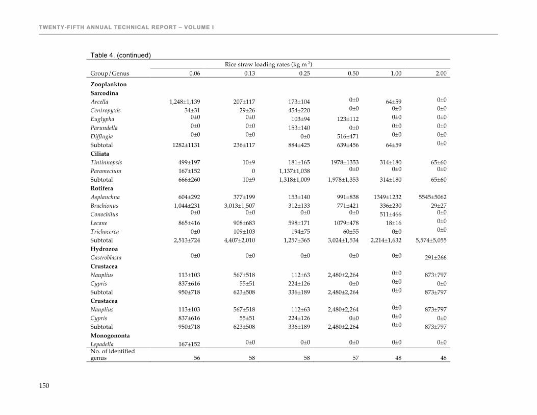
TWENTY-FIFTH ANNUAL TECHNICAL REPORT – VOLUME I
150
Table 4. (continued)
Rice straw loading rates (kg m-2) Group/Genus 0.06 0.13 0.25 0.50 1.00 2.00
Zooplankton Sarcodina Arcella 1,248±1,139 207±117 173±104 0±0 64±59 0±0
Centropyxis 34±31 29±26 454±220 0±0 0±0 0±0
Euglypha 0±0 0±0 103±94 123±112 0±0 0±0
Parundella 0±0 0±0 153±140 0±0 0±0 0±0
Difflugia 0±0 0±0 0±0 516±471 0±0 0±0
Subtotal 1282±1131 236±117 884±425 639±456 64±59 0±0
Ciliata Tintinnopsis 499±197 10±9 181±165 1978±1353 314±180 65±60 Paramecium 167±152 0 1,137±1,038 0±0 0±0 0±0
Subtotal 666±260 10±9 1,318±1,009 1,978±1,353 314±180 65±60 Rotifera Asplanchna 604±292 377±199 153±140 991±838 1349±1232 5545±5062 Brachionus 1,044±231 3,013±1,507 312±133 771±421 336±230 29±27 Conochilus 0±0 0±0 0±0 0±0 511±466 0±0
Lecane 865±416 908±683 598±171 1079±478 18±16 0±0
Trichocerca 0±0 109±103 194±75 60±55 0±0 0±0
Subtotal 2,513±724 4,407±2,010 1,257±365 3,024±1,534 2,214±1,632 5,574±5,055 Hydrozoa Gastroblasta 0±0 0±0 0±0 0±0 0±0 291±266 Crustacea Nauplius 113±103 567±518 112±63 2,480±2,264 0±0 873±797 Cypris 837±616 55±51 224±126 0±0 0±0 0±0 Subtotal 950±718 623±508 336±189 2,480±2,264 0±0 873±797 Crustacea Nauplius 113±103 567±518 112±63 2,480±2,264 0±0 873±797 Cypris 837±616 55±51 224±126 0±0 0±0 0±0 Subtotal 950±718 623±508 336±189 2,480±2,264 0±0 873±797 Monogononta Lepadella 167±152 0±0 0±0 0±0 0±0 0±0 No. of identified genus 56 58 58 57 48 48

PRODUCTION SYSTEM DESIGN & INTEGRATION
151
Table 5. Periphyton biomass and pigment concentration in each treatment with rice straw in experiment I.
Rice straw loading rate (kg m-2) Parameters 0.06 0.13 0.25 0.50 1.00 2.00
Dry matter (mg cm-2) 0.68±0.10a 0.72±0.02a 0.62±0.04a 0.64±0.03a 0.27±0.02b 0.21±0.03b Ash free dry matter (mg cm-2) 0.42±0.09a 0.49±0.04a 0.45±0.04a 0.45±0.02a 0.19±0.06b 0.16±0.03b Ash content (%) 38.5±6.25a 31.2±1.02ab 24.5±2.60b 27.6±1.39ab 28.8±4.82ab 22.7±3.29b Chlorophyll a (µg cm-2) 8.0±0.4abc 9.7±2.4a 7.83±0.2abc 9.1±0.4ab 5.70±1.3bc 5.25±0.5c Different superscript letters in the same row are significantly different (P<0.05).
Table 6. Summary of water quality parameters (valves mg L-1 except where noted) in each treatment in experiment II.
Treatment Parameter RS0 RSS RS1 RS2 RS3 RS4
Temperature at 0600 h (0C) 25.4±0.1 25.4±0.1 25.4±0.1 25.3±0.0 25.4±0.1 25.4±0.1
Temperature at 1800 h (0C) 27.8±0.1 27.8±0.1 27.7±0.1 27.7±0.0 27.8±0.1 27.7±0.0 DO at 0600 h 10 cm 4.8±0.1a 3.9±0.0b 4.2±0.2ab 4.4±0.0ab 4.2±0.3ab 4.2±0.2ab 50 cm 4.0±0.2 3.1±0.1 3.4±0.3 3.6±0.1 3.2±0.3 3.5±0.2 70 cm 2.7±0.3 1.9±0.1 2.4±0.4 2.2±0.1 2.4±0.4 2.6±0.2 DO at 1800 h 10 cm 9.4±0.2 9.1±0.1 9.0±0.2 9.1±0.0 8.9±0.1 9.3±0.0 50 cm 6.8±0.4 6.2±0.1 6.4±0.4 6.4±0.2 6.4±0.4 6.6±0.3 70 cm 4.7±0.5 4.2±0.2 4.3±0.5 4.1±0.5 4.2±0.5 4.3±0.4 pH at 0600 h 7.9±0.1 7.9±0.0 7.9±0.0 7.9±0.1 7.8±0.0 7.8±0.0 pH at 1800 h 8.4±0.0 8.3±0.1 8.3±0.1 8.3±0.0 8.4±0.1 8.3±0.1 Secchi disk visibility (cm) 23±1 24±1 23±1 23±1 23±1 23±1 Total alkalinity 107±12 101±4 109±8 108±3 104±9 96±7 Chlorophyll a 119±13 124±9 101±11 134±29 92±1 125±12

TWENTY-FIFTH ANNUAL TECHNICAL REPORT – VOLUME I
152
Table 6 (continued)
Treatment
Parameter RS0 RSS RS1 RS2 RS3 RS4
Total ammonia nitrogen 0.63±0.23 0.52±0.06 0.80±0.32 0.53±0.18 0.57±0.15 0.47±0.10
Nitrite nitrogen 0.015±0.001 0.032±0.001 0.015±0.004 0.016±0.001 0.012±0.002 0.015±0.000
Nitrate nitrogen 0.12±0.01 0.15±0.01 0.12±0.01 0.12±0.03 0.13±0.02 0.11±0.00
Total nitrogen 1.91±0.45b 2.15±0.11ab 2.06±0.27b 1.88±0.01b 2.63±0.19a 1.91±0.26b Soluble reactive phosphorous 1.51±0.38 1.26±0.09 1.22±0.09 1.57±0.37 1.34±0.09 0.96±0.14
Total phosphorous 1.86±0.33 1.89±0.18 1.82±0.04 1.95±0.19 1.71±0.14 1.44±0.26
Total suspended solids 65±6 60±2 60±13 52±5 68±2 66±5
Total volatile solids 21±1 20±1 18± 3 18±1 23±2 24±0 Mean values with different superscript letters in the same row are significantly different (P<0.05).
Table 7. Abundance of plankton (units L-1) in pond water in each treatment in experiment II. Treatment
Group/Genus Control Dyke-covered One mat Two mats Three mats Four mats
PHYTOPLANKTON Bacillariophyceae Coscinodiscus 3,203±2,300 420±151 1,040±330 1,512±508 1,708±370 1,643±272 Cyclotella 3,542±,081 2,398±43 1,920±1210 1,413±399 2,852±720 3,235±874 Diatoma 1,077±256 940±166 907±214 1,173±297 1,095±130 1,483±207 Fragilaria 13,378±1,639 2,222±1,770 1,237±253 920±360 3,258±2,226 8,468±6,010 Gomphonema 42±42 52±52 633±633 0±0 312±174 108±108 Melosira 1,247±197 643±181 1,702±602 728±109 830±183 1,543±509 Navicula 1,580±381 1,640±387 873±72 1,520±537 2,055±762 1,552±228 Nitzschia 27,582±11,121 76,672±31,335 46,907±17,571 16,957±7,249 37,872±10,073 35,762±8,806 Surirella 1,305±836 205±103 707±468 310±156 208±83 687±229 Synedra 1,857 ±903 1,147± 334 1,552± 400 802 ±340 1,887± 588 1,253±311 Subtotal 54,812±25,119 86,338±32,223 57,477±16,209 25,335±7,294 52,077±10,452 55,735±14,440 Chlorophyceae

PRODUCTION SYSTEM DESIGN & INTEGRATION
153
Table 7 (continued)
Treatment Group/Genus Control Dyke-covered One mat Two mats Three mats Four mats Actinastrum 3,843±729 1,640±616 1,893±244 5,693±1,595 3,255±924 2,312±604 Ankistrodesmus 575±226 827±344 302±53 915±23 550±284 465±87 Chlamydomonas 50 ±50 0±0 200 ±115 0±0 0±0 250 ±250 Characium 0±0 642± 392 42 ±42 497± 248 398 ±81 483 ±254 Chlorella 30,578±12,978 27,898± 12,610 46,652 ±25,699 33,122± 3,658 26,260± 4,360 36,610 ±18,114 Chodatella 127± 127b 0±0 0±0 648± 141a 100 ±100b 258± 134ab Closterium 843± 339 607 ±403 687± 47 1,358 ±292 620± 134 1,242± 262 Coelastrum 543± 286 330 ±±92 180± 99 253 ±171 310± 214 373± 112 Cosmarium 168 ±85 123 ±123 67± 67 140 ±140 257± 150 323± 162 Crucigenia 5,535± 2,902 3,593 ±318 6,323± 2,263 6,313± 626 4,652± 781 3,505± 1,322 Gonatozygon 613± 77ab 310± 155b 518± 242ab 1,393 ±197a 260 ±100b 900 ±281a Mougeotia 0±0 108± 108 0±0 0±0 0±0 108 ±108 Oocystis 1,688 ±633 1,783± 439 1,515± 278 1,687 ±208 1,665 ±318 2,308± 872 Pediastrum 1,628± 119 2,390 ±449 2,145 ±792 2,102± 445 2,232± 736 2,457± 592 Scenedesmus 20,397±3,424ab 10,730±2,312b 14,663±1,379ab 24,422±2,287a 19,198±781ab 20,833±1,886ab Selenastrum 2,128 ±747 552 ±121 2,418± 1,305 1,478 ±378 2,080± 566 2,573± 590 Sphaerocystis 842 ±780 402±150 678 ±228 305 ±181 353 ±228 2,547 ±1,544 Staurastrum 620± 241 83 ±42 1,662± 1,600 370± 197 462 ±279 767± 259 Tetraedron 350 ±200 1,430 ±747 533 ±12 570± 435 383± 133 542± 56 Tetraspora 1,695± 996 1,507± 442 1,492± 406 3,317± 1,092 842± 260 575 ±295 Treubaria 1,058± 559 385 ±385 295± 148 1,515± 631 690 ±287 1,053± 814 Ulothrix 375± 133 53± 39 448 ±78 432± 208 330 ±38 280 ±72 Volvox 0±0 113± 57 67± 67 268 ±174 307± 53 212± 106 Subtotal 73,658±21,116 55,507±14,294 82,780±23,298 86,798±3,354 65,203±4,208 80,977±21,516 Cyanophyceae Anabaena 92±92 550±397 172±172 167±86 42±42 83±83 Aphanocapsa sp. 500±50 273±60 665±335 437±376 580±261 392±331 Chroococcus 4,000±1,966 1,920±545 4,363±1,110 9,910±4,471 3,690±328 2,308±1,234 Gloeocapsa 4,747±2,209 2,093±511 5,180±2,478 4,137±1,304 3,402±564 3,830±2,166 Gomphosphaeria 1,045±330 755±374 1,777±737 1,380±180 955±438 1,217±309 Merismopedia 870±425 423±224 527±277 1,770±1,063 368±184 498±251 Microcystis 453±176 757±378 1,160±291 513±59 445±42 488±114

TWENTY-FIFTH ANNUAL TECHNICAL REPORT – VOLUME I
154
Table 7 (continued) Treatment Group/Genus
Control Dyke-covered One mat Two mats Three mats Four mats Oscillatoria 8,418±2,356 1,987±1,525 817±594 11,552±3,086 7,583±6,864 1,492±1,159 Subtotal 20,125±6,246 8,758±2,281 14,660±2,729 29,865±8,486 17,065±7,291 10,308±3,294 Euglenophyceae 5,378±1,223 2,932±1,349 6,182±1,607 5,490±863 5,683±1,064 7,310±1,676 Euglena 860±292 615±301 722±291 1,110±350 767±131 1,103±217 Phacus 3,327±729 1,730±401 2,415±371 2,028±383 2,468±361 2,238±923 Subtotal 9,565±1,010 5,277±1,132 9,318±1,798 8,628±1,183 8,918±600 10,652±2,652 Unknown 307±160 422±289 612±257 42±42 517±120 108±108 Total phytoplankton 158,467 ±11,937 156,302± 16,265 164,847 ±14,707 150,668 ±14,826 143,780 ±17,968 157,780±18,708 ZOOPLANKTON Sarcodina Difflugia 83±42ab 0±0 42±42ab 290±83a 153±98ab 0±0 Rotifera Asplanchna 1,655 ±398 1,175± 98 843± 263 1,812±429 487 ±247 1,412 ±217 Brachionus 1,993± 72 2,458± 890 2,080 ±245 2,278± 139 2,153± 594 1,830± 425 Filinia 383± 193 187 ±135 498± 138 42± 42 272± 212 0±0 Keratella 785±223 865±301 1,477±587 850±238 990±50 1,732±973 Lecane 127±67 345±345 150±95 248±124 202±144 168±94 Polyarthra 738± 263 1,622 ±360 1,377± 192 1,405± 528 1,383 ±474 1,272± 477 Trichocerca 1,143 ±519 787± 178 685 ±183 398± 239 453 ±198 908 ±222 Subtotal 6,825±123 7,439±1,285 7,110±1,164 7,033±218 5,940±123 7,322±498 Crustacea Cyclops 538± 75 375± 51 335± 105 288± 90 345± 63 595± 261 Dioptomus 667± 184 473 ±176 462± 209 290± 55 175 ±39 302 ±218 Daphnia 100± 50 105± 53 115 ±115 63± 63 185± 63 172± 97 Diaphanosoma 50± 50 122± 65 100 ±100 202± 48 0±0 50 ±50 Moina 273± 203 143 ±78 50± 50 200± 142 133± 11 342 ±171 Nauplius 1,643± 498 1,295± 207 1,682± 297 1,570 ±428 1,402 ±283 1,118± 392 Subtotal 3,272±627 2,513±329 2,743±174 2,613±623 2,240±160 2,578±865 Total zooplankton 10,180± 674 9,952± 1130 9,895 ±1,290 9,937± 504 8,333 ±264 9,900± 1,090 Number of identified genus 55 55 56 55 55 56 Mean values with different superscript letters in the same row are significantly different (P<0.05).

PRODUCTION SYSTEM DESIGN & INTEGRATION
155
Table 8. Abundance of periphyton (units g -1) on rice straw in each treatment in experiment II.
Treatment Group/Genus Dyke-covered One mat Two mats Three mats Four mats
PHYTOPLANKTON Bacillariophyceae Coscinodiscus 17,450±9,422 17,136±3,345 9,807±8,802 6,200±6,200 0±0 Cyclotella 57,885±14,085 38,019±19,244 44,076±14,997 26,620±5,738 36,996±18,888 Cymbella 2,451±2,451 217±217 4,386±4,386 374±374 0±0 Diatoma 77,761±43,222 44,844±12,675 104,493±7,430 28,365±24,343 18,637±15,442 Fragillaria 17,129±8,840 5,297±3,017 8,272±5,739 36,531±14,373 7,242±5,330 Gomphonema 14,990±7,237 3,496±2,833 15,717±8,611 18,707±12,503 16,687±8,627 Melosira 7,943±4,629 6,902±4,659 5,396±3,978 11,611±5,151 553±332 Navicula 84,094±32,053 46,395±26,601 90659±37,903 65,562±42,985 15,258±6,100 Nitzschia 131,964±24,746 29,359±16,950 90,922±61,118 87,260±55,890 53,514±16,087 Pinnularia 14,981±9,861 7,714±3,868 4,993±4,993 12,399±12,399 4,073±4,073 Surirella 0±0 6,173±6,173 17,528±1,716 6,908±6,472 8,699±8,133 Synedra 24,771±10,709 4,778±3,557 17,233±7,862 17,249±8,693 14,545±6,337 Subtotal 451,419±112,495 210,328±42,723 413,481±126,341 317,785±102,237 176,205±52,506 Chlorophyceae Actinastrum 772±772 225±225 505±505 521±521 960±719 Ankistrodesmus 2,193±2,193 4,041±3,390 5,069±4,078 3,917±3,168 171±171 Ceratium 5,597±5,597 3,686±3,686 683±683 521±521 0±0 Centritractus 772±772 0±0 2,193±2,193 521±521 382±382 Characium 0±0 0±0 0±0 521±521 4,336±3,948 Chlorella 299,135±159,401 18,2784±30,982 420,613±50,401 209,858±109,259 115,590±63,166 Closterium 3,788±3,788 14,050±4,056 7,186±4,335 6,573±6,021 0±0 Coelastrum 4,925±1,321 3,686±3,686 4,993±4,993 0±0 5,296±3,828 Cosmarium 4,664±3,951 7,371±7,371 4,738±4,738 6,573±6,021 4,073±4,073 Crucigenia 127,771±55,825 34,763±16,866 26,341±24,104 8,844±7,842 24,060±10,486 Gonatozygon 39,061±19,603 25,634±4,771 22,265±6,391 374±374 5,968±3,639 Mougeotia 3,559±1,595 3,311±2,980 1,010±1,010 374±374 0±0 Oocystis 10,034±8,145 8,511±7,186 11,470±10,721 8,577±5,743 11,550±10,160 Pediastrum 10,965±10,965 878±216 16,559±15,808 6,947±5,862 816±183 Scenedesmus 275,359±24,418a 46,900±10,304b 102,690±60,612b 52,049±15,434b 55,272±15,091b Selenastrum 39,957±13,530 16,106±15,106 9,807±8,802 0±0 8,528±7,962 Staurastrum 0±0 891±596 0±0 1,042±1,042 0±0

TWENTY-FIFTH ANNUAL TECHNICAL REPORT – VOLUME I
156
Table 8. (continued) Treatment Group/Genus
Dyke-covered One mat Two mats Three mats Four mats Tetraedon 9,540±3,305 4,783±3,555 7,191±6,195 668±341 697±464 Tetraspora 10,070±10,070 0±0 2,193±2,193 521±521 0±0 Ulothrix 37,708±23,055 24,002±12,906 21,510±11,510 294±294 28,511±28,511 Volvox 0±0 0±0 2,193±2,193 747±747 434±231 Subtotal 885,869±296,324 381,622±73,939 669,209±194,532 309,442±119,244 266,645±133,951 Cyanophyceae Anabaena 3,788±3,788 873±873 15,195±639 0±0 765±765 A phanozomenon 0±0 6,173±6,173 0±0 0±0 0±0 Chroococcus 54,879±30,998 36,557±14,008 57,145±7,701 10,116±4,918 33,965±33,180 Gleocapsa 9,209±4,665 4,135 ±4,135 10,342±5,225 8,068±5,508 1,855±366 Gomphosphaeria 27,534±15,577 20,565±4,961 52,902±17,003 2,389±1,670 20,799±20,406 Merismopedia 0±0 0±0 0±0 0±0 263±263 Microcystis 3,788± 3,788 34,801± 8,871 10,236±5,160 12,399±12,399 8,409±8,018 Oscillatoria 26,581±3,501 0±0 9,311±5,752 9,595±5,377 6,307±5,801 Phormidium 0±0 436±436 0±0 3,396±3,396 13,736±7,467 Subtotal 125,779±56,347 105,540±14,246 155,130±21,984 45,964±26,027 86,099±51,764 Euglenophyceae Euglena 16,397± 6,185 6,834 ±5,845 33,118± 6,975 11,199 ±5,924 16,057 ± 8,870 Phacus 6,858± 4,972 225 ± 225 2,876 ± 1,944 0±0 5,873± 5,618 Trachelomonas 17,233± 8,047 1,526 ±1,215 16,315± 7,484 3,137± 2,398 14,724± 7,490 Subtotal 40,488±4,864ab 8,584±5,410b 52,309±7,814a 14,335±6,815ab 36,654±15,272ab ZOOPLANKTON Sarcodina Difflugia 4,278±3,568 3,520±3,520 4,993±4,993 0±0 697±464 Rotifera Asplanchna 7,067±5,025 3,686±3,686 4,738±4,738 0±0 8,353±4,180 Brachionus 10,070±10,070 0±0 4,993±4,993 0±0 5,176±5,176 Lecane 0±0 0±0 0±0 3,396±3,396 4,280±4,280 Subtotal 17,138±9,996 3,686±3,686 9,731±4,870 3,396±3,396 17,809±4,050
Total 1,524,970±
404,701 713,281± 113,342 1,304,852 ±318,068 690,922 ±207,142 584,109± 225,623 Number of identified genus 41 41 43 40 41 Mean values with different superscript letters are significantly different.

PRODUCTION SYSTEM DESIGN & INTEGRATION
157
Table 9. Growth performance of carps stocked in each treatment in experiment II. Treatment Parameter
Control Dyke-covered One mat Two mats Three mats Four mats Rohu Initial total weight (kg pond-1) 0.29±0.01 0.31±0.00 0.31±0.00 0.30±0.02 0.30±0.00 0.32±0.01 Initial mean weight (g fish-1) 24.4± 0.5 25.8± 0.3 26.0± 0.2 25.1± 1.45 24.8± 0.3 26.7 ±0.7 Final total weight (kg pond-1) 0.45±0.08 0.62±0.12 0.62±0.04 0.51±0.06 0.69±0.08 0.70±0.04 Final mean weight (g fish-1) 53.8± 0.7 59.5± 4.0 54.4± 2.3 55.4± 2.1 59.0± 6.0 60.0± 3.6 Daily weight gain (g-1fish-1day-1) 0.33± 0.01 0.37± 0.05 0.31± 0.02 0.34± 0.04 0.38± 0.07 0.37± 0.03 Total weight gain (kg pond-1) 0.16±0.09 0.31±0.12 0.31±0.12 0.21±0.05 0.39±0.08 0.38±0.03 Survival 72.2 ±14.7 86.1 ±13.9 94.4±2.8 77.8 ±12.1 97.2± 2.8 97.2± 2.8 Catla Initial total weight (kg pond-1) 0.18 ±0.02 0.20 ±0.02 0.20 ±0.03 0.22 ±0.01 0.18 ±0.02 0.18± 0.02 Initial mean weight (g fish-1) 21.9± 2.1 24.5 ±2.2 24.5± 3.2 27.3 ±1.3 22.9± 2.3 22.8± 1.9 Final total weight (kg pond-1) 0.32±0.04 0.48±0.06 0.45±0.06 0.49±0.05 0.51±0.11 0.50±0.11 Final mean weight (g fish-1) 53.6± 8.9 59.9± 7.1 56.7± 7.6 60.7± 6.0 66.1± 13.3 61.9± 13.6 Daily weight gain (g-1fish-1day-1) 0.35± 0.12 0.39± 0.10 0.36± 0.12 0.37± 0.05 0.48± 0.17 0.43± 0.17 Total weight gain (kg pond-1) 0.14±0.04 0.28±0.07 0.26±0.09 0.27±0.04 0.33±0.13 0.31±0.12 Survival 75.0 ±7.2b 100.0± 0.0a 100.0± 0.0a 100.0± 0.0a 95.8± 4.2a 100.0± 0.0a Mrigal Initial total weight (kg pond-1) 0.20± 0.01 0.22± 0.02 0.24 ±0.01 0.21± 0.01 0.20 ±0.03 0.20± 0.01 Initial mean weight (g fish-1) 24.2± 1.6 27.3± 2.8 29.9± 1.6 26.0± 1.9 24.3 ±3.8 25.3± 1.8 Final total weight (kg pond-1) 0.28±0.02 0.33±0.09 0.28±0.06 0.33±0.03 0.34±0.02 0.42±0.04 Final mean weight (g fish-1) 53.6 ±4.8 51.9± 3.2 63.1± 2.5 57.2± 6.6 57.2± 4.0 57.1± 3.7 Daily weight gain (g-1fish-1day-1) 0.33± 0.06 0.27± 0.05 0.37± 0.03 0.35± 0.07 0.37± 0.04 0.35± 0.06 Total weight gain (kg pond-1) 0.08±0.02 0.11±0.11 0.04±0.07 0.12±0.05 0.14±0.03 0.22±0.05 Survival 66.7± 8.3 79.2± 20.8 54.2± 11.0 75.0± 14.4 79.2± 4.2 91.7± 4.2 Common carp Initial total weight (kg pond-1) 0.21±0.03 0.16±0.00 0.17±0.01 0.20±0.01 0.18±0.02 0.22±0.01 Initial mean weight (g fish-1) 24.8± 2.8 19.7 ±0.2 21.8± 0.8 24.7± 1.0 22.8± 2.9 26.9± 1.6

TWENTY-FIFTH ANNUAL TECHNICAL REPORT – VOLUME I
158
Table 9. (Continued)
Treatment Parameter
Control Dyke-covered One mat Two mats Three mats Four mats Final total weight (kg pond-1) 0.35±0.01 0.43±0.04 0.46±0.03 0.41±0.02 0.43±0.03 0.43±0.04 Final mean weight (g fish-1) 49.8±2.0 58.9± 3.1 56.8± 3.8 51.5± 2.7 58.0±2.7 58.1± 3.2 Daily weight gain (g-1fish-1day-1) 0.28± 0.02 0.44± 0.03 0.39± 0.04 0.30± 0.02 0.39 ±0.03 0.35± 0.04 Total weight gain (kg pond-1) 0.14±0.02b 0.27±0.04ab 0.29±0.03a 0.21±0.01ab 0.24±0.02ab 0.21±0.04ab Survival 87.5± 0.0 91.7± 8.3 100.0± 0.0 100.0± 0.0 87.5± 0.0 91.7± 4.2 Silver carp Initial total weight (kg pond-1) 0.12±0.01 0.11±0.00 0.10±0.01 0.10±0.00 0.10±0.01 0.10±0.01 Initial mean weight (g fish-1) 26.9 ±1.1 27.3± 0.6 25.4± 1.5 24.9± 0.4 25.4± 1.6 25.3 ±1.9 Final total weight (kg pond-1) 0.51±0.12 0.47±0.11 0.54±0.12 0.62±0.04 0.76±0.06 0.53±0.07 Final mean weight (g fish-1) 149.0 ±8.8 139.8 ±5.9 161.3± 10.6 170.9 ±14.6 189.2± 14.1 191.1± 48.5 Daily weight gain (g-1fish-1day-1) 1.36± 0.09 1.25± 0.06 1.51± 0.10 1.62± 0.16 1.82± 0.14 1.84± 0.52 Total weight gain (kg pond-1) 0.39±0.11 0.36±0.11 0.44±0.11 0.52±0.04 0.66±0.05 0.43±0.06 Survival 83.3 ±16.7 83.3± 16.7 83.3± 16.7 91.7± 8.3 100.0± 0.0 75.0 ±14.4 Combined Initial total weight (kg pond-1) 1.00±0.04 0.99±0.04 1.02±0.04 1.03±0.01 0.96±0.03 1.02±22.92 Final total weight (kg pond-1) 1.90±0.09b 2.33±0.16ab 2.34±0.04ab 2.36±0.07ab 2.72±0.29a 2.57±0.15ab Total weight gain (kg pond-1) 0.90± 0.05b 1.34± 0.19ab 1.32± 0.08ab 1.33± 0.06ab 1.76± 0.28a 1.55± 0.17ab Mean values with different superscript letters in the same row are significantly different (P<0.05).

PRODUCTION SYSTEM DESIGN & INTEGRATION
159
Table 10. Gross margin analysis in Bangladeshi Taka for each treatment in experiment II .
Control Dyke-covered One mat Two mats Three mats Four mats Item Unit Price Quantity Taka Quantity Taka Quantity Taka Quantity Taka Quantity Taka Quantity Taka
Gross return Rohu kg 30 0.45 14±3 0.62 19±3 0.62 19±1 0.51 15±2 0.69 21±2 0.7 21±1 Catla kg 30 0.31 9±1 0.48 14±2 0.45 14±2 0.49 15±1 0.51 15±3 0.5 15±3 Mrigal kg 30 0.28 8±0 0.33 10±3 0.27 8±2 0.33 10±1 0.34 10±1 0.42 13±1 Common kg 30 0.35 11±0 0.43 13±1 0.45 14±1 0.41 12±1 0.43 13±1 0.43 13±1 Silver kg 30 0.51 15±4 0.47 14±3 0.54 16±3 0.62 19±1 0.76 23±2 0.53 16±2 Total gross return 1.9 57±3b 2.33 70±5ab 2.34 70±1ab 2.36 71±2ab 2.72 82±9a 2.57 78±5ab Variable cost Fingerlings Rohu Pcs 3.5 12 42 12 42 12 42 12 42 12 42 12 42 Catla Pcs 3.5 8 28 8 28 8 28 8 28 8 28 8 28 Mrigal Pcs 3.5 8 28 8 28 8 28 8 28 8 28 8 28 Common Pcs 3.5 8 28 8 28 8 28 8 28 8 28 8 28 Silver Pcs 3.5 4 14 4 14 4 14 4 14 4 14 4 14 Urea kg 8 0.87 7 0.9 7 0.9 7 0.9 7 0.9 7 0.9 7 TSP kg 15 0.45 7 0.4 7 0.4 7 0.4 7 0.4 7 0.4 7 Cowdung kg 0.4 35.00 14 35 14 35 14 35 14 35 14 35 14 Lime kg 12 1.00 12 1 12 1 12 1 12 1 12 1 12 Bamboo Pcs 130 1 14 1 14 1.5 22 2 29 3 43 Wire 20 10 15 20 25 Interest on working capital 10% 5 5 6 6 6 7 Total variable cost 212±0 227±0 237±0 250±0 263±0 282±0 Gross margin -155±3a -157±5ab -167±1ab -179±2b -181±9b -205±5c Mean values with different superscript letters in the same row are significantly different (P<0.05).

TWENTY-FIFTH ANNUAL TECHNICAL REPORT – VOLUME I
160
Table 11. Summary of water quality parameters in each treatment in experiment III.
Water quality parameters Control Rice straw Kanchi Temperature at 0600 h (oC) Temperature at 1800 h (oC)
25.8±0.6 29.3±0.1
25.9±0.5 29.4±0.1
26.1±0.1 29.3±0.0
DO at 0600 h (mg L-1) 10 cm 50 cm 70 cm DO at 1800 h (mg L-1) 10 cm 50 cm 70 cm
5.3±0.1a 4.6±0.2a 4.0±0.2a
9.3±0.3a 7.4±0.3a 5.9±0.3a
3.7±0.0b 3.2±0.1b 2.7±0.1b
7.5±0.2b 5.8±0.2b 4.8±0.1b
4.9±0.0a 4.2±0.1a 3.5±0.1a
9.2±0.2a 7.8±0.4a 5.9±0.1a
pH at 0600 h pH at 1800 h
8.5±0.0 8.9±0.0
8.4±0.0 8.7±0.0
8.5±0.0 8.9±0.0
Sechi disc depth (cm) 18±0 22±2 21±1 Total alkalinity (mg L-1 as CaCO3) 128±8 138±5 129±5 Chlorophyll a (µg L-1) 56±6 48±11 61±13 Total ammonia nitrogen (mg L-1) 0.17±0.08 0.10±0.02 0.14±0.04 Nitrite nitrogen (mg L-1) 0.01±0.00 0.01±0.00 0.01±0.00 Total nitrogen (mg L-1) 1.43±0.28 1.52±0.32 1.60±0.09 Soluble reactive phosphorous (mg L-1) 2.30±0.43 1.03±0.11 1.53±0.53 Total phosphorous (mg L-1) 2.30±0.27 1.71±0.11 1.80±0.13 Total suspended solids (mg L-1) Total volatile solids (mg L-1)
75±15 43±8
70±3 39±1
58±7 32±1
Mean values with different superscript letters in the same row are significantly different (P<0.05).

PRODUCTION SYSTEM DESIGN & INTEGRATION
161
Table 12. Abundance of phytoplankton (units L-1) in the pond water in each treatment in experiment III.
Control Rice straw Kanchi Group Genus
Bacillariophyceae Coscinodiscus 2,457±477 3,405±1,413 4,233±836 Cyclotella 6,145±1,618 26,418±12,666 9,000±2,678 Cymbella 67±67 0±0 0±0 Diatoma 257±163 303±182 250±144 Gomphonema 512±179 473±133 597±376 Melosira 6,310±4,248 1,477±518 2,510±1,259 Fragillaria 2,005±485 1,765±618 1,348±357 Navicula 1,875±1,037 1,390±498 2,127±600 Nitzschia 4,853±1,302 2,967±827 17,970±12,203 Surirella 575±307 1,047±268 700±513 Synedra 1,953±952 2,080±415 1,345±75 Tabellaria 173±88 322±217 167±167 Subtotal 27,182±5,578 41,647±12,203 40,247±11,640 Chlorophyceae Actinastrum 412±302 1,062±529 1,302±873 Ankistrodesmus 423±234 743±632 597±233 Centritractus 78±78 0±0 1,000±1,000 Chlamydomonas 0±0 513±120 710±374 Chlorella 13,087±5,716 12,305±3,495 57,668±48,926 Chodatella 228±228 0±0 0±0 Closterium 125±63 1,557±1,120 1,017±627 Coelastrum 1,253±1,066 712±461 472±369 Crucigenia 4,692±2,515 3,843±2,171 1,696±484 Gonatozygon 350±180 72±72 375±189 Mougeotia 2,225±1,690 2,798±1,342 1,440±737 Oedogonium 0±0 72±72 167±167 Oocystis 6,695±1,073 4,483±335 17,107±6,063 Pediastrum 2,598±831 933±390 2,127±610 Scenedesmus 9,593±4,442 10,213±3,103 8,082±2,725 Selenastrum 268±173 140±140 2,832±2,698 Sphaerocystis 5,457±3,420 2,253±576 10,047±3,420 Spirogyra 67±67 0±0 0±0 Staurastrum 95±95 212±121 83±83 Tetraedron 543±339 503±272 250±215 Tetraspora 290±146 783±529 313±250 Treubaria 95±95 233±123 167±167 Ulothrix 1,025±364 142±71 142±74 Volvox 75±75 70±70 167±167 Subtotal 49,675±12,263 43,643±5,836 107,759±57,292 Cyanophyceae Anabaena 75±67 0±0 0±0 Aphanocapsa sp. 0±0 140±140 167±167

TWENTY-FIFTH ANNUAL TECHNICAL REPORT – VOLUME I
162
Table 13. Abundance of zooplankton (units L-1) in the pond water in each treatment in experiment III.
Control Rice straw Kanchi Group Genus
Sarcodina Difflugia 962±302 820±340 1,678±842 Rotifera Asplanchna 740±159 837±352 1,833±761 Brachionus 1,343±308 2,027±103 4,477±1,640 Filinia 1,278±527 227±227 337±64 Keratella 1,577±538 1,153±42 1,260±101 Lecane 200±14 445±253 575±218 Monostylla 0±0 0±0 250±144 Polyarthra 1,055±571 987±178 2,013±308 Trichocerca 577±189 150±75 330±208 Subtotal 6,848±1,180 5,895±406 11,075±2,386 Crustacea Cyclpos 545±78 1,068±169 590±296 Ceriodaphnia 58±58 130±66 600±306 Daphnia 75±75 338±68 0±0 Diaptomus 235±24 148±74 303±211 Diaphanosoma 290±105 87±87 67±67 Moina 240±140 450±293 553±129 Nauplius 772±75 1,308±341 1,215±77 Subtotal 2,215±362 3,530±325 3,328±518 Total zooplankton 9,947 ±796 10,176 ±669 16,082± 2,360 Number of identified genus 15 15 15
Table 14. Abundance of periphyton (103 x units m-2) in the rice straw and kanchi treatments in experiment III.
Rice straw Kanchi Group Genus
Bacillariophyceae Coscinodiscus 794±794 0±0 Cyclotella 3,720±682a 174±174b Cymbella 2,863±1,433 0±0 Diatoma 34,999±9,597a 3,991±459b Fragillaria 15,931±4,136 5,553±1,932 Gomphonema 7,680±1,708a 521±301b Melosira 7,095±2,270 868±459 Navicula 40,196±27,364 13,362±4,562 Nitzschia 64,369±19,286a 6,594±1,056b Surirella 1,589±1,589 0±0 Synedra 30,476±7,487 12,147±5,512 Tabellaria 1,838±944 174±174 Subtotal 211,550±17,738a 43,382±3,611b

PRODUCTION SYSTEM DESIGN & INTEGRATION
163
Table 14. (Continued)
Rice straw Kanchi Group
Genus
Chlorophyceae Actinastrum 531±531 0±0 Centritractus 1,592±1,592 0±0 Characium 2,196±1.217 3,471±1,483 Chlamydomonas 0±0 174±174 Chlorella 40,049±4,538a 5,900±2,215 b Closterium 1,805±1,805 0±0 Coelastrum 0±0 347±347 Cosmarium 5,045±1,442 1,215±174 Crucigenia 37,428±15,131 1,562±795 Cylindrocapsa 0±0 22,038±13,202 Gonatozygon 4,822±1,345 0±0 Microspora 3,839±336 1,041±1,041 Mougeotia 7,095±4,068 868±626 Oedogonium 5,420±4,285 9,718±4,601 Oocystis 3,592±2,247 4,165±902 Scenedesmus 60,020±9,238a 5,206±301b Stigeoclonium 1,589±1,589 476,160±145,359 Sphaerocystis 720±720 0±0 Staurastrum 1,016±1,016 0±0 Tetraspora 0±0 694±174 Tetraedron 0±0 1,041±795 Triplocerus 5,384±1,708 0±0 Ulothrix 0±0 1,735±918 Subtotal 182,141±16,041 535,332±137,868 Cyanophyceae Chroococcus 4,800±4,030 2,082±521 Gleocapsa 0±0 3,991±626 Gomphosphaeria 1,203±614 0±0 Merismopedia 1,044±1,044 0±0 Oscillatoria 19,493±7,310 2,429±694 Phormidium 25,304±8,058a 1,215±966b Subtotal 51,844±13,989 9,718±347 Euglenophyceae Euglena 5,426±2,016 1,388±626 Phacus 720±720 0±0 Trachelomonas 2,842±1,422 174±174 Subtotal 8,989±746a 1,562±795 b Sarcodina Diffugia 531±531 0±0 Rotifera Asplanchna 1,589±1,589 694±174 Brachionus 1,838±944 521 ±301 Conochilus 0±0 1,562±521 Lecane 1,346±1,346 0±0 Subtotal 4,773±1,216 2,776±459 Total periphyton 459,826±18,629 592,770±134,932 Number of identified genus 41 34 Mean values with different superscript letters in the same row are significantly different (P<0.05).

TWENTY-FIFTH ANNUAL TECHNICAL REPORT – VOLUME I
164
Table 16. Abundance of zoobenthos (ind. m-2) in each treatment in experiment III. Group/Genus Control Rice straw Kanchi Oligochaete 138.3±78.9 22.0±11.0 93.7±29.6 Arthropoda Chironomid 216.3±37.7 289.0±101.8 179.0±73.7 Insecta 3.7±2.0 5.0±5.0 2.3±2.3 Subtotal 219.7±38.0 294.0±105.1 181.3±76.0 Molluska Thiara 1.3±1.3 1.3±1.3 0±0 viviparous 0±0 2.3±2.3 0±00 Unio 1.3±1.3 0±0 0±0 Subtotal 2.7±1.3 3.7±1.3 0±0 Total 360.7±100.6 319.7±103. 275.3±89.7
Table 15. Periphyton biomass in the rice straw and kanchi treatments in experiment III.
Parameter Rice straw Kanchi Dry matter (g pond-1) 540.4±81.2 620.3±34.7 Ash (%) 41.7±2.1 36.9±4.2 Ash Free Dry Matter (g pond-1) 280.0±21.1b 382.8±21.3a Chlorophyll-a (g pond-1) 0.75±0.14 2.18±0.54 Mean values with different superscript letters in the same row are significantly different (P<0.05).

PRODUCTION SYSTEM DESIGN & INTEGRATION
165
Table 17. Growth performance of carps stocked in each treatment in experiment III. Parameter Control Rice straw Kanchi Rohu Initial total weight (kg pond-1) 0.30±0.01 0.28±0.01 0.30±0.01 Initial mean weight (g fish-1) 25.1±0.5 23.2±0.9 25.3±0.5 Final total weight (kg pond-1) 1.19±0.04b 1.66±0.05a 1.90±0.16a Final mean weight (g fish-1) 105.4±0.5b 138.72±4.4a 162.82±9.7a Daily weight gain (g fish -1 day -1) Total weight gain (kg pond-1) Survival (%)
0.89±0.00b 0.89±0.03b
94.7±4.6
1.28±0.07a 1.39±0.05a 100.0±0.0
1.53±0.05a 1.60±0.15a
97.3±4.6 Catla Initial total weight (kg pond-1) 0.20±0.01 0.21±0.01 0.21±0.02 Initial mean weight (g fish-1) 25.5±0.8 25.8±0.8 26.0±0.5 Final total weight (kg pond-1) 0.43±0.03b 0.63±0.02a 0.73±0.03a Final mean weight (g fish-1) 59.0±6.0b 68.7±12.3ab 99.4±5.4a Daily weight gain (g fish -1 day -1) Total weight gain (kg pond-1) Survival (%)
0.37±0.07b 0.23±0.04b
96.0±6.9
0.48±0.13ab 0.42±0.02a
96.0±6.9
0.81±0.07a 0.52±0.04a
92.0±6.9 Mrigal Initial total weight (kg pond-1) 0.20±0.01 0.21±0.01 0.19±0.00 Initial mean weight (g fish-1) 24.8±1.0 26.1±1.5 24.3±0.6 Final total weight (kg pond-1) 0.89±0.77 1.16±0.61 1.19±0.15 Final mean weight (g fish-1) 130.5±4.2 139.8±22.3 161.2±10.9 Daily weight gain (g fish -1 day -1) 1.17±0.05 1.26±0.23 1.52±0.13 Total weight gain (kg pond-1) Survival (%)
0.69±0.07 96.0±6.9
0.96±0.05 96.0±6.9
0.99±0.16 91.7±14.4
Common carp Initial total weight (kg pond-1) 0.22±0.01 0.21±0.01 0.23±0.00 Initial mean weight (g fish-1) 27.9±0.6 25.7±0.8 29.2±0.6 Final total weight (kg pond-1) 0.58±0.04 0.71±0.05 0.64±0.05 Final mean weight (g fish-1) 72.7±4.6b 90.3±3.1a 92.0±1.5a Daily weight gain (g fish -1 day -1) 0.50±0.05b 0.72±0.03a 0.70±0.02a Total weight gain (kg pond-1) Survival (%)
0.36±0.03 100.0±0.0
0.50±0.05 96.0±6.9
0.41±0.05 87.7±12.5
Silver carp Initial total weight (kg pond-1) 0.13±0.01 0.11±0.01 0.13±0.01 Initial mean weight (g fish-1) 31.4±1.2 28.5±2.3 31.4±0.9 Final total weight (kg pond-1) 1.35±0.16 1.53±0.02 1.60±0.16 Final mean weight (g fish-1) 406.2±18.6 365.7±10.8 402.5±29.9 Daily weight gain (g fish -1 day -1) 4.16±0.20 3.75±0.11 4.12±0.32 Total weight gain (kg pond-1) Survival (%)
1.22±0.11 83.0±14.4
1.44±0.02 100.0±0.0
1.47±0.11 100.0±0.0
Combined Initial total weight (kg pond-1) 1.05±0.04 1.01±0.03 1.07±0.01 Final total weight (kg pond-1) 4.44±0.36b 5.70±0.06a 6.06±0.70a Total weight gain (kg pond-1) 3.39±0.32b 4.69±0.06a 4.99±0.70a Mean values (±SE) with different superscript letters in the same row are significantly different (P<0.05).

TWENTY-FIFTH ANNUAL TECHNICAL REPORT – VOLUME I
166
Table 18. Gross margin analysis of each treatment in experiment III in Bangladeshi Taka.
Control Rice straw Kanchi
Item Unit Taka/unit Quantity Taka Quantity Taka Quantity Taka Gross return Rohu kg 60 1.19 72±2b 1.66 100±3a 1.90 114±9a Catla kg 60 0.43 26±2b 0.63 38±1a 0.73 44±2a Mrigal kg 60 0.89 53±5 1.16 70±4 1.19 71±9 Common carp kg 60 0.58 35±2 0.71 42±3 0.64 39±3 Silver carp kg 60 1.35 81±7 1.53 92±1 1.60 96±7 Total 267±12b 342±2a 364±24a
Variable cost Fingerlings Rohu Pcs 3.5 12 42 12 42 12 42 Catla Pcs 3.5 8 28 8 28 8 28 Mrigal Pcs 3.5 8 28 8 28 8 28 Common carp Pcs 3.5 8 28 8 28 8 28 Silver carp Pcs 3.5 4 14 4 14 4 14
Fertilizer Urea kg 8 0.9 7 0.9 7 0.9 7 TSP kg 15 0.4 7 0.4 7 0.4 7 Cow dung kg 0.4 35.0 14 35.0 14 35.0 14 Lime kg 12 1.0 12 1.0 12 1.0 12
Kanchi Pcs 1 - - - - 390 for 4
crops 98
Bamboo Pcs 130 - - 2 for 9 crops 29 - -
Wire 20 Interest on working capital 10% 4 6 7 Total 184±0 235±0 285±0 Gross margin 83±12 107±2 79±24 Mean values with different superscript letters in the same row are significantly different (P<0.05).

PRODUCTION SYSTEM DESIGN & INTEGRATION
167
USE OF RICE STRAW AS A RESOURCE FOR FRESHWATER POND CULTURE: GROWTH PERFORMANCE Twelfth Work Plan, Production System Design & Integration 3b (12PSD3b)
Final Report Published as Submitted by Contributing Authors
A.M. Shahabuddin, Dhirendra Prasad Thakur & Yang Yi
Asian Institute of Technology Pathumthani, Thailand
James S. Diana & C. Kwei Lin
University of Michigan Ann Arbor, Michigan, USA
ABSTRACT An experiment was conducted with different rice straw loading rates in fertilized earthen ponds at the Asian Institute of Technology, Thailand to assess effects of rice straw mats on growth performance of Nile tilapia (Oreochromis niloticus), water quality, periphyton, plankton, bacterial biofilm and benthos. There were six treatments with three replicates each: (1) control (without rice straw mats); (2) rice straw mats of 5x0.5 m covering dikes; (3) one rice straw mat of 5x1 m in the water column; (4) two rice straw mats; (5) three rice straw mats; and (6) four rice straw mats. All ponds were fertilized weekly with urea and triple super phosphate at rates of 28 kg N and 7 kg P ha-1 week-1. Sex-reversed all-male tilapia of 24.7±3.0 g in size were stocked at 2 fish m-2 on day 39 after placing straw mats in the ponds. Tilapia growth performance was not significantly different among treatments, except the treatment with two straw mats, which had significantly lower mean weight gain and mean yield than the control (P<0.05). There was no significant difference (P>0.05) in mean survival and yield among the treatments. Rice straw loading had no significant effect on measured water quality parameters, plankton density, bacterial biofilm or benthos. A sharp decline in dissolve oxygen concentration was observed in the rice straw treatments after placing the mats in the ponds. Eighty-seven genera of phytoplankton were identified, belonging to the following groups in order to total number: Bacillariophyceae, Chlorophyceae, Cyanophyceae and Euglenophyceae. Three genera, namely, Cyclotella, Microcystis and Euglena were dominant among all identified genera. Twenty genera of zooplankton were identified among those Rotifera and Crustacea were the most dominant groups, whereas Brachionus and Nauplius were the dominant genera. Total plate count of bacteria in water did not significantly differ among treatments, but total counts declined toward the end of the experiment. Total benthic invertebrate abundance was also not significant different among treatments, and oligochaete was the dominant group. Rice straw loading to fertilized ponds did not enhance tilapia growth and yield, and had no apparent effect on major water quality parameters, plankton community, bacterial growth and benthos. However, rice straw mat structure collapsed during the early experimental period (15 days after stocking fish) and the rice straw sank, so the full potential of rice straw as a substrate for periphyton attachment was not realized in this study.
INTRODUCTION Development of low-cost technologies and their application in current farming practices would help to enhance aquaculture production. Periphyton-based aquaculture is such a technology that has generated interest in recent years (Wahab et al., 1999; Tidwell et al. 2000; Azim, 2001; Keshavanath et al., 2001). By providing organic matter and suitable substrates, heterotrophic food production can be increased several fold, and fish should be able to harvest more microorganisms directly if the natural foods grow on the substrates (Schroeder, 1978), which would support higher fish production. Moreover, artificial substrate increases total pond production (Azim, 2001). Provision of substrate is therefore useful for the growth of microbial biofilm. Most pond-cultured

TWENTY-FIFTH ANNUAL TECHNICAL REPORT – VOLUME I
168
species feed low in the food chain, mostly filter feeders, herbivores or omnivores. Plankton and periphyton are most important in terms of energy fixation and fuelling of the pond food web. Herbivorous fish species mainly feed on larger, benthic, epilithic or periphytic algae, rather than on phytoplankton, and that requires substrate to grow (Horn, 1989). Bacteria are the primary colonizing organisms at solid-liquid interface and normally constitute the predominant organisms in most biofilm (Shankar and Mohan, 2001). The role of microorganisms is well documented in the nutrition of fish and shellfish (Wahab et al., 1999; Tidwell et al, 2000; Azim, 2001; Dharmaraj et al., 2002; Mridula et al., 2003 and 2005). Promotion of microbial biofilm on substrates in ponds is an important low-cost strategy to boost production of warmwater omnivorous and herbivorous fish and has been demonstrated by several authors (Shankar et al., 1998; Dharmaraj et al., 2002; Joice et al., 2002; Mridula et al., 2005). Higher microbial density and plankton biomass can increase production of species such as rohu (Labeo rohita) (Mridula et al., 2005). Periphyton is a complex mixture of autotrophic and heterotrophic organisms. There is an intense exchange of inorganic and organic nutrients between autotrophic and heterotrophic components of the periphyton assemblage. Suspended organic material is trapped and processed by the periphyton and thus the biomass produced remains in the aerobic layer of the pond where decomposition is faster and more accessible to grazing by fish. In this way periphyton-based aquaculture systems increase both real primary production and food availability in the pond (Wahab et al., 1999). In periphyton-based aquaculture systems, several types of substrates have been used for development of bacterial biofilm and periphyton, including easily biodegradable sugarcane bagasse, dried Eichhornea, rice straw (Ramesh et al., 1999; Keshavanath et al., 2001), less biodegradable bamboo (Hem and Avit, 1994; Wahab et al., 1999; Azim, 2001; Keshavanath et al., 2001), non- biodegradable plastic (Shrestha and Knud-Hansen, 1994), and AquaMats™ (Weerasooriya, 2001). Compared with less decomposition-resistant substrates, biodegradable plants providing more fiber and surface area may favor better growth of fish through bacterial biofilm and periphyton and lead to better periphyton production than substrates like bamboo, PVC, and plastic (Shankar et al., 1998). Rice is the lifeline of Asia, and nearly 90% of the world’s rice is produced there on 250 million hectares of farms. Nine of the top 10 rice-producing countries are from Asia: China, India, Indonesia, Bangladesh, Vietnam, Thailand, Myanmar, Japan and the Philippines (The Manila Times, 2003). Rice straw, a by-product of rice crop, is commonly available and a low-cost material. Normally, straws are burnt in the field or sometimes they are used for livestock or household products. Limited research has been done to explore the potential of using rice straw to enhance fish production. Recently, a study using rice straw to cover pond dikes demonstrated that covering pond dikes with rice straw not only reduced clay turbidity but also enhanced Nile tilapia (Oreochromis niloticus) growth (Yi et al., 2003). The authors concluded that enhanced tilapia production may have occurred through development of microbial biofilm and periphyton on the rice straw. Though bamboo substrates give better results in periphyton-based aquaculture systems, use of bamboo may not be cost-effective or sustainable to resource-poor farmers. If there is any alternative material that will yield better results and is widely available, it may be suitable for resource poor farmers. Rice straw is commonly available to Asian farmers and on-farm at no cost has potential to be used to enhance fish production. However, little research has been conducted to investigate the physical, chemical and biological changes caused by rice straw in fish ponds, as well as the optimum-loading rate of rice straw addition to fish ponds. This study was undertaken to develop a cheaper technology for utilization of rice straw for the growth of periphyton and biofilm to increase pond-based aquaculture production. The objective of this study was to develop a periphyton-based aquaculture system using rice straw as low-cost substrate in fertilized Nile tilapia ponds. The specific objectives were to assess

PRODUCTION SYSTEM DESIGN & INTEGRATION
169
effects of rice straw mats on fish production, water quality, periphyton, plankton, bacterial biofilm and benthos, as well as to optimize loading of rice straw mats in ponds
MATERIALS AND METHODS This experiment was conducted in a completely randomized design to assess effects of rice straw loading rates on water quality and growth of Nile tilapia in fertilized ponds for 117 days from 25 November 2005 to 22 March 2006. It was conducted in 18 earthen ponds of 200 m2 in surface area and 1 m in average water depth at the Asian Institute of Technology (AIT), Thailand. There were six treatments with three replicates each: (1) control (without rice straw mats); (2) rice straw mats of 5x0.5 m covering dikes; (3) one rice straw mat of 5x1 m in the water column; (4) two rice straw mats of 5x1 m in the water column; (5) three rice straw mats of 5x1 m in the water column; and (6) four rice straw mats of 5x1 m in the water column. Rice straw in each mat weighed 12.5 kg (dry weight), except for the dike covered treatment in which smaller mats (3.1 kg) were used to cover the pond dikes. The loading rate of rice straw for the dike covered treatment and the four-mat treatment were same (37.5 kg). Sex-reversed all-male Nile tilapia fingerlings of about 24.7±2.98 g in size were stocked at 2 fish m-2 in all experimental ponds. Prior to the start of the experiment, all ponds were drained completely and dried for one week. Pond bottom soil samples were then collected and analyzed to determine general soil features and lime requirement, after which ponds were limed using CaCO3 at a rate of 80-85 kg. Three days after liming, all ponds were filled with water from a nearby canal to a depth of 1 m, and water level was maintained at 1 m by topping up water weekly to replace water losses due to seepage and evaporation. The rice straw mats were made by tying rice straw onto a bamboo frame using iron wire. For treatments three to six, the mats were placed vertically in the water column using bamboo poles. In treatment two, the entire pond dike was covered using mats of 5 m in length and 50 cm in width, placed with 20 cm in pond water and 30 cm above pond water. All ponds were fertilized with urea and triple super phosphate (TSP) at rates of 28 kg N and 7 kg P ha-1 week-1, respectively. Pond fertilization commenced two weeks prior to fish stocking. At the end of the experiment, all substrates were removed from the ponds, and ponds were drained to collect fish. All fish from each pond were counted and batch weighed. Mean wet weight was calculated as batch weight/number of fish, and mean weight gain (g/fish-1) was estimated from initial and final mean size. Dissolved oxygen (DO), temperature, and pH measurements were made at 0900 h biweekly from depths of 25 cm above the bottom, 50 cm, and 25 cm below water surface using a YSI model 58 oxygen meter (Yellow Spring Instrument, Yellow Spring, OH, USA) and a pH meter (Model HI 8424, HANNA Instruments, Thailand). DO concentrations in all ponds were monitored daily at 0600 h for one month at the same three depths, until all depths had DO concentrations exceeding 2 mg/l. Integrated water samples were taken biweekly at 0900 – 0930 h from the entire water column near the center of each pond for analyses of total alkalinity, total ammonia nitrogen (TAN), nitrate nitrogen (nitrate-N), nitrite nitrogen (nitrite-N), total Kjeldahl nitrogen (TKN), TP, soluble reactive phosphate (SRP), total suspended solids (TSS) and total volatile solids (TVS) following standard methods (APHA et al., 1992). Concentrations of chlorophyll a were measured monthly by the spectrophotometric method (APHA et al., 1992). Tannin concentration was determined at the beginning and end of experiment using colorimetric method (AOAC, 2000). To identify periphyton attached to the rice straw and to measure content of chlorophyll a, rice straw samples were collected from each pond at different depths. The samples were pooled and put into BOD bottles with 5 mL distilled water and 2 mL formalin, then kept for 3 hours incubation. Then samples were placed in an ultrasonic bath for a few hours to separate attached organisms from rice straw, then samples were stored in a dark and cool place. After removing periphyton from straw, dry weight of straw was determined after drying at 108 °C. Then, 50 mL of
TWENTY-FIFTH ANNUAL TECHNICAL REPORT – VOLUME I
170
the suspension was filtered to determine chlorophyll a content, while the rest was fixed with Lugol’s solution (3 drops per sample). Identification of periphyton and plankton was done according to Bellinger (1992) and APHA et al. (1992). Periphyton density was estimated by Sedgewick-Rafter (S-R cell) counting cell. During the experiment, rice straw decomposed in water, and rice straw fell off the frame 1.5 months after placing mats in ponds. Thus, it was not possible to collect rice straw samples during the rest of the experimental period. Plankton samples were collected by removing 5 L of pond waterfrom the entire water column at 5 locations of each pond and pooling the samples. One L of this water was passed through a plankton net with mesh size of 25 µm for phytoplankton samples. Two L were passed through plankton net with mesh size of 86 µm for zooplankton samples. Plankton samples were then preserved in small sealed plastic bottles containing 5% buffered formalin. Plankton density was estimated by S-R counting cell. Identification of plankton was carried out according to Bellinger (1992) and APHA et al. (1992). Bacterial samples were collected from each pond by using sterilized glass sample bottles. Water samples were collected at 15-20 cm below the water surface to avoid surface contamination. Samples were transported to the laboratory within 15-30 minutes and microbial examinations were carried out immediately. Total plate count (TPC) of bacteria was estimated on nutrient agar at room temperature by the spread plate method (APHA et al. 1992). Invertebrate fauna in pond bottom sediments were collected by taking samples using a 6-in2 Ekman dredge (APHA et al., 1992). In each pond, two samples were taken, one near the rice straw mat and another from equal distance between the mat and dike. In control ponds, samples were taken from the middle. The content of each dredge was washed over a Standard U.S. No. 30 (0.595 mm pore size) sieve and the organisms sorted alive. The samples in each group were preserved in 10% buffered formalin. Organisms were identified using stereoscope and counted (Needham and Needham, 1964). Data on fish growth, water quality, plankton density, bacterial load, periphyton abundance and benthos were analyzed for significant differences among treatments by one-way analysis of variance (ANOVA) (Steele and Torrie, 1980) using SPSS (version 11.5) statistical software (SPSS Inc., Chicago, USA). Multiple comparisons were done using Tukey’s multiple range tests. Differences among treatment means were considered significant at an alpha level of 0.05. Means were given with ± standard error (S.E.).
RESULTS Mean tilapia survival rates ranged from 75.6% to 84.4%, which were not significantly different among treatments (Table 1). Final mean weight and mean weight gain of fish in the two-mat treatment were significantly smaller than those in all other treatments (P<0.05), among which there were no significant differences. Gross and net yields of Nile tilapia ranged from 4.07 to 6.97 t ha-1 year-1 and 2.57 to 5.33 t ha-1 year-1, respectively, without significant differences among treatments (Table 1). DO concentrations at dawn decreased steadily after placing rice straw mats in ponds, and started recovery around 28 days later (Figure 1). DO concentrations in the treatments with higher loading rates of rice straw declined to 0.5 mg L-1 (Table 2; Figure 1). DO concentrations in all ponds recovered to more than 2 mg L-1 by 35 days after placing mats in the ponds. Mean pH values showed increasing trends in all ponds during the pre-stocking period (Figure 1), giving overall mean values from 7.5±0.1 to 7.8±0.1 (Table 2). Temperature was stable during the first month , then sharply decreased (Figure 1), while the overall mean temperature ranged from 27.8 to 28.6oC (Table 2). No significant differences in overall mean values of DO, pH and temperature were observed among all treatments during the pre-stocking period (Table 2). Overall mean and final values of all water quality parameters measured biweekly and monthly during the experimental period were not significantly different (P>0.05) among treatments (Table 3). DO concentrations at

PRODUCTION SYSTEM DESIGN & INTEGRATION
171
dawn fluctuated during the first month of experiment, decreased sharply to the lowest levels of between 2 and 3 mg L-1 at around day 45 in all treatments, then increased toward the end of the experiment (Figure 2). The pH values fluctuated between 7.2 to 8.7, while temperature reached the lowest in the first month, and increased toward the end of the experiment (Figure 2). Overall mean and final concentrations of tannin did not significantly differ between treatments (Table 3). A total 26 genera of periphyton were identified from samples collected during the first month of experiment. The periphyton community comprised of five groups of phytoplankton, namely, Bacillariophyceae, Chlorophyceae, Cyanophyceae, Englenophyceae, Xanthophyceae, and two groups of zooplankton including Crustacea and Rotifera (Table 4). Cyanophyceae showed the highest number followed by Bacillariophyceae, Englenophyceae, Chlorophyceae and Xanthophyceae. Overall mean numbers of phytoplankton and zooplankton ranged from 613,353±48,640 to 4,158,960±871,835 and 8,493±2,390 to 17,180±2,161 units L-1 (Table 5). Phytoplankton identified in pond water comprised of 87 genera, belonging to Bacillariophyceae (20 genera), Chlorophyceae (38 genera), Chrysophyceae (4 genera), Cryptophyceae (6 genera), Cyanophyceae (13 genera), Euglenophyceae (4 genera) and Xenthophyceae (1 genus) (Table 6), while Zooplankton identified in pond water comprised of 23 genera, belonging to Crustacean (6 genera), Rotifera (8 genera), Ciliata (4 genera), Sarcodina (2 genera), Monogononta (1 genus) and Hydrozoa (1 genus) (Table 7). The major groups of both phytoplankton and zooplankton varied in different treatments. Bacillariophyceae, Euglenophyceae and Chlorophyceae were the dominant phytoplankton groups, while Rotifera and Crustacea were the dominate zooplankton groups (Table 5). There were no significant differences in the numbers of both phytoplankton and zooplankton groups among all treatments (Tables 5, 6 and 7). Overall mean values of total plate count of bacteria, ranging from 1,699±465 to 4,140±1,078, were not significantly different among treatments (Table 8). Overall mean numbers of benthos at pond bottom did not significantly differ significantly among treatments (Table 8). Four groups of benthos were identified, namely, Oligochaete, Chironomids, Mollusks and Crustacean, while Oligochaete in all treatments was the dominant group (Table 8). The mean numbers of Mollusks were lowest in the control, intermediate in the mat treatments, and highest in the dike covered treatment (P<0.05), while there were no significant differences in other benthos groups among all treatments (Table 8).
DISCUSSION
Loading rice straw into fertilized ponds did not result in improved growth performance of Nile tilapia as compared to the control. Tilapia survival was more than 75% in all treatments. Mridula et al. (2005) reported 78.67% and 70.67% survival for rohu in a tank experiment with rice straw and sugarcane bagasse as substrate, and found significantly higher production in rice straw tanks than other treatments. Mridula et al. (2003) also found that introduction of biodegradable or plant substrate into culture tanks increased growth of Labeo fimbriatus, because biofilm acted as a biofilter, lowering ammonia and nitrate-nitrogen levels. Yi et al. (2003) reported that rice straw covering pond dikes enhanced tilapia production in wet season, because rice straw reduced clay turbidity caused by runoff, and this increased plankton production in pond water. However, in the present study, no significant improvement in tilapia production was observed in rice straw treatments as compared to the control. Rice straw used in the present study collapsed just a month after installation in the ponds, thus the rice straw settled down to the bottom rather than remaining in the water column. Since the present study was conducted in dry season, clay turbidity in ponds was not increased by runoff, and thus, rice straw covering pond dikes did not reduce turbidity or improve tilapia production. A rapid decrease in DO concentrations was recorded in all ponds after placing rice straw mats, and it took one month (pre-stocking period) to recover DO to a suitable level for stocking (around

TWENTY-FIFTH ANNUAL TECHNICAL REPORT – VOLUME I
172
4 mg L-1). This can be attributed to the increased biological oxygen demand in water due to rice straw decomposition (Yi et al., 2003) and predominantly heterotrophic food production which accounts for bulk of the oxygen consumption (Moriarty, 1997). However, even control ponds had low DO prior to stocking, so other factors were also involved. Mridula et al. (2003) also observed that applications of plant materials affected water quality, especially DO, at the beginning of the experiment. There were no significant differences in all measured water quality parameters between the control and treatments with rice straw mats or among treatments with different loading rates of rice straw. Similar results were reported by Wahab et al. (1999) and Azim et al. (2001). In contrast, it has been reported that the enhanced bacteria biofilm by using plant substrates has been reported to reduce ammonia by nitrification (Langis et al., 1988; Ramesh et al., 1999; Umesh et al., 1999). Weerasooriya (2001) reported that AquaMatsTM did not effectively improve water quality in the earthen ponds stocked with Nile tilapia and resulted in no significant development of bacterial biofilm. There was no significant difference in tannin concentrations between the control and the treatments with rice straw mats in the present study, and the overall mean and final concentrations of tannic acid were less than 8 mg L-1. Saha and Kaviraj (1996) reported that concentrations of tannic acid have significant effects on the opercular movements of tilapia but were much higher concentrations than our values, at 85 mg L-1 as analytical grade tannic acid and 30 mg L-1 as spent bark tannic acid. Periphyton was not sampled after the first month of the experiment because rice straw mats collapsed and rice straw sank to the bottom. The rice straw used was machine-harvested, which might be a reason for the poor strength. Rice straw harvested by hand is common in South Asia, and could have resulted in stronger and more durable rice straw mats. The periphyton samples that were collected at the beginning of the experiment showed diverse varieties of periphyton, which is similar to those identified by Wahab (1999), Huchette et al. (2000) and Azim (2001). Total number of phytoplankton genera identified in the present study was 87, which is more than that reported by Azim (2001). Control ponds had the highest number of phytoplankton among all treatments, while phytoplankton concentrations in all other treatments fluctuated widely during the experimental period. Azim (2001) observed higher concentration of chlorophyll a and higher abundance of phytoplankton in the treatment without fish, and concluded that periphyton might use more nutrients than phytoplankton. In the control ponds, Bacillariophyceae were the most dominant group of phytoplankton followed by Chlorophyceae and Cyanophyceae. However, in the rice straw treatments Chlorophyceae, Bacillariophyceae and Cyanophyceae were the most dominant groups. The results are in agreement with those reported by Mridula et al. (2005), who observed that using rice straw and sugarcane bagasse in the tanks with rohu resulted in higher numbers of Cyanophyceae and Chlorphyceae than the control tanks. Azim (2001) also mentioned that Cyanophyceae were the most dominant group in ponds with bamboo and kanchi, whereas Chlorphyceae were the most dominant group in the hizol substrate ponds. Phytoplankton qualitative distribution observed in the present study was similar to that reported by Azim (2001), who mentioned that Actinella and Navicula genera of Bacillariophyceae, Chlorella of Chlorphyceae, Microcystis of Cyanophyceae, and Euglena of Euglenophyceae were the dominant genera in substrate-based pond culture. Moreover, in the present study phytoplankton genera were more diverse than those reported previously in the substrate-based aquaculture system (Azim, 2001). Green algae, blue green algae, diatom and euglenoids were dominant phytoplankton in treatments with rice straw mats. This result is similar to the finding of Abdel-Tawwab and El-Marakby (2004) and suggests that the plankton community could provide rich nutrients for Nile tilapia growth. Tucker et al. (2003) reported that Nile tilapia reduced more of the large phytoplankton numbers than the physically smaller phytoplankton. Zooplankton density fluctuated widely over the experimental period and appeared to depend on density of phytoplankton. During the study, the peak zooplankton population was recorded in

PRODUCTION SYSTEM DESIGN & INTEGRATION
173
the third month of the experiment, and the result is similar to the result reported by Mridula et al. (2005). The total plate count (TPC) of bacteria in water increased rapidly in the second month of the experiment and declined gradually in all treatments at the end of the experiment. The mean bacterial load varied from 1.9 to 4.1 x 10³, which was higher than the bacterial load (0.75 x 10⁴ CFU/ml) reported earlier in paddy straw tanks (Mridula et al., 2005). Al-Harabi and Uddin (2005) reported that heterotrophic bacterial load in brackish water ponds varied from 6.0 x 10² to 1.0 x 10⁴ CFU/ml water. The reduction in density of bacterial biofilm, phytoplankton, and zooplankton toward the end of experiment might have slowed Nile tilapia growth in the present study. The decrease in bacterial count toward the end of the experiment might also be related to the unavailability of the biodegradable substrate (rice straw) which decomposed during the experiment. Biodegradable substrate has been reported to increase bacterial biofilm, however, bacterial activity was dependent on the types of organic matter, loading rate and season (Cromar and Fallowfied, 2003; Hargreaves, 2006). The density of benthic invertebrates in this experiment increased at the beginning of the experiment and sharply decreased after the second month of culture. Among the four different groups of benthic invertebrates identified, Oligochaeta was the most dominant group. The diversity of benthic groups observed in this study was similar to the report of Kelly and Kawes (2005) who reported that the invertebrates communities in littoral zone with aquatic plants were dominated by Oligochaetes, nematodes and snails; whereas, Chironomids, snails and caddis flies were dominated in littoral areas with terrestrial plant leaves. The result of the present study indicates that rice straw loading had positive effect on the growth of molluscs. No mortality of benthic organisms was observed in any treatment and dissolved oxygen never declined below the critical levels. The decrease in benthos numbers toward the end of the experiment might be caused by fish grazing. Schroeder (1978) mentioned that production of all organisms, autotrophic and heterotrophic, pelagic and benthic were directly used by fish.
ANTICIPATED BENEFITS This is the first study to test rice straw as a low cost substrate for periphyton-based Nile tilapia culture. The experiment will help to develop appropriate strategy and designing proper structure for the use of rice straw as substrate in ponds. The successful adoption of this low cost technology is expected to bring benefit to the large number of resource poor fish farmers in South East and South Asia.
ACKNOWLEDGMENTS The authors wish to acknowledge the Asian Institute of Technology (AIT), Thailand for providing the research filed and laboratory facilities. Mr. Apiyut Siyapan and Mrs. Aye. Aye Mon are greatly appreciated for their field and lab assistance.
LITERATURE CITED
Abdel, T., and H.I El-Marakby, 2004. Length-weight relationship, natural food and feeding selectivity of Nile tilapia (Oreochromis niloticus L.) in fertilized earthen ponds. In: R. Boliver, G. Mair and K. Fitzsimmons, Editors. Proceedings of the 6th International Symposium on Tilapia in Aquaculture. Manila, Philippines, pp. 500-509.
Al-Harabi, A.H., and N. Uddin, 2005. Bacterial diversity of tilapia (Oreochromis niloticus) cultured in brackish water in Saudi Arabia. Aquaculture, 250:566-572.
AOAC (Association of Official Analytical Chemists), 2000. Official Methods of Analysis of the Association of Official Analytical Chemists, 17th edition. Association of Official Analytical Chemists, Arlington, Virginia, USA.
TWENTY-FIFTH ANNUAL TECHNICAL REPORT – VOLUME I
174
APHA, AWWW and WPCF, 1992. Standard Methods for the Examination of Water and Wastewater, 18th edition. American Public Health Association, American Water Works Association and Water Pollution Control Federation, Washington, D.C., U.S.A.
Azim, M.E., 2001. The Potential of Periphyton-Based Aquaculture Production Systems. Unpublished PhD Dissertation. Wageningen University, The Netherlands, 190 pp.
Bellinger, E.G., 1992. A Key to Common Algae, 4th edition. The Institute of Water and Environmental Management, London, UK, 138 pp.
Cromar, N.J., and H.J Fallowficd, 2003. Use of image analysis to determine algal and bacterial biomass in a high rate algal pond following Percoll® fractionation. Water Science Technology, 48:53-60.
Dharmaraj, M., J.K. Manissery and P. Keshavanath, 2002. Effects of biodegradable substrate, sugarcane bagasse and supplemental feed on growth and production of fringe-lipped peninsula carp, Labeo fimbriatus (Bloch). Acta Ichthyological Piscatoria, 32:137-144.
Hargreaves, J.A., 2006. Photosynthetic suspended growth system in aquaculture. Aquacultural Engineering, 34:344-363.
Hem, S., and J.L.B. Avit, 1994. First result on “acadza enclose” as an extensive aquaculture system (West Africa). Bull. Mar. Sci., 55:1038-1049.
Horn, M.H., 1989. Biology of marine herbivorous fishes Oceanography and Marine Biology. Annual Reviews, 27:167-272.
Huchette, S.M.H., M.C.M. Beveridge, D.J. Baird and M. Ireland, 2000. The impacts of grazing by tilapias (Oreochromis niloticus) on periphyton communities growing on artificial substrate in cages. Aquaculture, 186:45-60.
Joice, A., K.M. Shankar and C.V. Mohan, 2002. Effect of bacterial biofilm in nursery on growth, survival and resistance to Aeromonas hydrophila of common carp, Cyprinus carpio. J. Aquaculture in the Tropics, 17:283-298.
Keshavanath, P., G. Gangadhar, T.J. Ramesh, J.M. van Rooij, M.C.M. Beveridge, D.J. Baird, M.C.J. Verdegem and A.A. Dam, 2001. Use of artificial substrate to enhance production of freshwater herbivorous fish in pond culture. Aquaculture Research, 32:189-197.
Kelly, D.J., and I. Kawes, 2005. Effects of invasive macrophytes on littoral-zone productivity and food web dynamics in a New Zealand high-country lake. Littoral benthic macro invertebrates under contrasting draw down in a reservoir and a natural lake. J. No. Amer. Benthological Soc., 25:19-31.
Langis, R, J. Proulx, N. Dela and P. Coulture, 1988. Effects of bacterial biofilm on intensive Daphnia culture. Aquacultural Engineering, 7:21-38.
Moriarty, D.J.W., 1997. The role of microorganisms in aquaculture ponds. Aquaculture, 151:333-349.
Mridula, R.M., J.K. Manissery, P. Keshavanath, K.M. Shankar, M.C. Nandeesha and K.M. Rajesh, 2003. Water quality, biofilm production and growth of fringe-lipped carp (Labeo fimbriatus) in tanks provided with two solid substrates. Bioresources Technology, 87:263-267.
Mridula, R.M., J.K. Manissery, P. Keshavananth, K.M. Shankar, M.C. Nandeesha and K.M. Rajesh, 2005. Effects of paddy straw and sugarcane bagasse on water quality, bacterial biofilm production and growth and survival of rohu, Labeo rohita (Hamilton). Aquaculture Research, 36:635-642.
Needham, J.G., and P.R. Needham, 1964. A Guide to the Study of Fresh Water Biology, 5th edn. Holden-Day, San Francisco, CA, USA, 108 pp.
Ramesh, M.R., K.M. Dhankar, C.V. Mohan and T.J. Varghese, 1999. Comparison of three plant substrates for enhancing carp growth through bacterial biofilm. Aquacultural Engineering, 19:119-131.
Saha, N.C., and A. Kaviraj, 1996. Acute and chronic toxicity of tannic acid and spent bark of cinchona to tilapia Oreochromis mossambicus. Aquaculture, 145:119-127.
Schroeder, G.L., 1978. Autotrophic and heterotrophic production of microorganisms in intensively-manured fish ponds, and related fish yields. Aquaculture, 14:303-325.
Shankar, K.M., and C.V. Mohan, 2001. The potential of biofilm in aquaculture. World Aquaculture, 32:62-63.

PRODUCTION SYSTEM DESIGN & INTEGRATION
175
Shankar, K.M., C.V. Mohan and M.C. Nandeesha, 1998. Promotion of substrate based microbial biofilm in pods—a low cost technology to boost fish production. NAGA, 1:18-22.
Shrestha, M.K., and C.F. Knud-Hansen, 1994. Increasing attached microorganism biomass as a management strategy for Nile tilapia (Oreochromis niloticus) production. Aquacultural Engineering, 13:101-108.
Steele, R.G.D., and J.H. Torrie, 1980. Principles and Procedures of Statistics, 2nd Edition. McGraw-Hill, New York, USA, 633 pp.
The Manila Times, 2003. The Rice production in Asia may fall short of demand, Agribusiness, 27 May 2003.
Tidwell, J.H., S.D. Coyle, A. van Arnum and C. Weibel, 2000. Production response of freshwater prawn Macrobranchium rosenbergii to increasing amounts of artificial substrate in ponds. J. World Aquaculture Soc., 31:452-458.
Tucker, H., A.G. Eversole and D.E. Brune, 2003. Comparative Nile tilapia and silver carp filtration rates of partitioned aquaculture system phytoplankton. Aquaculture, 220:449-457.
Umesh, N.R., K.M. Shankar and C.V. Mohan, 1999. Enhancing growth of common carp, rohu and Mozambique tilapia through plant substrate: the role of bacterial biofilm. Aquaculture International, 7:251-260.
Wahab, M.A., M.E. Azim, M.H. Ali, M.C.M. Beveridge and S. Khan, 1999. The potential of periphyton-based culture of the native major carp calbaush, Labeo calbasu (Hamilton). Aquaculture Research, 30:409-419.
Weerasooriya, A.C., 2001. Effects of Aqua Mats TM on the Growth of Nile Tilapia (Oreochromis niloticus) Fry in Earthen Ponds. Unpublished MSc Thesis, Asian Institute of Technology, Thailand.
Yi, Y., Lin, C.K and J.S. Diana, 2003. Techniques to mitigate clay turbidity problems in fertilized earthen fish ponds. Aquacultural Engineering, 27:39-51.
Zhu, Y, Y. Yang, J. Wan, D. Hua and J.A. Mathias, 1990. The effect of manure application rate and frequency on fish yield in integrated fish farm ponds. Aquaculture, 91:233-251.

TWENTY-FIFTH ANNUAL TECHNICAL REPORT – VOLUME I
176
One matTwo matThree matFour mat
DayControlDike coveredOne matTwo matThree matFour mat
0.00.51.01.52.02.53.03.54.04.55.05.56.06.57.07.5
0 2 4 6 8 10 12 14 16 18 20 22 24 26 28 30 32 34 36 38 40
DO
(mg
L-1
)
6.0
6.5
7.0
7.5
8.0
8.5
9.0
0 2 4 6 8 10 12 14 16 18 20 22 24 26 28 30 32 34 36 38 40
pH
23
24
25
26
27
28
29
30
0 2 4 6 8 10 12 14 16 18 20 22 24 26 28 30 32 34 36 38 40
Preliminary monitoring period (days)
Tem
pera
ture
(o C
)
Control Dike covered One mat Two mat Three mat Four mat
Figure 1. Fluctuations of dissolved oxygen at dawn, pH and temperature in different treatments during the pre-stocking period.

PRODUCTION SYSTEM DESIGN & INTEGRATION
177
2.003.004.005.006.007.008.009.00
10.00
0 14 28 42 56 70 84 98 112 126
Experimental period (days)
DO
(mg
L-1)
7.00
7.50
8.00
8.50
9.00
0 14 28 42 56 70 84 98 112 126
Experimental period (days)
pH
22.0
24.0
26.0
28.0
30.0
32.0
34.0
0 14 28 42 56 70 84 98 112 126
Experimental period (days)
Tem
pera
ture
(o C)
Control Dike covered One mat Two mat Three mat Four mat
Figure 2. Fluctuations of dissolved oxygen at dawn, pH and temperature in different treatments over the experimental period.
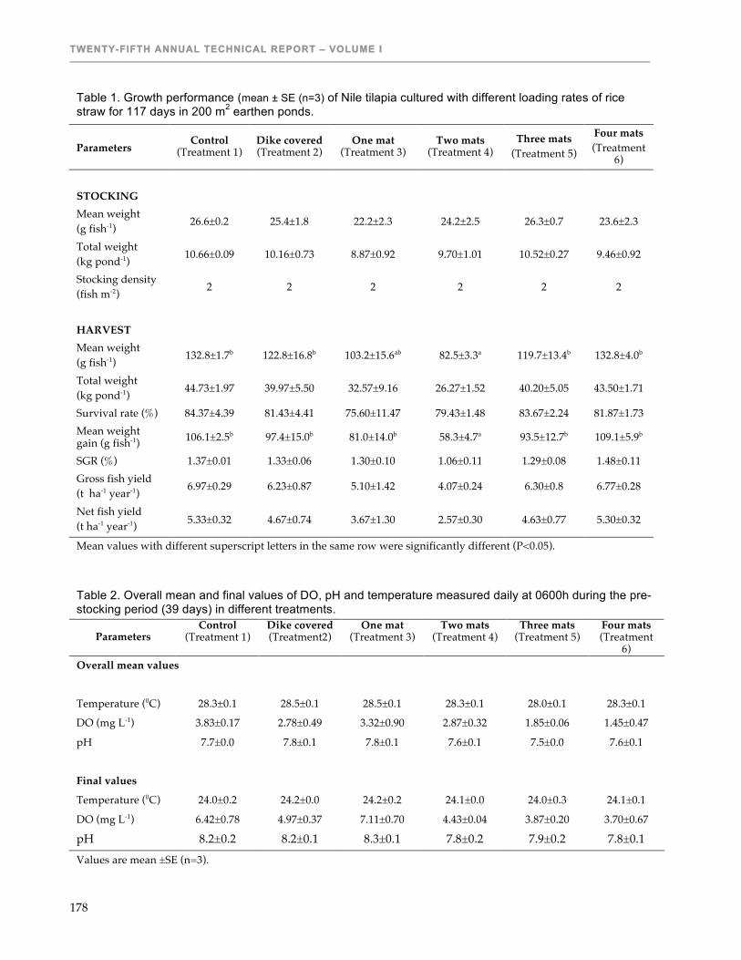
TWENTY-FIFTH ANNUAL TECHNICAL REPORT – VOLUME I
178
Table 1. Growth performance (mean ± SE (n=3) of Nile tilapia cultured with different loading rates of rice straw for 117 days in 200 m2 earthen ponds.
Parameters
Control (Treatment 1)
Dike covered (Treatment 2)
One mat (Treatment 3)
Two mats (Treatment 4)
Three mats (Treatment 5)
Four mats (Treatment
6) STOCKING Mean weight (g fish-1) 26.6±0.2 25.4±1.8 22.2±2.3 24.2±2.5 26.3±0.7 23.6±2.3
Total weight (kg pond-1) 10.66±0.09 10.16±0.73 8.87±0.92 9.70±1.01 10.52±0.27 9.46±0.92
Stocking density (fish m-2) 2 2 2 2 2 2
HARVEST Mean weight (g fish-1) 132.8±1.7b 122.8±16.8b 103.2±15.6ab 82.5±3.3a 119.7±13.4b 132.8±4.0b
Total weight (kg pond-1) 44.73±1.97 39.97±5.50 32.57±9.16 26.27±1.52 40.20±5.05 43.50±1.71
Survival rate (%) 84.37±4.39 81.43±4.41 75.60±11.47 79.43±1.48 83.67±2.24 81.87±1.73 Mean weight gain (g fish-1) 106.1±2.5b 97.4±15.0b 81.0±14.0b 58.3±4.7a 93.5±12.7b 109.1±5.9b
SGR (%) 1.37±0.01 1.33±0.06 1.30±0.10 1.06±0.11 1.29±0.08 1.48±0.11 Gross fish yield (t ha-1 year-1) 6.97±0.29 6.23±0.87 5.10±1.42 4.07±0.24 6.30±0.8 6.77±0.28
Net fish yield (t ha-1 year-1) 5.33±0.32 4.67±0.74 3.67±1.30 2.57±0.30 4.63±0.77 5.30±0.32
Mean values with different superscript letters in the same row were significantly different (P<0.05).
Table 2. Overall mean and final values of DO, pH and temperature measured daily at 0600h during the pre-stocking period (39 days) in different treatments.
Control Dike covered One mat Two mats Three mats Four mats Parameters (Treatment 1) (Treatment2) (Treatment 3) (Treatment 4) (Treatment 5) (Treatment
6) Overall mean values
Temperature (0C) 28.3±0.1 28.5±0.1 28.5±0.1 28.3±0.1 28.0±0.1 28.3±0.1
DO (mg L-1) 3.83±0.17 2.78±0.49 3.32±0.90 2.87±0.32 1.85±0.06 1.45±0.47
pH 7.7±0.0 7.8±0.1 7.8±0.1 7.6±0.1 7.5±0.0 7.6±0.1
Final values
Temperature (0C) 24.0±0.2 24.2±0.0 24.2±0.2 24.1±0.0 24.0±0.3 24.1±0.1
DO (mg L-1) 6.42±0.78 4.97±0.37 7.11±0.70 4.43±0.04 3.87±0.20 3.70±0.67
pH 8.2±0.2 8.2±0.1 8.3±0.1 7.8±0.2 7.9±0.2 7.8±0.1 Values are mean ±SE (n=3).

PRODUCTION SYSTEM DESIGN & INTEGRATION
179
Table 3. Overall mean and final values of water quality parameters measured at 0900h during the experimental period.
Control Dike covered
One mat Two mats Three mats Four mats Parameters (Treatment
1) (Treatment
2) (Treatment
3) (Treatment
4) (Treatment
5) (Treatment
6) Overall mean values
Temperature (0C) 27.2±0.1 27.4±0.1 27.4±0.3 27.6±0.1 27.2±0.3 27.5±0.1 DO (mg L-1) (0600 h) 3.07±0.36 2.75±0.32 2.56±0.33 2.48±0.07 2.38±0.25 2.18±0.29
DO (mg L-1) (0900 h) 5.87±0.22 5.23±0.28 4.63±0.75 4.03±0.24 4.63±0.54 4.60±0.61
pH 8.3±0.3 8.2±0.2 8.0±0.2 7.6±0.1 7.9±0.3 8.0±0.2 Secchi disk depth (cm) 18±0 18±1 26±6 27±2 27±8 23±2
Total alkalinity (mg L-1) 133±14 104±5 112±6 128±10 127±6 128±11
TAN (mg L-1) 0.88±0.13 1.27±0.24 1.13±0.10 1.49±0.23 1.28±0.13 1.49±0.31 Nitrate-N (mg L-1) 0.52±0.09 0.55±0.07 0.60±0.09 0.65±0.03 0.45±0.04 0.42±0.02 Nitrite-N (mg/L) 0.15±0.07 0.16±0.03 0.13±0.04 0.16±0.03 0.09±0.03 0.08±0.01 TKN (mg L-1) 7.63±0.51 8.38±0.25 7.01±1.19 6.75±0.2 9.01±1.02 8.00±0.63 TP (mg L-1) 0.72±0.18 0.52±0.11 0.72±.0.16 0.27±0.02 0.54±0.10 0.47±0.07 SRP (mg L-1) 0.19±0.15 0.02±0.01 0.09±0.06 0.04±0.03 0.05±0.03 0.07±0.02 TSS (mg L-1) 117±18 115±18 131±66 59±6 121±31 73±17 TVS (mg L-1) 54±2 50±8 49±14 31±0 49±8 41±5 Chl-a (mg m-3) 413±84 267±92 255±164 63±6 261±114 225±85 Tannin (mg/L) 5.32±0.14 5.56±0.20 6.82±0.97 7.12±0.75 5.41±0.10 6.41±0.36 Final values Temperature (0C) 29.5±0.2 30.0±0.1 30.0±0.5 30.0±0.1 29.5±0.3 30.0±0.2 DO (mg L-1) (0600 h) 2.63±0.63 1.77±0.24 2.10±0.06 2.47±0.22 2.13±0.48 2.07±0.12
DO (mg L-1) (0900 h) 6.11±0.36 6.02±1.12 4.42±1.16 3.78±0.25 6.63±0.62 6.11±1.92
pH 8.4±0.4 7.9±0.5 7.9±0.5 7.4±0.1 8.3±0.4 7.9±0.2 Secchi disk depth (cm) 13±0 12±1 16±5 17±2 16±3 18±3
Total alkalinity (mg L-1) 157±30 92±11 111±18 101±7 113±5 123±4
TAN (mg L-1) 1.19±0.12 1.42±0.98 1.16±0.51 2.96±0.36 1.88±0.34 2.07±0.38 Nitrate-N (mg L-1) 0.54±0.03 0.56±0.11 0.61±0.09 0.81±0.04 0.57±0.07 0.52±0.03 Nitrite-N (mg L-1) 0.18±0.08 0.22±0.12 0.15±0.08 0.22±0.02 0.11±0.07 0.09±0.02 TKN (mg L-1) 5.89±0.93 6.85±0.68 5.32±1.15 4.89±1.46 6.33±0.86 5.39±0.58 TP (mg L-1) 1.05±.41 0.65±0.21 0.54±0.10 0.29±0.04 0.58±0.17 0.39±0.08 SRP (mg L-1) 0.36±0.28 0.07±0.05 0.10±0.07 0.02±0.01 0.04±0.02 0.01±0.01 TSS (mg L-1) 125±27 108±15 121±43 72±7 90±9 91±24 TVS (mg L-1) 69±7 61±17 52±17 28±0 56±17 45±11 Chl-a (mg m-3) 613±213 409±180 251±189 46±4 355±160 187±65 Tannin (mg L-1) 3.96±0.21 4.35±0.26 4.95±0.48 4.72±0.70 4.00±0.34 4.49±0.39

TWENTY-FIFTH ANNUAL TECHNICAL REPORT – VOLUME I
180
Table 4. Number of periphyton g-1 dry rice straw in all treatments during the first sampling day of the experimental period (n=3).
Dike covered One mat Two mats Three mats Four mats Group/genus (Treatment 2) (Treatment 3) (Treatment 4) (Treatment 5) (Treatment 6)
Bacillariophyceae Cyclotella 45455 18519 33333 181818 222222 Fragillaria 0 0 333333 0 0 Navicula 900433 1400000 5083333 2900433 1452381 Surirella 0 0 500000 307359 305556 Total 945887 1418519 5950000 3389610 1980159 Chlorophyceae Ankistrodesmus 0 0 0 0 119048 Chlamydomonas 0 18519 416667 0 0 Chlorococcum 0 0 0 166667 0 Closterium 0 0 0 45455 0 Coelastrum 0 133333 100000 0 277778 Eudorina 0 0 100000 0 0 Micrasterium 45455 0 0 0 0 Scenedesmus 248052 0 333333 880952 912698 Tetraedon 69264 83333 33333 0 0 Ulothrix 0 0 83333 0 0 Total 362771 235185 1066667 1093074 1309524 Cyanophyceae Microcystis 200000 0 0 0 0 Oscillatoria 2635498 3574074 3716667 7896104 8166667 Rivularia 0 129630 0 0 0 Spirulina 0 133333 0 0 0 Total 2835498 3837037 3716667 7896104 8166667 Euglenophyceae Euglena 0 0 83333 0 0 Phacus 0 0 0 95238 0 Trachelomonas 339394 542593 500000 1841991 1543651 Total 339394 542593 583333 1937229 1543651 Xanthophyceae Centritractus 0 0 0 45455 0 Zooplankton Crustacea Daphnia 45455 0 0 0 0 Nauplius 0 0 83333 95238 0 Total 45455 0 83333 95238 0 Rotifera Brachionus 0 133333 0 45455 0 Total 0 133333 0 45455 0 Grand total 4529005 6166667 11400000 14502165 13000001

PRODUCTION SYSTEM DESIGN & INTEGRATION
181
Table 5. Overall abundance (mean and SE) of phytoplankton and zooplankton (units L-1) in pond water during the experimental period. Control Dike covered One mat Two mats Three mats Four mats
Parameters (Treatment 1) (Treatment 2) (Treatment 3) (Treatment 4) (Treatment 5) (Treatment 6)
PHYTOPLANKTON
Bacillariophyceae 1460140±1019161 431680±137821 592133±521832 174673±21740 655447±364249 422287±199243
Chlorophyceae 554273±81078 876640±412214 304387±187073 111527±13317 651613±324953 584993±210035
Chrysophyceae 333±333 733±733 00±00 3533±3533 333±333 5600±5600
Cryptophyceae 181093±59688 95640±11265 103347±60610 154920±32150 133113±98288 232667±66834
Cyanophyceae 547653±195812 695000±333165 427213±308255 61040±24574 514407±227671 449900±228786
Euglenophyceae 1411093±1127908 123607±27687 185380±488867 107327±37072 268273±100100 171660±39029
Xanthophyceae 333±333 367±367 0±0 0±0 1333±882 0±0 Overall means 4158960±871835 2228027±885757 1614247±1067151 613353±48640 2232133±947374 1867107±547264 ZOOPLANKTON
Crustacea 4773±905 4083±330 5058±1046 5653±969 3723±819 5123±990
Rotifera 9040±3356 8300±3544 5775±2399 2390±1826 7793±3385 4283±1298
Ciliata 1183±933 642±510 175±88 275±159 92±92 450±247
Sarcodina 260±152 92±92 92±92 92±92 00±00 83±83
Monogononta 1832±326 600±362 617±385 83±83 965±488 353±221
Hydrozoa 0±0 0±0 0±0 0±0 92±92 92±92 Overall means 17180±2161 13892±2633 11717±3487 8493±2390 12665±4753 10385±384

TWENTY-FIFTH ANNUAL TECHNICAL REPORT – VOLUME I
182
Table 6. Average number of phytoplankton per liter of pond water different treatments. Phytoplankton
Control Dike covered One mats Two mats Three mats Four mats
Group/genus (Treatment 1) (Treatment 2) (Treatment 3) (Treatment 4) (Treatment 5) (Treatment 6)
Bacillariophyceae
Achnathes 0 667 367 0 0 0
Amphora 0 0 367 1133 0 1600
Amphipleura 0 0 733 0 0 0
Chaetoceros 0 0 333 0 400 356
Coscinodiscus 0 367 0 0 0 0
Cyclotella 1397853 331207 520127 54560 600820 329780
Cymatopleura 1333 0 0 1333 0 0
Cymbella 800 11947 2200 0 0 5200
Epithemia 0 0 0 0 0 400
Fragilaria 0 0 333 1533 0 0
Navicula 46933 73573 49720 100573 50253 68540
Nitzschia 11487 11853 16307 9367 4373 10333
Odontella 0 667 0 0 0 0
Pinnularia 0 733 827 0 0 0
Pleurosigma 0 0 367 2400 0 400
Rhizosolenia 0 0 0 0 0 2000
Skeletonema 0 667 0 0 0 0
Surirella 1733 0 0 3107 0 3633
Synedra 0 0 787 0 0 0
Tabellaria 0 0 0 333 0 0
Total 1460140 431680 592133 174673 655447 422287
Chlorophyceae
Actidesmium 0 1100 980 0 0 0
Actinastrum 12520 9253 10940 6193 8580 9200
Ankistrodesmus 86827 41213 3367 12720 65773 45233
Arthrodesmus 0 0 0 0 0 400
Asteroococcus 0 0 2567 0 0 0
Cateria 333 0 0 0 0 0
Chlamydomonas 145373 215647 129140 5773 174740 175847
Chlorella 5333 1100 2233 2667 7760 3600
Chlorococcum 4893 8767 0 0 3440 2400

PRODUCTION SYSTEM DESIGN & INTEGRATION
183
Table 6 (continued) Phytoplankton Control Dike covered One mats Two mats Three mats Four mats Group/Genus (Treatment 1) (Treatment 2) (Treatment 3) (Treatment 4) (Treatment 5) (Treatment 6)
Chodatella 0 367 700 1720 3333 0
Closterium 1707 1040 400 1867 1480 3167
Coelastrum 23013 370473 25047 6300 154607 129033
Cosmarium 0 1033 3000 333 0 1067
Crucigenia 9547 16600 5620 7933 14973 7267
Dictyosphaerium 33307 35233 12127 1100 51353 63100
Eudorina 2333 733 1467 0 1333 6800
Golenkinia 333 367 1573 0 2233 0
Gonatozygon 1333 0 0 0 0 400
Kirchneriella 0 367 0 800 0 400
Lobomonas 0 0 0 0 0 0 Melosira 0 0 3300 333 0 400 Micractinium 2613 367 0 0 2333 0 Mougeotia 333 0 0 0 0 0 Oedogonium 0 0 0 1920 0 0 Oocystis 2280 2773 1467 333 0 3000 Pandorina 1413 0 0 0 1000 0 Pediastrum 24493 18613 10607 6533 12327 12867
Pedinoperopsis 7533 0 0 0 2307 1467
Planktosphaeria 1000 367 2833 0 667 0 Scenedesmus 159040 140520 69980 42947 131520 97080 Selenastrum 0 1000 367 1600 1333 8667 Spirogyra 0 0 2200 1333 0 800 Staurastrum 1000 0 767 1133 0 0 Tetraedron 24713 6040 13707 4133 5820 8467 Tetraspora 0 0 0 0 733 0 Treubaria 0 1100 0 0 1433 733 Ulothrix 1333 1833 0 3520 333 0 Volvox 1667 733 0 333 2200 3600 Total 554273 876640 304387 111527 651613 584993 Chrysophyceae Chrysococcus 0 0 0 333 333 0 Mallomonas 0 733 0 3200 0 5600 Prymnesium 0 0 0 0 0 0 Synura 333 0 0 0 0 0 Total 333 733 0 3533 333 5600 Cryptophyceae Chroomonas 0 0 0 0 0 0 Cryptomonas 160180 88427 89840 147233 113827 217067 Gonyostomum 10113 7213 10153 7687 10673 10667 Gymnodinium 0 0 0 0 0 4933 Peridinium 6800 0 3353 0 8613 0 Rhodomonas 4000 0 0 0 0 0 Total 181093 95640 103347 154920 133113 232667

TWENTY-FIFTH ANNUAL TECHNICAL REPORT – VOLUME I
184
Table 6 (continued) Phytoplankton Control Dike covered One mat Two mat Three mat Four mat Group/Genus (Treatment 1) (Treatment 2) (Treatment 3) (Treatment 4) (Treatment 5) (Treatment 6)
Cyanophyceae Anabaena 667 2000 5400 1333 1100 6600 Aphanocapsa sp. 1000 0 57233 0 0 2800 Aphanothece 0 0 0 0 2200 0 Chroococcus 1000 733 3733 800 0 1600 Cylindrospemum 2200 10400 0 0 0 0 Gloeocapsa 19333 733 1100 0 0 4400 Gomphosphaeria 1000 367 400 0 367 1200 Merismopedia 183213 180533 21840 3500 122600 182633 Microcystis 255707 352213 268627 5573 331767 176200 Nostoc 0 1440 0 1080 0 0 Oscillatoria 82493 45520 39913 28620 55013 31933 Raphidiopsis 1040 101300 10267 19800 1360 42533 Spirulina 0 0 18700 333 0 0 Total 547653 695240 427213 61040 514407 449900 Euglenophyceae Euglena 1290480 96500 133040 80307 175593 126073 Lepocinclis 667 0 0 1600 733 0 Phacus 40740 15073 16533 17013 45180 28867 Trachalomonas 79207 12033 35807 8407 46767 16720 Total 1411093 123607 185380 107327 268273 171660 Xanthophyceae Centritractus 333 367 0 0 1333 0 Total 333 367 0 0 1333 0 Unknown 4040 4120 1787 333 7613 0
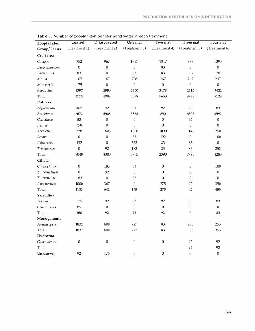
PRODUCTION SYSTEM DESIGN & INTEGRATION
185
Table 7. Number of zooplankton per liter pond water in each treatment.
Zooplankton Control Dike covered One mat Two mat Three mat Four mat
Group/Genus (Treatment 1) (Treatment 2) (Treatment 3) (Treatment 4) (Treatment 5) (Treatment 6)
Crustacea Cyclpos 952 967 1767 1847 878 1395 Diaphanosoma 0 0 0 83 0 0 Diaptomus 83 0 83 83 167 70 Moina 167 167 708 167 267 237 Monostyla 175 0 0 0 0 0 Nauplius 3397 2950 2500 3473 2412 3422 Total 4773 4083 5058 5653 3723 5123 Rotifera Asplanchan 367 92 83 92 92 83 Brachionus 6672 6508 3883 850 6303 3592 Collotheca 83 0 0 0 83 0 Filinia 758 0 0 0 0 0 Keratella 728 1608 1008 1090 1148 250 Lecane 0 0 83 192 0 100 Polyarthra 432 0 533 83 83 0 Trichocerca 0 92 183 83 83 258 Total 9040 8300 5775 2390 7793 4283 Ciliata Cinetochilum 0 183 83 0 0 100 Tintinnidium 0 92 0 0 0 0 Tintinnopsis 183 0 92 0 0 0 Paramecium 1000 367 0 275 92 350 Total 1183 642 175 275 92 450 Sarcodina Arcella 175 92 92 92 0 83 Centropyxis 85 0 0 0 0 0 Total 260 92 92 92 0 83 Monogononta Anuraeopsis 1832 600 727 83 965 253 Total 1832 600 727 83 965 353 Hydrozoa Gastroblasta 0 0 0 0 92 92 Total 92 92 Unknown 92 175 0 0 0 0

TWENTY-FIFTH ANNUAL TECHNICAL REPORT – VOLUME I
186
Table 8. Overall mean values of total plate counts of bacteria count (TPC ml-1) in pond water and benthos abundance (organisms m-2) at pond bottom in different treatments. Numbers are means of three ponds and five sampling days for bacteria and four sampling days for benthos.
Control Dike covered One mat Two mats Three mats Four mats Parameter (Treatment 1) (Treatment 2) (Treatment 3) (Treatment 4) (Treatment 5) (Treatment 6) Bacteria
Overall means 1,905±193 1,849±483 1,738±289 1,699±465 2,058±174 4,140±1,078
Benthos Overall means 531±239 852±146 1,001±59 499±36 729±246 795±206 Groups Oligochaete 368±204 567±136 738±34 298±11 561±186 664±248
Chironomids 142±57 75±43 164±29 56±8 88±59 59±22
Mollusks 22±6a 197±67c 95±9ab 144±31bc 74±10ab 68±28ab
Crustacean 0±0 13±13 5±0 2±2 5±5 3±2
Values are mean ± SE (n=3), mean values with different superscript letters in the same row were significantly different (P<0.05).
PRODUCTION SYSTEM DESIGN & INTEGRATION
187
DEVELOPMENT OF A RECIRCULATING AQUACULTURE SYSTEM MODULE FOR FAMILY/MULTI-FAMILY USE
Twelfth Work Plan, Production System Design & Integration 4 (12PSD4) Final Report
Published as Submitted by Contributing Authors
Michael B. Timmons & Dale Baker Cornell University
Ithaca, New York, USA
ABSTRACT A small scale recirculating aquaculture module for raising tilapia was designed. The nitrification system used was a fluidized sand filter. A packed column was the primary means of controlling other water chemistry and a combination of settling and screen filtering was used for settleable solids removal. The production capacity of the system was approximately 100 to 500 kg per year, depending upon loading conditions and the tolerance for risk. The small scale system module shows promise for widespread adaptation, although it is unlikely that the system developed in this design will be that vehicle.
INTRODUCTION Creating jobs, providing healthy food for human consumption, and protecting the environment are universally identified as some of our world's most pressing concerns. Aquaculture will continue to supply an ever increasing percentage of the seafood being consumed. This trend affords the opportunity to do this in an environmentally friendly and sustainable manner. All aquaculture development is constrained by the available of suitable water resources. Recirculating aquaculture systems (RAS) represent a very sustainable approach to aquaculture production. The primary advantage of recirculating aquaculture is the control of the environment (air and water). Environmental control is important to obtain optimal growth conditions of the target species and keep out unwanted diseases that can spread in the open environment. Even in well established aquaculture industries such as the salmon, catfish, tilapia, and shrimp farming industries, RAS systems are typically employed when strict environmental control is needed to ensure maximum production efficiency (e.g., nursery stages of development). Recirculating facilities can have no impact on the surrounding environment if complete recirculation is used. Recirculating facilities discharge very small quantities of water compared to other forms of culture systems, total water use is less than 0.2% of a typical raceway for the same amount of production (Timmons 2002). Because only small volumes of water are discharged, it is possible to treat the effluent efficiently for pollutants and ensure that there are no negative environmental impacts from the facility.
OBJECTIVES Based upon development opportunities within Mexico that show maximum promise for job creation and economic development, a system production module was designed for commercial implementation for a small family unit (Project Theme: Production System Design and Integration). Specific objectives were: 1. Identify aquaculture goals of Mexican family/multi-family stakeholders, 2. Design a suitable recirculating aquaculture system module to meet these goals (may be done
as part of a special seminar at the technology transfer workshop), 3. Build and operate the recirculating aquaculture module (additional funds may be required).

TWENTY-FIFTH ANNUAL TECHNICAL REPORT – VOLUME I
188
4. Evaluate the performance of the module. Results of Objectives 3 and 4 are described in Appendix A (Additional Deliverable: Demonstration Project 12 PSD4).
METHODS AND MATERIALS Activity 1: Identify aquaculture goals of the family/multi-family stakeholder community The first step in designing a recirculating aquaculture system was to determine the aquaculture goals of the single family/multi-family stakeholder community. A significant amount of information towards this goal was obtained from both the 1st Annual Sustainable Technology Transfer Workshop (described in a separate document) and the work being performed by CRSP in the Santa Maria Bay Management Project. The initial concept of a small semi-intensive RAS system for family or multi-family groups was to provide an additional source of protein that integrates effectively with current agriculture practices. A commercial intensive RAS system of 1 hectare can produce 100 to 200 times the biomass of tilapia produced in a one-hectare pond. Such intense systems require sophisticated water treatment and monitoring systems however to minimize crop loss. A semi-intensive system typical of this project would have a maximum carrying density of 30 kg tilapia/m3 production tank volume. This density of tilapia would require relatively simple design for water treatment and would greatly reduce the risk associated with more intensive systems (density > 100 kg/m3). A graduate student supervised by host country co-PI performed the majority of this first activity and is reported under Annual Report List of Publications (MS Thesis). Dr. Timmons (Cornell University) served as an advisor on the graduate student's committee. It was concluded at the mentioned workshop that the system design should only be for a single family and that the design should be such to minimize total fish loss related to power outages, i.e., harvest densities of < 30 kg/m3. Activity 2: Design a suitable recirculating aquaculture system module to meet these goals. Based upon the goals and typical farming situation of the identified family or multi-family stakeholders established in Activity 1 above, a recirculating aquaculture system was designed. The design was based upon a well-known text by Timmons and Ebeling (2007). The RAS system to achieve the goals of this investigation was to be relatively simple yet robust in design to allow for maximum growth with low risk under likely grow out conditions. The primary components of the RAS system will include production tanks, a settling tank, biofilter, pumps, aeration, and gas transfer equipment. The target cost for the systems will be established based upon local considerations, i.e., design will be reflective of regional investment needs and likely available capital.
CONCLUSIONS A design was developed to address the goals identified for a small family production system. There was ineffective involvement of Dr. Timmons (the primary identified advisor to the design project) related to internal constraints placed on the MS student and her advisor Dr. Trujano by the Graduate over-sight committee at the host university (Instituto Tecnologico del Mar, Veracruz). However, there appeared to be strong support from the local communities for such an approach. Further work on developing a more suitable design for these applications is needed.
ANTICIPATED BENEFITS Design and implementation of small-scale RAS systems as part of sustainable food production at the family/multi-family level could have significant beneficial effects in rural areas of Mexico. If successful design can be developed and shown to be repetitive without complications to a small family unit, then, similar systems could be established throughout Mexico in areas that do not traditionally support aquaculture at the family or multi-family level (e.g., areas of small land
PRODUCTION SYSTEM DESIGN & INTEGRATION
189
availability or well-drained soils). The target species of this investigation, tilapia, is already a popular fish species in Mexico and is known to be a beneficial form of protein for human consumption. In addition to its food value, the resources to grow tilapia such as fingerlings and feed are readily available throughout Mexico.
ACKNOWLEDGMENTS The primary Project leader for this effort was Dr. Margarita Cervantes Trujano, Instituto Tecnologico del Mar, Veracruz. Support of this effort was provided by CETRA Director Eunice Perez-Sanchez (Universidad Juarez Autonoma de Tabasco). Additional support was provided by:
• Dale Baker (NY SeaGrant), and • Dr. Michael B. Timmons (Cornell University) • Dr. Raul Piedrahita (UC Davis)
LITERATURE CITED
Timmons, M.B. and J.E. Ebeling, 2007. Recirculating Aquaculture. Cayuga Aqua Ventures. Ithaca, NY.

TWENTY-FIFTH ANNUAL TECHNICAL REPORT – VOLUME I
190
APPENDIX A: ADDITIONAL DELIVERABLE: DEMONSTRATION PROJECT 12PSD4
DEVELOPMENT OF A RECIRCULATING AQUACULTURE SYSTEM MODULE FOR FAMILY/MULTI-FAMILY USE
Investigators Margarita Cervantes Trujano HC Principal Investigator Instituto Tecnologico del Mar, Veracruz Eunice Perez-Sanchez HC Principal Co-Investigator Universidad Juarez Autonoma de Tabasco Dale Baker US Principal Investigator NY SeaGrant Michael B. Timmons US Co-Principal Investigator Cornell University Master of Science Student Supported Ana Gabriela Trasviña-Moreno Division de Estudios de Posgrado e Investigacion Instituto Tecnologico de Boca del Rio Carretera Veracruz Cordoba Km 12 CP 94290 Boca del Rio, Veracruz, Mexico. Tel 2299860189 http://www.itboca.edu.mx/ Gender: Female Nationality: Mexican Graduation date: January 2007 Thesis Title APLICACIÓN DE UN SISTEMA DE CALIDAD PARA EL APROVECHAMIENTO DEL RECURSO HÍDRICO EN UNA GRANJA DE PRODUCCIÓN ACUÍCOLA.
Location of Demonstration Project A small farm (Los Fierro) in a location called La Piedra at Alvarado, Veracruz. Objectives 1. Identify aquaculture goals of Mexican family/multi- family stakeholders. 2. Design a suitable recirculating aquaculture system module to meet these goals (may be done as
part of a special seminar at the technology transfer workshop). 3. Develop a manual for technology implementation and management. 4. Identify stakeholder participants for demonstration projects and determine project performance
evaluation criteria. Results This portion of the project had reasonable success in terms of the design of a system module was followed up by actually building the system and then installing it on a small family farm. No funds from the CETRA project (CRSP funds) were used in this effort. Good information was collected during the project relative to what would be an appropriate design. A user’s manual was created for the particular design created. Most of this manual will be useful in a generic sense for small family farms that produce tilapia. We expect improvements to occur in the actual design.

PRODUCTION SYSTEM DESIGN & INTEGRATION
191
Collection of Data to Define Design Goals In order to determine aquaculture goals of the single family/multi-family stakeholder community, information was obtained from both the First and Second Annual Sustainable Technology Transfer Workshop. The outcome of this was prepared by Dr. Margarita Cervantes-Trujano and her research graduate students Ana G. Trasviña-Moreno and Gerardo A. García-Moreno. Results have shown that the goals and constraints of RAS–based sustainable tilapia production at the family/multi-family scale in Mexico was limited among respondents (8%), as the most of their experience is on extensive and semi-intensive systems (Fig. 1. A significant majority of respondents (67%) found the workshop very helpful, as they pointed out that it provided updated technical information. From this group, 34% out of this percentage are interested in technical information availability and 33% are looking forward for more updated information. A minority of the respondents (18%) were more interested in technology transfer information (Fig. 2).
When asked on their interest to attend workshops on technology transfer in aquaculture, they responded to be interested in 3-day workshops (98%). Most (70%) of the respondents were
EXPERIENCIA EN ACUACULTURA/
AQUACULTURE EXPERIENCE.
ALGUNA/SOME61%
LIMITADA/LIMITED
8%
EXTENSA/EXTENSIVE
31%
Figure 1
MAYOR AYUDA DEL TALLER/What was most helpful at the workshop?
INFOMACION ACTUAL I ZADA
3 3 %
INTERCAMBIO DE EXPERIENCIA
6 %
C O N T A C T O S -V INCULAC ION
9 %
TRANSFERENCIA TECNOLOG ICA
1 8 %
INFORMACION TECN ICA
3 4 %
Technical information
Technology Transfer /
Experience exchange /
Updated information
Figure 2

TWENTY-FIFTH ANNUAL TECHNICAL REPORT – VOLUME I
192
IN T ER ES D EL S EC T O R /R ES EA R C H A N D EX T EN S IO N N EED S .
0% 5% 10% 15% 20% 25% 30%
ASESORIAS
SEMILLA
TECNOLOGIA VIABLE REGION
FINANCIAMIENTO
INFRAESTRUCCTURA Y EQUIPO
INFORMACION TECNICA
INFORMACION JURIDICA
PORCENTAJE
Figure 3
satisfied with the information provided in the First Workshop (referring to the first CETRA workshop in Nov 05 in Sonora) and reported that amongst their research and extension needs-- consulting is the most important (Fig. 3). Based upon the goals and typical farming situation described above, a family or multi-family recirculating aquaculture system was designed. Ana G. Trasviña-Moreno was the research graduate student elected to carry out the design of the RAS system under Dr. Margarita Cervantes-Trujano supervision. Trasviña-Moreno developed the design considerations for water quality and biomass. To achieve the goals of this activity, the design was intended to be relatively simple. Operating and management guidelines were developed and provided in a manual (another deliverable of this project), which included information on how to construct the RAS module, operational instructions and how to grow tilapia properly in it. Stakeholders were identified in Veracruz and Tabasco to demonstrate the operation of the RAS module. Funds were eventually found to support this part of the project independent of CETRA CRSP funding.
Figure 3

PRODUCTION SYSTEM DESIGN & INTEGRATION
193
INSULIN-LIKE GROWTH FACTOR-I GENE EXPRESSION AS A GROWTH INDICATOR IN NILE TILAPIA
Twelfth Work Plan, Production System Design & Integration 5 (12PSD5) Final Report
Published as Submitted by Contributing Authors
Christopher L. Brown Florida International University
North Miami, Florida, USA
Remedios B. Bolivar Central Luzon State University
Science City of Muñoz, Nueva Ecija, Philippines
ABSTRACT A set of studies constituting a doctoral research program was carried out on the expression of the IGF-I gene in juvenile tilapia, using fish approximately of the initial size that is stocked for growout in commercial aquaculture in the Philippines (~1-1.5 g). IGF-I is a mitogenic polypeptide that is an important regulator of growth in fish. The potential of IGF-I mRNA abundance as an instantaneous growth indicator in juvenile Nile tilapia, Oreochromis niloticus, was evaluated. Hepatic IGF-I cDNA was isolated and partially cloned. The partial sequence having 539 bp was found to encode for the signal peptide (44 amino acids), mature protein (68 aa) and a portion of the E domain (19 aa). The deduced 68 aa sequence for mature IGF-I showed 84-90% and 77-79% sequence identity with fish and mammalian counterparts, respectively, confirming the highly conserved sequence homology among species. The B and A domains were even more highly conserved with respect to the deduced amino acid sequence (90-96%). Based on the mature IGF-I peptide, a sensitive TaqMan real time qRT-PCR assay for O. niloticus was developed for measures of hepatic IGF-I mRNA levels. Hepatic IGF-I mRNA levels were found to be significantly correlated with growth rate of individual juvenile fish reared under different feeding regimes and temperature conditions. Higher feed consumption and water temperature produced faster growing fish and increased hepatic IGF-I mRNA expression. These findings suggest that hepatic IGF-I plays a key role in controlling growth in O. niloticus and indicates IGF-I mRNA measures could prove useful to assess current growth rate in this species. Initial studies on feeding and temperature establishing the validity of the association between IGF-I mRNA expression and growth were followed by examinations of gene expression as associated with photoperiod and with social status.
INTRODUCTION
Increased and efficient fish production demands fast growing strains, efficient feeds and feeding protocols, and optimization of the culture environment and other parameters known to impact the growth and health of fish. Evaluation of the effect of a particular parameter on growth usually requires numerous and costly production trials. Aside from the considerable expense involved, research progress is also limited by the length of time required to see gross changes in body weight or length for a specific growth trial (for example, see Brown et al., 2000). Normally this involves controlled laboratory or research scale tests followed by large-scale farm trials; both approaches require proper controls and replication for statistical validity. To save time and money, there is a need, therefore, for the development of a means for rapid and direct assessment of growth of fish over short periods of exposure to the parameter being tested. Somatic growth in fish, as in other vertebrates, is regulated by a variety of growth factors/hormones acting through endocrine, paracrine and/or autocrine modes. A central step in this hormonal network is the growth hormone (GH) – insulin-like growth factor (IGF) axis (Duan, 1997, 1998). The IGF system is composed of ligands (IGF-I and IGF-II), receptors, and IGF binding
TWENTY-FIFTH ANNUAL TECHNICAL REPORT – VOLUME I
194
proteins (IGFBPs). Of the components of the IGF system, IGF-I is the most promising candidate as an instantaneous growth indicator in fish. IGF-I is a naturally produced molecule of approximately 70 amino acid residues with structural homology to proinsulin and is an important regulator of growth and differentiation (Meton et al., 2000; Degger et al., 2000). The IGF-I prepropeptide has S-, B-, C-, A-, D-, and E-domains. The S- and E-domains are removed by proteolytic processing of the propeptide to yield mature IGF-I, which is released into the serum (Chen et al., 2000). Pituitary GH secreted into the blood stream stimulates the production of the mitogenic peptide IGF-I in the liver (Duan, 1998; Kajimura et al., 2001; Pierce et al., 2004). IGF-I is also produced in several tissues and acts locally in a paracrine and/or autocrine manner (McRory and Shewood, 1994; Duan, 1997; Plisetskaya, 1998). IGF-I mediates the growth promoting actions of GH as well as regulates excessively high production of GH through a negative feedback mechanism (Rotwein et al., 1994; Duan, 1997; Fruchtman et al., 2000). Most of the hepatic-derived circulating IGF-I is bound to a number of IGF binding proteins (IGFBPs) which regulate their availability to target tissues, prolong their half-lives and prevent their insulin–like activity (Duan, 1997; Hwa et al., 1999, Degger et al., 2000; Kelly et al., 2001). Upon release from these IGFBPs, the majority of IGF-I actions are mediated through the type I IGF receptor (IGF-IR) (LeRoith et al., 1995). Circulating IGF-I is predominantly derived from the liver (Schwander, et al., 1983, Duan et al., 1994; Reinecke et al., 1997; Duan, 1998; Pierce et al., 2004). Both homologous and heterologous IGF-I’s have been shown to promote growth in teleosts (McCormick et al., 1992; Negatu and Meier, 1995; Chen et al., 2000; Degger et al., 2000). Several studies indicated a significant and positive correlation between circulating IGF-I and growth rates (Jones and Clemmons, 1995; Beckman et al., 1998; Shimizu et al., 2000; Larsen et al., 2001; Kajimura et al., 2001). The relationship of IGF levels and growth rate is more consistent than that of GH with growth rate. Growth hormone levels can become dissociated with growth rate under some conditions (e.g. malnutrition; prolonged starvation), under which the correlation of IGF-I with growth persists (Duan and Plisetskaya,1993; Duan, 1997, 1998). For these reasons, the detection of IGF-I is gaining more appeal as a possible indicator of growth rate in fishes (Shimizu et al., 2000; Larsen et al., 2001). In the present study, we cloned a portion of O. niloticus IGF-I cDNA and developed a sensitive TaqMan real time quantitative reverse transcription-polymerase chain reaction (qRT-PCR) assay for measures of IGF-I mRNA abundance. We report the use of hepatic IGF-I mRNA as an instantaneous growth indicator in Nile tilapia, with respect to investigations on growth control by temperature and feeding regimen.
MATERIALS AND METHODS Fish Juvenile Nile tilapia (~1-1.5g) obtained from Aquasafra, Inc., Bredenton, Florida were maintained in circular (1.7 m3, 1.7 m diameter) tanks at the Marine Biology Laboratory, Florida International University. This size is comparable to the optimal stocking size for juvenile tilapia to be used for growout (see Final technical report, Investigation 11FNFR2). Fish were reared in fresh water under natural photoperiod and fed a commercial (AquaMax) pelleted diet. Studies were conducted under the authority of Florida International University’s Animal Care and Use Committee (FIU IACUC protocol number 02-018) Cloning of IGF-I cDNA RNA isolation: Liver was collected from juvenile Nile tilapia, immediately frozen on dry ice, and stored at –80ºC. Total RNA was isolated according to Chomczynski and Sacchi (1987). Excess glycogen was removed during RNA extraction via lithium chloride (Puissant and Houdebine, 1990).
Oligonucleotide design: Primers for the polymerase chain reaction (PCR) (InvitrogenTM, Carlsbad, California, USA) were designed based on the previously cloned sequence for IGF-I in O. mossambicus (NCBI Genbank accession no: AF033796). The forward primer for standard PCR

PRODUCTION SYSTEM DESIGN & INTEGRATION
195
was 5´-TTCTCCAAAACGAGCCTGCG-3´ (5´-promoter region) and the reverse primer was 5´-TCTGCTACTAACCTTGGGTGC-3´ (E domain).
Reverse-transcription and cloning: First-strand cDNA was synthesized from 1 µg of total RNA using the gene-specific reverse primer (1 µM) described above, 1X buffer RT, 0.5 mM of each dNTP, 10-units RNase inhibitor, and 4-units reverse transcriptase in a total reaction volume of 20 µl (Omniscript™ RT kit, Qiagen Inc., Valencia, California, USA). The reaction was incubated for 60 min at 37°C, inactivated by heating the reaction to 93°C for 5 min, and stored at –20°C. The PCR was carried out in a Hybaid thermal cycler (Thermo Electron Corp., Waltham, Massachusetts, USA) using the HotStar Taq™ PCR Kit (Qiagen Inc.). For PCR reactions, 2 µl of the reverse-transcription reaction (~100 ng template DNA), 1X PCR buffer (1.5 mM MgCl2), 200 µM of each dNTP, 0.2 µM gene-specific forward and reverse primers, and 2.5 units of HotStarTaq DNA polymerase were mixed for a total reaction volume of 50 µl. Thermal cycling conditions were as follows: initial activation at 95°C for 15 min, 30-PCR cycles at 94°C for 1 min, 62.5°C for 1 min, 72°C for 1 min, and a final extension at 72°C for 10 min. The PCR above was repeated to generate a greater amount of the amplicon using the product above as the template. PCR products were electrophoresed on a 1% agarose gel. A distinct band estimated at ~540 nucleotides was generated. This band was extracted from the agarose gel and purified using a QIAquick Gel Extraction Kit (Qiagen Inc.). The product was ligated into pCR®II vector and resulting plasmids were transformed into INVaF´ One Shot® competent cells for ‘blue/white screening’ (TA Cloning® Kit, Invitrogen™). Six white colonies were selected for culture in Luria Bertani/ampicillin media and grown for ~18 hours in a shaking incubator at 37°C. Plasmid DNA was purified using the QIAprep® miniprep kit (Qiagen Inc.). An aliquot (5-8 µl) of each plasmid DNA sample was digested with EcoR I + Buffer H to verify insert size. A clone containing an insert of the predicted size was selected for sequencing at the University of Chicago, Cancer Research Center-DNA Sequencing Facility. The sequence was obtained using M13/pUC universal forward primers. Resulting sequences were compared to those for other species at the National Center for Biotechnology Information (NCBI) website using the BLAST search service. Sequence alignments and comparisons to other IGF-I sequences were performed using MacVector™ 7.0 software (Genetics Computer Group, Oxford, Molecular, Madison, Wisconsin, USA). Experiments IGF-I and growth modulation using different feeding regimes: A feeding regime experiment was conducted to evaluate the relationship of IGF-I level to growth of the fish. Tilapia fingerlings from a holding tank were distributed randomly into 12, 64-liter aquaria at a density of 15 fish per aquarium. The aquaria were divided into three blocks and the following treatments were assigned randomly in each block: (i) daily feeding (DF, 6% of BW), (ii) alternate-day feeding (ADF, 6% of BW), (iii) daily feeding to satiation (SAT) and (iv) feeding at restriction level (RLF, 1% of BW). Fish in the first two treatments (DF and ADF) were supposed to be fed following a feeding guide based on their body weight but the amount of feed consumed by fish at satiation level was lower than amount based on the feeding guide. This resulted in the reduction of the amount of food equal to that given at satiation level. Thus the DF group was essentially fed to satiation daily just as the SAT group. Fish in the RLF group were fed at 16% of the satiation level. Fish were fed once daily except for ADF. Fish in each aquarium were bulk weighed at the start and end of the study. The experiment was terminated after four weeks and two fish per aquarium or group (3 replicate aquaria/group) were anesthetized in tricaine methanesulfonate (MS-222) and the liver was rapidly removed and snap frozen on liquid nitrogen prior to RNA extraction. IGF-1 mRNA levels and growth modulation using different water temperatures: The fish were fasted in an experimental tank for a period of one month (fed at 1% of BW, given thrice a week for the first 15 days and food-deprived for the last 15 days) prior to the start of the experiment. Fingerlings were distributed randomly into three 64-liter aquaria at a density of 10 fish per aquarium. Aquaria were assigned randomly to the following treatments: (i) water temperature manipulated, higher or equal to 28°C, (ii) non-manipulated, natural water temperature and (iii)
TWENTY-FIFTH ANNUAL TECHNICAL REPORT – VOLUME I
196
water temperature manipulated, lower or equal to 24°C. The water temperature fluctuations in the experimental groups are presented in Figure 1. Fish were fed once daily, to satiation. Fish in each temperature condition were bulk weighed at the start and end of the study. The experiment was terminated after three weeks and four fish per aquaria were anesthetized in MS-222, individually weighed, and the livers were rapidly dissected and snap frozen in liquid nitrogen for RNA extraction and quantification.
IGF-1 mRNA levels and growth modulation depending on photoperiod and social status: Fish were individually weighed and six fish were anesthetized in 0.02% MS-222 and the liver tissues were rapidly removed and snap frozen on liquid nitrogen for RNA extraction and IGF-I mRNA quantification. The mean IGF-I mRNA level of six fish was used as the basal value. Immediately after the measurement of ECP, the remaining fish were sized-matched for the later pairing with maximum size difference of 11% (mean = 7.01% ± 0.79). Both fish in a pair were marked by a small cut in the upper or lower part of the caudal fin. To assure a clear dominant-resident relationship, a resident-intruder situation was imposed by the introduction of an intruder fish into the aquarium occupied by a similarly-sized conspecific fish. The resident fish was taken out and reintroduced, together with the intruder, into the aquarium to control the handling effects. After a 15-min pairing, the total number of agonistic attacks was recorded for 10 min during which the ECPs were also recorded. At 2 h after introduction of intruder fish, the ECPs were recorded, and then fish were hand fed in excess to ensure that food was available for subordinates. Twenty four hours after pairing, ECPs and individual body weights of six pairs of fish were measured. Fish were then anesthetized in 0.02% MS-222 and the liver was rapidly removed and snap frozen on liquid nitrogen prior to RNA extraction and IGF-I mRNA quantification. The remaining fish were hand fed once daily. After 10 days of pairing, ECP and body weight of each remaining fish were measured followed by the removal of the liver. The fish specific growth rate (SGR) was calculated as: SGR (weight; %·day-1) = [(ln Wf – ln Wi)·(t)-1] x 100 where Wf is the final body weight (g), Wi is the initial body weight (g) and t is the growth time (days). RNA isolation and processing: Liver tissues were collected from experimental fish at time zero and upon termination of the experiment. Total RNA was isolated following the extraction method in the manufacturer’s protocol (Trizol®, Invitrogen™). High salt precipitation solution was used for glycogen removal in the samples. RNA was treated with DNA-free™ (Ambion®, Austin, Texas, USA) in two separate reactions to remove any possible genomic DNA contamination. RNA was quantified and purity was assessed by spectrophotometry (NanoDrop® ND-1000 spectrophotometer). The A260/A280 values ranged from 1.7 –2.0 with most samples having values from 1.9-2.0. Reverse transcription: First strand cDNA was synthesized in 20 µl RT reactions with 1 ug total RNA template, Omniscript® reverse transcriptase, 10x RT buffer, 5 µM dNTP, 10 µM oligo-dT primer (Promega®, Madison, Wisconsin, USA), and RNase inhibitor (RNasin®, Promega®). Samples were reversed transcribed by incubation at 37 °C for 60 min. Quantification of IGF-1: TaqMan® qRT-PCR was performed on GeneAmp® 5700 Sequence Detector (Applied Biosystems, Foster City, California, USA), using the standard cycling conditions recommended by the manufacturer (50 °C for 2 min, 95 °C for 10 min, followed by 40 cycles of 95 °C for 15 s, 60 °C for 1 min). Gene specific primers and FRET probes (Biosource, Camarillo, California, USA) for qRT-PCR were designed with Primer Express® program (Applied Biosystems). The forward primer was 5´-GTCTGTGGAGAGCGAGGCTTT-3´ (5´-preproIGF-I region) and the reverse primer was 5´-CACGTGACCGCCTTGCA-3´ (E domain). The sequence of the probe was 5’ TTTCAATAAACCAACAGGCTATGGCCCC 3’. The selected reporter and quencher dyes for the probe were FAM and TAMRA, respectively. Reactions for each sample

PRODUCTION SYSTEM DESIGN & INTEGRATION
197
were done in triplicate with each well containing 25 µl PCR mixture (10 ng cDNA template, 1x TaqMan® universal PCR master mix, 900 nM forwards and reverse primers and 250 nM probe). No template controls (NTC) were used to confirm that reagents were not contaminated with carryover PCR products. No amplification controls (NAC) were included in triplicate to test for any possible genomic DNA contamination in RNA preparations. Cycle threshold (CT) values corresponded to the number of cycles at which monitored fluorescence emission in qRT-PCR exceeded the threshold limit. A serial dilution of pooled sample cDNA was run to generate a standard curve of IGF-1 (0.01 -100 ng) and to assess PCR efficiency. The amount of IGF mRNA was determined by comparison with the generated standard curve and normalized to total RNA as suggested by Bustin (2000, 2002). Values of IGF-I mRNA were then expressed relative the lowest sample level measured within an experiment (assigned an arbitrary value of 1). Statistical analyses: Data were analyzed using one-way analysis of variance (ANOVA). The Least Significant Difference test was used to determine significant difference between means. Linear relationship between gain in weight and relative abundance of IGF-I mRNA was assessed using linear regression and Pearson correlation coefficient. All statistical analyses were done using version 11 SPSS software.
RESULTS Sequence of IGF-I cDNA The amplicon generated for O. niloticus using two primers localized in the 5’ preproIGF-I and E domain was 539 nucleotides (Figure 2). The identified sequence contains the signal peptide, B, C, A, D domains and portion of the E domain. The sequence exhibits the six (2 in B domain and 4 in A domain) conserved cysteine residues. BLAST search results demonstrated that the amplicon showed high sequence homology to IGF-I in other fishes. Identities between O. niloticus IGF-I and the corresponding region in fish species including O. mossambicus ranged from 75-99%, whereas those between O. niloticus IGF-I and other vertebrates ranged from 70-80%. The mature IGF-I peptide (B-D domain) was 100% identical to that of O. mossambicus. Comparison of the deduced 68 amino acid sequence of IGF-I (B-D domain) shows 84 to 90% sequence identity with fish counterparts and 77 to 79% with the corresponding mammalian hormones (Figure 3). The expressed mature IGF-I sequence was found to be two amino acids shorter at its C domain than the comparable domain in mammalian and other fish species. Effect of feeding regimes on growth The mean weight gains of the fish are presented in Figure 4. Feeding to satiation (SAT) led to the highest weight gain (2.56g + 0.06), which was not significantly different compared to the daily feeding (DF) group (2.25g+0.18). Not unexpectedly, fish on the restricted diet (RLF) showed the lowest weight gain of 0.56g + 0.10, which was significantly different (P<0.01) compared to all treatments. ADF (1.78g + 0.15) was also significantly different from all treatments. Increased growth related to increased IGF-1 mRNA levels in liver Mean IGF-I mRNA levels in DF, ADF, SAT and RLF fish were elevated 4.1-fold, 3.8-fold, 4.6-fold and 2.3-fold, respectively compared to that of time 0 fish. Statistical analysis, however, showed no significant difference among treatments, which may be attributed to the wide variation of the relative abundance of IGF-I mRNA within treatment. A very high positive correlation (r2=0.98, P<0.01) however was observed between mean weight gain and relative abundance of hepatic IGF-I mRNA. Higher temperature dramatically increased IGF-I mRNA Mean (of 10 fish) weight gains of fish reared in low, non-manipulated, and high temperatures were 1.25g, 8.68g and 10.11g, respectively. Compared to fasted fish, mean IGF mRNA levels increased 13–fold, 60-fold and 269–fold in fish reared at low, non-manipulated and high temperatures, respectively. This indicates a dramatic elevation of IGF-I mRNA expression as growth rate increases with increased water temperature. Comparison of individual gain in weight
TWENTY-FIFTH ANNUAL TECHNICAL REPORT – VOLUME I
198
to relative IGF-I mRNA abundance showed a significant and positive correlation (r = 0.64, P<0.05; Figure 6). Photoperiod, Social status and IGF levels After the 21-day experiment, fish in the long photoperiod (LP) group showed a trend favoring higher mean SGRW (3.44 ± 0.17 %·day-1; Fig. 1), but the apparent difference was not significantly significant (P = 0.057) in comparison with those in the short photoperiod (SP; 2.97 ± 0.07 %·day-1). In terms of growth in length, LP also had the higher mean SGRL (1.07 ± 0.05 %·day-1), but again this trend was not accompanied by a significantly differece (P = 0.055) when the LP treatment group was compared with the SP group (0.91 ± 0.04 %·day-1). There were no significant differences among the mean SGRs within the basal population, in a comparison of subsequently dominant and subordinate fish during the isolation period. The mean specific growth rates (SGRs ±S.E.) ranged from 4.11 ± 0.08 %·day-1 to 4.52 ± 0.04 %·day-1. The SGRs of fish at different periods during the experiment are shown in Figure 1. After the experimental aggressive encounter, reduced specific growth rates were observed in both dominant and subordinate fish, but the observed reductions were greater in subordinate fish. The subordinates were also observed not consuming food when fed after the social interaction. One day after experimentation, mean SGR (2.88 ± 0.61 %·day-1) of dominant fish (DOM-1) was significantly (P<0.001) higher than that (-2.16 ± 0.17 %·day-1) of the subordinate fish (SUB-1) but was not significantly different than the basal value (4.11 ± 0.08 %·day-1). Ten days after the interaction, mean SGR (1.48 ± 0.36 %·day-1) of dominant fish (DOM-10) was significantly (P<0.01) lower than the basal value but no significant difference was found with that (0.43 ± 0.22 %·day-1) of subordinate fish (SUB-10). The SGRs of both SUB-1 and SUB-10 were significantly lower (P<0.01) than the basal value. The endocrine response to social interaction was measured. The mean basal value ± S.E. for hepatic IGF-I mRNA expression was 92.09 ± 18.53 ng/µl. After one day of experimentation mean hepatic IGF-I mRNA expression in dominant fish was 152.47 ± 41.38 ng/µl, while in submissive fish it was 45.38 ± 6.25 ng/µl. Although no significant difference was found between IGF-I mRNA in dominant and submissive fish at this point, there is a slight tendency that dominant fish had higher IGF-I mRNA compared to those in the submissive group (P = 0.06). After ten days, dominant fish had significantly (P<0.01) higher mean IGF-I mRNA expression (269.88 ± 74.02 ng/µl) than submissive fish (25.95 ± 11.87 ng/µl). The IGF-I mRNA levels in experimental fish were not significantly different from the basal values. The hepatic IGF-I mRNA expression of the fish was positively correlated to SGR (n = 24, r2 = 0. 23, P<0.05; Fig. 3). When treated separately, the change in SGR explained by change in IGF-I mRNA expression was similar one day after the aggressive encounter (n = 12, r2 = 0.48, P<0.05) and 10 days later (n = 12, r2 = 0.49, P<0.05). Homogeneity of slope analysis using ANCOVA showed that the relationship between SGR and IGF-I was status but not time dependent. The IGF-I mRNA expression of the dominant fish was also positively correlated (n = 12, r2 = 0.71, P<0.01) with the recorded number of attacks in the period of 10 minutes during the experimental interaction. On the other hand, a negative association was observed between IGF-I expression of the subordinate fish and number of attacks (r2 = 0.06) but the association was not statistically significant.
DISCUSSION Sequence of IGF-I cDNA The partial O. niloticus IGF-I cDNA sequence of 539 nucleotides, as shown in Fig. 2, encodes for 132 amino acid (aa) residues. The identified sequence contains a signal peptide, beginning with the first ATG, (132 bp; 44 aa), B domain (87 bp; 29 aa), C domain (30 bp; 10 aa), A domain (63 bp; 21 aa), D domain (24 bp; 8 aa), and partial E domain (60 bp; 20 aa). Mature IGF-I (B-D domain) in turbot, Psetta maxima, (Duval et al., 2002), flounder, Paralichthys olivaceus (Tanaka et al., 1998), barramundi, Lates calcarifer (Stahlbom et al., 1999), rabbitfish, Siganus guttatus (Ayson et al., 2002), coho salmon, Oncorynchus kisutch (Cao et al., 1989), common carp, Cyprinus carpio (Liang et al., 1996), Goldfish, Carassius auratus (Kermouni et al., 1998), chicken, Gallus gallus (Kajimoto and Rotwein, 1989), rat, Rattus norvegicus (Roberts et al., 1987) and human (Rinderknecht and

PRODUCTION SYSTEM DESIGN & INTEGRATION
199
Humbel, 1978; Jansen et al., 1983) differ from tilapia IGF-I by 7, 7, 9, 9, 9, 10, 11, 15, 16 and 16 amino acids, respectively (77-90% homology; Figure 3). Comparison of the nucleotide sequences for fish and non-human mammals shows high evolutionary conservation. The homology between IGF-Is indicates that amino acid substitutions are relatively few, and the IGF-I mature peptide sequence is highly conserved during phylogeny. Greater conservation of the amino acid composition can be observed in the B and A domains, while considerably less conservation is found in C and D domains. It is in the B and A domains where the conserved cysteine residues are located which are responsible for maintenance of tertiary structure (Reinecke et al., 1997). The importance of this high sequence identity of B and A domains in different species can be ascribed to the functional roles of these regions in the binding of IGF-I with its receptor and IGFBP (Duval et al., 2002). This degree of structural conservation during vertebrate evolution reflects the importance of the biological actions of IGF-I (Upton et al., 1998). Feeding regimes, growth and IGF levels Growth of juvenile fish was significantly affected by the feeding regime as varied in our first experiment. Fish that consumed greater amount of food generally had faster growth rate. The absence of significant difference on weight gain between DF and SAT may be attributed to the reduction of the ration in DF, which was equal to that of SAT. It is interesting to note that feeding on alternate days resulted in weight gain only slightly reduced in comparison to feeding daily, or feeding daily to satiation (see Figure 4). The efficiency and hence the economics of heavy daily feeding have been called into question by recent studies that indicate that Nile tilapia thrive on diets reduced by half through alternate-day feeding (Brown et al., 2004; Bolivar et al., submitted). The wide variation of the relative abundance of IGF-I mRNA within treatments observed in this study might be explained by the observed variation of sizes of fish within the same treatment during the end of the study. Probably because of the limited space available, there was an establishment of hierarchies in feeding among the fish. Dominant individuals within a population have consumed more food and have grown faster than submissive individuals. Dominant individuals were observed chasing the submissive individuals during feeding periods, which may have reduced the amount of food consumed by the latter. The individual weight of fish was, however, not recorded in this study. Nutritional status affects production of hepatic and circulating IGF-I in several species of fish (Duan and Plisetskaya, 1993; Perez-Sanchez et al., 1995; Larsen et al., 2001). In the present study, manipulation of growth rates by using different feeding regimes (varying amount of ration and interval of feeding) resulted in a good correlation between hepatic IGF-I mRNA levels and growth. Perez-Sanchez et al. (1995) reported positive correlation between circulating IGF-I level and growth rates in gilthead sea bream by regulating nutrition using different feeding and dietary protein levels. In O. mossambicus, hepatic IGF-I mRNA levels were significantly increased after rbGH and Posilac® injections (Kajimura et al., 2001). In the same study, significant correlation was observed between circulating IGF-I levels, body length and mass. This similarity in the changes of mRNA levels in both the plasma and the liver of O. mossambicus, infer that a similar phenomenon might occur in O. niloticus. Significant correlation between circulating IGF-I level and growth rate was also observed by Beckman et al. (1998) in juvenile Chinook salmon (Oncorhynchus tshawytscha) in spring. Faster growing channel catfish (Ictalurus punctatus) had higher circulating IGF-I levels than slower growing groups (Silverstein et al., 2000). Exogenous treatment with IGF-I can also stimulate growth and protein synthesis (Negatu and Meier, 1995). McCormick et al. (1992) found that injection of rbIGF-I stimulated growth in coho salmon (O. kisutch); similarly, Chen et al. (2000) observed enhanced growth of juvenile tilapia (O. mossambicus) following injection of recombinant tilapia IGF-I. The relationship of IGF-I levels and growth rate is more consistent than that of GH and growth rate. Under some conditions, GH levels can become dissociated with growth rate, under which the correlation of IGF-I with growth still persists (Duan, 1997, 1998). In coho salmon, prolonged starvation resulted in cessation of growth but significantly increased level of circulating GH (Duan and Plisetskaya, 1993). This

TWENTY-FIFTH ANNUAL TECHNICAL REPORT – VOLUME I
200
starvation-induced elevation of circulating GH level is associated with significant decrease in the hepatic binding sites for GH (Gray et al., 1992), suggesting GH resistance at tissue level. The subsequent low levels of circulating IGF-I resulted in an alleviation of the negative feedback on GH secretion. In contrast to IGF-I, circulating insulin and thyroxine levels did not show any clear relationship to body growth of yearling Coho salmon (Larsen et al., 2001). These findings suggest that IGF-I, both hepatic and circulating, plays a key role in controlling somatic growth in several species of fish and indicates that it can be used as an index for growth. Temperature, growth and IGF levels Fish used in the study were fasted for one-month prior to start of the experiment. Fasting reduced the energy source and the fish displayed suppressed growth. When given sufficient nutrition and ideal environment, fasted fish may undergo rapid compensatory growth (Ali et al. 2003; Picha et al., 2004; Skalski et al., submitted). Growth of fish in the second study was predominantly influenced by temperature. Warm-reared (> 28°C) fish grew steadily throughout the experiment, whereas fish reared under relatively cooler condition (< 24°C) had limited growth. This may be explained in part because food consumption of fish was influenced by temperature. The optimum rearing temperature for this species of fish is from 26-32°C (Balarin and Haller, 1982). It was observed that fish reared under cold condition consumed only small amount of food (around 19%) compared to the amount consumed by fish reared at high temperatures. The low temperature suppressed the appetite of the fish and large portion of the food consumed apparently was used for maintenance, as opposed to growth. The fish reared under non-manipulated temperature consumed around 13% less than the total amount of food consumed by fish reared at high temperature. The appetite of fish reared under non-manipulated temperature condition was reduced during the cooler periods. The growth rates of refed fasted fish reared under different temperature conditions may partly be attributed to the degree of alterations in hepatic IGF-I mRNA production. In this study higher hepatic IGF-I mRNA expression was observed in faster growing fish reared at higher temperatures. Refeeding increased mean IGF mRNA levels 13–fold, 60-fold and 269–fold in fish reared at low, non-manipulated and high temperatures, respectively. This effect of temperature on growth and IGF-I levels is in agreement with the findings of Beckman et al. (1998) that Chinook salmon reared under warmer conditions in spring had higher growth rates and circulating IGF-I levels than those reared under relatively cooler conditions. Similar results were observed in channel catfish reared in 21.7 or 26°C (Silverstein et al., 2000); in Atlantic salmon (Salmo salar) reared at 2-3 or 10°C (McCormick et al., 2000); and in coho salmon reared at 2.5 or 10°C (Larsen et al., 2001). The increase in hepatic IGF-I mRNA levels after refeeding was also reported by Duan and Plisetskaya (1993), in salmon. Chauvigne et al. (2003) also observed dramatic increase of IGF-I mRNA expression, but in this case in muscle, from refed rainbow trout (O. mykiss). Refeeding and provision of ideal environmental conditions, therefore, induces both systemic and local IGF-I productions. Photoperiod, Social status and IGF levels Trends favoring accelerated growth of tilapia were found to be altered by environmental photoperiod – an important transducer of information on seasonality to fish and other vertebrates. In the simplest of terms, we have found that long photoperiods favored the stimulation of growth (that is, elevated expression of the IGF-I gene) as compared with growth under short photoperiods. Detailed results are presented in a manuscript (Vera Cruz and Brown, submitted).
In addition, the process of obtaining food is competitive, and dominant fish are far more successful at doing so. For this reason we established a competitive model in which male tilapia of similar sizes were placed in aquaria, fed, and analyzed for IGF-I gene expression. This paper (Vera Cruz and Brown, in press) demonstrates that dominant fish consistently display higher levels of IGF-I mRNA and hence, growth rate. We anticipate that the dynamics of growth are complex in pond culture, in which social interactions of thousands of tilapia are commonplace. A
PRODUCTION SYSTEM DESIGN & INTEGRATION
201
more thorough understanding of the social structure of tilapia ponds and the effects thereof on growth could help lead to improvements in the commercial production of tilapia.
CONCLUSIONS
A distinct relationship of IGF-I gene expression to growth in individual juvenile O. niloticus has been confrirmed. IGF-I cDNA from this species was cloned and the high sequence identity among related species was confirmed. Greater conservation of the amino acid composition was observed in the B and A domains, demonstrating the highly conservative evolution of these functionally important domains. Based on the partial 539 nucleotide sequence, which spans from the 5’-preproIGF-I region to the E domain, a sensitive TaqMan real time qRT-PCR assay was developed. Nutritional and environmental (temperature) regulation of IGF-I expression was observed in the liver of juvenile O. niloticus. Using the assay, hepatic IGF-I mRNA level was found to be significantly correlated with growth manipulated through both alterations in temperature and feed regimen. We have also found that growth rate is altered by variations in photoperiod and that it is linked to dominance or submissiveness (social status) in these fish. Our findings suggest that hepatic IGF-I plays a key role in controlling growth in O. niloticus and indicate that it could prove useful as an instantaneous indicator for growth in this species.
ANTICIPATED BENEFITS This work has resulted in a series of 4 publications in international journals, half of which have now been accepted or published. A fifth, presenting an overview of all of the work, is in preparation. Our project has demonstrated a means of ascertaining growth rate using just a small number of fish at any particular point in time. We believe the instantaneous assessment of growth offers a huge advantage over costly and time-consuming determinations of growth on a commercial scale. Farmers and scientists will be able to test environmental and nutritional effects on fish growth in a much more cost-effective manner, allowing the pace of refinement of culture technology to move faster.
ACKNOWLEDGMENTS This work resulted from joint efforts between Florida International University, Central Luzon State University, North Carolina State University, and the Aquaculture Collaborative Research Support Program (CRSP). The work was funded in part by USAID grant no. LAG-G-00-96-90015-00, with institutional matching contributions from the three universities mentioned above.
LITERATURE CITED Ali, M., Nicieza, A., Wootton, R. J., 2003. Compensatory growth in fishes: a response to growth
depression. Fish and Fisheries 4,147-190. Ayson, F.G., de Jesus, E.G.T., Moriyama, S., Hyodo, S., Funkenstein, B., Gerter, A., Kawauchi, H.,
2002. Differential expression of insulin-like growth factor I and II mRNAs during embryogenesis and early larval development in Rabbitfish, Siganus guttatus. Gen. Comp. Endocrinol. 126, 165-174
Balarin, J.D., Haller, R.D., 1982. The Intensive Culture of Tilapia in Tanks, Raceway and Cages. In: Muir, J.K., Roberts, R.J. (Eds.), Recent Advances in Aquaculture. pp. 265-355. Croom Held LTd., London and Canberra.
Beckman, B.R., Larsen, D.A., Moriyama, S., Lee-Pawlak, B., Dickhoff, W.W., 1998. Insulin-like growth factor-I and environmental modulation of growth during smoltification of spring chinook salmon (Oncorhynchus tshawytscha). Gen. Comp. Endocrinol. 109, 325-335.
Bolivar, R.B., Jimenez, E.B.T., Brown, C.L. (submitted). An alternate-day feeding strategy for tilapia growout in the Philippines – production and economic evaluation. North American Journal of Aquaculture (NAJA)
Brown, C.L., Bolivar, R.B., Jimenez, E.B.T.,. Szyper, J.P., 2000. Timing of the onset of supplemental feeding of Nile tilapia (Oreochromis niloticus) in ponds. p. 237-240 . In: Fitzsimmons, K. and Filho, J.C. (Eds.), Tilapia Aquaculture in the 21st Century. Proceedings of
TWENTY-FIFTH ANNUAL TECHNICAL REPORT – VOLUME I
202
the Fifth International Symposium on Tilapia Aquaculture. 03-07 September, Rio de Janiero, Brazil. 682 p.
Brown, C.L., Bolivar. R.B., Jimenez, E.B.T., 2004. Philippine studies support moderate feeding in tilapia. Global Aquaculture Alliance Advocate 7(4), 70.
Bustin, S.A., 2000. Absolute quantification of mRNA using real-time reverse transcription polymerase chain reaction assays. J. Mol. Endocrinol. 25, 169-193.
Bustin, S.A., 2002. Quantification of mRNA using real-time reverse transcription PCR (RT-PCR): trends and problems. J. Mol. Endocrinol. 29, 23-39.
Cao, Q.P., Dugay, S.J., Plisetskaya, E., Steiner, D.F., Chen, S.J., 1989. Nucleotide sequence and growth hormone regulated expression of salmon insulin-like growth factor I mRNA. Mol. Endocrinol. 3, 2005-2010.
Chauvigne, F., Gabillard, J.C., Weil, C., Rescan, P.Y., 2003. Effect of refeeding on IGFI, IGFII, IGF receptors, FGF2, FGF6, and myostatin mRNA expression in rainbow trout myotomal muscle. Gen. Comp. Endocrinol.132, 209-215.
Chen, J.Y., Chen, J.C., Chang, C.Y., Shen, S.C., Chen, M.S., Wu, J.L., 2000. Expression of recombinant tilapia insulin-like growth factor I and stimulation of juvenile tilapia growth by injection of recombinant IGFs polypeptides. Aquaculture 181, 347-360.
Chomczynski, P., Sacchi, S., 1987. Single-step method for RNA isolation by acid guanidinium thiocyanate phenol chloroform extraction. Anal. Biochem. 162, 156-159.
Degger B., Upton, Z., Soole, K., Collet, C., Richarson, N., 2000. Comparison of recombinant barramundi and human insulin-like growth factor (IGF)-I in juvenile Barramundi (Lates calcarifer): In vivo metabolic effects, association with circulating IGF-binding proteins, and tissue localization. Gen. Comp. Endocrinol. 117, 395-403.
Duan, C., 1997. The insulin-like growth factor system and its biological actions in fish. Amer. Zool. 37, 491-503.
Duan, C., 1998. Nutritional and developmental regulation of insulin-like growth factors in fish. J. Nutr. 128, 306S-314S
Duan, C., Dugay, S.J., Swanson, P. Dickhoff, W.W., Plisetskaya, E.M., 1994. Regulation of insulin-like growth factor gene expression in salmon. In: Davey, K.G., Peter, R.E., Tobe S.S. (Eds.), Perspective in Comparative Endocrinology, National Research Council, Ottawa, Canada, pp. 365-372.
Duan, C., Plisetskaya, E.E., 1993. Nutritional regulation of insulin-like growth factor-I mRNA expression in salmon tissues. J. Endocrinol.. 139, 243-252.
Duval, H., Rousseau, K, Elies, G., Le bail, P.Y., Dufour, S., Boeuf, G., Boujard, D., 2002. Cloning, characterization, and comparative activity of turbot IGF-I and IGF-II. Gen. Comp. Endocrinol.. 126, 269-278.
Fruchtman, S., Jackson, L. Borski, R.J., 2000. Insulin-like growth factor-I disparately regulates prolactin and growth hormone synthesis and secretion: studies utilizing the teleost pituitary model. Endocrinology 141, 2886-2894.
Fruchtman, S., McVey, D.C., Borski, R.J., 1997. Insulin-like growth factor-I regulation of prolactin and growth hormone secretion in hybrid striped bass. Amer. Zool. 37, 180A.
Gray, E.S., Kelley, K.M., Law, S., Tsai, R., Young, G., Bern, H.A., 1992. Regulation of hepatic
growth hormone receptors in coho salmon (Oncorhynchus kisutch). Gen. Comp. Endocrinol. 88, 243-252.
Hwa, V., Oh, Y., Rosenseld, R.G., 1999. The insulin-like growth factor binding protein (IGFBP) superfamily. Endo. Rev. 20, 761-787.
Jansen, M., Van Schaik, F.M., Ricker, A., Bullock, B., Woods, D.E., Gabbay, K.H., Nussbaumm, A.L., Sussenbach, J.S, Van den Brande, J.L., 1983. Sequence of cDNA encoding human insulin-like growth factor I precursor. Nature 306, 609-611.
Jones, J.I., Clemmons, D.R., 1995. Insulin-like growth factors and their binding proteins: biological actions. Endocr. Rev. 16, 3-34.
Kajimoto, Y., Rotwein, P., 1989. Structure and expression of chicken insulin-like growth factor I precursor. Mol. Endocrinol. 3, 1907-1913.

PRODUCTION SYSTEM DESIGN & INTEGRATION
203
Kajimura, S., Uchida, K., Yada, T., Riley, L.G., Byatt, J.C., Collier, R.J., Aida, K., Hirano, T., Grau, E.G., 2001. Stimulation of insulin-like growth factor-I production by recombinant bovine growth hormone in Mozambique tilapia, Oreochromis mossambicus. Fish Physiol. and Biochem. 25, 221-230.
Kelley, K.M., Haigwood, J.T., Perez, M., Galima, M.M., 2001. Serum insulin-like growth factor binding proteins (IGFBPs) as markers for anabolic/catabolic conditions in fishes. Comp. Biochem. Physiol. B 129(2-3), 229-236.
Kermouni, A., Mahmoud, S.S., Wang, S., Moloney, M., Habibi, H.R., 1998. Cloning of a full-length insulin-like growth factor-I complementary DNA in the Goldfish liver and ovary and development of a quantitative PCR method for its measurement. Gen. Comp. Endocrinol. 11, 51-60.
Larsen, D.A., Beckman, B.R., Dickhoff, W.W., 2001. The effects of low temperature and fasting during the winter on metabolic stores and endocrine physiology (insulin, insulin-like growth factor-I and thyroxine) of coho Salmon, Oncorhynchus kisutch. Gen. Comp. Endocrinol. 123, 308-323.
LeRoith, D., Warner, H., Beitner-Johnson, D., Roberts, Jr., C.T., 1995. Molecular and cellular aspects of the insulin–like growth factor I receptor: a review. Endocrine Rev. 16, 143-163.
Liang, Y.H., Cheng, C.H., Chan, K.M., 1996. Insulin-like growth factor-IEa2 is the predominantly expressed form of IGF-I in common carp (Cyprinus carpio). Mol. Marine Biol. Biotechnol. 5, 145-152.
McCormick, S.D., Kelley, K.M., Young, G., Nishioka, R.S., Bern, H.A., 1992. Stimulation of coho salmon growth by insulin-like growth factor-I. Gen Comp. Endocrinol. 86, 398-406.
McCormick, S.D., Moriyama, S., Bjornsson, B.T., 2000. Low temperature limits photoperiod control of smolting in Atlantic salmon through endocrine mechanisms. Am. J. Physiol. Reg. Int. Comp. Physiol. 278, R1352-R1361.
McRory J.E., Sherwood, N.M., 1994. Catfish express two forms of insulin-like growth factor-I (IGF-I) in the brain, ubiquitous IGF-I and brain-specific IGF-I. J Biol. Chem. 269: 18588-18592.
Meton, I., Caseras, A., Canto, E., Fernandez F., Baanante, I.V., 2000. Liver insulin-like growth factor-I mRNA is not affected by diet composition or ration size but shows diurnal variations in regularly-fed gilthead sea bream (Sparus aurata). J. Nutr. 130, 757-760.
Negatu Z and AH Meier. 1995. In vitro incorporation of [14C]glycine into muscle protein of gulf killifish (Fundulus grandis) in response to insulin-like growth factor-I. Gen Comp. Endocrinol. 98: 193-201.
Negatu, Z, Meier, A.H., 1995. In vitro incorporation of [14C]glycine into muscle protein of gulf killifish (Fundulus grandis) in response to insulin-like growth factor-I. Gen Comp. Endocrinol. 98, 193-201.
Perez-Sanchez J, Martipalanca, H., Kaushik, S.J., 1995. Ration size and protein intake affect circulating growth hormone concentration, hepatic growth hormone binding and plasma insulin-like growth factor-I immunoactivity in a marine teleost, the gilthead sea bream (Sparus aurata). J. Nutrition 125, 546-552
Picha, M.E., Fruchtman, S., Noga, E.J., Borski, R.J., (in press). Increases in insulin-like growth factor-I during compensatory growth in a teleost fish. Integ. and Comp. Biol., 44(6) (Abstract)
Pierce, A.L., Dickey, J.T., Larsen, D.A., Fukada, H., Swanson, P., Dickhoff, W.W., 2004. A quantitative real-time RT-PCR assay for salmon IGF-I mRNA, and its application in the study of GH regularion in IGF-I gene expression in primary culture of salmon hepatocytes. Gen. Comp. Endocrinol. 135, 401-411.
Plisetskaya E.M., 1998. Some of my not so favorite things about insulin and insulin-like growth factors in fish. Comp. Biochem. Physiol. B 121: 3-11.
Puissant, C., Houdebine, L.M., 1990. An improvement of the single-step method of RNA isolation by acid guanidinium thiocyanate-phenol-chloroform extraction. Biotechniques 8, 148-149.
Reinecke, M., Schmid A., Ermatinger, R., Loffing-Cueni, D., 1997. Insulin-like growth factor I in the Teleost Oreochromis mosssambicus, the tilapia: Gene sequence, tissue expression, and cellular localization. Endocrinology 138, 3613-3619.
Rinderknecht, E., Humbel, R.E., 1978. The amino acid sequence of human insulin –like growth factor I and its structural homology with proinsulin. J. Biol. Chem. 253, 2769-2776.

TWENTY-FIFTH ANNUAL TECHNICAL REPORT – VOLUME I
204
Roberts, C.T., Lasky, S.R., Lowe, W.L., Seaman, W.T., LeRoith, D., 1987. Molecular cloning of rat insulin-like growth factor I complementary deoxyribonucleic acids: differential messenger ribonucleic acid processing and regulation by growth hormone in extrahepatic tissues. Mol. Endocrinol. 1, 243-248.
Rotwein, P., Thomas, M.J., Gronowski, A.M., Bichell, D.P., Kikuchi, K., 1994. The somatomedin hypothesis revisited: early events in growth hormone actions. In: Baxter, R.C., Gluckman, P.D., Rosenfeld, R.G. (Eds.), The Insulin–Like Growth Factors and their Regulatory Proteins, pp 13- 33.
Schwander, J.C., Hauri, C., Zapf, J., Froesch, E.R., 1983. Synthesis and secretion of IGF and its binding protein by the perfused rat liver: Dependence on growth hormone status. Endocrinology 113, 297-305.
Shimizu, M., Swanson, P., Fukada, H., Hara, A., Dickhoff, W.W., 2000. Comparison of extraction methods and assay validation for salmon insulin-like growth factor-I using commercially available components. Gen. Comp. Endocrinol. 119, 26-36
Silverstein, J.T., Wolters, W.R., Shimizu, M. Dickhoff, W.W., 2000. Bovine growth hormone treatment of channel catfish: strain and temperature effects on growth, plasma IGF-levels, feed intake and efficiency and body composition. Aquaculture 190, 77-88.
Skalski, G.T., Picha, M.E., Gilliam, J.F., Borski, R.J. (submitted) Compensatory growth and increased growth efficiency in a teleost fish: models and mechanisms. Ecology
Stahlbom, A.K., Sara, V.R., Hoeben, P., 1999. Insulin-like growth factor mRNA in barramundi (Lates calcarifer); alternative splicing and nonresponsiveness to growth hormone. Biochem. Genet. 37, 69-93.
Tanaka, M., Tanigutsi, T., Yamamoto, I., Sakagutsi, K., Yoshizato, H., Ohkubo, T., Nakashima, K., 1998. Gene and DNA structures of flounder insulin-like growth factor I (IGF-I): Multiple mRNA species encode a single short mature IGF-I. DNA Cell Biol. 17, 859-868.
Upton, Z., Yandell, C.A., Degger, B.G., Chan, S.J., Morijama, S., Francis, G.L., Ballard, F.J., 1998. Evolution of insulin-like growth factor-I (IGF-I) action: in vitro characterization of vertebrate IGF-I proteins. Comp. Biochem. and Physiol. Part B. 121, 35-41.
Vera Cruz, E., Brown, C.L., Luckenbach, J.A., Picha, M.E., Borski, R.J., and Bolivar, R.B. (2006). PCR-cloning of Nile tilapia, Oreochromis niloticus L., insulin-like growth factor-I and its possible use as an instantaneous growth indicator. Aquaculture 251:585-595.
Vera Cruz, E.M. and Brown, C.L. (in press) The influence of social status on the rate of growth, eye color pattern and Insulin-like Growth Factor-I gene expression in Nile tilapia, Oreochromis niloticus. Accepted by Hormones and Behavior.
Vera Cruz, E.M. and Brown, C.L. (submitted 4/07). Influence of photoperiod on growth rate and Insulin-like Growth Factor-I gene expression in Nile tilapia, Oreochromis niloticus.
Vera Cruz, E.M. and Brown, C.L. (submitted 6/06) Dynamics of increase in Insulin-Like Growth Factor-I mRNA expression in Nile Tilapia, Oreochromis niloticus, in response to elevatedtemperature.

PRODUCTION SYSTEM DESIGN & INTEGRATION
205
0
5
10
15
20
25
30
35
1 2 3 4 5 6 7 8 9 10 11 12 13 14 15 16 17 18 19 20 21
Day
Tem
pera
ture
(°C
)
Figure 1. Water temperatures of experimental groups in study 2. (♦) manipulated; > 28°C; (■) non-manipulated; (▲) manipulated; <24°C

TWENTY-FIFTH ANNUAL TECHNICAL REPORT – VOLUME I
206
1 TTCTCCAAAACGAGCCTGCGCAATGGAACAAAGTCGGAATATTGAGATGTGACATCGCC 59 60 CGCATCTCATCCTCTTTCTCCCTGTTTTAATGACTTTAAACAAGTTCATTTTCGTCGGGC 119 Signal Peptide (144-275) 120 TTTGTCTTGTGGAGACCCGTGGGGATGTCTAGCGCTTTTTCCCTTCAGTGGCATTTATGT 179 M S S A F S L Q W H L C 180 GATGTCTTCAAGAGTGCGATGTGCTGTATCTCCTGTAGCCACACCCTCTCACTACTGCCG 239 D V F K S A M C C I S C S H T L S L L P B domain(276-362) 240 TGCGTCCTCACCCTGACTCCGACGGCAACAGGGGCGGGCCCTGAGACCCTGTGCGGGGCG 299 C V L T L T P T A T G A G P E T L C G A 300 GAGCTGGTCGACACGCTGCAGTTTGTCTGTGGAGAGCGAGGCTTTTATTTCAATAAACCA 359 E L V D T L Q F V C G E R G F Y F N K P
C DOMAIN (363-392) A DOMAIN (393-455)
360 ACAGGCTATGGCCCCAGTGCAAGGCGGTCACGTGGCATCGTGGACGAGTGCTGCTTCCAA 419 T G Y G P S A R R S R G I V D E C C F Q
D DOMAIN (456-479)
420 AGCTGTGAGCTGCAGCGCCTTGAGATGTACTGTGCACCTGTCAAGACTCCCAAGATTTCT 479 S C E L R Q L E M Y C A P V K T P K I S E DOMAIN (480-539)
480 CGCTCTGTGCGTTCACAGCGGCACACAGACATGCCAAGAGCACCCAAGGTTAGTAGCAGA 539 R S V R S Q R H T D M P R A P K V S S R Figure 2. Partial nucleotide sequence for IGF-I cDNA in the Nile tilapia, Oreochromis niloticus. The 539 nucleotide sequence spans from the 5’-preproIGF-I region to the E domain. Predicted amino acid sequence is shown below the nucleotide sequence. The mature peptide contains 68 aa. Conserved cysteines are highlighted.

PRODUCTION SYSTEM DESIGN & INTEGRATION
207
B-Domain % homology 10 20 .
Tilapia GPETLCGAELVDTLQFVCGERGFYFNKPT - Turbot -------------------------S--- 97 Flounder -------------------------S--- 97 Rabbitfish -------------------------S--- 97 Common carp -------------------D-----S--- 93 Goldfish -------------------D-----S--- 93 Salmon -------------------------S--- 97 Barramundi -------------------------S--# 93 Chicken ------------A------D-----S--- 90 Rat ------------A------P--------- 93 Human ------------A------D--------- 93 C-Domain 30 40 Tilapia GYGPSARRS##R - Turbot ----N------- 90 Flounder ----N------- 90 Rabbitfish ----NS--P--- 70 Common carp -----S---HN- 75 Goldfish ----NS---HN- 67 Salmon -----S---HN- 75 Barramundi ---SN------- 80 Chicken ---S-S--LHHK 50 Rat ---S-I—-APQT 50 Human ---S-S--APQT 50 A-Domain _ 50 60. Tilapia GIVDECCFQSCELRQLEMYCA - Turbot --------------W------ 95 Flounder --------------R------ 95 Rabbitfish --------------R------ 95 Common carp --------------R------ 95 Goldfish --------------R------ 95 Salmon --------------R------ 95 Barramundi --------------R------ 95 Chicken -----------D—-R------ 90 Rat --------R—-D—-R------ 86 Human --------R—-D—-R------ 86 D-Domain 70 Tilapia PVKTPKIS - Turbot -A—-S-AA 50 Flounder -A--S-AA 50 Rabbitfish -A--S-AA 50 Common carp ---PG-TP 50 Goldfish ---PG-TP 50 Salmon ---SG-AA 50 Barramundi -P--#-AA 50 Chicken -I-P--SA 50 Rat -L-PT-SA 38 Human -L-PA-SA 38
Figure 3. Amino acid sequence comparison of tilapia (O. niloticus), turbot, flounder, rabbitfish, common carp, goldfish, coho salmon, barramundi, chicken, rat and human IGF-I. Numbering is according to longest amino acid sequence. Identical residues compared to tilapia are indicated as dashes (-). Hash (#) symbols were used to maximize the sequence of alignment. Comparison with tilapia amino acid sequence is expressed in percentage identity, rounded to the nearest whole number.
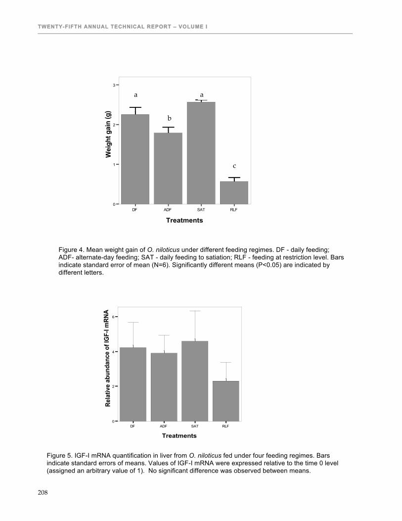
TWENTY-FIFTH ANNUAL TECHNICAL REPORT – VOLUME I
208
Figure 4. Mean weight gain of O. niloticus under different feeding regimes. DF - daily feeding; ADF- alternate-day feeding; SAT - daily feeding to satiation; RLF - feeding at restriction level. Bars indicate standard error of mean (N=6). Significantly different means (P<0.05) are indicated by different letters.
Error Bars show Mean +/- 0.5 SE
Bars show Means
DF ADF SAT RLF
Treatments
0
2
4
6
Rela
tive
abun
danc
e of
IGF-
I mRN
A
]]
]
]
Figure 5. IGF-I mRNA quantification in liver from O. niloticus fed under four feeding regimes. Bars indicate standard errors of means. Values of IGF-I mRNA were expressed relative to the time 0 level (assigned an arbitrary value of 1). No significant difference was observed between means.
Error Bars show Mean +/- 1.0 SE
Bars show Means
DF ADF SAT RLF
Treatments
0
1
2
3
Wei
ght g
ain
(g)
]
]
]
]
a
b
a
c

PRODUCTION SYSTEM DESIGN & INTEGRATION
209
Dot/Lines show Means
2 4 6 8 10 12
Weight gain (g)
0
100
200
300
400
500R
elat
ive
abun
danc
e of
IGF-
I mR
NA
^^̂
^
^
^̂
^
^^
^
^
Figure 6. Correlation of relative IGF-I mRNA abundance and individual weight gain in the temperature study (N=12), r=0.64 (P<0.05).

TWENTY-FIFTH ANNUAL TECHNICAL REPORT – VOLUME I
210
DEVELOPMENT OF NILE TILAPIA FILLETS AS AN EXPORT PRODUCT FOR THE PHILIPPINES
Twelfth Work Plan, Production System Design & Integration 6 (12PSD6) Final Report
Published as Submitted by Contributing Authors
Remedios B. Bolivar, Eddie Boy T. Jimenez, Jun Rey A. Sugue & Dimalyn P. Lagmay
Central Luzon State University Science City of Muñoz, Nueva Ecija, Philippines
Christopher L. Brown
Florida International University North Miami, Florida, USA
Ruben A. Reyes, Joyce L. Cuanan
& Maria Jodecel C. Danting
National Freshwater Fisheries Technology Center Science City of Muñoz, Nueva Ecija, Philippines
ABSTRACT The experiment was undertaken to determine the culture period of Nile tilapia to reach approximately an average weight of 600 g at a stocking size of 50-120 g. The grow out study was conducted in six 500 m2 earthen ponds. GET-ExCEL Nile tilapias were stocked at a density of 1 pc m-2 (Treatment I) and 2 pcs m-2 (Treatment II). Analysis of variance revealed no significant differences in the initial weight of the fish between treatments (P>0.05). After a culture period of four months, fish in Treatment I had a mean weight of 590.17 g while in Treatment II, the harvested fish had a mean weight of 512.99 g. However, analysis of variance likewise did not show significant difference on the mean final weights of fish between treatments. There were also no significant differences in the mean final length, mean survival rates, daily weight gains, specific growth rates, feed conversion ratios and feed conversion efficiencies of the fish stocks in the two treatments (P>0.05). Significant differences (P<0.05) were observed between the extrapolated fish yield in Treatment I (5,250.93 ± 313.05 kg ha-1) and Treatment II (8,256.43 ± 423.16 kg ha-1) and on fish biomass in Treatment I (219.84 ± 15.93 kg) and Treatment II (327.77 ± 21.91 kg). The highest percent fillet recovery was observed in fish sizes ranging from 601-700 g, 701-800 g and 501-600 g with mean values of 36%, 34.99% and 34.03%, respectively. Economic analysis showed that Treatment 1 had better cost benefit ratio compared with Treatment II. This suggests that rearing of Nile tilapia at a density of 1 pc m-1 was more profitable for the production of tilapia for fillet.
INTRODUCTION Tilapia aquaculture started when Tilapia mossambica was introduced in the Philippines in 1950’s from Thailand and was considered as pest and nuisance in milkfish ponds in 1970’s. However, tilapia farming became popular in 1980’s due to the introduction of fast-growing species called Nile tilapia (Oreochromis niloticus) (Tayamen and Guerrero, 1988). According to Guerrero (1982), tilapia is the major farmed species produced in ponds and cages because it has wide range of tolerance to environmental conditions, resistant to diseases, can be bred in captivity and shows excellent growth rate even in low protein diet. The fish can easily adapt to virtually any freshwater environments from ponds to lakes, even swamps and marshes and brackish waters. It has the ability to use various food sources and readily takes prepared feeds from fry to adult size (Badullis et al., 2004). Nile tilapia are mouth brooders and they exhibit high degree of parental care. It is considered as everyman’s fish (Guerrero, 1982). According to Fitzsimmons (2000),

PRODUCTION SYSTEM DESIGN & INTEGRATION
211
tilapia is one of the most important aquaculture species in the 21st century and is produced in more than 100 countries. In the Philippines, tilapia aquaculture is growing rapidly as tilapia become more acceptable to consumers. The proven value of tilapia in aquaculture has led to increased interest to further development its culture worldwide, particularly in Southeast Asia where the greatest volume of fish is produced (Guerrero, 2002). In 2004, Asia continues to lead the world in tilapia production with China, Egypt, Indonesia and Philippines as the major producing nations (Fitzsimmons, 2006).
REVIEW OF LITERATURE In the polyculture of Nile tilapia and shrimp (Penaeus monodon), the mean daily weight gains and final mean weight of low density tilapia treatment was significantly greater than those in medium and high tilapia density treatments. However, the total weight gain and net and gross yields of tilapia were highest in high-density treatment, intermediate in medium density and lowest in low-density treatment (Thien et al., 2004). According to Diana et al. (2004), growth and survival differed among treatments. Low-density tilapia treatment had higher growth than intermediate density tilapia treatment. According to Brett (1970), the absolute growth rate accelerates during the juvenile period. Growth rates generally decline with increasing fish size (age) (Welcomme, 2001). In a study of Arce and Lopez (1981), they concluded that the larger the stocking size, the heavier the mean weight at harvest. They also noted that recovery increases with increased stocking size. Melstein (1995) reported that carp and tilapia have better growth when stocked at larger size and cultured for short period. In addition, Dureza et al. (1994) stated that mean apparent feed conversion ratio (AFCR) of small fish (5g) is 2.0 which is slightly lower to AFCR of big fish (225g), which is 2.4. This suggests the benefit of bigger stocking size for culture. In the polyculture of Nile tilapia and hybrid catfish (Clarias macrocephalus x C. gariepinus), mean tilapia weights at harvest decreased linearly with increasing stocking ratios, however, net and gross tilapia yields increased linearly with increasing stocking ratios (Long and Yi, 2004). Lanuza (2000) studied the effect of stocking size on the growth, yield and survival of Nile tilapia; however, result showed that there were no significant differences on the growth, yield and survival of Nile tilapia using stocking sizes ranging from 0.10g-1.20g after 90 days of culture. This can be attributed to short culture period and small stocking sizes; fishes were not able to reach sizes that would show differences in growth and yield of Nile tilapia. In the polyculture of grass carp (Ctenopharyngodon idella) and Nile tilapia (Oreochromis niloticus) that was studied by Pandit et al. (2004), the mean weight of Nile tilapia at harvest decreased linearly with increasing stocking density while net fish yield of Nile tilapia increased linearly. In the study of Bolivar et al. (2004), initial stocking mean weights of Nile tilapia were highly significant among treatments where Treatment I, Treatment II and Treatment III were stocked with fingerling sizes # 22, # 14 and # 10, respectively. Fish yield, feed conversion ratio and survival rate were highest in Treatment III, followed by Treatment II and lowest in Treatment I, however, specific growth rate was highest in Treatment I and lowest in Treatment III. The study revealed that the smallest stocking size exhibit a reduced survival rate compared with the larger stocking sizes. Density dependent growth occurred in the study of Diana et al. (1995) with the lowest stocking density (3 pcs m-2) having significantly higher growth rate than the intermediate density (6 pcs m-
2), and with the highest density (9 pcs m-2) having the lowest growth rate. Survival is lowest at highest density. In the study of Silva et al. (2000), result showed that fishes stocked at density of 2

TWENTY-FIFTH ANNUAL TECHNICAL REPORT – VOLUME I
212
pcs m-2 had higher average final body weight gain than fishes stocked at densities of 3 pcs m-2 and 4 pcs m-2. According to Rangaswami (1988) as cited by Guerrero (2002), fingerlings weighing 2-6 g stocked at densities 10,000-12,000 per 0.2 ha ponds were harvested at sizes 450-600 g in six months. The study revealed that reduced stocking densities shorten the length of culture period of export sizes Nile tilapia. Liao and Chen (1983) as cited by Guerrero (2002) stocked tilapia with weight range of 100-200 g at densities of 50-100 pcs m-2 in 100 m-2 octagonal tanks with water exchange and aeration. The tilapia attained a mean harvest weight of 600 g after a culture period of 3-4 months. Tilapia has white soft and mild-tasting flesh, its nutritional value (protein and fat content) and edible parts are comparable to high value species such as grouper and red snapper. Tilapia has several processing advantages. First, freshness will not be a problem when processing tilapia since it can be purchased alive. Second, it does not need to be deboned compared to milkfish. Lastly, tilapia lends itself to various traditional and modern processing methods (Snir, 2002). Tilapia can be easily processed into traditional products such as dried, smoked and fermented. This can be a good raw material for various value-added products such as fillet, surimi and surimi-based products. Fillet and its products such as battered and breaded fillets, nuggets and fish fingers are very popular and market is fast growing in developed countries. In addition, tilapia can be processed into burger, quekiam, balls, dumplings, sausages and salami, sashimi, sushi and sandwich spread. By-product wastes from tilapia processing can be converted into valuable products such as fish sauce, fishmeal, silage and fertilizer. Carcasses, heads and trimmings are also used for animal feeds, especially hogs. Tilapia scales are used in creating flower ornaments. Heads are used for soup in some countries. One of the most valuable by-products of tilapia processing is the tilapia skin. Skins are used to make leather goods, clothing and accessories. It can also be made into snack food. Skin with no scale are cut into thin strips and deep-fried. Skins are also used to produce pharmaceutical products (Fitzsimmons, 2004). Table 1 shows the fillet recovery of Nile tilapia from different sizes. Ribeiro et al. (1998) as cited by Souza and Macedo-Viegas (2000) reported that fillet size is linearly correlated with fish weight. Nile tilapias weighing 169 g, 351 g, 550 g and 909.7 g have fillet yields of 57.7 g, 108.81 g, 170.5 g and 324.4 g, respectively. In addition, Souza et al. (1998b) as cited by Souza and Macedo-Viegas (2000) reported that 126.76 g and 196.84 g fillet were recovered from 395 g and 530 g Nile tilapia, respectively. Macedo-Viegas et al. (1998) as cited by Souza and Macedo-Viegas (2000) reported that fillet yield from 250 g and 450 g Nile tilapia were 80.38 g and 181.76 g, respectively. Souza and Maranhao (1998) as cited by Souza and Macedo-Viegas (2000) reported that fillet recovery from 300 g to 400 g and 401 g to 500 g Nile tilapia were 36.5% and 36.84%, respectively. There was a small difference of percent fillet recovery between Nile tilapia weighing 530 g and 909.7 g, which were 37.14% and 37.08%, respectively. In calculating the cost and return, this indicates that raising 530 g Nile tilapia was more economical and it was in the range of export sizes of 400-600 g. Table 2 presents the fillet recovery of Nile tilapia from different size ranges in the two trials conducted at the BFAR-NFFTC. Result from the first trial showed that 601-650 g fish had the highest fillet recovery (38.19%) followed by 551-600 g with 38.11%. Trial 2 showed that 500-550 g fish high fillet recovery of 36.93%. Fishes of sizes 551-600 g and 601-650 g have fillet recovery of 36.1% and 35.37%. Fishes larger than 650 g have lower fillet recovery in both trials (BFAR, 2004). The trial revealed that sizes of 551-650g are the sizes suitable for high fillet recovery; however, fishes weighing 500 g can also be used.

PRODUCTION SYSTEM DESIGN & INTEGRATION
213
Table 1. Fillet recovery from different Nile tilapia sizes. Weight of Fish (g) Percent Recovery (%) Fillet Recovered (g)
169 26.32 57.70
250 32.15 80.38
351 31.90 108.81
395 32.09 126.76
450 40.39 181.76
530 37.14 196.84
550 31.90 170.50
909.7 37.08 324.40
300-400 36.50 109.50-146.00
401-500 36.84 147.53-184.20
Source: Souza and Macedo-Viegas (2000)
Table 2. Average fillet recovery of different size ranges of Nile tilapia. Fillet Recovery (%)
Size Range (g) Trial 1 Trial 2
500-550 36.00 36.93
551-600 38.11 36.10
601-650 38.19 35.37
651-700 33.81 34.06
701-750 35.63 33.78
751-800 35.32 35.00
801-850 23.62 30.67
Source: BFAR (2004)
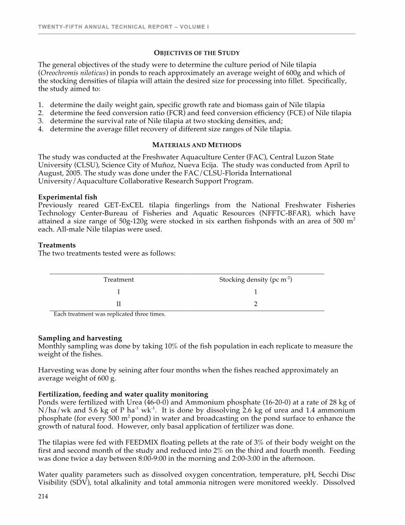
TWENTY-FIFTH ANNUAL TECHNICAL REPORT – VOLUME I
214
OBJECTIVES OF THE STUDY
The general objectives of the study were to determine the culture period of Nile tilapia (Oreochromis niloticus) in ponds to reach approximately an average weight of 600g and which of the stocking densities of tilapia will attain the desired size for processing into fillet. Specifically, the study aimed to: 1. determine the daily weight gain, specific growth rate and biomass gain of Nile tilapia 2. determine the feed conversion ratio (FCR) and feed conversion efficiency (FCE) of Nile tilapia 3. determine the survival rate of Nile tilapia at two stocking densities, and; 4. determine the average fillet recovery of different size ranges of Nile tilapia.
MATERIALS AND METHODS
The study was conducted at the Freshwater Aquaculture Center (FAC), Central Luzon State University (CLSU), Science City of Muñoz, Nueva Ecija. The study was conducted from April to August, 2005. The study was done under the FAC/CLSU-Florida International University/Aquaculture Collaborative Research Support Program. Experimental fish Previously reared GET-ExCEL tilapia fingerlings from the National Freshwater Fisheries Technology Center-Bureau of Fisheries and Aquatic Resources (NFFTC-BFAR), which have attained a size range of 50g-120g were stocked in six earthen fishponds with an area of 500 m2 each. All-male Nile tilapias were used. Treatments The two treatments tested were as follows:
Treatment Stocking density (pc m-2)
I 1
II 2 Each treatment was replicated three times.
Sampling and harvesting Monthly sampling was done by taking 10% of the fish population in each replicate to measure the weight of the fishes. Harvesting was done by seining after four months when the fishes reached approximately an average weight of 600 g. Fertilization, feeding and water quality monitoring Ponds were fertilized with Urea (46-0-0) and Ammonium phosphate (16-20-0) at a rate of 28 kg of N/ha/wk and 5.6 kg of P ha-1 wk-1. It is done by dissolving 2.6 kg of urea and 1.4 ammonium phosphate (for every 500 m2 pond) in water and broadcasting on the pond surface to enhance the growth of natural food. However, only basal application of fertilizer was done. The tilapias were fed with FEEDMIX floating pellets at the rate of 3% of their body weight on the first and second month of the study and reduced into 2% on the third and fourth month. Feeding was done twice a day between 8:00-9:00 in the morning and 2:00-3:00 in the afternoon. Water quality parameters such as dissolved oxygen concentration, temperature, pH, Secchi Disc Visibility (SDV), total alkalinity and total ammonia nitrogen were monitored weekly. Dissolved
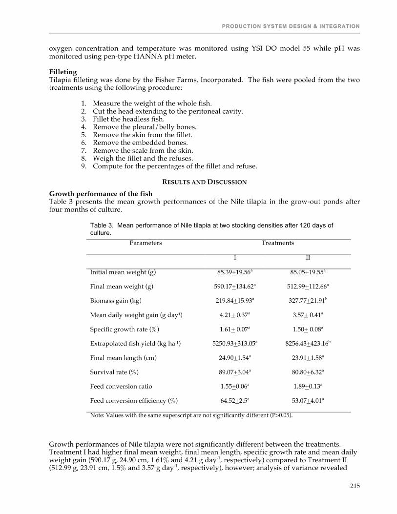
PRODUCTION SYSTEM DESIGN & INTEGRATION
215
oxygen concentration and temperature was monitored using YSI DO model 55 while pH was monitored using pen-type HANNA pH meter. Filleting Tilapia filleting was done by the Fisher Farms, Incorporated. The fish were pooled from the two treatments using the following procedure:
1. Measure the weight of the whole fish. 2. Cut the head extending to the peritoneal cavity. 3. Fillet the headless fish. 4. Remove the pleural/belly bones. 5. Remove the skin from the fillet. 6. Remove the embedded bones. 7. Remove the scale from the skin. 8. Weigh the fillet and the refuses. 9. Compute for the percentages of the fillet and refuse.
RESULTS AND DISCUSSION Growth performance of the fish Table 3 presents the mean growth performances of the Nile tilapia in the grow-out ponds after four months of culture.
Table 3. Mean performance of Nile tilapia at two stocking densities after 120 days of culture.
Parameters Treatments
I II
Initial mean weight (g) 85.39+19.56ª 85.05+19.55ª
Final mean weight (g) 590.17+134.62ª 512.99+112.66ª
Biomass gain (kg) 219.84+15.93ª 327.77+21.91b
Mean daily weight gain (g day¹) 4.21+ 0.37ª 3.57+ 0.41ª
Specific growth rate (%) 1.61+ 0.07ª 1.50+ 0.08ª
Extrapolated fish yield (kg ha-¹) 5250.93+313.05ª 8256.43+423.16b
Final mean length (cm) 24.90+1.54ª 23.91+1.58ª
Survival rate (%) 89.07+3.04ª 80.80+6.32ª
Feed conversion ratio 1.55+0.06ª 1.89+0.13ª
Feed conversion efficiency (%) 64.52+2.5ª 53.07+4.01ª
Note: Values with the same superscript are not significantly different (P>0.05).
Growth performances of Nile tilapia were not significantly different between the treatments. Treatment I had higher final mean weight, final mean length, specific growth rate and mean daily weight gain (590.17 g, 24.90 cm, 1.61% and 4.21 g day-1, respectively) compared to Treatment II (512.99 g, 23.91 cm, 1.5% and 3.57 g day-1, respectively), however; analysis of variance revealed

TWENTY-FIFTH ANNUAL TECHNICAL REPORT – VOLUME I
216
that there was no significant difference between the treatments. Fishes in Treatment I attained an average final weight of 590.17 g after four months of culture while Treatment II attained an average final weight of 512.99 g. On the other hand, extrapolated fish yield (kg ha-1) and biomass gain were significantly different in Treatment II (8256.43 kg ha -1 and 327.77 kg, respectively) than in Treatment I (5250.93 kg ha-1 and 219.88 kg, respectively). Green et al. (1994) reported that mean individual fish size decreased linearly as the stocking density increases, however, gross tilapia yield increased linearly as the stocking density increases. Higher mean survival rate was observed in Treatment I (89.07%) compared to Treatment II (80.8%), however; the mean values were not significantly different. Mortality can be attributed to stress in handling during sampling. Sampling was initially done by individual weighing of the fish but one to two days after the first monthly sampling, fish mortalities were observed. Based from this observation, the second and third monthly samplings were done by getting the bulk weight of 10% of the fish population in each replicate. No fish mortality was observed after the succeeding monthly sampling. The result of this study was the same with the study of Diana et al. (1995) and Diana et al. (2004) where survival is highest in low-density tilapia treatment and lowest in high-density tilapia treatment. Treatment I had higher feed conversion ratio (1.55) than Treatment II (1.89), however; these were not significantly different but this explains why Treatment I had better Return on Investment (Table 6) although Treatment II had higher biomass gain and fish yield. Feeding rate was reduced to 2% of the fish body weight on the third month. Based from the observation during feeding, fishes were not able to eat all the feed given at 3% of their body weight on the last week of the second month. Growth trajectories of Nile tilapia grown at different stocking densities are presented in Figure 1. Fishes in Treatment I have an average weight of 85.39 g while in Treatment II, fishes weighed an average of 85.05 g at stocking. After 30 days, fishes in Treatment I weighed an average of 230.80 g. On the 60th and 90th days of culture, fishes weighed an average of 358.67 g and 497.33 g, respectively. Fishes reached an average weight of 590.17 g after 120 days of culture. Fishes in
Figure 1. Growth trend of Nile tilapia grown in ponds at two stocking densities. Treatment II had an average weight of 213.64 g after 30, an average weight of 319.33 g after 60 and 436 g after 90 days of culture, respectively. Finally, fishes weighed an average of 512.99 g after 120 days. Fishes in both treatments were harvested after 120 days of culture.

PRODUCTION SYSTEM DESIGN & INTEGRATION
217
Water quality parameters: Table 4 presents the mean values of water quality parameters monitored in the study. Analysis of variance revealed no significant difference between treatments with respect to the water quality parameters except for water temperature and total ammonia nitrogen. Average water quality measurements for Treatment I were: dissolved oxygen: 3.52 mg l-1 (range 2.89-3.87), water temperature: 30.15 ºC (range 30-30.26), pH: 8.5 (range 8.4-8.6), total alkalinity: 215.41 mg l-1 (range 214.82-216.29 mg l-1), total ammonia nitrogen: 0.167 mg l-1 (range 0.15-0.194 mg l-1) and Secchi disc visibility: 20 cm (range 19-20 cm). Water quality parameter measurements in Treatment II were: dissolved oxygen: 3.89 mg l-1(range 3.53-4.38 mg l-
1), water temperature: 30.17 ºC (range 30.15-30.18), pH: 8.4 (range 8.3-8.5), total alkalinity: 214.23 mg l-1 (range 199.88-234.76 mg l-1), total ammonia nitrogen: 0.19 mg l-1 (range 0.186-0.211 mg l-1) and Secchi disc visibility: 19 cm (range 18-20). Dissolved oxygen concentrations were lower than the desirable range for the culture of Nile tilapia (5 mg l-1). Bigger fishes consume higher amount of dissolved oxygen compared to the smaller ones. Temperature, pH, total alkalinity and total ammonia nitrogen were within the desirable ranges. Ammonia is the primary end product of organic decomposition either directly from protein or other nitrogenous composition. It is the excretory product of the aquatic animals. The higher amount of total ammonia nitrogen in Treatment II can be attributed to the higher stocking density where more fish produced fecal waste. Nutrient leaching can not be controlled once the feed is thrown in the water, since more feeds were provided in Treatment II, more nutrients were present in the ponds than in Treatment I. This resulted to higher amount of ammonia in Treatment II. Pond fertilization was done once during the culture period (1st week). Each pond was fertilized with 2.6 kg urea and 1.4 kg ammonium phosphate. Secchi disc visibility readings showed that the phytoplankton was still abundant in the grow-out ponds until the experiment has ended.
Table 4. Mean values of water quality parameters in the grow out ponds Treatment Rep DO Temp pH Alk TAN SDV
(mg l-1) (ºC) (mg l-1) (mg l-1) (cm)
I 1 2.89 30 8.6 214.82 0.194 19
I 2 3.79 30.26 8.4 216.29 0.156 20
I 3 3.87 30.2 8.4 215.12 0.15 20
Mean 3.52 30.15 8.5 215.41 0.167 20
II 1 4.38 30.15 8.4 208.06 0.186 18
II 2 3.53 30.19 8.5 199.88 0.211 20
II 3 3.75 30.18 8.3 234.76 0.193 18
Mean 3.89 30.17 8.4 214.23 0.197 19
Fillet recovery: After harvesting, fishes were sorted in different size ranges for filleting. Afterwards, the fish were transported to the dispersal area of the National Freshwater Fisheries Technology Center-Bureau of Fisheries and Aquatic Resources. Filleting was done by the Fisher Farms, Incorporated. Table 5 presents the mean fillet recovery of Nile tilapia from different size

TWENTY-FIFTH ANNUAL TECHNICAL REPORT – VOLUME I
218
ranges. Tilapia weighing 601-700g gave the highest fillet recovery followed by 701-800 g and 501-600 g yielding 36.05%, 34.99% and 34.03%, respectively. Analysis of variance revealed significant differences between the fillet recoveries from different size ranges. Fillet recovered from fish weighing 601-700 g was significantly different to the fillet recovered from fishes weighing 100-200 g, 201-300 g, 301-400 g, 401-500 g and 801-900 g, however, it was not significantly different to the fillet recovered from fishes weighing 501-600 g and 701-800 g while fillet recovery of fishes weighing 100-200 g and 201-300 g were not significantly different. Differences in the fillet recovery can be attributed to the differences in the other parts of the fish especially the head and gills where it had the second highest weight next to fillet. Fishes weighing 201-300 g had the highest head and gill weight followed by those weighing 401-500 g, 301-400 g and 100-200 g with 33.37%, 33.25 %, 32.1% and 32.9% recovery, respectively. Fishes weighing 601-700 g had the lowest head and gill weight. Fishes weighing 701-800 had higher head and gill percentage than those weighing 601-700 g while those weighing 801-900 g had higher head and gill percentage than those weighing 701-800 g.
Table 5. Mean percent fillet recovery of Nile tilapia in different size ranges. Size Range (g) Mean Fillet Recovered (g) Mean Fillet Recovery (%)
100-200 53.03 32.61c
201-300 83.79 31.99c
301-400 115.90 33.30bc
401-500 150.44 33.23bc
501-600 189.73 34.03abc
601-700 233.57 36.05a
701-800 260.80 34.99ab
801-900 285.63 33.80bc
Values with the same superscript are not significantly different (P>0.05).
Mean fillet recovery of Nile tilapia from different size ranges is presented in Figure 2. The figure shows that the lowest fillet recovery was from fishes weighing 201-300 g, followed by 100-200 g, 301-400 g and 401-500 g while the highest fillet recovery was observed in fishes weighing 601-700 g. Fishes weighing 701-800 g had higher fillet recovery than fishes weighing 801-900 g. Size frequency distribution: The size frequency distributions of Nile tilapia at stocking and at harvest are presented in Figures 3 and 4, respectively. Figure 3 shows that a size range of 101-110 g had highest size frequency in Treatments I and II (26.9% and 24.8%, respectively) followed by 81.90 g in Treatment II (19.1%). Figure 4 shows that more fishes weighing 501-600 g, 601-700 g and 701-800 g were harvested in Treatment I having a frequency of 25.93%, 24% and 13.4 % respectively. However, more fishes weighing 401-500 g were harvested in Treatment II (24.77%). Cost and return analysis: A budget analysis was done to determine the economic returns of the two treatments (Table 6). The analysis reflected that higher net return was found in stocking fish at a density of 1 pc m-2 because Treatment I had better Return on Investment (52.91%) compared to Treatment II (30.50%). Labor cost was not included in the cost and return analysis because in the Philippines not all laborers were paid, some were given incentives as the payment for their time and effort.

PRODUCTION SYSTEM DESIGN & INTEGRATION
219
0102030
50-60 61-70 71-80 81-90 91-100
101-110
111-120
Size Range (g)
Size
Fre
quen
cy at
St
ocki
ng (%
) Trt ITrt II
05
1015202530
100-2
00
201-3
00
301-4
00
401-5
00
501-6
00
601-7
00
701-8
00
801-9
00
901-1
000
Size Range (g)
Size
Fre
quen
cy at
Har
vest(
%) Trt I
Trt II
Figure 2. Mean fillet recovery of Nile tilapia from different size ranges
Figure 3. Size frequency distribution of Nile tilapia at stocking in Treatment I and Treatment II.
Figure 4. Size frequency distribution of Nile tilapia at harvest in Treatment I and Treatment II.

TWENTY-FIFTH ANNUAL TECHNICAL REPORT – VOLUME I
220
Assumptions: Culture period: four months Price of stock: P40.00 kg-1 Price of Feeds: P20.00 kg-1
Price of tilapia at harvest: P50.00 kg-1
SUMMARY The study was conducted to evaluate the stocking density to be used to harvest marketable size tilapia suitable for fillet at a shorter culture period. GET ExCEL Nile tilapia weighing 50-120 g were stocked in six 500 m-2 earthen ponds at a density of 1pc m-2 and 2pcs m-2. Data on initial and final weight, final length and water quality parameters were gathered. The experiment was set-up following a Randomized Complete Block Design. Analysis of variance was used to determine differences between treatments while Least Significant Difference was used to compare the treatment means. Each treatment was replicated three times. Duncan’s Multiple Range Test was used to compare the means of fillet recovery of Nile tilapia from different size ranges. Mean weight of Nile tilapia at harvest as well as daily weight gain, specific growth rate and final weight decreased linearly with increasing stocking density. Treatment I had higher growth performances, however; analysis of variance showed no significant difference between the treatments. On the other hand, extrapolated fish yield and biomass gain of Nile tilapia increased linearly with increasing stocking density, treatment II had higher values than Treatment I. Analysis of variance revealed that Treatment II was significantly higher than Treatment I. Survival rate was higher in Treatment I (89.07%) than in Treatment II (80.8%). Higher feed conversion ratio and feed conversion efficiency were observed in Treatment I resulting to better growth performance. Fishes in Treatment I were able to reach an average weight of 590.168g after four months of culture compared to Treatment II with a final mean weight of 512.994g. Better Return on Investment was also obtained in Treatment I (52.91%). Highest average fillet recovery was observed in fishes weighing 601-700 g followed by 701-800 g and 501-600 g having 36.05%, 34.99% and 34.03%, respectively.
Table 6. Simple cost and return analysis for a 500 m2 pond stocked with Nile tilapia at two stocking densities.
Item Treatment I Treatment II
Gross income (P) 13,127.3 20,641.05
Operational Cost (P)
Stock 1,707. 8 (19.89%) 3,402.08 (21.51%)
Feeds 6,815.4 (79.39%) 12,353 (78.10%)
Total Cost 8,584.88 15,816.76
Net Return (P) 4,542.42 4,824.29
Return on Investment 52.91% 30.50%

PRODUCTION SYSTEM DESIGN & INTEGRATION
221
CONCLUSION Based from the results of this study, we conclude that the stocking at 1 pc m-1 was more profitable for growing marketable size tilapia suitable for fillet than stocking at 2 pcs m-1 and resulted in better growth performance of the fish.
Recommendations Stocking uniform size fish is highly recommended to have uniform size at harvest. Avoiding stress in handling when rearing large size tilapia is important to reduce mortality. Further studies should be conducted to determine the separately the fillet recovery of Nile tilapia stocked at 1 pc m-2 and 2 pcs m-2.
ACKNOWLEDGMENTS Funding for this research was provided by the Aquaculture Collaborative Research Support Program. The Aquaculture CRSP is funded in part by United States Agency for International Development (USAID) Grant No. LAG-G-00-96-90015-00 and by participating institutions. We would also like to acknowledge the Bureau of Fisheries and Aquatic Resources (BFAR) for providing the scholarship grant to Ms. Dimalyn Lagmay to complete her degree in Bachelor of Science in Fisheries at the Central Luzon State University (CLSU), the Freshwater Aquaculture Center and the Aquaculture CRSP project staff at CLSU for the assistance during the conduct of this experiment. The National Fisheries Technology Center-BFAR is also acknowledged for providing the tilapia fingerlings used in the study.
LITERATURE CITED Arce, R.R. and Lopez, E.A. 1981. Effects of stocking weight on the culture of Tilapia nilotica in
paddy field. Progress Report No. 12. Freshwater Aquaculture Center Central Luzon State University, Science City of Munoz, Nueva Ecija. p. 25-29.
Badulis, R.J., Herrera, A.A., Fabillo, M.D. and Abucay, J.S. 2004. The development of the tail kidney and testis of starved genetically male (GMT) Nile tilapia (Oreochromis niloticus). p. 724-732. In: R. Bolivar, G. Mair and K. Fitzsimmons (Eds.). New Dimensions in Farmed Tilapia. Proceedings from the 6th International Symposium on Tilapia in Aquaculture. Manila, Philippines. p. 805.
Bart, A. 2004. Contribution of Aquaculture and Aquatic Resources Management (AARM) Programs of the Asian Institute of Technology (AIT) to Tilapia Research. p. 711-720. In: R. Bolivar, G. Mair and K. Fitzsimmons (Eds.). New Dimensions in Farmed Tilapia. Proceedings from the 6th International Symposium on Tilapia in Aquaculture. Manila, Philippines. p. 805.
BFAR. 2003. Philippine Fisheries Profile. Bureau of Fisheries and Aquatic Resources. Quezon City, Manila, Philippines.
BFAR. 2004. Sampling and filleting of Nile tilapia. Bureau of Fisheries and Aquatic Resources. Science City of Munoz, Nueva Ecija, Philippines. p. 8.
Bolivar, R.B., Jimenez, E.B.T., Sugue, J.R.A. and Brown, C.L. 2004. Effect of stocking sizes on the yield and survival of Nile tilapia (Oreochromis niloticus) on grown in ponds. p. 574-583. In: R. Bolivar, G. Mair and K. Fitzsimmons (Eds.) New Dimensions in Farmed Tilapia. Proceedings from the 6th International Symposium on Tilapia in Aquaculture. Manila, Philippines. p. 805.
Brett, J.R. 1970. Fish – the energy cost of living. p. 37-52. In: Mc Neil, W.J. (Ed.) Marine Aquaculture, Oregon State University Press. 170 p.
Carro-Anzalotta, A.E. and McGinty, A.S. 1986. Effect of stocking density on growth of Tilapia nilotica cultured in cages in ponds. Journal of the World Aquaculture Society 17: 52-57.
Diana, J.S., Lin C.K. and Yi, Y. 1995. Stocking density and supplemental feeding. p. 30. In: McNamara M., Egna, H., Goetze, B., Herbison, B. and Clair, D. (eds.). Pond Dynamics/Aquaculture Collaborative Research Support Program. Thirteenth Annual Administrative Report. Oregon State University. p. 96.

TWENTY-FIFTH ANNUAL TECHNICAL REPORT – VOLUME I
222
Diana, J.S., Lin, C.K. and Yi, Y. 1996. Timing of supplemental feeding for tilapia production. Journal of the World Aquaculture Society, 27(4): 410-419.
Diana, J.S., Yi, Y. and Lin, C.K. 2004. Stocking densities and fertilization regimes for Nile tilapia (Oreochromis niloticus) production in ponds with supplemental feeding. p. 487-499. In: R. Bolivar, G. Mair and K. Fitzsimmons (Eds.). New Dimensions in Farmed Tilapia. Proceedings from the 6th International Symposium on Tilapia in Aquaculture. Manila, Philippines. p. 805.
Dureza, L.A., Gempis, C.C., Salvador, R.C., Sombrero, R.P. and Belmonte, B.D. 1994. Effects of selected factors on the growth and survival of tilapia hybrids in cages of saline water. p. 41-43. In: Villacorta, C.G., and Dureza, L.A. (Eds.). Proceedings from the 3rd National Symposium and Workshop on Tilapia Farming. University of the Philippines-Visayas, Iloilo City. PCAMRD. p. 67.
Engle, C. 2000. Raising tilapia in shrimp ponds. Economic and marketing considerations. AQUANEWS, Pond Dynamics/Aquaculture Collaborative Research Support Program Newsletter, 15:1-3.
Fitzsimmons, K. 2000. Tilapia: the most important aquaculture species in the 21st century. p. 3-8. In: K. Fitzsimmons and J. Carvalho Filho (Eds.). Tilapia Aquaculture in the 21st Century. Proceedings from the Fifth International Symposium on Tilapia in Aquaculture. Rio de Janeiro, Brazil. p. 682.
Fitzsimmons, K. 2004. Development of new products and markets for the global tilapia trade. p. 624-633. In: R. Bolivar, G. Mair and K. Fitzsimmons. (Eds.). New Dimensions in Farmed Tilapia. Proceedings from the 6th International Symposium on Tilapia in Aquaculture. Manila, Philippines. p. 805.
Fitzsimmons, K. 2006. Prospect and potential for global production. In: Webster, C. and Lim, C. (Eds.). Tilapia: Biology, Culture and Nutrition. Haworth Press. Binghamton, New York.
Green, B.W., Teichert-Coddington, D.R. and Hanson, T.R. 1994. Effect of stocking rate on the yield of tilapia offered a formulated feed. Development of Semi-Intensive Aquaculture Technologies in Honduras. Summary of Freshwater Aquacultural Research conducted from 1983-1992. Auburn University, Alabama. p. 48.
Guerrero, R.D. III. 1982. Control of Tilapia Reproduction. p. 309-316. In: R.S.V. Pullin and R.H. Lowe-McConnell (Eds.). The Biology and Culture of Tilapias. ICLARM, Proceedings 7. International Center for Living Aquatic Resources Management. Manila, Philippines. p. 432.
Guerrero, R.D. III. 1989a. Commercial red Nile tilapia in Malaysia. Agribusiness Weekly, 13:8-14. Guerrero, R.D. III. 1989b. Intensive tilapia farming in Pampanga. Agribusiness Weekly, 37:13-19. Guerrero, R.D. III. 2002. Tilapia farming in the Asia-Pacific Region p. 42-48. In: Guerrero, R.D. III
and del Castillo, M.R.G. (Eds.). Proceedings of the International Forum on Tilapia Farming in the 21st Century (Tilapia Forum 2002). Los Banos, Laguna, Philippines. p. 184.
Lanuza, J.D. 2000. Effect of stocking sizes on the growth and survival performance of Nile tilapia (Orechromis niloticus). Undergraduate Thesis. Central Luzon State University, Science City of Munoz, Nueva Ecija. p. 32.
Long, N.T. and Yi, Y. 2004. Stocking ratios of hybrid catfish (Clarias macrocephalus x C. gariepinus) and Nile tilapia (Oreochromis niloticus) in an intensive polyculture. p. 518. In: R. Bolivar, G. Mair and K. Fitzsimmons (Eds.). New Dimensions in Farmed Tilapia. Proceedings from the 6th International Symposium on Tilapia in Aquaculture. Manila, Philippines. p. 805.
Mair, G.C. 2003. Investment and business opportunities in tilapia from a technological perspective. Asian Aquaculture Magazine. (November-December, 2003). p. 14-17.
Melstein, A. 1995. Fish management relationships in Israel commercial fish farming. Aquaculture International, 3 (4): 292-314.
Pandit, N.P., Shrestha, M.K., Yi, Y. and Diana, J.S. 2004. Polyculture of grass carp and Nile tilapia with napier grass as the sole nutrient input in the subtropical climate of Nepal. p. 558-573. In: R. Bolivar, G. Mair and K. Fitzsimmons (Eds.). New Dimensions in Farmed Tilapia. Proceedings from the 6th International Symposium on Tilapia in Aquaculture. Manila, Philippines. p. 805.
Silva, P.C., Souza, V.L., Cantisani Padua, D.M., Dalacorte P.C. and Goncalves, D.C. 2000. Effect of stocking density on growth and fillet composition of tetra hybrid red tilapia, Israeli strain. p. 341-345. In: K. Fitzsimmons and J. Carvalho Filho (Eds.). Tilapia Aquaculture in the 21st

PRODUCTION SYSTEM DESIGN & INTEGRATION
223
Century, Proceedings from the Fifth International Symposium on Tilapia in Aquaculture. Rio de Janeiro, Brazil. p. 682.
Snir, I. 2002. Processing and marketing. p. 152-159. In: Guerrero, R.D. III and del Castillo, M.R.G. (Eds.). Proceedings of the International Forum on Tilapia Farming in the 21st Century (Tilapia Forum 2002). Los Banos, Laguna, Philippines. p. 184.
Souza, M.L.R. and Macedo-Viegas, E.M. 2000. Effect of filleting methods on processing yield of Nile tilapia (Oreochromis niloticus). p. 451-457. In: K. Fitzsimmons and J. Carvalho Filho (Eds.). Tilapia Aquaculture in the 21st Century, Proceedings from the Fifth International Symposium on Tilapia in Aquaculture. Rio de Janeiro, Brazil. p. 682.
Tayamen M.M and Guerrero, R.D. 1988. The status of wild and cultured tilapia genetic resources in Asia. p. 42. In: R.S.V. Pullin (Ed.). Tilapia Genetic Resources for Aquaculture. ICLARM Conference Proceedings. International Center for Living Resources Management. Manila, Philippines. p. 42.
Tayamen, M.M., Abella, T.A., Reyes, R.A., Danting, Ma. J.C., Mendoza, A.M., Marquez, E.B., Salguet, A.C., Apaga, M.M. and Gonzales, R.C. 2004. Development of tilapia for saline waters in the Philippines. p. 463-478. In: R. Bolivar, G. Mair and K. Fitzsimmons (Eds.). New Dimensions in Farmed Tilapia. Proceedings from the 6th International Symposium on Tilapia in Aquaculture. Manila, Philippines. p. 805.
Thien, P. C., Yi, Y. and Fitzsimmons, K. 2004. Effects of adding shrimp (Penaeus monodon) into intensive culture ponds of Nile tilapia (Oreochromis niloticus) at Different Densities. p. 794-805. In: R. Bolivar, G. Mair and K. Fitzsimmons (Eds.). New Dimensions in Farmed Tilapia. Proceedings from the 6th International Symposium on Tilapia in Aquaculture. Manila, Philippines. p. 805.
Welcomme, R. L. 2001. Inland Fisheries Ecology and Management. Fishing News Books. 358 p.

TWENTY-FIFTH ANNUAL TECHNICAL REPORT – VOLUME I
224
TILAPIA-SHRIMP POLYCULTURE IN NEGROS OCCIDENTAL, PHILIPPINES
Twelfth Work Plan, Production System Design & Integration 7 (12PSD7) Final Report
Published as Submitted by Contributing Authors
Philip S. Cruz Cruz Aquaculture Corporation
Singcag, Bacolod City, Philippines
Merlina N. Andalecio
University of the Philippines in the Visayas Miag-ao, Iloilo, Philippines
Remedios B. Bolivar
Central Luzon State University Science City of Muñoz, Nueva Ecia, Philippines
Kevin Fitzsimmons
University of Arizona Tucson, Arizona, USA
ABSTRACT During the Tenth Work Plan, the Aquaculture CRSP funded a survey identifying tilapia-shrimp polyculture production operations in Honduras, Mexico, the Philippines, Thailand, and Vietnam. Results from these surveys indicated that many shrimp ponds have been abandoned due to disease, poor management, and environmental degradation. Raising tilapia with low densities of shrimp in abandoned shrimp ponds could help support local fish farmers that did not benefit from the earlier shrimp farming boom. To this end, the Aquaculture CRSP funded on-farm research trials to study the production of tilapia and shrimp in polyculture. During this reporting period, two studies are ongoing to evaluate and compare tilapia-shrimp polyculture in Mexico and the Philippines. The Mexico component is reported in the Mexico Project: Watershed Management section of this report. The Philippines component is reported here. This research involves collaborators from the University of Arizona, Central Luzon State University (the Philippines), and the Asian Institute of Technology (Thailand). The project began with FYD Corporation as the primary partner, but after the first year, business changes within the corporation required that we switch the partnership to the Cruz Corporation. Philip Cruz worked with the CLSU and University of Philippines in the Visayas to complete the research and prepare the report. The use of tilapia as biomanipulators in shrimp farming, or also known as green water technology, has played an important role in the current efforts in the Philippines to control luminous bacteria disease caused by Vibrio harveyi. At present, green water technology is most extensively used by shrimp farmers on the island of Negros, in the central part of the Philippines. While the contribution of tilapia as a biomanipulator is highlighted in the literature, the mechanism of action is not well-understood. This study was conducted mainly to assess the contribution of tilapia in a green water system. The data gathered came from shrimp ponds practicing two production systems: a) green water system (probiotics + tilapia) and b) closed/semi-closed system (probiotics alone). There was no difference between luminous vibrio count (p<0.05) in both systems and that water quality was found to be similar (p<0.05). Because the green water system utilizes a bigger reservoir to raise the tilapia biomass, the net shrimp production was lower. In terms of direct cost of production, however, the green water system was around 10-15% lower than the closed/semi-closed system due to significantly less aeration

PRODUCTION SYSTEM DESIGN & INTEGRATION
225
required. Also, in green water system, there was a more stable plankton environment during the early months of culture, which promoted better survival of shrimps. Various pathways are presented for the control of luminous bacterial growth in shrimp ponds by green water technology, namely: a) fish feeding on organic wastes and conversion to feces; b) selective fish foraging to increase the dominance of beneficial phytoplankton; c) bioturbation of pond sediments; and d) release in the water column of antimicrobials, fungi, or competing bacteria from the skin and gut mucus of the fish. The combined actions of these pathways and not just any single effect are believed to be responsible for the overall effectiveness of the green water technology.
INTRODUCTION After being the world’s biggest producer of black tiger shrimp (Penaeus monodon) in 1984, and after attaining a peak production of 90,426 mt a decade later in 1994, Philippine shrimp production abruptly dropped in the mid-90s due to widespread disease and auto-pollution problems. By 1997, farmed shrimp production was down to 40,080 mt (Figure 1). Since then, annual shrimp production has remained at a level of only 35,000-40,000 mt with the bulk of the harvest coming from extensive farms. Most severely affected by the disease problems were the high-density shrimp farms, especially those on Negros Island.
Figure 1. Philippine farmed shrimp production and shrimp exports.
At its peak in the early 1990s, Negros Island, the center of intensive shrimp culture in the Philippines, had some 3,000 ha of farms and was harvesting around 12,000 MT of black tiger Penaeus monodon annually. By 1997, however, production dropped by more than 90%. Central to the disease problem was the bacteria Vibrio harveyi, which caused the disease known as luminous vibriosis. In managing this disease, many farmers initially adopted the use of antibiotics and chemical-based pond sanitizers. The effectiveness of this strategy turned out to be short-lived as disease virulence increased within a few culture cycles, causing farmers to stop their production. A breakthrough was finally achieved in the control of the luminous vibriosis in the late 1990s with the development of a fish-shrimp integrated culture technology, which comes in various names such as ‘green water culture technique’, ‘tilapia-shrimp polyculutre’, ‘tilapia-integration to shrimp culture technique’ or TIPS, and ‘finfish-based biological control’ (NPPMCI, 2000; Paclibare et al., 2001). The technology basically involves culturing saline-tolerant tilapia in reservoir ponds or net pens to condition the water used for shrimp culture. Through this practice, which noticeably promotes the stable bloom of green algae, it was found that the growth of luminous bacteria in

TWENTY-FIFTH ANNUAL TECHNICAL REPORT – VOLUME I
226
shrimp ponds was effectively curtailed, as well as the proliferation of undesirable plankton species, which negatively affected water quality and growth of the cultured shrimps. Complementing this development was the farmers’ rediscovery of the use of probiotics. Popularly used in the past for water quality augmentation, the use of probiotics diminished in the early 1990s due to erratic field results. In recent years, newer generation probiotics have been found to effectively discourage the growth of Vibrio bacteria in the pond environment. The usefulness of the original green water and probiotic technologies, however, turned out to be short-lived. Just as farmers were learning to manage luminous vibriosis in 2000, the dreaded white spot disease started to affect farms around the archipelago, most especially in Negros Island. This prompted the industry to overhaul its entire production protocol, under a strategy of minimum water exchange and strict biosecurity. Among the key measures introduced are the use of biocides to remove crustacean carriers of white spot syndrome virus (WSSV), multiple PCR screening of shrimp post-larvae prior to stocking, use of specialized probiotics, increased aeration to cut down on water exchange, use of dietary immunostimulants, and adoption of stringent sanitary practices by workers. All these new management strategies put together have now made production more predictable and risks more manageable, developing renewed business interests in intensive shrimp farming. By 2004, both luminous vibriosis and white spot disease were declared to be manageable and this has since led to a revival of the industry in the island. Table 1 presents the production data from the Negros Prawn Producers Marketing Cooperative, Inc. (NPPMCI) which indicate that the aggregate volume of shrimps harvested from farms within the island has increased from 848 mt during the 2003-04 culture season to 950 mt and 1,370 mt, in 2004-05 and 2005-06 culture seasons, respectively. This is equivalent to an average annual increase in production of 12.0% and 30.7%, respectively in two succeeding seasons.
Table 1. Black tiger shrimp production from intensive culture.
Culture Season Production Parameters 2003-04 2004-05 2005-06
Total harvest 848 mt 950 mt 1,370 mt Harvest biomass/ha 4.5 mt 5.3 mt 4.9 mt Harvest (average body weight) 32.0 g 32.7 g 30.2 g Stocking density/m2 20.4 20.6 21.8 Production period 155 days 130 days 129 days Survival 69% 75% 85% Feed conversion ratio 2.2 1.83 1.95 Total shrimp pond area 188 ha 203 ha 244 ha Total water area 537 ha 624 ha 650 ha Total Post Larvae stocked 38M 48.8M 53.3M Source: Negros Prawn Producers Marketing Coop., Inc. (NPPMCI)
In the last three years in Negros Island, it is interesting to note that the average culture period to attain a minimum harvest size of 30 g significantly dropped from 155 days in 2003 to 129 days in 2005. Similarly, survival rates have improved from 69% to 85%. Currently, Negros Island (Negros Occidental and Negros Oriental provinces) operates only around 650 ha of intensive farms although the area is increasing yearly. At its 1994 peak, shrimp farmers in Negros Island operated a total of some 3,000 ha of intensive farms. At present, more that 60% of the farms employ the green water technology. This paper presents a review of the current practice and understanding of green water culture technique and its impact on pond dynamics, shrimp production, and production economics, based on experience of

PRODUCTION SYSTEM DESIGN & INTEGRATION
227
farmers in Negros Island. For the purpose of this paper, which focuses on the biomanipulator role of tilapia in shrimp culture, the more appropriate name ‘tilapia-based biomanipulation technology’ or TBT for short, shall be used to also refer to green water technology. Research areas and recommendations are provided for improving the technology. Luminous Vibrio disease in shrimp In the Philippines, as in other shrimp farming nations in the region, the source of water supply for shrimp farms are usually coastal rivers and mangrove estuaries. While suited for use in traditional culture, experience now shows that such water resources are undesirable for intensive shrimp farming because of the high organic load (Kongkeo, 1997). Effluents of intensive shrimp farms, which are rich in organic waste have further aggravated the problem causing the eutrophication of surrounding waters and the creation of anoxic sediment conditions. A direct effect of these has been the proliferation of opportunistic and pathogenic Vibrios (Table 2). Among the most pathogenic is the luminous Vibrio harveyi, a naturally occurring gram-negative marine bacterium in near-shore seawater, which has become a major cause of disease and mortalities in Philippine shrimp culture since the early 1990s (Lavilla-Pitogo et al.; 1998).
Table 2. Vibrio species affecting aquaculture.
Pathogen Cultured species affected Culture system Reference V. harveyi
White shrimp (Litopenaeus vannamei) Black tiger prawn (Penaeus monodon) Kuruma prawn (Penaeus japonicus) Pearl oyster (Pinctada maxima)
Hatchery, ponds Chari and Dubey (2006)
V. harveyi V. orientalis V. splendidus
Penaeus monodon broodstock and adult shrimps
Hatchery Abrahama and Palaniappan (2004)
V. harveyi V. parahaemolyticus V. penaeicida.
White shrimp (Litopenaeus vannamei)
Culture tanks Aguirre-Guzman et al. (2001)
V. harveyi Penaeus monodon larvae Hatchery, ponds Vinod et al. (in press)
Luminous Vibrio disease, locally referred to as lumbac, is the result of predisposing stress combined with Vibrio harveyi strain-specific virulence factors (Pasharawipas et al. 2005). For further information on the nature of the disease, the reader is referred to the works of Milton (2006), Hung-Hung et al. (2001), Hung-Hung et al. (1999), (Scholz et al. 1999), and Janda et al. (1988). Efforts to control luminous Vibrio in the past were largely based on antibiotics treatment, which unfortunately brought about more virulent and drug-resistant strains. According to a recent study of Chari and Dubey (2006) on the use of antibiotics, Vibrio harveyi strains were found to be resistant to ampicillin (88.23%), chloramphenicol (70.58%), nalidixic acid (72.72%), rifampin (81.82%), polymyxin-B (63.63%), trimethoprim (85.27%), and penicillin (77.27%) due to continuous usage of these antibiotics/antibacterial agents in aquaculture. It is interesting to note that while luminous vibriosis similarly affected shrimp farmers throughout the region, it is only the Philippines that experienced persistent outbreaks of the said disease. A recent study by Southeast Asia Fisheries Development Center – Aquaculture Department (SEAFDEC-AQD) on the molecular characteristics of Philippine Vibrio strains indicate a distinct pathogen group from the established Vibrio harveyi and Vibrio campbellii strains (Dr. Leobert dela Peña, pers. com.), suggesting that a unique and perhaps more virulent strain of the bacteria may have been involved in the disease outbreaks in the past.

TWENTY-FIFTH ANNUAL TECHNICAL REPORT – VOLUME I
228
Figure 2. Saline tilapia hybrid of Tilapia hornorum and Oreochromis niloticus.
Use of Tilapia as a Biomanipulator Species in Negros Shrimp Farms The use of tilapia as a biomanipulator in shrimp culture was stumbled upon by a Negros shrimp farmer in 1995 who discovered that black tigers somehow were not affected by the luminous vibriosis disease when cultured in plankton-rich tilapia effluent water. Monitoring of the plankton profile later identified the green algae Chlorella to be largely responsible for inhibiting the proliferation of luminous bacteria (Corre et al. 1999). Further field trials by the NPPMCI also showed that tilapia effluent water improved water quality in shrimp culture. This novel technology, which was also shown to work with other omnivorous fish species (i.e. milkfish, Mozambique tilapia), became commonly known as the green water culture technique (NPPMCI, 2000). Studies conducted at SEAFDEC-AQD in recent years have demonstrated that tilapia effluent water produced substances antagonistic to Vibrio harveyi populations, which at the right fish biomass (at least 300 g/m3) effectively prevented luminous Vibrio growth and proliferation (Tendencia et al. 2004; Tendencia et al. 2005).
Of the various fish species used for green water culture technology by Negros shrimp farmers, the saline-tolerant hybrid of the male Tilapia hornorum crossed with female Oreochromis niloticus (commercially sold under the name Jewel tilapia) is the most popular. Also commonly used is the sexed-reversed hybrid of the Oreochromis niloticus and O. mossambicus. Between the two hybrids, the Jewel tilapia is more preferred due to its bigger size and wider salinity range of 0 to 25 ppt (NPPMCI, 2000), and its high fecundity rate yielding 800 eggs per female every 28 days of the breeding cycle Tendencia et al. 2004). Also, an important advantage of the Jewel tilapia is that the hybridization process produces predominantly-male offspring and hence does not require hormone treatment for sex reversal.
As a biomanipulator species, tilapia offers several advantages compared to milkfish. Tilapia hatchery operations are basic, it is hardy when transferring from pond to pond, tilapia tolerate fluctuations of water quality particularly dissolved oxygen, they thrive on plankton and detritus and provide bio-perturbation of the pond sediments. In adopting the TBT, a large reservoir is essential for growing the fish biomass and establishing a stable plankton bloom. Most farmers utilize a reservoir area of around 20-30% of the total farm area. This size is generally considered adequate without sacrificing too much of the grow-out area for shrimp. In practice, TBT involves stocking the reservoir with tilapia juveniles (average body weight: 10-15 g) at a density of around 15,000-20,000/ha. The fish are fed at around 3% bodyweight and allowed to grow until a maximum standing biomass of 1,000-1,500 kg/ha is attained. From thereon, partial harvesting is routinely conducted to maintain this biomass of tilapia. During the early years of the technology, the standing biomass was allowed to grow to 3,000-3,500 kg/ha and maintained at such as this biomass was observed to promote the rapid bloom of Chlorella. While it worked well in creating an ideal plankton density early during the culture, it tended to result to an overbloom during the latter months since the water coming from the reservoir is already rich in plankton. Such overbloom tended to cause wide fluctuations in dissolved oxygen and pH and also increased the risk of an algal collapse in the shrimp ponds.
In practice, raw river water, which is normally high in luminous Vibrio (105 cfu/ml), is pumped into the tilapia reservoir. The reservoir water attains acceptable levels of less than 102 cfu/ml in a

PRODUCTION SYSTEM DESIGN & INTEGRATION
229
period of 3-7 days. To take greater advantage of the bioremediation effect of tilapia, some farmers are now stocking the fish in cages within the shrimp grow-out pond, in addition to stocking them in the reservoir. Typically, 2-3 cages, each with a dimension of 5 x 5 meters, are used per half hectare. Cages are located along the central area of the pond where the circulating water deposits much of the wastes. The bottom of the cage is allowed to rest directly on the pond bottom where settled sediments soon cover it. These organic matter-rich wastes together with plankton serve as the feed for the tilapia. By properly situating the cages, the possibility of the tilapias competing with the shrimps for dissolved oxygen is minimized. This practice of raising caged tilapia within the shrimp pond reportedly provides a better plankton profile in the grow-out and reduces waste accumulation (William Kramer, pers. com.). During the first two months after stocking the shrimp, a fine-meshed net is placed around the cage to prevent juvenile shrimp from entering the cage. All-male tilapia juveniles (manually sexed) are stocked at a biomass of around 100 kg/cage. As in the reservoir, this biomass level is maintained until the end of the crop through partial harvesting. Dynamics of Tilapia-Based Biomanipulation Technology In the last decade of using TBT in shrimp culture, three valuable effects have been consistently observed by farmers, namely: (1) suppression of growth of Vibrio harveyi, (2) improvement in water quality, and (3) improvement in sediment quality. The dynamics of how tilapia does this as a biomanipulator species is not really well understood. A review of field data and published literature on the subject suggests that the shrimp and its environment benefit from tilapia biomanipulation through four ways, namely: (1) promotion of Chlorella as dominant algal species, (2) feeding on organic waste, (3) bio-perturbation of sediment, and (4) production of natural antimicrobials. 1. Promotion of dominance of Chlorella: In shrimp culture, it is important that beneficial phytoplankton, specifically of the green algae group, dominate the culture environment. When beneficial green algae dominate, this results in increased dissolved oxygen, reduced ammonia and carbon dioxide, more stable pH, and suppression of cyanobacterial blooms (Burford 1997). Beneficial phytoplankton also plays an important role in reducing the proliferation of potentially pathogenic organisms by out-competing them for space and nourishment. In the presence of sufficient tilapia biomass, the green algae Chlorella, which is among the smallest phytoplankton present in shrimp ponds, consistently becomes the dominant species. The most likely reason for this is that the gill rakers of tilapia are able to effectively “harvest” more of the larger mostly non-beneficial blue-green algae filaments, as well as the larger zooplankton which feed on the smaller phytoplankton. This allows the considerably smaller Chlorella, to eventually dominate in the absence of competitors and predators. In a study by Turker et al. (2003a), Nile tilapia and silver carp (Hypophthalmichthys molitrix) were found to effectively filter feed on cyanobacterial blooms developing green algal-dominated phytoplankton communities in the process. They found that Nile tilapia filtered more of the larger-sized phytoplankton and have observed that cyanobacteria occurrence was 2–3 times higher in the absence of tilapia compared to when it is present in a partitioned aquaculture system set-up. The phytoplankton community in the tilapia units had lower density, higher growth rates and contained fewer cyanobacteria. In a follow-up study (Turker et al., 2003b), it was found that Nile tilapia and silver carp filtration reduced the number of large phytoplankton individuals more than the smaller ones. Beneficial phytoplankton not only improves water quality and provides a stable bloom, but equally important is that certain species directly inhibit the growth of pathogenic bacteria. Many beneficial phytoplankton species are now known to have antimicrobial activities against pathogens. Lio Po et al. (2005) found that at 105 cells/ml, phytoplankton associated with green water such as Chlorella spp., Chaetoceros calcitrans, Nitzchia sp., Skeletonema costatum, Nannochlorum sp., and Leptolyngbia sp., can effectively inhibit the multiplication of Vibrio harveyi in shrimp culture. According to Naviner et al. (1999), three marine microalgae that inhibit the development of Vibrio are Phaeodactylum tricornutum, Skeletonema costatum and Tetraselmis suecica. Makridis et al. (in press) found that Chlorella and Tetraselmis cultures inhibited the growth of Vibrio and

TWENTY-FIFTH ANNUAL TECHNICAL REPORT – VOLUME I
230
suggested that the bactericidal effect of the microalgae might be due to the production of superoxide. They observed a significant proportion of gram-positive bacterial strains in the cultures of Chlorella and Tetraselmis, which may mean that antimicrobial activity is selectively directed against gram-negative bacterial strains. In a study by Tendencia and dela Peña (2003), Chlorella alone was found to initially delay the growth of luminous bacteria within 72 h. In another study, Chlorella vulgaris was demonstrated to be highly active against the growth of Pseudomonas aeruginosa and Aeromonas hydrophila (Tendencia et al. 2004). The use of the TBT further improves the plankton profile in shrimp ponds by preventing the bloom of non-beneficial blue greens. Blue green algae or cyanobacteria are often associated with poor water quality and poor growth, and several species impart unpleasant odors and taste to water and to the cultured organisms as well (Avault 2005; Yusoff et al. 2002; Yusoff et al. 2001; Burford 1997). Blue green algae require relatively higher levels of phosphorus compared to green algae and hence will tend to bloom in shrimp culture water where dissolved phosphorus abounds. This is particularly true for old ponds. 2. Feeding on organic waste: The shrimp pond environment is rich in organic wastes coming mainly from uneaten feeds. This organic matter-rich environment inevitably causes the deterioration of water quality and enhances the proliferation of the pathogenic luminous bacteria, which is a major disease problem of shrimp in the Philippines. Tilapia by nature is an omnivorous fish feeding on a wide variety of natural foods including aquatic plants, small aquatic animals, plankton, as well as decaying organic matter. The tilapias are especially adapted to obtaining nourishment from decaying detritus through their highly acidic guts. In the shrimp pond environment, tilapia will readily feed on organic wastes in the absence of prepared feeds. As a standard practice, many shrimp farmers in Negros now stock tilapia immediately after harvesting shrimp, to graze on the accumulated organic waste. Typically, 100-200 g tilapia are stocked at a density of 4,000-10,000 fish/ha without feeding. Water depth is maintained at 20-30 cm and the stocks are harvested after 20-60 days with a biomass gain of around 250-500 kg (Roslyn Usero, pers. com.). Experience shows that the presence of tilapia physically foraging on the organic wastes brings down the luminous Vibrio count in the pond soil to non-detectable levels. The mechanism by which this happens is not clear. A possible explanation is that the tilapia reduces the organic matter load on the surface sediment where the luminous Vibrio grow. Another possible explanation is that as the organic wastes are eaten by the tilapia, the environment within the fish’s gut is not favorable for the bacterial pathogens to multiply or even survive. In a study with turbot, Westerdahl et al. (1991) reported that the intestinal lumen and mucus of the gastro-intestinal tract of the fish contains an indigenous microflora that had inhibitory effects against Vibrio anguillarum. Tendencia et al. (2004) recently found that 6 out of 8 bacteria isolated in tilapia feces possessed anti-Vibrio activity, suggesting that luminous bacteria growing on organic waste that is grazed upon by tilapia is likely lost in the gut. The study suggests that tilapia fecal waste itself has a more desirable bacterial flora than the original organic waste ingested. In a related study, it was reported that the gut and feces of tilapia abound with beneficial fungi (filamentous—e.g., Penicillium and Aspergillus and yeasts), which can also work against the proliferation of luminous bacteria (Leaño et al. 2005). Yeasts, for instance, are good source of glucans, which serve as immunostimulants for fish and crustaceans (Sung, Kou and Song 1994; Sakai 1999; Chang, Chen, Su and Liao 2000 as cited in Leaño et al. (2005). 3. Bioturbation of sediment: Bioturbation is the mechanical mixing of the water column and the bottom sediment brought about by the movement of aquatic organisms. Under intensive culture densities, bioturbation can be a significant process and this is known to accelerate microbial activity, enhance aerobic decomposition of sediment, and increase the suspension of nutrients. The integration of tilapia, which is an active sediment grazer, in the reservoir, is believed to play an important role in conditioning the water although the exact mechanism is not yet clear. Through bioturbation, organic wastes become frequently re-suspended in the water column favoring aerobic decomposition over anaerobic decomposition that yields harmful by-products such as ammonia and hydrogen sulfide. Erler et al. (2004) working on mullet found that

PRODUCTION SYSTEM DESIGN & INTEGRATION
231
bioturbation reduces the amount of sediment accumulation and elevated the quantity of solids in the water column. This was found to be accompanied by a reduction of ammonia. Through bioturbation, there is an increased and sustained nutrient influx to the water column (Yusoff et al. 2001). This is believed to be responsible for the more stable plankton bloom observed by farmers. It is interesting to note that by frequently disturbing the bottom sediment, bioturbation may also directly suppress the bloom of blue green algae by preventing cyanobacterial mats on the sediment to develop. Alternatively, an increase in the availability of inorganic carbon in the water column resulting from bioturbation can stimulate the bloom of green algae (Yusoff et al. 2001). 4. Production of natural antimicrobials: As a first line of defense against pathogens, finfish secrete mucus through their skin that is rich in natural antimicrobials. The effectiveness of these natural antimicrobials against pathogens is well established and is discussed elsewhere. Mucus with similar anti-microbial properties is also secreted in the intestinal tract (Garcia et al. 1997) and buccopharyngeal cavity (Sanderson et al. 1996). Mucus is continuously shed or excreted by fish into the aquatic environment and is hypothesized to be another factor which contributes to the effectiveness of the green water technology. In an indoor study by Tendencia and co-workers (Tendencia et al. 2004), they demonstrated that tilapia mucus alone (i.e. in the absence of microalgae) effectively eliminated luminous bacteria in shrimp rearing water, indicating that mucus alone may play a role in the control of unwanted Vibrio in the environment. This effect has been attributed to non-specific defense factors such as immunoglobullins, complement lysozyme, and agglutins (Lio-Po et al. 2005). Leaño et al. (2005) found that beneficial gut fungi which have anti-Vibrio properties have also been found in the rearing water, an indication that beneficial microorganisms released to the aquatic environment through feces can perhaps further enhance competition with and inhibition of pathogenic Vibrio. Tendencia and dela Peña (2003) found that tanks stocked with tilapia (Tilapia hornorum) alone (without algae) can prevent initial growth of luminous bacteria and they attribute this to the bacteria present in the gut flora. These are excreted into the water with the feces and have an inhibitory effect on luminous bacteria over a time period of up to 5-6 days.
METHODS AND MATERIALS Andalecio and Bolivar traveled to Negros on several occasions to meet first with the FYD staff and eventually with Cruz and partners to develop experimental plans and collect information from existing farm operations. Some of the experimental work was completed on farms within the scope of their normal operations, by their staff and some was completed with an intern from CLSU. Much of the data was also collected in conjunction with the Negros Cooperative’s regional aquaculture health center.
RESULTS Tilapia-based bioremediation technology, which was originally practiced only on Negros Island, is now employed by intensive and semi-intensive shrimp farmers in many places around the Philippines and abroad. Since its development in the late 1990s, the technology has been refined considerably with tilapia now firmly established as the biomanipulator species of choice. Despite the advances, however, the mechanism by which tilapia positively affects the cultured shrimp and its environment is not fully understood and appears to be more complex than what is currently understood. From Figure 3, various processes are seen to be involved leading to the desired effect of TBT on the suppression of luminous Vibrio and on the improvement of water and soil quality. In all, as many as ten “pathways” may be at work. Of the recognized desirable effects of TBT in shrimp culture, the suppression of the growth of Vibrio harveyi is the most important. As discussed earlier, four key processes are recognized to contribute to this effect, namely: establishment of Chlorella as the dominant plankton species, the

TWENTY-FIFTH ANNUAL TECHNICAL REPORT – VOLUME I
232
feeding on organic waste, bioturbation, and the production of natural anti-microbials from mucus (Figure 3). Of these factors, only the inhibitory effects of Chlorella and tilapia mucus on Vibrio have been studied. Both have shown to have strong anti-microbial properties on pathogenic Vibrio in laboratory conditions and these are regarded to be largely responsible for the effectiveness of the green water technology. As to which biomanipulation action between the two is more important still needs to be investigated. Because Chlorella is freely suspended in the water column, large amounts of this green algae are transferred to the shrimp pond during water change. The regular introduction of Chlorella-rich water to the shrimp pond environment therefore not only brings in “conditioned” water that is low in luminous Vibrio and organic waste metabolites (e.g. ammonia), but also re-seeds the pond with desirable plankton species. This favors the blooming of Chlorella in the shrimp pond, allowing it to dominate and continue its effect on Vibrio suppression and also improvement of water quality. Data from the NPPMCI Analytical Laboratory (Table 3) show that Chlorella is indeed the single most dominant species in shrimp ponds employing TBT, ranging from 76%-93% of the total phytoplankton population. The other remaining species mostly consist of 17 beneficial and 18 non-beneficial phytoplankton. Among the beneficial species are Cyclotella, Oocystis, Coscinodiscus, Chaetoceros and Gramatophora. Whereas, Nitzchia (considered a gill irritant), Scenedesmus, Trichodesmium, Oscillatoria, Anabaena, and dinoflagellates are classified as non-beneficial phytoplankton. Negros shrimp farmers using TBT prefer at least 90% of the algal profile as green algal species. It is interesting to note that Chlorella in nature is a valuable source of protein and essential amino acids, and exhibits a remarkable spectrum of physiological properties (Kravolec et al. in press). An anti-tumor-promoting glyceroglycolipid was isolated from the microalga Chlorella vulgaris, and water extracts of this microalga were shown to increase host-defense against bacterial infections (Morimoto et al. 1995 and Tanaka et al. 1986 as cited in Rosa et al. 2005). A lipophilic substance named chlorellin produced by Chlorella vulgaris has also been reported to have strong antibacterial properties (Naviner et al. 1999). The extent to which viable tilapia skin mucus anti-microbials are actually transferred with the water into the shrimp pond has not been investigated. While several studies have shown that the anti-microbial properties of mucus can be detected in the water column (Tendencia and dela Peña 2003; Tendencia et al. 2004; Leaño et al. 2005), these have not been investigated under actual pond conditions where the natural elements play a significant role. If indeed significant quantities of mucus do get transferred to the shrimp pond, it would be reasonable to speculate that aside from its anti-microbial effect on Vibrio, its non-specificity (Lio-Po et al. 2005) would negatively affect the beneficial probiotic populations as well. No such antagonisms between TBT and probiotic use have been reported to date, which suggest that the role of these natural anti-microbials on preventing the proliferation of Vibrio harveyi may not be as significant as laboratory studies indicate. The tilapia-enhanced bloom of Chlorella in this regard, may play the more important role in the green water culture technology. Clearly, this is an area that needs more in-depth research.
CONCLUSIONS AND DISCUSSION The contribution of tilapia feeding on organic waste and that of bioturbation to the overall effectiveness of TBT, though perceived as significant, is yet to be backed by scientific data. Conceivably, in the presence of sufficient tilapia biomass, organic waste in the pond undergoes a continuous cycle of being consumed and defecated, constantly ridding itself of Vibrio growth and gradually reducing its organic matter load in the process. As the tilapia forages and feed on the sediment, it also physically disturbs the settled organic matter, aerating and perhaps creating an

PRODUCTION SYSTEM DESIGN & INTEGRATION
233
Promotion of Chlorella
dominance
Feeding on organic waste
Bioturbation of sediment
Production of natural
antimicrobials
IMPROVED SEDIMENT QUALITY
IMPROVED WATER QUALITY
SUPRESSION OF GROWTH OF V. harveyi
Figure 3. Pathways in the use of tilapia as biomanipulator in shrimp farms.
Table 3. Proportion of beneficial and non-beneficial phytoplankton in shrimp farms in Negros adopting the tilapia green water technology.
Pond % Beneficial phytoplankton
% Non-beneficial
phytoplankton %Chlorella of
Total Plankton
Farm A, Pond 7 - 1st crop 2004 93.10 6.90 83.53 Farm A, Pond 7 - 2nd crop 2005 95.37 4.63 92.55 Farm A, Pond 8 - 1st crop 2004 92.36 7.64 79.10 Farm A, Pond 8 - 2nd crop 2005 94.02 5.98 75.65 Farm A, Pond 9 - 1st crop 2004 93.53 6.47 83.60 Farm A, Pond 9 - 2nd crop 2004 85.88 14.12 77.09 Farm B, Pond 49 - 2nd crop 2005 95.37 4.63 92.55 Farm C, Pond 4 - 2004 94.65 5.35 no data Farm C, Pond 24 - 2004 93.58 6.52 no data Farm C, Pond 22 - 2004 93.45 6.55 no data Farm D, Pond 4-1 - 2003 95.33 4.01 no data Farm D, Pond 12 - 2003 96.33 3.67 no data Source: Negros Prawn Producers Marketing Coop., Inc.

TWENTY-FIFTH ANNUAL TECHNICAL REPORT – VOLUME I
234
environment less suited for Vibrio to proliferate. This scenario would most probably be the case in the reservoir where the tilapia are stocked directly into the pond. In the case of the shrimp pond, however, where the organic load is much higher, and the tilapia biomass much lower and confined within a cage, the effectiveness of the practice for biomanipulation could be questioned. At the typical feed conversion of 1.7-2.0, only around 40-50% of the feed dry matter is actually converted to shrimp biomass and the rest ends up mainly as feed and fecal waste. Thus with the usual harvest biomass of 5 mt of shrimp/ha, some 2-2.5 mt of organic waste ends up in the pond environment (this is excluding the dead plankton biomass which is also significant). The practice, therefore, of stocking a limited quantity of some 300-400 kg/ha of tilapia in small cages with foraging access to no more than 5% of the pond bottom may have negligible impact on waste reduction or luminous Vibrio suppression. Because the cages also cover only a small area of the pond center where the waste accumulates, any significant benefit from bioturbation is unlikely. The usefulness of this practice needs to be further evaluated. Placement of a bigger cage at the center of the pond and stocking a higher tilapia biomass have been tried by farmers but this reportedly leads to lower dissolved oxygen level. Probably a better strategy, if the physical layout allows, is to alternately use the grow-out ponds as reservoir after every crop (crop rotation). In recent years, the widespread occurrence of WSSV disease in the wild has led Negros farmers to cut down on water exchange by as much as 75%. To prevent the pond environment from rapidly deteriorating, farmers now employ the routine use of probiotics. Compared to probiotic products of the past, bacterial strains presently used are advertised not only to improve water and soil quality but as effective suppressors of Vibrio harveyi as well. It is reasonable to speculate, therefore, that the use probiotics could make the use the green water technology obsolete. Interestingly, this has not been the case, despite the suggestion that the use of a full probiotic system could rid the farmer of the need to allocate 30-40% of the farm area for reservoir for raising tilapia. Instead, farmers have continued to use the tilapia green water technology but this time with the use of probiotics. The advantage being recognized of the current practice is that it significantly cuts down the expense for probiotics and aeration, which are among the costliest inputs in shrimp culture. Production cost for the TBT system is 15-20% lower compared to a full probiotic system, allowing significant cost savings. Farmers practicing TBT also report that the plankton bloom and pH are more stable. This can be attributed to the bioturbation activities of tilapia, which facilitates the slow but continuous release of nutrients in the water column. Under the full probiotic system, there is a high risk for the plankton bloom to collapse during the first few weeks of culture. Such plankton die-offs during early post-larval stages are known to lead to poor survival and at times even trigger WSSV disease. A further area of research in TBT that needs immediate attention is the potential benefit, or risk, of using tilapia biomanipulators in the overall management of the WSSV disease. In the reservoir, tilapia actively grazes on larger plankton including the undesirable cyanobacteria and the zooplankton that graze the smaller phytoplankton. In this system, tilapia also feeds on the potential carriers of WSSV including small crustaceans, copepods, and insect larvae, among others. There is reason to believe that tilapia stocked in the reservoir consumes many of the potential vectors (all of which are relatively large in size) coming in with the raw seawater. On the negative side, tilapias are known to harbor crustacean parasites, such as copepods and isopods, and can therefore be a potential biosecurity risk. The susceptibility of these parasites to WSSV infection, or other shrimp viruses for that matter, has never been studied in Negros shrimp farms. If some of the tilapia parasites can indeed be carriers of WSSV, the TBT system may be a major biosecurity risk and may require the prophylactic treatment of parasiticides (or perhaps a freshwater bath) for all tilapia stocks prior to use. Should tilapia crustacean fauna prove to be carriers of WSSV, biosecurity measures will likely limit its use only in the reservoir and not in cages within the shrimp pond. In summary, the TBT or green water technology is a proven environment-friendly technology for managing luminous vibrio disease and water quality. Based on field experience, it also appears to be a viable technology for reducing organic matter accumulation in the sediment, promoting

PRODUCTION SYSTEM DESIGN & INTEGRATION
235
sustainability of culture operations. There is a need however to better appreciate the dynamics of green water technology to allow refinement and improve production efficiency. The potential risk of tilapia parasites being carriers of WSSV is a research area that needs immediate attention.
ANTICIPATED BENEFITS Farmers across Negros Island and other islands in the Philippines have adopted tilapia–shrimp polyculture as an economically and environmentally sustainable production system. Documented benefits include an increase in production, shortened production cycle, reduced water exchange (lower pumping costs and less effluent), and lowered disease incidence. Presentations, publications, and training provided in Myanmar, Thailand, Mexico, Ecuador, and Indonesia have contributed to increases in adoption of tilapia-shrimp polyculture in those countries. Several environmental NGO’s have also listed tilapia-shrimp polyculture as one of the preferred and more sustainable farming systems that they support and encourage. Specifically, the Tilapia and Shrimp dialogues led by the World Wildlife Fund has identified tilapia-shrimp polyculture as a target technique.
ACKNOWLEDGMENTS The project benefited from the contributions of many shrimp and tilapia farmers on Negros Island, especially the members of the Negros Prawn Producers Marketing Coop., Inc. and the staff of the FYD farm prior to and after the farm ceased operations. We are especially appreciative that Phil Cruz was willing to provide a leadership position to replace our FYD partners.
LITERATURE CITED Abrahama, T.J. and R. Palaniappan. 2004. Distribution of luminous bacteria in semi-intensive
penaeid shrimp hatcheries of Tamil Nadu, India. Aquaculture 232: 81–90. Aguirre-Guzman, G., R. Vazquez-Juarez, and F. Ascencio. 2001. Differences in the susceptibility
of American white shrimp larval substages (Litopenaeus vannamei) to four Vibrio species. Journal of Invertebrate Pathology 78: 215–219.
Avault, J.W. 2005. Water management in ponds - Some basics reviewed: Part V. Aquaculture Magazine March/April, 50-51.
Burford, M. 1997. Phytoplankton dynamics in shrimp ponds. Aquaculture Research 28: 351-360. Chari, P.V.B. and S.K. Dubey. 2006. Rapid and specific detection of luminous Vibrio harveyi
isolates by PCR amplification. Current Science 90(8): 1105-1108. Corre, V.L., R.L. Janeo, C.M.A. Caipang and A.T. Calpe. 1999. Sustainable shrimp culture
techniques: use of probiotics and reservoirs with “green water”. Philippine Council for Aquatic and Marine Research and Development, Los Baños, Laguna and University of the Philippines in the Visayas, Miagao, Iloilo. 32p.
Erler, D., P. Pollard, P. Duncan and W. Knibb. 2004. Treatment of shrimp farm effluent with omnivorous finfish and artificial substrates. Aquaculture Research 35: 816-827.
Garcia, T., K. Otto, S. Kjelleberg and D.R. Nelson. 1997. Growth of Vibrio anguillarum in salmon intestinal mucus. Applied and Environmental Microbiology 63(3): 1034- 1039.
Hung-Hung Sung, Hai-Ching Li, Fu-Ming Tsai, Yun-Yuan Ting, Wei, Liang Chao. 1999. Changes in the composition of Vibrio communities in pond water during tiger shrimp (Penaeus monodon) cultivation and in the hepatopancreas of healthy and diseased shrimp. Journal of Experimental Marine Biology and Ecology 236: 261–271.
Hung-Hung Sung, Shi-Fang Hsu, Chih-Kun Chen, Yun-Yuan Ting, Wei-Liang Chao. 2001. Relationships between disease outbreak in cultured tiger shrimp Penaeus monodon and the composition of Vibrio communities in pond water and shrimp hepatopancreas during cultivation. Aquaculture 192: 101–110.
Jana, R. K., B. C. Mohapatra, B.L. Dhir (eds). 2004. Screening of Chlorella extracts against fish pathogens. CIFA News Vol. 11, No.1, January-March 2004. Central Institute of Freshwater Aquaculture. 8p.

TWENTY-FIFTH ANNUAL TECHNICAL REPORT – VOLUME I
236
Janda, J.M., C. Powers, R.G. Bryant, and S.L. Abbott. 1988. Current Perspectives on the Epidemiology and Pathogenesis of Clinically Significant Vibrio spp. Clinical Microbiology Reviews 1(3): 245- 267.
Kongkeo, H. 1997. Comparison of intensive shrimp farming systems in Indonesia, Philippines, Taiwan and Thailand. Aquaculture Research 28: 789- 796.
Kravolec, J.A., K.L. Metera, J.R. Kumar, L.V. Watson, G.S. Girouard, Y. Guan,R.I. Carr, C.J. Barrow, H.S. Ewart. Immunostimulatory principles from Chlorella pyrenoidosa—Part 1: Isolation and biological assessment in vitro. Phytomedicine (in press).
Lavilla-Pitogo, C.R., Leaño, E.M. and Paner M.G. 1998. Mortalities in pond-cultured juvenile shrimp, Penaeus monodon, associated with dominance of lumisniscent vibrios in the rearing environment. Aquaculture, 164: 337-349.
Leaño, E.M., G.D. Lio-Po, L.A. Nadong, A.C. Tirado, R.B. Sadaba and N.G. Guanzon Jr. 2005. Mycoflora of the ‘green water’ culture system of tiger shrimp Penaeus monodon Fabricius. Aquaculture Research 36: 1581-1587.
Lio-Po, G.D., E.M. Leaño, M.M.D. Peñaranda, A. U. Villa-Franco, C.D. Sombito, N.G. Guanzon Jr. 2005. Anti-luminous vibrio factors associated with the ‘green water’ grow-out culture of the tiger shrimp Penaeus monodon. Aquaculture 250: 1–7.
Makridis, P., R.A. Costa, M.T. Dinis. Microbial conditions and antimicrobial activity in cultures of two microalgae species, Tetraselmis chuii and Chlorella minutissima, and effect on bacterial load of enriched Artemia metanauplii. Aquaculture (in press).
Milton, D.L. 2006. Quorum sensing in vibrios: Complexity for diversification. International Journal of Medical Microbiology 296: 61–71.
Naviner, M., J.-P. Berge, P. Durand, H. Le Bris. 999. Antibacterial activity of the marine diatom Skeletonema costatum against aquacultural pathogens. Aquaculture 174: 15–24.
Negros Prawn Producers Marketing Cooperative, Inc. (NPPMCI). 2000. Successful prawn culture management techniques in Bacolod City, Negros Occ., Philippines 200p.
Paclibare, J.O., R.C. Usero, J.R. Somga and R. Visitacion. 2001. Integration of fishfish in shrimp (Penaeus monodon) culture: an effective disease prevention strategy. In: Proceedings of the SEAFDEC-OIE Seminar-Workshop on Disease Control in Fish and Shrimp Aquaculture in Southeast Asia: Diagnosis and Husbandry practices. p. 151-271.
Pasharawipas, T., S. Thaikua, S. Sriurairatana, L. Ruangpan, S. Direkbusarakum, J. Manopvisetcharean and T.W. Flegel. 2005. Partial characterization of a novel bacteriophage of Vibrio harveyi isolated from shrimp culture ponds in Thailand. Virus Research 114: 63–69.
Rosa, A., D. Deiada, A. Serra, M. Deiana, M.A. Dessì and R. Pompei. 2005. Omega-3 fatty acid composition and biological activity of three microalgae species. Journal of Food, Agriculture and Environment 3 (2): 120-124
Sanderson, S.L., M.C. Stebar, K.L. Ackermann, S.H. Jones, I.E. Batjakas and L. Kaufman. 1996. Mucus entrapment of particles by a suspension-feeding tilapia (Pisces: Cichlidae). The Journal of Experimental Biology 199: 1743–1756.
Scholz, U., G.G. Diaz, D. Ricque , L.E. Cruz Suarez, F. Vargas Albores and J. Latchford. 1999. Enhancement of vibriosis resistance in juvenile Penaeus vannamei by supplementation of diets with different yeast products. Aquaculture 176: 271–283.
Tendencia, E.A. and M.R. dela Peña. 2003. Investigation of some components of the green water system which makes it effective in the initial control of luminous bacteria. Aquaculture 218: 115–119.
Tendencia, E.A., M. R. dela Peña, C.H. Choresca Jr. 2005. Efficiency of Chlorella sp. and Tilapia hornorum in controlling the growth of luminous bacteria in a simulated shrimp culture environment. Aquaculture 249: 55– 62.
Tendencia, E.A., M. R. dela Peña, C.H. Choresca Jr. 2006. Effect of shrimp biomass and feeding on the anti-Vibrio harveyi activity of Tilapia sp. in a simulated shrimp–tilapia polyculture system. Aquaculture 253: 154– 162.
Tendencia, E.A., M.R. dela Peña, A.C. Fermin, G. Lio-Po, C.H. Choresca Jr. 2004. Antibacterial activity of tilapia Tilapia hornorum against Vibrio harveyi. Aquaculture 232: 145–152.
Turker, H. A.G. Eversole, D.E. Brune. 2003a. Filtration of green algae and cyanobacteria by Nile tilapia, Oreochromis niloticus, in the Partitioned Aquaculture System. Aquaculture 215: 93–101.

PRODUCTION SYSTEM DESIGN & INTEGRATION
237
Turker, H. A.G. Eversole, D.E. Brune. 2003b. Comparative Nile tilapia and silver carp filtration rates of Partitioned Aquaculture System phytoplankton. Aquaculture 220: 449–457.
Vinod, M.G., M.M. Shivu, K.R. Umesha, B.C. Rajeeva, G. Krohne, Indrani Karunasagar, Iddya Karunasagar. Isolation of Vibrio harveyi bacteriophage with a potential for biocontrol of luminous vibriosis in hatchery environments. Aquaculture (in press).
Westerdahl, A., J.C. Olsson, S.K. Jelleberg and P.L. Conway. 1991. Isolation and characterization of turbot (Scophtalmus maximus) - Associated bacteria with inhibitory effects against Vibrio anguillarum. Applied and Environmental Microbiology 57(8): 2223-2228.
Yusoff, F.M., H.B. Matias, Z.A. Khalid, S.M. Phang. 2001. Culture of microalgae using interstitial water extracted from shrimp pond bottom sediments. Aquaculture 201: 263–270.
Yusoff, F.M., M.S. Zubaidah, H.B. Matias and T.S. Kwan. 2002. Phytoplankton succession in intensive marine shrimp culture ponds treated with a commercial bacterial product. Aquaculture Research 33: 269-278.

TWENTY-FIFTH ANNUAL TECHNICAL REPORT – VOLUME I
238
TESTING THREE STYLES OF TILAPIA–SHRIMP POLYCULTURE IN TABASCO, MEXICO
Twelfth Work Plan, Production System Design & Integration 8 (12PSD8) Final Report
Published as Submitted by Contributing Authors
Wilfrido M. Contreras-Sanchez, Carlos A. Álvarez-González, Gabriel Márquez-Couturier, Ulises Hernández-Vidal
& Estuardo González-Arévalo Universidad Juárez Autónoma de Tabasco
Villahermosa, Tabasco, México
Kevin Fitzsimmons, Rafael Martinez-Garcia & Cesar Hernandez
University of Arizona Tucson, Arizona, USA
ABSTRACT The polyculture systems surge nowadays is a solution for the bacterial and viral diseases in the traditional systems of shrimp monoculture. The main goal of this study was to reactivate the culture systems in the community of Puerto Ceiba, Tabasco, through three shrimp-tilapia polyculture systems; 1) sequential, with tilapia in supply pond, 2) simultaneous, with tilapia loose in ponds and, 3) simultaneous with tilapia in cages in ponds with shrimp. These ponds were modified for the polyculture trials. Fifteen 10 x 20 m ponds were modified and used as the experimental units. Control ponds were stocked with shrimp at 30 PL’s/m2, with make-up water from other tilapia ponds. The treatments correspond to T1 (Shrimp + water from Tilapia pond): Shrimp were stocked at 30 PL’s/m2, make-up water from a 0.1 ha pond stocked with 0.5 tilapia /m2 (500 fish). T2 (Shrimp + Tilapia): Shrimp were stocked at 30 PL’s/m2 and tilapia at 0.5 fish/m2 (500 fish), make up water from supply channel, and T3 (Shrimp + Tilapia (cage)). The final statistical analysis of weight growth of the experiment, showed statistical differences (P<0.05) where the treatment shrimp (control) showed the highest average weight (12 ± 1 g) of all treatments. The length showed statistical differences (P<0.05) where the shrimp treatment (control), showed the greatest length (11 ± 0.3 cm) with respect to the other treatments. The T3 treatment shrimp+tilapia (cage) showed the second best growth in length being statistically greater than the treatments T1 shrimp+water of tilapia pond and T2 shrimp+tilapia. In these two treatments, T2 shrimp+tilapia was greater statistically than T1 shrimp+water of tilapia pond.
INTRODUCTION Tilapia-shrimp polyculture has rapidly spread to most of the tropical shrimp farming countries in response to environmental and disease problems. There appear to be several benefits to stocking tilapia in conjunction with lower densities of shrimp. By contributing to a more sustainable aquaculture system, rearing tilapia with penaeid shrimp would benefit the entire industry. More specifically, returning abandoned ponds to a productive system would benefit local populations who have lost employment with the shrimp farms. It would also ameliorate the loss of natural resources that provided nursery areas for fisheries harvest. This project will contribute to the larger goal of developing sustainable coastal aquaculture, development of mangrove ecosystems for aquaculture and other uses could be slowed or even reversed if we can develop farming methods that utilize polyculture and integrated plant-fish systems to recycle nutrients rather than contributing to eutrophication of aquatic ecosystems. Incorporating seaweeds and mangroves as biofilters and assimilators of nutrients provides for a more comprehensive, ecological approach to the aquaculture system. The efforts within this proposal fit the investigation description for CRSP purposes. The objective of this study was to

PRODUCTION SYSTEM DESIGN & INTEGRATION
239
conduct tilapia-shrimp polyculture experiment in abandoned shrimp ponds in Tabasco and to compare three polyculture systems; sequential, with tilapia in supply pond, simultaneous with tilapia in cages in ponds and simultaneous with tilapia loose in ponds with shrimp.
MATERIALS AND METHODS
This investigation was designed to build upon the earlier work conducted by A. MacDonald et al (2004) in Mexico, by Domingo (2002) in the Philippines, and by Yang Yi et al (2004, 2002) and Thien (2004) in Thailand. UJAT had access to several abandoned ponds formerly used in tilapia culture in Puerto Ceiba farm governmental facilities. These ponds were modified for the polyculture trials. Fifteen 10 x 20 m ponds were modified and used as the experimental units. Three replicate ponds were used for each treatment and three ponds were used as a control with no tilapia involved. The original plan was to have four ponds for each experimental and control treatment, however, due to damage from flooding only twelve ponds were available for the experiment while the other ponds were stocked with tilapia for a source of tilapia effluent water. Control ponds were stocked with shrimp at 30 PL’s/m2, with make-up water from other tilapia ponds. The treatments correspond to T1 (shrimp + water from tilapia pond): shrimp were stocked at 30 PL’s/m2, make up water from a 0.1 ha pond stocked with 0.5 tilapia /m2 (500 fish). T2 (shrimp + tilapia): shrimp were stocked at 30 PL’s/m2 and tilapia at 0.5 fish/m2 (500 fish), make up water from supply channel, and T3 (shrimp + tilapia (cage)). An additional treatment used as control (shrimp) with only 30 PL’s/m2. Shrimp were stocked at 30 PL’s/m2 and contain one floating cage (1.0 m3) each containing 200 tilapias. PL +12 day shrimp (Specific Pathogen Free Litopenaeus vannamei) and 5.0 g tilapia fingerlings saline tolerant red variety O. mossambicus hybrid) were obtained from Peña-Benitez farm. Due to a shortage of fingerlings available at time of stocking, 200 fish were stocked into one cage rather than 500 stocked into 5 cages as in the original plan. Shrimp were stocked at least three days prior to tilapia being stocked into their respective ponds. This allowed the shrimp to acclimate before the tilapia introductions. Control ponds were fed at 10% of the shrimp biomass per day with a weekly adjustment based on sample data. Treatment 1 ponds were also fed at 10% of shrimp biomass, with weekly adjustment based on sample weights. The tilapias in the supply pond were also fed 10% of their biomass daily with weekly adjustments. Treatment 2 ponds were fed the total of 10% of the shrimp biomass plus 10% of the tilapia biomass, adjusted weekly. Treatment 3 ponds were fed 10% of the shrimp biomass daily while the cages were fed 10% of the tilapia biomass daily. Both amounts were adjusted weekly. All shrimp ponds received an equal volume of make up water to account for evaporation and flushing. The target value for make up water was 2% per week, but this was adjusted as needed for conditions. Obviously the tilapia pond used to supply the four shrimp ponds in Treatment 1 were 4 times the volume of water as the other ponds. Tilapia and shrimp were fed with a commercially available shrimp feed (Silver Cup or equivalent 40% protein production diet). Sampling occurred monthly with at least 20 individual shrimp and 20 tilapia collected for each replicate. The organisms were weighed to the nearest 0.1 g and a new biomass estimate developed. At the end of the experiment all ponds were harvested on two days. Instantaneous growth rates were calculated along with the total growth. Physical, chemical and biological water quality parameters were monitored weekly. Water quality parameters included temperature (28ºC), pH (7.8), salinity (7 ppt), dissolved oxygen (4.5 mg/L), that were determined twice daily (07:00 and 16:00). Ammonia-nitrogen and nitrite-nitrogen were determined on a weekly or bi-weekly basis.

TWENTY-FIFTH ANNUAL TECHNICAL REPORT – VOLUME I
240
Time (days)0 30 60
Weight (g)
0
2
4
6
8
10
12
14Shrimp+tilapia(cage)Shrimp+water of tilapia pond Shrimp+tilapiaShrimp (control)
Shrimp+tilapia(cage)
Shrimp+water of tilapia pond
Shrimp+tilapia
Shrimp (control)
Weigth (g)
0
2
4
6
8
10
12
14a
bc
c
Growth rates, survival, and final biomass per pond were compared between treatments for significant differences using Single-way ANOVA’s. Differences amongst all treatments were compared with SNK.
RESULTS The weight growth according to time showed differences between shrimp postlarvae treatments in day 30 and 60, treatments shrimp+tilapia (cage) and shrimp+water of tilapia pond showed the best growth between all the treatments in day 30 (Table 1). In day 60 was observed a fast growth in the treatments; control shrimp and shrimp+tilapia (cage), being the treatment shrimp+water of tilapia pond less different than all the treatments (Fig. 1). The final statistical analysis of growth, showed statistical differences (P<0.05), where the treatment shrimp (control) showed the highest weight (12 ± 1 g) than all the treatments (Fig. 2).
Figure 1. Average weight of shrimp (mean ± SD) in the polyculture shrimp-tilapia after 60 days.
Figure 2. Comparison of the final shrimp weight (mean ± SD) for the polyculture shrimp-tilapia experiment.

PRODUCTION SYSTEM DESIGN & INTEGRATION
241
Time (days)0 30 60
Total Length (cm)
0
2
4
6
8
10
12
14Shrimp+tilapia(cage)Shrimp+water of tilapia pond Shrimp+tilapiaShrimp (control)
Shrimp+tilapia(cage)
Shrimp+water of tilapia pond
Shrimp+tilapia
Shrimp (control)
Total length (cm)
0
2
4
6
8
10
12a
bc
d
Figure 3. Increase in total shrimp length (mean ± SD) in the polyculture shrimp-tilapia treatments after 60 days.
Figure 4. Comparison of the final total length of shrimp (mean ± SD) for the polyculture shrimp-tilapia experiment.
Regarding the total length of the shrimp over time, the treatments showed significant differences at day 30 and 60. At day 30 the treatments shrimp+tilapia (cage) and shrimp (control), showed a greater statistical difference and the treatments shrimp+water of tilapia pond and shrimp+tilapia was not statistically different. On day 60 the shrimp treatment (control) observed a better growth in length follow of treatments shrimp+tilapia (cage) and shrimp+tilapia with a less growth in length. The treatments shrimp+water of tilapia pond was the smallest in length growth (Fig. 3).

TWENTY-FIFTH ANNUAL TECHNICAL REPORT – VOLUME I
242
The statistical analysis of length growth at the end of the experiment, showed statistical differences (P<0.05), where the shrimp treatment (control), showed the highest length growth (11 ± 0.3 cm) of all the treatments. The treatment shrimp+tilapia (cage) showed the second best length growth being statistically greater than the treatments shrimp+water of tilapia pond and shrimp+tilapia. The treatment shrimp+tilapia was greater statistically than shrimp+water of tilapia pond (Fig.4). Table 1, shows that the production (shrimp biomass) at the end of the experiment was irregular among the treatments, although the statistical analysis did not show any significant differences (P>0.05), where the treatment shrimp+water from tilapia pond obtained the highest biomass production, followed by shrimp (control), and shrimp+tilapia (cage), the smallest treatment was shrimp+tilapia.
Table 1. Production, survival percentage and biomass of other species obtained for the harvest of polyculture ponds.
Treatment Biomass (kg/Treatment)
Biomass (kg/ha)
Individual mean weight of
Tilapia (g)
Biomass for other species
(kg)*
Shrimp survival
(%) Shrimp + Tilapia (cage) 7.0 ± 1.4 350 15.36 ± 6.45 6.02 ± 2.69 1.0 ± 0.9 Shrimp + water from Tilapia pond 11.3 ± 3.6 565 8.79 ± 3.06 4.3 ± 3.5
Shrimp + Tilapia 4.7 ± 2.5 235 4.69 ± 2.45 4.0 ± 2.5 Shrimp (Control) 7.7 ± 4.7 385 7.72 ± 4.66 0.4 ± 0.2 *Represents: Cichlasoma urophthalmus, Alopias vulpinus, Callinectes sp, other shrimp species, and poecilids.
The tilapias average weight seeded in cages was 15.36 g, the final survival was 95%. There is a very important factor to take into account that in the shrimp harvest was extracted different species of other fishes, the highest amount of species of other fishes harvested was found in the treatment shrimp+water from tilapia pond, followed by shrimp (control), in third position was the treatment shrimp+tilapia (cage) and at the end the treatment shrimp+tilapia. The best survival was obtained in the treatment shrimp+water from tilapia pond, followed by shrimp+tilapia, shrimp +tilapia (cage) and the smallest was shrimp (Control).
DISCUSSION
The results obtained of the best treatment for average weight were for the shrimp in monoculture (control). However, the survival obtained for that treatment was the lowest. The best treatment for total biomass obtained and survival is represented in the treatment in which the culture was done with pumping water from the tilapia ponds to shrimp ponds. These results resemble the study from Wang et al. (1998). They completed a study with Chinese shrimp (Penaeus chinensis) and red Taiwanese tilapia hybrids (Oreochromis mossambicus× O. niloticus) obtaining good growth in the tilapia and shrimps, remarking the use of tilapias as a strategy to avoid diseases in shrimp culture, and obtaining an increase with the production of tilapia. In our study the production was similar to the Thailand study (500 kg/ha), although our tilapia production was higher at 600 kg/ha. The present study shows a low survival and biomass compared to other studies in polyculture. This problem was the result of a lack of control over pond management, which allowed the introduction of diverse species in the ponds including; Cichlasoma urophthalmus, Alopias vulpinus, Callinectes spp. This represented a serious depredation problem in the shrimp postlarvae and a strong competition for feed. The use of water coming from the tilapia ponds for the shrimp culture could have a synergetic effect having a high plankton biomass, (Tian et al., 2001b) and represents a good protein source for

PRODUCTION SYSTEM DESIGN & INTEGRATION
243
the shrimp postlarvae despite the continuous feeding with shrimp and tilapia food. Akiyama and Anggawati (1999) attributed this positive effect to improving and stabilizing water quality by cleaning pond bottom, and having a probiotic effect in the pond environment by tilapia. From other perspective, the shrimp monoculture has several issues respect to water quality due to the increase in densities for make more affordable the culture. (Briggs and Fung-Smith, 1998; Fast and Menasveta, 2000), thus the reuse of water can minimize the adverse effects in the environment (Lin and Yi, 2003).
CONCLUSIONS This kind of culture system had his origin in integrated systems realized in extensive systems as an alternative to complement the food supply of habitants in countries with developing economies, mainly in countries like; Malaysia, Thailand, Philippines, (AlsagoffHoward et al., 1990; Little et al., 1995; Yi and Fitzsimmons, 2002). Currently the environmental, viral and bacterial issues (Tendencia et al., 2006), in the shrimp monoculture have caused the abandonment of several shrimp farms world wide, which have caused the change from traditional monoculture systems to semi- intensive polyculture systems using the rotation system, this like a solution for these problems. These systems continue to be evaluated (Fitzsimmons, 2001; Yi et al., 2002). In Mexico these studies have not been totally evaluated (Cohen, 1991; Green, 1998; Ponce-Palafox, 2000; Macdonald et al., 2004), but there are encouraging results like the polyculture study of tilapia Oreochromis niloticus and Cherax quadricarinatus in Yucatan with very good results, which leaves open the opportunity for future projects.
ANTICIPATED BENEFITS We expect that more Mexican shrimp farms will incorporate polyculture as we further distribute the results and explain the benefits to farmers. There is great interest from farmers on the western coast of Mexico who have been more severely impacted by White Spot and other diseases. The interest from Asian and Latin American farms has also been encouraging. Many farms in Southeast Asia have adopted polyculture in part due to the benefits seen in the current work and the associate work in the Philippines and Thailand.
ACKNOWLEDGMENTS
Sources of funding other than the CRSP: State of Tabasco and UJAT, and the University of Arizona.
LITERATURE CITED Publications Watanabe, W. Fitzsimmons, K. and Yang Yi. (2006) Salt water culture of tilapia. In: Webster, C.
and Lim, C., eds. Tilapia Culture, Nutrition, and Feeding. Hawthorn Press. Fitzsimmons, K. Tilapia culture. (2005) pp. 563-590. In: Kelly A.M. and Silverstein, J. eds.
Aquaculture in the 21st Century. American Fisheries Society, Symposium 46, Bethesda, Maryland.
Zimmerman, S. and Fitzsimmons, K. (2004) Tilapia Intensiva. Pp. 239-266. In: Cyrino, J.E.P., Urbinati, E.C., Fracalossi, D.M. and Castagnolli, N. (Eds.) Topicos Especiais em Piscicultura de Agua Doce Tropical Intensiva. Sociedade Brasileira de Aquicultura e Biología Aquatica. TecArt, Sao Paulo.
Fitzsimmons, K. and Pantoja, C. 2005. El mercado norteamericano de tilapia. Panorama Acuícola 10(2):18-21.
Presentations/Conferences Martinez-Garcia, R., Contreras-Sanchez, W., Álvarez-González, C.A., Márquez-Couturier, G.,
Fitzsimmons, K. and Hernández-Vidal, U. 2007. Testing Three Styles of Tilapia–Shrimp Polyculture in Tabasco, Mexico. WAS Meetings Nov 2007. Puerto Rico.

TWENTY-FIFTH ANNUAL TECHNICAL REPORT – VOLUME I
244
Workshops/Seminars/Educational Outreach Email discussions with farmers in Ecuador and the western coast of Mexico who are interested in
data from projects as it is collected. Workshop Topic: Tilapia-shrimp polyculture practices Location: Hermosillo, Sonora, Mexico Date: December 1-2, 2006 Audience: Farmers and government workers Seminar Topic: Tilapia-shrimp polyculture practices Location: Hermosillo, Sonora, Mexico Date: December 1-2, 2006 Audience: Farmers and government workers Seminar Topic: Tilapia-shrimp polyculture practices Location: UJAT, Tabasco Mexico Date: November, 21, 2005 Audience: UJAT students and faculty Seminar Topic: Experiencias con Tilapias Cultivos Location: Lima, Peru Date: April 20 , 2006 Audience: Farmers, investors, financial and government workers References Akiyama, D.M., Anggawa, A.M. 1999. Polyculture of shrimp and tilapia in East Java. American
Soybean Association (ASA). Technical Bulletin AQ 47-1999, 7 pp. AlsagoffHoward, S.A.K., Clonts, A., Jolly, C.M. 1990. An integrated poultry, multi-species
aquaculture for Malaysian rice farmers: A mixed integer programming approach. Agricultural Systems 32(3), 207-231.
Briggs, M.R.P., Funge-Smith, S.J. 1994. A nutrient budget of some intensive marine shrimp ponds in Thailand. Aquacult. Fisheries Manage. 25,789-811.
Brummetta, R.E., Alon, N.C. 1994. Polyculture of Nile tilapia (Oreochromis niloticus) and Australian red claw crayfish (Cherax quadricarinatus) in earthen ponds. Aquaculture 122(1), 47-54.
Cohen, D. 1991. The production of Penaeus vannamei and all male tilapia hybrids in polyculture system for export: A new aquaculture strategy for Central America. 309-318. In Simposium Centroamericano sobre camarón cultivado, 24-26 april, 1991. Federación de Productores y Exportadores Agropecuarios y Agroindustriales de Honduras, San Pedro Sula, Honduras.
Cruz, E.M., Laudencia, I.L. 1980. Polyculture of milkfish (Chanos chanos Forskal), all-male Nile tilapia (Tilapia nilotica) and snakehead (Ophicephalus striatus) in freshwater ponds with supplemental feeding. Aquaculture 20(3), 231-237.
Domingo, F.Y. III. Investment in shrimps: The FYD International experience. Technical paper presented during the Third National Shrimp Industry Congress (Shrimp Congress 2002). Bacolod Convention Plaza Hotel, Bacolod City, Negros Occidental, Philippines. 1-4 July 2002. p. 55-59.
Fast, A.W., Menasveta, P. 2000. Some recent issues and innovations in marine shrimp pond culture. Reviews in Fisheries Science 8(3), 151-233.
Fitzsimmons, K. 2001. Polyculture of tilapia and penaeid shrimp. Global Aquaculture Advocate, 4(3):43–44.

PRODUCTION SYSTEM DESIGN & INTEGRATION
245
Green, B.W. 1998. Inclusion of tilapia as a diversification strategy for penaeid shrimp culture. 85-93. En Alston, D.E., Green, B.W., Clifford, H.C. (Eds.). IV Symposium on Aquaculture in Central America: Focus on Shrimp and Tilapia.
Lin, C.K., Yi, Y. 2003. Minimizing environmental impact of fresh water aquaculture and reuse of pond effluents and mud. Aquaculture 226, 57-68.
Little, D.C., Surintaraseree, P., Innes-Taylor, N. 1995. Fish culture in rainfed rice fields of northeast Thailand. Aquaculture 140(4), 295-321.
Macdonald-Vera, A., Duncan, N.J., Contreras-Sánchez, W. M., and Fitzsimmons, K. 2004. Effect of stocking density of red hybrid tilapia (Oreochromis sp.) on growth and survival of juvenile tilapia and shrimp (Litopenaeus vannamei) in polyculture. Pp.484-486. In: Bolivar, R., Mair, G. Fitzsimmons, K. New Dimensions in Tilapia Aquaculture: Proceedings of the Sixth International Symposium on Tilapia in Aquaculture. American Tilapia Association and Aquaculture CRSP. Manila, Philippines. 854pp.
Ponce, D., Hernández, J. Gasca, E. 2005. Viabilidad económica del policultivo de Tilapia Nilótico y Langosta Australiana en el estado de Yucatán, México. Documento de Trabajo 2005-03. CINVESTAV-IPN, México 24 pp.
Ponce-Palafox, T.J. 2000. Estudio de las estrategias de planeación de la acuacultura en el estado de Nayarit. Propuesta del proyecto SEPLADET-CONACYT-UAN. 35 pp.
Teichert-Coddington, D.R. 1996. Effect of stocking ratio on semi-intensive polyculture of Colossoma macropomum and Oreochromis niloticus in Honduras, Central America Aquaculture 143 (3-4), 291-302.
Tendencia, E.A., Fermin, A.C., dela Peña, M.R., Choresca Jr., C.H. 2006. Effect of Epinephelus coioides, Chanos chanos, and GIFT tilapia in polyculture with Penaeus monodon on the growth of the luminous bacteria Vibrio harveyi Aquaculture 253(1-4), 48-56.
Thien, Pham Cu, Yi, Y. and K. Fitzsimmons 2004. Effects of adding shrimp (Penaeus monodon) into intensive culture ponds of Nile tilapia (Oreochromis niloticus) at different densities. pp. 790-805. In: Bolivar, R., Mair, G. and Fitzsimmons, K. (eds). New Dimensions in Farmed Tilapia. Proceedings of ISTA 6. Bureau of Fisheries and Aquatic Resources. Manila, Philippines.
Tian, X., Deshang Li, Shuanglin Dong, Xizhu Yan, Zhenxiong Qi, Guocai Liu and Jing Lu 2001a. An experimental study on closed-polyculture of penaeid shrimp with tilapia and constricted tagelus Aquaculture 202(1-2), 57-71.
Tian, X., Li, D., Dong, S., Liu, G., Qi, Z., Lu, J. 2001 b. Water quality of closed polyculture of penaeid shrimp with tilapia and constricted tagelus. The Journal of Applied Ecology, 12 (2), p.287-292
Wang, J.-Q., Li, D., Dong, S., Wang, K., Tian, X. 1998. Experimental studies on polyculture in closed shrimp ponds I. Intensive polyculture of Chinese shrimp (Penaeus chinensis) with tilapia hybrids. Aquaculture 163(1-2), 11-27.
Yang Yi, P. Nadtirom, V. Tansakul and K. Fitzsimmons, 2002. Current status of tilapia - shrimp polyculture in Thailand. In: Proceedings of the 4th National Symposium on Marine Shrimp, BIOTECH, Thailand, pp. 77-92.
Yi, Y., Fitzsimmons, K. 2002. Survey of tilapia-shrimp polycultures in Thailand. In: R. Harris, I. Courter, and H. Egna (Editors), Twenty-First Annual Technical Report. Aquaculture CRSP, Oregon State University, Corvallis, Oregon, 94- 104pp.
Yi, Y., Fitzsimmons, K., Saelee, W., and Clayden, P. 2004. Stocking densisties of Nile Tilapia in shrimp ponds under different feedings strategies. Pp.402-420. In: Bolivar, R., Mair, G. Fitzsimmons, K. New Dimensions in Tilapia Aquaculture: Proceedings of the Sixth International Symposium on Tilapia in Aquaculture. American Tilapia Association and Aquaculture CRSP. Manila, Philippines. 854pp.

TWENTY-FIFTH ANNUAL TECHNICAL REPORT – VOLUME I
246
STUDENT EXCHANGE PROGRAM TO STRENGTHEN CAPACITY IN CHINESE ENVIRONMENTAL STUDIES OF AQUACULTURE: PRELIMINARY ASSESSMENT OF INTEGRATED SHRIMP/SEAWEED,
SHRIMP/ABALONE, AND SHRIMP/SEAWEED/DUCK FARMING PRACTICES IN YINBIN BAY, HAINAN PROVINCE, CHINA
Twelfth Work Plan, Production System Design & Integration 9a (12PSD9a)
Final Report Published as Submitted by Contributing Authors
Lauren Theodore & James Diana
University of Michigan Ann Arbor, Michigan, USA
Lai Qiuming
Hainan University Haikou, China
Yang Yi
Asian Institute of Technology Pathumthani, Thailand
ABSTRACT This study focuses on two types of integrated aquaculture systems used in Yingbin Bay, Hainan Province, China: a shrimp (intensive) and abalone system, and a shrimp (semi-intensive), seaweed and duck system. The specific goals of the study were to 1) evaluate water and sediment quality in ponds for these two integrated farming systems; 2) determine common farming methods in the region; and 3) evaluate effects of integrated culture on water quality in Yingbin Bay. In order to accomplish these goals, a combination of on-site water and soil quality analysis, as well as interviews, were conducted from March to June 2006. The two integrated systems varied greatly in their design and management. The shrimp and abalone system was comprised of three intensive shrimp ponds that were fed by abalone effluent and groundwater. The shrimp, seaweed and duck system was comprised of one semi-intensive shrimp pond and one seaweed and duck pond. The farmer used the seaweed and duck pond for biofiltration of his shrimp effluent, such that water was recirculated between the two ponds. Both integrated systems were able to maintain water quality adequate for shrimp growth. However, both systems failed to meet Global Aquaculture Alliance’s standards for total phosphorus and total suspended solids. The seaweed and duck pond was hypothesized to have lower nutrient concentrations relative to all of the shrimp ponds in the study due to seaweed’s ability to uptake nutrients, but nitrate and total phosphorus concentrations were much higher in the seaweed and duck pond than in the shrimp ponds. Other nutrient parameters in the duck and seaweed pond were found in concentrations similar to those in the intensive shrimp ponds. Total ammonia and phosphate concentrations decreased downstream through the Yingbin Bay culture area, implying that water quality improved on an upstream to downstream gradient. This may be the result of aquaculture activities utilizing nutrients flowing downstream. However, total phosphorus, and COD concentrations did not decrease (and in some cases increased). In particular, high total phosphorus concentrations were observed throughout the study ponds and bay in April (as high as 1.70 mg/L); phosphate concentrations did not increase as dramatically, indicating that the phosphorus source was not inorganic fertilizer.
PRODUCTION SYSTEM DESIGN & INTEGRATION
247
INTRODUCTION China is by far the largest producer of aquaculture products in the world: it was responsible for 69.9% (41.3 million tons) of world aquaculture production in 2004 (FAO, 2006). Integrated aquaculture practices date back over 2,000 years in China (Li, 2003). However, only in the past decade have Chinese researchers begun to publish frequently in the international environmental science and technology literature (Zhu et al., 2007). This study focused on two types of integrated aquaculture systems used in Yingbin Bay, in the Hainan Province of China: one with shrimp and abalone, and one with shrimp, seaweed and ducks. Farmers in Yingbin Bay have developed these integrated systems in order to cope with surface water that is too nutrient rich to allow for shrimp culture. The specific goals of the study were to 1) evaluate water and sediment quality in ponds for the two integrated farming systems over a three month grow-out cycle; 2) determine common farming methods in the region; and 3) evaluate effects of integrated culture on water quality in Yingbin Bay. Data were collected from March to June 2006. An indirect goal of the study was to establish a stronger relationship between local farmers and the Hainan University Food Technology Department.
MATERIALS AND METHODS Hainan Province is an island located in South China. Yingbin Bay is a long, narrow bay located just west of Haikou City. The bay has been altered hydrologically by a dam constructed approximately four to six kilometers upstream from the confluence of the bay with Qiongzhou Strait. During the study, salinity at the upstream end of the main channel ranged anywhere from zero to six ppm, while salinity at the dam was consistently 12-13 ppm. The Area A farmer managed three out of the five total study ponds (ponds A1, A2 and A3) for intensive production of Pacific white shrimp Litopenaeus vannamei. These three ponds were considered replicates (Table 1). The ponds were 0.22 ha (A1), 0.23 ha (A2), and 0.25 ha (A3). Seven sampling sites were established in and around the Area A ponds. The Area B farmer managed the two other study ponds (B1 and B3) for integrated shrimp, seaweed, and duck culture; these ponds were not replicates. Three sampling sites were established in Area B. Six open water sampling sites were established throughout the study area. Two of the sites (C1 and C2) were located at bridges along the main channel upstream of the Area A and B ponds. Site B2 in Area B was used as a third open water site. Two open water sites (W1 and W2) were located on the fringe of the shallow, open seaweed farming area, which was downstream of Areas A and B. These sites were within approximately 750 m of the dam. The final open water site (C3) was located along the earthen dike for the dam that controls outflow to the bay. Water and sediment quality samples from each location were analyzed over a three-month period on March 18, April 15, May 13, and June 18. Water temperature, dissolved oxygen, salinity, pH, and Secchi disk depths were measured in situ at each sampling location. In all study ponds, dissolved oxygen, salinity, pH and temperature were measured at three different depths in the center of the pond. Water samples were collected from each sampling location using a water column sampler. Water samples were stored and transported on ice to Hainan University for analysis of total ammonia nitrogen, nitrite nitrogen, nitrate nitrogen, Kjeldahl nitrogen, phosphate, total phosphorus, total suspended solids and chemical oxygen demand. Two Chinese reference manuals were used as sources for standard analytical methods (Jiarong 1996; Lin, 2002).

TWENTY-FIFTH ANNUAL TECHNICAL REPORT – VOLUME I
248
RESULTS Pond management techniques The Area A shrimp ponds were 3 to 3.5 times as large as the Area B shrimp pond. Both farmers applied approximately the same amount of inorganic fertilizer per square meter of pond. Additionally, the Area A farmer stocked an average of 110 post-larvae/m2, while the Area B farmer stocked 81 post-larvae/m2 (Table 1). The Area A farmer also applied more feed per square meter of pond. In both Areas A and B, inorganic fertilizer was applied only once, at the start of the growout cycle, and both farmers applied about 0.008 kg fertilizer/m2 pond. The Area A shrimp farmer exchanged an average of 11,000 m3 of water in the shrimp ponds. The Area B shrimp farmer exchanged 3335 m3 in shrimp pond B1. The Area B farmer only maintained management records for his shrimp pond, so data regarding management of pond B3 was unavailable. According to the questionnaire he completed, he stocked the seaweed and duck pond with approximately 7,496 kg seaweed/ha and approximately 285-380 ducks/ha. He stated that he harvested about 5,997-7,496 kg seaweed/ha from the pond approximately once every 25 days. He had two to three duck crops each year. Water quality in shrimp ponds Concentrations of some nutrients, such as nitrate and COD, were similar in the Area A and B shrimp ponds (Tables 2,3). Other parameters, such as total phosphorus and total ammonia, were much lower in the Area B shrimp ponds than in the Area A ponds. In fact, maximum concentrations for total phosphorus and total ammonia in Area B were less than half those in Area A ponds. The two integrated systems experienced significant differences in dissolved oxygen (DO) levels as summer temperatures increased. The Area A intensive shrimp ponds stratified and DO dropped as low as 0.90 mg/L in bottom waters of pond A1 and 4.13 mg/L in bottom waters of pond A3 (Table 2). Because dissolved oxygen measurements were only conducted once per month, it is not possible to know the frequency or duration of these low DO events. On the other hand, DO levels never dropped below 6.45 mg/L in pond B1, and never dropped below 9.80 mg/L in pond B3 (Table 3). Shrimp pond B1 did not stratify in spite of the significant temperature increases in April and May, perhaps due to its small size. A substantial increase in phosphorus occurred in both culture systems and their inflow water in April (Tables 2-4). In fact, this sharp increase in phosphorus was observed at all sampling sites throughout the bay. Total phosphorus increased by over 1 mg/L from March to April in the intensive shrimp ponds in Area A, and by approximately 0.5 mg/L in the semi-intensive shrimp pond in Area B. However, both farmers applied the same amount (0.007 to 0.008 kg/m2) of inorganic fertilizer per unit area only once during the first few days of the growout cycle. Total phosphorus concentrations also increased dramatically in both the abalone farm effluent (from 0.04 mg/L to 1.58 mg/L) upstream of the Area A system, and at other open water sampling sites throughout the bay (Table 5). The high total phosphorus concentrations in April were followed by similar, though less dramatic increases in phosphate in May. Water quality in shrimp ponds and the duck and seaweed pond We expected water quality in the seaweed and duck pond (B3) to be better than in any of the shrimp ponds, but this was not the case. Total phosphorus concentrations (Table 3) in the seaweed and duck pond were similar to those in the Area A ponds and were considerably higher than those in pond B1 (with which it shared water). Nitrate concentrations were much higher at the beginning and end of the study in the duck and seaweed pond (0.03 to 0.05 mg/L higher) than in any of the shrimp ponds. For the rest of the nutrient parameters, the seaweed and duck pond maintained concentrations within the same range as the shrimp ponds. Pond effluent water quality The effluents from the two systems were compared to water quality in the two main channel sampling sites located upstream of both culture systems. Since the shrimp, seaweed and duck

PRODUCTION SYSTEM DESIGN & INTEGRATION
249
system cycled water via a small, open channel (B2), and sampling was not conducted when this cycling occurred, it was difficult to characterize effluent from this system. For the purposes of comparison, the water in the small channel (B2) was considered to be characteristic of the effluent from Area B, even though channel B2 was connected to–and thus influenced to some degree by–the main channel. Effluent for Area A was sampled by lifting the standpipes that controlled pond outflow. Average total phosphorus, TSS, and nitrite concentrations were highest in the shrimp and abalone system effluent (Table 6). Average total phosphorus and TSS concentrations in effluents were lowest in the shrimp, seaweed and duck system. Nitrate concentrations were by far highest in the shrimp, seaweed and duck system. Total ammonia concentrations were highest in the main channel (C1) site, which was furthest upstream. Total ammonia concentrations were similar in Area A effluent, Area B effluent and main channel C2 site. Average COD values were similar in effluent and main channel sites. Pond effluents relative to international effluent standards An underlying goal of this research was to find shrimp culture techniques that caused fewer and less severe impacts to water quality. One way to assess the general efficacy of these two integrated systems is to compare effluent water quality to current accepted water quality standards for aquaculture effluents (Table 7). One well-known set of standards is published by the Global Aquaculture Alliance (GAA). GAA has begun certifying aquaculture farms based upon these standards (Boyd, 2003). Both the Area A and B inflows and effluents met the total ammonia standard 100% of the time. But both Area A and B effluents violated the total phosphorus standard 75-100% of the time. The Area B inflow water also violated the total phosphorus standard 75% of the time, thus the water feeding the Area B system was already high in phosphorus. The Area A inflow never violated the total phosphorus standard. Area A inflow and effluents exceeded standards for TSS (mean was 118 mg/L) 100% of the time. The Area B system exceeded the TSS standard only 25% of the time; its inflow exceeded the TSS standard 50% of the time. The Area B system effluent failed to meet the DO standard 50% of the time. We were unable to sample the Area A effluent for DO, as it was too dangerous to get down near the standpipes when they were released. Pond sediment quality Changes in total phosphorus, total nitrogen and organic matter of sediments were tracked. Because the Area A (shrimp and abalone system) ponds were lined, they started with no sediment, and thus could only show positive or no gains in phosphorus, nitrogen and organic matter. Pond B1 was lined with cement, but a considerable amount of sediment was present on the pond bottom at the start of the study so it was able either to gain or lose nitrogen, phosphorus and organic matter (Table 8). Pond B3 was not lined and also was able to gain or lose nutrients. The intensive ponds in Area A accumulated more nitrogen in their sediments than did the Area B shrimp pond. The Area B ponds saw a small decrease in sediment total phosphorus throughout the growout period, and the Area A intensive shrimp ponds showed a slight increase in total phosphorus. While the small sample size prohibited statistical analysis, it is likely that the small changes in total phosphorus were insignificant. Out of all the ponds, B1 had the greatest increase in organic matter. Interestingly, pond A2 experienced little gain in organic matter relative to the other shrimp ponds—in spite of the fact that all Area A ponds were managed similarly. At the end of the study, sediments in pond A2 had the lowest total phosphorus concentrations (0.04 g/kg), while pond B1 had the lowest total nitrogen concentrations (2.85 g/kg). In all three Area B sites, total nitrogen increased in sediments from the beginning to end of the study while total phosphorus levels decreased.

TWENTY-FIFTH ANNUAL TECHNICAL REPORT – VOLUME I
250
Yingbin Bay water quality Data from these open water sites indicated that there may have been some improvement in water quality as water flowed through the aquaculture production area toward the dam. Phosphate and total ammonia concentrations were consistently lower at downstream sites than they were at upstream sites (Table 5). Nitrite concentrations were also lower at downstream sites; however, the reductions were not as striking. There were no similar reductions observed in COD, TSS and total phosphorus concentrations. In fact, these parameters were sometimes higher at downstream sites than the upstream sites. One intriguing result was that a “slug” of total phosphorus was observed in April, similar to that seen in the Area A and B ponds in April (Table 5). The sampling sites with the highest concentrations of total phosphorus were site C3 at the dam (1.70 mg/L), the abalone farm effluent (1.58 mg/L), and site W1 just upstream of the dam (1.55 mg/L). The abalone farm effluent was included in the graph because its total phosphorus concentration was so high. Interestingly, the abalone farm inflow was miles upstream of the dam. Site C1, located furthest upstream in the main channel, maintained the lowest concentration of total phosphorus in April (0.16 mg/L). Phosphate concentrations at these sites did not increase enough to account for this more dramatic increase in total phosphorus. Sediment total nitrogen concentrations increased by between 5 and 10 g/kg in all open water sites between March and June; and sediment total phosphorus concentrations at these sites decreased by between 0.01 and 0.07 g/kg during that time (Table 9). Total nitrogen concentrations were consistently higher in upstream locations; this was not always the case for phosphorus. If nitrogen was limiting in this system, which it is in many coastal ecosystems, then nitrogen accumulating in the sediment as a result of pond discharges may have allowed phosphorus in the sediment to be utilized for algal and plant growth. Site C1, located furthest upstream in the main channel, maintained the highest concentrations of sediment total nitrogen and phosphorus throughout the three months (2.95 g/kg in March and 11.04 g/kg in June). Organic matter increased at some sites, such as the main channel site near the Area B ponds (C2), but decreased at other open water sites, such as C1 (furthest upstream). This may be an effect of sediment transport throughout the channel.
DISCUSSION In terms of overall shrimp pond water quality, inflow to Area A ponds had lower nutrient concentrations than did inflow to Area B, with the exception of TSS and ammonia. Ammonia concentrations were equal in both inflows. TSS concentrations were quite high in the Area A inflow and it is possible that this was the result of a sampling or laboratory error. In general, it appears that Area A had the benefit of “cleaner” inflow water during growout. We hypothesized that water quality would be equivalent in Area A and B shrimp ponds during the growout cycle. This was true only for some parameters, such as nitrate and COD. Other parameters, such as total phosphorus and total ammonia, were much lower in the Area B shrimp pond than in the Area A ponds. Thus, while the Area A ponds began the growout cycle with cleaner water, the Area B system appears to have been more effective at maintaining water quality. When compared to a traditional (not integrated) intensive shrimp farm in Australia (Jackson et al., 2004), effluents from our study ponds had lower average total nitrogen concentrations (1.09 mg/L in Area A, 1.17 mg/L in Area B, and 2.47 mg/L at the Australian farm), but higher average total phosphorus concentrations (1.97 mg/L in Area A, 0.56 mg/L in Area B, and 0.25 mg/L at the Australian farm). Average TSS concentrations were lower in Area B effluent than in the Australia study, but were higher in Area A’s effluent than in the Australia study (118 mg/L in Area A, 49 mg/L in Area B, and 79 mg/L at the Australian farm). Given the differences in stocking, water
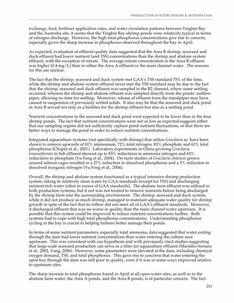
PRODUCTION SYSTEM DESIGN & INTEGRATION
251
exchange, feed, fertilizer application rates, and water circulation patterns between Yingbin Bay and the Australia site, it seems that the Yingbin Bay shrimp ponds were relatively typical in terms of nitrogen discharge. However, the high total phosphorus concentrations give rise to concern, especially given the sharp increase in phosphorus observed throughout the bay in April. As expected, evaluation of effluent quality data suggested that the Area B shrimp, seaweed and duck effluent had lower nutrient (and TSS) concentrations than the shrimp and abalone system effluent, with the exception of nitrate. The average nitrate concentration in the Area B effluent was higher (0.4 mg/L) than in either the Area A effluent or the main channel water. The reasons for this are unclear. The fact that the shrimp, seaweed and duck system met GAA’s TSS standard 75% of the time, while the shrimp and abalone system effluent never met the TSS standard may be due to the fact that the shrimp, seaweed and duck effluent was sampled in the B2 channel, where some settling occurred, whereas the shrimp and abalone effluent was sampled directly from the ponds’ outflow pipes, allowing no time for settling. Moreover, release of effluent from the standpipes may have caused re-suspension of previously settled solids. It also may be that the seaweed and duck pond in Area B served not only as a biofilter for the shrimp effluent but also as a settling pond. Nutrient concentrations in the seaweed and duck pond were expected to be lower than in the four shrimp ponds. The fact that nutrient concentrations were not as low as expected suggests either that our sampling regime did not sufficiently capture pond nutrient fluctuations, or that there are better ways to manage the pond in order to reduce nutrient concentrations. Integrated aquaculture systems (not specifically with shrimp) that utilize Gracilaria sp. have been shown to remove upwards of 81% ammonium, 72% total nitrogen, 83% phosphate and 61% total phosphorus (Chopin et al., 2001). Laboratory experiments in China growing Gracilaria lemaneiformis in fish effluent showed up to 85% reductions in ammonia nitrogen and 65% reductions in phosphate (Yu Feng et al., 2004). On-farm studies of Gracilaria chilensis grown around salmon cages resulted in a 27% reduction in dissolved phosphorus and a 5% reduction in dissolved inorganic nitrogen (Yu Feng et al., 2004). Overall, the shrimp and abalone system functioned as a typical intensive shrimp production system, taking in relatively clean water by GAA standards (except for TSS) and discharging nutrient rich water (often in excess of GAA standards). The abalone farm effluent was utilized in both production systems, but it not was not treated to remove nutrients before being discharged by the shrimp farm into the surrounding environment. The shrimp, seaweed and duck system, while it did not produce as much shrimp, managed to maintain adequate water quality for shrimp growth in spite of the fact that its inflow did not meet all of GAA’s effluent standards. Moreover, it discharged effluent that was no worse in quality than the main channel water upstream. It is possible that this system could be improved to reduce nutrient concentrations further. Both systems had to cope with high total phosphorus concentrations. Understanding phosphorus cycling in the bay is crucial to helping farmers better manage their ponds. In terms of some nutrient parameters, especially total ammonia, data suggested that water exiting through the dam had lower nutrient concentrations than water entering the culture area upstream. This was consistent with our hypothesis and with previously cited studies suggesting that large-scale seaweed production can serve as a filter for aquaculture effluent (Marinho-Soriano et al., 2002, Yang, 2006). However, some parameters were elevated at the dam, including chemical oxygen demand, TSS, and total phosphorus. This gave rise to concerns that water entering the open bay through the dam was still poor in quality, even if it was in some ways improved relative to upstream sites. The sharp increase in total phosphorus found in April at all open water sites, as well as in the abalone farm water, the Area A ponds, and the Area B ponds, is of particular concern. The fact

TWENTY-FIFTH ANNUAL TECHNICAL REPORT – VOLUME I
252
that sampling sites at the dam and the abalone farm effluent miles upstream had the two highest total phosphorus concentrations in April is bewildering and implies that either phosphorus sources, water circulation patterns, or both, are not well understood. It may be that the abalone farm simply had several discharge channels that flowed in different directions toward the open seaweed area. The abalone farm and other discharges need to be more accurately mapped in order to make a further determination. The sediment quality data showed a universal increase in total nitrogen and decrease in total phosphorus in all of the open water sites during the study period, which may be due to the increased rainfall and runoff from adjacent land. The fluctuation in sediment nitrogen and phosphorus may also have resulted from farmers in the bay initiating their growout cycles simultaneously, in which case they would all be discharging nutrient-rich water during the same months. In order to assess the effectiveness of the open seaweed culture area as a biofilter, water quality in Yingbin Bay’s main channel and open seaweed culture area was compared to water quality found in a coastal creek that received shrimp farm effluent in China’s more northerly Jiangsu Province (Biao et al., 2004). Average COD levels were higher in Yingbin Bay than in the Jiangsu Province coastal creek (20.3 mg/L in Yingbin Bay’s main channel, 18.64 mg/L in the open seaweed culture area, and 5.77 mg/L in the Jiangsu Province coastal creek). Mean total phosphorus concentrations were also higher in Yingbin Bay (0.64 mg/L in Yingbin Bay’s main channel, 0.47 mg/L in the open seaweed culture area, compared to 0.024 mg/L in the Jiangsu Province coastal creek). Average total ammonia nitrogen concentrations were lower in the Yingbin Bay open seaweed culture area (0.23 mg/L) than in either the Yingbin Bay main channel (1.24 mg/L) or the Jiangsu Province coastal creek (1.5 mg/L). Relative to a 2002 study in Brazil that investigated effectiveness of Gracilaria sp. grown in shrimp effluent (Marinho-Soriano et al., 2002), the open seaweed culture area in Yingbin Bay maintained similar phosphate concentrations, and lower total ammonia and nitrate concentrations (Table 8). Nutrient concentrations in Yingbin Bay’s open seaweed area were similar to those found in the Area B seaweed and duck pond (Table 8). The Marinho-Soriano et al. study looked at Gracilaria grown in ponds that receive intensive shrimp farm effluent. The lowest total ammonia level observed in that study was 4 mg/L, whereas the highest concentration of total ammonia observed in Yingbin Bay’s open seaweed culture area was only 0.474 mg/L. The lowest nitrate concentration found at the Brazil site was 2.97 mg/L; whereas highest nitrate concentration found in the Yingbin Bay open seaweed area was only 0.059 mg/L. Phosphate concentrations were similar at all three sites. Aquacultural activities in the bay–particularly the large open seaweed farming area–may have a beneficial effect on nutrient-rich freshwater that otherwise would flow directly into the open bay. However, much is still unknown about seaweed filtration of aquaculture and other effluents. Studies examining use of seaweeds as biofilters in nutrient-rich waters point to many successes with biofiltration, but also to a large number of unknowns (Chen Jia, 1989; Chopin et al., 2001; Neori et al., 2004; Yang et al., 2005; Yang, 2006). For example, without relatively intensive study it is difficult to know what ratio of seaweed to effluent to use in any given coastal ecosystem in order to achieve maximum absorption of nutrients. Authors stress the need to understand better 1) the effect of non-native seaweeds on native ecosystems; 2) how to avoid overproduction of seaweed; 3) the life histories of different seaweed species; and 4) how to integrate seaweeds effectively into different types of aquaculture production systems (Chopin et al., 2001; Neori et al., 2004). While seaweed overproduction does not seem to be a concern in Yingbin Bay, under-production of Gracilaria verrucosa certainly is an important issue. Understanding the life history of Gracilaria verrucosa may be key to understanding why it was not thriving in Yingbin Bay. Additionally, the specific abilities of Gracilaria sp. and other seaweeds to absorb nutrients is not completely understood. Gracilaria sp. appears to work well in some settings (Marinho-Soriano et

PRODUCTION SYSTEM DESIGN & INTEGRATION
253
al., 2002) and not in others (Neori et al., 2000). It may be that a different species of seaweed would be more suited to the bay. Generally speaking, the study area appeared effective in reducing ammonia and phosphate concentrations, which is promising. However, the significance of these reductions is unknown. Moreover, dam management, water circulation, tidal fluctuations, and nutrient fluctuations (including seaweed uptake) in the bay must be better understood before conclusions can be drawn regarding the effectiveness of seaweed as a biofilter for aquaculture effluents.
ANTICIPATED BENEFITS Use of seaweed as a biofilter for water based nutrients is a technology that is used in many parts of the world but has developed more as an art than a science. This study was an initial attempt to both measure water quality and sedimentation around aquaculture facilities that employed such an integrated culture system, and to train students in China on such methodologies. We anticipate that over the longer term, students and faculty in our collaborating Chinese universities will benefit from the preliminary work done as part of this study, and will also develop better methods and designs for future studies. In the end, aquaculturists will utilize systems that are more environmentally benign and that also treat waste water before it ends up in the next person’s pond, which will benefit both aquaculture and the environment.
ACKNOWLEDGMENTS Special thanks to to the Hainan University students who helped with the field work and lab analysis: Qiu Yunhao, Sun Jie, Jane, Wang Jianguo, Ricky, You Zhengrong, Wang Huangxing, and Chen Xuebei. Thanks also to the following farmers who participated in our interviews (those farmers who asked to remain anonymous are not listed here, but are thanked just the same): Cai Du Xiu, Cai Du Jieng, Kuang Yao, Cai Ducheng, Cai Weiming, Chen Shunji, Wu Boming, Wu Zhongyin, Chen Shunji, Cai Duyu, Chen Huasheng, Cai Duyu, Chen Sheng, Lin Daoli, Cai Duyong, Cai Huaxin, Wu Ganghua, Fong Ergi, Chen Dongcheng. Thanks to Cao Ling, Mr. Yuan and his family, and Professor Fan and his family for your support.
LITERATURE CITED Biao, X., D. Zhuhong and W. Xiaorong, 2004. Impact of intensive shrimp farming on the water
quality of adjacent coastal creeks from Eastern China. Marine Pollution Bulletin, 48:543-553. Boyd, C.E., 2003. Guidelines for aquaculture effluent management at the farm level. Aquaculture,
226:101-112. Chen Jia, X., 1989. Gracilaria culture in China. NACA-SF/WP/89/12. Chopin, T., A.H. Buschmann, C. Halling, M. Troell, N. Kautsky, A. Neori, G.P. Kraemer, J.A.
Zertuche-González, C. Yarish and C. Neefus, 2001. Integrating seaweeds into marine aquaculture systems: a key toward sustainability. Journal of Phycology, 37:975-986.
FAO, 2006. State of World Aquaculture 2006 (Advance Copy). FAO Fisheries Technical Paper No. 500, Rome.
Jackson, C., N. Preston and P. Thompson, 2004. Intake and discharge nutrient loads at three intensive shrimp farms. Aquaculture Research, 35:1053-1061.
Jiarong, C., 1996. The Instructional Book of Water Quality Analysis (manual). China Agriculture Science and Technology Publishing House, Beijing.
Li, S.F., 2003. Aquaculture research and its relation to development in China, Agricultural Development and the Opportunities for Aquatic Resources Research in China. World Fish Center Conference Proceedings 65:17-28.
Lin, Y., 2002. Water Quality Monitoring and Analysis Methods, Standard Practice Handbook (manual). China Environmental Science Publishing, Beijing.
Marinho-Soriano, E., C. Morales and W.S.C. Moreira, 2002. Cultivation of Gracilaria (Rhodophyta) in shrimp pond effluents in Brazil. Aquaculture Research, 33:1081-1086.

TWENTY-FIFTH ANNUAL TECHNICAL REPORT – VOLUME I
254
Neori, A., T. Chopin, M. Troell, A.H. Buschmann, G.P. Kraemer, C. Halling, M. Shpigel and C. Yarish, 2004. Integrated aquaculture: rationale, evolution and state of the art emphasizing seaweed biofiltration in modern mariculture. Aquaculture, 231:361-391.
Neori, A., M. Shpigel and D. Ben-Ezra, 2000. A sustainable integrated system for culture of fish, seaweed and abalone. Aquaculture, 186:279-291.
Yang, H., Y. Zhou, Y. Mao, X. Li, Y. Liu and F. Zhang, 2005. Growth characters and photosynthetic capacity of Gracilaria lemaneiformis as a biofilter in a shellfish farming area in Sanggou Bay, China. Journal of Applied Phycology, 17:199-206.
Yang, Y., 2006. Growth of Gracilaria lemaneiformis under different cultivation conditions and its effects on nutrient removal in Chinese coastal waters. Aquaculture, 254:248-255.
Yu Feng, Y., L. Chun Hou, N. Xiang Ping, T. Dan Ling and C. Ik Kyo, 2004. Development of mariculture and its impacts in Chinese coastal waters. Reviews in Fish Biology and Fisheries, 14:1-10.
Zhu, Y., P. O’Connor and J. Cao, 2007. Where do Chinese scientists publish their research in environmental science and technology? Environmental Pollution, 147:1-3.

PRODUCTION SYSTEM DESIGN & INTEGRATION
255
Table 1. Description of shrimp pond management techniques, as recorded by farmers.
Pond Name
Pond Area (m2)
Production Type
Growout (Days)
Stocking Density (PL/m2)
Feed application
rate (kg/m2)
Fertilizer application
rate (kg/m2)
Total water
exchanged (m3)
Shrimp Production (kg m -2 d-1)
Avg. Body
Weight (g) at
harvest
Feed Conversion
Ratio
A1 2249
Intensive 98 133 1.5 0.008 10,120 0.013 11.5 1.22
A2 2724
Intensive 99 110 1.3 0.007 13,075 0.012 13.0 1.12
A3 2605
Intensive 99 115 1.6 0.007 12,244 0.014 12.7 1.18
B1 776
Semi-intensive
99 81 1.0 0.008 3335 0.008 10.4 1.26
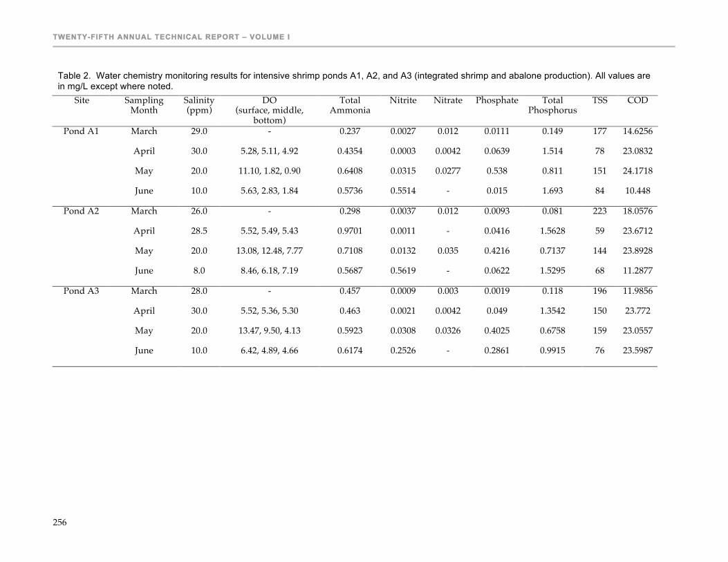
TWENTY-FIFTH ANNUAL TECHNICAL REPORT – VOLUME I
256
Table 2. Water chemistry monitoring results for intensive shrimp ponds A1, A2, and A3 (integrated shrimp and abalone production). All values are in mg/L except where noted.
Site Sampling Month
Salinity (ppm)
DO (surface, middle,
bottom)
Total Ammonia
Nitrite Nitrate Phosphate Total Phosphorus
TSS COD
March 29.0 - 0.237 0.0027 0.012 0.0111 0.149 177 14.6256
April 30.0 5.28, 5.11, 4.92 0.4354 0.0003 0.0042 0.0639 1.514 78 23.0832
May 20.0 11.10, 1.82, 0.90 0.6408 0.0315 0.0277 0.538 0.811 151 24.1718
Pond A1
June 10.0 5.63, 2.83, 1.84 0.5736 0.5514 - 0.015 1.693 84 10.448
March 26.0 - 0.298 0.0037 0.012 0.0093 0.081 223 18.0576
April 28.5 5.52, 5.49, 5.43 0.9701 0.0011 - 0.0416 1.5628 59 23.6712
May 20.0 13.08, 12.48, 7.77 0.7108 0.0132 0.035 0.4216 0.7137 144 23.8928
Pond A2
June 8.0 8.46, 6.18, 7.19 0.5687 0.5619 - 0.0622 1.5295 68 11.2877
March 28.0 - 0.457 0.0009 0.003 0.0019 0.118 196 11.9856
April 30.0 5.52, 5.36, 5.30 0.463 0.0021 0.0042 0.049 1.3542 150 23.772
May 20.0 13.47, 9.50, 4.13 0.5923 0.0308 0.0326 0.4025 0.6758 159 23.0557
Pond A3
June 10.0 6.42, 4.89, 4.66 0.6174 0.2526 - 0.2861 0.9915 76 23.5987

PRODUCTION SYSTEM DESIGN & INTEGRATION
257
Table 4. Nutrient concentrations of inflow water to Area A (intensive) shrimp ponds and Area B (semi-intensive) shrimp pond. Nutrient concentrations for the three Area A ponds in March were averaged. Nutrient concentrations in April and May in the seaweed and duck pond were averaged. All values in are in mg/L. Source of Inflow Water
Ammonia
Nitrate
Phosphate
Total Phosphorus
TSS
COD Average of Area A Shrimp Ponds in March 0.33 0.002 0.007 0.12 199 14.89
Seaweed and Duck Pond (Inflow to Area B Pond)
0.33 0.04 0.20 0.65 63 21.65
Table 3. Water chemistry monitoring results for pond B1, B3, and the water exchange canal (B2). All values are in mg/L except where noted.
Site Sampling Month
Salinity (ppm)
DO (surface, middle,
bottom)
Total Ammonia
Nitrite Nitrate Phosphate Total Phosphorus
TSS COD
March 10.00 10.85, 10.74, 11.11 0.0210 0.0018 0.0040 0.0538 0.1250 78 18.8848
April 5.00 6.71, 6.53, 6.45 0.1543 0.0050 0.0032 0.0654 0.5994 33 22.0080
May 5.00 11.34, 11.21, 10.23 0.3285 0.0187 0.0289 0.1068 0.2541 75 22.8464
Pond B1
June - - - - - - - - -
March 9.00 14.84 0.5400 0.0352 0.0560 0.0798 0.1590 122 19.3072
April 10.00 4.20 0.5181 0.0042 0.0042 0.1605 1.4918 30 22.1928
May 9.50 10.10 0.1238 0.0025 0.0247 0.2980 0.4920 62 22.9859
Pond B3
June 12.80 12.34 0.1264 0.0030 0.0613 0.2625 0.4377 38 22.0973
March 3.00 3.09 0.8780 0.0343 0.3610 0.0872 0.1550 45 15.2416
April 4.00 6.39 0.6449 0.0295 0.2804 0.2080 1.2698 36 20.9664
May 0.50 7.34 0.8831 0.0674 0.4884 0.2248 0.3893 69 21.8174
B2
June 5.00 2.58 0.4667 0.0543 0.4763 0.1785 0.4061 44 21.6403

TWENTY-FIFTH ANNUAL TECHNICAL REPORT – VOLUME I
258
Table 5. Water chemistry monitoring results for open water sampling sites. All values are in mg/L except where noted.
Sampling Site
Sampling Month
Salinity (ppm) DO pH Total
Ammonia Nitrite Nitrate Kjeldahl N Phosphate Total
Phosphorus TSS COD
March 0.00 0.46 7.1 2.3200 0.0491 0.0680 - 0.0817 0.1620 45 20.6976 April 6.00 0.95 7.2 1.7472 0.0955 0.1554 - 0.2556 0.9412 71 18.9168 May 0.50 4.02 7.0 1.8685 0.1012 0.0657 - 0.1364 0.8488 69 20.7187
C1
June 0.00 0.90 8.2 0.4375 0.0029 0.0288 - 0.1372 0.6065 73 23.1091 March 12.00 7.12 8.7 0.8430 0.0427 0.0140 - 0.0928 0.2640 103 19.5536 April 10.50 6.75 7.8 1.0142 0.0311 0.0399 - 0.3180 1.0123 41 20.3448 May 12.00 8.45 8.6 0.5277 0.0066 0.0344 - 0.4491 0.8164 58 20.3448
C2
June 8.00 4.23 8.0 1.0986 0.0439 0.0325 - 0.4416 0.8649 58 20.3448 March 3.00 3.09 7.4 0.8780 0.0343 0.3610 - 0.0872 0.1550 45 15.2416 April 4.00 6.39 7.5 0.6449 0.0295 0.2804 - 0.2080 1.2698 36 20.9664 May 0.50 7.34 7.8 0.8831 0.0674 0.4884 - 0.2248 0.3893 69 21.8174
B2
June 5.00 2.58 6.9 0.4667 0.0543 0.4763 - 0.1785 0.4061 44 21.6403 March 12.00 - 9.3 0.4340 0.0027 0.0360 7.5180 0.0557 0.0910 73 16.8256 April 12.00 8.06 8.3 0.4740 0.0026 0.0063 0.5320 0.1025 1.5495 42 11.7936 May 10.00 8.20 8.9 0.1077 0.0079 0.0319 1.3160 0.1180 0.1784 81 22.1837
W1
June 9.50 8.20 8.6 0.1653 0.0087 0.0454 1.4000 0.1138 0.2373 55 23.9578 March 10.00 9.3 0.2240 0.0033 - 7.7000 0.0631 0.0980 80 14.9776 April 13.00 4.29 7.1 0.1709 0.0053 0.0063 0.9800 0.1471 1.1188 25 22.1592 May 10.30 8.15 8.7 0.0538 0.0179 0.0344 1.0920 0.0805 0.1568 75 22.6546
W2
June 7.80 7.07 8.5 0.1799 0.0103 0.0588 1.9600 0.0441 0.1265 67 23.2723 March 13.00 - 9.2 0.1050 0.0027 0.0320 - 0.0089 0.0640 94 11.3168 April 13.00 7.72 8.3 0.2094 0.0043 0.0084 - 0.0936 1.6960 45 19.8408 May 12.00 8.43 8.8 0.0754 0.0091 0.0591 - 0.1210 0.1405 73 15.6088
C3
June 12.00 8.43 8.8 0.1264 0.0042 0.0466 - 0.0768 0.1476 46 19.0944

PRODUCTION SYSTEM DESIGN & INTEGRATION
259
Table 6. Average nutrient concentrations (mg/L) in pond effluent and main channel sampling sites.
Sampling Site Total Ammonia
Nitrate Nitrite Total Phosphorus
Phosphate TSS COD
Area A Effluent 0.90 0.03 0.16 1.97 0.32 118 21.48
Area B Effluent 0.72 0.40 0.05 0.56 0.17 49 19.92
Main Channel C1 1.59 0.08 0.06 0.64 0.15 65 20.86
Main Channel C2 0.87 0.03 0.03 0.74 0.33 65 20.15
Table 7. A comparison of pond inflow and effluent water quality to standards recommended by the Global Aquaculture Alliance. Values are presented as the ratio of samples that violated GAA’s target standard to the total number of samples collected. Dissolved oxygen and pH were not measured in the Area A pond effluent. Variable GAA
Target Ratio of Samples Violating Target in Pond A1 Effluent
Ratio of Samples Violating Target in Pond A2 Effluent
Ratio of Samples Violating Target in Pond A3 Effluent
Ratio of Samples Violating Target in Area B Effluent
Ratio of Samples Violating Target in Area A Inflow
Ratio of Samples Violating Target in Area B Inflow
pH 6 - 9 n/a n/a n/a 0/4 0/3 0/4 TSS ≤50
mg/L 3/3 3/3 3/3 1/4 3/3 2/4
TP ≤0.3 mg/L
3/3 3/3 3/3 3/4 0/3 3/4
NH3 ≤ 3 mg/L
0/3 0/3 0/3 0/4 0/3 0/4
DO ≥ 5 mg/L
n/a n/a n/a 2/4 n/a 1/4

TWENTY-FIFTH ANNUAL TECHNICAL REPORT – VOLUME I
260
Table 8. Soil quality changes in the two integrated systems. All values expressed in g/kg.
Sampling Site
∆ in TN ∆ in TP ∆ in Organic Matter
Pond A1 6.0675 0.1395 16.3200
Pond A2 4.4108 0.0400 3.6580
Pond A3 7.0840 0.2820 19.1860
Pond B1 2.4272 -0.0628 21.6939
Channel B2 5.8199 -0.0572 3.0050
Pond B3 6.2920 -0.1953 3.0929
Table 9. Sediment chemistry for open water sampling sites at the start and end of the study. No sediment samples were taken at C3, the sampling site furthest downstream at the dam, as the substrate was large boulders. Samplin
g Site Sampling
Month Bulk
Density (g/cm3)
Total Nitrogen
(g/kg)
Total Phosphorus
(g/kg)
Organic Matter (g/kg)
March 0.6930 2.9514 0.1480 45.6479 C1
June 1.5270 11.0497 0.0810 27.1530
March 1.1060 1.8637 0.0896 23.9538 C2
June 1.0210 7.8306 0.0710 42.6680
March 1.2600 1.8018 0.0767 14.2300 B2
June 1.4160 7.6217 0.0195 17.2350
March 1.5800 0.0447 0.0940 16.4800 W1
June 1.4770 5.8856 0.0265 23.6490
March 1.5470 0.4621 0.0715 14.5958 W2
June 1.5940 6.6734 0.0595 12.1310

PRODUCTION SYSTEM DESIGN & INTEGRATION
261
STUDENT EXCHANGE PROGRAM TO STRENGTHEN CAPACITY IN CHINESE ENVIRONMENTAL STUDIES OF AQUACULTURE: APPLICATION OF PHYTASE IN NILE TILAPIA FEED
Twelfth Work Plan, Production System Design & Integration 9b (12PSD9b)
Final Report Published as Submitted by Contributing Authors
Ling Cao & Weimin Wang Huazhong Agricultural University
Wuhan, Hubei, China
Yang Yi, Amararatne Yakupitiyage & Derun Yuan Asian Institute of Technology
Pathumthani, Thailand
James Diana University of Michigan
Ann Arbor, Michigan, USA
ABSTRACT This study was conducted at the Asian Institute of Technology to assess effects of the pretreatment in all-plant based diets with microbial phytase on phosphorous utilization and growth performance of Nile tilapia (Oreochromis niloticus).
Pretreatment trials were conducted using phytase at graded doses to determine the optimal dose of phytase. Available P levels increased significantly with the increased doses of phytase and the dose of 1,000 U kg-1 was most efficient. Based on the pretreatment trials, plant based diets for Nile tilapia were formulated by pre-treating with phytase at 1,000 U kg-1. Experimental diets were supplemented with graded levels of mono calcium phosphate (MCP) at 25, 18.75, 12.5, 6.25, and 0 g kg -1 diet. In addition, there were three controls: one phytase control, one inorganic P control and one pre-treatment control. The results showed that diets pre-treated with phytase gave better growth performance, feed conversion ratio and protein efficiency ratio of Nile tilapia compared to the phytase control diet and pretreatment control diet (P<0.05). There were no significant differences in growth performance of Nile tilapia between the inorganic control diet and phytase pre-treated diets supplemented with MCP at 25, 18.75 and 12.5 g kg-1 (P>0.05), which resulted in significantly better performance than those at 6.25 and 0 g kg-1 (P<0.05). Dietary interaction effects of phytase were observed for phosphorus retention efficiency and phosphorus load. Apparent digestibility coefficient of P (ADCp) was improved significantly by phytase pretreatment (P<0.05). No significant difference was detected on ADCac of crude protein among all experimental diets (P>0.05). Phytase can be used to efficiently pre-treat all-plant based diets at a dose of 1,000 U/kg while inorganic P can be supplemented at 12.5 g kg-1 to ensure that the adequate amount of P is available to juvenile Nile tilapia.
INTRODUCTION Currently, there are increasing interests in the complete replacement of fish meal by various grain products such as soybean meal, wheat flour, and corn gluten meal (Cain and Garling, 1995). One of the major problems limiting the use of grain products in fish feed is the presence of phytate (inositol hexaphosphate). Phytate is the primary form of phosphorus (P) in grains, accounting for approximately two thirds of the total P bound as phytate P (Lall, 1991). Phytate is an indigestible P form, which is practically not available for fish such as tilapias (NRC, 1993) due to lack of an intestinal phytase for efficient hydrolysis of phytate during digestion (Jackson et al., 1996).

TWENTY-FIFTH ANNUAL TECHNICAL REPORT – VOLUME I
262
Consequently, the available P in all-plant diets may not meet the requirements of fish, and inorganic P is usually supplemented to the diets. On the other hand, undigested phytate P excreted via feces contributes to environmental pollution, causing eutrophication in receiving water bodies. Exogenous phytase has been used successfully to hydrolyze phytate and increase nutrient digestibility (Cao et al., 2007). Specifically for hydrolysis of phytate, phytase is most promising in producing cost-effective fish feed formula that can reduce the need to supplement of inorganic P in feeds and also lower phytate P levels in fish excretion (Simons et al., 1990; Liener, 1994). Phytase is not heat stable and should be applied by avoiding excess heat during extrusion and other steps in diet manufacture (Vielma et al., 2002). It is deactivated at temperatures above 65oC, while the temperature during feed processing often exceeds 65oC (Cao et al., 2007). Phytase can be utilized in fish feeds by pre-treating feedstuffs (Cain and Garling, 1995), or spraying onto pellets (Vielma et al., 2004) to avoid deactivation. Studies on the role of supplemental phytase for nutrient utilization or growth of fish focus on commonly cultured species such as rainbow trout (Oncorhynchus mykiss) (Rodehutscord and Pfeffer 1995; Forster et al., 1999), common carp (Cyprinus carpio L.) (Schäfer et al., 1995), channel catfish (Ictalurus punctatus) (Jackson et al., 1996; Li and Robinson, 1997) and Nile tilapia (Oreochromis niloticus) (Furuya et al., 2001; Liebert and Portz 2005). Biological factors such as the rearing temperature of fish may influence the function of phytase applied onto a diet. Thus, pretreatment seems to be more promising than top-spraying since the dephytinization process happens in vitro by fishes. Due to the increasing price and decreasing resources, inorganic P supplementation in fish diets could be replaced partially or fully by phytase (Cao et al., 2007). There have been inconsistent results from studies evaluating the effects of phytase pretreatment on feed quality and utilization. Cain and Garling (1995) reported that pretreatment of soybean meal with phytase enhanced growth performance and P utilization of juvenile rainbow trout. Similarly, dephytinization of soy protein concentrate increased protein and P utilization in Atlantic salmon (Salmo salar) in seawater (Storebakken et al., 1998), whereas a decrease in rapeseed protein quality by dephytinization was noted by Teskeredzic et al., (1995) in rainbow trout. Results related to weight gain, apparent digestibility of crude protein and amino acids after phytase addition also showed great inconsistency (Sajjadi and Carter 2004). Some studies found that addition of phytase had positive effects on weight gain of rainbow trout (Rodedutscord and Preffer, 1995; Vielma et al., 1998) and channel catfish (Jackson et al., 1996; Li and Robinson, 1997), while other studies detected no effects for the same species (Lanari et al., 1998; Yan and Reigh 2002). Many studies have demonstrated that addition of phytase to fish feeds can improve utilization of phytate P and decrease total P load to the environment for several species (Vielma et al., 1998; Liebert and Portz 2005). In Nile tilapia, phytase supplementation between 500 and 1,500 U kg-1 improved P availability, crude protein digestibility, and bone mineralization (Furuya et al., 2001). Liebert and Portz (2005) reported that phytase supplementation of 750 U kg-1 in Nile tilapia diets resulted in the same performance as inorganic P addition (NaH2PO4; 15 g kg-1 diet). The available P requirement of Nile tilapia is between 5 (NRC, 1993) and 9 g kg-1 (Watanabe et al., 1980; Beveridge and McAndrew 2000), and tilapia juveniles usually need higher P levels than adults. When all-plant diets are used, total P content from plant ingredients is usually less than that in fishmeal-based diets. Thus, P content in all-plant diets may not meet the P requirement of Nile tilapia juveniles and partial supplementation of inorganic P may be needed. Whether inorganic P supplementation could be partially or completely replaced in Nile tilapia feed needs further investigation. Besides, the approximate amount of phytate P converted to available P in plant ingredients after phytase pretreatment is also uncertain.

PRODUCTION SYSTEM DESIGN & INTEGRATION
263
The purposes of this study were: 1. To determine the optimal dose of phytase for pretreatment of plant ingredients and the
amount of available P released from phytate P; 2. To investigate the effects of the phytase pretreatment and replacement levels of inorganic P on
growth performance, as well as apparent digestibility of crude protein and P of Nile tilapia juveniles fed all-plant diets.
MATERIALS AND METHODS Pretreatment trials Two pretreatment trials were conducted using a completely randomized design at the Asian Institute of Technology (AIT), Thailand, from 5 January to 5 February 2006. In the first trial, soybean meal was treated with microbial phytase (Habio® Phytase-5,000 FTU g-1, Sichuan Habio Bioengineering Co. Ltd., Chengdu, China) at 0 (control), 500, 750, 1,000, and 1,500 U kg-1. The second trial was conducted to treat mixed plant meal consisting of soybean meal (64.4%), wheat meal (11.9%) and corn gluten meal (23.7%) with phytase at 0 (control), 500, 750, 1,000, 1,500, and 3,000 U kg-1. Each treatment had three replicates. The pretreatment method described by Cain and Garling (1995) was used and adapted in this study. The procedures of the method were to: (1) prepare 0.2 M citrate buffer (dissolve 15.38 g citric acid and 37.29 g sodium citrate into 1-L distilled water) at room temperature; (2) dissolve 2 g phytase (5,000 U g-1) into 1-L citrate buffer using a magnetic stirrer for 30 min; (3) add meal to the buffer at 1:1 (w:v), place the mixture in aluminum trays, and rapidly heat with constant stirring to 50-55oC (cover the mixture with aluminum foil and incubate at 55oC for 6 h); (4) dry the mixture in a forced-air drying oven at 60oC for 24 h to reduce the moisture content to approximately 10%. In the control, the same method was used but without adding phytase (Riche et al., 2001). Experimental diets Experimental design and basal diet formulations were based on the assumption that effects of phytase pretreatment can be most accurately measured using P utilization as the indicator of phytic acid hydrolysis (Vielma et al., 1998). Therefore, an all-plant basal diet was formulated to contain low levels of available P (Table 1). Five treatment diets were supplemented with mono calcium phosphate (MCP) at 25 g kg-1 (100% MCP supplement, diet 3), 18.75 g kg-1 (75% MCP supplement, diet 4), 12.5 g kg-1 (50% MCP supplement, diet 5), 6.25 g kg-1 (25% MCP supplement, diet 6) and 0 g kg-1 (0% MCP supplement, diet 7) respectively by cassava replacement for different experimental treatments (Table 2). In addition, there were three controls: one phytase control (diet 1, basal diet) with neither phytase pretreatment nor inorganic P supplement; one inorganic P control (diet 2) without phytase pretreatment but with 25 g kg-1 supplement of MCP by replacing the same amount of cassava starch in the basal diet; and one pretreatment control (diet 8) with neither phytase pretreatment nor inorganic P supplement but with phytase added directly to feed ingredients. Diet 8 was prepared at a phytase dose of 1,000 U kg -1 by dissolving phytase in distilled water before pelleting. For diet preparation, dry ingredients were mixed in a Hobart-type mixer. Fish oil in the diets was included in the mixer prior to extrusion. Diets were pelleted (3 mm in diameter) with a laboratory extrusion system at 80oC. Pelleted diets were air dried, crumbled into 1-2 mm in diameter with a grinder, and stored in sealed plastic bags at 4oC until use. Growth trial A growth trial was conducted in 24 indoor recirculating circular cement tanks (1 m in both depth and diameter) at AIT from 20 March to 21 May 2006, to assess effects of experimental diets on the growth performance of Nile tilapia. Water flow rate was fixed at 1 L min-1 to maintain a water

TWENTY-FIFTH ANNUAL TECHNICAL REPORT – VOLUME I
264
depth of 0.7 m in all experimental tanks. Eight experimental diets were assigned randomly to experimental tanks with three replicates each. Sex-reversed all-male Nile tilapia fingerlings of 0.7 – 0.8 g in size were stocked at 30 fish tank-1, and fed with the experimental diets to apparent satiation twice daily at 09:00 – 10:00 h and 16:00 – 17:00 h. All experimental fish were purchased from the hatchery at Asian Institute of Technology. Samples of diets and six fish per tank were collected at the beginning for analyses of whole body composition. Uneaten pellets and feces in all tanks were removed by siphon everyday. Tank water samples, taken weekly at 09:00 h, were analyzed for total alkalinity, total ammonia nitrogen (TAN), total Kjeldahl nitrogen (TKN) and total phosphorus (TP), using standard methods (APHA et al., 1985). Temperature, dissolved oxygen (DO), and pH (at 20 cm below the water surface) were measured in situ according to the same schedule. Water quality parameters in the experimental tanks were maintained within acceptable levels for tilapia (Plumb, 1999) by using physical and biological filters in the recycling system. Feed intake was calculated by subtracting the number of uneaten from supplied pellets. Feed intake was monitored in this way everyday throughout the experiment. At the end of the growth trial, all fish were deprived of food for one day before counting and weighing. Six fish per tank were collected for analyses of whole body composition, then feed conversion ratio (FCR), specific growth rate (SGR) and protein efficiency ratio (PER) were calculated. Nutrient retention efficiency of phosphorus was calculated as:
Phosphorus retention % = 100 * [(FBW * Nf) – (IBW * Ni)]/ (feed intake * Ndiet)
Where FBW is the final body weight and IBW is the initial body weight of fish, N is the concentration of nutrient (P) in the fish at the start (Ni) and end (Nf) of the experiment (Storebakken et al., 1998).
Phosphorus load was calculated as: P load (g P kg-1) = [(P fed, g) – (P deposited, g) / (Weight gain, kg) (Vielma et al., 2002).
Digestibility trial A digestibility trial was conducted after termination of the growth trial in twenty- four 80-L fiberglass tanks. Ten sex-reversed, all-male Nile tilapia fingerlings of approximately 25 g in size were stocked in each fiberglass tank, and aeration provided by an air stone. Experimental diets used in the growth trial were the same as those used in the digestibility trial with three replicates for each diet. The digestibility trial was conducted from 25 May to 10 June 2006 for 15 days. Fish were fed commercial feed during a 3-day acclimation period, after which the experimental diets were fed twice daily (09:00 – 10:00 h and 16:00 – 17:00 h) at a rate of 3% body weight per day for 5 days of dietary adaptation. Starting from day 6, feces were collected twice a day for 10 days and pooled by each treatment tank. One hour after feeding, water was completely changed in all tanks to remove uneaten feed, and feces were collected three hours after each feeding according to the method described by Lim et al., (2004). Collected feces were air-dried at 55oC. Samples of feces were kept in a desiccator for analyses of crude protein and total P using standard methods (AOAC 2000). Apparent digestibility coefficients (ADC) of crude protein and P for eight diets were determined by the hydrolysis resistant organic matter (HROM) method (Buddington, 1980). ADC was calculated according to: Chemical analysis The chemical analyses of diets, fish whole-body and faeces were performed according to standard methods (AOAC, 2000): dry matter (dried at 105oC); crude protein (Kjeldahl method); crude lipid (ether extract according to soxhlet method); and ash (combusted at 550oC for 6 h). The measurement of crude fibre (CF) involves extraction of a ground feed sample with diethyl ether

PRODUCTION SYSTEM DESIGN & INTEGRATION
265
followed by sequential boiling in dilute acid and dilute base. The residue is then burned in a 500-600oC muffle furnace. CF % is calculated from the difference in weight of the sample before and after burning (AOAC, 2000). Calcium was analyzed using atomic absorption phase spectrophotometer (Spectra-55, Varian) after acid digestion. Phosphorus content in fish whole body was determined in three replicates using the vanadium–molybdate method described by AOAC (2000). Absorbance of the vanado-molybdo phosphorus complex was measured at 430 nm using a UV–VIS spectrophotometer (Specord S100, Carl Zeiss). Phytate P in feed ingredients was analyzed by anion-exchange method (Latta and Eskin, 1980; Harland and Oberleas, 1986) using a 100-200 mesh AG1-X4 chloride anion exchange column (Bio-Rad Laboratory, USA). Phytate was extracted from feed ingredients using diluted HCl. The extraction product was then placed on an ion-exchange column. Phytate was eluted with 0.7 M NaCl solution and wet-digested with mixture of concentrated HNO3/H2SO4 to release phytate P, which was measured colorimetrically at 640 nm using a UV–VIS spectrophotometer (Specord S100, Carl Zeiss) (Harland and Oberleas, 1986). Available P was calculated by deducting phytate P from total P (Sajjadi and Carter, 2004). Phytase efficacy was calculated as follows: Efficacy �100* (Initial phytate P - Final phytate P)/ Initial phytate P. Statistical analysis Data were analyzed statistically using one-way analysis of variance (ANOVA) and regression (Steele and Torrie, 1980) with SPSS (version 11.5) statistical software package (SPSS Inc., Chicago, USA). ANOVA was performed for percentage data after arcsine transformation, while percentage data were presented in the original scale. Treatment means were compared using Least Significant Difference (LSD) and differences among treatments were considered significant at an alpha level of 0.05. Mean values were given with ± 1 standard deviation (SD).
RESULTS Pretreatment of plant ingredients After pretreatment, phytate P contents of both soybean meal and mixed plant meal decreased, while the available P contents increased for all levels of phytase doses including controls (Tables 3 and 4). Final available P and efficacy of converting phytate P to available P increased significantly with increasing doses of phytase for both soybean meal (Figure 1) and mixed plant meal (Figure 2). Based on the two figures, equations for soybean meal can be written as Y = 11.1907 X0.2841 (R2=0.9078, n = 15, P < 0.05); while mixed plant meal had the equation Y=29.7048 X0.14567 (R2=0.9158, n = 18, P<0.05), where Y is the efficacy of phytase indicating how much phytate P was converted to available P; X is the dose of phytase. According to the inflexion calculation of curves (Lanari et al., 1998; Jiang et al., 2006), the dose of 1,000 U kg -1 was determined as the most efficient. Growth performance Pretreatment of plant ingredients with phytase and P supplementation both had significantly positive effects on growth performance of Nile tilapia. Survival values were all higher than 90% in all treatments, ranging from 90% to 96.67% (Table 5). Growth performance in terms of final mean weight, total weight gain, and daily weight gain was best in treatments supplemented with 12.5, 18.75 and 25 g kg-1 MCP and the inorganic P control, intermediate in the treatments supplemented with MCP at 6.25 and 0 g kg-1, and poorest in the pretreatment control and the phytase control (P<0.05). SGR showed similar patterns of differences among treatments to other growth performance parameters, with the highest SGR in the treatment with MCP supplement at 12.5 g kg-1. Fish fed diets without phytase showed poorer FCR, while FCR ranging from 1.10 to 1.85 was best in the treatments with MCP supplement at 12.5 and 25 g kg-1 as well as the inorganic P control (P<0.05), which were not significantly different from the treatment with MCP supplement at 18.75 g kg-1 (P>0.05), but were significantly better than all other treatments (P<0.05). Protein

TWENTY-FIFTH ANNUAL TECHNICAL REPORT – VOLUME I
266
efficiency ratio (PER) ranged from 1.49 in the phytase control to 2.66 in the diet supplemented with MCP at 12.5 g kg-1.
The addition of phytase and inorganic P to the basal diet significantly increased the contents of ash, P and crude protein in the whole body of Nile tilapia (Table 6), while dry matter and lipid contents decreased significantly (P<0.05). Compared to the phytase control and pretreatment control, significantly higher levels of P contents in tilapia carcass, ranging from 1.68% to 1.83%, were found in the inorganic P control (diet 2), 25 g kg-1 MCP supplement (diet 3), 18.75 g kg-1 MCP supplement (diet 4), 12.5 g kg-1 MCP supplement (diet 5), 6.25 g kg-1 MCP supplement (diet 6) and 0 g kg-1 MCP supplement (diet 7) (P<0.05). There were no significant differences in P contents for whole body of Nile tilapia between the inorganic P control (diet 2), 25 g kg-1 MCP supplement (diet 3), 18.75 g kg-1 MCP supplement (diet 4) and 12.5 g kg-1 MCP supplement (diet 5) (P>0.05). P deficiency was observed for Nile tilapia in the phytase control (diet 1), 0 g kg-1 MCP supplement (diet 7) and pretreatment control (diet 8), evidenced by abnormal head shape, curved vertebrae, and loose scales. The lowest levels of ash, P and crude protein contents and highest contents of dry matter and lipid in the whole body of Nile tilapia were all found in the phytase control (diet 1).
Phosphorus retention efficiency and load Dietary interaction effects of phytase were observed for phosphorus retention efficiency and phosphorus load (Table 7). P retention efficiency was significantly higher for diet 5, 6 and 7, intermediate for 2, 3 and 4 and significantly lower for 1 and 8 (P<0.05). P load was significantly higher for diet 1 and 8, intermediate for 2, 3 and 4 and significantly lower for 5, 6 and 7 (P<0.05). Apparent digestibility Apparent digestibility coefficients of phosphorus (ADCp) were enhanced by phytase pretreatment, however, there were no significant differences in apparent digestibility coefficients of crude protein (ADCcp) among all treatments. ADCCP of the eight experimental diets ranged from 83.10% to 85.27% did not significantly differ from each other (P>0.05, Table 8). However, phytase pretreatment significantly increased ADCP of the experimental diets (P<0.05). ADCP values in the diets supplemented with 12.5 g kg-1 or less MCP (diets 5, 6 and 7) were significantly higher than those in all other diets including the diets supplemented with more than 12.5 g kg-1 MCP as well as the three control diets (P<0.05).
DISCUSSION Pretreatment of plant ingredients using microbial phytase significantly increased available P content in feed, indicating that the indigestible phytate P was successfully converted to available P by phytase. The relationships between the amount of available P released from phytate P and the doses of phytase administered can be used to predict the amount of available P to be released and the amount of inorganic P that may need to be supplemented at different dosages of phytase. In the present study, the release rates of available P from phytate P in soybean meal were about 66% and 82% at phytase doses of 500 and 1,000 U kg-1, respectively, which are similar to those achieved by Yu and Wang (2000). Other studies have shown that soybean meal treated by phytase at 500 U kg -1 released about 20% of phytate P (Schafer et al., 1995), which increased to about 40% when the dose of phyase increased to 1,000 U kg -1 (Cain and Garling, 1995). In the present study, the release rates of available P from phytate P were 16.73% for soybean meal and 24.67% for the mixed plant ingredients when no phytase was added, due probably to the effect of citrate acid on hydrolysis of phytate in plant ingredients during the incubation. Sugiura et al., (2001) found that citric acid could chelate minerals and prevent their precipitation, indicating that citric acid can convert phytate P to available P to some extent. Thus, the pretreatment method might be an effective alternative for fish to maximize phytase activity and overcome temperature limitation (Cain and Garling, 1995; Yoo et al., 2005). The growth performance and FCR of Nile tilapia after the 60-day growth trial was improved significantly when the pre-treated diets with phytase at 1,000 U kg -1 were used, compared to the

PRODUCTION SYSTEM DESIGN & INTEGRATION
267
phytase control diet. Higher protein efficiency ratio of fish fed the diets containing phytase-treated than untreated meal indicates that phytase or heating of the meal during phytase treatment improved nutritional quality of the mixed plant meal. Liebert and Portz (2005) reported the optimal growth of Nile tilapia was achieved by phytase supplementation at 750~1,250 U kg-1 in plant-based diets. Growth improvement was also observed in rainbow trout fed phytase-supplemented diets (Rodehutsord and Pfeffer, 1995; Papatryphon et al., 1999), and salmon and rainbow trout fed the diets with phytase pretreated ingredients (Cain and Garling, 1995; Vielma et al., 2002). However, the inclusion of phytase did not improve growth of rainbow trout fed diets containing canola protein concentrate (Forster et al., 1999) and juvenile Korean rockfish (Sebastes schlegeli) fed diets containing soybean meal (Yoo et al., 2005). The available P contents in the phytase control diet, the diets without MCP supplement and the pretreatment control diet were lower than the minimum P requirement of Nile tilapia (5 g kg-1), and caused poor fish growth. The available P content in the diet supplemented with 6.25 g kg-1 MCP was 5.6 g kg-1, which was slightly higher than the minimum requirement, but still resulted in poorer growth of Nile tilapia than the inorganic P control, probably because juvenile fish have higher P requirements than large fish (NRC, 1993; Cain and Garling, 1995). Diets supplemented with more than 12.5 g kg-1 MCP and the inorganic P control diet that contained around 9 g kg-1 of available P gave tilapia better growth than other diets in the present study, in agreement with findings of Watanabe et al., (1980). Vielma et al., (2002) found better growth and feed utilization efficiency by pretreatment could be attributed partially to more efficient phytic acid hydrolysis in comparison to top-spraying with phytase. Forster et al., (1999) reported that phytase top-sprayed onto soy protein-based diets at doses of 0, 500, 1500 or 4500 U kg-1 diet did not affect growth or feed utilization efficiency in rainbow trout. Similarly, 2,000 U phytase kg-1 mixed in the feed prior to pelleting did not enhance performance of sea bass (Dicentrarchus labrax) despite a clear increase in P digestibility (Oliva-Teles et al., 1998). Further studies should be conducted to compare the economic benefits between pretreatment and top-spraying with phytase at industrial levels. Ash, crude protein, and phosphorous contents in the whole Nile tilapia fed phytase pre-treated diets (diet 3, 4, 5, 6, and 7) were significantly higher than those fed diets 1 and 8, indicating that phytase pretreatment led to improvement in carcass quality and P retention. Among all the diets, diets 2, 3, 4, and 5 performed best in terms of the growth, nutrient utilization, and inorganic P replacement in the present study. Compared to diet 2, 3, and 4, diet 5 supplemented the least inorganic P, only 50% of the inorganic control (diet 2) and diet 3. The cost of diet 5 was less than the other three diets. So diet 5 supplemented with phytase at 1,000 U kg -1 and 12.5 g kg-1 MCP was the best, indicating that phytase at 1,000 U kg -1 is comparable to 12.5 g MCP kg-1 diet. Schäfer et al., (1995) suggested that diets mainly based on plant proteins such as soybean meal have high contents of phytic acid, and the supplementation of phytase at levels of either 500 or 1,000 U kg -1 can replace 1.9 g P from MCP. Phytase also increased deposition of P in the whole fish body, indicating that P load to the environment was reduced. Therefore, using phytase in plant-based diets can reduce the need for inorganic P supplementation in diets, leading to the reductions of P discharged to the environment from fish farms. Lipid and dry matter contents in the whole body also increased when Nile tilapia were fed low available P diets (diets 1 and 8), which agreed with the results in carp (Onishi et al., 1981) and rainbow trout (Rodehutscord, 1996). The enhanced lipid and dry matter contents were probably caused by inhibition of the β-oxidation of fatty acids resulting from a deficiency of P (Schäfer et al., 1995). Phosphorus retention efficiency was significantly higher in fish fed phytase-supplemented diets compared to phytase control in the present study, indicating that phytase could improve phosphorus utilization. The lower retention values in diets 2, 3 and 4 were due to phosphorus being provided at well above the phosphorus requirement, demonstrating improved utilization at dietary phosphorus near the required level. When dietary phosphorus concentration increased above that level, retention efficacy decreased. Factors like feed conversion ratio, ingredient digestibility, and dietary phosphorus content affect phosphorus load (Vielma et al., 2002). Using phytase in plant based diets reduced phosphorus load. Hence, the inclusion of phytase in diets is effective for aquaculture waste management. In the present study, phosphorus utilization was

TWENTY-FIFTH ANNUAL TECHNICAL REPORT – VOLUME I
268
higher in the fish fed either phytase or MCP-phytase diets. But in combination of phytase and MCP diets, there was no further advantage when phosphorous level was above P requirement of tilapia. Because of the positive effect of phytase, the P retention in juvenile Nile tilapia was improved while the total P load to the environment was reduced. Similar results have also been reported in salmon (Cain and Garling, 1995) and rainbow trout (Lanari et al., 1998; Sugiura et al., 2001) fed diets based on soybean meal. The pretreatment of mixed plant ingredients using phytase at 1,000 U kg -1 significantly improved ADCp in the present study, compared to the phytase control diet and pretreatment control diet. The ADCp was reported to be highest when dietary P level reached the P requirement for cultured fish, then declined with increasing dietary P levels (Riche and Brown, 1996). The dietary P level in our diet with MCP supplement at 25 g kg-1 (diet 3) was the highest among all diets, and even higher than the P requirement of juvenile Nile tilapia due to release of available P from phytate P. However, the ADCp in this diet was significantly lower than the diets with less MCP supplements (diets 4, 5, 6, and 7) as well as the P control (P<0.05), but significantly higher than that in the phytase control. The results with respect to digestibility of diets with MCP supplement and phytase pretreatment may also be due to the interaction between MCP and phytase. Sugiura et al., (2001) also observed that the ADCp reached 93% in rainbow trout fed with a phytase pre-treated diet containing 4.21 g kg-1 of total P. However, when the total P level increased to 14.7 g kg-1, the ADCp in diet containing phytase at 1,000 U kg -1 was only 62%. No significant difference was observed in the ADCcp in the present study, and this result was consistent with results reported by other studies (Riche et al., 2001; Sajjadi and Carter, 2004; Yoo et al., 2005). However, Furuya et al., (2001) observed that phytase at 500 to 1,500 U kg -1 improved P availability and crude protein digestibility in Nile tilapia. More research should focus on the apparent digestibility of crude protein and profiles of amino acids in tilapia fed phytase pretreated plant-based diets. In conclusion, our results indicate that the optimal dose of phytase for pretreatment of plant ingredients is 1,000 U kg -1, which can efficiently convert phytate P to available P and replace 12.5 g kg-1of the inorganic P supplementation to diets for Nile tilapia juveniles without affecting growth performance or apparent digestibility coefficients of both crude protein and phosphorous. The addition of phytase in the diets of Nile tilapia juveniles can reduce the use of MCP, enhance the utilization of P in plant ingredients, and thus minimize the P discharged into the environment.
ANTICPIPATED BENEFITS Based on the result, we have a reasonable measure of the phytase dose for releasing the desired amount of available phosphorus from plant feeds. Diets supplemented with phytase can decrease the nutrient loss in effluents and increase the utilization of phytate phosphorous, protein and mineral elements. Therefore, using phytase in diets based on plant-meal will reduce the need for inorganic P supplementation, which will lead to reductions in phosphorus discharge from fish farms.
ACKNOWLEDGMENTS The authors wish to thank the Asian Institute of Technology (AIT), Thailand for providing field research and laboratory facilities. The authors also wish to thank the staff of Aquaculture Laboratory at AIT for their field and lab assistance, and Mr. Yang Chengtai at Huazhong Agricultural University, China for his assistance in the report preparation.
LITERATURE CITED AOAC (Association of Official Analytical Chemists), 2000. Official Methods of Analysis of the
Association of Official Analytical Chemists, 19th edition. Association of Official Analytical Chemists, Arlington, Virginia, USA.
PRODUCTION SYSTEM DESIGN & INTEGRATION
269
APHA, AWWA, WPCF, 1985. Standard Methods for The Examination of Water and Wastewater, 15th edn. American Public Health Association, American Water Works Association and Water Pollution Control Federation, Washington DC, U.S.A., 1134 p.
Beveridge M.C.M. and McAndrew B.J., eds., 2000. Tilapias: Biology and Exploitation. Kluwer Academic Publishers, Fish and Fisheries Series 25, 360 p.
Buddington, R.K., 1980. Hydrolysis resistant organic matter as a reference for measurement of fish digestive efficiency. Transactions of the American Fisheries Society, 109:653-656.
Cain, K.D. and Garling, D.L., 1995. Pretreatment of soybean meal with phytase for salmonid diets to reduce phosphorus concentrations in hatchery effluents. Progressive Fish-Culturist, 57:114-119.
Cao, L., Wang, W.M., Yang, C.T., Yang, Y., Diana, J.S, Yakupitiyage, A., Luo, Z. and Li, D.P., 2007. Application of microbial phytase in fish feed. Enzyme and Microbial Technology, 40:497–507.
Debnath, D., Pal, A.K. and Sahu, N.P., 2005. Effect of dietary microbial phytase supplementation on growth and nutrient digestibility of Pangasius pangasius (Hamilton) fingerlings. Aquaculture Research, 36:180-187.
Eya, J.C. and Lovell, R.T., 1997. Net absorption of dietary phosphorus from various inorganic sources and effect of fungal phytase on net absorption of plant phosphorus by channel catfish Ictalurus punctatus. Journal of the World Aquaculture Society, 28:386-391.
Forster, I., Higgs, D.A., Dosanjh, B.S., Rowshandeli, M. and Parr, J., 1999. Potential for dietary phytase to improve the nutritive value of canola protein concentrate and decrease phosphorus output in rainbow trout (Oncorhynchus mykiss) held in 11ºC fresh water. Aquaculture, 179:109-125.
Furuya, W.M., Gonçalves, G.S., Rossetto, V., Furuya, B. and Hayashi, C., 2001. Phytase as feeding for Nile tilapia (Oreochromis niloticus): performance and digestibility. Review of Brazil Zootechnique, 30(3):924-929.
Harland, B.F. and Oberleas, D., 1986. Anion-exchange method for determination of phytate in foods: collaborative study. Journal of AOAC International, 69:667-670.
Hughes, K.P. and Soares Jr, J.H., 1998. Efficacy of phytase on phosphorus utilization in practical diets fed to striped bass, Morone saxatilis. Aquaculture Nutrition, 4:133-140.
Jackson, L., Li, M.H. and Robinson, E.H., 1996. Use of microbial phytase in channel catfish Ictalurus punctatus diets to improve utilization of phytate phosphorus. Journal of the World Aquaculture Society, 27:309-313.
Jiang, J.L., He, J.H., Deng, J.P. and Zhong, N., 2006. Advance in phosphorous equivalency of phytase. Feed industry, 27:47-51. (in Chinese)
Lall, S.P., 1991. Digestibility, metabolism and excretion of dietary phosphorus in fish. In: C.B. Cowey, C.Y. Cho, (eds.), Nutritional Strategies and Aquaculture Waste. University of Guelph, Guelph, Ontario, Canada, pp 21-36.
Lanari, D., Agaro, E.D. and Turri, C., 1998. Use of nonlinear regression to evaluate the effects of phytase enzyme treatment of plant protein diets for rainbow trout (Oncorhynchus mykiss). Aquaculture, 161:345-356.
Latta, M. and Eskin, M., 1980. A simple and rapid colorimetric method for phytate determination. Journal of Agriculture and Food Chemistry, 28:1313-1315.
Li, M.H. and Robinson, E.H., 1997. Microbial phytase can replace inorganic phosphorus supplements in channel catfish Ictalurus punctatus diets. Journal of the World Aquaculture Society, 28:402-406.
Liebert, F. and Portz, L., 2005. Nutrient utilization of Nile tilapia Oreochromis niloticus fed plant based low phosphorus diets supplemented with graded levels of different sources of microbial phytase. Aquaculture, 248:111-119.
Liener, I.E., 1994. Implications of antinutritional components in soybean foods. Critical Reviews in Food Science and Nutrition, 34:31-67.
Lim, S.R., Choi, S.M., Wang, X.J., Kim. K.W., Shin, J.S., Min, T.S. and Bai, S.C., 2004. Effects of dehulled soybean meal as a fish meal replacer in diets for fingerlings and growing Korean rockfish Sebastes schlegeli. Aquaculture, 231:457-468.
NRC (National Research Council), 1993. Nutrient Requirements of Fish. National Academy Press, Washington, DC.

TWENTY-FIFTH ANNUAL TECHNICAL REPORT – VOLUME I
270
Oliva-Teles, A., Pereira, J.P., Gouveia, A. and Gomes, E., 1998. Utilization of diets supplemented with microbial phytase by sea bass (Dicentrarchus labrax) juveniles. Aquatic Living Resources, 11:255-259.
Onishi, T., Suzuki, M. and Takeuchi, M., 1981. Changes in carp hepatopancreatic enzyme activities with dietary phosphorus levels. Bulletin of the Japanese Society of Scientific Fisheries, 47:353-357.
Papatryphon, E., Howell, R.A. and Soares Jr. J.H., 1999. Growth and mineral absorption by striped bass Morone saxatilis fed a plant feedstuff based diet supplemented with phytase. Journal of the World Aquaculture Society, 30:161-173.
Plumb, J.A., 1999. Health maintenance and principal microbian diseases of cultured fishes. Iowa State University Press, Ames, IA, pp. 108-126.
Riche, M. and Brown, P.B., 1996. Availability of phosphorous from feedstuffs fed to rainbow trout, Oncorhynchus mykiss. Aquaculture, 142:269-282.
Riche, M., Trottier N.L., Ku P.K. and Garling D.L., 2001. Apparent digestibility of crude protein and apparent availability of individual amino acids in tilapia (Oreochromis niloticus) fed phytase pretreated soybean meal diets. Fish Physiology and Biochemistry, 25:181–194.
Rodehutscord, M. and Pfeffer, E., 1995. Effects of supplemental microbial phytase on phosphorus digestibility and utilization in rainbow trout (Oncorhynchus mykiss). Water Science and Technology, 31:143-147.
Rodehutscord, M., 1996. Response of rainbow trout (Oncorhynchus mykiss) growing from 50-200 g to supplements of dibasic sodium phosphate in a purified diet. Aquaculture, 126:328 - 331.
Sajjadi, M. and Carter, C.G., 2004. Effect of phytic acid and phytase on feed intake, growth, digestibility and trypsin activity in Atlantic salmon (Salmo salar, L.). Aquaculture Nutrition, 10:135-142.
Schäfer, A., Koppe, W.M., Meyer-Burgdorff, K.H. and Günther, K.D., 1995. Effect of a microbial phytase on utilization of native phosphorus by carp in a diet based on soybean meal. Water Science and Technology, 31(1):149-155.
Simons, P.C., Versteegh, H.A., Jongbloed, A.W., Kemme, P.A. and Slump, P., 1990. Improvement of phosphorus availability by microbial phytase in broilers and pigs. Britain Journal of Nutrition, 64:525-540.
Steele, R.G.D. and Torrie, J.H., 1980. Principles and Procedures of Statistics, 2nd edn. McGraw-Hill, New York.
Storebakken, T., Shearer, K.D. and Roem, A.J., 1998. Availability of protein, phosphorus and other elements in fishmeal, soy-protein concentrate and phytase-treated soy-protein concentrate-based diets to Atlantic salmon, Salmo salar. Aquaculture, 161:365-379.
Sugiura, S.H., Gabaudan, J., Dong, F.M. and Hardy, R.W., 2001. Dietary microbial phytase supplementation and the utilization of phosphorus, trace minerals and protein by rainbow trout Oncorhynchus mykiss (Walbaum) fed soybean meal-based diets. Aquaculture Research, 32:583-592.
Teskeredzic, Z., Higgs, D.A., Dosanjh, B.S., McBride, J.R., Hardy, R.W., Beames, R.M. and Simell, M., 1995. Assessment of unphytinized and dephytinized rapeseed protein concentrate as sources of dietary protein for juvenile rainbow trout (Oncorhynchus mykiss). Aquaculture, 131:261-277.
Van Weerd, J.H., Khalaf, K.H., Aartsen, E.J. and Tijssen, P.A.T., 1999. Balance trials with African catfish Clarias gariepinus fed phytase-treated soybean meal-based diets. Aquaculture Nutrition, 5:135-142.
Vielma, J., Lall, S.P., Koskela, J., Schöner, F.J. and Mattila, P., 1998. Effects of dietary phytase and cholecalciferol on phosphorus bioavailability in rainbow trout (Oncorhynchus mykiss). Aquaculture, 163:309-323.
Vielma, J., Ruohonen, K. and Peisker, M., 2002. Dephytinization of two soy proteins increases phosphorus and protein utilization by rainbow trout, Oncorhynchus mykiss. Aquaculture, 204:145-156
Vielma, J., Ruohonen, K., Gabaudan, J. and Vogel, K., 2004. Top-spraying soybean meal-based diets with phytase improves protein and mineral digestibilities but not lysine utilization in rainbow trout, Oncorhynchus mykiss (Walbaum). Aquaculture Research, 35:955-964.

PRODUCTION SYSTEM DESIGN & INTEGRATION
271
Watanabe, T., Takeuchi, T., Murakami, A. and Ogino, C., 1980. The availability to Tilapia niloticus of phosphorous in white fish meal. Bulletin of the Japanese Society of Scientific Fisheries, 46:897-899.
Yan, W. and Reigh, R.C., 2002. Effects of fungal phytase on utilization of dietary protein and minerals, and dephosphorylation of phytic acid in the alimentary tract of channel catfish Ictalurus punctatus fed an all-plant protein diet. Journal of the World Aquaculture Society, 33:10-22.
Yoo, G.Y., Wang, X.J., Choi, S.M., Han, K.M., Kang, J.C. and Bai, S.C., 2005. Dietary microbial phytase increased the phosphorus digestibility in juvenile Korean rockfish Sebastes schlegeli fed diets containing soybean meal. Aquaculture, 243:315-322.
Yu, F.N. and Wang, D.Z., 2000. The effects of supplemental phytase on growth and the utilization of phosphorus by crucian carp Carassius carassius. Journal of Fishery Sciences of China, 7:106-109. (in Chinese with English abstract)
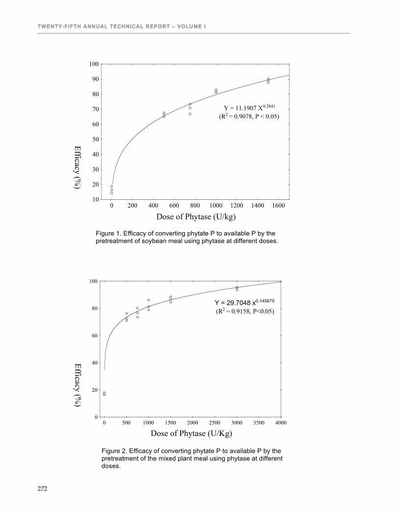
TWENTY-FIFTH ANNUAL TECHNICAL REPORT – VOLUME I
272
0 200 400 600 800 1000 1200 1400 1600
Dose of Phytase (U/kg)
10
20
30
40
50
60
70
80
90
100
Efficacy (%)
Y = 11.1907 X0.2841
(R2 = 0.9078, P < 0.05)
Figure 1. Efficacy of converting phytate P to available P by the pretreatment of soybean meal using phytase at different doses.
0 500 1000 1500 2000 2500 3000 3500 4000
Dose of Phytase (U/Kg)
0
20
40
60
80
100
Efficacy (%)
Y = 29.7048 x0.145675
(R2 = 0.9158, P<0.05)
Figure 2. Efficacy of converting phytate P to available P by the pretreatment of the mixed plant meal using phytase at different doses.

PRODUCTION SYSTEM DESIGN & INTEGRATION
273
Table 1. Composition of the basal diet fed to Nile tilapia juveniles.
INGREDIENTS g kg-1 (as-fed basis)
Soybean meal (oil-extracted) 536.5 Wheat 100.0 Corn gluten meal 200.0 Cassava 103.5 Mineral premix a 10.0
Fish oil 35.0 Soy lecithin 10.0 Vitamin premix b 5.0 TOTAL 1000.0 PROXIMATE ANALYSIS g kg-1 (Dry matter basis) MOISTURE 109.1 Crude protein 363.8 Crude lipid 57.1 Fibre 28.2 Ash 51.0 Nitrogen-free extract c 499.9 Calcium 2.0 Total P 4.5 Phytate P 3.0 Available P d 1.5 a Mineral premix (per kg of diet): MnSO4, 54 mg; Ferric citrate, 142 mg; CuSO4, 10 mg; ZnCO3, 29 mg; NaCl, 3.3 mg; KI, 0.9 mg; K2SO4, 90 mg; CoCl, 0.21 mg; MgO, 10mg. b Vitamin premix Roche 2118 (Hoffman-La Roche, Inc., Nutley, NJ, USA) (per kg of diet): Vitamin A, 12000 UI; Vitamin D3, 5000 UI; Vitamin E, 30 mg; Vitamin K3, 3 mg; Vitamin B1, 2.2 mg; Vitamin B2, 8 mg; Vitamin B6, 5 mg; Vitamin B12, 11 mg; Folic acid, 1.5 mg; Biotin, 150 mg; Pantothenic acid: 25 mg; inositol, 65 mg. c Calculated as: NFE%=100%-(moisture% + ash% + crude protein% + lipid% + fibre%)
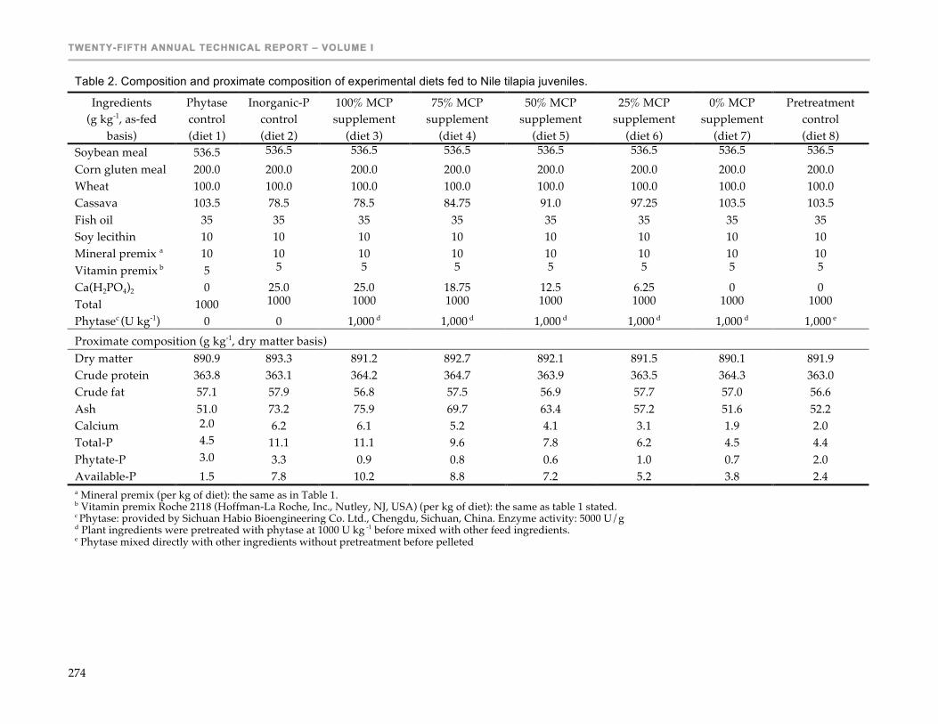
TWENTY-FIFTH ANNUAL TECHNICAL REPORT – VOLUME I
274
Table 2. Composition and proximate composition of experimental diets fed to Nile tilapia juveniles.
Ingredients (g kg-1, as-fed
basis)
Phytase control (diet 1)
Inorganic-P control (diet 2)
100% MCP supplement
(diet 3)
75% MCP supplement
(diet 4)
50% MCP supplement
(diet 5)
25% MCP supplement
(diet 6)
0% MCP supplement
(diet 7)
Pretreatment control (diet 8)
Soybean meal 536.5 536.5 536.5 536.5 536.5 536.5 536.5 536.5 Corn gluten meal 200.0 200.0 200.0 200.0 200.0 200.0 200.0 200.0 Wheat 100.0 100.0 100.0 100.0 100.0 100.0 100.0 100.0 Cassava 103.5 78.5 78.5 84.75 91.0 97.25 103.5 103.5 Fish oil 35 35 35 35 35 35 35 35 Soy lecithin 10 10 10 10 10 10 10 10 Mineral premix a 10 10 10 10 10 10 10 10 Vitamin premix b 5 5 5 5 5 5 5 5
Ca(H2PO4)2 0 25.0 25.0 18.75 12.5 6.25 0 0 Total 1000 1000 1000 1000 1000 1000 1000 1000
Phytasec (U kg-1) 0 0 1,000 d 1,000 d 1,000 d 1,000 d 1,000 d 1,000 e Proximate composition (g kg-1, dry matter basis) Dry matter 890.9 893.3 891.2 892.7 892.1 891.5 890.1 891.9 Crude protein 363.8 363.1 364.2 364.7 363.9 363.5 364.3 363.0 Crude fat 57.1 57.9 56.8 57.5 56.9 57.7 57.0 56.6 Ash 51.0 73.2 75.9 69.7 63.4 57.2 51.6 52.2 Calcium 2.0 6.2 6.1 5.2 4.1 3.1 1.9 2.0 Total-P 4.5 11.1 11.1 9.6 7.8 6.2 4.5 4.4 Phytate-P 3.0 3.3 0.9 0.8 0.6 1.0 0.7 2.0 Available-P 1.5 7.8 10.2 8.8 7.2 5.2 3.8 2.4 a Mineral premix (per kg of diet): the same as in Table 1. b Vitamin premix Roche 2118 (Hoffman-La Roche, Inc., Nutley, NJ, USA) (per kg of diet): the same as table 1 stated. c Phytase: provided by Sichuan Habio Bioengineering Co. Ltd., Chengdu, Sichuan, China. Enzyme activity: 5000 U/g d Plant ingredients were pretreated with phytase at 1000 U kg -1 before mixed with other feed ingredients. e Phytase mixed directly with other ingredients without pretreatment before pelleted
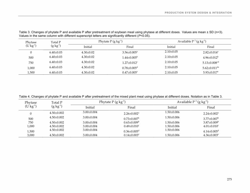
PRODUCTION SYSTEM DESIGN & INTEGRATION
275
Table 3. Changes of phytate P and available P after pretreatment of soybean meal using phytase at different doses. Values are mean ± SD (n=3). Values in the same column with different superscript letters are significantly different (P<0.05).
Phytate P (g kg-1) Available P 2 (g kg-1) Phytase (U kg-1)
Total P (g kg-1) Initial Final Initial Final
0 6.40±0.03 4.30±0.02 3.56±0.005a 2.10±0.05 2.82±0.014a 500 6.40±0.03 4.30±0.02 1.44±0.005b 2.10±0.05 4.96±0.012b 750 6.40±0.03 4.30±0.02 1.27±0.012c 2.10±0.05 5.13±0.008cd
1,000 6.40±0.03 4.30±0.02 0.78±0.005d 2.10±0.05 5.62±0.011de 1,500 6.40±0.03 4.30±0.02 0.47±0.005e 2.10±0.05 5.93±0.017e
Table 4. Changes of phytate P and available P after pretreatment of the mixed plant meal using phytase at different doses. Notation as in Table 3.
Phytate P (g kg-1) Available P 2 (g kg-1) Phytase (U kg-1)
Total P (g kg-1) Initial Final Initial Final
0 4.50±0.002 3.00±0.004 2.26±0.002a 1.50±0.006 2.24±0.002a 500 4.50±0.002 3.00±0.004 0.73±0.007b 1.50±0.006 3.77±0.007b 750 4.50±0.002 3.00±0.004 0.63±0.009b 1.50±0.006 3.87±0.009b
1,000 4.50±0.002 3.00±0.004 0.49±0.010c 1.50±0.006 4.01±0.010c 1,500 4.50±0.002 3.00±0.004 0.36±0.005d 1.50±0.006 4.14±0.005d 3,000 4.50±0.002 3.00±0.004 0.14±0.003e 1.50±0.006 4.36±0.003e

TWENTY-FIFTH ANNUAL TECHNICAL REPORT – VOLUME I
276
Table 5. Growth performance of Nile tilapia juveniles fed experimental diets for 60 days. Values are mean ± SD (n=3), values with different superscript letters in the same row are significantly different (P<0.05).
Experimental Diets
Parameter
Unit
Phytase control (diet 1)
Inorganic P control (diet 2)
100% MCP supplement
(diet 3)
75% MCP supplement
(diet 4)
50% MCP supplement
(diet 5)
25% MCP supplement
(diet 6)
0% MCP supplement
(diet 7)
Pretreatment control (diet 8)
Initial mean weight g 0.74±0.09 0.74±0.09 0.73±0.00 0.74±0.09 0.70±0.04 0.77±0.05 0.80±0.00 0.74±0.09 Final mean weight g 19.1±0.60 e 34.6±0.76 a 34.9±1.23 a 34.6±0.56 a 35.8±1.21 a 30.8±0.74 b 26.8±0.45 c 23.0±1.07 d Survival % 95.00±2.36 a 96.67±0.00 a 91.67±2.35 c 93.34±4.27 b 91.67±2.35 c 93.34±4.27 b 90.00±0.00 c 96.67±0.00 a FCR1 1.85±0.03 e 1.12±0.07 a 1.14±0.00 a 1.16±0.01 ab 1.10±0.06 a 1.24±0.04 b 1.35±0.02 c 1.64±0.04 d SGR2 % day-1 5.45±0.16 e 6.43±0.25 ab 6.44±0.06 ab 6.43±0.18 ab 6.56±0.06 a 6.16±0.14 bc 5.85±0.03 cd 5.75±0.14 de PER3 1.49±0.02 e 2.59±0.04 a 2.54±0.08 a 2.61±0.04 a 2.66±0.08 a 2.36±0.06 b 2.16±0.04 c 1.68±0.04 d

PRODUCTION SYSTEM DESIGN & INTEGRATION
277
Table 6. Chemical composition (g kg-1, dry matter basis) of Nile tilapia juveniles fed experimental diets for 60 days. Notation as in Table 5.
Experimental Diets
Parameter Phytase control (diet 1)
Inorganic P
control (diet 2)
100% MCP supplement
(diet 3)
75% MCP supplement
(diet 4)
50% MCP supplement
(diet 5)
25% MCP supplement
(diet 6)
0% MCP supplement
(diet 7)
Pretreatment control (diet 8)
Dry matter 259.3±0.4
a 231.0±0.3 e 230.5±0.1 e 230.9±0.6 e 231.3±0.4 e 232.9±1.0 d 237.8±1.1 c 253.6±0.4 b Ash 88.0±0.1 d 106.1±0.3 a 106.1±1.0 a 105.5±0.7 a 105.3±0.4 ab 104.2±0.6 b 96.5±0.7 c 89.0±0.1 d
Lipid 188.4±0.1
a 133.8±0.3
cd 132.9±0.7 d 134.0±0.6 cd 133.1±0.4 d 134.8±2.4 cd 135.9±1.1 c 175.3±0.9 b Crude protein
507.6±6.5
c 553.4±4.0 a 549.7±3.9 a 548.1±2.7 a 550.0±3.4 a 531.4±6.0 b 527.2±6.3 b 513.7±9.7 c Phosphorous 13.3±0.5 e 18.3±0.4 a 18.6±0.5 a 17.9±0.4 a 18.1±0.5 a 17.4±0.2 b 16.8±0.3 c 14.3±0.3 d Table 7. Phosphorus retention efficiency and P load of Nile tilapia fed test diets for 60 days. Notation as in Table 3.
Diet Treatment P retention (%) P load (g kg-1) Phytase control (diet 1) None 28.56±1.17 c 6.39±0.17 a Inorganic P control (diet 2) + 25 g MCP kg-1 49.67±1.11 b 4.64±0.55 b 100% MCP supplement (diet 3) Phytase + 25 g MCP kg-1 51.75±1.02 b 4.32±0.05 b 75% MCP supplement (diet 4) Phytase + 18.75 g MCP kg-1 52.48±2.33 b 4.06±0.34 b 50% MCP supplement (diet 5) Phytase + 12.5 g MCP kg
59.84±1.34a 3.49±0.02 c 25% MCP supplement (diet 6) Phytase + 6.25 g MCP kg
59.69±2.01 a 3.73±0.05 c 0% MCP supplement (diet 7) Phytase
57.38±1.07 a 3.30±0.02 c Pretreatment control (diet 8) Phytase added directly
32.59±1.14 c 6.11±0.19 a Table 8. Apparent digestibility coefficients of crude protein (ADCCP) and P (ADCP) for experimental diets fed to Nile tilapia juveniles. Notation as in Table 3.
Diet Treatment ADCCP (%) ADCP (%) Phytase control (diet 1) None 84.40±1.47 28.23±1.15 f Inorganic P control (diet 2) + 25 g MCP kg-1 84.37±0.83 52.37±2.31 c 100% MCP supplement (diet 3) Phytase + 25 g MCP kg-1 84.43±0.56 47.10±0.65 d 75% MCP supplement (diet 4) Phytase + 18.75 g MCP kg-1 84.57±0.61 55.33±1.68 b 50% MCP supplement (diet 5) Phytase + 12.5 g MCP kg
85.27±0.65 69.03±2.00 a 25% MCP supplement (diet 6) Phytase + 6.25 g MCP kg
83.63±0.47 69.47±0.38 a 0% MCP supplement (diet 7) Phytase
83.10±0.91 67.83±1.84 a Pretreatment control (diet 8) Phytase added directly
83.40±1.17 36.03±0.97 e

TWENTY-FIFTH ANNUAL TECHNICAL REPORT – VOLUME I
278
CONTROLLED REPRODUCTION OF AN IMPORTANT INDIGENOUS SPECIES, SPINIBARBUS DENTICULATUS, IN SOUTHEAST ASIA
Twelfth Work Plan, Indigenous Species Development 1 (12ISD1)
Final Report Published as Submitted by Contributing Authors
Amrit N. Bart & Dinh Van Trung
Asian Institute of Technology Pathumthani, Thailand
James S. Diana
University of Michigan Ann Arbor, Michigan, USA
ABSTRACT Preliminary studies were conducted to understand some basic reproductive parameters of the indigenous carp, Spinibarbus denticulatus as a prelude to more specific research studies and subsequent development of hatchery technology. The study objectives were to: 1) understand the seasonal pattern of gonad development, sexual maturation, and various reproductive parameters; and 2) induce this species to spawn in captivity using natural and artificial methods. The study was carried out on sub-adult and adult fish. Gonad and egg development were assessed over a 12-month period. Annual rings on fish scales were found to be a reliable measure of age. In a population including males and females of similar age, males were generally smaller (2.54 ±0.34 kg) than females (3.46±0.45 kg). The age at sexual maturation of a natural stock was earlier for males (4 years) than females (5 or older). The gonadosomic index revealed two peaks, April and October. Further examination of the ovaries and eggs during January, February, and March suggested that eggs were developing at various stages. During January, the eggs in the ovary of mature females were uniformly small (0.7±0.1mm diameter.). Two distinct egg groups (0.7±0.1mm, 36% and 1.0±0.2mm, 54%) were observed in February. Three distinct size groups were observed during March (1.1±0.03mm, 1.6±0.01mm and 2.1±0.03mm). The proportion of large eggs (55%) was higher compared to mid (26%) and small eggs (19%) during the near-peak spawning month. The average number of eggs in the ovary of a female (3.1±0.4 kg) was 31,041 (12,632- 45,359). Males synchronized milt production with egg maturation and ovulation under pond conditions. Milt flowed out readily from males during the spawning season. Sperm characteristics were similar to those of most teleosts. The mean sperm concentration was 8.42±0.36 million cells per ml with only a small amount (3.3±0.2ml) of total expressible milt per male. However, when induced with LHRHa (10µg kg-1) the milt production increased to 6.2±0.5 ml without an increase in the total number of sperm cells. While this new species for aquaculture shows potential for mass production of seed, low fecundity and late puberty could present obstacles to artificial seed production. Induced breeding trials indicated that natural induction methods (rain simulation, decreased/increased water depth and flow) did not stimulate mature females to spawn in ponds. A series of locally available hormones (e.g., HCG, LHRHa+Domperidone, CPE), singly or in combinations, was used to induce females to ovulate. Administration of LHRHa, CPE, and HCG were effective in inducing ovulation for S. denticulatus. However, LHRHa or CPE induced ovulation more consistently compared to HCG. Fertilization rate and hatch rates were also higher in LHRHa or CPE than HCG induced group. Individual females released 4.2 - 9.4 x 10³ eggs when stripped, and egg numbers were correlated with BW of the female. Simultaneous injection of LHRHa and domperidone was required to achieve high success in induced spawning of S. denticulatus. Furthermore, no clear advantages were evident to the other hormone combination strategies.

INDIGENOUS SPECIES DEVELOPMENT
279
INTRODUCTION
Chinese carps, Indian major carps and tilapias make up over 90% of freshwater species cultured. Over 95% of these come from Asia (FAO, 2003a), and most are exotic species in Southeast Asia (Liste and Chevey, 1932). Although the culture of introduced species is profitable, they have also been implicated in either displacement of indigenous species or introgression with local species (Ogutu-Ohwayo and Hecky, 1991; De Long and Van Zon, 1993; NaNakorn et al., 1999). Additionally, exotic species are more susceptible to local diseases (e.g., grass carp is prone to red spot disease; Kim et al., 1999). Grass carp, a primary cultured species for the rural poor and a major source of animal protein in their diet, has been so severely affected by this pathogen that many poor farmers of North Vietnam have abandoned its culture (Bart, 2000). There is a need to identify an alternative species, preferably indigenous, to grass carp, which can be fed on readily available and low-cost grass. Southeast Asia has one of the largest diversities of freshwater fish species in the world (FAO, 2003b). Unfortunately, comparatively few species from this region are widely cultured, partly due to the lack of sufficient knowledge of their reproduction. The carp, Spinibarbus denticulatus (Oshima, 1926) has significant potential to become a more widely farmed species, particularly for the low-input system relevant for developing countries, if hatchery produced seed is available. With the local name ‘ca bong’, S. denticulatus is indigenous to north Vietnam with a distribution from upstream to the middle reaches of the Red, Lo and Gam river systems. There is distinct cold and warm seasonal variation with water temperature ranging from 9-16oC during winter and 25-30oC during summer. This species contributed nearly 25-30% to the total wild fish capture in the Lo and Gam river systems in the past, and 20-30% of that in the Ba Be reservoir (Hao, 1993). S. denticulatus belongs to the sub-family, Barbinae of the Cyprinidae family. The largest S. denticulatus recorded was 30.0 kg (Dau and Le, 1971). It is a macrophagous herbivore with diets very similar to that of the grass carp (Bau, 1998). No studies on its life history or habitat description have been published to date. An attractive feature of this species is its resistance to some local pathogens such as red spot disease, even when raised in the same cage with infected grass carp (personal communication, Mr. Pham Bau, Research Institute for Aquaculture No. I, Vietnam). Spawning is thought to take place during the spring and fall months. Natural stocks are declining because of increasing fishing pressure, habitat destruction through construction of hydropower dams and improper capture practices using dynamite and poison. There has been no publication describing even the most fundamental biology of this species to date. A thorough study would help to better understand the reproductive biology prior to producing seed for stocking. Therefore, in this study we first carried out preliminary investigation to understand the basic reproduction biology of the species and then attempted to induce spawn using natural and artificial methods.
MATERIALS AND METHODS Reproductive biology of S. denticulatus Male and female S. denticulatus (n=270) ranging from 3 to 7 years of age were acquired from fish cages in Ha Giang and Tuyen Quang provinces, transported to Me Linh Research Station, Vinh Phuc province and held in nine earthen ponds (300m2) for the study. Fish were fed a combination of grass and rice sprouts ad libitum. Water quality (pH, dissolved oxygen, total ammonia and nitrite) was monitored weekly throughout the study period. o assess gonadal development and maturation, 10 fish (5 year or older) were sacrificed monthly (December 2001 to November 2002); fish weight and gonad weight measured to the nearest 0.01g. To determine age at sexual maturation 3- (n=8), 4- (n=10), and 5-year-old females (n=19) were harvested in April. All fish in the three age groups were dissected to assess the condition of the gonads.
TWENTY-FIFTH ANNUAL TECHNICAL REPORT – VOLUME I
280
Age was determined by counting scale annual rings for scales. Scales were removed from above and below the lateral line, washed, and then visual observation was made under the microscope. Scale readings were cross-checked with farmer information on the size and date of stocking. Monthly observations of scales from a male and a female fish over the 12-month period were also made to observe the appearance of the dark ring. Visual observations of experimental animals were made during the peak and off spawning seasons for color changes and other sexual dimorphic characteristics. Nine females were dissected each month and their ovaries removed to assess fecundity. The number of eggs in the ovary was estimated by first removing all eggs from the connective tissue of the ovary, and by sampling approximately 15 g of mixed eggs from each female. From the 15 g of mixed eggs, 50 oocytes were randomly removed, and each egg was measured to the nearest 0.01mm using the micrometer of a compound microscope. The diameter of various size eggs was enumerated starting from January (prior to the spawning period), and ovarian oocyte size-frequency distribution was determined over a 3-month period (January to March). Eggs belonging to the same size group were separated and classified into three categories, and monthly change in size composition was determined. Male fish (4 to 7 years of age) were removed from water, dried, and gentle abdominal pressure was applied, using a thumb and an index finger to remove sperm. The pressure was applied starting below the pectoral fins and moving down towards the genital pore. This process was repeated until sperm stopped flowing. Total expressible milt was pooled from an individual male and drawn into a 5.0 ml syringe to assess total volume. Sperm motility was assessed by adding a droplet of distilled water on the freshly stripped sperm and observing under the microscope. Two stages of motility, progressive (vigorous movement) and vibration (movement in loco) were observed. Sperm concentration (spermatozoa mL-1 of milt) was estimated using Neubaur’s counting chamber following Vutiphandchai & Zohar (1999). To increase the amount of expressible sperm, mature males (n=13) of similar size (2.6±0.3kg) were harvested and six were injected with LHRHa at 10µg kg-1, while the other seven were injected with 0.9% saline solution as blank controls. Males were stripped after 6h of injection and volume measured using a 10.0 ml standard syringe. The number of sperm per ml of milt was estimated using Neubaur’s counting chamber. Induced breeding Male and female S. denticulatus ranging from 3 to 7 years of age were acquired from fish cages in Ha Giang and Tuyen Quang provinces, transported to Me Linh Research Station, Vinh Phuc province and held in earthen ponds (300 m2) for the study. A total of 30 fish (20 females and 10 males) were stocked in each 300-m2 pond (1.4 m deep) and were fed rice sprouts at 3% of BW day-1 6 days a week. A total of 239 females (2.81±0.71 kg BW) and 90 males (2.28±0.39 kg BW) were used for induced breeding trials during the reproductive season of 2002-2005. Pond water was exchanged over 3-day intervals and water quality (temperature, pH and DO) was monitored weekly during the experiment. Induced spawning experiments were conducted using a hormone that was commercially available in North Vietnam. Mature brood fish were selected and kept in circular tanks under constant water sprinkling to simulate rain. Selected females displayed enlarged abdomens with swollen and pink genital papilla while males released milt readily with a slight pressure on the abdomen. Common carp pituitary extract (CPE) (2 mg unit-1 preserved in the acetone solution), luteinizing hormone-releasing hormone analogue (LHRHa), domperidone maleate (Motilium–M), and human chorionic gonadotrophin (HCG) were used to induce females. HCG doses of 3000-5000 IU kg-1, pituitary gland doses of 20-40 mg kg-1, and LHRHa doses of 30-50 µg kg-1 combined with or without domperidone were used for each hormone dose. These hormones were injected intraperitoneally with two doses including priming and resolving doses administrated 8 h apart. The males were given a single dose at the same rate. Injection volume was maintained at 1 ml kg-1

INDIGENOUS SPECIES DEVELOPMENT
281
BW. A group of nine fish were injected with 0.9% saline solution as a control. Female and male fish were kept separately. Females were stripped and eggs were fertilization using dry methods. The weight of freshly stripped ova was determined for 190 females for estimation of fecundity. The excess milt was removed several times after fertilization, and then the fertilized eggs were placed in incubators. Water temperature was recorded at 1-hour intervals over the embryonic development for estimation of degree-hours (time interval between resolving dose and stripping × water temperature). The fertilization rate of eggs was determined after blastopore closure from a sample of 30 eggs collected from the incubator. Ovulation time was recorded, and fertilization and hatch rates were estimated. Fertilized eggs were sampled from the incubator in 10-minute intervals, placed in a Petri dish, and observed under the microscope. The fertilization rate was expressed as the percentage of fertilized eggs from the total number of eggs spawned, and hatch rate was expressed as the percentage of larvae hatched from the total number of fertilized eggs. Data were analyzed by one-way ANOVA, and differences were considered significant at α=0.05. Significant differences between treatment means were compared using the Duncan Multiple Range Test (Pratapa, 2000). Data calculated as percents were arcsine transformed before analysis. A correlation curve of fecundity and coelomic fluid content related to weight was fitted. Statistical analysis was performed using SPSS 11.0 software (SPSS, Chicago, USA).
RESULTS Reproductive biology of S. denticulatus During the peak spawning season, mature bi-lobular ovaries appeared turgid and brownish in color. Prior to spawning, ovaries made up over 60% of the abdominal cavity. Similarly, the mature bi-lobular testis appeared pink in color and comprised a smaller portion (<10%) of the abdominal cavity. A bi-modal gonadosomatic index (GSI) was apparent in females observed over a 12-month period, with a major spike occurring in April (3.65±0.7) and a minor spike (2.64±0.2) in October (Fig. 1). The largest ovary sampled in April was 130g, 5.0 GSI. The lowest gonadal weight was found in December (19g, 0.54 GSI) followed by slightly larger one in June (28g, 0.85 GSI). During January, February and March an increasing GSI was paralleled by an increased proportion of the maturing large oocytes sampled. A similar bi-modal GSI was observed in males (Fig. 1), but of a lower magnitude compared to the females. A major peak occurred in April (1.37±0.2) and a minor peak (1.36±0.1) in October. The largest testis sampled in April was 40.0g with a 1.4 GSI. The lowest gonadal weight was found in December (14.0g, 0.8 GSI) followed by one in June (16.0g, 0.6 GSI). Oocyte size assessment in the ovary revealed that there were distinct size classes of developing eggs rather than a continuous size distribution (Fig. 2). The size of oocytes during the early spawning season (January) was found in a single class, 0.7mm (0.6-0.8mm). These oocyte size variations added a second class size in February, 1.0mm (0.9-1.2mm). Approximately 36% of the eggs were small while the remainder (54%) was a larger size during this sampling. In March, three class sizes were observed, 1.1(0.8-1.4mm), 1.6(1.4-1.8mm), and 2.1(1.9-2.4mm), with relative proportions of 18.7, 26.4 and 54.9%, respectively. A progressive color change from opaque white to translucent yellow was observed during the early February to March sampling. The smallest size class was pale yellow while progressively larger eggs were dark-yellow to light brown in color. There was a wide range of egg numbers among females sampled (13,000-45,000 eggs.fish-1). The number of eggs.kg-1 of female ranged from 6,000 to 14,000, with a mean of 9,873. However, there was no correlation between weight and fecundity among the eight females (3.1± 0.4kg) examined.

TWENTY-FIFTH ANNUAL TECHNICAL REPORT – VOLUME I
282
Microscopic observation of sperm cells (100x–oil emersion) indicated that they were similar to those of other teleosts with a head, mid-piece and a single tail. While progressive or vigorous motility duration was only 1.9±0.3 min, total motility (progressive motility and vibration in loco) was longer, 2.7±0.3min. Fish injected with hormones expressed a considerably higher volume of milt (6.2±0.5) compared with those injected with saline only (3.3±0.2). The density of sperm in fish without hormonal induction (16x106 ml-1) was double that of hormone injected males (8.4x10⁶ ml-1) indicating that the total sperm number was unchanged by hormone treatment. While sperm remained motile over a 5-hour period (sampled every 30 min from the time of stripping), there was progressive decline in the duration of motility after 2 hours. Although males and females of age 3 to 7 years were held in nine ponds for a 12-month period, neither mating behavior nor recruitment was observed. A clear and distinctive annual ring was observed on scales of mature fish (Fig. 3). The scale dark rings were irregular in shape with the varying distances between the rings and between stocks. While most rings were complete circles, a few were only partly complete. The monthly observation of rings for males and females did not differ. Initiation of the dark ring was first observed in January, although temperatures started to decline by the end of November. S. denticulatus males tended to be smaller (2.3±0.2 kg) than females (3.3±0.4 kg; Fig 4) in the 5, 6, and 7-year age class. It was difficult to ascertain sexual dimorphism before maturation and out of the spawning season. However, during the spawning season, males tended to be more colorful with an iridescent green appearance. Males possessed a rough texture (pearl organs) along the exterior of the operculum running below the eyes towards the mouth during the peak spawning period. One of the most obvious signs of a mature male during the spawning season was the release of milt. Milt flowed readily out of the genital pore with slight pressure to the abdomen. During the spawning period, mature females had an enlarged abdomen. Both spawning females and males became more colorful with the females slightly lighter in color than males. Unlike the genital papilla, which is often swollen and pink during the spawning season in most fish, the female genital opening was covered with a white fleshy protrusion. Males appeared to have only a simple opening without a protrusion. The mean weight of a 5-year-old fish’s ovary was significantly higher (81.4±34.8g) than in 3 (14.9±1.1g) or 4-year-old (24.7±3.4g) females (Table 1). A large variation in gonad size was observed between different age groups with approximately a two-fold increase in 4-than in 3-year-old, but six times higher in the 5-year-old group. The gonadosomatic index of 5-year-old fish was also higher (2.8±1.2) than those of 3- (1.1±0.1) and 4-year-old (1.2±1.0) females. No observable difference was found between the GSI of 3- and 4-year old fish. The mean weight of females varied with age, where 3-, 4- and 5-year-old females were 1.4±0.1, 2.1±0.1 and 2.9±0.5 kg, respectively. Induced breeding Ovulation was observed in fish injected with LHRHa at a dosage of 40 or 50 µg kg-1, but fish did not ovulate when injected with 30 µg LHRHa kg-1 (Table 2). LHRHa at 40 or 50 µg kg-1 BW resulted in 25% and 50% ovulation, respectively, whereas addition of domperidone (10 mg kg-1) to the LHRHa injection (40 and 50 µg kg-1) resulted in 100% ovulation and also a reduced latency period. Mean fertilization and hatch rates were high for induced females injected with LHRHa, and there were no significant differences in fertilization and hatch rates between the dosages of LHRHa injected. Carp pituitary extract (CPE) of 30 or 40 mg kg-1 induced females spawning, although 20 mg kg-1 failed to induce ovulation. Mean degree-hours for induced spawning with CPE was 489 and 487 at 30 and 40 mg kg-1, respectively. This was much lower than the degree hour (622-724) observed in
INDIGENOUS SPECIES DEVELOPMENT
283
the case of LHRHa. Fertilization and hatch rates were not different between the dosages of CPE-treated females and were similar to the rates obtained with LHRHa injection. HCG at 3000 IU kg-1 could not induce ovulation, though HCG injection of 4000 and 5000 IU kg-1 only succeeded in inducing ovulation in only one female out of the three injected. Fertilization and hatch rates obtained with HCG induction were lower than the rates obtained with LHRHa and CPE injection. Combining LHRHa and CPE at a dose of LHRHa 30 µg kg-1 + CPE 6 mg kg-1 did not result in successful spawning. The minimum successful dosage of LHRHa was 35 µg kg-1 when combined with CPE (6 mg kg-1), but that dosage resulted in a significantly lower stripping response, fertilization rate and hatch rate than those observed with LHRHa at higher dosages (40 or 50 µg kg-1), given either as single or in combination with CPE. Combining LHRHa at dosage of 40 or 50 µg kg-1 with CPE (6 mg kg-1) resulted in successful spawning, and the results, in terms of stripping response, fertilization rate, and hatch rate, were comparable to those obtained with LHRHa alone. With HCG used in combination with CPE (6 mg kg-1), the minimum effective dosage of HCG to induce ovulation was 3500 IU kg-1 with an ovulation response of 57%. Combining CPE (6 mg kg-1) with HCG at 4000 and 5000 IU kg-1 also resulted in a significant increase in ovulation response, fertilization and hatch rates as compared to the HCG injection alone. In addition, combined injection of HCG and CPE resulted in fewer degree-hours to ovulation than the treatment with only HCG stimulation. Overall, fertilization rates observed in this study with different hormone stimulation were high (>90%). Mean hatch rates obtained in this study varied between 80 to 93% and generally tended to increase with higher fertilization rate (Table 2). In this study, none of the fish given saline injection ovulated (Table 2). Similarly, fish injected with LHRH-a (30 µg kg-1), PG (20 mg kg-1), HCG (3000 IU kg-1), LHRHa (30 µg kg-1) + PG (6 mg kg-1) and PG (6 mg kg-1) + HCG (3000 IU kg-1) also did not spawn. Degree-hours to maturation during the induced breeding trials varied widely from 487 to 724 with the type and dosages of hormone injected. The lowest degree-hours were observed in the trials with CPE injection followed by LHRHa and HCG. Individual females released 4.2-9.4 x 10³ eggs when stripped, and the number of eggs generally increased with the female BW (Table 2). This relationship could be described by a highly significant (P<0.001) linear regression (Fig. 5). Coelomic fluid content per female spawned ranged from 18.4 to 42.7 g and accounted for 18.3 to 31.0% of the total oocyte mass weight released (Table 2). Coelomic fluid content was highly correlated (P<000.1) with the female BW (Fig. 6).
DISCUSSION Reproductive biology of S. denticulatus Monitoring egg size in dissected ovaries over a period of 3 months (January, February and March) clearly showed that eggs matured in stages. Three distinct size classes of eggs observed out of the spawning season suggests possible multiple spawning within a season. The gonadosomatic index monitored over a 12-month period showed that the ovary and testis become reproductively competent twice a year with two major peaks occurring in April and October. Additionally, the relatively high GSI observed from March to May and July to October indicated continuous maturation of eggs in the ovary throughout the warmer months. Overall, low maximum GSI (3.65%) also indicated that females might spawn over a several month period. Eggs developing in the ovary at various stages during the year suggest that this species, although typically thought to spawn twice a year, could be induced to spawn more frequently during warmer months. Despite relatively low fecundity (9,873±3,354 kg-1) compared to grass carp, the yolk-filled egg size was larger (2.01±0.03mm diameter) than that typically found in other cyprinids indicating possibly more robust larvae with a potentially high survival rate; these are both important traits in
TWENTY-FIFTH ANNUAL TECHNICAL REPORT – VOLUME I
284
an aquaculture species. Lower fecundity rate per spawn could be compensated for by the potential for multiple spawns per year and high fry survival rates. Sperm characteristics of S. denticulatus were similar to other cyprinids with a short duration (1.99±0.3 min) of progressive motility followed by vibration in loco (2.7±0.3 min) before complete cessation of motility. The volume of expressible milt was low (3.3±0.3 ml from 2.6±0.5 kg-1 males). An attempt to increase total sperm by administration of LHRHa resulted in doubling the expressible milt to 6.2±0.5 ml, but the total number of spermatozoa remained the same. Previous studies on induction of males have shown similar results (Kwantong and Bart, 2003). While the increased volume of milt would make artificial fertilization more convenient, whether there is any change in the quality of sperm from induced males needs to be determined. The lack of recruitment in ponds where mature brood fish were held for two years suggested that perhaps pond-based husbandry is not conducive to natural spawning. Further studies on natural spawning, egg incubation and larval rearing conditions are required as well as induced spawning trials by manipulating the environment and/or endocrine hormones. The annual rings of fin rays, otoliths or scales are commonly used to assess the age of finfish (Geffen, 1992; Ikejima et al., 1998). Otolith reading requires sacrificing the animal, and pectoral fin assessment requires cross sectioning and the use of a stereo microscope. However, the examination of scales in this study required only simple observation of the rings against a light source for them to be clearly visible to the naked eye. It is therefore the least invasive, and appears to be an excellent means to quickly assess age under field conditions. Since the natural habitat of S. denticulatus has distinct cold and warm seasons and the rate of feeding and growth slowed in the ponds during the coldest periods, it was assumed that the dark rings indicated seasonal growth variation. This was verified by observing scales taken from the same male and female over a 12-month period. This preliminary study attempted to estimate the age of fish by collecting the broods from a known source and matching the age with presumed annuli rings. Moreover, observation of scales from the same male and female over a 12-month period suggested that annuli are in fact annual rings. Dark rings could also be caused by a number of other events including environmental stress or poor feeding during harvest and transport. Since study animals were collected from cages, further validation of this method of assessing age should be experimentally assessed. These preliminary observations indicated that males were smaller than females as commonly observed in many other teleosts. This observation was based on both sexes having the same number of annual rings and farmers’ accounting of the date and size at stocking. If such dimorphic characteristics do in fact occur, it would be important to understand when they become apparent in the life of this species. Typically, the age of sexual maturation in tropical and subtropical species does not exceed 2-3-years. Observations of 37 females (2.9±0.5 kg) sampled during the peak spawning period indicated that only females of age 5 had sufficiently mature ovaries. The implication of this is that a long-term investment would be required to develop and maintain broodstock, which could present an obstacle for low-input aquaculture. The determinants of precocious sexual maturation are thought to be environment, endocrine hormones, and domestication (Le Bail, 1988; Holland et al., 1996). Studies have also shown that long-term hormone therapy may also reduce the time to puberty in some species (Gur et al., 1995). This provides an opportunity to explore means to reduce the time to maturation by manipulating hormones, feed, nutrition, and husbandry practices. Induced breeding Attempts to breed S. denticulatus naturally by regulating environmental cues, such as water depth, water flow, and rainfall were largely unsuccessful, and the fish would not spawn naturally in

INDIGENOUS SPECIES DEVELOPMENT
285
captivity. Therefore, induced breeding of S. denticulatus is needed for successful culture of this species. This study for the first time demonstrated that intramuscular injection of LHRHa, CPE, and HCG are all effective methods for inducing final maturation and successful spawning of S. denticulatus. While all three hormones used could bring successful spawning, HCG was the least effective in inducing ovulation. Furthermore, the use of combined hormone strategy had no apparent advantage over single hormone strategy, and therefore the latter can be suggested to be the ideal for induced spawning of S. denticulatus. Requirement of domperidone, dopaminergic antagist, to induce spawning in S. denticulatus was clearly observed in this study. Injection of LHRHa at doses of 30 and 40 µg kg-1 resulted in 25 and 50% ovulation, respectively; whereas LHRHa injected at similar dosages in combination with domperidone (10 mg kg-1) resulted in 100% ovulation (Table 2). The lower rate of ovulation in females treated with LHRHa than fish injected simultaneously with LHRHa and domperidone clearly reflected the predominance of dopamine inhibition in the control of gonadotropin release in S. denticulatus. The role in potentiating the effects of LHRHa in several teleosts species by blocking the inhibitory effects of dopamine on gonadotropin release has been described by many others (Chang and Peter, 1983; Chang et al., 1984; Sokolowska et al., 1984; De Leeuw et al., 1985; Lin et al., 1985; Peter et al., 1988; Manickam and Joy, 1989; De Leeuw et al., 1989; Glubokov et al., 1991). Tan-Fermin (1997) reported that catfish Clarias macrocephalus failed to ovulate after treatment with LHRHa, but a high ovulation rate resulted when catfish were injected simultaneously with LHRHa and pimozide. Ovulation response with HCG was lower than the stripping response obtained with LHRHa and CPE stimulation (Table 2). Though HCG has been used effectively in fish reproduction of some species, it is less effective if given alone (Epler et al., 1986). Using 30-40 mg CPE to replace 5000 IU HCG can produce a higher rate of spawning success in S. denticulatus. Previously, Lee et al. (1988) described CPE as a better spawning agent than HCG for induced spawning of grey mullet (Mugil cephalus). In this study LHRHa or CPE administration resulted in consistently high stripping response, fertilization rate and hatch rate (Table 2), suggesting that LHRHa and CPE both are equally efficient for induce spawning of S. denticulatus. Given that this species does not spawn in ponds it will be necessary to develop a low cost method of induction. Although all the hormones tested are commercially available in Vietnam, LHRHa and domperidone may be too costly for a low input culture species such as S. denticulatus. Since HCG is relatively inexpensive compared with LHRHa and domperidone, some combinations of HCG and CPE need to be further tested in this species.
CONCLUSION
To culture a new species requires years of coordinated research, not only to understand its basic biology but also to manipulate this biology or environment to make the process feasible for culture. An early decision on the selection of an appropriate species for further targeted study minimizes failure and waste of resources. These preliminary observations on some of the important maturation and reproductive parameters of this promising species for more widespread culture provide essential information on the age of sexual maturation, gonadal development and reproductive cycle, male and female characteristics as well as fecundity and gamete characteristics. Furthermore, this study for the first time demonstrated successful hormone induced ovulation and artificial fertilization of S. denticulatus. The high (>80%) fertilization and hatch rates obtained in this study showed the potential of the induced spawning protocol used in the study for its successful commercial application. This is the first study on the reproduction biology and seed production of S. denticulatus, which is expected to help in establishment of commercial hatcheries and thus, contribute to its aquaculture development.
TWENTY-FIFTH ANNUAL TECHNICAL REPORT – VOLUME I
286
ANTICIPATED BENEFITS Now that we have successfully bred this species in captivity, when commercialized, it should lower seed collection pressure in natural population. Moreover, increased availability of seed in a more predictable manner at a lower cost increases the possibility of making this species more widely cultured throughout southeast. Availability of seed resulting in increased culture of this species would add one more low-cost freshwater fish to the list of aquaculture species with the potential to directly benefit the rural poor.
ACKNOWLEDGMENTS The authors wish to thank AIT and RIA I research staff for their assistance during the conducting of these experiments.
LITERATURE CITED Bart, A.N., 2000. Conservation of aquatic biodiversity heats-up in Vietnam. Aquaculture and
Aquatic Resources Management Newsletter, 5: 34-36. Bau, P., 1998. Investigation of valuable fish species in the Lo and Gam river systems. Annual
Research Report, Research Institute for Aquaculture No. I, Vietnam. pp.59. Bhowmick, R.M., 1979. Observation of the use of human chorionic gonadotropin prepared in the
laboratory in inducing spawning in major carp, Labeo rohita Ham. Symposium on Inland Aquaculture, Barrackpore, India. Tech. Paper No. 16, pp. 11-12.
Carreon, J.A., Estocapio, F.A., and Enderez, E. M., 1976. Recommended procedure for induced spawning and fingerling production of Clarias macrocephalus (Gunther). Aquaculture, 8: 269-281.
Chang J.P., and Peter R.E., 1983. Effects of pimozide and des-gly10-[D-Ala6] luteinizing hormone-releasing hormone ethylamide on serum gonadotropin concentrations, germinal vesicle migration, and ovulation in female goldfish Carassius auratus. Gen. Comp. Endocrinol., 52, 30-37.
Chang J.P., Peter R.E. Nahorniak, C.S., and Sokolowska, M., 1984. Effects of catecholaminergic agonists on serum gonadotropin concentrations and ovulation in goldfish: evidence for specificity of dopamine inhibition of gonadotropin secretion. Gen. Comp. Endocrinol., 55: 351-360.
Dau, D.V., and Le, L.T., 1971. Biological features of ca bong. Spinibarbichthys denticulatus (Oshima). Scientific and Technology Press. Hanoi. pp. 171-191.
De Leeuw, R., Goos, H.J. Th., Richter, C.J.J., and Ending, E.H., 1985. Pimozide-LHRHa-induced breeding of African catfish, Clarias gariepinus (Burchell). Aquaculture 44, 295-302.
De Leeuw R., Habibi H. R., Nahorniak C.S., and Peter, R.E., 1989. Dopaminnergic regulation of pituitary gonadotropin-releasing hormone receptor activity in the goldfish Carassius auratus. Journal of Endocrinology 121, 239-247.
De Longh, H.H., and Van Zon, J.C.J., 1993. Assessment of impact of the introduction of fish species in Northeast Thailand. Aquaculture Fisheries Management. 24: 279-289.
Epler, P. Sokolowska, W. P., and Bieniarz, K., 1986. Joint action of carp (Cyprinus carpio L.) pituitary homogenate and human chorionic gonadotropin (HCG) in carp oocyte maturation and ovulation: in vitro and in vivo studies. Aquaculture, 51: 133-142.
FAO, 2003a. Review of the state of world aquaculture. FAO Fisheries Circular. No. 886 (Rev. 2). Rome, FAO. pp.67.
FAO, 2003b. Review of state of world fisheries resources: inland fisheries. FAO Fisheries Circular No. 942 (Rev. 1) Rome, FAO. pp.60.
Fontaine, M., 1976. Hormones and the control of reproduction in aquaculture. J. Fish. Res. Board Can., 33: 922-939.
Geffen, A.J. 1992. Otolith microstructure examination and analysis. Canadian Special Publication on Fisheries and Aquatic Science. 117: 101-113.
Glubokov A.I., Motloch N.N., and Sedova M.A., 1991. Effect of a synthetic LHRH analogue and dopamine antagolists on the maturation of bream Abramis brama L. Aquaculture 95, 373-377.
INDIGENOUS SPECIES DEVELOPMENT
287
Gur, G., Melamed, P., Levavi-Sivan, B., Holland, C., Gissis, A., Bayer, D., Elizur, A., and Zohar, Y., 1995. Long-term testosterone treatment stimulates GTH II synthesis and release in the pituitary of the black carp, Mylopharyngodon piceus. In Reproductive Physiology of Fish (Goetz, F.W. & Thomas, P. eds.). Fish Symposium 95, Austin. 32-33.
Hao, N.V., 1993. Fish taxonomy and ichthyologic investigation of the different water bodies. Vietnamese Agricultural Publisher. 2: 126-129.
Hirose, K., and Ishida, R., 1974. Induction of ovulation in ayu, Plecoglossus altivelis with LH-releasing hormone LH-RH. Bull. Jpn. Soc. Sci. Fish., 40: 1235-1240.
Holland, C., Mylonas, C.C., and Zohar, Y., 1996. Sperm characteristics of precocious 1-year-old male striped bass Morone saxatilis. Journal of the World Aquaculture Society. 27: 208-212.
Ikejima, K., Mizuno, N., Kurokura, H., and Shimizu, M.,1998. Daily increments in the otolith of Repomucenus valenciennei. Fisheries Science. 64: 838-839.
Ishida, R., Kafuku, T., and Matsushima, M., 1970. Control of the spawning of fish by the injection of mammalian gonadotropic hormones. I. Determination of the optimum level dosage on “ayu” Plecoglossus altivelis. Bull. Freshwater Fish. Res. Lab., Tokyo, 20: 15-25.
Kim, V.V., Turnbull, J.F., and Chinabut, S., 1999. Investigation of red spot disease of grass carp (Ctenopharyngodon idella) in cultural systems in Vietnam. Fourth Symposium on Diseases in Asian Aquaculture. 22-26 Nov 1999. Philippines. pp. 79-82.
Kwantong, S., and Bart, A.N., 2003. Effect of cryoprotectants, extenders and freezing rates on the fertilization rate of frozen striped catfish, Pangasious hypophthalmus (Sauvage), sperm. Aquaculture Research. 34: 887-893.
Lam, T.J., 1982. Application of endocrinology to fish culture. Canadian Journal of Fisheries and Aquatic Science 39: 111-137.
Le Bail, P.Y., 1988. Growth-reproduction interaction in salmonids. In Reproduction in fish- Basic and applied aspects in endocrinology and genetics (Zohar, Y. & Breton, B. eds.). INRA, Paris 1988 no. 44, Tel-Aviv, Isreal. pp.91-108.
Lee, C.S., Tamuru, C.S., and Kelley, C.D., 1988. The cost and effectiveness of CPH, HCG and LHRH-a on the induced spawning of grey mullet, Mugil cephalus. Aquaculture, 73: 341-347.
Leonardo, A.F.G., Romagosa, E., Borella, M.I., and Batlouni, S.R., 2004. Induced spawning of hatchery -raised Brazilian catfish, cachara Pseudoplatystoma fasciatum (Linnaeus, 1966). Aquaculture, 240: 451-461.
Lin, H.R., Peng, C., Lu, L.Z., Zhou, X.J., Van der Kraak G., and Peter, R.E., 1985. Induction of ovulation in the Loach (Paramisgurnus dabryanus) using pimozide and [D-Ala6, Pro9-N-ethylamide]-LHRH. Aquaculture, 46. 333-340.
Liste, D., and Chevey, P., 1932. Inventaire de la faune icthyologique de l’ Indochine, Station Maritime De Cauda, Province de Nhatrang (Core d’ Annam). pp.33.
Manickam, P., and Joy, K.P., 1989. Induction of maturation and ovulation by pimozide-LHRH analogue treatment and resulting high quality egg production in the Asian catfish, Clarias batrachus (L). Aquaculture, 83: 193-199.
Mylonas, C.C., Hinshaw, J.M., and Sullivan, C.V., 1992. GnRH-a induced ovulation of brown trout (Salmo trutta) and its effect of egg quality. Aquaculture, 106: 379-392.
NaNakorn, N., Taniguchi, E., Nugroho, E., Seki, S., and Kamonart, W., 1999. Isolation and characterization of microsatellite Loci of Clarias macrocephalus and their application to genetic diversity study. Fisheries Science. 65: 520-526.
Ogutu-Ohwayo, R., and Hecky, R.E., 1991. Fish introduction in Africa and some of their implications. Canadian Journal of Fisheries and Aquatic Science. 48: 8-12.
Peter, R.E., Lin, H.R., and Van Der Kraak G., 1988. Induced ovulation and spawning of cultured freshwater fish in China: advances in application of GnRH analogues and dopamine antagonists. Aquaculture, 74: 1-10.
Shoonbee, H.J., Brandt, F., and Bekker, C.A., 1978. Induced spwaning of the two phytophagous Chinese arp sepcies Ctenopharyngodon idella (Val.) and Hypophthalmichthys molitrix (Val.) with reference to the possible use of the grass carp in the control of aquatic weeds. Water S. A., 4: 93-103.

TWENTY-FIFTH ANNUAL TECHNICAL REPORT – VOLUME I
288
Sokolowska, M., Peter, R.E., Nahomiak, C.S., Pan, C.H., Chang, J.P., Crim, L.W., and Well, C., 1984. Induction of ovulation in goldfish Carassius auratus by pimozide and antagonues of LH-RH. Aquaculture 36, 71-83.
Stacey, N.E., Cook, A.F., and Peter, R.E., 1979. Spontaneous and gonadotropin-induced ovulation in goldfish, Carassius auratus L.: effects of external factors. Journal of Fish Biology, 15: 349-361.
Tan-Fermin, J.D., Pagador, R.R., and Chavez, R.C., 1997. LHRHa and pimozide-induced spawning of Asian catfish Clarias macrocephalus (Gunther) at different times during an annual reproductive cycle. Aquaculture, 148: 323-331.
Vutiphandchai, V., and Zohar Y., 1999. Age related sperm quality of captive striped bass, Morone saxalitis. Journal of the World Aquaculture Society. 30: 65-72.

INDIGENOUS SPECIES DEVELOPMENT
289
Figure 1. Monthly changes in gonadosomatic index - (gonad weight/body weight x 100) of male and female S. denticulatus (>5 years old) over a 12-month period. Error bars indicate S.D.
Figure 2. Three class size eggs: 1.1(0.8-1.4mm), 1.6(1.4-1.8mm), and 2.1(1.9-2.4mm) in the ovary of a 5-year-old female examined in March-April.

TWENTY-FIFTH ANNUAL TECHNICAL REPORT – VOLUME I
290
Figure 3. Scales of Spinibarbus denticulatus removed from below the lateral line of three females of S. denticulatus of age 4, 5 and 6 (left to right, respectively). Dark rings represent the annual growth.
Figure 4. Mean weight of females (n=24) and males (n=19) at age of 5; 6; and 7 years fish over 12 month-culture. Error bars represent S.D.

INDIGENOUS SPECIES DEVELOPMENT
291
Figure 5. Correlation between body weight of Spinibarbus denticulatus females and number of eggs released during hormone-induced strip-spawning (n = 190).
Figure 6. Correlation between body weight of Spinibarbus denticulatus females and coelomic fluid produced under induced breeding (n = 190).
Table 1. Mean (±SD) gonad weight, body weight and gondosomatic index of 3, 4 and 5-year old females during April (the peak spawning period). Different letters in a row indicate significant difference among values (P<0.05) Parameters Age of female (years)
3 4 5
Gonad weight (g) 16.7 ±3.8b 24.7±3.4b 81.4± 35.8a Weight of female (kg) 1.4 ±0.1c 2.1±0.1b 2.9± 0.5a Gonadosomic Index (%) 1.1± 0.1b 1.2±1.0b 2.8 ±1.2a Number of individuals 8 10 19
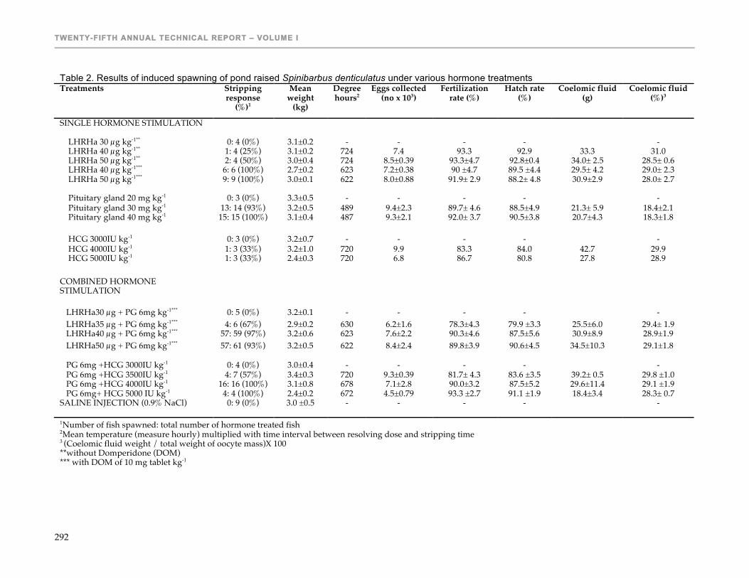
TWENTY-FIFTH ANNUAL TECHNICAL REPORT – VOLUME I
292
Table 2. Results of induced spawning of pond raised Spinibarbus denticulatus under various hormone treatments Treatments Stripping
response (%)1
Mean weight
(kg)
Degree hours2
Eggs collected (no x 103)
Fertilization rate (%)
Hatch rate (%)
Coelomic fluid (g)
Coelomic fluid (%)3
SINGLE HORMONE STIMULATION LHRHa 30 µg kg-1** 0: 4 (0%) 3.1±0.2 - - - - - LHRHa 40 µg kg-1** 1: 4 (25%) 3.1±0.2 724 7.4 93.3 92.9 33.3 31.0 LHRHa 50 µg kg-1** 2: 4 (50%) 3.0±0.4 724 8.5±0.39 93.3±4.7 92.8±0.4 34.0± 2.5 28.5± 0.6 LHRHa 40 µg kg-1*** 6: 6 (100%) 2.7±0.2 623 7.2±0.38 90 ±4.7 89.5 ±4.4 29.5± 4.2 29.0± 2.3 LHRHa 50 µg kg-1*** 9: 9 (100%) 3.0±0.1 622 8.0±0.88 91.9± 2.9 88.2± 4.8 30.9±2.9 28.0± 2.7 Pituitary gland 20 mg kg-1 0: 3 (0%) 3.3±0.5 - - - - - Pituitary gland 30 mg kg-1 13: 14 (93%) 3.2±0.5 489 9.4±2.3 89.7± 4.6 88.5±4.9 21.3± 5.9 18.4±2.1 Pituitary gland 40 mg kg-1 15: 15 (100%) 3.1±0.4 487 9.3±2.1 92.0± 3.7 90.5±3.8 20.7±4.3 18.3±1.8 HCG 3000IU kg-1 0: 3 (0%) 3.2±0.7 - - - - - HCG 4000IU kg-1 1: 3 (33%) 3.2±1.0 720 9.9 83.3 84.0 42.7 29.9 HCG 5000IU kg-1 1: 3 (33%) 2.4±0.3 720 6.8 86.7 80.8 27.8 28.9 COMBINED HORMONE STIMULATION
LHRHa30 µg + PG 6mg kg-1*** 0: 5 (0%) 3.2±0.1 - - - - - LHRHa35 µg + PG 6mg kg-1*** 4: 6 (67%) 2.9±0.2 630 6.2±1.6 78.3±4.3 79.9 ±3.3 25.5±6.0 29.4± 1.9 LHRHa40 µg + PG 6mg kg-1*** 57: 59 (97%) 3.2±0.6 623 7.6±2.2 90.3±4.6 87.5±5.6 30.9±8.9 28.9±1.9 LHRHa50 µg + PG 6mg kg-1*** 57: 61 (93%) 3.2±0.5 622 8.4±2.4 89.8±3.9 90.6±4.5 34.5±10.3 29.1±1.8 PG 6mg +HCG 3000IU kg-1 0: 4 (0%) 3.0±0.4 - - - - - PG 6mg +HCG 3500IU kg-1 4: 7 (57%) 3.4±0.3 720 9.3±0.39 81.7± 4.3 83.6 ±3.5 39.2± 0.5 29.8 ±1.0 PG 6mg +HCG 4000IU kg-1 16: 16 (100%) 3.1±0.8 678 7.1±2.8 90.0±3.2 87.5±5.2 29.6±11.4 29.1 ±1.9 PG 6mg+ HCG 5000 IU kg-1 4: 4 (100%) 2.4±0.2 672 4.5±0.79 93.3 ±2.7 91.1 ±1.9 18.4±3.4 28.3± 0.7 SALINE INJECTION (0.9% NaCl) 0: 9 (0%) 3.0 ±0.5 - - - - - 1Number of fish spawned: total number of hormone treated fish 2Mean temperature (measure hourly) multiplied with time interval between resolving dose and stripping time 3 (Coelomic fluid weight / total weight of oocyte mass)X 100 **without Domperidone (DOM) *** with DOM of 10 mg tablet kg-1

INDIGENOUS SPECIES DEVELOPMENT
293
INCORPORATION OF THE NATIVE CICHLID PETENIA SPLENDIDA INTO SUSTAINABLE AQUACULTURE: REPRODUCTION SYSTEMS, NUTRIENT REQUIREMENTS AND FEEDING STRATEGIES
Twelfth Work Plan, Indigenous Species Development 3 (12ISD3)
Final Report Published as Submitted by Contributing Authors
Wilfrido M. Contreras-Sánchez, Carlos Alfonso Alvarez González,
Gabriel Márquez-Couturier, Ulises Hernández-Vidal, Arkady Uskanga-Martínez, Luis D. Jímenez-Martínez, José Angel Almeida-Madrigal & Lander Lara-Aguilar
Universidad Juárez Autónoma de Tabasco Villahermosa, Tabasco, México
Grant W. Feist, & Guillermo Giannico
Oregon State University Corvallis, OR, USA
Carl B. Schreck
Biological Resources Division, USGS Oregon State University
Corvallis, OR, USA
ABSTRACT Our experiments have significantly contributed to the development of the technological package for the culture of the native cichlid tenhuayaca (Petenia splendida). Information on reproduction in captivity, larval rearing conditions and feeding during different stages of development has generated an important starting point for the management and conservation of native cichlids. The aim of this investigation was to address three research areas: 1) reproductive performance with different sex ratios; 2) intensive fry culture using high stocking densities and 3) protein requirements for fry, juvenile and adult growth using practical diets. To determine the best broodstock stocking rates, three male/female sex ratios were evaluated (1:1, 1:2, and 1:3). Each treatment consisted of three 2 m-diameter tanks that were divided into six spawning compartments. Fertilization rates, hatching success and larval survival were evaluated from each spawning. Reproductive behavior was also observed in each tank. The effect of stocking density was evaluated using sex reversed Petenia fingerlings. Fish were stocked at densities of 0.5, 1, 5, 10 and 20 fish/L using 70-L cylindrical-conical fiber glass tanks connected to a recirculating system. The use of vegetable meal at different life stages (larvae, juveniles and adults) was also studied by replacing fish meal with wheat gluten at different percentages (0, 25, 50, 75 and 100%). The control groups consisted of Artemia nauplii for larvae, or commercial feeds for carnivorous species (Silver Cup™). The 1:2 male/female ratio produced the largest number of fry, reaching 81,364 over 70 days of experimentation. This treatment produced more than 5,000 fry/Kg of female than the other ratios and more than one thousand fry per day. The average number of eggs produced per female (2,325), fertilization and hatching rates (above 97%), and survival during the early stages (100%) were high for this species. The results obtained using different stocking densities indicated that the optimal density for P. splendida was between five and ten larvae/L. This density resulted in good growth and survival. Stocking densities of 0.5 and one larvae/L provided the best growth, but the number of fish produced per tank was significantly reduced. The diet study produced important results in two areas: a) the development of a practical diet that can be used for larvae, juveniles and adults and b) the utilization of alternative ingredients in the diets (i.e. wheat gluten) which reduces costs by using lower amounts of fish meal. Experiments using larvae, juveniles and adults provided similar results regarding the amount of fish meal that can be replaced with wheat gluten. Even though P. splendida is considered to be a carnivorous cichlid, fish meal replacement in diets ranging from 25 to 50% (in relation to protein) can be used.
TWENTY-FIFTH ANNUAL TECHNICAL REPORT – VOLUME I
294
INTRODUCTION The first steps for a successful aquaculture program are to obtain spawns systematically and produce high quality eggs and healthy fry. To reach this point, it is necessary to obtain a high-quality broodstock and select for the most desirable traits to be expressed in subsequent generations. All of this, is required to develop aquaculture programs capable of supporting medium to large-scale facilities. For many native cichlids these aspects have not been evaluated, and because of the introduction of non-native species with high reproductive performance, growth rates and survival, their potential has been ignored. In Southeastern Mexico, a growing number of fish producers are requesting the development of alternative culture techniques that involve native species. Since the early 1970’s, the only species that has been available in this region is the Nile tilapia and little effort has been devoted to developing any alternatives. The culture of native species of fish is important from an economic and a conservation standpoint at a time when the local and foreign demand has imposed great pressures on their natural populations. In Tabasco and Chiapas, several species of native cichlids have been proposed for aquacultural purposes. Among those species, Petenia splendida, Cichlasoma urophthalmus and C. synspillum are of special interest because of their local demand and cultural value (Mendoza, 1988). Few studies have evaluated the basic biological parameters for incorporation of new species into aquacultural processes and information is needed in order to participate in the recovery of their populations and launch a different kind of aquaculture; one based on sustainability of native species and food security. During the last decade the culture of native species has been ignored. Some information has been obtained from wild populations and little is known about the reproductive performance of native species in captivity. In our laboratory, we have studied some reproductive features of P. splendida, C. urophthalmus and C. synspillum. We have found indications that tenhuayaca (P. splendida) may be a very good candidate for aquaculture purposes. Commercially, tenhuayaca is the most desirable species. Among cichlids, it has the highest value in the local market to the point of competing with snooks in price and the demand is very high. This investigation addressed whether tenhuayacas could be produced on a large scale with the goal of developing methodologies for sustainable mass-production. In order to do this three research areas were addressed: 1) reproductive performance with different sex ratios; 2) intensive fry culture using high stocking densities and 3) protein requirements for fry, juvenile and adult growth using practical diets. If successful, the technological package developed can be transferred to local hatcheries located in poor areas of the states of Tabasco and Chiapas, México. The use of reliable methods in these hatcheries will have a significant benefit for thousands of small farmers that currently see their productivity limited to the use of tilapia.
METHODS AND MATERIALS Study 1: Intensive spawning and nursery techniques for Petenia splendida. Experiment 1 (Parental sex ratios). Fish used as broodstock were obtained from “Pantanos de Centla”. All fish were weighed, sexed and tagged for individual identification. Three sex ratios were evaluated to determine the best fry production rates. The male/female ratios evaluated were 1:1, 1:2, and 1:3. Each treatment consisted of three 2 m-diameter tanks that were divided into six spawning compartments. A plastic mat (0.3-m2) was placed as spawning substrate in each compartment. In the first treatment, 6 males and 6 females were placed in each tank; in the second treatment 3 males and 6 females were placed in each replicate; in the last treatment, 2 males and 6 females were placed in each replicate. The fish were allowed to spawn over a six-month period. Each substrate was observed daily for nesting activity. Substrates found to have eggs were removed and replaced. Eggs in each nest were counted. Brooders were fed daily to

INDIGENOUS SPECIES DEVELOPMENT
295
satiation with pieces of frozen fish. Dissolved oxygen and temperature were recorded at 7:00 am and 7:00 pm. Statistical Analysis: Because the variable fry produced per spawn did not meet the assumption of normality, a Kruskal-Wallis test was performed using STATGRAPHICS PLUS® 4.0 software. All differences were considered as significant at P < 0.05 for this, and all subsequent experiments. Experiment 2 (Petenia fecundity and hatching success). Using spawnings obtained in Experiment 1, the fecundity of P. splendida was determined and hatching success established. A 1.5% sodium sulfite solution was used to remove the adhesive eggs from the substrate. A minimum of 10 spawns were separated from the nest substrate and enumerated. The females that produced each spawn were weighed and fecundity calculated as the number of eggs/g of female. Nests were transferred to a hatching tray. Fertilized and none fertilized eggs were counted. The percent hatch and larval survival to swim-up stage were determined. Statistical analysis: Percent data were analyzed using a contingency table analysis with a Chi square test (STATGRAPHICS PLUS® 4.0). A linear regression analysis was conducted to determine if the number of eggs produced per female was related to the weight or length of the fish. Experiment 3 (Effect of stocking density on growth and survival of P. splendida fry). For this experiment larvae were placed in 70-L cylindrical-conical fiber glass tanks connected to a recirculating system. Sex reversed P. splendida fingerlings were stocked at densities of 0.5, 1, 5, 10 and 20 fish/L using 3 replicates/stocking density. Dissolved oxygen and temperature were recorded daily and ammonia, nitrites and nitrates were recorded each week. Every fifteen days at least 10% of all fish in each tank were sampled. Weight and total length were recorded. After 45-d all nursery tanks were harvested and the total number of fish and their weights determined. Statistical Analysis: Growth was analyzed with a one-way ANOVA test. Survival was analyzed using a contingency table analysis with a Chi square test (STATGRAPHICS PLUS® 4.0). Study 2: Vegetable meal utilization of Petenia splendida at different life stages. This study consisted of three experiments which evaluated the substitution of fish meal with wheat gluten on growth and survival of larvae, juveniles and adults of P. splendida fed with practical diets. The three experiments were conduced at the Laboratory of Aquaculture at UJAT, Tabasco, Mexico. For the first and second experiments larvae and juveniles were obtained from the domesticated broodstock of P. splendida. Hatched larvae were collected by siphoning (3 days post fertilization). Yolk-sac larvae were counted and placed in a recirculating system until yolk absorption (6 days post fertilization). Experiment 1 (Larvae). Larvae were counted and placed in a recirculating system containing 21 circular plastic tanks (70 L) connected to a biological, sand and UV filters, and a 1500-L reservoir. Additionally, two titanium heaters were connected to the reservoir. The initial stocking density for all tanks was 100 larvae/L. Daily 10% water exchanges were performed and each tank had a continuous air supply. Before the experiment, larvae were fed for 15 days with Artemia nauplii enriched with 20 mg/L of 17-α methyltestosterone (MT). The experiment started on day 16 when larvae were fed with the experimental and commercial diets. The experimental design consisted of five MT enriched experimental practical diets, one MT enriched control diet (Silver cup trout diet) and Artemia nauplii (Table 1) which were evaluated for 30 days. Experimental diets were designed to be isoproteinic and isolipidic (45 % protein and 8 % lipid content). Feeding was conducted four times per day (8:00. 12:00, 16:00, and 20:00 h). The sampling schedule for fry consisted of collecting the entire population from all tanks at the beginning of the experiment and every 15 days. Total length and weight were measured to the nearest 0.001 mm or g. Mortality was recorded daily. Experimental treatments were as follows:

TWENTY-FIFTH ANNUAL TECHNICAL REPORT – VOLUME I
296
1) Tenhuayaca fry fed with a diet containing 0% wheat gluten and 100% fish meal. 2) Tenhuayaca fry fed with a diet containing 25% wheat gluten and 75% fish meal. 3) Tenhuayaca fry fed with a diet containing 50% wheat gluten and 50% fish meal. 4) Tenhuayaca fry fed with a diet containing 75% wheat gluten and 25% fish meal. 5) Tenhuayaca fry fed with a diet containing 100% wheat gluten and 0% fish meal. 6) Tenhuayaca fry fed with Artemia nauplii (Control No. 1). 7) Tenhuayaca fry fed with a Silver Cup trout diet (Control No. 2).
Statistical analysis: To determine differences of growth between treatments, a one-way ANOVA was conducted and differences were evaluated using a Tukey test. Survival was compared using a Kruskal-Wallis test and differences between treatments were tested with a Nemenyi test. All statistical analyses were conducted using STATISTICA 7.0 software. Experiment 2 (Juveniles). Masculinized juveniles were selected from a group of 5,000 fry produced at the Laboratory of Aquaculture at UJAT. The production of masculinized juveniles consisted of feeding larvae with 17 α-Methyltestosterone (20 mg/L) enriched Artemia nauplii for 15 days and 17 α-Methyltestosterone (60 mg/Kg of diet) enriched commercial trout diet (Silver Cup) for 30 additional days. One thousand six hundred and twenty fish (averaging 0.055 g and 1.7 mm) were selected and placed in a recirculating system. Water for grow-out was recirculated using bio-filters and 25% of the volume was exchanged twice a week. Feeding was conducted four times per day (8:00. 12:00, 16:00, and 20:00 h) and the diets were evaluated for 56 days. Sampling schedule for Petenia juveniles consisted of collecting all fish in each tank at the beginning of the experiment and every 14 days. Total length and weight were measured to the nearest 0.001 mm or g. Mortality was recorded daily. Growth and food quality indices were calculated at the end of the experiment: feed conversion rate (FCR), specific growth rate (SGR), condition factor (CF), protein efficiency rate (PER), and percentile weight gain (WG %). Experimental treatments were as follows:
1) Tenhuayaca juveniles fed with a diet containing 0% wheat gluten and 100% fish meal. 2) Tenhuayaca juveniles fed with a diet containing 25% wheat gluten and 75% fish meal. 3) Tenhuayaca juveniles fed with a diet containing 50% wheat gluten and 50% fish meal. 4) Tenhuayaca juveniles fed with a diet containing 75% wheat gluten and 25% fish meal. 5) Tenhuayaca juveniles fed with a diet containing 100% wheat gluten and 0% fish meal. 6) Tenhuayaca juveniles fed with a Silver Cup trout diet (Control).
Statistical analysis: To determine differences of growth between treatments, a one-way ANOVA was conducted and differences were evaluated using a Tukey test. Survival was compared using a Kruskal-Wallis test and differences between treatments were tested with a Nemenyi test (STATISTICA 7.0). Experiment 3 (Adults). Tenhuayaca adults were obtained from a commercial farm located in Ranchería Chicozapote, Nacajuca, Tabasco. One hundred and thirty five adults (66.6 g and 17.5 cm) were selected using a sex proportion of 1:2 male/female and transported to the Aquaculture Laboratory at UJAT. Fish were randomly assigned to 1.5 m3-circular plastic tanks (three males and six females per tank). A twenty-five percent water exchange was conducted twice a week. Feeding was conducted three times per day (8:00, 14:00, and 20:00 h). Fish received daily rations containing 10 percent of the tank biomass. Daily rations were estimated using a spread-sheet constructed with previous growth data. Diets were evaluated for 84 days Sampling schedule for Petenia adults consisted of collecting all fish from each tank at the beginning of the experiment and every 14 days. Total length and weight were measured to the nearest 0.001 mm or g. Mortality was recorded daily. Growth and food quality indices were calculated at the end of the experiment: feed conversion rate (FCR), specific growth rate (SGR),

INDIGENOUS SPECIES DEVELOPMENT
297
condition factor (CF), protein efficiency rate (PER), and percentile weight gain (WG %). Experimental treatments were as follows:
1) Tenhuayaca adults fed with a diet containing 0% wheat gluten and 100% fish meal. 2) Tenhuayaca adults fed with a diet containing 25% wheat gluten and 75% fish meal. 3) Tenhuayaca adults fed with a diet containing 50% wheat gluten and 50% fish meal. 4) Tenhuayaca adults fed with a diet containing 75% wheat gluten and 25% fish meal. 5) Tenhuayaca adults fed with a diet containing 100% wheat gluten and 0% fish meal.
Statistical analysis: To determine differences of growth between treatments, a one-way ANOVA was conducted and differences were evaluated using a Tukey test. Survival was compared using a Kruskal-Wallis test and differences between treatments were tested with a Nemenyi test (STATISTICA 7.0).
RESULTS Study 1: Intensive spawning and nursery techniques for Petenia splendida. Experiment 1 (Parental sex ratios). Significant differences were observed between treatments for total fry production (Fig. 1). The 1:2 male/female ratio had the highest production, reaching 81,364 fry during the experiment. For the fish stocked at the 1:1 and 1:3 sex ratios, the fry production was statistically similar, reaching 63,597 and 55,035 fry, respectively. The number of spawning events per treatment was not statistically different, ranging from 25 to 29; however, the number of fry produced per kilogram of female and per day was significantly different between treatments showing the same trend as that found for total production of fry (Table 2). The treatment with 1:2 male/female produced more than 5,000 fry/Kg of female than the other ratios. This treatment produced more than one thousand fry per day. Experiment 2 (Petenia fecundity and hatching success). No significant differences were detected when the number of eggs per female, fertilization rate and hatching success were compared between treatments. In all treatments, the mean fertilization rate was higher than 97% (Fig. 2). The linear regression analysis indicated that the number of eggs or fry were not significantly related to the weight or length of the females (P = 0.93 and 0.90, respectively) for the range of female sizes used in this experiment (88 to 362 g and 145 to 235 mm). Therefore, it is difficult to estimate the productivity of each female based on size. The range of eggs produced by females was 854 – 6869, with an average value of 2325 eggs. During the 70 days of this experiment, most females spawned once (78%); one female spawned four times, six females spawned three times and 18 females spawned twice. Twelve females (22%) never spawned during the experiment. Females that spawned more than once took between 15 and 42 days to spawn again, with the majority of them showing an interval of 20 days. From all the females used in the experiment, two of them spawned repeatedly in relatively shorter intervals. One over a period of time of two days and another one over a period of time of three days. The first one spawned 3,580 and 2,465 eggs in each spawning event and the second female spawned 2,450 and 1,215 eggs in each spawning. In terms of mating behavior, we observed that females did not create strong bonds with males. One female spawned with three different males and one male spawned with five different females. Experiment 3 (Effect of stocking density on growth and survival of P. splendida fry). Water quality in the recirculating system was adequate for the culture of P. splendida larvae (Table 3). Differences in weight and total length were observed at 30 days of experimentation (Fig. 3A and 3B). Larvae stocked at 0.5 and 1 larvae/L were larger than larvae stocked at higher densities (5, 10 and 20 larvae/L). At the end of the experiment (day 45) significant differences were detected for weight and total length, showing three distinct sizes (Fig. 3C and 3D). The first group were larvae stocked at low densities (0.5 and 1/L) which showed the highest growth; the second group were larvae stocked at a medium density (5 larvae/L), and the third group were larvae stocked at the highest densities (10 and 20 larvae/L). These results indicate that medium and low densities are preferable for larval culture.

TWENTY-FIFTH ANNUAL TECHNICAL REPORT – VOLUME I
298
Significant differences were found for survival among treatments (Table 4). The lowest survival was seen at a density of 20 larvae/L (65%), while survival for larvae stocked at 0.5, 1, 5 and 10/L was high (97-100%). Despite the mortality observed, total juvenile production was significantly higher when larvae were stocked at 20/L. Study 2: Vegetable meal utilization of Petenia splendida at different life stages. Experiment 1 (Larvae). The analysis of variance for weight and total length at the end of the experiment indicated significant differences between treatments (Fig. 4). Fish fed with the diet containing 25% fish meal replaced with wheat gluten showed the highest weights and lengths followed by the diet with 100% fish meal and the diet with 50% fish meal replacement. The lowest growth was observed in fish fed with diets of 75 and 100% fish meal replacement. No significant differences were observed between fish fed with the diet containing 50% fish meal replacement and those fed with the commercial diet Silver Cup™. No significant differences in survival were detected among treatments (Fig. 5). Experiment 2 (Juveniles). Juvenile growth showed similar results as those seen for larvae (Fig. 6). The analysis of variance for weight and total length at the end of the experiment indicated significant differences among treatments. Fish fed with the diet containing 25% fish meal replaced with wheat gluten showed the highest weights and lengths followed by the diet with 100% fish meal and the diet with 50% fish meal replacement. The lowest growth was observed in fish fed with diets of 75 and 100% fish meal replacement. Fish fed with the commercial diet Silver Cup™ had average growth. No significant differences in survival were detected among treatments ranging from 82.2 to 95.6 %. Significant differences were detected for growth (weight and total length) from day 14 and onwards (Tables 5 and 6). Fish fed with 0, 25 and 50 % wheat gluten, and commercial diets, were larger than fish receiving the 100 and 75 % wheat gluten diets. Growth and food quality indices showed significant differences among treatments (Table 7). The best indicators were obtained from fish fed with the diet containing 75% fish meal and the lowest values were from those fed with diets containing 100 % wheat gluten. Similar results were obtained for survival. The lowest survival was obtained for fish feed with 100 % wheat gluten. All other treatments ranged from 82.2 to 95.6 % survival. Experiment 3 (Adults). Significant differences were detected for weight and length from day 28 onwards, these differences remained until the end of the experiment (Fig. 7). Diets with 25 and 50% wheat gluten, and 100 % fish meal were higher than the other treatments. At the end of the experiment, these differences were evident for weight but not for total length (Fig. 8). No significant differences between treatments were detected for any growth and food quality indices or survival (Table 8).
DISCUSSION Our experiments have significantly contributed to the development of the technological package for Petenia splendida culture. Information on reproduction in captivity, larval rearing conditions and feeding during different stages of development has generated an important starting point for the management and conservation of native cichlids. Small and easy-to-handle spawning systems are very effective for Petenia reproduction. This species tends to provide extended periods of parental care; therefore, systems with clean water and localized nests help farmers locate egg clutches and once the larvae hatch, they can be easily removed from the reproduction tank by gentle siphoning. We were able to optimize the use of broodstock. Our results indicate that significantly more fry can be produced when a ratio of one male per two females is used. Fry production increased by 47% when the 1:2 ratio was used

INDIGENOUS SPECIES DEVELOPMENT
299
compared to the 1:1 ratio. This sex ratio did not affect fecundity rates, hatching success nor quality of fry. Keenleyside (1983) and Desprez et al. (2006) found that there are several advantages when appropriate sex ratios are used; first, the amount of food used is optimized by feeding more egg-producing fish in the system; second, aggressive behavior between males (which usually disturbs nesting behavior) is significantly reduced by having fewer males per tank. Similar results have been observed in other species; for example, in common dentex (Dentex dentex) and zebrafish, (Danio rerio), the use of the proper sex ratio increased egg production and diminished aggression between adults (Pavlidis et al., 2004; Spence and Smith, 2005). An additional effect of lowering aggression between adults is the reduction of diseases that result from injuries and stress. Fighting for space, food or mating generates a significant amount of stress. This has been observed in tilapia (Oreochromis mossambicus) where the use of a sex ratios of 1:3 (male:female) decreased the incidence of Aeromonas hydrophila (Binuramesh et al., 2006). Another benefit of reducing the number of males participating in spawning events is that if all of the fish are tagged and can be easily identified; the specific traits of a batch of fish can be studied and a genetic program can be started. These types of studies will help improve the phenotypic characteristics of fish used in aquaculture (Cottona et al., 2006). The average number of eggs produced per female (2,325), fertilization and hatching rates (above 97%), and survival during the early stages (100%) were high for this species. Interestingly, the number of eggs produced was not associated with the weight or length of the female. The lack of correlation between these factors may be due to the effects of captivity, since fecundity is well correlated to size in wild Petenias (Resendez and Salvadores, 1983; Chávez et al., 1989). It is possible that the disruption of parental care and the consequent re-initiation of gonadal maturation in females is related to the high variability in egg/female variation. We observed that two females spawned over very short periods of times (2 and 3 days). It was observed that these females released some of the mature eggs in one nest and the rest were released in a different nest with a different male. This behavior may have been produced by the interruption of spawning; nevertheless the eggs were viable and good quality larvae were collected in both cases. Fertilization rates in aquaculture vary widely, particularly when the spawns occur naturally in the reproduction units. In our study we obtained high fertilization rates (average above 97%) and excellent hatching rates (100% in all cases). For the most cultivated cichlids –the tilapias- fertilization rate is variable. However, most studies have reported high fertilization rates (between 90-100%). Fertility tests under controlled conditions using frozen and unfrozen tilapia milt resulted in a fertilization rate of 72.7% and 85.7%, respectively. While frozen and unfrozen milt of the O. nilolicus×O. aureus hybrid used to fertilize the eggs of O. honorum, resulted in 93.4% and 90% fertilization, respectively (Nai-Hsien, et al., 1987). Over a period of 70 days we obtained more than 200,000 fry in nine 2m-diameter tanks; considering that Petenia spawn from early March to the end of October, it is feasible to produce over 685,000 fish in the same system in a single year. These values are very encouraging for Petenia reproduction in captivity. The results obtained using different stocking densities of larvae indicate that the optimal density for P. splendida is between five and ten larvae/L, providing good growth indicators and survival. Stocking densities of 0.5 and 1 larvae/L provided the best growth, but the number of fish produced per tank was significantly reduced. Monitoring of water in this study indicated high water quality in all systems; therefore, it is feasible to use stocking densities above 20 larvae/L. However, other issues should be taken into consideration because higher densities can cause an increase in intraspecific competition, higher variability in size and a significant reduction in survival and growth. There is also a higher risk for diseases due to lower water quality (De Angelis et al., 1979; McKinnon, 1985; Valerio and Barlow, 1986; Hecht and Pienaar, 1993). Additionally, high densities of fish may provoke cannibalism, especially during larval stages, which can result in high mortality. This behavior is common in marine species and carnivorous freshwater species. No information has been generated for larval stages of Petenia, but in general this species is considered to be piscivorous (Resendez and Salvadores, 1983). Atencio and
TWENTY-FIFTH ANNUAL TECHNICAL REPORT – VOLUME I
300
Zaniboni-Filho (2006) consider that in wild larvae, cannibalism is associated with food availability and rearing space. For this reason, administration of sufficient amounts of food in captivity is very important to avoid this behavior. In our experiments we used a feeding table based on previous experiments. At the start of the experiment, 15 prey were provided per fish, this provided enough food for fish in all rearing densities. Through time, the amount of prey was modified to ensure food availability. Mortality in our higher densities (particularly 20 larvae/L) was not directly associated with cannibalism; however, aggression was observed between fish. It is possible that this behavior was caused by social ranking in the tanks. Several authors have reported aggression between fish during the early stages of development due to lack of sufficient space (Houde, 1975; Taniguchi, 1981; Teng, 1982a, 1982b; Al-Ameeri et al., 1982; Leu and Chou, 1996). Wedemeyer and McLeay (1981) have documented that high densities often result in reductions in growth, higher variability in size, aggressive behavior, cannibalism and an increase in disease susceptibility. The diet study produced important results in two areas: a) the development of a practical diet that can be used for larvae, juveniles and adults and b) the utilization of alternative ingredients in the diets (such as wheat gluten) which reduces costs by using lower amounts of fish meal. Experiments using larvae, juveniles and adults provided similar results regarding the amount of fish meal that can be replaced with wheat gluten. Even though P. splendida has been considered a carnivorous cichlid, fish meal replacement in diets can range between 25 and 50% (in relation to protein). Similar studies have been conducted in Atlantic salmon (Salmo salar) where a mixture of full-fat soybean meal and maize gluten meal (28% and 55% respectively) was used. Results indicated similar growth in treatment diets when compared to the control group which received a diet containing 89% fish meal (Opstvedt et al., 2003). Regost et al. (1999) evaluated substitution of fish meal with corn gluten in turbot (Psetta maxima); in this study a 20% substitution yielded the best growth. Tibaldi et al. (2006), worked with European sea bass (Dicentrarchus labrax) with differently processed soybean meals; toasted, dehulled and solvent-extracted soybean meal (SE), dehulled and toasted soy seeds subjected to dry extrusion and mechanical oil extraction (ME) and enzyme-treated soybean meal (ET). The authors concluded that fish meal substituted with 25% SE, 50% ET or 60% soy composed of 30% SE and 30% ET did not affect fish performance or the activity of digestive enzymes. Several studies have pointed out that the incorporation of vegetable ingredients in fish diets must take into consideration the origin of the source, the quality control during processing, amino acid and fatty acid profiles, digestive physiology of the organism, stage of development of the organism and substitution level allowed without hampering fish performance (Kaushik et al., 2006; Lee et al., 2006; Albrektsen et al., 2006). In our study, we were able to substitute a significant amount of fish meal by using wheat gluten. More research is needed regarding improvements to these diets. The incorporation of native species into aquaculture practices, such as tenhuayacas, is important to promote the development of regional enterprises; both social and private initiatives can invest economic resources in this type of aquaculture. Our studies on tenhuayaca culture have generated critical information to complete the life cycle of this species in captivity (reproduction, larval rearing, diets and closed systems for rearing). The use of native species in aquaculture may help to reduce the pressure on the traditional fishery, resulting in the conservation of this important species.
LITERATURE CITED Albrektsen, S., Mundheim, H., Aksnes, A. 2006. Growth, feed efficiency, digestibility and nutrient
distribution in Atlantic cod (Gadus morhua) fed two different fish meal qualities at three dietary levels of vegetable protein sources. Aquaculture 261(2): 626-640.
Al-Ameeri. A., Al-Maraouk, A., Teng, S.K., Khamis, M.F.I. 1982. Effects of stocking density on sobaity (Acanthopagrus cuvieri). Pages 60-61 In: Annual Research Report. Kuwait Institute for Scientific Research. Kuwait City, Kuwait.
INDIGENOUS SPECIES DEVELOPMENT
301
Atencio-Garcia, V.Y., Zaniboni-Filho, E., 2006. El canibalismo en la larvicultura de peces. Medicina Veterinaria y Zootecnia. Córdoba 1, 9-19.
Binuramesh, C., Prabakaran, M., Steinhagen, D., Michael, R.D. 2006. Effect of sex ratio on the immune system of Oreochromis mossambicus (Peters). Brain Behav. Immun. 20(3):300-308.
Chávez-Lomelí, M., Mettheuws, A; Pérez, H. 1989. Biología de los peces del río San Pedro en vista de determinar su potencial para la piscicultura. Ediciones INIREB. México. 222 pp.
Cottona, S., Smalla, J., Pomiankowski, A. 2006. Sexual selection and condition-dependent mate preferences. Curr. Biol. 16(17): R755-R765
De Angelis, D.L., Cox, D.K., Countant, C.C. 1979. Cannibalism and size dispersal in young of the year largemount bass: experiment and model. Ecol. Mod. 8:133-148.
Desprez, D., Briand, C., Hoareau, M.C., Mélard, C., Bosc, P. and Baroille, J.F. 2006. Study of sex ratio in progeny of a complex Oreochromis hybrid, the Florida red tilapia. Aquaculture 251(2-4): 231-237.
Hecht, T., Pienaar, A.G. 1993. A review of cannibalism and its implications in fish larviculture. J. World Aquac. Soc. 24: 246-261.
Houde, E.D. 1975. Effects of stocking density and food density on survival, growth and yield of laboratory-reared larvae of seabream Archosargus rhomboidalis (L.) (Sparidae). J. Fish Biol. 7:115-129.
Kaushik, S.J., Covès, D., Dutto, G., Blanc, D. 2006. Almost total replacement of fish meal by plant protein sources in the diet of a marine teleost, the European seabass, Dicentrarchus labrax. Aquaculture 230(1-4): 391-404.
Keenleyside, M.H.A. 1983. Mate desertion in relation to adult sex ratio in the biparental cichlid fish Herotilapia multispinosa Animal Beha. 31(3): 683-688.
Lee, K.J., Rinchard, J., Dabrowski, K., Babiak, I., Ottobre, J.S., Christensen, J.E. 2006. Long-term effects of dietary cottonseed meal on growth and reproductive performance of rainbow trout: Three-year study. Animal Feed Sci. Tech. 126(1-2): 93-106.
Leu, M.Y., Chou, Y. 1996. Induced spawning and larval rearing of captive yellowfin porgy Acanthopagrus latus (Houttuyn). Aquaculture 143: 155-166.
McKinnon, M.R. 1985. Barramundi breeding and culture in Thailand. Queensland Dept. of Primary Industries Study Tour Report. Sohgkhla, Thailand. 19 pp.
Mendoza, E. 1988. Desarrollo larval de Cichlasoma urophthalmus. Memorias del primer seminario sobre peces nativos con uso potencial en acuacultura. Cardenas, tabasco, México. CEICADES-UJAT-INIREB pp. 16-17.
Nai-Hsien C., Wei-Chung C., Kuo-Chun L., I-Chiu L. 1987. The properties of tilapia sperm and its cryopreservation. Journal of Fish Biology 30 (2), 107–118.
Opstvedt, J., Aksnes, A., Hope, B., Pike, I.H. 2003. Efficiency of feed utilization in Atlantic salmon (Salmo salar L.) fed diets with increasing substitution of fish meal with vegetable proteins. Aquaculture 221(1-4): 365-379.
Regost, C., Arzel, J. Kaushik, S.J. 1999. Partial or total replacement of fish meal by corn gluten meal in diet for turbot (Psetta maxima) Aquaculture 180(1-2): 99-117.
Pavlidis, M., Greenwood, L., Scott, A.P. 2004. The role of sex ratio on spawning performance and on the free and conjugated sex steroids released into the water by common dentex (Dentex dentex) broodstock. Gen. Comp. Endocrinol. 138(3):255-262.
Resendez, A. and Salvadores, M.L. 1983. Contribución al conocimiento de la biología del pejelagarto, Atractosteus tropicus (Gill) y Tenguayaca Petenia splendida (Gunther) del Estado de Tabasco. Biótica 8 (4):413-426.
Spence, R., Smith, C. 2005. Male territoriality mediates density and sex ratio effects on oviposition in the zebrafish, Danio rerio. Animal Behav. 69(6):1317-1323.
Taniguchi, K. 1981. Survival and growth of larval spoted seatrout (Cynoscion nebulosus) in relation to temperature, prey abundance and stocking densities. Report of the V meeting of the International Council for the Exploration of the Sea 178:507-508.
Teng, S.K., Akatsu, S., Abdul-Elah, K.M., El-Zahr, C.R., Downing, N., Al-Mamuk, A., Ghazal, N. 1982a. Spawning. fingerling, production and market size culture of sobaity (Acanthopagrus cuvieri) in Kuwait. Pages 66-71. In: Annual Research Report. Kuwait Institute for Scientific Research. Kuwait City, Kuwait.
TWENTY-FIFTH ANNUAL TECHNICAL REPORT – VOLUME I
302
Teng, S.K., Akatsu, S., Ahdul-Elah, K.M., Al-Manouk, A., Downing, N., El-Zahr, C.R., Al-Ghenlas, K. 1982b. Spawning, fingerling, production and market size culture of hamoor (Epinephelus tauvina). In: Kuwait. Pages 71-74. In: Annual Research Report. Kuwait Institute for Scientific Research. Kuwait City, Kuwait.
Tibaldi, E., Hakim, Y., Uni, Z., Tulli, F., Francesco, M., Luzzana, U., Harpaz, S. 2006. Effects of the partial substitution of dietary fish meal by differently processed soybean meals on growth performance, nutrient digestibility and activity of intestinal brush border enzymes in the European sea bass (Dicentrarchus labrax). Aquaculture 261(1):182-193.
Valerio, M., Barlow, G.W. 1986. Ontogeny of young midas cichlids: a study of feeding, filial cannibalism and antagonism in relation of difference in size. Biol. Behaviour 11:16-35.
Wedemayer, G.A., McLeay, D.J. 1981. Methods for determining the tolerance of fishes to enviromental stressors. 51-78. In: D. Pickering. Stress and Fish. Academic Press. London.

INDIGENOUS SPECIES DEVELOPMENT
303
Figure 1. Egg production (+SE) from P. plendida broodstock under three male:female sex ratios.broodstock under three male:female sex ratios.
Sex ratio (male : female)
1 : 1 1 : 2 1 : 3
Eggs produced
0
500
1000
1500
2000
2500
3000
Sex ratio (male : female)
1 : 1 1 : 2 1 : 3Fertilization (%
)
0
20
40
60
80
100
Figure 2. Percent fertilization (+SE) for eggs under three male:female sex ratios.
Figure 3. Weight (A) and total length (B) for 45 days (mean ± SD), and final weight (C) and total length (D) of P. splendida larvae raised at different densities. n = number of fish sampled. Different letters indicate significant differences (P < 0.05).

TWENTY-FIFTH ANNUAL TECHNICAL REPORT – VOLUME I
304
Substitution
0%FM/100%WG
25%FM/75%WG
50%FM/50%WG
75%FM/25%WG
100%FM/0%WG
CD AN
Weight (g)
0.00
0.05
0.10
0.15
0.20
0.25
a
b
c cd d
ef
Substitution
0%FM/100%WG
25%FM/75%WG
50%FM/50%WG
75%FM/25%WG
100%FM/0%WG
CD AN
Total length (mm
)
0
5
10
15
20
25
30
abc
d de
f
Figure 4. Average (± SE) weight (A) and total length (B) of P. splendida larvae fed with different amounts of wheat gluten (WG) substituted for fish meal (FM). CD: Commercial diet, AN: Artemia nauplii. Different letters indicate significant differences (P < 0.05).
(A)
(B)

INDIGENOUS SPECIES DEVELOPMENT
305
Substitution
0%FM/100%WG
25%FM/75%WG
50%FM/50%WG
75%FM/25%WG
100%FM/0%WG
CD AN
Survival (%)
0
20
40
60
80
100
Substitution
0%FM/100%WG
25%FM/75%WG
50%FM/50%WG
75%FM/25%WG
100%FM/0%WG
CD
Weight (g)
0.0
0.5
1.0
1.5
2.0
2.5
a
b
d
c
ee
Substitution
0%FM/100%WG
25%FM/75%WG
50%FM/50%WG
75%FM/25%WG
100%FM/0%WG
CD
Total length (mm
)
0
10
20
30
40
50
60a a
bb
cc
Time (days)0 14 28 42 56 70 84
Total length (cm)
17
18
19
20
0%FM/100% WG 25%FM/75% WG50%FM/50% WG 75%FM/25% WG100%FM/0% WG
Time (days)0 14 28 42 56 70 84
Weight (g) 60
65
70
75
80
85
90
950%FM/100% WG 25%FM/75% WG 50%FM/50% WG 75%FM/25% WG 100%FM/0% WG
Figure 5. Survival rate (% ± SE) of P. splendida larvae fed with different amounts of wheat gluten (WG) substituted for fish meal (FM). CD: Commercial diet, AN: Artemia nauplii.
Figure 6. Mean (± SE) weight (A) and Total Length (B) of P. splendida juveniles fed with different amounts of wheat gluten (WG) substituted for fish meal (FM). CD: Commercial diet. Different letters indicate significant differences (P < 0.05). Figure 7. Mean dry weight (g ± SD; A) and total length (cm ± SD; B) through time of P. splendida adults fed with different amounts of wheat gluten (WG) substituted for fish meal (FM). Different letters shown in parentheses in the legend box indicate significant differences between treatments (P < 0.05).
(B)
(A) (B)
(A)
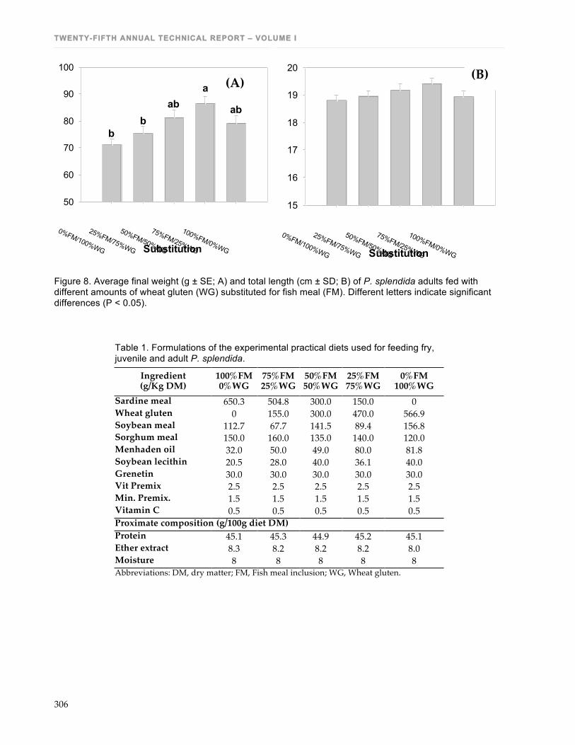
TWENTY-FIFTH ANNUAL TECHNICAL REPORT – VOLUME I
306
Substitution
0%FM/100%WG
25%FM/75%WG
50%FM/50%WG
75%FM/25%WG
100%FM/0%WG
Weight (g) 50
60
70
80
90
100
aab ab
bb
Substitution
0%FM/100%WG
25%FM/75%WG
50%FM/50%WG
75%FM/25%WG
100%FM/0%WG
Total length (cm)
15
16
17
18
19
20 Figure 8. Average final weight (g ± SE; A) and total length (cm ± SD; B) of P. splendida adults fed with different amounts of wheat gluten (WG) substituted for fish meal (FM). Different letters indicate significant differences (P < 0.05).
Table 1. Formulations of the experimental practical diets used for feeding fry, juvenile and adult P. splendida.
Ingredient (g/Kg DM)
100%FM 0%WG
75%FM 25%WG
50%FM 50%WG
25%FM 75%WG
0%FM 100%WG
Sardine meal 650.3 504.8 300.0 150.0 0 Wheat gluten 0 155.0 300.0 470.0 566.9 Soybean meal 112.7 67.7 141.5 89.4 156.8 Sorghum meal 150.0 160.0 135.0 140.0 120.0 Menhaden oil 32.0 50.0 49.0 80.0 81.8 Soybean lecithin 20.5 28.0 40.0 36.1 40.0 Grenetin 30.0 30.0 30.0 30.0 30.0 Vit Premix 2.5 2.5 2.5 2.5 2.5 Min. Premix. 1.5 1.5 1.5 1.5 1.5 Vitamin C 0.5 0.5 0.5 0.5 0.5 Proximate composition (g/100g diet DM) Protein 45.1 45.3 44.9 45.2 45.1 Ether extract 8.3 8.2 8.2 8.2 8.0 Moisture 8 8 8 8 8 Abbreviations: DM, dry matter; FM, Fish meal inclusion; WG, Wheat gluten.
(A) (B)
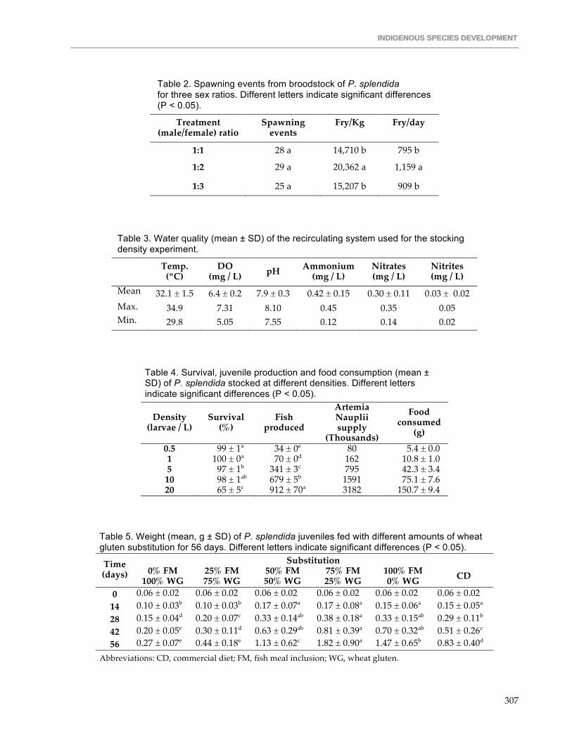
INDIGENOUS SPECIES DEVELOPMENT
307
Table 2. Spawning events from broodstock of P. splendida for three sex ratios. Different letters indicate significant differences (P < 0.05).
Treatment (male/female) ratio
Spawning events
Fry/Kg Fry/day
1:1 28 a 14,710 b 795 b
1:2 29 a 20,362 a 1,159 a
1:3 25 a 15,207 b 909 b
Table 3. Water quality (mean ± SD) of the recirculating system used for the stocking density experiment.
Temp. (ºC)
DO (mg / L) pH Ammonium
(mg / L) Nitrates (mg / L)
Nitrites (mg / L)
Mean 32.1 ± 1.5 6.4 ± 0.2 7.9 ± 0.3 0.42 ± 0.15 0.30 ± 0.11 0.03 ± 0.02 Max. 34.9 7.31 8.10 0.45 0.35 0.05 Min. 29.8 5.05 7.55 0.12 0.14 0.02
Table 4. Survival, juvenile production and food consumption (mean ± SD) of P. splendida stocked at different densities. Different letters indicate significant differences (P < 0.05).
Density (larvae / L)
Survival (%)
Fish produced
Artemia Nauplii supply
(Thousands)
Food consumed
(g)
0.5 99 ± 1a 34 ± 0e 80 5.4 ± 0.0 1 100 ± 0a 70 ± 0d 162 10.8 ± 1.0 5 97 ± 1b 341 ± 3c 795 42.3 ± 3.4
10 98 ± 1ab 679 ± 5b 1591 75.1 ± 7.6 20 65 ± 5c 912 ± 70a 3182 150.7 ± 9.4
Table 5. Weight (mean, g ± SD) of P. splendida juveniles fed with different amounts of wheat gluten substitution for 56 days. Different letters indicate significant differences (P < 0.05).
Substitution Time (days) 0% FM
100% WG 25% FM 75% WG
50% FM 50% WG
75% FM 25% WG
100% FM 0% WG CD
0 0.06 ± 0.02 0.06 ± 0.02 0.06 ± 0.02 0.06 ± 0.02 0.06 ± 0.02 0.06 ± 0.02 14 0.10 ± 0.03b 0.10 ± 0.03b 0.17 ± 0.07a 0.17 ± 0.08a 0.15 ± 0.06a 0.15 ± 0.05a 28 0.15 ± 0.04d 0.20 ± 0.07c 0.33 ± 0.14ab 0.38 ± 0.18a 0.33 ± 0.15ab 0.29 ± 0.11b 42 0.20 ± 0.05e 0.30 ± 0.11d 0.63 ± 0.29ab 0.81 ± 0.39a 0.70 ± 0.32ab 0.51 ± 0.26c 56 0.27 ± 0.07e 0.44 ± 0.18e 1.13 ± 0.62c 1.82 ± 0.90a 1.47 ± 0.65b 0.83 ± 0.40d
Abbreviations: CD, commercial diet; FM, fish meal inclusion; WG, wheat gluten.

TWENTY-FIFTH ANNUAL TECHNICAL REPORT – VOLUME I
308
Table 6. Total length (mean, mm ± SD) of P. splendida juveniles fed with different amounts of wheat gluten substitution for 56 days. Different letters indicate significant differences (P < 0.05).
Substitution Time (days) 0% FM
100% WG 25% FM 75% WG
50% FM 50% WG
75% FM 25% WG
100% FM 0% WG CD
0 0.06 ± 0.02 0.06 ± 0.02 0.06 ± 0.02 0.06 ± 0.02 0.06 ± 0.02 0.06 ± 0.02 14 0.10 ± 0.03b 0.10 ± 0.03b 0.17 ± 0.07a 0.17 ± 0.08a 0.15 ± 0.06a 0.15 ± 0.05a 28 0.15 ± 0.04d 0.20 ± 0.07c 0.33 ± 0.14ab 0.38 ± 0.18a 0.33 ± 0.15ab 0.29 ± 0.11b 42 0.20 ± 0.05e 0.30 ± 0.11d 0.63 ± 0.29ab 0.81 ± 0.39a 0.70 ± 0.32ab 0.51 ± 0.26c 56 0.27 ± 0.07e 0.44 ± 0.18e 1.13 ± 0.62c 1.82 ± 0.90a 1.47 ± 0.65b 0.83 ± 0.40d
Abbreviations: CD, commercial diet; FM, fish meal inclusion; WG, wheat gluten. Table 7. Growth and food quality indices (mean ± SD) of P. splendida juveniles fed diets with different amounts of wheat gluten substitution. Different letters indicate significant differences (P < 0.05).
Indices 0% FM 100% WG
25% FM 75% WG
50% FM 50% WG
75% FM 25% WG
100% FM 0% WG CD
Food consumption (g DM)
17.1 ± 1.6b 19.1 ± 1.0ab 30.4 ± 4.5ab 41.2 ± 0.9a 36.3 ± 0.3ab 25.5 ± 1.7ab
FCR 2.6 ± 0.4b 1.5 ± 0.2ab 0.9 ± 0.3ab 0.7 ± 0.0a 0.8 ± 0.1ab 1.0 ± 0.2ab
SGR (%/day) 2.7 ± 0.3b 3.6 ± 0.3ab 5.2 ± 0.4ab 6.2 ± 0.1a 5.9 ± 0.2ab 4.6 ± 0.3ab CF 1.3 ± 0.0 1.3 ± 0.1 1.4 ± 0.0 1.4 ± 0.1 1.2 ± 0.0 1.3 ± 0.0 PER 0.9 ± 0.1b 1.5 ± 0.2ab 2.7 ± 0.9ab 3.1 ± 0.2a 2.9 ± 0.5ab 2.2 ± 0.5ab WG (%) 354.6 ± 62.4b 647.7 ± 110.0ab 1721.1 ± 374.9ab 3140.6 ± 130.9a 2571.8 ± 295.7ab 1249.5 ± 221.5ab Survival (%) 48.9 ± 22.7b 82.2 ± 3.5ab 95.6 ± 7.7ab 98.9 ± 1.9a 86.7 ± 8.8ab 95.6 ± 19ab Abbreviations: CD, commercial diet; CF, conversion factor; DM, dry matter; FCR, feed conversion rate, FM, fish meal inclusion; PER, protein efficiency rate; SGR, specific growth rate; WG, weight gain (index) or wheat gluten. Table 8. Growth and food quality indexes (mean ± SD) of P. splendida adults fed diets with different amounts of wheat gluten substitution.
Indexes 0% FM 100% WG
25% FM 75% WG
50% FM 50% WG
75% FM 25% WG
100% FM 0% WG
Initial weight (g) 67.7 ± 1.7 65.1 ± 1.8 66.6 ± 1.7 68.5 ± 1.3 66.4 ± 1.7 Final weight (g) 71.0 ± 2.2 75.4 ± 2.7 81.0 ± 2.9 86.4 ± 2.9 79.0 ± 2.8 Food consume (g DM) 341.1 ± 5.5 425.3 ± 80.1 405.8 ± 51.4 492.4 ± 63.0 472.0 ± 16.0 FCR 11.3 ± 2.3 5.1 ± 1.5 3.1 ± 0.3 3.4 ± 1.2 4.2 ± 0.4 SGR (%/day) 0.2 ± 0.0 0.3 ± 0.1 0.4 ± 0.1 0.5 ± 0.1 0.3 ± 0.0 CF 1.1 ± 0.0 1.1 ± 0.0 1.2 ± 0.0 1.2 ± 0.0 1.2 ± 0.0 DFI 0.5 ± 0.0 0.6 ± 0.1 0.5 ± 0.1 0.7 ± 0.1 0.6 ± 0.0 WG (%) 5.1 ± 1.0 15.8 ± 8.1 21.7 ± 3.4 25.9 ± 10.2 19.1 ± 2.9 Survival (%) 100 100 100 100 100 Abbreviations: CD, commercial diet; CF, conversion factor; DFI, Daily feed intake; DM, dry matter; FCR, feed conversion rate, FM, fish meal inclusion; SGR, specific growth rate; WG, weight gain (index) or wheat gluten.

INDIGENOUS SPECIES DEVELOPMENT
309
EGG HATCHING QUALITY OF AMAZONIAN FISHES
Twelfth Work Plan, Indigenous Species Development 5 (12ISD5) Final Report
Published as Submitted by Contributing Authors
Christopher C. Kohler & William N. Camargo Southern Illinois University Carbondale, Illinois, USA
Miguel Angel Landines, Santiago Dúque
& Adriana Corredor Castillo Universidad Nacional de Colombia Leticia & Villavicencio, Colombia
ABSTRACT Two paco Piaractus brachypomus broodstock (1 male and 1 female) were maintained under standard broodstock conditions (pH < 7, temperature 26±1 ºC, alkalinity near 34 mg L-1-measured as CaCO3, and hardness near 12.5 mg L-1) at La Terraza Aquaculture Research Facility, Universidad Nacional de Colombia (Colombia) during July 2007. Fish were induced to spawn by carp pituitary extract injections and milt from the male broodstock was added to the egg mass for fertilization. To evaluate Mg2+ and Ca2+ as egg hatching success factors, the fertilized egg mass (approximately 85,800 eggs) was divided into 39 aliquots by weight (approximately 2,200 eggs per aliquot) and placed randomly in 2.0 L polyethylene aerated hatching jars with water of a given hardness and Mg2+ and Ca2+ concentration (according to each treatment), suspended in a temperature controlled water bath maintained at the same temperature (26±1 ºC) as that of the broodstock. Continuous aeration was provided. The treatments were: standard hatchery water (control) and water modified to obtain four levels of hardness (30, 60, 90 and 120 mg L-1, with three replicates), each with different Mg2+ and Ca2+ proportions: 0:100, 50:50, 80:20 and 100:0 (obtained by the addition of a stock solution previously prepared with analytical grade CaCl2 and/or MgCl2 to the hatchery water). After 10 min., dead or unfertilized eggs were removed manually from each hatching jar. New water was replenished (100%) daily in each jar, maintaining the original ion proportion for the respective treatment. Mg2+ and Ca2+ ions in each treatment were analyzed by an Atomic Absorption Flame Emission Spectrophotometer to maintain the Mg2+ and Ca2+ content for each treatment. Hatching rate (HR), post-hatch survival (PHS) and larval length were considered as a final indicator of egg and larval quality. After hatching, larvae were maintained in the incubators for 36 h to calculate PHS. Water temperature (27 ± 1 ºC), D.O. (5.9 ± 1.4 mg L-1), pH (6.3 ± 0.15), and conductivity (130.6 ± 33.4 µS cm-1) were monitored three times per day; CO2 (5.0 mg L-1) and ammonia were monitored once daily; and hardness, alkalinity, ammonium (0.41 ± 0.02 mg L-1), nitrite (0.12 ± 0.07 mg L-1), and nitrate (0.64 ± 0.02 mg L-1) were monitored once weekly; all parameters were within permissible levels for P. brachypomus egg hatching and subsequent larval survival. The control water was characterized by having low alkalinities (34 mg L-1) and hardness (13 mg L-1). P. brachypomus egg fertilization rate improved significantly (p<0.05) up to 60 mg L-1 CaCO3 water hardness. P. brachypomus egg HR increased significantly (p<0.05) as water hardness was increased from 13 to 120 mg L-1 CaCO3, independently of Mg2+ concentration. PHS decreased as Ca2+ concentrations increased and as Mg2+ decreased including the control (13 mg L-1 CaCO3), at all four tested water hardness levels (30, 60, 90, and 120 mg L-1 CaCO3). P. brachypomus larval lengths were affected by Ca2+: Mg2+
proportions at water hardness levels at 30, 90, and 120 mg L-1 CaCO3 with the most significant (p<0.05) being those at the 100:0 (Ca2+: Mg2+) proportions. The highest FR, HR and PHS were obtained at the 50:50 ratio (Ca2+: Mg2+), particularly at water hardness below 60 mg L-1 CaCO3, and 11.9 mg L-1 Ca2+ and 7.6 mg L-1 Mg2+.

TWENTY-FIFTH ANNUAL TECHNICAL REPORT – VOLUME I
310
INTRODUCTION The largest diversity of freshwater fishes in the world is contained within the Amazon and Orinoco River drainages. Within these drainages, fish flesh is a major source of protein and harvest of fish has increased dramatically in recent years (DeJesus and Kohler, 2004). Recent information about harvest suggests catch rates are declining and species composition is changing (DeJesus and Kohler, 2004). Considering fish are a major part of the diet of Amazon communities (Brazil and Peru; Eckmann, 1983), aquaculture will serve to maintain their consumption without overfishing natural populations and, in effect, promote the utilization and conservation of wild stocks in the Amazon rainforest. Studies on propagation of gamitana and paco (frugivorous fishes) are important because they are over-exploited by commercial fisheries; thus, the populations are severely affected as gamitana Colossoma macropomum and paco Piaractus brachypomus are commanding increasingly high prices. There is also increasing pressure in the conversion of the flood plains to rice paddies and cattle pastures (Achard et al., 2002), and viable aquaculture may prevent this disturbing trend. The quaternary history of the Amazon lowlands is characterized by deposition of sediments of Andean origin and by the influences of changing sea levels (Irion et.al, 1995). Amazon fish have evolved in an environment characterized by the low hardness and alkalinity waters of the basin, which are a consequence of its geologic constitution (Sioli, 1957). Ca2+ and Mg2+ are important for ionic regulation of freshwater fish because both ions influence the permeability of biological membranes, preventing diffusive flow and high ionic loss to water (Alderdice, 1988; Eddy et. al., 1990; Bijvelds et. al., 1998). Hardness has been reported to affect fish egg hatchability and larvae survival in fresh water in teleosts fish (Tucker and Steeby, 1993; Hwang et. al., 1996; Molokwu and Okpokwasili, 2002; Townsend et. al., 2003; Silva et al., 2003); however, no data are available regarding the effect of this parameter, and more specifically Ca2+ and Mg2+ ions, on hatchability of Amazon fish eggs and subsequent survival. Previous studies on other tropical fish eggs (silver catfish) have demonstrated that increasing water hardness to 70 mg L-1 CaCO3, using either Ca2+ or Mg2+ improved hatch rate (Silva et al., 2003).
MATERIALS AND METHODS Objective 1. Improve egg hatching quality and larval survival by manipulating water quality for paco (Piaractus brachypomus). This study was carried out in La Terraza Aquaculture Research Facility of the Universidad Nacional de Colombia, (Meta, Colombia) during July 2007. Two Piaractus brachypomus broodstock (1 male and 1 female) were maintained under standard broodstock conditions (pH < 7, temperature 26±1 ºC, alkalinity near 34 mg L-1-measured as CaCO3, and hardness near 12.5 mg L-1). Fish were induced to spawn by carp pituitary extract injections and milt from the male broodstock was added to the egg mass for fertilization (Woynarovich, 1986). To evaluate Mg2+ and Ca2+ as egg hatching success factors, the fertilized egg mass (approximately 85,800 eggs) was divided into 39 aliquots by weight (approximately 2,200 eggs per aliquot) and placed randomly in 2.0 L polyethylene aerated hatching jars with water with a given hardness and Mg2+ and Ca2+ concentration (according to each treatment), suspended in a temperature controlled water bath maintained at the same temperature (26±1 ºC) as that of the broodstock. Continuous aeration was provided. The treatments were: standard hatchery water (control) and water modified to obtain four levels of hardness (30, 60, 90 and 120 mg L-1, with three replicates), each with different Mg2+ and Ca2+
proportions: 0:100, 50:50, 80:20 and 100:0 (obtained by the addition of a stock solution previously prepared with analytical grade CaCl2 and/or MgCl2 to the hatchery water). After 10 min., eggs were placed in a Petri dish to observe cell division with a stereoscope, and dead or unfertilized eggs were removed manually from each jar.
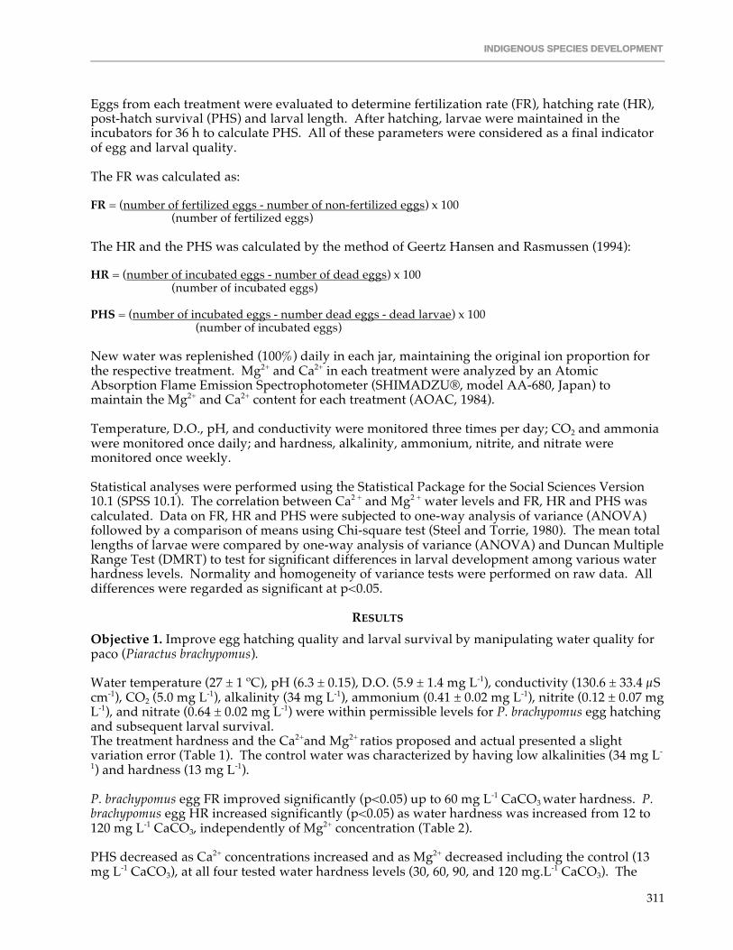
INDIGENOUS SPECIES DEVELOPMENT
311
Eggs from each treatment were evaluated to determine fertilization rate (FR), hatching rate (HR), post-hatch survival (PHS) and larval length. After hatching, larvae were maintained in the incubators for 36 h to calculate PHS. All of these parameters were considered as a final indicator of egg and larval quality. The FR was calculated as: FR = (number of fertilized eggs - number of non-fertilized eggs) x 100 (number of fertilized eggs) The HR and the PHS was calculated by the method of Geertz Hansen and Rasmussen (1994): HR = (number of incubated eggs - number of dead eggs) x 100 (number of incubated eggs) PHS = (number of incubated eggs - number dead eggs - dead larvae) x 100 (number of incubated eggs) New water was replenished (100%) daily in each jar, maintaining the original ion proportion for the respective treatment. Mg2+ and Ca2+ in each treatment were analyzed by an Atomic Absorption Flame Emission Spectrophotometer (SHIMADZU®, model AA-680, Japan) to maintain the Mg2+ and Ca2+ content for each treatment (AOAC, 1984). Temperature, D.O., pH, and conductivity were monitored three times per day; CO2 and ammonia were monitored once daily; and hardness, alkalinity, ammonium, nitrite, and nitrate were monitored once weekly. Statistical analyses were performed using the Statistical Package for the Social Sciences Version 10.1 (SPSS 10.1). The correlation between Ca2 + and Mg2 + water levels and FR, HR and PHS was calculated. Data on FR, HR and PHS were subjected to one-way analysis of variance (ANOVA) followed by a comparison of means using Chi-square test (Steel and Torrie, 1980). The mean total lengths of larvae were compared by one-way analysis of variance (ANOVA) and Duncan Multiple Range Test (DMRT) to test for significant differences in larval development among various water hardness levels. Normality and homogeneity of variance tests were performed on raw data. All differences were regarded as significant at p<0.05.
RESULTS
Objective 1. Improve egg hatching quality and larval survival by manipulating water quality for paco (Piaractus brachypomus). Water temperature (27 ± 1 ºC), pH (6.3 ± 0.15), D.O. (5.9 ± 1.4 mg L-1), conductivity (130.6 ± 33.4 µS cm-1), CO2 (5.0 mg L-1), alkalinity (34 mg L-1), ammonium (0.41 ± 0.02 mg L-1), nitrite (0.12 ± 0.07 mg L-1), and nitrate (0.64 ± 0.02 mg L-1) were within permissible levels for P. brachypomus egg hatching and subsequent larval survival. The treatment hardness and the Ca2+and Mg2+ ratios proposed and actual presented a slight variation error (Table 1). The control water was characterized by having low alkalinities (34 mg L-
1) and hardness (13 mg L-1). P. brachypomus egg FR improved significantly (p<0.05) up to 60 mg L-1 CaCO3 water hardness. P. brachypomus egg HR increased significantly (p<0.05) as water hardness was increased from 12 to 120 mg L-1 CaCO3, independently of Mg2+ concentration (Table 2). PHS decreased as Ca2+ concentrations increased and as Mg2+ decreased including the control (13 mg L-1 CaCO3), at all four tested water hardness levels (30, 60, 90, and 120 mg.L-1 CaCO3). The

TWENTY-FIFTH ANNUAL TECHNICAL REPORT – VOLUME I
312
highest FR, HR and PHS were obtained at the 50:50 ratio (Ca2+: Mg2+), particularly at water hardness between 30 to 60 mg L-1 CaCO3, and 11.9 mg L-1 Ca2+ and 7.6 mg L-1 Mg2+ at a pH of 6.3. P. brachypomus larval lengths were affected by Ca2+: Mg2+ proportions at water hardness levels of 30, 90, and 120 mg L-1 CaCO3 evaluated; with the most significant (p<0.05) being those at the 100:0 (Ca2+: Mg2+) ratios. No larval deformities were observed in any of the treatments groups.
DISCUSSION Amazon fish have evolved in an environment characterized by the low hardness and alkalinity waters of the basin, which are a consequence of its geologic constitution (Sioli, 1957). Our results with P. brachypomus eggs where FR, HR and PHS increased with water hardness near 60 mg L-1 CaCO3 and 50:50 (Ca2+: Mg2+) ratios (Table 2) are similar that those obtained with other teleost fishes by Molokwu and Okpokwasili (2002) with African catfish Clarias gariepinus, and by Silva et. al. (2003) with silver catfish Rhamdia quelen. Ca2 + proved to be a limiting ion in egg hatching and post hatching survival on P. brachypomus (Table 2). Ca2+ plays an important role in the chain reaction of fertilization in fish eggs in terms of stimulation, reception of stimulation, fertilization and activation of enzymes (Yamamoto, 1961). However, at 100:0 proportions (Ca2+: Mg2+), Ca2+ affected negatively HR and PHS at all water hardness levels evaluated. These results could be attributed to the fact that excess Ca2+ reduces water uptake by the egg (Ketola et al., 1988). The proportion that proved to be more suitable for P. brachypomus egg fertilization and hatching was the 50:50 (Ca2+: Mg2+) proportion. The uptake rate of Ca2+ and Mg2+ appears to depend on the total divalent ion concentration in the water and is dictated by the electrochemical potential difference between the chorionic fluid and the water (Van der Velden et al., 1991). The same authors observed the stimulation of Ca2+ uptake by common carp eggs by decreasing ambient Mg2+ levels, indicating a competition mechanism between Ca2+ and Mg2+ for passive uptake into developing eggs. The addition of waterborne Ca2+ above 12 mg L-1, irrespective of water hardness, is not recommended for incubation of P. brachypomus eggs because it negatively affects PHS. Early life stages of common carp Cyprinus carpio depend on Mg2+ in the water. Although the eggs and yolk contain significant levels of Mg2+, a low concentration in the water (< 0.243 mg L-1 Mg2+) leads to a decrease or arrest of the Mg2+ uptake by eggs, an increased mortality and higher levels of deformation, embolism and tissue necrosis (Van der Velden et al., 1991). P. brachypomus larval lengths were affected by Ca2+: Mg2+ proportions at water hardness levels of 30, 90, and 120 mgL-1 CaCO3; with the largest larval length being significant (p<0.05) among those at the 100:0 (Ca2+: Mg2+) ratios. According to our results, larval Ca2+:Mg2 ratio requirements are different than those for egg hatching. Although teleost larval gills (major Ca2+ intake organ) are under-developed, they still acquire Ca2+, presumably via the chloride skin cells (Hwang and Hirano, 1985).
CONCLUSION 1. P. brachypomus egg FR improved significantly (p<0.05) up to 60 mg L-1 CaCO3 water
hardness. 2. P. brachypomus egg HR increased significantly (p<0.05) as water hardness was increased,
independently of Mg2+ concentration.
3. PHS decreased for P. brachypomus as waterborne Ca2+ concentrations increased and as Mg2+ decreased, at all four water hardness levels tested.
4. The highest FR, HR and PHS were obtained at the 50:50 ratio (Ca2+:Mg2+), particularly at
water hardness levels between 30 to 60 mg L-1 CaCO3, and 11.9 mg L-1 Ca2+ and 7.6 mg L-1 Mg2+ at a pH of 6.3.

INDIGENOUS SPECIES DEVELOPMENT
313
5. P. brachypomus larval lengths were affected by Ca2+:Mg2+ proportions at water hardness levels of 30, 90, and 120 mg L-1 CaCO3, with the largest significant (p<0.05) differences being those at the 100:0 proportions (Ca2+: Mg2+).
ANTICIPATED BENEFITS
The study investigated key aspects of the reproductive biology of P. brachypomus, through a collaborative effort with Colombian investigators in order to improve or develop sustainable aquaculture technology. The main beneficiaries of the research will be the fish producers in the Amazon region. Development of the technology of intensive growth of these species and stocking 4 to 6 week-old fingerlings will dramatically increase their survival and efficiency of production. More importantly, this study also contributed towards institutional strengthening by providing training on various aspects of fish reproduction for staff of the Universidad Nacional de Colombia (Instituto de Investigaciones IMANI) and Instituto Amazónico de Investigaciones Científicas-SINCHI (Programa de Ecosistemas Acuáticos, Colombia), as well as serving as a thesis project for a student.
ACKNOWLEDGMENTS
We would like to acknowledge the assistance received from the Colombian student Adriana Soliris Corredor Castillo and to all technical assistants at La Terraza Aquaculture Research Facility, Universidad Nacional de Colombia.
LITERATURE CITED
Achard, F., Eva, H.D., Stibig, H.-J., Mayaux, P., Gallego, J., Richards, T., and Malingreau, J.-P. 2002. Determination of deforestation rates of the world's humid tropical forests. Science 297:999-1002.
Alderdice, D.F. 1988. Osmotic and ionic regulation in teleost eggs and larvae. In: Hoar, W.S., Randall, D.J. (Eds.), Fish Physiology: V. XI-Part A. Eggs and Larvae. Academic, San Diego, pp. 163-165.
AOAC (Association of Official Analytical Chemists). 1984. Official methods of analysis of the Association of Official Analytical Chemists. 14th ed. Arlington. VA 22209 USA : AOAC.
Bijvelds, M.J.C., Van Der Velden, J.A., Kolar, Z., and Flik, G. 1998. Magnesium transport in freshwater teleosts. Journal of Experimental Biology 201: 1981– 1990.
DeJesus, M.J. and C.C. Kohler. 2004. The commercial fishery of the Peruvian Amazon. Fisheries 29(4):10-16.
Eckmann, V.R. 1983. The fisheries situation in the Peruvian Amazon Region. Arch. Hydrobiol. 97: 509-539.
Eddy, F.B., Ward, M.R., Talbot, C.P. and Primmett, D. 1990. Ionic movement across the chorion in newly shed salmon eggs (Salmo salar L.). Journal of Comparative Physiology 159: 771– 776.
Geertz Hansen, P. and Rasmussen, G. 1994. Influence of ochre and acidification on the survival and hatching of brown trout eggs (Salmo trutta). In: Müller, R., Lloyd, R. (Eds.), Chronic Effects of Pollutants on Freshwater Fish. FAO-Fishing New Books, Cambridge. 317 pp.
Hwang, P.P., and Hirano, R. 1985. Effect of environmental salinity on intercellular organization and junctional structure of chloride cells in early stages of teleost development. Journal of Experimental Zoology 236: 115– 126.
Hwang, P.P., Tung, Y.C. and Chang, M.H. 1996. Effect of environmental calcium levels on calcium uptake in tilapia larvae (Oreochromis mossambicus). Fish Physiology and Biochemistry 15 (5): 363– 370.
Irion, G., Müller, J., Nunes de Mello, J. and Junk, W.J. 1995. Quaternary geology of the Amazonian Lowland. February 25, 2005. Geo-Marine Letters 15(2-4):172-178.
Ketola, H.G., Longacre, D., Greulich, A., Phetterplace, L., and Lashomb, R. 1988. High calcium concentration in water increases mortality of salmon and trout eggs. The Progressive Fish-Culturist 50: 129– 135.
TWENTY-FIFTH ANNUAL TECHNICAL REPORT – VOLUME I
314
Molokwu, C.N. and Okpokwasili, G.C. 2002. Effect of water hardness on egg hatchability and larval viability of Clarias gariepinus. Aquaculture International 10(1): 57–64.
Silva, L.V.F., Golombieski, J.I., and Baldisserotto, B. 2003. Incubation of silver catfish, Rhamdia quelen (Pimelodidae), eggs at different calcium and magnesium concentrations. Aquaculture 228: 279–287
Sioli, H. 1957. Sedimentation im Amazonasgebiet: Geologische Rundschau 45: 608–633. Steel, R.G.D. and Torrie, J.H. 1980. Principles and Procedures of Statistics. McGraw-Hill Book
Company, New York. Townsend, C.R. and Silva, L.V.F., Baldisserotto, B. 2003. Growth and survival of Rhamdia quelen
(Siluriformes, Pimelodidae) larvae exposed to different water hardness levels. Aquaculture 215: 103–108.
Tucker, C.S. and Steeby, J.A. 1993. A practical calcium hardness criterion for channel catfish hatchery water supplies. Journal of the World Aquaculture Society 24: 396– 401.
Van der Velden, J.A., Spanings, F.A.T., Flik, G., and Bonga, S.E.W. 1991. Early stages of carp (Cyprinus carpio) depend on ambient for their development. Journal Experimental Biology 158: 431– 438.
Woynarovich, E. 1986. Tambaqui e pirapitinga, propagação artificial e criação de alevinos. Companhia de Desenvolvimento do Vale de São Francisco, Publicação 2/86, Brasilia, Brasil, 68 p.
Yamamoto, T. 1961. The physiology of fertilization in fish egg. International Review of Cytology 12: 361– 405.

INDIGENOUS SPECIES DEVELOPMENT
315
INFLUENCE OF DIETARY FATTY ACID COMPOSITION ON REPRODUCTIVE PERFORMANCE OF COLOSSOMA MACROPOMUM
Twelfth Work Plan, Indigenous Species Development 6 (12ISD6)
Final Report Published as Submitted by Contributing Authors
Christopher C. Kohler, Susan T. Kohler,
William N. Camargo & Jesse T. Trushenski Southern Illinois University Carbondale, Illinois, USA
Fred Chu-Koo & Luis Campos-Baca Instituto de Investigaciones de Amazonia (IIAP)
Loreto, Péru
ABSTRACT In August 2007, spawning was initiated and gametes were successfully collected from two Colossoma macropomum females and five males within 24 h following priming and resolving doses of luteinizing hormone releasing hormone (LHRH, 25µg/kg intramuscular injections, given 12 hours apart). Each clutch of eggs was fertilized with milt from 2+ males and incubated in MacDonald jars at approximately 26 ±1 °C. Hatching activity began at approximately 36-48 hours post-fertilization and was completed within 72 hours post-fertilization. Although no attempts were made to quantify fertilization success or hatch rate, qualitative observations suggested high rate of success for both parameters. Five days after hatching, the fry were transferred to two, 0.1 acre ponds that had been filled with screened surface water. Approximately one month after stocking, the ponds were harvested and yielded approximately 1000, 2-4 cm fingerlings. This effort represents the first successful spawning and larval rearing of C. macropomum at Southern Illinois University Carbondale.
Unfortunately, for the purposes of the nutritional study, both mature females were from the low-HUFA treatment, preventing comparison between the dietary treatment groups. We believe the low rate of spawning success was due to the immaturity of most of the broodfish (~3-4 years of age at spawning). However, the fatty acid composition of the eggs from both females was determined. Compared to oocytes from white bass Morone chrysops (freshwater, temperate species) fed the same corn-oil based feed, C. macropomum oocytes contained more saturates and less unsaturates. 20:5n-3 and 22:6n-3, and total highly unsaturated fatty acid (HUFA) content were lower in C. macropomum oocytes, but the n-3 to n-6 ratio was the same for both species. Although saturates appear to be important constituents for C. macropomum oocytes, perhaps increasing membrane structural integrity at warmer temperatures, higher-than-expected levels of n-3 and HUFA suggest these FA may serve a functional role in oocyte/embryo development of C. macropomum. We have begun a repeat feeding trial and hope to collect gametes from a greater number of individuals during the 2008 spawning season to further address this hypothesis.
INTRODUCTION Success of commercial aquaculture is dependent on numerous factors, but perhaps the greatest limitation to industry growth and diversification is availability of viable fry and fingerlings. Although year-round, bulk availability of on-growing livestock has been achieved in some established sectors, such as the U.S. catfish industry, limited volume and/or temporal availability remain problematic for many species. Methods to optimize broodfish performance and ensure robust offspring must be developed to overcome bottlenecks in fingerling production. As a tolerant, fast-growing, highly sought food fish species, Colossoma macropomum is an excellent

TWENTY-FIFTH ANNUAL TECHNICAL REPORT – VOLUME I
316
candidate for aquaculture and is raised commercially in Latin America. However, complications in propagation of C. macropomum and restricted availability of progeny impede expansion of this emerging aquaculture industry. Nutrition is widely recognized as a determining factor in reproductive health and performance of vertebrates. Poor nutrition, either generally or with respect to certain critical dietary components, can impair reproductive output or result in complete loss of reproductive competence. Dietary lipid source, or more specifically, the fatty acid (FA) composition of the diet, has been shown to dramatically impact gamete production and offspring viability. Reproductive performance of broodfish is enhanced by dietary long-chain highly unsaturated fatty acids (HUFA), particularly arachidonic (20:4n-6, ARA), eicosapentaenoic (20:5n-3, EPA), and docosahexaenoic (22:6n-3, DHA) acids (Watanabe et al., 1984; Watanabe et al., 1985; Mourente and Odriozola, 1990; Fernández-Palacios et al., 1995; Bell et al. 1997; Fernández-Palacios et al., 1997; Navas et al. 1997; Almansa et al. 1999; Bruce et al., 1999; Mazorra et al., 2003; Lane and Kohler, 2006). Moreover, survival and vigor of offspring have been improved through maternal transfer of long-chain HUFA to developing fry (Fernández-Palacios et al., 1995; Lane and Kohler, 2006). Although the relationship between dietary FA composition and reproductive success is relatively well-established, the influence of dietary lipid source on C. macropomum reproduction has not been addressed. Adult C. macropomum have been described as predominantly frugivorous and, accordingly, most prepared feeds used in C. macropomum culture have relatively low nutrient density (14-35% crude protein, 3-10% crude lipid) and are largely comprised of carbohydrate-rich, plant-derived feedstuffs (Araujo-Lima and Goulding, 1997). However, zooplankton consistently represents a substantial portion of the natural adult diet (Campos-Baca and Kohler, 2006) and may represent as much as 95% of the diet during the dry season when fruits and seeds are unavailable (Oliveira et al., 2006). Fruits and seeds of terrestrial plants do not contain long-chain HUFA, and thus zooplankton consumed during the dry season serve as the primary source of intact HUFA for C. macropomum. Zooplanktivory associated with the dry season coincides with the period of gonadal maturation in the wild (da Silva et al., 2000), suggesting nutrients of animal origin support reproduction of C. macropomum. Given the fundamental relationship of HUFA and reproductive competence of vertebrates and the temporal link between HUFA consumption and spawning in the wild, it is reasonable to assume dietary HUFA content is functionally related to reproductive performance of C. macropomum. Supplementing broodstock diets for C. macropomum with long-chain HUFA may enhance production of quality gametes and survivability of resultant fry, however, the effect(s) of dietary FA profile on reproduction of this species has not been quantitatively assessed. Accordingly, our objectives were to quantify the reproductive performance and gamete quality of C. macropomum broodfish fed diets containing different levels of HUFA, and to assess the viability and stress tolerance of the resultant progeny.
MATERIALS AND METHODS Objective 1. Quantify the effect(s) of dietary highly unsaturated fatty acid (HUFA) content on fecundity of female C. macropomum; egg lipid content and fatty acid (FA) composition; as well as egg fertilization and hatching rates. Two iso-caloric, iso-nitrogenous (45% crude protein, 12% crude lipid, dry matter basis) practical diets were formulated, differing only in primary lipid source and HUFA content. One diet was formulated as a high-HUFA content diet and contained menhaden fish oil (FO) as the primary lipid source, whereas the other was formulated as a low-HUFA content diet and contained canola oil (FO). Both diets were produced as floating, extruded feeds by a commercial aquafeed manufacturer, and stored refrigerated prior to use. Crude dietary composition was confirmed according to standardized methods for animal feeds (AOAC 1995). Diet samples were prepared for FA analysis according to the methods of Folch et al. (1957) and Christie (1982), and analyzed according to standard gas chromatography procedures used in our laboratory. Induction of gonadal maturation and collection of gametes, facilitated by use of exogenous hormone preparations, was conducted as described by Campos-Baca and Kohler (2006). Both groups were spawned in early summer, 2007.

INDIGENOUS SPECIES DEVELOPMENT
317
Statistical Analyses: All data were subjected to analysis of variance (ANOVA) using the General Linear Model of the Statistical Analysis System, version 9.1 (SAS Institute, Cary, North Carolina, USA). Differences were considered significant at p < 0.05.
Objective 2. Compare results of Objective 1 with gametes from broodstock reared in Iquitos, Peru. Mixed-sex groups of adult C. macropomum were stocked in 10, 1900- L tanks within a recirculation system. Each diet was assigned to 5 tanks each, individual tanks served as experimental units. For 9-12 months prior to spawning, fish were fed assigned feeds to apparent satiation. Broodstock at the IIAP field station were fed their standard diets (Campos-Baca and Kohler 2006; Table 1). Unfortunately, C. macropomum bloodstock did not successfully spawn and no data were collected for this objective. However, a comparison was made with white bass Morone chrysops broodstock fed the same diets as the pacu that spawned. Objective 3. Quantify the effect(s) of dietary HUFA content on semen volume and spermatozoan density; as well as spermatozoan motility, lipid content, and FA composition. Semen volume from the few sexually mature males available was only sufficient in volume for fertilizing eggs and no data could be collected for this objective. Objective 4. Assess 10-day survival of resultant larvae under normal culture conditions and after temporary heat stress. With only two females successfully spawning, and both being from the same treatment group, this objective could not be addressed.
RESULTS In August 2007, spawning was initiated and gametes were successfully collected from two females and 5 males within 24 h following priming and resolving doses of luteinizing hormone releasing hormone (LHRH, 25µg/kg intramuscular injections, given 12 hours apart). Each clutch of eggs was fertilized with milt from 2+ males and incubated in MacDonald jars at approximately 26 ±1 °C. Hatching activity began at approximately 36-48 hours post-fertilization and was completed within 72 hours post-fertilization. Although no attempts were made to quantify fertilization success or hatch rate, qualitative observations suggested high rate of success for both parameters. Five days after hatching, the fry were transferred to two, 0.1 acre ponds that had been filled with screened surface water. Approximately 1 month after stocking, the ponds were harvested, yielded approximately 1000, 2-4 cm fingerlings. This effort represents the first successful spawning and larval rearing of C. macropomum at Southern Illinois University Carbondale. Unfortunately, for the purposes of the nutritional study, both mature females were from the low-HUFA treatment, preventing comparison between the dietary treatment groups. We believe the low rate of spawning success was due to the immaturity of most of the broodfish (~3-4 years of age at spawning). However, the fatty acid composition of the eggs from both females was determined (see Table 1). Compared to oocytes from white bass Morone chrysops (freshwater, temperate species) fed the same corn-oil based feed, C. macropomum oocytes contained more saturates and less unsaturates. 20:5n-3 and 22:6n-3, and total highly unsaturated fatty acid (HUFA) content was lower in C. macropomum oocytes, but the n-3 to n-6 ratio was the same for both species. Although saturates appear to be important constituents for C. macropomum oocytes, perhaps increasing membrane structural integrity at warmer temperatures, higher-than-expected levels of n-3 and HUFA suggest these FA may serve a functional role in oocyte/embryo development of C. macropomum.

TWENTY-FIFTH ANNUAL TECHNICAL REPORT – VOLUME I
318
Although WP 12 is coming to a close, we have begun a repeat feeding trial and hope to collect gametes from a greater number of individuals during the 2008 spawning season to further address this hypothesis and complete objectives not fully addressed.
ANTICIPATED BENEFITS
We expected dietary HUFA content to modulate reproductive performance of C. macropomum. If inclusion of marine-derived lipid enhances performance of broodfish and progeny, inclusion of these high HUFA-content products may increase productivity of C. macropomum hatcheries. If increased HUFA content does not improve performance, producers and feed manufacturers will have more information to facilitate least-cost diet formulation for these fish.
CONCLUSIONS Compared to oocytes from white bass Morone chrysops (freshwater, temperate species) fed the same corn-oil based feed, C. macropomum oocytes contained more saturates and less unsaturates. 20:5n-3 and 22:6n-3, and total highly unsaturated fatty acid (HUFA) content was lower in C. macropomum oocytes. The n-3 to n-6 ratio was the same for both species. Although saturates appear to be important constituents for C. macropomum oocytes, perhaps increasing membrane structural integrity at warmer temperatures, higher-than-expected levels of n-3 and HUFA suggest these FA may serve a functional role in oocyte/embryo development of C. macropomum.
LITERATURE CITED Almansa, E., M.J. Pérez, J.R. Cejas, P. Badía, J.E. Villamandos, and A. Lorenzo. 1999. Influence of
broodstock gilthead seabream (Sparus aurata L.) dietary fatty acids on egg quality and egg fatty acid composition throughout the spawning season. Aquaculture 170:323-336.
AOAC (Association of Official Analytical Chemists). 1995. Official methods of analysis, 15th edition. Association of Official Analytical Chemists, Washington, D.C.
Araujo-Lima, C., and M. Goulding. 1997. So fruitful a fish: ecology, conservation, and aquaculture of the Amazon’s tambaqui. Columbia University Press, New York, New York.
Bell, J.G., B.M. Farndale, M.P. Bruce, J.M. Navas, and M. Carillo. 1997. Effects of broodstock dietary lipid on fatty acid compositions of eggs from sea bass (Dicentrarchus labrax). Aquaculture 149:107-119.
Bruce, M., F. Oyen, G. Bell, J.F. Asturiano, B. Farndale, M. Carrillo, S. Zanuy, J. Ramos, N. Bromage. 1999. Development of broodstock diets for the European sea bass (Dicentrarchus labrax) with special emphasis on the importance of n-3 and n-6 highly unsaturated fatty acid to reproductive performance. Aquaculture 177:85-97.
Campos-Baca, L., and C.C. Kohler. 2006. Aquaculture of Colossoma macropomum and related species in Latin America. Pages 541-561 in A.M. Kelly and J. Silverstein, editors. Aquaculture in the 21st Century. American Fisheries Society, Bethesda, Maryland.
Christie, W.W. 1982. The preparation of derivatives of lipids. Pages 51-61 in W. W. Christie, editor. Lipid Analysis 2nd Edition. Pergamon Press, Oxford, United Kingdom.
da Silva, J.A.M., M. Pereira-Filho, and M.I. de Oliveira-Pereira. 2000. Seasonal variation of nutrient and energy in tambaqui’s (Colossoma macropomum Cuvier, 1818) natural food. Reviews in Brasilian Biology 60(4):599-605.
Fernández-Palacios, H., M.S. Izquierdo, L. Robaina, A. Valencia, M. Salhi, and J. Vergara. 1995. Effect of n-3 HUFA level in broodstock diets on egg quality of gilthead seabream (Sparus aurata L.). Aquaculture 132:325-337.
Fernández-Palacios, H., M.S. Izquierdo, L. Robaina, A. Valencia, M. Salhi, and D. Montero. 1997. The effect of dietary protein and lipid from squid and fish meals on egg quality of broodstock for gilthead seabream (Sparus aurata). Aquaculture 148:233:246.
Folch, J., M. Lees, and G.H. Sloane-Stanley. 1957. A simple method for the isolation and purification of total lipids from animal tissues. Journal of Biological Chemistry 276:497-507.

INDIGENOUS SPECIES DEVELOPMENT
319
Lane, R.L., and C.C. Kohler. 2006. Effects of dietary lipid and fatty acids on reproductive performance, egg hatchability, and overall quality of progeny of white bass Morone chrysops. North American Journal of Aquaculture 68:141-150.
Mazorra, C., M. Bruce, J.G. Bell, A. Davie, E. Alorend, N. Jordan, J. Rees, N. Papanikos, M. Porter, N. Bromage. 2003. Dietary lipid enhancement of broodstock reproductive performance and egg and larval quality in Atlantic halibut (Hippoglossus hippoglossus). Aquaculture 227:21-33.
Mourente, G., and J.M. Odriozola. 1990. Effect of broodstock diets on lipid classes and their fatty acid composition in eggs of gilthead sea bream (Sparus aurata L.). Fish Physiology and Biochemistry 8:93-101.
Navas, J.M., M. Bruce, M. Thrush, B.M. Farndale, M. Bromage, S. Zanuy, M. Carrillo, J.G. Bell, and J. Ramos. 1997. The impact of seasonal alteration in the lipid composition of broodstock diets on egg quality in the European sea bass. Journal of Fish Biology 51:760-773.
Oliveira, A.C.B., L.A. Martinelli, M.Z. Moreira, M.G.M. Soares, and J.E.P. Cyrino. 2006. Seasonality of energy sources of Colossoma macropomum in a floodplain lake in the Amazon—lake Camaleão, Amazonas, Brazil. Fisheries Management and Ecology 13:135-142.
Watanabe, T., T. Takeuchi, M. Saito, and K. Nishimura. 1984. Effect of low protein-high calory or essential fatty acid deficiency diet of reproduction of rainbow trout. Nippon Suissan Gakkaishi 50:1207-1215.
Watanabe, T., T. Koizumi, and H. Suzuki. 1985. Improvement of quality of red sea bream eggs by feeding broodstock on a diet containing cuttlefish meal or raw krill shortly before spawning. Nippon Suisan Gakkaishi 51:1511-1521.

TWENTY-FIFTH ANNUAL TECHNICAL REPORT – VOLUME I
320
Table 1. Relative fatty acid methyl ester (%FAME) composition of oocytes from Colossoma macropomum and Morone chrysops fed diets containing corn oil as the supplementary lipid source. Fatty Acid(s) Pacu Oocyte White Bass
14:0 1.0 1.6 16:0 23.3 11.9 18:0 12.9 3.5 Saturates 37.2 17.6 16:1n-7 2.9 12.2 18:1n-7 2.6 4.4 18:1n-9 26.3 20.1 MUFA2 32.8 37.4 18:2n-6 9.4 15.2 20:4n-6 1.0 3.2 n-6 12.3 19.7 18:3n-3 0.8 3.4 18:4n-3 0.1 0.1 20:4n-3 0.2 0.5 20:5n-3 4.0 4.8 22:5n-3 1.7 1.8 22:6n-3 10.5 14.6 n-3 17.5 25.1 PUFA3 29.9 44.9 HUFA4 18.0 25.0 18C PUFA5 10.4 19.3 n-3:n-6 1.4 1.4
1. Values represent mean egg composition from 2+ females. 2. Monounsaturated fatty acids—sum of all FA with a single double bond. 3. Polyunsaturated fatty acids—sum of all FA with ≥ 2 double bonds. 4. Highly unsaturated fatty acids—sum of all FA with chain length ≥ 20 carbon atoms
and double bonds ≥ 3. 5. PUFA with chain length of 18 carbon atoms.
WATER QUALITY & AVAILABILITY
321
POND DESIGN AND WATERSHED ANALYSES TRAINING
Twelfth Work Plan, Water Quality & Availability 1 (12WQA1) Final Report
Published as Submitted by Contributing Authors
E. W. Tollner University of Georgia Athens, Georgia, USA
Dan Meyer & Suyapa Triminio-Meyer
Escuela Agrícola Panamericana Zamorano, Honduras
Joseph J. Molnar
Auburn University Auburn, Alabama, USA
ABSTRACT The overall project objective was to conduct training in pond design and watershed analysis for technical staff and managers in Central American nongovernmental organizations and governmental resource management agencies. Variable rainfall distribution and terrain make surface water harvesting and storage a challenge in many developing countries. The development of watershed assessment tools and pond design tools served as a basis for numerous training programs in Honduras and other Central American countries. The specific object of this study is to collect and develop cost information required to equip extension, nongovernmental organization (NGO) agents, contractors and engineers for surface water development and aquaculture enterprise development in Honduras and Latin America. A spreadsheet-based computational tool was developed in English and Spanish on the Microsoft Excel® platform. Knowing the original land slope and desired pond volume, one may compute excavation amounts that provide an acceptable cut-fill balance. The model computes projected costs in local currency. Guidelines are provided for establishing pond bottom elevations and achieving the desired water depth. The model is relevant for hillside or levee ponds customarily used in aquacultural production. The model is not suitable for a watershed catchment pond. The model completes a package for designing hillside and levee pond-based aquaculture systems. Coupling these with other cooperative development concerns such as marketing association provides a platform for helping groups of people in a watershed to realize further the potential of enlightened self-interest in developing common solutions to water problems. The economic analyses software tool is the third of three tools that comprise the basic suite of tools and accompanying presentations used for technician training and development.
INTRODUCTION Honduras is a developing Central American country of approximately 11 million hectares with both Atlantic and Pacific coasts. Mountains may be as high as 2600 meters. Rainfall varies from 600 mm to 3400 mm annually, with the highest precipitation generally associated with higher elevations (Anon, 2001). Temperatures above 1300 meters are usually too cool for some economically important fish specie (e.g., Tilapia) production. Rainfall is unevenly distributed in the elevations where fish would most likely be produced, which requires innovative schemes for water supply development. The wide diversity in elevation and rainfall, coupled with enterprise driven needs for water development and the need to make the results accessible to local producers via a suitable network of non-governmental organization representatives motivated the development of a water supply analysis and training software suite.

TWENTY-FIFTH ANNUAL TECHNICAL REPORT – VOLUME I
322
The most common approach for supplying small to medium sized communities and ponds with water is the water tube-spring. For this supply, polyvinylchloride or polyethylene pipe (12 mm to 25 mm diameter) is directed down slope from a naturally occurring spring to a site, which may be a kilometer or more from the spring. Springs are prevalent in mountainous areas at altitudes below 1300 meters. The excavated earthen levee pond is currently the most popular containment for fish production. Hillside levee ponds (excavated levee on a hillside and supplied via a diversion ditch or other means) are not widely used. Watershed ponds are not widely used because steep valleys do not readily enable suitable diversion spillways for adequate handling of high runoff rates during rainy seasons. Tollner et al (2004) provides a spreadsheet implementation of the hillside and levee pond design for water supply development. This paper documents many of the issues associated with diffusing computer technology into developing countries. There is a budding willingness to cooperate, particularly when it is in their interest to do so (not unlike anywhere in the world), based on assessments of cooperative marketing and production of Tilapia in the region. The enlightened self-interest idea represents our reason for optimism in continuing the pursuit of the modeling strategy. There are resources available for pond design and watershed assessment. Nath et al. (1995) present a comprehensive pond water quality simulation model. Yoo and Boyd (1994) summarize the state-of-the-art in pond hydrology. Commercially available software for pond design economic analyses is available (e.g., AquaCAD2, AutoCAD Land Desktop), however, much technical skill is required for appropriately using both these versatile, expensive tools. The Food and Agriculture Organization has been interested in water resources development in the developing world and have published a recent guide on pond design (Coche et al., 1995) that does not discuss economic aspects. We therefore choose to develop a simple tool that is appropriate for small and medium sized producers desiring a hillside or levee pond. Figure 1 shows some details of hillside, levee and watershed ponds. The watershed pond case is not addrssed by the model herein but is shown to provide a clear definition of a case not covered. The overall goal of this study is to Conduct training in pond design and watershed analysis for technical staff and managers in Central American non-governmental organizations and governmental resource management agencies. This report completes a software suite for collecting and developing information required to facilitate pond design in Central America and other developing countries. We chose Microsoft Excel® because it is widely available. The specific objectives is to develop an Excel® model that will compute pond and water volumes, cut-fill ratios and cost estimates for hillside and levee ponds. Iterative use of the economics model, will allow assessment of sustainability of the proposed pond. Model Development The model is based on soil and water volume calculations, and economics of excavation are computed by applying a cost per unit volume of soil moved to the total volume of soil excavated. To begin building the spreadsheet model, we defined 22 rows and 22 columns of cells to represent the water-filled volume of the pond. Additionally, four rows of cells and four columns of cells surround the water volume to represent the berm around the pond. The essence of the approach is to let each cell in the spreadsheet represent a defined area of the pond-to-be. Cells in the surrounding berm area may also be scaled to reflect realistic outside slope conditions (three boundary row-columns) and the berm width (the fourth row or column into the pond). Cells interior to the fourth row or column represent the wetted pond volume and may be collectively scaled in width and length dimensions (e.g., X, into the slope; and Y, along the contour) to enable the 22 rows/columns represent a realistic pond size. English or SI units are available for use. The numerical entry into each cell represents the elevation relative to a nearby benchmark elevation. A utility is available to insert slopes to calculate automatically the initial elevations. A copy of the spreadsheet with an initial set of elevations for a hypothetical pond is shown in Figure 2. The 2 AquaCAD Pond Design software, Louisiana Autodesk, Inc.; 111 McInnis Parkway, San Rafael, CA 94903 USA

WATER QUALITY & AVAILABILITY
323
spreadsheet was structured around linked pages that enables computations on one page to be linked to data on other pages. Hyperlinks were established to further enhance navigation from one page to the other. A separate page reflects the final excavated elevations. Each cell must contain an elevation that reflects realistic slope conditions (e.g., a 2:1 or 3:1 {horizontal: vertical} slope is recommended within the wetted volume). After setting an elevation for maximum water depth, one may estimate the required elevation of each cell to achieve the desired side slope on the pond sides along the original slope and normal to the original slope. One can then use the ‘drag-drop’ feature to minimize the number of hand entries. Interior slopes should be first created, then one may use ‘drag-drop’ to complete the entries. An example of a model page showing an excavated hypothetical pond is shown in Figure 3. The water elevation is then established. On a similar page to the excavation page, the elevation of the water surface is entered using the ‘drag-drop’ utility. One should confirm that the water depth is satisfactory. The water volume is computed by the length x width x water depth computation. A formula in the background sums these results for all cells with a positive water volume to give a total pond volume. Results for the hypothetical pond are shown in Figure 4. The model computes the pond showing the cuts, fills, and composite cut-fill results for the pond volume relative to the initial topography. Composite cut-fill results for the hypothetical pond are shown in Figure 5. It is assumed here that the soil is suitable for sealing. Cuts are shown as positive departures from the original surface and fills are shown as negative departures from the original surface. A cut-fill ratio is computed, which should lie between 1.2 and 1.5. The cut-fill ratio should be greater than 1 to enable some compaction. A review of the cut-fill diagram enables a ready check on data accuracy, for example, Figure 5 reflects some minor data entry errors in that there are indicated cuts where the data should require a fill. Errors of this type can be readily fixed by reviewing the other model pages. Summary data, including cost, are shown on a separate sheet (see Figure 6). The model computes the time required to excavate the pond based on the volumetric capacity of common construction equipment. Knowing the equipment time enables ready calculation of equipment costs and labor costs for excavating the pond.
RESULTS AND DISCUSSION To facilitate use of the model in training classes, a ‘follow-the-numbers’ approach was adopted. Eight entries are required for the initial page and two entries are required for the summary page. Complete directions are provided on the introductory page of the model and are summarized in Table 1. Some guidelines for using the model emerged from applications. In locations where soils are suitable for sealing, ponds may be built using a cut-fill ratio ranging from 1.2 to 1.5. Yoo and Boyd (1994), Coche et al (1995) and Tollner et al (2004) discuss details of pond construction and site evaluation. One should remove the top 0.15 to 0.3 meters of soil as the top layer is frequently unsuitable for use as fill material. It is suggested that, on a uniform slope not exceeding 8% to 10%, one would set the pond bottom elevation at that of the soil surface (after removal of the top 0.15 to 0.3 m) about 1/3 to 1/4 the pond width as measured from the down slope (e.g., fill) end to the upslope (e.g., cut) level. On a level site one would establish a pond bottom elevation somewhat below the soil elevation to begin the process. The setting of the pond bottom elevation to yield an excavation plan that gives the cut-fill ratio within the 1.2 to 1.5 range is inherently an iterative process. Slopes exceeding 3 or 4 % require much excavation if one is to maintain the Yoo and Boyd (1994) recommendation that ponds be approximately square. Slopes exceeding 8% are not amenable for pond construction. The hypothetical pond shown is on an 8% slope and the width scale factor (X, up slope) is 1.2 units per cell while the length (Y, along contour) was 9.5 units per cell. In cases

TWENTY-FIFTH ANNUAL TECHNICAL REPORT – VOLUME I
324
where some or all of the fill material was not used on site, one would monitor both the cut volume to achieve the desired pond size. The hypothetical pond computations were performed in English units, although SI units could have been used if desired. The clientele have been favorably impressed by the capability of the model and their ability to use the model. The tedious data entry requirement of the final excavation elevations, compounded by the realization that multiple iterations will be required for each design is the only major drawback to the use of the model. Only very sophisticated programs such as AutoCAD Land Desktop are able to automate this process, and only then if sophisticated automated survey data are available. We anticipate continued increases in model usage as the clientele become more familiar and comfortable with what the model does. For example, in earlier workshops the point had to be carefully that the model computation did not automatically impose soil properties on a given site. Nongovernmental organization (NGO) personnel and technically trained personnel have demonstrated good grasp of the capabilities and limitations of the models. Water resources development is become increasingly recognized as a critical need in Honduras and many other developing countries. As the popularity of tilapia increase, so will the demand for adequate water supplies. This tool is useful for evaluating water resources on upland watersheds (<500 ha) and can complement larger, basin scale watershed development work. We anticipate continued increases in model usage. The model is employed in instruction at Zamorano University and at the University of Georgia. Based on repeat attendees at the series of workshops, we feel that the model has begun to catch on and that its use will continue to grow. The ultimate limiting factor of the use of this and other models in Tollner et al 2004 is no doubt social, given the fact that water movement and control is not limited to territory that any one person may control. Historical successes in managing at the watershed scale require the realization that the desired outcome rests beyond the individual but can be influenced at the societal level. Religious systems in antiquity worked toward this end. Lansing (1991) provides an interesting discussion of how water management was embodied in religious systems of Bali, persisting into the 19th century. Watersheds there were controlled by the priesthood of a series of water temples. The priesthood maintained historical records and used weirs to monitor flow rates well before weir hydraulic processes were well understood in the west. This system represents the highest form of enlightened self-interest. Enlightened self-interest is the key to the advancement of water management in most parts of the world. Success in advancing models such as shown in this paper will depend on our ability to convey this vision. The notion that marketing association development can solidify the benefits of working together provides a platform from which one can propagate the idea of community water supply development.
ANTICIPATED BENEFITS Economics are an important component of the pond design and build decision. This tool, along with the water balance and water supply tools recently developed, completes the package of pond design tools. The economic analysis has been integrated with other pond design presentations in Central America. A recent workshop was completed in the Dominican Republic (The trip report is attached in Appendix A). Details of our 2007 CostaRica/Panama workshop are attached as Appendix B.
CONCLUSIONS The spreadsheet (particularly, Microsoft Excel) platform is widely available, portable, easy to follow and highly interactive. The platform can easily be adapted to include more sophisticated analyses approaches as data becomes available. The major disadvantage of the platform is that detailed data entry requirements simply are unavoidable for the excavation volume calculation. Guidelines were provided to minimize the negative impacts of the inherent iterative nature of the pond design process. The economics component completed the overall objective of the study and gave a concise view of how one may cope with extremely variable rainfall patterns and
WATER QUALITY & AVAILABILITY
325
development an economically feasible management approach. The overall object of providing training in watershed assessment and economical pond design was met in each training session.
ACKNOWLEDGMENTS The authors express grateful appreciation to Mr. Pablo Martinez for his assistance in translating the spreadsheet models and other accompanying materials to Spanish. The authors acknowledge the support of the PD/A CRSP as well as the Georgia Agricultural Experiment Stations in making the work possible.
LITERATURE CITED Coche, A.G., J.F. Muir and T. Laughlin. 1995. Pond Construction for freshwater fish culture. FAO
Training Series 20/1. FAO, Rome, Italy. Lansing, J. S. 1991. Priests and programmers: Technologies of power in the engineered landscape
of Bali, Princeton Univ. Press, Princeton, NJ. Nath, S.S., J. P. Bolte and D. H. Ernst. 1995. Decision support for pond aquaculture planning and
management. Presented at the Sustainable Aquaculture Conference, PACON International, June 11-14, Hololulu, HI. Available at www.biosys.bre.orst.edu/pond/sustaqua/sustaqua.htm.
Tollner, E.W. 2002. Natural Resources Engineering, Iowa State University Press, Ames, IO. Tollner, E.W., D. Meyer, S. Triminio-Meyer, B. Verma, G. Pilz and J.J. Molnar. 2004. Spreadsheet
tools for developing surface water supplies for freshwater fish in developing countries. Jour. Of Aquacultural Engineering 31(1-2):31-49.
Yoo, K.H. and C.E. Boyd. 1994. Hydrology and water supply for pond aquaculture. Chapman & Hall, New York, NY.

TWENTY-FIFTH ANNUAL TECHNICAL REPORT – VOLUME I
326
Photo 3. Participants in the pond design and construction course, Santiago, Dominican Republic, April, 2006.
Photos 5 and 6. Field and classroom activities during the courses
Photo 4. Courses facilitators: Daniel Meyer, Suyapa Triminio Meyer y William Tollner, ISA Dominican Republic, April, 2006.
Photo 1 (left). Inauguration ceremony in ISA Campus (from right to left, Ing.Leonel Guerrero, (DR AGEAP member), Dr. Daniel Meyer (Zamorano), Ing. Mercedes Garcia Marin (IDIAF), Ing. Benito Ferreiras (ISA), M.Sc. Suyapa Triminio Meyer (Zamorano), Dr. William Tollner (University of Georgia), Ing. Pilar Ramirez, (DR AGEAP member). Photo 2 (right). Participants from Dominican Republic and Haiti to the tilapia production and marketing course, ISA, Santiago, Dominican Republic, April, 2006
WATER QUALITY & AVAILABILITY
327
Table 1. Summary directions for use of the pond economics model. The Levee Pond Cost Estimator was developed to aid in computing the cost of excavating a Levee pond. The model figures the volume of the cut, the fill volume and the volume of water in the pond. The cost of excavating the pond using a primary excavator(s) plus other machinery that may be engaged for a fraction of the time required for primary excavation. The slope of the site is assumed uniform and may range from 0 to 15%. The pond is represented by a block of cells, with the outside three rows representing the bank, the next cell in represents the top of the dam and the remaining inner cells represent the water-covered area. The initial volume is set by entering a reference elevation plus the slope and the model fills in the remaining cells. In the final volume page, the user must manipulate the cells to insure a 3:1 slope on the wet side and a 2:1 slope on the outside. The user may take maximum advantage of the auto fill feature of Excel on the final volume sheet. The user must then select the modeled water elevation after satisfying the cut-fill ratio of 1.2 to 1.5. The user must select the capacity of soil moved per hour by the excavator. The cost per hour of renting the excavator must be supplied by the user. The user must also account for other machines sch as rollers and haulers that are used in construction of the pond by lumping them with the primary excavator. Skills and other items needed: 1) Ability to read a topographic map and use a scale; 2) surveying level; 3) knowledge of how to compute areas; 4) knowledge for evaluating soils and other site conditions; and, 5) availability of equipment and skilled operators.
1. Obtain a topographic map of the site. Tab to the Initial page and input scaled length and width. Enter the length (1); choose units (2) and width (3). Enter the depth (4). Enter the scaled distance of the exterior bank (distance per cell) in the x (5) and y (6) directions. Enter the reference leftside elevation (8). The model computes scale factors, which are in general not equal. The model then fills in the elevation values assuming a uniform slope. The actual water-containing part and top width are enclosed in dotted lines.
2. Tab to the Final page. Input the final dimensions after the cut and fill is finished. Note that slopes inside the wetted area should be 3:1 and slopes outside the wetted area may be 2:1. One will use judgment to set evaluations of the exterior banks based on the scale factors here. Likewise, one will use judgment on the inside slope to establish an approximate Z=3 here. All this must be done manually, using auto fill where possible. Much trial and error required to get this sheet correct. Look at the Results page frequently to ensure reasonable results.
3. Tab to the Water page. Input the water depth inside the dotted area. Note that water depth
must be greater than the final cut value at any portion of the pond. Note that the auto fill is very convenient for this task. As a final check, be sure the scale dimensions on the input page are all reasonable. Water volume is computed below. Check the water volume cells to insure that none are negative. This is a good check.
4. View the results of the cut and fill analyses on the Results page. A composite cut-fill
diagram, a cut diagram, a fill diagram and a final construction height diagram are provided.
5. Tab to the summary page. The ratio of cuts to fills should be between 1.2 and 1.4. One
must have knowledge of the machine hours required per unit volume (9). One must also have knowledge of the hourly price of the excavator (10). One may then compute the estimated cost.
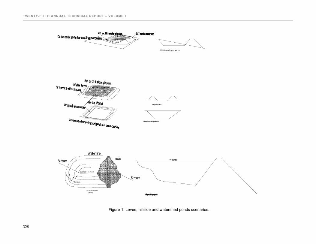
TWENTY-FIFTH ANNUAL TECHNICAL REPORT – VOLUME I
328
Levee pond cross section
Levee pond cross section, spoil removed
Hills ide pond cross section
Plan view of w atershed pond
(not to sca le)
Co n to u rs
Pond Dam
Watershed pond cross section along submerged stream
Su b me rg e d s tre a m
Stream
Stream
Water lineWater line
Figure 1. Levee, hillside and watershed ponds scenarios.
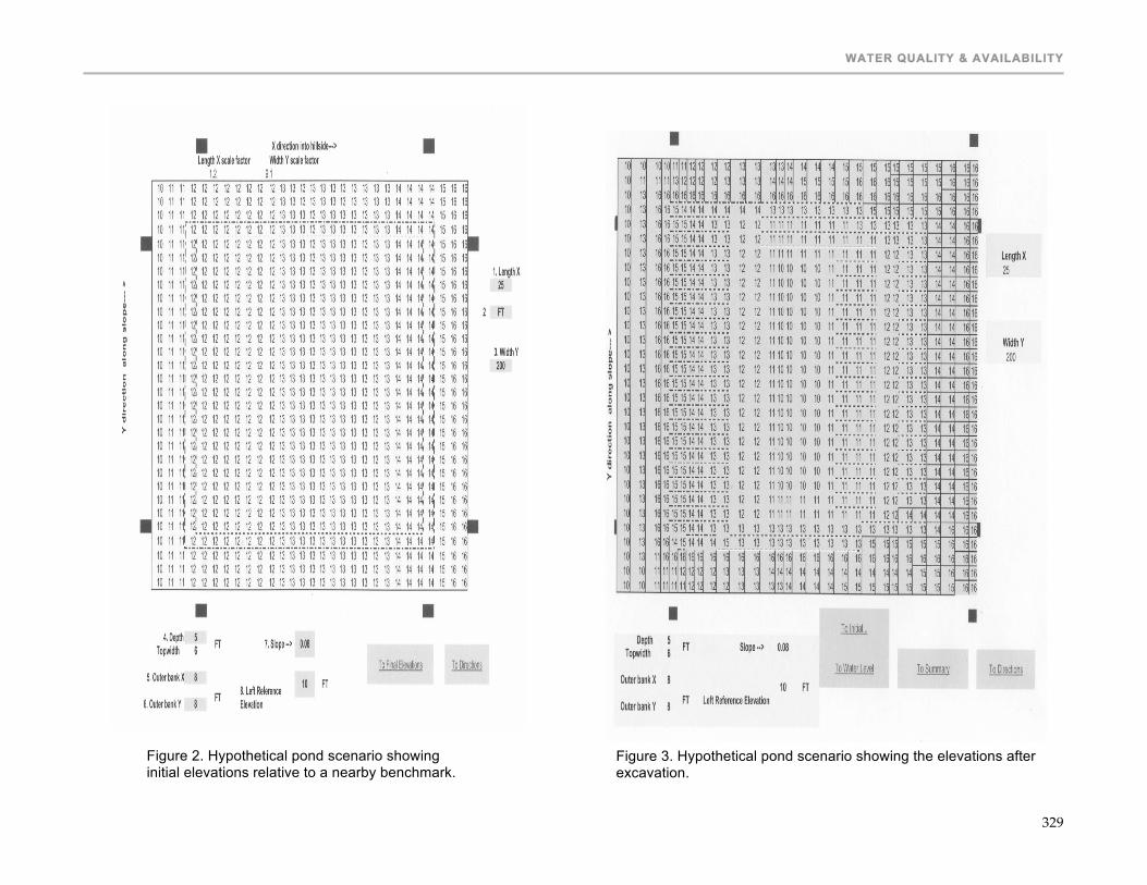
WATER QUALITY & AVAILABILITY
329
Figure 2. Hypothetical pond scenario showing
initial elevations relative to a nearby benchmark.
Figure 3. Hypothetical pond scenario showing the elevations after excavation.

TWENTY-FIFTH ANNUAL TECHNICAL REPORT – VOLUME I
330
Figure 4. The cut-fill (fill negative, light shade and cut is positive, darker shade) diagram for the hypothetical pond.
Figure 5. Hypothetical pond showing exterior and wetted volume excavations at the design water depth.

WATER QUALITY & AVAILABILITY
331
Figure 6. Summary data for the hypothetical pond scenario.

TWENTY-FIFTH ANNUAL TECHNICAL REPORT – VOLUME I
332
APPENDIX A
ZAMORANO AQUACULTURE CRSP-HONDURAS
INTERNATIONAL COURSE ON TILAPIA CULTURE AND MARKETING, AND POND DESIGN AND CONSTRUCTION FOR AQUACULTURE AND WATER HARVEST
SANTIAGO, DOMINICAN REPUBLIC APRIL 10 AND 11, 2006
Introduction Daniel Meyer (DM) and Suyapa Triminio Meyer (STM) offered a short course on the fundamentals of tilapia culture to 43 participants in the Dominican Republic as part of our ACRSP activities in Honduras. We also coordinated the logistics and promotion of a course on pond construction given by Dr. Bill Tollner of the University of Georgia (UGA). The courses were planned with the objective to expose participants from Haiti and the Dominican Republic to the fundamentals of tilapia culture and pond construction. The courses were given simultaneously at the “Instituto Superior de Agricultura” (ISA), in Santiago de Los Caballeros, DR. Much of the preparatory work for the two courses was performed by members of the Association of Graduates of Zamorano in the DR. These preparations included selection of the site for teaching the courses, organizing the logistics and accommodations for the ACRSP team members and participants in Santiago, obtaining the photocopies of materials for use in the courses and attention to all relevant details. Leonel Guerrreo (Zamorano class 1970) and Pilar Ramirez (Zamorano class 1975) were instrumental in these activities. ISA has excellent facilities for short courses and for teaching aquaculture. The tilapia course was offered in an amphitheatre type classroom using a multimedia projector. The room was comfortable and located in an area on campus removed from most distractions and noise. The course on tilapia culture had 43 participants (Appendix 1) and included the following topics and activities: Day-one:
• Inauguration of the courses with comments by Ing. Benito Ferreiras, Director of the ISA
• Talk on the status of aquaculture in the DR (Ing. Mercedes Garcia, IDIAF) • Tilapia culture in Latinamerica (DM) • Biology of tilapia (DM) • Reproduction of tilapia (DM) • Production costs in tilapia culture (STM) • Pond construction (DM) • Pond fertilization and tilapia culture (DM)
Day-two:
• Nutrition and feeding of tilapia (DM) • Marketing tilapia (STM) • Identifying the sexes in tilapia (field exercise) • Sex reversal procedure in tilapia culture (DM) • Fundamentals for managing cultured tilapia (DM)
All participants were given a multiple choice type exam (20 questions) at the beginning and conclusion of the course in order to evaluate the effectiveness of our teaching and their level of learning. The exam is included as Appendix 2. Results of the exam are included with the participant registration information (Appendix 1). The participants improved their score on the

WATER QUALITY & AVAILABILITY
333
exam by a margin of approximately 50%. They scored an average of 60% in the “before” exam and 89% average in the “after” exam. Each participant received electronic copies of our manuals on Introduction to Aquaculture (159 p.) and Field Practices in Aquaculture (119 p.). We also distributed 40 printed copies of the manual on Tilapia Culture Using Low-cost Inputs as well as copies of a guide on Determining Costs and the Importance of Record Keeping in Tilapia Culture. Copies of these documents were distributed to the libraries of the participant’s institutions. In addition to support from the Aquaculture CRSP, financial and other assistance for this course was received form the following agencies:
• The “Instituto Dominicano de Investigación en Agricultura y Forestales” (IDIAF) contributed funds to cover the expenses for several of the course participants.
• “Instituto Superior de Agricultura” (ISA) contributed subsidized housing and food for
participants and meeting room for event
• AGEAP Dominicana provided local transportation and assistance with logistics and communications
The courses offered at the ISA in the Dominican Republic were successful due in part to support and assistance provided by several agencies in the DR and planning and preparation by the ACRSP-Honduras team. We were pleased to have so many people in each event. The DR has the potential to develop aquaculture at all levels (small and medium scale operations and commercial/industrial). Although the country has an obviously better standard of living compared to Honduras and Nicaragua, there are still many poor people in rural areas of the country. The DR has a year-round warm climate and abundant water resources. To our surprise, we observed many rivers full of water in the DR during our travels, a time that coincides with the driest months of each year in Central America. The island tourism industry should be perceived as a ready market for fresh fish and seafood that can be supplied year round by local aquaculture enterprises. Additionally, the DR is advantageously positioned close to North American markets.

TWENTY-FIFTH ANNUAL TECHNICAL REPORT – VOLUME I
334
Appendix 1. List of participants in an ACRSP sponsored course on fundamentals of tilapia culture, Santiago de Los Caballeros, Dominican Republic, April 10 and 11, 2006.
Name Country Company or institution
Telephone: Quiz
1 Luis Eduardo German C. DR INAPA 809-534-1590 75 95 2 Pedro de Leon Ferreras DR INAPA 809-528-4313 85 95 3 Paulino Turbí DR IDIAF 809-363-0361 65 100 4 Laurent Merisier Haití MARDR 509-458-8145 70 90 5 Jean Pierre P. Obed Haití AVC 509-485-7393 30 80 6 Oyama Michel Romain Haiti Veterimed 509-414-1863 50 85 7 Jean Verdieu Nelson Haiti Univ. Caribe 509-407-0989 65 80 8 Chantale Audate Haiti GADRU 509-217-0296 80 100 9 Karl Geossy Emilien Haiti Student at ISA 509-262-9708 45 95 10 Constantin Joseph Haiti GADRU 509-425-2488 70 95 11 Saint-Vitmar Ally Haiti Grupo 73
Foundation 509-415-7831 25 90
12 Theard Romen DR Student at ISA 809-873-2217 70 95 13 William Guzman DR CIMPA 809-581-5913 80 95 14 Crucito Santos Guzman DR Independent
producer 809-394-7723 40 85
15 Rafael Diaz Ortiz DR PROCARYN 809-574-6727 60 85 16 Mercedes Garcia Marin DR/Spain IDIAF 809-533-0379
Spanish Cooperation
85
17 Jules Emmanuel Haiti Student at ISA 809-873-2217 70 85 18 Petil Gabriel Haiti Student at ISA 60 90 19 Ramos Anibel Almonte DR Student at ISA 20 Omar Lopez Abreu DR Student at ISA 21 Chalis Jose Betanco DR Student at ISA 22 Deymi Gonzalez DR Student at ISA 23 Ricardo Joselin Haiti Student at ISA 809-603-7628 50 95 24 Jean Charles Audate Haiti Student at ISA 509-512-9261 60 100 25 Jean Baptiste Wanel Haiti Student at ISA 809-415-7575 60 80 26 Octavio Bautista Melo DR Student at ISA 809-519-9143 60 27 Álcides Acosta Ruiz DR Student at ISA 384-0619, 370-9095 70 85 28 Epifanio Balbuena DR Independent
producer 809-471-7610 40 70
29 Nompremier Leclerc Haiti Student at ISA 809-201-6908 50 85 30 Julio Cesar Sepulveda DR Independent
producer 809-724-3773 60 95
31 Saintalus Pierre Haiti Student at ISA 809-721-6373 45 70 32 Andres Paniagua DR Independent
producer 809-775-9376 60 75
33 Ramon Anibal Almonte DR 55 90 34 Horet Angelina Almonte Haiti Student at ISA 809-225-0934 60 95 35 Hector Rafael Gómez
Nuñez DR Head Animal
Sciences at ISA 809-510-4096 80 95
38 Miguel Bueno Jarabacoa, DR
PROCARYN 809-574-6727 45 90
39 Rodeley Pierre 75 95 40 Patricio Mena Farias Chile/DR IDIAF station at ISA ing_acuicultura@hot
mail.com
41 Nixon Manuel Furniel Ramos
DR 60 90
42 Mercius Dalmyr Haiti 50 85 43 Colvert Batuel Wilson Herradura,
DR 809-454-2867 60 80
Averages = 60% 89%

WATER QUALITY & AVAILABILITY
335
Appendix 2. Exam utilized to evaluate participants in an ACRSP sponsored course on the fundamentals of tilapia culture, Santiago de Los Caballeros, Dominican Republic, April 10 and 11, 2006.
CURSO SOBRE CULTIVO DE TILAPIA 10 Y 11 DE ABRIL DE 2006
SANTIAGO DE LOS CABALLEROS, REPUBLICA DOMINICANA
Nombre: __________________________________________________ 1. La tilapia NO es pez nativo de Centro América. ¿De dónde es oriunda la tilapia? a.
Norteamérica b. África c. Asia d. Suramérica 2. La cantidad de oxigeno disuelto en el agua es . . .
a. mayor durante las horas de la noche b. mayor durante las horas del día c. no fluctúa durante las 24 horas, normalmente d. de poca importancia en manejar cultivos de peces
3. En su medio natural la tilapia se alimenta mayormente de . . . a. carne b. hierbas c. insectos d. algas
4. En comparar los machos y hembras de tilapia . . . a. el macho crece más rápidamente que la hembra b. la hembra crece más rápidamente que el macho c. la hembra alcanza un mayor tamaño que el macho d. los peces de ambos sexos crecen iguales
5. Cuando tenemos demasiados peces sembrados en un estanque, resulta en a. un efecto de “achaparramiento” de los peces
b. un efecto de insuficiente luz para fotosíntesis c. un efecto de aumentar el oxigeno en el agua del estanque d. no tiene ningún efecto importante
6. Cuando el agua del estanque se pone de color verde como la grama en el invierno, significa que hay . . .
a. condiciones malas o adversas para la tilapia b. problemas con los peces adquiriendo una enfermedad c. abundante alimento natural para la tilapia d. poco alimento natural para la tilapia
7. Cuál es el rendimiento en filete en comparación con el peso vivo de una tilapia? a. 3% b. 33% c. 53% d. 73%
8. Es la parte del día o noche cuando la concentración de oxígeno en el agua alcanza su menor nivel cada 24 horas?
a. en las horas de la tarde b. en las horas de la mañana c. en el atardecer del día d. en el amanecer del día
9. ¿El producto principal de excreción de los peces es? a. urea b. amoníaco c. acido úrico d. triple-super-fosfato
Verdadero o Falsa: Indique si la declaración es verídica (V) o falsa (F).
10. _____ Los peces pequeños recién nacidos requieren una dieta más rica en proteína que peces ya desarrollados. 11. ____ Cuando hay muy poco oxigeno en solución en el agua de un estanque, son los peces mas grandes que mueren primero por falta de oxigeno. 12. ____ Se puede dañar, y hasta matar a los peces de cultivo con ofrecerles una cantidad excesiva de alimento concentrado.

TWENTY-FIFTH ANNUAL TECHNICAL REPORT – VOLUME I
336
13. ____ Muchas veces los peces nos enseñan cuando las condiciones del agua son adversas o malas. 14. ____ La profundidad del agua en estanques para cultivo de tilapia varía de unos 80 a 150 cm. 15.____ Estanques con una profundidad de agua mayor a 2 metros son más productivos que los con solamente 1 metro de profundidad. 16. _____ La compra del alimento concentrado y la adquisición de los alevines para sembrar un estanque son dos costos fijos importantes en el cultivo de tilapia. 17. _____ Es factible cultivar la tilapia con éxito utilizando como insumo principal el excremento o estiércol de pollos, cerdos o vacas. 18. _____ Las paredes interiores de los estanques dedicados al cultivo de peces son verticales para retener bien el agua. 19. _____ El cultivo de peces en jaulas es una técnica popular hoy día en muchas partes del mundo. 20. _____ Con la intensificación del manejo de los cultivos de peces, aumentan los riesgos y la posibilidad de sufrir perdidas económicas. Simultaneously to the tilapia course, Dr. William Tollner, Professor from University of Georgia, one our partner in the CRSP project presented one day course (10 of April) on Pond Design and construction. This course as well as the Tilapia production course received organizational and financial assistance from the same institutions. At this course the assistance was of 24 participants from Dominican Republic and Haiti. As results of the courses; in both courses we had about 50% of participants of each country and we established a relationship with institutions in both countries that are interested in research and training.

WATER QUALITY & AVAILABILITY
337
APPENDIX B
COSTA RICA AND PANAMA 2007 TRAINING POND DESIGN AND WATERSHED ANALYSIS TRAINING
E. WILLIAM TOLLNER 1. Publication Addenda: Tollner, E.W., Dan Meyer, Suyapa Triminio-Meyer and J. J. Molnar. 2007. Spreadsheet tool for
levee pond design and costing in developing countries. Aquacultural Engineering. In Preparation.
2. Students: None 3. Abstract Pond Design Workshop in San Luis, Costa Rica, Feb 24-25, 2007: The station is in the highlands. There is much mist and fog, wet and dry seasonality, much under story. There is a very high tree line. Monteverde is a protected area. The San Luis community features about 380 inhabitants. Some trout and Tilapia are grown. Environmental legislation is rather advanced but weakly enforced. Governmental institutions are generally weak at the local level. People get things done by coming together and organizing efforts to maintain roads and basic infrastructure. Cooperative farming is routinely done. A 11 am to 1:30 pond design workshop sampler program went for two hours, counting the presentation and questions-discussion (30 minutes). The audience consisted of 7 farm workers from the community. Fabricio Camacho and Quint Newcomer provided translation to the 7 workers. Handouts were provided in Spanish (Exhibit C) and a CDRom was left behind that contained English and Spanish versions of the three spreadsheet programs and the handouts. Total attendance was 10 counting myself. The extended discussion was encouraging. Two of the workers had Tilapia projects. They had many pond and biology questions. One of the workers had trout, and also had some production biology questions that I could not answer. The attendance list is attached (See Exhibit D).
Pond Design Workshop, David, Panama and Canas, Costa Rica, May 2-10, 2007: The pond design course was conducted in a computer lab at the Universidad Santa Maria de Antigua in David, Panama on May 5, 2007. David is in the state of Chirique, about an hours drive from the Costa Rican border. The attendance (list attached) was 37. The computer lab had 30 stations, requiring some sharing. Handouts were provided in Spanish while the lectures were done in English. A CD was distributed containing all handouts and models in both English and Spanish. Mr. Patricio Paz provided excellent translation assistance. Partricio is a student of Dr. Joe Molnar, who was also in attendance along with Dan and Suyapa Meyer. The audience had a mix of faculty members, students and consulting architects. The Panamanian president of the AIA (American

TWENTY-FIFTH ANNUAL TECHNICAL REPORT – VOLUME I
338
Institute of Architects) was a course attendee. A class photo is attached as is a photo of the group in the field. Diplomas were presented. The last day of the course featured a field practicum. The same course was given in Cannas, Costa Rica on May 7. The venue was a well equipped computer lab at the Colegio Universe tario de Reigo y desarrallo ail Tropico peco (CURDT). The college is located about 20 km off the main highway between San Jose and Cannas. The attendance (list attached) was approximately 20.

WATER QUALITY & AVAILABILITY
339

TWENTY-FIFTH ANNUAL TECHNICAL REPORT – VOLUME I
340
ELIMINATION OF METHYLTESTOSTERONE FROM INTENSIVE MASCULINIZATION SYSTEMS: USE OF ULTRAVIOLET IRRADIATION OF WATER
Twelfth Work Plan, Water Quality & Availability 2 (12WQA2)
Final Report Published as Submitted by Contributing Authors
Wilfrido M. Contreras-Sánchez, Carlos Alfonso Alvarez González, Ulises Hernández-Vidal, Gabriel Márquez-Couturier, Arkady Uskanga-Martínez & Beatriz Ramón López
Universidad Juárez Autónoma de Tabasco Tabasco, México
Grant W. Feist & Guillermo Giannico
Oregon State University Corvallis, Oregon, USA
Carl B. Schreck
Biological Resources Division, USGS Oregon State University Corvallis, Oregon, USA
ABSTRACT Masculinization of tilapia fry by oral administration of 17α-methyltestosterone (MT) is considered the most successful method employed; however, under certain conditions this technique is sometimes unreliable. Furthermore, significant "leakage" of MT into the pond environment may occur from uneaten or unmetabolized food. This leakage poses a risk of unintended exposure of hatchery workers, as well as fish or other non-target aquatic organisms, to the steroid or its metabolites. This study tested the hypothesis that MT could be eliminated from the water used in intensive sex-inversion systems using UV light. Water was recirculated through 5,000 l tanks with or without UV sterilizers. Fish were stocked at 2,500/m3 for each experimental unit. Fish in exposure tanks received MT-treated feed (60 mg/kg food for 28 days); fish in the control tanks received food without MT. Water samples were collected daily and extracted with Sep-Pak cartridges and MT content was determined by radioimmunoassay. Our results indicated that the use of MT-enriched food produced a significant masculinization of Nile tilapia fry. Fish in the control group averaged 46% males, while fish treated with MT had 92 and 91 % males. We found very low levels of MT in most water samples suggesting that in the presence of fish; both UV light and biofiltration can effectively remove the steroid from masculinization tanks.
INTRODUCTION All-male populations are used in tilapia (Oreochromis spp) aquaculture because the culture of mixed sex populations often results in precocious maturation and early reproduction (Schreck, 1974; Mires, 1995). Furthermore, all-male tilapia populations are desirable because males achieve a larger final size than females (MacIntosh and Little, 1995). Masculinization of tilapia fry by oral administration of 17α-methyltestosterone (MT) is considered the most successful method employed; however, under certain conditions this technique is sometimes unreliable. Furthermore, significant "leakage" of MT into the pond environment may occur from uneaten or unmetabolized food. This leakage poses a risk of unintended exposure of hatchery workers, as well as fish or other non-target aquatic organisms, to the steroid or its metabolites. We have found that masculinization of fry through dietary treatment with MT resulted in the accumulation of MT in sediments which produced both intersex fish and females with altered ovarian development (Contreras-Sánchez, 2001). In systems where substrate was not present,

WATER QUALITY & AVAILABILITY
341
there were higher concentrations of MT in the water and lower (sometimes null) masculinization rates than in systems with either soil or gravel. We found that charcoal filtration of water from systems where substrate was not present lowered the amount of MT in water to almost background levels and the treatment resulted in almost complete masculinization of all three broods tested (100, 98 and 100% males, respectively). Apparently, the recommended dose of MT for masculinizing tilapia is higher than needed and a significant portion of it separates from the food and remains either in suspension in the water for the short term or persists in the sediments over the long term (Contreras-Sánchez et al., 2001). In the cited study, we recommended the use of activated charcoal filtration systems to eliminate excess MT, to increase masculinization and to prevent potential risks to humans of unintended exposure to MT due to contamination of water and soils in farms. Alternative techniques, such as ultraviolet (UV) irradiation of water, may provide a more efficient method for removal of MT and eliminate the handling of MT-laden charcoal. In Mexico, the use of MT for masculinizing tilapia fry is a new activity. Little is known regarding the use of MT and the scarce information available to hatchery producers and fish farmers does not deal with the potential risks of this practice. In the Southeastern region of the country, hatchery production goals have not been reached and the methods used are far from being efficient. Despite almost 30 years of tilapia farming in Mexico, the use of mixed sex populations is still a very common practice and as a result, the productivity of many hatcheries and farms is severely affected. Methyltestosterone is a light sensitive hormone which is subject to photodegradation (Budavari et al., 1989; Sigma Chemical Company, 1994). The type of light most likely responsible for photodegradation is UV-B (wavelengths of 280-315 nm). Methyltestosterone absorbs UV light strongly at a wavelength of 254 nm, which is in the UV-C part of the spectrum (100-280 nm), and absorbs UV weakly in the UV-B area of the spectrum. Unlike UV-B, UV-C is quickly absorbed in the atmosphere and does not reach the earths surface. Since MT does not absorb UV-B very effectively, treatment with irradiation at 254 nm should be much more effective than exposure to sunlight or UV-B. Virtually nothing is known about the amount of exposure to UV needed to remove MT or of possible metabolites produced during photodegradation. Commercial ultraviolet water sterilizers are currently being used by some growers to destroy pathogens. These sterilizers emit UV light at a wavelength of 254 nm. We propose the use of intensive systems for masculinizing tilapia fry using MT-impregnated food at a large scale where excess MT is eliminated from the water by means of continuous filtration through UV sterilizers. Removal of MT should both increase masculinization rates and reduce the amount entering substrates which could affect other aquatic organisms. This method may allow for the production of large numbers of all-male populations of tilapia fry using a reliable technique compatible with the proposed Best Management Practices for aquaculture systems. Ultraviolet sterilizers are relatively cheap, available in many sizes for different volumes of water in aquaculture systems and can be readily obtained in Southern Mexico.
METHODS AND MATERIALS The experiment was conducted at the Laboratory of Aquaculture at UJAT, Tabasco, Mexico. Analysis of MT in water samples was conducted by radioimmunoassay (RIA) at Oregon State University. Experiment: Elimination of MT from the water of intensive sex-inversion systems at a production scale: use of ultraviolet irradiation of water. Water was recirculated through 5,000 l tanks with or without UV sterilizers. Fish were stocked at 2,500/m3 for each experimental unit. Fish in exposure tanks received MT-treated feed (60 mg/kg food for 28 days); fish in the control tanks received food without MT. Water was maintained at ambient temperature. Treatments were as follows: T1) Fry fed control food for 28 days; water not recirculated through a UV sterilizer; T2)

TWENTY-FIFTH ANNUAL TECHNICAL REPORT – VOLUME I
342
Fry fed MT at 60 mg/kg food for 28 days; water not recirculated through a UV sterilizer; T3) Fry fed MT at 60 mg/kg food for 28 days; water recirculated through a UV sterilizer. All treatments were run in triplicate, but a failure in one of the UV lamps forced us to end the experiment with only two replicates for treatment 3. Nine concrete tanks (5.0 x 1.0 x 1.0 m) were used as experimental units. All tanks had a recirculation system equipped with a 1/2 hp centrifugal pump connected to a PVC pipeline used to recirculate water from the bottom of the tank. All treatments had biofiltration (a 200-l tank with a biofilter bed; see Contreras et al., 2004 for details). At the end of the returning section, the pipe line was perforated with several holes to create a water curtain as water returned to the concrete tank. Water flow was 40 l/min. Water samples (20 ml) were collected daily and extracted with Sep-Pak cartridges as directed by the manufacturer and MT content was determined by RIA. All cartridges used for extracting MT were frozen (–20°C) and preserved until processing. Radioimmunoassay. Each dried extract was reconstituted in 0.5 ml of phosphate-buffered saline containing gelatin. Aliquots of the reconstituted extracts were removed to 12x75 mm tubes for determination of MT concentration by RIA. The RIA methods followed the procedure outlined by Fitzpatrick et al. (1986). Antiserum specific to MT was purchased from Animal Pharm Services, and 3H-MT was obtained from Amersham. Standards of known concentration of MT were made in ethanol and used in each assay to generate a standard curve. The assay was validated by demonstration of parallelism between serial dilutions of several samples and the standard curve, and by demonstration of low cross-reactivity with testosterone and 11-ketotestosterone. Statistical analysis. Fish sex ratios were compared using contingency tables with a Chi square test with p<0.05. Because the MT aspect of the study was descriptive, no statistical comparisons were made. Means and standard errors were calculated using Statgraphics Plus® v. 4.0. Data were analyzed graphically using Sigma Plot® v. 8.0.
RESULTS Use of MT-enriched food resulted in significant masculinization of Nile tilapia fry (figure 1). Fish in the control group averaged 46% males (± 6.7 SD), while fish treated with MT had 92 and 91 % males (± 1.7 and 1.4 SD, respectively). No significant differences where found between MT-treated fish placed in tanks with or without UV filters Very low levels of MT were detected throughout the trial (figure 2). Values ranged from 0.0 to 0.158 ng/ml of water. A slight increase of MT was observed during the first week of experimentation in both treatments that received the steroid. However, during this week values were lower in the treatments with UV light. On Day 8 an increase in MT content was seen in one replicate from each of the UV and non-UV treated groups. Controls on this sampling date showed a small increase in MT content as well. Large variations in MT content seen on days 12 and 20 were due to a high level of MT detected in one of the UV treated replicates. After day 12, MT concentrations were similar among both UV and non-UV exposed water. Very low levels of MT were also detected in some of the control samples during this time.
DISCUSSION In this investigation we found very low levels of MT in the water suggesting that in the presence of fish, both UV light and biofiltration can effectively remove the steroid from masculinization tanks. These values were significantly lower from those obtained in a simulated feeding trial with no fish present in the tanks and using sunlight and biofiltration (Contreras et al. 2007; investigation 12WQA3). In that study, MT values ranged from two to four ng/ml of water during the last week of investigation. In the current study, it appeared that fish metabolized most of the
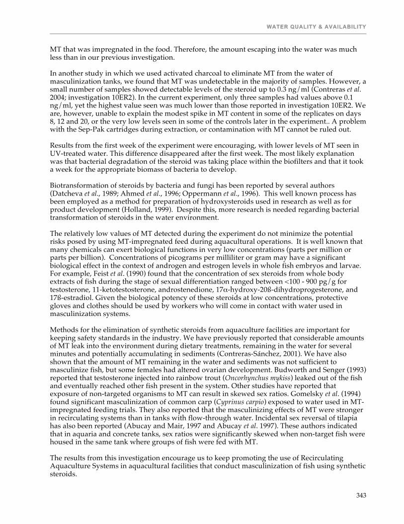
WATER QUALITY & AVAILABILITY
343
MT that was impregnated in the food. Therefore, the amount escaping into the water was much less than in our previous investigation. In another study in which we used activated charcoal to eliminate MT from the water of masculinization tanks, we found that MT was undetectable in the majority of samples. However, a small number of samples showed detectable levels of the steroid up to 0.3 ng/ml (Contreras et al. 2004; investigation 10ER2). In the current experiment, only three samples had values above 0.1 ng/ml, yet the highest value seen was much lower than those reported in investigation 10ER2. We are, however, unable to explain the modest spike in MT content in some of the replicates on days 8, 12 and 20, or the very low levels seen in some of the controls later in the experiment.. A problem with the Sep-Pak cartridges during extraction, or contamination with MT cannot be ruled out. Results from the first week of the experiment were encouraging, with lower levels of MT seen in UV-treated water. This difference disappeared after the first week. The most likely explanation was that bacterial degradation of the steroid was taking place within the biofilters and that it took a week for the appropriate biomass of bacteria to develop. Biotransformation of steroids by bacteria and fungi has been reported by several authors (Datcheva et al., 1989; Ahmed et al., 1996; Oppermann et al., 1996). This well known process has been employed as a method for preparation of hydroxysteroids used in research as well as for product development (Holland, 1999). Despite this, more research is needed regarding bacterial transformation of steroids in the water environment. The relatively low values of MT detected during the experiment do not minimize the potential risks posed by using MT-impregnated feed during aquacultural operations. It is well known that many chemicals can exert biological functions in very low concentrations (parts per million or parts per billion). Concentrations of picograms per milliliter or gram may have a significant biological effect in the context of androgen and estrogen levels in whole fish embryos and larvae. For example, Feist et al. (1990) found that the concentration of sex steroids from whole body extracts of fish during the stage of sexual differentiation ranged between <100 - 900 pg/g for testosterone, 11-ketotestosterone, androstenedione, 17α-hydroxy-20ß-dihydroprogesterone, and 17ß-estradiol. Given the biological potency of these steroids at low concentrations, protective gloves and clothes should be used by workers who will come in contact with water used in masculinization systems. Methods for the elimination of synthetic steroids from aquaculture facilities are important for keeping safety standards in the industry. We have previously reported that considerable amounts of MT leak into the environment during dietary treatments, remaining in the water for several minutes and potentially accumulating in sediments (Contreras-Sánchez, 2001). We have also shown that the amount of MT remaining in the water and sediments was not sufficient to masculinize fish, but some females had altered ovarian development. Budworth and Senger (1993) reported that testosterone injected into rainbow trout (Oncorhynchus mykiss) leaked out of the fish and eventually reached other fish present in the system. Other studies have reported that exposure of non-targeted organisms to MT can result in skewed sex ratios. Gomelsky et al. (1994) found significant masculinization of common carp (Cyprinus carpio) exposed to water used in MT-impregnated feeding trials. They also reported that the masculinizing effects of MT were stronger in recirculating systems than in tanks with flow-through water. Incidental sex reversal of tilapia has also been reported (Abucay and Mair, 1997 and Abucay et al. 1997). These authors indicated that in aquaria and concrete tanks, sex ratios were significantly skewed when non-target fish were housed in the same tank where groups of fish were fed with MT. The results from this investigation encourage us to keep promoting the use of Recirculating Aquaculture Systems in aquacultural facilities that conduct masculinization of fish using synthetic steroids.
TWENTY-FIFTH ANNUAL TECHNICAL REPORT – VOLUME I
344
LITERATURE CITED Abucay J.S. and G.C. Mair, 1997. Hormonal sex reversal of tilapias: implications of hormone
treatment application in closed water systems. Aquacult. Res. 28:841–845. Abucay J.S., G.C. Mair, D.O.F. Skibinski, and J.A. Beardmore, 1997. The occurrence of incidental
sex reversal in Oreochromis niloticus L. In: K. Fitzsimmons (Editor), Proceedings from the Fourth International Symposium on Tilapia in Aquaculture, NRAES, Cooperative Extension, Ithaca N.Y., pp. 729–738.
Ahmed, F., Williams, R.A.D. and Smith, K.E., 1996. Microbial transformations of steroids-X. cytochromes P-450 11α-hydroxylase and C17-C20 lyase and A 1-ene dehydrogenase transform steroids in Nectria haematococca. J. Steroid Biochem. Molec. Biol. 58, 337-349.
Budworth, P.R. and P.L. Senger, 1993. Fish to fish testosterone transfer in a recirculating system. Prog. Fish Cult. 55:250–254.
Budavari, S., M.J. O'Neil, A. Smith, and P.E. Heckelman (Eds), 1989. Merck Index: An Encyclopedia of Chemicals, Drugs, and Biologicals, 11th Edition. Merck and Co., Rahway, New Jersey, p. 962.
Contreras-Sánchez, W.M. 2001 Masculinization of Nile Tilapia Oreochromis niloticus: II. Efficacy of the Masculinizing Agent 17α-Methyltestosterone in Different Environments. Ph.D. thesis. Oregon State University.
Contreras-Sanchez, W.M., M.S. Fitzpatrick, and C.B. Schreck, 2001. Fate of Methyltestosterone in the Pond Environment: Detection of MT in Pond Soil from a CRSP Site. In: A. Gupta, K. McElwee, D. Burke, J. Burright, X. Cummings, and H. Egna (Editors), Eighteenth Annual Technical Report. Pond Dynamics/ Aquaculture CRSP, Oregon State University, Corvallis, Oregon, pp. 79-82.
Contreras-Sánchez, W.M., Márquez-Couturier, G., Feist, G.W., Giannico, G., and Schreck, C.B. 2004. Elimination of methyltestosterone (MT) from intensive masculinization systems: use of activated charcoal in concrete tanks. In: R. Harris, I. Courter, and H. Egna (Editors), Twenty-First Annual Technical Report. Aquaculture CRSP, Oregon State University, Corvallis, Oregon, pp. 145-155.
Contreras-Sánchez, W.M.,, Feist G. W., Alvarez-González C. A., Padrón-López R. M., Hernández-Vidal U., Márquez-Couturier G., SchreckC. B. and Giannico G. 2007. Elimination of methyltestosterone from intensive masculinization systems: use of solar irradiation and bacterial degradation. Investigation 12WQA3. In press.
Datcheva, V.K., Voishvillo, N.E., Kamernitskii, A.V., Vlahov, R.J. and Reshetova, I.G., 1989. Synthesis of 9α-hydroxysteroids by a Rhodococcus sp. Steroids, 54, 271-286.
Feist, G., C.B. Schreck, M.S. Fitzpatrick, and J.M. Redding, 1990. Sex steroid profiles of coho salmon (Oncorhynchus kisutch) during early development and sexual differentiation. Gen. Comp. Endocrinol., 80:299–313.
Fitzpatrick, M.S., G. Van Der Kraak, and C.B. Schreck, 1986. Profiles of plasma sex steroids and gonadotropin in coho salmon, Oncorhynchus kisutch, during final maturation. Gen. Comp. Endocrinol. 62:437-451.
Gomelzky, B., N.B. Cherfas, Y. Peretz, N. Ben-Dom, and G. Hulata, 1994. Hormonal sex inversion in the common carp (Cyprinus carpio L.). Aquaculture. 126, 265-270.
Holland, J.L., 1999. Recent advances in applied and mechanistic aspects of the enzymatic hydroxylation of steroids by whole-cell biocatalysts. Steroids, 64, 178-186.
MacIntosh, D.J. and Little, D.C., 1995. Nile tilapia (Oreochromis niloticus). In: N.R. Bromage and R.J. Roberts (Eds), Broodstock Management and Egg and Larval Quality, Chapter 12, Blackwell Scientific Ltd., Cambridge, Massachusetts, USA, pp. 277-320.
Mires, D. 1995. The Tilapias. In: C.E. Nash and A.J. Novotony (Eds), Production of Aquatic Animals, Chapter 7, Elsevier, New York, pp. 133-152.
Oppermann, U.C.T., Belai, I. and Maser, E., 1996. Antibiotic resistance and enhanced insecticide catabolism as consequences of steroid induction in the gram-negative bacterium Comamonas testosteroni. J. Steroid Biochem. Molec. Biol. 58, 217-223.
Schreck, C.B., 1974. Hormonal treatment and sex manipulation in fishes. In: C.B. Schreck (Ed) Control of sex in fishes. Virginia Polytechnic Institute and State University Extension Division, Blacksburg, Virginia, pp. 84-106
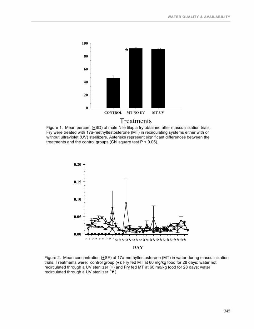
WATER QUALITY & AVAILABILITY
345
1 2 3 4 5 6 7 8 9 10 11 12 13 14 15 16 17 18 19 20 21 22 23 24 25 26 27 28 29 32
MT (ng/m
l) 0.00
0.05
0.10
0.15
0.20
DAY vs control DAY vs control DAY vs EE1
TreatmentsCONTROL MT-NO UV MT-UV
Males (%
) 0
20
40
60
80
100
Figure 1. Mean percent (+SD) of male Nile tilapia fry obtained after masculinization trials. Fry were treated with 17a-methyltestosterone (MT) in recirculating systems either with or without ultraviolet (UV) sterilizers. Asterisks represent significant differences between the treatments and the control groups (Chi square test P < 0.05).
DAY
Figure 2. Mean concentration (+SE) of 17a-methyltestosterone (MT) in water during masculinization trials. Treatments were: control group (●); Fry fed MT at 60 mg/kg food for 28 days; water not recirculated through a UV sterilizer (○) and Fry fed MT at 60 mg/kg food for 28 days; water recirculated through a UV sterilizer (▼).
* *

TWENTY-FIFTH ANNUAL TECHNICAL REPORT – VOLUME I
346
ELIMINATION OF METHYLTESTOSTERONE FROM INTENSIVE MASCULINIZATION SYSTEMS: USE OF SOLAR IRRADIATION AND BACTERIAL DEGRADATION
Twelfth Work Plan, Water Quality & Availability 3 (12WQA3)
Final Report Published as Submitted by Contributing Authors
Wilfrido M. Contreras-Sánchez, Carlos A. Alvarez González, Rosa M. Padrón-López, Ulises Hernández-Vidal , Gabriel Márquez-Couturier,
Arkady Uskanga-Martínez & Beatriz Ramón López Universidad Juárez Autónoma de Tabasco
Villahermosa, Tabasco, México
Grant W. Feist & Guillermo Giannico Oregon State University
Corvallis, OR, USA
Carl B. Schreck Biological Resources Division, USGS
Oregon State University Corvallis, OR, USA
ABSTRACT One of the major problems in aquaculture is the elimination of culture wastes from water. The amount and type of residues will depend on the species cultured, the stage of development and the feeds used. Steroids are commonly used in aquaculture for sex reversal of fish. Methods for the elimination of synthetic steroids from aquaculture facilities are important for maintaining safety standards in the industry. We have previously reported that considerable amounts of 17α-methyltestosterone (MT) leak into the environment during dietary treatments, remaining in the water for several minutes and potentially accumulating in sediments. The goal of this investigation was to determine whether biofiltration, charcoal or sunlight could eliminate MT from culture water. Two experiments were conducted at the Laboratory of Aquaculture at UJAT, in Tabasco, Mexico. MT content of water was determined by radioimmunoassay at Oregon State University. Results from this research indicate that large amounts of MT in the water can be completely removed when activated charcoal is used in a Recirculating Aquaculture System (RAS) and partially removed by either exposure to sunlight and/or biofiltration. Activated charcoal in a RAS can efficiently remove MT in less than 24 hours of treatment. Both sunlight and biological filtration follow a very similar pattern of MT degradation, suggesting that these treatments can eliminate the synthetic steroid if water is exposed for a significant amount of time. The results from this investigation encourage us to keep promoting the use of Recirculating Aquaculture Systems in aquacultural facilities that conduct masculinization of fish using synthetic steroids.
INTRODUCTION All-male populations are used in tilapia (Oreochromis spp) aquaculture because the culture of mixed sex populations often results in precocious maturation and early reproduction (Schreck, 1974; Mires, 1995). Furthermore, all-male tilapia populations are desirable because males achieve a larger final size than females (MacIntosh and Little, 1995). Masculinization of tilapia fry by oral administration of 17α-methyltestosterone (MT) is considered the most successful method employed; however, under certain conditions this technique is sometimes less favorable. Furthermore, significant "leakage" of MT into the pond environment may occur from uneaten or unmetabolized food. This leakage poses a risk of unintended exposure of hatchery workers, as well as fish or other non-target aquatic organisms, to the steroid or its metabolites.

WATER QUALITY & AVAILABILITY
347
In recent studies (Contreras-Sánchez, 2001), we found that masculinization of fry through dietary treatment with MT resulted in the accumulation of MT in sediments which produced both intersex fish and females with altered ovarian development. In systems where substrate was not present, there were higher concentrations of MT in the water and lower (sometimes null) masculinization rates than in systems with either soil or gravel. We found that charcoal filtration of water from systems where substrate was not present lowered the amount of MT in water to almost background levels and the treatment resulted in almost complete masculinization of all three broods tested (100, 98 and 100% males, respectively). Apparently, the recommended dose of MT for masculinizing tilapia is higher than needed and a significant portion of it separates from the food and remains either in suspension in the water for the short term or persists in the sediments over the long term (Contreras-Sánchez, 2001). In the cited study, we recommended the use of activated charcoal filtration systems to eliminate excess MT to increase masculinization, and to prevent potential risks to humans of unintended exposure to MT due to contamination of water and soils in farms. In Mexico, the use of MT for masculinizing tilapia fry is a new activity. Little is known regarding the use of MT and the scarce information available to hatchery producers and fish farmers does not deal with the potential risks of this practice. In the Southeastern region of the country, hatchery production goals have not been reached and the methods used are far from being efficient. Despite almost 30 years of tilapia farming in Mexico, the use of mixed sex populations is still a very common practice and as a result, the productivity of many hatcheries and farms is severely affected. It is well known that one of the major problems in aquaculture is the elimination of culture wastes from water. The amount and type of residues will depend on the species cultured, the stage of development and the feeds used (Wheaton, 1982). To lower the environmental impacts caused by aquaculture practices, different technologies have been developed to preserve water quality and reduce residue levels during fish culture. These systems are known as Recirculation Aquaculture Systems (RAS; Timmons, et al. 2001) and are widely used because they allow for efficient disposal of wastes in aquaculture. In a previous investigation (Contreras-Sánchez, et al., 2004) we developed a RAS to eliminate MT from aquaculture effluents in an intensive system for masculinizing tilapia fry at a large scale. In this system the excess MT was eliminated from the water and the substrate by means of continuous filtration through activated charcoal filters. The RAS is economical, easily constructed, and is composed of a submersible pump, sediment trap, charcoal filter section, mechanical filter section, and a biological filter section. After the water leaves the RAS it returns to the tank though a perforated section of PVC pipe resulting in a “water curtain” which both aerates the water and exposes it to sunlight. Results from that investigation showed that although MT was eliminated from the water and accumulated in the charcoal of the RAS, water from control treatments (MT-treated water, but with no charcoal and passed through the RAS) also did not have detectable levels of MT. In another investigation (Schreck, et al., 2005), we demonstrated that exposure of MT treated water to sunlight resulted in reduced levels of the compound but it was not completely eliminated. Methyltestosterone is a light sensitive hormone which is subject to photodegradation (Budavari et al., 1989; Sigma Chemical Company, 1994). It is also known that some bacteria are capable of degrading steroids (see Mobus et al., 1997). From this information and results from the previous two investigations we hypothesized that MT was being eliminated from control water by solar irradiation and/or bacterial degradation within the RAS. The goal of the present investigation was to determine whether biofiltration, charcoal or sunlight could eliminate MT from culture water. It is also possible that MT is present in control water, but at very low concentrations which are below the detection limits of our assay. Even though MT is not detectable it could be
TWENTY-FIFTH ANNUAL TECHNICAL REPORT – VOLUME I
348
accumulating in fish over time. For this reason we conducted two experiments. In the first we used a large dose of MT (with no fish present) which ensured detection by our radioimmunoassay (RIA). The second experiment simulated the daily pulses of low levels of MT seen during intensive masculinization of tilapia fry. A much larger water sample (20 times that of the first experiment) was extracted to enhance the detection limits of the assay.
METHODS AND MATERIALS Experiments were conducted at the Laboratory of Aquaculture at UJAT, Tabasco, Mexico. Analysis of MT in water samples was conducted by RIA at Oregon State University. Experiment 1a: Elimination of MT from the water of intensive sex-inversion systems; large single dose. This experiment consisted of six treatments where the effects of sunlight and/or biofiltration (use of a RAS with a biological filter) on MT were evaluated. Water was recirculated through 5,000 l tanks with or without a RAS. No fish were used in this experiment. Water was maintained at ambient temperature for exposure to sunlight and/or the RAS. Exposure tanks received MT-treated water; control tanks received untreated water (Table 1). Treatments were as follows: T1) MT treated water recirculated in the dark with no RAS; T2) MT treated water exposed to sunlight with no RAS; T3) MT treated water passed through a RAS in the dark; T4) MT treated water exposed to sunlight and passed through a RAS; C1) control water recirculated in the dark with no RAS; C2) control water exposed to sunlight and passed through a RAS. MT treatments were run in duplicate; controls were not replicated. Ten concrete tanks (5.0 x 1.0 x 1.0 m) were used as experimental units. All tanks had a recirculation system equipped with a 1/2 hp centrifugal pump connected to a PVC pipeline used to recirculate water from the bottom of the tank. Treatments with biofiltration had a 200-l tank with a biofilter bed (see Contreras et al., 2004 for details). At the end of the returning section, the pipe line was perforated with several holes to create a water curtain as water returned to the concrete tank. Those tanks that were not exposed to sunlight were located under a covered area. Tanks exposed to sunlight were located outside of the laboratory. Water flow was 40 l/min. Experimental water was treated with MT at 100 mg l-1and exposed to sunlight and/or passed through the RAS in the same manner as for control water. This was a dose that assured detection of MT in our assay during the early phases of the experiment. All exposures lasted 9 days. Water (2 ml) samples were collected at 0, 2, 4, and 8 hours on day 1 and then once daily for the remainder of the experiment. Since it was possible that MT was being trapped in the sediments within the RAS (but not degraded), sediment samples were planned to be collected from various parts of the RAS; however, no sediments accumulated during this experiment and we were unable to collect samples. Water samples were frozen (–20°C) until processed. Experiment 1b: Elimination of MT from the water of intensive sex-inversion systems; use of activated charcoal. This experiment investigated the effects of sunlight, charcoal and biofiltration on degradation of MT were evaluated. Water was recirculated through 5,000 l tanks with or without a RAS. No fish were used in this experiment. Exposure tanks received MT-treated water; control tanks received untreated water. Water was maintained at ambient temperature for exposure to sunlight and/or the RAS. The experiment consisted of ten treatments with no replication (Table 2). Treatments were: T1) MT treated water recirculated in the dark with no charcoal or biological filter (BF); T2) MT treated water exposed to sunlight with no charcoal or BF; T3) MT treated water passed through a RAS with a BF and no charcoal in the dark; T4) MT treated water exposed to sunlight and passed through a RAS with a BF and no charcoal; T5) control water recirculated in the dark with no charcoal or RAS; T6) control water exposed to sunlight and passed through a RAS with a BF and no charcoal; T7) MT treated water recirculated in the dark through a RAS with charcoal and no BF; T8) MT treated water passed through a RAS with charcoal and a BF in the dark; T9) MT treated water exposed to sunlight and passed through a RAS with charcoal and a BF; and T10) MT treated water exposed to sunlight and passed through a RAS with charcoal and no BF.

WATER QUALITY & AVAILABILITY
349
Experimental units and conditions were similar to those used in experiment 1a. Experiment 2: Elimination of MT from the water of intensive sex-inversion systems; simulated feeding regime. In this experiment a tilapia feeding regime was simulated by adding doses of MT as if 5,000 tilapia fry were being masculinized. Water was recirculated through 5,000 l tanks equipped with a RAS. No fish were used in this experiment. Exposure tanks received MT-treated water; control tanks received untreated water. Water was maintained at ambient temperature, exposed to sunlight and passed through the RAS. The experiment consisted of two treatments done in duplicate: 1) MT treated water exposed to sunlight and passed through the RAS, and 2) Control water exposed to sunlight and passed through the RAS. All exposures lasted for 24 days. Water samples (20 ml) were collected daily and extracted with Sep-Pak cartridges as directed by the manufacturer and MT content was determined by RIA. All cartridges used for extracting MT were frozen (–20°C) and preserved until processed. Radioimmunoassay. For analysis, 1.0 ml of each water sample was extracted with 8 ml of diethyl ether. The organic phase of each sample was collected in a new tube after the aqueous phase was snap frozen in liquid nitrogen. The extraction procedure was repeated and the ether extracts were pooled for each sample and dried down in a Speed-Vac. Each dried extract was reconstituted in 0.5 ml of Phosphate-Buffered Saline containing gelatin (PBSG). Aliquots of the reconstituted extracts were removed to 12x75 mm tubes for determination of MT concentration by RIA. The RIA methods followed the procedure outlined by Fitzpatrick et al. (1986). Antiserum specific to MT was purchased from Animal Pharm Services, and 3H-MT (Amersham) was generously donated by Dr. Gordon Grau of the Hawaii Institute of Marine Biology. Standards of known concentration of MT were made in ethanol and used in each assay to generate a standard curve. The assay was validated by demonstration of parallelism between serial dilutions of several samples and the standard curve, and by demonstration of low cross-reactivity with testosterone and 11-ketotestosterone. Extraction efficiency for MT for the RIA was determined by adding a known amount of 3H-MT to water, (n=5 for each extraction), and then extracting the samples as described above. Once each of these tubes was reconstituted in 1 ml of PBSG, 0.5 ml was removed from each and the amount of radioactivity was determined by scintillation spectroscopy. Extraction efficien-cies for water were 94.7 + 0.6%. Statistical analysis. Because this study is descriptive, no statistical comparisons were made. Means and standard errors were calculated using Statgraphics Plus® v. 4.0. Data were analyzed graphically using Sigma Plot® v. 8.0
RESULTS Experiment 1a: Elimination of MT from the water of intensive sex-inversion systems; large single dose. MT was partially eliminated when water was exposed to either direct sunlight or a RAS with biofiltration (Figure 1). After addition of MT, an average of 33.9 ng/ml of MT was detected in treated water. All combinations of sunlight and biofiltration showed an average elimination of 6.4% of the MT after 24 hours. At the end of the experiment, sunlight exposure and/or biofiltration eliminated an average of 75.5% of the MT detected at the beginning of the experiment. Water recirculated in the dark with no biofiltration showed a similar pattern to the other treatments. MT was not detected in the control treatments at any sampling time. Experiment 1b: Elimination of MT from the water of intensive sex-inversion systems; large single dose. MT was partially eliminated when water was exposed to either direct sunlight or a RAS with biofiltration; however, MT was completely eliminated from water circulated through a RAS with activated charcoal either with or without biofiltration or sunlight within 24 hours of treatment (Figure 2). When charcoal was not present in the system, all possible combinations of sunlight and biofiltration eliminated approximately 62% of the MT within 24 hours; afterwards,

TWENTY-FIFTH ANNUAL TECHNICAL REPORT – VOLUME I
350
MT was eliminated at an average rate of 4% per day. At the end of the experiment, sunlight exposure and/or biofiltration in the absence of charcoal eliminated between 80.4 and 91.3% of the MT detected at the beginning of the experiment. Water recirculated in the dark with no biofiltration or exposure to charcoal showed a similar pattern to the other treatments. MT was not detected in the control group at any sampling time. Experiment 2: Elimination of MT from the water of intensive sex-inversion systems; simulated feeding regime. MT was detectable during the 28 days of the experiment. Concentrations of MT remained under 1 ng/ml for 13 days, between day 14 and 26 the concentration of the steroid remained under 10 ng/ml, but increased significantly afterwards reaching 18.4 ng/ml on the last day of experimentation. MT was detected in four of the samples from the control treatments (Figure 3).
DISCUSSION Results from this research indicate that MT in culture water can be completely removed when activated charcoal is used in Recirculating Aquaculture Systems and partially removed by either sunlight exposure and/or biofiltration. Activated charcoal in a RAS efficiently removed MT in less than 24 hours of treatment. Both sunlight and biological filtration followed a very similar pattern of MT degradation, suggesting that these treatments can eliminate the synthetic steroid if exposed for a significant amount of time. We are not able to explain the decrease in MT concentrations in water that was recirculated in the dark with no RAS. When the feeding regime was simulated, neither sunlight, nor biofiltration were capable of eliminating MT from the systems. There was a clear increase of MT at the end of the trial indicating that these strategies were not efficient when activated charcoal is not present. Our previous research has shown, however, that the presence of fish greatly reduces the amount of MT present in the water during masculinization, and the use of sunlight or biofiltration under these circumstances may aid in the removal of smaller amounts of MT. These results support our previous findings where MT was efficiently removed from masculinization tanks using a RAS with charcoal and biological filtration (Contreras-Sánchez, et al., 2004). However, at that time we were not able to separate the effects of charcoal and biological filtration. In the current study we observed that when charcoal was not present in the recirculating system, MT remained in the water for up to nine days. Surprisingly, there was no additive effect of sunlight exposure and biofiltration since alone or combined these two factors showed very similar trends of MT elimination. Very little is understood regarding these two processes in aquaculture; biotransformation of steroids by bacteria and fungi has been reported by several authors (Datcheva et al., 1989; Ahmed et al., 1996; Oppermann et al., 1996). This process has been employed as a method for preparation of hydroxysteroids used in research as well as for product development (Holland, 1999). Despite this, little research has been conducted regarding bacterial transformation of steroids in culture water. Degradation of some steroids by exposure to sunlight is a well-known process and some companies that sell synthetic steroids recommend keeping them in the dark. Budavari et al. (1989) and Sigma Chemical Company (1994) have indicated that MT is a light sensitive steroid subject to photodegradation; however no information is available on either the intensity of light needed or the time required for elimination MT after exposure to sunlight.in aquaculture facilities. Methods for the elimination of synthetic steroids from aquaculture facilities are important for maintaining safety standards in the industry. We have previously reported that considerable amounts of MT leak into the environment during dietary treatments, remaining in the water for several minutes and potentially accumulating in sediments (Contreras-Sánchez, 2001). We have also shown that the amount of MT remaining in the water and sediments was not sufficient to masculinize fish, but some females had altered ovarian development. Budworth and Senger (1993) reported that testosterone injected into rainbow trout (Oncorhynchus mykiss) leaked out of the fish and eventually reached other fish present in the system. Other studies have reported that

WATER QUALITY & AVAILABILITY
351
exposure of non-target organisms to MT can result in skewed sex ratios. Gomelsky et al. (1994) found significant masculinization of common carp (Cyprinus carpio) exposed to water used in MT-impregnated feeding trials. They also reported that the masculinizing effects of MT were stronger in recirculating systems than in tanks with flow-through water. Incidental sex reversal of tilapia has also been reported (Abucay and Mair, 1997; Abucay et al. 1997). These authors found that in aquaria and concrete tanks, sex ratios were significantly skewed when non-target fish were housed in the same tank where groups of fish were fed MT. The RAS used in our experiments allowed water to be exposed to different combinations of biofiltration and sunlight degradation. This system may therefore have created conditions that are favorable for these two processes to metabolize MT. The flow rate created by the pump (60 l/min), allowed for at least 9 complete passes each day of the entire volume of water through the biofilter which had a large surface area that was in constant contact with the water. The water curtain created by the perforated return pipe also allowed for constant exposure of water to sunlight for at least 8 hours a day. We were able to demonstrate that activated charcoal efficiently captures MT, but that exposure to biofiltration or sunlight does not efficiently degrade the steroid. More research is needed to improve conditions that allow for complete elimination of MT without the use of charcoal filtration. This is important because once MT is trapped in the charcoal; further treatment is required to degrade the steroid. The relatively low values of MT detected during our second experiment do not minimize the potential risks posed by using MT-impregnated feed during aquaculture operations. It is well known that many chemicals can have a physiological effect at very low concentrations (parts per million or parts per billion). Concentrations of picograms per milliliter or gram may have a significant biological effect in the context of androgen and estrogen levels in whole fish embryos and larvae. For example, Feist et al. (1990) found that the concentration of sex steroids from whole body extracts of fish during the stage of sexual differentiation ranged between 100 - 900 pg/g for testosterone, 11-ketotestosterone, androstenedione, 17α-hydroxy-20β-dihydroprogesterone, and 17β-estradiol. Given the biological potency of these steroids at low concentrations, protective gloves and clothes should be used by workers who will come in contact with water used in masculinization systems. The results from this investigation encourage us to keep promoting the use of Recirculating Aquaculture Systems in aquacultural facilities that conduct masculinization of fish using synthetic steroids.
LITERATURE CITED Abucay J.S. and G.C. Mair, 1997. Hormonal sex reversal of tilapias: implications of hormone
treatment application in closed water systems. Aquacult. Res. 28:841–845. Abucay J.S., G.C. Mair, D.O.F. Skibinski, and J.A. Beardmore, 1997. The occurrence of incidental
sex reversal in Oreochromis niloticus L. In: K. Fitzsimmons (Editor), Proceedings from the Fourth International Symposium on Tilapia in Aquaculture, NRAES, Cooperative Extension, Ithaca N.Y., pp. 729–738.
Ahmed, F., R.A.D. Williams, and K.E. Smith, 1996. Microbial transformations of steroids-X. cytochromes P-450 11α-hydroxylase and C17-C20 lyase and A 1-ene dehydrogenase transform steroids in Nectria haematococca. J. Steroid Biochem. Molec. Biol., 58(3):337–349.
Budavari, S., M.J. O'Neil, A. Smith, and P.E. Heckelman (Eds), 1989. Merck Index: An Encyclopedia of Chemicals, Drugs, and Biologicals, 11th Edition. Merck and Co., Rahway, New Jersey, p. 962.
Budworth, P.R. and P.L. Senger, 1993. Fish to fish tes¬tosterone transfer in a recirculating system. Prog. Fish Cult. 55:250–254.
Contreras-Sánchez, W.M. 2001 Masculinization of Nile Tilapia Oreochromis niloticus: II. Efficacy of the Masculinizing Agent 17α-Methyltestosterone in Different Environments. Ph.D. thesis. Oregon State University.

TWENTY-FIFTH ANNUAL TECHNICAL REPORT – VOLUME I
352
Contreras-Sánchez, W.M., Márquez-Couturier, G., Feist, G.W., Giannico, G., and Schreck, C.B. 2004. Elimination of methyltestosterone (MT) from intensive masculinization systems: use of activated charcoal in concrete tanks. In: R. Harris, I. Courter, and H. Egna (Editors), Twenty-First Annual Technical Report. Aquaculture CRSP, Oregon State University, Corvallis, Oregon, pp. 145-155.
Datcheva, V.K., N.E. Voishvillo, A.V. Kamernitskii, R.J. Vlahov, and I.G. Reshetova, 1989. Synthesis of 9α-hydroxysteroids by a Rhodococcus sp. Steroids, 54(3):271–286.
Feist, G., C.B. Schreck, M.S. Fitzpatrick, and J.M. Redding, 1990. Sex steroid profiles of coho salmon (Oncorhynchus kisutch) during early development and sexual differentiation. Gen. Comp. Endocrinol., 80:299–313.
Fitzpatrick, M.S., G. van Der Kraak, and C.B. Schreck. 1986. Profiles of plasma sex steroids and gonadotropin in coho salmon (Oncorhynchus kisutch) during final maturation. General and Comparative Endocrinology 62:437-451.
Gomelzky, B., N.B. Cherfas, Y. Peretz, N. Ben-Dom, and G. Hulata, 1994. Hormonal sex inversion in the common carp (Cyprinus carpio L.). Aquaculture. 126, 265-270.
Holland, H.L., 1999. Recent advances in applied and mechanistic aspects of the enzymatic hydroxylation of steroids by whole-cell biocatalysts. Steroids, 64(3):178–186.
MacIntosh, D.J. and Little, D.C., 1995. Nile tilapia (Oreochromis niloticus). In: N.R. Bromage and R.J. Roberts (Eds), Broodstock Management and Egg and Larval Quality, Chapter 12, Blackwell Scientific Ltd., Cambridge, Massachusetts, USA, pp. 277-320.
Mires, D., 1995. The Tilapias. In: C.E. Nash and A.J. Novotony (Eds), Production of Aquatic Animals, Chapter 7, Elsevier, New York, pp. 133-152.
Mobus E., Jahn, M., Schmid, R., Jahn, D. and Maser, E. 1997. Testosterone-regulated expression of enzymes involved in steroid and aromatic hydrocarbon catabolism in Comamonas testosteroni. J Bacteriol: 5951-5.
Oppermann, U.C.T., I. Belai, and E. Maser, 1996. Antibiotic resistance and enhanced insecticide catabolism as consequences of steroid induction in the gram-negative bacterium Comamonas testosteroni. J. Steroid Biochem. Molec. Biol., 58:217–223.
Schreck, C.B., 1974. Hormonal treatment and sex manipulation in fishes. In C.B. Schreck (Ed) Control of sex in fishes. Virginia Polytechnic Institute and State University Extension Division, Blacksburg, Virginia, pp. 84-106.
Schreck, C.B., Feist, G.W., Giannico, G., Contreras-Sánchez, W.M., Pascual-Valencia L.E., Hernández-Vidal U., and Campos-Campos B. 2005. Elimination of methyltestosterone from intensive masculinization systems: use of ultraviolet irradiation of water. In: J. Burright, C. Flemming, and H. Egna (Editors), Twenty-Second Annual Technical Report. Aquaculture CRSP, Oregon State University, Corvallis, Oregon, pp. 185-194.
Sigma Chemical Company, 1994. Material Safety Data Sheet. St. Louis, MO, USA 2pp Timmons, M.B., J.M. Ebeling, F.W. Wheaton, S.T. Summerfelt and B.J. Vinci. 2001. Recirculating
Aquaculture Systems. Cayuga Aqua Ventures, Ithaca, New York. 650 pp. Wheaton, W.F. 1982. Acuacultura. Diseño y construcción de sistemas. AGT editor, México. 704
pp.

WATER QUALITY & AVAILABILITY
353
0 5 10 15 20 25
MT (ng/m
l) 0
10
20
30
40
50
Time (hours)
50 100 150 200
T1 T2T3T4C1C2
Figure 1. Levels of 17α-methyltestosterone (MT, ng/ml + SE) detected in water during experiment 1a: T1) MT treated water recirculated in the dark with no Recirculating Aquaculture System (RAS) (●); T2) MT treated water exposed to sunlight with no RAS (○); T3) MT treated water passed through a RAS in the dark (▼); T4) MT treated water exposed to sunlight and passed through a RAS (); C1) control water recirculated in the dark with no RAS (■); C2) control water exposed to sunlight and passed through a RAS (□). The scale on the X-axis increases by 10-fold after 25 hours.
Table 1. Water treatments in experiment 1a.
MT BIOLOGICAL
FILTER SOLAR
IRRADIATION TREATMENT
CODE OBSERV. YES NO NO T1 YES NO YES T2 YES YES NO T3 YES YES YES T4 NO NO NO C1 control NO YES YES C2 control
Table 2. Water treatments in experiment 1b.
MT CHARCOAL BIOLOGICAL
FILTER SOLAR
IRRADIATION TREATMENT
CODE OBSERV. YES NO NO NO T1 YES NO NO YES T2 YES NO YES NO T3 YES NO YES YES T4 NO NO NO NO C1 control NO NO YES YES C2 control YES YES NO NO T7 YES YES YES NO T8 YES YES YES YES T9 YES YES NO YES T10

TWENTY-FIFTH ANNUAL TECHNICAL REPORT – VOLUME I
354
0 5 10 15 20 25
MT
(ng/ml) 0
2468
101214161820
Time (hours)
50 100 150 200
T1 T2T3T4C1C2T7T8T9T10
Time (days)
0 3 6 9 12 15 18 21 24 27
MT
(ng/ml)
0
5
10
15
20
25CONTROLMT
Figure 2. Levels of 17α-methyltestosterone (MT, ng/ml + SE) detected in water during experiment 1b: T1) MT treated water recirculated in the dark with no charcoal or Recirculating Aquaculture System (RAS) (●); T2) MT treated water exposed to sunlight with no charcoal or RAS (○); T3) MT treated water passed through a RAS with a biological filter (BF) and no charcoal in the dark (▼); T4) MT treated water exposed to sunlight and passed through a RAS with a BF and no charcoal (); T5) control water recirculated in the dark with no charcoal or RAS (■); T6) control water exposed to sunlight and passed through a RAS with a BF and no charcoal (□); T7) MT treated water recirculated in the dark though a RAS with charcoal and no BF (♦); T8) MT treated water passed through a RAS with charcoal and a BF in the dark (◊); T9) MT treated water exposed to sunlight and passed through a RAS with charcoal and a BF (▲); and T10) MT treated water exposed to sunlight and passed through a RAS with charcoal and no BF (∆).The scale on the X-axis increases by 10-fold after 25 hours.. Figure 3. Levels of 17α-methyltestosterone (MT, ng/ml + SE) detected in water during experiment 2: MT treated or control water was exposed to sunlight and passed through
A RECIRCULATING AQUACULTURE SYSTEM WITH A BIOLOGICAL FILTER.

WATER QUALITY & AVAILABILITY
355
ECOLOGICAL ASSESSMENT OF SELECTED SUB-WATERSHEDS OF THE NZOIA RIVER BASIN
Twelfth Work Plan, Water Quality & Availability 4 (12WQA4) Final Report
Published as Submitted by Contributing Authors
Mucai Muchiri & Frank Masese Moi University Eldoret, Kenya
William A. Shivoga Edgerton University
Njoro, Kenya
Nancy Gitonga Department of Fisheries
Nairobi, Kenya
E. W. Tollner University of Georgia Athens, Georgia, USA
Geoff Habron
Michigan State University Lansing, Michigan, USA
ABSTRACT
Macroinvertebrates were sampled at eight stations along River Moiben using a Surber sampler between the months of February and July 2006. Eight sampling sites, each 100m long were selected along the stream, which drained land under forestry, agricultural, and residential use. The Shannon-Weiner and Simpson indices were used to test quality of biodiversity among sampling stations. Water physico-chemical data was also collected. Analysis of variance results revealed significant differences (p< 0.05) in relative abundance between the different stations and sampling occasions. Taxon richness and diversity of macroinvertebrates were not significantly different between the stations but taxon composition did as one moved downstream. This study showed that significant changes in macroinvertebrate assemblages were primarily due to water quality rather than prevailing climatic conditions.
INTRODUCTION Rapid growth in agriculture in developing countries plus an enormous increase in the amount of wastes produced by a rapidly growing human population and its livestock are placing tremendous demands on the lotic water resources available. This trend coupled with freshwater scarcity in most countries including Kenya (Postel, 1992) continue to strain the available sources. Streams and rivers continue to bear untoward consequences of pollution emanating from point and non-point sources. As a result these delicate ecosystems have increasingly lost their integrity by a vast array of human activities including poor agricultural practices, land development, hydrological alterations, resource overexploitation, pollution from mines, urban areas and industry leading to sedimentation and eutrophication (Osano et al., 2003; Raburu, 2003; Global Environmental Facility, 2004). The use of biological indicators (or bioindicators) to assess environmental quality is based on the premise that organisms provide information about their habitat (Foote and Hornung, 2005). Studies have shown that water quality in aquatic systems has a strong impact on biological

TWENTY-FIFTH ANNUAL TECHNICAL REPORT – VOLUME I
356
components (Harding et al., 1999; Ometo et al., 2000). Aquatic communities are sensitive indicators of pollution in their systems as they integrate and reflect the effects of stress, both natural and human induced, over extended periods of time. In doing so they act as early warning signals of pollutant loads that degrade water quality and ecological integrity. In this regard community response is used as a measure of perturbation that affect water quality. Aquatic macroinvertebrates have gained prominence as indicators of environmental quality of lotic systems and information about their response to changes in environmental quality continue to grow (e.g. Lemly, 1982; Rosenberge and Resh, 1993; Lenat and Crawford, 1994; Baker and Sharp 1998; Brooks et al., 1998; Harding et al., 1999). In Kenya research on macroinvertebrates as indicators of water quality in lotic systems has only recently begun and therefore rare in the literature (Kinyua and Pacini, 1991; Raburu, 2003; Ndaruga et al., 2004). Most of the studies have focused on the structure and composition of macroinvertebrate communities in a few lotic systems without relating them to water quality (Barnard and Biggs, 1988; Dobson et al., 2002; Mathooko, 2002). Macroinvertebrates constitute an important component of biodiversity in lotic systems (Merritt and Cummins, 1996). Their diversity, distribution and community composition are important in understanding the quality of habitat and that of the water in which they occur. Community structure varies both spatially and temporarily in relation to environmental factors (Townsend, 1989; Richards et al., 1993; Tate and Heiny, 1995). These factors include discharge, substrate type, dissolved substances, turbidity, riparian vegetation, land use, temperature, altitude and latitude (Giller and Malmqvist, 1998). However, human activities influence the effect of these factors on water quality, which in turn affect the composition and distribution of macroinvertebrates. Abiotic factors, especially those related to disturbance determine the composition of stream communities (Reice et al., 1990). In Kenya, especially in the Nzoia basin and its sub-watersheds agricultural development is on the rise (Osano et al., 2003; GEF, 2004). Human land use practices at the watersheds drained by rivers that flow into Lake Victoria continue to impose threats on the ecological integrity not only of rivers but also of the recipient lake. In this regard the waters of River Moiben, as part of the Nzoia basin, face possible pollution from agricultural farms where inorganic fertilizers, herbicides and pesticides are used on a wide scale (Osano et al., 2003). In the effort to meet the required food supplies to feed the ever-growing human population forestlands and riparian vegetation have been cleared for both small scale and large-scale agriculture. As such, a major challenge in the area remains to be a sustained increase in food production without compromising the integrity of the environment within which that much required food is produced. This study was designed as part of the wider project “Hydraulic, Water Quality and Social Assessment of the Nzoia Basin” to assess water quality of River Moiben by utilizing resident macroinvertebrate communities in the river as indicators of water quality. Specifically, it addresses the composition, distribution, taxa richness and abundance of macroinvertebrates in relation to in-stream physicochemical features of the river. In addition, it sought to determine how changes in community composition relate to the spatial arrangement of riparian land use along the river which are expected to affect water quality in the river.
MATERIALS AND METHODS Study area The Moiben basin is part of the expansive Nzoia watershed that is 12,903 Km2. It transcends a broad range of land use systems and practices ranging from small-scale holder farmland to large-scale mechanized agriculture. The watershed occurs in generally high potential and high population region and therefore the influence of land use, mostly agriculture and settlement, on the system is extremely important. The altitude varies between 2600m above sea level at the highlands and 1500m above sea level to the south. The watershed has a highland equatorial climate. Due to diverse relief features rainfall varies from one region to another. The highlands
WATER QUALITY & AVAILABILITY
357
receive heavier rainfall than the lowlands. The mean annual rainfall is 1124 mm, which is evenly distributed and occurs in one long season March-September with two distinct peaks in May and August. The average temperature experienced in the region is 18 °C during the wet season with a maximum of 28 °C during the dry season and a minimum of 7 degrees centigrade in the coolest season. February is the hottest month while June-July is the coolest. River Moiben is a 4th order stream that originates in the western side of the Kerio escarpment 2500 m above sea level and flows through human settlement areas integrated with forestry. The river passes through swampy areas at its upper reaches before entering a manmade dam at 2252 m above sea level. The stream is affected by various human activities along the channels and in the catchment. Station 1 is in the upper parts of the stream after the impoundment, situated in a forested area. There is minimal human impact on the surrounding area and therefore the station acted as a reference point. Station 2 is on a 3rd order tributary of River Moiben. The riparian zone is grassland with minimal human impact. Intensive mixed farming is the major form of land use around station 3. There was excessive use of animals on the banks that were eroded and devoid of littoral vegetation. Station 4 is on a 2nd order tributary. Human impact at the site included animal watering, washing and water abstraction. Station 5 and 6 are situated in areas with maize farming. Intensive mixed farming and pockets of forests are common. Station 6 has stable banks with littoral vegetation and the riparian zone was > 15m. Station 7 and 8 are situated in an area characterized with intensive maize farming and animal production on the riparian zone. At station 8 additional human impacts include sand harvesting and wastes from a nearby shopping center. The stream water was brown and characterized by heavy sediment loads. Macroinvertebrates samples At each station a 100m reach that was representative of the characteristics of the stream were selected for sampling. Macroinvertebrates were collected from pools, riffles and runs, which were identified according to Jeffries and Mills (1990). Sampling was done semi-quantitatively by making a standard one-minute sweep per habitat using a Surber sampler (0.5mm mesh). This was replicated three times per habitat. The samples were then pooled to make one sample per habitat per station. The sampler was placed on the stream bottom and upstream substrate disturbed by vigorous kicking. As substrate was disturbed, the operator and the sampler moved upstream for the required time. Samples collected from the net were then preserved in 10% formalin. Laboratory sample processing In the laboratory, samples were washed through a 250 µm mesh sieve to remove formalin, mud and sand. The macroinvertebrates were then sorted and counted using a stereoscope. Identification to genus level was done according to Merritt and Cummins (1996) for insects and Karl and Dudley (1972) and Macan (1977) for non-insects. Owing to lack of identification keys for Kenyan stream fauna, some specimens were assigned only to the lowest taxon within which they could be placed with certainty. To address changes in macroinvertebrate community structure among sites, macroinvertebrate composition measures were done for each sampling station and sampling occasion using number of taxa (S), total number of individuals and relative abundance of each taxon. Measures of richness and evenness were quantified and a compositional index commonly used to indicate environmental stress. The Shannon-Weiner Diversity Index was used to assess diversity:
H’ = -∑ ((n/N) * In (n/N))
where n= number of individuals of a taxon; N = total number of individuals in the station. An associated evenness measure calculated from H’ was also used. This index assumes that maximum diversity occurs when all taxa are equally abundant (i.e. H’ = H’max = ln S). Therefore, the ratio of H’/H’max represents a measure of evenness where an assemblage with an equal abundance of taxa would have a value of 1 (Pielou, 1969). As an additional measure of evenness the percentage of the total numbers accounted for by the five most dominant taxa at each site was

TWENTY-FIFTH ANNUAL TECHNICAL REPORT – VOLUME I
358
used (% 5 Dominant) (Barbour et al., 1999). To assess compositional differences among sites, the percentage of commonly intolerant taxa (Ephemeroptera + Plecoptera + Trichoptera, EPT), widely used as an indicator of disturbance to stream communities (e.g. Lenat And Crawford, 1994), was also used. Water samples On each sampling occasion, except the second, physical and chemical parameters were measured at each station before macroinvertebrates were sampled. Conductivity was measured using conductivity meter while temperature and pH were measured by a combined pH-and temperature-meter. Triplicate water samples were taken and used to calculate dissolved oxygen (DO) and biological oxygen demsnd (BOD) according to APHA (1995). Also during sampling stream width, depth, water velocity and discharge were assessed at each sampling station. Water velocity was determined by the floatation method and discharge calculated as a function of cross-sectional area and water velocity. Data analysis After all data had been collected the count data was log-transformed log 10(x + 1) prior to analysis to meet the statistical criteria of normality. Mean values of the physico-chemical parameters were calculated for each station. Analysis of variance (ANOVA) was used to test for differences in relative abundance and taxon richness of macroinvertebrates at different stations along the river. Two-way ANOVA was used to test for any differences in water quality parameters and community indices between different sampling stations and sampling occasions. Spearman’s correlation analysis was performed to investigate the relationship between community indices and physico-chemical parameters. Significant differences were accepted at P < 0.05 for all tests. Data analysis was done using Minitab Version 13.0 for windows.
RESULTS Physico-chemical parameters Mean values for physico-chemical parameters obtained during the study are presented in Table 1. Conductivity, velocity, discharge and river width showed significant variation in both space and time (p<0.05). Depth, DO and BOD showed significant variation with respect to time only (p<0.05) but not with space (p>0.05). Water temperature and pH were not significantly different between sampling stations and sampling occasions. Conductivity values increased from 70.33 µs/cm at the highest headwater station to 184.96 µs/cm at a downstream station 7. Also BOD values increased from 0.86mg/l at station 2 to 2.43mg/l at station 7 and this corresponded with a general increase in turbidity downstream marked by a brown water coloring as one moved downstream. Macroinvertebrate assemblages ANOVA results obtained did not reveal any significant differences in abundance between the three habitats (p> 0.05) so the data was pooled. Two-way ANOVA performed on the pooled data revealed highly significant differences in abundance between the 8 stations and sampling periods (p<0.05). Therefore, the different stations and different sampling occasions were treated separately in subsequent analysis. Total abundance and taxon richness A total of 13910 specimens were collected, with 73 taxa identified belonging to 13 orders and 51 families (Table 2). There were significant differences in abundance between the stations and the sampling periods (P< 0.05). Considering spatial variation in taxon richness is that station 6 had the highest, 41, while station 8 with 31 taxa had the lowest (Figure 1). Station 4 had the highest abundance, 4708, while station 8 had the lowest, 771. Stations 1, 2, 4, and 5 had the highest families represented, 28, in the samples while station 7 had 25. Diptera had the highest number of families, 10, and and total abundance, 5124, while Coleopteran had the highest taxon richness, 14. Arachnida and Lepidoptera were least represented with one family each with Lepidoptera recording 1 individual.

WATER QUALITY & AVAILABILITY
359
Taxon richness was negatively correlated with temperature, discharge and conductivity (P< 0.05). Abundance was negatively correlated with discharge, river width and conductivity. During the study it was generally observed that abundance was lowest during the dry period in February (Figure 2). It increased progressively during the onset of the rainy season but started to decline during the peak and spates in July. At this period the river was characterized by large quantities of suspended matter and high sediment loads. Community composition measures The results of diversity indices are given in Table 3. The taxon diversity measured by the Shannon Diversity index was highest in station 8 followed by station 1. Station 4 had the lowest. The evenness index was highest in station 8 and lowest in station 4. Taxon richness was highest in station 1 with 9.52 followed by station 8 with 9.03 while the lowest was recorded in station 4 with 4.1. The percentage of the five most dominant taxa was highest in station 4 with 97.22 % while it was lowest at station 3 with 86.37 %. A correlation performed to test the relationship between the indices and physico-chemical parameters revealed a negative relationship between evenness and dissolved oxygen (p<0.05). The main taxonomic groups encountered are presented in figure 3. There were significant differences in EPT between the stations (P< 0.05) but not between the sampling periods. There was no particular trend in percentage EPT downstream. Station 2 recorded the highest percentage (57.6 %), while station 3 had the lowest (16.8 %). There was an increase from station 3 to station 6 with a decrease in station 7 which slightly increased in station 8. High abundance of EPT in station 4 was accounted for by the net spinning Hydropsyche sp. The importance of Coleoptera and Oligochaeta varied greatly from site to site with elmids common downriver. Oligochaeta gained greatest importance in station 5. In overall order Diptera dominated the study area occurring in each station (Figure3). Other orders that were sampled in the eight stations include Ephemeroptera, Coleoptera, Oligochaeta, Trichoptera, Gastropoda, and Odonata and Hemiptera. Plecoptera was not represented in station 2, 3 and 5. Hirudinea occurred in station 1, 3, 4, and 5, while Crustacea did not occur in station 8. Arachnida was only sampled in station 3, 4 and 5 while Lepidoptera occurred in station 1 only.
DISCUSSION According to the River Continuum Concept (RCC) (Vannote et al., 1980), community structure and function conform with certain geomorphic, physical and biotic characteristics such as stream flow, channel morphology, detritus loading, size of particulate organic matter, characteristic of autotrophic production and thermal loading. However this concept seldom holds in many lotic systems due to longitudinal changes in environmental conditions caused by agricultural, human settlements or other land use activities that affect water quality. In the present study and according to ANOVA results, conductivity, water velocity, water depth, DO and BOD were significantly different between the stations (p< 0.05). Although these factors can be linked to the observed changes in the biota of River Moiben, it is often difficult to isolate the influence of a particular factor (Buss et al., 2002). Overall, this combined effect created a gradient of environmental, physical and water quality conditions that led to the observed spatial and temporal variations in taxon richness, evenness and distribution of macroinvertebrates in the river. Changes in the macroinvertebrate assemblages along a river indicate the ability of different taxa to occupy different microhabitats and process organic matter. From station 1-8 the replacement of taxa was observed from less to more pollution tolerant ones. Genera of Ephemeroptera showed clear preference for station 1 and 2. Station 3, 4 and 5 had the highest number of the pollution tolerant Diptera and Oligochaeta where they formed more than 50 % of total abundance in the three stations. Despite the wide distribution of Chironomus sp (Chironomidae, Diptera) in all stations, the genus showed higher abundance in station 3 and 4 and this can be attributed to

TWENTY-FIFTH ANNUAL TECHNICAL REPORT – VOLUME I
360
increasing organic pollution at the two stations (Buss et al., 2002) and enrichment especially in an agricultural watershed (Fore et al., 1996). Studies in impacted stream ecosystems (mostly agricultural) have documented high macroinvertebrate density, often associated with numerical dominance by environmentally tolerant taxa (e.g. Lenat and Crawford, 1994). The two stations are devoid of riparian cover and are points for watering animals hence they receive higher amounts of animal wastes as compared to station 1 and 2 which are located in an area with a well protected riparian zone with limited access to animals and other human activities. The aquatic coleopterans did not show any sensitivity to poor water quality in the study area. In the first four stations there was an increase in coleopteran taxon richness and abundance. The numbers also increased downriver where together with Diptera they formed more than 50 % of the total individuals in the stations. Coleopteran abundance was highest in station 4 where elmids formed more than 80 % of the total coleopteran population at the station. With station 4 considered degraded the high abundance of Coleoptera indicates that they are tolerant to poor water quality. Station 6 recorded the highest number of coleopteran genera (8) and this can be attributed to habitat diversity and quality at the station. The abundance of Odonata, Crustacea and Gastropoda decreased downstream indicating that the orders were responding to some factors that were affecting their distribution and abundance. The three orders are considered to be indicators of intermediate levels of pollution (USEPA, 1996). Odonates have been used to replace Ephemeroptera in the EPO index for water quality as a metric in Ohio streams (USEPA, 1996). In this study the decline of Odonata downstream can be attributed to their sensitivity to poor water quality. Being predators, their distribution is also influenced by the presence or absence of appropriate prey taxa, which are also supported by good water quality. Order Hemiptera displayed a widespread occurrence along the river. This order displayed a general increase in abundance and taxon richness downstream even though it did not occur in station four. The increase downstream indicate that the members of this order are resistant to pollution. Members of order Hemiptera are mainly predators-piercers in their trophic relationship. This characteristic make the order appropriately adapted for survival as it has a wide supply of food being at the top of the food chain. Their habit, climbers/clingers/divers (Merritt and Cummins, 1996) also helps them avoid adverse water quality conditions. In some stations in river Moiben high diversity of macroinvertebrates were obtained despite point and non-point sources of pollution. Station 6 recorded the highest taxon diversity despite the cumulative effects of pollution from upstream that was expected to lower diversity and abundance in downstream stations. This station has well protected banks with vegetation cover that offer wider habitat diversity to aquatic biota. This also explains the high abundance and taxon richness at the station as compared to other stations downstream. Also in river Nyando high diversity was recorded below point sources of pollution and this was attributed to riparian vegetation cover and instream habitat quality at the stations (Raburu, 2003). Apart from the effect of anthropogenic impacts, natural stress also may influence macroinvertebrate assemblage distribution such as spates and floods in the tropics. This may explain the temporal differences in taxon richness and abundance in River Moiben. During the study high abundance during the onset of rains and during the long rains were significantly reduced by the spates in July. A study by Shivoga (200l) in some two tropical streams in Kenya found that abundance of macroinvertebrates was highest at the onset of the rains and declined progressively as the rainfall increased. There was no clear trend in taxon richness and abundance downstream. Stations at the upper reaches of the river had lower taxon richness, which increased in middle stations and then decreased at the lower reaches. This is the trend expected in most riverine systems (Vannote et al., 1980) as they reflect changes in stream order and other factors that influence community

WATER QUALITY & AVAILABILITY
361
composition and structure. However, Station 1 had the largest diversity followed by station 8, 3 and 2 respectively. High diversity in station 1 can be attributed to habitat quality and high water quality in the upper reaches of River Moiben. The forested surrounding in station 1 is a good source of allochthonous organic matter for stream biota. Canopy along the river help maintain water quality and provide diverse habitats for a variety of macroinvertebrates leading to increased diversity. Diversity decrease downstream can also be linked to agricultural land use intensification downstream. The low evenness values obtained downstream corresponded with a high dominance of the community by pollution tolerant taxa as percentage of the pollution tolerant EPT decreased. High abundance of Chironomidae and Oligochaetae in station 4 suggest organic pollution. The station receives animal wastes from a cattle market situated a few meters from the river. Animal wastes from the roads and domestic wastes from the nearby shopping centre are washed and deposited into the river during the rainy period. The station also suffers degradation from animals and human beings as the station is a watering point for the animals, washing and bathing. The high evenness values and diversity at Station 7 and 8 indicate that no particular taxon dominated others in terms of abundance. However the abundance of Diptera in the two stations indicate that water quality was deteriorating downstream. As a measure composition and abundance, the five dominant taxa had the highest percentage in Station 4. This also explains the low evenness value recorded in the station. The dominant genera were Chironomus, Hydropsyche, Simulium, Glossiphonia and Baetis. This means that pollution sensitive taxa were eliminated and replaced by ones that are tolerant to poor water quality. This station is considered degraded and the composition of taxa represents its true character, as is the case in most degraded stations. Despite the poor riparian cover station 3 recorded the lowest value of the percentage 5 dominant taxa. Evenness and taxon richness values were also high. This indicates that water quality is good and this can be explained by the forested nature of the area upstream of the station. There was a general decline in relative abundance and taxon richness of EPT downstream and this indicates that the three orders are sensitive to anthropogenic stress. Station 1 and 2 were dominated by the pollution intolerant EPT and this is characteristic of an area with good water and habitat quality. These stations are characterised with pristine riparian areas with minimal human impact. The sensitivity of EPT can be explained by their need for clean water with high dissolved oxygen and low siltation. A study of the effect of siltation and organic enrichment on the aquatic biota showed that accumulation of fine sand and inorganic silt on gills of Plecoptera and Ephemeroptera explain their elimination from degraded stations (Lemly, 1982). In the current study area it was possible to differentiate ecologically good stations from poor ones by assessing the composition of EPT at the stations. For instance, the relative abundance of EPT at pristine stations 1 and 2 were 0.45 and 0.58 respectively as compared to stations 3 and 7 with 0.17 and 0.23 respectively both with degraded riparian zones and in-stream habitats. This concurs with several other studies (Lemly, 1982; Baker and Sharp, 1998; Raburu, 2003) in which low relative abundance of EPT were observed in degraded areas. However, Hydropsyche sp (Hydropsychidae, Trichoptera) showed the greatest abundance at station 4. There was also a higher relative abundance of Baetis sp (Baetidae, Epheneroptera) at the station. This can be explained by the fact that family Hydropsychidae in the Trichoptera and Baetidae in Ephemeroptera are considered to be less sensitive to pollution (Buss et al., 2002). The high number of Hydropsyche sp at this station can also be explained by the higher levels of turbidity that provide more suspended food particles to the net spinning larvae (Lobinske et al., 1997). Turbidity at the station is maintained by animals that disturb the ground loosening organic materials at the bottom making them available to the organisms.

TWENTY-FIFTH ANNUAL TECHNICAL REPORT – VOLUME I
362
Despite the sensitivity of Plecoptera to pollution their representation in the current study area was rather poor. With two taxa and a total of 20 individuals sampled in the whole study area and their absence in station 2, 3 and 5 means that their use as indicators of water quality in the current study area is limiting. Similar low numbers in tropical streams has also been reported (e.g. Richards et al., 1997). Durand and Leveque (1981, quoted in Richards et al., 1997) reported only one species in the whole of West Africa. However, this order was well represented in River Nyando, Kenya (Raburu, 2003) where it formed a better composition of percentage EPT than in the current study. The low diversity and abundance in River Moiben can therefore be attributed to degradation of the sampled stations. Also the instream habitats in River Moiben are mostly composed of sandy and muddy bottoms which affect plecopteran distribution, diversity and abundance (Lemly, 1982). Though considered pristine, the absence of Plecoptera in station 2 indicates that the site is experiencing some level of stress. In summary, this study revealed that macroinvertebrate communities responded to changes in water quality along the river. Despite little apparent change in richness observed in the different stations, there were marked shifts in species dominance and composition. Headwater stations were dominated by taxa associated with pristine or un-impacted waters (Harding et al., 1999) whereas downstream a decrease in the pollution intolerant EPT was witnessed. An increase in the composition of Diptera and Oligochaeta downstream also indicates a decline in water quality. This response is a clear indication that macroinvertebrates communities in the River are good candidates for assessing water quality and general ecosystem integrity. With agriculture intensifying in the watershed there is need to incorporate macroinvertebrate assemblages in future water quality monitoring programs in the river.
CONCLUSIONS Analysis of variance results revealed significant differences (p< 0.05) in relative abundance between the different stations and sampling occasions. Taxon richness and diversity of macroinvertebrates were not significantly different between the stations but taxon composition did shift as one moved downstream. Among the physico-chemical parameters studied, only conductivity, velocity, discharge and river width showed significant variation in both space and time (p<0.05). Depth, DO and BOD showed significant variation with respect to time only (p<0.05). Taxon richness was negatively correlated with temperature, discharge and conductivity (P< 0.05) but positively with DO. Abundance was negatively correlated with discharge, river width and conductivity. Ephemeroptera was important in upstream sites whilst Diptera and Oligochaeta dominance increased downstream corresponding with the deterioration in water quality. This study showed that significant changes in macroinvertebrate assemblages were primarily due to water quality rather than prevailing climatic conditions.
ANTICIPATED BENEFITS Seasonal samplings of macroinvetertebrate assemblages indicated overall declines in water quality as one moved downstream. This provides key evidence that development in the Nzoia watershed must be better understood and managed in order to protect the Lake Victoria fishery. This work correlates well with what is being found in our GIS analyses of the watershed. This work underscores the need to address urban waste treatment issues and to address the legal framework underlying the management of riparian buffers.
ACKNOWLEDGMENTS Funds for this study were provided by USAID through the project “Hydraulic, Water Quality and Social Assessment of the Nzoia Basin, Kenya”. Isaac Ebenyo assisted during fieldwork. Mr. Lubanga of Moi University in Kenya helped in identifying the macroinvertebrates. Mr. William Kinyua of Moi University assisted with equipment for measuring conductivity, pH and temperature.
WATER QUALITY & AVAILABILITY
363
LITERATURE CITED American Public Health Association (APHA). (1995). Standard methods for the examination of
water and wastewater. American Public Health Association, American Water Works Association, and Water Pollution Control Federation. 19th edition, Washington, D.C.
Baker, S.C., and Sharp, H.F. (1998). Evaluation of the recovery of a polluted urban stream using Ephemeroptera-Plecoptera-Trichoptera Index. Journal of Freshwater Ecology 13 (2): 229-234
Barbour M.T., Gerritsen J., Snyder B.D. & Stribling J.B.(1999) Rapid Bioassessment Protocols For Use in Wadeable Streams and Rivers: Periphyton, Benthic Invertebrates, and Fish, 2nd edn.EPA841-B-99–002. EPA, Washington, DC.
Barnard, P.C. and Biggs, J. (1988). Macroinvertebrates in the catchment streams of Lake Naivasha, Kenya. Rev. Hydrobiol. Trop. 21: 127–134.
Brooks, R.P., O’Connell, T.J., Wardrop, D.H. and Jackson, L.E. (1998). Towards a regional index of biological integrity: the example of forested riparian ecosystems. Environmental Monitoring and Assessment 51: 131–143.
Buss, D.F., D.F. Baptista, M.P. Silveira, J.L. Nessimian, and Dorville, L.F.M. (2002). Influence of water chemistry and environmental degradadtion on macroinvertebrate assemblages in a river basin in south-east Brazil. Hydrobiologia 481: 125-136.
Dobson M., Mathooko J.M., Magana A. and Ndegwa F.K. (2002). Macroinvertebrate assemblages and detritus processing in Kenyan highland streams: more evidence for the paucity of shredders in the tropics? Freshwater Biology 47: 909–919.
Faith, D.P. and Walker, P.A. (1996). How do indicator groups provide information about the relative biodiversity of different sets of areas?: on hotspots, complementarity and pattern-based approaches. Biodiversity Letters 3: 18–25.
Foote, A.L. and Hornung, C.L.R. (2005). Odonates as biological indicators of grazing effects on Canadian prairie wetlands. Ecological Entomology 30: 273–283.
Fore, L.S., J.R. Karr, and Wisseman, R.W. 1996. Assessing invertebrate responses to human activities: Evaluating alternative approaches. Journal of the North American Benthological Society 15(2): 212-231.
G.E.F. (Global Environmental Facility) (2004). Western Kenya Integrated Ecosystem. Project Executive Summary. http://www.gefweb.org/Documents/Council-Documents/- C23/MFA-Kenya-Executive summary.
Giller, P.S., and Malmsqvist, B. (1998) The Biology of Streams and Rivers. Oxford University Press, New York. 296 pp.
Harding, J.S., R.G. Young, J.W. Hayes, Shearer, K.A., and Stark, J.D. (1999). Changes in agricultural intensity and river health along a river continuum. Freshwater Biology 42: 345-357.
Jeffries, M., and Mills, D. (1990). Freshwater Ecology Principles and Applications. Belhaven Press, London. 285pp.
Kinyua, A.M. and Pacini, N. (1991). The impact of pollution on the ecology of the Nairobi-Athi River system in Kenya. J. Biochem. Phys. 1: 5–7.
Lemly, A.D. (1982). Modification of benthic insect communities in polluted streams: combined effects of sedimentation and nutrient enrichment. Hydrobiologia 87: 229-246.
Lenat, D.R. and J.K. Crawford (1994). Effects of land use: Hydrology for Urban Land Planning- A Guidebook of the Hydrologic Effect of Urban Land Use. U.S Geological Survey Circular 554.
Lobinske, R.J., A. Ali, and Stout, I.A. (1997). Benthic macroinvertebrates and selected physico-chenical parameters in two tributaries of Wekiva River, Central Florida. USA Medical Entomology and Zoology 48 (3): 219-231.
Macan, T.T. (1977). A guide to freshwater invertebrate animals. Longman Publishers, London. 118pp.
Mathooko, J.M. (2002). The sizes, maturity stages and biomass of mayfly assemblages colonizing disturbed streambed patches in Central Kenya. Afri. J. Ecol. 40: 84–93.
Merritt, R.W and Cummins, K.W. (1996). An introduction to the Aquatic Insects of North America. 3rd Ed. Kendall / Hunt Publishing Company, Dubuque, IO.
TWENTY-FIFTH ANNUAL TECHNICAL REPORT – VOLUME I
364
Naiman R.J., Melillo J.M., Lock M.A., Ford T.E. and Reice, S.R. (1987). Longitudinal patterns of ecosystem processes and community structure in a subarctic river continuum. Ecology 68: 1139-1156.
Ndaruga, A.M., George, G.N., Nathan, N.G., and Wamicha, W.N. (2004). Impact of water qualityu on macroinvertebrate assemblages along a tropical stream in Kenya. African Journal of Ecoclogy 42: 208-216.
Ometo, J.P.H.B., Martinelli, L.A., Ballester, M.V., Gessner, A., Krusche, A.V., Victoria, R.L. & Williams, M. (2000) Effects of land use on water chemistry and macroinvertebrates in two streams of the Piracicaba river basin, Southeast Brazil. Freshw. Biol. 44: 327–337.
Osano, O., Nzyuko, D., and Admiraal, W. (2003) The fate of Chloroacetalinide Herbicides and Their Degradation Products in the Nzoia Basin, Kenya. Ambio 32:424-427.
Pielou E.C. (1969). An Introduction to Mathematical Ecology. Wiley, New York. Postel, S. (1992). The last oasis: facing water scarcity. Worldwatch environmental series. Earthscan
publications Limited, London. 27pp Raburu, P.O. (2003). Water quality and the status of aquatic macroinvertebrates and ichthyofauna
in River Nyando, Kenya. D.Phil. thesis. Moi University, Kenya. Reice, S.R., R.C. Wissmar, and Naiman, R.J. (1990). Disturbance regimes, resilience, and recovery
of animal communities and habitats in lotic ecosystems. Environmental management 14: 647-659.
Richards C., Haro R.J., Johnson L.B. and Host G.E. (1997). Catchment and reach-scale properties as indicators of macroinvertebrate species traits. Freshwater Biology 37: 219–230.
Richards C., Haro R.J., Johnson L.B. and Host G.E. (1997). Catchment and reach-scale properties as indicators of macroinvertebrate species traits. Freshwater Biology 37: 219–230.
Richards, C., G.E Host, and Arthur, J.W. (1993). Identification of predominant environmental factors structuring stream macroinvertebrate communities within a large agricultural catchment. Freshwater Biology 29: 285-294.
Rosenburg, D.H. and Resh D.H. (1996). Use of aquatic insects in biomonitoring. An Introduction to the Aquatic Insects of North America, 3rd Edn (ed. by R. W. Merritt and K. W. Cummins), 87–97. Kendell/Hunt Publishing, Dubuque, Iowa.
Roux, D.J. (1997) National Aquatic Ecosystem Biomonitoring Programme: Overview of the Design Process and Guidelines for Implementation. NAEBP Report Series no. 6. Institute for Water Quality Studies, Department of Water Affairs and Forestry, Pretoria, South Africa.
Shivoga, W.A. (2001). The influence of hydrology on the structure of invertebrate communities in two streams flowing into Lake Nakuru, Kenya. Hydrobiologia 458: 121-130.
Tate, C.M. and Heiny, J.S. (1995). The ordination of benthic invertebrate communities in the South Platte River Basin in relation to environmental factors. Freshwater Biology 33: 439-454.
Townsend, C.R. (1989). The patch dynamics concept of stream community ecology. Journal of North American Benthological Society 8: 36-50.
U.S. Environmental Protection Agency (1996) Revision of rapid bioassessment protocols for use in stream and rivers: Periphyton, benthic macroinvertebrates, and fish. Document on Internet for comment. http://www.epa.com
Vannote R.L., G.W., Minshall, K.W., Cummins, J.R. Sedell, and Cushing C.E. (1980). The River Continuum Concept. Canadian Journal of Fisheries and Aquatic Sciences 37: 130-137.
W.E.F. (1998). Urban runoff quality management. WEF Manual of Practice No. 23. (ASCE Manual and report on engineering practice No. 87). Water Environmental Federation, Alexandria, Virginia.
Ward J.V. and Stanford J.A. (1983). The Serial Discontinuity Concept of lotic ecosystems. Dynamics of Lotic Ecosystems, (eds T. D. Fontaine and S. M. Bartell). Ann Arbor Science, Collingwood, MI. 29-42 pp.

WATER QUALITY & AVAILABILITY
365
0
1000
2000
3000
4000
5000
Feb Mar Apr May Jun JulSampling occassion (month)
Tota
l ab
unda
nce
0
10
20
30
40
50
Taxo
n ric
hnes
s
Total Abundance Taxon Richness
0%
20%
40%
60%
80%
100%
1 2 3 4 5 6 7 8
sampling station
Ass
embl
age
com
posi
tion
(%)
Ephemeroptera Plecoptera Trichoptera
Oligochaeta Gastropoda Odonata
Coleoptera Diptera Others
Figure 3. The percentage coposition of main taxonomic groups of mcroinvertebrates for all the study stations collected during the study period, February – July 2006.
Figure 2. Trends in total abundance and taxon richness during the sampling periods in River Moiben, February – July 2006.
Figure 1. Variation in total abundance and taxon richness between the sampling stations, February- July 2006

TWENTY-FIFTH ANNUAL TECHNICAL REPORT – VOLUME I
366
Table 1. Summary of the mean (± standard deviation) physico-chemical properties of the study stations, Moiben River, March - August 2006 (number of samples = 5) Properties Stations Physical characteristics 1 2 3 4 5 6 7 8 Air Temperature (oC) 23.3±2.8 22.6 ± 3.73 25±2.18 25.1± 1.59 23.6 ± 3.28 23.7±0.83 25.2±2.22 25±2.73 Water temperature (oC) 17.2±0.88 18.9±2.35 17.9±2.6 19±2.59 18±0.23 18.7±1.52 20±1.49 21.4±0.99 River width (m) 3.62±0.48 4.38±1.25 3.25±0.87 1.83±0.24 7.5±1 4.5±0.58 5.75±1.5 4.25±0.29 Water depth (m) 4.02±4.41 4.26±4.76 3.99±4.23 4.14±4.66 4.17±4.59 4±4.18 3.82±4.05 3.83±4.09 Current velocity (m/s) 0.51±0.16 0.53±0.12 0.64±0.1 0.63±0.14 0.5±0.14 0.63±0.14 0.69±0.17 0.73±0.18
Chemical characteristics pH value 9.42±0.88 8.74±1.41 9.18±0.96 8.79±1.02 8.79±0.64 9.45±1.61 9.35±1.26 10.5±0.7 Dissolved Oxygen (mg/l) 7.58±1.04 7.34±1.47 7.79±0.24 7.95±0.52 7.12±1.57 6.75±1.8 7.32±1.05 7.32±0.94 BOD (mg/l) 1.43±0.53 0.86±0.36 2.07±1.07 2.27±1.28 1.63±1.11 1.79±0.97 2.43±0.85 2.32±0.78
Conductivity (µs/cm) 70.33±33.14 143.84±147.87 83.55±30.19 126.84±145.81 110.45±40.65 161.92±111.23 184.96±82.9 178.68±55.44
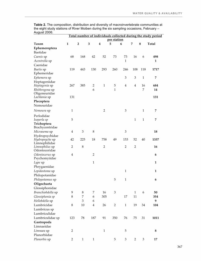
WATER QUALITY & AVAILABILITY
367
Table 2. The composition, distribution and diversity of macroinvertebrate communities at the eight study stations of River Moiben during the six sampling occasions, February – August 2006.
Total number of individuals collected during the study period
per station Taxon 1 2 3 4 5 6 7 8 Total Ephemeroptera Baetidae Caenis sp 68 168 42 52 73 73 16 6 498 Acentrella sp 1 1 Caenidae Baetis sp 119 443 130 293 260 246 108 118 1717 Ephemeridae Ephemera sp 3 3 1 7 Heptageniidae Heptagenia sp 267 385 2 1 5 4 4 16 684 Rhithrogena sp 6 1 7 14 Oligoneuridae Lachlania sp 131 131 Plecoptera Nemouridae Nemoura sp 1 2 3 1 7 Perlodidae Isoperla sp 5 1 1 7 Trichoptera Brachycentridae Micrasema sp 4 3 8 3 18 Hydropsychidae Hydropsyche sp 42 225 18 758 49 153 52 40 1337 Limnephilidae Limnephilus sp 2 8 2 2 2 16 Odontoceridae Odontocerus sp 4 2 6 Psychomyiidae Lype sp 1 1 Phrygaenidae Lepidostoma sp 1 1 Philopotanidae Philopotamus sp 5 1 6 Oligochaeta Glossiphonidae Branchiobdella sp 9 8 7 16 3 1 6 50 Glossiphonia sp 8 7 6 305 17 11 354 Hellobdella sp 3 6 9 Lumbricidae 8 10 4 26 2 1 19 34 104 Lumbricus sp Lumbriculidae Lumbriculidae sp 123 78 187 91 350 76 75 31 1011 Gastropoda Limnaeidae Limnaea sp 2 1 5 8 Planorbiidae Planorbis sp 2 1 1 5 3 2 3 17

TWENTY-FIFTH ANNUAL TECHNICAL REPORT – VOLUME I
368
Table 2 (continued)
Total number of individuals collected during the study period
per station Taxon 1 2 3 4 5 6 7 8 Total Sphaeriidae Pisidium sp 195 4 194 48 63 51 15 49 619 Sphaerium sp 2 1 2 3 8 Unionidae Anadonta sp 1 1 Crustacea Amphipoda Eriocheir sp 27 12 24 40 22 5 4 134 Arachnida Arachnida Arachnida 1 2 3 Hirudinea Branchiobdellidae Hirudo sp 6 6 Erpobdellidae Erpobdella sp 3 3 Odonata Coenagrionidae Enallagma sp 6 2 6 3 2 10 6 35 Gomphidae Gomphus sp 76 36 58 18 35 9 4 236 Epertogomphus sp 2 2 4 3 11 Aeshna sp 17 6 4 18 4 4 53 Aphylla sp 1 1 Lepidoptera Pyralidae Elophila sp 1 1 Hemiptera Belostomatidae Belostoma sp 1 2 1 5 9 Corixidae Corisella sp 1 4 2 5 10 5 27 Gerridae Metrobates sp 3 2 3 3 1 4 16 Naucoridae Ilyocoris sp 9 4 5 18 Corixidae Notonecta sp 1 3 4 Corixa sp 1 1 Veliidae 1 2 3 Microvelia sp 2 2 Trochopus sp Nepidae Nepa sp 2 2 Coleoptera Elmidae Ancyronyx sp 4 4 8
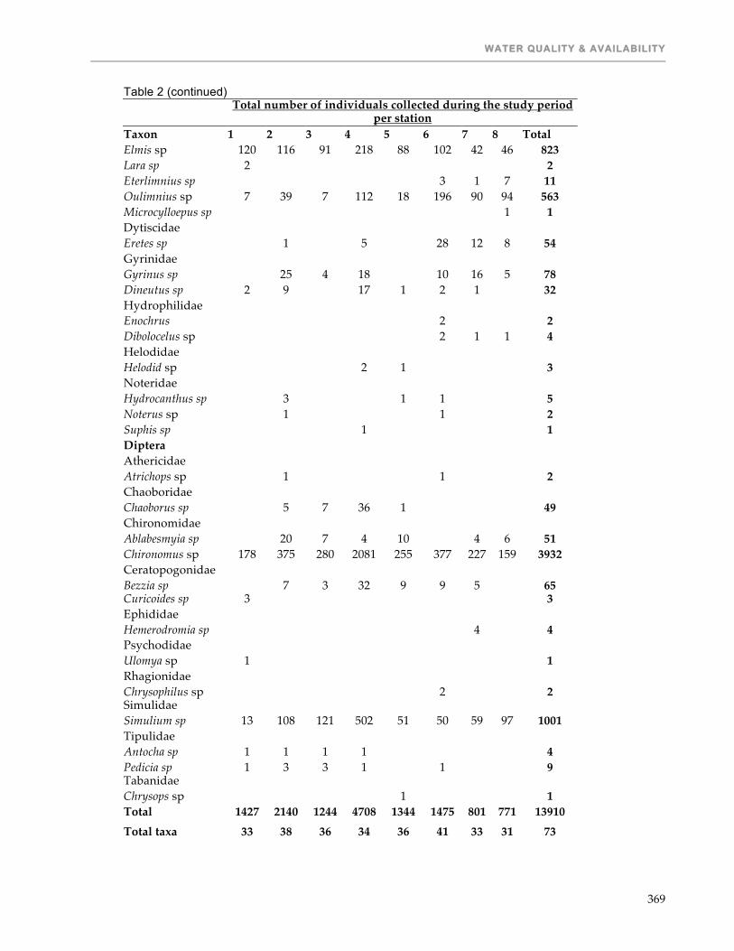
WATER QUALITY & AVAILABILITY
369
Table 2 (continued)
Total number of individuals collected during the study period
per station Taxon 1 2 3 4 5 6 7 8 Total Elmis sp 120 116 91 218 88 102 42 46 823 Lara sp 2 2 Eterlimnius sp 3 1 7 11 Oulimnius sp 7 39 7 112 18 196 90 94 563 Microcylloepus sp 1 1 Dytiscidae Eretes sp 1 5 28 12 8 54 Gyrinidae Gyrinus sp 25 4 18 10 16 5 78 Dineutus sp 2 9 17 1 2 1 32 Hydrophilidae Enochrus 2 2 Dibolocelus sp 2 1 1 4 Helodidae Helodid sp 2 1 3 Noteridae Hydrocanthus sp 3 1 1 5 Noterus sp 1 1 2 Suphis sp 1 1 Diptera Athericidae Atrichops sp 1 1 2 Chaoboridae Chaoborus sp 5 7 36 1 49 Chironomidae Ablabesmyia sp 20 7 4 10 4 6 51 Chironomus sp 178 375 280 2081 255 377 227 159 3932 Ceratopogonidae Bezzia sp 7 3 32 9 9 5 65 Curicoides sp 3 3 Ephididae Hemerodromia sp 4 4 Psychodidae Ulomya sp 1 1 Rhagionidae Chrysophilus sp 2 2 Simulidae Simulium sp 13 108 121 502 51 50 59 97 1001 Tipulidae Antocha sp 1 1 1 1 4 Pedicia sp 1 3 3 1 1 9 Tabanidae Chrysops sp 1 1 Total 1427 2140 1244 4708 1344 1475 801 771 13910 Total taxa 33 38 36 34 36 41 33 31 73
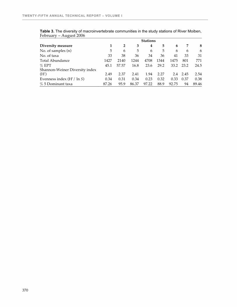
TWENTY-FIFTH ANNUAL TECHNICAL REPORT – VOLUME I
370
Table 3. The diversity of macroinvertebrate communities in the study stations of River Moiben, February – August 2006
Stations Diversity measure 1 2 3 4 5 6 7 8 No. of samples (n) 5 6 5 6 5 6 6 6 No. of taxa 33 38 36 34 36 41 33 31 Total Abundance 1427 2140 1244 4708 1344 1475 801 771 % EPT 45.1 57.57 16.8 23.6 29.2 33.2 23.2 24.5 Shannon-Weiner Diversity index (H') 2.49 2.37 2.41 1.94 2.27 2.4 2.45 2.54 Evenness index (H’/ ln S) 0.34 0.31 0.34 0.23 0.32 0.33 0.37 0.38 % 5 Dominant taxa 87.26 95.9 86.37 97.22 88.9 92.75 94 89.46

WATER QUALITY & AVAILABILITY
371
DETERMINATION OF HYDROLOGIC BASELINES FOR THE NZOIA BASIN
Twelfth Work Plan, Water Quality & Availability 5 (12WQA5) Final Report
Published as Submitted by Contributing Authors
Herbert Ssegane & E. W. Tollner University of Georgia Athens, Georgia, USA
Mucai Muchiri Moi University Eldoret, Kenya
Nancy Gitonga
Department of Fisheries Nairobi, Kenya
Geoff Habron
Michigan State University Lansing, Michigan, USA
ABSTRACT
A software suite consisting of GoogleEarth, GoldenGraphics Surfer, and UTS TKSolver was assembled and evaluated in a preliminary fashion for assessing the potential of soil erosion due to large scale agricultural development to enter and damage the Nzoia River basin in Kenya. Based on comparisons of elevations obtained with hand held GPS units onsite and measurements made with GoogleEarth software, we determined that one can use elevation data and area measurements, water shed cover assessments to assess the relative potential for agricultural practices to contribute to sedimentation in streams. The Moore’s bridge subwatershed, located near Eldoret, Kenya on the Moiben river, was selected as the first of many subwatersheds. An extensive analyses of the components of the Universal Soil Loss Equation and the US Forest Service sediment delivery ratio method was made. Based on the fact that rainfall energy in the central to south Africa were close to those in the US and that common crops of the US were in production, we felt confident that US experience would be applicable. Soils of the region are of the Ultisol and Oxisol classification, deemed similar to soils in the southeast US. Using the Universal Soil Loss Equation coupled with the US Forest Service sediment delivery ratio method, it was determined that topography could be easily mapped and determinations made of erosion potential. Preliminary results suggest that agricultural pollution is not a serious issue in this particular region.
INTRODUCTION Background The intensification of agriculture the world over has led to the deterioration of the water quality draining from agricultural catchments to the receiving surface waters. Earlier recognition of this development encouraged the endorsement of vegetative filters strips in the United States of America (USA) by 1988 as an approved USDA cost-share practice under the conservation reserve program of the Food Security Act of 1985. By 1992, the United Kingdom had also considered similar measures due to the economical threat created by erosion of fertile soils which were draining into surface water bodies (Muscutt, 1993). The accelerated soil erosion due to water has prompted the global trend of promoting sustainable Agriculture and utilization of natural resources (Oldeman, 1994). Target areas for promoting sustainable utilization of natural resources include conservation and restoration of wetlands and riparian buffer areas because of their role in the reduction of Non Point Source (NPS) pollutants. NPS pollution activities include runoff from

TWENTY-FIFTH ANNUAL TECHNICAL REPORT – VOLUME I
372
agricultural lands, urban areas, construction and industrial sites, and failed septic tanks. These activities introduce harmful sediments, nutrients, bacteria, organic wastes, chemicals, and metals into surface waters. Damage to streams, lakes, and estuaries from NPS pollution in the USA was estimated to be about $7 to $9 billion a year in the mid-1980s (Ribaudo 1986). Sediment has economic implications due to increase in the cost of water purification & hydropower generation, increased flood risk (Hansen et al., 2002) and reduction in the productivity of the fishery industry. Sediment does clog up and scrape fish gills, suffocate fish eggs and aquatic insect larvae, and cause fish to modify their feeding and reproductive behaviors. In addition to mineral soil particles, eroding sediments may transport other substances such as plant and animal wastes, nutrients, pesticides, petroleum products, metals, and other compounds that cause water quality problems (Clark 1985, Neary et al. 1988). Riparian forest buffers are a component of an integrated management system including nutrient management, sediment and erosion control practices to effectively remove excess nutrients and sediment from surface runoff and shallow groundwater. Thus, the riparian areas act as buffers such that water quality in nutrient sensitive ecosystems is not contaminated by nutrient enriched sediment from agricultural land (Likens and Bormann, 1995). Forested riparian zones and vegetative filter strips reduce sediment movement from agricultural land by intercepting flow, reducing the flow velocity, increasing the retention time, and accordingly decreasing the sediment delivery to the surface water bodies. Their hydrologic functioning is attained in three fold by the canopy, the roots, and the forest floor (forest litter / debris). The canopy intercepts precipitation, changes the raindrop side and reduces the drop velocity. The roots stabilize the soil aggregates and stream banks, increase macroscopic space and infiltration, and take up water and nutrients from deep in the soil profile. The depth and surface roughness of the forest floor litter greatly increase infiltration, slows overland flow, traps sediments, and sequesters nutrients (Travis, 2003). Throughout the African humid tropics there are numerous surface water bodies and riparian forests that have provided indigenous people with many of their social and economic needs (Leakey and Simons, 1998; Okafor and Lamb, 1994; Abbiw, 1990). But with the rapid population growth, the riparian forests are being depleted owing to the increasing demand for productive agricultural land. This mainly explains the increased degradation of the surface water quality due to sedimentation. One of the affected water bodies includes Lake Victoria, the world’s second largest source of fresh water. Lake Victoria basin is a source of livelihood to the populace of Kenya, Uganda, and Tanzania, since it’s used as a source of drinking & irrigation water, food, energy, and transport. Development activities, nutrient discharge, and population growth (3% on the Kenyan side) have caused changes in the lake’s ecosystem. Massive flourishing of algae and the water hyacinth are blocking waterways and water supply intakes (LVEMP, 1995). The main processes that drive the degradation of the Lake Victoria basin can be summarized in four folds: loss of 89% of forest cover to poor agricultural practices; pollution from mines, urban areas, and industry; loss of lake fish species diversity due to introduction of the non-native Nile perch; and poor fisheries management practices (Wangila and shallow, 2001). Lake Victoria Basin and Subwatershed Lake Victoria is the world’s second largest source of fresh water in surface area, second to Lake Superior of North America. It’s bordered by Kenya, Tanzania, and Uganda, though some inflowing rivers like Kagera do drain Burundi and Rwanda. From North to the South it’s located between latitudes 0030’N and 3012’S while from West to East between longitudes 31037’E and 34053’E. It’s situated at an elevation of 1134m above sea level, a volume of about 2760Km3 with an average depth of 40m. It has a surface area of 68,800Km2 and a total catchment area of 193,000Km2(LVEMP, 2001). The main rivers flowing into Lake Victoria from Tanzanian catchment are Mara, Kagera, Mirongo, Grumeti, Mbalageti, simiyu, and Mori (LVEMP, 2001). The main rivers from the Kenyan catchment are Nzoia, Sio, Yala, Nyando, Sondu-Miriu, Kuja, Migori, Riaria, and Mawa. From Ugandan catchment, the main rivers are Kagera, Bukora, Katonga, and Sio (LVEMP, 2003). Kagera drains both Burundi and Rwanda. Rivers from Kenyan catchment contribute 37.6% of the inflows into Lake Victoria.

WATER QUALITY & AVAILABILITY
373
Within Lake Victoria catchment, agricultural activity accounts for about half of land use. Vegetation, forest, swamps and water bodies are part of the catchment land cover. Agricultural activities with a target of increased food production contribute a high proportion of surface run off which is laden with large amounts of water pollutants including nutrients. Soil erosion in the order of 5-10 tonnes /ha-year is associated with significant losses in soil nutrients that contribute significantly to negative farm nitrogen and phosphorous balances (Van den Bosch et al. 1998). In 1983 about 60% of the land in the Kenyan catchment was natural vegetation and 30% was in agricultural use - half of this for staples and the rest for cash crops or managed grassland. Productivity varies considerably, with the more arid uplands being least productive and increasingly subject to over-exploitation and degradation. The dominant land use in the Tanzanian part of the catchment is grassland for livestock rearing, which accounts for from 50% to over 70% of land use, while the extent of cultivated land in these areas is between 30% and 10%. In the Ugandan catchment area, there is balance between cultivated land, pasture and forest. In Kenya and Uganda, the extent of land taken for urban development, infrastructure and related uses is estimated to be over 20% and increasing, however, this value is much lower in the Tanzanian catchment. Sedimentation and nutrients runoff, urban and industrial point sources pollution and biomass burning have induced the rapid eutrophication of Lake Victoria, leading to decreased productivity of the fishery industry. Afulo (1995) proposed that the increase in phosphorus is primarily due to increase in atmospheric deposition from forest burning and wind erosion. Bullock et al. (1995) estimated that 50% of Nitrogen input and 56% of the phosphorus input into Lake Victoria is due to run-off from agricultural land. Studies carried out by Sangale et al (2001) and Okungu and Opango (2001) show that river Nzoai contributes the most sediment loading to Lake Victoria from the Kenyan catchment mainly because of its high discharge of 118m3/s. Nzoia River Basin Nzoia River Basin covers an area of 12,842 Km2 and drains through several districts on its way to Lake Victoria. These include Uasin Gishu and Trans Nzoia Districts in the Rift Valley Province, Mt. Elgon, Lugari, Teso, Bungoma, Kakamega, Butere-Mumias and Busia Districts in Western Province, and Siaya District- Nyanza Province. River Nzoia is 355 km long with a mean discharge of 118 m3/second and is the largest basin within the Lake Victoria Basin. The river originates from Cherengany Hills and Mt Elgon at 4320 meters above sea level and is fed by several streams namely Kamukuywa, Moiben, Sosio, Kimilili, Kibisi, Kuywa, Malakisi, Tisi, Lwakhakha, Suam, Kisawai and Kimothon among others. On its way to the lake the river drains through small and large-scale maize and wheat farms, coffee plantations, Pan Paper Factory in Webuye, Nzoia and Mumias Sugar Factories. Runoff from rural and urban centers from areas with mixed land use practices are drained by the river before reaching the Budalangi floodplains. The river is assumed to cause the periodic flooding of the Budalangi floodplains which brings with it heavy silt from the deforested upper catchment areas. It also significantly contributes to pollution of Lake Victoria as the river drains areas with high agro-industrial activities. Further, input of pollutants comes from improperly treated wastewater from industries and urban centers situated along the river which eventually drain into the lake. The wetlands found within the catchment of the Nzoia River Basin differ depending on the section of the basin where they are found. The main wetlands in the Nzoia river basin include Chepkoilel, Budalangi, Maji Mazuri, Ziwa-Sirikwa Dam, Saiwa Swamp, Siaga Wetland, Nyasanda Wetland, Kaplogoi Stream, Sosiot wetland, Kaptule Wetland, Kapkis Wetland, Sergoit Dam / Lake Sergoit, Kerita swamp, Kholera stream, Saf Stream Wetland, Ukwala wetlands, Nambusi Wetland , Kisama Wetland, Tande Wetland, Kipsaina and Anyiko Wetland.

TWENTY-FIFTH ANNUAL TECHNICAL REPORT – VOLUME I
374
OBJECTIVES The object of this project is to present an economical approach for using remote sensing approaches for watershed assessment and assess their use based on selected watersheds. Specifically the objectives of this paper are to
1. Carry out a reconnaissance survey to determine key sites that exhibit different land use patterns, farmer practices, and land cover for the study in the Nzoia river basin.
2. Assess the use of Google earth Pro as a feasible tool for defining basin characteristics at the selected sites.
3. Develop an approach for assessing erosion, delivered sediment through riparian zones and this assess impact of cultural practices and buffer areas on nearby the Nzoia River or its tributaries.
Analysis of Factors Affecting Erosion Soil erosion in Africa: In Africa, the soil erosion problem has been worsened by conversion of shifting cultivation to intensive cropping due to population increase, Poor drainage outlet from roads and buildings, Foot paths and cattle trails to rivers, low input and subsistence agriculture, lack of conservation effective measures, high stocking rate and mechanization with inappropriate plowing techniques. These trends have resulted into erosion hot spots in Southeastern Nigeria (West Africa) and the highlands of Eastern Africa (Lal, 1998). Other factors attributed to accelerated soil erosion in Africa include tropical deforestation (Lal, 1981), overstocking by livestock and wildlife in eastern Africa especially Kenya (Ongwenyi et al., 1993), lack of maintenance of traditional hillside terraces (Conelly, 1994), low soil fertility, and low available water holding capacity (Zaongo et al., 1994). The main on-site impact is the reduction in soil quality which results from the loss of the nutrient-rich upper layers of the soil, and the reduced water-holding capacity of many eroded soils. Erosion’s removal of the upper horizons of the soil results in a reduction in soil quality this is because the eroded upper horizons tend to be the most nutrient-rich. Also, because the finest constituents of eroded soil tend to be transported furthest and the eroded soils become preferentially depleted of their finer fraction over time. This often reduces the soils water-holding capacity and the effective rooting depth. Thus, erosion removes the cream of the soil. Increased use of artificial fertilizers may to an extent, and for a time, compensate for erosion-induced loss of soil quality where economic circumstances are favorable. This is not usually feasible in developing countries however. Loss of soil quality is a long-term problem; globally, soil erosion's most serious impact may well be its threat to the long-term sustainability of agricultural productivity, which results from the 'on-site' damage it causes. Water erosion’s main off-site effect is the movement of sediment and agricultural pollutants into watercourses. This can lead to the silting-up of dams, disruption of the ecosystems of lakes, and contamination of drinking water. In some cases, increased downstream flooding may also occur due to the reduced capacity of eroded soil to absorb water. Movement of sediment and associated agricultural pollutants into watercourses is the major off-site impact resulting from erosion. This leads to sedimentation in watercourses and dams, disruption of the ecosystems of lakes, and contamination of drinking water (Lal and Stewart, 1994; Lal, 1995c). Sedimentation of streams can have a pronounced effect on water quality and stream life. Sediment can clog and abrade fish gills, suffocate fish eggs and aquatic insect larvae, and cause fish to modify their feeding and reproductive behaviors. Sediment also interferes with recreational activities as it reduces water clarity and fills in water bodies. In addition to mineral soil particles, eroding sediments may transport other substances such as plant and animal wastes, nutrients, pesticides, petroleum products, metals, and other compounds that can cause water quality problems (Clark, 1985; Neary, 1988; Neary et al 1988). Pimentel et al (1995) estimated that the total cost of soil eroded in the world is about $225 billion a year. The cost of all off-site environmental impact of soil erosion in the U.S. was estimated to be about $7 billion per year in the mid-1980s and $17 billion per year in the mid-1990s (Ribaudo, 1986a, b). In Australia, the off-site costs from water-induced erosion have been estimated at $10
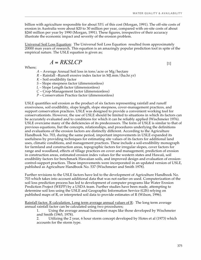
WATER QUALITY & AVAILABILITY
375
billion with agriculture responsible for about 53% of this cost (Morgan, 1991). The off-site costs of erosion in Australia were about $20 to 30 million per year, compared with on-site costs of about $260 million per year by 1990 (Morgan, 1991). These figures, irrespective of their accuracy illustrate the economic impact and severity of the erosion problem. Universal Soil Loss Equation: The Universal Soil Loss Equation resulted from approximately 20000 man years of research. This equation is an amazingly popular prediction tool in spite of the empirical nature. The USLE equation is given as;
RKSLCPA = [1] Where; A – Average Annual Soil loss in tons/acre or Mg/hectare R – Rainfall –Runoff erosive index factor in MJ.mm/(ha.hr.yr) K – Soil erodibility factor S – Slope steepness factor (dimensionless) L – Slope Length factor (dimensionless) C – Crop-Management factor (dimensionless) P – Conservation Practice factor (dimensionless) USLE quantifies soil erosion as the product of six factors representing rainfall and runoff erosiveness, soil erodibility, slope length, slope steepness, cover-management practices, and support conservation practices. USLE was designed to provide a convenient working tool for conservationists. However, the use of USLE should be limited to situations in which its factors can be accurately evaluated and to conditions for which it can be reliably applied (Wischmeier 1976). USLE overcame many of the deficiencies of its predecessors. The form of USLE is similar to that of previous equations, but the concepts, relationships, and procedures underlying the definitions and evaluations of the erosion factors are distinctly different. According to the Agriculture Handbook No. 703, during the same period, important improvements in USLE expanded its usefulness by providing techniques for estimating site values of its factors for additional land uses, climatic conditions, and management practices. These include a soil-erodibility monograph for farmland and construction areas, topographic factors for irregular slopes, cover factors for range and woodland, effects of tillage practices on cover and management, prediction of erosion in construction areas, estimated erosion index values for the western states and Hawaii, soil erodibility factors for benchmark Hawaiian soils, and improved design and evaluation of erosion-control-support practices. These improvements were incorporated in an updated version of USLE, published as Agriculture Handbook No. 537 (Wischmeier and Smith 1978). Further revisions to the USLE factors have led to the development of Agriculture Handbook No. 703 which takes into account additional data that was not earlier on used. Computerization of the soil loss prediction process has led to development of computer programs like Water Erosion Prediction Project (WEPP) by a USDA team. Further studies have been made, attempting to determine soil loss using the USLE and Geographic Information Service (GIS) relying on published maps of R, or interpreted soil data to provide estimates of R (Wilson, 1996). Rainfall factor, R calculation, Long term average annual values of R: The long term average annual rainfall factor can be calculated using two procedures;
1. Using the average annual Isoerodent maps like those developed by Wischmeier and Smith (1965, 1978). 2. Utilizing the 2 year, 6 hour storm concept developed by Hotes et al (1973) which accounts for the storm type.

TWENTY-FIFTH ANNUAL TECHNICAL REPORT – VOLUME I
376
a. Storm type I; 2.2)6,2(55.16
100PEIR == [2a]
b. Storm type II
2.2)6,2(27
100PEIR == [2b]
Where P(2,6) is the 2 year, 6 hr precipitation in inches. Storm based values of R Hotes et al (1973) developed another relationship for determine the storm R factor given the precipitation, P (inches) and the storm duration, D (hours).
a. Storm type I;
6065.0
2.215DPRst = [3a]
b. Storm type II
4672.0
2.225.19D
PRst = [3b]
For standard units, multiply the result by 17.02 and divide the precipitation (inches) by 25.4 yielding an equation like
=−−− 4672.0
2.2
4.2525.19
*02.17)/(D
P
yrhrhammMJRst [3c]
Cooley (1980) further developed the above relationships to cater for all storm types. That is for the storm R value for Soil Conservation Services (SCS) types I, Ia, II, and IIa.
1
)(1
b
Df
st DPaR = [3d]
Where 0086.0119.2)( DDf = , P (inches), D (hrs), and for the values of a1 and b1, refer to table 1.
Table 1: Coefficient values for the different storm types for Cooley’s equation SCS Storm Type a1 b1
I 15.03 0.5780 Ia 12.98 0.7488 II 17.90 0.4134
IIa 21.51 0.2811 Renard et al (1997) proposed another approach for determining single storm R value. The computations are as follows;
( )∑∑=
−−==N
i
Iist
iePIEI
R1
05.0max30
30 129.0100
[4]
Where, Pi – Precipitation (mm) occurring during the ith storm segment Ii – Intensity (mm/hr) during the ith storm segment N – Number of storm segments I30max – Is the 30 minute storm segment yielding the highest intensity

WATER QUALITY & AVAILABILITY
377
Soil Erodibility factor, K calculation: The k factor can be computed as a simple soil Erodibility factor, Ksimple (Renard et al, 1997) or as a complex soil Erodibility factor, Kcomplex. The simple K factor is calculated independently, while the complex K factor is computed as a composite KLS factor. Simple K, Ksimple
( )( )[ ] ( ) ( ) ( )310*3.3210*3.412*%100%%10*8.2 3314.17 −+−+−−+= −−− cbaClayVFSSiltKsimple [5] Where, %Silt – Percent Silt %VFS – Percent Very Fine Sand %Clay – Percent Clay a – Percent Organic Matter b – Structure Code; 1 – Very fine granular 2 – Fine granular 3 – Medium to Coarse granular 4 – Massive, blocky or Platy
c – Permeability Class; 1 – Rapid 2 – Moderate to Fast 3 – Moderate 4 – Slow to Moderate 5 – Slow 6 – Very Slow Complex K, Kcomplex (KLS) The Complex Soil Erodibility factor calculation is more suited for slopes that are not uniformly distributed (complex slopes) where different slope segments have different slopes. The procedure involves five steps for each slope segment; calculation of slope length factor, slope steepness factor, slope length adjustment factor, soil Erodibility factor, and summing up the product of the above four segment factors. Slope length factor, Li: The slope length is computed using the following relationships:
Mer
ilL
=22
[6a]
( ) 05.0sin269.0sinsin*
8.0 ++=
θθ
θRillFactorMer [6b]
= −
100tan 1 s
θ [6c]
Where, l – length along the slope face (m). if the length is in feet change 22 to 72.16. Mer - Factor relating angle to slope length erosion severity. RillFactor – Rill erosion susceptibility factor; 0.5 – Not susceptible 1 – Average susceptibility 2 – Very susceptible Slope Steepness factor, Si: ( ) 56.0sin*3 8.0 == θiS If l < 4m. [7a]
03.0sin*8.10 += θiS If l > 4m and s < 9% [7b] 5.0sin*8.16 −= θiS If l > 4m and s > 9% [7c]
For irregular slopes, the use of a Slope length Adjustment Factor (SAF) is applied.

TWENTY-FIFTH ANNUAL TECHNICAL REPORT – VOLUME I
378
( )m
mm
i niiSAF
11 1 ++ −−= [8]
Where i – the slope length segment number n – Total number of segments Ki – is calculated as in the case of simple K
Thus, ∑=
=n
iiiii SAFSLKKLS
1)( [9]
The Cropping management factor, C: According to Renard (1997), the cropping management factor C is a combination of five sub-factors in an agricultural setting. These factors include; prior land use, canopy cover, surface cover, surface roughness, and soil moisture. Since these sub-factors vary throughout the year or growing season, Tollner (2002), Haan et al (1994), Renard et al (1997) present a method of aggregating the C factor basing on the percentage canopy cover throughout the year and the rainfall distribution. Computed Practice factor, P: The practice factor P is a dimensionless factor that has a maximum value of 1 for no conservation services. It’s divided into three components; Contouring practice sub-factor (Pi), Strip-cropping practice sub-factor (Ps), and the terracing practice sub-factor (Pt). Pc can be estimated using a slope dependant table (Haan et al, 1994; Tollner, 2002). In case the slope exceeds the table slopes, Pc = 1. Ps is 1 for contouring only, 0.75 for a 4 year rotation with 2 year row crop and 2 year meadow or small grain. Ps is 0.5 with 1 year row crop with 3 year meadow or small grain. Ps is 1 for shorter rotations and if strip width for a given slope is exceeded. Pt is 1 for no terraces, 0.2 for terraces with graded sod outlets, and 0.1 with tile terraces. Pt = 1 for construction, mining, and clear cut forest harvest areas.
tsc PPPP **= [10] Sediment Delivery Ratio (SDR) calculation: Soil eroded as predicted by the USLE and its variants is not the same as the soil that may be delivered to a point down stream due to settling opportunities between the eroding field and the downstream measurement point. The relationships between SDR and catchment/drainage area has been established in form of curves. Watersheds with large drainage area and the fields with a long distance to the streams have a low sediment delivery ratio. This is because large areas have more chances to trap soil particles, thus the chance of soil particles reaching the water channel system is low. At regional scale, the most widely used method to estimate SDR is through an SDR-area power function first proposed by Maner (1958) and also Roehl (1962):
βαASDR = [11] Where A is the catchment area (km2), the constant α and a scaling exponent β are empirical Parameters. Field measurements by Walling (1983) and Richards (1993) suggest that β is in the range –0.01 to –0.025. This depicts an inverse relationship between SDR and Area, thus SDR decreases with increasing catchment area. The scaling exponent β contains key physical information about catchment sediment transport processes and its close linkage to rainfall-runoff processes. It seems that β decreases with increasing aridity (Richards 1993). However, field data from studies carried in different catchments of the world show that the relationship between SDR and drainage area changes considerably for each catchment. A more generalized model for estimating SDR form SDR – Area power function was developed by Vanoni (1975) using data from 300 watersheds throughout the world. It’s given as;

WATER QUALITY & AVAILABILITY
379
125.042.0 −= ASDR Where; A = drainage area in square miles. The USDA SCS (1979) developed a SDR model based on the data from the Blackland Prairie, Texas. A power function is derived from the graphed data points:
11.051.0 −= ASDR [12] Where; A = drainage area in square miles. Other relationships observed in the literature include the following approaches. Maner (1958); LRSDR log854.0869.0962.2)log( −+= [13a] Maner (1962); )log(14191.07935.1)log( ASDR −= [13b] Roehl(1962); BRLRcoASDR log786.2)/log(510.0log23.05.4)log( 10 −−−= [13c]
Williams and Berndt (1972); 403.0627.0 dsSDR = [13d]
Williams (1977); 444.5363.01.011 .)/.(.10*366.1 CNLRASDR −−= [13e] Mou and Meng (1980); InAInRCSDR 025.037.129.1 −+= [13f]
Where; R is basin relief defined as the difference in elevation between the average elevation of the watershed divide and the watershed outlet, L is maximum basin length measured roughly parallel to mainstream drainage; R/L is the basin relief to length ratio; BR is bifurcation ratio; sd is slope of main channel (%); CN is the long-term average SCS curve number; A is drainage area (km2) and RC is gully density.
The United States Forestry Services (USFS)-SDR and the Stiff Diagram was originally developed by the USEPA (1980) for use in silvicultural applications but it’s been found to be viable in evaluating a wide variety of buffer types. The model evaluates the following parameters; percent ground cover, texture of eroded material (% silt & smaller), surface runoff (cfs/ft), slope gradient, surface roughness, delivery distance (feet) and slope shape. Basing the sediment delivery on a multitude of factors is believed to add robustness to the approach lacking in other approaches. Compute the values for each parameter; connect the points with a line resulting into a polygon. Then determine the area of the enclosed polygon and form a ratio of this area to the area enclosed by the bounding rectangle. Then enter this ratio into the SDR predictive curve. The factors on the on the stiff diagram are obvious influences on the ability of runoff to transport sediment. The slope is that of the zone (e.g., a riparian zone) between the sediment producing zone and the receiving water way (channel). The slope shape of 0 represents a convex slope, 2 represent a uniform slope and that of 4 represents a concave slope. Surface roughness (within the riparian zone) is assigned by the researcher where a factor of 0 represents a smooth surface, and 4 represent a rough surface. GIS, Remote sensing and Estimation of soil erosion: The interfacing of Geographical Information System (GIS), Digital Elevation Model (DEM) and Satellite Remote Sensing (RS) has provided a new capability to analyze and monitor the dynamics of land-use change. GIS is a system which deals with information related to the spatial distribution of features on the earth's surface. The system is designed to efficiently capture, store, update, manipulate, analyze and display all forms of geographically referenced information. RS is the gathering and recording of information by a sensor on board a satellite orbiting in space without any physical contact with the object or area being investigated. It can refer to, for instance, to satellite imagery, to aerial photographs or to ocean bathymetry explored from a ship using radar data. RS is used to collect information about the earth's features, such as its geology, vegetation, soil, atmosphere, water, ice surfaces and land-use. The Digital Elevation Model (DEM) is defined as "any digital representation of the continuous variation of relief over space" (Burrough 1986). It can be created from stereo-pairs derived from RS data or aerial photographs, or can be generated from digital terrain elevation data. DEM derived products can be readily combined with RS data for data analysis. For example,

TWENTY-FIFTH ANNUAL TECHNICAL REPORT – VOLUME I
380
Guneriussen and Johnsen (1996) used DEM to calibrate and geocode satellite data for monitoring snow. DEM is also very useful for discriminating land use and ground cover classes during the digital processing of RS data. Since the launch of ERTS-1 (Landsat 1) in 1972, digital remote sensing has been used with some success to monitor natural resources and provide input to better manage the Earth. Applications have included monitoring of deforestation, agro-ecologic zoning, ozone layer depletion, food early warning systems (FEWS), monitoring of large atmospheric-oceanic anomalies such as El Niño, climate and weather prediction, ocean mapping and monitoring, wetland degradation, vegetation mapping, soil mapping, natural disaster and hazard assessment and mapping, and land cover maps for input to global climate models. A number of satellite systems have been put aside to monitor the global environment. The most commonly used satellite for natural resource management is the NOAA AVHRR, which has a twice daily overpass and can be freely downloaded by low-cost ground receiving stations. It has a nominal pixel size of 1.1 km and records two spectral bands in the visible and near infrared. The data from the AVHRR have been used to map global land cover which is an input layer to global climate models, in addition to being important for estimating the pattern of soil erosion over the Earth. GIS and RS application for predicting soil erosion utilize the USLE model. Each factor of the USLE is computed by use of RS data organized in form of overlaid layers and mathematical manipulations enabled by the GIS capabilities. Remote sensing and GIS have been used to study other fields like the mangrove forests ( Ramachandran et al., 1998), seagrass beds (Ferguson and Korfmacher, 1997) and coral reefs ( Holden and Ledrew, 1999). The quality and accuracy of the GIS outputs relies primarily on the quality of ‘spatial resolution. In fact, three basic qualities inherent to remote sensing data must be recognized: spatial resolution, temporal resolution and spectral resolution. Erosion and Sediment Control Management Practices – the riparian buffer and approaches for evaluating its effectiveness: Environmental Protection Agency (EPA) and USDA-SCS (1988) suggest the following practices as viable measures for controlling erosion and sediment. The riparian buffer is a versatile tool for stream protection and will be exploited in this work. Kenya currently mandates riparian buffers but has found the mandated buffers difficult to enforce. Pollutants are known to enter surface waters from point sources, such as industrial discharges and waste-water treatment plants but most pollution to surface waters is from nonpoint source pollution activities that include runoff from agricultural lands, urban areas, construction and industrial sites, and failed septic tanks. These activities introduce harmful sediments, nutrients, bacteria, organic wastes, chemicals, and metals into surface waters. Nonpoint source pollution is hard to control, measure, and monitor. One of the Best Management Practices (BMP) which can be very effective in controlling nonpoint source pollution, thus influencing water quality is the utilization of naturally occurring or construction of riparian forest buffers along streams, lakes, and other surface waters. Through the interaction of their unique soils, hydrology, and vegetation, riparian forest buffers influence water quality as contaminants are taken up into plant tissues, adsorbed onto soil particles, or modified by soil organisms. The riparian area is that area of land located immediately adjacent to streams, lakes, or other surface waters. The riparian areas differ from the adjoining uplands because of high levels of soil moisture, frequent flooding, and the unique assemblage of plant and animal communities found there. Studies indicate that both forest and grass riparian buffers can effectively trap sediment. For example: Researchers in Blacksburg, Virginia, found that orchard grass filter strips 30 feet wide removed 84 percent of the sediment and soluble solids from surface runoff, while grass strips 15 feet wide reduced sediment loads by 70 percent (Dillaha et al, 1989). In North Carolina, scientists estimated that 84 percent to 90 percent of the sediment from cultivated agricultural fields was trapped in an adjoining deciduous hardwood riparian area (Cooper et al, 1987). Sand was deposited along the edge of the riparian forest, while silt and clay were deposited further in the

WATER QUALITY & AVAILABILITY
381
forest. Along the Little River in Georgia, scientists found that a riparian forest had accumulated 311,600 to 471,900 pounds per acre of sediment annually over the last 100 years (Lowrance et al, 1986). Many factors influence the effectiveness of the buffer to remove sediments from land runoff, including the sediment size and loads, slope, type and density of riparian vegetation, presence or absence of a surface litter layer, soil structure, subsurface drainage patterns, and frequency and force of storm events (Osborne and Kovacic 1993). Riparian buffers need to be properly maintained and regularly monitored in order to maintain their effectiveness because some research has showed a decrease in their effectiveness over time in case of clogging. Probably the most important consideration is the maintenance of shallow sheet flow into and across the buffer. Where concentrated flow paths begin to form or deep sediments begin to accumulate, the buffer can no longer maintain its filtering ability. Nutrients such as Nitrogen (N) and Phosphorous (P) are essential elements for aquatic ecosystems, but in excess amounts, they can lead to many changes in the aquatic environment like eutrophication and reduce the quality of water (Dupont, 1992). Some nutrient inputs into surface waters are entirely natural, such as nutrients contained in plant materials or naturally eroding soils (Clark et al, 1985). Grass and forest buffers are both effective at removing N and P from runoff, however forests are more efficient at removing dissolved nutrients from groundwater (Osborn and Kovacic, 1993). Several studies have found that buffers that include both grass and forest zones have increased nutrient removal capacities (Dillaha et al., 1989; Lowrance et al., 2000 and 2005; Novak et al., 2002; Lee et al., 2003). To monitor the effectiveness of the respective BMPs in controlling erosion and sediment, there should be a way of determining the amount of soil eroded and how much is likely to end down stream. The USLE has been adopted the world over as an effective approach to estimate the amount of soil eroded from a plot, a catchment, and even from construction sites. Since USLE does not determine sediment deposition, the SDR enables the determination of how much of the eroded soils are deposited in the riparian zones. Therefore, the USLE and the USFS-SDR will be used as monitoring tools.
METHODS Basin Reconnaissance Survey: The Nzoia basin is characterized by three physiographic regions: the highlands, characterized by Mount Elgon and the Cherangany Hills; the upper plateau which includes Eldoret and Kitale; and the lowlands including Busia which experiences the majority of the flooding that occurs in the basin. The reconnaissance survey was carried out by moving along the sub-basins of Nzoia River basin. The Moiben sub-basin was selected for the preliminary analysis. The Moiben River is in the upper region of the Nzoia basin above the Eldoret valley in Kenya. Seven sites along the Moiben River were selected for analysis based on their agricultural intensity, heavy cattle grazing incidences, riparian forest encroachment, and some due to zero agricultural activity. Some of the sites were selected due to the mucky appearance of the water at the site. The Geographical Position System (GPS) coordinates (Latitude and Longitude) and the elevation values of the sites were recorded using a hand held Garmin GPS displaying an elevation error of plus or minus 1 to 9m depending on the surrounding coverage. Google Earth Pro and basin Characteristics: Google Earth Pro is a virtual globe program that maps the entire earth by pasting images obtained from satellite imagery, aerial photography and GIS over a three dimensional (3-D) globe. The degree of resolution available is based on points of interest, but all land is covered in at least 15 meters of resolution (15m x 15m pixel size). Google Earth allows users to search for locations and addresses by entering coordinates, or simply using the mouse to browse to a location. Most land areas are covered in satellite imagery with a resolution of about 15 m per pixel, and some population centers are also covered in airplane imagery of several pixels per meter. Oceans are covered in much lower resolution. For the

TWENTY-FIFTH ANNUAL TECHNICAL REPORT – VOLUME I
382
coordinate system, the data is stored and presented using the standard World Geographical System (WGS84) datum. The data is usually less than 3 years old. The special features of Google Earth Pro are its ability to measure distance in miles, kilometers, or feet and area measurements for any polygon. It allows the user to interact with the software by adding user specific attributes. Google Earth Pro will be used to extract the following data from each site: average slope length; average slope; and area of the Eroded area (area under cultivation and / or developed land), riparian buffer, and the total land contributing the eroding precipitation. Using the GPS generated latitude and longitude coordinates of the selected sites, Google Earth Pro can zoom onto a site up to an eye altitude determined by the user for clarity. The eye altitude defines the elevation of the viewer above the globe in reference to the sea level. At a chosen eye altitude, one can clearly define the river / stream, the riparian buffer, cultivated land and other land use forms. Also, coordinates and elevation values of desired features can be recorded. For each site Surfer software will be used to enhance the performance of Google Earth Pro in defining basin characteristics. Surfer is hydrologic software that’s used for contouring, determining water flow direction, and 3-D view of a watershed. It will be used to clearly show the direction of flow that is useful in determining slope and slope length for the buffer, eroded area and total area. Also it will be used to clearly delineate the watershed divide and determining the curvature of the slope (whether concave, convex, or uniform). Estimation of soil erosion using the USLE: According to Tiwari et al (2000), Oliviera et al (2004), Rapp et al (2001) the USLE and RUSLE models had a better performance efficiency compared to the WEPP model and this is greatly attributed to the fact that the input variables are site specific. However, it was noted that these two models tend to over estimate soil losses on plots with low erosion rates and under estimate soil losses on plots with high erosion rates. These research findings coupled with the world wide acceptance of the USLE model, explain the choice of USLE as the soil erosion prediction model. The method involves the calculation of six factors of rainfall, soil erodibility, slope length, slope steepness, crop management, and the support practice described in literature review. Specific details of the USLE factors are presented as this is not a trivial issue when applying the USLE outside the United States, where much data is available. The emphasis here is to bring forward tools that have robustness. Hudson (1971) presented data showing that the rainfall-energy relation for storms in southern Africa were similar to those in the continental US, which are known to be the Type II storm. Rainfall factor, R calculation: Cooley (1980) equations will be used to calculate the storm R value, given the precipitation, P (inches) and storm duration, D (hrs). The equation calculates R values for the Soil Conservation Services (SCS) storm types I, Ia, II, and IIa. Refer to [3].
=−−−1
)(
14.25*02.17)/( b
Df
st D
P
ayrhrhammMJR
0086.0119.2)( DDf = For the respective storm types, the values of a1 and b1 are given in table 1. For some cases, the R value will be approximated depending on the availability of the data. For such instances, the approximate R value will be used directly. For storm events, the R value will be calculated using the Renard et al (1997) method. For uniform and regular slopes, the K value will be calculated using the simple K method while for irregular and complex slopes, the complex k method.

WATER QUALITY & AVAILABILITY
383
The slope length and slope steepness factors will be calculated using the methods described under the calculation of the complex K value. The cropping management (C) factor will be calculated using the approach proposed by Tollner (2002), Haan et al (1997), Barfield et al (1990) , which aggregates the C factor depending on the rainfall distribution and the crop/canopy cover. The support practice factor, P calculation is given by [10] P = Pc*Pt*Pt Finally, soil erosion in tones / year is given as (refer to [1]);
RKSLCPA = A computer program has been developed to estimate soil erosion with the USLE using a TK Solver3 software. The main motivation for this program is the diversity and flexibility it gives the user such that each site or plot is treated independently. One does not have to integrate or transform data to fit a particular form or pattern to use the program. Determination of Sediment Yield: The SDR approach developed by the United States Forestry Services (USFS) is preferred because it accounts for more site specific variables than other approaches. The parameters include ground cover, texture of eroded material, surface run-off, slope gradient, surface roughness, delivery distance, and slope shape. These seven parameters better describe the site characteristics than just relating the relief - length, drainage area, stream slope, bifurcation ratio or gully density to the sediment delivery ratio. Below are figures of the Stiff diagram and diagram to convert the percent area from the Stiff diagram to the Sediment delivery ratio. With the help of the above two figures, mathematical relations have been developed to computerize the process of SDR determination. Since area of a polygon can be calculated using coordinates of the polygon vertices, equations have been developed to determine the coordinates corresponding to the seven vertices that form the stiff diagram area. The entire stiff diagram is considered to have a total area of one unit. The stiff diagram coordinates were determined using the following relationships: Texture of eroded material
textureYX
*005.05.05.0
1
1
+=
= [14a]
Surface Runoff
runoffYrunoffX
*55.0*55.0
2
2
+=
+= Note: If runoff >0.1cfs/ft, then set X2 and Y2 = 0.1 [14b]
Slope gradient
slopeYslopeX
*005.05.0*005.05.0
3
3
+=
+= [14c]
3 TK Solver 5.0, Universal Technical Systems, Chicago, IL.

TWENTY-FIFTH ANNUAL TECHNICAL REPORT – VOLUME I
384
Figure 1. USFS and USEPA stiff diagram for assessing riparian buffer capability of trapping incoming sediment.
Figure 2. Diagram for converting the percent area from the Stiff diagram to the Sediment delivery ratio
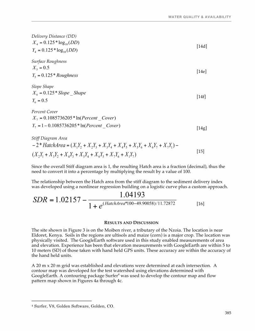
WATER QUALITY & AVAILABILITY
385
Delivery Distance (DD)
)(log*125.0)(log*125.0
104
104
DDYDDX
=
= [14d]
Surface Roughness
RoughnessYX
*125.05.0
5
5
=
= [14e]
Slope Shape
5.0_*125.0
6
6
=
=
YShapeSlopeX
[14f]
Percent Cover
)_ln(*1085736205.01)_ln(*1085736205.0
7
7
CoverPercentYCoverPercentX
−=
=
[14g] Stiff Diagram Area
)()(*2
71675645342312
17766554433221
YXYXYXYXYXYXYXYXYXYXYXYXYXYXHatchArea
++++++
−++++++=− [15]
Since the overall Stiff diagram area is 1, the resulting Hatch area is a fraction (decimal), thus the need to convert it into a percentage by multiplying the result by a value of 100. The relationship between the Hatch area from the stiff diagram to the sediment delivery index was developed using a nonlinear regression building on a logistic curve plus a custom approach.
72872.11/)90058.49100*(104193.102157.1 −+
−= HatchAreaeSDR [16]
RESULTS AND DISCUSSION The site shown in Figure 3 is on the Moiben river, a tributary of the Nzoia. The location is near Eldoret, Kenya. Soils in the regions are ultisols and maize (corn) is a major crop. The location was physically visited. The GoogleEarth software used in this study enabled measurements of area and elevation. Experience has been that elevation measurements with GoogleEarth are within 5 to 10 meters (SD) of those taken with hand held GPS units. These accuracy are within the accuracy of the hand held units. A 20 m x 20 m grid was established and elevations were determined at each intersection. A contour map was developed for the test watershed using elevations determined with GoogleEarth. A contouring package Surfer4 was used to develop the contour map and flow pattern map shown in Figures 4a through 4c.
4 Surfer, V8, Golden Software, Golden, CO.

TWENTY-FIFTH ANNUAL TECHNICAL REPORT – VOLUME I
386
Ordinarily, one would not have to be concerned with the details of the catchment for erosion prediction with the USLE. However, the application of the US Forest Service SDR approach required a runoff estimate of peak flow running into the riparian buffer. Thus, efforts were made to define the runoff producing area and estimate the peak flow based on the two year storm. Factors for the USLE and the sediment delivery ratio are summarized in Table 2 for the Moore’s Dam watershed. The three plots shown on Figure 1 are tilled soils with corn. Since the average annual erosion value, or the erosion to be expected roughly at least every two years, a weighted C factor was required based on prevailing cultural practice data and on the rainfall distribution for the area. Rainfall distribution data for the Eldoret area were available, which was deemed sufficient for the Moore’s Dam subwatershed.
Figure 3. Areal photograph of the Moore’s Dam subwatershed as viewed from 4.95 km with GoogleEarth. The general land use / land cover of the area is characterized by forests, shrubs, rangeland, and cultivated land. The main crops grown are maize (corn) and wheat with maize covering over 80% of the cultivated land. Apart from the traditional croplands, the population pressure and the practice of agriculture as a livelihood source has encouraged the encroachment onto the forests. There are cultivated land patches scattered all over the Moiben watershed as the forests are cleared for agricultural land. During the site visits, the authors experienced freshly cut and burnt forests. In some places, the maize growing is along the Moiben River. The other farmer activity is cattle keeping. The river acts as a source of drinking water for the cattle. As the cattle are driven to their drinking points, they carry soil particles to the river and their stampede of the soil along the way loosens the soil making it more susceptible to erosion.
Moore’s Dam Site
Buffer
A=40 ha L=349 m S=4.9%
A=4.39 ha L=253 m S=8.92 %
A=3.64 ha L=186 m S=20.9 %
A=4 ha L=277 m S=11.9 %
Plot 1
Plot2
Plot3
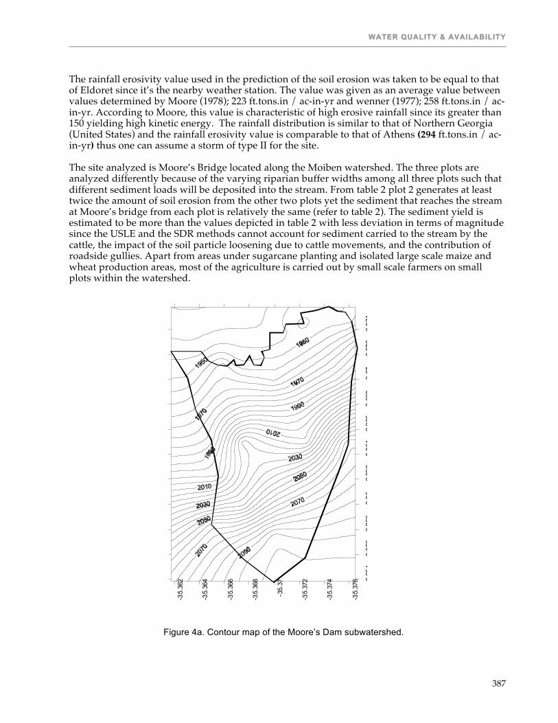
WATER QUALITY & AVAILABILITY
387
0.854
0.856
0.858
0.86
0.862
0.864
0.866
0.868
0.87
0.872
0.874
-35.376
-35.374
-35.372
-35.37
-35.368
-35.366
-35.364
-35.362
The rainfall erosivity value used in the prediction of the soil erosion was taken to be equal to that of Eldoret since it’s the nearby weather station. The value was given as an average value between values determined by Moore (1978); 223 ft.tons.in / ac-in-yr and wenner (1977); 258 ft.tons.in / ac-in-yr. According to Moore, this value is characteristic of high erosive rainfall since its greater than 150 yielding high kinetic energy. The rainfall distribution is similar to that of Northern Georgia (United States) and the rainfall erosivity value is comparable to that of Athens (294 ft.tons.in / ac-in-yr) thus one can assume a storm of type II for the site. The site analyzed is Moore’s Bridge located along the Moiben watershed. The three plots are analyzed differently because of the varying riparian buffer widths among all three plots such that different sediment loads will be deposited into the stream. From table 2 plot 2 generates at least twice the amount of soil erosion from the other two plots yet the sediment that reaches the stream at Moore’s bridge from each plot is relatively the same (refer to table 2). The sediment yield is estimated to be more than the values depicted in table 2 with less deviation in terms of magnitude since the USLE and the SDR methods cannot account for sediment carried to the stream by the cattle, the impact of the soil particle loosening due to cattle movements, and the contribution of roadside gullies. Apart from areas under sugarcane planting and isolated large scale maize and wheat production areas, most of the agriculture is carried out by small scale farmers on small plots within the watershed.
Figure 4a. Contour map of the Moore’s Dam subwatershed.

TWENTY-FIFTH ANNUAL TECHNICAL REPORT – VOLUME I
388
0.854
0.856
0.858
0.86
0.862
0.864
0.866
0.868
0.87
0.872
0.874
-35.376
-35.374
-35.372
-35.37
-35.368
-35.366
-35.364
-35.362
Figure 4b. Flow path map based on the contour map in Figure 4a.
Figure 4c. Three dimensional view of the Moore’s Dam test watershed.

WATER QUALITY & AVAILABILITY
389
Moore’s Bridge Site Roadside Gullies in Moiben watershed
Moiben Bridge Site Clearing of Riparian
forests for Agriculture
Streamside cultivation along Tangasir River
Streamside cultivation along Moiben River

TWENTY-FIFTH ANNUAL TECHNICAL REPORT – VOLUME I
390
Table 2. USLE and Sediment Delivery Ratio calculation test data for three tilled plots.
Moore's Bridge Site Plot 1 Plot 2 Plot 3 Delivery Distance (ft) 820 2348 2756 Ground Cover (%) 90 90 90 Slope gradient (%) 4.9 8.5 6 Slope Shape 0 0 0 Surface Roughness 2 2 2 Texture of Eroded Material (%) 87 87 87 Excess rainfall intensity (in/hr) 2 2 2 Disturbed Slope Length (ft) 830 610 909 Surface Runoff (Cfs/ft) 0.03834 0.02819 0.04198
R Factor (Hotes et al Method) or Input Input (Average of 223 and 258)-MJ.mm/ha.hr.yr
240.5*17.02 (4093.31) 4093 4093
C Factor 0.3806 0.3806 0.3806
K Factor Percent Silt (%) 17 17 17 Percent Very Fine Sand (%) 13 13 13 Percent clay (%) 70 70 70 Percent Organic Matter content (%) 5.2 5.2 5.2 Soil structural Code 3 3 3 Soil Permeability class 6 6 6
LS Factor Slope Length 253 186 277 Slope steepness 8.9 20.9 11.9 Eroded Soil (Mg/ha-yr) 97.2 320.1 171.4 Plot Area (ha) 4.39 3.64 4 Total Eroded Soil (Mg/yr) 426.7 1165.2 685.6 Sediment Delivery Index (SDR) 0.01535562 0.006605424 0.009875543 Stream Sediment Yield (Mg/yr) 6.6 7.7 6.8

WATER QUALITY & AVAILABILITY
391
CONCLUSIONS An extensive analysis of the components of the Universal Soil Loss Equation and the US Forest Service sediment delivery ratio method was made. Based on the fact that rainfall energy in the central to south Africa were close to those in the US and that common crops of the US were in production, we felt confident that US experience would be applicable. Soils of the region are of the Ultisol and Oxisol classification, deemed similar to soils in the southeast US. Using the Universal Soil Loss Equation coupled with the US Forest Service sediment delivery ratio method, it was determined that topography could be easily mapped and determinations made of erosion potential. The preliminary project findings indicate that Agricultural pollution appears not to be a significant problem now in this particular region, but could become so with time as more riparian forests are cleared for farmland. Also, Google Earth Pro appears useful for the initial surveys in extracting site topological and land use characteristics.
LITERATURE CITED Abbiw DK (1990) Useful Plants of Ghana, West African Uses of Wild and Cultivated Plants, pp
66–67. Intermediate Technology Publications and The Royal Botanic Gardens, Kew, London Afulo Otieno A.T, 1995. Pollution of Lake Victoria by inorganic fertilizers used in West Kano
irrigation Scheme, a MSc. Thesis , Moi University Bullock, A., Keya, S.O., Muthuri, F.M., Bailey-Watts, T., Williams, R. and Waughray, D., 1995.
Lake Victoria Environment Programme Task Force II. Final report by the regional consultants on Tasks 11, 16 and 17 (Water quality, land use and wetlands). Wallingford, U.K: Centre for Ecology and Hydrology (CEH) and FAO
Clark, E.H. II. 1985. The off-site costs of soil erosion. Journal of Soil and Water Conservation, 40:19-22.
Conelly, W. T. 1994. Population pressure, labor availability, and agricultural disintensification: the decline of farming on Rusinga Island, Kenya. Human Ecol. (New York) 22: 145– 170.
Cooley, K.R. 1980. Erosivity “R” for individual design storms. IN: CREAMS: A Field-Scale Model for
Chemicals, Runoff, and Erosion from Agricultural Management Systems, W.G. Knisel, ed., p. 386- 397. USDA-SEA Conservation Research Report No. 26. USDA, Washington, DC.
Table 3. Rainfall weighted average annual C factor calculation Eldoret Rainfall
Land cover: Continuous corn /maize with varying coverage over the year
Month (mm)
Cumulative (mm)
Cumulative (%)/100
Incremental rain (ratio)
Cpracfrac weighted Cprac
jan 10.4 10.4 0.008343361 0.008343361 0.3 0.002503008 feb 20.3 30.7 0.024628961 0.0162856 0.3 0.00488568 mar 130.3 161 0.129161653 0.104532692 0.3 0.031359807 apr 196.6 357.6 0.286883273 0.157721621 0.36 0.056779783 may 130.3 487.9 0.391415965 0.104532692 0.6 0.062719615 jun 162.3 650.2 0.521620538 0.130204573 0.52 0.067706378 jul 223.5 873.7 0.700922583 0.179302046 0.41 0.073513839 aug 173.2 1046.9 0.839871641 0.138949057 0.24 0.033347774 sep 3.6 1050.5 0.842759727 0.002888087 0.2 0.000577617 oct 47.2 1097.7 0.880625752 0.037866025 0.3 0.011359807 nov 148.8 1246.5 1 0.119374248 0.3 0.035812274 dec 0 1246.5 1 0 0.3 0 Cprac 0.380565584

TWENTY-FIFTH ANNUAL TECHNICAL REPORT – VOLUME I
392
Cooper, J.R., J.W. Gilliam, R.B. Daniels, and W.P. Robarge. 1987. Riparian areas as filters for agricultural sediment. Soil Science Society of America Journal 51: 416-420.
Dillaha, T.A., R.B. Reneau, S. Mostaghimi, and D. Lee. 1989. Vegetative Filter Strips for Agricultural Nonpoint Source Pollution Control. Transactions of the ASAE 32(2): 513-519.
Dupont, D.P. 1992. Economic assessment of the performance of alternative environmental policy instruments as they pertain to agriculture and water quality. In: Miller, M.H., J.E. FitzGibbon, G.C. Fox, R.W. Gillham, H.R. Whiteley (editors). Agriculture and Water Quality. Proceedings of An Interdisciplinary Symposium April 23-24, 1991. Centre for Soil and Water Conservation. University of Guelph. Guelph, Ontario. Canada. 213 pages.
Ferguson, R.L. and Korfmacher, K.: 1997, ‘Remote sensing and GIS analysis of seagrass meadows in North Carolina, USA’, Aquatic Botany 58, 241–258.
Guneriussen, T. and H. Johnsen. 1996. DEM Corrected ERS-1 SAR data for snow monitoring. International Journal of Remote Sensing. 17, 1: 181-195.
Haan, C.T., J. C. Hayes, and B.J. Barfield. 1994. hydrology and Sedimentation of small catchments. Academic press, New York, NY.
Hansen AJ, Rotella JJ, Kraska PV, Brown D. 1999. Dynamic habitat and population analysis: an approach to resolve the biodiversity manager’s dilemma. Ecological Applications 9(4): 1459–1476.
Holden, H. and Ledrew, E.: 1999, ‘Hyperspectral identification of coral reef features’, International Journal of Remote Sensing 20(13), 2545–2563.
Hotes, F.L., K.H. Ateshian and B. Sheikh 1973. Comparative costs of erosion and sediment control Construction activities. Report No. EPA-430/9-73-016, U. S. Environmental Protection Agency, Washington D. C.
Lal, R. 1981. Deforestation of tropical rainforest and hydrological problems. In: Lal, R. and Russell, E. W., Eds. Tropical Agricultural Hydrology, John Wiley & Sons, Chichester, U.K., 131–140.
Lal, R. and Stewart, B. A., Eds. 1994. Soil Processes and Water Quality. Adv. Soil Sci., CRC Lewis Publishers, Boca Raton, FL, 398 pp.
Lal, R. 1995c. Global soil erosion by water and carbon dynamics. In: Lal, R., Kimble, J., Levine, E., and Stewart, B. A.,Eds. Soils and Global Change, CRC/Lewis Publishers, Boca Raton, FL, 131–142.
Lal. R. 1998. Soil Erosion Impact on Agronomic Productivity and Environment Quality. Critical Reviews in Plant Sciences, 17(4):319–464
Leakey R.R.B and Simons A.J (1998) The domestication and commercialization of indigenous trees in agroforestry for the alleviation of poverty. Agroforestry Systems 38, 165–176
Lee, K.H., T.M. Isenhart, and R.C. Schultz. 2003. Sediment and Nutrient Removal in an Established multi-Species Riparian Buffer. Journal of Soil and Water Conservation, 58(1): 1-8.
Likens GE&Bormann FH (1995) Biogeochemistry of a Forested Ecosystem. SpringerVerlag, New York, 159 pp
Lowrance, R, J. K Sharpe, JM Sheridan . 1986. Long-term sediment deposition in the riparian zone of a coastal plain watershed.Journal of Soil and Water Conservation 41:44, 266-271.
LVEMP, 1995. Lake Victoria Environmental Management Project Document, Governments of Kenya, Uganda and the United Republic of Tanzania
LVEMP, 2001. Water hyacinth control component. In: First Lake Victoria Environmental Management Programme
(LVEMP) Regional Scientific Conference. Kisumu, Kenya. LVEMP. (2003). Lake Victoria Environmental Management Project Phase 1, Rised Draft Scientific
Stocking Report- Progress During LVEMP1 and Challenges for the Future, World Bank Maner, S.B. 1958. Factors affecting sediment delivery rates in the Red Hills physiographic area,
Transaction of American Geophysics, 39, 669-675. Moore, T. R. 1978. An initial Assessment of rainfall erosivity in East Africa. Dept. Soil science,
University of Nairobi. Tech. Comm. 11. Morgan, C. L. 1991. U.S., Australia address environmental concerns in different ways. Farmline 12:
6–9. Mou J, Meng Q. 1980. Sediment delivery ratio as used in the computation of the watershed
sediment yield. Chinese Society of Hydraulic Engineering: Beijing.

WATER QUALITY & AVAILABILITY
393
Muscutt AD, Harris GL, Bailey SW & Davies DB (1993) Buffer zones to improve water quality: A review of their potential use in UK agriculture. Agric. Ecosyst. and Environ. 45: 59–77
Neary, D.G. 1988. Effects of pesticide applications on forested watersheds. pp. 325-337. In: Forest Hydrology and Ecology at Coweeta (W.T. Swank and D.A. Crossley, Jr., eds.). Springer-Verlag. New York.
Neary, D. G. , W. T. Swank, and H. Riekerk, 1988. An Overview of Non-point Source Pollution in the Southern United Sates. Symposium Proceedings of the Forested Wetlands of the Southern United States. Orlando, Fl, July 12-14, 1988. Forest Service General Technical Report. SE-50. pp 1-7.
Novak, J.M., P.G. Hunt, K.C. Stone, D.W. Watts, and M.H. Johnson. 2002. Riparian Zone Impact on Phosphorus Movement to a Coastal Plain Black Water Stream. Journal of Soil and Water Conservation, 57(3): 127-133.
Okafor JC and Lamb A (1994) Fruit trees: diversity and conservation strategies. In: Leakey RRB and Newton AC (eds) Tropical Trees: the Potential for Domestication and the Rebuilding of Forest Resources, pp 34–41. HMSO, London, UK
Okungu. J, P. Opango . 2001. Pollution loads into Lake Victoria from Kenyan catchment, Regional Scientific Conference Held at Kisumu, Kenya, 2001
Oldeman, L. R. 1994. The global extent of soil degradation. In: Greenland, D. J. and Szabolcs, I., Eds., Soil Resilience and Sustainable LandUse, CAB International, Wallingford, U.K., 99–118.
Oliveira, F.F. , R.A. Cecílio, R.G. Rodriguez, L.G.N. Baena, F.G. Pruski, A.M. Stephan and J.M.A. Silva. 2004. Analysis of the RUSLE and WEPP models for a small watershed located in Viçosa, Minas Gerais state, Brazil. ISCO 2004 - 13th International Soil Conservation Organisation Conference – Brisbane, July 2004 . Conserving Soil and Water for Society: Sharing Solutions
Ongwenyi, G. S., Kithiia, S. M., Denga, F. O., Hadley, F. R., Ed., and Mizuyama, T. 1993. An overview of the soil erosion and sedimentation problems in Kenya. Proc. of an Intl. Symp. held at Yokohama, Japan, July 19–21, 1993, IAHS Publication No. 217, Wallingford, U.K., 217–224.
Osborne, L.L. and D.A. Kovacic. 1993. Riparian vegetated buffer strips in water-quality restoration and stream management. Freshwater Biology 29: 243-258.
Pimentel, D., Allen, J., Beers, A., Guinand, L., Hawkins, A., Linder, R., McLaughlin, P., Meer, B., Musonda, D., Perdue, D., Poisson, S., Salazar, R., Siebert, S., and Stoner, K. 1993. Soil erosion and agricultural productivity. In: World Soil Erosion and Conservation, Cambridge Studies in Applied Ecology and Resource Management, Cambridge, U.K., 277–292.
Pimentel, D., Harvey, C., Resodudarmo, P., Sinclair, K., Jurz, D., McNair, M., Crist, S., Shpritz, L., Fitton, L., Saffouri, R., and Blair, R. 1995. Environmental and economic costs of soil erosion and conservation benefits. Science 267:1117–1123.
Rapp J.F, Vicente L. Lopes, Kenneth G. Renard. 2001. Comparing Soil Erosion Estimates from RUSLE and USLE on Natural Runoff Plots. Pp. 24-27 in Soil Erosion Research for the 21st Century, Proc. Int. Symp. (3-5 January 2001, Honolulu, HI, USA).Eds. J.C. Ascough II and D.C. Flanagan. St. Joseph, MI: ASAE.701P0007
Ramachandran, S., Sundaramoorthy, S., Krishnamoorthy, R., Devasenapathy, J., and Thanikachalam, M.:1998, ‘Application of remote sensing and GIS to coastal wetland ecology of Tamil Nadu and Andaman and Nicobar group of islands with special reference to mangroves’, Current Science 75(3), 236–244.
Renard, K.G., G.R.Foster, G.A.Weesies, D.K. McCool, and D. C. Yoder. 1997. predicting soil erosion by water: A guide to conservation planning with the revised universal soil loss equation (RUSLE). USDA – ARS Agricultural Handbook 703. U.S. Department of Agriculture, Washington DC.
Ribaudo, M. O. 1986a. Regional estimates of offsite damages from soil erosion. The off-site costs of soil erosion, Conserv. Found., Washington, D.C., 29–48
Ribaudo, M. O. 1986b. Agricultural Economic Report, Economic Research Service, USDA No. 561, Washington, D.C.,24pp.
Richards, K. 1993. Sediment delivery and drainage network. In: Channel Network Hydrology, edited by K. Beven and M.J. Kirkby, 221-254.

TWENTY-FIFTH ANNUAL TECHNICAL REPORT – VOLUME I
394
Roehl, J.E. 1962. Sediment source areas, and delivery ratios influencing morphological factors, International Association of Hydrological Sciences, 59, 202-213.
Sangale Felix, Okungu John, and Opango Peterlis. 2001. Variation of flow of water from Rivers Nzoia, Yala and Sio into Lake Victoria. Regional Scientific Conference Held at Kisumu, Kenya, 2001
Walling, D.E. 1983. The sediment delivery problem, Journal of Hydrology 65, 209-37. Tiwari, A.K.; Risse, L.M. and Nearing, M.A. 2000. Evaluation of WEPP and its comparison with
USLE and RUSLE.Transactions of the ASAE 43, 1129-1135. Travis Idol, 2003. Hydrologic effects of changes in forest structure and species composition lecture notes.
Dept. Natural Resources and Environmental Management. CTAHR, Univ. Hawaii – Manoa. Wangila, J. and B. M. Swallow (compilers), 2001. Design Principles for Land and Watershed
Management in Western Kenya. USDA, 1988. Sediment Basins. Minnesota Technical Release 8. St. Paul, Minnesota. USDA-SCS. 1979. United States Department of Agriculture - Soil Conservation Service. National
Engineering Handbook, Sec. 4. Hydrology. USEPA 1980: Ambient water quality criteria for pentachlorophenol. Criteria and Standards Division, U. S. Environmental Protection Agency, Washington D. C. EPA-440/5-8O-O65. Van den Bosch, H., Gitari, J.N., Ogaro, J.N., Maobe, S. and Vlaming, J., 1998. Monitoring nutrient
flows and economic performance in African farming systems (NUTMON) III. Monitoring nutrient flows in three districts in Kenya. Ag. Ecosyst. & Env. 71: 63-80
Vanoni, V.A., (ed). 1975. Sedimentation Engineering. ASCE Manuals and Reports on Engineering Practice No.54. American Society of Civil Engineers, New York.
Wenner, C. G .1977. Soil Conservation in Kenya. Land and Management division. Ministry of Agriculture, Nairobi. 205pp.
Williams, J.R. and Berndt, H.D. 1972. Sediment Yield Computed with Universal Equation", Journal of the Hydraulics Division: Proceedings of the American Society of Civil Engineers, 98, 2087-2098.
Williams, J.R. and Berndt, H.D. 1977. Sediment Yield Prediction Based on Watershed Hydrology", Transactions of the ASAE, 23, 1100-1104
Wischmeier, W.H., D.D. Smith, and Uhland, R.E. 1958. Evaluation of factors in the soil loss equation. Agric. Eng. 39:458-462, 474.
Wischmeier, W.H., and D.D. Smith. 1965. Predicting rainfall-erosion losses from cropland east of the Rocky Mountains: Guide for selection of practices for soil and water conservation. U.S. Dep. Agric., Agric. Handb. No. 282
Wischmeier, W.H., and D.D. Smith. 1978. Predicting rainfall erosion losses: A guide to conservation planning. U.S. Dep. Agric., Agric. Handbook. No. 537.
Wischmeier, W.H. 1976. Use and misuse of the universal soil loss equation. J. Soil and Water Conserv. 31:5-9.
Wischmeier, W. H. and D. D. Smith. 1965. Rainfall erosion losses from cropland east of the Rocky mountains. Agriculture Handbook No. 282, U.S. Department of Agriculture, Washington, DC
Wischmeier, W. H. and D. D. Smith. 1978. Predicting rainfall erosion losses – a guide to conservation planning . U.S. Department of Agriculture, Agriculture Handbook No. 537.
Wilson, J. H. 1996. GIS based land surface/subsurface modeling: New potential for new models In Proceedings, Third International Conference/Workshop on Integrating GIS and Environmental Modeling, Santa Fe, NM, January 21-26, 1996. National Center for Geographic Information and Analysis: Santa Barbara. http://www.ncgia.ucsb.edu/conf/SANTA_FE_CD-ROM/main.html.
Zaongo, C. G. L., Wendt, C. W., and Hossner, L. R. 1994. Constraints of Sahelian sandy soils and management implications for sustainable rainfed crop production. J. Sust. Agric. 4: 47–78.

WATER QUALITY & AVAILABILITY
395
STUDENT RESEARCH TO ASSESS ENVIRONMENTAL IMPACTS OF CAGE AQUACULTURE IN THE FUJIAN PROVINCE OF CHINA
Twelfth Work Plan, Water Quality & Availability 6 (12WQA6)
Final Report Published as Submitted by Contributing Authors
Cai A-Yuan & Su Yong-Quan Xiamen University
Xiamen, Fujian, China
Yang Yi & Yuan DeRun Asian Institute of Technology
Pathumthani, Thailand
James Diana & C. Kwei Lin University of Michigan
Ann Arbor, Michigan, USA
ABSTRACT The objectives of this study were to investigate integrated cage/seaweed culture systems, to estimate the environmental conditions throughout the culture area, to assess the potential effects of seaweed on reuse of nutrients derived from cage culture, and to enhance the environmental awareness of undergraduate and graduate students, farmers and local government staff. This study was conducted at Quangang area of Mei Zhou Bay, Hui An, Fujian Province during October 2006 – May 2007. A survey was conducted by interviewing 100 farmers using a structured checklist and open-ended type of questionnaires. Field measurements were conducted by collecting water samples monthly from three water depths at four locations (cage culture area, seaweed culture areas, at the mouth of the small bay, and at the mouth of Mei Zhou Bay) for analyses of major water quality parameters. A workshop was held to report the findings of this study. There were 2,700 net-cages of 36 m3 in volume in the study area, with the major culture species of red drum (Sciaenops ocellatus), red seabream (Pagrosomus major) and Japanese seabass (Lateolabrax japonicus). The culture periods for seaweeds were October – December 2006 for Porphyra spp. and January – May 2007 for kelp (Laminaria japonica). The average water depth was about 18 m. The results showed that average concentrations of TN, TAN, nitrite-N and nitrate nitrogen were significantly lower at the mouth of Mei Zhou Bay than those in the cage culture area (P<0.05), while there were no significant differences in TP, TOC, or chlorophyll a among all sampling stations (P>0.05). The highest concentrations of the nutrients occurred almost in December 2006 and January 2007, when culture of Porphyra spp. was terminated and kelp culture just started, while the lowest concentrations occurred almost in November 2006 and February 2007, which were the fast growing periods for seaweeds.
INTRODUCTION Cage culture is commonly practiced worldwide in both freshwater and marine environments, including open seas, estuaries, lakes, reservoirs, ponds and rivers (Ling, 1977; Beveridge, 1996). Rising global demand for seafood and declining catches have resulted in the volume of mariculture doubling each decade (Neori et al., 2004). Mariculture, including cage culture in coastal areas of China, has played relatively minor role in food production until recently. China is endowed with 32,000 km of coastline along its mainland and numerous islands, accounting for 1.3

TWENTY-FIFTH ANNUAL TECHNICAL REPORT – VOLUME I
396
million hectares of shallow seas and mudflats. The potential coastal habitats for aquaculture sites are estimated to occupy 170,000 ha of shallow seas, 180,000 ha bays and gulfs, and 589,000 ha of mudflats. In China, cage culture has developed rapidly since 1990s. Almost all marine finfish are cultured in cages which are located in sheltered bays and shallow seas. In southern China, it is estimated that one million cages are used in culture of marine fish in which more than 50 species are reared. The typical cages are a dimension of 3 x 3 m and 3-4 m deep, and constructed with multifilament nylon nets and Styrofoam floats. Each farm may own from a dozen to a hundred cages. Each cage complex is also furnished with living quarters on site to manage and guard the cages. The congregation of cage farmers forms sizable communities in many bays along the coast in southern China, especially Fujan and Hainan provinces. As a result of rapid expansion in cage culture in bays, water quality is reported to have deteriorated so much that fish disease outbreaks have occurred. Lack of proper sanitation facilities for household wastes poses a serious risk to public health with water born diseases, and to fish marketability as well as water quality for fish culture. Caged fish are fed with high protein diets, and most of the given feed also becomes waste, released directly to the environment. The environmental impact of waste from cage culture has been a serious concern for water quality. As official permits and regulations for setting up cages vary with local governments, rampant unregulated development is a common occurrence (Lin, 2005). Seaweeds are plants that can effectively assimilate nutrients from water. Thus, they can be used to reduce one environmental impact of mariculture, as well as to generate income (Neori et al., 2004). The mechanism of absorbing nutrients makes them suitable to be biofilters, and seaweeds have long been used for human consumption in many parts of the world. There are several species of seaweeds cultured in southern China. The genera cultured in Fujan province with cooler water are Porphyra, Undaria and Gracilaria. In bays and lagoons, seaweeds are cultured next to fish cages to extract the nutrients derived from cage wastes (Chen, 2000). However, those integrated systems, while adopted by local farmers, have seldom been surveyed or investigated scientifically (Lin, 2005). At Mei Zhou Bay, farmers have cultured seaweeds near the cage culture area not primarily to mitigate the environmental impacts of cage culture, but to generate income. Therefore, the objectives of this study were:
To investigate the integrated cage/seaweed culture system; To investigate the environmental conditions throughout the culture area; To assess the potential effects of seaweed on reuse of nutrients derived from cage culture; To enhance the environmental awareness of students, farmers and local government staff.
MATERIALS AND METHODS
This study was conducted at Meizhou Bay, located at the central of coastal area of Fujian Province, China during October 2006 - April 2007. The cage culture area was located at 25o12'N, 118o59'E. There were 2,700 net cages of 36-m3 in volume (3 x 3 x 4 m), with 200 cages in one cluster for the culture of red drum (Sciaenops ocellatus), red seabream (Pagrosomus major) and Japanese seabass (Lateolabrax japonicus). Porphyra was cultured in a second cluster from October 2006 - December 2006, and this changed over to kelp (Laminaria japonica) from January 2007 – April 2007. The average water depth was about 18 m in both areas, and the velocity of water current was about 20-30 cm/sec. Japanese seabass fingerlings of 3 cm size were stocked at a density of 1,000 fish cage-1, and were harvested after 10-12 months when they reached 500 g in size. Seabream fingerlings of 150 g in size were stocked at a density of 370 fish cage-1, and were harvested after 10-12 months when they reached 750 g in size. They were fed fresh fish (jacks of the genus Caranx) or mixed feed (50% fresh Caranx and 50% fishmeal) 3-4 times daily at the beginning of the culture period reducing to

WATER QUALITY & AVAILABILITY
397
2-3 times daily toward the end. Survival of Japanese seabass and seabream was 50% and 90%, respectively. Six water sampling stations were set up: A) two in the middle of the cage culture area (N25°11.532, E118°58.762); B) two in the middle of the seaweed culture area (2,774 m distant from A: N25°10.411, E118°59.594); C) one at the mouth of a small bay used for cage and seaweed culture (712 m from the seaweed culture area and 2,284 m from cages: N25°10.119, E118°59.319); and D) one at the mouth of Meizhou Bay (12.1 km from cages: N25°05.476, E119°02.810) (Figure 1). Water samples were taken monthly from the 6 stations at the time during ebb tide for the analyses of total ammonia nitrogen (TAN), nitrite nitrogen (nitrite-N), nitrate nitrogen (nitrate-N), total nitrogen (TN), total phosphorus (TP), total organic carbon (TOC), and chlorophyll a, following the standard methods (APHA et al., 1985). Water temperature, salinity, dissolved oxygen (DO) and pH were measured in situ prior to taking water samples. A GPS navigator (MLR SP24) was used to record locations of the water sampling stations. Data were analyzed statistically by one-way analysis of variance (ANOVA) using SPSS (version 10.0) statistical software (SPSS Inc., Chicago, USA). Differences were considered significant at an alpha level of 0.05. All means were given with ±1 standard error (SE).
RESULTS Water temperature and salinity ranged from 11.3° to 24.6° and 33.4 ppt to 35.4 ppt, respectively. DO fluctuated between 6.9 mg/L to 8.7 mg/L, and pH from 7.1 to 7.8, and the values were not significantly different among the different sampling stations (P>0.05). Average TAN concentration was highest in the cage culture area, intermediate in station B (seaweed culture) and C (small bay), and lowest at station D (the mouth of Meizhou Bay). These values were all significantly different (P<0.05). TAN concentration in the cage culture area increased toward the end of the culture period, while it remained stable in the other locations (Figure 2). Average Nitrite-N concentrations near the cage culture, seaweed culture area and small bay were 0.012, 0.012 and 0.013 mg/L, respectively, and were not significantly different from each other, but were significantly higher than that at the mouth of Meizhou Bay (P<0.05; Table 1). Nitrite-N had a similar trend at all stations, increasing in fall, reaching a peak in December, declining until February, then increasing toward the end of the experimental period (Figure 3). Nitrate peaked at the time of changeover from Porphyra to kelp culture and reached lowest levels in February, during the maximum growth period for kelp. Average Nitrate-N concentration was highest in the cage culture area, intermediate at the mouth of the small bay and in the seaweed culture area, and lowest at the mouth of Meizhou Bay (P<0.05; Table 1). Nitrate-N concentration showed no seasonal trend at each sampling station (Figure 4). Average TN concentration was 0.494 mg/L in the cage culture area, which was significantly higher than those at the other three sampling stations (P<0.05), among which there were no significant differences (Table 1). TN concentrations fluctuated somewhat seasonally with no clear trends (Figure 5). Average concentrations of TP, TOC and chlorophyll a were not significantly different among the sampling stations (Table 1). TP fluctuated considerably over time, with similar patterns among stations (Figure 6). The lowest TP concentration was 0.05 mg/L in November 2006, and the highest 0.17 mg/L in January 2007 (Figure 6). TOC showed sporadic changes over time, with no clear trends (Figure 7), while chlorophyll a declined in fall and increased in spring at all stations (Figure 8).

TWENTY-FIFTH ANNUAL TECHNICAL REPORT – VOLUME I
398
A half-day workshop was held on 24 January 2008 at Quangang, Fujian province, and organized jointly by Aquaculture CRSP and Xiamen University. The workshop was attended by a total of thirty-eight participants among which eight are women, representing College of Oceanography and Environmental Science at Xiamen University, Bureau of Oceanography and Fishery at Quangang County, Third Institute of Oceanography of State Oceanic Administration and local farmers (Table 2). The participants include two MSc students and three PhD students from College of Oceanography and Environmental Science at Xiamen University. The workshop was opened by a welcome address by Prof. Su Yongquan of College of Oceanography and Environmental Science at Xiamen University, followed by the self-introduction of all participants. Prof. Su gave a presentation to introduce the history, activities and achievements of ACRSP during the past 25 years and briefed the objectives of the workshop. Miss Cai A-Yuan, a MSc student from College of Oceanography and Environmental Science at Xiamen University gave presentation to introduce the objectives, process and findings of this study. An open discussion was facilitated by Prof. Su to discuss the future plan to fine-tune and promote the integrated seaweed-cage culture system. The workshop ended with closing marks by Prof. Su.
DISCUSSION Seaweeds, have been used as biofilters to recycle wastes released from mariculture, since they can absorb the nutrients in soluble forms effectively, and can be harvested easily compared to phytoplankton (Neori et al., 2004). The results of the present study showed that the concentrations of all forms of nitrogen were lowest at the mouth of Mei Zhou Bay compared to other stations, possibly due to nutrient absorption in the seaweed culture area. Total phosphorus concentration was similar at all the sampling stations. One possible reason for similar levels of total phosphorus at all sampling stations is that the concentrations of PO4-P (which is the form of phosphorus absorbed by seaweeds) were very low and could not be detected as a small portion of total phosphorus. Another possible reason is that loading of total phosphorus from many sources, such as industrial and domestic wastes, is more than seaweeds can remove efficiently. In conclusion, this study demonstrated that seaweeds had potential to recycle nutrients derived from cage culture and at least partially mitigated the environmental impacts of cage culture.
ANTICIPATED BENEFITS This research will enhance environmental awareness of farmers and provide information directly to farmers for better management of their cage culture areas based on water quality. It also began analysis on which governmental agencies can establish policies and plans for cage culture development. Such policies could benefit thousands of cage farmers in coastal areas in China and other countries.
ACKNOWLEDGMENTS The authors wish to thank the Xiamen University, China and the Asian Institute of Technology for their support to implement this research.
LITERATURE CITED APHA, AWWA, and WPCF. 1985. Standard Methods for the Examination of Water and
Wastewater, 16th Editon. American Public Health Association, American Water Works Association, and Water Pollution Control Federation, Washington, D.C., USA, 1268 pp.
Beveridge, M.C.M. 1996. Cage Aquaculture, 2nd Edition. Fishing News Books Ltd., Oxford, UK, 346 pp.

WATER QUALITY & AVAILABILITY
399
Chen, C. 2000. Culture of Gracilaria spp. and ocean environmental protection, Pages 234-237, In Proceedings of the Annual Meeting of the Chinese Society of Fisheries, March 2-4, 2000. China Society of Fisheries, Beijing, China, pp. 234-237.
Lin, C. K. 2005. Status and evaluation of coastal aquaculture in southern China (unpublished survey report).
Ling, S.W., and L. Mumaw. 1977. Aquaculture in Southeast Asia, a historical overview. University of Washington Press, Seattle, Washington, USA.108pp.
Neori, A., T. Chopin, M. Troell, A. H. Buschmann, G.P. Kraemer, C. Halling, M. Shpigel, and C. Yarish. 2004. Integrated aquaculture: rationale, evolution and state of the art emphasizing seaweed biofiltration in modern mariculture. Aquaculture, 231:361-391.

TWENTY-FIFTH ANNUAL TECHNICAL REPORT – VOLUME I
400
Figure 1. Map of the study area. A: Middle of cage culture area; B: Middle of seaweed culture areas; C: At the mouth of the small bay for cage and seaweed culture; D: At the mouth of Meizhou bay.
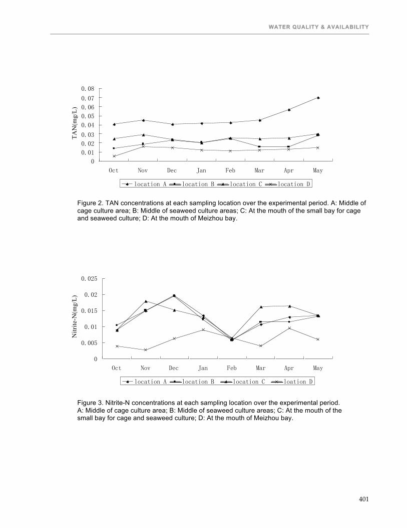
WATER QUALITY & AVAILABILITY
401
0
0.01
0.02
0.03
0.04
0.05
0.06
0.07
0.08
Oct Nov Dec Jan Feb Mar Apr May
TAN(mg/L)
location A location B location C location D
0
0.005
0.01
0.015
0.02
0.025
Oct Nov Dec Jan Feb Mar Apr May
Nitrite-N(mg/L)
location A location B location C loation D
Figure 2. TAN concentrations at each sampling location over the experimental period. A: Middle of cage culture area; B: Middle of seaweed culture areas; C: At the mouth of the small bay for cage and seaweed culture; D: At the mouth of Meizhou bay.
Figure 3. Nitrite-N concentrations at each sampling location over the experimental period. A: Middle of cage culture area; B: Middle of seaweed culture areas; C: At the mouth of the small bay for cage and seaweed culture; D: At the mouth of Meizhou bay.

TWENTY-FIFTH ANNUAL TECHNICAL REPORT – VOLUME I
402
0
0.1
0.2
0.3
0.4
0.5
0.6
0.7
Oct Nov Dec Jan Feb Mar Apr May
TN (m
g/L)
location A location B location C location D
0
0.05
0.1
0.15
0.2
0.25
0.3
0.35
Oct Nov Dec Jan Feb Mar Apr May
Nitrate-N(mg/L)
location A location B location C location D
Figure 4. Nitrate-N concentrations at each each sampling location over the experimental period. A: Middle of cage culture area; B: Middle of seaweed culture areas; C: At the mouth of the small bay for cage and seaweed culture; D: At the mouth of Meizhou bay.
Figure 5. TN concentrations at each sampling location over the experimental period. A: Middle of cage culture area; B: Middle of seaweed culture areas; C: At the mouth of the small bay for cage and seaweed culture; D: At the mouth of Meizhou bay.
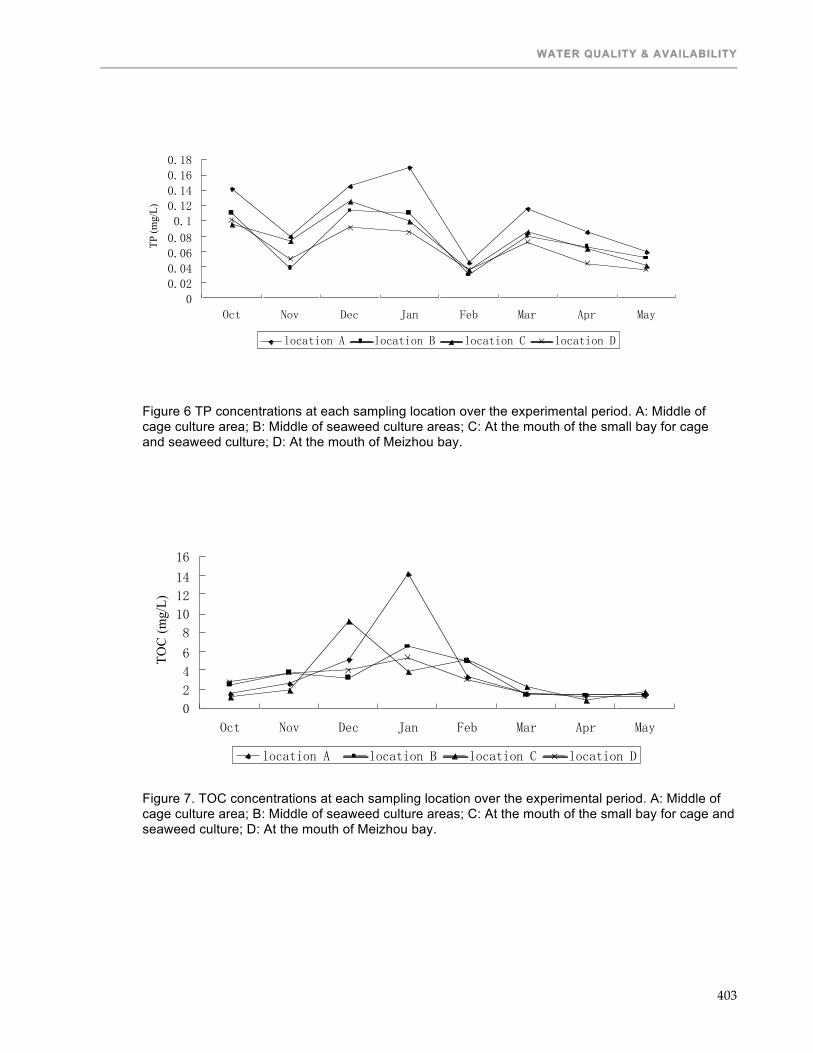
WATER QUALITY & AVAILABILITY
403
0
0.02
0.04
0.06
0.08
0.1
0.12
0.14
0.16
0.18
Oct Nov Dec Jan Feb Mar Apr May
TP (m
g/L)
location A location B location C location D
0
2
4
6
8
10
12
14
16
Oct Nov Dec Jan Feb Mar Apr May
TOC
(mg/
L)
location A location B location C location D
Figure 6 TP concentrations at each sampling location over the experimental period. A: Middle of cage culture area; B: Middle of seaweed culture areas; C: At the mouth of the small bay for cage and seaweed culture; D: At the mouth of Meizhou bay.
Figure 7. TOC concentrations at each sampling location over the experimental period. A: Middle of cage culture area; B: Middle of seaweed culture areas; C: At the mouth of the small bay for cage and seaweed culture; D: At the mouth of Meizhou bay.
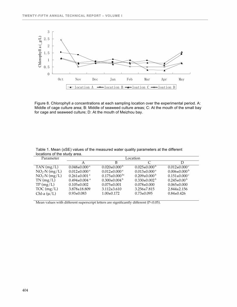
TWENTY-FIFTH ANNUAL TECHNICAL REPORT – VOLUME I
404
0
0.5
1
1.5
2
2.5
3
Oct Nov Dec Jan Feb Mar Apr May
Chl
orop
hyll
a (_
g/L)
location A location B loation C loation D
Figure 8. Chlorophyll a concentrations at each sampling location over the experimental period. A: Middle of cage culture area; B: Middle of seaweed culture areas; C: At the mouth of the small bay for cage and seaweed culture; D: At the mouth of Meizhou bay.
Table 1. Mean (±SE) values of the measured water quality parameters at the different locations of the study area.
Parameter Location A B C D
TAN (mg/L) 0.048±0.000 a 0.020±0.000 b 0.025±0.000 b 0.012±0.000 c NO2-N (mg/L) 0.012±0.000 a 0.012±0.000 a 0.013±0.000 a 0.006±0.000 b NO3-N (mg/L) 0.261±0.001 a 0.175±0.000 bc 0.209±0.000 b 0.151±0.000 c TN (mg/L) 0.494±0.004 a 0.300±0.004 b 0.330±0.002 b 0.245±0.00 b TP (mg/L) 0.105±0.002 0.075±0.001 0.078±0.000 0.065±0.000 TOC (mg/L) 3.878±18.809 3.112±3.610 3.256±7.815 2.844±2.156 Chl-a (µ/L) 0.93±0.083 1.00±0.172 0.73±0.095 0.84±0.426 Mean values with different superscript letters are significantly different (P<0.05).

WATER QUALITY & AVAILABILITY
405
Table 2. List of participants of the workshop on integrated cage-seaweed culture system held on 24 January 2008 at Quangang, Fujian province of China.
Name Gender Position and Institution Mr. Yuenan Chen Male Director General, Bureau of Oceanography and
Fishery, Quangang County Mr. Yipeng Zhuang Male Deputy Director, Bureau of Oceanography and
Fishery, Quangang County Prof. Yongquan Su Male Professor, College of Oceanography and
Environmental Science, Xiamen University, Xiamen Miss Ayuan Cai Female MSc student, College of Oceanography and
Environmental Science, Xiamen University, Xiamen Prof. Jun Wang Female Professor, College of Oceanography and
Environmental Science, Xiamen University, Xiamen Prof. Lingfeng Huang Male Professor, College of Oceanography and
Environmental Science, Xiamen University, Xiamen Dr. Dexiang Wang Male Associate Professor, College of Oceanography and
Environmental Science, Xiamen University, Xiamen Ms. Minglan Guo Female PhD student, College of Oceanography and
Environmental Science, Xiamen University, Xiamen Ms. Xin Chen
Female PhD student, College of Oceanography and Environmental Science, Xiamen University, Xiamen
Mr. Xinxin You
Male MSc student, College of Oceanography and Environmental Science, Xiamen University, Xiamen
Mr. Yong Mao Male PhD student, College of Oceanography and Environmental Science, Xiamen University, Xiamen
Dr. Feng Guo Male Associate Professor, College of Oceanography and Environmental Science, Xiamen University, Xiamen
Mr. Zongyao Xiao
Male Consultant, Office of Oceanography and Fishery, Quangang
Dr. Xiangzhi Lin Male Associate Professor, Third Institute of Oceanography, State Oceanic Administration
Mr. Menghui Xiao Male Farmer, Quangang Ms. Liangzhen Xiao Female Farmer, Quangang Mr. Ruchun Xiao Male Farmer, Quangang Mr. Liyang Xiao Male Farmer, Quangang Mr. Jinquan Xiao Male Farmer, Quangang Mr. Qinghui Xiao Male Farmer, Quangang Mr. Chengchuan Xiao Male Farmer, Quangang Mr. Mengqiang Xiao Male Farmer, Quangang Mr. Zonghan Xiao Male Farmer, Quangang Mr. Xianan Xiao Male Farmer, Quangang Mr. Dezhang Xiao Male Farmer, Quangang Mrs. Meishen Xiao Female Farmer, Quangang Mr. Qiquan Chen Male Farmer, Quangang Mrs. Meihong Xiao Female Farmer, Quangang Mr. Guoning Xiao Male Farmer, Quangang Mr. Fukun Xiao Male Farmer, Quangang Mr. Chang Xiao Male Farmer, Quangang Mr. Kaigui Xiao Male Farmer, Quangang Mr. Yongqin Xiao Male Farmer, Quangang Mr. Liangyi Xiao Male Farmer, Quangang Mr. Jihui Xiao Male Farmer, Quangang Mr. Dexing Xiao Male Farmer, Quangang Mrs. Meiru Xiao Female Farmer, Quangang
TWENTY-FIFTH ANNUAL TECHNICAL REPORT – VOLUME I
406
PELAGIC (FISH) AND BENTHIC ECOLOGY OF SELECTED SUB-WATERSHEDS OF THE NZOIA RIVER BASIN
Twelfth Work Plan, Water Quality & Availability 7 (12WQA7) Final Report
Published as Submitted by Contributing Authors
E. W. Tollner University of Georgia Athens, Georgia, USA
Mucai Muchiri, Frank Onderi Masese
& Philip Okoth Raburu Moi University, Eldoret, Kenya
Betty Nyandat
Department of Fisheries Nairobi, Kenya
Geoff Habron
Michigan State University Lansing, Michigan, USA
ABSTRACT
Assessment of habitat and water quality has been very important in identifying sources of impairment to streams and rivers as registered by changes in aquatic community structure. This study assessed the response of benthic macroinvertebrates to changes in habitat and water quality along River Moiben, which drained land under forestry, agricultural and residential use. Habitat and water parameters were assessed and measured at eight stations along the river, which were selected to correspond to different land uses. Benthic macroinvertebrates were sampled at the stations using a surber sampler. Metrics were selected that reflected the structural and functional composition of benthic macroinvertebrates at the sampled stations. These were correlated against habitat quality index and water quality parameters to determine their interrelationships. Of the twenty metrics tested, 10 met the test criteria and were included in the final index. The study revealed that benthic macroinvertebrates were responding to changes in habitat and water quality along the river.
INTRODUCTION Riverine ecosystems have increasingly lost their integrity to a number of human impacts (Jackson et al. 2001). Most severely, human activities at near-stream riparian areas, which affect the condition of instream habitats along rivers and streams (Malmqvist and Rundle, 2002) have been found to exert the greatest influence in determining stream habitat and biotic characteristics (Johnson et al. 1997; Lammert and Allan, 1999). For instance, riparian vegetation play important roles in regulating stream hydraulics, substrate characteristics, light and thermal regimes, water chemistry and organic matter supply, which in turn affect various stream communities (Giller and Malmqvist 1998, Harding 1998). In order to identify causes of degradation and assess overall integrity considerable research effort has focused on the response of aquatic communities to habitat degradation (Maddock, 1999). Results have indicated that benthic macroinvertebrates exhibit highly diverse taxonomic, morphological, trophic, and physiological level responses to changes in stream ecosystems (Allan 1995, Merritt and Cummins 1996). Following Karr’s (1981) introduction of a multimetric index of biotic integrity on the basis of fish assemblages, similar indices have been developed for benthic macroinvertebrates (Kerans and Karr, 1994). The underlying principle behind the indices is that a

WATER QUALITY & AVAILABILITY
407
set of quantifiable attributes (termed “metrics”) representing community structure, pollution tolerance, functional feeding groups and habitat occurrences, life history strategies, disease, and density gives robust and sensitive insights into how an assemblage responds to natural and human induced stress ((Karr 1981, Plafkin et al. 1989, Kerans and Karr 1994, Barbour et al. 1996). Because of this, the indices can be used to develop biological criteria for stream assessment and protection (Yoder, 1995). The need for this study was to develop a benthic macroinvertebrate based index of biotic integrity for monitoring River Moiben. In the larger River Nzoia basin loss of riparian areas to human activities in the catchment area and along the rivers have been concerns, as they degrade habitats and water quality (Wangila and Swallow, 2001; Osano et al. 2003; Okungu and Opango, 2005). Among the practices, poor agricultural practices, settlement, sand harvesting, bathing, washing, and animal overuse on the riparian areas are the most common.
MATERIALS AND METHODS Study area The Moiben sub-watershed (Figure 1) is approximately 1050Km2 and forms part of the expansive River Nzoia watershed that is 12,903 Km2. The watershed occurs in a high agricultural potential and high population region and therefore the influence of land use on the system is extremely important. The altitude ranges between 1500m and 2400m above sea level between longitudes 35° 06’E and 35° 34’E and latitudes 00° 37’N and 00° 62’N. The watershed has a highland equatorial climate. Due to diverse relief features rainfall varies from one region to another with the highlands receiving heavier rainfall than the lowlands. The mean annual rainfall is 1124 mm and occurs in one long season, March-September, with two distinct peaks in May and August. The average temperature experienced in the region is 18 °C during the wet season with a maximum of 28 °C during the dry season and a minimum temperature of 7 °C in recorded during the coolest season. February is the hottest month while June-July is the coolest. River Moiben is a 4th order stream that originates in the western side of the Kerio escarpment 2400 m above sea level. The river flows through a forested area at its upper reaches before entering an area where mixed farming is practiced. The stream is affected by various human activities along the channels and in the catchment. Station 1, on a 3rd order section of the river, is in the upper reaches located in a forested area. There is minimal human impact on the surrounding area and therefore the station acted as a reference point. Station 2 is on a 3rd order tributary of River Moiben. The riparian zone is grassland with minimal human impact. Intensive mixed farming is the major form of land use around station 3. There was excessive use of animals on the banks that were eroded and devoid of littoral vegetation. Station 4 is on a 3rd order tributary. Human impact at the site included animal watering, washing and water abstraction for domestic use. Station 5 and 6 are situated in areas with maize farming. Intensive mixed farming and pockets of forestry are common. Station 6 has stable banks with littoral vegetation and the riparian zone was more than 15m wide. Stations 7 and 8 are situated in an area characterized by intensive maize farming and animal production on the riparian zone. At station 8 additional human impacts include sand harvesting and wastes from a nearby shopping centre. Data collection Stream physical habitats were measured at each site between February and March 2006. Because macroinvertebrate composition is more strongly correlated with reach scale environmental characteristics than physical features (Carter et al. 1996), stream habitats were assessed at a site whose length was 40 times the mean stream width. Such a site length was sufficient to encompass about three meander sequences (Simonson et al. 1994; Wang et al. 1996). At each site, habitat variables encompassing channel morphology, bottom substrates, instream cover, pool-riffle-run conditions, bank conditions, riparian vegetation, and land use were measured or visually estimated along 3 transects using standardized procedures (Barbour et al. 1999). Physical and chemical parameters were measured at each station. Conductivity was measured in situ using

TWENTY-FIFTH ANNUAL TECHNICAL REPORT – VOLUME I
408
conductivity meter (OAKTONR, Model WD-35607-10, Singapore), while temperature and pH were also measured in situ by a combined pH-and-temperature-meter, (OAKTONR, Model pH/Mv/ºC METER, Singapore). The Winkler method was used to determine dissolved oxygen and biological oxygen demand (APHA, 1998). At each station benthic macroinvertebrates were collected from pools, riffles and runs. To avoid bias in spatial variations or patchiness, three samples were randomly collected from each of the three microhabitats as follows: a transect was established at each sampling reach in a station with five equally spaced points and a sampling point was determined from the points using random numbers. This procedure was replicated three times for each microhabitat (9 samples per reach). At the points sampling was done using a Surber sampler (0.09m2, 250µm mesh size). The replicate samples were then pooled to make one composite sample per habitat per station. Samples collected from the net were preserved in 10% formalin and then transported to the laboratory. In the laboratory, samples were washed through a 250µm mesh size sieve to remove mud and sand. The macroinvertebrates were then sorted and counted using a stereoscope. Identification to genus level and assignment to functional feeding groups were done according to Merritt and Cummins (1996) for insects and non-insects according to Quigley (1977) and Macan (1977). Index development Metric selection Twenty-two metrics were selected for further investigation to determine their utility in assessing ecological condition of the river (Table 1). The metrics fall into four categories that describe richness, composition, tolerance and functional feeding groups. Their classification followed the conceptual framework of Barbour et al. (1995). The various categories are described below. Taxon richness: Taxon richness is used to measure the diversity of a stream. This measure has been identified as an effect metric for use with macroinvertebrates (Resh and Jackson, 1993). Taxon richness can be done at the level of families, genera or species. Total number of genera belonging to orders Ephemeroptera, Plecoptera and Trichoptera (EPT) were evaluated. The three orders of EPT are considered to be sensitive to organic pollution (Barbour et al., 1995). This measure has been identified as an effective metric for use with macroinvertebrates (Resh and Jackson, 1993). Composition measures: Metrics tested here included Shannon-Wiener diversity index, % EPT individuals, % Chironomidae individuals, and the ratio of EPT relative to Chironomidae individuals. As groups, EPT orders are considered to be sensitive to pollution while Chironomidae is said to be pollution tolerant, occurring exclusively at severely degraded areas (Henne, 1997). Tolerance measures: These rely on the assignment of tolerance measures to various macroinvertebrate taxa. Many are designed to utilize family-level data but their use is limited from one region to another as different families can be encountered (Thorne and Williams, 1997). Tolerance measures are intended to be representative of relative sensitivity to perturbation and may include numbers of pollution tolerant and intolerant taxa or percent composition (Barbour et al. 1995). The metrics under this group included number of intolerant taxa, % tolerant organisms and % 3 dominant taxa. Functional measures: These encompass functional feeding groups. Pollution may influence the distribution and relative abundance of these groups by altering the availability of various food types or the action of various toxins associated with the food types. Various measures have been proposed for bioassessment using macroinvertebrates (Plafkin et al. 1989), which can be designated to the relevant FFGs using developed guidelines (Merritt and Cummins, 1996). In this study metrics considered included percentage filterers, scrapers, predators, and gatherers.

WATER QUALITY & AVAILABILITY
409
Metric testing To determine the discriminatory ability of the various metrics, they were evaluated by comparing the value distribution of each across all sites. This was done by graphical displays using box-and-whisker plots. If there was minimal or no overlap between the distribution of a metric at both degraded and least impaired sites then the metric was considered to be a strong discriminator of the pollution gradient. To confirm the validity and responsiveness of retained metrics they were tested via Pearson correlations with habitat characteristics and physicochemical parameters. Metrics that showed significant relationships were retained and tested for redundancy using Pearson correlation coefficients. Redundancy was evaluated by Pearson correlation coefficients. Metrics with a correlation coefficient (r) > 0.7 were considered redundant. Only one metric, which showed significant correlations with most of the habitat and physicochemical parameters, from a group of redundant metrics was included in the final index. The HQI and M-IBI metrics were further correlated to validate the utility of the overall M-IBI for quantifying effects of physical and chemical deficiencies on the ecological integrity of River Moiben. All analyses were run using SPSS statistical software (Version 13.0) and tests were considered significant at the p < 0.05 level. Before running any analyses, we tested all macroinvertebrate metrics for normality and used biplots of the residuals and predicted values to assess homogeneity of variance. Arcsin-square root transformations normalized metrics calculated as proportions (e.g., %EPT). Generic richness and B-IBI scores were square-root transformed. Metric scoring Reference sites were selected a priori based on physical habitats, water quality and riparian land use (Karr, 1981, Karr et al., 1986). Two reference sites were arrived at and formed the baseline for developing the scoring criteria. Each metric was scored on an interval scale, 1, 3 and 5. For positive metrics (i.e., those that increased with improving conditions), the upper expectation was the 95th percentile of the highest value of a metric at the two reference sites. The ranges of values from 0 to the 95th percentile were then trisected. Values above the upper one-third received a score of 5, those in the middle received a score of 3 while those in the lower one-third received a score of 1, corresponding to unimpaired, intermediate and impaired biota respectively (USEPA, 1996). For negative metrics, those that decreased with improving condition, the lower expectation was the 5th percentile. The range from the 5th percentile was trisected but scoring done in reverse, i.e. values above the upper one third received a score of 1, those in the middle a score of 3 while those in the lower one-third a score of 1. To calculate the M-IBI value, we added the metric scores together and scaled the sum by (100/55) for a range of 0 to 100 for the M-IBI.
RESULTS Macroinvertebrate communities During the study, 72 macroinvertebrate taxa were encountered representing 14 orders and 51 families with a total abundance of 14,181 specimens. By composition, Diptera and Ephemeroptera dominated the study area accounting for more than 59% of all taxa by numbers. Headwater stations were dominated by taxa associated with pristine waters, mostly EPT, whereas downstream major reductions were witnessed in pollution sensitive taxa where they were replaced by Chironomus sp., Hydropsyche sp., Simulium sp., Baetis sp., elmids and oligochaetes. Among the functional feeding groups (FFGs) encountered, gatherers had the highest abundance followed by filterers, detritivores, predators and scrapers. Shredders were poorly represented in the study area. Habitat quality index The results obtained for each metric at the eight stations are shown in Table 2. Station 1 scored the highest values for all the metrics. Station T1 scored the same value as station 1 for substrate and instream cover metrics while station 5 scored the lowest values. The metric on channel morphology received a score of zero in stations 2 and T2. The riparian zone and bank erosion metric also scored lowest at station T2. The banks were eroded and cultivation on the right bank was done at less than 10m from the river. In general human activity at the riparian zone was the

TWENTY-FIFTH ANNUAL TECHNICAL REPORT – VOLUME I
410
main descriptor of the condition of each metric at the stations. Watering points for animals were seen at all stations sampled except 1 and T1. Bathing, washing, and water abstraction were seen in all stations downstream. In addition sand harvesting occurred in station 3, 5 and 6. All these activities contributed to a general decline of the HQI downstream. Table 3 shows the results of the physical and chemical parameters measured in the stations. Conductivity, velocity, temperature, discharge and river width showed significant variation (p<0.05) in both space` and time. Depth, DO, and BOD showed significant variation (p<0.05) with respect to time only. Generally BOD values were increasing downstream corresponding with a general increase in turbidity marked by brown water as one moved downstream. The pH values were not significantly different between sampling stations but differed between sampling occasions (p<0.05). There were highly significant differences in altitude between the sampling points (p<0.001). Conductivity generally increased downstream with station 7 and 8 registering the highest values. Highly significant differences (p<0.001) were also obtained between sampling occasions with a general decline from the first to the last. Station 1 and sampling occasion 1 recorded the lowest and highest temperature respectively that significantly differed from the rest of the stations and sampling occasions (p<0.005). Sampling 4 recorded the highest pH value while sampling occasion 1 recorded the lowest. Sampling 1 recorded the lowest DO that differed from the rest of the sampling occasions (p<0.05). In terms of BOD station 1 recorded the lowest value and this differed only from station 6 which recorded the highest value (p<0.05). With respect to time the last sampling occasion recorded the highest BOD that differed from the rest (p<0.05). The water was murky and laden with sediment loads during the rainy season, a condition attributed to erosion. Macroinvertebrate index Of the 22 metrics tested 6 were eliminated because they failed to exhibit variability along a gradient of human influence. Their distributions showed overlap and therefore could not discriminate the different sites according to their levels of degradation (Figure 2). Of the 16 metrics remaining 10 followed the predicted response to environmental gradients and showed a significant correlation with atleast one of the habitat and physicochemical parameters. The metrics that were eliminated include EPT richness, % Diptera individuals, % noninsect individuals, % chironomid individuals and % Ephemeroptera individuals and % predator individuals. Redundancy tests showed that Ephemeroprera richness was redundant with % gatherers. Percent EPT individuals was redundant with % scraper individuals and ratio of EPT to Diptera. In total seven metrics were used in the final B-IBI index for River Moiben (Table 4). Relationship between B-IBI and physico-chemical variables A number of relationships were observed as shown in Table 8. Temperature was negatively related with all metrics. Water pH was positively related with percentage tolerant metrics of M-IBI. Percentage salutation of DO was negatively related to all metrics. BOD was negatively related to all metrics. Conductivity was negatively related with all M-IBI metrics except number of Trichoptera taxa. A strong positive relationship (Spearman’s R=0.87, R2=0.97, p=0.005) was found between the value of the M-IBI and the HQI (Figure 9).
DISCUSSION The River Continuum Concept (Vannote et al. 1980) describes the downstream gradient in physical characteristics of streams and the resulting biological responses under natural conditions. However, this concept seldom holds in many lotic systems due to longitudinal changes in habitat conditions caused by human activities. In the present study shifts in structural and functional composition of benthic macroinvertebrates downstream, as reflected in variability of tested B-IBI metrics, can be linked to hydromorphological impacts that caused significant variations in habitat and water quality along the river.

WATER QUALITY & AVAILABILITY
411
Richness metrics did not perform well because only one metric, number of Trichoptera taxa, met the test criteria. Poor performance of Ephemeroptera taxa can be explained by tolerance to pollution of families Baetidae and Caenidae, which were widely distributed in all stations. Similar findings have been found in the tropics (Thorne and Williams, 1997) and this compromises the number of Ephemeroptera taxa as a metric for assessing degradation. Plecoptera was poorly represented in the study area. Similar findings have been recorded in tropical rivers in Africa (Thorne and Williams, 1997, Kibichii, 2007). The low diversity and abundance in River Moiben can be attributed to degradation of the sampled stations. The instream habitats in River Moiben are mostly composed of sandy and muddy bottoms which affect plecopteran distribution, diversity and abundance (Lemly, 1982). The EPT are considered most sensitive orders to pollution and their taxon richness at a site indicates good habitat and water quality. Because of this number of EPT taxa has been recommended for use in developing countries (Resh, 1995; Thorne and Williams, 1997). However, in this study total number of EPT taxa as a metric failed to meet the test criteria. As already observed, tolerance of some families to pollution might have compromised the metric. These findings contrast with those by Thorne and Williams (1997) in which number of EPT families were able to separate impacted from unimpacted sites. Despite their findings, they also observed that as the level of pollution increases the utility of this metric decline and it cannot separate moderate from gross pollution. Community composition metrics performed relatively well as compared to richness measures. The relative abundance of EPT did well and met the test criteria. In River Moiben the group was most abundant at the first two stations, 1 and 2, where they formed 52% and 58% respectively of the total abundance. The group declined downstream occurring in low numbers at degraded sites. This occurrence was a clear indication of the response of the group to poor habitat and water quality. The order Diptera was widely distributed in the study area. In all stations family Chironomidae, which showed higher abundance with increased organic pollution, dominated this order. Chironomids are considered the most tolerant to pollution and high numbers have been reported at degraded sites (Buss et al. 2002). This high abundance is said to mask the true contribution of order Diptera to the total fauna at a site, hence left out or considered alone. In this regard, relative abundance of the family was considered in relation to the pollution tolerant EPT to aid in delineating polluted sites. This proved true as stations with high EPT had low chironomids. Station 1 recorded the best score for this metric, indicating that the site was not degraded while stations 2, T2, 5 and 6 scored the lowest, indicating that they were degraded. The Shannon-Weiner index performed poorly in the study area. Similar findings have been obtained in the tropics. Thorne and Williams (1997) found similar results in which the index was variable and could not discriminate between impacted and unimpacted sites. They attributed this failure to the fact that in degraded sites the few available taxa are relatively even in their abundances, and conversely the rich fauna at an unimpacted site may be numerically dominated by a few taxa, such as chironomids. This explanation holds for River Moiben because as one moved downstream pollution tolerant taxa were evenly distributed while the pollution sensitive taxa at the upper reaches were also evenly distributed. As a measure of sensitivity, the percentage of pollution tolerant taxa proved to be a very important metric in delineating degraded sites from minimally degraded ones. There was a reduction in abundance caused by exclusion of sensitive species and an increase in tolerant taxa. The taxa that showed tolerance to pollution in the river included orders Hirudinea, Amphipoda, Oligochaeta, and families Chironomidae, Planorbiidae, and Physidae. Station 1 scored the highest value for this metric indicating that it has low abundance of tolerant taxa while stations T2, 3 and 5 scored the lowest, having a greater abundance of pollution tolerant taxa. This also reflected the

TWENTY-FIFTH ANNUAL TECHNICAL REPORT – VOLUME I
412
quality of habitat at the stations as stations 1 had an excellent habitat quality, stations T2 and 5 a very poor habitat quality while station 3 had a poor habitat quality. Functional metrics did not do well because only two metrics, percentage scrapers, and ratio of percentage scrapers to percentage filterers met the test criteria. The distribution of scrapers indicated a response to the shifting environmental conditions along the river. Similar findings were obtained by Resh and Jackson (1993) who considered the metric to be the most accurate in separating sites according to their level of degradation. In River Moiben percentage scrapers and proportion of scrappers to filtering collectors received the highest scores at stations 1 and T1 while the rest of the stations received the lowest values. Scrapers are particularly sensitive to sedimentation and turbulence which smoother and disturb their grazing beds. Their distribution in the area showed that as turbidity increased downstream, as indicated by increased levels of brown water as one moved downstream, their distribution was greatly affected. The proportion of scrappers to filtering collectors is considered to represent the balance between food sources, and an increase in the relative abundance of filtering collectors in downstream stations suggest an input of organic effluents that increase the availability of FPOM. For this reason the metric proved capable of delineating sites that received organic wastes. In general the 7 metrics were able to delineate different sites according to their level of degradation. The attributes showed variability across a gradient of human influence, which is a key ingredient in bioassessment (Karr, 1999). Their validity was also reinforced by the strong positive relationship between the overall B-IBI and the HQI suggesting that the variation they exhibited was congruent with habitat and water quality. For management, the metrics are indicative of a changing environment under the influence of intermediate levels of human impacts. With increasing human population on the catchment area, the situation is likely to be exacerbated. Therefore, the challenge is to halt the current trend and improve the B-IBI scores at the stations. However, development of IBI for Kenyan ecosystems face the setback of inadequate reference information from which to construct indices. The application of IBI on management is therefore faced with the limitation of information such as the biology, and ecology of aquatic biota. The B-IBI developed in this study may, therefore, need further refining before its use on a wider scale.
ANTICIPATED BENEFITS The benthic index is useful as an integrated indicator of stream health. The index is far more economical and far more effective than intensive chemical monitoring for stream health. This information will provided needed reference information for subsequent studies.
ACKNOWLEDGMENTS Funds for this study were provided by the Aquaculture CRSP funded in part by United States Agency for International Development (USAID) Grant No. LAG-G-00-96-90015-00 and by participating institutions, Moi University and University of Georgia, Athens through the project “Hydraulic, Water Quality and Social Assessment of the Nzoia Basin, Kenya”. Isaac Ebenyo assisted during fieldwork. Mr. Lubanga Lunaligo of Moi University, Kenya helped in identifying the macroinvertebrates. Mr. William Kinyua of Moi University assisted with equipment for field work.
LITERATURE CITED ALLAN JD (1995) Stream Ecology: Structure and Function of Running Waters. Kluwer Academic
Press, Boston. ASTON RJ (1973) Tubificids and Water Quality: a review. Environmental Pollution 5: 1-10. BARBOUR MT, STRIBLING JB and KARR JR (1995) Multimetric approach for establishing
biocriteria and measuring biological condition. In: Davis WS and Simon TP (eds) Biological

WATER QUALITY & AVAILABILITY
413
assessment and criteria. tools for water resource planning and decision making Lewis Publishers, Boca Raton. pp 63-77.
BUSS DF, BAPTISTA DF, SILVEIRA MP, NESSIMIAN JL and DORVILLE LFM (2002) Influence of water chemistry and environmental degradadtion on macroinvertebrate assemblages in a river basin in south-east Brazil. Hydrobiologia 481: 125-136.
CARTER JL, FEND SV and KENNELLY, SS (1996) The Relationships Among Three Habitat Scales and Stream Benthic Invertebrate Community Structure. Freshwater Biology 35:109-124.
CHAPMAN D (1992) Water Quality Assessments: A Guide to the Use of Biota, Sediments and Water in Environmental Monitoring. Chapman and Hall, London.
FRAPPIER B and ECKERT RT (2007) A new index of habitat alteration and a comparison of approaches to predict stream habitat conditions. Freshwater Biology 52: 2009–2020.
GILLER PS and MALMSQVIST B (1998) The Biology of Streams and Rivers. Oxford University Press, New York.
JACKSON RB, CARPENTER SR, DAHM CN, MCKNIGHT DM, NAIMAN RJ, POSTAL SL, and RUNNING, S.W. (2001). Water in a changing world. Ecological Applications 11: 1027-1045.
JEFFRIES M and MILLS D (1990) Freshwater Ecology Principles and Applications. Belhaven Press, London. 285pp.
JOHNSON LB, RICHARDS CR, HOST GE and ARTHUR JW (1997) Landscape Influences on Water Chemistry in Midwestern Stream Ecosystems. Freshwater Biology 37:193-208.
KARR JR (1991) Biological integrity: a long-neglected aspect of water resource management. Ecological Application 1: 66–84.
KARR JR (1999) Defining and measuring river health. Freshwater Biology 41: 221-234. KARR JR, FAUSCH K, ANGERMEIER PL, YANT PR, and SCHLOSSER IJ (1986) Assessing
Biological Integrity in Running Waters: a method and its Rationale. Illinois Natural History Survey special Publication 5, Champaign, Illinois.
KIBICHII S, SHIVOGA WA, MUCHIRI M, and MILLER SN (2007) Macroinvertebrate assemblages along a land-use gradient in the upper River Njoro watershed of Lake Nakuru drainage basin, Kenya. Lakes & Reservoirs: Research and Management 12: 107-117.
LAMMERT M, and ALLAN JD (1999) Environmental Auditing - Assessing Biotic Integrity of Streams: Effects of Scale in Measuring the Influence of Land Use/Cover and Habitat Structure on Fish and macroinvertebrates. Environmental Management 23:257-270.
LEMLY AD (1982) Modification of benthic insect communities in polluted streams: combined effects of sedimentation and nutrient enrichment. Hydrobiologia 87: 229-246.
MACAN TT (1977) A guide to freshwater invertebrate animals. Longman publishers, London. 118pp.
MALMQVIST B and RUNDLE S (2002) Threats to the running water ecosystems of the world. Environmental Conservation 29: 134–153.
MERRITT RW and CUMMINS KW (1996) An introduction to the Aquatic Insects of North America. 3rd
edn. Kendall / Hunt Publishing Company, Dubuque, IA. 862pp. OKUNGU J and OPANGO P (2005) Knowledge and Experiences gained from Managing The Lake
Victoria Ecosystem. Regional Secretariat, Lake Victoria Environmental Management Project (LVEMP). Dar es Salaam, Tanzania. 725pp.
OMUKOTO JO (2007) Development of a Fish Index of Biotic Integrity (IBI) for Satellite Lakes within Yala Swamp, Lake Victoria Basin, Kenya. MPhil thesis, Moi University, Kenya.
OSANO O, NZYUKO D, and ADMIRAAL W (2003) The fate of Chloroacetalinide Herbicides and Their Degradation Products in the Nzoia Basin, Kenya. Ambio 32:424-427.
PIELOU EC (1975). Ecological diversity. Wiley and Sons, New York. PLAFKIN JL, BARBOUR MT, PORTER KD, GROSS SK and HUGHES RM (1989) Rapid
bioassessment protocols for use in streams and rivers: Benthic macroinvertebrates and fish. EPA 440-4-89-001. USEPA, Office of Water Regulations and Standards, Washington DC.
QUIGLEY M (1977) Invertebrates of streams and Rivers: a key to identification. Edward Arnold Ltd. London. 84pp.
QUINN JM, COOPER AB, DAVIES-COLLTY RJ, RUTHERFORD JC and WILLIAMSON RB (1997) Land-use effects on habitat, water quality, periphyton, and benthic macroinvertebrates

TWENTY-FIFTH ANNUAL TECHNICAL REPORT – VOLUME I
414
in Waikato, New Zealand, hill-country streams. New Zealand Journal of Marine and Freshwater Research 32: 579-597.
RABURU PO (2003) Water quality and the status of aquatic macroinvertebrates and ichthyofauna in River Nyando, Kenya. PhD thesis, Moi University, Kenya.
RAVEN PS, HOLMES NTH, DAWSON FH, FOX PSA, EVARD M, FOZZARD IR and ROWEN KJ (1998) River Habitat Quality: the physical character of rivers and streams in the UK and Isle of Man. Environmental Agency, Bristol, England.
RESH VH (1995) Freshwater benthic macroinvertebrates and rapid assessment procedures for water quality monitoring in developing and newly industrialized countries. In: Davies WS and Simon TP (eds) Biological assessment and criteria: tools for water resource planning and decision making. Lewis Publishers, Boca Raton. pp 167-177.
RESH VH and JACKSON JK (1993) Rapid assessment approaches to biomonitoring using benthic macroinvertebrates. In: Rosenberg DM and Resh VH (eds) Freshwater biomonitoring and benthic macroinvertebrates. Chapman and Hall, New York. pp. 195-233.
SIMONSON TD, LYONS J and KANEHL PD (1994) Guidelines for Evaluating Fish Habitat in Wisconsin Streams. U.S. Department of Agriculture, Forest Service, North Central ForestExperiment Station, St. Paul, Minnesota, General Technical Report NC-164, St. Paul, Minnesota.
THORNE RSTJ and WILLIAMS WP (1997) The response of benthic macroinvertebrates to pollution in developing countries: a multimetric system of bioassessment. Freshwater Biology 37: 671-686.
US Environmental Protection Agency (1996). Revision of rapid bioassessment protocols for use in stream and rivers: periphyton, benthic macroinvertebrates, and fish. Document on Internet at http://www.epa.com/
VANNOTE RL, MINSHALL GW, CUMMINS KW, SEDELL JR and CUSHING CE (1980) The River Continuum Concept. Canadian Journal of Fisheries and Aquatic Sciences 37: 130-137.
WANG L, SIMONSON TD, and LYONS J (1996) Accuracy and Precision of Selected Stream Habitat Estimates. North American Journal of Fisheries Management 16: 340-347.
WANGILA J and SWALLOW B (2001) Design principles for land and watershed management in Western Kenya, proceedings of a workshop held on 9th April 2001, Kisumu, Kenya. Natural Resource Problems, Priorities and Policies Programme Discussion Paper 2001-1. International Centre for Research in Agroforestry (ICRAF).

WATER QUALITY & AVAILABILITY
415
Table 1: Potential metrics for macroinvertebrates that were considered for assessing biological integrity of River Moiben and the predicted responses to pollution. Metric Predicted response
Richness measures Simpson richness index Decrease Number Ephemeroptera taxa Decrease Number Plecoptera taxa Decrease Number Trichoptera taxa Decrease Number EPT genera Decrease Total number of genera Decrease Number intolerant genera Decrease Composition measures Percent EPT individuals Decrease Percentage Chironomidae Increase EPT: Chironomidae Decrease Shannon-Weiner diversity index Decrease Percent dominant taxa Increase Percent 3 dominant taxa Increase Percent noninsects Increase Tolerance measures Number intolerant genera Decrease Percent intolerant individuals Decrease Percentage tolerant individuals Increase Functional measures Percentage filterers Increase Percentage scrapers Variable Percentage predators Decrease Percentage gatherers Variable Scrapers: Filterers individuals Variable
Table 2: Scores of metrics for the eight stations used in the calculation of habitat quality index for River Moiben
Metric for HQI 1 2 3 4 5 6 T1 T2
Substrate 12 11 6 9 3 4 12 7
Instream cover 18 7 9 13 5 10 18 9
Channel morphology 6 0 1 4 1 2 4 0 Riparian zone and bank erosion 9 6 4.5 6 4.5 6.5
7.5
3.5
Pool-riffle-run quality 10 9 10 10 9 7 8
9
Total HQI 55 33 30.5 42 22.5 29.5 49.5 28.5

TWENTY-FIFTH ANNUAL TECHNICAL REPORT – VOLUME I
416
8.007.006.005.004.003.002.001.00Station
25.00
20.00
15.00
10.00
5.00
0.00
T a x o n r i c h n e s s
1.00
8 .007 .006 .005 .004 .003 .002 .001 .00Stat io n
0 .80
0 .60
0 .40
0 .20
0 .00
S h a n n o n -W e i n e r
2 7
Figure 2: Examples of box-and-whisker plots used to test the variability of metrics. Metric (a) ratio EPT: Chironomidae and (b) percentage EPT perform well as they show a clear variability along gradient of human influence and there was little overlap between the distributions as the sites were discriminated according to their level of degradation. In contrast, the taxon richness (c) and Shannon-Weiner diversity (d) indices perform badly as they show a weak relationship with the gradient and there is overlap between the distributions. The labelled points (o) on the plot indicate outliers.
Figure 1: The map of the study area showing the position of sampling points (●); Stn stand for station
8.007.006.005.004.003.002.001.00Station
100.00
80.00
60.00
40.00
20.00
0.00
P er c en t ag e E PT
5.00
2.00
1.00
8.007.006.005.004.003.002.001.00Station
25.00
20.00
15.00
10.00
5.00
0.00
R a ti o E P T : C h i r o n o m i d a e
29
20
11
(a) (c)
(b) (d)

WATER QUALITY & AVAILABILITY
417
M-IBI = 0.75HQI - 12.4R2 = 0.97
0
10
20
30
40
10 20 30 40 50 60
HQI scores
M-IB
I sco
res
Figure 3: Regression between biological metrics scores of the B-IBI and physical metric scores of the HQI.
Table 9. Spearman rank correlation coefficients observed between metrics and physico-chemical parameters (physico-chemical units are identical to previous table; * designate significant correlation at ∝ = 0.05). M-IBI Metrics Temperature pH DO BOD Conductivity HQI
Number of Trichoptera taxa -0.57* 0.13 -0.46* -0.57* -0.29 0. 81* Percentage EPT -0.54* -0.22 -0.72* -0.93* -0.39* 0.84* Percentage Diptera -0.55* 0.38* -0.44* -0.44* -0.33 0.65* Percentage Tolerant taxa -0.46* 0.42* -0.26 -0.48* -0.37* 0.82* Percentage Scrapers -0.38* -0.25 -0.25 -0.76* -0.38* 0.76* Ratio EPT : Chironomidae -0.54* -0.22 -0.72* -0.93* -0.39* 0.85* Percentage scrapers : filterers -0.38* -0.25 -0.25 -0.76* -0.38* 0.76* HQI Metrics B-IBI Substrate -0.69* -0.29 -0.20 -0.83* -0.67* 0.66* Instream cover -0.25 0.07 -0.57* -0.75* -0.23 0.81* Channel morphology -0.21 0.34 -0.69* -0.57* -0.25 0.90* Riparian zone and Bank erosion -0.31 0.28 -0.36 -0.55* -0.23
0.93*
Pool-riffle-run quality -0.70* 0.06 -0.45* -0.35 -0.48* 0.13 Total HQI scores -0.71* -0.02 -0.55* -0.88* -0.57* 0.87* Total M-IBI scores -0.40* 0.37 -0.55* -0.60* -0.19 -

TWENTY-FIFTH ANNUAL TECHNICAL REPORT – VOLUME I
418
HYDROLOGIC MODELING IN THE NZOIA RIVER BASIN
Twelfth Work Plan, Water Quality & Availability 8 (12WQA8) Final Report
Published as Submitted by Contributing Authors
Herbert Ssegane & E. W. Tollner University of Georgia Athens, Georgia, USA
Mucai Muchiri Moi University Eldoret, Kenya
Nancy Gitonga
Department of Fisheries Nairobi, Kenya
Geoff Habron
Michigan State University Lansing, Michigan, USA
ABSTRACT The study describes the application of the universal soil loss equation model, to quantify soil erosion in Nzoia basin located entirely on the Kenyan side of Lake Victoria basin using the geographic information service, remote sensing, and global positioning service technologies. The approach adopted involved calculation of six universal soil loss equation factors inform of distributed remote sensing and geographic information service data using arcGIS / arcMap software. The data included spatial raster layers of soil, land cover, rainfall and digital elevation models ranging from 30 m to 1000 m spatial resolutions to adequately represent the surface characteristics. The soil erosion distribution map was generated as a product of the six raster layers using the spatial analyst tool in arcMap. Even with continental scale spatial resolutions, the predicted erosion levels had the same order of magnitude as predictions made with site specific parameters utilizing Google Earth Pro. For a site at Moore’s bridge along the Moiben sub-watershed the predicted erosion levels ranged between 31 – 51 tons/ha-yr compared to the value of 97.2 tons/ha-yr obtained using USLE and Google Earth Pro. To improve the accuracy levels, use of recent land cover and land use data plus use of smaller variation of the data spatial resolution was recommended.
INTRODUCTION The soil erosion process is a complex phenomena determined by joint interaction of climatic, geological, and land use and land cover factors. The spatial extent and severity of environmental risk of this process can be analyzed on global, continental, and regional scales. Oldeman (1994) estimated that the global land area affected by water erosion was about 1094 million hectares and on the continental scale, the problem being more severe in Asia, Africa, South America, and Europe in a descending order. The environmental risk posed by soil erosion is related to pollution activities due to runoff from agricultural lands, urban areas, construction sites, and industrial sites that introduce sediment, nutrients, bacteria, organic wastes, chemicals, and metals into surface waters. The economic implications of sedimentation of surface waters are due to increase in the cost of water purification, hydropower generation, increased flood risk (Hansen et al., 2002) and reduction in the productivity of the fishery industry. The fishing industry is greatly affected because sediment clogs and scrapes fish gills, suffocates fish eggs and aquatic insect larvae, and causes fish to modify feeding and reproductive behaviors.

WATER QUALITY & AVAILABILITY
419
One of the affected water bodies is Lake Victoria, the second largest source of fresh surface water. Lake Victoria basin is a source of livelihood to the populace of Kenya, Uganda, and Tanzania given that it’s a source of drinking and irrigation water, food, energy, and transport. Development activities, nutrient discharge, and population growth (3% on the Kenyan side) have caused changes in the lake’s ecosystem leading to massive flourishing of algae and the water hyacinth (LVEMP, 1995). Studies indicate that the dramatic changes in the lake’s water quality and fisheries have arisen from introduction of the exotic Nile Perch and human activities. The changes due to human activities are directly related to the nutrient enriched sediment that is discharged into the lake. Studies carried out by Sangale et al (2001) and Okungu and Opango (2001) show that river Nzoia contributes the most sediment loading to Lake Victoria from the Kenyan catchment mainly because of its high discharge of 118 m3/s. The Nzoia River Basin Nzoia basin is entirely found in Kenya and is located between latitudes 10 30’ N and 00 05’ S and longitudes 34 0 E and 350 45’ E. The river basin covers an area of 12,842 Km2 and drains through several districts on its way to Lake Victoria. These include Uasin Gishu and Trans Nzoia Districts in the Rift Valley Province, Mt. Elgon, Lugari, Teso, Bungoma, Kakamega, Butere-Mumias and Busia Districts in Western Province, and Siaya District- Nyanza Province. The total river line is 355 km long (the main river is about 225 Km) with a mean discharge of 118 m3/s. The river originates from Cherengany Hills and Mt Elgon at 4320 meters above sea level and is fed by several rivers. On the course to Lake Victoria the river drains through small and large-scale maize and wheat farms, coffee plantations, a paper factory and Sugar factories. The river greatly contributes to the periodic flooding of the Budalangi floodplains because of heavy silt it carries from the deforested upper catchment areas. According to Köppen’s classification (McKnight et al., 2000), the climate of Nzoia basin is mainly tropical humid and therefore its characterized by the tropical dry and wet type of climate. According to NRBMI (2006), the temperature varies from 16 0C in the highland areas of Cherangani and Mount Elgon to 28 0C in the lower semi-arid areas. The mean annual night temperatures vary between 4 0C in the highland areas to 16 0C in the semi-arid areas. The mean annual rainfall varies from a maximum of 1100 to 2700 mm to a minimum of 600 to 1100 mm while the humidity varies from 70 to 85 %. The basin experiences four seasons in a year influenced by the Inter-Tropical Convergence Zone. The four seasons consist of two rainy and two dry seasons. The rainy seasons are characterized by short rains from October to December and long rains from March to May. The dry seasons are experienced in the months of January to February, and June to September. The variations in the seasonality are greatly influenced by Lake Victoria’s climatology. The topography of the basin is characterized by high western slopes of Chengani Hills and south eastern parts of Mount Elgon at mean elevation of about 2300 m above sea level and lower elevations as it drains into Lake Victoria at an elevation of about 1000 m. The soils of the floodplains in the lower of the Nzoia River are of alluvial type. The major parts of the river contain black cotton soils while other areas have coarse textured sand – silt mixture. The basin’s climatology, topography, and soils encouraged the sprouting of an intensive agricultural and agro-industrial sector that has encroached onto the riparian zones and wetlands. As a control measure to reduce the amount of sediment deposition into the lake, the respective East African countries in collaboration with US agency for international aid (USAID) and aquaculture CRSP are encouraging the conservation and restoration of riparian buffers as part of an integrated natural resources management practice. Forested riparian zones and vegetative filter strips reduce sediment movement from agricultural land by intercepting flow, reducing the flow velocity, increasing the retention time, and accordingly decreasing the sediment delivery to the surface water bodies (Travis, 2003). All areas under the threat of soil erosion cannot be conserved at once due to financial and human resource constraints. Thus attention is focused on prioritizing sediment hotspots. The availability of continental and regional scale data in form of satellite images and global positioning system (GPS), as well as the new methodological
TWENTY-FIFTH ANNUAL TECHNICAL REPORT – VOLUME I
420
approaches like remote sensing, integrated into geographical information systems (GIS) allow to model soil erosion distribution. Thus, for a given watershed sediment hotspots are identified and targeted for conservation practices and monitoring purposes. Therefore, this study set out to generate erosion map depicting the soil erosion distribution for the Nzoia River basin using GIS and Remote sensing data.
METHODS AND MATERIALS The assessment of erosion potential in Nzoia river basin was based on the universal soil loss equation (USLE) model (Wischmeier and Smith, 1978). USLE quantifies soil erosion as the product of six factors representing rainfall and runoff erosiveness, soil erodibility, slope length, slope steepness, cover – management practices, and support conservation practices. The USLE is an empirical relationship expressed by equation 1:
RKSLCPA = (1)
Where A = Average Annual Soil loss in (tons / acre or Mg / hectare) R = Rainfall –Runoff erosive index factor in (MJ-mm / ha-hr-yr) K = Soil erodibility factor (ton-ha-hr / ha-MJ-mm) S = Slope steepness factor (dimensionless) L = Slope Length factor (dimensionless) C = Crop-Management factor (dimensionless) P = Conservation Practice factor (dimensionless) Each factor is calculated independently and the derived product of the six factors is the average annual soil loss in tons/acre or Mg/hectare. The USLE model only predicts soil loss due to rill and sheet erosion. Neither does it predict erosion due to gullies nor sediment deposition within riparian buffers.
Data Sources Digital Elevation Model (DEM): The DEM data was obtained from the Global land covers facility (GLCF). The DEM data is under the shuttle radar and thematic mapper (SRTM) data category. The DEM data has a spatial resolution of 90 m and is available for all world regions. The data can be accessed through the website link below; http://glcfapp.umiacs.umd.edu:8080/esdi/index.jsp Land Use and Land Cover: The US geological service (USGS) provides global land cover data. The data is available on continental scale with a spatial resolution of one kilometer. The data can be accessed through the website link below; http://edcdaac.usgs.gov/glcc/glcc.html Soils Data: The soils data was accessed in a binary format from the north oceanic and atmospheric administration (NOAA) at a spatial resolution of 0.0833 arc degrees. The data can be accessed through the website link below; http://www.ngdc.noaa.gov/seg/cdroms/reynolds/reynolds/reynolds.htm Annual Rainfall data: The rainfall data for Kenya was obtained from flood early warning system (FEWS), a program developed jointly by the USGS and USAID. The data can be accessed through the website link below; http://edcinti.cr.usgs.gov/fewsnetdata.html Nzoia river basin outline: The Nzoia river basin is classified as a level 6 under the Pfafstetter coding for African basins. The data can be accessed through the FEWS network under the Hydro 1 Km dataset: The data can be accessed through the website link below; http://edc.usgs.gov/products/elevation/gtopo30/hydro/africa.html

WATER QUALITY & AVAILABILITY
421
Nzoia river line: The Nzoia river line was obtained from the FEWS network under the Hydro 1 Km dataset. http://edc.usgs.gov/products/elevation/gtopo30/hydro/africa.html Data Preparation The Shuttle Radar Transmitter Mission (SRTM) DEM data is available by grid. The four grids covering the study area were mosaiced using ERDAS IMAGINE remote sensing program. The FAO soils map data from the north oceanic and atmospheric administration (NOAA) server is provided as a binary dataset. The dataset was imported into the ERDAS IMAGINE and saved as an image. The rainfall data was summarized for 102 Kenyan gauge stations with their respective latitude and longitude coordinates. The average rainfall amount ranging from 4 to 102 years was calculated and tabulated. From the African level 6 basins, the Nzoia basin was clipped as a level three basin for subsequent use as a sub-setting polygon. Figure 3 represents the process of deriving USLE layer maps from raw spatial data and the respective map calculations used to generate the soil erosion distribution map. Thematic Map Layer Results and Discussion Rainfall erosivity (R factor): The rainfall factor quantifies the interrelated erosive forces of rainfall and runoff that are direct results of the rainstorms. It’s an annual factor that represents all the erosive rains throughout the year and it’s based on the rainfall energy and intensity values. However due to the limited availability of rainfall intensity data, model used to predict rainfall-runoff erosivity was developed by Renard and Freimund (1994) by regressing annual precipitation and the R values for 155 stations in the United States. The empirical relationship is given by equation 2.
>+−
≤=
mmPPPmmPP
R850,004105.0249.18.587850,0483.0
2
610.1
(2)
Where
R = rainfall erosivity (MJ mm / ha hr yr), and
P = annual precipitation in mm
The Renard and Freimund (1994) equation approximates the R values for most East African areas due to the similarity in the rainfall energy of US and most East African regions (Moore, 1979). The annual precipitation was obtained by summarizing data from 102 stations in Kenya ranging from 4 to 102 years of rainfall data. A point feature was created for Kenya with the respective station geographical coordinates using arcMap. From the point feature map, a rainfall raster map was created using inverse distance weighted (IDW) interpolation method. The R raster layer (figure 5) was then generated using the spatial analyst tool of arcGIS / arcMap with the math and map algebra tools. Soil erodibility (K factor): The soil erodibility factor estimates the long term soil and soil profile response to the rainfall and runoff erosive forces. It relates the susceptibility of the soil to erode with respect to its inherent physical properties. According to Renard et al (1997), the K factor is determined using soil properties of soil texture, soil structure, soil permeability, and the soil organic matter content. For this study due to absence of the soil permeability and soil structure data, the global erodibility equation recommended by Torri et al (1997) was used. Equation 3 expresses the global erodibility equation:

TWENTY-FIFTH ANNUAL TECHNICAL REPORT – VOLUME I
422
(3)
Where
K = soil erodibility (ton.ha.hr / ha.MJ.mm),
OM = percent organic matter ,
fsand = sand fraction,
fsilt = silt fraction,
fclay = clay fraction, and
Dg = the geometric mean of particle size.
The data used was developed by Reynolds et al (1999). Reynolds et al (1999) explains the procedure used to extract soil properties for the FAO soil units by utilizing statistical analyses and taxo-transfer depth algorithms. The representative soil properties were estimated for two-layers of depths (0-30 and 30-100 cm). For this study the top layers of 0 to 30 cm shown in figure 4 were used to generate the soil erodibility map (figure 6). The Slope Length (L factor): The slope length factor relates the effect of the slope length on soil loss because there is greater accumulation of runoff on longer lengths and more runoff volume leads to high runoff velocities According to Renard et al (1997), the slope factor depends on the plot flow length and slope gradient. With raster data, map calculations are carried out on pixel basis. The approach used in this study (equation 4) was developed by Desmet and Govers (1996) and takes into account the fact that raster layer calculations are carried out at pixel level. It estimates the slope length factor by incorporating pixel (cell) size and flow accumulation using expressions in equation 4. The resulting slope length factor layer is shown in figure 7. (4) Slope Steepness (S factor): Renard et al (1997) recommend different relationships for determining slope steepness factor depending on the slope length and slope steepness (gradient). The relationship used in this study for its simplicity was developed by Smith and Wischmeier (1957) and is given as; (5)
Where
S = slope steepness factor, and
s = the percent slope.
( )
sandsiltclayg
clayclayclayclay
gg
fffD
fffOM
fOMDDK
5.00.25.3
72.102.400037.00021.0exp24.065.00293.0 2
2
2
−−−=
+−
−−+−=
( )4.0
4.14.1
13.22*
*
CellSizeL
CellSizeCellSizelationFlowAccumu
λλ
λλ
λ
−=
+=
=
⊗
⊗
[ ]613.6
043.030.043.0 2ssS ++=

WATER QUALITY & AVAILABILITY
423
This relationship is accurate for slope gradients less than and equal to 20%. For slope gradients greater than 20%, equation 5 is best used for comparison purposes. Figure 8 depicts the slope steepness factor layer. Crop management (C factor) and conservation practice (P factor): The C and P factors were determined from the land use / land cover map. An attribute table was created relating the land use / land cover type to the crop management and conservation practice factors. Some of the C and P factors can be found in Renard et al (1994), Tollner (2002), and Renard et al (1997). The attribute table used in this study is shown in table 1. The C and P layers are shown in figure 9 and figure 10 respectively. The erosion map (figure 11) was generated as a product of the six USLE factor layers using map algebra and map calculations in arcMap / arcGIS. The erosion index map was created based on the classification in the table 2. The majority of the areas within the basin are under the low or slight sediment risk. This is attributed to the forest and grassland cover in addition to the low rainfall values. However areas at high elevations are among the high - severe risk regions due to the high rainfall amounts experienced in these regions and encroachment on the forest and woodlands as more land is being cleared for agricultural use. The erosion amount obtained by GIS, RS, and USLE model for a site at Moore’s bridge along the Moiben sub-watershed is 31 – 51 tons/ha-yr compared to the value of 97.2 tons/ha-yr obtained using USLE with more detailed site description. The order of magnitude is the same and the difference can be attributed to the accuracy of the C factor for the site since C is a very sensitive factor in erosion prediction using USLE model. The more accurate C factor aggregates the different cover stages over the year against the respective rainfall amount yet in the GIS, RS, USLE approach; the C factor was estimated depending on the cover type. Another possible source of variation is the different input data resolutions ranging from 0.083 – 1000 m. Work done by Lee and Lee (2006) depicted that a resolution of 125 m was best suited for predicting erosion in Korea when using USLE/RUSLE and GIS. The study describes the application of the RUSLE model, to quantify soil loss in Nzoia basin located within the Lake Victoria basin (Kenyan side), using the GIS, RS, and GPS technologies. The approach adopted was, firstly, to calculate the six USLE factors using distributed RS and GIS data (e.g. soil, land cover, and DEM ) to adequately represent the surface characteristics and, secondly, to estimate spatial distribution of soil loss in the basin. To improve the accuracy levels, use of recent land cover and land use data plus use of smaller variation of the data spatial resolution is recommended.
ANTICIPATED BENEFITS An extensive analysis of the components of the Universal Soil Loss Equation and the US Forest Service sediment delivery ratio method was made. The soil loss at Moore site of 192 tons ha-1 yr-1 is severe while at Sergoit site is low (5.3 tons ha-1 yr-1 ). However, the sediment yield at both sites is low in the magnitudes of 1.8 and 0.05 tons ha-1 yr-1. This depicts the effectiveness of the riparian buffers. Therefore, the buffers should be protected from future encroachment. The rainfall energy of the region is close to that in the US, common crops of the US are in production, and the soils of the region are of the Ultisol and Oxisol classification (southeast US). To improve the performance of the USFS (1980) stiff diagram model, there is a need to integrate the concept of channelization into the model. This can be achieved by envisaging the mechanisms and processes that influence the transformation of flow from sheet overland flow into channelized flow based on the ground cover, elevation, and soil type. Therefore, the US experience would be applicable. Using Google Earth Pro, the USLE model coupled with the US Forest Service sediment delivery ratio method, it was determined that topography could be mapped and predictions of erosion potential made. It can be deduced that Google Earth Pro appears useful for the initial surveys in extracting site topographic and land use patterns.

TWENTY-FIFTH ANNUAL TECHNICAL REPORT – VOLUME I
424
The GIS study will be an important bridge between the possibility for GIS and actual applications of GIS technology. The fact that this GIS analyses of erosion potential has been done and can be done in Kenya at Moi University is prompting a GIS analyses of fish production in Kenya by the Fisheries Department at Moi University. The study provided tangible evidence that the benefits discussed at the workshop can indeed be realized with resources and talent in country.
LITERATURE CITED Desmet, P.J.J. and Govers, G. 1996. A GIS procedure for automatically calculating the USLE LS
factor on topographically complex landscape units. J. Soil Water Cons. 51: 427–433. Hansen AJ, Rotella JJ, Kraska PV, Brown D. 1999. Dynamic habitat and population analysis: an
approach to resolve the biodiversity manager’s dilemma. Ecological Applications 9(4): 1459–1476.
Lee, G. S. and K. H. Lee. 2006. Scaling effect for estimating soil loss in the RUSLE model using remotely sensed geospatial data in Korea. Hydrol. Earth Syst. Sci. Discuss., 3, 135–157, 2006. www.copernicus.org/EGU/hess/hessd/3/135/LVEMP, 1995. Lake Victoria Environmental Management Project Document, Governments of Kenya, Uganda and the United Republic of Tanzania McKnight, Tom L; Hess, Darrel (2000). "Climate Zones and Types: The Köppen System", Physical Geography: A Landscape Appreciation. Upper Saddle River, NJ: Prentice Hall, pp. 200-1.
Moore, T. R. 1979. Rainfall Erosivity in East Africa. Geografiska Annaler. Series A, Physical Geography, Vol. 61, No. ¾, pp. 147-156 NRBMI, 2006. Nzoia river basin management initiative (NRBMI) report; A public private partnership between water resources management authority and civil society, learning institutions and communities for 2006 - 2011
Okungu. J, P. Opango . 2001. Pollution loads into Lake Victoria from Kenyan catchment, Regional Scientific Conference Held at Kisumu, Kenya, 2001
Oldeman, L. R. 1994. The global extent of soil degradation. In: Greenland, D. J. and Szabolcs, I., Eds., Soil Resilience and Sustainable LandUse, CAB International, Wallingford, U.K., 99–118.
Renard, K. G., and J. R. Freidmund. 1994. Using monthly precipitation data to estimate the R-factor in the revised USLE. J. Hydrology 157: 287-306.
Renard, K.G., G.R.Foster, G.A.Weesies, D.K. McCool, and D. C. Yoder. 1997. Predicting soil erosion by water: A guide to conservation planning with the revised universal soil loss equation (RUSLE). USDA – ARS Agricultural Handbook 703. U.S. Department of Agriculture, Washington DC.
Renard, K.G., G.R. Foster, G.A. Weesies, and J.P. Porter. 1991. RUSLE: Revised universal soil loss equation. J. Soil Water Conserv. 46(1): 30-33.
Reynolds, C. A., T. J. Jackson, and W. J. Rawls. 1999. Estimating Available Water Content by Linking the FAO Soil Map of theWorld with Global Soil Profile Databases and Pedo-transfer Functions. Proceedings of the AGU 1999 Spring Conference, Boston, MA. May31-June 4, 1999.
Sangale Felix, Okungu John, and Opango Peterlis. 2001. Variation of flow of water from Rivers Nzoia, Yala and Sio into Lake Victoria. Regional Scientific Conference Held at Kisumu, Kenya, 2001.
Smith, D. D and W. H. Wischmeier. 1957. Factor s affecting sheet and rill erosion. Trans. AGU, 38(6): 889 – 896.
Tollner, E. W. 2002. Erosion by water. In Natural resources engineering. Iowas state press, Iowa. Pp 137 – 174.
Torri D, Poesen J, Borselli L. 1997. Predictability and uncertainty of the soil erodibility factor using a global dataset. Catena 31: 1–22.
Travis Idol, 2003. Hydrologic effects of changes in forest structure and species composition lecture notes. Dept. Natural Resources and Environmental Management. CTAHR, Univ. Hawaii – Manoa.
Wischmeier, W.H., and D.D. Smith. 1978. Predicting rainfall erosion losses: A guide to conservation planning. U.S. Dep. Agric., Agric. Handbook. No. 537.
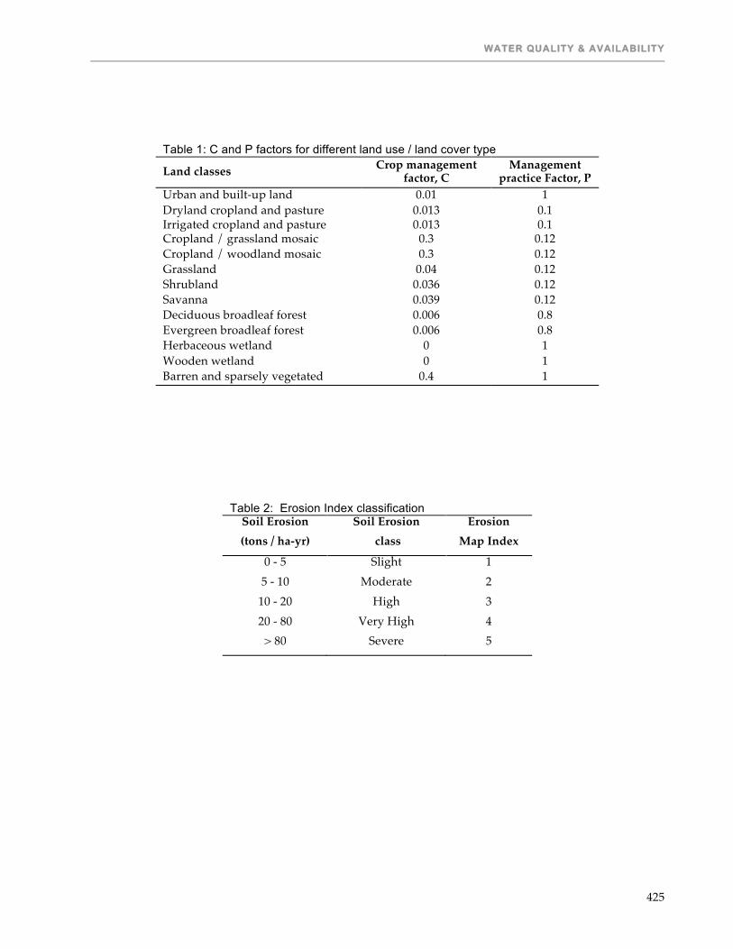
WATER QUALITY & AVAILABILITY
425
Table 1: C and P factors for different land use / land cover type
Land classes Crop management factor, C
Management practice Factor, P
Urban and built-up land 0.01 1 Dryland cropland and pasture 0.013 0.1 Irrigated cropland and pasture 0.013 0.1 Cropland / grassland mosaic 0.3 0.12 Cropland / woodland mosaic 0.3 0.12 Grassland 0.04 0.12 Shrubland 0.036 0.12 Savanna 0.039 0.12 Deciduous broadleaf forest 0.006 0.8 Evergreen broadleaf forest 0.006 0.8 Herbaceous wetland 0 1 Wooden wetland 0 1 Barren and sparsely vegetated 0.4 1
Table 2: Erosion Index classification
Soil Erosion (tons / ha-yr)
Soil Erosion class
Erosion Map Index
0 - 5 Slight 1 5 - 10 Moderate 2
10 - 20 High 3 20 - 80 Very High 4 > 80 Severe 5

TWENTY-FIFTH ANNUAL TECHNICAL REPORT – VOLUME I
426
Nzoia Basin
Figure 1: location of Lake Victoria and Nzoia basin
Figure 2: Lake Victoria basins

WATER QUALITY & AVAILABILITY
427
Rainfall Map
FAO Landuse/cover
NOAA Soils Map
Reclassify
Inverse Distance Weighted (IDW) interpolation
Station Rainfall
Data
Soil Texture Map
Flow Accumulation
Erosion Map
Rainfall Factor, R Management Factor, P Erodibility Factor, K Length Factor, L Slope Factor, S Crop Factor, C
Map Calculations
Slope Angle
Hydrologic Calculations
Erosion Index Map
Reclassify
Overlay Analysis
SRTM DEM Mosaic
Map Calculations
Map
Calculations
Map
Calculations
Figure 3: GIS erosion prediction flow chart

TWENTY-FIFTH ANNUAL TECHNICAL REPORT – VOLUME I
428
Figure 4: Maps depicting the African soil properties extracted from the NOAA server
Sand percent Clay percent
Silt percent Organic matter percent
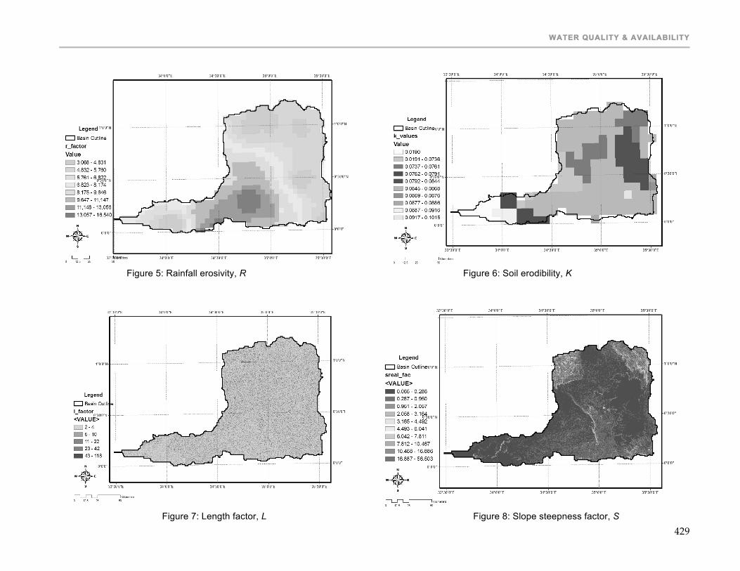
WATER QUALITY & AVAILABILITY
429 Figure 7: Length factor, L Figure 8: Slope steepness factor, S
Figure 5: Rainfall erosivity, R Figure 6: Soil erodibility, K

TWENTY-FIFTH ANNUAL TECHNICAL REPORT – VOLUME I
430
Figure 9: Crop factor, C Figure10: Practice management factor, P
Figure 11. Soil erosion distribution map
Figure 12. Soil erosion index map
Related Documents