April 1, 2008 - USTCstaff.ustc.edu.cn/~lgliu/Courses/SummerSchool_2015/FinalTest/... · each pair of corresponding vertices along predetermined ... tration and animation. ... length

GEOMETRIC MODELING IN SHAPE SPACE 1

Liu Gang(Department of Mathematics, Zhejiang University, Hangzhou 310027)

April 1, 2008

1Report for the course of Digital Geometry Processing

Abstract

In this report, we conclude some of these papers which involve solving the tra-jectory problem in boundary representation based shape interpolation as one oftheir main contributions. These three main methods are: Computing intrinsicsolution, Poisson shape interpolation and Shape space method. We comparethese methods from theoretical views and their applications. In this report, wetake the main emphasis on shape space method and pay more attention to 2-Dmethod construction and 3-D promotion in this method.

1

Contents

1 Introduction and past works 31.1 Introduction . . . . . . . . . . . . . . . . . . . . . . . . . . . . 31.2 Past Works . . . . . . . . . . . . . . . . . . . . . . . . . . . . 3

2 Computing intrinsic solution and Poisson shape interpola-tion 52.1 Computing intrinsic solution . . . . . . . . . . . . . . . . . . 52.2 Poisson shape interpolation . . . . . . . . . . . . . . . . . . . 6

3 Geometric modeling in Shape space 103.1 Analysis of planar shapes using geodesic paths on shape space 103.2 Geometric modeling in shape space . . . . . . . . . . . . . . . 15

4 Comparisons 20

Acknowledgements 22

References 23

2

Chapter 1

Introduction and past works

It is well-understood that there are two major issues in Boundary represen-tation (B-rep) based shape interpolation. The first is how to find a featurepreserving correspondence map between the given models, known as cor-respondence problem. The second is how to interpolate the positions foreach pair of corresponding vertices along predetermined paths, known astrajectory problem.

1.1 Introduction

Shape interpolation, also known as shape blending or morphing, has beenwidely applied to various aspects of computer graphics industry, e.g. illus-tration and animation. Given two input models, shape interpolation cangenerate a sequence of intermediate shapes which gradually changes fromthe source shape to the target one.

This report considers three of these novel approaches based on geometricintrinsic variable, Poisson equation and Shape space theory.

1.2 Past Works

In 1992, Sederberg and Greenwood decomposed the deformation of in-betweenshapes into stretch and bend. And later Sederberg et al. propose a geomet-ric algorithm with global optimization to ensure these blended polylines areclose without local self-intersection. Liu Ligang and Wang Guojin gener-alize this idea to 3D meshes. But all the final morphing results are de-pendent of the computation order of dihedral angels and edge length. Tohandle large scale rotation in boundary representation based morphing, alot methods which give various constraints have been proposed. Poissonshape interpolation is representative to these kind methods and takes bothvertex coordinates and surface orientation into account. Since this methodconsider preserving rigid (as rigid as possible) as the main aim morphing,

3

the result can not radically avoid shrinkage problem and the interpolationshapes might be unstable in variation of pose orientations.

In 2004, Klassen et al. presented a computational approach to spacesof curves to interpolate the given two models successfully and gave moreapplication in shape analysis. But it has no natural extension to surface.The paper Geometric modeling in shape space proposed a general 3D com-putational modeling framework and give algorithms to shape deformationsthat satisfy various user given constraints.

The main body of this report is divided as follows.Chap.2 analyzes the main steps of Computing intrinsic solution and Poissonshape interpolation.Chap.3 discuss the idea using geodesic paths on shape space to shape anal-ysis and geometric modeling.Chap.4, list the main contributions of these methods in shape interpolationand compare latter two methods in examples and applications.

4

Chapter 2

Computing intrinsic solutionand Poisson shapeinterpolation

In this chapter, we analyze two classical methods Computing intrinsic so-lution and Poisson shape interpolation in the simple theoretical view andapplications.

2.1 Computing intrinsic solution

In computing intrinsic solution, the intrinsic variables consisting of edgelength and the angels between edges in 2-D or edge length and the sphericalcoordinates in the moving coordinate system constructed by the previouspoints in 3-D should be computed first. These variables can be determinedby the polylines uniquely and generate the same polylines differed by a rigidbody motion. Interpolating these two intrinsic variables determined by thegiven two polylines linearly can naturally generate the in-between intrinsicvariables and polylines can be reconstructed soon. To preserve the interme-diate polylies closed when the reference and target polylines are closed is themain problem in this method. By using Lagrange multipliers method, wefind the adjustment to make the polylines closed under changing the edgelength only. Since almost any surface representation (spline, implicit sur-face, volumetric) can be converted with arbitrary accuracy to a quadrilateralmesh by polygonization processes, this geometric method should be general-ized to quadrilateral meshes. The intrinsic variables of quadrilateral can beestablished by iteratively defining the spherical coordinates from the bound-ary coordinates. The interpolation implementation is similar. The pictureFig.1 showed below is the transformation from a 3-D digitalized sculptureinto an ”S” shaped subject.

5

Fig 1. The transformation from a 3-D digitized sculpture into an ”S”shaped subject, The intermediate frames are interpolated at time

t = 0.0, 0.25, 0.5, 0.75, 1.0

2.2 Poisson shape interpolation

In the Poisson shape interpolation approach, we formulate the trajectoryproblem of shape interpolation as solving Poisson equations defined on adomain mesh. By Constructing the non-linear gradient field which involvesboth vertex coordinates and surface orientation. There are three steps toaccomplish this program.

1. Compute correspondence map and generate compatible meshes

from two input 3D meshes.

This method requires that the source model and the target one should berepresented by compatible meshes, i.e. meshes with the same connectivity.These two models can be interpreted as three scalar fields (vertex positions)defined on a common domain that is actually an abstract mesh structurecalled domain mesh. In this report, we assumes the input models and domainmeshes are all single-connected and 2-manifold triangular meshes through-out this report. We uses various feature-preserving remeshing methods. Inthe implementation, base domain is constructed after manually selected sev-eral pairs of corresponding feature vertices. Then, both source model andtarget model are parameterized onto the common base domain and relax-ation is performed to reduce the parameterization distortion. Finally, thetarget model is remeshed using the connectivity of the source model. Iter-ative error-driven vertex relaxation and edge splitting are performed untilapproximation error is under user-specified threshold.

2. Compute and decompose the local transformation

For each corresponding triangle pair of compatible meshes, determine thelocal transform from source triangle to target one and decompose the trans-form into rigid rotation and stretch part.

6

Let T0 and T1 be a pair of corresponding triangles in source model meshS0 and target mesh S1 which has been remeshed, respectively. we denoteνi0 and νi

1 (i = 1, 2, 3) as corresponding vertices, n0 and n1 as correspond-ing unit face normals. For gradients are translation invariant, we choosethe first vertex ν1

j (j = 0, 1) of each triangle as the origin, and the threeaxes of affine frames Fj are ν2

j − ν1j , ν3

j − ν1j and nj . Thus we have con-

structed the local reference system. The unique transform matrix H canbe determined such that F1 = H(F0), that is the matrix H can be regardas the deformation gradient relating the reference configuration F0 and thepresent configuration F1. We factorizes the deformation gradient tensor intothe rigid rotation part and the pure stretch part with the polar decompo-sition. That is, H = RS, where R is the closest rotation matrix to Hin Frobenius norm, and S is a symmetric, positive definite matrix(See theFig2). We define the local continuous transform function Ht in the timet(t ∈ [0, 1]) for a given transition state h(ν, t) = t as Ht = Rt((1− t)I + tS),where The function h(ν, t) is named transition state function whose valuealso lies in [0, 1], and satisfies h(·, 0) = 0 and h(·, 1) = 1, The transition statefunction is used to provide flexible non-uniform controls. Since there is noprior knowledge of movements in morphing process we choose the transitionstate function in the simplest form h(ν, t) = t; Rh is the rotation matrixdefined by linearly interpolating the rotation angle of R using quaternion,and I is the identity matrix. Now we have the general detail transformationHt then compute in the each triangle .We apply Ht to three source gradientvectors simultaneously for generating interpolated gradient vectors. Thatis,

Git = Ht(Gi

0)(i = x, y, z) : (2.1)

Fig2. The deformation gradient (matrix) H is factorized into the rigidrotation part R and pure stretch part S

7

After gradient fields interpolation, each triangle is locally transformed bythe transformation Ht . The triangles of target mesh become disconnected,i.e., yielding a triangular soup. The Poisson equation stitches together thetriangles in the final step.

3. Reconstruct the intermediate shapes by Poisson equation solver

The Poisson equation with Direchlet boundary conditions is formulated as:{∆f = ∇ · wf |∂ω = f∗|∂ω

(2.2)

Where the divergence operator ∇ = ( ∂∂x , ∂

∂y , ∂∂z )T over a a vector field ω =

(ωx, ωy, ωz) is ∇·ω = ∂ωx∂x + ∂ωy

∂y + ∂ωz∂z ; ∆ = ∂2

∂x2 + ∂2

∂y2 + ∂2

∂z2 is the Laplacianoperator; f is an umknown scalar function and f∗ provides the desirablevalue on the boundary ∂ω.

In 2003, Tong et al. proposed well-defined discrete differential operatorsof scalar and vector fields on irregular domains. Based on their result, thediscrete Poisson equation on triangular meshes is formulated as follows.

A mesh scalar field f on M is defined to be a piecewise linear combina-tion f(ν) =

∑i fiφi(ν)(ν is a point on M). The function φ(ν) defined

as: φi(νj) = 1, if j = i and φi(νj) = 0, if j 6= i. The discrete gra-dient of mesh scalar function f on the domain mesh M is expressed as:∇f(ν) =

∑i fi∇φi(ν). Given a piecewise constant vector field ω, which has

constant value in each triangle of M , the discrete divergence of ω at vertexνi is defined as (divω)(νi) :=

∑T∈NT (νi)

ω(T ) · ∇φi|T AT where AT denotesthe area of triangle T . Therefore, the discrete Laplacian operator on domainmesh M is:

∆f(νi) =∑

νj∈Nν(νi)

12(cot αj + cot βj)(fi − fj), (2.3)

where αj and βj are two angles opposite to the edge (vi, vj).Finally, the discrete Poisson equation is expressed as ∆f ≡ div(∇f) = divω.With specified boundary conditions, the above equation can be reformulatedas a sparse linear system:

Ax = b(t). (2.4)

where the unknown vector x represents coordinates to be reconstructed inthe intermediate shape. The coefficient matrix A is determined by the (2.3)and the fixed domain mesh; b(t) comes from the smoothly changing gradients(2.1) and boundary conditions.

The Fig3 demonstrated below shows that this method can be using inhuman pose interpolation. More examples will be given in Chap 4.

8

Fig3. Human pose morphing

9

Chapter 3

Geometric modeling inShape space

In this chapter, we consider geometric modeling especially shape interpo-lation by using geometric paths on shape spaces. In the first section weanalyze the planar shapes. In the second section we take our emphases onthe 3-D surface.

3.1 Analysis of planar shapes using geodesic pathson shape space

Historically, there have been many exemplary efforts in characterizationand quantification of shapes. From the view of elegant statistical theoryof shapes, Shapes are represented using a finite number of salient points orlandmarks. Shapes invariant transformation includes rigid rotations, trans-lations and non-rigid uniform scaling, the resulting quotient space is a finite-dimensional Riemannian manifold, called a shape manifold. Different shapescorrespond to these elements of this space and quantification of shape dif-ferences is achieved via a Riemannian metric on this space. But from theGrenander’s formulation, shapes are considered as points on some infinite-dimension differentiable manifold. The variations between the shapes aremodeled by the action of Lie group (deformations) on the manifold. Lowdimensional groups, such as rotation, translation, and scaling, keep theshapes unchanged, while high dimensional groups smoothly change the ob-ject shapes, a central idea behind deformation template theory. The actionof diffeomorphisms group suffers from a high cost in computing.

This part of research makes contribution over the past works in severalfacets. We consider each contour as a continuous curves avoiding to findinglandmarks and deal more intrinsically with the shape spaces to avoid thediffeomorphism of Euclidean spaces. The main idea proposed here is the

10

use of computational differential geometry, i.e., a computational analysis ofshapes using differential geometry of both curves and spaces of curves. Inthe rest of this chapter, we present the framework in details.

1. Geometric representation of closed, planar curves

In this section, we assume that curves boundaries are closed curves with asingle component views as closed immersed curves in the plane. We wantto find the shape representation that is invariant to these transformations,such as rigid motions (including rigid rotation and translation in R2) anduniform scaling of R2 because they represent the same shapes.

We assume that curves parameterized by arclength: α(s) = (α1(s), α2(s)) :R → R2 satisfy two conditions: 1. periodic: α(2π + s) = α(s); 2. Tangentunit length |α′(s)| = 1. Associated with each α, there is a tangent indicatrixν : R→ S1 R2 given by ν(s) = α′(s) = ejθ(s)(j =

√−i), where θ(s) is the

direction function.From the next paragraph, we will construct the direction function preshapespace C and shape space S

By analyzing the function θ(s) in the unit circle: θ0(s) = s, we knowany closed curves of rotation index 1 have the direction function taking theforms θ = θ0 + f, f ∈ L2. For any two elements: α, β ∈ θ0 + L2, we haveα − β ∈ L2. So the space θ0 + L2.is an affine space but not vector space.In the meaning time, it is obvious that the tangent space at any point isnaturally identified with L2 because θ′ = f ′ ∈ L2

Now we will give more restricts: Because addition of a constant to thedirection function θ results in a rotation of the corresponding curve in theplane. That is: ν1(s) = α′

1(s) = ejθ(s)+c = ejθ(s)ec we want to mod outby this group action to make shapes invariant to rotation and give the firstrestriction:

12π

∫ 2π

0θ(s)ds = π (3.1)

Although any constant can be used instead of π, we choose it to includethe identity function in the restricted set.In the meaning time, θ(s) must be satisfy the closure condition and this isthe second restriction: ∫ 2π

0ejθ(s)ds = 0 (3.2)

Consequently, we define ’the set’ as a subset of θ0 + L2 satisfying the twoconditions mentioned above.

11

If we define the map φ = (φ1, φ2, φ3) : (θ0 + L2) → R3satisfying:

φ1 =12π

∫ 2π

0θ(s)ds, (3.3)

φ2 =12π

∫ 2π

0cos(θ(s))ds, (3.4)

φ3 =12π

∫ 2π

0sin(θ(s))ds (3.5)

Then, C can be written as φ−1(π, 0, 0), and is a complete submanifold ofθ0 + L2 of condimension three. By restricting the L2-inner product to thetangent space of C, it becomes a Hilbert manifold. But it is a preshapespace since it is possible to have multiple elements of C denoting the sameshape. This variability is due to the choice of the reference point(s = 0)along the curve. For x ∈ R, θ ∈ C, if we define (x · θ)(s) = θ(s − x) + x,This operation corresponds to change the initial point(s = 0) on the closedcurve by a distance of x along the curve. By defining the action on the R:S1 = R/2πZ(S1 is called reparametrization group), S = C/S1 is the space ofplanar shapes under θ representations. S is also a manifold except the setof shapes with rotational symmetries, a negligible set.

2. Geometries of the resulting shape spaces and Computing geodesic

on this shape space.

An important tool in the process which analyze shapes and perform statis-tical inferences on the shape space S is a technique for computing geodesicpaths between arbitrary points on the preshape space C. Firstly we willdraw infinitesimal tangent lines in the affine spaces θ0 + L2; then projectthem onto the preshape spaces C. So we need specify the tangent spaces orequivalent the normal spaces on these manifolds and construct a mechanismfor projecting points from θ0 + L2 to CTangents and Normals to preshape space Rather than specifying thetangent spaces on these manifold, it is easier to describe the spaces of nor-mals to C, inside L2. The direction derivative dφ, at a point θ ∈ θ0 + L2 inthe direction of an f ∈ L2 (means θ′(s) = f(s)) is defined:

dφ1(f) =12π

∫ 2π

0f(s)ds = 〈f,

12π〉 (3.6)

dφ2(f) = − 12π

∫ 2π

0sin(θ(s))f(s)ds = −〈f, sin(θ)〉 (3.7)

dφ3(f) =12π

∫ 2π

0cos(θ(s))f(s)ds = 〈f, cos(θ)〉 (3.8)

12

These functions mean that dφ is a surjective from L2 to R3 and f ∈ L2 istangent to C at θ if and only if f is orthogonal to the subspace spanned by{1, cos(θ), sin(θ)}. So the basis {1, cos(θ), sin(θ)} span the normal space atθ, the tangent space is given as:

Tθ(C1) = {f ∈ L2|f ⊥ span{1, cos(θ), sin(θ)}}

Theoretical idea is to move in direction perpendicular to the level setsuch that their images under φ form a straight line in R3. we will constructthe level set as follow. For any b ∈ R3, set φ−1(b) = {θ ∈ θ0 + L2|φ(θ) = b}is the level set of φ and the level set for b = (π, 0, 0) is the preshape space.

For the reason φ : L2 → R3, there will be dφ : Tθ(L2) → Tθ(R3) = R3.So for any point in this level set θ ∈ φ−1(b), we need find the nearest pointand the straight line connecting these two point perpendicular to the normalvector of this level set. That means give a displacement dθ moving in C andorthogonal to this level set. dθ is the normal vector at θ (φ(θ) = b) whichtakes φ(θ+dθ) to the desire point b1 ∈ R3. We can define a Jacobian matrixto approximate the first order.Iteration method to find the superior trajectory as follow.

Define the residual vector of approximation of b1 is r1(θ) = b1 − φ(θ).Then the desire tangent vector is given by:

dθ = J(θ)−1r1(θ)(1, sin(θ), cos(θ))T (3.9)

The Jacobian matrix is:

J(θ) =

〈 12π , 1〉 〈 1

2π , sin(θ)〉 〈 12π , cos(θ)〉

−〈sin(θ), 1〉 −〈sin(θ), sin(θ)〉 −〈sin(θ), cos(θ)〉〈cos(θ), 1〉 〈cos(θ), sin(θ)〉 〈cos(θ), cos(θ)〉

Then update the curve using θ = θ + dθ, and iterate till the norm |r1(θ)|converges to zero. Thus we have this projection: P : L2 → CGeodesic on preshape space We consider the ”Most efficient deforma-tion” as to construct the shortest path between the corresponding points inthe preshape space with respect to the Riemannian metric given by the L2

inner product on the tangent space, i.e., a length-minimizing geodesic. Ageodesic on a manifold embedded in a Euclidean space is defined to be aconstant speed curve on the manifold, whose acceleration vector is alwaysperpendicular to the manifold.

We now construct geodesic paths on the preshape space and the corre-sponding algorithm will be proposed later. Let θ ∈ C and f ∈ Tθ(C), wewant to generate a geodesic path or a parameter flow starting from θ andwith tangent vector f at θ; denote this flow by Ψ(θ, t, f) where t is the timeparameter. We will evaluate this flow for discrete times t = ∆, 2∆, ..., for asmall ∆ > 0. Setting Ψ(θ, 0, f) = θ, take the first increment to reach θ+∆fin L2 and apply the projection P to this point. Set Ψ(θ, ∆, f) = P(θ + ∆f)

13

to get the next point along the geodesic. Iterating this process provides suc-cessive points along the geodesic Ψ in C. To transport the tangent vector fto the tangent space at the next point, we normalize it to keep the ”speed”of the geodesic constant.

Let θ1 be the point along the geodesic path; we want to find f1 that istangent to C1 at θ1 and is parallel transport of f . This can be accomplishedusing:

f1 = ‖f‖ g

‖g‖, where g = f −

3∑k=1

〈f, hk〉hk, (3.10)

Here hks form an orthogonal basis of the normal space: span{1, sin(θ1), cos(θ1)}An algorithm summarizing the steps for constructing a geodesic path on Cis as follows:Algorithm Start with a point θ ∈ C and a direction f ∈ Tθ(C). Set l = 0and Ψ(θ, l∆, f) = 0, and choose a small ∆ = 0.1. Add increment Ψ(θ, l∆, f)+∆f and set Ψ(θ, (l+1)∆, f) = P(Ψ(θ, l∆, f)+∆f)2. Transport f to the new point by using Ψ(θ, (l + 1)∆, f) for(3.10)3. Set l = l + 1, Go to Step 1 with f = f1

It can be shown that ∆ → 0, Ψ converges to a geodesic path on C.Geodesic on shape space To find a geodesic in C which is orthogonalto the S1-orbit, we simply restrict the allowable tangent directions to beorthogonal to the S1-orbit, i.e., use only those f ∈ Tθ(C) which are perpen-dicular to Tθ(S1). It can be shown that this one-dimension space is spannedby 1 − θ′ and hence, f should be orthogonal to 1 − θ′. The algorithm forconstructing geodesic in S1 is identical to the previous algorithm in thischapter except that, in(3.10), the vector g is now given by:

g = f −4∑

k=1

〈f, hk〉hk (3.11)

where hks form an orthogonal basis of the space span {1, sin(θ1), cos(θ1), θ′1}

3. Application in shape interpolation.

Given θ, ϑ ∈ S1, let Ψ be the desired one-parameter flow from θ to ϑ. wewant to find that appropriate direction f ∈ Tθ(S1) such that a geodesicin that direction passed through the S1-orbit of ϑ. That is to solve for anf ∈ Tθ(C) such that Ψ(θ, 0, f) = θ and Ψ(θ, 1, f) = s · ϑ, for some s ∈ S1

We can treat this problem as an optimization problem over the Tθ(S1).The cost function for minimizing is given by the functional:

H[f ] = infs∈S1

‖Ψ(θ, 1, f)− s · ϑ‖ (3.12)

14

and we look for that f ∈ Tθ(S1) satisfies that H[f ] is zero and ‖f‖ isminimum among all such tangents.

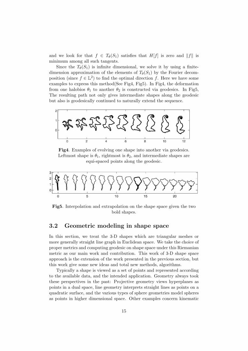
Since the Tθ(S1) is infinite dimensional, we solve it by using a finite-dimension approximation of the elements of Tθ(S1) by the Fourier decom-position (since f ∈ L2) to find the optimal direction f . Here we have someexamples to express this method(See Fig4, Fig5). In Fig4, the deformationfrom one halobios θ1 to another θ2 is constructed via geodesics. In Fig5,The resulting path not only gives intermediate shapes along the geodesicbut also is geodesically continued to naturally extend the sequence.

Fig4. Examples of evolving one shape into another via geodesics.Leftmost shape is θ1, rightmost is θ2, and intermediate shapes are

equi-spaced points along the geodesic.

Fig5. Interpolation and extrapolation on the shape space given the twobold shapes.

3.2 Geometric modeling in shape space

In this section, we treat the 3-D shapes which are triangular meshes ormore generally straight line graph in Euclidean space. We take the choice ofproper metrics and computing geodesic on shape space under this Riemanianmetric as our main work and contribution. This work of 3-D shape spaceapproach is the extension of the work presented in the previous section, butthis work give some new ideas and total new methods, algorithms.

Typically a shape is viewed as a set of points and represented accordingto the available data, and the intended application. Geometry always tookthese perspectives in the past: Projective geometry views hyperplanes aspoints in a dual space, line geometry interprets straight lines as points on aquadratic surface, and the various types of sphere geometries model spheresas points in higher dimensional space. Other examples concern kinematic

15

spaces and Lie groups which are convenient for handling congruent shapesand motion design. We will show that many geometry processing tasks canbe solved by endowing the set of closed orientable surfaces C called shapeshenceforth C with a Riemannian structure.

1. Choose proper metrics and Construct shape space

By shape-triangular meshes in Euclidean 3-space, shape can be separatedinto its connectivity. Here we have Some Assumptions: we require allmeshes to be 2-dimensional manifolds C boundaries are allowed; any twotriangles share a common edge, or share a common vertex, or have no pointsin common; the star of any non-boundary vertex is a topological disk anda boundary vertex is a half disk. In what follows, we keep the connectivityfixed, and change only the vertex positions.

Given a fixed simplicial complex, we consider the space S of all immer-sions of this connectivity in Euclidean 3- space. Such an immersion is seenas a point in shape space, that is p ∈ R3m(we assume this shape M involvem points). For any vertex p ∈ M , there will be a vector Xp ∈ R3 andassigned a tangent vector X ∈ TM (S). A smooth deformation of M is amapping φ : [0, 1]×M → R3 such that all the shapes consisting a functionp(t) := φ(t, p) is smooth. Given a deformation of M , X(t) := ( d

dtp(t))p∈M

defines the deformation field at time t. In this point, The affine deformationp(t) = A(t)·p+a(t) is a smooth rigid body motion if A(t) is a smoothly vary-ing matrix and orthogonal at every instant of time and a(t) is a translationvector. A mesh is deformed isometrically if distances measured on the meshare preserved during deformation. So a deformation of a shape M is isomet-ric if and only if ‖p(t)−q(t)‖2 the length of each edge in the triangulation ispreserved in the deformation, that is 〈Xp(t)−Xq(t), p(t)−q(t)〉 = 0 for eachedge (p(t), q(t)) of the mesh M(t), where 〈, 〉 denotes the canonical innerproduct in R3. The vector field corresponding to isometric deformations ofM named Killing vector fields is a linear subspace of TM (S).

We use the following design paradigm when it comes to defining a met-ric, i.e., an inner product: Given a property of a shape to be preservedduring deformation, we translate this property to an equivalent conditionon deformation fields. The norm of a deformation field is derived from thiscondition. In this section, we choose preserving distances measured on themesh rather than pairwise Euclidean distances between vertices(See Fig6.for a comparison of metrics.). In a first step, we extract the part that pre-serves isometry. Unfortunately Killing fields are harder to express explicitly.In addition, the given mesh might not be flexible at all. In such cases, wechoose to deform a shape as isometrically as possible. To achieve this we

16

take:

〈〈X, Y 〉〉IM :=∑

(p,q)∈M

〈Xp −Xq, p− q〉〈Yp − Yq, p− q〉 (3.13)

Fig6. Comparing the as-rigid-as-possible shape metric (left) with theas-isometric-as-possible shape metric (right).

as the inner product of two deformation fields. This expression is symmetricand bilinear and hence defines a semi-Riemannian metric. It is just a semi-Riemannian metric since there are non-vanishing deformation fields X with〈〈X, X〉〉M = 0. Thus all the shapes which are congruent to a given shapeM form points of a fiber in S(like the reparametrization group S1 in the2-D case). Any smooth curve in a fiber has length zero and corresponds toa smooth isometric motion of M . This observation also shows that shortestpaths (geodesics) in the described metrics are only unique up to changeswithin the fibers.

To overcome this problem, we add a small regularization term to thelength which is minimized by geodesics, rather than mod out this congruencerelation. The obvious choice for this term is the L2 shape metric: Givenvector fields X, Y on a shape M , let

〈〈X, Y 〉〉L2

M :=∑p∈M

〈Xp, Yp〉Ap, (3.14)

where Ap is one-third of the area of all triangles adjacent to the vertexp. Blending the L2 inner product with the metrics (3.13) or (3.14) yieldsRiemannian metrics

〈〈X, Y 〉〉M,λ := 〈〈X, Y 〉〉M + λ〈〈X, Y 〉〉L2

M (3.15)

that have the same visual behavior as their semi-Riemannian counterpartsif l is chosen appropriately small.So till now we have constructed a Riemannian metric based shape space

17

(S, 〈〈, 〉〉). Recall that a geodesic is a locally shortest curve, i.e., given twopoints on a geodesic the part between those points is a local minimum of thelength functional with respect to small perturbations of the curve. For themetric (3.15) this means that the length of a deformation decreases as thedeformation becomes more isometric. From the below figure, we know theisometric metric(as isometric as possible) is better than the rigid metric(asrigid as possible).

2. Computing geodesic on shape space

We now describe how to solve the following problem: Interpolation prob-lem: Given two isomorphic shapes, how to compute a geodesic path joiningthem; We solve this problems using a multi-resolution framework. Propa-gating the solution from coarser to finer resolutions not only leads to fasterconvergence, but also makes the approach more robust.Interpolation problem Assumptions: The input shapes are two compat-ible meshes M and N , i.e., the underlying simplicial complexes are iso-morphic; the input meshes are concurrently decimated to preserve corre-spondences across all resolutions of the resulting progressive meshes; edgesin the two meshes are paired according to the underlying isomorphism.These assumptions mean that our input meshes are two mesh hierarchies(M0,M1, . . . ,M l = M) and (N0, N1, . . . , N l = N). To get an initial esti-mate of a geodesic path we linearly blend the meshes M0 and N0. So weget the initial path P 0 = (M0,M0N0, N0).

Assume the vertices of the polyline are given by shapes P0, P1, . . . , Pn+1

(we drop the superscripts indicating mesh resolution), and the segments aregiven as X0, X1, . . . , Xn(Xi = PiPi+1). Since the local minimizers of thisenergy are geodesics in a scaled arc length parametrization, we discretizethe energy

∫〈〈X, X〉〉P (t)dt of a curve P (t) as

E(P ) :=n∑

i=0

(〈〈Xi, Xi〉〉pi + 〈〈Xi, Xi〉〉pi+1) (3.16)

A quasi-Newton method is used to minimize (3.16). After attaining a lo-cal minimum of the energy at a given resolution we perform refinementwhich comes in two flavors: (a) Space Refinement: increase the resolutionof the meshes, we linearly blend neighboring meshes to refine the path. (b)Time Refinement: refine the path by inserting more vertices in the polyline.Firstly we simply increase the resolution of the progressive meshes to get re-fined boundary meshes from P k

0 and P kn+1 to P k+1

0 and P k+1n+1 . Then we trans-

fer the detail of P k+10 , P k+1

n+1 to the intermediate meshes. For any new vertex,P k

i as a example, we project P ki onto P k+1

0 , P k+1n+1 . Denote f1, f2 are the index

of the faces that carry the projection p′, p′′, and Nf1 , Nf2 are the normals of

18

the faces f1, f2, we compute barycentric coordinates of the projected verticeswith respect to the face f1, f2 and denoted by P k+1

i,0 = 〈P ki − p′, Nf1〉 and

P k+1i,n+1 = 〈P k

i − p′′, Nf2〉. The refined mesh at position i of the path is givenby:

P k+1i =

n + 1− i

n + 1P k+1

i,0 +i

n + 1P k+1

i,n+1

. These steps are mutually independent, and can be applied in any order.After re- finement, we repeat the optimization on the new path.

3. Some other applications

Similarly, we can solve Extrapolation problem Given a shape and a defor-mation field, how to compute a geodesic that originates at this point, andmoves in the direction of the deformation field by using a multi-resolutionframework. From the theoretical view, geodesic equation expresses vanish-ing geodesic curvature. So geodesics can be described by the Euler Lagrangeequation of the energy. Alternatively computing a first-order ODE and anoptimization process under a multi-resolution framework, we solve this prob-lem. In this shape space framework many concepts from classical differentialgeometry can be applied to a wide variety of geometry processing tasks: par-allel transport to deformation transfer, and the exponential map to shapeexploration (See the pictures below).

Fig7. Deformation transfer. The blue input shapes of the cat (top row) arejoined by a geodesic to get a deformation. This deformation is transferred tothe blue lion model (bottom row). The middle row (in right part of graph)shows hybrids generated during deformation transfer.

19

Chapter 4

Comparisons

In this chapter, we demonstrate some 3-D experiment results to comparethe methods Poisson shape interpolation and Shape space methods.

In all of the examples, the mesh reconstructions part use gradient-basedmethod(presented in the paper YU, Y., ZHOU, K., XU, D., SHI, X., BAO,H., GUO, B., AND SHUM, H.-Y. 2004. Mesh editing with Poisson-basedgradient field manipulation. ACM Trans. Graph. 23, 3, 644-651.). Some-times if we globally align poses of two models and then do shape inter-polation, the result of the method Poisson shape interpolation can be im-proved(See Example 1). However, we present a example that it is useless tohandle using a single global alignment (See Example 2).

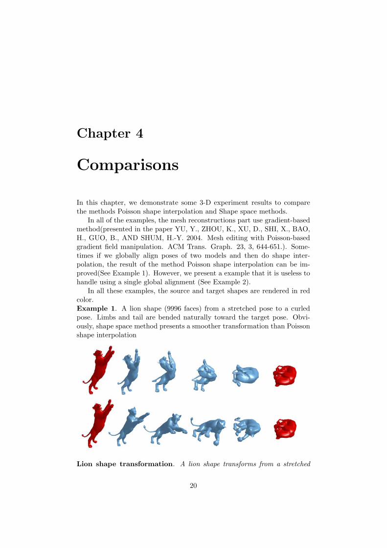
In all these examples, the source and target shapes are rendered in redcolor.Example 1. A lion shape (9996 faces) from a stretched pose to a curledpose. Limbs and tail are bended naturally toward the target pose. Obvi-ously, shape space method presents a smoother transformation than Poissonshape interpolation

Lion shape transformation. A lion shape transforms from a stretched

20

pose to a curled pose by Poisson shape interpolation(above) and Shape spacemethod(blow).

Although Poisson shape interpolation can generate better result withrough global shape alignment, it still has some defects.

Lion shape transformation after global alignment. The interpolationgenerated by Poisson shape interpolation still suffers from several fallacies:See the changes of tail in the transformation.Example 2.Shape interpolation of a male shape (34970 faces) from a crouchedpose into a stretched pose. Notice the natural bending of the body, limbsand fingers, and the preservation of the local details (lines of the muscle)during the interpolation.

Male shape transformation. A male shape transforms from a crouchedpose to a stretched pose by Poisson shape interpolation(above) and Shapespace method(blow). The latter shows superiority in the transformationEven with the aid of global shape alignment, the improvement to the resultof the transformation based on Poisson shape interpolation is little.

21

Male shape transformation after global alignment The global align-ment can not avoid the critical shrinkage in the arms.

The comparisons in the theoretical view

To the method Poisson shape interpolation, interpolating vector fields ingradient domain results in the morphing results depending on the quality ofcompatible meshes. Reconstruction of intermediate shape which graduallychange both vertex coordinates and face normals by Poisson equation solveris the main contribution. In essence, Poisson shape interpolation is a as-rigid-as possible algorithm and it can not avoid shrinkage in variation ofpose orientation. In this point, the shape space method give a significantlyprofound understanding of interpolation.

shape space promotion from planar shape analysisto 3-D geometric modeling

As-isometric-as possible shape interpolation is one of important contribu-tions in the paper Geometric modeling in shape space. Except the choice ofmetrics, there are totally different solutions in dealing with reparametriza-tion groups in 2-D or fiber consisting of shapes with vanishing distancein 3-D. The authors find the quotient space by moding that space in the2-D case but the latter solve it dexterously by adding a small regulariza-tion term from the L2 shape metric to the length which is minimized bygeodesic. Since the authors of these two papers focus different emphases onthe concept shape space, the anterior presents more theoretical derivationand application in statistical analysis, while the latter propose a marvelousapproach in geometric modeling

Acknowledgements

I thank for Dr Liu Ligang for his nice patience and the ease atmosphere atthe CAGD Group.

22

References

[1] SEDERBERG. T. W., GAO, P., WANG, G., AND MU, H. 1993. 2-dshape blending: An intrinsic solution to the vertex path problem. InComputer Graphics (SIGGRAPH ’93 Proceedings), vol. 27, 15-18.

[2] Liu, L.-G., AND WANG, G.-J. 1999. Three-dimensional shape blend-ing: intrinsic solutions to spatial interpolation problems. Computers& Graphics 23, 4, 535-545.

[3] XU, D., ZHANG, H., WANG, Q., BAO, H. 2005. Poisson shape in-terpolation. In SPM ’05: Proc. ACM Symp. On Solid and PhysicalModeling, 267-274.

[4] KLASSEN, E., SRIVASTAVA, A., MIO, W., JOSHI, S. H. 2004. Anal-ysis of planar shape using geodesic paths on shape spaces. IEEE trans-actions on Pattern analysis and machine intelligence. Volume 26, 3,372-383.

[5] MARTIN, K., NILOY J. M., AND HELMUT P. 2007. GeometricModeling in Shape Space. In Computer Graphics (SIGGRAPH ’07Proceedings), Volume 26, Issue 3

23