Approximations of Shape Metrics and Application to Shape Warping and Empirical Shape Statistics

Approximations of shape metrics andapplication to shape warping and empiricalshape statistics

Guillaume Charpiat1, Olivier Faugeras2, Renaud Keriven3, and PierreMaurel4

1 Odyssee Laboratory, ENS, 45 rue d’Ulm, 75005 Paris, [email protected]

2 Odyssee Laboratory, INRIA Sophia Antipolis, 2004 route des Lucioles, BP 9306902, Sophia-Antipolis Cedex, France [email protected]

3 Odyssee Laboratory, ENPC, 6 av Blaise Pascal, 77455 Marne la Vallee, [email protected]

4 Odyssee Laboratory, ENS, 45 rue d’Ulm, 75005 Paris, [email protected]

This chapter proposes a framework for dealing with two problems related tothe analysis of shapes: the definition of the relevant set of shapes and thatof defining a metric on it. Following a recent research monograph by Delfourand Zolesio [8], we consider the characteristic functions of the subsets of R2

and their distance functions. The L2 norm of the difference of characteristicfunctions, the L∞ and the W 1,2 norms of the difference of distance functionsdefine interesting topologies, in particular that induced by the well-knownHausdorff distance. Because of practical considerations arising from the factthat we deal with image shapes defined on finite grids of pixels we restrict ourattention to subsets of R2 of positive reach in the sense of Federer [12], withsmooth boundaries of bounded curvature. For this particular set of shapeswe show that the three previous topologies are equivalent. The next problemwe consider is that of warping a shape onto another by infinitesimal gradientdescent, minimizing the corresponding distance. Because the distance functioninvolves an inf, it is not differentiable with respect to the shape. We propose afamily of smooth approximations of the distance function which are continuouswith respect to the Hausdorff topology, and hence with respect to the othertwo topologies. We compute the corresponding Gateaux derivatives. Theydefine deformation flows that can be used to warp a shape onto another bysolving an initial value problem. We show several examples of this warpingand prove properties of our approximations that relate to the existence oflocal minima. We then use this tool to produce computational definitions ofthe empirical mean and covariance of a set of shape examples. They yield an

2 Guillaume Charpiat, Olivier Faugeras, Renaud Keriven, and Pierre Maurel

analog of the notion of principal modes of variation. We illustrate them on avariety of examples.

1 Introduction

Learning shape models from examples, using them to recognize new instancesof the same class of shapes are fascinating problems that have attracted theattention of many scientists for many years. Central to this problem is the no-tion of a random shape which in itself has occupied people for decades. Frechet[15] is probably one of the first mathematicians to develop some interest forthe analysis of random shapes, i.e. curves. He was followed by Matheron [27]who founded with Serra the french school of mathematical morphology and byDavid Kendall [19, 21, 22] and his colleagues, e.g. Small [35]. In addition, andindependently, a rich body of theory and practice for the statistical analysisof shapes has been developed by Bookstein [1], Dryden and Mardia [9], Carne[2], Cootes, Taylor and colleagues [5]. Except for the mostly theoretical workof Frechet and Matheron, the tools developed by these authors are very muchtied to the point-wise representation of the shapes they study: objects arerepresented by a finite number of salient points or landmarks. This is an im-portant difference with our work which deals explicitely with curves as such,independently of their sampling or even parametrization.

In effect, our work bears more resemblance with that of several other au-thors. Like in Grenander’s theory of patterns [16, 17], we consider shapes aspoints of an infinite dimensional manifold but we do not model the variationsof the shapes by the action of Lie groups on this manifold, except in the caseof such finite-dimensional Lie groups as rigid displacements (translation androtation) or affine transformations (including scaling). For infinite dimensionalgroups such as diffeomorphisms [10, 40] which smoothly change the objects’shapes previous authors have been dependent upon the choice of parametriza-tions and origins of coordinates [43, 44, 42, 41, 28, 18]. For them, warping ashape onto another requires the construction of families of diffeomorphismsthat use these parametrizations. Our approach, based upon the use of the dis-tance functions, does not require the arbitrary choice of parametrizations andorigins. From our viewpoint this is already very nice in two dimensions butbecomes even nicer in three dimensions and higher where finding parametriza-tions and tracking origins of coordinates can be a real problem: this is notrequired in our case. Another piece of related work is that of Soatto and Yezzi[36] who tackle the problem of jointly extracting and characterizing the mo-tion of a shape and its deformation. In order to do this they find inspirationin the above work on the use of diffeomorphisms and propose the use of adistance between shapes (based on the set-symmetric difference described insection 2.2). This distance poses a number of problems that we address in thesame section where we propose two other distances which we believe to bemore suitable.

Approximations of shape metrics for shape warping and statistics 3

Some of these authors have also tried to build a Riemannian structure onthe set of shapes, i.e. to go from an infinitesimal metric structure to a globalone. The infinitesimal structure is defined by an inner product in the tangentspace (the set of normal deformation fields) and has to vary continuouslyfrom point to point, i.e. from shape to shape. The Riemannian metric isthen used to compute geodesic curves between two shapes: these geodesicsdefine a way of warping either shape onto the other. This is dealt with inthe work of Trouve and Younes [43, 44, 40, 42, 41, 45] and, more recently,in the work of Klassen and Srivastava [24], again at the cost of working withparametrizations. The problem with these approaches, beside that of havingto deal with parametrizations of the shapes, is that there exist global metricstructures on the set of shapes (see section 2.2) which are useful and relevantto the problem of the comparison of shapes but that do not derive from aninfinitesimal structure. Our approach can be seen as taking the problem fromexactly the opposite viewpoint from the previous one: we start with a globalmetric on the set of shapes and build smooth functions (in effect smoothapproximations of these metrics) that are dissimilarity measures, or energyfunctions; we then minimize these functions using techniques of the calculusof variation by computing their gradient and performing infinitesimal gradientdescent: this minimization defines another way of warping either shape ontothe other. In this endeavour we build on the seminal work of Delfour andZolesio who have introduced new families of sets, complete metric topologies,and compactness theorems. This work is now available in book form [8]. Thebook provides a fairly broad coverage and a synthetic treatment of the fieldalong with many new important results, examples, and constructions whichhave not been published elsewhere. Its full impact on image processing androbotics has yet to be fully assessed.

In this article we also revisit the problem of computing empirical statis-tics on sets of 2D shapes and propose a new approach by combining severalnotions such as topologies on set of shapes, calculus of variations, and somemeasure theory. Section 2 sets the stage and introduces some notations andtools. In particular in section 2.2 we discuss three of the main topologies thatcan be defined on sets of shapes and motivate the choice of two of them. Insection 3 we introduce the particular set of shapes we work with in this paper,show that it has nice compactness properties and that the three topologiesdefined in the previous section are in fact equivalent on this set of shapes.In section 4 we introduce one of the basic tools we use for computing shapestatistics, i.e., given a measure of the dissimilarity between two shapes, thecurve gradient flow that is used to deform a shape into another. Having moti-vated the introduction of the measures of dissimilarity, we proceed in section5 with the construction of classes of such measures which are based on theidea of approximating some of the shape distances that have been presentedin section 2.2; we also prove the continuity of our approximations with respectto these distances and compute the corresponding curve gradient flows. Thisbeing settled, we are in a position to warp any given shape onto another by


solving the Partial Differential Equation (PDE) attached to the particularcurve gradient flow. This problem is studied in section 6 where examples arealso presented. In section 7.1 we use all these tools to define a mean-shapeand to provide algorithms for computing it from sample shape examples. Insection 7.2, we extend the notion of covariance matrix of a set of samples tothat of a covariance operator of a set of sample shape examples from whichthe notion of principal modes of variation follows naturally.

2 Shapes and shape topologies

To define fully the notion of a shape is beyond the scope of this article inwhich we use a limited, i.e purely geometric, definition. It could be arguedthat the perceptual shape of an object also depends upon the distributiion ofillumination, the reflectance and texture of its surface; these aspects are notdiscussed in this paper. In our context we define a shape to be a measurablesubset of R2. Since we are driven by image applications we also assume thatall our shapes are contained in a hold-all open bounded subset of R2 whichwe denote by D. The reader can think of D as the ”image”.

In the next section we will restrict our interest to a more limited set ofshapes but presently this is sufficient to allow us to introduce some methodsfor representing shapes.

2.1 Definitions

Since, as mentioned in the introduction, we want to be independent of anyparticular parametrisation of the shape, we use two main ingredients, thecharacteristic function of a shape Ω

χΩ(x) = 1 if x ∈ Ω and 0 if x /∈ Ω,and the distance function to a shape Ω

dΩ(x) = infy∈Ω

|y − x| = infy∈Ω

d(x, y) if Ω 6= ∅ and +∞ if Ω = ∅.

Note the important property [8, chapter 4, theorem 2.1]:

(1) dΩ1 = dΩ2 ⇐⇒ Ω1 = Ω2

Also of interest is the distance function to the complement of the shape, dΩand the distance function to its boundary, d∂Ω . In the case where Ω = ∂Ωand Ω is closed, we have

dΩ = d∂Ω dΩ = 0

We note Cd(D) the set of distance functions of nonempty sets of D. Similarly,we note Ccd(D) the set of distance functions to the complements of open


subsets of D (for technical reasons which are irrelevant here, it is sufficient toconsider open sets).

Another function of great interest is the oriented distance function bΩdefined as

bΩ = dΩ − dΩ

Note that for closed sets such that Ω = ∂Ω, one has bΩ = dΩ .We briefly recall some well known results about these two functions. The

integral of the characteristic function is equal to the measure (area) m(Ω) ofΩ: ∫

Ω

χΩ(x) dx = m(Ω)

Note that this integral does not change if we add to or subtract from Ω ameasurable set of Lebesgue measure 0 (also called a negligible set).

Concerning the distance functions, they are continuous, in effect Lipschitzcontinuous with a Lipschitz constant equal to 1 [6, 8]:

|dΩ(x)− dΩ(y)| ≤ |x− y| ∀x, y, ∈ D.

Thanks to the Rademacher theorem [11], this implies that dΩ is differentiablealmost everywhere inD, i.e. outside of a negligible set, and that the magnitudeof its gradient, when it exists, is less than or equal to 1

|∇dΩ(x)| ≤ 1 a.e..

The same is true of dΩ and bΩ (if ∂Ω 6= ∅ for the second), [8, Chapter 5,theorem 8.1].

Closely related to the various distance functions (more precisely to theirgradients) are the projections associated withΩ and Ω. These are also relatedto the notion of skeleton [8, Chapter 4 definition 3.1].

2.2 Some shape topologies

The next question we want to address is that of the definition of the similaritybetween two shapes. This question of similarity is closely connected to thatof metrics on sets of shapes which in turn touches that of what is knownas shape topologies. We now briefly review three main similarity measuresbetween shapes which turn out to define three distances.

Characteristic functions

The similarity measure we are about to define is based upon the characteristicfunctions of the two shapes we want to compare. We denote by X(D) the setof characteristic functions of measurable subsets of D.

Given two such sets Ω1 and Ω2, we define their distance


ρ2(Ω1, Ω2) = ‖χΩ1 − χΩ2‖L2 =(∫

D

(χΩ1(x)− χΩ2(x))2 dx

)1/2

This definition also shows that this measure does not ”see” differences betweentwo shapes that are of measure 0 (see [8, Chapter 3, Figure 3.1]) since theintegral does not change if we modify the values of χΩ1 or χΩ2 over negligiblesets. In other words, this is not a distance between the two shapes Ω1 andΩ2 but between their equivalence classes [Ω1]m and [Ω2]m of measurable sets.Given a measurable subset Ω of D, we define its equivalence class [Ω]m as[Ω]m = Ω′|Ω′ is measurable and Ω∆Ω′ is negligible, where Ω∆Ω′ is thesymmetric difference

Ω∆Ω′ = ΩΩ′ ∪ Ω′ΩThe proof that this defines a distance follows from the fact that the L2

norm defines a distance over the set of equivalence classes of square integrablefunctions (see e.g. [32, 11]).

This is nice and one has even more ([8, Chapter 3, Theorem 2.1]: the setX(D) is closed and bounded in L2(D) and ρ2(·, ·) defines a complete metricstructure on the set of equivalence classes of measurable subsets of D. Notethat ρ2 is closely related to the symmetric difference:

ρ2(Ω1, Ω2) = m(Ω1∆Ω2)12

The completeness is important in applications: any Cauchy sequence of char-acteristic functions χΩn converges for this distance to a characteristic func-tion χΩ of a limit set Ω. Unfortunately in applications not all sequences areCauchy sequences, for example the minimizing sequences of the energy func-tions defined in section 5, and one often requires more, i.e. that any sequenceof characteristic functions contains a subsequence that converges to a charac-teristic function. This stronger property, called compactness, is not satisfiedby X(D) (see [8, Chapter 3]).

Distance functions

We therefore turn ourselves toward a different similarity measure which isbased upon the distance function to a shape. As in the case of characteristicfunctions, we define equivalent sets and say that two subsets Ω1 and Ω2 of Dare equivalent iff Ω1 = Ω2. We note [Ω]d the corresponding equivalence classof Ω. Let T (D) be the set of these equivalence classes. The application

[Ω]d → dΩ T (D) → Cd(D) ⊂ C(D)

is injective according to (1). We can therefore identify the set Cd(D) of dis-tance functions to sets of D with the just defined set of equivalence classes ofsets. Since Cd(D) is a subset of the set C(D) of continuous functions on D, aBanach space5 when endowed with the norm

5A Banach space is a complete normed vector space.


‖f‖C(D) = supx∈D

|f(x)|,

it can be shown (e.g. [8]), that the similarity measure

(2) ρ([Ω1]d, [Ω2]d) = ‖dΩ1 − dΩ2‖C(D) = supx∈D

|dΩ1(x)− dΩ2(x)|,

is a distance on the set of equivalence classes of sets which induces on thisset a complete metric. Moreover, because we have assumed D bounded, thecorresponding topology is identical to the one induced by the well-knownHausdorff metric (see [27, 33, 8])

(3) ρH([Ω1]d, [Ω2]d) = max

supx∈Ω2

dΩ1(x), supx∈Ω1

dΩ2(x)

In fact we have even more than the identity of the two topologies, see [8,Chapter 4, Theorem 2.2]:

Proposition 1. If the hold-all set D is bounded ρ = ρH .

An important improvement with respect to the situation in the previoussection is the (see [8, Chapter 4, Theorem 2.2])

Theorem 2. The set Cd(D) is compact in the set C(D) for the topologydefined by the Hausdorff distance.

In particular, from any sequence dΩn of distance functions to sets Ωn onecan extract a sequence converging toward the distance function dΩ to a subsetΩ of D.

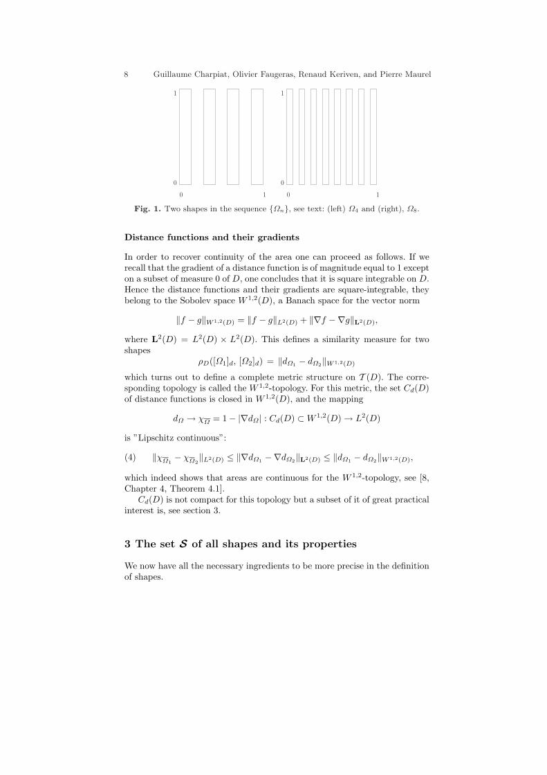
It would appear that we have reached an interesting stage and that theHausdorff distance is what we want to measure shape similarities. Unfortu-nately this is not so because the convergence of areas and perimeters is lostin the Hausdorff metric, as shown in the following example taken from [8,Chapter 4, Example 4.1 and Figure 4.3]

Consider the sequence Ωn of sets in the open square ]− 1, 2[2:

Ωn = (x, y) ∈ D :2k2n

≤ x ≤ 2k + 12n

, 0 ≤ k < n

Figure 1 shows the sets Ω4 and Ω8. This defines n vertical stripes of equalwidth 1/2n each distant of 1/2n. It is easy to verify that, for all n ≥ 1,m(Ωn) = 1/2 and |∂Ωn| = 2n + 1. Moreover, if S is the unit square [0, 1]2,for all x ∈ S, dΩn(x) ≤ 1/4n, hence dΩn → dS in C(D). The sequence Ωnconverges to S for the Hausdorff distance but since m(Ωn) = m(Ωn) = 1/2 91 = m(S), χΩn 9 χS in L2(D) and hence we do not have convergence for theρ2 topology. Note also that |∂Ωn| = 2n+ 1 9 |∂S| = 4.


0 1

0

1

0 1

0

1

Fig. 1. Two shapes in the sequence Ωn, see text: (left) Ω4 and (right), Ω8.

Distance functions and their gradients

In order to recover continuity of the area one can proceed as follows. If werecall that the gradient of a distance function is of magnitude equal to 1 excepton a subset of measure 0 of D, one concludes that it is square integrable on D.Hence the distance functions and their gradients are square-integrable, theybelong to the Sobolev space W 1,2(D), a Banach space for the vector norm

‖f − g‖W 1,2(D) = ‖f − g‖L2(D) + ‖∇f −∇g‖L2(D),

where L2(D) = L2(D) × L2(D). This defines a similarity measure for twoshapes

ρD([Ω1]d, [Ω2]d) = ‖dΩ1 − dΩ2‖W 1,2(D)

which turns out to define a complete metric structure on T (D). The corre-sponding topology is called the W 1,2-topology. For this metric, the set Cd(D)of distance functions is closed in W 1,2(D), and the mapping

dΩ → χΩ = 1− |∇dΩ | : Cd(D) ⊂W 1,2(D) → L2(D)

is ”Lipschitz continuous”:

(4) ‖χΩ1− χΩ2

‖L2(D) ≤ ‖∇dΩ1 −∇dΩ2‖L2(D) ≤ ‖dΩ1 − dΩ2‖W 1,2(D),

which indeed shows that areas are continuous for the W 1,2-topology, see [8,Chapter 4, Theorem 4.1].

Cd(D) is not compact for this topology but a subset of it of great practicalinterest is, see section 3.

3 The set S of all shapes and its properties

We now have all the necessary ingredients to be more precise in the definitionof shapes.


3.1 The set of all shapes

We restrict ourselves to sets of D with compact boundary and consider threedifferent sets of shapes. The first one is adapted from [8, Chapter 4, definition5.1]:

Definition 3 (Set DZ of sets of bounded curvature). The set DZ ofsets of bounded curvature contains those subsets Ω of D, Ω, Ω 6= ∅ suchthat ∇dΩ and ∇dΩ are in BV (D)2, where BV (D) is the set of functions ofbounded variations.

This is a large set (too large for our applications) which we use as a ”frameof reference”.DZ was introduced by Delfour and Zolesio [6, 7] and contains thesets F and C2 introduced below. For technical reasons related to compactnessproperties (see section 3.2) we consider the following subset of DZ.

Definition 4 (Set DZ0). The set DZ0 is the subset of DZ such that thereexists c0 > 0 such that for all Ω ∈ DZ0,

‖D2dΩ‖M1(D) ≤ c0 and ‖D2dΩ‖M1(D) ≤ c0

M1(D) is the set of bounded measures on D and ‖D2dΩ‖M1(D) is defined asfollows. Let Φ be a 2× 2 matrix of functions in C1(D), we have

‖D2dΩ‖M1(D) = supΦ∈C1(D)2×2, ‖Φ‖C≤1

∣∣∣∣∫

D

∇dΩ · divΦ dx∣∣∣∣ ,

where‖Φ‖C = sup

x∈D|Φ(x)|R2×2 ,

anddivΦ = [divΦ1, divΦ2],

where Φi, i = 1, 2 are the row vectors of the matrix Φ.

The set DZ0 has the following property (see [8, Chapter 4, Theorem 5.2])

Proposition 5. Any Ω ∈ DZ0 has a finite perimeter upper-bounded by 2c0.

We next introduce three related sets of shapes.

Definition 6 (Sets of smooth shapes). The set C0 (resp. C1, C2) of smoothshapes is the set of subsets of D whose boundary is non-empty and can be lo-cally represented as the epigraph of a C0 (resp. C1, C2) function. One furtherdistinguishes the sets Cci and Coi , i = 0, 1, 2 of subsets whose boundary is closedand open, respectively.

Note that this implies that the boundary is a simple regular curve (hencecompact) since otherwise it cannot be represented as the epigraph of a C1

(resp. C2) function in the vicinity of a multiple point. Also note that C2 ⊂C1 ⊂ DZ ([6, 7]).

The third set has been introduced by Federer [12].


Definition 7 (Set F of shapes of positive reach). A nonempty subset Ωof D is said to have positive reach if there exists h > 0 such that ΠΩ(x) is asingleton for every x ∈ Uh(Ω). The maximum h for which the property holdsis called the reach of Ω and is noted reach(Ω).

We will also be interested in the subsets, called h0-Federer’s sets and notedFh0 , h0 > 0, of F which contain all Federer’s sets Ω such that reach(Ω) ≥ h0.Note that Ci, i = 1, 2 ⊂ F but Ci 6⊂ Fh0 .

We are now ready to define the set of shapes of interest.

Definition 8 (Set of all shapes). The set, noted S, of all shapes (of interest)is the subset of C2 whose elements are also h0-Federer’s sets for a given andfixed h0 > 0.

S def= C2 ∩ Fh0

This set contains the two subsets Sc and So obtained by considering Cc2 andCo2 , respectively.

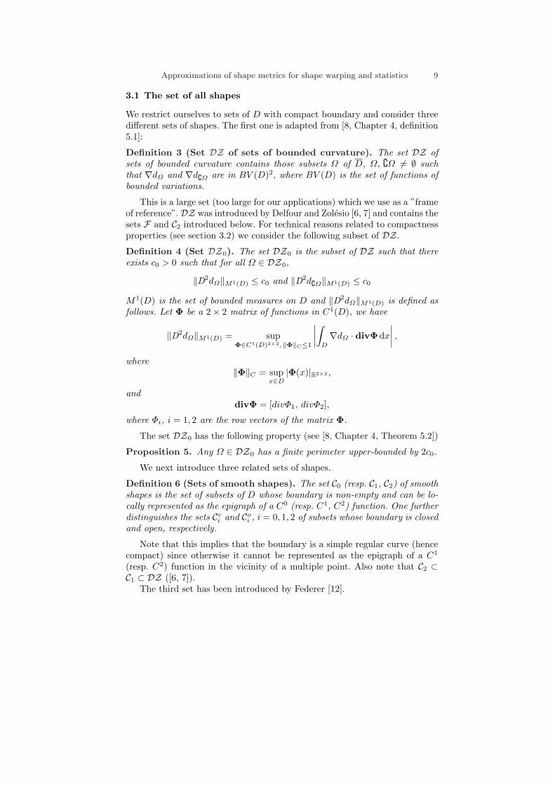
Note that S ⊂ DZ. Note also that the curvature of ∂Ω is well defined andupperbounded by 1/h0, noted κ0. Hence, c0 in definition 4 can be chosen insuch a way that S ⊂ DZ0.

Ω

∂Ω

Ω = ∂Ω

d > h0

d > h0

κ ≤ κ0 = 1h0

Fig. 2. Examples of admissible shapes: a simple, closed, regular curve (left); asimple, open regular curve (right). In both cases the curvature is upperbounded byκ0 and the pinch distance is larger than h0.

At this point, we can represent regular (i.e. C2) simple curves with andwithout boundaries that do not curve or pinch too much (in the sense of κ0

and h0, see figure 2.There are two reasons why we choose S as our frame of reference. The

first one is because our implementations work with discrete objects definedon an underlying discrete square grid of pixels. As a result we are not able


to describe details smaller than the distance between two pixels. This is ourunit and h0 is chosen to be smaller than or equal to it. The second reason isthat S is included in DZ0 which, as shown in section 3.2, is compact. Thiswill turn out to be important when minimizing shape functionals.

The question of the deformation of a shape by an element of a group oftransformations could be raised at this point. What we have in mind hereis the question of deciding whether a square and the same square rotatedby 45 degrees are the same shape. There is no real answer to this question,more precisely the answer depends on the application. Note that the group inquestion can be finite dimensional, as in the case of the Euclidean and affinegroups which are the most common in applications, or infinite dimensional.In this work we will, for the most part, not consider the action of groups oftransformations on shapes.

3.2 Compactness properties

Interestingly enough, the definition of the set DZ0 (definition 4) implies thatit is compact for all three topologies. This is the result of the following theoremwhose proof can be found in [8, Chapter 4, Theorems 8.2, 8.3].

Theorem 9. Let D be a nonempty bounded regular6 open subset of R2 andDZ the set defined in definition 3. The embedding

BC(D) = dΩ ∈ Cd(D) ∩ Ccd(D) : ∇dΩ , ∇dΩ ∈ BV (D)2 →W 1,2(D),

is compact.

This means that for any bounded sequence Ωn, ∅ 6= Ωn of elements ofDZ, i.e. for any sequence of DZ0, there exists a set Ω 6= ∅ of DZ such thatthere exists a subsequence Ωnk

such that

dΩnk→ dΩ and dΩnk

→ dΩ in W 1,2(D).

Since bΩ = dΩ − dΩ , we also have the convergence of bΩnkto bΩ , and since

the mapping bΩ → |bΩ | = d∂Ω is continuous in W 1,2(D) (see [8, Chapter5, Theorem 5.1 (iv)]), we also have the convergence of d∂Ωnk

to d∂Ω . Theconvergence for the ρ2 distance follows from equation (4):

χΩnk→ χΩ in L2(D),

and the convergence for the Hausdorff distance follows from theorem 2, takingsubsequences if necessary.

In other words, the set DZ0 is compact for the topologies defined by theρ2, Hausdorff and W 1,2 distances.

Note that, even though S ⊂ DZ0, this does not imply that it is compactfor either one of these three topologies. But it does imply that its closure Sfor each of these topologies is compact in the compact set DZ0.

6Regular means uniformly Lipschitzian in the sense of [8, Chapter 2, Definition5.1].


3.3 Comparison between the three topologies on S

The three topologies we have considered turn out to be closely related on S.This is summarized in the following

Theorem 10. The three topologies defined by the three distances ρ2, ρD andρH are equivalent on Sc. The two topologies defined by ρD and ρH are equiv-alent on So.

This means that, for example, given a set Ω of Sc, a sequence Ωn ofelements of Sc converging toward Ω ∈ Sc for any of the three distances ρ2, ρ(ρH) and ρD also converges toward the same Ω for the other two distances.

We refer to [3] for the proof of this theorem.An interesting and practically important consequence of this theorem is the

following. Consider the set S, included in DZ0, and its closure S for any oneof the three topologies of interest. S is a closed subset of the compact metricspace DZ0 and is therefore compact as well. Given a continuous functionf : S → R we consider its lower semi-continuous (l.s.c.) envelope f defined onS as follows

f(x) =

f(x) if x ∈ Slim infy→x, y∈S f(y)

The useful result for us is summarized in the

Proposition 11. f is l.s.c. in S and therefore has at least a minimum in S.

Proof. In a metric space E, a real function f is said to be l.s.c. if and only if

f(x) ≤ lim infy→x

f(y) ∀x ∈ E.

Therefore f is l.s.c. by construction. The existence of minimum of an l.s.c.function defined on a compact metric space is well-known (see e.g. [4, 11])and will be needed later to prove that some of our minimization problems arewell-posed.

4 Deforming shapes

The problem of continuously deforming a shape so that it turns into anotheris central to this paper. The reasons for this will become more clear in thesequel. Let us just mention here that it can be seen as an instance of thewarping problem: given two shapes Ω1 and Ω2, how do I deform Ω1 ontoΩ2? The applications in the field of medical image processing and analysisare immense (see for example [39, 38]). It can also be seen as an instance ofthe famous (in computer vision) correspondence problem: given two shapesΩ1 and Ω2, how do I find the corresponding point P2 in Ω2 of a given pointP1 in Ω1? Note that a solution of the warping problem provides a solution of


the correspondence problem if we can track the evolution of any given pointduring the smooth deformation of the first shape onto the second.

In order to make things more quantitative, we assume that we are given afunction E : C0×C0 → R+, called the Energy, which is continuous on S×S forone of the shape topologies of interest. This Energy can also be thought of asa measure of the dissimilarity between the two shapes. By smooth, we meanthat it is continuous with respect to this topology and that its derivatives arewell-defined in a sense we now make more precise.

We first need the notion of a normal deformation flow of a curve Γ in S.This is a smooth (i.e. C0) function β : [0, 1] → R (when Γ ∈ So, one furtherrequires that β(0) = β(1)). Let Γ : [0, 1] → R2 be a parameterization of Γ ,n(p) the unit normal at the point Γ (p) of Γ ; the normal deformation flow βassociates the point Γ (p) + β(p)n(p) to Γ (p). The resulting shape is notedΓ +β, where β = βn. There is no guarantee that Γ +β is still a shape in S ingeneral but if β is C0 and ε is small enough, Γ +β is in C0. Given two shapesΓ and Γ0, the corresponding Energy E(Γ, Γ0), and a normal deformation flowβ of Γ , the Energy E(Γ + εβ, Γ0)is now well-defined for ε sufficiently small.The derivative of E(Γ, Γ0) with respect to Γ in the direction of the flow β isthen defined, when it exists, as

(5) GΓ (E(Γ, Γ0),β) = limε→0

E(Γ + εβ, Γ0)− E(Γ, Γ0)ε

This kind of derivative is also known as a Gateaux semi-derivative. In our casethe function β → GΓ (E(Γ, Γ0),β) is linear and continuous (it is then calleda Gateaux derivative) and defines a continuous linear form on the vectorspace of normal deformation flows of Γ . This is a vector subspace of theHilbert space L2(Γ ) with the usual Hilbert product 〈β1, β2〉 = 1

|Γ |∫Γβ1 β2 =

1|Γ |

∫Γβ1(x)β2(x) dΓ (x), where |Γ | is the length of Γ . Given such an inner

product, we can apply Riesz’s representation theorem [32] to the Gateauxderivative GΓ (E(Γ, Γ0),β): There exists a deformation flow, noted∇E(Γ, Γ0),such that

GΓ (E(Γ, Γ0),β) = 〈∇E(Γ, Γ0), β〉.This flow is called the gradient of E(Γ, Γ0).

We now return to the initial problem of smoothly deforming a curve Γ1

onto a curve Γ2. We can state it as that of defining a family Γ (t), t ≥ 0 ofshapes such that Γ (0) = Γ1, Γ (T ) = Γ2 for some T > 0 and for each valueof t ≥ 0 the deformation flow of the current shape Γ (t) is equal to minusthe gradient ∇E(Γ, Γ2) defined previously. This is equivalent to solving thefollowing PDE

Γt = −∇E(Γ, Γ2)n(6)Γ (0) = Γ1

In this paper we do not address the question of the existence of solutions to(6).


Natural candidates for the Energy function E are the distances definedin section 2.2. The problem we are faced with is that none of these distancesare Gateaux differentiable. This is why the next section is devoted to thedefinition of smooth approximations of some of them.

5 How to approximate shape distances

The goal of this section is to provide smooth approximations of some of thesedistances, i.e. that admit Gateaux derivatives. We start with some notations.

5.1 Averages

Let Γ be a given curve in C1 and consider an integrable function f : Γ → Rn.We denote by 〈f〉Γ the average of f along the curve Γ :

(7) 〈f〉Γ =1|Γ |

∫

Γ

f =1|Γ |

∫

Γ

f(x) dΓ (x)

For real positive integrable functions f , and for any continuous strictlymonotonous (hence one to one) function ϕ from R+ or R+∗ to R+ we willalso need the ϕ-average of f along Γ which we define as

(8) 〈f〉ϕΓ = ϕ−1

(1|Γ |

∫

Γ

ϕ f)

= ϕ−1

(1|Γ |

∫

Γ

ϕ(f(x)) dΓ (x))

Note that ϕ−1 is also strictly monotonous and continous from R+ to R+ orR+∗. Also note that the unit of the ϕ-average of f is the same as that of f ,thanks to the normalization by |Γ |.

The discrete version of the ϕ-average is also useful: let ai, i = 1, . . . , n ben positive numbers, we note

(9) 〈a1, · · · , an〉ϕ = ϕ−1

(1n

n∑

i=1

ϕ(ai)

),

their ϕ-average.

5.2 Approximations of the Hausdorff distance

We now build a series of smooth approximations of the Hausdorff distanceρH(Γ, Γ ′) of two shapes Γ and Γ ′. According to (3) we have to consider thefunctions dΓ ′ : Γ → R+ and dΓ : Γ ′ → R+. Let us focus on the second one.Since dΓ is Lipschitz continuous on the bounded hold-all set D it is certainlyintegrable on the compact set Γ ′ and we have [32, Chapter 3, problem 4]


(10) limβ→+∞

(1|Γ ′|

∫

Γ ′dβΓ (x′) dΓ ′(x′)

) 1β

= supx′∈Γ ′

dΓ (x′).

Moreover, the function R+ → R+ defined by β →(

1|Γ ′|

∫Γ ′ d

βΓ (x′) dΓ ′(x′)

) 1β

is monotonously increasing [32, Chapter 3, problem 5].Similar properties hold for dΓ ′ .If we note pβ the function R+ → R+ defined by pβ(x) = xβ we can rewrite

(10)lim

β→+∞〈dΓ 〉pβ

Γ ′ = supx′∈Γ ′

dΓ (x′).

〈dΓ 〉pβ

Γ ′ is therefore a monotonically increasing approximation of supx′∈Γ ′ dΓ (x′).We go one step further and approximate dΓ ′(x).

Consider a continuous strictly monotonously decreasing function ϕ : R+ →R+∗. Because ϕ is strictly monotonously decreasing

supx′∈Γ ′

ϕ(d(x, x′)) = ϕ( infx′∈Γ ′

d(x, x′)) = ϕ(dΓ ′(x)),

and moreover

limα→+∞

(1|Γ ′|

∫

Γ ′ϕα(d(x, x′)) dΓ ′(x′)

) 1α

= supx′∈Γ ′

ϕ(d(x, x′)).

Because ϕ is continuous and strictly monotonously decreasing, it is one to oneand ϕ−1 is strictly monotonously decreasing and continuous. Therefore

dΓ ′(x) = limα→+∞

ϕ−1

((1|Γ ′|

∫

Γ ′ϕα(d(x, x′)) dΓ ′(x′)

) 1α

)

We can simplify this equation by introducing the function ϕα = pα ϕ:

(11) dΓ ′(x) = limα→+∞

〈d(x, ·)〉ϕα

Γ ′

Any α > 0 provides us with an approximation, noted dΓ ′ , of dΓ ′ :

(12) dΓ ′(x) = 〈d(x, ·)〉ϕα

Γ ′

We have a similar expression for dΓ .

Note that because(

1|Γ ′|

∫Γ ′ ϕ

α(d(x, x′)) dΓ ′(x′)) 1

α

increases with α to-

ward its limit supx′ ϕ(d(x, x′)) = ϕ(dΓ ′(x)), ϕ−1

((1|Γ ′|

∫Γ ′ ϕ

α(d(x, x′)) dΓ ′(x′)) 1

α

)

decreases with α toward its limit dΓ ′(x).Examples of functions ϕ are


ϕ1(z) =1

z + εε > 0, z ≥ 0

ϕ2(z) = µ exp(−λz) µ, λ > 0, z ≥ 0

ϕ3(z) =1√

2πσ2exp(− z2

2σ2) σ > 0, z ≥ 0

Putting all this together we have the following result

supx∈Γ

dΓ ′(x) = limα, β→+∞

〈〈d(·, ·)〉ϕα

Γ ′ 〉pβ

Γ

supx∈Γ ′

dΓ (x) = limα, β→+∞

〈〈d(·, ·)〉ϕα

Γ 〉pβ

Γ ′

Any positive values of α and β yield approximations of supx∈Γ dΓ ′(x) andsupx∈Γ ′ dΓ (x).

The last point to address is the max that appears in the definition of theHausdorff distance. We use (9), choose ϕ = pγ and note that, for a1 and a2

positive,lim

γ→+∞〈a1, a2〉pγ = max(a1, a2).

This yields the following expression for the Hausdorff distance between twoshapes Γ and Γ ′

ρH(Γ, Γ ′) = limα, β, γ→+∞

⟨〈〈d(·, ·)〉ϕα

Γ ′ 〉pβ

Γ , 〈〈d(·, ·)〉ϕα

Γ 〉pβ

Γ ′⟩pγ

This equation is symmetric and yields approximations ρH of the Hausdorffdistance for all positive values of α, β and γ:

(13) ρH(Γ, Γ ′) =⟨〈〈d(·, ·)〉ϕα

Γ ′ 〉pβ

Γ , 〈〈d(·, ·)〉ϕα

Γ 〉pβ

Γ ′⟩pγ

This approximation is ”nice” in several ways, the first one being the obviousone, stated in the following

Proposition 12. For each triplet (α, β, γ) in (R+∗)3 the function ρH : S ×S → R+ defined by equation (13) is continuous for the Hausdorff topology.

The complete proof of this proposition can be found in [3].

5.3 Computing the gradient of the approximation to theHausdorff distance

We now proceed with showing that the approximation ρH(Γ, Γ0) of the Haus-dorff distance ρH(Γ, Γ0) is differentiable with respect to Γ and compute itsgradient ∇ ρH(Γ, Γ0), in the sense of section 4. To simplify notations werewrite (13) as

(14) ρH(Γ, Γ0) =⟨⟨〈d(·, ·)〉ϕΓ0

⟩ψΓ, 〈〈d(·, ·)〉ϕΓ 〉

ψ

Γ0

⟩θ,

and state the result, the reader interested in the proof being referred to [3].


Proposition 13. The gradient of ρH(Γ, Γ0) at any point y of Γ is given by

(15) ∇ρH(Γ, Γ0)(y) =1

θ′(ρH(Γ, Γ0))(α(y)κ(y) + β(y)) ,

where κ(y) is the curvature of Γ at y, the functions α(y) and β(y) are givenby

(16) α(y) = ν

∫

Γ0

ψ′

ϕ′(〈d(x, ·)〉ϕΓ ) [ ϕ 〈d(x, ·)〉ϕΓ − ϕ d(x, y) ] dΓ0(x)

+ |Γ0|η[ψ

(⟨〈d(·, ·)〉ϕΓ0

⟩ψΓ

)− ψ

(〈d(·, y)〉ϕΓ0

) ],

(17)

β(y) =∫

Γ0

ϕ′d(x, y)[νψ′

ϕ′(〈d(x, ·)〉ϕΓ ) + η

ψ′

ϕ′(〈d(·, y)〉ϕΓ0

)] y − x

d(x, y)·n(y) dΓ0(x),

where ν =1

|Γ | |Γ0|θ′

ψ′

(〈〈d(·, ·)〉ϕΓ 〉

ψ

Γ0

)and η =

1|Γ | |Γ0|

θ′

ψ′

(⟨〈d(·, ·)〉ϕΓ0

⟩ψΓ

).

Note that the function β(y) is well-defined even if y belongs to Γ0 sincethe term y−x

d(x,y) is of unit norm.The first two terms of the gradient show explicitely that minimizing the

energy implies homogenizing the distance to Γ0 along the curve Γ , that is tosay the algorithm will take care in priority of the points of Γ which are thefurthest from Γ0.

Also note that the expression of the gradient in proposition 13 still standswhen Γ and Γ0 are two surfaces (embedded in R3), if κ stands for the meancurvature.

5.4 Other alternatives related to the Hausdorff distance

There exist several alternatives to the method presented in the previous sec-tions if we use ρ (equation (2)) rather than ρH (equation (3)) to define theHausdorff distance. A first alternative is to use the following approximation

ρ(Γ, Γ ′) = 〈|dΓ − dΓ ′ |〉pα

D ,

where the bracket 〈 f(.) 〉ϕD is defined the obvious way for any integrable func-tion f : D → R+

〈 f 〉ϕD = ϕ−1

(1

m(D)

∫

D

ϕ(f(x)) dx),

and which can be minimized, as in section 5.6, with respect to dΓ . A secondalternative is to approximate ρ using:

(18) ρ(Γ, Γ ′) = 〈|〈d(·, ·)〉ϕβ

Γ ′ − 〈d(·, ·)〉ϕβ

Γ |〉pα

D ,

and to compute is derivative with respect to Γ as we did in the previoussection for ρH .


5.5 Approximations to the W 1,2 norm and computation of theirgradient

The previous results can be used to construct approximations ρD to the dis-tance ρD defined in section 2.2:

(19) ρD(Γ1, Γ2) = ‖dΓ1 − dΓ2‖W 1,2(D),

where dΓi, i = 1, 2 is obtained from (12).

This approximation is also ”nice” in the usual way and we have the

Proposition 14. For each α in R+∗ the function ρD : S × S → R+ iscontinuous for the W 1,2 topology.

Its proof is left to the reader.The gradient ∇ρD(Γ, Γ0), of our approximation ρD(Γ, Γ0) of the distance

ρD(Γ, Γ0) given by (19) in the sense of section 4 can be computed. The inter-ested reader is referred to the appendix of [3]. We simply state the result inthe

Proposition 15. The gradient of ρD(Γ, Γ0) at any point y of Γ is given by

(20) ∇ρD(Γ, Γ0)(y) =∫

D

[B(x, y)

(C1(x)− ϕ”

ϕ′(dΓ (x))

(C2(x) · ∇dΓ (x)

))+ C2(x) · ∇B(x, y)

]dx,

where

B(x, y) = κ(y) (〈ϕ d(x, ·)〉Γ − ϕ d(x, y)) + ϕ′(d(x, y))y − x

d(x, y)· n(y),

κ(y) is the curvature of Γ at y,

C1(x) =1

|Γ | ϕ′(dΓ (x))‖dΓ − dΓ0‖−1

L2(D)

(dΓ (x)− dΓ0)(x)

),

and

C2(x) =1

|Γ | ϕ′(dΓ (x))‖∇(dΓ − dΓ0)‖−1

L2(D) ∇(dΓ − dΓ0)(x),

5.6 Direct minimization of the W 1,2 norm

An alternative to the method presented in the previous section is to evolve notthe curve Γ but its distance function dΓ . Minimizing ρD(Γ, Γ0) with respectto dΓ implies computing the corresponding Euler-Lagrange equation EL. Thereader will verify that the result is


(21) EL =dΓ − dΓ0

‖dΓ − dΓ0‖L2(D)− div

( ∇ (dΓ − dΓ0)‖∇(dΓ − dΓ0)‖L2(D))

)

To simplify notations we now use d instead of dΓ . The problem of warping Γ1

onto Γ0 is then transformed into the problem of solving the following PDE

dt = −ELd(0, ·) = dΓ1(·).

The problem that this PDE does not preserve the fact that d is a distancefunction is alleviated by ”reprojecting” at each iteration the current function donto the set of distance functions by running a few iterations of the ”standard”restoration PDE [37]

dt = (1− |∇d|)sign(d0)d(0, ·) = d0

6 Application to curve evolutions: Hausdorff warping

In this section we show a number of examples of solving equation (6) with thegradient given by equation (15). Our hope is that, starting from Γ1, we willfollow the gradient (15) and smoothly converge to the curve Γ2 where the min-imum of ρH is attained. Let us examine more closely these assumptions. First,it is clear from the expression (13) of ρH that in general ρH(Γ, Γ ) 6= 0, whichimplies in particular that ρH , unlike ρH , is not a distance. But worse things canhappen: there may exist a shape Γ ′ such that ρH(Γ, Γ ′) is strictly less thanρH(Γ, Γ ) or there may not exist any minima for the function Γ → ρH(Γ, Γ ′)!This sounds like the end of our attempt to warp a shape onto another usingan approximation of the Hausdorff distance. But things turn out not to be sobad. First, the existence of a minimum is guaranteed by proposition 12 whichsays that ρH is continuous on S for the Hausdorff topology, theorem 9 whichsays that DZ0 is compact for this topology, and proposition 11 which tells usthat the l.s.c. extension of ρH(·, Γ ) has a minimum in the closure S of S inDZ0.

We show in the next section that phenomena like the one described aboveare for all practical matters ”invisible” since confined to an arbitrarily smallHausdorff ball centered at Γ .

6.1 Quality of the approximation ρH of ρH

In this section we make more precise the idea that ρH can be made arbitrarilyclose to ρH . Because of the form of (14) we seek upper and lower bounds ofsuch quantities as 〈f〉ψΓ , where f is a continuous real function defined on Γ .We note fmin the minimum value of f on Γ .


The expression

〈f〉ψΓ = ψ−1

(1|Γ |

∫

Γ

ψ f),

yields, if ψ is strictly increasing, and if f > fmoy on a set F of the curve Γ , oflength |F | (6 |Γ |):

〈f〉ψΓ = ψ−1

(1|Γ |

∫

F

ψ f +1|Γ |

∫

Γ\Fψ f

)

> ψ−1

( |F ||Γ |ψ fmoy +

|Γ | − |F ||Γ | ψ fmin

)

> ψ−1

( |F ||Γ |ψ fmoy

)

To analyse this lower bound, we introduce the following notation. Given∆, α > 0, we note P(∆,α) the following property:

P(∆,α) : ∀x ∈ R+, ∆ψ(x) > ψ(αx)

This property is satisfied for example for ψ(x) = xβ , β ≥ 0. The best pairs(∆,α) verifying P are such that ∆ = αβ . In the sequel, we consider a functionψ which satisfies:

∀∆ ∈]0; 1[, ∃α ∈]0; 1[,P(∆,α),

and, conversely,∀α ∈]0; 1[, ∃∆ ∈]0; 1[,P(∆,α)

Then for ∆ψ = |F ||Γ | and a corresponding αψ such that P(∆ψ, αψ) is satis-

fied, we have〈f〉ψΓ > ψ−1 (∆ψ ψ(fmoy)) > αψ fmoy

and deduce from that kind of considerations the following property (seecomplete proof in [3]):

Proposition 16. ρH(Γ, Γ ′) has the following upper and lower bounds(22)

αθαψ(ρH(Γ, Γ ′)−∆ψ|Γ |+ |Γ ′|

2) ≤ ρH(Γ, Γ ′) ≤ αϕ(ρH(Γ, Γ ′)+∆ϕ

|Γ |+ |Γ ′|2

).

where αθ, αψ and αϕ are constants depending on functions θ, ψ and ϕ andcan be set arbitrarily close to 1 with a good choice of these functions, while∆ψ and ∆ϕ are positive constants depending on functions ψ and ϕ and can beset arbitrarily close to 0 in the same time. Consequently, the approximationρH(Γ, Γ ′) of ρH(Γ, Γ ′) can be arbitrarily accurate.

We can now characterize the shapes Γ and Γ ′ such that

(23) ρH(Γ, Γ ′) < ρH(Γ, Γ ).


Theorem 17. The condition (23) is equivalent (see [3] again) to

ρH(Γ, Γ ′) < 4c0∆,

where the constant c0 is defined in definition 4 and theorem 5, and ∆ =max(∆ψ,∆ϕ).

From this we conclude that, since ∆ can be made arbitrarily close to 0,and the length of shapes is bounded, strange phenomena such as a shape Γ ′

closer to a shape Γ than Γ itself (in the sense of ρH) cannot occur or ratherwill be ”invisible” to our algorithms.

6.2 Applying the theory

In practice, the Energy that we minimize is not ρH but in fact a ”regular-ized” version obtained by combining ρH with a term EL which depends uponthe lengths of the two curves. A natural candidate for EL is max(|Γ |, |Γ ′|)since it acts only if |Γ | becomes larger than |Γ ′|, thereby avoiding undesirableoscillations. To obtain smoothness, we approximate the max with a Ψ -average:

(24) EL(|Γ |, |Γ ′|) = 〈|Γ |, |Γ ′|〉Ψ

We know that the function Γ → |Γ | is in general l.s.c.. It is in fact continuouson S (see the proof of proposition 12) and takes its values in the interval[0, 2c0], hence

Proposition 18. The function S → R+ given by Γ → EL(Γ, Γ ′) is contin-uous for the Hausdorff topology.

Proof. It is clear since EL is a combination of continuous functions.

We combine EL with ρH the expected way, i.e. by computing their Ψaverage so that the final energy is

(25) E(Γ, Γ ′) = 〈ρH(Γ, Γ ′), EL(|Γ |, |Γ ′|)〉Ψ

The function E : S × S → R+ is continuous for the Hausdorff metric becauseof propositions 12 and 18 and therefore

Proposition 19. The function Γ → E(Γ, Γ ′) defined on the set of shapes Shas at least a minimum in the closure S of S in L0.

Proof. This is a direct application of proposition 11 applied to the functionE.

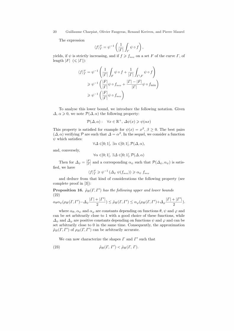
We call the resulting warping technique the Hausdorff warping. An exam-ple, the Hausdorff warping of two hand silhouettes, is shown in figure 3.


Fig. 3. The result of the Hausdorff warping of two hand silhouettes. The two handsare represented in continuous line while the intermediate shapes are represented indotted lines.

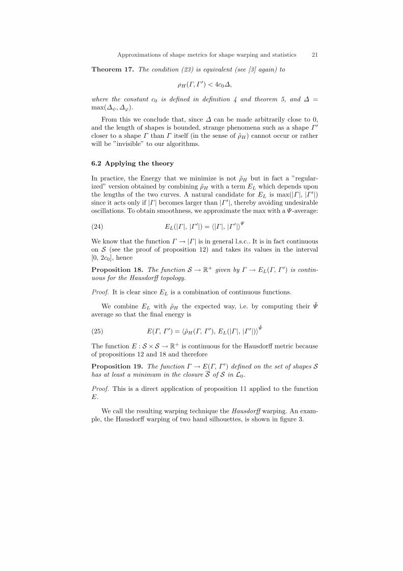
Fig. 4. Hausdorff warping a fish onto another.

We have borrowed the example in figure 4 from the database of fish sil-houettes (www.ee.surrey.ac.uk/Research/ VSSP/imagedb/demo.html) col-lected by the researchers of the University of Surrey at the center for Vision,Speech and Signal Processing (www.ee.surrey.ac.uk/Research/VSSP). Thisdatabase contains 1100 silhouettes. A few steps of the result of Hausdorffwarping one of these silhouettes onto another are shown in figure 4.

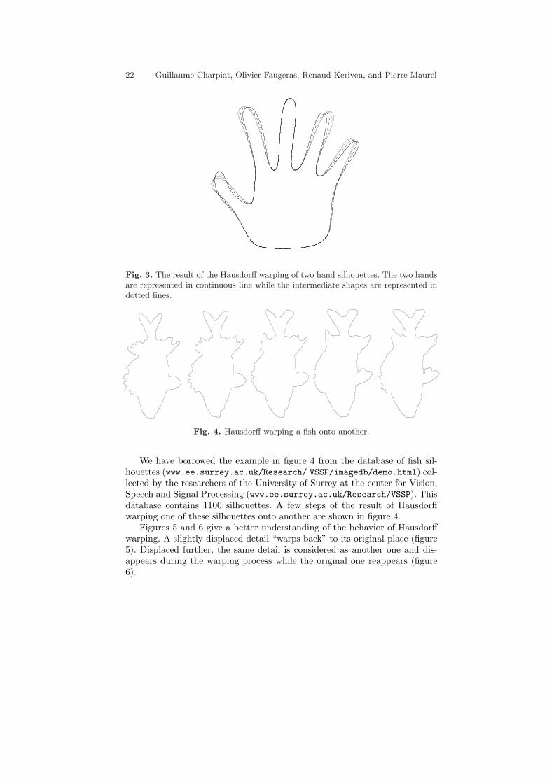
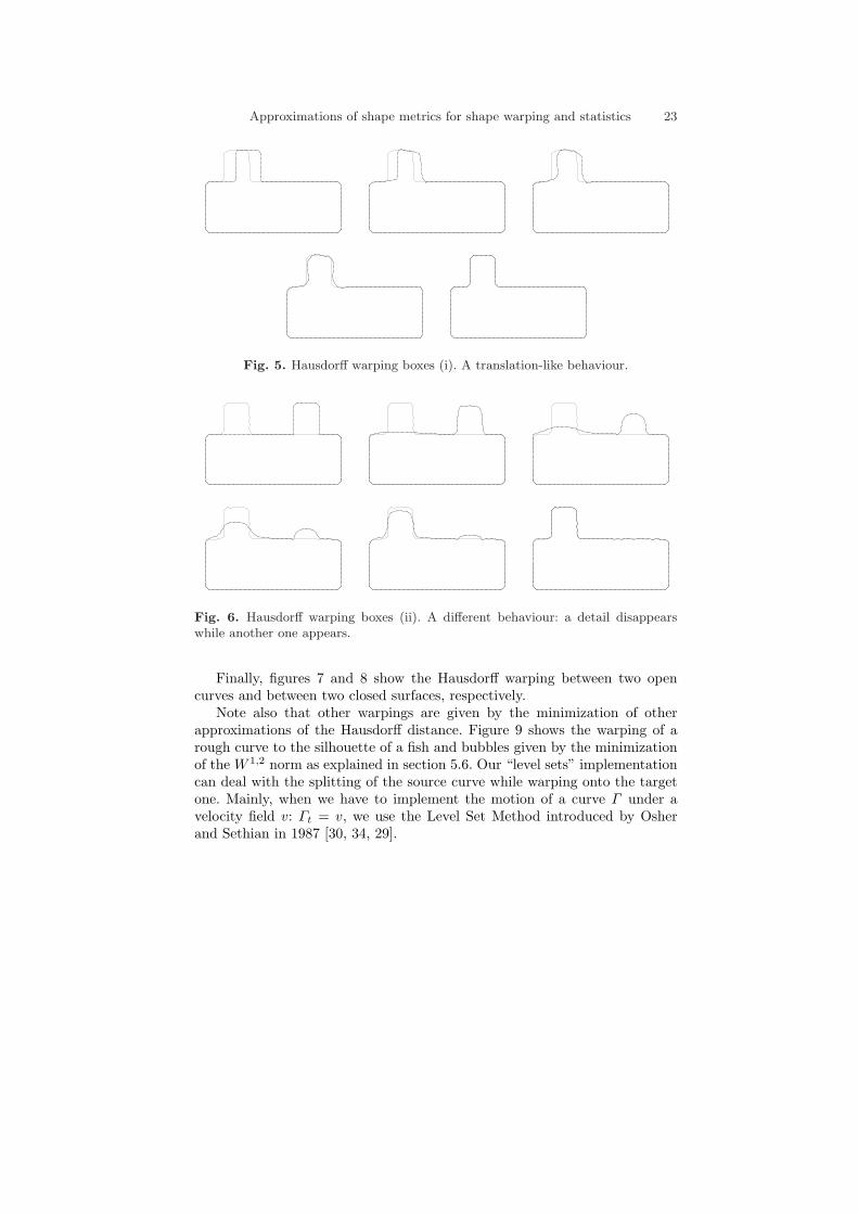
Figures 5 and 6 give a better understanding of the behavior of Hausdorffwarping. A slightly displaced detail “warps back” to its original place (figure5). Displaced further, the same detail is considered as another one and dis-appears during the warping process while the original one reappears (figure6).


Fig. 5. Hausdorff warping boxes (i). A translation-like behaviour.

Fig. 6. Hausdorff warping boxes (ii). A different behaviour: a detail disappearswhile another one appears.

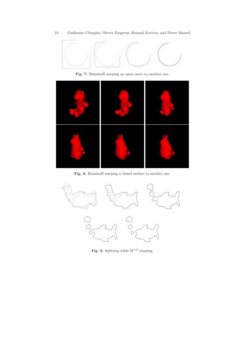
Finally, figures 7 and 8 show the Hausdorff warping between two opencurves and between two closed surfaces, respectively.

Note also that other warpings are given by the minimization of otherapproximations of the Hausdorff distance. Figure 9 shows the warping of arough curve to the silhouette of a fish and bubbles given by the minimizationof the W 1,2 norm as explained in section 5.6. Our “level sets” implementationcan deal with the splitting of the source curve while warping onto the targetone. Mainly, when we have to implement the motion of a curve Γ under avelocity field v: Γt = v, we use the Level Set Method introduced by Osherand Sethian in 1987 [30, 34, 29].


Fig. 7. Hausdorff warping an open curve to another one.

Fig. 8. Hausdorff warping a closed surface to another one.

Fig. 9. Splitting while W 1,2 warping.


7 Application to the computation of the empirical meanand covariance of a set of shape examples

We have now developed the tools for defining several concepts relevant to atheory of stochastic shapes as well as providing the means for their effectivecomputation. They are based on the use of the function E defined by (25).

7.1 Empirical mean

The first one is that of the mean of a set of shapes. Inspired by the work ofFrechet [13, 14], Karcher [20], Kendall [23], and Pennec [31], we provide thefollowing (classical)

Definition 20. Given Γ1, · · · , ΓN , N shapes, we define their empirical meanas any shape Γ that achieves a local minimimum of the function µ : S → R+

defined by

Γ → µ(Γ, Γ1, · · · , ΓN ) =1N

∑

i=1,··· ,NE2(Γ, Γi)

Note that there may exist several means. We know from proposition 19that there exists at least one. An algorithm for computing approximations toan empirical mean of N shapes readily follows from the previous section: startfrom an initial shape Γ0 and solve the PDE

Γt = −∇µ(Γ, Γ1, · · · , ΓN )n(26)Γ (0, .) = Γ0(.)

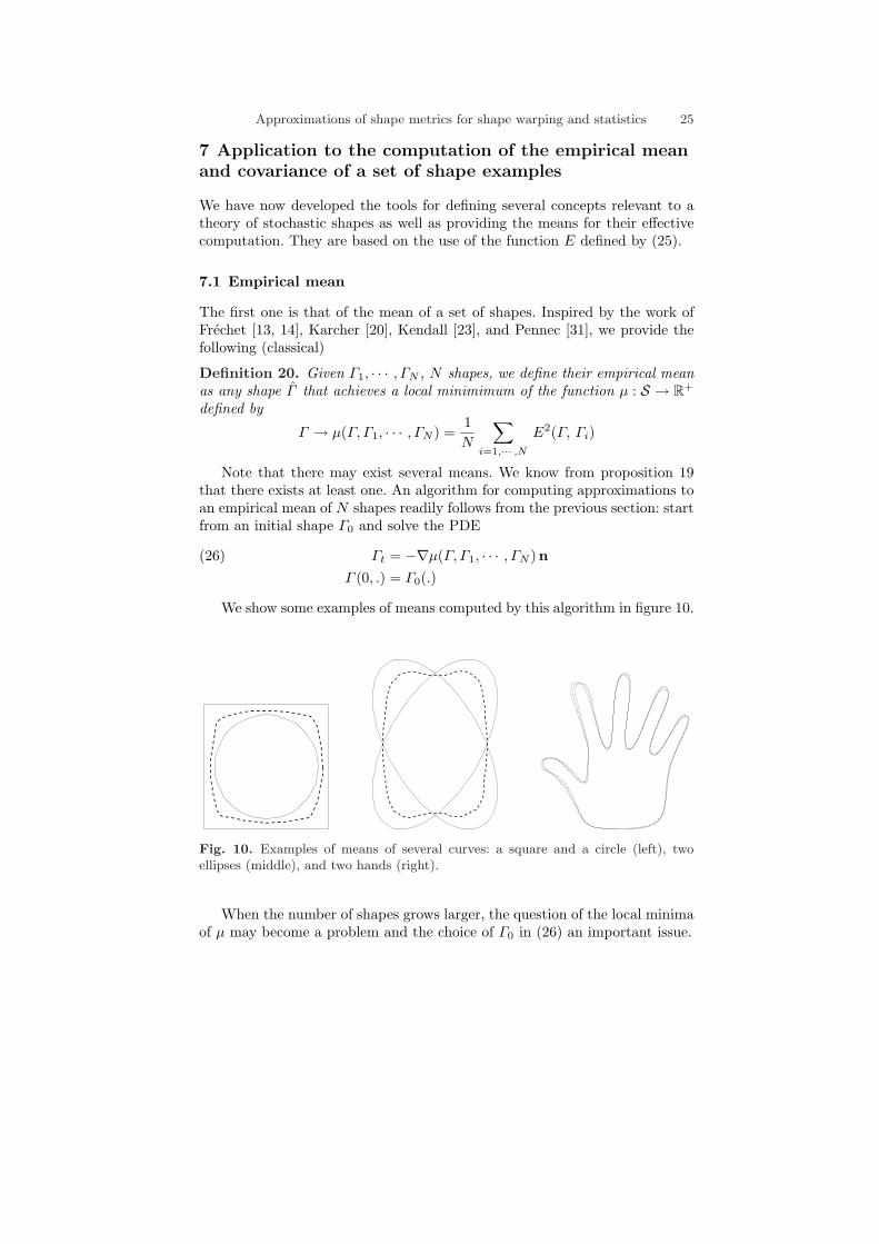
We show some examples of means computed by this algorithm in figure 10.

Fig. 10. Examples of means of several curves: a square and a circle (left), twoellipses (middle), and two hands (right).

When the number of shapes grows larger, the question of the local minimaof µ may become a problem and the choice of Γ0 in (26) an important issue.


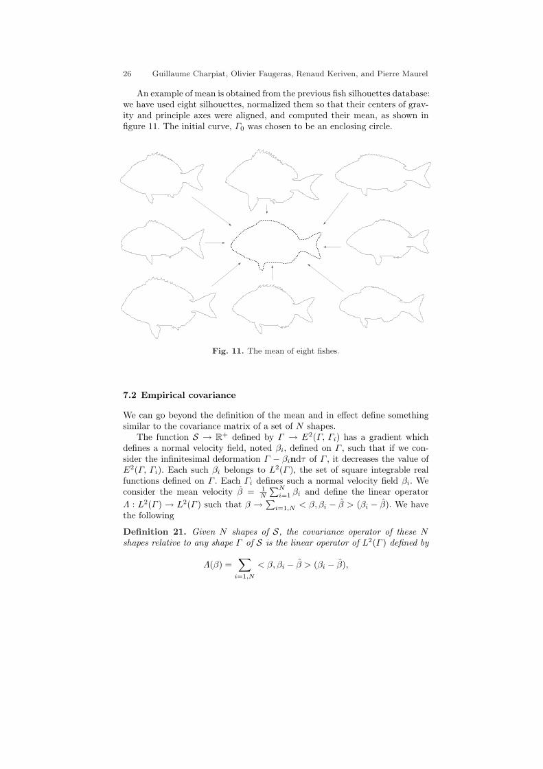
An example of mean is obtained from the previous fish silhouettes database:we have used eight silhouettes, normalized them so that their centers of grav-ity and principle axes were aligned, and computed their mean, as shown infigure 11. The initial curve, Γ0 was chosen to be an enclosing circle.

Fig. 11. The mean of eight fishes.

7.2 Empirical covariance

We can go beyond the definition of the mean and in effect define somethingsimilar to the covariance matrix of a set of N shapes.

The function S → R+ defined by Γ → E2(Γ, Γi) has a gradient whichdefines a normal velocity field, noted βi, defined on Γ , such that if we con-sider the infinitesimal deformation Γ − βindτ of Γ , it decreases the value ofE2(Γ, Γi). Each such βi belongs to L2(Γ ), the set of square integrable realfunctions defined on Γ . Each Γi defines such a normal velocity field βi. Weconsider the mean velocity β = 1

N

∑Ni=1 βi and define the linear operator

Λ : L2(Γ ) → L2(Γ ) such that β → ∑i=1,N < β, βi − β > (βi − β). We have

the following

Definition 21. Given N shapes of S, the covariance operator of these Nshapes relative to any shape Γ of S is the linear operator of L2(Γ ) defined by

Λ(β) =∑

i=1,N

< β, βi − β > (βi − β),


where the βi are defined as above, relatively to the shape Γ .

This operator has some interesting properties which we study next.

Proposition 22. The operator Λ is a continuous mapping of L2(Γ ) intoL2(Γ ).

Proof. We have ‖∑i=1,N < β, βi − β > (βi − β)‖2 ≤

∑i=1,N | < β, βi − β >

|‖βi−β‖2 and, because of Schwarz inequality, | < β, βi−β > | ≤ ‖β‖2‖βi−β‖2.This implies that ‖∑

i=1,N < β, βi − β > (βi − β)‖2 ≤ K‖β‖2 with K =∑i=1,N ‖βi − β‖22.

Λ is in effect a mapping from L2(Γ ) into its Hilbert subspace A(Γ ) gener-ated by the N functions βi − β. Note that if Γ is one of the empirical meansof the shapes Γi, by definition we have β = 0.

This operator acts on what can be thought of as the tangent space to themanifold of all shapes at the point Γ . We then have the

Proposition 23. The covariance operator is symmetric positive definite.

Proof. This follows from the fact that < Λ(β), β >=< β,Λ(β) >=∑i=1,N <

β, βi − β >2.

It is also instructive to look at the eigenvalues and eigenvectors of Λ. Forthis purpose we introduce the N ×N matrix Λ defined by Λij =< βi− β, βj−β >. We have the

Proposition 24. The N × N matrix Λ is symmetric semi positive definite.Let p ≤ N be its rank, σ2

1 ≥ σ22 ≥ · · · ≥ σ2

p > 0 its positive eigenvalues,u1, · · · ,uN the corresponding eigenvectors. They satisfy

ui · uj = δij i, j = 1, · · · , NΛui = σ2

i ui i = 1, · · · , pΛui = 0 p+ 1 ≤ i ≤ N

Proof. The matrix Λ is clearly symmetric. Let now α = [α1, · · · , αN ]T be avector of RN , αT Λα = ‖β‖22, where β =

∑Ni=1 αi(βi − β). The remaining of

the proposition is simply a statement of the existence of an orthonormal basisof eigenvectors for a symmetric matrix of RN .

The N -dimensional vectors uj , j = 1, · · · , p and the p eigenvalues σ2k, k =

1, · · · , p define p modes of variation of the shape Γ . These modes of variationare normal deformation flows which are defined as follows. We note uij , i, j =1, · · · , N the ith coordinate of the vector uj and vj the element of A(Γ )defined by


(27) vj =1σj

N∑

i=1

uij(βi − β)

In the case Γ = Γ , β = 0. We have the proposition

Proposition 25. The functions vj, j = 1, · · · , p are an orthonormal set ofeigenvectors of the operator Λ and form a basis of A(Γ ).

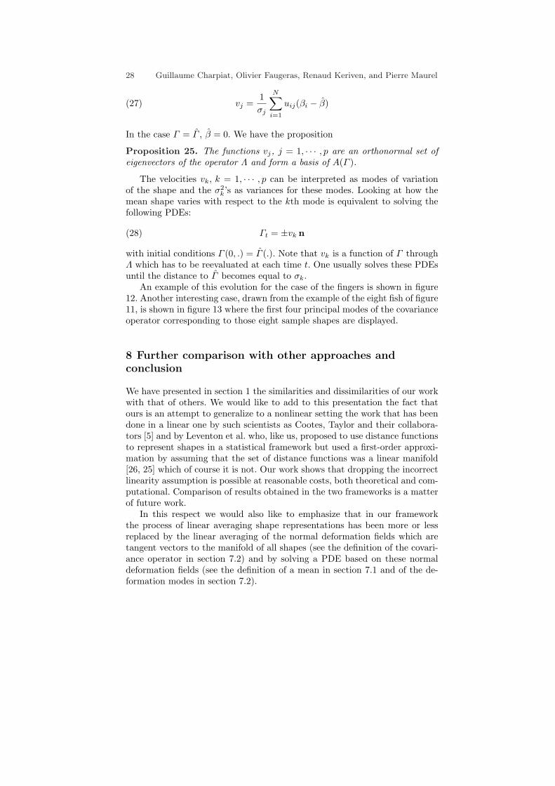
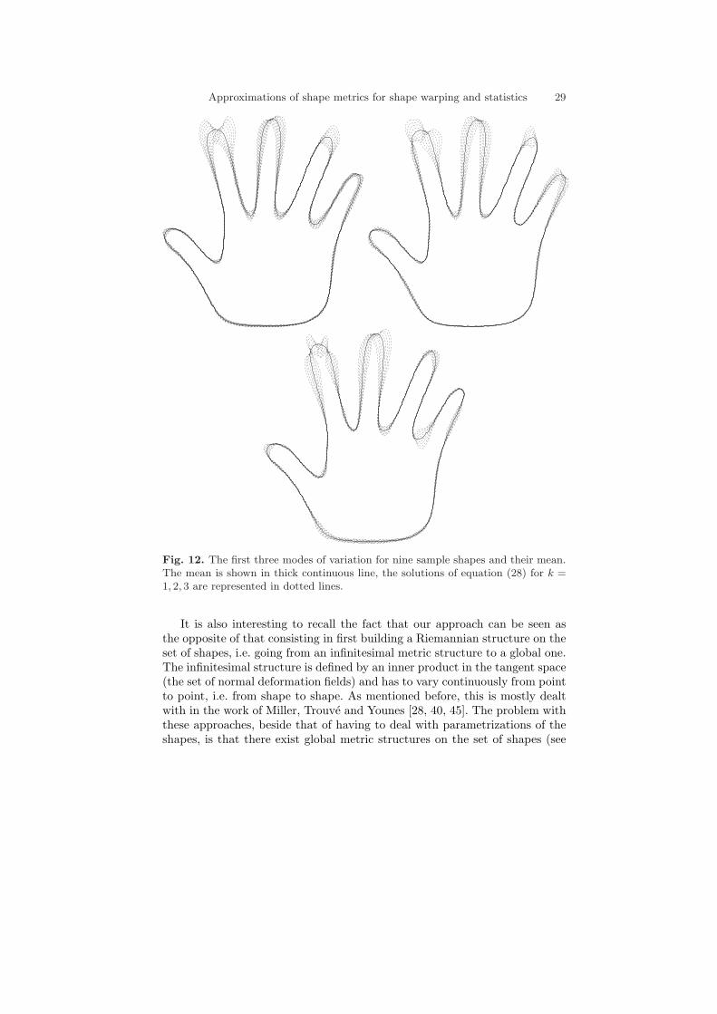
The velocities vk, k = 1, · · · , p can be interpreted as modes of variationof the shape and the σ2

k’s as variances for these modes. Looking at how themean shape varies with respect to the kth mode is equivalent to solving thefollowing PDEs:

(28) Γt = ±vk n

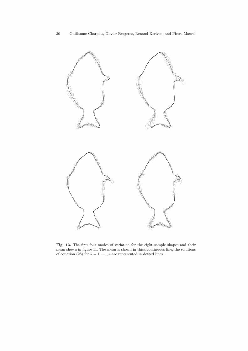
with initial conditions Γ (0, .) = Γ (.). Note that vk is a function of Γ throughΛ which has to be reevaluated at each time t. One usually solves these PDEsuntil the distance to Γ becomes equal to σk.

An example of this evolution for the case of the fingers is shown in figure12. Another interesting case, drawn from the example of the eight fish of figure11, is shown in figure 13 where the first four principal modes of the covarianceoperator corresponding to those eight sample shapes are displayed.

8 Further comparison with other approaches andconclusion

We have presented in section 1 the similarities and dissimilarities of our workwith that of others. We would like to add to this presentation the fact thatours is an attempt to generalize to a nonlinear setting the work that has beendone in a linear one by such scientists as Cootes, Taylor and their collabora-tors [5] and by Leventon et al. who, like us, proposed to use distance functionsto represent shapes in a statistical framework but used a first-order approxi-mation by assuming that the set of distance functions was a linear manifold[26, 25] which of course it is not. Our work shows that dropping the incorrectlinearity assumption is possible at reasonable costs, both theoretical and com-putational. Comparison of results obtained in the two frameworks is a matterof future work.

In this respect we would also like to emphasize that in our frameworkthe process of linear averaging shape representations has been more or lessreplaced by the linear averaging of the normal deformation fields which aretangent vectors to the manifold of all shapes (see the definition of the covari-ance operator in section 7.2) and by solving a PDE based on these normaldeformation fields (see the definition of a mean in section 7.1 and of the de-formation modes in section 7.2).


Fig. 12. The first three modes of variation for nine sample shapes and their mean.The mean is shown in thick continuous line, the solutions of equation (28) for k =1, 2, 3 are represented in dotted lines.

It is also interesting to recall the fact that our approach can be seen asthe opposite of that consisting in first building a Riemannian structure on theset of shapes, i.e. going from an infinitesimal metric structure to a global one.The infinitesimal structure is defined by an inner product in the tangent space(the set of normal deformation fields) and has to vary continuously from pointto point, i.e. from shape to shape. As mentioned before, this is mostly dealtwith in the work of Miller, Trouve and Younes [28, 40, 45]. The problem withthese approaches, beside that of having to deal with parametrizations of theshapes, is that there exist global metric structures on the set of shapes (see


Fig. 13. The first four modes of variation for the eight sample shapes and theirmean shown in figure 11. The mean is shown in thick continuous line, the solutionsof equation (28) for k = 1, · · · , 4 are represented in dotted lines.


section 2.2) which are useful and relevant to the problem of the comparisonof shapes but that do not arise from an infinitesimal structure.

Our approach can be seen as taking the problem from exactly the oppositeviewpoint from the previous one: we start with a global metric on the set ofshapes (ρH or the W 1,2 metric) and build smooth functions (in effect smoothapproximations of these metrics) that we use as dissimilarity measure or en-ergy functions and minimize using techniques of the calculus of variation bycomputing their gradient and performing infinitesimal gradient descent. Wehave seen that in order to compute the gradients we need to define an inner-product of normal deformation flowss and the choice of this inner-productmay influence the way our algorithms evolve from one shape to another. Thislast point is related to but different from the choice of the Riemaniann metricin the first approach. Its investigation is also a topic of future work.

Another advantage of our viewpoint is that it apparently extends gra-ciously to higher dimensions thanks to the fact that we do not rely onparametrizations of the shapes and work intrinsically with their distance func-tions (or approximations thereof). This is clearly also worth pursuing in futurework.

References

1. Bookstein FL (1986) Size and shape spaces for landmark data in two dimensions.Statistical Science 1:181–242

2. Carne TK (1990) The geometry of shape spaces. Proc. of the London Math.Soc. 3(61):407–432

3. Charpiat G, Faugeras O, Keriven R (2004) Approximations of shape metricsand application to shape warping and empirical shape statistics. Foundationsof Computational Mathematics

4. Choquet G (1969) Cours d’Analyse, volume II. Masson5. Cootes T, Taylor C, Cooper D, Graham J (1995) Active shape models-their

training and application. Computer Vision and Image Understanding 61(1):38–59

6. Delfour MC, Zolesio J-P (July 1994) Shape analysis via oriented distance func-tions. Journal of Functional Analysis 123(1):129–201

7. Delfour MC, Zolesio J-P (1998) Shape analysis via distance functions: Localtheory. In: Boundaries, interfaces and transitions, volume 13 of CRM Proc.Lecture Notes, pages 91–123. AMS, Providence, RI

8. Delfour MC, Zolesio J-P (2001) Shapes and geometries. Advances in Design andControl. Siam

9. Dryden IL, Mardia KV (1998) Statistical Shape Analysis. John Wiley & Son10. Dupuis P, Grenander U, Miller M (1998) Variational problems on flows of dif-

feomorphisms for image matching. Quarterly of Applied Math. 56:587–60011. Evans LC (1998) Partial Differential Equations, volume 19 of Graduate Studies

in Mathematics. Proceedings of the American Mathematical Society12. Federer H (1951) Hausdorff measure and Lebesgue area. Proc. Nat. Acad. Sci.

USA 37:90–94


13. Frechet M (1944) L’integrale abstraite d’une fonction abstraite d’une variableabstraite et son application a la moyenne d’un element aleatoire de nature quel-conque. Revue Scientifique, pages 483–512 (82eme annee)

14. Frechet M (1948) Les elements aleatoires de nature quelconque dans un espacedistancie. Ann. Inst. H. Poincare X(IV):215–310

15. Frechet M (1961) Les courbes aleatoires. Bull. Inst. Internat. Statist. 38:499–50416. Grenander U (1993) General Pattern Theory. Oxford University Press17. Grenander U, Chow Y, Keenan D (1990) HANDS: A Pattern Theoretic Study

of Biological Shapes. Springer-Verlag18. Grenander U, Miller M (1998) Computational anatomy: an emerging discipline.

Quart. Appl. Math. 56(4):617–69419. Harding EG, Kendall DG, editors (1973) Stochastic Geometry, chapter Foun-

dation of a theory of random sets, pages 322–376. John Wiley Sons, New-York20. Karcher H (1977) Riemannian centre of mass and mollifier smoothing. Comm.

Pure Appl. Math 30:509–54121. Kendall DG (1984) Shape manifolds, procrustean metrics and complex projec-

tive spaces. Bulletin of London Mathematical Society 16:81–12122. Kendall DG (1989) A survey of the statistical theory of shape. Statist. Sci.

4(2):87–12023. Kendall W (1990) Probability, convexity, and harmonic maps with small image

i: uniqueness and fine existence. Proc. London Math. Soc. 61(2):371–40624. Klassen E, Srivastava A, Mio W, Joshi SH (2004) Analysis of planar shapes

using geodesic paths on shape spaces. IEEE Transactions on Pattern Analysisand Machine Intelligence 26(3):372–383

25. Leventon M, Grimson E, Faugeras O (June 2000) Statistical Shape Influence inGeodesic Active Contours. In: Proceedings of the International Conference onComputer Vision and Pattern Recognition, pages 316–323, Hilton Head Island,South Carolina. IEEE Computer Society

26. Leventon M (2000) Anatomical Shape Models for Medical Image Analysis. PhDthesis, MIT

27. Matheron G (1975) Random Sets and Integral Geometry. John Wiley & Sons28. Miller M, L. Younes (2001) Group actions, homeomorphisms, and matching: A

general framework. International Journal of Computer Vision 41(1/2):61–8429. Osher S, Paragios N, editors (2003) Geometric Level Set Methods in Imaging,

Vision and Graphics. Springer-Verlag30. Osher S, Sethian JA (1988) Fronts propagating with curvature-dependent speed:

Algorithms based on Hamilton–Jacobi formulations. Journal of ComputationalPhysics 79(1):12–49

31. Pennec X (December 1996) L’Incertitude dans les Problemes de Reconnaissanceet de Recalage – Applications en Imagerie Medicale et Biologie Moleculaire. PhDthesis, Ecole Polytechnique, Palaiseau (France)

32. Rudin W (1966) Real and Complex Analysis. McGraw-Hill33. Serra J (1982) Image Analysis and Mathematical Morphology. Academic Press,

London34. Sethian JA (1999) Level Set Methods and Fast Marching Methods: Evolv-

ing Interfaces in Computational Geometry, Fluid Mechanics, Computer Vision,and Materials Sciences. Cambridge Monograph on Applied and ComputationalMathematics. Cambridge University Press

35. Small CG (1996) The Statistical Theory of Shapes. Springer-Verlag


36. Soatto S, Yezzi AJ (May 2002) DEFORMOTION, deforming motion, shapeaverage and the joint registration and segmentation of images. In: Heyden A,Sparr G, Nielsen M, Johansen P, editors, Proceedings of the 7th European Con-ference on Computer Vision, pages 32–47, Copenhagen, Denmark. Springer–Verlag

37. Sussman M, Smereka P, Osher S (1994) A Level Set Approach for Comput-ing Solutions to Incompressible Two-Phase Flow. J. Computational Physics114:146–159

38. Toga A, Thompson P (2001) The role of image registration in brain mapping.Image and Vision Computing 19(1-2):3–24

39. Toga A, editor (1998) Brain Warping. Academic Press40. Trouve A (1998) Diffeomorphisms groups and pattern matching in image anal-

ysis. The International Journal of Computer Vision 28(3):213–2141. Trouve A, Younes L (June 2000) Diffeomorphic matching problems in one di-

mension: designing and minimizing matching functionals. In: Proceedings of the6th European Conference on Computer Vision, pages 573–587, Dublin, Ireland

42. Trouve A, Younes L (February 2000) Mise en correspondance pardiffeomorphismes en une dimension: definition et maximisation de fonction-nelles. In: 12eme Congres RFIA‘00, Paris

43. Younes L (1998) Computable elastic distances between shapes. SIAM Journalof Applied Mathematics 58(2):565–586

44. Younes L (1999) Optimal matching between shapes via elastic deformations.Image and Vision Computing 17(5/6):381–389

45. Younes L (2003) Invariance, deformations et reconnaissance de formes.Mathematiques et Applications. Springer-Verlag

Approximations of Shape Metrics and Application to Shape Warping and Empirical Shape Statistics

Documents