Approximation Theorems of Mathematical Statistics Robert J. Serfling JOHN WILEY & SONS

Welcome message from author
This document is posted to help you gain knowledge. Please leave a comment to let me know what you think about it! Share it to your friends and learn new things together.
Transcript

Approximation Theorems ofMathematical Statistics
Robert J. Serfling
JOHNWILEY & SONS

This Page Intentionally Left Blank

Approximation Theorems of Mathematical Statistics

WILEY SERIES M PROBABILITY AND STATISTICS
Established by WALTER A. SHEWHART and SAMUEL S. WILKS
Editors: Peter Bloomfield, Noel A. C. Cressie, Nicholas I . Fisher, Iain M. Johnstone, J . B. Kadane, Louise M. Ryan, David W. Scott, Bernard W. Silverman, Adrian F. M. Smith, Jozef L. Teugels; Editors Emeriti: Vic Barnett, Ralph A. Bradley, J. Stuart Hunter, David G. Kendall
A complete list of the titles in this series appears at the end of this volume.
Approximation Theorems of Mathematical Statistics
ROBERT J. SERFLING The Johns Hopkins University
A Wiley-lnterscience Publication JOHN WILEY & SONS, INC.

This text is printed 011 acid-free paper. @
Copyright Q 1980 by John Wiley & Sons. Inc. All rights reserved.
Paperback edition published 2002.
Published simultaneously in Canada.
No part of this publication may be reproduced, stored in a retrieval system or transmitted in any form or by any means, electronic. mechanical, photocopying, recording, scanning or otherwise, except as pennitted under Section 107 or 108 of the 1976 United States Copyright Act, without either the prior written permission of the Publisher, or authorization through payment of the appropriate per-copy fee to the Copyright Clearance Center, 222 Rosewood Drive, Danvers. MA 01923. (978) 750-8400. fax (978) 750-4744. Requests to the Publisher for permission should be addressed to the Permissions Department, John Wiley & Sons. Inc.. 605 Third Avenue. New York. N Y 10158-0012. (212) 850-601 I , fax (212) 850-6008, E-Mail: PERMREQ @ WILEY.COM.
For ordering and customer service, call I -800-CALL-WILEY.
Library of Congress Cataloging in Publication Data is available.
ISBN 0-471-21927-4

To my parents and to the memory of my wife’s parents

This Page Intentionally Left Blank

Preface
This book covers a broad range of limit theorems useful in mathematical statistics, along with methods of proof and techniques of application. The manipulation of “probability” theorems to obtain “statistical” theorems is emphasized. It is hoped that, besides a knowledge of these basic statistical theorems, an appreciation on the instrumental role of probability theory and a perspective on practical needs for its further development may be gained.
A one-semester course each on probability theory and mathematical statistics at the beginning graduate level is presupposed. However, highly polished expertise is not necessary, the treatment here being self-contained at an elementary level. The content is readily accessible to students in statistics, general mathematics, operations research, and selected engineering fields.
Chapter 1 lays out a variety of tools and foundations basic to asymptotic theory in statistics as treated in this book. Foremost are: modes of conver- gence of a sequence of random variables (convergence in distribution, con- vergence in probability, convergence almost surely, and convergence in the rth mean); probability limit laws (the law of large numbers, the central limit theorem, and related results).
Chapter 2 deals systematically with the usual statistics computed from a sample: the sample distribution function, the sample moments, the sample quantiles, the order statistics, and cell frequency vectors. Properties such as asymptotic normality and almost sure convergence are derived. Also, deeper insights are pursued, including R. R. Bahadur’s fruitful almost sure repre- sentations for sample quantiles and order statistics. Building on the results of Chapter 2, Chapter 3 treats the asymptotics of statistics concocted as transformations of vectors of more basic statistics. Typical examples are the sample coefficient of variation and the chi-squared statistic. Taylor series approximations play a key role in the methodology.
The next six chapters deal with important special classes of statistics. Chapter 4 concerns statistics arising in classical parametric inference and contingency table analysis. These include maximum likelihood estimates,
vii
viii PREFACE
likelihood ratio tests, minimum chi-square methods, and other asymptoti- cally efficient procedures.
Chapter 5 is devoted to the sweeping class of W. Hoeffding’s U-statistics, which elegantly and usefully generalize the notion of a sample mean. Basic convergence theorems, probability inequalities, and structural properties are derived. Introduced and applied here is the important “projection” method, for approximation of a statistic of arbitrary form by a simple sum of independent random variables.
Chapter 6 treats the class of R. von Mises’ “differentiable statistical functions,” statistics that are formulated as functionals of the sample dis- tribution function. By differentiation of such a functional in the sense of the Gateaux derivative, a reduction to an approximating statistic of simpler structure (essentially a &statistic) may be developed, leading in a quite mechanical way to the relevant convergence properties of the statistical function. This powerful approach is broadly applicable, as most statistics of interest may be expressed either exactly or approximately as a “statistical function.”
Chapters 7, 8, and 9 treat statistics obtained as solutions of equations (“M-estimates ”), linear functions of order statistics (“L-estimates ”), and rank statistics (“R-estimates ”), respectively, three classes important in robust parametric inference and in nonparametric inference. Various methods, including the projection method introduced in Chapter 5 and the differential approach of Chapter 6, are utilized in developing the asymptotic properties of members of these classes.
Chapter 10 presents a survey of approaches toward asymptotic relative efficiency of statistical test procedures, with special emphasis on the contri- butions of E. J. G. Pitman, H. Chernoff, R. R. Bahadur, and W. Hoeffding. To get to the end of the book in a one-semester course, some timecon-
suming material may be skipped without loss of continuity. For example, Sections 1.4, 1.1 1, 2.8, 3.6, and 4.3, and the proofs of Theorems 2.3.3C and 9.2.6A, B, C, may be so omitted.
This book evolved in conjunction with teaching such a course at The Florida State University in the Department of Statistics, chaired by R. A. Bradley. I am thankful for the stimulating professional environment con- ducive to this activity. Very special thanks are due D. D. Boos for collabora- tion on portions of Chapters 6, 7, and 8 and for many useful suggestions overall. I also thank J. Lynch, W. Pirie, R. Randles, I. R. Savage, and J. Sethuraman for many helpful comments. To the students who have taken this course with me, I acknowledge warmly that each has contributed a con- structive impact on the development of this book. The support of the Office of Naval Research, which has sponsored part of the research in Chapters 5,6,7,8, and 9 is acknowledged with appreciation. Also, I thank Mrs. Kathy
PREFACE ix
Strickland for excellent typing of the manuscript. Finally, most important of all, I express deep gratitude to my wife, Jackie, for encouragement without which this book would not have been completed.
ROBERT J. SERFLING
Baltimore, Maryland September 1980

This Page Intentionally Left Blank

Contents
1 Preliminary Tools and Foundations
I . 1 Preliminary Notation and Definitions, 1 1.2 Modes of Convergence of a Sequence
of Random Variables, 6 1.3 Relationships Among the Modes of Convergence, 9 1.4 Convergence of Moments; Uniform Integrability, 13 1.5 Further Discussion of Convergence
in Distribution, 16 1.6 Operations on Sequences to Produce
Specified Convergence Properties, 22 1.7 Convergence Properties of Transformed Sequences, 24 1.8 Basic Probability Limit Theorems:
The WLLN and SLLN, 26 1.9 Basic Probability Limit Theorems : The CLT, 28 1.10 Basic Probability Limit Theorems : The LIL, 35 1.1 1 Stochastic Process Formulation of the CLT, 37 1.12 Taylor’s Theorem; Differentials, 43 1.13 Conditions for Determination of a
Distribution by Its Moments, 45 1.14 Conditions for Existence of Moments
of a Distribution, 46 I , 15 Asymptotic Aspects of Statistical
Inference Procedures, 47 1 .P Problems, 52
1
55 2 Tbe Basic Sample Statistics
2.1 The Sample Distribution Function, 56 2.2 The Sample Moments, 66 2.3 The Sample Quantiles, 74 2.4 The Order Statistics, 87
xi
xii CONTENTS
2.5 Asymptotic Representation Theory for Sample Quantiles, Order Statistics, and Sample Distribution Functions, 91
2.6 Confidence Intervals for Quantiles, 102 2.7 Asymptotic Multivariate Normality of Cell
Frequency Vectors, 107 2.8 Stochastic Processes Associated with a Sample, 109 2.P Problems, 113
3 Transformations of Given Statistics
3.1 Functions of Asymptotically Normal Statistics : Univariate Case, 1 I8
3.2 Examples and Applications, 120 3.3 Functions of Asymptotically Normal Vectors, 122 3.4 Further Examples and Applications, 125 3.5 Quadratic Forms in Asymptotically Multivariate
Normal Vectors, 128 3.6 Functions of Order Statistics, 134 3.P Problems, 136
4 Asymptotic Theory in Parametric Inference
4.1 Asymptotic Optimality in Estimation, 138 4.2 Estimation by the Method of Maximum Likelihood, 143 4.3 Other Approaches toward Estimation, 150 4.4 Hypothesis Testing by Likelihood Methods, 151 4.5 Estimation via Product-Multinomial Data, 160 4.6 Hypothesis Testing via Product-Multinomial Data, 165 4.P Problems, 169
117
138
5 LI-Statlstics 171
5.1 5.2 5.3
5.4 5.5 5.6
5.7 5.P
Basic Description of I/-Statistics, 172 The Variance and Other Moments of a U-Statistic, 181 The Projection of a [/-Statistic on the Basic Observations, 187 Almost Sure Behavior of O-Statistics, 190 Asymptotic Distribution Theory of O-Statistics, 192 Probability Inequalities and Deviation Probabilities for U-Statistics, 199 Complements, 203 Problems, 207

CONTENTS
6 Von Mises Differentiable Statistical Functions
6. I Statistics Considered as Functions of the Sample Distribution Function, 211
6.2 Reduction to a Differential Approximation, 214 6.3 Methodology for Analysis of the Differential
Approximation, 22 I 6.4 Asymptotic Properties of Differentiable
Statistical Functions, 225 6.5 Examples, 231 6.6 Complements, 238 6.P Problems, 241
7 M-Estimates
7.1 Basic Formulation and Examples, 243 7.2 Asymptotic Properties of M-Estimates, 248 7.3 Complements, 257 7.P Problems, 260
8 L-Estimates
8. I Basic Formulation and Examples, 262 8.2 Asymptotic Properties of L-Estimates, 271 8.P Problems, 290
9 &Estimates
9.1 Basic Formulation and Examples, 292 9.2 Asymptotic Normality of Simple Linear Rank
Statistics, 295 9.3 Complements, 31 1 9.P Problems, 312
10 Asymptotic Relative Emciency
10.1 Approaches toward Comparison of Test Procedures, 3 14
10.2 The Pitman Approach, 316 10.3 The Chemoff lndex, 325 10.4 Bahadur’s “Stochastic Comparison,” 332 10.5 The Hodges-Lehmann Asymptotic Relative
Efficiency, 34 1
xiii
210
243
262
292
314

xiv CONTENTS
10.6 Hoeffding’s Investigation (Multinomial Distributions), 342
10.7 The Rubin-Sethuraman “ Bayes Risk” Efficiency, 347 10.P Problems, 348
Appendix References Author Index Subject Index
351 353 365 369

Approximation Theorems of Mathematical Statistics

This Page Intentionally Left Blank

C H A P T E R 1
Preliminary Tools and Foundations
This chapter lays out tools and foundations basic to asymptotic theory in statistics as treated in this book. It is intended to reinforce previous knowledge as well as perhaps to fill gaps. As for actual proficiency, that may be gained in later chapters through the process of implementation of the material.
Of particular importance, Sections 1.2-1.7 treat notions of convergence of a sequence of random variables, Sections 1.8-1.1 1 present key probability limit theorems underlying the statistical limit theorems to be derived, Section 1.12 concerns differentials and Taylor series, and Section 1.15 introduces concepts of asymptotics of interest in the context of statistical inference procedures.
1.1 PRELIMINARY NOTATION AND DEFINITIONS
1.1.1 Greatest Integer Part
For x real, [x] denotes the greatest integer less than or equal to x.
1.1.2 O(*), o(*), and - These symbols are called “big oh,” “little oh,” and “twiddle,” respectively. They denote ways ofcomparing the magnitudes of two functions u(x) and u(x) as the argument x tends to a limit L (not necessarily finite). The notation u(x) = O(o(x)), x -+ L, denotes that Iu(x)/o(x)l remains bounded as x + L. The notation u(x) = o(u(x)), x + L, stands for
u(x ) lim - = 0, x + L dx)
1

2 PRELIMINARY TOOLS AND FOUNDATIONS
and the notation u(x) - dx), x + L, stands for
Probabilistic versions of these “order of magnitude’, relations are given in 1.2.6, after introduction of some convergence notions.
Example. Consider the function
f ( n ) = 1 - (1 -;)(I -$. Obviously, f(n) + 0 as n + 00. But we can say more. Check that
3 f(n) = n + O(n-Z), n -b 00,
3 n
= - + o(n-’)* n -b 00,
, n - + a o . 3 n
r y -
1.13 Probability Space, Random Variables, Random Vectors
In our discussions there will usually be (sometimes only implicitly) an underlying probability space (Q, d, P), where Q is a set of points, d is a a-field of subsets of Q and P is a probability distribution or measure defined on the elements of d. A random variable X(w) is a transformation off2 into the real line R such that images X - ’ ( E ) of Bore1 sets B are elements of d. A collection of random variables X,(o) , X,(w), . . , on a given pair (n, d) will typically be denoted simply by XI, X2,. . . . A random uector is a k-tuple x = (XI, . . . , xk) of random variables defined on a given pair (Q d).
1.1.4 Distributions, Laws, Expectations, Quantiles
Associated with a random vector X = (XI,. . ., xk) on (n. d, P) is a right-continuous distribution junction defined on Rk by
F X l , . , . , X k ( t l , * * * I t k ) = P({O: l l , - - * 3 xk(0) tk))
for all t = ( t l , . . . , t k ) E Rk. This is also known as the probability law of X. (There is also a left-continuous version.) Two random vectors X and Y, defined on possibly different probability spaces, “have the same law *I if their distribution functions are the same, and this is denoted by U ( X ) = U(Y), or Fx = Fy.

PRELlMlNARY NOTATION AND DEFlNITlONS 3 By expectation of a random variable X is meant the Lebesgue-Stieltjes
integral of X(o) with respect to the measure P. Commonly used notations for this expectation are E{X}, EX, jn X(w)dP(o), jn X(o)P(do) , X dP, 1 X , jfm t dF,(t), and t d F x . All denote the same quantity. Expectation may also be represented as a Riemann-Stieltjes integral (see Cramkr (1946), Sections 7.5 and 9.4). The expectation E{X} is also called the mean of the random variable X. For a random vector X = (XI, . . . , XJ, the mean is defined as E{X} = ( E { X , ) , a . 9 E{Xk}).
Some important characteristics of random variables may be represented conveniently in terms of expectations, provided that the relevant integrals exist. For example, the variance of X is given by E{(X - E{X})z}, denoted Var{X}. More generally, the covariance of two random variables X and Y is given by E{(X - E { X } ) ( Y - E { V})}, denoted Cov{X, Y}. (Note that Cov{X, X) = Var{X}.) Of course, such an expectation may also be repre- sented as a Riemann-Stieltjes integral,
For a random vector x = (XI, , . . , xk), the covariance matrix is given by C = (61,)kxk, where ut, = Cov{Xf, X,}.
For any univariate distribution function F, and for 0 < p < 1, the quantity
F - ' ( p ) = inf{x: F(x) 2 p}
is called the pth quantile orfractile of F . It is also denoted C,. In particular,
The function F-'( t ) , 0 < c -= 1, is called the inoerse function of F. The following proposition, giving useful properties of F and F - I , is easily checked (Problem l.P. 1).
= F-'(+) is called the median of F.
Lemma. Let F be a distribution function. The function F-'(t), 0 < t < 1, is nondecreasing and left-continuous, and sat is-es
(i) F-'(F(x)) s x, --a0 < x < 00, and
(ii) F(F-'(t)) 2 t, 0 < t < 1.
Hence
(iii) F(x) 2 t ifand only ifx 2 F-'(t).
A further useful lemma, concerning the inverse functions of a weakly convergent sequence of distributions, is given in 1.5.6.
4 PRELIMINARY TOOLS AND FOUNDATIONS
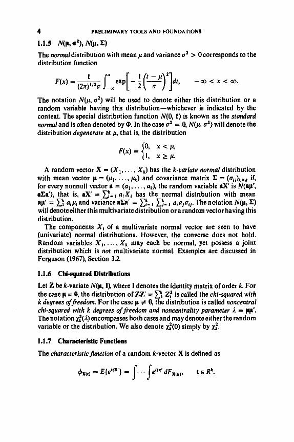
1.1.5 4, a2), Mlr, The normal distribution with mean p and variance o2 > Ocorresponds to the distribution function
F(x) = - 1 ex,[ - 1 ( - a ) D ] d r , r - p -GO < x < GO. (27t)"20 - m
The notation N ( p , d) will be used to denote either this distribution or a random variable having this distribution-whichever is indicated by the context. The special distribution function N(0, 1) is known as the standard normal and is often denoted by 0. In the case o2 = 0, N @ , 0') will denote the distribution degenerate at p, that is, the distribution
A random vector X = (XI, . . . , xk) has the k-oariate normal distribution with mean vector p = (pl, . . . , pk) and covariance matrix I: = (0tj)kxk if, for every nonnull vector a = ( a l , . . . , ak), the random variable a x is N(ap', nu'), that is, a x = c:-, a l X , has the normal distribution with mean ap' = c: alpl and variance aCa' = xt- B,= alalorj. The notation N(p, C) will denoteeither this multivariatedistribution or a random vector having this distribution.
The components XI of a multivariate normal vector are seen to have (univariate) normal distributions. However, the converse does not hold. Random variables X I , . , . , xk may each be normal, yet possess a joint distribution which is not multivariate normal. Examples are discussed in Ferguson (1967), Section 3.2.
1.1.6 Chi-squared Distributions
Let Z be k-variate N(p, I), where I denotes the identity matrix of order k. For the case p = 0, the distribution of Z Z = 2: is called the chi-squared with k degrees offleedom. For the case p # 0, the distribution is called noncentral chi-squared with k degrees offreedom and noncentrality parameter A = pp'. The notation &A) encompasses both cases and may denote either the random variable or the distribution. We also denote x,'(O) simply by xf .
1.1.7 Characteristic Functions
The characteristicfunction of a random k-vector X is defined as
4x(t) = E{eftX'} = /. - - /eltx' dFxcx), t E Rk.

PRELIMINARY NOTATION AND DEFINITIONS 5
In particular, the characteristic function of N(0, 1) is exp( -it2). See Lukacs (1970) for a full treatment of characteristic functions.
1.1.8 Absolutely Continuous Distribution Functions
An a6solutely continuous distribution function F is one which satisfies
F(x) = J:J‘(t)dr, -a c x < co.
That is, F may be represented as the indefinite integral of its derivative. In this case, any function f such that F(x) = I”- f ( t )d t , all x , is called a density for F. Any such density must agree with F‘ except possibly on a Lebesgue-null set. Further, iff is continuous at x o , then f ( x o ) = F’(xo) must hold. This latter may be seen by elementary arguments. For detailed discussion, see Natanson (1961), Chapter IX.
1.1.9 I.I.D. With reference to a sequence {Xi} of random vectors, the abbreviation I.I.D. will stand for “independent and identically distributed.”
1.1.10 lndicator Functions For any set S, the associated indicatorfunction is
1, XES, = (00, x # S .
For convenience, the alternate notation I ( S ) will sometimes be used for Is, when the argument x is suppressed.
1.1.11 Binomial (n,p)
The binomialdistribution with parameters nand p , where n is a positive integer and 0 5 p 5 1, corresponds to the probability mass function
k = 0, 1, ..., n.
The notation B(n, p ) will denote either this distribution or a random variable having this distribution. As is well known, B(n, p) is the distribution of the number of successes in a series of n independent trials each having success probability p.
1.1.12 Uniform (a, 6 )
The unrorm distribution on the interval [a, 61, denoted U(a, 6), corresponds to the density function f ( x ) = l/(b-u), a s x 5 6, and =0, otherwise.

6 PRELIMlNARY TOOLS AND FOUXWATIONS
1.2 MODES OF CONVERGENCE OF A SEQUENCE OF RANDOM VARIABLES
Two forms of approximation are of central importance in statistical ap- plications. In one form, a given random variable is approximated by another random variable. In the other, a given distribution function is approximated by another distribution function. Concerning the first case, three modes of convergence for a sequence of random variables are introduced in 1.2.1, 1.2.2, and 1.2.3. These modes apply also to the second type of approximation, along with a fourth distinctive mode introduced in 1.2.4. Using certain of these convergence notions, stochastic versions of the O(.$, o(0) relations in 1.1.2 are introduced in 1.2.5. A brief illustration of ideas is provided in 1.2.6.
1.2.1 Convergence In Probability
Let X,, X,, . . . and X be random variables on a probability space (9 d, P). We say that X, converges in probability to X if
lim P(IX, - XI < E ) = 1, every e > 0. n- a0
This is written X, 3 X , n -+ 00, or p-lim,,+m X, = X. Examples are in 1.2.6, Section 1.8, and later chapters. Extension to the case of X,, X,, . . . and X random elements of a metric space is straightforward, by replacing (X, - XI by the relevant metric (see Billingsley (1968)). In particular, for random k- vectors X,, X,, . . . and X, we shall say that X, 3 X if IlX,, - Xll 4 0 in the above sense, where llzll = (zi- , for z E Rk. It then follows (Problem 1.P.2) that X, 3 X if and only if the corresponding component-wise con- vergences hold.
1.2.2 Convergence with Probability 1
Consider random variables X,, X,, . . . and X on (Q d, P). We say that X , converges with probability 1 (or strongly, almost surely, almost euerywhere, etc.) to X if
P limX,= - 1.
This is written X , * X , n + 00, or pl-lim,+m X, = X . Examples are in 1.2.6, Section 1.9, and later chapters. Extension to more general random elements is straightforward.
(n-m X)
An equivalent condition for convergence wpl is
lim P(lX,,, - XI < e, all rn 2 n) = 1, each e > 0. n-m

MODES OF CONVERGENCE OF A SEQUENCE OF RANDOM VARIABLES 7
This facilitates comparison with convergence in probability. The equivalence is proved by simple set-theoretic arguments (Halmos (1950), Section 22), as follows. First check that
(*I {a: lim x,(a) = x(a)) = n u {a: IX,,,(~) - x(w)l< s, all m 2 n),
whence
(**I
m
R+ 09 r > O n - 1
. . k: lim x,,(a) = x(o)j = lim lim {a: IX,,,(~) - x ( a ) l < e, all m 2 n}.
By the continuity theorem for probability functions (Appendix), (**) implies
P(X, + X) = lim lim P(JX,,, - XI < e,allm 2 n),
which immediately yields one part of the equivalence. Likewise, (*) implies, for any E > 0,
P(X,+X)S l imP((X,-X(<e,al lmrn) ,
w m 8-0 n-m
8 - 0 n-m
14 m
yielding the other part. The relation (*) serves also to establish that the set {m: X,(w) + X ( a ) }
truly belongs to d, as is necessary for "convergence wpl to be well defined. A somewhat stronger version of this mode of convergence will be noted in
1.3.4.
1.2.3 Convergence in rth Mean Consider random variables XI, Xz , . . . and X on (Q d, P). For r > 0, we say that X, converges in rth mean to X if
lim EIX, - X r = 0.
This is written X,- X or L,-lim,,+m X, = X. The higher the value of r, the more stringent the condition, for an application of Jensen's inequality (Ap- pendix) immediately yields
I- m rtb
Given (Q d, P) and r > 0, denote by L,(Q d, P) the space of random variables Y such that El Y I' < 00. The usual metric in L, is given by d( Y, 2) = IIY - Zll,, where
O < r < l , [El Yl'l''', r 2 1.

8 PRELIMINARY TOOLS A N D FOUNDATIONS
Thus convergence in the rth mean may be interpreted as convergence in the L, metric, in the case of random variables XI, X2, . . . and X belonging to L,.
1.2.4 Convergence in Distribution
Consider distribution functions F,(.), F2(.), . . , and F(.), Let XI, X2,. . . and X denote random variables (not necessarily on a common probability space) having these distributions, respectively. We say that X , converges in distribution (or in law) to X if
lim F,(t) = F(t), each continuity point t of F.
This is written X, 4 X , or d-iim,-= X , = X . A detailed examination of this mode of convergence is provided in Section 1.5. Examples are in 1.2.6, Section 1.9, and later chapters.
The reader should figure out why this definition would not afford a satisfactory notion of approximation of a given distribution function by other ones if the convergence were required to hold for all t.
In as much as the definition of X , A X is formulated wholly in terms of the corresponding distribution functions F, and F, it is sometimes convenient to use the more direct notation “F, * F” and the alternate terminology “F, conuerges weakly to F.” However, as in this book the discussions will tend to refer directly to various random variables under consideration, the notation X , % X will be quite useful also.
Remark. The convergences 3, %, and 3 each represent a sense in which, for n sufficiently large, X,(w) and X(w) approximate each other as functions ofw, o E R. This means that the distributions of X , and X cannot be too dissimilar, whereby approximation in distribution should follow. On the other hand, the convergence 5 depends only on the distribution functions involved and does not necessitate that the relevant X , and X approximate each other as functions of o. In fact, X, and X need not be defined on the same probability space. Section 1.3 deals formally with these interrelationships. W
1.2.5 Stochastic O(.) and 4) A sequence of random variables {X,,}, with respective distribution functions {F,}, is said to be bounded in probability if for every e > 0 there exist M , and N, such that
n- a~
F,(M,) - F,( - M,) > 1 - e all n > N,.
The notation X , = 0,,(1) will be used. It is readily seen that X , 5 X 3 X, = 0,,(1) (Problem 1.P.3).

RELATIONSHIPS AMONG THE MODES OF CONVERGENCE 9
More generally, for two sequences of random variables { U,} and { K}, the notation U, = O p ( K ) denotes that the sequence {UJV,} is Op(l). Further, the notation U, = op(K) denotes that UJV,, 4 0. Verify (Problem 1.P.4) that u, = op(v,) * u, = OP(v,).
1.2.6 Example: Proportion of Successes in a Series of Trials
Consider an infinite series of independent trials each having the outcome “success” with probability p . (The underlying probability space would be based on the set f2 of all infinite sequences o of outcomes of such a series of trials.) Let X, denote the proportion of successes in the first n trials. Then
P (i) X, + P;
Is it true that
Justification and answers regarding (i)-(v) await material to be covered in Sections 1.8-1.10. Items(vi)and(vii)may be resolved at once, however,simply by computing variances (Problem 1.P.5).
1.3 RELATIONSHIPS AMONG THE MODES OF CONVERGENCE
For the four modes ofconvergence introduced in Section 1.2, we examine here the key relationships as given by direct implications (1.3.1-1.3.3), partial converses (1.3.4-1.3.9, and various counter-examples (1.3.8). The question of convergence of moments, which is related to the topic of convergence in rth mean, is treated in Section 1.4.
10 PRELIMINARY TOOLS AND FOUNDATIONS
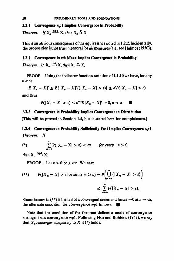
1.3.1 Convergence wpl Implies Convergence in Probability
Theorem. If X,, wp? X , then X , 4 X .
This is an obvious consequence of the equivalence noted in 1.2.2. Incidentally, the proposition is not true in gerreral for all measures(e.g., see Halmos (1950)).
1.3.2 Convergence in rth Mean Implies Convergence in Probability
Theorem. If X , 2% then X , X.
PROOF. Using the indicator function notation of 1.1.10 we have, for any E > 0,
E I X , - Xl'r E { I X , - X r q l X , - XI > E ) } 2 E'P(IX, - XI > E )
and thus
P( IX,, - x I > E ) s E-'E I x, - x I' -+ 0, n -+ ao. H
13.3 Convergence in Probability Implies Convergence in Distribution
(This will be proved in Section 1.5, but is stated here for completeness.)
1.3.4 Convergence in Probability Sufficiently Fast Implies Convergence wpl
Theorem. If m 2 P ( I X , - X I > E) < 00 for every E > 0,
n = 1
then X , =% X .
PROOF. Let E > 0 be given. We have
m
(**) p(lx,,, - XI > e for some m 2 n) = P u { IX, - X I > 8 1 ) d . n
m
5 C p(IXm - XI > E). m = n
Since the sum in (**)is the tail of aconvergent series and hence -+0 as n -+ 00,
the alternate condition for convergence wpl follows. H
Note that the condition of the theorem defines a mode of convergence stronger than convergence wpl. Following Hsu and Robbins (1947), we say that X , converges completely to X if (*) holds.

RELATIONSHIPS AMONG THE MODES OF CONVERGENCE 11
1.3.5 Convergence in rth Mean Sufficiently Fast Implies Convergence wpl
The preceding result, in conjunction with the proof of Theorem 1.3.2, yields
Theorem. lf c."- EIX, - XI' < 00, then X, % X.
The hypothesis ofthe theorem in fact yields the much stronger conclusion that the random series EX1 !X, - XI' converges wpl (see Lukacs (1975), Section 4.2, for details).
1.3.6 Dominated Convergence in Probability Implies Convergence in Mean
Theorem. Suppose that X, 3 X, I X, I < I Y I wpl (all n), and E I Y l r < 00.
Then X, * X. PROOF. First let us check that 1x1 5 I Y Iwpl. Given 6 > 0, we have
P(IX( > lYl+ 6) s P ( I X ( > IX,,l+ 6) < P((X, - XI > 6)+0, n + m. HencelXl S ( Y I + S w p l f o r a n y S > O a n d s o f o r S = O .
Consequently, IX, - XI s 1x1 + IX,I s 21 Y IwpI. Now choose and fix E > 0. Since El Y I' < 00, there exists a finite constant
A, > E such that E { I Y rl(21 Y I > A,)} s E. We thus have
E(X, - XI'= E{JX, - X('l((X, - XI > At)} + E{IX, - XI'l(lXn - XI 5 E ) }
+ E{lX, - xl'l(~ < IX, - XI 5 A,)} S E{(12Y)'1(2(YI > A,)} + E' + A:P(IX, - XI > E )
5 2'E + E' + A:P()X, - XI > E).
Since P ( ) X , - XI > E ) + 0, n + 00, the right-hand side becomes less than 2'6 + 26' for all n sufficiently large.
More general theorems of this type are discussed in Section 1.4.
1.3.7 Dominated Convergence wpl Implies Convergence in Mean
By 1.3.1 we may replace 4 by * in Theorem 1.3.6, obtaining
Theorem. Suppose that X, * X, 1 X, I s; I Y I wpl (all n), and E I Y 1' < 00.
Then X, 5 X .
1.3.8 Some Counterexamples
Sequences {X,} convergent in probability but not wpl are provided in Examples A, B and C. The sequence in Example B is also convergent in mean square. A sequence convergent in probability but not in rth mean for any r > 0 is provided in Example D. Finally, to obtain a sequence convergent

12 PRELIMINARY TOOLS AND FOUNDATIONS
wpl but not in rth mean for any r > 0, take an appropriate subsequence of the sequence in Example D (Problem 1.P.6). For more counterexamples, see Chung (1974), Section 4.1, and Lukacs (1975), Section 2.2, and see Section 2.1.
Example A. The usual textbook examples are versions of the following (Royden (1968), p. 92). Let (n, d, P) be the probability space corresponding to R the interval [0,1], d the Bore1 sets in [0, 13, and P the Lebesgue measure on d. For each n = 1,2, . . . , let k, and v, satisfy n = k, + 2"", 0 5 k, < 2'", and define
1, if O E [k,2-'", (k, + 1)2-'"] X n ( 0 ) = { 0, otherwise.
It is easily seen that X, 4 0 yet X,(o) --* 0 holds nowhere, o E [0,1]. H
Example B. Let Yl, Yz, . . . be I.I.D. random variables with mean 0 and variance 1. Define
c1 yr (n log log n)l'Si
x, =
By the central limit theorem (Section 1.9) and theorems presented in Section 1.5, it is clear that X, 4 0. Also, by direct computation, it is immediate that X, 5 0 , However, by the law of the iterated logarithm (Section LlO), it is evident that X,(o) -P 0, n --* 00, only for o in a set of probability 0.
Example C (contributed by J. Sethuraman). Let Yl, Y,, . . , be I.I.D. random variables. Define X, = YJn.'+hen clearly X, 1: 0. However, X, "p'. 0 if and only if El Y, I < m. To verify this claim, we apply
Lemma (Chung (1974), Theorem 3.2.1) For any positive random variable z,
m f' P(Z 2 n) s E{Z) 5 1 + c P(Z 2 n). n i l n= 1
Thus, utilizing the identical distributions assumption, we have
1 m f P(lxnl* = c ~ ( 1 y1 I 2 n&) 5 ; EJ yi I, m m
n- 1 n= 1
n= 1 n= 1
1 1 + C P(IXnI 2 8) = 1 + C p(I Y. I 2 na) 2 e EI Yi I.
The result now follows, with the use of the independence assumption, by an application of the Borel-Cantelli lemma (Appendix). H
CONVERGENCE OF MOMENTS ; UNIFORM INTEGRABILITY 13
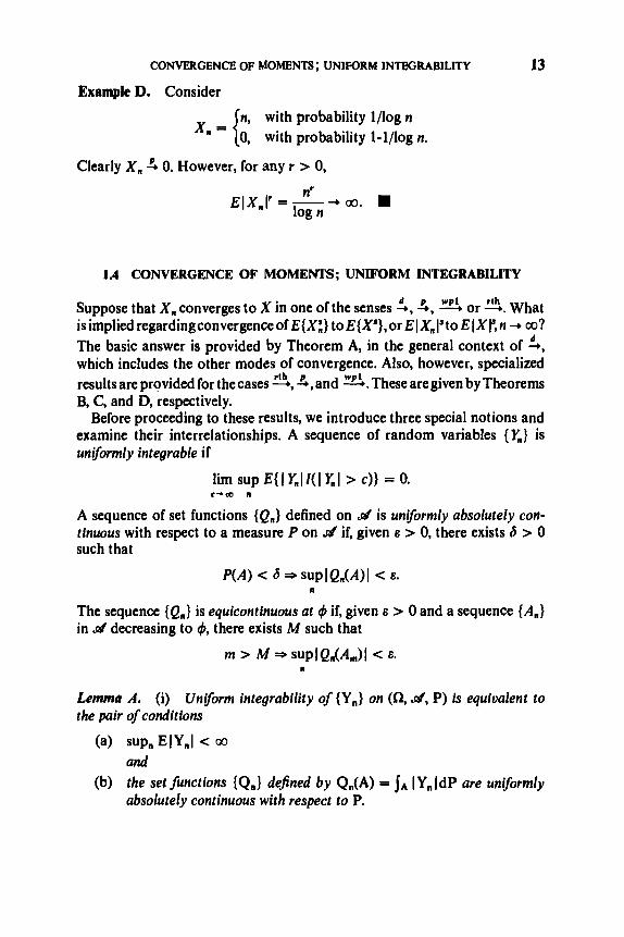
Example D. Consider
n, with probability l/log n xn= { 0, with probability l-l/log n.
Clearly X, 1: 0. However, for any r > 0,
1 A CONVERGENCE OF MOMENTS; UNIFORM INTEGRABILITY
Suppose that X, converges to X in one of the senses $,A, ws? or 5. What isimpliedregardingconvergenceofE{X:} toE{X'},or E IX,p toEIXI',n + co? The basic answer is provided by Theorem A, in the general context of 5, which includes the other modes of convergence. Also, however, specialized resultsareprovided for thecases 3, 3,and *.These aregiven by Theorems B, C, and D, respectively.
Before proceeding to these results, we introduce three special notions and examine their interrelationships. A sequence of random variables { Y,} is uniformly integrable if
limsupE{JY,II(IY,I > c ) } = O .
A sequence of set functions {Q.} defined on d is uniformly absolutely con- tinuous with respect to a measure P on d if, given E > 0, there exists S > 0 such that
P(A) < 6 =$ sup( Q,(A)I < E.
The sequence { Q n } is equicontinuous at 4 if, given E > 0 and a sequence {A,} in d decreasing to 4, there exists M such that
c+oo n
n
m > M supIQ,(A,)J c E. n
Lemma A. (i) the pair of conditions
and
(b) the set Junctions {Q,} defined by Q,(A) = I,, IY,(dP are uniformly absolutely continuous with respect to P.
Uniform integrability of {Y,} on (a, d, P) is equivalent to
(a) SUPn EIYnI < 00

14 PRELIMINARY TOOLS AND FOUNDATIONS
(ii) Susfcientfor uniform integrability of {Y,} is that
sup EIYnI1+' < 00 n
for some E > 0.
variable Y such that E I Y I < 00 and (iii) Susfcient for uniform integrability of {Y,} is that there be a random
P(IY,( 2 Y) 5 P(IYI 2 y),alln 2 1,ally > 0.
(iv) For set functions Q, each absolutely continuous with respect to a meusure P , equicontinuity at 4 implies uniform absolute continuity with respect to P.
PROOF. (i) Chung (1974), p. 96; (ii) note that
H I y,lI(l Kl > c ) ) 5 c - T I XI'+'; (iii) Billingsley (1968), p. 32; (iv) Kingman and Taylor (1966), p. 178.
Theorem A. Suppose that X, % X and the sequence {X:} is uniformly integrable, where r > 0. Then ElXl' < 00, limn E{X:} = E{X'}, and lim, EIXn(' = EJXI'.
PROOF. Denote the distribution function of X by F. Let 8 > 0 be given. Choose c such that fc are continuity points of F and, by the uniform integrability, such that
SUP E { l ~ I r ~ ( l ~ I l 2 c)} < e. I
For any d > c such that f d are also continuity points of F, we obtain from the second theorem of Helly (Appendix) that
lim E{IX,I'I(c s IX,l s, 4) = E{IXI'I(c s 1x1 s 4).
It follows that E{ IXrf(c 5 IX I s d)} < e for all such choices of d. Letting d-,oo,weobtainE{lXI'I(IXI Zc)} <6,whenceEJXr< 00.
n+m
Now, for the same c as above, write
IE{X:} - E{X'}I s IE{X~(lxnl 5 c)} - E{X'I(IXl 5 c))l + E{lXnI'I(lXnl > c)} + E{IXI'I(IXI > c)}*
By the Helly theorem again, the first term on the right-hand side tends to 0 as n + 00. The other two terms on the right are each less than 8. Thus lim;E{X:} = E{X'}. A similar argument yields limn ElX,,r = EIXI'. By arguments similar to the preceding, the following partial converse to
Theorem A may be obtained (Problem 1.P.7).

CONVERGENCE OF MOMENTS ; UNIFORM MTBORABILITY 15
Lemma B. Suppose that X , 5 X and limn EIXnr = EJXI ' < 00. Then the sequence {X:} is uniformly integrable.
We now can easily establish a simple theorem apropos to the case 3.
Theorem B. Suppose that Xn*X and EIX( ' < 00. Then limn E{X:} = E{X'} and limn EIX,(' = EIXI'.
PROOF. For 0 < r S 1, apply the inequality Ix + y r S I x r + Iyr to write Ilxr - I y r l s Ix - y J ' and thus
IEIX,r - E l X r l S EJX, - XI'. For r > 1, apply Minkowski's inequality (Appendix) to obtain
l(ElX,r)l/r - (EIxr)lq s (EJX, - XI')'". In either case, limn E(X, ( ' = EIX < 00 follows. Therefore, by Lemma B, {X:} is uniformly integrable. Hence, by Theorem A, limn E{X:} = E{Xr} follows.
Next we present results oriented to the case 3.
Lemma C. Suppose that X , 3 X and E I X , I' < 00, all n. Then the following statements hold.
(i) X , (ii) Ifthe set functions {Q,} defined by Q,(A) = JA l X n r dP are equicon-
PROOF. (i) see Chung (1974), pp. 96-97; (ii) see Kingman and Taylor
It is easily checked (Problem 1.P.8) that each of parts (i) and (ii)generalizes
Combining Lemma C with Theorem B and Lemma A, we have
X i f and only i f the sequence {X:} is uniformly integrable.
tinuous at 4, then X , s X and EJXI' < 00.
(1966), pp. 178-180.
Theorem 1.3.6.
Theorem C. Suppose that X , -% X and that either (i) E I X 1' < 00 and {X:} is uniformly integrable,
or (ii) sup, EIX,I' < 00 and the set functions {Q,} defined by Q,(A) = I X , (' dP are equicontinuous at 4.
Then limn E{X:} = E{X'} and limn EJX,/ ' = EIXJ'.
16 PRELIMINARY TOOLS AND FOUNDATIONS
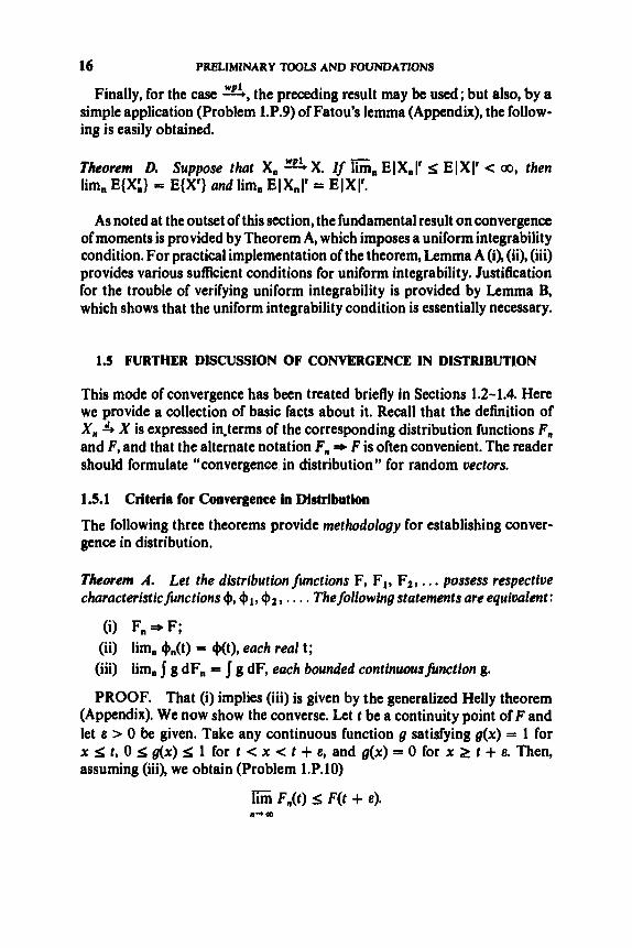
Finally, for the case 5, the preceding result may be used; but also, by a simple application (Problem l.P.9) of Fatou’s lemma (Appendix), the follow- ing is easily obtained.
Theorem D. Suppose that Xn * X. If G n EIXnr S ElXl’ < 00, then limn E{X:} = E{X’} and limn EIX,)’ = ElX)’.
As noted at the outset of this section, the fundamental result on convergence of moments is provided by Theorem A, which imposes a uniform integrability condition. For practical implementation of the theorem, Lemma A(i), (ii), (iii) provides various sufficient conditions for uniform integrability. Justification for the trouble of verifying uniform integrability is provided by Lemma B, which shows that the uniform integrability condition is essentially necessary.
1.5 FURTHER DISCUSSION OF CONVERGENCE 1N DISTRlBUTION
This mode of convergence has been treated briefly in Sections 1.2-1.4. Here we provide a collection of basic facts about it. Recall that the definition of X , A X is expressed in.terms of the corresponding distribution functions F, and F, and that the alternate notation Fn F is often convenient. The reader should formulate “convergence in distribution” for random vectors.
1.5.1 Criteria for Convergence in Distributibn
The following three theorems provide methodology for establishing conver- gence in distribution.
Theorem A. Let the distribution functions F, F1, F2, . . . possess respective characteristic functions 4, 41, 42, . . . . The following statements are equivalent:
(i) F, =* F; (ii) limn +,(t) = Nt), each real t; (iii) limn g dF, = g dF, each bounded continuousfitnction g.
PROOF. That (i) implies (iii) is given by the generalized Helly theorem (Appendix). We now show the converse. Let t be a continuity point of F and let E > 0 be given. Take any continuous function g satisfying g ( x ) = 1 for x 1s t , 0 5 g(x) S 1 for t < x < t + e, and g(x) = 0 for x 2 t + e. Then, assuming (iii), we obtain (Problem 1.P.10)
Tim F,(t) 5 F(t + 6). n-+ m

FURTHER DISCUSSION OF CONVERGENCE IN DISTRIBUTION 17
Similarly, (iii) also gives
- lim F,(t) 2 F(t - 8). n+ m
Thus (i) follows. For proof that (i) and (ii) are equivalent, see Gnedenko (1962), p. 285.
Example. If the characteristic function of a random variable X, tends to the function exp(-+t2) as n --* 00, then X, % N(0, 1). H
The multivariate version of Theorem A is easily formulated.
Theorem B (Frkchet and Shohat). Let the distribution functions F, possess Jinite moments arb = j tk dF,(t) for k = 1, 2,. . . and n = 1,2,. . . . Assume that the limits ak = limn ap) exist (finite), each k. Then
(i) the limits {ak} are the moments o f a distributionfunction F; (ii) Vthe F gioen by (i) is unique, then F, =+ F.
For proof, see Frtchet and Shohat (1931), or Loeve (1977), Section 11.4. This result provides a convergence of moments criterion for convergence in distribution. In implementing the criterion, one would also utilize Theorem 1.13, which provides conditions under which the moments {ak} determine a unique F.
The following result, due to Scheff6 (1947) provides a convergence of densities criterion. (See Problem 1.P.11.)
Theorem C (Scheffk). Let {f.) be a sequence of densities of absolutely continuous distribution functions, with limn f,(x) = f(x), each real x. IJ f is a densityfunction, then limn (f,(x) - f(x)ldx = 0.
PROOF. Put gn(x) = [ f ( x ) - f , (x ) ] ! ( f (x ) 2 h ( x ) ) , each x . Using the fact that f is a density, check that
11 fn(x) - f ( x ) I dx = 2 Jen(x)dx*
Now Ig,(x)l $ f ( x ) , all x,each n. Hence, by dominated convergence(Theorem 1.3.7), limn g,(x)dx = 0. H
1.5.2 Reduction of Multivariate Case to Univariate Case The following result, due to Cramer and Wold (1936), allows the question of convergence of multivariate distribution functions to be reduced to that of convergence of univariate distribution functions.
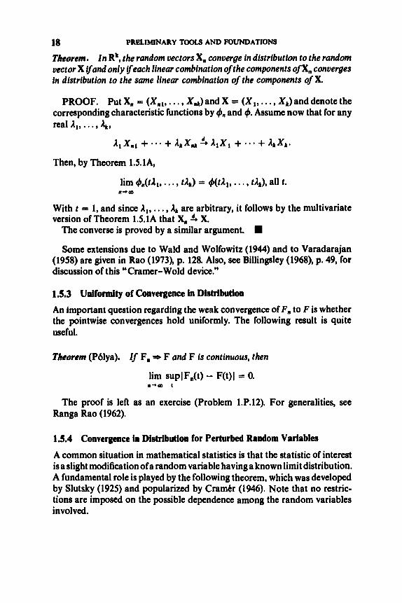
18 PRBLlMlNARY TOOLS AND FOUNDATIONS
Theorem. In R', the random vectors X, converge in distribution to the random vector X tfand only tfeach linear combination of the components of X, converges In distribution to the same linear combination of the components ofX.
PROOF. Put X, = (X,,,, . . . , X,,,Jand X = (Xl,. . . , Xk)and denote the corresponding characteristic functions by 4, and 4. Assume now that for any real A,, . . . ,
AlXn1 + ' * ' + AkXx,, 1, Alxl + * " + A k x k .
Then, by Theorem 1.5.1A,
lim #&Al,. . . , t&) = 4(rA,, . . . , th), all r.
With t = 1, and since A t , . . . , Ak are arbitrary, it follows by the multivariate version of Theorem 1.5.1A that X,, % X.
n+ w
The converse is proved by a similar argument. H
Some extensions due to Wald and Wolfowitz (1944) and to Varadarajan (1958) are given in Rao (1973), p. 128. Also, see Billingsley (1968), p. 49, for discussion of this "Cramer-Wold device."
1.5.3 Uniformity of Convergence in Distribution
An important question regarding the weak convergence of F,, to F is whether the pointwise convergences hold uniformly. The following result is quite useful.
Theorem (Pblya), f'f F, * F and F is continuous, then
lim supIF,(t) - F(t)I = 0. ,-+a I
The proof is left as an exercise (Problem 1.P.12). For generalities, see Ranga Rao (1962).
1.5.4 Convergence in Distribution for Perturbed Random Variables
A common situation in mathematical statistics is that the statistic of interest is a slight modification of a random variable having a known limit distribution. A fundamental role is played by the following theorem, which was developed by Slutsky (1925) and popularized by CramCr (1946). Note that no restric- tions are imposed on the possible dependence among the random variables involved.

FURTHER DISCUSSION OF CONVERGENCE IN DISTRIBUTION 19
Theorem (Slutsky). Let X , 4 X and Y, J$ C, where c is a finite constant. Then
(i) X, + Y, x + c; (ii) X,Y, 5 CX;
(iii) XJY, 5 X/C ifc z 0.
Coroffury A. Convergence in probability, X , .% X , implies convergence In distribution, X , 5 x.
Coroffury B. Convergence in probability to a constant is equivalent to con- vergence in distribution to the given constant.
Note that Corollary A was given previously in 1.3.3. The method of proof of the theorem is demonstrated sufficiently by proving (i). The proofs of (ii) and (iii) and of the corollaries are left as exercises (see Problems 1.P.13-14).
PROOF OF (i). Choose and fix t such that t - c is a continuity point of F x . Let e > 0 be such that t - c + E and t - c - E are also continuity points of F x . Then
Fx. + ~ , ( t ) = p(xn + Yn S t ) 5 p(x, + Yn S t, lYn - CI < 6) + P ( ( Y, - CI 2 E)
s p ( X , S t - c + 6) + P(lY, - CI 2 6).
Hence, by the hypotheses of the theorem, and by the choice oft - c + e,
(*) EG Fxn+yn(t) S G P ( X n S t - c + 8) + TimP(JY, - CI 2 E ) n n n
= Fx(t - c + E) .
Similarly,
P(Xn 5 t - c - e) 5 P(Xn + Yn S t ) + P(lYn - cl 2 e )
and thus
Since t - c is a continuity point of F x , and since e may be taken arbitrarily small, (*) and (**) yield
lim Fxn+yn(t) = F,(t - c) = FX+&). I n

20 PRBLIMINARY TOOLS AND FOUNDATIONS
1.5.5 Asymptotic Normality The most important special case of convergence in distribution consists of convergence to a normal distribution. A sequence of random variables {X,} converges in distribution to N ( p , u2), u > 0, if equivalently, the sequence {(X, - p)/u} converges in distribution to N(0, 1). (Verify by Slutsky’s Theorem.)
More generally, a sequence of random variables { X , } is asymptotically normal with “mean” p, and “variance” a,” if a, > 0 for all n sufficiently large and
x, - A 5 N(0,l). all
We write “ X , is AN(!,, a:).” Here {p,} and {a,} are sequences of constants. It is not necessary that A,, and u,” be the mean and variance of X,, nor even that A’, possess such moments. Note that if X, is AN@,, u:), it does not necessarily follow that {X,} converges in distribution to anything. Nevertheless in any case we have (show why)
sup I p(X , s t ) - P(N(p,, of) s t ) I + 0, n + 00, I
so that for a range of probability calculations we may treat X, as a Nb,, a,’) random variable. As exercises (Problems 1.P.15-16), prove the following useful lemmas.
Lemma A. If Xn is AN(&,, a:), then also Xn is AN(&, a,”) if and only i f
Lemma B. I . X n is AN(Pn, o:), then also anX, + bn is AN&, af) if and only if
Example. If X , is AN(n, 2n), then so is
n - 1 n X,
but not - Jn - 1 x,. Jr;
FURTHER DISCUSSION OF CONVERGENCE IN DISTRIBUTION 21
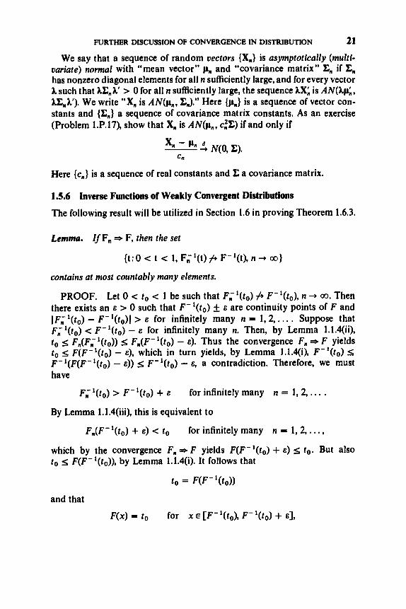
We say that a sequence of random uectors {X,} is asymptotically (multf- uariate) normal with "mean vector" pn and "covariance matrix" C,, if C, has nonzero diagonal elements for all n sufficiently large, and for every vector 1 such that 1Z,X > 0 for all n sufficiently large, the sequence AX; is AN(&&, AE,X), We write "X, is AN(pn, I;,)." Here {p,} is a sequence of vector con- stants and {&} a sequence of covariance matrix constants. As an exercise (Problem l.P.17), show that X, is AN(p, , C ~ C ) if and only if
xn - 5 N(0, Z). Cn
Here {c,} is a sequence of real constants and I; a covariance matrix.
1.5.6 Inverse Functions of Weakly Convergent Distributions
The following result will be utilized in Section 1.6 in proving Theorem 1.6.3.
Lemma. IfFn =s F, then the set
{ t :O<t < l,F,'(t)f*F-'(t),n-,co}
contains at most countably many elements.
PROOF. Let 0 < to < 1 be such that F;'( to) f i F-'( t0) , n -+ 00. Then there exists an E > 0 such that F - ' ( t o ) f E are continuity points of F and IF; ' ( to) - F-'(to)l > E for infinitely many n = 1.2,. . , , Suppose that F;l( to) < F - ' ( t 0 ) - E for infinitely many n. Then, by Lemma 1.1.4(ii), to 5 F,(F; ' ( t o ) ) s F,(F-'(to) - E). Thus the convergence F, =s F yields to 4 F(F-' ( to) - E), which in turn yields, by Lemma 1.1.4(i), F-' ( to) 5 F-'(F(F-'( to) - E ) ) I; F-' ( t0) - E, a contradiction. Therefore, we must have
~ ; ' ( t ~ ) > F-' ( to) + e for infinitely many n = 1,2, . . . . By Lemma 1.1.4(iii), this is equivalent to
F,(F-'(C,) + E ) < to for infinitely many n = 1,2,. . . , F yields F(F-'( to) + E ) 5 to. But also which by the convergence F ,
to s F(F-'(to)), by Lemma 1.1.4(i). It follows that
to = F(F-'(to))
and that
F(x) = to for x E [F-'( t , ) , F - ' ( t o ) + E ] ,

22 PRELIMINARY TOOLS AND FOUNDATIONS
that is, that F is flat in a right neighborhood of F-'(t,,). We have thus shown a one-to-one correspondence between the elements of the set { t : 0 < t < 1, F; ' ( t ) P F-'( t ) , n -+ do} and a subset of the flat portions of F. Since (justify) there are at most countably many flat portions, the proof is complete.
1.6 OPERATIONS ON SEQUENCES TO PRODUCE SPECIFIED CONVERGENCE PROPERTIES
Here we consider the following question: given a sequence {X,} which is convergent in some sense other than wpl, is there a closely related sequence {X:} which retains the convergence properties of the original sequence but also converges wpl? The question is answered in three parts, corresponding respectively to postulated convergence in probability, in rth mean, and in distribution.
1.6.1 Conversion of Convergence in Probability to Convergence wpl A standard result of measure theory is the following (see Royden (1968), p. 230).
Theorem. IfX, 3 X, then there exists a subsequence XnI; such that X, X, k -+ a.
Note that this is merely an existence result. For implications of the theorem for statistical purposes, see Simons (1971).
1.6.2 Conversion of Convergence in rth Mean to Convergence wpl
Consider the following question: given that X, 3 0, under what circum- stances does the "smoothed" sequence
converge wpl? (Note that simple averaging is included as the special case w, = 1.) Several results, along with statistical interpretations, are given by Hall, Kielson and Simons (1971). One of their theorems is the following.
Theorem. A s a c i e n t conditionfor {X:} to converge to 0 with probability 1 is that
Since convergence in rth mean implies convergence,in probability, a com- peting result in the present context is provided, by Theorem 1.6.1, which however gives only an existence result whereas the above theorem-is con- structiue.

OPERATIONS TO PRODUCE SPECIFIED CONVERGENCE PROPERTIES 23
1.6.3 Conversion of Convergence in Distribution to Convergence wpl
Let ale, denote the Bore1 sets in [0, 13 and mlo, 11 the Lebesgue measure restricted to [0, 13.
Theorem. In R‘, suppose that Xn 3 X. Then there exist random k-vectors Y, Y1, Y2, . . . defined on the probability space ([0, 13, Wlo, mIO, 1,) such that
9 ( Y ) = 9 ( X ) and 9(Y, ) = 9(Xn), n = 1,2,. , . , and
y n Y, i e . , mlo, ll(yn -, Y) = 1.
We shall prove this result only for the case k = 1. The theorem may, in fact, be established in much greater generality. Namely, the mappings X, XI, X2, . , , may be random elements of any separable complete metric space, a generality which is of interest in considerations involving stochastic processes. See Skorokhod (1956) for the general treatment, or Breiman (1968), Section 13.9, for a thorough treatment of the case R“.
The device given by the theorem is sometimes called the “Skorokhod construction ” and the theorem the “Skorokhod representation theorem.”
PROOF (for the case k = 1). For 0 < t < 1, define
Y(t ) = F;’(t) and Ym(t) = F;:(t), n = 1,2,. . . . Then, using Lemma 1.1.4, we have
F Y W = “10. I]({t: Y(t) 5 Y ) ) = mro, I l ( k t s FXCV)})
= FAY), all Y ,
that is, 9 ( Y ) = 9 ( X ) . Similarly, U(YJ = 9 ( X n ) , n = 1,2,. . . . It remains to establish that
M [ O . 1l({t: yn(t) f , Y ( t ) ) ) = 0.
This follows immediately from Lemma 1.5.6.
Remarks. (i) The exceptional set on which Y. fails to converge to Y is at most countably infinite.
(ii) Similar theorems may be proved in terms of constructions on prob- ability spaces other than ([0, 11, mIo, However, a desirable feature of the present theorem is that it does permit the use of this convenient prob- ability space.
(iii) The theorem is “constructive,” not existential, as is demonstrated by the proof. W
24 PRELIMINARY TOOLS AND MWN'DATIONS
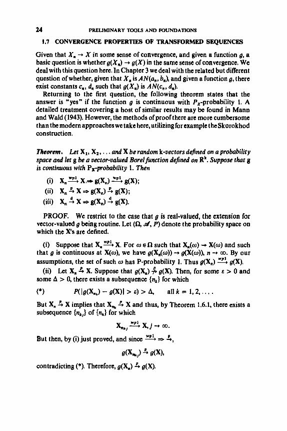
1.7 CONVERGENCE PROPERTIES OF TRANSFORMED SEQUENCES
Given that X, + X in some sense of convergence, and given a function g, a basic question is whether g(X,) -+ g(X) in the same sense of convergence. We deal with this question here. In Chapter 3 we deal with the related but different question of whether, given that X , is AN(a,, b,,), and given a function g, there exist constants c,, d, such that g(X,) is AN(c,, d,,).
Returning to the first question, the following theorem states that the answer is "yes" if the function g is continuous with P,-probability 1. A detailed treatment covering a host of similar results may be found in Mann and Wald (1943). However, the methods of proof there are more cumbersome than the modern approaches we take here, utilizing for example the Skorokhod construction.
Theorem. Let XI, X,, . . . and X be random k-vectors defined on a probability space and let g be a uector-valued Borel function defined on Rk. Suppose that g is continuous with Px-probability 1. Then
(i) X, vp? x.* g(X.1 wp? g(X); (ii) X, 4 x =- g(X,) 3 g(X);
(iii) X, S x =s g(x,) S g(x).
PROOF. We restrict to the case that g is real-valued, the extension for vector-valued g being routine. Let (Q d, P) denote the probability space on which the X's are defined.
(i) Suppose that X, * X. For o E R such that X,(o) + X(o) and such that g is continuous at X(o), we have g(X,(o)) + g(X(o)), n + 00. By our assumptions, the set of such w has P-probability 1. Thus g(X,) wp! g(X).
Q(X). Then, for some e > 0 and some A > 0, there exists a subsequence {nk} for which
(*I P( lg(X,,) - g(X)I > E ) > A, But X, 5 X implies that X,, 3 X and thus, by Theorem 1.6.1, there exists a subsequence {nk,} of {nk} for which
(ii) Let X, 3 X. Suppose that g(X,)
all k = 1,2, . . . .
But then, by (i) just proved, and since 3 =$ 3,
contradicting (*). Therefore, g(X,) 3 g(X).

CONVERGENCE PROPERTIES OF TRANSFORMED SEQUENCEs 25
(iii) Let X , A X . By the Skorokhod construction of 1.6.3, we may con- struct on some probability space (CY, d, P') some random vectors Y I , Y,, . . . and Y such that U ( Y l ) = U(Xl ) , S'(Y,) = U(X,), . . . , and U ( Y ) = 9 ( X ) , and, moreover, Y , -t Y with P'-probability 1. Let D denote the discontinuity set of the function g. Then
P ' ( { o ' : g is discontinuous at Y(o')}) = P'(Y-'(D)) = P;(D) = P,(D) = P(X-'(D)) = 0.
Hence, again invoking (i), g(Y,) -t g(Y) with P'-probability 1 and thus
g(Y,) g(Y). But the latter is the same as g(X,) & g(X).
Examples. (i) If X , 4 N(0, l), then X ; A x i . (ii) If (X,, Y,) 4 N(0, I), then XJY, A Cauchy. (iii) Illustration of g for which X , 1: X but g(X,,) #+ g(X). Let
t - 1 , t < o , g(t ) = { t + 1, t 2 0,
1 n X, = - -with probability 1,
and
X = 0 with probability 1.
The function g has a single discontinuity, located at t = 0, so that g is dis- continuous with Px-probability 1. And indeed X , 3 X = 0, whereas
(iv) In Section 2.2 it will be seen that under typical conditions the sample variance s2 = (n - l)-I cy ( X , - x), converges wpl to the population variance c2. It then follows that the analogue holds for the standard deviation:
W P 1 s + 6.
(v) Linear and quadratic functions of vectors. The most commonly considered functions of vectors conwerging in some stochastic sense are linear transformations and quadratic forms.
g(X,) 3 - 1 but g ( X ) = g(0) = 1 # - 1.
Corollary. Suppose that the k-vectors X, converge to the k-vector X wpl, or in probability, or in distribution. Let A, k and k be matrices. Then AX'-+ AX' and X,BX:, + XBX' in the given mode of convergence.

26
PROOF. The
PRELIMINARY TOOLS AND FOUNDATIONS
vector-valued function
f = I 1=1
and the real-valued function k k
XBX’ = bl,xfx, 1 - 1 1 - 1
are continuous functions of x = ( x i , . . . , x k ) .
Some key applications of the corollary are as follows.
d Applicution A. I n Rk, let X, 3 N(p, C). Let C, ,, k be a matrix. Then CX, + N(Cp’, CCC).
(This follows simply by noting that if X is N(p, C), then C X is N(Cp’, CZC).)
Application B. Let X, be AN@, b$). Then
‘lXn - ”’ a limit random variable. ‘bn
(Proof left as exercise-Problem 1.P.22) If b, + 0 (typically, b, - n- ll2), then follows X, 3 p. More generally, however, we can establish (Problem 1.P.23)
Application C. Let X, be AN@, En), with C, --* 0. Then X, 3 p.
Application D . (Sums and products ofrandom variables conoerging wpl or in probability.) lf X , X + Y and X,Y, a XY. If X , 3 X and Y , 1: Y, then X , + Y , 3 X + Y and X,Y, 1: XY.
X and Y , 2 Y, then X , + Y,
(Proof left as cxercise-Problem 1.P.24)
18 BASIC PROBABILITY LIMIT THEOREMS: THE WLLN AND SLLN
“Weak laws of large numbers”(WLLN) refer to convergence in probability of averages of random variables, whereas “strong laws of large numbers (SLLN) refer to convergence wpl. The first two theorems below give the WLLN and SLLN for sequences of I.I.D. random variables, the case of central importance in this book.

BASIC PROBABILITY LIMT THEOREMS : THE WLLN AND SLLN 27
Theorem A. Let {XI} be I.I.D. with distribution function F. The existence of constants {a,}for which
1 i x l - a n s o n I = 1
holds ifand only i f
(*I t[1 - F(t) + F( - t)] + 0, t -+ 00,
in which case we may choose a, = I"-,, x dF(x).
A sufficient condition for (*) is finiteness of JTrn IxldF(x), but in this case the following result asserts a stronger convergence.
Theorem B (Kolmogorov). Let {XI} be I.I.D. The existence of a finite constant c jor which
'1 1 = 1
holds if and only if E{X is finite and equals c.
The following theorems provide WLLN or SLLN under relaxation of the I.I.D. assumptions, but at the expense of assuming existence of variances and restricting their growth with increasing n.
Theorem C (Chebyshev). Lef Xl, X, , . . . be uncorrelated wizh means pl, pz, . . . and variances a:, a:, . . . . l f c y a: = o(n2), n -+ 00, then
Theorem D (Kolmogorov). Let X l , X2, . . . be independent with means pl, p2 , . . . and variances a:, a;,. . . . If the series c p a:/i2 conuerges, then
Theorem E. Let X l , X,, . . . have means pl, p2, . . . , variances a:, a:, . . . , and cooariances Cov{ XI, X,} satisfying
Cov{X,, XJ s ~ ~ . - ~ a , q ( i s j), where O s Pk s lfor all k = 4 1 , . . . . Ifthe series zr pi and zr a:(log i)l/i2 are both conuergent, then (**) holds.

28 PRELIMINARY TOOLS AND FOUNDATIONS
Further reading on Theorem A is found in Feller (1966), p. 232, on Theorems B, C and D in Rao (1973, pp. 112-1 14, and on Theorem E in Serfling (1970). Other useful material is provided by Gnedenko and Kolmogorov (1954) and Chung (1974).
1.9 BASIC PROBABILITY LIMIT THEOREMS: THE CLT
The central limit theorem (CLT) pertains to the convergence in distribution of (normalized) sums of random variables. The case of chief importance, I.I.D. summands, is treated in 1.9.1. Generalizations allowing non-identical distri bu tions,dou blearra ys, and a random number ofsummands are presented in 1.9.2,1.9.3, and 1.9.4, respectively. Finally, error estimates and asymptotic expansions related to the CLTarediscussed in 1.9.5. AIso,some further aspects of the CLT are treated in Section 1.11.
1.9.1 The I.I.D. Case
Perhaps the most widely known version of the CLT is
Theorem A (Lindeberg-Uvy). Let {Xi} be I.I.D. with mean p andfinire variance crZ. Then
that is,
The multivariate extension of Theorem A may be derived from Theorem A itself with the use of the Cramtr-Wold device (Theorem 1.5.2). We obtain
Theorem B. Let {Xi} be I.I.D. random vectors with mean p and covariance matrix C. Then
that is (by Problem l.P./7),
- 1 ” c xi is AN(^ t z). n 1-1
Remark. It is not necessary, however, to assume finite variances. Feller (1966), p. 303, gives

BASIC PROBABlLlTY LIMIT THEOREMS : THE CLT 29
Theorem C. Let {Xi} be 1.I.D. with distributionfunction F. Then the existence ofconstants {a,,}, {b,} such that
i n
XI is AN(a,, b,) n 1=1
holds ifand only if
t2[1 - F(t) + F(-I)] U(t)
’0, t’oo,
where U(t) = f-, x2 dF(x).
(Condition (*) is equivalent to the condition that U(t) uary slowly at 00, that is, for every a > 0, U(at) /V(t) 4 1, t + 00.)
1.9.2 Generalization : Independent Random Variables Not Necessarily Identically Distributed
The Lindeberg-Lkvy Theorem of 1.9.1 is a special case of
Theorem A (Lindeberg-Feller). Let {X,} be independent with means {p,}, finite variances {o:}, and distribution functions {Fi}. Suppose that B: = C; 0: satisfies
a,’ - -+ 0, BD2
as n -+ 00.
Then
ifand only if the Lindeberg condition
is satisfied.
(See Feller (1966), pp. 256 and 492.) The following corollary provides a practical criterion for establishing conditions (L) and (V). Indeed, as seen in the proof, (V) actually follows from (L), so that the key issue is verification of (L).

30 PRELIMNARY TOOLS AND FOUNDATIONS
Corollary. Let {XI} be independent with means {pl} and finite variances {cr?}. Suppose that,for some v > 2,
~ E I X , - pllv = O(B;), n -, a. I= 1
Then
PROOF. First we establish that condition (L) follows from the given hypothesis. For E > 0, write
J (t - pi)' ~ F X O s (8Bn)z-v J - f i r I' d ~ i ( t ) If- Ptl> #En l f -Pd>8Bn
5: (ED,)' - "E I Xi - pi 1'. By summing these relations, we readily obtain (L).
Next we show that (L) implies
For we have, for 1 s i s n,
6: S 1 max c; 5: J;
(t - pI)' dF,(t) + s'E:. If - ~t I > *En
Hence
(t - pi)' dF,(t) + s2~:. , Jsn 1-1 f-Pil>dJn
Thus (L) implies (V*). Finally, check that (V*) implies Bn -, 00, n + 00.
A useful special case consists of independent {Xi} with common mean p, common variance Q', and uniformly bounded vth absolute central moments, EIXi - pi's M < 00 (all i), where v > 2.
A convenient multivariate extension of Theorem A is given by Rao (1973), p. 147:
Theorem B. Let {XI} be independent random uectors with means {k), covariance matrices {XI} and distribution functions {Fl}. Suppose that

BASIC PROBABILITY LIMIT THEOREMS : THE CLT 31
and that
Then
1.9.3 Generalization: Double Arrays of Random Variables In the theorems previously considered, asymptotic normality was asserted for a sequence of sums XI generated by a single sequence X1, X2,. . . of random variables. More generally, we may consider a double array of random variables :
x l l , x l 2 , - * * , x l k ~ ; x21, x22, * * 9 X2k2i
For each n 2 1, there are k, random variables {X,,,, 1 s j s k,,}. It is
Denote by FnJ the distribution function of XnJ. Also, put assumed that k, + 00. The case k,, = n is called a “triangular” array.
PnJ = E{XnJ},
The Lindeberg-Feller Theorem of 1.9.2 is a special case of
Theurem. Let {XnJ: 1 5 j S k,; n = 1,2, . . .} be a double array with inde- pendent random variables within rows. Then the “uniform asymptotic neglibility ” condition
max P(IX,J - p,,l > IB,) + 0, n + 00, each s > 0, I < J $ k n
and the asymptotic normality condition

32 PRELIMINARY TOOLS AND FOUNDATIONS
together hold ifand only i f the tindeberg condition
is satisfied.
(See Chung (1974), Section 7.2.) The independence is assumed only within rows, which themselves may be arbitrarily dependent.
The analogue of Corollary 1.9.2 is (Problem l.P.26)
Corollary. Let {X,,: 1 s j 5 k,; n = 1,2,. . .} be a double array with independent random variables within rows. Suppose that, for some v > 2,
kn
1-1 C El&, - c ~ n ~ ( v = o(B3 n + 00.
Then
5 X,, is AN(A,, Bi), J-1
1.9.4 Generalization: A Random Number of Summands
The following is a generalization of the classical Theorem 1.9.1A. See Billings- ley (1968), Chung (1974), and Feller (1966) for further details and generaliza- tions.
Theorem. Let {XI} be 1.1.D. with mean p andfinite variance us. Let {v,} be a sequence of integer-valued random variables and {a,} a sequence of positive constants tending to 00, such that
Vn P
an - + C
for some positive constant c. Then
1.9.5 Error Bounds and Asymptotic Expansions
It is of both theoretical and practical interest to characterize the error of approximation in the CLT. Denote by
G&) = P(S: St)

BASIC PROBABILITY LIMIT THEOREMS : THE CLT 33
the distribution function of the normalized sum
For the I.I.D. case, an exact bound on the error of approximation is provided by the following theorem due to Berry (1941) and EssCen (1945). (However, the earliest result of this kind was established by Liapounoff (1900, 1901).)
Theorem (Berry-Essten). Let {X,} be I.I.D. with mean p and variance u2 > 0. Then
The fact that sup,)G,(t) - @(t)I + 0, n -+ 00, is, of course, provided under second-order moment assumptions by the Lindeberg-Uvy Theorem 1.9.1 A, in conjunction with Pblya’s Theorem 1.5.3. Introducing higher-order moment assumptions, the Berry-Essten Theorem asserts for this convergence the rate O(n-l/z). It is the best possible rate in the sense of not being subject to improvement without narrowing theclass ofdistribution functionsconsidered.
However, various authors have sought to improve the constant 33/4. Introducing new methods, Zolotarev (1967) reduced to 0.91 ; subsequently, van Beeck (1972) sharpened to 0.7975. On the other hand, Esden (1956) has determined the following “asymptotically best ’* constant:
More generally, independent summands not necessarily identically dis- tributed are also treated in Berry and Essten’s work. For this case the right- hand side of (*) takes the form
where C is a universal constant. Extension in another direction, to the case of a random number of (I.I.D.) summands, has recently been carried out by Landers and Rogge (1976).
For t sufficiently large, while n remains fixed, the quantities G,(t) and @(t) each become so close to 1 that the bound given by (*) is too crude. The problem in this case may be characterized as one of approximation of “large deviation” probabilities, with the object of attention becoming the relative

34 PRELIMINARY TOOLS AND FOUNDATIONS
error in approximation of 1 - G,(t) by 1 - Wt). Cramtr (1938) developed a general theorem characterizing the ratio
1 - Gn(ti) 1 - @(Q
under the restriction tn = ~ ( n ’ / ~ ) , n + 00, for the case of LLD. X i s having a moment generating function. In particular, for t, = ~ ( n ” ~ ) , the ratio tends to 1, whereas for t, + 00 at a faster rate the ratio can behave differently. An important special case oft, = ~ ( n ” ~ ) , namely t,, - c(log n)Iiz, has arisen in connection with the asymptotic relative efficiency of certain statistical pro- cedures. For this case, 1 - G,,(t,,) has been dubbed a “moderate deviation’’ probability, and the Cramtr result [l - G&JJ/ [ l - @(t,)] + 1 has been obtained by Rubin and Sethuraman (1965a) under less restrictive moment assumptions. Another “large deviation” case important in statistical applica- tions is t, - cn1/2, a case not covered by Crambr’s theorem. For this case Chemoff (1952) has characterized the exponential rate of convergence of [l - Gn(tn)] to 0. We shall examine this in Chapter 10.
Still another approach to the problem is to refine the Berry-EssCen bound on I G,(t) - @(t)l, to reflect dependence on t as well as n. In this direction, (*) has been replaced by
where Cis a universal constant. For details, see Ibragimov and Linnik (1971). In the same vein, under more restrictive assumptions on the distribution functions involved, an asymptotic expansion of G,(t) - q t ) in powers of n-’I2 may be given, the last term in the expansion playing the role of error bound. For example, a simple result of this form is
uniformly in t (see Ibragimov and Linnik (1971), p. 97). For further reading, see Cram& (1970), Theorems 25 and 26 and related discussion, Abramowitz and Stegun (1965), pp. 935 and 955, Wilks (1962), Section 9.4, the book by Bhattacharya and Ranga Rao (1976), and the expository survey paper by Bhattacharya (1977).
Alternatively to the measure of discrepancy sup, I G,(t) - @(t) I used in the Berry-Eden Theorem, one may also consider L, metrics (see Ibragimov and Linnik (1971)) or weak convergence metrics (see Bhattacharya and Ranga Rao (1976)), and likewise obtain 0(n“l2) as a rate of convergence.
The rate of convergence in the CLT is not only an interesting theoretical issue, but also has various applications. For example, Bahadur and Ranga
BASIC PROBABILITY LIMIT THJ3OREMS : THE LIL 35
Rao (1960) make use of such a result in establishing a large deviation theorem for the sample mean, which theorem then plays a role in asymptotic relative efficiency considerations. Rubin and Sethuraman (1965a, b) develop “moder- ate deviation ” results, as discussed above, and make similar applications. Another type of application concerns the law of the iterated logarithm, to be discussed in the next section.
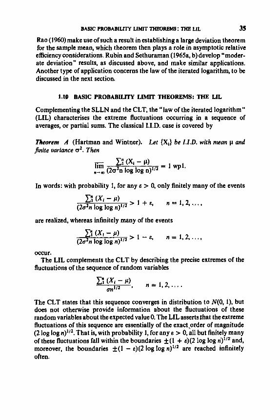
1.10 BASIC PROBABILITY LIMIT THEOREMS: THE LIL
Complementing the SLLN and the CLT, the “law of the iterated logarithm” (LIL) characterises the extreme fluctuations occurring in a sequence of averages, or partial sums. The classical I.I.D. case is covered by
Theorem A (Hartman and Wintner). Let { X , } be I.I.D. with mean p and finite oariunce 6’. Then
In words: with probability 1, for any e > 0, only finitely many of the events
n = 1,2 ,...., c”1 (XI - cc) (2dn log log n)1’2
> 1 + E,
are realized, whereas infinitely many of the events
mxf-cc) > 1 - e , n = l , 2 ,..., (2a’n log log n)l”
occur.
fluctuations of the sequence of random variables The LIL complements the CLT by describing the precise extremes of the
, n = l , 2 ,.... c“1 (XI - cc) UtPZ
The CLT states that this sequence converges in distribution to N(0, I), but does not otherwise provide information about the fluctuations of these random variables about the expected value 0. The LILassertsthat the extreme fluctuations of this sequence are essentially of the exact ,order of magnitude (2 log log n)lI2. That is, with probability 1, for any e > 0, all but finitely many of these fluctuations fall within the boundaries f ( 1 + e)(2 log log ri)’/*and, moreover, the boundaries f ( 1 - e)(2 log log n)1/2 are reached infinitely often.

36 PRELIMINARY TOOL2 AND FOUNDATIONS
The LIL also complements-indeed, refines-the SLLN (but assumes existence of 2nd moments). In terms of the averages dealt with by the SLLN,
the LIL asserts that the extreme fluctuations are essentially of the exact order of magnitude
a(2 log log n)’l2 n1/2
Thus, with probability 1, for any e > 0, the infinite sequence of “confidence intervals”
contains p with only finitely many exceptions. In this fashion the LIL provides the basis for concepts of 100 % confidence intervals and tests of power 1. For further details on such statistical applications of the LIL, consult Robbins (1970), Robbins and Siegmund (1973,1974) and Lai (1977).
A version of the LIL for independent X,’s not necessarily identically distributed was given by Kolmogorov (1929):
Theorem B (Kolmogorov). Let {Xi} be independent with means {pi} and finite uariances {of}. Suppose that B: = c; of --* m and that, for some sequence of constants {mn}, with probability 1,
Then
(To facilitate comparison of Theorems A and B, note that log log(a2) - Extension of Theorems A and B to the case of {X,} a sequence of martingale
Another version of the LIL for independent X i s not necessarily identically
log log x, x + 00.)
diferences has been carried out by Stout (1970a, b).
distributed has been given by Chung (1974), Theorem 7.5.1 :
Theorem C (Chung). Let { X i } be independent with means {pi} andfinite uariunces {of}, Suppose that BX = cy af + 00 and that,for some E > 0,

STOCHASTIC PROCESS FORMULATION OF THE CLT 37
Then
= 1 wpl. c1 (XI - Pi) lim n-,m (2B: log log B,)l/*
Note that (*) and (**) are overlapping conditions, but very different in nature.
As discussed above, the LIL augments the information provided by the CLT. On the other hand, the CLT in conjunction with a suitable rate ofconvergence implies the LIL and thus implicitly contains all the “extra” information stated by the LIL. This was discovered independently by Chung (1950) and Petrov (1966). The following result is given by Petrov (1971). Note the absence of moment assumptions, and the mildness of the rate ofconvergence assumption.
Theorem D (Petrov). Let {Xi} be independent random variables and {B,} a sequence of numbers satisfying
1, n + m . B n + 1 B,+ a,- Bn
Suppose that, for some E > 0,
Then
= 1 wpl. lim c1 xi n-.m (2Bt log log B,)’12
For further discussion and background on the LIL, see Stout (1974), Chapter 5, Chung (1974), Section 7.5, Freedman (1971), Section 1.5, Breiman (1968), pp. 291-292, Lamperti (1966), pp. 41-49, and Feller (1957), pp. 191- 198. The latter source provides a simple treatment of the case that {X,} is a sequence of I.I.D. Bernoulli trials and provides discussion of general forms of the LIL.
More broadly, for general reading on the “almost sure behavior” of sequences of random variables, with thorough attention to extensions to dependent sequences, see the books by RCvisz (1968) and Stout (1974).
1.11 STOCHASTIC PROCESS FORMULATION OF THE CLT
Here the CLT is formulated in a stochastic process setting, generalizing the formulation considered in 1.9 and 1.10. A motivating example, which illustrates the need for such greater generality, is considered in 1.11.1. An

38 PRELIMINARY 700L.S AND FOUNDATIONS
appropriate stochastic process defined in terms of the sequence of partial sums,isintroduced in 1.11.2. As a final preparation, thenotion of"convergence in distribution" in the general setting of stochastic processes is discussed in 1.11.3. On this basis, the stochastic process formulation of the CLT is presented in 1.11.4, with implications regarding the motivating example and the usual CLT. Some complementary remarks are given in 1.11.5.
1.11.1 A Motivating Example Let {XI} be I.I.D. with mean p and finite variance u2 > 0. The Lindeberg- Uvy CLT (1.9.1A) concerns the sequence of random variables
and asserts that S,+ 4 N(0, 1). This useful result has broad application con- cerning approximation of the distribution of the random variable S, =
( X , - p) for large n. However, suppose that our goal is to approximate the distribution of the random variable
k
max C ( X l - p) = max(0, sI,. . . , S,} for large n. In terms of a suitably normalized random variable, the problem may be stated as that of approximating the distribution of
O d h d n I - 1
Here a difficulty emerges. It is seen that M, is not subject to representation as a direct transformation, g(S3, of Sz only. Thus it is not feasible to solve the problem simply by applying Theorem 1.7 (iii) on transformations in con- junction with the convergence s,+ 4 N(0,l) . However, such a scenario can be implemented if S,+ becomes replaced by an appropriate stochastlc process or randomfunction, say { Y,(t), 0 s t s l}, and the concept of 3 is suitably extended.
1.11.2 A Relevant Stochastic Process
Let (XI} and {S,} be as in 1.11.1. We define an associated random function &(t), 0 s t s 1, by setting
and
K(0) = 0

STOCHASTIC PROCESS FORMULATION OF THE CLT 39
and defining x( t ) elsewhere on 0 s t S 1 by linear interpolation. Explicitly, in terms of XI, . . . , X,,, the stochastic process & ( a ) is given by
As n + a, we have a sequence of such random functions generated by the sequence {X,}. The original associated sequence {S:} is recovered by taking the sequence of values { Y,( 1)).
It is convenient to think of the stochastic process { x(t), 0 5 t s 1) as a random element of a suitable function space. Here the space may be taken to be C[O, 11, the collection of all continuous functions on the unit interval
We now observe that the random variable M,, considered in 1.11.1 may be co, 13.
expressed as a direct function of the process &( -), that is,
Mn = SUP YAt) = g(Yn(*)), O S t S I
where g is the function defined on C[O, 13 by
g(x(* ) ) = sup X W , X(’) E cco, 13. osrs1
Consequently, a scenario for dealing with the convergence in distribution of M,, consists of
(a) establishing a “convergence in distribution” result for the random function Y,(.), and
(b) establishing that the transformation g satisfies the hypothesis of an appropriate generalization of Theorem 1.7 (iii).
After laying a general foundation in 1.11.3, we return to this example in 1.1 1.4.
1.11.3 Notions of Convergence in Distribution
Consider a collection of random variables XI, X2, . . . and X having respec- tive distribution functions F1, F2, . . . and F defined on the real line and having respective probability measures PI, P2, . . . and P defined on the Bore1 sets of the real line. Three equivalent versions of “convergence of X, to X in dis- tribution” will now be examined. Recall that in 1.2.4 we defined this to mean that
lim F,,(t) = F(t), each continuity point t of F,
and we introduced the notation X, 5 X and alternate terminology “weak convergence of distributions” and notation F,, =i- F.
n+ OD
(*I

40 PRELIMINARY TOOLS AND FOUNDATIONS
We next consider a condition equivalent to (*) but expressed in terms of PI, Pz, . . . and P. First we need further terminology. For any set A, the boundary is defined to be the closure minus the interior and is denoted by 8A. For any measure P, a set A for which P(8A) = 0 is called a P-continuity set. In these terms, a condition equivalent to (*) is
lim P,,(A) = P(A), each P-continuity set A. (**I
The equivalence is proved in Billingsley (1968), Chapter 1, and is discussed also in Cramkr (1946), Sections 6.7 and 8.5. In connection with (**), the terminology “weak convergence of probability measures” and the notation P,, * P is used.
There is a significant advantage of (**) over (*): it may be formulated in a considerably more general context. Namely, the variables XI, X z , . . . and X may take values in an arbitrary metric space S. In this case PI, Pz, . , . and P are defined on the Bore1 sets in S (i.e., on’the a-field generated by the open sets with respect to the metric associated with S). In particular, if S is a metrizable function space, then P,, * P denotes “convergence in distribution“ of a sequence of stochastic processes to a limit stochastic process. Thus, for example, for the process Y,(.) discussed in 1.11.2, Y,,(.) 4 Y(-) becomes defined for an appropriate limit process Y(-).
For completeness, we mention a further equivalent version of weak con- vergence, also meaningful in the more general setting, and indeed often adopted as the primary definition. This is the condition
(***) lini g dP,, = g dP, each bounded continuous function on S.
The equivalence is proved in Billingsley (1968), Chapter 1. See also the proof of Theorem 1.5.1A.
n-m
II- aD s, s, 1.1 1.4 Donsker’s Theorem and Some Implications Here we treat formally the “partial sum” stochastic process introduced in 1.11.2. Specifically, for an I.I.D. sequence of random variables {X,} defined on a probability space (Q d, P) and having mean p and finite variance u2, we consider for each n(n = 1,2, . . .) the stochastic process
which is a random element of the space C[O, 1). When convenient, we suppress the o notation. The space C[O, 13 may be metrized by
P ( X , Y) = SUP Ix(0 - Y(t)l O 5 f 5 l

STOCHASTIC PROCESS FORMULATION OF THE CLT 41
for x = x(.) and y = y ( . ) in C[O, 13. Denote by A? the class of Bore1 sets in C[O, 11 relative to p. Denote by Q,, the probability distribution of Y , ( . ) in C[O, I], that is, the probability measure on (C, A?) induced by the measure P through the relation
We have this designated a new probability space, (C, A?, QJ, to serve as a probability model for the partial sum process Y,(.). In order to be able to associate with the sequence of-processes { Y,,(.)} a limit process Y(.), in the sense of convergence in distribution, we seek a measure Q on (C, A?) such that Q, es Q. This will be given by Donsker’s Theorem below.
An important probability measure on (C, A?) is the Wiener measure, that is, the probability distribution of one coordinate of the random path traced by a particlein “Brownian motion,”or formally the probability measuredefined by the properties:
Q,,(B) = P({o: & ( a , o)EB}), BEA?.
(a) W ( { x ( . ) : x(0) = 0)) = 1; (b) for all 0 < I I; 1 and - a0 < a < m,
(c) for 0 5 to I; tl I, t k I; 1 and - m < al, . . . , ak < 03,
k
= n W ( { x ( * ) : X( t , ) - dt i - 1) s ad). 1 1 1
The existence and uniqueness of such a measure is established, for example, in Billingsley (1968), Section 9.
A random element of C[O, 13 having the distribution W is called a Wiener process and is denoted for convenience by { W(t) , 0 I; t s l}, or simply by W. Thus, for a Wiener process W(.), properties (a), (b) and (c) tell us that
(a) W(0) = 0 with probability 1 ; (b) W(t) is N(0, t ) , each t E (0, 13; (c) for 0 s to I; t l 5 * * I; t, s 1, the increments W(r , ) - W(to), , . . ,
w(tk) - w(tk- 1) are mutually independent.
We are now ready to state the generalization of the Lindeberg-Evy CLT.
Theorem (Donsker). Let {Xi} be I.I.D. with mean p andfinite variance 02,
Define Yn(.) and Q, as above. Then
Qn =S W.

42 PRELIMINARY TOOLS AND FOUNDATIONS
(Alternatively, we may state this convergence as x ( * ) 3 W(.) in C[O, 13.) The theorem as stated above is proved in Billingsley (19681 Section 10. However, the theorem was first established, in a different form, by Donsker
To see that the Donsker theorem contains the Lindeberg-Ltvy CLT, (195 1).
consider the set
B, = {x(-): x(1) s a}
in C[O, 13. It may be verified that B. E 1. Since
we have
It may be verified that B, is a W-continuity set, that is, W(dB,) = 0. Hence, by (**) of 1.11.3, Donslcer’s Theorem yields
lim Q,(B,) = W(B,). n+ m
Next one verifies (see 1.11.5(i) for discussion) that
W(Ba) = @(a).
Since a is chosen arbitrarily, the Lindeberg-Livy CLT follows.
variable Now let us apply the Donsker theorem in connection with the random
considered in 1.11.2. Consider the set
B,’ = x(*): sup ~ ( t ) s a . I OStSl I It may be verified that B,’ belongs to 1 and is a W-continuity set, so that
lim P ( M , S a) = lim Q,(BZ) = W(B,‘). II’ OD ,-.OD
By determining (again, see 1.11.5(i) for discussion) that
one obtains the limit distribution of M,.

TAYLOR’S THEOREM ; DIFPERENTULS 43
The fact that the sets {BZ, a > 0} are W-continuity sets is equivalent to the functional g: g(x(-)) = S U ~ ~ ~ ~ ~ I x( t ) being continuous (relative to the metric p ) with W-probability 1. Thus, by an appropriate extension of Theorem 1.7(iii), the preceding argument could be structured as follows:
Mn = g(Yn(*)) 4 B(w(.)) = SUP ~ ( t ) . O S f S 1
Elaboration of this approach is found in Billingsley (1968).
1.1 1.5 Complementary Remarks
(i) The application of Donsker’s Theorem to obtain the limit distribution of some functional of the partial sum process Y,( .) requires the evaluation of quantities such as W(B,) and W(B,+). This step may be carried out by a separate application of Donsker’s Theorem. For example, to evaluate W(B,+), the quantity limn P(M, I; a) is evaluated for a particular I.I.D. sequence {XI}, one selected to make the computations easy. Then Donsker’s Theorem tells us that the limit so obtained is in fact W(B,+). Thus W(B,*) has been evaluated, so that-again by Donsker’s Theorem-the quantity limn P(Mn I; a) is known for the general case of I.I.D. X i s with finite variance. Such a technique for finding limn P(M, 5 a) in the general case represents an application of what is known as the “inuariance principle.’’ It is based on the fact that the limit in question is invariant over the choice of sequence {X,} , within a wide class of sequences.
(ii) Other limit theorems besides the CLT can likewise be reformulated and generalized via the theory of convergence of probability measures on metric spaces. In connection with a given sequence of random variables {X,}, we may consider other random functions than K(.), and other function spaces than C[O, 13.
(iii) In later chapters, a number of relevant stochastic processes will be pointed out in connection with various statistics arising for consideration. However, stochastic process aspects will not be stressed in this book. The intention is merely to orient the reader for investigation of these matters elsewhere.
(iv) For detailed treatment of the topic of convergence of probability measures on metric spaces, the reader is referred to Billingsley (1968) and Parthasarathy (1967).
1.12 TAYLOR’S THEOREM; DIFFERENTIALS
1.12.1 Taylor’s Theorem The following theorem is proved in Apostol(1957), p. 96.
Theorem A (Taylor). Let the function g h u e a jni te nth deriuatiue g‘”) euerywhere in the open interual (a, b) and (n - 1)th deriuatiue 8‘”- I ) continuous

44 PRELIMINARY TOOLS AND FOUNDATIONS
in the closed interval [a, b]. Let x E [a, b). For each point y E [a, b], y # x, there exists a point z interior to the interval joining x and y such that
Remarks. (i) For the case x = a, we may replace g")(x) in the above formula by g$)(a), the kth order right-hand derivative of g at the point a; in place ofcontinuity ofg("- ')(x) at x = a, it is assumed that g$)(x) is continuous at x = a, for each k = 1, ..., n - 1. Likewise, for x = 6, g(k)(x) may be replaced by the left-hand derivative &6). These extensions are obtained by minor modification of Apostol's proof of Theorem A.
(ii) For a generalized Taylor formula replacing derivatives by finite differences, see Feller (1966), p. 227.
We can readily establish a multivariate version of Theorem A by reduction to the univariate case. (We follow Apostol(1957), p. 124.)
Theorem B (Multivariate Version). Let thefunction gdefned on Rm possess continuous partial derivatives of order n at each point of an open set S c Rm. Let x E S. For each point y, y # x, such that the line segment L(x, y) joining x and y lies in S, there exists a point z in the interior of L(x, y) such that
PROOF. Define H(a) = g(x + a(y - x)) for real a. By the assumed continuity of the partial derivatives of g, we may apply an extended chain rule for differentiation of H and obtain
and likewise, for 2 s k 5; n,
Since L(x, y) c S, S open, it follows that the function H satisfies the con- ditions of Theorem A with respect to the interval [a, 61 = [0,1]. Conse- quently, we have
where 0 < z < 1. Now note that H(1) = g(y), H(0) = g(x), etc. H

CONDITIONS FOR DETERMINATION OF A DISTRIBUTION BY ITS MOMENTS 45
A useful alternate form of Taylor’s Theorem is the following, which re- quires the nth order differentiability to hold only at the point x and which characterizes the asymptotic behavior of the remainder term.
Theorem C (Young’s form of Taylor’s Theorem). Let g have afinite nth deriuatiue at the point x. Then
PROOF. Follows readily by induction. Or see Hardy (1952), p. 278.
1.12.2 Differentials
The appropriate multi-dimensional generalization of derivative of a function of one argument is given in terms of the diflerential. A function g defined on R” is said to have a diflerential, or to be totally diferentiable, at the point xo if the partial derivatives
all exist at x = xo and the function
(called the “differential”) satisfies the property that, for every E > 0, there exists a neighborhood N8(xo) such that
Idx) - B(XO) - d x o ; x - X O ) ~ I; ellx - x0IL all x E N,(xo).
Some interrelationships among differentials, partial derivatives, and con- tinuity are expressed in the following result.
Lemma (Apostol(1957), pp. 110 and 118). (i) Ifg has a diflerential at xo, then g is continuous at xo.
(ii) Zfthe partial deriuatiues ag/axl, 1 I; i I; m, exist in a neighborhood of xo and are continuous at xo, then g has a duerential at xo.
1.13 CONDITIONS FOR DETERMINATION OF A DISTRIBUTION BY IT!3 MOMENTS
Let F be a distribution on the real line with moment sequence Q
ak = /-m2 dF(x), k = 1,2, , . . I
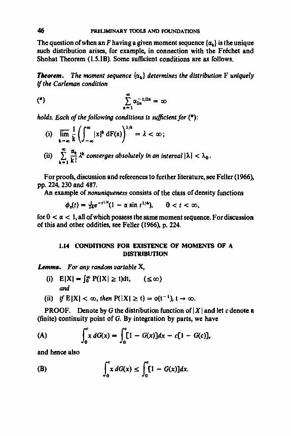
46 PRELIMINARY TOOLS AND FOUNDATIONS
The question of when an F having a given moment sequence {ak} is the unique such distribution arises, for example, in connection with the Frdchet and Shohat Theorem (1.5.1B). Some sufficient conditions are as follows.
Theorem. The moment sequence {ar} determines the distribution F uniquely i f the Carleman condition
n- 1
holds. Each of the following conditions is sficient for (*):
(i) lim 1 (I_”.lxlr dF(x))’lk 3: I < 00;
(ii)
t -rm
m
C !!! Ik conuerges absolutely in an interval lkl < ko. k - 1 k!
For proofs, discussion and references to further literature, see Feller (1966),
An example of nonuniqueness consists of the class of density functions pp. 224,230 and 487.
4dt) = f fe - f ’ ’4( i - a sin t”’),
for 0 < a < 1, all ofwhich possess the same moment sequence. For discussion of this and. other oddities, see Feller (1966), p. 224.
o < t < 00,
1.14 CONDITIONS FOR EXISTENCE OF MOMENTS OF A DISTRIBUTION
Lemma. For any random variable X,
(i) ElXl= j? P ( l X l 2 t)dt, (Sm) and
(ii) if ElXl < 00, then P(lXl 2 t) = o(t-’), t + 00.
PROOF. Denote by G the distribution function of ( X I and let c denote a (finite) continuity point of G. By integration by parts, we have
(A)
and hence also
/:x dG(x) = l [ l - G(x)]dx - cC1 - G(c)],
x dG(x) 5 [ l - G ( x ) ] ~ x . Jo Jo
ASYMPTOTIC MPECTS OF STATISTICAL INFERENCE PROCEDURES 47
Further, it is easily seen that
c [ l - G(c)] S r x dG(x).
Now suppose that E l X l = 00. Then (B) yields (i) for this case. On the other hand, suppose that E l X l < 00. Then (C) yields (ii). Also, making use of (ii) in conjunction with (A), we obtain (i) for this case.
The lemma immediately yields (Problem 1.P.29) its own generalization:
Corollary. For any random variable X and real number r > 0,
(i) ElXl’ = r @ t’-’P(IXI 2 t)dt and
(ii) ifElXr < 00, then P(lX1 2 t) = o(t-‘), t
Remark. It follows that a necessary and sufficient condition for E l X r < 00 is that t‘-’P(IXI 2 t ) be integrable. Also, if P ( ( X ( 2 t ) = O(t-7, then EIXY < 00 for all r < s. W
co.
1.15 ASYMPTOTIC ASPEClS OF STATISTICAL INFERENCE PROCEDURES
By “inference procedure” is usually meant a statistical procedure for esti- mating a parameter or testing a hypothesis about a parameter. More generally, it may be cast in decision-theoretic terms as a procedure for selecting an action in the face of risks that depend upon an unknown parameter. In the present discussion, the more general context will not be stressed but should be kept in mind nevertheless.
Let the family of possible models for the data be represented as a collection of probability spaces {(Q 91, Pel, 8 E O}, indexed by the “parameter” 8. In discussing “estimation,” we shall consider estimation of some parametric function g(8). In discussing “hypothesis testing,” we have in mind some “null hypothesis”: 8 E Q,( c0). In either case, the relevant statistic (“estimator” or “test statistic”) will be represented as a sequence of statistics T,, T’, . . . . Typically, by “statistic” we mean a specified function of the sample, and T,, denotes the evaluation of the function at the first n sample observations XI, . . . , X,. This book deals with the asymptotic properties of a great variety of sequences { T,,} of proven or potential interest in statistical inference.
For such sequences { G}, we treat several important asymptotic features: “asymptotic unbiasedness”(in the context of estimation only); “consistency” (in estimation) and “almost sure behavior ”; “ asymptoticdistribution theory”; “asymptotic relative efficiency.”These notions are discussed in 1.15.1-1.15.4,

48 PRELIMINARY MOLS AND FOUNDATIONS
respectively. The concept of “asymptotic efficiency,” which is related to “asymptotic relative efficiency,” will be introduced in Chapter 4, in connection with the theory of maximum likelihood estimation. Some further important concepts-“deficiency,” “asymptotic sufficiency,” “local asymptotic nor- mality,”“local asymptotic admissibility,” and ” local asymptotic minimaxity” -are not treated in this book.
1.15.1 Asymptotic Unbiasedneas (in Estimation) Recall that in estimation we say that an estimator T of a parametric function g(8) is unbiased if fie{ T } = g(O), all 8 E 8. Accordingly, we say that a sequence of estimators {T,} is asymptotically unbiased for estimation of g(8) if
lim E,{ T,} = g(8), each 8 E 0.
(In hypothesis testing, a test is unbiased if at each 8 9 Oo, the “power” of the test is at least as high as the “size” of the test. An asymptotic version of this concept may be defined also, but we shall not pursue it.)
1.15.2 Consistency (in Estimation) and Almost Sure Behavior A sequence of estimators {T,} for a parametric function g(8) is “consistent” if T, converges to g(8)in some appropriate sense. We speakof weak consistency,
strong consistency,
and consistency in rth mean,
When the term “consistent” is used without qualification, usually the weak mode is meant.
(In hypothesis testing, consistency means that at each 8 9 Qo, the power of the test tends to 1 as n -+ 00. We shall not pursue this notion.)
Consistency is usually considered a minimal requirement for an inference procedure, Those procedures not having such a property are usually dropped from consideration.
A useful technique for establishing mean square consistency of an estimator T, is to show that it is asymptotically unbiased and has variance tending to 0.
Recalling the relationships considered in Section 1.3, we see that strong consistency may be established by proving weak or rth mean consistency with a sufficiently fast rate of convergence.
There arises the question of which of these forms of consistency is of the greatest practical interest. To a large extent, this is a philosophical issue, the answer depending upon one’s point of view. Concerning rth mean consistency
n-r Q
T, 4
T, g(e),
T, 3 de).

ASYMPTOTIC ASPECTS OF STATISTICAL INFERENCE PROCEDURES 49
versus the weak or strong versions, the issue is between “moments” and “probability concentrations” (see 1.15.4 for some further discussion). Regarding weak versus strong consistency, some remarks in support of insisting on the strong version follow.
(i) Many statisticians would find it distasteful to use an estimator which, if sampling were to continue indefinitely, could possibly fail to converge to the correct value. After all, there should be some pay-off for increased samp- ling, which advantage should be exploited by any “good” estimator.
(ii) An example presented by Stout (1974),Chapter 1,concerns aphysician treating patients with a drug having unknown cure probability 8 (the same for each patient). The physician intends to continue use of the drug until a superior alternative is known. Occasionally he assesses his experience by estimating 8 by the proportion 8, ofcures for the n patients treated up to that point in time. He wants to be able to estimate 8 within a prescribed tolerance e > 0. Moreover, he desires the reassuring feature that, with a specified high probability, he can reach a point in time such that his current estimate has become within E of 8 and no subsequent value of the estimator would mislead- ingly wander more than E from 8. That is, the physician desires, for prescribed 6 > 0, that there exist an integer N such that
p rnaxld, - el s 8 ) 2 1 - 6. ( n a N
Weak consistency (which follows in this case by the WLLN) asserts only that
and hence fails to supply the reassurance desired. Only by strong consistency (which follows in this case by the SLLN) is the existence of such an N guar- anteed.
(iii) When confronted with two competing sequences {T,} and {T:} of estimators or test statistics, one wishes to select the best. This decision calls upon knowledge of the optimum properties, whatever they may be, possessed by the two sequences. In particular, strong consistency thus becomes a useful distinguishing property.
So far we have discussed “consistency” and have focused upon the strong version. More broadly, we can retain the focus on strong consistency but widen the scope to include the precise asymptotic order of‘mangitude of the fluctuations T,, - g(0), just as in 1.10 we considered the LIL as a refinement of the SLLN. In this sense, as a refinement of strong convergence, we will seek to characterize the “almost sure behavior” of sequences { T,}. Such characteriza- tions are of interest not only for sequences of estimators but also for sequences of test statistics. (In the latter case g(8) represents a parameter to which the test statistic T,, converges under the model indexed by 0.)
p(l6, - el s E ) -, 1, n -, OC),
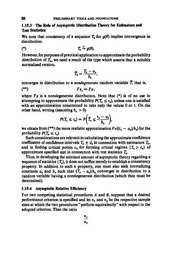
50 PRELIMINARY TOOLS A N D FOUNDATIONS
1.15.3 The Role of Asymptotic Distribution Theory for Estimators and Test Statistics We note that consistency of a sequence T, for g(8) implies convergence in distribution:
However, for purposes of practical application to approximate the probability distribution of T,, we need a result of the t y p which asserts that a suitably normalized version,
converges in distribution to a nondegenerate random variable p, that is,
where Fp is a nondegenerate distribution. Note that (*) is of no use in attempting to approximate the probability P(T, s t,,), unless one is satisfied with an approximation constrained to take only the values 0 or 1. On the other hand, writing (assuming b,, > 0)
(**I Ff, * FT Y
we obtain from (**)the more realistic approximation Fr((t, - a,)/b3 for the probability P(T, s re).
Such considerations are relevant in calculating the approximate confidence coefficients of confidence intervals T, f d,, in connection with estimators T,, and in finding critical points c, for forming critical regions {T, > c,} of approximate specified size in connection with test statistics T,.
Thus, in developing the minimal amount of asymptotic theory regarding a sequence of statistics { q}, it does not suffice merely to establish a consistency property. In addition to such a property, one must also seek normalizing constants a, and b,, such that (T, - converges in distribution to a random variable having a nondegenerate distribution (which then must be determined).
1.15.4 Asymptotic Relative Efficiency For two competing statistical procedures A and E , suppose that a desired performance criterion is specified and let nl and n2 be the respective sample sizes at which the two procedures “perform equivalently” with respect to the adopted criterion. Then the ratio
n1
n2
-

ASYMPTOTIC ASPECTS OF STATISTICAL INFERENCE PROCEDURES 51
is usually regarded as the relative eflciency (in the given sense) of procedure B relative to procedure A. Suppose that the specified performance criterion is tightened in a way that causes the required sample sizes n , and n, to tend to 00. If in this case the ratio n, /n , approaches to limit L, then the value L represents the asymptotic relatioe eflaiency of procedure B relative to procedure A. It is stressed that the value L obtained depends upon the par- ticular performance criterion adopted.
As an example, consider estimation. Let { TAn} and { TBn} denote competing estimation sequences for a parametric function g(0). Suppose that
If our criterion is based upon the variance parameters ofi(0) and a%@ of the asymptotic distributions, then the two procedures “perform equivalently” at respective sample sizes n , and n2 satisfying
a m 4(@ -N-
n1 n2
in which case
Thus afi(O)/a;((e) emerges as a measure of asymptotic relative efficiency of procedure B relative to procedure A. If, however, we adopt as performance criterion the probability concentration of the estimate in an &-neighborhood of g(8), for E specified and fixed, then a different quantity emerges as the measure of asymptotic relative efficiency. For a comparison of { TAn} and { TBn} by this criterion, we may consider the quantities
PAn(&, 8) = P#(l TAn - dell > PBn(&, 0) = P@(l TBn - g(@I >
and compare the rates at which these quantities tend to 0 as n + 00. In typical cases, the convergence is “exponentially fast **;
In such a case, the two procedures may be said to “perform equivalently” at respective sample sizes n, and n2 satisfying

52 PRELIMJNARY TOOLS AND FOUNDATIONS
In this case
yielding y&, O)/yA(e, 0) as a measure of asymptotic relative efficiency of procedure E relative to procedure A, in the sense of the probability con- cen tra t ion criterion.
It is thus seen that the “asymptotic variance” and “probability concentra- tion” criteria yield differing measures of asymptotic relative efficiency. It can happen in a given problem that these two approaches lead to discordant measures (one having value > 1, the other < 1). For an example, see Basu (1956).
The preceding discussion has been confined to asymptotic relative efficiency in estimation. Various examples will appear in Chapters 2-9. For the asymp- totic variance criterion, the multidimensional version and the related concept of asymptotic eflciency (in an “absolute” sense) will be treated in Chapter 4. The notion of asymptotic relative efficiency in testing is deferred to Chapter 10, which is devoted wholly to the topic. (The apparent dichotomy between estimation and testing should not, however, be taken too seriously, for “testing” problems can usually be recast in the context of estimation, and vice versa.)
Further introductory discussion of asymptotic relative efficiency is found in Cramtr (1946), Sections 37.3-37.5, Fraser (19571 Section 7.3, Rao (1973), Sections 5c.2 and 7a.7, and Bahadur (1967).
l.P PROBLEMS
Section 1.1 1. Prove Lemma 1.1.4.
Section 1.2
2. (a) Show that (Xnl, . . . , X,) 1: (Xl, . , . , Xk)if and only if X,, 5 X, for each j = 1, . . . , k.
(b) Same problem for wp!. (c) Show that X, = (Xnl, , . . , Xnk) % X, = (Xm1, . . . , X m k ) if
and only if, for every e > 0. lim P{llX,,, - X,ll < e, all m 2 n} = 1. n-rm
3. Show that X,$ X implies X, = Op(l). 4. Show that U, = op(K) implies U, = O,(V,,). 5. Resolve the question posed in 1.2.6.

PROBLEMS 53
Section 1.3
6. Construct a sequence {X,} convergent wpl but not in rth mean, for any r > 0, by taking an appropriate subsequence of the sequence in Example 1.3.8D.
Section 1.4
7. Prove Lemma 1.4B. 8. Verify that Lemma 1.4C contains two generalizations of Theorem
1.3.6. 9. Prove Theorem 1.4D.
Section 1.5
10. Do the task assigned in the proof of Theorem 1.5.1A. 11. (a) Show that Scheffk's Theorem (1S.lC) is indeed a criterion for
(b) Exemplify a sequence of densities f, pointwise convergent to a convergence in distribution.
function f not a density. 12. (a) Prove P6lya's Theorem (1 5 3 ) .
(b) Give a counterexample for the case of F having discontinuities. 13. Prove part (ii) of Slutsky's Theorem (1.5.4). 14. (a) Prove Corollary 1.5.4A by direct application ofTheorem 1.5.4(i).
(b) Prove Corollary 1.5.48. 15. Prove Lemma 1.5.5A. (Hint: apply Polya's Theorem.) 16. Prove Lemma 1.5.5B. 17. Show that X, is AN((r,, c,'C) if and only if
xn - 5 N(0, C). Cn
Here {c,} is a sequence of real constants and C a covariance matrix. 18. Prove or give counter-example: If X, 1: X and Y. 3 Y, then X, +
19. Let X, be AN(p , a2/n), let Y. be AN@, u/n), c # 0, and put 2, = &(X, - p)/Y,. Show that Z, is AN(0, a2/c2). (Hint: apply Problem 1.P.20.)
20. Let X, be AN(p, at). Show that X, 3 p if and only if a, + 0, n + 00.
(See Problem 1.P.23 for a multivariate extension.) 21. Let X, be A N @ , ox) and let Y, = 0 with probability 1 - n-' and
= n with probability n - ' . Show that X, + Y. is A N @ , 0,').
y , $ X + Y

54 PRELIMINARY Mots AND POUM)ATIONS
Section 1.7 22. Verify Application B of Corollary 1.7. (Hint: Apply Problem 1.P.17,
Corollary 1.7 and then Theorem 1.7 with g(x) - fi) 23. Verify Application C of Corollary 1.7. (Hint: Apply the Cram&-
Wold device, Problem 1.P.20, and the argument used in the previous problem. Alternatively, instead of the latter, Problems 1.P.2 and l.P.l4(b) may be used.)
(b) Do analogues hold for convergence in distribution?
Section 1.9
24. (a) Verify Application D of Corollary 1.7.
25. Derive Theorem 1.9.1B from Theorem 1;9.1A. 26. Obtain Corollary 1.9.3. 27. Let X, be a 1,' random variable.
(a) Show that X, is AN(n, 2n). (b) Evaluate the bound on the error of approximation provided
by the Berry-Esseen Theorem (with van Beeck's improved constant).
Section 1.13
moments.
Section 1.14
28. Justify that the distribution N(p, u2) is uniquely determined by its
29. Obtain Corollary 1.14 from Lemma 1.14.
Section 1.15
parameter 8 by X,. Answer (with justifications): 30. Let X, have k i t e mean p,, n = 1,2, . . . . Consider estimation of a
(a) If X , is consistent for 8, must X, be asymptotically unbiased? (b) If X, is asymptotically unbiased, must X, be consistent? (c) If X, is asymptotically unbiased and Var{X,} -+ 0, must X, be
consistent 7 (Hint: See Problem 1.P.21.)

C H A P T E R 2
The Basic Sample Statistics
This chapter considers a sample XI, . . . , X , of independent observations on a distribution function F and examines the most basic types of statistic usually ofinterest. Thesampledistributionfunction and the closely related Kolmogorov- Smirnov and Cramtr-von Mises statistics, along with sample density functions, are treated in Section 2.1. The sample moments, the sample quantiles, and the order statistics are treated in Sections 2.2,2.3 and 2.4, respectively.
There exist useful asymptotic representations, first introduced by R. R. Bahadur, by which the sample quantiles and the order statistics may be expressed in terms of the sample distribution function as simple sums of random variables. These relationships and their applications are examined in Section 2.5.
By way of illustration of some of the results on sample moments, sample quantiles, and order statistics, a study of confidence intervals for (population) quantiles is provided in Section 2.6.
A common form of statistical reduction of a sample consists of grouping the observations into cells. The asymptotic multivariate normality of the corresponding cell frequency vectors is derived in Section 2.7.
Deeper investigation of the basic sample statistics may be carried out within the framework of stochastic process theory. Some relevant stochastic processes associated with a sample are pointed out in Section 2.8.
Many statistics of interest may be represented as transjiormations of one or more of the “basic” sample statistics. The case of functions of several sample moments or sample quantiles, or of cell frequency vectors, and the like, is treated in Chapter 3. The case of statistics defined as functionals of the sample distribution function is dealt with in Chapter 6.
Further, many statistics of interest may be conceptualized as some sorts of generalization of a “basic” type. A generalization of the idea of forming a
55

56 THE BASIC SAMPLE STATlSTlCS
sample average consists of the U-statistics, introduced by W. Hoeffding. These are studied in Chapter 5. As a generalization of single order statistics, the so-called linear functions of order statistics are investigated in Chapter 8.
2.1 THE SAMPLE DISTRIBUTION FUNCTION
Consider an LLD. sequence {X , ) with distribution function F. For each sample of size n, { X . . . , X,,}, a corresponding sample distributionfunction F,, is constructed by placing at each observation Xi a mass l/n. Thus F,, may be represented as
1 ’ n I - 1
F,,(x) = - C I ( X 1 s x), -00 < x < 00.
(The definition for F defined on Rk is completely analogous.) For each fixed sample {XI, . . . , X,,}, F,,(-) is a distribution function, con-
sidered as a function of x. On the other hand, for each fixed value of x, F,,(x) is a random uuriable, considered as a function of the sample. In a view encom- passing both features, F,,(.) is a randum distribution function and thus may be treated as a particular stochastic process (a random element of a suitable function space).
The simplest aspect of F,, is that, for each fixed x, F,,(x) serves as an estimator of F(x). For example, note that F,,(x) is unbiased: E{F,,(x)} - F(x). Other properties, such as consistency and asymptotic normality, are treated in 2.1.1.
Considered as a whole, however, the function F,, is a very basic sample statistic, for from it the entire set of sample values can be recovered (although their order of occurrence is lost). Therefore, it can and does play a fundamental role in statistical inference. Various aspects are discussed in 2.1.2, and some important random variables closely related to F,, are introduced. One of these, the Kolmogorou-Smirnou statistic, may be formulated in two ways: as a measure of distance between F,, and F, and as a test statistic for a hypothesis H: F = F,,. For the Kolmogorov-Smirnov distance, some probability in- equalities are presented in 2.1.3, the almost sure behavior is characterized in 2.1.4, and the asymptotic distribution theory is given in 2.1.5. Asymptotic distribution theory for the Kolmogorov-Smirnov test statistic is discussed in 2.1.6. For another such random variable, the Cram&-uon Mises statistic, almost sure behavior and asymptotic distribution theory is discussed in 2.1.7.
For the case of a distribution function F having a densityf, “sample density function” estimators (off) are of interest and play similar roles to F,,. However, their theoretical treatment is more difficult. A brief introduction is given in 2.1.8.

THE SAMPLE DISTRIBUTION FWNCTION 57
Finally, in 2.1.9, some complementary remarks are made. For a stochastic process formulation of the sample distribution function, and for related con- siderations, see Section 2.8.
2.1.1 FJx) as Pointwise Estimator of F(x)
We have noted above that F,(x) is unbiased for estimation of F(x). Moreover,
so that F,(x) 2 F(x). That is, F,(x) is consisrent in mean square (and hence weakly consistent) for estimation of F(x). Furthermore, by a direct a plica- tion of the SLLN (Theorem 1.8B), F,(x) is strongly consistenr: F,(x) % F(x). Indeed, the latter convergence holds unijbrnly in x (see 2.1.4).
Regarding the distribution theory of F,(x), note that the exact distribution of nF,(x) is simply binomial (n, F(x)). And, immediately from the Lindeberg- Uvy CLT (1.9.1A), the asymptotic distribution is given by
P
Theorem. For eachfixed x, - 00 < x < 00,
2.1.2 The Role of the Sample Distribution Function in Statistical Inference We shall consider several ways in which the sample distribution function is utilized in statistical inference. Firstly, its most direct application is for estimation of the population distribution function F. Besides pointwise estimation of F(x), each x, as considered in 2.1.1, it is also of interest to char- acterize globally the estimation of F by F,. To this effect, a very useful measure of closeness of F, to F is the Kolmogoroo-Smirnoo distance
D, = SUP I F,(x) - F(x) I .
A related problem is to express co@dence bands for F(x), -00 < x < 00.
Thus, for selected functions a(x) and b(x), it is of interest to compute prob- abilities of the form
--oD<x<aD
P(F,(X) - U ( X ) 5 F(x) S F,(x) + b(x), - 00 < x < 00).
The general problem is quite difficult; for discussion and references, see Durbin (1973a), Section 2.5. However, in the simplest case, namely a(x) I b(x) = d, the problem reduces to computation of
P(Dn < 4 .

ss THE BASIC SAMPLE STATISTICS
In this form, and for F continuous, the problem of confidence bands is treated in Wilks (1962), Section 11.7, as well as in Durbin (1973a).
Secondly, we consider “goodness of fit ** test statistics based on the sample distribution function. The null hypothesis in the simple case is H: F = Fo, where Fo is specified. A useful procedure is the Kolmogorou-Smirnov test stutisttc
4 S U P I FJx) - Fob) I, - Q < X < m
which reduces to D, under the null hypothesis. More broadly, a class of such statistics is obtained by introducing weight functions:
SUP Iw(x) [FAX) - F~(xll I * - m < r < m
(Similarly, more general versions of D, may be formulated.) There are also one-sided versions of A, :
A: = SUP [FAX) .- FO(x)I, - m < x < m
A, = SUP [F~(x) - F,(x)]. - Q < X < Q
Another important class of statistics is based on the Crumb-oon Mises test statistic
cn n s_Om;Fn(x) - ~0(x)12 d ~ o ( x )
and takes thegeneral form n w(Fo(x)) [F,(x) - Fo(x)I2 dFo(x). For example, for w(t) = [t(l - t ) ] - ’ , each discrepancy F,(x) - Fo(x) becomes weighted by the reciprocal of its standard deviation (under Ho), yielding the Anderson- Darling statistic.
Thirdly, some so-called “tests on the circle” are based on F,. The context concerns data in the form of directions, and the null hypothesis of randomness of directions is formulated as randomness of n points distributed on the circumference of the unit circle. With appropriately defined Xis, a suitable test statistic is the Kuiper statistic
K = A : - A , .
This statistic also happens to have useful properties when used as an alter- native to A,, in the goodness-of-fit problem.
Finally, we mention that the theoretical investigation of many statistics of interest can advantageously be carried out by representing the statistics, either exactly or approximately, as functionals of the sample distribution function, or as functionals of a stochastic process based on the sample

THE SAMPLE DISTRIBUTION FUNCTION 59
distribution function. (See Section 2.8 and Chapter 6). In this respect, metrics such as 0, play a useful role.
In light of the foregoing remarks, it is seen that the random variable D, and related random variables merit extensive investigation. Thus we devote 2.1.3-2.1.6 to this purpose.
An excellent introduction to the theory underlying statistical tests based on F, is the monograph by Durbin (1973a). An excellent overview of the prob- abilistic theory for F, considered as a stochastic process, and with attention to multidimensional F, is the survey paper of Gaenssler and Stute (1979). Useful further reading is provided by the references in these manuscripts. Also, further elementary reading of general scope consists of Bickel and Doksum (1977), Section 9.6, Cramtr (1946), Section 25.3, Lindgren (1968), Section 6.4, Noether (1967), Chapter 4, Rao (1973), Section 6f.1, and Wilks (1962), Chapters 11 and 14.
2.1.3 Probability Inequalities for the KolmogorovSmimov Distance Consider an I.I.D. sequence {XI} of elements of R', let F and F, denote the corresponding population and sample distribution functions, and put
D, = sup IF,(x) - F(x)l . X € R *
For the case k = 1, an exponential-type probability inequality for D, was established by Dvoretzky, Kiefer, and Wolfowitz (1956).
Theorem A (Dvoretzky, Kiefer, and Wolfowitz). Let F be defined on R. There exists afinite positive constant C (not depending on F ) such that
P(D, > d) < Ce-'nd2, for all n = 1,2,. . . . Remarks. (i) DKW actually prove this result only for F uniform on [O, 13, extension to the general case being left implicit. The extension may be seen as follows. Given independent observations X, having distribution F and defined on a common probability space, one can construct independent uniform LO, 13 variates 8 such that PIXl = F-'(&)] = 1, 1 5 i 5 n. Let G denote the uniform [0, 13 distribution and G, the sample distribution function of the Y,'s. Then F(x) = G(F(x)) and, by Lemma 1.1.4(iii), (wpl) F,(x) = G,(F(x)). Thus
d > 0,
OX = SUP IFn(x) - F(x)l = SUP IGn(F(x)) - G(F(x))I --ao<x<m - m < x < m
I; SUP I G,(t) - G(t)( = D,G, 0<1<1
so that P(D: > d ) s P(Df > d).

60 THE BASIC SAMPLE STATISTICS
Alternatively, reduction to the uniform case may be carried out as follows. Let Yl, , , , , Y. be independent uniform [O, 11 random variables. Then Y { ( X , , . . . , X, ) } = Y { ( F - ' ( Y l ) , , . , , F - ' ( x ) ) } . Thus
Y{Dn(XI , * * * 9 Xn)} = Y{Dn(F- ' (Yl ) , * - - 9 f+-'(K))I* But
D,(F-l(Yl), . . . , F - i ( G ) ) = sup I n-1 i I ( F - l ( K ) 5 x) - F(x) I -olcx<ol 1-1
= sup ln-1 i I ( K s F(x)) - ~ ( x ) l
s sup n - l z I ( K S t ) - t
- w e x e m 111
octc I I ,:I
= D,( Y1, . . . , K). (ii) The foregoing construction does not retain the distribution-free
property in generalizing to multidimensional F. For F in Rk, let F, denote the j th marginal of F, 1 s j 5; k, and put F(x) = (Fl(xl), . . . , F&)) for x = xI, . . . , xk). Putting Y, = F(X,), 1 S i S n, and letting GF denote the distribu- tion of each Y,, and G, the sample distribution function of the Y(s, we have F(x) = Gp(@(x)) and F,,(x) = G,,($(x)), so that
Again, we have achieved a reduction to the case of distributions on the k- dimensional unit cube, but in some cases the distribution GP depends on F. (Also, see Kiefer and Wolfowitz (1958).)
(iii) The inequality in Theorem A may be expressed in the form: P(n1I2D, > d ) s C exp( - 2d2).
In 2.1.5 a limit distribution for n'/2Dn will be given. Thus the present result augments the limit distribution result by providing a useful bound for probabilities of large deviations.
(iv) Theorem A also yields important results on the almost sure behavior of D,. See 2.1.4.
The exponential bound of Theorem A is quite powerful, as the following corollary shows.
Fn(x) .- ~ ( x ) = Gn(@(x)) - G ~ c ~ ( x o ) *
Corollary. Let F and C be as in Theorem A. Then, for every E > 0,
where p. = exp(-2EZ).

THE SAMPLE DISTRIBUTION FUNCTION 61
PROOF. Let E > 0.
The extension of Theorem A to multidimensional F was established by Kiefer (1961):
Theorem B (Kiefer). Let F be defined on R’, k 2 2. For each E > 0, there exists afinite positive constant C = C(E, k) (not depending on F ) such that
P(D, > d) 5 Ce-(2-L)”d’ , d > O ,
for all n = 1,2, . . . . As a counter-example to the possibility of extending the result to the case
E = 0, as was possible for the 1-dimensional case, Kiefer cites a 2-dimensional F satisfying P ( ~ I ” ~ D , 2 d)
(An analogue of the corollary to Theorem A follows from Theorem B.) 8d2 exp( -2d2), n + co.
2.1.4 Almost Sure Behavior of the KolmogorovSmirnov Distance
(We continue the notation of 2.1.3.) The simplest almost sure property of D, is that it converges to 0 with probability 1 :
Theorem A (Glivenko-Cantelli). D, 2 0.
PROOF. For the 1-dimensional case, this result was proved by Glivenko (1933)forcontinuousFand by Cantelli (1933)forgeneral F. See Lotve(1977), p. 21, or Gnedenko (1962), Section 67, for a proof based on application of the SLLN. Alternatively, simply apply the Dvoretzky-Kiefer-Wolfowitz prob- ability inequality (Theorem 2.1.3A) in conjunction with Theorem 1.3.4 to obtain
m
n= 1 C P(D, > E ) < 00 for every E > 0,
showing thus that D, converges completely to 0. Even more strongly, we can utilize Corollary 2.1.3 in similar fashion to establish that supmzn D, converges completely to 0.
Likewise, the multidimensional case of the above theorem may be deduced from Theorem 2.1.3B.
The extreme fluctuations in the convergence of D, to 0 are characterized by the following LIL.

62 THE BASIC SAMPLE STATISTICS
Theorem B. With probability 1,
- n‘12D, lim = c(F).
(2 log log n)lI2
where
c(F) = SUP {F(x)[l - F(x)]}”~. XCRL
(Note that c(F) = 4 if F is continuous.) For F 1-dimensional and continuous, proofs are contained in the papers of
Smirnov (1944), Chung (1949), and Cshki (1968). Kiefer (1961) extended to multidimensional continuous F and Richter (1974) to general multidimen- sional F.
2.1.5 Asymptotic Distribution Theory for the Kolmogorov-Smirnov Distance
We confine attention to the case of F 1-dimensional The exact distribution of D, is complicated to express. See Durbin (1973a),
Section 2.4, for discussion of various computational approaches. On the other.hand, the asymptotic distribution theory, for continuous F, is easy to state:
Theorem A (Kolmogorov). Let F be 1-dimensional and continuous. Then OD
lim P(n1IZDn 5 d) = 1 - 2 (- 1)J+1e-2J’d’, d > 0. n-m J- 1
The proposition was originally established by Kolmogorov (1933), using a representation ofF, as a conditioned Poisson process (see 2.1.9). Later writers have found other approaches. For proof via convergence in distribution in C[O, 11, see Hhjek and Sidak (1967), Section V.3, or Billingsley (1968), Section 13. Alternatively, see Breiman (1968) or Brillinger (1969) for proof via Skorokhod constructions.
A convenient feature of the preceding approximation is that it does not depend upon F. In fact, this is true also of the exact distribution of D, for the class of continuous F‘s (see, e.g., Lindgren (1968). Section 8.1.)
In the case of F having discontinuities, n1/2D, still has a limit distribution, but it depends on F (through the values of F at the points of discontinuity). Extension to the case of F having finitely many discontinuities and not being purely atomic was obtained by Schmid (19519, who gives the limit distribution explicitly. The general case is treated in Billingsley (1968), Section 16. Here there is only implicit characterization of the limit distribution, namely, as

THE SAMPLE DISTRIBUTION FUNCTION 63
that of a specified functional of a specified Gaussian stochastic process (see Section 2.8 for details).
For multidimensional F, also, n112D,, has a limit distribution. This has been established by Kiefer and Wolfowitz (1958) primarily as an existence result, the limit distribution not being characterized in general. For dimension 2 2, the limit distribution depends on F even in the continuous case.
Let us also consider one-sided Kolmogorov-Smirnov distances, typified by
0: = SUP [F,,(x) - F(x)]. - m < z < m
For continuous F, the distribution of 0: does not depend on F. The exact distribution is somewhat more tractable than that of D,, (see Durbin (1973a) for details). The asymptotic distribution, due to Smirnov (1944) (or see Billingsley (1968), p. 85), is quite simple:
Theorem B (Smirnov). Let F be 1-dimensional and continuous. Then
lim P(n1l2D; I; d) = lim P(n1l2D; 5 -d) = 1 - e-2d*, d > 0. n + m n-m
An associated Berry-Essden bound of order O(n-’/’ log n) has been est- ablished by Komlbs, Major and Tusnhdy (1975). Asymptotic expansions in powers of n-’/’ are discussed’in Durbin (1973a) and Gaenssler and Stute ( 1979).
2.1.6 Asymptotic Distribution Theory for the KolmogorovSmirnov Test Statistic Let X1, X 2 , . . . be1.I.D. with (1-diinensiona1)continuousdistribution function F, and let Fo be a specified hypothetical continuous distribution. For the null hypothesisH: F = Fo,the Kolmogorov-Smirnovtest statisticwasintroduced in 2.1.2:
A n = SUP IFJx) - Fo(x)l* - m < x < m
The asymptotic distribution of A,, under the null hypothesis is given by Theorem 2.1.5A,for in thiscase A,, = D,. Under thealternatiue hypothesis H*: F # Fo, the parameter
A = SUP I F(x) - F ~ ( x ) I - m < x < m
is relevant. Raghavachari (1973) obtains the limit distribution ofn1’2(A,, - A), expressed as the distribution of a specified functional of a specified Gaussian stochastic process, both specifications depending on F and Fo (see Section 2.8 for details). He also obtains analogous results for other Kolmogorov- Smirnov type statistics considered in 2.1.2.

64 THE BASIC SAMPLE STATISTICS
2.1.7 Almost Sure Behavior and Asymptotic Distribution Theory of the CramCr-von Mises Test Statistic Let {X,}, F and Fo be as in 2.1.6. We confine attention to the null hypothesis situation, in which case F = Fo and the test statistic introduced in 2.1.2 may be viewed and written as a measure of disparity between F, and F :
m
cn = n J’- JFn(x) - ~ ( x ) ] ’ d ~ ( x ) .
In this respect, we present analogues of results for D, established in 2.1.4 and 2.1.5. We also remark that in the present context C,, like D,, has a distribution not depending on F.
Theorem A (Finkelstein). With probability I,
Finkelstein (1971) obtains this as a corollary of her general theorem on the LIL for the sample distribution function.
Theorem B. Let 5 be a random variable representable as
where xil, xt2 , . . . are independent x i variates. Then
lim P(Cn c) = P(6 s c), c > 0. n-m
For details of proof, and of computation of P(4 < c), see Durbin (1973a), Section 4.4.
2.1.8 Sample Density Functions Let XI, X 2 , . , . be I.1.D. with (l-dimensiona1)absolutelycontinuous F having density f = F’. A natural way to estimate f ( x ) is by a difference quotient
Here {b,} is a sequence of constants selected to +Oat a suitable rate. Noting that Znb,fn(x) has the binomial (n, F(x + b,) - F(x - 6,)) distribution, one finds (Problem 2.P.3) that
E { f , ( x ) ) + / W if b n + 4 n + 00,
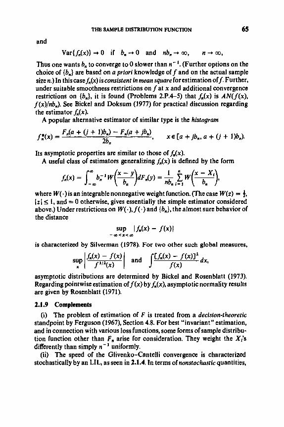
THE SAMPLE DISTRIBUTION FUNCTION 65
and
Var{f,(x)} + 0 if b, 4 0 and nb, + 00, n + co,
Thus one wants b, to converge to 0 slower than n-'. (Further options on the choice of (6,) are based on a priori knowledge off and on the actual sample size n.) In this caseS,(x) is consistent in mean square for estimation off. Further, under suitable smoothness restrictions on f a t x and additional convergence restrictions on {bJ, it is found (Problems 2.P.4-5) that fn(x) is AN( f(x), f (x)/nb,). See Bickel and Doksum (1977) for practical discussion regarding the estimator f,(x).
A popular alternative estimator of similar type is the histogram
F,(a + (j + l)b,) - F,(a + jb,) 2bn
, X E [ ~ + jb, ,a + G + 1)bn). f 3 x 1 =
Its asymptotic properties are similar to those of h(x). A useful class of estimators generalizing f,,(x) is defined by the form
where W( .) is an integrable nonnegative weight function. (The case W ( z ) = i, I z I s 1, and = 0 otherwise, gives essentially the simple estimator considered above.) Under restrictions on W( .), f (.) and {b,}, the almost sure behavior of the distance
SUP If,(x) - f(x)l -ao<.z<m
is characterized by Silverman (1978). For two other such global measures,
asymptotic distributions are determined by Bickel and Rosenblatt (1973). Regarding pointwise estimation off(x) by fn(x), asymptotic normality results are given by Rosenblatt (1971).
2.1.9 Complements
(i) The problem of estimation of F is treated from a decision-theoretic standpoint by Ferguson (1967), Section 4.8. For best "invariant" estimation, and in connection with various loss functions, some forms of sample distribu- tion function other than F, arise for consideration. They weight the XI)s differently than simply n- ' uniformly.
(ii) The speed of the Glivenko-Cantelli convergence is characterized stochastically by an LIL, as seen in 2.1.4. In terms of nonstochastic quantities,

66 THE BASIC SAMPLE STATISTICS
such as E(D,,} and E{J IF,,(%) - F(x)Jdx}, Dudley (1969) establishes rates O(n- 1/2).
(iii) The Kolmogorov-Smirnov test statistic A,, considered in 2.1.2 and 2.1.6 is also of interest when the hypothesized Fo involves unknown nuisance parameters which have to be estimated from the data in order to formulate A,. See Durbin (1973a, b) for development of the relevant theory. For further development, see Neuhaus (1976).
(iv) For theory of Kolmogorov-Smirnov type test statistics generalized to include regression constants, for power against regression alternatives, see Hhjek and Sidhk (1967).
(v) Consider continuous F and thus reduce without loss of generality to F uniform on [0, 13. Then (see Durbin (1973a))
(a) {F,,(t)} is a Markou process: for any 0 < t l < - < t k < t k < 1, the conditional distribution of F,,(tk) given F,(rI), . . . , F,,(tk) depends only on
(b) {F,,(t)} is a conditioned Poisson process: it has the same distribution as the stochastic process {P,,(t)} given P,,(1) = 1, where {P,,(t)} is the Poisson process with occurrence rate n and jumps of n- ’ .
(vi) In 2.1.3 we stated large deviation probability inequalities for 0,. *Large deuiation” probabilities for F,, may also be characterized. For suitable types of set So of distribution functions, and for F not in So, there exist numbers c(F, So) such that
Fn(tk - 1).
See Hoadley (1967), Bahadur (1971), Bahadur and Zabell (1979), and Chapter 10.
2.2 THE SAMPLE MOMENTS
Let XI, X2, . . . be I.I.D. with distribution function F. For a positive integer k, the kth moment of F is defined as
OD
ak = dF(x) = E { X : } .
The first moment a, is also called the mean and denoted by! when convenient. likewise, the kth central moment of F is defined as
(x - /Ok dF(x) E{(Xi - PY}.

THE SAMPLE MOMENTS 67
Note that g1 = 0. The { a f } and {p f } represent important parameters in terms of which the description of F, or manipulations with F, can sometimes be greatly simplified. Natural estimators of these parameters are given by the corresponding moments of the sample distribution function F,. Thus ak may be estimated by
(and let a, also be denoted by x), and & may be estimated by
Since F , possesses desirable properties as an estimator of F, as seen in Section 2.1, it might be expected that the sample moments ak and the sample central moments mk possess desirable features as estimators of and gk. Indeed, we shall establish that these estimators are consistent in the usual senses and jointly are asymptotically multivariate normal in distribution. Further, we shall examine bias and oariance quantities. The estimates ak are treated in 2.2.1. Following some preliminaries in 2.2.2, the estimates mk are treated in 2.2.3. The results include treatment of the joint asymptotic distribution of the ak's and m;s taken together. In 2.2.4 some complements are presented.
2.2.1 The Estimates uk
Note that ak is a mean of I.I.D. random variables having mean ak and variance aZk - a;. Thus by trivial computations and the SLLN (Theorem 1.8B), we have
Theorem A. W P l (i) ai -a,;
(ii) E{ak} = a k :
a 2 k - 4 (iii) Var{ak} = n
(It is implicitly assumed that all stated moments are finite.) Note that (i) implies strong consistency and (ii) and (iii) together yield mean square consistency.
More comprehensively, the vector (al, a2, . . . , ak) is the mean of the I.I.D. vectors (X,, X:, . . . , XI), 1 s i s n. Thus a direct application of the multi- variate Lindeberg-Ltvy CLT (Theorem 1.9.1B) yields. that (a,, . . . , f f k ) is asymptotically normal with mean vector (a1,. .: , ak) and covariances ( a f + , - a,a,)/n. Formally:

68 THE BASIC SAMPLE STATISTICS
Theorem B. 1’ aZk < 00, the random uector n1I2(al - ul, . . . , ak - ark)
conuerges in distribution to k-oariate normal with mean oector (0, . . . , 0) and covariance matrix [ q J ] k ,, k , where biJ = al + J - alaJ.
2.2.2 Some Preliminary and Auxiliary Results
Preliminary to deriving properties of the estimates mk, it is advantageous to consider the closely related random variables
Properties of the m;s will be deduced from those of the 6;s. The same arguments employed in dealing with the ais immediately yield
Lemma A.
(iii)
(iv) For p2k < a, the random oector (bl, . . . , bk) is asymptoticaIly normal with mean uector (pl,. . . , pk) and cooariances (pl+J - plpJ)/n.
Note that bk and mk represent alternate ways of estimating pk by moment statistics. The use of bk presupposes knowledge of p, whereas mk employs the sample meanx in place of p. This makes mk of greater practical utility than bk, but more cumbersome to analyze theoretically.
As another preliminary, we state
Lemma B. Let {Zi} be Z.Z.D. with E{Zl} = 0 and with E(ZI I’ < m, where v 2 2. Then
E Zi = O(n1’2’), n a.
For proof and more general results, see LoCve (1977), p. 276, or Marcinkiewicz and Zygmund (1937). See also Lemma 9.2.6A.
II We shall utilize Lemma B through the implication
~ { b ’ , } = E{(X - p)’} = O(n-(1’2)’), n + a,
for f 2 2.

THE SAMPLE MOMENTS 69
2.2.3 The Estimates mk
Although analogous in form to bk, the random variable mk differs crucially in not being expressible as an average of I.I.D. random variables. Therefore, instead of dealing with mk directly, we exploit the connection between mk and the b,’s. Writing
we obtain
(*)
where we define bo = 1 .
error, and strong consistency of mk . The following result treats the bias, mean square consistency, mean square
Theorem A.
(i) mk 3 pk;
(ii) The bias ofmr satisfies
(iii) The uariance ofmk satisfies
(iv) Hence E(mk - C(k)’ - Var{mk} = o(n-’),
PROOF. (i) In relation (*), apply Lemma 2.2.2A(i) in conjunction with
(ii) Again utilize (*) to write
n + 03.
Application D of Corollary 1.7, and note that pl = 0.
Now, making use of the independence of the X;s,

70 THB BASIC SAMPLE STATISTICS
Similarly,
since the expectation of a term in the triple summation is 0 if i3 # i2 . Hence
Similarly (exercise),
E{bk-36:) = O(n-’), n + 00.
For j > 3, use H6lder.s inequality (Appendix)
I E{bk - j b ’ , I 5 [ E I b k - J lk’a-h]‘k -’lk[E 16 1 Ik]’lk.
By application of Minkowski’s inequality (Appendix) in connection with the first factor on the right, and Lemma 2.2.2B in connection with the second factor, we obtain
E { I 4 - , M } = O(l)[O(n-~l~’)k)]J’k = O(n-“’’”) = O(n-’), n 3 00 (j > 3).
Collecting these results, we have
(iii) Writing Var{mk} = E(mi} - [E(mk}]2, we seek to compute E{mlf} and combine with the result in (ii). For E ( m i } , we need to compute quantities of the form
E { h - ~,H’bk - j 2 # } = E{bk-j,bk - j a n’l( +’I},
for 0 5 jl,jz 5 k. For/, = j 2 = 0, we have

71
For j , = j 2 = 1, we have (exercise)
and
Finally, for j , + j 2 > 2, we have (exercise)
E{bk- , lbk - ,2w+'2} = O(n-'), n -+ 00.
Consequently, by (*),
E{mi} = E{bi} - 2kE{bkbk- ,bl} + k2E{bi-:_,b:}
+ k(k - 1)E(bkbk-,b:} + O(n-'), n -+ 00,
h k - c ( I - 2k@l + pk-lpk-1) + k2/4-lc(2 + k(k - 1)c(kc(k-2p2 = p; +
n
+ O(n-'), n + 00.
(iv) trivial.
Next we establish asymptotic normality of the vector ( m 2 , . . . , mk). The following lemma is useful.

The second term on the right is a product of two factors, the first converging in distribution and the second converging to 0 wpl, these properties following from Lemma 2.2.2A. Therefore, by Slutsky’s Theorem (1.5.4), the product converges to 0 in probability.
Theorem B. If pzk < 00, the random oector n1I2(m2 - p2, . . . , mk - k) conoerges in distribution to (k - lkoariate normal with mean vector (0, . . . , 0) and cooariunce matrix [a&- l ) x ( k - 1), where
ufi = pI+J+Z - pItlpJ+I - (i + 1 h p J + Z - (i + l)C(I+ZpJ + (i + l)(i + 1)CIIc(#2.
PROOF. By the preceding lemma, in conjunction with the Cramdr-Wold device (Theorem 1.5.2) and Slutsky’s Theorem, the :andom vector
n1’’b2 - c(2 - - * 9 mk - c ( k )
has the same limit distribution (if any) as ihe vector n112(bz - pz - 2p1bl, . . . , bk - p k - kpk- lbl). But the latter is simply nl/’ times the average of the I.I.D. vectors
[(XI - - pZ - 2pl(x, - * * * Y (XI - py - p k - kpk - l(xI - 1 S i s n .
Application of the CLT (Theorem 1.9.1B) gives the desired result.
By similar techniques, we can obtain asymptotic normality of any vector (al , . , . , ah,, m z , . . . , mkZ), In particular, let us consider (al , m2) = (sample mean, sample variance) = (X, s’). It is readily seen (Problem 2.P.8) that
Here we have denoted p2 by a’, as usual.
2.2.4 Complements
(i) Examples: the sample mean and the sample variance. The joint asymp- totic distribution ofX and s2 was expressed at the conclusion of 2.2.3. From

THE SAMPLE MOMENTS 73
this, or directly from Theorems 2.2.1B and 2.2.3B, it is seen that each of these statistics is asymptotically normal:
and
(ii) Rates of convergence in connection with the asymptotic normality of the sample mean and sample oariance. Regardingx, the rate of convergence to 0 of the normal approximation error follows from the Berry-Essten Theorem (1.9.5). For s2, the rate of this convergence is found via consideration of s2 as a U-statistic (Section 5.5).
(iii) E’ciency of”rnoment” estimators. Despite the good properties of the moment estimators, there typically are more efficient estimators available when the distribution F is known to belong to a parametric family. Further, the “method of moments” is inapplicable if F fails to possess the relevant moments, as in the case of the Cauchy distribution. (See additional discussion in 2.3.5 and 4.3.)
hold (k = 2, 3, . . .) and so the two sets of estimates {a2, a 3 , . . .} and {mz , m,, . . .} offer alternative ways to estimate the parameters (a2 = p2 , a3 = p 3 , . . .}. In this situation, Lemma 2.2.3 shows that
(iv) The case p = 0. In this case the relations =
mk - pk = ak - pk - kpk- 1x + op(n-l’z)a
That is, the errors of estimation using ak and mk differ by a nonnegligible component, except in the case k = 2.
(v) Correction factors to achieve unbiased estimators. If desired, correction factors may be introduced to convert the mk’s into unbiased consistent estimators
n(n2 - 2n + 3) M4 = m4 - (n - l)(n - 2)(n - 3)
3n(2n - 3) ( n - I ) ( n - 2)(n -- 3)
etc., for p 2 , p 3 , p4, . . . . However, as seen from Theorem 2.2.3A, the bias of the unadjusted mL)s is asymptotically negligible. Its contribution to the mean square error is O(n-’), while that of the variance is of order n - l .

74 THE BASIC SAMPLE STATISTICS
(vi) Rates of conuergence in connection with the strong convergence of Uk
(vii) Further reading. Cramtr (1946), Sections 27.1-6 and 28.1 -3, and Rao and mk. This topic is treated in 5.1.5.
\(1973), Section 6h. 4
2.3 THE SAMPLE QUANTILES
Let F be a distribution function (continuous from the right, as usual). For 0 < p < 1, the pth quantile orfractile of F is defined (recall 1.1.4) as
4, = inf {x: F(x) 2 p )
and is alternately denoted by F-'(p). Note that C, satisfies
Other useful properties have been presented in Lemmas 1.1.4 and 1.5.6. Corresponding to a sample {X,, . , . , X,} of observations on F, the sample
pth quantile is defined as the pth quantile of the sample distribution function F,, that is, as F; l(p). Regarding the sample pth quantile as an estimator of C,, we denote it by e,,, or simply by e,, when convenient.
It will be seen (2.3.1) that e, is strongly consistent for estimation of C,, under mild restrictions on Fin the neighborhood oft,. We exhibit (2.3.2) bounds on the related probability
F(Cp-1 2s P 2s FceJ
p SUPIt, - t,l > e), d, n
showing that it converges to 0 at an exponential rate. is treated in 2.3.3. In particular,
under mild smoothness requirements on F i n the neighborhoods of the points t,,,.. ., Cm, the vector of sample quantiles (e,,, . . . , e,) is asymptotically normal. Also, several complementary results will be given, including a rate of convergence for the asymptotic normality.
If F has a density, then so does the distribution oft,. This result and its application are discussed in 2.3.4.
Comparison of quantiles uersus moments as estimators is made in 2.3.5, and the mean and median are compared for illustration. In 2.3.6 a meusure of dispersion based on quantiles is examined. Finally, in 2.3.7, brief discussion of nonparametric tests based on quantiles is provided.
Further background reading may be found in Cramtr (1946), Section 28.5, and Rao (1973), Section 6f.2.
23.1 Strong Consistency of &, The following result asserts that t p is strongly consistent for estimation of C,, unless both F(Cp) = p and F is flat in a right-neighborhood of C,.
The asymptotic distribution theory of

THE SAMPLE QUANTILES 75
Theorem. Let 0 < p < 1. If 5, is the unique solution x ofF(x-) s p s F(x), then t,, 2 6,.
PROOF. Let E > 0. By the uniqueness condition and the definition of Cp, we have
F(tp - 4 < P < F(Cp + el. It was seen in 2.1.1 that Fn(CP - e) - F(CP - E) and Fn(tp + e) % F([, + e). Hence (review 1.2.2)
WP 1
P(F,(Cp - e) < p < F,,,(tp + E), all m 2 n) + 1,
~(t , - e < t,,,,, s tp + e, all m 2 n) + I ,
n + 00.
Thus, by Lemma 1.1.4(iii),
n -+ 00.
That is,
P (m sup l t , -~p ,>e ) -o , n - m .
As an exercise, show that the uniqueness requirement on Cp cannot be
In the following subsection, we obtain results which contain the preceding dropped (Problem 2.P.11).
theorem, but which require more powerful techniques of proof.
23.2 A Probability Inequality for 14, - &,I We shall use the following result of Hoeffding (1963).
Lemma (Hoeffding). Let Y,, . . . , Y, be independent random variables satisfying P(a 5 Yl 5 b) = 1, each i, where a < b. Then, for t > 0,
Theorem. Let 0 < p < 1. Suppose that 6, is the unique solution x of F(x -) S p s F(x). Then,for every E > 0,
P(I$, - 6,1 > E) s 2e-Zn*!,
where 6, = min{F(ep + E) - p, p - F([, - E)}.
of proof of Smirnov (1952).) Let e > 0. Write
all n,
PROOF. (We apply Hoeffding's lemma in conjunction with a technique
p<Itpn - CpI > = P < t p n > t p + E) + p < t p n < Cp - 8).

76 THE BASIC SAMPLE STATISTICS
By Lemma 1.1.4,
p ( t p n > € p + 6 ) = P(P > FJtp + E) )
4 = P X I ( & > c, + E ) > n(l -
= P( i v, - iE{v ,} > d, ) , I - 1 I = ,
where V, = I ( X I > 4, + E ) and d1 = F ( t , + E ) - p . Likewise,
PtCpn < t p - 6 ) s P(P s F,(€, - E ) )
where W, = I ( X I s tP - E ) and b2 = p - F ( t p - E). Therefore, utilizing Hoeffding's lemma, we have
P<C, > t, + E ) s e- lnsf
P ( ( , < tP - e) s e-2nd!
and
Putting 6, = min{6,, a2}, the proof is complete.
1.3.4) that epn conuerges completely to t,. Even more strongly, we have
Corollary. Under the assumptions ofthe theorem, for every E > 0,
Thus P( I &,, - €,I > 8) + 0 exponentfallyjast, which implies (via Theorem
where pe = exp( -26;) and 6, = min(F(6, + E ) - p, p - F(5, - E ) } .
(derived the same way as the corollary to Theorem 2.1.3A)
Remarks. (i) The value of E (> 0) in the preceding results may depend upon n if desired.
(ii) The bounds established in these results are exact. They hold for each n 3: 1,2,. . . and so may be applied for any fixed n as well as for asymptstic analyses.
(iii) A slightly modified version of the preceding theorem, asserting the same exponential rate, may be obtained by using the Dvoretzky-Kiefer- Wolfowitz probability inequality for D,, instead of the Hoeffding lemma, in the proof. (Problem 2.P.12).

THE SAMPLE QUANTILES 77
2.3.3 Asymptotic Normality of g p The exact distribution of p , will be examined in 2.3.4. Here we prove asymp- totic normality of [, in the case that F possesses left- or right-hand derivatives at the point cp. If F lacks this degree of smoothness at cP, the limit distribution of (,(suitably normalized) need not be normal (no pun intended). The various possibilities are all covered in Theorem 4 of Smirnov (1952). In the present treatment we confine attention to the case of chief importance, that in which a normal law arises as limit.
The following theorem slightly extends Smirnov’s result for the case of a normal law as limit. However, the corollaries we state are included in Smirnov’s result also.
When assumed to exist, the left- and right-hand derivatives of F at 6, will be denoted by F’({,-) and F‘(<, +), respectively.
Theorem A. Let 0 < p < 1. Suppose that F is continuous at 6,. (i) Ifthere exists F’(S,-) > 0, thenfor t < 0,
(ii) If there exists F(S,+) > 0, thenfor t > 0, C
Corollary A . Let 0 c p < 1. If F is diflerentiable at 6, and F(6,) > 0, then
Corollary B. Let 0 < p < 1. If F possesses a density f i n a neighborhood of 6, and f is positive and continuous at 6,’ then
These corollaries follow immediately from Theorem A. Firstly, if F is differentiable at Cp, then F’((,-) = F‘(C,+) = F’((,,). Thus Corollary A follows. Secondly,iffis adensity of F,it is not necessary thatf = F‘. However,
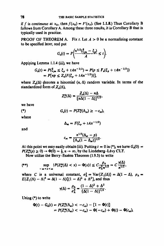
78 THE BASIC SAMPLE STATISTICS
i f f is continuous at xo, thenf(xo) = F’(xo). (See 1.1.8.) Thus Corollary B follows from Corollary A. Among these three results, it is Corollary B that is typically used in practice.
PROOF O F THEOREM A. Fix t. Let A > 0 be a normalizing constant to be specified later, and put
Applying Lemma 1.1.4 (iii), we have
GXt) = P(2, s tP + tAn”’’) = P(p s Fn(tp + tAn-l/’)) = PCnp s Z,(F(CP + tAn- 1/2))],
where Z,(A) enotes a binomial (n,A) random variable. In terms of the standardized P orm of .Z,(A),
we have
(*) GAt) = P W A n r ) 2 -cnr),
where
and A,, = F(C, + tAn- ’/’)
112 A n ( nr - P) = [Anr(l - AM)]1/‘*
At this point we may easily obtain (iii). Putting t = 0 in (*), we have G,(O) = P(Z,+@) 2 0) + @(O) = 4, n + 00, by the Lindeberg-LCvy CLT.
Now utilize the Berry-Eden Theorem (1.9.5) to write
where C is a universal constant, uf = Var{Zl(A)} = A(1 - A), pa = EIZl(A) - A13 = A(1 - A)[(1 - A)2 + A2], and thus

THE: SAMPLE QUANTILM 79
we have by (**) that
Y(A 1
Since F is continuous at ep, we have AJ1 - A,J + p(1 - p) > 0, and thus y(A,,)n- ' I 2 + 0, n + 00. It remains to investigate whether c,, + t. Writing
I Gn(t) - Wt) I s C + IWt) - CD(c,JI.
A F((, + tAn-'l2) - F(Cp) c,, = t *
[A",(1 - An,)I1I2 * tAn- ' I 2 Y
we see that, if t > 0, then
and, if t < 0, then
Thus cnr + t if either
t > 0 and A = Cp(1 - P)]"~/F'(<~+)
t < 0 and A = Cp(1 - P)]"' /F'((~-) . or
This establishes (i) and (ii). H Remark. The specific rate O(n- 1/2) provided by the Berry-Essten Theorem was not actually utilized in the preceding proof. However, in proving Theorem C we do make application of thi! specific order of magnitude.
Corollaries A and B cover typical cases in which e p is asymptotically nor- mal, that is, a suitably normalized version of &, converges in distribution to N(0,l). However, more generally, Theorem A may provide a normal ap- proximation even when no limit distribution exists. That is, nllz(lpn - t,) may fail to have a limit distribution, but its distribution may nevertheless be approximated, as a function of t , by normal distribution probabilities: for t < 0, based on the distribution N(0, p(1 - p)/[F'((,-)12); for t > 0, based on the distribution N(0, p(1 - p)/[F'((,+)I2). The various possibilities are illustrated in the following example.
Example. Estimation ojthe median. Consider estimation of the median tlI2 of F by the sample median ell,.
(i) If F has a positive derivative F(t1,,) at x = then

80 THE BASIC SAMPLE STATISTICS
(ii) If, further, F has a density f continuous at then equivalently we may write
(iii) b However, suppose that F has a densityf which is discontinuousat €1 /2 .
For example, consider the distribution
O < X S f ,
A density for F is
which is discontinuous at is not asymp- totically normal in the strict sense, but nevertheless we can approximate the probability
= f . Thus the sample median
P(n1~2(el/2 - 41/21 t).
We use the distribution N(0, )) if t < 0 and the distribution N(0, &) if t > 0. For t = 0, we use the value f as an approximation.
The multivariate generalization of Corollary B is
Theorem B. Let 0 < p1 < - < Pk < 1. Suppose that F has a density f in neighborhoods of tPr, . . . , em and that f is positive and continuous at ep,, . . . ,5,. Then (sPl, . . . , epk) is asymptotically normal with mean vector (Cpl, . . . , Spk) and covariances al,/n, where
and alj = allfor i > j.
One method of proof will be seen in 2.3.4, another in 2.5.1. Or see Cramtr (1946), p. 369.
We now consider the rate of convergence in connection with the asymptotic normality of tP. Theorem C below provides the rate O(n-'l2). Although left implicit here, an explicit constant of proportionality could be determined by careful scrutiny of the details of proof (Problem 2.P.13). In proving the theorem, we shall utilize the probability inequality for It,,,, - {,I given by Theorem 2.3.2, as well as the following lemma.

THE SAMPLE QUANTILES 81
Lemma. For lax I I; 4. IWx + ax2) - Wx)( I; 51alsup[x2+(x)].
a
PROOF. By the mean value theorem,
Wx + ax2) - @(x) = ux2&(x*),
where x* lies between x and x + ax2, both of which have the same sign. Since +(x) is increasing on (- o0,O) and decreasing on (0, a), we have
and hence 9(x*) I; 4(x + M + +(x - 3x)
x2&x*) s X2&X + 4x) + x2f$(x - 4x) = 4(3X>”(3X> + 4(4x)2&4x) 5 5 SUPCX2&X)3. H
x
Theorem C. Let 0 < p < 1. Suppose that in a neighborhood of 5, , F possesses a positive continuous density f and a bounded second derivative F . Then
PROOF. Put A = Cp(1 - p)] ’ / ’ / f(Cp) and
Gdt) = p(n’”( tpn - CJA I; t)*
Let Ln = B(log n)’12. We shall introduce restrictions on the constant B as needed in the course of the proof. Now note that (1)
SUP IGn(t) - Wt)I = max SUP IGn(t) - @(t)I, suplGn(t) - Wl)l} Itl>Ln I< -L. t >L,
S max{Gn( - L,) + @(- L,), 1 - G,(Ln) + 1 - @(L,)}
I; Gn(-L,) + 1 - Gn(Ln) + 1 - WLn)
s p < I t p n - (PI 2 ALnn-1/2) + 1 - WLJ. As is well-known and easily checked (or see Gnedenko (1962), p. 134),
so that
(2)

82 THE BASIC SAMPLE STATISTICS
provided that
(3) 8’ 2 1.
To obtain a similar result for the other term in (1). we use the probability inequality given by Theorem 2.3.2, with e given by
E, = ( A - EO)Lnn-1’2,
where eo is arbitrarily chosen subject to 0 < e0 < A. In order to deal with 6,” = min(F(6, + en) - p , p - F(Cp - en)}, we utilize Taylor’s Theorem (1.12.1A) to write
where z* lies between t p and t p + en, and
where z** lies between t p and t p - en. Then
Stn = min{f2(tp)ef + f(tp)~‘’(z*)e: + S[F“(Z*)]~S.*,
F(tp + En) - P = f ( t p ) E n + W’(Z*)E,I,
P - F(tp - En) = f(tp)En - iF”(z**)Ef,
f’(Cp>Ef - f(t,)F“(Z**)e: + S[F”(z**l124 2 & , l f ( C p ) C f ( C p ) - ~ e n I ,
where M satisfies
(4) sup IFff((, + z)l S M < 00 I ~ s en
for all n under consideration. Hence
- 2n6tn 5 - 2&f(tp) [ f ( t p ) - Men] = -2L,l(A - e o ) 2 f ( t p ) C f ( t p ) - MGJ.
For convenience let us now put
EO = )A.
Recalling the definition of A, we thus have
= O(n- I/’),

THE? SAMPLE QUANTILEs
provided that 83
and
and thus
CAJl - AJ] - 1'2 = Cp( 1 - p)]- + g'(z,,)Atn- l",
where z , ~ lies between tp and r, + A C ~ - ' / ~ . Inspection of ~ ' ( z ) shows that the quantity
w, = sup Ig'(z)l I* - Cpl S ALnn - '1'
is finite; in fact
W. -+ W , = m , ) 1 4 - P I M ~ - P ) I - ~ / ~
as n + 00. Hence also the quantity
Yn = SUP ~(Anr) I f lSLn
is finite; in fact
(8) Y. -+ yra = c(1 - + p2icp(1 - p11-3'2.
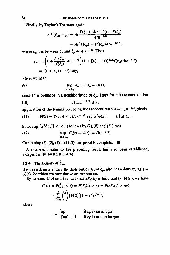
84 THE BASIC SAMPLE STATISTICS
Finally, by Taylor's Theorem again,
= At[ f (e,) + F"(t,,)Atn- 1/21,
where t,, lies between C, and e , + Atn-'12. Thus
= t ( l + h,,tn- 112), say,
where we have
SUP Ih:l = Ha = 0(1), III5Ln
(9)
(10) H"L"n-1'2 I; 4,
(1 1)
since F" is bounded in a neighborhood of C,. Thus, for n large enough that
application of the lemma preceding the theorem, with a = h,,n-1'2, yields
IWt) - WcdI 5 5H,n-'" supCx2$(~)I, ItI s L n . X
Since supx[x2$(x)] < m, it follows by (7), (8) and (1 1) that
(12) SUP I G,(t) - Wt) I = O(n- ' I 2 ) . It1 s Ln
Combining (l), (2), (5) and (12), the proof is complete.
independently, by Reiss (1974).
2.3.4 The Density of &,, If F has a density f, then the distribution G, of &,,, also has a density, g,(t) = G#), for which we now derive an expression.
By Lemma 1.1.4 and the fact that nF,(A) is binomial (n, F(A)), we have
A theorem similar to the preceding result has also been established,
G,(O = p<e, t ) = W , ( t ) 2 P ) = P(nF,(t) 2 np)
where
m - I n p [np] + 1
if np is an integer if np is not an integer.

THE SAMPLE QUANTILES
Taking derivatives, i t is found (Problem 2.P.14) that
85
gn(t) = .( - ;) [F(t)I"-- 1[1 - F(t)]"-y(t). m -
Incidentally, this result provides another way to prove the asymptotic normality of gpn, as stated in Corollary 2.3.3B. The density of the random variable ni/z(&, - tp) is
h,(t) = n- 1'2gn(tp + tn- 1@).
Using the expression just derived, it may be shown that
lim h,(t) = 4(tf(tp)b(1 - p ) ] - l/'), each t , n* Q,
("1
that is, h,(t) converges pointwise to the density of N(0, p(1 - p ) / f 2 ( t , ) ) . Then Scheffd's Theorem (1.5.1C) yields the desired conclusion. For details of proof of (*), see Cram& (1946) or Rao (1973). Moreover, this technique of proof generalizes easily for the multivariate extension, Theorem 2.3.38.
Finally, we comment that from the above expression for G,(t) one can establish that if F has a finite mean, then for each k, ppn has finite kth moment for all sufficiently large n (Problem 2.P.15).
2.3.5 Quantiles Versus Moments
In some instances the quantile approach is feasible and useful when other approaches are out of the question. For example, to estimate the parameter of a Cauchy distribution, with density f ( x ) = 1/n[1 + (x - p)'], -m c x < 00, the sample meanx is not a consistent estimate of the location param- eter p. However, the sample median is A N @ , n2/4n) and thus quite well- behaved.
When both the quantile and moment approaches are feasible, it is of interest to examine their relative efficiency. For example, consider a sym- metric distribution F having finite variance u2 and mean (= median) p (= t1/2). In this case both X and are competitors for estimation of p, Assume that F has a density f positive and continuous at p. Then, according to the theorems we have established,
x is AN p, - ( and
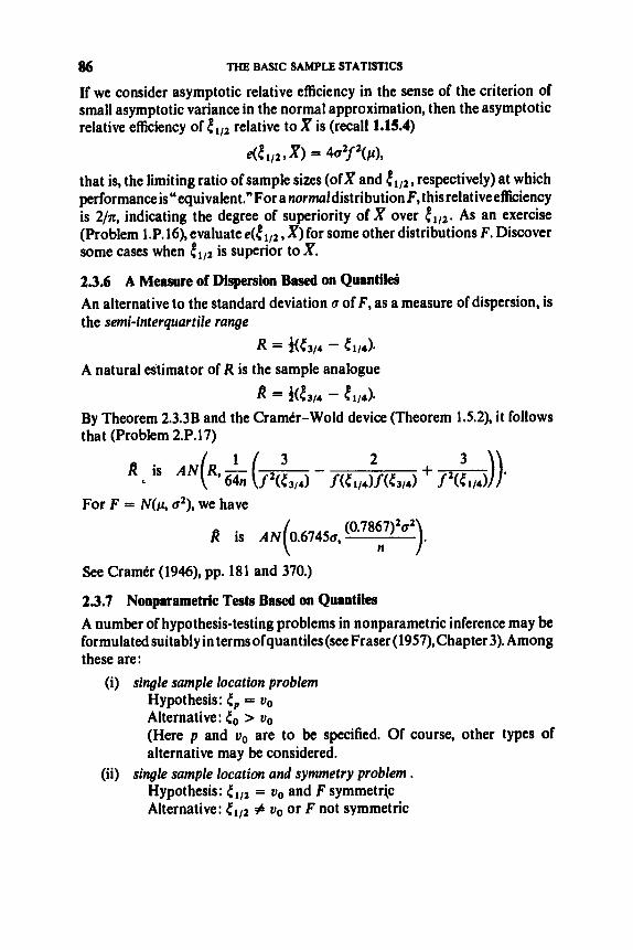
86 THE BASIC SAMPLE STATISTICS
If we consider asymptotic relative efficiency in the sense of the criterion of small asymptotic variance in the normal approximation, then the asymptotic relative efficiency of el/, relative to X is (recall 1.15.4)
that is, the limiting ratio of sample sizes (ofx and el,,, respectively) at which performanceis"equivalent." For a normaldistribution F,thisrelativeefficiency is 2/x, indicating the degree of superiority of x over el,,. As an exercise (Problem l.P.16), evaluate e(e,,, , x) for some other distributions F. Discover some cases when el,, is superior to x. 2.3.6 A Measure of Dispersion Based on Quantiles An alternative to the standard deviation CJ of F, as a measure of dispersion, is the semi-interquartile range
A natural estimator of R is the sample analogue
By Theorem 2.3.38 and the CramCr-Wold device (Theorem 1.5.2), it follows that (Problem 2.P. 17)
e<e,/, 9 X) = 4@Y2(P),
= %(e3/4 - (el/,>*
a = f c e 3 / 4 - e,/4,.
For F = N(p, c2), we have
n
See Cram& (1946), pp. 181 and 370.)
23.7 Nonparametric Tests Based on Quantiles A number of hypothesis-testing problems in nonparametric inference may be formulated suitably in terms ofquantiles(see Fraser (1957), Chapter 3). Among these are:
(i) single sample location problem Hypothesis: (e, = uo Alternative: to > uo (Here p and uo are to be specified, Of course, other types of alternative may be considered.
(ii) single sample location and symmetry problem . Hypothesis: (el/, = uo and F symmetric Alternative: (ell, # uo or F not symmetric

THE ORDER STATISTICS 87
(iii) two-sample scale problem (Given XI,. . . , X,, I.I.D. F and Yl,. . . , Y,, I.I.D. G) Hypothesis: F(x) = G(x + c), all x Alternative: t,,(F) - t,,(F) < t,,,(G> - <,,(GI, all p1 < p z .
The most widely known “quantile” test arising for these problems is the sign test for problem (i). Most texts provide some discussion of it, often in the context of order statistics, which we shall examine in the forthcoming section.
2.4 THE ORDER STATISTICS
For a sample of independent observations XI, . . . , X , on a distribution F, the ordered sample values
X(1) I; X(Z) 5 X(n),
or, in more explicit notation,
X,I S Xnz I; I; X,n, are called the order statistics and the vector
X(n) = ( X ~ I , - * * 9 Xnn)
is called the order statistic of the sample. If F is continuous, then with prob- ability 1 the order statistics of the sample take distinct values (and conversely).
The exact distribution of the kth order statistic Xnk is easily found, but cumbersome to use:
P ( X , s x ) = f: c ) [ F ( x ) ] ‘ [ l - F(x)Y-‘, -m < x < 00. I - k
The asymptotic theory of sequences {x&} of order statistics is discussed in 2.4.3, with some particular results exhibited in 2.4.4. We further discuss asymptotic theory of order statistics in 2.5, 3.6 and Chapter 8.
Comments on the fundamental role of order statistics and their connection with sample quantiles are provided in 2.4.1, and on their scope of application in 2.4.2.
Useful general reading on order statistics consists of David (1970), Galambos (1978), Renyi (1953), Sarhan and Greenberg (1962), and Wilks (1948,1962).
2.4.1 Fnndamental Role 01 the Order Statistics; Connection with the Sample Quaatiles
Since the order statistic X(,,) is equivalent to the sample distribution function F,, its role is fundamental even if not always explicit. Thus, for example, the

88 THE BASIC SAMPLE STATISTICS
sample mean X may be regarded as the mean of the order statistics, and the sample pth quantile may be expressed as
f p n = p * n p if np is an integer, if np is not an integer. xn, [ n p ~ + 1
(*I
The representations o fx and tpn in terms of order statistics are a bit artificial. On the other hand, for many useful statistics, the most natural and effective representations are in terms of order statistics. Examples are the extreme ualues Xm1 and X,,, and the sample range X,, - X",. (In 2.4.4 it is seen that these latter examples have asymptotic behavior quite different from asymp- totic normality.)
(**I x n k = t k / n , n , 1 s k s n.
In view of (*) and (**),the entire discussion of order statistics could be carried out formally in terms of sample quantiles, and vice versa. The choice of formulation depends upon the point of view which is most relevant and convenient to the particular purpose or application at hand. Together, there- fore, the previous section (2.3) and the present section (2.4) comprise the two basic elements of a single general theory. The cohesion of these basic elements will be viewed more fully in a complementary analysis developed in 2.5.
The relation (*) may be inverted:
2.4.2 Remarks on Applications of Order Statistics
The extreme values, X,, and X,,, arise quite naturally in the study of floods or droughts, and in problems of breaking strength or fatigue failure.
A quick measure of dispersion is provided by the sample range, suitably normalized. More generally, a variety of short-cut procedures for quick estimates of location or dispersion, or for quick tests of hypotheses about location or dispersion, are provided in the form of linearfunctions oforder statistics, that is, statistics of the form c;- c,,Xnl. The class of such statistics is important also in the context of robust inference. We shall study these statistics technically in Chapter 8.
Order statistics are clearly relevant in problems with censored data. A typical situation arises in connection with life-testing experiments, in which a fixed number n of items are placed on test and the experiment is terminated as soon as a prescribed number r have failed. The observed lifetimes are thus X,, S ... I; X,, whereas the lifetimes Xn,r+l < s X,, remain un- observed. For a survey of some important results on order statistics and their role in estimation and hypothesis testingin life testing and reliabilfty problems, see Gupta and Panchapakesan (1974). A useful methodological text consists of Mann, Schafer and Singpurwalla (1974).
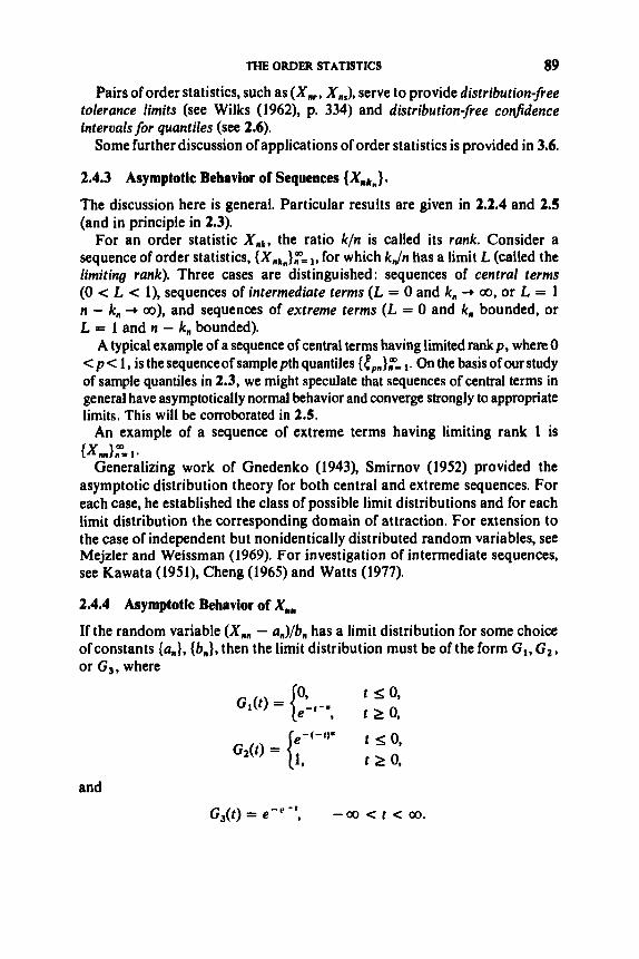
THE ORDER STATISTICS 89
Pairs of order statistics, such as (X,,, X,,), serve to provide distribution-free tolerance h i t s (see Wilks (1 962), p. 334) and distribution-free confidence interuals for quantiles (see 2.6).
Some further discussion of applications of order statistics is provided in 3.6.
2.4.3 Asymptotic Behavior of Sequences { Xakm).
The discussion here is general. Particular results are given in 2.2.4 and 2.5 (and in principle in 2.3).
For an order statistic Xnk, the ratio k/n is called its rank. Consider a sequence of order statistics, {Xnkm}?' 1, for which k Jn has a limit L (called the limiting rank). Three cases are distinguished : sequences of central terms (0 < L < 1). sequences of intermediate terms (L = 0 and k , + m, or L = 1 n - k, + m), and sequences of extreme terms (t = 0 and k , bounded, or L = 1 and n - k, bounded).
A typical example of a sequence of central terms having limited rankp, where 0 C p < 1, is the sequenceof samplepth quantiles { tp,,}?= On the basis of our study of sample quantiles in 2.3, we might speculate that sequences of central terms in general have asymptotically normal behavior and converge strongly to appropriate limits. This will be corroborated in 2.5.
An example of a sequence of extreme terms having limiting rank 1 is
Generalizing work of Gnedenko (1943), Smirnov (1952) provided the asymptotic distribution theory for both central and extreme sequences. For each case, he established the class of possible limit distributions and for each limit distribution the corresponding domain of attraction. For extension to the case of independent but nonidentically distributed random variables, see Mejzler and Weissman (1969). For investigation of intermediate sequences, see Kawata (1951), Cheng (1965) and Watts (1977).
2.4.4 Asymptotic Behavior of X,,,
If the random variable (X,, - a,)/b, has a limit distribution for some choice of constants {a,,}, {b"}, then the limit distribution must be of the form GI, G l , or G 3 , where
{Xnn}:= 1.
and
G,(t) = e-' -', -00 < t < 00.

90 THE BASIC SAMPLE STATISTICS
(In GI and GI, a is a positive constant.) This result was established by Gnedenko (1943), following less rigorous treatments by earlier authors. Each of the three types GI, G2, and G3 arises in practice, but G3 occupies the pre- eminent position, Typical cases are illustrated by the following examples.
Example A. F is exponential : F(x) = 1 - exp(-x), x > 0. Putting a, = log n and 6, = 1, we have
Example B. F is logistic: F(x) = [l + exp(-x)]-', - 00 < x < ao. Again taking a, = log n and 6, = 1, we may obtain (Problem 2.P.18)
P(X,, - log n 5 t ) -+ e-'-', n 00.
Example C. F is normal: F = @. With
a, = (2 log n)'l2 - BlOg log n + log 4n)(2 log n)-"'
and
b, = (2 log n)-'/*
it is found (Cram& (1946), p. 374) that
n -* 00.
In Examples A and B, the rate of the convergence in distribution is quite fast. In Example C, however, the error of approximation tends to 0 at the rate O((1og n)-b), for some 0, but not faster. For discussion and pictorial illustration, see CramCr (1946), Section 28.6. The lack of agreement between the exact and limit distributions is seen to be in the tails of the distributions. Further literature on the issue is cited in David (1970), p. 209. See also Galambos (1978), Section 2.10.
Statistics closely related to X,, include the range X,, - XnI and the studentized extreme deuiate, whose asymptotic distributions are discussed in Section 3.6.
The almost sure asymptotic properties of X, can also be characterized. For example, in connection with F normal, we anticipate by Example C above that

ASYMPTOTIC REPRESENTATION THEORY 91
X,, is close to (2 log n)l l2 in appropriate stochastic senses. This is in fact true: both
[x,, - (2 log n)’’’] =
and
X n n
Thus X,, satisfies both additive and multiplicative forms of strong con- vergence. For a treatment of the almost sure behavior of X,, for arbitrary F, see Galambos (1978), Chapter 4.
2.5 ASYMFTOTIC REPRESENTATION THEORY FOR SAMPLE QUANTILES, ORDER STATISTICS, AND SAMPLE DISTRIBUTION
FUNCTIONS
Throughout we deal as usual with a sequence of I.I.D. observations XI, Xz , . . . having distribution function F.
We shall see that it is possible to express sample quantiles and “central” order statistics asymptotically as sums, via representation as a linear trans- form of the sample distribution function evaluated at the relevant quantile. From these representations, a number of important insights and properties follow.
The representations were pre-figured in Wilks (1962), Section 9.6. However, they were first presented in their own right, and with a full view of their significance, by Bahadur (1966). His work gave impetus to a number of important additional studies, as will be noted.
Bahadur’s representations for sample quantiles and order statistics are presented in 25.1 and 2.5.2, respectively, with discussion of their implications. A sketch of the proof is presented in general terms in 2.5.3, and the full details of proof are given in 2.5.4, Further properties of the errors of approximation in the representations are examined in 2.5.5. An application of the representa- tion theory will be made in Section 2.6, in connection with the problem of confidence intervals for quantiles.
Besides references cited herein, further discussion and bibliography may be found in Kiefer (1970b).
2.5.1 Sample Quantiles as Sums Via the Sample Distribution Function Theorem (Bahadur (1966)). Let 0 < p < 1. Suppose that F is twice dgerentiable at sp, with F‘(6,) = f(5,) > 0. Then

92 THE BASIC SAMPLE STATISTICS
where with probability 1
R, = O(n-3/4(log n)314), n --* ao.
Details of proof are given in 2.5.3 and 2.5.4, and the random variable R, is examined somewhat further in 2.5.5.
Remarks. (i) By the statement "with probability 1 , Y,, = O(g(n)) as n + 00 " is meant that there exists a set Ro such that P(R,) = 1 and for each w E Qo there exists a constant B(w) such that
I Yn(w)) S B(w)g(n), all n sufficiently large.
(For Y, given by the R, of the theorem, it can be seen from the proof that the constants B(w) may be chosen not to depend upon w.)
(ii) Bahadur (1966) actually assumes in addition that F exists and is bounded in a neighborhood of 4,. However, by substituting in his argument the use of Young's form of Taylor's Theorem instead of the standard version, the extra requirements on F may be dropped.
(iii) Actually, Bahadur established that
R, = O(n-3/4(log n)*I2(log log t ~ ) ' / ~ ) , n --* 00,
with probability 1. (See Remark 2.5.4D.) Further, Kiefer (1967) obtained the exact order for R,, namely O(n- jI4(l0g log n)jI4). See 2.5.5 for precise details.
(iv) (continuation) However, for many statistical applications, it suffices merely to have R, = op(n- Ghosh (1971) has obtained this weaker con- clusion by a simpler proof requiring only that F be once differentiable at e, with F'(e,) > 0.
(v) The conclusion stated in the theorem may alternatively be expressed as follows: with probability 1
(vi) (continuation) The theorem thus provides a link between two asymptotic normality results, that of tp, and that of F,(e,). We have seen previously as separate results (Corollary 2.3.3B and Theorem 2.1.1, respec- tively) that the random variables
each converge in distribution to N(0, p(l - p)/f2({,)). The theorem of Bahadur goes much further, by revealing that the actual difference between these random variables tends to 0 wpl, and this at a rate O(n-3/4(log n)'").

ASYMPTOTIC REPRESENTATION THEORY
(vii) Representation of a sample quantile as a sample mean. Let
93
Then the conclusion of the theorem may be expressed as follows: wpl
That is, wpl epn is asymptotically (bur not exactly) the mean of the first n members of the I.I.D. sequence { yl}.
(viii) Law of the iterated logarithm for sample quantiles (under the con- ditions of the theorem). As a consequence of the preceding remark, in con- junction with the classical LIL (Theorem l.lOA), we have: wpl
for either choice of sign (Problem 2.P.20). This result has been extended to a larger class of distributions F by de Haan (1974).
(ix) Asymptotic multiuariate normality of sample quantiles (under the conditions of the theorem). As another consequence of remark (vii), the conclusion of Theorem 2.3.3B is obtained (Problem 2.P.21).
2.5.2 Central Order Statistics as Sums Via the Sample Distribution Function
The following theorem applies to a sequence of “central” order statistics {Xnkm} as considered in 2.4.3. It is required, in addition, that the convergence of kn/n to p be at a sufficiently fast rate.
Theorem (Bahadur (1966)). Let 0 < p < 1. Suppose that F is twice diferentiable at tp, with F(5,) = f(5,) > 0. Let {k,} be a sequence ofpositiue integers (1 I; k, I; n) such that
for some A 2 4. Then
where with probability 1

94 THE BASIC SAMPLE STATISTICS
Remarks. (i) Bahadur (1966) actually assumes in addition that F” exists and is bounded in a neighborhood of tp. Refer to discussion in Remark 2.5.l(ii).
(ii) Extension to certain cases of “intermediate” order statistics has been carried out by Watts (1977). 4
This theorem, taken in conjunction with Theorem 2.5.1, shows that the order statistic Xnkn and the sample pth quantile p,,, are roughly equivalent as estimates of tp, provided that the rank k,Jn tends to p sufficiently fast. More precisely, we have (Problem 2.P.22) the following useful and interesting result.
Corollary. Assume the conditions of the preceding theorem and suppose that
Then
(*I
and
By (*) it is seen that x,k, trails along with e,,, as a strongly consistent estimator of tp. We also see from (*) that the closeness of x,k, to eP,, is regulated rigidly by the exact rate of the convergence of k,Jn to p . Further, despite theconsistencyofXnkmforestimationof{,,it isseen by(**)that,on the other hand, the normalized estimator has a limit normal distribution not centered at 0 (unless k = 0), but rather at a constant determined by the exact rate of convergence of kJn to p. These aspects will be of particular interest in our treatment of confidence intervals for quantiles (Section 2.6).
2.5.3 Sketch of Bahadur’s Method of Proof
Here we sketch, in general form, the line of argument used to establish Theorems 2.5.1 and 2.5.2. Complete details of proof are provided in 2.5.4.
Objectiue. Suppose that we have an estimator T, satisfying T, wp‘. 8 and that we seek to represent T, asymptotically as simply a linear transformation of G,(8), where G,( .) is a random function which pointwise has the structure of a sample mean. (For example, G, might be the sample distribution function.)

ASYMPTOTIC REPRESENTATION THEORY 95
Approach. (i) Let G( .) be the function that G, estimates. Assume that G is sufficiently regular at t, to apply Taylor's Theorem (in Young's form) and obtain a linearization of G(T,):
(1) G(T,) - G(e) = G(e)(T, - e) + A,,, where wpl A,, = O((T, - 0)2), n + 00.
another component A; to the remainder. This yields (ii) In the left-hand side of (l), switch from G to G,, subject to adding
(2) G,(T,) - c,(e) = c ( e ) ( K - e) + A,, + A;, (iii) Express G,(T,) in the form
G,(T,) = c, + A:, where c, is a constant and A: is suitably negligible. Introduce into (2) and solve for T,, obtaining:
(3)
Clearly, the usefulness of (3) depends upon the O( .) terms. This requires 'udi- cious choices of T, and G,. In 2.5.4 we take G, to be F, and T, to be either t!,,,, or Xakn. In this case A; = O(n-'). Regarding A,,, it will be shown that for these T,wehavethatwpl(T, - 01 = O(r~-"~(log n)''2),yieldingA, = O(n-'logn). Finally, regarding A;, Bahadur proves a unique and interesting lemma show- ing that wpl A; = O(n-'/'(log n)(112)(qt I)), under the condition that I T, - el= O(n- '/'(log n)l), where q 2 ).
2.5.4 Basic Lemmas and Proofs for Theorems 2.5.1 and 2.5.2
As a preliminary, we consider the following probability inequality, one of many attributed to S. N. Bernstein. For proof, see Uspensky (1937).
Lemma A (Bernstein). Let Y . . . , Y, be independent random variables satisfving P( I YI - E{Y,} I 5 m) = 1, each i, where m < 00. Then,@ t > 0,
for all n = 1,2, . . . . Remarks A . (i) For the case Var{ &} E 02, the bound reduces to

96 THE BASIC SAMPLE STATISTICS
(ii) For binomial ( 1 , p), the bound may be replaced by
This version will serve our purposes in the proof of Lemma E below.
The next two lemmas give conditions under which tp, and Xnkn are contained in a suitably small neighborhood of t, for all sufficiently large n,
Lemma B. Let 0 < p < 1. Suppose that F is differentiable at 4,, with F'(Q = f({,) > 0. Then with probability 1
wpl.
PROOF. Since F is continuous at t, with F ' ( Q > 0, t, is the unique solution of F ( x - ) 5 p s F(x) and F(t , ) = p . Thus we may apply Theorem 2.3.2. Put
2(Iog n)l l2 En =
f (€,In ' I 2 '
We then have
for all n sufficiently large. (log n)ll2
2 n112 '
Likewise, p - F(Cy, - en) satisfies a similar relation. Thus, for 6,. = min{F(t, + en) - p, p - F(t, - E,,)}, we have
Hence, by Theorem 2.3.2,
2n6: 2 2 log n, for all a sufficiently large.
2 ~(lt,,, - {,I > en) s ?, for a11 n sufficiently large.
By the Borel-Cantelli Lemma (Appendix), it follows that wpl the relations
Remark B. Note from Remark 2.5.1 (viii) that if in addition F"(Cy$ exists, then we may assert: with probability 1 ,
- t,l > E, hold for only finitely many n.
(log log n)'I2 l t p n - [PI f ( e p ) n 1 i 2 3 for all sufficiently large n.

ASYMPTOTIC REPRESENTATION THEORY 97
Lemma C. Let 0 < p < 1. Suppose that in a neighborhood of gp, F'(x) = f(x) exists, is positive, and is continuous at 5,. Let {k,} be a sequence of positive integers (1 I; k, < n) such that
for some A 2 4. Then with probability 1
2(log n)A 1X.h - {PI f(g,)nl/21 for all n sufficiently large.
PROOF. Define
2(Iog n)' en =
f (t& ' I 2 *
Following the proof of Theorem 2.3.2, we can establish
P(IXnk,, - tpI > En) I; ~e-~"':n, all n, where den = min{F(t, + E,,) - k,,/n, kJn - F(C, - E,,)} . Then, following the proof of Lemma B above, we can establish
2n8tn 2 2 log n, for all n sufficiently large,
and obtain the desired conclusion. (Complete all details as an exercise, Problem 2.P.24.)
As an exercise (Problem 2.P.25), verify
Lemma D. T, 2 5,. Theri with probability 1
Let 0 < p < 1. Suppose that F is twice dryerentiable at 5,. Let
F(Tn) - F($) = F'(kp)(Tn - 5,) + O((Tn - Sp)2), n + 00.
As our final preparation, we establish the following ingenious result of Bahadur (1966).
Lemma E (Bahadur). Let 0 < p < 1. Suppose that F is twicediflerentiable at sp, with F(5,) = f(5,) > 0. Let {a,} be a sequence of positive constants such that
a, - con - 1'2(log n)q, n -P 00,
for some constants co > 0 and q 2 ). Put
H p n = SUP ICFASp + X) - Fn(&)l - C V 5 p + X) - F(6p)lI- I X l S h

98 THE BASIC SAMPLE STATISTICS
Then with probability 1
H,, = O(r~-~/~( log n)(1’2)(q+1’), n 4 GO.
PROOF. Let {b,} be a sequence of positive integers such that b, - conl/*(log n)q, n + 00. For integers r = -b,, . . . , b,, put
and rtr, n = t p + anbi ‘r, ar, n = JTv, + 1, n ) - JTv,. n),
G,n = I CFAvr, n) - Fn(tpI1 - CF(r t r ,n) - H t p l l I. Using the monotonicity of F, and F, it is easily seen (exercise) that
where
and
Hpn 5 Kn + P n
K, = max{G,,: -b, s r S b,}
fl, = max{a,,,: -b, 5 r s b, - 1).
Since v r + l , n - rtr,, - - a n b-I n = n-314, -b, 5 r s b, - 1, we have by the Mean Value Theorem that
ar,n s [ SUP ~ ” t p + x ) (vr+ 1,” - v r , n ) = sup ~ ( t p + x ) n-3’49 Ixlso. 1 [ Ixlrcr. 1
- b,, S r 5 b, - 1, and thus
(1) P, = 0(~-3/4), -+
We now establish that with probability 1
(2) K, = O(n-3/4(l~g t~ ) (~ /~ ) (q+~) ) , n + GO.
For this it suffices by the Borel-Cantclli Lemma to show that m
C P(Kn 2 7,) < GO, n= I
(3)
where y, = ~ ~ n ’ ~ / * ( l o g n)(1’2)(q+1), for a constant cI > 0 to be specified later. Now, crudely but nevertheless effectively, we use
(4)
Note that nGr,, is distributed as Iz & - E{Yf}l, where the rs are independent binomial (1, z,,,), with z,,, = IF(vr,,) - F(tp)l. Therefore, by Bernstein’s Inequality (Lemma A, Remark A@)), we have
bn
C P(G,,n 2 Vn)* P(Kn 2 Y,) 5 ? = - b n
P(Gp,, 2 Yn) 5 2e-er~”,

ASYMPTOTIC REPRESENTATION THEORY 99
where
Let cz be a constant > f(tp). Then (justijy) there exists N such that
F ( t p + an) - F ( t p ) < czan
and
F ( t p ) - F ( t p - an) < cz an
for all n > N. Then z,,, 5 cza, for Irl 5 6, and n > N. Hence O,,, 2 6, for 1 1 - 1 5 6, and n > N, where
nv,2 2(cza, + Y")'
6, =
Note that
for all n sufficiently large. Given co and cz , we may choose cI large enough that c~/4cocz > 2. It then follows that there exists N* such that
P(Gr,, 2 Yn) 2n-'
for 1 1 - 1 5 6, and n > N*. Consequently, for n 2 N*,
That is,
Hence (3) holds and (2) is valid. Combining with (l), the proofis complete.
Remark C. For an extension of the preceding result to the random variable H, = s u p o < p < l Hp,, see Sen and Ghosh (1971), pp. 192-194. H
PROOF OF THEOREM 2.5.1. Under the conditions of the theorem, we may apply Lemma B. Therefore, Lemma D is applicable with T. = fpn, and we have: wpl
Utilizing Lemma E with q = 4, and again appealing to Lemma B, we may pass from (*) to: wpl
(*I ~ ( t p n ) - ~ ( t p ) = f ( t p > < f p n - t p ) + ~ ( n - log n), n + a*
(**) Fn(Ppm) - F A t p ) f< tp>( tp , - t p ) + 0(n-~'~(10g n)"*), n 4 00.

100 THE BASIC SAMPLE STATISTICS
Finally, since wpl F,(ep,,) = p + O(n-’), n 4 00, we have: wpl
p - Fn(tp) f ( tp><epn - tp> + ~ ( n - ~ / ~ ( i o g n 4 00.
This completes the proof.
A similar argument (Problem 2.P.27) yields Theorem 2.5.2.
Remark D. As a corollaryof Theorem 2.5.1, we have the option of replacing Lemma B by Remark B, in the proof of Theorem 2.5.1. Therefore, instead of requiring
a, = O(n- ”’(log n)Q)
in Lemma E, we could for this purpose assume merely
a,, = O(n- ‘/’(log log n)’”).
In this case a revised form of Lemma E would assert the rate
o(n - jl4(i0g n)1/2(iog log II)’/~).
Consequently, this same rate could be asserted in Theorem 2.5.1.
2.5.5 The Precise Behavior of the Remainder Term R,
Bahadur (1966) showed (see Theorem 2.5.1 and Remark 2.5.4D) that wpl R, = O(n-3/4(log n)’/’(log log t ~ ) ’ / ~ ) , n + 00. Further analysis by Eicker (1966) revealed that R, = ~ , ( n - ~ ’ ~ g ( n ) ) if and only if g(n) 4 00.
Kiefer (1967) obtained very precise details, given by the following two theorems.
Concerning the precise order of magnitude of the deviations R,, we have
Theorem A (Kiefer). With probability 1
for either choice of sign.
Concerning the asymptotic distribution theory of R,, we have that n3/*R, has a nondegenerate limit distribution:
Theorem B (Kiefer).
(Here and 4 denote, as usual, the N(0, 1 ) distribution function and density.)

ASYMPTOTIC REPRESENTATION THEORY 101
The limit distribution in the preceding theorem has mean 0 and variance [2p(l - p)/n]1/2. A complementary result has been given by Duttweiler (1973), as follows.
Theorem C (Duttweiler). For any E > 0,
E{(n3/4f(5,)Rn)2} = [2p(l - p)/n]lI2 + o(n-'14+*), n + 00.
It is also of interest and of value to describe the behavior of the worst deoiation of the form R,, for p taking values 0 < p c 1. For such a discussion, the quantity R, defined in Theorem 2.5.1, is denoted more explicitly as a function of p, by R,@). We thus are concerned now with
R: = SUP .f(tp)lRn(P)l* o < p < 1
This and some related random variables are investigated very thoroughly by Kiefer (1970a).
Concerning the precise order of magnitude of R:, we have
Theorem D (Kiefer). With probability 1
Concerning the asymptotic distribution theory of R:, we have that n314(log n)-'I2R,* has a nondegenerate limit distribution:
Theorem E (Kiefer).
It is interesting that the limit distribution appearing in the preceding result happens to be the same as that of the random variable n1/4D,'12 considered in Section 2.1 (see Theorem 2.1.5A). That is, the random variables
have the same limit distribution. This is, in fact, more than a mere coincidence, For the following result shows that these random variables are closely related to each other, in the sense of a multiplicative form of the WLLN.

102 THE BASIC SAMPLE STATISTICS
Theorem F (Kiefer).
Note that Theorem E then follows from Theorem F in conjunction with Theorem 2.1.5A (Kolmogorov) and Theorem 1.5.4 (Slutsky).
2.6 CONFIDENCE INTERVALS FOR QUANTlLES
Here we consider various methods of determining a confidence interval for a givenquantile t.,ofadistribution function F. It isassumed that 0 < p < 1 and that F is continuous and strictly increasing in a neighborhood oft.,. Additional regularity properties for F, such as introduced in Sections 2.3-2.5, will be postulated as needed, either explicitly or implicitly. Throughout, we deal with I.I.D. observations X I , Xz, . . . on F. As usual, (0 denotes N(0, 1). Also, K, will denote (0- l( 1 - a), the (1 - a)-quantile of (0.
An exact (that is, fixed sample size) distribution-free confidence interval approach is described in 2.6.1. Then we examine four asymptotic approaches: one based on sample quantiles in 2.6.2, one based on order statistics in 2.6.3(an equivalence between these two procedures is shown in 2.6.4) one based on order statistics in terms of the Wilcoxon one-sample statistic in 2.6.5, and one based on the sample mean in 2.6.6 (in each of the latter two approaches, attention is confined to the case of the median, i.e., the case p = 4). Finally, in 2.6.7 the asymptotic relative eflciencies of the four asymptotic procedures are derived according to one criterion of comparison, and also an alternate criterion is discussed.
2.6.1 An Exact Distribution-Free Approach Based on Order Statistics Form a confidence interval for t., by using as endpoints two order statistics, X&*, and x,ka, where k l and kz are integers, 1 s k , c k z i; n. The interval thus defined,
has confidence coefficient not depending on F. For it is easily justified (exercise) that
(XnkI, X n d
P(XnkI < t p < X n k a ) = P(F(Xnk8) < p < F(Xmk2)) = p(Unk, < P < unkz),
where Un1 s - a s Unn denote the order statistics for a sample of size n from the uniform (0, 1) distribution. The computation of theconfidence coefficient may thus be carried out via
P ( ~ M I < P < Unka) = lp(k~, n - kl + 1) - I p ( k 2 , n - kz + I),

CONFIDENCE INTERVALS EOR QUANTILeS
where Ip(ul, u2) is the incomplete beta function,
103
Tables of Ip(ul, u2) may be used to select values of k l and k2 to achieve a specified confidence coefficient. Ordinarily, one chooses k l and k z as close together as possible. See Wilks (1962), Section 11.2, for further details.
Alternatively, the computations can be carried out via tables of binomial probabilities, since P(u,k, < p < u n k 2 ) may be represented as the probability that a binomial (n, p ) variable takes a value at least k , but less than k 2 .
The asymptotic approaches in the following subsections provide for avoiding these cumbersome computations.
2.6.2 An Asymptotic Approach Based on the Sample pth Quantile
We utilize the asymptotic distribution theory for tpn, which was seen in 2.3.3 to be AN(( , , p(l - p)/f’({,)n). Therefore, the confidence interval
satisfies
(*)
and
confidence coefficient of I,,, 1 - 2a, n + 00,
2K,M1 - p]”’
f(C,)n”’ ’ length of interval I,, = all n. (**I
A drawback of this procedure is that st(,) must be known in order to express the interval IQ4. Of course, a modified procedure replacingf({,) by a consistent estimator would eliminate this difficulty. In effect, this is accom- plished by the procedure we consider next.
2.6.3 An Asymptotic Approach Based on Order Statistics
An asymptotic version of the distribution-free approach of 2.6.1 is obtained by choosing k l and k2 to be appropriate functions of n. Let {kin} and { k Z n } be sequences of integers satisfying 1 5 kl, < kzn 5 n and

104 THE BASIC SAMPLE STATISTICS
n + 00. Then the intervals
Is,, = (XnkI,,, Xnkl,), fl = 1, 2, * * * 9
are distribution-free and, we shall show, satisfy
(*I and
(**) with probability 1,
confidence coefficient of Is,, + 1 - Za, n + 00,
It follows from (*) and (**) that the interval I;, is asymptotically equivalent to the interval I,,, in a sense discussed precisely in 2.6.4. Yet f(&,) need not be known for use of the interval Is,. To establish (*) and (**), we first show that I,,, and Is,, in fact coincide
asymptotically, in the sense that wpl the nonoverlapping portions have length negligible relative to that of the overlap, as n + 00. Write
Applying Corollary 2.5.2 to the right-hand side, we obtain that wpl
That is, the lower endpoints of I,, and Is,, are separated by an amount which wpl is o(n-'12), n + 00. The same is true for the upper endpoints. Since the length of IQ,, is of exact order n- (**) follows. Further, utilizing (1) to write
we have from Theorem 1.5.4 (Slutsky) that P(X,,, > {,) -P a. Similarly, P(Xnk,, < &,) + a. Hence (*) is valid.
2.6.4 Asymptotic Equivalence of and /& . Let us formalize the notion of relative efficiency suggested by the preceding discussion. Take as an efficiency criterion the (almost sure) rate at which the
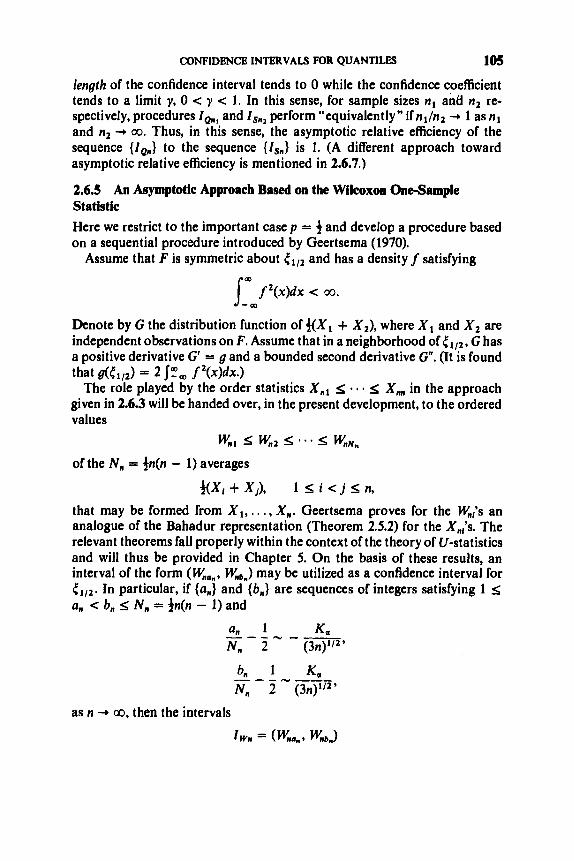
CONFIDENCE INTERVALS FOR QUANTILES 105
length of the confidence interval tends to 0 while the confidence coefficient tends to a limit y, 0 < y < 1. In this sense, for sample sizes nl and nz re- spectively, procedures I,,, and ISul perform “equivalently” if n1/n2 + 1 as nl and n, + m. Thus, in this sense, the asymptotic relative efficiency of the sequence {I,,} to the sequence {Isu} is 1. (A different approach toward asymptotic relative efficiency is mentioned in 2.6.7.)
2.6.5 An Asymptotic Approach Based on the Wilcoxon One-Sarnple Statistic Here we restrict to the important case p = 4 and develop a procedure based on a sequential procedure introduced by Geertsema (1970).
Assume that F is symmetric about el,, and has a density f satisfying (ID
S _ , / Z ( X ) d X < **
Denote by G the distribution function of g X l + Xz), where X1 and Xz are independent observations on F. Assume that in a neighborhood oft.,,,, G has a positive derivative G‘ = g and a bounded second derivative G”. (It is found
s X, in the approach given in 2.6.3 will be handed over, in the present development, to the ordered values
of the N. = 4n(n - 1) averages
that B(t1,Z) = 2 f2(X)dX.) The role played by the order statistics Xul 5
w,, 5 wu, s * * * 4 WuNn
fix, + X,), 1 s i cj s n, that may be formed from X1,. . . , X,. Geertsema proves for the Wul)s an analogue of the Bahadur representation (Theorem 2.5.2) for the X,l)s. The relevant theorems fall properly within the context of the theory of LI-statistics and will thus be provided in Chapter 5. On the basis of these results, an interval of the form (WUam, WUbJ may be utilized as a confidence interval for t.,,,. In particular, if {a,} and {b,} are sequences of integers satisfying 1 5 a, < b, 5 N, = .)n(n - 1) and
as n -P 00, then the intervals

106 THE BASIC SAMPLE STATISTICS
satisfy
(*I and
(**) with probability 1,
confidence coefficient of Iwn -+ 1 - 2a, n + 00,
n - + 00. K , length of interval Iwn - llz DD 3 fz(x)dx)nl/z’
These assertions will be justified in Chapter 5.
2.6.6 An Asymptotic Approach B a d on the Sample Mean
Still another confidence interval for is given by
-) Kasn 1Mn = @n - F s x n + nl i2 9
where xn = n-’ 2 X I , sf = n- ’ E(X, - Xn)2, and it is assumed that F is symmetric about Ctl2 and has finite variance oz. Verify (Problem 2.P.28) that the intervals ( IMMn} satisfy
(*I and
(**I with probability 1,
confidence coefficient of IMn + 1 - 2% n + 00,
n 4 00. 2K,a length of interval IMn - 7,
2.6.7 Relative EfRdency ComparisonS
Let us make comparisons in the same sense as formulated in 2.6.4. Denote by e(A, B) the asymptotic relative efficiency of procedure A relative to pro- cedure B. We have seen already that
e(Q, S) = 1.
Further, it is readily seen from 2.6.3, 2.6.5 and 2.6.6 that, for confidence intervals for the median

ASYMPTOTIC MULTIVARIATE NORMALITY OF CELL FREQUENCY VECTORS 107
As an exercise, examine these asymptotic relative efficiencies for various choices of distribution F meeting the relevant assumptions.
The asymptotic relative.efficiencies just listed are identical with the Pitman asymptotic relative efficiencies of the corresponding test procedures, as will be seen from developments in Chapter 10. This relationship is due to a direct correspondence between consideration of a confidence interval as the length tends to 0 while the confidence coefficient tends to a constant y, 0 < y < 1, and consideration of a test procedure as the “distance” between the alter- native and the null hypothesis tends to 0 while the power tends to a limit A, O < A < l .
Other notions of asymptotic comparison of confidence intervals are possible. For example, we may formulate the sequences of intervals in such a way that the lengths tend to a specified limit L while the confidence coef- ficients tend to 1. In this case, efficiency is measured by the rate at which the confidence coefficients tend to 1, or, more precisely, by the rate at which the noncoverage probability tends to 0. (The asymptotic relative efficiences obtained in this way correspond to the notion of Hodges-Lehmann asymptotic relative efficiency of test procedures, as will be seen in Chapter 10.)
The two notions of asymptotic comparison lead to differing measures of relative efficiency. In the context of sequential confidence interval procedures, the notion in which length -+ 0 while confidence coefficient + 1 - 2a (< 1) has been used by Geertsema (1970) in comparing confidence interval pro- cedures based on the sign test, the Wilcoxon test, and the mean test (i.e., basically the intervals {Is,}, { I w , } , and { I M m } which we have considered). The other notion, in which length + L ( > O ) while confidence coefficient +1, has been employed by Serfling and Wackerly (1976) for an alternate comparison of sequential confidence intervals related to the sign test and mean test. (Extension to the Wilcoxon test remains open.)
In these two approaches toward asymptotic relative efficiency of con- fidence interval procedures, differing probabilistic tools are utilized. In the case of length + 0 while confidence coefficient + 1 - 2a (< l), the main tool is central limit theory. In the other case, large deviation theory is the key.
2.7 ASYMPTOTIC MULTIVARIATE NORMALITY OF CELL FREQUENCY WCl’ORS
Consider a sequence of n independent trials, with k possible outcomes for each trial. Let pj denote the probability of occurrence of the jth outcome in any given trial (rl pj = 1). To avoid trivialities, we assume that pj > 0, each j. Let nJ denote the number of occurrences of thejth outcome in the series of n trials (z nj = n). We call (n l , . . . , nt) the “cell frequency vector” associated with the n trials.
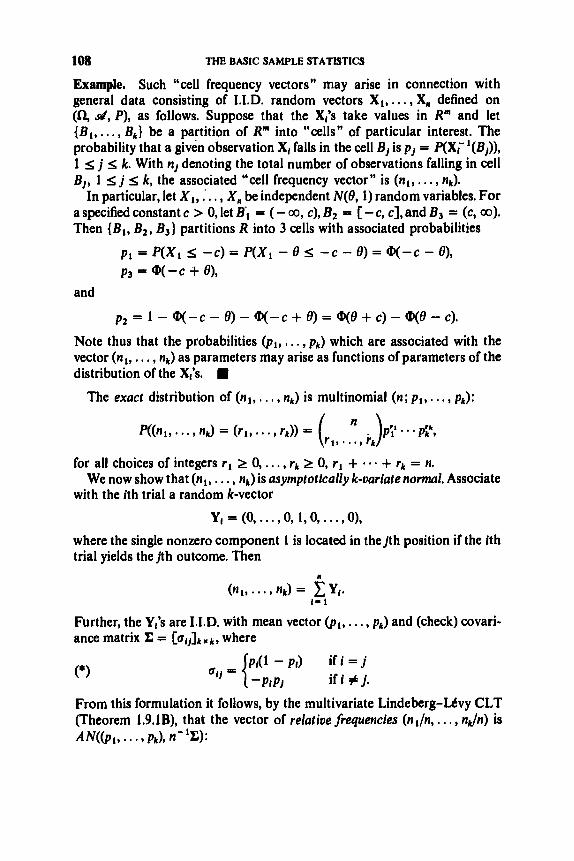
108 THE BASIC SAMPLE STATISTICS
Example. Such “cell frequency vectors’’ may arise in connection with general data consisting of I.I.D. random vectors XI,. . . , X, defined on (Q, d, P), as follows. Suppose that the X,‘s take values in R” and let {Bl , . . . , Bk} be a partition of R“ into “cells” of particular interest. The probability that a given observation X, falls in the cell B, is pJ = P(Xil(Bj)), 1 5 j 5 k. With nJ denoting the total number of observations falling in cell B,, 1 5 j 5 k, the associated “cell frequency vector” is (nl, . . . , nk).
In particular, let X1, .’. . , X, be independent N(0, 1) random variables. For a specified constant c > 0, let B; = (- to, c), E2 = [ -c, c ] , and B3 = (c, GO). Then {Bl, B2, B,) partitions R into 3 cells with associated probabilities
p1 = p(xI 5 -c) = P(X, - e 5 - c - e) = q - c - el, p3 = q - c + el,
p2 = 1 - uq-c - e) - q - c + e) = q e + c) - we - c).
and
Note thus that the probabilities (PI, . . . , pk) which are associated with the vector (nl,. . . , nk) as parameters may arise as functions of parameters of the distribution of the Xis. W
The exact distribution of (n l , . . . , nk) is multinomial (n; p I , . . . , pk):
for all choices of integers rl 2 0,. . . , rk 2 0, rl + .- . + rk = n.
with the ith trial a random k-vector We now show that (n l , . . . , nk) is asymptotically k-oariate normal. Associate
Y , = ( O ,..., 0,1,0 ,..., O),
where the single nonzero component 1 is located in thejth position if the ith trial yields thejth outcome. Then
Further, the Y,’s are I.I.D. with mean vector (pl,. . . , pk) and (check) covari- ance matrix Z = [61,]kxk, where
pr(l - pi) -PI PJ
if i = j if i # j . CIJ =
From this formulation it follows, by the multivariate Lindeberg-Uvy CLT (Theorem 1.9.1B), that the vector of relative frequencies (nl/n, . . . , nJn) is AN((p1, * * * ? pk), n-’E):
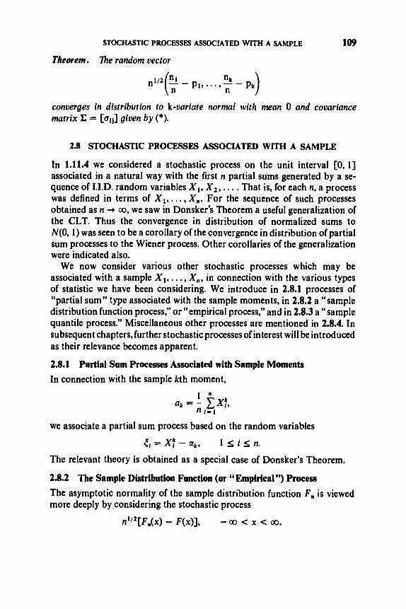
STOCHASTIC PROCESSES ASSOCIATED WITH A SAMPLE 109
Theorem. ‘Ihe random vector
n ’ / Z e - pl, . . , , - nk - p,) n
converges in distribution to k-variate normal with mean 0 and covariance matrix C = [a,J given by (*).
2.8 STOCHASTIC PROCESSES ASSOCIATED WITH A SAMPLE
In 1.11.4 we considered a stochastic process on the unit interval [0, 13 associated in a natural way with the first n partial sums generated by a se- quence of LLD. random variables XI, X2,. . . . That is, for each n, a process was defined in terms of XI,. . . , X,. For the sequence of such processes obtained as n + 00, we saw in Donsker’s Theorem a useful generalization of the CLT. Thus the convergence in distribution of normalized sums to N(0,l) was seen to be a corollary of the convergence in distribution of partial sum processes to the Wiener process. Other corollaries of the generalization were indicated also.
We now consider various other stochastic processes which may be associated with a sample XI,. . . , X,, in connection with the various types of statistic we have been considering. We introduce in 2.8.1 processes of “partial sum” type associated with the sample moments, in 2.8.2 a “sample distribution function process,” or “empirical process,” and in 2.8.3 a “sample quantile process.” Miscellaneous other processes are mentioned in 2.8.4. In subsequent chapters, further stochastic processes of interest will beintroduced as their relevance becomes apparent.
2.8.1 Partial Sum Processes Associated with Sample Moments In connection with the sample kth moment,
we associate a partial sum process based on the random variables
ti = x! - ak, l s i s n .
The relevant theory is obtained as a special case of Donsker’s Theorem.
2.8.2 The Sample Distribution Function (or “Empirical”) Process The asymptotic normality of the sample distribution function F, is viewed more deeply by considering the stochastic process
n1’2[F,(x) - F(x)], -co < x < 00.

110 THB BASIC SAMPLE STATISTICS
Let us assume that F is continuous, so that we may equivalently consider the process
obtained by transforming the domain from (- 00,m) to [0, 13, by putting x = F-'( t ) , 0 < c < 1, and defining G(0) = K(1) = 0.
The random function {I#), 0 s t s 1) is not an element of the function space CEO, 13 considered in Section 1.1 1. Rather, the natural setting here is the space D[O, 13 of functions on [O, 13 which are rightcontinuous and have left- hand limits. Suitably metrizing D[O, 11 and utilizing the concept of weak convergence of probability measures on D[O, 13, we have
Y, A Wo (in D[O, 11 suitably metrized), where W o denotes a random element of D[O, 13 having the unique Gaussian measure determined by the mean function
and the covariance function
0 s s s I s 1. We shall use the notation Wo also for the measure just defined.
The stochastic process Wo is essentially a random element of C[O, 13, in fact. That is, Wo(CIO, 11) = 1. Thus, with probability 1, the sample path of the process Wo is a continuous function on [0, 13. Further, with probability 1, Wo(0) = 0 and Wo(l) = 0, that is, the random function takes the value 0 at each endpoint of the interval [O, 13. Thus W o is picturesquely termed the "Brownian bridge," or the "tied-down Wiener" process.
The convergence Y, 4 Wo is proved in Billingsley (1968). An immediate corollary is that for each fixed x, F,(x) is asymptotically normal as given by Theorem 2.1.1. Another corollary is the asymptotic distribution of the (normalized) Kolmogorov-Smirnov distonce n'/'D,, which may be written in terms of the process Y,( a ) as
n'12Dn = sup I x(t)l .
%(I ) = n"2[F,(F-'(t)) - t], 0 S t S 1,
E{WO(r)} = 0
COV{WO(S), WO(t)} = s(l - t),
O < I < l
It follows from Y, 4 Wo that
lim P(n''2D, s d) = W o x(m): sup Ix(t)l s d , Il'Q ({ O i 1 5 l 1) (1)
since {x(s): up^,,,^ Ix(t)l s d} can be shown to be a Wo-continuity set. Also,

STOCHASTIC PROCESSES ASSOCIATED WITH A SAMPLE 111
(See Billingsley (1968) for proofs of these details.) Thus follows Theorem 2.1.5A (Kolmogorov).
As discussed in 2.1.6, the result just stated may be recast as the null- hypothesis asymptotic distribution of the Kolmogorov-Smirnov test statistic
A, = SUP IFAX) - F~(x)l . - - C X < Q
That is, for the process
l ( t ) = n1/2[F,,(F;1(t)) - t], O I; t s 1,
we have
n'/'A,, = sup I t ( t ) I
and thus, under H,: F = F, , we have n1l2An 3 supc I Wo(t)l. Thus, under H,, n112A,, has the limit distribution (1) above.
It is also of interest to have asymptotic distribution theory for A, under a fixed alternatioe hypothesis, that is, in the case F # F,. This has been obtained by Raghavachari (1973). To state the result we introduce some further notation. Put
O C I C l
A = SUP (F(x) - F&)( - m < x c m
and
C1 = {XI F(x) - F&) = A}, Cz = {x: F(x) - F,(x) = -A}.
It is convenient to switch from --a0 < x < co to 0 < t < 1. Noting that
A = SUP IF(F;'(t)) - t i , O C I C l
we accordingly put
K f = Fo(Cf) = { t : F; ' ( t ) E C,}, i = 1, 2.
Finally, on the measurable space (C[O, 13, @) considered in 1.11, denote by Wo a random element having the unique Gaussian measure determined by the mean function
E { W J ( t ) } = 0
and the covariance function
COV{~~'(S), fio(t)) = F(Fc'(s))[l - F(FC1(t))], 0 I; s I; t i; 1.
We shall use the notation also for the measure just defined.

112 THe BASIC SAMPLE STATISTICS
Theorem (Raghavachari). Let F be continuous. Then
lim P(n'/'(A, - A) s d) = mo x(.): sup x(t) s d; sup x(t) 2 -d n - r a ({ t 8 K 1 I r K i
for -GO < d < 00.
The preceding result contains (1) above as the special case corresponding to A = 0, A, = D, and K1 = Kz = [0,1], in which case the measure wo reduces to Wo.
It is also of interest to investigate n'/'A, under a sequence of local alter- natives converging weakly to Fo at a suitable rate. In this context, Chibisov (1965) has derived the limit behavior of the process p,(.).
2.8.3 The Sample Quantile Process The asymptotic normality of sample quantiles, established in 2.3 and 2.5, may be viewed from more general perspective by considering the stochastic process
For further discussion of empirical processes, see 2.8.3 below.
zn(P) = n'"<tpn - CJ, 0 < P < 1,
with Z,(O) = Z,(l) = 0. We may equivalently write
Z,(p) = n"'[Fi'(p) - F-'(P)] , 0 < p < 1.
There is a close relationship between the empirical process Y,(.) considered in 2.8.2 above and the quantile process Z,(.). This is seen heuristically as follows (we assume that F is absolutely continuous):
G(t) = n1/2[F,(F-1(t)) - t ]
= - j ( F - '(t))Z,(r). That is, there holds the approximate relationship
For the case of F uniform [0, I], this becomes &(P) = -Zm(p), 0 5 p I; 1, which suggests Z, 4 - Wo, which is the same as Z, % Wo.
A precise and illuminating technical discussion of the empirical and quantile processes taken together has been given in the appendix of a paper by Shorack (1972). Another way to see the relationship between the Y,(.) and
UP) -L - f ( t p ) z n ( p ) , 0 P 1.

PROBLEMS 113
Z,(.) processes is through the Bahadur representation (recall 2.5), which gives exactly
where for each fixed p, wpl n1’2R,,(p) = O(n-’I4 log n), n
2.8.4 Miscellaneous Other Processes
(i) The remainder process in the Bahadur representation. This process, {R,(p), 0 5 p 5 I}, has just been discussed in 2.8.3 above and has also been considered in 2.5.5. Its fundamental role is evident.
(ii) Empirical processes with random perturbations. A modified empirical process based on a sample distribution function subject to random perturba- tions and scale factors is treated by Rao and Sethuraman (1975).
(iii) Empirical processes with estimated parameters. It is of interest to consider modifications of the process Y,(.) in connection with composite goodness-of-fit hypotheses, where the stated null hypothesis distributions may depend on parameters which are unknown and thus must be estimated from thedata. In thisregard,seeDurbin(1973b), Wood(1975),and Neuhaus(l976).
(iv) “Extremal processes.” A stochastic process associated with the extreme order statistics {x,k}, k fixed, is defined by
00.
where a, and b, are suitable normalizing constants. See Dwass (1964), Lamperti (1964), and Galambos (1978).
(v) “Spacings” processes. Another type of process based on order statistics is noted in Section 3.6.
2.P PROBLEMS
Miscellaneous
random variables { X n } satisfying 1. Let {a,,} be a sequence of constants. Does there exist a sequence of
(a) X , X for some random variable X
and
(b) E { X , } = a,, all n?
Justify your answer.

114 THE BASIC SAMPLE STATISTICS
2. Let {a,} be a sequence of constants and Y a random variable. Does
(a)
(b) x, - Y,
(c) E { X , } = 0, all n?
If "yes," prove. Otherwise give counter-example.
Seetion 2.1
there exist a sequence of random variables {X,} satisfying
X , 1, X for some random variable X ,
and
3. For the density estimator
Fn(x + bn) - FXx - bn) 26,
L ( x ) = 9
(a) show that 2nb,L(x) is distributed binomial (n, F(x + b,) - F(.u - h,)).
(b) show that E(fn(x)} + j ( x ) if b, + 0, (c) show that Var{/,(x)} + 0 if b, + 0 and nb, + 00.
4. (continuation) Apply the Berry-EssCen Theorem (1.9.5) to show that iff is continuous and positive at x, then there exists a constant K depending onf(x) but not on n, such that
5. (continuation) (a) Deduce from the preceding results that (WJ"'CL(X) - ~{L(x)~I//'/'(x) 5 NO, 1):
(b) Apply Taylor's Theorem to obtain (nb,)'/'[E{L(x)} - f ( x ) ] + 0, n + 00, under suitable smoothness restrictions on Sand rate of convergence restrictions on {b,} ;
(c) From (a) and (b), establish (2nb,)''2[f,(x) - S(x)]/j"'(x) 5 N(0, 1) under suitable (stated explicitly) conditions onfand {b,} .
6. Justify that n'/'DJ(log log n)'12 converges to 0 in probability but not with probability 1.
Section 2.2
7. Do some of the exercises assigned in the proof of Theorem 2.2.3A. 8. Show that

PROBLEMS 115
(Hint: Use Lemma 2.2.3 to determine that the offdiagonal element of the covariance matrix is given by Cov{X,, (XI - P ) ~ } . )
9. Show that (x, m 2 , m 3 , . . . , mk) is asymptotically k-variate normal with mean (p, c2, p 3 , . . . , pk), and find the asymptotic covariance matrix n-’ Z.
10. Let {XI,. . . , X,} be I.I.D. with mean p and variance a? < 00, The “Student’s t-statistic” for the sample is
n1/2(Xn - p) T,= 9
Sn
whereX, = n - l c! Xi and s.’ = (n - 1)- c’i ( X i - X,)’. Derive the limit distribution of T,.
Section 2.3
be dropped.
see Remark 2.3.2 (iii).)
of Theorem 2.3.3C.
11. Show that the uniqueness assumption on C, in Theorem 2.3.1 cannot
12. Prove Theorem 2.3.2 as an application of Theorem 2.1.3A. (Hint:
13. Obtain an explicit constant of proportionality in the term O(n-1/2)
14. Complete the details of derivation of the density of f,,,, in 2.3.4. 15. Let F beadistributionfunction posessingafinitemean. Let 0 < p < 1.
Show that for any k the sample pth quantile I&,,, possesses a finite kth moment for all n sufficiently large. (Hint: apply 1.14.)
relative toX by the criterion ofasymptotic variance, for various choices of underlying distribution F. Follow the guidelines of 2.3.5.
17. Check the asymptotic normality parameters for the sample semi- interquartile range, considered in 2.3.6.
Section 2.4
16. Evaluate the asymptotic relative efficiency of
18. Check the details of Example 2.4.48.
Section 2.5
19. Show that X,Z’O(g(n)) implies X, = O,,(g(n)). 20. Verify Remark 2.5.1 (viii). 21. Verify Remark 2.5.1 (ix). 22. Prove Corollary 2.5.2. 23. Derive from Theorem 2.5.2 an LIL for sequences of central order
statistics {x&} for which kJn + p sufficiently fast.
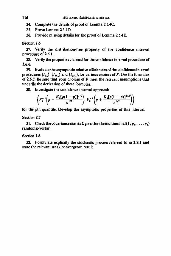
116 THE BASIC SAMPLE STATISTICS
24. Complete the details of proof of Lemma 2.5.4C. 25. Prove Lemma 2.5.4D. 26. Provide missing details for the proof of Lemma 2.5.48.
Section 2.6 27. Verify the distribution-free property of the confidence interval
procedure of 2.6.1. 28. Verify the properties claimed for the confidence interval procedure of
2.6.6. 29. Evaluate the asymptotic relative efficiencies of the confidence interval
procedures {Isn}, {Iw,} and {IMm}, for various choices of F. Use the formulas of 2.6.7. Be sure that your choices of F meet the relevant assumptions that underlie the derivation of these formulas.
30. Investigate the confidence interval approach
for the pth quantile. Develop the asymptotic properties of this interval.
Section 2.7
random k-vector.
Section 2.8
state the relevant weak convergence result.
31. CheckthecovariancematrixCgivenforthemultinomial(1; pl, . . . , pk)
32. Formulate explicitly the stochastic process referred to in 2.8.1 and

C H A P T E R 3
Transformations of Given Statistics
In Chapter 2 we examined a variety of statistics which arise fundamentally, in connection with a sample XI, . . . , X,. Several instances of asymptotically normal vectors of statistics were seen. A broad class of statistics of interest, such as the sample coeficient of variation s/’, may be expressed as a smooth function of a vector of the basic sample statistics. This chapter provides methodology for deriving the asymptotic behavior of such statistics and considers various examples.
More precisely, suppose that a statistic of interest T,, is given by g(X,), where X, is a vector of “basic” statistics about which the asymptotic be- havior is already known, and g is a function satisfying some mild regularity conditions. The aim is to deduce the asymptotic behavior of T,,.
It suffices for many applications to consider the situations
(a) X, * c, or X, 3 c ;
(b) X,,s X;
(c) X,AN(p, X,), where Z,, -, 0.
For situations (a) and (b), under mild continuity requirements on g(*), we may apply Theorem 1.7 to obtain conclusions such as T,, * g(c), xs g(c), or T,, 5 g(X). However, for situation (c), a different type of theorem is needed. In Section 3.1 we treat the (univariate) case Xn(p , of), cm -, 0, and present theorems which, under additional regularity conditions on g, yield conclusions such as “T,, is AN(g(p) , [g’(p)]20:).” In Section 3.2 the application of these results, and of Theorem 1.7 as well, is illustrated in connection with the situations (a), (b), and (c). In particular, variance-stabilizing transformations and a device called “Tukey’s hanging rootogram” are discussed. Extension of the theorems of Section 3.1 to vector-valued g and vector X, is carried out
117

118 TRANSFORMATIONS OF QMiN STATISTICS
in Section 3.3, followed in Section 3.4 by exemplification for functions of several sample moments and for “best ” linear combinations of several estimates.
Section 3.5 treats the application of Theorem 1.7 to the important special case of quadraticforms in asymptotically normal random vectors. The asymp- totic behavior of the chi-squared statistic, both under the null hypothesis and under local alternatives, is derived.
Finally, in Section 3.6 some statistics which arise naturally as functions of order statistics are discussed.
Although much of the development of this chapter is oriented to the case of functions of asymptotically normal vectors, the methods are applicable more wide I y .
3.1 FUNCTIONS OF ASYMPTOTICALLY NORMAL STATISTICS: UNIVARIATE CASE
Here we present some results apropos to functions g applied to random variables X, which are asymptotically normal. For convenience and sim- plicity, we deal with the univariate case separately, Thus here we treat the simple case that g is real-valued and X, isAN@, 0:)’ with a, --* 0. Multivariate extensions are developed in Section 3.3.
Theorem A. Suppose that X, is AN(p, at), with a, + 0. Let g be a real- uuluedjiunction dtgerentiable at x = p, with g‘(p) # 0. Then
dxn) is AN(g(p), Cg’(~)Yat)* PROOF. We shall show that
Then, by Theorem 1.5.4 (Slutsky), the random variable b(X,,) - g@)]/g‘@)a,, has the same limit distribution as (X, - p)/an, namely N(0, 1) by assumption.
Define h(p) = 0 and
Then, by the differentiability ofg at cc, h(x) is continuous at p. Therefore, since Xn 3 ~byProbleml.P.20,itfollowsbyTheorem 1.7(ii)thath(Xn) 1: h(p) = 0 and thus, by Slutsky’s Theorem again, that
that is, (1) holds. This completes the proof.

FUNCTIONS OF ASYMPTOTICALLY NORMAL STATISTICS 119
Remarks. (i) If, further, g is differentiable in a neighborhood of p and g’(x) is continuous at p, then we may replace g‘(p) by the estimate g’(xn) and have the modified conclusion
(ii) If, further, u,’ is given by u2(p)/n, where u(p) is a continuous function of p, then we may replace un by the estimate a(Xn)/n’’’ and obtain
Example A. It was seen in 2.2.4 that
It follows that the sample standard deviation s is also asymptotically normal, namely
s is AN ( a,- p:;C)* . We now consider the case that g is differentiable at p but g’(p) = 0. The
following result generalizes Theorem A to include this case.
Theorem B. Suppose that X, is AN(p, of), with on 4 0. Let g be u real- uulued function diferentiuble m ( r 1) rimes at x = p., with g(”’)(p) # 0 but g(j)(p) = ofor j < m. Then
PROOF. The argument is similar to that for Theorem A, this time using the function h defined by h(p) = 0 and
and applying Young’s form of Taylor’s Theorem (1.12.1C).

120 TRANSFORMATIONS OF QrvEN STATISTICS
Example B. Let X, be AN(0, a,'), a,, + 0. Then
b 2 ( 1 + Xn) 5 x:. 0,'
(Apply the theorem with g(x) = log2(1 + x), p = 0, rn = 2.)
3.2 EXAMPLES AND APPLICATIONS
Some miscellaneous illustrations ofTheorems 1.7,3.1A and 3.1B are provided in 3.2.1. Further applications of Theorem 3.1 A, in connection with variance- stabilizing transformations and Tukey's hanging rootogram, are provided in 3.2.2 and 3.2.3.
3.2.1 Miscellaneous Illustrations In the following, assume that X,, is AN(p, a,'), a, + 0. What can be said about the asymptotic behavior of the random variables
Regarding convergence in probability, we have X , 3 p since a, by Theorem 1.7,
0 and thus,
Moreover, regarding asymptotic distribution theory, we have the following results.
(i) For p # 0, X,' is ANb2, 4p2u,'), by Theorem 3.1A. For p = 0, X,'/a,' 3 x t , by Theorem 3.1B or Theorem 1.7.
(ii) For p # O,l/X,, is A N ( l / p , u,'/p4), by Theorem 3.1A. The case p = 0 is not covered by Theorem 3.1B, but Theorem 1.7 yields oJX, 5 l/N(O, 1).
(iii) For any p, 8- is AN(ep, e2%;). (iv) For p # 0, log I X, I is AN(log I p I, a;/p2). For p = 0, log I XJu, I 5
log I N O , 1) I * 3.2.2 VarIance-Stabilizlng Transformations Sometimes the statistic of interest for inference about a parameter 8 is conveniently asymptotically normal, but with an asymptotic variance parameter functionally dependent on 8. That is, we have X, AN(8, u,"(8)). This aspect can pose a difficulty. For example, in testing a hypothesis about 8 by using X,, the rejection region would thus depend upon 8. However, by a

EXAMPLES AND APPLICATIONS 121
suitable transformation g(*), we may equivalently use r, = g(X,) for inference about g(O) and achieve the feature that Y , is AN(g(O), y,), where yn does not depend upon 8.
In the case that a@) is the form a;(O) = hz(0)u,, where u, + 0, the appropriate choice of g may be found via Theorem 3.1A. For, if Y, = g ( X n ) and g’(O) # 0, we have
Thus, in order to obtain that Y. is AN(g(O), c’u,), where c is a constant inde- pendent of 0, we choose g to be the solution of the differential equation
Y. is AN(g(O), Ce‘(~)12h2(~)o,).
d g = - C
dO h(8)’
Example. Let X, be Poisson with mean On, where 8 > 0. Then (Problem 3.P.1) X , is A N @ , On), or equivalently,
Let g be the solution of
Thus g(x) = 2cx112. Choose c = 4 for convenience. It follows that (X,/n)’lz is AN(OIIz, 1/4n), or equivalently Xi12 is AN((On)’/2, a). This result is the basis for the following commonly used approximation: i f X is Poisson with mean p and p is large, then X112 is approximately N(p’12, 4).
A further illustration of the variance-stabilizing technique arises in the following subsection. Other examples may be found in Rao (1973), Section 64.
3.2.3 Tukey’s “Hanging Rootogram” Histograms and other forms of density estimator (recall 2.1.8) provide popular ways to test a hypothesized distribution. A plot is made depicting both the observed density estimator, say f.(x), and the hypothesized density, say fo(x), for - 00 < x < 00 (or a < x < 6). This enables one to visually assess the disparity between (the population density generating) the observed h( -) and the hypothetical so( .). Several features are noteworthy, as follows.
(i) Typically, f , (x ) is asymptotically normal. For example, in the case of the simple h(-) considered in 2.1.8 and in Problems 2.P.3-5, we have that
where nb, + 00. Thus the observed discrepancies h(x) - /b(x) are
I
h(x) is A N ( f ( x ) , f(x)/2nbn),
AN(f(x) - fo(x), f(x)/2nb,).

122 TRANSFORMATIONS OF GIVEN STATISTICS
(ii) The observed discrepancies fluctuate about the curve traced by fo(x). (iii) Under the null hypothesis, all discrepancies are asymptotically
normal with mean 0, but nevertheless two observed discrepancies of equal size may have quite different levels of significance since the asymptotic variance in the normal approximation depends on x.
Regarding property (i), we comment that it is quite satisfactory to have a normal approximation available. However, properties (ii) and (iii) make rather difficult a simultaneous visual assessment of the levels of significance of these discrepancies. A solution proposed by Tukey to alleviate this difficulty involves two elements. First, make a variance-stabilizing trans- formation. From 3.2.2 it is immediately clear that g(x) = x112 is appro- priate, giving
f;12(x) is AN(f112(x), 1/8nb,)
Thus we now compare the curves ff12(x) and fb12(x), and under the null hypothesis the observed discrepancies f;12(x) - f#’ (x) are AN(0, in&), each x. Secondly, instead of standing the curve f;12(x) on the base line, it is suspended from the hypothetical curve fV2(x ) . This causes the discrepancies f ;12(x) - f i12 (x ) all to fluctuate about a fixed base line, all with a common standard deviation (8nb,)- ‘ I2. The device is picturesquely called a hanging rootogram. For an illustrated practical application, see Healy (1968).
3 3 FUNCTIONS OF ASYMPTOTICALLY NORMAL VECTORS
The following theorem extends Theorem 3.1A to the case of a vector-valued function g applied to a vector X, which is AN(p, btZ), where b, + 0.
Theorem A. Suppose that X, = (Xnl,. . ., xnk) is AN@, bfC), with C a couariancematrix and b, + 0. Let g(x) = (gl(x), . . . , g,,,(x)), x = (xl, . . . , xk), be a vector-valued function for which each component function g,(x) is real- valued and has a nonzero diferential gi(p; t), t - (tl, :. . , r,), at x = p. Put
PROOF. Put Z,, = bfZ. By the definition of asymptotic multivariate normality (l.S.S), we need to show that for every vector 5 = (Al, . . . , A,,,) such that ADZ,Dk‘ > 0 for all sufficiently large n, we have

FUNCTIONS OF ASYMPTOTICALLY NORMAL VECTORS 123
Let 5 satisfy the required condition and suppose that n is already sufficiently large, and put b,, = (bDCnD’I.’)l’z. Define functions h f , 1 I; i 5 m, by hl(p) = 0 and
By the definition of gf having a differential at p (1.12.2), h,(x) is continuous at p.
Now
m
I = I
(2)
XCQ(Xn) - d~)I’b<n’ = C &bL’CBLXn) - BXP)I m m
i= 1 f = 1 = C 4bL’MXn)IlXn - PII + C AibC;Bi(P; Xn - PI-
By the linear form of the differential, we have
By the assumption on b, and by the definition of asymptotic multivariate normality, the right-hand side of(3) converges in distribution to N(0, 1). Thus
m
(4)
Now write m m
By Application C of Corollary 1.7, since Cn + 0 we have X, 4 p. Therefore, since each hf is continuous at p, Theorem 1.7 yields
11 ht(Xn) 1: 2 1 1 ht(p) = 0. f = l f=1
Also, now utilizing the fact that Cn is of the form b i z , and applying Application B of Corollary 1.7, we have
b ~ ~ l l X , - = (5DCD’I.’)-1’2b~’(~X, - 5 (-).
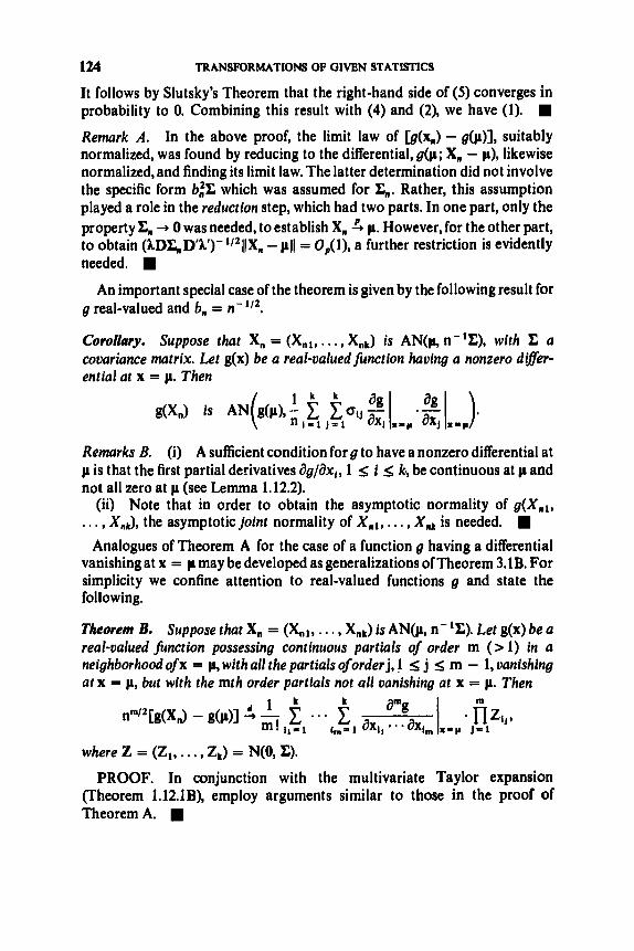
124 TRANSFORMATIONS OF GIVEN STATISTICS
It follows by Slutsky's Theorem that the right-hand side of (5 ) converges in probability to 0. Combining this result with (4) and (2), we have (1). W
Remark A . In the above proof, the limit law of b(x,) - g(p)], suitably normalized, was found by reducing to the differential, g(p; X, - p), likewise normalized, and finding its limit law. The latter determination did not involve the specific form 632 which was assumed for C,. Rather, this assumption played a role in the reduction step, which had two parts. In one part, only the property C, 4 0 was needed, to establish X, 3 p. However, for the other part, to obtain (LDC,D'A')-1~2~~X, - pll = Op(l), a further restriction is evidently needed.
An important special case of the theorem is given by the following result for g real-valued and 6, = n-'I2.
Coroffary. Suppose that X, = (Xnl , . . . , Xnk) is AN@, n-'Z), with C a covariance matrix. Let g(x) be a real-valued function having a nonzero differ- ential at x = p. Then
Remarks B. (i) A sufficient condition for g to have a nonzero differential at pis that the first partial derivatives dg/dx,, 1 5 i 5 k, be continuous at p and not all zero at p (see Lemma 1.12.2).
(ii) Note that in order to obtain the asymptotic normality of g(X, , , . . . , x, , ) , the asymptotic joint normality of X , , , . . . , Xnk is needed.
Analogues of Theorem A for the case of a function g having a differential vanishing at x = p may be developed as generalizations of Theorem 3.1B. For simplicity we confine attention to real-valued functions g and state the following.
Theorem B. Suppose that X, = (X,,, . . . , Xnk) is AN@, n- 'Z). Let g(x) be a real-valued finction possessing continuous partials of order m (> 1) in a neighborhood of x = p, with all the partials of order j, 1 4 j s m - 1, vanishing at x = p, but with the mth order partials not all vanishing at x = p. Then
where Z = (Zl , . . . , 2,) = N(0, Z).
PROOF. In conjunction with the multivariate Taylor expansion (Theorem 1.12.1B), employ arguments similar to those in the proof of Theorem A.

FURTHER EXAMPLES AND APPLICATIONS 125
Remark C. For the simplest case, m = 2, the limit random variable appear- ing in the preceding result is a quadraticform ZAZ, where
We shall further discuss such random variables in Section 3.5. a
3.4 FURTHER EXAMPLES AND APPLICATIONS
The behavior offuncrions ofseoeral sample moments is discussed in general in 3.4.1 and illustrated for the sample correlation coeficient in 3.4.2. It should be noted that statistics which are functions of several sample quantiles, or of both moments and quantiles, could be treated similarly. In 3.4.3 we consider the problem of forming an “optimal” linear combination of several asymp- totically jointly normal statistics.
3.4.1 Functions of Several Sample Moments Various statistics of interest may be expressed as functions of sample moments. One group of examples consists of the sample “coefficients” of various kinds, such as the sample coefficients of variation, of skewness, of kurtosis, of regression, and of correlation. By Theorem 2.2.1B, the vector of sample moments (al,. . , , ak) is A N ( ( a l , . . . , ak), n-’C), for some C. It follows by Corollary 3.3 that statistics which are functions of (a , , . . . , ak) are typically asymptotically normal with means given by the corresponding functions of (al, . . . , ak) and with variances of the form c/n, c constant. As an example, the correlation coefficient is treated in 3.4.2. Another example, the sample coefficient of variation s/X, is assigned as an exercise. Useful further discussion is found in Cramtr (1946), Section 28.4. For a treatment of c-sample applica- tions, see Hsu (1945). For Berry-Essten rates of order O(n-’) for the error of approximation in asymptotic normality of functions of sample moments, see Bhattacharya (1977).
3.4.2 Illustration: the Sample Correlation Coefflcient
Let (Xl, Yl), . . . , (X”, Y.) be independent observations on a bivariate distribution. The correlation of X1 and Yl is p = uxy/uxuy, where ux =
Var{ Yl}. The sample analogue,
I N X l - P W - 1 - P y ) L P x = W l l , f l y = H Y l ) , 0: = Var{X1), Qy =

126 TRANSFORMATIONS OF GIVEN STATISTICS
may be expressed as = g(V), where
and
The vector V is AN(B{V}, n-'I:), where C, ,, is the covariance matrix of (x1, y1, x:, Y:, x1 Y,). (Compute I: as an exercise.) It ~OIIOWS from Corollary 3.3 that
1 is AN@, n-IdXd),
where
The elements of d are readily found. Since
we obtain
Likewise
Verify that
3.43 Optimal Linear Combinations
Suppose that we have several estimators 8,,, , . . , 8* each having merit as an estimator of the same parameter 8, and suppose that the vector of estimators is asymptotically jointly normal: X, = @,,, . . . , 8,) is AN((&. . . , e), n-'~). Consider estimation of 0 by a linear combination of the given estimates, say
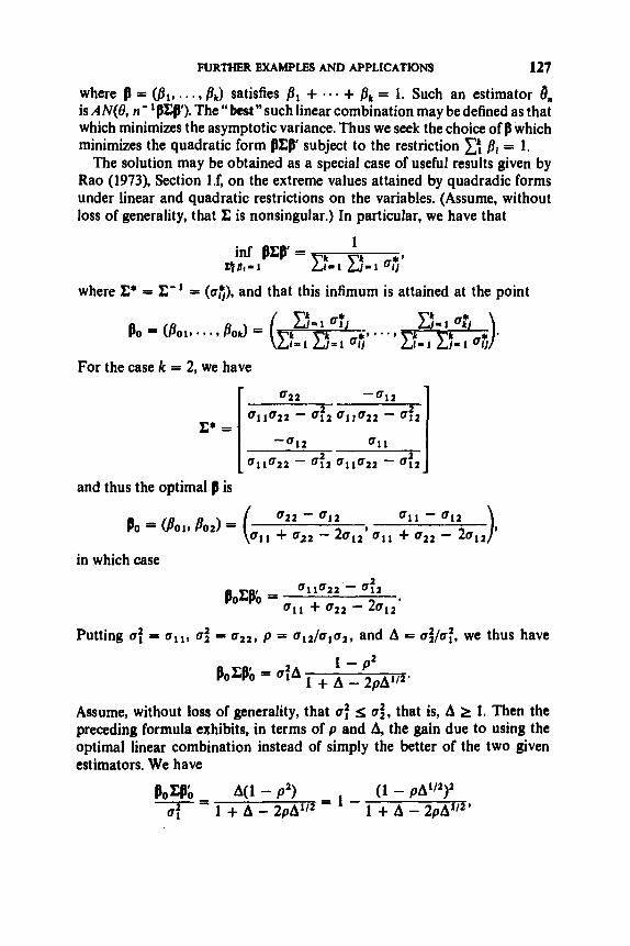
FURTHER EXAMPLES A N D APPLICATIONS 127
where fl = (I1,. . . , f l k ) satisfies /I1 + - - . + f lk = 1. Such an estimator On is AN(0, n- 'PZg'). The "best"such linear combination may be defined as that which minimizes the asymptotic variance. Thus we seek the choice of fl which minimizes the quadratic form flCg' subject to the restriction Ci f l , = 1.
The solution may be obtained as a special case of useful results given by Rao (1973), Section l.f, on the extreme values attained by quadradic forms under linear and quadratic restrictions on the variables. (Assume, without loss of generality, that C is nonsingular.) In particular, we have that
1 CI1' inf PCF =
Zfel=i
where C* = C-' = (at), and that this infimum is attained at the point
For the case k = 2, we have
6 2 2 - 6 1 2
0 1 1 6 2 2 - 4 2 611622 - 4 2
=11=22 - 4 2 Q l l Q 2 2 - 4 2
Z * = [ - u 1 2 Ql l ] and thus the optimal fl is
6 2 2 - Q12 6 1 1 - 6 1 2 Bo = 0301, P o 2 1 =
11 + 6 2 2 - 2 ~ 1 2 ' ~ I l + 6 2 2 - 2 6 1 2
in which case
=11=22'- .:2
6 1 1 + 622 - 2 6 1 2 ' flocro =
Putting 6: = 011, uf = n22, p = and A = &a:, we thus have
1 - pz floCgo = u:A 1 + A - 2pA"''
Assume, without loss of generality, that 6: s t~;, that is, A 2 1. Then the preceding formula exhibits, in terms of p and A, the gain due to using the optimal linear combination instead of simply the better of the two given estimators. We have
flozro A(1 - P2) (1 - PA^")^ 7 = 1 + A - 2pA112 = - 1 + A - 2pA""
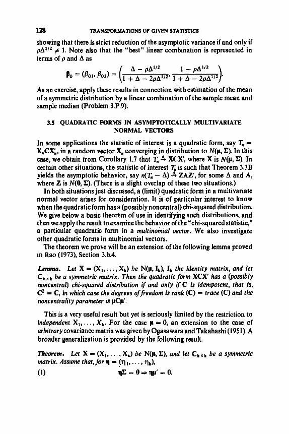
12s TRANSFORMATIONS OF GIVEN STATISTICS
showing that there is strict reduction of the asymptotic variance if and only if pA’lz # 1. Note also that the “best” linear combination is represented in terms of p and A as
As an exercise, apply these results in connection with estimation of the mean of a symmetric distribution by a linear combination of the sample mean and sample median (Problem 3.P.9).
3.5 QUADRATIC FORMS IN ASYMPTOTICALLY MULTIVARIATE NORMAL VECTORS
In some applications the statistic of interest is a quadratic form, say T, = X,CXL, in a random vector X , converging in distribution to N(p, C). In this case, we obtain from Corollary 1.7 that T, X C X , where X is N(p, C). In certain other situations, the statistic of interest T, is such that Theorem 3.3B yields the asymptotic behavior, say n(T, - A) 4 Z A Z , for some A and A, where Z is N(0, C). (There is a slight overlap of these two situations.)
In both situations just discussed, a (limit) quadratic form in a multivariate normal vector arises for consideration. It is of particular interest to know when the quadratic form has a (possibly noncentral) chi-squared distribution. We give below a basic theorem of use in identifying such distributions, and then we apply the result to examine the behavior of the “chi-squared statistic,” a particular quadratic form in a multinomial uector. We also investigate other quadratic forms in multinomial vectors.
The theorem we prove will be an extension of the following lemma proved in Rao (1973), Section 3.b.4.
Lemma. Let X = (XI,. . . , X,) be N(p, Ik), the identity matrix, and let ck ,, k be a symmetric matrix. Then the quadratic form xcx’ has a (possibly noncentraI) chi-squared distribution if and only if C is idempotent, that is, C2 = C, in which case the degrees offieedom is rank (C) = trace (C) and the noncentrality parameter is ~ c p ’ .
This is a very useful result but yet is seriously limited by the restriction to independent XI,. . . , X I . For the case p = 0, an extension to the case of arbitrary covariance matrix was given by Ogasawara and Takahashi (1951). A broader generalization is provided by the following result.
Theorem. Let X = (XI, . . . , x k ) be N(p, C), and let c k x k be a symmetric matrix. Assume that, for q = (ql , . . . , q k ) ,
(1) qc = 0 r+ qp‘ = 0.

FORMS IN ASYMPTOTICALLY MULTIVARIATE NORMAL VECTORS 129
Then XCX has a (possibly noncentral) chi-squared distribution rand only if (2) zcccc = CCZ,
in which case the degrees offreedom is trace (CC) and the noncentrality param- eter is pCp’.
2 Ak 2 0 denote the eigenvalues of C. Since C is symmetric, there exists (see Rao (1973), Section l.C.3(i) and related dis- cussion)an orthogonal matrix B havingrows b,, , . . , bk which areeigenvectors corresponding to A,, . . . , A,, that is,
PROOF. Let A, 2
btC = Aib,, 1 s i 5 k.
Thus
where 6, = I ( i = ~9, or
(**I B’AB = C.
Put
v = XB’.
Since X is N(p, Z), it follows by (*) that V is N(pB’, A). Also, since B .is orthogonal, X = VB and thus
XCX = VBCBV‘.
We now seek to represent V as V = WA“’, where W = N(a, Ik) for some a and All2 = (#’2d,,)kxf# Since pB’ = (pb;, . . . , pbi), we have by (1) that the jth component of pB’ is 0 whenever A, = 0. Define
Q, = {;bW’, i f 4 z 0, if A, = 0.
ThusaA1I2 = (alA:l2,. . . , akAi3.2) = pBand V has thedesiredrepresentation for this choice of a. Hence we may write
XCX’ = WA”2BCB’A’/’W = WDW,
where D = A”2BCB’A’/2. It follows from the lemma that XCX‘ has a chi- squared distribution if and only if D2 = D. Now
DZ = (A1/ZBCB’A1/2)(A1/2BCB~i~z) = A ~ / ~ B C B ’ A B C B ’ A ~ / ~ = A~/~BcccB’A~/~,

130 TRANSPORMATIONS OF GIVEN STA'MSTICS
making use of (**). Thus DZ = D if and only if
(3) A ~ I ~ B C X C B ' A ~ I ~ = A ~ I Z B C B ' A ~ ~ Z .
Now check that
AA1 = A A a o A 1 1 2 A I = A"'A1
and
AIA = A z A o A I A 1 l Z = AZA1".
Thus (3) is equivalent to
(4) ABCCCB'A = ABCB'A.
Now premultiplying by B' and postmultiplying by B on each side of (4), we have (2). Thus we have shown that Dz = D if and only if (2) holds. In this case the degrees of freedom is given by rank (D). Since trace (A1/zAA1/2) = trace (AA) and since AB = BC, we have
rank(D) = trace(ABCB') = trace(BCCB) = trace(CC).
It remains to determine the noncentrality parameter, which is given by
aDa' = aA1/ZBCBA1lZa' = pB'BCB'Bp' = pCp'.
Example A. The case C nonsingular and C = Z-I. In this case conditions (1) and (2) of the theorem are trivially satisfied, and thus XI;-'x' is distributed as x w - 'r').
Example B. Multinomial vectors and the "chi-squared statistic." Let (nl,. . ., nk) be multinomial (n;pl , . . ., pk), with each p , > 0. As seen in Section 2.7, the vector
converges in distribution to N(0, C), where
A popular statistic for testing hypotheses in various situations is the chi- squared statistic
& (n, - np,y 1 n 2
TI- 1-1 c np, =nC 1-1 Pi -(;-PI).

FORMS IN ASYMPlWl’lCALLY MULTIVARIATE NORMAL VECTORS 131
This may be represented as a quadratic form in X,:
where
C = = (k4,).
We now apply the theorem to determine that the “chi-squared statistic” is, indeed, asymptotically chi-squared in distribution, with k - 1 degrees of freedom. That is,
T, 5 xf - 1.
We apply the theorem with p = 0, in which case condition (1) is trivially satisfied. Writing ulJ = pl(Gl, - p,), we have
= (A P1 ul,) = (61, - p,)
and thus
and hence (2) holds. We also see from the last step that k
1- 1
trace(CL;) = (1 - p,) = k - 1 (= rank(CC)).
Thus we have that, for the given matrices L; and C,
x, 5 N(0, C) * T, = x,cx; 5 xf - 1’ rn Example C (continuation). It is also of interest to consider the behavior of the statistic T. when the actual distribution of (nl, . . . , n k ) is not the hypothe- sized multinomial (n; pl, . . . , p k ) distribution in terms of which T, is defined, but rather some other multinomial distribution, say multinomial (n; pnl, . . . , p&), where the parameter (Pnl,. . . , p n k ) converges to (pi,. . . , pk) at a suitable rate. Whereas the foregoing asymptotic result for T, corresponds to its behavior under the null hypothesis, the present consideration concerns the behavior of T, under a sequence of “local” alternatioes to the null hypothesis. In particular, take
Pml = pi + AIn-”’, 1 5 i 5 k, n = 132, .i. .

132 TRANSFORMATlONS OF GIVEN STATISTICS
Then we may express X, in the form
Pnk) + (Al, * * * > Ak)s X, = n1/2(% - pnl, . . . , - nk -
n n that is,
X, = X: + A,
where A = ( A l , . . . , Ak) satisfies c{ A1 = 0 and n-'lZX: is a mean of I.I.D. random vectors, each multinomial (1 ; pnl, . . . , Pnk). By an appropriate multivariate CLT for triangular arrays (Problem 3.P.10), we have X i N(0, C) and thus X, 5 N(A, C). We now apply our theorem to find that in this case T, converges in distribution to a noncentrd chi-squared variate. We have already established in Example B that (2) holds and that rank (CC) = k - 1. This implies that rank (C) = k - 1 since rank (C) = k. Thus the value 0 occurs with multiplicity 1 as an eigenvahe of C. Further, note that l k = (1, . . , , 1) is an eigenvector for the eigenvalue 0, that is, Cl; = 0. Finally, Al; = c: Al = 0. It is seen thus that (1) holds. Noting that
we obtain from the theorem that, for C and C as given,
Note that this noncentrality parameter may be written as
n A (.k} - PI)'. 1-1 PI
An application of the foregoing convergence is to calculate the approximate power of T, as a test statistic relative to the null hypothesis
against an alternative
Suppose that the critical region is { T, > t o } , where the choice of to for a level a test would be based upon the null hypothesis asymptotic 1:- distribution of T,,. Then the approximate power of T, at the alternative HI is given by inter- preting (pf, . . , , pz) as (pnl, . . , , p&) and calculating the probability that a random variable having the distribution
H o : (nl, . . . , nk)
HI : (nl, . , . , nk)
is multinomial (n; p l , . , . , Pk)
is multinomial (n; pt, . . . , p:).
exceeds the value to .

FORMS IN ASYMPTOTICALLY MULTIVARIATE NORMAL VECTORS 133
Example D (.continuation). Further quadratic forms in multinomiul uectors. Quadratic forms in
xn = n1/2(2 - P I , . . . , - nk - p k ) n n
other than the chi-squared sthtistic may be of interest. As a general treatment, Rao (1973), Section 6.a.1, considers equivalently the vector
which is related to X,, by V,, = X,D, where
p ; 112
D = [ ' * . ] = (p,-11z6,j). p; 112
+ = (py, . . . , p y ) Rao puts
and establishes the proposition : a su@cient condition for the quadratic form V,,CVb, C symmetric, to conuerge in distribution to a chi-squared distribution is
(*I C'= C and +C=a+,
that is, C is idempotent and + is an eigenuector of C, in which case the degrees of freedom is rank (C) ifa = 0 and rank (C) - 1 i f a # 0. We now show that this result follows from our theorem. By Application A
of Corollary 1.7, V,, 5 N(0, X*), where
= - @@a
Applying (*), we have
CE* = C - C+'+ = C - a+'+
and hence (check)
CC*CC* = C - 2a@+ + a'+'+.
But (*) implies a = 0 or 1, so that
CC*CZ* = C - a@+ = CZ*,

134 TRANSFORMATIONS OF GIVEN STATISTIC!?
that is, CC* is idempotent. Further, it is seen that
trace(<=) -- rank(C) if a = 0 trace(C) - 1 3: rank(C) - 1
Thus the proposition is established. In particular, with C = Ik, the quadratic form V,CVk is simply the chi-
squared statistic and converges in distribution to x i - as seen in Example B. rn
if a # 0. trace(CC*) = {
3.6 FUNCTIONS OF ORDER STATISTICS
Order statistics have previously been discussed in some detail in Section 2.4. Here we augment that discussion, giving further attention to statistics which may be expressed asfunctions of order statistics, and giving brief indication of some relevant asymptotic distribution theory. As before, the order statistics of a sample X1, . . . , X, are denoted by X, I 5 .
A variety of short-cut procedures for quick estimates of location or scale parameters, or for quick tests of related hypotheses, are provided in the form of linear functions of order statistics, that is statistics of the form
s X,,.
For example, the sample range X,, - X,, belongs to this class. Another example is given by the a-trimmed mean.
which is a popular competitor of X for robust estimation of location. A broad treatment of linear functions of order statistics is provided in Chapter 8.
or *“wild” observations) are of concern, a useful statistic for their detection is the studentized range.
In robustness problems where outliers (“contaminated
where 8, is an appropriate estimator of 6. A one-sided version, for detection of excessively large observations, may be based on the so-called extreme deviate X, - X. Likewise, a studentized extreme deviate is given by (X, - x)/s.
The differences between successive order statistics of the sample are called the spacings. These are
Dn1 = X,I - Xn,l-l, 2 S i S n*
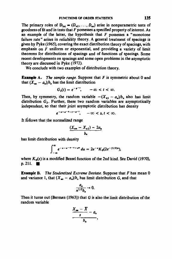
FUNCTIONS OF ORDER STATISTICS 135
The primary roles of DC) = (Dnl , . . . , D,,,,) arise in nonparametric tests of goodness of fit and in tests that F possesses a specified property of interest, As an example of the latter, the hypothesis that F possesses a "monotone failure rate" arises in reliability theory. A general treatment of spacings is given by Pyke (1965), covering the exact distribution theory of spacings, with emphasis on F uniform or exponential, and providing a variety of limit theorems for distributions of spacings and of functions of spacings. Some recent developments on spacings and some open problems in the asymptotic theory are discussed in Pyke (1972).
We conclude with two examples of distribution theory.
Example A. The sample range. Suppose that F is symmetric about 0 and that (Xnn - an)/b,, has the limit distribution
G,(t) = e-'-', -co < t < co.
Then, by symmetry, the random variable -(Xn1 - a,,)/b,, also has limit distribution G5. Further, these two random variables are asymptotically independent, so that their joint asymptotic distribution has density
e , --oo < S , t < co.
It f6llows that the normalized range
- I - e - a - , - e - t
( x n n - xn1) - 20" b m
has limit distribution with density m
e - * -e - ' -"- e" du = 2e-*K,(2e- (1 /29, s_, where K,(z) is a modified Bessel function of the 2nd kind. See David (1970), p. 211. rn Example B. The Studentized Extreme Deviate. Suppose that F has mean 0 and variance 1, that (X,,,, - a,,)/b,, has limit distribution G, and that
Then it turns out (Berman (1963)) that G is also the limit distribution of the random variable

136 TRANSFORMATIONS OF GIVEN STATISTICS
where x = n-’ cy X I and sz = ( n - l)-’ r, ( X , - X ) z . In particular, for F “0, 1)-
3.P PROBLEMS
Sections 3.1,3.2
Show that X , is AN(A,,, A,), n + co. (Hint: use characteristic functions.)
show that 4n(D:)’ s x i .
1. Let X , be Poisson with mean A,, and suppose that A,, -+ 00 as n -P 00.
2. For the one-sided Kolmogorov-Smirnov distance 0: treated in 2.1.5,
3. Let X , 4 N(p, uz) and let Y, be AN@, uz/n). Let
Investigate the limiting behavior of g(X,) and g(Y,). (By “limiting behavior” is meant both consistency and asymptotic distribution theory.)
4. Let X,, . . . , X, be independent N(8,l) variables, 8 unknown. Con- sider estimation of the parametric function
v(e) = P,,(x, 5 c) = w - e), where c is a specified number. It is well known that the minimum variance unbiased estimator of y(8) is
c - x, 1 ) ” Z )
Determine the limiting behavior of this estimator.
sections 343 .4
5. Provide details of proof for Theorem 3.3B. 6. Complete the details of the sample correlation coefficient illustration
in 3.4.2. 7. Show that the sample correlation coefficient (defined in 3.4.2) con-
verges with probability 1 to the population correlation coefficient. Show also that it converges in rth mean, each r > 0.
8. Let XI, Xz ,... be I.I.D. with mean p and variance crz, and with p4 < 00. The sample coefficient of variation is sn/Xn, where x, = n- ’ c; X I

PROBLEMS 137
and s,' = (n - l ) - l c1 (X, - X,J2. Derive the asymptotic behavior of SJX,. That is, show:
(i) If p # 0, then
(ii) If p = 0, then
9. Consider independent observations XI, Xz, . . . on a distribution F having density F' = f symmetric about p. Assume that F has finite variance and that F" exists at p. Consider estimation of p by a linear combination of the sample mean X and the sample median el,Z.
(a) Derive the asymptotic bivariate normal distribution of (X, el,,). (Hint: use the Bahadur representation.)
(b) Determine the "best" linear combination.
Section 3.5 10. Multivariate CLTfor triangular array. Let X, = (Xnl, . . . , Xnk) be a
mean of n I.I.D. random k-vectors ((,,,, . . . , t,p), 1 S j I; n, each having mean (0, . . . , 0) and covariance matrix C,. Suppose that C, -+ Z, n -+ 00, where C is a covariance matrix. Suppose that all Cnlr satisfy E((n,!12+e < K for some fixed e > Oand K < 00. Show that X, is AN(0, n-92). (Hint: apply Corollary 1.9.3 in conjunction with the Cramtr-Wold device.)
11. Discuss the asymptotic distribution theory of T. = X,CX; when X, 5 X and C, 3 C, where C is a constant matrix. In particular, deal with the modified chi-square statistic

C H A P T E R 4
Asymptotic Theory in
Parametric Inference
This chapter treats statistics which arise in connection with estimation or hypothesis testing relative to a parametric family of possible distributions for the data,
Section 4.1 presents a concept of asymptotic optimality in the context of estimation on the basis of a random sample from a distribution belonging to the specified family. In particular, Section 4.2 treats estimation by the method of maximum likelihood, and Section 4.3 considers some other methods of estimation. Some closely related results concerning hypothesis testing are given in Section 4.4.
We have seen in Section 2.7 how data in the form of a random sample may be reduced to multinomial form by grouping the observations into cells. Thus,asanadjunctto thetreatment ofSections4.1-4.4, wedeal with"product- multinomial" data in Sections 4.5 (estimation results) and 4.6 (hypothesis testing results). Of course, this methodology is applicable also without refer- ence to a parametric family of distributions.
The concept of asymptotic optimality introduced in Section 4.1 is based on a notion of asymptotic relative efficiency formulated in terms of the gener- alized variance of multidimensional distributions. This generalizes the one- dimensional version given in 1.15.4. For the hypothesis testing context, the treatment of asymptotic relative efficiency is deferred to Chapter 10, which provides several distinctive notions. (These notions may also be recast in the estimation context.)
4.1 ASYMPTOTIC OPTIMALITY IN ESTIMATION
Two notions of asymptotic relative efficiency of estimation procedures were discussed in 1.15.4, based on the criteria of variance and probability concentra- tion. The version based on variance has been exemplified in 2.3.5 and 2.6.7.
138
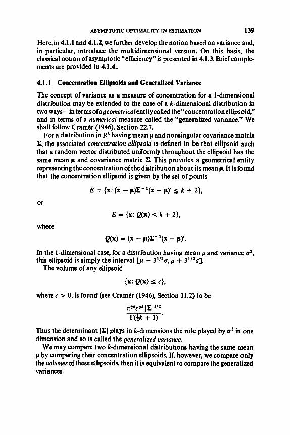
ASYMPTOTIC OPTIhfALlTY IN ESTIMATION 139
Here, in 4.1.1 and 4.1.2, we further develop the notion based on variance and, in particular, introduce the multidimensional version. On this basis, the classical notion of asymptotic “efficiency” is presented in 4.1.3. Brief comple- ments are provided in 4.1.4..
4.1.1 Concentration Ellipsoids and Generalized Variance
The concept of variance as a measure of concentration for a 1-dimensional distribution may be extended to the case of a kdimensional distribution in two ways-in terms ofageometricalentity called the “concentration ellipsoid,” and in terms of a numerical measure called the “generalized variance.” We shall follow CramCr (1946), Section 22.7.
For a distribution in Rk having mean p and nonsingular covariance matrix C, the associated concentration ellipsoid is defined to be that ellipsoid such that a random vector distributed uniformly throughout the ellipsoid has the same mean p and covariance matrix C. This provides a geometrical entity representing the concentration of the distribution about its mean p. It is found that the concentration ellipsoid is given by the set of points
E = {x: (x - p)C-’(x - py 5 k + 2},
or
E = {x: Q(x) S k + 2},
where
Q(x) = (X - ~) )C- ’ (X - p)’. In the 1-dimensional case, for a distribution having mean p and variance 02, this ellipsoid is simply the interval
The volume of any ellipsoid - 3’%7, p + 3’%].
{x: Q(x) s 4, where c > 0, is found (see Cramtr (1946), Section 11.2) to be
atkc+& I C 1112
rok + 1) - Thus the determinant 1x1 plays in k-dimensions the role played by o2 in one dimension and so is called the generalized uariance.
We may compare two &-dimensional distributions having the same mean p by comparing their concentration ellipsoids. If, however, we compare only the wlumesof these ellipsoids, then it is equivalent to compare the generalized variances.

140 ASYMPTOTIC THHORY IN PARAMETRIC INFERENCE
4.1.2 Application to Estimation: Confidence Ellipsoids and Asymptotic Relative EfRciency
Consider now the context of estimation of a k-dimensional parameter 8 = (el,. . . , 0,) by 8, = (On,, . . . , n - l ~ ) , with C, non- singular. An ellipsoidal confidence region for 8 is given by
where 8, is
E, = {e: ,(8, - e)co;1(8, - ey 5 c } 112 8 = {a: Q(n ( n - 01, %"') 5 c),
where
and it is assumed that Z&' is defined. Assuming further that
Q(A,C) = ACA'
ce;' 2 it follows (why?) that
~ ( n 1 / 2 ( 8 ~ - el, ce;') - Q(n1/2((1, - el, c; 1) 3 0.
Q(P(~, - el, g;) 3 1:.
pe(e E E,) = P ~ ( Q ( ~ I ~ / ~ ( ~ , - e), qml) s c,) + ~(1, ' s c,) = I - a,
Consequently, by Example 3SA, we have
Therefore, if c = c, is chosen so that P(x: > c,) = a, we have
as n + 00, so that En represents an ellipsoidal confidence region (confidence ellipsoid) for 8 having limiting confidence coefficient 1 - a as n + 00.
One approach toward comparison of two such estimation pmedures is to compare the volumes of the corresponding confidence ellipsoids, for a specified value of the limiting confidence coefficient. Such a comparison reduces to comparison of the generalized variances of the asymptotic multivariate normal distributions involved and is independent of the choice of confidence coefficient. This is seen as follows. Let us compare the sequences {8f)} and {8i2)}, where
8t) is AN@, n-l~#)),
and
for i = 1,2. Then the corresponding confidence ellipsoids
E:) = {e: ~(~1'2(4:) - e), ( ~ % ) ) - 1 ) ca}, i = 1 , ~

ASYMPTOTIC OPTIMALITY IN ESTIMATION 141
each have asymptotic confidence coefficient 1 - ct and, by 4.1.1, have volumes
n( 1 / 2 1 k ( c ~ n ) ( 1 /2 )k I z(& I 112 , i = 1, 2. rok + 1)
It follows that the ratio of sample sizes nz/nl at which 6::) and 6:;) perform “equivalently” (i.e., have confidence ellipsoids whose volumes are asymp- totically equivalent “in probability”) satisfies
Hence a numerical measure of the asymptotic relative efficiency of {6i2)} with respect to {&,‘I} is given by
Note that the dimension k is involved in this measure. Note also that we arrive at the same measure if we compare {Oil)} and {6i2]} on the basis of the concentration eillipsoids of the respective asymptotic multivariate normal distributions.
By the preceding approach, we have that {ei’)} is better than {&’)}, in the sense of asymptotically smaller confidence ellipsoids (or concentration ellipsoids), if and only if
(1) tzpt 5 Ic&z’I. A closely related, but stronger, form of comparison is based on the condition
(2) Z&’) - Z&’) nonnegative definite,
or equivalently (see Rao (1973), p. 70, Problem 9),
(2’)
or equivalently
(2”) xZbl)x’ s xZ&’]x‘, all x.
Condition (2) is thus a condition for the asymptotic distribution of 6:’) to possess a concentration ellipsoid contained entirely within that of the asymp- totic distribution of 6f). Note that (2) implies (1).
Under certain regularity conditions, there exists a “best” matrix in the sense of condition (2). This is the topic of 4.1.3.
(C&’))- ’ - (C&2))- ’ nonnegative definite,
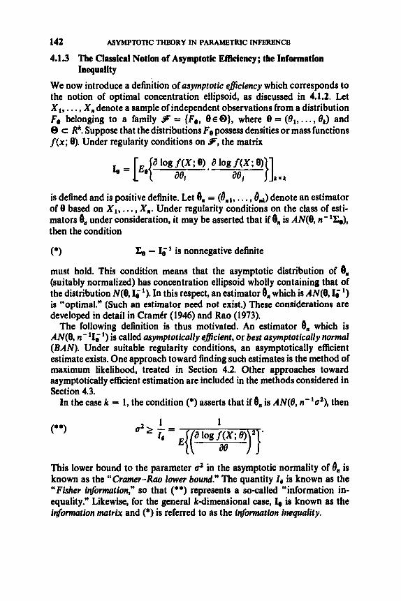
142 ASYMPTOTIC THEORY IN PARAMETRIC INFERENCE
4.13 The Classical Notion of Asymptotic Efflciency; the Information Inequality
We now introduce a definition of asymptotic eficiency which corresponds to the notion of optimal concentration ellipsoid, as discussed in 4.1.2. Let XI, . , . , X , denote a sample of independent observations from a distribution F, belonging to a family 9 = {F,, 8 E Q}, where 8 = (el,. . . , O& and 8 c R‘. Suppose that the distributions F, possess densities or mass functions f ( x ; 8). Under regularity conditions on 9, the matrix
is defined and is positive definite. Let 6, = (d,,,, . . . , 8 , k ) denote an estimator of 8 based on XI, . . . , X,. Under regularity conditions on the class of esti- mators 6, under consideration, it may be asserted that if 6, is AN(& n-’&), then the condition
(*I C, - 1;’ is nonnegative definite
must hold. This condition means that the asymptotic distribution of 6, (suitably normalized) has concentration ellipsoid wholly containing that of the distribution N(8,I; I). In this respect, an estimator 6, which is AN(@, I i I )
is “optimal.” (Such an estimator need not exist.) These considerations are developed in detail in Cramtr (1946) and Rao (1973).
The following definition is thus motivated. An estimator 6, which is AN(8, n-II; I) is called asymptotically eficient, or best asymptotically normal (BAN). Under suitable regularity conditions, an asymptotically efficient estimate exists. One approach toward finding such estimates is the method of maximum likelihood, treated in Section 4.2. Other approaches toward asymptotically efficient estimation are included in the methods considered in Section 4.3.
In the case k = 1, the condition (*) asserts that if 6, is AN(& n-’o’), then
1
This lower bound to the parameter d in the asymptotic normality of 8, is known as the “Cramer-Rao lower bound.” The quantity Zb is known as the “Fisher information,” so that (**) represents a so-called “information in- equality.” Likewise, for the general kdimensional case, I, is known as the information matrix and (*) is referred to as the informution inequality.

ESTIMATION BY THB METHOD OF MAXIMUM LIKELIHOOD
Example. Consider the family F = (N(8 , cf), 8 E R}. Writing
143
f ( x ; e) = ( 2 ~ ) - 1 / 2 ~ ; exp[ - ($)2], -m < x c m,
we have
so that
Therefore, for estimation of the mean of a normal distribution with variance ez, any “regular” estimator 8, which is AN(& n-lu) must satisfy u 2 c2. It is thus seen that, in particular, the sample mean X is asymptotically efficient whereas the sample median is not. However, X is not the only asymptotically efficient estimator in this problem. See Chapters 6, 7, 8 and 9.
4.1.4 Complements
. (i) Further discussion of the Crarnkr-Rao bound. See Cramtr (1946), Sections 32.3,32.6,32.7. Also, see Rao (1973), Sections 5a.2-5a.4, for informa- tion-theoretic interpretations and, references to other results giving different bounds under different assumptions on F and 6,, .
(ii) Other notions ofeflciency. See Rao (19731, Section 5c.2. (iii) Asymptotic eflectiue uariance. To avoid pathologies of “super-
efficient” estimates, Bahadur (1967) introduces a quantity, “asymptotic effective variance,” to replace asymptotic variance as a criterion.
4.2 ESTIMATION BY THE METHOD OF MAXIMUM LIKELIHOOD
We treat here an approach first suggested by C. F. Gauss, but first developed into a full-fledged methodology by Fisher (1912). Our treatment will be based on Cramtr (1946). In 4.2.1 we define the method, and in 4.2.2 we characterize the asymptotic properties of estimates produced by the method.
4.2.1 The Method
Let XI, . . . , X , be I.I.D. with distribution Fa belonging to a family F = { F e , 8 E a}, and suppose that the distributions Fe possess densities or mass functions f ( x ; 0). Assume 0 c Rk.
The likelihood function of the sample XI, . . . , X,, is defined as n
I = 1 W ; XI, . * * 9 X n ) = fl f(x,; 8).

144 ASYMPTOTIC THEORY IN PARAMETRIC INFERENCE
That is, the joint density (or mass function) of the observations is treated as a function of 8.
The method of maximum likelihood provides as estimate of 8 any value 8 which maximizes L in 8. (Equivalently, log t may be maximized if convenient for computations.)
Often the estimate 8 may be obtained by solving the system of likelihood equations,
and confirming that the solution 6 indeed maximizes L.
Remark. Obviously, the method may be formulated analogously without the I.I.D. assumption on XI, X 2 , . . . . However, in our development of the asymptotic behavior of the maximum likelihood estimates, the I.I.D. assumption will be utilized crucially. fl
4.2.2 Consistency, Asymptotic Normality, and Asymptotic EfRciency of Maximum Likelihood Estimates
We shall show that, under regularity conditions on %, the maximum likeli- hood estimates are strongly consistent, asymptotically normal, and asymp- totically eficient. For simplicity, our treatment will be confined to the case of a ldimensional parameter. The multivariate extension will be indicated without proof. We also confine attention to the case that f ( x ; 0) is a density. The treatment for a mass function is similar.
Regularity Conditions on 9. Consider 8 to be an open interval (not necessarily finite) in R. We assume:
(R 1) For each 0 E 8, the derivatives
a log f(x; e) a* log f(x ; e) i33 log j ( x ; e) ae * a2 * ae3
exist, all x; (R2) For each 8, E 0, there exist functions &), h(x) and H(x) (possibly
depending on 0,) such that for 8 in a neighborhood N(B,) the relations

ESTIMATION BY THE METHOD OF MAXIMUM LIKELIHOOD 145
(R3) For each 8 e 0,
Some interpretations of these conditions are as follows. Condition ( R 1) insures that the function a log f ( x ; 8)@l has, for each x, a Taylor expansion as a function of 8. Condition (R2) insures (justijy) that J f ( x ; 8 ) d x and S [a log f ( x ; 8)/a8]dx may be differentiated with respect to 8 under the integralsign. Condition (R3) states that the random variable a log f(X; 6)/a8 has finite positive variance (we shall see that the mean is 0).
Theorem. Assume regularity conditions ( R l), (R2) and (R3) on thefamily 9. Consider 1J.D. observations on Fg, for 8 an element of 0. Then, with Pg- probability 1, the likelihood equations admit a sequence of solutions {bn} satisfying
(i) strong consistency: 6" + 8, n + m; (ii) asymptotic normality and eficiency :
PROOF. (modeled after CramCr (1946)) By (Rl) and (R2) we have for A in the neighborhood N(8) a Taylor expansion of a log f ( x ; A)/aA about the point A = 8, as follows;
a2 log f ( x ; 4 1-( a12
= ( A - e) A-0
+ $32 - Wm), I a log f ( x ; A) - a log f ( x ; A)
an
where Ill < 1. Therefore, putting
A,, =E - 9
n l = l dri A = 0
and
we have
( * c )
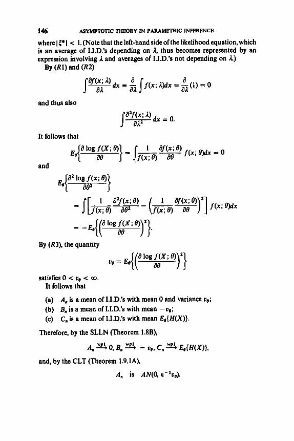
146 ASYMPTOTIC THEORY IN PARAMETRIC INFERENCE
where I {* I < 1. (Note that the left-hand side of the likelihood equation, which is an average of 1.1.D.’~ depending on A, thus becomes represented by an expression involving A and averages of 1.1.D.’~ not depending on A.)
By (R 1) and (R2)
and thus also
It follows that
and
By (R3), the quantity
satisfies 0 < ve < 00. It follows that
(a) A,, is a mean of I.I.D.3 with mean 0 and variance 00;
(b) B,, is a mean of 1.1.D.’~ with mean -ve; (c) C,, is a mean of 1.1.D.’~ with mean E e { H ( X ) } .
Therefore, by the SLLN (Theorem 1.8B),
WP 1 A,, * 0, B,, - - ve, c,, 2 E e { H ( x ) } ,
and, by the CLT (Theorem 1.9.1A),
A, is AN(O, n-’ve).

ESTIMATION BY THE METHOD OF MAXIMUM LIKELIHOOD 147
Now let e > 0 begiven,such that e < Ve/&{H(X)} and such that the points A, = 8 - e and A, = 8 + E lie in N(8), the neighborhood specified in condition (R2). Then, by (*),
and
By the strong convergences of A,, B, and C, noted above, we have that with Pe-probability 1 the right-hand side of each of the above inequalities becomes <($)Ve& for all n sufficiently large. For such n, the interval
thus contains the point 0 and hence, by the continuity of a log L(A)/aA, the interval
re - 6, e + E] = [A,, AJ
contains a solution of the likelihood equation. In particular, it contains the solution
an A: 8 - E s 1 5 8 + E and
Before going further, 4et us verify that em, is a proper random variable, that is, is measurable. Note that, for all t 2 8 - E,
Also, by continuity of a log L(A)/aA in [8 - E, 8 + E ] ,
e-asA5r an e - 8 5 A s t an a log L(A)
= inf a log L(A)
inf A ratlond
and
Thus {one > t } is a measurable set.

148 ASYMPTOTIC THEORY IN PARAMETRIC INFERENCE
Next let us obtain a sequence of solutions {On} not depending upon the choice of e. For this, let us denote by (n, d, Po) the underlying probability space and let us express one explicitly as fine(o). Our definition of 8,,*(w) required that n be suficiently large, n 2 N,(w), say, and that w belong to a set n, having Pe-probability 1. Let us now define
aD
= n n l / k * k = I
Then Pe(n0) = 1 also. For the moment, confine attention to w ~ n , . Here, without loss of generality, we may require that
N l ( 4 I; N,/Z(N s Nl/d@ s# ..’ * Hence, for NlIk(co) I; n < Nl,(k+
for k = 1,2,. . . . And for n < Nl(w), we set 8, w) = 0. Finally, for o$R,,
variables which with Pe-probability 1 satisfies:
we may define
B,(w) = On.
we set 8,(w) = 0, all n. It is readily seen that { ‘e ,} is a sequence of random
(1) 8, is a solution of the likelihood equation for all n sufficiently large, and
(2) 8, + 8, + CO.
We have thus established strong consistency, statement (i) of the theorem. To obtain statement (ii), write
which with Pe-probability 1 is valid for all n sufficiently large. Therefore,
Also, since 8, ”p? 8, we have B, + i(*C,,(8, - 0) % - v e . Further, n112A, N(0, oo). Consequently, by Slutsky’s Theorem,
~ I ~ ’ ~ ( O , - e) 5 N(O, U; 11, establishing statement (ii) of the theorem.
Multidimensional Generalization. For the case of several unknown para- meters 8 = (el, . . . , &), and under appropriate generalizations of the regularity conditions (R1)-(R3), there exists a se uence @,,} of solutions to the likelihood equations such that 8 and\, is AN(8,n-11g1), where I, is the information matrix defined in 4.1.3.

ESTIMATION BY THE METHOD OF MAXIMUM LIKELIHOOD 149
Remarks. (i) Other sequences of solutions. The argument leading to state- ment (ii) of the theorem may be modified to handle an sequence {&} of solutions which are weakly consistent for 8. Therefore, if 4 is any solution of the likelihood equations satisfying& 3 8, then 8; is AN(8, n - ‘LIB ‘)(Problem 4.P.3).
(ii) Transformation ofparameters, It is readily seen that if we transform to newparametersp = (PI, . . . , @,),where& = g,(8,, . . . , OJ,thenthemaximum likelihood estimate of p is given by the corresponding transformation of the maximum likelihood estimate (I, of 8. Thus, under mild regularity conditions on the transformation, the consistency and asymptotic normality properties survive under the transformation.
(iii) “Likelihood processes” associated with a sample. See Rubin (1961). (iv) Reguhity assumptions not inuoluing diferentiability. See Wald (1949)
for other assumptions yielding consistency of 8,. (v) Zteratiue Solution of the Likelihood Equations. The Taylor expansion
appearing in the proof of the theorem is the basis for the following iterative approach. For an initial guess one, we have
This yields the next iterate
The process is continued until the sequence one, a solution 8,. A modification of this procedure is to replace
on’, . . . has converged to
by its expected value, in order to simplify computations. This version is called scoring, and the quantity
a log an L(A) I A-&,
is called the “eficient score.”
Sections Sf, 5g and 8a. (vi) Further reading. For techniques of application, see Rao (1973),

150 ASYMPTOTIC THEORY IN PARAMETRIC INFERENCE
4 3 OTHER APPROACHES TOWARD ESTIMATION
Here we discuss the method of moments (4.3.1), minimization methods (4.3.2), and statistics of special form (4.3.3).
43.1 The Method of Moments Consider a sample XI, . . . , X, from a distribution Fa of known form but with unknown parameter 8 = (81, . . . , 8,) to be estimated. The method ofmoments consists of producing estimates of 81, . . . , 8, by first estimating the distribu- tion Fe by estimating its moments. This is carried out by equating an ap- propriate number of sample moments to the corresponding population moments, the latter being expressed as functionsofO.Theestimatesof8,, . . . ,e, are then obtained by inverting the relationships with the moments.
For example, a N(p, a’) distribution may be estimated by writing u2 = a2 - p2 and estimating p by X and a2 by a2 = X:. This leads to estimation of the N(p, a’) distribution by N(X, s2), where s’ = as - x’.
Of course, in general, the parameters el, . . . , 8, need not be such simple functions of the moments of Fe as in the preceding example.
The method of moments, introduced by Pearson (1894), has enjoyed wide appeal because of its naturalness and expediency. Further, typically the parameters el, . . . , 8, are well-behaved functions of the population moments, so that the estimates given by the corresponding functions of the sample moments are consistent and asymptotically normal. Indeed, as discussed in 3.4.1, the asymptotic variances are of the form c/n.
On the other hand, typically the method-of-moments estimators are not asymptotically efficient (an exception being the example considered above). Thus various authors have introduced schemes for modified method-of- moments estimators possessing enhanced efficiency. For example, a relatively simple approach is advanced by Soong (1969), whose “combined moment estimators” for parameters 8,, . . . , 8, are optimal linear combinations (recall 3.4.3) of simple moment estimators. Soong also discusses related earlier work of other investigators and provides for various examples the asymptotic efficiency curves of several estimators.
Further reading on the method of moments is available in Cramtr (1946), Section 33.1.
4.3.2 Minimization Methods; M-Estimation A variety of estimation methods are based on minimization of some function of the observations {X,} and the unknown parameter 8. For example, if 8 is a location parameter for the observations XI, . . . , X,, the “least-squares estimator” of 8 is found by minimizing
n
I = 1 d(e; xi,. . . , x,) = ~ ( x , - 812,

HYPOTHESIS TESTING BY LlKELlHOOD METHODS 151
considered as a function of 8. Similarly, the “ least-absolute-ualues estimator ** of 8 is given by minimizing c: I X i - 8 I. (These solutions are found to be the sample mean and sample median, respectively.) Likewise, the maximum likelihood method of Section 4.2 may be regarded as an approach of this type.
In Section 4.5 we shall consider approaches of this type in connection with product-multinomial data. There the function to be minimized will be a distancefunctiond(g(0), J) between a parametricfunctiong(8)and an estimator 4 of g(0) based on the data. Several distance functions will be considered.
Typically, the problem of minimizing a function of data and parameter reduces to a problem involving solution of a system of equations for an estimator 6. In Chapter 7 we treat in general the properties of statistics given as solutions of equations. Such statistics are termed “M-statistics.”
A related approach toward estimation is to consider a particular class of estimators, for example those obtained as solutions of equations, and, within this class, to select the estimator for which a nonrandom function of 0 and 8 is minimized. For example, the mean square error E(b - 8)2 might be mini- mized. The method of maximum likelihood may also be derived by this approach. See also 4.33 below.
4.33 Statistics of Special Form; L-Estimation and R-Estimation
As mentioned above, the principle of minimization typically leads to the class of M-estimates (having the special form of being given as solutions of equa- tions). On the other hand, it is sometimes of interest to restrict attention to some class of statistics quite different (perhaps more appealing, or simpler) in form, and within the given class to select an estimator which optimizes some specfied criterion. The criterion might be to minimize E(8 - 8)*, or E 18 - 8 I, for example.
A case of special interest consists of linear functions of order statistics, which we have considered already in Sections 2.4 and 3.6. A general treatment of these “L-statistics” is provided in Chapter 8, including discussion of eficient estimation via Lestimates.
Another case of special interest concerns estimators which are expressed as functions of the ranks of the observations. These “R-statistics” are treated in Chapter 9, and again the question of eficient estimation is considered.
4.4 HYPOTHESIS TESTING BY LIKELIHOOD METHODS
Here we shall consider hypothesis testing and shall treat three special test statistics, each based on the maximum likelihood method. A reason for involving the maximum likelihood method is to exploit the asymptotic efficiency. Thus other asymptotically efficient estimates, where applicable, could be used in the role of the maximum likelihood estimates.
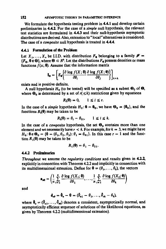
152 ASYMPTOTIC THEORY IN PARAMETRIC INFERENCE
We formulate the hypothesis testing problem in 4.4.1 and develop certain preliminaries in 4.4.2. For the case of a simple null hypothesis, the relevant test statistics are formulated in 4.4.3 and their null-hypothesis asymptotic distributions are derived. Also, extension to “local” alternatives is considered. The case of a composite null hypothesis is treated in 4.4.4.
4.4.1 Formulation of the Problem Let XI,, , . , X, be I.I.D. with distribution Fe belonging to a family 9 = {Fe , 0 E 0}, where 8 c Rk. Let the distributions Fe possess densities or mass functions f ( x ; 0). Assume that the information matrix
exists and is positive definite.
where 8, is determined by a set of r( s k) restrictions given by equations A null hypothesis H, (to be tested) will be specified as a subset e0 of S,
R,(0) = 0,
In the case of a simple hypothesis Ho: 0 = 0,, we have 8, = {Oo}, and the functions R,(O) may be taken to be
1 5 i S r.
Ri(e) = 8, - e,,, 1 s i s k. In the case of a composite hypothesis, the set e0 contains more than one element and we necessarily have r < k. For example, fork = 3, we might have H,: 0 E 8 , = {fJ = (el, 02, &): 8, = Bol}. In this case r = 1 and the func- tion Rl(8) may be taken to be
R,(e) = el - eol. 4.4.2 Preliminaries Throughout we assume the regularity conditions and results given in 4.2.2, explicitly in connection with Theorem 4.2.2 and implicitly in connection with its multidimensional extension. Define for 8 = (el, . . . , &), the vectors
and
dne = 8, - 8 = (dnl - el, . . . , Bnr - ek), where 8, = (Oni, . . . ,e,) denotes a consistent, asymptotically normal, and asymptotically efficient sequence of solutions of the likelihood equations, as given by Theorem 4.2.2 (multidimensional extension).

HYPOTHESIS TESTING BY LIKELIHOOD METHODS 153
Lemma A. Let XI, X2,. . . be I.I.D. with distribution Fe. Then (under ap- propriate regularity conditions)
(i) n1/2ane N(O, I@); (ii) n112dne N(0, Ib I);
(iii) nan& lake XI,;
(iv) nd,,I,d,e 5 X i . PROOF. (i) follows directly from the multivariate Lindeberg-Levy
CLT; (ii) is simply the multidimensional version ofTheorem 4.2.2; (iii) and (iv) follow from (i) and (ii), respectively, by means of Example 3.5A.
d 2
It is seen from (i) and (ii) that the vectors
n1l2ane, n112dd I@
have the same limit distribution namely N(0, I@). In fact, there holds the following stronger relationship.
Lemma B. Let XI, X2, ... be I.I.D. with distribution Fe. Then (under appropriate regularity conditions)
n1/2(ane - dneIe) 3 0.
PROOF. Noting that
we obtain by Theorem 1.12B the Taylor expansion
where lies on the line joining 8 and 0,. From the regularity conditions (extended to the multidimensional parameter case), and from the con- vergence in distribution of the normalized maximum likelihood estimates, we see that the second term on the right-hand side may be characterized as o,(n-1/2). Thus we have, for each i = 1,. . . , k,
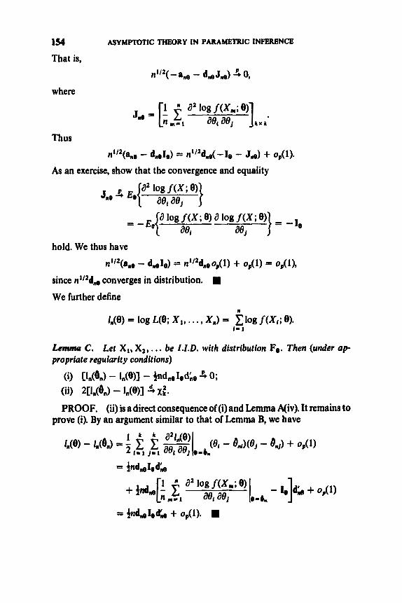
154 ASYMPTOTIC THEORY IN PARAMETRIC INFERENCE
That is, ,'I2( - ane - dne Jne) 4 0,
where
Thus
nl/'(ane - ddIe) = nl/'dne( -Ie - Js) + op(l).
As an exercise, show that the convergence and equality
hold. We thus have
n112(ane - dneIe) = n1'2dneop(l) + op(l) = o,,(l),
since n1I2dd converges in distribution. W We further define
Lemma C. Let XI, X,, . . . be Z.Z.D. with distribution Fa. Then (under ap- propriate regularity conditions)
(i) (ii)
CM4J - W)I - 3ndneIedne J; 0;
W n @ n ) - w)] 5 xi . PROOF. (ii) is a direct consequence of (i) and Lemma A(iv). It remains to
prove (i). By an argument similar to that of Lemma B, we have

HYPOTHESIS TESTING BY LIKELIHOOD METHODS 155
4.4.3 Test Statistics for a Simple Null Hypothesis
Consider testing Ho : 6 =’ 6,. A “likelihood ratio” statistic,
was introduced by Neyman and Pearson (1928). Clearly, A,, takes values in the interval [0, 11 and Ho is to be rejected for sufficiently small values of A,,. Equivalently, the test may be carried out in terms of the statistic
A,, = - 2 log A,,,
which turns out to be more convenient for asymptotic considerations. A second statistic,
was introduced by Wald (1943). A third statistic,
K = nan~oIi~aneo,
was introduced by Rao (1947). The three statistics differ somewhat in computational features. Note that
Rao’s statistic does not require explicit computation of the maximum like- lihood estimates. Nevertheless all three statistics have the same limit chi- squared distribution under the null hypothesis:
Theorem. tribution to x i .
PROOF. The result for A,, follows by observing that
Under H,, the statistics A,, W,, and V, each converge in dis-
and applying Lemma 4.4.2C (ii). (It is assumed that the solution &,, of the likelihood equations indeed maximizes the likelihood function.) The result for W, follows from Lemma 4.4.2A (iv) and the fact that 16 I@. The result for V , is given by Lemma 4.4.2A (iii).
Let us now consider the behavior of A,,, W,, and V , under “local”alternatives, that is, for a sequence (0,) of the form
en = 6, + n-’12A,

156 ASYMPTOTIC THEORY IN PARAMETRIC INFERENCE
where A = ( A l , . . . , Ak). Let us suppose that the convergences expressed in Lemmas 4.4.2A (ii), B, and C (i) may be established uniformly in 8 for 8 in a neighborhood of 8,. It then would follow that
and
(3) A, - w . 3 0 ,
where by (3) is meant that Pen( I A, - W, I > E ) + 0, n -* co, for each E > 0. By (l), (2), (3) and Lemma 3SB, since Ie is nonsingular, it then would follow that the statistics A,,, W,, and V, each converge in distribution to xf(A1eA').
Therefore, under appropriate regularity conditions, the statistics A,, W,, and V , are asymptotically equiuulent in distribution, both under the null hypo- thesis and under local alternatives converging sufficiently fast. However, at fixed alternatives these equivalences are not anticipated to hold.
The technique of application of the limit distribution xi(A1,A) to calculate the power of the test statistics A,, W, or V, is as for the chi-squared statistic discussed in Example 3 . X
Regarding the uniformity assumed above, see the references cited at the end of 4.4.4.
4.4.4 Test Statistics for a Composite Null Hypothesis We adopt the formulation given in 4.4.1, and we assume also that the specification of 0, may equivalently be given as a transformation
81 = g l ( V 1 , * * ' 9 vk-r),
..., e k = gk(v1, * * * I V k - r ) ,
where v = ( v l , . . . , vk-,) ranges through an open subset N c Rk-'. For example, if k = 3 and Qo = (8: 8, = BOl}, then we may take N = { (v , , vz ) :
v l , ~~)~0~}andthefunctionsg~,g,,g, tobeg,(vl, v2) = OO1,g2(V1,v2) = v I , and g,(v,, v 2 ) = v 2 .
that Assume that Ri and gi possess continuous first order partial derivatives and

HYPOTHESIS TESTING BY LIKELIHOOD METHODS 157
is of rank rand
is of rank k - r. In the present context the three test statistics considered in 4.4.3 have the
following more general formulations. The likelihood ratio statistic is given by
Equivalently, we use
A, = - 2 log A,,,
The Wald statistic will be based on the vector
be = ( R I (81, * * - 9 Me)) . Concerning this vector, we have by Theorem 3.3A the following result. (Here 6, is as in 4.4.2 and 4.4.3.)
Lemma A . Let XI, X2,. . . be I.I.D. with distribution Fe. Then
ba, is AN(b0, n-'C,I; 'Ce),
The Wald statistic is defined as
W, = nbbn( Cb, I&1 C&J - ' be,.
The Rao statistic is based on the estimate 0: which maximizes L(8) subject to the restrictions R,(8) = 0, 1 5 i 5 r. Equivalently, 0: may be represented as
e,+ = d o n ) = (gl(tJ, * * 9 gdtn)),
where 0, is the maximum likelihood estimate of v in the reparametrization specified by the null hypothesis. Denoting by J, the information matrix for the v-formulation of the model, we have by Theorems 4.2.2 and 3.3A the following result.
Lemma B. and thus 8 = g(v) for some v E N , we have
Under Ho, that is, VX,, X2, . . . have a distribution F, for 8 E Oo,
(i) 0, is AN(v, n- 'J; I )
and (ii) 8: is AN@, n- 'D, J; ID;).

15s ASYMPTOTlC THEORY IN PARAMETRIC INFERENCE
Noting that for 8 E Qo, that is, for 8 = g(v),
we have
where
which is the analogue in the v-formulation of ad in the unrestricted model. An immediate application of Lemma 4.4.2A(i), but in the v-formulation,
yields
Lemma C. Under Ho,
t,, is AN(0, n''J,).
On the other hand,application of Lemma4.4.2A (i) tor,, with the use of the relation t,, = aneDV, yields that
t,,, is AN(0, n-'D:IeD,).
Hence
Lemma D. For 8 = g(v), J, = D/IeD,.
Thus the analogue of the Rao statistic given in 4.4.3 is
V , = nt,o,Jc;,'t:o,.
which may be expressed in terms of the statistic 8: as
V, = nr,,Do,(D~,Ie:,Don)- lD;na;a,.
The asymptotic distribution theory of A,,, W, and V , under the null hypo- thesis is given by
Theorem. Under Ho, each of the statistics X,, W, and V, converges in distribution to x t .
PROOF. We first deal with W,, which presents the least difficulty. Under Ho, we have be = 0 and thus, by Lemma A,
n1/2bdn 5 N(0, C& 'C;).

HYPOTHESIS TESTING BY LIKELIHOOD METHODS 159
Hence Theorem 3.5 immediately yields
nbbm( Ce I i 'Ci)- be,, -$ x,'. Since
(Cbm Iin' Cb,)- 4 (Ce IB 'C&)- I ,
we thus have
w, s x,'. Next we deal with A,,. By an argument similar to the proof of Lemma 4.4.2C, it is established that
(1) A,, = -2[4(4) - I,@:)] = n(c)" - e,*)I,,(c), - e:y + op(l) and that
bb, = bbn - be:, = (6, - O:)G, + op(len - @ , + I ) and
112 c) n ( n - 03 = O p ( 1 h
whence
and hence
rank %K& = trace BeKeBe = trace B; Ce(Ce && Ce)- 'Ce Be = trace (Ce Be B& C&)(Ca & B; C 0 ) - I
= trace I k x k
= k.
Since &K&, is idempotent, symmetric, of order k and rank k,
&b& = I k X k .
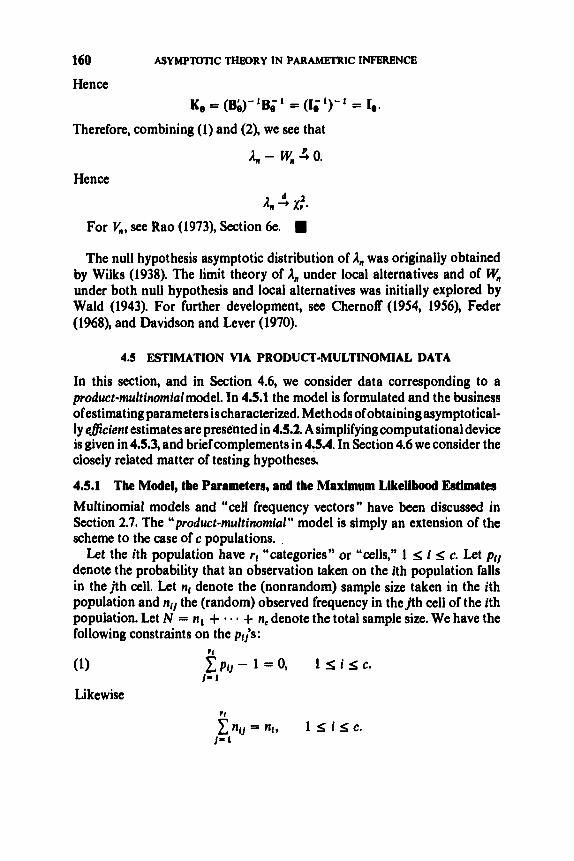
160 ASYMPTOTIC THEORY IN PARAMETRIC INFERENCE
Hence Ke = (Bh)- ‘B; I = (I; I)- I = 1,.
Therefore, combining (1) and (2), we see that
A,, - W” 4 0.
A,, : x,’. Hence
For 6, see Rao (1973), Section 6e.
The null hypothesis asymptotic distribution of A,, was originally obtained by Wilks (1938). The limit theory of A,, under local alternatives and of W,, under both null hypothesis and local alternatives was initially explored by Wald (1943). For further development, see Chernoff (1954, 1956), Feder (1968), and Davidson and Lever (1970).
4.5 ESTIMATION VIA PRODUCT-MULTINOMIAL DATA
In this section, and in Section 4.6, we consider data corresponding to a product-multinomiul model. In 4.5.1 the model is formulated and the business ofestimatingparameters is characterized. Methods ofobtainingasymptotical- ly eficient estimates are presented in 4.5.2. A simplifying computational device is given in 4.5.3, and brief complements in 4.5.4. In Section 4.6 we consider the closely related matter of testing hypotheses.
4.5.1 The Model, the Parameters, and the Maximum Likelihood Estimate8 Multinomial models and “cell frequency vectors” have been discussed in Section 2.7. The “product-mukinomiul” model is simply an extension of the scheme to the case of c populations.
Let the ith population have rf “categories” or “cells,” 1 5 i s c. Let pu denote the probability that tin observation taken on the Ith population falls in the jth cell. Let nf denote the (nonrandom) sample size taken in the ith population and nU the (random) observed frequency in thejth cell of the ith population. Let N = nl + * + n, denote the total sample size. We have the following constraints on the pf,’s:
(1)
Likewise
t p t j - 1 = 0, 1 s i < c. 1-1
rt
E n f 1 = nf, 1-1
1 < i 5 c.

ESTIMATION VIA PRODUCT-MULTINOMIAL DATA 161
Finally, the probability of the observed frequency matrix
is {nt j : 1 s j s r l , 1 s i s c }
Regarding estimation, let us first note (Problem 4.P.6) that the maximum likelihood estimates of the pl;s are given by their sample analogues,
BfJ = - %’, 1 Sj 5s t i , 1 5 i S c. ni
(This is found by maximizing the likelihood function subject to the constraints (l).) We shall employ the notation
P = ( P I 19 * * * 9 P l r l ; * * * ; pel, * * * 9 ~ e , )
for the vector of parameters, and
B = 0 1 1, * * B I r , ; * * ; B c l , * - * Bere)*
for the vector of maximum likelihood estimates. More generally, we shall suppose that the p,;s are given as specified func-
tions of a set of parameters 81, . . . , ek, and that the problem is to estimate 8 = (el,. . . , &)a An example of such a problem was seen in Section 2.7. Another example follows.
Example A. Suppose that the c populations of the product-multinomial model represent diflerent levels ofa treatment, and that the rl cells of the ith population represent response categories. Let us take rl = ... = r, = t. Further, suppose that the response and factor are each “structured.” That is, attached to the response categories are certain known weights al, , . , , a,, and attached to the treatment levels are known weights bl, . . . , be. Finally, sup- pose that the expected response weights at the various treatment levels have a linear regression on the treatment level weights. This latter supposition is expressed as a set of relations
r
I= 1 ~ a j p u = 1 + &, 1 s i s c, (*)
where 1 and ~1 are unknown parameters. We now identify the relevant parameter vector 8. First, suppose (without loss of generality) that al # a,. Now note that, by the constraints (l), we may write

162 ASYMPTOTIC THEORY IN PARAMETRIC INFERENCE
Also, after eliminating each plr by (i), we have by (*) that
Finally, we also write
(iii) 2 5; j I; r - 1,
It thus follows from (i), (ii) and (iii) that the components of pmay be expressed entirely in terms of the parameters
Of, = pl,, 1 5; i 5; C.
el = 1; O2 = p ; 8 , = pi,, 2 s j I; r - 1, 1 I; i I; C,
that is, in terms of 8 containing k = (r - 2)c + 2 components. We shall consider this example further below, as well as in 4.6.3.
The condition that the pI;s are specified functions of 8,
p I j = PI,@), 1 I; i s r l , 1 5; i I; c,
is equivalent to a set of m = CI rl - c - k constraints, say
(2) H,(p) = 0, 1 s 1 s m,
obtained by eliminating the parameters el, . . . , 0,. These equations are independent of the c constraints given by (1).
Example B (continuation). For the preceding example, we have m = cr - c - [(r - 2)c + 23 = c - 2. These c - 2 constraints are obtained from (*) by eliminating 1 and p. (Problem 4.P.7).
Example C. The problem of estimation of p may be represented as estima- tion of 8, where the 8,'s consist of the k = zII rl - cpI;s remaining after elimination of pl,,, . . . , per= by the use of (1). In this case m = 0, that is, there are no additional constraint equations (2).
The problem of estimation of 8 thus becomes equivalent to that of estima- tion of the original vector p subject to the combined set of m + c constraint equations (1) and (2). If the representation of 8 in terms of p,;s is given by
= 8(P) = b I (PI, * * 9 gk(P)),
then an estimator of 8 is given by
= 8(B) = <s,<b), * * * Y 8k(b)h

ESTIMATION VIA PRODUCT-MULTINOMIAL DATA 163
where = @ll , ... ; ... ; ..., be,,)denotes a vector estimate of p under the constraints (1) and (2). In particular, if denotes the maximum likelihood estimate of p subject to these constraints, then (under appropriate regularity conditions on g) the maximum likelihood estimate of 8 is given by 6 = g@). Therefore, asymptotically efficient estimates of 8 are provided by g(B*) for any BAN estimate B* of p subject to (1) and (2).
There are two principal advantages to the formulation entirely in terms of constraints on the pi,%:
(a) in testing, it is sometimes convenient to express the null hypothesis in the form of a set of constraint equations on the p i i s , rather than by a statement naming further parameters el, . . . , Ok (see 4.6.2 and 4.6.3);
(b) this formulation is suitable for making a computational simplification of the problem by a linearization technique (4.5.3).
4.5.2 Methods of Asymptotically EfRcient Estimation
Regarding estimation of the B,‘s, several approaches will be considered, following Neyman (1949). Neyman’s objective was to provide estimators possessing the same large sample eficiency as the maximum likelihood estimates but possibly superior computational ease or small sample e@ciency. Although the issue of computational ease is now of less concern after great advances in computer technology, the small sample efficiency remains an important consideration.
The “maximum likelihood” approach consists of maximizing
with respect to 81, . . . , ($9 subject to the constraints (1) (of 4.5.1). The “minimum 1’” approach consists of minimizing
with respect to 81,. . . , e k , subject to the constraints (1). Finally, the “modified minimum x’ *’ approach consists of minimizing
with respect to 81, . . . , ek, subject to the constraints (1).

164 ASYMPTOTIC THEORY IN PARAMETRIC INFERENCE
Noting that dl and d2 are measures of discrepancy between p and B, we may characterize the maximum likelihood approach in this fashion in terms of
do(Pm B) = -2 108 IYP(f0, B), where
Each approach leads to a system of equations. However, the relative convenience of the three systems of equations depends on the nature of the functions pf 0). In the case that these are linear in O,, . . . , &, the modified
In any case, the three systems of equations are asymptotically equioalent in probability, in the sense that the estimates produced differ only by o,,(N' 'I2), as N + 00 in such fashion that each nl/N has a limit l , , 0 < 1, < 1,l 5 i s c. For these details, see Cramdr (1946), Sections 30.3 and 33.4, and Neyman ( 1949).
For appropriate regularity conditions on the parameter space 0 and the functions pi,@), in order for the maximum likelihood estimates to be asymp- totically efficient, see Rao (1973), Section 5e.2.
4.53 Wnearization Technique Corresponding to the set of (possibly nonlinear) constraint equations (2) (of 4.54, we associate the set of linear constraint equations
(2*) Hj"(p) = 0, 1 s I s m,
where
minimum 1' approach yields a linear system of equations for O,, . . . , 6,.
which is the linear part of the Taylor expansion of H,(p) about the point p = B, the maximum likelihood estimate in the model unrestricted by the constraints (2).
Neyman (1949) proves that minimization of do(p, fi), dl(p, fi), or d2(p, B) with respect to the pl,'s, subject to the constraints (1) and (2), and minimization alternatively subject to the constraints (1) andl2*), yields estimates band p, respectively, which satisfy
b - 8+ = o,(" 1'2).
Further, regarding estimation f the parameters O r , Neyman establishes analogous results for estimates i e and * based on (2) and (2*), respectively.
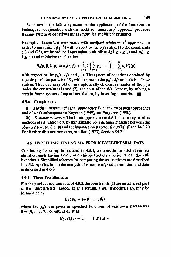
HYPOTHESIS TBSTJNG VIA PRODUCT-MULTINOMIAL DATA 165
As shown in the following example, the application of the linearization technique in conjunction with the modified minimum xz approach produces a linear system of equations for asymptotically efficient estimates.
Example. Linearized constraints with modijied minimum x z approach. In order to minimize d2(p, 8) with respect to the p,;s subject to the constraints (1) and (2*), we introduce Lagrangian multipliers 1,(1 I; i 15 c ) and pl ( l I; l I; m) and minimize the function
m
D2(P, B, 5, P) = d2(P, B) + c 1, c P i j - 1 + c P I W P ) f = 1 c1 1 1 1 1
with respect to the p i i s , A i s and pis. The system of equations obtained by equating to 0 the partials of D 2 with respect to the piis, A,‘s and pis is a linear system. Thus one may obtain asymptotically efficient estimates of the p,;s under the constraints (1) and (2), and thus of the 0,‘s likewise, by solving a certain linear system of equations, that is, by inverting a matrix.
4.5.4 Complements
(i) Further “minimum x2 type”approaches. For a review of such approaches and of work subsequent to Neyman (1949), see Ferguson (1958).
(ii) Distance measures. The three approaches in 4.5.2 may be regarded as methods of estimation of 8 by minimization of a distance measure between the obseroed p vector (i.e., 8) and the hypothetical p vector (i.e., p(0)). (Recall 4.3.2.) For further distance measures, see Rao (1973), Section 5d.2.
4.6 HYPOTHESIS TESTING VIA PRODUCT-MULTINOMIAL DATA
Continuing the set-up introduced in 4.5.1, we consider in 4.6.1 three test statistics, each having asymptotic chi-squared distribution under the null hypothesis. Simplified schemes for computing the test statistics are described in 4.6.2. Application to the analysis of variance of product-multinomial data is described in 4.6.3.
4.6.1 Three Test Statistics For the product-multinomial of 4.5.1, the constraints (1) are an inherent part of the “unrestricted” model. In this setting, a null hypothesis Ho may be formulated as
HO: PI, = Pij(01, . * * O k ) ,
where the pi’s are given as specified functions of unknown parameters 8 = (el, . . . , &), or equivalently as
Ho: Hl(p) = 0, 1 s 1 s m.

166 ASYMPTOTIC THEORY IN PARAMETRIC INFERENCE
As in 4.5.2, denote by fi the maximum likelihood estimate of p in the unre- stricted model, and let b* denote an asymptotically eficient estimate of p under Ho or under the corresponding linearized hypothesis (4.5.3). Each of the three distance measures considered in 4.5.2 serves as a test statistic when evaluated at @* and 8. That is, each of
di(B*, a,, i = 4 1 9 %
is considered as a test statistic for H o , with Ho to be rejected for large values of the statistic. Thus the null hypothesis becomes rejected if fl and B* are sufficiently “far apart.”
Theorem (Neyman (1949)). Under Ho, each of dl(@*, B), i = 4 1,2, converges in distribution to 2’.
4.6.2 Simplified Computational Schemes
Consider the statistic ti2(#*, B) in the case that B* denotes the estimate obtained by minimizing dz(p, fl) with respect to p under (1) and the con- straints specified by H o e For some types of hypothesis Ho, the statistic dz(@*, B)can actually be computed without first computing 8’. Thesecomputa- tional schemes are due to Bhapkar (1961, 1966).
Bhapkar confines attention to linear hypotheses, on the grounds that non- linear hypotheses may be reduced to linear ones if desired, by Neyman’s linearization technique (4.5.3). Also, we shall now confine attention to the case of an equal number of cells in each population: rl = - -. = re = r.
Two forms of linear hypothesis Ho will be considered. Firstly, let Ho be defined by m linearly independent constraints (also independent of (1) of 4.5.1),
H o : W P ) = i i hIl,P, + hl = 4 1 5 1 5; m, 1-1 1-1
where h,,, and h, are known constants such that the hypothesis equations together with (1) have at least one solution for which the pl,’s are positive. For this hypothesis, Bhapkar shows that
M B * , P) z= CHI@, * * * 9 Hm(B)ICilCH1(BX * > Hm(B)I’,
where CN denotes the sample estimate of the covariance matrix of the vector [HI(#), . . . , H,(B)]. Check that this vector has covariance matrix [c, JmX,,
where

HYPOTHEPIS m n N Q VIA PRODUCT-MULTINOMIAL DATA 167
Thus the matrix C, is [ C N & ] m x m , where CNIk is obtained by putting f i f J for
Note that the use of d2(#*, B) for testing H o is thus exactly equioalent to the “natural” test based on the asymptotic normality of the unbiased estimate [HI(#), . . . , H,(#)] of [Hl(p), . . . , H,(p)], with the covariance matrix of this estimate estimated by its sample analogue. Note also that, in this situation, d2(#*, fi) represents the Wald-type statistic of 4.4.4.
PfJ in c f k *
Secondly, consider a hypothesis of the form r k
Ho: xa,p l , = x b f , 8 , , 1 s i s c, J = 1 I= I
where the a;s and bl,’s are known constants and the 8,’s are unknown param- eters, and rank [br,], k =i u S c - 1. This is a linear hypothesis, defined by linear functions of unknown parameters, and so it may be reduced to the form of H o considered previously. (In this case we would have m = c - u.) For example, recall Example 4.5.1 A, B. However, in many cases the reduction would be tedious to carry out and not of intrinsic interest. Instead, the problem may be viewed as a standard problem in “least squares analysis,” Bhapkar shows. That is,
d,(#*, B) = “Residual Sum of Squares,”
corresponding to application of the general least squares technique on the variables ajpij with the variances estimated by sample variances. Thus dz(@*, @) may be obtained as the residual sum of squares corresponding to minimization of
where .
4.6.3 Applications: Analysis of Variance of Product-Multlnomlal Data For a product-multinomial model as in 4.5.1, let “ i” correspond tofactor and “ j” to response. Thus factor cattgories are indexed by i = 1,. . . , c and response categories by j = 1, . . . , r. (For simplicity, assume rl = a . = rc = r.) A response or factor is said to be structured if weights are attached to its categories, as illustrated earlier in Example 4.5.1A. We now examine some typical hypotheses and apply the results of 4.6.1 and 4.6.2.
Hypothesis ofhomogeneity (Neither response nor factor is structured.) The null hypothesis is
Ho: p f , does not depend on i.

168 ASYMPTOTlC m R Y IN PARAMBTRIC INFERENCE
In terms of constraint functions, this is written
Ho: Hi,(p) = p f I - pcI = 0, ( i = 1,. . . , c - 1; j = 1,. , . , r - 1).
The hypothesis thus specifies m = (r - l)(c - 1) constraints in addition to the constraints (1).
Under I f o , the product-multinomial model reduces to a single multinomial model, and corresponding BAN estimates of the pi,'s are
nlj + * . *
N +'cJ, i = I, ..., c ; j = 1, ..., r. at =
Therefore, by Theorem 4.6.1, each of the statistics dl(B*, B), i = 0, 1, 2, is asymptotically x& I)(c-
Hypothesis o j mean homogeneity. (The response is structured, and the hypothesis is "no treatment effects,")
r
I= I Ho:
In terms of constraint functions, this is written
alpij does not depend on j .
Ho: Hi(p) = c alpiI - c a ip l j = 0, ( i = 1, . . . , c - 1). I- 1 I= 1
In terms of further parameters d,, this is written
H ~ : C a p i , = e, ( i = I, ..., c). I- 1
Instead ofestimating the pi;s under Ho (as we did in the previous illustration), we may apply either of Bhapkar's devices to evaluate d2(#*, fi). The least- squares representation enables us to write immediately
where
(As an exercise, check that this is the proper identification with standard least-squares formulas.) By Theorem 4.6.1, d,(B*, 6) is asymptotically x,'-

PROBLEMS 169
Hypothesis of linearity of regression. (Both response and factor are structured. The hypothesis of linearity of the regression of response on “treatment level” is to be tested.)
r
Ho: C ~ j p i j 1 1 1
1 + pbl, (i = 1,. . . , c). By the least-squares analogy,
where a, and yi are as in the preceding illustration, and C C C
c c
s = C~iY,, d = Ca,b,y , .
15: ? P = -
I = 1 I = 1
Estimates of A and p are ES - 6d vd - 6s y& - .I ye - a2 ’
The statistic d,()*, )) is asymptotically xz- 2 .
test for quadratic regression, etc.
13.7-13.9and 13.11-13.12.
If linearity is not sustained by the test, then the method may be extended to
Further examples and discussion. See, for example, Wilks (1962), Problems
4.P PROBLEMS
Miscellaneous
1. Suppose that
(a) x n = (Xnl, * - 9 x # k ) -% XO = (XOli * * 9 X O k )
and (b) Y,, = (GI, .. . , Yd) 3 c = ( ~ 1 , . . ., ck).
(i) Show that (XRl Y,,) -% (x0, c).
(ii) Apply (i) to obtain that X, + Y,, (iii) What are your conclusions in (i) if (b) is replaced by (b’) Y,, 5 c?
(iv) What are your conclusions in (i) if (b) is replaced by ( 6 ) Y,, 3 Yo =
Xo + c and X,Y; 4 Xoc‘.
(Yo19 * * ’, YOJ?
(Justify all answers.)

170 ASYMPTOTIC THEORY IN PARAMETRIC INFERENCE
Section 4.2 2. Justify the interpretations of regularity conditions (R1)-(R3) in 4.2.2. 3. Prove Remark 4.2.2 (i).
Section 4.4
4. Do the exercise assigned in the proof of Lemma 4.4.2B. 5. Check that B e K e b is idempotent (in the proof of Theorem 4.4.4).
Section 4.5
likelihood estimates of the pf,’s are pf, = nfi/nf, respectively.
Section 4.6
6. Verify for the product-multinomial model of 4.5.1 that the maximum
7. Provide the details for Example 4.5.1B.
8. Verify the covariance matrix [c,J asserted in 4.6.2. 9. Do the exercises assigned in 4.6.3.

C H A P T E R 5
U-S tatis tics
From a purely mathematical standpoint, it is desirable and appropriate to view any given statistic as but a single member of some general class of statistics having certain important features in common. In such fashion, several interesting and useful collections of statistics have been formulated as generalizations of particular statistics that have arisen for consideration as special cases.
In this and the following four chapters, five such classes will be introduced. For each class, key features and propositions will be examined, with emphasis on results pertaining to consistency and asymptotic distribution theory. As a by-product, new ways of looking at some familiar statistics will be discovered.
The class ofstatistics to be considered in the present chapter was introduced in a fundamental paper by Hoeffding (1948). In part, the development rested upon a paper of Halmos (1946). The class arises as a generalization of the sample mean, that is, as a generalization of the notion of forming an uueruge. Typically, although not without important exceptions, the members of the class are asymptotically normal statistics. They also have good consistency properties. .
The so-called “ U-statistics” are closely connected with a class of statistics introduced by von Mises (1947), which we shall examine in Chapter 6. Many statistics of interest fall within these two classes, and,many other statistics may be approximated by a member of one of these classes.
The basic description of U-statistics is provided in Section 5.1. This includes relevant definitions, examples, connections with certain other statistics, martingale structure and other representations, and an optimality property of Uatatistics among unbiased estimators. Section 5.2 deals with the moments, especially the variance, of U-statistics. An important tool in deriving the asymptotic theory of U-statistics, the “projection” of a U-statistic on the basic observations of the sample, is introduced in Section 5.3. Sections 5.4 and 5.5 treat, respectively, thealmost sure behavior and asymptoticdistribution theory
171

172 U-STATISTICS
of U-statistics. Section 5.6 provides some further probability bounds and limit theorems. Several complements are provided in Section 5.7, including a look at stochastic processes associated with a sequence of U-statistics, and an examination of the Wilcoxon one-sample statistic as a U-statistic in connection with the problem of confidence intervals for quantiles (recall 2.6.5).
The method of “projection” introduced in Section 5.3 is of quite general scope and will be utilized again with other types of statistic in Chapters 8 and 9.
5.1 BASIC DESCRIPTION OF USTATISTICS
Basic definitions and examples are given in 5.1.1, and a class of closely related statistics is noted in 5.1.2. These considerations apply to one-sample U- statistics. Generalization to several samples is given in 5.1.3, and to weighted versions in 5.1.7. An important optimulity property of U-statistics in unbiased estimation is shown in 5.1.4. The representation of a U-statistic as a martingale is provided in 5.1.5, and as an average of I.I.D. averages in 5.1.6.
Additionalgeneral discussion of U-statistics may be found in Fraser (1957). Section 4.2, and in Puri and Sen (1971), Section 3.3.
5.1.1 First Definitions and Examples
LetXI, X2,. . . beindependentobservationsonadistributionF.(Theymaybe vector-valued, but usually for simplicity we shall confine attention to the real- valued case.) Consider a “parametric function” 8 = 8(F) for which there is an unbiased estimator. That is, 8(F) may be represented as
e (F) = E , , { ~ ( X ~ , . . . , x,)) = S. - . Jh(xl, . . . , x,)d~(x,) - - - m x , , ~ ,
for some function h = h(xl,. . . , x,,,), called a “kernel.” Without loss of generality, we may assume that h is symmetric. For, if not, it may be replaced by the symmetric kernel
where c,, denotes summation over the m! permutations ( i l l . . . , i,) of (1,. . , , m).
For any kernel h, the corresponding U-statistic for estimation of 8 on the basis of a sample XI, . , . , Xn of size n 2 m is obtained by averaging the kernel h symmetrically over the observations:
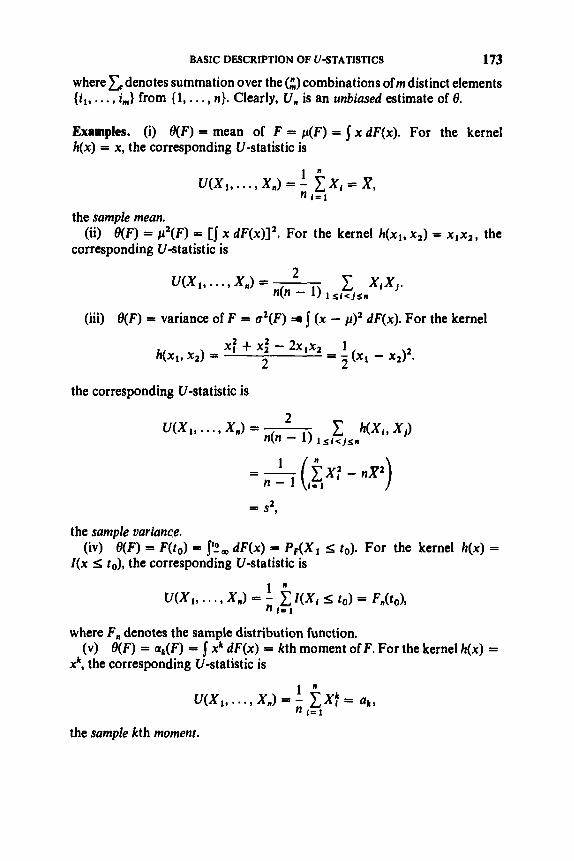
BASIC DESCRIPTION OF U-STATISTICS 173
where {il , . . . , i,} from (1,. . . , n}. Clearly, U, is an unbiased estimate of 8.
denotes summation over the C) combinations of m distinct elements
Examples. (i) K F ) = mean of F = p(F) = x dF(x). For the kernel h(x) = x , the corresponding U-statistic is
1 “ n 1 9 1
U(X1 , . . . , X,) = - p, = x, the sample mean.
corresponding U-statistic is (ii) 8(F) = f12(F) = [J x dF(x)l2. For the kernel h(xl, x2) = x l x z , the
(iii) B(F) = variance of F = aZ(F) =m (x - p)2 dF(x). For the kernel
the corresponding U-statistic is
= s2,
the sample variance.
I(x I; to), the corresponding Lr-statistic is (iv) 8(F) = F(to) = r!m dF(x) = P F ( X 1 s to). For the kernel h(x) =
where F, denotes the sample distribution function.
xk, the corresponding LI-statistic is (v) 8(F) = ak(F) = xk dF(x) = kth moment of F. For the kernel h(x) =
the sample kth moment.

174 USTATISTICS
(vi) O(F) = E,(XI - X21, a measure of concentration. For the kernel h(xl, x2) = Ixl - x2 I, the corresponding U-statistic is
the statistic known as “Gini’s mean difference.”
Wilks (1962), p. 200). (vii) Fisher’s katatistics for estimation of cumulants are U-statistics (see
(viii) 8(F) = Epy(x1) = y(x)dF(x); CJ, = n-l y(X,). (ix) The Wflcoxon one-sample statistic. For estimation of e(F) =
PF(XI + X2 5 O), a kernel is given by h(x,, x2) = I(xl + x2 SO) and the corresponding U-statistic is
(x) O(F) = IJ [F(x, y) - F(x, oo)F(m, y)I2 dF(x, y), a measure of de- pendence for a bivariate distribution F. Putting
11(z1, z2,z3) = m z s Zl) - I(Z3 s z1) and
MXl, Vl), * - * * (x5, v 5 ) ) = SJ/(X*, x2, XdJ/(Xl, x49 x5) )kQl, Y2, Y3))k(Yl, Y4, Y5)9
we have EF{h} = O(F), and the corresponding U-statistic is
5.1.2 Some Closely Related Statistics: V-Stntistks
Corresponding to a U-statistic
for estimation of O(F) = E p ( h } , the associated oon Mises statistic is

BASIC DESCRIPTION OF U-STATISTICS 175
where F, denotes the sample distribution function. Let us term this statistic, in connection with a kernel h, the associated V-statistic. The connection between U, and V , will be examined closely in 5.7.3 and pursued further in Chapter 6.
Certain other statistics, too, may be treated as approximately a U-statistic, the gap being bridged via Slutsky's Theorem and the like. Thus the domain of application of the asymptotic theory of U-statistics is considerably wider than the context of unbiased estimation.
5.1.3 Generalized U-Statistics
The extension to the case of several samples is straightforward. Consider k independent collections, of independent observations {Xi1), Xi1), . . .}, . , . , {Xik), Xf), . . .} taken from distributions . . . , Fk), respectively. Let 8 = 8(Ff1), . . . , Fk)) denote a parametric function for which there is an unbiased estimator. That is,
where h is assumed, without loss of generality, to be symmetric within each of its k blocks of arguments. Corresponding to the "kernel" h and assuming nl 2 ml, . . . , ?tk 2 mk, the U-statistic for estimation of 8 is defined as
Here {ill, . . . , i," } denotes a set of mJdistinct elements of the set { 1,2,. . . , n,}, 1 s j 5 k, and ic denotes summation over all such combinations.
The extension of Hoeffding's treatment of one-sample U-statistics to the k- sample case is due to Lehmann (1951) and Dwass (1956). Many statistics of interest are of the k-sample U-statistic type.
Example. The Wilcoxon 2-sample statistic. Let {Xl, . . . , X, , } and { Yl, . . . , x2} be independent observations from continuous distributions F and G, respectively. Then, for
8(F, G) = JF dG = P(X S Y),
an unbiased estimator is
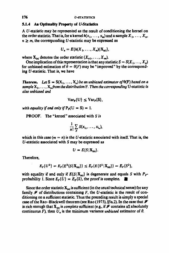
176 U-STATISTICS
5.1.4 An Optimality Property of U-Statistics
A U-statistic may be represented as the result of conditioning the kernel on the order statistic. That is, for a kernel h(xl, . . . , x,) and a sample XI, . . . , X,, n 2 m, the corresponding U-statistic may be expressed as
un = E(h(X1, * * * 9 XnJlX(nJ,
where X(,) denotes the order statistic (X,,, . . . , X,,). Oneimplication of this representation is that any statistics = S(X, , . . . , XJ
for unbiased estimation of 0 = 0(F) may be “improved” by the correspond- ing U-statistic. That is, we have
Theorem. Let S = S ( X , , . . . , X,) be an unbiased estimator ojCJ(F) based on a samplex,, . . . , XJrom thedistribution F. Then thecorresponding U-statistic is also unbiased and
VarF{U} s VardS},
with equality g a d only gPF(U = S ) = 1.
PROOF. The “kernel” associated with S is
which in this case (m = n) is the U-statistic associated with itself. That is, the tl-statistic associated with S may be expressed as
u E{SlX(n,)-
Therefore,
E F { u 2 ) = EdE’{sIX(n,)I 5 EdE{S21X(n))) = EF{Sz),
with equality if and only if B(S1X,,,} is degenerate and equals S with Pp- probability 1. Since EF{U} = EF{S}, the proof is complete.
Since the order statistic X, is sufficient (in the usual technical sense) for any family 9 of distributions containing F, the U-statistic is the result of con- ditioning on a sufficient statistic. Thus the preceding res’ult is simply a special case of the Rao-Blackwell theorem (see Rao (1973), g5a.2). In the case that 9 is rich enough that X,, is complete sufficient (e.g., if 9r contains all absolutely continuous F), then Un is the minimum variance unbiased estimator of 8.

BASIC DESCRIPTION OF U-STATISTICS 177
5.15 Martingale Structure of U-Statistics
Some important properties of U-statistics (see 5.2.1,5.3.3,53.4, Section 5.4) flow from their martingale structure and a related representation.
Demtions. Consider a probability space (Q d, P), a sequence of random variables { Y,,}, and a sequence of a-fields (9,) contained in d, such that Y, is 9,-measurable and El Y,l c a. Then the sequence { Y,, 9,) is called a forward martingale if
(a) 9tl c P2 c . . . , (b) E { Y , + , 19,) = Y. wpl, all n,
and a reverse martingale if
(a') PI 3 .F2 3.. . , (b') E{Y~19,+1} = Y.+l wp1,alln.
Thefollowinglemmas,due to Hoeffding(l96l)and Berk(1966),respectively, provide both forward and reverse martingale characterizations for U- statistics. For the first lemma, some preliminary notation is needed. Consider a symmetric kernel h(x , , . . . , x,) satisfying E F ( h ( X l , . . . , X,)( c o. We define the associated functions
h,(x1, * * * 9 x,) = W h ( X I , 8 ' ' 9 xc, x,+ 1, * * 9 X,)) for each c = 1, . . . , m - 1 and put h, = h. Since
for every Bore1 set A in RC, h, is (a version of) the cohditional expectation of h(X1, . . . , X,) given XI, . . . , X,:
hc(x1,. . . 9 xc) = EF(h(X1, s * X , ) I x , = X I , . . - 9 x c = Xc}.
Further, note that for 1 s c 5 m - 1
hc(x1, * * 9 xc) = EF{hc+ l(X1, * * * 9 xc, x c + 1)).
It is convenient to center at expectations, by defining
NF) = EAh(X1, . . . , Xm)}, ii = h - e(F),
and
hc = h, - e(F) , 1 4 c 5 m.

178
We now define
U-STATISTICS
...,
where
s n = C Nxt1, * 9 xirn)* l s I ~ < - . < l , s n
(1)
Finally, for 1 s c s m, put
sen = C ~ r ( X i 1 . * * 9 XIc). 1 < I 1 <.-<l ,sn
Hoeffding's lemma, which we now state, asserts a martingale property for the sequence {Srn}nrc for each c = 1, . . . , m, and gives a representation for U, in terms of Sin,. . . , Sm,.
Lemma A (Hoeffding). Let h = h(x,, . . , , x,) be a symmetric kernel for 8 = 8(F), with EFlhl < QO. Then
u, - 8 = f (;)(p"* E l l

BASIC DESCRIPTION OF U-STATISTICS 179
FurtherJor each c = 1, . . . , m,
(3) EF(ScnIX1s.. . , Xk} = Sck, C 5 k I; n.
Thus, with 9Ft = a{X,, . . . , xk}, the sequence {S,,, 9n}n2c is a forward martingale.
PROOF. The definition of gm in (*) expresses h in terms of gl,. . . , gm. Substitution in (1) then yields
m - 1
S" = s,, + --E- c c 8c(x1,1~ . * - 9 XI, ) . c = 1 1 S ~ I < a * . < 1msn 1 SII < ... < Jc 5 m
On the right-hand side, the term for c = 1 may be written
c f d X i , ) . Isi l<-*<Imsn J = 1
In this sum, each g(X,), 1 s i s n, is represented the same number of times. Since the sum contains (4) * m terms, each g(X , ) appears n-'(:)m times. That is, the sum S1, = c; g(X , ) appears (1)- l(:)(T) times. In this fashion we obtain
Thus
Example A. For the case m = 1 and h(x) = x, Lemma A states simply that
and that {c! (X1 - O), a(X, , . . . , X,)} is a forward martingale.

180 U-STATISTICS
The other martingale representation for U, is much simpler:
Lemma B (Berk). Let h = h(x,, . . . , x,) be a symmetric kernel for 0 = 0(F), with E,lhJ < a. Then, with 9, = U{X(, , ) ,X~+~, Xn+z ,... 1, the sequence { U, , 9,,}, , is a reverse martingale.
PROOF. (exercise) Apply the representation
un = E{h(XI, * * * 9 Xm)lX(n)} considered in 5.1.4.
Example B (conrinuation). For the case m = 1 and h(x) = x, Lemma B asserts that X is a reverse martingale. H
5.1.6 Representation of a U-Statistic as an Average of (Dependent) Averages of I.I.D. Random Variables Consider a symmetric kernel h(xl,. . . , x,) and a sample XI,. . . , X , of size n 2 m. Define k = [n/m], the greatest integer <n/m, and define
W(x8, - * * Xn)
= ~(xI,.**,x,) + h(xm+1,***,Xzm) + a * . + h ( x ~ m - m + l , * . * , X ~ m )
k Letting cp denote summation over all n! permutations (i,, . . ., in) of (1, . . . , n) and denote summation over all (:) combinations {i,, . . . , i,} from (1,. . . , n}, we have
k W(x,,, . . . , xi") = km!(n - m ) ! h(xi l , . . . , xlm), P C
and thus
or
This expresses U, as an average of n ! terms, each of which is itself an average of k I.I.D. random variables. This type of representation was introduced and utilized by Hoeffding (1963). We shall apply it in Section 5.6.
5.1.7 Weighted U-Statistics Consider now an arbitrary kernel h(x l , . . . , x,),not necessarily symmetric, to be applied as usual to observations XI, . . . , X, taken m at a time. Suppose alsothateachtermh(X,,, ...., XI,)becomesweightedbyafactorw(i,, ..., i,)
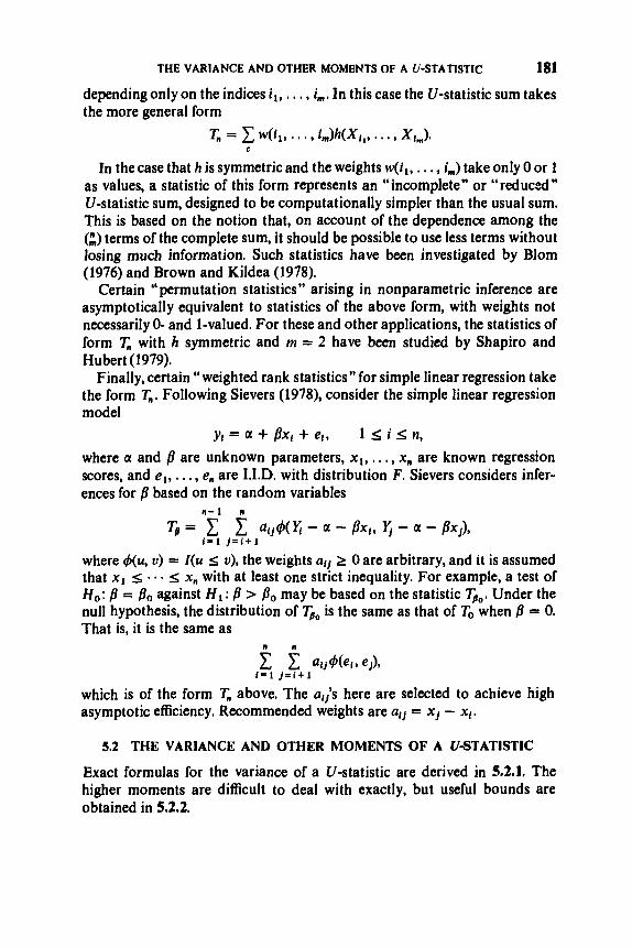
THE VARIANCE AND OTHER MOMENTS OF A U-STATISTIC 181
depending only on the indices i l , . . . , i,. In this case the U-statistic sum takes the more general form
T,, = c w(il , . . . , i,)h(X,,, . . . , X , J . C
In the case that h is symmetric and the weights w(il , , . . , i,,,) take only 0 or 1 as values, a statistic of this form represents an “incomplete” or “reduced” U-statistic sum, designed to be computationally simpler than the usual sum. This is based on the notion that, on account of the dependence among the (3 terms of the complete sum, it should be possible to use less terms without losing much information. Such statistics have been investigated by Blom (1976) and Brown and Kildea (1978).
Certain “permutation statistics” arising in nonparametric inference are asymptotically equivalent to statistics of the above form, with weights not necessarily 0- and 1-valued. For these and other applications, the statistics of form T. with h symmetric and m = 2 have been studied by Shapiro and Hubert (1979).
Finally, certain “weighted rank statistics ” for simple linear regression take the form T,,. Following Sievers (1978), consider the simple linear regression model
where a and f l are unknown parameters, xl, . . . , x, are known regression scores, and el, , . . , en are I.I.D. with distribution F. Sievers considers infer- ences for f l based on the random variables
yl = a + f ix , + e l , 1 5 i 5 n,
5 = “i at j4 (8 - a - fix,, yj - a - p X J ) , 1=1 J = t + l
where d(u, u) = I(u 5 o), the weights aiJ 2 0 are arbitrary, and it is assumed that x1 5 . a - 5 xn with at least one strict inequality. For example, a test of H,: B = Po against HI: B > Po may be based on the statistic Go. Under the null hypothesis, the distribution of Go is the same as that of To when f l = 0. That is, it is the same as
n n c c a,,$& el), 1=1 J=i+l
which is of the form T,, above. The ai,’s here are selected to achieve high asymptotic efficiency. Recommended weights are ail = xi - x,.
5.2 THE VARIANCE AND OTHER MOMENTS OF A LISTATISTIC
Exact formulas for the variance of a U-statistic are derived in 5.2.1. The higher moments are difficult to deal with exactly, but useful bounds are obtained in 5.2.2.

182 U-STATISTICS
53.1 The Variance of a UStatistic Consider a symmetric kernel h(x,, . . . , x,) satisfying
We shall again make use of the functions hc and hc introduced in 5.1.5. Recall that h, = h and, for 1 I; c I; m - 1,
that h = h - 8, hc = h, - 8(1 s c I; m), where
and that, for 1 I; c I; m - 1,
Note that
EF{h2(X1,. . . , X,)} < 00.
hc(xl, . . . , x,) = E F { h ( X l , * ' 9 xc, xc+ 1, * ' 9 XIn)},
8 = W) = EF{h(X1,. . . , Xm)},
h,(x,, * * * 9 xc) = E F { h C + l ( X l , * ' , x c , xc+ 111.
E ~ ~ ~ ( X ~ , . . . , X,) = 0, 1 I; c s m.
Define Co = 0 and, for 1 S c I; m,
C, = VarF{hc(X,,. . . , x,)} = EF{&xl,. . . , xCN. We have (Problem S.P.3(i))
0 = lo 5 C1 s 0 . - s C, = Var,{h} < 00. Before proceeding further, let us exemplify these definitions. Note from the following example that the functions h, and hc depend on F for c s m - 1. The role of these functions is technical.
Example A. B(F) = a2(F). Writing p = p(F), us = a2(F) and p4 = p4(F), we have
h(x1, x2) = I(x: + x: - 2 X I X 2 ) = fix, - X 2 l 2 ,
R X l , x 2 ) = h ( x 1 , x 2 ) - g2,
h,(x) = N x 2 + g2 + p 2 - 2xp),
h,(x) = g x 2 - at + /42 - 2x/4) = +[(x - /4)2 - 621,
m21 = SN(X1 - /4) - (X2 - P)14}

THE VARIANCE AND OTHER MOMENTS OF A U-STATJSTIC 183
Next let us consider two sets { a l , . . . , a , } and {bl , . . . , b,} of m distinct integers from { 1, . . . , n } and let c be the number of integers common to the two sets. It follows (Problem 5.P.4) by symmetry of h and by independence of {Xl, . . . , X,] that
EF{~(XII, - * - 9 Xam$(Xbl, * * 9 Xb,,,)} = cc.
Note also that the number of distinct choices for two such sets having
With these preliminaries completed, we may now obtain the variance of a exactly c elements in common is (:)(:)G::).
U-statistic. Writing
- 2 n
= (:) Zo (:)C)t::)tc.
This result and other useful relations from Hoeffding (1948) may be stated as follows.
Lemma A . The variance of U, is given by
and satisfies
Note that (*) is a fixed sample size formula. Derive (i), (ii), and (iii) from (*) as an exercise.

184 U-STATISTICS
Exnmplc S (Continuation).
Yl 2cz - - 3-+ 4C1
n n(n - 1) n(n - 1)
p4 - 6 + 2a4 =- n(n - 1) n
The extension of (*) to the case of ageneralized Uatatistic is straightforward (Problem 5.P.6).
An alternative formula for Var,{ U,} is obtained by using, instead ofh, and fie, the functions g, introduced in 5.1.5 and the representation given by Lemma 5.1.5A.
Consider a set {Il, . . . , i,} of c distinct integers from { 1, . . . , n} and a set { I l , . . . , j d } of d distinct integers from {l, . . . , n}, where 1 s c, d 5; m. It is evident from the proof of Lemma 5.1.5A that if one of {il , . . . , i,} is not contained in {jl,. . . , j,,}, then
From this it follows that Ep(gc(XII, . . . , X&AXjI,. . . , X J } = 0 unless c = d and { i l l . . . , i,} = {jl,. . . , I d } . Therefore, for the functions
we have
19 c # d.
Hence
Lemma B. The variance of U, is gioen by
The result (iii) of Lemma A follows slightly more readily from (**) than from (*).

THE VARIANCE AND OTHER MOMENTS OF A LI-STATISTIC 185
Example C (Continuation). We have
gl(x) = hw = f [ ( x - PI2 - O2J,
82(X1 ' X I ) = k l , X I ) - k) - &I) = P 2 + X l P + X t P - X I X I ,
E { g ! } = Cl = 4(p4 - a4), as before, E { d ) = 04,
and thus
4 2 n n(n - 1)
as before. =-+-
VarF{s2} = - ~ { g : } + E { Q 3
P4 - 0 4 204
n n(n - 1)'
The rate of convergence of Var{ V,} to 0 depends upon the least c for which C, is nonvanishing. From either Lemma A or Lemma By we obtain
Corollary. Let c 2 1 and suppose that Co = - - = C,- = 0 < 4,. Then
n + 00. E(U, - €))I = O(n-'),
Note that the condition C,, = 0, d < c, is equivalent to the condition E { @ } = 0, d < c, and also to the condition E { g i } = 0, d < c.
5.2.2 Other Moments of U-Statlstks
Exact generalizations of Lemmas 5.2.1 A, B for moments of order other than 2 are difficult to work out and complicated even to state. However, for most purposes,suitable bounds suffice. Fortunately, these are rather easily obtained.
Lemma A. Let r be a real number 2 2. Suppose that EFI hi' < 00. Then
(*I EIU, - 81' = O(n-(1'2)'), n -+ 00.
PROOF. We utilize the representation of U, as an average of averages of 1.1.D.'~ (5.1.6),
v, - 8 = (n!) - ' C P(x,,, . .., X , J ,
where w ( X , , , . . . , XI") = W(XI, , . . . , XI") - 0 is an average of k = [n/m] 1.I.D. terms of the form h(XI , , . . . , Xi,,,). By Minkowski's inequality,
By Lemma 2.2.2B, El m(X,, . . . , X , ) r = O(k-(1/2)'), k + 00.
P
E I U , - 81' s E ~ ~ ( X ~ , . . . ~ X ~ ) ~ .

186 U -STATISTICS
Lemma B. Let c 2 1 and suppose that C0 = - . - = {,- = 0 < {,. Let r be an integer 2 2 and suppose that E F J h I' < m. Then
(**I E(U, - e)r 3 O(n-[(1/2)(rc+1)l), n 3 00,
where [.I denotes integer part.
PROOF. Write
where "1" identifies the factor within the product, and denotes summation over all (;)' of the indicated terms. Consider a typical term. For thejth factor, let p1 denote the number of indices repeated in other factors. If p1 ZS c - 1, then (justify)
E{h(X,,,, . . . , X,,,)(the p j repeated X,,is} = 0.
Thus a term in (1) can have nonzero expectation only if each factor in the product contains at least c indices which appear in other factors in the pro- duct. Denote by q the number of distinct elements among the repeated indices in the r factors of a given product. Then (justify)
For fixed values of q, pI, . . . , p r , the number of ways to select the indices in the r factors of a product is of order
(3) 9, qn' + (m - rd + ... + C - where the implicit constants depend upon rand m, but not upon n. Now, by (2). 4 s ci c;= 1 Pjl. Thus
since (verify), for any integer x, x - [ix] = [fix + I)]. Confiningattention to the case that p1 2 c, . . . , pr 2 c, we have & p1 L rc, so that
1-1 (4)
The number of ways to select the values q, pl, . . . , pr depends on r and m, but not upon n. Thus, by (3) and (4), it follows that the number of terms in the sum in (1) for which the expectation is possibly nonzero is of order
Since (:)-I = O(n-'"), the relation (*) is proved.
O(nm-IWWc+ I)]), +

THE PROJECTION OF A I/-STATISTIC ON THE BASIC OBSERVATIONS 187
Remarks. (i) Lemma A generalizes to rth order the relation E(U, - 0)’ = O(n-’ ) expressed in Lemma 5.2.1A.
(ii) Lemma B generalizes to rth order the relation E(U, - 0)’ = O(n-‘), given C,- I = 0, expressed in Corollary 5.2.1.
(iii) In the proof of Theorem 2.3.3, it was seen that
E(X - p)3 = pjn-2 = O(n-’).
This corresponds to (**) in the case m = 1, c = 1, r = 3 of Lemma B. (iv) For a generalized U-statistic based on k samples, (**) holds with n
given byn = min{nl, . . . ,.n,}.Theextension oftheprecedingproofisstraight- forward (Problem 5.P.8).
(v) An application of Lemma B in the case c r: 2 arises in connection with the approximation of a U-statistic by its projection, as discussed in 5.3.2 below. (Indeed, the proof of Lemma B is based on the method used by Grams and Serfling (1973) to prove Theorem 5.3.2.)
5.3 THE PROJECTION OF A U-STATISTIC ON THE BASIC OBSERVATIONS
An appealing feature of a U-statistic is its simple structure as a sum of identically distributed random variables. However, except in the case of a kernel of dimension m = 1, the summands are not all independent, so that a direct application of the abundant theory for sums of independent random variables is not possible. On the other hand, by the special device of “pro- jection,” a U-statistic may be approximated within a sufficient degree of accuracy by a sum of I.I.D. random variables. In this way, classical limit theory for sums does carry over to U-statistics and yields the relevant asymptotic distribution theory and almost sure behavior.
Throughout we consider as usual a U-statistic U, based on a symmetric kernel h = h(xl,. . . , x,) and a sample X I , . . . , X, (n 2 m) from a distribu- tion F, with 0 = E,{h(X,, . . . , Xm)).
In 5.3.1 we define and evaluate the projection 0‘“ of a U-statistic U,. In 5.3.2 the moments of U, - 0, are characterized, thus providing the basis for negligibility of U, - 0, in appropriate senses. As an application, a representa- tion for U, as a mean of I.I.D.’s plus a negligible random variable is obtained in 5.3.3. Further applications are made in Sections 5.4 and 5.5.
In the case C1 = 0, the projection 0, serves no purpose. Thus, in 5.3.4, we consider an extended notion of projection for the general case Co = =
In Chapter 9 we shall further treat the concept of projection, considering it L - I = 0 < L.
in general for an arbitrary statistic S, in place of the 21-statistic U,.

188 U-STATISTlCS
5.3.1 The Projection of U,,
Assume &lhl < co. The projection of the U-statistic U, is defined as
0, = C E F { U n l X , } - (n - l)8. t = 1
(1)
Note that it is exactly a sum of I.I.D. random variables. In terms of the func- tion h', considered in Section 5.2. we have
Verify (Problem 5.P;9) this in the wider context of a generalized U-statistic. From ( 2 ) it is evident that 0, is of no interest in the case C1 = 0. However, in this case we pass to a certain analogue (5.3.4).
5.3.2 The Moments of U,, - 0, Here we treat the difference U, - 0,. It is useful that U, - 0, may itself be expressed as a U-statistic, namely (Problem 5.P.10).
based on the symmetric kernel
H(x1, . . . , x,) = h(x1,. . . , x,) - h'l(x1) - - * - ~I(X,,,) - 8. Notethat E , { H } = E , { H I X , } = O.That is,inanobviousnotation,C") = 0. An application of Lemma 5.2.28 with c = 2 thus yields
Theorem. Let v be an even integer. If EFH' < oo (implied by EFh' < oo), then
(*I E&Jn - 0,)" = O(n-"), n + 00.
For v = 2, relation (*) was established by Hoeffding (1948) and applied to obtain the CLT for U-statistics, as will be seen in Section 5.5. It also yields the LIL for U-statistics (Section 5.4). Indeed, as seen below in 5.33, it leads to an almost sure representation of U, as a mean of 1.1.D.'~. However, for informa- tion on the rates of convergence in such results as the CLT and SLLN for U-statistics, the case v > 2 in (*) is apropos. This extension was obtained by Grams and Serfling (1973). Sections 5.4 and 5.5 exhibit some relevant rates of convergence.

THE PROJECTION OF A U-STATISTIC ON THE BASIC OBSERVATIONS
53.3 Almost Sure Representation of a [/-Statistic as a Mean of 1.1.D.'~
Theorem. Let v be an euen integer. Suppose that EFh' < 00. Put
U, = On + R,.
189
Then, for any 8 > l/v, with probability 1
R, = o(n-'(log n)"), n + co,
PROOF. Let 6 > l/v. Put 1, = n(log n)-&. It suffices to show that, for any E > 0, wpl 1,lR,I < e for all n sufficiently large, that is,
( 1 ) P(An I R, I > e for infinitely many n) = 0.
Let E > 0 begiven. By the Borel-Cantelli lemma, and since1, is nondecreasing for large n, it suffices for (1) to show that
(2)
Since R, = U, - on is itself a U-statistic as noted in 5.3.2 and hence a reverse martingale as noted in Lemma 5.1.5B, we may apply a standard result (Loeve (1978), Section 32) to write
( & k + t max IR.1 > e < 00. k = O 2 k s ; n s 2k+ 1 1
( j z n 1 P suplU, - 0,l > t 5 t -vEIUn - OJ.
Thus, by Theorem 5.3.2, the kth term in (2) is bounded by (check)
& - " ~ ~ I c + ~ E F I U ~ L - 0 2 k l v = O((k + I)-").
Since 6v > 1, the series in (2) is convergent.
The foregoing result is given and utilized by Geertsema (1970).
5.3.4 The "Projection" of U,, for the General Case
(It is assumed that EFh2 < co.) Since Cs = 0 ford < c, the variance formula for LI-statistics (Lemma 5.2.1A) yields
r, = * * ' 3: I&-, = 0 < 6,
Var,{U,} = + O(n-C-'), n --* co, nc
and thus
(1)

190 (I-STATISTICS
This suggests that in this case the random variable n(’/zk(U, - 0) converges in distribution to a nondegenerate law. Now, generalizing 5.3.1, let us define the “projection”of U, to be 0, given
by
On - Le c EF{UnIXIl, * * 9 XIc) I SIi <*Q.< L s n
Verify (Problem 5.P.11) that
Again (as in 5.3.2), U, - 0, is itself a U-statistic, based on the kernel
W X l , * * 9 x,) = &l, . . * > x,) - c j;XX,,r - * * 9 XIc) - 0, 1 Sit < - a < I, sa
With&{H) = E F ( H ( X 1 ) = = E p { H ) X l , . . . , X,) 0,andthusC:”) = 0. Hence the variance formula for U-statistics yields
so that E{n(”zk(U, - 0,)’) = O(n-’) and thus
(3) E(U, - 0,)’ = O(n-“+”),
n(’/’)C(U, - 0,) 4 0.
Hence the limit law of n(1’2k(’(U, - 0) may be found by obtaining that of n(l/z)c(on 0). For the cases c = 1 and c = 2, this approach is carried out in Section 5.5.
Note that, more generally, for any even integer v, if E F H v < a (implied by EFh’ < a), then
(4) E ( U, - on/’ = O(”(’/’’v(C+ ‘I), n 4 a,
The foregoing results may be extended easily to generalized U-statistics (Problem 5.P.12).
In the case under consideration, that is, Cc- = 0 < C,, the “projection” 0, - 0 corresponds to a term in the martingale representation of U, given by Lemma 5.1.5A. Check (Problem 5.P.13) that Son = 0 - - = S,- l , n = 0 and
5.4 ALMOST SURE BEHAVIOR OF USTATISTICS
The classical SLLN (Theorem 1.8B) generalizes to U-statistics:
Theorem A. I’EFlh( < a, then U, !% 0.

ALMOST SURE BEHAVIOR OF U-STATISTICS 191
This result was first established by Hoeffding (1961), using the forward martingale structure of U-statistics given by Lemma 5.1.5A. A more direct proof, noted by Berk (1966), utilizes the reuerse martingale representation of Lemma 5.1.5B. Since the classical SLLN has been generalized to reverse martingale sequences (see Doob (1953) or Lotve (1978)), Theorem A is immediate.
For generalized k-sample U-statistics, Sen (1977) obtains strong con- vergence of U under the condition EF{ Ihl(log+ I h l k - ' } < a.
Under a slightly stronger moment assumption, namely E,h2 < a, Theorem A can be proved very simply. For, in this case, we have
EAU, - On)2 = O(n-2)
as established in 5.3.2. Thus c."- EF(U, - 1.3.5 U, - f?" 2 0. Now, as an application of the classical SLLN,
< a, so that by Theorem
Thus U, 3 8. This argument extends to generalized U-statistics (Problem 5.P.14).
As an alternate proof, also restricted to the second order moment assump- tion, Theorem 5.3.3 may be applied for the part U, - 0"- 0.
In connection with the strong convergence of U-statistics, the following rate of convergence is established by Grams and Serfling (1973). The argu- ment uses Theorem 5.3.2 and the reverse martingale property to reduce to 0,.
Theorem B. Let v be an euen integer. If EFh' < a, then for any E > 0,
- 01 > c) = O(nl-V), n + a.
The classical LIL may also be extended to U-statistics. As an exercise (Problem 5.P.15), prove
Theorem C. Let h = h(x,, . . . , x,) be a kernel for 0 = B(F), with EFh2 < 00
andcl > 0. Then
n1'2(U, - e) lim = 1 wpl. ,,+= (2m2c1 log log n)1'2

192 U-STATISTICS
5.5 ASYMPTOTIC DISTRIBUTION THEORY OF U-STATISTICS
Consider a kernel h = h(x,, . . . , x,) for unbiased estimation of 0 = O(F) =
in 5.2.1. As discussed in 5.3.4, in the case C,- = 0 < C,, the random variable &{h}, with &h2 < a. k t 0 = S S * 9 * 5 C, = VarF{h} be as defined
n - 0) n' 1 / 2k( u
has variance tending to a positive constant and its asymptotic distribution may be obtained by replacing U, by its projection on. In the present section we examine the limit distributions for the cases c = 1 and c = 2, which cover the great majority of applications. For c = 1, treated in 5.5.1, the random variable n1'2(Un - 0) converges in distribution to a normal law. Correspond- ing rates of convergence are presented. For c = 2, treated in 5.5.2, the random variable n(Vn - 0) converges in distribution to a weighted sum of (possibly infinitely many) independent x i random variables.
5.5.1 The Case 1; > 0 The following result was established by Hoeffding (1948). The proof is left as an exercise (Problem 5.P.16).
Theorem A. If EFh2 < 00 and that is,
> 0, then n1/2(U, - 0) % N(0, m2<,),
U, is AN ( 0,- m;Cl).
Example A. The sample uariance. O(F) = a2(F). As seen in 5.1.1 and 5.2.1, h(xl, x 2 ) = &xi + x i - 2x1x2), C, = (p4 - a4)/4, and
Assuming that F is such that a* < p4 < 00, so that EFh2 < 00 and C1 > 0, we obtain from Theorem A that
Compare Section 2.2, where the same conclusion was established for m2 =
In particular, suppose that F is binomial (1, p) . Then X' = #l, say, and (check) s2 = nB(1 - fl)/(n - 1). Check that p4 - a4 > 0 if and only if p # f. Thus Theorem A is applicable for p # f. (The case p = f will be covered by Theorem 5.5.2.) I
(n - l)sZ/n.

ASYMPTOTIC DISTRIBUTION THEORY OF U-STATISTICS 193
By routine arguments (Problem 5.P.18) it may be shown that a uector of several U-statistics based on the same sample is asymptotically multivariate normal. The appropriate limit covariance matrix may be found by the same method used in 5.2.1 for the computation of variances to terms of order O(n - I).
It is also straightforward (Problem S.P.19) to extend Theorem A to generalized U-statistics. In an obvious notation, for a k-sample U-statistic, we have
provided that n mjCl,/n, 2 B > 0 as n = min{nl,. . . , nk} 00.
Example B. The Wilcoxon 2-sample statistic (continuation of Example 5.1.3). Here 8 = P(X s Y ) and h(x, y ) = I(x s y). Check that CI1 = P(X s Yl, X s Y2) - 02, C12 = P(X s Y, X 2 s Y) - 8'. Under the null hypothesis that 9 ( X ) = U( Y), we have0 = )and C1 = P( Y3 I; Yl, Y3 I; Y2) - t = $ - ~ = & = ~ 1 2 . 1 n t h i s c a s e
u is AN(;,^($+$)). The rate of convergence in the asymptotic normality of U-statistics has
been investigated by Grams and Serfling (1973), Bickel (1974), Chan and Wierman (1977) and Callaert and Janssen (1978), the latter obtaining the sharpest result, as follows.
Theorem E. I fv = El hi3 < 00 and Cl > 0, then
where C is an absolute constant.
5.5.2 The Case c, = 0 < c2 For the function h2(xl, x 2 ) associated with the kernel h = h(xl, . . . , x,) (m 2 2), we define an operator A on the function space L2(R, F) by
J - a ,
That is, A takes a function g into a new function Ag. In connection with any such operator A, we define the associated eigenvalues rtl, A 2 , . . . to be the real

194 U-STATISTICS
numbers 1 (not necessarily distinct) corresponding to the distinct solutions g,, g,, . . . of the equation
We shall establish
A g - & = 0.
Theorem. IfEFh' < 00 and C1 = 0 < (2, then
where Y is a random variable of theform aD
y = c k]<x:] - 11, I - 1
where x:,, x:,, . . . are independent x: variates, that is, Y has characteristic function
m
EF{ei'Y} I fi (1 - 2it~l)-1/ze-'1AJ, I = 1
Before developing the proof, let us illustrate the application of the theorem.
Eximple A. The sample variance (continuation of Examples 5.2.1A and 5.5.1A). We have hz(x, y ) = Hx - y)' - u2, C, = (fi4 - u4)/4, and Cz = &p4 + u4). Take now the case C, = 0, that is, p4 = c4. Then C2 = u4 > 0 and the preceding theorem may be applied. We seek values 1 such that the equation
/CHX - Y)' - ~21g(yMFOr) = &(x)
has solutions g in L,(R, F). It is readily seen (justify) that any such g must be quadratic in form: g(x) = axz + bx + c. Substituting this form of g in the equation and equating coefficients of xo, x1 and x4, we obtain the system of equations
Solutions (a, b, c, A) depend upon F. In particular, suppose that F is binomial (1, p), with p = 4. Then (check) uz = $, p4 = u4, f dF@) = 4 for all k. Then (check) the system of equations becomes equivalently
a + b + 2c = 4a5 a + b + c = -261, a + b + c = (4c + 2a)l.

ASYMPTOTIC DISTRIBUTION THEORY OF U-STATISTICS 195
It is then easily found (check) that a = 0, b = - 2c, and A = -$, in which case g(x) = c(2x - l), c arbitrary. The theorem thus yields, for this F,
n(s2 - $) 5 -sx; - 1). H
Remark. Do s2 and m2 (=(n - l)s2/n) always have the same asymptotic distribution? Intuitively this would seem plausible, and indeed typically it is true. However, for F binomial (1, i), we have (Problem 5.P.22)
which differs from the above result for s2.
Example B. O(F) = p2(F). We have h(xl , x2) = xlx2 and
m 2 - $1 - ix:,
1 u, = - (;) & x i x j *
Check that C1 = p2a2 and C2 = a4 - 2p2a2. Assume that 0 < a2 < 00. Then we have the case C I > 0 if p # 0 and the case C1 = 0 < C2 if p = 0. Thus
(i) If p # 0, Theorem 5.5.1A yields
V, is AN p2,- ( 4p:a2); (ii) If p = 0, the above theorem yields (check)
Example C. (conrinuarion of Example 5.1.1(ix)). Here find that C, > 0 for any value of 0,0 < 0 < 1. Thus Theorem 5.5.1A covers all situations, and the present theorem has no role. U
PROOF OF THE THEOREM. On the basis of the discussion in 5.3.4, our objective is to show that the random variable
converges in distribution to
where
m(m - 1) y, 2
m

196 U-STATISTICS
with W:, W:, . . . being independent x: random variables. Putting
1 T, = - c m, X,),
I t ,
we have
m(m - 1) n n(0, - e) = Tn- 2 n - 1
Thus our objective is to show that
(*I T,3 Y. We shall carry this out by the method of characteristic functions, that is, by showing that
(**I EF{e'XTn} + E{elxY}, n + 00, each x.
A special representation for h,(x, y ) will be used. Let {#,(a)} denote ortho- normal eigenfunctions corresponding to the eigenvalues {A,} defined in connection with h,. (See Dunford and Schwartz (1963), pp. 905,1009,1083, 1087). Thus
and h2(x, y ) may be expressed as the mean square limit of g- Ak #k(x )#k(Y)
as K + 00. That is,
and we write a0
Fi2(x, Y ) = c #k(x)#k(Y). k = 1
(2)
Then (Problem 5.P.24(a)), in the same sense,
(3)
Therefore, since ti = 0,
& { + k ( x ) } = 0, all k.
Furthermore (Problem 5.Pq24(b)),

ASYMPTOTIC DISTRIBUTION THEORY OF U-STATISTICS 197
whence (by (1)) m c AZ = EF{Rt(Xl, X2)I < 00.
k = 1
In terms of the representation (2), T, may be expressed as
Now put
Using the inequality I elr - 1 I 5 I z I, we have
IE{e'"'m} - E { e ' " T n K ) ( < E J e ' * T n - e i " T n K J
s IxIElT, - K K l
s Ixl[E(q - KK)2]1'2.
Next it is shown that
( 5 )
Observe that T, - xK is basically of the form of a U-statistic, that is,
m
c E(& - GK)' 5 2 k = K + l
where
with
Justify (Problem 5.P.24(c)) that

198 U-ST ATlSTlCS
Hence B { U , k } = 0 and, by Lemma 5.2.1A,
Thus
yielding (5). Now fix x and let E > 0 be given. Choose and fix K large enough that
Then we have established that
(7) IE{efXTn} - E { e r X T n K } ) c e, all n.
Next let us show that K
k = 1
d T , K * YK = c &(w: - 1). (8)
We may write K
k = 1 K K = c ak(w;n - Zkn),
where n
111 w,, = n- 1'2 c 4rXXf)
and n
I = 1 Zh = n- c &(X,).
From the foregoing considerations, it is seen that
E{ Wk,} = 0, all k and n,
and
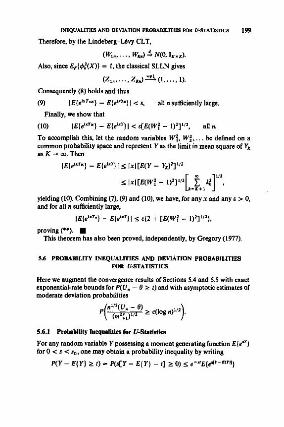
lNEQUALITI@S AND DEVIATION PROBABILITIES MIR U-STATISTICS 199
Therefore, by the Lindeberg-Ltvy CLT,
(win,*-*, w K n ) ' ~ ( o , I K x ~ ) *
Also, since EF(q$(X)} = 1, the classical SLLN gives
(Zln,. . . , Z,,)* (1,. . . , 1).
Consequently (8) holds and thus
(9) IE{eixTnR} - E(elxYX} I < E, all n sufficiently large.
Finally, we show that
(10) lE{eixYR} - E { e i X Y } ) < E[E(W: - 1)2]1/2, all n.
To accomplish this, let the random variables W:, W!, . . . be defined on a common probability space and represent Y as the limit in mean square of YK as K -P ao.Then
IE{e'"""} - E{efXY}I 5 Ix( [E(Y - YK)2]112
yielding (10). Combining (7), (9) and (lo), we have, for any x and any E > 0, and for all n sufficiently large,
IE{eixTn} - E{efXY}I I; E{Z + [E(W: - 1)2]1'2},
This theorem has also been proved, independently, by Gregory (1977). proving (**).
5.6 PROBABILITY INEQUALITIES AND DEVIATION PROBABLLITIES FOR U-STATISTICS
Here we augment the convergence results of Sections 5.4 and 5.5 with exact exponential-rate bounds for P(U, - 8 2 I ) and with asymptotic estimates of moderate deviation probabilities
5.6.1 Probability Inequalities for LI-Statistics
For any random variable Y possessing a moment generating function E{e"} for 0 < s < so, one may obtain a probability inequality by writing
P(Y - E{ Y} 2 t ) = P(s[Y - E { Y } - t ] 2 0) s e-"E{&Y-B(rIJ}

200 U-STATISTICS
and minimizing with respect to s E (0, so]. In applying this technique, we make use of the following lemmas. The first lemma will involve the function
X e-’ + - ex, f ( x , Y) = - X + Y
x > 0, y > 0. X + Y
Lemma A, Let E{Y} = p and Var{Y} = v.
(i) IfP(Y 5 b) = 1, then
1 5 Rs(b - lo, sv/(b - PI), > 0. E{e“Y - C)
(ii) YP(a I; Y s b) = 1, then E{ee(Y-l”} e(W)Sa(b-aIa, s > 0.
PROOF. (i) is proved in Bennett (1962), p. 42. Now, in the proof of Theorem 2 of Hoeffding (1963), it is shown that
qe-sP + peW 5 e(1 /W,
for 0 < p < 1, q - 1 - p. Putting p = y/(x + y ) and z = (x + y), we have
so that (i) yields
Now, as pointed out by Hoeffding (1963), v = E(Y - p)z = E(Y - p) (Y - a) S (b - p)E( Y - a) = (b - p)(p - a). Thus (ii) follows.
f ( x , y ) 5 e(UW(x+r)’
~ { ~ “ Y - f l ) ’ ) 5 e(l/e)ral(b-r)+*/(b-fl)ll~
The next lemma may be proved as an exercise (Problem 5.P.25).
Lemma B. rfE{eSY} < aofor 0 < s < so, and E{Y} = p, then
E{e’(Y-p)} = 1 + O(sz), s + 0.
In passing to U-statistics, we shall utilize the following relation between the moment generating function of a U-statistic and that of its kernel.
Lemma C. Let h = h(xl, . . . , x,) satisfv
+h(S) = Ep{eah(X1~*ii~XnJ} < 00, 0 < S s SO.
Then
where k = [n/m].

INEQUALITIES AND DEVIATION PROBABILITIES FOR U-STATISTICS 201
PROOF. By 5.1.6, Un = (n!)- ' cp W(X,, , . . . , XJ, where each W(.) is an average of k = [n/m] I.I.D. random variables. Since the exponential function is convex, it follows by Jensen's inequality that
&urn = es(nl)-l&W(.) 5 ( n ! ) - l 2 esW(X~,~... .X~m)
P
Complete the proof as an exercise (Problem 5.P.26).
We now give three probability inequalities for U-statistics. The first two, due to HoetTding (1963), require h to be bounded and give very useful explicit exponential-type bounds. The third, due to Berk (1970), requires less on h but asserts only an implicit exponential-type bound.
Theorem A . Let h = h(xl,. . ., x,) be a kernel for 8 = B(F), with a 5 h(xl, . . . , x,) 5 b. Put 8 = E{h(X,, . . . , X,)} ando* = Var{h(X,, . . . , X,,,)}, Then, for t > 0 and n 2 m,
p(u, - 8 2 t) 5 e-2tn/mlt2/(b-a)2 (1) and
(2) p(u, - 8 2 t) 5 e-ln/mlt'/2[0'+(1/3)(b-~)~l
PROOF. Write, by Lemmas A and C, with k = [n/m] and s > 0,
5 e-Jt+(l/8)S2(b-o)*/k.
Now minimize with respect to s and obtain (1). A similar argument leads to
It is shown in Bennett (1962) that the right-hand side of (2') is less than or equal to that of (2).
(Compare Lemmas 2.3.2 and 2.5.4A.)
Theorem B. Let h = h(x,, . . . , x,,,) be a kernel for 8 = qF), with EF{eSh(XI* . v t * X"} c 43, 0 < s 5 so.
all n 2 m.
Then,for ewry E > 0, there exist C, > 0 and pa < 1 such that
P(Un - 8 2 E ) s C,p:,

202 LI-STATISTICS
PROOF. For 0 < t $ s0k, where k = [n/m], we have by Lemma C that
= [e - re @h(s)]k,
where s = t /k . By Lemma B, e-"$,,(s) = 1 + O(s2), s 3 0, so that e-ace-a'JIh(s) = 1 - es + O(s2), s + 0,
< 1 for s = s, sufficiently small. Complete the proof as an exercise.
Note that Theorems A and B are applicable for n small as well as for n large.
5.6.2 "Moderate Deviation" Probability Estimates for U-Statistics A "moderate deviation" probability for a U-statistic is given by
where c > 0 and it is assumed that the relevant kernel h has finite second moment and > 0. Such probabilities are of interest in connection with certain asymptotic relative efficiency computations, as will be seen in Chapter 10. Now the CLT for U-statistics tells us that qn(c) 3 0. Indeed, Chebyshev's inequality yields a bound,
1 = O((1og n)- I). qn(c) ' c2 log n
However, this result and its analogues, O((1og n)-(1'2)v), under v-th order moment assumptions on h are quite weak. For, in fact, if h is bounded, then (Problem 5.P.29) Theorem 5.6.1A implies that for any S > 0
where u S h 1s b. Note also that if merely E , I h I3 < 00 is assumed, then for c sufficiently small (namely, c < l), the Berry-EssCen theorem for U-statistics (Theorem 5.5.1B) yields an estimate:
(1) q,(C) = O(n-l(I -4W:/~b-oPlcZ),
4
However, under the stronger assumption E , J h r < 00 for some v > 3, this approach does not yield greater latitude on the range of c. A more intricate analysis is needed. To this effect, the following result has been established by Funk (1970), generalizing a pioneering theorem of Rubin and Sethuraman (1965a) for the case U, a sample mean.
Theorem. lfEFl h r < 00, where v > 2, then (*) holdsfor ca < v - 2.

COMPLEMENTS 203
5.7 COMPLEMENTS
In 5.7.1 we discuss stochastic processes associated with a sequence of U- statistics and generalize the CLT for U-statistics. In 5.7.2 we examine the Wilcoxon one-sample statistic and prove assertions made in 2.6.5 for a particular confidence interval procedure. Extension of LI-statistic results to the related V-statistics is treated in 5.7.3. Finally, miscellaneous further complements and extensions are noted in 5.7.4.
5.7.1 Stochastic Processes Associated with a Sequence of U-Statistics Let h = h(xl, . . . , x,) be a kernel for 8 = 8(F), with EF(h2) < co and C1 > 0. For the corresponding sequence of U-statistics, { U,JnL,,,, we consider two associated sequences of stochastic processes on the unit interval [O, 13.
In one of these sequences of stochastic processes, the nth random function is based on U,, ..., U, and summarizes the past history of {U,},%,,. In the other sequence of processes, the nth random function is based on LI,, U , , l,. . . and summarizes the future history of { U,},>,,. Each sequence of processes converges in distribution to the Wiener process on [O, 13, which we denote by W ( . ) (recall 1.11.4).
The process pertaining to thefuture was introduced and studied by Loynes (1970). The nth random function, {Z,(t), 0 5 t 5 l}, i s defined by
Z,(O) = 0;
zn(t) = zn(tnk), cn, k + 1 < t < c n k *
For each n, the “times” t,,, c,, ,, + 1, . . . form a sequence tending to 0 and Z,( .) is a step function continuous from the left. We have
Theorem A (Loynes). Zn(*) 5 W(.) in DCO, 13.
This result generalizes Theorem 5.5.1A (asymptotic normality of U,) and provides additional information such as
Corollary. For x > 0,
(1) sup(& - e) 2 x(var{U,})1~2
sup W(t) 2 x) = 2[1 - qx)] O S l S l

204 U-STATISTICS
and
(2) ~ i m P inf(Uk - e) 5 -x(var{un})'/2 n - w ( kPn
= P inf W(t) 5 -x = 2[1 - Cp(x)].
As an exercise, show that the strong conoergence of Un to 8 follows from this
The process pertaining to the past has been dealt with by Miller and Sen
( 05151 1 corollary, under the assumption E F { h 2 ) < 00.
(1972). Here the nth random function, { %(t), 0 5 t 5 l}, is defined by
m - 1 , 0 4 t s -, n % ( t ) = 0,
x(t) defined elsewhere, 0 s t 5; 1, by linear interpolation.
Theorem B (Miller and Sen). Yn(.) 4 W(.) in CCO, 11.
This result likewise generalizes Theorem 5.5.1A and provides additional information such as
(3) Iim P sup k(Uk - e) 2 x(m2C1)1'2n1/2 = 2[1 - @@)I, x > 0. n-rw ( mSh5n 1
Comparison of (1) and (3) illustrates how Theorems A and B complement each other in the type of additional information provided beyond Theorem 5.5.1A.
See the Loynes paper for treatment of other random variables besides U-statistics. See the Miller and Sen paper for discussion of the use of Theorem B in the sequential analysis of U-statistics.
5.7.2 The Wilcoxon One-Sample Statistic as a UStatistic For testing the hypothesis that the median of a continuous symmetric distribution F is 0, that is, el,, = 0, the Wilcoxon one-sample test may be based on the statistic
1 I ( X , + x, > 0). I s l < l s n
Equivalently, one may perform the test by estimating G(O), where G is the distribution function G(r) = P(f(X, + X,) s t), with the null hypothesis to

COMPLEMENTS 205
be rejected if the estimate differs sufficiently from the value 3. In this way one may treat the related statistic
1 u, = - (;) c 4x1 + X , S O ) ISl<lSn
as an estimate of G(0). This, of course, is a U-statistic (recall Example 5.1.l(ix)), so that we have the convenience of asymptotic normality (recall Example 5.5.2C-check as exercise).
In particular, we considered a procedure of Geertsema (1970), giving an interval
In 2.6.5 we considered a related confidence interval procedure for
I w n = (Ka,,, WntJ formed by a pair of the ordered values W,, 5 s . 5 WnN, of the N, = (i) averages &Xi + X,), 1 s i < j 5 n. We now show how the properties stated for Iwn in 2.6.5 follow from a treatment of the U-statistic character of the random variable
Note that G,, considered as a function of x, represents a “sample distribution function” for the averages HX, + X,), 1 5 i < j s n. From our theory of U- statistics, we see that G,(x) is asymptotically normal. In particular, Gn({,/2) is asymptotically normal. The connection with the Wn;s is as follows. Recall the Bahadur representation (2.5.2) relating order statistics Xnkm to the sample distribution function F,. Geertsema proves the analogue of this result for Wnkn and G,. The argument is similar to that of Theorem 2.5.2, with the use of Theorem 5.6.1A in place of Lemma 2.5.4A.
Theorem. Let F satisfy the conditions stated in 2.6.5. Let
Then

206 LI-STATISTICS
where with probability 1
R, = O(n-j'* log n), n + 00.
It is thus seen, via this theorem, that properties of the interval Iwn may be derived from the theory of U-statistics.
5.7.3 Implications for Y-Statlstics In connection with a kernel h = h(xl, . . . , x,), let us consider again the V-statistic introduced in 5.1.2, Under appropriate moment conditions, the Uatatistic and V-statistic associated with h are closely related in behavior, as the following result shows.
Lemma. Let r be a positiue integer. Suppose that
EF(h(XI,, ..., X,Jr < 00, all i S il , . .., i, 5 m.
Then EIU, - V,Ir = O(n-7.
PROOF. Check that
n'"(Un - CJ = (n'" - n,mJ (Urn - K), where n,, = n(n - l)...(n - m + 1) and W, is the average of all terms h(X1,, . . . , Xi,,,) with at least one equality i, = ib, a # b. Next check that
nm - n(,,,) = O(nm-').
Finally, apply Minkowski's inequality. H
Application of the lemma in the case r = 2 yields
n"'(U, - v,) 4 0,
in which case nl''(U, - 0) and n1I2( V , - 0) have the same limit distribution, a useful relationship in the case C1 > 0. In fact, this latter result can actually be obtained under slightly weaker moment conditions on the kernel (see B6nner and Kirschner (1977).)
5.7.4 Further Complements and Extensions
by Sen (1960).
an not necessarily identical may be found in Sen (1967).
Sproule (1969a, b).
(i) Distribution-free estimation of the uariance of a U-statistic is considered
(ii) Consideration of U-statistics when the distribution of X1, X', . . . (iii) Sequential corlfidence interuuls based on U-statistics are treated by

PROBLEMS 207
(iv) Jackknifing of estimates which are functions of U-statistics, in order to reduce bias and to achieve other properties, is treated by Arvesen (1969).
(v) Further results on probabilities of deviations (recall 5.6.2) of U- statistics are obtained, via some further results on stochastic processes associated with U-statistics (recall 5.7.1), by Sen (1974).
(vi) Consideration of U-statistics for dependent observations XI, X 2 , , , . arises in various contexts. For the case of m-dependence, see Sen (1963), (1965). For the case of sampling without replacement from a finite population, see Nandi and Sen (1963). For a treatment of the Wilcoxon 2-sample statistic in the case of samples from a weakly dependent stationary process, see Serfling (1968).
(vii) A somewhat diflerent treatment of the case f l = 0 < C2 has been given by Rosin (1969). He obtains asymptotic normality for U , when the observations XI,. . . , X , are assumed to have a common distribution F("' which behaves in a specified fashion as n + 00. In this treatment F(") is constrained not to remain fixed as n -+ 00.
(viii) A general treatment of symmetric statistics exploiting an orthogonal expansion technique has been carried out by Rubin and Vitale (1980). For example, U-statistics and Ccstatistics are types of symmetric statistics. Rubin and Vitale provide a unified approach to the asymptotic distribution theory of such statistics, obtaining as limit random variable a weighted sum of products of Hermite polynomials evaluated at N(0, 1) variates.
5.P PROBLEMS
section 5.1
5.1.5. 1. Check the relations EF{gI(XI)} = 0, EF{g2(xI, X,)} = 0,. . . in
2. Prove Lemma 5.1.5B.
Section 5.2
3. (i) Show that Co s C1 5 ... s C,. (ii) Show that C1 s 4c2. (Hint: Consider the function g2 of 5.1.5.) 4. Let { a l , . . . , a,} and {b l , . .. , b,} be two sets of m distinct integers
from { 1, . . . , n } with exactly c integers in common. Show that
EF{I;(X,', * ' - 9 X,,)fi(X*,, * * * 9 X*J = Cc. 5. In Lemma 5.2.1A, derive (iii) from (*). 6. Extend Lemma 5.2.1A(*) to the case of a generalized U-statistic. 7. Complete the details of proof for Lemma 52.28. 8. Extend Lemma 5.2.2B to generalized U-statistics.

208 LI-STATISTICS
Section 5 3
9. The projection of a generalized U-statistic is defined as
0 = i: f E F { U I X I “ } - (N - l)e, J = l 1-1
where N 8: nl + ... + nk. Define
h&) = E,{h(X\”, . . . , Xg!; . . . ; Xik), . . . , X g i ) l X p = x} - 8.
Show that
10. (continuation) Show that U, - 0, is a Ustatistic based on a kernel
11. Verify relation (2) in 5.3.4.. 12. Extend (2), (3) and (4) of 5.3.4 to generalized U-statistics. 13. Let gc and S,, be as defined in 5.1.5. Define a kernel G, of order m by
H satisfying E p { H } = E , { H I X y } = 0.
G b i , - - 9 x 3 = C &iI, 9 x 3 1 S I 1 < - - < l c $ m
and let U,, be the U-statistic corresponding to G,. Show that
and thus m
c- 1 U , - O = CU,.
Now suppose that c,- = 0 < c,. Show that 0, defined in 53.4 satisfies
on - 8 = we,. Section 5.4
14. For EP h2 < 00, show strong convergence of generalized U-statistics. 15. Prove Theorem 5.4C, the LIL for U-statistics. (Hint: apply Theorem
5.3.3.)
Section 5.5 16. Prove Theorem 5.5.1A, the CLT for U-statistics. 17. Complete the details for Example 5.5.1A.

PROBLEMS 209
18. Extend Theorem 5.5.1A to a vector of several U-statistics defined on
19. Extend Theorem 5.5.1A to generalized U-statistics (continuation of
20. Check the details of Example 5.5.1B. 21, Check the details of Example 5.5.2A. 22. (continuation) Show, for F binomial (1, i), that
the same sample.
Problems 5.P.9, 10, 12).
n(m2 - 4) - 4x;. (Hint: One approach is simply to apply the result obtained in Example 5.5.2A. Another approach is to write m, = fl - f lz and apply the methods of Chapter 3.)
23. Check the details of Example 5528. 24. Complete the details of proof of Theorem 5.5.2. (a) Prove (3). (Hint: write h,(x) = EF{h2(x, X,)} and use Jensen's
inequality to show that
(b) Prove (4). (c) Prove(6).
Section 5.6 25. Prove Lemma 5.6.1B. (Hint: Without loss assume E{ Y} = 0. Show
that e'' = 1 + SY + L'Z, where 0 < 2 < Y2e'Or.) 26. Complete the proof of Lemma 5.6.1C. 27. Complete the proof of Theorem 5.6.1A. 28. Coriiplete the proof of Theorem 5.6.1B. 29. In 5.6.2, show that (1) follows from Theorem 5.6.1A and that (*) for
c 5; 1 follows from Theorem 5.5.1B.
Section 5.7
EF{h2} < 00, from Corollary 5.7.1. 30. Derive the strong convergence of U-statistics, under the assumption
31. Check the claim of Example 5.5.2C. 32. Apply Theorem 5.7.2 to obtain properties of the confidence interval
I W W
33. Complete the details of proof of Lemma 5.7.3.

C H A P T E R 6
Von Mises Differentiable
Statistical Functions
Statistics which are representable as functionals T(F,) of the sample distribu- tion F, are called “statistical functions.” For example, for the variance parameter u2 the relevant functional is T(F) 5 [x - x dF(x)]’ dF(x) and T(F,) is the statistic mz considered in Section 2.2. The theoretical investiga- tion of statistical functions as a class was initiated by von Mises (1947), who developed an approach for deriving the asymptotic distribution theory of such statistics. Further development is provided in von Mises (1964) and, using stochastic process concepts, by Filippova (1962). Notions of dCgerentiability of T play a key role in the von Mises approach,
analogous to the treatment in Chapter 3 of transformations of asymptotically normal random vectors. We thus speak of “differentiable statistical functions.” In typical cases, T(F,,) - T(F) is asymptotically normal. Otherwise a higher “type” of distribution applies, in close parallel with the hierarchy of cases seen for U-statistics in Chapter 5.
This chapter develops the “differential approach ” for deriving the asymp- totic distribution theory of statistical functions. In the case of asymptotically normal T(F,,), the related Berry-Essken rates and laws of iterated logarithm are obtained also. Section 6.1 formulates the representation of statistics as functions of F, and sketches the basic scheme for analysis of T(F,,) - T(F) by reduction by thedifferential method to an appropriate approximating random variable V,. Methodology for carrying out the reduction to V, is provided in Section 6.2, and useful characterizations of the structuie of V, are provided in Section 6.3. These results are applied in Section 6.4 to obtain general results on the asymptotic distribution theory and almost sure behavior of statistical functions. A variety of examples are treated in Section 6.5. Certain comple- ments are provided in Section 6.6, including discussion of some statistical interpretations of the derivative of a statistical function. Further applications of the development of this chapter will arise in Chapters 7,8 and 9.
210
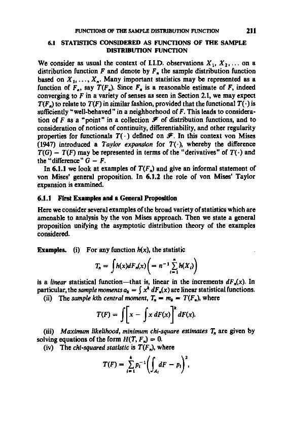
FUNCl9ONS OF THE SAMPLE DISTRIBUTION FUNCTION 211
6.1 STATISTICS CONSIDERED As FUNCTIONS OF THE SAMPLE DISTRIBUTION FUNCTION
We consider as usual the context of I.I.D. observations X1, X 1 , . , . on a distribution function F and denote by F, the sample distribution function based on X1,. . . , X,. Many important statistics may be represented as a function of F,, say T(F,). Since F, is a reasonable estimate of F, indeed converging to F in a variety of senses as seen in Section 2.1, we may expect T(F,) to relate to T(F) in similar fashion, provided that the functional T ( . ) is sufficiently “well-behaved” in a neighborhood of F. This leads to considera- tion of F as a “point” in a collection 9 of distribution functions, and to consideration of notions of continuity, differentiability, and other regularity properties for functionals T( a ) defined on 9. In this context von Mises (1947) introduced a Taylor expansion for T(.) , whereby the difference T(G) - T(F) may be represented in terms of the “derivatives” of T( . ) and the “difference” G - F.
In 6.1.1 we look at examples of T(F,) and give an informal statement of von Mises’ general proposition. In 6.1.2 the role of von Mises’ Taylor expansion is examined.
6.1.1 First Examples and a General Proposition
Here we consider several examples of the broad variety of statistics which are amenable to analysis by the von Mises approach. Then we state a general proposition unifying the asymptotic distribution theory of the examples considered.
Examples. (i) For any function h(x), the statistic
T, = lh(x)dF,(x) (= n-’ I - 1 f: h(X,))
is a linear statistical function-that is, linear in the increments dF,(x). In particular, thesample moments ak = j XL dF,(x) are linear statistical functions.
(ii) The sample kth central moment, T, = mk = T(F,), where
T(F) = ,[. - l x dF(x)]L dF(x).
(iii) Maximum likelihood, minimum chi-square estimates T, arc given by
(iv) The chi-squared statistic is T(F,), where solving equations of the form H(T, F,) = 0.

212 VON MlSES DIFFERENTIABLE STATISTICAL FUNCTIONS
where {A,} is a partition of R into k cells and { p i } is a set of specified (null- hypothesis) probabilities attached to the cells.
(v) The generalized Cramdr-oon Mises test statistic, considered in 2.1.2, is given by T(F,), where T(F) = w(Fo)(F - Fo)’ dFo, for w and Fo specified.
It turns out that examples (i), (ii) and (iii) are asymptotically normal (under appropriate conditions), example (iv) is asymptotically chi-squared, and example(v)issomethingstihdifferent (a weighted sumofchi-squared variates). Nevertheless, within von Mises’ framework, these examples all may be viewed as special cases of a single unifying theorem, which is stated informally as follows.
Proposition (von Mises). The type of asymptotic distribution of a diyer- entiable statistical function T, = T(F,) depends upon which is the first nonvanishing term in the Taylor development of the functional T(.) at the distribution F of the observations. If it is the linear term, the limit distribution is normal (under the usual restrictions corresponding to the central limit theorem). In other cases, “higher” types of limit distribution result.
More precisely, when the first nonvanishing term of the Taylor develop- ment of T ( . ) is the one of order m, the random variable nm/2[T(F,) - T(F)] converges in distribution to arandom variable with finite variance. Form = 1, the limit law is normal. (Actually, the normalization for the order m case can in some cases differ from nm”. See 6.6.4.)
6.1.2 The Basic Scheme for Analysis of T(FJ
In 6.2.1 a Taylor expansion of T(F,) - T(F) will be given:
Analysis of T(F,) - T(F) is to be carried out by reduction to
” 1 V,, =: 1 7-d T(F; F, - F)
, = i J ! ’ for an *appropriate choice of m. The reduction step is performed by dealing with the remainder term R,, = T(F,) - T(F) - V,,, and the properties of T(F,) - T(F) then are obtained from an m-linear structure typically possessed by V,,,.

FUNCTIONS OF THE SAMPLE DISTRIBUTION FUNCTION 213
In the case that T(F,) is asymptotically normal, we prove it by first showing that (*I n1/2R1 , 3 0.
Then it is checked that Vl, has the form of a sample mem of I.I.D. mean 0 random variables, so that n112Vl, N(0, 02(T, F)) for a certain constant a2( T, F), whereby
(1) In this case the law of the iterated logarithm for T(F,) - T(F) follows by a similar argument replacing (*) by
(") n1l2R1, = o.((log log n)'l2)wpl,
yielding
n"Z[T(F,) - T(F)I 5 N(0, a2(T, F)).
In addition, a Berry-Essten rate for the convergence in ( 1 ) may be obtained through a closer study of R1,. Invariably, standard methods applied to R , , fail to lead to the best rate, O(n-'12). However, it turns out that if T(FJ - T(F) is approximated by V2, instead of V,,, the resulting ("smaller") re- mainder term R2, behaves as needed for the standard devices to lead to the Berry-Esskn rate O(n- Namely, one establishes
(***) P(IR2,( > Bn-') = O(n-1 /2 )
for some constant B > 0, and obtains
InthecasethatP(V,, = c) = l,thatis, V,, = dIT(F; F, - F)isadegenerate random variable, the asymptotic distribution of T(F,) is found by finding the lowest m such that V,, is not degenerate. Then a limit law for n"'2[T(Fn) - T(F)] is found by establishing nm/2Rmn + 0 and dealing with nm/2V,,. For m > 1, the case of widest practical importance is m = 2. Thus the random variable V2,, has two important roles-one for the case that n[T(F,) - T(F)J has a limit law, and one for the Berry-Eden rate in the case that T(FJ is asymptotically normal.
Finally, we note that in general the strong consistency of T(F,) for estima- tion of T(F) typically may be established by proving R , , - 0.
Methodology for handling the remainder terms R,, is provided in 6.2.2. The structure of the V,, terms is studied in Section 6.3. These results are applied in Section 6.4 to obtain conclusions such as (l), (2), (3), etc.
WP 1

214 VON MIS= DrPFERBNTUBLE STATISTICAL FUNCnONS
6.2 REDUCTION TO A DIFFERENTUL APPROXIMATION
The basic method of differentiating a functional T(F) is described in 6.2.1 and applied to formulate a Taylor expansion of T(FJ about T(F). In 6.2.2 various techniques of treating the remainder term in the Taylor expansion are considered.
6.2.1 Differentiation of Functionab T( )
Given two points F and G in the space 9 of all distribution functions, the “line segment” in 9 joining F and G consists of the set of distribution functions ((1 - A)F + AG, 0 S A s l}, also written as { F + A(G - F), 0 s 1 $ 1). Consider a functional T. defined on F + A(G - F ) for all sufficiently small A. If the limit
T(F + rl(G - F)) - T(F) d,T(F; G - F) = lim .
1 - O t A
exists, it is called the Gllteuux dverential of T at F in the direction of G. Note that dIT(F; G - F) is simply the ordinary right-hand derivative, at 1 = 0, of the function Q(A) = T(F + A(G - F)) of the real variable A. In general, we d e h e the kth order Gateaux differential of T at F in the direction of G to be
provided the limit exists.
Example. Consider the functional
where h is symmetric. Writing
T(F + A(G - F))
and carrying out succcssive differentiations, we obtain

REDUCTION TO A DIFPBRHNlUL APPROXIMATION 215
and thus
d k T(F; G - F) = C(C - l )***(c - k + 1) c-& &
I - 1 I = 1 X f . . s h ( x l , . . . , x t . Y l , . . . . y , _ , ) n dFCydndCG(xJ - F(xl)J
fork = 1, ..., c,and dkT(F; G - F) = 0, k > c. In particular, for the mean functional T(F) = x dF(x), we have
dlT(F; G - F) = fi(x)d[G(x) - F(x)J = T(G) - T(F) andd&T(F;G-F)=Ofork> 1.
For the variance functional, corresponding to
h(x1, XJ = fcx: + x i - 2x,x2),
we have (check)
dIT(F; G - F) = sxz dG(x) - s x 2 dF(x) - 2
and
Suppose that the function Q(A) satisfies the usual assumptions for a Taylor expansion to be valid (the assumptions of Theorem 1.12.1A as extended in Remark 1.12.1(i)) with respect to the interval 0 S 1 s 1. (See Problem 6.P.2) Since Q(0) = T(F), Q(l) = T(G), Q':)(O) = I ,T(F; G - F), Q$?(O) = dz T(F; G - F), etc., the Taylor expansion for Q( .) may be expressed as a Taylor expansion jor the junctional T( .):
1 d"" (m + l)!dAmtl
+ where 0 I; A+ 5 1. Note that even though we are dealing here with a func- tional on 9, sophisticated functional analysis is not needed at this stage, since the terms of the expansion may be obtained by routine calculus methods.

216 VON MlSES DIFFERENTIABLE STATISTICAL FUNCTIONS
We are not bothering to state explicitly the conditions needed for (*) to hold formally, because in practice (*) is utilized rather informally, merely as a guiding concept. As discussed in 6.1.2, our chief concern is
which may be investi8ated without requiring that R , have the form dictated by (*), and without requiring that (+) hold for G other than F,.
6.2.2 Methods for HandUng the Remainder Term R,,,,, As discussed in 6.1.2, the basic property that one would seek to establish for R,, is
(1) nm12Rm, 4 0,
In the case that the Taylor expansion of 6.2.1 is rigorous, it sulfices for (1) to show that
This is the line of attack of von Mises (1947). Check (Problem 6.P.3), using Lemma 6.3.28, that (M) holds for the functionals
T(F) = f - Ih(xl, . . . , xe)dF(xl) * dF(xe)
considered in Example 6.2.1.
An inconvenience of this approach is that (M) involves an order of differ- entiability higher than that of interest in (1). In order to avoid dealing with the unnecessarily complicated random variable appearing in (M), we may attempt a direct analysis of R,,,". Usually this works out to be very effective in practice.
Example A. (Continuation of Example 6.2.1). For the variance functional T(F) = jj N x t , x2)dF(xl)dF(r2), where h(xl, x2) - f<x: + x i - 2x1x2), we have (check)
T(G) - T(F) - dIT(F; G - F) = -@a - ~ ( p ) ' ,
where pF and pa denote the means of F and G. Thus
R , , = -(X - /+)'.

REDUCTION TO A DIFFERENTIAL APPROXIMATION 217
It follows (check) by the Hartman and Wintner LIL (Theorem l.lOA) that
IR1,I = O(n-’ log log n) wpl
and hence in particular
and
n1’2RI, = o((1og log n)’”)wpl,
in conformity with (*) and (I*) of 6.1.2.
As a variant of the Taylor expansion idea, an alternative “guiding concept” consists of a differential for Tat F in a sense stronger than the GBteaux version. Let us formulate such a notion in close analogy with the differential of 1.12.2 for functions g defined on Rk. Let 9 be the linear space generated by differ- ences G - H of members of F, the space ofdistribution functions. (9 may be represented as {A: A = c(G - H), G, H E F, c real}.) Let 9 be equipped with a norm \)- ) I . The functional T defined on 9 is said to have a diflerential at the point F c 9F with respect to the norm 11.11 if there exists a functional T(F; A), defined on A E 9 and linear in the argument A, such that
(D) T(G) - T(F) - T(F; G - F ) = o(IIG - FII) as llG - Fll + 0 (T(F; A) is called the “differential”).
Remarks A. (i) To establish (D), it suffices (see Apostol(1957), p. 65) to verify it for all sequences {G,} satisfying IlG, - Fll + 0, n + 00.
(ii) By linearity of T(F; A) is meant that
for Al, . . . , Ak E 9 and real al, . . . , a k a
(iii) In the general context of differentiation in Banach spaces, the differ- ential T(F; A) would be called the Frbchet deriuatioe of T(see Frtkhet (1925), Dieudonnt (1960), Luenberger (1969), and Nashed (1971)). In such treat- ments, the space on which T is defined is assumed to be a normed linear space. We intentionally avoid this assumption here, in order that T need only be defined at points F which are distribution functions. a
It is evident from (D) that the differential approach approximates T(F,) - T(F) by the random variable T(F; F, - F), whereas the Taylor expansion approximates by dl T(F; F, - F). These approaches are in agreement, by the following result.
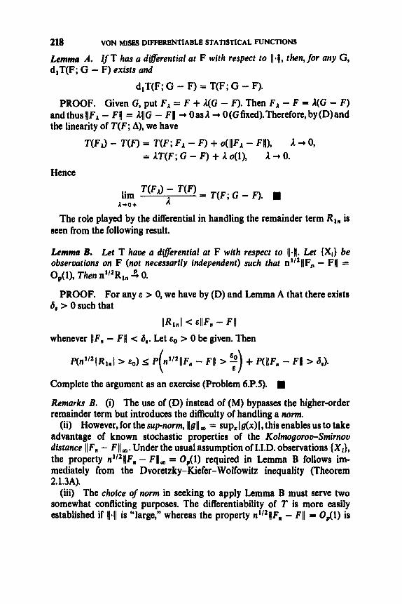
218 VON MlSBS DIFFERENTIABLE STATISTICAL FUNCTIONS
Lemma A. I fT has a diferential at F with respect to 11.11, then,jor any G, dlT(F; G - F) exists and
dlT(F; G - F) = T(F; G - F).
PROOF. Given G, put FA = F + 1(G - F). Then FA - F = A(G - F) and thus llFr - Fll = 1llG - Fll + Oasl+ O(Gfixed).Therefore,by(D)and the linearity of T(F; A), we have
T(F1) - T(F) = T(F; FA - F) + o(llF1- Fll), 1 + 0, = IT(F; G - F) + 1 ~ ( l ) , 1 + 0.
Hence
A A*O*
The role played by the differential in handling the remainder term R1, is seen from the following result.
Lemma B. Let T have (I diferential at F with respect to 11.11. Let {Xi} be observations on F (not necessarily independent) such that n’/’llF,, - Fll = O,,(l), Then n’/’RI,, 3 0.
PROOF. For any E > 0, we have by (D) and Lemma A that there exists 6, > 0 such that
IRlnl < ~ l l F n - Fll whenever llF,, - Fll c 6,. Let e, > 0 be given. Then
P(n’”IR1,I > go) S P n’“JIF, - FlJ > + P(IIF, - Fll > 6,). ( Complete the argument as an exercise (Problem 6.P.5). w Remarks 3. (i) The use of (D) instead of (M) bypasses the highersrder remainder term but introduces the difficulty of handling a norm.
(ii) However, for the sup-norm, llgll = sup,lg(x)l, this enables us to take advantage of known stochastic properties of the Kolmogorov-Smlmou distance [IF, - Fll,. Under the usual assumption of 1.I.D. observations {X,}, the property n”ZllFn - Fll, = 0,(1) required in Lemma B follows im- mediately from the Dvoretzky-Kiefer-Wolfowitz inequality (Theorem 2.1.3A).
(iii) The choice of norm in seeking to apply Lemma B must serve two somewhat conflicting purposes. The differentiability of T is more easily established if 11.11 is “large,” whereas the property nl”llFn - Fll = 0,,(1) is

REDUCTION TO A DIFFERENTIAL APPROXIMATION 219
more easily established if 11.11 is “small.” Also, the two requirements differ in type, one being related to differential analysis, the other to stochastic analysis.
(iv) In view of Lemma A, the “candidate”differentia1 T(F; G - F) to be employed in establishing (D) is given by d l T ( F ; G - F), which is found by routine calculus methods as noted in 6.2.1.
(v) Thus the choice of norm 11.11 in Lemma B plays no essential role in the actual application of the result, for the approximating random variable dl T(F; F, - F) is defined and found without specification of any norm.
(vi) Nevertheless, the differential approach actually asserts more, for it characterizes d ,T(F; F, - F ) as linear and hence as an aoerage of random variables. That is, letting 6, denote the distribution function degenerate at x, - 00 < x < 00, and expressing F, in the form
F,, = n-’ Z ~ X , , I = I
we have
= n-I 1 T(F; s,, - F). I = 1
(vii) Prove (Problem 6.P.6) an analogue of Lemma B replacing the convergence 0 (1) required for n’/’JIF, - Fll by “O((10g log n)1/2)wpl*’ and concluding 44n&2RI, = o((10g log n)’’’)wpl.” Justify that the requirement is met in the case of IJ.)lm and I.I.D. observations. H
Remarks C.. (i) In general the role of d , T ( F ; F , - F ) is to approximate n”’[T(F,) - T(F) - p(T, F ) ] by n”’[dlT(F; F, - F) - p(T, F)], where p(T, F) = E,{dlT(F; F, - F)}. Thus p(T, F) may be interpreted as an asymptotic bias quantity. In typical applications, p(.T, F ) = 0. Note that when d l T(F; F, - F) is linear, as in Remark B (vi) above, we have p( T, F ) =
(ii) The formulation of the differential of T w.r.t. a norm 11-11 has been geared to the objective of handling R In. Analogous higher-order derivatives may be formulated in straightforward fashion for use in connection with
(in) We have not concerned ourselves with the case that the functional T is defined only on a subclass of 9. The reason is that operationally we will utilize the differential only conceptually rather than strictly, as will be ex- plained below.
E A W ; a x , - F)}.
Rm?’*m ’ 1.
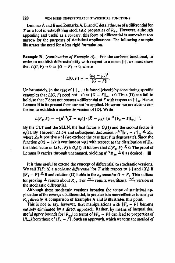
220 VON MISES DIFFERENTIABLE STATISTICAL FUNCTIONS
Lemmas A and B and Remarks A, B, and C detail the use of a differential for T as a tool in establishing stochastic properties of Rl,. However, although appealing and useful as a concept, this form of differential is somewhat too narrow for the purposes of statistical applications. The following example illustrates the need for a less rigid formulation.
Example B (continuation of Example A). For the uariance functional, in order to establish differentiability with respect to a norm 11.11, we must show that L(G, F) + 0 as llG - Fll + 0, where
Unfortunately, in the case of 11-11 it is found (check) by considering specific examples that L(G, F) need not +O as llG - Fll, + 0. Thus (D) can fail to hold, so that T does not possess a differential at F with respect to 11-11 Hence Lemma B in its present form cannot be applied. However, we are able never- theless to establish a stochastic version of (D). Write
By the CLT and the SLLN, the first factor is 0,,(1) and the second factor is op(l). By Theorem 2.1.5A and subsequent discussion, n'/21(F, - Fll, 4 ZF, where Zp is positive wpl (we exclude the case that F is degenerate). Since the function g(x) = l/x is continuous wpl with respect to the distribution of ZF, the third factor in L(F,, F) is O,,(l). It follows that L(F,, F) 1: 0. The proof of Lemma B carries through unchanged, yielding n1/2Rln 4 0 as desired.
It is thus useful to extend the concept of differential to stochastic versions. We call T(F; A) a stochastic diflerential for T with respect to 11.11 and {X,} if )IF, - Fll 3 0 and relation (D) holds in the 0, sense for G = F,. This suffices for proving 4 resultsabout R1,. For 2 results, we utilizea 2 version of the stochastic differential.
Although these stochastic versions broaden the scope of statistical ap- plication of the concept of differential, in practice it is more effective to analyze R1, directly. A comparison of Examples A and B illustrates this point.
This is not to say, however, that manipulations with /IF, - Fll become entirely eliminated by a direct approach. Rather, by means of inequalities, useful upper bounds for IR,I in terms of [IF, - Fll can lead to properties of I R , I from those of IlF, - Fll. Such an approach, which we term the method of

ANALYSIS OF THE DIFFERENTIAL APPROXIMATION 221
direrentid inequalities, will be exploited in connection with M-estimates (Chapter 7) and L-estimates (Chapter 8).
0, for the purpose of approximating n’12[T(F,) - T(F)] in limit distribution by n1/2dl T(F; F, - F). Note that this purpose is equally well served by reduction to T,(F,)d,T(F; F , - F), where TF(.) is any auxiliary functional defined on f such that T,(F,) 4 1. That is, it suffices to prove
We have discussed in detail how to prove n112R1,
(*I n”*[T(F,) - T(F) - T,(F,). d1 T(F; F, - F ) ] 3 0
in place of n1’*R1, 3 0. We apply this scheme as follows. First compute dl T(F; F, - F). Then select TF(.) for convenience to make the left-hand side of (*) manageable and to satisfy T,(F,) 4 1. Then proceed to establish (*) by, for example, the method of differential inequalities noted above. We will apply this device profitably in connection with M-estimates (Chapter 7).
The foregoing considerations suggest an extension of the concept of differential.-We call T(F; A) a quasi-dqerential with respect to 11-11 and TF(-) if the definition of differential is satisfied with (D) replaced by
6.3 METHODOLOGY FOR ANALYSIS OF THE DIFFERENTIAL APPROXlMATlON
Here we examine the structure of the random variable V,, to which considera- tion is reduced by the methods of Section 6.2. Under a multilinearity condition which typically is satisfied in applications, we may represent V,, as a V- statistic and as a stochastic integral. In Section 6.4 we make use of these representations to characterize the asymptotic properties of T(F,) - T(F).
6.3.1 Multi-Linearity Property
In typical cases the kth order Gateaux differential dk T(F; G - F) is k-linear: there exists a function T , [ F ; xl, . . . , xk], (xI, . . . , xk) E Rk, such that
1 1 k

222 VON MISES DIFFERENTIABLE STATISTICAL FUNCTIONS
Remarks. (i) A review of 1.12.1 is helpful in interpreting the quantity T , [ F ; xl, . . . , xk], which is the analogue of the kth order partial derivative,
as a function g defined on R‘. Thus T , [ F ; xI, , . . , xk] may be interpreted as the kth order partial derivative of the functional T(F), considered as a function of the arguments {dF(x), -00 < x < oo}, the partial being taken with all arguments except dF(x,), . . . , dF(xk) held fixed.
(ii) The function Tl[F; x] may be found, within an additive constant, simply by evaluating dIT(F; 6, - F). If (L) holds, then d,T(F; 6, - F) =
(iii) If&[F;xI, .. ., xk]isconstunt,consideredasafunctionofxl,. .., XI ,
then dkT(F; G - F) = 0 (all G). Note that a constant may be added to &[F; xi,. . . , xk] without altering its role in Condition (L).
(iv) If dl T(F; G - F) is a diflerential for T at F with respect to a norm, then by definition dlT(F; G - F) is linear and, as noted in Remark 6.2.2B (vi), we have
.Tl[F; x] - JT,[F; x]dF(x) = T(F; 6, - F) = dIT(F; 6, - F).
T , [ F ; X] - Tl [F; x]dF(x).
6.3.2 Represcntatlon as a VStatistic Under (L), the random variabledk T(F; F. - F) may be expressed in the form of a V-statistic. This is seen from the following result.
Lemma A. Let F befixed and h(xl, . . . , xk) be given. A functional of the form
may be written as a functional of the form
where the definition of h depends upon F.
PROOF. For k 3: 1, take h(x) = h(x) - J h(x)dF(x). For k = 2, take
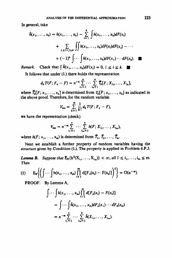
Remark. Check that & x l , . . . , xk)dF(xf) = 0, 1 5 i 5 k. D It follows that under (L) there holds the representation
R R
dk T ( F ; FR - F) = n-' c * * . 1 G [ F ; Xir, . . . , Xir], I 1 = 1 i k = 1
where $IF; x l , . . . , xk] is determined from T, [F; x I , . . . , xk] as indicated in the above proof. Therefore, for the random variable
m i
we have the representation (check) R R
V,, = n-'" C - * * 2 h(F; Xi1,. . . , Xim), l 1 = 1 f m = l
where h(F; x l , . . . , x,) is determined from r , F2,. . . , Tm. Next we establish a further property of random variables having the
structure given by Condition (L). The property is applied in Problem 6.P.3.
Lcmmu B. Suppose that EF{h2(X,,, . . . , Xi,)} < co, all 1 5 i l , . . . , i, 5 m. Then
PROOF. By Lemma A,
II R
= n-" c * ' . c li(Xir, . . * , X , J . 1 1 - 1 i m = l

224 VON MlSES DIFFERENTIABLE STATISTICAL FUNCTIONS
Thus the left-hand side of (1) is given by
By the remark following Lemma A, the typical term in (2) may be possibly nonzero only if the sequence of indices i l , . . . , i,,,, ill . . . , j , contains each member at least twice. The number of such cases is clearly O(n "). Thus (1) follows. a
We have seen in 5.7.3 the close connection between U- and V-statistics. In particular, we showed that El LI, - V,r = O(n-') under rth moment as- sumptions on the kernel h(xl, . . . , x,,,). We now prove, for the case m = 2, an important further relation between U, and V,. The result will be of use in connection with V,, .
Lemma C. Suppose that h(xl, x,) is symmetric in its arguments and satisfies EFh2(Xl, X2) < 00 and EFJh(Xl, Xl)l3l2 < 00. Then the corresponding U- and V-statistics U, and V , satis/y,for B > 2(EF{h(X,, X,) - h(X1, X,)} 1,
P(IU, - V,l > Bn-') = o(n-'I2).
PROOF. From the proof of Lemma 5.7.3, we have
u, - v, = n-yu, - Ww),
where
The first term on the right is O(n- l ) by Chebyshev's inequality and Lemma 5.2.1A. For the second term, we use Theorem 4 of Baum and Katz (1965), which imp1ies:for { K} I.I.D. with E{ Yl} = 0 and El Yl I' < 00, where r 2 1, P(lyl > e) = o(n'-')for all e > 0. Applying the result with r = 4, we have ~ ( P I - " ~ ) for the second term on the right.

PROPERTIES OF DIFFERENTIABLE STATISTICAL FUNCTIONS 225
6.3.3 Representation as a Stochastic Integral Under Condition (L), the random variable d , T(F; F, - F) may be expressed as a stochastic integral, that is, in the form
for a suitable kernel h. As in 2.1.3, let us represent Y ( X 1 , ..., X”} as 9 { F - l( Yl), . . . , F- l( K)}, where { &} are independent uniform (0, 1) variates. Let Gn(.) denote the sample distribution function of Yl, . . . , Y,, and consider the corresponding “empirical ” stochastic process m(t) = r~l/~[G,(t) - t ] , 0 s t 5 1.Thus
.V{nm’2d, T(F; F,, - F)}
so that the limit law of nm12d, T(F; F, - F) may be found through an application of the convergence Y,( .) 5 Wo considered in 2.8.2.
6.4 ASYMPTOTIC PROPERTIES OF DIFFERENTIABLE STATISTICAL FUNCTIONS
Application of the methodology of Sections 6.2 and 6.3 typically leads to approximation of T(F) by a particular V-statistic,
V,, = n-” C . - C h(F; X i , , . . . , Xi,,,). n n
i = 1 i m = l
(In Section 6.5, as a preliminary to a treatment of several examples, we discuss how to “find” the kernel h(F; x l , . . . , x,) effectively in practice.) As discussed in 6.1.2, under appropriate conditions on the remainder term R,, = T(F,) - T(F) - V,,, the properties of T(FJ - T(F) are thus given by the corre- sponding properties of V,, . In particular, 6.4.1 treats asymptotic distribution theory, 6.4.2 almost sure behavior, and 6.4.3 the Berry-Essden rate.
6.4.1 Asymptotic Distribution Theory Parallel to the asymptotic distribution theory of U-statistics (Section 5 . 9 , we have a hierarchy of cases, corresponding to the following condition for the cases m = 1,2, . . . . Condition A,
(i) Var,{h(F; X1,. , . , X,)} = 0 for k c m, >O for k = m; (ii) n’”lZR,, 4 0.

226 VON MISES DIFFERENTIABLE STATISTICAL FUNCTIONS
For the case m = 1, the V-statistic V,, is simply a sample mean, and by the CLT we have
Theorem A. Consider a sequence of independent observations {X,} on the distribution F. Let T beufunctionalfor which Condition A, holds. Put p(T, F) = EF{h(F; XI)} and o'fl, F) = VarF{h(F; XI)}. Assume that 0 < a'(T, F) < 00. Then
T(F,) is AN(T(F) + p(T, F), n-'a'(T, F)).
Example (Continuation of Examples 6.2.1, 6.2.2A). For the variance functional we have
dirrIF; F, - F) = fx2 dF,(x) - f x 2 dF(x) - 2
so that Condition (L) of 6.3.1 holds, and we approximate T(F,) - T(F) by V,, based on h(F; x) = ( x - pF)z - ug. We have
p(T, F) = E,h(F; X , ) = 0
and
UZ(T, F) = VarF{h(F; xi)} = C(,(F) - U;. Further, as seen in Example 6.2.2A, n112R1,, 3 0. Thus the conditions of Theorem A are fulfilled, and we have
as seen previously in Section 2.2.
For the case m = 2, we have a result similar to Theorem 5.5.2 for U- statistics.
TheoremB. Consider a sequence of independent observations { X , } on the distribution F. Let T be a functional for which Condition A2 holds. Assume that h(F; x, y) = h(F; y, x) and that EFh2(F; XI, X,) < 00, EF(h(F; Xi, XJ

PROPERTIES OF DIFFERENTIABLE STATISTICAL FUNCTIONS
C 00, and EF{h(F; x, XI)} E C (in x). Put P(T, F) = EFh(F; X1, X2). Denote by {A,} the eigenualues ofthe operator A defined on L2(R, F) by
227,
m
A d x ) = S__Ch(F; x, Y) - 10, F)lg(y)dF(y), x E R, g E L2(R, F).
Then
np(Fn) - T(F) - p(T, F)1 ' f, hk x i k 3
k = 1
where x:k (k = 1, 2, . . .) are independent
Remark. Observe that the limit distribution has mean zy d k , which is not necessarily 0. By Dunford and Schwartz (1963), p. 1087, E,{h(F; Xi, X , ) } - p(T, F) = x y d k , which is thus finite since E F l h ( F ; XI, Xl)l c 00. This assumption is not made in the analogous result for LI-statistics. H PROOF. By Condition Al , it suffices to show that
uariates.
where 9. is the V-statistic based on the kernel h(x, y ) = h(F; x, y ) - p(T, F). Consider also the associated LI-statistic, 0, = (2)- & & X i , X,). As seen in the proof of Lemma 5.7.3, 0, is related to c through
where n2(0, - p.1 = (n2 - q2))(0" - m,
tt. = n - l p i ( X , , X,). n
I = I
Thus
n ( R - 0") = - 0". Note that EF{h(Xl, X,)} = 0. Thus, by the strong convergence of U- statistics (Theorem 5.4A), 0. Furthermore, by the SLLN and the above remark, % wp? cp d k . Therefore,
m
n ( t - d k . k = 1
Also, since EFh(F; x, X,) = 0, 0, satisfies the conditions of Theorem 5.5.2 and we have
no, ' f d k ( x : k - I), k = I
completing the proof. H

228 VON MlSES DIFFERENTIABLE STATISTICAL FUNCTIONS
For arbitrary m, a general characterization of the limit law of nm/2[T(F,,) - T(F)] has been given by Filippova (1962), based on the stochastic integral representation of 6.6.3. Under Condition A,, the limit law is that of a random variable of the form
I B(g, WO) = J * * * S ’ d F ; C I , . . . , t,)dWO(t,) * - dWO(t,).
0 0
Alternatively, Rubin and Vitale (1980) characterize the limit law as that of a linear combination of products of Hermite polynomials of independent N(0, 1) random variables. (Theorems A and B correspond to special cases of the characterizations, for m = 1 and m = 2, respectively.) These general characterizations also apply, in modified form, to the higher-order cases for CI-statistics.
6.4.2 Almost Sure Behavior
Suppose simply that R1, g‘.Oand that EF(h(F; X,)l < 00. Then T(F,,) 2% T(F) + AT, F), where p(T, F) = EPh(F; Xl). Typically p(T, F) = 0, giving strong consistency of T(F,,) for estimation of T(F). Under higher-order moment assumptions, a law of iterated logarithm holds:
Theorem. Suppose that R,, = o(n- ‘/*(log log n)Il2) wpl. Put l(T, F) = E,{h(F; XI)} and a2(T, F) = Var,{h(F; XI)}. Assumehut 0 < u2(T, F) < 00. Then
Example (Continuation of Examples 6.2.1A and 6.4.1). For the variance functional the conditions of the above theorem have been established in previous examples.
6.4.3 Berry-EsseBn Rate
We have seen (Theorem 6.4.1A) that asymptotic normality of T(F,) - T(F) may be derived by means of an approximation V,, consisting (typically) of the first term of the Taylor expansion of 6.2.1 for T(F,) - T(F). A corresponding Berry-Essden rate can be investigated through a closer analysis of the re- mainder term Rl,. For such purposes, a standard device is the following (Problem 6.P.9).
Lemma. Let the sequence of random oariables (5,) satisfy
(9 SUPIP(S, 5 t) - Wt)( = O(n-1/2). t

PROPERTIES OF DIFFERENTIABLE STATISTICAL FUNCTIONS 229
Then, for any sequences of random variables {An} and positive constants {an},
(**I SUplP(Sn + A, I; t) - Wt)I = O(n-1’2) + O(an) + P(IAnI > a,,). I
In applying the lemma, we obtain for tn + A, the best Berry-Essden rate, O(n-’12), if we have P( 1A.l > Bn-’”) = O(n- l IZ) for some constant B > 0. In seeking to establish such a rate for statistical functions, we could apply the lemma with C,, = nilZ V,,, and A,, = nllzRln and thus seek to establish that, for some constant B > 0, P( lRl,,l > En-’) = O(n-”’). The following example illustrates the strength and limitations of this approach.
Example A (Continuation of Examples 6.4.1, 6.4.2). For the variance functional we have
n
1=1 t, = n- c [(X, - p)2 - UZ]
and
A, = -n’l2(X - P)~.
Note that, by the classical Berry-EssCen theorem (1.9.5), (*) holds if EIXl l6 < 00. However, the requirement P(IA,J > Bn-’”) = O(n-’/’) takes the form
P(n(X - p)Z > B) = O(n-”Z),
whichfails to hold since n(X - p)z has a nondegenerate limit distribution with support (0, a). Thus we cannot obtain the best Berry-Esseen rate, O(n-lIZ), by dealing with R1, in this fashion. However, we can do almost as well. By the classical Berry-EssCen theorem, we have (check)
P(n(X - p)Z > cz log n) = O(n-’/Z),
provided that E l X , I 3 < 00. Thus, with a,, = uz(log n)n-’12, we have P(JA,,I > a,) = O(n-’/’), so that (**) yields for n1Iz(m2 - 0’) the Berry- Essben rate O(n- l12(log n)). Of course, for the closely related statistic sz, we have already established the best rate O(n- ‘ I 2 ) by U-statistic theory. Thus we anticipate that mz should also satisfy this rate. We will in fact establish this below, after first developing a more sophisticated method of applying the above lemma in connection with statistical functions.
The preceding example represents a case when the remainder term R,, from approximation of T(FJ - T(F) by Vl, = d,T(F; F,, - F ) is not quite small enough for the device of the above lemma to yield O(n- lI2) as a Berry- &den rate. From consideration of other examples, it is found that this

230 VON MlSES DIFFERENTIABLE STATISTICAL FUNCTIONS
situation is quite typical. However, by taking as approximation the first two terms V,, = dl T(F; F, - F) + &iz T(F; F, - F) of the Taylor expansion for T(F,,) - T(F), the remainder term becomes sufficiently reduced for the method of the lemma typically to yield O(n-Il2) as the Berry-Es&n rate. In this regard, the approximating random variable is no longer a simple average. However, it typically is a V-statistic and hence approximately a U-statistic, enabling us to exploit the Berry-Essten rate O(n- established for U-statistics. We have
Theorem. Let T(Fn) - T(F) = V2, + Rzn, with n n
where
Put p(T, F) = Edh(F; XI, X2)) and d(T, F) = 4 VarF{h,(F; XI)}, where hl(F; x) = EF{h(F; x, XI)}. Then
PROOF. Let U2, be the U-statistic corresponding to h(F; x, y). By (1) and Lemma 6.3.2C, there exists A > 0 such that P( I U,, - Vz, I > An- ’) = ~ ( n - ~ l ~ ) . Also, by (1) and Theorem 5.5.1 B,
Thus (check) the above lemma yields
Then, by (2), a further application of the lemma yields (3) (check).
Example B (Continuation of Example A). For the uariance functional, check that
dz T(F; G - F) = - 2 ( ~ 0 - P,)’,
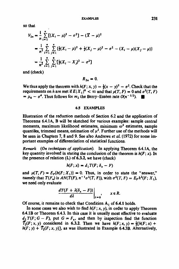
so that
EXAMPLES
. I
231
v,, = c [(Xi - p)2 - a21 - (X - p)2 n 1 1 1
and (check)
We thus apply the theorem with h(F; x, y ) = f i x - y)' - u'. Check that the requirements on h are met ifElX, l6 < 00 and that p(T, F) = 0 and uZ(T, F ) = p4 - u4. Thus follows for m2 the Berry-Essten rate O(n-1'2).
Rzn = 0.
6.5 EXAMPLES
Illustration of the reduction methods of Section 6.2 and the application of Theorems 6.4.1A, B will be sketched for various examples: sample central moments, maximum likelihood estimates, minimum w2 estimates, sample quantiles, trimmed means, estimation of p2. Further use of the methods will be seen in Chapters 7,8 and 9. See also Andrews et al. (1972) for some im- portant examples of differentiation of statistical functions.
Remark (On techniques of application). In applying Theorem 6.4.1A, the key quantity involved in stating the conclusion of the theorem is h(F; x). In the presence of relation (L) of 6.3.2, we have (check)
h(F; X ) = d ,T(F; 6, - F )
and p(T, F) = E,{h(F; X , ) } = 0. Thus, in order to state the "answer," namely that T(F,,) is AN(T(F), n-'u2(T, F)), with d ( T , F) = E,hZ(F; X,), we need only evaluate
, X E R . dT(F + 46, - F))
M ( A - 0
Of course, it remains to check that Condition A, of 6.4.1 holds. In some cases we also wish to find h(F; x, y), in order to apply Theorem
6.4.1B or Theorem 6.4.3. In this case it is usually most effective to evaluate dz T(F; G - F), put G = F,,, and then by inspection find the function Tz(F; x, y ) considered in 6.3.2. Then we have h(F; x, y ) = @(F; x ) + h(F; y ) + T'(F; x, y) ] , as was illustrated in Example 6.4.3B. Alternatively,

232 VON MISIB DIFFERENTIABLE STATISTICAL FUNCTIONS
we can evaluate d l T(F; Fn - F ) + i d , T ( F ; F, - F ) and then by inspection recognize h(F; x, y). H
Example A Sample central moments. The kth central moment of a dis- tribution F may be expressed as a functional as follows:
Q Q
pk = T(F) =: f [X - 1 y dFCy)]’dF(X).
The sample central moment is W
l)lk = T(F& = 1-2 - x ) k dFn(%).
Put = x dF(x) and FA = F + d(G - F). Then pPA = pF + d& - pp).
We have
and (check)
Thus
so that
h(F; X) = (X - /4)’ - kpk- 1X - E p { ( x - p)’ - kpk- ix}. Thus the assertion of Theorem 6.4.1A is that
mk iS AN(/lk, n-’U2(T, F)),

EXAMPLES 233
with
aZ(T, F) = p z k - plf - 2kPk- i p k + I + k 2 d - 1 h .
This result was derived previously in Section 2.2. However, by the present technique we have cranked out the “answer” in a purely mechanical fashion. Of course, we must validate the “answer” by showing that n1I2 RI , 3 0. Check that
Rim = mk - b k + kpk- ibis
where bJ = n-’ cy,, (X, - p r , 0 5 j 5 k, and thus (check)
Example B Maximum likelihood estimation. Under regularity conditions (4.4.2) on the family of distributions {F(x ; 6), 6 E 0) under consideration, the maximum likelihood estimate of 6 is the solution of
and

234 VON MISES DIFFERENTIABLE STATISTICAL FUNCTIONS
That is, the maximum likelihood estimate is 8(Fn), where 8(F) is the functional defined as the solution of
Under regularity condition on the family { F( -, O), 8 E O}, we have
Wc find
by implicit differentiation through the equation
H(8(FA), A) Y= 0,
where FA = F + A@,, - F) and H(8, A) = g(8, x)dFA(x). We have
aH d W , ) aH X l # - @ ( F ) * T l A - o ' Z l A - 0 O'
Thus
Check (using (BI), (B2) and the fact that e(F( ; 0,)) = B0, each 0,) that (B3) yields
and thus

EXAMPLES
Therefore, the assertion of Theorem 6.4.1A is that (check)
235
as seen previously in 4.2.2.
Example C Minimum w2 estimation. The “minimum w2 estimate” of 8, in connection with a family of distributions { F ( . ; O), 8 E O}, is the solution of
/q(e, x, FnMx = 0,
where d
q(8, X, G) = {CGW - ~ ( x ; e)iy(X; 8))
and
That is, the w2-minimum estimate is 8(F,,), where 8(G) is the functional defined as the solution of
Jq(e, x, GMX = 0.
By implicit diflerentiation as in Example B, check that
d f (xo; 8) -&j m o ; 8) d a 8(F + w x , , - 0 1 =
1-0 J[-$ f ( x ; ell2 d F ( x ; el’
from which Var,{h(F( - ; 8); X)} may be found readily. H
Example D Sample pth quantile. Let 0 < p < 1. The pth quantile of a distribution F is iven by I&, = T(F) = F- ‘(p) and the corresponding sample pth quantile by t,, = F; ‘(p) = T(F,,). We have
TCF + l(Sx, - .F)] = inf{x: F(x) + 1(6,,(x) - F(x)) 2 p}
= inf{x: F(x) + A[l(x 2 xo) - F(x)J 2 p}

236 VON MlSES DIFFERENTIABLE STATISTICAL FUNCTIONS
(for 1 sufficiently small). Confine attention now to the case that F has a positive densityfin a neighborhood of F - l(p). Then, for any xo other than tp. it is found (check) that
The assertion of Theorem 6.4.1A is thus that
as established previously in Section 2.3. In order to establish the validity of the assertion of the theorem, we find using (Dl) that
and we seek to establish that n112Rln 4 0. But R , , is precisely the remainder term Rn in the Bahadur representation (Theorem 2.5.1) for epn, and as noted in Remark 2.5.l(iv) Ghosh (1971) has shown that n'"R" 4 0, provided F ' ( t p ) ' 0.
Example E a-trimmed mean. Let F be symmetric and continuous. For estimation of the mean (=median), a competitor to the sample mean and the sample median is the "a-trimmed mean"
where 0 < a e f. This represents a compromise between the sample mean and the sample median, which represent the limiting cases as a + 0 and u + 4, respectively. An asymptotically equivalent (in all typical senses) version of the a-trimmed mean is defined as
X(o)n = V F n ) ,
where 1 pF-'( l -o)

EXAMPLES 237
We shall treat this version here. By application of (Dl) in conjunction with (El), we obtain
For the case F(xo) < a, this becomes
where
c(a) = l - a F - l ( t ) d t + aF-'(a) + aF-1(1- a).
The cases F(xo) > 1 - a and a s F(xo) s 1 - a may be treated in similar fashion (check). Furthermore, the symmetry assumption yields
c(a) = T(F) = el,,.
Thus we arrive at
dT[F + L(S, - F)] - dA Lo -
It follows that the assertion of Theorem 6.4.1A is

238 VON MSES DIFFERENTIABLE STATISTICAL FUNCTIONS
Example F Estimation ofp’. Consider
The corresponding statistical function is
T(F”) = x2. Derive h(F; x) and h(F; xl, x2), and apply Theorems 6.4.1A, B to obtain the asymptotic distribution theory for X’ in the cases p # 0, p = 0. (Compare Example 5.5.2B.)
6.6 COMPLEMENTS
Some useful statistical interpretations of the derivative of a statistical function are provided in 6.6.1. Comments on the differential approach for analysis of statistical functions based on functionals of a density f are provided in 6.6.2. Extension to the case of dependent Xis is discussed in 6.6.3. Normalizations other than nd2 are discussed in 6.6.4.
6.6.1 Statistical Interpretations of the Derivative of a Statistical Function In the case of a statistical function having nonvanishing first derivative (implying asymptotic normality, under mild restrictions), a variety of important features of the estimator may be characterized in terms of this derivative. Namely, the asymptotic variance parameter, and certain stability properties of the estimator under perturbation of the observations, may be characterized. These features are of special interest in studying robustness of estimators. We now make these remarks precise.
Consider observations X1, X2, . . . on a distribution F and a functional T(.) . Suppose that T satisfies relation (L) at F, that is, d,T(F; G - F) = Tl[F; x]d[G(x) - F(x)], as considered in 6.3.1, and put
h(F; X) = Tl[F; X ] - Ti[F; x]dF(x). s The reduction methodology of Section 6.2 shows that the error of estimation in estimating T(F) by T(F,) is given approximately by
Thus h(F; X,) represents the approximate contribution, or “influence,” of the observation X, toward the estimation error T(F,,) - T(F). This notion of interpreting h(F; x ) as a measure of “influence” toward error of estimation

COMPLEMENTS 239
is due to Hampel (1968,1974), who calls h(F; x), - 00 < x < 00, the injueirce curue of the estimator T(FJ for T(F). Note that the curve may be defined directly by
-ao < x < ao. dT[F + A(& - F)] M
h(F; x ) =
(In the robust estimation literature, the notation n d x ) or ZC(x; F, T) is sometimes used.)
In connection with the interpretation of TCF; a ] as an “influence curve,” Hampel (1974) identifies several key characteristics of the function. The “gross-error-sensitiuity ”
y* = sup(h(F; x)(
measures the effect of contamination of the data by gross errors, whereby some of the observations X i may have a distribution grossly different from F. Specifically, y* is interpreted as the worst possible influence which a fixed amount of contamination can have upon the estimator. The “local-shift- sensitiuity ”
x
measures the effect of “wiggling” the observations, that is, the local effects of rounding or grouping of the observations. The “rejection point” p* is defined as the distance from the center of symmetry of a distribution to the point at which the influence curve becomes identically 0. Thus all observations farther away than p* become completely rejected, that is, their “influence” is not only truncated but held to 0. This is of special interest in problems in which rejection of outliers is of importance.
Examples. The influence curve of the sample mean is
f C ( x ; T , F ) = x - p p , -ao < x < a .
We note that in this case y* = co, indicating the extreme sensitivity of the sample mean to the influence of “wild” observations. The a-trimmed mean, for 0 < 01 < f, provides a correction for this deficiency. Its y* (see Example 6.5E) is [F“(l - a) - T(F)]/(l - 2a). On the other hand, the sample mean has A* = 1 whereas the sample median has A* = 00, due to irregularity of its influence curve

240 VON MlSEs DIPPERENTIABLE STATISTICAL FUNCTIONS
at the point x = F- 'I2()). Also, contrary perhaps to intuition, the a-trimmed mean has p* = 00. However, Hampel (1978,1974) and Andrews et al. (1972) discuss estimators which are favorable simultaneously with respect to y*, A* and p* (see Chapter 7). fl
Further discussion of the influence curve and robust estimation is given by Huber (1972, 1977). Robustness principles dictate choosing T( 0 ) to control
6.6.2 Functionnls of Densities An analogous theory of statistical functions can be developed with respect to parameters given as functionals of densities, say T(f). For example, in 2.6.7 the efficacy parameter j f2(x)dx arose in certain asymptotic relative efficiency considerations. A natural estimator of any such T(f) is given by T(fn), where fn is a density estimator off such as considered in 2.1.8. The differential approach toward analysis of T(fn) - T(f) is quite useful and can be formu- lated in analogy with the treatment of Sections 6.1-6.5. We merely mention here certain additional complications that must be dealt with. First, ,the structure of the sample density function fn is typically not quite as simple as that of the sample distribution function F,. Whereas F,(x) is the average at the nth stage of the random variables I(Xl I; x), I ( X , I; x), . . . , the estimator f.(x) is typically an average over a double array of random variables. This carries over to the approximating random variable d,T(f; f, - f) here playing the role of d,T(F; F,, - F). Consequently, we need to use a double array CLT in deriving the asymptotic normality of T(fn), and we find that there does not exist a double array LIL at hand for us to exploit in deriving an LIL for T(fn) - T(f). Furthermore, unlike F,(x) as an estimator of F(x), the estimatorh(x) is typically biused for estimation off(x). Thus Ef T(f ; f . - f) # 0 in typical cases, so that the analysis must deal with this type of term also.
See Beran (1977a, b) for minimum Hellinger distance estimation based on statistical functions of densities.
6.6.3 Dependent Observations {X,}
Note that the asymptotic behavior of T(FJ - T(F) typically depends on the X1)s only through two elements,
IC(x; T, F).
and R1,. Often R1, can be handled via inequalities involving IlF, - Fll, and the like. Thus, for example, the entire theory extends readily to any sequence {X,} of possibly dependent variables for which a CLT has been established and for which suitable stochastic properties of IlF, - Fll, have beem est- ablished.

PROBLEMS 241
6.6.4 Other Normalizations For the random variable T(F,,) - T(F) to have anondegenerate limit law, the appropriate normalizing factor in the case that the first nonvanishing term in the Taylor expansion is the mth need not always be nmI2. For example, in the case m = 1, we have a sum of I.I.D. random variables as d l T(F; F,, - F), for which the correct normalization actually depends on the domain of attrac- tion. For attraction to a stable law withexponent a,O < a < 2, the appropriate normalization is ntp. See Gnedenko and Kolmogorov (1954) or Feller (1966).
6.6.5 Computation of Higher Gdteaux Derivativa In the presence of Condition (L) of 6.3.1, we have
Hence
etc.
6.P PROBLEMS
Section 6.2
1. Check the details for Example 6.2.1. 2. Formulate and prove the extended form of Theorem 1.12.1A germane
3. (Continuation of Example 6.2.1) Show, applying Lemma 6.3.28, that to the Taylor expansion discussed in 6.2.1.
dk sup lz T(F + A(F, - F)) 1 = o,(n-"'2'k).
osAsl
4. Complete the details of Example 6.2.2A. 5, Complete the argument for Lemma 6.2.2B. 6. Verify Remarks 6.2.2B (ii), (vii). 7. Check the claim of Example 6.2.2B.

242 VON MISeTl DIFFERENTIABLE STATISTICAL FUNCTIONS
Section 6.3
(6.3.2).
Section 6.4
8. Complete the details for the representation of V,, as a V-statistic
9. Prove Lemma 6.4.3. 10. Check details of Examples 6.4.3A, B. 11. Complete details of proof of Theorem 6.4.3.
12. Supply thcmissingdetails for Example6.5A(samplecentral moments). 13. Supply details for Example 6.5B (maximum likelihood estimate). 14. Supply details for Example 6.5C (minimum 0' estimate). 15. Supply details for Example 6.5D (sample pth quantile). 16. Supply details for Example 6.5E (a-trimmed mean). 17. Supply details for Example 6.5F (estimation of p2). 18. Apply Theorem 6.4.3 to obtain the Berry-EssCen theorem for the
Section 6.5
sample pth quantile (continuation of Problem 15 above).
Seetion 6.6 19. Provide details for 6.6.5.

C H A P T E R 7
M-Estimates
In this chapter we briefly consider the asymptotic properties of statistics which are obtained as solutions of equations. Often the equations correspond to some sort of minimization problem, such as in the cases of maximum like- lihood estimation, least squares estimation, and the like. We call such statistics “M-estimates.” (Recall previous discussion in 4.3.2.)
A treatment of the class of M-estimates could be carried out along the lines of the classical treatment of maximum likelihood estimates, as in 4.2.2. However, for an important subclass of M-estimates, we shall apply certain specialized methods introduced by Huber (1964). Also, as a general approach, we shall formulate M-estimates as statistical functions and apply the methods of Chapter 6. Section 7.1 provides a general formulation and various examples. The asymptotic properties ofM-estimates, namely consistency and asymptotic normality with related rates of convergence, are derived in Section 7.2. Various complements and extensions are discussed in Section 7.3.
Two closely related competing classes of statistics, L-estimates and R- estimates, are treated in Chapters 8 and 9. In particular, see Section 9.3.
7.1 BASIC FORMULATION AND EXAMPLES
A general formulation of M-estimation is presented in 7.1.1. The special case of M-estimation of a location parameter, with particular attention to robust estimators, is studied in 7.1.2.
7.1.1 General Formulation of M-Estimation
Corresponding to any function #(x, t) , we may associate a functional T defined on distribution functions F, T(F) being defined as a solution to of the equation
(*I [#(x , to)dF(x) = 0.
243

244 M-ESTIMATES
We call such a T(.) the Mfunctional corresponding to $. For a sample XI,. . . , X, from F , the M-estimate corresponding to $ is the “statistical function,’ T(F,), that is, a solution T, of the equation
In our theorems for such parameters and estimates, we have to allow for the possibility that (*) or (**) has multiple solutions.
When the $ function defining an M-functional has the form I,@, t ) = $(x - t ) for some function $, T(F) is called a location parameter. This case will be of special interest.
In typical cases, the equation (*) corresponds to minimization of some quantity
Jdx, to)dF(x),
the function $ being given by
d $(x, t ) = c P ( X , t )
for some constant c, in the case of p(x, .) sufficiently smooth. In a particular estimation problem, the parameter‘of interest 8 may be
represented as T(F) for various choices of $. The corresponding choices of T(F,) thus represent competing estimators. Quite a variety of $ functions can thus arise for consideration. It is important that our theorems cover a very broad class of such functions.
Example Parametric Estimation. Let So = {F( ; 0), O E 0 ) represent a Uparametric” family ofdistributions. Let t) = $(x, t ) be a function such that
J@(x, eMF(x; e) = 0, e E o,
that is, for F = F(.; 8) the solution of (*) coincides with 0. In this case the corresponding M-functional T satisfies T(F(.; 8)) = 0, Oe 0, so that a natural estimator of 8 is given by 6 = T(F,). Different choices of $ lead to different estimators. For example, if the distributions F(. ; 0) have densities or mass functionsf( ; e), then the maximum likelihood estimator corresponds to
P(X, e) = -log f ( x ; e),
$(x, 0) = - 3 log ftx; 0). d

BASIC FORMULATION AND EXAMPLES 245
We have studied maximum likelihood estimation in this fashion in Example 6.5B. Likewise, in Example 6.5C, we examined minimum o2 estimation, corresponding to a different $.
A location parameter problem is specified by supposing that the members of st, are of the form F(x; 0) = Fo(x - O), where Fo is a fixed distribution thus generating the family So. It then becomes appropriate from invariance considerations to restrict attention to $ of the form $(x, t ) = $(x - t) .
In classical parametric location estimation, the distribution Fo is assumed known. In robust estimation, it is merely assumed that Fo belongs to a neighborhood of some specified distribution such as a. (See Example 7.1.2E.)
In considering several possible $ for a given estimation problem, the corresponding influence curues are of interest (recall 6.6.1). Check (Problem 7.P.1) that the Gateaux differential of an M-functional is
provided that Ib(T(F)) # 0, where we define
&(t) = J$(x, t)dF(x), - 00 < t < 03.
Thus the influence curve of (the M-functional corresponding to) $ is
Note that IC is proportional to $. Thus the principle of M-estimation possesses the nice feature that desired properties for an influence curve may be achieved simply by choosing a @ with the given properties. This will be illustrated in some of the examples of 7.1.2.
Further information immediate from (1) is that, under appropriate regularity conditions,
T(F,) is AN(T(F), n-'o'(T, F)),
where typically
This is seen from Theorem 6.4.1A (see Remark 6.5) and the fact that IC(x, F, T)dF(x) = 0. A detailed treatment is carried out in 7.2.2. (In some
cases d ( T , F) comes out differently from the above.)

246 M-IBTIMATES
7.1.2 Examples Apropos to Location Parameter Estimation The following examples illustrate the wide variety of # functions arising for consideration in the contexts of efficient and robust estimation. We consider the M-functional T(F) to be a solution of
j$(x - to)dF(x) =: 0
and the corresponding M-estimate to be T(F,).
Example A The least squares estimate. Corresponding to minimization of (X , - 0)2, the relevant # function is
#(x) = x, -00 < x < 00.
For this $,the M-functional T is the mean functional and the M-estimate is the samplemean.
Example B The least absolute values estimate. Corresponding to mini- mization of PI IX, - 01, the relevant # function is
-1, x < 0, #(%) = 0, x = 0, [ 1, x > 0.
Here the corresponding M-functional is the median functional and the cor- responding M-estimate the sample median. m
Example C The maximum likelihood estimate. For the parametric location model considered in Example 7.1.1, let Fo have densityfo and take
The corresponding M-estimate is the maximum likelihood estimate. Note that this choice of $ depends on the particular Fo generating the model.
Example D A form oftrimmed mean. Huber (1964) considers minimization of c; p(X, - O), where

BASIC FORMULATION A N D EXAMPLES
The relevant # is 241
The corresponding M-estimator T, is a type of trimmed mean. In the case that no X, satisfies I X , - T,I = k, it turns out to be the sample mean of the X,’s satisfying I X, - T,I c k. (Problem 7.P.2) Note that this estimator eliminates the “influence” of outliers.
Example E A form of Winsorized mean. Huber (1964)considers minimization of c; p(X, - 8). where
The relevant $ is
-k , x < -k , x, 1x1 s k k, x > k.
#(x) =
The corresponding M-estimator T, is a type of Winsorized mean. It turns out to be the sample mean of the modified Xis, where X, becomes replaced by T,, f k, whichever is nearer, if I XI - T,,I > k (Problem 7.P.3). This estimator limits, but does not entirely eliminate, the influence of outliers. However, it has a smoother IC then the $ of Example D. The p( .) of the present example represents a compromise between least squares and least absolute values estimation. It also represents the optimal choice of p, in the minimax sense, for robust estimation of 8 in the normal location model. Specifically, let C denote the set of a11 symmetric contaminated normal distributions F = (1 - e)@ + EH, where 0 < E < 1 is fixed and H varies over all symmetric distributions. Huber (1964) defines a robust M-estimator $ to be the $o which minimaxes the asymptotic variance parameter d ( T , F), that is,
sup U’(T’,~, F) = inf sup a2(r’,, F). F $ F
Here F ranges through C, $ ranges over a class of “nice” # functions, and u2(‘&, F) is as given in 7.1.1. For the given C, the optimal $,, corresponds to the above form, for k defined by j fk &t)dt + 24(k)/k = 1/(1 - 6). The # functions of this form are now known as “Hubers.” Note that the IC function is continuous, nondecreasing, and bounded.
Example F. Hampel (1968,1974) suggested a modification of the “Hubers” in order to satisfy qualitative criteria such as low gross-error-sensitivity, small

248 M-ESTIMATES
local-sh~-sensitiuity, etc., as discussed in 6.6.1. He required +(x) to return to 0 for 1x1 sufficiently large:
O S x S a ,
a ~ ; x < b ,
x > c,
and #(x) = -#( -x), x < 0. This M-estimator has the property of com- pletely rejecting outliers while giving up very little efficiency (compared to the Hubers) at thenormal. M-estimators of this type are now known as“ Hampels.”
Example G A smoothed “Hampel”. One of many varieties of smoothed Hampels” is given by
A sin ax, 0 I; x < -,
a
x > -, a A
w =
A sin ax, 0 I; x < -,
a
x > -, a A
w =
and #(x) - - $( - x), x < 0. See Andrews et a1 (1972).
Remarks. (i) Further examples, and small sample size comparisons, are provided by Andrews et al. (1972).
(ii) Construction of robust M-estimates. For high eficiency at the model distribution Fo, one requires that the influence function be roughly pro- portional to - f~ (x ) / fo (x ) . For protection against outliers, one requires that the influence function be bounded. For protection against the effects of round- ofand grouping, one requires the influence function to be reasonably con- tinuous in x. In order to stabilize the asymptotic variance of the estimate under small changes in Fo, one requires the influence function to be reasonably continuous as afunction ofF. These requirements are apropos for any kind of estimator. However, in the case of M-estimators, they translate directly into similar requirements on the + function. One can thus find a suitable M- estimator simply by defining the $ function appropriately.
7.2 ASYMPTOTIC PROPERTIES OF M-ESTIMATES
We treat consistency in 7.2.1, asymptotic normality and the law ofthe iterated logarithm in 7.2.2, and Berry-Essken rates in 7.2.3.

ASYMPTOTIC PROPERTIES OF M-ESTIMATJ!S 249
7.2.1 Consistency As in 7.1.1, we consider a function $(x, t ) and put AF(t ) = j$(x, t)dF(x). Given that the “parametric” equation AF(t ) = 0 has a root to and the “em- pirical *’ equation &&) = 0 has a root T,,, under what conditions do we have T, wp‘. to? (Here, as usual, we consider a sample XI,. . . , X, from F, with sample distribution function F,.) As may be seen from the examples of 7.1.2, many I) functions of special interest are of the form $(x, t ) = $(x - t), where either $ is monotone or $ is continuous and bounded. These cases, among others, are covered by the following two lemmas, based on Huber (1964) and Boos (1977), respectively.
Lemma A . Let to be an isolated root ofhF(t) = 0. Let $(x, t) be monotone in t. Then to is unique and any solution sequence {T,} of the empirical equation XFn(t) = 0 converges to to wpl. Gfurther, $(x, t) is continuous in t in a neigh- borhood of to, then there exists such a solution sequence.
PROOF. Assume that $(x, t ) is nonincreasing in t. Then AF( t ) and AFn(t), each n, are nonincreasing functions of t . Since A F ( t ) is monotone, AF(tO) = 0, and to is an isolated root, to is the unique root. Let e > 0 be given. Then &(to + e) < 0 < &(to - 6). NOW, by the SLLN, AFa(t) * AF(t), each t. Therefore,
lim P(Ap,(to + E) -= 0 < AF,(tO - E), all m 2 n) = 1. n*m
Complete the argument as an exercise.
Remark A. Note that to need not actually be a root of &(t) = 0. It sufices that &(t) change sign uniquely in a neighborhood of to. Then we still have, for any E > 0, AF(tO + e) < 0 < &(to - E), and the assertions on { T.} follow as above.
For example, by the above lemma the sample mean, the sample median, and the Hubers (Examples 7.1.2AY B, E) are, under suitable restrictions, consistent estimators of the corresponding location parameters. However, for the Hampels (Example 7.1.2F), we need a result such as the following.
Lemma B. Let to be an isolated root ofXF(t) = 0. Let $(x, t ) be continuous in t and bounded. Then the empirical equation hF,(t) = 0 has a solution sequence {T,} which converges to to wpl.
PROOF. Justify that AF(t) and AFn(t), each n, are continuous functions oft. Then complete the proof as with Lemma A.
Corollary. For an M-functional T based on 9, let F be such that T(F) is an isolated root ofhF(t) = 0. Suppose that $(x, t) is continuous in t and either

250 M-ESTIMATES
monotone in t or bounded. Then the empirical equation Ap,,(t) = 0 admits a strongly consistent estimation sequence T,for T(F).
Remark B. In application of Lemma B in cases when the empirical equation A&) = 0 may have multiple solutions, there is the difficulty of fdentffying a consistent solution sequence { T,). Thus in practice one needs to go further than Lemma B and establish consistency for a particular solution sequence obtained by a specified algorithm.
For example, Collins (1976) considers a robust model for location in which the underlying F is governed by the standard normal density on an interval to f d and may be arbitrary elsewhere. He requires that # be continuous with continuous derivative, be skew-symmetric, and vanish outside an interval [ - c, c], c < d. He establishes consistency for T, the Newton method solution of d&) = 0 starting with the sample median.
Portnoy (1977) assumes that F has a symmetric density f satisfying certain regularity properties, and requires $ to be bounded and have a bounded and 8.9. (Lebesgue) uniformly continuous derivative. He establishes consistency for T,, the solution of A&) = 0 nearest to any given consistent estimator T .
7.2.2 Asymptotic Normality and the LIL Let $(x, t ) be given, put A&) = $(x, t)dF(x), and let to = T(F) be a solution of A&) = 0. Based on { X , } I.I.D. from F, let T, = T(F,) be a consistent (for to) solution sequence of d&) = 0. Conditions for consistency were given in 7.2.1. Here we investigate the nature of further conditions under which
n’”(T, - to) 5 N(0, a2(T, F)), (AN)
with a’(T, F) given by either #2(x, to)dF(x)/[d#o)]2 (as in 7.1.1) or $‘(x, to)dF(x)/[j(a$(x, t)/at)l, ,,)dF(x)]’,’depending upon the assumptions
on #(& 0. In some cases we are able also to conclude
n“’(T, - to) riiii = 1 wpl. ”+- a(T, F)(2 log log n)l”
Three theorems establishing (AN) will be given. Theorem A, parallel to Lemma 7.2.1A, is based on Huber (1964) and deals with #(x, t) monotone in t. In the absence of this monotonicity, we can obtain (AN) under differentiability restrictions on #(x, a), by an extension of the classical treatment of maximum likelihood estimation (recall 4.2.2). For example, conditions such as
< M(x), with sup E&fM(X) < 00, PE e

ASYMPTOTIC PROPERTIES OF M-ESTIMATES 251
play a role. A development of this type is indicated by Rao (1973), p. 378. As a variant of this approach, based on Huber (1964), Theorem B requires a condition somewhat weaker than the above. Finally, Theorem C, based on Boos (1977), obtains (AN) by a rather different approach employing methods of Chapter 6 in conjunction with stochastic properties of llF, - Fll,. Instead of differentiability restrictions on $(x, a), a condition is imposed on the varia- tion of the function $( ., t ) - $( e . to), as t -+ to, The approaches of Theorems B and C also lead to (LIL) in straightforward fashion.
We now give Theorem A. Note that its assumptions include those of Lemma 7.2.1A.
Theorem A. Let to be an isolated root of A&) = 0. Let $(x, t) be monotone in t. Suppose that A&) is diflerentiable at t = to, with X;(to) # 0. Suppose that
$2(x, t)dF(x) isfinitefor t in a neighborhood ofto and is continuous at t = to. Then any solution sequence T,, of the empirical equation AF,,(t) = 0 satisfies (AN) , with a2(T, F) given by I $'(x, to)dF(x)/[&(to)J2. (That T,* to is guaranteed by Lemma 7.2.1A.)
PROOF. Assume that $(x, t ) is nonincreasing in t, so that A,&) is nonincreasing. Thus (justify)
P(Sn(t) < O) s P ( x s t ) 5 f l A F n ( t ) 5;. 0).
Therefore, to obtain (AN), it suffices (check) to show that
lim P(AFn(tZ,,,) c 0) 3: lim flAFn(tr,,,) 5 0) = Wz), each z, I 'OO n*m
where ts,,, = to + z ~ n - ~ ' ~ , with Q = a(T, F). Equivalently (check), we wish to show that
where sf,,, = VarF{$(Xl, ts,,,)) and
Justify, using the assumptions of the theorem, that nl'zA&,,,) 4 &(t&g and that s~,,, -+ -&(tO)Q, as n -+ 00. Thus -n1'2AF(tJsz,n -+ z, n -+ 00, and it thus suffices (why?) to show that
X I I; z) = Wz), each z. n-m
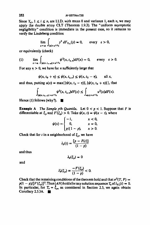
252 M-ESTIMATES
Since Ynl, 1 s i 5 n, are I.I.D. with mean 0 and variance 1, each n, we may apply the double array CLT (Theorem 1.9.3). The "uniform asymptotic negligibility" condition is immediate in the present case, so it remains to verify the Lindeberg condition
lim 1 y2 d ~ ~ , , ( y ) = 0, every e > 0, n-oD l y l > n W
or equivalently (check)
(1)
For any q > 0, we have for n sufficiently large that
lim J t,h2(x, t.,,)dF(x) = 0, every 8 > 0. 1 1 - 9 ) I W , t., dl > n'12s
Example A The Sample pth Quantile. Let 0 < p c 1. Suppose that F is differentiable at 4, and F'(t,) > 0. Take $(x, t ) = I,+ - t), where
x < 0, x = 0,
Check that for t in a neighborhood of t.,, we have
and thus
and
Check that the remaining conditions of the theorem hold and that a2(T, F) = p(l - p)/[F'(~,)J2.Thus AN)holdsforanysolutionsequence T,,ofl,(t) = 0. In particular, for T,, = t ,,, as considered in Section 2.3, we again obtain Corollary 2.3.3A.
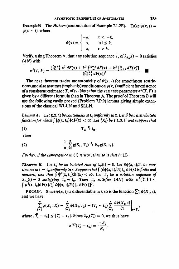
ASYMPTOTIC PROPERTIES OF M-ESTIMATES 253
ExampleB The Hubers (continuation of Example 7.1.2E). Take $(x, t ) = #(x - t), where
-k, x < -k, x, 1x1 S k, 1 k, x > k.
$(XI =
Verify, using Theorem A, that any solution sequence T. of A&) = 0 satisfies (AN) with
The nextl theorem trades monotonicity of #(x, a ) for smoothness restric- tions,and also assumes(implicit1y)conditions on $(x, t)suficient for existence of a consistent estimator Tn of to. Note that the variance parameter a2(T, F) is given by a different formula than in Theorem A. The proof of Theorem B will use the following easily proved (Problem 7.P.9) lemma giving simple exten- sions of the classical WLLN and SLLN.
Lemma A. Let g(x, t) be continuous at to uniformly in x. Let F be a distribution functionfor which Ig(x, to)IdF(x) < 00. Let {XI} be I.I.D. F and suppose that
P (1) T, -+ to.
Then
Further, ifthe convergence in (1) is wpl, then so is that in (2).
Theorem B. Let to be an isolated root of &(t) = 0. Let a\lr(x, t)/& be con- tinuous at t = to uniformly in x. Suppose that (J$(x, t)/dt)I,, dF(x) isfinite and nonzero, and chat j q2(x, to)dF(x) < 00. Let T, be a solution sequence of AFn(t) = 0 satisjying T, + to. Then T, satisfies (AN) with d(T, F) =
PROOF. Since $(x, t ) is differentiable in t , so is the function PI +(Xi, t), and we have
j 4f2(X, to)dF(x)/Cj W(x9 t)/WI,, dFWJ2.
where I - to I 5 I T, - to I . Since AFn( T.) = 0, we thus have
-An Bn
n'I2(K - to) = -,

254 M-ESTIMATES
where
and
Complete the proof using the CLT and Lemma A. a Remark A. A variant of Theorem B, due to Boos (1977), relaxes the uniform continuity of g(x, t ) = 2$(x, t)/& at t = to to just continuity, but imposes the additional conditions that the function g( ., t ) - g(., to) have variation O( 1) as t + to and that the function g(x, t)dF(x) be continuous at t = to. This follows by virtue of a corresponding variant of Lemma A (see Problem 7.P.14).
Example C The maximum likelihood estimate of a location parameter (con- tinuation of Example 7.1.2C). Here @(x) = -f6(x)/fo(x) is not necessarily monotone. However, under further regularity conditions onfo, Theorem A is applicable and yields (check) asymptotic normality with a2(T, F) = l/I(Fo),
The next theorem bypasses differentiability restrictions on $(x, t), except what is implied by differentiability of A&). The following lemma will be used. Denote by Il.llv the variation norm,
where W o ) = j ( f b / f o ) 2 dF0. a
llhllV = lim &b(h), 0 4 - w b-r w
where
the supremum veing taken over all partitions a = xo < - - - < xk = interval [a, b].
Lemma B. Let thefunction H be continuous with llH Ilv < 00 and thefunction K be right-continuous with 11K11 < 00 and K( f 00) = 0. Then
of the
I JH dK I s IlHllv, IlKll,.
PROOF. Apply integration by parts to write H d K - -I K d H , using the fact that IH( f 00)l < 00. Then check that I j K d H I 5; IlKll,. llHllv (or see Natanson (1961), p. 232).

ASYMPTOTIC PROPERTIES OF M-ESTIMATES 255
Theorem C. Let to be an isolated root ofkdt) = 0. Let Q(x, t) be continuous in x and satisJy
(V)
Suppose that hdt) is diflerentiable at t = to, with &(to) # 0. Suppose that Jr2(x, to)dF(x) < 00. Let T, be a solution sequence of kFn(t) = 0 satisfying
T , to. Then T, satisfies (AN) with a2(T, F) = q2(x, to)dF(x)/[&(to)]2.
PROOF. The differential methodology of Chapter 6 will be applied and, in particular, the quasi-diferential notion of 6.2.2 will be exploited. As noted in 7.1.1,
lim IN(-, t) - M., to)lIV = 0. 1- to
In order to deal with T(G) - T(F) - d , T(F; G - F), it is useful to define the function
Unfortunately, this expression is not especially manageable. However, the quasi-differential device is found to be productive using the auxiliary func- tional Tp(G) = X#o)/h(T(G)). We thus have

256 M-ESTIMATES
Check that Lemma B is applicable and, with the convergence T, 3 to,‘yields that the right-hand side of (1) is o,,(llFn - Film). It follows (why?) that
n1’2[K - to - TF(F,)dlT(F; F,, - F)] 4 0.
Finally, check that d’2TF(Fn)dl T(F; F,, - F) 5 N(0, 02(T, F)). H
Examples D. Consider M-estimation of a location parameter, in which case $(x, t ) may be replaced by $(x - t). The regularity conditions on $ imposed by Lemmas 7.2.1A, B (for existence of a consistent M-estimation sequence) and by Theorem C above (for asymptotic normality) are that $ be continuous, either bounded or monotone, and satisfy
limII$(. - b) - $ ( . ) l l v = 0.
These requirements are met by typical $ considered in robust estimation: “least pth power” estimates corresponding to I&) = Ixlp- sgn(x), provided that 1 < p S 2; the Hubers (Example 7.1.2E); the Hampels (Example 7.1.2F); the smoothed Hampel (Example 7.1.2G). In checking (*), a helpful relation is IlHll~ = IH’(x)Jdx, for H an absolutely continuous function.
be0 (*I
Remark B. LIL for M-Estimates. Under the conditions of either Theorem B or Theorem C, with the convergence of T, to to strengthened to wpl, T,, satisfies (LIL). This is readily seen by minor modification in the proofs of these results (Problem 7.P.16).
7.2.3 Berry-Wen Rates
The approach of 6.4.3 may be applied. For simplicity let us confine attention to the case $(x, r ) = $(x - t). As an exercise (Problem 7.P.17), augment the development in the proof of Theorem 7.2.2C by evaluating d2 T(F; F,, - F) and showing that the remainder R2,, =: T, - to - d,T(F; F,, - F) - fdz T(F; F,, - F) may be expressed in the form R2, = A,, + Bn + Cn + where

COMPLEMENTS 257
and
A brute force treatment of these quantities separately leads to
under moderate restrictions on JI, JI‘, JI” and on XF(t), &(t) and &‘(t) for t in a neighborhood of to. By application (check) of the Dvoretzky-Kiefer- Wolfowitz inequality (Theorem 2.1.3A), P ( ( R z n ( > Cn-’) = O(n-‘/’), so that Theorem 6.4.3 yields the Berry-EssCen rate O ( ~ I - ~ / ~ ) for the asymptotic normality of T,.
For other discussion of the Berry-EssCen rate for M-estimates, see Bickel (1974).
7.3 COMPLEMENTS
7.3.1 Information Inequality; Most EtRcient M-Estimation Assume regularity conditions permitting the following interchange of order of integration and differentiation:
Then the two forms of a*(”, F ) in 7.2.2 agree. Assume also that F has a density f with derivative f’. Further, consider now the case that JI(x, t ) = JI(x - t). Then, by integration by parts, (1) yields
&(to) = - I J I ‘ ( x - t o ) f (x )dx = - / J I ( x - to)f’(x)dx.
Hence
and thus, by the Schwarz inequality, (check)
which is again the “information inequality” discussed in 4.1.3. This lower bound is achieved if and only if JI(x - to) is of the form af‘(x) / f (x) for some constant a. To make this more transparent, suppose that F(x) = Fo(x - to), making to = T(F) a location parameter in the location model generated by a
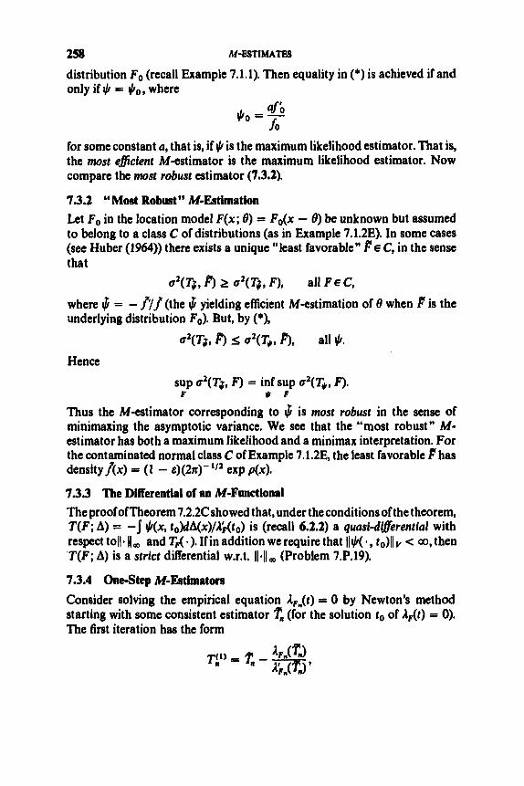
258 M-ESTIMATES
distribution Fo (recall Example 7.1.1). Then equality in (*) is achieved if and only if $ = $o, where
for some constant a, that is, if $ is the maximum likelihood estimator. That is, the most eflcient M-estimator is the maximum likelihood estimator. Now compare the most robust estimator (7.3.2).
73.2 “Most Robust” M-Estimation Let Fo in the location model F(x; 0) = Fo(x - 6) be unknown but assumed to belong to a class C of distributions (as in Example 7.1.2E). In some cases (see Huber (1964)) there exists a unique “least favorable” FE C, in the sense that
where $ = - fi/f (the $ yielding efficient M-estimation of 6 when F is the underlying distribution Fo). But, by (*),
a’(?$, 0 2 a’(?$, F), all F E C,
O2<T$, 0 5 a ( T$, F), all $.
Hence
sup u’(T$, F) = inf sup a2(T+, F). P $ P
Thus the M-estimator corresponding to $ is most robust in the sense of minimaxing the asymptotic variance. We see that the “most robust” M- estimator has both a maximum likelihood and a minimax interpretation. For the contaminated normal class C of Example 7.1.2E, the least favorable F has densityf(x) = (1 - e)(2n)-’” exp Ax). 73.3 The Differential of an M-Functional The proofofTheorem 7.2.2Cshowed that, under theconditions of the theorem, T(F; A) = -I $(x, to)dA(x)/&(to) is (recall 6.2.2) a quasf-dgerential with respect toll. 11 , and Tp( a). If in addition we require that I!$( 0 , to)ll < 00, then T(F; A) is a strict differential w.r.t. 11.11, (Problem 7.P.19).
7.3.4 One!-Step M-Estimators Consider solving the empirical equation A&) = 0 by Newton’s method starting with some consistent estimator (for the solution to of A&) = 0). The first iteration has the form

COMPLEhfENTS
with 259
Now check that
where
and
Assume the conditions of Theorem 7.2.28 and also
(1) rP2(R - to) = oP(1), n + 00.
Then immediately (justify)
n'/2An 1: N(0, n2(T, F))
and
n'l'c,, 4 0.
Find additional conditions on $ such that
n1I2B,, 3 0,
and thus conclude that n1'2(Ti1) - to) performance of the "one-step" is the same as the "full iterate."
7.3.5 Scaling
As discussed in Huber (1977), in order to make a location M-estimate scale- invariant, one must introduce a location-invariant scale estimate s,,, and then take T, to be the solution of
N(0, n2(T, F)), in which case the

260 M-ESTIMATES
In this case, if S, estimates u(F), then T,, estimates T(F) defined as the solution of
A recommended choice of s,, is the mean absolute deviation (MAD),
s, = median of {IX, - mi,. , , , (X, - mi),
where m = median of {X,, , . . , X,}. Another old favorite is the sample interquartile range (discussed in 2.3.6). The results of this chapter extend to this formulation of M-estimation.
73.6 Bahadur Representation for M-&timates Let T, be as defined in 7.3.5. Under various regularity conditions on $ and F, Carroll (1978) represents T,, as a linear combination of the scale estimate s,, and the average of n bounded random variables, except for a remainder term
7.3.7 M-Estimates for Regression See Huber (1973).
7.38 Multiparameter M-Estimates
See Huber (1977).
7.3.9 Connections Between M-Estimates and L- and R-Estimates See Chapter 9.
O(n-'(log log n))wpl.
7.P PROBLEMS
Section 7.1
1. Derive the IC for an M-estimate, as given in 7.1.1. (Hint: use the method of Example 6.5B.)
2. Verify the characterization of the M-estimator of Example 7.1.2D as a form of trimmed mean. Exemplify.
3. Verify the characterization of the M-estimator of Example 7.1.2E as a form of Winsorized mean. Exemplify.
Section 7.2
4. Complete the proofs of Lemmas 7.2.1A, B. 5. Does Remark 7.2.1A apply to Lemma B also? 6. Complete the details of proof of Theorem 7.2.2A.
PROBLEMS 261
7. Supply details for Example 7.2.2A (the sample pth quantile). 8. Supply details for Example 7.2.2B (the Hubers). 9. Prove Lemma 7.2.2A. Hint: write
10. Complete the proof of Theorem 7.2.28. 11. Check details of Example 7.2.2C (m.1.e. of location parameter). 12. Check details of proof of Lemma 7.2.28. 13. Supply details for the proof of Theorem 7.2.2C. 14. Prove the variant of Lemma 7.2.2A noted in Remark 7.2.2A. (Hint:
15. Check the claims of Examples 7.2.21). 16. Verify Remark 7.2.28 (LIL for M-estimates). 17. Provide details in 7.2.3 (Berry-Essken rates for M-estimates).
apply Lemma 7.2.2B.)
Section 7.3 18. Details for 7.3.1-2. 19. Details for 7.3.3. 20. Details for 7.3.4.

C H A P T E R 8
LEstimates
This chapter deals briefly with the asymptotic properties of statistics which may be represented as linear combinations of order statisrics, termed “L- estimates” here. This class of statistics is computationally more appealing than the M-estimates, yet competes well from the standpoints of robustness and efficiency. It also competes well against R-estimates (Chapter 9).
Section 8.1 provides the basic formulation and a variety of examples illustrating the scope of the class. Asymptotic properties, focusing on the case of asymptotically normal L-estimates, are treated in Section 8.2. Four different methodological approaches are examined.
8.1 BASIC FORMULATION AND EXAMPLES
A general formulation of L-estimation is presented in 8.1.1. The special case of eficient parametric L-estimation of location and scale parameters is treated in 8.1.2. Robust Lestimation is discussed in 8.1.3. From these con- siderations it will be seen that the theoretical treatment of L-estimates must serve a very wide scope of practical possibilities.
8.1.1 General Formulation and First Examples Consider independent observations X,, . . . , X, on a distribution function F and, as usual, denote the ordered values by Xn1 < - . s X,. As discussed in 2.4.2, many important statistics may be expressed as linear functions of the ordered values, that is, in the form
(1)
forsomechoiceofconstantscnlY . . . , c,,. Wetcrmsuchstatistics“L-estimates.” Simple examples are the sample mean X, the extremes Xn1 and X,,,,, and the sample range X, - Xn1. From the discussion of 2.4.3 and 2.4.4, it is clear that the asymptotic distribution theory of L-statistics takes quite different
262
n
T, = C C n i X n t I = 1

BASIC FORMULATION A N D EXAMPLES 263
forms,dependingon thecharacter ofthecoefficients {c,,~}. The present develop- ment will attend only to cases in which T,, is asymptotically normal.
Examples A. (i) The sample pth quantile, ern, may be expressed in the form (1) with cnI = 1 if i = np or if np # [np] and i = [np] + 1, and cnl = 0 otherwise.
(ii) Gini's mean digereme,
considered previously in 5.1.1 as a U-statistic for unbiased estimation of the dispersion parameter 8 = E F ( X 1 - X,l, may be represented as an L- estimate as follows (supply missing steps):
which is of form (1) with cRI = 2(2i - n - l)/n(n - 1).
A convenient subclass of (1) broad enough for all typical applications is given by
Here J(u), 0 5 u 5 1, represents a weights-generating function. It is assumed that 0 < p1 < * < p,,, < 1 and that a l , . . . , a,,, are nonzero constants. Thus T:, is of form (1) with c, ,~ given by n-'J(i/(n + 1)) plus an additional con- tribution a, if i = [np,] for somej E { 1, . . . , m}. Typically, J is a fairly smooth function. Thus L-estimates of form (1') are sums of two special types of L- estimate, one type weighting all the observations according to a reasonably smooth weight function, the other type consisting of a weighted sum of a fixed number of quantiles. In many cases, of course, the statistic of interest is just a single one of these types. Also, in many cases, the initial statistic of interest is modified slightly to bring it into the convenient form (1'). For example, the sample pth quantile T,, = epn is replaced by Tk = Xn,tnp,, given by (1') with the first term absent and the second term corresponding to m = 1, p1 = p ,
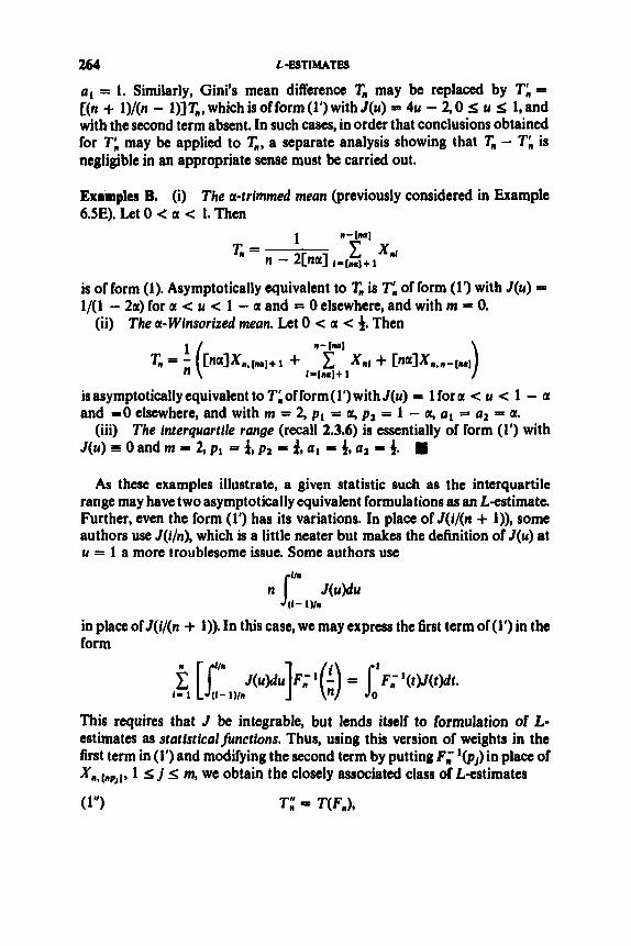
264 L-ESTIMATES
al = 1. Similarly, Gini's mean difference T, may be replaced by 7'; = [(n + l)/(n - l)]T,, which is ofform (1') with J(u) = 4u - 2,O s u s 1, and with the second term absent. In such cases, in order that conclusions obtained for TL may be applied to T,, a separate analysis showing that T, - Tn is negligible in an appropriate sense must be carried out.
Examples B. (i) The a-trimmed mean (previously considered in Example 6.5E). Let 0 < a < 1. Then
is of form (1). Asymptotically equivalent to T, is Tk of form (1') with J(u) = 1/(1 - 2a) for a < u < 1 - a and = 0 elsewhere, and with m - 0.
(ii) The a-Winsorized mean. Let 0 < a < 4. Then
isasymptoticallyequivalent to TLofform(1')with J(u) = 1 fora < u < 1 - a and -0 elsewhere, and with m = 2, p1 -- a, p l = 1 - a, al = a2 - a.
(iii) The interquartile range (recall 2.3.6) is essentially of form (1') with J(u) = 0 and m = 2, p1 = $, p 2 = $, aI = 4, a2 = f.
As these examples illustrate, a given statistic such as the interquartile range may have two asymptotically equivalent formulations as an Latimate. Further, even the form (1') has its variations. In place of J(i/(n + 1)), some authors use J(i/n), which is a little neater but makes the definition of J(u) at u = 1 a more troublesome issue. Some authors use
tin 1,- in place of J(i/(n + 1)). In this case, we may express the first term of (1') in the form
This requires that J be integrable, but lends itself to formulation of L- estimates as statistlcalfunctions. Thus, using this version of weights in the first term in (1') and modifying the second term by putting F,' I@,) in place of *#. tnpjl* 1 s j s m, we obtain the closely associated class of L-estimates
(1") 7": P T(Fn),

BASIC FORMULATlON AND EXAMPLES
where T( a ) denotes the functional
More generally, a wide class of L-estimates may be represented as statistical functions T(F,), in terms of functionals of the form
T(F) = 1 F-'(t)dK(t),
where K ( . ) denotes a linear combination of distribution functions on the interval [0,1].
Not only does the functional representation help us see what an L-estimate is actually estimating, but also it brings into action the useful heuristic tool of influence curve analysis. From Example 6.5D and 6.6.1, the influence curve of the tth quantile F - ' ( t ) is
1
0
-00 < x < 00. t - I(x 5 F- ' ( t ) )
m- '(0) ' IC(x; F-'( t ) , F ) =
(See also Problem 8.P.2.) Thus the functional T2( -)given by the second term of (*) has influence curve
Let us now deal with the functional Ti given by thefirst term of (*). Putting Kl(t) = fi J(u)du, we have (Problem 8.P.3)
Lemma A. F-'(t)J(t)dt isfinite, then
JO1F-'(t)J(t)dt = dKl(F(x)).
We thus obtain (Problem 8.P.4), for Kl(.) a linear combination of distribu- tion functions, and in particular for K,( t ) = fi J(u)du,
Lemma B. Tl(G) - Tl(F) = - j Z W [K,(G(x)) - K,(F(x))]dx.
Applying Lemma B, we may obtain the Gateaux differential of T' at F (see Problem 8.P.5 for details) and in particular the influence curve
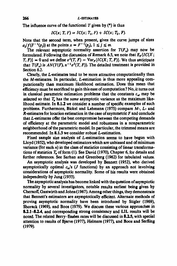
266 L-ESTIMATES
The influence curve of the functional T given by (*) is thus
IC(X; T, F) fC(X; Ti, F) + IC(X; Tz, F).
Note that the second term, when present, gives the curve jumps of sizes a,/f(F-'(p,)) at the points x = F-I(p,), 1 I; j I; m.
The relevant asymptotic normality assertion for T(F,,) may now be formulated. Following the discussion of Remark 6.5, we note that E F { f C ( X ; T, F)} = 0 and we define az(T, F) = Var,{IC(X; T, F)}. We thus anticipate that T(F,,) is AN(T(F), n-'a'(T, F)). The detailed treatment is provided in Section 8.2.
Clearly, the L-estimates tend to be more attractive computationally than the M-estimates. In particular, L-estimation is thus more appealing com- putationally than maximum likelihood estimation. Does this mean that efficiency must be sacrificed to p i n this ease of computation? No, it turns out in classical parametric estimation problems that the constants cnl may be selected so that T, has the same asymptotic variance as the maximum likc- lihood estimate. In 8.1.2 we consider a number of specific examples of such problems. Furthermore, Bickel and Lehmann (1975) compare M-, L- and R-estimates for location estimation in the case of asymmetric F and conclude that L-estimates offer the best compromise between the competing demands of efficiency at the parametric model and robustness in a nonparametric neighborhood of the parametric model. In particular, the trimmed means are recommended. In 8.1.3 we consider robust L-estimation.
Fixed sample size analysis of L-estimation seems to have begun with Lloyd (1952), who developed estimators which are unbiased and of minimum variance (for each n) in the class of statistics consisting of linear transforma- tions of statistia T, of form (1). See David (1970), Chapter 6, for details and further references. See Sarhan and Greenberg (1962) for tabulated values.
An asymptotic analysis was developed by Bennett (1952), who derived asymptotically optimal c,,,'s (J functions) by an approach not involving considerations of asymptotic normality. Some of his results were obtained independently by Jung (1955).
The asymptotic analysis has become linked with the question ofasymptotic normality by several investigators, notable results earliest being given by Chernoff, Gastwirth and Johns (1967). Among other things, they demonstrate that Bennett's estimators are asymptotically efficient. Alternate methods of proving asymptotic normality have been introduced by Stigler (1969), Shorack (1969), and Boos (1979). We discuss these various approaches in 8.2.1-8.2.4, and corresponding strong consistency and LIL results will be noted. The related Berry-Essten rates will be discussed in 8.2.5, with special attention to results of Bjerve (1977), Helmers (1977), and BOOS and Serfling (1979).

BASIC FORMULATION AND BXAMPLBS 267
8.1.2 Examples in Parametric Ipcation and Scale Estimation Let the distribution of X,l,. . . , X n be a member F(x; el, 0,) of a specified location and scale parameter family 9F = {F(x ; el, a,), (el, 0,) E a}, where
with density
and F is a specified distribution with density f. For example, if F = d), then S is a family of normal distributions. One or both of and 0, may be unknown. The problem under consideration is that of estimation of each unknown parameter by an L-estimate, that is, by a statistic of the convenient form
with the J function selected optimally. Furthermore, solutions are desired in both the cases of censored and uncensored data (censored data arises in connection with life-testing experiments, or in connection with outlier- rejection procedures). We will consider several examples from Chernoff, Gastwirth and Johns (1967).
Assume that 9c satisfies regularity conditions (recall Section 4.2) suf- ficient for the asymptotic covariance matrix of the normalized maximum likelihood estimates of and 0, to coincide with the inverse of the informa- tion matrix
Defining
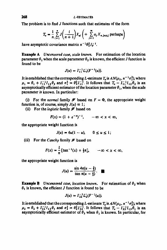
268 L-ESTIMATES
The problem is to find J functions such that estimates of the form
have asymptotic covariance matrix n- '8:l; l .
Example A Uncensorgd case, scale known. For estimation of the location parameter 8, when the scale parameter O2 is known, the efficient J function is found to be
J(u) = lT;Li(F-'(u)).
It is established that the corresponding L-estimate T, is AN(!', n- 'u:), where p1 = 8, + 1;;l128, and u: = 8:lif. It follows that T, - li;llz82 is an asymptotically efficient estimator of the location parameter el, when the scale parameter is known. In particular:
(i) For the normal family 9 based on F = @, the appropriate weight function is, of course, simply J(u) E 1 ;
(ii) For the logistic family 9 based on
F(x) = (1 + e-*)-', -00 < x < 00,
the appropriate weight function is
J(u) = 6 ~ ( l - u), 0 S u S 1;
(iii) For the Cauchy family 9c based on
1 n F(x) = - [tan-'(x) + in], -00 < x < 00,
the appropriate weight function is
Example B Uncensored case, location known. For estimation of O2 when 81 is known, the efficient J function is found to be
J(u) = l;&(F- '(u)).
It is established that the corresponding L-estimate T, isAN(p,, n- '&,where p2 = 8, + 11;'lI28, and at = 8$ l ; / . It follows that T, - l ; ~ l I 2 O 1 is an asymptotically efficient estimator of B2 when is known. In particular, for

BASIC FORMULATION AND EXAMPLES 269 the normal, logistic, and Cauchy families considered in Example A, the corresponding appropriate weight functions are
J(u) = a- yu),
J(u) = - n2 + 3
and
tan x(u - f) secZ n(u - 4)' J(u) = 8
respectively.
Example C Uncensored case, location and scale both unknown. In this case the vector (T;'), T!?) corresponding to
CJ l ( 4 , J2(u)3 = C G ( F - 1(4), G ( F - l(u))lI;
is AN ((el, ez), n- let IF I). rn Example D Censored case, location and scale both unknown. In the case of symmetric two-sided censoring of the upper loop% and lower lOOp % observations, it is found that the asymptotically efficient estimate of the location parameter is formed by using weights specified by
J(u) = I~;L \ (F- ' (U) )
w = z ; , 'Cp- ' f2(F- ' (p) ) - f'(F-yp))]
for the uncensored observations and additional weight
for the largest and smallest uncensored observations. For the normal family we have, putting 6, = 0- I@),
J(u) = IT:, p < u < 1 - p , = 0, otherwise,
and
As a numerical example, for p = 0.05 we have ZI = 0.986 and w = 0.0437, yielding the efficient L-estimate
w = ri,'CPd2(tp) + tp+(tp)I-
Note the similarity to the p-Winsorized mean (Example 8.l.lB (ii)). a

270 L-ESTIMATES
8.1.3 Examples in Robust Estimation For robust L-estimation, the influence curve IC(x; T, F) derived in 8.1.1 should be bounded and reasonably smooth. This curve is the sum of the two curves
IC(X; Ti, F) = - [lo/ 2 X ) - F ~ / ) ] J ( F ~ / ) M J J
and
The first curve is smooth, having derivative J(F(x)) (Problem 8.P.6), but can be unbounded. To avoid this, robust L-estimation requires that J(u) vanish outside some interval (a, b), 0 < a < 6 < 1. The second curve is bounded, but has m discontinuities.
Example A The “Gastwirth”. In the Monte Carlo study by Andrews et al. (1972), favorable properties were found for the L-estimate
0.3F; ‘(4) + 0.4F; ‘(4) + 0.3F; ‘(j),
proposed by Gastwirth (1966).
Example B The a-trimmed mean (see Example 8.1.1B(i)). This is the L-estimate T(FJ, where
For F symmetric about F‘ ‘(i), the influence curve is (recall Example 6.5E)
[F-’(a) - F-’(+)], x < F-’(a), 1
F- ‘(a) 5 x 5 F- ‘(1 - a), 1
IC(x; T, F) = - [x - F“(f)], { 1 - 2 a
I x > P 1 ( 1 - a) .
Thus this L-estimate behaves the same as a certain M-estimate, the “Huber” (Example 7.2.2B) with k = F-I(l - a).

ASYMPTOTIC PROPERTIES OF L-ESTIMATES 271 Example C The a-Winsorized mean (see Example 8.1.1B(ii)). This is T(F,,) based on
T ( F ) = l - ' ~ - l ( t ) d t + aF- ' (a) + ctF-1(1- a).
Find its influence curve (Problem 8.P.8).
ExampleD Thesmoothlytrimmedmean. Stigler (1973)providesanexample showing that the trimmed mean has nonnormul asymptotic distribution if the trimming is at non-unique quantiles of F. As one remedy, he introduces the "smoothly trimmed mean," corresponding to a J function of the form
J(u) = 0, u < f.,
= c , a < u < l - a ,
8.2 ASYMPTOTIC PROPERTIES OF L-ESTIMATES
In this section we exhibit asymptotic normality of L-estimates under various restrictions on J and F. Four different methodological approaches will be considered, in 8.2.1-8.2.4, respectively. Consistency and LlL results will also be noted, along the way. In 8.2.5 we consider Berry-Essden rates.
8.2.1 The Approach of Chernoff, Gastwirth and J o b (1967)
Chernoff, Gastwirth and Johns (1967) deal with L-estimates in the general form
I
T, = n - I c Cn1 h(X,,) 1 1 1
where h is some measurable function. (This includes as a special case the formulation of Section 8.1, given by h(x) = x and replacing cRf in (1) by ncRl .) For the purpose of deriving distribution theory for T,, we may assume that X , , X z ,... are given by F-'(U1), F"(U,) ,..., where U1, Uz ,... are independent unifbrm (0, 1) variates. Thus X,, = F 1 ( U n f ) , 1 s f 5 n. Also, Put
v,, = -log(l - U,,,), 1 s i s n.

272 L-ESTIMATES
It is readily seen that the V,, are the order statistics of a sample from the negatiue exponential distribution, G(x) = 1 - exp(-x), x > 0. Thus, put- ting R = h 0 F“ 0 G, the composition of h, F1, and G, we have the re- presentation
n
I = 1 T,, = n-’ CC,,~R(V, , ) .
We now apply differentiability of R in conjunction with the following special representation of the V,, (see, e.g., David (1970)).
Lemma A. The V,, may be represented in distribution as
f s i s n , Z1 Zl v,, = - + n + n - i + l ’
where Z1,. . . , Z , are independent random uariables with distribution G.
Assumprim A. R(v) is continuously digerentiable for 0 < v < 00. Define On, = E{V,,} and note that
l s i s n . 1 1
J,, x - + . * . n + n - i + l *
Now apply Lemma A and Assumption A to write
where
= 0, v =
We thus have the representation (check)
(2) Tn = P n + Qn + Rn, where
n
pn n- C cni R J n i ) , 1- 1
n

ASYMPTOTIC PROPERTIES OF L-ESTIMATES 273
with
and n
I - 1 Rn = n-' Ccni(Vni - cni)Gni(Vni)*
Here p,, is nonrandom, Q, can be shown asymptotically normal by standard central limit theory, and R, is a remainder which is found to be asymptotically negligible. Note that Q, has variance a:/n, where
n
The following further assumptions are needed. First we state an easily proved (Problem 8.P.9) preliminary.
Lemma B. The random variables U,, and Vni can be simultaneously bounded in probability: given 8 > 0, there exists
Uni(E), un'(~), Vni(E), vni(E)
such that
P(Uni(E) < Uni < uni(E), 1 I; i s n) 2 1 - E
and
P(Vni(E) < Vn, < vni(E),
Vn,(E) = -log[l - U,,(E)],
I < i n) 2 1 - E,
with
V"1(&) = -log[l - LP(€)]
and
Assumption B. For each E > 0,
where
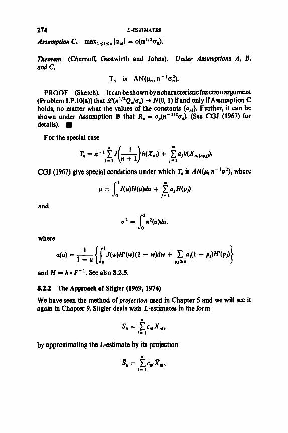
274 L-EsnmTEs
Assumption C. max,,,,, la,,,l = o(n1/2u,,).
Theorem (Chernoff, Gastwirth and Johns). Under Assumptions A, B, and c,
T, is AN(p,,,n^’uX).
PROOF (Sketch). It can beshown byacharacteristicfunction argument (Problem 8.P.lqa)) that 9’(n1/2Q,,/u,,) + N(0, 1) if and only if Assumption C holds, no matter what the values of the constants {a,,,}, Further, it can be shown under Assumption B that R, - op(n-1/20,,). (See CGJ (1967) for details).
For the special case
CGJ (1967) give special conditions under which T, is AN@, n-’a2), where
and
where
and H = h 0 F- See also 8.2.5.
8.2.2 The Approach of Stigler (1969, 1974)
We have seen the method of projection used in Chapter 5 and we will see it again in Chapter 9. Stigler deals with L-estimates in the form
Sn = C C n 1 X n l , I - 1
by approximating the L-estimate by its projection

ASYMPTOTIC PROPERTIES OF L-ESTIMATES 275 wheregnI is the projection of the order statistic Xnf. To express this projection, we introduce the notation
and
The latter is the density of Unf, the ith order statistic of a sample from uniform (0,l). Stigler (1969) proves
Lemma. There is some no = no(F) such that for i 2 no and n - i + 1 2 no,
(In particular, since 9’{Xn1} = 9{F4’(Unf)}, E{Xnf} = F-’(u)g,,,(u)du.) S t igler develops conditions under which
so that for S,, AN(E{S,,} , d(S,,)) it suffices to deal with S,, by standard central limit theory. Noting that
s,, = n-
where A,, is nonrandom and Z,,k = c,,, jg(”*) #(u)g,,l(u)du, it suffices to verify the Lindeberg condition for &: i z , , k - EZ,,,). (See details in Stigler (1969).) As noted by Stigler (1974), his assumptions leading to S,, AN(E{S,}, a2(S,,)) may be characterized informally as follows:
(i) the extremal order statistics do not contribute too much to S,,; (ii) the tails ofthe population distribution are smooth and the population
(iii) the variance of S,, is of the same order as that of Stigler (1974) confines attention to the case
z , , k + A,,, k = 1
density is continuous and positive over its support: (cnI I Xnf.

276 L-WITMATES
and strengthens the condition (ii) (through assumptions on J) in order essentially to be able to dispense with conditions (i) and (ii). He establishes several results. (See also Stigler (1979).)
Theorem A. Suppose that E{X2} < 00, and that J is bounded and continuous a.e. F-’. Suppose that
- 4 )
a2(J, F) = I, S_~(F(x))J(F(y))CF(min(x, Y)) - F(X)F(YlldX dY
is positive. Then
Also, S, is AN(E{S,}, a2(S,)).
lim na2(S,) = a2(J, F). n+m
Theorem B. Suppose that [F(x)(l - F(x))]~/~ dx < a0 and that J(u) = 0 for 0 < u < a and 1 - a 2 u < 1, is bounded, and satisjies a Lipschitz condition of order >+ (except possibly at a finite number of points of F- meusure 0). Then
lim n’/2[E{S,} - p(J, F)] = 0, n+ m
where 1
0 p(J, F) = F-’(u)J(u)du.
(As nokd by Stigler, if F has regularly varying tails (see Feller (1966), p. 268) with a finite exponent, then the conditions E { X 2 } < 00 and
j[F(x)(l - F(x))]’” dx < 00
are equivalent.) Under the combined conditions of Theorems A and B, we have that S, is
AN@(J, F), n-lu2(J, F)). Further, if J puts no weight on the extremes, the tail restrictions on F can be dropped (see Stigler’s Theorem 5 and Remark 3):
Theorem C. Suppose that J(u) is bounded and continuous a.e. F-’, =O for 0 < u < a and 1 - a < u < 1, and is Lipschitz of order >+ except at ajinite set of points of F- measure 0. Then
S, is AN(p(J, F), n-’a2(J, F)).

ASYMPTOTIC PROPERTIES OF L-ESTIMATES 277
Example. The a-trimmed mean satisfies the preceding, provided that the ath and (1 - a)th quantiles of F are unique.
For robust L-estimation, it is quite appropriate to place the burden of restrictions on J rather than F.
8.2.3 The Approach of Shorack (1969,1972) Shorack (1969, 1972) considers L-estimates in the form
I
and, without loss of generality, assumes that XI, Xz, . . . are uniform (0, 1) variates. In effect Shorack introduces a signed measure v on (0 , l ) such that T. estimates 1 = g dv. He introduces a sequence of signed measures v, which approach v in a certain sense and such that v, puts mass n-'cnl at i/n, 1 s i 5 n, and 0 elsewhere. Thus
He then introduces the stochastic process L,(t) = nl/zb 0 F;'(t) - g(t)], 0 s t s 1, and considers
By establishing negligibility of the second term, treating the convergence of the stochastic process I,,(.), and treating the convergence of the functional J L, dv over I,,(.), the asymptotic distribution of T. is derived. His results yield the following examples.
Example A. Let {X,) be I.I.D. F (F arbitrary), with E ( X ( ' < GO for some r > 0. Let
n
I = 1 T, = n-' C J ( t n i ) X n l ,
where maxIsfs,, It,, - i / n l + 0 as n 4 GO and where for some a > 0
a[min(:, 1 - 31 5 t,, s 1 - a[min(:, 1 - $1, 1 s i 5 n.
Suppose that J is continuous except at a finite number of points at which F" is continuous, and suppose that
IJ(t)l < M[t(l - t)]-(1'2)+1/'+d, 0 < t < 1,

278 L-ESTIMATES
for some b > 0. Let J , be a function on [O, 13 equal to J(tRr) for ( I - l)/n < t 5 i/n and 1 s 1 5 n with J,(O) = J(tRl). Then
n”’(T, - AJ,, F)) 5 N O , u2(J, F)), F-’(t)J,(t)dt and
u z ( ~ , F) = I’ jl[min(s, t ) - s t ]J ( s )J ( t )dF-~(s )d~- l ( t ) .
where C((Jn, F) =
0 0
It is desirable to replace p(J,, F) by p(J, F) -- done if J‘ exists and is continuous on (0, 1 ) with
F’ ‘(t)J(t)dt. This may be
IJ(t)l 5 M[t(l - t)]-“”’+’/‘+a, 0 < t < 1,
for some 6 > 0, and the “max-condition” is strengthened to
n max t,,, - - = O(1). 1 srsn I 1)
Ex8mple Al. Let XI,. . , , X, be a sample from (9 7 N(0, 1). For integral r > 0, an estimator of E{X‘+ l} is given by
By Example A,
Ex8mple B The a-trinuned mean. Let XI, .. ., X , be a sample from Fd = F(. - O), where F is any distribution symmetric about 0. Let 0 < a < 4. For n even define
(Omit n odd.) Then
where W(-) is the Wiener process (1.11.4).
Note that Shorack requires J to be smooth but not necessarily boundad, and requires little on F. He also deals with mare general J functions under additional restrictions on F.

ASYMPTWl'lC PROPERTIES OF L-ESTIMATES 279
Wellner (1977a, b) follows the Shorack set-up and establishes almost sure results for T, given by (1). Define J , on [O, 13 by J,(O) = cM1 and J,,(t) = cnl for (i - l)/n < t 5 i/n. Set p,, = J,,(t)g(t)dt and y = J(t)g(t)dt.
Assumption 1. The function g is left continuous on (0, 1) and is of bounded variation on (0,l - 0)for all 0 > 0. Forfixed bl, b2 and M,
IJ(t)l S Mt-bl(l - t)-b', 0 < t < 1,
and the same bound holds for J,( a), each n. Further,
lg(t)l < Mt-l+bt+G(f - t)-"+b'+a , O < t < l ,
for some 6 > 0, and t'-bI-(1/2)8(1 - t)1-b1-(1/2)8 dl g l < 00. m Assunrprion 2. limndm J,(t) = J(t), t E (0, 1).
Theorem. Under Assumption 1, T, - p, * 0. I f also Assumption 2 holds, then T, 2 p.
Example A* (parallel to Example A above). Let { X,}, F, T,, and {t,,} be as in Example A. Suppose that
IJ(t)I s M[t ( l - t ) ] - ' + 1 / ' + d , 0 < t < 1,
for some S > 0, and that J is continuous except at finitely many points. Then
1
T, J% p(J, F) = F- '(t)J(t)dt. Jb Note that the requirements on J in Example A* are milder than in Example
A. Wellner also develops the LIL for T, given by (1). For this, however, the requirements on J follow exactly those of Example A.
8.2.4 The Differentiable Statistical Function Approach
Consider the functional T(F) = T,(F) + T2(F), where
TI(F) = IO1F- '(t)J(c)dt,
with J such that K ( t ) = functions on (0, l), and
J(u)dt is a linear combination of distribution
m

280 L-ESTIMATES
We consider here the L-estimate given by the statistical function T(F,). Applying the methods of Chapter 6, we obtain asymptotic normality and the LlL in relatively straightforward fashion.
From 8.1.1 it is readily seen that n
i- I dIT(F; F, - F) = n-I h(F; Xi),
where
Note that EF{h(F; X)} = 0. Put a2(T, F) = VarF{h(F; X ) } . If 0 < a2(T, F) < 00, we obtain that T(F,) is AN(T(F), n-'a2(T, F)) if we can establish nli2R1, 3 0, where RI, = Aln + A?,, with
Now, in Example 6.SD, we have already established
n112A2, 3 0, provided that F'(F-l(pJ)) > 0, j = 1, , ;. , m. It remains to deal with A,,. By Lemma 8.1.1B, we have (check)
A,, = 7i(Fn) - T ( F ) - d l T ( F ; F, - F), i 3: 1,2.
where we define
= 0, G ( x ) = F(x ) .
Via (l), A,, may be handled by any of several natural approaches, each involving different trade-offs between restrictions on J and restrictions on F. For example, (1) immediately implies
(2A) I A I n l 5 IIWF~,FIIL.~ * l lFn - f'llm, where llhll, = sup, Ih(x)l and llhllL, = Jh(x) ldx. Since llF, - Fll, = Op(n-1'2) as noted earlier in Remark 6.2.2B(ii), we can obtain 1A1,1 = o,(n- ' I 2 ) by showing
To this effect, following Boos (1977, 1979), we introduce
( 3 4 IIWF",FllL, 4 0.
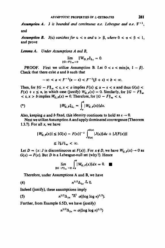
ASYMPTOTIC PROPERTIES OF L-ESTIMATES 281
Assumption A. J is bounded and continuous a.e. Lebesgue and a.e. F-',
and
Assumption B. J(u) vanishes for u c a and u > p, where 0 < a < p < 1, and prove
Lemma A. Under Assumptions A and 8,
Jim IIW0,FIlL, = 0. 110- Fll oo 4 0
PROOF. First we utilize Assumption B. Let 0 < e < min{a, 1 - 8) .
-a < a < F-'(a - e) < . F - ' ( p + e) < b < ao.
Then, for llG - Fll, < e, x < a implies F(x) I; a - E c a and thus G(x) < F(x) + e 5 a, in which case (iustify) WG,,(x) = 0. Similarly, for llG - Fll, < e, x > b implies W,,,(X) = 0. Therefore, for llG - Fll, < E,
Check that there exist a and b such that
Also, keeping a and b fixed, this identity continues to hold as e -t 0.
1.3.7). For all x , we have Next we utilize Assumption A and apply dominated convergence (Theorem
5 211J11, < 00.
Let D = { x : J is discontinuous at F(x)} . For x 9 D, we have W G , p ( ~ ) + 0 as G(x) + F(x). But D is a Lebesgue-null set (why?). Hence
~ i m l , W G , F ( x ) l d x = 0. IlG -pII.. - 0
Therefore, under Assumptions A and B, we have
(4) n112Aln 4 0.
Indeed (justify), these assumptions imply
(5)
Further, from Example 6SD, we have (justify)
n l / 2 ~ ~ ~ "g' o((log log n)'").
n1I2A2,, = o((1og log n)Il2)

282 L-ESTIMATES
provided that F is twice differentiable at the points F'I(p,), 1 5 j S m. Therefore, we have proved
Theorem A. Consider the Lestimate T(F,) = T,(F,) + T2(F,). Suppose that Assumptions A and B hold, and that F has positive derivatives at its pJ- quantiles, 1 s j 5 m. Assume 0 c a2(T, F) c ao. Then
n1IZ(T(F,) - T(F)) 4 N(0, &(TI F)).
rf,/icrrher, F is twice dlgerentiable at its p,-quantiles, 1 5 j 5 m, then the corresponding LIL holds.
Examples A. (i) The trimmed mean. Consider T,(F) based on J(t) = I(a s t 5 /3)/(/3 - a) and T2(.) E 0. The conditions of the theorem are satisfied if the a- and flquantiles of F are unique.
(ii) The Winsorfzed mean. (Problem 8.P.13).
It is desirable also to deal with untrimmed J functions. To this effect, Boos (1977,1979) uses the following implication of (1):
where q can be any strategically selected function satisfying
Assumption B*. jZrn q(F(x))dx c 00.
In this case the role of Lemma A is given to the following analogue.
Lemma B. Under Assumptions A and B',
Iim ll(q F)WO,FlIL, = 0. 110- Fll no+ 0
PROOF. analogous to that of Lemma A (Problem 8.P.14). 4
In order to exploit Lemma B to establish (4) and (9, we require that ll(Fn - F)/q 0 FII, satisfy analogues of the properties Op(n- 'I2) and
0,1(n-1/2(log log n)'")
known for !IF, - Fll,. OReilly (1974) gives weak convergence results which yield the first property for a class of q functions containing in particular
Q = (4: q(t) = [t(l - t)](1/2)-d, 0 < t < 1; 0 < 6 < 3,. James (1975) gives functional LIL results which yield the second property for a class of q functions also containing Q.

ASYMPTOTIC PROPERTIES OF L-ESTIMATES 283
On the other hand, Gaenssler and Stute (1976) note that the Op(n’1/2) property fails for q(t) = “(1 - t)]’/’. For this q, the other property also fails, by results of James (1975). Although some of the aforementioned results are established only for uniform (0, 1) variates, the conclusions we are drawing are valid for general F. We assert:
and
Consequently, we have (4) and (5) under Assumptions A and B*. That is,
Theorem B. Assume the conditions of Theorem A, with Assumption B replaced by Assumption B* for some q E Q. Then the assertions of Theorem A remain valid.
Examples B. Let F satisfy 1 [F(x)(l - F ( X ) ) ] ( ” ~ ) - ~ dx < 00 for some 6 > 0. Then Theorem B is applicable to
(i) The mean: J(u) = 1 ; (ii) Gini’s mean difference: J(u) = 4u - 2;
(iii) The asymptotically efficient L-estimator for location for the logistic family: J(u) = 6u(l - u). W
Remark. Boos (1977, 1979) actually establishes that
T(F; A) = - A(x)J(F(x) )~x s is a duerentid of T( .) at F w.r.t. suitable II * 11’s.
Still more can be extracted from (I), via the implication
(2C) IAln1 5 IIWn,Fllao ’ llFn - FllL,*
Thus one approach toward obtaining (4) is to establish llF, - FllL, = 0,,(n-1/2) under suitable restrictions on F, and to establish IIWpn,F((aD 3 0 under suitable restrictions on J . We start with llF, - FllL,.
Lemma D. Let F satisfy [F(x) [ 1 - F(x))] ‘ I2 dx c a. Then
E{(IFn - FllL,} = O(n-’/2).
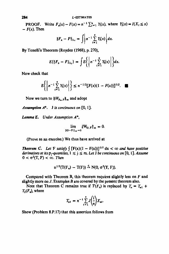
2a4 L-ESTIMATES
PROOF. Write F,(x) - F(x) = n- cy- Ydx), where q(x ) = I ( X , s x) - F(x). Then
By Tonelli’s Theorem (Royden (1968), p. 270),
Now check that
Now we turn to IIWPm,Fl(m and adopt
Assumption A*. J is continuous on [0, 11.
Lemma E. Under Assumption A*,
(Prove as an exercise.) We thus have arrived at
Theorem C. Let F satisfy [F(x)(l - F(x))]’I2 dx < 00 and h u e positive deriuatiues at its p,-quantiles, 1 S j 5 m. Let J be continuous on [0, I]. Assume 0 < aZ(T, F) -c ao. Then
n1’2(T(F,) - T(F)) 4 N(0, d(T, F)).
Compared with Theorem B, this theorem requires slightly less on F and slightly more on J. Examples B are covered by the present theorem also.
Note that Theorem C remains true if T(F,) is replaced by T, = + T,(F,), where
Show (Problem 8.P.17) that this assertion follows from

ASYMPTOTIC PROPERTIES OF L-ESTIMATES
Lemma F. Under Assumption A*,
285
Prove Lemma F as an exercise.
8.2.5 Berry-Esden Rates
For L-estimates in the case of zero weight given to extreme order statistics, Rosenkrantz and OReilly (1972) derived the Berry-Essden rate O(n- 1’4).
However, as we saw in Theorem 2.3.3C, for sample quantiles the rate O(n- applies. Thus it is not surprising that the rate O(n-’’4) can be improved to O(n- ’ I 2 ) . We shall give three such results. Theorem A, due to Bjerve (1977), is obtained by a refinement of the approach of CGJ (1967) discussed in 8.2.1. The result permits quite general weights on the observations between the ath and /?th quantiles, where 0 < a < /3 < 1, but requires zero weights on the remaining observations. Thus the distribution F need not satisfy any moment condition. However, strong smoothness is required. Theorem B, due to Helmers (1977a, b), allows weights to be put on all the observations, under sufficient smoothness of the weight function and under moment restrictions on F. However, F need not be continuous. Helmers’ methods, as well as Bjerve’s, incorporate Fourier techniques. Theorem C, due to Boos and Serfling (1979), applies the method developed in 6.4.3 and thus implicitly uses the Berry- Essden theorem for U-statistics (Theorem 5.5.1B) due to Callaert and Janssen (1978). Thus Fourier techniques are bypassed, being subsumed into the U- statistic result. Theorem C is close to Theorem B in character. It should be noted that a major influence underlying all of these developments was provided by ideas in Bickel(1974).
Bjerve treats L-estimates in the form
n
I = 1 T. n- ’ C cni h(Xn,)
and utilizes the function I? = h 0 F - ’ 0 G and the notation pn and 8, defined in 8.2.1. He confines attention to the case that
c,,, = 0 for i 5 an or i > pn, where 0 < a < /3 < 1,
and introduces constants a and b satisfying 0 < a < -log(l - a) and -log(l - p) < b < 00. His theorem imposes further conditions on the c,;s as well as severe regularity conditions on R. Namely, Bjerve proves

286 L-ESTIMATES
Theorem A . Let R satisfy a first order Llpschitz condition on [a, b] and assume for some constants c > 0 and d < 00 that
(i) a: > c, all n, and
(ii) n-I EP I C , , ~ c d, all n. Then
PROOF (Sketch). The representation T, = p,, + Q,, + R,, of 8.2.1 is refined by writing R,, = M,, + A,,, where
and
with
= 0, u = Vn1.
It can be shown that
P(IA,,l > n-'I2) = O(n-*l2)
and, by a characteristic function approach, that
(See Bjerve (1977) for details.) The result then follows by Lemma 6.4.3. H For the special case
considered also by CGJ (1967), Theorem A yields (*) with p,, and a,, replaced by the constants p and Q defined at the end of 8.2.1; that is, with H = h 0 F- ', we have
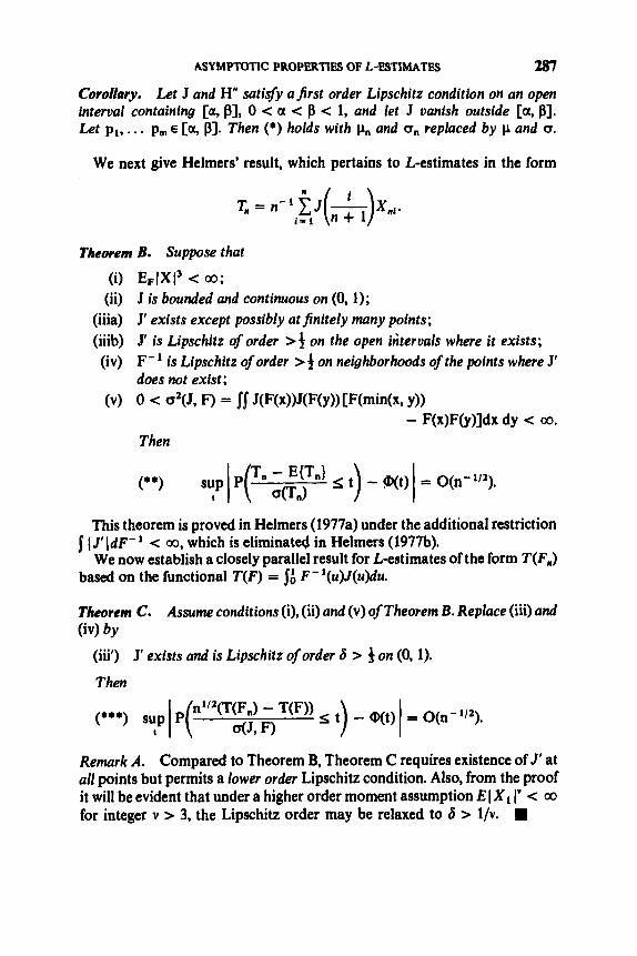
ASYMPTOTIC PROPERTIES OF L-ESTIMATES 287
Corollary. Let J and H" satisfy afirst order Lipschitz condition on an open interual containing [a, $3, 0 < u < $ < 1, and let J vanish outside [a, $1. Let pi , . . . pm E [q $1. Then (*) holds with p, and a, replaced by p and a.
We next give Helmers' result, which pertains to L-estimates in the form
Theorem B. Suppose that (i) EFlX13 < 00;
(ii) J is bounded and continuous on (0,l); (iiia) J' exists except possibly at finitely many points; (iiib) J' is Lipschitz of order ># on the open intervals where it exists; (iv) F- is Lipschitz oforder > 4 on neighborhoods ofthe points where J'
does not exist ; (v) 0 < a2(J, F) = JJ J(F(x))J(F(y))CF(min(x, Y))
Then - F(x)FQ)]dx dy < 00.
This theorem is proved in Helmers (1977a) under the additional restriction
We now establish a closely parallel result for L-estimates of the form T(FJ 1 I J' ( d F - < 00, which is eliminated in Helmers (1977b).
based on the functional T(F) = F-'(u)J(u)du.
Theorem C. Assume conditions (i), (ii) and (v) of Theorem B. Replace (iii) and (iv) by
(iii') J' exists and is Lipschitz of order 6 > 3 on (0, 1).
Then
Remark A. Compared to Theorem B, Theorem C requires existence of J' at all points but permits a lower order Lipschitz condition. Also, from the proof it will be evident that under a higher order moment assumption EIXl 1' < 00 for integer v > 3, the Lipschitz order may be relaxed to S > l /v. W

288 L-ESTIMATES
The proof of Theorem C will require the following lemmas, the second of which is a parallel of Lemma 8.2.4D. Here llhllL, = [j h2(x)dx]1'2.
Lemma A. Let the random variable X have distribution F and satigy El X I' < a, where k is a positive integer. Let g be a bounded function. Then
(0 E { j CW 4 Y) - F(Y)lg(Y)dY) = 0
6) E { [ j l I ( X 5 Y) - F(Y)IgwldYl') < 00- and
PROOF. Since E ( X ( < 00, we have (why?) y [ F ( - y ) + 1 - Fb)] + 0 as y 3 ao. Thus yll(X 5 y) - F(y)J + 0 as y + f 00 and hence, by integra- tion by parts,
Sll(X 4 Y ) - Fcv)ldY 5; 1x1 + ElXl.
Thus (ii) readily follows. Also, by Fubini's theorem, this justifies an inter- change of E{ .} and in (i). W
Lemma B. t e t EFIXlk < 00, where k is a positive integer. Then
ElIIF" - Flit:) = O(n-'). PROOF. Put Ydt) = I (X i I; t ) - F(t), 1 s i 4 n. Then
(a)
By the use of Lemma A and Fubini's Theorem (check), we have
E{IIF. - ~112:) = n - 2 k f:
Check that we have E{ x , ( t l ) ~ l ( t , ) . xk(tk)qk(tk)} = 0 except possibly in the case that each index in the list i l , j l , . . . , ik,jk appears at least twice. In this case the number of distinct elements in the set { i l , j l , . , , , ik,jk} is s k. It follows that the number of ways to choose i l , j l , , . . , ik,jk such that the expectation in (b) is nonzero is O(nk). Thus the number of nonzero terms in the summation in (a) is o(nk).
PROOF OF THEOREM C. We apply Theorem 6.4.3. Thus we express T(F,) - T(F) as V2, + R2,, where
V,,, = dIT(F; F,, - F) + i d , T(F; F, - F ) I n
= n - 2 2 h(F; XI, X,). 1=1 J=l

ASYMPTOTIC PROPERTIES OF L-ESTIMATES 289
By Problem 8.P.5,
and
d z T(F; Fn - F) = - [Fn(t) - F(t)]'J' 0 F(t)dt. I-, Thus (check) the desired h(F; x, y ) = J[a(x) + a(y) + P(x, y)], where
W
a(x) = - [ l ( x 5 t ) - F( t ) ]JoF( t )d t s_, and
4)
P(x, Y ) = - 1- p x 5 t ) - FWl Cl(y 5 t ) - F(t)]J' 0 F(t)dt.
- J-, Therefore (check), Rzn is given by
(0
{K 0 F,(t) - K 0 F ( t ) - J 0 F(t)[F, , ( t ) - F(t)J
- 45' 0 F(t)[F,(t) - F(t)J2}dt,
where K(u) = JyO J(o)do. By the Lip condition on J', we obtain
4- P(nS'61(Fn - Flit, > 1).
For 6 > 3, the first right-hand term is (check) O(n-"') by an application of Theorem 2.1.3A. The second term is O(n-'l2) by Lemma B above. Therefore,
P(IR2,I > An-') = O ( ~ I " ' ~ ) ,
as required in Theorem 6.4.3.
above (check). The required properties of h(F; x, y ) are obtained by use of Lemma A

290 L-ESTIMATES
Remark B (Problem 8.P.21). Under the same conditions on F and J , (***) holds also with T(F,,) replaced by
(Hint: Show that I T(F,) - T(F)) 5 Mn-'
inequality.) H
I IX,l for a constant M. Thus showthatP(JT(F,,) - T(F)J > 2 M E J X , I n - c ) = O(n-'),usingChebyshev's
8.P PROBLEMS
Section 8.1
1. Complete details for Example 8.1.1A (Gini's mean difference). 2. For the functional T(F) = F-'(p) , show that the Gateaux derivative
of Tat F in the direction of G is
in the case that F has a positive density f at F"(p). (Hint: following Huber (1977), put FA = F + A(G - F) and differentiate implicitly with respect to 1 in the equation FA(&' ' ( p ) ) = p.)
3. Prove Lemma 8.1.1A. (Hint: Let D be the discontinuity set of F and put A = [0, 13 - D. Deal with F-'(t)dK,(t) by a general change of variables lemma (e.g., Dunford and Schwartz (1963), p. 182).)
4. Prove Lemma 8.1.lB. (Hint: Apply Lemma 8.1.1A and integrate by parts.)
5. For the functional TI@) = F'l(r)J(r)dt, put FA = F + 1(G - F) and show
(Hint: Apply Lemma 8.1.1B.) 6. (Continuation). Show that the influence curve of TI( .) is differentiable,
with derivative J(F(x)). 7. (Complement to Problem 5). For the functional T(F) = F - l ( p ) , find
d2 T(F; G - F) for arbitrary G. 8. Derive the influence curve of the a-Winsorized mean (Example
8.1.3C).

PROBLEMS 291
Section 8.2 9. Prove Lemma 8.2.1 B.
10. (a) Let {u,,,} be arbitrary constants and put a," = C;=, a,"l. Let (2,) be IID negative exponential variates. Put XI = Z I - 1, i = 1,2,. . . , and W, = n-' 2.: anlX1. Show that W, is AN(0, n-la;) if and only if
11. 12. 13. 14. 15. 16. 17. 18. 19. 20. 21.
max Ian,[ = ~(n''~a,,). I s l s n
(*I
(Hint: use characteristic functions.) (b) Now let {XI} be IID F, where F has mean 0 and finite variance. Show
that (*) suffices for W, to be AN(0, n-'a,"). (Hint: apply Theorem 1.9.3.) Show that Example 8.2.3A1 is a special case of Example 8.2.3A. Complete the details of proof of Lemma 8.2.4A. Details for Example 8.2.4A(ii). Verify Lemma 8.2.48. Minor details for proof of Lemma 8.2.4D. Prove Lemma 8.2.4E. Prove the assertion preceding Lemma 8.2.4F. Prove Lemma 8.2.4F. Details for proof of Lemmas 8.2.5A, B. Details for proof of Theorem 8.2.5C. Verify Remark 8.2.58.

C H A P T E R 9
R-Es ti mates
Consider a sample ofindependent observations XI, . . . , XN having respective distribution functions F1, . . . , FN not necessarily idenrical. For example, the XI)s may correspond to a combined sample formed from samples from several different populations. It is often desired to base inference purely on the ranks R1, . . . , RN of XI, . . . , XN. This may be due to invariance considerations, or to gain the mathematical simplicity of having a finite sample space, or because rank procedures are convenient to apply. Section 9.1 provides a basic formulation and some examples. We shall confine attention primarily to simple linear rank statistics and present in Section 9.2 several methodologies for treating asymptotic normality. Some complements are provided in Section 9.3, including, in particular, the connections between R-estimates and the M- and L-estimates of Chapters 7 and 8.
9.1 BASIC FORMULATION AND EXAMPLES
A motivatingexample is provided in 9.1.1, and theclass of linear rank statistics is examined in 9.1.2. Our treatment in this chapter emphasizes test statistics. However, in 9.1.3 the role of rank-type statistics in estimation is noted, and here the connection with the “statistical function” approach of Chapter 6 is seen.
9.1.1 A Motivating Example: Testing Homogeneity of Two Samples Consider mutually independent observations XI, . . . , X,, where X,, . . . , X, have continuous distribution F and X,, I , . . . , XN have continuous distribu- tion function G. The problem is to test the hypothesis H o : F = G.
An instructive treatment of the problem is provided by Fraser (1957), (j5.3, to which the reader is referred for details. By invariance considerations, the
292

BASIC FORMULATION AND EXAMPLES 293
data ‘vector X = (XI,. .., X,) is reduced to the vector of ranks R = (R . . . , R,). By sufficiency considerations, a further reduction is made, to the vector (Rml, . . . , Rmm) of ordered values of the ranks R I , . . . , R , of the first sample. Hence we consider basing a test of H, upon the statistic
T(W = = ( R m l s * * * , R m m ) .
The “best” test statistic based on T(X) depends on the particular class of alternatives to Ho against which protection is most desired. We shall consider three cases.
(i) HI : G = F2. For this alternative, the most powerful rank test is found to have test function of the form
m
P(reject HoIR,,,) = log(R,, + i - 1) $ c.
Accordingly, an appropriate test statistic is m
(ii) H,: G = qF + pF’(0 < p 5 1, q = 1 - p). For this alternative, the locally most powerful rank test (for p in a neighborhood of the “null” valueO) is based on the test statistic
m
I = I
(iii) I f 3 : F = N(pI, a2),G = N ( p 2 . c2), pI < p2. For thisalternative,the locally most powerful rank test (for p, - p1 in a neighborhood of 0) is the “c,-test,” based on the statistic
m
where (ZN1, . , . , Z N N ) denotes the order statistic for a random sample of size N from N ( 0 , 1).
Observe that, even having reduced the data to T(X) = R(,,, a variety of statistics based on Tarise for consideration. The class of useful rank statistics is clearly very rich.
Note that in each of the three preceding cases, the relevant statistic is of the form
m
S = CaN(i, R m i ) I= 1
for some choice of constants aN(i,j), 1 < i, j I; N.

294 R-ESTIMATES
9.1.2 Linear Rank Statistics
In general, any statistic T which is a function of R = (R , , . . . , RN) is called a rank statistic. An important class of rank statistics consists of the linear type, given by the form
N
1- 1 T(R) = Cdi, 8th
where {a(i, j)} is an arbitrary N x N matrix. Any choice of the set ofconstants defines such a statistic. As will be discussed in 9.2.5, an arbitrary rank statistic may often be suitably approximated by its projection into the family of linear rank statistics.
A useful subclass of the linear rank statistics consists of the simple type, given by the form
N
I = 1 S(R) = CC,UN(RI),
where cl, . . . , cN are arbitrary “regression” constants and aN(1), . . . , aN(N) are “scores.” Typically, the scores are generated by a function h(t), 0 < t < 1, either by
(i) a,&) = h(i/(N + l)), 1 5 i s N, or by
(ii) aN = Eh(U,,), 1 5 i S N,
where U , denotes the ith order statistic in a random sample of size N from the uniform [O, 11 distribution. The scores given by (ii) occur in statistics yielding locally most powerful tests. Those given by (i) have the appeal of simplicity.
Thespecialcaseofc,= l f o r l s i S m a n d q = O f o r m + l j i S N i s called a two-sample simple linear rank statistic, Note that the statistics S2 and S3 mentioned in 9.1.1 are of this type, with scores generated by
h(t) = t , 0 S t s 1,
and
h(t) = V ( t ) , 0 < t s 1,
respectively. The statistic S1 of 9.1.1 is of linear form, hut not of the simple tY P e a

WYMPTOTIC NORMALITY OF SIMPLE LINEAR RANK STATISTICS 295
9.1.3 &Estimates Consider a two-sample simple Linear rank statistic for shift. That is, the null hypothesis is I f o : G(x) = F(x - A), and the test statistic is of the form S = c;I1 a,(R,). A related estimator 8, of the shift parameter A may be developed as follows. Find the choice of d such that the statistic S, when recomputed using the values X,, - d , . . . , X , - d in place of X,, . . . , XN, comes as close as possible to its null hypothesis expected value, which is mN-' cy= a(i). This value bN makes the sample X,, I - &, . . . , XN - A N appear to be distributed as a sample from the distribution F and thus serves as a natural estimator of A.
By a similar device, the location parameter of a single sample may be estimated. Let XI, . . . , X, be a sample from a distribution F symmetric about a location parameter 8. Construct (from the same observations) a "second sample *'
where d is chosen arbitrarily. Now find the value d = 6, such that the statistic S computed from the two samples comes as close as possible to its null value. For example, if S denotes the two-sample Wilcoxon statistic, based on the scores a(i) = i, then 6, turns out to be the Hodges-Lehmann estimate, median {&Xi + X,), 1 s i < j 5 m}.
a(i) = s'" h(t)dt.
Then the location estimator just discussed is given by T(F,), where F, denotes the usual sample distribution function and T ( . ) is the functional defined by the implicit equation
6
2d - XI,. . . , 2 d - X , ,
Let the scores a(i) be generated via
( 1 - 1 )/m
I h{)[t + 1 - F(2T(F) - F-'( t ) ) ]}dt = 0. J
See Huber (1977) for further details. Thus the methods of Chapter 6 may be applied.
9.2 ASYMPTOTIC NORMALITY OF SIMPLE LINEAR RANK STATISTICS
Several approaches to the problem of asymptotic normality will be described, broadly in 9.2.1 and more specifically in 9.2.2-4. In 9.2.5 we examine in general form the important projection method introduced in 5.3.1 in dealing with U-statistics and further noted in 8.2.2 in dealing with L-estimates. In 9.2.6 we present Berry-Essken rates, making use of the projection method.
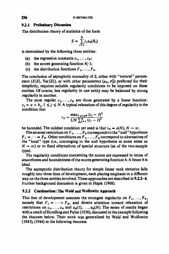
2% R-mrimrm
9.2.1 Preliminary Discussion
The distribution theory of statistics of the form N
1 0 1 S C c t a N ( h )
is determined by the following three entities:
(a) the regression constants cl, . . . , cN; (b) the scores generating function h( .); (c) the distribution functions F,, . . . , FN.
The conclusion of asymptotic normality of S, either with “natural” param- eters ( E { S } , Var{S}), or with other parameters ( p N , u;) preferred for their simplicity, requires suitable regularity conditions to be imposed on these entities. Of course, less regularity in one entity may be balanced by strong regularity in another.
The most regular cl,. . . , cN are those generated by a linear function: cj = a + b,, 1 S j S N. A typical relaxation of this degree of regularity is the condition that
be bounded. The mildest condition yet used is that vN = o(N), N + co. The severest restriction on F . . . , F N corresponds to the“nu1l” hypothesis
F1 = . = FN. Other conditions on F l , . . . , FN correspond to alternatives of the “local” type (i.e., converging to the null hypothesis in some sense as N + 00) or to fixed alternatives of special structure (as of the two-sample
The regularity conditions concerning the scores are expressed in terms of smoothness and boundedness of the scores generating function h. A linear h is ideal.
The asymptotic distribution theory for simple linear rank statistics falls roughly into three lines of development, each placing emphasis in a different way on the three entities involved. These approaches are described in 9.2.2-4. Further background discussion is given in Hdjek (1968).
9.2.2 Continuation: The Wald and Wolfowitz Approach
This line of development assumes the strongest regularity on F,, . . . , FN, namely that F 1 = = FN, and directs attention toward relaxation of restrictions on cl, . . . , cN and a&), . . . , aN(N). The series of results began with a result of Hotelling and Pabst (1936), discussed in the example following the theorem below. Their work was generalized by Wald and Wolfowitz (1943), (1944) in the following theorem.
tYP+

ASYMPTOTIC NORMALITY OF SIMPLE LINEAR RANK STATlSTICS 297
Theorem (Wald and Wolfowitz). Suppose that FI = = FN, each N = 1,2,. . . . Suppose that the quantities
are O(N - z'"-2)), N 4 oo,for each r = 3,4, . . . . Then N
SN = CcNiaNR, is AN(PN, of> I = I
and
E(SN) = PN, Var(SN) = ($3
where pN = NPNtiN and of = (N - l)aicofa, with ( c N ~ - CN)2 and of,
= (N - 1)-' xy PROOF, (Sketch). The moments of ( S N - pN)/aN are shown to con-
verge to those of N(0, 1). Then the Frtchet-Shohat Theorem (1.5.1B) is applied. For details, see Fraser (1957). Chapter 6, or Wilks (1962), §9.5.
Example. Testing independence by the rank correlation coeficient. A test may be based on
(N - l ) - ' zy (aNi -
N
l = I SN = C i R i ,
which under the null hypothesis is found (check) by the preceding theorem to be AN(pN, ~ f ) , with
N(N + 1)2 N 3 4 4
h- PN =
and
N*(NZ - 1)2 N5 w -
" = 14qN - 1) 144'
A series of extensions of the preceding theorem culminated with necessary and sufficient conditions being provided by Hhjek (1961). For detailed bibliographic discussion and further results, see Hajek and Sidik (1967), pp. 152-168 and 192-198.
9.2.3 Continuation: The Chernoff and Savage Approach
The line of development, initiated by Chernoff and Savage (1958), concerns the two-sample problem and allows broad assumptions regarding FI, . . . , FN but imposes stringent conditions on the regression constants and the scores

298 R-ESTIMATES
generating function. The basic device introduced by Chernoff and Savage is the representation of a simple linear rank statistic as a function of the sample distribution function, in order to utilize theory for the latter. The representa- tion is as follows.
. . . , X N } be independent random samples from (not necessarily continuous) distribution functions F and G, respectively. Put 1, = m/N and n = N - m. Then the distribution function for the combined sample is
Likewise, if F: and G,’ denote the sample distribution functions of the sub- samples
Let {XI,. . . , X,} and {X,+
H(r) = dNF(t) + (1 - dN)G(t), -a < t < a.
Hdt) = ANF:(t) + (1 - AN)G,+(t), -00 < t < 00. The statistic of interest is
rn
smu = aN(Rf). I - I
Define
Then 00
sm, = m J- /N(HN(x)MG(X)*
since if XI has rank R f , then HN(XI) = RJN andthus JN(HN(XJ) = JN(RJN)
The following regularity conditions are assumed for the scores a&), with = aN(R1).
respect to some nonconstant function h:
(1) lim aN(1 + [uN]) = h(u), 0 < u < 1 ; N-m
(3) 1
lim - aN(N) = 0; N-m f i
K[t(l - t)]-k-l/Z+d (k = 4 1 , . , .) for some 6 > 0, K < 00.

ASYMPTOTIC NORMALITY OF SIMPLE LINEAR RANK STATISTICS 299
Theorem (Chernoff and Savage). Ler m, n + 00 such that kN is bounded awayfrom 0 and 1. Assume conditions (1)-(4). Then
where
and
with
and
provided that a:. > 0. Further, the asymptotic normality holds uniformly in (F, G ) satisfying
inf Var[B(X1)] > 0, inf Var[B*(Xk)] > 0. P,Q) (F.0)
For proof, see Chernoff and Savage (1958) or, for a somewhat more straight- forward development utilizing stochastic process methods, see Pyke and Shorack (1968). For related results and extensions, see Hdjek and Siddk (1967), pp. 233-237, HBjek (1968), Hoeffding (1973), and Lai (1975). In HBjek (1968) the method of projection is used, and a much broader class of regression constants is considered. (In 9.2.6 we follow up Hhjek’s treatment with corresponding Berry-Esseen rates.)
9.2.4 Continuation: The LeCam and HPjek Approach
This line of development was originated independently by Le Cam (1960) and Hdjek (1962). As regards FI, . . . , FN, this approach is intermediate between the two previously considered ones. It is assumed that the set of distributions F 1 , . . . , F N is “local” to the (composite) null hypothesis F1 = . = F N in a certain special sense called contiguous. However, the c;s are allowed to satisfy merely the weakest restrictions on
and the function h is allowed to be merely square integrable. For introductory discussion, see Hdjek and Siddk (1967), pp. 201-210.
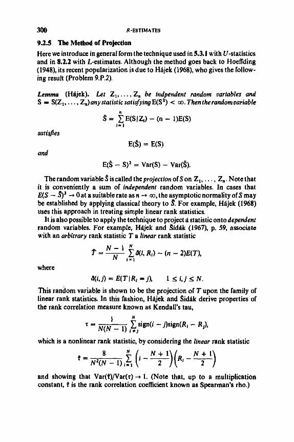
300 R-ESTIMATES
9.2.5 The Method of Projection Here we introduce in general form the technique used in 5.3.1 with U-statistics and in 8.2.2 with L-estimates. Although the method goes back to HoeKding (1948), its recent popularization is due to Hiljek (1968), who gives the follow- ing result (Problem 9.P.2).
Lemma (Hhjek). Let Z1, . . . , Z, be indpendent random variables and S = S(Z1,. . . , Z,)anystatisticsatisSyingE(S') < 00. Thentherandomoariable
= fE(SJZ,) - (n - l)E(S) I * 1
sat isfes
and E(S) = E(S)
E(S - S)' = Var(S) - Var(S).
The random variable 3 is called the projection of S on Zl, . . . , Z, . Note that it is conveniently a sum of independent random variables. In cases that E(S - 3)' 4 0 at a suitable rate as n 4 a, the asymptotic normality of S may be established by applying classical theory to s. For example, Hhjek (1968) uses this approach in treating simple linear rank statistics.
It is also possible to apply the technique to project ti statistic onto dependent random variables. For example, Hdjek and Siddk (1967) p. 59, associate with an arbitrary rank statistic T a linear rank statistic
where
This random variable is shown to be the projection of T upon the family of linear rank statistics. In this fashion, Hiljek and Sidtik derive properties of the rank correlation measure known as Kendall's tau,
d(i, j ) = E ( T J R , = j ) , 1 I; i, j 5 N.
N
sign(i - j)sign(R, - R,), 1
5 = N(N - 1) ,+,
which is a nonlinear rank statistic, by considering the linear rank statistic
and showing that Var(Q)/Var(r) 4 1. (Note that, up to a multiplication constant, 9 is the rank correlation coefficient known as Spearman's rho.)

ASYMPTOTIC NORMALITY OF SIMPLE LINEAR RANK STATISTICS 301
9.2.6 Berry-Wen Rates for Simple Linear Rank Statistics
The rate of convergence O(N-’/2+d) for any 6 > 0 is established for two theorems of Hdjek (1968) on asymptotic normality of simple linear rank statistics. These pertain to smooth and bounded scores, arbitrary regression constants, and broad conditions on the distributions of individual observa- tions. The results parallel those of Bergstriim and Puri (1977). Whereas Bergstrdm and Puri provide explicit constants of proportionality in the O( .) terms, the present development is in closer touch with Hdjek (1968), provides some alternative arguments of proof, and provides explicit application to relax the conditions of a theorem of JureCkovil and Puri (1975) giving the above rate for the case of location-shift alternatives.
Generalizing the line of development of Chernoff and Savage (see 9.2.3), Hdjek (1968) established the asymptotic normality of simple linear rank statistics under broad conditions. Corresponding to his asymptotic normality theorems for the case of smooth and bounded scores, rates of convergence are obtained in Theorems B and C below. The method of proof consists in approximating the simple linear rank statistic by asumofindependent random variables and establishing, for arbitrary v, a suitable bound on the vth moment of the error of approximation (Theorem A).
Let XNI, , . . , X” be independent random variables with ranks RN1, , . . , R”. The simple linear rank statistic to be considered is
N
S N = x C N i a N ( R N 1 ) , i = 1
where cN1, . . . , C” are arbitrary “regression constants” and aN(l), . . . , aN(N) are “scores.” Throughout, the following condition will be assumed.
Condition A. (i) The scores are generated by a function r#(t), 0 < t < 1, in either of the following ways:
(A21 a&) = E4(U$)), 1 < i 5 N,
where U$)denotes the ith order statistic in a sample of size N from the uniform distribution on (0, 1).
(ii) 4 has a bounded second derivative. (iii) The regression constants satisfy
N N
C C N 1 = 0, Cck, = 1, i = 1 1= 1
643)
044) max c i i = O(N-’ log N), N 4 00. l S 1 S . N
Note that (A3) may be assumed without loss of generality.

302 R-ESTIMATES
The XNI)s are assumed to have continuous distribution functions F N I , 1 5; i S N. Put H N ( x ) = N - I cr-l FN,(x). The derivatives of 4 will be denoted by r#i, 4"* etc. Also, put p+ = +(t)dt and u$ = JA [4(t) - $+I2 dt. As usual, denote by Q, the standard normal cdf. Hereafter the suffix N will be omitted from X N I , R N I , cNI , S N , F N I , H N and other notation.
Thestatistics will be approximated by thesamesum ofindependent random variables introduced by Hijek (1968), namely
where
with
u(x) = 1, x 2 0; u(x) = 0, x < 0.
Theorem A . Assume Condition A. Then, for every integer r, there exists a constant M = M(+, r) such that
E(S - ES - T)2r S MN-', all N.
The case r = 1 was proved by Hajek (1968). The extension to higher order is needed for the present purposes.
Theorem B. Assume Condition A. (i) If Var S > B > O* N 3 00, then for every 6 > 0.
suplP(S - ES < x(Var S)ll2) - 4(x)I = O(N-1/2+6), N + 00. I
(ii) The assertion remains true with Var S replaced by Var T. (iii) Both assertions remain true with ES replaced by
Compare Theorem 2.1 of Hajek (1968) and Theorem 1.2 of Bergstrdm and Puri (1977).

ASYMPTOTIC NORMALITY OF SIMPLE LINEAR RANK STATISTICS 303
Theorem C. Assume Condition A and that
suplFi(x) - Fj(x)l = O(N-”’ log N), I , 1, x
N + 00.
Thenfor every 6 > 0
SUPIP(S - ES < XU+) - (D(X)~ = O(N-’”+*), N 4 00. I
The assertion remains true with cr: replaced by either Var S or Var T, andlor ES replaced by p.
Compare Theorem 2.2 of Hajek (1968). As a corollary of Theorem C, the case of local location-shift alternatives will be treated. The following condition will be assumed.
Condition B. (i) The cdf’s F, are generated by a cdf F as follows: F,(x) = F(x - Ado, 1 s i s N, with A # 0.
(ii) F has a density f with bounded derivative f‘. (iii) The shift coefficients satisfy
C d , = 0, N N
I = 1 I = 1 C d f = 1, (B1)
max df = O(N-’ log N), I S I S N
(B2)
Note that (Bl) may be assumed without loss of generality.
N --* 00.
Corollary. Assume Conditions A ahd B and that U
xc:d: = O(N-’ log N), N -+ 00. I = 1
Then for every 6 > 0
where
(The corresponding result of JureCkovd and Puri (1975) requires 4 to have four bounded derivatives and requires further conditions on the cis and d;s. On the other hand, their result for the case of all F;s identical requires only a single bounded derivative for 4.)
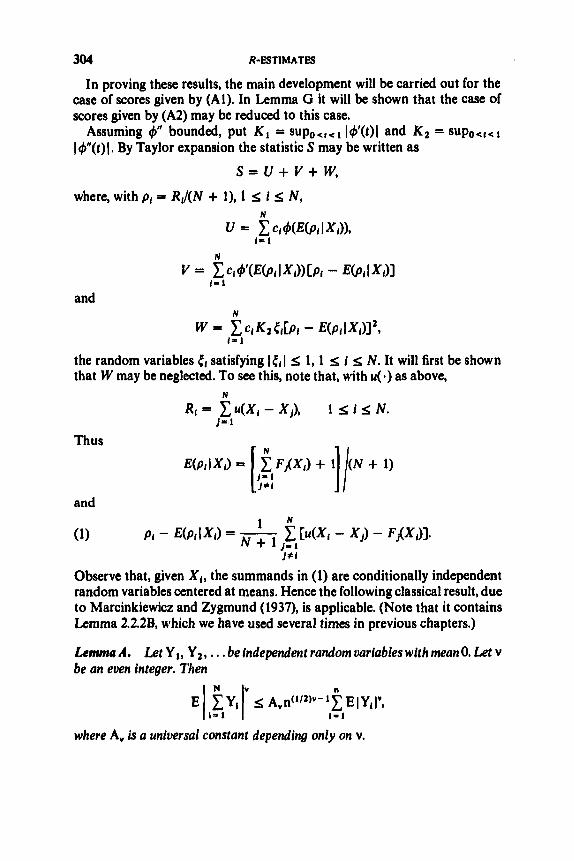
304 R-ESTIMATES
In proving these results, the main development will be carried out for the case of scores given by (Al). In Lemma G it will be shown that the case of scores given by (A2) may be reduced to this case.
Assuming #' bounded, put K 1 = S U ~ ~ < , < ~ I#(t)l and K 2 = S U ~ ~ < ~ < ~
Ir$"(t)l. By Taylor expansion the statistic S may be written as
s - u + v + w, where, with pi = R,/(N + I), 1 5 i s N ,
N
N
v = c CI &(E(Pl I XI)) CPr - E(Pl I xi11
w = C C l K 2 e r C P l - E(PllX312,
I = 1
and N
I = I
the random variables e, satisfying l C l l s 1, 1 s i s N. It will first be shown that W may be neglected. To see this, note that, with u( .) as above,
N
I= 1 Ri = c u(X1- XI), 1 s i s N.
and
Observe that, given XI, the summands in (1) are conditionally independent random variables centered at means. Hence the following classical result, due to Marcinkiewicz and Zygmund (1937), is applicable. (Note that it contains Lemma 2.2.28, which we have used several times in previous chapters.)
Lemma A. Let Y Y2, . . . be independent random variables with mean 0. Let v be an even integer. Then
I N Iv n
where A, is a universal constant depending only on v.
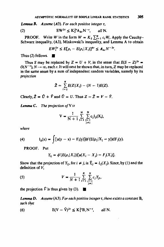
ASYMPTOTIC NORMALITY OF SIMPLE LINEAR RANK STATISTICS 305
Lemma 8. Assume (A3). For each positiue integer r,
(2) EW" 5 K:'Ao,N-', all N.
PROOF. Write W in the form W = K 2 xr= c, U;. Apply the Cauchy- Schwarz inequality, (A3), Minkowski's inequality, and Lemma A to obtain
EW:' 5 E [ p , - E ( p , I X,)I4' 5 A g r N- 2r.
Thus (2) follows.
Thus S may be replaced by Z = U + V, in the sense that E(S - Z)2r = O(N-'), N + 00, each r. It will next be shown that, in turn, Z may be replaced in the same sense by a sum of independent random variables, namely by its project ion
N
i= 1 2 = E(ZIX,) - (N - l)E(Z).
Clearly,2 = 0 + Pand 0 = U.ThusZ - 2 = V - 9.
Lemma C. The projection ofV is
where
I+,
the projection f? is thus given by (3).
Lemma D. Assume (A3). For each positive integer r, there exists a constant B , such that
(6) E(V - 9lzr 5 K:,B,N-', all^.

306 R-ESTIMATES
PROOF. By (3) and (3, N N N
1 1 = 1 I a r p l 11- 1 II *I1
E(V - V ) 2 r = (N + l)-lr " ' C CI," .Cl , , c ..' (7)
where
Consider a typical term of the form (8). Argue that the expectation in (8) is possibly nonzero only if each factor has both indices repeated in other factors. Among such cases, consider now only those terms corresponding to a given pattern of the possible identities i,, = ib , i, = j b , j,, = j b for 1 I; a I; 2r, 1 5 b 5 2r. For example, for r = 3, one such specific pattern is: i2 = i l , i3 # i t , i4 = i l , i5 = i 3 , i6 # i l , 16 # i 3 , j 2 = j l , 13 =jl, i4 P ~ I , h =L j 6 = j , , jl = i3,j4 # i l . In general, there are at most 26r such patterns. For such a pattern, let q denote the number of distinct values among il, . . . , izr and p the number of distinct values among jl,. . . , j . Let p1 denote the number of distinct values amongjl, . . . , j l r not appearing among i l , . . . ,-i2r and put p 2 = p - pI. Within the given constraints, and after selection of il, . . . , i I r , the number of choices for j , , . . . , j t r clearly is of order O(NPa). Now clearly2pl s 2r - p 2 , i.e., pI s r - 3 p 2 . Now let q1 denote the number of i l , . . . , i2, used only once among i l , . . . , i2,. Then obviously qr 5 p z . It is thus seen that the contribution to (7) from summation over jl, . . . , I Z r is of order at most O(Nr-(1/2)gc) , since the quantity in (8) is of magnitude SKY. It follows that
I!
N N
where al, . . , , a, are integers satisfying al 2 1, u1 + *
exactly q1 of the a;s are equal to 1. Now, for (I 2 2, + a, = 2r, and
by (A3). Further,
(9)

ASYMP'IDTIC NORMALITY OF SIMPLE LINEAR RANK STATISTICS 307
Thus N N c . . * c Ic$l . . C"P < N(1/2)ql,
1, I 11= 1 lq= I
and we obtain (6).
Next it is shown that 2 may be replaced by 2 = 0 + v, where N
f = 1 6 = c Cf4(H(XfN
and
with
Lemma E. Assume (A3). Then 12 - 21 S (K2 + 3K1)N-'I2.
PROOF. Check that
And hence
Lemma F. We have 2 - p = T and there exists a constant ' K , = K4(+) such that IES - pl 5 K4N-'/*.

308 R-ESTIMATES
PROOF. The second assertion is shown by Hiijek (1968), p. 340. To obtain the first, check that
N
Now, by integration by parts, for any distribution function G we have
j+'(H(x))G(x)dH(x) = - $(H(x))dG(x) + constant,
where the constant may depend on 4 and H(.) but not on G( . ) . Thus the above sum reduces to 0.
Up to this point, only the scores given by (Al) have been considered. The next result provides the basis for interchanging with the scores given by (A2).
Lemma G. Denote crm c,aN(R,) by S in the case corresponding to (Al) and by S' in the case corresponding to (A2). Assume (A3). Then there exists K5 =
s
K5(4) such that
I S - ES - (S' - ES')( 5 K 5 N - ' 1 2 .
PROOF. It is easily found (see HAjek (1968), p. 341) that
where KO does not depend on i or N. Thus, by (9), ( S - S'I I; KoN-'12 and hence also ( E S - ES') s KoN-'12. Thus the desired assertion follows with
PROOF OFTHEOREM A. Consider first thecase (Al). By Minkowski's
K 5 = 2 K o .
inequality,
(10) [E(S - ES - T)2']1'2' $ [E(S - 2)2']1'2r + [E(Z - 2)"]"2'
+ [E(Z - 2 ) 2 7 " 2 ' + [E(Z - /J - T)2']1/2'
+ ( E S - PI.
By Lemmas B, D, E and F, each term on the right-hand side of (10) may be bounded by K N - l I 2 for a constant K = K ( 4 , r ) depending only on 4 and r. Thus follows the assertion of the theorem. In the case of scores given by (A2), we combine Lemma G with the preceding argument.

ASYMPTOTIC NORMALITY OF SIMPLE LINEAR RANK STATISTICS 309
PROOF OF THEOREM B. First assertion (i) will be proved. Put
aN = suplP(S - ES < x(Var S)"') - @(x)I,
PN = supIP(T c x(Var S)"') - O(x)I,
X
X
and
yN = supIP(T < x(Var T)'/') - @(x)I. x
By Lemma 6.4.3, if
(1 1) B N = O(aN), N --* 00,
for a sequence of constants {aN}, then
(12) d(N = O(U,) + P(JS - ES - TI/(Var S)l" > uN), N 4 OC).
We shall obtain a condition of form (11) by first considering y N . By the classical Berry-Essten theorem (1.9.5),
N
I = 1 YN 5 C(Var T ) - ~ / ' C E I ~ ~ ( X ~ ) I ~ ,
where C is a universal constant. Clearly, N
I = 1 l4(XJl I; KIN-' C Icj - ci I .
Now
By the elementary inequality (Lokve (1977), p. 157)
I X + Y I " I; emlxl" + emlyl'", where m > 0 and 0, = 1 or 2'"-' according as m s 1 or m 2 1, we thus have
and hence
(13)
Check (Problem 9.P.8) that

310 R-ESTIMATES
so that by Theorem A we have
(14) l(Var S)'12 - (Var T)l/zl < M , , N - ' / ~ ,
where the constant Mo depends only on 4. It follows that if Var S is bounded away from 0, then the same holds for Var T, and conversely. Consequently, by the hypothesis of the theorem, and by (12), (13) and (14), we have
Therefore, by (A3) and (A4), y N = O ( N - 'Iz log N), N -+ 00. Now it is easily seen that
By (14) the right-most term is O(N-'/'). Hence / I N = O(N- 'I2 log N). There- fore, for any sequence of constants uN satisfying N-'I2 log = o(u,), we have (1 1) and thus (12). A further application of Theorem A, with Markov's inequality, yields for arbitrary r
Hence (12) becomes
aN = O(UN) + O(ai"N-').
Choosing uN = O(N-'/'"+ 'I), we obtain
aN I fJ(N-'/(zr+l)), N + 00.
Since this holds for arbitrarily large r, the first assertion of Theorem B is established.
Assertions (ii) and (iii) are obtained easily from the foregoing arguments.
PROOF OF THEOREM C. It is shown by Hiijek (1968), p. 342, that
I(Var T)"' - c41 5 2'/'(K1 + K2)sup(F,(x) - F,(x)l.
The proof is now straightforward using the arguments of the preceding proof. I
I , 1, x
PROOF OF THE COROLLARY. By Taylor expansion,
(15) IFh) - a x ) - (-A d,f(x))l s AAZ 4,
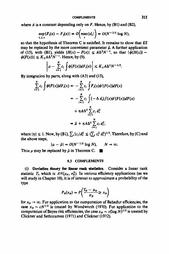
COMPLEMENTS 31 1
where A is a constant depending only on F. Hence, by (Bl) and (B2),
sup IFAX) - Fkx) I = 0 = U(N' log N), 1.1. x
so that the hypothesis of Theorem C is satisfied. It remains to show that ES may be replaced by the more convenient parameter p, A further application of (15), with (Bl), yields IH(x) - F(x)( S AA2N- ' , so that J#(H(x)) - t,b(F(x))) 5 K 1 A A 2 N - ' . Hence, by (9).
By integration by parts, along with (A3) and (15), N
f = 1
N
N
I = I = f i + qAAf C Ci d f ,
where lql 5 1. Now, by (Bl), xi Icild: s (xi c: d:)'12. Therefore, by (C) and the above steps,
Thus p may be replaced by p in Theorem C. l/.t - = O(N"" log N ) , N + 00.
9.3 COMPLEMENTS
(i) Deviation theory for b a r rank statistics. Consider a linear rank statistic Th. which is AN(pN, a;). In various efficiency applications (as we will study in Chapter lo), it is of interest to approximate a probability of the type
for x N + a. For application to the computation of Bahadur efficiencies, the case xN - cN"' is treated by Woodworth (1970). For application to the computation of Bayes risk efficiencies, the case xN - c(log N)'I2 is treated by Clickner and Sethuraman (1971) and Clickner (1972).

312 R-ESTIMATES
(ii) Connection with sampling of finite populations. Note that a two- sample simple linear rank statistic may be regarded, under the null-hypothesis Fl = - . = FN, as the mean of a sample of size m drawn without replacement from the population {a&), . . . ,aN(N)},
(iii) Probability inequalities for two-sample linear rank statistics. In view of (ii) just discussed, see Serfling (1974).
(iv) Further general reading. See Savage (1969). (v) Connections between M-, L-, and R-statistics. See Jaeckel(l971) for
initial discussion of these interconnections. One such relation, as discussed in Huber (1972,1977), is as follows. For estimation of the location parameter 8 of a location family based on a distribution F with density f , by an estimate 8 given as a statistical function T(F,,), where F,, is the sample distribution function, we have: an M-estimate of T(G) is defined by solving
!I& - T(G))dG(x) = 0;
an L-estimate of T(G) is defined by
T(G) = j ~ ( t y ‘ ( rwt ;
an R-estimate of T(G) is defined by solving
It turns out that the M-estimate for $o = - f ‘/ f, the L-estimate for J( t ) = ~ & ( F - ~ ( t ) ) / l , , where IF = I [f’lf]’ dF, and the R-estimate for J ( t ) = ij0(F- ‘(t)), are ail asymptotically equivalent in distribution and, moreover, asymptotically &dent. For general comparison of M-, L- and R-estimates, see Bickel and Lehmann (1975).
9.P PROBLEMS
Section 9.2
1. Complete the details for Example 9.2.2. 2. Prove Lemma 9.2.5 (Projection Lemma). 3. Complete details for proof of Lemma 9.2.68. 4. Details for proof of Lemma 9.2.6C. 5. Details for proof of Lemma 9.2.6D. 6. Details for proof of Lemma 9.2.68. 7. Details for proof of Lemma 9.2.6F.
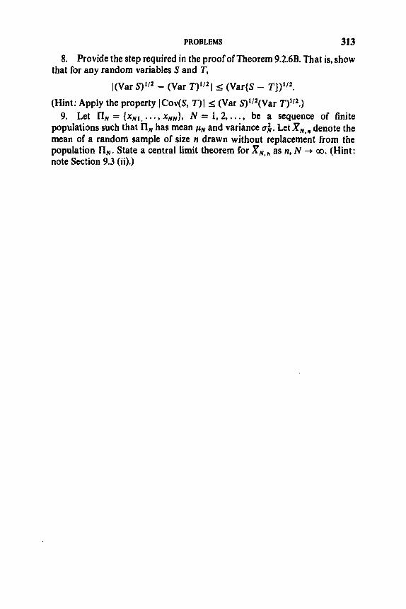
PROBLEMS 313
8. Provide the step required in the proof of Theorem 9.2.68. That is, show that for any random variables S and T,
I(Var s)lI2 - (Var T)*”( s (Var{s - T ) ) ’ ’ ~ .
(Hint: Apply the property )Cov(S, 7’)) s (Var S)’’’(Var T)’I2.) 9. Let nN = {x,,,, ..., x”), N = 1,2, ..., be a sequence of finite
populations such that llN has mean pN and variance cr;, Let X N , n denote the mean of a random sample of size n drawn without replacement from the population nN. State a central limit theorem for XN,n as n, N 4 00. (Hint: note Section 9.3 (ii).)

C H A P T E R 10
Asymptotic
Relative Esciency
Here we consider a variety of approaches toward assessment of the relative efficiency of two test procedures in the case of large sample size. The various methods of comparison differ with respect to the manner in which the Type I and Type I1 error probabilities vary with increasing sample size, and also with respect to the manner in which the alternatives under consideration are required to behave. Section 10.1 provides a general discussion of six con- tributions, due to Pitman, Chernoff, Bahadur, Hodges and Lehman, Hoeff- ding, and Rubin and Sethuraman. Detailed examination of their work is provided in Sections 10.2-7, respectively. The roles of central limit theory, Berry-Esskn theorems, and general deviation theory will be viewed.
10.1 APPROACHES TOWARD COMPARISON OF TEST PROCEDURES
Let H, denote a null hypothesis to be tested. Typically, we may represent Ho as a specified family Fo of distributions for the data. For any test procedure T, we shall denote by T, the version based on a sample of size n. The function
defined for distribution functions F, is called the powerfunction of T, (or of T). For F E .Fo, y,(T, F) represents the probability ofa Type I error. The quantity
an(T, $0) = SUP F) F s F o
is called the size of the test. For F # Po, the quantity
P n V , F) = 1 - Y n ( T F)
314

APPROACHES TOWARD COMPARISON OF TEST PROCEDURES 315
represents the probability of a Type I I error. Usually, attention is confined to consistent tests: for fixed F # So, B,,(T, F ) + 0 as n -+ 00. Also, usually attention is confined to unbiased tests: for F # Po, y,,(T, F) 1 a,,(T, go).
A general way to compare two such test procedures is through their power functions. In this regard we shall use the concept of asymptotic relative eficiency (ARE) given in 1.15.4. For two test procedures TA and TB, suppose that a performance criterion is tightened in such a way that the respective sample sizes n , and n2 for TA and TB to perform "equivalently" tend to 00 but have ratio nl/nz tending to some limit. Then this limit represents the ARE of procedure TB relative to procedure TA and is denoted by e(TB, TA).
We shall consider several performance criteria. Each entails specifications regarding
(a) a = limn a,,(T, Po), (b) an alternative distribution F(") allowed to depend on n,
and (c) B = lim, B,,(T, F'")).
With respect to (a), the cases a = 0 and a > 0 are distinguished. With respect to (c), the cases B = 0 and > 0 are distinguished. With respect to (b), the cases F(") E F (fixed), and F(") + 5, in some sense, are distinguished.
The following table gives relevant details and notation regarding the methods we shall examine in Sections 10.2-7.
Behavior of Behavior of Names of Type I Error Type I1 Error Behavior of Notation Contributors Probability a,, Probability /I,, Alternatives for ARE Section
Pitman a,, -+ a > 0 P,, -+ P > 0 F(") -+ S o ep(- , .) 10.2 F(") = F fixed e d - , .) 10.3
Bahadur a,, -+ 0 fl,, + f l > 0 F(") = F fixed es(., -) 10.4 Hodges & Lehmann a , - + a > O P , + O F") = F fixed eHL( ., +) 10.5
F(") = F fixed eH(- , .) 10.6 Rubin & Sethuraman a,, -+ 0 P n + 0 F(") + S o eRS(- ,*) 10.7
Chernoff a,, + 0 B n -+O
HoelTding a,, -+ 0 B n + 0
Each of the approaches has its own special motivation and appeal, as we shall see. However, it should be noted also that each method, apart from intuitive and philosophical appeal, is in part motivated by the availability of convenient mathematical tools suitable for theoretical derivation of the relevant quantities e(., a). In the Pitman approach, the key tool is central limit

316 ASYMPTOTIC RELATIVE EFFICIENCY
theory. In the Rubin-Sethuraman approach, the theory of moderate deviations is used. In the other approaches, the theory of large deviations is employed. The technique of application of these ARE approaches in any actual statistical problem thus involves a trade-off between relevant intuitive considerations and relevant technical issues.
10.2 THE PITMAN APPROACH
The earliest approach to asymptotic relative efficiency was introduced by Pitman (1949). For exposition, see Noether (1955).
In this approach, two tests sequences T = { T,} and V = { V,} are com- pared as the Type I and Type I1 error probabilities tend to positive limits a and fly respectively. In order that a, + a > 0 and simultaneously fl, -+ f l > 0, it is necessary to consider p,,( .) evaluated at an alternative F(") converging at a suitable rate to the null hypothesis .Fo. (Why?)
In justification of this approach, we might argue that large sample sizes would be relevant in practice only if the alternative of interest were close to the null hypothesis and thus hard to distinguish with only a small sample .On the other hand, a practical objection to the Pitman approach is that the measure of ARE obtained does not depend upon a particular alternative. In any case, the approach is very easily carried out, requiring mainly just a knowledge of the asymptotic distribution theory of the relevant test statistics. As we have .seen in previous chapters, such theorems are readily available under mild restrictions. Thus the Pitman approach turns out to be widely applicable.
In 10.2.1 we develop the basic theorem on Pitman A R E and in 10.2.2 exemplify it for the problem of testing location. The relationships between Pitman ARE and the asymptotic correlation of test statistics is examined in 10.2.3. Some complements are noted in 10.2.4.
10.2.1 The Basic'Theorem
Suppose that the distributions F under consideration may be indexed by a set 0 c R, and consider a simple null hypothesis
to be tested against alternatives
e > 8,.
Consider the comparison of test sequences T = { T,} satisfying the following conditions, relative to a neighborhood Bo s 8 s Bo + S of the null hypothesis.
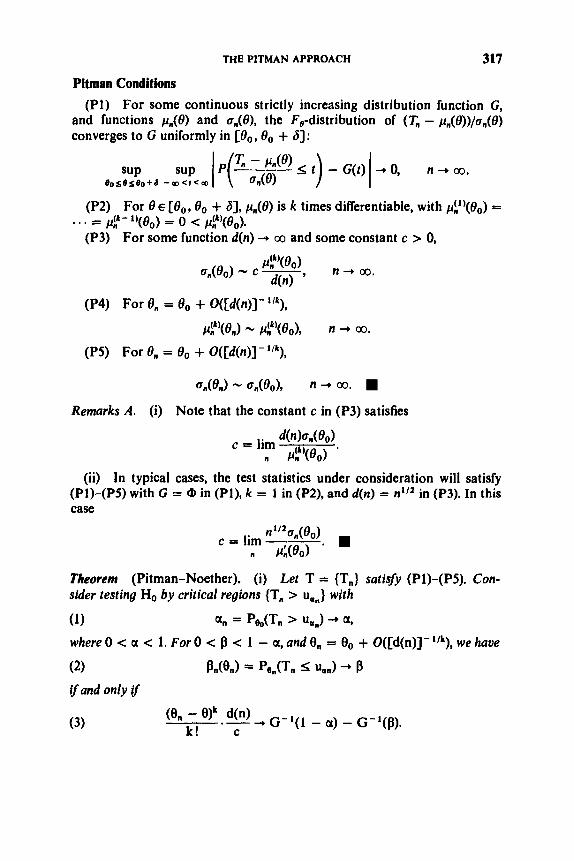
THE PITMAN APPROACH 317
Pitman Conditions
(Pl) For some continuous strictly increasing distribution function G, and functions pn(0) and on(@, the F,-distribution of (T,, - pn(0))/on(O) converges to G uniformly in [e,, 0, + 81:
(P2) For 6~ [O,, 8, + S ] , pn(0) is k times differentiable, with p!')(O0) =
(P3) For some function d(n) . . . = pik- l)(eo) = o < pik)(eo).
00 and some constant c > 0,
(P4) For 0, = 0, + O([d(n)]-l 'k),
(P5) For 8, = 8, + O([d(n)]-'"),
pik'(en) - pik)(eo), n -+ 00.
on(en) N on(Oo), n + 00%
Remarks A. (i) Note that the constant c in (P3) satisfies
(ii) In typical cases, the test statistics under consideration will satisfy (Pl)-(P5) with G = CP in (Pl), k = 1 in (P2), and d(n) = nl/* in (P3). in this case
n"*on(Oo) c = lim . B
n P X ~ O ) Theorem (Pitman-Noether). (i) Let T = {T,} satisjy (Pl)-(PS). Con- sider tesring Ho by critical regions {T,, > uan} with
(1) an = Peo(Tn > urnn) 4 a,
where 0 < a < 1. For 0 < fl < 1 - a, and 8, = 8, + O([d(n)J- we haue
(2) P A W = Po.(Tn uan) -+ P ifand only if
(3)
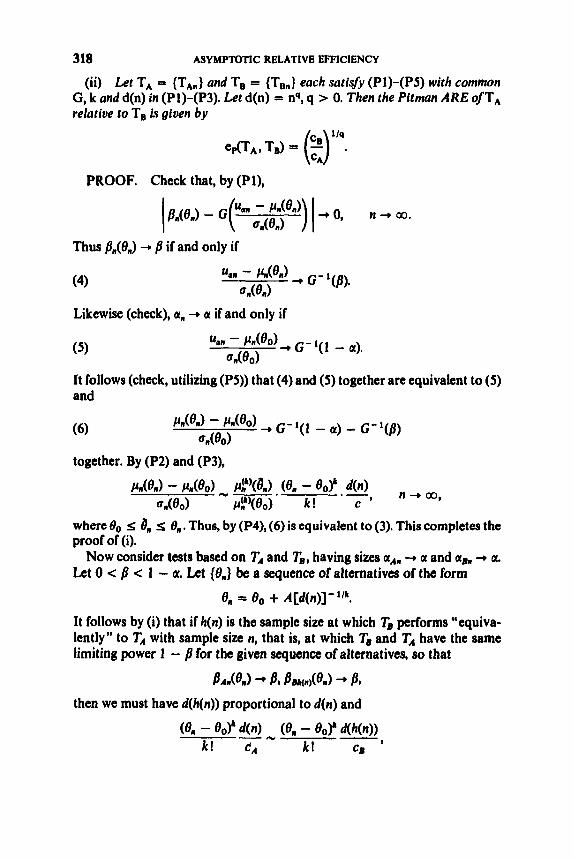
318 ASYMPTOTIC RELATIVE EFFICIENCY
(ii) Let T, = {TAn) and TB = {Tsn) each satigy (Pl)-(PS) with common G, k and d(n) in (Pl)-(P3). Let d(n) = nq, q > 0. Then the Pitman ARB o ~ T A relative to TB is giuen by
PROOF. Check that, by (Pl),
Thus &(O,) -+ /3 if and only if
(4)
Likewise (check), a, -+ a if and only if
It follows (check, utilizing (PS)) that (4) and (5) together are equivalent to (5) and
together. By (P2) and (P3),
9 n-bm, H(U - k(&J F i k ' ( k ) . (0, - e O l k .- 44 a.(e,) pikve0) k ! C
where 0, s 8, s 0,. Thus, by (P4), (6) is equivalent to (3). This completes the proof of (i).
Now consider tests based on TA and TB, having sizes aAn -P a and a,,, -+ a. Let 0 < p < 1 - a. kt (0,) be a sequence of alternatives of the form
0, = e0 + A[d(n)]-''k.
It follows by (i) that if h(n) is the sample size at which TB performs "equiva- lently" to T A with sample size n, that is, at which TB and TA have the same limiting power 1 - for the given sequence of alternatives, 50 that
BAn(8n) -+ pBMm)(en) -b fl, then we must have d(h(n)) proportional to d(n) and
(en - eoY d(n) - (0, - eoY d(h(n)) k! 6 A k! CB '

T m PITMAN APPROACH 319
or
For d(n) = nq, this yields ( / ~ ( n ) / n ) ~ --* (cB/cA), proving (ii). W
Remarks B. (i) By Remarks A we see that for d(n) = nq,
For the typical case k = 1 and d(n) = n112, we have
(ii) For a test T satisfying the Pitman conditions, the limiting power against local alternatives is given by part (i) of the theorem: for
e, = eo + A [ d ( t ~ ) ] - ~ / ~ + o([d(n)]-"'),
we have from (3) that
yielding as limiting power
In particular, for G = @, k = 1, d(n) = we have simply
I - B = 1 -ak-1(1 - a ) - ! ) . c
10.2.2 Example: Teating for Loeation
Let X, , . . . , X , be independent observations having distribution F(x - O), for an unknown value 8 E R, where F is a distribution having density f sym- metric about 0 and continuous at 0, and having variance og < 00. Consider testing
H o : e = o
e > 0.
versus alternatives
For several test statistics, we shall derive the Pitman ARE'S as functions of F, and then consider particular cases of F.

320 ASYMPTOTIC RELATIVE EFFICIENCY
The test statistics to be considered are the “mean statistic” i n
TI, = e x , = x, n l = l
the “ t-statistic”
(where s2 = (n - 1)- 11 ( X , - X),), the “sign test” statistic
and the “ Wilcoxon test” statistic
The statistics based on X have optimal features when F is a normal distri- bution. The sign test has optimal features for F double exponential and for a nonparametric formulation of the location problem (see Fraser (1957), p. 274, for discussion). The Wilcoxon statistic has optimal features in the case of F logistic.
We begin by showing that TI, satisfies the Pitman conditions with Fl,(8) = 8, a:,(@ = a$/n, G = 0. k = 1 and d(n) = dl2. Firstly (justify),
Also,
by now-familiar results. Thus(P1) is satisfied with G = 4. Also, p’&l) = 1, so that (P2) holds with k = 1, and we see that (P3) holds with cI = aF and d(n) = nl/Z. Finally, clearly (P4) and (P5) hold.
We next consider the statistic T,,, and find that it satisfies the Pitman conditions with G = 4, k = 1, d(n) = nilZ, and c2 = c1 -- a,,. Wc take p,,,(e) = O/aF and af,(e) = l/n. Then

THE PITMAN APPROACH
Further, by Problem 2.P.10,
321
sup Po n1I2- s t - Wt) +O, n + 00. ‘ I [ f 1 I Thus (Pl) is satisfied with G = (0. Also, pi,,(@ = l/a, and we find easily that (P2)-(P4) are satisfied with k = 1, d(n) = nilz and, in (P3), c2 = a,.
At this point we may see from Theorem 10.2.1 that the mean statistic and the t-statistic are equivalent test statistics from the standpoint of Pitman ARE:
e,(T,, 7.2) = 1.
Considering now T,, , take
p3,(0) = EeTj, = Eef(X1 > 0) = Pe(X, > 0) = 1 - F ( - 0 ) = F(0)
and
Then
is a standardized binomial (n, F(0)) random variable. Since F(0) lies in a neighborhood off for 8 in a neighborhood of 0, it follows by an application of the Berry-Essden Theorem (1.9.5), as in the proof of Theorem 2.3.3A, that (Pl) holds with G = (0. Also, p;,(0) = f(0) and it is readily found that conditions (P2)-(P5) hold with k = 1, d(n) = nilZ and e3 = 1/2f(O).
The treatment of T4, is left as an exercise. By considering T4“ as a U- statistic, show that the Pitman conditions are satisfied with G = 0, k = 1, d(n) = nilZ and c4 = 1/(12)1’2 f2 (x )dx .
Now denote by M the “mean” test TI, by t the “t-test” G, by S the ‘‘sign” test T3, and by W the “Wilcoxon” test T4. It now follows from Theorem 10.2.1 that
e p W , 0 = 1,
M) = 40:.~(0),
and

322 ASYMPTOTIC RELATIVE EFFICIENCY
(Of course, ep(S, W ) is thus determined also.) Note that these give the same measures of asymptotic relative efficiency as obtained in 2.6.7 for the as- sociated confidence interval procedures.
We now examine these measures for some particular choices of F.
Examples. For each choice of F below, the values of eAS, M ) and er(W, M) will not otherwise depend upon at. Hence for each F we shall take a “con- ventional ’* representative.
(i) F normal: F = CD. In this case,
2 ep(S, M ) = - = 0.637
1c
and 3
er(W, M ) = - = 0.955. 1c
It is of interest that in this instance the limiting value edS, M ) represents the worst efficiency of the sign test relative to the mean (or t-) test. The exact relative efficiency is 0.95 for n = 5,0.80 for n 3: 140.70 for n = 20, decreasing to 2/n = 0.64 as n + 00. For details, see Dixon (1953).
We note that the Wilcoxon test is a very good competitor of the mean test even in the present case of optimality of the latter. See also the remarks following these examples.
(ii) F double exponential: f ( x ) = ie-Ixl, -OD < x < OD. In this case (check)
and er(S, M ) = 2
ep(W, M) = 3.
eP(s, M) = 8 (iii) F unifbrrn: f ( x ) = 1, Ix I < 4. In this case (check)
ond
ep(W, M ) = 1.
(iv) F logistic: f ( x ) = e-x( l + e - x ) - 2 , -OD < x < 00. Explore as an exercise.
Remark. Note in the preceding examples that er(W, M ) is quite high for a variety of Fs. In fact, the inequality
ep( W, M) 2 # = 0.864

THE PITMAN APPROACH 323 is shown to hold for all continuous F, with the equality attained for a partic- ular F, by Hodges and Lehmann (1956).
For consideration of the “normal scores” statistic (recall Chapter 9) in this regard, see Hodges and Lehmann (1961). W
10.2.3 Relationship between Pitman ARE and Correlation
Note that if a test sequence T = {x} satisfies the Pitman conditions, then also the “standardized” (in the null hypothesis sense) test sequence T* = { T:}, where
satisfies the conditions with
and with the same G, k, d(n) and c. Thus, it is equivalent to deal with T* in place of T.
In what follows, we consider two standardized test sequences To = {Ton} and TI = {TI,,} satisfying the Pitman conditions with G = CP, k = 1, d(n) = n1I2, and with constants co 5 c,. Thus e,(Tl, .To) = (co/c1)2 5; 1, so T, is as good as T,, if not better. We also assume condition (P6) To, and T,, are asymptotically bivariate normal uniformly in 0 in a
neighborhood of O0. We shall denote by p(0) the asymptotic correlation of Ton and TI, under the
&distribution. We now consider some results of van Eeden (1963).
Theorem. Let To = {To,} and TI = {TI,} satisfy the conditions (Pl)-(P6) in standardized form and suppose that
P(%) -+ ~ ( 0 0 1 = P* as e n -+ 00 *
(i) For 0 S 1 s 1, tests oftheform
Tin = (1 - h)Ton + satisfy the Pitman conditions.
(ii) The “best” such test, that is, the one which maximizes ep(T,, To), is TT for
ifp # 1 and for y taking any value ifp = 1.
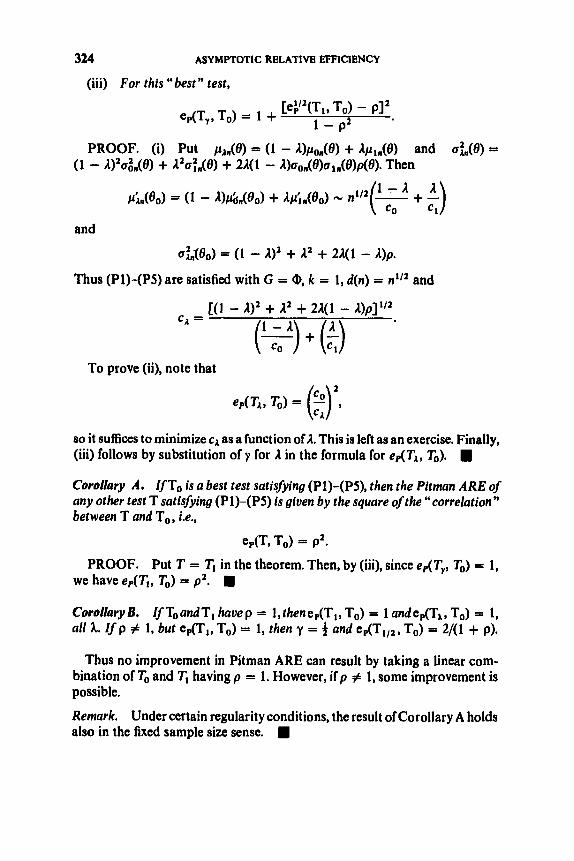
324 ASYMPTOTIC RELATIVE EFFICIENCY
(iii) For this “best” test,
and
a;,,fe0) = (1 - a)z + + 21(1 - I )P.
Thus (Pl)-(PS) are satisfied with G = (D, k = 1, d(n) = nilz and
[(l - A ) Z + P + 2A(1 - I)p]l’Z CA =
(T) + ($) To prove (ii), note that
so it suffices to minimize cA as a function of I. This is left as an exercise. Finally, (iii) follows by substitution of y for I in the formula for ep(TA, To).
Corollary A. IfTo is a best test satisfying (Pl)-(P5), then the Pitman ARE of any other test T satisfying (Pl)-(P5) is given by the square ofthe “correlation” between T and To, i.e.,
e,(T, To) = P2.
PROOF. Put T = TI in the theorem. Then, by (iii)* since ep(T,, To) = 1, we have e,(T,, To) = p2. m CovollaryB. IfToandTl hauep = l,thene,(T,, To) = landedTk, To) = 1, all k. I f p # 1, but ep(TI, To) = 1, then y = 4 and ep(TIIz, To) = 2/(1 + p).
Thus no improvement in Pitman ARE can result by taking a linear com- bination of To and TI having p = 1. However, if p # 1, some improvement is possible.
Remark. Under certain regularity conditions, the result of Corollary A holds also in the fixed sample size sense.

THE CHERNOFF INDEX 325
10.2.4 Complements
(i) Eff’icucy. We note that the strength of a given test, from the standpoint of Pitman ARE, is an increasing function of l/c, where c is the constant ap- pearing in the Pitman condition (P3). The quantity l/c is called the “efficacy” of the test. Thus the Pitman ARE of one test relative to another is given by the corresponding ratio of their respective efficacies.
(ii) Contiguity. A broader approach toward asymptotic power against alternatives local to a null hypothesis involves the notion of “contiguity.” See Hiijek and Sidiik (1967)for exposition in the context of rank tests and Roussas (1972) for general exposition.
10.3 THE CHERNOFF INDEX
One might argue that error probabilities (of both types) of a test ought .to decrease to Oas the sample size tends to 03, in order that the increasing expense be justified. Accordingly, one might compare two tests asymptotically by comparing the rate of convergence to 0 of the relevant error probabilities. Chernoff (1952) introduced a method of comparison which falls within such a context.
Specifically, consider testing a simple hypothesis H o versus a simple alternative H,, on the basis of a test statistic which is a sum of I.I.D.’s,
n
whereby H o is rejected if S, > c,, where c, is a selected constant. For example, the likelihood ratio test for fixed sample size may be reduced to this form (exercise).
For such sums S,, Chernoff establishes a useful large deviation probability result: for t 2 E { Y } , P(S, > nt) behaves roughly like m”, where m is the minimum value of the moment generating function of Y - t . (Thus note that P(S, > nt) decreases at an exponential rate.) This result is applied to establish the following: if c, is chosen to minimize p, + Aa, (where 2 > 0), then the minimum value of p, + l a , behaves roughly like p”, where p does not depend upon 2. In effect, the critical point c, is selected so that the Type I and Type I1 error probabilities tend to 0 at the same rate. The value p is called the index of the test. In this spirit we may compare two tests A and B by comparing sample sizes at which the tests perform equivalently with respect to the criterion fl, + da,. The corresponding ARE turns out to be (log pA)/(log pB).
These remarks will now be precise. In 10.3.1 we present Chernoff’s general large deviation theorem, which is of interest in itself and has found wide application. In 10.3.2 we utilize the result to develop Chernofl’s ARE.

326 ASYMPTOTIC RELATIVE EFFICIENCY
103.1 A Large Deviation Theorem
Let Yl,. . ., Y, be I.I.D. with distribution F and put S, = Yl + ... + Y,. Assume existence of the moment generating function M ( z ) = Ep{ezY}, z real, and put
m(r) = inf E{ex(r-')} = inf e-"M(z).
The behavior of large deviation probabilities P(S, 2 r,), where r, + 00 at rates slower than O(n), has been discussed in 1.9.5. The case tn = tn is covered in the following result.
x I
Theorem (Chernofl). lf - 00 < t 5 E { Y } , then
(1) P(S, 5 nt) 5 [m(t)]".
IfE{Y} 5 t < + 00, then
(2) P(S, ;L nt) 5 [m(t)]".
If0 < E < m(t), thenfor the given cases oft, respectfoely,
(3)
Remark. Thus P(S, 2 nr) is bounded above by [m(r)Y, yet for any small E > 0 greatly exceeds, for all large n, [m( t ) - 6)". W
PROOF. To establish (1) we use two simple inequalities. First, check that for any z 5 0,
P(S, s nt) 4 [e-"M(z)l".
Then check that for t 5 E{ Y } and for any z 2 0, e-"M(z) 2 1. Thus deduce (1). In similar fashion (2) is obtained.
We now establish (3). First, check that it suffices to treat the case t = 0, to which we confine attention for convenience. Now check that if P( Y > 0) = 0 or P(Y < 0) = 0, then m(0) = P(Y = 0) and (3) readily follows. Hereafter we assume that P(Y > 0) > 0 and P(Y < 0) > 0. We next show that the general case may be reduced to the discrete case, by defining
i i - 1 i YU = - if - < Y s; , 1 - -1,0,1,..., s = 1,2, .... S S
Letting Sf) = the sum of the Yr) corresponding to Y4, . . . , x , we have
and P(S, 5 0) 2 P(S!" 5 0)
M(')(z) = E{err")} 2 e-I'I"M(z).
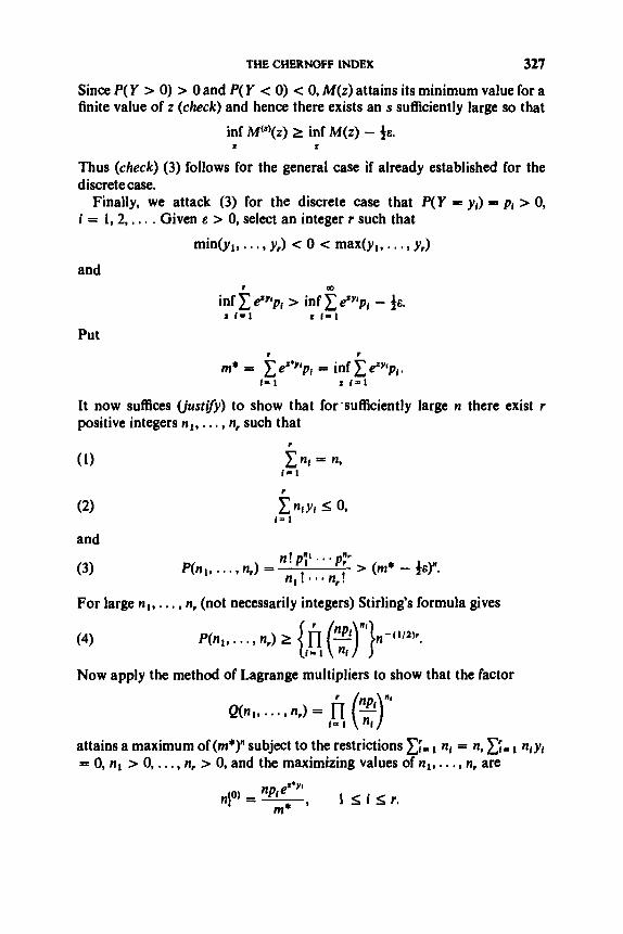
THE CHERNOFF INDEX 327
Since P( Y > 0) > 0 and P( Y < 0) < 0, M(z) attains its minimum value for a finite value of z (check) and hence there exists an s sufficiently large so that
inf M($)(z) 2 inf M ( z ) - IE.
Thus (check) (3) follows for the general case if already established for the discrete case.
Finally, we attack (3) for the discrete case that P(Y = yl ) = p I > 0, i = 1,2,. . . . Given 8 > 0, select an integer r such that
2 2
min(yl, . . . , y r ) -= 0 < max(yl,. . . , y r )
and
Put
r Q)
m* = C e2*y'pI = inf C e'ylp,.
It now suffices (justfy) to show that for.sufficiently large n there exist r positive integers n,, . . . , n, such that
I = I 2 1 = 1
and
(3) n ! p;' . . . p:'
n, ! * * * n,! P(n,, . . . , n,) = > (m* - #@".
For large nl , . . . , n, (not necessarily integers) Stirling's formula gives
(4)
Now apply the method of Lagrange multipliers to show that the factor
Q(n,, . . . , n,) = fi (!!!!)"' 1 - 1
attains a maximum of (rn*)" subject to the restrictions C;= ni = n, C;= nlyi = 0, nl > 0,. . . , n, > 0, and the maximizing values of n,, . . . , n, are

328 ASYMPTOTIC RELATIVE EFFICIENCY
Assume that y l S y , for i I; r, and put
nll) = [nlO)], 2 s i s r,
where C.3 denotes greatest integer part. For large n, the nll) are positive integers satisfying (l), (2) and
and thus (3) by virtue of (4). This completes the proof. W
using “exponential centering,” see the development in Bahadur (1971). The foregoing proof adheres to Chernoff (1952). For another approach,
We have previously examined large deviation probabilities,
P(S, - ss, 2 nr), t > 0,
in 5.6.1, in the more general context 0f.U-statistics. There we derived expon- ential-rate exact upper bounds for such probabilities. Here, on the other hand, we have obtained exponential rate asymptotic approximations, but only for the narrower context of sums S,. Specifically, from the above theorem we have the following useful
Corollary. For t > 0,
lim n-l log P(Sn - ES, 2 nt) = log m(t + E{Y}). n
10.3.2 A Measure of Asymptotic Relative Efficiency
Let H o and Hl be two hypotheses which determine the distribution of Y so that po = E{ Y IH,} I; p, = E { Y lHl}. For each value of f , we consider a testwhichrejectsH,,ifS, > nt.Leta, = P(S, > nrIHo),/3, = P(S, I; nt lH1) and L be any positive number. Put
m,(t) = inf E{ez(r - ‘ ) lHI} , i = 0, 1, 2
and
p( t ) = max{mo(t), m,( t ) } .
The index of the test determined by Y is defined as
p = inf p(t). (rOSlS(rl

THE CHERNOFF INDEX 329
The role of this index is as follows. Let Q,, be the minimum value attained by fin + la,, as the number t varies. Then the rate of exponential decrease of Q, to 0 is characterized by the index p . That is, Chernoff (1952) proves
Theorem. For E > 0,
(Al) Qn lim - = 0.
n (P +el"
PROOF. For any t in [go, p, ] , we immediately have using Theorem 10.3.1 that
Q n 5 P(Sn S nt I HI) + Ap(Sn 2 nt I H o ) 5 Cm,(t)3" + lCmo(t)I" 5 (1 + mm".
Let E > 0 be given. By the definition of p, there exists t l in [&, p l ] such that p(tJ $ p + 4 ~ . Thus (Al) follows.
On the other hand, for any t in [po, p l ] , we have
P(Sn S n t l H , ) 5 P(Sn 5 nt'IH,), all t' 2 t,
and
P(S, 2 nt IH,) 5 P(S, > nt'IHo), all t' 5 t ,
yielding (check)
For 0 10.3.1
Thus,
Q n 2 min{P(Sn S nt lHI) , IP(S,, 2 ntIHo)}.
< E c min{m,(r), ml(t)}, we thus have by the second part of Theorem that
in order to obtain (A2), it suffices to find tz in [ p o , p l ] such that p S min{mo(t2), ml(cz)}. Indeed, such a value is given by
t2 = inf{t: ml(t) 2 p , po 5 t 5 p, } .
First of all, the value t2 is welldefined since ml(pl) = 1 2 p. Next we need to use the following continuity properties of the function m(t). Let yo satisfy
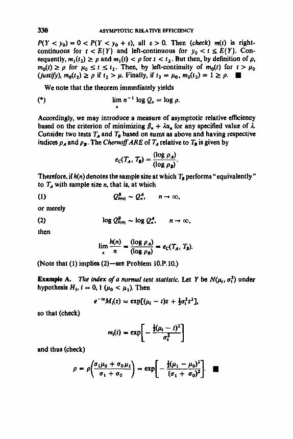
330 ASYMPTOTIC RELATIVE EFFICIENCY
P(Y c yo) = 0 < P(Y < yo + E), all e > 0. Then (check) m(t) is right- continuous for t c E{ Y} and left-continuous for yo < t s E{ Y}. Con- sequently, ml(tz) 2 p and ml(t) c p for t < t,. But then, by definition of p, mo(t) 2 p for p o I; t I; t 2 . Then, by left-continuity of mo(t) for t > po (justify), mo(tz) 2 p if t , > p. Finally, if t , = p o , mo(t2) = 1 2 p. W
We note that the theorem immediately yields
lim n-' log Q, = log p. W
Accordingly, we may introduce a measure of asymptotic relative efficiency based on the criterion of minimizing /3, + Act, for any specified value of 1. Consider two tests TA and TB based on sums as above and having respective indices pA and pB. The ChernoflARE of TA relative to TB is given by
Therefore, if h(n) denotes the sample size at which TB performs "equivalently" to TA with sample size n, that is, at which
(1) Qt.1 - Q,", n + a,
or merely
(2) log Qf(n, log Q,", n + 00,
then
(Note that (1) implies (2)-see Problem 10.P. 10.)
Example A. Tke index of a normal test statistic. kt Y be NM,, a:) under hypothesis HI, i = 0, l (po < b,). Then
e-"M,(z) = exp[(p, - t)z + iub:z2],
so that (check)
and thus (check)

THE CHERNOFF lNDEX 331
Example B. The index of a binomial test statistic. Let Y be B(r. pl) under hypothesis H I , i = 0, l(pp < p l ) . Put q1 = 1 - p l , i = 0, 1. Then
e-"M,(z) = e-"(p,e' + q,)',
so that (check)
and (check)
log p = r { (1 - c)log "1 - 4_" .,I + l o g p g j ,
where
Example C. Comparison of Pitman ARE and Chernoff ARE. To illustrate the differences between the Pitman ARE and the Chernoff ARE, we will con- sider the normal location problem and compare the mean test and the sign test. As in 10.2.2, let X I , . . . , X, be independent observations having distribution F(x - O), for an unknown value 8 E R, but here confine attention to the case F = 4 = N(0, 1). Let us test the hypotheses.
H o : O = 0 versus H I : O = O, ,
where O1 > 0. Let TA denote the mean test, based on X, and let TB denote the sign test, based on n-' I (X, > 0). From Examples A and B we obtain (check)
where a(O) = (logC1 have from 10.2.2
- @(O)]}/log{[l - @(O)]/U)(O)}. By comparison, we
eP(T,, TB) = h. We note that the measure e&T,, TB) depends on the particular alternative under consideration, whereas ep(T,, T,) does not. We also note the com- putational difficulties with the ec measure. As an exercise, numerically evaluate the above quantity for a range of values of O1 near and far from the null value. Show also that ec(T,, T,) 3 in = ep(T,, TB) as O1 3 0. H

332 ASYMPTOTIC RELATIVE EFFICIENCY
10.4 BAHADUR’S “STOCHASTIC COMPARISON ”
A popular procedure in statistical hypothesis testing is to compute the signiJcance leuel of the observed value of the test statistic. This is interpreted as a measure of the strength of the observed sample as evidence against the null hypothesis. This concept provides another way to compare two test procedures, the better procedure being the one which, when the alternative is true, on the average yields stronger evidence against the null hypothesis. Bahadur (196Oa) introduced a formal notion ofsuch “stochasticcomparison” and developed a corresponding measure of asymptotic relative efficiency. We present this method in 10.4.1. The relationship between this “stochastic comparison “ and methods given in terms of Type I and Type I1 error prob- abilities is examined in 10.4.2. Here also the connection with large deoiation probabilities is seen. In 10.4.4 a general theorem on the evaluation of Bahadur ARE is given. Various examples are provided in 10.4.5.
10.4.1 “Stochastic Comparison” and a Measure of ARE We consider I.I.D. observations XI,. , . , X, in a general sample space,
having a distribution indexed by an abstract parameter 0 taking values in a set 0. We consider testing the hypothesis
Ho: l k 0 0
by a real-valued test statistic T,, whereby H o becomes rejected for sufficiently large values of T,. Let Ge, denote the distribution function of T, under the Odistribution of XI,. . , , X,.
A natural indicator of the significance of the observed data against the null hypothesis is given by the “level attained,” defined as
L, = L”(XI, - - X,) = SUp[l .- Gen(T,)]. Bee0
Thequantity SUpe,eo[l - G,,(t)] represents the maximum probability, under any one of the null hypothesis models, that the experiment will lead to a test statistic exceeding the value t. It is a decreasing function oft. Evaluated at the observed T,, it represents the largest probability, under the possible null distributions, that a more extreme value than T, would be observed in a repetition of the experiment. Thus the “level attained” is a random variable representing the degree to which the test statistic T, tends to reject H o . The lower the value of the level attained, the greater the evidence against I f o .
Bahadur (1960) suggests comparison of two test sequences T’, = { TAn} and 7‘’ = { TBn} in terms of their performances with respect to “level attained,” arguing as follows. Under a nonnull Cdistribution, the test T’,, is “more

BAHADUR’S “STOCHASTIC COMPARlSON ”
successful” than the test TBn at the observed sample XI, . . , , X, if
LAn(xl , * * - Y xn) < LBn(xl, * - . Y xn)- Equivalently, defining
K , = -2 log L,,
333
T’,, is more successful than Tsn at the observed sample if K,, > KBn. Note that this approach is a stochastic comparison of TA and TB.
In typical cases the behavior of L, is as follows. For 8 E Oo , L, converges in &distribution to some nondegenerate random variable. On the other hand, under an alternative 8 # Oo, L, 4 0 at an exponential rate depending on 8.
Example. The Location Problem. Let the X,’s have distribution function F(x - O), where F is continuous and 8 E O = [0, 00). Let Qo = (0). Consider the mean test statistic,
x T, = n112 -, QF
where Q: = VarF{X). We have
L n = 1 - G d T J
and thus
Po(& 5 1) = P d G d T , ) 2 1 - 0 = P,(T, 2 G&yl - I ) ) = 1 - Go,,(G;,(l - I ) ) = I ,
that is, under H, L, has thedistribution uniform (0, 1). Note also that
Go, * @ = N(0, 1).
Now consider 8 # Oo. We have, by the SLLN,
P,(n-’”T, -+ 8) = 1,
in which case L, behaves approximately as
1 - @ ( n W ) (2nn)-1W1 exp(-fnP).
That is, in the nonnull case L, behaves approximately as a quantity tending to 0 exponentially fast. Equivalently, K, behaves approximately as a quantity tending to a finite positive limit (in this case 02). These considerations will be made more precise in what follows.
It is thus clear how the stochastic comparison of two test sequences is influenced in the case of nonnull 8 by the respective indices of exponential

334 ASYMPTOTIC RELATIVE EFFICIENCY
convergence to 0 of the levels attained. A test sequence T = {T,} is said to have (exact) slope 48) when 0 “obtains” (that is, when the X i s have 8- distribution) if
(*I n- ‘K, -+ c(e) as . (Pe).
In the nonnull case the limit c(8) may be regarded as a measure of the per- formance of T,; the larger the value of c(8), the “faster” T, tends to reject H o e For two such test sequences TA and TB, the ratio
C A ( 8 ) - cB(@
thus represents a measure of the asymptotic relative efficiency of TA relative to TB at the (fixed) alternative 8. Indeed, if h(n) represents the sample size at which procedure TB performs “equivalently” to TA in the sense of being equally “successful” asymptotically, that is, KB,,(”) may replace K A , in relation (*), then we must have (check)
Thus the (exact) Bahadur ARE of TA relative to 7’’ is defined as eB(TA, TB) = C A ~ ) / C B ( @ .
The qualification “exact” in the preceding definitions is to distinguish from “approximate *’ versions of these concepts, also introduced by Bahadur (1960a), based on the substitution of G for GBn in the definition of L,, where Gk * G for all 8 E 0,. We shall not pursue this modification.
The terminology “s1ope”for c(8) is motivated by the fact that in the case of nonnull 8 the random sequence of points {(n,K,) ,n 2 I } moves out to infinity in the plane in the direction of a ray from the origin, with angle tan‘ ‘~(0) between the ray and the maxis.
A useful characterization of the slope is as follows. Given e, 0 c e < 1, and the sequence { X i } , denote by N(E) the random sample size required for the test sequence { T,} to become significant at the level e and remain so. Thus
N(e) = inf{m: L, < E, all n 2 m } ( S 00).
Bahadur (1967) gives
Theorem. If(*) holds, with 0 < c(9) < 00, then

BAHADUR’S “STOCHASTIC COMPARISON *’ 335
PROOF. Let S2 denote the sample space in the Pe-model. By (*), 3R0 c R such that Pe(S2o) = 1 and for the sequence {X,(w)} is such that n-’K,(w) + c(8). Now fix w €a,,. Since c(8) > 0, we have L,(w) > 0 for all sufficiently large n and t , (w) 4 0 as n + 00. Therefore (justify), N(E, o) < m for every E > 0 and thus N(E, w ) --* 00 through a subsequence of the integers as e + 0. Thus 2 5 N(E, w ) < 00 for all E sufficiently small, say <el. For all 8 < E ~ , we thus may write
The proof is readily completed (as an exercise). W
It follows that the sample sizes N&) and NB(e) required for procedures TA and TB to perform “equivalently,” in the sense of becoming and remaining significant at level E, must satisfy
LN(C,U)(~) L N ( c . ~ , ) -
providing another interpretation of the Bahadur ARE. Another important aspect of the Bahadur ARE is the connection with
Type I and Type I1 error probabilities. Not only does this afford another way to interpret eB, but also it supports comparison with other ARE measures such as e p and ec. These considerations will be developed in 10.4.2. and will lead toward the issue of computation of eB, treated in 10.4.3.
Futther important discussion of slopes and related matters, with references to other work also, is found in Bahadur (1960a, 1967,1971).
10.4.2 Relationship between Stocbastic Comparison and Error Probabilities Consider testing Ho by critical regions { T, > t,,} based on { T,}. The relevant Type I and Type I1 error probabilities are
a, = SUP Pe(T, > t,,) B e e o
and
respectively. B R ( @ = PdT, 5; tJ9
Theorem (Bahadur). Suppose that - 2 log an
+ d n

336 ASYMPTOTIC RELATIVE EFFICIENCY
Then
(0
(ii)
d > c(e) =, P,@) -, 1,
d < c(e) =, p,(e) -* 0.
and
PROOF. Write
Bn(8) Po(& > an) = Po (Kn < - 2 log an) = Pe(n-'K, < n-'(-2 loga,)).
If d > 48) + E, then for n sufficiently large we have n-'(-2 log u,) > 46) + e and thus Bn(6) 2 PAn- 'K, < 48) + e) + 1, proving (i). Similarly, (ii) is proved.
Corollary. Suppose that
- 2 log a, n + d,
and
Then d = c(0).
By virtue of this result, ke see that eB(TA, TB), although based on a concept of "stochastic comparison," may also be formulated as the measure of ARE obtained by comparing the rates at which the Type I error probabilities (of TA and TB) tend to 0 while the Type I1 error probabilities remain fixed at (or tend to) a value b(8), 0 < p(8) < 1, for fixed 8. That is, if h(n) denotes the sample size at which TB performs equivalently to 7'' with sample size n, in the sense that
then

BAHADUR’S “STOCHASTIC COMPARISON ” 337
Therefore, in effect, the Bahadur ARE relates to situations in which having small Type I error probability is of greater importance than having small Type I1 error probabilities. In Section 10.5 we consider a measure of similar nature but with the roles of Type I and Type I1 error reversed. In comparison, the Chernoff ARE relates to situations in which it is important to have both types of error probability small, on more or less an equal basis.
Like the Chernoff ARE, the Bahadur ARE depends upon a specific alterna- tive and thus may pose more computational difficulty than the Pitman ARE. However, the Bahadur ARE is easier to evaluate than the Chernoff ARE, because it entails precise estimation only of a,, instead of both a, and 8.. This is evident from the preceding corollary and will be further clarified from the theorem of 10.4.3.
10.4.3 A Basic Theorem
We now develop a result which is of use in finding slopes in the Bahadur sense. The test statistics considered will be assumed to satisfy the following con- ditions. We put O1 = 0 - Oo.
Bahadur Conditions (Bl) For B E 01,
n-’12T, -+ b(8) as. (Po),
where -00 < b(8) < 00.
function g continuous on I, such that (B2) There exists an open interval I containing (b(8): 8 E e,}, and a
lim -2n- ’ log sup [l - Ge,,(n”2t)] = &),
Theorem (Bahadur). 1fT. satisfies (Bl)-(B2), thenfor 8 E 0,
r €1. n eeeo
n- ’ K, + g(b(9)) as. (Pe).
PROOF. Fix 8 E O,, and let R denote the sample space in the Pe-model. By (Bl), 30, c R such that Pe(R0) = 1 and for w E R, the sequence {X,(w)} is such that n- ’ /2T, (o) -+ b(8). Now fix w E Q,, For any E > 0, we have
n1/2(b(8) - E ) < T,(o) < n1’2(b(8) + E )
for all sufficiently large n, and thus also
-2 log sUPeeeo C1 - GeJn’”(b(8) + &))I Kn(w) n n
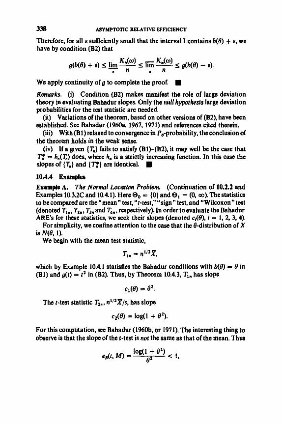
338 ASYMPTOTIC RELATIVE EFFICIENCY
Therefore, for all E sufficiently small that the interval I contains b(8) f E, we have by condition (B2) that
We apply continuity of g to complete the proof.
Remarks. (i) Condition (B2) makes manifest the role of large deviation theory in evaluating Bahadur slopes. Only the null hypothesis large deviation probabilities for the test statistic are needed.
(ii) Variations of the theorem, based on other versions of (B2), have been established. See Bahadur (1960a, 1967,1971) and references cited therein.
(iii) With (Bl) relaxed to convergence in P,-probability, the conclusion of the theorem holds in the weak sense.
(iv) If a given {T,} fails to satisfy (Bl)-(B2), it may well be the case that T,’ = h,(T,) does, where h, is a strictly increasing function. In this case the slopes of {T.} and {T:} are identical.
10.4.4 Examples Example A. The Normal Location Problem. (Continuation of 10.2.2 and Examples 10.3.2C and 10.4.1). Here Oo = {0} and 63, = (0, 00). The statistics to becompared are the “mean” test, “t-test,” “sign” test, and “Wilcoxon” test (denoted T,,, T,,, T3, and T&,, respectively). In order to evaluate the Bahadur ARES for these statistics, we seek their slopes (denoted c@), I = 1, 2, 3,4).
For simplicity, we confine attention to the case that the &distribution of X is N(8, 1).
We begin with the mean test statistic,
T,, = n*I2X,
which by Example 10.4.1 statisfies the Bahadur conditions with b(0) = 0 in (BI) and g(t) = t2 in (B2). Thus, by Theorem 10.4.3, T,, has slope
cl(e) = 8,.
c2(e) = iog(i + ez).
The t-test statistic T2,, n’12X/s, has slope
For this computation, see Bahadur (1960b, or 1971). The interesting thing to observe is that the slope of the t-test is not the same as that of the mean. Thus

BAHADUR’S “STOCHASTIC COMPARISON ” 339
so that the r-test and mean test are not equivalent from the standpoint of Bahadur ARE, in contrast to the equivalence from the standpoint of Pitman ARE, as seen in 10.2.2. (For further evidence against the t-test, see Example C below.)
The slope of the sign test statistic, T,, = n1I2(2V, - l), where
n
v, = C I ( X , > O), I = 1
may be found by a direct handling of the level attained,
It is shown by Bahadur (1960b) that
log H(p)] + 2(npq)”2(, log
where p = we), q = 1 - p, H ( y ) = 2yy(1 - for 0 < y < 1, and
112 112 t n = (p4)- n (V, - P)*
Since Cn N(0, l), we have
Thus it is seen that T’, has slope
c,(e) = 2 10g{2@(8)*(~)[1 - We can also obtain this result by an application of Theorem 10.4.3, as follows. Check that condition (Bl) holds with b(8) = 2@(0) - 1. Next use Chernors Theorem (specifically, Corollary 10.3.1) in conjunction with Example 10.3.2B, to obtain condition (B2). That is, write 1 - GOn(n112t) = P(V, > )(t + 1)) and apply the Chernoff results to obtain (B2) with g(t) = 2 log H(fi1 + t)), for H ( y ) as above. We thus have
2 iOg{2qe)*(~)ci - cp(e)ll-*(e)) 82 M) =
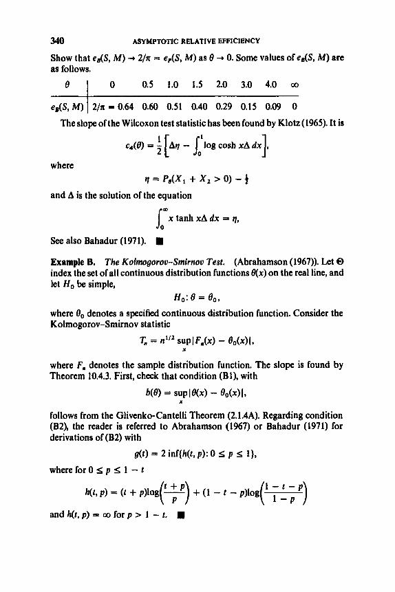
e
eB(S, M)
cJB) = A b q - j,'log cosh x A dx , 2 1
0 0.5 1.0 1.5 2.0 3.0 4.0 co
2/71 = 0.64 0.60 0.51 0.40 0.29 0.15 0.09 0
where q = PO(X, + x , > 0) - 4
and A is the solution of the equation
c x tanh XA dx = q,
See also Bahadur (1971).
Example B. The Kolmogoroo-Srnirnou Test. (Abrahamson (1967)). Let 0 index the set of all continuous distribution functions e(x) on the real line, and let Ho be simple,
where 8, denotes a specified continuous distribution function. Consider the Kolmogorov-Smirnov statistic
H,: 8 = e0,
T, = sUPIF,,(X) - eo(x)l, x
where F,, denotes the sample distribution function. The slope is found by Theorem 10.4.3. First, check that condition (Bl), with
= SUP I w - e O ( 4 I , X
follows from the Glivenko-Cantelli Theorem (2.1.4A). Regarding condition (B2), the reader is referred to Abrahamson (1967) or Bahadur (1971) for derivations of (B2) with
g(t) = 2 inf{h(t, p ) : 0 5 p 5 l},
where for 0 < p < 1 - t
and h(t, p ) = 00 for p > 1 - t. H
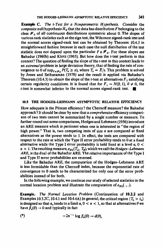
THE HODGES-LEHMANN ASYMPTOTIC RELATIVE EFFICIENCY 341
Example C. The t-Test for a Nonparametric Hypothesis. Consider the composite null hypothesis Ho that the data has distribution F belonging to the class So of all continuous distributions symmetric about 0. The slopes of various rank statistics such as the sign test, the Wilcoxon signed-rank test and the normal scores signed-rank test can be obtained by Theorem 10.4.3 in straightforward fashion because in each case the null distribution of the test statistic does not depend upon the particular F E 9,. For these slopes see Bahadur (1960b) and Klotz (1965). But how does the t-test perform in this context? The question of finding the slope of the t-test in this context leads to an extremal problem in large deviation theory, that of finding the rate of con- vergence to 0 of supFeSo P(T, 2 a), where T, = X/s . This problem is solved by Jones and Sethuraman (1978) and the result is applied via Bahadur’s Theorem (10.4.3) to obtain the slope of the t-test at alternatives F, satisfying certain regularity conditions. It is found that for F, = N(8, I), 8 # 0, the t-test is somewhat inferior to the normal scores signed-rank test.
10.5 THE HODCES-LEHMANN ASYMPTOTIC RELATIVE EFFICIENCY
How adequate is the Pitman efficiency? the Chernoff measure? the Bahadur approach? It should be clear by now that a comprehensive efficiency compari- son of two tests cannot be summarized by a single number or measure. To further round out some comparisons, Hodges and Lehmann (1956) introduce an ARE measure which is pertinent when one is interested in “the region of high power.” That is, two competing tests of size a are compared at fixed alternatives as the power tends to 1. In effect, the tests are compared with respect to the rate at which the Type I1 error probability tends to 0 at a fixed alternative while the Type I error probability is held fixed at a level a, 0 < a -= 1. The resulting measure, eHL(TA, Ts), which we call the Hodges-Lehmann ARE, is the dual of the Bahadur ARE. The relative importances of the Type I and Type I1 error probabilities are reversed.
Like the Bahadur ARE, the computation of the Hodges-Lehmann ARE is less formidable than the Chernoff index, because the exponential rate of convergence to 0 needs to be characterized for only one of the error prob- abilities instead of for both.
In the following example, we continue our study of selected statistics in the normal location problem and illustrate the computation of eHL(. , .).
Example. The Normal Location Problem (Continuation of 10.2.2 and Examples 10.3.2C, 10.4.1 and 10.4.4A) In general, the critical region { T, > t,,} is designed so that a,, tends to a limit a, 0 < a c 1, so that at alternatives 8 we have P,(O) + 0 and typically in fact
(9 - 2n - log p,,(e) -, d(8),
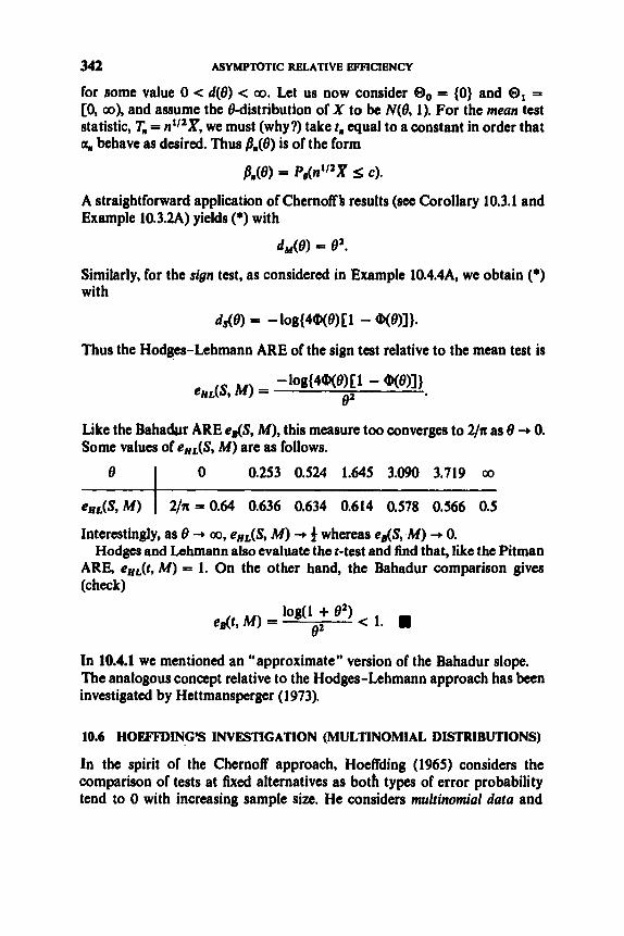
342 ASYMPTOTIC RELATIVE EFFICIENCY
for some value 0 < d(0) < 00. Let us now consider 6, = (0) and 0, = [0, a), and assume the B-distribution of X to be N(B, 1). For the meun test statistic, T, = n112X, we must (why?) take t, equal to a constant in order that or, behave as desired. Thus B,(B) is of the form
p,,(e) = P, (~PX 5 c).
A straightforward application of Chernoff B results (see Corollary 10.3.1 and Example 10.3.2A) yields (*) with
dM(e) - 82.
Similarly, for the sign test, as considered in Example 10.4.4A, we obtain (*) with
ds(e) = -1og{4a(e)[i - uqe)]).
Thus the Hodges-Lehmann ARE of the sign test relative to the mean test is
Like the Bahadur ARE e& M), this measure too converges to 2/n as 8 + 0. Some values of enL(S, M) are as follows.
e l 0 0.253 0.524 1.645 3.090 3.719 00
enL(S, M) I 2/n = 0.64 0.636 0.634 0.614 0.578 0.566 0.5
Interestingly, as 0 + GO, eHL(S, M) + 4 whereas e&M) + 0. Hodges and Lehmann also evaluate the t-test and find that, like the Pitman
ARE, eHL(t, M) = 1. On the other hand, the Bahadur comparison gives (check)
In 10.4.1 we mentioned an “approximate” version of the Bahadur slope. The analogous concept relative to the Hodges-Lehmann approach has been investigated by Hettmansperger (1973).
10.6 HOEFFDINC’S INVESTIGATION (MULTINOMIAL DISTRIBUTIONS)
In the spirit of the Chernoff approach, Hoeffding (1965) considers the comparison of tests at fixed alternatives as both types of error probability tend to 0 with increasing sample size. He considers muftinomid d m and

HOEFFDING'S INVESTIGATION (MULTINOMIAL DISTRIBUTIONS) 343
brings to light certain superior features of the likelihood ratio test, establishing the following
Proposition. I f a given test of size a,, is "suficiently diflerent " from a likeli- hood ratio test, then there is a likelihood ratio test of size Sa,, which is con- siderably more powerful then the given test at "most" points in the set of alternatives when the sample size n is large enough, provided that a,, tends to 0 at a suitably fast rate.
In particular, Hoeffding compares the chi-squared test to the likelihood ratio test and finds that, in the sense described, chi-square tests of simple hypotheses (and of some composite hypotheses) are inferior to the cor- responding likelihood ratio tests.
In 10.6.1 we present a basic large deoiation theorem for the multinomial distribution. This is applied in 10.6.2 to characterize optimulity of the likeli- hood ratio test. Connections with information numbers are discussed in 10.6.3, The chi-squared and likelihood ratio tests are compared in 10.6.4, with dis- cussion of the Pitman and Bahadur ARES also.
10.6.1 A Large Deviation Theorem
Here we follow Hoeffding (1965), whose development is based essentially on work of Sanov (1957). A treatment is also available in Bahadur (1971).
Let z,, = (nl/n, . . . , nJn) denote the relative frequency vector associated with the point (n l , . . . , nk) in the sample space of the multinomial ( p l , . . . , pk; n) distribution. Let 0 be the parameter space,
Let P,,( - I p) denote the probability function corresponding to the parameter p. Thus
For any subset A of 0, let A(") denote the set of points of the form z,, which lie in A. We may extend the definition of P,,(.) to arbitrary sets A in 0 by defining
Pn(A I P) = Pn(A'"'I PI* For points x = (xl, . . . , x k ) and p = (pl, . . . , pk) in @,define

344 ASYMP"€)TIC RELATIVE EFFICIENCY
As will be seen in 10.6.3, this function may be thought of as a distance between the points x and p in 0. For sets A c 0 and A c 8, define
and
These extend I(x, p) to a distance between a point and a set. In this context, "large deviation** probability refers to a probability of the form P,,(Alp) where the distance &A, p) is positive (and remains bounded away from 0 as n + 00).
Theorem. For sets A c 0 and points p E 0, we have uniJbrmly
Remarks. (i) The qualification "uniformly" means that the O( 0 ) function depends only on k and not on the choice of A, p and n.
(ii) Note that the above approximation is crude, in the sense of giving an asymptotic expression for log P,,(A I p) but not one for P,(A 1 p). However, as we have seen in Sections 10.3-10.5, this is strong enough for basic applications to asymptotic relative efficiency.
(iii) If the set A corresponds to the critical region of a test (of a hypothesis concerning p), then the above result provides an approximation to the asymp- totic behavior of the error probabilities. Clearly, we must confine attention to tests for which the size a,, tends to 0 faster than any power of n. The case where a,, tends to 0 more slowly is not resolved by the present development. (See Problem 10.P.19).
10.6.2 The Emergence of the Likelihood Ratio Test It is quickly seen (exercise) that
(1) P,,(z, I p) = P,,(z, I z,,)e- "('n* '1
Now consider the problem of testing the hypothesis
versus an alternative H,: PEA(A c 0)
H : P E A ' = 0 - A ,
on the basis of an observation Z, = Z,,. The likelihood ratio (LR) test is based on the statistic
SuPr6A pfl(z#lP) - e-nI(xn,A)
SUPpc A P"(% I PI -
HOEFFDING’S INVESTIGATION (MULTINOMIAL DISTRIBUTIONS) 345
(since 0 S I (x , p) I; 00 and I(x, x) = 0). Thus the LR test rejects H, when
Z(z,, A) > constant.
Now an arbitrary test rejects Ho when z, E A, where A, is a specified subset of 0. By the theorem, the size a, of the test A, satisfies
a, = sup pn(~,lp) = e-n~(A!?.A)+o(lorN
Let us now compare the test A, with the LR test which rejects I f o when z, E En, where
D, = {x: f(x, A) 2 c,}
P e A
and
C, = I ( A r ) , A).
The critical region B, contains the critical region A,. In fact, En is the union of all critical regions of tests A; for which I (A; , A) 2 c,, that is, of all tests A; with size <a, (approximately). Moreover, the size a,‘ of the test B, satisfies .: = - ncn + O(10r n)
since I(@’, A) = c,. Hence we have
log a,’ = log a, + O(log n).
Therefore, if the size a, 4 0 faster than any power of n, the right-hand side is dominated by the term log a,, so that the sizes of the tests are approximately equal.
These considerations establish: Given any test A, of size a,, such that a, 4 0 faster than any power of n, there exists a LR test which is uniformly at least US powerful and asymptotically of the same size. (Why uniformly?)
Furthermore, at “most” points p E 0 - A, the test En is considerably more powerful than A n , in the sense that the ratio of Type I1 error probabilities at p tends to 0 more rapidly than any power of n. For we have
At these points p for which
and
we have that the ratio of error probabilities 40 faster than any power of n.

346 ASYMP"IC RELATIVE EFFICIENCY
10.6.3 The Function Z(x, p ) p8 a Distance; Information
The function I(x, p) has a natural generalization including distributions other than multinomial. Suppose that a model is given by a family of distributions {Fe, B E 0). For any distributions Fb, and F,,, suppose that Fe0 and F,, have densities fe, with respect to some measure p, for example the measure dp = fidFe, + dF8,). Define
with fe, log(feJfe,) interpreted as 0 where &(x) = 0 and interpreted as 00 where feo(x) > 0, fe , (x) = 0. Note that this is a generalization of I(x, p). For example, let j t be counting measure.
I(F, G ) is an asymmetric measure of distance between F and G. We have
(i) 0 S I(F, G) 5 ao; (ii) If I(F, G) < 00, then F 4 G and I(F, G ) = I log(dF/dG)dF; (iii) I(F, G ) = 0 if and only if F 3: G.
I(F, G) represents an information measure. It measures the ability to dis- criminate against G on the basis of observations taken from the distribution F. As such, this is asymmetric. To see what this means, consider the following example from Chernoff (1952).
Example Let 0 = {p = (pl, pa): p f 2 0, pI + p 2 = 1). Consider the dis- tributions po = (1,O) and p1 = (0.9,O.l). We have
I(Po9 PI) < a, I(P1, Po) = 00.
What does this mean? If p1 is the true distribution, only a finite number of observations will be needed to obtain an observation in the second cell, completely disproving the hypothesis po. Thus the ability of pI to discrimi- nate against po is perfect, and this is measured by I(pl, po) = 00. On the other hand, if po is the true distribution, the fact that no observations ever occur in the second cell will build up evidence against pI in only a gradual fashion. In general, points on the boundary of 0 are infinitely far from interiors points, but not vice versa.
Let us now interpret statistically the large deviation theorem of 10.6.1, which may be expressed in the form
pn(~lp) = e - n W " ) . p ) + O ( l o l n ) e
The quantity I(A("), p) represents the shortest distance from the point p to the set A("). Suppose that A is the critical region of a test: "reject H,: p = po when the observed relative frequency vector falls in the region A."The above approximation tells us that the size a,, of the test is'not much increased by

THE RUBIN-SETHURAMAN “BAYES RISK” EFFICIENCY 347
adjoining to A all points whose “distance” from po is at least I(A, po). The test so obtained is at least as powerful, since the new critical region contains the first, and has approximately the same size. It turns out that the latter test is simply the LR test.
10.6.4 Comparison of %‘.and LR Tests From the considerations of 10.6.2, we see the superiority of the LR test over the xz test, with respect to power at “most” points in the parameter space, provided that the tests under consideration have size a, tending to 0 at a suitably fast rate. The superiority of the LR test is also affirmed by the Bahadur approach. From Abrahamson (1965) (or see Bahadur (1971)), we have for the x2 test the slope
Cl@) = 21(A(fA Po), Po), where po is the (simple) null hypothesis, and
and we have for the LR test the slope
It is readily checked that cl(@ s cz(8), that is, cZ(o) = w e , p0).
eB(xZ,LR) s 1.
As discussed in Bahadur (1971), the set E on which cl(8) = cz(0) is not yet known precisely, although some of its features are known.
With respect to Pitman ARE, however, the x2 and LR tests are equivalent. This follows from the equivalence in distribution under the null hypothesis, as we saw in Theorem 4.6.1.
10.7 THE RUBINSEXHURAMAN “BAYES RISK *’ EFFICIENCY
Rubin and Sethuraman (1965b) consider efficiency of tests from a Bayesian point of view, and define the “Bayes Risk” ARE of two tests as the limit of the ratio of sample sizes needed to obtain equal Bayes risks. Namely, for a statistical procedure T,,, and for e > 0, let N(s ) denote the minimum no such that for sample size n > no the Bayes risk of T, is <E. Then the Rubin- Sethuraman ARE of a test TA relative to a test TB is given by
By “Bayes risk of T,” is meant the Bayes risk of the optimal critical region based on T,.

348 ASYMPTOTIC RELATIVE EFFICIENCY
Illustration. Consider the parameter space 0 = R. Let the null hypothesis be Ho : 8 = 0. Let l(8, i ) , i = 1,2, denote the losses associated with accepting or rejecting Ho, respectively, when 8 is true. Let A@, 8 E 0, denote a prior distribution on 0. Then the Bayes risk of a critical region C based on a statistic T, is
Bn(c) = f ( o ) ~ o , ~ ) P O ( T , Ec) + l + o f ( ~ ~ ~ ( o , ~)P#(T, cw
and the “Bayes risk of T,,” is B:(T) = inf, B,(C). Typically, an asymptotically optimal critical region is given by
C, = { T, > c(Iog n)’”},
where T, is normalized to have a nondegenerate limit distribution under Ho. Thus moderate deviation probability approximations play a role in evaluating B:(T). Why do we wish to approximate the rate at which B:( T) + 01 Because these approximations enable us to compute eRs(. , . ). In typical problems, it is found that B:(T) satisfies
B,*(T) - g(c:n-’(log n)), n 00,
where g is a function depending on the problem but not upon the particular procedure T. For two such competing procedures, it thus follows by inverting g(.) that
Moreover, in typical classical problems, this measure eRs(. , .) coincides with the Pitman ARE. Like the Pitman approach, the present approach is “local” in that the (optimal) Bayes procedure based on T places emphasis on “local” alternatives. However, the present approach differs from the Pitman approach in the important respect that the size of the test tends to 0 as n + GO. (Explain), I
1O.P PROBLEMS
Section 10.2
1. Complete details for proof of Theorem 10.2.1. 2. Provide details for the application of the Berry-Eden theorem in
showing that the sign test statistic considered as T’, in 10.2.2 satisfies the Pitman condition (Pl). Check the other conditions (P2)-(P5) also.
3. Show that the Wilcoxon statistic considered as T4, in 10.2.2 satisfies the Pitman conditions.

PROBLEMS
4. Do the exercises assigned in Examples 10.2.2. 5. Complete details of proof of Theorem 10.2.3.
Section 103
349
6. Show that the likelihood ratio test may be represented as a test
7. Complete the details of proof of Theorem 10.3.1. 8. Complete the details of proof of Theorem 10.3.2. 9. Verify Corollary 10.3.1 and also relation (*) in 10.3.2.
10. Let {a,) and (6,) be sequences of nonnegative constants such that
11. Let {a,} and (6,) be sequences of nonnegative constants such that
12. Supply details for Example 10.3.2A. 13. Supply details for Example 10.3.2B. 14. Supply details for Example 10.3.2C.
statistic of the form of a sum of 1.1.D.’~.
a, -+ 0 and a, - 6,. Show that log a, - log 6,.
a, -+ 0 and log a, - log b,. Does it follow that a, - 6,?
Section 10.4
equivalent performance, as asserted in defining eB. 15. Justify that en(,, .) is the limit of a ratio h(n)/n of sample sizes for
16. Complete the details of proof of Theorem 10.4.1. 17. Complete details on computation of the slope of the sign test in
Example 10.4.4A.
Section 10.5
18. Complete details for Example 10.5.
Section 10.6
19. Consider two tests { T,,}, {T:} having sizes a,, a$ which satisfy
log a: = log a,, + O(log n), n 4 a.
Show that if a, 3 0 faster than any power of n, then the right-hand side is dominated by the term log a,. Thus, if a,+O faster than any power of n, then log a,* - log a,. Show, however, that this does not imply that a,* - a,.
20. Verify relation (1) in 10.6.2. 21. Check that the Bahadur slope of the x 2 test does not exceed that of the
LR test, as discussed in 10.6.4.
Section 10.7
22. Justify the assertion at the conclusion of Example 10.7.

This Page Intentionally Left Blank

Appendix
1. CONTINUITY THEOREM FOR PROBABILITY FUNCTIONS
If events {B,,) are monotone (either B , c B2 c limit B, then
lim P(E,) = P(B).
or B , 3 B2 3 ...) with
n*@
2. JENSENS INEQUALITY
If g(.) is a convex function on R, and X and g ( X ) are integrable r.v.’s, then
B(E{X)) w . l ( X ) ) .
3. BORELYCANTELLI LEMMA
(i) For arbitrary events {BJ, if I,, P(B,,) < 00, then P(B,, infinitely often) = 0.
(ii) For independent events {Em}, if & P(B,,) = 00, then P(B,, infinitely often) = 1.
4. MINKOWSKI’S INEQUALITY
For p 2 1, and r.v.’s X,, ..., X,,,
351

352 APPENDIX
5. FATOU’S LEMMA
If X n 2 0 wpl , then
E !ig X, 5 lim E { X n } . {n-m } n-m
6. HELLY’S THEOREMS
(i) Any sequence of nondecreasing functions
f‘,(x), J‘,(x), * * * 9 Fn(x), * * *
which are uniformly bounded contains at least one subsequence
f‘n,(x), Fn,(x), * * 9 Fn,,(x), * *
which converges weakly to some nondecreasing function F(x).
decreasing uniformly bounded functions (ii) Let f ( x ) be a continuous function and let the sequence of non-
F,(x), F,(x), * * * 9 FAX), * - - converge weakly to the function F(x) on some finite interval a S x S b, where a and b are points of continuity of the function F(x) ; then
b b
n+ lim m Ja f (xwFn(x ) = [ . / ( x ) ~ x ) -
(iii) If the function J ( x ) is continuous and bounded over the entire real line -00 i: x < 00, the sequence of nondecreasing uniformly bounded functions Fl(x) , F2(x), . . . converges weakly to the function F(x), and Fn( - 00) + F( - a) and Fn( + 00) + F( + a), then
n-rm iim J’j(xwFn(x) = J ’~xw~(x) .
7. HOLDER’S INEQUALITY
For p > 0 and q > 0 such that l/p + l/q = 1, and for random variables X and

References
Abrahamson, 1. 0. (1965), “On the stochastic comparison of tests of hypotheses,” Ph.D.
Abrahamson, 1. G. (1967), “The exact Bahadur efficiencies for the Kolmogorov-Smirnov and
Abramowitz, M. and Stegun, 1. A. (1965), eds. Handbook of Marhemurical Functions, National
Andrews, D. F.. Bickel, P. J., Hampel, F. R., Huber, P. J., Rogers, W. H., and Tukey, J. W.
Apostol, T. M. (1957), Marhemarical Analysis, Addison-Wesley, Reading, Mass. Arvesen, J. N. (l969), “Jackknifing U-statistics,” Ann. Marh. Srarisr., 40, 2076-2100. Bahadur, R. R. (l960a), “Stochastic comparison of tests,” Ann. Marh. Srarisi., 31,276-295. Bahadur, R. R. (1960b), “Simultaneous comparison of the optimum and sign tests of a normal
mean,” in Contributions lo Prob. and Srarisr.-Essays in Honor of Harold Hotelling, Stanford University Press, 79-88.
Bahadur, R. R. (1966). “A note on quantiles in large samples,’’ Ann. Marh. Sratisr., 37,577-580. Bahadur, R. R. (1967), “Rates of convergence of estimates and test statistics,” Ann. Math.
Bahadur, R. R. (1971), Some Limit Theorems in Sraristics, SIAM, Philadelphia. Bahadur, R. P,. and Ranga Rao, R. (1960). “On deviations of the sample mean,” Ann. Marh.
Bahadur, R. R. and Zabell, S. L. (1979), “Large deviations of the sample mean in general vector
Basu, D. (1956), “On the concept of asymptotic relative efficiency,” Sankhyd, 17,93-96. Baum, L. E. and Katz, M. (1965), “Convergence rates in the law of large numbers,” Trans.
Bennett, C. A. (l952), “Asymptotic properties of ideal linear estimators,” Ph.D. dissertation,
Bennett, G. (1962), “Probability inequalities for the sum of independent random variables,” J.
Beran, R. (1977a), “Robust location estimates,” Ann. Statist., 5,431-444.
dissertation, University of Chicago.
Kuiper one- and two-sample statistics,” Ann. Marh. Srarisr., 38, 1475-1490.
Bureau of Standards, U.S. Government Printing Office, Washington, D.C.
(1972). Robust Esrimares of Locution. Princeton University Press, Princeton, N.J.
S t ~ t i ~ t . , 38, 303-324.
Stutisr., 31, 1015-1027.
spaces,” Ann. Prob., 7, 587-621.
Amer. Math. Soc., 120, 108-123.
University of Michigan.
Amer. Starist. dssoc., 57, 33-45.
353

354 REFERENCES
Beran, R. (1977b), “Minimum Helhger distance estimates for parametric models,” Ann.
BergatrSm, H. and Puri, M. L. (1977), “Convergence and remainder terms in linear rank
Berk, R. H. (1966), “Limiting behavior of posterior distributions when the model is incorrect,”
Berk, R. H. (1970), “Consistency a posteriori,” Ann. Marh. Sfarisr., 41,894-907. Berman, S. M. (l963), “Limiting distribution of the studentized largest observation,” Skand.
Berry, A. C. (1941), “The accuracy of the Gaussian approximation to the sum of independent
Bhapkar, V. P. (196l), “Some tests for categorical data,” Ann. Mafh. Sfatisr., 32,7243. Bhapkar, V. P. (1966), “A note on the equivalence of two test criteria for hypotheses in categoti-
Bhattacharya, R. N. (1977), “Refinements of the multidimensional central limit theorem and
Bhattacharya, R. N. and Rango Rao. R. (1976). Normal Approximarion and Asymptofic Expan-
Bickel, P. J. (1974), “ Edgeworth expansions in nonparametric statiatics,” Ann. Stafisr., 2, 1-20. Bickel, P. J., and Doksum, K. A. (1977). Marhemarical Sfafisrics, Holden-Day, San Francisco. Bickel, P. J. and Lehmann, E. L. (1975), “Descriptive statistics for nonparametric models. 1.
Introduction,” Ann. Sfarisr., 3,1038-1044; “11. Location,” Ann. Srarist., 3,1045-1069. Bickel, P. J. and Rosenblatt, M. (1973), “On some global measures of the deviations of density
function estimates,” Ann. Statist., 1, 1071-1096. Billingsley, P. (1968), Conwrgence oJProbabiliry Measures, Wiley. New York. Bjerve, S. (1973, “Error bounds for linear combinations of order statistics,” Ann. Srafist., 5,
Blom, 0. (l976), “Some properties of incomplete U-statistics,” Biometrika, 63, 573-580. BOnner, N. and Kirschner, H.-P. (1977), “Note on conditions for weak convergence of von
Boos, D. D. (1977). “The differential approach in statistical theory and robust inference,”
Booa, D. D. (1979). “A difkrential for L-statistics,” Ann. Sfarist., 7,955-959. Boos, D. D. and Serfling, R. J. (1979), “On Berry-Esakn rates for statistical functions, with
Breiman, L. (1968), Probability. Addison-Waley, Reading, Mass. Brillinger, D. R. (l969), “An asymptotic representation of the sample distribution function,’’
Brown, B. M. and Kildea, D. 0. (1978). “Reduced U-atatistics and the Hodges-Lehmann esti-
Callaen, H. and Janssen, P. (l978), “The Berry-Essten theorem for U-statistics,” Ann. Statist.,
Cantelli, F. P. (1933), “Sulla determinazione empirica delle leggi di probabilita,” Giorn. Insr.
Carroll, R. J. (1978). “On almost sure expansions for M-estimatee,” Ann. Statist., 6, 314-318.
Sfarisr., 5, 445-463.
statistics,” Ann. Sfarisf., 5,671-680.
Ann. Marh. Srarisr.. 37. 51-58.
Akruarieridskr., 46, 154-161.
variables,” Trans. Amer. Marh. Soc., 49, 122-136.
cal data,” J. Amer. Sfarisf. Assoc., 61,228-236.
applications,” Ann. Prob., 5, 1-27.
sions, Wiley, New York.
357-369.
Misea’ differentiable itatistical functions,” Ann. Srarisr., 5, 405-407.
Ph.D. dissertation. Florida State University.
application to L-estimates,” Preprint.
Bull. Amer. Marh. Soc., 75,545-547.
mator,” Ann. Statist., 6,828-835.
6,417-421.
Ital. Affuari, 4,421-424.

REFERENCES 355
Chan, Y. K. and Wierman, J. (1977), “On the Berry-Eden theorem for &statistics,” Ann.
Cheng, B. (1965), “The limiting distributions of order statistics,” Chinese Marh,, 6,84-104. Chernofl, H. (1952), “A measure of asymptotic efficiency for tests of an hypothesis based on
Chernof, H. (1954), “On the distribution of the likelihood ratio,” Ann. Math. Starisr., 25,
ChernotT, H. (l956), “Large-sample theory: parametric case,” Ann. Marh. Srarisr., 27,1-22. ChernotT, H., Gastwirth, J. L., and Johns, M. V., Jr. (1967). “Asymptotic distribution of linear
combinations of order statistics, with applications to estimation,” Ann. Marh. Srarisr.,
ChernotT, H. and Savage, 1. R. (1958). “Asymptotic normality and efficiency of certain non-
Chibisov, D. M. (1965), “An investigation of the asymptotic power of the tests of fit,” 771. Prob.
Chung, K. L. (l949), “An estimate concerning the Kolmogorov limit distribution,” Trans. Amer.
Chung, K. L. (1950), Nores on Limir Theorems, Columbia Univ. Graduate Mathematical
Chung, K. L. (l974), A Course in Probabiliry Theory, 2nd ed., Academic Press, New York. Clickner, R. P. (1972), “Contributions to rates of convergence and efficiencies in* non-para-
metric statistics,” Ph.D. dissertation, Florida State University. Clickner, R. P. and Sethuraman, J. (1971), “Probabilities of excessive deviations of simple
linear rank statistics-the two-sample case,” Florida State University Statistics Report M226, Tallahassee.
Collins, J. R. (l976), “ Robust estimation of a location parameter in the presence of asymmetry,” Ann. Statist., 4, 68-85.
Cramtr, H. (1938), “Sur un nouveau thtor&me-limite de la thkorie des probabilitts,” A d . Sci., er Ind., 736, 5-23.
Cramtr, H. (1946), Marhemarical Methods of Sratisrics, Princeton Univ. Press, Princeton. Cramtr, H. (t970), Random Variables and Probabiliry Disrriburions, 3rd ed., Cambridge Univ.
CramCr, H. and Wold, H. (1936), “Some theorems on distribution functions,” J . London Math.
Cshki. E. (l968), “An iterated logarithm law for semimartingales and itsapplication toempirical
David, H. A. (1970), Order Srarisrics, Wiley, New York. Davidson, R. and Lever, W. (1970), “The limiting distribution of the likelihood ratio statistic
deHaan, L. (l974), “On sample quantities from a regularly varying distribution function.”
Dieudonnt, J. (1960), Foundarions of Modern Analysis, Wiley, New York, Dixon, W. J. (1953), “Power functions of the sign test and power efficienc;y for normal alterna-
Donsker, M. (1951), “An invariance principle for certain probability limit theorems,” Mem.
Rob., 5, 136-139.
the sum of observations,” Ann. Marh. Srarisr., 23,493-507.
573-578.
38,52-72.
parametric test statistics,” Ann. Marh. Srarisr., 29, 972-994.
Applic., 10,421-437.
Math. SOC., 67, 36-50.
Statistical Society (mimeo).
Press, Cambridge.
SOC., 11, 290-295.
distribution function,” Srudia Sci. Math. Hung., 3,287-292.
under a class of local alternatives,” Sankhyd, Ser. A, 32,209-224.
Ann. Srarisr., 2, 815-818.
tives,” Ann. Math. Statist., 24,467473.
Amer. Marh. Soc., 6.
\

356 REFERENCES
Doob, J. L. (1953), Srochastic Processes, Wiley, New York. Dudley, R. M. (1969), “The speed of mean Glivenko-Cantelli convergence,” Ann. Math.
Dunford, N. and Schwartz, J. T. (1963), Linear Operators, Wiley, New York. Durbin, J. (1973a), Distribution neory for Tests Based on the Sample Distribution Function,
SIAM, Philadelphia, PA. Durbin, J. (1973b), “Weak convergence of the sample distribution function when parameters
are estimated,” Ann. Statist., I , 279-290. Duttweiler, D. L. (l973), The mean-square error of Bahadur’s order-statistic approximation.”
Ann. Siarist., I, 446-453. Dvoretzky, A. Kiefer, J., and Wolfowitz, J. (1956), “Asymptotic minimax character of the
sample distribution function and of the classical multinomial estimator,” Ann. Marh. Statist., 27,642-669.
Dwas, M. (1956). “The large-sample power of rank tests in the two-sample problem,” Ann. Math. Statist., 27, 352-374.
Dwass, M. (1964), “Extremal processes,” Ann. Math. Statist., 35, 1718-1725. Eicker, F. (1966), “On the asymptotic representation of sample quantiles,” (Abstract) Ann.
Eseten. C. 0. (1945). “Fourier analysis of distribution functions,” Acta Math., 77, 1-125. Eseten, C. G. (1956), “ A moment inequality with an application to the central limit theorem,”
Skand. Aktuarietidskr., 39, 160-170. Feder, P. 1. (1968)‘ “On the distribution of the log likelihood ratio test statistic when the true
parameter is ‘near’ the boundaries of the hypothesis regions,” Ann. Math. Sratisr., 39, 2044-2055.
Feller, W. (1957, 1966), An Introduction to Probability Theory and Its Applicarions, Vol. I (2nd edit.) and Vol. 11, Wlley, New York.
Ferguson, T. S. (1958), “A method of generating best asymptotically normal estimates with application to the estimation of bacterial densities,” Ann. Math. Statist., 29, 1046-1062.
Ferguson, T. S. (l967), MathematicalStarisrics: A Decision Theoretic Approach, Academic Press, New York.
Filippova, A. A. (1962), “Mises’ theorem on the asymptotic behavior of functionals of empirical distribution functions and its statistical applications,” Th. h o b . Applic., 7, 24-57.
Finkelstein, H. (l97l), “The law of the iterated logarithm for empirical distributions,” Ann. Math. Starist., 42, 607-615.
Sratisr., 40,4040.
Math. Srarisr., 37, 1424.
Fisher, R. A. (1912), “On an absolutecriterion for fitting frequency curves,” Mess. olMarh.,Ql, 155.
Fraser. D. A. S. (l957), Nonparametric Methods in Statisrics, Wiley, New York. Frtchet, M. (1925), “La notion de differentielie dans I’analyse generale,” Ann. Ecole. Norm.
Frtchet, M. and Shohat, J. (1931), “A proof of the generalized second limit theorem in the
Freedman, D. (1971), BrowniaN Motion and Difusion, Holden-Day, San Francisco. Funk, 0. M. (1970), “The probabilities of moderate deviations of O-statistics and excessin
deviations of Kolmogorov-Smirnov and Kuiper statistics,” Ph.D. dissertation, Michigan State University.
Sup., 42,293.
theory of probability,” Trans. Amer. Math. SOC., 33.
REFERENCES 357
Gaenssler. R. and Stute, W. (1979), “Empirical processes: a survey of results for independent
Galambos, J. (l978), The Asymproric Theory ofExtreme Order Srarisrics, Wiley, New York. Gastwirth, J. L. (1966). “On robust procedures,” J . Amer. Statist. Assoc., 61.929-948. Geertsema, J. C. (1970), “Sequential confidence intervals based on rank tests,” Ann. Math.
Ghosh, J. K. (1971). “A new proof of the Bahadur representation of quantiles and an appli-
Glivenko. V. (l933), ”Sulla determinazione empirica delta legge di probabilita,” Giorn. Rsr .
Gnedenko, B. V. (1943). “Sur la distribution limite du terme maximum d’un serie albatoire,”
Gnedenko, B. V. (1962), The Theory ofProbability, 4th ed., Chelsea, New York. Gnedenko, B. V. and Kolmogorov, A. N. (1954), Limit Disfribution for Sums of Independent
Grams, W . F. and Serfling. R. J. (1973), “Convergence rates for LI-statistics and related
Gregory, G. G. (1977), “Large sample theory for U-statistics and test of fit,” Ann. Statist., 5,
Gupta, S . S. and Panchapakesan, S. (1974), “Inference for restricted families: (A) multiple decision procedures, (B) order statistics inequalities,” Froc. Conference on Reliability and Biometry, Tallahassee (ed. by F. Proschan and R. J. Serfling), SIAM, 503-596.
Hhjek, J. (196l), “Some extensions of the Wald-Wolfowitz-Noether theorem,” Ann. Math.
Hajek, J. (l962), “Asymptotically most powerful ranktests,” Ann. Morh. Sratisf., 33, 1124-1 147. Hhjek, J. (l968), “Asymptotic normality of simple linear rank statistics under alternatives.”
Hhjek. J. and Sidhk, Z. (1967), Theory of Rank Tests, Academic Press, New York. Hall, W. J., Kielson, J. and Simons. G. (1971), “Conversion of convergence in the mean to
almost sure convergence by smoothing,” Technical Report, Center for System Science, Univ. of Rochester, Rochester, N.Y.
and identically distributed random variables,” Ann. Frob., 7 , 193-243.
Statisf., 41, 1016-1026.
cation,” Ann. Math. Sratist., 42, 1957-1961 I
Ital. Attuari, 4, 92-99.
Ann. Math., 44,423453.
Random Variables, Addison-Wesley, Reading. Mass.
statistics,” Ann. Statist., I, 153-160.
110-123.
Stati~t., 32, 506-523.
Ann. Math. Statist., 39, 325-346.
Halmos, P. R. (1946), “The theory of unbiased estimation,” Ann. Marh. Statisr., 11,3443.
Halmos, P. R. (1950). Measure Theory. Van Nostrand, Princeton. Hampel, F. R. (1968). “Contributions to the theory of robust estimation,” Ph.D. dissertation,
Hampel, F. R. (1974), “The influence curve and ts role in robust estimation,” J. Amer. Statisr.
Hardy, G. H. (1952), A Course of Pure Mathematics, 10th ed., Cambridge University Press,
Hartman, P. and Wintner, A. (1941), “On the law of the iterated logarithm,” Amer. J . Marh.,
Healy, M. J. R. (I968), “Disciplining of medical data,” British Med. Bull., 24, 210-214. Helmers, R. (l977a), “The order of the normal approximation for linear combinations of order
Univ. of California.
ASSOC., 69, 383-397.
New York.
63, 169-176.
statistics with smooth weight functions,” Ann. Prgb., 5,940-953.

358 REFeRENCES
Helmers, R. (1977b). “ A Berry-EssCen theorem for linear combinations of order statistics,”
Hettmansperger, T. P. (1973). “On the Hodges-Lehmann approximate efficiency,” Ann. Insr.
Hoadley, A. B. (1967). “On the probability of large deviations of functions of several empirical
Hodges, J. L., Jr. and Lehmann, E. L. (1956), “The efficiency of some nonparametric com-
Hodgcs, J. L.. Jr., and Lchmann, E. L. (196l), “Comparison of the normal scoresand Wilcoxon
Hoeffding, W. (1948), “ A class of statistics with asymptotically normal distribution,” Ann.
Hoeffding, W. (1961), “The strong law of large numbers for U-statistics,” Univ. of North
Hoeffding, W. (1963). “Probability inequalities for sums of bounded random variables,” J.
Hoeffding, W. (1%5), “Asymptotically optimal tests for multinomial distributions” (with dis-
Haffding. W. (l973), “On the centeringof a simple linear rank statistic,” Ann. Sfafisr., 1,54-66. Hotelling, H. and Pabst, M. R. (1936), “Rank correlation and tests of significance involving no
assumption of normality,” Ann. Marb. Srutisr., 7,2943. Hsu, P. L. (1945), “The limiting distribution of functions of sample means and application to
testing hypotheses,” Proc. Firsf Berkeley Symp. on Math. Sfailsf. and Prob., 359-402. Hsu, P. L. and Robbins, H. (1947). “Complete convergence and the law of large numbers,”
Proc. Nat. Acad. Sci. U.S.A., 33,25-31. Huber, P. J. (1%4), “Robust estimation of a location parameter,” Ann. Marh. Statfar., 35,
Huber, P. J. (1972), “Robust statistics: a review,” Ann. M a I . Starts/., 43, 1041-1067. Huber, P. J. (1973), “Robust regression: Asymptotics, conjectures and Monte Carlo,” Ann.
Huber, P. J. (l977), Robusr Sraristical Procedures, SIAM, Philadelphia. Ibragimov, I. A. and Linnik, Yu. V. (1971), Independent and Stationary Sequences o/Randorn
Jaeckel, L. A. (l97l), ‘‘ Robust estimatesoflocation: symmetry and asymmetriccontamination,”
James, B. R. (1975), “ A functional law of the iterated logarithm for weighted empirical distri-
Jones, D. H. and Scthuraman, J. (1978), “Bahadur efficiencies of the Student’s I-tats,” Ann.
Jung, 1. (1955). “On linear estimates defined by a continuous weight function,’’ Arkiv. fur
JurcEkovh. J. and Puri, M. L. (1975), “Order of normal approximation Tor rank test statistic
Kawata, T. (1951). “Limit distributions of single order statistics,”,Rep. Star. Appl. Res. Union
Preprint.
Srarisi. Marh., 25, 279-286.
cdf‘s,” Agn. Marh. Srarisr., 38,360-381.
petitors of the t-test,” Ann. Math. Srarlsr., 27,324-335.
tests,” Proc. 4rh Berk. Symp. on Math. Starist. and Prob., Vol. I, 307-317.
Math. Srarisr., 19, 293-325.
Carolina Institute OF Statistics Mimeo Series, No. 302.
h e r . Srarisr. Assoc., 58, 13-30.
cussion), Ann. Marh. Starisr., 36,369-408.
73-101.
Srarist., I, 799-821.
Variables, Wolters-Noordhoff, Groningen, Netherlands.
Ann. Math. Srarisr.. 42, 1020-1034.
butions,” Ann. Prob., 3, 762-772.
Sratisr., 6, 559-566.
Maiemarik, 3, 199-209.
distribution,” Ann. Prob., 3, 526-533.
of Jap. Scientists and Engineers, I, 4-9.

REFERENCBS 359
Kiefer, J. (1961). “On large deviations of the empiric D. F. of vector chance variables and a law
Kiefer, J. (l967), “On Bahadur’s representation of sample quantiles,” Ann. Math. Statist., 33,
Kiefer, J. (1970a), “Deviations between the sample quantile process and the sample df,” Proc. Coderence on Nonparametric Techniques in Statistical Iderence, Bloomington (ed. by M. L. Puri), Cambridge University Press, 299-319.
Kiefer, J. (1970b). “Old and new methods for studying order statistics and sample quantiles,”
Kiefer, J. and Wolfowitz, J. (1958), “On the deviations of the empiric distribution function of
Kingman, J. F. C. and Taylor, S . J. (l966), Introduction to Measure and Probability, Cambridge
Klotz, J. (1965), “Alternative efficiencies for signed rank tests,” Ann. Math. Statist., 36, 1759-
Kolmogorov. A. N. (1929), “Uber das Gesetz des iterierten Logarithmus.” Math. Annalen,
Kolmogorov, A. N. (1933), “Sulla determinazione empirica di una legge di distribuzione,” Giurn. Inst. Ital. Attuari, 4, 83-91.
Komlc)s, J., Major, P. and Tusnhdy, 0. (1975), “An approximation of partial sums of indepen- dent rv’s, and the sample df. 1.” Z . Wahrscheinlichkeitstheorie und uerw. Gebiete, 32, 111-131.
Lai, T. 2. (1975), “On Chernoff-Savage statistics and sequential rank tests,” Ann. Statist., 3, 825-845.
Lai, T. L. (1977), “Power-one tests based on sample sums,” Ann. Statist., 5,866-880. Lamperti, J. (1964), “On extreme order statistics,” Ann. Math. Statist., 35, 1726-1737. Lamperti, J. (1966), Probability, Benjamin, New York. Landers, D. and Rogge, L. (1976), “The exact approximation order in the central limit theorem
for random summation,” 2. Wahrscheinlichkeitstheorie und. Verw. Gebiete, 36, 269-283. LaCam, L. (1960), “Locally asymptotically normal families of distributions,” Llniu. of Calg
Public. in Statist., 3, 37-98. Lehmann, E. L. (1951), “Consistency and unbiasedness of certain nonparametric tests,”
Ann. Math. Statist., 22, 165-179. Liapounoff, A. (1900), “Sur une proposition de la thborie des probabilitb,” Bull. Acad. Sci.
St. Phtersbourg, 13, 359-386. Liapounoff, A. (1901), “Nouvelle forme du thtortme sur la limite de probabilid,” Mdm. Acad.
Sci. St. PJtersbourg, 12, No. 5 . Lindgren, B. W . (1968), Statistical Theory, 2nd ed., Macmillan, Toronto. Lloyd, E. H. (1952), “Least-squares estimation of location and scale parameters using order
Lobve. M. (1977), Probability Theory I. 4th ed., Springer-Verlag, New York. Lotve, M. (1978), Probability Theory II,4th ed., Springer-Verlag, New York. Loynes, R. M. (1970), “An invariance principle for reversed martingales,” Proc. h e r . Math.
Luenbcrger. D. 0. (1969), Optimization by Vector Space Methods, Wiley, New York.
of iterated logarithm,” Pacific J . Math., 11,649-660.
1323-1342.
IMd., 349-357.
vector chance variables,” Trans. Amer. Math. Soc., 87, 173-186.
University Press, Cambridge.
1766.
101, 126-136.
statistics.” Biometrika, 34, 41-67.
Soc., 25, 56-64.

360 REFBRENCES
Lukacs, E. (1970), Characferisfic Funcfions, 2nd ed., Hafner, New York. Mann, N. R.. Schaefer, R. E., and Singpurwalla, N. D. (1974), Mefhodr for Sfarisfical Analysis
Marcinkiewicz, J and Zygmund, A. (1937). “Sur les fonctions ind&pendantw,” f ind. Math.,
Mejzler, D. and Weissman, 1. (1969), “On some results of N. V. Smirnov, concerning limit distributions for variational series,” Ann. Math. Sfafisf., 40,480-491.
Miller, R. G., Jr. and Sen. P. K. (1972), “Weak convergence of U-statistia and von Mises’ differentiable statistical functions,’’ Ann. Math. Sfafisf., 43,3141.
Nandi, H. K. and Sen, P. K. (1963), “On the properties of U-statistics when the observations are not independent. Part II . Unbiased estimation of the parametera ofa finite population,” Cal. Sfafisf. Assoc. Bull., 12, 125-143.
Nashed, M. 2. (1971). “Differentiability and related properties of nonlinear operators: some aspects of the role of differentials in nonlinear functional analysis,” in Nonlinear fincfional Analysis and Applicafions (edit, by L. 9. Rall), Academic Press, New York, 103-309.
Natanson, 1. P. (l96l), Theoryoffinrfionsofa Real Variable, Vol. I, rev. ed., Ungar, New York. Neuhaus. 0. (1976). “Weak convergence under contiguous alternatives of the empirical
process when parameters are estimated: the Dh approach,” Proc. Cod on Emphicar Distributions and ProcesseJ, Oberwolfach (ed. by P. Gaenssler and P. RCvCsz), Springer- Verlag, 68-82.
Neyman, J. (1949). “Contributions to the theory of the x’ test,” First Berk. Symp. on Math. Statist and Prob., 239-273.
Newman, J. and Pearson, E. S. (l928), “On the use and interpretation of certain test criteria for purposes of statistical inference,” Biometrika, MA, 175-240 and 263-294.
Noether, G. E. (1955). “On a theorem of Pitman.” Ann. Math. Statist., 26.64-68. Noether, G. E. (1967), Elements ofNonparametric Siafisfics, Wiley, New York. 0gasawara.T. and Takehashi, M. (l95l), “Independence ofquadratic forms in normal system,”
O’Reilly, N. E. (1974), “On the weak convergence of empirical processes in sup-norm metrics,”
Parthasarathy, K. P. (1967), Probability Measureson Mefric Spaces, Academic Press, New York. pearson, K. (1894), “Contributions to the mathematical theory of evolution,” Phil. 7lans.
Petrov, V. V. (1966), “On the relation between an estimate of the remainder in the central limit
Petrov, V. V. (1971), “A theorem on the law of the iterated logarithm,” 771. hob. Applic., 16,
Pitman, E. J. G. (1949), “Lecture Notes on Nonparametric Statistical Inference,” Columbia
Portnoy, S. L. (1977), “Robust estimation in dependent situations,” Ann. Statist., $22-43. Puri, M. L. and Sen, P. K. (1971), Nonparametric Mefhodc In Multivariate Analysis, Wiley, New
Pyke, R. (196% “Spacings,” J. Roy Staffst. SOC. (B), 27,395436 (with discussion), 437-449. Pyke, R. (l972), “Spacings revisited,” Proc. 6fh Berk. Symp. on Math. Sfatisf. and Prob., Vol.
of Reliability and Ll/r Data, Wiley, New York.
29, (50-90.
J. Sci. Hiroshima Univ., 1s. 1-9.
Ann. Prob., 4,642-65 I.
Roy. Soc., London, A, lES, 71-78.
theorem and the law of the iterated logarithm,” Th. Bob. Applic., 11,454458.
700-702.
University.
York.
I, 41 7-427.

REFERENCES 361
Pyke, R. and Shorack, G. (1968), “Weak convergence of a two-sample empirical process and a
Raghavachari, M. (l973), “Limiting distributions of Kolmogorov-Smirnov type statistics
Ranga Rao, R. (1962), “Relations between weak and uniform convergence of measures with
Rao, C. R. (1947), “Large sample tests of statistical hypotheses concerning several parameters
Rao, C. R. (1973), Linear Starisrical Inference and I r s Applications, 2nd ed., Wiley, New York. Rao, J. S. and Sethuraman, J. (1975), “Weak convergence of empirical distribution functions
of random variables subject to perturbations and scale factors,” Ann. Sraiisf., 3, 299-313. Reiss, R.-D. (1974), “On the accuracy of the normal approximation for quantiles,” Ann. Prob.,
Renyi, A. (1953), “On the theory of order statistics,” Acta Math. Acad. Sci. Hung., 4,191-231. RCvCsz, P. (l968), The Laws of Large Numbers, Academic Press, New York. Richter, H. (1974). “Das Gesetz vom iterierten Logarithmus fur empirische Verteilungs-
funktionen im R‘.” Manuscripra math., 11,291-303. Robbins, H. (1970),“Statisticalmethodsrelated to thelaw oftheiteratedlogarithm,” Ann. Marh.
Srarisr., 41, 1397-1409. Robbins, H. and Siegmund, D. (1973), “Statistical tests of power one and the integral representa-
tion of solutions of certain partial differential equations,” Bull. Insf. Marh., Acad. Sinica,
Robbins, H. and Siegmund, D. (1974), “The expected sample size of some tests of power one,”
RosCn, B. (1969), “A note on asymptotic normality of sums of higher-dimensionally indexed
Rosenblatt, M. (1971), “Curve estimates,” Ann. Marh. Sfafist.. 42, 1815-1842. Roussas, G. G. (1972), Conriguity of Probabiliry Measures: Some Applications in Srarisrics,
Royden, H. L. (l968), Real Analysis, 2nd ed., Macmillan, New York. Rubin, H. (196l), “The estimation of discontinuities in multivariate densities, and related
problems in stochastic processes,” Proc. Fourrh Berk. Symp. on Marh. Srarist. and Prob.,
Rubin, H. and Sethuraman, J. (1965a), “Probabilities of moderate deviations,” Sankhyii, 27A,
Rubin, H. and Sethuraman, J. (196Sb). “Bayes risk efficiency,” Sankhyii, 27A, 347-356. Rubin, H. and Vitale, R. A. (1980), “Asymptotic distribution of symmetric statistics,’’ Ann.
Sanov, 1. N. (1957), “On the probability of large deviations of random variables,” Sel. Transl.
Sarhan, A. E. and Greenberg, E. G. (1962), eds., Conrriburions lo Order Sratisrics, Wiley, New
Savage, 1. R. (1969), “Nonparametric statistics: a personal review,” Sankhyii A, 31, 107-143. ScheffC, H. (1947), “A useful convergence theorem for probability distributions,” Ann. Marh.
new approach to Chernoff-Savage theorems,” Ann. Math. Starisr., 39, 755-771.
under the alternative,” Ann. Srarist., 1,67-73.
applications,” Ann. Marh. Statist., 33,659-681.
with applications to problems of estimation,” Proc. Comb. Phil. Soc., 44, 50-57.
2,741-744.
1.93-120,
Ann. Srarisr., 2, 415-436.
random variables,” Ark. for Mat., 8,3343.
Cambridge University Press, Cambridge.
VOI. 1,563-574.
325-346.
Starisr., 8, 165-170.
Marh. Starisr. Prob., 1, 213-244.
York.
Sratist., 18, 434-438.

362 REFERENCES
Schmid, P. (1958), “On the Kolmogorov and Smirnov limit theorems for discontinuous distri-
Sen, P. K. (I%O), “On some convergence properties of U-statistics,” Cal. Statisf. Assoc. Bull.,
Sen, P. K. (1963), “On the properties of U-statistics when the observations are not independent. Part one: Estimation of the non-serial parameters of a stationary procesEI,” Cal. Sfafisf.
Sen, P. K. (1965), “Some nonparametric tests for m-dependent time series,” J. Amer. Sfatisf.
Sen, P. K. (1967), “ U-statistics and combination of independent estimators of regular func-
Sen, P. K. (1974), “Almost sure behavior of U-statistics and von Mises’ differential statistical
Sen, P. K. (1977), “Almost sureconvergenceofgeneralized U-statistics,” Ann. Prob., 5,287-290. Sen, P. K. and Ghosh, M. (1971), “On bounded length sequentialconfidence intervals based on
Serfling, R. J. (1968), “The Wilcoxon two-sample statistic on strongly mixing processes,” Ann.
Serfling, R. J. (1970). “Convergence properties of S, under moment restrictions,” Ann. Math.
Serfling, R. J. (1974), “Probability inequalities for the sum in sampling without replacement.”
Serfling, R. J . and Wackerly, D. D. (1976), “Asymptotic theory of sequential fixed-width con-
Shapiro, C. P. and Hupert, L. (1979), “Asymptotic normality of permutation statistics derived
Shorack, 0. R. (1969), “Asymptotic normality of linear combinations of functions of order
Shorack, 0. R. (1972), “Functions of order statistics,” Ann. Math. Sfarisf., 43,412427. Sievers, 0. L. (1978). “Weighted rank statistics for simple linear regreion,” J. Amer. Sfatlsr.
Silverman, 8. (1978). “Weak and strong uniform consistency of the kernel estimate of a density
Simons, 0. (1971), “Identifying probability limits,” Ann. Math. Statist., 42. 1429-1433. Skorokhod, A. V. (1956). “Limit theorems for stochastic processes,” Th. hob. Applic., I,
Slutsky, E. (1925). ‘‘Uber stochastiche Asymptoter und Gnnnverte,” Muth. Annulen, S,93. Smirnov, N. V. (1944), “An approximation to the distribution laws of random quantities
Smirnov, N. V. (1952), Limit 4isrributions for the Terms o f a Variational Series, Amer. Math.
Soong, T. T. (19691, “An extension of the moment method in statirtical estimation,” SIAM J.
Sproule. R. N. (1969a), “A squential fixed-width confidence interval for the mean of a U-
Sproule, R. N. (1%9b), “Some asymptotic properties of U-statistics,” (Abstract) Ann. M u l .
bution functions.’. Ann. Math. Sfallst., 29, 101 1-1027.
10, 1-18.
ASSOC. Bull., 12, 69-92.
ASSOC., 60, 134-147.
tionals.” Cal. Stafisf. Assoc. Bull., 16, 1-14.
functions,’’ Ann. Sfarlst., 2, 387-395.
one-sample rank-order statistics,” Ann. Math. Statist.. 42, 189-203.
Math. Sfarisf.. 39, 1202-1209.
Statist., 41, 1235-1248.
Ann. Stafisf., 2, 3948.
fidence intervals,” J. Amer. Sfafisf. ASSOC., 71,949-955.
from weighted sums of bivariate functions,” Ann. Sfarisf., 7, 788-794.
statistics,” Ann. Math. Sfatisf., 40, 2041-2050.
A~soc., 73, 628-63 I .
and its derivativer.” Ann. Bafisr., 6, 177-184.
261-290.
determined by empirical data,” Uspehi Mat. Nauk, 10,179-206.
SOC., Translation No. 67.
Applied Math., 17.560-568.
statistic,” Ph.D. dissertation, Univ. of North Carolina.
Sfaflsl., 40, 1879.

REFERENCES 363
Stigler, S. M. (1969). “Linear functions oforder statistics,” Ann. Math. Starisr., 40,770-788. Stigler, S. M. (1973), “The asymptotic distribution of the trimmed mean,” Ann. Statist., 1.472-
Stigler, S. M. (1974), “Linear functions of order statistics with smooth weight functions,” Ann.
Stout, W. F. (1970a), “The Hartman-Wintner law of the iterated logarithm for martingales.”
Stout, W. F. (1970b), “A martingale analogue of Kolmogorov’s law of the iterated logarithm,”
Stout, W. F. (1974), Almosf Sure Convergence, Academic Press, New York. Uspensky, J. V. (1937), Inrroducrion to Mathemarical Probability, McGraw-Hill, New York. van Beeck, P. (1972), “An application of Fourier methods to the problem of sharpening the
Berry-EssCn inequality,” Z . Wahrscheinlichkeitstheorie und Verw. Cebiete, 23, 187-1 96. van Eeden, C. (1963), “The relation between Pitman’s asymptotic relative efficiency of two tests
and the correlation coefficient between their test statistics,’’ Ann. Math. Statist., 34. 1442- 1451.
477.
Statist., 2,676-693; (1979), “Correction note,” Ann. Starisr., 7,466.
Ann. Math. Statist., 41,2158-2160.
Z . Wahrscheinlichkeitstheorie und. Verw. Cebiete, IS, 279-290.
Varadarajan, V. S. (l958), “ A useful convergence theorem,’’ Sankhyii, 20,221-222. von Mises, R. (1947), “On the asymptotic distribution of dill‘erentiable statistical functions,”
Ann. Math. Statist., 18, 309-348.
von Mises, R. (l964), Mathematical Theory o/ Probability and Statistics (edited and comple- mented by Hilda Geiringer), Academic Press, New York.
Wald, A. (1943), “Tests of statistical hypotheses concerning several parameters when the number of observations is large,’’ Trans. Amer. Math. Soc., 54,426482.
Wald, A. (1949), “Note on the consistency of the maximum likelihood estimate.” Ann. Math. Statist., 20, 595-601.
Wald, A. and Wolfowitz, J. (1943), “An exact test of randomness in the nonparametric case based on serial correlation,” Ann. Moth. Statist., 14.378-388.
Wald, A. and Wolfowitz, J. (1944), “Statistical tests based on permutations of the observations,” Ann. Math. Statist., 15.358-372.
Watts, J. H. V. (1977), “Limit theorems and representations for order statistics from dependent sequences,” Ph.D. dissertation, Univ. of North Carolina.
Wellner. J. A. (1977a), “A Glivenko-Cantelli theorem and strong laws of large numbers for functions of order statistics,’’ Ann. Statisr. 5, 473480 (correction note, Ann. Statist., 6, 1394).
Wellner, J. A. (1977b), “ A law of the iterated logarithm for fuoctions of order statistics.”
Wilks, S. S. (1938). “The large-sample distribution of the likelihood ratio for testing composite
Wilks, S. S. (1948), “Order statistics,” Bull. h e r . Math. SOC., 5,640. Wilks, S. S. (1962), Marhemaricol Srarisrics, Wiley, New York, Wood, C. L. (1975), ‘I Weak convergence of a modified empirical stochastic process with appli-
cations to Kolmogorov-Smirnov statistics,” Ph.D. dissertation, Florida State University. Woodworth, G. C. (1970), “Large deviations and Bahadur efficiencies of linear rank statistics,”
Ann. Math. Statist., 41, 251-283. Zolotarev, M. (1967), “A sharpening of the inequality of Berry-Essten,” Z . Wahrschein-
lichkritsrheorie und Verw. Gebiete, 8. 332-342.
Ann. Statist., 5,481-494.
hypothesis,” Ann. Math. Statisr.. 9. 60-62.

This Page Intentionally Left Blank

Note: Following each author’s name are listed the subsections containing references to the author.
Abrahamson, 1. C., 10.4.4,10.6.4 Abramowitz, M., 1.9.5 Andrews, D. F.,6.5,6.6.1,8.1.3 Aposto1,T. M., 1.12.1, 1.12.2 Arvesen, J. N., 5.7.4
Bahadur, R. R., 1.9.5, 1.15.4,2.1.9,2.5.0, 2.5.1,2.5.2,2.5.4,2.5.5,4.1.4, 10.3.1, 10.4.0, 10.4.1,10.4.3,10.4.4, 10.6.1, 10.6.4
Bssu, D., 1.15.4 Baum, L. E., 6.3.2 Bennett,C. A,, 8.1.1 Bennett, G., 5.6.1 Beran, R., 6.6.2 Bergstrom, H., 9.2.6 Berk, R. H., 5.1.5,5.4,5.6.1 Berman, S. M., 3.6 Berry, A. C., 1.9.5 Bhapkar, V. P., 4.6.2 Bhattacharya, R. N., 1.9.5, 3.4.1 Bickel,P. J., 2.1.2,2.1.8,5.5.1,6.5,
6.6.1,7.2.3,8.1.1,8.1.3,8.2.5,9.3 Biiiingsley, P., 1.2.1, 1.4, 1.9.4, 1.1 1.3,
1.11.4, 1.11.5,2.1.5,2.8.2 Bjerve,S., 8.1.1,8.2.5 Blom, G., 5.1.7 Biinner, N., 5.7.3 Boos, D. D., 7.2.1,7.2.2,8.1.1,8.2.4,
Breiman, L., 1.6.3, 1.10,2,1.5 Brillinger, D. R., 2.1.5 Brown, B. M., 5.1.7
8.2.5
Cantelli, F. P., 2.1.4 Carroll, R. J., 7.3.6 Chan, Y. K., 5.5.1 Cheng, B., 2.4.3 Chernoff, H., 1.9.5,4.4.4,8.1.1,8.1.2,
8.2.1,8.2.5,9.2.3, 10.3.0, 10.3.1, 10.3.2, 10.6.3
Chibiaov, D. M., 2.8.2 Chung, K. L., 1.3.8, 1.4, 1.8, 1.9.3.1.9.4,
Clickner, R. P., 9.3 Collins, J. R., 7.2.1 Cram&,H., 1.1.4, 1.5.2, 1.9.5, 1.11, 1.15.4,
1.10.2.1.4
2.1.2,2.2.4,2.3.0,2.3.3,2.3.4,2.3.6, 2.4.4,3.4.1,4.1.1,4.1.3,4.1.4
Cdki, E., 2.1.4
David, H. A.. 2.4.0,2.4.4,3.6,8.1.1 Davidson, R., 4.4.4 de Haan, L., 2.5.1 Dieudonnd, J., 6.2.2 Dixon, W. J., 10.2.2 Doksum,K. A., 2.1.2.2.1.8 Donsker, M., 1.11.4 Doob, J. L., 5.4 Dudley, R. M., 2.1.9 Dunford, N., 5.5.2,6.4.1,8.P Durbin, J.,2.1.2,2.1.5,2.1.7,2.1.9,
Duttweiler, D. L., 2.5.5 Dvoretzky, A., 2.1.3 Dwass,M., 2.8.4,5.1.3
Eicker, F., 2.5.5 Essden, C. G., 1.9.5
2.8.4
Callaert, H., 5.5.1,8.2.5
365

AUTHOR INDEX
Feder, P. I., 4.4.4 Feller, W., 1.8, 1.9.1, 1.9.2, 1.9.4, 1-10,
1.12.1,1.13,6.6.4,8.2.2 Fergumn,T. S., 1.1.5,2.1.9,4.5.4 Filippova, A. A., 6.0,6.4.1 Finkelstein, H., 2.1.7 Fisher, R. A., 4.2.0 Fraaer,D. A. S., 1.15.4,2.3.7,5.1.0,9.1.1,
Frdchet, M., 1.5.1.6.2.2 Freedman, D., 1.10 Funk, G. M., 5.6.2
Gaensrler, P., 2.1.2,2.1.5,8.2.4 Galambos, J., 2.4.0,2.4.4,2.8.4 Gastwirth, J. L., 8.1.1,8.1.2,8.1.3,8.2.1,
Geertsema, J. C., 2.6.5,2.6.7,5.3.3,
Ghosh, 1. K., 2.5.1 Ghosh, M., 2.5.4 Glivenko, V., 2.1.4 Gnedenko,B. V., 1.5.1, 1.8,2.1.4,2.4.3,
Grams, W. F., 5.2.2,5.3.2,5.4,5.5.1 Greenberg,B.G., 2.4.0.8.1.1 Gregory, G. G., 5.5.2 Gupta, S; S., 2.4.2
Hdjek, J.. 2.1.5,2.1.9,9.2.1,9.2.2,9.2.3, 9.2.4,9.2.5,9.2.6,10.2.4
Hall, W. J., 1.6.2 Ha1mos.P. R., 1.2.2, 1.3.1,S.O Hampe1,F. R.,6.5,6.6.1,7.1.2,8.1.3 Hardy,G. H., 1.12.1 Hartman, P., 1.10 Healy, M. J. R., 3.2.3 Helmets, R., 8.1.1.8.2.5 Hattmanaperger, T. P., 10.5 Hoadley, A. B., 2.1.9 Hodger, J. L., Jr., 10.2.2, 10.5 Hoeffding, W., 2.3.2,5.0,5.1.5,5.1.6,
9.2.2, 10.2.2
8.2.5
5.7.2
2.4.4,6.6.4
5.2.1,5.3.2,5.4,5.5.1,5.6.1,9.2.3,9.2.5, 10.6.0,10.6.1
Hotelling, H., 9.2.2 Hsu, P. L., 1.3.4,4.3.1 Huber,P. J.,6.5,6.6.1,7.0,7.1.2,7.2.1,
7.2.2,7.3.2,7.3.5,7.3.7,7.3.8,8.1.3, 8.P, 9.1.3,9.3
Hubert, L., 5.1.7
Ibragimov, 1. A., 1.9.5
Jaeckel, L. A., 9.3 Jamer, B. R., 8.2.4 Jansaen, P., 5.5.1,8.2.5 Johna,M. V., Jr., 8.1.1,8.1.2,8.2.1,8.2.5 Jones, D. H., 10.4.4 Jung, J., 8.1.1 JureEkovh, J., 9.2.6
Katz, M., 6.3.2 Kawata, T., 2.4.3 Kiefer, J., 2.1.3,2.1.4,2.1.5,2.5.0,2.5.1,
Kielson, J., 1.6.2 Kildea, D. G., 5.1.7 Kingman, J. F. C., 1.4 Kirschner, H.P., 5.7.3 Klotz, J., 10.4.4 Kolmogorov, A. N., 1.8,1.10,2.1.5,6.6.4 Komids, J., 2.1.5
2.5.5
Lei, T. Z., 1.10,9.2.3 Lampertl, J., 1.10,2.8.4 Landera, D., 1.9.5 Le Cam, L., 9.2.4 Lehmann,E. L., 5.1.3,8.1.1,9.3,10.2.2,
Lever, W., 4.4.4 Liapounoff, A,, 1.9.5 Lindgren,B. W.,2.1.2,2.1.5 Linnik, Yu. V., 1.9.5 Lloyd, E. H., 8.1.1 Lodve, M., 1.5.1,2.1.4,2.2.2,5.3.3,5.4 Loynes. R. M., 5.7.1 Luenberger, D. G., 6.2.1.6.2.2 Lukacs,E., 1.1.7,1.3.5, 1.3.8
10.5
Major, P., 2.1.5 Mann, N. R., 2.4.2 Marclnkiewicz, J., 2.2.2,9.2.6 Mejzler, D., 2.4.3 Miller, R. G., Jr., 5.7.1
Nandi, H. K., 5.7.4 Nashed, M. Z., 6.2.2 Natanson, 1. P., 1.1.8.7.2.2 Neuhaus,C., 2.1.9,2.8.4 Neyman, J., 4.4.3,4.5.2,4.5.3,4.5.4,4.6.1 Nocther, G . E., 2.1.2.10.2.0

AUTHOR INDEX 367
Ogasawara,T., 3.5 O’Reilly, N. E., 8.2.4
Pabst, M. R., 9.2.2 Panchapakesan, S.. 2.4.2 Parthasarathy, K . R., 1.11.5 Pearson, E. S., 4.3.4 Pearson, K., 4.3.1 Petrov. V. V., 1.10 Pitman, E. J. G., 10.2.0 Portnoy, S. L., 7.2.1 Puri, M. L.,S.l.O, 9.2.6 Pyke, R., 3.6,9.2.3
Raghavachari, M., 2.1 -6.2.8.2 Ranga Rao, R., 1.5.3, 1.9.5 Rao,C. R., 1.5.2, 1.8, 1.9.2, 1.15.4.2.1.2,
2.2.4,2.3.0,2.3.4,3.2.2,3.4.3,3.5, 4.1.2,4.1.3,4.1.4,4.2.2,4.4.3,4.4.4, 4.5.2,5.1.4,7.2.2
Rao, J. S., 2.8.4 Reiss, R.-D., 2.3.3 Renyi, A., 2.4.0 Re’v&z, P., 1.10 Richter, H., 2.1.4 Robbins, H., 1.3.4, 1.10 Rogers,W. H., 6.5,6.6.1,8.1.3 Rogge, L., 1.9.5 RosCn, B., 5.7.4 Rosenblatt, M., 2.1.8 Roussas, G. G., 10.2.4 Royden, H. L., 1.3.8. 1.6.1,8.2.4 Rubin, H., 1.9.5,4.2.2,5.6.2,5.1.4,6.4.1,
10.7
Sanov, 1. N., 10.6.1 Sarhan, A. E., 2.4.0,E.l.l Savage, 1. R., 9.2.3,9.3 Schaefer, R. E., 2.4.2 Scheffd, H., 1.5.1 Schmid, P., 2.1.5 Schwartz, J. T., 5.5.2.6.4.1.8.P Sen, P. K., 2.5.4,5.1.0, 5.7.1,5.7.4 Serfling, R. J . , 1.8,2.6.7,5.2.2,5.3.2,5.4,
Sethursman, J., 2.8.4,9.3, 10.4.4 Shapiro, C. P., 5.1.7 Shohat, J., 1.5.1 Shorack,G. R., 2.8.3,8.1.1,8.2.3,9.2.3
5.5.1,5.7.4
iiddk, Z., 2.1.5,2.1.9,9.2.2.9.2.3.
Siegmund, D., 1.10 Severs, G . L., 5.1.7 Silverman, B., 2.1.8 Simons, G., 1.6.1, 1.6.2 Skorokhod, A. V., 1.6.3 Slutsky, E., 1.5.4 Smirnov,N. V., 2.1.4,2.1.5,2.3.2,2.3.3,
Soong, T. T., 4.3.1 Sproule, R. N., 5.7.4 SteRun, 1. A., 1.9.5 Stigler,S. M., 8.1.1,8.1.3,8.2.2 Stout, W. F., 1.10, 1.15.2 Stute, W., 2.1.2,2.15,8.2.4
Takahashi, M., 3.5 Taylor, S. J., 1.4 Tukey, J . W., 6.5,6.6.1,8.1.3 Tuanddy, G., 2.1.5
9.2.4,9.2.5, 10.2.4
2.4.3
Uspensky, J. V., 2.5.4
van Beeck, P., 1.9.5 van Eeden, C., 10.2.3 Varadarajan, V. S., 1.5.2 Vitale, R. A., 5.7.4.6.4.1 von Mises, R., 5.0,6.0,6.1,
6.2.2
Wackerly, D. D., 2.6.7 Wald, A., 1.5.2,4.2.2,4.4.3,4.4.4,
Watts, J. H. V., 2.4.3,2.5.2 Weissman, I., 2.4.3 Wellner, J. A., 8.2.3 Wierman, J., 5.5.1 Wilks, S. S.. 1.9.5,2.1.2,2.4.0,2.6.1,
Wintner, A.. 1.10 Wold, H., 1.5.2 Wolfowitz, J., 2.1.3,2.1.5,9.2.2 Wood, C. L., 2.8.4 Woodworth, G. C., 9.3
Zabell, S. L.. 2.1.4 Zolotarev, M., 1.9.5 Zygmund, A., 2.2.2,9.2.6
9.2.2
4.4.4.4.6.3.5.1.1.9.2.2

This Page Intentionally Left Blank

Subject Index
Absolute continuity, 5 Asymptotic efficiency, 142,163 Asymptotic normality, 20-21 Asymptotic relative efflciency, 50-52.85,
106-107, 140-141,314-315 Pitman approach, 316-325 Chernoff approach, 325-331 Bahadur approach, 332-341 Hodges and Lehmann approach. 341-
Hoeffding’s investigation, 342-347 Rubin and Sethuraman approach, 347-348
342
Asymptotic unbiasedness, 48
Bahadur representations, 91-102 Bernstein’s inequality, 95 Berry-Esden theorems, 33 Best asymptotically normal, 142 Binomial distrlbutlon, 5 BorelCantelli lemma, 12,35 1 Boundary of a set, 40 Bounded in probability, 8
CIO. 11,39 Carleman condition, 46 Cell frequency vectors, 107-109,130-134 Central limit theorem:
general, 28-32, 137,313 stochastic process formulation, 3743
Characteristic function, 4 Chisquared dlstribution,4
statistic, 130-132, 137 Chi-squared versus likelihood ratio test,
Concentration ellipsoid, 139 Confidence ellipsoid, 140 Confidence intervals for quantiies, 102-107 Consistency, 48
347
Continuity theorem for probability
Convergence: functions, 7,351
complete, 10 in distribution, 8 of moments, 13-16 in probability, 6 with probability 1,6 relationships among model of, 9-13 in r-th mean, 7 weak, 8
Covariance matrix, 3 Cram&Von Miser test statistic, 58,
Cramck-Wold device, 18 64
Differential, 45 quasi-, 221 stochastic, 220
almost sure behavior, 228 asymptotic distribution theory, 225-231 differential approximation, 214 multi-linearity property, 221 statistical interpretation of derivative,
stochastic integral representation, 225 Taylor expansion, 215 V-statistic representation, 222
Distribution function, 2 Double array, 31
Differentiable statistical functions, 21 1,
238-240
Equicontinuity, 13 Expectation, 3
Fatou’s lemma, 16,352
Ggteaux differential, 214
369

370 SUBJECT INDEX
Heliy’s theorems, 14,16,352 Histogram, 65 HEllder’s Inequality, 70,352
Indicator function, 5 Information inequality, 142
distance, 346 matrix, 142
Invariance principle, 43
Jenaen’s inequality, 7.351
Kolmogorov-SmQnov ditance, 57,62 test statistic, 58,63
Lrge deviation probability, 33
Law of iterated logarithm, 12,3547 Law of large numbers, 26 bast-squarer estimation, 246 Lcstlmation, 15 1,262-271
Likelihood equations. 144,149 Likelihood methods in testing, 151-160 Undeberg condition, 29 Linear functions of order statistics, 88,
134-136. See also Lcstimation Llnear transformations. 25 Linearization technique, 164 Location problem, 319-323,331,338-
theorem, 326
asymptotlc normality and LIL, 271-290
342
Marttngale differences, 36 Maximum likelihood method, 143-151,160,
Mcstlmation: 150,243-248 233-235,246
lsymptotic normallty and LIL, 250.256 consistency, 249-250 one-stepr, 258-259
Minimum chi-squared method, 163 Minkowski’s inequality, 15,351 Moderate deviation probability, 34-35 Moments, 13,4547,66
Multinomial distribution, 108
Normal distribution, 4
method of, 150
Optimal linear combinations, 126-128 Order statistics, 87
Pcontlnuity set, 40 Pdlya’s theorem, 18 Probabillty law, 2 Product-multlnomial model, 160.169
Quadratic forms, 25,125,128-134 Quantiles, 3 QunntUes versus moments, 85-86
Random function, 38 Random vector, 2 Rcstimation, 151,292-295
asymptotlc normality, 295-31 1 connections with M- and Lcstimatlon,
312
Sampk coefficknts, 117,125-126 Sample density function, 6465 Sample distribution function, 56 Sample moments, 66-74,232-233 Sample quantiles, 74-87,91-102,235-236,
Skorokhod construction, 23 Skorokhod repreaentation theorem, 23 Statbticsl functions, see Differentiable
statistical functions Stochustic order of magnitude. 8 Stochastic prowsws, 38
25 2
associated with sample, 109-1 13 associated with U-rtatistics, 203-206
Taylor’s theorem, 43 Young’s form, 45
Trimmed mean, 236-237,246,264,270. 27 1,278,282
Tukey’s hanging rootogram, 121
Uniform absolute continuity, 13 Uniform asymptotlc negligibfflty, 31 Uniform distribution, 5 Uniform integrablllty, 13 U-statirtlcs, 172
almost sum behavior, 190 asymptotic dlstdbutlon theory, 192-1 99 generalized, 175 marttngale structure, 177-180 probabUity inequalities, 199-202 projection, 187 variance, 182 weighted, 180
SUBJECT INDEX 371
Variance. 3 Wiener: generalized, 139 measure, 41
Varlanceatabilizing transformations, 120 process, 41 von Mises differentiable statistical Wilcoxon statistic:
functions, see Differentiable statistical functions two-sample, 175,193
one-sample, 105, 174,204-205
Vatatistics, 174,206 Winsorized mean, 247,264,271,282

This Page Intentionally Left Blank

WILEY SERIES IN PROBABILITY AND STATISTICS ESTABLISHED BY WALTER A. SHEWHART AND SAMUEL S. WILKS
Editors Peter Bloomjield, Noel A. C. Cressie, Nicholas I. Fisher, lain M. Johnstone, J. B. Kadane, Louise M. Ryan# David W. Scott, Bernard W. Silverman, Adrian F. M. Smith, Jozef L. Teugels Editors Emeriti: Vic Barnetr, Ralph A. Bradley, J. Stuart Hunter, David G. Kendall
The Wi/ey Series in Probability andSrarisrics is well established and authoritative. It covers many topics of current research interest in both pure and applied statistics and probability theory. Written by leading statisticians and institutions, the titles span both state-of-the-art developments in the field and classical methods.
Reflecting the wide range of current research in statistics, the series encompasses applied, methodological and theoretical statistics, ranging from applications and new techniques made possible by advances in computerized practice to rigorous treatment o f theoretical approaches.
This series provides essential and invaluable reading for all statisticians, whether in aca- demia, industry, government, or research.
ABRAHAM and LEDOLTER . Statistical Methods for Forecasting AGRESTI . Analysis of Ordinal Categorical Data AGRESTI . An Introduction to Categorical Data Analysis AGRESTI . Categorical Data Analysis ANDEL . Mathematics of Chance ANDERSON * An Introduction to Multivariate Statistical Analysis, Second Edition
ANDERSON, AUQUIER, HAUCK, OAKES, VANDAELE, and WEISBERG .
ANDERSON and LOYNES . The Teaching of Practical Statistics ARMITAGE and DAVID (editors) . Advances in Biometry ARNOLD. BALAKRISHNAN, and NAGARAJA . Records
*ANDERSON . The Statistical Analysis of Time Series
Statistical Methods for Comparative Studies
*ARTHANARl and DODGE . Mathematical Programming in Statistics *BAILEY . The Elements of Stochastic Processes with Applications to the Natural
Sciences BALAKRISHNAN and KOUTRAS . Runs and Scans with Applications BARNETT . Comparative Statistical Inference, Third Edition BARNETT and LEWIS * Outliers in Statistical Data, Third Edition BARTOSZYNSKI and NIEWIADOMSKA-BUGAJ . Probability and Statistical Inference BASILEVSKY . Statistical Factor Analysis and Related Methods: Theory and
BASU and RIGDON . Statistical Methods for the Reliability of Repairable Systems BATES and WATTS . Nonlinear Regression Analysis and Its Applications BECHHOFER. SANTNER, and GOLDSMAN . Design and Analysis of Experiments for
BELSLEY . Conditioning Diagnostics: Collinearity and Weak Data in Regression BELSLEY, KUH, and WELSCH . Regression Diagnostics: Identifying Influential
BENDAT and PIERSOL . Random Data: Analysis and Measurement Procedures,
*Now available in a lower priced paperback edition in the Wiley Classics Library.
Applications
Statistical Selection, Screening, and Multiple Comparisons
Data and Sources of Collinearity
Third Edition

BERRY, CHALONER, and GEWEKE * Bayesian Analysis in Statistics and
BERNARD0 and SMITH Bayesian Theory BHAT Elements of Applied Stochastic Processes, Second Edition BHATTACHARYA and JOHNSON . Statistical Concepts and Methods BHATTACHARYA and WAYMIRE * Stochastic Processes with Applications BILLINGSLEY * Convergence of Probability Measures, Second Edition BILLINGSLEY * Probability and Measure, Third Edition BIRKES and DODGE * Alternative Methods of Regression BLISCHKE AND MURTHY - Reliability: Modeling, Prediction, and Optimization BLOOMFIELD Fourier Analysis of Time Series: An Introduction, Second Edition BOLLEN Structural Equations with Latent Variables BOROVKOV * Ergodicity and Stability of Stochastic Processes BOULEAU * Numerical Methods for Stochastic Processes BOX * Bayesian Inference in Statistical Analysis BOX R. A. Fisher, the Life of a Scientist BOX and DRAPER * Empirical Model-Building and Response Surfaces
Econometrics: Essays in Honor of Arnold Zellner
*BOX and DRAPER * Evolutionary Operation: A Statistical Method for Process Improvement
Design, Data tnalysis, and Model Building BOX, HUNTER, and HUNTER * Statistics for Experimenters: An Introduction to
BOX and LUCENO * Statistical Control by Monitoring and Feedback Adjustment BRANDIMARTE * Numerical Methods in Finance: A MATLAB-Based Introduction BROWN and HOLLANDER Statistics: A Biomedical Introduction BRUNNER, DOMHOF, and LANGER * Nonparametric Analysis of Longitudinal Data in
BUCKLEW * Large Deviation Techniques in Decision, Simulation, and Estimation CAIROLI and DALANG * Sequential Stochastic Optimization CHATTERJEE and HAD1 Sensitivity Analysis in Linear Regression CHATTERJEE and PRICE - Regression Analysis by Example, Third Edition CHERNICK * Bootstrap Methods: A Practitioner's Guide CHILBS and DELFINER - Geostatistics: Modeling Spatial Uncertainty CHOW and LIU Design and Analysis of Clinical Trials: Concepts and Methodologies CLARKE and DISNEY Probability and Random Processes: A First Course with
Factorial Experiments
Applications, Second Edition *COCHRAN and COX * Experimental Designs, Second Edition CONGDON * Bayesian Statistical Modelling CONOVER * Practical Nonparametric Statistics, Second Edition COOK * Regression Graphics COOK and WEISBERG * Applied Regression Including Computing and Graphics COOK and WEISBERG * An Introduction to Regression Graphics CORNELL * Experiments with Mixtures, Designs, Models, and the Analysis of Mixture
COVER and THOMAS * Elements of Information Theory COX * A Handbook of Introductory Statistical Methods
CRESSIE * Statistics for Spatial Data, Revised Edition CSoRGo and HORVATH * Limit Theorems in Change Point Analysis DANIEL * Applications of Statistics to Industrial Experimentation DANIEL Biostatistics: A Foundation for Analysis in the Health Sciences, Skth Edition
Data, Second Edition
*COX Planning of Experiments
*DANIEL * Fitting Equations to Data: Computer Analysis of Multifactor Data, Second Edition
DAVID - Order Statistics. Second Edition
*Now available in a lower priced paperback edition in the Wiley Classics Library.

*DEGROOT, FIENBERG, and KADANE . Statistics and the Law DETTE and STUDDEN . The Theory of Canonical Moments with Applications in
DEY and MUKERJEE * Fractional Factorial Plans DILLON and GOLDSTEIN Multivariate Analysis: Methods and Applications DODGE . Alternative Methods of Regression
Statistics, Probability, and Analysis
*DODGE and R O M E . Sampling Inspection Tables, Second Edition *DOOB * Stochastic Processes DOWDY and WEARDEN * Statistics for Research, Second Edition DRAPER and SMITH Applied Regression Analysis, Third Edition DRYDEN and MARDIA . Statistical Shape Analysis DUDEWICZ and MISHRA * Modem Mathematical Statistics DUNN and CLARK . Applied Statistics: Analysis of Variance and Regression, Second
DUNN and CLARK . Basic Statistics: A Primer for the Biomedical Sciences,
DUPUIS and ELLIS * A Weak Convergence Approach to the Theory of Large Deviations
ETHIER and KURTZ * Markov Processes: Characterization and Convergence EVANS, HASTINGS, and PEACOCK * Statistical Distributions, Third Edition FELLER . An Introduction to Probability Theory and Its Applications, Volume 1,
FISHER and VAN BELLE * Biostatistics: A Methodology for the Health Sciences
FLEISS * Statistical Methods for Rates and Proportions, Second Edition FLEMING and HARRINGTON . Counting Processes and Survival Analysis FULLER * Introduction to Statistical Time Series, Second Edition FULLER * Measurement Error Models GALLANT * Nonlinear Statistical Models GHOSH, MUKHOPADHYAY, and SEN * Sequential Estimation GIFl * Nonlinear Multivariate Analysis GLASSERMAN and YAO . Monotone Structure in Discrete-Event Systems GNANADESIKAN * Methods for Statistical Data Analysis of Multivariate Observations,
GOLDSTEIN and LEWIS * Assessment: Problems, Development, and Statistical Issues GREENWOOD and NIKULM * A Guide to Chi-Squared Testing GROSS and HARRIS . Fundamentals of Queueing Theory, Third Edition
HAHN and MEEKER . Statistical Intervals: A Guide for Practitioners HALD * A History of Probability and Statistics and their Applications Before 1750 HALD . A History of Mathematical Statistics from 1750 to 1930 HAMPEL * Robust Statistics: The Approach Based on Influence Functions HANNAN and DEISTLER - The Statistical Theory of Linear Systems HEIBERGER Computation for the Analysis of Designed Experiments HEDAYAT and SlNHA . Design and Inference in Finite Population Sampling HELLER - MACSYMA for Statisticians HINKELMAN and KEMPTHORNE: * Design and Analysis of Experiments, Volume 1:
Introduction to Experimental Design HOAGLIN, MOSTELLER, and TUKEY * Exploratory Approach to Analysis
of Variance HOAGLM, MOSTELLER, and TUKEY * Exploring Data Tables, Trends and Shapes
Edition
Third Edition
*ELANDT-JOHNSON and JOHNSON * Survival Models and Data Analysis
Third Edition, Revised; Volume 11, Second Edition
*FLEISS The Design and Analysis of Clinical Experiments
Second Edition
*HAHN Statistical Models in Engineering
*HOAGLIN, MOSTELLER, and TUKEY + Understanding Robust and Exploratory Data Analysis
HOCHBERG and TAMHANE - Multiple Comparison Procedures
*Now available in a lower priced paperback edition in the Wiley Classics Library.

HOCKING * Methods and Applications of Linear Models: Regression and the Analysis
HOEL . Introduction to Mathematical Statistics, Fifrh Edition HOGG and KLUGMAN * Loss Distributions HOLLANDER and WOLFE * Nonparametric Statistical Methods, Second Edition HOSMER and LEMESHOW * Applied Logistic Regression, Second Edition HOSMER and LEMESHOW * Applied Survival Analysis: Regression Modeling of
H0YLAND and RAUSAND * System Reliability Theory: Models and Statistical Methods HUBER * Robust Statistics HUBERTY * Applied Discriminant Analysis HUNT and KENNEDY * Financial Derivatives in Theory and Practice HUSKOVA, BERAN, and DUPAC * Collected Works of Jaroslav Hajek-
IMAN and CONOVER * A Modem Approach to Statistics JACKSON A User’s Guide to Principle Components JOHN * Statistical Methods in Engineering and Quality Assurance JOHNSON * Multivariate Statistical Simulation JOHNSON and BALAKRISHNAN * Advances in the Theory and Practice of Statistics: A
JUDGE, GRIFFITHS, HILL, LUTKEPOHL, and LEE * The Theory and Practice of
JOHNSON and KOTZ * Distributions in Statistics JOHNSON and KOTZ (editors) * Leading Personalities in Statistical Sciences: From the
JOHNSON, KOTZ, and BALAKRISHNAN * Continuous Univariate Distributions,
JOHNSON, KOTZ, and BALAKRISHNAN a Continuous Univariate Distributions,
JOHNSON, KOTZ, and BALAKRISHNAN * Discrete Multivariate Distributions JOHNSON, KOTZ, and KEMP * Univariate Discrete Distributions, Second Edition JURECKOVA and SEN Robust Statistical Procedures: Aymptotics and Interrelations JUREK and MASON Operator-Limit Distributions in Probability Theory KADANE * Bayesian Methods and Ethics in a Clinical Trial Design KADANE AND SCHUM A Probabilistic Analysis of the Sacco and Vanzetti Evidence KALBFLEISCH and PRENTICE . The Statistical Analysis of Failure Time Data KASS and VOS * Geometrical Foundations of Asymptotic Inference KAUFMAN and ROUSSEEUW * Finding Groups in Data: An Introduction to Cluster
KENDALL, BARDEN, CARNE, and LE * Shape and Shape Theory KHURI * Advanced Calculus with Applications in Statistics KHURI, MATHEW, and SINHA Statistical Tests for Mixed Linear Models KLUGMAN, PANJER, and WILLMOT Loss Models: From Data to Decisions KLUGMAN, PANJER, and WILLMOT Solutions Manual to Accompany Loss Models:
KOTZ, BALAKRISHNAN, and JOHNSON * Continuous Multivariate Distributions,
KOTZ and JOHNSON (editors) * Encyclopedia of Statistical Sciences: Volumes 1 to 9
KOTZ and JOHNSON (editors) * Encyclopedia of Statistical Sciences: Supplement
KOTZ, READ, and BANKS (editors) * Encyclopedia of Statistical Sciences: Update
KOTZ, READ, and BANKS (editors) * Encyclopedia of Statistical Sciences: Update
*Now available in a lower priced paperback edition in the Wiley Classics Library.
of Variables
Time to Event Data
with Commentary
Volume in Honor of Samuel Kotz
Econometrics, Second Edition
Seventeenth Century to the Present
Volume I, Second Edition
Volume 2, Second Edition
Analysis
From Data to Decisions
Volume I , Second Edition
with Index
Volume
Volume I
Volume 2

KOVALENKO, KUZNETZOV, and PEGG Mathematical Theory of Reliability of
LACHIN * Biostatistical Methods: The Assessment of Relative Risks LAD Operational Subjective Statistical Methods: A Mathematical, Philosophical, and
LAMPERTI * Probability: A Survey of the Mathematical Theory, Second Edition LANGE, RYAN, BILLARD, BRILLINGER, CONQUEST, and GREENHOUSE - LARSON Introduction to Probability Theory and Statistical Inference, Third Edition LAWLESS * Statistical Models and Methods for Lifetime Data LAWSON Statistical Methods in Spatial Epidemiology LE . Applied Categorical Data Analysis LE * Applied Survival Analysis LEE * Statistical Methods for Survival Data Analysis, Second Edition LEPAGE and BILLARD * Exploring the Limits of Bootstrap LEYLAND and GOLDSTEIN (editors) - Multilevel Modelling of Health Statistics LINDVALL * Lectures on the Coupling Method LINHART and ZUCCHINI * Model Selection LITTLE and RUBIN * Statistical Analysis with Missing Data LLOYD * The Statistical Analysis of Categorical Data MAGNUS and NEUDECKER . Matrix Differential Calculus with Applications in
Statistics and Econometrics, Revised Edition MALLER and ZHOU * Survival Analysis with Long Term Survivors MALLOWS * Design, Data, and Analysis by Some Friends of Cuthbert Daniel MANN, SCHAFER, and SINGPURWALLA Methods for Statistical Analysis of
MANTON, WOODBURY, and TOLLEY * Statistical Applications Using Fuzzy Sets MARDIA and JUPP * Directional Statistics MASON, GUNST, and HESS * Statistical Design and Analysis of Experiments with
McCULLOCH and SEARLE Generalized, Linear, and Mixed Models McFADDEN Management of Data in Clinical Trials McLACHLAN Discriminant Analysis and Statistical Pattern Recognition McLACHLAN and KRISHNAN * The EM Algorithm and Extensions McLACHLAN and PEEL * Finite Mixture Models McNEIL * Epidemiological Research Methods MEEKER and ESCOBAR . Statistical Methods for Reliability Data MEERSCHAERT and SCHEFFLER . Limit Distributions for Sums of Independent
MYERS, MONTGOMERY, and VINMG . Generalized Linear Models. With
Time-Dependent Systems with Practical Applications
Historical Introduction
Case Studies in Biometry
Reliability and Life Data
Applications to Engineering and Science
Random Vectors: Heavy Tails in Theory and Practice
Applications in Engineering and the Sciences *MILLER * Survival Analysis, Second Edition MONTGOMERY, PECK, and VINING . Introduction to Linear Regression Analysis,
Third Edition MORGENTHALER and TUKEY . Configural Polysampling: A Route to Practical
Robustness MUIRHEAD Aspects of Multivariate Statistical Theory MURRAY * X-STAT 2.0 Statistical Experimentation, Design Data Analysis, and
MYERS and MONTGOMERY Response Surface Methodology: Process and Product
NELSON * Accelerated Testing, Statistical Models, Test Plans, and Data Analyses NELSON * Applied Life Data Analysis NEWMAN * Biostatistical Methods in Epidemiology
Nonlinear Optimization
in Optimization Using Designed Experiments
*Now available in a lower priced paperback edition in the Wiley Classics Library.

OCHI . Applied Probability and Stochastic Processes in Engineering and Physical Sciences-
OKABE, BOOTS, SUGIHARA, and CHIU * Spatial Tesselations: Concepts and Applications of Voronoi Diagrams, Second Edition
OLIVER and SMITH * Influence Diagrams, Belief Nets and Decision Analysis PANKRATZ . Forecasting with Dynamic Regression Models PANKRATZ * Forecasting with Univariate Box-Jenkins Models: Concepts and Cases
PERA, TIAO, and TSAY * A Course in Time Series Analysis PIANTADOSI * Clinical Trials: A Methodologic Perspective PORT * Theoretical Probability for Applications POURAHMADI * Foundations of Time Series Analysis and Prediction Theory PRESS * Bayesian Statistics: Principles, Models, and Applications PRESS and TANUR * The Subjectivity of Scientists and the Bayesian Approach PUKELSHEIM Optimal Experimental Design PURI, VILAPLANA, and WERTZ - New Perspectives in Theoretical and Applied
PUTERMAN * Markov Decision Processes: Discrete Stochastic Dynamic Programming
RENCHER * Linear Models in Statistics RENCHER Methods of Multivariate Analysis RENCHER - Multivariate Statistical Inference with Applications RIPLEY * Spatial Statistics RIPLEY * Stochastic Simulation ROBINSON * Practical Strategies for Experimenting ROHATGI and SALEH * An Introduction to Probability and Statistics, Second Edition ROLSKI, SCHMIDLI, SCHMIDT, and TEUGELS * Stochastic Processes for Insurance
ROSS Introduction to Probability and Statistics for Engineers and Scientists ROUSSEEUW and LEROY * Robust Regression and Outlier Detection RUBIN * Multiple Imputation for Nonresponse in Surveys RUBINSTEIN * Simulation and the Monte Carlo Method RUBINSTEIN and MELAMED * Modem Simulation and Modeling RYAN - Modem Regression Methods RYAN - Statistical Methods for Quality Improvement, Second Edition SALTELLI, CHAN, and SCOTT (editors) * Sensitivity Analysis
SCHIMEK * Smoothing and Regression: Approaches, Computation, and Application SCHOTT . Matrix Analysis for Statistics SCHUSS Theory and Applications of Stochastic Differential Equations SCOTT Multivariate Density Estimation: Theory, Practice, and Visualization
SEARLE * Linear Models for Unbalanced Data SEARLE * Matrix Algebra Useful for Statistics SEARLE, CASELLA, and McCULLOCH * Variance Components SEARLE and WILLETT * Matrix Algebra for Applied Economics SEBER * Linear Regression Analysis SEBER - Multivariate Observations SEBER and WILD Nonlinear Regression SENNOTT * Stochastic Dynamic Programming and the Control of Queueing Systems
'SERFLING * Approximation Theorems of Mathematical Statistics SHAFER and VOVK * Probability and Finance: It's Only a Game! SMALL and McLEISH * Hilbert Space Methods in Probability and Statistical Inference STAPLETON * Linear Statistical Models STAUDTE and SHEATHER Robust Estimation and Testing
*Now available in a lower priced paperback edition in the Wiley Classics Library.
*PARZEN * Modem Probability Theory and Its Applications
Statistics
*RAO * Linear Statistical Inference and Its Applications, Second Edition
and Finance
*SCHEFFE * The Analysis of Variance
'SEARLE Linear Models

STOYAN, KENDALL, and MECKE Stochastic Geometry and Its Applications, Second
STOYAN and STOYAN . Fractals, Random Shapes and Point Fields: Methods of
STYAN . The Collected Papers of T. W. Anderson: 1943-1985 SUTTON, ABRAMS, JONES, SHELDON, and SONG 1 Methods for Meta-Analysis in
TANAKA 9 Time Series Analysis: Nonstationary and Noninvertible Distribution Theory THOMPSON * Empirical Model Building THOMPSON Sampling THOMPSON * Simulation: A Modeler’s Approach THOMPSON and SEBER . Adaptive Sampling TIAO, BISGAARD, HILL, PEnA, and STIGLER (editors) - Box on Quality and
TIERNEY * LISP-STAT: An Object-Oriented Environment for Statistical Computing
UPTON and FINGLETON . Spatial Data Analysis by Example, Volume 11:
VIDAKOVIC * Statistical Modeling by Wavelets WE1 SBERG Applied Linear Regression, Second Edition WELSH . Aspects of Statistical Inference WESTFALL and YOUNG Resampling-Based Multiple Testing: Examples and
WHITTAKER . Graphical Models in Applied Multivariate Statistics WINKER Optimization Heuristics in Economics: Applications of Threshold Accepting WONNACOTT and WONNACOTT * Econometrics, Second Edition WOODING * Planning Pharmaceutical Clinical Trials: Basic Statistical Principles WOOLSON . Statistical Methods for the Analysis of Biomedical Data WU and HAMADA * Experiments: Planning, Analysis, and Parameter Design
YANG * The Construction Theory of Denumerable Markov Processes
Edition
Geometrical Statistics
Medical Research
Discovery: with Design, Control, and Robustness
and Dynamic Graphics
Categorical and Directional Data
Methods forp-Value Adjustment
Optimization
*ZELLNER An Introduction to Bayesian Inference in Econometrics
*Now available in a lower priced paperback edition in the Wiley Classics Library.

Printed in the United States 56532LVS00003B/70- 156 1111 111ll II lllllll1111111 llllj
9 780471 219279
Related Documents