Approximation Algorithms for Metric Facility Location Problems

Approximation Algorithms for Metric Facility Location Problems∗

Mohammad Mahdian† Yinyu Ye‡ Jiawei Zhang§

Abstract

In this paper we present a 1.52-approximation algorithm for the metric uncapacitated facility loca-tion problem, and a 2-approximation algorithm for the metric capacitated facility location problem withsoft capacities. Both these algorithms improve the best previously known approximation factor for thecorresponding problem, and our soft-capacitated facility location algorithm achieves the integrality gapof the standard LP relaxation of the problem. Furthermore, we will show, using a result of Thorup, thatour algorithms can be implemented in quasi-linear time.

Keyword: approximation algorithms, facility location problem, greedy method, linear programming

1 Introduction

Variants of the facility location problem (FLP) have been studied extensively in the operations researchand management science literatures and have received considerable attention in the area of approximationalgorithms (See [21] for a survey). In the metric uncapacitated facility location problem (UFLP), which isthe most basic facility location problem, we are given a setF of facilities, a setC of cities(a.k.a. clients), acostfi for opening facilityi ∈ F , and a connection costcij for connecting clientj to facility i. The objectiveis to open a subset of the facilities inF , and connect each city to an open facility so that the total cost, thatis, the cost of opening facilities and connecting the clients, is minimized. We assume that the connectioncosts form a metric, meaning that they are symmetric and satisfy the triangle inequality.

Since the first constant factor approximation algorithm due to Shmoys, Tardos and Aardal [22], a largenumber of approximation algorithms have been proposed for UFLP [23, 12, 25, 14, 2, 4, 6, 8, 14, 15]. Table1 shows a summary of these results. Prior to this work, the best known approximation factor for UFLP was1.58, given by Sviridenko [23], which was achieved using LP rounding. Guha and Khuller [8] proved thatit is impossible to get an approximation guarantee of 1.463 for UFLP, unlessNP ⊆ DTIME[nO(log log n)].In this paper, we give a 1.52-approximation algorithm for UFLP which can be implemented in quasi-lineartime, using a result of Thorup [24]. Our algorithm combines the greedy algorithm of Jain, Mahdian, andSaberi [13, 12] with the idea of cost scaling, and is analyzed using a factor-revealing LP.

∗This paper is based on preliminary versions [18, 19].†Laboratory for Computer Science, MIT, Cambridge, MA 02139, USA. E-mail:[email protected] .‡Department of Management Science and Engineering, School of Engineering, Stanford University, Stanford, CA 94305, USA.

E-mail: [email protected] . Research supported in part by NSF grant DMI-0231600.§IOMS-Operations Management, Stern School of Business, New York University, 44 West 4th Street, Suite 8-66, New York,

NY 10012-1126. Email:[email protected] . Research supported in part by NSF grant DMI-0231600.

1

approx. factor reference technique/running timeO(lnnc) Hochbaum [10] greedy algorithm/O(n3)

3.16 Shmoys et al. [22] LP rounding2.41 Guha and Khuller [8] LP rounding + greedy augmentation1.736 Chudak and Shmoys [6] LP rounding5 + ε Korupolu et al. [15] local search/O(n6 log(n/ε))

3 Jain and Vazirani [14] primal-dual method/O(n2 log n)1.853 Charikar and Guha [4] primal-dual method + greedy augmentation/O(n3)1.728 Charikar and Guha [4] LP rounding + primal-dual method + greedy augmentation1.861 Mahdian et al. [16, 12] greedy algorithm/O(n2 log n)1.61 Jain et al. [13, 12] greedy algorithm/O(n3)1.582 Sviridenko [23] LP rounding1.52 This paper greedy algorithm + cost scaling/O(n)

Table 1: Approximation Algorithms UFLP

The growing interest in UFLP is not only due to its applications in a large number of settings [7], but alsodue to the fact that UFLP is one of the most basic models among discrete location problems. The insightsgained in dealing with UFLP may also apply to more complicated location models, and in many cases thelatter can be reduced directly to UFLP.

In the second part of this paper, we give a 2-approximation algorithm for the soft-capacitated facility locationproblem (SCFLP) by reducing it to UFLP. SCFLP is similar to UFLP, except that there is a capacityui

associated with each facilityi, which means that if we want this facility to servex cities, we have to open itdx/uie times at a cost offidx/uie. This problem is also known as the facility location problem with integerdecision variables in the operations research literature (See [3] and [20]). Chudak and Shmoys [5] gave a3-approximation algorithm for SCFLP with uniform capacities (i.e.,ui = u for all i ∈ F) using LP rounding.For non-uniform capacities, Jain and Vazirani [14] showed how to reduce this problem to UFLP, and bysolving UFLP through a primal-dual algorithm, they obtained a4-approximation. Arya et al [2] proposeda local search algorithm that achieves an approximation ratio of3.72. Following the approach of Jain andVazirani [14], Jain, Mahdian, and Saberi [13, 12] showed that SCFLP can be approximated within a factorof 3. This was the best previously known algorithm for this problem. We improve this factor to 2, achievingthe integrality gap of the natural LP relaxation of the problem. The main idea of our algorithm is to consideralgorithms and reductions that have separate (not necessarily equal) approximation factors for the facilityand connection costs. We will define the concept ofbifactor approximate reduction in this paper, and showhow it can be used to get an approximation factor of 2 for SCFLP. The idea of using bifactor approximationalgorithms and reductions can be used to improve the approximation factor of several other problems.

The rest of this paper is organized as follows: In Section 2 the necessary definitions and notations arepresented. In Section 3, we present the algorithm for UFLP and its underlying intuition, and we prove theupper bound of 1.52 on the approximation factor of the algorithm. In Section 4 we present a lemma on theapproximability of the linear-cost facility location problem. In Section 5 we define the concept of a bifactorapproximate reduction between facility location problems. Using bifactor reductions to the linear-cost FLPand the lemma proved in Section 4, we present algorithms for SCFLP and the concave soft-capacitated FLP.Concluding remarks are given in Section 6.

2

2 Preliminaries

In this paper, we will define reductions between various facility location problems. Many such problemscan be considered as special cases of theuniversal facility location problem, as defined below. This problemwas first defined [9] and further studied in [17].

Definition 1 In themetric universal facility location problem, we are given a setC of nc cities, a setF ofnf facilities, a connection costcij between cityj and facility i for everyi ∈ F , j ∈ C, and a facility costfunctionfi : {0, . . . , nc} 7→ R+ for everyi ∈ F . Connection costs are symmetric and obey the triangleinequality. The value offi(k) equals the cost of opening facilityi, if it is used to servek cities. A solution tothe problem is a functionφ : C → F assigning each city to a facility. Thefacility costFφ of the solutionφ isdefined as

∑i∈F fi(|{j : φ(j) = i}|), i.e., the total cost for opening facilities. Theconnection cost(a.k.a.

service cost)Cφ of φ is∑

j∈C cφ(j),j , i.e., the total cost of opening each city to its assigned facility. Theobjective is to find a solutionφ that minimizes the sumFφ + Cφ.

For the metric universal facility location problem, we distinguish two models by how the connection costsare given. In the distance oracle model, the connection costs are explicitly given by a matrix(cij) for anyi ∈ F andj ∈ C. In the sparse graph model,C andF are nodes of an undirected graph (which may not becomplete) in which the cost of each edge is given, and the connection cost between a facilityi and a clientj is implicitly given by the shortest distance betweeni andj.

Now we can define the uncapacitated and soft-capacitated facility location problems as special cases of theuniversal FLP:

Definition 2 Themetric uncapacitated facility location problem (UFLP)is a special case of the universalFLP in which all facility cost functions are of the following form: for eachi ∈ F , fi(k) = 0 if k = 0, andfi(k) = fi if k > 0, wherefi is a constant which is called the facility cost ofi.

Definition 3 Themetric soft-capacitated facility location problem (SCFLP)is a special case of the universalFLP in which all facility cost functions are of the formfi(k) = fidk/uie, wherefi andui are constants foreveryi ∈ F , andui is called the capacity of facilityi.

The algorithms presented in this paper build upon an earlier approximation algorithm of Jain, Mahdian, andSaberi [13, 12], which is sketched below. We denote this algorithm by the JMS algorithm.

The JMS Algorithm

1. At the beginning, all cities areunconnected, all facilities areunopened, and thebudgetof every cityj, denoted byBj , is initialized to 0. At every moment, each cityj offers some money from its budgetto eachunopenedfacility i. The amount of this offer is equal tomax(Bj − cij , 0) if j is unconnected,andmax(ci′j − cij , 0) if it is connected to some other facilityi′.

2. While there is an unconnected city, increase the budget of eachunconnectedcity at the same rate,until one of the following events occurs:

3

(a) For some unopened facilityi, the total offer that it receives from cities is equal to the cost ofopeningi. In this case, we open facilityi, and for every cityj (connected or unconnected) whichhas a non-zero offer toi, we connectj to i.

(b) For some unconnected cityj, and some facilityi that is already open, the budget ofj is equal tothe connection costcij . In this case, we connectj to i.

The analysis of the JMS algorithm has the feature that allows the approximation factor for the facility cost tobe different from the approximation factor for the connection cost, and gives a way to compute the tradeoffbetween these two factors. The following definition captures this notion.

Definition 4 An algorithm is called a(γf , γc)-approximation algorithm for the universal FLP, if for everyinstanceI of the universal FLP, and foreverysolutionSOL for I with facility costFSOL and connectioncostCSOL, the cost of the solution found by the algorithm is at mostγfFSOL + γcCSOL.

Recall the following theorem of Jain et al. [13, 12] on the approximation factor of the JMS algorithm.

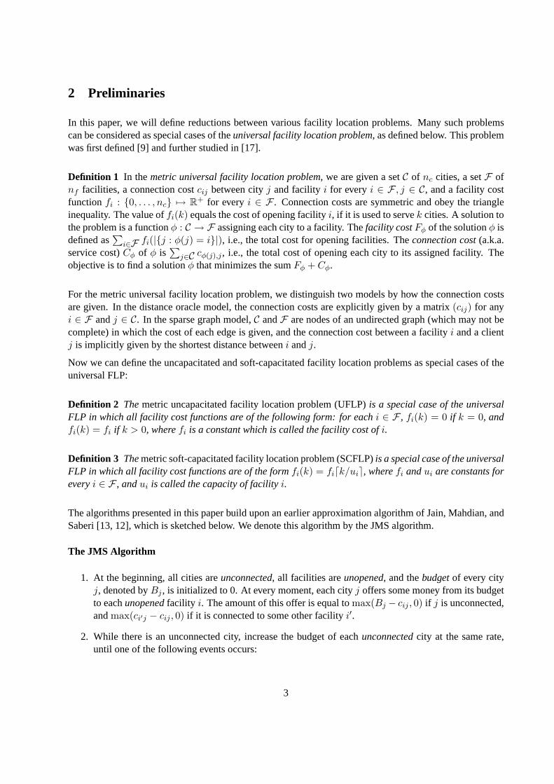
Theorem A [13, 12]. Let γf ≥ 1 be fixed andγc := supk{zk}, wherezk is the solution of the followingoptimization program which is referred to as the factor-revealing LP.

maximize

∑ki=1 αi − γff∑k

i=1 di

(LP1)

subject to ∀ 1 ≤ i < k : αi ≤ αi+1 (1)

∀ 1 ≤ j < i < k : rj,i ≥ rj,i+1 (2)

∀ 1 ≤ j < i ≤ k : αi ≤ rj,i + di + dj (3)

∀ 1 ≤ i ≤ k :i−1∑

j=1

max(rj,i − dj , 0) +k∑

j=i

max(αi − dj , 0) ≤ f (4)

∀ 1 ≤ j ≤ i ≤ k : αj , dj , f, rj,i ≥ 0 (5)

Then the JMS algorithm is a(γf , γc)-approximation algorithm for UFLP. Furthermore, forγf = 1 we haveγc ≤ 2.

3 The uncapacitated facility location algorithm

3.1 The description of the algorithm

We use the JMS algorithm to solve UFLP with an improved approximation factor. Our algorithm has twophases. In thefirst phase, we scale up the opening costs of all facilities by a factor ofδ (which is a constantthat will be fixed later) and then run the JMS algorithm to find a solution. The technique of cost scaling hasbeen previously used by Charikar and Guha [4] for the facility location problem in order to take advantage ofthe asymmetry between the performance of the algorithm with respect to the facility and connection costs.Here we give a different intuitive reason: Intuitively, the facilities that are opened by the JMS algorithmwith the scaled-up facility costs are those that are very economical, because we weigh the facility cost more

4

than the connection cost in the objective function. Therefore, we open these facilities in the first phase ofthe algorithm.

One important property of the JMS algorithm is that it finds a solution in which there is no unopened facilitythat one can open to decrease the cost (without closing any other facility). This is because for each cityj andfacility i, j offers toi the amount that it would save in the connection cost if it gets its service fromi. Thisis, in fact, the main advantage of the JMS algorithm over a previous algorithm of Mahdian et al. [16, 12].

However, the facility costs have been scaled up in the first phase of our algorithm. Therefore, it is possiblethat the total cost (in terms of the original cost) can be reduced by opening an unopened facility that byreconnecting each city to its closest open facility. This motivates the second phase of our algorithm.

In the secondphase of the algorithm, we decrease the scaling factorδ at rate 1, so at timet, the cost offacility i has reduced to(δ − t)fi. If at any point during this process, a facility could be opened withoutincreasing the total cost (i.e., if the opening cost of the facility equals the total amount that cities can saveby switching their “service provider” to that facility), then we open the facility and connect each city to itsclosest open facility. We stop when the scaling factor becomes 1. This is equivalent to a greedy procedureintroduced by Guha and Khuller [8] and Charikar and Guha [4]. In this procedure, in each iteration, we picka facility u of opening costfu such that if by openingu, the total connection cost decreases fromC to C ′

u,the ratio(C − C ′

u − fu)/fu is maximized. If this ratio is positive, then we open the facilityu, and iterate;otherwise we stop. It is not hard to see that the second phase of our algorithm is equivalent to the Charikar-Guha-Khuller procedure: in the second phase of our algorithm, the first facilityu that is opened correspondsto the minimum value oft, or the maximum value ofδ− t, for which we have(δ− t)fu = C−C ′

u. In otherwords, our algorithm picks the facilityu for which the value of(C −C ′

u)/fu is maximized, and stops whenthis value becomes less than or equal to 1 for allu. This is the same as what the Charikar-Guha-Khullerprocedure does. The original analysis of our algorithm in [18] was based on a lemma by Charikar andGuha [4]. Here we give an alternative analysis of our algorithm that only uses a single factor-revealing LP.

We denote our two-phase algorithm by algorithmA. In the remainder of this section, we analyze algorithmA, and prove that it always outputs a solution to the uncapacitated facility location problem of cost at most1.52 times the optimum. The analysis is divided into three parts. First, in Section 3.2, we derive the factor-revealing linear program whose solution gives the approximation ratio of our algorithm. Next, in Section 3.3,we analyze this linear program, and compute its solution in terms of the approximation factors of the JMSalgorithm. This gives the following result.

Theorem 1 Let (γf , γc) be a pair obtained from the factor-revealing LP (LP1). Then for everyδ ≥ 1,algorithmA is a (γf + ln(δ) + ε, 1 + γc−1

δ )-approximation algorithm for UFLP.

Finally, we analyze the factor-revealing LP (LP1), and show that the JMS algorithm is a(1.11, 1.78)-approximation algorithm for UFLP. This, together with the above theorem forδ = 1.504, implies thatalgorithmA is a1.52-approximation algorithm for UFLP. We will show in Section 3.4 that this algorithmcan be implemented in quasi-linear time, both for the distance oracle model and for the sparse graph model.

3.2 Deriving the factor-revealing LP

Recall that the JMS algorithm, in addition to finding a solution for the scaled instance, outputs theshareofeach city in the total cost of the solution. Letαj denote the share of cityj in the total cost. In other words,

5

αj is the value of the variableBj at the end of the JMS algorithm. Therefore the total cost of the solutionis

∑j αj . Consider an arbitrary collectionS consisting of a single facilityfS andk cities. Letδf (f in the

original instance) denote the opening cost of facilityfS ; αj denote the share of cityj in the total cost (wherecities are ordered such thatα1 ≤ · · · ≤ αk); dj denote the connection cost between cityj and facilityfS ;andrj,i (i > j) denote the connection cost between cityj and the facility that it is connected to at timeαi,right before cityi gets connected for the first time (or if citiesi andj get connected at the same time, definerj,i = αi). The main step in the analysis of the JMS algorithm is to prove that for any such collectionS, theδf , dj , αj , andrj,i values constitute a feasible solution to the program (LP1), wheref is now replaced withδf since the facility costs have been scaled up byδ.

We implement and analyze the second phase as the following. Instead of decreasing the scaling factorcontinuously fromδ to 1, we decrease it discretely inL steps whereL is a constant. Letδi denote the valueof the scaling factor in thei’th step. Therefore,δ = δ1 > δ2 > . . . > δL = 1. We will fix the value of theδi’s later. After decreasing the scaling factor fromδi−1 to δi, we consider facilities in anarbitrary order, andopen those that can be opened without increasing the total cost. We denote this modified algorithm byAL.Clearly, if L is sufficiently large (depending on the instance), the algorithmAL computes the same solutionas algorithmA.

In order to analyze the above algorithm, we need to add extra variables and inequalities to the inequalitiesin the factor-revealing program (LP1) given in Theorem A. Letrj,k+i denote the connection cost that cityjin S pays after we change the scaling factor toδi and process all facilities as described above (Thus,rj,k+1

is the connection cost of cityj after the first phase). Therefore, by the description of the algorithm, we have

∀ 1 ≤ i ≤ L :k∑

j=1

max(rj,k+i − dj , 0) ≤ δif.

This is because if the above inequality is violated and iffS is not open, we could openfS and decrease thetotal cost. IffS is open, thenrj,k+i ≤ dj for all j and the inequality holds.

Now, we compute the share of the cityj in the total cost of the solution that algorithmAL finds. In thefirst phase of the algorithm, the share of cityj in the total cost isαj . Of this amount,rj,k+1 is spent on theconnection cost, andαj − rj,k+1 is spent on the facility costs. However, since the facility costs are scaledup by a factor ofδ in the first phase, therefore the share of cityj in the facility costsin the original instanceis equal to(αj − rj,k+1)/δ. After we reduce the scaling factor fromδi to δi+1 (i = 1, . . . , L − 1), theconnection cost of cityj is reduced fromrj,k+i to rj,k+i+1. Therefore, in this step, the share of cityj in thefacility costs isrj,k+i− rj,k+i+1 with respect to the scaled instance, or(rj,k+i− rj,k+i+1)/δi+1 with respectto the original instance. Thus, at the end of the algorithm, the total share of cityj in the facility costs is

αj − rj,k+1

δ+

L−1∑

i=1

rj,k+i − rj,k+i+1

δi+1.

We also know that the final amount that cityj pays for the connection cost isrj,k+L. Therefore, the shareof the cityj in the total cost of the solution is:

αj − rj,k+1

δ+

L−1∑

i=1

rj,k+i − rj,k+i+1

δi+1+ rj,k+L+1 =

αj

δ+

L−1∑

i=1

(1

δi+1− 1

δi

)rj,k+i. (6)

This, together with adual fittingargument similar to [12], implies the following.

6

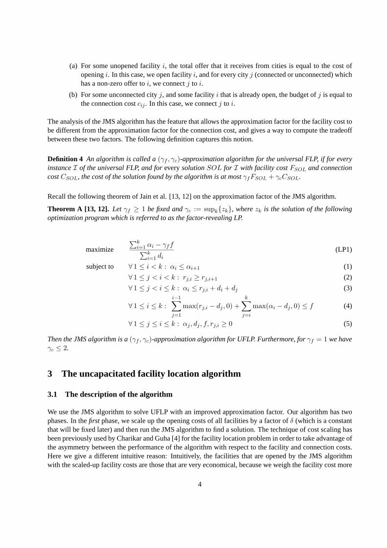
Theorem 2 Let (ξf , ξc) be such thatξf ≥ 1 and ξc is an upper bound on the solution of the followingmaximization program for everyk.

maximize

∑kj=1

(αj

δ +∑L−1

i=1

(1

δi+1− 1

δi

)rj,k+i

)− ξff

∑ki=1 di

(LP2)

subject to ∀ 1 ≤ i < k : αi ≤ αi+1 (7)

∀ 1 ≤ j < i < k : rj,i ≥ rj,i+1 (8)

∀ 1 ≤ j < i ≤ k : αi ≤ rj,i + di + dj (9)

∀ 1 ≤ i ≤ k :i−1∑

j=1

max(rj,i − dj , 0) +k∑

j=i

max(αi − dj , 0) ≤ δf (10)

∀ 1 ≤ i ≤ L :k∑

j=1

max(rj,k+i − dj , 0) ≤ δif (11)

∀ 1 ≤ j ≤ i ≤ k : αj , dj , f, rj,i ≥ 0 (12)

Then, algorithmAL is a (ξf , ξc)-approximation algorithm for UFLP.

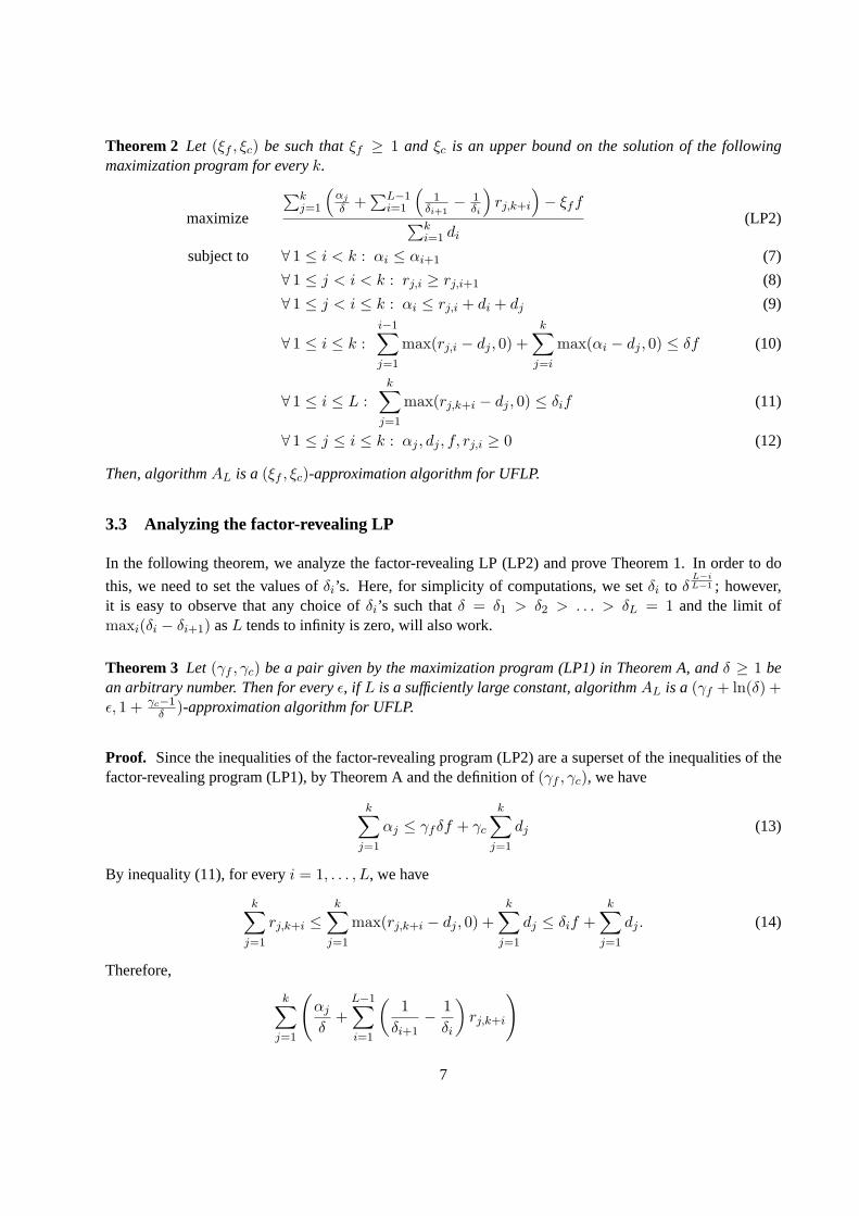
3.3 Analyzing the factor-revealing LP

In the following theorem, we analyze the factor-revealing LP (LP2) and prove Theorem 1. In order to do

this, we need to set the values ofδi’s. Here, for simplicity of computations, we setδi to δL−iL−1 ; however,

it is easy to observe that any choice ofδi’s such thatδ = δ1 > δ2 > . . . > δL = 1 and the limit ofmaxi(δi − δi+1) asL tends to infinity is zero, will also work.

Theorem 3 Let (γf , γc) be a pair given by the maximization program (LP1) in Theorem A, andδ ≥ 1 bean arbitrary number. Then for everyε, if L is a sufficiently large constant, algorithmAL is a (γf + ln(δ) +ε, 1 + γc−1

δ )-approximation algorithm for UFLP.

Proof. Since the inequalities of the factor-revealing program (LP2) are a superset of the inequalities of thefactor-revealing program (LP1), by Theorem A and the definition of(γf , γc), we have

k∑

j=1

αj ≤ γfδf + γc

k∑

j=1

dj (13)

By inequality (11), for everyi = 1, . . . , L, we have

k∑

j=1

rj,k+i ≤k∑

j=1

max(rj,k+i − dj , 0) +k∑

j=1

dj ≤ δif +k∑

j=1

dj . (14)

Therefore,

k∑

j=1

(αj

δ+

L−1∑

i=1

(1

δi+1− 1

δi

)rj,k+i

)

7

=1δ(

k∑

j=1

αj) +L−1∑

i=1

(

1δi+1

− 1δi

)k∑

j=1

rj,k+i

≤ 1δ(γfδf + γc

k∑

j=1

dj) +L−1∑

i=1

(

1δi+1

− 1δi

)(δif +k∑

j=1

dj)

= γff +γc

δ

k∑

j=1

dj +L−1∑

i=1

(δi

δi+1− 1)f + (

1δL− 1

δ1)

k∑

j=1

dj

=(γf + (L− 1)(δ1/(L−1) − 1)

)f + (

γc

δ+ 1− 1

δ)

k∑

j=1

dj .

This, together with Theorem 2, shows thatAL is a(γf + (L− 1)(δ1/(L−1) − 1), 1 + γc−1δ )-approximation

algorithm for UFLP. The fact that the limit of(L−1)(δ1/(L−1)−1) asL tends to infinity isln(δ) completesthe proof.

We observe that the proof of Theorem 3 goes through as long as the limit of∑L−1

i=1 ( δiδi+1

− 1) asL tends toinfinity is ln(δ). This condition holds if we chooseδi’s such thatδ = δ1 > δ2 > . . . > δL = 1 and the limitof maxi(δi − δi+1) asL tends to infinity is zero. It can be seen as follows. Letxi = δi

δi+1− 1 > 0. Then,

for i = 1, 2, · · · , L− 1,

xi − o(xi) ≤ ln(δi

δi+1) ≤ xi.

It follows that,L−1∑

i=1

xi(1− o(xi)/xi) ≤ ln(δ) ≤L−1∑

i=1

xi.

SincelimL→∞o(xi)

xi= limxi→0

o(xi)xi

= 0, we conclude thatlimL→∞∑L−1

i=1 xi = ln(δ).

Now we analyze the factor-revealing LP (LP1) and show that the JMS algorithm is a(1.11, 1.78)-approximationalgorithm.

Lemma 4 Letγf = 1.11. Then for everyk, the solution of the factor-revealing LP (LP1) is at most 1.78.

Proof. See Appendix.

Remark 1 Numerical computations using CPLEX show thatz500 ≈ 1.7743 and thereforeγc > 1.774 forγf = 1.11. Thus, the estimate provided by the above lemma for the value ofγc is close to its actual value.

3.4 Running time

The above analysis of the algorithmA, together with a recent result of Thorup [24], enables us to prove thefollowing result.

8

Corollary 5 For everyε > 0, there is a quasi-linear time(1.52 + ε)-approximation algorithm for UFLP,both in the distance oracle model and in the sparse graph model.

Proof Sketch. We use the algorithmAL for a large constantL. Thorup [24] shows that for everyε > 0, theJMS algorithm can be implemented in quasi-linear time (in both the distance oracle and the graph models)with an approximation factor of1.61 + ε. It is straightforward to see that his argument actually implies thestronger conclusion that the quasi-linear algorithm is a(γf + ε, γc + ε)-approximation, where(γf , γc) aregiven by Theorem A. This shows that the first phase of algorithmAL can be implemented in quasi-lineartime. The second phase consists of a constant number of rounds. Therefore, we only need to show that eachof these rounds can be implemented in quasi-linear time. This is easy to see in the distance oracle model. Inthe graph model, we can use the exact same argument as the one used by Thorup in the proof of Lemma 5.1of [24].

4 The linear-cost facility location problem

Thelinear-cost facility location problemis a special case of the universal FLP in which the facility costs areof the form

fi(k) ={

0 k = 0aik + bi k > 0

whereai andbi are nonnegative values for eachi ∈ F . ai andbi are called the marginal (a.k.a. incremental)and setup cost of facilityi, respectively.

We denote an instance of the linear-cost FLP with marginal costs(ai), setup costs(bi), and connection costs(cij) by LFLP (a, b, c). Clearly, the regular UFLP is a special case of the linear-cost FLP withai = 0,i.e.,LFLP (0, b, c). Furthermore, it is straightforward to see thatLFLP (a, b, c) is equivalent to an instanceof the regular UFLP in which the marginal costs are added to the connection costs. More precisely, letcij = cij + ai for i ∈ F and j ∈ C, and consider an instance of UFLP with facility costs(bi) andconnection costs(cij). We denote this instance byUFLP (b, c + a). It is easy to see thatLFLP (a, b, c)is equivalent toUFLP (b, c + a). Thus, the linear-cost FLP can be solved using any algorithm for UFLP,and the overall approximation ratio will be the same. However, for applications in the next section, we needbifactor approximation factors of the algorithm (as defined in Definition 4).

It is not necessarily true that applying a(γf , γc)-approximation algorithm for UFLP on the instanceUFLP (b, a+c) will give a (γf , γc)-approximate solution forLFLP (a, b, c). However, we will show that the JMS algo-rithm has this property. The following lemma generalizes Theorem A for the linear-cost FLP.

Lemma 6 Let (γf , γc) be a pair obtained from the factor-revealing LP in Theorem A. Then applying theJMS algorithm on the instanceUFLP (b, a+c) will give a(γf , γc)-approximate solution forLFLP (a, b, c).

Proof. Let SOL be an arbitrary solution forLFLP (a, b, c), which can also be viewed as a solution forUFLP (b, c) for c = c + a. Consider a facilityf that is open inSOL, and the set of clients connected to itin SOL. Let k denote the number of these clients,f(k) = ak + b (for k > 0) be the facility cost functionof f , anddj denote the connection cost between clientj and the facilityf in the instanceUFLP (b, a + c).Therefore,dj = dj − a is the corresponding connection cost in the original instanceLFLP (a, b, c). Recall

9

the definition ofαj andrj,i in the factor-revealing LP of Theorem A. By inequality (3) we also know thatαi ≤ rj,i + dj + di. We strengthen this inequality as follows.

Claim 7 αi ≤ rj,i + dj + di

Proof. It is true if αi = αj since it happens only ifrj,i = αj . Otherwise, consider clientsi andj(< i) attime t = αi − ε. Let s be the facilityj is assigned to at timet. By triangle inequality, we have

csi = csi + as ≤ csj + di + dj + as = csj + di + dj ≤ rj,i + di + dj .

On the other handαi ≤ csi since otherwisei could have connected to facilitys at a time earlier thant.

Also, by inequality (4) we know that

i−1∑

j=1

max(rj,i − dj , 0) +k∑

j=i

max(αi − dj , 0) ≤ b.

Notice thatmax(a− x, 0) ≥ max(a, 0)− x if x ≥ 0. Therefore, we have

i−1∑

j=1

max(rj,i − dj , 0) +k∑

j=i

max(αi − dj , 0) ≤ b + ka. (15)

Claim 7 and Inequality (15) show that the valuesαj , rj,i, dj , a, andb constitute a feasible solution of thefollowing optimization program.

maximize

∑ki=1 αi − γf (ak + b)∑k

i=1 di

subject to ∀ 1 ≤ i < k : αi ≤ αi+1

∀ 1 ≤ j < i < k : rj,i ≥ rj,i+1

∀ 1 ≤ j < i ≤ k : αi ≤ rj,i + di + dj

∀ 1 ≤ i ≤ k :i−1∑

j=1

max(rj,i − dj , 0) +k∑

j=i

max(αi − dj , 0) ≤ b + ka

∀ 1 ≤ j ≤ i ≤ k : αj , dj , a, b, rj,i ≥ 0

However, it is clear that the above optimization program and the factor-revealing LP in Theorem A areequivalent. This completes the proof of this lemma.

The above lemma and Theorem A give us the following corollary, which will be used in the next section.

Corollary 8 There is a(1, 2)-approximation algorithm for the linear-cost facility location problem.

It is worth mentioning that algorithmA can also be generalized for the linear-cost FLP. The only trick is toscale up botha andb in the first phase by a factor ofδ, and scale them both down in the second phase. Therest of the proof is almost the same as the proof of Lemma 6.

10

5 The soft-capacitated facility location problem

In this section we will show how the soft-capacitated facility location problem can be reduced to the linear-cost FLP. In Section 5.1 we define the concept of reduction between facility location problems. We will usethis concept in Sections 5.2 and 5.3 to obtain approximation algorithms for SCFLP and a generalization ofSCFLP and the concave-cost FLP.

5.1 Reduction between facility location problems

Definition. A reduction from a facility location problemA to another facility location problemB is apolynomial-time procedureR that maps every instanceI of A to an instanceR(I) of B. This procedure iscalled a(σf , σc)-reduction if the following conditions hold.

1. For any instanceI ofA and any feasible solution forI with facility costF ∗A and connection costC∗A,there is a corresponding solution for the instanceR(I) with facility costF ∗B ≤ σfF ∗A and connectioncostC∗B ≤ σcC

∗A.

2. For any feasible solution for the instanceR(I), there is a corresponding feasible solution forI whosetotal cost is at most as much as the total cost of the original solution forR(I). In other words, cost ofthe instanceR(I) is an over-estimate of cost of the instanceI.

Theorem 9 If there is a(σf , σc)-reduction from a facility location problemA to another facility locationproblemB, and a(γf , γc)-approximation algorithm forB, then there is a(γfσf , γcσc)-approximation al-gorithm forA.

Proof. On an instanceI of the problemA, we computeR(I), run the(γf , γc)-approximation algorithmfor B on R(I), and output the corresponding solution forI. In order to see why this is a(γfσf , γcσc)-approximation algorithm forA, letSOL denote an arbitrary solution forI, ALG denote the solution that theabove algorithm finds, andF ∗P andC∗P (FALGP andCALGP , respectively) denote the facility and connectioncosts ofSOL (ALG, respectively) when viewed as a solution for the problemP (P = A,B). By thedefinition of(σf , σc)-reductions and(γf , γc)-approximation algorithms we have

FALGA + CALGA ≤ FALGB + CALGB ≤ γfF ∗B + γcC∗B ≤ γfσfF ∗A + γcσcC

∗A,

which completes the proof of the lemma.

We will see examples of reductions in the rest of this paper.

5.2 The soft-capacitated facility location problem

In this subsection, we give a2-approximation algorithm for the soft-capacitated FLP by reducing it to thelinear-cost FLP.

Theorem 10 There is a2-approximation algorithm for the soft-capacitated facility location problem.

11

Proof. We use the following reduction: Construct an instance of the linear-cost FLP, where we have thesame sets of facilities and clients. The connection costs remain the same. However, the facility cost ofthe ith facility is (1 + k−1

ui)fi if k ≥ 1 and0 if k = 0. Note that, for everyk ≥ 1, d k

uie ≤ 1 + k−1

ui≤

2 · d kuie. Therefore, it is easy to see that this reduction is a(2, 1)-reduction. By Lemma 8, there is a(1, 2)-

approximation algorithm for the linear-cost FLP, which together with Theorem 9 completes the proof.

Furthermore, we now illustrate that the following natural linear programming formulation of SCFLP has anintegrality gap of2. This means that we cannot obtain a better approximation ratio using this LP relaxationas the lower bound.

minimize∑

i∈Ffiyi +

∑

i∈F

∑

j∈Ccijxij

subject to ∀ i ∈ F , j ∈ C : xij ≤ yi

∀ i ∈ F :∑

j∈Cxij ≤ uiyi

∀ j ∈ C :∑

i∈Fxij = 1

∀ i ∈ F , j ∈ C : xij ∈ {0, 1} (16)

∀ i ∈ F : yi is a nonnegative integer (17)

In a natural linear program relaxation, we replace the constraints (16) and (17) byxij ≥ 0 andyi ≥ 0. Herewe see that even if we only relax constraint (17), the integrality gap is2. Consider an instance of SCFLPthat consists of only one potential facilityi, andk ≥ 2 clients. Assume that the capacity of facilityi isk − 1, the facility cost is1, and all connection costs are0. It is clear that the optimal integral solution hascost2. However, after relaxing constraint (17), the optimal fractional solution has cost1 + 1

k−1 . Therefore,

the integrality gap between the integer program and its relaxation is2(k−1)k which tends to2 ask tends to

infinity.

5.3 The concave soft-capacitated facility location problem

In this subsection, we consider a common generalization of the soft-capacitated facility location problem andthe concave-cost facility location problem. This problem, which we refer to as theconcave soft-capacitatedFLP, is the same as the soft-capacitated FLP except that ifr ≥ 0 copies of facilityi are open, then thefacility cost isgi(r)ai wheregi(r) is a given concave increasing function ofr. In other words, the concavesoft-capacitated FLP is a special case of the universal FLP in which the facility cost functions are of the formfi(x) = aigi(dx/uie) for constantsai, ui and a concave increasing functiongi. It is also a special case ofthe so-called stair-case cost facility location problem [11]. On the other hand, it is a common generalizationof the soft-capacitated FLP (whengi(r) = r) and the concave-cost FLP (whenui = 1 for all i). Theconcave-cost FLP is a special case of the universal FLP in which facility cost functions are required to beconcave and increasing (See [9]). The main result of this subsection is the following.

Theorem 11 The concave soft-capacitated FLP is(maxi∈F gi(2)gi(1) , 1)-reducible to the linear-cost FLP.

The above theorem is established by the following lemmas which show the reductions between the concavesoft-capacitated FLP, the concave-cost FLP and the linear-cost FLP. Notice thatmaxi∈F gi(2)

gi(1) ≤ 2.

12

Lemma 12 The concave soft-capacitated FLP is(maxi∈F gi(2)gi(1) , 1) reducible to the concave-cost FLP.

Proof. Given an instanceI of the concave soft-capacitated FLP, where the facility cost function of thefacility i is fi(k) = gi(dk/uie)ai, we construct an instanceR(I) of the concave-cost FLP as follows: Wehave the same sets of facilities and clients and the same connection costs as inI. The facility cost functionof theith facility is given by

f ′i(k) =

{ (gi(r) + (gi(r + 1)− gi(r))(k−1

ui− r + 1)

)ai if k > 0, r := dk/uie

0 if k = 0.

Concavity ofgi implies that the above function is also concave, and thereforeR(I) is an instance of concave-cost FLP. Also, it is easy to see from the above definition that

gi(dk/uie)ai ≤ f ′i(k) ≤ gi(dk/uie+ 1)ai.

By the concavity of the functiongi, we havegi(r+1)gi(r)

≤ gi(2)gi(1) for everyr ≥ 1. Therefore, for every facilityi

and numberk,

fi(k) ≤ f ′i(k) ≤ gi(2)gi(1)

fi(k).

This completes the proof of the lemma.

Now, we will show a simple(1, 1)-reduction from the concave-cost FLP to the linear-cost FLP. This, togetherwith the above lemma, reduces the concave soft-capacitated facility location problem to the linear-cost FLP.

Lemma 13 There is a(1, 1)-reduction from the concave-cost FLP to the linear-cost FLP.

Proof. Given an instanceI of concave-cost FLP, we construct an instanceR(I) of linear-cost FLP asfollows: Corresponding to each facilityi in I with facility cost functionfi(k), we putn copies of thisfacility in R(I) (wheren is the number of clients), and let the facility cost function of thel’th copy be

f(l)i (k) =

{fi(l) + (fi(l)− fi(l − 1))(k − l) if k > 00 if k = 0.

In other words, the facility cost function is the line that passes through the points(l − 1, f(l − 1)) and(l, f(l)). The set of clients, and the connection costs between clients and facilities are unchanged. We provethat this reduction is a(1, 1)-reduction.

For any feasible solutionSOL for I, we can construct a feasible solutionSOL′ for R(I) as follows: Ifa facility i is open andk clients are connected to it inSOL, we open thek’th copy of the correspondingfacility in R(I), and connect the clients to it. Sincefi(k) = f

(k)i (k), the facility and connection costs of

SOL′ is the same as those ofSOL.

Conversely, consider an arbitrary feasible solutionSOL for R(I). We construct a solutionSOL′ for I asfollows. For any facilityi, if at least one of the copies ofi is open inSOL, we openi and connect allclients that were served by a copy ofi in SOL to it. We show that this does not increase the total cost ofthe solution: Assume thel1’th, l2’th, . . . , andls’th copies ofi were open inSOL, servingk1, k2, . . ., andks

clients, respectively. By concavity offi, and the fact thatf (l)i (k) ≥ f

(k)i (k) = fi(k) for everyl, we have

fi(k1 + · · ·+ ks) ≤ fi(k1) + · · ·+ fi(ks) ≤ f(l1)i (k1) + · · ·+ f

(ls)i (ks).

This shows that the facility cost ofSOL′ is at most the facility cost ofSOL.

13

6 Conclusion

We have obtained the best approximation ratios for two well-studied facility location problems,1.52 forUFLP and2 for SCFLP, respectively. The approximation ratio for UFLP almost matches the lower bound of1.463, and the approximation ratio for SCFLP achieves the integrality gap of the standard LP relaxation ofthe problem. An interesting open question in this area is to close the gap between1.52 and1.463 for UFLP.

Although the performance guarantee of our algorithm for UFLP is very close to the lower bound of1.463,it would be nice to show that the bound of1.52 is actually tight. In [12], it was shown that a solution to thefactor-revealing LP for the JMS algorithm provides a tight bound on the performance guarantee of the JMSalgorithm. It is reasonable to expect that a solution to (LP2) may also be used to construct a tight examplefor our1.52-approximation algorithm. However, we were unsuccessful in constructing such an example.

Our results (Theorem 1 and Lemma 4) for UFLP and/or the idea of bifactor reduction have been used toget the currently best known approximations ratios for several multi-level facility location problems [1, 26].Since UFLP is the most basic facility location problem, we expect to see more applications of our results.

Acknowledgments. We would like to thank Asaf Levin for pointing out that our analysis of the2-approximation algorithm for the soft-capacitated facility location problem is tight. We also like to men-tion that an idea to derive better approximation factors for UFLP using the(1, 2) bifactor guarantee wasindependently proposed earlier by Kamal Jain in a private communication to the first author, and by thelast two authors. We thank anonymous referees for their helpful suggestions that significantly improved theexposition of our paper.

References

[1] A. Ageev, Y. Ye, and J. Zhang. Improved combinatorial approximation algorithms for the k-levelfacility location problem.SIAM J Discrete Math., 18(1):207–217, 2004.

[2] V. Arya, N. Garg, R. Khandekar, A. Meyerson, K. Munagala, and V. Pandit. Local search heuristicsfor k-median and facility location problems.SIAM Journal of Computing, 33(3):544–562, 2004.

[3] P. Bauer and R. Enders. A capacitated facility location problem with integer decision variables. InInternational Symposium on Mathematical Programming (ISMP), 1997.

[4] M. Charikar and S. Guha. Improved combinatorial algorithms for facility location and k-median prob-lems. InProceedings of the 40th Annual IEEE Symposium on Foundations of Computer Science, pages378–388, October 1999.

[5] F.A. Chudak and D. Shmoys. Improved approximation algorithms for the capacitated facility locationproblem. InProc. 10th Annual ACM-SIAM Symposium on Discrete Algorithms, pages 875–876, 1999.

[6] F.A. Chudak and D. Shmoys. Improved approximation algorithms for the uncapacitated facility loca-tion problem.SIAM J. Comput., 33(1):1–25, 2003.

[7] G. Cornuejols, G.L. Nemhauser, and L.A. Wolsey. The uncapacitated facility location problem. InP. Mirchandani and R. Francis, editors,Discrete Location Theory, pages 119–171. John Wiley andSons Inc., 1990.

14

[8] S. Guha and S. Khuller. Greedy strikes back: Improved facility location algorithms.Journal ofAlgorithms, 31:228–248, 1999.

[9] M. Hajiaghayi, M. Mahdian, and V.S. Mirrokni. The facility location problem with general cost func-tions. Networks, 42(1):42–47, August 2003.

[10] D. S. Hochbaum. Heuristics for the fixed cost median problem.Mathematical Programming,22(2):148–162, 1982.

[11] K. Holmberg. Solving the staircase cost facility location problem with decomposition and piecewiselinearization.European Journal of Operational Research, 74:41–61, 1994.

[12] K. Jain, M. Mahdian, E. Markakis, A. Saberi, and V.V. Vazirani. Approximation algorithms for facilitylocation via dual fitting with factor-revealing LP.Journal of the ACM, 50(6):795–824, November2003.

[13] K. Jain, M. Mahdian, and A. Saberi. A new greedy approach for facility location problems. InPro-ceedings of the 34st Annual ACM Symposium on Theory of Computing, pages 731–740, 2002.

[14] K. Jain and V.V. Vazirani. Approximation algorithms for metric facility location and k-median prob-lems using the primal-dual schema and lagrangian relaxation.Journal of the ACM, 48:274–296, 2001.

[15] M.R. Korupolu, C.G. Plaxton, and R. Rajaraman. Analysis of a local search heuristic for facilitylocation problems.J. Algorithms, 37(1):146–188, 2000.

[16] M. Mahdian, E. Markakis, A. Saberi, and V.V. Vazirani. A greedy facility location algorithm analyzedusing dual fitting. InProceedings of 5th International Workshop on Randomization and ApproximationTechniques in Computer Science, volume 2129 ofLecture Notes in Computer Science, pages 127–137.Springer-Verlag, 2001.

[17] M. Mahdian and M. Pal. Universal facility location. InProceedings of the 11th Annual EuropeanSymposium on Algorithms (ESA), 2003.

[18] M. Mahdian, Y. Ye, and J. Zhang. Improved approximation algorithms for metric facility locationproblems. InProceedings of 5th International Workshop on Approximation Algorithms for Combi-natorial Optimization (APPROX 2002), volume 2462 ofLecture Notes in Computer Science, pages229–242, 2002.

[19] M. Mahdian, Y. Ye, and J. Zhang. A 2-approximation algorithm for the soft-capacitated facility loca-tion problem. InProceedings of 6th International Workshop on Approximation Algorithms for Com-binatorial Optimization (APPROX 2003), volume 2764 ofLecture Notes in Computer Science, pages129–140, 2003.

[20] C.S. Revell and G. Laporte. The plant location problem: New models and research prospects.Opera-tions Research, 44:864–874, 1996.

[21] D.B. Shmoys. Approximation algorithms for facility location problems. In K. Jansen and S. Khuller,editors,Approximation Algorithms for Combinatorial Optimization, volume 1913 ofLecture Notes inComputer Science, pages 27–33. Springer, Berlin, 2000.

15

[22] D.B. Shmoys, E. Tardos, and K.I. Aardal. Approximation algorithms for facility location problems. InProceedings of the 29th Annual ACM Symposium on Theory of Computing, pages 265–274, 1997.

[23] M. Sviridenko. An improved approximation algorithm for the metric uncapacitated facility locationproblem. InProceedings of the 9th Conference on Integer Programming and Combinatorial Optimiza-tion, pages 240–257, 2002.

[24] M. Thorup. Quick and good facility location. InProceedings of the 14th ACM-SIAM symposium onDiscrete Algorithms, 2003.

[25] M. Thorup. Quickk-median,k-center, and facility location for sparse graphs.SIAM Journal onComputing, 34(2):405–432, 2005.

[26] J. Zhang. Approximating thetwo-level facility location problem via a quasi-greedy approach. InProceedings of the 15th Annual ACM-SIAM Symposium on Discrete Algorithms (SODA 2004), 2004.

A Proof of Lemma 4

Proof. By doubling a feasible solution of the factor-revealing program (LP1) (as in the proof of Lemma 12in [13]) it is easy to show that for everyk, zk ≤ z2k. Therefore, without loss of generality, we can assumethatk is sufficiently large.

Consider a feasible solution of the factor-revealing LP. Letxj,i := max(rj,i − dj , 0). Inequality (4) of thefactor-revealing LP implies that for everyi ≤ i′,

(i′ − i + 1)αi − f ≤i′∑

j=i

dj −i−1∑

j=1

xj,i. (18)

Now, we defineli as follows:

li ={

p2k if i ≤ p1kk if i > p1k

wherep1 andp2 are two constants withp1 < p2 that will be fixed later. Consider Inequality (18) for everyi ≤ p2k andi′ = li:

(li − i + 1)αi − f ≤li∑

j=i

dj −i−1∑

j=1

xj,i. (19)

For everyi = 1, . . . , k, we defineθi as follows. Herep3 andp4 are two constants withp1 < p3 < 1−p3 < p2

andp4 ≤ 1− p2 that will be fixed later.

θi =

1li−i+1 if i ≤ p3k

1(1−p3)k if p3k < i ≤ (1− p3)k

p4k(k−i)(k−i+1) if (1− p3)k < i ≤ p2k

0 if i > p2k

(20)

16

By multiplying both sides of inequality (19) byθi and adding up this inequality fori = 1, . . . , p1k, i =p1k + 1, . . . , p3k, i = p3k + 1 . . . , (1 − p3)k, and i = (1 − p3)k + 1, . . . , p2k, we get the followinginequalities.

p1k∑

i=1

αi − (p1k∑

i=1

θi)f ≤p1k∑

i=1

p2k∑

j=i

dj

p2k − i + 1−

p1k∑

i=1

i−1∑

j=1

max(rj,i − dj , 0)p2k − i + 1

(21)

p3k∑

i=p1k+1

αi − (p3k∑

i=p1k+1

θi)f ≤p3k∑

i=p1k+1

k∑

j=i

dj

k − i + 1−

p3k∑

i=p1k+1

i−1∑

j=1

max(rj,i − dj , 0)k − i + 1

(22)

(1−p3)k∑

i=p3k+1

k − i + 1(1− p3)k

αi − ((1−p3)k∑

i=p3k+1

θi)f ≤(1−p3)k∑

i=p3k+1

k∑

j=i

dj

(1− p3)k−

(1−p3)k∑

i=p3k+1

i−1∑

j=1

max(rj,i − dj , 0)(1− p3)k

(23)

p2k∑

i=(1−p3)k+1

p4k

k − iαi − (

p2k∑

i=(1−p3)k+1

θi)f ≤p2k∑

i=(1−p3)k+1

k∑

j=i

p4kdj

(k − i)(k − i + 1)

−p2k∑

i=(1−p3)k+1

i−1∑

j=1

p4k max(rj,i − dj , 0)(k − i)(k − i + 1)

(24)

We definesi := maxl≥i(αl − dl). Using this definition and inequalities (2) and (3) of the factor-revealingLP (LP1) we obtain

∀i : rj,i ≥ si − dj =⇒ ∀i : max(rj,i − dj , 0) ≥ max(si − 2dj , 0) (25)

∀i : αi ≤ si + di (26)

s1 ≥ s2 ≥ . . . ≥ sk (≥ 0) (27)

We assumesk ≥ 0 here because that, if on contraryαk < dk, we can always setαk equal todk withoutviolating any constraint in the factor-revealing LP (LP1) and increasezk.

Inequality (26) andp4 ≤ 1− p2 imply

(1−p3)k∑

i=p3k+1

(1− k − i + 1

(1− p3)k

)αi +

p2k∑

i=(1−p3)k+1

(1− p4k

k − i

)αi +

k∑

i=p2k+1

αi

≤(1−p3)k∑

i=p3k+1

i− p3k − 1(1− p3)k

(si + di) +p2k∑

i=(1−p3)k+1

(1− p4k

k − i

)(si + di) +

k∑

i=p2k+1

(si + di)

(28)

Let ζ :=∑k

i=1 θi. Thus,

ζ =p1k∑

i=1

1p2k − i + 1

+p3k∑

i=p1k+1

1k − i + 1

+(1−p3)k∑

i=p3k+1

1(1− p3)k

+p2k∑

i=(1−p3)k+1

(p4k

k − i− p4k

k − i + 1

)

= ln(

p2

p2 − p1

)+ ln

(1− p1

1− p3

)+

1− 2p3

1− p3+

p4

1− p2− p4

p3+ o(1). (29)

17

By adding the inequalities (21), (22), (23), (24), (28) and using (25), (27), and the fact thatmax(x, 0) ≥ δxfor every0 ≤ δ ≤ 1, we obtain

k∑

i=1

αi − ζf

≤p1k∑

i=1

p2k∑

j=i

dj

p2k − i + 1−

p1k∑

i=1

i−1∑

j=1

si − 2dj

2(p2k − i + 1)

+p3k∑

i=p1k+1

k∑

j=i

dj

k − i + 1−

p3k∑

i=p1k+1

i−1∑

j=1

si − 2dj

k − i + 1

+(1−p3)k∑

i=p3k+1

k∑

j=i

dj

(1− p3)k−

(1−p3)k∑

i=p3k+1

i−1∑

j=1

si − 2dj

(1− p3)k

+p2k∑

i=(1−p3)k+1

k∑

j=i

p4kdj

(k − i)(k − i + 1)−

p2k∑

i=(1−p3)k+1

i−1∑

j=1

p4k max(sp2k+1 − 2dj , 0)(k − i)(k − i + 1)

+(1−p3)k∑

i=p3k+1

i− p3k − 1(1− p3)k

(si + di) +p2k∑

i=(1−p3)k+1

(1− p4k

k − i

)(si + di) +

k∑

i=p2k+1

(sp2k+1 + di)

=p2k∑

j=1

min(j,p1k)∑

i=1

dj

p2k − i + 1−

p1k∑

i=1

i− 12(p2k − i + 1)

si +p1k∑

j=1

p1k∑

i=j+1

dj

p2k − i + 1

+k∑

j=p1k+1

min(j,p3k)∑

i=p1k+1

dj

k − i + 1−

p3k∑

i=p1k+1

i− 1k − i + 1

si +p3k∑

j=1

p3k∑

i=max(j,p1k)+1

2dj

k − i + 1

+k∑

j=p3k+1

min(j,(1−p3)k)∑

i=p3k+1

dj

(1− p3)k−

(1−p3)k∑

i=p3k+1

i− 1(1− p3)k

si

+(1−p3)k∑

j=1

(1−p3)k∑

i=max(j,p3k)+1

2dj

(1− p3)k

+k∑

j=(1−p3)k+1

min(j,p2k)∑

i=(1−p3)k+1

(1

k − i− 1

k − i + 1

)p4kdj

−p2k∑

j=1

p2k∑

i=max(j,(1−p3)k)+1

p4k

(1

k − i− 1

k − i + 1

)max(sp2k+1 − 2dj , 0)

+(1−p3)k∑

i=p3k+1

i− p3k − 1(1− p3)k

(si + di) +p2k∑

i=(1−p3)k+1

(1− p4k

k − i

)(si + di) +

k∑

i=p2k+1

di

+(1− p2)ksp2k+1

18

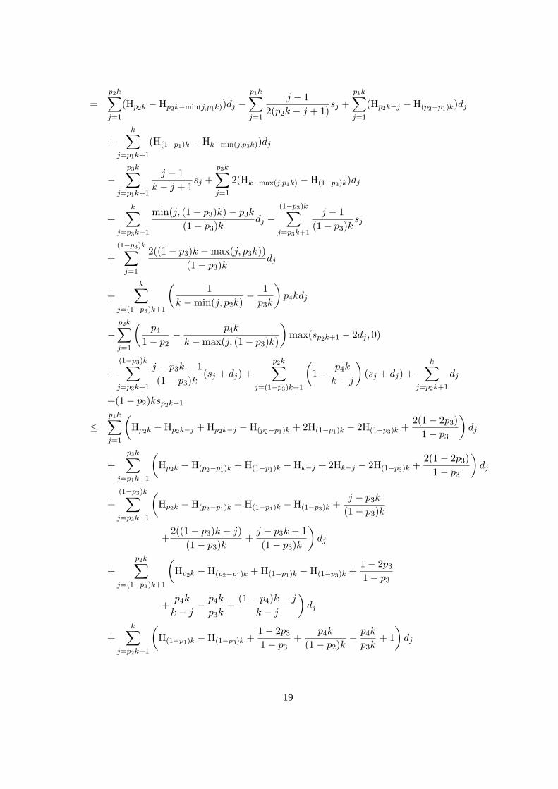
=p2k∑

j=1

(Hp2k −Hp2k−min(j,p1k))dj −p1k∑

j=1

j − 12(p2k − j + 1)

sj +p1k∑

j=1

(Hp2k−j −H(p2−p1)k)dj

+k∑

j=p1k+1

(H(1−p1)k −Hk−min(j,p3k))dj

−p3k∑

j=p1k+1

j − 1k − j + 1

sj +p3k∑

j=1

2(Hk−max(j,p1k) −H(1−p3)k)dj

+k∑

j=p3k+1

min(j, (1− p3)k)− p3k

(1− p3)kdj −

(1−p3)k∑

j=p3k+1

j − 1(1− p3)k

sj

+(1−p3)k∑

j=1

2((1− p3)k −max(j, p3k))(1− p3)k

dj

+k∑

j=(1−p3)k+1

(1

k −min(j, p2k)− 1

p3k

)p4kdj

−p2k∑

j=1

(p4

1− p2− p4k

k −max(j, (1− p3)k)

)max(sp2k+1 − 2dj , 0)

+(1−p3)k∑

j=p3k+1

j − p3k − 1(1− p3)k

(sj + dj) +p2k∑

j=(1−p3)k+1

(1− p4k

k − j

)(sj + dj) +

k∑

j=p2k+1

dj

+(1− p2)ksp2k+1

≤p1k∑

j=1

(Hp2k −Hp2k−j + Hp2k−j −H(p2−p1)k + 2H(1−p1)k − 2H(1−p3)k +

2(1− 2p3)1− p3

)dj

+p3k∑

j=p1k+1

(Hp2k −H(p2−p1)k + H(1−p1)k −Hk−j + 2Hk−j − 2H(1−p3)k +

2(1− 2p3)1− p3

)dj

+(1−p3)k∑

j=p3k+1

(Hp2k −H(p2−p1)k + H(1−p1)k −H(1−p3)k +

j − p3k

(1− p3)k

+2((1− p3)k − j)

(1− p3)k+

j − p3k − 1(1− p3)k

)dj

+p2k∑

j=(1−p3)k+1

(Hp2k −H(p2−p1)k + H(1−p1)k −H(1−p3)k +

1− 2p3

1− p3

+p4k

k − j− p4k

p3k+

(1− p4)k − j

k − j

)dj

+k∑

j=p2k+1

(H(1−p1)k −H(1−p3)k +

1− 2p3

1− p3+

p4k

(1− p2)k− p4k

p3k+ 1

)dj

19

−p3k∑

j=1

(p4

1− p2− p4

p3

)max(sp2k+1 − 2dj , 0)−

(1−p3)k∑

j=p3k+1

(p4

1− p2− p4

p3

)(sp2k+1 − 2dj)

−p1k∑

j=1

j − 12(p2k − j + 1)

sj −p3k∑

j=p1k+1

j − 1k − j + 1

sj −(1−p3)k∑

j=p3k+1

p3k

(1− p3)ksj

+p2k∑

j=(1−p3)k+1

(1− p4k

k − j

)sj + (1− p2)ksp2k+1 (30)

Let’s denote the coefficients ofdj in the above expression byλj . Therefore, we have

k∑

i=1

αi − ζf

≤k∑

j=1

λjdj −p1k∑

j=1

j − 12(p2k − j + 1)

sj −p3k∑

j=p1k+1

j − 1k − j + 1

sj −(1−p3)k∑

j=p3k+1

p3k

(1− p3)ksj

+p2k∑

j=(1−p3)k+1

(1− p4k

k − j

)sj +

(1− p2 − (1− 2p3)

(p4

1− p2− p4

p3

))ksp2k+1

−(

p4

1− p2− p4

p3

) p3k∑

j=1

max(sp2k+1 − 2dj , 0), (31)

where

λj :=

ln(p2

p2 − p1) + 2 ln(

1− p1

1− p3) +

2(1− 2p3)1− p3

+ o(1) if 1 ≤ j ≤ p1k

ln(p2

p2 − p1) + ln(

1− p1

1− p3) +

2(1− 2p3)1− p3

+ Hk−j −H(1−p3)k + o(1) if p1k < j ≤ p3k

ln(p2

p2 − p1) + ln(

1− p1

1− p3) +

2(1− 2p3)1− p3

+2p4

1− p2− 2p4

p3+ o(1) if p3k < j ≤ (1− p3)k

ln(p2

p2 − p1) + ln(

1− p1

1− p3) +

1− 2p3

1− p3+ 1− p4

p3+ o(1) if (1− p3)k < j ≤ p2k

ln(1− p1

1− p3) +

1− 2p3

1− p3+ 1 +

p4

1− p2− p4

p3+ o(1) if p2k < j ≤ k.

For everyj ≤ p3k, we have

λ(1−p3)k − λj ≤ 2p4

1− p2− 2p4

p3⇒ δj := (λ(1−p3)k − λj)

/(2p4

1− p2− 2p4

p3

)≤ 1. (32)

Also, if we choosep1, p2, p3, p4 in a way that

ln(1− p1

1− p3) <

2p4

1− p2− 2p4

p3, (33)

20

then for everyj ≤ p3k, λj ≤ λ(1−p3)k and thereforeδj ≥ 0. Then, since0 ≤ δj ≤ 1, we can replacemax(sp2k+1 − 2dj , 0) by δj(sp2k+1 − 2dj) in (31). This gives us

k∑

i=1

αi − ζf

≤k∑

j=1

λjdj −p1k∑

j=1

j − 12(p2k − j + 1)

sj −p3k∑

j=p1k+1

j − 1k − j + 1

sj −(1−p3)k∑

j=p3k+1

p3k

(1− p3)ksj

+p2k∑

j=(1−p3)k+1

(1− p4k

k − j

)sj +

(1− p2 − (1− 2p3)

(p4

1− p2− p4

p3

))ksp2k+1

−12

p3k∑

j=1

(λ(1−p3)k − λj)(sp2k+1 − 2dj) (34)

Let µj denote the coefficient ofsj in the above expression. Therefore the above inequality can be written as

k∑

i=1

αi − ζf ≤ λ(1−p3)k

(1−p3)k∑

j=1

dj +k∑

j=(1−p3)k+1

λjdj +p2k+1∑

j=1

µjsj , (35)

where

µj =

− j − 12(p2k − j + 1)

if 1 ≤ j ≤ p1k

− j − 1k − j + 1

if p1k < j ≤ p3k

− p3

1− p3if p3k < j ≤ (1− p3)k

1− p4k

k − jif (1− p3)k < j ≤ p2k

(36)

and

µp2k+1

=(

1− p2 − (1− 2p3)(

p4

1− p2− p4

p3

))k − 1

2λ(1−p3)kp3k +

12

p3k∑

j=1

λj

=(

1− p2 − (1− 2p3)(

p4

1− p2− p4

p3

))k − 1

2λ(1−p3)kp3k

+p1k

2

(ln(

p2

p2 − p1) + 2 ln(

1− p1

1− p3) +

2(1− 2p3)1− p3

+ o(1))

+(p3 − p1)k

2

(ln(

p2

p2 − p1) + ln(

1− p1

1− p3) +

2(1− 2p3)1− p3

+ o(1))

+12

p3k∑

j=p1k+1

k−j∑

i=(1−p3)k+1

1i

=(

ln(1− p1

1− p3) + 2− 2p2 − p3 + p1 − 2(1− p3)

(p4

1− p2− p4

p3

)+ o(1)

)k

2(37)

21

Now, if we pickp1, p2, p3, p4 in such a way thatλj ≤ γ for everyj ≥ (1− p3)k, i.e.,

ln(p2

p2 − p1) + ln(

1− p1

1− p3) +

2(1− 2p3)1− p3

+2p4

1− p2− 2p4

p3< γ (38)

ln(p2

p2 − p1) + ln(

1− p1

1− p3) +

1− 2p3

1− p3+ 1− p4

p3< γ (39)

and

ln(1− p1

1− p3) +

1− 2p3

1− p3+ 1 +

p4

1− p2− p4

p3< γ. (40)

then the termλ(1−p3)k

∑(1−p3)kj=1 dj+

∑kj=(1−p3)k+1 λjdj on the right-hand side of (35) is at mostγ

∑kj=1 dj .

Also, if for everyi ≤ p2k + 1, we have

µ1 + µ2 + · · ·+ µi ≤ 0, (41)

then by inequality (27), we have∑p2k+1

j=1 µjsj ≤ 0. Therefore, ifp1, p2, p3, p4 are chosen in such a way thatin addition to the above inequalities, we have

ln(

p2

p2 − p1

)+ ln

(1− p1

1− p3

)+

1− 2p3

1− p3+

p4

1− p2− p4

p3< 1.11, (42)

then inequality (35) can be written as

k∑

i=1

αi − 1.11f ≤ γ

k∑

j=1

dj , (43)

which shows that the solution of the maximization program (LP1) is at mostγ. From (36), it is clear thatµj ≤ 0 for everyj ≤ (1−p3)k andµj ≥ 0 for every(1−p3)k ≤ j ≤ p2k. Therefore, it is enough to checkinequality (41) fori = p2k andi = p2k + 1. We have

p2k∑

j=1

µj = −p1k∑

j=1

p2k − p2k + j − 12(p2k − j + 1)

−p3k∑

j=p1k+1

k − k + j − 1k − j + 1

− p3(1− 2p3)k1− p3

+(p2 − 1 + p3)k −p2k∑

j=(1−p3)k+1

p4k

k − j

= −p2k

2(Hp2k −H(p2−p1)k) +

p1k

2− k(H(1−p1)k −H(1−p3)k) + (p3 − p1)k

−p3(1− 2p3)k1− p3

+ (p2 − 1 + p3)k − p4k(Hp3k −H(1−p2)k)

=(−p1

2+ p2 + 2p3 − 1− p2

2ln(

p2

p2 − p1)− ln(

1− p1

1− p3)− p3(1− 2p3)

1− p3

−p4 ln(p3

1− p2) + o(1)

)k (44)

Therefore, inequality (41) is equivalent to the following two inequalities.

22

−p1

2+ p2 + 2p3 − 1− p2

2ln(

p2

p2 − p1)− ln(

1− p1

1− p3)− p3(1− 2p3)

1− p3− p4 ln(

p3

1− p2) < 0 (45)

−p1

2+ p2 + 2p3 − 1− p2

2ln(

p2

p2 − p1)− ln(

1− p1

1− p3)− p3(1− 2p3)

1− p3− p4 ln(

p3

1− p2)

+12

ln(1− p1

1− p3) + 1− p2 − p3

2+

p1

2− (1− p3)

(p4

1− p2− p4

p3

)< 0 (46)

Now, it is enough to observe that if we letp1 = 0.225, p2 = 0.791, p3 = 0.30499, p4 = 0.06984, andγ = 1.7764, thenp1 < p3 < 1 − p3 < p2 andp4 < 1 − p2 as specified earlier, and inequalities (33), (38),(39), (40), (42), (45), and (46) are all satisfied. Therefore, the solution of the optimization program (LP1) isat most1.7764 < 1.78.

23