ApproximateGaussianEliminationforLaplacians –Fast,Sparse ... · a simple, nearly linear time algorithm that approximates a Laplacian by a matrix with a sparse Cholesky factorization

arX

iv:1

605.

0235

3v1

[cs

.DS]

8 M

ay 2

016

Approximate Gaussian Elimination for Laplacians

– Fast, Sparse, and Simple

Rasmus Kyng∗

Yale University

[email protected]

Sushant Sachdeva†

Yale University

[email protected]

May 10, 2016

Abstract

We show how to perform sparse approximate Gaussian elimination for Laplacian matrices. We presenta simple, nearly linear time algorithm that approximates a Laplacian by a matrix with a sparse Choleskyfactorization – the version of Gaussian elimination for symmetric matrices. This is the first nearly lineartime solver for Laplacian systems that is based purely on random sampling, and does not use any graphtheoretic constructions such as low-stretch trees, sparsifiers, or expanders. The crux of our analysisis a novel concentration bound for matrix martingales where the differences are sums of conditionallyindependent variables.

∗Supported by NSF grant CCF-1111257 and ONR Award N00014-16-1-2374.†Supported by a Simons Investigator Award to Daniel A. Spielman.

1 Introduction

A symmetric matrix L is called Symmetric and Diagonally Dominant (SDD) if for all i, L(i, i) ≥∑j 6=i |L(i, j)|.An SDD matrix L is a Laplacian if L(i, j) ≤ 0 for i 6= j, and for all i,

∑j L(i, j) = 0. A Laplacian matrix is

naturally associated with a graph on its vertices, where i, j are adjacent if L(i, j) 6= 0. The problem of solvingsystems of linear equations Lx = b, where L is an SDD matrix (and often a Laplacian), is a fundamental prim-itive and arises in varied applications in both theory and practice. Example applications include solutionsof partial differential equations via the finite element method [Str86, BHV08], semi-supervised learning ongraphs [ZGL03, ZS04, ZBL+04], and computing maximum flows in graphs [DS08, CKM+11, Mad13, LS14].It has also been used as a primitive in the design of several fast algorithms [KM09, OSV12, KMP12, LKP12,KRS15]. It is known that solving SDD linear systems can be reduced to solving Laplacian systems [Gre96].

Cholesky Factorization. A natural approach to solving systems of linear equations is Gaussian elimi-nation, or its variant for symmetric matrices, Cholesky factorization. Cholesky factorization of a matrix Lproduces a factorization L = LDL⊤, where L is a lower-triangular matrix, and D is a diagonal matrix. Sucha factorization allows us to solve a system Lx = b by computing x = L−1b = (L−1)⊤D−1L−1b, where theinverse of L, and D can be applied quickly since they are lower-triangular and diagonal, respectively.

The fundamental obstacle to using Cholesky factorization for quickly solving systems of linear equationsis that L can be a dense matrix even if the original matrix L is sparse. The reason is that the key step inCholesky factorization, eliminating a variable, say xi, from a system of equations, creates a new coefficientL′(j, k) for every pair j, k such that L(j, i) and L(i, k) are non-zero. This phenomenon is called fill-in. ForLaplacian systems, eliminating the first variable corresponds to eliminating the first vertex in the graph, andthe fill-in corresponds to adding a clique on all the neighbors of the first vertex. Sequentially eliminatingvariables often produces a sequence of increasingly-dense systems, resulting in an O(n3) worst-case timeeven for sparse L. Informally, the algorithm for generating the Cholesky factorization for a Laplacian can beexpressed as follows:

for i = 1 to n− 1

Use equation i to express the variable for vertex i in terms of the remaining variables.

Eliminate vertex i, adding a clique on the neighbors of i.

Eliminating the vertices in an order given by a permutation π generates a factorization L = PπLDL⊤P⊤π ,

where Pπ denotes the permutation matrix of π, i.e., (Pπz)i = zπ(i) for all z. Though picking a good orderof elimination can significantly reduce the running time of Cholesky factorization, it gives no guarantees forgeneral systems, e.g., for sparse expander graphs, every ordering results in an Ω(n3) running time [RJL79].

Our Results. In this paper, we present the first nearly linear time algorithm that generates a sparseapproximate Cholesky decomposition for Laplacian matrices, with provable approximation guarantees. Ouralgorithm SparseCholesky can be described informally as follows (see Section 3 for a precise description):

Randomly permute the vertices.

for i = 1 to n− 1

Use equation i to express the variable for vertex i in terms of the remaining variables.

Eliminate vertex i, adding random samples from the clique on the neighbors of i.

We prove the following theorem about our algorithm, where for symmetric matrices A,B, we write A Bif B −A is positive semidefinite (PSD).

Theorem 1.1 The algorithm SparseCholesky, given an n × n Laplacian matrix L with m non-zero en-tries, runs in expected time O(m log3 n) and computes a permutation π, a lower triangular matrix L withO(m log3 n) non-zero entries, and a diagonal matrix D such that with probability 1− 1

poly(n) , we have

1/2 · L Z 3/2 · L,

where Z = PπLDL⊤P⊤π , i.e., Z has a sparse Cholesky factorization.

1

The sparse approximate Cholesky factorization for L given by Theorem C.1 immediately implies fastsolvers for Laplacian systems. We can use the simplest iterative method, called iterative refinement [Hig02,Chapter 12] to solve the system Lx = b as follows. We let,

x(0) = 0, x(i+1) = x(i) − 1/2 · Z+(Lx(i) − b),

where we use the Z+, the pseudo-inverse of Z since Z has a kernel identical to L. Let 1 denote the all ones

vector, and for any vector v, let ‖v‖Ldef=√v⊤Lv.

Theorem 1.2 For all Laplacian systems Lx = b with 1⊤b = 0, and all ǫ > 0, using the sparse approximate

Cholesky factorization Z given by Theorem C.1, the above iterate for t = 3 log 1/ǫ satisfies∥∥∥x(t) − L+b

∥∥∥L≤

ǫ∥∥L+b

∥∥L. We can compute such an x(t) in time O(m log3 n log 1/ǫ).

In our opinion, this is the simplest nearly-linear time solver for Laplacian systems. Our algorithm onlyuses random sampling, and no graph-theoretic constructions, in contrast with all previous Laplacian solvers.The analysis is also entirely contained in this paper. We also remark that there is a possibility that ouranalysis is not tight, and that the bounds can be improved by a stronger matrix concentration result.

Technical Contributions. There are several key ideas that are central to our result: The first is ran-domizing the order of elimination. At step i of the algorithm, if we eliminate a fixed vertex and samplethe resulting clique, we do not know useful bounds on the sample variances that would allow us to proveconcentration. Randomizing over the choice of vertex to eliminate allows us to bound the sample varianceby roughly 1/n times the Laplacian at the previous step.

The second key idea is our approach to estimating effective resistances: A core element in all nearlylinear time Laplacian solvers is a procedure for estimating effective resistances (or leverage scores) for edgesin order to compute sampling probabilities. In previous solvers, these estimates are obtained using fairlyinvolved procedures (e.g. low-stretch trees, ultrasparsifiers, or the subsampling procedure due to Cohen etal. [CLM+15]). In contrast, our solver starts with the crudest possible estimates of 1 for every edge, andthen uses the triangle inequality for effective resistances (Lemma 5.1) to obtain estimates for the new edgesgenerated. We show that these estimates suffice for constructing a nearly linear time Laplacian solver.

Finally, we develop new concentration bounds for a class of matrix martingales that we call bags-of-dicemartingales. The name is motivated by a simple scalar model: at each step, we pick a random bag of dicefrom a collection of bags (in the algorithm, this corresponds to picking a random vertex to eliminate), andthen we independently roll each die in the selected bag (corresponding to drawing independent samples fromthe clique added). The guarantees obtained from existing matrix concentration results are too weak for ourapplication. The concentration bound gives us a powerful tool for handling conditionally independent sumsof variables. We defer a formal description of the martingales and the concentration bound to Section 4.2.

Comparison to other Laplacian solvers. Though the current best algorithm for solving a generaln× n positive semidefinite linear system with m non-zero entries takes time O(minmn, n2.2373) [Wil12], abreakthrough result by Spielman and Teng [ST04, ST14] showed that linear systems in graph Laplacians couldbe solved in time O(m · poly(logn) log 1/ǫ). There has been a lot of progress over the past decade [KMP10,

KMP11, KOSZ13, CKM+14, PS14, KLP+16], and the current best running time is O(m log1/2 n log 1/ǫ) (up

to polylog n factors) [CKM+14]. All of these algorithms have relied on graph-theoretic constructions – low-stretch trees [ST04, KMP10, KMP11, KOSZ13, CKM+14], graph sparsification [ST04, KMP10, KMP11,CKM+14, PS14], and explicit expander graphs [KLP+16].

In contrast, our algorithm requires no graph-theoretic construction, and is based purely on randomsampling. Our result only uses two algebraic facts about Laplacian matrices: 1. They are closed undertaking Schur complements, and 2. They satisfy the effective resistance triangle inequality (Lemma 5.1).

[KLP+16] presented the first nearly linear time solver for block Diagonally Dominant (bDD) systems –a generalization of SDD systems. If bDD matrices satisfy the effective resistance triangle inequality (we are

2

unaware if they do), then the algorithm in the main body of this paper immediately applies to bDD systems,giving a sparse approximate block Cholesky decomposition and a nearly linear time solver for bDD matrices.

In Section C, we sketch a near-linear time algorithm for computing a sparse approximate block Choleskyfactorization for bDD matrices. It combines the approach of SparseCholesky with a recursive approachfor estimating effective resistances, as in [KLP+16], using the subsampling procedure [CLM+15]. Thoughthe algorithm is more involved than SparseCholesky, it runs in time O(m log3 n+n log5 n), and producesa sparse approximate Cholesky decomposition with only O(m log2 n+ n log4 n) entries. The algorithm onlyuses that bDD matrices are closed under taking Schur complements, and that the Schur complements havea clique structure similar to Laplacians (see Section 2).

Comparison to Incomplete Cholesky Factorization. A popular approach to tackling fill-in is In-complete Cholesky factorization, where we throw away most of the new entries generated when eliminatingvariables. The hope is that the resulting factorization is still an approximation to the original matrix L, inwhich case such an approximate factorization can be used to quickly solve systems in L. Though variantsof this approach are used often in practice, and we have approximation guarantees for some families ofLaplacians [Gus78, Gua97, BGH+06], there are no known guarantees for general Laplacians to the best ofour knowledge.

2 Preliminaries

Laplacians and Multi-Graphs. We consider a connected undirected multi-graph G = (V,E), withpositive edges weights w : E → R+. Let n = |V | and m = |E|. We label vertices 1 through n, s.t.V = 1, . . . , n. Let e i denote the ith standard basis vector. Given an ordered pair of vertices (u, v), wedefine the pair-vector bu,v ∈ R

n as bu,v = ev − eu. For a multi-edge e, with endpoints u, v (arbitrarilyordered), we define be = bu,v. By assigning an arbitrary direction to each multi-edge of G we define the

Laplacian of G as L =∑

e∈E w(e)beb⊤e . Note that the Laplacian does not depend on the choice of direction

for each edge. Given a single multi-edge e, we refer to w(e)beb⊤e as the Laplacian of e.

A weighted multi-graph G is not uniquely defined by its Laplacian, since the Laplacian only depends onthe sum of the weights of the multi-edges on each edge. We want to establish a one-to-one correspondencebetween a weighted multi-graph G and its Laplacian L, so from now on, we will consider every Laplacianto be maintained explicitly as a sum of Laplacians of multi-edges, and we will maintain this multi-edgedecomposition as part of our algorithms.

Fact 2.1 If G is connected, then the kernel of L is the span of the vector 1.

Let L+ denote the pseudo-inverse of L. Let Jdef= 11⊤. Then, we define Π

def= LL+ = I − 1

nJ.

Cholesky Factorization in Sum and Product Forms. We now formally introduce Cholesky factor-ization. Rather than the usual perspective where we factor out lower triangular matrices at every step ofthe algorithm, we present an equivalent perspective where we subtract a rank one term from the currentmatrix, obtaining its Schur complement. The lower triangular structure follows from the fact that the matrixeffectively become smaller at every step.

Let L be any symmetric positive-semidefinite matrix. Let L(:, i) denote the ith column of L. Using thefirst equation in the system Lx = b to eliminate the variable x1 produces another system S(1)x′ = b′, whereb′1 = 0, x′ is x with x1 replaced by 0, and

S(1) def= L− 1

L(1, 1)L(:, 1)L(:, 1)⊤,

is called the Schur complement of L with respect to 1. The first row and column of S(1) are identically 0, and

thus this is effectively a system in the remaining n − 1 variables. Letting α1def= L(v1, v1), c1

def= 1

α1L(:, v1),

we have L = S(1) + α1c1c⊤1 .

3

For computing the Cholesky factorization, we perform a sequence of such operations, where in the kth

step, we select an index vk ∈ V \ v1, . . . , vk−1 and eliminate the variable vk. We define

αk = S(k−1)(vk, vk)

ck =1

αkS(k−1)(:, vk)

S(k) = S(k−1) − αkckc⊤k .

If at some step k, S(k−1)(vk, vk) = 0, then we define αk = 0, and ck = 0. Continuing until k = n− 1, S(k)

will have at most one non-zero entry, which will be on the vn diagonal. We define αn = S(k) and cn = evn .Let C be the n × n matrix with ci as its ith column, and D be the n × n diagonal matrix D(i, i) = αi,

then L =∑n

i=1 αicic⊤i = CDC⊤. Define the permutation matrix P by Pei = evi . Letting L = P⊤C, we have

L = PLDL⊤P⊤. This decomposition is known as Cholesky factorization. Crucially, L is lower triangular,since L(i, j) = (P⊤cj)(i) = cj(vi), and for i < j, we have cj(vi) = 0.

Clique Structure of the Schur Complement. Given a Laplacian L, let (L)v ∈ Rn×n denote the

Laplacian corresponding to the edges incident on vertex v, i.e.

(L)vdef=

∑

e∈E:e∋v

w(e)beb⊤e . (1)

For example, we denote the first column of L by

(d−aaa

), then L1 =

[d −aaa⊤

−aaa Diag (aaa)

]. We can write the

Schur complement S(1) as S(1) = L− (L)v + (L)v − 1L(v,v)L(:, v)L(:, v)

⊤. It is immediate that L− (L)v is a

Laplacian matrix, since L− (L)v =∑

e∈E:e6∋v w(e)beb⊤e . A more surprising (but well-known) fact is that

Cv(L)def= (L)v −

1

L(v, v)L(:, v)L(:, v)⊤ (2)

is also a Laplacian, and its edges form a clique on the neighbors of v. It suffices to show it for v = 1. Wewrite i ∼ j to denote (i, j) ∈ E. Then

C1(L) = L1 −1

L(1, 1)L(:, 1)L(:, 1)⊤ =

[0 0⊤

0 Diag (aaa)− aaaaaa⊤

d

]=∑

i∼1

∑

j∼1

w(1, i)w(1, j)

db(i,j)b

⊤(i,j). (3)

Thus S(1) is a Laplacian since it is a sum of two Laplacians. By induction, for all k, S(k) is a Laplacian.

3 The SparseCholesky Algorithm

Algorithm 1 gives the pseudo-code for our algorithm SparseCholesky. Our main result, Theorem 3.1 (amore precise version of Theorem C.1), shows that the algorithm computes an approximate sparse Choleskydecomposition in nearly linear time. We assume the Real RAM model. We prove the theorem in Section 4.

Theorem 3.1 Given a connected undirected multi-graph G = (V,E), with positive edges weights w : E →R+, and associated Laplacian L, and scalars δ > 1, 0 < ǫ ≤ 1/2, the algorithm SparseCholesky(L, ǫ, δ)returns an approximate sparse Cholesky decomposition (P,L,D) s.t. with probability at least 1− 2/nδ,

(1− ǫ)L PLDL⊤P⊤ (1 + ǫ)L. (4)

The expected number of non-zero entries in L is O( δ2

ǫ2 m log3 n). The algorithm runs in expected time

O( δ2

ǫ2 m log3 n).

4

Algorithm 1: SparseCholesky(ǫ, L) : Given an ǫ > 0 and a Laplacian L, outputs (P,L,D), a sparse approxi-mate Cholesky factorization of L

1. S(0) ← L with edges split into ρ =⌈12(1 + δ)2ǫ−2 ln2 n

⌉copies with 1/ρ of the original weight

2. Define the diagonal matrix D ← 0n×n

3. Let π be a uniformly random permutation. Let Pπ be its permutation matrix, i.e., (Pπx)i = xπi

4. for k = 1 to n− 1

5. D(π(k), π(k))← (π(k), π(k)) entry of S(k−1)

6. ck ← π(k)th column of S(k−1) divided by D(π(k), π(k)) if D(π(k), π(k)) 6= 0, or zero otherwise

7. Ck ← CliqueSample(S(k−1), π(k))

8. S(k) ← S(k−1) −(S(k−1)

)π(k)

+ Ck

9. D(π(n), π(n))← S(n) and cn ← eπ(n)

10. L ← P⊤π

(c1 c2 . . . cn

)

11. return (Pπ ,L,D)

Algorithm 2:∑

iYi = CliqueSample(S, v) : Returns several i.i.d samples of edges from the clique generated

after eliminating vertex v from the multi-graph represented by S

1. for i← 1 to degS(v)

2. Sample e1 from list of multi-edges incident on v with probability w(e)/wS(v).

3. Sample e2 uniformly from list of multi-edges incident on v.

4. if e1 has endpoints v, u1 and e2 has endpoints v, u2 and u1 6= u2

5. Yi ← w(e1)w(e2)w(e1)+w(e2)

bu1,u2b⊤u1,u2

6. else Yi ← 0

7. return∑

i Yi

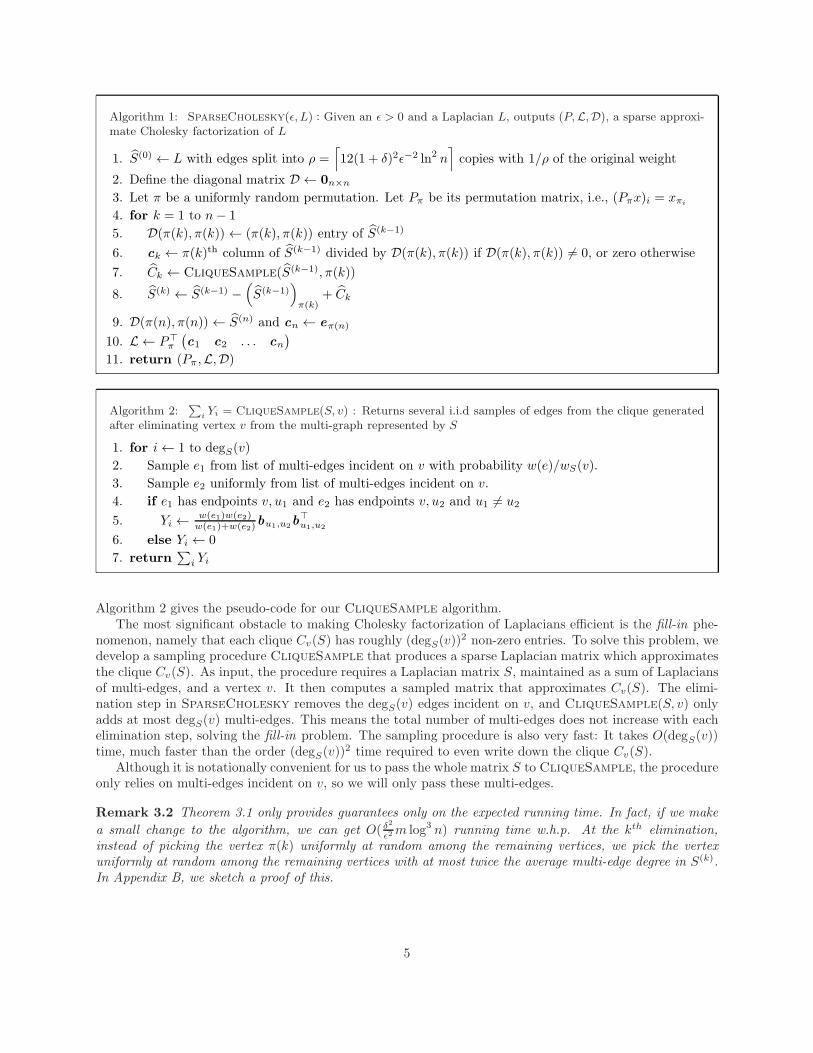
Algorithm 2 gives the pseudo-code for our CliqueSample algorithm.The most significant obstacle to making Cholesky factorization of Laplacians efficient is the fill-in phe-

nomenon, namely that each clique Cv(S) has roughly (degS(v))2 non-zero entries. To solve this problem, we

develop a sampling procedure CliqueSample that produces a sparse Laplacian matrix which approximatesthe clique Cv(S). As input, the procedure requires a Laplacian matrix S, maintained as a sum of Laplaciansof multi-edges, and a vertex v. It then computes a sampled matrix that approximates Cv(S). The elimi-nation step in SparseCholesky removes the degS(v) edges incident on v, and CliqueSample(S, v) onlyadds at most degS(v) multi-edges. This means the total number of multi-edges does not increase with eachelimination step, solving the fill-in problem. The sampling procedure is also very fast: It takes O(degS(v))time, much faster than the order (degS(v))

2 time required to even write down the clique Cv(S).Although it is notationally convenient for us to pass the whole matrix S to CliqueSample, the procedure

only relies on multi-edges incident on v, so we will only pass these multi-edges.

Remark 3.2 Theorem 3.1 only provides guarantees only on the expected running time. In fact, if we make

a small change to the algorithm, we can get O( δ2

ǫ2 m log3 n) running time w.h.p. At the kth elimination,instead of picking the vertex π(k) uniformly at random among the remaining vertices, we pick the vertexuniformly at random among the remaining vertices with at most twice the average multi-edge degree in S(k).In Appendix B, we sketch a proof of this.

5

4 Analysis of the Algorithm using Matrix Concentration

In this section, we analyze the SparseCholesky algorithm, and prove Theorem 3.1. To prove the theorem,we need several intermediate results which we will now present. In Section 4.1, we show how the output theSparseCholesky and CliqueSample algorithms can be used to define a matrix martingale. In Section 4.2,we introduce a new type of martingale, called a bags-of-dice martingale, and a novel matrix concentrationresult for these martingales. In Section 4.3, we show how to apply our new matrix concentration results tothe SparseCholesky martingale and prove Theorem 3.1. We defer proofs of the lemmas that characterizeCliqueSample to Section 5, and proofs of our matrix concentration results to Section 6.

4.1 Clique Sampling and Martingales for Cholesky Factorization

Throughout this section, we will study matrices that arise in the when using SparseCholesky to producea sparse approximate Cholesky factorization of the Laplacian L of a multi-graph G. We will very frequentlyneed to refer to matrices that are normalized by L. We adopt the following notation: Given a symmetricmatrix S s.t. ker(L) ⊆ ker(S),

Sdef= (L+)1/2S(L+)1/2.

We will only use this notation for matrices S that satisfy the condition ker(L) ⊆ ker(S). Note that L = Π, andA B iff A B. Normalization is always done with respect to the Laplacian L input to SparseCholesky.We say a multi-edge e is 1/ρ-bounded if

∥∥∥w(e)beb⊤e

∥∥∥ ≤ 1/ρ.

Given a Laplacian S that corresponds to a multi-graph GS , and a scalar ρ > 0, we say that S is 1/ρ-boundedif every multi-edge of S is 1/ρ-bounded. Since every multi-edge of L is trivially 1-bounded, we can obtain a1/ρ-bounded Laplacian that corresponds to the same matrix, by splitting each multi-edge into ⌈ρ⌉ identicalcopies, with a fraction 1/ ⌈ρ⌉ of the initial weight. The resulting Laplacian has at most ⌈ρ⌉m multi-edges.

Our next lemma describes some basic properties of the samples output by CliqueSample. We provethe lemma in Section 5.

Lemma 4.1 Given a Laplacian matrix S that is 1/ρ-bounded w.r.t. L and a vertex v, CliqueSample(S, v)returns a sum

∑e Ye of degS(v) IID samples Ye ∈ R

n×n. The following conditions hold

1. Ye is 0 or the Laplacian of a multi-edge with endpoints u1, u2, where u1, u2 are neighbors of v in S.

2. E∑

e Ye = Cv(S).

3.∥∥∥Y e

∥∥∥ ≤ 1/ρ, i.e. Ye is 1/ρ-bounded w.r.t. L.

The algorithm runs in time O(degS(v)).

The lemma tells us that the samples in expectation behave like the clique Cv(S), and that each sample is 1/ρ-bounded. This will be crucial to proving concentration properties of our algorithm. We will use the fact thatthe expectation of the CliqueSample algorithm output equals the matrix produced by standard Choleskyelimination, to show that in expectation, the sparse approximate Cholesky decomposition produced by ourSparseCholesky algorithm equals the original Laplacian. We will also see how we can use this expectedbehaviour to represent our sampling process as a martingale. We define the kth approximate Laplacian as

L(k) = S(k) +

k∑

i=1

αicic⊤i . (5)

Thus our final output equals L(n). Note that Line (9) of the SparseCholesky algorithm does not introduceany sampling error, and so L(n) = L(n−1). The only significance of Line (9) is that it puts the matrix in theform we need for our factorization. Now

L(k) − L(k−1) = αkckc⊤k + S(k) − S(k−1)

6

= αkckc⊤k + Ck −

(S(k−1)

)π(k)

= Ck − Cπ(k)(S(k−1)).

Each call to CliqueSample returns a sum of sample edges. Letting Y(k)e denote the eth sample in the

kth call to CliqueSample, we can write this sum as∑

e Y(k)e . Thus, conditional on the choices of the

SparseCholesky algorithm until step k − 1, and conditional on π(k), we can apply Lemma 4.1 to find

that the expected value of Ck is∑

e EY(k)e

Y(k)e = Cπ(k)(S

(k−1)). Hence the expected value of L(k) is exactly

L(k−1), and we can write

L(k) − L(k−1) =∑

e

Y (k)e − E

Y(k)e

Y (k)e .

By defining X(k)e

def= Y

(k)e − E

Y(k)e

Y(k)e , this becomes L(k) − L(k−1) =

∑eX

(k)e . So, without conditioning on

the choices of the SparseCholesky algorithm, we can write

L(n) − L = L(n) − L(0) =n−1∑

i=1

∑

e

X(i)e .

This is a martingale. To prove multiplicative concentration bounds, we need to normalize the martingale byL, and so instead we consider

L(n) − L = L(n−1) − L = L(n) −Π =

n−1∑

i=1

∑

e

X(i)e . (6)

This martingale has considerable structure beyond a standard martingale. Conditional on the choices of the

SparseCholesky algorithm until step k − 1, and conditional on π(k), the terms X(k)e are independent.

In Section 4.2 we define a type of martingale that formalizes the important aspects of this structure.

4.2 Bags-of-Dice Martingales and Matrix Concentration Results

We use the following shorthand notation: Given a sequence of random variables (r1, R(1), r2, R

(2), . . . , rk, R(k)),

for every i, we writeE(i)

[ · ] = Er1

ER(1)· · ·E

riE

R(i)[ · ] .

Extending this notation to conditional expectations, we write,

Eri

[·∣∣(i − 1)

]= E

ri

[·∣∣∣r1, R(1), . . . , ri−1, R

(i−1)]

Definition 4.2 A bags-of-dice martingale is a sum of random d×d matrices Z =∑k

i=1

∑lie=1 Z

(i)e , with

some additional structure. We require that there exists a sequence of random variables (r1, R(1), r2, R

(2), . . . , rk, R(k)),

s.t. for all 1 ≤ i ≤ k, conditional on (i−1) and ri, li is a non-negative integer, and R(i) is a tuple of li indepen-

dent random variables: R(i) = (R(i)1 , . . . , R

(i)li). We also require that conditional on (r1, R

(1), r2, R(2), . . . , ri, R

(i))

and ri, for all 1 ≤ e ≤ li Z(i)e is a symmetric matrix, and a deterministic function of R

(i)e . Finally, we require

that ER

(i)e

[Z

(i)e

∣∣∣(i− 1), ri

]= 0.

Note that li is allowed to be random, as long as it is fixed conditional on (i − 1) and ri. The martingale

given in Equation (6) is a bags-of-dice martingale, with ri = π(i), and R(i)e = Y

(i)e . The name is motivated

by a simple model: At each step of the martingale we pick a random bag of dice from a collection of bags

7

(this corresponds to the outcome of ri) and then we independently roll each die in the bag (corresponds to

the outcomes R(i)e ).

It is instructive to compare the bags-of-dice martingales with matrix martingales such as those consideredby Tropp [Tro12]. A naive application of the results from [Tro12] tells us that if we have good uniform norm

bounds on each term Z(i)e , and there exists fixed matrices Ω

(i)e s.t. that for all i, e and for all possible

outcomes we get deterministic bounds on the matrix variances: ER

(i)e(Z

(i)e )2 Ω

(i)e , then the concentration

of the martingale is governed by the norm of the sum of the variances∥∥∥∑

i

∑eΩ

(i)e

∥∥∥. In our case, this result

is much too weak: Good enough Ω(i)e do not exist.

A slight extension of the results from [Tro12] allows us to do a somewhat better: Since the terms Z(i)e

are independent conditional on ri, it suffices to produce fixed matrices Ω(i) s.t. that for all i, e and for allpossible outcomes we get deterministic bounds on the matrix variances of the sum of variables in each “bag”:∑

e ER(i)e(Z

(i)e )2 Ω(i). Then the concentration of the martingale is governed by

∥∥∥∑

iΩ(i)∥∥∥. Again, this

result is not strong enough: Good fixed Ω(i) do not seem to exist.

We show a stronger result: If we can produce a uniform norm bound on ER

(i)e(Z

(i)e )2, then it suffices to pro-

duce fixed matrices Ω(i) that upper bound the matrix variance averaged over all bags : Eri

∑e ER

(i)e(Z

(i)e )2 Ω(i).

The concentration of the martingale is then governed by∥∥∥∑

i Ω(i)∥∥∥. In the context where we apply our con-

centration result, our estimates of∥∥∥∑

iΩ(i)∥∥∥ are larger than

∥∥∥∑

i Ω(i)∥∥∥ by a factor ≈ n

lnn . Consequently, we

would not obtain strong enough concentration using the weaker result.The precise statement we prove is:

Theorem 4.3 Suppose Z =∑k

i=1

∑lie=1 Z

(i)e is a bags-of-dice martingale of d× d matrices that satisfies

1. Every sample Z(i)e satisfies

∥∥∥Z(i)e

∥∥∥2

≤ σ21 ,

2. For every i we have

∥∥∥∥∑

e ER(i)e

[(Z

(i)e )2

∣∣∣(i − 1), ri

]∥∥∥∥ ≤ σ22 , and

3. There exist deterministic matrices Ωi such that Eri

[∑e ER

(i)e(Z

(i)e )2

∣∣∣(i− 1)] Ωi, and

∥∥∑i Ωi

∥∥ ≤ σ23 .

Then, for all ǫ > 0, we have

Pr [Z 6 ǫI] ≤ exp(−ǫ2/4σ2

),

where

σ2 = max

σ23 ,

ǫ

2σ1,

4ǫ

5σ2

.

We remark that this theorem, and all the results in this section extend immediately to Hermitian matrices.We prove the above theorem in Section 6. This result is based on the techniques introduced by Tropp [Tro12]for using Lieb’s Concavity Theorem to prove matrix concentration results. Tropp’s result improved on earlierwork, such as Ahlswede and Winter [AW02] and Rudelson and Vershynin [RV07]. These earlier matrixconcentration results required IID sampling, making them unsuitable for our purposes.

Unfortunately, we cannot apply Theorem 4.3 directly to the bags-of-dice martingale in Equation (6). As

we will see later, the variance of∑

eX(i)e can have norm proportional to

∥∥∥L(i)∥∥∥, which can grow large.

However, we expect that the probability of∥∥∥L(i)

∥∥∥ growing large is very small. Our next construction

allows us to leverage this idea, and avoid the small probability tail events that prevent us from directlyapplying Theorem 4.3 to the bags-of-dice martingale in Equation (6).

Definition 4.4 Given a bags-of-dice martingale of d× d matrices Z =∑k

i=1

∑lie=1 Z

(i)e , and a scalar ǫ > 0,

8

we define for each h ∈ 1, 2, . . . , k + 1 the event

Ah =

∀1 ≤ j < h.

j∑

i=1

li∑

e=1

Z(i)e ǫI

.

We also define the ǫ-truncated martingale:

Z =

k∑

i=1

1Ai

li∑

e=1

Z(i)e

The truncated martingale is derived from another martingale by forcing the martingale to get “stuck” ifit grows too large. This ensures that so long as the martingale is not stuck, it is not too large. On theother hand, as our next result shows, the truncated martingale fails more often than the original martingale,and so it suffices to prove concentration of the truncated martingale to prove concentration of the originalmartingale. The theorem stated below is proven in Section 6.

Theorem 4.5 Given a bags-of-dice martingale of d × d matrices Z =∑k

i=1

∑lie=1 Z

(i)e , a scalar ǫ > 0, the

associated ǫ-truncated martingale Z is also a bags-of-dice martingale, and

Pr[−ǫI 6 Z or Z 6 ǫI] ≤ Pr[−ǫI 6 Z or Z 6 ǫI]

4.3 Analyzing the SparseCholesky Algorithm Using Bags-of-Dice Martingales

By taking Z(k)e = X

(k)e , ri = π(i) and R

(i)e = Y

(i)e , we obtain a bags-of-dice martingale Z =

∑n−1i=1

∑e Z

(i)e .

Let Z denote the corresponding ǫ-truncated bags-of-dice martingale. The next lemma shows that Z iswell-behaved. The lemma is proven in Section 5.

Lemma 4.6 Given an integer 1 ≤ k ≤ n− 1, conditional on the choices of the SparseCholesky algorithm

until step k−1, let∑e Ye = CliqueSample(S(k−1), π(k)). Let Xedef= Ye − EYe

Ye. The following statementshold

1. Conditional on π(k), EYe1Ak

Xe = 0.

2.∥∥∥1Ak

Xe

∥∥∥ ≤ 1/ρ holds always.

3. Conditional on π(k),∑

e EYe(1Ak

Xe)2 1Ak

1ρCv(S).

4.

∥∥∥∥1AkCπ(k)(S(k−1))

∥∥∥∥ ≤ 1 + ǫ holds always.

5. Eπ(k) 1AkCπ(k)(S(k−1)) 2(1+ǫ)

n+1−kI.

We are now ready to prove Theorem 3.1.

Proof of Theorem 3.1: We have L(n) = Π + Z. Since for all k, e, ker(L) ⊆ ker(Y(k)e ), the statement

(1 − ǫ)L L(n) (1 + ǫ)L is equivalent to −ǫΠ Z ǫΠ. Further, ΠZΠ = Z, and so it is equivalent to−ǫI Z ǫI. By Theorem 4.5, we have,

Pr[(1− ǫ)L L(n) (1 + ǫ)L] = 1− Pr [−Z 6 ǫI or Z 6 ǫI] ≥ 1− Pr[−Z 6 ǫI or Z 6 ǫI

]

≥ 1− Pr[−Z 6 ǫI

]− Pr

[Z 6 ǫI

](7)

To lower bound this probability, we’ll prove concentration using Theorem 4.3. We now compute the parame-

ters for applying the theorem. From Lemma 4.1, for all k and e, we have EYe1Ak

X(k)e = 0,

∥∥∥∥1AkX

(k)e

∥∥∥∥ ≤ 1ρ .

9

Thus, we can pick σ1 = 1ρ . Next, again by Lemma 4.1, we have

∥∥∥∥∥∥

[∑

e

E

Y(k)e

(1Ak

X(k)e

)2∣∣∣∣∣(k), rk

]∥∥∥∥∥∥≤ 1

ρ

∥∥∥1AkCπ(k)(S)

∥∥∥ ≤ 1 + ǫ

ρ≤ 3

2ρ.

Thus, we can pick σ2 =√

32ρ . Finally, Lemma 4.1 also gives,

Eπ(k)

∑

e

E

Y(k)e

(1Ak

X(k)e

)2

1

ρE

π(k)1Ak

Cπ(k)(S(k−1)) 2(1 + ǫ)

ρ(n+ 1− k)I 3

ρ(n+ 1− k)I.

Thus, we can pick Ωk = 3ρ(n+1−k) I, and

σ23 =

3 lnn

ρ≥

n−1∑

k=1

3

ρ(n+ 1− k).

Similarly, we obtain concentration for −Z with the same parameters. Thus, by Theorem 4.3,

Pr[−Z 6 ǫI

]+ Pr

[Z 6 ǫI

]≤ 2n exp

(−ǫ2/4σ2

),

for

σ2 = max

σ23 ,

ǫ

2σ1,

4ǫ

5σ2

= max

3 lnn

ρ,ǫ

2

√3

2ρ,4ǫ

5ρ

.

Picking ρ =⌈12(1 + δ)2ǫ−2 ln2 n

⌉, we get σ2 ≤ ǫ2

4(1+δ) lnn , and

Pr[−Z 6 ǫI

]+ Pr

[Z 6 ǫI

]≤ 2n exp

(−ǫ2/4σ2

)= 2n exp

(−(1 + δ) lnn

)= 2n−δ.

Combining this with Equation (7) establishes Equation (11).Finally, we need to bound the expected running time of the algorithm. We start by observing that the

algorithm maintains the two following invariants:

1. Every multi-edge in S(k−1) is 1/ρ-bounded.

2. The total number of multi-edges is at most ρm.

We establish the first invariant inductively. The invariant holds for S(0), because of the splitting of original

edges into ρ copies with weight 1/ρ. The invariant thus also holds for S(0) −(S(0)

)π(1)

, since the multi-

edges of this Laplacian are a subset of the previous ones. By Lemma 4.1, every multi-edge Ye output by

CliqueSample is 1/ρ-bounded, so S(1) = S(0)−(S(0)

)π(1)

+ C1 is 1/ρ-bounded. If we apply this argument

repeatedly for k = 1, . . . , n− 1 we get invariant (1).

Invariant (2) is also very simple to establish: It holds for S(0), because splitting of original edges into ρ

copies does not produce more than ρmmulti-edges in total. When computing S(k), we subtract(S(k−1)

)π(k)

,

which removes exactly degS(k−1)(π(k)) multi-edges, while we add the multi-edges produced by the call to

CliqueSample(S(k−1), π(k)), which is at most degS(k−1)(π(k)). So the number of multi-edges is not in-creasing.

By Lemma 4.1, the running time for the call to CliqueSample is O(degS(k)(π(k))). Given the invariants,we get that the expected time for the kth call to CliqueSample is O(Eπ(k) degS(k)(π(k))) = O(ρm/(n+1−k)). Thus the expected running time of all calls to CliqueSample is O(mρ

∑n−1i=1

1n−i ) = O(mδ2ǫ−2 ln3 n).

The total number of entries in the L,D matrices must also be bounded by O(mδ2ǫ−2 ln3 n) in expectation,and so the permutation step in Line 10 can be applied in expected time O(mδ2ǫ−2 ln3 n), and this alsobounds the expected running time of the whole algorithm.

10

5 Clique Sampling Proofs

In this section, we prove Lemmas 4.1 and 4.6 that characterize the behaviour of our algorithmCliqueSample,which is used in SparseCholesky to approximate the clique generated by eliminating a variable.

A important element of the CliqueSample algorithm is our very simple approach to leverage scoreestimation. Using the well-known result that effective resistance in Laplacians is a distance (see Lemma 5.2),we give a bound on the leverage scores of all edges in a clique that arises from elimination. We let

wS(v) =∑

e∈E(S)e∋v

w(e).

Then by Equation (3)

Cv(S) =1

2

∑

e∈E(S)e has

endpointsv,u

∑

e′∈E(S)e′ has

endpointsv,z 6=u

w(e)w(e′)

wS(v)bu,zb

⊤u,z . (8)

Note that the factor 1/2 accounts for the fact that every pair is double counted.

Lemma 5.1 Suppose multi-edges e, e′ ∋ v are 1/ρ-bounded w.r.t. L, and have endpoints v, u and v, z

respectively, and z 6= u, then w(e)w(e′)bu,zb⊤u,z is w(e)+w(e′)

ρ -bounded.

To prove Lemma 5.1, we need the following result about Laplacians:

Lemma 5.2 Given a connected weighted multi-graph G = (V,E,w) with associated Laplacian matrix L inG, consider three distinct vertices u, v, z ∈ V , and the pair-vectors bu,v, bv,z and bu,z.

∥∥∥bu,zb⊤u,z

∥∥∥ ≤∥∥∥bu,vb

⊤u,v

∥∥∥+∥∥∥bv,zb

⊤v,z

∥∥∥ .

This is known as phenomenon that Effective Resistance is a distance [KR93].

Proof of Lemma 5.1: Using the previous lemma:

w(e)w(e′)∥∥∥bu,zb

⊤u,z

∥∥∥ ≤ w(e)w(e′)

(∥∥∥bu,vb⊤u,v

∥∥∥ +∥∥∥bv,zb

⊤v,z

∥∥∥)≤ 1

ρ

(w(e) + w(e′)

)

To prove Lemma 4.1, we need the following result of Walker [Wal77] (see Bringmann and Panagiotou [BP12]for a modern statement of the result).

Lemma 5.3 Given a vector p ∈ Rd of non-negative values, the procedure UnsortedProportionalSampling

requires O(d) preprocessing time and after this allows for IID sampling for a random variable x distributeds.t.

Pr[x = i] = p(i)/ ‖p‖1 .The time required for each sample is O(1).

Remark 5.4 We note that there are simpler sampling constructions than that of Lemma 5.3 that needO(log n) time per sample, and using such a method would only worsen our running time by a factor O(log n).

Proof of Lemma 4.1: From Lines (5) and (6), Yi is 0 or the Laplacian of a multi-edge with endpointsu1, u2. To upper bound the running time, it is important to note that we do not need access to the entirematrix S. We only need the multi-edges incident on v. When calling CliqueSample, we only pass a copyof just these multi-edges.

11

We observe that the uniform samples in Line (3) can be done in O(1) time each, provided we count thenumber of multi-edges incident on v to find degS(v). We can compute degS(v) in O(degS(v)) time. UsingLemma 5.3, if we do O(degS(v)) time preprocessing, we can compute each sample in Line (2) in time O(1).Since we do O(degS(v)) samples, the total time for sampling is hence O(degS(v)).

Now we determine the expected value of the sum of the samples. Note that in the sum below, each pairof multi-edges appears twice, with different weights.

E

∑

i

Yi = degS(v)∑

e∈E(S)e has

endpointsv,u

∑

e′∈E(S)e′ has

endpointsv,z 6=u

w(e)

wS(v)

1

degS(v)

w(e)w(e′)

w(e) + w(e′)bu,zb

⊤u,z = Cv(S).

By Lemma 5.1, ∥∥∥Yi

∥∥∥ ≤ maxe,e′∈E(S)e,e′ hasendpoints

v,u and v,z 6=u

w(e)w(e′)

w(e) + w(e′)

∥∥∥bu,zb⊤u,z

∥∥∥ ≤ 1/ρ.

Proof of Lemma 4.6: Throughout the proof of this lemma, all the random variables considered areconditional on the choices of the SparseCholesky algorithm up to and including step k − 1.

Observe, by Lemma 4.1:

∑

e

EYe

Ye2 E

∑

e

EYe

∥∥∥Ye

∥∥∥Ye 1

ρCπ(k)(S(k−1)).

NowEYe

1AkXe = 1Ak

EYe

Xe = 0.

Note that Ye and EYeYe are PSD, and

∥∥∥EYeYe

∥∥∥ ≤ EYe

∥∥∥Ye

∥∥∥ ≤ 1/ρ so

∥∥∥Xe

∥∥∥ =

∥∥∥∥Ye − EYe

Ye

∥∥∥∥ ≤ max

∥∥∥Ye

∥∥∥ ,∥∥∥∥EYe

Ye

∥∥∥∥

≤ 1/ρ.

Also EYe(1Ak

Xe)2 = 1Ak

EYeXe

2, so

EYe

Xe2= (E

Ye

Ye2)− (E

Ye

Ye)2 (E

Ye

Ye2),

where, in the last line, we used 0 (EYeYe)

2. Thus∑

e EYe(1Ai

Xe)2 1Ak

1ρCπ(k)(S(k−1)). Equation (6)

gives:

L(k−1) = L+

k−1∑

i=1

∑

e

X(i)e . (9)

Consequently, 1Ak= 1 gives L(k−1) (1 + ǫ)L.

Now, Cπ(k)(S(k−1)) is PSD since it is a Laplacian, so

∥∥∥∥Cπ(k)(S(k−1))

∥∥∥∥ = λmax(Cπ(k)(S(k−1))). By Equa-

tion (2), we get Cπ(k)(S(k−1))

(S(k−1)

)π(k)

and by Equation (1) we get(S(k−1)

)π(k) S(k−1), finally by

Equation (5) we get S(k−1) L(k−1) so∥∥∥∥1Ak

Cπ(k)(S(k−1))

∥∥∥∥ ≤ 1Akλmax(Cπ(k)(S(k−1))) ≤ 1Ak

λmax(L(k−1)) ≤ 1 + ǫ.

12

Again, using Cπ(k)(S(k−1))

(S(k−1)

)π(k)

, we get

Eπ(k)

1AkCπ(k)(S(k−1)) 1Ak

Eπ(k)

(S(k−1)

)π(k)

= 1Ak

2

n+ 1− kS(k−1) 2(1 + ǫ)

n+ 1− kI. (10)

6 Matrix Concentration Analysis

6.1 Concentration of Bags-of-Dice Martingales

To prove Theorem 4.3, we need the following lemma, which is the main technical result of this section.

Lemma 6.1 Given a bags-of-dice martingale of d × d matrices Z =∑k

i=1

∑lie=1 Z

(i)e that is for all θ such

that 0 < θ2 ≤ min 1σ21, 512σ2

2, we have,

ETr exp (θZ) ≤ d exp(θ2σ2

3

).

Before proving this lemma, we will see how to use it to prove Theorem 4.3.

Proof of Theorem 4.3: Given Lemma 6.1, we can show Theorem 4.3 using the following bound via traceexponentials, which was first developed by Ahlswede and Winter [AW02].

P [Z 6 ǫI] = P[λmax(Z) ≥ ǫ

]= P

[λmax(exp (θZ)) ≥ exp (θǫ)

]≤ exp (−ǫθ)Eλmax(exp (θZ))

≤ exp (−ǫθ)ETr exp (θZ)

≤ d exp(−ǫθ + θ2σ2

3

).

Picking θ = ǫ2σ2 , where σ

2 = maxσ23 ,

ǫ2σ1,

4ǫ5 σ2

, the condition for Lemma 6.1 that 0 < θ2 ≤ min 1

σ21, 512σ2

2

is satisfied, and we get, P [Z 6 ǫI] = d exp

(− ǫ2

2σ2

(1− σ2

3

2σ2

))≤ d exp

(− ǫ2

4σ2

).

To show Lemma 6.1 will need the following result by Tropp [Tro12], which is a corollary of Lieb’s ConcavityTheorem [Lie73].

Theorem 6.2 Given a random symmetric matrix Z, and a fixed symmetric matrix H,

ETr exp (H + Z) ≤ Tr exp(H + logE exp(Z)

).

We will use the following claim to control the above trace by an inductive argument.

Claim 6.3 For all j = 1, . . . , k, and all θ such that 0 < θ2 ≤ min 1σ21, 512σ2

2, we have,

E(j)

Tr exp

θ2

k∑

i=j+1

Ωi

+ θ

j∑

i=1

li∑

e=1

Z(i)e

≤ E

(j−1)Tr exp

θ2

k∑

i=j

Ωi

+ θ

j−1∑

i=1

li∑

e=1

Z(i)e

.

Before proving this claim, we see that it immediately implies Lemma 6.1.

Proof of Lemma 6.1: We chain the inequalities given by Claim 6.3 for j = k, k − 1, . . . , 1 to obtain,

E(k)

Tr exp (θZ) = E(k)

Tr exp

θ

k∑

i=1

li∑

e=1

Z(i)e

≤ Tr exp

θ2

k∑

i=1

Ωi

≤ d exp

(θ2σ2

3

),

where the last inequality follows from Tr exp (A) ≤ d exp(‖A‖

)for symmetric A and

∥∥∥∑k

i=1 Ωi

∥∥∥ ≤ σ23 .

13

We will also need the next two lemmas, which essentially appear in the work of Tropp [Tro12]. For com-pleteness, we also prove these lemmas in Appendix A.

Lemma 6.4 Suppose Z is a random matrix s.t. EZ 0, ‖Z‖ ≤ 1, then, logE exp (Z) 45 EZ2.

Lemma 6.5 Suppose C is a PSD random matrix s.t. ‖C‖ ≤ 1/3, then, logE exp (C) 65 EC.

We also need the following well-known fact (see for example [Tro12]):

Fact 6.6 Given symmetric matrices A,B s.t. A B, Tr exp (A) Tr exp (B).

Lemma 6.7 For all θ such that 0 < θ2 ≤ 1σ21, all j = 1, . . . , k and for all symmetric H that are fixed given

(r1, R1), . . . , (rj−1, Rj−1),

E(j)

Tr exp

(H + θ

∑

e

Z(j)e

)≤ E

(j−1)ErjTr exp

(H +

4

5θ2 E

R(j)e

∑

e

(Z(j)e )2

).

Proof: We have

E(j)

Tr exp

(H + θ

∑

e

Z(j)e

)= E

(j−1)Erj

E

R(j)1

. . . E

R(j)lj

Tr exp

H + θ

lj∑

e=1

Z(j)e

Using Theorem 6.2 with H = H + θ∑lj−1

e=1 Z(j)e

≤ E(j−1)

Erj

E

R(j)1

. . . E

R(j)lj−1

Tr exp

H + θ

lj−1∑

e=1

Z(j)e + log E

R(j)lj

exp(θZ

(j)lj

)

... (Using Theorem 6.2 lj − 1 times)

≤ E(j−1)

ErjTr exp

H +

lj∑

e=1

log E

R(j)e

exp(θZ(j)

e

)

For all j, e, we have ER

(j)e

θZje 0, and

∥∥∥θZ(j)e

∥∥∥ ≤ 1 (since∥∥∥Z(j)

e

∥∥∥ ≤ σ1 and θ ≤ 1σ1), thus Lemma 6.4 gives

∑

e

log E

R(j)e

exp(θZ(j)

e

) 4

5θ2∑

e

E

R(j)e

(Z(j)e )2.

Now, using Fact 6.6 which states that Tr exp (·) is monotone increasing with respect to the PSD order, weobtain the lemma.

Proof of Claim 6.3: Since 0 < θ2 ≤ 1σ21, using Lemma 6.7 with H = θ2

(∑ki=j+1 Ωi

)+ θ

∑j−1i=1

∑e Z

(i)e ,

we obtain,

E(j)

Tr exp

θ2

k∑

i=j+1

Ωi

+ θ

j∑

i=1

∑

e

Z(i)e

≤ E

(j−1)ErjTr exp

θ2

k∑

i=j+1

Ωi

+ θ

j−1∑

i=1

∑

e

Z(i)e +

4

5θ2∑

e

E

R(j)e

(Z(j)e )2

≤ E(j−1)

Tr exp

θ2

k∑

i=j+1

Ωi

+ θ

j−1∑

i=1

∑

e

Z(i)e + log E

rjexp

(4

5θ2∑

e

E

R(j)e

(Z(j)e )2

),

14

where the last inequality uses Theorem 6.2 with H = θ2(∑k

i=j+1 Ωi

)+ θ

∑j−1i=1

∑e Z

(i)e . Now, since 0

∑e ER

(j)e(Z

(j)e )2, and

∥∥∥ 45θ

2∑

e ER(j)e(Z

(j)e )2

∥∥∥ ≤ 45θ

2σ22 ≤ 1

3 , thus Lemma 6.5 gives

log Erjexp

(4

5θ2∑

e

E

R(j)e

(Z(j)e )2

) 6

5

4

5θ2 E

rj

∑

e

E

R(j)e

(Z(j)e )2 θ2 E

rj

∑

e

E

R(j)e

(Z(j)e )2 θ2Ωj .

Now, using Fact 6.6, namely that Tr exp (·) is monotone increasing with respect to the PSD order, we obtainthe lemma.

6.2 Truncating Bags-of-Dice Martingales

To prove this theorem, we use the next lemma, which we will prove later in this section:

Lemma 6.8

Ak+1 =[Z ǫI

].

Proof of Theorem 4.5:

Note that Ak+1 implies Z ǫI. Thus Z 6 ǫI implies ¬Ak+1, or equivalently [Z 6 ǫI] ⊆ ¬Ak+1. Usingthe above lemma, it immediately implies the first part of the claim. Also note that Ak+1 implies Ai for alli ≤ k. Thus, if Ak+1 occurs then 1Ai

= 1 for all i ≤ k.

Pr[−ǫI 6 Z or Z 6 ǫI] ≤ Pr

−ǫI 6

k∑

i=1

∑

e

Z(i)e or ¬Ak+1

= Pr

−ǫI 6

k∑

i=1

(1Ai

∑

e

Z(i)e

)and Ak+1

or ¬Ak+1

= Pr

−ǫI 6

k∑

i=1

(1Ai

∑

e

Z(i)e

)or ¬Ak+1

= Pr[−ǫI 6 Z or Z 6 ǫI].

In the last line, we used Lemma 6.8.Z is a bags-of-dice martingale, because conditional on (i − 1) and ri, the indicator 1Ai

is fixed at either

0 or 1, and so in both cases, the variables 1AiZ

(i)e are independent and zero mean.

Proof Lemma 6.8: We start by showing that Ak+1 implies the event

[∑ki=1

(1Ai

∑e Z

(i)e

) ǫI

].

Suppose Ak+1 occurs. Then Ai occurs for all i ≤ k + 1, so 1Ai= 1 for all i ≤ k + 1. But then,∑k

i=1 1Ai

∑e Z

(i)e =

∑ki=1

∑e Z

(i)e and

∑ki=1

∑e Z

(i)e ǫI follows from Ak+1, so

∑ki=1 1Ai

∑e Z

(i)e ǫI.

This proves that Ak+1 implies the event[∑k

i=1 1Ai

∑e Z

(i)e ǫI

].

Next we show that[∑k

i=1 1Ai

∑e Z

(i)e ǫI

]implies the eventAk+1. It suffices to show the contrapositive:

¬Ak+1 implies ¬[∑k

i=1 1Ai

∑e Z

(i)e ǫI

]. Suppose ¬Ak+1 occurs. This means there must exist j ≤ k s.t.

∑ji=1

∑e Z

(i)e 6 ǫI. Let j∗ denote the least such j. Observe that 1Ai

= 1 for all i ≤ j∗, and 1Ai= 0 for all

i > j∗. Thusk∑

i=1

1Ai

∑

e

Z(i)e =

j∗∑

i=1

∑

e

Z(i)e 6 ǫI.

So ¬[∑k

i=1 1Ai

∑e Z

(i)e ǫI

]occurs.

15

Acknowledgements

We thank Daniel Spielman for suggesting this project and for helpful comments and discussions.

References

[AW02] Rudolf Ahlswede and Andreas Winter. Strong converse for identification via quantum channels.Information Theory, IEEE Transactions on, 48(3):569–579, 2002.

[BGH+06] Marshall Bern, John R. Gilbert, Bruce Hendrickson, Nhat Nguyen, and Sivan Toledo. Support-graph preconditioners. SIAM Journal on Matrix Analysis and Applications, 27(4):930–951, 2006.

[BHV08] Erik G. Boman, Bruce Hendrickson, and Stephen A. Vavasis. Solving elliptic finite element sys-tems in near-linear time with support preconditioners. SIAM J. Numerical Analysis, 46(6):3264–3284, 2008.

[BP12] Karl Bringmann and Konstantinos Panagiotou. Efficient sampling methods for discrete distri-butions. In Automata, Languages, and Programming, pages 133–144. Springer, 2012.

[CKM+11] Paul Christiano, Jonathan A. Kelner, Aleksander Madry, Daniel A. Spielman, and Shang-HuaTeng. Electrical flows, laplacian systems, and faster approximation of maximum flow in undi-rected graphs. In Proceedings of the 43rd annual ACM symposium on Theory of computing,STOC ’11, pages 273–282, New York, NY, USA, 2011. ACM.

[CKM+14] Michael B. Cohen, Rasmus Kyng, Gary L. Miller, Jakub W. Pachocki, Richard Peng, Anup B.Rao, and Shen Chen Xu. Solving sdd linear systems in nearly mlog1/2n time. In Proceedingsof the 46th Annual ACM Symposium on Theory of Computing, STOC ’14, pages 343–352, NewYork, NY, USA, 2014. ACM.

[CLM+15] Michael B. Cohen, Yin Tat Lee, Cameron Musco, Christopher Musco, Richard Peng, and AaronSidford. Uniform sampling for matrix approximation. In Proceedings of the 2015 Conference onInnovations in Theoretical Computer Science, ITCS ’15, pages 181–190, New York, NY, USA,2015. ACM.

[DS08] Samuel I Daitch and Daniel A Spielman. Faster approximate lossy generalized flow via interiorpoint algorithms. In Proceedings of the 40th annual ACM symposium on Theory of computing,pages 451–460. ACM, 2008.

[Gre96] Keith Gremban. Combinatorial Preconditioners for Sparse, Symmetric, Diagonally DominantLinear Systems. PhD thesis, Carnegie Mellon University, Pittsburgh, October 1996. CMU CSTech Report CMU-CS-96-123.

[Gua97] Stephen Guattery. Graph embedding techniques for bounding condition numbers of incompletefactor preconditioning. 1997.

[Gus78] Ivar Gustafsson. A class of first order factorization methods. BIT Numerical Mathematics,18(2):142–156, 1978.

[Hig02] N. Higham. Accuracy and Stability of Numerical Algorithms. Society for Industrial and AppliedMathematics, second edition, 2002.

[KLP+16] Rasmus Kyng, Yin Tat Lee, Richard Peng, Sushant Sachdeva, and Daniel A. Spielman. Sparsifiedcholesky and multigrid solvers for connection laplacians. 2016. To appear at ACM on Symposiumon Theory of Computing.

16

[KM09] J.A. Kelner and A. Madry. Faster generation of random spanning trees. In Foundations ofComputer Science, 2009. FOCS’09. 50th Annual IEEE Symposium on, pages 13–21. IEEE, 2009.This result was substantially improved as a result of an observation by James Propp. He will beadded as a coauthor on the journal version.

[KMP10] I. Koutis, G.L. Miller, and R. Peng. Approaching optimality for solving SDD linear systems. InFoundations of Computer Science (FOCS), 2010 51st Annual IEEE Symposium on, pages 235–244, 2010.

[KMP11] I. Koutis, G.L. Miller, and R. Peng. A nearly-m logn time solver for SDD linear systems. InFoundations of Computer Science (FOCS), 2011 52nd Annual IEEE Symposium on, pages 590–598, 2011.

[KMP12] Jonathan A. Kelner, Gary L. Miller, and Richard Peng. Faster approximate multicommodityflow using quadratically coupled flows. In Proceedings of the 44th symposium on Theory ofComputing, STOC ’12, pages 1–18, New York, NY, USA, 2012. ACM.

[KOSZ13] Jonathan A Kelner, Lorenzo Orecchia, Aaron Sidford, and Zeyuan Allen Zhu. A simple, com-binatorial algorithm for solving sdd systems in nearly-linear time. In Proceedings of the 45thannual ACM symposium on Symposium on theory of computing, pages 911–920. ACM, 2013.

[KR93] Douglas J Klein and Milan Randic. Resistance distance. Journal of Mathematical Chemistry,12(1):81–95, 1993.

[KRS15] Rasmus Kyng, Anup Rao, and Sushant Sachdeva. Fast, provable algorithms for isotonic regressionin all l p-norms. In C. Cortes, N. D. Lawrence, D. D. Lee, M. Sugiyama, and R. Garnett, editors,Advances in Neural Information Processing Systems 28, pages 2719–2727. Curran Associates,Inc., 2015.

[Lie73] Elliott H Lieb. Convex trace functions and the wigner-yanase-dyson conjecture. Advances inMathematics, 11(3):267 – 288, 1973.

[LKP12] Alex Levin, Ioannis Koutis, and Richard Peng. Improved spectral sparsification and numericalalgorithms for sdd matrices. In Proceedings of the 29th Symposium on Theoretical Aspects ofComputer Science (STACS), 2012. to appear.

[LS14] Y. T. Lee and A. Sidford. Path finding methods for linear programming: Solving linear programsin O(vrank) iterations and faster algorithms for maximum flow. In Foundations of ComputerScience (FOCS), 2014 IEEE 55th Annual Symposium on, pages 424–433, Oct 2014.

[Mad13] Aleksander Madry. Navigating central path with electrical flows: From flows to matchings, andback. In 54th Annual IEEE Symposium on Foundations of Computer Science, FOCS 2013, 26-29October, 2013, Berkeley, CA, USA, pages 253–262, 2013.

[OSV12] Lorenzo Orecchia, Sushant Sachdeva, and Nisheeth K. Vishnoi. Approximating the exponential,the lanczos method and an O(m)-time spectral algorithm for balanced separator. In Proceedingsof The Fourty-Fourth Annual ACM Symposium On The Theory Of Computing (STOC ’12),2012. to appear.

[PS14] Richard Peng and Daniel A. Spielman. An efficient parallel solver for SDD linear systems. InSymposium on Theory of Computing, STOC 2014, New York, NY, USA, May 31 - June 03,2014, pages 333–342, 2014.

[RJL79] Robert Endre Tarjan Richard J. Lipton, Donald J. Rose. Generalized nested dissection. SIAMJournal on Numerical Analysis, 16(2):346–358, 1979.

17

[RV07] Mark Rudelson and Roman Vershynin. Sampling from large matrices: An approach throughgeometric functional analysis. J. ACM, 54(4), July 2007.

[ST04] Daniel A. Spielman and Shang-Hua Teng. Nearly-linear time algorithms for graph partitioning,graph sparsification, and solving linear systems. In Proceedings of the Thirty-sixth Annual ACMSymposium on Theory of Computing, STOC ’04, pages 81–90, New York, NY, USA, 2004. ACM.

[ST14] Daniel A. Spielman and Shang-Hua Teng. Nearly-linear time algorithms for preconditioningand solving symmetric, diagonally dominant linear systems. SIAM. J. Matrix Anal. & Appl.,35:835885, 2014.

[Str86] G. Strang. Introduction to Applied Mathematics. Wellesley-Cambridge Press, 1986.

[Tro12] Joel A Tropp. User-friendly tail bounds for sums of random matrices. Foundations of Computa-tional Mathematics, 12(4):389–434, 2012.

[Wal77] Alastair J. Walker. An efficient method for generating discrete random variables with generaldistributions. ACM Trans. Math. Softw., 3(3):253–256, September 1977.

[Wil12] Virginia Vassilevska Williams. Multiplying matrices faster than coppersmith-winograd. In Pro-ceedings of the Forty-fourth Annual ACM Symposium on Theory of Computing, STOC ’12, pages887–898, New York, NY, USA, 2012. ACM.

[ZBL+04] Dengyong Zhou, Olivier Bousquet, Thomas Navin Lal, Jason Weston, and Bernhard Scholkopf.Learning with local and global consistency. Advances in neural information processing systems,16(16):321–328, 2004.

[ZGL03] X. Zhu, Z. Ghahramani, and J. D. Lafferty. Semi-supervised learning using gaussian fields andharmonic functions. ICML, 2003.

[ZS04] Dengyong Zhou and Bernhard Scholkopf. A regularization framework for learning from graphdata. In ICML workshop on statistical relational learning and Its connections to other fields,volume 15, pages 67–68, 2004.

A Conditions for Bounding Matrix Moment Generating Func-

tions

Proof of Lemma 6.4: We define f(z) = ez−z−1z2 . Note that f(1) ≤ 4/5. The function f is positive and

increasing in z for all real z. This means for every symmetric matrix A, f(A) f(‖A‖)I, and so for anysymmetric matrix B, Bf(A)B f(‖A‖)B2. Thus

E exp (Z) = E[I + Z + Zf(‖Z‖)Z

] I + 0 + f(‖Z‖)EZ2

The lemma now follows from using the fact that log is operator monotone (increasing), that log(1 + z) ≤ zfor all real z > 0, and E[Z2] 0.

Proof of Lemma 6.5: We define g(z) = ez−1z . The function g is positive and increasing in z for all real

z ≥ 0. This means for every symmetric matrix A, g(A) g(‖A‖)I, and so for any symmetric matrix B,Bg(A)B g(‖A‖)B2. Also g(1/3) ≤ 6/5. Thus

E exp (C) = E

[I + C1/2g(C)C1/2

] I + g(1/3)EC I +

6

5EC.

The lemma now follows using the fact that log is operator monotone (increasing), log(1 + z) ≤ z for all realz > 0, and C 0.

18

B Obtaining Concentration of Running Time

As indicated in Remark 3.2, we can obtain a version of Theorem 3.1 that provides running time guaran-tees with high probability instead of in expectation, by making a slight change to the SparseCholesky

algorithm. In this appendix, we briefly sketch how to prove this. We refer to the modified algorithm asLowDegreeSparseCholesky. The algorithm is requires only two small modifications: Firstly, instead ofinitially choosing a permutation at random, we choose the kth vertex to eliminate by sampling it uniformlyat random amongst the remaining vertices that have degree at most twice the average multi-edge degree inS(k−1). We can do this by keeping track of all vertex degrees, and sampling a remaining vertex at random,and resampling if the degree is too high, until we get a low degree vertex. Secondly, to make up for the slightreduction in the randomization of the choice of vertex, we double the value of ρ used in Line 1.

We get the following result:

Theorem B.1 Given a connected undirected multi-graph G = (V,E), with positive edges weights w : E →R+, and associated Laplacian L, and scalars δ > 1, 0 < ǫ ≤ 1/2, the algorithm LowDegreeSparseCholesky(L, ǫ, δ)returns a sparse approximate Cholesky decomposition (P,L,D) s.t. with probability at least 1− 2/nδ,

(1− ǫ)L PLDL⊤P⊤ (1 + ǫ)L. (11)

The number of non-zero entries in L is O( δ2

ǫ2 m log3 n). With high probability the algorithm runs in time

O( δ2

ǫ2 m log3 n).

Proof Sketch. The new procedure for choosing a random vertex will select a vertex uniformly amongthe remaining vertices with degree at most twice the average degree in S(k−1). An application of Markov’stheorem tells us that at least half the vertices in S(k−1) will satisfy this. The only change in our matrixconcentration analysis that results from this is that Lemma 4.6 Part 4 will lose a factor 2 and becomes:

Eπ(k) 1AkCπ(k)(S(k−1)) 4(1+ǫ)

n+1−k I. This means that when applying the Theorem 4.3, our bound on σ23 will

be worse by a factor 2. Doubling ρ will suffice to obtain the same concentration bound as in Theorem 3.1.Next, the running time spent on calls on CliqueSample in the kth step will now be deterministicallybounded by O(ρm/(n + 1 − k)). Finally, since we pick each vertex using rejection sampling, we have tobound the time spent picking each vertex. Each resampling will take O(1) time. The number of samplesrequired to pick one v will be distributed as a geometric variable with success probability at least 1/2. Thus,the total number of vertex resamplings is distributed as a sum of n − 1 independent geometric randomvariables with success probability 1/2. The sum of these variables will be bounded by 10n w.h.p., so the

total time of the algorithm is bounded by O( δ2

ǫ2 m log3 n) w.h.p.

C Sparse Cholesky Factorization for bDD Matrices

In this appendix, we sketch a version of our approximate Cholesky factorization algorithm, that is alsoapplicable to BDD matrices, which include the class of Connection Laplacian matrices. We call this algorithmBDDSparseCholesky. It follows closely the algorithmic structure used in [KLP+16]. Like [KLP+16], weneed the input matrix to be non-singular, which we can achieve using the approach described in Claims 2.4and 2.5 of [KLP+16].

Our algorithm replace their expander-based Schur complement approximation routine with our simpleone-by-one vertex elimination, while still using their recursive subsampling based framework for estimationof leverage scores. The constants in this appendix are not optimized.

We study bDD matrices as defined in [KLP+16], with r × r blocks, where r is a constant (see theirSection 1.1). The class of bDD matrices is Hermitian, rather than symmetric, but our notion of spectralapproximation and our matrix concentration results extend immediately to Hermitian matrices. Throughoutthis section, we use (·)† to conjugate transpose. Our algorithm will still compute a Cholesky composition,except we do not factor the individual r × r block matrices. We will sketch a proof of the following result:

19

Theorem C.1 The algorithm BDDSparseCholesky, given an nr × nr bDD matrix L with m non-zeroblocks entries, runs in time O(m log3 n+ n log5 n) whp. and computes a permutation π, a lower triangularmatrix L with O(m log2 n + n log4 n) non-zero entries, and a diagonal matrix D such that with probability1− 1

poly(n) , we have1/2 · L Z 3/2 · L,

where Z = PπLDL†P †π , i.e., Z has a sparse Cholesky factorization.

We choose a fixed ǫ = 1/2, but the algorithms can be adapted to produce approximate Cholesky decompo-sitions with ǫ ≤ 1/2 spectral approximation and running time dependence ǫ−2.

For BDD matrices, we do not know a result analogous to the fact that effective resistance is a distance inLaplacians (see Lemma 5.2). Instead, we use a result that is weaker by a factor 2: Given two bDD multi-edgematrices e, e′ w(e)Bu,vB

†u,v and w(e′)Bv,zB

†v,z that are incident on vertex blocks v, u and v, z respectively,

if we eliminate vertex block v, this creates a multi-edge e′′ with BDD matrix w(e′′)Bu,zB†u,z satisfying

∥∥∥∥Bu,zB†u,z

∥∥∥∥ ≤ 2

(∥∥∥∥Bv,uB†v,u

∥∥∥∥+∥∥∥∥Bv,zB

†v,z

∥∥∥∥

)(12)

We will sketch how to modify the LowDegreeSparseCholesky algorithm to solve BDD matrices. Wecall this BDDSparseCholesky. This algorithm is similar to SparseCholesky and LowDegreeSparseCholesky,except that the number of multi-edges in the approximate factorization will be slowly increasing with eachelimination and to counter this we will need to occasionally sparsify the matrices we produce. First wewill assume an oracle procedure Sparsify, which we will later see how to construct using a boot-strappingapproach that recursively calls BDDSparseCholesky on smaller matrices.

Solving bDD matrices using a sparsification oracle. We assume the existence of a procedure Sparsify.Given a nr×nr bDD matrix S, s.t. S 2L, and S is 1/ρ-bounded w.r.t. L, Sparsify(S, ρ) returns ρ2·2·105nrIID distributed samples Ye of multi-edges s.t. E

∑e Ye = S, and each sample is 1/ρ-bounded w.r.t. L.

BDDSparseCholesky(S, ρ) should be identical to LowDegreeSparseCholesky, except

1. The sampling rate ρ is an explicit parameter to BDDSparseCholesky.

2. BDDSparseCholesky should not split the initial input multi-edge into ρ smaller copies. This willbe important because we use BDDSparseCholesky recursively, and we will only split edges at thetop level.

3. We adapt the CliqueSample routine to sample from a bDD elimination clique, and we produce2 degS(v) samples, and scale all samples by a factor 1/2.

4. After eliminating 910n vertices, it calls Sparsify(S(9n/10), ρ) to produce a sampled matrix S′ of dimen-

sion nr/10× nr/10, and then calls BDDSparseCholesky(S′, ρ) to recursively produce an approxi-mate Cholesky decomposition of S′.

5. To compute an approximate Cholesky decomposition of L, we set ρ =⌈103 log2 n

⌉.

Form S(0) by splitting each edge of L into ρ copies with 1/ρ of their initial weight.Call BDDSparseCholesky(S(0), ρ).

The clique sampling routine for bDD matrices uses more conservative sampling than CliqueSample ,because we use the weaker Equation (12). The sparsification step then becomes necessary because our cliquesampling routine now causes the total number of number of multi-edges to increase with each elimination.However, the increase will not exceed a factor (1 + 8/n), so after 9

10n eliminations, the total number ofmulti-edges has not grown by more than 2 · 104.

We can use a truncated martingale to analyze the entire approximate Cholesky decomposition producedby BDDSparseCholesky and its recursive calls using Theorems 4.3 and 4.5 (these theorems extend to

20

Hermitian matrices immediately). The calls to Sparsify will cause our bound on the martingale varianceσ3 to grow larger, but only by a constant factor. By increasing ρ by an appropriate constant, we still obtainconcentration.

On the other hand, the calls to Sparsify will ensure that the time spent in the recursive calls toBDDSparseCholesky is only a constant fraction of the time spent in the initial call, assuming the totalnumber of multi-edges in S exceeds ρ2 · 2 · 106nr (if not, we can always split edges to achieve this). Thiscorresponds to assuming that before the initial edge splitting at the start of the algorithm, we have at leastρ · 2 · 106nr edges.

This means the total time to compute the approximate Cholesky decomposition of L usingBDDSparseCholesky

will only be O(ρ(m+ ρn)), excluding calls to Sparsify. The decomposition will have O(m log2 n+n log4 n)non-zeros, and its approximate inverse can be applied in O(m log2 n+ n log4 n) time.

We now sketch briefly how to implement the Sparsify routine. It closely resembles the Sparsify routineof [KLP+16] (see their Lemma H.1).

Implementing the sparsification routine. Sparsify(S(9n/10), ρ) uses the subsampling-based tech-niques of [CLM+15]. It is identical to the sparsification routine of [KLP+16], except the recursive callto a linear solver uses BDDSparseCholesky. The routine first samples each multi-edge with probability

12·105ρ to produce a sparse matrix S′′, and then uses Johnson-Lindenstrauss-based leverage score estimation

(see [CLM+15]) to compute IID samples with the desired 1/ρ-bound w.r.t. L. The IID samples are summedto give the output matrix S′. This requires approximately solving

√ρ systems of linear equations in the

sparse matrix S′′. To do so, Sparsify first splits every edge of S′′ into ρ copies (increasing the number ofmulti-edges by a factor ρ), then makes a single recursive call to BDDSparseCholesky(S′′, ρ), and thenuses the resulting Cholesky decomposition

√ρ times to compute approximate solutions to systems of linear

equations. One issue requires some care: The subsampling guarantees provided by [CLM+15] are with re-

spect to S(9n/10) and not L, however, by using a truncated martingale in our analysis, we can assume thatS(9n/10) 2L.

Running time including sparsification. Finally, if we take account of time spent on calls to Sparsify

and its recursive calls to BDDSparseCholesky(S′′, ρ), we get a time recursion for BDDSparseCholesky

ofT (m) ≤ 107ρm+ 100ρ0.5ρm+ 2T (m/10),

(assuming initially for L that m ≥ ρ2 ·106n), which can be solved to give a running time bound of O(mρ1.5+nρ2.5) = O(m log3 n+ n log5 n).

Fixing ρ at the top level ensures that a union bound across all recursive calls in BDDSparseCholesky

will give that the approximate Cholesky decomposition obtains a 1/2 factor spectral approximation withhigh probability.

Remark C.2 By applying the sparsification approach described in this section once, we can compute anapproximate Cholesky decomposition of Laplacian matrices in time O(m log2 n log logn) time w.h.p.

We run LowDegreeSparseCholesky with a modification: after eliminating all but n/log100n ver-tices, we do sparsification on the remaining graph with ρm multi-edges and n/log100n vertices. The call toLowDegreeSparseCholesky until sparsification will take O(m log2 n log logn) time w.h.p. The sparsifi-cation is done using a modified version of the Sparsify routine described above. Instead of sampling eachmulti-edge with probability 1

2·105ρ , we use a probability of 1log8 n

. The recursive linear solve in Sparsify can

be done using unmodified LowDegreeSparseCholesky, and O(log n) linear system solves for Johnson-Lindenstrauss leverage score estimation can be done using this decomposition, all in O(m+n) time. The out-put graph S′ from Sparsify can be Cholesky decomposed using unmodified LowDegreeSparseCholesky

as well, and this will take time O(m+n). In total, we get a running time and number of non-zeros boundedby O(m log2 n log logn) time w.h.p.

21