VM0015, Version 1.1 Sectoral Scope 15 Page 0 Approved VCS Methodology VM0015 Version 1.1, 3 December 2012 Sectoral Scope 14 Methodology for Avoided Unplanned Deforestation

Welcome message from author
This document is posted to help you gain knowledge. Please leave a comment to let me know what you think about it! Share it to your friends and learn new things together.
Transcript

VM0015, Version 1.1 Sectoral Scope 15
Page 0
Approved VCS Methodology
VM0015
Version 1.1, 3 December 2012
Sectoral Scope 14
Methodology for
Avoided Unplanned Deforestation
VM0015, Version 1.1 Sectoral Scope 15
Page 1
This methodology is developed by:
Acknowledgements
FAS and Idesam acknowledge the leading author of this methodology, Mr. Lucio Pedroni (Carbon
Decisions International), the World Bank’s BioCarbon Fund for publishing the draft methodology for
“mosaic deforestation”, and Marriott International for supporting financially the development and validation
of the “frontier methodology”, which greatly facilitated the development of this methodology.
Methodology Developers
Amazonas Sustainable Foundation
BioCarbon Fund
Carbon Decisions International
Institute for the Conservation and Sustainable Development of
Amazonas
Author Lucio Pedroni (Carbon Decisions International)
Collaborators
Institute for the Conservation
and Sustainable Development
of Amazonas
Carbon Decisions
International
Amazonas Sustainable
Foundation
Mariano Cenamo Álvaro Vallejo Virgilio Viana
Mariana Pavan Peter Schlesinger João Tezza
Gabriel Carrero Juan Felipe Villegas Gabriel Ribenboim
Thais Megid
Victor Salviati
The BioCarbon Fund would like to acknowledge the many persons that contributed to the initial drafts of
the methodology with informal reviews, suggestions, and corrections. In addition to the collaborators of
Carbon Decisions International, listed above, a special thank is due to: Andrea Garcia, Ben de Jong,
Bernhard Schlamadinger, Kenneth Andrasko, Marc Steiniger, Sandra Brown, Sebastian Scholz, Tim
Pearson, and Tom Clemens.
VM0015, Version 1.1 Sectoral Scope 15
Page 2
TABLE OF CONTENTS
Table of Contents .................................................................................................................................... 2
Sources ................................................................................................................................................... 6
Summary Description of the Methodology ................................................................................................ 6
Part 1 – Scope, applicability conditions and additionality .......................................................................... 9
Scope of the methodology ............................................................................................................. 9 1
Applicability conditions ................................................................................................................ 15 2
Additionality ................................................................................................................................ 15 3
Part 2 - Methodology steps for ex-ante estimation of GHG emission reductions ..................................... 15
Step 1: Definition of boundaries ................................................................................................... 16 1
1.1 Spatial boundaries ............................................................................................................... 17
1.1.1 Reference region ........................................................................................................... 17
1.1.2 Project area................................................................................................................... 20
1.1.3 Leakage belt ................................................................................................................. 20
1.1.4 Leakage management areas ......................................................................................... 24
1.1.5 Forest ........................................................................................................................... 25
1.2 Temporal boundaries ........................................................................................................... 25
1.2.1 Starting date and end date of the historical reference period .......................................... 25
1.2.2 Starting date of the project crediting period of the AUD project activity ........................... 25
1.2.3 Starting date and end date of the first fixed baseline period ........................................... 26
1.2.4 Monitoring period .......................................................................................................... 26
1.3 Carbon pools........................................................................................................................ 26
1.4 Sources of GHG emissions .................................................................................................. 28
Step 2: Analysis of historical land-use and land-cover change ..................................................... 29 2
2.1 Collection of appropriate data sources .................................................................................. 29
2.2 Definition of classes of land-use and land-cover ................................................................... 30
2.3 Definition of categories of land-use and land-cover change .................................................. 32
2.4 Analysis of historical land-use and land-cover change .......................................................... 33
2.4.1 Pre-processing .............................................................................................................. 33
2.4.2 Interpretation and classification ..................................................................................... 34
2.4.3 Post-processing ............................................................................................................ 35
2.5 Map accuracy assessment ................................................................................................... 36
2.6 Preparation of a methodology annex to the PD ..................................................................... 37
VM0015, Version 1.1 Sectoral Scope 15
Page 3
Step 3: Analysis of agents, drivers and underlying causes of deforestation and their likely future 3
development ............................................................................................................................... 37
3.1 Identification of agents of deforestation................................................................................. 38
3.2 Identification of deforestation drivers .................................................................................... 38
3.3 Identification of underlying causes of deforestation ............................................................... 39
3.4 Analysis of chain of events leading to deforestation .............................................................. 40
3.5 Conclusion ........................................................................................................................... 40
Step 4: Projection of future deforestation ..................................................................................... 41 4
4.1 Projection of the quantity of future deforestation ................................................................... 41
4.1.1 Selection of the baseline approach ................................................................................ 42
4.1.2 Quantitative projection of future deforestation ................................................................ 43
4.2 Projection of the location of future deforestation ................................................................... 50
4.2.1 Preparation of factor maps ............................................................................................ 51
4.2.2 Preparation of deforestation risk maps ........................................................................... 52
4.2.3 Selection of the most accurate deforestation risk map ................................................... 53
4.2.4 Mapping of the locations of future deforestation ............................................................. 54
Step 5: Definition of the land-use and land-cover change component of the baseline ................... 55 5
5.1 Calculation of baseline activity data per forest class ............................................................. 56
5.2 Calculation of baseline activity data per post-deforestation forest class ................................. 57
5.3 Calculation of baseline activity data per LU/LC change category........................................... 60
Step 6: Estimation of baseline carbon stock changes and non-CO2 emissions ............................. 61 6
6.1 Estimation of baseline carbon stock changes ....................................................................... 61
6.1.1 Estimation of the average carbon stocks of each LU/LC class........................................ 61
6.1.2 Calculation of carbon stock change factors .................................................................... 69
6.1.3 Calculation of baseline carbon stock changes ................................................................ 72
6.2 Baseline non-CO2 emissions from forest fires ....................................................................... 81
Step 7: Ex ante estimation of actual carbon stock changes and non-CO2 emissions in the project 7
area............................................................................................................................................ 84
7.1 Ex ante estimation of actual carbon stock changes ............................................................... 84
7.1.1 Ex ante estimation of actual carbon stock changes due to planned activities .................. 84
7.1.2 Ex ante estimation of carbon stock changes due to unavoidable unplanned deforestation
within the project area ................................................................................................................. 90
7.1.3 Ex ante estimated net actual carbon stock changes in the project area .......................... 90
7.2 Ex ante estimation of actual non-CO2 emissions from forest fires .......................................... 91
VM0015, Version 1.1 Sectoral Scope 15
Page 4
7.3 Total ex ante estimations for the project area ....................................................................... 92
Step 8:Ex ante estimation of leakage ........................................................................................... 92 8
8.1 Ex ante estimation of the decrease in carbon stocks and increase in GHG emissions due to
leakage prevention measures ......................................................................................................... 93
8.1.1 Carbon stock changes due to activities implemented in leakage management areas ..... 93
8.1.2 Ex ante estimation of CH4 and N2O emissions from grazing animals .............................. 96
8.1.3 Total ex ante estimated carbon stock changes and increases in GHG emissions due to
leakage prevention measures ...................................................................................................... 99
8.2 Ex ante estimation of the decrease in carbon stocks and increase in GHG emissions due to
activity displacement leakage ......................................................................................................... 99
8.3 Ex ante estimation of total leakage ..................................................................................... 101
Step 9: Ex ante total net anthropogenic GHG emission reductions ............................................. 102 9
9.1 Significance assessment .................................................................................................... 102
9.2 Calculation of ex-ante estimation of total net GHG emissions reductions ............................ 102
9.3 Calculation of ex-ante Verified Carbon Units (VCUs) .......................................................... 102
Part 3 – Methodology for monitoring and re-validation of the baseline .................................................. 105
Task 1: Monitoring of carbon stock changes and GHG emissions for periodical verifications ...... 105 1
1.1 Monitoring of actual carbon stock changes and GHG emissions within the project area ...... 105
1.1.1 Monitoring of project implementation ........................................................................... 106
1.1.2 Monitoring of land-use and land-cover change within the project area .......................... 106
1.1.3 Monitoring of carbon stock changes and non-CO2 emissions from forest fires .............. 107
1.1.4 Monitoring of impacts of natural disturbances and other catastrophic events ................ 112
1.1.5 Total ex post estimated actual net carbon stock changes and GHG emissions in the
project area ............................................................................................................................... 113
1.2 Monitoring of leakage ......................................................................................................... 113
1.2.1 Monitoring of carbon stock changes and GHG emissions associated to leakage
prevention activities ................................................................................................................... 113
1.2.2 Monitoring of carbon stock decrease and increases in GHG emissions due to activity
displacement leakage................................................................................................................ 114
1.2.3 Total ex post estimated leakage .................................................................................. 115
1.3 Ex post net anthropogenic GHG emission reductions ......................................................... 116
Task 2: Revisiting the baseline projections for future fixed baseline period ................................. 116 2
2.1 Update information on agents, drivers and underlying causes of deforestation .................... 116
2.2 Adjustment of the land-use and land-cover change component of the baseline ................... 117
2.2.1 Adjustment of the annual areas of baseline deforestation ............................................ 117
VM0015, Version 1.1 Sectoral Scope 15
Page 5
2.2.2 Adjustment of the location of the projected baseline deforestation................................ 117
2.3 Adjustment of the carbon component of the baseline .......................................................... 117
LITERATURE CITED........................................................................................................................... 118
Appendix 1: Definition of terms frequently used in the methodology ..................................................... 122
Appendix 2: Indicative tables ............................................................................................................... 128
Appendix 3: Methods to estimate carbon stocks................................................................................... 132
Appendix 4: Methods to estimate emissions from enteric fermentation and manure management ........ 157
Appendix 5: Data and parameters used in this methodology ................................................................ 161
Appendix 6: List of tables used in this methodology ............................................................................. 199
VM0015, Version 1.1 Sectoral Scope 15
Page 6
SOURCES
This methodology is based on the draft REDD project description for the “Reserva do Juma Conservation
Project” in Amazonas (Brazil), whose baseline study, monitoring and project design documents were
prepared by IDESAM, the Amazonas Sustainable Foundation (FAS) and the Government of Amazonas
(SDS/SEPLAN-AM), with inputs and review from a selected group of experts and scientists in Brazil.
The methodology is an adaptation to all kinds of “Unplanned Deforestation” of the draft methodology for
“Mosaic Deforestation” developed by the BioCarbon Fund for the REDD project activity “Ankeniheny -
Zahamena Biological Corridor” in Madagascar, whose baseline study, monitoring and project design
documents are being prepared by the Ministry of the Environment, Water, Forests and Tourism of
Madagascar with assistance of Conservation International and the International Bank for Reconstruction
and Development as Trustee of the BioCarbon Fund.
SUMMARY DESCRIPTION OF THE METHODOLOGY
This methodology is for estimating and monitoring greenhouse gas (GHG) emissions of project activities
that avoid unplanned deforestation (AUD). It also gives the option to account for carbon stock
enhancements in forests that would be deforested in the baseline case, when these are measurable and
significant. Credits for reducing GHG emissions from avoided degradation are excluded in this
methodology.
The methodology has no geographic restrictions and is applicable globally under the following conditions:
a) Baseline activities may include planned or unplanned logging for timber, fuel-wood collection,
charcoal production, agricultural and grazing activities as long as the category is unplanned
deforestation according to the most recent VCS AFOLU guidelines.
b) Project activities may include one or a combination of the eligible categories defined in the description
of the scope of the methodology (see table 1 and figure 2).
c) The project area can include different types of forest, such as, but not limited to, old-growth forest,
degraded forest, secondary forests, planted forests and agro-forestry systems meeting the definition
of “forest”.
d) At project commencement, the project area shall include only land qualifying as “forest” for a
minimum of 10 years prior to the project start date.
e) The project area can include forested wetlands (such as bottomland forests, floodplain forests,
mangrove forests) as long as they do not grow on peat. Peat shall be defined as organic soils with at
least 65% organic matter and a minimum thickness of 50 cm. If the project area includes a forested
wetlands growing on peat (e.g. peat swamp forests), this methodology is not applicable.
The methodology requires the use of existing deforestation baselines if these meet the applicability
criteria of the methodology.
Leakage in this methodology is subject to monitoring, reporting, verification and accounting (MRV-A).
However, if the project area is located within a broader sub-national or national region that is subject to
MRV-A of GHG emissions from deforestation under a VCS or UNFCCC registered (and VCS endorsed)
program (= “jurisdictional program”), leakage may be subject to special provisions because any change in
carbon stocks or increase in GHG emissions outside the project area would be subject to MRV-A under
VM0015, Version 1.1 Sectoral Scope 15
Page 7
the broader jurisdictional program. In such cases, the most recent VCS Jurisdictional and Nested REDD+
(JNR) Requirements shall be applied.
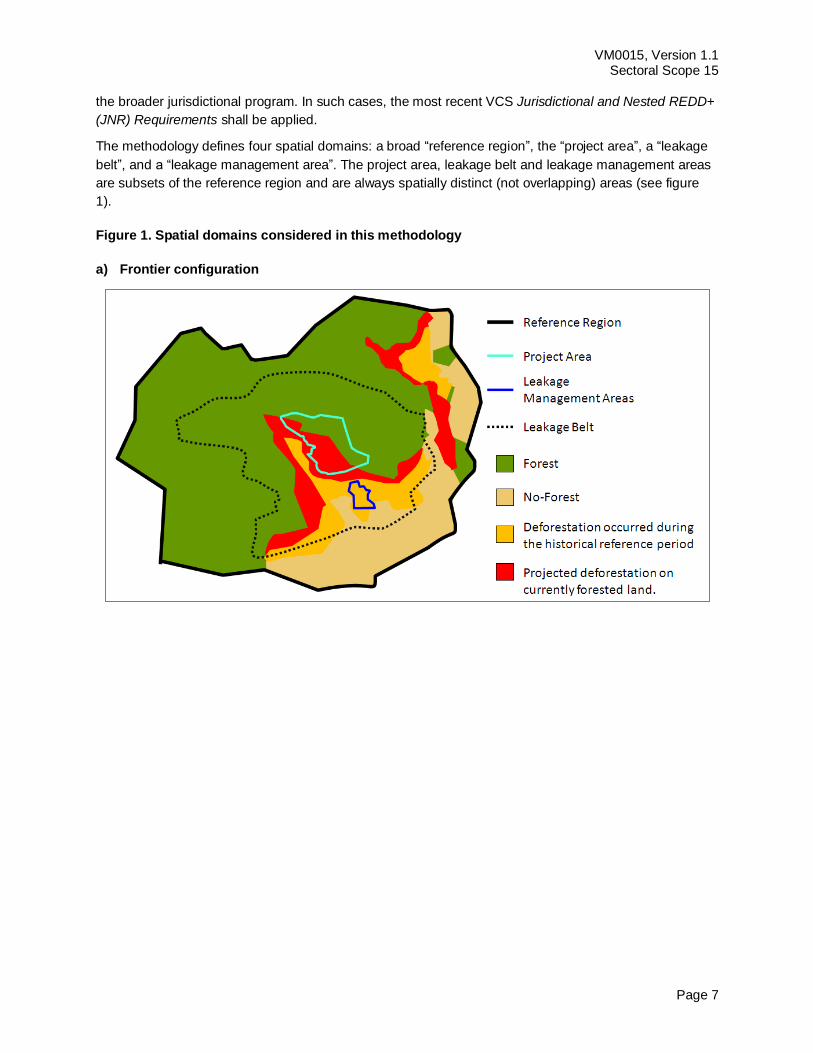
The methodology defines four spatial domains: a broad “reference region”, the “project area”, a “leakage
belt”, and a “leakage management area”. The project area, leakage belt and leakage management areas
are subsets of the reference region and are always spatially distinct (not overlapping) areas (see figure
1).
Figure 1. Spatial domains considered in this methodology
a) Frontier configuration
VM0015, Version 1.1 Sectoral Scope 15
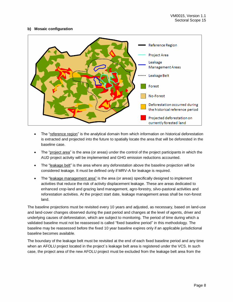
Page 8
b) Mosaic configuration
The “reference region” is the analytical domain from which information on historical deforestation
is extracted and projected into the future to spatially locate the area that will be deforested in the
baseline case.
The “project area” is the area (or areas) under the control of the project participants in which the
AUD project activity will be implemented and GHG emission reductions accounted.
The “leakage belt” is the area where any deforestation above the baseline projection will be
considered leakage. It must be defined only if MRV-A for leakage is required.
The “leakage management area” is the area (or areas) specifically designed to implement
activities that reduce the risk of activity displacement leakage. These are areas dedicated to
enhanced crop-land and grazing land management, agro-forestry, silvo-pastoral activities and
reforestation activities. At the project start date, leakage management areas shall be non-forest
land.
The baseline projections must be revisited every 10 years and adjusted, as necessary, based on land-use
and land-cover changes observed during the past period and changes at the level of agents, driver and
underlying causes of deforestation, which are subject to monitoring. The period of time during which a
validated baseline must not be reassessed is called “fixed baseline period” in this methodology. The
baseline may be reassessed before the fixed 10 year baseline expires only if an applicable jurisdictional
baseline becomes available.
The boundary of the leakage belt must be revisited at the end of each fixed baseline period and any time
when an AFOLU project located in the project´s leakage belt area is registered under the VCS. In such
case, the project area of the new AFOLU project must be excluded from the leakage belt area from the
VM0015, Version 1.1 Sectoral Scope 15
Page 9
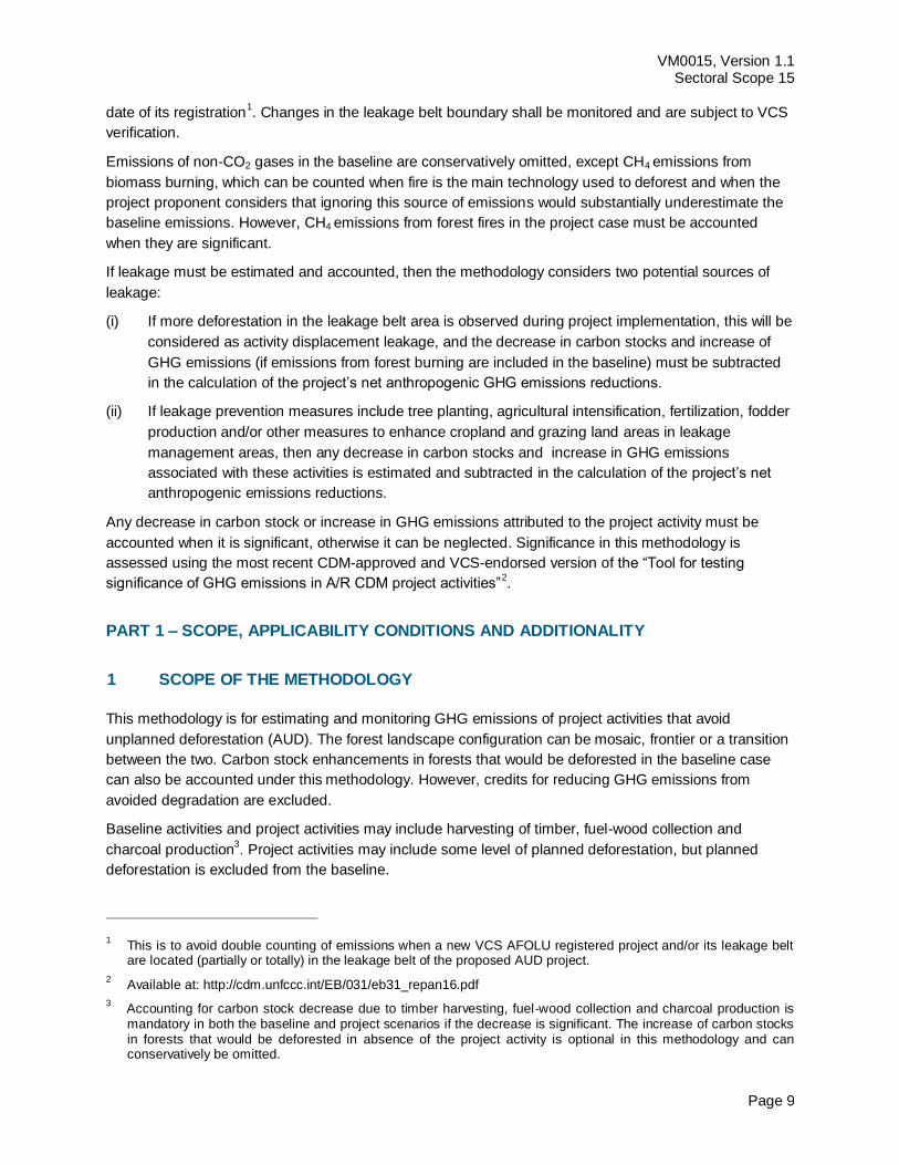
date of its registration1. Changes in the leakage belt boundary shall be monitored and are subject to VCS
verification.
Emissions of non-CO2 gases in the baseline are conservatively omitted, except CH4 emissions from
biomass burning, which can be counted when fire is the main technology used to deforest and when the
project proponent considers that ignoring this source of emissions would substantially underestimate the
baseline emissions. However, CH4 emissions from forest fires in the project case must be accounted
when they are significant.
If leakage must be estimated and accounted, then the methodology considers two potential sources of
leakage:
(i) If more deforestation in the leakage belt area is observed during project implementation, this will be
considered as activity displacement leakage, and the decrease in carbon stocks and increase of
GHG emissions (if emissions from forest burning are included in the baseline) must be subtracted
in the calculation of the project’s net anthropogenic GHG emissions reductions.
(ii) If leakage prevention measures include tree planting, agricultural intensification, fertilization, fodder
production and/or other measures to enhance cropland and grazing land areas in leakage
management areas, then any decrease in carbon stocks and increase in GHG emissions
associated with these activities is estimated and subtracted in the calculation of the project’s net
anthropogenic emissions reductions.
Any decrease in carbon stock or increase in GHG emissions attributed to the project activity must be
accounted when it is significant, otherwise it can be neglected. Significance in this methodology is
assessed using the most recent CDM-approved and VCS-endorsed version of the “Tool for testing
significance of GHG emissions in A/R CDM project activities”2.
PART 1 – SCOPE, APPLICABILITY CONDITIONS AND ADDITIONALITY
SCOPE OF THE METHODOLOGY 1
This methodology is for estimating and monitoring GHG emissions of project activities that avoid
unplanned deforestation (AUD). The forest landscape configuration can be mosaic, frontier or a transition
between the two. Carbon stock enhancements in forests that would be deforested in the baseline case
can also be accounted under this methodology. However, credits for reducing GHG emissions from
avoided degradation are excluded.
Baseline activities and project activities may include harvesting of timber, fuel-wood collection and
charcoal production3. Project activities may include some level of planned deforestation, but planned
deforestation is excluded from the baseline.
1 This is to avoid double counting of emissions when a new VCS AFOLU registered project and/or its leakage belt
are located (partially or totally) in the leakage belt of the proposed AUD project.
2 Available at: http://cdm.unfccc.int/EB/031/eb31_repan16.pdf
3 Accounting for carbon stock decrease due to timber harvesting, fuel-wood collection and charcoal production is
mandatory in both the baseline and project scenarios if the decrease is significant. The increase of carbon stocks in forests that would be deforested in absence of the project activity is optional in this methodology and can conservatively be omitted.
VM0015, Version 1.1 Sectoral Scope 15
Page 10
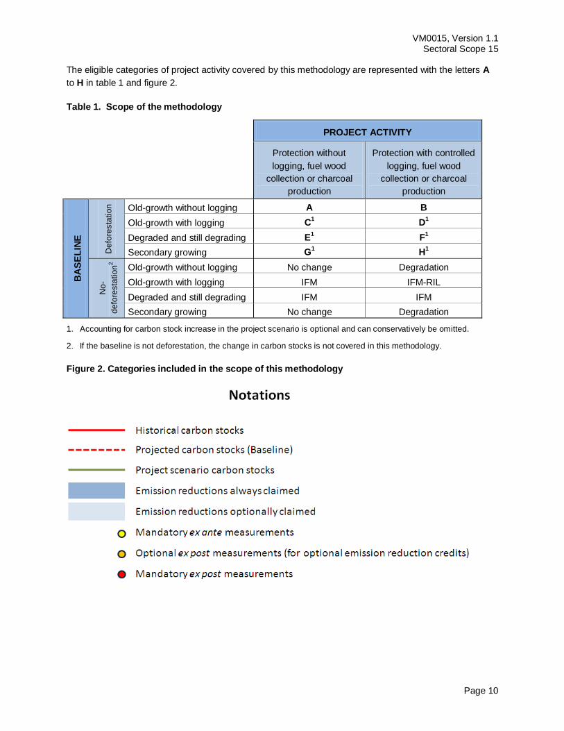
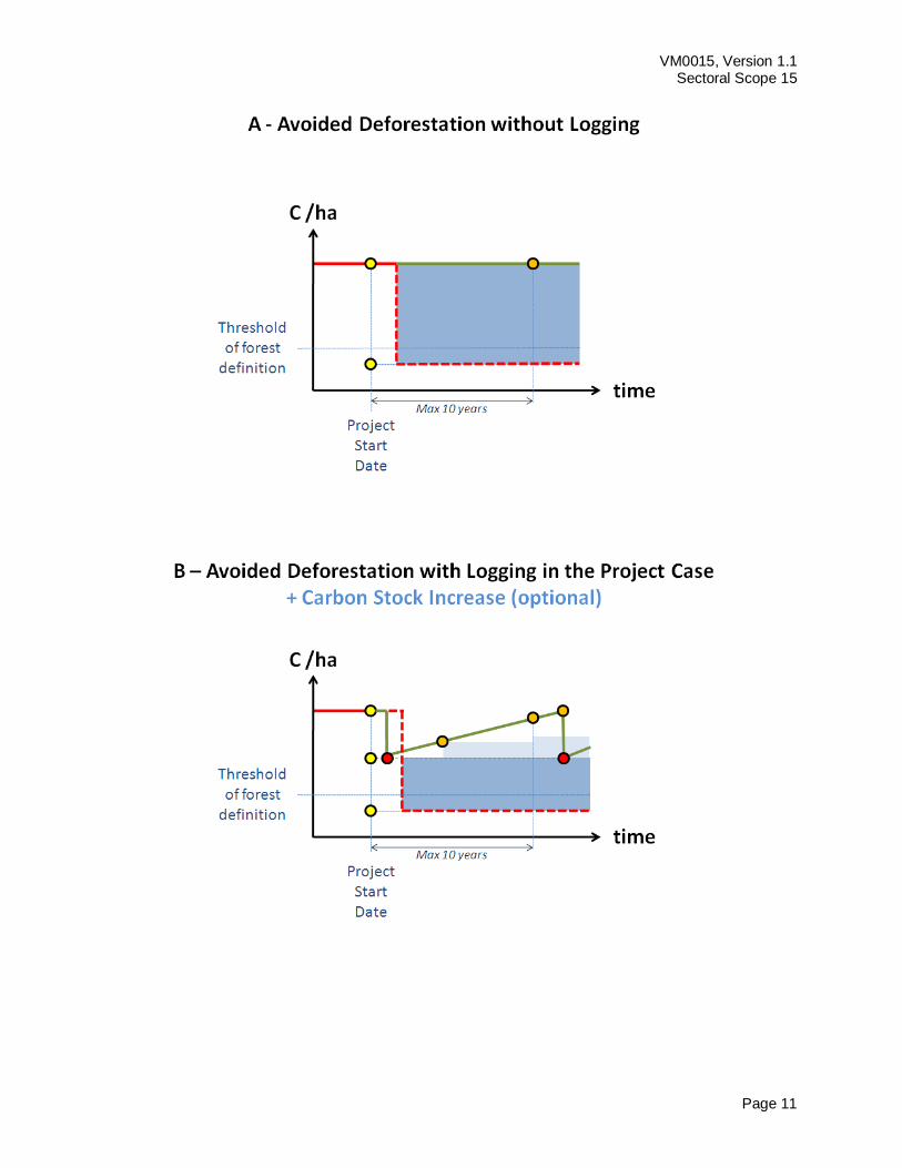
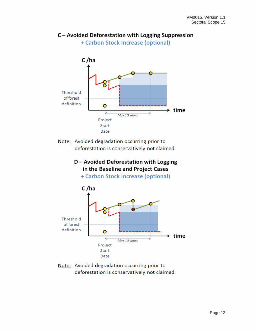
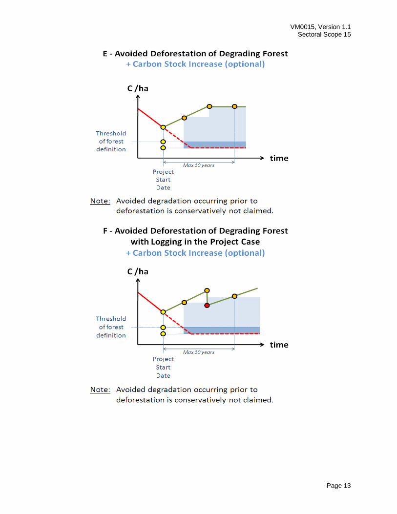
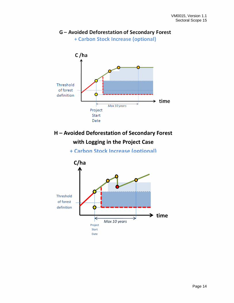
The eligible categories of project activity covered by this methodology are represented with the letters A
to H in table 1 and figure 2.
Table 1. Scope of the methodology
PROJECT ACTIVITY
Protection without
logging, fuel wood
collection or charcoal
production
Protection with controlled
logging, fuel wood
collection or charcoal
production
BA
SE
LIN
E
De
fore
sta
tio
n
Old-growth without logging A B
Old-growth with logging C1 D
1
Degraded and still degrading E1 F
1
Secondary growing G1 H
1
No
-
de
fore
sta
tio
n2
Old-growth without logging No change Degradation
Old-growth with logging IFM IFM-RIL
Degraded and still degrading IFM IFM
Secondary growing No change Degradation
1. Accounting for carbon stock increase in the project scenario is optional and can conservatively be omitted.
2. If the baseline is not deforestation, the change in carbon stocks is not covered in this methodology.
Figure 2. Categories included in the scope of this methodology
VM0015, Version 1.1 Sectoral Scope 15
Page 11
VM0015, Version 1.1 Sectoral Scope 15
Page 12
VM0015, Version 1.1 Sectoral Scope 15
Page 13
VM0015, Version 1.1 Sectoral Scope 15
Page 14
Project
Start
Date
Threshold
of forest
definition
C/ha
/ha
time
Max 10 years
H – Avoided Deforestation of Secondary Forest
with Logging in the Project Case
+ Carbon Stock Increase (optional)
VM0015, Version 1.1 Sectoral Scope 15
Page 15
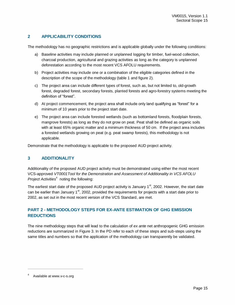
APPLICABILITY CONDITIONS 2
The methodology has no geographic restrictions and is applicable globally under the following conditions:
a) Baseline activities may include planned or unplanned logging for timber, fuel-wood collection,
charcoal production, agricultural and grazing activities as long as the category is unplanned
deforestation according to the most recent VCS AFOLU requirements.
b) Project activities may include one or a combination of the eligible categories defined in the
description of the scope of the methodology (table 1 and figure 2).
c) The project area can include different types of forest, such as, but not limited to, old-growth
forest, degraded forest, secondary forests, planted forests and agro-forestry systems meeting the
definition of “forest”.
d) At project commencement, the project area shall include only land qualifying as “forest” for a
minimum of 10 years prior to the project start date.
e) The project area can include forested wetlands (such as bottomland forests, floodplain forests,
mangrove forests) as long as they do not grow on peat. Peat shall be defined as organic soils
with at least 65% organic matter and a minimum thickness of 50 cm. If the project area includes
a forested wetlands growing on peat (e.g. peat swamp forests), this methodology is not
applicable.
Demonstrate that the methodology is applicable to the proposed AUD project activity.
ADDITIONALITY 3
Additionality of the proposed AUD project activity must be demonstrated using either the most recent
VCS-approved VT0001Tool for the Demonstration and Assessment of Additionality in VCS AFOLU
Project Activities4 noting the following:
The earliest start date of the proposed AUD project activity is January 1st, 2002. However, the start date
can be earlier than January 1st, 2002, provided the requirements for projects with a start date prior to
2002, as set out in the most recent version of the VCS Standard, are met.
PART 2 - METHODOLOGY STEPS FOR EX-ANTE ESTIMATION OF GHG EMISSION
REDUCTIONS
The nine methodology steps that will lead to the calculation of ex ante net anthropogenic GHG emission
reductions are summarized in Figure 3. In the PD refer to each of these steps and sub-steps using the
same titles and numbers so that the application of the methodology can transparently be validated.
4 Available at www.v-c-s.org
VM0015, Version 1.1 Sectoral Scope 15
Page 16
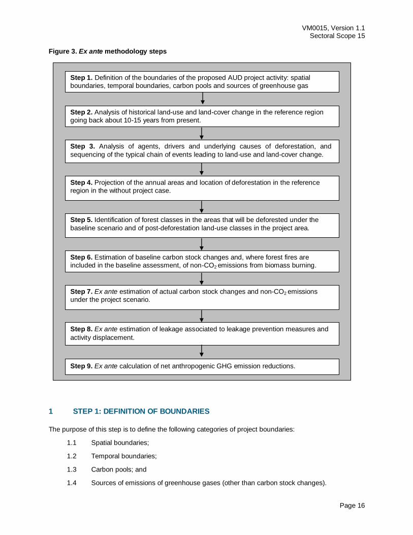
Figure 3. Ex ante methodology steps
STEP 1: DEFINITION OF BOUNDARIES 1
The purpose of this step is to define the following categories of project boundaries:
1.1 Spatial boundaries;
1.2 Temporal boundaries;
1.3 Carbon pools; and
1.4 Sources of emissions of greenhouse gases (other than carbon stock changes).
Step 4. Projection of the annual areas and location of deforestation in the reference
region in the without project case.
Step 1. Definition of the boundaries of the proposed AUD project activity: spatial
boundaries, temporal boundaries, carbon pools and sources of greenhouse gas emissions.
Step 3. Analysis of agents, drivers and underlying causes of deforestation, and
sequencing of the typical chain of events leading to land-use and land-cover change.
Step 5. Identification of forest classes in the areas that will be deforested under the
baseline scenario and of post-deforestation land-use classes in the project area.
Step 7. Ex ante estimation of actual carbon stock changes and non-CO2 emissions
under the project scenario.
Step 2. Analysis of historical land-use and land-cover change in the reference region
going back about 10-15 years from present.
Step 9. Ex ante calculation of net anthropogenic GHG emission reductions.
Step 8. Ex ante estimation of leakage associated to leakage prevention measures and
activity displacement.
Step 6. Estimation of baseline carbon stock changes and, where forest fires are
included in the baseline assessment, of non-CO2 emissions from biomass burning.
VM0015, Version 1.1 Sectoral Scope 15
Page 17
1.1 Spatial boundaries
Define the boundaries of the following spatial features:
1.1.1 Reference region;
1.1.2 Project area;
1.1.3 Leakage belt;
1.1.4 Leakage management areas; and
1.1.5 Forest.
The reference region is the largest unit of land and the project area, leakage belt and leakage
management areas are subsets of the reference region. For each spatial feature, the criteria used to
define their boundaries must be described and justified in the PD. Vector or raster files in a common
projection and GIS software formats shall be provided in order to allow the identification of the boundaries
unambiguously.
1.1.1 Reference region
The boundary of the reference region is the spatial delimitation of the analytic domain from which
information about rates, agents, drivers, and patterns of land-use and land-cover change (LU/LC-change)
will be obtained, projected into the future and monitored.
The reference region should contain strata with agents, drivers and patterns of deforestation that in the
10-15 year period prior to the start date of the proposed AUD project activity are similar to those expected
to exist within the project area.
The boundary of the reference region shall be defined as follows:
1. If sub-national or national baselines exist, that meet VCS specific guidance on applicability of
existing baselines, such baselines must be used. Any pre-existing baseline should be analyzed
and if it meets the criteria listed in table 2, it should be used. In both cases, the existing baseline
will determine the boundary of the reference region.
2. If no such applicable sub-national or national baseline is available, the national and, where
applicable, sub-national government shall be consulted to determine whether the country or sub-
national region has been divided in spatial units for which deforestation baselines will be
developed. If such divisions exist and are endorsed by the national or sub-national government,
they must be used to determine the boundary of the reference region.
3. If such divisions do not exist, a baseline must be developed for a reference region encompassing
the project area, the leakage belt and any other geographic area (stratum i) that is relevant to
determine the baseline of the project area.
4. A geographic area is relevant for determining the baseline of the project area when agents,
drivers and overall deforestation patterns observed in it during the 10-15 year period preceding
the start date of the proposed AUD project activity represent a credible proxy for possible future
deforestation patterns in the project area.

VM0015, Version 1.1 Sectoral Scope 15
Page 18
Table 2. Criteria determining the applicability of existing baselines
Applicability criteria
1 The existing baseline must cover a broader geographical region than the project area. If a
leakage belt must be defined1, the broader region must include the leakage belt area.
2 The existing baseline must cover at least the duration of the first fixed baseline period and is not
outdated2.
3 The existing baseline must depict the location of future deforestation on a yearly base.
4 The spatial resolution of the existing baseline must be equal or finer than the minimum mapping
unit of “forest land” that will be used for monitoring deforestation during the fixed baseline period.
5 Methods used to develop the existing baseline must be transparently documented and be
consistent with a VCS approved and applicable baseline methodology.
1. If the project area is located within a jurisdictional program the most recent VCS JNR Requirements
must be applied to determine whether a leakage belt is required. In all other cases, a leakage belt is
required.
2. A baseline is considered outdated 10 years after its establishment.
The reference region may include one or several discrete areas. It must be larger5 than the project area
and include the project area.
Where the current situation within the project area is expected to change (e.g. because of population
growth, infrastructure development or any other plausible reason), the reference region should be divided
in i strata, each representing proxies for the chrono-sequence of current and future conditions within the
project area. The boundary of such strata may be static (fixed during a fixed baseline period) or dynamic6
(changing every year), depending on the modeling approaches used.
Three main criteria are relevant to demonstrate that the conditions determining the likelihood of
deforestation within the project area are similar or expected to become similar to those found within the
reference region
Agents and drivers of deforestation expected to cause deforestation within the project area in
absence of the proposed AUD project activity must exist or have existed elsewhere in the
reference region. The following requirements are to be met:
5 Brown et al. (2007) suggest the following rule of thumb:
For projects above 100,000 ha, the reference region should be about 5-7 times larger than the project area.
For projects below 100,000 ha, the reference region should be 20-40 times the size of the project area.
These figures are indicatives; the exact ratio between the two areas depends on the particular regional and project circumstances. Where a project activity deals with an entire island, the reference region must include other islands or forested landscapes with similar conditions.
6 Dynamic = with shifting boundaries, according to modeled changes at the level of driver variables such as
population, infrastructure and other to be determined by the project proponent.
VM0015, Version 1.1 Sectoral Scope 15
Page 19
- Agent groups: Deforestation agent´s groups (as identified in step 3) expected to encroach
into the project area must exist or have existed and caused deforestation elsewhere in the
reference region during the historical reference period.
- Infrastructure drivers. If new or improved infrastructure (such as roads, railroads, bridges,
hydroelectric reservoirs, etc.) is expected to develop near or inside the project area7, the
reference region must include a stratum where such infrastructure was built in the past and
where the impact on forest cover was similar to the one expected from the new or improved
infrastructure in the project area.
- Other spatial drivers expected to influence the project area. Any spatial deforestation
driver considered relevant according to the analysis of step 3 (e.g. resettlement programs,
mining and oil concessions, etc.) must exist or have existed elsewhere in the reference
region. The historical impact of such drivers must have been similar to the one expected in
the project area.
Landscape configuration and ecological conditions: At least three of the following four
conditions must be satisfied:
- Forest/vegetation classes: At least 90% of the project area must have forest classes or
vegetation types that exist in at least 90% of the rest of the reference region.
- Elevation: At least 90% of the project area must be within the elevation range of at least
90% of the rest of the reference region.
- Slope: The average slope of at least 90% of the project area shall be within 10% of the
average slope of at least 90% of the rest of the reference region.
- Rainfall: The average annual rainfall in at least 90% of the project area shall be within
10% of the average annual rainfall of at least 90% of the rest of the reference region.
Socio-economic and cultural conditions: The following conditions must be met:
- Legal status of the land: The legal status of the land (private, forest concession,
conservation concession, etc.) in the baseline case within the project area must exist
elsewhere in the reference region. If the legal status of the project area is a unique case,
demonstrate that legal status is not biasing the baseline of the project area (e.g. by
demonstrating that access to the land by deforestation agents is similar to other areas with a
different legal status).
- Land tenure: The land-tenure system prevalent in the project area in the baseline case is
found elsewhere in the reference region.
- Land use: Current and projected classes of land-use in the project area are found
elsewhere in the reference region.
- Enforced policies and regulations: The project area shall be governed by the same
policies, legislation and regulations that apply elsewhere in the reference region.
7 Areas of planned deforestation in the baseline case must be excluded from the project area.

VM0015, Version 1.1 Sectoral Scope 15
Page 20
1.1.2 Project area
The project area is the area or areas of land under the control of the project proponent on which the
project proponent will undertake the project activities. At the project start date, the project area must
include only forest land.
Any area affected by planned deforestation due to the construction of planned infrastructure (except if
such planned infrastructure is a project activity) must be excluded from the project area.
The project area must include areas projected to be deforested in the baseline case and may include
some other areas that are not threatened according to the first baseline assessment (see figure 1). Such
areas will not generate carbon credits, but they may be included if the project proponent considers that
future baseline assessments, which have to be carried out at least every 10 years, are likely to indicate
that a future deforestation threat will exist, also the demonstration is not possible at the time of validation.
Where less than 80 percent of the total proposed area of the project is under control at validation, new
discrete units of land may be integrated into an existing project area if included in the monitoring report at
the time of the first verification. For the full rules and requirements regarding control over the entire
project area at validation, please see the most recent version of the VCS AFOLU requirements.
The boundary of the project area shall be defined unambiguously as follows:
Name (or names, as appropriate) of the project area.
Physical boundary of each discrete area of land included in the project area (using appropriate
GIS software formats).
Description of current land-tenure and ownership, including any legal arrangement related to land
ownership and the AUD project activity.
List of the project participants and brief description of their roles in the proposed AUD project
activity.
1.1.3 Leakage belt
If the project area is located within a jurisdictional program, leakage may not have be assessed and a
leakage belt may not be required because any decrease in carbon stocks or increase in GHG emissions
outside the project area would be measured, reported, verified and accounted under the jurisdictional
program8. In such cases, the most recent VCS JNR Requirements shall be applied. In all other cases,
leakage is subject to MRV-A in an area called “leakage belt” in this methodology.
The leakage belt is the land area or land areas surrounding or adjacent to the project area in which
baseline activities could be displaced due to the project activities implemented in the project area.
To define the boundary of the leakage belt, two methodological options can be used:
Opportunity cost analysis (Option I); and
Mobility analysis (Option II).
Under both options, the boundary of the leakage belt must be revisited at the end of each fixed baseline
period, as opportunity costs and mobility parameters are likely to change over time. In addition, the
8 In such cases, the sub-national or national government may define specific sub-national or national policies and
regulations to deal with the issue of leakage.

VM0015, Version 1.1 Sectoral Scope 15
Page 21
boundary of the leakage belt may have to be revisited when other VCS-AFOLU projects are registered
nearby the project area, as further explained below.
If mobility parameters or opportunity costs are projected for each future year, the boundary of the leakage
belt that will remain static for the whole duration of the fixed baseline period shall be the one determined
for the last year of the fixed baseline period.
Option I: Opportunity cost analysis
This option is applicable where economic profit is an important driver of deforestation. To demonstrate
that Option I is applicable, use historical records, i.e. demonstrate that at least 80% of the area deforested
in the reference region (or some of its strata) during the historical reference period9 has occurred at
locations where deforesting was profitable (i.e. for at least one product, PPxl > 1). Alternatively, use
literature studies, surveys and other credible and verifiable sources of information. If Option I is not
applicable, use Option 2.
If the main motivation is economic profit, agents not allowed to deforest within the project area will only
displace deforestation outside the project area if doing so brings economic benefits to them. Based on
this rationale leakage can only occur on land outside the project area where the total cost of establishing
and growing crops or cattle and transporting the products to the market is less than the price of the
products (i.e. opportunity costs are > 0).To identify this land area do the following:
a) List the main land-uses that deforestation agents are likely to implement within the project area in
the baseline case, such as cattle ranching and/or different types of crops.
b) Find credible and verifiable sources of information on the following variables:
S$x = Average selling price per ton of the main product Px (or product mixture in case of
agro-forestry or mixed production systems) that would be established in the project area in
the baseline case (meat, crop type A, crop type B, etc.);
SPxl = Most important selling points (spatial locations) for each main product Px in the
reference region.
PCxi = Average in situ production costs per ton of product. Stratify the reference region as
necessary in i strata, as production costs may vary depending on local conditions (soil,
technology available to the producer, etc.).
TCv = Average transport cost per kilometer for one ton of product Px transported on different
types of land-uses (e.g. pasture, cropland, forest), roads, railroads, navigable rivers, etc.
using the most typical transport technology available to the producer.
Note: For simplicity, current prices and costs can be used to project opportunity costs. Price and cost
projections shall only be used if reliable and verifiable sources of information are available.
c) Using a GIS, generate for each main product a surface representing the least transport cost of
one ton of product to the most important selling points within the reference region. Do this by
considering the most typical transport technology available to deforestation agents.
9 See section 1.2.1 for the definition of “historical reference period.”
VM0015, Version 1.1 Sectoral Scope 15
Page 22
d) For each main product, add to the surface created in the previous step the average in situ cost for
producing one ton of product. The result is a surface representing the total cost of producing and
bringing to the market one ton of product.
e) For each main product, subtract from the average price of one ton of product the total cost
surface created in the previous step. The result is a surface representing potential profitability of
each product.
Note: If several products exist and can be produced on the same site, the maximum value of all
potential profitability surfaces will represent the opportunity cost of conserving the forest.
f) The leakage belt is the area where the surface created in the previous step (potential profitability)
has a positive value at the last year of the fixed baseline period.
The above methodology procedure can be summarized as follows:
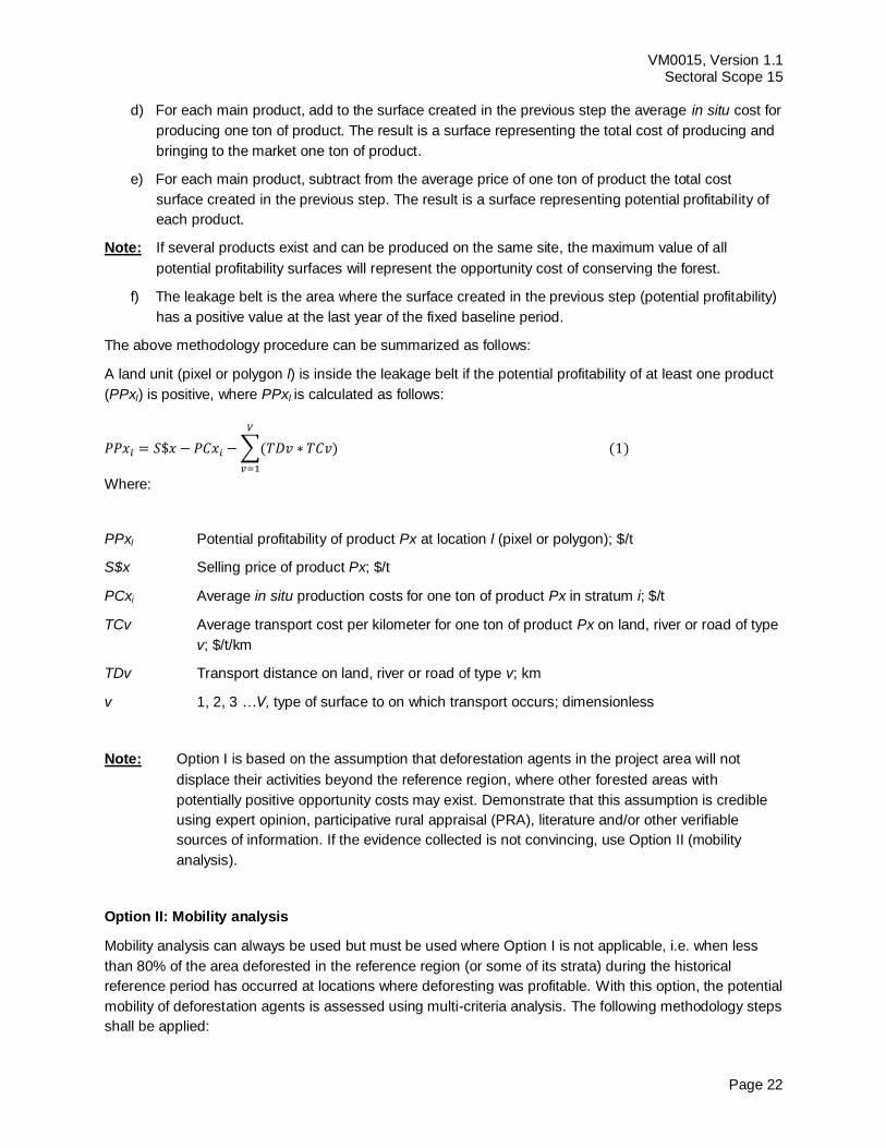
A land unit (pixel or polygon l) is inside the leakage belt if the potential profitability of at least one product
(PPxl) is positive, where PPxl is calculated as follows:
∑
Where:
PPxl Potential profitability of product Px at location l (pixel or polygon); $/t
S$x Selling price of product Px; $/t
PCxi Average in situ production costs for one ton of product Px in stratum i; $/t
TCv Average transport cost per kilometer for one ton of product Px on land, river or road of type
v; $/t/km
TDv Transport distance on land, river or road of type v; km
v 1, 2, 3 …V, type of surface to on which transport occurs; dimensionless
Note: Option I is based on the assumption that deforestation agents in the project area will not
displace their activities beyond the reference region, where other forested areas with
potentially positive opportunity costs may exist. Demonstrate that this assumption is credible
using expert opinion, participative rural appraisal (PRA), literature and/or other verifiable
sources of information. If the evidence collected is not convincing, use Option II (mobility
analysis).
Option II: Mobility analysis
Mobility analysis can always be used but must be used where Option I is not applicable, i.e. when less
than 80% of the area deforested in the reference region (or some of its strata) during the historical
reference period has occurred at locations where deforesting was profitable. With this option, the potential
mobility of deforestation agents is assessed using multi-criteria analysis. The following methodology steps
shall be applied:
VM0015, Version 1.1 Sectoral Scope 15
Page 23
a) Using historical data, expert opinion, participative rural appraisal (PRA), literature and/or other
verifiable sources of information list all relevant criteria that facilitate (at least one criterion) and
constrain (at least one criterion) the mobility of the main deforestation agents identified in step 3.
The overall suitability of the land for the activities of deforestation agents shall be considered.
b) For each criterion, generate a map using a GIS.
c) Using multi-criteria analysis, determine the boundary of the leakage belt. Justify any assumption
and weight assigned to the individual criteria.
d) Methods used to perform the analysis shall be transparently documented and presented to VCS
verifiers at the validation.
Consideration of other VCS AFOLU projects
If the leakage belt area of the proposed AUD project includes the area or part of the areas of other VCS
AFOLU projects, do the following to avoid double counting of emissions:
Exclude from the leakage belt area of the proposed AUD project the project area of the other
VCS AFOLU project(s).
a) The exclusion shall enter into force at the registration date of the other project
b) Carbon accounting shall consider the exclusion of the project area of the other project
beginning with the start date of the other projects
c) An excluded area shall again be included in the leakage belt area of the proposed AUD
project at the time the other project has not verified its emission reductions for more than five
consecutive years, or when it ends its project crediting period under the VCS.
If the leakage belt overlaps with the leakage belt of other VCS AFOLU projects, do the following:
a) Identify the carbon pools and sources of GHG emissions that are monitored by the other
projects. Only for common carbon pools and sources of GHG emissions the boundary of the
leakage belt area can be modified as further explained below.
b) Analyze the overlapping area(s) with the proponents of each of the other VCS AFOLU
projects and come to an agreement with them on the location of the boundaries of the
different leakage belts, so that there will be no overlaps and gaps between the different
leakage belt areas as well as carbon pools and GHG sources.
c) As an indicative rule, the percentage of forest land area within the leakage belt of a project
relative to the total forest area of all leakage belts shall be similar to the percentage of
baseline deforestation of the project relative to the total baseline deforestation of all projects:
%LKBA = BLDA / (BLDA + BLDB + … + BLDN) (2.a)
%LKBB = BLDB / (BLDA + BLDB + … + BLDN) (2.b)
…
%LKBN = BLDN / (BLDA + BLDB + … + BLDN) (2.n)
VM0015, Version 1.1 Sectoral Scope 15
Page 24
Where:
%LKBA Percentage of the overlapping leakage belts area to be assigned to Project A; %
%LKBB Percentage of the overlapping leakage belts area to be assigned to Project B; %
%LKBN Percentage of the overlapping leakage belts area to be assigned to Project N; %
BLDA Total area of projected baseline deforestation during the fixed baseline period of
Project A (see PD of project A); ha
BLDB Total area of projected baseline deforestation during the fixed baseline period of
Project B (see PD of project B); ha
BLDN Total area of projected baseline deforestation during the fixed baseline period of
Project N (see PD of Project N); ha
Note: The proponents of the different projects shall agree on the criteria used to define
the boundaries of their leakage belts in the overlapping areas and are not required
to use the above rule. However, if they decide to use this rule, the area of the
overlapping leakage belts assigned to Project A shall be the closest to the
boundary of Project A; the area of the overlapping leakage belts assigned to
Project B shall be the closest to the boundary of Project B and so on (the area of
the overlapping leakage belts assigned to Project N shall be the closest to the
boundary of Project N).
d) The final boundary of the leakage belt of each project is subject to validation and periodical
verification. A project may report a smaller leakage belt only if another VCS registered project
has included in its leakage belt the portion left out.
e) If the proponents of the different projects do not agree on how to split the overlapping
leakage belt area, each project will have to include in its leakage belt the overlapping areas.
f) A “Leakage Belt Agreement” between the proponents of the different projects must be signed
and presented to VCS verifiers at the time of validation/verification. The agreement shall
contain the maps of the agreed leakage belts and each project shall have a digital copy of
these maps in the projection and GIS software formats used in each project.
g) If a project ends or has not presented a verification to the VCS for more than five consecutive
years, the other projects participating in the “leakage belt agreement” shall amend the
agreement in order to ensure that the whole area of the originally overlapping leakage belts is
always subject to MRV-A. The amendment is subject to VCS verification. If no amendment is
made, the proposed project will have to include in its leakage belt the land area that is no
longer be subject to MRV-A by a another VCS project.
1.1.4 Leakage management areas
These are non-forest areas located outside the project boundary in which the project proponent intends to
implement activities that will reduce the risk of activity displacement leakage, such as afforestation,
reforestation or enhanced crop and grazing land management. The boundary of such areas must be
defined according to existing management plans or other plans related to the proposed AUD project
activity. Such plans shall be made available to the VCS Validation/Verification Body (VVB) at the time of
validation. The boundary of leakage management areas must be clearly defined using the common
VM0015, Version 1.1 Sectoral Scope 15
Page 25
projection and GIS software formats used in the project and shall be reassessed and validated at each
fixed baseline period
1.1.5 Forest
The boundary of the forest is dynamic and will change over time. It must be defined using an explicit and
consistent forest definition over different time periods.
In the baseline case, changes in the boundary of forest land will be projected, and the baseline
projections must be reassessed at least every 10 years. In the project area and leakage belt, the ex post
boundary of forest land will be subject to periodical monitoring, verification and reporting (MRV).
To define the boundary of the forest, specify:
The definition of forest that will be used for measuring deforestation during the project crediting
period (see appendix 1 for criteria to define “forest”).
The Minimum Mapping Unit (MMU). The MMU size of the LULC maps created using RS
impagery shall not be more than one hectare irrespective of forest definition.
An initial Forest Cover Benchmark Map is required to report only gross deforestation going forward. It
should depict the locations where forest land exists at the project start date. The baseline projections in
step 4.2 will generate one such map for each future year of the fixed baseline period and, optionally,
project crediting period.
Areas covered by clouds or shadows should be analyzed by complementing the analysis of optical sensor
data with non-optical sensor data. However, if some obscured areas remain for which no spatially explicit
and verifiable information on forest cover can be found or collected (using ground-based or other
methods), such areas shall be excluded (masked out). This exclusion would be:
Permanent, unless it can reasonably be assumed that these areas are covered by forests (e.g.
due to their location).
Temporal in case information was available for the historical reference period, but not for a
specific monitoring period. In this case, the area with no information must be excluded from the
calculation of net anthropogenic GHG emission reductions of the current monitoring period, but
not for subsequent periods, when information may become available again. When information
becomes available again, and the land appears with vegetation parameters below the thresholds
for defining “forest”, the land should be considered as “deforested”.
1.2 Temporal boundaries
Define the temporal boundaries listed below.
1.2.1 Starting date and end date of the historical reference period
The starting date should not be more than 10-15 years in the past and the end date as close as possible
to the project start date. The project start date is the date at which the additional AUD project activities
have or are to be started.
1.2.2 Starting date of the project crediting period of the AUD project activity
The length of the project crediting period shall be established as set out on the most recent version of the
VCS Standard.

VM0015, Version 1.1 Sectoral Scope 15
Page 26
1.2.3 Starting date and end date of the first fixed baseline period
The fixed baseline period shall be 10 years. The starting and end dates must be defined.
1.2.4 Monitoring period
The minimum duration of a monitoring period is one year and the maximum duration is one fixed baseline
period.
1.3 Carbon pools
The six carbon pools listed in table 3 are considered in this methodology.
Table 3. Carbon pools included or excluded within the boundary of the proposed AUD project
activity
Carbon pools Included / TBD1/
Excluded
Justification / Explanation of choice
Above-ground
Tree: Included Carbon stock change in this pool is always significant
Non-tree: TBD Must be included in categories with final land cover of
perennial crop
Below-ground+ TBD Optional and recommended but not mandatory
Dead wood+ TBD Recommended only when significant
Harvested wood products+ Included To be included when significant
Litter TBD Recommended only when significant.
Soil organic carbon+ TBD
Recommended when forests are converted to
cropland. Not to be measured in conversions to
pasture grasses and perennial crop according to VCS
Program Update of May 24th, 2010.
1. TBD = To Be Decided by the project proponent. The pool can be excluded only when its exclusion does
not lead to a significant over-estimation of the net anthropogenic GHG emission reductions of the AUD
project activity.
2. The VCS defines as “significant” those carbon pools and sources that account more than 5% of the total
GHG benefits generated (VCS 2007.1, 2008 p.17). To determine significance, the most recent version of
the “Tool for testing significance of GHG emissions in A/R CDM project activities” shall be used10
.
3. + = The VCS AFOLU Requirements require methodologies to consider the decay of carbon in soil carbon,
belowground biomass, dead wood and harvested wood products. Note that the immediate release of
carbon from these pools in the baseline case must not be assumed.
Carbon pools that are expected to decrease their carbon stocks in the project scenario compared to
the baseline case must be included if the exclusion would lead to a significant overestimation of the
net anthropogenic GHG emission reductions generated during the fixed baseline period.
10 Available at: http://cdm.unfccc.int/EB/031/eb31_repan16.pdf
VM0015, Version 1.1 Sectoral Scope 15
Page 27
Carbon pools considered insignificant according to the latest VCS AFOLU requirements can always be
neglected.
Above-ground biomass of trees must always be selected because it is in this pool that the greatest
carbon stock change will occur.
Non-tree biomass must be included if the carbon stock in this pool is likely to be relatively large in the
baseline compared to the project scenario such as when short-rotation woody corps are commonly
planted in the region where the project area is located. The significance criterion shall apply.
Below-ground biomass of trees is recommended, as it usually represents between 15% and 30% of
the above-ground biomass.
Harvested wood products must be included if removal of timber is associated with significantly more
carbon stored in long-term wood products in the baseline case compared to the project scenario. The
significance criterion shall apply. When included, short-lived fraction (decaying in less than 3 years) is
assumed to decay inmidiatly at the year of deforestation (t = t*), the medium-lived fraction (decaying in
3-100 years) is assumed to decay in a 20-year period and the long-term fraction is assumed to never
decay (i.e. it never results in an emission). Thus, it is conservative to assume that 100% of the carbon
stock in wood products is long-lived.
In most cases the exclusion of a carbon pool will be conservative, except when the carbon stock in the
pool is higher in the baseline compared to the project scenario.
The inclusion of a carbon pool is recommended (but not mandatory) where the pool is likely to
represent an important proportion (> 10%) of the total carbon stock change attributable to the project
activity (“expected magnitude of change”).
For excluded pools, briefly explain why the exclusion is conservative.
When the exclusion of a carbon pool is not conservative, demonstrate that the exclusion will not lead
to a significant overestimation of the net anthropogenic GHG emission reduction. If the exclusion is
significant, the pool must be included.
Carbon pools that are excluded or not significant according to the ex ante assessment do not need to
be monitored ex post.
In most cases the same carbon pools shall be considered for all categories of LU/LC change.
However, including different carbon pools for different categories of LU/LC change is allowed
depending on “significance”, “conservativeness” and “expected magnitude of change”. For instance,
harvested wood products may only be considered in the categories where this pool exists.
The final selection of carbon pools per category is done in step 2.3. Within a category of LU/LC-
change, the same carbon pools must be selected for the two classes involved. Table 1 in appendix 2
provides an indication of the level of priority for including different carbon pools depending on the
category of LU/LC change.
If a pool is conservatively excluded at validation, project proponent cannot in subsequent monitoring
and verification periods decide to measure, report and verify the excluded carbon pool. However, the
reverse is possible i.e., if a pool is included at validation, it may be conservatively excluded in
subsequent monitoring and verification periods provided all methodology requirements are applied to
carry out the estimations and these are independently verified. Further guidance on the selection of
VM0015, Version 1.1 Sectoral Scope 15
Page 28
carbon pools can be found in the most recent version of the GOFC-GOLD sourcebook for REDD11
and
further details are given in appendix 3.
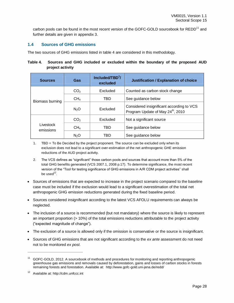
1.4 Sources of GHG emissions
The two sources of GHG emissions listed in table 4 are considered in this methodology.
Table 4. Sources and GHG included or excluded within the boundary of the proposed AUD
project activity
Sources Gas Included/TBD
1/
excluded Justification / Explanation of choice
Biomass burning
CO2 Excluded Counted as carbon stock change
CH4 TBD See guidance below
N2O Excluded Considered insignificant according to VCS
Program Update of May 24th, 2010
Livestock
emissions
CO2 Excluded Not a significant source
CH4 TBD See guidance below
N2O TBD See guidance below
1. TBD = To Be Decided by the project proponent. The source can be excluded only when its
exclusion does not lead to a significant over-estimation of the net anthropogenic GHE emission
reductions of the AUD project activity.
2. The VCS defines as “significant” those carbon pools and sources that account more than 5% of the
total GHG benefits generated (VCS 2007.1, 2008 p.17). To determine significance, the most recent
version of the “Tool for testing significance of GHG emissions in A/R CDM project activities” shall
be used12
.
Sources of emissions that are expected to increase in the project scenario compared to the baseline
case must be included if the exclusion would lead to a significant overestimation of the total net
anthropogenic GHG emission reductions generated during the fixed baseline period.
Sources considered insignificant according to the latest VCS AFOLU requirements can always be
neglected.
The inclusion of a source is recommended (but not mandatory) where the source is likely to represent
an important proportion (> 10%) of the total emissions reductions attributable to the project activity
(“expected magnitude of change”).
The exclusion of a source is allowed only if the omission is conservative or the source is insignificant.
Sources of GHG emissions that are not significant according to the ex ante assessment do not need
not to be monitored ex post.
11 GOFC-GOLD, 2012. A sourcebook of methods and procedures for monitoring and reporting anthropogenic
greenhouse gas emissions and removals caused by deforestation, gains and losses of carbon stocks in forests remaining forests and forestation. Available at: http://www.gofc-gold.uni-jena.de/redd/
12 Available at: http://cdm.unfccc.int
VM0015, Version 1.1 Sectoral Scope 15
Page 29
For excluded sources, briefly explain why the exclusion is conservative.
In the baseline scenario: Non-CO2 emissions from fires used to clear forests can be counted when
sufficient data are available to estimate them. However, accounting for these emissions can
conservatively be omitted. GHG emissions from land-uses implemented on deforested lands (including
from biomass burning) are conservatively omitted in this methodology.
In the project scenario: It is reasonable to assume that the project activity, including when harvest
activities are planned (such as logging for timber, fuel-wood collection and charcoal production),
produces less emissions of GHG than the baseline activities implemented prior and after deforestation
on the deforested lands. Therefore, the omission of certain sources of GHG emissions, such as the
consumption of fossil fuels, will not cause an overestimation of the net anthropogenic GHG emission
reductions. However, non-CO2 emissions from forest fires must be counted in the project scenario
when they are significant.
In the estimation of leakage: GHG emissions by sources that are attributable to leakage prevention
measures (e.g. those implemented in leakage management areas) and that are increased compared
to pre-existing GHG emissions count as leakage and should be estimated and counted if they are
significant. Non-CO2 emissions from displaced baseline activities, which are conservatively omitted in
the baseline, can be ignored, as in the worst case scenario they would be similar to baseline
emissions. However, if non-CO2 emissions from forest fires used to clear forests are counted in the
baseline, they must also be counted in the estimation of activity displacement leakage.
STEP 2: ANALYSIS OF HISTORICAL LAND-USE AND LAND-COVER CHANGE 2
The goal of this step is to collect and analyze spatial data in order to identify current land-use and land-
cover conditions and to analyze LU/LC change during the historical reference period within the reference
region and project area. The tasks to be accomplished are the following:
2.1 Collection of appropriate data sources;
2.2 Definition of classes of land-use and land-cover;
2.3 Definition of categories of land-use and land-cover change;
2.4 Analysis of historical land-use and land-cover change;
2.5 Map accuracy assessment; and
2.6 Preparation of a methodology annex to the PD.
2.1 Collection of appropriate data sources
Collect the data that will be used to analyze land-use and land-cover change during the historical
reference period within the reference region and project area. It is good practice to do this for at least
three time points, about 3-5 years apart. For areas covered by intact forests, it is sufficient to collect data
for one single date, which must be as closest as possible to the project start date (< 2 years).
VM0015, Version 1.1 Sectoral Scope 15
Page 30
As a minimum requirement:
Collect medium resolution spatial data13
(from 10m x 10m up to a maximum of 100m x 100m
resolution) from optical and non-optical sensor systems, such as (but not limited to) Landsat14
,
SPOT, ALOS, AVNIR2, ASTER, IRS sensor data) covering the past 10-15 years.
Collect high resolution data from remote sensors (< 5 x 5 m pixels) and/or from direct field
observations for ground-truth validation of the posterior analysis. Describe the type of data,
coordinates and the sampling design used to collect them.
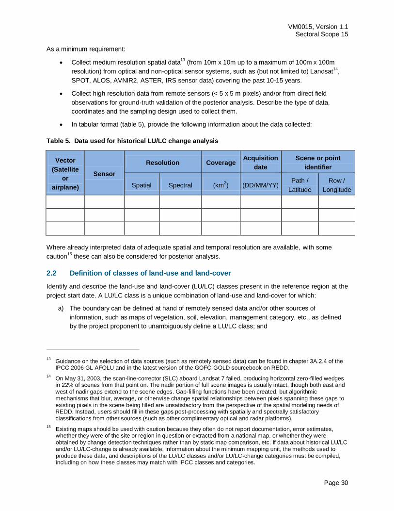
In tabular format (table 5), provide the following information about the data collected:
Table 5. Data used for historical LU/LC change analysis
Vector
(Satellite
or
airplane)
Sensor
Resolution Coverage Acquisition
date
Scene or point
identifier
Spatial Spectral (km2) (DD/MM/YY)
Path /
Latitude
Row /
Longitude
Where already interpreted data of adequate spatial and temporal resolution are available, with some
caution15
these can also be considered for posterior analysis.
2.2 Definition of classes of land-use and land-cover
Identify and describe the land-use and land-cover (LU/LC) classes present in the reference region at the
project start date. A LU/LC class is a unique combination of land-use and land-cover for which:
a) The boundary can be defined at hand of remotely sensed data and/or other sources of
information, such as maps of vegetation, soil, elevation, management category, etc., as defined
by the project proponent to unambiguously define a LU/LC class; and
13 Guidance on the selection of data sources (such as remotely sensed data) can be found in chapter 3A.2.4 of the
IPCC 2006 GL AFOLU and in the latest version of the GOFC-GOLD sourcebook on REDD.
14 On May 31, 2003, the scan-line-corrector (SLC) aboard Landsat 7 failed, producing horizontal zero-filled wedges
in 22% of scenes from that point on. The nadir portion of full scene images is usually intact, though both east and west of nadir gaps extend to the scene edges. Gap-filling functions have been created, but algorithmic mechanisms that blur, average, or otherwise change spatial relationships between pixels spanning these gaps to existing pixels in the scene being filled are unsatisfactory from the perspective of the spatial modeling needs of REDD. Instead, users should fill in these gaps post-processing with spatially and spectrally satisfactory classifications from other sources (such as other complimentary optical and radar platforms).
15 Existing maps should be used with caution because they often do not report documentation, error estimates,
whether they were of the site or region in question or extracted from a national map, or whether they were obtained by change detection techniques rather than by static map comparison, etc. If data about historical LU/LC and/or LU/LC-change is already available, information about the minimum mapping unit, the methods used to produce these data, and descriptions of the LU/LC classes and/or LU/LC-change categories must be compiled, including on how these classes may match with IPCC classes and categories.
VM0015, Version 1.1 Sectoral Scope 15
Page 31
b) Carbon stocks per hectare (tCO2-e ha-1
)16
within each class are about homogeneous across the
landscape. Carbon stocks must only be estimated for classes inside the project area, leakage belt
and leakage management areas, which will be done in step 6.
The following criteria shall be used to define the LU/LC classes:
The minimum classes shall be “Forest Land” and “Non-Forest Land”.
“Forest-land” will in most cases include strata with different carbon stocks. Forest-land must
therefore be further stratified in forest classes having different average carbon densities within
each class.
“Non-Forest Land” may be further stratified in strata representing different non-forest classes.
IPCC classes used for national GHG inventories may be used to define such classes (Crop Land,
Grass Land, Wetlands, Settlements, and Other Land). See IPCC 2006 GL AFOLU Chapter 3,
Section 3.2, p. 3.5 for a description of these classes. However, where appropriate to increase the
accuracy of carbon stock estimates, additional or different sub-classes may be defined.
The description of a LU/LC class must include criteria and thresholds that are relevant for the
discrimination of that class from all other classes. Select criteria and thresholds allowing a
transparent definition of the boundaries of the LU/LC polygons of each class. Such criteria may
include spectral definitions as well as other criteria used in post-processing of image data, such
as elevation above sea level, aspect, soil type, distance to roads17
and existing vegetation maps.
Where needed, in the column “description” of table 6 refer to more detailed descriptions in the
methodological annex to be prepared in step 2.6.
For all forest classes present in the project area, specify whether logging for timber, fuel wood
collection or charcoal production are happening in the baseline case. If different combinations of
classes and baseline activities are present in the project area, define different classes for each
combination, even if carbon stocks are similar at the project start date.
If a forest class has predictably growing carbon stocks (i.e. the class is a secondary forest) and
the class is located both in the project area and leakage belt, two different classes must be
defined (see step 6.1 for explanations).
In most cases one single Land-Use and Land-Cover Map representing the spatial distribution of
forest classes at the project start date will be sufficient. However, where certain areas of land are
expected to undergo significant changes in carbon stock due to growth or degradation in the
baseline case, a sequence of Land-Use and Land-Cover Maps representing the mosaic of forest-
classes of each future year may be generated.
16 The carbon stock per hectare is sometimes referred to as “carbon density” in the literature.
17 Some classes may be defined using indirect criteria (e.g. “Intact old-growth forest” = Forest at more than 500 m
from the nearest road; “Degraded forest” = Forest within 500 m from the nearest road. In this example, the assumption is made that logging activities usually do not occur, or are of very low intensity, when the trees are at more than 500 m from the nearest road). The use of indirect criteria shall be briefly justified in the PD at hand of verifiable information, such as independent studies, literature, etc. Using a definition of “degraded forest” as in this example, the boundary of the polygon class “degraded forest” would be a function of how the road network develops over time, which implies that such development will have to be monitored.
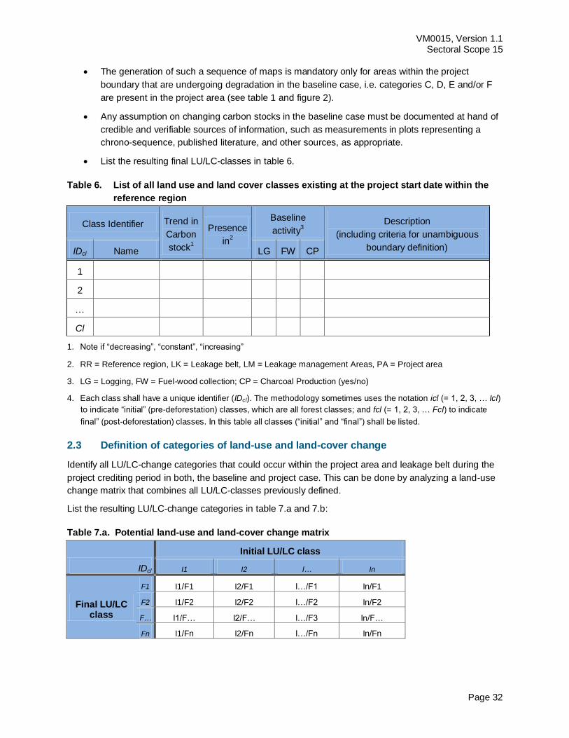
VM0015, Version 1.1 Sectoral Scope 15
Page 32
The generation of such a sequence of maps is mandatory only for areas within the project
boundary that are undergoing degradation in the baseline case, i.e. categories C, D, E and/or F
are present in the project area (see table 1 and figure 2).
Any assumption on changing carbon stocks in the baseline case must be documented at hand of
credible and verifiable sources of information, such as measurements in plots representing a
chrono-sequence, published literature, and other sources, as appropriate.
List the resulting final LU/LC-classes in table 6.
Table 6. List of all land use and land cover classes existing at the project start date within the
reference region
Class Identifier Trend in
Carbon
stock1
Presence
in2
Baseline
activity3
Description
(including criteria for unambiguous
boundary definition) IDcl Name LG FW CP
1
2
…
Cl
1. Note if “decreasing”, “constant”, “increasing”
2. RR = Reference region, LK = Leakage belt, LM = Leakage management Areas, PA = Project area
3. LG = Logging, FW = Fuel-wood collection; CP = Charcoal Production (yes/no)
4. Each class shall have a unique identifier (IDcl). The methodology sometimes uses the notation icl (= 1, 2, 3, … Icl)
to indicate “initial” (pre-deforestation) classes, which are all forest classes; and fcl (= 1, 2, 3, … Fcl) to indicate
final” (post-deforestation) classes. In this table all classes (“initial” and “final”) shall be listed.
2.3 Definition of categories of land-use and land-cover change
Identify all LU/LC-change categories that could occur within the project area and leakage belt during the
project crediting period in both, the baseline and project case. This can be done by analyzing a land-use
change matrix that combines all LU/LC-classes previously defined.
List the resulting LU/LC-change categories in table 7.a and 7.b:
Table 7.a. Potential land-use and land-cover change matrix
IDcl
Initial LU/LC class
I1 I2 I… In
Final LU/LC class
F1 I1/F1 I2/F1 I…/F1 In/F1
F2 I1/F2 I2/F2 I…/F2 In/F2
F… I1/F… I2/F… I…/F3 In/F…
Fn I1/Fn I2/Fn I…/Fn In/Fn
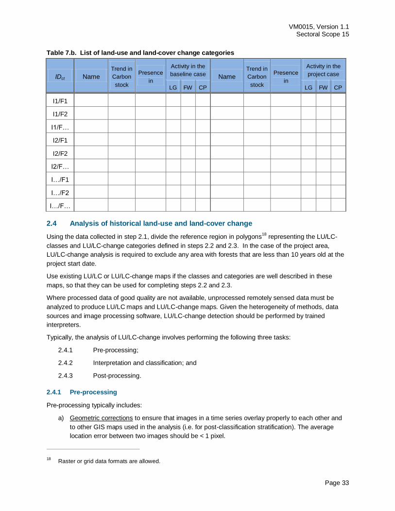
VM0015, Version 1.1 Sectoral Scope 15
Page 33
Table 7.b. List of land-use and land-cover change categories
IDct Name
Trend in
Carbon
stock
Presence
in
Activity in the
baseline case Name
Trend in
Carbon
stock
Presence
in
Activity in the
project case
LG FW CP LG FW CP
I1/F1
I1/F2
I1/F…
I2/F1
I2/F2
I2/F…
I…/F1
I…/F2
I…/F…
2.4 Analysis of historical land-use and land-cover change
Using the data collected in step 2.1, divide the reference region in polygons18
representing the LU/LC-
classes and LU/LC-change categories defined in steps 2.2 and 2.3. In the case of the project area,
LU/LC-change analysis is required to exclude any area with forests that are less than 10 years old at the
project start date.
Use existing LU/LC or LU/LC-change maps if the classes and categories are well described in these
maps, so that they can be used for completing steps 2.2 and 2.3.
Where processed data of good quality are not available, unprocessed remotely sensed data must be
analyzed to produce LU/LC maps and LU/LC-change maps. Given the heterogeneity of methods, data
sources and image processing software, LU/LC-change detection should be performed by trained
interpreters.
Typically, the analysis of LU/LC-change involves performing the following three tasks:
2.4.1 Pre-processing;
2.4.2 Interpretation and classification; and
2.4.3 Post-processing.
2.4.1 Pre-processing
Pre-processing typically includes:
a) Geometric corrections to ensure that images in a time series overlay properly to each other and
to other GIS maps used in the analysis (i.e. for post-classification stratification). The average
location error between two images should be < 1 pixel.
18 Raster or grid data formats are allowed.
VM0015, Version 1.1 Sectoral Scope 15
Page 34
b) Cloud and shadow removal using additional sources of data (e.g. radar, aerial photographs, field-
surveys).
c) Radiometric corrections may be necessary (depending on the change-detection technique used)
to ensure that similar objects have the same spectral response in multi-temporal datasets.
d) Reduction of haze, as needed.
See the most recent version of the GOFC-GOLD sourcebook for REDD or consult experts and literature
for further guidance on pre-processing techniques.
Duly record all pre-processing steps for later reporting.
2.4.2 Interpretation and classification
Two main categories of change detection exist and can be used (see IPCC 2006 GL AFOLU, Chapter
3A.2.4):
(1) Post-classification change detection: Two LU/LC maps are generated for two different time
points and then compared to detect LU/LC changes. The techniques are straightforward but are
also sensitive to inconsistencies in interpretation and classification of the LU/LC classes.
(2) Pre-classification change detection: These are more sophisticated approaches to LU/LC-
change detection. They also require more pre-processing of the data (i.e. radiometric
corrections). The basic approach is to compare by statistical methods the spectral response of
the ground using two data sets acquired at different dates to detect the locations where a
change has occurred and then to allocate different patterns of spectral change to specific
LU/LC-change categories. This approach is less sensitive to interpretation inconsistencies but
the methods involved are less straightforward and require access to the original unclassified
remotely sensed data.
As several methods are available to derive LU/LC and LU/LC-change maps from multi-temporal data
sets, the methodology does not prescribe any specific method. As a general guidance:
Automated classification methods should be preferred because the interpretation is more
efficient and repeatable than a visual interpretation.
Independent interpretation of multi-temporal images should be avoided (but is not forbidden).
Interpretation is usually more accurate when it focuses on change detection with
interdependent assessment of two multi-temporal images together. A technique that may be
effective is image segmentation followed by supervised object classification.
Minimum mapping unit size shall not be more than one hectare irrespective of forest definition.
See the most recent version of the GOFC-GOLD sourcebook on REDD or consult experts and
literature for further guidance on methods to analyze LU/LC-change using remotely sensed
data.
Duly record all interpretation and classification steps for later reporting.
VM0015, Version 1.1 Sectoral Scope 15
Page 35
2.4.3 Post-processing
Post-processing includes the use of non-spectral data to further stratify LU/LC-classes with
heterogeneous carbon density in LU/LC classes with homogenous carbon density. Post-classification
stratification can be performed efficiently using a Geographical Information System (GIS).
Current remote sensing technology is unable to discriminate carbon density classes, although some
progress is being made using lidar and other technologies that combined with field-surveys can be used
under this methodology. Some forest types (e.g. broadleaved forest, coniferous forests, mangroves) can
be discriminated with high accuracy using remotely-sensed data only.
LU/LC-classes that cannot be stratified further using remote sensing techniques but that are likely to
contain a broad range of carbon density classes should be stratified using:
Biophysical criteria (e.g. climate or ecological zone, soil and vegetation type, elevation, rainfall,
aspect, etc.)19
;
Disturbance indicators (e.g. vicinity to roads; forestry concession areas; etc.); age (in cases of
plantations and secondary forests);
Land management categories (e.g. protected forest, indigenous reserve, etc.); and/or
Other criteria relevant to distinguish carbon density classes.
See the most recent version of the GOFC-GOLD sourcebook for REDD and IPCC 2006 GL AFOLU for
further guidance on stratification. The criteria finally used should be reported transparently in the PD and
referenced to in table 6. Some iteration between steps 2.2, 2.3, and 2.4.3 may be necessary.
Duly record all post-processing steps for later reporting.
At the end of step 2, the following products should be prepared for the reference region and project area:
a) A Forest Cover Benchmark Map for at least the most recent date (2 years from the project start
date) and 10 ( 2) years20
prior to the project start date, showing only “forest” and “non-forest”.
b) A Land-Use and Land-Cover Map for at least the most recent date (2 years from the project start
date) depicting the LU/LC-classes defined in step 2.2. If such a map cannot be generated at the
levels of accuracy required by this methodology (see step 2.5), areas of the different LU/LC-
classes may be estimated by sampling techniques (e.g. by overlaying a grid of dots on the
satellite image and then counting the points falling in each LU/LC-class, or by sampling the
landscape with higher resolution images and then classifying the sampled images), or by using
other sources of data, such as official statistical data on land-use (e.g. agricultural census data):
c) A Deforestation Map for each sub-period analyzed, depicting at least the category “deforestation”.
Many projects will have some level of no-data areas because of cloud-cover. In this case change
rates should be calculated for each time step based only on areas that were not cloud-obscured
in either date in question. Then, a maximum possible forest cover map should be made for the
most recent year (2 years from the project start date). The historical rate in % should be
19 IPCC 2006 Guidelines for National GHG Inventories provide default climate and soil classification schemes in
Annex 3A.5 and guidance on stratifying LU/LC areas in Section 3.3.2.
20 This is to exclude from the project area forests that are less than 10 years old at the project start date.
VM0015, Version 1.1 Sectoral Scope 15
Page 36
multiplied by the maximum forest cover area at the start of the period for estimating the total area
of deforestation during the period.
d) A Land-Use and Land-Cover Change Map for at least the most recent period analyzed (3-5
years) depicting the LU/LC-change categories defined in step 2.3. In most cases, this map will be
prepared by combining the Deforestation Map of the most recent period (3-5 years) with the most
recent Land-Use and Land-Cover Map. If the area of the LU/LC-classes was estimated using
sampling techniques or other sources of information, a LU/LC-Change Map is not required.
e) A Land-Use and Land-Cover Change Matrix for at least the most recent period analyzed, derived
from the LU/LC-change map or the Deforestation Map and the post-deforestation land-use data
mentioned above, showing activity data for each LU/LC-change category. See appendix 2, table
4 for an example of a LU/LC change matrix.
2.5 Map accuracy assessment
A verifiable accuracy assessment of the maps produced in the previous step is necessary to produce a
credible baseline21
.
The accuracy must be estimated on a class-by-class (LU/LC map) and, where applicable, category-by-
category (LU/LC-change map) basis, respectively. A number of sample points on the map and their
corresponding correct classification (as determined by ground-surveys or interpretation of higher
resolution data as collected in step 2.1) can be used to create an error matrix with the diagonal showing
the proportion of correct classification and the off-diagonal cells showing the relative proportion of
misclassification of each class or category into the other class or, respectively, categories. Based on the
error matrix (also called confusion matrix), a number of accuracy indices can be derived (see e.g.
Congalton, 1991 and Pontius, 2000).
The minimum overall accuracy of the Forest Cover Benchmark Map should be 90%.
The minimum classification accuracy of each class or category in the Land-Use and Land-Cover Map and
Land-Use and Land-Cover Change Map, respectively, should be 80%. If the classification of a class or
category is lower than 80%:
Consider merging the class/category with other classes/categories22
; or
Exclude from the Forest Cover Benchmark Map the forest-classes that are causing the greatest
confusion with non-forest classes according to the error matrix (e.g. initial secondary
succession and heavily degraded forest may be difficult to distinguish from certain types of
grassland or cropland, such as agro-forestry and silvo-pastoral systems not meeting the
definition of “forest”). This implies conservatively reducing the area of the Forest Cover
Benchmark Map.
Both commission errors (false detection of a class/category, such as “deforestation”) and
omission errors (non-detection of actual class/category, such as “deforestation”) should be
estimated and reported.
21 See Chapter 5 of IPCC 2003 GPG, Chapter 3A.2.4 of IPPC 2006 Guidelines for AFOLU, and the most recent
version of the GOFC-GOLD Sourcebook on REDD for guidance on map accuracy assessment.
22 The tradeoff of merging classes or categories is that carbon estimates will be subject to a higher degree of
variability.
VM0015, Version 1.1 Sectoral Scope 15
Page 37
If ground-truthing data are not available for time periods in the past, the accuracy can be
assessed only at the most recent date, for which ground-truthing data can be collected.
Where the assessment of map accuracy requires merging or eliminating classes or categories to achieve
the required map accuracy, the definitions in the previous sub-steps must be adjusted accordingly. The
final maps and the class/category definitions must be consistent.
2.6 Preparation of a methodology annex to the PD
LU/LC-change analysis is an evolving field and will be performed several times during the project
crediting period. A consistent time-series of LU/LC-change data must emerge from this process.
In general, the same source of remotely sensed data and data analysis techniques must be used within a
period for which the baseline is fixed (fixed baseline period). However, if remotely sensed data have
become available from new and higher resolution sources (e.g. from a different sensor system) during
this period, these can only be used if the images based on interpretation of the new data overlap the
images based on interpretation of the old data by at least 1 year and they cross calibrate to acceptable
levels based on commonly used methods in the remote sensing community.
To achieve a consistent time-series, the risk of introducing artifacts from method change must be
minimized. For this reason, the detailed methodological procedures used in pre-processing, classification,
post classification processing, and accuracy assessment of the remotely sensed data, must be carefully
documented in an Annex to the PD. In particular, the following information must be documented:
a) Data sources and pre-processing: Type, resolution, source and acquisition date of the remotely
sensed data (and other data) used; geometric, radiometric and other corrections performed, if
any; spectral bands and indexes used (such as NDVI); projection and parameters used to geo-
reference the images; error estimate of the geometric correction; software and software version
used to perform pre-processing tasks; etc.
b) Data classification and post-processing: Definition of the LU/LC classes and LU/LC-change
categories; classification approach and classification algorithms; coordinates and description of
the ground-truthing data collected for training purposes; ancillary data used in the classification, if
any; software and software version used to perform the classification; additional spatial data and
analysis used for post-classification analysis, including class subdivisions using non-spectral
criteria, if any; etc.
c) Classification accuracy assessment: Accuracy assessment technique used; coordinates and
description of the ground-truth data collected for classification accuracy assessment; post-
processing decisions made based on the preliminary classification accuracy assessment, if any;
and final classification accuracy assessment.
STEP 3: ANALYSIS OF AGENTS, DRIVERS AND UNDERLYING CAUSES OF 3
DEFORESTATION AND THEIR LIKELY FUTURE DEVELOPMENT
Understanding “who” is deforesting the forest (the “agent”) and what drives land-use decisions (“drivers”
and “underlying causes”) is necessary for two mains reasons: (i) Estimating the quantity and location of
future deforestation; and (ii) Designing effective measures to address deforestation, including leakage
prevention measures.
VM0015, Version 1.1 Sectoral Scope 15
Page 38
This analysis is performed through the following five sub-steps23
:
3.1 Identification of agents of deforestation;
3.2 Identification of deforestation drivers;
3.3 Identification of underlying causes;
3.4 Analysis of chain of events leading to deforestation; and
3.5 Conclusion
3.1 Identification of agents of deforestation
Identify the main agent groups of deforestation (farmers, ranchers, loggers, etc.) and their relative
importance (i.e. the amount of historical LU/LC-change that can be attributed to each of them). To do this
identification, use existing studies, the maps prepared in step 2, expert-consultations, field-surveys and
other verifiable sources of information, as needed.
Sometimes, the relative importance of each agent can be determined from the LU/LC-change matrix
developed in step 2.4, since each agent usually converts forests for a specific purpose (cattle ranching,
cash-crop production, subsistence farming, etc.).
If the relative importance of different agents is spatially correlated (e.g. small farmers are concentrated in
the hills, while ranchers on the planes) it may be useful to stratify the reference region, the project area
and the leakage belt accordingly (in IRR strata), and to continue the baseline assessment for each stratum
i separately in order to increase the accuracy of the projections.
For each identified agent group, provide the following information:
a) Name of the main agent group or agent;
b) Brief description of the main social, economic, cultural and other relevant features of each main
agent group. Limit the description to aspects that are relevant to understand why the agent group
is deforesting;
c) Brief assessment of the most likely development of the population size of the identified main
agent groups in the reference region, project area and leakage belt;
d) Statistics on historical deforestation attributable to each main agent group in the reference region,
project area and leakage belt.
3.2 Identification of deforestation drivers
For each identified agent group, analyze factors that drive their land-use decisions. The goal is to identify
the immediate causes of deforestation.
Two sets of driver variables have to be distinguished:
a) Driver variables explaining the quantity (hectares) of deforestation (to be used in step 4.1 and
4.3, as appropriate), such as:
Prices of agricultural products;
23 See Angelsen and Kaimowitz (1999) and Chomiz et al. (2006) for comprehensive analysis of deforestation agents
and drivers.
VM0015, Version 1.1 Sectoral Scope 15
Page 39
Costs of agricultural inputs;
Population density;
Rural wages;
Etc.
b) Driver variables explaining the location of deforestation, also called “predisposing factors” (de
Jong, 2007) (to be used in step 4.2), such as:
Access to forests (such as vicinity to existing roads, railroads, navigable rivers and
coastal lines);
Slope;
Proximity to markets;
Proximity to existing or industrial facilities (e.g. sawmills, pulp and paper mills,
agricultural products processing facilities, etc.);
Proximity to forest edges;
Proximity to existing settlements;
Spatial variables indicating availability within the forest of land with good ecological
conditions to expand agricultural activities, such as soil fertility and rainfall;
Management category of the land (e.g. national park, indigenous reserve, etc.);
Etc.
For each of these two sets of variables:
1) List the 1 to 5 key driver variables and provide any relevant source of information that provides
evidence that the identified variables have been a driver for deforestation during the historical
reference period.
2) Briefly describe for each main agent group identified in step 3.1 how the key driver variables
have and will most likely impact on each agent group’s decision to deforest.
3) For each identified key driver variable provide information about its likely future development24
,
by providing any relevant source of information.
4) For each identified driver variable briefly describe the project measures that will be implemented
to address them33
, if applicable.
3.3 Identification of underlying causes of deforestation
The agents’ characteristics and decisions are themselves determined by broader forces, the underlying
causes of deforestation, such as:
Land-use policies and their enforcement;
Population pressure;
Poverty and wealth;
War and other types of conflicts;
Property regime;
Etc.
24 This does not apply to spatial variables, such slope, elevation etc.
VM0015, Version 1.1 Sectoral Scope 15
Page 40
1) List the 1 to 5 key underlying causes and cite any relevant source of information that provides
evidence that the identified variables have been an underlying cause for deforestation during
the historical reference period.
2) Briefly describe how each key underlying cause has determined and will most likely determine
the key drivers identified in step 3.2 and the decisions of the main agent groups identified in
step 3.1.
3) For each identified key underlying cause provide information about its likely future
development, by citing any relevant source of information.
4) For each identified underlying cause describe the project measures that will be implemented to
address them, if applicable.
3.4 Analysis of chain of events leading to deforestation
Based on the historical evidence collected, analyze the relations between main agent groups, key drivers
and underlying causes and explain the sequence of events that typically has lead and most likely will lead
to deforestation. Consult local experts, literature and other sources of information, as necessary. Briefly
summarize the results of this analysis in the PD.
3.5 Conclusion
The analysis of step 3 must conclude with a statement about whether the available evidence about the
most likely future deforestation trend within the reference region and project area is:
Inconclusive or
Conclusive.
“Conclusive” evidence in this methodology means that the hypothesized relationships between agent
groups, driver variables, underlying causes and historical levels of deforestation can be verified at hand of
statistical tests, literature studies, or other verifiable sources of information, such as documented
information provided by local experts, communities, deforestation agents and other groups with good
knowledge about the project area and the reference region.
To arrive at an overall “conclusive” conclusion when multiple agents and drivers are present, the evidence
obtained for each of them must lead to a “conclusive” decision for all.
When the evidence is conclusive, state whether the weight of the available evidence suggests that the
overall trend in future baseline deforestation rates will be:
Decreasing;
About constant;
Increasing.
Then proceed to step 4.
When the evidence is inconclusive and the historical deforestation trend has been decreasing or about
constant, additional analysis must be carried out under step 3, such as more literature reviews, expert
consultations, and, as the case may be, additional field surveys, until conclusive evidence on the most
likely future deforestation trend is found, otherwise it will not be possible to continue with the next steps of
the methodology. If the historical deforestation trend has been increasing and the evidence is
inconclusive, the deforestation rate to be used in the projections will be the average historical rate (see
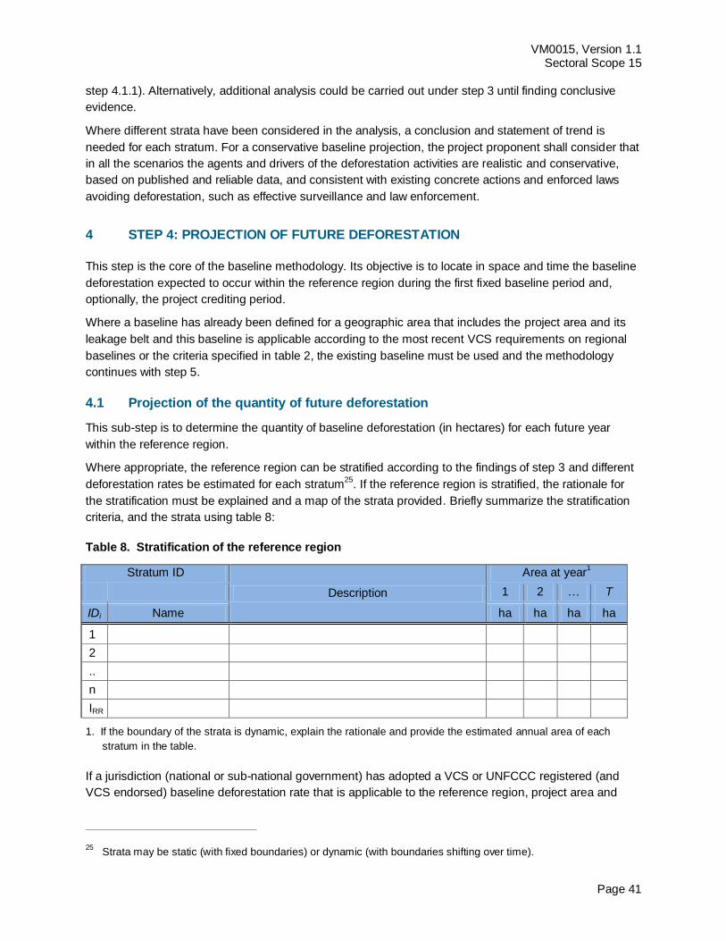
VM0015, Version 1.1 Sectoral Scope 15
Page 41
step 4.1.1). Alternatively, additional analysis could be carried out under step 3 until finding conclusive
evidence.
Where different strata have been considered in the analysis, a conclusion and statement of trend is
needed for each stratum. For a conservative baseline projection, the project proponent shall consider that
in all the scenarios the agents and drivers of the deforestation activities are realistic and conservative,
based on published and reliable data, and consistent with existing concrete actions and enforced laws
avoiding deforestation, such as effective surveillance and law enforcement.
STEP 4: PROJECTION OF FUTURE DEFORESTATION 4
This step is the core of the baseline methodology. Its objective is to locate in space and time the baseline
deforestation expected to occur within the reference region during the first fixed baseline period and,
optionally, the project crediting period.
Where a baseline has already been defined for a geographic area that includes the project area and its
leakage belt and this baseline is applicable according to the most recent VCS requirements on regional
baselines or the criteria specified in table 2, the existing baseline must be used and the methodology
continues with step 5.
4.1 Projection of the quantity of future deforestation
This sub-step is to determine the quantity of baseline deforestation (in hectares) for each future year
within the reference region.
Where appropriate, the reference region can be stratified according to the findings of step 3 and different
deforestation rates be estimated for each stratum25
. If the reference region is stratified, the rationale for
the stratification must be explained and a map of the strata provided. Briefly summarize the stratification
criteria, and the strata using table 8:
Table 8. Stratification of the reference region
Stratum ID
Description
Area at year1
1 2 … T
IDi Name ha ha ha ha
1
2
..
n
IRR
1. If the boundary of the strata is dynamic, explain the rationale and provide the estimated annual area of each
stratum in the table.
If a jurisdiction (national or sub-national government) has adopted a VCS or UNFCCC registered (and
VCS endorsed) baseline deforestation rate that is applicable to the reference region, project area and
25 Strata may be static (with fixed boundaries) or dynamic (with boundaries shifting over time).
VM0015, Version 1.1 Sectoral Scope 15
Page 42
leakage belt according to the most recent VCS JNR Requirements, the adopted rate must be used and
no further analysis is required under this sub-step (continue with step 4.2).
Where the above condition does not exist, a projected deforestation rate must be determined by the
project proponent taking into account possible future changes at the level of agents, drivers and
underlying causes of deforestation, as well as the remaining forest area that is potentially available for
conversion to non-forest uses. This task is performed through the following three analytical sub-steps:
4.1.1 Selection of the baseline approach;
4.1.2 Quantitative projection of future deforestation.
4.1.1 Selection of the baseline approach
To project future deforestation three baseline approaches are available:
a) Historical average approach: Under this approach, the rate of baseline deforestation is assumed
to be a continuation of the average annual rate measured during the historical reference period
within the reference region or, where appropriate, within different strata of the reference region.
b) Time function approach: With this approach, the rate of baseline deforestation is estimated by
extrapolating the historical trend observed within the reference region (or its strata) as a function
of time using either linear regression, logistic regression or any other statistically sound
regression technique (see step 4.1.3). This approach requires multiple deforestation
measurements during the past 10-15 years.
c) Modeling approach: With this approach, the rate of baseline deforestation will be estimated using
a model that expresses deforestation as a function of driver variables selected by the project
proponents. Such driver variables may be spatial and consistency with the analysis of step 3
must exist.
Select and justify the most appropriate baseline approach following the decision criteria described below.
Different approaches can be used in different strata of the reference region, where appropriate.
1. The deforestation rates measured in different historical sub-periods in the reference region (or a
stratum of it) do not reveal any trend (decreasing, constant or increasing deforestation) and:
1.1 No conclusive evidence emerges from the analysis of agents and drivers explaining the
different historical deforestation rates: do additional assessments under step 3, such as
more literature reviews, expert consultations, and, as the case may be, additional field
surveys, until finding conclusive evidence.
1.2 Conclusive evidence emerges from the analysis of agents and drivers explaining the
different historical deforestation rates: use approach “c” if there is at least one variable
that can be used to project the deforestation rate, otherwise use approach “a”.
2. The deforestation rates measured in different historical sub-periods in the reference region (or a
stratum of it) reveal a clear trend and this trend is:
2.1 A decrease of the deforestation rate and:
Conclusive evidence emerges from the analysis of agents and drivers explaining the
decreasing trend and making it likely that this trend will continue in the future: use
approach “b”.
VM0015, Version 1.1 Sectoral Scope 15
Page 43
Conclusive evidence emerges from the analysis of agents and drivers explaining the
decreasing trend and this evidence also suggest that the decreasing trend will
change in the future due to predictable changes at the level of agents and drivers:
use approach “c”.
No conclusive evidence emerges from the analysis of agents and drivers explaining
the decreasing trend: do additional assessments under step 3, such as more
literature reviews, expert consultations, and, as the case may be, additional field
surveys, until finding conclusive evidence, then use approach “b”.
2.2 A constant deforestation rate and:
Conclusive evidence emerges from the analysis of agents and drivers explaining the
historical trend and making it likely that this trend will continue in the future: use
approach “a”.
Conclusive evidence emerges from the analysis of agents and drivers explaining the
historical trend and this evidence also suggests that the historical trend will change in
the future due to predictable changes at the level of agents and drivers: use approach
“c”.
No conclusive evidence emerges from the analysis of agents and drivers explaining
the historical trend: do additional assessments under step 3, such as more literature
reviews, expert consultations, and, as the case may be, additional field surveys, until
finding conclusive evidence, then use approach “a”.
2.3 An increase of the deforestation rate and:
Conclusive evidence emerges from the analysis of agents and drivers explaining the
increased trend and making it likely that this trend will continue in the future: use
approach “b”. If the future deforestation trend is likely to be higher than predicted with
approach “b”, use approach “c”.
Conclusive evidence emerges from the analysis of agents and drivers explaining the
increased trend but this evidence also suggests that the future trend will change: use
approach “a” or develop a model (approach “c”).
No conclusive evidence emerges from the analysis of agents and drivers explaining
the increasing trend: use approach “a”.
4.1.2 Quantitative projection of future deforestation
The methodology procedure is to first project the annual areas or rates of baseline deforestation within
the reference region (or – where appropriate – within different strata of the reference region), then to
analyze the spatial location of these annual areas in the reference region (step 4.2), and finally, to
determine the annual areas and location of deforestation in the project area and leakage belt.
4.1.2.1 Projection of the annual areas of baseline deforestation in the reference region
The method to be used depends on the baseline approach selected.
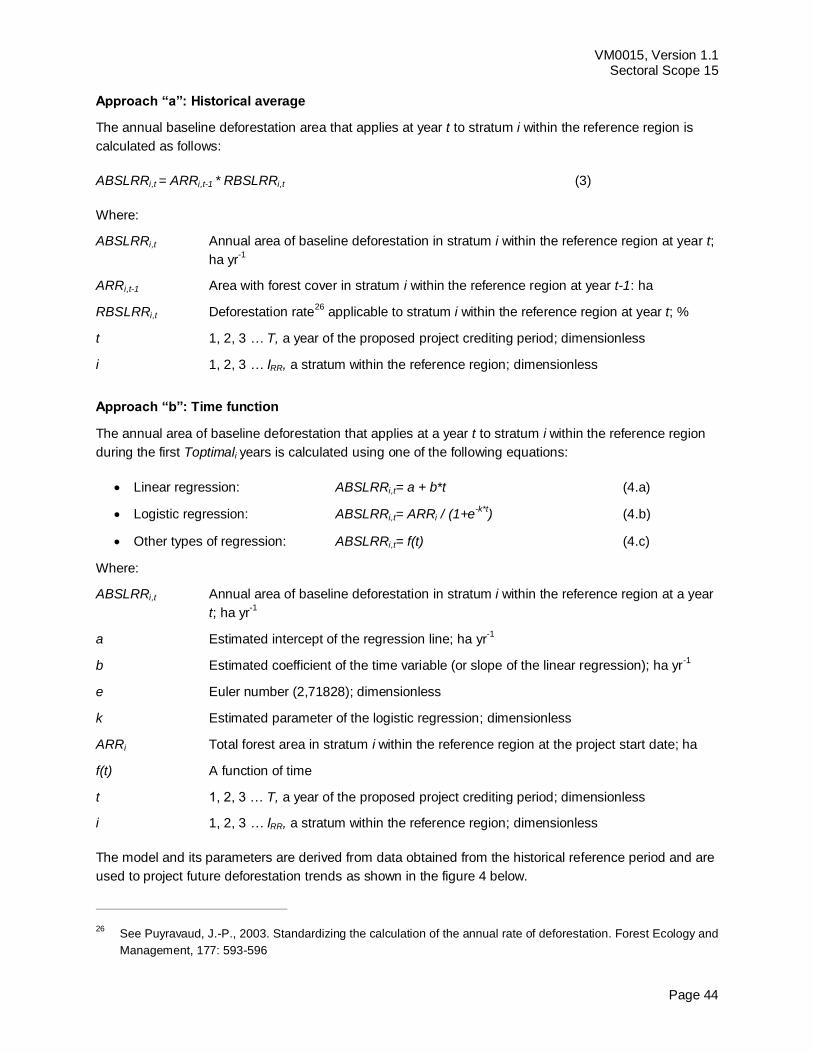
VM0015, Version 1.1 Sectoral Scope 15
Page 44
Approach “a”: Historical average
The annual baseline deforestation area that applies at year t to stratum i within the reference region is
calculated as follows:
ABSLRRi,t = ARRi,t-1 * RBSLRRi,t (3)
Where:
ABSLRRi,t Annual area of baseline deforestation in stratum i within the reference region at year t;
ha yr-1
ARRi,t-1 Area with forest cover in stratum i within the reference region at year t-1: ha
RBSLRRi,t Deforestation rate26
applicable to stratum i within the reference region at year t; %
t 1, 2, 3 … T, a year of the proposed project crediting period; dimensionless
i 1, 2, 3 … IRR, a stratum within the reference region; dimensionless
Approach “b”: Time function
The annual area of baseline deforestation that applies at a year t to stratum i within the reference region
during the first Toptimali years is calculated using one of the following equations:
Linear regression: ABSLRRi,t= a + b*t (4.a)
Logistic regression: ABSLRRi,t= ARRi / (1+e-k*t
) (4.b)
Other types of regression: ABSLRRi,t= f(t) (4.c)
Where:
ABSLRRi,t Annual area of baseline deforestation in stratum i within the reference region at a year
t; ha yr-1
a Estimated intercept of the regression line; ha yr-1
b Estimated coefficient of the time variable (or slope of the linear regression); ha yr-1
e Euler number (2,71828); dimensionless
k Estimated parameter of the logistic regression; dimensionless
ARRi Total forest area in stratum i within the reference region at the project start date; ha
f(t) A function of time
t 1, 2, 3 … T, a year of the proposed project crediting period; dimensionless
i 1, 2, 3 … IRR, a stratum within the reference region; dimensionless
The model and its parameters are derived from data obtained from the historical reference period and are
used to project future deforestation trends as shown in the figure 4 below.
26 See Puyravaud, J.-P., 2003. Standardizing the calculation of the annual rate of deforestation. Forest Ecology and
Management, 177: 593-596
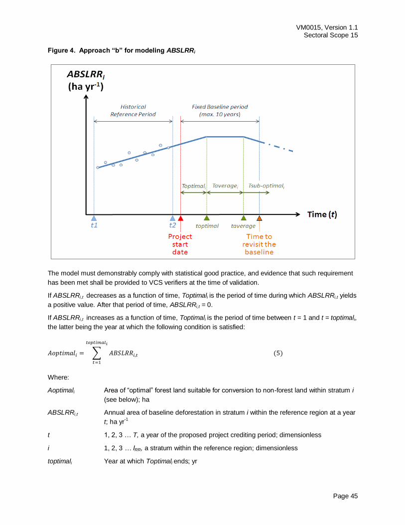
VM0015, Version 1.1 Sectoral Scope 15
Page 45
Figure 4. Approach “b” for modeling ABSLRRi
The model must demonstrably comply with statistical good practice, and evidence that such requirement
has been met shall be provided to VCS verifiers at the time of validation.
If ABSLRRi,t decreases as a function of time, Toptimali is the period of time during which ABSLRRi,t yields
a positive value. After that period of time, ABSLRRi,t = 0.
If ABSLRRi,t increases as a function of time, Toptimali is the period of time between t = 1 and t = toptimali,
the latter being the year at which the following condition is satisfied:
∑
Where:
Aoptimali Area of “optimal” forest land suitable for conversion to non-forest land within stratum i
(see below); ha
ABSLRRi,t Annual area of baseline deforestation in stratum i within the reference region at a year
t; ha yr-1
t 1, 2, 3 … T, a year of the proposed project crediting period; dimensionless
i 1, 2, 3 … IRR, a stratum within the reference region; dimensionless
toptimali Year at which Toptimali ends; yr
VM0015, Version 1.1 Sectoral Scope 15
Page 46
If: Toptimali > Project crediting period: ABSLRRi,t calculated with equations 4 is applicable during the
entire project crediting period.
If: Toptimali < Project crediting period: ABSLRRi,t calculated with equations 4 is applicable only to the
first Toptimali years. For the following Taveragei years use value of ABSLRRi,t calculated for the year t
= Toptimali :Taveragei is the period of time between t = toptimali and t = taveragei, the latter being the
year at which the following condition is satisfied:
∑
Where:
Aaveragei Area of “average” forest land suitable for conversion to non-forest land within stratum i
(see below); ha
ABSLRRi,t Annual area of baseline deforestation in stratum i within the reference region at a year
t; ha yr-1
t 1, 2, 3 … T, a year of the proposed project crediting period; dimensionless
i 1, 2, 3 … IRR, a stratum within the reference region; dimensionless
toptimali Year at which Toptimali ends; yr
taveragei Year at which Taveragei ends; yr
If: Toptimali + Taveragei > Project crediting period: ABSLRRi,t calculated for the year t = toptimali is
applicable during the period of time between t = toptimali and t = taveragei.
If: Toptimali + Taveragei < Project crediting period: ABSLRRi,t calculated for the year t = toptimali is
applicable only to the first Taveragei years following after year toptimali. For the following 20 years
assume a linear decrease of ABSLRRi,t down to zero hectares per year in t=faverage+20.
ABSLRRi,t = ABSLRRtaverage,i (1 – 1/20 * (t – taveragei)) (7)
Where:
ABSLRRi,t Annual area of baseline deforestation in stratum i within the reference region at a year
t; ha yr-1
ABSLRRtaverage,i Annual area of baseline deforestation in stratum i within the reference region at a year
taveragei; ha yr-1
taveragei Year at which Taveragei ends; yr
t 1, 2, 3 … T, a year of the proposed project crediting period; dimensionless
i 1, 2, 3 … IRR, a stratum within the reference region; dimensionless
Note: After taveragei + 20 years ABSLRRi,t will be zero hectares per year in all cases..
VM0015, Version 1.1 Sectoral Scope 15
Page 47
Calculation of Aoptimali and Aaveragei under Approach “b”
Aoptimali (area of “optimal” forest land suitable for conversion to non-forest land within stratum i) and
Aaveragei (area of “average” forest land suitable for conversion to non-forest land within stratum i) must
be determined to avoid non-conservative projections of baseline deforestation when “increasing
deforestation” is projected under Approach “b”. Deforestation can increase in the future only if there are
no constraints to the conversion of forest land to non-forest land. This is typically the case when the
project area is located in a country or region still with significant forest cover (Olander et al., 2006).
To assess whether there is scarcity of forest land that is accessible to deforestation agents and potentially
exposed to the risk of deforestation do the following:
1) Identify land-use constraints: Identify the appropriate biophysical constraints (e.g. soil, climate,
elevation and/or slope) and appropriate socio-economic constraints (e.g, mobility, land-use
rights and/or areas with presence of conflicts and crime) that limit the geographical area where
deforestation agents could expand their land-use activities in currently forested areas. Consider
the constraints as they are perceived by the main groups of deforestation agents, taking into
consideration their socio-economic conditions. To determine how constraints are perceived by
the main groups of deforestation agents, determine the threshold conditions under which they
have deforested historically (for example, range of slopes, types of soil, minimum/maximum
rainfall, and/or elevation range, are relevant to determine the range where main types of crops
and animals could survive). Use spatial data, literature, surveys, and/or participative rural
appraisal (PRA) as appropriate.
2) Estimate the remaining forest area that could be converted to non-forest land: Using the
constraints identified above, develop a Maximum Potential Deforestation Map, which maps the
area currently covered by forests that is potentially available for the further expansion of non-
forest uses in the reference region.
3) Stratify the Maximum Potential Deforestation Map in broad suitability classes: Considering the
constraints identified above, define criteria and thresholds that delineate “optimal”, “average”
and “sub-optimal” conditions for each of the main land uses implemented by the main agent
groups (e.g. by defining ranges of slope, rainfall or types of soils, or ranges of deforestation
risks according to the deforestation risk map created for the spatial model (See step 4.2)).
Select thresholds that are relevant from the point of view of the deforestation agents. Using the
selected criteria and thresholds stratify the Maximum Potential Deforestation Map in three
broad suitability classes representing “optimal”, “average” and “sub-optimal” areas for non-
forest uses. When available from other sources, use existing maps.
4) Aoptimali will be the area of the “optimal” suitability class within stratum i; and Aaveragei will be
the area of the “average” suitability class within stratum i.
Approach “c”: Modeling
The annual area of baseline deforestation that applies at year t in stratum i within the reference region is
estimated using a statistical model, such as simple regression, multiple regressions, logistic regression, or
any other possible model to be proposed and justified by the project proponent. The proposed model
must demonstrably comply with statistical good practice, and evidence that such requirement has been
met shall be provided to VCS verifiers at the time of validation.
The following equations are given for illustration purposes only:
VM0015, Version 1.1 Sectoral Scope 15
Page 48
ABSLRRi,t = a + b1i*V1i,t (8.a)
ABSLRRi,t = a + b1i*V1i,t + b2i*V2i,t (8.b)
) (8.c)
Where:
ABSLRRi,t Annual area of baseline deforestation in stratum i within the reference region at a
year t; ha yr-1
a; b1i; b2i; ... ; bni; k Estimated coefficients of the model
e Euler number (2,71828); dimensionless
V1i,t; V2i,t; ...;Vni,t Variables included in the model
ARRi Total forest area in stratum i within the reference region at the project start date;
ha
t 1, 2, 3 … T, a year of the proposed project crediting period; dimensionless
i 1, 2, 3 … IRR, a stratum within the reference region; dimensionless
The model may also be constructed with the annual area deforested (ABSLRRi,t), or the deforestation rate
(RBSLRRi,t = percentage of remaining forest area at year t-1 in stratum i to be deforested at year t) as the
dependent variable, and independent variable(s) (e.g. population density in stratum i at time t, average
opportunity costs in stratum i at time t, etc.) from which the annual areas of deforestation (ABSLRRi,t) or
the deforestation rates (RBSLRRi,t) are inferred from changes in the independent variables.
For each of the selected independent variables, there must be a description of the historical data
(including source), an explanation of the rationale for using the variable(s), and a credible future
projection based on documented and verifiable sources. To determine the future values of the variables
included in the model, official projections, expert opinion, other models, and any other relevant and
verifiable source of information must be used. Justify with logical and credible explanations any
assumption about future trends of the driver variables and use values that yield conservative estimates of
the projected deforestation (ABSLRRi,t or RBSLRRi,t).
The model and its rationale must be explained by the project proponent using logical arguments and
verifiable sources of information and must be consistent with the analysis of step 3.The model must
demonstrably comply with statistical good practice, and evidence that such requirement has been met
shall be provided to VCS verifiers at the time of validation.
4.1.2.2 Projection of the annual areas of baseline deforestation in the project area and leakage
belt
Location analysis of future deforestation within reference region is required to determine the annual areas
of deforestation within the project area and leakage belt (step 4.2). Once location analysis is completed,
the portion of annual areas of baseline deforestation of each stratum i within the project area and leakage
belt must be determined using a GIS.
To do this step, step 4.2.4 must be completed first.

VM0015, Version 1.1 Sectoral Scope 15
Page 49
4.1.2.3 Summary of step 4.1.2
Present the results of the previous assessments in Tables 9.a and 9.b. Do this at least for the fixed
baseline period and, optionally, for the entire project crediting period.
Table 9.a. Annual areas of baseline deforestation in the reference region
Project
year t
Stratum i in the reference region Total
1 2 … IRR annual cumulative
ABSLRRi,t ABSLRRi,t ABSLRRi,t ABSLRRi,t ABSLRRt ABSLRR
ha ha ha ha ha ha
0
1
2
. . .
T
Table 9.b. Annual areas of baseline deforestation in the project area
Project
year t
Stratum i of the reference region in the project area Total
1 2 … IRR annual cumulative
ABSLPAi,t ABSLPAi,t ABSLPAi,t ABSLPAi,t ABSLPAt ABSLPA
ha ha ha ha ha ha
0
1
2
. . .
T
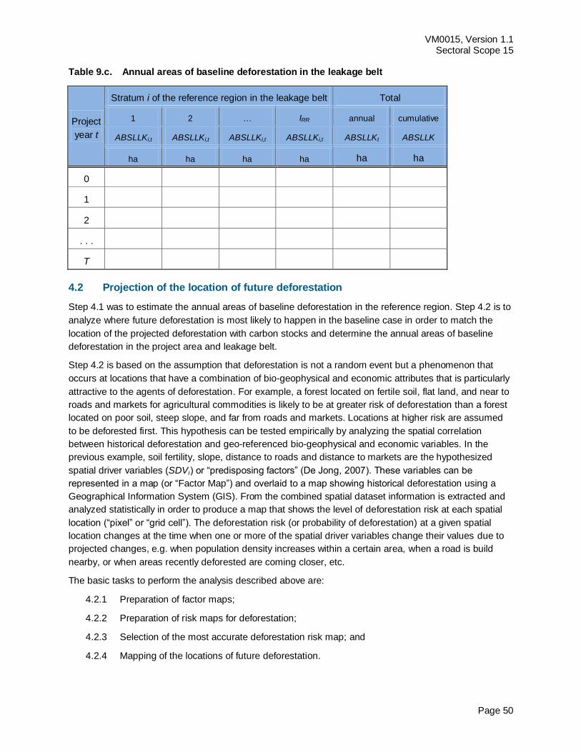
VM0015, Version 1.1 Sectoral Scope 15
Page 50
Table 9.c. Annual areas of baseline deforestation in the leakage belt
Project
year t
Stratum i of the reference region in the leakage belt Total
1 2 … IRR annual cumulative
ABSLLKi,t ABSLLKi,t ABSLLKi,t ABSLLKi,t ABSLLKt ABSLLK
ha ha ha ha ha ha
0
1
2
. . .
T
4.2 Projection of the location of future deforestation
Step 4.1 was to estimate the annual areas of baseline deforestation in the reference region. Step 4.2 is to
analyze where future deforestation is most likely to happen in the baseline case in order to match the
location of the projected deforestation with carbon stocks and determine the annual areas of baseline
deforestation in the project area and leakage belt.
Step 4.2 is based on the assumption that deforestation is not a random event but a phenomenon that
occurs at locations that have a combination of bio-geophysical and economic attributes that is particularly
attractive to the agents of deforestation. For example, a forest located on fertile soil, flat land, and near to
roads and markets for agricultural commodities is likely to be at greater risk of deforestation than a forest
located on poor soil, steep slope, and far from roads and markets. Locations at higher risk are assumed
to be deforested first. This hypothesis can be tested empirically by analyzing the spatial correlation
between historical deforestation and geo-referenced bio-geophysical and economic variables. In the
previous example, soil fertility, slope, distance to roads and distance to markets are the hypothesized
spatial driver variables (SDVi) or “predisposing factors” (De Jong, 2007). These variables can be
represented in a map (or “Factor Map”) and overlaid to a map showing historical deforestation using a
Geographical Information System (GIS). From the combined spatial dataset information is extracted and
analyzed statistically in order to produce a map that shows the level of deforestation risk at each spatial
location (“pixel” or “grid cell”). The deforestation risk (or probability of deforestation) at a given spatial
location changes at the time when one or more of the spatial driver variables change their values due to
projected changes, e.g. when population density increases within a certain area, when a road is build
nearby, or when areas recently deforested are coming closer, etc.
The basic tasks to perform the analysis described above are:
4.2.1 Preparation of factor maps;
4.2.2 Preparation of risk maps for deforestation;
4.2.3 Selection of the most accurate deforestation risk map; and
4.2.4 Mapping of the locations of future deforestation.
VM0015, Version 1.1 Sectoral Scope 15
Page 51
Several model/software are available and can be used to perform these tasks in slightly different ways,
such as Geomod, Idrisi Taiga, Dinamica Ego, Clue, and Land-Use Change Modeler. The model/software
used must be peer-reviewed and must be consistent with the methodology (to be proven at validation).
4.2.1 Preparation of factor maps
Based on the analysis of step 3 and step 4.1, identify the spatial variables that most likely explain the
patterns of baseline deforestation in the reference region. Obtain spatial data for each variable and create
digital maps representing the Spatial Features of each variable (i.e. the shape files representing the point,
lines or polygon features or the raster files representing surface features). Some models will require
producing Distance Maps from the mapped features (e.g. distance to roads or distance to already
deforested lands) or maps representing continuous variables (e.g. slope classes) and categorical
variables (e.g. soil quality classes). If the model/software allows working with dynamic Distance Maps (i.e.
the software can calculate a new Distance Maps at each time step), these should be used. For simplicity,
these maps are called “Factor Maps”. Other models do not require Factor Maps for each variable, and
instead analyze all the variables and deforestation patterns together to produce a risk map.
Where some of the spatial variables are expected to change, collect information on the expected changes
from credible and verifiable sources of information. Then prepare Factor Maps that represent the changes
that will occur in different future periods. Sometimes, projected changes can be represented by a dynamic
spatial model that may change in response to deforestation.
In case of planned infrastructure (e.g. roads, industrial facilities, settlements) provide documented
evidence that the planned infrastructure will actually be constructed and the time table of the construction.
In case of planned new roads, road improvements, or railroads provide credible and verifiable information
on the planned construction of different segments (e.g. how many kilometers will be constructed, where
and when). Evidence includes: approved plans and budgets for the construction, signed construction
contracts or at least an open bidding process with approved budgets and finance. If such evidence is not
available exclude the planned infrastructure from the factors considered in the analysis.
Any area affected by planned deforestation due to the construction of planned infrastructure must be
excluded from the project area.
In case of unplanned infrastructure (e.g. secondary roads), provide evidence that the unplanned
infrastructure will actually develop, e.g. from historical developments. Specifically, from a wall-to-wall
assessment (or at least five randomly sampled observations in the reference region) or from literature
sources appropriate to the reference region, estimate the average annual length27
of new unplanned
infrastructure per square kilometer28
that was constructed during the historical reference period.
Alternatively, determine the historical rate of change as related to variables for which there are good
projections (e.g. km of new unplanned infrastructure as related to population). To avoid projecting
unplanned infrastructure in areas where geographic and socio-economic conditions are unfavorable for
infrastructure developments (e.g. areas with steep slopes, swampy soils, low opportunity costs, etc.),
develop a map representing a proxy of the suitability for future infrastructure development. For each
27 Other parameters relevant for modeling the construction of secondary roads may also be measured in this
analysis, such as distance between roads, number of destinations per year, etc. Parameters to be assessed are dependent on the modeling approach used to project the development of the road network and are therefore not further specified here.
28 Or per km of official new road constructed, or per other landscape features that can be mapped (such as new
industrial facilities, settlements, mining concessions etc.), as appropriate.
VM0015, Version 1.1 Sectoral Scope 15
Page 52
“suitability” class or gradient (using a minimum of two classes, e.g. suitable, not suitable), determine the
most plausible rate of unplanned infrastructure development. To do this, apply the following steps:
a) Using historical data, expert opinion, participative rural appraisal (PRA), literature and/or other
verifiable sources of information list all relevant criteria that facilitate (at least one criterion) and
constrain (at least one criterion) the development of new unplanned infrastructure.
b) For each criterion, generate a map using a GIS.
c) Using multi-criteria analysis, determine the most likely rate of unplanned infrastructure
development (e.g. km km-2
yr-1
or a similar indicator) per different sectors (suitability classes or
gradients) within the reference region.
Projections of unplanned infrastructure development shall be conservative, in particular projections in
forested areas shall meet this requirement.
To create the Factor Maps use one of the following two approaches:
Empirical approach: Categorize each Distance Map in a number of predefined distance classes
(e.g. class 1 = distance between 0 and 50 m; class 2 = distance between 50 and 100 m, etc.). In
a table describe the rule used to build classes and the deforestation likelihood assigned to each
distance class29
. The deforestation likelihood is estimated as the percentage of pixels that were
deforested during the period of analysis (i.e. the historical reference period).
Heuristic approach: Define “value functions” representing the likelihood of deforestation as a
function of distance from point features (e.g., saw mills) or linear features (e.g., roads), or as a
function of polygon features representing classes (e.g. of soil type, population density) based on
expert opinion or other sources of information. Specify and briefly explain each value function in
the PD.
For Distance Maps, a useful approach to estimate value functions is to sample spatially
uncorrelated points and their corresponding location in the maps representing historical
deforestation (Land-Use and Land-Cover Change Maps produced with step 2) and to use
regression techniques30
to define the probability of deforestation as a function of “distance”.
The empirical approach should be preferred over the heuristic approach. Use the heuristic approach only
where there is insufficient information about the spatial location of historical deforestation or where the
empirical approach does not produce accurate results when validated against a historical period.
4.2.2 Preparation of deforestation risk maps
A Risk Map shows at each pixel location l the risk (or “probability”) of deforestation in a numerical scale
(e.g., 0 = minimum risk; 255 = maximum risk).
29 When building classes of continuous variables it is important to build classes that are meaningful in terms of
deforestation risk. This implies the parameterization of a “value function” based on specific measurements. For instance, the criterion “distance to roads” might not have a linear response to assess the deforestation risk: a forest located at 50 km from the nearest road may be subject to the same deforestation risk of a forest located at 100 km, while at 0.5 km the risk may be twice as much as at 1.0 km. Data to model the value function and build meaningful classes can be obtained by analyzing the distribution of sample points taken from historical ly deforested areas.
30 e.g. logistic regression.
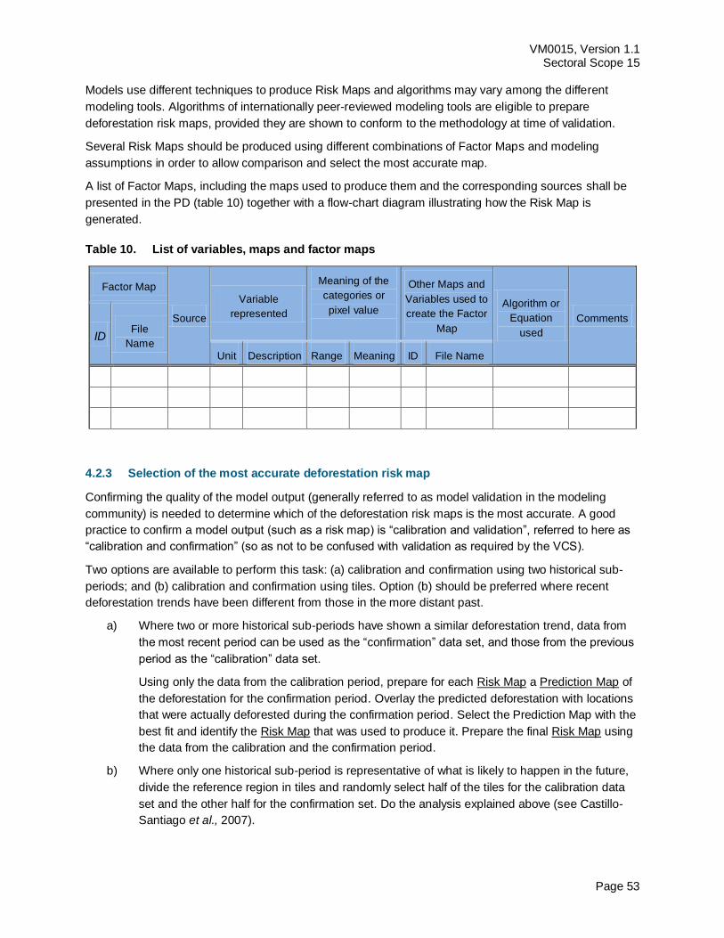
VM0015, Version 1.1 Sectoral Scope 15
Page 53
Models use different techniques to produce Risk Maps and algorithms may vary among the different
modeling tools. Algorithms of internationally peer-reviewed modeling tools are eligible to prepare
deforestation risk maps, provided they are shown to conform to the methodology at time of validation.
Several Risk Maps should be produced using different combinations of Factor Maps and modeling
assumptions in order to allow comparison and select the most accurate map.
A list of Factor Maps, including the maps used to produce them and the corresponding sources shall be
presented in the PD (table 10) together with a flow-chart diagram illustrating how the Risk Map is
generated.
Table 10. List of variables, maps and factor maps
Factor Map
Source
Variable
represented
Meaning of the
categories or
pixel value
Other Maps and
Variables used to
create the Factor
Map
Algorithm or
Equation
used
Comments
ID File
Name Unit Description Range Meaning ID File Name
4.2.3 Selection of the most accurate deforestation risk map
Confirming the quality of the model output (generally referred to as model validation in the modeling
community) is needed to determine which of the deforestation risk maps is the most accurate. A good
practice to confirm a model output (such as a risk map) is “calibration and validation”, referred to here as
“calibration and confirmation” (so as not to be confused with validation as required by the VCS).
Two options are available to perform this task: (a) calibration and confirmation using two historical sub-
periods; and (b) calibration and confirmation using tiles. Option (b) should be preferred where recent
deforestation trends have been different from those in the more distant past.
a) Where two or more historical sub-periods have shown a similar deforestation trend, data from
the most recent period can be used as the “confirmation” data set, and those from the previous
period as the “calibration” data set.
Using only the data from the calibration period, prepare for each Risk Map a Prediction Map of
the deforestation for the confirmation period. Overlay the predicted deforestation with locations
that were actually deforested during the confirmation period. Select the Prediction Map with the
best fit and identify the Risk Map that was used to produce it. Prepare the final Risk Map using
the data from the calibration and the confirmation period.
b) Where only one historical sub-period is representative of what is likely to happen in the future,
divide the reference region in tiles and randomly select half of the tiles for the calibration data
set and the other half for the confirmation set. Do the analysis explained above (see Castillo-
Santiago et al., 2007).
VM0015, Version 1.1 Sectoral Scope 15
Page 54
The Prediction Map with the best fit is the map that best reproduced actual deforestation in the
confirmation period. The best fit must be assessed using appropriate statistical techniques. Most peer-
reviewed modeling tools, such as Geomod, Idrisi Taiga, Land Use Change Modeler, and Dinamica Ego,
include in the software package appropriate assessment techniques, which can be used under this
methodology. Preference should be given to techniques that assess the accuracy of the prediction at the
polygon level, such as the predicted quantity of total deforestation within the project area as compared to
the observed one.
One of the assessment techniques that can be used is the “Figure of Merit” (FOM) that confirms the
model prediction in statistical manner (Pontius et al. 2008; Pontius et al. 2007)31
.
The FOM is a ratio of the intersection of the observed change (change between the reference maps in
time 1 and time 2) and the predicted change (change between the reference map in time 1 and simulated
map in time 2) to the union of the observed change and the predicted change (equation 9). The FOM
ranges from 0.0, where there is no overlap between observed and predicted change, to 1.0 where there is
a perfect overlap between observed and predicted change. The highest percent FOM must be used as
the criterion for selecting the most accurate Deforestation Risk Map to be used for predicting future
deforestation.
FOM = B / (A+B+C) (9)
Where:
FOM “Figure of Merit”; dimensionless
A Area of error due to observed change predicted as persistence; ha
B Area correct due to observed change predicted as change; ha
C Area of error due to observed persistence predicted as change; ha
The minimum threshold for the best fit as measured by the Figure of Merit (FOM) shall be defined by the
net observed change in the reference region for the calibration period of the model. Net observed change
shall be calculated as the total area of change being modeled in reference region during the calibration
period as percentage of the total area of the reference region. The FOM value shall be at least equivalent
to this value. If the FOM value is below this threshold, the project proponent must demonstrate that at
least three models have been tested, and that the one with the best FOM is used.
4.2.4 Mapping of the locations of future deforestation
Future deforestation is assumed to happen first at the pixel locations with the highest deforestation risk
value. To determine the locations of future deforestation do the following:
31 Pontius, R. G., Jr, W Boersma, J-C Castella, K Clarke, T de Nijs, C Dietzel, Z Duan, E Fotsing, N Goldstein, K
Kok, E Koomen, C D Lippitt, W McConnell, A Mohd Sood, B Pijanowski, S Pithadia, S Sweeney, T N Trung, A T Veldkamp, and P H Verburg. 2008. Comparing input, output, and validation maps for several models of land change. Annals of Regional Science, 42(1): 11-47. Pontius, R G, Jr, R Walker, R Yao-Kumah, E Arima, S Aldrich, M Caldas and D Vergara. 2007. Accuracy assessment for a simulation model of Amazonian deforestation. Annals of Association of American Geographers, 97(4): 677-695
VM0015, Version 1.1 Sectoral Scope 15
Page 55
In the most accurate Deforestation Risk Map select the pixels with the highest value of
deforestation probability. Add the area of these pixels until their total area is equal to the area
expected to be deforested in the reference region in project year one according to table 9.a. The
result is the Map of Baseline Deforestation for Year 1.
Repeat the above pixel selection procedure for each successive project year t to produce a
series of Maps of Baseline Deforestation for each future project year. Do this at least for the
upcoming fixed baseline period and, optionally, for the entire project crediting period.
Add all yearly (baseline deforestation maps in one single map showing the expected Baseline
Deforestation for the fixed baseline period and, optionally, for the entire project crediting period.
Present this map in the PD.
The described pixel selection procedure and production of annual maps of baseline deforestation can be
programmed in most state of the art modeling tools/software.
To obtain the annual areas of baseline deforestation within the project area, combine the annual maps of
baseline deforestation for the reference region with a map depicting only the polygon corresponding to
the project area. After this step, table 9.b can be filled-out. The same must be done for the leakage belt
area to fill-out table 9.c.
STEP 5: DEFINITION OF THE LAND-USE AND LAND-COVER CHANGE 5
COMPONENT OF THE BASELINE
The goal of this step is to calculate activity data32
of the initial forest classes (icl) that will be deforested
and activity data of the post-deforestation classes (fcl) that will replace them in the baseline case.
After step 4, the area and location of future deforestation are both known and pre-deforestation carbon
stocks can be determined by matching the predicted location of deforestation with the location of forest
classes with known carbon stocks.
Pre-deforestation carbon stocks shall be those existing or projected to exist at the year of the projected
deforestation. This implies that forest classes in areas undergoing degradation in the baseline case will
not be the ones existing at the project start date, but the ones projected to exist at the year of
deforestation.
Post-deforestation carbon stocks can either be determined as the historical area-weighted average
carbon stock, or using location analysis (modeling).
Apply the following sub-steps:
5.1 Calculation of baseline activity data per forest class;
5.2 Calculation of baseline activity data per post-deforestation class; and
5.3 Calculation of baseline activity data per LU/LC change category.
Sub-step 5.3 applies only if the location of post-deforestation classes is known (i.e. the location of post-
deforestation classes has been modeled).
32 Activity data = hectares per year
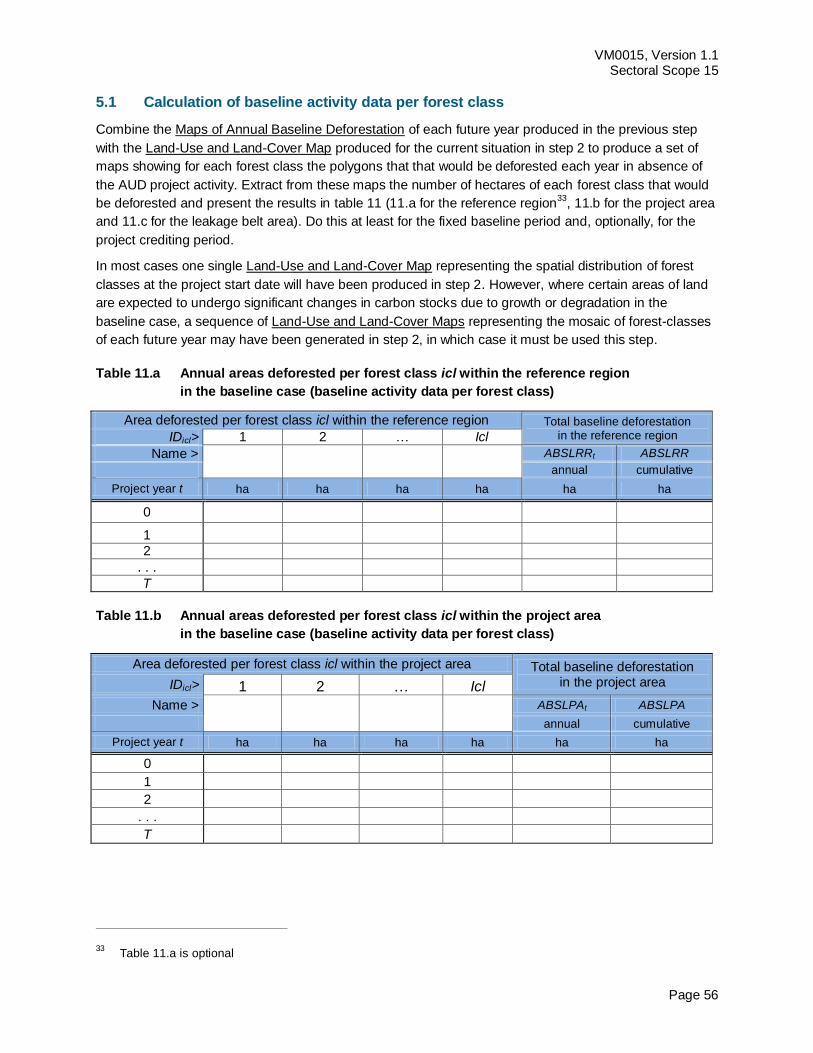
VM0015, Version 1.1 Sectoral Scope 15
Page 56
5.1 Calculation of baseline activity data per forest class
Combine the Maps of Annual Baseline Deforestation of each future year produced in the previous step
with the Land-Use and Land-Cover Map produced for the current situation in step 2 to produce a set of
maps showing for each forest class the polygons that that would be deforested each year in absence of
the AUD project activity. Extract from these maps the number of hectares of each forest class that would
be deforested and present the results in table 11 (11.a for the reference region33
, 11.b for the project area
and 11.c for the leakage belt area). Do this at least for the fixed baseline period and, optionally, for the
project crediting period.
In most cases one single Land-Use and Land-Cover Map representing the spatial distribution of forest
classes at the project start date will have been produced in step 2. However, where certain areas of land
are expected to undergo significant changes in carbon stocks due to growth or degradation in the
baseline case, a sequence of Land-Use and Land-Cover Maps representing the mosaic of forest-classes
of each future year may have been generated in step 2, in which case it must be used this step.
Table 11.a Annual areas deforested per forest class icl within the reference region
in the baseline case (baseline activity data per forest class)
Area deforested per forest class icl within the reference region Total baseline deforestation in the reference region IDicl> 1 2 … Icl
Name >
ABSLRRt ABSLRR
annual cumulative
Project year t ha ha ha ha ha ha
0 1 2 . . . T
Table 11.b Annual areas deforested per forest class icl within the project area
in the baseline case (baseline activity data per forest class)
Area deforested per forest class icl within the project area Total baseline deforestation in the project area IDicl> 1 2 … Icl
Name >
ABSLPAt ABSLPA
annual cumulative
Project year t ha ha ha ha ha ha
0 1 2 . . . T
33 Table 11.a is optional
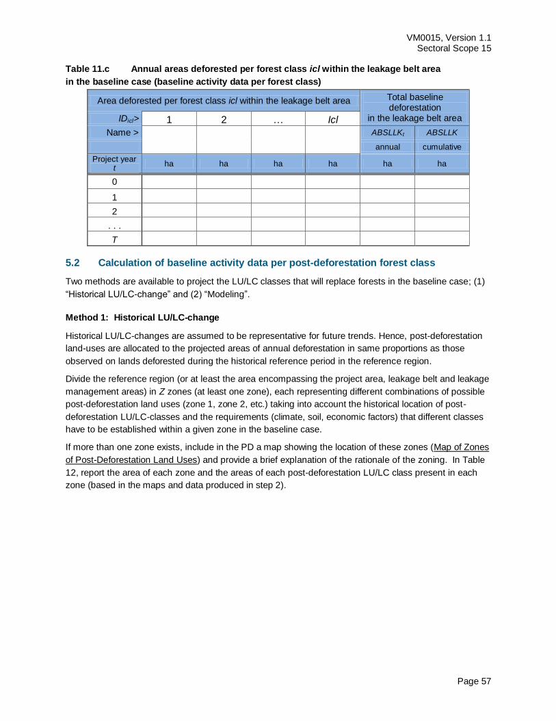
VM0015, Version 1.1 Sectoral Scope 15
Page 57
Table 11.c Annual areas deforested per forest class icl within the leakage belt area
in the baseline case (baseline activity data per forest class)
Area deforested per forest class icl within the leakage belt area Total baseline deforestation
in the leakage belt area IDicl> 1 2 … Icl
Name >
ABSLLKt ABSLLK
annual cumulative
Project year t
ha ha ha ha ha ha
0 1 2 . . . T
5.2 Calculation of baseline activity data per post-deforestation forest class
Two methods are available to project the LU/LC classes that will replace forests in the baseline case; (1)
“Historical LU/LC-change” and (2) “Modeling”.
Method 1: Historical LU/LC-change
Historical LU/LC-changes are assumed to be representative for future trends. Hence, post-deforestation
land-uses are allocated to the projected areas of annual deforestation in same proportions as those
observed on lands deforested during the historical reference period in the reference region.
Divide the reference region (or at least the area encompassing the project area, leakage belt and leakage
management areas) in Z zones (at least one zone), each representing different combinations of possible
post-deforestation land uses (zone 1, zone 2, etc.) taking into account the historical location of post-
deforestation LU/LC-classes and the requirements (climate, soil, economic factors) that different classes
have to be established within a given zone in the baseline case.
If more than one zone exists, include in the PD a map showing the location of these zones (Map of Zones
of Post-Deforestation Land Uses) and provide a brief explanation of the rationale of the zoning. In Table
12, report the area of each zone and the areas of each post-deforestation LU/LC class present in each
zone (based in the maps and data produced in step 2).
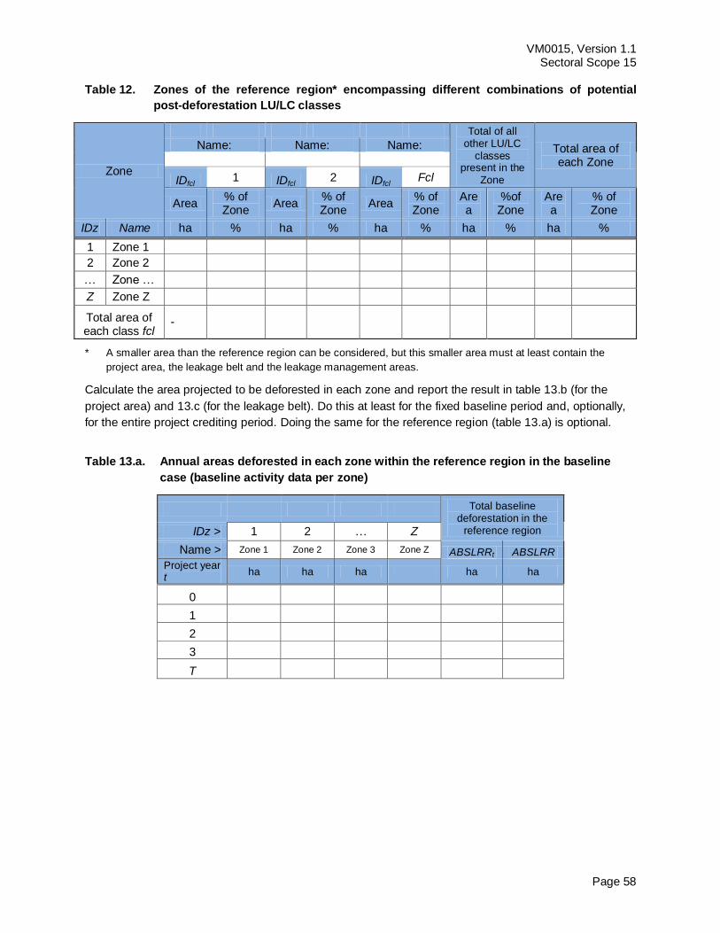
VM0015, Version 1.1 Sectoral Scope 15
Page 58
Table 12. Zones of the reference region* encompassing different combinations of potential
post-deforestation LU/LC classes
Zone
Total of all other LU/LC
classes present in the
Zone
Total area of each Zone
Name: Name: Name:
F1 F2 F50
IDfcl 1 IDfcl 2 IDfcl Fcl
Area % of Zone
Area % of Zone
Area % of Zone
Area
%of Zone
Area
% of Zone
IDz Name ha % ha % ha % ha % ha %
1 Zone 1 0.0% 0.0% 0.0% 0.0% -
0.0%
2 Zone 2 0.0% 0.0% 0.0% 0.0% -
0.0%
… Zone … 0.0% 0.0% 0.0% 0.0% -
0.0%
Z Zone Z 0.0% 0.0% 0.0% 0.0% -
0.0%
Total area of each class fcl
- 0.0% -
0.0% -
0.0% -
0.0% -
0.0%
* A smaller area than the reference region can be considered, but this smaller area must at least contain the
project area, the leakage belt and the leakage management areas.
Calculate the area projected to be deforested in each zone and report the result in table 13.b (for the
project area) and 13.c (for the leakage belt). Do this at least for the fixed baseline period and, optionally,
for the entire project crediting period. Doing the same for the reference region (table 13.a) is optional.
Table 13.a. Annual areas deforested in each zone within the reference region in the baseline
case (baseline activity data per zone)
Total baseline deforestation in the
reference region IDz > 1 2 … Z
Name > Zone 1 Zone 2 Zone 3 Zone Z ABSLRRt ABSLRR
Project year t
ha ha ha ha ha
0
1
2
3
T
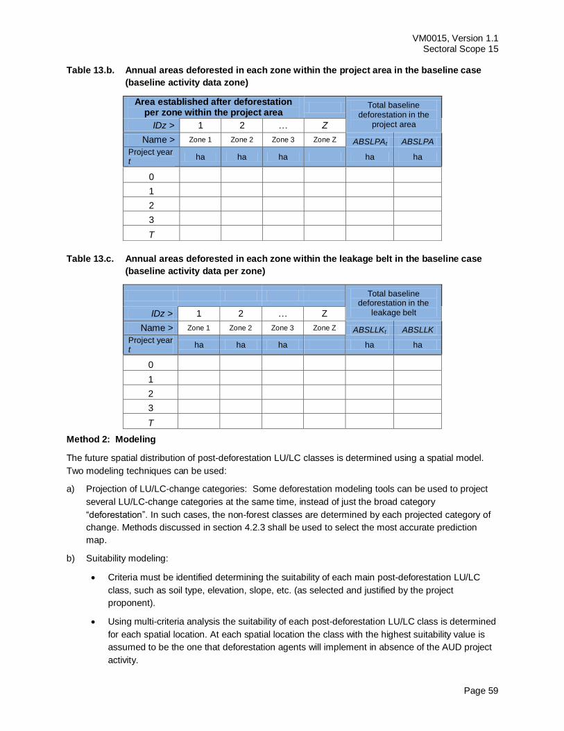
VM0015, Version 1.1 Sectoral Scope 15
Page 59
Table 13.b. Annual areas deforested in each zone within the project area in the baseline case
(baseline activity data zone)
Area established after deforestation per zone within the project area
Total baseline deforestation in the
project area IDz > 1 2 … Z
Name > Zone 1 Zone 2 Zone 3 Zone Z ABSLPAt ABSLPA
Project year t
ha ha ha ha ha
0
1
2
3
T
Table 13.c. Annual areas deforested in each zone within the leakage belt in the baseline case
(baseline activity data per zone)
Total baseline deforestation in the
leakage belt IDz > 1 2 … Z
Name > Zone 1 Zone 2 Zone 3 Zone Z ABSLLKt ABSLLK
Project year t
ha ha ha ha ha
0
1
2
3
T
Method 2: Modeling
The future spatial distribution of post-deforestation LU/LC classes is determined using a spatial model.
Two modeling techniques can be used:
a) Projection of LU/LC-change categories: Some deforestation modeling tools can be used to project
several LU/LC-change categories at the same time, instead of just the broad category
“deforestation”. In such cases, the non-forest classes are determined by each projected category of
change. Methods discussed in section 4.2.3 shall be used to select the most accurate prediction
map.
b) Suitability modeling:
Criteria must be identified determining the suitability of each main post-deforestation LU/LC
class, such as soil type, elevation, slope, etc. (as selected and justified by the project
proponent).
Using multi-criteria analysis the suitability of each post-deforestation LU/LC class is determined
for each spatial location. At each spatial location the class with the highest suitability value is
assumed to be the one that deforestation agents will implement in absence of the AUD project
activity.
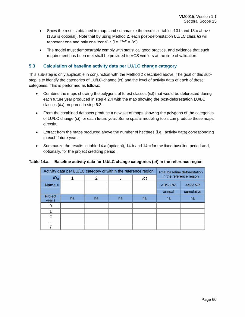
VM0015, Version 1.1 Sectoral Scope 15
Page 60
Show the results obtained in maps and summarize the results in tables 13.b and 13.c above
(13.a is optional). Note that by using Method 2, each post-deforestation LU/LC class fcl will
represent one and only one “zone” z (i.e. “fcl” = “z”)
The model must demonstrably comply with statistical good practice, and evidence that such
requirement has been met shall be provided to VCS verifiers at the time of validation.
5.3 Calculation of baseline activity data per LU/LC change category
This sub-step is only applicable in conjunction with the Method 2 described above. The goal of this sub-
step is to identify the categories of LU/LC-change (ct) and the level of activity data of each of these
categories. This is performed as follows:
Combine the maps showing the polygons of forest classes (icl) that would be deforested during
each future year produced in step 4.2.4 with the map showing the post-deforestation LU/LC
classes (fcl) prepared in step 5.2.
From the combined datasets produce a new set of maps showing the polygons of the categories
of LU/LC change (ct) for each future year. Some spatial modeling tools can produce these maps
directly.
Extract from the maps produced above the number of hectares (i.e., activity data) corresponding
to each future year.
Summarize the results in table 14.a (optional), 14.b and 14.c for the fixed baseline period and,
optionally, for the project crediting period.
Table 14.a. Baseline activity data for LU/LC change categories (ct) in the reference region
Activity data per LU/LC category ct within the reference region Total baseline deforestation in the reference region IDct 1 2 … Ict
Name >
ABSLRRt ABSLRR
annual cumulative
Project year t
ha ha ha ha ha ha
0 1
2 . . .
T
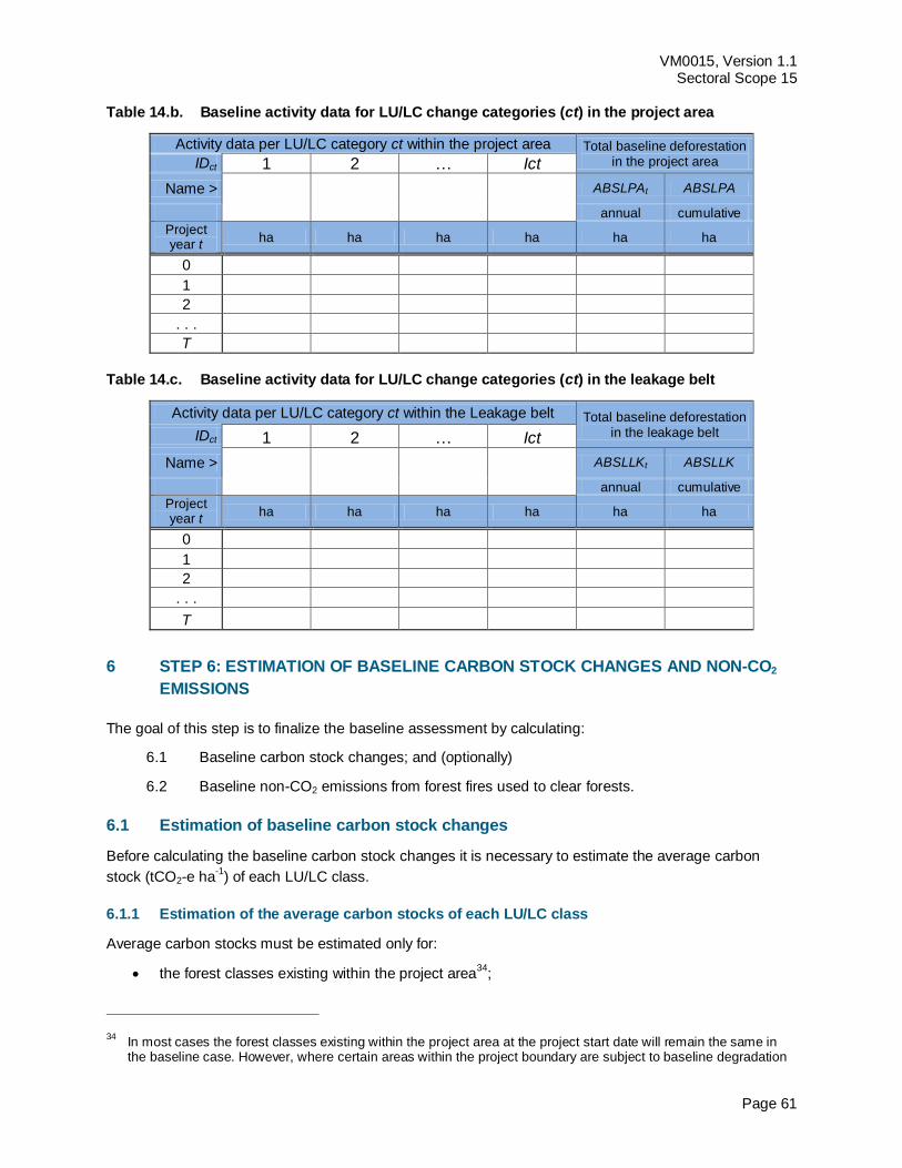
VM0015, Version 1.1 Sectoral Scope 15
Page 61
Table 14.b. Baseline activity data for LU/LC change categories (ct) in the project area
Activity data per LU/LC category ct within the project area Total baseline deforestation in the project area IDct 1 2 … Ict
Name >
ABSLPAt ABSLPA
annual cumulative
Project year t
ha ha ha ha ha ha
0
1 2
. . . T
Table 14.c. Baseline activity data for LU/LC change categories (ct) in the leakage belt
Activity data per LU/LC category ct within the Leakage belt Total baseline deforestation in the leakage belt IDct 1 2 … Ict
Name >
ABSLLKt ABSLLK
annual cumulative
Project year t
ha ha ha ha ha ha
0
1 2
. . .
T
STEP 6: ESTIMATION OF BASELINE CARBON STOCK CHANGES AND NON-CO2 6
EMISSIONS
The goal of this step is to finalize the baseline assessment by calculating:
6.1 Baseline carbon stock changes; and (optionally)
6.2 Baseline non-CO2 emissions from forest fires used to clear forests.
6.1 Estimation of baseline carbon stock changes
Before calculating the baseline carbon stock changes it is necessary to estimate the average carbon
stock (tCO2-e ha-1
) of each LU/LC class.
6.1.1 Estimation of the average carbon stocks of each LU/LC class
Average carbon stocks must be estimated only for:
the forest classes existing within the project area34
;
34 In most cases the forest classes existing within the project area at the project start date will remain the same in
the baseline case. However, where certain areas within the project boundary are subject to baseline degradation
VM0015, Version 1.1 Sectoral Scope 15
Page 62
the forest classes existing within the leakage belt35
;
the post-deforestation classes projected to exist in the project area in the baseline case;
the post-deforestation classes projected to exist in the leakage belt in the project case; and
the non-forest classes existing in leakage management areas.
Collect existing carbon-stock data for these classes from local published studies and existing forest and
carbon inventories. Do additional field measurements for the classes for which there is insufficient
information. Follow the guidance below:
a) Assess the existing data collected and, where appropriate, use them. It is likely that some existing
data could be used to quantify the carbon stocks of one or more classes. These data could be
derived from a forest inventory or perhaps from scientific studies. Analyze these data and use them
if the following criteria are fulfilled:
The data are less than 10 years old;
The data are derived from multiple measurement plots;
All species above a minimum diameter are included in the inventories;
The minimum diameter for trees included is 30 cm or less at breast height (DBH);
Data are sampled from good coverage of the classes over which they will be extrapolated.
Existing data that meet the above criteria shall only be applied across the classes from which they
were representatively sampled and not beyond that. See the latest version of the GOFC-GOLD
sourcebook on REDD and Gillespie, et al. (1992) for methods to analyze these data.
b) Collect missing data. For the classes for which no existing data are available it will be necessary to
either obtain the data from field measurement or to use conservative estimates from the literature.
Field measurements:
Locate the sampling sites. If the locations of future deforestation are known at the time of field
measurements, the sample sites should be located at the locations expected to be deforested
to achieve maximum accuracy of the carbon stock estimates.
Design the sampling framework and conduct the field measurements following the guidance of
appendix 3 (see also chapter 4.3 of GPG LULUCF and in the sourcebook for LULUCF by
Pearson et al., 2005). Summarize the sampling design in the PD and provide a map and the
coordinates of all sampled locations.
Literature estimates:
The use of carbon stock estimates in similar ecosystems derived from local studies, literature
and IPCC defaults is permitted36
, provided the accuracy and conservativeness of the
estimates are demonstrated.
due to unsustainable logging, fuel wood collection, charcoal production and other reasons, the decrease in carbon stocks must be projected. If carbon stocks are subject to enhancement, the projection is optional and can conservatively be omitted.
35 In most cases the forest classes existing at the project start date within the leakage belt will remain the same in
the baseline case. However, where certain areas within the leakage belt are subject to enhancement in the baseline case, carbon stocks must be projected for each year. If carbon stocks are subject to baseline degradation, projecting the changes in carbon stocks is optional and can conservatively be omitted.
VM0015, Version 1.1 Sectoral Scope 15
Page 63
When defaults are used, the lowest value of the range given in the literature source (or the
value reduced by 30%) must be used for the forest classes, and the highest value (or the
value augmented by 30%) for non-forest classes.
c) Calculate the carbon stocks existing in each forest class in the project area prior to the year of
baseline deforestation. For all years preceding the year in which the projected baseline
deforestation will occur (t <= t*) carbon stocks and boundaries of the forest-classes are assumed to
remain the same, except in the following cases:
If in the baseline case the forest within certain polygons of the project area is degrading and
loosing carbon stocks, a map sequence showing the spatial and temporal sequence of forest
classes with successively lower carbon stocks must be prepared to account for the
degradation occurring prior to deforestation. If the boundary of the forest classes undergoing
degradation is fixed (i.e. does not change over time) it is sufficient to show the estimated
changes in carbon stocks in a table (Table 15a and Table 15b). To do the projection, use
credible and verifiable sources of data from existing studies, or measure field plots in
degraded forests of different known age.
If in the baseline case the forest within certain polygons of the project area has increasing
carbon stocks, changes in carbon stocks can conservatively be omitted. If a projection is done,
use credible and verifiable sources of data from existing studies, or measure field plots in
secondary forests of different known age.
If carbon stocks in the project area are decreasing more in the project case than in the
baseline case (e.g. when the project activity involves logging for timber, fuel-wood collection or
charcoal production in areas not subject to such activities in the baseline case), this will have
to be accounted in the project case.
If logging activities are present in the baseline, the harvested wood product carbon pool must
be estimated and, if significantly higher in the baseline compared to the project scenario, it will
have to be accounted.
Report the results of the estimations in Table 15.a (estimated values) and Table 15.b (values
used in calculations after considering discounts for uncertainties according to “f” below).
Carbon stocks in the harvested wood products carbon pool must be estimated as the sum of
planned and unplanned harvesting activities in the baseline case and the additional volume
harvested prior to the deforestation event in year t* (if applicable).
d) Calculate the carbon stocks existing in each forest class in the leakage belt prior to the year of
baseline deforestation (t = t*): For all years preceding the year in which the projected baseline
deforestation will occur (t > t*) carbon stocks and boundaries of the forest-classes are assumed to
remain the same, except in the following cases:
If in the baseline case the forest within certain polygons of the leakage belt is growing and
carbon stocks are increasing, a map sequence showing the spatial and temporal sequence of
forest classes with successively higher carbon stocks must be prepared to account for the
36 Attention must be paid on data units. In this methodology calculations are done in tCO2-e while IPCC tables often
provide data in tC (1 tC = 44/12 t CO2-e)

VM0015, Version 1.1 Sectoral Scope 15
Page 64
carbon stock enhancement. To do the projection, use credible and verifiable sources of data
from existing studies, or measure field plots in secondary forests of different known age.
If in the baseline case the forest within certain polygons of the leakage belt is degrading and
loosing carbon stocks, changes in carbon stocks can conservatively be omitted and preparing
a map sequence is optional for these polygons.
Report the results of the estimations in Table 15.a (estimated values) and Table 15.b (values
used in calculations after considering discounts for uncertainties according to “f” below).
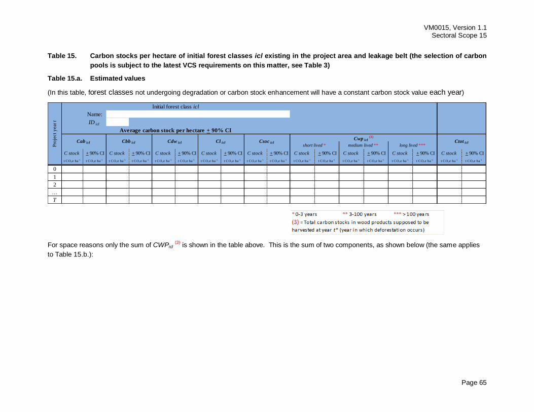
VM0015, Version 1.1 Sectoral Scope 15
Page 65
Table 15. Carbon stocks per hectare of initial forest classes icl existing in the project area and leakage belt (the selection of carbon
pools is subject to the latest VCS requirements on this matter, see Table 3)
Table 15.a. Estimated values
(In this table, forest classes not undergoing degradation or carbon stock enhancement will have a constant carbon stock value each year)
For space reasons only the sum of CWPicl (3)
is shown in the table above. This is the sum of two components, as shown below (the same applies
to Table 15.b.):
Name:
ID icl
C stock + 90% CI C stock + 90% CI C stock + 90% CI C stock + 90% CI C stock + 90% CI C stock + 90% CI C stock + 90% CI C stock + 90% CI C stock + 90% CI
t CO2e ha -1 t CO2e ha -1 t CO2e ha -1 t CO2e ha -1 t CO2e ha -1 t CO2e ha -1 t CO2e ha -1 t CO2e ha -1 t CO2e ha -1 t CO2e ha -1 t CO2e ha -1 t CO2e ha -1 t CO2e ha -1 t CO2e ha -1 t CO2e ha -1 t CO2e ha -1 t CO2e ha -1 t CO2e ha -1
0
1
2
…
T
Pro
ject
year t
medium lived ** long lived ***Ctot icl
Cwp icl (3)
short lived *Cab icl Cbb icl Cdw icl Cl icl Csoc icl
Initial forest class icl
Average carbon stock per hectare + 90% CI
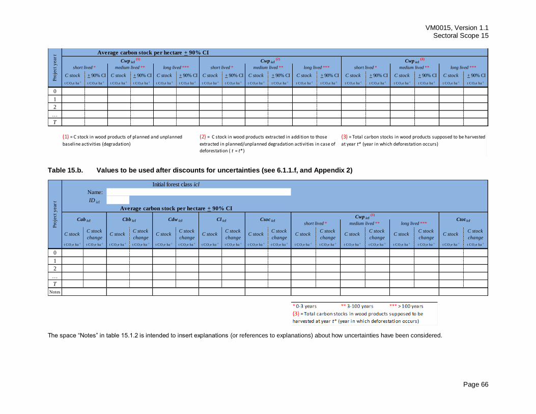
VM0015, Version 1.1 Sectoral Scope 15
Page 66
Table 15.b. Values to be used after discounts for uncertainties (see 6.1.1.f, and Appendix 2)
The space “Notes” in table 15.1.2 is intended to insert explanations (or references to explanations) about how uncertainties have been considered.
C stock + 90% CI C stock + 90% CI C stock + 90% CI C stock + 90% CI C stock + 90% CI C stock + 90% CI C stock + 90% CI C stock + 90% CI C stock + 90% CI
t CO2e ha -1 t CO2e ha -1 t CO2e ha -1 t CO2e ha -1 t CO2e ha -1 t CO2e ha -1 t CO2e ha -1 t CO2e ha -1 t CO2e ha -1 t CO2e ha -1 t CO2e ha -1 t CO2e ha -1 t CO2e ha -1 t CO2e ha -1 t CO2e ha -1 t CO2e ha -1 t CO2e ha -1 t CO2e ha -1
0
1
2
…
T
Pro
ject
year t
medium lived ** long lived ***
Cwp icl (2)
short lived * medium lived ** long lived ***short lived * medium lived ** long lived ***
Cwp icl (3)
short lived *
Cwp icl (1)
Average carbon stock per hectare + 90% CI
(1) = C stock in wood products of planned and unplanned
baseline activities (degradation)
(2) = C stock in wood products extracted in addition to those
extracted in planned/unplanned degradation activities in case of
deforestation ( t = t* )
(3) = Total carbon stocks in wood products supposed to be harvested
at year t* (year in which deforestation occurs)
Name:
ID icl
C stockC stock
changeC stock
C stock
changeC stock
C stock
changeC stock
C stock
changeC stock
C stock
changeC stock
C stock
changeC stock
C stock
changeC stock
C stock
changeC stock
C stock
change
t CO2e ha -1 t CO2e ha -1 t CO2e ha -1 t CO2e ha -1 t CO2e ha -1 t CO2e ha -1 t CO2e ha -1 t CO2e ha -1 t CO2e ha -1 t CO2e ha -1 t CO2e ha -1 t CO2e ha -1 t CO2e ha -1 t CO2e ha -1 t CO2e ha -1 t CO2e ha -1 t CO2e ha -1 t CO2e ha -1
0
1
2
…
T
Notes
Pro
ject
year t
Cwp icl (3)
Ctot iclshort lived * medium lived ** long lived ***
Cab icl Cbb icl Cdw icl Cl icl Csoc icl
Initial forest class icl
Average carbon stock per hectare + 90% CI
VM0015, Version 1.1 Sectoral Scope 15
Page 67
Where:
Cabicl Average carbon stock per hectare in the above-ground biomass carbon pool of class icl;
tCO2-e ha-1
Cbbicl Average carbon stock per hectare in the below-ground biomass carbon pool of class icl;
tCO2-e ha-1
Cdwicl Average carbon stock per hectare in the dead wood biomass carbon pool of class icl; tCO2-e
ha-1
Clicl Average carbon stock per hectare in the litter carbon pool of LU/LC class icl; tCO2-e ha-1
Csocicl Average carbon stock per hectare in the soil organic carbon pool of LU/LC class icl; tCO2-e
ha-1
Cwpicl Average carbon stock per hectare accumulated in the harvested wood products carbon pool
between project start and the year of deforestation of class icl; tCO2-e ha-1
Note: In the baseline case, Cwpcl must be subtracted from the sum of the other pools in the calculation of
Ctotcl
Ctoticl Average carbon stock per hectare in all accounted carbon pools of LU/LC icl; tCO2-e ha-1
e) Calculate the long-term (20-years) average carbon stocks of post-deforestation classes: These
classes often do not have a stable carbon stock because different land uses may be implemented
in a time sequence or because the land use after deforestation implies carbon stocks changes over
time (e.g. in case of tree plantations). The carbon stock of post-deforestation classes must be
estimated as the long-term (20 years) average carbon stock and can be determined from
measurements in plots of known age, long-term studies and other verifiable sources.
For each post-deforestation LU/LC class, report the calculation of the long-term (20-year) average
carbon stock using Table 16.
f) Do an uncertainty assessment of all carbon stock estimates following the methods described in
appendix 2, Box 2. If the uncertainty of the total average carbon stock (Ctotcl) of a class cl is less
than 10% of the average value, the average carbon stock value can be used. If the uncertainty is
higher than 10%, the lower boundary of the 90% confidence interval must be considered in the
calculations if the class is an initial forest class in the project area or a final non-forest class in the
leakage belt, and the higher boundary of the 90% confidence interval if the class is an initial forest
class in the leakage belt or a final non-forest class in the project area.
g) Calculate the area-weighted average carbon stocks of the post-deforestation LU/LC classes
existing within each zone using Table 17.
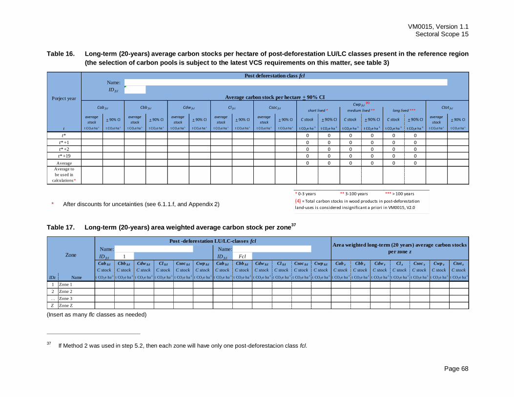
VM0015, Version 1.1 Sectoral Scope 15
Page 68
Table 16. Long-term (20-years) average carbon stocks per hectare of post-deforestation LU/LC classes present in the reference region
(the selection of carbon pools is subject to the latest VCS requirements on this matter, see table 3)
Table 17. Long-term (20-years) area weighted average carbon stock per zone37
(Insert as many flc classes as needed)
37 If Method 2 was used in step 5.2, then each zone will have only one post-deforestacion class fcl.
Name:
ID fcl 1
average
stock+ 90% CI
average
stock+ 90% CI
average
stock+ 90% CI
average
stock+ 90% CI
average
stock+ 90% CI C stock + 90% CI C stock + 90% CI C stock + 90% CI
average
stock+ 90% CI
t t CO2e ha-1 t CO2e ha-1 t CO2e ha-1 t CO2e ha-1 t CO2e ha-1 t CO2e ha-1 t CO2e ha-1 t CO2e ha-1 t CO2e ha-1 t CO2e ha-1 t CO2e ha -1 t CO2e ha -1 t CO2e ha -1 t CO2e ha -1 t CO2e ha -1 t CO2e ha -1 t CO2e ha-1 t CO2e ha-1
t* 0 0 0 0 0 0
t* +1 0 0 0 0 0 0
t* +2 0 0 0 0 0 0
t* +19 0 0 0 0 0 0
Average 0 0 0 0 0 0 0 0 0 0 0 0 0 0 0 0 0 0Average to
be used in
calculations*
Cab fcl Cbb fcl Cdw fcl Cl fcl
Porject year
Post deforestation class fcl
F1
Average carbon stock per hectare + 90% CI
Cwp fcl (4)
short lived * medium lived ** long lived ***Csoc fcl Ctot fcl
* 0-3 years ** 3-100 years *** > 100 years
(4) = Total carbon stocks in wood products in post-deforestation
land-uses is considered insignificant a priori in VM0015, V2.0
Name: Name:
ID fcl 1 ID fcl Fcl
Cab fcl Cbb fcl Cdw fcl Cl fcl Csoc fcl Cwp fcl Cab fcl Cbb fcl Cdw fcl Cl fcl Csoc fcl Cwp fcl Cab z Cbb z Cdw z Cl z Csoc z Cwp z Ctot z
C stock C stock C stock C stock C stock C stock C stock C stock C stock C stock C stock C stock C stock C stock C stock C stock C stock C stock C stock
IDz Name t CO2e ha-1
t CO2e ha-1
t CO2e ha-1
t CO2e ha-1
t CO2e ha-1
t CO2e ha-1
t CO2e ha-1
t CO2e ha-1
t CO2e ha-1
t CO2e ha-1
t CO2e ha-1
t CO2e ha-1
t CO2e ha-1
t CO2e ha-1
t CO2e ha-1
t CO2e ha-1
t CO2e ha-1
t CO2e ha-1
t CO2e ha-1
1 Zone 1 0 0 0 0 0 0 0 0 0 0 0 0 0 0 0 0 0 0 0
2 Zone 2 0 0 0 0 0 0 0 0 0 0 0 0 0 0 0 0 0 0 0
… Zone 3 0 0 0 0 0 0 0 0 0 0 0 0 0 0 0 0 0 0 0
Z Zone Z 0 0 0 0 0 0 0 0 0 0 0 0 0 0 0 0 0 0 0
F50Zone
F1Area weighted long-term (20 years) average carbon stocks
per zone z
Post -deforestation LU/LC-classes fcl
* After discounts for uncetainties (see 6.1.1.f, and Appendix 2)
VM0015, Version 1.1 Sectoral Scope 15
Page 69
6.1.2 Calculation of carbon stock change factors
The AFOLU Requirements requires methodologies to consider the decay of carbon stock in soil carbon,
below-ground biomass, dead wood and harvested wood products in the baseline case.
In this methodology default linear functions are applied to account for the decay of carbon stock in initial
forest classes (icl) and increase in carbon stock in post-deforestation classes. This is done as follows:
a) Above-ground biomass:
Initial forest classes (icl): immediate release of 100% of the carbon stock (as estimated in
Table 15.b) is assumed to happen at the end of year t = t* (= year in which deforestation
occurs).
Post-deforestation classes (fcl) (or their area weighted average per zone z): linear increase
from 0 tCO2-e/ha in year t = t* to 100% of the long-term (20-years) average carbon stock (as
estimated in Table 17) in year t = t*+9 is assumed to happen in the 10-years period following
deforestation (i.e. 1/10th of the final carbon stock is accumulated each year).
b) Below-ground biomass:
Initial forest classes (icl): an annual release of 1/10th of the initial carbon stock (as estimated
in Table 15.b) is assumed to happen each year between t = t* and t = t*+9.
Post-deforestation classes (fcl) (or their area weighted average per zone z): linear increase
from 0 tCO2-e/ha in year t = t* to 100% of the long-term (20-years) average carbon stock (as
estimated in Table 17) in year t = t*+9 is assumed to happen in the 10 years period following
deforestation (i.e. 1/10th of the final carbon stock is accumulated each year).
c) Litter:
Initial forest classes (icl): immediate release of 100% of the carbon stock (as estimated in
Table 15.b) is assumed to happen at the end of year t = t*.
Post-deforestation classes (fcl) (or their area weighted average per zone z): a linear increase
from 0 tCO2-e/ha in year t = t* to 100% of the long-term (20-years) average carbon stock (as
estimated in Table 17) in year t = t*+9 is assumed to happen in the 10-years period following
deforestation (i.e. 1/10th of the final carbon stock is accumulated each year).
d) Dead wood:
Initial forest classes (icl): an annual release of 1/10th of the initial carbon stock (as estimated
in Table 15.b) is assumed to happen each year between t = t* and t = t*+9.
Post-deforestation classes (fcl) (or their area weighted average per zone z): a linear increase
from 0 tCO2-e/ha in year t = t* to 100% of the long-term (20-years) average carbon stock (as
estimated in Table 17) in year t = t*+9 is assumed to happen in the 10-years period following
deforestation (i.e. 1/10th of the final carbon stock is accumulated each year).
e) Wood products:
Initial forest classes (icl): Three fractions are considered:
1) Fraction decaying in less than three years: This short-lived fraction is assumed to be
released 100% at the end of year t* (i.e. 100% of the stock estimated in Table 15.b).
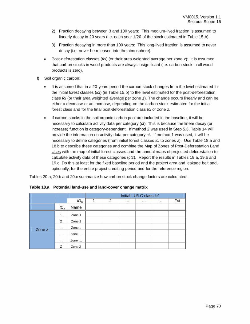
VM0015, Version 1.1 Sectoral Scope 15
Page 70
2) Fraction decaying between 3 and 100 years: This medium-lived fraction is assumed to
linearly decay in 20 years (i.e. each year 1/20 of the stock estimated in Table 15.b).
3) Fraction decaying in more than 100 years: This long-lived fraction is assumed to never
decay (i.e. never be released into the atmosphere).
Post-deforestation classes (fcl) (or their area weighted average per zone z): it is assumed
that carbon stocks in wood products are always insignificant (i.e. carbon stock in all wood
products is zero).
f) Soil organic carbon:
It is assumed that in a 20-years period the carbon stock changes from the level estimated for
the initial forest classes (icl) (in Table 15.b) to the level estimated for the post-deforestation
class fcl (or their area weighted average per zone z). The change occurs linearly and can be
either a decrease or an increase, depending on the carbon stock estimated for the initial
forest class and for the final post-deforestation class fcl or zone z.
If carbon stocks in the soil organic carbon pool are included in the baseline, it will be
necessary to calculate activity data per category (ct). This is because the linear decay (or
increase) function is category-dependent. If method 2 was used in Step 5.3, Table 14 will
provide the information on activity data per category ct. If method 1 was used, it will be
necessary to define categories (from initial forest classes icl to zones z). Use Table 18.a and
18.b to describe these categories and combine the Map of Zones of Post-Deforestation Land
Uses with the map of initial forest classes and the annual maps of projected deforestation to
calculate activity data of these categories (ctz). Report the results in Tables 19.a, 19.b and
19.c. Do this at least for the fixed baseline period and the project area and leakage belt and,
optionally, for the entire project crediting period and for the reference region.
Tables 20.a, 20.b and 20.c summarize how carbon stock change factors are calculated.
Table 18.a Potential land-use and land-cover change matrix
Initial LU/LC class icl
IDcl 1 2 … … … Fcl
IDz Name B1 B2 … B4 B5 B50
Zone z
1 Zone 1 I1/Z1 I2/Z1 I…/Z1 I4/Z1 I5/Z1 IFcl/Z1
2 Zone 2 I1/Z2 I2/Z2 I…/Z2 I4/Z2 I5/Z2 IFcl/Z2
… Zone .. I1/Z… I2/Z… I…/Z… I4/Z… I5/Z… IFcl/Z…
… Zone … I1/Z4 I2/Z4 I…/Z4 I4/Z4 I5/Z4 IFcl/Z4
… Zone … I1/Z5 I2/Z5 I…/Z5 I4/Z5 I5/Z5 IFcl/Z5
Z Zone Z I1/ZZ I2/ZZ I…/ZZ I4/ZZ I5/ZZ IFcl/ZZ
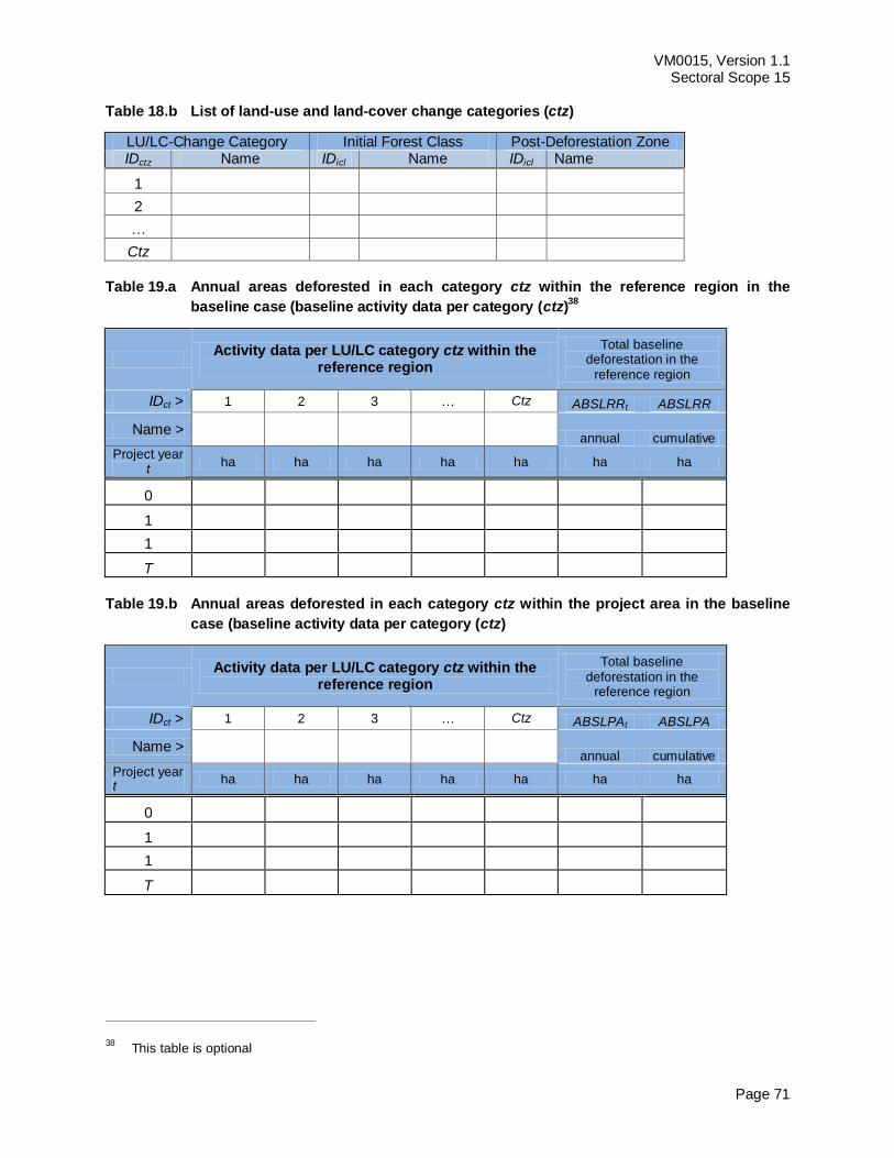
VM0015, Version 1.1 Sectoral Scope 15
Page 71
Table 18.b List of land-use and land-cover change categories (ctz)
LU/LC-Change Category Initial Forest Class Post-Deforestation Zone IDctz Name IDicl Name IDicl Name
1 ZoneCat1 1 B1 1 Zone 1
2 ZoneCat2 1 B1 2 Zone 2
… ZoneCat3 1 B1 … Zone 3
Ctz ZoneCat4 1 B1 4 Zone 4
Table 19.a Annual areas deforested in each category ctz within the reference region in the
baseline case (baseline activity data per category (ctz)38
Activity data per LU/LC category ctz within the
reference region
Total baseline deforestation in the
reference region
IDct > 1 2 3 … Ctz ABSLRRt ABSLRR
Name > ZoneCat1 ZoneCat2 ZoneCat3 ZoneCat4 ZoneCat5 annual cumulative
Project year t
ha ha ha ha ha ha ha
0
1
1
T
Table 19.b Annual areas deforested in each category ctz within the project area in the baseline
case (baseline activity data per category (ctz)
Activity data per LU/LC category ctz within the
reference region
Total baseline deforestation in the
reference region
IDct > 1 2 3 … Ctz ABSLPAt ABSLPA
Name > ZoneCat1 ZoneCat2 ZoneCat3 ZoneCat4 ZoneCat5 annual cumulative
Project year t
ha ha ha ha ha ha ha
0
1
1
T
38 This table is optional
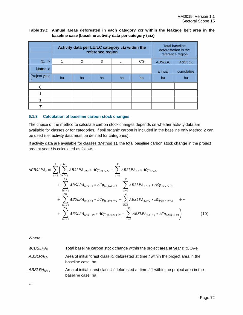
VM0015, Version 1.1 Sectoral Scope 15
Page 72
Table 19.c Annual areas deforested in each category ctz within the leakage belt area in the
baseline case (baseline activity data per category (ctz)
Activity data per LU/LC category ctz within the
reference region
Total baseline deforestation in the
reference region
IDct > 1 2 3 … Ctz ABSLLKt ABSLLK
Name > ZoneCat1 ZoneCat2 ZoneCat3 ZoneCat4 ZoneCat5 annual cumulative
Project year t
ha ha ha ha ha ha ha
0
1
1
T
6.1.3 Calculation of baseline carbon stock changes
The choice of the method to calculate carbon stock changes depends on whether activity data are
available for classes or for categories. If soil organic carbon is included in the baseline only Method 2 can
be used (i.e. activity data must be defined for categories).
If activity data are available for classes (Method 1), the total baseline carbon stock change in the project
area at year t is calculated as follows:
∑ ( ∑ ∑
∑ ∑
∑ ∑
∑ ∑
)
Where:
CBSLPAt Total baseline carbon stock change within the project area at year t; tCO2-e
ABSLPAicl,t Area of initial forest class icl deforested at time t within the project area in the
baseline case; ha
ABSLPAicl,t-1 Area of initial forest class icl deforested at time t-1 within the project area in the
baseline case; ha
…
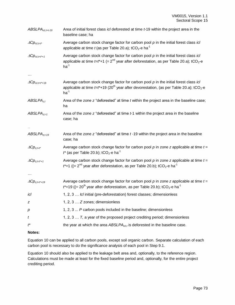
VM0015, Version 1.1 Sectoral Scope 15
Page 73
ABSLPAicl,t=t-19 Area of initial forest class icl deforested at time t-19 within the project area in the
baseline case; ha
Cpicl,t=t* Average carbon stock change factor for carbon pool p in the initial forest class icl
applicable at time t (as per Table 20.a); tCO2-e ha-1
Cpicl,t=t*+1 Average carbon stock change factor for carbon pool p in the initial forest class icl
applicable at time t=t*+1 (= 2nd
year after deforestation, as per Table 20.a); tCO2-e
ha-1
…
Cpicl,t=t*+19 Average carbon stock change factor for carbon pool p in the initial forest class icl
applicable at time t=t*+19 (20th year after devorestation, (as per Table 20.a); tCO2-e
ha-1
ABSLPAz,t Area of the zone z “deforested” at time t within the project area in the baseline case;
ha
ABSLPAz,t-1 Area of the zone z “deforested” at time t-1 within the project area in the baseline
case; ha
…
ABSLPAz,t-19 Area of the zone z “deforested” at time t -19 within the project area in the baseline
case; ha
Cpz,t=t* Average carbon stock change factor for carbon pool p in zone z applicable at time t =
t* (as per Table 20.b); tCO2-e ha-1
Cpz,t=t*+1 Average carbon stock change factor for carbon pool p in zone z applicable at time t =
t*+1 ((= 2nd
year after deforestation, as per Table 20.b); tCO2-e ha-1
…
Cpz,t=t*+19 Average carbon stock change factor for carbon pool p in zone z applicable at time t =
t*+19 ((= 20th year after deforestation, as per Table 20.b); tCO2-e ha
-1
icl 1, 2, 3 … Icl initial (pre-deforestation) forest classes; dimensionless
z 1, 2, 3 … Z zones; dimensionless
p 1, 2, 3 ... P carbon pools included in the baseline; dimensionless
t 1, 2, 3 … T, a year of the proposed project crediting period; dimensionless
t* the year at which the area ABSLPAicl,t is deforested in the baseline case.
Notes:
Equation 10 can be applied to all carbon pools, except soil organic carbon. Separate calculation of each
carbon pool is necessary to do the significance analysis of each pool in Step 9.1.
Equation 10 should also be applied to the leakage belt area and, optionally, to the reference region.
Calculations must be made at least for the fixed baseline period and, optionally, for the entire project
crediting period.
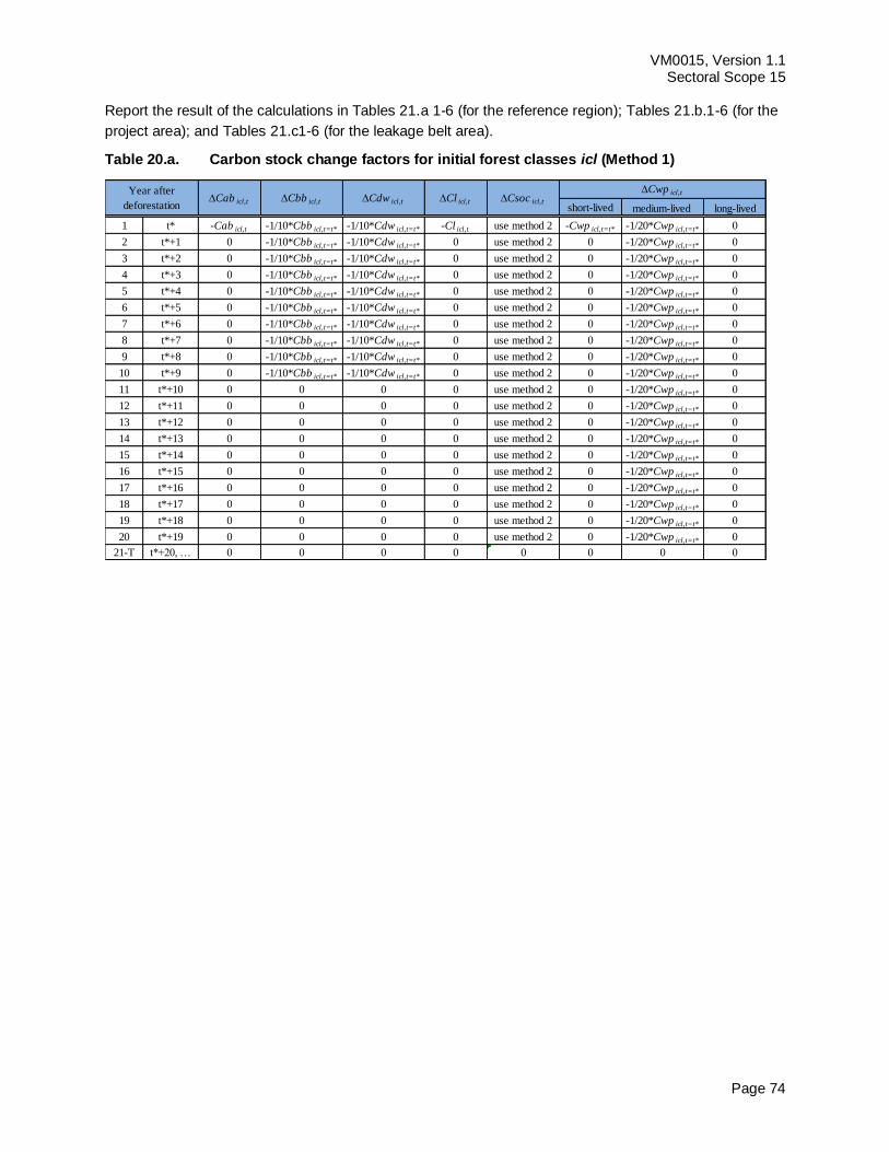
VM0015, Version 1.1 Sectoral Scope 15
Page 74
Report the result of the calculations in Tables 21.a 1-6 (for the reference region); Tables 21.b.1-6 (for the
project area); and Tables 21.c1-6 (for the leakage belt area).
Table 20.a. Carbon stock change factors for initial forest classes icl (Method 1)
short-lived medium-lived long-lived
1 t* -Cab icl,t -1/10*Cbb icl,t=t* -1/10*Cdw icl,t=t* -Cl icl,t use method 2 -Cwp icl,t=t* -1/20*Cwp icl,t=t* 0
2 t*+1 0 -1/10*Cbb icl,t=t* -1/10*Cdw icl,t=t* 0 use method 2 0 -1/20*Cwp icl,t=t* 0
3 t*+2 0 -1/10*Cbb icl,t=t* -1/10*Cdw icl,t=t* 0 use method 2 0 -1/20*Cwp icl,t=t* 0
4 t*+3 0 -1/10*Cbb icl,t=t* -1/10*Cdw icl,t=t* 0 use method 2 0 -1/20*Cwp icl,t=t* 0
5 t*+4 0 -1/10*Cbb icl,t=t* -1/10*Cdw icl,t=t* 0 use method 2 0 -1/20*Cwp icl,t=t* 0
6 t*+5 0 -1/10*Cbb icl,t=t* -1/10*Cdw icl,t=t* 0 use method 2 0 -1/20*Cwp icl,t=t* 0
7 t*+6 0 -1/10*Cbb icl,t=t* -1/10*Cdw icl,t=t* 0 use method 2 0 -1/20*Cwp icl,t=t* 0
8 t*+7 0 -1/10*Cbb icl,t=t* -1/10*Cdw icl,t=t* 0 use method 2 0 -1/20*Cwp icl,t=t* 0
9 t*+8 0 -1/10*Cbb icl,t=t* -1/10*Cdw icl,t=t* 0 use method 2 0 -1/20*Cwp icl,t=t* 0
10 t*+9 0 -1/10*Cbb icl,t=t* -1/10*Cdw icl,t=t* 0 use method 2 0 -1/20*Cwp icl,t=t* 0
11 t*+10 0 0 0 0 use method 2 0 -1/20*Cwp icl,t=t* 0
12 t*+11 0 0 0 0 use method 2 0 -1/20*Cwp icl,t=t* 0
13 t*+12 0 0 0 0 use method 2 0 -1/20*Cwp icl,t=t* 0
14 t*+13 0 0 0 0 use method 2 0 -1/20*Cwp icl,t=t* 0
15 t*+14 0 0 0 0 use method 2 0 -1/20*Cwp icl,t=t* 0
16 t*+15 0 0 0 0 use method 2 0 -1/20*Cwp icl,t=t* 0
17 t*+16 0 0 0 0 use method 2 0 -1/20*Cwp icl,t=t* 0
18 t*+17 0 0 0 0 use method 2 0 -1/20*Cwp icl,t=t* 0
19 t*+18 0 0 0 0 use method 2 0 -1/20*Cwp icl,t=t* 0
20 t*+19 0 0 0 0 use method 2 0 -1/20*Cwp icl,t=t* 0
21-T t*+20, … 0 0 0 0 0 0 0 0
Csoc icl,t
Year after
deforestation Cab icl,t Cbb icl,t Cdw icl,t Cl icl,t
Cwp icl,t
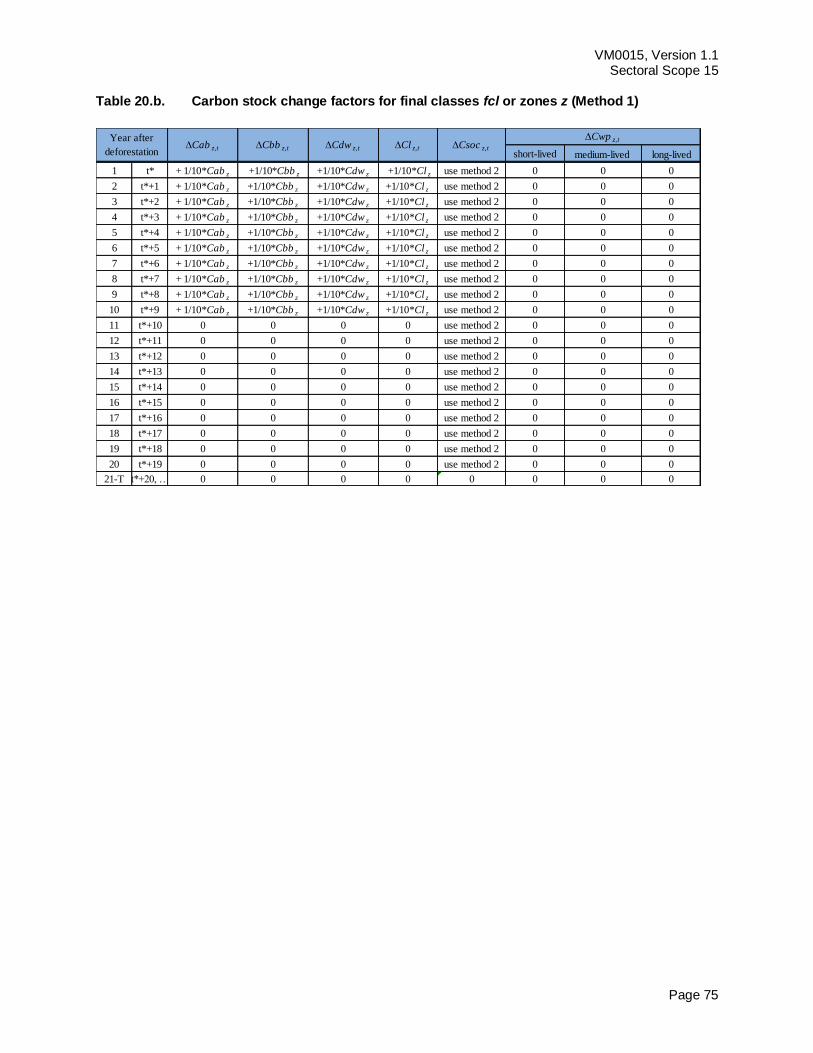
VM0015, Version 1.1 Sectoral Scope 15
Page 75
Table 20.b. Carbon stock change factors for final classes fcl or zones z (Method 1)
short-lived medium-lived long-lived
1 t* +1/10*Cab z +1/10*Cbb z +1/10*Cdw z +1/10*Cl z use method 2 0 0 0
2 t*+1 +1/10*Cab z +1/10*Cbb z +1/10*Cdw z +1/10*Cl z use method 2 0 0 0
3 t*+2 +1/10*Cab z +1/10*Cbb z +1/10*Cdw z +1/10*Cl z use method 2 0 0 0
4 t*+3 +1/10*Cab z +1/10*Cbb z +1/10*Cdw z +1/10*Cl z use method 2 0 0 0
5 t*+4 +1/10*Cab z +1/10*Cbb z +1/10*Cdw z +1/10*Cl z use method 2 0 0 0
6 t*+5 +1/10*Cab z +1/10*Cbb z +1/10*Cdw z +1/10*Cl z use method 2 0 0 0
7 t*+6 +1/10*Cab z +1/10*Cbb z +1/10*Cdw z +1/10*Cl z use method 2 0 0 0
8 t*+7 +1/10*Cab z +1/10*Cbb z +1/10*Cdw z +1/10*Cl z use method 2 0 0 0
9 t*+8 +1/10*Cab z +1/10*Cbb z +1/10*Cdw z +1/10*Cl z use method 2 0 0 0
10 t*+9 +1/10*Cab z +1/10*Cbb z +1/10*Cdw z +1/10*Cl z use method 2 0 0 0
11 t*+10 0 0 0 0 use method 2 0 0 0
12 t*+11 0 0 0 0 use method 2 0 0 0
13 t*+12 0 0 0 0 use method 2 0 0 0
14 t*+13 0 0 0 0 use method 2 0 0 0
15 t*+14 0 0 0 0 use method 2 0 0 0
16 t*+15 0 0 0 0 use method 2 0 0 0
17 t*+16 0 0 0 0 use method 2 0 0 0
18 t*+17 0 0 0 0 use method 2 0 0 0
19 t*+18 0 0 0 0 use method 2 0 0 0
20 t*+19 0 0 0 0 use method 2 0 0 0
21-T t*+20, … 0 0 0 0 0 0 0 0
Csoc z,t
Cwp z,tYear after
deforestation Cab z,t Cbb z,t Cdw z,t Cl z,t
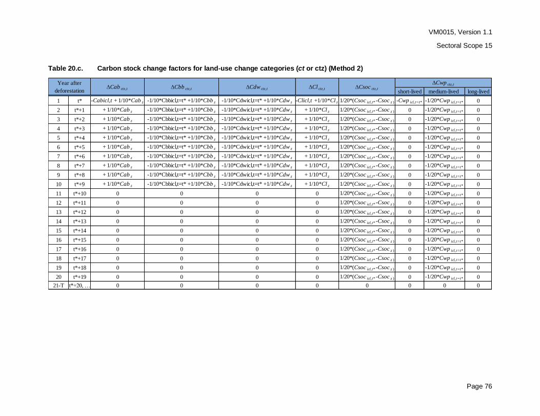
VM0015, Version 1.1
Sectoral Scope 15
Page 76
Table 20.c. Carbon stock change factors for land-use change categories (ct or ctz) (Method 2)
short-lived medium-lived long-lived
1 t* -Cabicl,t + 1/10*Cab z -1/10*Cbbicl,t=t* +1/10*Cbb z -1/10*Cdwicl,t=t* +1/10*Cdw z -Clicl,t +1/10*Cl z 1/20*(Csoc icl,t* -Csoc z ) -Cwp icl,t=t* -1/20*Cwp icl,t=t* 0
2 t*+1 +1/10*Cab z -1/10*Cbbicl,t=t* +1/10*Cbb z -1/10*Cdwicl,t=t* +1/10*Cdw z + 1/10*Cl z 1/20*(Csoc icl,t* -Csoc z ) 0 -1/20*Cwp icl,t=t* 0
3 t*+2 +1/10*Cab z -1/10*Cbbicl,t=t* +1/10*Cbb z -1/10*Cdwicl,t=t* +1/10*Cdw z + 1/10*Cl z 1/20*(Csoc icl,t* -Csoc z ) 0 -1/20*Cwp icl,t=t* 0
4 t*+3 +1/10*Cab z -1/10*Cbbicl,t=t* +1/10*Cbb z -1/10*Cdwicl,t=t* +1/10*Cdw z + 1/10*Cl z 1/20*(Csoc icl,t* -Csoc z ) 0 -1/20*Cwp icl,t=t* 0
5 t*+4 +1/10*Cab z -1/10*Cbbicl,t=t* +1/10*Cbb z -1/10*Cdwicl,t=t* +1/10*Cdw z + 1/10*Cl z 1/20*(Csoc icl,t* -Csoc z ) 0 -1/20*Cwp icl,t=t* 0
6 t*+5 +1/10*Cab z -1/10*Cbbicl,t=t* +1/10*Cbb z -1/10*Cdwicl,t=t* +1/10*Cdw z + 1/10*Cl z 1/20*(Csoc icl,t* -Csoc z ) 0 -1/20*Cwp icl,t=t* 0
7 t*+6 +1/10*Cab z -1/10*Cbbicl,t=t* +1/10*Cbb z -1/10*Cdwicl,t=t* +1/10*Cdw z + 1/10*Cl z 1/20*(Csoc icl,t* -Csoc z ) 0 -1/20*Cwp icl,t=t* 0
8 t*+7 +1/10*Cab z -1/10*Cbbicl,t=t* +1/10*Cbb z -1/10*Cdwicl,t=t* +1/10*Cdw z + 1/10*Cl z 1/20*(Csoc icl,t* -Csoc z ) 0 -1/20*Cwp icl,t=t* 0
9 t*+8 +1/10*Cab z -1/10*Cbbicl,t=t* +1/10*Cbb z -1/10*Cdwicl,t=t* +1/10*Cdw z + 1/10*Cl z 1/20*(Csoc icl,t* -Csoc z ) 0 -1/20*Cwp icl,t=t* 0
10 t*+9 +1/10*Cab z -1/10*Cbbicl,t=t* +1/10*Cbb z -1/10*Cdwicl,t=t* +1/10*Cdw z + 1/10*Cl z 1/20*(Csoc icl,t* -Csoc z ) 0 -1/20*Cwp icl,t=t* 0
11 t*+10 0 0 0 0 1/20*(Csoc icl,t* -Csoc z ) 0 -1/20*Cwp icl,t=t* 0
12 t*+11 0 0 0 0 1/20*(Csoc icl,t* -Csoc z ) 0 -1/20*Cwp icl,t=t* 0
13 t*+12 0 0 0 0 1/20*(Csoc icl,t* -Csoc z ) 0 -1/20*Cwp icl,t=t* 0
14 t*+13 0 0 0 0 1/20*(Csoc icl,t* -Csoc z ) 0 -1/20*Cwp icl,t=t* 0
15 t*+14 0 0 0 0 1/20*(Csoc icl,t* -Csoc z ) 0 -1/20*Cwp icl,t=t* 0
16 t*+15 0 0 0 0 1/20*(Csoc icl,t* -Csoc z ) 0 -1/20*Cwp icl,t=t* 0
17 t*+16 0 0 0 0 1/20*(Csoc icl,t* -Csoc z ) 0 -1/20*Cwp icl,t=t* 0
18 t*+17 0 0 0 0 1/20*(Csoc icl,t* -Csoc z ) 0 -1/20*Cwp icl,t=t* 0
19 t*+18 0 0 0 0 1/20*(Csoc icl,t* -Csoc z ) 0 -1/20*Cwp icl,t=t* 0
20 t*+19 0 0 0 0 1/20*(Csoc icl,t* -Csoc z ) 0 -1/20*Cwp icl,t=t* 0
21-T t*+20, … 0 0 0 0 0 0 0 0
Cl ctz,t Cab ctz,t
Cwp ctz,tYear after
deforestation Csoc ctz,t Cbb ctz,t Cdw ctz,t
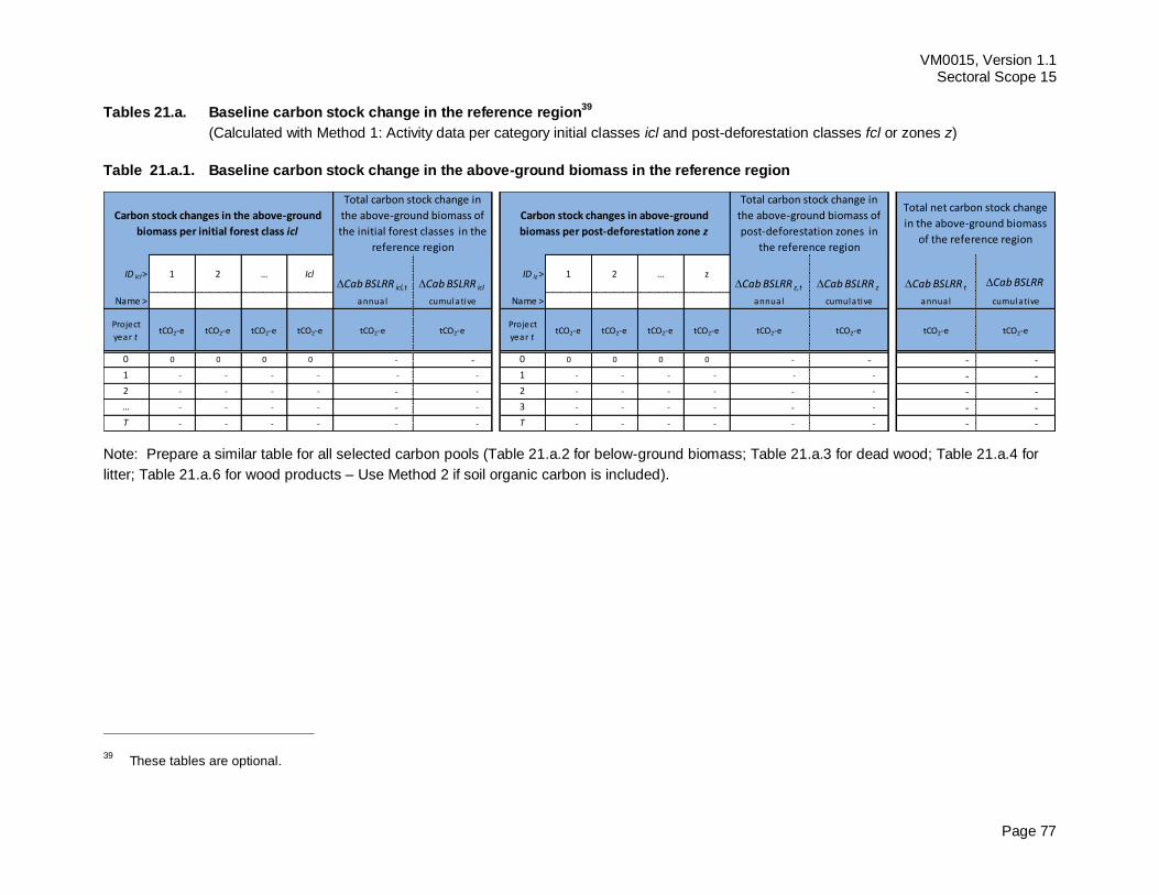
VM0015, Version 1.1 Sectoral Scope 15
Page 77
Tables 21.a. Baseline carbon stock change in the reference region39
(Calculated with Method 1: Activity data per category initial classes icl and post-deforestation classes fcl or zones z)
Table 21.a.1. Baseline carbon stock change in the above-ground biomass in the reference region
Note: Prepare a similar table for all selected carbon pools (Table 21.a.2 for below-ground biomass; Table 21.a.3 for dead wood; Table 21.a.4 for
litter; Table 21.a.6 for wood products – Use Method 2 if soil organic carbon is included).
39 These tables are optional.
ID icl> 1 2 … Icl Cab BSLRR icl,t Cab BSLRR icl
ID iz > 1 2 … z Cab BSLRR z,t Cab BSLRR z Cab BSLRR t Cab BSLRR
Name > annual cumulative Name > annual cumulative annual cumulative
Project
year ttCO2-e tCO2-e tCO2-e tCO2-e tCO2-e tCO2-e
Project
year ttCO2-e tCO2-e tCO2-e tCO2-e tCO2-e tCO2-e tCO2-e tCO2-e
0 0 0 0 - - 0 0 0 0 - - - - - - - - - - - - - - - - - - - - - - - - - - - - - - - - - - - - - - - - - - - - - -
- - - - - - - - - - - - - -
2
1
0
T
0
1
2
3
Total net carbon stock change
in the above-ground biomass
of the reference region
T
Carbon stock changes in above-ground
biomass per post-deforestation zone z
Total carbon stock change in
the above-ground biomass of
post-deforestation zones in
the reference region
…
Carbon stock changes in the above-ground
biomass per initial forest class icl
Total carbon stock change in
the above-ground biomass of
the initial forest classes in the
reference region
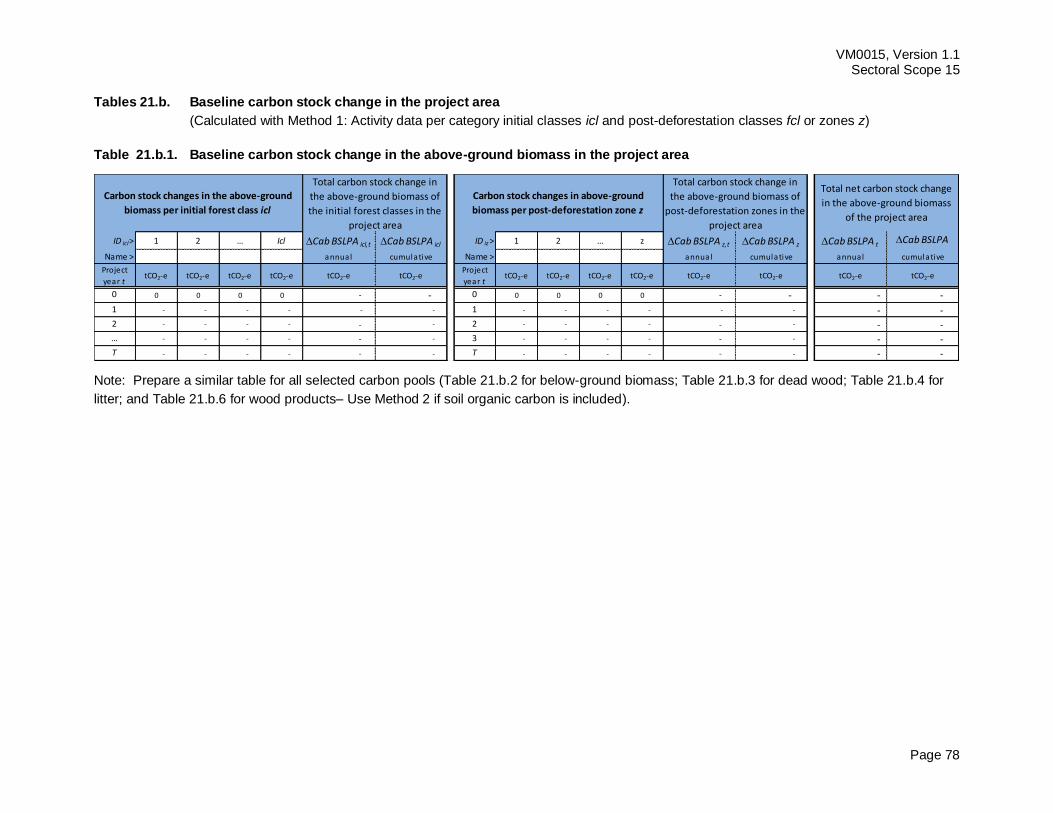
VM0015, Version 1.1 Sectoral Scope 15
Page 78
Tables 21.b. Baseline carbon stock change in the project area
(Calculated with Method 1: Activity data per category initial classes icl and post-deforestation classes fcl or zones z)
Table 21.b.1. Baseline carbon stock change in the above-ground biomass in the project area
Note: Prepare a similar table for all selected carbon pools (Table 21.b.2 for below-ground biomass; Table 21.b.3 for dead wood; Table 21.b.4 for
litter; and Table 21.b.6 for wood products– Use Method 2 if soil organic carbon is included).
ID icl> 1 2 … Icl Cab BSLPA icl,t Cab BSLPA icl ID iz > 1 2 … z Cab BSLPA z,t Cab BSLPA z Cab BSLPA t Cab BSLPA
Name > annual cumulative Name > annual cumulative annual cumulative
Project
year ttCO2-e tCO2-e tCO2-e tCO2-e tCO2-e tCO2-e
Project
year ttCO2-e tCO2-e tCO2-e tCO2-e tCO2-e tCO2-e tCO2-e tCO2-e
0 0 0 0 - - 0 0 0 0 - - - -
- - - - - - - - - - - - - - - - - - - - - - - - - - - - - - - - - - - - - - - - - -
- - - - - - - - - - - - - - T T
1 1
2 2
… 3
0 0
Carbon stock changes in the above-ground
biomass per initial forest class icl
Total carbon stock change in
the above-ground biomass of
the initial forest classes in the
project area
Carbon stock changes in above-ground
biomass per post-deforestation zone z
Total carbon stock change in
the above-ground biomass of
post-deforestation zones in the
project area
Total net carbon stock change
in the above-ground biomass
of the project area
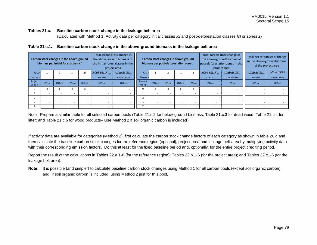
VM0015, Version 1.1 Sectoral Scope 15
Page 79
Tables 21.c. Baseline carbon stock change in the leakage belt area
(Calculated with Method 1: Activity data per category initial classes icl and post-deforestation classes fcl or zones z)
Table 21.c.1. Baseline carbon stock change in the above-ground biomass in the leakage belt area
Note: Prepare a similar table for all selected carbon pools (Table 21.c.2 for below-ground biomass; Table 21.c.3 for dead wood; Table 21.c.4 for
litter; and Table 21.c.6 for wood products– Use Method 2 if soil organic carbon is included).
If activity data are available for categories (Method 2), first calculate the carbon stock change factors of each category as shown in table 20.c and
then calculate the baseline carbon stock changes for the reference region (optional), project area and leakage belt area by multiplying activity data
with their corresponding emission factors. Do this at least for the fixed baseline period and, optionally, for the entire project crediting period.
Report the result of the calculations in Tables 22.a 1-6 (for the reference region); Tables 22.b.1-6 (for the project area); and Tables 22.c1-6 (for the
leakage belt area).
Note: It is possible (and simpler) to calculate baseline carbon stock changes using Method 1 for all carbon pools (except soil organic carbon)
and, if soil organic carbon is included, using Method 2 just for this pool.
ID icl> 1 2 … Icl Cab BSLLK icl,t Cab BSLLK icl ID iz > 1 2 … z Cab BSLLK z,t Cab BSLLK z Cab BSLLK t Cab BSLLK
Name > annual cumulative Name > annual cumulative annual cumulative
Project
year ttCO2-e tCO2-e tCO2-e tCO2-e tCO2-e tCO2-e
Project
year ttCO2-e tCO2-e tCO2-e tCO2-e tCO2-e tCO2-e tCO2-e tCO2-e
0 0 0 0 0 - - 0 0 0 0 0 - - - -
1 - - - - - - 1 - - - - - - - - 2 - - - - - - 2 - - - - - - - - … - - - - - - … - - - - - - - - T - - - - - - T - - - - - - - -
Total net carbon stock change
in the above-ground biomass
of the project area
Carbon stock changes in the above-ground
biomass per initial forest class icl
Total carbon stock change in
the above-ground biomass of
the initial forest classes in the
project area
Carbon stock changes in above-ground
biomass per post-deforestation zone z
Total carbon stock change in
the above-ground biomass of
post-deforestation zones in the
project area
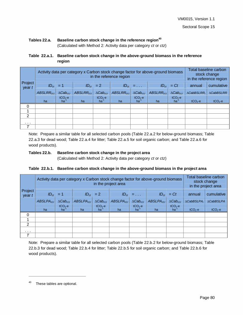
VM0015, Version 1.1
Sectoral Scope 15
Page 80
Tables 22.a. Baseline carbon stock change in the reference region40
(Calculated with Method 2: Activity data per category ct or ctz)
Table 22.a.1. Baseline carbon stock change in the above-ground biomass in the reference
region
Project year t
Activity data per category x Carbon stock change factor for above-ground biomass in the reference region
Total baseline carbon stock change
in the reference region
IDct = 1 IDct = 2 IDct = . . . IDct = Ct annual cumulative
ABSLRRct,t Cabct,t ABSLRRct,t Cabct,t ABSLRRct,t Cabct,t ABSLRRct,t Cabct,t CabBSLRRt CabBSLRR
ha tCO2-e
ha-1
ha tCO2-e
ha-1
ha tCO2-e
ha-1
ha tCO2-e
ha-1
tCO2-e tCO2-e
0
1 2
. . .
T
Note: Prepare a similar table for all selected carbon pools (Table 22.a.2 for below-ground biomass; Table
22.a.3 for dead wood; Table 22.a.4 for litter; Table 22.a.5 for soil organic carbon; and Table 22.a.6 for
wood products).
Tables 22.b. Baseline carbon stock change in the project area
(Calculated with Method 2: Activity data per category ct or ctz)
Table 22.b.1. Baseline carbon stock change in the above-ground biomass in the project area
Project year t
Activity data per category x Carbon stock change factor for above-ground biomass in the project area
Total baseline carbon stock change
in the project area
IDct = 1 IDct = 2 IDct = . . . IDct = Ct annual cumulative
ABSLPAct,t Cabct,t ABSLPAct,t Cabct,t ABSLPAct,t Cabct,t ABSLPAct,t Cabct,t CabBSLPAt CabBSLPA
ha tCO2-e
ha-1
ha tCO2-e
ha-1
ha tCO2-e
ha-1
ha tCO2-e
ha-1
tCO2-e tCO2-e
0
1 2
. . .
T
Note: Prepare a similar table for all selected carbon pools (Table 22.b.2 for below-ground biomass; Table
22.b.3 for dead wood; Table 22.b.4 for litter; Table 22.b.5 for soil organic carbon; and Table 22.b.6 for
wood products).
40 These tables are optional.
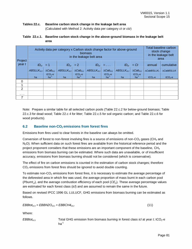
VM0015, Version 1.1 Sectoral Scope 15
Page 81
Tables 22.c. Baseline carbon stock change in the leakage belt area
(Calculated with Method 2: Activity data per category ct or ctz)
Table 22.c.1. Baseline carbon stock change in the above-ground biomass in the leakage belt
area
Project year t
Activity data per category x Carbon stock change factor for above-ground biomass
in the leakage belt area
Total baseline carbon stock change
in the leakage belt area
IDct = 1 IDct = 2 IDct = . . . IDct = Ct annual cumulative
ABSLLKct,t Cabct,t ABSLLKct,t Cabct,t ABSLLKct,t Cabct,t ABSLLKct,t Cabct,t CabBSLLKt CabBSLLK
ha
tCO2-e
ha-1
ha
tCO2-e
ha-1
ha
tCO2-e
ha-1
ha
tCO2-e
ha-1
tCO2-e tCO2-e
0
1 2
. . .
T
Note: Prepare a similar table for all selected carbon pools (Table 22.c.2 for below-ground biomass; Table
22.c.3 for dead wood; Table 22.c 4 for litter; Table 22.c.5 for soil organic carbon; and Table 22.c.6 for
wood products).
6.2 Baseline non-CO2 emissions from forest fires
Emissions from fires used to clear forests in the baseline can always be omitted.
Conversion of forest to non-forest involving fires is a source of emissions of non-CO2 gases (CH4 and
N2O). When sufficient data on such forest fires are available from the historical reference period and the
project proponent considers that these emissions are an important component of the baseline, CH4
emissions from biomass burning can be estimated. Where such data are unavailable, or of insufficient
accuracy, emissions from biomass burning should not be considered (which is conservative).
The effect of fire on carbon emissions is counted in the estimation of carbon stock changes; therefore
CO2 emissions from forest fires should be ignored to avoid double counting.
To estimate non-CO2 emissions from forest fires, it is necessary to estimate the average percentage of
the deforested area in which fire was used, the average proportion of mass burnt in each carbon pool
(Pburnt,p), and the average combustion efficiency of each pool (CEp). These average percentage values
are estimated for each forest class (icl) and are assumed to remain the same in the future.
Based on revised IPCC 1996 GL LULUCF, GHG emissions from biomass burning can be estimated as
follows.
EBBtoticl,t = EBBN2Oicl,t + EBBCH4icl,t (11)
Where:
EBBtoticl,t Total GHG emission from biomass burning in forest class icl at year t; tCO2-e
ha-1
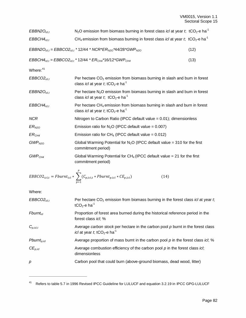
VM0015, Version 1.1 Sectoral Scope 15
Page 82
EBBN2Oicl,t N2O emission from biomass burning in forest class icl at year t; tCO2-e ha-1
EBBCH4icl,t CH4 emission from biomass burning in forest class icl at year t; tCO2-e ha-1
EBBN2Oicl,t = EBBCO2icl,t * 12/44 * NCR*ERN2O*44/28*GWPN2O (12)
EBBCH4icl,t = EBBCO2icl,t * 12/44 * ERCH4*16/12*GWPCH4 (13)
Where:41
EBBCO2icl,t Per hectare CO2 emission from biomass burning in slash and burn in forest
class icl at year t; tCO2-e ha-1
EBBN2Oicl,t Per hectare N2O emission from biomass burning in slash and burn in forest
class icl at year t; tCO2-e ha-1
EBBCH4icl,t Per hectare CH4 emission from biomass burning in slash and burn in forest
class icl at year t; tCO2-e ha-1
NCR Nitrogen to Carbon Ratio (IPCC default value = 0.01); dimensionless
ERN2O Emission ratio for N2O (IPCC default value = 0.007)
ERCH4 Emission ratio for CH4 (IPCC default value = 0.012)
GWPN2O Global Warming Potential for N2O (IPCC default value = 310 for the first
commitment period)
GWPCH4 Global Warming Potential for CH4 (IPCC default value = 21 for the first
commitment period)
∑
Where:
EBBCO2icl,t Per hectare CO2 emission from biomass burning in the forest class icl at year t;
tCO2-e ha-1
Fburnticl Proportion of forest area burned during the historical reference period in the
forest class icl; %
Cp,icl,t Average carbon stock per hectare in the carbon pool p burnt in the forest class
icl at year t; tCO2-e ha-1
Pburntp,icl Average proportion of mass burnt in the carbon pool p in the forest class icl; %
CEp,icl Average combustion efficiency of the carbon pool p in the forest class icl;
dimensionless
p Carbon pool that could burn (above-ground biomass, dead wood, litter)
41 Refers to table 5.7 in 1996 Revised IPCC Guideline for LULUCF and equation 3.2.19 in IPCC GPG-LULUCF
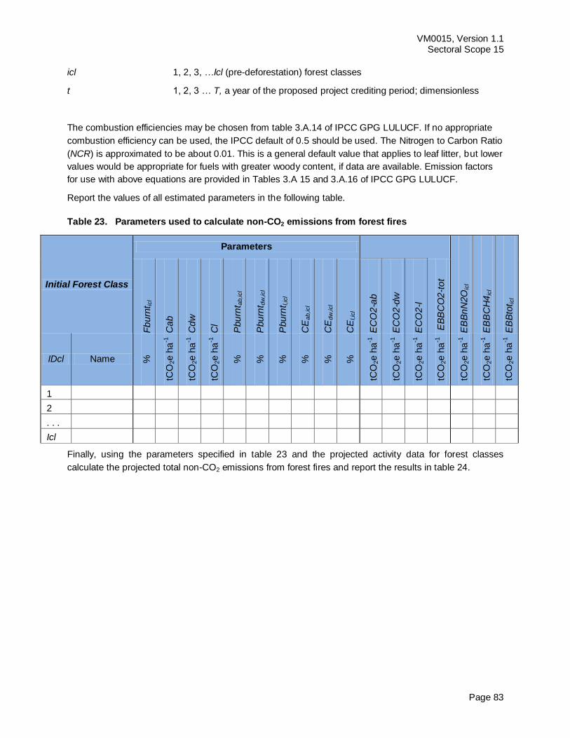
VM0015, Version 1.1 Sectoral Scope 15
Page 83
icl 1, 2, 3, …Icl (pre-deforestation) forest classes
t 1, 2, 3 … T, a year of the proposed project crediting period; dimensionless
The combustion efficiencies may be chosen from table 3.A.14 of IPCC GPG LULUCF. If no appropriate
combustion efficiency can be used, the IPCC default of 0.5 should be used. The Nitrogen to Carbon Ratio
(NCR) is approximated to be about 0.01. This is a general default value that applies to leaf litter, but lower
values would be appropriate for fuels with greater woody content, if data are available. Emission factors
for use with above equations are provided in Tables 3.A 15 and 3.A.16 of IPCC GPG LULUCF.
Report the values of all estimated parameters in the following table.
Table 23. Parameters used to calculate non-CO2 emissions from forest fires
Initial Forest Class
Parameters
EB
Bn
N2O
icl
EB
BC
H4
icl
EB
Bto
t icl
Fb
urn
t icl
Ca
b
Cd
w
Cl
Pbu
rnt a
b,icl
Pbu
rnt d
w,icl
Pbu
rnt l,
icl
CE
ab,icl
CE
dw
,icl
CE
l,ic
l
EC
O2
-ab
EC
O2
-dw
EC
O2
-l
EB
BC
O2
-to
t
IDcl Name %
tCO
2e
ha
-1
tCO
2e
ha
-1
tCO
2e
ha
-1
%
%
%
%
%
%
tCO
2e
ha
-1
tCO
2e
ha
-1
tCO
2e
ha
-1
tCO
2e
ha
-1
tCO
2e
ha
-1
tCO
2e
ha
-1
tCO
2e
ha
-1
1
2
. . .
Icl
Finally, using the parameters specified in table 23 and the projected activity data for forest classes
calculate the projected total non-CO2 emissions from forest fires and report the results in table 24.
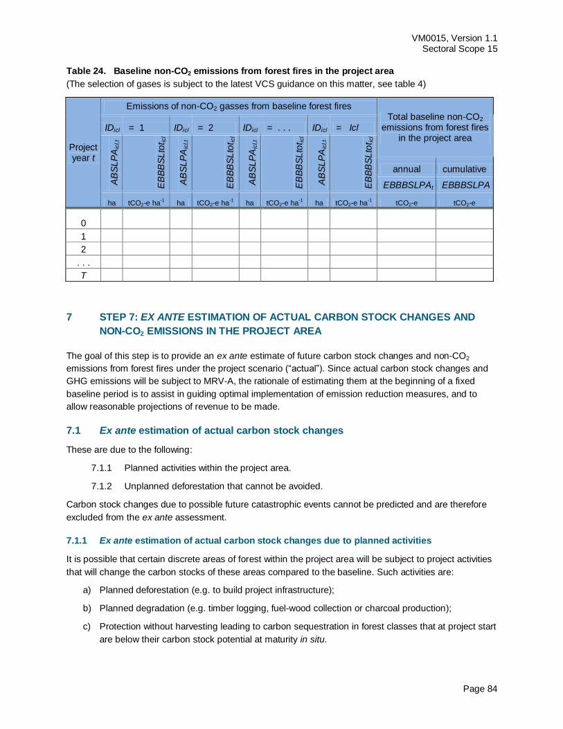
VM0015, Version 1.1 Sectoral Scope 15
Page 84
Table 24. Baseline non-CO2 emissions from forest fires in the project area
(The selection of gases is subject to the latest VCS guidance on this matter, see table 4)
Project year t
Emissions of non-CO2 gasses from baseline forest fires Total baseline non-CO2
emissions from forest fires in the project area
IDicl = 1 IDicl = 2 IDicl = . . . IDicl = Icl
AB
SL
PA
icl,t
EB
BB
SL
tot ic
l
AB
SL
PA
icl,t
EB
BB
SL
tot ic
l
AB
SL
PA
icl,t
EB
BB
SL
tot ic
l
AB
SL
PA
icl,t
EB
BB
SL
tot ic
l
annual cumulative
EBBBSLPAt EBBBSLPA
ha tCO2-e ha-1
ha tCO2-e ha-1
ha tCO2-e ha-1
ha tCO2-e ha-1
tCO2-e tCO2-e
0
1
2
. . .
T
STEP 7: EX ANTE ESTIMATION OF ACTUAL CARBON STOCK CHANGES AND 7
NON-CO2 EMISSIONS IN THE PROJECT AREA
The goal of this step is to provide an ex ante estimate of future carbon stock changes and non-CO2
emissions from forest fires under the project scenario (“actual”). Since actual carbon stock changes and
GHG emissions will be subject to MRV-A, the rationale of estimating them at the beginning of a fixed
baseline period is to assist in guiding optimal implementation of emission reduction measures, and to
allow reasonable projections of revenue to be made.
7.1 Ex ante estimation of actual carbon stock changes
These are due to the following:
7.1.1 Planned activities within the project area.
7.1.2 Unplanned deforestation that cannot be avoided.
Carbon stock changes due to possible future catastrophic events cannot be predicted and are therefore
excluded from the ex ante assessment.
7.1.1 Ex ante estimation of actual carbon stock changes due to planned activities
It is possible that certain discrete areas of forest within the project area will be subject to project activities
that will change the carbon stocks of these areas compared to the baseline. Such activities are:
a) Planned deforestation (e.g. to build project infrastructure);
b) Planned degradation (e.g. timber logging, fuel-wood collection or charcoal production);
c) Protection without harvesting leading to carbon sequestration in forest classes that at project start
are below their carbon stock potential at maturity in situ.
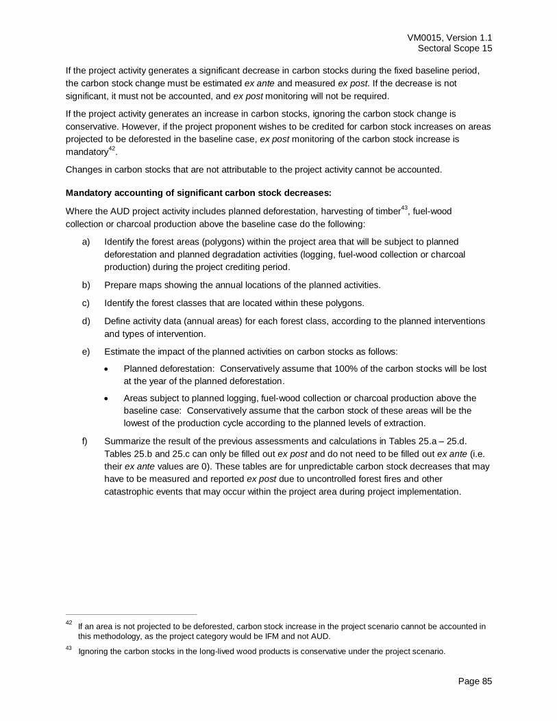
VM0015, Version 1.1 Sectoral Scope 15
Page 85
If the project activity generates a significant decrease in carbon stocks during the fixed baseline period,
the carbon stock change must be estimated ex ante and measured ex post. If the decrease is not
significant, it must not be accounted, and ex post monitoring will not be required.
If the project activity generates an increase in carbon stocks, ignoring the carbon stock change is
conservative. However, if the project proponent wishes to be credited for carbon stock increases on areas
projected to be deforested in the baseline case, ex post monitoring of the carbon stock increase is
mandatory42
.
Changes in carbon stocks that are not attributable to the project activity cannot be accounted.
Mandatory accounting of significant carbon stock decreases:
Where the AUD project activity includes planned deforestation, harvesting of timber43
, fuel-wood
collection or charcoal production above the baseline case do the following:
a) Identify the forest areas (polygons) within the project area that will be subject to planned
deforestation and planned degradation activities (logging, fuel-wood collection or charcoal
production) during the project crediting period.
b) Prepare maps showing the annual locations of the planned activities.
c) Identify the forest classes that are located within these polygons.
d) Define activity data (annual areas) for each forest class, according to the planned interventions
and types of intervention.
e) Estimate the impact of the planned activities on carbon stocks as follows:
Planned deforestation: Conservatively assume that 100% of the carbon stocks will be lost
at the year of the planned deforestation.
Areas subject to planned logging, fuel-wood collection or charcoal production above the
baseline case: Conservatively assume that the carbon stock of these areas will be the
lowest of the production cycle according to the planned levels of extraction.
f) Summarize the result of the previous assessments and calculations in Tables 25.a – 25.d.
Tables 25.b and 25.c can only be filled out ex post and do not need to be filled out ex ante (i.e.
their ex ante values are 0). These tables are for unpredictable carbon stock decreases that may
have to be measured and reported ex post due to uncontrolled forest fires and other
catastrophic events that may occur within the project area during project implementation.
42
If an area is not projected to be deforested, carbon stock increase in the project scenario cannot be accounted in
this methodology, as the project category would be IFM and not AUD.
43 Ignoring the carbon stocks in the long-lived wood products is conservative under the project scenario.
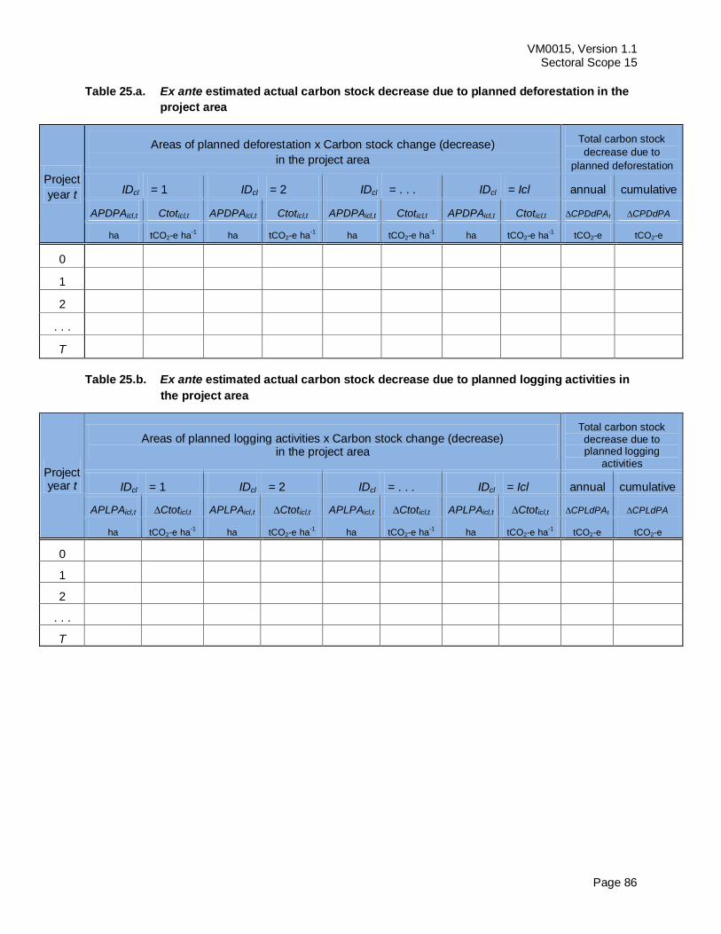
VM0015, Version 1.1 Sectoral Scope 15
Page 86
Table 25.a. Ex ante estimated actual carbon stock decrease due to planned deforestation in the
project area
Project
year t
Areas of planned deforestation x Carbon stock change (decrease)
in the project area
Total carbon stock
decrease due to
planned deforestation
IDcl = 1 IDcl = 2 IDcl = . . . IDcl = Icl annual cumulative
APDPAicl,t Ctoticl,t APDPAicl,t Ctoticl,t APDPAicl,t Ctoticl,t APDPAicl,t Ctoticl,t CPDdPAt CPDdPA
ha tCO2-e ha-1
ha tCO2-e ha-1
ha tCO2-e ha-1
ha tCO2-e ha-1
tCO2-e tCO2-e
0
1
2
. . .
T
Table 25.b. Ex ante estimated actual carbon stock decrease due to planned logging activities in
the project area
Project year t
Areas of planned logging activities x Carbon stock change (decrease) in the project area
Total carbon stock decrease due to planned logging
activities
IDcl = 1 IDcl = 2 IDcl = . . . IDcl = Icl annual cumulative
APLPAicl,t Ctoticl,t APLPAicl,t Ctoticl,t APLPAicl,t Ctoticl,t APLPAicl,t Ctoticl,t CPLdPAt CPLdPA
ha tCO2-e ha-1
ha tCO2-e ha-1
ha tCO2-e ha-1
ha tCO2-e ha-1
tCO2-e tCO2-e
0
1
2
. . .
T

VM0015, Version 1.1 Sectoral Scope 15
Page 87
Table 25.c. Ex ante estimated actual carbon stock decrease due to planned fuel wood collection
and charcoal production in the project area
Project year t
Areas of planned fuel-wood & charcoal activities x Carbon stock change (decrease) in the project areas
Total carbon stock decrease due to
planned fuel-wood and charcoal activities
IDcl = 1 IDcl = 2 IDcl = . . . IDcl = Icl annual cumulative
APFPAicl,t Ctoticl,t APFPAicl,t Ctoticl,t APFPAicl,t Ctoticl,t APFPAicl,t Ctoticl,t CPFdPAt CPFdPA
ha tCO2-e ha-1
ha tCO2-e ha-1
ha tCO2-e ha-1
ha tCO2-e ha-1
tCO2-e tCO2-e
0
1
2
. . .
T
Table 25.d. Total ex ante carbon stock decrease due to planned activities in the project area
Project year t
Total carbon stock decrease due to
planned deforestation
Total carbon stock decrease due to planned logging
activities
Total carbon stock decrease due to
planned fuel-wood and charcoal activities
Total carbon stock decrease due to planned activities
annual cumulative annual cumulative annual cumulative annual cumulative
CPDdPAt CPDdPA CPLdPAt CPLdPA CPFdPAt CPFdPA CPAdPAt CPAdPA
tCO2-e tCO2-e tCO2-e tCO2-e tCO2-e tCO2-e tCO2-e tCO2-e
0
1
2
. . .
T
Optional accounting of significant carbon stock increase
Consideration of carbon stock increase due to planned activities in areas that would be deforested in the
baseline case is optional in this methodology and can always be omitted.
However, if the project area includes degraded and secondary forests that in the baseline case would be
deforested and due to the project activity these areas will recover and sequester additional carbon,
credits for the increased carbon stocks can be claimed. In the case, do the following:
a) Identify within the project area the polygons that are at the same time projected to be deforested
in the baseline case and that are currently covered by secondary forests or degraded forests
that have the potential to grow and accumulate significant carbon stocks;
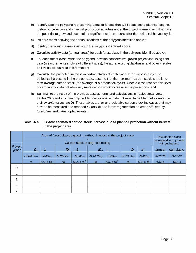
VM0015, Version 1.1 Sectoral Scope 15
Page 88
b) Identify also the polygons representing areas of forests that will be subject to planned logging,
fuel-wood collection and charcoal production activities under the project scenario and that have
the potential to grow and accumulate significant carbon stocks after the periodical harvest cycle;
c) Prepare maps showing the annual locations of the polygons identified above;
d) Identify the forest classes existing in the polygons identified above;
e) Calculate activity data (annual areas) for each forest class in the polygons identified above;
f) For each forest class within the polygons, develop conservative growth projections using field
data (measurements in plots of different ages), literature, existing databases and other credible
and verifiable sources of information;
g) Calculate the projected increase in carbon stocks of each class. If the class is subject to
periodical harvesting in the project case, assume that the maximum carbon stock is the long
term average carbon stock (the average of a production cycle). Once a class reaches this level
of carbon stock, do not allow any more carbon stock increase in the projections; and
h) Summarize the result of the previous assessments and calculations in Tables 26.a –26.d.
Tables 26.b and 26.c can only be filled out ex post and do not need to be filled out ex ante (i.e.
their ex ante values are 0). These tables are for unpredictable carbon stock increases that may
have to be measured and reported ex post due to forest regeneration on areas affected by
forest fires and catastrophic events.
Table 26.a. Ex ante estimated carbon stock increase due to planned protection without harvest
in the project area
Project year t
Area of forest classes growing without harvest in the project case x
Carbon stock change (increase)
Total carbon stock increase due to growth
without harvest
IDcl = 1 IDcl = 2 IDcl = . . . IDcl = Icl annual cumulative
APNiPAicl,t Ctoticl,t APNiPAicl,t Ctoticl,t APNiPAicl,t Ctoticl,t APNiPAicl,t Ctoticl,t CPNiPAt CPNiPA
ha tCO2-e ha-1
ha tCO2-e ha-1
ha tCO2-e ha-1
ha tCO2-e ha-1
tCO2-e tCO2-e
0
1
2
. . .
T
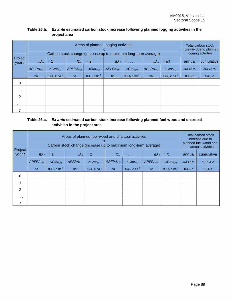
VM0015, Version 1.1 Sectoral Scope 15
Page 89
Table 26.b. Ex ante estimated carbon stock increase following planned logging activities in the
project area
Project year t
Areas of planned logging activities x
Carbon stock change (increase up to maximum long-term average)
Total carbon stock increase due to planned
logging activities
IDcl = 1 IDcl = 2 IDcl = . . . IDcl = Icl annual cumulative
APLPAicl,t Ctoticl,t APLPAicl,t Ctoticl,t APLPAicl,t Ctoticl,t APLPAicl,t Ctoticl,t CPLiPAt CPLiPA
ha tCO2-e ha-1
ha tCO2-e ha-1
ha tCO2-e ha-1
ha tCO2-e ha-1
tCO2-e tCO2-e
0
1
2
. . .
T
Table 26.c. Ex ante estimated carbon stock increase following planned fuel-wood and charcoal
activities in the project area
Project year t
Areas of planned fuel-wood and charcoal activities x
Carbon stock change (increase up to maximum long-term average)
Total carbon stock increase due to
planned fuel-wood and charcoal activities
IDcl = 1 IDcl = 2 IDcl = . . . IDcl = Icl annual cumulative
APFPAicl,t Ctoticl,t APFPAicl,t Ctoticl,t APFPAicl,t Ctoticl,t APFPAicl,t Ctoticl,t CPFiPAt CPFiPA
ha tCO2-e ha-1
ha tCO2-e ha-1
ha tCO2-e ha-1
ha tCO2-e ha-1
tCO2-e tCO2-e
0
1
2
. . .
T
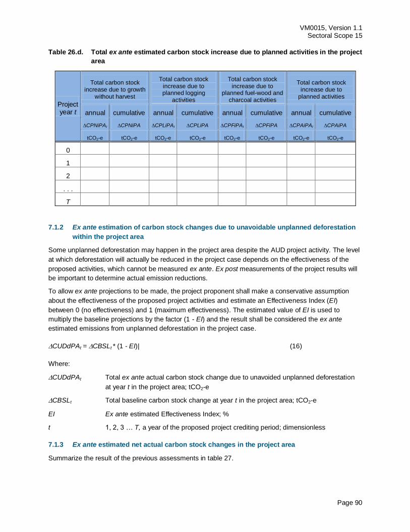
VM0015, Version 1.1 Sectoral Scope 15
Page 90
Table 26.d. Total ex ante estimated carbon stock increase due to planned activities in the project
area
Project year t
Total carbon stock increase due to growth
without harvest
Total carbon stock increase due to planned logging
activities
Total carbon stock increase due to
planned fuel-wood and charcoal activities
Total carbon stock increase due to
planned activities
annual cumulative annual cumulative annual cumulative annual cumulative
CPNiPAt CPNiPA CPLiPAt CPLiPA CPFiPAt CPFiPA CPAiPAt CPAiPA
tCO2-e tCO2-e tCO2-e tCO2-e tCO2-e tCO2-e tCO2-e tCO2-e
0
1
2
. . .
T
7.1.2 Ex ante estimation of carbon stock changes due to unavoidable unplanned deforestation
within the project area
Some unplanned deforestation may happen in the project area despite the AUD project activity. The level
at which deforestation will actually be reduced in the project case depends on the effectiveness of the
proposed activities, which cannot be measured ex ante. Ex post measurements of the project results will
be important to determine actual emission reductions.
To allow ex ante projections to be made, the project proponent shall make a conservative assumption
about the effectiveness of the proposed project activities and estimate an Effectiveness Index (EI)
between 0 (no effectiveness) and 1 (maximum effectiveness). The estimated value of EI is used to
multiply the baseline projections by the factor (1 - EI) and the result shall be considered the ex ante
estimated emissions from unplanned deforestation in the project case.
CUDdPAt = CBSLt * (1 - EI)| (16)
Where:
CUDdPAt Total ex ante actual carbon stock change due to unavoided unplanned deforestation
at year t in the project area; tCO2-e
CBSLt Total baseline carbon stock change at year t in the project area; tCO2-e
EI Ex ante estimated Effectiveness Index; %
t 1, 2, 3 … T, a year of the proposed project crediting period; dimensionless
7.1.3 Ex ante estimated net actual carbon stock changes in the project area
Summarize the result of the previous assessments in table 27.
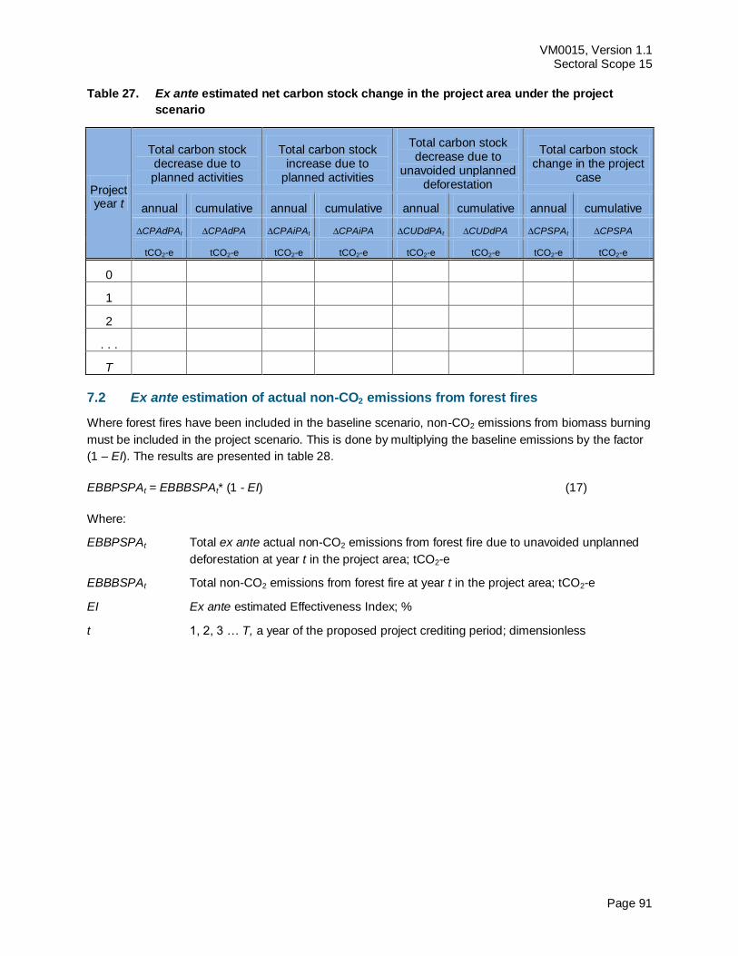
VM0015, Version 1.1 Sectoral Scope 15
Page 91
Table 27. Ex ante estimated net carbon stock change in the project area under the project
scenario
Project year t
Total carbon stock decrease due to planned activities
Total carbon stock increase due to
planned activities
Total carbon stock decrease due to
unavoided unplanned deforestation
Total carbon stock change in the project
case
annual cumulative annual cumulative annual cumulative annual cumulative
CPAdPAt CPAdPA CPAiPAt CPAiPA CUDdPAt CUDdPA CPSPAt CPSPA
tCO2-e tCO2-e tCO2-e tCO2-e tCO2-e tCO2-e tCO2-e tCO2-e
0
1
2
. . .
T
7.2 Ex ante estimation of actual non-CO2 emissions from forest fires
Where forest fires have been included in the baseline scenario, non-CO2 emissions from biomass burning
must be included in the project scenario. This is done by multiplying the baseline emissions by the factor
(1 – EI). The results are presented in table 28.
EBBPSPAt = EBBBSPAt* (1 - EI) (17)
Where:
EBBPSPAt Total ex ante actual non-CO2 emissions from forest fire due to unavoided unplanned
deforestation at year t in the project area; tCO2-e
EBBBSPAt Total non-CO2 emissions from forest fire at year t in the project area; tCO2-e
EI Ex ante estimated Effectiveness Index; %
t 1, 2, 3 … T, a year of the proposed project crediting period; dimensionless
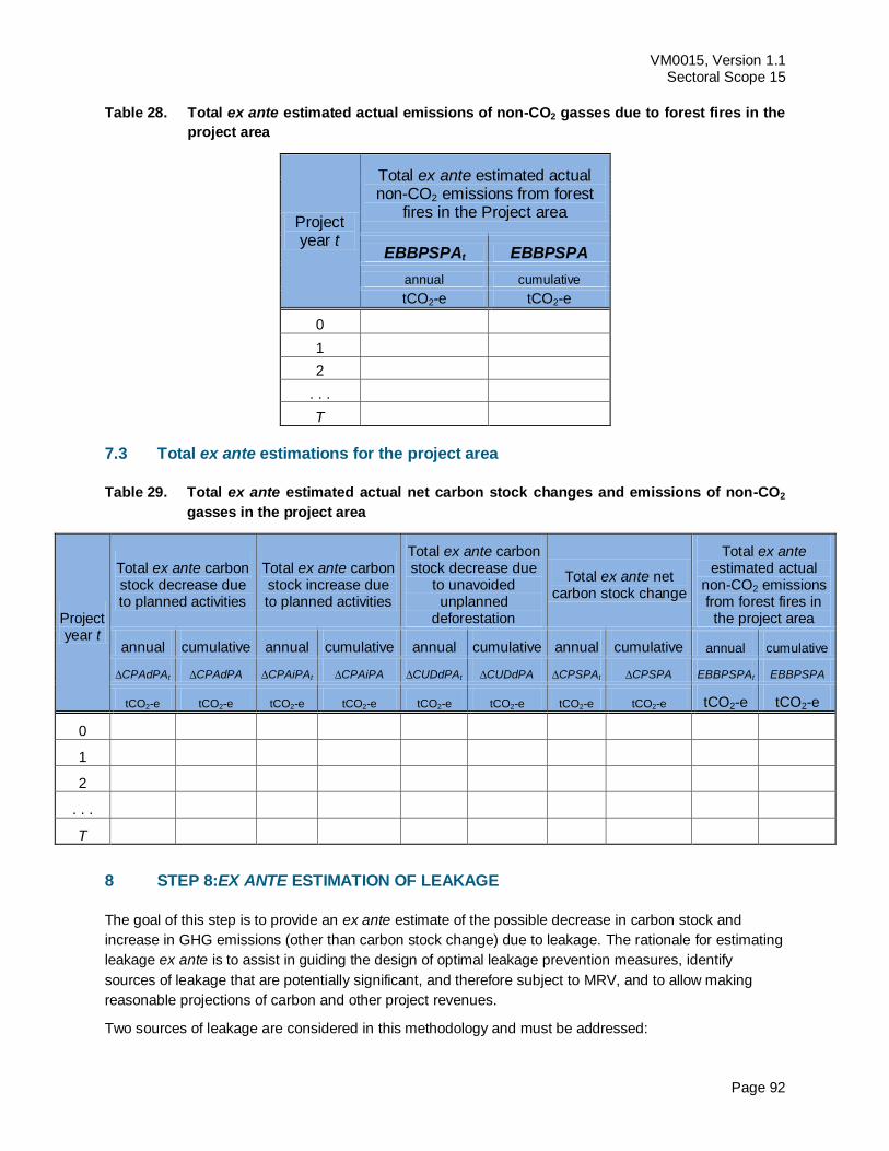
VM0015, Version 1.1 Sectoral Scope 15
Page 92
Table 28. Total ex ante estimated actual emissions of non-CO2 gasses due to forest fires in the
project area
Project year t
Total ex ante estimated actual non-CO2 emissions from forest
fires in the Project area
EBBPSPAt EBBPSPA
annual cumulative
tCO2-e tCO2-e
0
1
2
. . .
T
7.3 Total ex ante estimations for the project area
Table 29. Total ex ante estimated actual net carbon stock changes and emissions of non-CO2
gasses in the project area
Project year t
Total ex ante carbon stock decrease due to planned activities
Total ex ante carbon stock increase due to planned activities
Total ex ante carbon stock decrease due
to unavoided unplanned
deforestation
Total ex ante net carbon stock change
Total ex ante estimated actual
non-CO2 emissions from forest fires in the project area
annual cumulative annual cumulative annual cumulative annual cumulative annual cumulative
CPAdPAt CPAdPA CPAiPAt CPAiPA CUDdPAt CUDdPA CPSPAt CPSPA EBBPSPAt EBBPSPA
tCO2-e tCO2-e tCO2-e tCO2-e tCO2-e tCO2-e tCO2-e tCO2-e tCO2-e tCO2-e
0
1
2
. . .
T
STEP 8:EX ANTE ESTIMATION OF LEAKAGE 8
The goal of this step is to provide an ex ante estimate of the possible decrease in carbon stock and
increase in GHG emissions (other than carbon stock change) due to leakage. The rationale for estimating
leakage ex ante is to assist in guiding the design of optimal leakage prevention measures, identify
sources of leakage that are potentially significant, and therefore subject to MRV, and to allow making
reasonable projections of carbon and other project revenues.
Two sources of leakage are considered in this methodology and must be addressed:
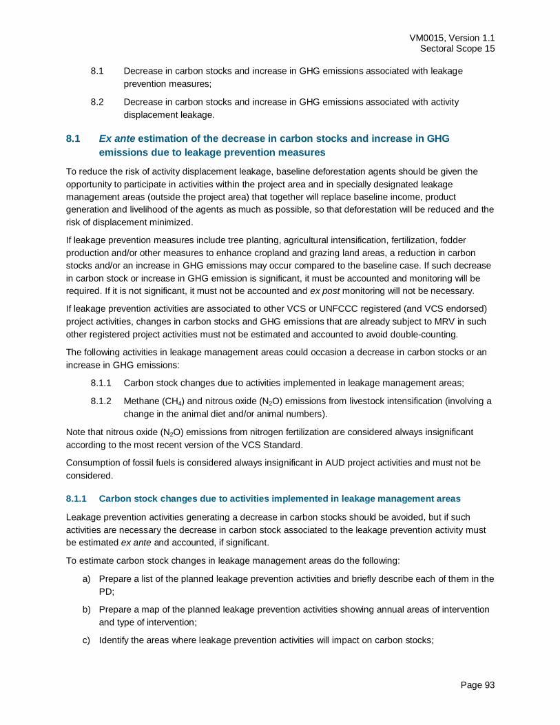
VM0015, Version 1.1 Sectoral Scope 15
Page 93
8.1 Decrease in carbon stocks and increase in GHG emissions associated with leakage
prevention measures;
8.2 Decrease in carbon stocks and increase in GHG emissions associated with activity
displacement leakage.
8.1 Ex ante estimation of the decrease in carbon stocks and increase in GHG
emissions due to leakage prevention measures
To reduce the risk of activity displacement leakage, baseline deforestation agents should be given the
opportunity to participate in activities within the project area and in specially designated leakage
management areas (outside the project area) that together will replace baseline income, product
generation and livelihood of the agents as much as possible, so that deforestation will be reduced and the
risk of displacement minimized.
If leakage prevention measures include tree planting, agricultural intensification, fertilization, fodder
production and/or other measures to enhance cropland and grazing land areas, a reduction in carbon
stocks and/or an increase in GHG emissions may occur compared to the baseline case. If such decrease
in carbon stock or increase in GHG emission is significant, it must be accounted and monitoring will be
required. If it is not significant, it must not be accounted and ex post monitoring will not be necessary.
If leakage prevention activities are associated to other VCS or UNFCCC registered (and VCS endorsed)
project activities, changes in carbon stocks and GHG emissions that are already subject to MRV in such
other registered project activities must not be estimated and accounted to avoid double-counting.
The following activities in leakage management areas could occasion a decrease in carbon stocks or an
increase in GHG emissions:
8.1.1 Carbon stock changes due to activities implemented in leakage management areas;
8.1.2 Methane (CH4) and nitrous oxide (N2O) emissions from livestock intensification (involving a
change in the animal diet and/or animal numbers).
Note that nitrous oxide (N2O) emissions from nitrogen fertilization are considered always insignificant
according to the most recent version of the VCS Standard.
Consumption of fossil fuels is considered always insignificant in AUD project activities and must not be
considered.
8.1.1 Carbon stock changes due to activities implemented in leakage management areas
Leakage prevention activities generating a decrease in carbon stocks should be avoided, but if such
activities are necessary the decrease in carbon stock associated to the leakage prevention activity must
be estimated ex ante and accounted, if significant.
To estimate carbon stock changes in leakage management areas do the following:
a) Prepare a list of the planned leakage prevention activities and briefly describe each of them in the
PD;
b) Prepare a map of the planned leakage prevention activities showing annual areas of intervention
and type of intervention;
c) Identify the areas where leakage prevention activities will impact on carbon stocks;
VM0015, Version 1.1 Sectoral Scope 15
Page 94
d) Identify the non-forest classes44
existing within these areas in the baseline case;
e) Measure the carbon stocks in the identified classes or use conservative literature estimates for
each of the identified classes. If some classes have changing carbon stocks in the baseline, do
carbon stock projections using growths data and other relevant and verifiable sources of
information;
f) Report in table 30.a the projected baseline carbon stock changes in the leakage management
areas;
g) According to the planned interventions, estimate the projected carbon stocks in the leakage
management areas under the project scenario. Use conservative growth projections. Report the
result in table 30.b; and
h) Calculate the net carbon stock changes that the planned leakage prevention measures are
expected to occasion during the fixed baseline period and, optionally, the project crediting period.
Report the results of the calculations in table 30.c
If the net sum of carbon stock changes within a monitoring period is more than zero, leakage
prevention measures are not causing any carbon stock decrease. The net increase shall
conservatively be ignored in the calculation of net GHG emission reductions of the project
activity.
If the net sum is negative, determine the significance using the most recent version of the
EB-CDM approved “Tool for testing significance of GHG emissions in A/R CDM project
activities”. If the decrease is significant, it must be accounted in the ex ante estimation of
leakage and carbon stock changes in the land units where leakage prevention measures are
implemented will be subject to MRV. If the decrease is not significant, it must not be
accounted and carbon stock changes will not be subject to MRV.
44 Forest classes cannot be present in leakage management areas at the project start date (see section 1.1.4).
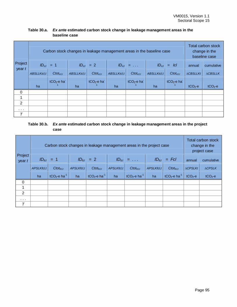
VM0015, Version 1.1 Sectoral Scope 15
Page 95
Table 30.a. Ex ante estimated carbon stock change in leakage management areas in the
baseline case
Project
year t
Carbon stock changes in leakage management areas in the baseline case
Total carbon stock
change in the
baseline case
IDicl = 1 IDicl = 2 IDicl = . . . IDicl = Icl annual cumulative
ABSLLKicl,t Ctoticl,t ABSLLKicl,t Ctoticl,t ABSLLKicl,t Ctoticl,t ABSLLKicl,t Ctoticl,t CBSLLKt CBSLLK
ha
tCO2-e ha-
1 ha
tCO2-e ha-
1 ha
tCO2-e ha-
1 ha
tCO2-e ha-
1 tCO2-e tCO2-e
0
1
2
. . .
T
Table 30.b. Ex ante estimated carbon stock change in leakage management areas in the project
case
Project
year t
Carbon stock changes in leakage management areas in the project case
Total carbon stock
change in the
project case
IDfcl = 1 IDfcl = 2 IDfcl = . . . IDfcl = Fcl annual cumulative
APSLKfcl,t Ctotfcl,t APSLKfcl,t Ctotfcl,t APSLKfcl,t Ctotfcl,t APSLKfcl,t Ctotfcl,t CPSLKt CPSLK
ha tCO2-e ha-1
ha tCO2-e ha-1
ha tCO2-e ha-1
ha tCO2-e ha-1
tCO2-e tCO2-e
0
1
2
. . .
T
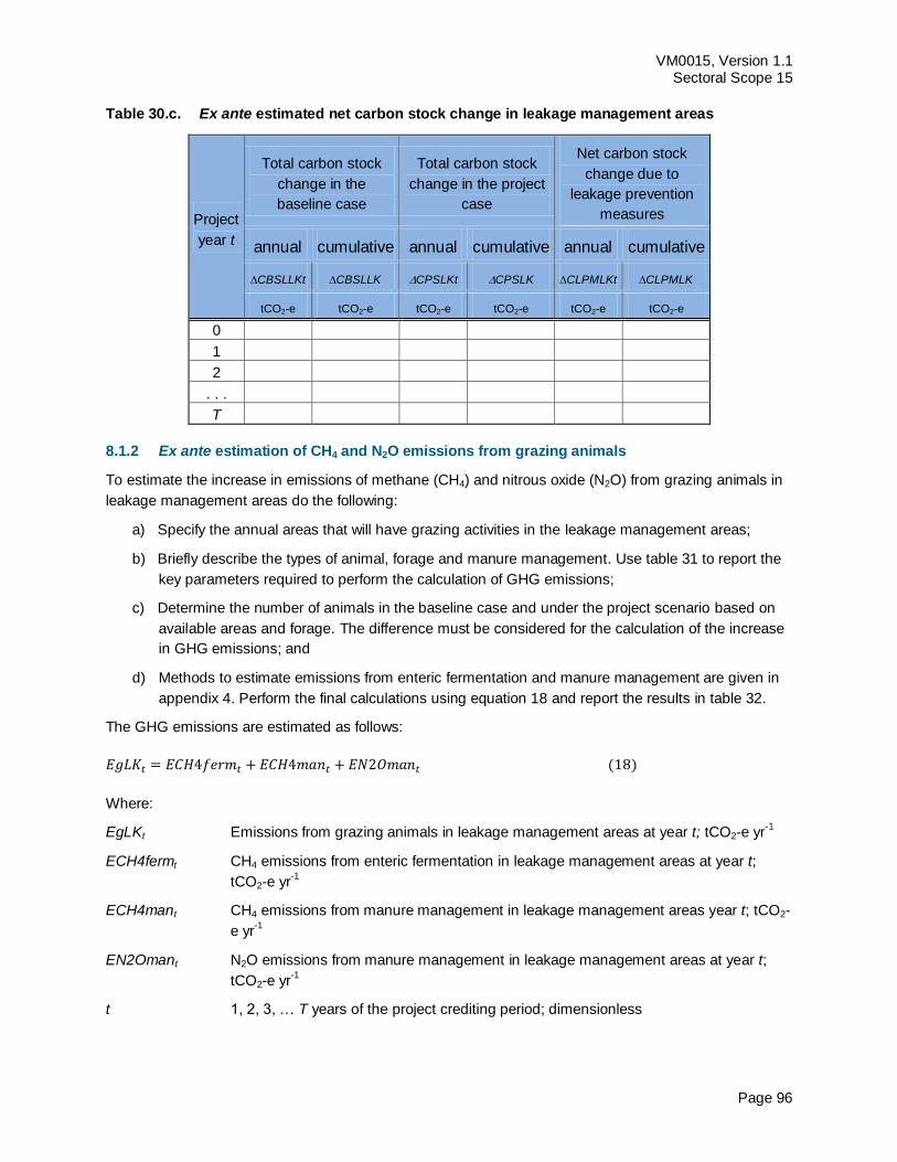
VM0015, Version 1.1 Sectoral Scope 15
Page 96
Table 30.c. Ex ante estimated net carbon stock change in leakage management areas
Project
year t
Total carbon stock
change in the
baseline case
Total carbon stock
change in the project
case
Net carbon stock
change due to
leakage prevention
measures
annual cumulative annual cumulative annual cumulative
CBSLLKt CBSLLK CPSLKt CPSLK CLPMLKt CLPMLK
tCO2-e tCO2-e tCO2-e tCO2-e tCO2-e tCO2-e
0
1
2
. . .
T
8.1.2 Ex ante estimation of CH4 and N2O emissions from grazing animals
To estimate the increase in emissions of methane (CH4) and nitrous oxide (N2O) from grazing animals in
leakage management areas do the following:
a) Specify the annual areas that will have grazing activities in the leakage management areas;
b) Briefly describe the types of animal, forage and manure management. Use table 31 to report the
key parameters required to perform the calculation of GHG emissions;
c) Determine the number of animals in the baseline case and under the project scenario based on
available areas and forage. The difference must be considered for the calculation of the increase
in GHG emissions; and
d) Methods to estimate emissions from enteric fermentation and manure management are given in
appendix 4. Perform the final calculations using equation 18 and report the results in table 32.
The GHG emissions are estimated as follows:
Where:
EgLKt Emissions from grazing animals in leakage management areas at year t; tCO2-e yr-1
ECH4fermt CH4 emissions from enteric fermentation in leakage management areas at year t;
tCO2-e yr-1
ECH4mant CH4 emissions from manure management in leakage management areas year t; tCO2-
e yr-1
EN2Omant N2O emissions from manure management in leakage management areas at year t;
tCO2-e yr-1
t 1, 2, 3, … T years of the project crediting period; dimensionless
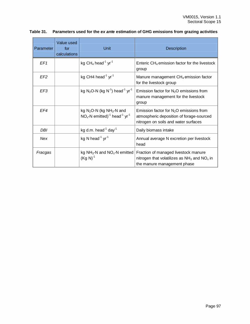
VM0015, Version 1.1 Sectoral Scope 15
Page 97
Table 31. Parameters used for the ex ante estimation of GHG emissions from grazing activities
Parameter
Value used
for
calculations
Unit Description
EF1 kg CH4 head-1
yr-1
Enteric CH4 emission factor for the livestock
group
EF2 kg CH4 head-1
yr-1
Manure management CH4 emission factor
for the livestock group
EF3 kg N2O-N (kg N-1
) head-1
yr-1
Emission factor for N2O emissions from
manure management for the livestock
group
EF4 kg N2O-N (kg NH3-N and
NOx-N emitted)-1
head-1
yr-1
Emission factor for N2O emissions from
atmospheric deposition of forage-sourced
nitrogen on soils and water surfaces
DBI kg d.m. head-1
day-1
Daily biomass intake
Nex kg N head-1
yr-1
Annual average N excretion per livestock
head
Fracgas kg NH3-N and NOx-N emitted
(Kg N)-1
Fraction of managed livestock manure
nitrogen that volatilizes as NH3 and NOx in
the manure management phase
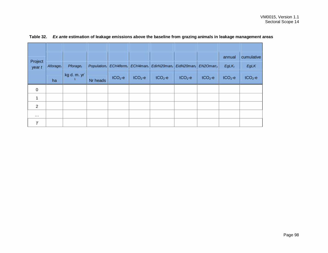
VM0015, Version 1.1 Sectoral Scope 14
Page 98
Table 32. Ex ante estimation of leakage emissions above the baseline from grazing animals in leakage management areas
Project
year t
annual cumulative
Aforaget Pforaget Populationt ECH4fermt ECH4mant EdirN20mant EidN20mant EN2Oman,t EgLKt EgLK
ha
kg d. m. yr-
1 Nr heads
tCO2-e tCO2-e tCO2-e tCO2-e tCO2-e tCO2-e tCO2-e
0
1
2
…
T
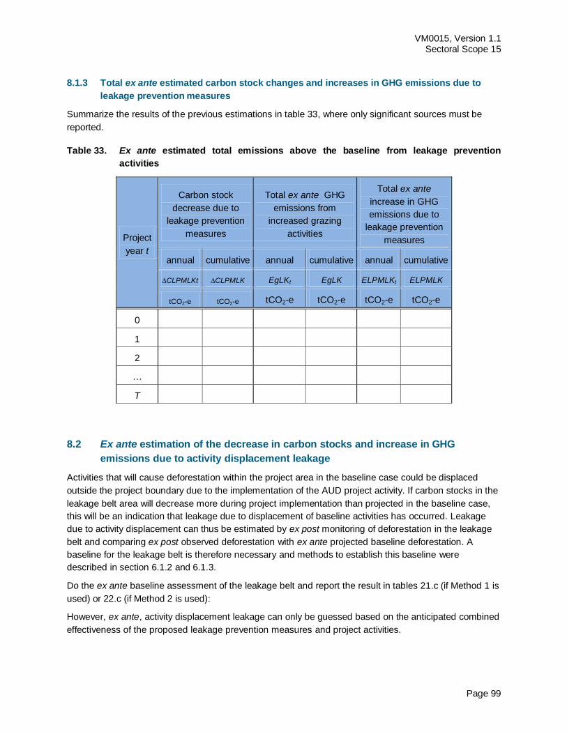
VM0015, Version 1.1 Sectoral Scope 15
Page 99
8.1.3 Total ex ante estimated carbon stock changes and increases in GHG emissions due to
leakage prevention measures
Summarize the results of the previous estimations in table 33, where only significant sources must be
reported.
Table 33. Ex ante estimated total emissions above the baseline from leakage prevention
activities
Project
year t
Carbon stock
decrease due to
leakage prevention
measures
Total ex ante GHG
emissions from
increased grazing
activities
Total ex ante
increase in GHG
emissions due to
leakage prevention
measures
annual cumulative annual cumulative annual cumulative
CLPMLKt CLPMLK EgLKt EgLK ELPMLKt ELPMLK
tCO2-e tCO2-e tCO2-e tCO2-e tCO2-e tCO2-e
0
1
2
…
T
8.2 Ex ante estimation of the decrease in carbon stocks and increase in GHG
emissions due to activity displacement leakage
Activities that will cause deforestation within the project area in the baseline case could be displaced
outside the project boundary due to the implementation of the AUD project activity. If carbon stocks in the
leakage belt area will decrease more during project implementation than projected in the baseline case,
this will be an indication that leakage due to displacement of baseline activities has occurred. Leakage
due to activity displacement can thus be estimated by ex post monitoring of deforestation in the leakage
belt and comparing ex post observed deforestation with ex ante projected baseline deforestation. A
baseline for the leakage belt is therefore necessary and methods to establish this baseline were
described in section 6.1.2 and 6.1.3.
Do the ex ante baseline assessment of the leakage belt and report the result in tables 21.c (if Method 1 is
used) or 22.c (if Method 2 is used):
However, ex ante, activity displacement leakage can only be guessed based on the anticipated combined
effectiveness of the proposed leakage prevention measures and project activities.
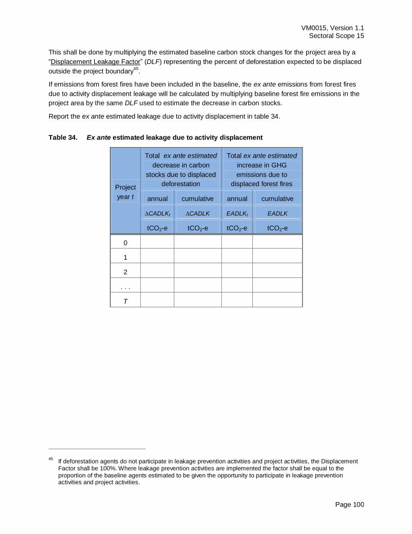
VM0015, Version 1.1 Sectoral Scope 15
Page 100
This shall be done by multiplying the estimated baseline carbon stock changes for the project area by a
“Displacement Leakage Factor” (DLF) representing the percent of deforestation expected to be displaced
outside the project boundary45
.
If emissions from forest fires have been included in the baseline, the ex ante emissions from forest fires
due to activity displacement leakage will be calculated by multiplying baseline forest fire emissions in the
project area by the same DLF used to estimate the decrease in carbon stocks.
Report the ex ante estimated leakage due to activity displacement in table 34.
Table 34. Ex ante estimated leakage due to activity displacement
Project
year t
Total ex ante estimated
decrease in carbon
stocks due to displaced
deforestation
Total ex ante estimated
increase in GHG
emissions due to
displaced forest fires
annual cumulative annual cumulative
CADLKt CADLK EADLKt EADLK
tCO2-e tCO2-e tCO2-e tCO2-e
0
1
2
. . .
T
45 If deforestation agents do not participate in leakage prevention activities and project activities, the Displacement
Factor shall be 100%. Where leakage prevention activities are implemented the factor shall be equal to the proportion of the baseline agents estimated to be given the opportunity to participate in leakage prevention activities and project activities.
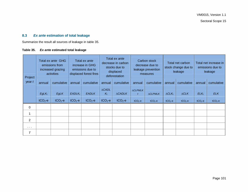
VM0015, Version 1.1
Sectoral Scope 15
Page 101
8.3 Ex ante estimation of total leakage
Summarize the result all sources of leakage in table 35.
Table 35. Ex ante estimated total leakage
Project
year t
Total ex ante GHG
emissions from
increased grazing
activities
Total ex ante
increase in GHG
emissions due to
displaced forest fires
Total ex ante
decrease in carbon
stocks due to
displaced
deforestation
Carbon stock
decrease due to
leakage prevention
measures
Total net carbon
stock change due to
leakage
Total net increase in
emissions due to
leakage
annual cumulative annual cumulative annual cumulative annual cumulative annual cumulative annual cumulative
EgLKt EgLK EADLKt EADLK
CADL
Kt CADLK
CLPMLK
t CLPMLK CLKt CLK ELKt ELK
tCO2-e tCO2-e tCO2-e tCO2-e tCO2-e tCO2-e tCO2-e tCO2-e tCO2-e tCO2-e tCO2-e tCO2-e
0
1
2
. . .
T
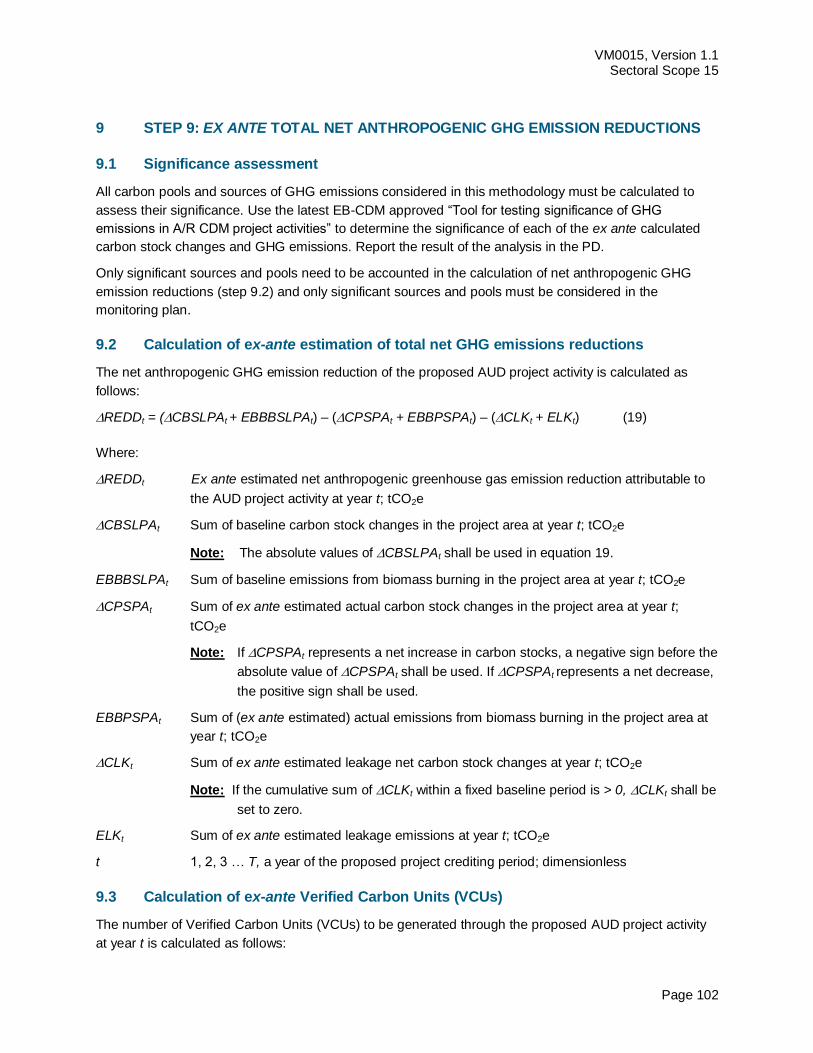
VM0015, Version 1.1 Sectoral Scope 15
Page 102
STEP 9: EX ANTE TOTAL NET ANTHROPOGENIC GHG EMISSION REDUCTIONS 9
9.1 Significance assessment
All carbon pools and sources of GHG emissions considered in this methodology must be calculated to
assess their significance. Use the latest EB-CDM approved “Tool for testing significance of GHG
emissions in A/R CDM project activities” to determine the significance of each of the ex ante calculated
carbon stock changes and GHG emissions. Report the result of the analysis in the PD.
Only significant sources and pools need to be accounted in the calculation of net anthropogenic GHG
emission reductions (step 9.2) and only significant sources and pools must be considered in the
monitoring plan.
9.2 Calculation of ex-ante estimation of total net GHG emissions reductions
The net anthropogenic GHG emission reduction of the proposed AUD project activity is calculated as
follows:
REDDt = ( CBSLPAt + EBBBSLPAt) – ( CPSPAt + EBBPSPAt) – ( CLKt + ELKt) (19)
Where:
REDDt Ex ante estimated net anthropogenic greenhouse gas emission reduction attributable to
the AUD project activity at year t; tCO2e
CBSLPAt Sum of baseline carbon stock changes in the project area at year t; tCO2e
Note: The absolute values of CBSLPAt shall be used in equation 19.
EBBBSLPAt Sum of baseline emissions from biomass burning in the project area at year t; tCO2e
CPSPAt Sum of ex ante estimated actual carbon stock changes in the project area at year t;
tCO2e
Note: If CPSPAt represents a net increase in carbon stocks, a negative sign before the
absolute value of CPSPAt shall be used. If CPSPAt represents a net decrease,
the positive sign shall be used.
EBBPSPAt Sum of (ex ante estimated) actual emissions from biomass burning in the project area at
year t; tCO2e
CLKt Sum of ex ante estimated leakage net carbon stock changes at year t; tCO2e
Note: If the cumulative sum of CLKt within a fixed baseline period is > 0, CLKt shall be
set to zero.
ELKt Sum of ex ante estimated leakage emissions at year t; tCO2e
t 1, 2, 3 … T, a year of the proposed project crediting period; dimensionless
9.3 Calculation of ex-ante Verified Carbon Units (VCUs)
The number of Verified Carbon Units (VCUs) to be generated through the proposed AUD project activity
at year t is calculated as follows:
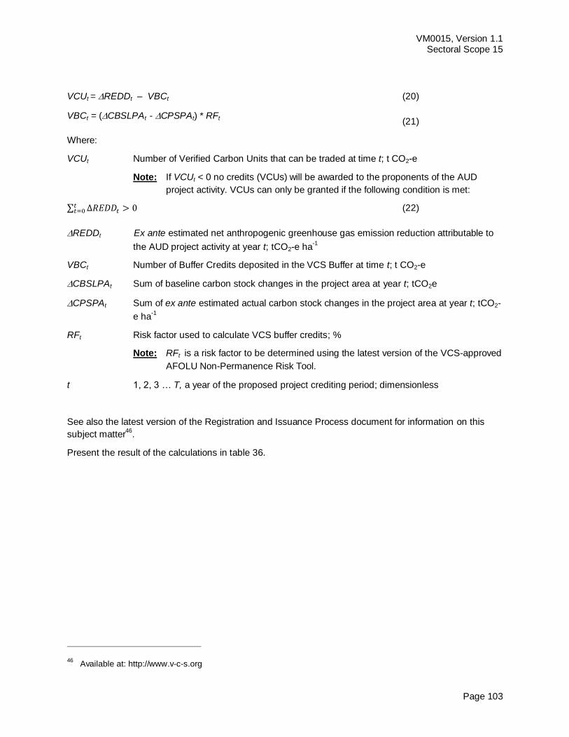
VM0015, Version 1.1 Sectoral Scope 15
Page 103
VCUt = REDDt – VBCt (20)
VBCt = ( CBSLPAt - CPSPAt) * RFt (21)
Where:
VCUt Number of Verified Carbon Units that can be traded at time t; t CO2-e
Note: If VCUt < 0 no credits (VCUs) will be awarded to the proponents of the AUD
project activity. VCUs can only be granted if the following condition is met:
∑ (22)
REDDt Ex ante estimated net anthropogenic greenhouse gas emission reduction attributable to
the AUD project activity at year t; tCO2-e ha-1
VBCt Number of Buffer Credits deposited in the VCS Buffer at time t; t CO2-e
CBSLPAt Sum of baseline carbon stock changes in the project area at year t; tCO2e
CPSPAt Sum of ex ante estimated actual carbon stock changes in the project area at year t; tCO2-
e ha-1
RFt Risk factor used to calculate VCS buffer credits; %
Note: RFt is a risk factor to be determined using the latest version of the VCS-approved
AFOLU Non-Permanence Risk Tool.
t 1, 2, 3 … T, a year of the proposed project crediting period; dimensionless
See also the latest version of the Registration and Issuance Process document for information on this
subject matter46
.
Present the result of the calculations in table 36.
46 Available at: http://www.v-c-s.org
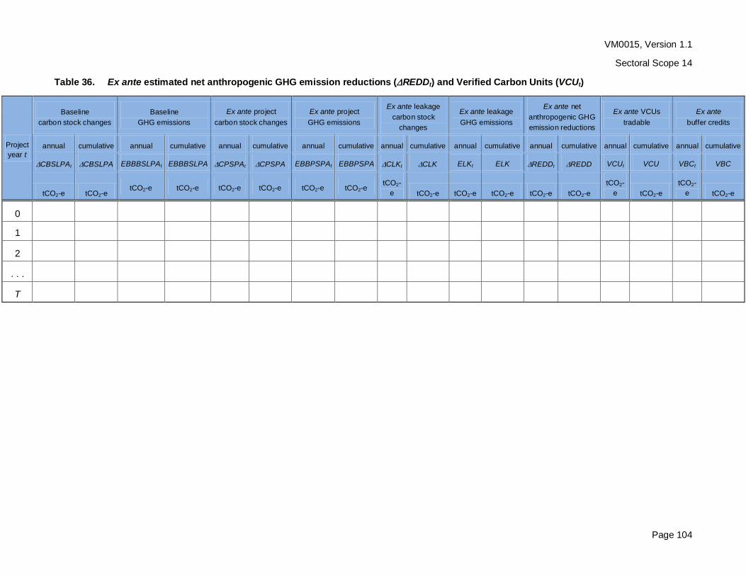
VM0015, Version 1.1
Sectoral Scope 14
Page 104
Table 36. Ex ante estimated net anthropogenic GHG emission reductions ( REDDt) and Verified Carbon Units (VCUt)
Project
year t
Baseline
carbon stock changes
Baseline
GHG emissions
Ex ante project
carbon stock changes
Ex ante project
GHG emissions
Ex ante leakage
carbon stock
changes
Ex ante leakage
GHG emissions
Ex ante net
anthropogenic GHG
emission reductions
Ex ante VCUs
tradable
Ex ante
buffer credits
annual cumulative annual cumulative annual cumulative annual cumulative annual cumulative annual cumulative annual cumulative annual cumulative annual cumulative
CBSLPAt CBSLPA EBBBSLPAt EBBBSLPA CPSPAt CPSPA EBBPSPAt EBBPSPA CLKt CLK ELKt ELK REDDt REDD VCUt VCU VBCt VBC
tCO2-e tCO2-e tCO2-e tCO2-e tCO2-e tCO2-e tCO2-e tCO2-e
tCO2-
e tCO2-e tCO2-e tCO2-e tCO2-e tCO2-e
tCO2-
e tCO2-e
tCO2-
e tCO2-e
0
1
2
. . .
T
VM0015, Version 1.1
Sectoral Scope 15
Page 105
PART 3 – METHODOLOGY FOR MONITORING AND RE-VALIDATION OF THE BASELINE
The ex post methodology (to be implemented immediately after project start) includes two main tasks:
1) Monitoring of carbon stock changes and GHG emissions for periodical verifications within the
fixed baseline period; and
2) Monitoring of key baseline parameters for revisiting the baseline at the end of the fixed baseline
period.
Appendix 6 provides an overview of the tables that should be prepared to report monitoring results.
TASK 1: MONITORING OF CARBON STOCK CHANGES AND GHG EMISSIONS 1
FOR PERIODICAL VERIFICATIONS
There are three main monitoring tasks:
1.1 Monitoring of actual carbon stock changes and GHG emissions within the project area;
1.2 Monitoring of leakage; and
1.3 Ex post calculation of net anthropogenic GHG emission reduction.
Prepare a Monitoring Plan describing how these tasks will be implemented. For each task the monitoring
plan must include the following sections:
a) Technical description of the monitoring tasks.
b) Data to be collected (see appendix 5).
c) Overview of data collection procedures.
d) Quality control and quality assurance procedures.
e) Data archiving.
f) Organization and responsibilities of the parties involved in all the above.
To allow a transparent comparison between ex ante and ex post estimates, use the same formats and
tables presented in Part 2 of the methodology to report the results of monitoring.
1.1 Monitoring of actual carbon stock changes and GHG emissions within the project
area
This task involves:
1.1.1 Monitoring of project implementation;
1.1.2 Monitoring of land-use and land-cover change;
1.1.3 Monitoring of carbon stocks and non-CO2 emissions; and
1.1.4 Monitoring of impacts of natural disturbances and other catastrophic events.

VM0015, Version 1.1 Sectoral Scope 15
Page 106
1.1.1 Monitoring of project implementation
Project activities implemented within the project area should be consistent with the management plans of
the project area and the PD. All maps and records generated during project implementation should be
conserved and made available to VCS verifiers at verification for inspection to demonstrate that the AUD
project activity has actually been implemented.
1.1.2 Monitoring of land-use and land-cover change within the project area
The categories of changes that may be subject to MRV are summarized in table 37.
Table 37. Categories subject to MRV
ID Type Conditions under which monitoring is mandatory
Explanations
I Area of forest land converted to non-forest land.
Mandatory in all AUD project activities
II Area of forest land undergoing carbon stock decrease.
Mandatory only for AUD project activities having planned logging, fuel-wood collection and charcoal production activities above the baseline.
Change in carbon stock must be significant according to ex ante assessment, otherwise monitoring is not required.
III Area of forest land undergoing carbon stock increase.
Mandatory only for AUD project activities wishing to claim carbon credits for carbon stock increase.
Increase must be significant according to ex ante assessment and can only be accounted on areas that will be deforested in the baseline case.
If the project area is located within a region subject to MRV by a jurisdictional program, the MRV data
generated by this program must be used.
Similarly, if the project area is located within a region that is subject to a monitoring program that is
approved or sanctioned by the national or sub-national government, the data generated by such program
must be used, unless they are not applicable according to the criteria listed below:
a) Monitoring occurs in the entire project area and, if the project must monitor a leakage belt, in the
leakage belt.
b) If data from the existing monitoring program are used to periodically revisit the baseline,
monitoring must occur in the entire reference region at least at the beginning, middle and end of
the fixed baseline period.
c) At least category I (table 37) is subject to monitoring (conversion of forest land to non-forest land).
d) It the project must do a monitoring of other categories (II and/or III) and these are not included in
the existing program, the existing program can only be used for monitoring category I, and the
project proponent must implement a separate monitoring program for category II and/or III.
e) Monitoring will occur during the entire fixed baseline period.
VM0015, Version 1.1 Sectoral Scope 15
Page 107
f) Monitoring methods are transparently documented and are similar to those used to determine the
baseline of the AUD project activity.
g) Monitoring protocols and data must be accessible for inspection by VCS accredited verifier.
If no existing monitoring program exist or can be used, monitoring must be done by the project proponent
or outsourced to a third party having sufficient capacities to perform the monitoring tasks. Methods used
to monitor LU/LC change categories and to assess accuracy must be similar to those explained in part 2,
step 2.4 and part 2, step 2.5, respectively.
The results of monitoring shall be reported by creating ex post tables of activity data per stratum (Tables
9.a, 9.b and 9.c); per initial forest class icl (Tables 11.a, 11.b and 11.c); per post-deforestation zone z
(Tables 13.a, 13.b and 13.c) and, where applicable, per category of land-use change ct (Tables 14.a,
14.b and 14.c).or ctz (Tables 19.a, 19.b and 19.c).
1.1.3 Monitoring of carbon stock changes and non-CO2 emissions from forest fires
Monitoring of carbon stock changes
In most cases, the ex ante estimated average carbon stocks per LU/LC class (or carbon stock change
factors per LU/LC change category) will not change during a fixed baseline period and monitoring of
carbon stocks will not be necessary.
However, monitoring of carbon stocks is mandatory in the following cases:
Within the project area:
a) Areas subject to significant carbon stock decrease in the project scenario according to the ex
ante assessment. These will be areas subject to controlled deforestation and planned harvest
activities, such as logging, fuel wood collection and charcoal production. In these areas, carbon
stock changes must be estimated at least once after each harvest event.
b) Areas subject to unplanned and significant carbon stock decrease, e.g. due to uncontrolled forest
fires and other catastrophic events. In these areas, carbon stock losses must be estimated as
soon as possible after the catastrophic event. See section 1.1.4 below for more detailed
guidance.
Within leakage management areas:
a) Areas subject to planned and significant carbon stock decrease in the project scenario according
to the ex ante assessment. In these areas, carbon stocks must be estimated at least once after
the planned event that caused the carbon stock decrease.
Monitoring of carbon stocks is optional in the following cases:
Within the project area:
a) Areas subject to carbon stock increase after planned harvest activities, such as logging, fuel
wood collection and charcoal production. In these areas, the carbon stock increase occurring
after the harvest event can be measured and accounted, when significant.
b) Areas recovering after disturbances, such unplanned forest fires and other catastrophic events. In
these areas, the carbon stock increase occurring after the catastrophic event can be measured
and accounted, when significant. See section 1.1.4 below for more detailed guidance.
Within leakage management areas:
VM0015, Version 1.1 Sectoral Scope 15
Page 108
a) Areas subject to carbon stock increase due to leakage prevention measures. In these areas, the
carbon stock increase can be measured and accounted only up to the amount necessary to offset
any carbon stock decrease caused by leakage prevention measures in other leakage
management areas or in previous years.
Within the leakage belt:
a) Areas undergoing significant changes in carbon stock may be measured at the end of each fixed
baseline period in order to update carbon stock information for the subsequent period.
Where carbon stocks are monitored, the methods on sampling and measuring carbon stocks described in
appendix 3 must be used.
Some project proponents may wish to do additional carbon stock measurements during project
implementation to gain accuracy and credits. If new and more accurate carbon stock data become
available, these can be used to estimate the net anthropogenic GHG emission reduction of the
subsequent fixed baseline period. For the current fixed baseline period, new data on carbon stocks can
only be used if they are validated by an accredited VCS verifier. If new data are used in the current fixed
baseline period, the baseline must be recalculated using the new data.
The results of monitoring activity data and carbon stocks must be reported using the same formats and
tables used for the ex ante assessment:
Table 15 Ex post carbon stock per hectare of initial forest classes icl existing in the project area
and leakage belt
Table 16 Ex post carbon stock per hectare of initial final classes fcl existing in the project area and
leakage belt
Table 25.a Ex post carbon stock decrease due to planned and unplanned deforestation in the project
area.
Table 25.b Ex post carbon stock decrease due to planned logging activities.
Table 25.c Ex post carbon stock decrease due to planned fuel-wood and charcoal activities.
Table 25.d Total ex post carbon stock decrease due to planned activities in the project area.
Table 25.e Ex post carbon stock decrease due to forest fires (see below).
Table 25.f Ex post carbon stock decrease due to catastrophic events (see below and section 1.1.4).
Table 25.g Total ex post carbon stock decrease due to forest fires and catastrophic events (see
below)
Table 26.a Ex post carbon stock increase due to growth without harvest.
Table 26.b Ex post carbon stock increase following planned logging activities.
Table 26.c Ex post carbon stock increase following planned fuel-wood and charcoal activities.
Table 26.d Total ex post carbon stock increase due to planned activities in the project area.
Table 26.e Ex post carbon stock increase on areas affected by forest fires (see below).
Table 26.f Ex post carbon stock increase on areas affected by catastrophic events (see below and
section 1.1.4).
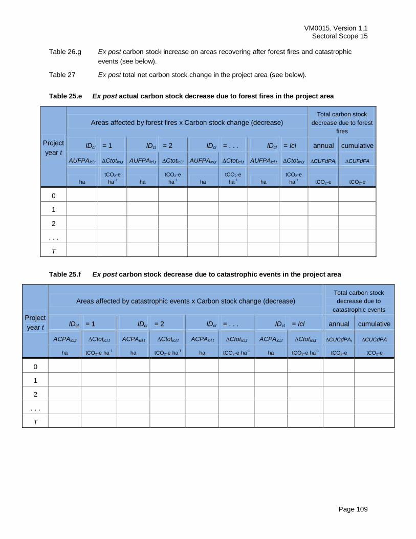
VM0015, Version 1.1 Sectoral Scope 15
Page 109
Table 26.g Ex post carbon stock increase on areas recovering after forest fires and catastrophic
events (see below).
Table 27 Ex post total net carbon stock change in the project area (see below).
Table 25.e Ex post actual carbon stock decrease due to forest fires in the project area
Project
year t
Areas affected by forest fires x Carbon stock change (decrease)
Total carbon stock
decrease due to forest
fires
IDcl = 1 IDcl = 2 IDcl = . . . IDcl = Icl annual cumulative
AUFPAicl,t Ctoticl,t AUFPAicl,t Ctoticl,t AUFPAicl,t Ctoticl,t AUFPAicl,t Ctoticl,t CUFdPAt CUFdFA
ha
tCO2-e
ha-1
ha
tCO2-e
ha-1
ha
tCO2-e
ha-1
ha
tCO2-e
ha-1
tCO2-e tCO2-e
0
1
2
. . .
T
Table 25.f Ex post carbon stock decrease due to catastrophic events in the project area
Project
year t
Areas affected by catastrophic events x Carbon stock change (decrease)
Total carbon stock
decrease due to
catastrophic events
IDcl = 1 IDcl = 2 IDcl = . . . IDcl = Icl annual cumulative
ACPAicl,t Ctoticl,t ACPAicl,t Ctoticl,t ACPAicl,t Ctoticl,t ACPAicl,t Ctoticl,t CUCdPAt CUCdPA
ha tCO2-e ha-1
ha tCO2-e ha-1
ha tCO2-e ha-1
ha tCO2-e ha-1
tCO2-e tCO2-e
0
1
2
. . .
T
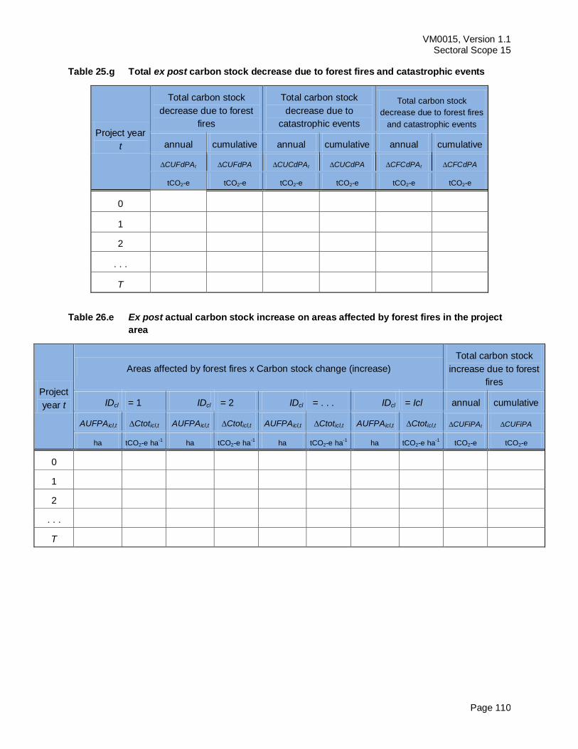
VM0015, Version 1.1 Sectoral Scope 15
Page 110
Table 25.g Total ex post carbon stock decrease due to forest fires and catastrophic events
Project year
t
Total carbon stock
decrease due to forest
fires
Total carbon stock
decrease due to
catastrophic events
Total carbon stock
decrease due to forest fires
and catastrophic events
annual cumulative annual cumulative annual cumulative
CUFdPAt CUFdPA CUCdPAt CUCdPA CFCdPAt CFCdPA
tCO2-e tCO2-e tCO2-e tCO2-e tCO2-e tCO2-e
0
1
2
. . .
T
Table 26.e Ex post actual carbon stock increase on areas affected by forest fires in the project
area
Project
year t
Areas affected by forest fires x Carbon stock change (increase)
Total carbon stock
increase due to forest
fires
IDcl = 1 IDcl = 2 IDcl = . . . IDcl = Icl annual cumulative
AUFPAicl,t Ctoticl,t AUFPAicl,t Ctoticl,t AUFPAicl,t Ctoticl,t AUFPAicl,t Ctoticl,t CUFiPAt CUFiPA
ha tCO2-e ha-1
ha tCO2-e ha-1
ha tCO2-e ha-1
ha tCO2-e ha-1
tCO2-e tCO2-e
0
1
2
. . .
T
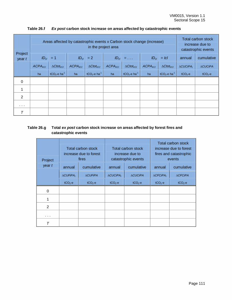
VM0015, Version 1.1 Sectoral Scope 15
Page 111
Table 26.f Ex post carbon stock increase on areas affected by catastrophic events
Project
year t
Areas affected by catastrophic events x Carbon stock change (increase)
in the project area
Total carbon stock
increase due to
catastrophic events
IDcl = 1 IDcl = 2 IDcl = . . . IDcl = Icl annual cumulative
ACPAicl,t Ctoticl,t ACPAicl,t Ctoticl,t ACPAicl,t Ctoticl,t ACPAicl,t Ctoticl,t CUCiPAt CUCiPA
ha tCO2-e ha-1
ha tCO2-e ha-1
ha tCO2-e ha-1
ha tCO2-e ha-1
tCO2-e tCO2-e
0
1
2
. . .
T
Table 26.g Total ex post carbon stock increase on areas affected by forest fires and
catastrophic events
Project
year t
Total carbon stock
increase due to forest
fires
Total carbon stock
increase due to
catastrophic events
Total carbon stock
increase due to forest
fires and catastrophic
events
annual cumulative annual cumulative annual cumulative
CUFiPAt CUFiPA CUCiPAt CUCiPA CFCiPAt CFCiPA
tCO2-e tCO2-e tCO2-e tCO2-e tCO2-e tCO2-e
0
1
2
. . .
T
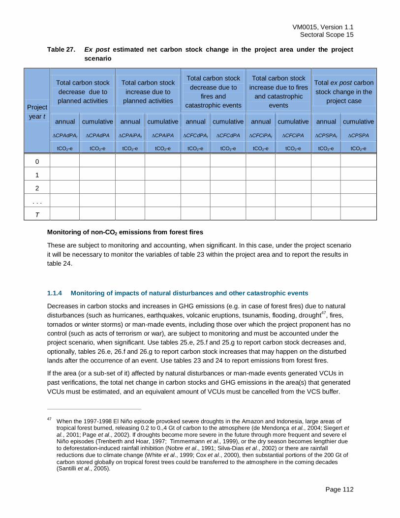
VM0015, Version 1.1 Sectoral Scope 15
Page 112
Table 27. Ex post estimated net carbon stock change in the project area under the project
scenario
Project
year t
Total carbon stock
decrease due to
planned activities
Total carbon stock
increase due to
planned activities
Total carbon stock
decrease due to
fires and
catastrophic events
Total carbon stock
increase due to fires
and catastrophic
events
Total ex post carbon
stock change in the
project case
annual cumulative annual cumulative annual cumulative annual cumulative annual cumulative
CPAdPAt CPAdPA CPAiPAt CPAiPA CFCdPAt CFCdPA CFCiPAt CFCiPA CPSPAt CPSPA
tCO2-e tCO2-e tCO2-e tCO2-e tCO2-e tCO2-e tCO2-e tCO2-e tCO2-e tCO2-e
0
1
2
. . .
T
Monitoring of non-CO2 emissions from forest fires
These are subject to monitoring and accounting, when significant. In this case, under the project scenario
it will be necessary to monitor the variables of table 23 within the project area and to report the results in
table 24.
1.1.4 Monitoring of impacts of natural disturbances and other catastrophic events
Decreases in carbon stocks and increases in GHG emissions (e.g. in case of forest fires) due to natural
disturbances (such as hurricanes, earthquakes, volcanic eruptions, tsunamis, flooding, drought47
, fires,
tornados or winter storms) or man-made events, including those over which the project proponent has no
control (such as acts of terrorism or war), are subject to monitoring and must be accounted under the
project scenario, when significant. Use tables 25.e, 25.f and 25.g to report carbon stock decreases and,
optionally, tables 26.e, 26.f and 26.g to report carbon stock increases that may happen on the disturbed
lands after the occurrence of an event. Use tables 23 and 24 to report emissions from forest fires.
If the area (or a sub-set of it) affected by natural disturbances or man-made events generated VCUs in
past verifications, the total net change in carbon stocks and GHG emissions in the area(s) that generated
VCUs must be estimated, and an equivalent amount of VCUs must be cancelled from the VCS buffer.
47 When the 1997-1998 El Niño episode provoked severe droughts in the Amazon and Indonesia, large areas of
tropical forest burned, releasing 0.2 to 0.,4 Gt of carbon to the atmosphere (de Mendonça et al., 2004; Siegert et al., 2001; Page et al., 2002). If droughts become more severe in the future through more frequent and severe el Niño episodes (Trenberth and Hoar, 1997; Timmermann et al., 1999), or the dry season becomes lengthier due to deforestation-induced rainfall inhibition (Nobre et al., 1991; Silva-Dias et al., 2002) or there are rainfall reductions due to climate change (White et al., 1999; Cox et al., 2000), then substantial portions of the 200 Gt of
carbon stored globally on tropical forest trees could be transferred to the atmosphere in the coming decades (Santilli et al., 2005).

VM0015, Version 1.1 Sectoral Scope 15
Page 113
No VCUs can be issued to the project until all carbon stock losses and increases in GHG emissions have
been offset, i.e. until the following condition is satisfied:
∑ (23)
Where:
REDDt Ex post estimated net anthropogenic greenhouse gas emission reduction attributable to
the AUD project activity at year t; tCO2e
t 1, 2, 3 … T, a year of the proposed project crediting period; dimensionless
1.1.5 Total ex post estimated actual net carbon stock changes and GHG emissions in the
project area
Summarize the results of all ex post estimations in the project area using the same table format used for
the ex ante assessment:
Table 29: Total ex post estimated actual net changes in carbon stocks and emissions of GHG gases
in the project area.
1.2 Monitoring of leakage
Monitoring of leakage may not be required if the project area is located within a jurisdiction that is
monitoring, reporting, verifying and accounting GHG emissions from deforestation under a VCS or
UNFCCC registered (and VCS endorsed) program. In such cases, the most recent VCS JNR
Requirements shall be applied.
In all other circumstances, the sources of leakage identified as significant in the ex ante assessment are
subject to monitoring. Two sources of leakage are potentially subject to monitoring:
1.2.1 Decrease in carbon stocks and increase in GHG emissions associated with leakage
prevention activities;
1.2.2 Decrease in carbon stocks and increase in GHG emissions in due to activity displacement
leakage.
1.2.1 Monitoring of carbon stock changes and GHG emissions associated to leakage prevention
activities
Monitoring of the sources of emissions associated with leakage prevention activities must follow the
methods and tools described in part 2, step 8.1 of the methodology.
Results must be reported using the same formats and tables used in the ex ante assessment:
Table 30.b Ex post carbon stock change in leakage management areas.
Table 30.c Ex post net carbon stock change in leakage management areas48
.
48 Calculations of total net carbon stock changes in Leakage Management Areas use the ex ante estimated baseline
carbon stock changes in the Leakage Management Area and the measured ex post carbon stock changes. If the
cumulative value of the carbon stock change within a Fixed Baseline Period is > 0, CLPMLKt shall be set to zero.
VM0015, Version 1.1 Sectoral Scope 15
Page 114
Table 31 Ex post parameters for estimating GHG emissions from grazing activities
Table 32 Ex post estimation of emissions from grazing animals in leakage management areas.
Table 33 Ex post estimation of net carbon stock changes and GHG emissions from leakage
prevention activities.
1.2.2 Monitoring of carbon stock decrease and increases in GHG emissions due to activity
displacement leakage
Monitoring of carbon stock changes
Deforestation above the baseline in the leakage belt area will be considered activity displacement
leakage.
Activity data for the leakage belt area must be determined using the same methods applied to monitoring
deforestation activity data (category I, table 37) in the project area. Monitoring of the categories II and III
outside the project area is not required because no credits are claimed for avoided degradation under this
methodology.
The result of the ex post estimations of carbon stock changes must be reported using the same table
formats used in the ex ante assessment of baseline carbon stock changes in the leakage belt.
Table 21.c Ex post total net carbon stock changes in the leakage belt (when using method 1 based on
activity data per class).
or
Table 22.c Ex post total net carbon stock changes in the leakage belt (when using method 2 based on
activity data per category).
Leakage will be calculated as the difference between the ex ante and the ex post assessment. Report the
results in table 21.d

VM0015, Version 1.1 Sectoral Scope 15
Page 115
Table 21.d. Total net baseline carbon stock change in the leakage belt
(Calculated with Method 1: Activity data per class)
Project
year t
Total ex ante net baseline
carbon stock change
Total ex post net actual
carbon stock change Total ex post leakage
annual cumulative annual cumulative annual cumulative
CBSLLKt CBSLLK CBSLLKt CBSLLK CBSLLKt CBSLLK
tCO2-e tCO2-e tCO2-e tCO2-e tCO2-e tCO2-e
0
1
2
. . .
T
Where strong evidence can be collected that deforestation in the leakage belt is attributable to
deforestation agents that are not linked to the project area, the detected deforestation may not be
attributed to the project activity and considered leakage. The operational entity verifying the monitoring
data shall determine whether the documentation provided by the project proponent represents sufficient
evidence to consider the detected deforestation as not attributable to the project activity and therefore not
leakage.
Monitoring of increases in GHG emissions
These must only be estimated and accounted if emissions from forest fires are included in the baseline.
To estimate the increased GHG emissions due to forest fires in the leakage belt area the assumption is
made that forest clearing is done by burning the forest. The parameter values used to estimate emissions
shall be the same used for estimating forest fires in the baseline (table 23), except for the initial carbon
stocks (Cab, Cdw) which shall be those of the initial forest classes burned in the leakage belt area.
Report the result of the estimations using the same table formats used in the ex ante assessment of
baseline GHG emissions from forest fires in the project area:
Table 23: Parameters used to calculate emissions from forest fires in the leakage belt area
Table 24: Ex post estimated non-CO2 emissions from forest fires in the leakage belt area
1.2.3 Total ex post estimated leakage
Summarize the results of all ex post estimations of leakage using the same table format used for the ex
ante assessment:
Table 35. Total ex post estimated leakage.
Note: Monitoring of leakage may become obsolete at the date when a VCS or UNFCCC registered (and
VCS endorsed) program is monitoring, reporting, verifying and accounting GHG emissions from
VM0015, Version 1.1 Sectoral Scope 15
Page 116
deforestation in a broader region encompassing the project area. In such cases, the most recent
VCS guidelines on this subject matter shall be applied.
1.3 Ex post net anthropogenic GHG emission reductions
The calculation of ex post net anthropogenic GHG emission reductions is similar to the ex ante
calculation with the only difference that ex post estimated carbon stock changes and GHG emissions
must be used in the case of the project scenario and leakage.
Report the ex post estimated net anthropogenic GHG emissions and calculation of Verified Carbon Units
(VCUt, and VBCt) using the same table format used for the ex ante assessment:
Table 36: Ex post estimated net anthropogenic GHG emission reductions and VCUs.
Note: A map showing Cumulative Areas Credited within the project area shall be updated and
presented to VCS verifiers at each verification event. The cumulative area cannot generate
additional VCUs in future periods.
TASK 2: REVISITING THE BASELINE PROJECTIONS FOR FUTURE FIXED 2
BASELINE PERIOD
Baselines, independently from the approach chosen to establish them, must be revisited over time
because agents, drivers and underlying causes of deforestation change dynamically. Frequent and
unpredicted updating of the baseline can create serious market uncertainties. Therefore, the baseline
must be revisited only every 10 years. Where an applicable sub-national or national jurisdictional baseline
becomes available, baselines may be reassessed earlier in accordance with section 2.2 below. Tasks
involved in revisiting the baseline are:
2.1 Update information on agents, drivers and underlying causes of deforestation.
2.2 Adjust the land-use and land-cover change component of the baseline.
2.3 Adjust, as needed, the carbon component of the baseline.
2.1 Update information on agents, drivers and underlying causes of deforestation
Information on agents, drivers and underlying causes of deforestation in the reference region must be
collected periodically, as these are essential for improving future deforestation projections and the design
of the project activity.
Collect information that is relevant to understand deforestation agents, drivers and underlying
causes.
Redo step 3 of the ex ante methodology at the beginning of each fixed baseline period.
Where a spatial model was used to locate future deforestation, new data on the spatial driver
variables used to model the deforestation risk must be collected as they become available. These
must be used to create updated spatial datasets and new “Factor Maps” for the subsequent fixed
baseline period.
VM0015, Version 1.1 Sectoral Scope 15
Page 117
2.2 Adjustment of the land-use and land-cover change component of the baseline
If an applicable sub-national or national baseline becomes available during the fixed baseline period, it
must be used for the subsequent period. Use the criteria of table 2 to assess the applicability of sub-
national or national baselines. If VCS requirements on regional baselines are available, use the most
recent version of these guidelines instead of table 2.
If an applicable sub-national or national baseline is not available, the baseline projections must be
revisited and adjusted as necessary.
The two components of the baseline projections that must be reassessed are:
2.2.1 The annual areas of baseline deforestation; and
2.2.2 The location of baseline deforestation.
2.2.1 Adjustment of the annual areas of baseline deforestation
At the end of each fixed baseline period, the projected annual areas of baseline deforestation for the
reference region need to be revisited and eventually adjusted for the subsequent fixed baseline period.
The adjusted baseline rates must be submitted to an independent validation.
Adjustments must be made using the methods described in part 2 of the methodology and using the data
obtained from monitoring LU/LC changes in the reference region during the past fixed baseline period,
updated information on deforestation agents, drivers and underlying cases of deforestation and, where
applicable, any updated information on the variables included in the estimation of the projected areas of
baseline deforestation.
2.2.2 Adjustment of the location of the projected baseline deforestation
Using the adjusted projections for annual areas of baseline deforestation and any improved spatial data
for the creation of the factor maps included in the spatial model, the location of the projected baseline
deforestation must be reassessed using the methods explained in part 2 of the methodology.
All areas credited for avoided deforestation in past fixed baseline periods must be excluded from the
revisited baseline projections as these areas cannot be credited again. To perform this exclusion use the
map of “cumulative areas credited” that was updated in all previous verification events.
Note: If the boundary of the leakage belt area was assessed using equation (1) or any other spatial
model, the boundary of the leakage belt will have to be reassessed at the end of each fixed
baseline period using the same methodological approaches used in the first period. This will be
required until monitoring of leakage will become unnecessary49
.
2.3 Adjustment of the carbon component of the baseline
Adjusting the carbon component of the baseline will not be necessary in most cases (see section 1.1.3 in
Part 3 for more detailed guidance). However, improved carbon stock data are likely to become available
over time and if this is the case, they must be used when revisiting the baseline projections. Methods to
measure and estimate carbon stocks are described in appendix 3.
49 Monitoring of leakage will become obsolete at the date when a VCS or UNFCCC registered (and VCS endorsed)
program is monitoring, reporting, verifying and accounting emissions from deforestation in a broader area
encompassing the project area.
VM0015, Version 1.1 Sectoral Scope 15
Page 118
LITERATURE CITED
Achard et al., 2004. Presentation at UNFCCC Workshop in Rome on Reducing emissions from
deforestation.
Achard, F., H. D. Eva, H. J. Stibig, P. Mayaux, J. Gallego, T. Richards, and J. P. Malingreau, 2002.
Determination of deforestation rates of the world’s humid tropical forests, Science, 297:999-1002
Angelsen, A. and D. Kaimowitz, 1999. Rethinking the causes of deforestation: lessons from economic
models. The world Bank Research Observer, Vol. 14, No.1
Brown, S. 1997. Estimating Biomass and Biomass Change of Tropical Forests: A primer. FAO Forestry
Paper 134, UN FAO, Rome.
Brown, S. and A. Dushku, 2003. Spatial modeling for LULUCF carbon projects: the GEOMOD modeling
approach. 2003 International Conference on Tropical Forests and Climate Change: “Carbon
Sequestration and the Clean Development mechanism”, Manila – October 21. 13 p.
Brown, S., M. Hall, K. Andrasko, F. Ruiz, W. Marzoli, G. Guerrero, O. Masera, A. Dushku, B. DeJong, and
J. Cornell, 2007. Baselines for land-use change in the tropics: application to avoided deforestation
projects. Mitigation and Adaptation Strategies for Climate Change, 12:1001-1026
Castillo-Santiago, G. Hellier et al. 2007. Carbon emissions from land-use change: a regional analysis of
causal factors in Chiapas, México. Mitigation Adaptation Strategies Global Change, 12 (6):
Chomitz, K. M., P. Buys, C. De Luca, T. S. Thomas, and S. Wertz-Kanounnikoff, 2006. At loggerheads?
Agricultural Expansion, Poverty Reduction, and Environment in the Tropical Forests. World Bank
Policy Research Report. 308 pp.
Cox, P. M., R. A. Betts, C. D. Jones, S. A. Spall, and I. J. Totterdell, 2000. Acceleration of global warming
due to carbon-cycle feedbacks in a coupled climate model. Nature, 408:184-187
De Jong, B. H. J., A. Hellier, M. A. Castillo-Santiago, and R. Tipper, 2005. Application of the ‘Climafor’
approach to estimate baseline carbon emissions of a forest conservation project in the La Selva
Lacandona, Chiapas, Mexico. Mitigation and Adaptation Strategies for Global Change, 10:265-278
De Jong, B. H. J. and E. Esquivel Bazán, 2007. Application of the “Climafor” baseline to determine
leakage: the case of Scolel Té
De Mendonça M. J. C. , M. C. del Vera Diaz, D. C. Nepsad, R. Seroa da Motta, A. Alentar, J. C. Gomes,
and R. A. Ortiz, 2004. The economic cost of the use of fire in Amazon. Ecol. Econ. 49:89-105.
DeFries R. S., R. A. Houghton, M. C. Hansen, C. B. Field, D. Skole, and J. Townshend, 2002. Carbon
emissions from tropical deforestation and regrowth based on satellite observations for the 1980s
and 1990s, PNAS, 99: 14256-14261.
Figueroa, B., M. Kanninen, B. Louman, L. Pedroni, and M. Gómez, 2004. Contenido de carbono en los
productos y residuos forestales generados por el aprovechamiento y el aserrío en la reserva de
Biosfera Maya . Recursos Naturales y Ambiente, 2004: 102-110.
Freese, F. 1962. Elementary Forest Sampling. USDA Handbook 232. GPO Washington, DC. 91 pp
Gillespie, A. J. R, S. Brown, and A. E. Lugo. 1992. Tropical forest biomass estimation from truncated
stand tables. Forest Ecology and Management, 48:69-88.
VM0015, Version 1.1 Sectoral Scope 15
Page 119
GOFC-GOLD, 2010, A sourcebook of methods and procedures for monitoring and reporting
anthropogenic greenhouse gas emissions and removals caused by deforestation, gains and losses
of carbon stocks in forests remaining forests and forestation.,– available at: http://www.gofc-
gold.uni-jena.de/REDD/
Houghton R. A., 2006. Presentation at the UNFCCC Rome workshop on Reducing emissions from
deforestation.
Houghton, R.A., 2005, Aboveground forest biomass and the global carbon balance. Global Change
Biology 11(6), 945-958.
Intergovernmental Panel on Climate Change, 1996. IPCC Guidelines for National Greenhouse Gas
Inventories.
Intergovernmental Panel on Climate Change, 2003. Good Practice Guidance for Land Use, Land Use-
Change, and Forestry.
Intergovernmental Panel on Climate Change, 2006. Guidelines for National Greenhouse Gas Inventories,
Volume 4, Agriculture, Forestry and Other land Uses
Intergovernmental Panel on Climate Change, 2007. Climate Change 2007, Physical Science basis.
Lesschen, J. P., P. H. Verburg, and S. J. Staal, 2005. Statistical methods for analyzing the spatial
dimension of changes in land use and farming systems. LUCC Report series No. 7, International
Livestock Research Institute (Nairobi, Kenya) and Wageningen University (the Netherlands), 80 p.
(http://home.medewerker.uva.nl/j.p.lesschen/bestanden/LUCC%20report%207.pdf)
Loetsch, F. and Haller, K. 1964. Forest Inventory. Volume 1. BLV-VERLAGS GESE LLSCHAFT,
München.
Malhi Y., T. Naker, O. L. Phillips, S. Almeida, E. Alvarez, L. Arroyo, J. Chave, C. I. Czimezik, A. DiFiore,
N. Higuchi, T.J. Killeen, S. G. Laurance, W. F. Lewis, L. M. M. Montoya, A. Monteagudo, D. A. Neill,
P.N. Vargas, S. Patina, N.C.A. Pitman, C. A. Quesada, J. N. M. Silva, A. T. Lezama, R. V.
Martinez, J. Terborgh, B. Vinceti, and J. Lloyd, 2004. The above-ground wood productivity and net
primary productivity of 100 Neotropical forest plots. Global Change Biol., 10:563-591.
Nobre C. A., P. Sellers, and J. Shukla, 1991. Regional climate change and Amazonian deforestation
model. J. Clim. 4:957-988.
Olander L. P., B. C. Murry, H. Gibbs, and M. Steininger, 2006. Establishing credible national baselines for
efforts to reduce emissions from degradation and deforestation. Coalition for Rainforest Nations.
Page S. E., F. Siegert, J. O. Rieley, V. Boehm Hans-Dieter, A. Jaya, and S. Lenin, 2002. The amount of
carbon released from peat and forest fires in Indonesia during 1997. Nature, 420: 61-65.
Pearson T., S. Walker and S. Brown. 2005. Sourcebook for Land Use, Land Use Change and Forestry
Projects. BioCarbon Fund (World Bank) and Winrock International, Washington D.C., p. 64
Pontius, R.G. Jr., S. Peethambaram, and J-C Castella, 2011. Comparison of three maps at Multiple
Resolutions: a case study of land change simulation in Cho Don District, Vietnan. Annals of the
Association of American Geographers, 101 (1): 45-62.
Pontius, R. G. Jr. and H. Chen, 2006. GEOMOD Modeling. Clark University.
VM0015, Version 1.1 Sectoral Scope 15
Page 120
Pontius, R. G. Jr., 2002. Statistical methods to partition effects of quantity and location during comparison
of categorical maps at multiple resolutions. Photogrammetric Engineering and Remote Sensing, 68
(1):1041-1049
Pontius, R. G., J. D. Cornell, C. A. S. Hall, 2001. Modeling the spatial pattern of land-use change within
GEOMOD2: application and validation in Costa Rica. Agriculture, Ecosystems and Environment:
85, 191-203.
Pontius, R. G., Jr., 2000. Quantification error versus location error in comparison of categorical maps.
Photogrammetric Engineering and Remote Sensing, 66:1011-1016
Pontius, R. G., Jr, W Boersma, J-C Castella, K Clarke, T de Nijs, C Dietzel, Z Duan, E Fotsing, N
Goldstein, K Kok, E Koomen, C D Lippitt, W McConnell, A Mohd Sood, B Pijanowski, S Pithadia, S
Sweeney, T N Trung, A T Veldkamp, and P H Verburg. 2008. Comparing input, output, and
validation maps for several models of land change. Annals of Regional Science, 42(1): 11-47.
Pontius, R G, Jr, R Walker, R Yao-Kumah, E Arima, S Aldrich, M Caldas and D Vergara. 2007. Accuracy
assessment for a simulation model of Amazonian deforestation. Annals of Association of American
Geographers, 97(4): 677-695
Puyravaud, J.-P., 2003. Standardizing the calculation of the annual rate of deforestation. Forest Ecology
and Management, 177: 593-596.
Reyes et al., 1992. Wood densities of tropical tree species. USDA
Santilli M., P. Moutinho, S. Schwartzman, D. Nepstad, L. Curran and C. Norbe, 2005. Tropical
deforestation and the Kyoto Protocol, and editorial essay. Climatic Change, 71:267-276.
Sathaye, J. A. and K. Andrasko, 2007. Land use change and forestry climate project regional baselines: a
review. Mitigation and Adaptation Strategies for Global Change, 12:971-1000.
Schlamandinger, B., H. Carlens, N. Bird, I. Emmer, J. F. Garcia-Quijano, L. F. Jara, B. Muys, C. Robledo,
A. Stilma, and T. Tennigkeit, 2006. Guiding principles for including avoidance of emission from
deforestation, forest degradation and devegetation (DDD) in the international response to climate
change. Submission by the ENCOFOR project team www.joanneum.at/encofor. See also
Submission to the UNFCCC/SBSTA/2006/L.25
Siegert F., G. Ruecker, A. Hinrichs, and A. A. Hoffmann, 2001. Increased damage from fires in logged
forests during droughts caused by El Niño. Nature, 414 : 437-440.
Sierra, C.A. et al., 2007. Total carbon stocks in a tropical forest landscape of the Porce region, Colombia.
Forest Ecology and Management, 243: 299-309.
Silva-Dias M. A. F., S. Rutledge, P. Kabat, P. L. Silva-Dias, C. Nobre, G. Fisch, A. J. Dolman, E. Zipser,
M. Garstang, A. O. Manzi, J. D. Fuentes, H. R. Rocha, J. Marengo, A. Plana-Fattori, L. D. A. Sa, R.
C. S. Alvala, M. O. Andreae, P. Artaxo, R. Gielow, and L. Gatti, 2002. Clouds and rain processes in
a biosphere atmosphere interaction context in the Amazon Region. J. Geophys. Res.-Atmos.,
107:8072-8092.
Smith, Diana, 1954. Maximum moisture content method for determining specific gravity of small wood
samples. Forest Products Laboratory, Forest Service, U.S. Department of Agriculture. 9 pp.
Soares-Filho, B. S., D. C. Nepstad, L. M. Curran, G. C. Cerqueira, R. A. Garcia, C. A. Ramos, E. Voll, A.
McDonald, P. Lefevre, and P. Schlesinger, 2006. Modeling conservation in the Amazon basin.
Nature, 440: 520-523.
VM0015, Version 1.1 Sectoral Scope 15
Page 121
Timmermann A., J. Oberhuber, A. Bacher, M. Esch, M. Latif, and E. Roeckner, 1999. Increased El Niño
frequency in a climate model forced by future greenhouse warming. Geophys. Res. Lett. 24:3057-
3060.
Trenberth K. E. and T. J. Hoar, 1997. El Niño and Climate Change. Geophys. Res. Lett. 24: 3057-3060.
“Voluntary Carbon Standard – Guidance for Agriculture, Forestry and Other Land Use Projects (VCS
2007.1, 2008).” VCS Association. Available at: www.v-c-s.org
Wenger, K.F. (ed). 1984. Forestry handbook (2nd edition). New York: John Wiley and Sons.
White A. M., G. R. Cannell, and A. D. Friend, 1999. Climate change impacts on ecosystems and the
terrestrial carbon sink: a new assessment. Global Environ. Change, 9 (Suppl. 1): S21-S30.
Winjum, J.K., Brown, S. and Schlamadinger, B. 1998. Forest harvests and wood products: sources and
sinks of atmospheric carbon dioxide. Forest Science 44: 272-284
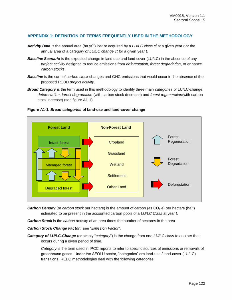
VM0015, Version 1.1 Sectoral Scope 15
Page 122
APPENDIX 1: DEFINITION OF TERMS FREQUENTLY USED IN THE METHODOLOGY
Activity Data is the annual area (ha yr-1
) lost or acquired by a LU/LC class cl at a given year t or the
annual area of a category of LU/LC change ct for a given year t.
Baseline Scenario is the expected change in land use and land cover (LU/LC) in the absence of any
project activity designed to reduce emissions from deforestation, forest degradation, or enhance
carbon stocks.
Baseline is the sum of carbon stock changes and GHG emissions that would occur in the absence of the
proposed REDD project activity.
Broad Category is the term used in this methodology to identify three main categories of LU/LC-change:
deforestation, forest degradation (with carbon stock decrease) and forest regeneration(with carbon
stock increase) (see figure A1-1):
Figure A1-1. Broad categories of land-use and land-cover change
Carbon Density (or carbon stock per hectare) is the amount of carbon (as CO2-e) per hectare (ha-1
)
estimated to be present in the accounted carbon pools of a LU/LC Class at year t.
Carbon Stock is the carbon density of an area times the number of hectares in the area.
Carbon Stock Change Factor: see “Emission Factor”.
Category of LU/LC-Change (or simply “category”) is the change from one LU/LC class to another that
occurs during a given period of time.
Category is the term used in IPCC reports to refer to specific sources of emissions or removals of
greenhouse gases. Under the AFOLU sector, “categories” are land-use / land-cover (LU/LC)
transitions. REDD methodologies deal with the following categories:
Intact forest Cropland
Grassland
Wetland
Settlement
Other Land
Forest Land Non-Forest Land
Forest
Regeneration
Forest
Degradation
Deforestation Degraded forest
Managed forest
VM0015, Version 1.1 Sectoral Scope 15
Page 123
(a) Forest Land to Forest Land (degradation and regeneration of forest land remaining
forest land)
(b) Forest Land to Crop Land (deforestation followed by agriculture)
(c) Forest Land to Grass Land (deforestation followed by pasture)
(d) Forest Land to Settlements (deforestation followed by settlements)
(e) Forest Land to Wetlands (deforestation followed by wetlands)
(f) Forest Land to Other Land (deforestation followed by other land)
Activities that convert non forest land back to forest (Crop Land to Forest Land, Grass Land to
Forest Land, etc.) are considered afforestation and reforestation and are excluded from this
REDD methodology.
Class. See LU/LC Class.
Deforestation is the direct, human-induced and long-term (or permanent) conversion of forest land to
non-forest land50
. It occurs when at least one of the parameter values used to define “forest land”
is reduced from above the threshold for defining “forest” to below this threshold for a period of
time that is longer than the period of time used to define “temporarily un-stocked”51
. For example,
if a country defines a forest as having a crown cover greater than 30% and “temporarily un-
stocked” as a maximum period of 3 years, then deforestation would not be recorded until the
crown cover is reduced below 30% for at least three consecutive years52
. Country should develop
and report criteria by which temporary removal or loss of tree cover can be distinguished from
deforestation.
Eligible Land. To avoid double counting of emission reductions, land areas registered under the CDM or
the VCS or any other carbon trading scheme (both voluntary and compliance-oriented) should be
transparently reported and excluded from the project area.
Emission Factor (or Carbon Stock Change Factor) is the difference between the carbon density of the
two LU/LC classes describing a category of LU/LC change.
Fixed baseline period is the period of time for which the validated baseline is fixed, which under the
VCS can be up to 10 years. After this period of time, the baseline must be reassessed using a
VCS approved methodology.
50 Forest area and carbon stock losses due to natural disturbances (landslides, consequences of volcanic
eruptions, and see level rise, among other) are not considered “deforestation”.
51 According to IPCC (GPG LUUCF, 2003, Chapter 4.2.6.2.) “The identification of units of land subject to
deforestation activities requires the delineation of units of land that:
(a) Meet or exceed the size of the country’s minimum forest area (i.e., 0.05 to 1 ha); and
(b) Have met the definition of forest on 31 December 1989; and
(c) Have ceased to meet the definition of forest at some time after 1 January 1990 as the result of direct human-induced deforestation.”
52 Deforestation can be the result of an abrupt event (deforestation = forest non-forest), in which case the change
in land-cover and land-use occurs immediately and simultaneously; or of a process of progressive degradation (deforestation = forest degraded forest non-forest), in which case the change in land-cover occurs when one of the parameters used for defining “forest land” falls below its minimum threshold, but the change in land-use may have already occurred or will occur later (e.g. use of the land for the production of crops or grazing animals). Land-use is thus not a reliable indicator for identifying a forest class or for defining a category of change. .
VM0015, Version 1.1 Sectoral Scope 15
Page 124
Forest is a land with woody vegetation consistent with the thresholds used to define “forest land” in the
country where the REDD project activity will be implemented. Where the country has adopted a
forest definition for the Kyoto Protocol, the minimum thresholds of the vegetation indicators
(minimum area, tree crown cover and height)53
used for defining “forests”, as communicated by
the DNA54
consistent with decision 11/CP.7 and 19/CP.9, should be used. Otherwise, the
definition used to define “Forest Land” in national GHG inventory should be used.
Land defined as “forest land” can include areas that do not, but at maturity in situ could potentially
reach, the thresholds used to define “forest land”. To distinguish between “non-forest” (and hence
“deforested”) and “temporarily un-stocked” areas in managed forests, the definition of “forest”
should include the maximum period of time that the woody vegetation can remain below the
thresholds used to define “forest land”. This maximum period can be specific for each category of
land-use / land-cover change (LU/LC-change). For instance, it could be zero years for conversion
from “forest land to crop land”, but up to 5 or more years for transitions between forest classes
(e.g. age classes)55
.
Areas covered with planted forests as well as with any other anthropogenic vegetation type that
meet the definition of “forest” since the earliest date of the historical reference period used to
assess deforestation can be considered “forest land”. Hence, “forests” can be natural, semi-
natural, or anthropogenic and they may include primary or old-growth forests (intact or logged),
secondary forests, planted forests, agro-forestry and silvo-pastoral systems.
Forest degradation is “forest land remaining forest land” but gradually losing carbon stocks as a
consequence of direct-human intervention (e.g. logging, fuel-wood collection, fire, grazing, etc.)56
.
Units of forest land subject to degradation are allocated to different forest classes over time, with
each successive class having a lower carbon density than the previous one. The difference in
average carbon density between two contiguous forest classes should be at least 10%. The
difference refers to the upper and lower levels of the confidence intervals of the two contiguous
forest classes in the degradation sequence (figure A1-2).
Forest management. Areas subject to sustainable forest management (with logging activities) represent
a particular class of “degraded forest”. An undisturbed natural forest that will be subject to
53 “Forest is a minimum area of land of 0.05 – 1.0 hectares with tree crown cover (or equivalent stocking level) of
more than 10 – 30 per cent with trees with the potential to reach a minimum height of 2 – 5 meters at maturity in situ. A forest may consist either of closed forest formations where trees of various storeys and undergrowth cover
a high portion of the ground or open forest. Young natural stands and all plantations which have yet to reach a crown density of 10 – 30 per cent or tree height of 2 – 5 meters are included under forest, as are areas normally forming part of the forest area which are temporarily un-stocked as a result of human intervention such as harvesting or natural causes but which are expected to revert to forest”.
54 DNA = Designated National Authority of the Clean Development Mechanism
55 Project proponents should report on how they distinguish between deforestation and areas that remain forests but
where tree cover has been removed temporarily, notably areas that have been harvested or have been subject to other human or natural disturbance but for which it is expected that forest will be replanted or regenerate naturally. See IPCC GPG LULUCF, 2003, Chapter. 4.2.6.2.1 for further guidance on this issue.
56 According to IPCC GPG LLUCF “forest degradation” is “a direct, human-induced, long-term (persisting for X years
or more) or at least Y% of forest carbon stock [and forest values] since time T and not qualifying as deforestation”. Note that X, Y% and T are not quantified. See IPCC 2003 (Report on Definitions and Methodological Options to
Inventory Emissions from Direct Human-induced Degradation of Forests and Devegetation of Other Vegetation Types, Chapter 2.2) for a discussion on the definition of “forest degradation”, in particular table 2.1 for alternative definitions of direct human-induced forest degradation.
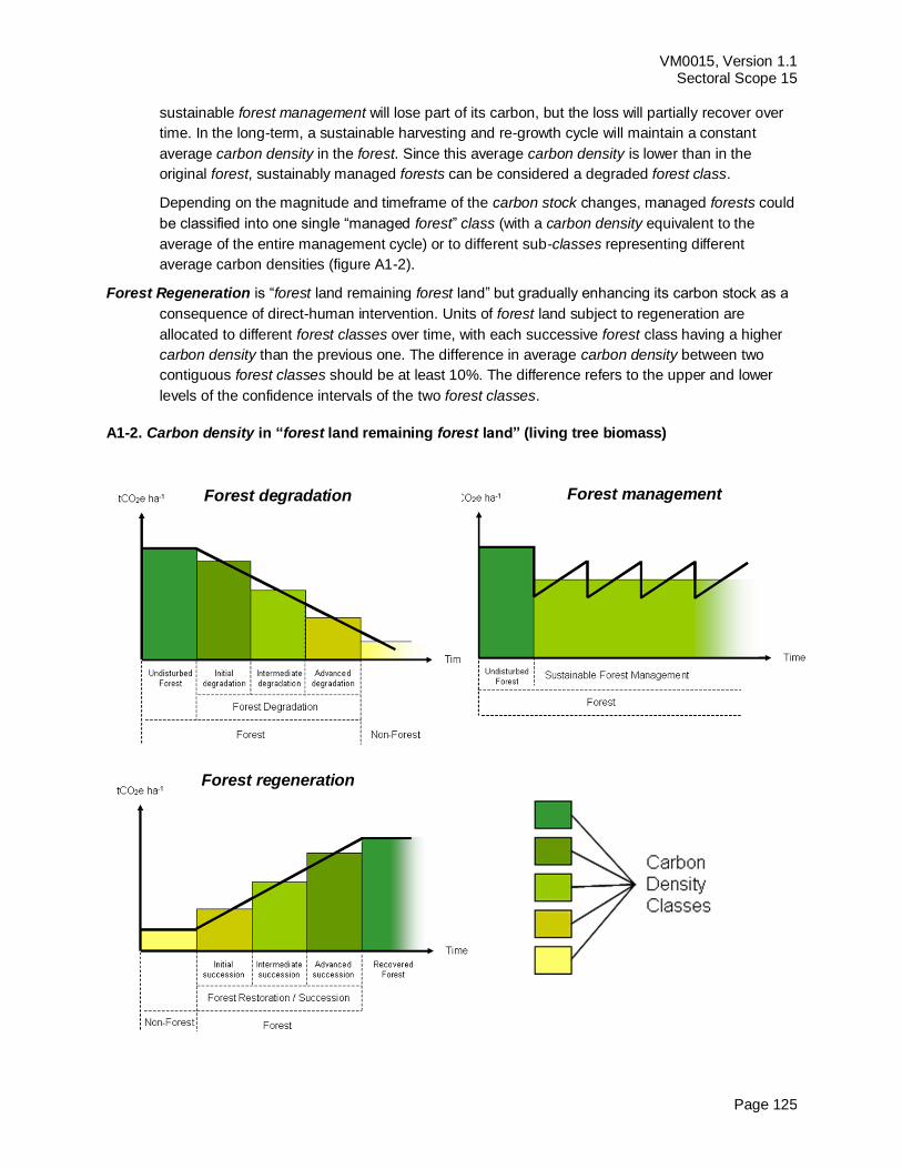
VM0015, Version 1.1 Sectoral Scope 15
Page 125
sustainable forest management will lose part of its carbon, but the loss will partially recover over
time. In the long-term, a sustainable harvesting and re-growth cycle will maintain a constant
average carbon density in the forest. Since this average carbon density is lower than in the
original forest, sustainably managed forests can be considered a degraded forest class.
Depending on the magnitude and timeframe of the carbon stock changes, managed forests could
be classified into one single “managed forest” class (with a carbon density equivalent to the
average of the entire management cycle) or to different sub-classes representing different
average carbon densities (figure A1-2).
Forest Regeneration is “forest land remaining forest land” but gradually enhancing its carbon stock as a
consequence of direct-human intervention. Units of forest land subject to regeneration are
allocated to different forest classes over time, with each successive forest class having a higher
carbon density than the previous one. The difference in average carbon density between two
contiguous forest classes should be at least 10%. The difference refers to the upper and lower
levels of the confidence intervals of the two forest classes.
A1-2. Carbon density in “forest land remaining forest land” (living tree biomass)
Forest degradation Forest management
Forest regeneration
VM0015, Version 1.1 Sectoral Scope 15
Page 126
Frontier Deforestation is the conversion of forest land to non-forest land occurring when the agricultural
frontier expands as a result of improved access to forest into areas with relatively little human
activity.
Historical Reference Period is a time period preceding the starting date of the proposed REDD project
activity. It is analyzed to determine the magnitude of deforestation and forest degradation in the
reference region and to identify agents and drivers of DD and the chain of events leading to land-
use / land-cover change. In order to be useful for understanding recent and likely future DD
trends, the starting date of the historical reference period should be selected between 10 and 15
years in the past, and the end date as close as possible to present.
Leakage is the decrease in carbon stocks and the increase in GHG emissions attributable to the
implementation of the REDD project activity that occurs outside the boundary of the Project area.
Leakage Belt is the geographical area surrounding or adjacent to the project area which activity
displacement leakage could occur.
Leakage Management Area(s) are areas outside the project area in which activities are implemented to
avoid leakage. At the project start date, leakage management areas must be non-forest land
LU/LC Class (or simply “class”) is a unique combination of land use and land cover having a specific
carbon density at time t.
LU/LC Polygon is a discrete area falling into a single LU/LC class.
Monitoring period is the period of time (in years) between two monitoring and verification events.
Typically it is a fraction of the fixed baseline period. The minimum duration is one year and the
maximum is the duration of the fixed baseline period.
Mosaic Deforestation is the conversion of forest land to non-forest land occurring in a patchy pattern
where human population and associated agricultural activities and infrastructure (roads, towns,
etc.) are spread out across the landscape and most areas of forest within such a configured
region or country are practically already accessible.
Planned Deforestation is the legally authorized conversion of forest land to non-forest land occurring in
a discrete area of land. Deforestation within an area can be planned (designated and sanctioned)
or unplanned (unsanctioned). Planned deforestation can include a wide variety of activities such
as national resettlement programs from non-forested to forested regions; a component of a
national land plan to reduce the forest estate and convert it to other industrial-scale production of
goods such as soybeans, pulpwood plantations, and oil palm plantations; or plans to convert well-
managed community-owned forests to other non-forest uses. Other forms of planned
deforestation could also include decisions by individual land owners, whose land is legally zoned
for agriculture, to convert their say selectively logged forest to crop production. These planned
deforestation activities would be a component of some land planning or management document
and could be readily verified.
Project Activity is the series of planned steps and activities by which the proponent intends to reduce
deforestation and forest degradation and/or enhance forest regeneration.
Project area is the area or areas of land on which the proponent will undertake the project activities. No
lands on which the project activity will not be undertaken can be included in the project area.
Project crediting period. Please see current VCS definition.

VM0015, Version 1.1 Sectoral Scope 15
Page 127
Project Scenario is the expected change in land use and land cover within the boundary of the project
area resulting from the undertaking of the project activity.
Project Term is the projected lifetime of the REDD project activity, which under the VCS is equivalent to
the project crediting period.
Reference region is the spatial delimitation of the analytic domain from which information about
deforestation and degradation agents, drivers and LU/LC-change is obtained, projected into the
future and monitored. The reference region includes the Project area57
and is defined by the
project proponent using transparent criteria. It must contain LU/LC classes and deforestation
agents and drivers similar to those found in the project area under the baseline and project
scenarios.
Zone is a stratum of the reference region containing a distinctive mix of final post-deforestation classes fcl
57 The methodology thus adopts a so called “Stratified Regional Baseline” (SRB) approach, which has been
recommended in recent literature (Sataye and Andrasko, 2007; Brown et al., 2007)
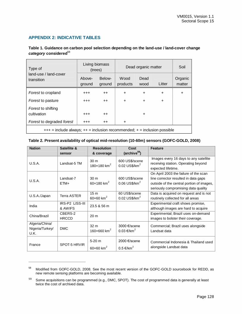
VM0015, Version 1.1 Sectoral Scope 15
Page 128
APPENDIX 2: INDICATIVE TABLES
Table 1. Guidance on carbon pool selection depending on the land-use / land-cover change
category considered58
Type of
land-use / land-cover
transition
Living biomass
(trees) Dead organic matter Soil
Above-
ground
Below-
ground
Wood
products
Dead
wood Litter
Organic
matter
Forest to cropland +++ ++ + + + +
Forest to pasture +++ ++ + + +
Forest to shifting
cultivation +++ ++
+
Forest to degraded forest +++ ++ +
+++ = include always; ++ = inclusion recommended; + = inclusion possible
Table 2. Present availability of optical mid-resolution (10-60m) sensors (GOFC-GOLD, 2008)
Nation Satellite &
sensor
Resolution
& coverage
Cost
(archive59
)
Feature
U.S.A. Landsat-5 TM 30 m
180×180 km2
600 US$/scene
0.02 US$/km2
Images every 16 days to any satellite
receiving station. Operating beyond
expected lifetime.
U.S.A. Landsat-7
ETM+
30 m
60×180 km2
600 US$/scene
0.06 US$/km2
On April 2003 the failure of the scan
line corrector resulted in data gaps
outside of the central portion of images,
seriously compromising data quality
U.S.A./Japan Terra ASTER 15 m
60×60 km2
60 US$/scene
0.02 US$/km2
Data is acquired on request and is not
routinely collected for all areas
India IRS-P2 LISS-III
& AWIFS 23.5 & 56 m
Experimental craft shows promise,
although images are hard to acquire
China/Brazil CBERS-2
HRCCD 20 m
Experimental; Brazil uses on-demand
images to bolster their coverage.
Algeria/China/
Nigeria/Turkey/
U.K.
DMC 32 m
160×660 km2
3000 €/scene
0.03 €/km2
Commercial; Brazil uses alongside
Landsat data
France SPOT-5 HRVIR 5-20 m
60×60 km2
2000 €/scene
0.5 €/km2
Commercial Indonesia & Thailand used
alongside Landsat data
58 Modified from GOFC-GOLD, 2008. See the most recent version of the GOFC-GOLD sourcebook for REDD, as
new remote sensing platforms are becoming available.
59 Some acquisitions can be programmed (e.g., DMC, SPOT). The cost of programmed data is generally at least twice the cost of archived data.
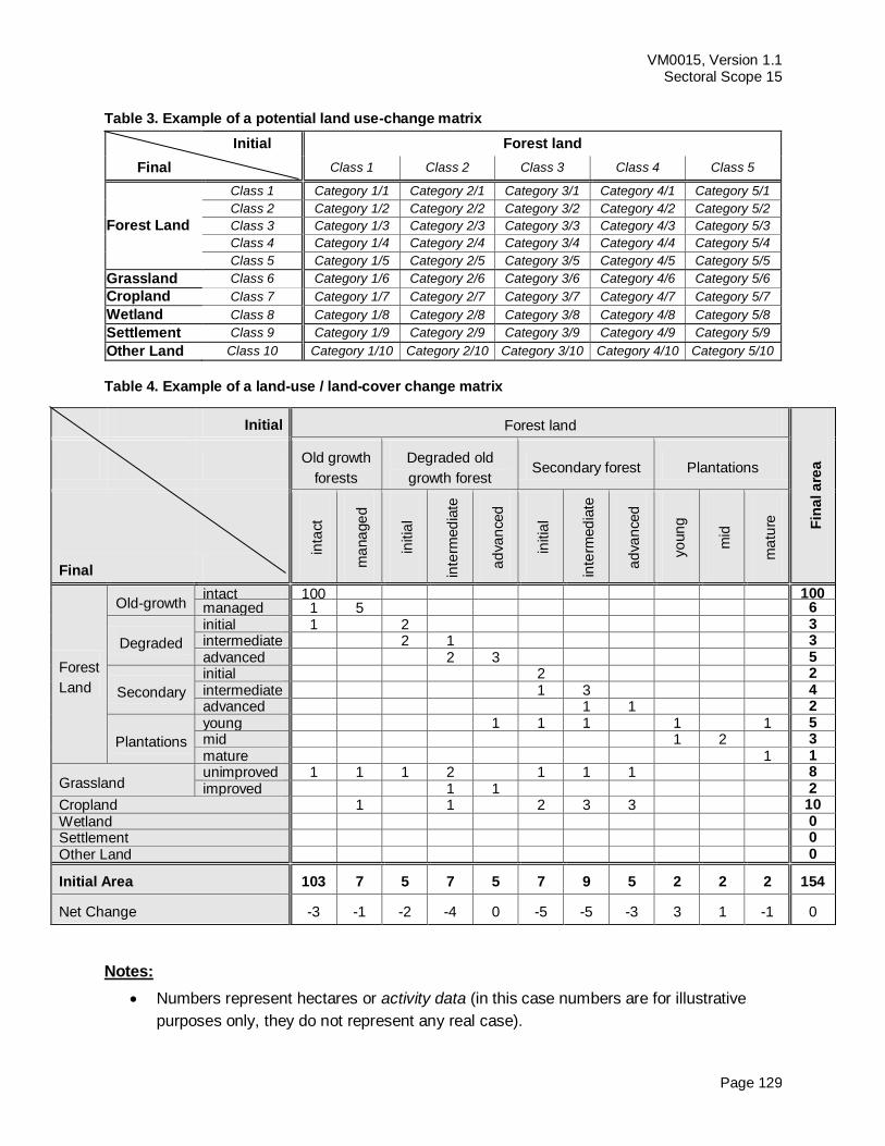
VM0015, Version 1.1 Sectoral Scope 15
Page 129
Table 3. Example of a potential land use-change matrix
Initial Forest land
Final Class 1 Class 2 Class 3 Class 4 Class 5
Forest Land
Class 1 Category 1/1 Category 2/1 Category 3/1 Category 4/1 Category 5/1
Class 2 Category 1/2 Category 2/2 Category 3/2 Category 4/2 Category 5/2
Class 3 Category 1/3 Category 2/3 Category 3/3 Category 4/3 Category 5/3
Class 4 Category 1/4 Category 2/4 Category 3/4 Category 4/4 Category 5/4
Class 5 Category 1/5 Category 2/5 Category 3/5 Category 4/5 Category 5/5
Grassland Class 6 Category 1/6 Category 2/6 Category 3/6 Category 4/6 Category 5/6
Cropland Class 7 Category 1/7 Category 2/7 Category 3/7 Category 4/7 Category 5/7
Wetland Class 8 Category 1/8 Category 2/8 Category 3/8 Category 4/8 Category 5/8
Settlement Class 9 Category 1/9 Category 2/9 Category 3/9 Category 4/9 Category 5/9
Other Land Class 10 Category 1/10 Category 2/10 Category 3/10 Category 4/10 Category 5/10
Table 4. Example of a land-use / land-cover change matrix
Initial Forest land
Fin
al a
rea
Old growth
forests
Degraded old
growth forest Secondary forest Plantations
Final
inta
ct
ma
na
ge
d
initia
l
inte
rmed
iate
ad
van
ced
initia
l
inte
rmed
iate
ad
van
ced
yo
un
g
mid
ma
ture
Forest
Land
Old-growth intact 100 100 managed 1 5 6
Degraded
initial 1 2 3 intermediate 2 1 3
advanced 2 3 5
Secondary
initial 2 2
intermediate 1 3 4 advanced 1 1 2
Plantations
young 1 1 1 1 1 5 mid 1 2 3
mature 1 1
Grassland unimproved 1 1 1 2 1 1 1 8
improved 1 1 2 Cropland 1 1 2 3 3 10
Wetland 0 Settlement 0
Other Land 0
Initial Area 103 7 5 7 5 7 9 5 2 2 2 154
Net Change -3 -1 -2 -4 0 -5 -5 -3 3 1 -1 0
Notes:
Numbers represent hectares or activity data (in this case numbers are for illustrative
purposes only, they do not represent any real case).
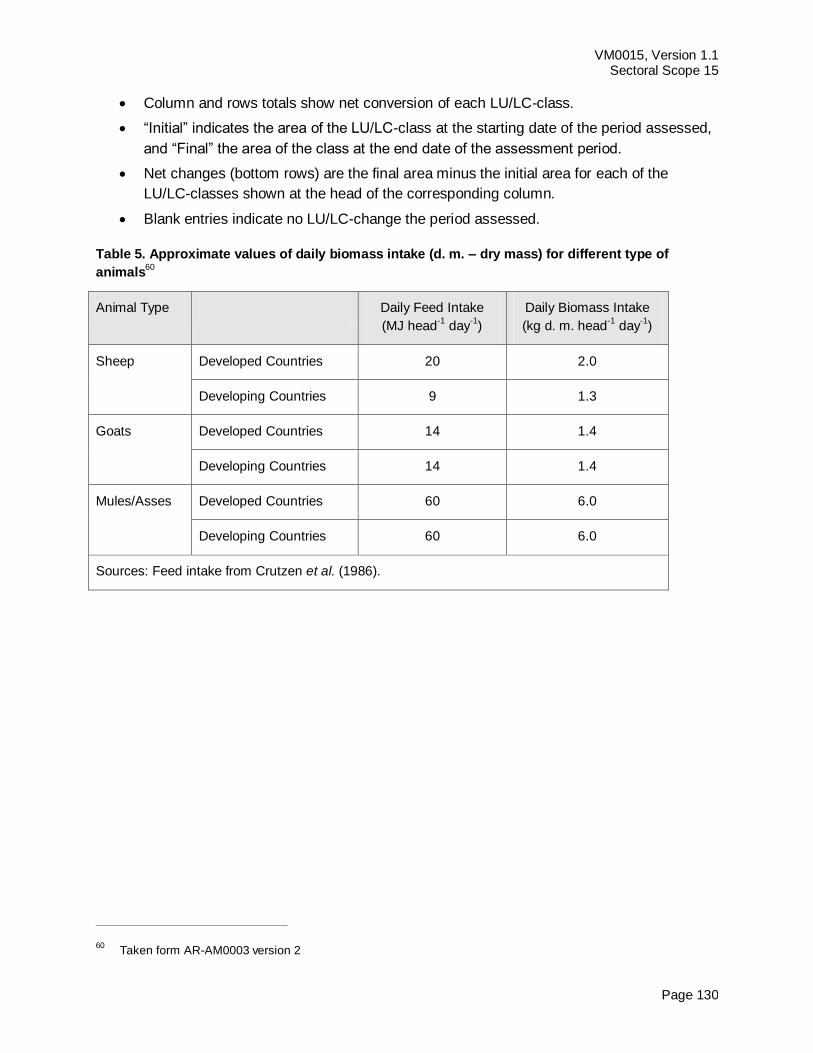
VM0015, Version 1.1 Sectoral Scope 15
Page 130
Column and rows totals show net conversion of each LU/LC-class.
“Initial” indicates the area of the LU/LC-class at the starting date of the period assessed,
and “Final” the area of the class at the end date of the assessment period.
Net changes (bottom rows) are the final area minus the initial area for each of the
LU/LC-classes shown at the head of the corresponding column.
Blank entries indicate no LU/LC-change the period assessed.
Table 5. Approximate values of daily biomass intake (d. m. – dry mass) for different type of
animals60
Animal Type Daily Feed Intake
(MJ head-1
day-1
)
Daily Biomass Intake
(kg d. m. head-1
day-1
)
Sheep Developed Countries 20 2.0
Developing Countries 9 1.3
Goats Developed Countries 14 1.4
Developing Countries 14 1.4
Mules/Asses Developed Countries 60 6.0
Developing Countries 60 6.0
Sources: Feed intake from Crutzen et al. (1986).
60 Taken form AR-AM0003 version 2
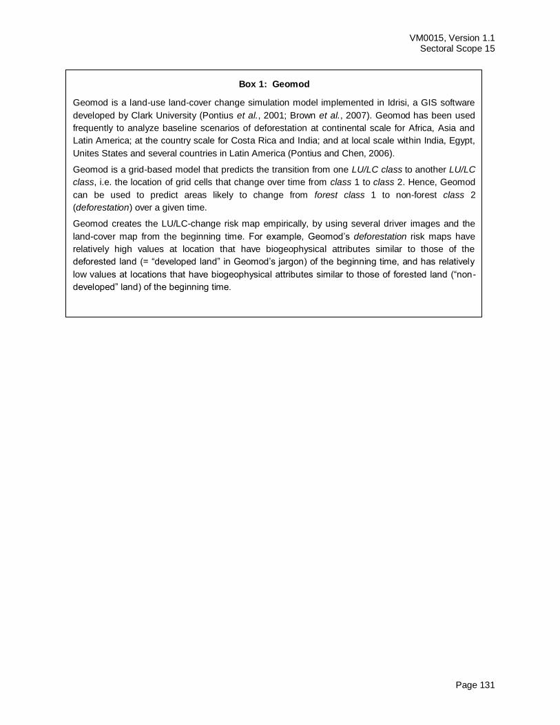
VM0015, Version 1.1 Sectoral Scope 15
Page 131
Box 1: Geomod
Geomod is a land-use land-cover change simulation model implemented in Idrisi, a GIS software
developed by Clark University (Pontius et al., 2001; Brown et al., 2007). Geomod has been used
frequently to analyze baseline scenarios of deforestation at continental scale for Africa, Asia and
Latin America; at the country scale for Costa Rica and India; and at local scale within India, Egypt,
Unites States and several countries in Latin America (Pontius and Chen, 2006).
Geomod is a grid-based model that predicts the transition from one LU/LC class to another LU/LC
class, i.e. the location of grid cells that change over time from class 1 to class 2. Hence, Geomod
can be used to predict areas likely to change from forest class 1 to non-forest class 2
(deforestation) over a given time.
Geomod creates the LU/LC-change risk map empirically, by using several driver images and the
land-cover map from the beginning time. For example, Geomod’s deforestation risk maps have
relatively high values at location that have biogeophysical attributes similar to those of the
deforested land (= “developed land” in Geomod’s jargon) of the beginning time, and has relatively
low values at locations that have biogeophysical attributes similar to those of forested land (“non-
developed” land) of the beginning time.
VM0015, Version 1.1 Sectoral Scope 15
Page 132
APPENDIX 3: METHODS TO ESTIMATE CARBON STOCKS
Sampling framework
The sampling framework, including sample size, plot size, plot shape and plot location should be
specified in the PD.
Areas to be sampled in forest classes should be at locations expected to be deforested according to the
baseline projections.
The sampling areas for non-forest classes should be selected within the reference region at locations that
represent a chrono-sequence of 10 to 30 years since the deforestation date.
Temporary or permanent plots
Plots can be temporary or permanent depending on the specific project circumstances, interests and
needs, but in general temporary plots should be sufficient.
Where changes in carbon stocks are to be monitored, permanent sampling plots are recommended.
Permanent sample plots are generally regarded as statistically efficient in estimating changes in forest
carbon stocks because typically there is high covariance between observations at successive sampling
events. However, it should be ensured that the plots are treated in the same way as other lands within the
project boundary, e.g., during logging operations, and should not be destroyed over the monitoring
interval. Ideally, staff involved in forest management activities should not be aware of the location of
monitoring plots. Where local markers are used, these should not be visible. If trees markers are required
(e.g. if plots are also used for ecological or structural monitoring), these should be as unconspicous as
possible and no bias in the treatment of plots compared to the surrounding forest must be granted.
Permanent plots may also be considered to reduce the uncertainty of the average carbon density of a
forest class undergoing carbon stock changes due to management and to detect changes in carbon
stocks induced by climate change or large-scale natural disturbances.
Definition of the sample size and allocation among LU/LC-classes
The number of sample plots is estimated as dependent on accuracy, variability of the parameter to
estimate in each class and costs. The sample size calculation also corresponds to the method of samples
drawn without replacement. Where at the beginning of a REDD project activity accurate data for sample
size estimation and allocation are not available, the sampling size can initially be estimated by using a
desired level of accuracy (10% of sampling error at 90% confidence level), and by allocating the
estimated sample size proportionally to the area of each class61
, using respectively equations 1, and 2.
Then, once data on carbon stock variability within each class become available, the sample size and
allocation is recalculated using the methodology described by Wenger (1984)62
, which also accounts for
the cost of sampling (see equations 3 and 4).
Equation 1 was chosen because it works with percentages rather than absolute units (biomass, carbon,
or CO2), and coefficient variation data could be more easy to find in the literature at the beginning of a
project activity. The initial allocation of the sample plots shall be proportional to the area of the LU/LC-
61 Loetsch, F. and Haller, K. 1964. Forest Inventory. Volume 1. BLV-VERLAGS GESE LLSCHAFT, München.
62 Wenger, K.F. (ed). 1984. Forestry handbook (2nd edition). New York: John Wiley and Sons.
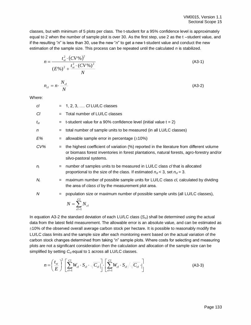
VM0015, Version 1.1 Sectoral Scope 15
Page 133
classes, but with minimum of 5 plots per class. The t-student for a 95% confidence level is approximately
equal to 2 when the number of sample plot is over 30. As the first step, use 2 as the t –student value, and
if the resulting “n” is less than 30, use the new “n” to get a new t-student value and conduct the new
estimation of the sample size. This process can be repeated until the calculated n is stabilized.
N
CVtE
CVtn
st
st
22
2
22
%)(%)(
%
(A3-1)
N
Nnn cl
cl (A3-2)
Where:
cl = 1, 2, 3, …. Cl LU/LC classes
Cl = Total number of LU/LC classes
tst = t-student value for a 90% confidence level (initial value t = 2)
n = total number of sample units to be measured (in all LU/LC classes)
E% = allowable sample error in percentage (10%)
CV% = the highest coefficient of variation (%) reported in the literature from different volume
or biomass forest inventories in forest plantations, natural forests, agro-forestry and/or
silvo-pastoral systems.
ni = number of samples units to be measured in LU/LC class cl that is allocated
proportional to the size of the class. If estimated ncl < 3, set ncl = 3.
Ni = maximum number of possible sample units for LU/LC class cl, calculated by dividing
the area of class cl by the measurement plot area.
N = population size or maximum number of possible sample units (all LU/LC classes),
Cl
cl
clNN1
In equation A3-2 the standard deviation of each LU/LC class (Scl) shall be determined using the actual
data from the latest field measurement. The allowable error is an absolute value, and can be estimated as
10% of the observed overall average carbon stock per hectare. It is possible to reasonably modify the
LU/LC class limits and the sample size after each monitoring event based on the actual variation of the
carbon stock changes determined from taking “n” sample plots. Where costs for selecting and measuring
plots are not a significant consideration then the calculation and allocation of the sample size can be
simplified by setting Ccl equal to 1 across all LU/LC classes.
Cl
cl
clclcl
Cl
cl
clclclst CSWCSWE
tn
11
2
(A3-3)
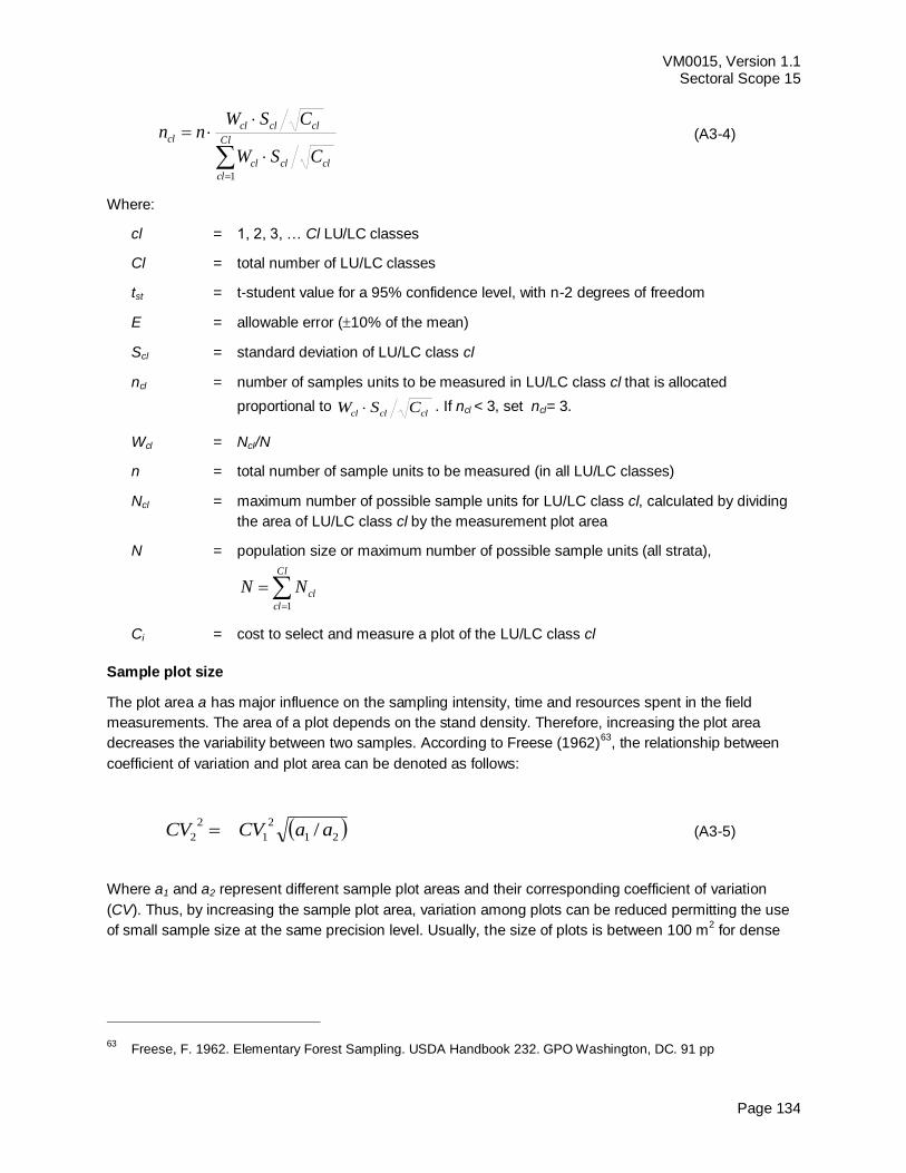
VM0015, Version 1.1 Sectoral Scope 15
Page 134
Cl
cl
clclcl
clclcl
cl
CSW
CSWnn
1
(A3-4)
Where:
cl = 1, 2, 3, … Cl LU/LC classes
Cl = total number of LU/LC classes
tst = t-student value for a 95% confidence level, with n-2 degrees of freedom
E = allowable error (10% of the mean)
Scl = standard deviation of LU/LC class cl
ncl = number of samples units to be measured in LU/LC class cl that is allocated
proportional to clclcl CSW . If ncl < 3, set ncl= 3.
Wcl = Ncl/N
n = total number of sample units to be measured (in all LU/LC classes)
Ncl = maximum number of possible sample units for LU/LC class cl, calculated by dividing
the area of LU/LC class cl by the measurement plot area
N = population size or maximum number of possible sample units (all strata),
Cl
cl
clNN1
Ci = cost to select and measure a plot of the LU/LC class cl
Sample plot size
The plot area a has major influence on the sampling intensity, time and resources spent in the field
measurements. The area of a plot depends on the stand density. Therefore, increasing the plot area
decreases the variability between two samples. According to Freese (1962)63
, the relationship between
coefficient of variation and plot area can be denoted as follows:
21
2
1
2
2 / aaCVCV (A3-5)
Where a1 and a2 represent different sample plot areas and their corresponding coefficient of variation
(CV). Thus, by increasing the sample plot area, variation among plots can be reduced permitting the use
of small sample size at the same precision level. Usually, the size of plots is between 100 m2 for dense
63 Freese, F. 1962. Elementary Forest Sampling. USDA Handbook 232. GPO Washington, DC. 91 pp
VM0015, Version 1.1 Sectoral Scope 15
Page 135
stands and 1000 m2 for open stands
64.
Plot location
To avoid subjective choice of plot locations (plot centers, plot reference points, movement of plot centers
to more “convenient” positions), the permanent sample plots shall be located either systematically with a
random start (which is considered good practice in IPCC GPG-LULUCF) or completely randomly inside
each defined stratum. This can be accomplished with the help of the project GIS platform and a GPS in
the field. The geographical position (GPS coordinate), administrative location, stratum and stand, series
number of each plot, as well as the procedure used for locating them shall be recorded and archived.
Also, it is recommended that the sampling plots are as evenly distributed as possible. For example, if one
stratum consists of three geographically separated sites, then it is proposed to
Divide the total stratum area by the number of plots, resulting in the average area represented by
each plot;
Divide the area of each site by this average area per plot, and assign the integer part of the result
to this site. e.g., if the division results in 6.3 plots, then 6 plots are assigned to this site, and 0.3
plots are carried over to the next site, and so on.
However, remote areas and areas with poor accessibility (either because of physical or social barriers
such as unsafe areas) may be excluded for the location of sampling plots, using a transparent and
conservative procedure, such as creating a buffer zone along roads, paths or navigable rivers that may
be used for reaching the sampling plots. In this case, the representativeness of the plots for the
corresponding stratum must be ensured.
The exact total number of plots is unknown at the beginning of the field sampling and thus a perfectly
even distribution of sampling plots is not possible. This is also the case if pre existing inventory data is
used. In any case, the uneven distribution of sampling plots will be accepted provided that statistical
representativeness and the use of standard sampling techniques are granted, clearly reported and
archived.
Estimation of carbon stocks
The total average carbon stock per hectare (= carbon density) in a LU/LC class is estimated by the
following equation:
clclclclclclcl CwpCsocClCdwCbbCabCtot (A3-6)
Where:
Ctotcl = Average carbon stock per hectare in all accounted carbon pools of the LU/LC-class cl;
tCO2-e ha-1
Note: Cwpcl is subtracted if cl is an initial pre-deforestation forest class in the baseline
case. It is added if cl is a final post-deforestation class or a forest class not
deforested in the project scenario.
64
It is recommended to use sample plots of equal area for the strata. This methodology cannot be used if sample plots area varies within the same stratum. The density of trees to be considered is the one at maturity of the trees.
VM0015, Version 1.1 Sectoral Scope 15
Page 136
Cabcl = Average carbon stock per hectare in the above-ground biomass carbon pool of the LU/LC
class cl; tCO2-e ha-1
Cbbcl = Average carbon stock per hectare in the below-ground biomass carbon pool of the LU/LC
class cl; tCO2-e ha-1
Cdwcl = Average carbon stock per hectare in the dead wood carbon pool of the LU/LC class cl;
tCO2-e ha-1
Clcl = Average carbon stock per hectare in the litter carbon pool of the LU/LC class cl; tCO2-e
ha-1
Csoccl = Average carbon stock per hectare in the soil organic carbon pool of the LU/LC class cl;
tCO2-e ha-1
Cwpcl = Average carbon stock per hectare in the wood products carbon pool of the LU/LC class
cl;
Note: See methodology Part 2 on mandatory carbon pools.
Estimation of carbon stocks in the living biomass carbon pools (Cabcl and Cbbcl )
In a forest most of the carbon is stored in the tree component of the living biomass. Hence, for a majority
of forest classes it is sufficient to estimate the carbon stock in the tree component and to ignore the
carbon stock in the non-tree vegetation component.
However, there might be situations where carbon stocks in the non-tree vegetation component are
significantly increased in the LU/LC-classes adopted after deforestation (e.g. coffee plantations). Under
such circumstances, carbon stocks in the non-tree vegetation component should be estimated65
.
The living biomass components that are measured and the minimum diameter at breast height (DBH)
above which trees are measured should be specified in the PD.
Carbon stocks in the living biomass are given by the following equations:
clclcl CabntCabtCab (A3-7)
clclcl CbbntCbbtCbb (A3-8)
Where:
Cabcl = Average carbon stock per hectare in the above-ground biomass carbon pool of the
LU/LC class cl; tCO2-e ha-1
Cabtcl = Average carbon stock per hectare in the above-ground tree biomass carbon pool of
the LU/LC class cl; tCO2-e ha-1
Cabntcl = Average carbon stock per hectare in the above-ground non-tree biomass carbon
pool of the LU/LC class cl; tCO2-e ha-1
Cbbcl = Average carbon stock per hectare in the below-ground biomass carbon pool of the
LU/LC class cl; tCO2-e ha-1
65 The same carbon pools are to be estimated for the two classes of a LU/LC-change category
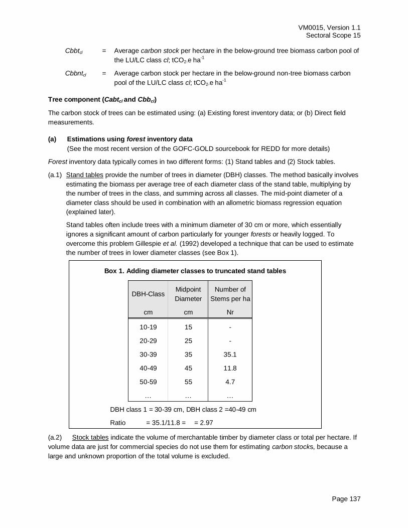
VM0015, Version 1.1 Sectoral Scope 15
Page 137
Cbbtcl = Average carbon stock per hectare in the below-ground tree biomass carbon pool of
the LU/LC class cl; tCO2-e ha-1
Cbbntcl = Average carbon stock per hectare in the below-ground non-tree biomass carbon
pool of the LU/LC class cl; tCO2-e ha-1
Tree component (Cabtcl and Cbbcl)
The carbon stock of trees can be estimated using: (a) Existing forest inventory data; or (b) Direct field
measurements.
(a) Estimations using forest inventory data
(See the most recent version of the GOFC-GOLD sourcebook for REDD for more details)
Forest inventory data typically comes in two different forms: (1) Stand tables and (2) Stock tables.
(a.1) Stand tables provide the number of trees in diameter (DBH) classes. The method basically involves
estimating the biomass per average tree of each diameter class of the stand table, multiplying by
the number of trees in the class, and summing across all classes. The mid-point diameter of a
diameter class should be used in combination with an allometric biomass regression equation
(explained later).
Stand tables often include trees with a minimum diameter of 30 cm or more, which essentially
ignores a significant amount of carbon particularly for younger forests or heavily logged. To
overcome this problem Gillespie et al. (1992) developed a technique that can be used to estimate
the number of trees in lower diameter classes (see Box 1).
(a.2) Stock tables indicate the volume of merchantable timber by diameter class or total per hectare. If
volume data are just for commercial species do not use them for estimating carbon stocks, because a
large and unknown proportion of the total volume is excluded.
Box 1. Adding diameter classes to truncated stand tables
DBH-Class Midpoint
Diameter
Number of
Stems per ha
cm cm Nr
10-19 15 -
20-29 25 -
30-39 35 35.1
40-49 45 11.8
50-59 55 4.7
… … …
DBH class 1 = 30-39 cm, DBH class 2 =40-49 cm
Ratio = 35.1/11.8 = = 2.97
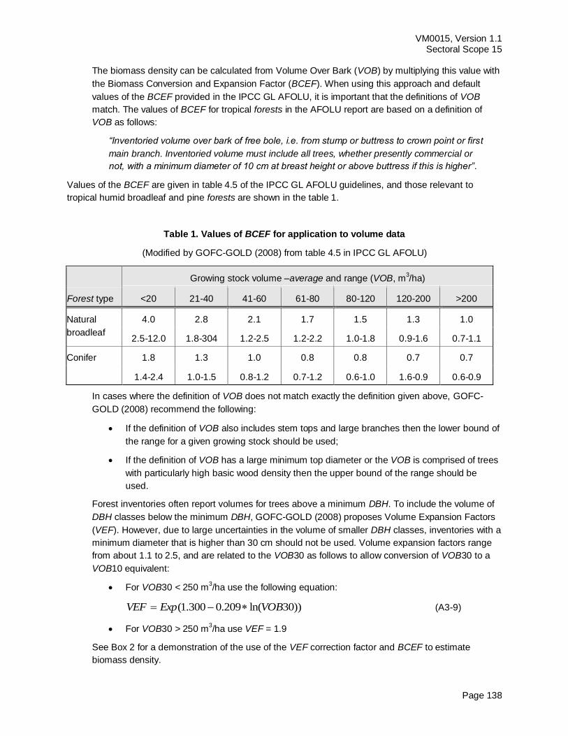
VM0015, Version 1.1 Sectoral Scope 15
Page 138
The biomass density can be calculated from Volume Over Bark (VOB) by multiplying this value with
the Biomass Conversion and Expansion Factor (BCEF). When using this approach and default
values of the BCEF provided in the IPCC GL AFOLU, it is important that the definitions of VOB
match. The values of BCEF for tropical forests in the AFOLU report are based on a definition of
VOB as follows:
“Inventoried volume over bark of free bole, i.e. from stump or buttress to crown point or first
main branch. Inventoried volume must include all trees, whether presently commercial or
not, with a minimum diameter of 10 cm at breast height or above buttress if this is higher”.
Values of the BCEF are given in table 4.5 of the IPCC GL AFOLU guidelines, and those relevant to
tropical humid broadleaf and pine forests are shown in the table 1.
Table 1. Values of BCEF for application to volume data
(Modified by GOFC-GOLD (2008) from table 4.5 in IPCC GL AFOLU)
Forest type
Growing stock volume –average and range (VOB, m3/ha)
<20 21-40 41-60 61-80 80-120 120-200 >200
Natural
broadleaf
4.0 2.8 2.1 1.7 1.5 1.3 1.0
2.5-12.0 1.8-304 1.2-2.5 1.2-2.2 1.0-1.8 0.9-1.6 0.7-1.1
Conifer 1.8 1.3 1.0 0.8 0.8 0.7 0.7
1.4-2.4 1.0-1.5 0.8-1.2 0.7-1.2 0.6-1.0 1.6-0.9 0.6-0.9
In cases where the definition of VOB does not match exactly the definition given above, GOFC-
GOLD (2008) recommend the following:
If the definition of VOB also includes stem tops and large branches then the lower bound of
the range for a given growing stock should be used;
If the definition of VOB has a large minimum top diameter or the VOB is comprised of trees
with particularly high basic wood density then the upper bound of the range should be
used.
Forest inventories often report volumes for trees above a minimum DBH. To include the volume of
DBH classes below the minimum DBH, GOFC-GOLD (2008) proposes Volume Expansion Factors
(VEF). However, due to large uncertainties in the volume of smaller DBH classes, inventories with a
minimum diameter that is higher than 30 cm should not be used. Volume expansion factors range
from about 1.1 to 2.5, and are related to the VOB30 as follows to allow conversion of VOB30 to a
VOB10 equivalent:
For VOB30 < 250 m3/ha use the following equation:
))30ln(209.0300.1( VOBExpVEF (A3-9)
For VOB30 > 250 m3/ha use VEF = 1.9
See Box 2 for a demonstration of the use of the VEF correction factor and BCEF to estimate
biomass density.
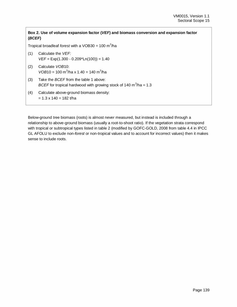
VM0015, Version 1.1 Sectoral Scope 15
Page 139
Box 2. Use of volume expansion factor (VEF) and biomass conversion and expansion factor
(BCEF)
Tropical broadleaf forest with a VOB30 = 100 m3/ha
(1) Calculate the VEF:
VEF = Exp(1.300 - 0.209*Ln(100)) = 1.40
(2) Calculate VOB10:
VOB10 = 100 m3/ha x 1.40 = 140 m
3/ha
(3) Take the BCEF from the table 1 above:
BCEF for tropical hardwood with growing stock of 140 m3/ha = 1.3
(4) Calculate above-ground biomass density:
= 1.3 x 140 = 182 t/ha
Below-ground tree biomass (roots) is almost never measured, but instead is included through a
relationship to above-ground biomass (usually a root-to-shoot ratio). If the vegetation strata correspond
with tropical or subtropical types listed in table 2 (modified by GOFC-GOLD, 2008 from table 4.4 in IPCC
GL AFOLU to exclude non-forest or non-tropical values and to account for incorrect values) then it makes
sense to include roots.
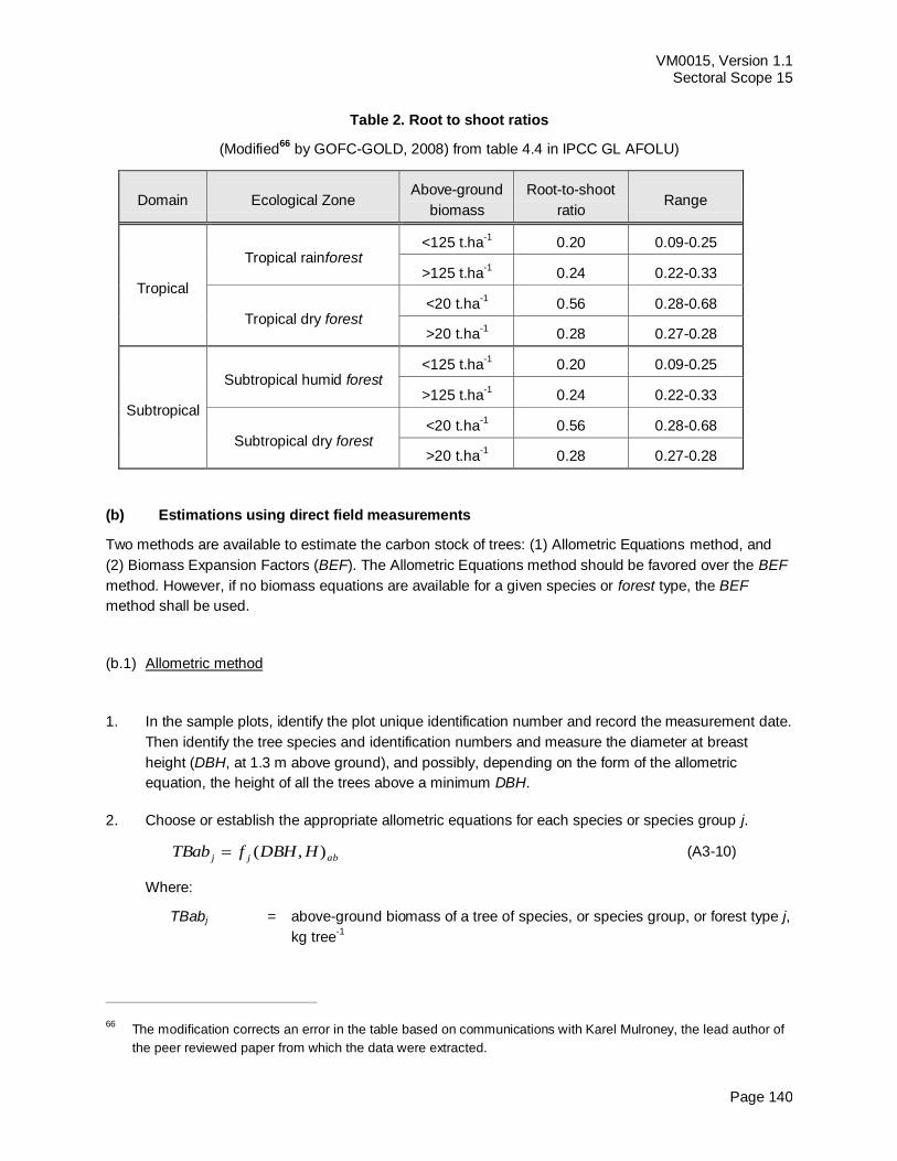
VM0015, Version 1.1 Sectoral Scope 15
Page 140
Table 2. Root to shoot ratios
(Modified66
by GOFC-GOLD, 2008) from table 4.4 in IPCC GL AFOLU)
Domain Ecological Zone Above-ground
biomass
Root-to-shoot
ratio Range
Tropical
Tropical rainforest <125 t.ha
-1 0.20 0.09-0.25
>125 t.ha-1
0.24 0.22-0.33
Tropical dry forest <20 t.ha
-1 0.56 0.28-0.68
>20 t.ha-1 0.28 0.27-0.28
Subtropical
Subtropical humid forest <125 t.ha
-1 0.20 0.09-0.25
>125 t.ha-1
0.24 0.22-0.33
Subtropical dry forest <20 t.ha
-1 0.56 0.28-0.68
>20 t.ha-1 0.28 0.27-0.28
(b) Estimations using direct field measurements
Two methods are available to estimate the carbon stock of trees: (1) Allometric Equations method, and
(2) Biomass Expansion Factors (BEF). The Allometric Equations method should be favored over the BEF
method. However, if no biomass equations are available for a given species or forest type, the BEF
method shall be used.
(b.1) Allometric method
1. In the sample plots, identify the plot unique identification number and record the measurement date.
Then identify the tree species and identification numbers and measure the diameter at breast
height (DBH, at 1.3 m above ground), and possibly, depending on the form of the allometric
equation, the height of all the trees above a minimum DBH.
2. Choose or establish the appropriate allometric equations for each species or species group j.
abjj HDBHfTBab ),( (A3-10)
Where:
TBabj = above-ground biomass of a tree of species, or species group, or forest type j,
kg tree-1
66 The modification corrects an error in the table based on communications with Karel Mulroney, the lead author of
the peer reviewed paper from which the data were extracted.
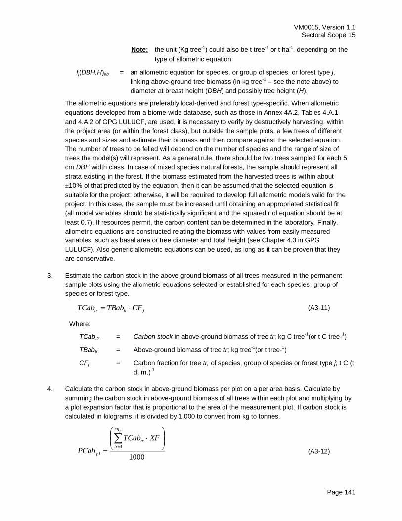
VM0015, Version 1.1 Sectoral Scope 15
Page 141
Note: the unit (Kg tree-1
) could also be t tree-1
or t ha-1
, depending on the
type of allometric equation
fj(DBH,H)ab = an allometric equation for species, or group of species, or forest type j,
linking above-ground tree biomass (in kg tree-1
– see the note above) to
diameter at breast height (DBH) and possibly tree height (H).
The allometric equations are preferably local-derived and forest type-specific. When allometric
equations developed from a biome-wide database, such as those in Annex 4A.2, Tables 4.A.1
and 4.A.2 of GPG LULUCF, are used, it is necessary to verify by destructively harvesting, within
the project area (or within the forest class), but outside the sample plots, a few trees of different
species and sizes and estimate their biomass and then compare against the selected equation.
The number of trees to be felled will depend on the number of species and the range of size of
trees the model(s) will represent. As a general rule, there should be two trees sampled for each 5
cm DBH width class. In case of mixed species natural forests, the sample should represent all
strata existing in the forest. If the biomass estimated from the harvested trees is within about
10% of that predicted by the equation, then it can be assumed that the selected equation is
suitable for the project; otherwise, it will be required to develop full allometric models valid for the
project. In this case, the sample must be increased until obtaining an appropriated statistical fit
(all model variables should be statistically significant and the squared r of equation should be at
least 0.7). If resources permit, the carbon content can be determined in the laboratory. Finally,
allometric equations are constructed relating the biomass with values from easily measured
variables, such as basal area or tree diameter and total height (see Chapter 4.3 in GPG
LULUCF). Also generic allometric equations can be used, as long as it can be proven that they
are conservative.
3. Estimate the carbon stock in the above-ground biomass of all trees measured in the permanent
sample plots using the allometric equations selected or established for each species, group of
species or forest type.
jtrtr CFTBabTCab (A3-11)
Where:
TCab,tr = Carbon stock in above-ground biomass of tree tr; kg C tree-1
(or t C tree-1)
TBabtr = Above-ground biomass of tree tr; kg tree-1
(or t tree-1)
CFj = Carbon fraction for tree tr, of species, group of species or forest type j; t C (t
d. m.)-1
4. Calculate the carbon stock in above-ground biomass per plot on a per area basis. Calculate by
summing the carbon stock in above-ground biomass of all trees within each plot and multiplying by
a plot expansion factor that is proportional to the area of the measurement plot. If carbon stock is
calculated in kilograms, it is divided by 1,000 to convert from kg to tonnes.
1000
1
plTR
tr
tr
pl
XFTCab
PCab (A3-12)
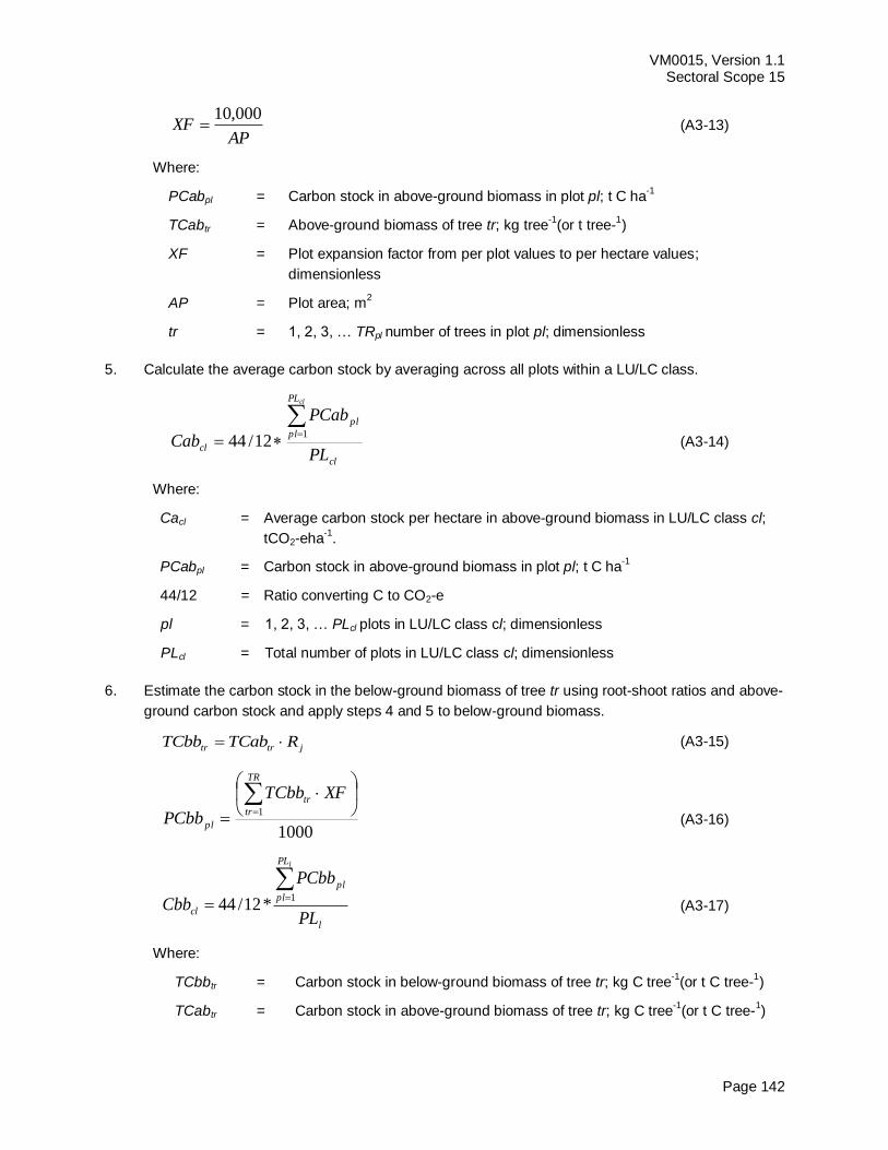
VM0015, Version 1.1 Sectoral Scope 15
Page 142
APXF
000,10 (A3-13)
Where:
PCabpl = Carbon stock in above-ground biomass in plot pl; t C ha-1
TCabtr = Above-ground biomass of tree tr; kg tree-1
(or t tree-1)
XF = Plot expansion factor from per plot values to per hectare values;
dimensionless
AP = Plot area; m2
tr = 1, 2, 3, … TRpl number of trees in plot pl; dimensionless
5. Calculate the average carbon stock by averaging across all plots within a LU/LC class.
cl
PL
pl
pl
clPL
PCab
Cab
cl
1
12/44 (A3-14)
Where:
Cacl = Average carbon stock per hectare in above-ground biomass in LU/LC class cl;
tCO2-eha-1
.
PCabpl = Carbon stock in above-ground biomass in plot pl; t C ha-1
44/12 = Ratio converting C to CO2-e
pl = 1, 2, 3, … PLcl plots in LU/LC class cl; dimensionless
PLcl = Total number of plots in LU/LC class cl; dimensionless
6. Estimate the carbon stock in the below-ground biomass of tree tr using root-shoot ratios and above-
ground carbon stock and apply steps 4 and 5 to below-ground biomass.
jtrtr RTCabTCbb (A3-15)
1000
1
TR
tr
tr
pl
XFTCbb
PCbb (A3-16)
l
PL
pl
pl
clPL
PCbb
Cbb
l
1
*12/44 (A3-17)
Where:
TCbbtr = Carbon stock in below-ground biomass of tree tr; kg C tree-1
(or t C tree-1)
TCabtr = Carbon stock in above-ground biomass of tree tr; kg C tree-1
(or t C tree-1)
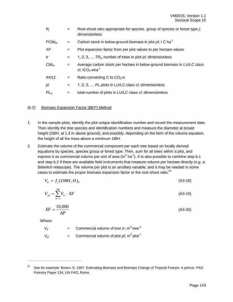
VM0015, Version 1.1 Sectoral Scope 15
Page 143
Rj = Root-shoot ratio appropriate for species, group of species or forest type j;
dimensionless
PCbbpl = Carbon stock in below-ground biomass in plot pl; t C ha-1
XF = Plot expansion factor from per plot values to per hectare values
tr = 1, 2, 3, … TRpl number of trees in plot pl; dimensionless
Cbbcl = Average carbon stock per hectare in below-ground biomass in LU/LC class
cl; tCO2-eha-1
44/12 = Ratio converting C to CO2-e
pl = 1, 2, 3, … PLl plots in LU/LC class cl; dimensionless
PLcl = total number of plots in LU/LC class cl; dimensionless
(b.2) Biomass Expansion Factor (BEF) Method
1. In the sample plots, identify the plot unique identification number and record the measurement date.
Then identify the tree species and identification numbers and measure the diameter at breast
height (DBH, at 1.3 m above ground), and possibly, depending on the form of the volume equation,
the height of all the trees above a minimum DBH.
2. Estimate the volume of the commercial component per each tree based on locally derived
equations by species, species group or forest type. Then, sum for all trees within a plot, and
express it as commercial volume per unit of area (m3 ha
-1). It is also possible to combine step b.1
and step b.2 if there are available field instruments that measure volume per hectare directly (e.g. a
Bitterlich relascope). The volume per plot is an ancillary variable, and it may be needed in some
cases to estimate the proper biomass expansion factor or the root-shoot ratio.67
Vjtr HDBHfV ),( (A3-18)
XFVVTR
tr
trpl 1
(A3-19)
APXF
000,10 (A3-20)
Where:
Vtr = Commercial volume of tree tr; m3 tree
-1
Vpl = Commercial volume of plot pl; m3 plot
-1
67 See for example: Brown, S. 1997. Estimating Biomass and Biomass Change of Tropical Forests: A primer. FAO
Forestry Paper 134, UN FAO, Rome.
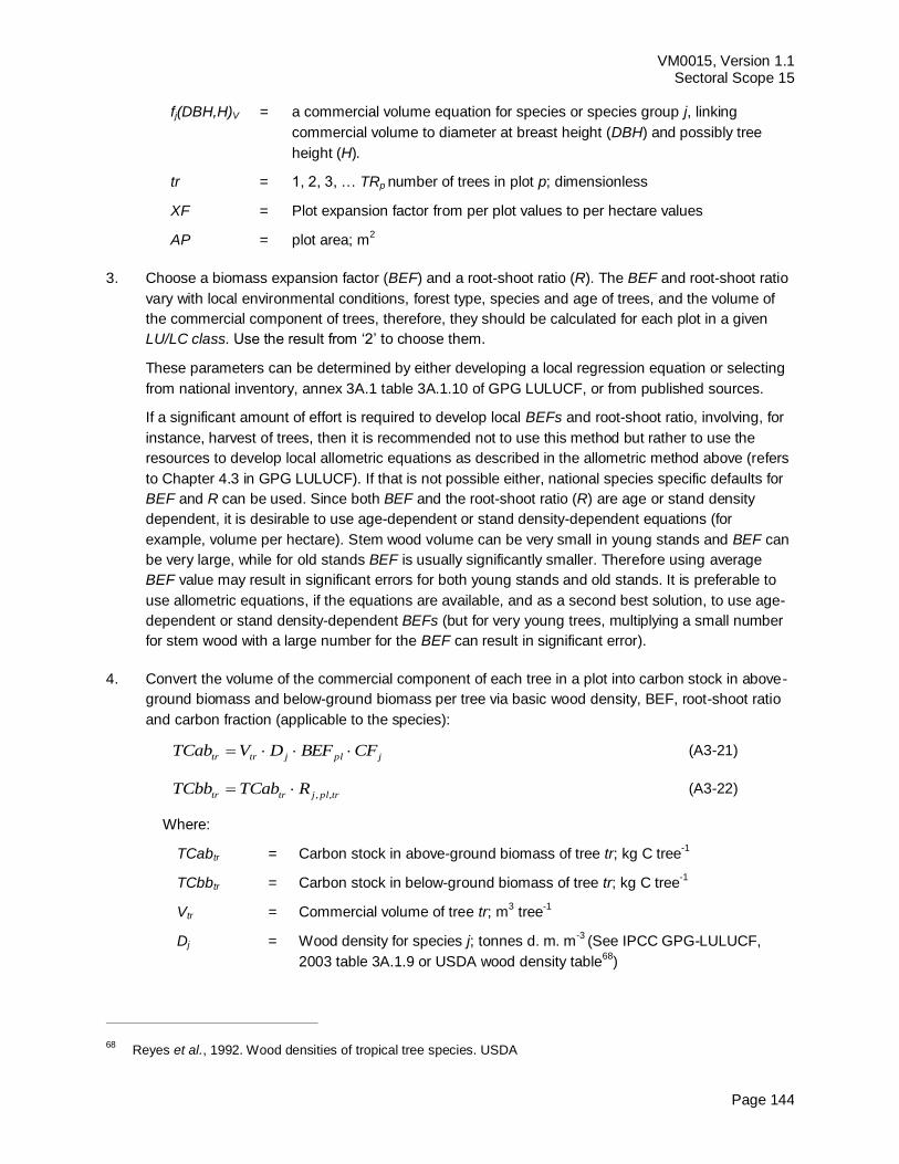
VM0015, Version 1.1 Sectoral Scope 15
Page 144
fj(DBH,H)V = a commercial volume equation for species or species group j, linking
commercial volume to diameter at breast height (DBH) and possibly tree
height (H).
tr = 1, 2, 3, … TRp number of trees in plot p; dimensionless
XF = Plot expansion factor from per plot values to per hectare values
AP = plot area; m2
3. Choose a biomass expansion factor (BEF) and a root-shoot ratio (R). The BEF and root-shoot ratio
vary with local environmental conditions, forest type, species and age of trees, and the volume of
the commercial component of trees, therefore, they should be calculated for each plot in a given
LU/LC class. Use the result from ‘2’ to choose them.
These parameters can be determined by either developing a local regression equation or selecting
from national inventory, annex 3A.1 table 3A.1.10 of GPG LULUCF, or from published sources.
If a significant amount of effort is required to develop local BEFs and root-shoot ratio, involving, for
instance, harvest of trees, then it is recommended not to use this method but rather to use the
resources to develop local allometric equations as described in the allometric method above (refers
to Chapter 4.3 in GPG LULUCF). If that is not possible either, national species specific defaults for
BEF and R can be used. Since both BEF and the root-shoot ratio (R) are age or stand density
dependent, it is desirable to use age-dependent or stand density-dependent equations (for
example, volume per hectare). Stem wood volume can be very small in young stands and BEF can
be very large, while for old stands BEF is usually significantly smaller. Therefore using average
BEF value may result in significant errors for both young stands and old stands. It is preferable to
use allometric equations, if the equations are available, and as a second best solution, to use age-
dependent or stand density-dependent BEFs (but for very young trees, multiplying a small number
for stem wood with a large number for the BEF can result in significant error).
4. Convert the volume of the commercial component of each tree in a plot into carbon stock in above-
ground biomass and below-ground biomass per tree via basic wood density, BEF, root-shoot ratio
and carbon fraction (applicable to the species):
jpljtrtr CFBEFDVTCab (A3-21)
trpljtrtr RTCabTCbb ,, (A3-22)
Where:
TCabtr = Carbon stock in above-ground biomass of tree tr; kg C tree-1
TCbbtr = Carbon stock in below-ground biomass of tree tr; kg C tree-1
Vtr = Commercial volume of tree tr; m3 tree
-1
Dj = Wood density for species j; tonnes d. m. m-3
(See IPCC GPG-LULUCF,
2003 table 3A.1.9 or USDA wood density table68
)
68 Reyes et al., 1992. Wood densities of tropical tree species. USDA
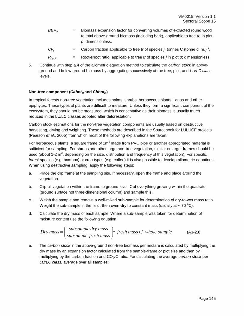
VM0015, Version 1.1 Sectoral Scope 15
Page 145
BEFpl = Biomass expansion factor for converting volumes of extracted round wood
to total above-ground biomass (including bark), applicable to tree tr, in plot
p; dimensionless.
CFj = Carbon fraction applicable to tree tr of species j; tonnes C (tonne d. m.)-1
.
Rj,pl,tr = Root-shoot ratio, applicable to tree tr of species j in plot p; dimensionless
5. Continue with step a.4 of the allometric equation method to calculate the carbon stock in above-
ground and below-ground biomass by aggregating successively at the tree, plot, and LU/LC class
levels.
Non-tree component (Cabntcl and Cbbntcl)
In tropical forests non-tree vegetation includes palms, shrubs, herbaceous plants, lianas and other
epiphytes. These types of plants are difficult to measure. Unless they form a significant component of the
ecosystem, they should not be measured, which is conservative as their biomass is usually much
reduced in the LU/LC classes adopted after deforestation.
Carbon stock estimations for the non-tree vegetation components are usually based on destructive
harvesting, drying and weighting. These methods are described in the Sourcebook for LULUCF projects
(Pearson et al., 2005) from which most of the following explanations are taken.
For herbaceous plants, a square frame of 1m2 made from PVC pipe or another appropriated material is
sufficient for sampling. For shrubs and other large non-tree vegetation, similar or larger frames should be
used (about 1-2 m2, depending on the size, distribution and frequency of this vegetation). For specific
forest species (e.g. bamboo) or crop types (e.g. coffee) it is also possible to develop allometric equations.
When using destructive sampling, apply the following steps:
a. Place the clip frame at the sampling site. If necessary, open the frame and place around the
vegetation.
b. Clip all vegetation within the frame to ground level. Cut everything growing within the quadrate
(ground surface not three-dimensional column) and sample this.
c. Weigh the sample and remove a well-mixed sub-sample for determination of dry-to-wet mass ratio.
Weight the sub-sample in the field, then oven-dry to constant mass (usually at ~ 70 oC).
d. Calculate the dry mass of each sample. Where a sub-sample was taken for determination of
moisture content use the following equation:
samplewholeofmassfreshmassfreshsubsample
massdrysubsamplemassDry
(A3-23)
e. The carbon stock in the above-ground non-tree biomass per hectare is calculated by multiplying the
dry mass by an expansion factor calculated from the sample-frame or plot size and then by
multiplying by the carbon fraction and CO2/C ratio. For calculating the average carbon stock per
LU/LC class, average over all samples:
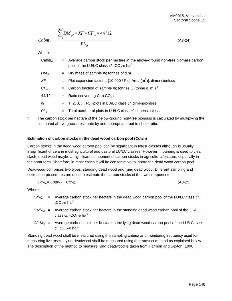
VM0015, Version 1.1 Sectoral Scope 15
Page 146
cl
PLcl
pl
plpl
clPL
CFXFDM
Cabnt
1
12/44
(A3-24)
Where:
Cabntcl = Average carbon stock per hectare in the above-ground non-tree biomass carbon
pool of the LU/LC class cl; tCO2-e ha-1
DMpl = Dry mass of sample pl; tonnes of d.m.
XF = Plot expansion factor = [10.000 / Plot Area (m2)]; dimensionless
CFpl = Carbon fraction of sample pl; tonnes C (tonne d. m.)-1
44/12 = Ratio converting C to CO2-e
pl = 1, 2, 3, … PLpl plots in LU/LC class cl; dimensionless
PLcl = Total number of plots in LU/LC class cl; dimensionless
f. The carbon stock per hectare of the below-ground non-tree biomass is calculated by multiplying the
estimated above-ground estimate by and appropriate root to shoot ratio.
Estimation of carbon stocks in the dead wood carbon pool (Cdwcl)
Carbon stocks in the dead wood carbon pool can be significant in forest classes although is usually
insignificant or zero in most agricultural and pastoral LU/LC classes. However, if burning is used to clear
slash, dead wood maybe a significant component of carbon stocks in agricultural/pasture, especially in
the short term. Therefore, in most cases it will be conservative to ignore the dead wood carbon pool.
Deadwood comprises two types: standing dead wood and lying dead wood. Different sampling and
estimation procedures are used to estimate the carbon stocks of the two components.
Cdwcl= Csdwcl + Cldwcl (A3-25)
Where:
Cdwcl = Average carbon stock per hectare in the dead wood carbon pool of the LU/LC class cl;
tCO2-e ha-1
Csdwcl = Average carbon stock per hectare in the standing dead wood carbon pool of the LU/LC
class cl; tCO2-e ha-1
Cñdwcl = Average carbon stock per hectare in the lying dead wood carbon pool of the LU/LC class
cl; tCO2-e ha-1
Standing dead wood shall be measured using the sampling criteria and monitoring frequency used for
measuring live trees. Lying deadwood shall be measured using the transect method as explained below.
The description of the method to measure lying deadwood is taken from Harmon and Sexton (1996).
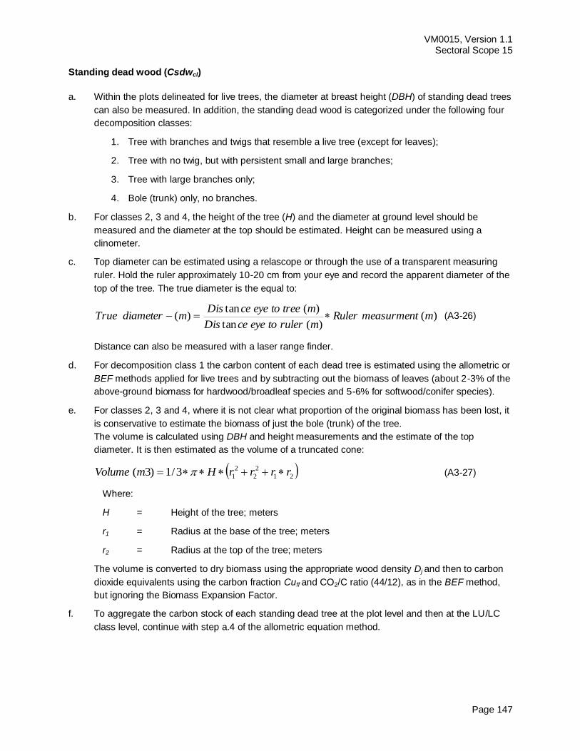
VM0015, Version 1.1 Sectoral Scope 15
Page 147
Standing dead wood (Csdwcl)
a. Within the plots delineated for live trees, the diameter at breast height (DBH) of standing dead trees
can also be measured. In addition, the standing dead wood is categorized under the following four
decomposition classes:
1. Tree with branches and twigs that resemble a live tree (except for leaves);
2. Tree with no twig, but with persistent small and large branches;
3. Tree with large branches only;
4. Bole (trunk) only, no branches.
b. For classes 2, 3 and 4, the height of the tree (H) and the diameter at ground level should be
measured and the diameter at the top should be estimated. Height can be measured using a
clinometer.
c. Top diameter can be estimated using a relascope or through the use of a transparent measuring
ruler. Hold the ruler approximately 10-20 cm from your eye and record the apparent diameter of the
top of the tree. The true diameter is the equal to:
)()(tan
)(tan)( mmeasurmentRuler
mrulertoeyeceDis
mtreetoeyeceDismdiameterTrue (A3-26)
Distance can also be measured with a laser range finder.
d. For decomposition class 1 the carbon content of each dead tree is estimated using the allometric or
BEF methods applied for live trees and by subtracting out the biomass of leaves (about 2-3% of the
above-ground biomass for hardwood/broadleaf species and 5-6% for softwood/conifer species).
e. For classes 2, 3 and 4, where it is not clear what proportion of the original biomass has been lost, it
is conservative to estimate the biomass of just the bole (trunk) of the tree.
The volume is calculated using DBH and height measurements and the estimate of the top
diameter. It is then estimated as the volume of a truncated cone:
21
2
2
2
13/1)3( rrrrHmVolume (A3-27)
Where:
H = Height of the tree; meters
r1 = Radius at the base of the tree; meters
r2 = Radius at the top of the tree; meters
The volume is converted to dry biomass using the appropriate wood density Dj and then to carbon
dioxide equivalents using the carbon fraction Cuff and CO2/C ratio (44/12), as in the BEF method,
but ignoring the Biomass Expansion Factor.
f. To aggregate the carbon stock of each standing dead tree at the plot level and then at the LU/LC
class level, continue with step a.4 of the allometric equation method.

VM0015, Version 1.1 Sectoral Scope 15
Page 148
Lying dead wood (Cldwcl)
Lying dead wood is most efficiently measured using the line-intersect method. Only coarse dead wood
above a predefined minimum diameter (e.g. > 10 cm) is measured with this method – dead wood with
smaller diameter can be measured with litter.
a. At each plot location, lay out two lines of 50 meters either in a single line or at right angles. The
lines should be outside the boundaries of the plot to avoid damage to seedlings in the plots during
measurement, and also to biasing the dead wood pool by damaging during tree measurement.
Alternatively, separate and independent sampling of lying deadwood may be used, in which case
deadwood transects must be randomly located (to avoid subjective choice of plots locations),
without sample replacement, using the same procedure used for live trees69
. Their location must
also be permanently marked and their coordinates reported.
b. Along the length of the lines, measure the diameter of each intersecting piece of coarse dead wood
above a predefined minimum diameter (e.g. > 10 cm). Calipers work best for measuring the
diameter. A piece of dead wood should only be measured if: (a) more than 50% of the log is above-
ground and (b) the sampling line crosses through at least 50% of the diameter of the piece. If the
log is hollow at the intersection point, measure the diameter of the hollow: the hollow portion in the
volume estimates should be excluded.
c. Assign each piece of dead wood to one of the three following density classes:
1. Sound
2. Intermediate
3. Rotten
To determine what density class a piece of dead wood fits into, each piece should be struck with a
machete. If the blade does not sink into the piece (that is, it bounces off), it is classified as sound. If
it sinks partly into the piece and there has been some wood loss, it is classified as intermediate. If
the blade sinks into the piece, there is more extensive wood loss and the piece is crumbly, it is
classified as rotten.
d. At least 10 random dead wood samples of each three density classes, representing a range of
species present, should be collected for density determination. This determination can be
accomplished using the maximum moisture content method (Smith 1954), which does not require
sample volume determination. Using a chainsaw or a handsaw, cut a compete disc or a piece of
reasonable size from the selected piece of dead wood and bring to the laboratory for wood density
determination.
e. Submerge wood samples in water until saturation is reached. Weight saturated samples. Then, dry
samples at 105°C for 26 hours. Extract and weight samples again. Do this last weight quickly,
withdrawing samples from oven immediately before weighting them, so that no moisture is
absorbed by dried samples before obtaining weights.
69 Using this alternate approach, transects may be located in places distant to live trees plots, increasing sampling
costs. Even if lying deadwood stocks are very homogeneous in all the strata, implying that fewer samples will be required, the cost of additional displacements and work won’t probably compensate for the decrease in samples number.
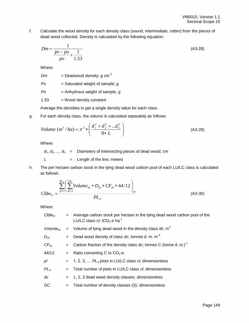
VM0015, Version 1.1 Sectoral Scope 15
Page 149
f. Calculate the wood density for each density class (sound, intermediate, rotten) from the pieces of
dead wood collected. Density is calculated by the following equation:
1
1
1.53
Dmps po
po
(A3-28)
Where:
Dm = Deadwood density; g cm-3
Ps = Saturated weight of sample; g
Po = Anhydrous weight of sample, g
1.53 = Wood density constant
Average the densities to get a single density value for each class.
g. For each density class, the volume is calculated separately as follows:
L
dddhamVolume n
8
...)/(
22
2
2
123 (A3-29)
Where:
d1, d2, ..., dn = Diameters of intersecting pieces of dead wood; cm
L = Length of the line; meters
h. The per hectare carbon stock in the lying dead wood carbon pool of each LU/LC class is calculated
as follows:
cl
PL
pl pl
dcdc
DC
dc
dc
clPL
CFDVolume
Cldw
cl
1 1
12/44
(A3-30)
Where:
Cldwcl = Average carbon stock per hectare in the lying dead wood carbon pool of the
LU/LC class cl; tCO2-e ha-1
Volumedc = Volume of lying dead wood in the density class dc; m3
Ddc = Dead wood density of class dc; tonnes d. m. m-3
CFdc = Carbon fraction of the density class dc; tonnes C (tonne d. m.)-1
44/12 = Ratio converting C to CO2-e
pl = 1, 2, 3, … PLcl plots in LU/LC class cl; dimensionless
PLcl = Total number of plots in LU/LC class cl; dimensionless
dc = 1, 2, 3 dead wood density classes; dimensionless
DC = Total number of density classes (3); dimensionless
VM0015, Version 1.1 Sectoral Scope 15
Page 150
Estimation of carbon stocks in the litter carbon pool (CLcl)
In some forest ecosystem litter carbon stocks in the litter carbon pool can be a significant component of
the total carbon stock while in anthropogenic ecosystem, particularly in agricultural or pastoral systems,
litter is almost absent.
Litter is defined as all dead organic surface material on top of the mineral soil not considered in the lying
dead wood pool. Some of this material is recognizable (for example dead leaves, twigs, dead grasses
and small branches) and some is unidentifiable (decomposed fragments of different components of
originally live biomass. To differentiate small woody debris from the lying dead wood it is necessary to
define a diameter (i.e. 10 cm) below which small dead wood pieces are classified as litter and above
which they are considered dead wood.
If litter is measured, it should be sampled at the same time of the year at each monitoring event in order
to eliminate seasonal effects. The sampling technique is similar to the one used for non-tree vegetation: a
square frame of 1.0 m2 made from PVC pipe or another suitable material can be used. The following
description of the sampling and data analysis techniques is taken from the sourcebook for LULUCF
projects (Pearson et al., 2005).
a. Place the sampling frame at the sample site.
b. Collect all the litter inside the frame. Pieces of twigs or wood that cross the border of the frame
should be cut using a knife or pruning scissors. Place all the litter on a tarpaulin beside the frame
or inside a weighting bag. Weigh the sample on-site, then oven-dry to a constant weight.
c. Where sample bulk is excessive, the fresh weight of the total sample should be recorded in the
field and a sub-sample of manageable size (approximately 80-100 g) taken for moisture content
determination, from which the total dry mass can be calculated.
d. Calculate the dry mass of the sample. Where a sub-sample was taken for determination of the
moisture content use equation 23 to estimate the dry mass of the whole sample.
e. The carbon stock per hectare in the litter carbon pool is calculated by multiplying the dry mass by
an expansion factor calculated from the sample-frame or plot size and then by multiplying by the
carbon fraction and CO2/C ratio. For calculating the average carbon stock per LU/LC class,
average over all samples (see equation 24).
Estimation of carbon stocks in soil organic carbon pool (Csoccl)
Methods to estimate carbon stocks in the soil organic carbon pool are described in the sourcebook for
LULUCF projects (Pearson et al., 2006) from which the following explanations have been taken.
Three types of variables must be measured to estimate soil organic carbon stocks: (1) depth, (2) bulk
density (calculated from the oven-dried weight of soil from a known volume of sampled material), and (3)
the concentrations of organic carbon within the sample.
The sample depth should be constant, 30 cm is usually a sufficient sampling depth.
a. Steadily insert the soil probe to a 30 cm depth. If the soil is compacted, use a rubber mallet to
fully insert. If the probe will not penetrate to the full depth, do not force it as it is likely a stone or
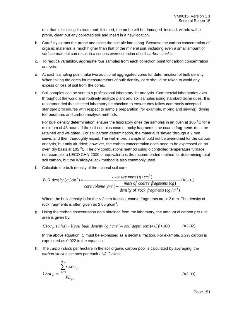
VM0015, Version 1.1 Sectoral Scope 15
Page 151
root that is blocking its route and, if forced, the probe will be damaged. Instead, withdraw the
probe, clean out any collected soil and insert in a new location.
b. Carefully extract the probe and place the sample into a bag. Because the carbon concentration of
organic materials is much higher than that of the mineral soil, including even a small amount of
surface material can result in a serious overestimation of soil carbon stocks.
c. To reduce variability, aggregate four samples from each collection point for carbon concentration
analysis.
d. At each sampling point, take two additional aggregated cores for determination of bulk density.
When taking the cores for measurements of bulk density, care should be taken to avoid any
excess or loss of soil from the cores.
e. Soil samples can be sent to a professional laboratory for analysis. Commercial laboratories exist
throughout the world and routinely analyze plant and soil samples using standard techniques. It is
recommended the selected laboratory be checked to ensure they follow commonly accepted
standard procedures with respect to sample preparation (for example, mixing and sieving), drying
temperatures and carbon analysis methods.
For bulk density determination, ensure the laboratory dries the samples in an oven at 105 oC for a
minimum of 48 hours. If the soil contains coarse, rocky fragments, the coarse fragments must be
retained and weighted. For soil carbon determination, the material is sieved through a 2 mm
sieve, and then thoroughly mixed. The well-mixed sample should not be oven-dried for the carbon
analysis, but only air-dried; however, the carbon concentration does need to be expressed on an
oven dry basis at 105 oC. The dry combustions method using o controlled temperature furnace
(for example, a LECO CHN-2000 or equivalent) is the recommended method for determining total
soil carbon, but the Walkley-Black method is also commonly used.
f. Calculate the bulk density of the mineral soil core:
)/(
)()(
)/()/(
3
3
33
mcgfragmentsrockofdensity
cgfragmentscoarseofmasscmvolumecore
cmgmassdryovencmgdensityBulk
(A3-31)
Where the bulk density is for the < 2 mm fraction, coarse fragments are > 2 mm. The density of
rock fragments is often given as 2.65 g/cm3.
g. Using the carbon concentration data obtained from the laboratory, the amount of carbon per unit
area is given by:
100)])()/([()/( 3 CcmdepthsoilcmgdensitybulksoilhatCsoccl (A3-32)
In the above equation, C must be expressed as a decimal fraction. For example, 2.2% carbon is
expressed as 0.022 in the equation.
h. The carbon stock per hectare in the soil organic carbon pool is calculated by averaging the
carbon stock estimates per each LU/LC class:
pl
PL
pl
pl
clPL
Csoc
Csoc
pl
1
(A3-33)
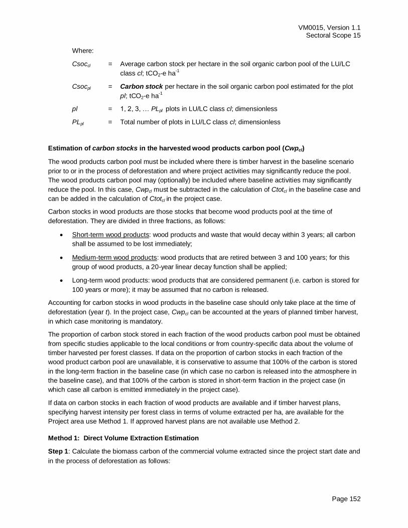
VM0015, Version 1.1 Sectoral Scope 15
Page 152
Where:
Csoccl = Average carbon stock per hectare in the soil organic carbon pool of the LU/LC
class cl; tCO2-e ha-1
Csocpl = Carbon stock per hectare in the soil organic carbon pool estimated for the plot
pl; tCO2-e ha-1
pl = 1, 2, 3, … PLpl plots in LU/LC class cl; dimensionless
PLpl = Total number of plots in LU/LC class cl; dimensionless
Estimation of carbon stocks in the harvested wood products carbon pool (Cwpcl)
The wood products carbon pool must be included where there is timber harvest in the baseline scenario
prior to or in the process of deforestation and where project activities may significantly reduce the pool.
The wood products carbon pool may (optionally) be included where baseline activities may significantly
reduce the pool. In this case, Cwpcl must be subtracted in the calculation of Ctotcl in the baseline case and
can be added in the calculation of Ctotcl in the project case.
Carbon stocks in wood products are those stocks that become wood products pool at the time of
deforestation. They are divided in three fractions, as follows:
Short-term wood products: wood products and waste that would decay within 3 years; all carbon
shall be assumed to be lost immediately;
Medium-term wood products: wood products that are retired between 3 and 100 years; for this
group of wood products, a 20-year linear decay function shall be applied;
Long-term wood products: wood products that are considered permanent (i.e. carbon is stored for
100 years or more); it may be assumed that no carbon is released.
Accounting for carbon stocks in wood products in the baseline case should only take place at the time of
deforestation (year t). In the project case, Cwpcl can be accounted at the years of planned timber harvest,
in which case monitoring is mandatory.
The proportion of carbon stock stored in each fraction of the wood products carbon pool must be obtained
from specific studies applicable to the local conditions or from country-specific data about the volume of
timber harvested per forest classes. If data on the proportion of carbon stocks in each fraction of the
wood product carbon pool are unavailable, it is conservative to assume that 100% of the carbon is stored
in the long-term fraction in the baseline case (in which case no carbon is released into the atmosphere in
the baseline case), and that 100% of the carbon is stored in short-term fraction in the project case (in
which case all carbon is emitted immediately in the project case).
If data on carbon stocks in each fraction of wood products are available and if timber harvest plans,
specifying harvest intensity per forest class in terms of volume extracted per ha, are available for the
Project area use Method 1. If approved harvest plans are not available use Method 2.
Method 1: Direct Volume Extraction Estimation
Step 1: Calculate the biomass carbon of the commercial volume extracted since the project start date and
in the process of deforestation as follows:
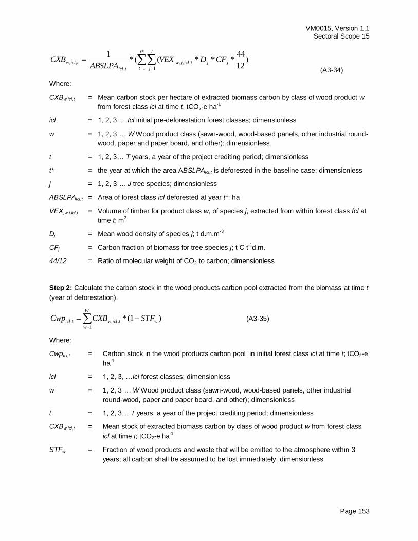
VM0015, Version 1.1 Sectoral Scope 15
Page 153
*
1 1
,,,
,
,, )12
44***((*
1 t
t
j
J
j
jticljw
ticl
ticlw CFDVEXABSLPA
CXB
(A3-34)
Where:
CXBw,icl,t = Mean carbon stock per hectare of extracted biomass carbon by class of wood product w
from forest class icl at time t; tCO2-e ha-1
icl = 1, 2, 3, …Icl initial pre-deforestation forest classes; dimensionless
w = 1, 2, 3 … W Wood product class (sawn-wood, wood-based panels, other industrial round-
wood, paper and paper board, and other); dimensionless
t = 1, 2, 3… T years, a year of the project crediting period; dimensionless
t* = the year at which the area ABSLPAicl,t is deforested in the baseline case; dimensionless
j = 1, 2, 3 … J tree species; dimensionless
ABSLPAicl,t = Area of forest class icl deforested at year t*; ha
VEX,w,j,fcl,t = Volume of timber for product class w, of species j, extracted from within forest class fcl at
time t; m3
Dj = Mean wood density of species j; t d.m.m-3
CFj = Carbon fraction of biomass for tree species j; t C t-1d.m.
44/12 = Ratio of molecular weight of CO2 to carbon; dimensionless
Step 2: Calculate the carbon stock in the wood products carbon pool extracted from the biomass at time t
(year of deforestation).
W
w
wticlwticl STFCXBCwp1
,,, )1(* (A3-35)
Where:
Cwpicl,t = Carbon stock in the wood products carbon pool in initial forest class icl at time t; tCO2-e
ha-1
icl = 1, 2, 3, …Icl forest classes; dimensionless
w = 1, 2, 3 … W Wood product class (sawn-wood, wood-based panels, other industrial
round-wood, paper and paper board, and other); dimensionless
t = 1, 2, 3… T years, a year of the project crediting period; dimensionless
CXBw,icl,t = Mean stock of extracted biomass carbon by class of wood product w from forest class
icl at time t; tCO2-e ha-1
STFw = Fraction of wood products and waste that will be emitted to the atmosphere within 3
years; all carbon shall be assumed to be lost immediately; dimensionless
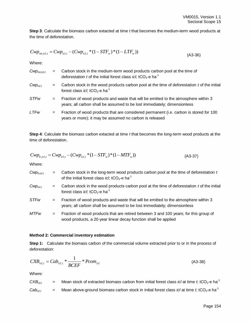
VM0015, Version 1.1 Sectoral Scope 15
Page 154
Step 3: Calculate the biomass carbon extacted at time t that becomes the medium-term wood products at
the time of deforestation.
(A3-36)
Where:
Cwpmt,icl,t = Carbon stock in the medium-term wood products carbon pool at the time of
deforestation t of the initial forest class icl; tCO2-e ha-1
Cwpicl,t = Carbon stock in the wood products carbon pool at the time of deforestation t of the initial
forest class icl; tCO2-e ha-1
STFw = Fraction of wood products and waste that will be emitted to the atmosphere within 3
years; all carbon shall be assumed to be lost immediately; dimensionless
LTFw = Fraction of wood products that are considered permanent (i.e. carbon is stored for 100
years or more); it may be assumed no carbon is released
Step 4: Calculate the biomass carbon extacted at time t that becomes the long-term wood products at the
time of deforestation.
(A3-37)
Where:
Cwplt,icl,t = Carbon stock in the long-term wood products carbon pool at the time of deforestation t
of the initial forest class icl; tCO2-e ha-1
Cwpicl,t = Carbon stock in the wood products carbon pool at the time of deforestation t of the initial
forest class icl; tCO2-e ha-1
STFw = Fraction of wood products and waste that will be emitted to the atmosphere within 3
years; all carbon shall be assumed to be lost immediately; dimensionless
MTFw = Fraction of wood products that are retired between 3 and 100 years; for this group of
wood products, a 20-year linear decay function shall be applied
Method 2: Commercial inventory estimation
Step 1: Calculate the biomass carbon of the commercial volume extracted prior to or in the process of
deforestation:
iclticlticl PcomBCEF
CabCXB *1
*,, (A3-38)
Where:
CXBicl,t = Mean stock of extracted biomass carbon from initial forest class icl at time t; tCO2-e ha-1
Cabicl,t = Mean above-ground biomass carbon stock in initial forest class icl at time t; tCO2-e ha-1
))1(*)1(*( ,,,, wwticlticlticlmt LTFSTFCwpCwpCwp
, , , ,( *(1 )*(1 ))lt icl t icl t icl t w wCwp Cwp Cwp STF MTF
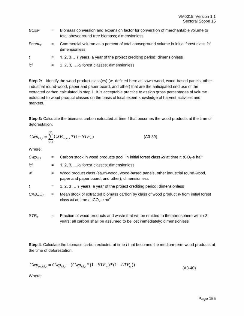
VM0015, Version 1.1 Sectoral Scope 15
Page 155
BCEF = Biomass conversion and expansion factor for conversion of merchantable volume to
total aboveground tree biomass; dimensionless
Pcomicl = Commercial volume as a percent of total aboveground volume in initial forest class icl;
dimensionless
t = 1, 2, 3… T years, a year of the project crediting period; dimensionless
icl = 1, 2, 3, …Icl forest classes; dimensionless
Step 2: Identify the wood product class(es) (w, defined here as sawn-wood, wood-based panels, other
industrial round-wood, paper and paper board, and other) that are the anticipated end use of the
extracted carbon calculated in step 1. It is acceptable practice to assign gross percentages of volume
extracted to wood product classes on the basis of local expert knowledge of harvest activities and
markets.
Step 3: Calculate the biomass carbon extracted at time t that becomes the wood products at the time of
deforestation.
W
w
wticlwticl STFCXBCwp1
,,, )1(* (A3-39)
Where:
Cwpicl,t = Carbon stock in wood products pool in initial forest class icl at time t; tCO2-e ha-1
icl = 1, 2, 3, …Icl forest classes; dimensionless
w = Wood product class (sawn-wood, wood-based panels, other industrial round-wood,
paper and paper board, and other); dimensionless
t = 1, 2, 3 … T years, a year of the project crediting period; dimensionless
CXBw,icl,t = Mean stock of extracted biomass carbon by class of wood product w from initial forest
class icl at time t; tCO2-e ha-1
STFw = Fraction of wood products and waste that will be emitted to the atmosphere within 3
years; all carbon shall be assumed to be lost immediately; dimensionless
Step 4: Calculate the biomass carbon extacted at time t that becomes the medium-term wood products at
the time of deforestation.
(A3-40)
Where:
))1(*)1(*( ,,,, wwticlticlticlmt LTFSTFCwpCwpCwp
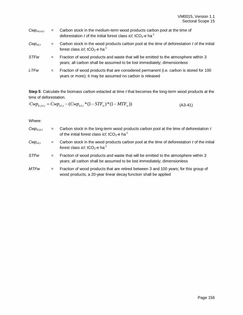
VM0015, Version 1.1 Sectoral Scope 15
Page 156
Cwpmt,icl,t = Carbon stock in the medium-term wood products carbon pool at the time of
deforestation t of the initial forest class icl; tCO2-e ha-1
Cwpicl,t = Carbon stock in the wood products carbon pool at the time of deforestation t of the initial
forest class icl; tCO2-e ha-1
STFw = Fraction of wood products and waste that will be emitted to the atmosphere within 3
years; all carbon shall be assumed to be lost immediately; dimensionless
LTFw = Fraction of wood products that are considered permanent (i.e. carbon is stored for 100
years or more); it may be assumed no carbon is released
Step 5: Calculate the biomass carbon extacted at time t that becomes the long-term wood products at the
time of deforestation.
(A3-41)
Where:
Cwplt,icl,t = Carbon stock in the long-term wood products carbon pool at the time of deforestation t
of the initial forest class icl; tCO2-e ha-1
Cwpicl,t = Carbon stock in the wood products carbon pool at the time of deforestation t of the initial
forest class icl; tCO2-e ha-1
STFw = Fraction of wood products and waste that will be emitted to the atmosphere within 3
years; all carbon shall be assumed to be lost immediately; dimensionless
MTFw = Fraction of wood products that are retired between 3 and 100 years; for this group of
wood products, a 20-year linear decay function shall be applied
, , , ,( *(1 )*(1 ))lt icl t icl t icl t w wCwp Cwp Cwp STF MTF
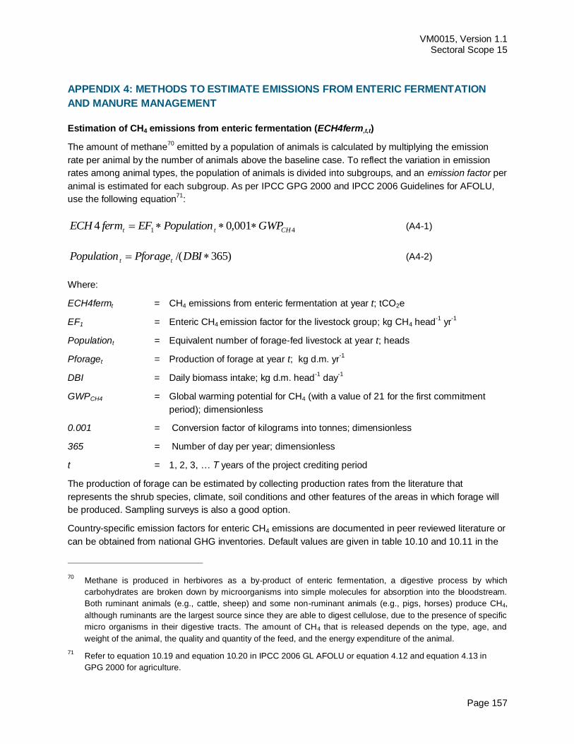
VM0015, Version 1.1 Sectoral Scope 15
Page 157
APPENDIX 4: METHODS TO ESTIMATE EMISSIONS FROM ENTERIC FERMENTATION
AND MANURE MANAGEMENT
Estimation of CH4 emissions from enteric fermentation (ECH4ferm,t,t)
The amount of methane70
emitted by a population of animals is calculated by multiplying the emission
rate per animal by the number of animals above the baseline case. To reflect the variation in emission
rates among animal types, the population of animals is divided into subgroups, and an emission factor per
animal is estimated for each subgroup. As per IPCC GPG 2000 and IPCC 2006 Guidelines for AFOLU,
use the following equation71
:
41 001,04 CHtt GWPPopulationEFfermECH (A4-1)
)365/( DBIPforagePopulation tt (A4-2)
Where:
ECH4fermt = CH4 emissions from enteric fermentation at year t; tCO2e
EF1 = Enteric CH4 emission factor for the livestock group; kg CH4 head-1
yr-1
Populationt = Equivalent number of forage-fed livestock at year t; heads
Pforaget = Production of forage at year t; kg d.m. yr-1
DBI = Daily biomass intake; kg d.m. head-1
day-1
GWPCH4 = Global warming potential for CH4 (with a value of 21 for the first commitment
period); dimensionless
0.001 = Conversion factor of kilograms into tonnes; dimensionless
365 = Number of day per year; dimensionless
t = 1, 2, 3, … T years of the project crediting period
The production of forage can be estimated by collecting production rates from the literature that
represents the shrub species, climate, soil conditions and other features of the areas in which forage will
be produced. Sampling surveys is also a good option.
Country-specific emission factors for enteric CH4 emissions are documented in peer reviewed literature or
can be obtained from national GHG inventories. Default values are given in table 10.10 and 10.11 in the
70 Methane is produced in herbivores as a by-product of enteric fermentation, a digestive process by which
carbohydrates are broken down by microorganisms into simple molecules for absorption into the bloodstream.
Both ruminant animals (e.g., cattle, sheep) and some non-ruminant animals (e.g., pigs, horses) produce CH4,
although ruminants are the largest source since they are able to digest cellulose, due to the presence of specific
micro organisms in their digestive tracts. The amount of CH4 that is released depends on the type, age, and
weight of the animal, the quality and quantity of the feed, and the energy expenditure of the animal.
71 Refer to equation 10.19 and equation 10.20 in IPCC 2006 GL AFOLU or equation 4.12 and equation 4.13 in
GPG 2000 for agriculture.
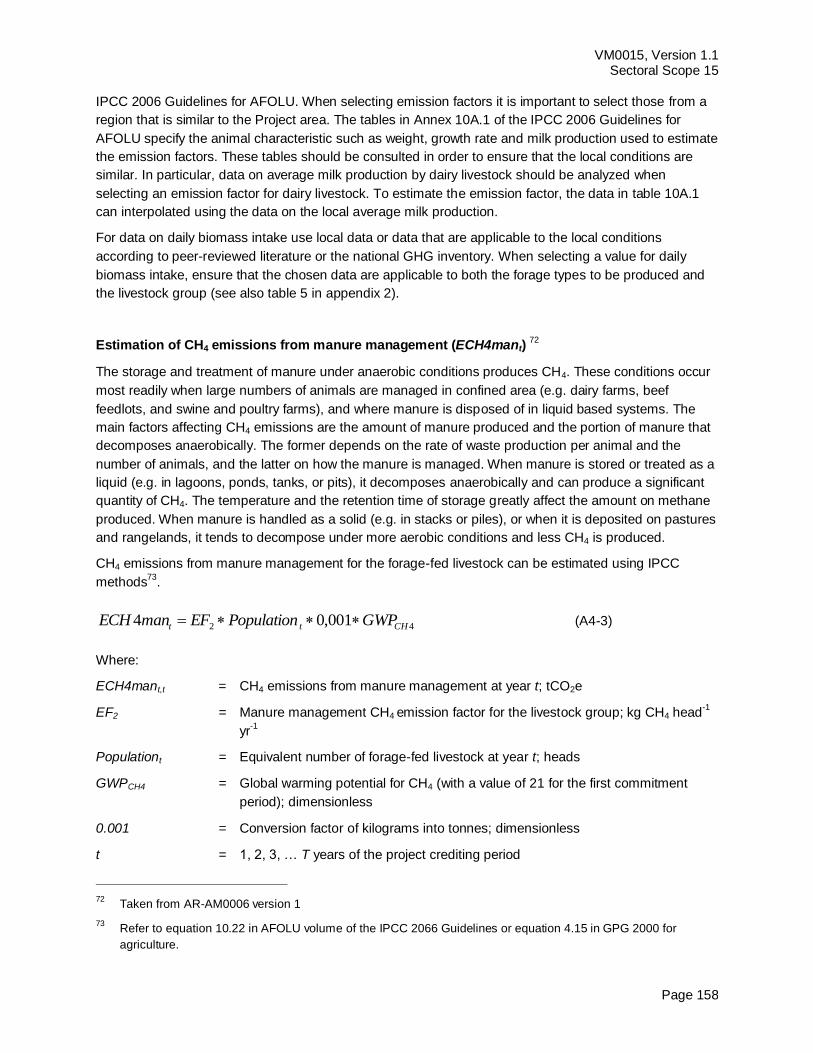
VM0015, Version 1.1 Sectoral Scope 15
Page 158
IPCC 2006 Guidelines for AFOLU. When selecting emission factors it is important to select those from a
region that is similar to the Project area. The tables in Annex 10A.1 of the IPCC 2006 Guidelines for
AFOLU specify the animal characteristic such as weight, growth rate and milk production used to estimate
the emission factors. These tables should be consulted in order to ensure that the local conditions are
similar. In particular, data on average milk production by dairy livestock should be analyzed when
selecting an emission factor for dairy livestock. To estimate the emission factor, the data in table 10A.1
can interpolated using the data on the local average milk production.
For data on daily biomass intake use local data or data that are applicable to the local conditions
according to peer-reviewed literature or the national GHG inventory. When selecting a value for daily
biomass intake, ensure that the chosen data are applicable to both the forage types to be produced and
the livestock group (see also table 5 in appendix 2).
Estimation of CH4 emissions from manure management (ECH4mant) 72
The storage and treatment of manure under anaerobic conditions produces CH4. These conditions occur
most readily when large numbers of animals are managed in confined area (e.g. dairy farms, beef
feedlots, and swine and poultry farms), and where manure is disposed of in liquid based systems. The
main factors affecting CH4 emissions are the amount of manure produced and the portion of manure that
decomposes anaerobically. The former depends on the rate of waste production per animal and the
number of animals, and the latter on how the manure is managed. When manure is stored or treated as a
liquid (e.g. in lagoons, ponds, tanks, or pits), it decomposes anaerobically and can produce a significant
quantity of CH4. The temperature and the retention time of storage greatly affect the amount on methane
produced. When manure is handled as a solid (e.g. in stacks or piles), or when it is deposited on pastures
and rangelands, it tends to decompose under more aerobic conditions and less CH4 is produced.
CH4 emissions from manure management for the forage-fed livestock can be estimated using IPCC
methods73
.
42 001,04 CHtt GWPPopulationEFmanECH (A4-3)
Where:
ECH4mant,t = CH4 emissions from manure management at year t; tCO2e
EF2 = Manure management CH4 emission factor for the livestock group; kg CH4 head-1
yr-1
Populationt = Equivalent number of forage-fed livestock at year t; heads
GWPCH4 = Global warming potential for CH4 (with a value of 21 for the first commitment
period); dimensionless
0.001 = Conversion factor of kilograms into tonnes; dimensionless
t = 1, 2, 3, … T years of the project crediting period
72
Taken from AR-AM0006 version 1
73 Refer to equation 10.22 in AFOLU volume of the IPCC 2066 Guidelines or equation 4.15 in GPG 2000 for
agriculture.
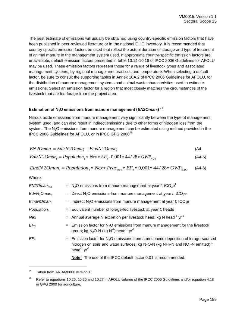
VM0015, Version 1.1 Sectoral Scope 15
Page 159
The best estimate of emissions will usually be obtained using country-specific emission factors that have
been published in peer-reviewed literature or in the national GHG inventory. It is recommended that
country-specific emission factors be used that reflect the actual duration of storage and type of treatment
of animal manure in the management system used. If appropriate country-specific emission factors are
unavailable, default emission factors presented in table 10.14-10.16 of IPCC 2006 Guidelines for AFOLU
may be used. These emission factors represent those for a range of livestock types and associated
management systems, by regional management practices and temperature. When selecting a default
factor, be sure to consult the supporting tables in Annex 10A.2 of IPCC 2006 Guidelines for AFOLU, for
the distribution of manure management systems and animal waste characteristics used to estimate
emissions. Select an emission factor for a region that most closely matches the circumstances of the
livestock that are fed forage from the project area.
Estimation of N2O emissions from manure management (EN2Omant) 74
Nitrous oxide emissions from manure management vary significantly between the type of management
system used, and can also result in indirect emissions due to other forms of nitrogen loss from the
system. The N2O emissions from manure management can be estimated using method provided in the
IPCC 2006 Guidelines for AFOLU, or in IPCC GPG 200075
ttt OmanEindNOmanEdirNOmanEN 222 (A4
203 28/44001,02 Ntt GWPEFNexPopulationOmanEdirN (A4-5)
ONgastt GWPEFFracNexPopulationOmanEindN 24 28/44001,02 (A4-6)
Where:
EN2Omanfcl,t = N2O emissions from manure management at year t; tCO2e1
EdirN2Omant = Direct N2O emissions from manure management at year t; tCO2e
EindNOmant = Indirect N2O emissions from manure management at year t; tCO2e
Populationt = Equivalent number of forage-fed livestock at year t; heads
Nex = Annual average N excretion per livestock head; kg N head-1
yr-1
EF3 = Emission factor for N2O emissions from manure management for the livestock
group; kg N2O-N (kg N-1
) head-1
yr-1
EF4 = Emission factor for N2O emissions from atmospheric deposition of forage-sourced
nitrogen on soils and water surfaces; kg N2O-N (kg NH3-N and NOx-N emitted)-1
head-1
yr-1
Note: The use of the IPCC default factor 0.01 is recommended.
74
Taken from AR-AM0006 version 1
75 Refer to equations 10.25, 10.26 and 10.27 in AFOLU volume of the IPCC 2006 Guidelines and/or equation 4.18
in GPG 2000 for agriculture.

VM0015, Version 1.1 Sectoral Scope 15
Page 160
Fracgas = Fraction of managed livestock manure nitrogen that volatilizes as NH3 and NOx
in the manure management phase; kg NH3-N and NOx-N emitted (Kg N)-1
GWPN2O = Global warming potential for N2O (310 for the first commitment period);
dimensionless
44/28 = Conversion of N20-N emissions to N2O emissions
0.001 = Conversion factor of kilograms into tonnes; dimensionless
The best estimate of the annual nitrogen excretion rates for each livestock group will usually be obtained
using country-specific rates from published peer reviewed literature or from the national GHG inventory. If
country-specific data cannot be collected or derived, or appropriate data are not available from another
country with similar conditions, default nitrogen excretion rates can be obtained from table 10.19 of IPCC
2006 Guidelines for AFOLU.
The possible data sources for emission factors are similar. Default emission factors are given in table
10.21 and 11.3 of the IPCC 2006 Guidelines for AFOLU and default values for volatilization of NH3 and
NOx (Fracgas) in the manure management system are presented in table 10.22 of the same IPCC 2006
Guidelines. For EF4the IPCC default value 0.01 is recommended (equation 10.27, IPCC 2006 Guidelines
for AFOLU).
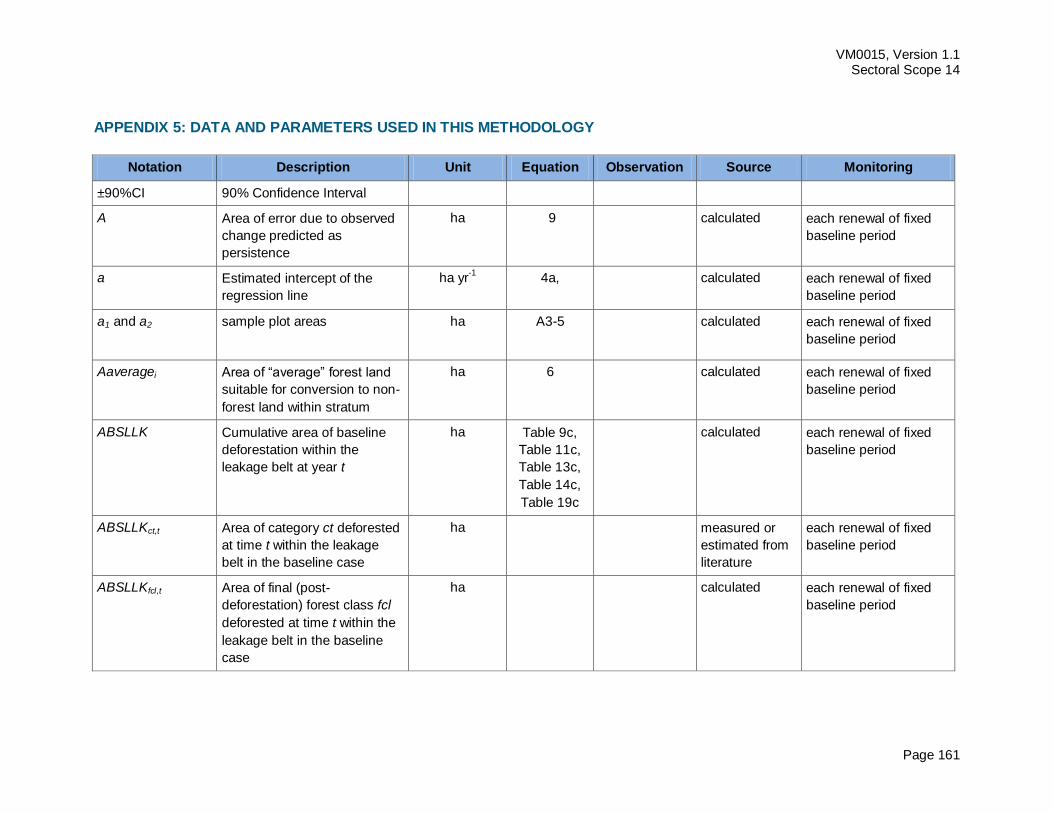
VM0015, Version 1.1 Sectoral Scope 14
Page 161
APPENDIX 5: DATA AND PARAMETERS USED IN THIS METHODOLOGY
Notation Description Unit Equation Observation Source Monitoring
±90%CI 90% Confidence Interval
A Area of error due to observed
change predicted as
persistence
ha 9 calculated each renewal of fixed
baseline period
a Estimated intercept of the
regression line
ha yr-1
4a, calculated each renewal of fixed
baseline period
a1 and a2 sample plot areas ha A3-5 calculated each renewal of fixed
baseline period
Aaveragei Area of “average” forest land
suitable for conversion to non-
forest land within stratum
ha 6 calculated each renewal of fixed
baseline period
ABSLLK Cumulative area of baseline
deforestation within the
leakage belt at year t
ha Table 9c,
Table 11c,
Table 13c,
Table 14c,
Table 19c
calculated each renewal of fixed
baseline period
ABSLLKct,t Area of category ct deforested
at time t within the leakage
belt in the baseline case
ha measured or
estimated from
literature
each renewal of fixed
baseline period
ABSLLKfcl,t Area of final (post-
deforestation) forest class fcl
deforested at time t within the
leakage belt in the baseline
case
ha calculated each renewal of fixed
baseline period
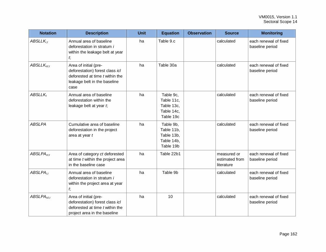
VM0015, Version 1.1 Sectoral Scope 14
Page 162
Notation Description Unit Equation Observation Source Monitoring
ABSLLKi,t Annual area of baseline
deforestation in stratum i
within the leakage belt at year
t;
ha Table 9.c calculated each renewal of fixed
baseline period
ABSLLKicl,t Area of initial (pre-
deforestation) forest class icl
deforested at time t within the
leakage belt in the baseline
case
ha Table 30a calculated each renewal of fixed
baseline period
ABSLLKt Annual area of baseline
deforestation within the
leakage belt at year t;
ha Table 9c,
Table 11c,
Table 13c,
Table 14c,
Table 19c
calculated each renewal of fixed
baseline period
ABSLPA Cumulative area of baseline
deforestation in the project
area at year t
ha Table 9b,
Table 11b,
Table 13b,
Table 14b,
Table 19b
calculated each renewal of fixed
baseline period
ABSLPAct,t Area of category ct deforested
at time t within the project area
in the baseline case
ha Table 22b1 measured or
estimated from
literature
each renewal of fixed
baseline period
ABSLPAi,t Annual area of baseline
deforestation in stratum i
within the project area at year
t;
ha Table 9b
calculated each renewal of fixed
baseline period
ABSLPAicl,t Area of initial (pre-
deforestation) forest class icl
deforested at time t within the
project area in the baseline
ha 10 calculated each renewal of fixed
baseline period
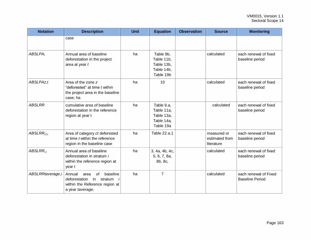
VM0015, Version 1.1 Sectoral Scope 14
Page 163
Notation Description Unit Equation Observation Source Monitoring
case
ABSLPAt Annual area of baseline
deforestation in the project
area at year t
ha Table 9b,
Table 11b,
Table 13b,
Table 14b,
Table 19b
calculated each renewal of fixed
baseline period
ABSLPAz,t Area of the zone z
“deforested” at time t within
the project area in the baseline
case; ha
ha 10 calculated each renewal of fixed
baseline period
ABSLRR cumulative area of baseline
deforestation in the reference
region at year t
ha Table 9.a,
Table 11a,
Table 13a,
Table 14a,
Table 19a
calculated each renewal of fixed
baseline period
ABSLRRct,t Area of category ct deforested
at time t within the reference
region in the baseline case
ha Table 22.a.1 measured or
estimated from
literature
each renewal of fixed
baseline period
ABSLRRi,t Annual area of baseline
deforestation in stratum i
within the reference region at
year t
ha 3, 4a, 4b, 4c,
5, 6, 7, 8a,
8b, 8c,
calculated each renewal of fixed
baseline period
ABSLRRtaverage,i Annual area of baseline
deforestation in stratum i
within the Reference region at
a year taveragei
ha 7 calculated each renewal of Fixed
Baseline Period
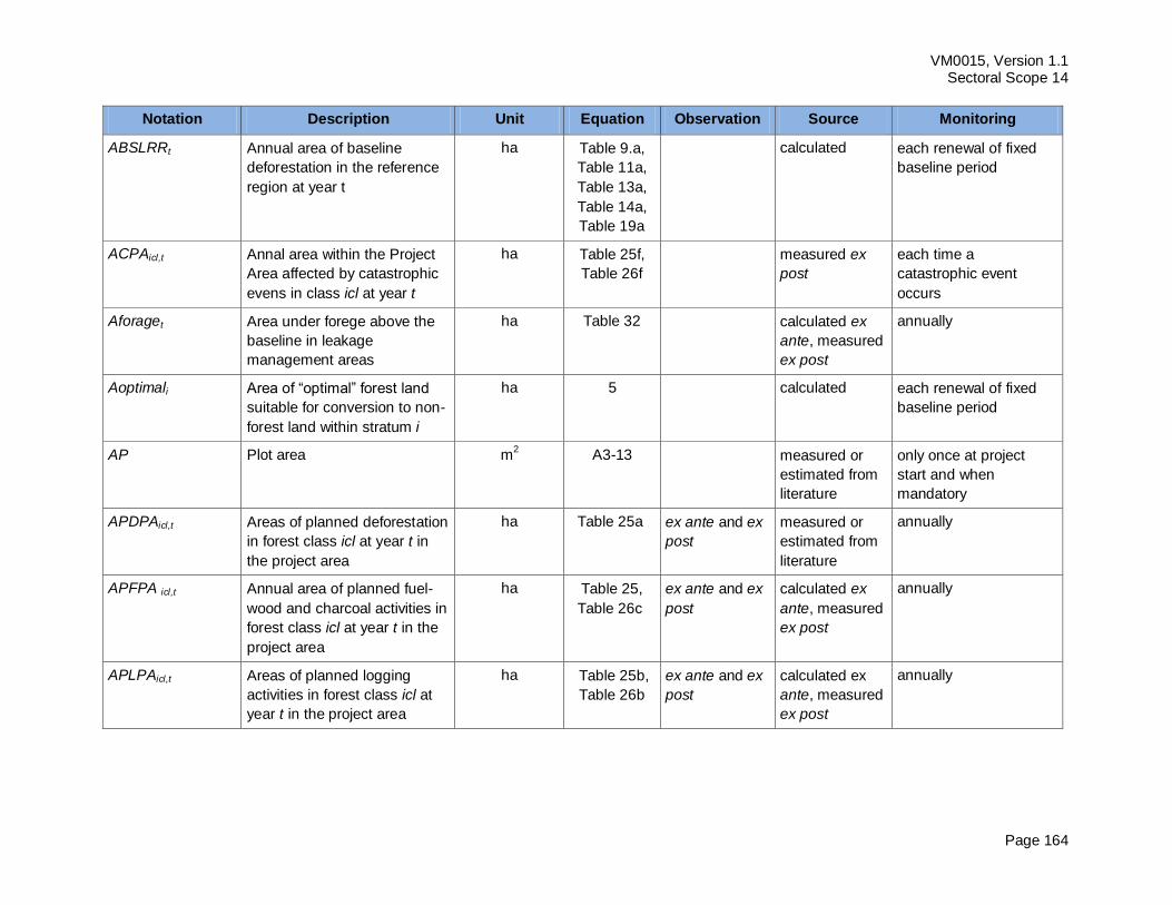
VM0015, Version 1.1 Sectoral Scope 14
Page 164
Notation Description Unit Equation Observation Source Monitoring
ABSLRRt Annual area of baseline
deforestation in the reference
region at year t
ha Table 9.a,
Table 11a,
Table 13a,
Table 14a,
Table 19a
calculated each renewal of fixed
baseline period
ACPAicl,t Annal area within the Project
Area affected by catastrophic
evens in class icl at year t
ha Table 25f,
Table 26f
measured ex
post
each time a
catastrophic event
occurs
Aforaget Area under forege above the
baseline in leakage
management areas
ha Table 32 calculated ex
ante, measured
ex post
annually
Aoptimali Area of “optimal” forest land
suitable for conversion to non-
forest land within stratum i
ha 5 calculated each renewal of fixed
baseline period
AP Plot area m2 A3-13 measured or
estimated from
literature
only once at project
start and when
mandatory
APDPAicl,t Areas of planned deforestation
in forest class icl at year t in
the project area
ha Table 25a ex ante and ex
post
measured or
estimated from
literature
annually
APFPA icl,t Annual area of planned fuel-
wood and charcoal activities in
forest class icl at year t in the
project area
ha Table 25,
Table 26c
ex ante and ex
post
calculated ex
ante, measured
ex post
annually
APLPAicl,t Areas of planned logging
activities in forest class icl at
year t in the project area
ha Table 25b,
Table 26b
ex ante and ex
post
calculated ex
ante, measured
ex post
annually
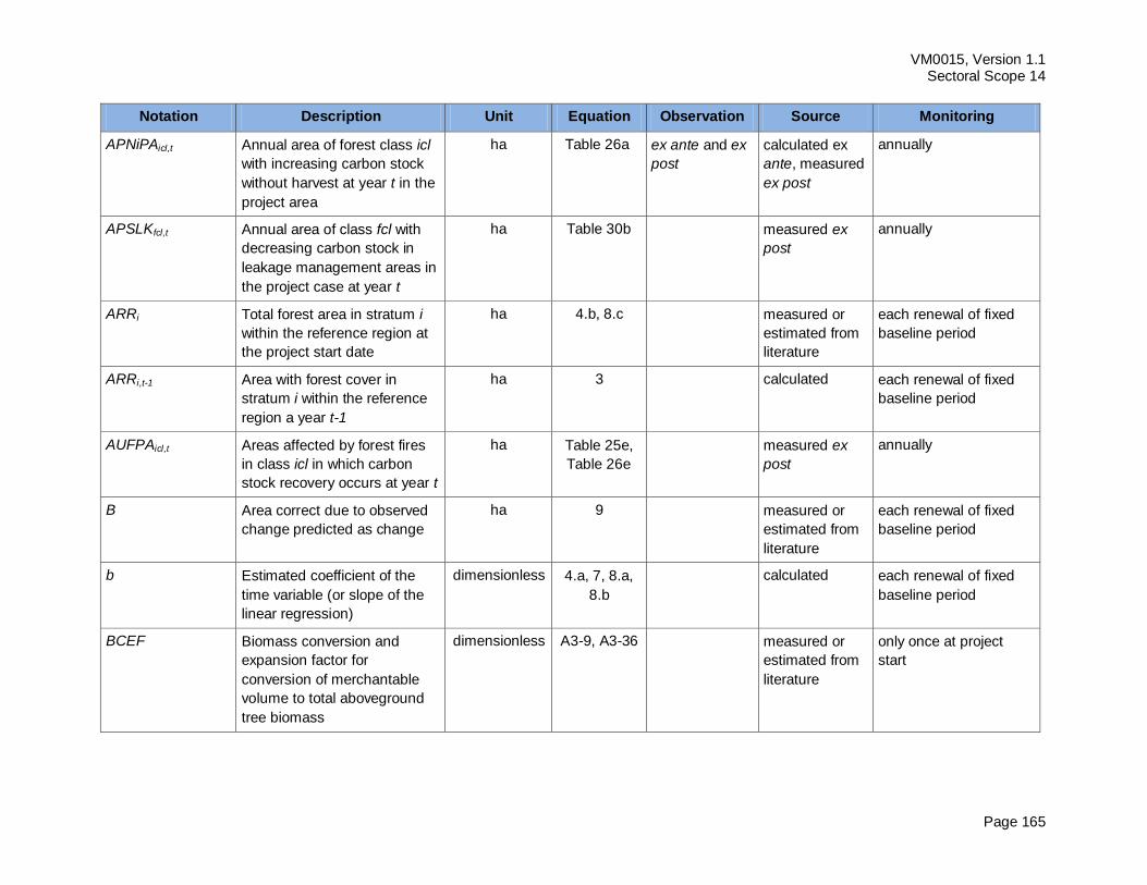
VM0015, Version 1.1 Sectoral Scope 14
Page 165
Notation Description Unit Equation Observation Source Monitoring
APNiPAicl,t Annual area of forest class icl
with increasing carbon stock
without harvest at year t in the
project area
ha Table 26a ex ante and ex
post
calculated ex
ante, measured
ex post
annually
APSLKfcl,t Annual area of class fcl with
decreasing carbon stock in
leakage management areas in
the project case at year t
ha Table 30b measured ex
post
annually
ARRi Total forest area in stratum i
within the reference region at
the project start date
ha 4.b, 8.c measured or
estimated from
literature
each renewal of fixed
baseline period
ARRi,t-1 Area with forest cover in
stratum i within the reference
region a year t-1
ha 3 calculated each renewal of fixed
baseline period
AUFPAicl,t Areas affected by forest fires
in class icl in which carbon
stock recovery occurs at year t
ha Table 25e,
Table 26e
measured ex
post
annually
B Area correct due to observed
change predicted as change
ha 9 measured or
estimated from
literature
each renewal of fixed
baseline period
b Estimated coefficient of the
time variable (or slope of the
linear regression)
dimensionless 4.a, 7, 8.a,
8.b
calculated each renewal of fixed
baseline period
BCEF Biomass conversion and
expansion factor for
conversion of merchantable
volume to total aboveground
tree biomass
dimensionless A3-9, A3-36 measured or
estimated from
literature
only once at project
start
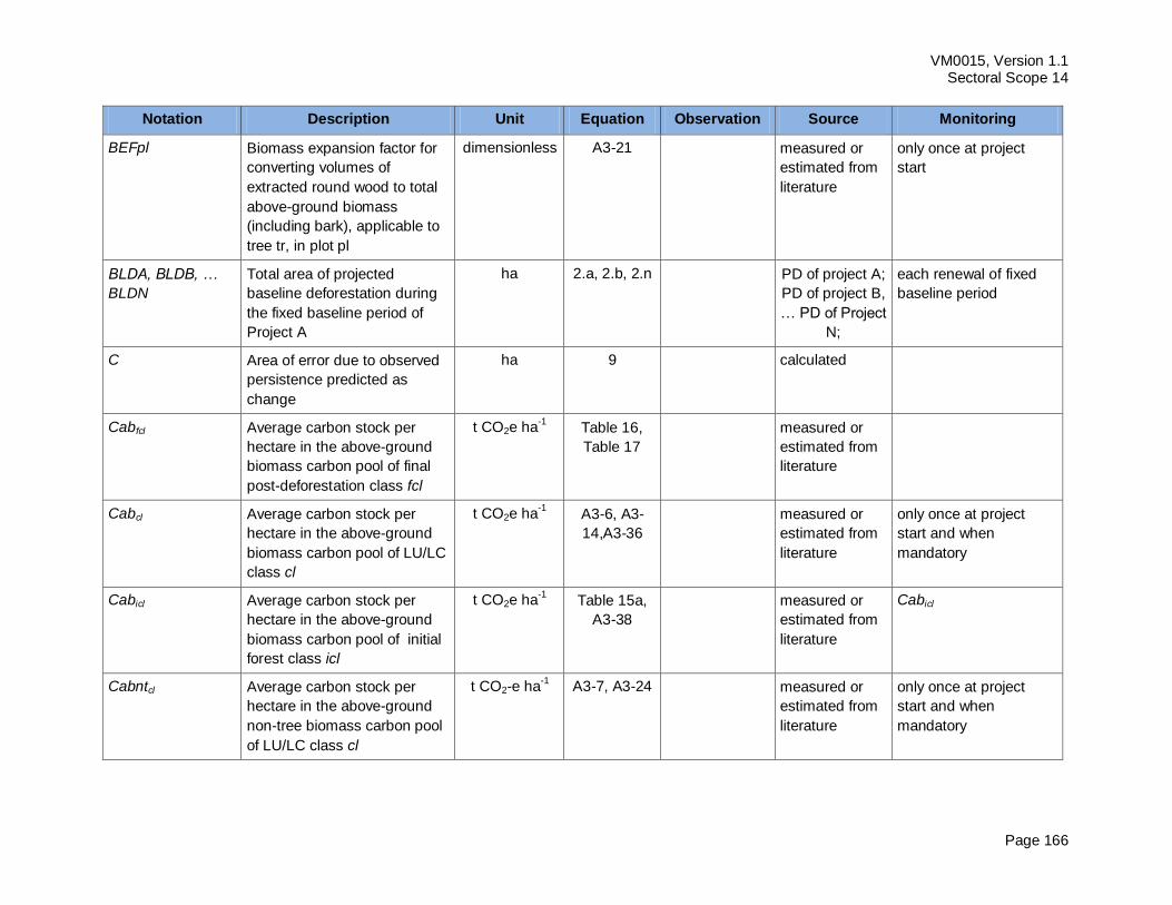
VM0015, Version 1.1 Sectoral Scope 14
Page 166
Notation Description Unit Equation Observation Source Monitoring
BEFpl Biomass expansion factor for
converting volumes of
extracted round wood to total
above-ground biomass
(including bark), applicable to
tree tr, in plot pl
dimensionless A3-21 measured or
estimated from
literature
only once at project
start
BLDA, BLDB, …
BLDN
Total area of projected
baseline deforestation during
the fixed baseline period of
Project A
ha 2.a, 2.b, 2.n PD of project A;
PD of project B,
… PD of Project
N;
each renewal of fixed
baseline period
C Area of error due to observed
persistence predicted as
change
ha 9 calculated
Cabfcl Average carbon stock per
hectare in the above-ground
biomass carbon pool of final
post-deforestation class fcl
t CO2e ha-1 Table 16,
Table 17
measured or
estimated from
literature
Cabcl Average carbon stock per
hectare in the above-ground
biomass carbon pool of LU/LC
class cl
t CO2e ha-1 A3-6, A3-
14,A3-36
measured or
estimated from
literature
only once at project
start and when
mandatory
Cabicl Average carbon stock per
hectare in the above-ground
biomass carbon pool of initial
forest class icl
t CO2e ha-1 Table 15a,
A3-38
measured or
estimated from
literature
Cabicl
Cabntcl Average carbon stock per
hectare in the above-ground
non-tree biomass carbon pool
of LU/LC class cl
t CO2-e ha-1 A3-7, A3-24 measured or
estimated from
literature
only once at project
start and when
mandatory
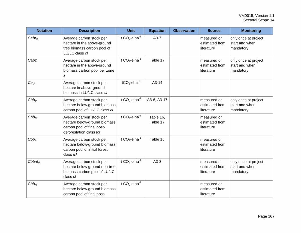
VM0015, Version 1.1 Sectoral Scope 14
Page 167
Notation Description Unit Equation Observation Source Monitoring
Cabtcl Average carbon stock per
hectare in the above-ground
tree biomass carbon pool of
LU/LC class cl
t CO2-e ha-1 A3-7 measured or
estimated from
literature
only once at project
start and when
mandatory
Cabz Average carbon stock per
hectare in the above-ground
biomass carbon pool per zone
z
t CO2-e ha-1 Table 17 measured or
estimated from
literature
only once at project
start and when
mandatory
Cacl Average carbon stock per
hectare in above-ground
biomass in LU/LC class cl
tCO2-eha-1
A3-14
Cbbcl Average carbon stock per
hectare below-ground biomass
carbon pool of LU/LC class cl
t CO2-e ha-1 A3-6, A3-17 measured or
estimated from
literature
only once at project
start and when
mandatory
Cbbfcl Average carbon stock per
hectare below-ground biomass
carbon pool of final post-
deforestation class fcl
t CO2-e ha-1 Table 16,
Table 17
measured or
estimated from
literature
Cbbicl Average carbon stock per
hectare below-ground biomass
carbon pool of initial forest
class icl
t CO2-e ha-1 Table 15 measured or
estimated from
literature
Cbbntcl Average carbon stock per
hectare below-ground non-tree
biomass carbon pool of LU/LC
class cl
t CO2-e ha-1 A3-8 measured or
estimated from
literature
only once at project
start and when
mandatory
Cbbfcl Average carbon stock per
hectare below-ground biomass
carbon pool of final post-
t CO2-e ha-1 measured or
estimated from
literature
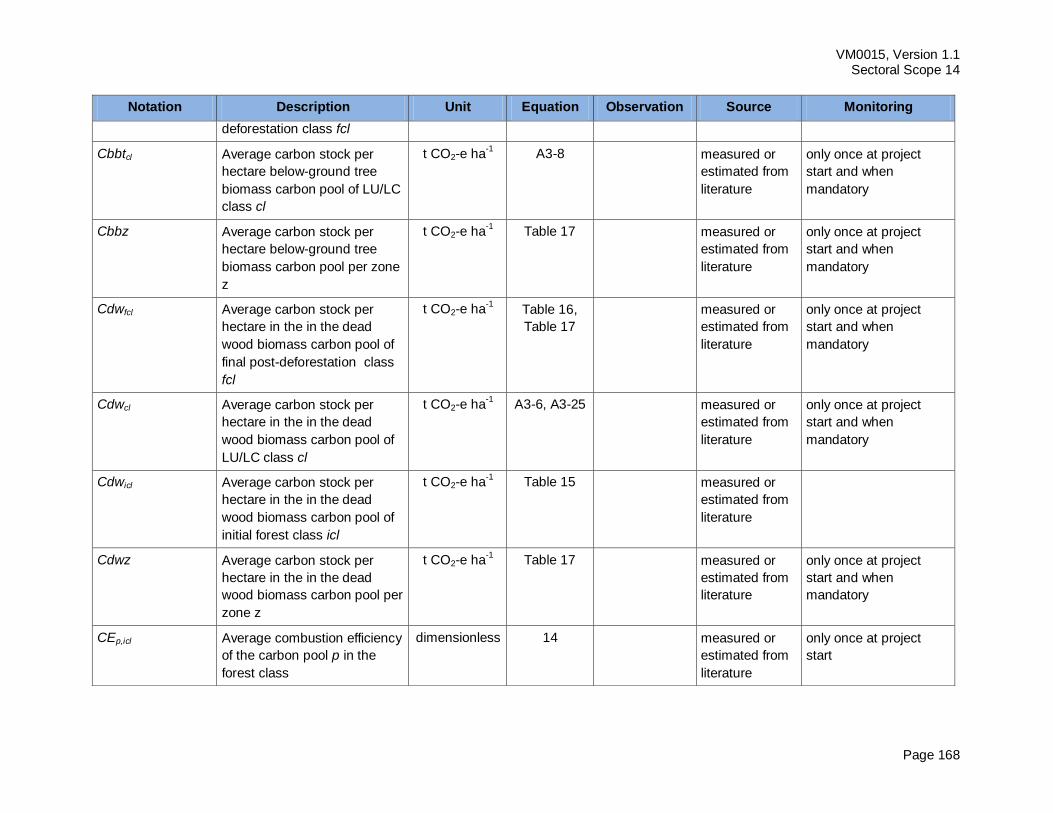
VM0015, Version 1.1 Sectoral Scope 14
Page 168
Notation Description Unit Equation Observation Source Monitoring
deforestation class fcl
Cbbtcl Average carbon stock per
hectare below-ground tree
biomass carbon pool of LU/LC
class cl
t CO2-e ha-1 A3-8 measured or
estimated from
literature
only once at project
start and when
mandatory
Cbbz Average carbon stock per
hectare below-ground tree
biomass carbon pool per zone
z
t CO2-e ha-1 Table 17 measured or
estimated from
literature
only once at project
start and when
mandatory
Cdwfcl Average carbon stock per
hectare in the in the dead
wood biomass carbon pool of
final post-deforestation class
fcl
t CO2-e ha-1 Table 16,
Table 17
measured or
estimated from
literature
only once at project
start and when
mandatory
Cdwcl Average carbon stock per
hectare in the in the dead
wood biomass carbon pool of
LU/LC class cl
t CO2-e ha-1 A3-6, A3-25 measured or
estimated from
literature
only once at project
start and when
mandatory
Cdwicl Average carbon stock per
hectare in the in the dead
wood biomass carbon pool of
initial forest class icl
t CO2-e ha-1 Table 15 measured or
estimated from
literature
Cdwz Average carbon stock per
hectare in the in the dead
wood biomass carbon pool per
zone z
t CO2-e ha-1 Table 17 measured or
estimated from
literature
only once at project
start and when
mandatory
CEp,icl Average combustion efficiency
of the carbon pool p in the
forest class
dimensionless 14 measured or
estimated from
literature
only once at project
start
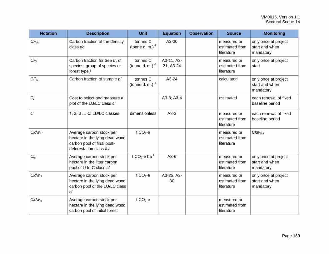
VM0015, Version 1.1 Sectoral Scope 14
Page 169
Notation Description Unit Equation Observation Source Monitoring
CFdc Carbon fraction of the density
class dc
tonnes C
(tonne d. m.)-1
A3-30 measured or
estimated from
literature
only once at project
start and when
mandatory
CFj Carbon fraction for tree tr, of
species, group of species or
forest type j
tonnes C
(tonne d. m.) -1
A3-11, A3-
21, A3-24
measured or
estimated from
literature
only once at project
start
CFpl Carbon fraction of sample pl tonnes C
(tonne d. m.) -1
A3-24 calculated only once at project
start and when
mandatory
Ci Cost to select and measure a
plot of the LU/LC class cl
A3-3; A3-4 estimated each renewal of fixed
baseline period
cl 1, 2, 3 … Cl LU/LC classes dimensionless A3-3 measured or
estimated from
literature
each renewal of fixed
baseline period
Cldwfcl Average carbon stock per
hectare in the lying dead wood
carbon pool of final post-
deforestation class fcl
t CO2-e measured or
estimated from
literature
Cldwfcl
Clcl Average carbon stock per
hectare in the litter carbon
pool of LU/LC class cl
t CO2-e ha-1 A3-6 measured or
estimated from
literature
only once at project
start and when
mandatory
Cldwcl Average carbon stock per
hectare in the lying dead wood
carbon pool of the LU/LC class
cl
t CO2-e A3-25, A3-
30
measured or
estimated from
literature
only once at project
start and when
mandatory
Cldwicl Average carbon stock per
hectare in the lying dead wood
carbon pool of initial forest
t CO2-e measured or
estimated from
literature
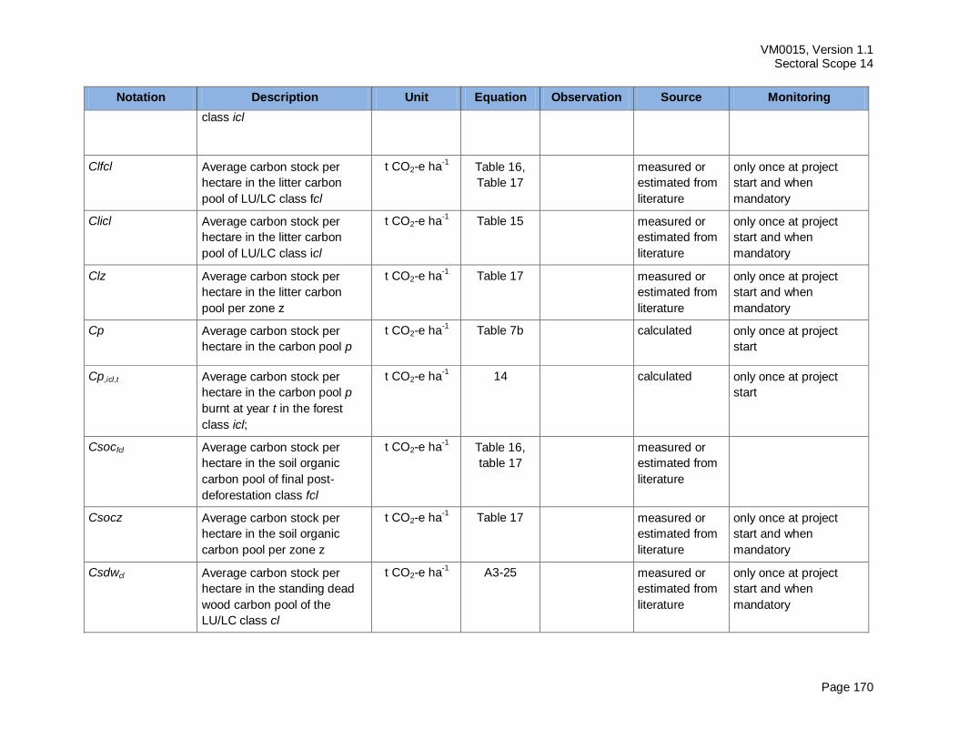
VM0015, Version 1.1 Sectoral Scope 14
Page 170
Notation Description Unit Equation Observation Source Monitoring
class icl
Clfcl Average carbon stock per
hectare in the litter carbon
pool of LU/LC class fcl
t CO2-e ha-1 Table 16,
Table 17
measured or
estimated from
literature
only once at project
start and when
mandatory
Clicl Average carbon stock per
hectare in the litter carbon
pool of LU/LC class icl
t CO2-e ha-1 Table 15 measured or
estimated from
literature
only once at project
start and when
mandatory
Clz Average carbon stock per
hectare in the litter carbon
pool per zone z
t CO2-e ha-1 Table 17 measured or
estimated from
literature
only once at project
start and when
mandatory
Cp Average carbon stock per
hectare in the carbon pool p
t CO2-e ha-1 Table 7b calculated only once at project
start
Cp,icl,t Average carbon stock per
hectare in the carbon pool p
burnt at year t in the forest
class icl;
t CO2-e ha-1 14 calculated only once at project
start
Csocfcl Average carbon stock per
hectare in the soil organic
carbon pool of final post-
deforestation class fcl
t CO2-e ha-1 Table 16,
table 17
measured or
estimated from
literature
Csocz Average carbon stock per
hectare in the soil organic
carbon pool per zone z
t CO2-e ha-1 Table 17 measured or
estimated from
literature
only once at project
start and when
mandatory
Csdwcl Average carbon stock per
hectare in the standing dead
wood carbon pool of the
LU/LC class cl
t CO2-e ha-1 A3-25 measured or
estimated from
literature
only once at project
start and when
mandatory
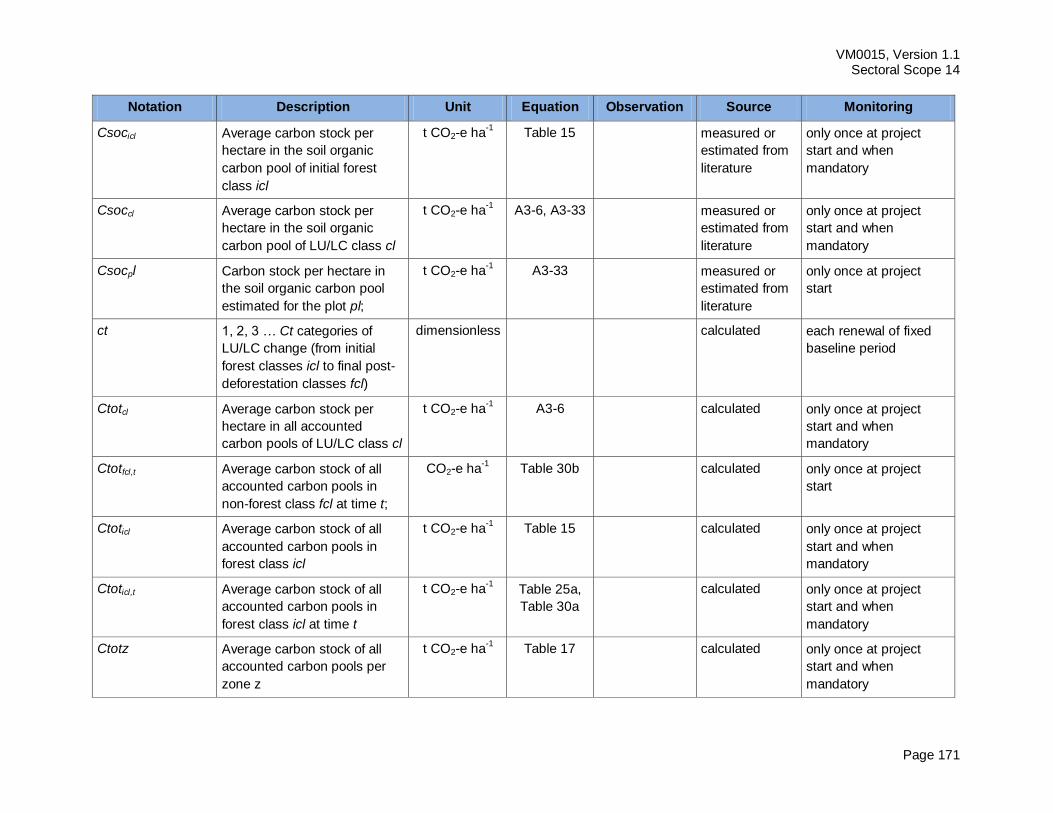
VM0015, Version 1.1 Sectoral Scope 14
Page 171
Notation Description Unit Equation Observation Source Monitoring
Csocicl Average carbon stock per
hectare in the soil organic
carbon pool of initial forest
class icl
t CO2-e ha-1 Table 15 measured or
estimated from
literature
only once at project
start and when
mandatory
Csoccl Average carbon stock per
hectare in the soil organic
carbon pool of LU/LC class cl
t CO2-e ha-1 A3-6, A3-33 measured or
estimated from
literature
only once at project
start and when
mandatory
Csocpl Carbon stock per hectare in
the soil organic carbon pool
estimated for the plot pl;
t CO2-e ha-1 A3-33 measured or
estimated from
literature
only once at project
start
ct 1, 2, 3 … Ct categories of
LU/LC change (from initial
forest classes icl to final post-
deforestation classes fcl)
dimensionless calculated each renewal of fixed
baseline period
Ctotcl Average carbon stock per
hectare in all accounted
carbon pools of LU/LC class cl
t CO2-e ha-1 A3-6 calculated only once at project
start and when
mandatory
Ctotfcl,t Average carbon stock of all
accounted carbon pools in
non-forest class fcl at time t;
CO2-e ha-1
Table 30b calculated only once at project
start
Ctoticl Average carbon stock of all
accounted carbon pools in
forest class icl
t CO2-e ha-1 Table 15 calculated only once at project
start and when
mandatory
Ctoticl,t Average carbon stock of all
accounted carbon pools in
forest class icl at time t
t CO2-e ha-1 Table 25a,
Table 30a
calculated only once at project
start and when
mandatory
Ctotz Average carbon stock of all
accounted carbon pools per
zone z
t CO2-e ha-1 Table 17 calculated only once at project
start and when
mandatory
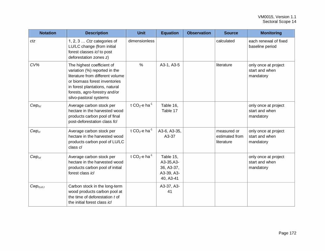
VM0015, Version 1.1 Sectoral Scope 14
Page 172
Notation Description Unit Equation Observation Source Monitoring
ctz 1, 2, 3 … Ctz categories of
LU/LC change (from initial
forest classes icl to post
deforestation zones z)
dimensionless calculated each renewal of fixed
baseline period
CV% The highest coefficient of
variation (%) reported in the
literature from different volume
or biomass forest inventories
in forest plantations, natural
forests, agro-forestry and/or
silvo-pastoral systems
% A3-1, A3-5 literature only once at project
start and when
mandatory
Cwpfcl Average carbon stock per
hectare in the harvested wood
products carbon pool of final
post-deforestation class fcl
t CO2-e ha-1 Table 16,
Table 17
only once at project
start and when
mandatory
Cwpcl Average carbon stock per
hectare in the harvested wood
products carbon pool of LU/LC
class cl
t CO2-e ha-1 A3-6, A3-35,
A3-37
measured or
estimated from
literature
only once at project
start and when
mandatory
Cwpicl Average carbon stock per
hectare in the harvested wood
products carbon pool of initial
forest class icl
t CO2-e ha-1 Table 15,
A3-35,A3-
36, A3-37,
A3-39, A3-
40, A3-41
only once at project
start and when
mandatory
Cwplt,icl,t Carbon stock in the long-term
wood products carbon pool at
the time of deforestation t of
the initial forest class icl
A3-37, A3-
41
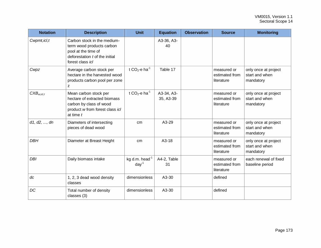
VM0015, Version 1.1 Sectoral Scope 14
Page 173
Notation Description Unit Equation Observation Source Monitoring
Cwpmt,icl,t Carbon stock in the medium-
term wood products carbon
pool at the time of
deforestation t of the initial
forest class icl
A3-36, A3-
40
Cwpz Average carbon stock per
hectare in the harvested wood
products carbon pool per zone
z
t CO2-e ha-1 Table 17 measured or
estimated from
literature
only once at project
start and when
mandatory
CXBw,icl,t Mean carbon stock per
hectare of extracted biomass
carbon by class of wood
product w from forest class icl
at time t
t CO2-e ha-1 A3-34, A3-
35, A3-39
measured or
estimated from
literature
only once at project
start and when
mandatory
d1, d2, ..., dn Diameters of intersecting
pieces of dead wood
cm A3-29 measured or
estimated from
literature
only once at project
start and when
mandatory
DBH Diameter at Breast Height cm A3-18 measured or
estimated from
literature
only once at project
start and when
mandatory
DBI Daily biomass intake kg d.m. head-1
day-1
A4-2, Table
31
measured or
estimated from
literature
each renewal of fixed
baseline period
dc 1, 2, 3 dead wood density
classes
dimensionless A3-30 defined
DC Total number of density
classes (3)
dimensionless A3-30 defined
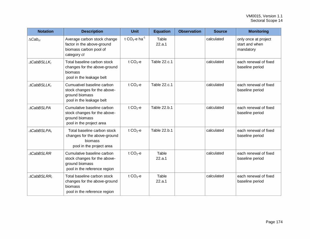
VM0015, Version 1.1 Sectoral Scope 14
Page 174
Notation Description Unit Equation Observation Source Monitoring
Cabct Average carbon stock change
factor in the above-ground
biomass carbon pool of
category ct
t CO2-e ha-1 Table
22.a.1
calculated only once at project
start and when
mandatory
CabBSLLKt Total baseline carbon stock
changes for the above-ground
biomass
pool in the leakage belt
t CO2-e Table 22.c.1 calculated each renewal of fixed
baseline period
CabBSLLKt Cumuativel baseline carbon
stock changes for the above-
ground biomass
pool in the leakage belt
t CO2-e Table 22.c.1 calculated each renewal of fixed
baseline period
CabBSLPA Cumulative baseline carbon
stock changes for the above-
ground biomass
pool in the project area
t CO2-e Table 22.b.1 calculated each renewal of fixed
baseline period
CabBSLPAt Total baseline carbon stock
changes for the above-ground
biomass
pool in the project area
t CO2-e Table 22.b.1 calculated each renewal of fixed
baseline period
CabBSLRR Cumulative baseline carbon
stock changes for the above-
ground biomass
pool in the reference region
t CO2-e Table
22.a.1
calculated each renewal of fixed
baseline period
CabBSLRRt Total baseline carbon stock
changes for the above-ground
biomass
pool in the reference region
t CO2-e Table
22.a.1
calculated each renewal of fixed
baseline period
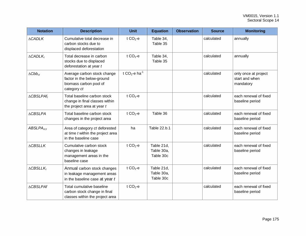
VM0015, Version 1.1 Sectoral Scope 14
Page 175
Notation Description Unit Equation Observation Source Monitoring
CADLK Cumulative total decrease in
carbon stocks due to
displaced deforestation
t CO2-e Table 34,
Table 35
calculated annually
CADLKt Total decrease in carbon
stocks due to displaced
deforestation at year t
t CO2-e Table 34,
Table 35
calculated annually
Cbbct Average carbon stock change
factor in the below-ground
biomass carbon pool of
category ct
t CO2-e ha-1 calculated only once at project
start and when
mandatory
CBSLPAft Total baseline carbon stock
change in final classes within
the project area at year t
t CO2-e calculated each renewal of fixed
baseline period
CBSLPA Total baseline carbon stock
changes in the project area
t CO2-e Table 36 calculated each renewal of fixed
baseline period
ABSLPAct,t Area of category ct deforested
at time t within the project area
in the baseline case
ha Table 22.b.1 calculated each renewal of fixed
baseline period
CBSLLK Cumulative carbon stock
changes in leakage
management areas in the
baseline case
t CO2-e Table 21d,
Table 30a,
Table 30c
calculated each renewal of fixed
baseline period
CBSLLKt Annual carbon stock changes
in leakage management areas
in the baseline case at year t
t CO2-e Table 21d,
Table 30a,
Table 30c
calculated each renewal of fixed
baseline period
CBSLPAf Total cumulative baseline
carbon stock change in final
classes within the project area
t CO2-e calculated each renewal of fixed
baseline period
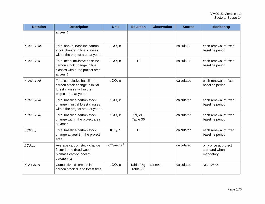
VM0015, Version 1.1 Sectoral Scope 14
Page 176
Notation Description Unit Equation Observation Source Monitoring
at year t
CBSLPAft Total annual baseline carbon
stock change in final classes
within the project area at year t
t CO2-e calculated each renewal of fixed
baseline period
CBSLPA Total net cumulative baseline
carbon stock change in final
classes within the project area
at year t
t CO2-e 10 calculated each renewal of fixed
baseline period
CBSLPAi Total cumulative baseline
carbon stock change in initial
forest classes within the
project area at year t
t CO2-e calculated each renewal of fixed
baseline period
CBSLPAit Total baseline carbon stock
change in initial forest classes
within the project area at year t
t CO2-e calculated each renewal of fixed
baseline period
CBSLPAt Total baseline carbon stock
change within the project area
at year t
t CO2-e 19, 21,
Table 36
calculated each renewal of fixed
baseline period
CBSLt Total baseline carbon stock
change at year t in the project
area
tCO2-e 16 calculated each renewal of fixed
baseline period
Cdwct Average carbon stock change
factor in the dead wood
biomass carbon pool of
category ct
t CO2-e ha-1 calculated only once at project
start and when
mandatory
CFCdPA Cumulative decrease in
carbon stock due to forest fires
t CO2-e Table 25g,
Table 27
ex post calculated CFCdPA
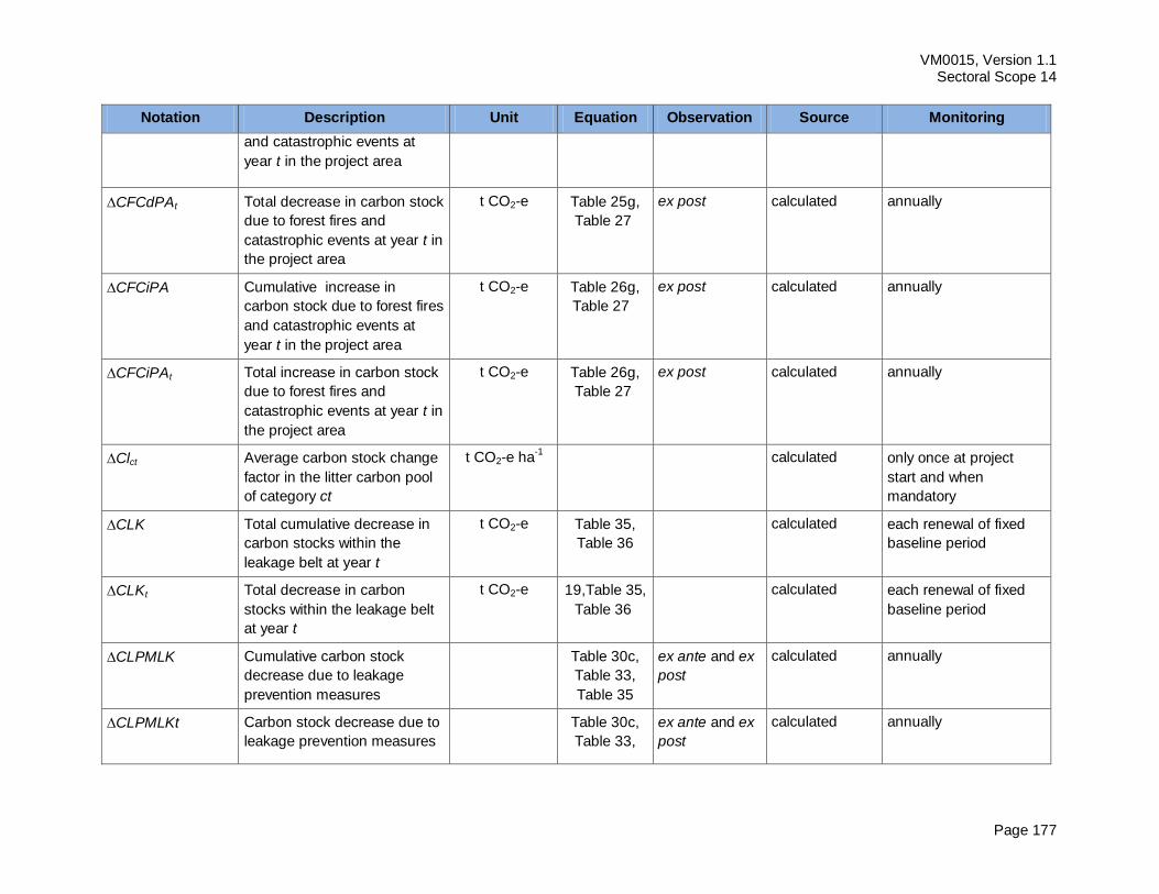
VM0015, Version 1.1 Sectoral Scope 14
Page 177
Notation Description Unit Equation Observation Source Monitoring
and catastrophic events at
year t in the project area
CFCdPAt Total decrease in carbon stock
due to forest fires and
catastrophic events at year t in
the project area
t CO2-e Table 25g,
Table 27
ex post calculated annually
CFCiPA Cumulative increase in
carbon stock due to forest fires
and catastrophic events at
year t in the project area
t CO2-e Table 26g,
Table 27
ex post calculated annually
CFCiPAt Total increase in carbon stock
due to forest fires and
catastrophic events at year t in
the project area
t CO2-e Table 26g,
Table 27
ex post calculated annually
Clct Average carbon stock change
factor in the litter carbon pool
of category ct
t CO2-e ha-1 calculated only once at project
start and when
mandatory
CLK Total cumulative decrease in
carbon stocks within the
leakage belt at year t
t CO2-e Table 35,
Table 36
calculated each renewal of fixed
baseline period
CLKt Total decrease in carbon
stocks within the leakage belt
at year t
t CO2-e 19,Table 35,
Table 36
calculated each renewal of fixed
baseline period
CLPMLK Cumulative carbon stock
decrease due to leakage
prevention measures
Table 30c,
Table 33,
Table 35
ex ante and ex
post
calculated annually
CLPMLKt Carbon stock decrease due to
leakage prevention measures
Table 30c,
Table 33,
ex ante and ex
post
calculated annually
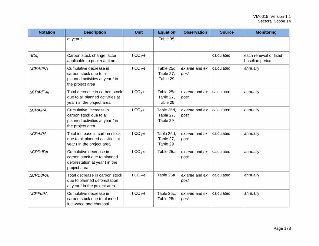
VM0015, Version 1.1 Sectoral Scope 14
Page 178
Notation Description Unit Equation Observation Source Monitoring
at year t Table 35
Cpt Carbon stock change factor
applicable to pool p at time t
t CO2-e calculated each renewal of fixed
baseline period
CPAdPA Cumulative decrease in
carbon stock due to all
planned activities at year t in
the project area
t CO2-e Table 25d,
Table 27,
Table 29
ex ante and ex
post
calculated annually
CPAdPAt Total decrease in carbon stock
due to all planned activities at
year t in the project area
t CO2-e Table 25d,
Table 27,
Table 29
ex ante and ex
post
calculated annually
CPAiPA Cumulative increase in
carbon stock due to all
planned activities at year t in
the project area
t CO2-e Table 26d,
Table 27,
Table 29
ex ante and ex
post
calculated annually
CPAiPAt Total increase in carbon stock
due to all planned activities at
year t in the project area
t CO2-e Table 26d,
Table 27,
Table 29
ex ante and ex
post
calculated annually
CPDdPA Cumulative decrease in
carbon stock due to planned
deforestation at year t in the
project area
t CO2-e Table 25a ex ante and ex
post
calculated annually
CPDdPAt Total decrease in carbon stock
due to planned deforestation
at year t in the project area
t CO2-e Table 25a ex ante and ex
post
calculated annually
CPFdPA Cumulative decrease in
carbon stock due to planned
fuel-wood and charcoal
t CO2-e Table 25c,
Table 25d
ex ante and ex
post
calculated annually
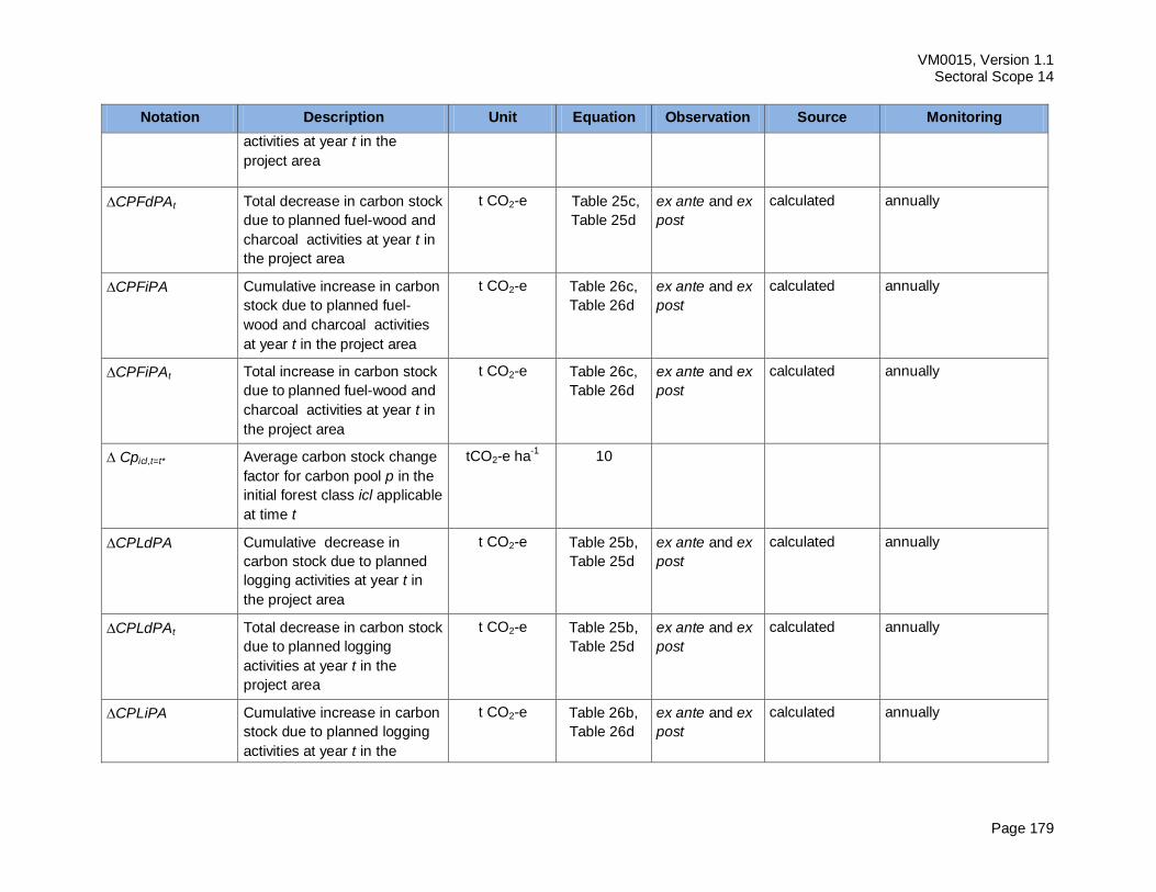
VM0015, Version 1.1 Sectoral Scope 14
Page 179
Notation Description Unit Equation Observation Source Monitoring
activities at year t in the
project area
CPFdPAt Total decrease in carbon stock
due to planned fuel-wood and
charcoal activities at year t in
the project area
t CO2-e Table 25c,
Table 25d
ex ante and ex
post
calculated annually
CPFiPA Cumulative increase in carbon
stock due to planned fuel-
wood and charcoal activities
at year t in the project area
t CO2-e Table 26c,
Table 26d
ex ante and ex
post
calculated annually
CPFiPAt Total increase in carbon stock
due to planned fuel-wood and
charcoal activities at year t in
the project area
t CO2-e Table 26c,
Table 26d
ex ante and ex
post
calculated annually
Cpicl,t=t* Average carbon stock change
factor for carbon pool p in the
initial forest class icl applicable
at time t
tCO2-e ha-1
10
CPLdPA Cumulative decrease in
carbon stock due to planned
logging activities at year t in
the project area
t CO2-e Table 25b,
Table 25d
ex ante and ex
post
calculated annually
CPLdPAt Total decrease in carbon stock
due to planned logging
activities at year t in the
project area
t CO2-e Table 25b,
Table 25d
ex ante and ex
post
calculated annually
CPLiPA Cumulative increase in carbon
stock due to planned logging
activities at year t in the
t CO2-e Table 26b,
Table 26d
ex ante and ex
post
calculated annually
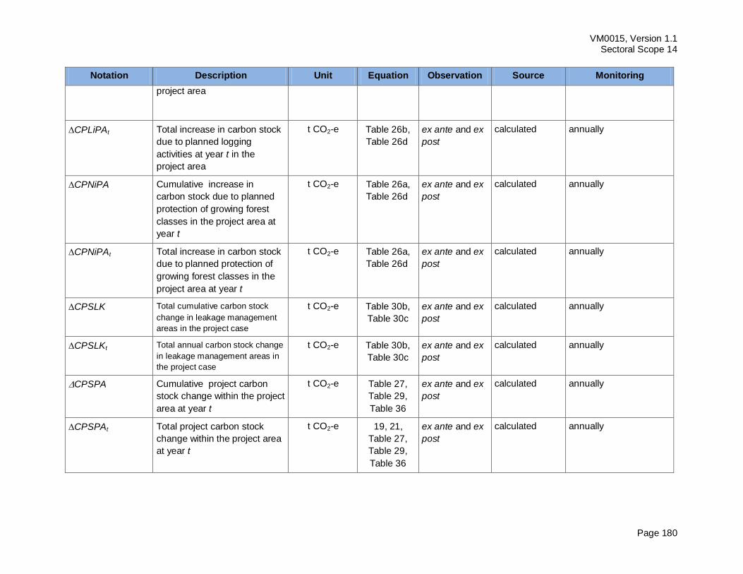
VM0015, Version 1.1 Sectoral Scope 14
Page 180
Notation Description Unit Equation Observation Source Monitoring
project area
CPLiPAt Total increase in carbon stock
due to planned logging
activities at year t in the
project area
t CO2-e Table 26b,
Table 26d
ex ante and ex
post
calculated annually
CPNiPA Cumulative increase in
carbon stock due to planned
protection of growing forest
classes in the project area at
year t
t CO2-e Table 26a,
Table 26d
ex ante and ex
post
calculated annually
CPNiPAt Total increase in carbon stock
due to planned protection of
growing forest classes in the
project area at year t
t CO2-e Table 26a,
Table 26d
ex ante and ex
post
calculated annually
CPSLK Total cumulative carbon stock
change in leakage management
areas in the project case
t CO2-e Table 30b,
Table 30c
ex ante and ex
post
calculated annually
CPSLKt Total annual carbon stock change
in leakage management areas in
the project case
t CO2-e Table 30b,
Table 30c
ex ante and ex
post
calculated annually
CPSPA Cumulative project carbon
stock change within the project
area at year t
t CO2-e Table 27,
Table 29,
Table 36
ex ante and ex
post
calculated annually
CPSPAt Total project carbon stock
change within the project area
at year t
t CO2-e 19, 21,
Table 27,
Table 29,
Table 36
ex ante and ex
post
calculated annually
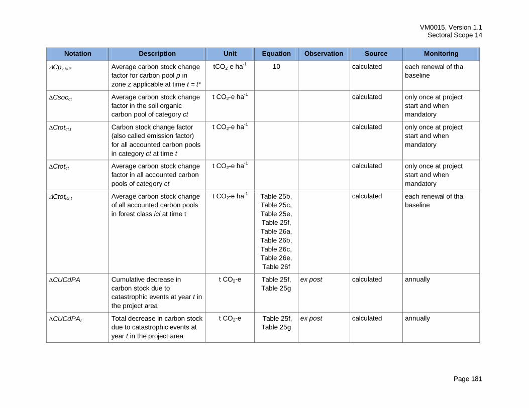
VM0015, Version 1.1 Sectoral Scope 14
Page 181
Notation Description Unit Equation Observation Source Monitoring
Cpz,t=t* Average carbon stock change
factor for carbon pool p in
zone z applicable at time t = t*
tCO2-e ha-1
10 calculated each renewal of tha
baseline
Csocct Average carbon stock change
factor in the soil organic
carbon pool of category ct
t CO2-e ha-1 calculated only once at project
start and when
mandatory
Ctotct,t Carbon stock change factor
(also called emission factor)
for all accounted carbon pools
in category ct at time t
t CO2-e ha-1 calculated only once at project
start and when
mandatory
Ctotct Average carbon stock change
factor in all accounted carbon
pools of category ct
t CO2-e ha-1 calculated only once at project
start and when
mandatory
Ctoticl,t Average carbon stock change
of all accounted carbon pools
in forest class icl at time t
t CO2-e ha-1 Table 25b,
Table 25c,
Table 25e,
Table 25f,
Table 26a,
Table 26b,
Table 26c,
Table 26e,
Table 26f
calculated each renewal of tha
baseline
CUCdPA Cumulative decrease in
carbon stock due to
catastrophic events at year t in
the project area
t CO2-e Table 25f,
Table 25g
ex post calculated annually
CUCdPAt Total decrease in carbon stock
due to catastrophic events at
year t in the project area
t CO2-e Table 25f,
Table 25g
ex post calculated annually
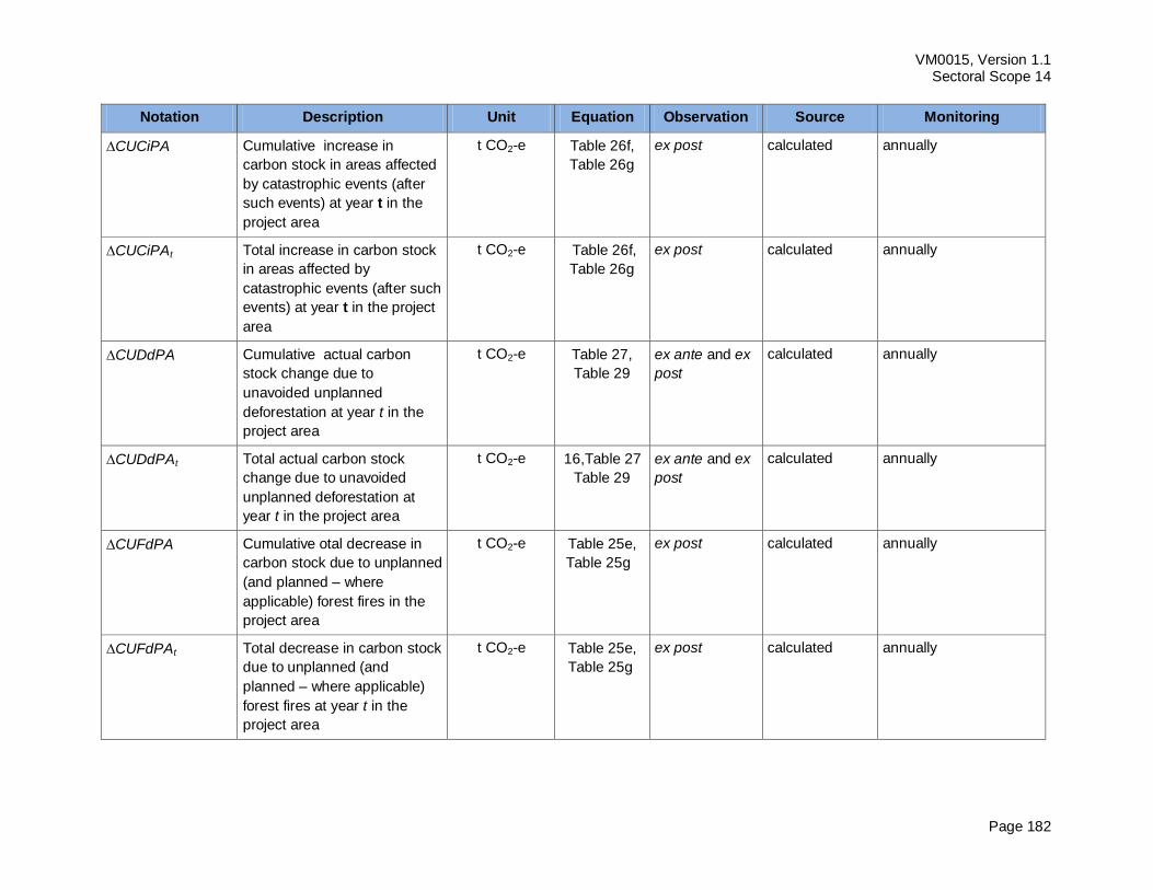
VM0015, Version 1.1 Sectoral Scope 14
Page 182
Notation Description Unit Equation Observation Source Monitoring
CUCiPA Cumulative increase in
carbon stock in areas affected
by catastrophic events (after
such events) at year t in the
project area
t CO2-e Table 26f,
Table 26g
ex post calculated annually
CUCiPAt Total increase in carbon stock
in areas affected by
catastrophic events (after such
events) at year t in the project
area
t CO2-e Table 26f,
Table 26g
ex post calculated annually
CUDdPA Cumulative actual carbon
stock change due to
unavoided unplanned
deforestation at year t in the
project area
t CO2-e Table 27,
Table 29
ex ante and ex
post
calculated annually
CUDdPAt Total actual carbon stock
change due to unavoided
unplanned deforestation at
year t in the project area
t CO2-e 16,Table 27
Table 29
ex ante and ex
post
calculated annually
CUFdPA Cumulative otal decrease in
carbon stock due to unplanned
(and planned – where
applicable) forest fires in the
project area
t CO2-e Table 25e,
Table 25g
ex post calculated annually
CUFdPAt Total decrease in carbon stock
due to unplanned (and
planned – where applicable)
forest fires at year t in the
project area
t CO2-e Table 25e,
Table 25g
ex post calculated annually
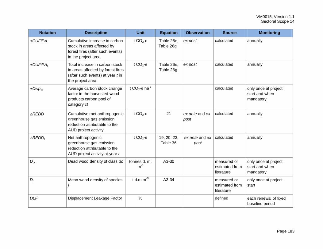
VM0015, Version 1.1 Sectoral Scope 14
Page 183
Notation Description Unit Equation Observation Source Monitoring
CUFiPA Cumulative increase in carbon
stock in areas affected by
forest fires (after such events)
in the project area
t CO2-e Table 26e,
Table 26g
ex post calculated annually
CUFiPAt Total increase in carbon stock
in areas affected by forest fires
(after such events) at year t in
the project area
t CO2-e Table 26e,
Table 26g
ex post calculated annually
Cwpct Average carbon stock change
factor in the harvested wood
products carbon pool of
category ct
t CO2-e ha-1 calculated only once at project
start and when
mandatory
REDD Cumulative met anthropogenic
greenhouse gas emission
reduction attributable to the
AUD project activity
t CO2-e 21 ex ante and ex
post
calculated annually
REDDt Net anthropogenic
greenhouse gas emission
reduction attributable to the
AUD project activity at year t
t CO2-e 19, 20, 23,
Table 36
ex ante and ex
post
calculated annually
Ddc Dead wood density of class dc tonnes d. m.
m-3
A3-30 measured or
estimated from
literature
only once at project
start and when
mandatory
Dj Mean wood density of species
j
t d.m.m-3 A3-34 measured or
estimated from
literature
only once at project
start
DLF Displacement Leakage Factor % defined each renewal of fixed
baseline period
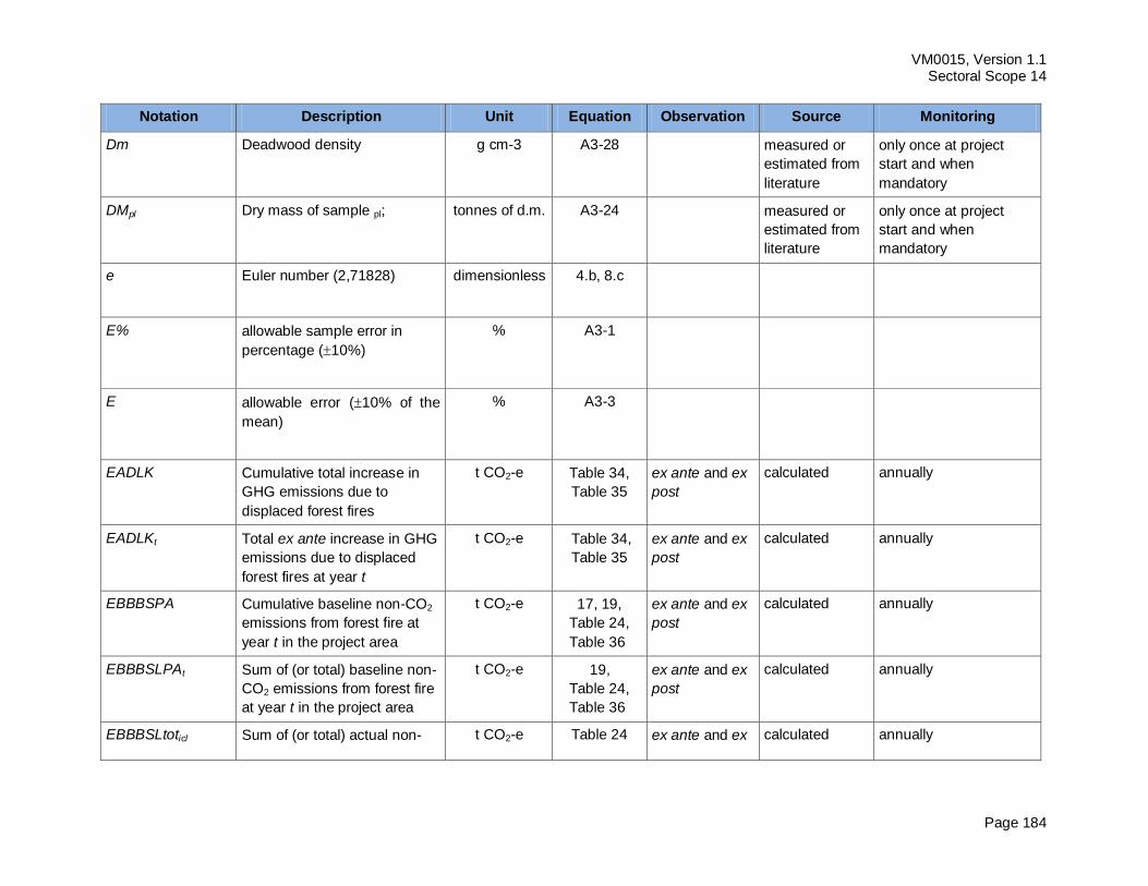
VM0015, Version 1.1 Sectoral Scope 14
Page 184
Notation Description Unit Equation Observation Source Monitoring
Dm Deadwood density g cm-3 A3-28 measured or
estimated from
literature
only once at project
start and when
mandatory
DMpl Dry mass of sample pl; tonnes of d.m. A3-24 measured or
estimated from
literature
only once at project
start and when
mandatory
e Euler number (2,71828) dimensionless 4.b, 8.c
E% allowable sample error in
percentage (10%)
% A3-1
E allowable error (10% of the
mean)
% A3-3
EADLK Cumulative total increase in
GHG emissions due to
displaced forest fires
t CO2-e Table 34,
Table 35
ex ante and ex
post
calculated annually
EADLKt Total ex ante increase in GHG
emissions due to displaced
forest fires at year t
t CO2-e Table 34,
Table 35
ex ante and ex
post
calculated annually
EBBBSPA Cumulative baseline non-CO2
emissions from forest fire at
year t in the project area
t CO2-e 17, 19,
Table 24,
Table 36
ex ante and ex
post
calculated annually
EBBBSLPAt Sum of (or total) baseline non-
CO2 emissions from forest fire
at year t in the project area
t CO2-e 19,
Table 24,
Table 36
ex ante and ex
post
calculated annually
EBBBSLtoticl Sum of (or total) actual non- t CO2-e Table 24 ex ante and ex calculated annually
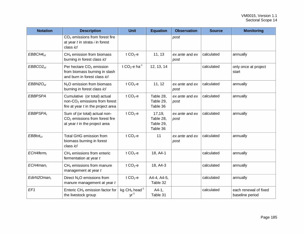
VM0015, Version 1.1 Sectoral Scope 14
Page 185
Notation Description Unit Equation Observation Source Monitoring
CO2 emissions from forest fire
at year t in strata i in forest
class icl
post
EBBCH4icl CH4 emission from biomass
burning in forest class icl
t CO2-e 11, 13 ex ante and ex
post
calculated annually
EBBCO2icl Per hectare CO2 emission
from biomass burning in slash
and burn in forest class icl
t CO2-e ha-1 12, 13, 14 calculated only once at project
start
EBBN2Oicl N2O emission from biomass
burning in forest class icl
t CO2-e 11, 12 ex ante and ex
post
calculated annually
EBBPSPA Cumulative (or total) actual
non-CO2 emissions from forest
fire at year t in the project area
t CO2-e Table 28,
Table 29,
Table 36
ex ante and ex
post
calculated annually
EBBPSPAt Sum of (or total) actual non-
CO2 emissions from forest fire
at year t in the project area
t CO2-e 17,19,
Table 28,
Table 29,
Table 36
ex ante and ex
post
calculated annually
EBBtoticl Total GHG emission from
biomass burning in forest
class icl
t CO2-e 11 ex ante and ex
post
calculated annually
ECH4fermt CH4 emissions from enteric
fermentation at year t
t CO2-e 18, A4-1 calculated annually
ECH4mant CH4 emissions from manure
management at year t
t CO2-e 18, A4-3 calculated annually
EdirN2Omant Direct N2O emissions from
manure management at year t
t CO2-e A4-4, A4-5,
Table 32
calculated annually
EF1 Enteric CH4 emission factor for
the livestock group
kg CH4 head-1
yr-1
A4-1,
Table 31
calculated each renewal of fixed
baseline period
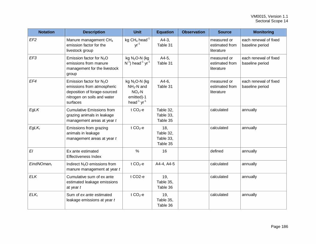
VM0015, Version 1.1 Sectoral Scope 14
Page 186
Notation Description Unit Equation Observation Source Monitoring
EF2 Manure management CH4
emission factor for the
livestock group
kg CH4 head-1
yr-1
A4-3,
Table 31
measured or
estimated from
literature
each renewal of fixed
baseline period
EF3 Emission factor for N2O
emissions from manure
management for the livestock
group
kg N2O-N (kg
N-1
) head-1
yr-1
A4-5,
Table 31
measured or
estimated from
literature
each renewal of fixed
baseline period
EF4 Emission factor for N2O
emissions from atmospheric
deposition of forage-sourced
nitrogen on soils and water
surfaces
kg N2O-N (kg
NH3-N and
NOx-N
emitted)-1
head-1
yr-1
A4-6,
Table 31
measured or
estimated from
literature
each renewal of fixed
baseline period
EgLK Cumulative Emissions from
grazing animals in leakage
management areas at year t
t CO2-e Table 32,
Table 33,
Table 35
calculated annually
EgLKt Emissions from grazing
animals in leakage
management areas at year t
t CO2-e 18,
Table 32,
Table 33,
Table 35
calculated annually
EI Ex ante estimated
Effectiveness Index
% 16 defined annually
EindNOmant Indirect N2O emissions from
manure management at year t
t CO2-e A4-4, A4-5 calculated annually
ELK Cumulative sum of ex ante
estimated leakage emissions
at year t
t CO2-e 19,
Table 35,
Table 36
calculated annually
ELKt Sum of ex ante estimated
leakage emissions at year t
t CO2-e 19,
Table 35,
Table 36
calculated annually
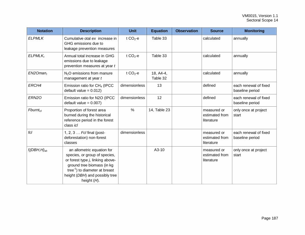
VM0015, Version 1.1 Sectoral Scope 14
Page 187
Notation Description Unit Equation Observation Source Monitoring
ELPMLK Cumulative otal ex increase in
GHG emissions due to
leakage prevention measures
t CO2-e Table 33 calculated annually
ELPMLKt Annual total increase in GHG
emissions due to leakage
prevention measures at year t
t CO2-e Table 33 calculated annually
EN2Omant N2O emissions from manure
management at year t
t CO2-e 18, A4-4,
Table 32
calculated annually
ERCH4 Emission ratio for CH4 (IPCC
default value = 0.012)
dimensionless 13 defined each renewal of fixed
baseline period
ERN2O Emission ratio for N2O (IPCC
default value = 0.007)
dimensionless 12 defined each renewal of fixed
baseline period
Fburnticl Proportion of forest area
burned during the historical
reference period in the forest
class icl
% 14, Table 23 measured or
estimated from
literature
only once at project
start
fcl 1, 2, 3 … Fcl final (post-
deforestation) non-forest
classes
dimensionless measured or
estimated from
literature
each renewal of fixed
baseline period
fj(DBH,H)ab an allometric equation for
species, or group of species,
or forest type j, linking above-
ground tree biomass (in kg
tree-1
) to diameter at breast
height (DBH) and possibly tree
height (H).
A3-10 measured or
estimated from
literature
only once at project
start
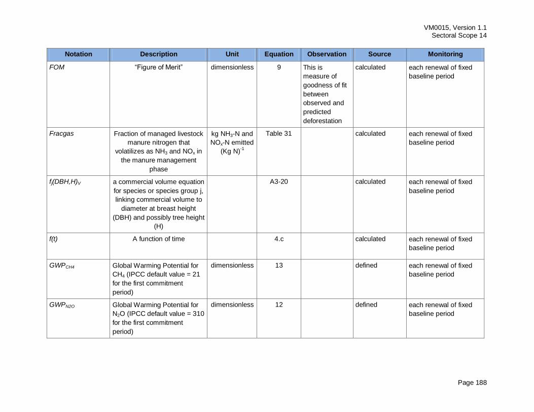
VM0015, Version 1.1 Sectoral Scope 14
Page 188
Notation Description Unit Equation Observation Source Monitoring
FOM “Figure of Merit” dimensionless 9 This is
measure of
goodness of fit
between
observed and
predicted
deforestation
calculated each renewal of fixed
baseline period
Fracgas
Fraction of managed livestock
manure nitrogen that
volatilizes as NH3 and NOx in
the manure management
phase
kg NH3-N and
NOx-N emitted
(Kg N)-1
Table 31 calculated each renewal of fixed
baseline period
fj(DBH,H)V a commercial volume equation
for species or species group j,
linking commercial volume to
diameter at breast height
(DBH) and possibly tree height
(H)
A3-20 calculated each renewal of fixed
baseline period
f(t) A function of time 4.c calculated each renewal of fixed
baseline period
GWPCH4 Global Warming Potential for
CH4 (IPCC default value = 21
for the first commitment
period)
dimensionless 13 defined each renewal of fixed
baseline period
GWPN2O Global Warming Potential for
N2O (IPCC default value = 310
for the first commitment
period)
dimensionless 12 defined each renewal of fixed
baseline period
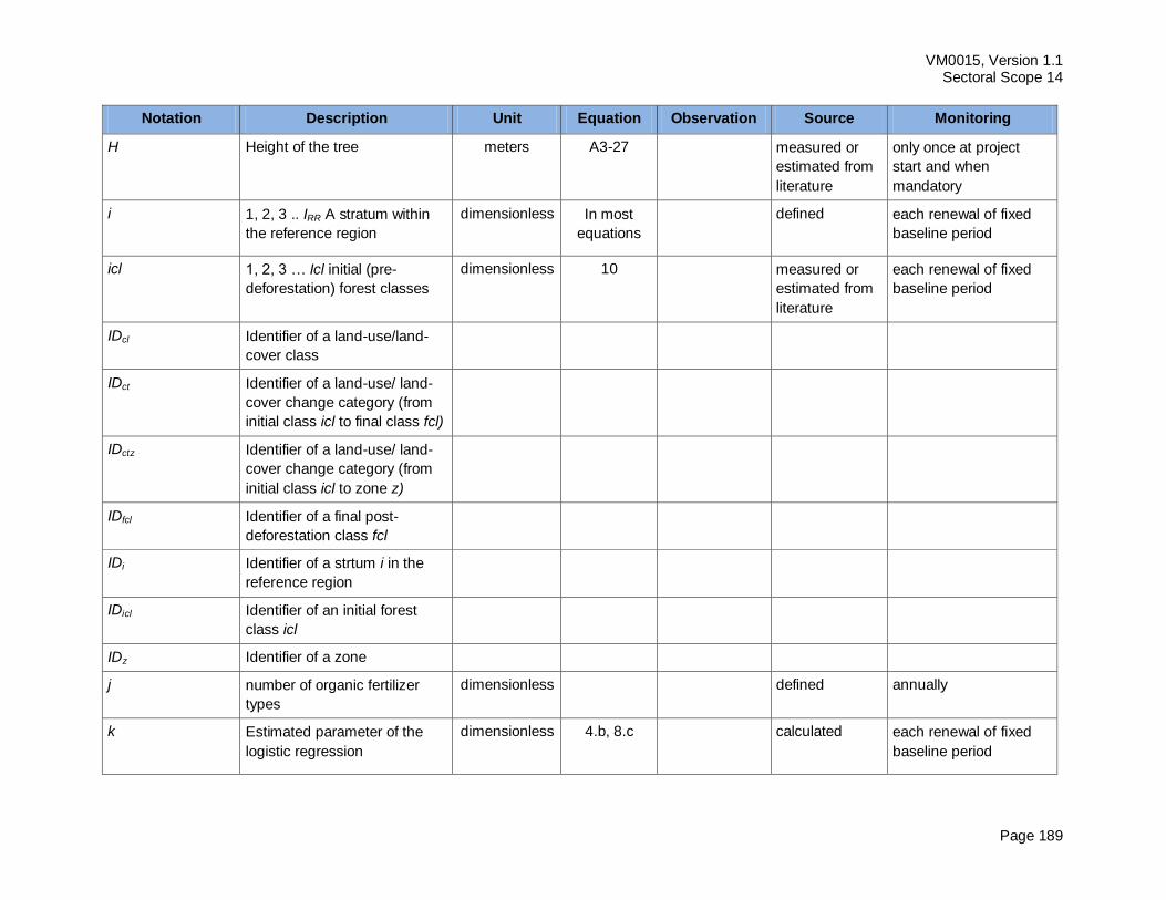
VM0015, Version 1.1 Sectoral Scope 14
Page 189
Notation Description Unit Equation Observation Source Monitoring
H Height of the tree meters A3-27 measured or
estimated from
literature
only once at project
start and when
mandatory
i 1, 2, 3 .. IRR A stratum within
the reference region
dimensionless In most
equations
defined each renewal of fixed
baseline period
icl 1, 2, 3 … Icl initial (pre-
deforestation) forest classes
dimensionless 10 measured or
estimated from
literature
each renewal of fixed
baseline period
IDcl Identifier of a land-use/land-
cover class
IDct Identifier of a land-use/ land-
cover change category (from
initial class icl to final class fcl)
IDctz Identifier of a land-use/ land-
cover change category (from
initial class icl to zone z)
IDfcl Identifier of a final post-
deforestation class fcl
IDi Identifier of a strtum i in the
reference region
IDicl Identifier of an initial forest
class icl
IDz Identifier of a zone
j number of organic fertilizer
types
dimensionless defined annually
k Estimated parameter of the
logistic regression
dimensionless 4.b, 8.c calculated each renewal of fixed
baseline period
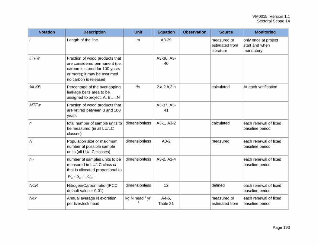
VM0015, Version 1.1 Sectoral Scope 14
Page 190
Notation Description Unit Equation Observation Source Monitoring
L Length of the line m A3-29 measured or
estimated from
literature
only once at project
start and when
mandatory
LTFw Fraction of wood products that
are considered permanent (i.e.
carbon is stored for 100 years
or more); it may be assumed
no carbon is released
A3-36, A3-
40
%LKB Percentage of the overlapping
leakage belts area to be
assigned to project, A, B…..N
% 2.a,2.b,2.n calculated At each verification
MTFw Fraction of wood products that
are retired between 3 and 100
years
A3-37, A3-
41
n total number of sample units to
be measured (in all LU/LC
classes)
dimensionless A3-1, A3-2 calculated each renewal of fixed
baseline period
N Population size or maximum
number of possible sample
units (all LU/LC classes)
dimensionless A3-2
measured each renewal of fixed
baseline period
ncl number of samples units to be
measured in LU/LC class cl
that is allocated proportional to
clclcl CSW .
dimensionless A3-2, A3-4
each renewal of fixed
baseline period
NCR Nitrogen/Carbon ratio (IPCC
default value = 0.01)
dimensionless 12 defined each renewal of fixed
baseline period
Nex Annual average N excretion
per livestock head
kg N head-1
yr-
1
A4-6,
Table 31
measured or
estimated from
each renewal of fixed
baseline period
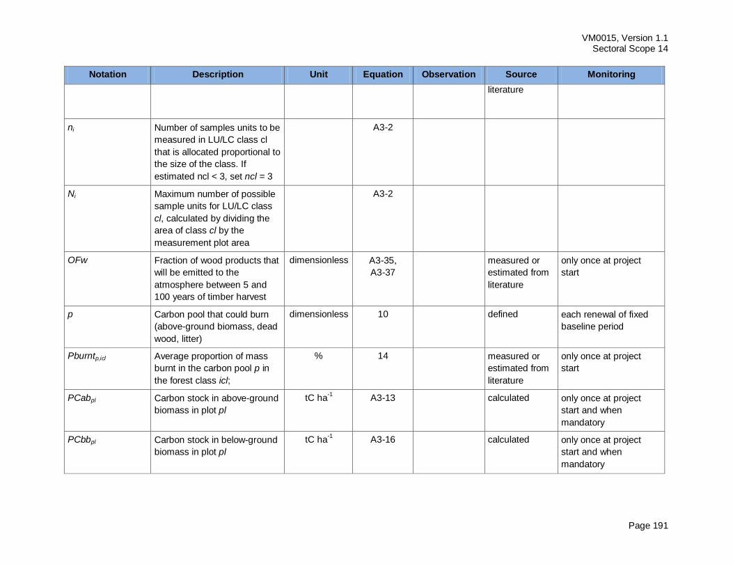
VM0015, Version 1.1 Sectoral Scope 14
Page 191
Notation Description Unit Equation Observation Source Monitoring
literature
ni Number of samples units to be
measured in LU/LC class cl
that is allocated proportional to
the size of the class. If
estimated ncl < 3, set ncl = 3
A3-2
Ni Maximum number of possible
sample units for LU/LC class
cl, calculated by dividing the
area of class cl by the
measurement plot area
A3-2
OFw Fraction of wood products that
will be emitted to the
atmosphere between 5 and
100 years of timber harvest
dimensionless A3-35,
A3-37
measured or
estimated from
literature
only once at project
start
p Carbon pool that could burn
(above-ground biomass, dead
wood, litter)
dimensionless 10 defined each renewal of fixed
baseline period
Pburntp,icl Average proportion of mass
burnt in the carbon pool p in
the forest class icl;
% 14 measured or
estimated from
literature
only once at project
start
PCabpl Carbon stock in above-ground
biomass in plot pl
tC ha-1 A3-13 calculated only once at project
start and when
mandatory
PCbbpl Carbon stock in below-ground
biomass in plot pl
tC ha-1 A3-16 calculated only once at project
start and when
mandatory
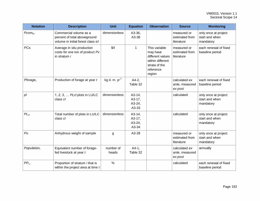
VM0015, Version 1.1 Sectoral Scope 14
Page 192
Notation Description Unit Equation Observation Source Monitoring
Pcomicl Commercial volume as a
percent of total aboveground
volume in initial forest class icl
dimensionless A3-36,
A3-38
measured or
estimated from
literature
only once at project
start and when
mandatory
PCxi Average in situ production
costs for one ton of product Px
in stratum i
$/t 1 This variable
may have
different values
within different
strata of the
reference
region
measured or
estimated from
literature
each renewal of fixed
baseline period
Pforaget Production of forage at year t kg d. m. yr-1
A4-2,
Table 32
calculated ex
ante, measured
ex post
each renewal of fixed
baseline period
pl 1, 2, 3, … PLcl plots in LU/LC
class cl
dimensionless A3-14,
A3-17,
A3-24,
A3-33
calculated only once at project
start and when
mandatory
PLcl Total number of plots in LU/LC
class cl
dimensionless A3-14,
A3-17,
A3-24,
A3-34
calculated only once at project
start and when
mandatory
Po Anhydrous weight of sample g A3-28 measured or
estimated from
literature
only once at project
start and when
mandatory
Populationt Equivalent number of forage-
fed livestock at year t
number of
heads
A4-1,
Table 32
calculated ex
ante, measured
ex post
annually
PPi,t Proportion of stratum i that is
within the project area at time t
% calculated each renewal of fixed
baseline period
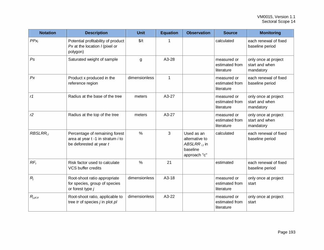
VM0015, Version 1.1 Sectoral Scope 14
Page 193
Notation Description Unit Equation Observation Source Monitoring
PPxl Potential profitability of product
Px at the location l (pixel or
polygon)
$/t 1 calculated each renewal of fixed
baseline period
Ps Saturated weight of sample g A3-28 measured or
estimated from
literature
only once at project
start and when
mandatory
Px Product x produced in the
reference region
dimensionless 1 measured or
estimated from
literature
each renewal of fixed
baseline period
r1 Radius at the base of the tree meters A3-27 measured or
estimated from
literature
only once at project
start and when
mandatory
r2 Radius at the top of the tree meters A3-27 measured or
estimated from
literature
only once at project
start and when
mandatory
RBSLRRi,t Percentage of remaining forest
area at year t -1 in stratum i to
be deforested at year t
% 3 Used as an
alternative to
ABSLRR i,t in
baseline
approach "c"
calculated each renewal of fixed
baseline period
RFt Risk factor used to calculate
VCS buffer credits
% 21 estimated each renewal of fixed
baseline period
Rj Root-shoot ratio appropriate
for species, group of species
or forest type j
dimensionless A3-18 measured or
estimated from
literature
only once at project
start
Rj,pl,tr Root-shoot ratio, applicable to
tree tr of species j in plot pl
dimensionless A3-22 measured or
estimated from
literature
only once at project
start
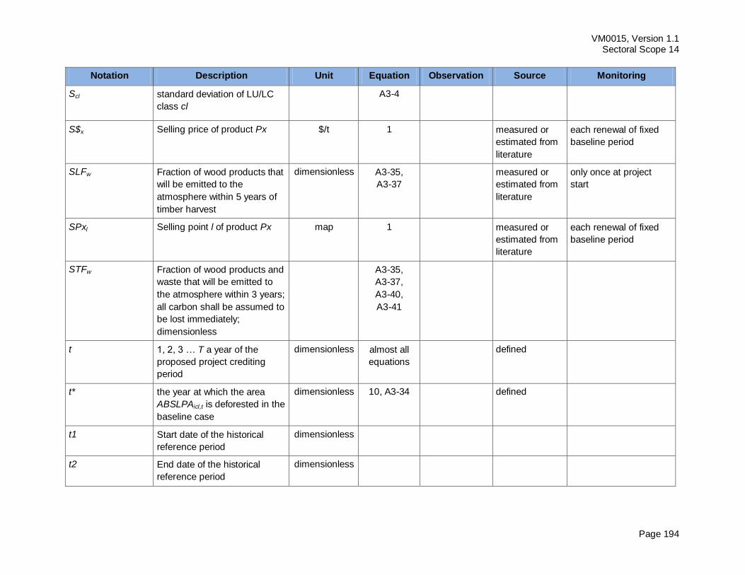
VM0015, Version 1.1 Sectoral Scope 14
Page 194
Notation Description Unit Equation Observation Source Monitoring
Scl standard deviation of LU/LC
class cl
A3-4
S$x Selling price of product Px $/t 1 measured or
estimated from
literature
each renewal of fixed
baseline period
SLFw Fraction of wood products that
will be emitted to the
atmosphere within 5 years of
timber harvest
dimensionless A3-35,
A3-37
measured or
estimated from
literature
only once at project
start
SPxl Selling point l of product Px map 1 measured or
estimated from
literature
each renewal of fixed
baseline period
STFw Fraction of wood products and
waste that will be emitted to
the atmosphere within 3 years;
all carbon shall be assumed to
be lost immediately;
dimensionless
A3-35,
A3-37,
A3-40,
A3-41
t 1, 2, 3 … T a year of the
proposed project crediting
period
dimensionless almost all
equations
defined
t* the year at which the area
ABSLPAicl,t is deforested in the
baseline case
dimensionless 10, A3-34 defined
t1 Start date of the historical
reference period
dimensionless
t2 End date of the historical
reference period
dimensionless
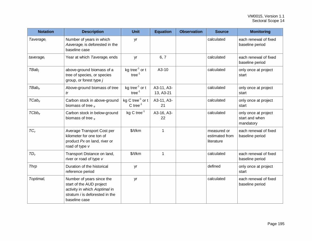
VM0015, Version 1.1 Sectoral Scope 14
Page 195
Notation Description Unit Equation Observation Source Monitoring
Taveragei Number of years in which
Aaveragei is deforested in the
baseline case
yr calculated each renewal of fixed
baseline period
taveragei Year at which Taveragei ends yr 6, 7 calculated each renewal of fixed
baseline period
TBabj above-ground biomass of a
tree of species, or species
group, or forest type j
kg tree-1
or t
tree-1
A3-10 calculated only once at project
start
TBabtr Above-ground biomass of tree
tr
kg tree-1
or t
tree-1
A3-11, A3-
13, A3-21
calculated only once at project
start
TCabtr Carbon stock in above-ground
biomass of tree tr
kg C tree-1
or t
C tree-1
A3-11, A3-
21
calculated only once at project
start
TCbbtr Carbon stock in below-ground
biomass of tree tr
kg C tree-1
A3-16, A3-
22
calculated only once at project
start and when
mandatory
TCv Average Transport Cost per
kilometer for one ton of
product Px on land, river or
road of type v
$/t/km 1 measured or
estimated from
literature
each renewal of fixed
baseline period
TDv Transport Distance on land,
river or road of type v
$/t/km 1 calculated each renewal of fixed
baseline period
Thrp Duration of the historical
reference period
yr defined only once at project
start
Toptimali Number of years since the
start of the AUD project
activity in which Aoptimal in
stratum i is deforested in the
baseline case
yr calculated each renewal of fixed
baseline period
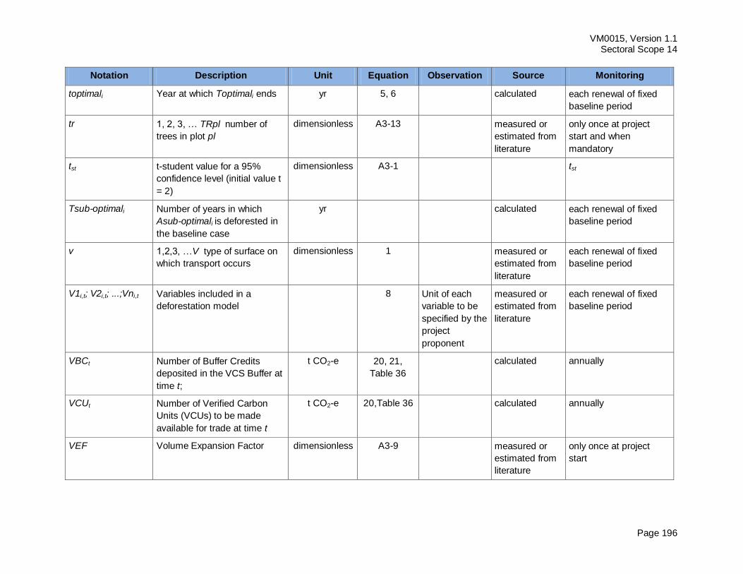
VM0015, Version 1.1 Sectoral Scope 14
Page 196
Notation Description Unit Equation Observation Source Monitoring
toptimali Year at which Toptimali ends yr 5, 6 calculated each renewal of fixed
baseline period
tr 1, 2, 3, … TRpl number of
trees in plot pl
dimensionless A3-13 measured or
estimated from
literature
only once at project
start and when
mandatory
tst t-student value for a 95%
confidence level (initial value t
= 2)
dimensionless A3-1 tst
Tsub-optimali Number of years in which
Asub-optimali is deforested in
the baseline case
yr calculated each renewal of fixed
baseline period
v 1,2,3, …V type of surface on
which transport occurs
dimensionless 1 measured or
estimated from
literature
each renewal of fixed
baseline period
V1i,t; V2i,t; ...;Vni,t Variables included in a
deforestation model
8 Unit of each
variable to be
specified by the
project
proponent
measured or
estimated from
literature
each renewal of fixed
baseline period
VBCt Number of Buffer Credits
deposited in the VCS Buffer at
time t;
t CO2-e 20, 21,
Table 36
calculated annually
VCUt Number of Verified Carbon
Units (VCUs) to be made
available for trade at time t
t CO2-e 20,Table 36 calculated annually
VEF Volume Expansion Factor dimensionless A3-9 measured or
estimated from
literature
only once at project
start
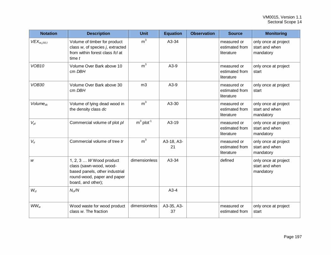
VM0015, Version 1.1 Sectoral Scope 14
Page 197
Notation Description Unit Equation Observation Source Monitoring
VEXw,j,fcl,t Volume of timber for product
class w, of species j, extracted
from within forest class fcl at
time t
m3 A3-34 measured or
estimated from
literature
only once at project
start and when
mandatory
VOB10 Volume Over Bark above 10
cm DBH
m3 A3-9 measured or
estimated from
literature
only once at project
start
VOB30 Volume Over Bark above 30
cm DBH
m3 A3-9 measured or
estimated from
literature
only once at project
start
Volumedc Volume of lying dead wood in
the density class dc
m3 A3-30 measured or
estimated from
literature
only once at project
start and when
mandatory
Vpl Commercial volume of plot pl m3 plot
-1 A3-19 measured or
estimated from
literature
only once at project
start and when
mandatory
Vtr Commercial volume of tree tr m3 A3-18, A3-
21
measured or
estimated from
literature
only once at project
start and when
mandatory
w 1, 2, 3 … W Wood product
class (sawn-wood, wood-
based panels, other industrial
round-wood, paper and paper
board, and other);
dimensionless A3-34 defined only once at project
start and when
mandatory
Wcl Ncl/N A3-4
WWw Wood waste for wood product
class w. The fraction
dimensionless A3-35, A3-
37
measured or
estimated from
only once at project
start
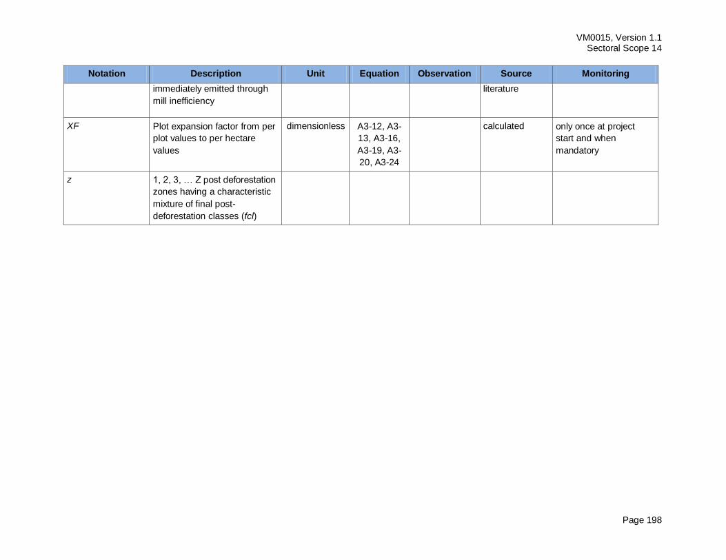
VM0015, Version 1.1 Sectoral Scope 14
Page 198
Notation Description Unit Equation Observation Source Monitoring
immediately emitted through
mill inefficiency
literature
XF Plot expansion factor from per
plot values to per hectare
values
dimensionless A3-12, A3-
13, A3-16,
A3-19, A3-
20, A3-24
calculated only once at project
start and when
mandatory
z 1, 2, 3, … Z post deforestation
zones having a characteristic
mixture of final post-
deforestation classes (fcl)
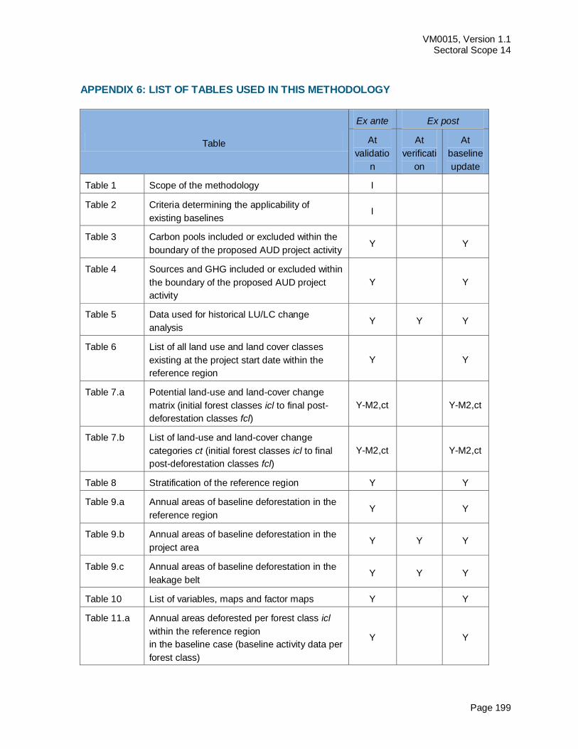
VM0015, Version 1.1 Sectoral Scope 14
Page 199
APPENDIX 6: LIST OF TABLES USED IN THIS METHODOLOGY
Table
Ex ante Ex post
At
validatio
n
At
verificati
on
At
baseline
update
Table 1 Scope of the methodology I
Table 2 Criteria determining the applicability of
existing baselines I
Table 3 Carbon pools included or excluded within the
boundary of the proposed AUD project activity Y Y
Table 4 Sources and GHG included or excluded within
the boundary of the proposed AUD project
activity
Y Y
Table 5 Data used for historical LU/LC change
analysis Y Y Y
Table 6 List of all land use and land cover classes
existing at the project start date within the
reference region
Y Y
Table 7.a Potential land-use and land-cover change
matrix (initial forest classes icl to final post-
deforestation classes fcl)
Y-M2,ct Y-M2,ct
Table 7.b List of land-use and land-cover change
categories ct (initial forest classes icl to final
post-deforestation classes fcl)
Y-M2,ct Y-M2,ct
Table 8 Stratification of the reference region Y Y
Table 9.a Annual areas of baseline deforestation in the
reference region Y Y
Table 9.b Annual areas of baseline deforestation in the
project area Y Y Y
Table 9.c Annual areas of baseline deforestation in the
leakage belt Y Y Y
Table 10 List of variables, maps and factor maps Y Y
Table 11.a Annual areas deforested per forest class icl
within the reference region
in the baseline case (baseline activity data per
forest class)
Y Y
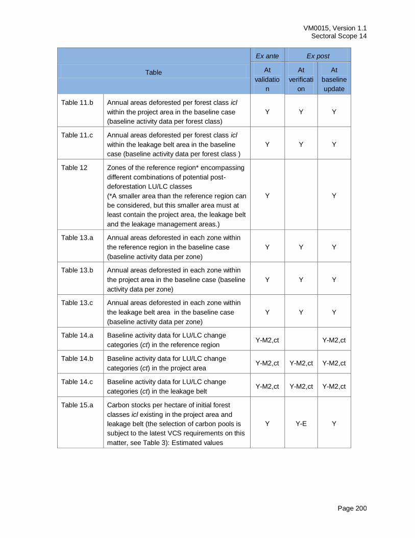
VM0015, Version 1.1 Sectoral Scope 14
Page 200
Table
Ex ante Ex post
At
validatio
n
At
verificati
on
At
baseline
update
Table 11.b Annual areas deforested per forest class icl
within the project area in the baseline case
(baseline activity data per forest class)
Y Y Y
Table 11.c Annual areas deforested per forest class icl
within the leakage belt area in the baseline
case (baseline activity data per forest class )
Y Y Y
Table 12 Zones of the reference region* encompassing
different combinations of potential post-
deforestation LU/LC classes
(*A smaller area than the reference region can
be considered, but this smaller area must at
least contain the project area, the leakage belt
and the leakage management areas.)
Y Y
Table 13.a Annual areas deforested in each zone within
the reference region in the baseline case
(baseline activity data per zone)
Y Y Y
Table 13.b Annual areas deforested in each zone within
the project area in the baseline case (baseline
activity data per zone)
Y Y Y
Table 13.c Annual areas deforested in each zone within
the leakage belt area in the baseline case
(baseline activity data per zone)
Y Y Y
Table 14.a Baseline activity data for LU/LC change
categories (ct) in the reference region Y-M2,ct Y-M2,ct
Table 14.b Baseline activity data for LU/LC change
categories (ct) in the project area Y-M2,ct Y-M2,ct Y-M2,ct
Table 14.c Baseline activity data for LU/LC change
categories (ct) in the leakage belt Y-M2,ct Y-M2,ct Y-M2,ct
Table 15.a Carbon stocks per hectare of initial forest
classes icl existing in the project area and
leakage belt (the selection of carbon pools is
subject to the latest VCS requirements on this
matter, see Table 3): Estimated values
Y Y-E Y
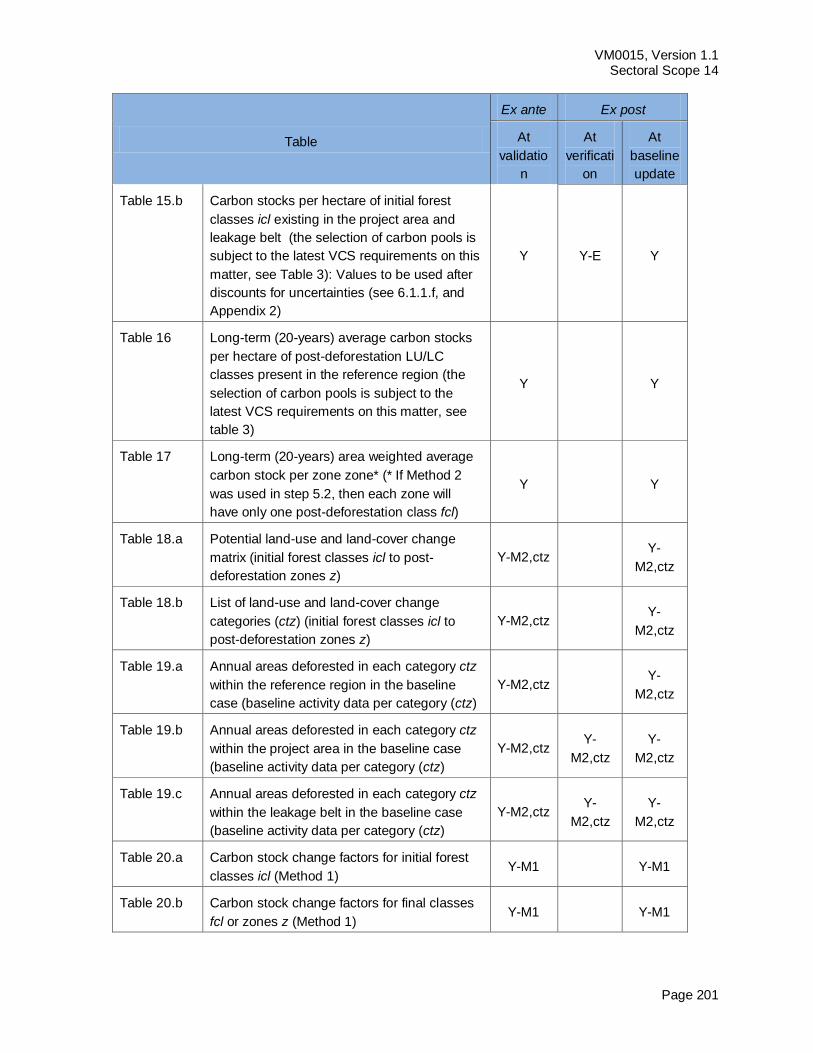
VM0015, Version 1.1 Sectoral Scope 14
Page 201
Table
Ex ante Ex post
At
validatio
n
At
verificati
on
At
baseline
update
Table 15.b Carbon stocks per hectare of initial forest
classes icl existing in the project area and
leakage belt (the selection of carbon pools is
subject to the latest VCS requirements on this
matter, see Table 3): Values to be used after
discounts for uncertainties (see 6.1.1.f, and
Appendix 2)
Y Y-E Y
Table 16 Long-term (20-years) average carbon stocks
per hectare of post-deforestation LU/LC
classes present in the reference region (the
selection of carbon pools is subject to the
latest VCS requirements on this matter, see
table 3)
Y Y
Table 17 Long-term (20-years) area weighted average
carbon stock per zone zone* (* If Method 2
was used in step 5.2, then each zone will
have only one post-deforestation class fcl)
Y Y
Table 18.a Potential land-use and land-cover change
matrix (initial forest classes icl to post-
deforestation zones z)
Y-M2,ctz Y-
M2,ctz
Table 18.b List of land-use and land-cover change
categories (ctz) (initial forest classes icl to
post-deforestation zones z)
Y-M2,ctz Y-
M2,ctz
Table 19.a Annual areas deforested in each category ctz
within the reference region in the baseline
case (baseline activity data per category (ctz)
Y-M2,ctz Y-
M2,ctz
Table 19.b Annual areas deforested in each category ctz
within the project area in the baseline case
(baseline activity data per category (ctz)
Y-M2,ctz Y-
M2,ctz
Y-
M2,ctz
Table 19.c Annual areas deforested in each category ctz
within the leakage belt in the baseline case
(baseline activity data per category (ctz)
Y-M2,ctz Y-
M2,ctz
Y-
M2,ctz
Table 20.a Carbon stock change factors for initial forest
classes icl (Method 1) Y-M1 Y-M1
Table 20.b Carbon stock change factors for final classes
fcl or zones z (Method 1) Y-M1 Y-M1
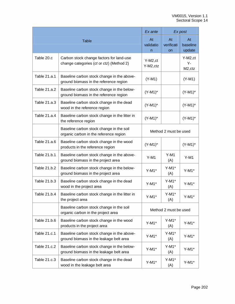
VM0015, Version 1.1 Sectoral Scope 14
Page 202
Table
Ex ante Ex post
At
validatio
n
At
verificati
on
At
baseline
update
Table 20.c Carbon stock change factors for land-use
change categories (ct or ctz) (Method 2) Y-M2,ct
Y-M2,ctz
Y-M2,ct
Y-
M2,ctz
Table 21.a.1 Baseline carbon stock change in the above-
ground biomass in the reference region (Y-M1) (Y-M1)
Table 21.a.2 Baseline carbon stock change in the below-
ground biomass in the reference region (Y-M1)* (Y-M1)*
Table 21.a.3 Baseline carbon stock change in the dead
wood in the reference region (Y-M1)* (Y-M1)*
Table 21.a.4 Baseline carbon stock change in the litter in
the reference region (Y-M1)* (Y-M1)*
Baseline carbon stock change in the soil
organic carbon in the reference region Method 2 must be used
Table 21.a.6 Baseline carbon stock change in the wood
products in the reference region (Y-M1)* (Y-M1)*
Table 21.b.1 Baseline carbon stock change in the above-
ground biomass in the project area Y-M1
Y-M1
(A) Y-M1
Table 21.b.2 Baseline carbon stock change in the below-
ground biomass in the project area Y-M1*
Y-M1*
(A) Y-M1*
Table 21.b.3 Baseline carbon stock change in the dead
wood in the project area Y-M1*
Y-M1*
(A) Y-M1*
Table 21.b.4 Baseline carbon stock change in the litter in
the project area Y-M1*
Y-M1*
(A) Y-M1*
Baseline carbon stock change in the soil
organic carbon in the project area Method 2 must be used
Table 21.b.6 Baseline carbon stock change in the wood
products in the project area Y-M1*
Y-M1*
(A) Y-M1*
Table 21.c.1 Baseline carbon stock change in the above-
ground biomass in the leakage belt area Y-M1*
Y-M1*
(A) Y-M1*
Table 21.c.2 Baseline carbon stock change in the below-
ground biomass in the leakage belt area Y-M1*
Y-M1*
(A) Y-M1*
Table 21.c.3 Baseline carbon stock change in the dead
wood in the leakage belt area Y-M1*
Y-M1*
(A) Y-M1*
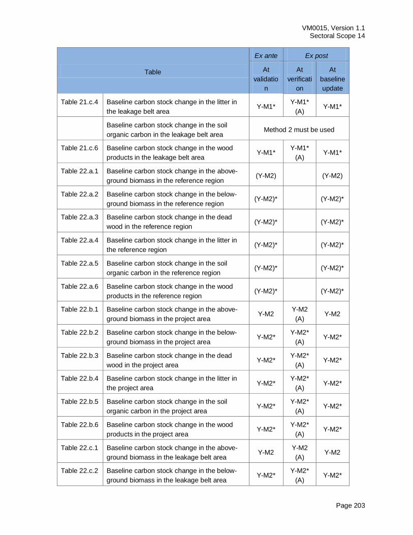
VM0015, Version 1.1 Sectoral Scope 14
Page 203
Table
Ex ante Ex post
At
validatio
n
At
verificati
on
At
baseline
update
Table 21.c.4 Baseline carbon stock change in the litter in
the leakage belt area Y-M1*
Y-M1*
(A) Y-M1*
Baseline carbon stock change in the soil
organic carbon in the leakage belt area Method 2 must be used
Table 21.c.6 Baseline carbon stock change in the wood
products in the leakage belt area Y-M1*
Y-M1*
(A) Y-M1*
Table 22.a.1 Baseline carbon stock change in the above-
ground biomass in the reference region (Y-M2) (Y-M2)
Table 22.a.2 Baseline carbon stock change in the below-
ground biomass in the reference region (Y-M2)* (Y-M2)*
Table 22.a.3 Baseline carbon stock change in the dead
wood in the reference region (Y-M2)* (Y-M2)*
Table 22.a.4 Baseline carbon stock change in the litter in
the reference region (Y-M2)* (Y-M2)*
Table 22.a.5 Baseline carbon stock change in the soil
organic carbon in the reference region (Y-M2)* (Y-M2)*
Table 22.a.6 Baseline carbon stock change in the wood
products in the reference region (Y-M2)* (Y-M2)*
Table 22.b.1 Baseline carbon stock change in the above-
ground biomass in the project area Y-M2
Y-M2
(A) Y-M2
Table 22.b.2 Baseline carbon stock change in the below-
ground biomass in the project area Y-M2*
Y-M2*
(A) Y-M2*
Table 22.b.3 Baseline carbon stock change in the dead
wood in the project area Y-M2*
Y-M2*
(A) Y-M2*
Table 22.b.4 Baseline carbon stock change in the litter in
the project area Y-M2*
Y-M2*
(A) Y-M2*
Table 22.b.5 Baseline carbon stock change in the soil
organic carbon in the project area Y-M2*
Y-M2*
(A) Y-M2*
Table 22.b.6 Baseline carbon stock change in the wood
products in the project area Y-M2*
Y-M2*
(A) Y-M2*
Table 22.c.1 Baseline carbon stock change in the above-
ground biomass in the leakage belt area Y-M2
Y-M2
(A) Y-M2
Table 22.c.2 Baseline carbon stock change in the below-
ground biomass in the leakage belt area Y-M2*
Y-M2*
(A) Y-M2*
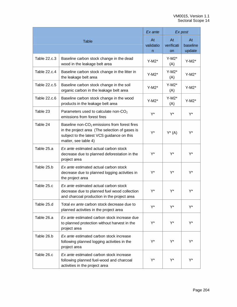
VM0015, Version 1.1 Sectoral Scope 14
Page 204
Table
Ex ante Ex post
At
validatio
n
At
verificati
on
At
baseline
update
Table 22.c.3 Baseline carbon stock change in the dead
wood in the leakage belt area Y-M2*
Y-M2*
(A) Y-M2*
Table 22.c.4 Baseline carbon stock change in the litter in
the leakage belt area Y-M2*
Y-M2*
(A) Y-M2*
Table 22.c.5 Baseline carbon stock change in the soil
organic carbon in the leakage belt area Y-M2*
Y-M2*
(A) Y-M2*
Table 22.c.6 Baseline carbon stock change in the wood
products in the leakage belt area Y-M2*
Y-M2*
(A) Y-M2*
Table 23 Parameters used to calculate non-CO2
emissions from forest fires Y* Y* Y*
Table 24 Baseline non-CO2 emissions from forest fires
in the project area (The selection of gases is
subject to the latest VCS guidance on this
matter, see table 4)
Y* Y* (A) Y*
Table 25.a Ex ante estimated actual carbon stock
decrease due to planned deforestation in the
project area
Y* Y* Y*
Table 25.b Ex ante estimated actual carbon stock
decrease due to planned logging activities in
the project area
Y* Y* Y*
Table 25.c Ex ante estimated actual carbon stock
decrease due to planned fuel wood collection
and charcoal production in the project area
Y* Y* Y*
Table 25.d Total ex ante carbon stock decrease due to
planned activities in the project area Y* Y* Y*
Table 26.a Ex ante estimated carbon stock increase due
to planned protection without harvest in the
project area
Y* Y* Y*
Table 26.b Ex ante estimated carbon stock increase
following planned logging activities in the
project area
Y* Y* Y*
Table 26.c Ex ante estimated carbon stock increase
following planned fuel-wood and charcoal
activities in the project area
Y* Y* Y*
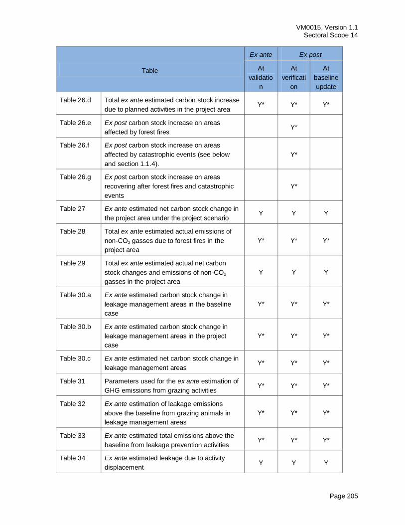
VM0015, Version 1.1 Sectoral Scope 14
Page 205
Table
Ex ante Ex post
At
validatio
n
At
verificati
on
At
baseline
update
Table 26.d Total ex ante estimated carbon stock increase
due to planned activities in the project area Y* Y* Y*
Table 26.e Ex post carbon stock increase on areas
affected by forest fires Y*
Table 26.f Ex post carbon stock increase on areas
affected by catastrophic events (see below
and section 1.1.4).
Y*
Table 26.g Ex post carbon stock increase on areas
recovering after forest fires and catastrophic
events
Y*
Table 27 Ex ante estimated net carbon stock change in
the project area under the project scenario Y Y Y
Table 28 Total ex ante estimated actual emissions of
non-CO2 gasses due to forest fires in the
project area
Y* Y* Y*
Table 29 Total ex ante estimated actual net carbon
stock changes and emissions of non-CO2
gasses in the project area
Y Y Y
Table 30.a Ex ante estimated carbon stock change in
leakage management areas in the baseline
case
Y* Y* Y*
Table 30.b Ex ante estimated carbon stock change in
leakage management areas in the project
case
Y* Y* Y*
Table 30.c Ex ante estimated net carbon stock change in
leakage management areas Y* Y* Y*
Table 31 Parameters used for the ex ante estimation of
GHG emissions from grazing activities Y* Y* Y*
Table 32 Ex ante estimation of leakage emissions
above the baseline from grazing animals in
leakage management areas
Y* Y* Y*
Table 33 Ex ante estimated total emissions above the
baseline from leakage prevention activities Y* Y* Y*
Table 34 Ex ante estimated leakage due to activity
displacement Y Y Y
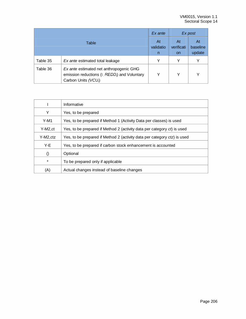
VM0015, Version 1.1 Sectoral Scope 14
Page 206
Table
Ex ante Ex post
At
validatio
n
At
verificati
on
At
baseline
update
Table 35 Ex ante estimated total leakage Y Y Y
Table 36 Ex ante estimated net anthropogenic GHG
emission reductions ( t) and Voluntary
Carbon Units (VCUt)
Y Y Y
I Informative
Y Yes, to be prepared
Y-M1 Yes, to be prepared if Method 1 (Activity Data per classes) is used
Y-M2,ct Yes, to be prepared if Method 2 (activity data per category ct) is used
Y-M2,ctz Yes, to be prepared if Method 2 (activity data per category ctz) is used
Y-E Yes, to be prepared if carbon stock enhancement is accounted
() Optional
* To be prepared only if applicable
(A) Actual changes instead of baseline changes
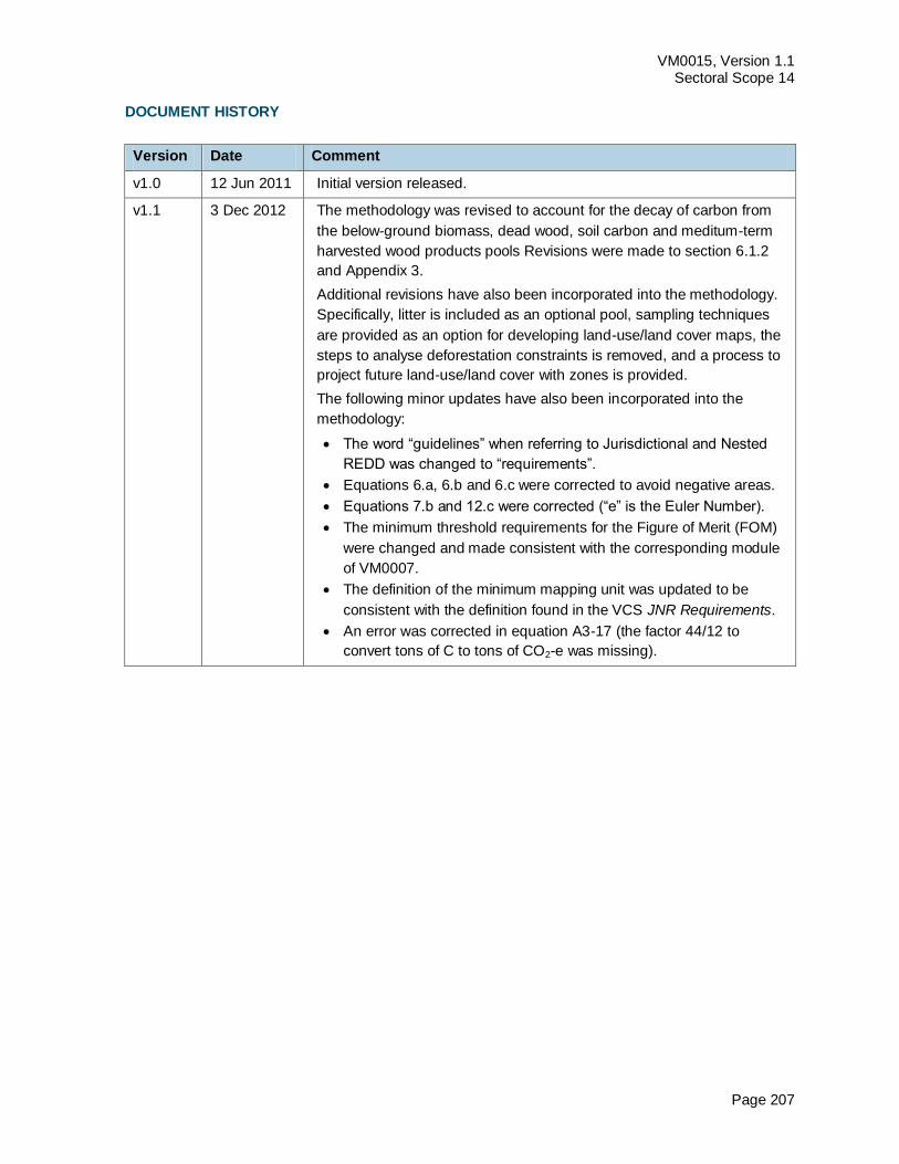
VM0015, Version 1.1 Sectoral Scope 14
Page 207
DOCUMENT HISTORY
Version Date Comment
v1.0 12 Jun 2011 Initial version released.
v1.1 3 Dec 2012 The methodology was revised to account for the decay of carbon from
the below-ground biomass, dead wood, soil carbon and meditum-term
harvested wood products pools Revisions were made to section 6.1.2
and Appendix 3.
Additional revisions have also been incorporated into the methodology.
Specifically, litter is included as an optional pool, sampling techniques
are provided as an option for developing land-use/land cover maps, the
steps to analyse deforestation constraints is removed, and a process to
project future land-use/land cover with zones is provided.
The following minor updates have also been incorporated into the
methodology:
The word “guidelines” when referring to Jurisdictional and Nested
REDD was changed to “requirements”.
Equations 6.a, 6.b and 6.c were corrected to avoid negative areas.
Equations 7.b and 12.c were corrected (“e” is the Euler Number).
The minimum threshold requirements for the Figure of Merit (FOM)
were changed and made consistent with the corresponding module
of VM0007.
The definition of the minimum mapping unit was updated to be
consistent with the definition found in the VCS JNR Requirements.
An error was corrected in equation A3-17 (the factor 44/12 to
convert tons of C to tons of CO2-e was missing).
Related Documents


