Approaches for dealing with various sources of overdispersion in modeling count data: Scale adjustment versus modeling

XML Template (2015) [27.5.2015–11:26am] [1–28]//blrnas3.glyph.com/cenpro/ApplicationFiles/Journals/SAGE/3B2/SMMJ/Vol00000/150037/APPFile/SG-SMMJ150037.3d (SMM) [PREPRINTERstage]

Article

Approaches for dealing withvarious sources of overdispersionin modeling count data: Scaleadjustment versus modeling

Elizabeth H Payne,1,2 James W Hardin,3

Leonard E Egede,1,2 Viswanathan Ramakrishnan,1

Anbesaw Selassie1 and Mulugeta Gebregziabher1,2

Abstract

Overdispersion is a common problem in count data. It can occur due to extra population-heterogeneity,

omission of key predictors, and outliers. Unless properly handled, this can lead to invalid inference. Our

goal is to assess the differential performance of methods for dealing with overdispersion from several

sources. We considered six different approaches: unadjusted Poisson regression (Poisson), deviance-scale-

adjusted Poisson regression (DS-Poisson), Pearson-scale-adjusted Poisson regression (PS-Poisson),

negative-binomial regression (NB), and two generalized linear mixed models (GLMM) with random

intercept, log-link and Poisson (Poisson-GLMM) and negative-binomial (NB-GLMM) distributions. To

rank order the preference of the models, we used Akaike’s information criteria/Bayesian information

criteria values, standard error, and 95% confidence-interval coverage of the parameter values. To compare

these methods, we used simulated count data with overdispersion of different magnitude from three

different sources. Mean of the count response was associated with three predictors. Data from two real-

case studies are also analyzed. The simulation results showed that NB and NB-GLMM were preferred for

dealing with overdispersion resulting from any of the sources we considered. Poisson and DS-Poisson

often produced smaller standard-error estimates than expected, while PS-Poisson conversely produced

larger standard-error estimates. Thus, it is good practice to compare several model options to determine

the best method of modeling count data.

Keywords

count data, generalized linear mixed model, negative-binomial, overdispersion, Poisson

1Department of Public Health Sciences – Biostatistics, Medical University of South Carolina, Charleston, SC, USA2Health Equity and Rural Outreach Innovation Center (HEROIC), Ralph H. Johnson Department of Veterans Affairs Medical Center,

Charleston, SC, USA3Division of Biostatistics, Department of Epidemiology and Biostatistics, University of South Carolina, Columbia, SC, USA

Corresponding author:

Mulugeta Gebregziabher, Department of Public Health Sciences, Medical University of South Carolina, 135 Cannon St, MSC 835,

Charleston, SC 29425, USA.

Email: [email protected]

Statistical Methods in Medical Research

0(0) 1–28

! The Author(s) 2015

Reprints and permissions:

sagepub.co.uk/journalsPermissions.nav

DOI: 10.1177/0962280215588569

smm.sagepub.com

at MUSC Library on June 1, 2015smm.sagepub.comDownloaded from

http://smm.sagepub.com/


Highlights

. Overdispersion occurs for several reasons, including omission of an important predictor, high orzero outliers, extra heterogeneity, and omission of random effects.

. Overdispersion in count data can lead to invalid inference.

. Negative-binomial regression and negative-binomial generalized linear mixed models showedgood performance in modeling count data characterized by overdispersion.

1 Introduction

Poisson regression is commonly used to study the association between count outcomes andcovariates. However, a restriction of Poisson regression is that the response mean must be equalto the variance. This equidispersion often does not hold true in real data. Often, data are morevariable than is accounted for under the Poisson model. This is called overdispersion.1 Theoverdispersion may occur due to population heterogeneity, correlated data, omission ofimportant covariates in the model, outliers, or other reasons.2,3 For example, if an importantcovariate is not measured, the residual variance estimate is increased because variability thatshould have been modeled through changes in the mean is now ‘‘picked up’’ as error variability ifthe model includes a dispersion parameter. The Poisson model has no such additional parameter.Another possible source of overdispersion is the presence of outliers: for example, excess zeroes (oranother value) in the count outcome.

An overdispersed model which assumes equidispersion can result in misleading inferences andconclusions, as overdispersion can lead to the underestimation of parameter standard errors andfalsely increase the significance of beta parameters.4–7 An earlier overview of the issue ofoverdispersion in both binary and count data was published by Hinde and Demetrio in 1998.8

More recently, a review of Poisson regression and overdispersion was published by Hayat andHiggins in 2014.9

Diagnosing and correcting overdispersion is a complicated process which is imperative tointerpreting count data correctly. As a result, numerous methods have been developed in aneffort to deal statistically with the issue when modeling count responses. The most effectivemethod will likely vary based on the source of the overdispersion. For example, the omission ofnecessary random effects in a model or their inclusion as fixed effects may increase the residual errorin the model and can lead to overdispersion. Including random effects in the model can therefore beuseful if overdispersion is present as the result of correlation in the count outcomes.10–13 Thisapproach is particularly useful when dealing with overdispersion in more complicated settings,such as longitudinal models.14 A straightforward post hoc method of addressing overdispersion isto scale the covariance by various dispersion parameters.4 Two commonly used scales are thedeviance statistic and the Pearson chi-squared statistic.2,15 Numerous other models have alsobeen discussed for dealing with overdispersion, including the hurdle16 and bivariate17 Poissonmodels. Bayesian methods have also been examined for dealing with overdispersion with randomprior parameters added to the model to account for additional variability.18,19 Two part (hurdle andzero-inflated) regression models including zero-inflated Poisson models20–22 have been furtherdeveloped to work with overdispersion caused by excess zeros.

The negative-binomial (NB) distribution is a common alternative to the Poisson distribution formodeling data that exhibit overdispersion relative to the Poisson.6,23,24 The NB distributionaccounts for further variance in count outcomes than the Poisson distribution through an

2 Statistical Methods in Medical Research 0(0)




additional gamma-distributed shape parameter to the Poisson scale parameter.13 NB regression hasbeen shown to be effective in accounting for overdispersion in count data models caused by omittedcovariates,3 outliers,6 and other population heterogeneity factors, and is commonly used instead ofPoisson in these situations.25–27

Despite numerous efforts to present a definitive answer regarding how best to adjust or accountfor overdispersion in count regression models,2,6,9,28 as has been recently discussed in R-user groupforums, there is no comprehensive approach or more definitive assessment of the different methodsfor dealing with overdispersion. Moreover, the most appropriate method for dealing withoverdispersion may vary by source. Thus, there is a need to examine the differential performanceof existing approaches for dealing with overdispersion with respect to the source of overdispersion.Our investigation is therefore an attempt to fill the gap and provide a comprehensive evaluation ofsix different approaches using simulation studies that consider three key sources of overdispersionand two case studies.

This paper is organized in the following manner. Subsequent to the introduction, the statisticalmodels and maximum likelihood estimation are described in section 2. Section 3 providesinformation about the design and results of the simulation study. Section 4 details the motivatingcase studies and results, and section 5 provides a discussion of all results as well as future researchplans in this area.

2 Statistical models and estimation

2.1 Models

Consider a random variable Y distributed Poisson with variance function Var Yð Þ ¼ �. If non-equidispersion relative to the Poisson is present, a variance function accounting for changes invariability can be specified as a scale-adjustment of the Poisson variance function Var Yð Þ ¼ ’�with dispersion parameter ’. In this case, if ’ ¼ 1 then there is equidispersion; if ’5 1 there isunderdispersion; and if ’4 1 there is overdispersion.

Another approach to modeling overdispersion relative to the Poisson is to consider a two-stagemodel for which Yj� � Poisð�Þ and � is a random variable such that E �ð Þ ¼ � and Var �ð Þ ¼ �2. Itthen follows that E Yð Þ ¼ � and Var Yð Þ ¼ �þ �2, allowing for variability that is greater than themean. When the distribution of � is assumed to be gamma then Y has a NB distribution withE Yð Þ ¼ k=� ¼ � and Var Yð Þ ¼ �þ �2=k.

Another approach is to include random effects in a generalized linear mixed model (GLMM) todeal with overdispersion. For vectors of fixed effect (Xi) and random effect (Zi) explanatoryvariables ( i ¼ 1, . . . , n) the GLMM family is given by

E YijXi,Zið Þ ¼ g�1 Xi�þ Zi�ið Þ ¼ �i

Here, g represents a monotone link function, � is a vector of p fixed coefficients, and �i is a vector ofunobserved random deviations (assumed to have zero mean) for which the variance will beestimated. When the distribution of Y is assumed to be Poisson and the link function is log, thenthe GLMM is referred to as the Poisson-GLMM. The variance function for this model withnormally distributed random effect is given by VarðYiÞ ¼ �i þ k�i

2, which is the same as thevariance function for NB. Similarly, when the distribution of Y is NB and the link function islog, the GLMM is referred to as the NB-GLMM.4 Because it includes an additional dispersionparameter, the NB-GLMM allows for additional residual overdispersion beyond what is capturedby Poisson-GLMM.

Payne et al. 3




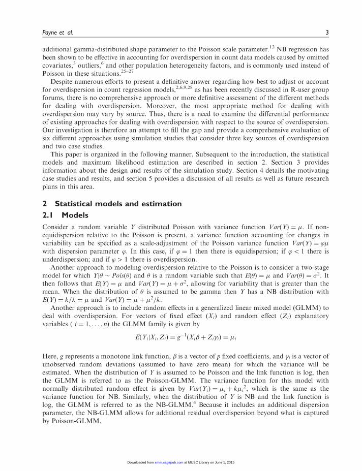
The six different methods considered in this study can be generally classified into two categories:scale adjustment and modeling methods. We considered two scale adjustment methods under thestandard Poisson regression (abbreviated simply Poisson): (1) deviance scale-adjusted Poissonregression (DS-Poisson) and (2) Pearson scale-adjusted Poisson regression (PS-Poisson). We alsoconsidered three modeling methods: (3) negative-binomial regression (NB) and (4, 5) two GLMMwith random intercept, log link, and compound symmetry covariance, with outcomes distributed asPoisson and negative-binomial (Poisson-GLMM, NB-GLMM, respectively). Table 1 gives asummary of the various models we considered, including a description of the particular methodand adjustment utilized for addressing overdispersion.

2.2 Estimation and inference

The parameters of the model that need to be estimated include dispersion, regression coefficientsand variance components. Estimation and inference for the model based methods can beaccomplished using maximum likelihood,4 quasi-likelihood,2 or pseudo-likelihood.29 In our case,the Poisson and NB were estimated via maximum likelihood and the NB-GLMM and Poisson-GLMM were estimated via pseudo-likelihood. On the other hand, in the scale based methods, thetwo most commonly used estimators of dispersion in the literature are the ratio of the modeldeviance to its corresponding degrees of freedom and the ratio of the Pearson XP

2 statistic to itscorresponding degrees of freedom. The degrees of freedom are typically given by n� p for a studywith sample size n observations and p parameters. When the assumption of equal mean andvariance is not violated, these ratios will be equal to 1. Relative to the model, if these ratios aregreater than 1 then the data are considered overdispersed. Higher values demonstrate a greatermagnitude of overdispersion.

2.3 Model comparison

Akaike’s information criteria (AIC)30 and Bayesian information criteria (BIC)31 were utilized tomeasure goodness-of-fit and make comparisons among the different models. Parameter standarderrors and the 95% confidence interval coverage for each parameter were also recorded to determinethe level of bias in the standard error estimates compared to the assumed value in the simulationstudy. These values were then compared across the models to determine which method for dealingwith overdispersion resulted in the lowest AIC and BIC values as well as offered standard errors thatare closer to the simulated value with nominal 95% confidence interval coverage. This modelcomparison using multiple criteria is similar in format to work recently published by Xia et al.,28

in which the authors compare Poisson, negative-binomial, and zero-inflated regression methods tomodel overdispersed and zero-inflated data from an HIV risk reduction intervention study. Gardneret al.32 also compared Poisson and NB methods of analyzing overdispersed count outcomes relatedto psychological datasets, while Ver Hoef and Boveng33 provide an overview and comparison ofthese methods for ecologists.

In this paper, we provide a more unified comparison among the many possible approaches todealing with overdispersion. We also provide a detailed derivation of dispersion in the context ofcount data fitted using different models under multiple covariate type scenarios (see technicalAppendix 1) to complement the simulation and case studies. SAS 9.4 was utilized in all analysesfor both simulated and real datasets, particularly Proc GENMOD and Proc GLIMMIXpackages.





3 Simulation study

We simulated 1000 datasets each with a sample size of n¼ 1000 random observations generatedfollowing scenarios given in Hilbe (2007)6 under three distributions of predictor scenarios. Scenariosunder a sample size of 500 did not lead to different conclusions (results not shown). Table 1 providesa list of all scenarios with their corresponding measure of overdispersion. After generatingoverdispersed datasets for these scenarios, analysis was made using the six models for allsimulated data from each scenario. Goodness-of-fit statistics including AIC, BIC, deviance,Pearson statistic, and parameter estimates for the regression coefficients corresponding to each

Table 1. Summary of models with estimated level of overdispersion.

Distribution Abbreviation Method Adjustment

Poisson Poisson Not adjusted N/A

Poisson DS-Poisson Scale-adjusted Deviance statistic

Poisson PS-Poisson Scale-adjusted Pearson X2 statistic

Poisson Poisson-GLMM GLMM Random effects

Negative-binomial NB Unadjusted Additional parameter

Negative-binomial NB-GLMM GLMM Additional parameter

and random effects

Estimated overdispersion

Covariate Source Deviance/df� sd Pearson V2/df� sd

Normal 1 covariate omitted 3.65� 0.66 4.55� 1.22

2 covariates omitted 15.90� 4.10 52.80� 51.94

Binary 1 covariate omitted 38.31� 1.11 33.93� 1.36


Uniform 1 covariate omitted 8.14� 0.90 8.48� 0.95


Normal Small outliers 2.50� 0.36 25.42� 17.06

Large outliers 9.42� 1.06 121.32� 59.30

Lower % zero outliers 2.61� 0.47 1.53� 0.31

Higher % zero outliers 4.34� 0.54 2.94� 0.45

Binary Small outliers 2.07� 0.10 7.97� 0.77

Large outliers 8.50� 0.28 50.64� 3.70



Uniform Small outliers 2.16� 0.11 8.88� 0.92

Large outliers 8.74� 0.30 54.74� 4.12



Normal Small variance random effects 5.68� 1.66 8.56� 4.68

Large variance random effects 18.28� 15.15 81.58� 217.85

Binary Small variance random effects 2.52� 0.34 3.94� 1.26


Uniform Small variance random effects 2.28� 0.30 3.54� 1.03


DS: deviance scale; NB: negative-binomial; PS: Pearson scale; GLMM: generalized linear mixed models.

Payne et al. 5




covariate with their corresponding variance and 95% confidence interval (CI) coverage werecalculated.

3.1 Covariate dependent overdispersion design

We considered three different scenarios. In scenario 1, each dataset included three normalindependent predictors with x1� Normal(1, 2), x2 �Normal(2, 3), and x3� Normal(3, 4). In thecount regression model, � ¼ ð�0, �1, �2, �3Þ were assigned values (1.0, 0.5, �0.75, and 0.25). Thesevariables were then utilized to create a count response Y using a Poisson error and log link functionthat ranged from 0 to 3443. The distributions of these variables are illustrated in Appendix 2(Figure 7(a) to (d)). In scenario 2, binary covariates were derived from the normally distributedcovariates described above. Values less than the mean were assigned a value of 0; values greater thanor equal to the mean were assigned a value of 1. The � ¼ ð�0, �1,�2, �3Þ for intercept, x1, x2, and x3were assigned to be (1.0, 2.0, 1.5, 1.0), respectively. In scenario 3, predictor x1 was drawn fromUniform(5, 10), x2 from Uniform(10, 15), and x3 from Uniform(15, 20). In this case, (�0, �1, �2,�3)for the intercept, x1, x2, and x3 were again assigned to be (1.0, 0.5, �0.75, 0.25), respectively.Overdispersion relative to the Poisson was then created in these datasets via the omission ofimportant predictors from the model where (i) predictor x1 was first removed from the modeland (ii) both x1 and x2 were removed from the model, creating overdispersion of a highermagnitude. Further details of the methodology are discussed in Appendix 1.

3.2 Covariate dependent overdispersion results

When one important predictor was omitted from the model, the mean deviance/df value for theunadjusted Poisson model was 3.65� 0.66 and the mean Pearson V 2/df value was 4.55� 1.22,indicating the presence of overdispersion. When two important predictors were omitted, these

01000200030004000500060007000

Mea

sure

AIC

BIC

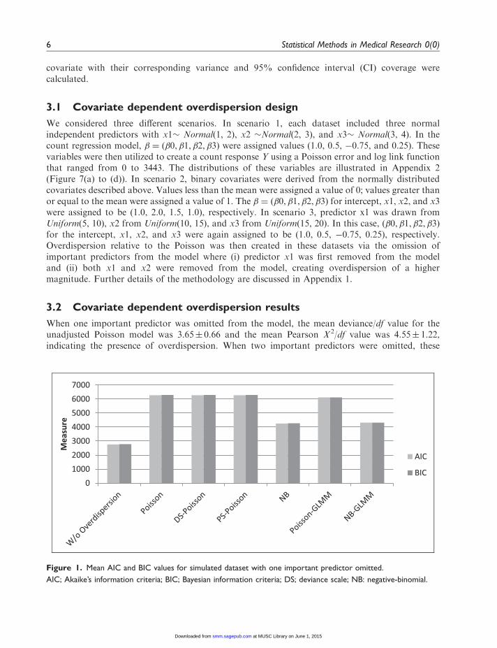
Figure 1. Mean AIC and BIC values for simulated dataset with one important predictor omitted.

AIC; Akaike’s information criteria; BIC; Bayesian information criteria; DS; deviance scale; NB: negative-binomial.





values increased to 15.90� 4.10 and 52.80� 51.94, respectively, indicating overdispersion of greatermagnitude. For binary covariates, after the omission of one predictor the mean deviance/df value forthe unadjusted Poisson model in binary covariate simulations was 38.31� 1.11, and the meanPearson V 2/df value was 33.93� 1.36. After the omission of two predictors, the mean deviance/dfvalue increased to 63.56� 1.95, and the mean Pearson V 2/df value increased to 70.87� 1.41. In thescenario where the covariates come from a uniform distribution, after the omission of one predictorthe mean deviance/df value for the unadjusted Poisson model in uniform covariate simulations was8.14� 0.90, and the mean Pearson V 2/df value was 8.48� 0.95. After the omission of two predictors,the mean deviance/df value increased to 44.98� 4.52, and the mean Pearson V 2/df value increased to80.50� 9.71 (Table 1).

Figure 1 shows the mean AIC and BIC values when one important predictor is omitted, for thenormal predictor scenario. The results indicate that the NB and NB-GLMM models have the lowestAIC and BIC that is comparable to the original model without overdispersion. All Poissonregression models exhibited very large values of AIC and BIC, indicating poorer fit to the datacompared to the NB models.

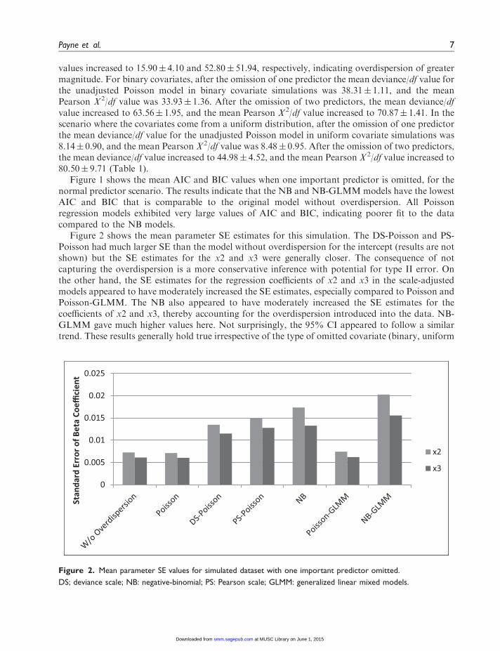
Figure 2 shows the mean parameter SE estimates for this simulation. The DS-Poisson and PS-Poisson had much larger SE than the model without overdispersion for the intercept (results are notshown) but the SE estimates for the x2 and x3 were generally closer. The consequence of notcapturing the overdispersion is a more conservative inference with potential for type II error. Onthe other hand, the SE estimates for the regression coefficients of x2 and x3 in the scale-adjustedmodels appeared to have moderately increased the SE estimates, especially compared to Poisson andPoisson-GLMM. The NB also appeared to have moderately increased the SE estimates for thecoefficients of x2 and x3, thereby accounting for the overdispersion introduced into the data. NB-GLMM gave much higher values here. Not surprisingly, the 95% CI appeared to follow a similartrend. These results generally hold true irrespective of the type of omitted covariate (binary, uniform

0

0.005

0.01

0.015

0.02

0.025

Stan

dard

Err

or o

f Bet

a Co

effici

ent

x2

x3

Figure 2. Mean parameter SE values for simulated dataset with one important predictor omitted.

DS; deviance scale; NB: negative-binomial; PS: Pearson scale; GLMM: generalized linear mixed models.

Payne et al. 7




or normal). Results for covariate dependent overdispersion resulting from the omission of twoimportant covariates are given in Appendix 2, and are qualitatively similar.

3.3 Outlier dependent overdispersion design

The second scenario for creating overdispersion relative to the Poisson was the addition ofeither high outliers or excess zero outliers to the count outcome Y. In the first scenario, variablex1 was left in the model and a random Y value in each group of each simulation was increased by50 to create outlier dependent overdispersion in the data. This gave 10 total outliers in each datasetcontaining 1000 values; i.e. 1% of the data were replaced by outliers. This was followed by anincrease in the outliers by 150, which created overdispersion of a higher magnitude. In thesecond scenario, varying percentages of the outcome were replaced with 0. For binary covariates,the � ¼ ð�0, �1, �2, �3Þ for intercept, x1, x2, and x3 were assigned to be (1.0, 0.5, �0.75, 0.25),respectively. Overdispersion was then created in the datasets as detailed above via the addition ofoutliers of differing magnitudes or zero values.

3.4 Outlier dependent overdispersion results

The simulated data were analyzed with all variables in the model and overdispersion created via theaddition of outliers. After the smaller outliers were added, the mean deviance/df value for theunadjusted Poisson model was 2.50� 0.36 and the mean Pearson V 2/df value was 25.42� 17.06,demonstrating the presence of overdispersion. After the addition of larger outliers, these valuesincreased to 9.42� 1.06 and 121.32� 59.30, respectively. After the addition of 20% zero outliers,these values were 2.61� 0.47 and 1.53� 0.31, respectively. After the addition of 40% zero outliers,these values increased to 4.34� 0.54 and 2.94� 0.45, respectively. For binary covariates, after theaddition of smaller outliers the mean deviance/df value for the unadjusted Poisson model in binarycovariate simulations was 2.07� 0.10, and the mean Pearson V 2/df value was 7.97� 0.77. After themagnitude of the outliers was increased, the mean deviance/df value increased to 8.50� 0.28, and themean Pearson V 2/df value increased to 50.64� 3.70. After the addition of 40% zero outliers, thesevalues were 1.86� 0.06 and 1.24� 0.06, respectively. After the addition of 60% zero outliers, thesevalues increased to 2.21� 0.04 and 1.84� 0.06, respectively. In the scenario where the covariatescome from a uniform distribution, after the addition of the smaller outliers the mean deviance/dfvalue for the unadjusted Poisson model in uniform covariate simulations was 2.16� 0.11, and themean Pearson V 2/df value was 8.88� 0.92. After the magnitude of the outliers was increased, themean deviance/df value increased to 8.74� 0.30, and the mean Pearson V 2/df value increased to54.74� 4.12 (Table 1). After the addition of 40% zero outliers, these values were 1.69� 0.05 and1.13� 0.05, respectively. After the addition of 60% zero outliers, these values increased to2.00� 0.04 and 1.67� 0.06, respectively.

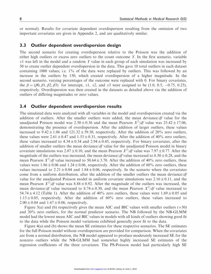
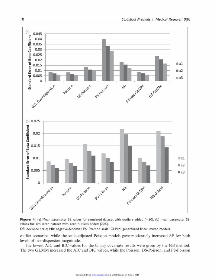
Figure 3(a) and (b) respectively gives the mean AIC and BIC values with smaller outliers (þ50)and 20% zero outliers, for the normal predictor scenario. The NB followed by the NB-GLMMmodel had the lowest mean AIC and BIC values in models with all kinds of outliers showing good fitto the data while the Poisson model variations exhibited generally poor fit to the data.

Figure 4(a) and (b) shows the mean SE estimates for these respective scenarios. The SE estimatesfor the full Poisson model without overdispersion are provided for comparison. When the covariatesare from a normal distribution, the NB model appeared to produce moderately increased SE for thenonzero outliers while the NB-GLMM had somewhat highly increased SE estimates of theregression coefficients of the three covariates. The PS-Poisson model had particularly high SE





estimates for all parameters, while the Poisson and Poisson-GLMM models gave much lowerestimates of the SE compared to what would be expected under the simulated dispersed data.The 95% CI appeared to follow the same trend. Therefore, it appears that the NB and DS-Poisson models may be considered superior for dealing with outlier dependent overdispersion inthis case, with NB demonstrating better goodness-of-fit. The NB models gave higher SE for the zero

0

1000

2000

3000

4000

5000

6000M

easu

re

AIC

BIC

0500

100015002000250030003500400045005000

Mea

sure

AIC

BIC

(a)

(b)

Figure 3. (a) Mean AIC and BIC values for simulated dataset with outliers added (þ50); (b) mean AIC and BIC

values for simulated dataset with zero outliers added (20%).

DS; deviance scale; NB: negative-binomial; PS: Pearson scale; GLMM: generalized linear mixed models; AIC: Akaike’s

information criteria; BIC: Bayesian information criteria.

Payne et al. 9




outlier scenarios, while the scale-adjusted Poisson models gave moderately increased SE for bothlevels of overdispersion magnitude.

The lowest AIC and BIC values for the binary covariate results were given by the NB method.The two GLMM increased the AIC and BIC values, while the Poisson, DS-Poisson, and PS-Poisson

00.005

0.010.015

0.020.025

0.030.035

0.040.045

Stan

dard

Err

or o

f Bet

a Co

effici

ent

x1

x2

x3

0

0.005

0.01

0.015

0.02

0.025

Stan

dard

Err

or o

f Bet

a Co

effici

ent

x1

x2

x3

(b)

(a)

Figure 4. (a) Mean parameter SE values for simulated dataset with outliers added (þ50); (b) mean parameter SE







gave identical results. NB and DS-Poisson gave moderate SE and 95% CI coverage. The NB-GLMM and PS-Poisson gave higher SE and 95% CI for all covariates, while the original Poissonand Poisson-GLMM gave lower values. Results are similar for the larger level outlier scenarios,given in Appendix 2.

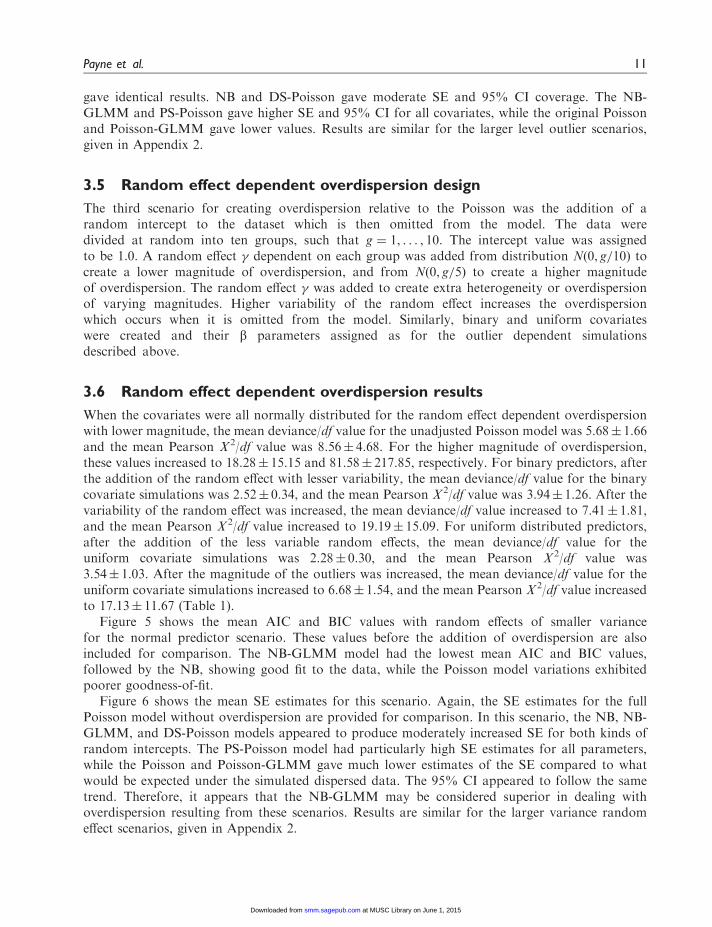
3.5 Random effect dependent overdispersion design

The third scenario for creating overdispersion relative to the Poisson was the addition of arandom intercept to the dataset which is then omitted from the model. The data weredivided at random into ten groups, such that g ¼ 1, . . . , 10. The intercept value was assignedto be 1.0. A random effect � dependent on each group was added from distribution Nð0, g=10Þ tocreate a lower magnitude of overdispersion, and from Nð0, g=5Þ to create a higher magnitudeof overdispersion. The random effect � was added to create extra heterogeneity or overdispersionof varying magnitudes. Higher variability of the random effect increases the overdispersionwhich occurs when it is omitted from the model. Similarly, binary and uniform covariateswere created and their b parameters assigned as for the outlier dependent simulationsdescribed above.

3.6 Random effect dependent overdispersion results

When the covariates were all normally distributed for the random effect dependent overdispersionwith lower magnitude, the mean deviance/df value for the unadjusted Poisson model was 5.68� 1.66and the mean Pearson V 2/df value was 8.56� 4.68. For the higher magnitude of overdispersion,these values increased to 18.28� 15.15 and 81.58� 217.85, respectively. For binary predictors, afterthe addition of the random effect with lesser variability, the mean deviance/df value for the binarycovariate simulations was 2.52� 0.34, and the mean Pearson V 2/df value was 3.94� 1.26. After thevariability of the random effect was increased, the mean deviance/df value increased to 7.41� 1.81,and the mean Pearson V 2/df value increased to 19.19� 15.09. For uniform distributed predictors,after the addition of the less variable random effects, the mean deviance/df value for theuniform covariate simulations was 2.28� 0.30, and the mean Pearson V 2/df value was3.54� 1.03. After the magnitude of the outliers was increased, the mean deviance/df value for theuniform covariate simulations increased to 6.68� 1.54, and the mean Pearson V 2/df value increasedto 17.13� 11.67 (Table 1).

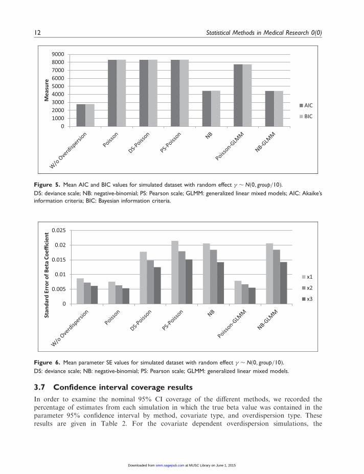
Figure 5 shows the mean AIC and BIC values with random effects of smaller variancefor the normal predictor scenario. These values before the addition of overdispersion are alsoincluded for comparison. The NB-GLMM model had the lowest mean AIC and BIC values,followed by the NB, showing good fit to the data, while the Poisson model variations exhibitedpoorer goodness-of-fit.

Figure 6 shows the mean SE estimates for this scenario. Again, the SE estimates for the fullPoisson model without overdispersion are provided for comparison. In this scenario, the NB, NB-GLMM, and DS-Poisson models appeared to produce moderately increased SE for both kinds ofrandom intercepts. The PS-Poisson model had particularly high SE estimates for all parameters,while the Poisson and Poisson-GLMM gave much lower estimates of the SE compared to whatwould be expected under the simulated dispersed data. The 95% CI appeared to follow the sametrend. Therefore, it appears that the NB-GLMM may be considered superior in dealing withoverdispersion resulting from these scenarios. Results are similar for the larger variance randomeffect scenarios, given in Appendix 2.

Payne et al. 11




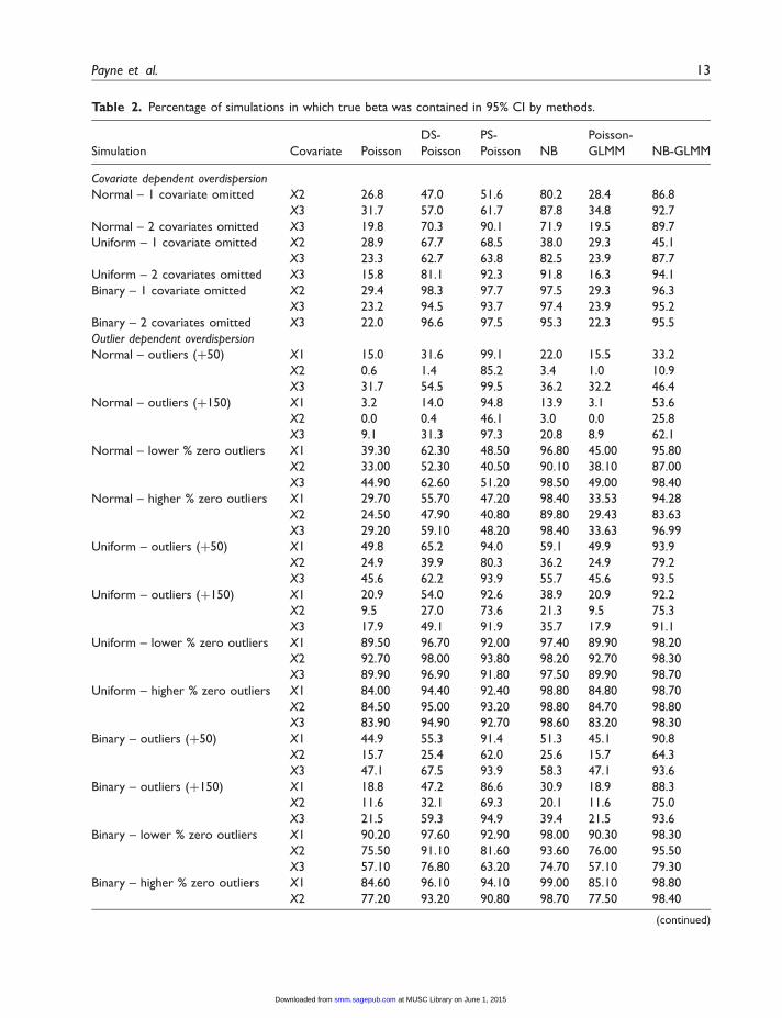
3.7 Confidence interval coverage results

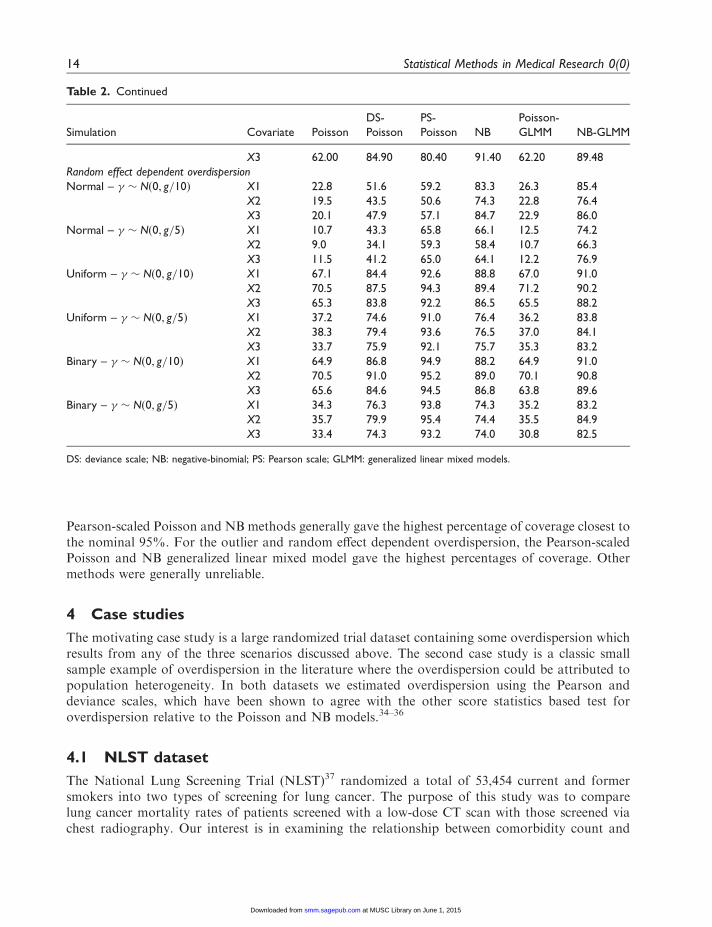
In order to examine the nominal 95% CI coverage of the different methods, we recorded thepercentage of estimates from each simulation in which the true beta value was contained in theparameter 95% confidence interval by method, covariate type, and overdispersion type. Theseresults are given in Table 2. For the covariate dependent overdispersion simulations, the

0100020003000400050006000700080009000

Mea

sure

AIC

BIC

Figure 5. Mean AIC and BIC values for simulated dataset with random effect � � Nð0, group=10Þ.

DS: deviance scale; NB: negative-binomial; PS: Pearson scale; GLMM: generalized linear mixed models; AIC: Akaike’s

information criteria; BIC: Bayesian information criteria.

0

0.005

0.01

0.015

0.02

0.025

Stan

dard

Err

or o

f Bet

a Co

effici

ent

x1

x2

x3

Figure 6. Mean parameter SE values for simulated dataset with random effect � � Nð0, group=10Þ.






Table 2. Percentage of simulations in which true beta was contained in 95% CI by methods.

Simulation Covariate Poisson

DS-

Poisson

PS-

Poisson NB

Poisson-

GLMM NB-GLMM

Covariate dependent overdispersion

Normal – 1 covariate omitted X2 26.8 47.0 51.6 80.2 28.4 86.8

X3 31.7 57.0 61.7 87.8 34.8 92.7

Normal – 2 covariates omitted X3 19.8 70.3 90.1 71.9 19.5 89.7

Uniform – 1 covariate omitted X2 28.9 67.7 68.5 38.0 29.3 45.1

X3 23.3 62.7 63.8 82.5 23.9 87.7

Uniform – 2 covariates omitted X3 15.8 81.1 92.3 91.8 16.3 94.1

Binary – 1 covariate omitted X2 29.4 98.3 97.7 97.5 29.3 96.3

X3 23.2 94.5 93.7 97.4 23.9 95.2

Binary – 2 covariates omitted X3 22.0 96.6 97.5 95.3 22.3 95.5

Outlier dependent overdispersion

Normal – outliers (þ50) X1 15.0 31.6 99.1 22.0 15.5 33.2

X2 0.6 1.4 85.2 3.4 1.0 10.9

X3 31.7 54.5 99.5 36.2 32.2 46.4

Normal – outliers (þ150) X1 3.2 14.0 94.8 13.9 3.1 53.6

X2 0.0 0.4 46.1 3.0 0.0 25.8

X3 9.1 31.3 97.3 20.8 8.9 62.1

Normal – lower % zero outliers X1 39.30 62.30 48.50 96.80 45.00 95.80

X2 33.00 52.30 40.50 90.10 38.10 87.00

X3 44.90 62.60 51.20 98.50 49.00 98.40

Normal – higher % zero outliers X1 29.70 55.70 47.20 98.40 33.53 94.28

X2 24.50 47.90 40.80 89.80 29.43 83.63

X3 29.20 59.10 48.20 98.40 33.63 96.99

Uniform – outliers (þ50) X1 49.8 65.2 94.0 59.1 49.9 93.9

X2 24.9 39.9 80.3 36.2 24.9 79.2

X3 45.6 62.2 93.9 55.7 45.6 93.5

Uniform – outliers (þ150) X1 20.9 54.0 92.6 38.9 20.9 92.2

X2 9.5 27.0 73.6 21.3 9.5 75.3

X3 17.9 49.1 91.9 35.7 17.9 91.1

Uniform – lower % zero outliers X1 89.50 96.70 92.00 97.40 89.90 98.20

X2 92.70 98.00 93.80 98.20 92.70 98.30

X3 89.90 96.90 91.80 97.50 89.90 98.70

Uniform – higher % zero outliers X1 84.00 94.40 92.40 98.80 84.80 98.70

X2 84.50 95.00 93.20 98.80 84.70 98.80

X3 83.90 94.90 92.70 98.60 83.20 98.30

Binary – outliers (þ50) X1 44.9 55.3 91.4 51.3 45.1 90.8

X2 15.7 25.4 62.0 25.6 15.7 64.3

X3 47.1 67.5 93.9 58.3 47.1 93.6

Binary – outliers (þ150) X1 18.8 47.2 86.6 30.9 18.9 88.3

X2 11.6 32.1 69.3 20.1 11.6 75.0

X3 21.5 59.3 94.9 39.4 21.5 93.6

Binary – lower % zero outliers X1 90.20 97.60 92.90 98.00 90.30 98.30

X2 75.50 91.10 81.60 93.60 76.00 95.50

X3 57.10 76.80 63.20 74.70 57.10 79.30

Binary – higher % zero outliers X1 84.60 96.10 94.10 99.00 85.10 98.80

X2 77.20 93.20 90.80 98.70 77.50 98.40

(continued)

Payne et al. 13




Pearson-scaled Poisson and NB methods generally gave the highest percentage of coverage closest tothe nominal 95%. For the outlier and random effect dependent overdispersion, the Pearson-scaledPoisson and NB generalized linear mixed model gave the highest percentages of coverage. Othermethods were generally unreliable.

4 Case studies

The motivating case study is a large randomized trial dataset containing some overdispersion whichresults from any of the three scenarios discussed above. The second case study is a classic smallsample example of overdispersion in the literature where the overdispersion could be attributed topopulation heterogeneity. In both datasets we estimated overdispersion using the Pearson anddeviance scales, which have been shown to agree with the other score statistics based test foroverdispersion relative to the Poisson and NB models.34–36

4.1 NLST dataset

The National Lung Screening Trial (NLST)37 randomized a total of 53,454 current and formersmokers into two types of screening for lung cancer. The purpose of this study was to comparelung cancer mortality rates of patients screened with a low-dose CT scan with those screened viachest radiography. Our interest is in examining the relationship between comorbidity count and

Table 2. Continued

Simulation Covariate Poisson

DS-

Poisson

PS-

Poisson NB

Poisson-

GLMM NB-GLMM

X3 62.00 84.90 80.40 91.40 62.20 89.48

Random effect dependent overdispersion

Normal – � � Nð0, g=10Þ X1 22.8 51.6 59.2 83.3 26.3 85.4

X2 19.5 43.5 50.6 74.3 22.8 76.4

X3 20.1 47.9 57.1 84.7 22.9 86.0

Normal – � � Nð0, g=5Þ X1 10.7 43.3 65.8 66.1 12.5 74.2

X2 9.0 34.1 59.3 58.4 10.7 66.3

X3 11.5 41.2 65.0 64.1 12.2 76.9

Uniform – � � Nð0, g=10Þ X1 67.1 84.4 92.6 88.8 67.0 91.0

X2 70.5 87.5 94.3 89.4 71.2 90.2

X3 65.3 83.8 92.2 86.5 65.5 88.2

Uniform – � � Nð0, g=5Þ X1 37.2 74.6 91.0 76.4 36.2 83.8

X2 38.3 79.4 93.6 76.5 37.0 84.1

X3 33.7 75.9 92.1 75.7 35.3 83.2

Binary – � � Nð0, g=10Þ X1 64.9 86.8 94.9 88.2 64.9 91.0

X2 70.5 91.0 95.2 89.0 70.1 90.8

X3 65.6 84.6 94.5 86.8 63.8 89.6

Binary – � � Nð0, g=5Þ X1 34.3 76.3 93.8 74.3 35.2 83.2

X2 35.7 79.9 95.4 74.4 35.5 84.9

X3 33.4 74.3 93.2 74.0 30.8 82.5






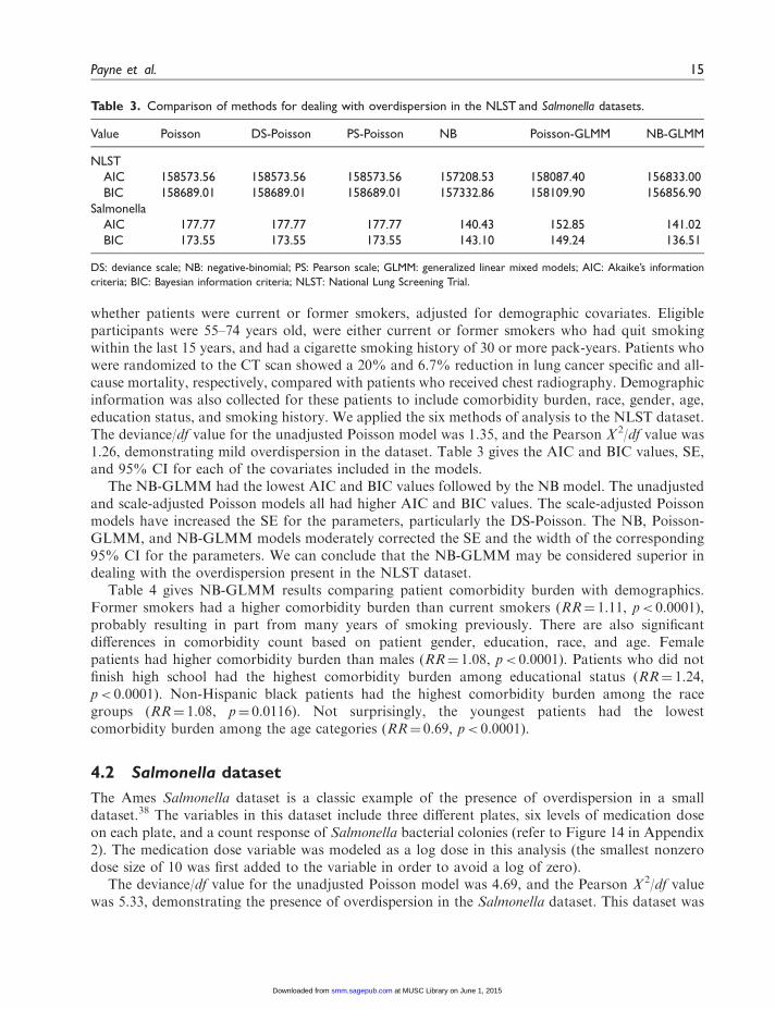
whether patients were current or former smokers, adjusted for demographic covariates. Eligibleparticipants were 55–74 years old, were either current or former smokers who had quit smokingwithin the last 15 years, and had a cigarette smoking history of 30 or more pack-years. Patients whowere randomized to the CT scan showed a 20% and 6.7% reduction in lung cancer specific and all-cause mortality, respectively, compared with patients who received chest radiography. Demographicinformation was also collected for these patients to include comorbidity burden, race, gender, age,education status, and smoking history. We applied the six methods of analysis to the NLST dataset.The deviance/df value for the unadjusted Poisson model was 1.35, and the Pearson V 2/df value was1.26, demonstrating mild overdispersion in the dataset. Table 3 gives the AIC and BIC values, SE,and 95% CI for each of the covariates included in the models.

The NB-GLMM had the lowest AIC and BIC values followed by the NB model. The unadjustedand scale-adjusted Poisson models all had higher AIC and BIC values. The scale-adjusted Poissonmodels have increased the SE for the parameters, particularly the DS-Poisson. The NB, Poisson-GLMM, and NB-GLMM models moderately corrected the SE and the width of the corresponding95% CI for the parameters. We can conclude that the NB-GLMM may be considered superior indealing with the overdispersion present in the NLST dataset.

Table 4 gives NB-GLMM results comparing patient comorbidity burden with demographics.Former smokers had a higher comorbidity burden than current smokers (RR¼ 1.11, p< 0.0001),probably resulting in part from many years of smoking previously. There are also significantdifferences in comorbidity count based on patient gender, education, race, and age. Femalepatients had higher comorbidity burden than males (RR¼ 1.08, p< 0.0001). Patients who did notfinish high school had the highest comorbidity burden among educational status (RR¼ 1.24,p< 0.0001). Non-Hispanic black patients had the highest comorbidity burden among the racegroups (RR¼ 1.08, p¼ 0.0116). Not surprisingly, the youngest patients had the lowestcomorbidity burden among the age categories (RR¼ 0.69, p< 0.0001).

4.2 Salmonella dataset

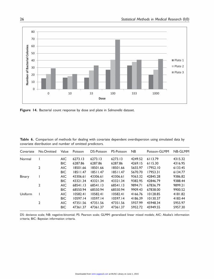
The Ames Salmonella dataset is a classic example of the presence of overdispersion in a smalldataset.38 The variables in this dataset include three different plates, six levels of medication doseon each plate, and a count response of Salmonella bacterial colonies (refer to Figure 14 in Appendix2). The medication dose variable was modeled as a log dose in this analysis (the smallest nonzerodose size of 10 was first added to the variable in order to avoid a log of zero).

The deviance/df value for the unadjusted Poisson model was 4.69, and the Pearson V 2/df valuewas 5.33, demonstrating the presence of overdispersion in the Salmonella dataset. This dataset was

Table 3. Comparison of methods for dealing with overdispersion in the NLST and Salmonella datasets.

Value Poisson DS-Poisson PS-Poisson NB Poisson-GLMM NB-GLMM

NLST

AIC 158573.56 158573.56 158573.56 157208.53 158087.40 156833.00

BIC 158689.01 158689.01 158689.01 157332.86 158109.90 156856.90

Salmonella

AIC 177.77 177.77 177.77 140.43 152.85 141.02

BIC 173.55 173.55 173.55 143.10 149.24 136.51

DS: deviance scale; NB: negative-binomial; PS: Pearson scale; GLMM: generalized linear mixed models; AIC: Akaike’s information

criteria; BIC: Bayesian information criteria; NLST: National Lung Screening Trial.

Payne et al. 15




analyzed using the six approaches and the results are reported in Table 3. The AIC and BIC values,parameter SE, and 95% parameter CI were included for comparison.

Based on the AIC and BIC criteria, the NB-GLMM demonstrated the best goodness-of-fit in thisoverdispersed dataset. The NB, NB-GLMM and Poisson-GLMM also gave SE values that arehigher than those in Poisson but lower than scale-adjusted Poisson. The scale-adjusted Poissonmodels both appeared to have much larger SE, particularly the PS-Poisson. The 95% CIappeared to follow the same trend. Overall, the NB-GLMM may be considered superior indealing with overdispersion present in the Salmonella dataset based on the AIC and BIC criteria,SE, and 95% CI estimates. This is likely because the overdispersion in this case study was at least inpart the result of correlation in bacterial count outcome by plate, which was included in the modelvia the random effect. In the NB-GLMM model, the log dose variable significantly effects bacterialcount outcome (RR¼ 1.13, p¼ 0.0194).

5 Discussion

In this paper, we provide a comprehensive comparative analysis of six different models for dealingwith overdispersion caused by different mechanisms when modeling count data. Overall, the NBmodels appeared to demonstrate superiority in adjusting for overdispersion in the simulationstudies. The NB-GLMM performed best in modeling count of comorbidity data in themotivating NLST study. This model also appeared to deal most effectively with overdispersion inthe small Salmonella dataset.

Based on our analyses, we conclude that NB-GLMM is superior overall for modeling count datacharacterized by overdispersion, jointly considering all criteria. The NB distribution is often usedinstead of Poisson to account for overdispersion resulting from omitted important covariates andpopulation heterogeneity, among other causes. Therefore, it is reasonable that overdispersion causedby the omission of important predictors, the addition of high or zero outliers to the outcome, andthe omission of a random effect would be effectively controlled by using models that are based on the

Table 4. NB-GLMM model comparing comorbidity count with patient demographics in the NLST

dataset.

Covariate Rate ratio 95% CI p-Value

Former smoker vs. current smoker 1.11 (1.09, 1.12) <0.0001

Female vs. Male 1.08 (1.07, 1.10) <0.0001

<High school 1.24 (1.15, 1.33) <0.0001

High school 1.08 (1.02, 1.15) 0.0149

College 0.94 (0.88, 1.01) 0.0795

Graduate school 0.94 (0.88, 1.01) 0.0733

Other education (ref) – – –

NHW 0.90 (0.86, 0.94) <0.0001

NHB 1.08 (1.02, 1.15) 0.0116

Asian 0.91 (0.84, 0.99) 0.0271

Hispanic/Other (ref) – – –

Age< 57 0.69 (0.67, 0.71) <0.0001

57�Age< 60 0.76 (0.75, 0.79) <0.0001

60�Age< 65 0.86 (0.84, 0.88) <0.0001

Age� 65 (ref) – – –





NB distribution. For example, as in the NB-GLMM, the addition of random effects is shown to beeffective in dealing with overdispersion resulting from with-in subject correlation of count outcome.

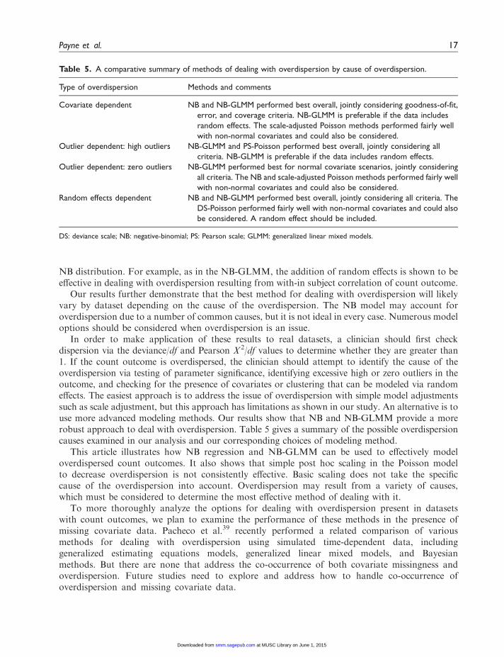
Our results further demonstrate that the best method for dealing with overdispersion will likelyvary by dataset depending on the cause of the overdispersion. The NB model may account foroverdispersion due to a number of common causes, but it is not ideal in every case. Numerous modeloptions should be considered when overdispersion is an issue.

In order to make application of these results to real datasets, a clinician should first checkdispersion via the deviance/df and Pearson V 2/df values to determine whether they are greater than1. If the count outcome is overdispersed, the clinician should attempt to identify the cause of theoverdispersion via testing of parameter significance, identifying excessive high or zero outliers in theoutcome, and checking for the presence of covariates or clustering that can be modeled via randomeffects. The easiest approach is to address the issue of overdispersion with simple model adjustmentssuch as scale adjustment, but this approach has limitations as shown in our study. An alternative is touse more advanced modeling methods. Our results show that NB and NB-GLMM provide a morerobust approach to deal with overdispersion. Table 5 gives a summary of the possible overdispersioncauses examined in our analysis and our corresponding choices of modeling method.

This article illustrates how NB regression and NB-GLMM can be used to effectively modeloverdispersed count outcomes. It also shows that simple post hoc scaling in the Poisson modelto decrease overdispersion is not consistently effective. Basic scaling does not take the specificcause of the overdispersion into account. Overdispersion may result from a variety of causes,which must be considered to determine the most effective method of dealing with it.

To more thoroughly analyze the options for dealing with overdispersion present in datasetswith count outcomes, we plan to examine the performance of these methods in the presence ofmissing covariate data. Pacheco et al.39 recently performed a related comparison of variousmethods for dealing with overdispersion using simulated time-dependent data, includinggeneralized estimating equations models, generalized linear mixed models, and Bayesianmethods. But there are none that address the co-occurrence of both covariate missingness andoverdispersion. Future studies need to explore and address how to handle co-occurrence ofoverdispersion and missing covariate data.

Table 5. A comparative summary of methods of dealing with overdispersion by cause of overdispersion.

Type of overdispersion Methods and comments

Covariate dependent NB and NB-GLMM performed best overall, jointly considering goodness-of-fit,

error, and coverage criteria. NB-GLMM is preferable if the data includes

random effects. The scale-adjusted Poisson methods performed fairly well

with non-normal covariates and could also be considered.

Outlier dependent: high outliers NB-GLMM and PS-Poisson performed best overall, jointly considering all

criteria. NB-GLMM is preferable if the data includes random effects.

Outlier dependent: zero outliers NB-GLMM performed best for normal covariate scenarios, jointly considering

all criteria. The NB and scale-adjusted Poisson methods performed fairly well

with non-normal covariates and could also be considered.

Random effects dependent NB and NB-GLMM performed best overall, jointly considering all criteria. The

DS-Poisson performed fairly well with non-normal covariates and could also

be considered. A random effect should be included.


Payne et al. 17




Authors’ contributions

Study concept and design: MG, EP

Acquisition of data: EP, MG

Analysis and interpretation of data: MG, EP, JH, LE, AS, VR.

Drafting of the manuscript: MG, EP, JH, LE, AS, VR

Critical revision of the manuscript for important intellectual content: MG, EP, JH, LE, AS, VR

Final approval of manuscript: MG, EP, JH, LE, AS, VR

Funding

This study was supported by grant #IIR-06-219 (PI: Leonard Egede) by the VHA Health Services Research and

Development (HSR&D) program. The funding agency did not participate in the design and conduct of the study;

collection, management, analysis, and interpretation of the data; and preparation, review, or approval of the

manuscript. TheNLSTdatawas obtained through a grant funded by theCHESTFoundation (PI:Nichole Tanner).

The manuscript represents the views of the authors and not those of the VA or HSR&D.

Conflict of interest

None declared.

References

1. Cox DR. Some remarks on overdispersion. Biometrika1983; 70: 269–274.

2. Hardin J and Hilbe JM. Generalized linear modelsand extensions. College Station, TX: Stata Press, 2001,p.2007.

3. Rigby RA, Stasinopoulos DM and Akantziliotou C.A framework for modelling overdispersed count data,including the Poisson-shifted generalized inverseGaussian distribution. Comput Stat Data Anal 2008; 53:381–393.

4. McCullagh P and Nelder JA. Generalized linear models.London, UK; New York, NY: Chapman and Hall, 1983,p.1989.

5. Breslow N. Tests of hypotheses in overdispersed Poissonregression and other quasi-likelihood models. J Am StatAssoc 1990; 85: 565–571.

6. Hilbe JM. Negative-binomial regression. Cambridge:Cambridge University Press, 2007, p.2011.

7. Faddy MJ and Smith DM. Analysis of count data withcovariate dependence in both mean and variance. J ApplStat 2011; 38: 2683–2694.

8. Hinde J and Demetrio CGB. Overdispersion: Models andestimation. Comput Stat Data Anal 1998; 27: 151–170.

9. Hayat MJ and Higgins M. Understanding Poissonregression. J Nurs Educ 2014; 53: 207–215.

10. Smith PJ and Heitjan DF. Testing and adjusting fordepartures from nominal dispersion in generalized linearmodels. Appl Stat 1993; 42: 31–41.

11. Yang Z, Hardin JW, Addy CL, et al. Testing approachesfor overdispersion in Poisson regression versus thegeneralized Poisson model. Biom J 2007; 49: 565–584.

12. Molenberghs G, Verbeke G and Demetrio CG. Anextended random-effects approach to modeling repeated,overdispersed count data. Lifetime Data Anal 2007; 13:513–531.

13. Booth JG, Casella G, Friedl H, et al. Negative-binomialloglinear mixed models. Stat Model 2003; 3: 179–191.

14. Milanzi E, Alonso A and Molenberghs G. Ignoringoverdispersion in hierarchical loglinear models: Possibleproblems and solutions. Stat Med 2011; 31: 1475–1482.

15. Pearson K. On the criterion that a given system ofdeviations from the probable in the case of a correlatedsystem of variables is such that it can be reasonablysupposed to have arisen from random sampling. PhilosMag Ser 1900; 50: 157–175.

16. Mullahy J. Specification and testing of some modifiedcount data models. J Econom 1986; 33: 341–365.

17. Cameron AC and Trivedi PK. Regression analysis of countdata. Cambridge: Cambridge University Press, 1998.

18. Dauxois JY, Druilhet P and Pommeret D. A Bayesianchoice between Poisson, binomial and negative-binomialmodels. Test 2006; 15: 423–432.

19. Aregay M, Shkedy Z, et al. A hierarchical Bayesianapproach for the analysis of longitudinal count data withoverdispersion: A simulation study. Comput Stat DataAnal 2013; 57: 233–245. ((2013)).

20. Lambert D. Zero-inflated Poisson regression, with anapplication to defects in manufacturing. Technometrics1992; 34: 1–14.

21. Long JS. Regression models for categorical and limiteddependent variables. Thousand Oaks, CA: Sage, 1997.

22. Tin A. Modeling zero-inflated count data withunderdispersion and overdispersion. SAS Global Forum,Statistics and Data Analysis, 2008.

23. Cameron AC. Advances in count data regression talk forthe applied statistics workshop. http://cameron.econ.ucdavis.edu/racd/count.html (accessed 28 March 2009).

24. Joe H and Zhu R. Generalized Poisson distribution: Theproperty of mixture of Poisson and comparison withnegative-binomial distribution. Biom J 2005; 47: 219–229.

25. Ramakrishnan V and Meeter D. Negative-binomialcrosstabulations, with applications to abundance data.Biometrics 1993; 49: 195–207.

26. Bouche G, Lepage B, Migeot V, et al. Application ofdetecting and taking overdispersion into account in



http://cameron.econ.ucdavis.edu/racd/count.html

http://cameron.econ.ucdavis.edu/racd/count.html



Poisson regression model. Rev Epidemiol Sante Publique2009; 57: 285–296.

27. Yau KKW, Wang K and Lee AH. Zero-inflated negative-binomial mixed regression modeling of over-dispersedcount data with extra zeros. Biom J 2003; 45: 437–452.

28. Xia Y, Morrison-Beedy D, Ma J, et al. Modeling countoutcomes from HIV risk reduction interventions: Acomparison of competing statistical models for countresponses. AIDS Res Treat 2012; 2012: 1–11.

29. Fitzmaurice G, Laird N and Ware J. Applied longitudinalanalysis. Hoboken, NJ: Wiley-Interscience, 2004.

30. Akaike H. A new look at the statistical modelidentification. IEEE Trans Autom Control 1974; 19:716–723.

31. Schwarz G. Estimating the dimension of a model. Ann Stat1978; 6: 461–464.

32. Gardner W, Mulvey EP, Shaw EC, et al. Regressionanalyses of counts and rates: Poisson overdispersedPoisson, and negative-binomial models. Psychol Bull 1995;118: 392–404.

33. Ver Hoef JM and Boveng PL. Quasi-Poisson vs negative-binomial regression: how should we model overdispersedcount data? Ecology 2007; 88: 2766–2772.

34. Dean C. Testing for overdispersion in Poisson andbinomial regression models. J Am Stat Assoc 1992; 87:451–457.

35. Dean C and Lawless JF. Tests for detecting overdispersionin Poisson regression models. J Am Stat Assoc 1989; 84:467–472.

36. Deng D and Paul SR. Score tests for zero inflation ingeneralized linear models. Can J Stat 2000; 28: 563–570.

37. Aberle DR, Adams AM, Berg CD, et al. Reduced lung-cancer mortality with low-dose computed tomographicscreening. N Engl J Med 2011; 365: 395–409.

38. Mortelmans K and Zeiger E. The Ames Salmonella/microsome mutagenicity assay. Mutat Res 2000; 455:29–60.

39. Duran Pacheco G, Hattendorf J and Colford Jr JM.Performance of analytical methods for overdispersedcounts in cluster randomized trials: Sample size, degree ofclustering and imbalance. Stat Med 2009; 28: 2989–3011.

40. Neuhaus JM and Jewell NP. A geometric approach toassess bias due to omitted covariates in generalized linearmodels. Biometrika 1993; 80: 807–815.

Appendix 1

Methodology

Throughout this section, we assume estimating the full generalized linear model

y ¼ exp �0 þ x1�1 þ x2�2 þ x3�3ð Þ

as well as the two reduced generalized linear models

y ¼ exp �0 þ x2�2 þ x3�3ð Þ

y ¼ exp �0 þ x3�3ð Þ

Coefficients of remaining terms are unbiased.40

If we generate three independent covariates

x1 � Bernoullið0:5Þ x2 � Bernoullið0:5Þ x3 � Bernoullið0:5Þ

then

1:00þ 2:00x1 þ 1:50x2 þ 1:00x3 � KnownDiscrete

If we define an outcome

y � Poisson exp 1:00þ 2:00x1 þ 1:50x2 þ 1:00x3ð Þð Þ

then EðyÞ � 58:10. Estimating a full model should result in unbiased estimates of the parameters

�0 � 1:00 �1 � 2:00 �2 � 1:50 �3 � 1:00

Payne et al. 19




Estimating a reduced model in which we leave out x1 should result in

�0 � 2:43 �2 � 1:50 �3 � 1:00

where the constant term can be solved from the discrete distribution. Estimating a reduced model inwhich we leave out x1 and x2 should result in

�0 � 3:44 �3 � 1:00

for which the constant term can be solved from the discrete distribution.Similarly, if we define three covariates

x1 � Normal 1, 2ð Þ x2 � Normal 2, 3ð Þ x3 � Normal ð3, 4Þ

then a linear combination of these covariates gives the following distribution

1þ 0:50x1 � 0:75x2 þ 0:25x3 � Normal3

4,39

16

� �

If we define an outcome as

y � Poisson exp 1þ 0:50x1 � 0:75x2 þ 0:25x3ð Þð Þ

then

Eð yÞ ¼ exp3

4þ

39

16

� �1

2

� �� ¼ exp

63

32

� �� 7:16

Estimating a full model should result in

�0 � 1:00 �1 � 0:50 �2 � �0:75 �3 � 0:25

Estimating a reduced model in which x1 is omitted should result in

�0 � 1:75 �2 � �0:75 �3 � 0:25

The constant term can be estimated under constrained maximum likelihood so that it isapproximately equal to

�0 � lnexp 3

4þ3916

� �12

� �� exp � 3

4þ3116

� �12

� �� !

¼63

32�

7

32¼ 1:7

Estimating a reduced model in which x1 and x2 are omitted should result in

�0 � 1:09 �3 � 0:25





The constant term can be estimated under constrained maximum likelihood so that it isapproximately equal to

�0 � lnexp 3

4þ3916

� �12

� �� exp 3

4þ14

� �12

� �� !

¼63

32�28

32¼ 1:09375

Finally, if we define three covariates

x1 � Uniform 5, 10ð Þ x2 � Uniform 10, 15ð Þ x3 � Uniformð15, 20Þ

and we define an outcome as

y � Poisson exp 1þ 0:50x1 � 0:75x2 þ 0:25x3ð Þð Þ

then EðyÞ � 1:81. Estimating a full model should result in unbiased estimates of the parameters

�0 � 1:00 �1 � 0:50 �2 � �0:75 �3 � 0:25

Estimating a reduced model in which we leave out x1 should result in

�0 � 5:00 �2 � �0:75 �3 � 0:25

where the constant term was obtained from simulation. Estimating a reduced model in which weleave out x1 and x2 should result in

�0 � �3:86 �3 � 0:25

where the constant term was obtained from simulation.

Appendix 2

Figures and tables

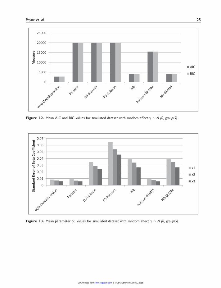
The figures in Appendix 2 correspond to those presented in the main paper, giving results formethods with larger magnitudes of overdispersion and normal predictors. A figure of AIC andBIC where two important predictors have been omitted from the model can be found inFigure 8, and the corresponding SE figure is given in Figure 9. Similar figures of AIC and BICfor the models containing larger outliers (þ150) and 40% zero outliers are given respectively inFigures 10(a) and (b), and the corresponding figures of SE can be found in Figure 11(a) and (b).Lastly, Figure 12 gives the AIC and BIC for the random effects model with larger variance, andFigure 13 shows the corresponding SE figure. The results from these additional analyses arequalitatively similar to those presented in the paper. The lowest AIC and BIC values andmoderately corrected standard errors are overall generally given by the NB-GLMM.

Appendix 2 also gives a summary of goodness-of-fit results for all covariate, outlier, and randomeffects dependent overdispersion models in Tables 6–9, respectively. The NB and NB-GLMM giveconsistently lower AIC and BIC values compared to other models. In general, the NB and NB-GLMM also give moderate SE and 95% CI coverage, the original Poisson and Poisson-GLMM givelower values, and the scale-adjusted models give mixed results.

Payne et al. 21




Figure 7. (a–d) Distributions of normal covariates and response for simulation study.

02000400060008000

100001200014000160001800020000

Mea

sure

AIC

BIC

Figure 8. Mean AIC and BIC values for simulated dataset with two important predictors omitted.

00.005

0.010.015

0.020.025

0.030.035

0.040.045

Mea

sure

x3

Figure 9. Mean parameter SE values for simulated dataset with two important predictors omitted.





0

2000

4000

6000

8000

10000

12000

14000M

easu

re

AIC

BIC

0

1000

2000

3000

4000

5000

6000

7000

Mea

sure

AIC

BIC

(a)

(b)

Figure 10. (a) Mean AIC and BIC values for simulated dataset with outliers added (+150), (b) Mean AIC and BIC


Payne et al. 23




00.010.020.030.040.050.060.070.080.09

0.1M

easu

re

x1

x2

x3

0

0.005

0.01

0.015

0.02

0.025

0.03

0.035

0.04

Stan

dard

Err

or o

f Bet

a Co

effici

ent

x1

x2

x3

(a)

(b)

Figure 11. (a) Mean parameter SE values for simulated dataset with outliers added (+150), (b) Mean parameter SE






0

0.01

0.02

0.03

0.04

0.05

0.06

0.07

Stan

dard

Err

or o

f Bet

a Co

effici

ent

x1

x2

x3

Figure 13. Mean parameter SE values for simulated dataset with random effect g � N (0, group/5).

0

5000

10000

15000

20000

25000M

easu

re

AIC

BIC

Figure 12. Mean AIC and BIC values for simulated dataset with random effect g � N (0, group/5).

Payne et al. 25




0

10

20

30

40

50

60

70

80

0 10 33 100 333 1000

Num

ber o

f Bac

teria

l Col

onie

s

Dose

Plate 1

Plate 2

Plate 3

Figure 14. Bacterial count response by dose and plate in Salmonella dataset.

Table 6. Comparison of methods for dealing with covariate dependent overdispersion using simulated data by

covariate distribution and number of omitted predictors.

Covariate No.Omitted Value Poisson DS-Poisson PS-Poisson NB Poisson-GLMM NB-GLMM

Normal 1 AIC 6273.13 6273.13 6273.13 4249.52 6113.79 4315.32

BIC 6287.86 6287.86 6287.86 4269.15 6115.30 4316.95

2 AIC 18501.66 18501.66 18501.66 5655.97 17952.10 6133.45

BIC 18511.47 18511.47 18511.47 5670.70 17953.31 6134.77

Binary 1 AIC 43306.61 43306.61 43306.61 9363.32 42845.28 9386.82

BIC 43321.34 43321.34 43321.34 9382.95 42846.79 9388.44

2 AIC 68541.13 68541.13 68541.13 9894.71 67836.79 9899.21

BIC 68550.94 68550.94 68550.94 9909.43 67838.00 9900.52

Uniform 1 AIC 10582.41 10582.41 10582.41 4166.76 10128.85 4181.82

BIC 10597.14 10597.14 10597.14 4186.39 10130.37 4183.44

2 AIC 47351.56 47351.56 47351.56 5937.99 45948.34 5955.97

BIC 47361.37 47361.37 47361.37 5952.72 45949.55 5957.30


criteria; BIC: Bayesian information criteria.





Table 7. Comparison of methods for dealing with outlier dependent overdispersion using simulated data by

covariate distribution and magnitude of outliers.

Covariate Outlier Value Poisson DS-Poisson PS-Poisson NB Poisson-GLMM NB-GLMM

Normal þ50 AIC 5153.42 5153.42 5153.42 4427.09 5156.79 4622.05

BIC 5173.05 5173.05 5173.05 4451.63 5158.60 4623.99

þ150 AIC 12055.89 12055.89 12055.89 5278.41 12051.44 6874.90

BIC 12075.52 12075.52 12075.52 5302.95 12053.26 6876.80

Binary þ50 AIC 4989.94 4989.94 4989.94 4192.88 4993.94 5313.65

BIC 5009.57 5009.57 5009.57 4217.42 4995.76 5315.47

þ150 AIC 11405.51 11405.51 11405.51 5075.12 11409.51 7613.69

BIC 11425.14 11425.14 11425.14 5099.66 11411.32 7615.51

Uniform þ50 AIC 4967.39 4967.39 4967.39 4099.04 4971.39 5306.66

BIC 4987.03 4987.03 4987.03 4123.58 4973.21 5308.47

þ150 AIC 11534.20 11534.20 11534.20 4963.86 11538.20 7610.13

BIC 11553.83 11553.83 11553.83 4988.40 11540.02 7611.94



Table 8. Comparison of methods for dealing with outlier dependent overdispersion using simulated data by

covariate distribution and percentage of excess zeros.

Covariate Outlier Value Poisson DS-Poisson PS-Poisson NB Poisson-GLMM NB-GLMM

Normal Lower % AIC 4708.91 4708.91 4708.91 3694.7 4647.39 3703.74

BIC 4728.54 4728.54 4728.54 3719.24 4649.2 3705.66

Higher % AIC 5905.90 5905.90 5905.90 3437.05 5763.10 3477.61

BIC 5925.53 5925.53 5925.53 3461.58 5764.91 3479.54

Binary Lower % AIC 3596.27 3596.27 3596.27 3477.75 3599.03 3488.81

BIC 3615.90 3615.90 3615.90 3502.29 3600.85 3490.73

Higher % AIC 3369.53 3369.53 3369.53 2886.92 3369.42 2893.47

BIC 3389.16 3389.16 3389.16 2911.46 3371.24 2895.40

Uniform Lower % AIC 3355.53 3355.53 3355.53 3278.80 3358.50 3297.99

BIC 3375.16 3375.16 3375.16 3303.34 3360.32 3299.92

Higher % AIC 3112.77 3112.77 3112.77 2739.91 3113.16 2743.07

BIC 3132.40 3132.40 3132.40 2764.44 3114.98 2744.99



Payne et al. 27




Table 9. Comparison of methods for dealing with lower random effect dependent overdispersion using simulated

data by covariate distribution and magnitude of outliers.

Covariate � Value Poisson DS-Poisson PS-Poisson NB Poisson-GLMM NB-GLMM

Normal N(0,g/10) AIC 8301.66 8301.66 8301.66 4424.69 7740.06 4418.28

BIC 8321.29 8321.29 8321.29 4449.23 7741.88 4420.39

N(0,g/5) AIC 20037.57 20037.57 20037.57 4098.81 15522.58 4044.95

BIC 20057.20 20057.20 20057.20 4123.35 15524.40 4047.06

Binary N(0,g/10) AIC 5410.88 5410.88 5410.88 4586.73 5327.46 4582.96

BIC 5430.51 5430.51 5430.51 4611.27 5329.28 4585.08

N(0,g/5) AIC 10269.75 10269.75 10269.75 5377.65 9717.36 5418.19

BIC 10289.38 10289.38 10289.38 5402.19 9719.18 5420.31

Uniform N(0,g/10) AIC 5056.44 5056.44 5056.44 4374.92 4983.67 4364.20

BIC 5076.07 5076.07 5076.07 4399.46 4985.49 4366.32

N(0,g/5) AIC 9427.43 9427.43 9427.43 5155.89 8931.69 5130.26

BIC 9447.07 9447.07 9447.07 5180.43 8933.50 5132.38






Approaches for dealing with various sources of overdispersion in modeling count data: Scale adjustment versus modeling

Documents