Approach to Fault Identification for Electronic Products Using Mahalanobis Distance

IEEE TRANSACTIONS ON INSTRUMENTATION AND MEASUREMENT, VOL. 59, NO. 8, AUGUST 2010 2055

Approach to Fault Identification for ElectronicProducts Using Mahalanobis Distance

Sachin Kumar, Member, IEEE, Tommy W. S. Chow, Senior Member, IEEE, and Michael Pecht, Fellow, IEEE

Abstract—This paper presents a Mahalanobis distance (MD)based diagnostic approach that employs a probabilistic approachto establish thresholds to classify a product as being healthyor unhealthy. A technique for detecting trends and biasness insystem health is presented by constructing a control chart forthe MD value. The performance parameters’ residuals, which arethe differences between the estimated values (from an empiricalmodel) and the observed values (from health monitoring), areused to isolate parameters that exhibit faults. To aid in the qual-ification of a product against a specific known fault, we suggestthat a fault-specific threshold MD value be defined by minimizingan error function. A case study on notebook computers is pre-sented to demonstrate the applicability of this proposed diagnosticapproach.

Index Terms—Computers, diagnostics, electronic products,fault identification, fault isolation, Mahalanobis distance (MD).

I. INTRODUCTION

QUANTIFICATION of degradation and fault progressionin an electronic system is difficult since not all faults nec-

essarily lead to system failure or functionality loss [1], [2]. Inaddition, there is a significant lack of knowledge about failureprecursors in electronics [3]. With limited failure precursorsand complex architecture, it is generally hard to implementa health-monitoring system that can directly monitor all theconditions in which fault incubation occurs.

The health of a system is a state of complete physical, struc-tural, and functional well-being and not merely conformance tothe system’s specifications. A health assessment of electronicproducts can be performed at the product level, assemblylevel, or component level [4]. The health assessment procedureshould also consider various environmental and usage condi-tions in which a product is likely to be used.

Manuscript received March 19, 2009; revised August 27, 2009; acceptedAugust 28, 2009. Date of publication October 30, 2009; date of current versionJuly 14, 2010. The Associate Editor coordinating the review process for thispaper was Dr. John Sheppard.

S. Kumar is with the Prognostics and Health Management Labora-tory, Center for Advanced Life Cycle Engineering (CALCE), Universityof Maryland, College Park, MD 20742 USA (e-mail: [email protected];[email protected]).

T. W. S. Chow is with the Prognostics and Health Management Centre, De-partment of Electronic Engineering, City University of Hong Kong, Kowloon,Hong Kong.

M. Pecht is with the Prognostics and Health Management Laboratory,CALCE, University of Maryland, College Park, MD 20742 USA, and also withthe Prognostics and Health Management Center, City University of Hong Kong,Kowloon, Hong Kong (e-mail: [email protected]).

Color versions of one or more of the figures in this paper are available onlineat http://ieeexplore.ieee.org.

Digital Object Identifier 10.1109/TIM.2009.2032884

The built-in test (BIT) and self-test abilities in a systemwere early attempts at providing diagnostic capabilities incor-porated into a system’s own structure. Gao and Suryavanshihave catalogued applications of BITs in many industries, in-cluding semiconductor production, manufacturing, aerospace,and transportation [5]. BIT system applicability is limited tothe failure definition embedded at the system’s manufactur-ing stage, whereas, with developments in sensor and dataanalysis capabilities, the development and implementation ofdata-driven diagnostic systems that can adapt to new failuredefinitions are now possible.

Today, a product’s health can be assessed in many ways,including monitoring changes in its performance parameters,which are used to characterize a system’s performance; moni-toring canaries (structures that have equivalent circuitry but arecalibrated to fail at a faster rate than the actual product); andestimating accumulated damage based on physics-of-failuremodeling [6]. Performance parameter analysis uncovers theinteractions between performance parameters and the influenceof environmental and operational conditions on these param-eters. In the absence of fault-indicating parameters, healthassessment can be performed by combining 1) damage estimateinformation obtained from physics-based models that utilizedata from environmental and operating conditions and 2) failureprecursor information extracted from data-driven models [7]. Aproduct’s historical data on intermittent failures (i.e., failuresthat cannot be reproduced in a laboratory environment [8])should be included in a product’s health assessment.

Sun Microsystems developed the Continuous SystemTelemetry Harness for collecting, conditioning, synchronizing,and storing computer systems’ telemetry signals [9]. The Mul-tivariate State Estimation Technique (MSET) provides an esti-mate of each parameter, and these estimates are later used fordecision making using the Sequential Probability Ratio Test andhypothesis testing. The Mahalanobis Distance (MD) approachconsidered in this paper is a distance measure in multidimen-sional space that considers correlations among parameters [10].The use of the MD approach over the MSET will reduce theanalytical burden, because the MD approach provides a numberfor determining a system’s health after combining informationon all performance parameters, whereas MSET provides anestimate for each parameter and needs analytical assessment ofeach parameter for determining a system’s health.

Other distance-based approaches that have been used fordiagnostics and classification include Manhattan distance,Euclidean distance, Hamming distance, Hotelling T-square, andsquare prediction error. Manhattan distance is the distancebetween two points measured along axes at right angles. It

0018-9456/$26.00 © 2009 IEEE

2056 IEEE TRANSACTIONS ON INSTRUMENTATION AND MEASUREMENT, VOL. 59, NO. 8, AUGUST 2010

has been used to classify text via the N-gram approach [11].Euclidean distance is the straight-line distance between twopoints and can be calculated as the sum of the squares of thedifferences between two points. The Hotelling T-square andsquare prediction error are used in principal component analysisfor representing statistical indices [12]. The Hotelling T-squareis a measure that accounts for the covariance structure of amultivariate normal distribution and is computed in reducedmodel space, which is defined by a few principal components(i.e., the number of principal components used is less than thenumber of original parameters) [13]. The squared predictionerror index is a measure computed in the residual space thatis not explained by the model space [14].

The Manhattan distance, Euclidean distance, and Hammingdistance do not use correlation among parameters and sufferfrom a scaling effect, in contrast to MD. The scaling effectdescribes a situation where the variability of one parametermasks the variability of another parameter, and it happenswhen the measurement ranges or scales of two parameters aredifferent [15]. To remove the scaling effect (i.e., eliminate theinfluence of measurement units), the data should be normalized.The Hotelling T-square and the square prediction error indicesare calculated in reduced dimensions (i.e., information loss)and use covariance as opposed to a correlation matrix, whichis one reason to consider using MD for fault diagnosis. MDcalculation uses the normalized values of measured parame-ters, which eliminates the problem of scaling. MD also usescorrelation among parameters, which makes it sensitive tointerparameter “health” changes. For example, consider a setof multiparameter points that are equidistant (i.e., estimated bythe Euclidean distance) from a sphere around a location. Thislocation is defined by the arithmetic mean of those points inmultidimension space. The MD stretches this sphere to evenoff the respective scales of the different dimensions and accountfor the correlation among the parameters.

The performance data of some electronic systems are multi-dimensional, such as multifunctional radio-frequency commu-nication devices, infrared imaging cameras, and hybrid siliconcomplementary metal–oxide–semiconductor (CMOS) circuits[16]. While a high-dimensional data set contains much valuableinformation, 1-D measures are easier to comprehend and can becomputed in quick succession.

Consideration of correlations among performance parame-ters is advantageous because an electronic product experiencesdiverse environmental and uses conditions. For example, thecapacitance and insulation resistance of a capacitor vary withchanges in ambient temperature. The effectiveness of a di-agnostic procedure increases by incorporating the change inrelationship among performance parameters. This is becauseeach performance parameter changes at a different rate withchanges in ambient conditions.

In an MD-based diagnostic approach, a healthy baseline anda threshold MD value are needed to classify a product as healthyor unhealthy. In the MD-based diagnostic approach, traditionalmethods for defining a threshold MD value are either basedon personal judgment or traded off to lower the economicconsequences of misclassifications, or an MD value that cor-responds to a known abnormal condition is given [17]–[20].

These traditional methods do not provide a generic frameworkfor defining a threshold MD value for fault identification. Theproposed diagnostic method does not require the definition of afaulty product during training and fault isolation, unlike othermethods such as clustering and supervised neural networks thatrequire a priori knowledge of the types of faults during training[21]. When unforeseen types of faults occur, supervised neuralnetworks or clustering approaches may fail to deliver a correctdecision on system health [21].

The MD approach suffers from the masking effect if thetraining data contain a significant amount of outliers [22]. Thisis because MD uses a sample mean and a correlation matrixthat can be influenced by a cluster of outliers. These outlierscan shift the sample mean and inflate the correlation matrix ina covariate direction. This is particularly true if the n/p ratiois small, where n is the number of observations and p is thenumber of features. Another issue is related to the computationtime needed to reach O(p2) for the p-dimensionality of featurevectors [23].

This paper provides a probabilistic approach for definingwarning and fault threshold MD values to improve upon thetraditional approaches where threshold MD values are decidedby experts. Since MD values do not follow any distribution andhave positive values, a Box–Cox transformation was appliedto the MD values to obtain a normally distributed transformedvariable. The transformed variable was used to construct acontrol chart and define threshold values to detect faults. Anoptimized MD value, using an error function, was obtained toqualify a product against a particular fault. The residual, whichis the difference between a parameter’s estimated and observedvalues, was calculated to isolate faulty parameters. A product’shealth was classified by comparing its MD value, which wascomputed for each observation, with a threshold MD value.

A. Mahalanobis Distance

The MD methodology distinguishes multivariable datagroups by a univariate distance measure, that is calculated fromthe measurements of multiple parameters. The MD value iscalculated using the normalized value of performance param-eters and their correlation coefficients, which is the reason forMD’s sensitivity [10].

A data set formed by measuring the performance parametersof a healthy product is used as training (or baseline) data. Thecollection of MD values for a healthy system is known asthe Mahalanobis space (MS). The performance parameters col-lected from a product are denoted as Xi, where i = 1, 2, . . . , p.Here, p is the total number of performance parameters. Theobservation of the ith parameter, on the jth instance, is denotedby Xij , where i = 1, 2, . . . , p, and j = 1, 2, . . . ,m; m is thetotal number of times an observation is made for all parameters.Thus, the (p × 1) data vector for the normal group is denotedby Xj , where j = 1, 2, . . . ,m. Each individual parameter inthe data vector is normalized using the mean and the standarddeviation of that parameter calculated from the baseline data.Thus, a parameter’s normalized values are

Zij =(Xij−Xi)

Si, i=1, 2, . . . , p; j =1, 2, . . . ,m (1)

KUMAR et al.: APPROACH TO FAULT IDENTIFICATION FOR ELECTRONIC PRODUCTS USING MD 2057

Fig. 1. Fault detection approach.

where

Xi =1m

m∑j=1

Xij Si =

√√√√√m∑

j=1

(Xij − Xi)2

(m − 1). (2)

Next, the values of the MDs are calculated for a healthyproduct

MDj =1pzTj C−1zj (3)

where zTj = [z1j , z2j , . . . , zpj ] is a vector comprising zij ; zj

is the transpose of zTj ; and C is the correlation matrix calcu-

lated as

C =1

(m − 1)

m∑j=1

zjzTj . (4)

For fault diagnosis, Betta and Pietrosanto [24] presented therequirements, including system monitoring; establishment of asuitable threshold; and estimation of residuals, which can beobtained by continuous comparison of the system under analy-sis with another system or by taking the differences betweenthe measured and expected quantities. The following sectionillustrates an MD-based diagnostic approach that meets theserequirements, including the creation of a healthy baseline frommeasured data, an approach for defining a threshold for faultdetection, and a residual-based approach for identifying faultyparameters.

II. DIAGNOSTIC APPROACH

Our anomaly detection approach (Fig. 1) starts with per-formance parameter monitoring. For a test product, the MDvalue for each observation is calculated using the performanceparameters’ mean, standard deviation, and a correlation coef-ficient matrix that is obtained from the training data (Fig. 2).The calculated MD value is then compared with a thresholdMD value τ , which is established from a baseline to classify

Fig. 2. MD calculation using test data.

Fig. 3. Baseline establishment methodology.

the product as being healthy or unhealthy. Then, if the productwere to be classified as unhealthy, further processing would beperformed to isolate the faulty parameter(s) to establish reasonsfor the fault. The process for defining the baseline and thethreshold MD values is discussed in the following sections.

A. Baseline Construction

A product’s performance range is defined by measurementsmade of its performance parameters under different operatingconditions. The combination of performance parameters can besummarized by a distance measure. A baseline consists of anMD profile, a threshold MD value, and the empirical models ofperformance parameters. The process of constructing a baselineis shown in Fig. 3.

The baseline construction process starts with the functionalevaluation of a product. Based on a failure modes, mechanisms,and effects analysis (FMMEA) of a product, parameters thatrepresent product performance should be selected for monitor-ing [1]. These parameters are monitored during the operationof a set of healthy products under various environmental, op-erational, and usage conditions. The collected information onparameters forms a data set that is used to train and calculatethe statistical features of each parameter. For MD calculation,performance parameter data are normalized, and a correlationcoefficient matrix is formed. The correlation coefficient be-tween two parameters expresses the linear dependence of oneparameter on the other and the direction of the dependence. TheMD values corresponding to each observation in the trainingdata are calculated, and this group of MD values forms the MS.From the MS, the min-max range, mean, and standard deviation


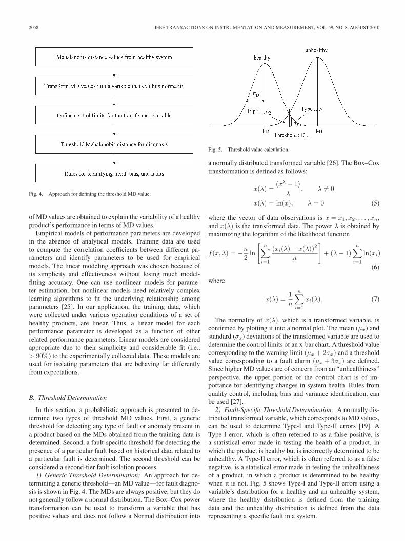
Fig. 4. Approach for defining the threshold MD value.

of MD values are obtained to explain the variability of a healthyproduct’s performance in terms of MD values.

Empirical models of performance parameters are developedin the absence of analytical models. Training data are usedto compute the correlation coefficients between different pa-rameters and identify parameters to be used for empiricalmodels. The linear modeling approach was chosen because ofits simplicity and effectiveness without losing much model-fitting accuracy. One can use nonlinear models for parame-ter estimation, but nonlinear models need relatively complexlearning algorithms to fit the underlying relationship amongparameters [25]. In our application, the training data, whichwere collected under various operation conditions of a set ofhealthy products, are linear. Thus, a linear model for eachperformance parameter is developed as a function of otherrelated performance parameters. Linear models are consideredappropriate due to their simplicity and considerable fit (i.e.,> 90%) to the experimentally collected data. These models areused for isolating parameters that are behaving far differentlyfrom expectations.

B. Threshold Determination

In this section, a probabilistic approach is presented to de-termine two types of threshold MD values. First, a genericthreshold for detecting any type of fault or anomaly present ina product based on the MDs obtained from the training data isdetermined. Second, a fault-specific threshold for detecting thepresence of a particular fault based on historical data related toa particular fault is determined. The second threshold can beconsidered a second-tier fault isolation process.

1) Generic Threshold Determination: An approach for de-termining a generic threshold—an MD value—for fault diagno-sis is shown in Fig. 4. The MDs are always positive, but they donot generally follow a normal distribution. The Box–Cox powertransformation can be used to transform a variable that haspositive values and does not follow a Normal distribution into

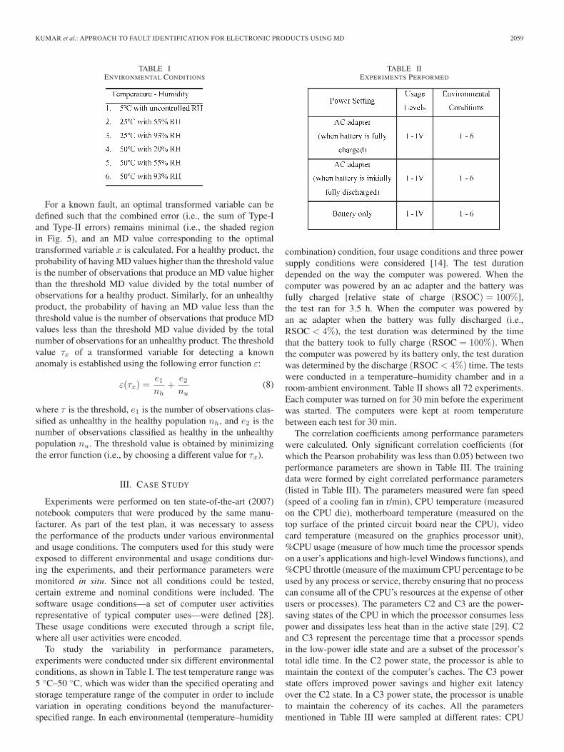
Fig. 5. Threshold value calculation.

a normally distributed transformed variable [26]. The Box–Coxtransformation is defined as follows:

x(λ) =(xλ − 1)

λ, λ �= 0

x(λ) = ln(x), λ = 0 (5)

where the vector of data observations is x = x1, x2, . . . , xn,and x(λ) is the transformed data. The power λ is obtained bymaximizing the logarithm of the likelihood function

f(x, λ) = −n

2ln

[n∑

i=1

(xi(λ) − x(λ))2

n

]+ (λ − 1)

n∑i=1

ln(xi)

(6)

where

x(λ) =1n

n∑i=1

xi(λ). (7)

The normality of x(λ), which is a transformed variable, isconfirmed by plotting it into a normal plot. The mean (μx) andstandard (σx) deviations of the transformed variable are used todetermine the control limits of an x-bar chart. A threshold valuecorresponding to the warning limit (μx + 2σx) and a thresholdvalue corresponding to a fault alarm (μx + 3σx) are defined.Since higher MD values are of concern from an “unhealthiness”perspective, the upper portion of the control chart is of im-portance for identifying changes in system health. Rules fromquality control, including bias and variance identification, canbe used [27].

2) Fault-Specific Threshold Determination: A normally dis-tributed transformed variable, which corresponds to MD values,can be used to determine Type-I and Type-II errors [19]. AType-I error, which is often referred to as a false positive, isa statistical error made in testing the health of a product, inwhich the product is healthy but is incorrectly determined to beunhealthy. A Type-II error, which is often referred to as a falsenegative, is a statistical error made in testing the unhealthinessof a product, in which a product is determined to be healthywhen it is not. Fig. 5 shows Type-I and Type-II errors using avariable’s distribution for a healthy and an unhealthy system,where the healthy distribution is defined from the trainingdata and the unhealthy distribution is defined from the datarepresenting a specific fault in a system.


TABLE IENVIRONMENTAL CONDITIONS

For a known fault, an optimal transformed variable can bedefined such that the combined error (i.e., the sum of Type-Iand Type-II errors) remains minimal (i.e., the shaded regionin Fig. 5), and an MD value corresponding to the optimaltransformed variable x is calculated. For a healthy product, theprobability of having MD values higher than the threshold valueis the number of observations that produce an MD value higherthan the threshold MD value divided by the total number ofobservations for a healthy product. Similarly, for an unhealthyproduct, the probability of having an MD value less than thethreshold value is the number of observations that produce MDvalues less than the threshold MD value divided by the totalnumber of observations for an unhealthy product. The thresholdvalue τx of a transformed variable for detecting a knownanomaly is established using the following error function ε:

ε(τx) =e1

nh+

e2

nu(8)

where τ is the threshold, e1 is the number of observations clas-sified as unhealthy in the healthy population nh, and e2 is thenumber of observations classified as healthy in the unhealthypopulation nu. The threshold value is obtained by minimizingthe error function (i.e., by choosing a different value for τx).

III. CASE STUDY

Experiments were performed on ten state-of-the-art (2007)notebook computers that were produced by the same manu-facturer. As part of the test plan, it was necessary to assessthe performance of the products under various environmentaland usage conditions. The computers used for this study wereexposed to different environmental and usage conditions dur-ing the experiments, and their performance parameters weremonitored in situ. Since not all conditions could be tested,certain extreme and nominal conditions were included. Thesoftware usage conditions—a set of computer user activitiesrepresentative of typical computer uses—were defined [28].These usage conditions were executed through a script file,where all user activities were encoded.

To study the variability in performance parameters,experiments were conducted under six different environmentalconditions, as shown in Table I. The test temperature range was5 ◦C–50 ◦C, which was wider than the specified operating andstorage temperature range of the computer in order to includevariation in operating conditions beyond the manufacturer-specified range. In each environmental (temperature–humidity

TABLE IIEXPERIMENTS PERFORMED

combination) condition, four usage conditions and three powersupply conditions were considered [14]. The test durationdepended on the way the computer was powered. When thecomputer was powered by an ac adapter and the battery wasfully charged [relative state of charge (RSOC) = 100%],the test ran for 3.5 h. When the computer was powered byan ac adapter when the battery was fully discharged (i.e.,RSOC < 4%), the test duration was determined by the timethat the battery took to fully charge (RSOC = 100%). Whenthe computer was powered by its battery only, the test durationwas determined by the discharge (RSOC < 4%) time. The testswere conducted in a temperature–humidity chamber and in aroom-ambient environment. Table II shows all 72 experiments.Each computer was turned on for 30 min before the experimentwas started. The computers were kept at room temperaturebetween each test for 30 min.

The correlation coefficients among performance parameterswere calculated. Only significant correlation coefficients (forwhich the Pearson probability was less than 0.05) between twoperformance parameters are shown in Table III. The trainingdata were formed by eight correlated performance parameters(listed in Table III). The parameters measured were fan speed(speed of a cooling fan in r/min), CPU temperature (measuredon the CPU die), motherboard temperature (measured on thetop surface of the printed circuit board near the CPU), videocard temperature (measured on the graphics processor unit),%CPU usage (measure of how much time the processor spendson a user’s applications and high-level Windows functions), and%CPU throttle (measure of the maximum CPU percentage to beused by any process or service, thereby ensuring that no processcan consume all of the CPU’s resources at the expense of otherusers or processes). The parameters C2 and C3 are the power-saving states of the CPU in which the processor consumes lesspower and dissipates less heat than in the active state [29]. C2and C3 represent the percentage time that a processor spendsin the low-power idle state and are a subset of the processor’stotal idle time. In the C2 power state, the processor is able tomaintain the context of the computer’s caches. The C3 powerstate offers improved power savings and higher exit latencyover the C2 state. In a C3 power state, the processor is unableto maintain the coherency of its caches. All the parametersmentioned in Table III were sampled at different rates: CPU


TABLE IIICORRELATION COEFFICIENTS FOR NOTEBOOK PERFORMANCE PARAMETERS

Fig. 6. Histogram of MD values for healthy population.

operation at every fifth second, and temperatures and fan speedat every 30th second.

The MD for each observation in the training data set wascalculated using (3). According to the flowchart shown inFig. 3, a healthy baseline was defined using MD values andempirical models of performance parameters. The training datawere comprised of approximately 25 000 observations. Thedistribution of these MD values corresponding to the trainingdata is shown in Fig. 6. Empirical models for each performanceparameter were developed as functions of other performanceparameters using training data. The “residuals” of each pa-rameter were calculated by subtracting the estimated valuefrom the observed value. For example, an empirical modelfor CPU temperature as a function of fan speed, motherboardtemperature, and video card temperature is

CPU Temp = −21.6 − 0.0025 ∗ Fan Speed

+ 0.44 ∗ MB Temp + 0.87 ∗ VC Temp. (9)

Fig. 7. Probability density of residual CPU temperature for a healthy product.

The residual analysis of CPU temperature indicated that aprobability density plot of CPU temperature residuals (Fig. 7)represents 94% of the variability in the CPU temperature. Theresidual analysis indicated that the mean residual for fan speedwas up to 500 r/min. Similarly, the mean residual for the CPUtemperature was 5 ◦C, and that for the motherboard and videocard temperature was 8 ◦C. Similar empirical models for otherparameters have been developed [30].

Two types of threshold MD values were determined: First,a generic threshold for detecting faults at the product levelwas developed, and second, a specific threshold for detectingthe presence of a particular fault was developed. For genericthreshold value determination, the Box–Cox transformationwas applied on the training MD values, and an optimized valueof λ(= −0.2) was obtained by maximizing the likelihood func-tion defined earlier. The plot of λ and the likelihood functionf(x, λ) is shown in Fig. 8.

The optimal λ value was used to obtain a normally distrib-uted transformed variable x from the training MD values. Thenormal probability plot of x is shown in Fig. 9. A control chartfor fault identification was developed, where control limits


Fig. 8. Plot of λ and likelihood function f(x, λ).

Fig. 9. Normal probability plot of transformed variable x.

Fig. 10. Control limits for fault identification.

were calculated using the mean and standard deviations of thetransformed variable x (Fig. 10). A warning limit and a faultlimit corresponding to μx + 2σx and μx + 3σx were defined.For fault identification, two rules were used: First, one or morepoints fall above the fault limit (i.e., μx + 3σx), and second,two (or three) out of three consecutive points are within thefault and warning limits (i.e., Zone A). From the training data,

TABLE IVPERCENTAGE OF ALARMS RAISED BY DIFFERENT RULES

only one data point fell above the fault limit, and 1.5% ofthe data fell in Zone A (i.e., above the warning limit). Thethreshold MD values corresponding to the warning limit andfault limit were 3.4 and 9.1, respectively. Quality control ruleswere applied to determine the bias and trend in the data alongwith the identification of faults [27]. Data exhibit a trend if six(or more) consecutive points are increasing or decreasing. Dataexhibit biasness if nine (or more) consecutive points fall on oneside of the central line (i.e., μx). Since MD values increase withabnormality, data that fall above the central line of the controlchart are of more concern.

A set of data obtained from one test notebook computer,which was field-returned, was plotted on the control chartconstructed for the transformed value x, and the quality controlrules were applied. The observations made (Table IV) weregiven as follows: 62.1% of the data were above the failure alarmlimit (μx + 3σx) (i.e., 62.1% of the data indicated the presenceof faults in the test system), in comparison with 0% for a healthysystem. In addition, 37.8% of the data were within Zone A (i.e.,37.8% of the data indicated the tendency of the test system to befaulty), in comparison with 1.5% for a healthy system. This alsoindicated that 99.9% of the data were above the warning limitμx + 2σx, in comparison with 1% for a healthy system. At 96%of the time, the data indicated the presence of a trend in the testsystem, in comparison to 2% for a healthy system. All test data(i.e., 100%) were on one side of the average, which indicatedthe presence of biasness in the test system, in comparison to33% for a healthy system. The marginal difference between ahealthy system and the test system, which was identified usingthe fault isolation approach, suggested that the test system hadproblems.

The MD values corresponding to the baseline (i.e., healthy)and the test computer are shown in Fig. 11. Both sets ofMD values obtained from the training and test data sets weretransformed into normally distributed variables. To detect aspecific fault, a threshold MD value corresponding to that faultwas defined using the error function approach discussed earlier.

An optimal threshold MD value τ was calculated by mini-mizing the error function [(6)]. The amount of error ε consid-ering different MD values is shown in Fig. 12. In this study,the optimal MD threshold value τ was 4.70, and the errorε(τ) was 0.025 (i.e., 2.5% misclassification, where 1.8% wascontributed by the training data and 0.7% was from the test


Fig. 11. MD value for a baseline and a test system.

Fig. 12. Optimal threshold evaluation.

Fig. 13. Robustness evaluation of the threshold value.

data). Higher misclassification of training data suggests thatthe defined threshold value was conservative in nature, becausethe healthy product was misclassified more than the unhealthyproduct.

The validity of the defined threshold value was evaluated bycalculating the misclassification of training data and test dataat various threshold values (Fig. 13). The graph in Fig. 13indicates that lowering the threshold value resulted in an in-crease in the number of observations from the training databeing classified as faulty (misclassification of healthy data asunhealthy data increased). Similarly, increasing the thresholdvalue resulted in an increase in the number of observationsbeing classified as healthy from the test data (misclassificationof unhealthy data as healthy data increased). Large-percentagechanges in misclassification were not observed, even afterchanging (increasing or decreasing) the threshold value of MDby 10%. Thus the threshold value can be considered robust.

The performance parameter residuals were used to isolate theparameters that were responsible for the drift in the health ofthe test computers. A few test data samples are presented inTable V, where the measured M and estimated E parametervalues are shown. From the residual analysis, it was observedthat the residual of the fan speed was greater than expected in90% of the instances, and in 10% of the instances, the residualof the temperature parameters was greater than expected. Thefan was judged to be faulty based on the residual analysis, andthis judgment was verified by investigation of raw data.

The case study demonstrated that the methodology presentedwas capable of identifying faults. A baseline generated fromexperimental data can be used to successfully analyze the onsetof a fault and the eventual failure of a similar computer. Thediagnostic approach can be applied to any product, but the casestudy results (and the baseline) cannot be extrapolated to allproducts and their variations. It would be expected that theproduct developers would develop baselines for their productsof interest.

IV. CONCLUSION

This paper presents a data-driven diagnostic approach thatutilizes MD. Instead of using an expert-opinion-based thresholdMD value, a probabilistic approach has been developed toestablish threshold MD values to classify a product as beinghealthy or unhealthy. An error function has been defined andminimized to determine a reference MD value to identifythe presence of a specific fault in a product. Once faults aredetected, a set of specific threshold values developed usingthe residuals of the performance parameters can be used forisolating known faults. This paper demonstrates that the distri-bution of the residuals of performance parameters can be usedto isolate parameters that exhibit faults.

This paper presents an approach for constructing an MDcontrol chart from a system’s performance data. The controlchart enables continuous monitoring of a system’s health usingthe MD value calculated from the system’s performance data.This MD control chart concept can also be used by the man-ufacturing industry for continuous process monitoring, insteadof following several performance parameter control charts.

Rules for detecting faults and observing trends and biases ina system’s performance have been presented in this paper. Theability to identify trends and biasness in the data will enablethe development of new tests to identify flawed system andprocesses. The ability to detect trends and biasness in systemhealth by observing a control chart constructed for MD valueswill allow for the detection of changes in a product’s healthbefore it experiences failure.

The case study on notebook computers demonstrates thatthe approach to define threshold MD value is a major im-provement. The defined thresholds were able to detect faultsin a product with 99% accuracy. In a known fault condition, aspecific threshold was defined, which classified a product with97.5% accuracy (i.e., 2.5% error). The residual analysis of theperformance parameters identified the fan as a problem 90% ofthe time. The temperature parameters that are correlated to thefan operation were identified as a problem 10% of the time. The


TABLE VESTIMATED VALUES OF THE PARAMETERS

results demonstrated that the suggested approach for defininga threshold MD value for the diagnostic approach was able toidentify faults. The residual-based parameter isolation approachidentified the cause of the problem.

MD is a good health measure that summarizes multiplemonitored parameters that are correlated. With the modifica-tions presented in this paper, MD will benefit manufacturers incontrolling the quality of their products and processes online oroffline.

ACKNOWLEDGMENT

The members of the Prognostics and Health ManagementConsortium, CALCE, University of Maryland, College Parkand The Prognostics and Health Management Center at CityUniversity of Hong Kong supported this work. I would like tothank M. Zimmerman of CALCE for copyediting this paper.

REFERENCES

[1] M. Pecht, Prognostics and Health Management of Electronics.New York: Wiley-Interscience, 2008.

[2] N. Vichare and M. Pecht, “Prognostics and health management of elec-tronics,” IEEE Trans. Compon. Packag. Technol., vol. 29, no. 1, pp. 222–229, Mar. 2006.

[3] K. Janasak and R. Beshears, “Diagnostics to prognostics—A productavailability technology evolution,” in Proc. Annu. RAMS, Jan. 2007,pp. 113–118.

[4] J. Gu, N. Vichare, T. Tracy, and M. Pecht, “Prognostics implementationmethods for electronics,” in Proc. Annu. RAMS, Jan. 2007, pp. 101–106.

[5] R. X. Gao and A. Suryavanshi, “BIT for intelligent system design and con-dition monitoring,” IEEE Trans. Instrum. Meas., vol. 51, no. 5, pp. 1061–1067, Oct. 2002.

[6] Z. Liu, D. S. Forsyth, J. P. Komorowski, K. Hanasaki, and T. Kirubarajan,“Survey: State of the art in NDE data fusion techniques,” IEEE Trans.Instrum. Meas., vol. 56, no. 6, pp. 2435–2451, Dec. 2007.

[7] M. Baybutt, C. Minnella, A. E. Ginart, P. W. Kalgren, and M. J. Roemer,“Improving digital system diagnostics through Prognostic and HealthManagement (PHM) technology,” IEEE Trans. Instrum. Meas., vol. 58,no. 2, pp. 255–262, Feb. 2009.

[8] D. Thomas, K. Ayers, and M. Pecht, “The ‘trouble not identified’ phenom-enon in automotive electronics,” Microelectron. Reliab., vol. 42, no. 4/5,pp. 641–651, Apr./May 2002.

[9] K. C. Gross, K. W. Whisnant, and A. Urmanov, “Electronic prognos-tics through continuous system telemetry,” in Proc. 60th Soc. Mach.Failure Prevention Technol. Meeting, Virginia Beach, VA, Apr. 2006,pp. 53–62.

[10] G. Taguchi, S. Chowdhury, and Y. Wu, The Mahalanobis-Taguchi System.New York: McGraw-Hill, 2001.

[11] L. Khreisat, “A machine learning approach for Arabic text classificationusing N-gram frequency statistics,” J. Informetr., vol. 3, no. 1, pp. 72–77,Jan. 2009.

[12] S. Bouhouche, M. Lahreche, A. Moussaoui, and J. Bast, “Quality moni-toring using principal component analysis and fuzzy logic application incontinuous casting process,” Amer. J. Appl. Sci., vol. 4, no. 9, pp. 637–644,2007.

[13] K. Choi, S. Singh, A. Kodali, K. R. Pattipati, J. W. Sheppard,S. M. Namburu, S. Chigusa, D. V. Prokhorov, and L. Qiao, “Novel clas-sifier fusion approaches for fault diagnosis in automotive systems,” IEEETrans. Instrum. Meas., vol. 58, no. 3, pp. 602–611, Mar. 2009.

[14] S. Kumar, V. Sotiris, and M. Pecht, “Health assessment of electronicproducts using Mahalanobis distance and projection pursuit analy-sis,” Int. J. Comput. Inf. Syst. Sci. Eng., vol. 2, no. 4, pp. 242–250,Fall 2008.

[15] G. Blöschl, “Scaling issues in snow hydrology,” Hydrol. Process., vol. 13,no. 14/15, pp. 2149–2175, 1999.

[16] J. Ahn, H. Kim, K. J. Lee, S. Jeon, S. J. Kang, Y. Sun, R. G. Nuzzo,and J. A. Rogers, “Heterogeneous three-dimensional electronics by useof printed semiconductor nanomaterials,” Science, vol. 314, no. 5806,pp. 1754–1757, Dec. 2006.

[17] T. Riho, A. Suzuki, J. Oro, K. Ohmi, and H. Tanaka, “The yield enhance-ment methodology for invisible defects using the MTS + method,” IEEETrans. Semicond. Manuf., vol. 18, no. 4, pp. 561–568, Nov. 2005.

[18] L. Abdesselam and C. Guy, “Time-frequency classification applied toinduction machine faults monitoring,” in Proc. 32nd IEEE IECON,Nov. 2006, pp. 5051–5056.

[19] O. Schabenberger and F. J. Pierce, Contemporary Statistical Models forthe Plant and Soil Sciences, 1st ed. Boca Raton, FL: CRC Press, 2001.

[20] S.-K. Si, X.-F. Wang, and X.-J. Sun, “Discrimination methods for theclassification of breast cancer diagnosis,” in Proc. ICNN, B, Oct. 2005,vol. 1, pp. 259–261.

[21] S. Wu and T. Chow, “Induction machine fault detection using SOM-basedRBF neural networks,” IEEE Trans. Ind. Electron., vol. 51, no. 1, pp. 183–194, Feb. 2004.

[22] P. J. Rousseeuw and B. C. van Zomeren, “Unmasking multivariate outliersand leverage points,” J. Amer. Stat. Assoc., vol. 85, no. 411, pp. 633–639,Sep. 1990.

[23] F. Sun, S. Omachi, N. Kato, H. Aso, S. Kono, and T. Takagi, “Two-stagecomputational cost reduction algorithm based on Mahalanobis distanceapproximations,” in Proc. 15th Int. Conf. Pattern Recog., Sep. 2000,vol. 2, pp. 696–699.

[24] G. Betta and A. Pietrosanto, “Instrument fault detection and isolation:State of the art and new research trends,” IEEE Trans. Instrum. Meas.,vol. 49, no. 1, pp. 100–107, Feb. 2000.

[25] T. Mitchell, Machine Learning, 1st ed. New York: McGraw-Hill, 1997.[26] G. Box and D. Cox, “An analysis of transformations,” J. R. Stat. Soc., Ser.

B Stat. Methodol., vol. 26, no. 2, pp. 211–252, 1964.[27] L. S. Nelson, “Technical aids,” J. Qual. Technol., vol. 16, no. 4, pp. 238–

239, Oct. 1984.


[28] J. C. Day, A. Janus, and J. Davis, “Computer and Internet use in the UnitedStates: 2003,” U.S. Bureau Labor Stat., Washington, DC, Oct. 2005.

[29] Hewlett-Packard, Intel, Microsoft, Phoenix, and Toshiba, Revision 3.0a,Last accessed on May 29, 2009, Advanced Configuration and PowerInterface Specification, Dec. 30, 2005. [Online]. Available: http://www.acpi.info/DOWNLOADS/ACPIspec30a.pdf

[30] S. Kumar and M. Pecht, “Baseline performance of notebook computerunder various environmental and usage conditions for prognostics,” IEEETrans. Compon. Packag. Technol., vol. 32, no. 3, pp. 667–676, Sep. 2009,Manuscript ID: TCPT-2008-024.R2.

Sachin Kumar (M’07) received the B.S. degreein metallurgical engineering from Bihar Institute ofTechnology, Sindri, India, and the M.Tech. degree inreliability engineering from Indian Institute of Tech-nology, Kharagpur, India. He is currently workingtoward the Ph.D. degree in reliability engineeringwith the Prognostics and Health Management Labo-ratory, Center for Advanced Life Cycle Engineering(CALCE), University of Maryland, College Park.

His research interests include reliability evalua-tion and prediction, model and algorithm develop-

ment for diagnostics and prognostics, electronic system health management,Bayesian methodology, statistical modeling, data mining, machine learning,and artificial intelligence.

Tommy W. S. Chow (M’93–SM’03) received theB.Sc. (first honors) and Ph.D. degrees from the Uni-versity of Sunderland, Sunderland, U.K.

He is currently a Professor with the Prognos-tics and Health Management Centre, Departmentof Electronic Engineering, City University of HongKong, Kowloon, Hong Kong. He has been workingon different consultancy projects with the Mass Tran-sit Railway, Kowloon–Canton Railway Corporation,Hong Kong. He has also conducted other collabo-rative projects with the Kong Electric Co. Ltd., the

MTR Hong Kong, and Observatory Hong Kong on the application of neuralnetworks for machine fault detection and forecasting. He is the author orcoauthor of more than 130 journal articles related to his research, five bookchapters, and one book. His research interests include neural networks, machinelearning, pattern recognition, fault diagnosis, and bioinformatics.

Dr. Chow received the Best Paper Award in 2002 IEEE Industrial ElectronicsSociety Annual Meeting in Seville, Spain. He is the Associate Editor ofPattern Analysis and Applications, and International Journal of InformationTechnology.

Michael Pecht (F’92) received the M.S. degree inelectrical engineering and the M.S. and Ph.D. de-grees in engineering mechanics from the Universityof Wisconsin, Madison.

He is currently a Visiting Professor in electricalengineering with the City University of Hong Kong,Kowloon, Hong Kong, and the founder of the Centerfor Advanced Life Cycle Engineering (CALCE),University of Maryland, College Park, where he isalso the George Dieter Chair Professor in mechanicalengineering and a Professor in applied mathematics.

He has been leading a research team in the area of prognostics for the pastten years. He has consulted for more than 100 major international electronicscompanies, providing expertise in strategic planning, design, test, prognostics,IP, and risk assessment of electronic products and systems. He has writtenmore than 20 books on electronic product development, use, and supply chainmanagement, and more than 400 technical papers. He is a Chief Editor forMicroelectronics Reliability.

Dr. Pecht is a Fellow of the American Society of Mechanical Engi-neers and the International Microelectronics and Packaging Society (IMAPS).He is a Professional Engineer. He served as Chief Editor for the IEEETRANSACTIONS ON RELIABILITY for eight years and on the advisory boardof IEEE SPECTRUM. He is an Associate Editor for the IEEE TRANSACTIONS

ON COMPONENTS AND PACKAGING TECHNOLOGY. He was the recipientof the highest reliability honor, i.e., the IEEE Reliability Society’s LifetimeAchievement Award in 2008; the European Micro and Nano-Reliability Awardfor outstanding contributions to reliability research; 3M Research Award forelectronics packaging; and the IMAPS William D. Ashman Memorial Achieve-ment Award for his contributions in electronic reliability analysis.

Approach to Fault Identification for Electronic Products Using Mahalanobis Distance

Documents