Appraising stone column settlement prediction methods using finite element analyses

RESEARCH PAPER

Appraising stone column settlement prediction methodsusing finite element analyses

Brian G. Sexton • Bryan A. McCabe •

Jorge Castro

Received: 23 August 2012 / Accepted: 31 May 2013 / Published online: 26 September 2013

� Springer-Verlag Berlin Heidelberg 2013

Abstract Numerous approaches exist for the prediction

of the settlement improvement offered by the vibro-

replacement technique in weak or marginal soil deposits.

The majority of the settlement prediction methods are

based on the unit cell assumption, with a small number

based on plane strain or homogenisation techniques. In this

paper, a comprehensive review and assessment of the more

popular settlement prediction methods is carried out with a

view to establishing which method(s) is/are in best agree-

ment with finite element predictions from a series of

PLAXIS 2D axisymmetric analyses on an end-bearing

column. The Hardening Soil Model in PLAXIS 2D has

been used to model the behaviour of both the granular

column material and the treated soft clay soil. This study

has shown that purely elastic settlement prediction methods

overestimate the settlement improvement for large modular

ratios, while the methods based on elastic–plastic theory

are in better agreement with finite element predictions at

higher modular ratios. In addition, a parameter sensitivity

study has been carried out to establish the influence of a

range of different design parameters on predictions

obtained using a selection of elastic–plastic methods.

Keywords Analytical design methods � Finite element

analyses � Stone columns � Settlement improvement factor

1 Introduction

The potential of vibro-replacement stone columns to

reduce settlement [41], improve bearing capacity [5],

accelerate consolidation [26], and reduce liquefaction

potential [35] in soft soils is now widely appreciated in

geotechnical engineering practice. The vibro-replacement

technique and associated equipment have been described in

detail by Slocombe et al. [37] and Sondermann and Wehr

[38]. Settlement performance tends to be the governing

design criterion in these soils, and most analytical design

methods provide a direct prediction of a settlement

improvement factor, n, defined as the settlement of

untreated ground (s0) divided by the settlement of the

ground treated with granular columns (st), see Eq. 1.

n ¼ s0

st

ð1Þ

This settlement improvement factor can then be used to

predict the settlement of treated ground (st = s0/n). The

value of s0 (for a scenario in which the loading extends over a

wide area) is usually calculated from elastic theory (Eq. 2),

where pa is the applied pressure, H is the thickness of the

treated soil layer, and Eoed is the oedometric soil modulus.

s0 ¼paH

Eoed

ð2Þ

Analytical design methods typically relate n to the area-

replacement ratio, Ac/A (where A is the cross-sectional area

of a unit cell treated with a single stone column of cross-

sectional area, Ac, see Fig. 1). The area-replacement ratio is

a measure of the amount of in situ soil replaced with stone

B. G. Sexton � B. A. McCabe (&)

College of Engineering and Informatics, National University

of Ireland, Galway, Ireland

e-mail: [email protected]

B. G. Sexton


J. Castro

Department of Ground Engineering and Materials Science,

University of Cantabria, Santander, Spain


123

Acta Geotechnica (2014) 9:993–1011

DOI 10.1007/s11440-013-0260-5

and is dependent on the column spacing, s and column

diameter, Dc (Eq. 3), where k is a constant depending on

the column arrangement.

A

Ac

¼ ks

Dc

� �2

ð3Þ

A number of other influential variables have been con-

sidered in analytical formulations, and these include the

effect of installation, load level, modular ratio and the fric-

tion and dilatancy angles of the column material. The pub-

lished solutions account for these variables in different ways,

although few capture all of them. The aim of this study is to

provide a systematic review of these methods before using a

2D/axisymmetric finite element (FE) parametric study to

appraise the ability of these methods to cater for the variables

identified above. The axisymmetric analyses are carried out

using the PLAXIS 2D (Brinkgreve et al. [9]) Hardening Soil

(HS) Model to model an infinite grid of columns installed in

a soft soil profile. It should be noted that the majority of the

analytical methods discussed here only consider potential

improvement to primary (consolidation) settlements. Sexton

and McCabe [36] have used finite element analyses to con-

sider the improvement to creep settlements, which are highly

relevant in organic soils.

2 Vibro-replacement settlement prediction methods

2.1 Theoretical considerations in vibro-replacement

design

Analytical settlement design approaches tend to be either

elastic (e.g. [1, 3, 7, 19]) or elastic–plastic (e.g. [4, 8, 10,

16, 29–32, 40]), with yielding of the column material

considered in the latter case. The elastic–plastic methods

are typically based on the Mohr–Coulomb failure criterion,

with some assuming that the granular material deforms at

constant volume as it yields (dilatancy angle, w = 0�),

while others have accounted for dilation of the granular

column material at yield using a constant dilatancy angle.

A selection of settlement design methods and their inherent

assumptions have been summarised in Table 1.

Balaam and Booker [4] and Pulko and Majes [31] have

highlighted that elastic–plastic methods are preferable to

purely elastic methods because the elastic methods tend to

overpredict the settlement improvement offered by column

installation, especially for high modular ratios (Ec/Es,

where Ec is the modulus of the column and Es is the

modulus of the soil). This over-prediction is as a result of

the fact that elastic methods overpredict the stress con-

centration factor (SCF = rc/rs, where rc is the stress in the

column and rs is the stress in the soil).

Approaches to modelling the behaviour of the column–soil

system vary; some, such as Han and Ye [19] have accounted

only for vertical deformation, while others have accounted for

both radial and vertical deformation. For elastic methods that

consider vertical deformation only, the SCF is equal to the

ratio of the oedometric moduli of the column and soil mate-

rials. Elastic solutions that consider both radial and vertical

deformation result in slightly lower SCFs (lateral deformation

reduces SCFs, e.g., Balaam and Booker [3]). However, these

SCFs will still be overpredicted because yielding of the col-

umn material is not considered (column yielding and plastic

strains will reduce SCFs). Barksdale and Bachus [5] have

suggested that SCFs in practice range from 3 to 10 depending

on the column spacing adopted in the field.

Fig. 1 Typical column grids encountered in practice; a triangular b square c hexagonal

994 Acta Geotechnica (2014) 9:993–1011

123

Ta

ble

1S

ettl

emen

td

esig

nm

eth

od

san

das

sum

pti

on

s

Set

tlem

ent

pre

dic

tion

met

hod

Ela

stic

(E)/

elas

tic–

pla

stic

(EP

)

Unit

cell

(UC

)/

Pla

ne

stra

in

(PS

)/

hom

ogen

isat

ion

(H)

Dra

ined

(D)/

undra

ined

?co

nso

lidat

ion

(U?

C)

Equal

ver

tica

l

stra

in?

Dil

atan

cy

of

gra

nula

r

mat

eria

l

consi

der

ed?

End-

bea

ring

colu

mns?

Shea

r

stre

sses

at

colu

mn–

soil

inte

rfac

e

(sin

t)?

Rad

ial

def

orm

atio

n

consi

der

ed?

Inst

alla

tion?

Inco

m-

pre

ssib

le

colu

mn?

Imm

edia

te

sett

lem

ent

giv

enby

met

hod?

Mohr–

Coulo

mb

(MC

)

fail

ure

crit

erio

n?

Iter

ativ

e

(I)/

close

d-

form

(CF

)?

Note

s

Abosh

iet

al.

[1]

EU

CD

/U?

C4

–4

s int

=0

Yes

–7

–C

F‘E

quil

ibri

um

met

hod’

Bal

aam

and

Booker

[3]

EU

CD

4–

4s i

nt

=0

Yes

–4

–C

F

Bau

man

nan

d

Bau

er[7

]

EU

CU

?C

4–

4s i

nt

=0

Yes

K0\

K\

Kp

4–

CF

Han

and

Ye

[19

]E

UC

U?

C4

–4

s int

=0

No

–7

–C

F

Bal

aam

and

Booker

[4]

EP

UC

D4

Const

antw

4s i

nt

=0

Yes

Input

K4

4I

*Im

med

iate

sett

lem

ent

neg

ligib

le

com

par

edto

the

tota

lfi

nal

sett

lem

ent

*It

erat

ive

appro

ach

requir

ing

num

eric

al

imple

men

tati

on

to

obta

ina

solu

tion

Pulk

oan

dM

ajes

[31]

EP

UC

D4

Const

antw

4s i

nt

=0

Yes

Input

K7

4C

F

Pulk

oet

al.

[32]

EP

UC

D4

Const

antw

4s i

nt

=0

Yes

Input

K7

4C

F

Pri

ebe

[29

]E

PU

CD

4w

=0

�4

s int

=0

Yes

K=

14

74

CF

Pri

ebe

[30

]E

PU

CD

4w

=0

�4

s int

=0

Yes

Input

K7

4C

F

Cas

tro

and

Sag

aset

a[1

0]

EP

UC

U?

C4

Const

antw

4s i

nt

=0

Yes

Input

K4

4C

F

Goughnour

and

Bay

uk

[16

,

17]

EP

UC

U?

C4

No

4s i

nt

=0

Yes

K0\

K\

1/

K0

47

4C

F‘I

ncr

emen

tal

met

hod’

Borg

eset

al.

[8]

EP

UC

U?

C*

4N

o(F

E

Bas

is)

4P

erfe

ct

bondin

g

from

soil

to

colu

mn

Yes

K=

0.7

74

CF

Fin

ite

elem

ent

(FE

)

bas

is

*N

um

eric

alan

alysi

s

isbas

edon

an

U?

Cap

pro

ach

but

des

ign

equat

ion

is

appli

cable

for

dra

ined

condit

ions

also

Van

Impe

and

De

Bee

r[3

9]

EP

PS

D/U

?C

4w

=0

�4

s int

=0

Yes

–7

4I

Acta Geotechnica (2014) 9:993–1011 995

123

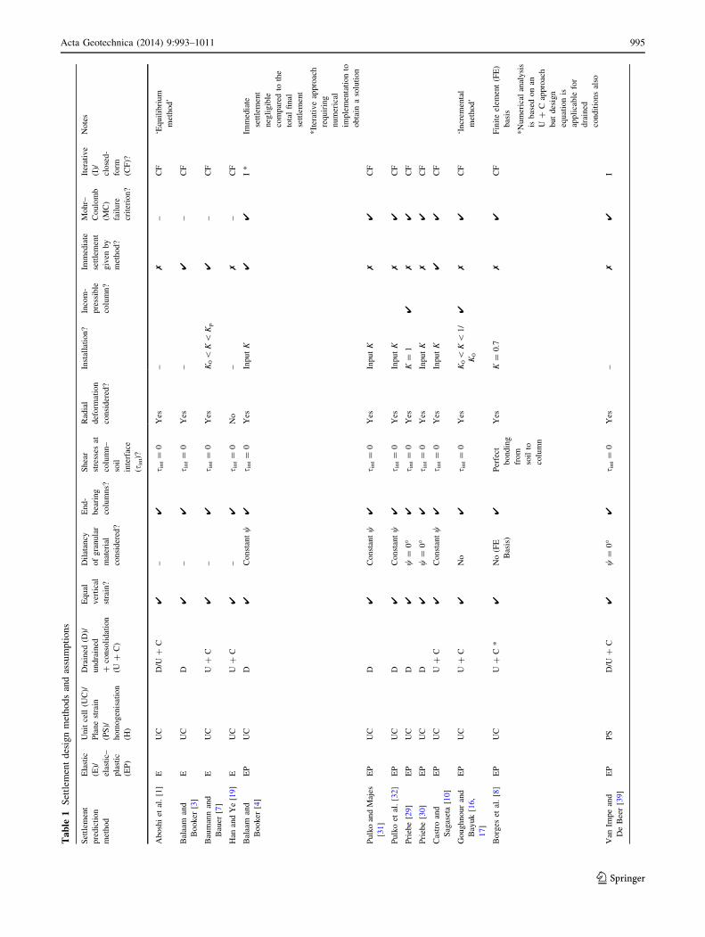
The densification effect resulting from column instal-

lation and subsequent bulging has been accounted for in

different ways. Priebe [29] has assumed an increase in the

coefficient of lateral earth pressure following column

installation to the liquid earth pressure of the soil (K = 1).

Other methods allow for the input of different values

depending on the designer’s discretion: Baumann and

Bauer [7] have limited allowable K values to the range

K0 \ K \ 1/K0; Goughnour and Bayuk [16] have limited

allowable K values to the range K0 \ K \ Kp, where K0

and Kp are the at-rest and passive earth pressure coeffi-

cients of the soil, respectively; Borges et al. [8] have for-

mulated their closed-form expression based on fitting

curves to the results of numerical analyses assuming

K = 0.7 (between the conservative, K = 1 - sin u0 for

normally consolidated soils and K = 1 approaches); Van

Impe and Madhav [40] have suggested the use of an

increased oedometric soil modulus depending on the

method of installation and the column spacing.

Solutions have been developed for drained conditions

and for undrained conditions with a follow-up consolida-

tion period to allow for the dissipation of excess pore

pressure. The undrained plus consolidation solutions (e.g.

Han and Ye [19], Castro and Sagaseta [10]) have been

based on Barron’s [6] solution for vertical drains (Barron’s

[6] solution assumes that the vertical stress on the soil is

constant during the consolidation process), but with mod-

ified coefficients of consolidation used to account for the

fact that the columns carry a considerable proportion of the

applied load (vertical drains have a much smaller stiffness

and diameter than stone columns). The Castro and Sagas-

eta [10] solution has been derived for the case of an elas-

tic–plastic column (radial deformation has been

considered), while Han and Ye [19] have based their

solution on an elastic column subjected to full lateral

confinement (i.e. no radial strain).

The Priebe [29] and Goughnour and Bayuk [16] solu-

tions are formulated on the assumption that the granular

column material is incompressible. Most neglect immedi-

ate settlement; Baumann and Bauer [7] and Balaam and

Booker [3] are notable exceptions.

2.2 Settlement prediction approaches

Greenwood [18] was the first to present a means of esti-

mating the settlement improvement achievable using the

vibro-replacement technique. Based on the column spac-

ing, the construction technique (i.e. wet/dry method), and

the undrained shear strength of the treated soil, Greenwood

[18] presented a set of empirical curves for the estimation

of the extent of settlement improvement, noting that pre-

cise mathematical solutions had not yet been developed at

the time. Similar to the analytical solutions that have beenTa

ble

1co

nti

nu

ed

Set

tlem

ent

pre

dic

tion

met

hod

Ela

stic

(E)/

elas

tic–

pla

stic

(EP

)

Unit

cell

(UC

)/

Pla

ne

stra

in

(PS

)/

hom

ogen

isat

ion

(H)

Dra

ined

(D)/

undra

ined

?co

nso

lidat

ion

(U?

C)

Equal

ver

tica

l

stra

in?

Dil

atan

cy

of

gra

nula

r

mat

eria

l

consi

der

ed?

End-

bea

ring

colu

mns?

Shea

r

stre

sses

at

colu

mn–

soil

inte

rfac

e

(sin

t)?

Rad

ial

def

orm

atio

n

consi

der

ed?

Inst

alla

tion?

Inco

m-

pre

ssib

le

colu

mn?

Imm

edia

te

sett

lem

ent

giv

enby

met

hod?

Mohr–

Coulo

mb

(MC

)

fail

ure

crit

erio

n?

Iter

ativ

e

(I)/

close

d-

form

(CF

)?

Note

s

Van

Impe

and

Mad

hav

[40]

EP

UC

D/U

?C

4Y

es(e

v,d

)4

s int

=0

Yes

Incr

ease

Eso

il7

4I

e v,d

isth

e

volu

met

ric

stra

in

due

todil

atio

n

Sch

wei

ger

and

Pan

de

[34

]

EP

HD

/U?

C4

Const

antw

7s i

nt\

s soil

Yes

–7

4I

s soil

isth

esh

ear

stre

ngth

of

the

soil

Gre

enw

ood

[18

]—

empir

ical

––

––

–4

s int

=0

––

–7

––

Em

pir

ical

curv

es


123

developed in the interim, Greenwood’s [18] curves have

been proposed for end-bearing columns neglecting imme-

diate settlements and shear displacements (as noted in

Greenwood’s original proposal).

At present, the majority of the design methods have

been derived for a unit cell representing an infinite grid of

regularly spaced end-bearing columns, e.g. [1, 3, 4, 7, 8,

10, 16, 19, 29–32, 40]. Other solutions have been devel-

oped based on plane strain (e.g. Van Impe and De Beer

[39]) or homogenisation techniques (e.g. Schweiger and

Pande [34], Lee and Pande [22]). For all three approaches,

simplifying assumptions are usually considered, e.g. the

column and the surrounding soil undergo equal vertical

settlement (referred to as the ‘equal vertical strain’

assumption) and the shear stresses at the column–soil

interface are assumed to be zero.

2.3 Plane strain/homogenisation techniques

The plane strain approach involves replacing the stone

columns with stone walls (trenches) having an ‘equivalent’

overall plan area. The homogenisation technique involves

modelling the stone column and treated soil as a composite

material with improved soil properties and is formulated

assuming that the influence of the columns is uniformly

and homogeneously distributed throughout the treated soil,

e.g. [34].

The homogenisation technique can be used in conjunc-

tion with flexible and rigid rafts (‘equal vertical stress’ and

‘equal vertical strain’ assumptions, respectively), which

makes it possible to isolate different behavioural aspects

associated with columns near the edge of a loaded area. It

can also be used to model the behaviour of floating col-

umns (the plane strain and unit cell approaches are gen-

erally based on end-bearing stone columns). However, they

can be used to model floating columns in conjunction with

FE analyses (FE solutions generally assume that there is no

slip at the column–soil interface).

2.4 Unit cell approaches

The unit cell approach is based on the assumption of a large

grid of regularly-spaced columns subjected to a uniform

load. Therefore, all of the columns will exhibit similar

behaviour and an analysis of one such column, and its

tributary soil area is sufficient. Owing to the symmetry of

the problem, the shear stresses along the perimeter of the

unit cell are assumed to be zero. The unit cell approach is

valid except for columns near the edges of the loaded area

[3, 25], which are assumed to be in the minority for large

groups.

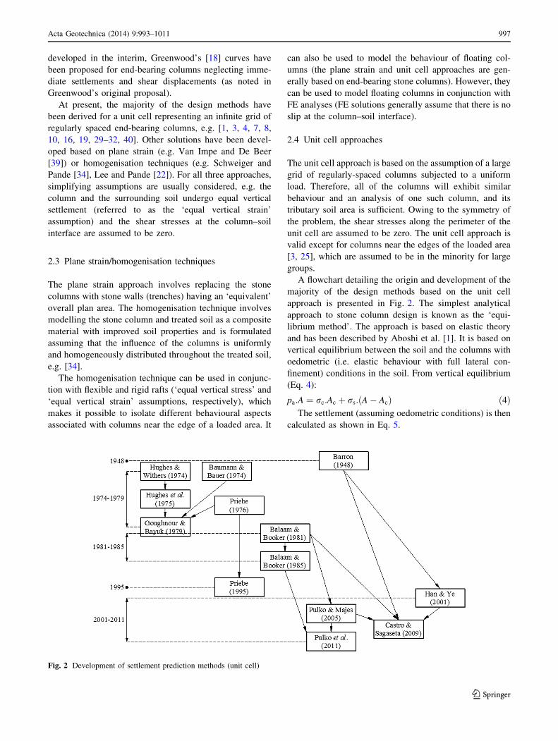
A flowchart detailing the origin and development of the

majority of the design methods based on the unit cell

approach is presented in Fig. 2. The simplest analytical

approach to stone column design is known as the ‘equi-

librium method’. The approach is based on elastic theory

and has been described by Aboshi et al. [1]. It is based on

vertical equilibrium between the soil and the columns with

oedometric (i.e. elastic behaviour with full lateral con-

finement) conditions in the soil. From vertical equilibrium

(Eq. 4):

pa:A ¼ rc:Ac þ rs:ðA� AcÞ ð4ÞThe settlement (assuming oedometric conditions) is then

calculated as shown in Eq. 5.

Fig. 2 Development of settlement prediction methods (unit cell)


123

st ¼rsH

Eoed

ð5Þ

The settlement improvement factor (n) is calculated as

s0/st (and rearranging gives the expression in Eq. 6), where

s0 = pa.H/Eoed as defined earlier. This approach

necessitates prior knowledge of the SCF (e.g. experience/

field measurements), whereas other methods such as Priebe

[29, 30] have used cylindrical cavity expansion (CCE)

theory to establish the SCF. The method by Aboshi et al.

[1] limits allowable SCFs based on the friction angles of

the soil and column materials and the undrained shear

strength of the soil.

n ¼ 1þ SCF� 1

A=Ac

ð6Þ

Balaam and Booker [3] have adopted an elastic

approach based on a unit cell of effective diameter, de,

which is dependent on the column spacing (s) and whether

the columns are arranged on either triangular (de = 1.05s),

square (de = 1.13s), or hexagonal grids (de = 1.29s).

Balaam and Booker [4] have extended the 1981 solution

using an interaction analysis to account for yield of the

granular material. The clay is assumed to behave elasti-

cally, while the stone is assumed to behave as a perfectly

elastic–plastic material (non-associative flow rule) satisfy-

ing the Mohr–Coulomb failure criterion. Elasto-plastic FE

analyses were performed to validate the assumptions

inherent in the interaction analysis. Balaam and Booker’s

[3] method can be used to obtain a closed-form analytical

solution, while Balaam and Booker’s [4] method is an

iterative approach requiring numerical implementation to

obtain a solution.

Goughnour and Bayuk [16] have formulated an elastic–

plastic method based on a unit cell of effective diameter,

de = 1.05s (triangular grid of columns). The method is

alternatively referred to as the ‘incremental method’ and is

an extension of earlier solutions developed by Baumann

and Bauer [7], Hughes et al. [20] and Priebe [29]. As

consolidation proceeds, stresses are gradually transferred

from the soil to the column. Two sets of analyses have been

performed, considering both elastic and plastic behaviour

of the column material. Firstly, an analysis is performed

assuming that the stone undergoes plastic deformation

while the surrounding soil undergoes consolidation. A

second analysis is performed assuming the stone to behave

elastically up until the end of consolidation. The vertical

strains (ev) evaluated using the two methods are compared.

The long-term vertical strain is then taken to be the larger

of the two values, and the resulting settlement, d, can be

calculated as d = ev.H, where H is the layer thickness.

Baumann and Bauer’s [7] analytical elastic approach was

developed assuming the total settlement of the loaded soil

layer to consist of the immediate settlement (no volume

change) and the consolidation settlement.

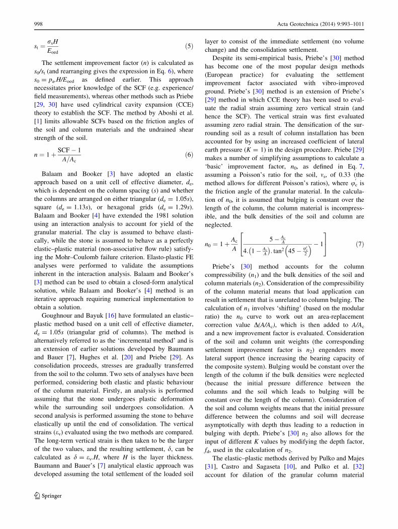
Despite its semi-empirical basis, Priebe’s [30] method

has become one of the most popular design methods

(European practice) for evaluating the settlement

improvement factor associated with vibro-improved

ground. Priebe’s [30] method is an extension of Priebe’s

[29] method in which CCE theory has been used to eval-

uate the radial strain assuming zero vertical strain (and

hence the SCF). The vertical strain was first evaluated

assuming zero radial strain. The densification of the sur-

rounding soil as a result of column installation has been

accounted for by using an increased coefficient of lateral

earth pressure (K = 1) in the design procedure. Priebe [29]

makes a number of simplifying assumptions to calculate a

‘basic’ improvement factor, n0, as defined in Eq. 7,

assuming a Poisson’s ratio for the soil, ms, of 0.33 (the

method allows for different Poisson’s ratios), where uc

0is

the friction angle of the granular material. In the calcula-

tion of n0, it is assumed that bulging is constant over the

length of the column, the column material is incompress-

ible, and the bulk densities of the soil and column are

neglected.

n0 ¼ 1þ Ac

A

5� Ac

A

4: 1� Ac

A

� �: tan2 45� u0c

2

� �� 1

24

35 ð7Þ

Priebe’s [30] method accounts for the column

compressibility (n1) and the bulk densities of the soil and

column materials (n2). Consideration of the compressibility

of the column material means that load application can

result in settlement that is unrelated to column bulging. The

calculation of n1 involves ‘shifting’ (based on the modular

ratio) the n0 curve to work out an area-replacement

correction value D(A/Ac), which is then added to A/Ac

and a new improvement factor is evaluated. Consideration

of the soil and column unit weights (the corresponding

settlement improvement factor is n2) engenders more

lateral support (hence increasing the bearing capacity of

the composite system). Bulging would be constant over the

length of the column if the bulk densities were neglected

(because the initial pressure difference between the

columns and the soil which leads to bulging will be

constant over the length of the column). Consideration of

the soil and column weights means that the initial pressure

difference between the columns and soil will decrease

asymptotically with depth thus leading to a reduction in

bulging with depth. Priebe’s [30] n2 also allows for the

input of different K values by modifying the depth factor,

fd, used in the calculation of n2.

The elastic–plastic methods derived by Pulko and Majes

[31], Castro and Sagaseta [10], and Pulko et al. [32]

account for dilation of the granular column material


123

(constant dilatancy angle, w) at yield, whereas Priebe’s

[29, 30] method assumes the granular column material to

deform at constant volume (w = 0�). Pulko and Majes [31]

and Castro and Sagaseta [10] are elastic–plastic extensions

of the earlier elastic solution developed by Balaam and

Booker [3] for drained conditions. Castro and Sagaseta [10]

have considered an undrained loading situation followed

by a consolidation process to allow for the dissipation of

excess pore pressures, whereas Pulko and Majes [31] and

Pulko et al. [32] have studied the unit cell problem under

drained conditions. As noted by Castro and Sagaseta [11],

both approaches are considered to be limiting cases of the

real situation because load application is not rapid enough

to be considered as undrained nor slow enough to be

considered as a drained process.

The method developed by Pulko et al. [32], which deals

with encased stone columns, is an extension of the previous

solution derived by Pulko and Majes [31]. The new method

by Pulko et al. [32] can also be applied to non-encased

stone columns by setting the encasement stiffness to zero.

The solutions derived by Castro and Sagaseta [10] and

Pulko and Majes [31] ignored the elastic strains in the

column during its plastic deformation, whereas the newer

solution by Pulko et al. [32] has taken them into account.

Figure 3 (from Castro and Sagaseta, [11]) shows the

different stress paths followed depending on whether the

problem is studied under drained or undrained (plus con-

solidation) conditions. For the case of an elastic column,

both approaches produce the same result. For a yielding

column (elastic–plastic case), although the stress paths are

different, the final settlements are very similar (provided

that the drained solutions account for elastic strains of the

column during its plastic deformation), as shown by Castro

and Sagaseta [11] using finite element calculations. For

drained analyses that neglect the elastic strains of the

column during its plastic deformation (e.g. Pulko and

Majes [31]), the final settlement will be underpredicted.

For undrained plus consolidation solutions (e.g. Castro and

Sagaseta [10]), neglecting the elastic strains of the column

during its plastic deformation leads to negligible error in

the solution. The newer drained solution by Pulko et al.

[32] accounts for the elastic strains of the column during its

plastic deformation. Under such conditions, the differences

between the drained and undrained plus consolidation

analyses will effectively vanish (i.e. Castro and Sagaseta

[10] and Pulko et al. [32] will produce almost identical

solutions for non-encased columns, as studied here).

The design methods derived by Castro and Sagaseta [10]

and Pulko et al. [32] have dealt with column yielding in

different ways. Castro and Sagaseta’s [10] undrained plus

consolidation formulation uses a factor Uye (elastic degree

of consolidation at the moment of column yielding) to

0

I: initialU: undrained loadingY: yieldF: final, drained

Y=F

U

I

σrc

/σzc

=Kac

K0c

1.0

Kpc

Radial stress, σrc

Ver

tical

str

ess,

σzc

(b) at yielding

FD

YC

YD

FC

U

I

σrc

/σzc

=Kac

K0c

1.0

Kpc

Radial stress, σrc

Ver

tical

str

ess,

σzc

(c) elastic-plastic case

Drained analysisConsolidation analysis

0

F

U

I

σrc

/σzc

=Kac

K0c

1.0

Kpc

Radial stress, σrc

Ver

tical

str

ess,

σzc

(a) elastic case

Fig. 3 Stress paths in the column; a elastic case b at yielding c elastic–plastic case (Castro and Sagaseta [11])


123

work out whether or not the column is in a plastic state (if

Uye [ 1, no yielding takes place, otherwise yielding of the

granular material occurs). Pulko et al. [32] have worked out

a final yield depth, zy (i.e. yielding starts at the surface and

progresses downward as the applied load increases), to

which plastic strains appear in the column.

Borges et al. [8] have proposed a design method (based on

a numerical rather than an analytical approach) relating the

settlement improvement factor (n) to the area-replacement

ratio, Ac/A, and to the ratio of the deformability of the soft

soil to the deformability of the column material (alterna-

tively referred to as the modular ratio, Ec/Es). Their resulting

design equation (and chart) is based on curve-fitting to the

results of a series of axisymmetric FE analyses of a unit cell

with a program incorporating Biot consolidation theory with

the p–q–h model (extension of the Modified Cam-Clay

(MCC) Model, based on the Drucker-Prager failure crite-

rion). In contrast to the MCC Model, the parameter

M (defining the slope of the critical state line) is not constant,

e.g., Lewis and Schrefler [24], Domingues et al. [14].

The authors have adopted a value of K = 0.7 for the

coefficient of lateral earth pressure at rest following col-

umn installation (in between K = 1 - sin u0 and K = 1).

The settlement improvement factor (Eq. 8) has been

derived based on statistical analysis techniques and has

been related to the two factors that the authors found had

the most significant influence on the results. A design chart

has been developed based on this design equation, which is

applicable for 10 B Ec/Es B 100 and 3 B A/Ac B 10, with

calculated improvement factors greater than 1.5.

n ¼ 0:125Ec

Es

þ 0:7742

� �A=Acð Þ

�0:0038EcEs�0:3423ð Þ

ð8Þ

3 Axisymmetric modelling (PLAXIS 2D)

Axisymmetric FE analyses using PLAXIS 2D (Brinkgreve

et al. [9]) have been carried out as a means of appraising the

capabilities of several of the aforementioned analytical

methods. A unit cell approach (Fig. 4) with a column radius,

Rc = 0.3 m (typical for columns at soft soil sites, e.g., Watts

et al. [41]), and a column length = 5 m has been adopted to

represent the behaviour of a single end-bearing column

within an infinite grid. Similar modelling approaches have

been adopted by Debats et al. [12] and Ambily and Gandhi

[2]. Horizontal deformation has been restricted at the sides

(roller boundaries), and both vertical and horizontal defor-

mations have been restricted at the base. The water table is

located at the surface. The columns are fully penetrating and

have been wished in place (as is common practice), e.g. Gab

et al. [15] and Killeen and McCabe [21]. For the initial study,

the coefficient of lateral earth pressure, K, is assumed to be

unaffected by column installation (K0 = 1 - sin u0 = 0.44).

A parameter sensitivity study considering different K values

has been described in Sect. 4.2.4, e.g., Priebe [29], Gough-

nour and Bayuk [17] and Gab et al. [15] have accounted for

the densification as a result of column installation by using

an increased coefficient of lateral earth pressure, K = 1 (for

the soil).

The behaviour of the composite model has been studied

under a 100 kPa load (the sensitivity study described in

Sect. 4.2.1 has also examined the behaviour of the system

under 50 and 75 kPa loads) applied through a plate element

(normal stiffness, EA = 5 9 106 kN/m, flexural rigidity,

EI = 8.5 9 103 kNm2/m, Poisson’s ratio, m = 0). The

plate element is intended to represent a rigid loading

platform to prevent differential settlements. Different series

of analyses have been carried out for different modular

ratios, Ec/Es, of 5, 10, 20, and 40 (note that good com-

parison with elastic methods necessitates the use of unre-

alistically low Ec/Es ratios). These values of Ec/Es are in

the same range as those adopted by Balaam and Booker

[3], Castro and Sagaseta [10], and Poorooshasb and Mey-

erhof [28]. In all cases, the properties of the column

material have been fixed, while the soil properties have

been varied to generate the necessary Ec/Es ratios. The

diameter of the unit cell has been altered to study the effect

of different area-replacement ratios, e.g., Domingues et al.

[14]. The column diameter has been fixed at 0.6 m (argu-

ably the column diameter in the field will be a function of

Ec/Es, but a fixed diameter has been considered here for

numerical purposes).

Load settlement behaviour (primary settlement) has

been analysed using the HS Model to model both the clay

and the stone. Both have been modelled as fully drained

materials. Similar results would be achieved modelling the

clay as an undrained material with a follow-up consolida-

tion period (analyses have been carried out in verification,

e.g., Fig. 5).

The HS Model is a hyperbolic elasto-plastic model that

accounts for increasing soil layer stiffness with stress-level

Fig. 4 Axisymmetric unit cell model (100 kPa load)


123

(no viscous effects). Its formulation has been described in

detail by Schanz et al. [33]. A friction angle (u0) of 45� has

been selected for the stone, representative of bottom feed

columns, while the dilatancy angle (w) was calculated as

w = u0 - 30�. Eoedref (oedometric modulus) was assumed

approximately equal to E50ref (secant modulus), and Eur

ref

(unload–reload modulus) was taken as 3E50ref, as recom-

mended by Brinkgreve et al. [9]. The values of Eoedref , E50

ref,

and Eurref for the stone quoted in Table 2 are based on Gab

et al. [15]. The properties have been altered using Eq. 9 to

correspond to a confining pressure of 50 kPa (closer to the

confining pressure in the subsequent numerical simula-

tions). Gab et al. [15] have defined the stiffness moduli at a

reference pressure, pref, of 100 kPa. The stress dependency

of soil stiffness is dictated by the power, m (m = 1 is

typical for soft soils [9]). For the granular column material,

a value of m = 0.3 has been used [15].

E ¼ Eref p

pref

� �m

ð9Þ

A complete list of the parameters used in the FE model

for the case when Ec/Es = 20 is given in Table 2. The

Ec/Es ratio has been defined as the ratio of the constrained/

oedometric moduli at a reference pressure of 50 kPa, i.e., at

pref = 50 kPa, Eoed,c/Eoed,s = 56,800/2,840 = 20. The soil

properties represent a simplified single layer profile loosely

based on parameters for the Bothkennar soft clay test site

(e.g. Leroueil et al. [23], Nash et al. [27]) proposed by

Killeen and McCabe [21]. The stiff crust has been excluded

from the soil profile. The values of Eoedref , E50

ref, and Eurref for

the soil have been doubled and quadrupled for modular

(a) Ec/Es = 20, K = 1.0 (No Columns - i.e. s0)

(b) Ec/Es = 20, K = 1 - sin ϕ’ = 0.44 (No Columns - i.e. s0)

-0.25

-0.20

-0.15

-0.10

-0.05

0.000 10 20 30 40 50 60 70 80 90 100

Sett

lem

ent (

m)

Load (kPa)

Drained

Max δ ≈ 0.235m

-0.25

-0.20

-0.15

-0.10

-0.05

0.00

Sett

lem

ent (

m)

Time (days)

Undrained + Consolidation

0.01 0.1 1 10 100 1000 1x104 1x106

Max δ ≈ 0.227m

-0.30

-0.25

-0.20

-0.15

-0.10

-0.05

0.000 10 20 30 40 50 60 70 80 90 100

Sett

lem

ent (

m)

Load (kPa)

Drained

Max δ ≈ 0.277m

-0.30

-0.25

-0.20

-0.15

-0.10

-0.05

0.00

Sett

lem

ent (

m)

Time (days)

Undrained + Consolidation

0.01 0.1 1 10 100 1000 1x104 1x106

Max δ ≈ 0.270m

Fig. 5 dDrained = dUndrained?Consolidation

Table 2 FE model parameters

Clay (drained) Stone backfill (drained)

c (kN/m3) 16.5 19.0

kx (m/day) 1 9 10-4 1.7

ky (m/day) 6.9 9 10-5 1.7

einit 2.0 0.5

/0 (�) 34 45

w (�) 0 15

K0nc 0.441 0.296

C0 (kPa) 1.0 1.0

Eoedref (kPa) 2,840 56,800

E50ref (kPa) 3,550 56,800

Eurref (kPa) 17,900 170,400

m (power) 1.0 0.3

pref (kPa) 50 50

mur 0.2 0.2

K0 0.441 –

OCR 1.0 –


123

ratios of Ec/Es = 10 and 5, respectively, while they have

been halved for Ec/Es = 40 (with all remaining soil prop-

erties remaining fixed), e.g., for a modular ratio of 40,

Eoed,c/Eoed,s = 56,800/1,420 = 40 at pref = 50 kPa.

It should be noted that the Ec/Es values quoted here are

just approximate indicators of the values that are actually

modelled in the numerical simulations (such values can

only be quoted as exact for a linear elastic soil model). In

this case (for the HS Model), the soil stiffness depends on

stress-level and over-consolidation ratio, so the values of

Ec/Es will only be exact for a normally consolidated soil for

which the reference pressures in the soil and column

materials are identical (in this case, at pref = 50 kPa).

Nash et al. [27], among others, have carried out exten-

sive site characterisation at the Bothkennar site for which

an over-consolidation ratio of between 1.5 and 1.6 has been

reported for the lower Carse clay. However, since the

analytical formulations are unable to consider an over-

consolidation effect, it was deemed more appropriate to use

OCR = 1.0 for defining the initial stress state for the

subsequent numerical analyses. It is acknowledged that all

soft clays will display at least a small over-consolidation

effect, for example due to ageing, e.g., Degago [13], or

groundwater level fluctuations. However, supplementary

analyses have confirmed that the exact value of OCR has

little bearing on calculated settlement improvement factors

in this case, which are virtually the same for OCR = 1.0

and OCR = 1.5.

4 Results

4.1 Design method predictions versus FE results (base

case)

Settlement improvement factors for a ‘base case’

(pa = 100 kPa, uc

0= 45�, wc = 15o, K0 = 0.44) are plot-

ted in Fig. 6 for the four different modular ratios consid-

ered in this study. The results in Fig. 6 indicate that

improvement factors predicted using the FE method

increase as the modular ratio increases, which is to be

expected. The FE n values appear to be converging as the

modular ratio is increasing, i.e., the influence of the mod-

ular ratio becomes negligible (again this is to be expec-

ted—only elastic design methods will show dependence on

the modular ratio once the column has yielded and this is

why elastic methods overpredict n values for high modular

ratios). Parameters with a more dominant influence on the

settlement behaviour include the friction angle of the col-

umn material, /c

0, and the coefficient of lateral earth

pressure, K.

1.0

1.5

2.0

2.5

3.0

3.5

4.0

3 4 5 6 7 8 9 10

n FE

A/Ac

Ec/Es = 5

Ec/Es = 10

Ec/Es = 20

Ec/Es = 40

Fig. 6 nFE versus A/Ac (influence of Ec/Es)

0.6

0.7

0.8

0.9

1.0

1.1

1.2

1.3

1.4

3 4 5 6 7 8 9 10

n/n F

E

A/Ac

Balaam & Booker (1981)

Priebe's n0 (1976)

Priebe's n1 (1995)

Priebe's n2 (1995)

Pulko & Majes (2005)

Pulko et al. (2011)

Castro & Sagaseta (2009)

Borges et al. (2009)

Aboshi et al. (1979)

0.6

0.7

0.8

0.9

1.0

1.1

1.2

1.3

1.4

3 4 5 6 7 8 9 10

n/n F

E

A/Ac


Priebe's n0 (1976)

Priebe's n1 (1995)

Priebe's n2 (1995)


Pulko et al. (2011)




0.6

0.7

0.8

0.9

1.0

1.1

1.2

1.3

1.4

3 4 5 6 7 8 9 10

n/n F

E

A/Ac


Priebe's n0 (1976)

Priebe's n1 (1995)

Priebe's n2 (1995)


Pulko et al. (2011)




0.6

0.7

0.8

0.9

1.0

1.1

1.2

1.3

1.4

3 4 5 6 7 8 9 10

n/n F

E

A/Ac


Priebe's n0 (1976)

Priebe's n1 (1995)

Priebe's n2 (1995)


Pulko et al. (2011)




(a)

(b)

(c)

(d)

Fig. 7 n/nFE versus A/Ac (pa = 100 kPa); a Ec/Es = 5 b Ec/Es = 10

c Ec/Es = 20 d Ec/Es = 40

0

1

2

3

4

5

6

7

8

3 4 5 6 7 8 9 10

SCF

A/Ac

Ec/Es = 5

Ec/Es = 10

Ec/Es = 20

Ec/Es = 40

Fig. 8 PLAXIS-calculated SCFs versus A/Ac (base case)


123

https://www.researchgate.net/publication/251543769_Geosynthetic-encased_stone_columns_Analytical_calculation_model?el=1_x_8&enrichId=rgreq-c0d319bc-2919-47cb-9a9b-9141034934bf&enrichSource=Y292ZXJQYWdlOzI2MjY4NjE3MztBUzoxODYzMDQzNzM0NjkxODRAMTQyMTQyOTgzMjU2OA==




Settlement improvement factors calculated using design

methods based on the unit cell assumption are compared to

the numerical results in Fig. 7a–d for the ‘base case’. The

data are presented as a ratio n/nFE (rather than n directly)

against A/Ac, e.g., n/nFE [ 1 indicates that the design

method ‘overpredicts’ the settlement improvement factor

(compared to the FE analyses), etc. Some of the analytical

predictions produce n/nFE values beyond the upper limit of

1.4 depicted on Fig. 7 and hence not every solution is

represented on every plot. The predictions using Aboshi

et al. [1] have been obtained by deducing the SCFs at the

surface from the numerical output. While this is a non-

standard approach, it is helpful in gauging the variation of

n/nFE against A/Ac predicted by this method. These pre-

dictions are just used to establish whether the simple

equilibrium method can in fact be used to obtain reliable

n values if sufficiently accurate input SCFs can be established.

4.1.1 Equilibrium approach

The simple equilibrium method described by Aboshi et al.

[1], based on FE-calculated surface SCFs (see Fig. 8),

consistently predicts n/nFE & 0.9 irrespective of the

modular ratio or area-replacement ratio. This indicates that

the method, despite its simple nature, could be safely

applied in real-life design situations provided that the SCF

is not overestimated.It is interesting to note that if the

average SCF over the complete soil profile was used

instead of the SCF at the surface, n/nFE would be mar-

ginally lower for each modular ratio (n/nFE & 0.8).

4.1.2 Analytical approaches

An appraisal of the analytical approaches can be summa-

rised as follows:

• Elastic methods, e.g., Balaam and Booker [3] over-

predict the settlement improvement for large modular

ratios, i.e., n/nFE � 1.4 for modular ratios of 20 and 40

(Fig. 7c, d, respectively). For elastic methods, the SCF

will be too high because yielding of the column

material is ignored (yielding/plastic strains reduces the

SCF and hence the predicted settlement improvement).

• The Pulko and Majes [31] solution appears to predict

n/nFE values consistently in the range 1.1–1.4 for modular

ratios of 10, 20, and 40. This clearly shows how neglecting

the elastic strains in the column during its plastic

deformation for a drained solution influences the results

(i.e. overpredicts settlement improvement factors because

neglecting the elastic strains means lower ‘treated’

settlements are predicted). As is clear from Fig. 7, the

deviation from n/nFE = 1 is larger at low A/Ac values, i.e.,

in cases where the elastic strains are more important.

• It appears that the newest methods (i.e. Castro and

Sagaseta [10], Pulko et al. [32]) offer the best agreement

with the FE data (0.95 \ n/nFE \ 1.1) over the entire

range of modular ratios considered and are in almost

perfect agreement with each other, despite the fact that the

former is based on an undrained loading situation with

subsequent consolidation, while the latter is based on

drained conditions. However, as highlighted in Sect. 2.4,

these methods (despite the different stress paths) are

expected to give more or less identical results (the drained

solution which considers the elastic strains in the column

during its plastic deformation will produce the same

results as the undrained plus consolidation solution).

• It is also worth noting that Balaam and Booker [4] (not

included in Fig. 7) will produce similar results. How-

ever, this method requires both numerical implemen-

tation and an iterative solution technique and has not

been included in the graphs.

• In general, it appears that the agreement between the

FE predictions (HS Model) and the elastic–plastic

analytical predictions improves with increasing modu-

lar ratio (1.0 \ n/nFE \ 1.3 in Fig. 7c, d).

• For the analytical methods, the reason for the better

predictions at higher modular ratios is likely to be due to

the variability of soil stiffness with stress-level. The

analytical formulations assume a constant stiffness mod-

ulus for the soil and column. However, the HS Model in

PLAXIS accounts for the stress dependency of stiffness

(i.e. the stiffness depends on the confining pressure, e.g.,

Eq. 9). As a result of this, the modular ratio used in the

analytical solutions will not be exactly the same as that in

the FE calculations. For low modular ratios, the column

will not take as much of the load as it would take for higher

modular ratios, i.e., for a lower modular ratio, the

confining pressure in the column will be lower. Accord-

ingly, the confining pressure in the soil will be higher at

lower modular ratios than at higher modular ratios. In

general, the differences between the analytical and FE

predictions will be more evident in situations where

elastic strains are more prominent (e.g. low A/Ac values).

4.1.3 Semi-empirical approaches

An examination of the Priebe [29, 30] predictions in Fig. 7

yields the following:

• Priebe’s n0 [29] is independent of the modular ratio,

Ec/Es (n0 predictions are closer to the FE results as the

modular ratio increases because the FE n values rise

and thus n/nFE approaches 1).

• Priebe’s n1 [30] predicts less of an improvement than n0

in all cases, i.e., accounting for the compressibility of

the column material leads to lower n values. For lower


123

A/Ac values (i.e. more stone), there is more compress-

ible column material to be accounted for, and hence n1

deviates further from n0 as the area-replacement ratio

increases (lower A/Ac values).

• The ratio n2/nFE (representing more lateral support) is

marginally greater than n1/nFE in all four graphs. The

difference between n2/nFE and n1/nFE would be more

pronounced for a higher at-rest coefficient of lateral

earth pressure, K, e.g., for K = 1, n2/nFE would be

above n0/nFE in some cases.

• In the case of Priebe [29, 30], the reason for the better

agreement with the FE predictions at higher modular

ratios is due to the semi-empirical nature of the method.

The predictions appear to be better for the more

‘realistic’ higher modular ratios. This could be due to

the assumption of a significant bulging mechanism

which is more prevalent in softer soils, i.e., higher

modular ratios (e.g. CCE theory has been used by

Hughes and Withers [20] to model the lateral bulging

failure of a single column and hence predict its ultimate

bearing capacity, while Priebe [29] has also used CCE

theory as the basis for the aforementioned design

method).

4.1.4 FE-based approaches

The Borges et al. [8] design chart (based on Eq. 8) indi-

cates that the design equation should perhaps only be

applied over a limited range (although not explicitly stated

in the paper). It appears that the design equation predicts

much less of an improvement than the other design meth-

ods for modular ratios of 5, 10 and 20 (n/nFE \ 0.8, pre-

dictions are out of the range of plotted n/nFE values in

Fig. 7a, b), i.e., n values\1.5 (which do not appear on the

design chart). For Ec/Es = 40, Borges et al. [8] show better

agreement with the other design methods.

For modular ratios larger than Ec/Es = 40, the method

proposed by Borges et al. [8] predicts even larger improve-

ment factors (greater than those predicted by the analytical

methods), so it appears the method is considerably more

sensitive to the modular ratio than the analytical design

methods (owing to the numerical basis of the method).

4.1.5 Summary

It is very noticeable that the majority of elastic–plastic

methods appear to converge (1.0 \ n/nFE \ 1.3) as the

modular ratio increases (more realistic for soft soils, e.g.,

Fig. 7c, d), highlighting the fact that regardless of the basis

or corresponding assumptions made in the derivation of

each method, predicted settlement improvement factors are

in the same range.

4.2 Parameter sensitivity study

The comparisons carried out in the previous section clearly

indicate that the methods derived by Castro and Sagaseta

[10] and Pulko et al. [32] offer the best agreement with

finite element predictions for the ‘base case’ considered.

Based on this, a parameter sensitivity study is carried out to

establish the effect of altering selected key parameters (pa,

uc

0, wc, K0). In addition, the influence of these parameters

on Priebe’s n2 [30] has also been examined because of its

popularity in European geotechnical practice.

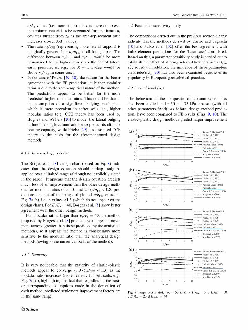
4.2.1 Load level (pa)

The behaviour of the composite soil–column system has

also been studied under 50 and 75 kPa stresses (with all

other parameters fixed). As before, design method predic-

tions have been compared to FE results (Figs. 9, 10). The

elastic–plastic design methods predict larger improvement

0.6

0.7

0.8

0.9

1.0

1.1

1.2

1.3

1.4

3 4 5 6 7 8 9 10

n/n

FE

A/Ac


Priebe's n0 (1976)

Priebe's n1 (1995)

Priebe's n2 (1995)


Pulko et al. (2011)




0.6

0.7

0.8

0.9

1.0

1.1

1.2

1.3

1.4

3 4 5 6 7 8 9 10

n/n

FE

A/Ac


Priebe's n0 (1976)

Priebe's n1 (1995)

Priebe's n2 (1995)


Pulko et al. (2011)




0.6

0.7

0.8

0.9

1.0

1.1

1.2

1.3

1.4

3 4 5 6 7 8 9 10

n/n

FE

A/Ac


Priebe's n0 (1976)

Priebe's n1 (1995)

Priebe's n2 (1995)


Pulko et al. (2011)




0.6

0.7

0.8

0.9

1.0

1.1

1.2

1.3

1.4

3 4 5 6 7 8 9 10

n/n

FE

A/Ac


Priebe's n0 (1976)

Priebe's n1 (1995)

Priebe's n2 (1995)


Pulko et al. (2011)




(a)

(b)

(c)

(d)




123





factors when columns are subjected to lower applied loads

(as do the FE simulations), indicating that stone columns

are more effective at lower load levels (less yielding).

Elastic design methods have no dependency on load level

(e.g. Balaam and Booker [3]), nor does Priebe’s n0 [29] or

the FE-based method derived by Borges et al. [8] which

depends only on Ac/A and Ec/Es. The SCFs used to obtain

n values for Aboshi et al. [1] have again been obtained

from the FE output.

As was the case with pa = 100 kPa, it is worth noting

that the elastic–plastic method n values converge with

increasing modular ratio for both pa = 50 kPa (e.g. Fig. 9c,

d) and 75 kPa (e.g. Fig. 10c, d), i.e., 1.0 \ n/nFE \ 1.3

(despite some divergence for large quantities of stone,

e.g., A/Ac \ 4). For Ec/Es = 5, Pulko and Majes [31] pre-

dicts lower n values at lower applied loads (this is in

contrast with other methods, e.g., Priebe [30], Castro and

Sagaseta [10], Pulko et al. [32]) and perhaps indicates that

the method may not be applicable for Ec/Es B 5. The

reason for the discrepancy at Ec/Es = 5 is attributable to

the fact that the drained solution neglects the elastic strains

of the column during its plastic deformation. For low

modular ratios, the elastic strains in the column during its

plastic deformation have a significant influence (i.e.

because the elastic stiffness of the column is of the same

order of that of the soil) and cannot be neglected when

adopting a drained approach. It is because of such extreme

cases (and also for realistic values for encased stone col-

umns) that Pulko et al. [32] improved on the earlier solu-

tion by Pulko and Majes [31], as clarified in Sect. 2.4.

Load level affects the depth to which plastic strains

appear in the column (yielding depends on the dimen-

sionless load factor pa/(c0.z) where c0 is the effective unit

weight of the soil and z is the depth below ground level),

i.e., yielding starts at the surface and progresses down-

wards with time (Castro and Sagaseta [10]); higher loads

result in more and more column yielding. Yielding has

been confirmed in the FE analyses by examining plots of

Mohr–Coulomb failure points (stresses lying on the Mohr–

Coulomb failure surface) in the PLAXIS output program.

Despite the different stress paths (drained vs. undrained

conditions) used by Castro and Sagaseta [10] and Pulko

et al. [32], these methods result in n values that are in

almost perfect agreement with one another, and under both

the 50 and 75 kPa loads, their predictions are consistently

in best agreement with the FE results, regardless of the

modular ratio or column spacing (i.e. n/nFE is almost

always in the range 0.9–1.1 which gives considerable

confidence in these design methods).

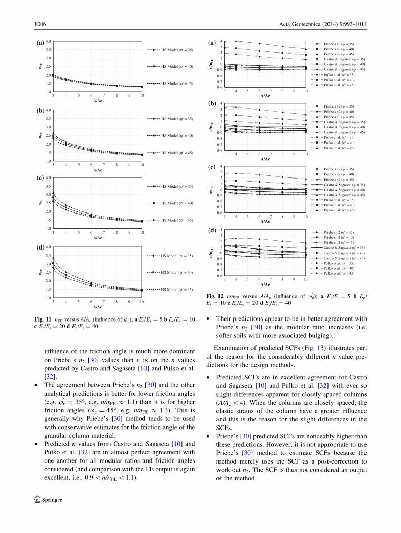
4.2.2 Friction angle of column material (uc

0)

Priebe [29, 30], Pulko and Majes [31], Castro and Sagaseta

[10], and Pulko et al. [32] predict larger n values for higher

column friction angles, uc

0(with the exception of Pulko and

Majes [31] at Ec/Es = 5, again illustrating that the method

may not be applicable for Ec/Es B 5). The method by

Borges et al. [8] is independent of the friction angle of the

column material, while the elastic methods are over-sim-

plified in this respect. nFE is plotted against A/Ac in

Fig. 11a–d to show that the FE n values are also higher for

higher friction angles. The influence of the friction angle

(uc

0= 35�, 40�, 45�) of the granular material is clearly

evident on the n/nFE values predicted by the favoured

analytical settlement design methods in Fig. 12a–d for the

four different modular ratios considered (the other param-

eters have been fixed at pa = 100 kPa, wc = 15� and

K0 = 0.44).

• Priebe’s n2 [30] appears to consistently overpredict

n values (i.e. n/nFE [ 1) for all friction angles consid-

ered in this study. It is interesting to note that the

0.6

0.7

0.8

0.9

1.0

1.1

1.2

1.3

1.4

3 4 5 6 7 8 9 10

n/n F

E

A/Ac


Priebe's n0 (1976)

Priebe's n1 (1995)

Priebe's n2 (1995)


Pulko et al. (2011)




0.6

0.7

0.8

0.9

1.0

1.1

1.2

1.3

1.4

3 4 5 6 7 8 9 10

n/n F

E

A/Ac


Priebe's n0 (1976)

Priebe's n1 (1995)

Priebe's n2 (1995)


Pulko et al. (2011)




0.6

0.7

0.8

0.9

1.0

1.1

1.2

1.3

1.4

3 4 5 6 7 8 9 10

n/n F

E

A/Ac


Priebe's n0 (1976)

Priebe's n1 (1995)

Priebe's n2 (1995)


Pulko et al. (2011)




0.6

0.7

0.8

0.9

1.0

1.1

1.2

1.3

1.4

3 4 5 6 7 8 9 10

n/n F

E

A/Ac


Priebe's n0 (1976)

Priebe's n1 (1995)

Priebe's n2 (1995)


Pulko et al. (2011)




(a)

(b)

(c)

(d)




123



influence of the friction angle is much more dominant

on Priebe’s n2 [30] values than it is on the n values

predicted by Castro and Sagaseta [10] and Pulko et al.

[32].

• The agreement between Priebe’s n2 [30] and the other

analytical predictions is better for lower friction angles

(e.g. uc

0= 35�, e.g. n/nFE & 1.1) than it is for higher

friction angles (uc

0= 45�, e.g. n/nFE & 1.3). This is

generally why Priebe’s [30] method tends to be used

with conservative estimates for the friction angle of the

granular column material.

• Predicted n values from Castro and Sagaseta [10] and

Pulko et al. [32] are in almost perfect agreement with

one another for all modular ratios and friction angles

considered (and comparison with the FE output is again

excellent, i.e., 0.9 \ n/nFE \ 1.1).

• Their predictions appear to be in better agreement with

Priebe’s n2 [30] as the modular ratio increases (i.e.

softer soils with more associated bulging).

Examination of predicted SCFs (Fig. 13) illustrates part

of the reason for the considerably different n value pre-

dictions for the design methods.

• Predicted SCFs are in excellent agreement for Castro

and Sagaseta [10] and Pulko et al. [32] with ever so

slight differences apparent for closely spaced columns

(A/Ac \ 4). When the columns are closely spaced, the

elastic strains of the column have a greater influence

and this is the reason for the slight differences in the

SCFs.

• Priebe’s [30] predicted SCFs are noticeably higher than

these predictions. However, it is not appropriate to use

Priebe’s [30] method to estimate SCFs because the

method merely uses the SCF as a post-correction to

work out n2. The SCF is thus not considered an output

of the method.

1.0

1.5

2.0

2.5

3.0

3.5

4.0

3 4 5 6 7 8 9 10

n FE

A/Ac

HS Model ( ' = 35)

HS Model ( ' = 40)

HS Model ( ' = 45)

1.0

1.5

2.0

2.5

3.0

3.5

4.0

3 4 5 6 7 8 9 10

n FE

A/Ac

HS Model ( ' = 35)

HS Model ( ' = 40)

HS Model (ϕ

ϕ

ϕ

ϕ

ϕ

ϕ

ϕ

ϕ

ϕ

ϕ

ϕ

ϕ

' = 45)

1.0

1.5

2.0

2.5

3.0

3.5

4.0

3 4 5 6 7 8 9 10

n FE

A/Ac

HS Model ( ' = 35)

HS Model ( ' = 40)

HS Model ( ' = 45)

1.0

1.5

2.0

2.5

3.0

3.5

4.0

3 4 5 6 7 8 9 10

n FE

A/Ac

HS Model ( ' = 35)

HS Model ( ' = 40)

HS Model ( ' = 45)

(a)

(b)

(c)

(d)

Fig. 11 nFE versus A/Ac (influence of uc

0); a Ec/Es = 5 b Ec/Es = 10


(a)

(b)

(c)

(d)

Fig. 12 n/nFE versus A/Ac (influence of uc

0); a Ec/Es = 5 b Ec/

Es = 10 c Ec/Es = 20 d Ec/Es = 40


123

• The SCFs calculated using the PLAXIS 2D HS Model

are in the range predicted by Castro and Sagaseta [10]

and Pulko et al. [32] which highlights why the

predicted n values are also in the same range.

• n values and SCFs are directly related for analytical

methods, but not for Priebe’s [30] method because of its

semi-empirical basis. Priebe’s [30] method is much

better at predicting n than it is at predicting SCFs (it is

not commonly used to predict SCFs). As the post-

correction of the column stiffness is carried out

independently of the initial stresses (which are used

as the basis for working out SCFs where analytical

methods are concerned), Priebe’s [30] method does not

consider the elastic modulus of the column in the

prediction of the SCF.

• Differences between the predicted SCFs are most

evident for the lowest modular ratio (Ec/Es = 5, e.g.,

Fig. 13a). The corresponding improvement factors also

exhibit the largest differences for this case (Fig. 12a).

• The good agreement between FE-calculated n values

and SCFs with those predicted by Castro and Sagaseta

[10] and Pulko et al. [32] again affirms their greater

applicability in design.

4.2.3 Dilatancy angle of column material (wc)

Pulko and Majes [31], Castro and Sagaseta [10], and Pulko

et al. [32] predict larger n values for higher dilatancy

angles, wc. The n values predicted by elastic methods (e.g.

Balaam and Booker [3]) and Borges et al. [8] are inde-

pendent of the dilatancy angle. The nFE predictions have

been included in Fig. 14a–d in order to show the direct

influence of wc on n (higher wc values lead to higher

n values). The influence of the dilatancy angle (Fig. 15a–d)

of the granular material has been examined in the range

0� \ wc \ 15� for Castro and Sagaseta [10] and Pulko

et al. [32]. In this case, the remaining parameters have been

0

2

4

6

8

10

12

14

16

3 4 5 6 7 8 9 10

SCF

A/Ac

Priebe's n2 (ϕ' = 35)Priebe's n2 (ϕ' = 40)Priebe's n2 (ϕ' = 45)Castro & Sagaseta (ϕ' = 35)Castro & Sagaseta (ϕ' = 40)Castro & Sagaseta (ϕ' = 45)Pulko et al. (ϕt' = 35)Pulko et al. (ϕ' = 40)Pulko et al. (ϕ' = 45)HS Model (ϕ' = 35)HS Model (ϕ' = 40)HS Model (ϕ' = 45)

0

2

4

6

8

10

12

14

16

3 4 5 6 7 8 9 10

SCF

A/Ac

Priebe's n2 (ϕ' = 35)Priebe's n2 (ϕ' = 40)Priebe's n2 (ϕ' = 45)Castro & Sagaseta (ϕ' = 35)Castro & Sagaseta (ϕ' = 40)Castro & Sagaseta (ϕ' = 45)Pulko et al. (ϕ' = 35)Pulko et al. (ϕ' = 40)Pulko et al. (ϕ' = 45)HS Model (ϕ' = 35)HS Model (ϕ' = 40)HS Model (ϕ' = 45)

0

2

4

6

8

10

12

14

16

3 4 5 6 7 8 9 10

SCF

A/Ac


0

2

4

6

8

10

12

14

16

3 4 5 6 7 8 9 10

SCF

A/Ac


(a)

(b)

(c)

(d)

Fig. 13 SCF versus A/Ac (influence of uc

0); a Ec/Es = 5 b Ec/Es = 10


1.0

1.5

2.0

2.5

3.0

3.5

4.0

3 4 5 6 7 8 9 10

n FE

A/Ac

HS Model (ψ = 0)

HS Model (ψ = 5)

HS Model (ψ = 10)

HS Model (ψ = 15)

1.0

1.5

2.0

2.5

3.0

3.5

4.0

3 4 5 6 7 8 9 10

n FE

A/Ac

HS Model (ψ = 0)

HS Model (ψ = 5)

HS Model (ψ = 10)

HS Model (ψ = 15)

1.0

1.5

2.0

2.5

3.0

3.5

4.0

3 4 5 6 7 8 9 10

n FE

A/Ac

HS Model (ψ = 0)

HS Model (ψ = 5)

HS Model (ψ = 10)

HS Model (ψ = 15)

1.0

1.5

2.0

2.5

3.0

3.5

4.0

3 4 5 6 7 8 9 10

n FE

A/Ac

HS Model (ψ = 0)

HS Model (ψ = 5)

HS Model (ψ = 10)

HS Model (ψ = 15)

(a)

(b)

(c)

(d)

Fig. 14 nFE versus A/Ac (influence of wc); a Ec/Es = 5 b Ec/Es = 10



123

fixed at those corresponding to the base case

(pa = 100 kPa, uc

0= 45�, K0 = 0.44). Priebe’s [30]

method has been formulated on the assumption of constant

volume deformation during yield, i.e., wc = 0�. Based on

this, it would be expected that Priebe’s n2 [30] would be in

direct agreement with Castro and Sagaseta [10] and Pulko

et al. [32] for wc = 0�. Examination of Fig. 15a–d

indicates:

• Priebe n2 [30] tends to significantly overpredict settle-

ment improvement factors in all cases for a column that

does not exhibit dilatant behaviour (i.e. n/nFE [ 1.4). It

thus appears that the method is more applicable for

dilatant columns (i.e. larger n values) even though it has

been formulated for non-dilatant column material. It

should be noted that the comparisons in Sect. 4.1 were

with FE analyses for which wc = 15�.

• The settlement improvement factors predicted by the

newer methods are again in direct agreement with one

another for all cases considered, and their agreement

with HS Model n values is particularly good for all

modular ratios (i.e. 1.0 \ n/nFE \ 1.1 with slight

departures evident for A/Ac \ 4).

• Focusing on the predicted SCFs (Fig. 16a–d), similar

conclusions as were drawn with regard to the friction

angle can again be drawn. The HS Model SCFs are in

almost direct agreement with the SCFs predicted by

Castro and Sagaseta [10] and Pulko et al. [32].

4.2.4 Coefficient of lateral earth pressure (K)

Priebe [30], Pulko and Majes [31], Castro and Sagaseta

[10], and Pulko et al. [32] predict larger n values for higher

K values (i.e. more lateral support). The n values predicted

by elastic methods (e.g. Balaam and Booker [3]) and

Borges et al. [8] are independent of K. The sensitivity of

Priebe [30], Castro and Sagaseta [10] and Pulko et al. [32]

with respect to the coefficient of lateral earth pressure

following column installation (K) has been examined for

three different K values (K0 = 0.44, 0.7, 1.0); these values

0.8

0.9

1.0

1.1

1.2

1.3

1.4

1.5

1.6

3 4 5 6 7 8 9 10

n/n F

E

A/Ac

Priebe's n2Castro & Sagaseta (ψ = 0)Castro & Sagaseta (ψ = 5)Castro & Sagaseta (ψ = 10)Castro & Sagaseta (ψ = 15)Pulko et al. (ψ = 0)Pulko et al. (ψ = 5)Pulko et al. (ψ = 10)Pulko et al. (ψ = 15)

0.8

0.9

1.0

1.1

1.2

1.3

1.4

1.5

1.6

3 4 5 6 7 8 9 10

n/n F

E

A/Ac


0.8

0.9

1.0

1.1

1.2

1.3

1.4

1.5

1.6

3 4 5 6 7 8 9 10

n/n F

E

A/Ac


0.8

0.9

1.0

1.1

1.2

1.3

1.4

1.5

1.6

3 4 5 6 7 8 9 10

n/n F

E

A/Ac


(a)

(b)

(c)

(d)

Fig. 15 n/nFE versus A/Ac (influence of wc); a Ec/Es = 5 b Ec/

Es = 10 c Ec/Es = 20 d Ec/Es = 40

0

2

4

6

8

10

12

14

16

3 4 5 6 7 8 9 10

SCF

A/Ac

Priebe's n2Castro & Sagaseta (ψ = 0)Castro & Sagaseta (ψ = 5)Castro & Sagaseta (ψ = 10)Castro & Sagaseta (ψ = 15)Pulko et al. (ψ = 0)Pulko et al. (ψ = 5)Pulko et al. (ψ = 10)Pulko et al. (ψ = 15)HS Model (ψ = 0)HS Model (ψ = 5)HS Model (ψ = 10)HS Model (ψ = 15)

0

2

4

6

8

10

12

14

16

3 4 5 6 7 8 9 10

SCF

A/Ac


0

2

4

6

8

10

12

14

16

3 4 5 6 7 8 9 10

SCF

A/Ac


0

2

4

6

8

10

12

14

16

3 4 5 6 7 8 9 10

SCF

A/Ac


(a)

(b)

(c)

(d)

Fig. 16 SCF versus A/Ac (influence of wc); a Ec/Es = 5 b Ec/Es = 10



123

have been chosen based on theoretical considerations

mentioned in Sect. 2.1. It should be noted that K for the

untreated case (no columns) is maintained equal to the at-

rest value (K0 = 1 - sin u0 = 0.44). Again, the direct

influence of K on the FE n values is plotted in Fig. 17a–d.

Larger K values result in larger settlement improvement

factors, i.e., larger K values leads to increased horizontal

stresses in the soil, hence providing more resistance to

lateral bulging of the granular material. It is noticeable that

K has a larger influence on n than either uc

0or wc.

Examining the predictions in Fig. 18a–d, similar con-

clusions to the previous sensitivity studies can again be

drawn, i.e., predictions with the newer methods are in good

comparison with one another but again, Priebe [30] over-

predicts the improvement (although Priebe’s [30] predic-

tions are closer to the newer methods at the higher modular

ratios, e.g., Fig. 18d). SCFs (at the surface) predicted by

Priebe [30], Pulko et al. [32], and Castro and Sagaseta [10]

are independent of the value of K (Fig. 19). FE-predicted

SCFs are also independent of K and are in good agreement

with the newer analytical design methods.

5 Conclusions

In this paper, a number of empirical and theoretical solu-

tions for evaluating settlement improvement factors have

been discussed and appraised in the context of comparable

2D finite element analyses. The following conclusions can

be drawn from the study:

• Elastic methods will overpredict the settlement

improvement and should really only be used in

relatively stiff soils for which the modular ratio, Ec/Es,

will be relatively small (or perhaps with unrealistic

conservative low values of the modular ratio).

• Analytical solutions assume the soil to behave in a

linear elastic manner, while in the numerical study

carried out in this paper, the soil behaviour includes the

stress dependency of stiffness (a more realistic

1.0

1.5

2.0

2.5

3.0

3.5

4.0

3 4 5 6 7 8 9 10

n FE

A/Ac

HS Model (K = 0.44)

HS Model (K = 0.7)

HS Model (K = 1.0)

1.0

1.5

2.0

2.5

3.0

3.5

4.0

3 4 5 6 7 8 9 10

n FE

A/Ac

HS Model (K = 0.44)

HS Model (K = 0.7)

HS Model (K = 1.0)

1.0

1.5

2.0

2.5

3.0

3.5

4.0

3 4 5 6 7 8 9 10

n FE

A/Ac

HS Model (K = 0.44)

HS Model (K = 0.7)

HS Model (K = 1.0)

1.0

1.5

2.0

2.5

3.0

3.5

4.0

3 4 5 6 7 8 9 10

n FE

A/Ac

HS Model (K = 0.44)

HS Model (K = 0.7)

HS Model (K = 1.0)

(a)

(b)

(c)

(d)

Fig. 17 nFE versus A/Ac (influence of K0); a Ec/Es = 5 b Ec/Es = 10


0.6

0.7

0.8

0.9

1.0

1.1

1.2

1.3

1.4

3 4 5 6 7 8 9 10

n/n F

E

A/Ac

Priebe's n2 (K = 0.44)Priebe's n2 (K = 0.7)Priebe's n2 (K = 1.0)Castro & Sagaseta (K = 0.44)Castro & Sagaseta (K = 0.7)Castro & Sagaseta (K = 1.0)Pulko et al. (K = 0.44)Pulko et al. (K = 0.7)Pulko et al. (K = 1.0)

0.6

0.7

0.8

0.9

1.0

1.1

1.2

1.3

1.4

3 4 5 6 7 8 9 10

n/n F

E

A/Ac


0.6

0.7

0.8

0.9

1.0

1.1

1.2

1.3

1.4

3 4 5 6 7 8 9 10n/

n FE

A/Ac


0.6

0.7

0.8

0.9

1.0

1.1

1.2

1.3

1.4

3 4 5 6 7 8 9 10

n/n F

E

A/Ac


(a)

(b)

(c)

(d)

Fig. 18 n/nFE versus A/Ac (influence of K0); a Ec/Es = 5 b Ec/

Es = 10 c Ec/Es = 20 d Ec/Es = 40


123

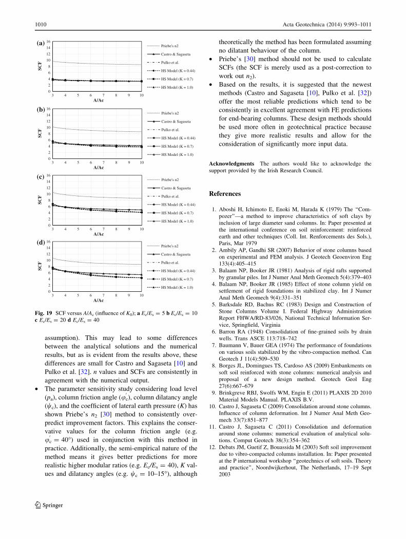
assumption). This may lead to some differences

between the analytical solutions and the numerical

results, but as is evident from the results above, these

differences are small for Castro and Sagaseta [10] and

Pulko et al. [32]. n values and SCFs are consistently in

agreement with the numerical output.

• The parameter sensitivity study considering load level

(pa), column friction angle (uc

0), column dilatancy angle

(wc), and the coefficient of lateral earth pressure (K) has

shown Priebe’s n2 [30] method to consistently over-

predict improvement factors. This explains the conser-

vative values for the column friction angle (e.g.

uc

0= 40�) used in conjunction with this method in

practice. Additionally, the semi-empirical nature of the

method means it gives better predictions for more

realistic higher modular ratios (e.g. Ec/Es = 40), K val-

ues and dilatancy angles (e.g. wc = 10–15�), although

theoretically the method has been formulated assuming

no dilatant behaviour of the column.

• Priebe’s [30] method should not be used to calculate

SCFs (the SCF is merely used as a post-correction to

work out n2).

• Based on the results, it is suggested that the newest

methods (Castro and Sagaseta [10], Pulko et al. [32])

offer the most reliable predictions which tend to be

consistently in excellent agreement with FE predictions

for end-bearing columns. These design methods should

be used more often in geotechnical practice because

they give more realistic results and allow for the

consideration of significantly more input data.

Acknowledgments The authors would like to acknowledge the

support provided by the Irish Research Council.

References

1. Aboshi H, Ichimoto E, Enoki M, Harada K (1979) The ‘‘Com-

pozer’’—a method to improve characteristics of soft clays by

inclusion of large diameter sand columns. In: Paper presented at

the international conference on soil reinforcement: reinforced

earth and other techniques (Coll. Int. Renforcements des Sols.),

Paris, Mar 1979

2. Ambily AP, Gandhi SR (2007) Behavior of stone columns based

on experimental and FEM analysis. J Geotech Geoenviron Eng

133(4):405–415

3. Balaam NP, Booker JR (1981) Analysis of rigid rafts supported

by granular piles. Int J Numer Anal Meth Geomech 5(4):379–403

4. Balaam NP, Booker JR (1985) Effect of stone column yield on

settlement of rigid foundations in stabilized clay. Int J Numer

Anal Meth Geomech 9(4):331–351

5. Barksdale RD, Bachus RC (1983) Design and Construction of

Stone Columns Volume I. Federal Highway Administration

Report FHWA/RD-83/026, National Technical Information Ser-

vice, Springfield, Virginia

6. Barron RA (1948) Consolidation of fine-grained soils by drain

wells. Trans ASCE 113:718–742

7. Baumann V, Bauer GEA (1974) The performance of foundations

on various soils stabilized by the vibro-compaction method. Can

Geotech J 11(4):509–530

8. Borges JL, Domingues TS, Cardoso AS (2009) Embankments on

soft soil reinforced with stone columns: numerical analysis and

proposal of a new design method. Geotech Geol Eng

27(6):667–679

9. Brinkgreve RBJ, Swolfs WM, Engin E (2011) PLAXIS 2D 2010

Material Models Manual. PLAXIS B.V.

10. Castro J, Sagaseta C (2009) Consolidation around stone columns.

Influence of column deformation. Int J Numer Anal Meth Geo-

mech 33(7):851–877

11. Castro J, Sagaseta C (2011) Consolidation and deformation

around stone columns: numerical evaluation of analytical solu-

tions. Comput Geotech 38(3):354–362

12. Debats JM, Guetif Z, Bouassida M (2003) Soft soil improvement

due to vibro-compacted columns installation. In: Paper presented

at the P international workshop ‘‘geotechnics of soft soils. Theory

and practice’’, Noordwijkerhout, The Netherlands, 17–19 Sept

2003

0

2

4

6

8

10

12

14

16

3 4 5 6 7 8 9 10

SCF

A/Ac

Priebe's n2

Castro & Sagaseta

Pulko et al.

HS Model (K = 0.44)

HS Model (K = 0.7)

HS Model (K = 1.0)

0

2

4

6

8

10

12

14

16

3 4 5 6 7 8 9 10

SCF

A/Ac

Priebe's n2

Castro & Sagaseta

Pulko et al.

HS Model (K = 0.44)

HS Model (K = 0.7)

HS Model (K = 1.0)

0

2

4

6

8

10

12

14

16

3 4 5 6 7 8 9 10

SCF

A/Ac

Priebe's n2

Castro & Sagaseta

Pulko et al.

HS Model (K = 0.44)

HS Model (K = 0.7)

HS Model (K = 1.0)

0

2

4

6

8

10

12

14

16

3 4 5 6 7 8 9 10

SCF

A/Ac

Priebe's n2

Castro & Sagaseta

Pulko et al.

HS Model (K = 0.44)

HS Model (K = 0.7)

HS Model (K = 1.0)

(a)

(b)

(c)

(d)

Fig. 19 SCF versus A/Ac (influence of K0); a Ec/Es = 5 b Ec/Es = 10



123

13. Degago SA (2011) On Creep during Primary Consolidation of

Clays. PhD Thesis, Norwegian University of Science and Tech-

nology (NTNU), Trondheim

14. Domingues TS, Borges JL, Cardoso AS (2007) Stone columns in

embankments on soft soils. Analysis of the effects of the gravel

deformability. In: Paper presented at the 14th European confer-

ence on soil mechanics and geotechnical engineering, Madrid,

Spain, 24–27 Sept 2012

15. Gab M, Schweiger HF, Kamrat-Pietraszewska D, Karstunen M

(2008) Numerical analysis of a floating stone column foundation

using different constitutive models. In: Paper presented at the 2nd

international workshop on the geotechnics of soft soils—focus on

ground improvement, Glasgow, 3–5 Sept 2008

16. Goughnour RR, Bayuk AA (1979) Analysis of stone column-soil

matrix interaction under vertical load. In: Paper presented at the

international conference on soil reinforcement: reinforced earth

and other techniques (Coll. Int. Renforcements des Sols.), Paris,

Mar 1979

17. Goughnour RR, Bayuk AA (1979) A field study of long term

settlements of loads supported by stone columns in soft ground.

In: Paper presented at the international conference on soil rein-

forcement: reinforced earth and other techniques (Coll. Int.

Renforcements des Sols.), Paris, Mar 1979

18. Greenwood DA (1970) Mechanical improvement of soils below

ground surface. In: Paper presented at the ground engineering

conference organised by the institution of civil engineers, Lon-

don, June 1970

19. Han J, Ye SL (2001) Simplified method for consolidation rate of

stone column reinforced foundations. J Geotech Geoenviron Eng

127(7):597–603

20. Hughes JMO, Withers NJ (1974) Reinforcing of soft cohesive

soils with stone columns. Ground Eng 7(3):42–49

21. Killeen MM, McCabe BA (2010) A numerical study of factors

affecting the performance of stone columns supporting rigid

footings on soft clay. In: Paper presented at the 7th European

conference on numerical methods in geotechnical engineering,

Trondheim (Norway), 2–4 June 2010

22. Lee JS, Pande GN (1998) Analysis of stone-column reinforced

foundations. Int J Numer Anal Meth Geomech 22(12):1001–1020

23. Leroueil S, Lerat P, Hight DW, Powell JJM (1992) Hydraulic

conductivity of a recent estuarine silty clay at Bothkennar.

Geotechnique 42(2):275–288

24. Lewis RW, Schrefler BA (1987) The finite element method in the

deformation and consolidation of porous media. Wiley, New

York

25. McKelvey D, Sivakumar V, Bell A, Graham J (2004) Modelling

vibrated stone columns in soft clay. Proc ICE Geotech Eng

157(3):137–149

26. Munfakh GA, Sarkar SK, Castelli RJ (1983) Performance of a

test embankment founded on stone columns. In: Paper presented

at the international conference on advances in piling and ground

treatment for foundations, London, 2–4 Mar 1983

27. Nash DFT, Powell JJM, Lloyd IM (1992) Initial investigations of

the soft clay test site at Bothkennar. Geotechnique 42(2):163–181

28. Poorooshasb HB, Meyerhof GG (1997) Analysis of behavior of

stone columns and lime columns. Comput Geotech 20(1):47–70

29. Priebe HJ (1976) Evaluation of the settlement reduction of a

foundation improved by Vibro-replacement. Bautechnik

2:160–162 (in German)

30. Priebe HJ (1995) The design of vibro replacement. Ground Eng

28(10):31–37

31. Pulko B, Majes B (2005) Simple and accurate prediction of set-

tlements of stone column reinforced soil. In: Paper presented at

the 16th international conference on soil mechanics and geo-

technical engineering, Osaka, Japan, 12–16 Sept 2005

32. Pulko B, Majes B, Logar J (2011) Geosynthetic-encased stone

columns: analytical calculation model. Geotext Geomembr

29(1):29–39

33. Schanz T, Vermeer PA, Bonnier PG (1999) The hardening soil

model: formulation and verification. In: Paper presented at

beyond 2000 in computational geotechnics. Ten years of PLAXIS

international, Amsterdam, 18–20 Mar 1999

34. Schweiger HF, Pande GN (1986) Numerical analysis of stone

column supported foundations. Comput Geotech 2(6):347–372

35. Seed HB, Booker JR (1977) Stabilization of potentially liquefi-

able sand deposits using gravel drains. J Geotech Eng Div

103(7):757–768

36. Sexton BG, McCabe BA (2013) Numerical modelling of the

improvements to primary and creep settlements offered by

granular columns. Acta Geotechnica. doi:10.1007/s11440-012-

0205-4

37. Slocombe BC, Bell AL, Baez JI (2000) The densification of

granular soils using vibro methods. Geotechnique 50(6):715–725

38. Sondermann W, Wehr W (2004) Deep vibro techniques. Ground

improvement, 2nd edn. Spon Press, Abingdon

39. Van Impe WF, De Beer E (1983) Improvement of settlement

behaviour of soft layers by means of stone columns. In: Paper

presented at the 8th European conference on soil mechanics and

foundation engineering, Helsinki, Finland, 23–26 May 1983

40. Van Impe WF, Madhav MR (1992) Analysis and settlement of

dilating stone column reinforced soil. Osterreichische Ingenieur-

und Architekten-Zeitschrift 137(3):114–121

41. Watts KS, Johnson D, Wood LA, Saadi A (2000) An instru-

mented trial of vibro ground treatment supporting strip founda-

tions in a variable fill. Geotechnique 50(6):699–708


123

http://dx.doi.org/10.1007/s11440-012-0205-4

http://dx.doi.org/10.1007/s11440-012-0205-4

Appraising stone column settlement prediction methods using finite element analyses

Documents