Applying Regression Methods to University Financial Aid Data

– Independent Work Report Spring 2018 –

Applying Regression Methods to University Financial Aid Data

Paulo FrazãoAdviser: Dr. Xiaoyan Li [IW 03]

Abstract

This project involves the application of a series of regression techniques to university financial

aid data compiled by the National Center for Education Statistics over the 2016-17 academic year.

This modeling suite helps us to better understand university aid distribution on a national level

and allows us to predict aid allotments for a given university in a consistent, effective manner.

This paper will examine the modeling techniques employed in this regression suite, evaluate their

strengths and limitations, and ultimately pave the way for future work towards the goal of providing

prospective university students with more information about their financial futures.

1. Introduction

It is no secret that a college education offers a tremendous advantage to any individual aiming

to be competitive in today’s occupational marketplace. In a report published by the Georgetown

Public Policy Institute’s Center on Education and the Workforce, Anthony Carnevale et al. observe

that, while there will be an estimated 55 million job openings in the United States through 2020,

people who have completed some form of post-secondary education will be best equipped to take

advantage of these opportunities [1].

Figure 1, created by Carnevale and included below, displays the approximate proportion of all

new job openings that will require a given threshold of educational attainment. While an estimated

36% of these positions will be accessible to individuals possessing a high school diploma, some

equivalent documentation, or even less educational background, that figure is eclipsed by the 35

million jobs open only to those with a post-secondary vocational certificate, some college, or a

higher degree. By no means will schooling beyond the high school level be necessary in order to

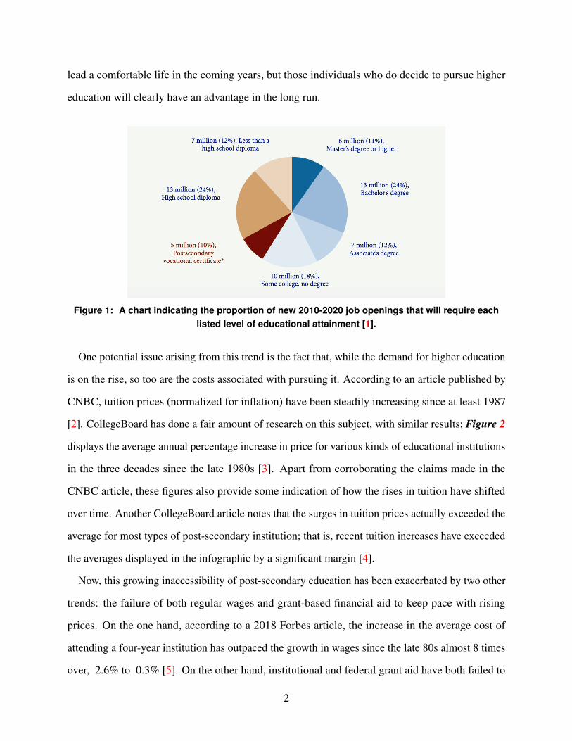
lead a comfortable life in the coming years, but those individuals who do decide to pursue higher

education will clearly have an advantage in the long run.

Figure 1: A chart indicating the proportion of new 2010-2020 job openings that will require eachlisted level of educational attainment [1].

One potential issue arising from this trend is the fact that, while the demand for higher education

is on the rise, so too are the costs associated with pursuing it. According to an article published by

CNBC, tuition prices (normalized for inflation) have been steadily increasing since at least 1987

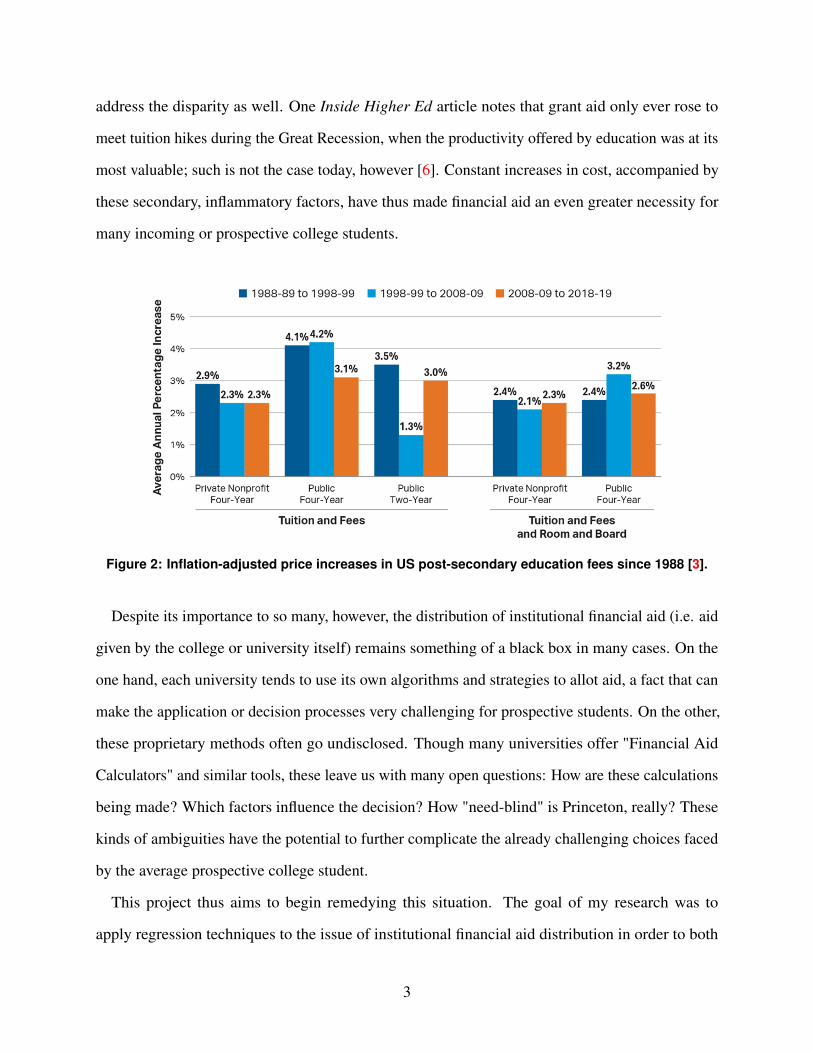
[2]. CollegeBoard has done a fair amount of research on this subject, with similar results; Figure 2

displays the average annual percentage increase in price for various kinds of educational institutions

in the three decades since the late 1980s [3]. Apart from corroborating the claims made in the

CNBC article, these figures also provide some indication of how the rises in tuition have shifted

over time. Another CollegeBoard article notes that the surges in tuition prices actually exceeded the

average for most types of post-secondary institution; that is, recent tuition increases have exceeded

the averages displayed in the infographic by a significant margin [4].

Now, this growing inaccessibility of post-secondary education has been exacerbated by two other

trends: the failure of both regular wages and grant-based financial aid to keep pace with rising

prices. On the one hand, according to a 2018 Forbes article, the increase in the average cost of

attending a four-year institution has outpaced the growth in wages since the late 80s almost 8 times

over, 2.6% to 0.3% [5]. On the other hand, institutional and federal grant aid have both failed to

2

address the disparity as well. One Inside Higher Ed article notes that grant aid only ever rose to

meet tuition hikes during the Great Recession, when the productivity offered by education was at its

most valuable; such is not the case today, however [6]. Constant increases in cost, accompanied by

these secondary, inflammatory factors, have thus made financial aid an even greater necessity for

many incoming or prospective college students.

Figure 2: Inflation-adjusted price increases in US post-secondary education fees since 1988 [3].

Despite its importance to so many, however, the distribution of institutional financial aid (i.e. aid

given by the college or university itself) remains something of a black box in many cases. On the

one hand, each university tends to use its own algorithms and strategies to allot aid, a fact that can

make the application or decision processes very challenging for prospective students. On the other,

these proprietary methods often go undisclosed. Though many universities offer "Financial Aid

Calculators" and similar tools, these leave us with many open questions: How are these calculations

being made? Which factors influence the decision? How "need-blind" is Princeton, really? These

kinds of ambiguities have the potential to further complicate the already challenging choices faced

by the average prospective college student.

This project thus aims to begin remedying this situation. The goal of my research was to

apply regression techniques to the issue of institutional financial aid distribution in order to both

3

a) understand the allocation process (i.e. which factors tend to influence the decisions that are

ultimately made) and to b) construct a system capable of estimating aid allotment in a consistent

manner. While this was admittedly a very large undertaking, I believe that this project has made

significant steps towards achieving both of these objectives.

2. Related Work

This section will discuss existing work at the intersection of financial aid and machine learning.

Admittedly, there was not much to be found; though the fields of financial aid distribution and

machine learning techniques are both highly saturated, few papers have attempted to bring the two

together in the way just described. Nonetheless, this section will explore each piece of related work

that I found along with how it affected my project.

Let us first consider the field that studies the distribution of financial aid and the consequences

of that process. Researchers have completed a surprising amount of work in this area. The

first example that I found came from the National Center for Education Statistics (NCES), an

organization that compiles data on various aspects of education in the United States each year and

performs exploratory analyses on it. This bureau supplied the dataset that I used for my project,

which the next section of this paper will discuss. Every two years, this organization conducts the

National Postsecondary Student Aid Study (NPSAS), a survey that collects data on many aspects

of post-secondary education throughout the country, compiles them into a series of datasets, and

then analyzes that information in relative depth [7]. This was a phenomenal starting point for my

research; it exposed me to the work of the NCES and showed me the level of intense, qualitative

study that already exists in this field. At the same time, however, it also helped me to understand

the limits of this existing work. While the biannual NPSAS provides some indication of how

universities might make their aid distribution decisions, it is difficult to build on this work; aside

from seeing whether these trends continue to hold by the time that the next NPSAS is completed,

there are few obvious opportunities for future research. Furthermore, this work does not provide a

way for individuals to put its theories to the test and actually predict university aid allotments, a

4

benefit that would presumably be limited to more quantitative methods.

Another similarly qualitative approach was detailed in a paper by Chen and DesJardins titled,

"Investigating the Impact of Financial Aid on Student Dropout Risks." In many ways, this essay

was a natural extension of the work done by the NCES and mentioned above; Chen and DesJardins

perform analysis on NCES datasets, explore many of the same dynamics noted in the NPSAS

reports, and generally provide a great example of how one might quantitatively examine NCES data

[8]. This final point was its primary benefit to my project. Like the NPSAS reports themselves,

however, the work of Chen and DesJardins was also limited in a number of ways. For one, it is

more narrow than is useful for the objectives undertaken by my paper; while their work examines

the relationship between financial aid and student dropout risks, I am interested in understanding

the financial aid distribution process as a whole. Due to this difference in scope, their analysis was

not exceptionally helpful to my own analytical process. Similarly, their work offers little in the way

of actual predictive modeling. The second objective of this project is to construct a system capable

of predicting aid from a given set of features, and their work simply did not involve this kind of

process.

I was able to find a paper more in line with this kind of work, titled, "Prospectively Predicting

4-Year College Graduation from Student Applications." Therein, Hutt et al. employ machine

learning on another NCES dataset with the stated goal of predicting the graduation rates of students

from their college applications using a random forest model. Though their predictive subject and

dataset differed markedly from my own, their work was very helpful to me in determining how I

would approach the process of fitting a series of models to an NCES dataset. Not only did it warn

me of the importance of thoroughly cleaning and understanding the data beforehand, but their paper

also convinced me that my objectives were tractable. As someone who has not done any work in

machine learning in the past, their efforts assured me that my methods could indeed prove effective

if employed correctly, an obvious yet very welcome reminder.

As has been discussed, then, the field investigating financial aid distribution is clearly very

saturated; the same can be said of machine learning research, as we seem to be in a golden age of

5

modeling and artificial intelligence. However, the intersection of these two fields is surprisingly

sparse. Most work involving the NCES and its financial aid data appears to be qualitative and

difficult to build upon, and the only clear example of machine learning applied to NCES data

revolves around a field completely distinct from my own. But this apparent lack of existing work

also served as an affirmation of sorts. Not only was there a clear space for research bridging ML and

financial aid distribution, but many limitations of the work that had already been done in either field

could be remedied through the use of regression techniques. Regression modeling is quantitative

and (ideally) consistent, and its very purpose is to make predictions; assuming that my models

perform well, then, I can be confident in assuming that my project will allow any individual to make

dependable guesses regarding financial aid allotments, unlike the work done by the NCES and these

other authors.

3. Approach

In my approach to the objectives that I set forth above, I decided to construct and fit an entire suite

of separate regression models, aggregating the results in an as-of-yet undecided fashion. These

models were fit on an NCES dataset (that will be discussed in the next section), and tasked with

predicting the average aid allotted by a given American university, given certain details about the

financials of that institution. Unlike Hutt, who implemented only a single kind of machine learning

classifier, I decided to instead research the benefits of different classes of regression techniques and

employ those that I thought would work best with my dataset.

Now, I decided to follow this approach because I believed that it offered a number of benefits,

including:

6

1. Diversity

(a) Much like any algorithm or strategy, each machine learning model has certain inherent

strengths, weaknesses, and assumptions. By including several different kinds of regressor

in my modeling suite, however, I hoped to ensure that my system could always make an

accurate prediction by considering the outputs of the different component models. For

instance, if I were to predict the average aid allotment for a given university, the prediction

would not be the result of any one member of the regression suite; rather, it would be

either some sort of weighted average over the outputs of all of the models or a comparably

thorough selection from the predictions by each regressor in the suite. Ideally, this ensures

that the system performs well on all (or most) inputs, as opposed to favoring only a select

subset.

2. Objectivity

(a) Throughout the research process, I found myself worrying about the biases intrinsic to

existing projects in financial aid distribution. While the data-driven insights that I found

were certainly interesting and perhaps truthful, I could not help but wonder whether the

authors were actively looking for certain results in the datasets as opposed to approaching

their projects with a clean slate. Either way, regression modeling minimized the possibility

of my own biases being reflected in my research. While there is certainly some bias to

model selection and evaluation, for example, there is less room for such influence when

one simply funnels all of their data into an existing algorithm that is disconnected from

their own decision-making. For this reason, I hoped that my approach would help me

insulate the analysis from my own biases.

3. Simplicity & Ease of Evaluation

(a) Apart from allowing one to make predictions on instances not in the testing suite, this

regression suite has the added benefit of being easy to evaluate. There are a number of

metrics that one might employ to compare each of the regressors to the others (i.e. MAE,

MSE, RMSE), each of which will be explored later in this paper. The ease with which one

7

might evaluate the results of their prediction is thus a clear benefit of this approach.

4. Scalability

(a) It is very straightforward to make additions to my work; anyone could simply add their

models to the existing regression suite. Since all of the candidate models are run on each

instance for which a prediction is made, any new model will simply be fit and evaluated in

the same way as the others. In this way, unlike much of the work already done regarding

financial aid distribution, anyone could continue my research with relative ease.

Clearly, my approach offers quite a few benefits over existing methods, primarily due to my use

of machine learning techniques. Arguably, however, the most important benefit is the fact that

regression modeling suits my objectives perfectly. First, the implicit feature selection that takes

place in the construction of many machine learning models allowed me to extract salient features

with ease. In addition, any individual could use my regression suite to make a prediction, as long as

they have the requisite information for the candidate university whose average aid allotment they

would like to estimate. Thus, I was able to rationalize my use of the approach noted above for a

number of different reasons, and the latter half of this paper will argue that it turned out to be a

fairly successful strategy.

4. Implementation

4.1. Dataset

Before considering my implementation of the above approach, this paper will describe the dataset

used to fit and evaluate all of the models that were included in the regression suite.

This dataset was compiled by the National Center for Education Statistics after the 2016-2017

academic year, and it contains data on the aid distributed to American university students throughout

that time frame [9]. Figure 3, pictured below, depicts three example instances as well as their

corresponding features and feature values. Each instance in the dataset corresponds to a specific

American university that has been anonymized in order to protect its confidentiality. Each of

these universities has exactly 552 descriptive features, half of which are imputation variables

8

(i.e. variables that describe how data had been imputed for each corresponding feature). They

appear nonsensical in the figure below, but the data included a legend detailing the meanings of

each codified feature; I imagine that this was done in order to minimize the size of the file or for

standardization purposes. Regardless, the dataset contains exactly 6,394 unique instances, though

many of them are missing entries for numerous fields (an issue that I resolved by imputing them

myself, which will be discussed shortly). After researching older iterations of this dataset, it appears

that the NCES conducts their financial aid surveys in the same way each year, as the 2015-16 dataset

was functionally identical in structure to the one that I used; older versions also appeared to contain

similarly few instances. Despite this low instance count (for which I hoped the high feature count

would compensate), I remained very optimistic about the success of this dataset.

Figure 3: Three example instances from the NCES 2016-17 financial aid dataset, along with severalcodified features and values.

4.2. Structure and Pipeline

My regression suite is composed of a series of Python scripts that make use of the scikit-learn

machine learning library, among other packages, in order to preprocess the data, fit each model, and

evaluate them all in turn. scikit-learn enabled me to employ each of the regression techniques that I

had previously researched without having to code the entire system from scratch, while matplotlib

allowed me to display the resultant evaluation metrics graphically.

Using this system, my project attempts to predict the "IGRN_T" variable ("Average amount of

institutional grant aid awarded to full-time first-time undergraduates") [9]. Though there are several

other response variables that also encapsulate some aspect of a university’s financial aid allotment,

this one appeared to be the most relevant; after all, my project has no real interest in federal aid

or local aid, and so focusing on a variable that reflects only institutional aid seemed ideal. In this

9

way, all of the other variables are treated as predictors in the hopes of consistently offering the most

accurate prediction of IGRN_T for a candidate university possible.

Now, the general pipeline of my project (that is, the sequence of operations that my system

performs) is as follows:

1. Preprocessing

(a) Execution begins when the user launches the "master.py" script. This Python script is

tasked with preparing the data for model fitting in several key ways.

The script first removed the imputation variables from the dataset, as they are a) chal-

lenging to process and b) are not related in any way to the response variable. Next, it

performed complete case analysis on instances that are missing the target feature, removing

all of those universities from the dataset. This was then followed by the imputation step,

where the script imputed a feature’s missing values if they made up less than 35% of the

total number of values and deleted that feature otherwise. Considering the relatively low

number of data points, I decided to concede and introduce a bit of bias into the models

through imputation in order to minimize shrinkage in the dataset. I also decided to proceed

with mean imputation as opposed to other common methods; as it is one of the most

straightforward types of imputation, it helped to keep the modeling suite simple (leaving

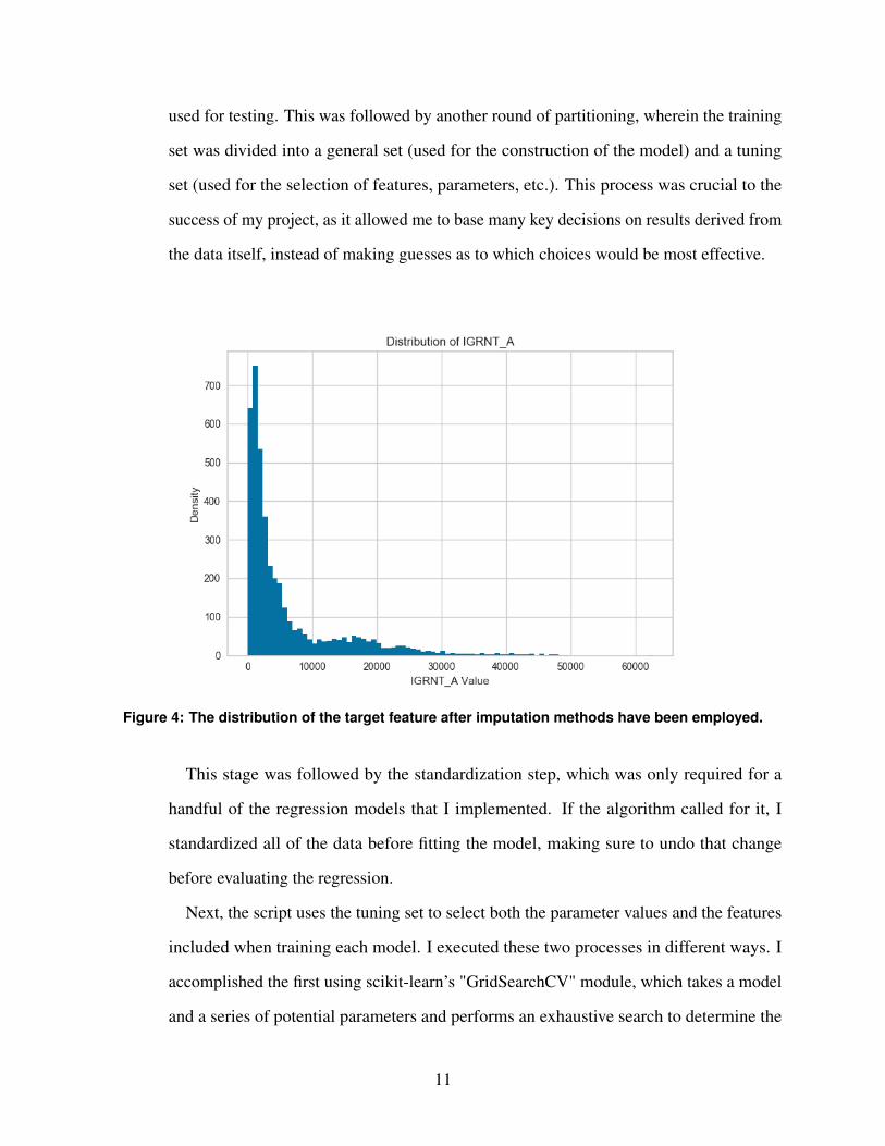
the complexity to the models themselves). After a handful of final preprocessing steps, this

master script displayed a histogram of the target feature (pictured in Figure 4), allowing

me to ensure that the distribution looks reasonable before moving on to the next stages of

the modeling process.

2. Model Fitting

(a) This phase of the project instantiates and fits each of the models. The actual models chosen

for this suite will be discussed in a future section; this portion of the paper will instead

explain the process through which each was constructed.

In each case, the first step was the partitioning of the data. I used the scikit-learn

"train_test_split" module to funnel 80% of my data into a training set, leaving the rest to be

10

used for testing. This was followed by another round of partitioning, wherein the training

set was divided into a general set (used for the construction of the model) and a tuning

set (used for the selection of features, parameters, etc.). This process was crucial to the

success of my project, as it allowed me to base many key decisions on results derived from

the data itself, instead of making guesses as to which choices would be most effective.

Figure 4: The distribution of the target feature after imputation methods have been employed.

This stage was followed by the standardization step, which was only required for a

handful of the regression models that I implemented. If the algorithm called for it, I

standardized all of the data before fitting the model, making sure to undo that change

before evaluating the regression.

Next, the script uses the tuning set to select both the parameter values and the features

included when training each model. I executed these two processes in different ways. I

accomplished the first using scikit-learn’s "GridSearchCV" module, which takes a model

and a series of potential parameters and performs an exhaustive search to determine the

11

best-performing combination of those inputs. This task was remarkably straightforward,

primarily due to the convenience of the scikit-learn library; I am incredibly grateful for

this resource, as it made the process of implementing my models considerably less painful

than it would have been otherwise. When implementing feature selection, for example,

I neglected to use scikit-learn and instead coded the component from scratch. For each

percentage k starting at 20%, ending at 75%, and incrementing by 5%, this part of the script

used scikit-learn’s "SelectPercentile" module to fit a regression model of the requisite

type on the training data using the k% best features; by randomizing the training-test split,

doing this 200 times for each k, and averaging the evaluation results for each iteration, the

script determines which percentile of features maximizes performance for each regression

technique. An example plot showing the "normalized root mean squared error" (a metric

explained later in this paper) resulting from these calculations on my ridge regression

model is pictured below in Figure 5.

As is clear from the figure, ridge regression improved as the percentage of retained

features approached 65%, but dropped off afterwards. This was a common trend amongst

most of the models: they would perform poorly with only the few best features, begin to

improve as more were included, and then drop off or plateau after a certain point. This

served as a convincing sanity check for me; after all, one would expect this pattern to

emerge, and so the fact that it indeed did assured me that I was calculating certain figures

correctly.

This script then asks the user to input the threshold that minimizes the NRMSE, fits a

model using the testing data and exactly that percentage of features, and shifts into the

evaluation phase.

12

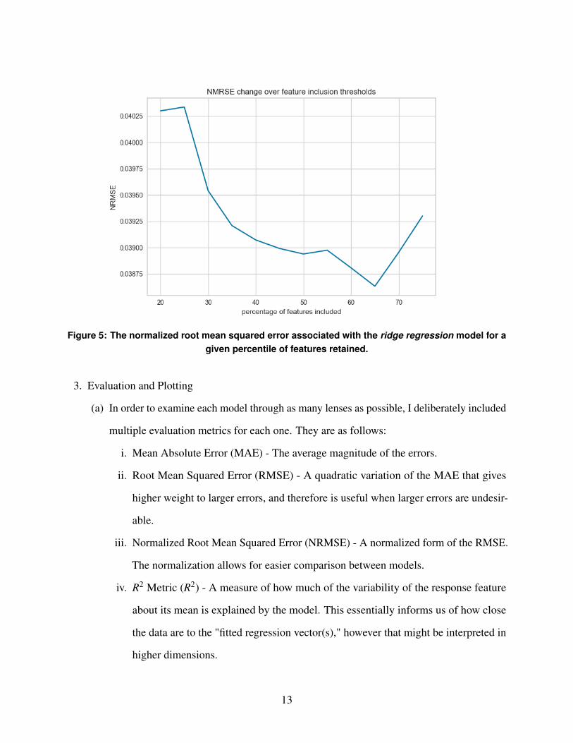
Figure 5: The normalized root mean squared error associated with the ridge regression model for agiven percentile of features retained.

3. Evaluation and Plotting

(a) In order to examine each model through as many lenses as possible, I deliberately included

multiple evaluation metrics for each one. They are as follows:

i. Mean Absolute Error (MAE) - The average magnitude of the errors.

ii. Root Mean Squared Error (RMSE) - A quadratic variation of the MAE that gives

higher weight to larger errors, and therefore is useful when larger errors are undesir-

able.

iii. Normalized Root Mean Squared Error (NRMSE) - A normalized form of the RMSE.

The normalization allows for easier comparison between models.

iv. R2 Metric (R2) - A measure of how much of the variability of the response feature

about its mean is explained by the model. This essentially informs us of how close

the data are to the "fitted regression vector(s)," however that might be interpreted in

higher dimensions.

13

After these figures have been calculated for each of the models in the suite, the script

plots the results. For each regression technique, it displays the residuals, allowing users to

visualize the success or failure of each attempt. It also creates a table of these results in

numerical form, which will be discussed later in this report.

Through this pipeline, the script is able to preprocess the data, fit all of the models, and

communicate all of the relevant evaluation metrics each time it is run.

4.3. Model Selection

There are clearly many kinds of regression techniques in existence; while I used 5-6 in my project,

there are as many variations as there are sorting or searching algorithms, for example. For this

reason, I made sure to research many regression strategies and include only those I believed could

be particularly effective when applied to my data. This section will provide a brief description of

each model included, as well as my rationale for its inclusion in the first place. The models are as

follows:

1. Linear Regression ("linear_model" in scikit-learn)

(a) Linear regression is arguably the simplest regression technique in use today. It is a

linear approach that employs gradient descent to find the relationship between a series

of predictors and a response variable. While not terribly complex, it is useful in many

instances, particularly when there is some underlying linear relationship in the data for it

to recognize and fit around.

I included this model in my suite mostly as a baseline from which to compare the

performance of other, more complex techniques. While it is certainly helpful, for example,

to have the evaluation metrics of ridge regression when discussing its performance, they

become significantly more useful if we understand how this simpler model performs

against the same data. I was able to use my linear regression in exactly this way, helping

me to understand how the other models were performing.

2. Linear Regression with Polynomial Features ("PolynomialFeatures" in scikit-learn)

14

(a) Since it is so simple, the base form of linear regression is rarely used when working with

more complex data. Instead, one of many permutations on linear regression, each of which

is suited to particular kinds of data. Linear regression with polynomial features is one such

example. This kind of regressor is useful when there is a non-linear pattern in the data,

unlike its simpler linear counterpart. Notably, the model itself does not differ from linear

regression at all. In order to perform polynomial regression, one must simply apply a series

of basis functions to the features being utilized and then fit the linear regressor on those

polynomial features. Varying these basis functions thus allows the modeler to tune this

model to great precision, making it a very effective strategy in a variety of circumstances.

I included this model in my suite in order to get a non-linear perspective. The data

with which I am working is complex and might thus contain non-linear relationships.

Furthermore, the benefits of implementing it clearly outweighed the effort required to do

so. By simply applying basis functions using scikit-learn’s "Polynomial Features" module,

I was able to test regressors of several different degrees, contributing immensely to the

diversity of my regression suite.

3. Ridge Regression ("Ridge" in scikit-learn’s "linear_model" module)

(a) As mentioned above, an issue that I encountered early on in the process was that of

feature collinearity. Collinearity is a phenomenon in which there exist linear or near-linear

relationships among independent variables. This issue might surface, for example, if a

hospital database contained the age, year of birth, and year of death of its patients; one

could derive the third variable by simply adding the first two (in most cases). Despite

appearing innocuous, this is a problem that could impact the regressors fitted to my

dataset. According to the NCSS Statistical Software handbook chapter on ridge regression,

multicollinearity can "create inaccurate estimates of the regression coefficients, inflate the

standard errors, ...deflate the partial t-tests...give false, nonsignificant p-values and degrade

the predictability of the model (and that’s just for starters)"[10].

That being said, I included ridge regression in my suite because it is designed precisely

15

to combat the phenomenon of overfitting. Essentially, ridge regression is identical to linear

regression, with two key differences. Firstly, all of the data must be standardized before

model fitting. Secondly, this technique introduces a user-selected interference ("ridge")

term k into the model in the hopes of offsetting the collinearity, a process also known as L2

regularization. This interference term should be large enough to ensure that the resultant

regression coefficients are stable, but as small as possible in order to minimize the bias

that it introduces into the model. This can be a challenging trade-off to understand, and

so I used a technique developed by Hoerl and Kennard in their seminal paper on ridge

regression: ridge tracing [11]. This process involves fitting a model for many values of k,

calculating the standardized regression coefficients, plotting them for all tested values of k,

and looking for the smallest k such that all coefficients are reasonably stable. Figure 6,

shown below, contains the ridge trace associated with the version of the ridge regression

implemented in the modeling suite; in this case, a value of about 0.005 was selected for

k since, despite a few regression coefficients continuing to change, the majority of these

variables seemed to have stabilized at this point.

Ridge regression was thus a welcome addition to the suite, as helped me manage the

threat of collinearity.

4. Lasso Regression ("Lasso" in scikit-learn’s "linear_model" module)

(a) Lasso regression is very similar to ridge regression, albeit with one key difference: it

performs L1 regularization instead of L2 regularization. The distinction between these

processes is that the former allows the regression coefficients to be shrunken without limit;

that is, if a large enough k is used, certain unhelpful features may be given a coefficient of

0 and thus removed from the model entirely.

I included this technique in my suite primarily to observe whether the inclusion of

additional feature selection would help with performance. Since feature selection is already

used in the preprocessing stage, I did not anticipate that this would have a very large effect

on the results, but this question was nevertheless worth exploring experimentally.

16

Figure 6: The ridge trace associated with the regression suite’s implementation of ridgeregression.

5. Random Forest Regression ("RandomForestRegressor" in scikit-learn)

(a) This regression method is among the more complex techniques that I included in my

suite. The random forest regressor is an example of an ensemble method, a technique that

combines several mediocre machine learning models into a single, aggregate predictor

that (ideally) outperforms each of its components. A random forest regression model, for

instance, aggregates several "decision stumps" (i.e. decision trees with a max depth of 1-2

levels), training each one on a random subset of features and of the instances in the dataset

(extracted through bootstrap and subspace sampling). All of these steps are employed

primarily to ensure that the randomization will help to cancel out any noise associated

with individual estimators. In order to make an overall prediction using this model, a result

is extracted from each of the decision stumps that comprise the random forest ensemble

and then aggregated through an error-based weighting system in order to arrive at a single,

17

averaged prediction.

I included this modeling technique in my suite primarily to gauge how well an ensemble

method would perform on this dataset in comparison to the basic linear regressor. Through

my research, I learned that machine learning ensembles often outdo their single-model

analogs by minimizing noise through randomization; in exchange, they clearly take much

longer on average to build and run due to their structure. Nevertheless, I figured that

this would be an excellent opportunity to put this theory into practice and gather some

experimental results about whether such would be the case with this dataset.

6. Support Vector Regression ("SVR" in scikit-learn)

(a) Support vector regression was perhaps the most involved technique that I explored in

this project. A variation on support vector machines, which are a very popular technique

used for classification problems, support vector regression essentially takes some training

instances as input and attempts to find a function that has at most ε deviation from each of

these data points. Unlike linear regression, for example, which attempts to fit a line to the

data, support vector regression simply tries to compartmentalize the training set within a

set of margins of minimal width. Much like linear regression, furthermore, this method

can also be extended to fit non-linear margins through the use of basis functions. As was

the case for random forest learning, however, this machine learning model takes very long

to fit and run, and so there is a clear trade-off between its theoretical predictive power and

the efficiency of the method.

I included this technique in my suite mainly due to curiosity. Truthfully, I did not do

very much research on support vector regression; I simply performed a quick search for

well-performing regression methods and settled on this one to round out my collection of

models. Regardless, I was still interested in understanding how this more involved model

would perform compared to the rest of the models in the suite.

18

5. Evaluation

5.1. Methods

After fitting each of the models in the regression suite as described above, the script evaluates each

model in turn. The script begins by plotting residuals; that is, it plots the difference between the true

value of each testing instance and the value outputted by each model. This visual display allows us

to understand whether each model is good fit for this dataset before we even consider the results of

the formal evaluation process. Ideally, the residuals should be a) evenly distributed, b) clustered

around lower values of the y-axis, and c) lacking any real patterns. If any of these conditions is

not fulfilled, the model may not be appropriate for the data, and so I used these as a gauge for

determining which models should actually be included in the regression suite.

This step was then followed by the formal evaluation, which is detailed in the "Structure and

Pipeline" subsection of the "Implementation" section above. Essentially, the script uses the testing

set predictions to calculate the mean absolute error (MAE), root mean squared error (RMSE),

normalized root mean squared error (NRMSE), and R2 metric for each model, displaying all of

these figures in a table for user inspection. These results offer a number of different perspectives on

how models performed in relation to one another, each of which will be discussed in the following

section.

5.2. Results

Let us first consider the residual plots associated with each of the models considered for the testing

suite. Figure 7, pictured below, shows all six of these residual plots.

19

Figure 7: The residual plots for all 6 models tested.

For the most part, these plots seemed reasonable. As was obvious from the histogram of the

IGRNT_A feature, pictured above, our dataset contains many more low values of the response

variable than it does high values; for this reason, the clustering of the residuals around lower

predicted values is unsurprising. Furthermore, apart from some outliers, most of the residual plots

tend towards lower residual values, and also appear to be evenly distributed about the x-axis.

20

The clear exception to these statements is the residual plot for support vector regression. Apart

from containing several very serious negative outliers (much larger errors than are contained in

the other residual plots), the residuals also appear to trend upwards after about x = 10000. This

pattern may have surfaced in the residuals for a number of different reasons. On the one hand, the

model may be unfit for this data; some other model might be able to identify this pattern in the

errors and respond accordingly. On the other hand, it may have been due to some human or coding

error, which might have resulted in a faulty model. Nevertheless, since I had several other, working

models in my suite and an unfortunate lack of time to make serious adjustments, I decided to simply

remove support vector regression from the suite.

Now, after examining the residual plots and making necessary changes, I used the script to

display the evaluation metrics of each remaining model in a table, pictured below in Figure 8.

The remainder of this section will consider the winner of each category, as well as any interesting

patterns observed in the results.

Figure 8: The MAE, RMSE, NRMSE, and R2 of each candidate model.

21

Let us first note that the models performed fairly well across the board. The normalized form of

the RMSE did not reach 5% among any candidate, and each model accounted for at least 90% of

the variation of the response variable around its mean (an observation derived from the R2 metric).

Furthermore, there was a lack of significant variation in both the MAE and in the the RMSE. The

range in MAE values was about 423, while the range in RMSEs was only about 561; while some

models certainly performed better than others, this resulted in an "average" difference of only a few

hundred dollars of aid in practice. While my original conception of this project involved selecting

only one best-fitting model for the dataset, this low variation may indicate that it might be better to

simply derive a prediction from each of the five models and average them together, with the added

bonus of reducing bias in the system.

Furthermore, it is worth noting that lasso regression actually performed significantly worse than

ridge regression. Perhaps enough feature selection is done in the preprocessing stage, and so any

further removal results in the poorer performance seen here. Also interesting is the fact that linear

regression bested the random forest model in MAE, but had a higher RMSE. This may indicate

that, while the ensemble method led to a greater total error, that error was distributed much more

evenly than in the case of linear regression. This fact perhaps makes it more useful than its simpler

counterpart; after all, egregious errors in predicting aid allotments are clearly undesirable, as they

would leave an individual with a very unrealistic understanding of how much they would have to

pay out-of-pocket.

In addition, there appears to be a clear winner among the five candidate models: linear regression

with polynomial features. Firstly, this model has the lowest MAE among the five. Let us recall that

the mean absolute error simply sums the absolute differences of the error of each prediction and

takes their average; therefore, in some ways the MAE offers the most objective indication of which

model performed the best without giving extra weight to large errors. From this perspective, the

polynomial regressor is the best candidate.

Furthermore, this technique also had the lowest RMSE, which illustrates that it, on average, had

the fewest large-scale errors. This observation is also visible in the residuals above. Despite the

22

varying scales applied to the y-axes of these plots, it is clear that polynomial regression has fewer

errors outside of the x-axis clusters than lasso or even ridge regression, for instance. Nevertheless,

this insulation against large errors is a very important quality for this application, for the reasons

described above. Therefore, its low RMSE gives polynomial regression a clear advantage over the

other models.

Notably, polynomial regression only achieved the second-lowest NRMSE; this is perhaps due

to the fact that the normalization scales against the highest and lowest values in the dataset and

certain models perform additional feature selection and instance deletion in their algorithms; for

this reason, the discrepancy was most likely due to some noise across the different models. More

importantly, however, polynomial regression achieved the highest R2 values among the candidate

models. With an R2 value of 0.98, we can claim that almost all of the variability of the response data

about its mean can be explained by our model, and so the fitted function fits the data especially well.

This model would thus do a very good job of predicting the average aid allotment for a university

that is similar to the instances contained in this dataset.

6. Conclusion

6.1. Strengths

In conclusion, I believe that my project ultimately succeeded in accomplishing the goals that were

laid out at the very beginning of this paper. Let us recall that the objectives of this work were

twofold: understanding the allocation process and creating a system capable of replicating it, given

some set of descriptive features.

For one, it is easy for us to extract the most relevant features in the dataset, at least as decided

by the regression suite. In addition to conducting feature selection during the proprocessing stage,

several of the models in the regression suite actually perform another round before evaluation.

Therefore, in a slightly recursive way, the features utilized by the models are those deemed to be

most predictive by the models themselves. I was easily able to run a separate script that extracted

these features from each model and funneled them into a separate file.

23

The results of this process were not terribly surprising. By far, the two most predictive features

were the "Percent of full-time first-time undergraduates awarded Pell grants" and the "Percent of

full-time first-time undergraduates awarded federal grant aid." This makes logical sense; on the

one hand, a university may have to supplement low Pell or federal grants with its own institutional

aid, but on the other low Pell and federal grants may be indicative of comparably lower financial

aid across the board. The relationship between these variables is unclear, but the existence of

a relationship at all does indeed comport with what one might expect of university aid policies.

Nevertheless, these models would be a bit more insightful, presumably, if they were trained on less

financial data. If I were to have included NCES data on student demographics, graduation rates,

and admissions policies, for instance, I wonder how the results of this feature extraction might have

changed. Either way, it is clear that this project satisfies the first objective set forth above.

The second objective also seems to have been met. After combining these five models into the

regression suite, we are left with a system that can take a new university (and its corresponding

financial descriptive features) as input and predict its average aid allotment. Furthermore, it can do

so fairly well. As is clear from the "Evaluation" section, each of the models is highly predictive and,

regardless of whether we use only the polynomial regressor or instead choose to average over the

predictions of all five component models, the output is likely to be fairly accurate. Furthermore,

this system also boasts a number of other benefits. For one, the suite is diverse; if predictions are

averaged across all component models, the individual strengths, weaknesses, and biases of each

model are (ideally) cancelled out, leaving us with a more accurate prediction than comparable

systems. In addition, the system is both generalizable and scalable; it performs well on instances

outside of the training set, and any individual working on it in the future need only add additional

models to the suite or tinker with the ones therein. It is clear, therefore, that the system constructed

through this project also satisfies the second objective laid out above.

24

6.2. Limitations and Future Work

In addition to the above successes of this project, however, it is also limited in a number of key

ways. This section will explore these limitations and the ways in which the current iteration of the

project could be improved through future work.

One such limitation is the aforementioned issue of the data being fairly limited in scope. All of

the data that I used to train the models was financial in nature and so it all, in some way, related

to the way in which aid was transferred from one party to another in the 2016-17 academic year.

Initially, I had planned to aggregate non-financial data from other NCES datasets, joining on the

university codes, in order to diversify the master dataset. Due to time constraints, however, I was not

able to complete this leg of the project, and so this represents a fairly straightforward opportunity

for future work.

Another obvious way in which one might further develop this project would be to simply add

more models to the suite, or to fine-tune the regressors already present within it. As mentioned

above, this project was designed to be scalable; in much the same way that I added regression

techniques throughout the semester, any individual could test a new kind of machine learning model

by implementing it and adding it to the master script. In some ways, this may be the most beneficial

kind of future work that one could undertake; though my models worked well with the dataset,

there could be some as-of-yet unexplored model that would surpass all five of them. In this way, I

hope that the project structure is straightforward enough where another individual could make these

additions in the same way that I did throughout the independent work process.

The decision of what to do with model predictions represents another interesting opportunity for

future work. As was mentioned above, I was left with the choice of using the polynomial regressor

as a standalone predictor for university aid allotments or including all of the candidate models,

averaging over their results when performing each prediction. Now, it is clear that there are benefits

to either strategy. On the one hand, the lone polynomial regressor is more lightweight, takes much

less time to run, and obviously outperformed the remaining models. On the other, there are implicit

biases and weaknesses to this regression technique that could be drowned out by the inclusion of

25

other predictors in an aggregated fashion. In order to confidently choose between these two options,

further experimentation is needed. This paper will not formally make such a decision, but it does

recognize the opportunity for others to perform the work necessary to do so in the future.

The size of the dataset was another clear limitation of this endeavor. Many machine learning

models take hundreds of thousands of entries as input; after complete case analysis and training-

testing partitions, my models were left with about 4,200. Unfortunately, this limitation is due to the

practical constraint of there not being hundreds of thousands of universities in the United States;

one could not just poll more institutions for financial aid data, for instance. That being said, there

are a number of ways one might work around this limitation. For one, they could add international

universities into the dataset. Assuming that this data is available for use, such a strategy would

surely increase the size of the dataset by a non-trivial percentage. Another technique would be to

add a temporal component to the data. Since the NCES has compiled these financial aid datasets

every year since 1999, it might be reasonable to aggregate all of them and create a new variable (e.g.

"YEAR") that lists the year to which each instance corresponds. Of course, the actual process of

implementing this change would be more involved than I have described, but nevertheless it would

expand the size of the dataset many times over (and introduce the possibility of exploring how these

trends have changed over time).

One final method through which we could expand the size of the dataset would be to fundamentally

reorganize the data itself. As I constructed my suite, it became clear to me that, in reality, the

models would not be very useful to the average prospective incoming college student. The reason

for this is the nature of the descriptive features in the data. These models are trained on information

such as the "Percent of full-time first-time undergraduates awarded Pell grants" and the "Percent of

full-time first-time undergraduates awarded federal grant aid" and more information that the average

individual might not be able to access. What those people can offer is their own characteristics:

their age, gender, intended major, background, life experiences, and so on. If the data were to

somehow be shifted to instead incorporate the details of each student offered financial aid, for

instance, we would a) have exponentially more instances from which to train the models and b)

26

develop a system that is much more practically useful to those individuals that, as I explained in

the "Introduction," perhaps need it most. This is no small task, but it does represent a concrete, yet

challenging opportunity for future work.

That being said, I am exceptionally happy with the groundwork that has been laid through this

project. As a personal beneficiary of the financial aid process, and as someone who has also had his

doubts about the ambiguity of it all, I hope that my independent work can lay the groundwork for

research that one day allows other individuals to pursue a higher education without the financial

stresses of these opportunities hanging over their heads.

7. Acknowledgements

I would first like to thank Dr. Xiaoyan Li. It was thanks to her seminar that I was able to learn

the foundations of machine learning, and to her many insights that I was able to develop this

groundwork into the work that I am so proud to present today. I would also like to thank all of

the other students in COS IW03. Each week, they offered crucial advice and support that made

the independent work process significantly more enriching. Lastly, I would like to thank the close

friends that supported me in this endeavor. It was our long conversations about the motivations of

my research and its potential consequences that pushed me to work as hard as I did, and so for that I

am very grateful.

8. Honor Code

This paper represents my own work in accordance with University regulations.

- Paulo Frazão

References[1] Anthony P. Carnevale, Nicole Smith, and Jeff Strohl. Recovery - Job Growth and Education

Requirements Through 2020. June 2013. URL: https://cew.georgetown.edu/cew-reports/recovery-job-growth-and-education-requirements-through-2020/.

[2] Emmie Martin. Here’s how much more expensive it is for you to go to college than it wasfor your parents. Nov. 2017. URL: https://www.cnbc.com/2017/11/29/how-much-college-tuition-has-increased-from-1988-to-2018.html.

27

[3] Average Rates of Growth of Published Charges by Decade. URL: https : / / trends .collegeboard.org/college-pricing/figures-tables/average-rates-growth-

published-charges-decade.[4] Average Published Undergraduate Charges by Sector and by Carnegie Classification, 2018-

19. URL: https : / / trends . collegeboard . org / college - pricing / figures -

tables/average-published-undergraduate-charges-sector-2018-19.[5] Camilo Maldonado. Price Of College Increasing Almost 8 Times Faster Than Wages. July

2018. URL: https : / / www . forbes . com / sites / camilomaldonado / 2018 / 07 /

24/price- of- college- increasing- almost- 8- times- faster- than- wages/

#9b87dad66c1d.[6] Rick Seltzer. Tuition and fees still rising faster than aid, College Board report shows. Oct.

2017. URL: https://www.insidehighered.com/news/2017/10/25/tuition-and-fees-still-rising-faster-aid-college-board-report-shows.

[7] David Radwin et al. 2015-16 National Postsecondary Student Aid Study. Jan. 2018. URL:https://nces.ed.gov/pubs2018/2018466.pdf.

[8] Rong Chen and Stephen L. Desjardins. “Investigating the Impact of Financial Aid on StudentDropout Risks: Racial and Ethnic Differences”. In: The Journal of Higher Education 81.2(Oct. 2016), pp. 179–208. DOI: 10.1353/jhe.0.0085.

[9] Years and Surveys. URL: https://nces.ed.gov/ipeds/datacenter/DataFiles.aspx.

[10] Ridge Regression. URL: https://ncss-wpengine.netdna-ssl.com/wp-content/themes/ncss/pdf/Procedures/NCSS/Ridge_Regression.pdf.

[11] Arthur E. Hoerl and Robert W. Kennard. “Ridge Regression: Biased Estimation for Nonorthog-onal Problems”. In: Technometrics 12.1 (1970), pp. 55–67. DOI: 10.1080/00401706.1970.10488634.

28