Applying a potential across a biomembrane: Electrostatic contribution to the bending rigidity and membrane instability

arX

iv:c

ond-

mat

/061

0355

v2 [

cond

-mat

.sof

t] 2

7 M

ar 2

007

Applying a potential across a biomembrane: electrostatic contribution to the bending

rigidity and membrane instability

Tobias Ambjornsson∗ and Michael A. Lomholt†

NORDITA - Nordic Institute for Theoretical Physics,Blegdamsvej 17, DK-2100 Copenhagen Ø, Denmark.‡

Per Lyngs HansenMEMPHYS - Center for Biomembrane Physics and Department of Physics,University of Southern Denmark, Campusvej 55, 5230 Odense M, Denmark.

We investigate the effect on biomembrane mechanical properties due to the presence an externalpotential for a non-conductive non-compressible membrane surrounded by different electrolytes.By solving the Debye-Huckel and Laplace equations for the electrostatic potential and using therelevant stress-tensor we find: in (1.) the small screening length limit, where the Debye screeninglength is smaller than the distance between the electrodes, the screening certifies that all electrostaticinteractions are short-range and the major effect of the applied potential is to decrease the membranetension and increase the bending rigidity; explicit expressions for electrostatic contribution to thetension and bending rigidity are derived as a function of the applied potential, the Debye screeninglengths and the dielectric constants of the membrane and the solvents. For sufficiently large voltagesthe negative contribution to the tension is expected to cause a membrane stretching instability. For(2.) the dielectric limit, i.e. no salt (and small wavevectors compared to the distance between theelectrodes), when the dielectric constant on the two sides are different the applied potential inducesan effective (unscreened) membrane charge density, whose long-range interaction is expected to leadto a membrane undulation instability.

I. INTRODUCTION

Biomembranes are thin fluid films composed mostlyof lipids. In cells they help separating different cellu-lar environments and compartments. Biomembranes aretypically “soft”, i.e., the typical energy required to bendthem is of the order the thermal energy and membranetension is often quite small. Softness implies that mem-brane geometry can become sensitive to different per-turbations, such as alteration of the electrostatic con-figuration. Much effort has for instance been devotedto calculation of the electrostatic contribution to tensionand bending rigidity for membranes with fixed charges orsurface potentials in an electrolyte solution, see [1] for areview; in general the presence of fixed (and screened dueto the electrolyte) charges tend to increase bending rigid-ity and hence make the membrane stiffer. However, it hasalso been found that when the membrane charges are notfixed but free to rearrange themselves on the surface andno electrolyte solution is present to screen the interac-tion, a long-wavelength undulation instability can occur[2], somewhat similar to DNA condensation [3]. Elec-tric fields can also be present across intrinsically neutralmembranes. An example would be a nerve cell, where

∗Present address: Department of Chemistry, Massachusetts Insti-

tute of Technology, 77 Massachusetts Avenue, Cambridge, Mas-

sachusetts 02139.†Present address: Department of Physics, University of Ottawa,

150 Louis Pasteur, Ottawa, Ontario K1N 6N5, Canada.‡These authors made an equal contribution to this work.

ion pumps create a potential difference between the twosides of the nerve cell membrane [4]. Another example isprovided in laboratories by the routine formation of lipo-somes in a process known as electroformation [5], duringwhich lipid membranes are swelling from electrodes un-der the application of electric fields.

In this study we investigate the electromechanical cou-pling of a membrane and an applied potential. In particu-lar, we solve the Debye-Huckel and Laplace equations forthe electrostatic potential for a non-conductive, incom-pressible membrane between two flat electrodes (kept atfixed potentials). On either side the membrane is sur-rounded by different electrolyte solutions. From the so-lutions for the potential we quantify how the correspond-ing induced membrane charges change the free energy forthe membrane and identify electrostatic contributions tomembrane mechanical parameters. In the presence of anelectrolyte (in the small screening length limit, see be-low) we find that the electrostatic contribution to mem-brane bending rigidity is positive. In the absence ofadded salt (the dielectric limit) the membrane becomesunstable against long wavelength undulations (in a some-what similar fashion to the behaviour of the interface be-tween two immiscible fluids, see Ref. [6]) if the two fluidssurrounding the membrane have different dielectric con-stants. For the symmetric dielectric case, as well as forthe small screening length limit, the membrane tensionreceives a negative contribution; for a sufficiently largeapplied potential this contribution would lead to a mem-brane stretching instability.

Several studies (see [1] and references therein) have in-vestigated the electrostatic contributions to tension andbending rigidity for membranes having a fixed surface

2

charge density or fixed potential at the membrane. How-ever, less work has been dedicated to the effect of induced

charges due to an applied potential, as considered in thepresent study. The results found here complement previ-ous results given in [7] (using coupled hydrodynamical-electric field equations, similar to [8])) for the symmetriccase of a membrane surrounded by identical electrolytes(in the small screening length limit), to the asymmetriccase and by giving an explicit expression for the bend-ing rigidity; in the limit of identical electrolytes on thetwo sides of the membrane our expression for the ten-sion agrees with that derived in [7]. Also, our formula-tion allows us to investigate the dielectric (no salt) limit,which was not considered in [7]. However, unlike [7] wedo not consider any dynamical effects. In contrast tothe study [9] based on electrolyte conductivities, our ap-proach through the Debye-Huckel equation allow us tostudy the effect of a finite Debye screening length. InRef. [9] a non-zero membrane conductivity was consid-ered, whereas we consider non-conductive membranes.Similar to the results in [9] we find a negative contribu-tion to the membrane tension in the presence of an elec-trolyte, although the two results are difficult to comparebecause of the different mathematical formulations.

This work is organized as follows: In Sec. II we givethe general equations governing the electrostatic responseof a non-conductive membrane of any shape; the mem-brane region is described by the Laplace equation andthe electrolyte solutions on either side satisfy the Debye-Huckel equations. In a standard fashion, the boundaryconditions are that the potential and the displacementfields should be continuous. In Sec. III these equationsare solved for the case of a flat membrane in an exter-nal potential. In Sec. IV corrections to the flat casesolutions are derived for a weakly curved incompressiblemembrane. In Sec. V the forces acting on the mem-brane, as well as the corresponding electrostatic contri-bution to the membrane free energy, are obtained. As-suming that membrane fluctuations occur on a time scaleslower than the relaxation time for the electrostatic po-tential we use the expressions for the forces for the weaklycurved membrane in order to obtain the renormalizedmembrane mechanical parameters, such as tension andbending rigidity, (in terms of a power series expansion inthe wavevector) as a function of the applied potential, thesalt concentrations (entering through the Debye screen-ing lengths) and the dielectric constants of the membraneand the solvents. We investigate three different limits:(1.) the small screening length limit, where the Debyescreening length is smaller than the distance between theelectrodes; (2.) the dielectric limit, i.e., no salt; (3.) the

symmetric case, where the salt concentration and dielec-tric constants on the two sides of membrane are equal.The results for the membrane mechanical parameters inthe three limits above (the main results in this study) aregiven in Eqs. (41)-(51). Finally, in Sec. VI a summaryand discussion are given.

II. GENERAL FORMULATION

We are interested in how biomembrane mechanical pa-rameters (and thereby, for instance, membrane fluctu-ations) are effected by an applied potential. Two pa-rameters characterizing a membrane in the absence ofan applied potential are the tension σ and the bendingstiffness K [10, 11]. As an external potential is appliedthere will in general be electrostatic contributions (σel

and Kel) to both of these quantities so that σ → σ + σel

and K → K + Kel in the presence of the applied poten-tial. An aim of this paper is to calculate σel and Kel.In a standard fashion we consider a small perturbationfrom a flat membrane, characterized by a height undula-tion h(x, y) (where x and y are coordinates in the planeof the flat membrane) and solve the electrostatic equa-tions (via a Fourier-transformation in the x- and y coor-dinates) for this weakly perturbed geometry. Through a

power series expansion in wavevector q (q =√

q2x + q2

y,

where qx and qy are the Fourier-transform variables of xand y respectively) of the free energy G one may iden-tify σel and Kel (see chapter 2 in Ref. [11]). We find itconvenient to, rather than utilize the free energy directly,consider the electrostatic contribution to the “restoring”force, from which we identify σel (Kel) as the prefactor infront of the −q2h (−q4h) term in a small q-expansion ofthe force, where h = h(qx, qy) is the Fourier-transform ofh(x, y). Notice that for obtaining the tension and bend-ing rigidity it suffices to keep terms linear in h in therestoring force expression. In general there may be otherterms in the power series expansion in q. For instance, asnoted in the introduction, for the asymmetric dielectriccase there is a membrane undulation instability whichmathematically arises due to the presence of a negativeterm linear in q in the series expansion.

The approach described above relies on a “quasi-static” approximation, i.e. we assume that membranefluctuations occur on a time scale tmem slower than thetime scale tel over which the electrostatic configurationadjusts itself (tel ≪ tmem). This assumption allows us tosolve the electrostatic problem for a fixed, weakly curved(but otherwise arbitrary) geometry. Let us estimate thetime scales tel and tmem: To estimate tel for an elec-trolyte we assume that this time scale equals the timefor an ion to diffuse the distance of the order the Debyescreening length, i.e. tel ≈ κ−2/D, where D is the iondiffusion constant and κ is the inverse Debye screeninglength introduced below (one may more realistically as-sume that tel = min{κ−2, q−2}/D, since for a wavelengthperturbation of the order 1/q the ions need only diffusea distance 1/q for the ion cloud to relax). From the Ein-stein relation and Stoke’s law, we have D = kBT/(6πηR),where η is the viscosity, kB is the Boltzmann constant,T the temperature and R the ion Stoke’s radius, usingkBT = 4 · 10−21 J, η = 10−3 Ns/m2 and R ≈ 0.1 − 0.3nm [12], we find D ≈ 10−9 m2/s. Furthermore, takingκ−1 = 10 nm we obtain: tel ≈ 10−7 s. For the membrane

3

relaxation time we estimate [13] tmem ≈ η/(q3K), and as-suming q−1 > 100 nm, K = 10−19 J we find tmem & 10−5

s. Therefore, indeed, we have tel ≪ tmem in general.We note from the expressions above that the longer thewavelength perturbation (smaller q) the better justifiedis our quasi-static approximation. In the dielectric limitthere are no ions and the relevant relaxation time tel is in-stead that of water relaxation (hydrogen-bond rearrange-ment time), which typically is of the order 10−12 s (seeRef. [14]) at room temperature, again certifying thattel ≪ tmem.

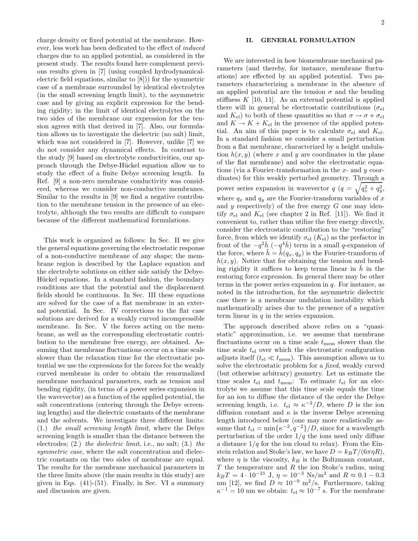
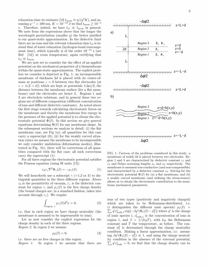
We are now set to consider the the effect of an appliedpotential on the mechanical properties of a biomembranewithin the quasi-static approximation. The explicit prob-lem we consider is depicted in Fig. 1: an incompressiblemembrane of thickness 2d is placed with its center-of-mass at positions z = 0 between two flat electrodes (atz = ±(L + d)) which are kept at potentials ∓∆φ/2; thedistance between the membrane surface (for a flat mem-brane) and the electrodes are hence L. Regions 1 and3 are electrolyte solutions, and in general these two re-gions are of different composition (different concentrationof ions and different dielectric constants). As noted abovethe first stage towards calculating electrostatic forces onthe membrane and thereby the membrane free energy inthe presence of the applied potential is to obtain the elec-trostatic potential Φ(~x). In this section we give generalequations determining Φ(~x) for any membrane shape. Inthe subsequent sections we analyze in detail: (i) the flatmembrane case, see Fig 1a); all quantities for this casecarry a superscript (0); (ii) for the weakly curved situa-tion (since we assume the membrane to be incompressiblewe only consider undulation deformation modes), illus-trated in Fig. 1b), there will be corrections of all quan-tities compared with the flat case; all such correctionscarry the superscript (1).

For all three regions the electrostatic potential satisfiesthe Poisson equation (using SI units [15])

ε0εγ∇2Φγ(~x) = −ργ(~x). (1)

We will henceforth use a subscript γ (=1,2 or 3) to dis-tinguish quantities in the three different regions. Aboveε0 is the permittivity of vacuum, εγ is the dielectric con-stant for region γ, and ργ(~x) is the free charge density(the bound charges are, in a standard fashion, taken intoaccount through εγ). We require

∫

region γ

ργ(~x)d3x = 0, (2)

i.e, that in each region we have charge neutrality (themembrane is assumed to be impermeable to ions).

Let us now consider the explicit expression for thecharge density in each of the three regions.Region 2. In region 2 we assume

ρ2(~x) = 0, (3)

i.e. there are no free charges in this region.Region 1. In region 1 we assume that there are

2

1κε1

3κε3

∆φ/2

a)

2d

L

L

Region 3

Region 2

Region 1

−∆φ/2z=L+d

z=0z=d

z=−dε

z=−L−d

z=L+d

z=−L−d

−∆φ/2

∆φ/2

Region 1

Region 3 z=d+h(x,y)z=h(x,y)

z=−d+h(x,y)

b)

Region 2

FIG. 1: Cartoon of the problems considered in this study: amembrane of width 2d is placed between two electrodes. Re-gion 1 and 3 are characterized by dielectric constant ε1 andε3 and Debye screening lengths κ1 and κ3 respectively. Themembrane is assumed non-conductive (and non-compressible)and characterized by a dielectric constant ε2. Solving for theelectrostatic potential Φ(~x) for (a) a flat membrane, and (b)a weakly curved membrane (and utilizing the stress-tensor)allows us to obtain the electrostatic contribution to the mem-brane mechanical parameters.

ions of two types (positively and negatively charged)which are taken to be Boltzmann-distributed, i.e.(i distinguishes the different ionic species) ρ1(~x) =∑

i qicibulk,1 exp[−βqi(Φ1(~x)−φ0

1)] where qi is the charge

of ionic species i, cibulk,1 is the concentration of ions in

region 1, and β = 1/(kBT ), with kB the Boltzmannconstant and T the temperature, as before. The con-stant φ0

1 is determined through the charge neutralitycondition. Making a linear approximation, i.e. assum-ing βqi(Φ1(~x) − φ0

1) ≪ 1, and using the charge neutral-ity condition in the absence of the external potential,∑

i qicibulk = 0, we find that the charge density can be

4

written:

ρ1(~x) = −ε0ε1κ21(Φ1(~x) − φ0

1), (4)

with

κ21 =

β

ε0ε1

∑

i

[qi]2cibulk,1, (5)

where κ1 is the inverse Debye screening length for region1.Region 3. For region 3, with the same approximations asabove, the charge density becomes:

ρ3(~x) = −ε0ε3κ23(Φ3(~x) − φ0

3), (6)

where

κ23 =

β

ε0ε3

∑

i

[qi]2cibulk,3 (7)

is the square of the inverse Debye screening length andcibulk,3 is the concentration of ions in region 3.

Inserting Eqs. (3) into Eq. (1) yields the Laplace equa-tion

∇2Φ2(~x) = 0 (8)

for the potential in region 2. Inserting (4) and (3) intoEq. (1) gives the Debye-Huckel equation (γ = 1, 3)

∇2Φγ(~x) − κ2γ(Φγ(~x) − φ0

γ) = 0 (9)

for regions 1 and 3. The charge neutrality condition, Eq.(2), for region 1 and 3 becomes

∫

region γ

[Φγ(~x) − φ0γ ]d3x = 0. (10)

Note that we have trivial charge neutrality in region 2[see Eq. (3)].

Let us now consider the boundary conditions supple-menting the equations above. At the electrodes we have:

Φ1(~x)|z=−L−d =∆φ

2,

Φ3(~x)|z=L+d = −∆φ

2. (11)

In addition we have that the potential and the nor-mal component of the displacement fields are continuousacross the region 1-region 2 and region 2-region 3 bound-aries, i.e. [15]

Φ1(~x) = Φ2(~x) at region 1 − 2 boundary,

Φ2(~x) = Φ3(~x) at region 2 − 3 boundary (12)

and

ε1n · ~∇Φ1(~x) = ε2n · ~∇Φ2(~x) at region 1 − 2 boundary,

ε2n · ~∇Φ2(~x) = ε3n · ~∇Φ3(~x) at region 2 − 3 boundary,

(13)

where n is the normal to the respective interface. Eqs.(8), (9) and (10), together with the boundary conditionsEqs. (11), (12) and (13) completely determine the elec-trostatic potential Φ(~x).

From the solutions for Φ(~x) one can calculate otherquantities. For instance, one may obtain the inducedpotential defined through Φind(~x) = Φ(~x) − Φappl(~x) ,where the applied potential is Φappl(~x) = −∆φz/[2(L +

d)]. The total electric field is given by ~E(~x) = −~∇Φ(~x),

the applied electric field is ~Eappl = −~∇Φappl and the

induced field is ~Eind = −~∇Φind = ~E − ~Eappl. In the nextsection we solve the equations given in this section forthe case of a flat membrane. In the section after we findcorrections to the flat case solutions for a weakly curvedmembrane.

III. POTENTIAL FOR A FLAT MEMBRANE

Below we obtain the electrostatic potential in andaround a flat membrane. We use a superscript (0) toindicate the flat case quantities.

For a flat membrane the solutions depend only on z,and explicitly the solutions to Eqs. (8) and (9) are

Φ(0)2 (z) = φ0

2 + A2z (14)

where φ02 and A2 are constants determined by the bound-

ary conditions below. Also,

Φ(0)1 (z) = φ0

1 + A1(eκ1(z+d) − e−κ1(L+d+z)) (15)

and

Φ(0)3 (z) = φ0

3 + A3(e−κ3(z−d) − e−κ3(L+d−z)) (16)

where φ01, φ0

3, A1 and A3 are constants, and we used thecharge neutrality condition, Eq. (10).

We now use the boundary conditions (together withthe fact that the boundary surfaces are at z = ±d forthe flat case considered here, see Fig 1a) in order to de-termine the unknown constants above. From Eq. (11),the condition that the potential is continuous, Eq. (12)and the fact that the displacement field is continuous,Eq. (13), we get 6 equations for the 6 constants φ0

γ andAγ (γ = 1, 2, 3). Solving these equations leads to

A1 = −∆φ

2(1 + e−κ1L)l1Γ

A2 = −∆φ

2ε2Γ

A3 =∆φ

2(1 + e−κ3L)l3Γ (17)

and

φ01 =

∆φ

2

(

1 − g(κ1)l1Γ)

φ02 = −

∆φ

2

(

g(κ1)l1 − g(κ3)l3

)

Γ

φ03 = −

∆φ

2

(

1 − g(κ3)l3Γ)

(18)

5

where

g(q) =1 − e−qL

1 + e−qL= tanh(

qL

2) (19)

and Γ = 1/[g(κ1)l1 + g(κ3)l3 + d/ε2], and we introducedthe “rescaled” Debye screening lengths l1 = (ε1κ1)

−1 andl3 = (ε3κ3)

−1.There are three limits of particular interest:

1. “small” screening length, κ1L, κ3L ≫ 1. For thiscase we have g(q) → 1 in Eqs. (17) and (18). Alsothe prefactors for A1 and A3 simplify.

2. we define the dielectric limit as the limit of no salt,i.e. ci

bulk,1, cibulk,3 → 0; within the Debye-Huckel

approximation this is the equivalent to κ1, κ3 → 0.Expanding the exponentials in Eqs. (15) and (16),and using the explicit form for A1 and A3 aboveone straightforwardly show that the solutions in allthree regions take the form Φ(~x) = az + b where aand b are constants independent of κ1 and κ3, asit should since in the dielectric limit the potentialsatisfies Laplace equation, ∇2Φ(~x) = 0, see Eq. (9).

3. the symmetric case, ε1 = ε3 and κ1 = κ3. In thislimit we find that A1 = −A3, φ0

1 = −φ03 and φ0

2 = 0.

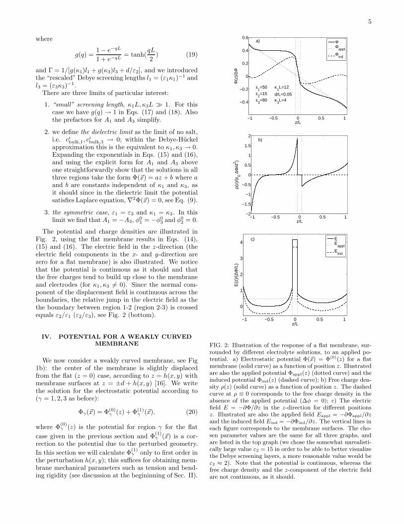
The potential and charge densities are illustrated inFig. 2, using the flat membrane results in Eqs. (14),(15) and (16). The electric field in the z-direction (theelectric field components in the x- and y-direction arezero for a flat membrane) is also illustrated. We noticethat the potential is continuous as it should and thatthe free charges tend to build up close to the membraneand electrodes (for κ1, κ3 6= 0). Since the normal com-ponent of the displacement field is continuous across theboundaries, the relative jump in the electric field as thethe boundary between region 1-2 (region 2-3) is crossedequals ε2/ε1 (ε2/ε3), see Fig. 2 (bottom).

IV. POTENTIAL FOR A WEAKLY CURVED

MEMBRANE

We now consider a weakly curved membrane, see Fig1b): the center of the membrane is slightly displacedfrom the flat (z = 0) case, according to z = h(x, y) withmembrane surfaces at z = ±d + h(x, y) [16]. We writethe solution for the electrostatic potential according to(γ = 1, 2, 3 as before):

Φγ(~x) = Φ(0)γ (z) + Φ(1)

γ (~x), (20)

where Φ(0)γ (z) is the potential for region γ for the flat

case given in the previous section and Φ(1)γ (~x) is a cor-

rection to the potential due to the perturbed geometry.

In this section we will calculate Φ(1)γ only to first order in

the perturbation h(x, y); this suffices for obtaining mem-brane mechanical parameters such as tension and bend-ing rigidity (see discussion at the begininning of Sec. II).

−1 −0.5 0 0.5 1

−0.4

−0.2

0

0.2

0.4

0.6

z/L

Φ(z

)/∆Φ

ε1=50

ε2=15

ε3=80

κ1L=12

d/L=0.05κ

3L=4

a)

ΦΦ

appl

Φind

−1 −0.5 0 0.5 1−2

−1.5

−1

−0.5

0

0.5

1

1.5

2b)

z/L

ρ(z)

/(ε 0 ∆

Φ/d

2 )

−1 −0.5 0 0.5 1

0

1

2

3

4

z/L

E(z

)/(∆

Φ/L

)c)

EE

applE

ind

FIG. 2: Illustration of the response of a flat membrane, sur-rounded by different electrolyte solutions, to an applied po-tential. a) Electrostatic potential Φ(~x) = Φ(0)(z) for a flatmembrane (solid curve) as a function of position z. Illustratedare also the applied potential Φappl(z) (dotted curve) and theinduced potential Φind(z) (dashed curve); b) Free charge den-sity ρ(z) (solid curve) as a function of position z. The dashedcurve at ρ ≡ 0 corresponds to the free charge density in theabsence of the applied potential (∆φ = 0); c) The electricfield E = −∂Φ/∂z in the z-direction for different positionsz. Illustrated are also the applied field Eappl = −∂Φappl/∂zand the induced field Eind = −∂Φind/∂z. The vertical lines ineach figure corresponds to the membrane surfaces. The cho-sen parameter values are the same for all three graphs, andare listed in the top graph (we chose the somewhat unrealisti-cally large value ε2 = 15 in order to be able to better visualizethe Debye screening layers, a more reasonable value would beε2 ≈ 2). Note that the potential is continuous, whereas thefree charge density and the z-component of the electric fieldare not continuous, as it should.

6

In each of the regions Eqs. (8) and (9) has to be satisfied.

Φ(0)γ (~x) satisfies these equations for h(x, y) ≡ 0, and we

therefore require that the corrections satisfy:

∇2Φ(1)2 (~x) = 0 (21)

and (γ = 1, 3)

∇2Φ(1)γ (~x) − κ2

γΦ(1)γ (~x) = 0. (22)

Let us now consider the boundary conditions (the bound-ary surfaces are at z = ±d +h(x, y) for the curved mem-

brane considered here). Since Φ(0)γ (z) satisfies Eq. (11)

we require for the perturbation:

Φ(1)1 (~x)|z=−L−d = 0,

Φ(1)3 (~x)|z=L+d = 0. (23)

Before imposing the conditions that the potential and thedisplacement fields are continuous, Eqs. (12) and (13),we note that for “small” h any scalar quantity g(~x) maybe expanded, to first order in h, according to:

g(~x) = g(0)(~x)|z=±d+h + g(1)(~x)|z=±d+h

≈(

g(0)(~x) + h∂g(0)(~x)

∂z+ g(1)(~x)

)

|z=±d,

we briefly discuss the quantitative meaning of “small” hat the end of this section. Eqs. (12) and (13) can thenbe written

(

h∂Φ

(0)1

∂z+ Φ

(1)1

)

|z=−d =(

h∂Φ

(0)2

∂z+ Φ

(1)2

)

|z=−d,

(

h∂Φ

(0)2

∂z+ Φ

(1)2

)

|z=d =(

h∂Φ

(0)3

∂z+ Φ

(1)3

)

|z=d (24)

and

ε1

(

h∂2Φ

(0)1

∂z2+

∂Φ(1)1

∂z

)

|z=−d = ε2

(

h∂2Φ

(0)2

∂z2+

∂Φ(1)2

∂z

)

|z=−d,

ε2

(

h∂2Φ

(0)2

∂z2+

∂Φ(1)2

∂z

)

|z=d = ε3

(

h∂2Φ

(0)3

∂z2+

∂Φ(1)3

∂z

)

|z=d,

(25)

where we used the fact that Φ(0)γ satisfies the boundary

conditions for h = 0. Eqs. (21) and (22) together withthe boundary conditions Eqs. (23), (24) and (25) com-

pletely determine the correction Φ(1)γ (~x).

We proceed by introducing the Fourier-transform in

the x- and y-direction (not for z-direction) of Φ(1)γ (~x):

Φ(1)γ (qx, qy, z) =

∫

dxdy eiqxx+iqyyΦ(1)γ (~x), (26)

and similarly we denote by h(qx, qy) the Fourier-transform of h(x, y). Eqs. (21) and (22) can then bewritten:

∂Φ(1)2

∂z2− q2Φ

(1)2 = 0 (27)

and (γ = 1, 3)

∂Φ(1)γ

∂z2− q2

γΦ(1)2 = 0, (28)

where q =√

q2x + q2

y and

qγ =√

q2 + κ2γ . (29)

The boundary conditions Eqs. (23), (24) and (25) re-

mains the same in Fourier-space (using the fact that Φ(0)γ

is independent of x and y), with the sole replacement

Φ(1)γ → Φ

(1)γ and h → h. The solution of Eq. (27) is

Φ(1)2 (q, z) = C2(q)e

qz + D2(q)e−qz , (30)

with q-dependent coefficients C2(q) and D2(q). Using theboundary condition Eq. (23) we find that the solutionsto Eq. (28) are:

Φ(1)1 (q, z) = D1(q)

(

eq1(z+d) − e−q1(z+d+2L))

(31)

and

Φ(1)3 (q, z) = D3(q)

(

e−q3(z−d) − eq3(z−d−2L))

. (32)

The unknown coefficients C2(q), D1(q), D2(q) and D3(q)are determined through the boundary conditions Eqs.(24) and (25). We find

D2(q) = −h

×eqdk+

3 (p1 + ε1q1r(q1)m−1 ) − e−qdk−

1 (p3 − ε3q3r(q3)m+3 )

e2qdk+1 k+

3 − e−2qdk−1 k−

3

,

(33)

where we introduced the short-hand notations (γ = 1, 3)

k±γ = k±

γ (q) = ε2q ± εγ qγr(qγ),

m±γ = A2 ± Aγκγ(1 + e−κγL),

pγ = εγAγκ2γ(1 − e−κγL),

r(q) =1 + e−2qL

1 − e−2qL, (34)

with Aγ given in Eq. (17). The remaining coefficientsare

C2(q) =eqd

k−1

(

D2(q)eqdk+

1 + hp1 + hε1q1r(q1)m−1

)

,

D1(q) =1

1 − e−2q1L

(

hm−1 + C2(q)e

−qd + D2(q)eqd)

,

D3(q) =1

1 − e−2q3L

(

hm+3 + C2(q)e

qd + D2(q)e−qd)

.

(35)

We notice that C1(q), D1(q), D2(q) and D3(q) are all pro-portional to h as they should be. The full solution for the

7

electrostatic potentials Φγ(~x) for a weakly curved mem-

brane is given by Eq. (20), where Φ(0)γ (z) were given in

the previous section and the Fourier-transform of Φ(1)γ (~x)

are given by Eqs. (30), (31) and (32) together with Eqs.(33), (34) and (35).

Again, we point out that in order to obtain mem-brane mechanical parameters, such as tension and bend-ing rigidity, it suffices to know the restoring force (cal-culated in the next section) to first order in h, i.e. itis enough to consider “small” fluctuation amplitudes.Therefore, even thought the results given above formallyassume that h is smaller than all other length scales inthe problem (d, κ−1

γ , q−1 and L), they are sufficient forthe purpose of calculating the tension and bending rigid-ity. A different matter is whether the Helfrich form of theelectrostatic contribution to the restoring force (in termstension and bending rigidity), derived in the next section,describe well “large” membrane fluctuations in the pres-ence of an applied potential. To address this question wemust clarify the meaning of “small” h, i.e. make clearwhat is the relevant dimensionless expansion parameter,in the context of calculating the electrostatic contribu-tion to the membrane restoring force or membrane freeenergy. The electrostatic contribution to the membranefree energy is determined by the interactions between in-duced charges at or in the vicinity of the membrane, withcharacteristic interaction distances of the order d and κ−1

γ

(here we consider the small screening length limit, whereκγ is non-zero). Therefore, whenever dq ≪ 1, κ−1

γ q ≪ 1and hq ≪ 1 all interactions are effectively local on a lo-cally flat membrane and the free energy must take theHelfrich form [10]. Note that this argument is valid inde-pendent of particular values of hκγ and h/d, and the freeenergy expansions given in the next section (in the smallscreening length limit) is therefore an expansion in the(small) parameters hq, dq, κ−1

γ q, but when these parame-ters are small there is no restriction on the values of hκγ

and h/d. In consistency with the discussion above, wepoint out that in Ref. [17] a method that formally avoidsthe assumptions hκγ ≪ 1 and h/d ≪ 1, by utilizing thegeometrical transformation z′ = z − h(x, y), was foundto give results consistent with results obtained by theflat membrane perturbative approach (of the kind usedin this paper) for a charged membrane in an electrolyte.

V. FORCES, FREE ENERGY AND

ELECTROSTATIC CONTRIBUTION TO

MEMBRANE MECHANICAL PARAMETERS

In this section we derive general expressions for themembrane forces (within the quasi-static approximation)and the corresponding electrostatic contribution to themembrane free energy, using the results from the previoustwo sections. In particular, we obtain the electrostaticcontribution to the membrane free energy for three cases:(1.) the small screening length limit, where the Debyescreening length is smaller than the distance between the

electrodes; (2.) the dielectric limit, i.e., no salt, and; (3.)the symmetric case, where the salt concentrations anddielectric constants on the two sides of the membraneare equal.

A. Membrane forces via a stress-tensor calculation

The forces acting on the membrane are obtained usingthe relevant stress-tensor, Tij . Following the derivationin Appendix A we have (in the Debye-Huckel regime con-sidered here)

Tij = ε0εγ

(

∂Φγ

∂xi

∂Φγ

∂xj

−1

2δij

∑

k

∂Φγ

∂xk

∂Φγ

∂xk

−δij

κ2γ

2

(

Φγ − φ0γ

)2)

− p0γδij , (36)

where x1 = x, x2 = y and x3 = z. The first two terms arethe usual Maxwell stress-tensor [15, 18], the third termis an osmotic contribution for the ions being “confined”by the electric potential (see appendix A), and the lastterm incorporates pressures p0

γ for each of the three re-gions (γ = 1, 2, 3). The discontinuities of Tij at the regionboundaries will produce forces on the membrane whichwill have to be balanced by other forces in the system,such as for example viscous forces within the membraneor from the surrounding bulk fluids. We are only inter-ested in calculating the electromechanical contribution ata given (x, y) to this total force balance here. To do thiswe note that the force (per unit area) in the i-directionon a region boundary from the stress in a given region is±∑

j njTji evaluated at the boundary, where the mem-brane normal nj is taken to point towards positive z andthe plus (minus) sign applies when the region is at larger(smaller) z than the boundary. Defining

fγ = f (0)γ + f (1)

γ

f (0)γ =

1

2ε0εγ

(

(∂Φ

(0)γ

∂z)2 − κ2

γ(Φ(0)γ − φ0

γ)2)

|z=±d

−p0γ

f (1)γ = ε0εγ

(∂Φ(0)γ

∂z[h

∂2Φ(0)γ

∂z2+

∂Φ(1)γ

∂z]

−κ2γ(Φ(0)

γ − φ0γ)[h

∂Φ(0)γ

∂z+ Φ(1)

γ ])

|z=±d,

(37)

where z = −d (z = d) is to be used for forces acting onthe interface separating region 1 and 2 (region 2 and 3),and using that to first order in h: nz = 1, nj = −∂jh(j = x, y), we find that the z-component of the totalforce acting on the surface separating regions 1 and 2 isf1−2 = f2 − f1. Using the explicit expressions for the

8

potentials from the previous two sections we find

f1−2 = f(0)1−2 + f

(1)1−2

f(0)1−2 = −ε0

(

2ε1A21κ

21e

−κ1L −ε2A

22

2

)

+ p01 − p0

2

f(1)1−2 = −ε0

(

D1(q)ε1A1κ1[q1(1 + e−κ1L)(1 + e−2q1L)

−κ1(1 − e−κ1L)(1 − e−2q1L)]

−ε2A2q[C2(q)e−qd − D2(q)e

qd])

, (38)

where f(0)1−2 is the force on a flat membrane interface,

and f(1)1−2 is the first order correction for a weakly curved

membrane, here expressed explicitly in terms of its

Fourier-transform f(1)1−2; note that f

(1)1−2 is proportional

to h (via D1, C2 and D2), as it should. Similarly, the z-component of the force acting on the surface separatingregions 2 and 3 is f2−3 = f3 − f2 and we find

f2−3 = f(0)2−3 + f

(1)2−3

f(0)2−3 = ε0

(

2ε3A23κ

23e

−κ3L −ε2A

22

2

)

+ p02 − p0

3

f(1)2−3 = ε0

(

D3(q)ε3A3κ3[q3(1 + e−κ3L)(1 + e−2q3L)

−κ3(1 − e−κ3L)(1 − e−2q3L)]

−ε2A2q[C2(q)eqd − D2(q)e

−qd])

(39)

where Aγ are given in Eq. (17) and C2(q), Dγ(q) aregiven in Eqs. (33) and (35). The results given in Eqs(38) and (39) completes the calculation of the forces act-ing on the membrane interfaces. In appendix B we utilizethese results in order obtain results for the total net forceon a flat membrane in some detail. In the next subsectionthe membrane free energy and the electrostatic contribu-tion to the membrane mechanical parameters in differentlimits are investigated.

B. Contribution to the free energy of the

membrane

Let us now investigate the electrostatic contribution tothe membrane free energy. We first note that if the flu-ids surrounding the membrane are incompressible, thenthe pressures p0

γ [occurring in the zero order terms inEqs. (38) and (39)] adjust such that there is no netforce (and hence no net movement of the membrane) inthe z-direction; we will here consider such incompress-ible fluids and also assume the membrane to be incom-pressible. Nevertheless the investigation of the net force

f (0) = f(0)1−2+f

(0)2−3 on a membrane provides some insights

into the electrostatic problem under consideration here,and is given in appendix B.

Let us now proceed by considering the z-component of

first order correction to the forces, f (1) = f(1)1−2 + f

(1)2−3;

from f (1) one can obtain the work on the membrane un-der an undulation deformation of the shape, and thereby

the free energy and electrostatic contribution to mem-brane mechanical parameters (through a power series inq, i.e. a long wavelength expansion). In particular wewant to compare the results of such an expansion to thecorresponding result for a “free” membrane: the free en-ergy G for a membrane is described by the Helfrich form[10, 11] G =

∫

dA(

2KH2 + σ)

where H is the meancurvature, dA the area element on the membrane, σ isthe tension and K is the bending rigidity. The restoringforce is then obtained as frs = −δG/δh giving in q-space

frs(q) = −[

σq2 + Kq4]

h + O(h2). (40)

This type of expansion requires only that the expectationvalue of (∇h(x, y))2 is small [11], i.e. that the character-istic fluctuation amplitude is small compared to 1/q. Inthe presence of an applied potential there will be elec-trostatic contributions σel and Kel to the tension andbending rigidity, so that σ → σ + σel and K → K + Kel.Below we proceed by expanding f (1), using the resultsin Eqs. (38) and (39), in a power series in q for differ-ent limits in order to obtain σel and Kel (note, however,in the expansion for the dielectric limit, for qL ≫ 1, wealso find terms odd in q). Note that since the tensionand bending rigidities are identified through terms in therestoring force expansion which are proportional to h,second and higher order terms in h (see discussion at theend of the previous section) do not contribute to σel andKel.

1. In the “small” screening length limit , κ1L, κ3L ≫1, a straightforward but lengthy expansion of f (1)

in a power series in q assuming that the wave-length of the perturbation (= 2π/q) is larger thanthe membrane thickness and the Debye screeninglengths, qd, q/κ1, q/κ3 ≪ 1, gives

f (1) = −[

σelq2 + Kelq

4 + O(q6)]

h. (41)

The explicit expression for the electrostatic contri-bution to the tension is

σel = −ε0∆φ2

m

2

l1 + l3 + 4d/ε2

(l1 + l3 + 2d/ε2)2, (42)

where, as before, the “rescaled” Debye screeninglengths are l1 = (ε1κ1)

−1 and l3 = (ε3κ3)−1. We

also introduced

∆φm = φ01 − φ0

3

=∆φ

2·l1 + l3 + 2d/ε2

l1 + l3 + d/ε2(43)

being the potential difference between the mainparts of the two bulk fluids. Notice that σel givesa negative contribution to the tension. The factthat σel < 0 originates from the fact that thatthe applied potential creates a net charge densityon either side of the membrane surfaces, see Fig.2; since ions of equal charge repel each other the

9

system would, for a compressible membrane, beable to decrease the free energy by separating thecharges through a stretching of the membrane (i.e.,by increasing the membrane area). For an incom-pressible membrane (as assumed here) the mem-brane is likely to respond to the electrostaticallyinduced negative tension by an opposite increase inthe membrane elastic contribution to the tension. Ifthe magnitude of σel exceeds the membrane elasticstrength (tensile strength) a stretching instability

occur. For the symmetric case (κ = κ1 = κ3 andε = ε1 = ε3) Eq. (42) becomes:

σel = σ0el

1 + εm(κd)−1/2

(1 + εm(κd)−1)2

σ0el = −

ε0ε2(∆φm)2

2d(44)

where we introduced the ratio εm ≡ ε2/ε betweenthe membrane and surrounding medium dielectricconstant (typically εm ≈ 1/40, see [1, 7]). Wenotice that when s = εm(κd)−1 ≪ 1, i.e. foran effectively small screening length compared tothe membrane width, the tension approaches σ0

el;the dimensionless parameter s is commonly appear-ing in membrane electromechanical problems, seeRefs. [1, 7]. From Eq. (42) we notice that forthe asymmetric case we similarly have σel ≈ σ0

el forsγ = (ε2/εγ)(κd)−1 ≪ 1, where γ = 1, 3. Sinceσ0

el only depend on the membrane dielectric con-stant, membrane width, and the applied potential,σel is for large salt concentration independent onthe properties of the surrounding medium (i.e. in-dependent on κ1, κ3, ε1 and ε3). The origin of thisresult is discussed below.

The electrostatic contribution to the bending rigid-ity is

Kel = ε0∆φ2m

b0 + b1d + b2d2 + b3d

3 + b4d4

(l1 + l3 + 2d/ε2)3(45)

with coefficients

b0 =1

8

(

(l1κ−21 + l3κ

−23 )(l1 + l3)

+2l1l3(κ−11 + κ−1

3 )2)

,

b1 =1

4

( 3

ε2(l1κ

−21 + l3κ

−23 )

+8l1l3(κ−11 + κ−1

3 ))

,

b2 = 2( 1

ε2(l1κ

−11 + l3κ

−13 ) + 2l1l3

)

,

b3 =8

3

1

ε2(l1 + l3),

b4 =4

3

1

ε22

. (46)

We point out that Kel > 0, i.e., the applied po-tential tends to make the membrane more rigid to-wards bending. During a bending deformation theinduced charge density on one side of the mem-brane gets compressed, whereas the charge densityon the opposite side gets expanded. The free energychanges of compression and expansion has differentsigns, but are in general of different magnitude. Itis only for the case that all Debye screening chargesare collapsed onto the surfaces (κ → ∞) and zeromembrane thickness d → 0 that the expansion andcompression free energies are identical and Kel = 0[see Eq. (45)]. Thus, loosely speaking, the smallerthe “effective” membrane thickness (the membranethickness including the Debye screening layer thick-nesses) the smaller is the bending rigidity. For thesymmetric case (κ = κ1 = κ3 and ε = ε1 = ε3) wewrite Eq. (45) according to

Kel = K0el(1 + εm(κd)−1)−3

×(

1 + 4εm(κd)−1 + 3εm(1 + εm)(κd)−2

+εm(9/8 + 3εm)(κd)−3 + (9/8)ε2m(κd)−4

)

K0el =

1

6ε0ε2d(∆φm)2 (47)

We note that in the limit of small relative mem-brane dielectric constant εm → 0 as well as forsmall screening length compared to the membranethickness, (κd)−1 → 0, we have Kel → K0

el. No-tice that, in practice, εm is always small ≈ 1/40,and therefore we have Kel → K0

el also for “nottoo small” values for (κd)−1. Similarly, we notefrom Eq. (45) that for the asymmetric case wehave Kel → K0

el in the ε2/εγ → 0 and in the(κγd)−1 → 0 (γ = 1, 3) limits. For the above con-sidered limits the major part of the potential dropis across the membrane (since ε2/εγ or (κd)−1 issmall), and hence the electric field is essentiallyzero everywhere except for the membrane region.Therefore, the membrane parameters play the dom-inant role in the expression for Kel and σel (noticethat K0

el and σ0el depend only on ε0ε2, d and ∆φm),

provided that the interactions of the induced sur-face charges do not occur through the surround-ing medium (again, certified if ε2/εγ or (κd)−1 issmall). Given that Kel and σel can only depend onε0ε2, d and ∆φm in the limits considered above onemay use dimensional arguments to argue that thelimiting results, K0

el and σ0el, for the bending rigid-

ity and tension must (up to a constant prefactor)take the forms given in Eqs. (44) and (47).

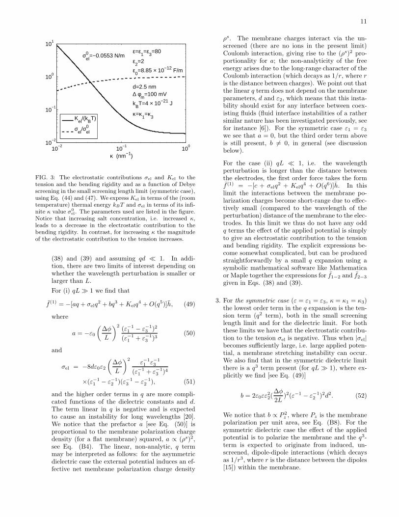
Fig. 3 illustrates the electrostatic contribution tothe tension and membrane bending rigidity and itsdependence on salt concentration (Debye screen-ing) for the symmetric case for simplicity. We seethat the absolute value of electrostatic contributionto the membrane tension increases with increasing

10

salt concentration, i.e. for increasing κ. We at-tribute this to an increase of screening charges (ina layer of decreased thickness) next to the mem-brane; the increased amount of charges will resultin larger electrostatic repulsion between ions in thescreening clouds [see discussion following Eq. (43)].In contrast to the effect on tension the electrostaticcontribution to the bending rigidity decreases withincreasing salt concentration (with Kel approach-ing K0

el as κ → ∞). The reason behind this is thatfor bending properties the thickness of the Debyescreening layers plays a role - a larger “effective”membrane thickness gives a higher bending rigidity[see discussion following Eq. (45), and the sponta-neous curvature calculation in Appendix C]. If wechoose the potential difference between the mem-brane sides ∆φm = 100 mV, ε2 = 2 and d = 2.5 nmwe find that K0

el = 0.018kBT (for room tempera-ture, kBT = 4 · 10−21). From Fig. 3 we see thatKel/K0

el can become quite large for small κ and,therefore, for sufficiently small salt concentrationthe bending rigidity Kel can exceed the thermalenergy kBT ; we therefore expect that the increaseof the bending rigidity in the presence of an appliedelectrostatic potential predicted in this study canindeed be experimentally observed for sufficientlylarge ∆φm and small salt concentrations (note how-ever, the below restriction on salt concentrationdue to assumptions in the Debye-Huckel approxi-mation).

Let us compare the results above for the symmet-ric case to the results obtained in [7]. We find thatthe result for σel given in Eq. (44) agrees with thefinite bilayer thickness, non-conductive membranetension (there denoted by Σin + Σout) obtained in[7] (note that in [7] the membrane thickness is de-noted by d, whereas we denote by d the size of alipid monolayer, so that in our case the membranethickness is 2d. Also note that, due to differentboundary conditions at the electrodes, the V in [7]should be equated with our ∆φm). Concerning thebending rigidity result, we note that no explicit ex-pression for Kel was given in [7], only a numericalvalue for a specific set of parameter values. Wechoose the same parameter values (∆φm = 50 mV,d = 2.5 nm, εm = 1/40, and 2dκ = 7.4), but notethat in order to get the expression for Kel one mustalso choose the actual value of ε2 (not just the ra-tio ε2/ε), which was not specified in [7]. We choosethe standard value ε2 = 2 [1, 9] and then find thatKel = 0.00467 kBT , which is a bit less than halfthe value found in Ref. [7]. Since no explicit ex-pression for Kel was given in [7] it is difficult tocomment on the nature of this discrepancy. Finally,using the approximate expression Kel ≈ K0

el for theparameters above we find that this approximationunderestimates Kel by merely 1 %.

Here, a few words on the validity of the Debye-

Huckel approximation, used throughout this study,are in place. This approximation should work whenthe quantity I = βqi(Φγ(~x)−φ0

γ), where γ = 1, 3, isvery small, i.e. I ≪ 1 (see Sec. II), but in practicethe Debye-Huckel approximation works well when-ever I < 1, see Ref [19]. The maximum of I occursat the membrane surfaces, see Eqs. (15), (16) andFig. 2, and we find that for the κγL ≫ 1 limit con-sidered here we have I = βqi∆φlγ/[2(l1+l3+d/ε2)].Using d ≈ 2.5 nm, ε2 ≈ 2 and εγ ≈ 80, the denomi-nator in the expression for I above is dominated bythe d/ε2 term whenever κ−1

γ < 50 nm (in this limitalso ∆φ ≈ ∆φm); for such ion concentrations wehave the following criterion for the validity of theDebye-Huckel approximation

I =1

2βqi∆φmsγ < 1. (48)

again involving the parameter sγ =(ε2/εγ)(κγd)−1. For a large potential differ-ence ∆φm = 100 mV we find that I < 1 whenκ−1

γ < 50 nm (using qi = 1.6 × 10−19 C andassuming room temperature). This means thatthe Debye-Huckel approximation, which was madein Sec. II in the main text, works surprisinglywell in general; the reason for this is the smallvalue of ε2/εγ (≈ 1/40) guaranteeing that themajor part of the potential drop occurs acrossthe membrane and that, therefore, the potentialdrop across the electrolytes, for which we appliedthe Debye-Huckel approximation, is modest, seeFig. 2. We point out that the dielectric limit,cibulk,γ → 0, does not rely on a Debye-Huckel

approximation and results to be given beloware therefore valid for any value of the appliedpotential. We have shown above that our resultsfor the small screening length limit (with the aboveexplicit restriction) and in the dielectric limit areusually valid. We note, however, that there isin general an intermediate salt regime where theDebye-Huckel approximation breaks down (forsufficiently large applied potentials). We leave theinvestigation of this intermediate regime for futurestudies.

We finally point out that there are alternative waysof computing the membrane mechanical parame-ters. For instance one can calculate the tension byfinding the integral of the deviation of the pressureprofile from the value of the pressure far from themembrane. This approach is demonstrated in Ap-pendix C, giving the same result as Eq. (42) forthe tension. In that appendix the same type of ap-proach is also used in order to obtain the electro-static contribution to the membrane spontaneouscurvature, see Eq. (C7).

2. in the dielectric limit, κ1, κ3 → 0, one can againperform a power series expansion in q using Eqs.

11

10−2

10−1

100

10−2

10−1

100

101

κ (nm−1)

ε=ε1=ε

3=80

ε2=2

ε0=8.85 × 10−12 F/m

d=2.5 nm∆ φ

m=100 mV

kBT=4 × 10−21 J

κ=κ1=κ

3

σel0 =−0.0553 N/m

Kel

/(kBT)

σel

/σel0

FIG. 3: The electrostatic contributions σel and Kel to thetension and the bending rigidity and as a function of Debyescreening in the small screening length limit (symmetric case),using Eq. (44) and (47). We express Kel in terms of the (roomtemperature) thermal energy kBT and σel in terms of its infi-nite κ value σ0

el. The parameters used are listed in the figure.Notice that increasing salt concentration, i.e. increased κ,leads to a decrease in the electrostatic contribution to thebending rigidity. In contrast, for increasing κ the magnitudeof the electrostatic contribution to the tension increases.

(38) and (39) and assuming qd ≪ 1. In addi-tion, there are two limits of interest depending onwhether the wavelength perturbation is smaller orlarger than L.

For (i) qL ≫ 1 we find that

f (1) = −[aq + σelq2 + bq3 + Kelq

4 + O(q5)]h, (49)

where

a = −ε0

(

∆φ

L

)2(ε−1

1 − ε−13 )2

(ε−11 + ε−1

3 )3(50)

and

σel = −8dε0ε2

(

∆φ

L

)2ε−11 ε−1

3

(ε−11 + ε−1

3 )4

×(ε−11 − ε−1

2 )(ε−13 − ε−1

2 ), (51)

and the higher order terms in q are more compli-cated functions of the dielectric constants and d.The term linear in q is negative and is expectedto cause an instability for long wavelengths [20].We notice that the prefactor a [see Eq. (50)] isproportional to the membrane polarization chargedensity (for a flat membrane) squared, a ∝ (ρs)2,see Eq. (B4). The linear, non-analytic, q termmay be interpreted as follows: for the asymmetricdielectric case the external potential induces an ef-fective net membrane polarization charge density

ρs. The membrane charges interact via the un-screened (there are no ions in the present limit)Coulomb interaction, giving rise to the (ρs)2 pro-portionality for a; the non-analyticity of the freeenergy arises due to the long-range character of theCoulomb interaction (which decays as 1/r, where ris the distance between charges). We point out thatthe linear q term does not depend on the membraneparameters, d and ε2, which means that this insta-bility should exist for any interface between coex-isting fluids (fluid interface instabilities of a rathersimilar nature has been investigated previously, seefor instance [6]). For the symmetric case ε1 = ε3

we see that a = 0, but the third order term aboveis still present, b 6= 0, in general (see discussionbelow).

For the case (ii) qL ≪ 1, i.e. the wavelengthperturbation is longer than the distance betweenthe electrodes, the first order force takes the formf (1) = −[c + σelq

2 + Kelq4 + O(q6)]h. In this

limit the interactions between the membrane po-larization charges become short-range due to effec-tively small (compared to the wavelength of theperturbation) distance of the membrane to the elec-trodes. In this limit we thus do not have any oddq terms the effect of the applied potential is simplyto give an electrostatic contribution to the tensionand bending rigidity. The explicit expressions be-come somewhat complicated, but can be producedstraightforwardly by a small q expansion using asymbolic mathematical software like Mathematicaor Maple together the expressions for f1−2 and f2−3

given in Eqs. (38) and (39).

3. For the symmetric case (ε = ε1 = ε3, κ = κ1 = κ3)the lowest order term in the q expansion is the ten-sion term (q2 term), both in the small screeninglength limit and for the dielectric limit. For boththese limits we have that the electrostatic contribu-tion to the tension σel is negative. Thus when |σel|becomes sufficiently large, i.e. large applied poten-tial, a membrane stretching instability can occur.We also find that in the symmetric dielectric limitthere is a q3 term present (for qL ≫ 1), where ex-plicitly we find [see Eq. (49)]

b = 2ε0εε22(

∆φ

2L)2(ε−1 − ε−1

2 )2d2. (52)

We notice that b ∝ P 2z , where Pz is the membrane

polarization per unit area, see Eq. (B8). For thesymmetric dielectric case the effect of the appliedpotential is to polarize the membrane and the q3-term is expected to originate from induced, un-screened, dipole-dipole interactions (which decaysas 1/r3, where r is the distance between the dipoles[15]) within the membrane.

12

VI. SUMMARY AND DISCUSSION

We have in this paper derived expressions for the elec-trostatic contributions to biomembrane mechanical pa-rameters (such as tension and bending rigidity) in thepresence of an static applied potential across a mem-brane. The membrane was assumed non-compressible,non-conductive (membrane region described by Laplaceequation) and surrounded by electrolyte solutions (de-scribed by the Debye-Huckel equation). By solving theequations for the electrostatic potential and using thestress-tensor the forces acting on the membrane were ob-tained, which in turn were used to obtain the free en-ergy and the electrostatic contribution to the membranemechanical parameters as a function of the applied po-tential, the salt concentrations (entering through the De-bye screening lengths) and the dielectric constants of themembrane and the solvents. Results of particular inter-est, that are found in this study, include: for (1.) thesmall screening length limit, where the Debye screeninglength is smaller than the distance between the elec-trodes, the screening certifies that all electrostatic in-teractions are short-range, leading to a free energy ex-pansion of the form ∼ σelq

2 + Kelq4 + O(q6) (where q is

the wavevectors), the main effects of the applied poten-tial are to decrease the membrane tension and increasethe bending rigidity; explicit expression are given in Eqs.(42) and (45). Our expression for the tension for thesymmetric case reproduces the result in [7]. In [9] it wasalso found that an applied electric field gives a negativecontribution to the tension. However in that study themedium surrounding the membrane was characterized byconductivities rather than Debye screening lengths, andit is therefore difficult to directly compare our results totheirs. For sufficiently large applied potentials the mag-nitude of the electrostatic contribution to the tension willexceed the maximum tension the membrane can sustain,leading to a membrane stretching instability. Possibly,this instability can result in the formation of pores andflow of ions through the membrane (in fact, the mem-brane tension is one of the key parameters in the model-ing of membrane electroporation dynamics [21]). For (2.)the dielectric limit, i.e. no salt (for small wavevectors qcompared to the distance between the electrodes), whenthe dielectric constants on the two sides are different, theapplied potential induces an effective (unscreened) mem-brane charge density, whose long-range interaction causesa membrane undulation instability if the dielectric con-stants of the two bulk fluids are different; this effect ischaracterized by a negative term linear in q in the free en-ergy expansion, see Eqs (49) and (50), i.e. this term is oflower order in q than the tension term. Previous similarresults include: In [6] the interface between two immisci-ble fluids of different dielectric constants was found to beunstable in the presence of a perpendicular electric field.The case of stiff (charged) DNA with bound, but mobile,counter ions was investigated in [3] and a shape instabil-ity found (supposedly leading to a DNA condensation).

If the two dielectrics on each side of the membrane areidentical, we found that then the applied electric fieldwill give a negative contribution to the tension. Hence,if the applied potential is sufficiently large a membraneinstability occurs also for the (dielectric) symmetric case.

We quantified the validity of the Debye-Huckel approx-imation (used throughout this study) and showed thatour results are in general valid in the small screeninglength limit as well as in the dielectric limit. Howeverfor “small”, but non-zero, salt concentration and largeapplied potential the Debye-Huckel approximation is nolonger valid and one needs to consider the full Poisson-Boltzmann equation. It remains a future challenge tosolve the full Poisson-Boltzmann problem in order to findexpressions for the free energy for arbitrary salt concen-tration, and, in particular, to investigate in more detailthe nature of the onset of the predicted membrane insta-bility (via the negative term linear in q in the free energy)as salt concentration is lowered.

Possible applications of the result for the small screen-ing length limit above would be to lipid membranes wherea potential difference across the membrane is enforcedby ion pumps incorporated in the membrane. Changesin membrane rigidity might then be observed in mi-cropipette or video microscopy experiments, if the screen-ing length and the membrane potential are large, see Fig.3. Another possible experiment would be to observe thestructural change of domains in a multi-component mem-brane using fluorescence correlation spectroscopy (FCS)as the membrane potential in a patch clamp experimentis altered; one might be able to observe a change from aphase with caps to one with stripes or buds as the effec-tive bending rigidity is changed by the applied potential[22].

For the cases discussed above where a membrane in-stability occurs, the system is expected to be driven fromthe quasi-flat shape into a new equilibrium configuration.Our perturbation analysis cannot in general say anythingabout this new configuration. However, for the smallscreening length limit we above speculated that the neg-ative electrostatic contribution to the tension (for largeapplied potentials) could lead to electroporation and acorresponding flux of ions through the membrane. Itmay also be speculated (similar to the studies in Refs.[2] and [9]) that the electrostatically induced new equi-librium configuration under certain conditions could bea spherical membrane (a vesicle); it is known that vesi-cles can be created in laboratories in a process knownas electroformation [5] under the application of electricfields. We hope that the present theory will stimulatefurther work directed towards the controlled estimationof vesicle sizes as a function of electrostatic parameters.e.g. potential differences and electrolyte concentration.

13

Acknowledgments

We would like to thank John H. Ipsen and James L.Harden for valuable discussions. We also acknowledgeour referees for useful comments.

APPENDIX A: DERIVATION OF BULK

EQUATIONS

In this appendix we show how the electrostatic equa-tions and the stress-tensor used in the main text can bederived as Euler-Lagrange equations from a free energy.Suppressing the region index γ for convenience we canwrite the appropriate free energy as

G =

∫

d3x

[

−1

2ε0ε|~∇Φ(~x)|2 + ρΦ − p

+∑

i

ci

(

kBT

(

lnci

cTotal− 1

)

+ µi

)]

. (A1)

Here p = p(~x) is the local pressure, ci = ci(~x) are thelocal concentrations of the ions, cTotal = cTotal(~x) is thetotal concentration of molecules of all kinds (includingwater) and µi are (constant) chemical potentials for theions. The logarithmic term corresponds to the entropyof mixing. Some of the Euler-Lagrange equations of thisfree energy can be found by demanding stationarity whenvarying the ion concentrations

0 =δG

δci

∣

∣

∣

∣

cTotal

= Φqi + kBT lnci

cTotal+ µi. (A2)

Solving for the ion concentrations we find

ci = cTotal exp

(

−qiΦ + µi

kBT

)

. (A3)

Inspection of the expression for the charge density ρ =∑

i qici with ci given by Eq. (A3) reveals that there is aunique value of Φ for which ρ vanishes. We define φ0 tobe this “equilibrium value”, i.e.

ρ|Φ=φ0 = 0. (A4)

The ion concentrations at “equilibrium” is labeled by

cibulk = ci

∣

∣

Φ=φ0. (A5)

The Euler-Lagrange equation for Φ is

0 =δG

δΦ= ε0ε~∇2Φ + ρ, (A6)

which is simply the Poisson equation. Insertion of Eq.(A3) and Eq. (A5) gives the Poisson-Boltzmann equation

ε0ε~∇2Φ +∑

i

qicibulk exp

(

−qi(Φ − φ0)

kBT

)

= 0, (A7)

which when linearized gives the Debye-Huckel equation,Eq. (9) in the main text.

The force-balance in the bulk regions can be found bydemanding that G should be stationary with respect tomoving all fluid elements, particles and fields by an in-finitesimal position dependent distance δ~x = δ~x(~x). De-noting fields after the move by a prime one has the newfields

Φ′(~x′) = Φ(x), (A8)

p′(~x′) = p(x), (A9)

ci′(~x′) = (1 − ~∇ · δ~x)ci(~x), (A10)

where ~x′ = ~x + δ~x. The free energy after the move is

G′ =

∫

d3x′

[

−1

2ε0ε|~∇

′Φ′(~x′)|2 + ρ′Φ′ − p′

+∑

i

ci′

(

kBT

(

lnci′

c′Total

− 1

)

+ µi

)

]

, (A11)

and using

d3x′ = (1 + ~∇ · δ~x)d3x, (A12)

∂

∂x′i

=∑

j

(

δij −∂δxj

∂xi

)

∂

∂xj

, (A13)

one finds that the change in free energy is

δG = G′ − G =

∫

d3x∑

i,j

Tij

∂δxj

∂xi

, (A14)

where Tij is the stress tensor for the system

Tij = ε0ε

(

∂Φ

∂xi

∂Φ

∂xj

−1

2δij

∑

k

∂Φ

∂xk

∂Φ

∂xk

)

− pδij . (A15)

Note that the first two terms on the right hand side ofEq. (A15) are simply the classic Maxwell stress tensor.Performing a partial integration in Eq. (A14) one cansee that the condition of stationarity of G implies theconservation of stress

∑

i

∂Tij

∂xi

= 0. (A16)

Combing this with Eq. (A6) one arrives at the morephysically revealing form

− ρ~∇Φ − ~∇p = 0, (A17)

i.e. electric forces should be balanced by changes in hy-drostatic pressure. Finally, since we know the behavior ofthe charge density ρ as a function of Φ from Eq. (A3) wecan integrate Eq. (A17) to find the pressure as a functionof Φ

p = p0 + kBT∑

i

cibulk

[

exp

(

−qi(Φ − φ0)

kBT

)

− 1

]

.

(A18)

14

The quadratic version of Eq. (A15) with Eq. (A18) in-serted is Eq. (36) of the main text. Note that the pres-sure can also be written p = p0 + kBT

∑

i(ci − ci

bulk), i.e.there is an osmotic contribution to the pressure when ionsare “confined” by the electric potential (see for instance[23]).

APPENDIX B: TOTAL NET FORCE ON A FLAT

MEMBRANE

In this appendix we investigate the total force actingon a flat membrane in some detail.

From Eqs. (38), (39) and Eq. (17) we obtain thefollowing explicit expression for the total force (per unitarea) acting on a flat membrane:

f (0) = f(0)1−2 + f

(0)2−3

= p01 − p0

3

−ε0

2(∆φ)2

( ε−11 e−κ1L

(1 + e−κ1L)2−

ε−13 e−κ3L

(1 + e−κ3L)2

)

Γ2 (B1)

and Γ = 1/[g(κ1)l1 + g(κ3)l3 + d/ε2], and l1 = (ε1κ1)−1

and l3 = (ε3κ3)−1 as before [the function g(q) is defined

in Eq. (19)]. If the fluids surrounding the membrane areincompressible, then the pressures p0

γ adjust such thatthe above force vanishes. In fact, in this study we assumethat both the membrane and the surrounding fluids areincompressible. Let us, however, in order to gain somephysical insights, investigate different limits of the non-pressure part of the above force (i.e. we take p0

1 = p03).

1. In the “small” screening length limit, κ1L, κ3L ≫1, the non-pressure part of Eq. (B1) becomes:

f (0) ≈ 0. (B2)

The force is zero whenever the screening length issmall compared to the distance between the elec-trodes. Thus it is not possible to get a net forceon the membrane solely by having different con-centration of ions (free charges) on the two sides.That there is no net force on the membrane can berelated to the fact that their is no net free chargearound the membrane, which can be understood

from Gauss’ law,∫

~D · ndS = Qfree, where ~D isthe displacement field and Qfree is the enclosedfree charge: since far from the membrane on bothsides the electric field is zero (in the here consid-ered limit, see Eqs. (15), (16) and Fig. 2) so isthe displacement field, and applying Gauss law (fora large “pillbox” enclosing the membrane and theDebye screening layers) one finds that Qfree = 0,as well as no net charge due to changes in polar-ization of the dielectric media. The effective netcharge for the membrane and the Debye screeninglayers is hence zero and there will be no net forcedue to these charges.

2. In the dielectric limit, κ1, κ3 → 0, we find

f (0) = −2ε0(∆φ

2L)2

×ε−11 − ε−1

3(

ε−11 + ε−1

3 + 2(d/L)ε−12

)2 (B3)

for the non-pressure part of the force. When thereare no free charges, as considered here, the Gausslaw argument above does not apply. One thenneeds to also take into account the bound charges,which create a polarization surface charge den-

sity ρs1−2 = −(~P2 − ~P1) · z (see [15], chap. 4)

on the region 1-2 interface. Similarly, for the re-gion 2-3 interface we have a polarization surface

charge density ρs2−3 = (~P2 − ~P3) · z. From the

fact that ~P = ~D − ε0~E and that the normal com-

ponent of the ~D-field is continuous we find that

ρs1−2 = ε0( ~E2− ~E1) · z and ρs

2−3 = −ε0( ~E2− ~E3) · z,i.e. the polarization surface charge density is de-termined by the jump in the electric field at theinterface. Using the explicit expressions for the po-tential Φ(z) given in Sec. III and that z-componentof the electric field is Ez = −∂Φ/∂z we findρs1−2 ≈ −ε0Ez,appl(ε

−11 − ε−1

2 )/(ε−11 + ε−1

3 ) and

ρs2−3 ≈ ε0Ez,appl(ε

−13 − ε−1

2 )/(ε−11 + ε−1

3 ), with theapplied field being Ez,appl = ∆φ/(2L) where we as-sumed a small membrane thickness d/L ≪ 1. Theeffective membrane charge density ρs = ρs

1−2+ρs2−3

then becomes proportional to the dielectric asym-metry between region 1 and region 3, explicitly

ρs ≈ ε0Ez,applε−13 − ε−1

1

ε−11 + ε−1

3

(B4)

where the proportionality ρs ∝ ε−13 − ε−1

1 followsdirectly from the fact that the jump in the electricfield is proportional to ε2/ε1 (ε2/ε3) for the region1-2 (region 2-3) interface (see discussion at the endof Sec. III and Fig. 2). Thus, whenever ε1 6= ε3 wehave that the membrane has an effective net chargeof induced bound charges, which when put into theapplied electric field Ez,appl gives rise to the forceabove; note that the force is proportional to ρs as itshould (for d/L ≪ 1). We also note that Eq. (B3)for d → 0 can be written

f (0) =1

2

(

ε1

ε3− 1

)

ε0ε1

(

z · ~E1

)2

, (B5)

which can be compared with for instance the for-mula in [18] for the pressure decrease in a fluid atthe fluid-air interface due to a normal electric field

z · ~E1 =∆φ

2L

2ε−11

ε−11 − ε−1

3

(B6)

on the fluid side.

15

3. For the symmetric case (ε1 = ε3 = ε, κ1 = κ3 andp01 = p0

3) the non-pressure part of Eq. (B1) is zero,

f (0) = 0, (B7)

since for the symmetric case there is no net surfacecharge, and hence no net force on the flat mem-brane. We point out, however, that the membranegets polarized. In particular, the polarization perunit area in the z-direction (using the results above)is

Pz = (−d)ρs1−2 + dρs

2−3

= ε0εEz,appl(ε−1 − ε−1

2 )d (B8)

in the dielectric limit.

APPENDIX C: ALTERNATIVE APPROACH TO

TENSION AND SPONTANEOUS CURVATURE

In this appendix we will demonstrate an alternative ap-proach to deriving the tension in the membrane, whichcan also be used to obtain the spontaneous curvatureinduced by the electric field. This approach consists ofcalculating moments of the deviation of the pressure pro-file from the value of the pressure far from the membrane.We will therefore in this appendix only study the smallscreening length limit where L → ∞, such that the pres-sure approaches a well defined pressure away from themembrane.

The tension is obtained as the integral of the lateralpressure profile deviation, or equivalently the excess lat-eral stress, of the planar membrane [24]. Choosing thediagonal x-component of the stress tensor to representthe lateral stress one has the precise formula [24]

σ =

∫ ∞

−∞

dz[

T (0)xx −

(

−p0)

]

, (C1)

where we have used that the pressure on the two sidesof the membrane should be identical p0 = p0

1 = p03, since

the zeroth order force in the small screening length limit,Eq (B2), vanishes. In terms of the zeroth order solutiongiven in Eqs. (14), (15) and (16) we obtain

σ = −ε0

2ε1κ1A

21 −

ε0

2ε3κ3A

23 − ε0ε2dA2

2

−2d(

p02 − p0

)

. (C2)

To obtain the final result we need to find p02. To do this

we note that in a flat equilibrium configuration the force

on the two region boundaries should vanish, f(0)1−2 = 0

and f(0)2−3 = 0 (or equivalently: T

(0)zz (z) = −p0 for all z).

From either Eq. (38) or Eq. (39) one finds

p02 = p0 +

1

2ε0ε2A

22 . (C3)

This gives

σ = −ε0

2ε1κ1A

21 −

ε0

2ε3κ3A

23 − 2ε0ε2dA2

2 . (C4)

This expression is identical to the tension given by Eq.(42) in the main text.

An advantage of the approach of integrating the stressprofile is that we can obtain the change in spontaneouscurvature C0 induced by the electric potential. If we in-clude a spontaneous curvature in the Helfrich free energyG given at the beginning of Sec. VB, writing it as

G =

∫

dA

[

1

2K(2H)2 − KC02H + σ

]

(C5)

and, as before, calculate the force frs = −δG/δh, thenthe spontaneous curvature will drop out at linear order inh and we would end up with our previous expression forthe force where C0 is not present; thus it is not possibleto obtain the spontaneous curvature using the approachof the main text. However, just like for the tension, thespontaneous curvature can be obtained from the lateralstress profile, namely as the negative first moment of thelateral stress profile, sometimes also called the bendingmoment. The formula is [24]

KC0 =

∫ ∞

−∞

dz z[

T (0)xx −

(

−p0)

]

, (C6)

and insertion of the zeroth order solution gives

KC0 =ε0ε1

4A2

1(1 − 2κ1d) −ε0ε3

4A2

3(1 − 2κ3d) ,

or explicitly

KC0 =ε0

4

(

∆φ

2

)2(

ε1l21(1 − 2κ1d)− ε3l

23(1 − 2κ3d)

)

Γ2,

(C7)where Γ = 1/[l1 + l3 + d/ε2], l1 = (ε1κ1)

−1 and l3 =(ε3κ3)

−1. Note that C0 vanishes in the symmetric casewhere κ1 = κ3 and ε1 = ε3 as it should.

[1] D. Andelman, in Handbook of Biological Physics, Ed. R.Lipowsky and E. Sackmann (Elsevier, 1995), p. 604-641.

[2] Y.W. Kim and W. Sung, Europhys. Lett. 58, 147 (2002).

[3] R. Golestanian, M. Kardar, T.B. Liverpool, Phys. Rev.Lett. 82, 4456 (1999).

[4] A.L. Hodgkin and A.F. Huxley, J. Physiol. 117, 500

16

(1952).[5] M. I. Angelova and D. S. Dimitrov, Faraday Discuss. 81,

303 (1986).[6] E.B. Devitt and J.R. Melcher, Phys. Fluids 8, 1193

(1965).[7] D. Lacoste, M. Consentino Lagomarsino, and J.F.

Joanny, Europhys. Lett. 77, 18006 (2007).[8] A. Ajdari, Phys. Rev. Lett 75, 755 (1995).[9] P. Sens and H. Isambert, Phys. Rev. Lett. 88, 128102

(2002).[10] W. Helfrich, Z. Naturforsch. 28c, 693 (1973).[11] U. Seifert, Adv. Phys. 46, 13 (1997).[12] J.E. Andersson, J. Non-Cryst. Solids 172-174, 1190

(1994).[13] L. Miao and M.A. Lomholt and J. Kleis, Eur. Phys. J. E

9, 143 (2002).[14] I. Ohmine and H. Tanaka, Chem. Rev. 93, 2545 (1993),

Section VI.C.[15] J.D. Jackson, Classical Electrodynamics, 3rd edition

(John Wiley & Sons, New York, 1999).[16] Note that the membrane thickness is not uniform along

the membrane for this type of displacement.[17] R.E. Goldstein, A.I. Pesci and V. Romero-Rochın, Phys.

Rev. A 41, 5504 (1990).

[18] L.D. Landau and E.M. Lifshitz, Electrodynamics of con-tinuous media (Pergamon Press, 1960).

[19] R.J. Hunter, Zeta Potential in Colloid Science (AcademicPress, London, 1981), p. 45 ff.

[20] A somewhat similar negative linear q term was found inthe study in [2] in a phenomenological model describinga membrane with a fixed net charge density, interactingvia unscreened (long-range) Coulomb-interactions, andwhere the charges are allowed to redistribute on the sur-face during a membrane deformation (this is in contrastto standard models [1] where the charges are assumedfixed on the surface). The fact that the charges are ableto redistribute allowed the system considered in [2] tolower its electrostatic free energy by creating large “wig-gles”, i.e. a membrane undulation instability occured.

[21] R.P. Joshi, Q. Hu, K.H. Schoenbach and H.P. Hjalmar-son, Phys. Rev. E 65, 041920 (2002).

[22] J.L. Harden, F.C. MacKintosh, and P.D. Olmsted, Phys.Rev. E 72, 011903 (2005).

[23] J.N. Israelachvili, Intermolecular and surface forces(Academic Press, London, 1985).

[24] M.A. Lomholt and L. Miao, J. Phys. A: Math. Gen. 39,10323 (2006).